i

2nd Proceeding of Civil Engineering Volume 1- Structure and Materials

Volume 2- Construction Management, Geotechnics and Transportation

Volume 3- Environmental Engineering, Hydraulics and Hydrology

Published by Faculty of Civil Engineering

Universiti Teknologi Malaysia

81310 Johor Bahru

Johor, MALAYSIA

© Faculty of Civil Engineering, Universiti Teknologi Malaysia

Perpustakaan Negara Malaysia Catalaguing-in-Publication Data Printed in Malaysia

ISBN 978-967-2171-06-5

List of Editors 1. Dr. Norhisham Bin Bakhary

2. Dr. Nur Hafizah Abd Khalid

3. Dr. Libriati Zardasti

4. Dr. Kogila Vani Annammala

5. Dr. Eeydzah Aminudin

6. Dr. Nur Syamimi Zaidi

7. Dr. Mohd Ridza Mohd Haniffah

8. Dr. Roslida Abd.Samat

9. Datin Fauziah Kasim

10. Mrs. Normala Hashim

11. Dr. Ain Naadia Mazlan

No responsibility is assumed by the Publisher for any injury and/or any damage to persons or properties as a matter of products

liability, negligence or otherwise, or from any use or operation of any method, product, instruction, or idea contained in the material

herein.

Copyright © 2017 by Faculty of Civil Engineering, Universiti Teknologi Malaysia. All rights reserved. This publication is

protected by Copyright and permission should be obtained from the publisher prior to any prohibited reproduction, storage in a

retrieval system, or transmission in any form or by any means, electronic, mechanical, photocopying, recording, or likewise.

ii

PREFACE

We proudly present the second proceeding of civil engineering research work by our final year

students in the Faculty of Civil Engineering at University Teknologi Malaysia in session 2016/2017. These

students had undergone two semesters of final year project where literature reviews were carried out and

proposals were prepared during the first semester while the research projects were executed and final year

project reports were written up during the second semester. Each of the completed research project was

presented by the student before a panel of presentation that consisted of academic staff that are well versed in

the particular research area together with a representative from the industry. The final year project

presentation that was held on the 4th to 5th June 2017 allowed the dissemination of knowledge and results in

theory, methodology and application on the different fields of civil engineering among the audience and

served as a platform where any vague knowledge was clarified and any misunderstood theories, procedures

and interpretation of the research works were corrected.

All accepted technical papers have been submitted to peer-review by a panel of expert referees, and

selected based on originality, significance and clarity for the purpose of the proceeding. The quality of these

technical papers ranged from good to excellent, illustrating the experience and training of the young

researchers. We sincerely hope that the proceeding provides a broad overview of the latest research results

on related fields. The articles of the proceeding are published in three volumes and are organized in broad

categories as follows:

Volume 1- Structure and Materials

Volume 2- Construction Management, Geotechnics and Transportation

Volume 3- Environmental Engineering, Hydraulics and Hydrology

The review process was owing to the educational nature of the proceeding. We would like to express

our sincere gratitude to all the Technical Proceeding Committee members for their hard work, precious time

and endeavor preparing for the proceeding. Last but not least, we would like to thank each and every

contributing final year project students for their efforts and academic staff who serve as supervisors for their

support for this proceeding.

iii

TABLE OF CONTENT TITLE PAGE Editorial Boards i Preface ii Table of Content iii Environmental Engineering Water Quality Index at Sungai Sebulung, Johor 1 Study on Potential Occurrence of Sludge Bulking in Wastewater Treatment Plant at Johor Bahru, Malaysia 6 Green Synthesis and Antibacterial Appraisal of Silver Nanoparticles 12 Investigation on the Potential of Sludge Bulking at Sewage Treatment Plant 19 Determination of the Nutrients and Metals Content in Food Wastes as Organic Plant Booster for Plant Growth 25 Oyster Mushroom Cultivation by Using Agricultural Residue (Pineapple Leaves Residue) 32 Biodegradation of Remazol Brilliant Violet 5r Dye Using Selected Fungus 38 Biodegradation of Solvent Green 3 (SG3) Dye Using Selected Fungus 44 Investigation on the Potential Occurrence of Sludge Bulking in Sewage Treatment Plant 50 Effectiveness of Food Waste Segregation in Arked Meranti, UTM 56 Ammonia in Aquaponics System And Its Impact to Plants 62 Effective Drying Method in the Process of Food Waste into Animal Feeds in UTM 68 Pollution of Sungai Melana: Effect of Littering in Residential Area 75 Water Quality Index of Sungai Melana 81 Heavy Metal Accumulation in Cockles along the Straits of Malacca 87 Electro-Assisted Phytoremediation by Using Water Lettuce (Pistia stratiotes L) 94 Performance Assessment of Universiti Teknologi Malaysia’s Sewage Treatment Plants 100 EAPR System by Using Water Hyacinth 106 Solid Waste Management of Tourist Attraction Area in Pantai Air Papan, Mersing 112 Solid Waste Management at Taman Universiti Wet Market, Skudai, Johor. 118 Qualitative Determination of Pharmaceuticals and Personal Care Products Bioaccumulated in Green Mussels (Perna Veridis): Base Fraction

123

Hydraulics

Scour Rate and Back Water Effect of the Viaduct Pier Along Sungai Kluang, Penang 128 Impact of Impervious Surface on Peak Discharge and Discharge Volume of Sungai Lebir Catchment using HEC-HMS

135

Performance of Turbine’s Bio-Inspired Blade Subjected to Perpendicular Flow 142 Souring of Pressure Flow through Bridge Abutments 150 Hydraulic and Mechanic of Riparian Vegatated Natural Compound Meandering River 157 Hydraulics and Mechanics of Non-vegetated Natural Compound Meandering River 165 Modification and Testing of Bed Sediment Samplers 172 Tidal Contribution to the Flood Event 179 Hydrology

Return Period Analysis of Major Flood Events in East Malaysia 185 Return Period Analysis of Major Flood Events in Peninsular Malaysia 191 The Relationship of Rainfall-Runoff within Putrajaya Catchment Area 197 Estimation of Evapotranspiration at Putrajaya Wetland 203 The Effectiveness of Sediment Removal within Putrajaya Wetlands and Lake 208 Effectiveness of Eco-Bio Block for River Water Rehabilitation and Treatment 215 Groundwater Study at Tok Bok Hot Springs, Machang, Kelantan 221 Sungai Kelantan Watershed Storage Threshold for Flood Detection 227 Laboratory Study for Light Non-Aqueous Phase Liquid Migration in Double Porosity Soil with Vibration Effect

233

Erosion Rate in Rubber Plantation in Kelantan River Basin 240 Impact of Forest Disturbance and Land Use Change on Soil Erosion - Case Study Segama Catchment, Sabah 246 Monitoring Shoreline Changes at Teluk Gorek Beach, Mersing, Johor 253

1

Water Quality Index at Sungai Sebulung, Johor Ahmad Firdaus bin Zaidi, Muzaffar bin Zainal Abideen Faculty of Civil Engineering, Universiti Teknologi Malaysia, Malaysia

muzaffar@utm.my

Keywords: Water Quality; Biochemical Oxygen Demand (BOD); Dissolved Oxygen (DO); Chemical Oxygen Demand (COD).

ABSTRACT. Nowadays, water pollution issues were considered to be a primary problem to humans and animals. It can cause serious health risks to the people in the community as well as aquatic life. It is important to study thewater quality and pollution level of the river because when the rivers are polluted, it will affect many routine of life. From the total of 22 rivers that have been badly polluted according to report by Department of Environment (DOE), 17 of them are the rivers in the state of Johor. Among the river that have serious pollution issue is Sungai Tebrau with the thrash problem, Sungai Melana with effluent from sewage treatmanet plant problem and also Sungai Sebulung with the squatter haouse effluent problem. Since rivers have many important uses, it is very necessary for the river to be monitored and the quality level of the river being studied continuously. For this research, Sungai Sebulung has been chosed for the study of Water Quality Index (WQI) of this river after being implemented with Effective Microorganism (EM) technology by the Johor Bahru Tengah Municipal Council (MBJBT) as the rehabilitation programme. The objective of this study is to determine the Water Quality Index (WQI) of Sungai Sebulung based on six parameters in the scope of WQI, to classify Sungai Sebulung based on the WQI that have been determined and to compare the WQI at Sungai Sebulung by comparing the result with the previous studies. This research on Sungai Sebulung was carried out to see how the involvement of EM can change the water quality of this river in terms of WQI. Referring to the six parameters of Water Quality Index (WQI), the overall class of this river was improved from Class IV in 2015 to Class III in 2016. Further study was needed to see whether the EM can conserve Sungai Sebulung in a longer period of time or not.

INTRODUCTION There is no river that totally free from water pollution. Every river has it own pollution issue. River like Sungai

Tebrau, Sungai Segget, Sungai Melana, Sungai Johor and Sungai Sebulung are the example of river that have pollution problems. Two types of pollution that occur in the river which are point source and non-point source pollution. Point source pollution is the type of pollution that we can identified the source that it come from such as discharge of wastewater from treatment plant, factory and house [6]. Non-point source pollution is the type of pollution that we hardly to identified the source of the pollution such as fertilizers and pesticides runoff, farm animal waste and garbage [6].

For this research, Sungai Sebulung have been chosed for the Water Quality Index (WQI) study. Sungai Sebulung is one of the river in Johor that have been polluted. Johor Bahru Tengah Municipal Council (MBJBT) have made an effort to rehabilitate the water quality of Sungai Sebulung by using the Effective Microorganism (EM) technology. The WQI study was made on this river to see how the EM technology affect the water quality of Sungai Sebulung. Problem Statement Pollution source of Sungai Sebulung for the upstream part of the river is mainly from the industrial areas in district of Larkin. According to the villagers, there is a animal feed producing factory and the workers dumping the factory waste directly into Sungai Sebulung and contaminate the river. Besides, Sungai Sebulung is also surrounded by a very pack squatter house. The houses are close to each other. Sullage are all drained directly into the river because there are no proper drain for each house. Additional pollution source that might effect the river quality is flower and herb trees planted along the side of the river-wall. Pollution occur when fertilizers and pesticides are applied on the plants by the villagers since the area has been established as Persisiran Herba by the local authority. Objectives The objectives of this study are:

1. To determine the Water Quality Index (WQI) of Sungai Sebulung based on six parameters in the scope of WQI. 2. To classify Sungai Sebulung based on the WQI that have been determined. 3. To compare the WQI at Sungai Sebulung by comparing the result with the previous studies.

Scope of Study Sungai Sebulung is located at Kampung Melayu Majidee in the district of Larkin. This study was conducted at this river because it is one of the rivers that implement (EM) method by MBJBT in preserving good water quality of the river. Before carrying this study, detailed information about the river need to be taken such as exact location of the river and

2

the coordinate of the stations for sampling. There are two type of analysis being carried out. In-situ analysis was conducted at the sampling site to check pH, temperature and DO. Laboratory analysis was conducted for biochemical oxygen demand (BOD), chemical oxygen demand (COD), total suspended solid (TSS), ammoniacal nitrogen (AN), orthophosphate and iron at the environmental laboratory.

LITERATURE REVIEW

Rivers are complex systems that do complicated work. They include the water flowing in their channels, food webs and also nutrient cycles that operate within their beds and banks, the pools and wetlands that form on their floodplains and the sediment load they carry. River systems include countless plant and animal species that together keep them become healthy and functioning [4]. Based on Jabatan Pengaliran & Saliran (JPS) Johor Bahru, there were 45 rivers in Johor with four main river which are Sungai Skudai, Sungai Tebrau, Sungai Johor and Sungai Pulai. For this research, Sungai Sebulung was being chosed for the Water Quality Index (WQI) study. Sungai Sebulung is approximately 5km long and 4 metres wide located at south region of Johor and a tributary of river basin catchment area for Tebrau.

Before any rehabilitation works implemented on Sungai Sebulung, the quality of this river is critical and classified as Class IV river based on National Water Quality Standard (NWQS) [3]. There are two types of pollution that contribute to the critical water quality of Sungai Sebulung. The upstream of Sungai Sebulung is the Larkin industrial area. There are a lot of factory and most of the factory directly discharge their waste into the river [3]. As the result, the industrial waste that come from the Larkin industrial area will flow along the Sungai Sebulung. Another example of point source pollution is the sullage that being discharge directly into the river from the squatter house. The squatter house around the Sungai Sebulung not have a proper drainage system and all the sullage will discharge directly into the river [3].

Another type of pollution that contaminate Sungai Sebulung is the non-point source pollution. The villagers around Sungai Sebulung were rearing a animals. Waste from these farm animals polluted the river when the rain wash through the soil and the waste will flow into the river along with the rain water. Fertilizers and pesticides runoff also contribute to the pollution of Sungai Sebulung. In the year 2005, MBJBT named Sungai Sebulung as Persisiran Herba area. The villagers are encouraged to plant the herbs tree along the river and this cause the high usage of fertilizers and pesticides [8].

Rapid urbanization and industrialization caused river water quality to decrease rapidly. EM is a good method to clean the river. Sungai Sebulung have been chosed by MBJBT as rehabilitation programme by using EM technology through the Local Agenda 21 (LA21) programme that have been started by MBJBT. This programme involved local authority and local community. EM in the solid form which being called EM Mudballs are work to inhibit the growth of algae, break down sludge, kill pathogens, and reduce odors problems caused by high levels of ammonia, hydrogen sulfide and methane. Besides, EM can also control the levels of total suspended solids (SS), dissolved oxygen (DO), chemical oxygen demand (COD), biological oxygen demand (BOD) and pH. The public need to be educated on the important of using EM Solution (EMAS) and EM mudball so that everyone can play their parts in helping the authorities to improve the river water quality. EMAS is a mixture of molasses which usually from sugar cane and EM in non-chlorinated water or rice rinse. EMAS is commonly applied in gardening, indoor plants, laundry and fish pond. The process to produce EMAS is simple and can be made at home and then poured into drains. This solution will then be flowed from the drains to rivers, thus indirectly cleaning water in the process [2].

In this study, Water Quality Index (WQI) is used as a result and indicator to conclude the effectiveness of using EM on Sungai Sebulung. WQI provides an index to expresses overall water quality at a certain location based on six water quality parameters. WQI can simplify the complex water quality data into small and compact information. In this study, measurement of Total Suspended Solid (TSS), temperature, pH, dissolved oxygen (DO), biochemical oxygen demand (BOD), chemical oxygen demand (COD), ammoniacal nitrogen (AN), orthophosphate and iron are conducted. National Water Quality Standard for Malaysia (NWQS) is the reference for the class of each parameters involved in WQI analysis. The WQI formula developed by Department of Environment Malaysia (DOE) serves as the basis for water quality assessment in relation to river water classification under the NWQS. NWQS defined six classes which are class I, IIA, IIB, III, IV, and V for river water quality classification based on the descending order of water quality [5].

METHODOLOGY

Study Location Sungai Sebulung is approximately 5 km in length. It is located at latitude, N 01° 30’ 44.11’’ and its longitude, E 103° 44’ 49.29’’. This river is located in Kampung Melayu Majidee, Larkin, Johor Bahru. It is 10 km from Johor Bahru causeway. Sungai Sebulung is a tributary of river basin catchment area for Tebrau. The upstream starts from Larkin Zone to the middle part of Kampung Melayu Majidee and ends downstream at Kampung Bendahara. Sungai Sebulung has been chosen as the location for this study as it is one of the rivers that applies Effective Microorganism technology. Sampling A total of six sampling stations have been chosed along the Sungai Sebulung for the sampling process. On every sampling process, all important information such as date, sampling point, coordinate and wheater condition. The period

3

range of sampling process is once in a two weeks time. The date for the sampling process are 12/2/2017, 26/2/2017, 12/3/2017 and 26/3/2017. In-situ Analysis Insitu analysis were conducted to identify the exact reading of parameters like pH, temperature and dissolved oxygen (DO) of Sungai Sebulung by using YSI Proplus multi parameter water quality checker. This is because these parameters does not involve any chemical usage to get the values. Hence the analyzing process can be directly done at the sampling site. Laboratory Analysis Laboratory analysis were conducted at Environmental Engineering Laboratotary, Faculty of Civil Engineering, UTM Skudai. This type of analysis are used to determine the results for water quality parameter that need the involvemenr of chemical usage and laboratoy tools which are total suspended solid (TSS), biochemical oxygen demand (BOD), chemical oxygen demand (COD), ammoniacal nitrogen (AN), orthophosphate dan iron.

RESULTS AND DISCUSSION

All results obtained from analysis conducted for both insitu and laboratory analysis were analyzed and discussed in this chapter. This is important to make sure that the water quality index can easily being calculated and reported for Sungai Sebulung. Parameter Analysis Dissolved Oxygen (DO). The range of value for DO concentration at Sungai Sebulung were between 3.04 to 4.40 mg/L. The average value of DO concentration recorded for each station was 3.88 mg/L. By referring DO concentration to the National Water Quality Standards (NWQS), it can be classified as Class III. Temperature. The range of value for temperature at Sungai Sebulung were between 27.2 to 27.9⁰ C. The average value of temperature recorded for each station was 27.6°C. This shows that the river have an optimal temperature for each station and suitable for aquatic life. Stations S1 to S3 temperature were same and lower compared to stations S4 to S6. This is because stations S1 to S3 were located at phase I Sungai Sebulung. Phase I was constructed 3 years earlier than phase II Thus, tress being planted in phase I had grown bigger and shady surrounding the river area. pH. The range of value for pH at Sungai Sebulung were between 6.17 to 6.71. The average value recorded for each station was 6.4. By referring to the National Water Quality Standards, it can classified as Class II. Biochemical Oxygen Demand (BOD). The range of value for BOD concentration at Sungai Sebulung were between 6.22 to 12.80 mg/L. The average BOD concentration recorded was 10.73 mg/L and classified as Class IV by referring to NWQS. There were an improvement in Bod concentration if compare to previous years. ChemicaL Oxygen Demand (COD). The range of value for COD concentration at Sungai Sebulung were between 29 to 62 mg/L. The average value recorded for each station was 54 mg/L and classified as Class IV based on the NWQS. High concentration of COD may be due to domestic wastewater generally from toilets, sinks and bathroom from the squatter houses are channel directly into the river. This indicates that the decomposition of organic matter and chemicals in the water consumed a lot of oxygen.

Total Suspended Solid (TSS). The range of value for TSS concentration at Sungai Sebulung were between 6.5 to 84.5 mg/L. The average value recorded for each station was 26.2 mg/L. By referring to NWQS, TSS concentration for Sungai Sebulung is classified as Class II. S1 contribute the highest TSS concentration due to high content of iron in the water in the form of Fe2+ which present in suspended solid form.

Ammoniacal Nitrogen (AN). The range of value for AN concentration at Sungai Sebulung were between 2.17 to 5.53 mg/L. The average AN concentration recorded for each station was 3.78 mg/L which showed there was an improvement compared to previous data. However, if refer to NWQS, it is still classified as Class V. Villagers use fertilizers to enhance growth of plant and herb tress is the major factor contributing to high value of AN in water. Despite of experiencing large run off of fertilizers into the river, EM was effectively reduce the concentration of AN at Sungai Sebulung. Orthophosphate. The range of value for orthophosphate concentration were between 0.46 to 2.46 mg/L. The average value of orthophosphate concentration recorded for each station is 1.50 mg/L. S3 shows the highest orthophosphate concentration because there are too many houses that channel sullage such as detergents directly into the river. High amount of orthophosphate can contribute to excessive algal growth and eutrophication.

4

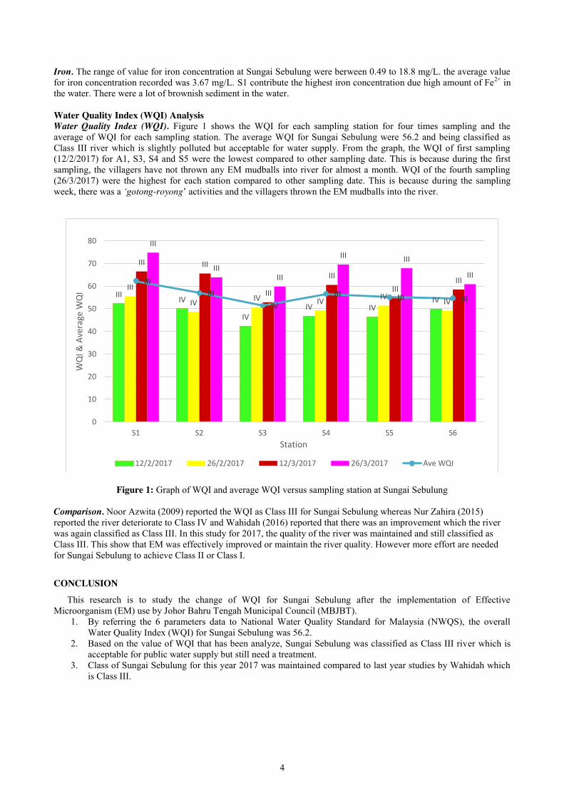
Iron. The range of value for iron concentration at Sungai Sebulung were berween 0.49 to 18.8 mg/L. the average value for iron concentration recorded was 3.67 mg/L. S1 contribute the highest iron concentration due high amount of Fe2+ in the water. There were a lot of brownish sediment in the water. Water Quality Index (WQI) Analysis Water Quality Index (WQI). Figure 1 shows the WQI for each sampling station for four times sampling and the average of WQI for each sampling station. The average WQI for Sungai Sebulung were 56.2 and being classified as Class III river which is slightly polluted but acceptable for water supply. From the graph, the WQI of first sampling (12/2/2017) for A1, S3, S4 and S5 were the lowest compared to other sampling date. This is because during the first sampling, the villagers have not thrown any EM mudballs into river for almost a month. WQI of the fourth sampling (26/3/2017) were the highest for each station compared to other sampling date. This is because during the sampling week, there was a ‘gotong-royong’ activities and the villagers thrown the EM mudballs into the river.

Figure 1: Graph of WQI and average WQI versus sampling station at Sungai Sebulung Comparison. Noor Azwita (2009) reported the WQI as Class III for Sungai Sebulung whereas Nur Zahira (2015) reported the river deteriorate to Class IV and Wahidah (2016) reported that there was an improvement which the river was again classified as Class III. In this study for 2017, the quality of the river was maintained and still classified as Class III. This show that EM was effectively improved or maintain the river quality. However more effort are needed for Sungai Sebulung to achieve Class II or Class I.

CONCLUSION

This research is to study the change of WQI for Sungai Sebulung after the implementation of Effective Microorganism (EM) use by Johor Bahru Tengah Municipal Council (MBJBT).

1. By referring the 6 parameters data to National Water Quality Standard for Malaysia (NWQS), the overall Water Quality Index (WQI) for Sungai Sebulung was 56.2.

2. Based on the value of WQI that has been analyze, Sungai Sebulung was classified as Class III river which is acceptable for public water supply but still need a treatment.

3. Class of Sungai Sebulung for this year 2017 was maintained compared to last year studies by Wahidah which is Class III.

III IV

IV IV IV

IV III

IV IV IV IV IV

III III

III

III III

III

III

III III

III III

III III

III IV

III III III

0

10

20

30

40

50

60

70

80

S1 S2 S3 S4 S5 S6

WQ

I & A

vera

ge W

QI

Station

12/2/2017 26/2/2017 12/3/2017 26/3/2017 Ave WQI

5

REFERENCES

[1] Weng, C. N. (2005). Sustainable management of rivers in Malaysia: Involving all stakeholders. International Journal of River Basin Management.

[2] Postel, S. & Richter, B. (2003).Rivers for life. Washington: Island Press..

[3] Majlis Bandaraya Johor Bahru (MBJB) (2014). Sebulung River Settlement Revival Programme [Brochure]. Johor Bahru. MBJB.

[4] Wahidah binti Wahid (2016). Improvement of Water Quality using Effective. Bachelor Degree Thesis, Universiti Teknologi Malaysia

[5] Jacquelyn Anak Liang (2014).The Effectiveness of Effective Microorganism in Conservation of Sungai Sebulung-Phase I.

[6] Zakaria, Z., Gairola, S., & Shariff, N. M. (2010). Effective microorganisms (EM) technology for water quality restoration and potential for sustainable water resources and management. In Proceedings international congress on environmental modelling and software S (pp. 0-04).

[7] I. Naubi, N. Zardari & S. Shirazi (2016). Effectiveness of Water Quality Index for Monitoring Malaysian River Water Quality.

6

Study on Potential Occurrence of Sludge Bulking in Wastewater Treatment Plant at Johor Bahru, Malaysia.

Amir Hariz Amran, Nur Syamimi Zaidi Faculty of Civil Engineering, Universiti Teknologi Malaysia, Malaysia

nursyamimi@utm.my

Keywords: Activated sludge; Sludge bulking; Filamentous microorganisms; Wastewater treatment

ABSTRACT. Filamentous sludge bulking is a phenomenon where the sludge cannot settle at the final clarifier due to the proliferation of filamentous microorganisms. It is a nuisance in activated sludge treatment system because poor settlement in the treatment system will lead to poor effluent quality and sludge wastage. The purpose of this study is to investigate characteristics of the sludge biomass in respective wastewater treatment plant, to determine the removal performances of the respective wastewater treatment plant and to determine the possibility occurrence of sludge bulking in the respective wastewater treatment plant. The wastewater used in this study was domestic wastewater that was collected from selected wastewater treatment plant. The wastewater was collected on three different days for continuous analysis and inventory. Basedon the results of aggregation and sludge volume index, it showed that there is no problem of sludge settleability in this respective treatment plant which then led to moderate removal perfomances for almost all parameters. The results of filamentous abundances indicated that there is no possible occurrence of filamentous sludge bulking in wastewater treatment plant of Taman Senai Utama.

INTRODUCTION

A biological treatment process of wastewater that takes advantage on the active microorganisms in biomass is called an activated sludge treatment process (ASP). The active microorganisms present in biomass that have been settled in the clarifier of the treatment process, is returned to the aeration tank to maximize the removal of soluble organic matter of the wastewater. One of the commonly present microorganisms in the system is the filamentous microorganisms. It grows in long thread-like strands. After cell division, the cells do not separate from each other but rather they form filaments. Filamentous microorganisms are actually important in formation and settling of flocs in the clarifier. The network formed by the filamentous microorganisms act as a network for floc formers to attach and build up [1]. However, having excessive growth of filamentous microorganisms could be fatal to the treatment process which causing sludge bulking [1].

Problem Statement Filamentous microorganisms are playing a double – edged role in an ASP [2]. In an ideal case where the abundance of filamentous and floc forming microorganisms are equal, it will lead to the formation of large, dense and strong flocs. Thus, contributes to a well settling sludge [1]. Nevertheless, excessive growth of filamentous microorganisms can cause sludge bulking because other than being the backbones of floc build up, it can also grow outside the flocs and form floc-to-floc. The excess filaments make the settling process impossible. Sludge bulking is widely occurred in many countries. However, in Malaysia, the occurrence has not been recorded thus its severity and frequency of occurrence remains unknown. Due to such mater, this study is conducted in order to obtain information on the occurrence of sludge bulking and its characteristics in Malaysia. As for start, this study is carried out in Johor Bahru area.

Objectives of the Study The objectives of this study are:

1. To investigate the physical, chemical and biological characteristics of the sludge biomass in respective wastewater treatment plant.

2. To determine the removal performances of the respective wastewater treatment plant. 3. To determine the possibility occurrence of sludge bulking in the respective wastewater treatment plant.

Scope of the Study Analysis of the study was conducted at Environmental Engineering Laboratory, Faculty of Civil Engineering, Universiti Teknologi Malaysia (UTM). The used of wastewater is municipal raw wastewater which was collected from the selected wastewater treatment plant in Senai, Johor Bahru. For this study, no laboratory set-up is involved. The study only comprised of influent and effluent analysis for the removal performances as well as sludge biomass analysis for physical, chemical and biological properties. The sampling time was maintained consistently which is in the morning for every three times of sampling frequency.

7

LITERATURE REVIEW

Filamentous sludge bulking can be a serious problem in the treatment system as it promotes poor settlability and compaction. Filamentous sludge bulking is caused by the excessive growth of filamentous microorganisms, both inside and crucially extending out from the floc. These filaments make the floc attach with one another, interlocking the filaments which lead to a network of attached thus, causing poorly settled biomass [3]. There are various types of filamentous microorganisms. Among the types that were commonly seen to cause severe sludge bulking occurrence are Microthrix parvicella [10], Eikelboom Type 0041/0675 and Eikelboom Type 021N. FEikelboom (2000) had isolated approximately 30 morphotypes of the filamentous microorganisms based on Gram and Neisser staining reactions. Sludge bulking is hard to detect visually in its early stages. Several methods that can be used to monitor and identify sludge bulking are by a settleability test such as sludge volume index (SVI). SVI of 150-200 mL/g can be categorized as sludge bulking [3]. Another method is by microscopic monitoring called filamentous index (FI) where a FI of 4 or more indicates a probability of sludge bulking occurrence.

There are many factors contributing to the growth of filamentous microorganism. Among of the factors are low dissolved oxygen (DO) concentration [4], low food to microorganisms (F/M) ratio, low nutrients content [5], low substrate concentrations [8] and the sulphide concentration. These variations of factors eventually proliferate different types of filamentous microorganisms. There are two strategies that can be applied to prevent bulking of sludge which are specific and non-specific method [9]. The non-specific method is basically a method to urgently reduce the SVI to 50 mg/L. Examples of non-specific methods are chlorination, metal salts addition and synthetic polymer addition. However, this method does not remove the cause of the excessive growth of filamentous microorganism and their effect is only transient [9]. The specific methods are preventive methods that destroys filamentous microorganism structures and at the same time favouring the growth of floc forming microorganism structures. Among the examples of specific approach are minimization of sludge retention time [9], maintain of higher level of dissolved oxygen concentration [4] and selector installation in an activated sludge reactor [6].

METHODOLOGY

The wastewater used in this study was a municipal/domestic wastewater that was collected from selected wastewater treatment plant which been authorized by Indah Water Konsortium (IWK). The wastewater was collected on 8th March, 15th March and 4th April 2017 for continuous analysis and inventory. The wastewater was collected at both influent and effluent point so that removal performances can be computed. For the activated sludge, the samples were collected at the same treatment plant. The sludge samples were collected in form of mixed liquor suspended solids (MLSS) in aeration tank. Analytical Methods Physical Properties Biomass concentration was determined based on Method No. 2540D and 2540E from the Standard Method APHA (2005). Aggregation was measured based on turbidity measurement [7]. SVI was determined by following method 2710 D (APHA, 2005). The surface hydrophobicity was conducted based on Canzi et al. (2005). Chemical Properties The biomass sample were chemically analysed for its iron content. The standard solution of 1 ppm, 1.5 ppm 2 ppm, 2.5 ppm and 3 ppm were prepared. The standard solutions were then tested using the Atomic Absorption Spectrometer (AAS) to obtain a graph of at least 0.98 gradient. After the graph was obtained, the biomass samples were inserted in an Atomic Absorption Spectrometer (AAS) to determine the concentration of iron. Biological Properties Biological property that been analysed in this study is regarding the potential abundance of filamentous microorganisms. The abundance can be determined by obtaining filamentous index (FI). Filamentous index is a subjective scoring system that helps in determining filamentous abundance exist in wastewater. This method was done according to Genkins et al., (2004). Removal Performances. Chemical Oxygen Demand (COD). A measured volume of potassium dichromate, sulphuric acid reagent that contains silver sulphate and wastewater sample are poured into a flask. Distilled water is added to the mix. The mixture is then refluxed for 2 hours. A blank sample was carried out through the same COD testing procedure with having distilled water as a replacement for wastewater sample. After that, the mixture and the blank are titrated with ferrous ammonium sulphate (FAS). The normality of FAS and COD value are calculated using equation 1 and 2 respectively.

Normality of FAS (N) = (𝑚𝐿 𝑜𝑓 𝑃𝑜𝑡𝑡𝑎𝑠𝑖𝑢𝑚 𝑑𝑖𝑐ℎ𝑟𝑜𝑚𝑎𝑡𝑒)×(0.25)(𝑚𝐿 𝑜𝑓 𝐹𝐴𝑆 𝑟𝑒𝑞𝑢𝑖𝑟𝑒𝑑)

Eq. 1

8

COD in mg/L= (𝑚𝐿 𝑜𝑓 𝐹𝐴𝑆 𝑢𝑠𝑒𝑑 𝑓𝑜𝑟 𝑏𝑙𝑎𝑛𝑘 − 𝑚𝐿 𝑜𝑓 𝐹𝐴𝑆 𝑢𝑠𝑒𝑑 𝑓𝑜𝑟 𝑠𝑎𝑚𝑝𝑙𝑒)×8000 ×𝑁𝑆𝑎𝑚𝑝𝑙𝑒 𝑉𝑜𝑙𝑢𝑚𝑒 (𝑚𝐿)

Eq. 2 Concentration of ammonia - nitrogen was determined using Nessler Method (APHA, 2005). Nitrogen. Both nitrite and nitrate analyses were measured using HACH Spectrophotometer based on Method No. 8039 and 8153, respectively. Phosphorus is measured using HACH Spectrophotometer based on Method No. 8048. The suspended solid were analysed in terms of total suspended solids (SS) and volatile suspended solids (VSS) based on Method no. 2540D and 2540E, respectively (APHA, 2005). The turbidity analysis was conducted by first preparing 10 mL of wastewater sample. The sample was placed in a glass cuvette and then measured by using a turbidity meter (Milwaukee turbidimeter).

RESULTS AND DISCUSSION

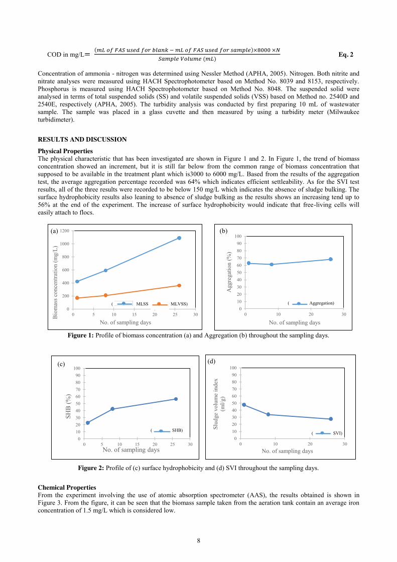
Physical Properties The physical characteristic that has been investigated are shown in Figure 1 and 2. In Figure 1, the trend of biomass concentration showed an increment, but it is still far below from the common range of biomass concentration that supposed to be available in the treatment plant which is3000 to 6000 mg/L. Based from the results of the aggregation test, the average aggregation percentage recorded was 64% which indicates efficient settleability. As for the SVI test results, all of the three results were recorded to be below 150 mg/L which indicates the absence of sludge bulking. The surface hydrophobicity results also leaning to absence of sludge bulking as the results shows an increasing tend up to 56% at the end of the experiment. The increase of surface hydrophobicity would indicate that free-living cells will easily attach to flocs.

Figure 1: Profile of biomass concentration (a) and Aggregation (b) throughout the sampling days.

Figure 2: Profile of (c) surface hydrophobicity and (d) SVI throughout the sampling days.

Chemical Properties From the experiment involving the use of atomic absorption spectrometer (AAS), the results obtained is shown in Figure 3. From the figure, it can be seen that the biomass sample taken from the aeration tank contain an average iron concentration of 1.5 mg/L which is considered low.

0

200

400

600

800

1000

1200

0 5 10 15 20 25 30Bio

mas

s con

cent

ratio

n (m

g/L)

No. of sampling days

( MLSS MLVSS) 0

102030405060708090

100

0 10 20 30

Agg

rega

tion

(%)

No. of sampling days

(a)

( Aggregation)

0102030405060708090

100

0 10 20 30

Slud

ge v

olum

e in

dex

(m

l/g)

No. of sampling days

( SVI) 0

102030405060708090

100

0 5 10 15 20 25 30

SHB

(%)

No. of sampling days

(c)

( SHB)

(b)

(d)

9

Biological Properties From Figure 3, there is no distinct abundance of filamentous microorganisms in the biomass samples for all three times of sampling. The first and second samples indicated FI = 0 which define clearly that there were no filaments observed. As for the third sample, it can be scored as FI = 1 which means that filaments were present but only observed in an occasional floc. These low indexes of filamentous abundances actually support the results obtained by parameter of SVI. Low index of filamentous means the biomass were unlikely been affected by the proliferation of filamentous Figure 3: Profile of (e) Iron concentration and microscopic observation of (f) sample 1, (g) sample 2 and (h) sample 3. Removal Performances The results of COD is shown in Figure 4. The figure shows an increasing value with the highest at 62%, but it still produces low quality effluent which means the COD removal performance of the wastewater treatment plant is low.

Figure 4: The profile of (i) COD concentration and (j) phosphorus concentration throughout the sampling days.

Figure 4 also shows the phosphorus concentration removability. The average removability percentage recorded was 55.4 %. Although the effluent phosphorus concentrations of the wastewater treatment plant are below the standard value which is 5 mg/L, it can be said that the final effluent meets the standard because of its low influent phosphorus concentration, but not because of the wastewater treatment plant removal performance. The suspended solid and volatile suspended solid removability are shown in Figure 5. The results show a high performance of removal ability. The

0.00.51.01.52.02.53.03.54.04.55.0

0 5 10 15 20 25 30

Fe c

once

ntra

tion

(mg/

L)

No. of sampling days

(e)

( Fe concentration)

(g)

(h)

( Influent Effluent Removability) (i)

0102030405060708090100

0.0

0.5

1.0

1.5

2.0

2.5

3.0

0 10 20 30

Phosphorus removal (%

) Phos

phor

us co

ncen

tratio

n (m

g/L)

No. of sampling days

( Influent Effluent Removability) (j)

(k)

0102030405060708090100

0

100

200

300

400

500

600

700

0 10 20 30

CO

D rem

oval (%)

CO

D c

once

ntra

tion

(mg/

L)

No. of sampling days

(f)

0102030405060708090100

0

100

200

300

400

500

600

700

0 10 20 30

CO

D rem

oval (%)

CO

D c

once

ntra

tion

(mg/

L)

No. of sampling days

(f)

(f)

(g) (g) (h)

(i) (j) ( Influent Effluent Removability) .

10

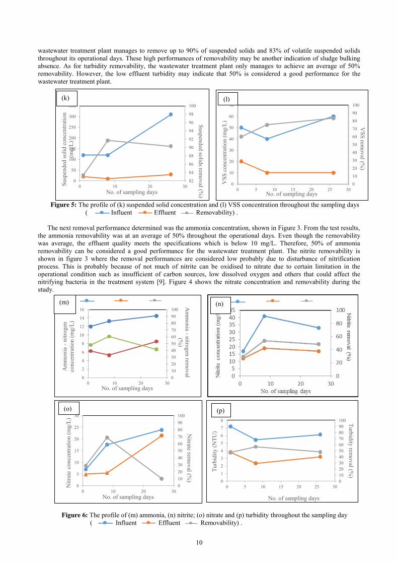
wastewater treatment plant manages to remove up to 90% of suspended solids and 83% of volatile suspended solids throughout its operational days. These high performances of removability may be another indication of sludge bulking absence. As for turbidity removability, the wastewater treatment plant only manages to achieve an average of 50% removability. However, the low effluent turbidity may indicate that 50% is considered a good performance for the wastewater treatment plant.

Figure 5: The profile of (k) suspended solid concentration and (l) VSS concentration throughout the sampling days

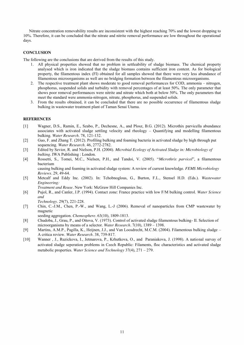
( Influent Effluent Removability) . The next removal performance determined was the ammonia concentration, shown in Figure 3. From the test results,

the ammonia removability was at an average of 50% throughout the operational days. Even though the removability was average, the effluent quality meets the specifications which is below 10 mg/L. Therefore, 50% of ammonia removability can be considered a good performance for the wastewater treatment plant. The nitrite removability is shown in figure 3 where the removal performances are considered low probably due to disturbance of nitrification process. This is probably because of not much of nitrite can be oxidised to nitrate due to certain limitation in the operational condition such as insufficient of carbon sources, low dissolved oxygen and others that could affect the nitrifying bacteria in the treatment system [9]. Figure 4 shows the nitrate concentration and removability during the study.

Figure 6: The profile of (m) ammonia, (n) nitrite; (o) nitrate and (p) turbidity throughout the sampling day ( Influent Effluent Removability) .

82

84

86

88

90

92

94

96

98

100

0

50

100

150

200

250

300

350

0 10 20 30

Suspended solids removal (%

)

Susp

ende

d so

lid c

once

ntra

tion

(mg/

L)

No. of sampling days 0

10

20

30

40

50

60

70

80

90

100

0

10

20

30

40

50

60

70

0 5 10 15 20 25 30

VSS rem

oval (%)

VSS

con

cent

ratio

n (m

g/L)

No. of sampling days

0102030405060708090100

0

5

10

15

20

25

30

0 10 20 30

Nitrate rem

oval (%)

Nitr

ate c

once

ntra

tion

(mg/

L)

No. of sampling days

0102030405060708090100

0

2

4

6

8

10

12

14

16

0 10 20 30

Am

monia - nitrogen rem

oval (%

)

Am

mon

ia -

nitro

gen

conc

entra

tion

(mg/

L)

No. of sampling days

0102030405060708090100

012345678

0 5 10 15 20 25 30

Turbidity removal (%

)

Turb

idity

(NTU

)

No. of sampling days

(k) (l)

(m) (n)

(o) (p)

11

Nitrate concentration removability results are inconsistent with the highest reaching 70% and the lowest dropping to 10%. Therefore, it can be concluded that the nitrate and nitrite removal performance are low throughout the operational days.

CONCLUSION

The following are the conclusions that are derived from the results of this study. 1. All physical properties showed that no problem in settleability of sludge biomass. The chemical property

analysed which is iron indicated that the sludge biomass contains sufficient iron content. As for biological property, the filamentous index (FI) obtained for all samples showed that there were very less abundance of filamentous microorganisms as well are no bridging formation between the filamentous microorganisms.

2. The respective treatment plant shows moderate to good removal performances for COD, ammonia – nitrogen, phosphorus, suspended solids and turbidity with removal percentages of at least 50%. The only parameter that shows poor removal performances were nitrite and nitrate which both at below 50%. The only parameters that meet the standard were ammonia-nitrogen, nitrate, phosphorus, and suspended solids.

3. From the results obtained, it can be concluded that there are no possible occurrence of filamentous sludge bulking in wastewater treatment plant of Taman Senai Utama.

REFERENCES

[1] Wagner, D.S., Ramin, E., Szabo, P., Dechesne, A., and Plosz, B.G. (2012). Microthix parvicella abundance associates with activated sludge settling velocity and rheology – Quantifying and modelling filamentous bulking. Water Research. 78, 121-132.

[2] Guo, F. and Zhang T. (2012). Profiling bulking and foaming bacteria in activated sludge by high through put sequencing. Water Research. 46, 2772-2782. [3] Edited by Sevior, R. and Nielson, P.H. (2004). Microbial Ecology of Activated Sludge in: Microbiology of bulking. IWA Publishing : London. [4] Rossetti, S., Tomei, M.C., Nielsen, P.H., and Tandoi, V. (2005). “Microthrix parvicel”, a filamentous

bacterium causing bulking and foaming in activated sludge system: A review of current knowledge. FEMS Microbiology Reviews. 29, 49-64. [5] Metcalf and Eddy Inc. (2002). In: Tchobnoglous, G., Burton, F.L., Stensel H.D. (Eds.). Wastewater

Engineering: Treatment and Reuse. New York: McGraw Hill Companies Inc. [6] Pujol, R., and Canler, J.P. (1994). Contact zone: France practice with low F/M bulking control. Water Science

and Technology. 29(7), 221-228. [7] Chin, C.-J.M., Chen, P.-W., and Wang, L.-J (2006). Removal of nanoparticles from CMP wastewater by

magnetic seeding aggregation. Chemosphere. 63(10), 1809-1813. [8] Chudoba, J., Grau, P., and Ottova, V. (1973). Control of activated sludge filamentous bulking- II. Selection of microorganisms by means of a selector. Water Research. 7(10), 1389 – 1398. [9] Martins, A.M.P., Pagilla, K., Heijnen, J.J., and Van Loosdrecht, M.C.M. (2004). Filamentous bulking sludge –

A critica review. Water Research. 38, 739-817. [10] Wanner , J., Ruzickova, I., Jetmarova, P., Krhutkova, O., and Paraniakova, J. (1998). A national survay of

activated sludge seperation problems in Czech Republic: Filaments, floc characteristics and activated sludge metabolic properties. Water Science and Technology 37(4), 271 – 279.

12

Green Synthesis and Antibacterial Appraisal of Silver Nanoparticles Amirul Syahid, Salmiati, Achmad Syaifuddin

Department of Environmental Engineering, Faculty of Civil Engineering, Universiti Teknologi Malaysia, Malaysia

salmiati@utm.my

Keywords: Silver nanoparticles, Plants extracts, Green synthesis, Antibacterial activity.

ABSTRACT. Design of new nanometals was developed due to the wide applications for various fields. Silver nanoparticles (AgNPs) is one of the most important nanometals because of their extensive applications in biotechnology and biomedical fields. AgNPs were traditionally synthesized using chemical and physical methods. However, in chemical method, various toxic and hazardous chemicals are used, which are harmful to the health of living organisms. In addition, physical method has drawback such as a lot of energy consumption. Therefore, the present work aims to investigate the suitability of plant extracts to synthesize AgNPs at room temperature and evaluate their antibacterial capability. AgNPs were synthesized using four different plant extracts namely Cyperus rotundus, Pachyrhizus erosus, Euphorbia hirta, and Eleusin indica. Then, AgNPs were characterized using UV-vis, Fourier-transform infrared spectroscopy (FTIR), Field Emission Scanning Electron Microscopy (FESEM), and Energy dispersive X-ray (EDX). In addition, antibacterial capability of AgNPs was also examined against Escherichia coli, Bacillus cereus, C. haemolyticum UDIN3, C. haemolyticum UDIN4 and C. haemolyticum UDIN2. This study found that AgNPs having size of 20.5±9.6, 55.0±24.1, 57.1±21, and 40.6±10.8 nm were produced when Cyperus rotundus, Pachyrhizus erosus, Euphorbia hirta, and Eleusin indica were employed, respectively. In addition, this study has also confirmed that the synthesized AgNPs have antibacterial activity against Escherichia coli, Bacillus cereus, C. haemolyticum UDIN3, C. haemolyticum UDIN4, and C. haemolyticum UDIN2. In general, the present work has successfully proposed a green synthesis of AgNPs and evaluated their antibacterial capability.

INTRODUCTION

Synthetization of nanoparticles has received massive attention because of greater surface area to volume ratio, modified structure and more activity of nanoparticles rather than macro molecules [1-12]. Nanoparticles have many applications in optical, electronic and textiles industries, medicine, cosmetic and drug delivery. The most important nanoproduct in the field of nanotechnology is AgNPs, which has already been known to exhibit a strong toxicity to a wide range of micro-organisms and no toxicity against human health. This nanoproduct are significantly used in textiles and clothing, food packaging, medical and cosmetic ingredients, water, wastewater and air treatment, household usage and pesticides. Green synthesis using biological method such as enzymes, microorganisms, and plant extracts is the best eco-friendly alternative to available traditional chemical and physical methods. The aim of this work is to review the green synthesis of AgNPs using various plants.

Problem Statement Various wild plant obtained from roadside at University Technology Malaysia (UTM) were selected to synthesis AgNPs. Four different kinds of plants named Cyperus rotundus, Pachyrhizus erosus, Euphorbia hirta, and Eleusin indica are common wild plant in Asia and have no attention from people despite their use in green synthesis. With this wild plant collected, an experiment were conducted to investigate and characterize the performance of AgNPs synthesised by these plant extracts and how their antibacterial activity triggered.Method of synthetization are called as green synthesis. Green synthesis are used throughout the experiment because of its cost effective and non-hazardous due to its environmental friendly and have no biological risks. Green synthesis using plants, fruit , or any substances that come with green environment and this is why this method are cost effective and less dangerous compared to the chemical and physical method to synthesized AgNPs.

These wild plants are chosen among the other plants because there are zero research about this plant connected with AgNPs extraction. With this plant, we hope there are new discovery and new finding that will contribute to the community usage. As we know, human beings are often infected by microorganisms such as bacterium, mold, yeast and virus. Silver or silver ions have been long known to have a strong inhibitory and bactericidal effects as well as abroad spectrum of antimicrobial activities. With this study, researching about AgNPs microbial activity can contribute to human beings need of protection from virus and harmful microorganisms. AgNPs antibacterial activity were monitored along the experiment to record how it reacted after synthesized with Cyperus rotundus, Pachyrhizus erosus, Euphorbia hirta, and Eleusin indica and what mechanism it has to destroy bacteria cell.

13

Objectives Therefore, the present work aims to investigate the suitability of plant extracts to synthesize AgNPs at room temperature and evaluate their antibacterial capability. The following objectives will be conducted to achieve the purpose of this study:

1. To propose a green synthesis of AgNPs using Cyperus rotundus, Pachyrhizus erosus, Euphorbia hirta, and Eleusin indica extracts.

2. To characterize properties of synthesized AgNPs in terms of plasmonic, biomolecule bonding, size, shape, and energy dispersive.

3. To evaluate antibacterial activity of synthesized AgNPs against bacteria gram positive and negative.

Scope of Study Cyperus rotundus, Pachyrhizus erosus, Euphorbia hirta, and Eleusin indica were selected to perform green synthesis of AgNPs. Further, we could monitor how their antibacterial activity. This experiment was conducted in the IPASA laboratory at Universiti Teknologi Malaysia (UTM). To synthesize AgNPs, we use the leaves of Cyperus rotundus, Pachyrhizus erosus, Euphorbia hirta, and Eleusin indica. The experiment has been conducted at room temperature. The experiment proceed until the targeted result are obtained. AgNPs properties can be characterized according to their plasmonic properties, FTIR to determine the functional groups present in the synthesized AgNPs, EDX, including the morphology and size. In this study, antibacterial activity against bacteria gram positive and negative can be evaluated. Colony forming and inhibition zone were be selected to evaluate their antibacterial properties. The magnitude of AgNPs antibacterial effects towards microorganism are monitored.

LITERATURE REVIEW

Silver has been used as an antimicrobial agent for thousands of years, and its use in medicine continues to the present day [2]. Despite increased silver research over the past few decades in antimicrobial, nutraceutical, and biomaterials applications, many questions remain about the safety and efficacy of silver-containing biomaterials in human use. Silver is currently used in several different chemical and physical forms in a variety of medical devices including coated catheters, wound coverings, and endotracheal tubes. This chapter elaborate details the extensive use of silver in biomedical applications, reported mechanisms of antibacterial activity, toxicity to human tissues, nanomaterial properties, and future directions for silver’s use in medicine and environment [3].

AgNPs are nanoparticles of silver that about between 1 nm and 100 nm in size. Some of the components are composed of a large percentage of silver oxide despite frequently described as being silver due to their large ratio of surface-to-bulk silver atoms. Innumerable shapes of nanoparticles can be manufacture depending on the application at hand. Regularly used are spherical silver nanoparticles but other structure like diamond, octagonal, and thin sheets are also popular. Their enormous large surface area permits the coordination of immeasurable number of ligands. The properties of silver nanoparticles are applicable to human in various way including biomedical application and daily routine hardware like clothing, kitchenware, cosmetics and toys.

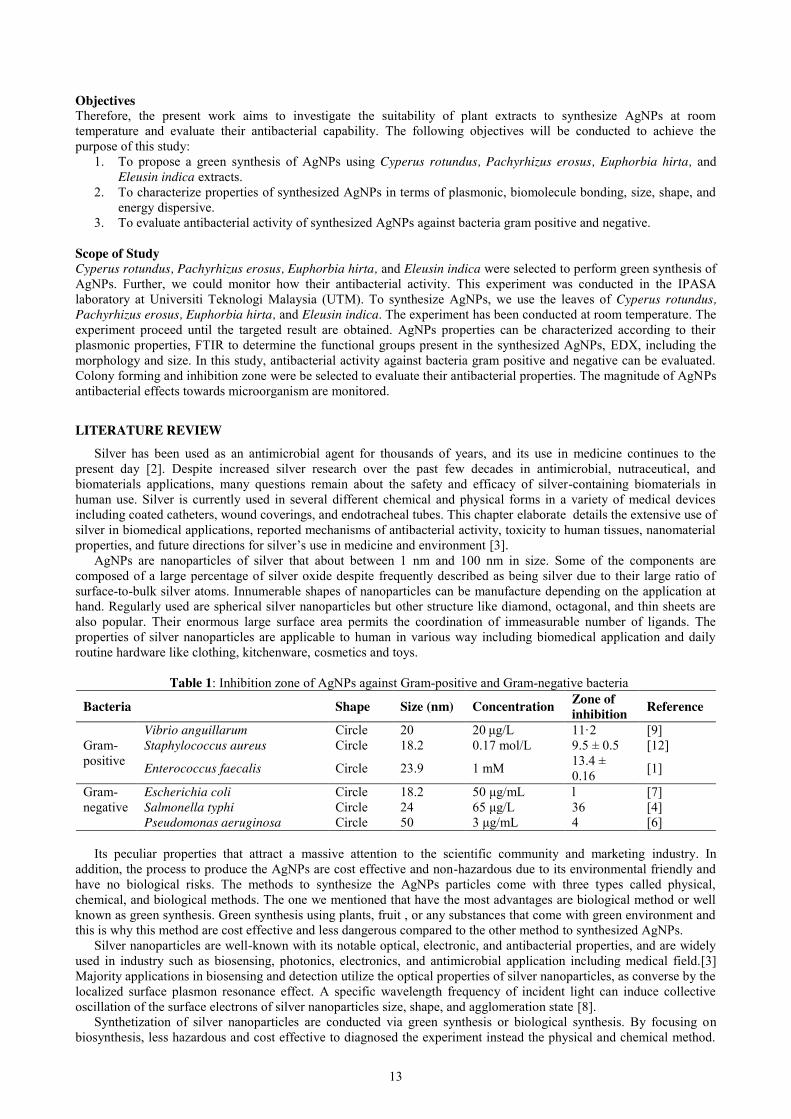
Table 1: Inhibition zone of AgNPs against Gram-positive and Gram-negative bacteria

Bacteria Shape Size (nm) Concentration Zone of inhibition Reference

Gram-positive

Vibrio anguillarum Circle 20 20 μg/L 11·2 [9] Staphylococcus aureus Circle 18.2 0.17 mol/L 9.5 ± 0.5 [12]

Enterococcus faecalis Circle 23.9 1 mM 13.4 ± 0.16 [1]

Gram-negative

Escherichia coli Circle 18.2 50 μg/mL l [7] Salmonella typhi Circle 24 65 μg/L 36 [4] Pseudomonas aeruginosa Circle 50 3 μg/mL 4 [6]

Its peculiar properties that attract a massive attention to the scientific community and marketing industry. In

addition, the process to produce the AgNPs are cost effective and non-hazardous due to its environmental friendly and have no biological risks. The methods to synthesize the AgNPs particles come with three types called physical, chemical, and biological methods. The one we mentioned that have the most advantages are biological method or well known as green synthesis. Green synthesis using plants, fruit , or any substances that come with green environment and this is why this method are cost effective and less dangerous compared to the other method to synthesized AgNPs.

Silver nanoparticles are well-known with its notable optical, electronic, and antibacterial properties, and are widely used in industry such as biosensing, photonics, electronics, and antimicrobial application including medical field.[3] Majority applications in biosensing and detection utilize the optical properties of silver nanoparticles, as converse by the localized surface plasmon resonance effect. A specific wavelength frequency of incident light can induce collective oscillation of the surface electrons of silver nanoparticles size, shape, and agglomeration state [8].

Synthetization of silver nanoparticles are conducted via green synthesis or biological synthesis. By focusing on biosynthesis, less hazardous and cost effective to diagnosed the experiment instead the physical and chemical method.

14

The extracts of plants are used such as oriental medicine herb Gynostemma pentaphyllum Makino, Pine (Pinus desiflora). Persimmon (Diopyros kaki), Ginkgo (Ginko biloba), Magnolia (Magnolia kobus) and Platanus (Platanus orientalis). The UV-vis spectra were recorded as a function of reaction time on a UV-1650CP Shimadzu spectrophometer operated at resolution of 1nm. Structure and composition were analysed by scanning electron microscopy (SEM, Hitachi S-25000C), field emission transmission electron microscopy (FE-SEM, Tecnai F30 S-Twin, FEI), energy dispersive X-ray spectroscopy (EDS,Sigma). Silver concentrations and conversions were determined using inductively coupled plasma spectrometry. Particle size and distribution were measured by using particle analyzer.by [11] . Shankar et al. (2008) reported that nanoparticles synthesized using plant extracts are surrounded by a thin layer of some capping organic material from plant extracts broth.

EXPERIMENTAL PROCEDURE

The main objective of the research is to study performance of antibacterial activity by silver nanoparticle. In addition, antibacterial activity of each plant extracts was compared with that conventional antibacterial agent as well. This research methodology consisted of many activities: plant extracts preparation, silver nanoparticles synthetization, antibacterial activity measurements, characterization (UV-Vis, FESEM, EDX, and FTIR) and inhibition zone study. Materials Cyperus rotundus, Pachyrhizus erosus, Euphorbia hirta, and Eleusin indica are obtained from surrounding Universiti Teknologi Malaysia (UTM). Silver nitrate (AgNO3) with QRëCTM brand was obtained from the Centre for Environmental Sustainability and Water Security (IPASA) laboratory at UTM as analytical grade and used as received. All glassware were washed using Dettol soap and rinsed thoroughly with ultrapure water before use and dried All solutions were prepared and diluted using ultrapure water. Preparation of plant extracts Cyperus rotundus, Pachyrhizus erosus, Euphorbia hirta, and Eleusin indica leaves were washed thoroughly in tapwater three times and rinsed with ultrapure water three times before prepared to boil. The plant extracts were prepared using water as a solvent. Eighteen grams of Cyperus rotundus, Pachyrhizus erosus, Euphorbia hirta, and Eleusin indica leaves was mixed with 200 ml of ultrapure water, and the mixture was boiled for 45 minutes. After cooling, the extracts were filtered and further centrifuged. The supernatant was stored at 4°C for further use Synthesis of AgNPs Cyperus rotundus, Pachyrhizus erosus, Euphorbia hirta, and Eleusin indica extracts are rinse thoroughly with ultrapurewater three times and boil to obtain the plant extract. The extract was added to 100 mL of 1 x 10-3 M aqueous solution of AgNO3 in conical flask, and then the mixture was shake gently to ensure the extract and AgNO3 are mix properly. Antibacterial activity measurements The antibacterial measurements activity of synthesised AgNPs was assayed by Kirby-Bauer disc diffusion method. Five typical aquatic pathogenic bacteria of Escherichia coli, Bacillus cereus, C.haemolyticum UDIN3, C.haemolyticum UDIN4 and C. haemolyticum UDIN2 were obtained from Centre for Environmental Sustainability and Water Security (IPASA). Bacteria suspension were spread evenly on separate nutrients agar plates. Then oxford cups 6 mm in diameter were gently placed on the plates, and 10 mL AgNPs solution was added into the cups. Four independent replicates were conducted, and the plate was incubated overnight at 36oC. The diameters of the zones of inhibition were measured, and mean value for each bacterium was calculated. The susceptibility of test bacteria was determined by measuring the mean diameters of inhibition zone.

RESULTS AND DISCUSSION

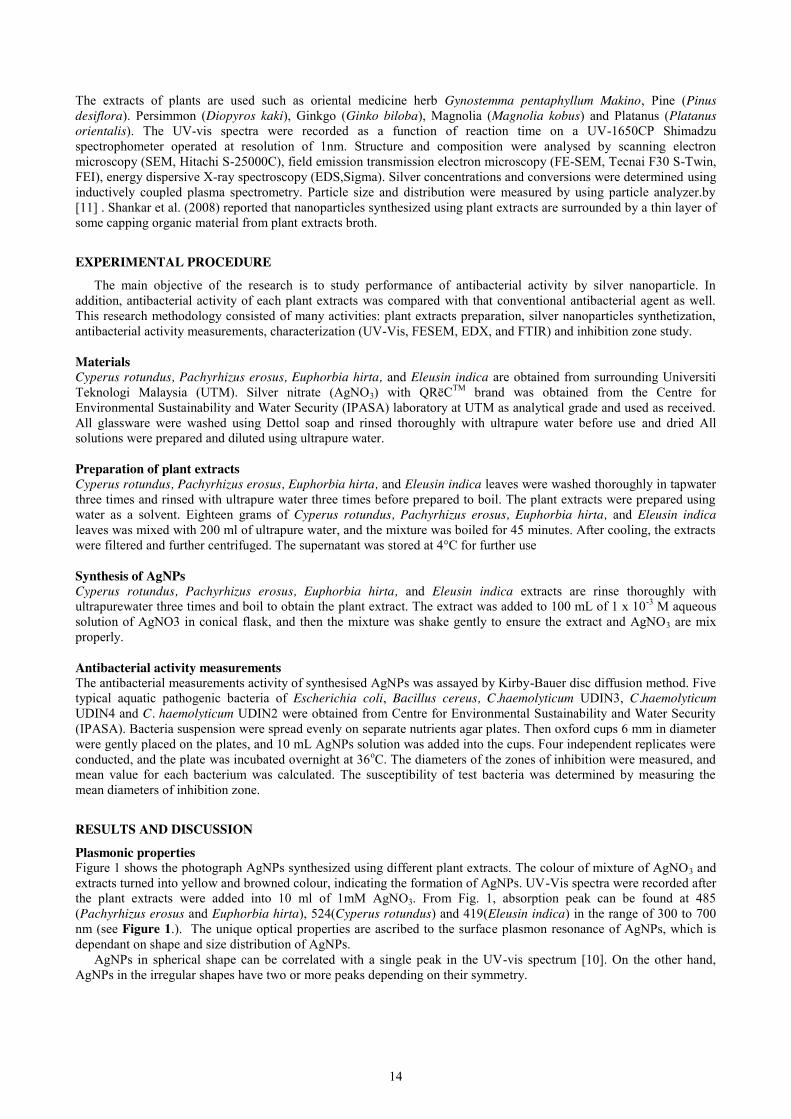
Plasmonic properties Figure 1 shows the photograph AgNPs synthesized using different plant extracts. The colour of mixture of AgNO3 and extracts turned into yellow and browned colour, indicating the formation of AgNPs. UV-Vis spectra were recorded after the plant extracts were added into 10 ml of 1mM AgNO3. From Fig. 1, absorption peak can be found at 485 (Pachyrhizus erosus and Euphorbia hirta), 524(Cyperus rotundus) and 419(Eleusin indica) in the range of 300 to 700 nm (see Figure 1.). The unique optical properties are ascribed to the surface plasmon resonance of AgNPs, which is dependant on shape and size distribution of AgNPs.

AgNPs in spherical shape can be correlated with a single peak in the UV-vis spectrum [10]. On the other hand, AgNPs in the irregular shapes have two or more peaks depending on their symmetry.

15

Figure 1. UV-Vis spectra of Cyperus rotundus, Pachyrhizus erosus, Euphorbia hirta, and Eleusin indica

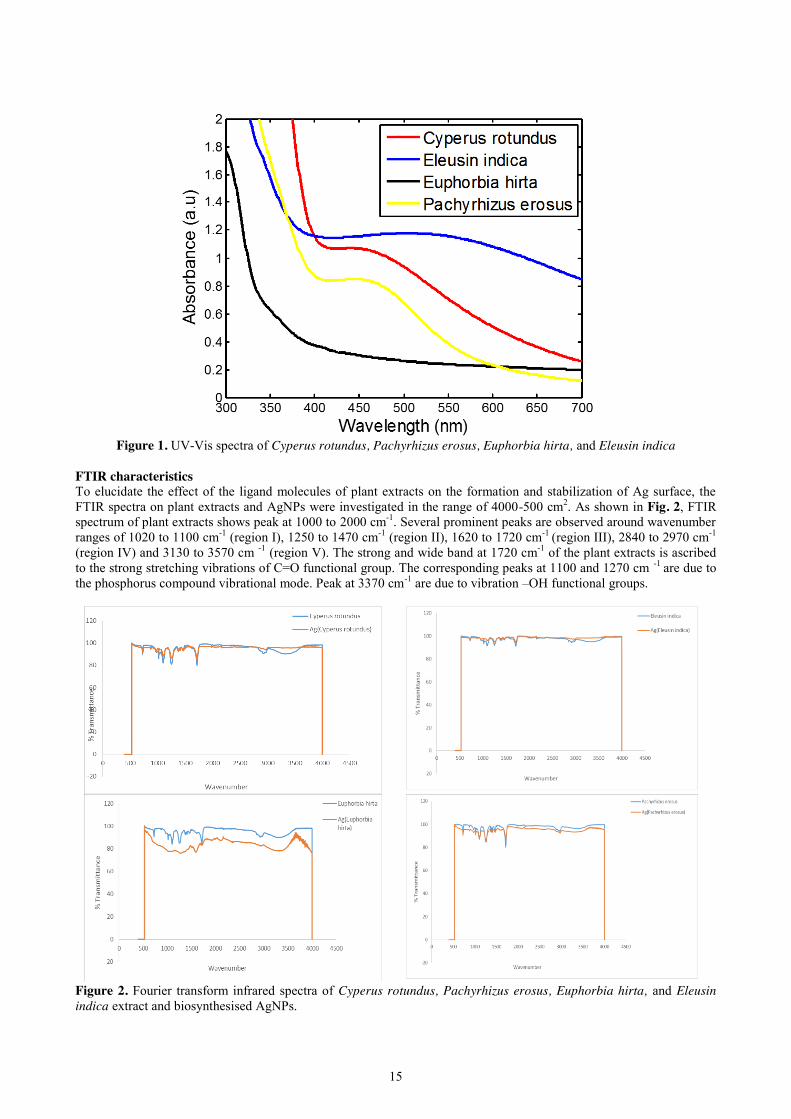
FTIR characteristics To elucidate the effect of the ligand molecules of plant extracts on the formation and stabilization of Ag surface, the FTIR spectra on plant extracts and AgNPs were investigated in the range of 4000-500 cm2. As shown in Fig. 2, FTIR spectrum of plant extracts shows peak at 1000 to 2000 cm-1. Several prominent peaks are observed around wavenumber ranges of 1020 to 1100 cm-1 (region I), 1250 to 1470 cm-1 (region II), 1620 to 1720 cm-1 (region III), 2840 to 2970 cm-1 (region IV) and 3130 to 3570 cm -1 (region V). The strong and wide band at 1720 cm-1 of the plant extracts is ascribed to the strong stretching vibrations of C=O functional group. The corresponding peaks at 1100 and 1270 cm -1 are due to the phosphorus compound vibrational mode. Peak at 3370 cm-1 are due to vibration –OH functional groups.

Figure 2. Fourier transform infrared spectra of Cyperus rotundus, Pachyrhizus erosus, Euphorbia hirta, and Eleusin indica extract and biosynthesised AgNPs.

16

EDX characteristics Energy dispersive X-ray spectroscopy characteristics generally depends on the source of X-ray excitation and sample. The SEM-EDX spectra of all synthesized AgNPs can be observed in Figs. 3a-3d. The spectra characteristics have confirmed the presence of AgNPs.The sharp signal peak of the spectrum exhibits that the reduction of AgNO3 to AgNPs using Cyperus rotundus, Pachyrhizus erosus, Euphorbia hirta, and Eleusin indica.

Percentages of AgNPs synthesized using Cyperus rotundus, Pachyrhizus erosus, Euphorbia hirta, and Eleusin indica observed in the EDX spectrophometer are 77.39, 73.07, 73.63, and 68.67 respectively. It is identified that AgNPs have a majority side in the samples compared to other elements. AgNPs synthesised using these plant extracts exhibit the EDX peak at 3 keV with spherical shapes. The other peaks shown in Figs. 3 are possibly due to the contribution from enzymes or proteins present within Cyperus rotundus, Pachyrhizus erosus, Euphorbia hirta, and Eleusin indica.

Figure 3 above shows the energy disperse by AgNPs synthesised by (a)Cyperus rotundus, (b)Eleusin indica, (c)Euphorbia hirta, and (d)Pachyrhizus erosus

Morphology and size Shape and size of AgNPs synthesized by Cyperus rotundus, Pachyrhizus erosus and Eleusin indica are spherical were concentrated within 18 to 83 nm have the average size of 20.5 nm, 40.6 nm and 55.0 nm (see Figure 4 and Table 2). In addition, for those synthesized using Euphorbia hirta have irregular shape pentagon and spherical with mean diameter size 57.1 nm and 55.4 nm. Generally, results from this study enhance the understanding of the effectiveness of the use of local leaves for synthesizing AgNPs.

Figure 4. Morphology of AgNPs synthesised by (a) Cyperus rotundus, (b) Eleusin indica, (c) Euphorbia hirta, and (d) Pachyrhizus erosus

(A) (B)

(D) (C)

(C)

(A)

(D)

(B)

17

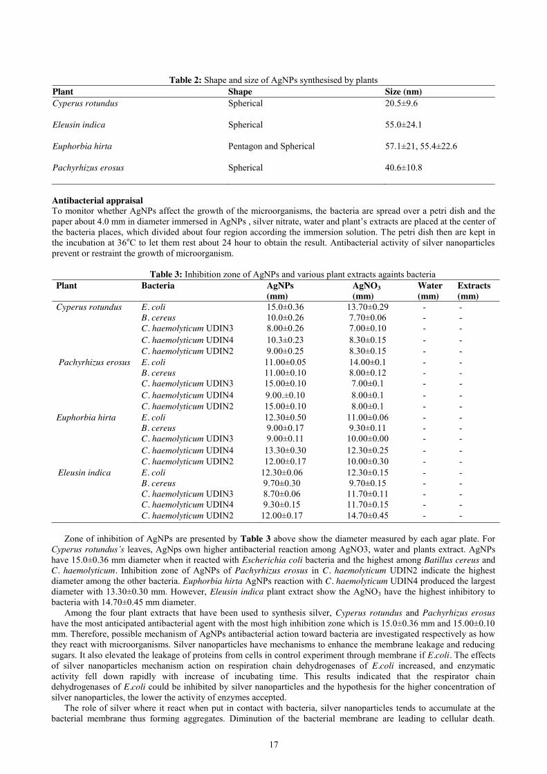
Table 2: Shape and size of AgNPs synthesised by plants

Plant Shape Size (nm) Cyperus rotundus

Spherical 20.5±9.6

Eleusin indica

Spherical 55.0±24.1

Euphorbia hirta

Pentagon and Spherical 57.1±21, 55.4±22.6

Pachyrhizus erosus Spherical 40.6±10.8

Antibacterial appraisal To monitor whether AgNPs affect the growth of the microorganisms, the bacteria are spread over a petri dish and the paper about 4.0 mm in diameter immersed in AgNPs , silver nitrate, water and plant’s extracts are placed at the center of the bacteria places, which divided about four region according the immersion solution. The petri dish then are kept in the incubation at 36oC to let them rest about 24 hour to obtain the result. Antibacterial activity of silver nanoparticles prevent or restraint the growth of microorganism.

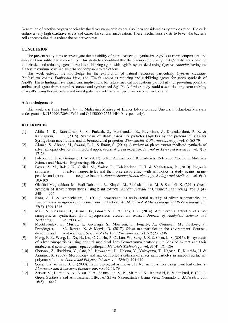
Table 3: Inhibition zone of AgNPs and various plant extracts againts bacteria Plant Bacteria AgNPs

(mm) AgNO3 (mm)

Water (mm)

Extracts (mm)

Cyperus rotundus

E. coli B. cereus C. haemolyticum UDIN3

15.0±0.36 10.0±0.26 8.00±0.26

13.70±0.29 7.70±0.06 7.00±0.10

- - -

- - -

C. haemolyticum UDIN4 10.3±0.23 8.30±0.15 - - C. haemolyticum UDIN2 9.00±0.25 8.30±0.15 - -

Pachyrhizus erosus

E. coli B. cereus C. haemolyticum UDIN3

11.00±0.05 11.00±0.10 15.00±0.10

14.00±0.1 8.00±0.12 7.00±0.1

- - -

- - -

C. haemolyticum UDIN4 9.00.±0.10 8.00±0.1 - - C. haemolyticum UDIN2 15.00±0.10 8.00±0.1 - - Euphorbia hirta E. coli

B. cereus C. haemolyticum UDIN3

12.30±0.50 9.00±0.17 9.00±0.11

11.00±0.06 9.30±0.11

10.00±0.00

- - -

- - -

C. haemolyticum UDIN4 13.30±0.30 12.30±0.25 - - C. haemolyticum UDIN2 12.00±0.17 10.00±0.30 - - Eleusin indica E. coli

B. cereus 12.30±0.06 9.70±0.30

12.30±0.15 9.70±0.15

- -

- -

C. haemolyticum UDIN3 8.70±0.06 11.70±0.11 - - C. haemolyticum UDIN4 9.30±0.15 11.70±0.15 - -

C. haemolyticum UDIN2 12.00±0.17 14.70±0.45 - - Zone of inhibition of AgNPs are presented by Table 3 above show the diameter measured by each agar plate. For

Cyperus rotundus’s leaves, AgNps own higher antibacterial reaction among AgNO3, water and plants extract. AgNPs have 15.0±0.36 mm diameter when it reacted with Escherichia coli bacteria and the highest among Batillus cereus and C. haemolyticum. Inhibition zone of AgNPs of Pachyrhizus erosus in C. haemolyticum UDIN2 indicate the highest diameter among the other bacteria. Euphorbia hirta AgNPs reaction with C. haemolyticum UDIN4 produced the largest diameter with 13.30±0.30 mm. However, Eleusin indica plant extract show the AgNO3 have the highest inhibitory to bacteria with 14.70±0.45 mm diameter.

Among the four plant extracts that have been used to synthesis silver, Cyperus rotundus and Pachyrhizus erosus have the most anticipated antibacterial agent with the most high inhibition zone which is 15.0±0.36 mm and 15.00±0.10 mm. Therefore, possible mechanism of AgNPs antibacterial action toward bacteria are investigated respectively as how they react with microorganisms. Silver nanoparticles have mechanisms to enhance the membrane leakage and reducing sugars. It also elevated the leakage of proteins from cells in control experiment through membrane if E.coli. The effects of silver nanoparticles mechanism action on respiration chain dehydrogenases of E.coli increased, and enzymatic activity fell down rapidly with increase of incubating time. This results indicated that the respirator chain dehydrogenases of E.coli could be inhibited by silver nanoparticles and the hypothesis for the higher concentration of silver nanoparticles, the lower the activity of enzymes accepted.

The role of silver where it react when put in contact with bacteria, silver nanoparticles tends to accumulate at the bacterial membrane thus forming aggregates. Diminution of the bacterial membrane are leading to cellular death.

18

Generation of reactive oxygen species by the silver nanoparticles are also been considered as cytotoxic action. The cells endure a very high oxidative stress and cause the cellular inactivation. These mechanisms exists to lower the bacteria cell concentration thus reduce the oxidative stress.

CONCLUSION

The present study aims to investigate the suitability of plant extracts to synthesize AgNPs at room temperature and evaluate their antibacterial capability. This study has identified that the plasmonic property of AgNPs differs according to their size and reducing agent as well as stabilizing agent with AgNPs synthesized using Cyperus rotundus having the highest maximum peak and absorbance compared to the others.

This work extends the knowledge for the exploration of natural resources particularly Cyperus rotundus, Pachyrhizus erosus, Euphorbia hirta, and Eleusin indica as reducing and stabilizing agents for green synthesis of AgNPs. These findings have significant implications for future medical applications particularly for providing potential antibacterial agent from natural resources and synthesized AgNPs. A further study could assess the long-term stability of AgNPs using this procedure and investigate their antibacterial performance on other bacteria.

Acknowledgements This work was fully funded by the Malaysian Ministry of Higher Education and Universiti Teknologi Malaysia

under grants (R.J130000.7809.4F619 and Q.J130000.2522.14H40, respectively).

REFERENCES

[1] Ahila, N. K., Ramkumar, V. S., Prakash, S., Manikandan, B., Ravindran, J., Dhanalakshmi, P. K. & Kannapiran, E. (2016). Synthesis of stable nanosilver particles (AgNPs) by the proteins of seagrass Syringodium isoetifolium and its biomedicinal properties. Biomedicine & Pharmacotherapy. vol. 84(60-70

[2] Ahmed, S., Ahmad, M., Swami, B. L. & Ikram, S. (2016). A review on plants extract mediated synthesis of silver nanoparticles for antimicrobial applications: A green expertise. Journal of Advanced Research. vol. 7(1). 17-28

[3] Falconer, J. L. & Grainger, D. W. (2017). Silver Antimicrobial Biomaterials. Reference Module in Materials Science and Materials Engineering, Elsevier.

[4] Fayaz, A. M., Balaji, K., Girilal, M., Yadav, R., Kalaichelvan, P. T. & Venketesan, R. (2010). Biogenic synthesis of silver nanoparticles and their synergistic effect with antibiotics: a study against gram-positive and gram- negative bacteria. Nanomedicine: Nanotechnology, Biology and Medicine. vol. 6(1). 103-109

[5] Ghaffari-Moghaddam, M., Hadi-Dabanlou, R., Khajeh, M., Rakhshanipour, M. & Shameli, K. (2014). Green synthesis of silver nanoparticles using plant extracts. Korean Journal of Chemical Engineering. vol. 31(4). 548- 557

[6] Kora, A. J. & Arunachalam, J. (2011). Assessment of antibacterial activity of silver nanoparticles on Pseudomonas aeruginosa and its mechanism of action. World Journal of Microbiology and Biotechnology. vol. 27(5). 1209-1216

[7] Maiti, S., Krishnan, D., Barman, G., Ghosh, S. K. & Laha, J. K. (2014). Antimicrobial activities of silver nanoparticles synthesized from Lycopersicon esculentum extract. Journal of Analytical Science and Technology. vol. 5(1). 40

[8] McGillicuddy, E., Murray, I., Kavanagh, S., Morrison, L., Fogarty, A., Cormican, M., Dockery, P., Prendergast, M., Rowan, N. & Morris, D. (2017). Silver nanoparticles in the environment: Sources, detection and ecotoxicology. Science of The Total Environment. vol. 575(231-246

[9] Meng, F. B., Wang, L., Xu, H., Liu, C. C., Hu, P. C., Lan, W., Song, J. X. & Chen, L. S. (2016). Biosynthesis of silver nanoparticles using oriental medicinal herb Gynostemma pentaphyllum Makino extract and their antibacterial activity against aquatic pathogen. Materials Technology. vol. 31(4). 181-186

[10] Shervani, Z., Ikushima, Y., Sato, M., Kawanami, H., Hakuta, Y., Yokoyama, T., Nagase, T., Kuneida, H. & Aramaki, K. (2007). Morphology and size-controlled synthesis of silver nanoparticles in aqueous surfactant polymer solutions. Colloid and Polymer Science. vol. 286(4). 403-410

[11] Song, J. Y. & Kim, B. S. (2008). Rapid biological synthesis of silver nanoparticles using plant leaf extracts. Bioprocess and Biosystems Engineering. vol. 32(1). 79

[12] Zargar, M., Hamid, A. A., Bakar, F. A., Shamsudin, M. N., Shameli, K., Jahanshiri, F. & Farahani, F. (2011). Green Synthesis and Antibacterial Effect of Silver Nanoparticles Using Vitex Negundo L. Molecules. vol. 16(8). 6667

19

Investigation on the Potential of Sludge Bulking at Sewage Treatment Plant

Aqilah Liyana binti Mohamed Afandi, Khalida binti Muda Faculty of Civil Engineering, Universiti Teknologi Malaysia, Malaysia

khalida@utm.my

Keywords: Sludge Bulking; Filamentous Index; Physico-chemical characteristics; Removal Perfomances.

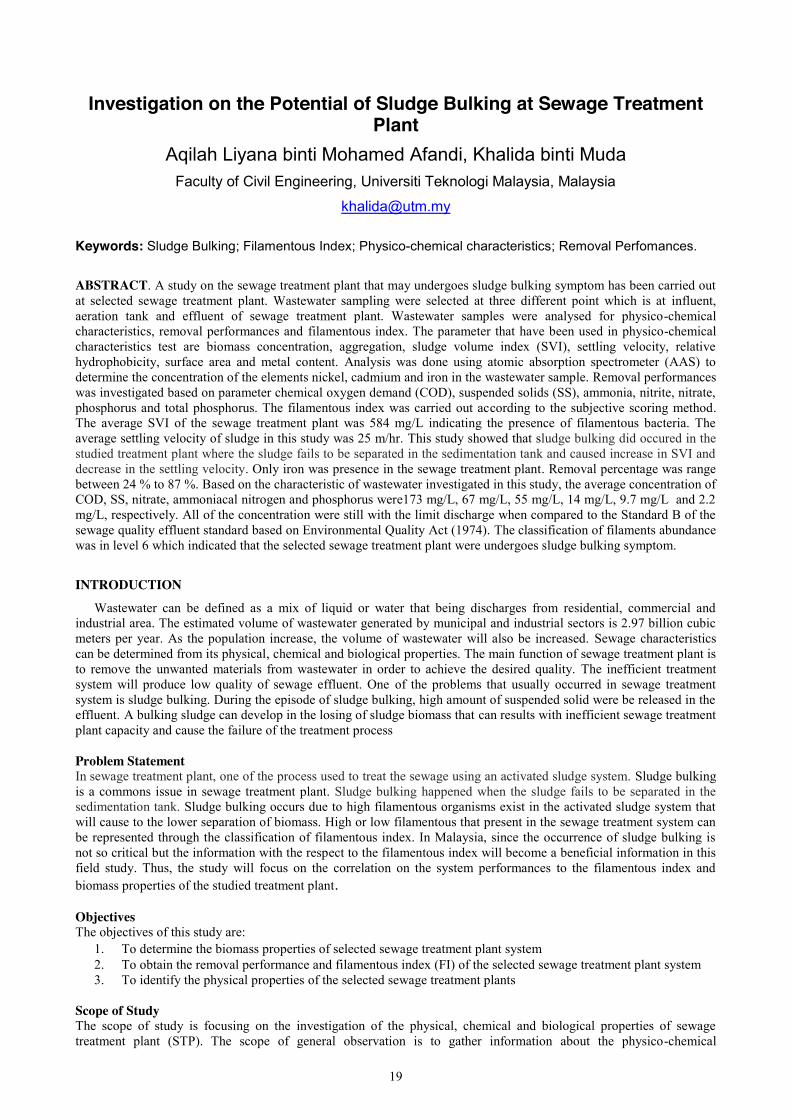
ABSTRACT. A study on the sewage treatment plant that may undergoes sludge bulking symptom has been carried out at selected sewage treatment plant. Wastewater sampling were selected at three different point which is at influent, aeration tank and effluent of sewage treatment plant. Wastewater samples were analysed for physico-chemical characteristics, removal performances and filamentous index. The parameter that have been used in physico-chemical characteristics test are biomass concentration, aggregation, sludge volume index (SVI), settling velocity, relative hydrophobicity, surface area and metal content. Analysis was done using atomic absorption spectrometer (AAS) to determine the concentration of the elements nickel, cadmium and iron in the wastewater sample. Removal performances was investigated based on parameter chemical oxygen demand (COD), suspended solids (SS), ammonia, nitrite, nitrate, phosphorus and total phosphorus. The filamentous index was carried out according to the subjective scoring method. The average SVI of the sewage treatment plant was 584 mg/L indicating the presence of filamentous bacteria. The average settling velocity of sludge in this study was 25 m/hr. This study showed that sludge bulking did occured in the studied treatment plant where the sludge fails to be separated in the sedimentation tank and caused increase in SVI and decrease in the settling velocity. Only iron was presence in the sewage treatment plant. Removal percentage was range between 24 % to 87 %. Based on the characteristic of wastewater investigated in this study, the average concentration of COD, SS, nitrate, ammoniacal nitrogen and phosphorus were173 mg/L, 67 mg/L, 55 mg/L, 14 mg/L, 9.7 mg/L and 2.2 mg/L, respectively. All of the concentration were still with the limit discharge when compared to the Standard B of the sewage quality effluent standard based on Environmental Quality Act (1974). The classification of filaments abundance was in level 6 which indicated that the selected sewage treatment plant were undergoes sludge bulking symptom.

INTRODUCTION

Wastewater can be defined as a mix of liquid or water that being discharges from residential, commercial and industrial area. The estimated volume of wastewater generated by municipal and industrial sectors is 2.97 billion cubic meters per year. As the population increase, the volume of wastewater will also be increased. Sewage characteristics can be determined from its physical, chemical and biological properties. The main function of sewage treatment plant is to remove the unwanted materials from wastewater in order to achieve the desired quality. The inefficient treatment system will produce low quality of sewage effluent. One of the problems that usually occurred in sewage treatment system is sludge bulking. During the episode of sludge bulking, high amount of suspended solid were be released in the effluent. A bulking sludge can develop in the losing of sludge biomass that can results with inefficient sewage treatment plant capacity and cause the failure of the treatment process Problem Statement In sewage treatment plant, one of the process used to treat the sewage using an activated sludge system. Sludge bulking is a commons issue in sewage treatment plant. Sludge bulking happened when the sludge fails to be separated in the sedimentation tank. Sludge bulking occurs due to high filamentous organisms exist in the activated sludge system that will cause to the lower separation of biomass. High or low filamentous that present in the sewage treatment system can be represented through the classification of filamentous index. In Malaysia, since the occurrence of sludge bulking is not so critical but the information with the respect to the filamentous index will become a beneficial information in this field study. Thus, the study will focus on the correlation on the system performances to the filamentous index and biomass properties of the studied treatment plant.

Objectives The objectives of this study are:

1. To determine the biomass properties of selected sewage treatment plant system 2. To obtain the removal performance and filamentous index (FI) of the selected sewage treatment plant system 3. To identify the physical properties of the selected sewage treatment plants

Scope of Study The scope of study is focusing on the investigation of the physical, chemical and biological properties of sewage treatment plant (STP). The scope of general observation is to gather information about the physico-chemical

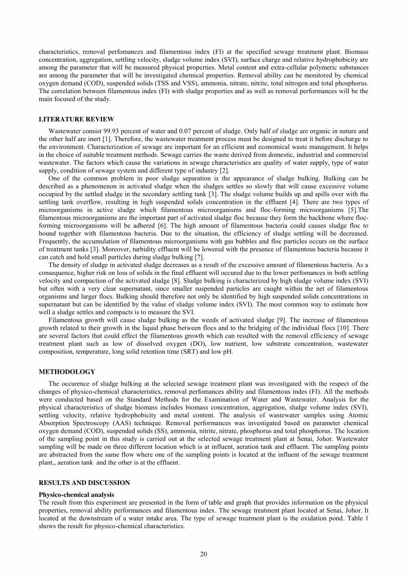
20

characteristics, removal perfomances and filamentous index (FI) at the specified sewage treatment plant. Biomass concentration, aggregation, settling velocity, sludge volume index (SVI), surface charge and relative hydrophobicity are among the parameter that will be measured physical properties. Metal content and extra-cellular polymeric substances are among the parameter that will be investigated chemical properties. Removal ability can be monitored by chemical oxygen demand (COD), suspended solids (TSS and VSS), ammonia, nitrate, nitrite, total nitrogen and total phosphorus. The correlation between filamentous index (FI) with sludge properties and as well as removal performances will be the main focused of the study.

LITERATURE REVIEW Wastewater consist 99.93 percent of water and 0.07 percent of sludge. Only half of sludge are organic in nature and

the other half are inert [1]. Therefore, the wastewater treatment process must be designed to treat it before discharge to the environment. Characterization of sewage are important for an efficient and economical waste management. It helps in the choice of suitable treatment methods. Sewage carries the waste derived from domestic, industrial and commercial wastewater. The factors which cause the variations in sewage characteristics are quality of water supply, type of water supply, condition of sewage system and different type of industry [2].

One of the common problem in poor sludge separation is the appearance of sludge bulking. Bulking can be described as a phenomenon in activated sludge when the sludges settles so slowly that will cause excessive volume occupied by the settled sludge in the secondary settling tank [3]. The sludge volume builds up and spills over with the settling tank overflow, resulting in high suspended solids concentration in the effluent [4]. There are two types of microorganisms in active sludge which filamentous microorganisms and floc-forming microorganisms [5].The filamentous microorganisms are the important part of activated sludge floc because they form the backbone where floc-forming microorganisms will be adhered [6]. The high amount of filamentous bacteria could causes sludge floc to bound together with filamentous bacteria. Due to the situation, the efficiency of sludge settling will be decreased. Frequently, the accumulation of filamentous microorganisms with gas bubbles and floc particles occurs on the surface of treatment tanks [3]. Moreover, turbidity effluent will be lowered with the presence of filamentous bacteria because it can catch and hold small particles during sludge bulking [7].

The density of sludge in activated sludge decreases as a result of the excessive amount of filamentous bacteria. As a consequence, higher risk on loss of solids in the final effluent will occured due to the lower perfomances in both settling velocity and compaction of the activated sludge [8]. Sludge bulking is characterized by high sludge volume index (SVI) but often with a very clear supernatant, since smaller suspended particles are caught within the net of filamentous organisms and larger flocs. Bulking should therefore not only be identified by high suspended solids concentrations in supernatant but can be identified by the value of sludge volume index (SVI). The most common way to estimate how well a sludge settles and compacts is to measure the SVI.

Filamentous growth will cause sludge bulking as the weeds of activated sludge [9]. The increase of filamentous growth related to their growth in the liquid phase between flocs and to the bridging of the individual flocs [10]. There are several factors that could effect the filamentous growth which can resulted with the removal efficiency of sewage treatment plant such as low of dissolved oxygen (DO), low nutrient, low substrate concentration, wastewater composition, temperature, long solid retention time (SRT) and low pH.

METHODOLOGY

The occurence of sludge bulking at the selected sewage treatment plant was investigated with the respect of the changes of physico-chemical characteristics, removal perfomances ability and filamentous indes (FI). All the methods were conducted based on the Standard Methods for the Examination of Water and Wastewater. Analysis for the physical characteristics of sludge biomass includes biomass concentration, aggregation, sludge volume index (SVI), settling velocity, relative hydrophobicity and metal content. The analysis of wastewater samples using Atomic Absorption Spectroscopy (AAS) technique. Removal performances was investigated based on parameter chemical oxygen demand (COD), suspended solids (SS), ammonia, nitrite, nitrate, phosphorus and total phosphorus. The location of the sampling point in this study is carried out at the selected sewage treatment plant at Senai, Johor. Wastewater sampling will be made on three different location which is at influent, aeration tank and effluent. The sampling points are abstracted from the same flow where one of the sampling points is located at the influent of the sewage treatment plant,, aeration tank and the other is at the effluent.

RESULTS AND DISCUSSION

Physico-chemical analysis The result from this experiment are presented in the form of table and graph that provides information on the physical properties, removal ability performances and filamentous index. The sewage treatment plant located at Senai, Johor. It located at the downstream of a water intake area. The type of sewage treatment plant is the oxidation pond. Table 1 shows the result for physico-chemical characteristics.

21

Table 1: Result of percentage of aggregation, percentage of surface hydrophobicity, SVI, Settling velocity, MLSS and MLVSS

Time Aggregation % Surface

hydrophobicity % SVI

(mg/L) Settling

Velocity (m/hr) MLSS MLVSS Week 1 14.88 55.58 543 27.4 1.64 1.54 Week 2 10.82 49.96 634 26.2 1.12 1.09 Week 3 22.5 70.95 576 24.3 0.99 0.96

Aggregation. The average percentage of aggregation was 16.1 ± 5.93 %. The percentage of aggregation between week 2 and week 3 has a high difference. This is because the low of aggregation percentage maybe due to low biomass based on low MLVSS. When the low biomass enter the sewage treatment plant, the presence of bacteria will be low. Thus, low collision between particles causing low in the percentage of aggregation. Surface Hydrophobicity. The average percentage of surface hydrophobicity was 58.83 %. Changes in surface hydrophobicity can be affected by many factors. The factors that cause stress to the culture condition such as growth rate, pH and temperature [11]. The normal pH at oxidation ditch is 6 to 9. If pH is more than 9, this will enhance the repulsive force of the bacterial surface charge and reduced the chances of bacteria cell forming aggregates which subsequently reducing the percentage of surface hydrophobicity. SVI and Settling Velocity. In this study, the average SVI for three different sampling time is 584 mg/L. The sewage treatment plant may contain the presence of filamentous bacteria since the value of SVI was over 250 mg/L. The average settling velocity of sludge in this experiment were 25 m/hr. It shows the correlation between settling velocity and sludge volume index (SVI) where as the SVI increased the settling velocity decrease. This is because settling is hindered by the high quantity of flocs [12] MLSS and MLVSS. The average concentration of mixed liquor suspended solids (MLSS) and mixed liquor volatile suspended solids (MLVSS) of the sample sampling activities were 1.25 g/L and 1.20 g/L respectively. The range MLSS and MLVSS concentration in oxidation pond are between 1.0 g/L to 4.0 g/L [13]. From Figure 4.1, it can be seen that the concentration of MLSS and MLVSS at week 3 are slightly lower than what has been reported by previous researcher which is 0.99 g/L and 0.96 g/L respectively. The lower value of MLSS and MLVSS due to the lower of COD removal [14]. The concentration and percentage of COD removal will be discussed later.

Removal Performances Analysis Removal performances was investigated based on parameter chemical oxygen demand (COD), suspended solids (SS), ammonia, nitrite, nitrate, phosphorus and total phosphorus. Table 2 show the concentration of removal perfomances parameter. Figure 1- 8 shows the removal percentage for each removal performances parameter.

Table 2: Experimental results for COD, turbidity, TSS, VSS, nitrite, nitrate, total nitrogen (TN), phosphorus, total phosphorus (TP) and ammonia.

Time Sources

COD

(mg/L)

Turbidity

(NTU)

TSS

(mg/L)

VSS

(mg/L)

Nitrite

(mg/L)

Nitrate

(mg/L)

TN

(mg/L )

Phosphorus

(mg/L)

TP

(mg/L)

Ammonia

(mg/L)

Week

1

Influent 663 204.5 92 84 30 3 16 3.4 15.1 12.5

Effluent 223 21.3 36 32 10 1 11 2.6 13.1 8.9

Week

2

Influent 593 218.5 304 256 40 11 17 5.1 22.1 12.1

Effluent 183 33.5 120 110 20 7 10 2 13.4 9.7

Week

3

Influent 458 205 138 128 60 14 20 4.2 13.2 13.7

Effluent 113 30.5 46 22 10 5 13 1.9 9.4 10.5

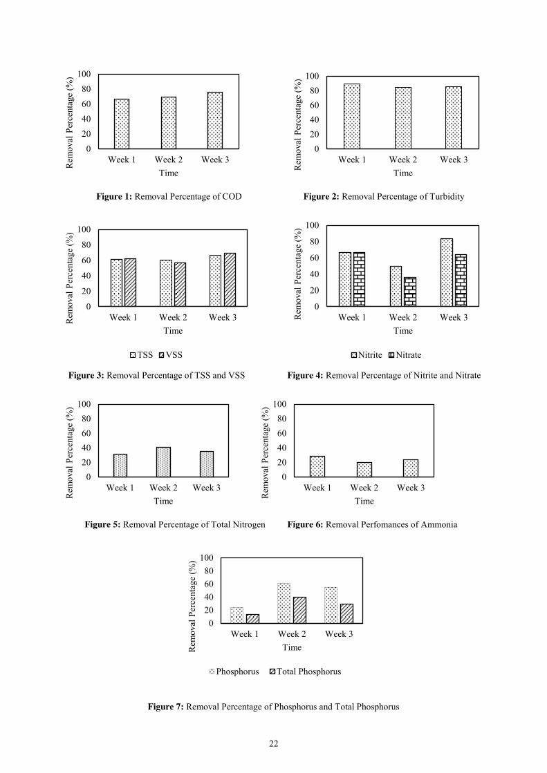
22

Figure 1: Removal Percentage of COD Figure 2: Removal Percentage of Turbidity

Figure 3: Removal Percentage of TSS and VSS Figure 4: Removal Percentage of Nitrite and Nitrate

Figure 5: Removal Percentage of Total Nitrogen Figure 6: Removal Perfomances of Ammonia

Figure 7: Removal Percentage of Phosphorus and Total Phosphorus

020406080

100

Week 1 Week 2 Week 3

Rem

oval

Per

cent

age

(%)

Time

020406080

100

Week 1 Week 2 Week 3

Rem

oval

Per

cent

age

(%)

Time

0

20

40

60

80

100

Week 1 Week 2 Week 3Rem

oval

Per

cent

age

(%)

Time

TSS VSS

0

20

40

60

80

100

Week 1 Week 2 Week 3Rem

oval

Per

cent

age

(%)

Time

Nitrite Nitrate

020406080

100

Week 1 Week 2 Week 3

Rem

oval

Per

cent

age

(%)

Time

020406080

100

Week 1 Week 2 Week 3

Rem

oval

Per

cent

age

(%)

Time

020406080

100

Week 1 Week 2 Week 3

Rem

oval

Per

cent

age

(%)

Time

Phosphorus Total Phosphorus

23

COD. The average influent and effluent concentration of COD are 571 mg/L and 173 mg/L respectively. From the data obtained, the removal percentage of COD at the study area is uniform. The discharge COD level in the effluent released from this treatment plant is comply the Standard B of in Environmental Quality Act (1974) for week 1, week 2 and week 3. The limit of Standard B for oxidation pond is 360 mg/L. From table 2, it can be seen that the value for all the week are lower than 360 mg/L. Turbidity. The average removal percentage for turbidity is 86.5 %. It shows that the efficiency percentage of turbidity in a good condition. The effluent concentration of turbidity is highest in week 2 which is 33.5 NTU. The average concentration of turbidity for influent and effluent is 209.3 ± 7.94 NTU and 28.4 ± 6.35 NTU respectively. TSS and VSS. The average removal percentage for both TSS and VSS are 62.7 ± 3.5 % and 62.6 ± 5.89 % respectively. From Table 4.7, the average effluent concentration for both TSS and VSS are 67 mg/L and 55 mg/L respectively. The level of suspended solids of the treated effluent before being discharged into river should be less than 150 mg/L for oxidation pond as stated in Standard B of the Environmental Quality Act (1974). The data, which ranges from 36 mg/L to 120 mg/L for TSS and 22 mg/L to 110 mg/L for VSS shows that the values are lower than 150 mg/L. Nitrite and Nitrate. The average removal percentage of nitrite and nitrate are 66.7 % and 55.8 % respectively. There is a high diferrence in removal percentage between week 2 and week 3. This situation might be due to analysis error or sampling error at week 2. Table 2 shows that the average effluent concentration for both nitrate and nitrite are 13 mg/L and 4 mg/L respectively. The level of nitrate of the treated effluent that enclosed water body should be less than 10 mg/L as stated in Standard B in Environmental Quality Act (1974). The nitrate effluent concentration data which ranges from 1 mg/L to 7 mg/L shows that the values are lower than 10 mg/L. Total Nitrogen. The average removal percentage of total nitrogen is 35.8 ± 5.01 %. The average influent and effluent concentration of total nitrogen are 18 mg/L and 11 mg/L respectively. The effluent of total nitrogen should less than 15 mg/L in other to prevent an excess amount of nitrogen in a waterway [15]. High amount of nitrogen lead to low levels of dissolved oxygen and negatively alter various plant life and organisms. Ammonia. The average influent concentration of ammonia is 12.7±0.83 mg/L while average effluent concentration is 9.7± 0.80 mg/L respectively . Figure 6 shows the removal percentage of ammonia are uniform for the three different week. The average removal percantge of ammonia is 24%. It shows that the overall efficiency percentage of ammonia is low. Since the effluent concentration of the study area are lower than 70 mg/L, it shows that the ammonia level at oxidation pond is comply with the Standard B in Environmental Quality Act (1974). High release of ammonia content in the sewage effluent would cause harmful to aquatic life. It is environmentally hazardous because of its toxicity to fish and because of its ease of oxidation, dissolved oxygen is depleted rapidly. Ammoniacal nitrogen are most likely to cause excessive algal growth in waterway [16]. Phosphorus and Total Phosphorus. The average effluent concentration of phosphorus and total phosphorus are 2.17 mg/L and 11.97 mg/L respectively. From Figure 7, the removal percentage of phosphorus and total phosphorus at week 1 is lower compared to week 2 and week 3. The removal percentage for three different duration for phosphorus and total phosphorus are in the range 14 % to 61%. It shown that the removal efficiency of the sample is low. Based on Environmental Quality Act (1974), the level of phosphorus of the treated effluent before being discharged into river should be less than 10 mg/L as stated in Standard B. The data, which ranges from 1.9 mg/L to 2.6 mg/L for phosphorus shows that the values are lower than 10 mg/L. Filamentous Index For a routine examination of activated sludge in sewage treatment plants, a fast and simple method of subjective scoring of filaments abundance was develop [17]. This study investigated on the total abundances of the available microorganisms that presence during the occurrence of sludge bulking. . In this study, three (3) samples at aeration tank were analysed. The classification of filaments abundance was in level 6 which indicated that the filamentous bacteria were present in all flocs, filaments appears more than flocs and filaments growing in high abundance in bulk solution. Figure 8 and 9 showed the image of filamentous bacteria which may also indicated the abundance of the identified microorganisms

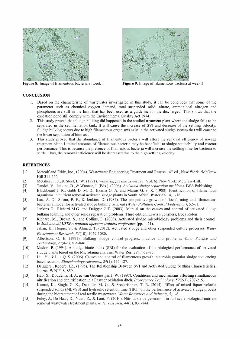
24

Figure 8: Image of filamentous bacteria at week 1 Figure 9: Image of filamentous bacteria at week 3

CONCLUSION

1. Based on the characteristic of wastewater investigated in this study, it can be concludes that some of the parameter such as chemical oxygen demand, total suspended solid, nitrate, ammoniacal nitrogen and phosphorus are still in the limit that has been used as a guideline for the discharged. This shows that the oxidation pond still comply with the Environmental Quality Act 1974.

2. This study proved that sludge bulking did happened in the studied treatment plant where the sludge fails to be separated in the sedimentation tank. It will cause the increase of SVI and decrease of the settling velocity. Sludge bulking occurs due to high filamentous organisms exist in the activated sludge system that will cause to the lower separation of biomass.

3. This study proved that the abundance of filamentous bacteria will affect the removal efficiency of sewage treatment plant. Limited amounts of filamentous bacteria may be beneficial to sludge settleability and reactor performance. This is because the presence of filamentous bacteria will increase the settling time for bacteria to settle. Thus, the removal efficiency will be decreased due to the high settling velocity..

REFERENCES

[1] Metcalf and Eddy, Inc., (2004). Wastewater Engineering Treatment and Resuse , 4th ed., New Work :McGraw Hill 311-556.

[2] McGhee, T. J., & Steel, E. W. (1991). Water supply and sewerage (Vol. 6). New York: McGraw-Hill. [3] Tandoi, V., Jenkins, D., & Wanner, J. (Eds.). (2006). Activated sludge separation problems. IWA Publishing. [4] Blackbeard J. R., Gabb D. M. D., Ekama G. A. and Marais G. v. R. (1988). Identification of filamentous

organisms in nutrient removal activated sludge plants in South Africa. Water SA 14, 1-18. [5] Lau, A. O., Strom, P. F., & Jenkins, D. (1984). The competitive growth of floc-forming and filamentous

bacteria: a model for activated sludge bulking. Journal (Water Pollution Control Federation), 52-61. [6] Jenkins D., Richard M.G. and Daigger G.T. (2003). Manual on the causes and control of activated sludge

bulking foaming and other solids separation problems, Third edition, Lewis Publishers, Boca Roton. [7] Richard, M., Brown, S., and Collins, F. (2003). Activated sludge microbiology problems and their control.

In 20th annual USEPA national operator trainers conference (pp. 1-21). [8] Jahan, K., Hoque, S., & Ahmed, T. (2012). Activated sludge and other suspended culture processes. Water

Environment Research, 84(10), 1029-1080. [9] Albertson, O. E. (1991). Bulking sludge control–progress, practice and problems. Water Science and

Technology, 23(4-6), 835-846. [10] Madoni P. (1994). A sludge biotic index (SBI) for the evaluation of the biological performance of activated

sludge plants based on the Microfauna analysis. Water Res, 28(1):67–75. [11] Liu, Y., & Liu, Q. S. (2006). Causes and control of filamentous growth in aerobic granular sludge sequencing

batch reactors. Biotechnology Advances, 24(1), 115-127. [12] Daiggere., Ropere. JR., (1995). The Relationship Between SVI and Activated Sludge Settling Characteristics.

Journal WPCF, 8, 859. [13] Hao, X., Doddema, H. J., & van Groenestijn, J. W. (1997). Conditions and mechanisms affecting simultaneous

nitrification and denitrification in a Pasveer oxidation ditch. Bioresource Technology, 59(2-3), 207-215. [14] Kumar, K., Singh, G. K., Dastidar, M. G., & Sreekrishnan, T. R. (2014). Effect of mixed liquor volatile

suspended solids (MLVSS) and hydraulic retention time (HRT) on the performance of activated sludge process during the biotreatment of real textile wastewater. Water Resources and Industry, 5, 1-8.

[15] Foley, J., De Haas, D., Yuan, Z., & Lant, P. (2010). Nitrous oxide generation in full-scale biological nutrient removal wastewater treatment plants. water research, 44(3), 831-844.

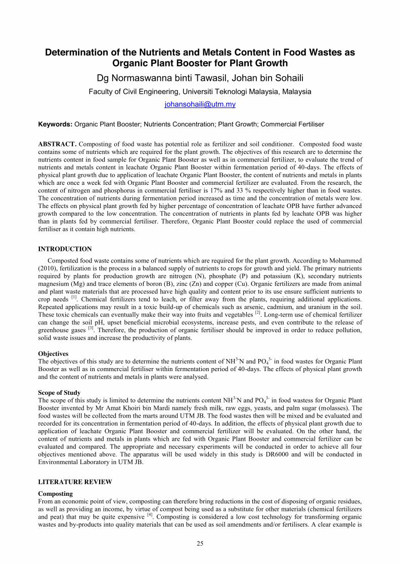
25

Determination of the Nutrients and Metals Content in Food Wastes as Organic Plant Booster for Plant Growth

Dg Normaswanna binti Tawasil, Johan bin Sohaili Faculty of Civil Engineering, Universiti Teknologi Malaysia, Malaysia

johansohaili@utm.my

Keywords: Organic Plant Booster; Nutrients Concentration; Plant Growth; Commercial Fertiliser

ABSTRACT. Composting of food waste has potential role as fertilizer and soil conditioner. Composted food waste contains some of nutrients which are required for the plant growth. The objectives of this research are to determine the nutrients content in food sample for Organic Plant Booster as well as in commercial fertilizer, to evaluate the trend of nutrients and metals content in leachate Organic Plant Booster within fermentation period of 40-days. The effects of physical plant growth due to application of leachate Organic Plant Booster, the content of nutrients and metals in plants which are once a week fed with Organic Plant Booster and commercial fertilizer are evaluated. From the research, the content of nitrogen and phosphorus in commercial fertiliser is 17% and 33 % respectively higher than in food wastes. The concentration of nutrients during fermentation period increased as time and the concentration of metals were low. The effects on physical plant growth fed by higher percentage of concentration of leachate OPB have further advanced growth compared to the low concentration. The concentration of nutrients in plants fed by leachate OPB was higher than in plants fed by commercial fertiliser. Therefore, Organic Plant Booster could replace the used of commercial fertiliser as it contain high nutrients.

INTRODUCTION

Composted food waste contains some of nutrients which are required for the plant growth. According to Mohammed (2010), fertilization is the process in a balanced supply of nutrients to crops for growth and yield. The primary nutrients required by plants for production growth are nitrogen (N), phosphate (P) and potassium (K), secondary nutrients magnesium (Mg) and trace elements of boron (B), zinc (Zn) and copper (Cu). Organic fertilizers are made from animal and plant waste materials that are processed have high quality and content prior to its use ensure sufficient nutrients to crop needs [1]. Chemical fertilizers tend to leach, or filter away from the plants, requiring additional applications. Repeated applications may result in a toxic build-up of chemicals such as arsenic, cadmium, and uranium in the soil. These toxic chemicals can eventually make their way into fruits and vegetables [2]. Long-term use of chemical fertilizer can change the soil pH, upset beneficial microbial ecosystems, increase pests, and even contribute to the release of greenhouse gases [3]. Therefore, the production of organic fertiliser should be improved in order to reduce pollution, solid waste issues and increase the productivity of plants.

Objectives The objectives of this study are to determine the nutrients content of NH3-N and PO4

3- in food wastes for Organic Plant Booster as well as in commercial fertiliser within fermentation period of 40-days. The effects of physical plant growth and the content of nutrients and metals in plants were analysed.

Scope of Study The scope of this study is limited to determine the nutrients content NH3-N and PO4

3- in food wastess for Organic Plant Booster invented by Mr Amat Khoiri bin Mardi namely fresh milk, raw eggs, yeasts, and palm sugar (molasses). The food wastes will be collected from the marts around UTM JB. The food wastes then will be mixed and be evaluated and recorded for its concentration in fermentation period of 40-days. In addition, the effects of physical plant growth due to application of leachate Organic Plant Booster and commercial fertilizer will be evaluated. On the other hand, the content of nutrients and metals in plants which are fed with Organic Plant Booster and commercial fertilizer can be evaluated and compared. The appropriate and necessary experiments will be conducted in order to achieve all four objectives mentioned above. The apparatus will be used widely in this study is DR6000 and will be conducted in Environmental Laboratory in UTM JB.

LITERATURE REVIEW

Composting From an economic point of view, composting can therefore bring reductions in the cost of disposing of organic residues, as well as providing an income, by virtue of compost being used as a substitute for other materials (chemical fertilizers and peat) that may be quite expensive [4]. Composting is considered a low cost technology for transforming organic wastes and by-products into quality materials that can be used as soil amendments and/or fertilisers. A clear example is

26

found in the Spanish olive oil industry, which generates a large amount of a solid by-product called “alperujo” [5]. In addition, composting can have a strong ecological environmental value, allowing organic by-products to be subtracted from the disposal cycle and put back into the production cycle, enhancing it and closing the organic carbon cycle, while also being a tool for the economic and social sustainability of production activities in rural areas.

Composting Food Waste Composting can be performed by using a variety of organic materials, such as: agricultural by-products (pruning, straw, other crop residues, etc.), agro-industry by products (pumice, marc and stalks, etc.), livestock waste, sewage sludge and the organic fraction of municipal solid waste [6]. In Europe, composting and anaerobic digestion account for 95% of current biological treatment operations for organic wastes. Some of the major objectives are to decompose organic matter into stable state and produce beneficial material such as fertilizer, reduce amount of waste in landfill and achieve recycling goals, disinfect pathogenically infected organic wastes and biodegradation or bioremediation of hazardous waste [4]. Nutrients in Fertiliser The important macronutrients for microbes are carbon, nitrogen, phosphorus and potassium while important micronutrients include manganese, copper, magnesium, cobalt and other elements. These nutrients must be available in form that easily to assimilate by the microbes. Nitrogen can be easily found where in the peptide or amino acid form and proteinaceous [7]. Nitrogen (N) is one element the produce during the composting process. The main non-synthetic sources of nitrogen are plants wastes, kitchen waste, animal manures, and sewage sludge. The nitrogen in these materials is transformed from atmosphere into organic forms through chemical and biological processes [8]. Phosphorus (P) is very vital as plant macronutrient. P is made up about 0.2% of a plant’s dry weight. P is the second most frequently limiting nutrient as macronutrient for the plant growth [9]. Potassium (K) has also been reported as an important nutrient in olive. In orchards grown under K deficient soils, fertilized trees showed increased growth and yields, in comparison to unfertilized trees [10].

METHODOLOGY

Chemical Analysis of Nutrients and Metals Concentration For this study, the equipment and reagents used are from Hach Company. The DR6000™ Uv-Vis Spectrophotometer is the industry’s most advanced lab spectrophotometer. Reagent is a substance that is used to test for the presence of another substance by causing a chemical reaction with it.

First, chemical analysis to determine the nutrients content which is Nitrogen (NH3-N) and Phospohorus (PO43-) in

food wastes and commercial fertiliser. After that, chemical analysis to determine the nutrients concentration such as Nitrogen (NH3-N) and Phospohorus (PO4

3-) and metals concentration such as Copper (Cu2+), Iron (Fe2+), Manganese (Mn2+) and Zinc (Zn2+) in Leachate OPB during 40 days of fermentation period. Finally, chemical analysis to determine the concentration such as Nitrogen (NH3-N) and Phospohorus (PO4

3-) and metals concentration such as Copper (Cu2+), Iron (Fe2+), Manganese (Mn2+) and Zinc (Zn2+) in different parts of plant which are leaf, stem and root.

Composting the Food Wastes The sample of food wastes used in this study was collected from the marts around the University Teknologi Malaysia, Skudai. The food wastes needed to be composted in this study are raw eggs, fresh milk, yeasts, palm sugar, banana, papaya, pumpkin, water spinach and shrimp paste. All food wastes will be weighed in certain amount and will be mixed together. After all the food wastes weighed accordingly, then the procedure for composting take places. The procedures of composting obtained from Department of Agriculture. However, slightly modification applied for the necessity in this study.

First of all, the food wastes and water are mixed together except for pumpkin and yeast. After that, let the mixture undergo partially anaerobic curing for a week. Then, put yeast and pumpkin into the curing and stir evenly. Close (do not need an airtight) the curing container and leave it again for 7 days. The mixture is considered mature when there is a white mycelium on the surface. Remove the husks of fermentation. Filtered and put the mixture in dark place. Observation on Physical Growth of Plant The selected plant used for this research was Solanum lycopersicum (SL). SL is known as tomato. The seed of tomato obtained from Nursery Pulai. There 6 set of 5 replicate plants needed in this study. All of the tested plants would receive same amount of feed volume of design solution of leachate. At the same time, the plants receiving same amounts of distilled water as usual. Plant growth is determined by obtaining the height of stem and size of leaf for each sample using ruler after day 29 where the leachate OPB was ready to be applied on plants. Finally, the comparison between application of organic plant booster and commercial fertiliser to the plant will be evaluated.

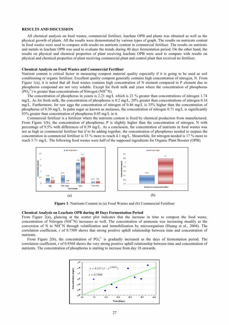
27

RESULTS AND DISCUSSION

All chemical analysis on food wastes, commercial fertiliser, leachate OPB and plants was obtained as well as the physical growth of plants. All the results were demonstrated by various types of graph. The results on nutrients content in food wastes were used to compare with results on nutrients content in commercial fertiliser. The results on nutrients and metals in leachate OPB was used to evaluate the trends during 40 days fermentation period. On the other hand, the results on physical and chemical properties of plant receiving leachate OPB were used to compare with results on physical and chemical properties of plant receiving commercial plant and control plant that received no fertiliser.

Chemical Analysis on Food Wastes and Commercial Fertiliser Nutrient content is critical factor in measuring compost material quality especially if it is going to be used as soil conditioning or organic fertilizer. Excellent quality compost generally contains high concentration of nitrogen, N. From Figure 1(a), it is noted that all food wastes contains high concentration of N element compared to P element due to phosphorus compound are not very soluble. Except for fresh milk and yeast where the concentration of phosphorus (PO4

3-) is greater than concentrations of Nitrogen (NH3-N). The concentration of phosphorus in yeasts is 2.21 mg/L which is 21 % greater than concentrations of nitrogen 1.74

mg/L. As for fresh milk, the concentration of phosphorus is 0.2 mg/L, 20% greater than concentrations of nitrogen 0.16 mg/L. Furthermore, for raw eggs the concentration of nitrogen of 0.46 mg/L is 35% higher than the concentration of phosphorus of 0.30 mg/L. In palm sugar as known as molasses, the concentration of nitrogen 0.71 mg/L is significantly 93% greater than concentration of phosphorus 0.05 mg/L in it.

Commercial fertilizer is a fertilizer where the nutrients content is fixed by chemical production from manufactured. From Figure 1(b), the concentration of phosphorus, P is slightly higher than the concentration of nitrogen, N with percentage of 9.5% with differences of 0.39 mg/L. As a conclusion, the concentration of nutrients in food wastes was not as high as commercial fertiliser but if to be adding together, the concentration of phosphorus needed to surpass the concentration in commercial fertiliser is 33 % more to reach 4.1 mg/L. Meanwhile, for nitrogen needed is 17 % more to reach 3.71 mg/L. The following food wastes were half of the supposed ingredients for Organic Plant Booster (OPB).

Figure 1: Nutrients Content in (a) Food Wastes and (b) Commercial Fertiliser

Chemical Analysis on Leachate OPB during 40 Days Fermentation Period From Figure 2(a), glancing at the scatter plot indicates that the increase in time to compost the food waste, concentration of Nitrogen (NH3-N) increases as well. The concentration of ammonia was increasing steadily as the conversion of N to NH3-N through volatilization and immobilization by microorganism (Huang et al., 2004). The correlation coefficient, r of 0.7509 shows that strong positive uphill relationship between time and concentration of nutrients.

From Figure 2(b), the concentration of PO43- is gradually increased as the days of fermentation period. The

correlation coefficient, r of 0.9568 shows the very strong positive uphill relationship between time and concentration of nutrients. The concentration of phosphorus is starting to increase from day 18 onwards.

y = 8.517 (1 – e-0.0042x)

r = 0.7509

(a) (b)

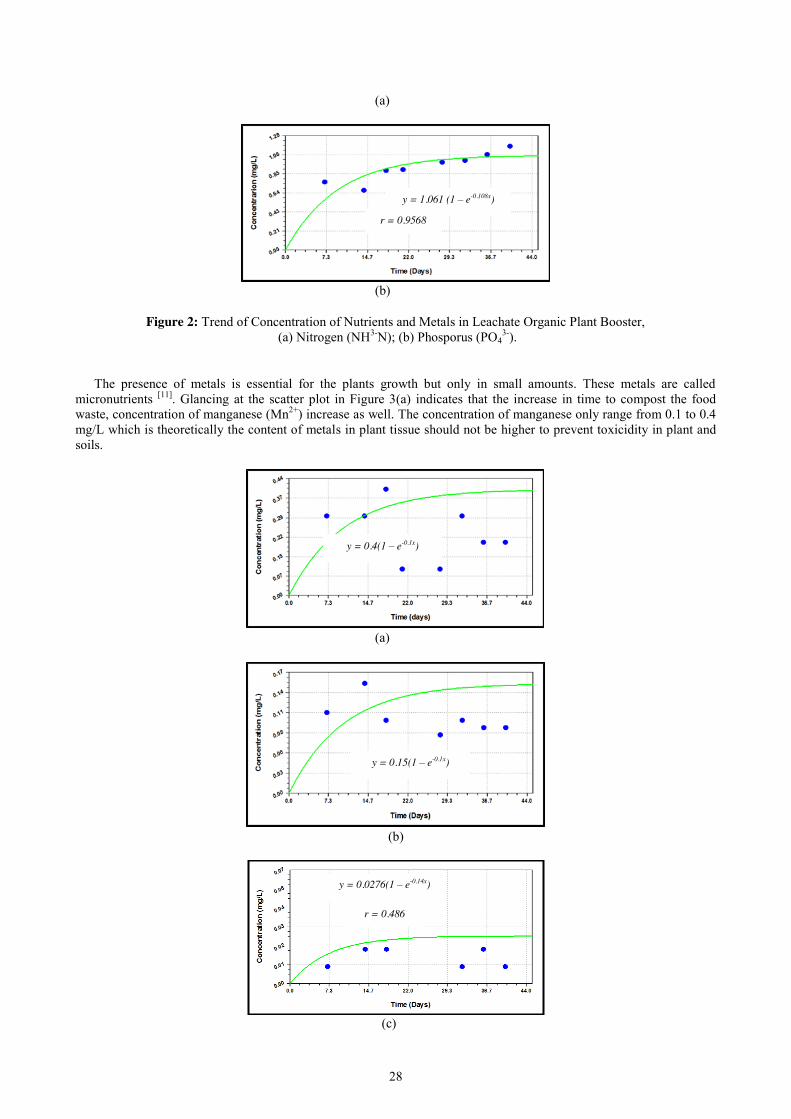
28

(a)

(b)

Figure 2: Trend of Concentration of Nutrients and Metals in Leachate Organic Plant Booster, (a) Nitrogen (NH3-N); (b) Phosporus (PO4

3-).

The presence of metals is essential for the plants growth but only in small amounts. These metals are called micronutrients [11]. Glancing at the scatter plot in Figure 3(a) indicates that the increase in time to compost the food waste, concentration of manganese (Mn2+) increase as well. The concentration of manganese only range from 0.1 to 0.4 mg/L which is theoretically the content of metals in plant tissue should not be higher to prevent toxicidity in plant and soils.

(a)

(b)

(c)

y = 1.061 (1 – e-0.108x)

r = 0.9568

y = 0.0276(1 – e-0.14x)

r = 0.486

y = 0.4(1 – e-0.1x)

y = 0.15(1 – e-0.1x)

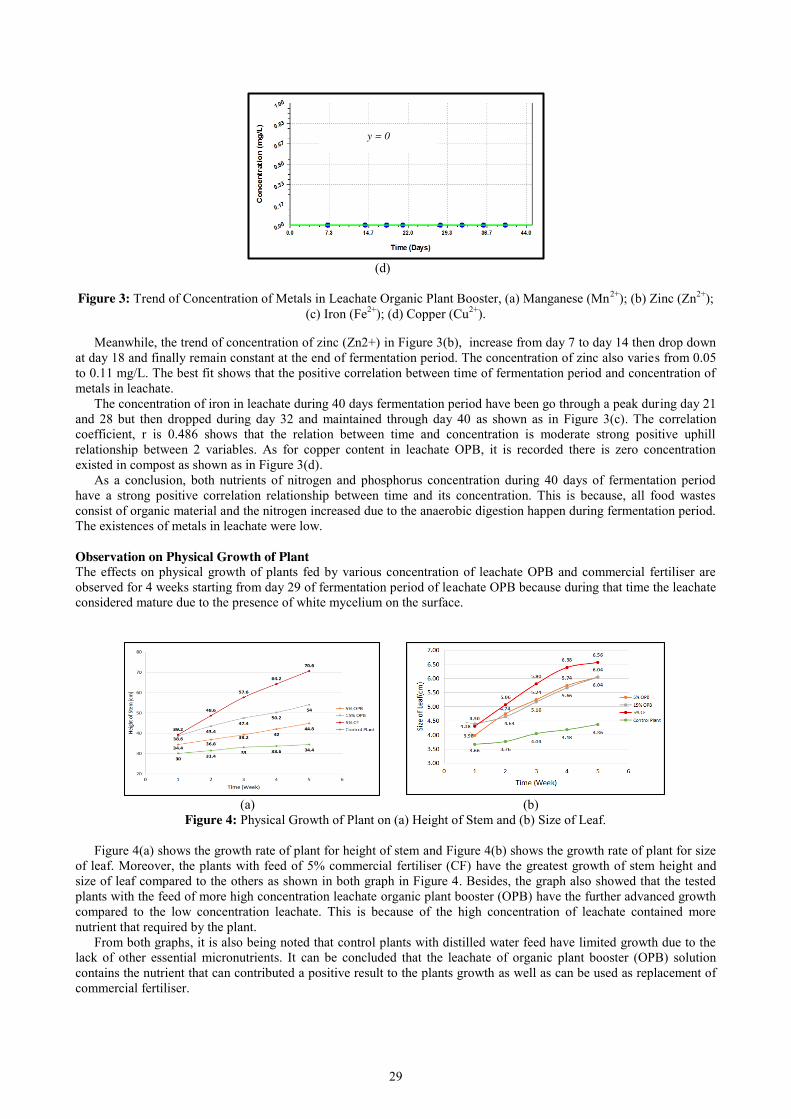
29

(d)

Figure 3: Trend of Concentration of Metals in Leachate Organic Plant Booster, (a) Manganese (Mn2+); (b) Zinc (Zn2+);

(c) Iron (Fe2+); (d) Copper (Cu2+).

Meanwhile, the trend of concentration of zinc (Zn2+) in Figure 3(b), increase from day 7 to day 14 then drop down at day 18 and finally remain constant at the end of fermentation period. The concentration of zinc also varies from 0.05 to 0.11 mg/L. The best fit shows that the positive correlation between time of fermentation period and concentration of metals in leachate.

The concentration of iron in leachate during 40 days fermentation period have been go through a peak during day 21 and 28 but then dropped during day 32 and maintained through day 40 as shown as in Figure 3(c). The correlation coefficient, r is 0.486 shows that the relation between time and concentration is moderate strong positive uphill relationship between 2 variables. As for copper content in leachate OPB, it is recorded there is zero concentration existed in compost as shown as in Figure 3(d).

As a conclusion, both nutrients of nitrogen and phosphorus concentration during 40 days of fermentation period have a strong positive correlation relationship between time and its concentration. This is because, all food wastes consist of organic material and the nitrogen increased due to the anaerobic digestion happen during fermentation period. The existences of metals in leachate were low. Observation on Physical Growth of Plant The effects on physical growth of plants fed by various concentration of leachate OPB and commercial fertiliser are observed for 4 weeks starting from day 29 of fermentation period of leachate OPB because during that time the leachate considered mature due to the presence of white mycelium on the surface.

(a) (b)

Figure 4: Physical Growth of Plant on (a) Height of Stem and (b) Size of Leaf.

Figure 4(a) shows the growth rate of plant for height of stem and Figure 4(b) shows the growth rate of plant for size of leaf. Moreover, the plants with feed of 5% commercial fertiliser (CF) have the greatest growth of stem height and size of leaf compared to the others as shown in both graph in Figure 4. Besides, the graph also showed that the tested plants with the feed of more high concentration leachate organic plant booster (OPB) have the further advanced growth compared to the low concentration leachate. This is because of the high concentration of leachate contained more nutrient that required by the plant.

From both graphs, it is also being noted that control plants with distilled water feed have limited growth due to the lack of other essential micronutrients. It can be concluded that the leachate of organic plant booster (OPB) solution contains the nutrient that can contributed a positive result to the plants growth as well as can be used as replacement of commercial fertiliser.

y = 0

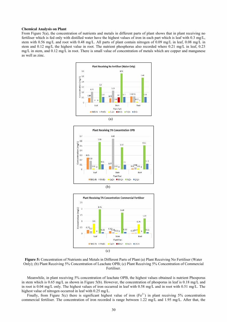
30

Chemical Analysis on Plant From Figure 5(a), the concentration of nutrients and metals in different parts of plant shows that in plant receiving no fertiliser which is fed only with distilled water have the highest values of iron in each part which is leaf with 0.3 mg/L, stem with 0.56 mg/L and root with 0.48 mg/L. All parts of plant contain nitrogen of 0.09 mg/L in leaf, 0.08 mg/L in stem and 0.12 mg/L the highest value in root. The nutrient phosphorus also recorded where 0.21 mg/L in leaf, 0.23 mg/L in stem, and 0.12 mg/L in root. There is small value of concentration of metals which are copper and manganese as well as zinc.

(a)

(b)

(c)

Figure 5: Concentration of Nutrients and Metals in Different Parts of Plant (a) Plant Receiving No Fertiliser (Water

Only); (b) Plant Receiving 5% Concentration of Leachate OPB; (c) Plant Receiving 5% Concentration of Commercial Fertiliser.

Meanwhile, in plant receiving 5% concentration of leachate OPB, the highest values obtained is nutrient Phosporus

in stem which is 0.65 mg/L as shown in Figure 5(b). However, the concentration of phosporus in leaf is 0.18 mg/L and in root is 0.04 mg/L only. The highest values of iron occurred in leaf with 0.58 mg/L and in root with 0.51 mg/L. The highest value of nitrogen occurred in leaf with 0.25 mg/L.

Finally, from Figure 5(c) there is significant highest value of iron (Fe2+) in plant receiving 5% concentration commercial fertiliser. The concentration of iron recorded is range between 1.22 mg/L and 1.95 mg/L. After that, the

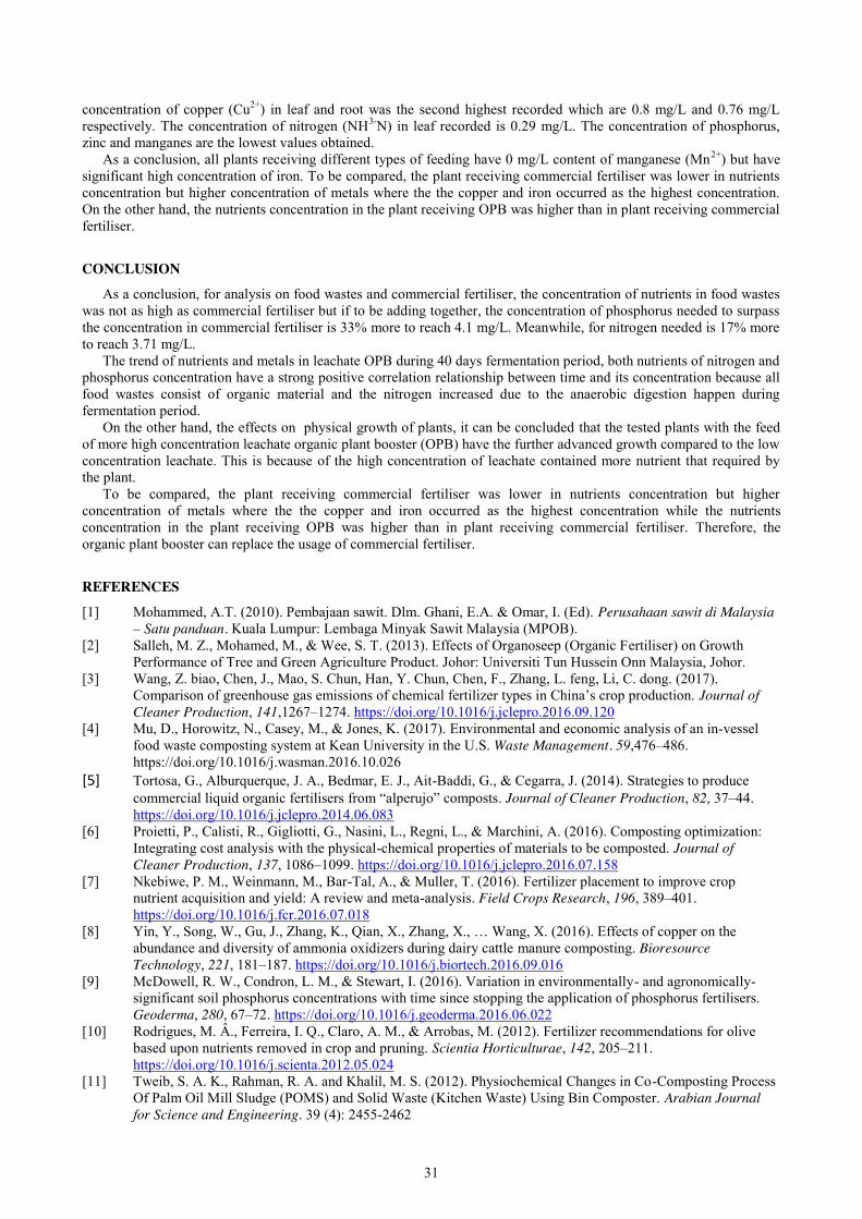
31

concentration of copper (Cu2+) in leaf and root was the second highest recorded which are 0.8 mg/L and 0.76 mg/L respectively. The concentration of nitrogen (NH3-N) in leaf recorded is 0.29 mg/L. The concentration of phosphorus, zinc and manganes are the lowest values obtained.

As a conclusion, all plants receiving different types of feeding have 0 mg/L content of manganese (Mn2+) but have significant high concentration of iron. To be compared, the plant receiving commercial fertiliser was lower in nutrients concentration but higher concentration of metals where the the copper and iron occurred as the highest concentration. On the other hand, the nutrients concentration in the plant receiving OPB was higher than in plant receiving commercial fertiliser.

CONCLUSION

As a conclusion, for analysis on food wastes and commercial fertiliser, the concentration of nutrients in food wastes was not as high as commercial fertiliser but if to be adding together, the concentration of phosphorus needed to surpass the concentration in commercial fertiliser is 33% more to reach 4.1 mg/L. Meanwhile, for nitrogen needed is 17% more to reach 3.71 mg/L.

The trend of nutrients and metals in leachate OPB during 40 days fermentation period, both nutrients of nitrogen and phosphorus concentration have a strong positive correlation relationship between time and its concentration because all food wastes consist of organic material and the nitrogen increased due to the anaerobic digestion happen during fermentation period.

On the other hand, the effects on physical growth of plants, it can be concluded that the tested plants with the feed of more high concentration leachate organic plant booster (OPB) have the further advanced growth compared to the low concentration leachate. This is because of the high concentration of leachate contained more nutrient that required by the plant.

To be compared, the plant receiving commercial fertiliser was lower in nutrients concentration but higher concentration of metals where the the copper and iron occurred as the highest concentration while the nutrients concentration in the plant receiving OPB was higher than in plant receiving commercial fertiliser. Therefore, the organic plant booster can replace the usage of commercial fertiliser.

REFERENCES

[1] Mohammed, A.T. (2010). Pembajaan sawit. Dlm. Ghani, E.A. & Omar, I. (Ed). Perusahaan sawit di Malaysia – Satu panduan. Kuala Lumpur: Lembaga Minyak Sawit Malaysia (MPOB).

[2] Salleh, M. Z., Mohamed, M., & Wee, S. T. (2013). Effects of Organoseep (Organic Fertiliser) on Growth Performance of Tree and Green Agriculture Product. Johor: Universiti Tun Hussein Onn Malaysia, Johor.

[3] Wang, Z. biao, Chen, J., Mao, S. Chun, Han, Y. Chun, Chen, F., Zhang, L. feng, Li, C. dong. (2017). Comparison of greenhouse gas emissions of chemical fertilizer types in China’s crop production. Journal of Cleaner Production, 141,1267–1274. https://doi.org/10.1016/j.jclepro.2016.09.120

[4] Mu, D., Horowitz, N., Casey, M., & Jones, K. (2017). Environmental and economic analysis of an in-vessel food waste composting system at Kean University in the U.S. Waste Management. 59,476–486. https://doi.org/10.1016/j.wasman.2016.10.026

[5] Tortosa, G., Alburquerque, J. A., Bedmar, E. J., Ait-Baddi, G., & Cegarra, J. (2014). Strategies to produce commercial liquid organic fertilisers from “alperujo” composts. Journal of Cleaner Production, 82, 37–44. https://doi.org/10.1016/j.jclepro.2014.06.083

[6] Proietti, P., Calisti, R., Gigliotti, G., Nasini, L., Regni, L., & Marchini, A. (2016). Composting optimization: Integrating cost analysis with the physical-chemical properties of materials to be composted. Journal of Cleaner Production, 137, 1086–1099. https://doi.org/10.1016/j.jclepro.2016.07.158

[7] Nkebiwe, P. M., Weinmann, M., Bar-Tal, A., & Muller, T. (2016). Fertilizer placement to improve crop nutrient acquisition and yield: A review and meta-analysis. Field Crops Research, 196, 389–401. https://doi.org/10.1016/j.fcr.2016.07.018

[8] Yin, Y., Song, W., Gu, J., Zhang, K., Qian, X., Zhang, X., … Wang, X. (2016). Effects of copper on the abundance and diversity of ammonia oxidizers during dairy cattle manure composting. Bioresource Technology, 221, 181–187. https://doi.org/10.1016/j.biortech.2016.09.016

[9] McDowell, R. W., Condron, L. M., & Stewart, I. (2016). Variation in environmentally- and agronomically-significant soil phosphorus concentrations with time since stopping the application of phosphorus fertilisers. Geoderma, 280, 67–72. https://doi.org/10.1016/j.geoderma.2016.06.022

[10] Rodrigues, M. Â., Ferreira, I. Q., Claro, A. M., & Arrobas, M. (2012). Fertilizer recommendations for olive based upon nutrients removed in crop and pruning. Scientia Horticulturae, 142, 205–211. https://doi.org/10.1016/j.scienta.2012.05.024

[11] Tweib, S. A. K., Rahman, R. A. and Khalil, M. S. (2012). Physiochemical Changes in Co-Composting Process Of Palm Oil Mill Sludge (POMS) and Solid Waste (Kitchen Waste) Using Bin Composter. Arabian Journal for Science and Engineering. 39 (4): 2455-2462

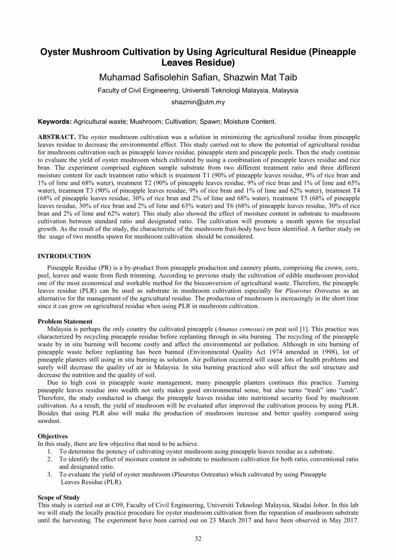
32

Oyster Mushroom Cultivation by Using Agricultural Residue (Pineapple Leaves Residue)

Muhamad Safisolehin Safian, Shazwin Mat Taib Faculty of Civil Engineering, Universiti Teknologi Malaysia, Malaysia

shazmin@utm.my

Keywords: Agricultural waste; Mushroom; Cultivation; Spawn; Moisture Content. ABSTRACT. The oyster mushroom cultivation was a solution in minimizing the agricultural residue from pineapple leaves residue to decrease the environmental effect. This study carried out to show the potential of agricultural residue for mushroom cultivation such as pineapple leaves residue, pineapple stem and pineapple peels. Then the study continue to evaluate the yield of oyster mushroom which cultivated by using a combination of pineapple leaves residue and rice bran. The experiment comprised eighteen sample substrate from two different treatment ratio and three different moisture content for each treatment ratio which is treatment T1 (90% of pineapple leaves residue, 9% of rice bran and 1% of lime and 68% water), treatment T2 (90% of pineapple leaves residue, 9% of rice bran and 1% of lime and 65% water), treatment T3 (90% of pineapple leaves residue, 9% of rice bran and 1% of lime and 62% water), treatment T4 (68% of pineapple leaves residue, 30% of rice bran and 2% of lime and 68% water), treatment T5 (68% of pineapple leaves residue, 30% of rice bran and 2% of lime and 63% water) and T6 (68% of pineapple leaves residue, 30% of rice bran and 2% of lime and 62% water). This study also showed the effect of moisture content in substrate to mushroom cultivation between standard ratio and designated ratio. The cultivation will promote a month spawn for mycelial growth. As the result of the study, the characteristic of the mushroom fruit-body have been identified. A further study on the usage of two months spawn for mushroom cultivation should be considered.

INTRODUCTION

Pineapple Residue (PR) is a by-product from pineapple production and cannery plants, comprising the crown, core, peel, leaves and waste from flesh trimming. According to previous study the cultivation of edible mushroom provided one of the most economical and workable method for the bioconversion of agricultural waste. Therefore, the pineapple leaves residue (PLR) can be used as substrate in mushroom cultivation especially for Plearotus Ostreatus as an alternative for the management of the agricultural residue. The production of mushroom is increasingly in the short time since it can grow on agricultural residue when using PLR in mushroom cultivation.

Problem Statement

Malaysia is perhaps the only country the cultivated pineapple (Ananas comosus) on peat soil [1]. This practice was characterized by recycling pineapple residue before replanting through in situ burning. The recycling of the pineapple waste by in situ burning will become costly and affect the environmental air pollution. Although in situ burning of pineapple waste before replanting has been banned (Environmental Quality Act 1974 amended in 1998), lot of pineapple planters still using in situ burning as solution. Air pollution occurred will cause lots of health problems and surely will decrease the quality of air in Malaysia. In situ burning practiced also will affect the soil structure and decrease the nutrition and the quality of soil.

Due to high cost in pineapple waste management, many pineapple planters continues this practice. Turning pineapple leaves residue into wealth not only makes good environmental sense, but also turns “trash” into “cash”. Therefore, the study conducted to change the pineapple leaves residue into nutritional security food by mushroom cultivation. As a result, the yield of mushroom will be evaluated after improved the cultivation process by using PLR. Besides that using PLR also will make the production of mushroom increase and better quality compared using sawdust.

Objectives In this study, there are few objective that need to be achieve.

1. To determine the potency of cultivating oyster mushroom using pineapple leaves residue as a substrate. 2. To identify the effect of moisture content in substrate to mushroom cultivation for both ratio, conventional ratio

and designated ratio. 3. To evaluate the yield of oyster mushroom (Pleurotus Ostreatus) which cultivated by using Pineapple

Leaves Residue (PLR).

Scope of Study This study is carried out at C09, Faculty of Civil Engineering, Universiti Teknologi Malaysia, Skudai Johor. In this lab we will study the locally practice procedure for oyster mushroom cultivation from the reparation of mushroom substrate until the harvesting. The experiment have been carried out on 23 March 2017 and have been observed in May 2017.

33

The pineapple leaves residue was manually collected in Pusat Pembangunan Teknologi Tanaman Nanas, Pekan Nanas Pontian Johor. The pineapple leaves residue was shredded using shredder machine. The pineapple leaves residue will combined with rice bran and lime hydrated agriculture. Eighteen treatment samples will be prepare with two different ratio. Each treatment ratio will have three types of moisture content and the production of mushroom will be evaluate whether high or low. After that, identification of potential different performance flow in process of mushroom cultivation will take place to improved the yield of mushroom.

LITERATURE REVIEW

The pineapple or also called as (Ananas Comosus) was rated as one of the most important fruits in the world and is the leading member in the family of Bromeliaceous. Pineapple juice is the third most preferred worldwide after orange juices and apple juices [2]. Pineapple plant can grow up height of 75-150 cm with spread of 90-120 cm. Pineapple got a very short, stout stem and strap-like leaves with long pointed (50-180 cm). Pineapple leaves usually needle tipped and generally bearing sharp, up-curved spines on the margins. The leaves may be all green or in variously stripped with red, yellow, orange or ivory down the middle or near the margins. The steam elongates and enlarge near the apex in the blooming time. The plant producess a cone-shaped, juicy and fleshy yellowish fruit with crown at the top of the fruit [3].

Pineapple by-products from industries they consist basically of the residual pulp, stem, leaves and peels. Massive waste generated with the increasing production of the pineapple processed items. This is due to the elimination and selection of parts that are inconsumable by human. Moreover rough handling of pineapple fruit, exposure to adverse environment during storage and transportation can lead to 55% of product waste [4]. During the process of pineapple fruit, large amount of unusable waste material are generated [5]. Studies have shown that 40 percent to 80 percent of pineapple fruit is discarded as waste having high biological oxygen demand (BOD) and chemical oxygen demand (COD) values [6].

Pineapple residue may cause environmental problems since it were accumulated in agriculture industrial yards having no proper treatment and without no commercial value. Since the disposal of pineapple wastes is expensive due to high costs of transportation and the limited of landfills, they are disposed using inappropriate ways causing concern as environmental problems. Another illegal ways that they use as method for waste disposal is in situ burning which causing the air pollution. Another problem in disposing by-products waste is further aggravated by legal restrictions. The high content of BOD and COD in pineapple residue make it more difficult to be dispose.

Many research have been done by the researcher around the globe in using and utilize the discarded fruit and waste material for further industrial process like extraction of bioactive component, fermentation, etc. Some effort have been done on pineapple residue to be use that has been obtained from different sources. Pineapple residue got a lot of used such as the substrate for organic acids, bromelain, etc. because these things are potential source of sugar, growth factors and vitamins [7], [8], [9]. There has been numerous work that have been carried out on trying to explore the possibility in fully utilize the pineapple residue.

Mushroom is one of the neutral food source, has been valued as edible, and provision for humankind. With the increasing popularity of mushroom industrial and farming, mushroom production continues to grow worldwide progressively [10]. There was a lot of progress in mushroom cultivation and science and biotechnology in the last decade. Some of the agricultural residue that have been used in mushroom cultivation is Empty Fruit Bunch (EFB) and Fermented Bamboo Sawdust (FBS). Mushroom contain 90% water and 10% dry matter. The protein content varies between 27% and 48%, carbohydrates are less than 60%, and lipids 2-8% [11]. Mushroom process involves different stage of operation, each stage must be carefully performed. First step is to get a pure mycelium of specific mushroom strain. The mycelium will be purchase from the supplier. After the spawn material has been prepared, the compost will be fill into the substrate. For this experiment, we used a month spawn rather than two months. A month spawn take about 30 to 45 days to fruiting the bodies.

METHODOLOGY

In this study, they are 4 stages that included in mushroom cultivation using Pineapple Leaves Residue (PLR). Each stage comprises different process and activities. For first stage, the study was about to identify the potential agricultural waste for mushroom cultivation. PLR has special characteristic such as macronutrients suitable for mushroom cultivation. PLR also was one of the waste that many pineapple planters neglected and do the in situ burning on their farm. For second stage is to compare between the design ratio and Malaysian standard ratio suitable for mushroom cultivation. There are procedure for preparation and handling of the mushroom cultivation process. Then for third stage involved the process to evaluate the yield of oyster mushroom (Pleurotus Ostreatus) which cultivated by using Pineapple Leaves Residue (PLR). Lastly, will be the conclusion and recommendation of the study for future study. Agricultural residue Preparation (Pineapple leaves residue). Pineapple leaves used in this study was obtained from residues after harvesting pineapple collected from Muzium Nanas, Pontian, Johor. Approximately 25 kg of sample from the leaves of different varieties of pineapple plants were picked randomly at the same time. The pineapple leaves and stems were manually chopped and has been shredded using shredder machine. Shredded pineapple leaves residue was

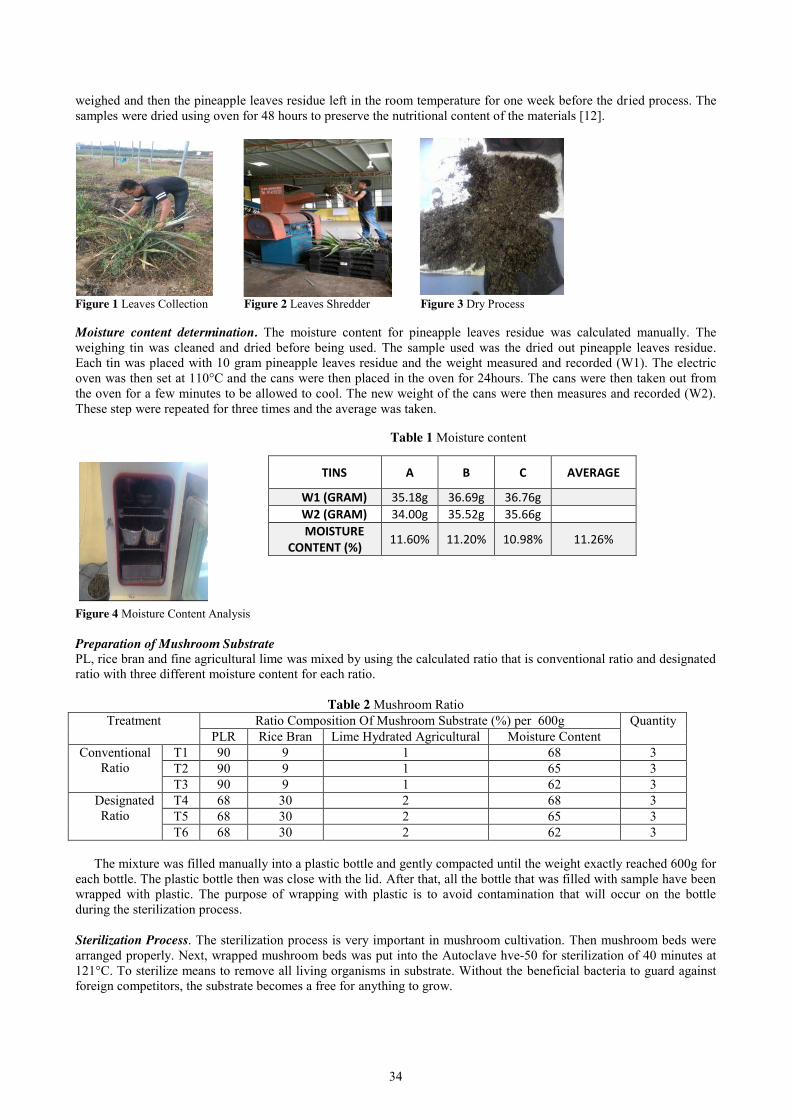
34

weighed and then the pineapple leaves residue left in the room temperature for one week before the dried process. The samples were dried using oven for 48 hours to preserve the nutritional content of the materials [12].

Figure 1 Leaves Collection Figure 2 Leaves Shredder Figure 3 Dry Process Moisture content determination. The moisture content for pineapple leaves residue was calculated manually. The weighing tin was cleaned and dried before being used. The sample used was the dried out pineapple leaves residue. Each tin was placed with 10 gram pineapple leaves residue and the weight measured and recorded (W1). The electric oven was then set at 110°C and the cans were then placed in the oven for 24hours. The cans were then taken out from the oven for a few minutes to be allowed to cool. The new weight of the cans were then measures and recorded (W2). These step were repeated for three times and the average was taken.

Figure 4 Moisture Content Analysis Preparation of Mushroom Substrate PL, rice bran and fine agricultural lime was mixed by using the calculated ratio that is conventional ratio and designated ratio with three different moisture content for each ratio.

Table 2 Mushroom Ratio Treatment Ratio Composition Of Mushroom Substrate (%) per 600g Quantity

PLR Rice Bran Lime Hydrated Agricultural Moisture Content Conventional

Ratio T1 90 9 1 68 3 T2 90 9 1 65 3 T3 90 9 1 62 3

Designated Ratio

T4 68 30 2 68 3 T5 68 30 2 65 3 T6 68 30 2 62 3

The mixture was filled manually into a plastic bottle and gently compacted until the weight exactly reached 600g for

each bottle. The plastic bottle then was close with the lid. After that, all the bottle that was filled with sample have been wrapped with plastic. The purpose of wrapping with plastic is to avoid contamination that will occur on the bottle during the sterilization process. Sterilization Process. The sterilization process is very important in mushroom cultivation. Then mushroom beds were arranged properly. Next, wrapped mushroom beds was put into the Autoclave hve-50 for sterilization of 40 minutes at 121°C. To sterilize means to remove all living organisms in substrate. Without the beneficial bacteria to guard against foreign competitors, the substrate becomes a free for anything to grow.

TINS A B C AVERAGE

W1 (GRAM) 35.18g 36.69g 36.76g W2 (GRAM) 34.00g 35.52g 35.66g MOISTURE

CONTENT (%) 11.60% 11.20% 10.98% 11.26%

Table 1 Moisture content

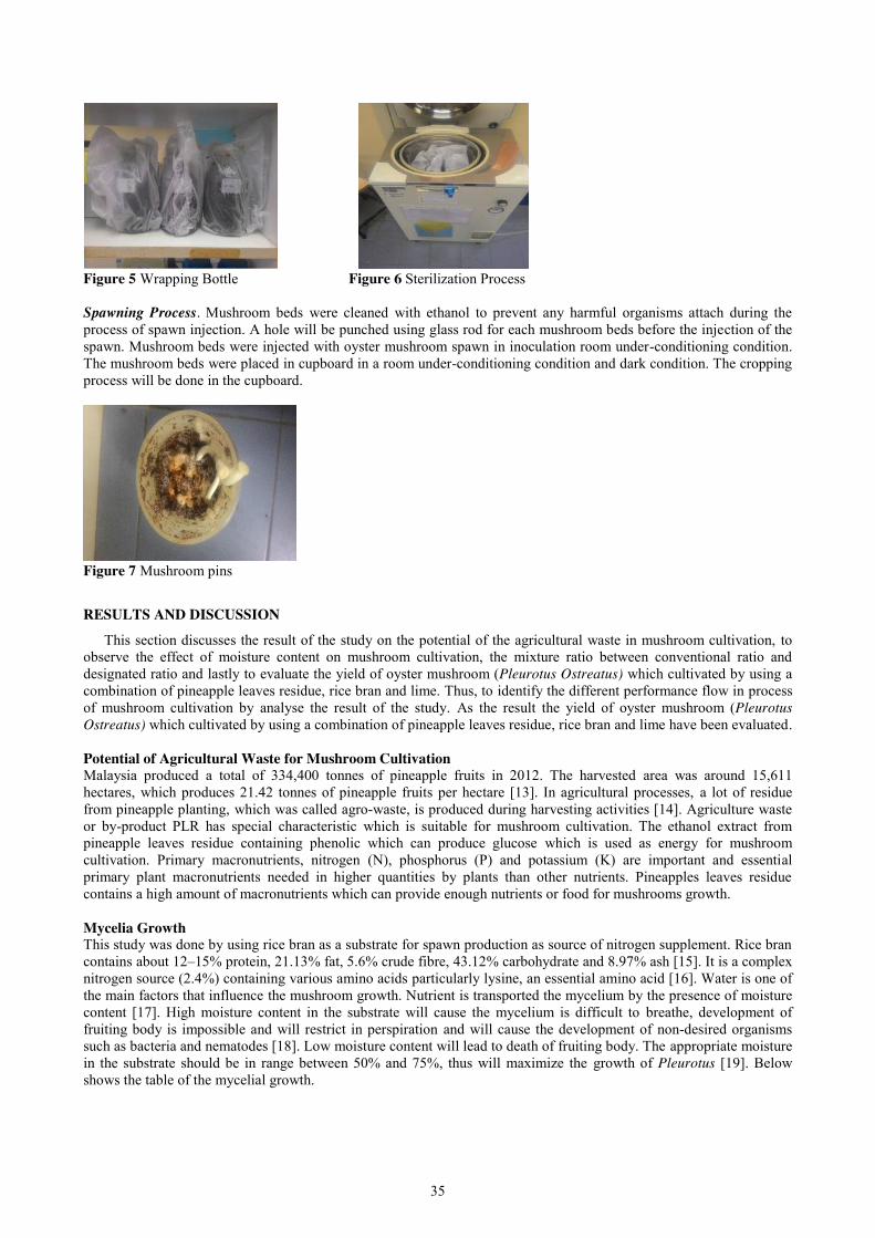
35

Figure 5 Wrapping Bottle Figure 6 Sterilization Process Spawning Process. Mushroom beds were cleaned with ethanol to prevent any harmful organisms attach during the process of spawn injection. A hole will be punched using glass rod for each mushroom beds before the injection of the spawn. Mushroom beds were injected with oyster mushroom spawn in inoculation room under-conditioning condition. The mushroom beds were placed in cupboard in a room under-conditioning condition and dark condition. The cropping process will be done in the cupboard.

Figure 7 Mushroom pins

RESULTS AND DISCUSSION

This section discusses the result of the study on the potential of the agricultural waste in mushroom cultivation, to observe the effect of moisture content on mushroom cultivation, the mixture ratio between conventional ratio and designated ratio and lastly to evaluate the yield of oyster mushroom (Pleurotus Ostreatus) which cultivated by using a combination of pineapple leaves residue, rice bran and lime. Thus, to identify the different performance flow in process of mushroom cultivation by analyse the result of the study. As the result the yield of oyster mushroom (Pleurotus Ostreatus) which cultivated by using a combination of pineapple leaves residue, rice bran and lime have been evaluated. Potential of Agricultural Waste for Mushroom Cultivation Malaysia produced a total of 334,400 tonnes of pineapple fruits in 2012. The harvested area was around 15,611 hectares, which produces 21.42 tonnes of pineapple fruits per hectare [13]. In agricultural processes, a lot of residue from pineapple planting, which was called agro-waste, is produced during harvesting activities [14]. Agriculture waste or by-product PLR has special characteristic which is suitable for mushroom cultivation. The ethanol extract from pineapple leaves residue containing phenolic which can produce glucose which is used as energy for mushroom cultivation. Primary macronutrients, nitrogen (N), phosphorus (P) and potassium (K) are important and essential primary plant macronutrients needed in higher quantities by plants than other nutrients. Pineapples leaves residue contains a high amount of macronutrients which can provide enough nutrients or food for mushrooms growth. Mycelia Growth This study was done by using rice bran as a substrate for spawn production as source of nitrogen supplement. Rice bran contains about 12–15% protein, 21.13% fat, 5.6% crude fibre, 43.12% carbohydrate and 8.97% ash [15]. It is a complex nitrogen source (2.4%) containing various amino acids particularly lysine, an essential amino acid [16]. Water is one of the main factors that influence the mushroom growth. Nutrient is transported the mycelium by the presence of moisture content [17]. High moisture content in the substrate will cause the mycelium is difficult to breathe, development of fruiting body is impossible and will restrict in perspiration and will cause the development of non-desired organisms such as bacteria and nematodes [18]. Low moisture content will lead to death of fruiting body. The appropriate moisture in the substrate should be in range between 50% and 75%, thus will maximize the growth of Pleurotus [19]. Below shows the table of the mycelial growth.

36

Table 3 Mycelial Growth Conventional

Ratio (PLR 90%)

Moisture 68% 65% 62% Treatment T1 (a) T1 (b) T1 (c) T2 (a) T2 (b) T2 (c) T3 (a) T3 (b) T3 (c)

Days 50 51 50 52 52 53 55 57 56 Designated

Ratio (PLR 68%)

Moisture 68% 65% 62% Treatment T4 (a) T4 (b) T4 (c) T5 (a) T5 (b) T5 (c) T6 (a) T6 (b) T6 (c)

Days 37 34 32 39 37 38 43 41 45

Based on Table 3 shows that treatment that used 68% moisture content have the shorter time for the mycelial to cover all around the bottle compare to the 65% moisture content and 62% moisture content. Between 90% PLR and 68% PLR, using 68% PLR along 68% moisture are the most suitable moisture for the mushroom cultivation. Mushroom Yield The yield of mushroom was covered during the day 45. Its shows that all the sample has produce number of mushroom. Table 4 shows the growth characteristics and yield of oyster mushroom on different substrate ratio.

Table 4: Number of ‘pins’ of oyster mushroom on 1st Flush Conventional

Ratio (PLR 90%)

Moisture 68% 65% 62% Treatment T1 (a) T1 (b) T1 (c) T2 (a) T2 (b) T2 (c) T3 (a) T3 (b) T3 (c)

1st flush 2 2 - - - - - - - Designated

Ratio (PLR 68%)

Moisture 68% 65% 62% Treatment T4 (a) T4 (b) T4 (c) T5 (a) T5 (b) T5 (c) T6 (a) T6 (b) T6 (c)

1st flush 10 11 13 7 9 - 6 5 4

Based on Table 4 shows that mostly each treatment has produce an oyster mushroom except for treatment T2 and T3 for 1st flush after 45 days of mycelia growth. The highest yield production are on treatment T4 which all three samples value with 10,11 and 13 number of pins, respectively. The yield of mushroom in different substrate ratio will indirectly contributed to the different in nutrient content, C/N ratio and the pH value [19].

CONCLUSION

For last stage, the processes are to make documentation for this study which is included with the detailed of study and will be end with conclusion and recommendation for future study. This study about oyster mushroom cultivation by using nutritional's agricultural waste for food security. As mentioned earlier in the introduction, the following conclusions can be drawn based on the findings of the study:

1) To identify the potential of agricultural residue for mushroom cultivation The agricultural waste that contain macronutrients, nitrogen (N), phosphorus (P) and potassium (K) are important and essential primary plant macronutrients needed in higher quantities by plants than other nutrients. Pineapples leaves residue contains high amount of macronutrients which can provide enough nutrients or food for mushrooms growth. The waste have nutrient that can utilize in mushroom cultivation or for crops field. Furthermore, by using agricultural residue will secured our food chain and enhance our food security.

2) To identify the effect of moisture content in substrate to mushroom cultivation for both ratio, conventional ratio and designated ratio. As we can see from the result, the moisture content will effect the duration of mycelial growth. From the previous study shows that the appropriate moisture in the substrate should be in range between 50% and 75%, thus will maximize the growth of mycelial. The observation shows that the 68% of moisture content have the best platform for the mycelial growth all around the bottle in a short time thus it will increase the production of the mushroom.

3) To evaluate the yield of Oyster mushroom (Pleurotus Ostreatus) which cultivated by using a combination of pineapple leaves residue (PLR) and rice bran. The waste from agricultural waste or by-product of pineapple, such as Pineapple Leaves Residue (PLR) can cultivate the Oyster Mushroom. Cultivation of oyster mushroom also can increase the economic country since the high demanding market. The residue product of pineapple also can be a valuable product rather than just mulching and dump the waste into ground surface. By recycling the waste from pineapple plantation, the depletion of air pollution to the environment can be controlled.

37

REFERENCES

[1] O. H. AHMED, M. H. A. H. A. R. A. &. M. M. H., 2001. Some Observations in Pineapple Production under Different Fertilizer Programmes and Different Pineapple Residue Management Practices, Selangor: Faculty of Agriculture,Universiti Putra Malaysia,43400 Serdang, Selangor, Malaysia.

[2] Cabrera H.A.P., Menezes H.C., Oliveira J.V. and Batista R.F.S. (2000). Evaluation of residual levels of benomyl, methyl parathion, diuron, and vamidothion in Pineapple Pulp and Bagasse (Smooth Cayenne),. J. Agric. FoodChem. 48: 5750-5753.

[3] Morton J. (1987). Pineapple. In: J.F. Morton (Ed.), Fruits of Warm Climates, Miami, FL, pp. 18–28. [4] Nunes M.C.N., Emond J.P., Rauth M., Dea S. and Chau K. V. (2009). Environmental conditions

encountered during typical consumer retail display affect fruit and vegetable quality and waste. Postharvest Biology and Technology. 51: 232-241.

[5] Tanaka K., Hilary Z. D. and Ishizaki A. (1999).Investigation of the utility of pineapple juice and pineapple waste material as low cost substrate for ethanol fermentation by Zymomonasmobilis. Journal of Bioscience and Bioengineering, 87: 642-646.

[6] Ban-Koffi, L. and Han, Y.W. (1990). Alcohol production from pineapple waste. World Journal of Microbiology and Biotechnology, 6: 281-284.

[7] Larrauri J A, Ruperez P. and Calixto F. S. (1997). Pineapple shell as a source of dietary fiber with associated polyphenols. Journal of Agricultural and Food Chemistry, 45: 4028-4031.

[8] Nigam J.N. (1999b). Continuous cultivation of the yeast Candida utilis at different dilution rates on pineapple cannery waste. World Journal of Microbiology & Biotechnology, 15: 115-117.

[9] Dacera D.D.M., Babel S. and Parkpian P. (2009). Potential for land application of contaminated sewage sludge treated with fermentaed liquid from pineapple wastes. Journal of Hazardous Materials, 167: 866-872.

[10] Kavitha, B., Rajannan and Jothimani. 2013. “Utilization of Empty Fruit Bunches of Oil Palm as Alternate Substrate for The Cultivationof Mushroom”. International Journal of Science, Environment and Technology, Vol. 2(5): 839-846.

[11] Rejo, E. S., 2013. Tanam Cendawan Sebaga Sumber Pertanian. Seminar Perkongsian Hasil Penyelidikan Dan Potensi Perniagaan Maktab Koperasi Malaysia, pp. pg 189-212

[12] Tran A V. (2006). Chemical analysis and pulping study of pineapple crown leaves. Industrial Crops and Products, 24: 66-74.

[13] Food and Agriculture Organization of the United Nations. Retrived 25 February, 2014. http://faostat3.fao.org/faostatgateway/

[14] Wan Mohd Aznan and Zainuddin Zakaria, 2013. Pineapple Leaf Fibre (PALF): From Western to Wealth. JURUTERA 18-20.

[15] Jiamyangyuen, S., V. Srijesdaruk, and W.J. Harper. 2005. Extraction of rice bran protein concentrate and its applicationin bread. Songklanakarin Journal of Science and Technology 27: 55–64.

[16] Kahlon, T.S. 2009. Rice bran: production, composition, functionality and food applications, physiological benefits. In Fiber ingredients: food applications and health benefits, ed. S.S. Cho, and P. Samuel, 305–321. Boca Raton: CRC Press.

[17] Oei, P., Nieuwenhuijzen, B.V., 2005. Small-scale Mushroom Cultivation: Oyster, Shiitake and Wood Ear Mushrooms. Agromisa Foundation and CTA, Wageningen.

[18] Urben, A.F., 2004. Produc¸a˜o de cogumelos por meio de tecnologia chinesa modificada. Embrapa Recursos Gene´ticos e Biotecnologia, Brası´lia (in Portuguese).

[19] Chang, S.T., Miles, P.G., 2004. Mushrooms: Cultivation, Nutritional Value Medicinal Effect and Environmental Impact. CRC Press, Boca Raton.

38

Biodegradation of Remazol Brilliant Violet 5r Dye Using Selected Fungus

Muhamad Salih Salim, Salmiati

Faculty of Civil Engineering, Universiti Teknologi Malaysia, Malaysia

salmiati@utm.my

Keywords: Remazol Brilliant Violet 5r; Decolorization; 18s rNA; Trichoderma Reesei

ABSTRACT. Most of the industries especially textile industry is the major contribution to the disposal of toxic dye into water. The dyes are hardly removed from conventional biological, physical and chemical treatment. So, this dye should be treated and removed from wastewater in an economical and efficient way. Remazol Brilliant Violet 5r dye is one of them.The use of fungi and their extracellular enzymes are currently an effective solution for removal of synthetic dye containing wastewater. This study was conducted to determine best fungi that that degrade and decolorize Remazol Brilliant Violet 5r dye.Remazol Brilliant Violet 5r dye is an azo dye and one of the most difficult dyes to be degraded. In this study, six different types of fungi were isolated from UTM orchard and labelled as K003, K003i, KB006, H002, 2 and 7. These fungi were screened for their ability to degrade Remazol Brilliant Violet 5r dye after 10 and 20 days of incubation. HOO2 fungus was chosen as best fungus based on the ability to decolorize 50 ppm Remazol Brilliant Violet 5r dye on liquid medium. The effect of environmental factors such as pH, initial concentration of Remazol Brilliant Violet 5r dye, carbon sources, nitrogen source and agitation were further investigated. The decolorizations of Remazol Brilliant Violet 5r dye were analyzed by using UV-vis spectrophotometer. The optimum pH for decolorizing activity was recorded at pH 5 (56.25%). H002 fungus showed efficient decolorization as glucose and yeast extract were act as carbon and nitrogen source at 57.92% and 57.29%, respectively. Maximum decolorization achieved at 40 ppm initial dye concentration (63.89%). Factor of agitation does not give impact on decolorization of Remazol Brilliant Violet 5r dye. H002 fungi was then identified using 18s rRNA sequence analysis method. From the phylogenetic tree, fungi H002 belong to Trichoderma Reesei. As conclusion, H002 have the capability to degrade Remazol Brilliant Violet 5r dye. For further investigation, several experiments can be carried out to enhance the use of isolated fungi in textile wastewater treatment.

INTRODUCTION Most of the industries especially textile industry is the major contribution to the disposal of toxic dye into the water.

The use of fungi and/or their extracellular enzymes are currently an effective solution for removal of synthetic dye containing wastewater [1]. The dyes are hardly removed from wastewater by conventional biological, physical, or chemical treatment. It is really important to remove dyes in wastewater because dyes are very toxic and are characterized by high chemical oxygen demand, biological oxygen demand, and highly aromatic conjugated and carcinogenic that can endanger human life [2].

Remazol Brilliant Violet 5r is one of the reactive azo dye group that being dispelled into the river. This synthetic Remazol Brilliant Violet 5r dye has been extensively used in textile industries around the world that producing dying cotton, woolen, and nylon fabric.Azo-based dye contained chromophore and different types of reactive groups such as chlorotriazine, trichloropyrimidine, and difluorochloropyrimidine. Azo dyes are the largest and most versatile class of dyes and account for more than 50% of the dyes produced annually [3].

There are a lot of treatments for decolorization of dyes such as electrocoagulation technique, coagulation– flocculation, and adsorption. Most of these technologies, however suffer from several shortcomings, including high amount sludge generation, requirements of high cost of chemical and techniques [4]. Extensive studies on biodegradation of synthetic dyes by fungi have been done by many researchers. Fungi are capable to degrade dyes from industial effluents.

The purpose of this study is to screening the fungi that have ability to degrade Remazol Brilliant Violet 5r and to investigate the optimum parameters for the growth of fungi thus maximized the decolorization of Remazol Brilliant Violet 5r dye. Problem Statement The release of dyes into wastewaters by various industries poses serious environmental problems due to various dyes’ persistent and recalcitrant nature. In Malaysia, a lot of industries including the textile industries also increased the water pollution level. Statically shows, in 2006, there were more than 68,000 worker employed by 645 licensed textile and apparel companies in Malaysia. The industry is mainly clustered in Johor and Penang [5]. From this industry, the water pollution has become worst especially in colour point of view. The effluent from the textile industry has a high level of colour concentration. Because of this, the best water treatment process is needed to encounter this pollution problem so that the best result will be achieved.

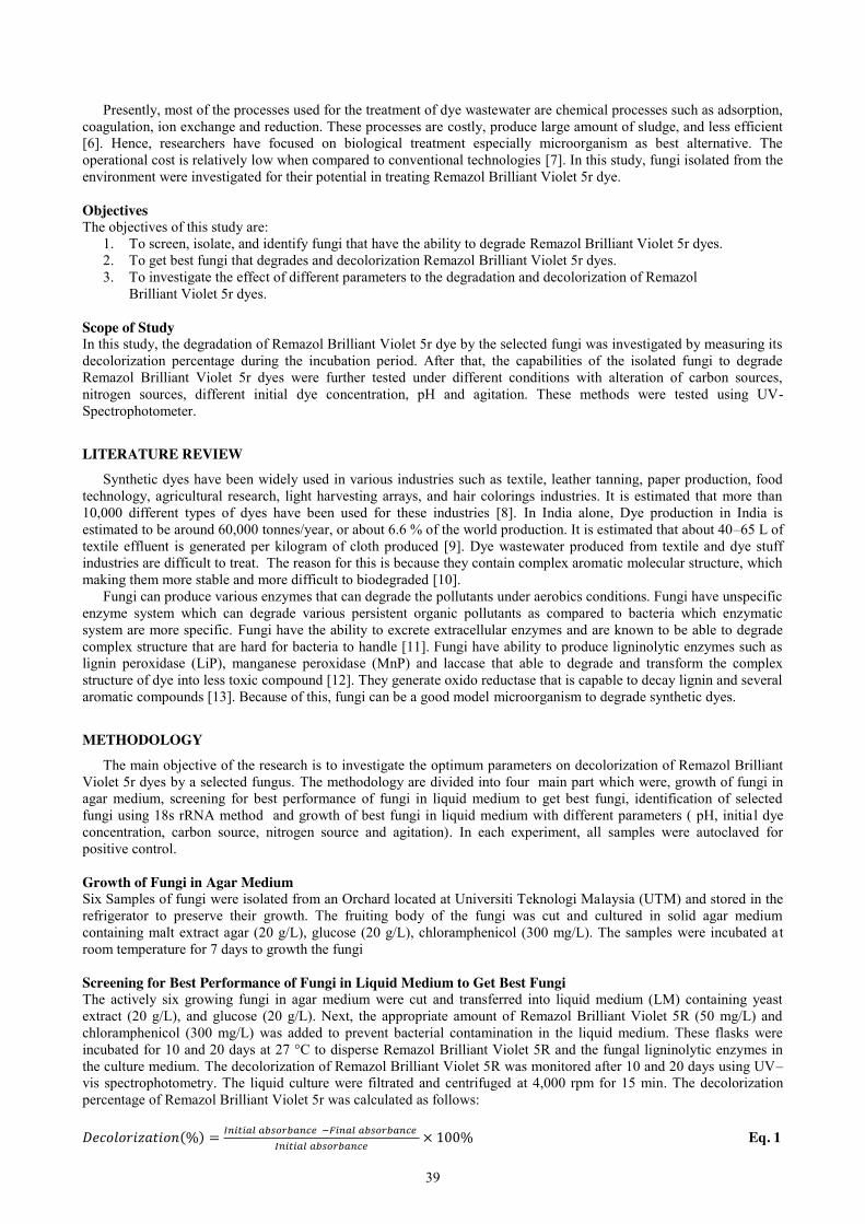
39

Presently, most of the processes used for the treatment of dye wastewater are chemical processes such as adsorption, coagulation, ion exchange and reduction. These processes are costly, produce large amount of sludge, and less efficient [6]. Hence, researchers have focused on biological treatment especially microorganism as best alternative. The operational cost is relatively low when compared to conventional technologies [7]. In this study, fungi isolated from the environment were investigated for their potential in treating Remazol Brilliant Violet 5r dye. Objectives The objectives of this study are:

1. To screen, isolate, and identify fungi that have the ability to degrade Remazol Brilliant Violet 5r dyes. 2. To get best fungi that degrades and decolorization Remazol Brilliant Violet 5r dyes. 3. To investigate the effect of different parameters to the degradation and decolorization of Remazol

Brilliant Violet 5r dyes. Scope of Study In this study, the degradation of Remazol Brilliant Violet 5r dye by the selected fungi was investigated by measuring its decolorization percentage during the incubation period. After that, the capabilities of the isolated fungi to degrade Remazol Brilliant Violet 5r dyes were further tested under different conditions with alteration of carbon sources, nitrogen sources, different initial dye concentration, pH and agitation. These methods were tested using UV-Spectrophotometer.

LITERATURE REVIEW Synthetic dyes have been widely used in various industries such as textile, leather tanning, paper production, food

technology, agricultural research, light harvesting arrays, and hair colorings industries. It is estimated that more than 10,000 different types of dyes have been used for these industries [8]. In India alone, Dye production in India is estimated to be around 60,000 tonnes/year, or about 6.6 % of the world production. It is estimated that about 40–65 L of textile effluent is generated per kilogram of cloth produced [9]. Dye wastewater produced from textile and dye stuff industries are difficult to treat. The reason for this is because they contain complex aromatic molecular structure, which making them more stable and more difficult to biodegraded [10].

Fungi can produce various enzymes that can degrade the pollutants under aerobics conditions. Fungi have unspecific enzyme system which can degrade various persistent organic pollutants as compared to bacteria which enzymatic system are more specific. Fungi have the ability to excrete extracellular enzymes and are known to be able to degrade complex structure that are hard for bacteria to handle [11]. Fungi have ability to produce ligninolytic enzymes such as lignin peroxidase (LiP), manganese peroxidase (MnP) and laccase that able to degrade and transform the complex structure of dye into less toxic compound [12]. They generate oxido reductase that is capable to decay lignin and several aromatic compounds [13]. Because of this, fungi can be a good model microorganism to degrade synthetic dyes.

METHODOLOGY

The main objective of the research is to investigate the optimum parameters on decolorization of Remazol Brilliant Violet 5r dyes by a selected fungus. The methodology are divided into four main part which were, growth of fungi in agar medium, screening for best performance of fungi in liquid medium to get best fungi, identification of selected fungi using 18s rRNA method and growth of best fungi in liquid medium with different parameters ( pH, initial dye concentration, carbon source, nitrogen source and agitation). In each experiment, all samples were autoclaved for positive control. Growth of Fungi in Agar Medium Six Samples of fungi were isolated from an Orchard located at Universiti Teknologi Malaysia (UTM) and stored in the refrigerator to preserve their growth. The fruiting body of the fungi was cut and cultured in solid agar medium containing malt extract agar (20 g/L), glucose (20 g/L), chloramphenicol (300 mg/L). The samples were incubated at room temperature for 7 days to growth the fungi Screening for Best Performance of Fungi in Liquid Medium to Get Best Fungi The actively six growing fungi in agar medium were cut and transferred into liquid medium (LM) containing yeast extract (20 g/L), and glucose (20 g/L). Next, the appropriate amount of Remazol Brilliant Violet 5R (50 mg/L) and chloramphenicol (300 mg/L) was added to prevent bacterial contamination in the liquid medium. These flasks were incubated for 10 and 20 days at 27 °C to disperse Remazol Brilliant Violet 5R and the fungal ligninolytic enzymes in the culture medium. The decolorization of Remazol Brilliant Violet 5R was monitored after 10 and 20 days using UV–vis spectrophotometry. The liquid culture were filtrated and centrifuged at 4,000 rpm for 15 min. The decolorization percentage of Remazol Brilliant Violet 5r was calculated as follows:

𝐷𝑒𝑐𝑜𝑙𝑜𝑟𝑖𝑧𝑎𝑡𝑖𝑜𝑛(%) = 𝐼𝑛𝑖𝑡𝑖𝑎𝑙 𝑎𝑏𝑠𝑜𝑟𝑏𝑎𝑛𝑐𝑒 −𝐹𝑖𝑛𝑎𝑙 𝑎𝑏𝑠𝑜𝑟𝑏𝑎𝑛𝑐𝑒

𝐼𝑛𝑖𝑡𝑖𝑎𝑙 𝑎𝑏𝑠𝑜𝑟𝑏𝑎𝑛𝑐𝑒× 100% Eq. 1

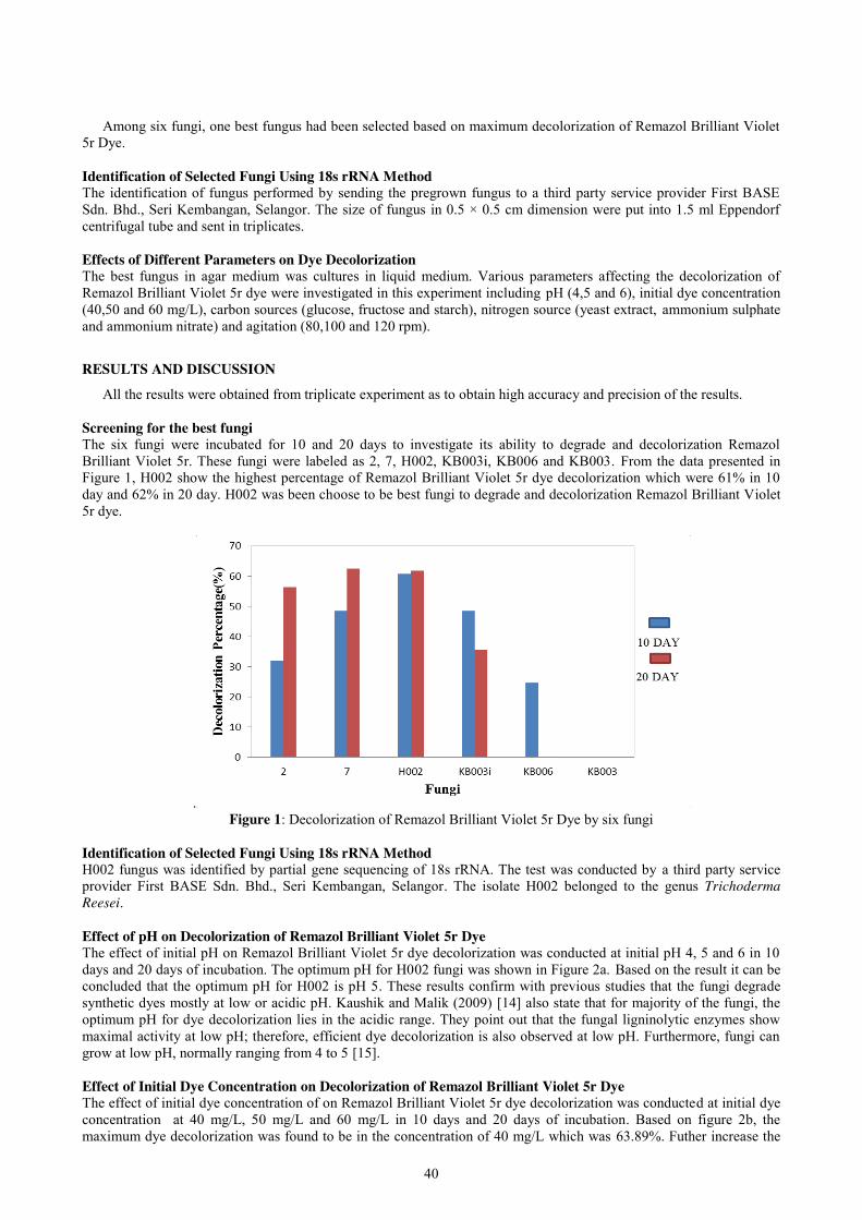
40

Among six fungi, one best fungus had been selected based on maximum decolorization of Remazol Brilliant Violet

5r Dye. Identification of Selected Fungi Using 18s rRNA Method The identification of fungus performed by sending the pregrown fungus to a third party service provider First BASE Sdn. Bhd., Seri Kembangan, Selangor. The size of fungus in 0.5 × 0.5 cm dimension were put into 1.5 ml Eppendorf centrifugal tube and sent in triplicates. Effects of Different Parameters on Dye Decolorization The best fungus in agar medium was cultures in liquid medium. Various parameters affecting the decolorization of Remazol Brilliant Violet 5r dye were investigated in this experiment including pH (4,5 and 6), initial dye concentration (40,50 and 60 mg/L), carbon sources (glucose, fructose and starch), nitrogen source (yeast extract, ammonium sulphate and ammonium nitrate) and agitation (80,100 and 120 rpm).

RESULTS AND DISCUSSION

All the results were obtained from triplicate experiment as to obtain high accuracy and precision of the results. Screening for the best fungi The six fungi were incubated for 10 and 20 days to investigate its ability to degrade and decolorization Remazol Brilliant Violet 5r. These fungi were labeled as 2, 7, H002, KB003i, KB006 and KB003. From the data presented in Figure 1, H002 show the highest percentage of Remazol Brilliant Violet 5r dye decolorization which were 61% in 10 day and 62% in 20 day. H002 was been choose to be best fungi to degrade and decolorization Remazol Brilliant Violet 5r dye.

. Figure 1: Decolorization of Remazol Brilliant Violet 5r Dye by six fungi

Identification of Selected Fungi Using 18s rRNA Method H002 fungus was identified by partial gene sequencing of 18s rRNA. The test was conducted by a third party service provider First BASE Sdn. Bhd., Seri Kembangan, Selangor. The isolate H002 belonged to the genus Trichoderma Reesei. Effect of pH on Decolorization of Remazol Brilliant Violet 5r Dye The effect of initial pH on Remazol Brilliant Violet 5r dye decolorization was conducted at initial pH 4, 5 and 6 in 10 days and 20 days of incubation. The optimum pH for H002 fungi was shown in Figure 2a. Based on the result it can be concluded that the optimum pH for H002 is pH 5. These results confirm with previous studies that the fungi degrade synthetic dyes mostly at low or acidic pH. Kaushik and Malik (2009) [14] also state that for majority of the fungi, the optimum pH for dye decolorization lies in the acidic range. They point out that the fungal ligninolytic enzymes show maximal activity at low pH; therefore, efficient dye decolorization is also observed at low pH. Furthermore, fungi can grow at low pH, normally ranging from 4 to 5 [15]. Effect of Initial Dye Concentration on Decolorization of Remazol Brilliant Violet 5r Dye The effect of initial dye concentration of on Remazol Brilliant Violet 5r dye decolorization was conducted at initial dye concentration at 40 mg/L, 50 mg/L and 60 mg/L in 10 days and 20 days of incubation. Based on figure 2b, the maximum dye decolorization was found to be in the concentration of 40 mg/L which was 63.89%. Futher increase the

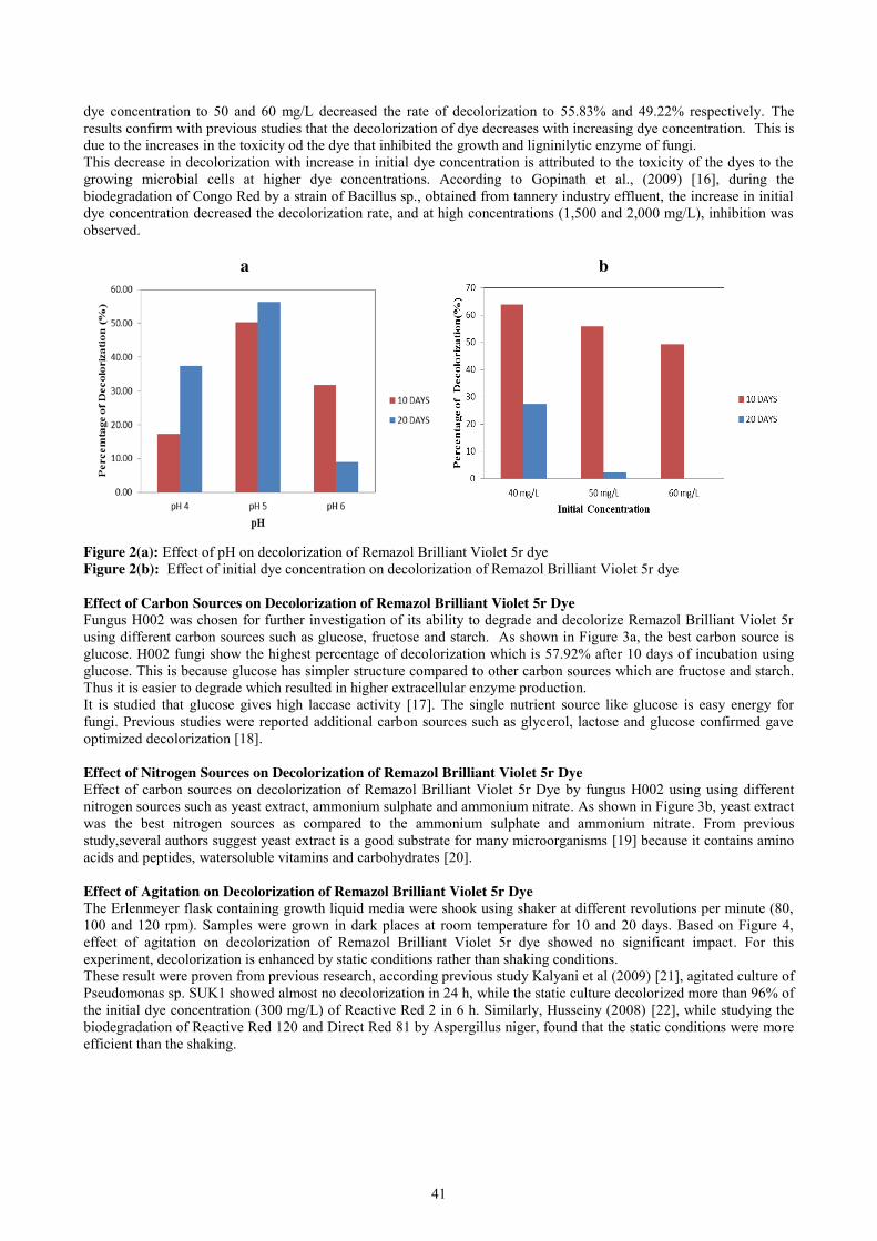
41

dye concentration to 50 and 60 mg/L decreased the rate of decolorization to 55.83% and 49.22% respectively. The results confirm with previous studies that the decolorization of dye decreases with increasing dye concentration. This is due to the increases in the toxicity od the dye that inhibited the growth and ligninilytic enzyme of fungi. This decrease in decolorization with increase in initial dye concentration is attributed to the toxicity of the dyes to the growing microbial cells at higher dye concentrations. According to Gopinath et al., (2009) [16], during the biodegradation of Congo Red by a strain of Bacillus sp., obtained from tannery industry effluent, the increase in initial dye concentration decreased the decolorization rate, and at high concentrations (1,500 and 2,000 mg/L), inhibition was observed. a b

Figure 2(a): Effect of pH on decolorization of Remazol Brilliant Violet 5r dye Figure 2(b): Effect of initial dye concentration on decolorization of Remazol Brilliant Violet 5r dye Effect of Carbon Sources on Decolorization of Remazol Brilliant Violet 5r Dye Fungus H002 was chosen for further investigation of its ability to degrade and decolorize Remazol Brilliant Violet 5r using different carbon sources such as glucose, fructose and starch. As shown in Figure 3a, the best carbon source is glucose. H002 fungi show the highest percentage of decolorization which is 57.92% after 10 days of incubation using glucose. This is because glucose has simpler structure compared to other carbon sources which are fructose and starch. Thus it is easier to degrade which resulted in higher extracellular enzyme production. It is studied that glucose gives high laccase activity [17]. The single nutrient source like glucose is easy energy for fungi. Previous studies were reported additional carbon sources such as glycerol, lactose and glucose confirmed gave optimized decolorization [18]. Effect of Nitrogen Sources on Decolorization of Remazol Brilliant Violet 5r Dye Effect of carbon sources on decolorization of Remazol Brilliant Violet 5r Dye by fungus H002 using using different nitrogen sources such as yeast extract, ammonium sulphate and ammonium nitrate. As shown in Figure 3b, yeast extract was the best nitrogen sources as compared to the ammonium sulphate and ammonium nitrate. From previous study,several authors suggest yeast extract is a good substrate for many microorganisms [19] because it contains amino acids and peptides, watersoluble vitamins and carbohydrates [20]. Effect of Agitation on Decolorization of Remazol Brilliant Violet 5r Dye The Erlenmeyer flask containing growth liquid media were shook using shaker at different revolutions per minute (80, 100 and 120 rpm). Samples were grown in dark places at room temperature for 10 and 20 days. Based on Figure 4, effect of agitation on decolorization of Remazol Brilliant Violet 5r dye showed no significant impact. For this experiment, decolorization is enhanced by static conditions rather than shaking conditions. These result were proven from previous research, according previous study Kalyani et al (2009) [21], agitated culture of Pseudomonas sp. SUK1 showed almost no decolorization in 24 h, while the static culture decolorized more than 96% of the initial dye concentration (300 mg/L) of Reactive Red 2 in 6 h. Similarly, Husseiny (2008) [22], while studying the biodegradation of Reactive Red 120 and Direct Red 81 by Aspergillus niger, found that the static conditions were more efficient than the shaking.

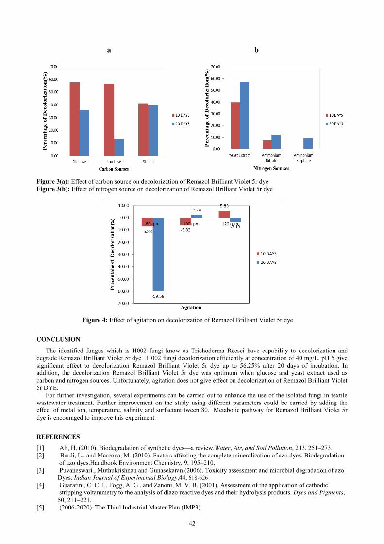
42

a b

Figure 3(a): Effect of carbon source on decolorization of Remazol Brilliant Violet 5r dye Figure 3(b): Effect of nitrogen source on decolorization of Remazol Brilliant Violet 5r dye

Figure 4: Effect of agitation on decolorization of Remazol Brilliant Violet 5r dye

CONCLUSION

The identified fungus which is H002 fungi know as Trichoderma Reesei have capability to decolorization and degrade Remazol Brilliant Violet 5r dye. H002 fungi decolorization efficiently at concentration of 40 mg/L. pH 5 give significant effect to decolorization Remazol Brilliant Violet 5r dye up to 56.25% after 20 days of incubation. In addition, the decolorization Remazol Brilliant Violet 5r dye was optimum when glucose and yeast extract used as carbon and nitrogen sources. Unfortunately, agitation does not give effect on decolorization of Remazol Brilliant Violet 5r DYE.

For further investigation, several experiments can be carried out to enhance the use of the isolated fungi in textile wastewater treatment. Further improvement on the study using different parameters could be carried by adding the effect of metal ion, temperature, salinity and surfactant tween 80. Metabolic pathway for Remazol Brilliant Violet 5r dye is encouraged to improve this experiment.

REFERENCES

[1] Ali, H. (2010). Biodegradation of synthetic dyes—a review.Water, Air, and Soil Pollution, 213, 251–273. [2] Bardi, L., and Marzona, M. (2010). Factors affecting the complete mineralization of azo dyes. Biodegradation of azo dyes.Handbook Environment Chemistry, 9, 195–210. [3] Puvaneswari., Muthukrishnan and Gunasekaran.(2006). Toxicity assessment and microbial degradation of azo Dyes. Indian Journal of Experimental Biology,44, 618-626 [4] Guaratini, C. C. I., Fogg, A. G., and Zanoni, M. V. B. (2001). Assessment of the application of cathodic stripping voltammetry to the analysis of diazo reactive dyes and their hydrolysis products. Dyes and Pigments, 50, 211–221. [5] (2006-2020). The Third Industrial Master Plan (IMP3).

43

[6] Rajeshkannan R., Rajasimman M., Rajamohan N. (2011). Decolourization of malachite green using tamarind seed: optimization, isotherm and kinetic studies. CICEQ, 17, 67–79. doi:10.2298/CICEQ100716056R

[7] Jadhav and Govindwar. (2006). Biotransformation of malachite green by Saccharomyces cerevisiae. Yeast, 23, 315–323. doi:0.1002/yea.1356

[8] Papadopoulou and Rigas. (2013). Degradation of dyes used in textile industries by selected white-rot fungi. 163-168. Retrieved from https://www.researchgate.net/publication/252931157_Degradation_of_dyes_used_in_textile_industries_by_selected_white-rot_fungi

[9] Manu, B and Chaudhari, S. (2002), Anaerobic decolorisation of simulated textile wastewater containing azo dyes, Bioresour Technol 82:225–231.

[10] Mohammad Fadhil Abid., Mumtaz Abdulahad Zablouk and Abeer Muhssen Abid-Alameer. (2012). Experimental study of dye removal from industrial wastewater by membrane technologies of reverse osmosis and nanofiltration. Iranian J Environ Health Sci Eng. doi:10.1186/1735-2746-9-1

[11] Forss and welander. (2009). Decolourization of reactive azo dyes with microorganisms growing on soft wood chips. International Biodeterioration & Biodegradation, 63(6), 752–758. doi:10.1016/j.ibiod.2009.05.005

[12] Hadibarata., Amilina., rahim., Yuniarto and Meor. (2013). Microbial Decolorization of an Azo Dye Reactive Black 5 Using White-Rot Fungus Pleurotus eryngii F032. Water Air Soil Pollution , 1-9.

[13] Nozaki., Mizuno., Isobe., Shiroishi and Kanda.(2008). Screening and investigation of dye decolorization activities of basidiomycetes. J. Biosci. Bioeng.. 105,69-72

[14] Kaushik and Malik. (2009). Fungal dye decolorization: Recent advances and future potential. Environment International, 35, 127–141.

[15] Yuzhu and Viraraghavan. (2001). Fungul decolorization of dye wastewater: a review. Biores Techno, 79, 251-262.

[16] Gopinath., Sahib., Muthukumar and Velan. (2009). Improved biodegradation of Congo red by Bacillus sp. Bioresource Technology, 100, 670–675.

[17] Stajića., Perskyb., Friesemb., Hadarb., Wasserc., Nevoc and Vukojevića. (2006). Effect of different carbon and nitrogen sources on laccase and peroxidases production by selected Pleurotus species. Enzyme and Microbial Technology, 38(1-2), 65–73. doi:doi.org/10.1016/j.enzmictec.2005.03.026

[18] Nigam., Banat., Singh and Marchant. (1996). Microbial process for the decolorization of textile effluent containing azo, diazo and reactive dyes. Process Biochemistry, 31, 435-442.

[19] Jackson., Frymier., Wilkinson., Zorner and Evans. (1998). Growth requirements for production of stable cells of the bioherbicidal bacterium Xanthomonas camprestris. Journal of Industrial Microbiology and Biotechnology, 21, 237–241.

[20] Crueger and Crueger. (1993). Substratos Para la Fermentacio´n Industrial. [21] Kalyani, D. C., Telke, A. A., Dhanve, R. S., and Jadhav, J. P. (2009). Ecofriendly biodegradation and

detoxification of Reactive Red 2 textile dye by newly isolated Pseudomonas sp. SUK1. Journal of Hazardous Materials, 163, 735–742.

[22] Husseiny. (2008). Biodegradation of the reactive and direct dyes using Egyptian isolates. Journal of Applied Science and Research, 4, 599–606.

44

Biodegradation of Solvent Green 3 (SG3) Dye Using Selected Fungus Muhammad Rozaid, Salmiati

Faculty of Civil Engineering, Universiti Teknologi Malaysia, Malaysia

salmiati@utm.my

Keywords: Anthraquinone; Decolorization; Solvent Green 3; Hypocrea jecorina.

ABSTRACT. Massive amount of dye concentrations have been released into the environment as textile wastewater. SG3 dye remains as one of the most difficult dyes to be degraded. SG3 is an anthraquinone dye and used in this research as representative of reactive dye. This study was conducted to identify best fungus and investigate the effect of different parameters towards the degradation of SG3 dye. Six different types of fungi were screened for their ability to degrade SG3 dye after 20 days of incubation. The sample of the fungi was collected from UTM Orchard soil. Based on the screening, fungus KB006 were chosen based on its ability to decolorize SG3 dye in liquid medium. According to the fungi identification results, KB006 was determined as Hypocrea jecorina. This fungus was further tested for its ability to degrade SG3 dye in liquid medium under several conditions which are carbon and nitrogen sources, pH, agitation, and different SG3 initial concentration. Based on the decolorization, Hypocrea jecorina showed potential efficiency in SG3 decolorization with using of glucose (53%), yeast extract (68%), agitation (56%), 40 ppm of initial SG3 dye concentration (54%) and pH 8 (51%). As a conclusion, is observed that fungus Hypocrea jecorina showed potential of ability to decolorize anthraquinone dye SG3.

INTRODUCTION

In 2015, Malaysia’s textile and apparel industry was one of the top ten largest export earners in the country, with an export value reaching RM 13.2 billion, representing 1.7% of Malaysia’s total exports of manufactured goods. The latest figure shows that Malaysia’s textile and apparel exports increased 10% from the same period in the previous year to RM 6.99 billion (US$ 1.7 billion) in the first half of 2016 [1]. Most of the industries especially textile industry is the major contribution to the disposal of toxic dye into the water. Among many industries, textile contribute the highest in utilize dyes for coloration of fiber. The effluent from textile industry carries a huge number of dyes and added with other additives throughout the colouring process.

Dye is a natural or synthetic substance used to add a colour to or change the colour of something. Such substances with considerable coloring capacity are widely employed in the production of consumer products, including paints, textile, printing inks, pharmaceutical, food, cosmetics, plastics, photographic, and paper industries. Dyes are classified according to their application and chemical structure, and are composed of a group of atoms known as chromophores, responsible for the dye color. These chromophore-containing centers are based on diverse functional groups, such as azo, anthraquinone, methine, nitro, arilmethane, carbonyl and others [1].

The dyes are hardly removed from wastewater by conventional biological, physical, or chemical treatment. It is really important to remove dyes in wastewater because dyes are very toxic and are characterized by high chemical oxygen demand, biological oxygen demand, and highly aromatic conjugated and carcinogenic that can endanger human life. Most of the dyes are carcinogenic and toxic in nature and when discharged into the water they pose serious hazards to the aquatic biota [2]. The propose biodegradation of dye using selected fungus is to overcome the discharge of coloured effluents from textile industry, and remove dyes fully from wastewater with using biological treatment.

Problem Statement Among many industries, textile contribute the highest in utilize dyes for coloration of fiber. The effluent from textile industry carries a huge number of dyes and added with other additives throughout the colouring process. The discharge of coloured effluents, although frequently less toxic than many colourless effluents, is resented by the public on the ground that colour is an indicator of pollution.

The dyes are hardly removed from wastewater by conventional biological, physical, or chemical treatment. The release of dyes into wastewaters by various industries poses serious environmental problems due to various dyes persistent and recalcitrant nature. Large production and usage of dyes have been attracted widespread interests. Such as textiles, pharmaceutical, cosmetics, paper, leather, and food. Objectives The objectives of this project are:

1. To identify best fungus to degrade SG3 dyes. 2. To determine the percentage removal of dye based on selected fungus. 3. To investigate the effect of different parameters towards the degradation of SG3 dye.

45

Scope of Study In this study, the degradation of SG3 dye by the selected fungi was investigated by measuring its decolorization percentage during the incubation period. The sample was collected at UTM Orchard soil. Six fungi samples were tested to degrade SG3 which are KB003, KB003i, H002, KB006, 7, and 2. After that, the capabilities of the fungi to degrade SG3 were further tested under different conditions with alteration of carbon sources, nitrogen sources, different initial dyes concentration, agitation, temperature and pH. The decolorization was determined using UV Vis-Spectrophotometer.

METHODOLOGY This research was divided into three main parts including sampling and screening of the fungi on agar medium,

identification of selected fungus that has high percentage SG3 dye removal, decolorization of SG3 dye on liquid medium, and assessment of decolorization in UV-Visible spectrophotometer measurement. Six fungi sample were collected at UTM orchard soil and these fungi were stored in the freezer prior to use. These fungi were then screened on agar medium and then transfer to the liquid medium to identify the best fungi for degradation of SG3 dyes. The result was collected in 10 and 20 days. Then, the decolorization determination of SG3 dye using UV-Visible Spectrophotometer by selected fungi was conducted in liquid medium under several parameters such as nitrogen and carbon source, pH, dye initial concentration, and agitation using. Malt Extracts (ME) Agar The solid medium was used in degradation of SG3 dye in dark condition for 30 days in incubation period for 30 days at room temperature. Malt extract (ME) agar was prepared by dissolving ME agar powder (20 g/L), yeast extract (20 g/L) and chloramphenicol (300 mg/L) as antibacteria in 250 mL of distilled water. The medium was then autoclaved at 121°C at 101.3 kPa for 15-20 minutes. The ME agar was left to cool to about 55°C. Then about 0.5 cm diameter of fungi plug was plugged using Stainless steel mounted needle and put onto the agar. Then the petri dish was sealed using parafilm. The samples were incubated for 7 days to screen the best performance of isolated fungus. Liquid Broth (LB) Medium LB medium was prepared by dissolving a mixture of glucose (20 g/L) and yeast extract (20 g/L) in 150 mL of distilled water. The medium was then autoclaved at 121°C at the pressure of 101.3 kPa for 15-20 minutes. To study the decolorization of SG3, inoculum were cut from the fungus mycelium that grow in agar medium and transferred into liquid medium (LB). These reagents were added with distilled water until it reached the volume of 20 mL in 100 mL Erlenmeyer flask. The decolorization of SG3 was monitored for 7, and 14 days using UV–vis spectrophotometer. Decolorization of SG3 Dye by Fungi Decolorization was monitored by scanning the absorbance between 400 and 750 nm using PerkinElmer UV–vis spectrophotometer and the maximum absorption of SG3 recorded at 597 nm. Reductions in the absorbance at 597 nm showed that decolorization have taken place. Dye concentrations were calculated from the calibration curve of absorbance and dye concentration (mg/L). The decolorization percentage of SG3 was calculated as follows: Decolorization (%) = C0−Ct

C0 𝑥100% Eq. 1

Parameters in This Study pH For the investigation of pH effect, the liquid medium were adjusted to pH 4, 5, 6, 7, and 8 repectively. This flask was then incubated for 7 days and 14 days at 25 C. Carbon Sources For the investigation of other carbon sources, glucose were replaced with galactose and starch. The samples were incubated at 37°C with best pH, and the color intensity was measured in for 7 days and 14 days at 25 C. Nitrogen Sources For the investigation of other nitrogen sources, yeast extract were replaced with ammonium sulphate and ammonium nitrate. The samples were incubated at 37°C with best pH, and the color intensity was measured in for 7 days and 14 days at 25 C. Initial Dye Concentration Various concentrations of SG3 (40 ppm, 50 ppm and 60 ppm) were used in order to achieve the best concentration of dye. The samples were incubated at 37°C with best pH, and the color intensity was measured in for 7 days and 14 days at 25 C.

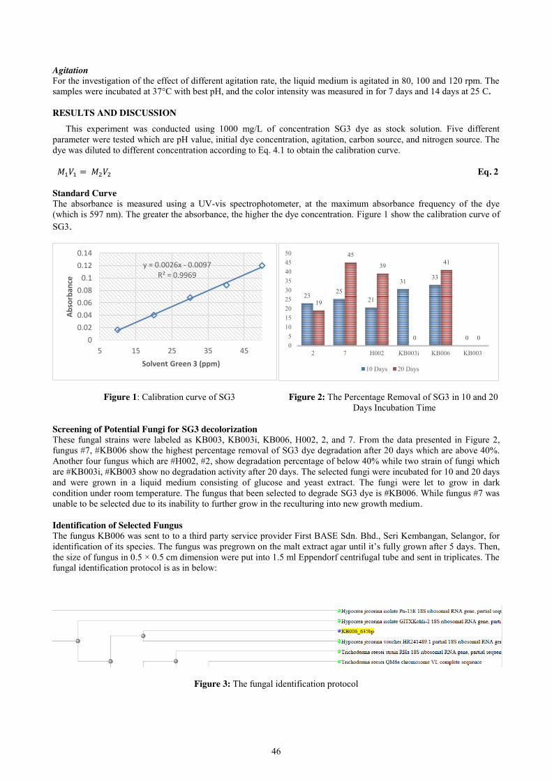
46

Agitation For the investigation of the effect of different agitation rate, the liquid medium is agitated in 80, 100 and 120 rpm. The samples were incubated at 37°C with best pH, and the color intensity was measured in for 7 days and 14 days at 25 C. RESULTS AND DISCUSSION

This experiment was conducted using 1000 mg/L of concentration SG3 dye as stock solution. Five different parameter were tested which are pH value, initial dye concentration, agitation, carbon source, and nitrogen source. The dye was diluted to different concentration according to Eq. 4.1 to obtain the calibration curve. 𝑀1𝑉1 = 𝑀2𝑉2 Eq. 2

Standard Curve The absorbance is measured using a UV-vis spectrophotometer, at the maximum absorbance frequency of the dye (which is 597 nm). The greater the absorbance, the higher the dye concentration. Figure 1 show the calibration curve of SG3.

Figure 1: Calibration curve of SG3 Figure 2: The Percentage Removal of SG3 in 10 and 20 Days Incubation Time Screening of Potential Fungi for SG3 decolorization These fungal strains were labeled as KB003, KB003i, KB006, H002, 2, and 7. From the data presented in Figure 2, fungus #7, #KB006 show the highest percentage removal of SG3 dye degradation after 20 days which are above 40%. Another four fungus which are #H002, #2, show degradation percentage of below 40% while two strain of fungi which are #KB003i, #KB003 show no degradation activity after 20 days. The selected fungi were incubated for 10 and 20 days and were grown in a liquid medium consisting of glucose and yeast extract. The fungi were let to grow in dark condition under room temperature. The fungus that been selected to degrade SG3 dye is #KB006. While fungus #7 was unable to be selected due to its inability to further grow in the reculturing into new growth medium. Identification of Selected Fungus The fungus KB006 was sent to to a third party service provider First BASE Sdn. Bhd., Seri Kembangan, Selangor, for identification of its species. The fungus was pregrown on the malt extract agar until it’s fully grown after 5 days. Then, the size of fungus in 0.5 × 0.5 cm dimension were put into 1.5 ml Eppendorf centrifugal tube and sent in triplicates. The fungal identification protocol is as in below:

Figure 3: The fungal identification protocol

y = 0.0026x - 0.0097 R² = 0.9969

00.020.040.060.08

0.10.120.14

5 15 25 35 45

Abso

rban

ce

Solvent Green 3 (ppm)

23 25 21

31 33

0

19

45

39

0

41

0 05

101520253035404550

2 7 H002 KB003i KB006 KB003

10 Days 20 Days

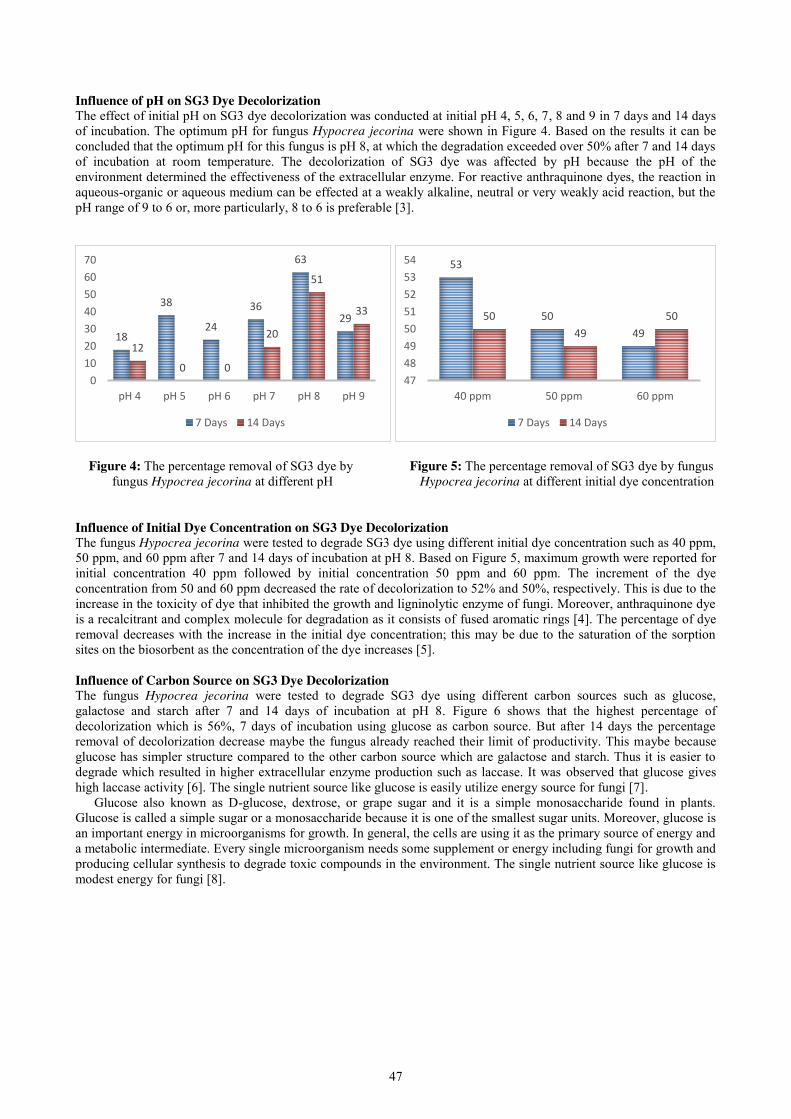
47

Influence of pH on SG3 Dye Decolorization The effect of initial pH on SG3 dye decolorization was conducted at initial pH 4, 5, 6, 7, 8 and 9 in 7 days and 14 days of incubation. The optimum pH for fungus Hypocrea jecorina were shown in Figure 4. Based on the results it can be concluded that the optimum pH for this fungus is pH 8, at which the degradation exceeded over 50% after 7 and 14 days of incubation at room temperature. The decolorization of SG3 dye was affected by pH because the pH of the environment determined the effectiveness of the extracellular enzyme. For reactive anthraquinone dyes, the reaction in aqueous-organic or aqueous medium can be effected at a weakly alkaline, neutral or very weakly acid reaction, but the pH range of 9 to 6 or, more particularly, 8 to 6 is preferable [3].

Figure 4: The percentage removal of SG3 dye by Figure 5: The percentage removal of SG3 dye by fungus fungus Hypocrea jecorina at different pH Hypocrea jecorina at different initial dye concentration Influence of Initial Dye Concentration on SG3 Dye Decolorization The fungus Hypocrea jecorina were tested to degrade SG3 dye using different initial dye concentration such as 40 ppm, 50 ppm, and 60 ppm after 7 and 14 days of incubation at pH 8. Based on Figure 5, maximum growth were reported for initial concentration 40 ppm followed by initial concentration 50 ppm and 60 ppm. The increment of the dye concentration from 50 and 60 ppm decreased the rate of decolorization to 52% and 50%, respectively. This is due to the increase in the toxicity of dye that inhibited the growth and ligninolytic enzyme of fungi. Moreover, anthraquinone dye is a recalcitrant and complex molecule for degradation as it consists of fused aromatic rings [4]. The percentage of dye removal decreases with the increase in the initial dye concentration; this may be due to the saturation of the sorption sites on the biosorbent as the concentration of the dye increases [5]. Influence of Carbon Source on SG3 Dye Decolorization The fungus Hypocrea jecorina were tested to degrade SG3 dye using different carbon sources such as glucose, galactose and starch after 7 and 14 days of incubation at pH 8. Figure 6 shows that the highest percentage of decolorization which is 56%, 7 days of incubation using glucose as carbon source. But after 14 days the percentage removal of decolorization decrease maybe the fungus already reached their limit of productivity. This maybe because glucose has simpler structure compared to the other carbon source which are galactose and starch. Thus it is easier to degrade which resulted in higher extracellular enzyme production such as laccase. It was observed that glucose gives high laccase activity [6]. The single nutrient source like glucose is easily utilize energy source for fungi [7].

Glucose also known as D-glucose, dextrose, or grape sugar and it is a simple monosaccharide found in plants. Glucose is called a simple sugar or a monosaccharide because it is one of the smallest sugar units. Moreover, glucose is an important energy in microorganisms for growth. In general, the cells are using it as the primary source of energy and a metabolic intermediate. Every single microorganism needs some supplement or energy including fungi for growth and producing cellular synthesis to degrade toxic compounds in the environment. The single nutrient source like glucose is modest energy for fungi [8].

18

38

24

36

63

29

12

0 0

20

51

33

010203040506070

pH 4 pH 5 pH 6 pH 7 pH 8 pH 9

7 Days 14 Days

53

50 49

50 49

50

4748495051525354

40 ppm 50 ppm 60 ppm

7 Days 14 Days

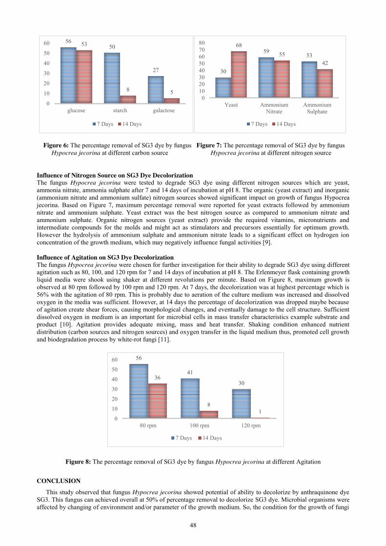
48

Figure 6: The percentage removal of SG3 dye by fungus Figure 7: The percentage removal of SG3 dye by fungus Hypocrea jecorina at different carbon source Hypocrea jecorina at different nitrogen source Influence of Nitrogen Source on SG3 Dye Decolorization The fungus Hypocrea jecorina were tested to degrade SG3 dye using different nitrogen sources which are yeast, ammonia nitrate, ammonia sulphate after 7 and 14 days of incubation at pH 8. The organic (yeast extract) and inorganic (ammonium nitrate and ammonium sulfate) nitrogen sources showed significant impact on growth of fungus Hypocrea jecorina. Based on Figure 7, maximum percentage removal were reported for yeast extracts followed by ammonium nitrate and ammonium sulphate. Yeast extract was the best nitrogen source as compared to ammonium nitrate and ammonium sulphate. Organic nitrogen sources (yeast extract) provide the required vitamins, micronutrients and intermediate compounds for the molds and might act as stimulators and precursors essentially for optimum growth. However the hydrolysis of ammonium sulphate and ammonium nitrate leads to a significant effect on hydrogen ion concentration of the growth medium, which may negatively influence fungal activities [9]. Influence of Agitation on SG3 Dye Decolorization The fungus Hypocrea jecorina were chosen for further investigation for their ability to degrade SG3 dye using different agitation such as 80, 100, and 120 rpm for 7 and 14 days of incubation at pH 8. The Erlenmeyer flask containing growth liquid media were shook using shaker at different revolutions per minute. Based on Figure 8, maximum growth is observed at 80 rpm followed by 100 rpm and 120 rpm. At 7 days, the decolorization was at highest percentage which is 56% with the agitation of 80 rpm. This is probably due to aeration of the culture medium was increased and dissolved oxygen in the media was sufficient. However, at 14 days the percentage of decolorization was dropped maybe because of agitation create shear forces, causing morphological changes, and eventually damage to the cell structure. Sufficient dissolved oxygen in medium is an important for microbial cells in mass transfer characteristics example substrate and product [10]. Agitation provides adequate mixing, mass and heat transfer. Shaking condition enhanced nutrient distribution (carbon sources and nitrogen sources) and oxygen transfer in the liquid medium thus, promoted cell growth and biodegradation process by white-rot fungi [11].

Figure 8: The percentage removal of SG3 dye by fungus Hypocrea jecorina at different Agitation

CONCLUSION

This study observed that fungus Hypocrea jecorina showed potential of ability to decolorize by anthraquinone dye SG3. This fungus can achieved overall at 50% of percentage removal to decolorize SG3 dye. Microbial organisms were affected by changing of environment and/or parameter of the growth medium. So, the condition for the growth of fungi

56 50

27

53

8 5

0

10

20

30

40

50

60

glucose starch galactose

7 Days 14 Days

30

59 53

68 55

42

01020304050607080

Yeast AmmoniumNitrate

AmmoniumSulphate

7 Days 14 Days

56

41

30 36

8 1

0

10

20

30

40

50

60

80 rpm 100 rpm 120 rpm

7 Days 14 Days

49

should be strictly monitored to enhance the secretion of ligninolytic enzymes that will decolorize dye completely. Fungus Hypocrea jecorina decolorize SG3 efficiently at the concentration of 40 ppm with agitation (80 rpm). In addition, the decolorization of SG3 was optimal at pH 8. In the microbial decomposition of pollutants, sustainable approach to the environment is a success in this study suggests that in nature there is a natural biological decomposition of pollutants. For benefit of our environment this fungus can be applied to promote a more natural way of dye waste water removal, which will provide more effective protection to the natural environment.

REFERENCES

[1] Nick. (2017, Feb 22). Malaysia’s Textile and Apparel Industry Expects Another Strong Year for Growth. Retrieved from https://www.bizvibe.com/blog/malaysias-textile-apparel-industry-expects-another-strong-year-growth/

[2] Hadibarata, T. A. (2013). Microbial Decolorization of an Azo Dye Reactive Black 5 Using White-Rot Fungus Pleurotus eryngii F032. Water, Air, & Soil Pollution, 224.

[3] Bitterli, P. (2001). Reactive anthraquinone dyes containing a trichloro pyrimidyl group. United States : Sandoz Ltd.

[4] Kumari, K. a. (2007). Biosorption of anionic textile dyes by nonviable biomass of fungi and yeast. Bioresource Technology, 98, 1704–1710.

[5] Mahmoud, M. (2014). Decolorization of certain reactive dye from aqueous solution using Baker’s Yeast (Saccharomyces cerevisiae) strain. HBRC Journal, 12, 88–98.

[6] Stajic, M. L. (2006). Effect of different carbon and nitrogen sources on laccase and peroxidases production by selected Pleurotus species. Enzyme Microb Tech, 38, 65-73.

[7] Hadibarata, T. Y. (2011). Decolorization of azo, triphelylmethane and antraquinone dyes by laccase of a newly isolated Armillariasp. F022. Water Air Soil Pollut., DOI:10.1007/s11270-011-0922-6.

[8] Hadibarata, T. T. (2007). Biodegradation of Phenanthrene Fungi Screened from Nature. Pakistan Journal of Biological Sciences, 10:2535-2543.

[9] Abeer Hashem, Elsayed Fathi Abd-Allah, Rashid Sultan Al-Obeed, Abdulaziz Abdullah Alqarawi, and Hend Awad Alwathnani (2015). Effect of Carbon, Nitrogen Sources and Water Activity on Growth and Ochratoxin Production of Aspergillus carbonarius (Bainier) Thom. Jundishapur Journal of Microbiology, 10.5812/jjm.17569.

[10] Darah Ibrahim, Haritharan Weloosamy, and Sheh-Hong Lim (2015). Effect of agitation speed on the morphology of Aspergillus niger HFD5A-1 hyphae and its pectinase production in submerged fermentation. World Juornal of Biological Chemistry, 6(3): 265–271.

[11] Naser, T. H. (2013). Microbial Decolorization of an Azo Dye Reactive Black 5 Using White-Rot Fungus Pleurotus eryngii F032. Water Air Soil Pollut, 192(1-4), 141-153.

50

Investigation on the Potential Occurrence of Sludge Bulking in Sewage Treatment Plant

Nazihah Yaacob, Khalida Muda Faculty of Civil Engineering, Universiti Teknologi Malaysia, Malaysia

khalida@utm.my

Keywords: Activated Sludge, Sludge Bulking, Filamentous, Sludge Biomass SVI, Settling Velocity.

ABSTRACT. Sewage is the combination of water and waste that come from kitchen sink, toilet, washing machine, dishwasher and shower from domestic premise. The sewage will be treated by municipal wastewater treatment plant for waste water treatment purpose before the effluent were release back into the river. Sludge bulking is the phenomenon of a poor sludge settling. During the occurrence of sludge bulking, normally suspended solid float on the surface of a final settlement tank. The objective of this research are to determine the biomass properties and to obtain the removal performance and filamentous index of selected sewage treatment plant system. Physical properties of sample will be tested on biomass concentration, settling velocity, SVI, aggregation and surface hydrophobicity. The metal content were determined using atomic absorption spectrometry (AAS). The removal performances of the sample were investigated on chemical oxygen demand (COD), suspended solids (SS) and nutrient. The filamentous index were analysed with subjective scoring method. The sewage treatment plant has poor settling velocity with average of 1.74±0.24 m/hr. The sample were tested with 3 element of metals which were Iron (Fe), nickel (Ni) and Cadmium (Cd) and the only metal found in the wastewater samples are Iron (Fe) with average of 0.214±0.182 mg/L. The overall removal performance for all the measured parameter were between 22.3% and 58%. It can be concluded that this treatment systems has poor removal performance. The filamentous index of the sewage treatment plant was classified as level 2. This indicated that the filaments were commonly observed but not present in all flocs. This study shows that poor performance and settleability of this treatment system may be due to the occurrence of sludge bulking. The occurrence of sludge bulking was due to non-filamentous type. Since the level of filamentous index was in level 2. The poor settleability and removal performances may be due to others factors such as shock loading.

INTRODUCTION The purpose of waste water treatment plant is to process the wastewater to become a clean and safe water that will

have minimal environmental impact when its flow back into the water bodies. The wastewater that flow from domestic premises is called sewage. Sewage is the combination of water and waste that come from kitchen sink, toilet, washing machine, dishwasher and shower from domestic premise. The sewage will be treated by municipal wastewater treatment plant for waste water treatment purpose before the effluent were release back into the river. During the treatment of the wastewater, sludge bulking might occurs and cause reduction on the treatment process. Sludge bulking is the phenomenon of a poor sludge settling. During the occurrence of sludge bulking, normally suspended solid float on the surface of a final settlement tank. Objectives The objectives of this study are:

1. To determine the biomass properties of selected sewage treatment plant system 2. To obtain the removal performance of the selected sewage treatment plant system. 3. To obtain the filamentous index (FI) of selected sewage treatment plant system.

Scope of Study The study will focus on the investigation of the physical, chemical and biological properties of sewage treatment plant. Sewage will be test on their physicochemical characteristic which are biomass concentration (MLSS and MLVSS), aggregation, settling velocity, sludge volume index (SVI), relative hydrophobicity and surface charge on physical properties, metal contents on chemical properties. The removal performance of the treatment plant will be determined by comparing the different on the selected parameter in the influent and effluent of the sewage treatment plant. Filamentous index will be determined by using microscopic image.

LITERATURE REVIEW

Wastewater is any water that have been affected on their physical, chemical and biological properties. Sewage treatment is the process with the purpose to remove the micro-organisms, contaminants and other types of pollutants from wastewater that came from domestic area. Due to the increasing number of population in Malaysia, the sources of fresh water are limited. Thus, to avoid from the natural sources being polluted, the sewage needs to be treated properly.

51

The sewage treatment plant consisted of 4 stages which are preliminary treatment, primary treatment, secondary treatment and tertiary treatment [1].

The sources of sewage effluent came from many different places. Thus, the constituents of the sewage effluent may vary on different sewage treatment plant. The constituents contain on sewage effluent are microorganisms, biodegradable organic materials and other organic materials, nutrients, metals and other inorganic materials, thermal effects, odour (and taste) and radioactivity. The characteristic of sewage can be known by measuring COD, BOD, nitrogen, ammonia, phosphorus, TSS and VSS. COD test is basically used to measure the number of organic compounds. BOD also called biological oxygen demand is the measurement of the dissolved oxygen used by the aerobic microorganism organisms to break down the organic material present in the sewage treatment plant at a certain temperature over specific period.

The purpose of sewage treatment plant is to produce effluents that have higher water quality and safe to the environment and human being. However, there are some operational issues that always happens in sewage treatment plant such as mechanical, chemical and biological issues. Sludge bulking is one of the issues that needs to be concerned because it will affect the efficiency of the sewage treatment plant. Sludge bulking occurs when the sludge failed to properly settle down during the settlement process [2].

Sludge bulking usually occurs at secondary treatment or secondary clarifiers. The process of compaction of sludge in thickener and storage tank are poor and the settling of sludge in clarifier are also in poor condition. If the machinery does not function well, it will interrupt the process of secondary clarifier and will lead to sludge bulking. There are several types of sludge bulking that lead to poor settling of sludge such as dispersed growth, microflocs (pinpoint flocs), viscous bulking, rising sludge, filamentous bulking and foaming and scumming [3].

There are two treatment strategies to prevent the wastewater treatment plant from having sludge bulking problem that will affect the efficiency of the treatment process. The treatment strategies can be divided into 2 types of method to control sludge bulking are non-specific method and specific method [3]. Non-specific method is a short term control included sludge juggling method [4], chlorination [3], ozonation, polymer and coagulant addition and application of hydrogen peroxide [5]. Specific method focus on the growth of floc-forming bacterial structures and the excessive growth of filamentous bacteria structures. The purpose is to find a permanent control or long-term control in a sustainable way of bulking in activated sludge systems. Specific method included control of influent waste septicity (organic acids and H2S), nutrient additions (industrial waste systems only), changes in aeration and changes in biomass concentration or changes in waste feeding pattern [3].

Filamentous microorganism is a natural microorganism that forms in activated sludge. Some of the report indicated that in the activated sludge, filamentous microorganism may not exist in sludge bulking thus this type of bulking is known as non-filamentous bulking [3]. There are many types of filamentous bacteria that form in sewage treatment plant. Generally, microbial population in mixed cultures has two forms which are dispersion of individual cells and aggregates of individual cells (flocs, biofilms).

METHODOLOGY

Raw municipal wastewater and sludge particles sample were collected once a week from a selected wastewater plant which located in Johor Bahru. Sample were stored in a cold room at 4°c prior to use. The activated sludge was obtained from the aeration unit of wastewater treatment plant located in Johor Bahru. The experiment was investigated for physio-chemical characteristics of the sludge with the removal performances and the filamentous index. The physical properties of the sludge are by analysing the aggregation, biomass concentration (MLSS and MLVSS), settling velocity, sludge volume index (SVI), surface hydrophobicity. The chemical properties of the sludge particles which is metal contents are tested with atomic absorption spectrometry (AAS) The removal performance is analyse using chemical oxygen demand (COD), suspended solids (TSS and VSS), ammonia, nitrogen (nitrite, nitrate and total nitrogen), phosphorus and total phosphorus. All test is conduct based on the Standard Methods for the Examination of Water and Wastewater- MLSS with method 2540B and settling velocity with method 2710B. The filamentous are observed using phase contrast microscope and the analysis of the level of filamentous index will refer to the subjective scoring method[18].

RESULT AND DISCUSSION Three samples are collected from sewage treatment plant located at Senai which are from inlet, aeration tank and

outlet. The system used in the sewage treatment plant is extended aeration system. The sewage treatment plant is designated for 2500 PE and the population equivalent (PE) treated in the sewage treatment plant are 2120. The result from the laboratory test were analyzed to obtain the characteristics of sewage which are physico-chemical characteristics, removal ability performances and filamentous index. Physico-chemical Characteristics The result of this study are presented in table and figure of graph. Physico-chemical characteristic including biomass concentration, settling velocity, SVI, aggregation, surface hydrophobicity and metal content.

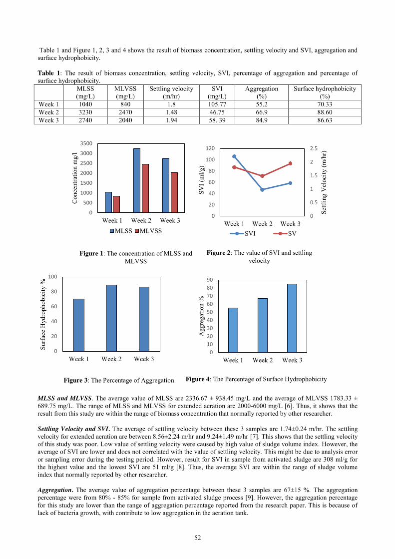
52

Table 1 and Figure 1, 2, 3 and 4 shows the result of biomass concentration, settling velocity and SVI, aggregation and surface hydrophobicity. Table 1: The result of biomass concentration, settling velocity, SVI, percentage of aggregation and percentage of surface hydrophobicity.

MLSS (mg/L)

MLVSS (mg/L)

Settling velocity (m/hr)

SVI (mg/L)

Aggregation (%)

Surface hydrophobicity (%)

Week 1 1040 840 1.8 105.77 55.2 70.33 Week 2 3230 2470 1.48 46.75 66.9 88.60 Week 3 2740 2040 1.94 58. 39 84.9 86.63

MLSS and MLVSS. The average value of MLSS are 2336.67 ± 938.45 mg/L and the average of MLVSS 1783.33 ± 689.75 mg/L. The range of MLSS and MLVSS for extended aeration are 2000-6000 mg/L [6]. Thus, it shows that the result from this study are within the range of biomass concentration that normally reported by other researcher. Settling Velocity and SVI. The average of settling velocity between these 3 samples are 1.74±0.24 m/hr. The settling velocity for extended aeration are between 8.56±2.24 m/hr and 9.24±1.49 m/hr [7]. This shows that the settling velocity of this study was poor. Low value of settling velocity were caused by high value of sludge volume index. However, the average of SVI are lower and does not correlated with the value of settling velocity. This might be due to analysis error or sampling error during the testing period. However, result for SVI in sample from activated sludge are 308 ml/g for the highest value and the lowest SVI are 51 ml/g [8]. Thus, the average SVI are within the range of sludge volume index that normally reported by other researcher. Aggregation. The average value of aggregation percentage between these 3 samples are 67±15 %. The aggregation percentage were from 80% - 85% for sample from activated sludge process [9]. However, the aggregation percentage for this study are lower than the range of aggregation percentage reported from the research paper. This is because of lack of bacteria growth, with contribute to low aggregation in the aeration tank.

0

500

1000

1500

2000

2500

3000

3500

Week 1 Week 2 Week 3

Con

cent

ratio

n m

g/l

MLSS MLVSS

0

0.5

1

1.5

2

2.5

0

20

40

60

80

100

120

Week 1 Week 2 Week 3

Settl

ing

Vel

ocity

(m/h

r)

SVI (

ml/g

)

SVI SV

0

20

40

60

80

100

Week 1 Week 2 Week 3

Surf

ace

Hyd

roph

obic

ity %

0102030405060708090

Week 1 Week 2 Week 3

Agg

rega

tion

%

Figure 1: The concentration of MLSS and MLVSS

Figure 2: The value of SVI and settling velocity

Figure 3: The Percentage of Aggregation Figure 4: The Percentage of Surface Hydrophobicity

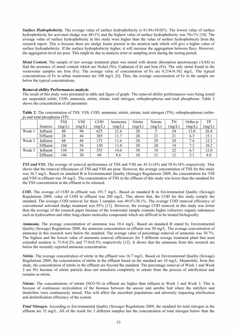
53

Surface Hydrophobicity. The average value of surface hydrophobicity is 81.86±10.02%. The lowest value of surface hydrophobicity for activated sludge was 48±1% and the highest value of surface hydrophobicity was 70±1% [10]. The average value of surface hydrophobicity in this study were higher than the value of surface hydrophobicity from the research report. This is because there are sludge foams present in the aeration tank which will give a higher value of surface hydrophobicity. If the surface hydrophobicity higher, it will increase the aggregation between flocs. However, the aggregation level are poor. This might be due to analysis error or sampling error during the testing period. Metal Content. The sample of raw sewage treatment plant was tested with atomic absorption spectroscopy (AAS) to find the presence of metal content which are Nickel (Ni), Cadmium (Cd) and Iron (Fe). The only metal found in the wastewater samples are Iron (Fe). The average value of concentration of Fe are 0.214±0.182 mg/L. The typical concentrations of Fe in urban wastewater are 100 mg/L [6]. Thus, the average concentration of Fe in the sample are below the typical concentrations. Removal ability Performances analysis The result of this study were presented in table and figure of graph. The removal ability performances were being tested are suspended solids, COD, ammonia, nitrite, nitrate, total nitrogen, orthophosphorus and total phosphorus. Table 2 shows the concentration of all parameter. Table 2: The concentration of TSS, VSS, COD, ammonia, nitrite, nitrate, total nitrogen (TN), orthophosphorus (ortho-p) and total phosphorus (TP).

Sources

TSS (mg/L)

VSS (mg/L)

COD (mg/L)

Ammonia (mg/L)

Nitrite (mg/L)

Nitrate (mg/L)

TN (mg/L)

Ortho-p (mg/L)

TP (mg/L)

Week 1 Influent 80 90 625 21.6 20 5 24 13.0 26.8 Effluent 28 44 385 11.7 20 21 21 6.3 15.1

Week 2 Influent 88 48 175 11.6 20 29 20 7.4 12.3 Effluent 104 56 130 11.0 20 20 18 7.3 10.2

Week 3 Influent 150 34 355 14.6 30 10 22 6.7 12.0 Effluent 146 30 60 8.6 10 31 12 5.1 8.0

TSS and VSS. The average of removal performance of TSS and VSS are 45.5±16% and 58.9±18% respectively. This shows that the removal efficiencies of TSS and VSS are poor. However, the average concentration of TSS for this study was 36.7 mg/L. Based on standard B in Environmental Quality (Sewage) Regulations 2009, the concentration for TSS and VSS in effluent was 50 mg/L. The concentration of TSS in the effluent of this study was lower than the standard for the TSS concentration in the effluent to be released. COD. The average of COD in effluent was 191.7 mg/L. Based on standard B in Environmental Quality (Sewage) Regulations 2009, value of COD in effluent was 200 mg/L. This shows that, the COD for this study comply the standard. The average COD removal for these 3 samples was 49.07±30.1%. The average COD removal efficiency of conventional activated sludge treatment was 85% [11]. However, the average COD removal in this study was lower than the average of the research paper because of the wastewater sample contains higher refractory organic substances such as hydrocarbon and other long-chains molecules compounds which are difficult to be treated biologically. Ammonia. The average concentration of ammonia was 10.4 mg/L. Based on standard B stated by Environmental Quality (Sewage) Regulations 2009, the ammonia concentration in effluent was 50 mg/L. The average concentration of ammonia in this research were below the standard. The average value of percentage removal of ammonia was 30.7%. The highest and the lowest value of ammonia removal efficiencies for 3 different sewage treatment plant that used extended aeration is 75.9±6.2% and 77.0±8.5% respectively [12]. It shows that the ammonia from this research are below the normally reported ammonia concentration. Nitrite. The average concentration of nitrite in the effluent was 16.7 mg/L. Based on Environmental Quality (Sewage) Regulations 2009, the concentration of nitrite in the effluent based on the standard are 10 mg/L. Meanwhile, from this study, the concentration of nitrite in the effluent are beyond the standard. The percentage removal of Week 1 and Week 2 are 0% because of nitrite particle does not transform completely to nitrate from the process of nitrification and remains as nitrite. Nitrate. The concentrations of nitrate (NO3-N) in effluent are higher than influent in Week 1 and Week 3. This is because of continuous recirculation of the biomass between the anoxic and aerobic bed where the nitrifiers and denitrifers were continuously mixed. This will affect the microbial populations and adversely impacting nitrification and denitrification efficiency of the system. Total Nitrogen. According to Environmental Quality (Sewage) Regulations 2009, the standard for total nitrogen in the effluent are 35 mg/L. All of the result for 3 different samples has the concentration of total nitrogen below than the

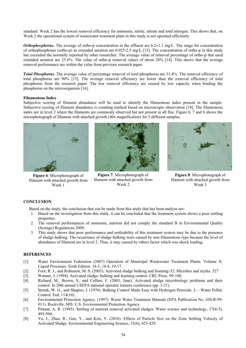
54

standard. Week 2 has the lowest removal efficiency for ammonia, nitrite, nitrate and total nitrogen. This shows that, on Week 2 the operational system of wastewater treatment plant in this study is not operated efficiently. Orthophosphorus. The average of ortho-p concentration in the effluent are 6.2±1.1 mg/L. The range for concentration of orthophosphorus (ortho-p) in extended aeration are 0.025-2.5 mg/L [13]. The concentration of ortho-p in this study has exceeded the normally reported by other researcher. The average value of removal percentage of ortho-p that used extended aeration are 25.6%. The value of ortho-p removal values of about 28% [14]. This shows that the average removal performance are within the value from previous research paper. Total Phosphorus. The average value of percentage removal of total phosphorus are 31.4%. The removal efficiency of total phosphorus are 90% [15]. The average removal efficiency are lower than the removal efficiency of total phosphorus from the research paper. The low removal efficiency are caused by low capacity when binding the phosphorus on the microorganism [16]. Filamentous Index Subjective scoring of filament abundance will be used to identify the filamentous index present in the sample. Subjective scoring of filament abundance is counting method based on microscopic observation [18]. The filamentous index are in level 2 where the filaments are commonly observed but not present in all floc. Figure 6, 7 and 8 shows the microphotograph of filament with attached growth (40x magnification) for 3 different samples.

CONCLUSION Based on the study, the conclusion that can be made from this study that has been analyse are: 1. Based on the investigation from this study, it can be concluded that the treatment system shows a poor settling

properties. 2. The removal performances of ammonia, nutrient did not comply the standard B in Environmental Quality

(Sewage) Regulations 2009. 3. This study shows that poor performance and settleability of this treatment system may be due to the presence

of sludge bulking. The occurrence of sludge bulking were caused by non-filamentous type because the level of abundance of filament are in level 2. Thus, it may caused by others factor which was shock loading.

REFERENCES

[1] Water Environment Federation (2007) Operation of Municipal Wastewater Treatment Plants. Volume II: Liquid Processes. Sixth Edition. 18-3, 18-4, 19-17.

[2] Foot, R. J., and Robinson, M. S. (2003). Activated sludge bulking and foaming-32: Microbes and myths. 527 [3] Wanner, J. (1994). Activated sludge: bulking and foaming control. CRC Press. 99-100. [4] Richard, M., Brown, S., and Collins, F. (2003, June). Activated sludge microbiology problems and their

control. In 20th annual USEPA national operator trainers conference (pp. 1-21). [5] Strunk, W. G., and Shapiro, J. (1976). Bulking Control Made Easy with Hydrogen Peroxide. J.—Water Pollut.

Control. Fed, 114(10). [6] Environmental Protection Agency. (1997). Waste Water Treatment Manuals (EPA Publication No. 430-R-99-

011). Rockville, MD: U.S. Environmental Protection Agency. [7] Pitman, A. R. (1985). Settling of nutrient removal activated sludges. Water science and technology, 17(4-5),

493-504. [8] Yu, J., Zhao, R., Gao, Y., and Kim, Y. (2016). Effects of Particle Size on the Zone Settling Velocity of

Activated Sludge. Environmental Engineering Science, 33(6), 423-429.

Figure 6: Microphotograph of filament with attached growth from

Week 1

Figure 7: Microphotograph of filament with attached growth from

Week 2

Figure 8: Microphotograph of filament with attached growth from

Week 3

55

[9] Zeng, J., Gao, J. M., Chen, Y. P., Yan, P., Dong, Y., Shen, Y., and Zhang, P. (2016). Composition and aggregation of extracellular polymeric substances (EPS) in hyperhaline and municipal wastewater treatment plants. Scientific reports, 6.

[10] Jin, B., Wilén, B. M., and Lant, P. (2004). Impacts of morphological, physical and chemical properties of sludge flocs on dewaterability of activated sludge. Chemical Engineering Journal, 98(1), 115-126.

[11] Jin, L., Zhang, G., and Tian, H. (2014). Current state of sewage treatment in China. Water research, 66, 85-98. [12] Colmenarejo, M. F., Rubio, A., Sanchez, E., Vicente, J., Garcia, M. G., and Borja, R. (2006). Evaluation of

municipal wastewater treatment plants with different technologies at Las Rozas, Madrid (Spain). Journal of environmental management, 81(4), 399-404.

[13] Ingvar-Nilsson, C., and Forså, N. (2016). Evaluation of an Extended Aeration System for Nutrient Removal, A Case Study of a Wastewater Treatment Plant in Kulai, Johor Baharu, Malaysia.

[14] Sotirakou, E., Kladitis, G., Diamantis, N., and Grigoropoulou, H. (1999). Ammonia and phosphorus removal in municipal wastewater treatment plant with extended aeration. Global Nest: the Int. J, 1(1), 47-53.

[15] Insel, G., Russell, D., Beck, B., and Vanrolleghem, P. A. (2003). Evaluation of nutrient removal performance for an ORBAL plant using the ASM2d model. Proceedings of the Water Environment Federation, 2003(12), 263-279.

[16] Petrinić, I., Čurlin, M., Korenak, J., and Simonić, M. (2011). Removal Efficiency of COD, Total P and Total N Components from Municipal Wastewater using Hollow-fibre MBR. Acta chimica Slovenica, 58(2).

[17] Department of Environment (DOE) (2009). Environmental Quality (Sewage) Regulations 2009, Environmental Quality Act (1974)

[18] Jenkins, D., Richard, M. G. and Daigger, G. T. (2004). Manual on theCauses and Control of Activated Sludge Bulking, Foaming, and Other Solids Separation Problems. London:

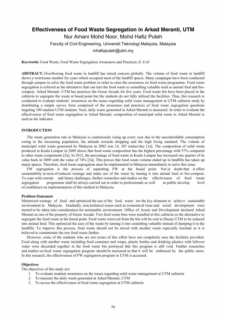
56

Effectiveness of Food Waste Segregation in Arked Meranti, UTM Nur Amani Mohd Noor, Mohd Hafiz Puteh

Faculty of Civil Engineering, Universiti Teknologi Malaysia, Malaysia mhafizputeh@utm.my

Keywords: Food Waste; Food Waste Segregation Awareness and Practices; E. Coli

ABSTRACT. Overflowing food waste in landfill has raised concern globally. The volume of food waste in landfill shows a worrisome number for years which occupied most of the landfill spaces. Many campaigns have been conducted through campus to solve the food waste problem in order to raise the awareness on food waste programme. Food waste segregation is referred as the alternative that can turn the food waste to something valuable such as animal feed and bio-compost. Arked Meranti, UTM has practices the Green Arcade for few years. Food waste bin have been placed in the cafeteria to segregate the waste at based point but the students do not fully utilized the facilities. Thus, this research is conducted to evaluate students’ awareness on the issues regarding solid waste management at UTM cafeteria study by distributing a simple survey form comprised of the awareness and practices of food waste segregation questions targeting 100 random UTM students. Next, daily waste generated in Arked Meranti is measured. In order to evaluate the effectiveness of food waste segregation in Arked Meranti, composition of municipal solid waste in Arked Meranti is used as the indicator.

INTRODUCTION

The waste generation rate in Malaysia is continuously rising up every year due to the uncontrollable consumption owing to the increasing population, the attitude towards shopping and the high living standard. The volume of municipal solid waste generated by Malaysia in 2002 was 14, 207 tonnes/day [1a]. The composition of solid waste produced in Kuala Lumpur in 2009 shows that food waste composition has the highest percentage with 57% compared to other waste components [2a]. In 2012, the percentage of food waste in Kuala Lumpur has increased one quarter of its value back in 2009 with the value of 74% [3a]. This proves that food waste volume ended up in landfills has taken up major spaces. Therefore, food waste segregation must be implemented in Malaysia immediately to solve this issue.

FW segregation is the process of separating FW at the based point. Not in doubt that it offers sustainability in term of reduced wastage and make use of the waste by turning it into animal feed or bio-compost. To cope with current and future challenges, further researches and studies on the effectiveness of food waste segregation programme shall be always carried out in order to professionals as well as public develop level of confidence on implementation of this method in Malaysia. Problem Statement Minimized wastage of food and optimized the use of the food waste are the key elements to achieve sustainable environment in Malaysia. Gradually, non-technical issues such as economical issue and social development were started to be taken into consideration for sustainable environment. Office of Assets and Development declared Arked Meranti as one of the property of Green Arcade. Two food waste bins were installed at this cafeteria as the alternative to segregate the food waste at the based point. Food waste retrieved from the bin will be sent to Dusun UTM to be reduced into animal feed. This optimized the uses of the waste by turning it into something valuable instead of dumping it to the landfills. To improve this process, food waste should not be mixed with another waste especially leachate as it is believed to contaminate the raw food waste further.

However, some of the students who are not aware of this effort have not completely uses the facilities provided. Food along with another waste including food container and wraps, plastic bottles and drinking plastics with leftover water were discarded together in the food waste bin portrayed that this program is still void. Further researches and studies on food waste segregation program should be increased so that it will be embraced by the public more. In this research, the effectiveness of FW segregation program in UTM is accessed. Objectives The objectives of this study are:

1. To evaluate students awareness on the issues regarding solid waste management at UTM cafeteria 2. To measure the daily waste generated at Arked Meranti, UTM 3. To access the effectiveness of food waste segregation at UTM cafeteria

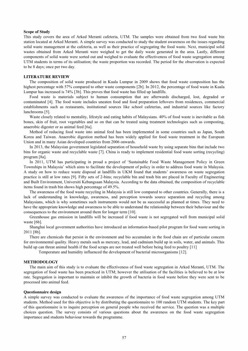
57

Scope of Study This study covers the area of Arked Meranti cafeteria, UTM. The samples were obtained from two food waste bin station located at Arked Meranti. A simple survey was conducted to study the student awareness on the issues regarding solid waste management at the cafeteria, as well as their practice of segregating the food waste. Next, municipal solid wastes obtained from Arked Meranti were weighed to get the daily waste generated in the area. Lastly, different components of solid waste were sorted out and weighed to evaluate the effectiveness of food waste segregation among UTM students in terms of its utilisation; the waste proportion was recorded. The period for the observation is expected to be 8 days; once per two day. LITERATURE REVIEW

The composition of solid waste produced in Kuala Lumpur in 2009 shows that food waste composition has the highest percentage with 57% compared to other waste components [2b]. In 2012, the percentage of food waste in Kuala Lumpur has increased is 74% [3b]. This proves that food waste has filled up landfills.

Food waste is materials subject to human consumption that are afterwards discharged, lost, degraded or contaminated [4]. The food waste includes uneaten food and food preparation leftovers from residences, commercial establishments such as restaurants, institutional sources like school cafeterias, and industrial sources like factory lunchrooms [5].

Waste closely related to mentality, lifestyle and eating habits of Malaysians. 40% of food waste is inevitable as fish bones, skin of fruit, root vegetables and so on that can be treated using treatment technologies such as composting, anaerobic digester or as animal feed [6a].

Method of reducing food waste into animal feed has been implemented in some countries such as Japan, South Korea and Taiwan. Anaerobic digestion method has been widely applied for food waste treatment in the European Union and in many Asian developed countries from 2006 onwards.

In 2013, the Malaysian government legislated separation of household waste by using separate bins that include two bins for organic waste and recyclable waste [7]. China is ready to implement residential food waste sorting (recycling) program [8a].

In 2011, UTM has participating in proud a project of ‘Sustainable Food Waste Management Policy in Green Townships in Malaysia’ which aims to facilitate the development of policy in order to address food waste in Malaysia. A study on how to reduce waste disposal at landfills in UKM found that students’ awareness on waste segregation practice is still at low rates [9]. Fifty sets of 2-bins; recyclable bin and trash bin are placed in Faculty of Engineering and Built Environment, Universiti Kebangsaan Malaysia. According to the data obtained, the composition of recyclable items found in trash bin shows high percentage of 49.5%.

The awareness of the food waste recycling in Malaysia is still low compared to other countries. Generally, there is a lack of understanding in knowledge, awareness, and perception towards source separation and recycling among Malaysians, which is why sometimes such instruments would not be as successful as planned at times. They need to have the appropriate knowledge and awareness to be able to understand the relationship between their behaviour and the consequences to the environment around them for longer term [10].

Greenhouse gas emission in landfills will be increased if food waste is not segregated well from municipal solid waste [6b].

Shanghai local government authorities have introduced an information-based pilot program for food waste sorting in 2011 [8b].

There are chemicals that persist in the environment and bio accumulate in the food chain are of particular concern for environmental quality. Heavy metals such as mercury, lead, and cadmium build up in soils, water, and animals. This build up can threat animal health if the food scraps are not treated well before being feed to poultry [11]

Temperature and humidity influenced the development of bacterial microorganisms [12]. METHODOLOGY

The main aim of this study is to evaluate the effectiveness of food waste segregation in Arked Meranti, UTM. The segregation of food waste has been practiced in UTM; however the utilisation of the facilities is believed to be at low rate. Segregation is important to maintain or inhibit the growth of bacteria in food waste before they were sent to be processed into animal feed.

Questionnaire design A simple survey was conducted to evaluate the awareness of the importance of food waste segregation among UTM students. Method used for this objective is by distributing the questionnaire to 100 random UTM students. The key part of this questionnaire is to inquire perception on general people who received the service. The question was a multiple choices question. The survey consists of various questions about the awareness on the food waste segregation importance and students behaviour towards the programme.

58

Daily waste generation in Arked Meranti UTM Daily waste generation in Arked Meranti,UTM was measured by weighing the solid waste generated by UTM students. The weight of wastes was weighed and recorded for the period of observation of 8 days; alternate days. Effectiveness of food waste segregation in Arked Meranti, UTM in terms of its utilisation In order to evaluate the effectiveness of food waste segregation in Arked Meranti, composition of municipal solid waste in Arked Meranti is used as the indicator. This method timeframe is 8 days; once per 2 day. Food waste from the catering in Arked Meranti is collected in a separate bin (for food waste only). Then, each bin is weighed by using weighing scale and the data. Next, food waste collected is spread on the slanted dripping table to collect leachate. This spread out method is also important since it can ease the process of sorting out food waste from other waste components. After sorting out the waste, each waste component is weighed by using weighing scale. Then, the mass of the items is recorded in a table. To obtain the composition of solid waste in terms of % by mass, use the equation stated below:

(𝑴𝒂𝒔𝒔 𝒐𝒇 𝒔𝒐𝒍𝒊𝒅 𝒘𝒂𝒔𝒕𝒆 𝒄𝒐𝒎𝒑𝒐𝒏𝒆𝒏𝒕𝒔 ÷ 𝒕𝒐𝒕𝒂𝒍 𝒎𝒂𝒔𝒔 𝒐𝒇 𝒔𝒐𝒍𝒊𝒅 𝒘𝒂𝒔𝒕𝒆) × 𝟏𝟎𝟎

RESULTS AND DISCUSSION

The results obtained throughout this study are discussed in this chapter. The distributed survey forms evaluate students’ awareness and practice on food waste segregation at UTM cafeteria. Weights of solid waste obtained from food waste bin in Arked Meranti were recorded. Then, the compositions of waste were categorized into few elements to access the effectiveness of food waste segregation at UTM cafeteria. Survey on UTM students’ awareness and behavior towards food waste segregation Table 1 and Figure 1 represent the data of UTM students’ awareness about food waste taking up major spaces in landfill. From the data, 53 of the students are aware that food wastes have an outstanding volume in landfill. However, 41 students still think that plastics have the largest capacity in landfill and followed by others, papers and tins. This could be due to wider exposure of plastic wastage compared to food wastage among the students. Many think food waste was only a secluded issue since no advertisement or aggressive campaigns about how food waste had been occupied the landfill area.

Thus, more of advertisement such as hanging the banner and interesting video about food waste recycle facts and its benefits should be made to raise concern regarding this issue. A short briefing about how food wastage had filled landfill should also be conducted to increase the students’ awareness about food waste. In Thailand, organic wastes are being dumped into landfills and release pollutants including greenhouse gases to the environment [13a]. Thus, volume of organic waste should be reduced to sustain the earth and maintain large area of landfills for another waste. Table 1: UTM students’ opinion on which municipal solid waste components show the highest composition in terms of % by mass in landfills.

Male Female

Food waste 26 27

Plastics 21 20

Paper 2 0

Tins 0 1

Others 1 2

Figure 2 present the data about the students’ opinion on food waste segregation. The pie chart indicates that 86

students agree that food waste segregation is environmentally friendly while 14 of them are neutral about it. Their opinion matters since we can conclude that the students who are neutral could have not expose to this agenda beforehand. More of food waste articles including food waste products list should be published and advertised to educate them as well as expose them to the food waste products. Implementation of urban organic waste utilization

0

10

20

30

Foodwaste

Plastics Paper Tins Others

no. o

f stu

dent

s

Municipal solid wastes

Awareness of UTM students on food waste took up major spaces in landfill

male

female

Figure 1: Awareness of UTM students on food waste took up major spaces in landfill

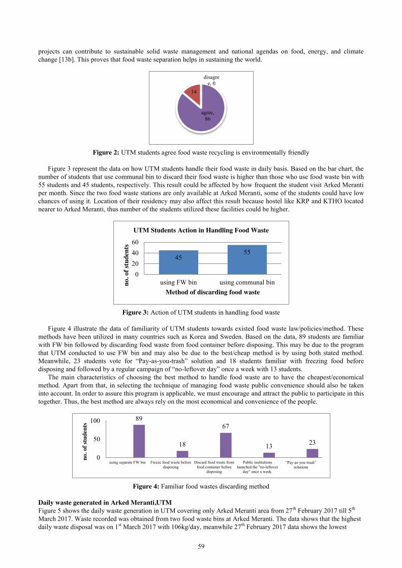
59

projects can contribute to sustainable solid waste management and national agendas on food, energy, and climate change [13b]. This proves that food waste separation helps in sustaining the world.

Figure 2: UTM students agree food waste recycling is environmentally friendly

Figure 3 represent the data on how UTM students handle their food waste in daily basis. Based on the bar chart, the

number of students that use communal bin to discard their food waste is higher than those who use food waste bin with 55 students and 45 students, respectively. This result could be affected by how frequent the student visit Arked Meranti per month. Since the two food waste stations are only available at Arked Meranti, some of the students could have low chances of using it. Location of their residency may also affect this result because hostel like KRP and KTHO located nearer to Arked Meranti, thus number of the students utilized these facilities could be higher.

Figure 3: Action of UTM students in handling food waste

Figure 4 illustrate the data of familiarity of UTM students towards existed food waste law/policies/method. These

methods have been utilized in many countries such as Korea and Sweden. Based on the data, 89 students are familiar with FW bin followed by discarding food waste from food container before disposing. This may be due to the program that UTM conducted to use FW bin and may also be due to the best/cheap method is by using both stated method. Meanwhile, 23 students vote for “Pay-as-you-trash” solution and 18 students familiar with freezing food before disposing and followed by a regular campaign of “no-leftover day” once a week with 13 students.

The main characteristics of choosing the best method to handle food waste are to have the cheapest/economical method. Apart from that, in selecting the technique of managing food waste public convenience should also be taken into account. In order to assure this program is applicable, we must encourage and attract the public to participate in this together. Thus, the best method are always rely on the most economical and convenience of the people.

Figure 4: Familiar food wastes discarding method

Daily waste generated in Arked Meranti,UTM Figure 5 shows the daily waste generation in UTM covering only Arked Meranti area from 27th February 2017 till 5th March 2017. Waste recorded was obtained from two food waste bins at Arked Meranti. The data shows that the highest daily waste disposal was on 1st March 2017 with 106kg/day, meanwhile 27th February 2017 data shows the lowest

agree, 86

14

disagree, 0

45 55

0204060

using FW bin using communal binno. o

f stu

dent

s

Method of discarding food waste

UTM Students Action in Handling Food Waste

89

18

67

13 23

0

50

100

using separate FW bin Freeze food waste beforedisposing

Discard food waste fromfood container before

disposing

Public institutionslaunched the "no-leftover

day" once a week.

“Pay-as-you-trash” solutions

no. o

f stu

dent

s

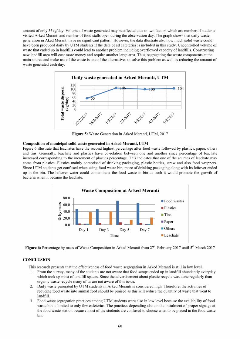
60

amount of only 55kg/day. Volume of waste generated may be affected due to two factors which are number of students visited Arked Meranti and number of food stalls open during the observation day. The graph shows that daily waste generation in Aked Meranti have no significant pattern. However, the data illustrate also how much solid waste could have been produced daily by UTM students if the data of all cafeterias is included in this study. Uncontrolled volume of waste that ended up in landfills could lead to another problem including overflowed capacity of landfills. Constructing new landfill area will cost more money and require another large area. Thus, segregating the waste components at the main source and make use of the waste is one of the alternatives to solve this problem as well as reducing the amount of waste generated each day.

Figure 5: Waste Generation in Arked Meranti, UTM, 2017

Composition of municipal solid waste generated in Arked Meranti, UTM Figure 6 illustrate that leachates have the second highest percentage after food waste followed by plastics, paper, others and tins. Generally, leachate and plastics have co-relation between one and another since percentage of leachate increased corresponding to the increment of plastics percentage. This indicates that one of the sources of leachate may come from plastics. Plastics mainly comprised of drinking packaging, plastic bottles, straw and also food wrappers. Since UTM students get confused when using food waste bin, more of drinking packaging along with its leftover ended up in the bin. The leftover water could contaminate the food waste in bin as such it would promote the growth of bacteria when it became the leachate.

Figure 6: Percentage by mass of Waste Composition in Arked Meranti from 27th February 2017 until 5th March 2017

CONCLUSION

This research presents that the effectiveness of food waste segregation in Arked Meranti is still in low level. 1. From the survey, many of the students are not aware that food scraps ended up in landfill abundantly everyday

which took up most of landfill spaces. Since the advertisement about plastic recycle was done regularly than organic waste recycle many of us are not aware of this issue.

2. Daily waste generated by UTM students in Arked Meranti is considered high. Therefore, the activities of reducing food waste into animal feed should be praised as this will reduce the quantity of waste that went to landfill.

3. Food waste segregation practices among UTM students were also in low level because the availability of food waste bin is limited to only few cafeterias. The practices depending also on the instalment of proper signage at the food waste station because most of the students are confused to choose what to be placed in the food waste bin.

55

106 100 104

020406080

100120

Tota

l was

te d

ispos

al

(kg/

day)

Daily waste generated in Arked Meranti, UTM

0.0

20.0

40.0

60.0

80.0

Day 1 Day 3 Day 5 Day 7

% b

y m

ass

Time

Waste Composition at Arked Meranti

Food wastes

Plastics

Tins

Paper

Others

Leachate

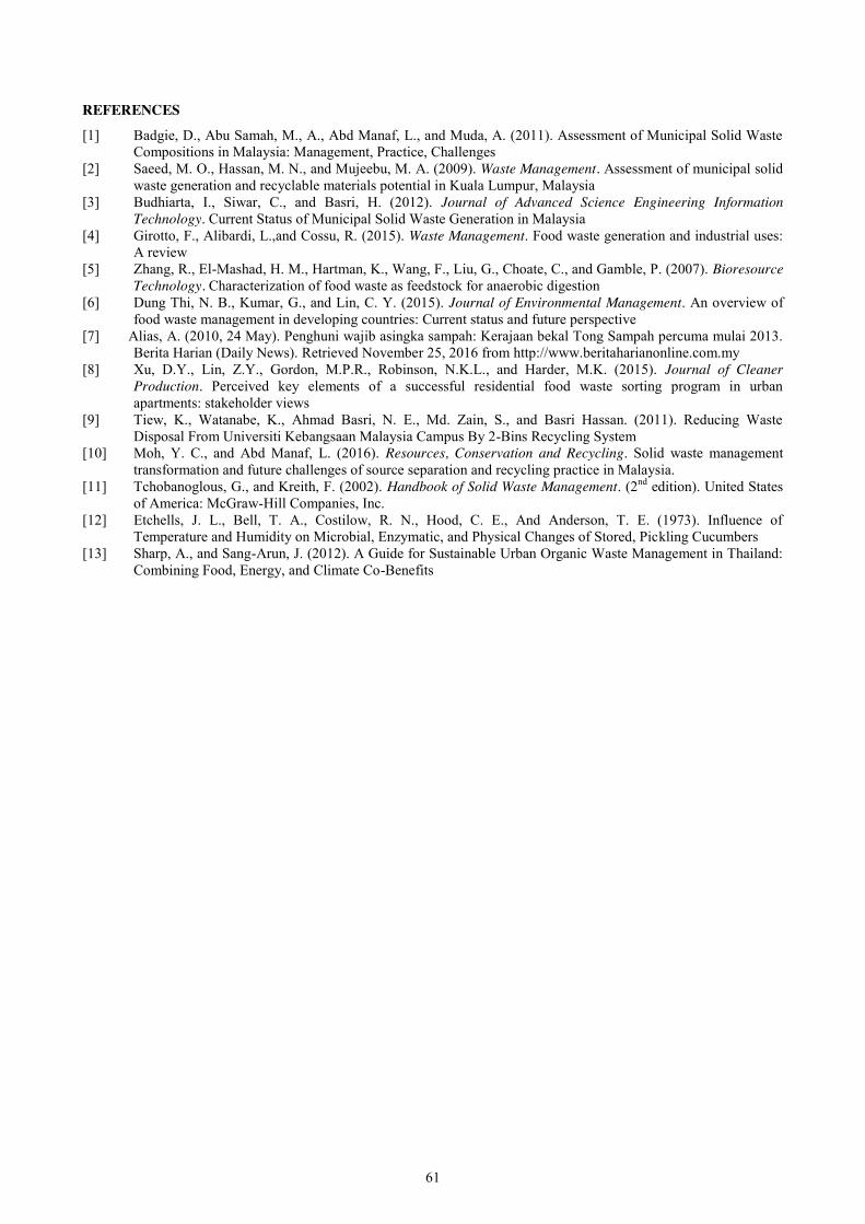
61

REFERENCES

[1] Badgie, D., Abu Samah, M., A., Abd Manaf, L., and Muda, A. (2011). Assessment of Municipal Solid Waste Compositions in Malaysia: Management, Practice, Challenges

[2] Saeed, M. O., Hassan, M. N., and Mujeebu, M. A. (2009). Waste Management. Assessment of municipal solid waste generation and recyclable materials potential in Kuala Lumpur, Malaysia

[3] Budhiarta, I., Siwar, C., and Basri, H. (2012). Journal of Advanced Science Engineering Information Technology. Current Status of Municipal Solid Waste Generation in Malaysia

[4] Girotto, F., Alibardi, L.,and Cossu, R. (2015). Waste Management. Food waste generation and industrial uses: A review

[5] Zhang, R., El-Mashad, H. M., Hartman, K., Wang, F., Liu, G., Choate, C., and Gamble, P. (2007). Bioresource Technology. Characterization of food waste as feedstock for anaerobic digestion

[6] Dung Thi, N. B., Kumar, G., and Lin, C. Y. (2015). Journal of Environmental Management. An overview of food waste management in developing countries: Current status and future perspective

[7] Alias, A. (2010, 24 May). Penghuni wajib asingka sampah: Kerajaan bekal Tong Sampah percuma mulai 2013. Berita Harian (Daily News). Retrieved November 25, 2016 from http://www.beritaharianonline.com.my

[8] Xu, D.Y., Lin, Z.Y., Gordon, M.P.R., Robinson, N.K.L., and Harder, M.K. (2015). Journal of Cleaner Production. Perceived key elements of a successful residential food waste sorting program in urban apartments: stakeholder views

[9] Tiew, K., Watanabe, K., Ahmad Basri, N. E., Md. Zain, S., and Basri Hassan. (2011). Reducing Waste Disposal From Universiti Kebangsaan Malaysia Campus By 2-Bins Recycling System

[10] Moh, Y. C., and Abd Manaf, L. (2016). Resources, Conservation and Recycling. Solid waste management transformation and future challenges of source separation and recycling practice in Malaysia.

[11] Tchobanoglous, G., and Kreith, F. (2002). Handbook of Solid Waste Management. (2nd edition). United States of America: McGraw-Hill Companies, Inc.

[12] Etchells, J. L., Bell, T. A., Costilow, R. N., Hood, C. E., And Anderson, T. E. (1973). Influence of Temperature and Humidity on Microbial, Enzymatic, and Physical Changes of Stored, Pickling Cucumbers

[13] Sharp, A., and Sang-Arun, J. (2012). A Guide for Sustainable Urban Organic Waste Management in Thailand: Combining Food, Energy, and Climate Co-Benefits

62

Ammonia in Aquaponics System And Its Impact to Plants Nur Azira bt Alias, Mohd Ismid bin Mohd Said

Faculty of Civil Engineering, Universiti Teknologi Malaysia, Malaysia

ismid@utm.my

Keywords: Aquaponics, Ammonia, Aquaculture, Agriculture

ABSTRACT. Aquaponics is the combined culture of fish and plants in recirculation systems. Aquaculture and agriculture systems are combined together to provide a symbiosis between plant and aquatic life. This combination help in the growth of the plants as the effluent from aquaculture system that is rich in nutrients will flows to the hydroponics system for plants to absorb the nutrients. While in the hydroponics system, the fish waste metabolites are removed by nitrification, thereby treating the water, which flow back to the fish tank. This study will focus on the ammonia as one of the element in the nitrogen cycle. Ammonia produced in the fish tank can harm the life of fish even in small amount so in this study, ammonia content will be observed along side with other water quality parameters such as BOD, COD, DO, pH, temperature, salinity and TDS.

INTRODUCTION

In Malaysia, aquaculture and agriculture plays an important role in supplying food and source of income for the population. There are various initiatives have been taken by the government to develop both these sectors in order to improve the national economy and to ensure national food security continues to be guaranteed. Aquaculture and agriculture systems are combined together to provide a symbiosis between plant and aquatic life. Water from fish farming that is high in ammonia content will be recycled into the hydroponics systems and the ammonia will be converted to nitrite and nitrate. The nutrient will be absorbed by plants in hydroponics system and clean water will return to the fish tank to be reuse.

Problem Statement Many people did not realized the pollution caused by agriculture. Development of the agricultural sector in Malaysia has resulted in widespread deforestation. In addition, agricultural waste which is not managed properly can also contribute to water pollution. The remnants such as fertilizers and pesticides discharged directly into rivers without being treated first. On the other hand, the aquaculture systems produce wastewater that contain a very high amount of ammonia and also will cause water pollution if discharged directly into the river.

Therefore, a suitable method used to overcome this problems is the by using a combination system of aquaculture and hydroponics system, the aquaponic.

Objectives The main objectives of this study is to examine the effectiveness of the aquaponics system by:

1. Reviewing the quantity of ammonia in a closed aquatic system and compare it to the quantity of ammonia in the aquaponic system.

2. Obtain the water quality parameters in aquaponic systems. 3. Reviewing the differences in plant growth in hydroponic systems and aquaponic system.

Scope of Study In this study, an aquaponic system model, a combination of aquaculture and hydroponics system will be built based on real aquaponic system. The size of the model is much smaller than the actual system but still can give a true picture of the real aquaponics system. The fish used in the system is a freshwater fish species and sizes of fish tank that will be used is 0.3 x 0.3 x 0.6 m. For plants, the type of vegetable that has a high absorption rate of nutrients will be grown hydroponically. Water from aquaculture systems will be channeled into the hydroponic containers to supply nutrients to the plant. Gravel will be used as a medium for bacterial growth that is required for the system. Pump also should be used to drain the water from the fish tank into hydroponic container.

LITERATURE REVIEW The growth of industrial development, economic and social whether in urban or rural areas, has affected the status of

the environment, especially activities such as agriculture and aquaculture. This development did not take into account the impact on the environment that has led to environmental pollution and thus indirectly pollute the water sources

For example, agricultural activities have led to a serious deforestation problem and disturbing the habitat of wild animals. In addition, agricultural waste which is not managed properly can also contribute to water pollution.

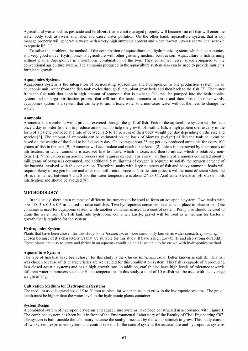
63

Agricultural waste such as pesticide and fertilizers that are not managed properly will become run off that will enter the water body such as rivers and lakes and cause water pollution. On the other hand, aquaculture system, that is not manage properly will generate a waste with a very high ammonia content and when thrown into a river will cause toxic to aquatic life [1].

To solve this problem, the method of the combination of aquaculture and hydroponics system, which is aquaponics, is a very good move. Hydroponics is agriculture with other growing medium besides soil. Aquaculture is fish farming without plants. Aquaponics is a symbiotic combination of the two. They consumed lesser space compared to the conventional agriculture system. The ammonia produced in the aquaculture system also can be used to provide nutrients for plants growth. Aquaponics Systems Aquaponics system is the integration of recirculating aquaculture and hydroponics in one production system. In an aquaponic unit, water from the fish tank cycles through filters, plant grow beds and then back to the fish [7]. The water from the fish tank that contain high amount of ammonia that is toxic to fish, will be pumped into the hydroponics system and undergo nitrification process that will turn the toxic ammonia to nitrite and then nitrite. In other words, aquaponics system is a system that can help to turn a toxic water to a non-toxic water without the need to change the water. Ammonia Ammonia is a metabolic waste product excreted through the gills of fish. Fish in the aquaculture system will be feed once a day in order fo them to produce ammonia. To help the growth of healthy fish, a high protein diet usually in the form of a palette provided at a rate of between 1.5 to 15 percent of their body weight per day depending on the size and species [8]. The amount of ammonia can be estimated on the basis of biomass (weight) of fish the tank or it can be based on the weight of the food to be fed every day. On average about 25 mg per day produced ammonia for every 100 grams of fish in the tank [9]. Ammonia will accumulate and reach toxic levels [2] unless it is removed by the process of nitrification, in which ammonia is oxidized first to nitrite, which is toxic, and then to nitrate, which is relatively non-toxic [3]. Nitrification is an aerobic process and requires oxygen. For every 1 milligram of ammonia converted about 5 milligrams of oxygen is consumed, and additional 5 milligrams of oxygen is required to satisfy the oxygen demand of the bacteria involved with this conversion. Therefore, tanks with large numbers of fish and heavy ammonia loads will require plenty of oxygen before and after the biofiltration process. Nitrification process will be most efficient when the pH is maintained between 7 and 8 and the water temperature is about 27-28 C. Acid water (less than pH 6.5) inhibits nitrification and should be avoided [8].

METHODOLOGY

In this study, there are a number of different instruments to be used to form an aquaponic system. Two tanks with size of 0.3 x 0.3 x 0.6 m is used to raise catfishes. Two hydroponics containers needed as a place to plant crops. One container is used for aquaponic system while another container is used as a control system. Pump also should be used to drain the water from the fish tank into hydroponic container. Lastly, gravel will be used as a medium for bacterial growth that is required for the system. Hydroponics System Plants that have been chosen for this study is the Ipomea sp. or more commonly known as water spinach. Ipomea sp. is chosen because of it’s characteristics that are suitable for this study. It have a high growth rte and also strong durability. These plants are easy to grow and thrive in an aqueous condition and is suitable to be grown with hydroponics method. Aquaculture System The type of fish that have been chosen for this study is the Clarias Batrachus sp. or better known as catfish. This fish was chosen because of its characteristics are well suited for this combination system. This fish is capable of reproducing in a closed aquatic systems and has a high growth rate. In addition, catfish also have high levels of tolerance towards different water parameters such as pH and temperature. In this study, a total of 10 catfish will be used with the average weight of 25g. Cultivation Medium for Hydroponics Systems The medium used is gravel sized 15 to 20 mm as place for water spinach to grow in the hydroponic systems. The gravel depth must be higher than the water level in the hydroponic plants container. System Design A combined system of hydroponic systems and aquaculture systems have been constructed in accordance with Figure 1. The combined system has been built in front of the Environmental Laboratory of the Faculty of Civil Engineering C07. The system is built outside the laboratory because the sunlight needed by the water spinach to grow. This study consist of two system, experiment system and control system. In the control system, the aquaculture and hydroponics systems

64

are not combined. Water spinach in hydroponic systems will absorb nutrients provided manually. While ammonia in aquaculture systems are not recycled.

Figure 1 Hydroponic and aquaqulture system

Determination Method Number Fish And Plants A tank with one square meter size can accommodate as many as 100 fish [6]. This study used a tank size of 0.6 x 0.3 x 0.3 m with a depth of half a tank. So the maximum amount of fish that can be used is 18 fishes. But only 5 catfishes were used. The number of water spinach used was dependent on the size of the growing area and also the number of catfish. In this system, 8 water spinach have been used for the efficient absorption of nutrients. Procedure In this study, two systems have been built which is experiment systems and control systems. In experiment system, aquaculture and hydroponics sytem are combined into an aquaponics system while in control system, the two systems are not combined. This is to get the comparison results. The study began with 5 catfish were put into the fish tank. The pump will also be installed and the water flow will occur. Then the water spinachs were planted. The data for BOD and COD will be taken once a week while the other parameters such as ammonia-nitrogen, pH, DO, water temperature, salinity and total dissolved solids were taken twice a week. Changes in weight of the fish will be taken up again at the last day of the study. While the growth of spinach will be measured once a week. Assessment of Water Samples Biochemical oxygen demand (BOD). For the BOD test, the volume of water sample is 50 ml. The DOi readings are taken with YSI 5000. After 5 days in incubator with temperature of 20ºC, the DO5 readings are taken and the value of BOD sre calculated using equation: BOD5= Where, DOi = DO value on the first day DO5 = DO value on the fifth day P = Dilution factor Chemical Oxygen Demand (COD). The test is conducted using HACH method (DR6000). Samples, with one blank were placed into a 2 mL test tube along with 3 mL of low range reaction material. The test tubes are then inserted into the reactor to undergo reflux for 2 hours. After 2 hours the sample is left to cool and the readings taken using the spektrofometer DR6000. Another parameters such as Ammonia, Ammonium, DO, pH, temperature, salinity and TDS were taken by meter probe YSI Professional Plus.

RESULTS AND DISCUSSION

Ammonia (NH3 ) At the beginning of the study, the value of ammonia is still low and in the safe range. The ammonia level should be less than 0.02 mg/L.[4]. In this study, the data obtained for ammonia is in the range of 0.00 to 0.03 mg/L for experiment tank, and 0.00 to 0.06 mg/L for the control tank. The amount of ammonia in the aquaponics system clearly shows a lower value than in the control system. Ammonia will accumulate and reach toxic levels unless it is removed by the process of nitrification in which ammonia is oxidized first to nitrite, which is toxic, and then to nitrate, which is relatively non-toxic. This process occur with the help of the Nitrifying bacteria that are grown in the biofilter at the aquaponics system. The amount of ammonia in the control tank is keep getting higher because the ammonia in the water will accumulate and only will reduce when the water is exchange.

𝐷𝑂𝑖 − 𝐷𝑂𝑓𝑝

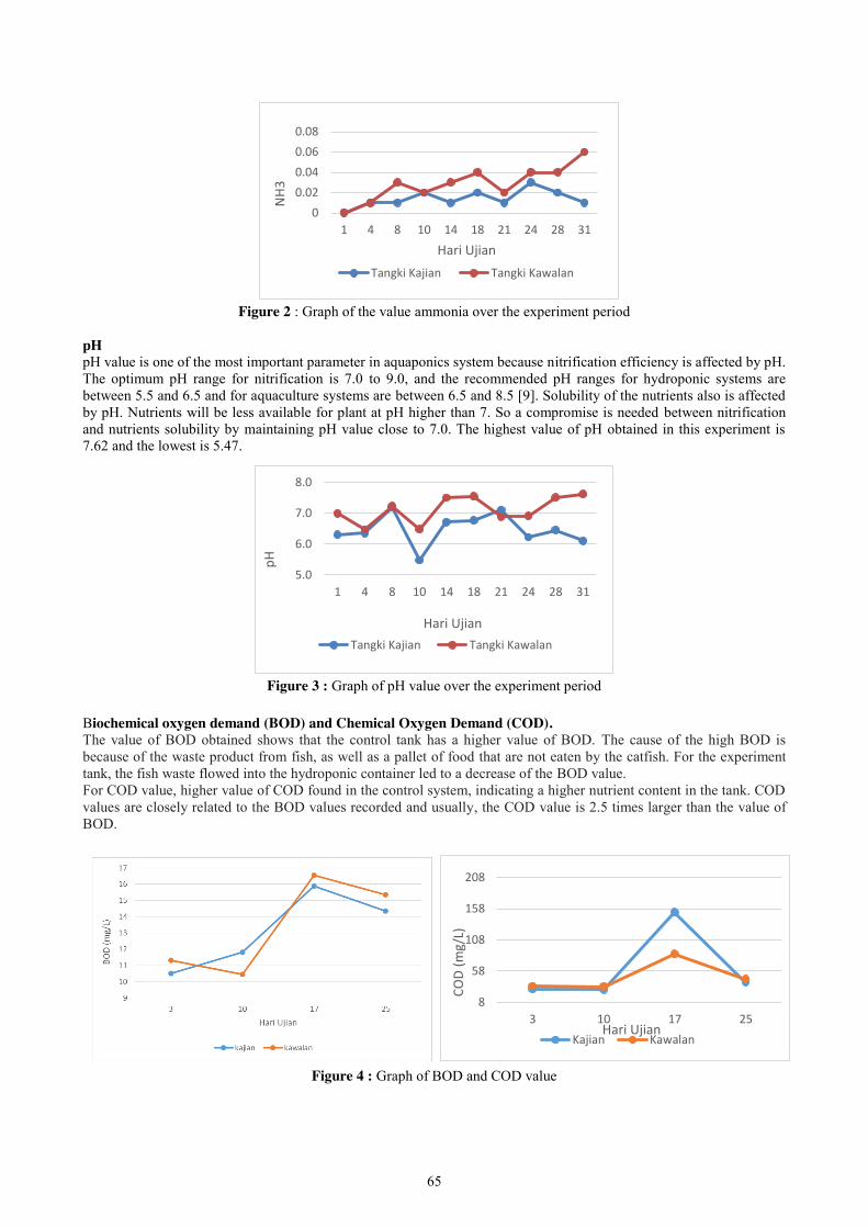
65

5.0

6.0

7.0

8.0

1 4 8 10 14 18 21 24 28 31

pH

Hari Ujian Tangki Kajian Tangki Kawalan

00.020.040.060.08

1 4 8 10 14 18 21 24 28 31

NH3

Hari Ujian Tangki Kajian Tangki Kawalan

8

58

108

158

208

3 10 17 25

COD

(mg/

L)

Hari Ujian Kajian Kawalan

Figure 2 : Graph of the value ammonia over the experiment period pH pH value is one of the most important parameter in aquaponics system because nitrification efficiency is affected by pH. The optimum pH range for nitrification is 7.0 to 9.0, and the recommended pH ranges for hydroponic systems are between 5.5 and 6.5 and for aquaculture systems are between 6.5 and 8.5 [9]. Solubility of the nutrients also is affected by pH. Nutrients will be less available for plant at pH higher than 7. So a compromise is needed between nitrification and nutrients solubility by maintaining pH value close to 7.0. The highest value of pH obtained in this experiment is 7.62 and the lowest is 5.47.

Figure 3 : Graph of pH value over the experiment period

Biochemical oxygen demand (BOD) and Chemical Oxygen Demand (COD). The value of BOD obtained shows that the control tank has a higher value of BOD. The cause of the high BOD is because of the waste product from fish, as well as a pallet of food that are not eaten by the catfish. For the experiment tank, the fish waste flowed into the hydroponic container led to a decrease of the BOD value. For COD value, higher value of COD found in the control system, indicating a higher nutrient content in the tank. COD values are closely related to the BOD values recorded and usually, the COD value is 2.5 times larger than the value of BOD.

Figure 4 : Graph of BOD and COD value

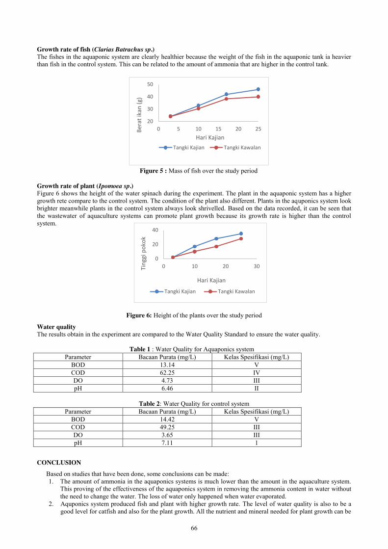
66

20

30

40

50

0 5 10 15 20 25Bera

t ika

n (g

) Hari Kajian

Tangki Kajian Tangki Kawalan

0

20

40

0 10 20 30Ting

gi p

okok

Hari Kajian

Tangki Kajian Tangki Kawalan

Growth rate of fish (Clarias Batrachus sp.) The fishes in the aquaponic system are clearly healthier because the weight of the fish in the aquaponic tank ia heavier than fish in the control system. This can be related to the amount of ammonia that are higher in the control tank.

Figure 5 : Mass of fish over the study period Growth rate of plant (Ipomoea sp.) Figure 6 shows the height of the water spinach during the experiment. The plant in the aquaponic system has a higher growth rete compare to the control system. The condition of the plant also different. Plants in the aquponics system look brighter meanwhile plants in the control system always look shrivelled. Based on the data recorded, it can be seen that the wastewater of aquaculture systems can promote plant growth because its growth rate is higher than the control system.

Figure 6: Height of the plants over the study period

Water quality The results obtain in the experiment are compared to the Water Quality Standard to ensure the water quality.

Table 1 : Water Quality for Aquaponics system

Parameter Bacaan Purata (mg/L) Kelas Spesifikasi (mg/L) BOD 13.14 V COD 62.25 IV DO 4.73 III pH 6.46 II

Table 2: Water Quality for control system

Parameter Bacaan Purata (mg/L) Kelas Spesifikasi (mg/L) BOD 14.42 V COD 49.25 III DO 3.65 III pH 7.11 1

CONCLUSION

Based on studies that have been done, some conclusions can be made: 1. The amount of ammonia in the aquaponics systems is much lower than the amount in the aquaculture system.

This proving of the effectiveness of the aquaponics system in removing the ammonia content in water without the need to change the water. The loss of water only happened when water evaporated.

2. Aquponics system produced fish and plant with higher growth rate. The level of water quality is also to be a good level for catfish and also for the plant growth. All the nutrient and mineral needed for plant growth can be

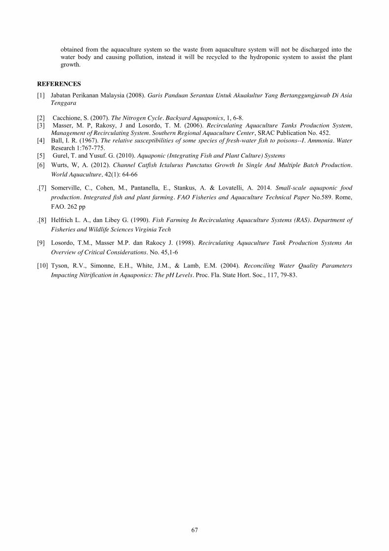
67

obtained from the aquaculture system so the waste from aquaculture system will not be discharged into the water body and causing pollution, instead it will be recycled to the hydroponic system to assist the plant growth.

REFERENCES

[1] Jabatan Perikanan Malaysia (2008). Garis Panduan Serantau Untuk Akuakultur Yang Bertanggungjawab Di Asia Tenggara

[2] Cacchione, S. (2007). The Nitrogen Cycle. Backyard Aquaponics, 1, 6-8. [3] Masser, M. P, Rakosy, J and Losordo, T. M. (2006). Recirculating Aquaculture Tanks Production System,

Management of Recirculating System. Southern Regional Aquaculture Center, SRAC Publication No. 452. [4] Ball, I. R. (1967). The relative susceptibilities of some species of fresh-water fish to poisons--I. Ammonia. Water

Research 1:767-775. [5] Gurel, T. and Yusuf. G. (2010). Aquaponic (Integrating Fish and Plant Culture) Systems [6] Wurts, W, A. (2012). Channel Catfish Ictalurus Punctatus Growth In Single And Multiple Batch Production.

World Aquaculture, 42(1): 64-66

.[7] Somerville, C., Cohen, M., Pantanella, E., Stankus, A. & Lovatelli, A. 2014. Small-scale aquaponic food production. Integrated fish and plant farming. FAO Fisheries and Aquaculture Technical Paper No.589. Rome, FAO. 262 pp

.[8] Helfrich L. A., dan Libey G. (1990). Fish Farming In Recirculating Aquaculture Systems (RAS). Department of Fisheries and Wildlife Sciences Virginia Tech

[9] Losordo, T.M., Masser M.P. dan Rakocy J. (1998). Recirculating Aquaculture Tank Production Systems An Overview of Critical Considerations. No. 45,1-6

[10] Tyson, R.V., Simonne, E.H., White, J.M., & Lamb, E.M. (2004). Reconciling Water Quality Parameters Impacting Nitrification in Aquaponics: The pH Levels. Proc. Fla. State Hort. Soc., 117, 79-83.

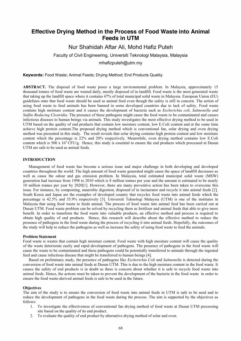
68

Effective Drying Method in the Process of Food Waste into Animal Feeds in UTM

Nur Shahidah Aftar Ali, Mohd Hafiz Puteh Faculty of Civil Engineering, Universiti Teknologi Malaysia, Malaysia

mhafizputeh@utm.my

Keywords: Food Waste; Animal Feeds; Drying Method; End Products Quality

ABSTRACT. The disposal of food waste poses a large environmental problem. In Malaysia, approximately 15 thousand tonnes of food waste are wasted daily, mostly disposed of in landfill. Food waste is the most generated waste that taking up the landfill space where it contains 47% of total municipal solid waste in Malaysia. European Union (EU) guidelines state that food waste should be used as animal feed even though the safety is still in concern. The action of using food waste to feed animals has been banned in some developed countries due to lack of safety. Food waste contains high moisture content and it causes the development of bacteria such as Escherichia coli, Salmonella and Sulfite Reducing Clostridia. The presence of these pathogens might cause the food waste to be contaminated and causes infectious diseases to human beings via animals. This study investigates the most effective drying method to be used in UTM based on the quality of end products that contain low moisture content, low E.Coli content and at the same time achieve high protein content.The proposed drying method which is conventional fan, solar drying and oven drying method was presented in this study. The result reveals that solar drying contains high protein content and low moisture content which the percentage is 22% and 20% respectively. Meanwhile, oven drying method contains low E.Coli content which is 500 x 103 CFU/g. Hence, this study is essential to ensure the end products which processed at Dusun UTM are safe to be used as animal feeds.

INTRODUCTION

Management of food waste has become a serious issue and major challenge in both developing and developed countries throughout the world. The high amount of food waste generated might cause the space of landfill decreases as well as cause the odour and gas emission problem. In Malaysia, total estimated municipal solid waste (MSW) generation had increase from 1998 to 2010 which is 8 million tonnes per year and the amount is estimated to be nearly 10 million tonnes per year by 2020[1]. However, there are many preventive action has been taken to overcome this issue. For instance, by composting, anaerobic digestion, disposed of in incinerator and recycle it into animal feeds [2]. South Korea and Japan are the examples of developed country that recycles food waste into animal feeds which the percentage is 42.5% and 35.9% respectively [3]. Universiti Teknologi Malaysia (UTM) is one of the institutes in Malaysia that using food waste to feeds animal. The process of food waste into animal feed has been carried out at Dusun UTM. Food waste problem can be solved by recycling them as fertilizer and animal feeds that able to give more benefit. In order to transform the food waste into valuable products, an effective method and process is required to obtain high quality of end products. Hence, this research will describe about the effective method to reduce the presence of pathogens in the food waste during the process of recycling it into animal feeds. Hopefully, the outcomes of the study will help to reduce the pathogens as well as increase the safety of using food waste to feed the animals.

Problem Statement Food waste is wastes that contain high moisture content. Food waste with high moisture content will cause the quality of the waste deteriorate easily and rapid development of pathogens. The presence of pathogens in the food waste will cause the waste to be contaminated and these pathogens could be potentially transferred to animals through the ingested feed and cause infectious disease that might be transferred to human beings [4].

Based on preliminary study, the presence of pathogens like Escherichia Coli and Salmonella is detected during the conversion of food waste into animal feeds at Dusun UTM. This is due to the high moisture content in the food waste. It causes the safety of end products is in doubt as there is concern about whether it is safe to recycle food waste into animal feeds. Hence, the actions must be taken to prevent the development of the bacteria in the food waste in order to ensure the food waste-derived animal feeds is safe to be used in the future.

Objectives The aim of the study is to ensure the conversion of food waste into animal feeds in UTM is safe to be used and to reduce the development of pathogens in the food waste during the process. The aim is supported by the objectives as follows:

1. To investigate the effectiveness of conventional fan drying method of food waste at Dusun UTM processing site based on the quality of its end product.

2. To evaluate the quality of end product by alternative drying method of solar and oven.

69

3. To compare the amount of bacteria presence in the end product of fan, solar drying and oven method.

Scope of Study The scope of the study was conducted within Universiti Teknologi Malaysia Johor Bahru Campus UTM JB at Dusun UTM. The material involved in this study was food waste that generated from Arked Meranti. The bins which contain raw food waste from Arked Meranti were collected and sent to Dusun UTM processing site. In this study, three different drying methods were conducted to dried the food waste which is conventional fan, oven and solar. The samples were sent to the laboratory to analyse the quality of end products. The moisture content, protein content and the presence of bacteria in the samples were examines, mainly according to the official methods of analysis of the AOAC [5]. At the end of the study, the most effective method was identified based on the highest quality of end products obtained from different drying methods.

LITERATURE REVIEW

Food waste has considered as a global issues due to the amount of waste generated has increases every day. It is also currently considered to be a major threatening factor for sustainable development and food waste management systems.

The developed countries nowadays are much concerned to find the effective management solution for the high amount of waste especially municipal solid waste (MSW). Composition of waste dumped at the Malaysian landfills consists of 47% food waste, 20% plastics, 17% paper, 4% metals,3% glass and the rest 9% is other waste[6]. High amount of food waste generated in MSW is the main cause of the problem in landfills such as odour, less landfill space and emission of greenhouse gases. In addition, dispose food waste in a landfill causes odour as it decomposes, attracts flies and vermin, and has the potential to add biological oxygen demand (BOD) to the leachate. Developed countries such as South Korea and Japan have started to separate food waste from municipal solid waste to avoid insufficient areas for landfills, incineration issues and problem with transportation to send food waste into disposal site. However, in Malaysia, the food waste management is still poor and disorganized due to lack of public awareness to minimise the waste generation, inadequate management, and rapid urbanizations. The most preferred of MSW disposal method in Malaysia is through landfilling. Composting, anaerobic digestion, disposed of in incinerator and recycle it into animal feeds are types of food waste management that has been implemented in some developed countries. Composting is a controlled and biological process of decomposition of organic material that transform organic waste into valuable material capable of upgrading the soil quality in gardens and fields. It helps to reduce volume of food waste disposed at landfill and improve the quality and nutrition of product. However, it also gives negative impact to the environment such a odour problems and the compost bins might attract flies, maggots and rats.

Recycle food waste into animal feeds is beneficial since food waste contains high nutritive value and easily accessible which serves it as a potential animal feed [3]. Feeding food waste to animals has been an important component of livestock production as it provides protein sources for a long time to the animals. The protein content of animal feeds from factory is minimum of 18% while food waste had adequate protein content which is minimum of 21%. Nutrient content especially protein will be able to increase the growth of animals and makes them becomes healthier and it will also give a great benefit to the human consumer as the animal is enrich with protein [7]. However, the very low self-sufficiency of animal feed is one of the major reasons of the low self-sufficiency of food and the poorly balanced feed supply makes the livestock sector unsustainable. The use of recycled food waste for feed is an effective method of improving feed self-sufficiency and reducing the environmental burden from food waste [8].

Even though the conversion of food waste into animal feeds has been used widely by developed countries, the safety is still in doubt. Firstly, this is due to the food waste contains high moisture content as it may lead to the rapid growth of the unpleasant pathogens such as Salmonella and E.coli. Then, it is concern whether the food waste-derived animal feed has sufficient nutrients to support animal growth and the spread of pandemic disease by bacterial production which caused by the feed. Food waste is very conducive for the growth of microorganisms that can lead to foot and mouth disease, salmonella, toxoplasmosis and swine fever virus. The concentration of chemical contaminants also becomes an issue as it must not exceed the standard limit and the feed produced from food waste contain hazardous component [7]. Safety measures have been taken during the development of food waste-animal feeds which is during the collection of raw materials. Foreign objects such as straw, toothpicks and chopsticks that mixed with food waste have been removed. For food waste storage and shipment, the collected food waste from the food industry must be swiftly as possible and should be kept in containers with lids to keep them from crows and from contamination with bacteria [9]. The use of antioxidants and antifungal agents such as Effective Microbes (EM) must be among those that have been officially approved. The management measure also should pay attention to improve the safety of food waste such as source- separated food waste collection.

To ensure the animal feeds is safe from the bacteria development as well as safe to be used, difference conversion method has been proposed nowadays. However, each conversion method will gives a great influence on the production of animal feeds from food waste which is in terms of nutrient content, moisture content and presence of bacteria. Drying off treatment is a method which involves a combined heat and mass transfer. It is one of the simplest processes to remove excess water from the food waste [10]. Fan, oven, solar radiation and microwave are some of the drying method that is recently used in drying process. These technologies will help to reduce moisture content in food waste by drying.

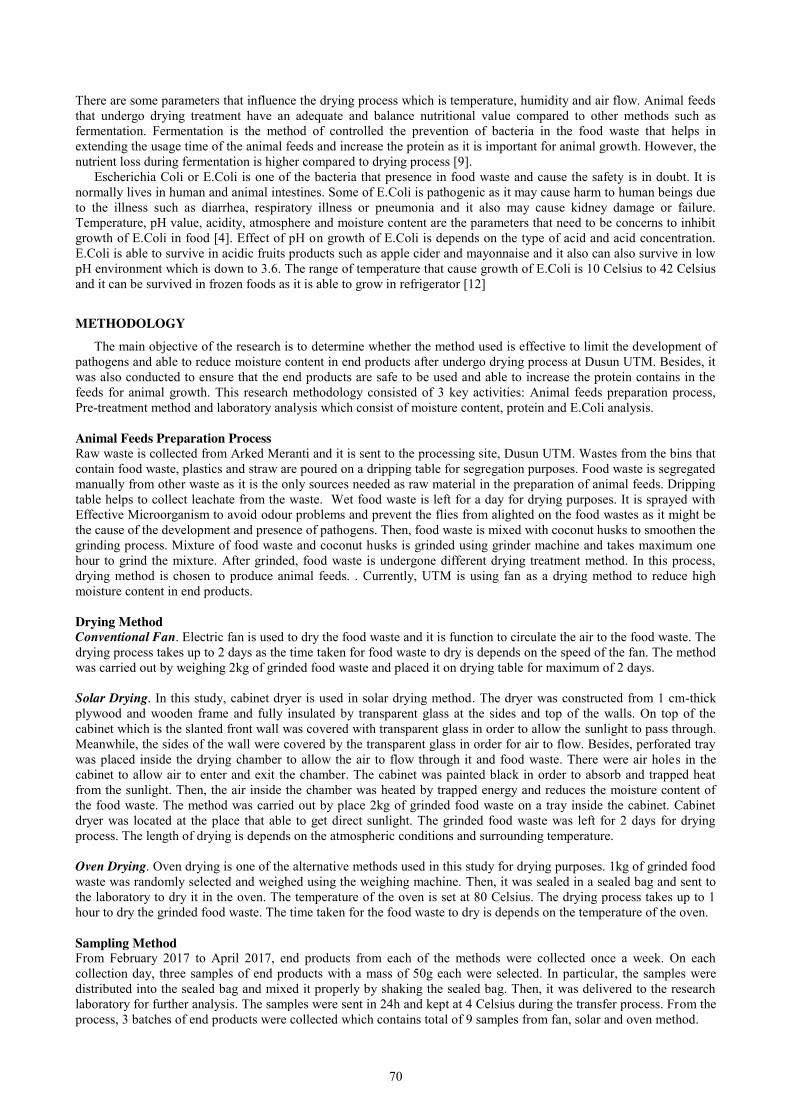
70

There are some parameters that influence the drying process which is temperature, humidity and air flow. Animal feeds that undergo drying treatment have an adequate and balance nutritional value compared to other methods such as fermentation. Fermentation is the method of controlled the prevention of bacteria in the food waste that helps in extending the usage time of the animal feeds and increase the protein as it is important for animal growth. However, the nutrient loss during fermentation is higher compared to drying process [9].

Escherichia Coli or E.Coli is one of the bacteria that presence in food waste and cause the safety is in doubt. It is normally lives in human and animal intestines. Some of E.Coli is pathogenic as it may cause harm to human beings due to the illness such as diarrhea, respiratory illness or pneumonia and it also may cause kidney damage or failure. Temperature, pH value, acidity, atmosphere and moisture content are the parameters that need to be concerns to inhibit growth of E.Coli in food [4]. Effect of pH on growth of E.Coli is depends on the type of acid and acid concentration. E.Coli is able to survive in acidic fruits products such as apple cider and mayonnaise and it also can also survive in low pH environment which is down to 3.6. The range of temperature that cause growth of E.Coli is 10 Celsius to 42 Celsius and it can be survived in frozen foods as it is able to grow in refrigerator [12]

METHODOLOGY The main objective of the research is to determine whether the method used is effective to limit the development of

pathogens and able to reduce moisture content in end products after undergo drying process at Dusun UTM. Besides, it was also conducted to ensure that the end products are safe to be used and able to increase the protein contains in the feeds for animal growth. This research methodology consisted of 3 key activities: Animal feeds preparation process, Pre-treatment method and laboratory analysis which consist of moisture content, protein and E.Coli analysis. Animal Feeds Preparation Process Raw waste is collected from Arked Meranti and it is sent to the processing site, Dusun UTM. Wastes from the bins that contain food waste, plastics and straw are poured on a dripping table for segregation purposes. Food waste is segregated manually from other waste as it is the only sources needed as raw material in the preparation of animal feeds. Dripping table helps to collect leachate from the waste. Wet food waste is left for a day for drying purposes. It is sprayed with Effective Microorganism to avoid odour problems and prevent the flies from alighted on the food wastes as it might be the cause of the development and presence of pathogens. Then, food waste is mixed with coconut husks to smoothen the grinding process. Mixture of food waste and coconut husks is grinded using grinder machine and takes maximum one hour to grind the mixture. After grinded, food waste is undergone different drying treatment method. In this process, drying method is chosen to produce animal feeds. . Currently, UTM is using fan as a drying method to reduce high moisture content in end products. Drying Method Conventional Fan. Electric fan is used to dry the food waste and it is function to circulate the air to the food waste. The drying process takes up to 2 days as the time taken for food waste to dry is depends on the speed of the fan. The method was carried out by weighing 2kg of grinded food waste and placed it on drying table for maximum of 2 days. Solar Drying. In this study, cabinet dryer is used in solar drying method. The dryer was constructed from 1 cm-thick plywood and wooden frame and fully insulated by transparent glass at the sides and top of the walls. On top of the cabinet which is the slanted front wall was covered with transparent glass in order to allow the sunlight to pass through. Meanwhile, the sides of the wall were covered by the transparent glass in order for air to flow. Besides, perforated tray was placed inside the drying chamber to allow the air to flow through it and food waste. There were air holes in the cabinet to allow air to enter and exit the chamber. The cabinet was painted black in order to absorb and trapped heat from the sunlight. Then, the air inside the chamber was heated by trapped energy and reduces the moisture content of the food waste. The method was carried out by place 2kg of grinded food waste on a tray inside the cabinet. Cabinet dryer was located at the place that able to get direct sunlight. The grinded food waste was left for 2 days for drying process. The length of drying is depends on the atmospheric conditions and surrounding temperature. Oven Drying. Oven drying is one of the alternative methods used in this study for drying purposes. 1kg of grinded food waste was randomly selected and weighed using the weighing machine. Then, it was sealed in a sealed bag and sent to the laboratory to dry it in the oven. The temperature of the oven is set at 80 Celsius. The drying process takes up to 1 hour to dry the grinded food waste. The time taken for the food waste to dry is depends on the temperature of the oven. Sampling Method From February 2017 to April 2017, end products from each of the methods were collected once a week. On each collection day, three samples of end products with a mass of 50g each were selected. In particular, the samples were distributed into the sealed bag and mixed it properly by shaking the sealed bag. Then, it was delivered to the research laboratory for further analysis. The samples were sent in 24h and kept at 4 Celsius during the transfer process. From the process, 3 batches of end products were collected which contains total of 9 samples from fan, solar and oven method.

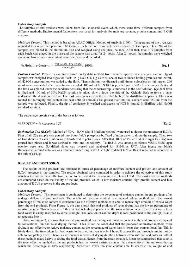
71

Laboratory Analysis The samples of end products were taken from fan, solar and ovens which there were three different samples from different methods. Environmental Laboratory was used for analysis for moisture content, protein content and E.Coli analysis. Moisture Content. This method is based on AOAC Official Method of Analysis (1990). Temperature of the oven was regulated to standard temperature, 105 Celsius. Each method from each batch consists of 3 samples. Then, 20g of the samples was placed in the aluminium dish and weighed using analytical balance. After that, total of 9 samples from each batch was placed in the oven and the sample was dried for 24 hours. After 24 hours, the samples were weighed again and loss of moisture content were calculated and recorded.

% 𝑀𝑜𝑖𝑠𝑡𝑢𝑟𝑒 𝐶𝑜𝑛𝑡𝑒𝑛𝑡 = 𝑊𝑒𝑡 𝑤𝑒𝑖𝑔ℎ𝑡−𝐷𝑟𝑦 𝑤𝑒𝑖𝑔ℎ𝑡

𝑊𝑒𝑡 𝑤𝑒𝑖𝑔ℎ𝑡𝑥 100% Eq. 1

Protein Content. Protein is examined based on kjedahl method from wendee approximate analysis method. 1g of samples was weighed into digestion flask. 15 g Na2SO4, 1 g CuSO4, one or two salinized boiling granules and 20 mL of H2SO4 concentration was added to the flask. Then, solution was digested until almost colourless or light green. 200 ml of water was added after the solution is cooled. 100 mL of 0.1 N HCl is pipetted into a 500 mL erlenmeyer flask and the flask was placed under the condenser ensuring that the condenser tip is immersed in the acid solution. Kjeldahl flask is tilted and 100 mL of 50% NaOH solution is added slowly down the side of the Kjeldahl flask to forms a layer underneath the digestion mixture. The flask was connected to the distilled bulb of the distillation apparatus. Flask was rotated to thoroughly mix content and heat until all ammonia has passed over into the standard acid. 150 ml from the sample was collected. Finally, the tip of condenser is washed and excess of HCI is titrated in distillate with NaOH standard solution.

The percentage protein (wet or dry basis) as follows

% PROTEIN = % nitrogen x 6.25 Eq. 2

Escherichia Coli (E.Coli). Method of FDA – BAM (Solid Medium Method) were used to detect the presence of E.Coli. First of all, 25g sample was poured into Butterfield's phosphate-buffered dilution water to dilute the sample. Then, two of 1ml aliquots of each dilution were transferred to petri dishes. After that, 10ml of Voilet Red Bile Agar (VRBA) was poured into plates and it was swirled to mix, and let solidify. To find E. coli among coliforms VRBA-MUG agar overlay were used. Solidified plates was inverted and incubated for 18-24h at 35oC. After incubation, bluish fluorescence around colonies was observed under long wave UV light to detect E.Coli. Result obtained is recorded in the unit of CFU/g.

RESULT AND DISCUSSION

The results of end products are obtained in terms of percentage of moisture content and protein and amount of E.Coli presence in the samples. The results obtained were compared in order to achieve the objectives of this study which is to find the most effective method to be used at the processing site, Dusun UTM. The most effective methods are compared based on the quality of the end products which is low moisture content, high protein content and less amount of E.Coli presence in the end products.

Laboratory Analysis Moisture Content. This experiment is conducted to determine the percentage of moisture content in end products after undergo different drying methods. The results of moisture content is compared where method with the lowest percentage of moisture content is considered as the effective method as it able to reduce high amount of excess water from the end products. From Figure 1, the data shows that end products of solar drying has the lowest percentage of moisture content.This is because of this method is highly dependent on the solar radiation where the excess water from food waste is easily absorbed by direct sunlight. The location of cabinet dryer is well positioned as the sunlight is able to penetrate into it.

Based on Figure 2, it shows that oven drying method has the highest moisture content in the end products compared to conventional fan and solar drying method. Thus, it can be concluded that the proposed alternative method, oven drying is not effective to reduce moisture content as the percentage of water loss is lower than conventional fan. This is likely due to the time taken for food waste to be dried in oven is only 1 hour. It causes the end products might not be able to completely dried. There is a differences in terms of drying duration between oven with fan and solar as both of these methods takes 2 days to drying the food waste. Hence, from the result obtained, it can be summarized that solar is the most effective method as the end products has the lowest moisture content than conventional fan and oven drying which the percentage is 18% respectively. Moreover, lower moisture content able to decrease the weight of end

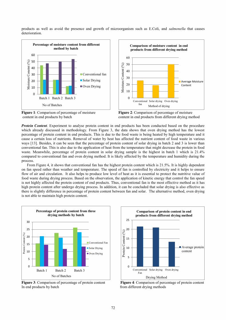
72

products as well as avoid the presence and growth of microorganism such as E.Coli, and salmonella that causes deterioration.

Figure 1: Comparison of percentage of moisture Figure 2: Comparison of percentage of moisture content in end products by batch content in end products from different drying method Protein Content. Experiment to analyse protein content in end products has been conducted based on the procedure which already discussed in methodology. From Figure 3, the data shows that oven drying method has the lowest percentage of protein content in end products. This is due to the food waste is being heated by high temperature and it cause a certain loss of nutrients. Removal of water by heat has affected the nutrient content of food waste in various ways [13]. Besides, it can be seen that the percentage of protein content of solar drying in batch 2 and 3 is lower than conventional fan. This is also due to the application of heat from the temperature that might decrease the protein in food waste. Meanwhile, percentage of protein content in solar drying sample is the highest in batch 1 which is 21.4% compared to conventional fan and oven drying method. It is likely affected by the temperature and humidity during the process.

From Figure 4, it shows that conventional fan has the highest protein content which is 21.5%. It is highly dependent on fan speed rather than weather and temperature. The speed of fan is controlled by electricity and it helps to ensure flow of air and circulation. It also helps to produce low level of heat as it is essential to protect the nutritive value of food waste during drying process. Based on the observation, the application of kinetic energy that control the fan speed is not highly affected the protein content of end products. Thus, conventional fan is the most effective method as it has high protein content after undergo drying process. In addition, it can be concluded that solar drying is also effective as there is slightly difference in percentage of protein content between fan and solar. The alternative method, oven drying is not able to maintain high protein content.

Figure 3: Comparison of percentage of protein content Figure 4: Comparison of percentage of protein content In end products by batch from different drying methods

0

10

20

30

40

50

60

Batch 1 Batch 2 Batch 3

Moi

stur

e C

onet

nt (%

)

No of Batches

Percentage of moisture content from different method by batch

Conventional fan

Solar Drying

Oven Drying

0

10

20

30

40

50

60

Conventionalfan

Solar drying Oven drying

Moi

stur

e C

onte

nt (%

)

Method of drying

Comparison of moisture content in end products from different drying method

Average MoistureContent

0

5

10

15

20

25

30

Batch 1 Batch 2 Batch 3

Prot

ein

Con

tent

(%)

No of Batches

Percentage of protein content from three drying methods by batch

Conventional Fan

Solar Drying

Oven Drying

0

5

10

15

20

25

ConventionalFan

Solar drying Oven drying

Prot

ein

Con

tent

(%)

Drying Method

Comparison of protein content in end products from different drying method

Average proteincontent

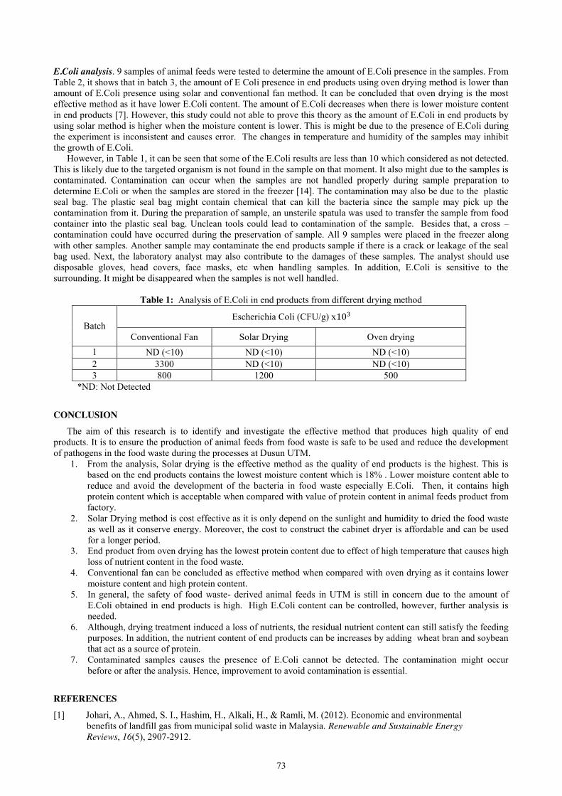
73

E.Coli analysis. 9 samples of animal feeds were tested to determine the amount of E.Coli presence in the samples. From Table 2, it shows that in batch 3, the amount of E Coli presence in end products using oven drying method is lower than amount of E.Coli presence using solar and conventional fan method. It can be concluded that oven drying is the most effective method as it have lower E.Coli content. The amount of E.Coli decreases when there is lower moisture content in end products [7]. However, this study could not able to prove this theory as the amount of E.Coli in end products by using solar method is higher when the moisture content is lower. This is might be due to the presence of E.Coli during the experiment is inconsistent and causes error. The changes in temperature and humidity of the samples may inhibit the growth of E.Coli.

However, in Table 1, it can be seen that some of the E.Coli results are less than 10 which considered as not detected. This is likely due to the targeted organism is not found in the sample on that moment. It also might due to the samples is contaminated. Contamination can occur when the samples are not handled properly during sample preparation to determine E.Coli or when the samples are stored in the freezer [14]. The contamination may also be due to the plastic seal bag. The plastic seal bag might contain chemical that can kill the bacteria since the sample may pick up the contamination from it. During the preparation of sample, an unsterile spatula was used to transfer the sample from food container into the plastic seal bag. Unclean tools could lead to contamination of the sample. Besides that, a cross – contamination could have occurred during the preservation of sample. All 9 samples were placed in the freezer along with other samples. Another sample may contaminate the end products sample if there is a crack or leakage of the seal bag used. Next, the laboratory analyst may also contribute to the damages of these samples. The analyst should use disposable gloves, head covers, face masks, etc when handling samples. In addition, E.Coli is sensitive to the surrounding. It might be disappeared when the samples is not well handled.

Table 1: Analysis of E.Coli in end products from different drying method

*ND: Not Detected

CONCLUSION

The aim of this research is to identify and investigate the effective method that produces high quality of end products. It is to ensure the production of animal feeds from food waste is safe to be used and reduce the development of pathogens in the food waste during the processes at Dusun UTM.

1. From the analysis, Solar drying is the effective method as the quality of end products is the highest. This is based on the end products contains the lowest moisture content which is 18% . Lower moisture content able to reduce and avoid the development of the bacteria in food waste especially E.Coli. Then, it contains high protein content which is acceptable when compared with value of protein content in animal feeds product from factory.

2. Solar Drying method is cost effective as it is only depend on the sunlight and humidity to dried the food waste as well as it conserve energy. Moreover, the cost to construct the cabinet dryer is affordable and can be used for a longer period.

3. End product from oven drying has the lowest protein content due to effect of high temperature that causes high loss of nutrient content in the food waste.

4. Conventional fan can be concluded as effective method when compared with oven drying as it contains lower moisture content and high protein content.

5. In general, the safety of food waste- derived animal feeds in UTM is still in concern due to the amount of E.Coli obtained in end products is high. High E.Coli content can be controlled, however, further analysis is needed.

6. Although, drying treatment induced a loss of nutrients, the residual nutrient content can still satisfy the feeding purposes. In addition, the nutrient content of end products can be increases by adding wheat bran and soybean that act as a source of protein.

7. Contaminated samples causes the presence of E.Coli cannot be detected. The contamination might occur before or after the analysis. Hence, improvement to avoid contamination is essential.

REFERENCES [1] Johari, A., Ahmed, S. I., Hashim, H., Alkali, H., & Ramli, M. (2012). Economic and environmental benefits of landfill gas from municipal solid waste in Malaysia. Renewable and Sustainable Energy Reviews, 16(5), 2907-2912.

Batch Escherichia Coli (CFU/g) x103

Conventional Fan Solar Drying Oven drying 1 ND (<10) ND (<10) ND (<10) 2 3300 ND (<10) ND (<10) 3 800 1200 500

74

[2] Komakech, A. J. (2014). Urban waste management and the environmental impact of organic waste treatment systems in Kampala, Uganda (Vol. 2014, No. 77).

[3] Salemdeeb, R., zu Ermgassen, E. K., Kim, M. H., Balmford, A., & Al-Tabbaa, A. (2016). Environmental and health impacts of using food waste as animal feed: a comparative analysis of food waste management options. Journal of Cleaner Production.

[4] Walker, P., Kelley, T. (1999). Bacterial concentration reduction of food waste amended animal feed using a single-screw dry-extrusion process. Bio resource Technology, 67, pp. 247-253 [5] AOAC, 1990. Official Methods of Analysis of AOAC, 1st ed., Association of Official Analytical Chemists, Arlington, VA, USA [6] Sharifah, A. S., Abidin, H. Z., Sulaiman, M. R., Khoo, K. H., & Ali, H. (2008). Combustion characteristics of

Malaysian municipal solid waste and predictions of air flow in a rotary kiln incinerator. Journal of material cycles and waste management, 10(2), 116-123.

[7] Chen, T., Jin, Y., & Shen, D. (2015). A safety analysis of food waste-derived animal feeds from three typical conversion techniques in China. Waste Management, 45, 42-50 [8] Kawashima, T. (2004). The use of food waste as a protein source for animal feed-current status and

technological development in Japan. In Protein sources for the animal feed industry. FAO Expert Consultation and Workshop, Bangkok, Thailand, 29 April-3 May 2002. (pp. 303-309). Food and Agriculture Organization of the United Nations (FAO).

[9] Sugiura, K., Yamatani, S., Watahara, M., & Onodera, T. (2009). Ecofeed, animal feed produced from Recycled food waste. Veterinaria italiana, 45(3), 397-404. [10] Navale, S. R., Harpale, V. M., & Mohite, K. C. Comparative study of open sun and cabinet solar drying for fenugreek leaves. [11] FAO, U. (2011). Global Food Losses and Food Waste. [12] Zeuthen, P., & Bøgh-Sørensen, L. (Eds.). (2003). Food preservation techniques. Elsevier. [13] Agoreyo, B. O., et al. "The effects of various drying methods on the nutritional composition of Musa paradisiaca, Dioscorea rotundata and Colocasia esculenta." Asian Journal of biochemistry 6.6 (2011): 458-464 [14] Environmental Protection Agency. (2006). Chapter 17: Bacteria indicator of Potential Pathogens. Retrieved From http://www.epa.gov/owow/estuaries/monitor

.

75

Pollution of Sungai Melana: Effect of Littering in Residential Area Nurul Farhana Muhamad Ali Hanafiah, Mohd Ismid Mohd Said

Faculty of Civil Engineering, Universiti Teknologi Malaysia, Malaysia

ismid@utm.my

Keywords: Littering Activity; Type of Littering Rubbish; Cause of Littering; Littering in Residential Area.

ABSTRACT. Littering activities also one of the major factors that contribute to water pollution. The biggest percentage in reducing the quality of water are contribute by the existing of unwanted elements either in solid or liquid form in water body. This elements are yield from the decomposition’s process of rubbish thrown by human on the ground. This study are conduct in order to obtain informations about the causes and impact of littering activity. This research are conduct in order to find the relationship between the causes and impact which may help to produce few ideas or solutions to reduce or eliminate littering activity as well as to reduce water pollution. From the study conducted, littering activities occurs in residential area are less than what are to be expected compare to others places. The result also showed that water from residential area did not give a huge impact to the water quality in Sungai Melana.

INTRODUCTION

Everyone are enforce to keep river clean and fresh in order to get benefit from river’s functions and continue their life healthily. Littering activities also one of the major factors that contribute to water pollution. Throwing rubbish or waste on public places such as park, playground, street and football field are one of the irresponsible attitude done by human. Many bad impact can occur if littering activity keep happen.

Problem Statement Some bad impact which result from water pollution are relate with environmental issues such as degradation of water quality and endanger wildlife and plant. This is because, when pollutant enter watercourse, water quality will decrease according to increasing of pollutant such as dangerous chemical reagent in water body which are unsafe for humans or animals to drinks as well as bad for plant’s processing.

Beside give effect on aesthetic value in term of changes in color of the polluted water, water pollution also can spread dangerous viruses and diseases. Babies, children pregnant woman, elders, and those who has weak immune system are tends to suffer a disease that attribute from use of polluted water easily compare to other group of people. Negative effect cause by water pollution should be overcome wisely in order to protect safety and health of living things. All the factors that contribute to pollution of water have to be identify first before all the prevention steps are taken.

Objectives The objectives of this study are:

1. To identify the main factors of littering 2. To investigate the perception of people on littering activity 3. To investigate the correlation between attitude and practice of littering in residential area of Mutiara Rini,

Skudai, Johor 4. To investigate the correlation between demographic characteristic and littering attitude 5. To investigate the relationship between littering activity and water pollution in Sungai Melana

Scope of Study Research about causes of littering activity which may lead to degradation of water are conduct at Sungai Melana. This research also conducted in residential area in Mutiara Rini. The research was carried by study the comparison between resident in study area in all aspect such as attitude, life routine, and culture. This research are conduct by distributing a questionnaire to resident randomly in residential area. A net and an observation was also carried out in Sungai Melana which received the effluent from the residential area in order to identify whether rubbish from residential area enter the water body or not. Water Quality Index was also establish to check whether the effluent from residential area give huge or small effect to the degradation of water quality.

LITERATURE REVIEW

Littering activities has become a big issues which contribute to pollution of river. Most of the people in world have been throwing rubbish or waste averaging on the ground. Only few of people has never litter in their whole life. ‘Litter can be defined as any piece of glass, plastic, paper, metal, cloth, rubber, food, or food by-product which is thrown away

76

in public place outsides waste collection containers’ are stated by [7]. Litter is not categorize under municipal solid waste (MSW). Municipal Solid Waste is a types or group of waste that are collect by municipalities or other local authorities. Litter are ‘any domestic or commercial waste and any material a person might reasonably refuse, debris, or rubbish’ and categorize as a material which disposed incorrectly [2]. Litter also defined as a solid waste that deposited in improper receptacles while littering means ‘careless and incorrect disposal of minor amount of waste [1].

All the rubbish or waste on the ground will be swept into drainage system by wind or water. The water in drainage system will flow together with all the rubbish dropped through drainage outlet to the river. These may contribute to degradation of water in the river. Many research had been conducted in order to investigate and determine the cause of factors that lead people to litter beside identify the type and effect of the littering activities.

People that practicing littering are coming from variety of groups. Each person have their own race, religion, interest, habit, and many other groups, therefore each person litter or throw different types of rubbish. However, some of them might have few similarities. This is because finding said that cigarette butt is the most amount found on the ground. People among each of these group are smoking and drop the cigarette butt on place where they are stand. Cigarette butt are more frequents to be drop on ground compare with waste that more obvious like plastic and wrappers and are socially accepted to thrown cigarette butt outside the dustbin [2].

Other researcher categorize litter’s waste in few group of waste which are cigarette butt as an offensive waste, broken glass and syringes as a dangerous waste, plastic bag and bottle, chip packets, and fast-food rubbish as a waste that last in a long time, animal droppings and food waste as an unhygienic waste, and dried chewing gum on the pavement as somewhat acceptable waste by most people [7].

Attitude or behavior of an individual person is the big reason for the increasing of littering activity in residential area. Many people had admitted that they are too lazy to throw rubbish properly into dustbin. They will just throw their trash on the street where they are passing by and will think that there are other person that will clean up the trash after them such as cleaner or rubbish collector. This attitude can related to lack of civic consciousness about littering activity which state that people thinking throwing away rubbish properly are too troublesome for them [2]. People keep on throwing trash outside the garbage bin are because they do not feel any sense of personal ownership to the object that being rejected.

The second factor that contribute to littering activity are the placement and appearance of rubbish bin on site [1]. Most people feels that carrying a waste material in their hand are probably inconvenient especially when they need to use their hand for other purposes. Therefore, if rubbish bins are invisible because off it placement are unable for people to find or the rubbish bin are too far to reach, people will take the simple step without troubling themselves which is throw the rubbish on the ground. The main driving cause for littering that has been recorded are insufficient availability of rubbish bins [7].

Absences of effective and consistence enforcement are one of the major factor that lead people to throw away rubbish as how they prefer to do. The increasing amount of waste on street and frequency of people litter in public place showed the enforcement apply in preventing littering are consider as weak and did not obtain full attention and cooperation from public. ‘The probability of being detected, arrested, and fined is simply too remote and intermittent to control such behavior’ [5]. A legal sanctions such as penalties or fines imposed on people who practice litter are ineffective because of infrequent number of enforcement.

The dirtiness of one place are also effect on the frequency of littering activity conduct in that place [7].The amount of waste that already exist on the ground as result to previous littering activity will make people who pass the place to litter without feeling wrong about doing so. Besides that, poor packaging in design of commercial product and lack of knowledge also became the reasons on why people keep litter [1].

Demographic characteristic such as gender, marital status, and level of income is one of the factor that lead to litter. Male, single, and highly paid worker are tend to litter more than female, married or widow, and low paid worker [1] while young people in the age of 21 to 35 are tend to litter three times more than elder aged 50 years and above [2]. Type of resident, marital status, level of education, age, family income status, occupation, and interest are strongly related to littering behavior of people [5].

Many prevention alternative are taken but most of them are useless and resulting to zero environmental improvement. Litter are one of the human activity that contribute to the pollution of water due to the high containing of unwanted elements in water body. Many other effects are rising due to the increasing number of litter waste as people are growing number. Aesthetic problem, environmental issues, illness and disease, and economic losses are among top bad impact happen because of littering activities in world.

Aesthetic problem is the clearest and simple result to littering problem [7]. Dirty place are familiar with odor or smell problem. Rubbish and trash on all over the ground will create unpleasant odor to smell which may lead to other problem such as reducing in economy due to low amount of tourism activity to take place.

Environmental issues such as degradation of water quality level, endanger and death of wildlife, and flooding are the impacts that will occur if littering activity are still running progressively [2]. Rubbish thrown by irresponsible people to the ground may be drag to nearest drain by people passing by or by running rain water. All the rubbish dropped into the drain will be flashed along the drainage system and finally enter the river through pipe outlet. Some of the rubbish may contain harmful or toxic waste such as chemical waste and cause the river contaminate with those contaminants which may harm to living things.

77

The other effect cause by the littering activity are illness and disease. A study reported that five percent off all injuries are because of glass-related injuries occurred on the street [7]. Most of the patient get injured because they step on broken glass when passing a street with full of trash on the ground. They are unaware about the environment and did not expect that a broken glass would be in the middle of the street.

Litter collection and the losses (direct and indirect) are the two losses caused by the presence of litter activity in public places [7]. The state must covered high expenses for collect rubbish in order to produce a clean and comfort place for people to live. Some authority need to bear a responsibility to clean streets and drains on behalf of others fault. Workers are paid high for cleaning a dirty public place because less people are willing to clean up after others.

METHODOLOGY

The main objective of the research is to identify the factors that lead people to keep litter. Some reasons for conducting this study are to obtain the relationship between people’s perspective and littering attitude, culture and human practices in managing waste, and to investigate the effect of littering activity to river pollution. Questionnaire Questionnaire is a method that involved a feedback from other people that called respondent. This method is a most popular method used in order to obtain data that cannot be measured by any parameter, equipment, or apparatus created by human. Respondent targeted for this study are resident from study area which are randomly picked. The questionnaire form will be given or distribute to respondent at their own house and are given a few minutes to answers all the question. Some of the questions that may be ask to the respondent in the distribute questionnaire are related on some issues such as the type and frequent of throwing a rubbish, reason to litter, suggestion to reduce littering, and level of awareness on littering effect. Rubbish Trap One of the proper method to collect info on types of waste involve in littering activity are by using rubbish trap method. Rubbish trap are able to trap all the floated solid materials which dropped into drainage system by installing a net across the river at location where the effluent from residential area will passed by. The trap will be install at two place for about three hours in each experiments on the decide date and time. Three experiments are proposed to be conducted in order to determine the type and quantity of rubbish thrown by irresponsible people. Observation Observation of rubbish’s amount are conducted in order to get the amount and size of rubbish that always take place in littering activities. This method was carried out by walking along the river for 50 meters in 10 minutes while observing the type, size, and amount of rubbish present in river and river bank (left and right bank) . River Gauging This method are conduct to get the flow rate of Sungai Melana by using current meter. This test was take place at two location which are the same location with the rubbish trap was establish. Besides flow rate’s value, others value such as velocity (v), depth of water (y), and width of Sungai Melana also can be determine. Water Quality Index Water quality of Sungai Melana can be determine by identify the parameters need in calculating Water Quality Index. DO (dissolve oxygen), BOD (biochemical oxygen demand), COD (chemical oxygen demand), SS (suspended solid), AN (ammoniacal nitrogen), and pH are the parameters need in identifying water quality. Sample of Sungai Melana was taken four times in order to get the best result.

RESULTS AND DISCUSSION

The feedback given by 35 respondents from residential area in Mutiara Rini was obtained. The answers given by respondent were used to compare with the result from the rubbish trap and observation test. The water quality index test are obtained to identify whether effluent from residential area give effect to the degradation of water quality in Sungai Melana.

Questionnaire From the feedback obtained, the main factors that lead to littering are people’s attitude and the feeling of burdernsome in finding dustbin which are choose by 21% of respondents as shown in Figure 1 while other reasons that lead to littering activity are because there are no nearby bin (14%), did not want pocket to get dirty (7%), more easy to litter (12%), the place already dirty (12%), and because want to copy others behavior (13%). Majority of respodents said that they are concern and aware about littering activity due to the bad effect a rubbish may contribute to environment. Most of them will throw their rubbish into dustbin or will hold the rubbish until they found a suitable place to dispose. From the data obtained, respondent are practicing recycle and reuse things such as plastic, paper, box, cans, and bottle.

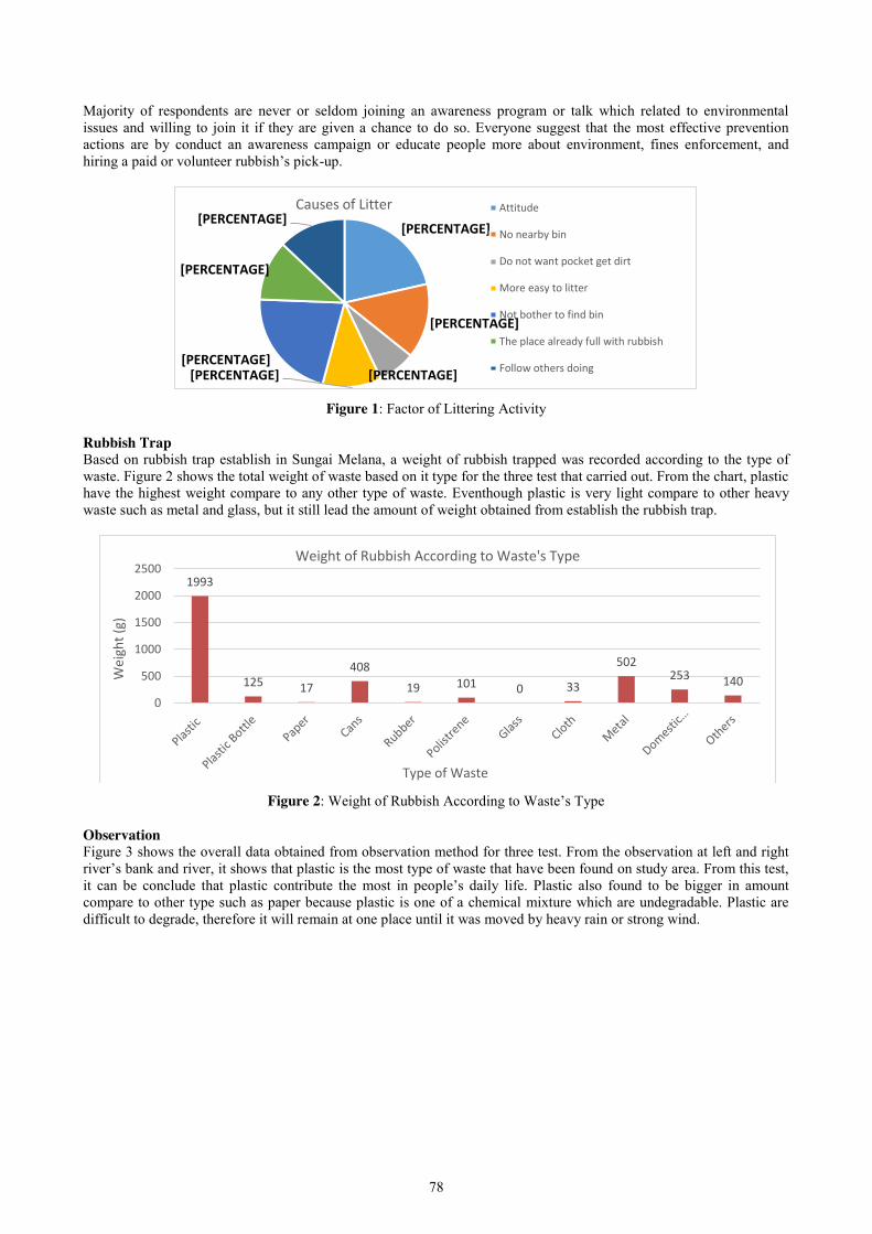
78

Majority of respondents are never or seldom joining an awareness program or talk which related to environmental issues and willing to join it if they are given a chance to do so. Everyone suggest that the most effective prevention actions are by conduct an awareness campaign or educate people more about environment, fines enforcement, and hiring a paid or volunteer rubbish’s pick-up.

Figure 1: Factor of Littering Activity

Rubbish Trap Based on rubbish trap establish in Sungai Melana, a weight of rubbish trapped was recorded according to the type of waste. Figure 2 shows the total weight of waste based on it type for the three test that carried out. From the chart, plastic have the highest weight compare to any other type of waste. Eventhough plastic is very light compare to other heavy waste such as metal and glass, but it still lead the amount of weight obtained from establish the rubbish trap.

Figure 2: Weight of Rubbish According to Waste’s Type

Observation Figure 3 shows the overall data obtained from observation method for three test. From the observation at left and right river’s bank and river, it shows that plastic is the most type of waste that have been found on study area. From this test, it can be conclude that plastic contribute the most in people’s daily life. Plastic also found to be bigger in amount compare to other type such as paper because plastic is one of a chemical mixture which are undegradable. Plastic are difficult to degrade, therefore it will remain at one place until it was moved by heavy rain or strong wind.

[PERCENTAGE]

[PERCENTAGE]

[PERCENTAGE] [PERCENTAGE] [PERCENTAGE]

[PERCENTAGE]

[PERCENTAGE] Causes of Litter Attitude

No nearby bin

Do not want pocket get dirt

More easy to litter

Not bother to find bin

The place already full with rubbish

Follow others doing

1993

125 17

408 19 101 0 33

502 253 140

0

500

1000

1500

2000

2500

Wei

ght (

g)

Type of Waste

Weight of Rubbish According to Waste's Type

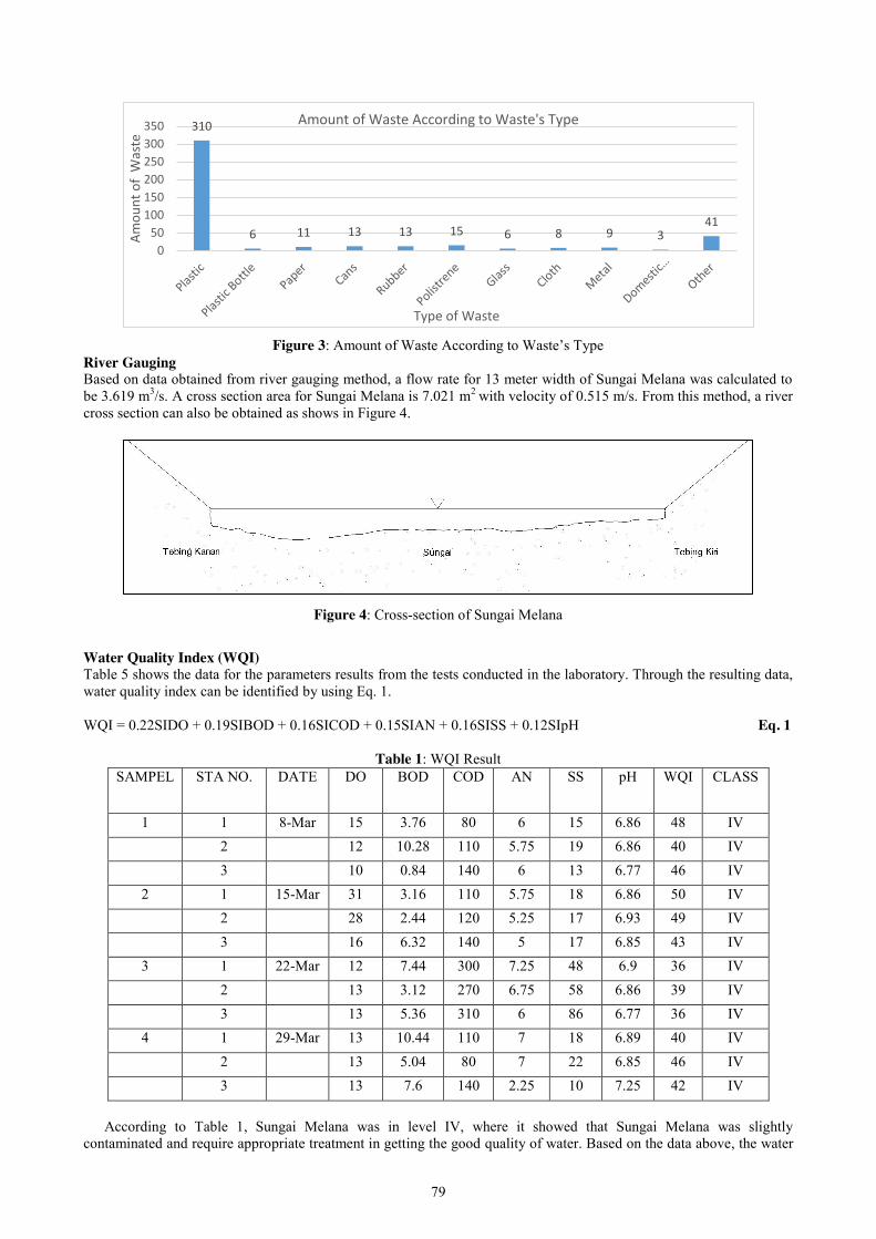
79

Figure 3: Amount of Waste According to Waste’s Type

River Gauging Based on data obtained from river gauging method, a flow rate for 13 meter width of Sungai Melana was calculated to be 3.619 m3/s. A cross section area for Sungai Melana is 7.021 m2 with velocity of 0.515 m/s. From this method, a river cross section can also be obtained as shows in Figure 4.

Figure 4: Cross-section of Sungai Melana

Water Quality Index (WQI) Table 5 shows the data for the parameters results from the tests conducted in the laboratory. Through the resulting data, water quality index can be identified by using Eq. 1.

WQI = 0.22SIDO + 0.19SIBOD + 0.16SICOD + 0.15SIAN + 0.16SISS + 0.12SIpH Eq. 1

Table 1: WQI Result SAMPEL STA NO. DATE DO BOD COD AN SS pH WQI CLASS

1 1 8-Mar 15 3.76 80 6 15 6.86 48 IV 2 12 10.28 110 5.75 19 6.86 40 IV 3 10 0.84 140 6 13 6.77 46 IV

2 1 15-Mar 31 3.16 110 5.75 18 6.86 50 IV 2 28 2.44 120 5.25 17 6.93 49 IV 3 16 6.32 140 5 17 6.85 43 IV

3 1 22-Mar 12 7.44 300 7.25 48 6.9 36 IV 2 13 3.12 270 6.75 58 6.86 39 IV 3 13 5.36 310 6 86 6.77 36 IV

4 1 29-Mar 13 10.44 110 7 18 6.89 40 IV 2 13 5.04 80 7 22 6.85 46 IV 3 13 7.6 140 2.25 10 7.25 42 IV

According to Table 1, Sungai Melana was in level IV, where it showed that Sungai Melana was slightly

contaminated and require appropriate treatment in getting the good quality of water. Based on the data above, the water

310

6 11 13 13 15 6 8 9 3 41

050

100150200250300350

Amou

nt o

f W

aste

Type of Waste

Amount of Waste According to Waste's Type

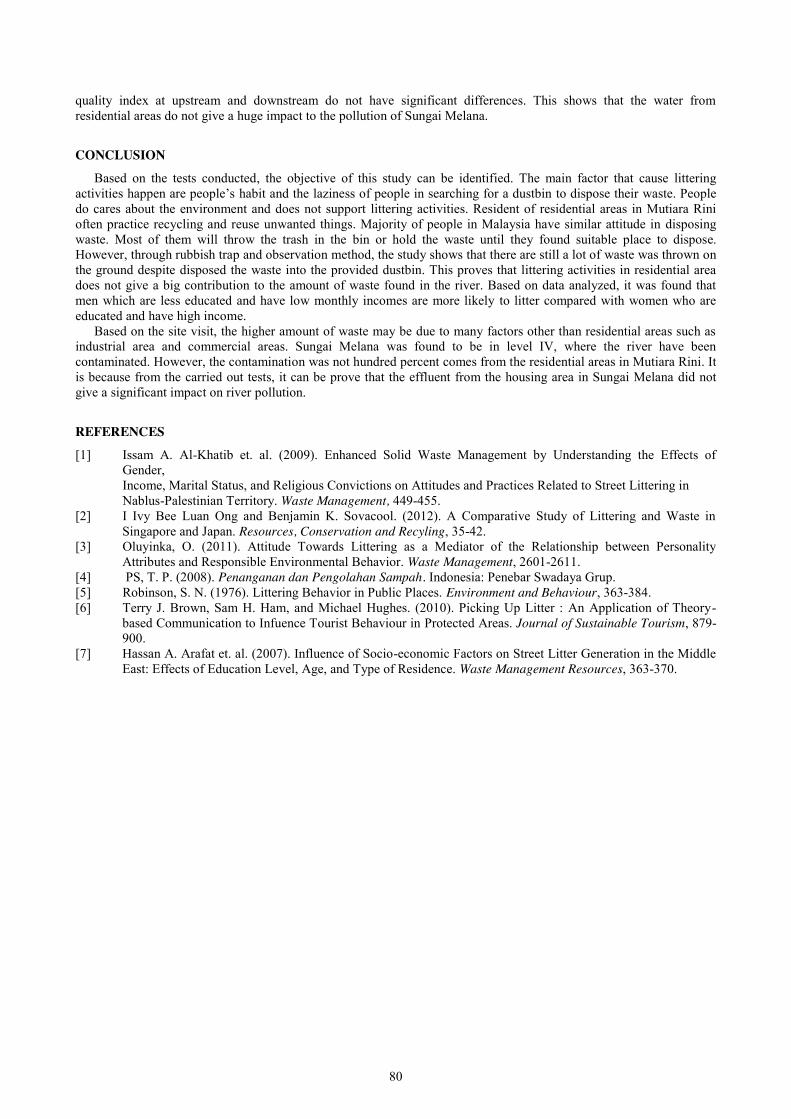
80

quality index at upstream and downstream do not have significant differences. This shows that the water from residential areas do not give a huge impact to the pollution of Sungai Melana.

CONCLUSION

Based on the tests conducted, the objective of this study can be identified. The main factor that cause littering activities happen are people’s habit and the laziness of people in searching for a dustbin to dispose their waste. People do cares about the environment and does not support littering activities. Resident of residential areas in Mutiara Rini often practice recycling and reuse unwanted things. Majority of people in Malaysia have similar attitude in disposing waste. Most of them will throw the trash in the bin or hold the waste until they found suitable place to dispose. However, through rubbish trap and observation method, the study shows that there are still a lot of waste was thrown on the ground despite disposed the waste into the provided dustbin. This proves that littering activities in residential area does not give a big contribution to the amount of waste found in the river. Based on data analyzed, it was found that men which are less educated and have low monthly incomes are more likely to litter compared with women who are educated and have high income.

Based on the site visit, the higher amount of waste may be due to many factors other than residential areas such as industrial area and commercial areas. Sungai Melana was found to be in level IV, where the river have been contaminated. However, the contamination was not hundred percent comes from the residential areas in Mutiara Rini. It is because from the carried out tests, it can be prove that the effluent from the housing area in Sungai Melana did not give a significant impact on river pollution.

REFERENCES

[1] Issam A. Al-Khatib et. al. (2009). Enhanced Solid Waste Management by Understanding the Effects of Gender,

Income, Marital Status, and Religious Convictions on Attitudes and Practices Related to Street Littering in Nablus-Palestinian Territory. Waste Management, 449-455. [2] I Ivy Bee Luan Ong and Benjamin K. Sovacool. (2012). A Comparative Study of Littering and Waste in

Singapore and Japan. Resources, Conservation and Recyling, 35-42. [3] Oluyinka, O. (2011). Attitude Towards Littering as a Mediator of the Relationship between Personality

Attributes and Responsible Environmental Behavior. Waste Management, 2601-2611. [4] PS, T. P. (2008). Penanganan dan Pengolahan Sampah. Indonesia: Penebar Swadaya Grup. [5] Robinson, S. N. (1976). Littering Behavior in Public Places. Environment and Behaviour, 363-384. [6] Terry J. Brown, Sam H. Ham, and Michael Hughes. (2010). Picking Up Litter : An Application of Theory-

based Communication to Infuence Tourist Behaviour in Protected Areas. Journal of Sustainable Tourism, 879-900.

[7] Hassan A. Arafat et. al. (2007). Influence of Socio-economic Factors on Street Litter Generation in the Middle East: Effects of Education Level, Age, and Type of Residence. Waste Management Resources, 363-370.

81

Water Quality Index of Sungai Melana Sajeev Nair A/L Radakrishnan, Muzaffar bin Zainal Abideen

Faculty of Civil Engineering, Universiti Teknologi Malaysia, Malaysia

muzaffar@utm.my

Keywords: Water Quality Index (WQI), Sungai Melana, Biochemical Oxygen Demand (BOD), Chemical Oxygen Demand (COD), Dissolved Oxygen (DO), Suspended Solids (SS), Ammoniacal Nitrogen (NH3-N)

ABSTRACT. WQI is the standard river water quality monitoring system established by the Department of Environment, Malaysia. The parameters required to calculate WQI are DO, BOD, COD, NH3-N, SS, and pH. The key objectives of this research are to identify the water quality parameters of Sungai Melana, compare the current water quality of Sungai Melana with previous data, classify the river according to WQI and identify the effects of various land use toward Sungai Melana. In-situ testing was done to obtain DO and pH values, meanwhile BOD, COD, NH3-N and SS values were obtained through laboratory experiments. The WQI of Sungai Melana in 2017 is 53, whereas the water quality parameters are; DO: 2.24 mg/L, BOD: 16.15 mg/L, COD: 13.4 mg/L, NH3-N: 2.80 mg/L, SS: 2.55 mg/L, pH: 7.17. The water quality at Sungai Melana has decreased slightly compared to the last year (2016) data which was 69. It is also found that various land uses influence the quality of water of Sungai Melana.

INTRODUCTION

Sungai Melana is a river in Johor that flows from Taman Teratai in Pulai through Skudai before merging with Sungai Skudai in Tampoi. Sungai Melana passes through areas with multiple land uses, especially residential and industrial areas. The variety of land use shows that there is a high possibility of contamination in Sungai Melana, thus affecting the quality of the river water. The Department of Environment has been monitoring river water quality in Malaysia since 1978 and have set up data collection stations along 143 rivers all over Malaysia. The water quality data is collected to identify the water quality status and classify the rivers as either Class I, II, III, IV, or V in accordance to the Water Quality Index (WQI) and Interim National Water Quality Standards for Malaysia (INWQS). The WQI is calculated based on six parameters: Dissolved Oxygen (DO), Suspended Solids (SS), Biochemical Oxygen Demand (BOD), Chemical Oxygen Demand (COD), Ammoniacal Nitrogen (NH3-N), and pH.

Problem Statement Among the issues that are present in the Sungai Melana sub-catchment area is the settlement of silt at the river bed due to rapid development of residential areas at the upstream area. Besides that, waste dumps from residential areas along the riverbank also pose a threat to the river water quality. Construction waste from construction sites around the river also affects the river water flow.

Further research and studies should be carried out to find out the effects of the issues stated above on the water quality and parameters that contribute to the WQI. It is also necessary to find out if there are any changes to the Sungai Melana WQI compared to previous WQI data.

Objectives The objectives of this study are:

1. To quantify water quality parameters at Sungai Melana. 2. To classify Sungai Melana according to WQI using the parameters. 3. To compare the water quality of Sungai Melana in 2017 and previous years. 4. To identify the effects of various land uses on the WQI of Sungai Melana.

Scope of Study This research is carried out by collecting water samples from Sungai Melana at the upstream, midstream, downstream and areas exposed to various land uses. Six parameters are analysed to obtain the WQI, which are DO, SS, BOD, COD, NH3-N, and pH. The value of DO and pH are obtained in situ, whereas SS, BOD, COD, NH3-N values are tested at the Environmental Laboratory, Faculty of Civil Engineering, UTM. Based on the WQI, Sungai Melana is classified to identify the water quality. The water quality classification is compared with previous research data to find out if there are any changes in the water quality of Sungai Melana. The effects of various land use on the water quality of Sungai Melana is monitored by comparing the water quality at the specific points with the upstream water quality.

82

LITERATURE REVIEW

Water Quality Index (WQI) is useful to evaluate the suitability of rivers for various usages such as agriculture, aquaculture and domestic usage. WQI is used to relate several water quality parameters into a unified scale and combined into a specific value [1]. In 1985, a research titled Developmet of Water Quality Criteria and Standards for Malaysia was conducted by the Malaysian government [2]. Through the research, the National Water Quality Standards (NWQS) defined six classes (I, IIA, IIB, III, IV, and V) to classify river water, with Class 1 being the highest quality and Class V is the worst [3]. There are six water quality parameters used to determine the quality of river water, which are Dissolved Oxygen (DO), Suspended Solids (SS), Biochemical Oxygen Demand (BOD), Chemical Oxxygen Demand (COD), Ammoniacal Nitrogen (NH3-N) and pH value.

There should be a high DO content in the water to maintain an aerobic condition in the water. The DO content is essential for the conservation of aesthetic quality of water and the lives of flora and fauna in the water. If the DO content falls below the normal level, the quality of water will be affected and aquatic lives may die [4]. Next, SS is the total amount of organic and inorganic particles suspended on a 1 µm filter paper. High SS content in the water will cause the water quality to deteriorate due to light absorption. This causes the water temperature to increase and the DO content to decrease. SS also causes breathing difficulties in aquatic lives [5]. Most organic materials such as sewerage plant waste, industrial effluent and surface runoff water go through the process of biodegradation. BOD is the amount of oxygen used by microorganisms in aerobic oxidation of organic materials [6].

COD is the parameter that shows the level of pollution in the water based on chemical properties. COD is the measure of oxygen content needed to oxidise organic materials through chemical processes ssuch as dichromate and sulphuric acid [7]. Ammonia is the most reactive form of nitrogen in an aquatic system. The main source of NH3-N is from minerals in the soil, fertilisers, animal waste, atmospheric deposition and urban and industrial point sources of pollution [8]. At normal temperatures and pH range, ammonia exists dominantly as NH4

+ ion. When the pH and temperature increases, ionized ammonia converts to deionized ammonia gas, NH3. Another water quality parameter is the pH value. Acidity and alkalinity depends on the presence of minerals salts such as chlorides, sulphate and phosphate [9]. pH is the measure of hydrogen ion concentration, [H+], in the water.

Various researches have been conducted in rivers all over Malaysia. One of the research is at Sungai Batu Feringghi which had an overall WQI 83 and classified as Class II river [10]. Another WQI research was conducted in the Sungai Terengganu basin from July to October 2008. Results show that anthropogenic activity in the basin resulted in high values of BOD, COD, TSS and NH3-N at the midstream and downstream stations compared to upstream stations. The average WQI is 87 and the river was classified as Slightly Polluted [11]. Besides that, Sungai Bunus which flows in the heart of Kuala Lumpur city was classified as Class V for BOD and NH3-N, Class I for SS and Class III for DO based on a research in 2012 [12]. A research conducted at the Sungai Skudai basin to identify the effectiveness of WQI method to measure the water quality shows that in Sungai Skudai, NH3-N was the main pollutant, with the lowest WQI index. The WQI at Sungai Melana was 69, and at Sungai Danga it was 57 [13].

The effects of sewerage treatment plant effluent on the river water quality of Sungai Anggerik in Kempas and Sungai Melana in Skudai was researched in 2010. Based on the research analysis of four parameters, BOD, COD, SS and NH3-N, the pollutants from the effluent has affected the river water quality. Both WQI values of Sungai Anggerik and Sungai Melana were 27 (Very Polluted, Class V) [14]. Another research was conducted in Sungai Melana in 2013 to compare the results between WQI and Biological Water Quality Index (BWQI). Comparisons were made based on invertebrate analysis and laboratory analysis. Based on the analysis, it was found that the WQI of Sungai Melana was 56 (Polluted) and classified as Class III [15].

Based on the literature reviews studies, a research should be done to identify the water quality of Sungai Melana using WQI method. The water quality parameters should be identified to know the effects on the water quality and to classify the river. Since Sungai Melana passes through areas with various land uses such as residential and industrial areas, the research should also be done to know the effects of various land uses on the water quality of the river.

METHODOLOGY

The main objective of this research is to identify the water quality parameters of Sungai Melana and to classify the river according to WQI using the parameters. The water quality is then to be compared with previous year results. The effects of various land uses are also to be identified through this research. To achieve these objectives, this research methodology mainly consists of four key activities: Preliminary Research, Data Collection, and Results and Analysis. Preliminary Research Literature review was done to identify the necessity and viability of conducting this research in Sungai Melana. Further reading was conducted to obtain the previous WQI results of rivers in Malaysia and specifically in the region of Skudai. The previous WQI of Sungai Melana was also obtained. The types of land use around the Sungai Melana catchment area was identified through literature reading and observation.

83

Data Collection The points for water collection stations were set according to upstream, midstream, downstream, and areas exposed to different land use. The sampling was done on 19 March 2017, 9 April 2017, 16 April 2017, 25 April 2017 and 9 May 2017. The sampling stations are listed below: 1. P1 Jalan Lumpit, Taman Teratai, Pulai. Upstream. (N 01˚ 34’ 28.5’’, E 103˚ 36’ 39.9’’) 2. P2 Persiaran Pulai Perdana. Commercial Area. (N 01˚ 33’ 41.5’’, E 103˚ 37’ 3.3’’) 3. P3 Jalan Pulai, Taman Pulai Utama. Residential Area. (N 01˚ 32’ 44.1’’, E 103˚ 37’ 9.4’’) 4. P4 Jalan Pendidikan, Taman Universiti. Industrial Area. (N 01˚ 32’ 8.4’’, E 103˚ 37’ 23.4’’) 5. P5 Persiaran Bakti, Mutiara Rini. Midstream. (N 01˚ 31’ 28.9’’, E 103˚ 37’ 48.6’’) 6. P6 Jalan Sutera Danga, Taman Sutera Utama. Random Point. (N 01˚ 30’ 11.3’’, E 103˚ 39’ 22.0’’) 7. P7 Kampung Teluk Serdang Pinggir. Downstream. (N 01˚ 43’ 45.5’’, E 103˚ 42’ 2.6’’) Once at the sampling station, In Situ Testing for DO and pH values were done and the water sample was taken in labelled bottles provided by Makmal Kejuruteraan Alam Sekitar (MKAS), Fakulti Kejuruteraan Awam (FKA), UTM. In-Situ Testing. The values of DO and pH were obtained by using the YSI Multiparameter instrument provided by MKAS. The instrument probe was inserted into the water and stirred and the results on the screen are recorded. Laboratory Testing. The water samples were brought back to MKAS to conduct experiments for the remaining parameters, BOD, COD, SS, NH3-N. The experiments were conducted on the same day as the quantity of DO in the water may be affected if kept more than 24 hours, thus affecting the values of BOD and COD. COD Testing. Firstly, COD testing is conducted. 2 mL of the sample is mixed with a prepared strong acid solution of low range (3-150 mg/L) consisting of Chromic Acid, Mercuric Sulphate, Silver Sulphate and Sulphuric Acid. A blank is also prepared by mixing 2 mL distilled water with the strong acid solution. The mixture is prepared in special vials used for HACH method. The vials are then refluxed in a preheated reflux machine at 150 ˚C for 2 hours. After reflux, the vials are allowed to cool down to room temperature. Once cooled, a blank is placed in the HACH DR 6000 Spectrophotometer and zeroed. Next, the samples are tested and the COD values given in mg/L is recorded. BOD Testing. 100 mL of sample is diluted with 300 mL of distilled water. The dilution is then poured into BOD bottle until it overflows and there are no bubbles. Initial DO readings are taken using the desktop YSI Multiparameter and recorded. The BOD bottles are then placed in the incubator at 20 ˚C. DO values of Day 1, 2, and 3 are taken and recorded. A graph of [𝑡

𝐵𝑂𝐷𝑡⁄ ]13 versus Time, t (day) is plotted and the value of BOD5 is extrapolated. The method to

calculate BODt is expressed by the following equation: 𝐵𝑂𝐷𝑡 = 𝐷𝑂𝑖−𝐷𝑂𝑡

𝑃 Eq. 1

Where, 𝑃 = 𝑉𝑜𝑙𝑢𝑚𝑒 𝑜𝑓 𝑠𝑎𝑚𝑝𝑙𝑒𝑉𝑜𝑙𝑢𝑚𝑒 𝑜𝑓 𝑠𝑎𝑚𝑝𝑙𝑒+𝑉𝑜𝑙𝑢𝑚𝑒 𝑜𝑓 𝑑𝑖𝑙𝑢𝑡𝑖𝑜𝑛 𝑤𝑎𝑡𝑒𝑟

Eq. 2 SS Testing. After zeroing the weighing balance, an aluminium dish with filter paper is weighed and the value is recorded, B. The filter is then placed on a flask attached to a vacuum pump. Once secure, the funnel is attached and clamped. With the vacuum turned on, 100 mL, C of sample is poured into the funnel. Once all the sample has drained through, the filter paper is placed in the aluminium dish and placed in an oven at 105 ˚C for one hour. The dish and the filter paper with residue is then weighed and the value is recorded, A. The calculation of SS is expressed by the following equation: 𝑇𝑆𝑆 = (𝐴−𝐵)𝑥100

𝐶 Eq. 3

NH3-N Testing. 25 mL of sample is filled into a mixing graduated cylinder. Another mixing graduated cylinder is filled with 25 mL distilled water as a blank. 3 drops of Mineral Stabiliser is added and the cylinder is stoppered and inverted to allow mixing. 3 drops of Polyvinyl Alcohol Dispersing Agent and the cylinder is stoppered and inverted. 1.0 mL Nessler’s Reagent is pippetted into the cylinder and it is stoppered and inverted. The solution is poured into the sample cell and the timer on the HACH DR 6000 Spectrophotometer is set to 1 minute. When the timer beeps, the blank cell containing blank is placed and the machine is zeroed. Next, the first sample cell is tested and the value of NH3-N is recorded in mg/L.

RESULTS AND DISCUSSION

Once the quantities of water quality parameters are known, the Subindex (SI) values of each parameter is calculated. The SI values are calculated based on the Table in [16]. Based on the SI values of each water quality parameter, the WQI for each point of sampling is calculated. The calculation method is expressed by the following equation:

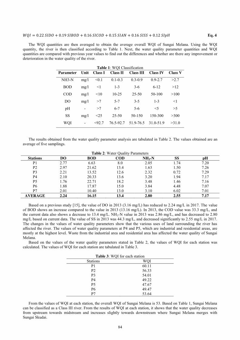
84

𝑊𝑄𝐼 = 0.22 𝑆𝐼𝐷𝑂 + 0.19 𝑆𝐼𝐵𝑂𝐷 + 0.16 𝑆𝐼𝐶𝑂𝐷 + 0.15 𝑆𝐼𝐴𝑁 + 0.16 𝑆𝐼𝑆𝑆 + 0.12 𝑆𝐼𝑝𝐻 Eq. 4

The WQI quantities are then averaged to obtain the average overall WQI of Sungai Melana. Using the WQI quantity, the river is then classified according to Table 1. Next, the water quality parameter quantities and WQI quantities are compared with previous year values to find out the differences and whether are there any improvement or deterioration in the water quality of the river.

Table 1: WQI Classification Parameter Unit Class I Class II Class III Class IV Class V

NH3-N mg/l <0.1 0.1-0.3 0.3-0.9 0.9-2.7 >2.7

BOD mg/l <1 1-3 3-6 6-12 >12

COD mg/l <10 10-25 25-50 50-100 >100

DO mg/l >7 5-7 3-5 1-3 <1

pH - >7 6-7 5-6 <5 >5

SS mg/l <25 25-50 50-150 150-300 >300

WQI - <92.7 76.5-92.7 51.9-76.5 31.0-51.9 >31.0

The results obtained from the water quality parameter analysis are tabulated in Table 2. The values obtained are an

average of five samplings.

Table 2: Water Quality Parameters Stations DO BOD COD NH3-N SS pH

P1 2.77 6.63 8.0 2.05 1.74 7.20 P2 2.97 21.62 13.4 1.63 1.50 7.26 P3 2.21 13.52 12.6 2.32 0.72 7.29 P4 2.10 20.33 13.6 3.20 1.94 7.17 P5 1.76 22.71 18.2 3.48 1.46 7.16 P6 1.88 17.87 15.0 3.84 4.48 7.07 P7 2.01 10.40 13.0 3.10 6.02 7.01

AVERAGE 2.24 16.15 13.4 2.80 2.55 7.17

Based on a previous study [15], the value of DO in 2013 (3.16 mg/L) has reduced to 2.24 mg/L in 2017. The value of BOD shows an increase compared to the value in 2013 (13.16 mg/L). In 2013, the COD value was 33.3 mg/L, and the current data also shows a decrease to 13.4 mg/L. NH3-N value in 2013 was 2.86 mg/L, and has decreased to 2.80 mg/L based on current data. The value of SS in 2013 was 44.3 mg/L, and decreased significantly to 2.55 mg/L in 2017. The changes in the values of water quality parameters show that the various uses of land surrounding the river has affected the river. The values of water quality parameters at P4 and P5, which are industrial and residential areas, are mostly at the highest level. Waste from the industrial area and residential area has affected the water quality of Sungai Melana.

Based on the values of the water quality parameters stated in Table 2, the values of WQI for each station was calculated. The values of WQI for each station are tabulated in Table 3.

Table 3: WQI for each station Stations WQI

P1 60.11 P2 56.33 P3 54.01 P4 49.22 P5 47.67 P6 49.47 P7 53.64

From the values of WQI at each station, the overall WQI of Sungai Melana is 53. Based on Table 1, Sungai Melana

can be classified as a Class III river. From the results of WQI at each station, it shows that the water quality decreases from upstream towards midstream and increases slightly towards downstream where Sungai Melana merges with Sungai Skudai.

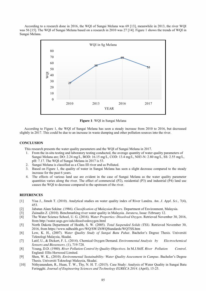
85

According to a research done in 2016, the WQI of Sungai Melana was 69 [13], meanwhile in 2013, the river WQI was 56 [15]. The WQI of Sungai Melana based on a research in 2010 was 27 [14]. Figure 1 shows the trends of WQI in Sungai Melana.

Figure 1: WQI in Sungai Melana

According to Figure 1, the WQI of Sungai Melana has seen a steady increase from 2010 to 2016, but decreased slightly in 2017. This could be due to an increase in waste dumping and other pollution sources into the river.

CONCLUSION

This research presents the water quality parameters and the WQI of Sungai Melana in 2017. 1. From the in-situ testing and laboratory testing conducted, the average quantity of water quality parameters of

Sungai Melana are; DO: 2.24 mg/L, BOD: 16.15 mg/L, COD: 13.4 mg/L, NH3-N: 2.80 mg/L, SS: 2.55 mg/L, pH: 7.17. The WQI of Sungai Melana in 2017 is 53.

2. Sungai Melana is classified as a Class III river and as Polluted. 3. Based on Figure 1, the quality of water in Sungai Melana has seen a slight decrease compared to the steady

increase for the past 6 years. 4. The effects of various land use are evident in the case of Sungai Melana as the water quality parameter

quantities varies along the river. The effect of commercial (P2), residential (P3) and industrial (P4) land use causes the WQI to decrease compared to the upstream of the river.

REFERENCES

[1] Yisa J., Jimoh T. (2010). Analytical studies on water quality index of River Landzu. Am. J. Appl. Sci., 7(4), 453.

[2] Jabatan Alam Sekitar. (1986). Classification of Malaysian Rivers. Department of Environment, Malaysia. [3] Zainudin Z. (2010). Benchmarking river water quality in Malaysia. Jurutera, Issue: February 12. [4] The Water Science School, U. G. (2016). Water Properties: Dissolved Oxygen. Retrieved November 30, 2016,

from http://water.usgs.gov/edu/dissolvedoxygen.html [5] North Dakota Department of Health, S. W. (2005). Total Suspended Solids (TSS). Retrieved November 30,

2016, from https://www.ndhealth.gov/WQ/SW/Z6WQStandards/WQTSS.htm [6] Low, K. H., (2007). Water Quality Study of Sungai Batu Pahat. Bachelor’s Degree Thesis. Universiti

Teknologi Malaysia, Skudai. [7] Latif, U., & Dickert, F. L. (2014). Chemical Oxygen Demand. Environmental Analysis by Electrochemical

Sensors and Biosensors. (1), 719-728. [8] Young, D.D. (1980). River Pollution Control by Quality Objectives. In M.J.Stiff. River Pollution Control.

England: Ellis Horwood Limited. [9] Shen, W. K., (2010). Environmental Sustainability: Water Quality Assessment in Campus. Bachelor’s Degree

Thesis. Universiti Teknologi Malaysia, Skudai. [10] Nithyanandam, R., Huan, T. W., Thy, N. H. T. (2015). Case Study: Analysis of Water Quality in Sungai Batu

Feringghi. Journal of Engineering Sciences and Technology EURECA 2014. (April), 15-25.

27

56

69

53

0

10

20

30

40

50

60

70

80

2010 2013 2016 2017

WQ

I

YEAR

WQI in Sg Melana

86

[11] Suratman, S., Sailan, M. I. M., Hee, Y. Y., Bedurus, E. A., Latif, M. T. (2015). A Preliminary Study of Water Quality Index in Terengganu River Basin, Malaysia. Sains Malaysiana. 44(1), 67-73.

[12] Kaur, P. (2012). Assessment of Water Quality Status in Sungai Bunus. Bachelor Degree Thesis. Universiti Teknologi Malaysia, Skudai.

[13] Zardari, N. H., Naubi, I., Shirazi, S. M., Farahen, N., Baloo, L. (2016). Effectiveness of Water Quality Index for Monitoring Malaysian River Water Quality. Pol. J. Environ. Stud. 25(1), 231-239.

[14] Ashikin, N. (2010). Effect of Domestic Sewage Treatment Plant Effluent on River Water Quality. Bachelor Degree Thesis. Universiti Teknologi Malaysia, Skudai.

[15] Salmiati, Azman, S., Hazim, M., Ismid, M., Arman, N. Z. (2013). Comparison Between Water Quality Index (WQI) and Biological Water Quality Index (BWQI) for Water Quality Assessment: Case Study of Melana River, Johor. The Malaysian Journal of Analytical Sciences. 17 (2), 224-229.

[16] Jabatan Alam Sekitar (2006). Malaysia Environmental Quality Report. Malaysia: Department of Environment Ministry of Natural Resources and Environment Malaysia.

87

Heavy Metal Accumulation in Cockles along the Straits of Malacca Ahmad Luqman bin Halit, Shamila Azman

Faculty of Civil Engineering, Universiti Teknologi Malaysia, Malaysia

shamila@utm.my

Keywords: Heavy Metals; Cockles (Anadara granosa).

ABSTRACT. Sungai Tampok and Sungai Sanglang located along the Straits of Malacca thrives in terms of aquaculture industry. Since the most of the villagers are fisherman, the aim of this study is to determine heavy metals on cockles (Anadara granosa), and seawater. Cockle was collected from four stations at Sungai Tampok on 26th December 2016, 16th March 2017. Meanwhile, cockle from Sungai Sanglang was collected from three stations on 11th January and 26th March 2017. The samples were then analysed for cadmium (Cd), chromium (Cr) and zinc (Zn). Water samples were also collected from the same location as cockle sampling stations. The in-situ test was conducted to identify the DO, pH, conductivity, salinity and temperature. Concentration of DO was highest at the first sampling taken during December and January for both sampling locations which were 6.58 and 3.9 mg/L respectively. Meanwhile the lowest concentration was 1.15 mg/L at station S1 on 16th March 2017 at Sungai Tampok and 1.36 mg/L at Sungai Sanglang. On certain occasions DO was found to be lower than 4 mg/L which is unsuitable for propagation of aquatic life. pH was 6.07 to 7.94. Conductivity was 44942 to 50803 µS/cm for both sampling locations. On 26th December 2016 the salinity was highest at S4 with 31.07 ppt at Sungai Tampok whereas Sungai Sanglang recorded salinity at 30.67 ppt on 11th January 2017. Temperature was normal at 27.3 to 30.6˚C. Cd and Cr in seawater were above Class 3 based on Marine Water Quality Criteria and Standard showing that the area is unsuitable for marine aquaculture, aquatic life and fishing activities. However, zinc in seawater was under Class 2 or E which means it is suitable for aquaculture. Accumulation of heavy metals on cockle also exceeded the Malaysian Food Regulation (1985) except for zinc.

INTRODUCTION

Cockle also known as Anadara granosa is a saltwater clam, a marine bivalve mollusk from the family of CARDIIDAE. Cockle has high economic value as food and it can be kept in aquaculture. Besides being consumed as a protein rich food, they are also used as a bio-indicator for detecting toxicity in aquatic communities [1]. Cockles lives in low oxygen environment and ingest more viruses and bacteria unlike other varieties of clams that are safe to eat. The study has been conducted on the toxicity of heavy metals in the tissue of cockles to ensure that cockles are safe for human consumption [2]. The sampling located at Sungai Tampok and Sungai Sanglang which are along the Straits of Malacca. The Strait of Malacca is a waterway that is narrow and 805 km stretch of water between Peninsular Malaysia (West Malaysia) and the Indonesian island of Sumatra. It is connecting the Indian Ocean and the South China Sea [3]. It is named after the state of Malacca, Malaysia.

Problem Statement Human activities or anthropogenic impact such as plantation, industrial and farming in Sungai Sanglang and Sungai Tampok, had affect the quality of water in the estuary. These factors have an important role to cause heavy metal accumulation in the area. Besides heavy metal accumulation, the distribution and quantity of the cockles have affected by the human activities along the areas. The polluted river can affect the cockles and spats (young cockles) which resulted in high mortality said Abu Talib Ahmad, a senior director of research at the Fisheries Research Institute [4].

Both river area serves as a very important natural resources for the local people. It also helps the local people in term of economics. Most of them depend on fishery as their income. The water quality on the area has significantly affected due to rapid urbanization and development. Therefore, it is important to study the level and the type of pollution in the area thus to determine the source of the pollution.

Objectives The objectives of this study are:

1. To study the accumulation of heavy metal in cockles along the estuary of Sungai Sanglang, Pontian and Sungai Tampok, Benut.

2. To identify the level and type of pollution in the area using Marine Water Quality Standard (MWQS) and Malaysian Food Regulation (1985).

3. To identify environmental factors and land use effects on cockles along the estuary.

Scope of Study This study will be conducted at Sungai Sanglang and Sungai Tampok along the Straits of Malacca. Sampling includes collection of cockle (Anadara granosa) specimen and seawater to determine water quality and concentration of heavy metals. The samples of water and cockles will be collected at 3 sampling stations for Sungai Sanglang and 4 sampling

88

stations at Sungai Tampok. In-situ measurement was conducted for dissolved oxygen (DO), pH, conductivity, temperature, and salinity. For laboratory analysis, heavy metal analysis includes chromium (Cr), zinc (Zn) and cadmium (Cd) using Perkin Elmer Atomic Absorption Spectrometer Model Pinnacle 900T. The extracted cockles were analyzed at Environmental Engineering Laboratory, Faculty of Civil Engineering, UTM by carrying out analysis based on standard method to analyze the heavy metal involved.

LITERATURE REVIEW

Anadara granosa is the scientific name for blood cockle. The name of the blood cockle comes from its soft tissues that consist of red hemoglobin liquid. It mostly found from the Southeast Asia that includes Malaysia. Blood cockle lives in a low oxygen environment. It is a filter feeder that will ingest viruses and bacteria including hepatitis A, E, typhoid and dysentery to receive its nutrients needed. As is the case in many bivalves, cockles display gonochorism (the sex of an individual varies according to conditions). Gonochorism or unisexualism can be describe as an individual organism that having just one of at least two distinct sexes.

Cockle culture accounted for about 11% of the country’s total fisheries production. In 1984 about 65,000 tonnes of cockles were produced [5]. The number of tonnes produced by the cockle is gradually increased each year. In 2005, Malaysia produced for about 100,000 tonnes of cockles during its peak harvesting for local consumption and export. However, in 2015, the amount of cockles per tonnes produced was surprisingly gone down to 16,000 tonnes. The harvested cockles in the industry estimated to be valued at about RM160 millions for 2015. Abu Talib Ahmad, senior director of research at the Fisheries Research Institute, said all three main cockle breeding states such as Selangor, Perak and Johor were affected by pollution which resulted in high mortality of cockles and spats (young cockles). The impact is being felt by consumers who have to pay between RM10 and RM15 per kilo in 2016 compared to just RM2 and RM3 previously [5].

Heavy metals are the main threat in human health. It is associated with cadmium, lead, arsenic, zinc and etc. Industries that uses heavy metals discharged a large amount of metal-contaminated wastewater, such as Cd, Cr, Cu, Ni, As, Pb, and Zn, are the most hazardous among the chemical-intensive industries. Heavy metals can be absorbed by living organisms because of their high solubility in the aquatic environments. Once they enter the food chain, large concentrations of heavy metals may accumulate in the human body. The metals that are ingested beyond the permitted concentration can cause serious health disorders [6].

There are many ways or paths for the heavy metals to emit to the environment. The air for example during combustion, extraction and processing, to the surface waters (e.g. runoff and releases from storage and transport) and to the soil (groundwaters and crops). The greatest concern in term of human health is the atmospheric emission. The quantities and widespread disperse along with the potential exposure are often ensues. The exposure does not result only from the presence of a harmful agent in the environment, in fact contact is the key word to get the exposure [7]. The contact should be between the agent and the outer boundary of human body such as airways, skins and the mouth.

Cadmium compounds are currently mainly used in rechargeable nickel cadmium batteries such as our mobile phone. The emission has increase dramatically during the 20th century. Its products are often dumped together with the household waste because the products are rarely recycled item. One major source of cadmium is the cigarette smoking and food. Cadmium is also present as a pollutant in phosphate fertilizers, sewage sludge to farm land and industrial emissions. These may lead to contamination of soils and increased cadmium uptake by crops and vegetables. The low pH will enhance the uptake process of soil cadmium by plants [8]. Cadmium exposure may cause kidney damage and its long term affects in high cadmium exposure may cause skeletal damage.

Zinc is a very common substance that occurs naturally. Many foodstuffs contain certain concentrations of zinc. Drinking water also contains certain amounts of zinc, which may be higher when it is stored in metal tanks. Industrial sources or toxic waste sites may cause the zinc amounts in drinking water to reach levels that can cause health problems. Zinc occurs naturally in air, water and soil, but zinc concentrations are rising unnaturally, due to addition of zinc through human activities. Most zinc is added during industrial activities, such as mining, coal and waste combustion and steel processing. Some soils are heavily contaminated with zinc, and these are to be found in areas where zinc has to be mined or refined, or were sewage sludge from industrial areas has been used as fertilizer. Water is polluted with zinc, due to the presence of large quantities of zinc in the wastewater of industrial plants. This wastewater is not purified satisfactory. One of the consequences is that rivers are depositing zinc-polluted sludge on their banks. Zinc may also increase the acidity of waters. Some fish can accumulate zinc in their bodies, when they live in zinc-contaminated waterways. When zinc enters the bodies of these fish it is able to bio magnify up the food chain.

Chromium can be exposed through breathing, eating or drinking and through skin contact with chromium or chromium compounds. The level of chromium in air and water is generally low. In drinking water, the level of chromium is usually low as well, but contaminated well water may contain the dangerous chromium(IV); hexavalent chromium. The main human activities that increase the concentrations of chromium (III) are leather and textile manufacturing. The main human activities that increase chromium (VI) concentrations are chemical, leather and textile manufacturing, electro painting and other chromium (VI) applications in the industry. These applications will mainly increase concentrations of chromium in water. Through coal combustion chromium will also end up in air and through waste disposal chromium will end up in soils. Chromium is not known to accumulate in the bodies of fish, but high concentrations of chromium, due to the disposal of metal products in surface waters, can damage the gills of fish that

89

swim near the point of disposal. In animal’s chromium can cause respiratory problems, a lower ability to fight disease, birth defects, infertility and tumor formation.

METHODOLOGY

Sampling Procedure Sampling were carried out once a month at an interval of two (2) sampling occasions for both rivers. The samples were collected at 3 different sampling stations for Sungai Sanglang, whereas 4 sampling stations for Sungai Tampok. The cockles were collected manually at low tide from the inter-tidal plants of the two areas. The cockles were then cleaned externally by washing it thoroughly with clean water before being transferred into sampling bags. In-situ Analysis In-situ analysis is a measurement on physical parameters on site. The test was conducted using YSI Proplus Water Quality Checker. There were 5 parameters conducted for in-situ water analysis which are dissolved oxygen (DO), pH, conductivity, salinity and temperature. Digestion of Cockles (Preparation before AAS analysis) The collected samples were kept frozen in the refrigerator prior to heavy metal analysis. The samples from every station need to be grouped into 3 groups of sizes, small, medium and large. The sizing of the samples was based on its size range. Small cockle is around 2 cm below, while medium and large sizes are around 2-3 cm and more than 4 cm respectively. The samples were prepared before analyzing the heavy metal concentration. The classified samples kept dried in the oven at 60ºC for a day until its totally dried. The samples will then be grinded. The samples were then digested.

Digestion of samples is the beginning before identify the concentration of heavy metal. The grinded samples for each size ranges were weighted for 1.0 g and added with 10 mL of HNO3 diluted with deionized water with ratio 1:1. The sample was transferred into a beaker and covered with a watch glass. The sample was heated at 95ºC for about 10-15 minutes using hot plate and be sure that it will not boiled. The lid of the beaker was kept closed to avoid the steam in the air to evaporate. After that, the sample was cooled and 5 mL of concentrated HNO3 was added. The sample were then refluxed for about 30 minutes. Then, let the was left lid opened and the solution was evaporated to 5 mL without boiling.

The sample was then cooled and 2 mL of water and 3 mL of H2O2 was added. The lid of the beaker was then closed and warmed on the hot plate until the solution started the peroxide reaction. Samples were then heated until effervescence subsides and cool in the beaker. Then H2O2 was continually added in 1 mL with warming until the effervescence is decrease and sample appearance unchanged. However, please ensure the added H2O2 was not greater than 10mL.

Then, the solution was added with 5 mL of concentrated HCL and 10 mL of water. The solution in the beaker was covered and returned to hot plate to reflux for 15 minutes without boiling. After cooled, sample was diluted with 100 mL of deionized water using volumetric flask. Then, the sample was filtered using filter paper to get its solution sample. Atomic Absorption Spectrometer (AAS); Perkin Elmer AAS Pinnacle 900T was used for analysis of heavy metals i.e. zinc (Zn), chromium (Cr) and cadmium (Cd).

RESULTS AND DISCUSSION

In-situ Analysis Water quality checking is a fundamental part on observing the environment. The ecosystem and the aquatic life is depending on the water quality. Based on in-situ test, there are 6 (six) physical parameter which are dissolved oxygen (DO), pH, conductivity, salinity and temperature which are affecting the water quality. Dissolved Oxygen The concentration of DO at Sungai Tampok on 26th December 2016 was in the range of 5.77-6.58 mg/L whereas on 16th March 2017 was 1.15-3.34 mg/L. Sungai Sanglang had the DO concentration of 3.58-3.90 mg/L on 11th January 2017 compared to 29th March 2017 was 1.36-3.01 mg/L. Concentration of DO had the highest at the first sampling taken during December and January for both sampling locations. This was due to raining season on both months. The uncertainty of the weather and the temperature affected the DO concentration. The solubility of oxygen decreases as water temperature increases.

The suggested concentration of DO based on Marine Water Quality Standard (MWQS) at 4.0 mg/L is classified as Class E while Class 2 is for 5 mg/L. Based on the result of the in-situ analysis, Sungai Tampok is classified as Class 2 which is beneficial used for marine life, fisheries, coral reefs, recreational and mariculture. However, Sungai Sanglang can be classified as Class E which is suitable as mangroves estuarine and river-mouth water.

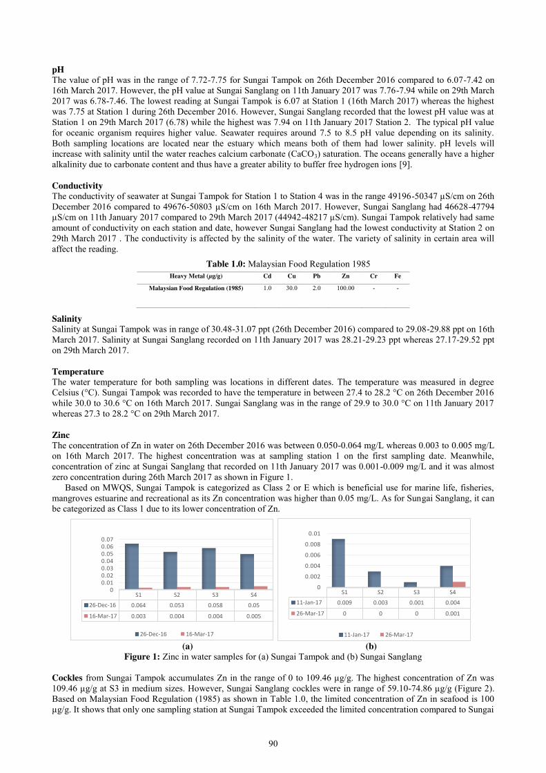
90

S1 S2 S3 S4

26-Dec-16 0.064 0.053 0.058 0.05

16-Mar-17 0.003 0.004 0.004 0.005

0 0.01 0.02 0.03 0.04 0.05 0.06 0.07

26-Dec-16 16-Mar-17

S1 S2 S3 S4

11-Jan-17 0.009 0.003 0.001 0.004

26-Mar-17 0 0 0 0.001

0

0.002

0.004

0.006

0.008

0.01

11-Jan-17 26-Mar-17

pH The value of pH was in the range of 7.72-7.75 for Sungai Tampok on 26th December 2016 compared to 6.07-7.42 on 16th March 2017. However, the pH value at Sungai Sanglang on 11th January 2017 was 7.76-7.94 while on 29th March 2017 was 6.78-7.46. The lowest reading at Sungai Tampok is 6.07 at Station 1 (16th March 2017) whereas the highest was 7.75 at Station 1 during 26th December 2016. However, Sungai Sanglang recorded that the lowest pH value was at Station 1 on 29th March 2017 (6.78) while the highest was 7.94 on 11th January 2017 Station 2. The typical pH value for oceanic organism requires higher value. Seawater requires around 7.5 to 8.5 pH value depending on its salinity. Both sampling locations are located near the estuary which means both of them had lower salinity. pH levels will increase with salinity until the water reaches calcium carbonate (CaCO3) saturation. The oceans generally have a higher alkalinity due to carbonate content and thus have a greater ability to buffer free hydrogen ions [9]. Conductivity The conductivity of seawater at Sungai Tampok for Station 1 to Station 4 was in the range 49196-50347 µS/cm on 26th December 2016 compared to 49676-50803 µS/cm on 16th March 2017. However, Sungai Sanglang had 46628-47794 µS/cm on 11th January 2017 compared to 29th March 2017 (44942-48217 µS/cm). Sungai Tampok relatively had same amount of conductivity on each station and date, however Sungai Sanglang had the lowest conductivity at Station 2 on 29th March 2017 . The conductivity is affected by the salinity of the water. The variety of salinity in certain area will affect the reading.

Salinity Salinity at Sungai Tampok was in range of 30.48-31.07 ppt (26th December 2016) compared to 29.08-29.88 ppt on 16th March 2017. Salinity at Sungai Sanglang recorded on 11th January 2017 was 28.21-29.23 ppt whereas 27.17-29.52 ppt on 29th March 2017. Temperature The water temperature for both sampling was locations in different dates. The temperature was measured in degree Celsius (°C). Sungai Tampok was recorded to have the temperature in between 27.4 to 28.2 °C on 26th December 2016 while 30.0 to 30.6 °C on 16th March 2017. Sungai Sanglang was in the range of 29.9 to 30.0 °C on 11th January 2017 whereas 27.3 to 28.2 °C on 29th March 2017. Zinc The concentration of Zn in water on 26th December 2016 was between 0.050-0.064 mg/L whereas 0.003 to 0.005 mg/L on 16th March 2017. The highest concentration was at sampling station 1 on the first sampling date. Meanwhile, concentration of zinc at Sungai Sanglang that recorded on 11th January 2017 was 0.001-0.009 mg/L and it was almost zero concentration during 26th March 2017 as shown in Figure 1.

Based on MWQS, Sungai Tampok is categorized as Class 2 or E which is beneficial use for marine life, fisheries, mangroves estuarine and recreational as its Zn concentration was higher than 0.05 mg/L. As for Sungai Sanglang, it can be categorized as Class 1 due to its lower concentration of Zn. (a) (b)

Figure 1: Zinc in water samples for (a) Sungai Tampok and (b) Sungai Sanglang Cockles from Sungai Tampok accumulates Zn in the range of 0 to 109.46 µg/g. The highest concentration of Zn was 109.46 µg/g at S3 in medium sizes. However, Sungai Sanglang cockles were in range of 59.10-74.86 µg/g (Figure 2). Based on Malaysian Food Regulation (1985) as shown in Table 1.0, the limited concentration of Zn in seafood is 100 µg/g. It shows that only one sampling station at Sungai Tampok exceeded the limited concentration compared to Sungai

Table 1.0: Malaysian Food Regulation 1985 Heavy Metal (µg/g) Cd Cu Pb Zn Cr Fe

Malaysian Food Regulation (1985) 1.0 30.0 2.0 100.00 - -

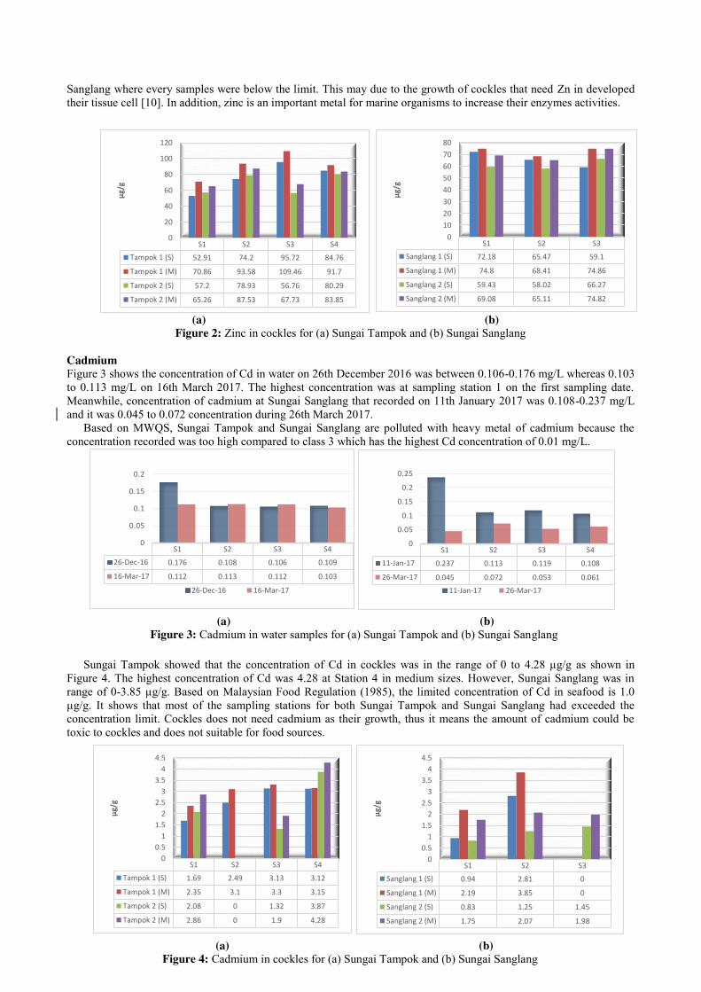
91

S1 S2 S3 S4

Tampok 1 (S) 52.91 74.2 95.72 84.76

Tampok 1 (M) 70.86 93.58 109.46 91.7

Tampok 2 (S) 57.2 78.93 56.76 80.29

Tampok 2 (M) 65.26 87.53 67.73 83.85

0

20

40

60

80

100

120

µg/g

S1 S2 S3

Sanglang 1 (S) 72.18 65.47 59.1

Sanglang 1 (M) 74.8 68.41 74.86

Sanglang 2 (S) 59.43 58.02 66.27

Sanglang 2 (M) 69.08 65.11 74.82

01020304050607080

µg/g

S1 S2 S3 S4

26-Dec-16 0.176 0.108 0.106 0.109

16-Mar-17 0.112 0.113 0.112 0.103

0

0.05

0.1

0.15

0.2

26-Dec-16 16-Mar-17

S1 S2 S3 S4

11-Jan-17 0.237 0.113 0.119 0.108

26-Mar-17 0.045 0.072 0.053 0.061

0

0.05

0.1

0.15

0.2

0.25

11-Jan-17 26-Mar-17

S1 S2 S3 S4

Tampok 1 (S) 1.69 2.49 3.13 3.12

Tampok 1 (M) 2.35 3.1 3.3 3.15

Tampok 2 (S) 2.08 0 1.32 3.87

Tampok 2 (M) 2.86 0 1.9 4.28

00.5

11.5

22.5

33.5

44.5

µg/g

S1 S2 S3

Sanglang 1 (S) 0.94 2.81 0

Sanglang 1 (M) 2.19 3.85 0

Sanglang 2 (S) 0.83 1.25 1.45

Sanglang 2 (M) 1.75 2.07 1.98

00.5

11.5

22.5

33.5

44.5

µg/g

(a) (b) Figure 4: Cadmium in cockles for (a) Sungai Tampok and (b) Sungai Sanglang

(a) (b) Figure 3: Cadmium in water samples for (a) Sungai Tampok and (b) Sungai Sanglang

Sanglang where every samples were below the limit. This may due to the growth of cockles that need Zn in developed their tissue cell [10]. In addition, zinc is an important metal for marine organisms to increase their enzymes activities. (a) (b)

Figure 2: Zinc in cockles for (a) Sungai Tampok and (b) Sungai Sanglang Cadmium Figure 3 shows the concentration of Cd in water on 26th December 2016 was between 0.106-0.176 mg/L whereas 0.103 to 0.113 mg/L on 16th March 2017. The highest concentration was at sampling station 1 on the first sampling date. Meanwhile, concentration of cadmium at Sungai Sanglang that recorded on 11th January 2017 was 0.108-0.237 mg/L and it was 0.045 to 0.072 concentration during 26th March 2017.

Based on MWQS, Sungai Tampok and Sungai Sanglang are polluted with heavy metal of cadmium because the concentration recorded was too high compared to class 3 which has the highest Cd concentration of 0.01 mg/L.

Sungai Tampok showed that the concentration of Cd in cockles was in the range of 0 to 4.28 µg/g as shown in

Figure 4. The highest concentration of Cd was 4.28 at Station 4 in medium sizes. However, Sungai Sanglang was in range of 0-3.85 µg/g. Based on Malaysian Food Regulation (1985), the limited concentration of Cd in seafood is 1.0 µg/g. It shows that most of the sampling stations for both Sungai Tampok and Sungai Sanglang had exceeded the concentration limit. Cockles does not need cadmium as their growth, thus it means the amount of cadmium could be toxic to cockles and does not suitable for food sources.

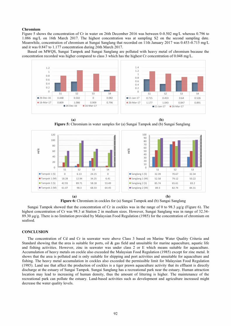
92

S1 S2 S3

Sanglang 1 (S) 32.39 70.67 32.34

Sanglang 1 (M) 52.58 79.12 50.22

Sanglang 2 (S) 85.74 65.61 83.2

Sanglang 2 (M) 89.3 82.74 84.31

0102030405060708090

100

µg/g

(a) (b) Figure 6: Chromium in cockles for (a) Sungai Tampok and (b) Sungai Sanglang

S1 S2 S3 S4

26-Dec-16 0.448 0.502 0 0.082

16-Mar-17 0.809 1.086 0.909 0.796

0 0.2 0.4 0.6 0.8

1 1.2

26-Dec-16 16-Mar-17

S1 S2 S3 S4

11-Jan-17 0.715 0.453 0.64 0.526

26-Mar-17 1.177 1.043 0.847 0.891

0 0.2 0.4 0.6 0.8

1 1.2 1.4

11-Jan-17 26-Mar-17

(a) (b) Figure 5: Chromium in water samples for (a) Sungai Tampok and (b) Sungai Sanglang

S1 S2 S3 S4

Tampok 1 (S) 0 6.13 24.15 0

Tampok 1 (M) 18.28 12.94 34.25 6.41

Tampok 2 (S) 42.93 89.71 58.18 53.49

Tampok 2 (M) 61.07 98.3 68.33 64.45

0

20

40

60

80

100

120

µg/g

Chromium Figure 5 shows the concentration of Cr in water on 26th December 2016 was between 0-0.502 mg/L whereas 0.796 to 1.086 mg/L on 16th March 2017. The highest concentration was at sampling S2 on the second sampling date. Meanwhile, concentration of chromium at Sungai Sanglang that recorded on 11th January 2017 was 0.453-0.715 mg/L and it was 0.847 to 1.177 concentration during 26th March 2017.

Based on MWQS, Sungai Tampok and Sungai Sanglang are polluted with heavy metal of chromium because the concentration recorded was higher compared to class 3 which has the highest Cr concentration of 0.048 mg/L.

Sungai Tampok showed that the concentration of Cr in cockles was in the range of 0 to 98.3 µg/g (Figure 6). The highest concentration of Cr was 98.3 at Station 2 in medium sizes. However, Sungai Sanglang was in range of 32.34-89.30 µg/g. There is no limitation provided by Malaysian Food Regulation (1985) for the concentration of chromium on seafood.

CONCLUSION

The concentration of Cd and Cr in seawater were above Class 3 based on Marine Water Quality Criteria and Standard showing that the area is suitable for ports, oil & gas field and unsuitable for marine aquaculture, aquatic life and fishing activities. However, zinc in seawater was under class 2 or E which means suitable for aquaculture. Accumulation of heavy metals on cockle also exceeded the Malaysian Food Regulation (1985) except for zinc metal. It shows that the area is polluted and is only suitable for shipping and port activities and unsuitable for aquaculture and fishing. The heavy metal accumulation in cockles also exceeded the permissible limit for Malaysian Food Regulation (1985). Land use that affect the production of cockles is a tiger prawn aquaculture activity that its effluent is directly discharge at the estuary of Sungai Tampok. Sungai Sanglang has a recreational park near the estuary. Human attraction location may lead to increasing of human density, thus the amount of littering is higher. The maintenance of the recreational park can pollute the estuary. Land-based activities such as development and agriculture increased might decrease the water quality levels.

93

REFERENCES [1] Tu N. P. C., Ha N. N., Agusa T., Ikemoto T., Tuyen B. C., Tanabe S., Takeuchi I., (2011). Trace elements in Anadara spp.

(Mollusca: Bivalva) collected along the coast of Vietnam, with emphasis on regional differences and human health risk assessment. Fisheries Science 77(6):1033–1043

[2] Yap C. K., Ismail A., Tan S. G., 2003 Heavy metal (Cd, Cu, Pb and Zn) concentrations in the green-lipped mussel Perna viridis (Linnaeus) collected from some wild and aquaculture sites in the west coast of Peninsular Malaysia. Food Chemistry 84:569-575.

[3] The Editors of Encyclopaedia Britannica, (2014, December 3). Straits of Malacca, Strait, Asia. Retrieved from https://global.britannica.com/place/Strait-of-Malacca

[4] Neville, S. (2016, May 17). Cockles Trade Threatened. The Star. Retrieved from http://www.thestar.com.my/news/nation/2016/05/17/cockle-trade-threatened-production-down-to-16000 tonnes-from-100000-tonnes

[5] Anon. (1985). Annual States Fisheries Statistics. 1984 Kuala Lumpur, Malaysia, Department of Fisheries, Mm. of Agriculture.

[6] Babel, S., Kurniawan, T.A., (2003). Various treatment technologies to remove arsenic and mercury from contaminated

groundwater: an overview. In: Proceedings of the First International Symposium on Southeast Asian Water Environment, Bangkok, Thailand, 24 25 October, pp. 433–440.

[7] Berglund M, Elinder CG, Järup L. (2001) Humans Exposure Assessment. An Introduction. WHO/SDE/OEH/01.3, 2001.

[8] Jarup L, Berglund M, Elinder CG, Nordberg G, Vahter M., (1998), Health effects of cadmium exposure—a review of the literature and a risk estimate. Scand J Work Environment Health 1998; 24 (Suppl 1): 1–51

[9] Radke, L. (2006). pH of Coastal Waterways. In Oz Coasts. Retrieved from http://www.ozcoasts.gov.au/indicators/ph_coastal_waterways.jsp.

[10] Zhao, S., Feng, C., Quan, W., Chen, X., Niu, J., and Shen, Z. (2012). Role of living environments in the accumulation characteristics of heavy metals in fishes and crabs in the Yangtze River Estuary, China. Marine Pollution Bulletin, 64(6): 1163–1171.

94

Electro-Assisted Phytoremediation by Using Water Lettuce (Pistia stratiotes L)

Nabilah Basirun, Normala Hashim Faculty of Civil Engineering, Universiti Teknologi Malaysia, Malaysia

normala@utm.my

Keywords: EAPR system; Phytoremediation; Water Lettuce (Pistia stratiotes L); Hydroponic System.

ABSTRACT. The use of electro kinetic system with phytoremediation methods or known as electro-assisted phytoremediation (EAPR) for hydroponic system has been demonstrated in a laboratory- scale experiment to observe the rapid removal of chromium and manganese from the contaminated water. Water lettuces (Pistia stratiotes L) were used to evaluate the potential uptake of chromium and manganese in hydroponic (soil-free) culture. The studied plants were harvested on day 7(4V), day 14(4V) and day 7(2V). The results obtained were used to compare the ability of water lettuces to uptake chromium and manganese in the contaminated water between EAPR system and phytoremediation method. Both treatments showed high level accumulation in the roots part. The metal uptake per plants mass by each treatment showed high uptake by the EAPR system. The overall results demonstrate higher uptake by water lettuce in EAPR system compare to the phytoremediation method.

INTRODUCTION

Phytoremediation is eco-friendly technologies which use plants to cleanup or reduce both organic and inorganic toxicity contaminant from the environment [1][2]. Phytoremediation is an emerging cheaper technology promotes aesthetic value to the environment, cost effective, non-intrusive and safe initiative compare with the conventional technology to treat water and soil [3].

The application of coupled technology of electro kinetic remediation (EKR) and phytoremediation technique has been gaining interest lately [10]. Electro-assisted phytoremediation or EAPR is one of the alternatives to enhance the performance of growing plants to accumulate the contaminants and beneficial to transport charged particles and uptake contaminant located deeper than root zone [3][4]. The application of EAPR can be use for both alternating current (AC) field and direct current (DC) field. Problem Statement Water is basic necessity for human kind. It is non-renewable natural sources that have to be conserve in order to balance our ecosystem along with the development. Rise of green technologies that help to maintain the sustainability, economical and most importantly high efficiency in removal of pollutant has been seen as the great effort worldwide. Application of phytoremediation however have limitation as it is time consuming. The uptake of the contaminant depends solely to the roots’ length of the plant species [13].

Electro kinetic assisted phytoremediation (EAPR) helped to enhance the hyperaccumulator plants to uptake the contaminants in deeper root zone area [3][13]. The need of study is to compare the uptake of the heavy metal by the water lettuce between electro-assisted phytoremediation and phytoremediation method.

Objectives The objectives of this study are:

1. To compare the heavy metal uptake between electro– assisted phytoremediation (EAPR) system and phytoremediation process.

2. To determine the ability of water lettuce to accumulate the heavy metal contaminants.

3. To determine the metal uptake per plants.

Scope of Study The research study focused on ability of water lettuce to uptake chromium and manganese by using EAPR system and phytoremediation process. Chromium (Cr) and Manganese (Mn) are the target contaminants in this study which significantly harmful to human health in excessive presence. This research study was conducted in Block C 07, Environmental Engineering Laboratory, Faculty of Civil Engineering (FKA) University of Technology Malaysia, Skudai, Johor. Water lettuce was placed in the hydroponic growth medium. The sample was analysed by using Atomic Absorption Spectroscopy (AAS) to determine the concentrations of heavy metals in the studied plants. The data obtained was used to analyse the accumulation of the heavy metal in the plants from the contaminated water. The research study was undergoing for 150 days.

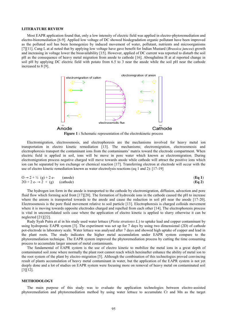
95

LITERATURE REVIEW

Most EAPR application found that, only a low intensity of electric field was applied in electro-phytoremediation and electro-bioremediation [6-9]. Applied low voltage of DC showed biodegradation organic pollutant have been improved as the polluted soil has been homogenize by induced movement of water, pollutant, nutrients and microorganisms [7][11]. Cang L at al noted that by applying low voltage have gave benefit for Indian Mustard (Brassica juncea) growth and increasing in voltage lower the bioavailability [15]. However, applied of DC current was reported to disturb the soil pH as the consequence of heavy metal migration from anode to cathode [16]. Aboughalma H at al reported change in soil pH by applying DC electric field with potato from 6.5 to 3 near the anode while the soil pH near the cathode increased to 8 [9].

Figure 1 : Schematic representation of the electrokinetic process

Electromigration, electroosmosis, and electrophoresis are the mechanisms involved for heavy metal ion

transportation in electro kinetic remediation [13]. The mechanisms; electromigration, electroosmosis and electrophoresis transport the contaminant ions from the contaminants’ matrix toward the electrode compartment. When electric field is applied in soil, ions will be move in pore water which known as electromigration. During electromigration process negative charged will move towards anode while cathode will attract the positive ions which ion can be separated by ion exchange or chemical reaction [17]. Transferring electron at electrode will occur with the use of electro kinetic remediation known as water electrolysis reactions (eq 1 and 2): [17-19]

O → 2 + ½ (g) + 2 e- (anode) (Eq 1) 2O + 2 e- → 2 + (g) (cathode) (Eq 2)

The hydrogen ion form in the anode is transported to the cathode by electromigration, diffusion, advection and pore

fluid flow which forming acid front [17][20]. The formation of hydroxide ions in the cathode caused the pH to increase where the anions is transported towards to the anode and cause the reduction in soil pH near the anode [17-20]. Electroosmosis is the pore fluid movement relative to soil particle [13]. Electrophoresis is charged colloids movement where it is moving towards opposite electrodes charged and repelled from each other [14]. The electrophoresis process is vital in unconsolidated soils case where the application of electro kinetic is applied to slurry otherwise it can be neglected [21][22].

Rudy Syah Putra et al in his study used water lettuce (Pistia stratiotes L.) to uptake lead and copper contaminant by using hydroponic EAPR system [3]. The experiment was set up for 7 days by using two dimensional (2D) of cathode pot-electrode in laboratory scale. Water lettuce was analysed after 7 days and showed high uptake of copper and lead in the plant roots. The study indicates the higher metal accumulation under EAPR system compare to the phytoremediation technique. The EAPR system improved the phytoremediation process by cutting the time consuming process to accumulate larger amount of metal contaminants.

The fundamental of EAPR system is the use of electro kinetic to mobilize the metal ions in a great depth of contaminated soil zone where normally the plant root cannot reach which hereinafter enhance the ability of metal ion to the root system of the plant by electro-migration [5]. Although the combination of this technologies proved convincing result of plants accumulation of heavy metal contaminant in water, but the application of the EAPR system is not yet deeply done and a lot of studies on EAPR system were focusing more on removal of heavy metal on contaminated soil [3][12].

METHODOLOGY

The main purpose of this study was to evaluate the application technologies between electro-assisted phytoremediation and phytoremediation method by using water lettuce to accumulate Cr and Mn as the target

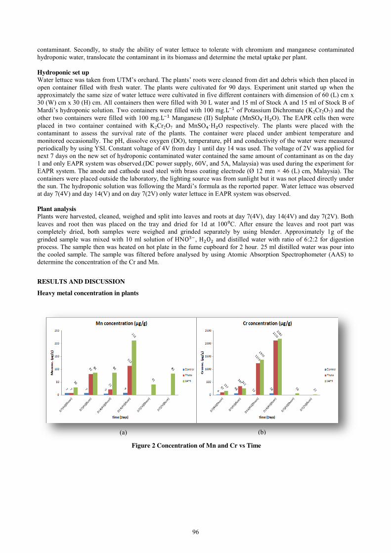
96

contaminant. Secondly, to study the ability of water lettuce to tolerate with chromium and manganese contaminated hydroponic water, translocate the contaminant in its biomass and determine the metal uptake per plant.

Hydroponic set up Water lettuce was taken from UTM’s orchard. The plants’ roots were cleaned from dirt and debris which then placed in open container filled with fresh water. The plants were cultivated for 90 days. Experiment unit started up when the approximately the same size of water lettuce were cultivated in five different containers with dimension of 60 (L) cm x 30 (W) cm x 30 (H) cm. All containers then were filled with 30 L water and 15 ml of Stock A and 15 ml of Stock B of Mardi’s hydroponic solution. Two containers were filled with 100 mg.L−1 of Potassium Dichromate (K2Cr2O7) and the other two containers were filled with 100 mg.L−1 Manganese (II) Sulphate (MnSO₄·H₂O). The EAPR cells then were placed in two container contained with K2Cr2O7 and MnSO₄·H₂O respectively. The plants were placed with the contaminant to assess the survival rate of the plants. The container were placed under ambient temperature and monitored occasionally. The pH, dissolve oxygen (DO), temperature, pH and conductivity of the water were measured periodically by using YSI. Constant voltage of 4V from day 1 until day 14 was used. The voltage of 2V was applied for next 7 days on the new set of hydroponic contaminated water contained the same amount of contaminant as on the day 1 and only EAPR system was observed.(DC power supply, 60V, and 5A, Malaysia) was used during the experiment for EAPR system. The anode and cathode used steel with brass coating electrode (Ø 12 mm × 46 (L) cm, Malaysia). The containers were placed outside the laboratory, the lighting source was from sunlight but it was not placed directly under the sun. The hydroponic solution was following the Mardi’s formula as the reported paper. Water lettuce was observed at day 7(4V) and day 14(V) and on day 7(2V) only water lettuce in EAPR system was observed. Plant analysis Plants were harvested, cleaned, weighed and split into leaves and roots at day 7(4V), day 14(4V) and day 7(2V). Both leaves and root then was placed on the tray and dried for 1d at 100⁰C. After ensure the leaves and root part was completely dried, both samples were weighed and grinded separately by using blender. Approximately 1g of the grinded sample was mixed with 10 ml solution of HNO3−, H2O2 and distilled water with ratio of 6:2:2 for digestion process. The sample then was heated on hot plate in the fume cupboard for 2 hour. 25 ml distilled water was pour into the cooled sample. The sample was filtered before analysed by using Atomic Absorption Spectrophometer (AAS) to determine the concentration of the Cr and Mn.

RESULTS AND DISCUSSION

Heavy metal concentration in plants

Figure 2 Concentration of Mn and Cr vs Time

(a) (b)

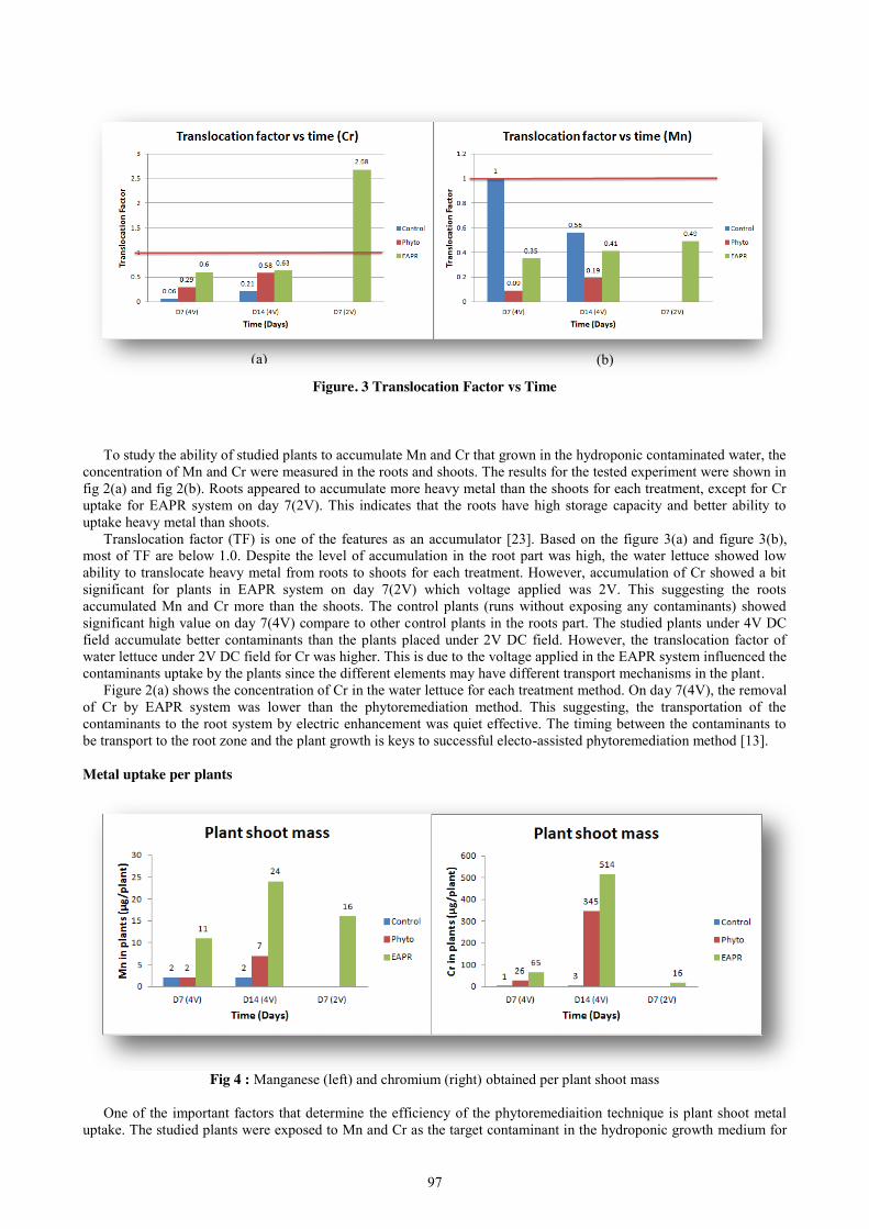
97

Figure. 3 Translocation Factor vs Time

To study the ability of studied plants to accumulate Mn and Cr that grown in the hydroponic contaminated water, the

concentration of Mn and Cr were measured in the roots and shoots. The results for the tested experiment were shown in fig 2(a) and fig 2(b). Roots appeared to accumulate more heavy metal than the shoots for each treatment, except for Cr uptake for EAPR system on day 7(2V). This indicates that the roots have high storage capacity and better ability to uptake heavy metal than shoots.

Translocation factor (TF) is one of the features as an accumulator [23]. Based on the figure 3(a) and figure 3(b), most of TF are below 1.0. Despite the level of accumulation in the root part was high, the water lettuce showed low ability to translocate heavy metal from roots to shoots for each treatment. However, accumulation of Cr showed a bit significant for plants in EAPR system on day 7(2V) which voltage applied was 2V. This suggesting the roots accumulated Mn and Cr more than the shoots. The control plants (runs without exposing any contaminants) showed significant high value on day 7(4V) compare to other control plants in the roots part. The studied plants under 4V DC field accumulate better contaminants than the plants placed under 2V DC field. However, the translocation factor of water lettuce under 2V DC field for Cr was higher. This is due to the voltage applied in the EAPR system influenced the contaminants uptake by the plants since the different elements may have different transport mechanisms in the plant.

Figure 2(a) shows the concentration of Cr in the water lettuce for each treatment method. On day 7(4V), the removal of Cr by EAPR system was lower than the phytoremediation method. This suggesting, the transportation of the contaminants to the root system by electric enhancement was quiet effective. The timing between the contaminants to be transport to the root zone and the plant growth is keys to successful electo-assisted phytoremediation method [13].

Metal uptake per plants

Fig 4 : Manganese (left) and chromium (right) obtained per plant shoot mass

One of the important factors that determine the efficiency of the phytoremediaition technique is plant shoot metal

uptake. The studied plants were exposed to Mn and Cr as the target contaminant in the hydroponic growth medium for

(a) (b)

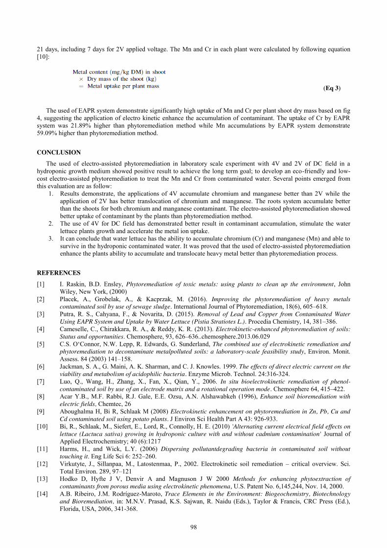
98

21 days, including 7 days for 2V applied voltage. The Mn and Cr in each plant were calculated by following equation [10]:

(Eq 3)

The used of EAPR system demonstrate significantly high uptake of Mn and Cr per plant shoot dry mass based on fig

4, suggesting the application of electro kinetic enhance the accumulation of contaminant. The uptake of Cr by EAPR system was 21.89% higher than phytoremediation method while Mn accumulations by EAPR system demonstrate 59.09% higher than phytoremediation method.

CONCLUSION The used of electro-assisted phytoremediation in laboratory scale experiment with 4V and 2V of DC field in a

hydroponic growth medium showed positive result to achieve the long term goal; to develop an eco-friendly and low-cost electro-assisted phytoremediation to treat the Mn and Cr from contaminated water. Several points emerged from this evaluation are as follow:

1. Results demonstrate, the applications of 4V accumulate chromium and manganese better than 2V while the application of 2V has better translocation of chromium and manganese. The roots system accumulate better than the shoots for both chromium and manganese contaminant. The electro-assisted phytoremediation showed better uptake of contaminant by the plants than phytoremediation method.

2. The use of 4V for DC field has demonstrated better result in contaminant accumulation, stimulate the water lettuce plants growth and accelerate the metal ion uptake.

3. It can conclude that water lettuce has the ability to accumulate chromium (Cr) and manganese (Mn) and able to survive in the hydroponic contaminated water. It was proved that the used of electro-assisted phytoremediation enhance the plants ability to accumulate and translocate heavy metal better than phytoremediation process.

REFERENCES

[1] I. Raskin, B.D. Ensley, Phytoremediation of toxic metals: using plants to clean up the environment, John Wiley, New York, (2000)

[2] Placek, A., Grobelak, A., & Kacprzak, M. (2016). Improving the phytoremediation of heavy metals contaminated soil by use of sewage sludge. International Journal of Phytoremediation, 18(6), 605–618.

[3] Putra, R. S., Cahyana, F., & Novarita, D. (2015). Removal of Lead and Copper from Contaminated Water Using EAPR System and Uptake by Water Lettuce (Pistia Stratiotes L.). Procedia Chemistry, 14, 381–386.

[4] Cameselle, C., Chirakkara, R. A., & Reddy, K. R. (2013). Electrokinetic-enhanced phytoremediation of soils: Status and opportunities. Chemosphere, 93, 626–636..chemosphere.2013.06.029

[5] C.S. O‘Connor, N.W. Lepp, R. Edwards, G. Sunderland, The combined use of electrokinetic remediation and phytoremediation to decontaminate metalpolluted soils: a laboratory-scale feasibility study, Environ. Monit. Assess. 84 (2003) 141–158.

[6] Jackman, S. A., G. Maini, A. K. Sharman, and C. J. Knowles. 1999. The effects of direct electric current on the viability and metabolism of acidophilic bacteria. Enzyme Microb. Technol. 24:316-324.

[7] Luo, Q., Wang, H., Zhang, X., Fan, X., Qian, Y., 2006. In situ bioelectrokinetic remediation of phenol-contaminated soil by use of an electrode matrix and a rotational operation mode. Chemosphere 64, 415–422.

[8] Acar Y.B., M.F. Rabbi, R.J. Gale, E.E. Ozsu, A.N. Alshawabkeh (1996), Enhance soil bioremediation with electric fields, Chemtec, 26

[9] Aboughalma H, Bi R, Schlaak M (2008) Electrokinetic enhancement on phytoremediation in Zn, Pb, Cu and Cd contaminated soil using potato plants. J Environ Sci Health Part A 43: 926-933.

[10] Bi, R., Schlaak, M., Siefert, E., Lord, R., Connolly, H. E. (2010) 'Alternating current electrical field effects on lettuce (Lactuca sativa) growing in hydroponic culture with and without cadmium contamination' Journal of Applied Electrochemistry; 40 (6):1217

[11] Harms, H., and Wick, L.Y. (2006) Dispersing pollutantdegrading bacteria in contaminated soil without touching it. Eng Life Sci 6: 252–260.

[12] Virkutyte, J., Sillanpaa, M., Latostenmaa, P., 2002. Electrokinetic soil remediation – critical overview. Sci. Total Environ. 289, 97–121

[13] Hodko D, Hyfte J V, Denvir A and Magnuson J W 2000 Methods for enhancing phytoextraction of contaminants from porous media using electrokinetic phenomena, U.S. Patent No. 6,145,244, Nov. 14, 2000.

[14] A.B. Ribeiro, J.M. Rodríguez-Maroto, Trace Elements in the Environment: Biogeochemistry, Biotechnology and Bioremediation, in: M.N.V. Prasad, K.S. Sajwan, R. Naidu (Eds.), Taylor & Francis, CRC Press (Ed.), Florida, USA, 2006, 341-368.

99

[15] Cang L, Wang QY, Zhou DM, Xu H (2011) Effects of electrokinetic-assisted phytoremediation of a multiple-metal contaminated soil on soil metal bioavailability and uptake by Indian mustard. Sep Purif Technol. 79: 246-253.

[16] Mao X, Han FX, Shao X, Su Y (2015) Coupled Electro-kinetic Remediation and Phytoremediation of Metal(loid) Contaminated Soils. J Bioremed Biodeg 6: e163. doi:10.4172/2155-6199.1000e163

[17] Ferreira, D. C. M. D. (2015). Electrokinetic treatment of environmental matrices. Contaminants removal and phosphorus recovery (Doctoral dissertation, Universidade Nova de Lisboa).

[18] Acar, Y.B., (1993). Principles of electrokinetic remediation. Environ. Sci. Technol. 27, 22 2638-2647. [19] Virkutyte, J., Sillanpää, M., Latostenmaa, P., 2002. Electrokinetic soil remediation – 4 Critical overview. Sci.

Total Environ. 289, 97-121. [20] Acar, Y.B., Gale, R.J., Alshawabkeh, A.N., Marks, R.E., Puppala, S., Bricka, M., 24 Parker, R., (1995).

Electrokinetic remediation: Basics and technology status. J. Hazard. 25 Mater. 40, 117-137 [21] Reed B.E., P.C. Carriere, J.C. Thompson, J.H. Hatfield, Electrokinetic (EK) remediation of a contaminated soil

at several Pb concentrations and applied voltages, Journal of Soil Contamination, 5 (1996) 95-120. 135 [22] Ottosen L., (1995) Electrokinetic remediation. Application to soils polluted from wood preservation, Ph.D.

Thesis, Technical University of Denmark, Lyngby, Denmark. [23] Zhang, X., Gao, B. & Xia, H. (2014). Effect of cadmium on growth, photosynthesis, mineral nutrition and

metal accumulation of bana grass and vetiver grass. Ecotoxicology and Environmental Safety, 106, 102-108.

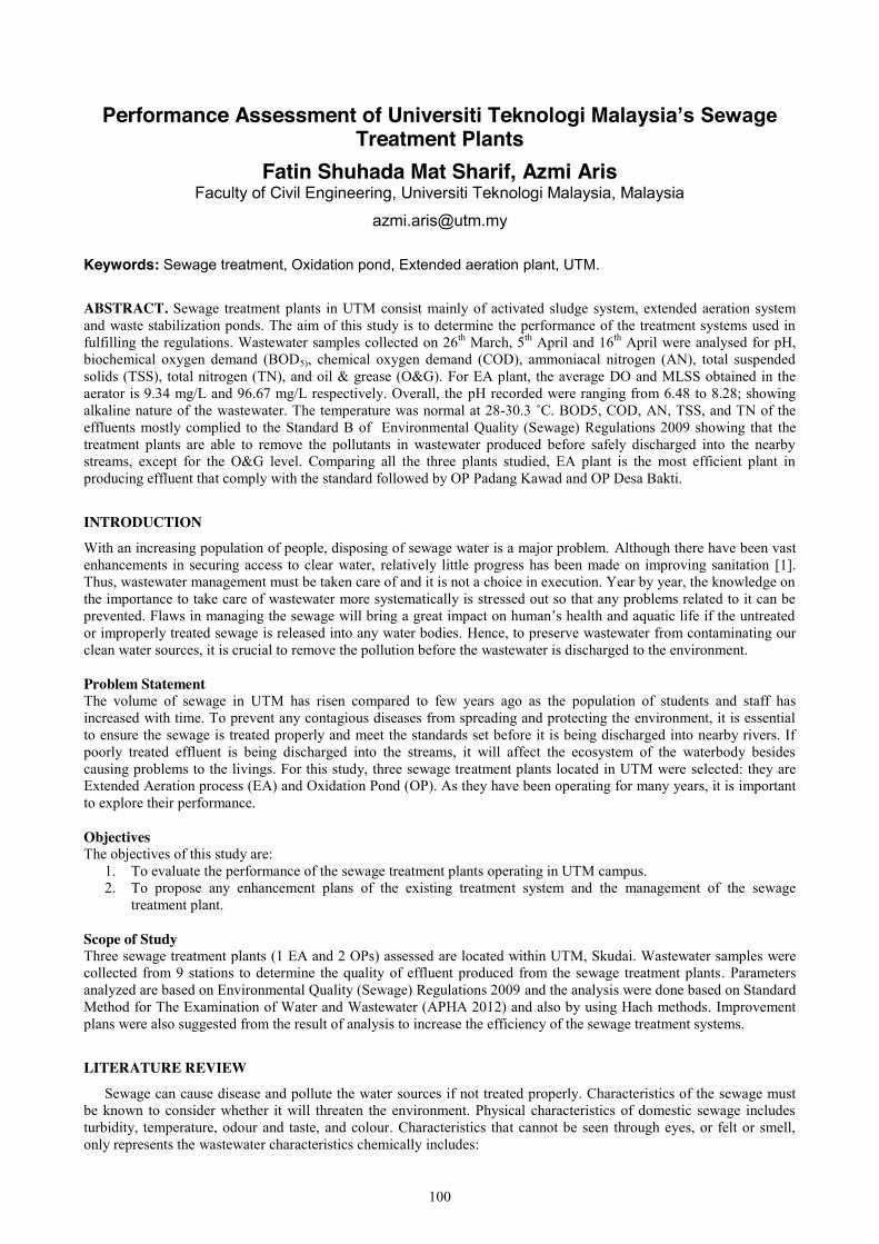
100

Performance Assessment of Universiti Teknologi Malaysia’s Sewage Treatment Plants

Fatin Shuhada Mat Sharif, Azmi Aris Faculty of Civil Engineering, Universiti Teknologi Malaysia, Malaysia

azmi.aris@utm.my

Keywords: Sewage treatment, Oxidation pond, Extended aeration plant, UTM.

ABSTRACT. Sewage treatment plants in UTM consist mainly of activated sludge system, extended aeration system and waste stabilization ponds. The aim of this study is to determine the performance of the treatment systems used in fulfilling the regulations. Wastewater samples collected on 26th March, 5th April and 16th April were analysed for pH, biochemical oxygen demand (BOD5), chemical oxygen demand (COD), ammoniacal nitrogen (AN), total suspended solids (TSS), total nitrogen (TN), and oil & grease (O&G). For EA plant, the average DO and MLSS obtained in the aerator is 9.34 mg/L and 96.67 mg/L respectively. Overall, the pH recorded were ranging from 6.48 to 8.28; showing alkaline nature of the wastewater. The temperature was normal at 28-30.3 ˚C. BOD5, COD, AN, TSS, and TN of the effluents mostly complied to the Standard B of Environmental Quality (Sewage) Regulations 2009 showing that the treatment plants are able to remove the pollutants in wastewater produced before safely discharged into the nearby streams, except for the O&G level. Comparing all the three plants studied, EA plant is the most efficient plant in producing effluent that comply with the standard followed by OP Padang Kawad and OP Desa Bakti.

INTRODUCTION

With an increasing population of people, disposing of sewage water is a major problem. Although there have been vast enhancements in securing access to clear water, relatively little progress has been made on improving sanitation [1]. Thus, wastewater management must be taken care of and it is not a choice in execution. Year by year, the knowledge on the importance to take care of wastewater more systematically is stressed out so that any problems related to it can be prevented. Flaws in managing the sewage will bring a great impact on human’s health and aquatic life if the untreated or improperly treated sewage is released into any water bodies. Hence, to preserve wastewater from contaminating our clean water sources, it is crucial to remove the pollution before the wastewater is discharged to the environment. Problem Statement The volume of sewage in UTM has risen compared to few years ago as the population of students and staff has increased with time. To prevent any contagious diseases from spreading and protecting the environment, it is essential to ensure the sewage is treated properly and meet the standards set before it is being discharged into nearby rivers. If poorly treated effluent is being discharged into the streams, it will affect the ecosystem of the waterbody besides causing problems to the livings. For this study, three sewage treatment plants located in UTM were selected: they are Extended Aeration process (EA) and Oxidation Pond (OP). As they have been operating for many years, it is important to explore their performance. Objectives The objectives of this study are:

1. To evaluate the performance of the sewage treatment plants operating in UTM campus. 2. To propose any enhancement plans of the existing treatment system and the management of the sewage

treatment plant. Scope of Study Three sewage treatment plants (1 EA and 2 OPs) assessed are located within UTM, Skudai. Wastewater samples were collected from 9 stations to determine the quality of effluent produced from the sewage treatment plants. Parameters analyzed are based on Environmental Quality (Sewage) Regulations 2009 and the analysis were done based on Standard Method for The Examination of Water and Wastewater (APHA 2012) and also by using Hach methods. Improvement plans were also suggested from the result of analysis to increase the efficiency of the sewage treatment systems.

LITERATURE REVIEW

Sewage can cause disease and pollute the water sources if not treated properly. Characteristics of the sewage must be known to consider whether it will threaten the environment. Physical characteristics of domestic sewage includes turbidity, temperature, odour and taste, and colour. Characteristics that cannot be seen through eyes, or felt or smell, only represents the wastewater characteristics chemically includes:

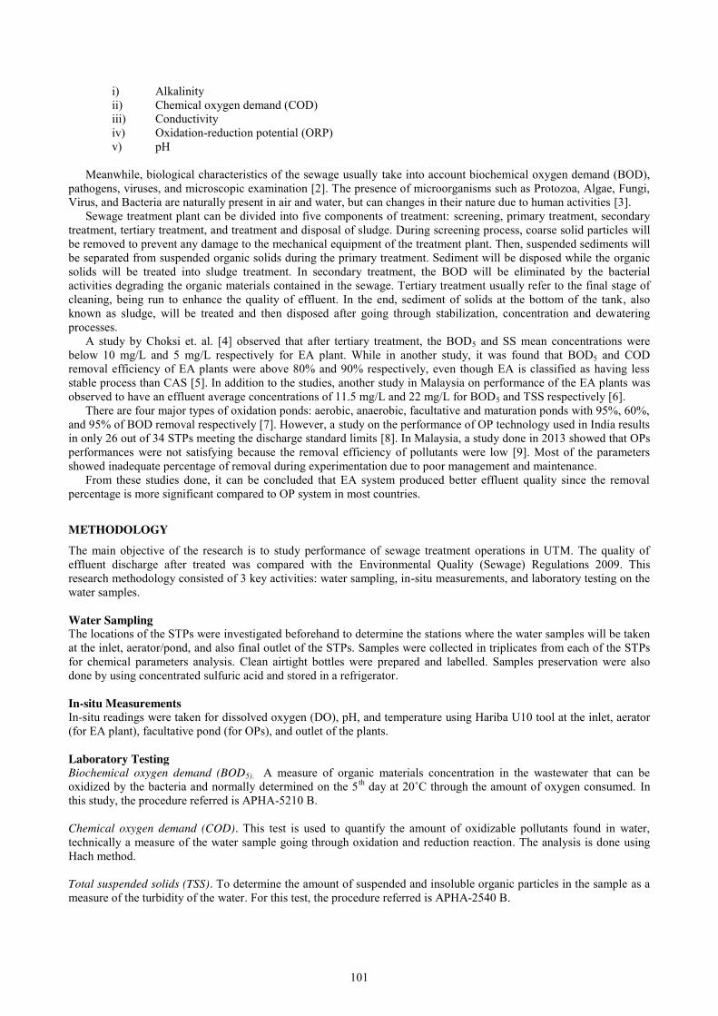
101

i) Alkalinity ii) Chemical oxygen demand (COD) iii) Conductivity iv) Oxidation-reduction potential (ORP) v) pH

Meanwhile, biological characteristics of the sewage usually take into account biochemical oxygen demand (BOD),

pathogens, viruses, and microscopic examination [2]. The presence of microorganisms such as Protozoa, Algae, Fungi, Virus, and Bacteria are naturally present in air and water, but can changes in their nature due to human activities [3].

Sewage treatment plant can be divided into five components of treatment: screening, primary treatment, secondary treatment, tertiary treatment, and treatment and disposal of sludge. During screening process, coarse solid particles will be removed to prevent any damage to the mechanical equipment of the treatment plant. Then, suspended sediments will be separated from suspended organic solids during the primary treatment. Sediment will be disposed while the organic solids will be treated into sludge treatment. In secondary treatment, the BOD will be eliminated by the bacterial activities degrading the organic materials contained in the sewage. Tertiary treatment usually refer to the final stage of cleaning, being run to enhance the quality of effluent. In the end, sediment of solids at the bottom of the tank, also known as sludge, will be treated and then disposed after going through stabilization, concentration and dewatering processes.

A study by Choksi et. al. [4] observed that after tertiary treatment, the BOD5 and SS mean concentrations were below 10 mg/L and 5 mg/L respectively for EA plant. While in another study, it was found that BOD5 and COD removal efficiency of EA plants were above 80% and 90% respectively, even though EA is classified as having less stable process than CAS [5]. In addition to the studies, another study in Malaysia on performance of the EA plants was observed to have an effluent average concentrations of 11.5 mg/L and 22 mg/L for BOD5 and TSS respectively [6].

There are four major types of oxidation ponds: aerobic, anaerobic, facultative and maturation ponds with 95%, 60%, and 95% of BOD removal respectively [7]. However, a study on the performance of OP technology used in India results in only 26 out of 34 STPs meeting the discharge standard limits [8]. In Malaysia, a study done in 2013 showed that OPs performances were not satisfying because the removal efficiency of pollutants were low [9]. Most of the parameters showed inadequate percentage of removal during experimentation due to poor management and maintenance.

From these studies done, it can be concluded that EA system produced better effluent quality since the removal percentage is more significant compared to OP system in most countries.

METHODOLOGY The main objective of the research is to study performance of sewage treatment operations in UTM. The quality of effluent discharge after treated was compared with the Environmental Quality (Sewage) Regulations 2009. This research methodology consisted of 3 key activities: water sampling, in-situ measurements, and laboratory testing on the water samples. Water Sampling The locations of the STPs were investigated beforehand to determine the stations where the water samples will be taken at the inlet, aerator/pond, and also final outlet of the STPs. Samples were collected in triplicates from each of the STPs for chemical parameters analysis. Clean airtight bottles were prepared and labelled. Samples preservation were also done by using concentrated sulfuric acid and stored in a refrigerator. In-situ Measurements In-situ readings were taken for dissolved oxygen (DO), pH, and temperature using Hariba U10 tool at the inlet, aerator (for EA plant), facultative pond (for OPs), and outlet of the plants. Laboratory Testing Biochemical oxygen demand (BOD5). A measure of organic materials concentration in the wastewater that can be oxidized by the bacteria and normally determined on the 5th day at 20˚C through the amount of oxygen consumed. In this study, the procedure referred is APHA-5210 B. Chemical oxygen demand (COD). This test is used to quantify the amount of oxidizable pollutants found in water, technically a measure of the water sample going through oxidation and reduction reaction. The analysis is done using Hach method. Total suspended solids (TSS). To determine the amount of suspended and insoluble organic particles in the sample as a measure of the turbidity of the water. For this test, the procedure referred is APHA-2540 B.

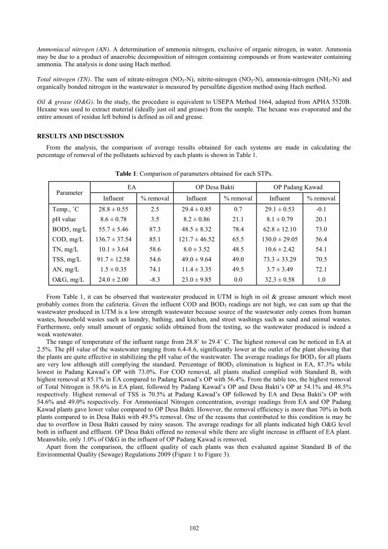
102

Ammoniacal nitrogen (AN). A determination of ammonia nitrogen, exclusive of organic nitrogen, in water. Ammonia may be due to a product of anaerobic decomposition of nitrogen containing compounds or from wastewater containing ammonia. The analysis is done using Hach method. Total nitrogen (TN). The sum of nitrate-nitrogen (NO3-N), nitrite-nitrogen (NO2-N), ammonia-nitrogen (NH3-N) and organically bonded nitrogen in the wastewater is measured by persulfate digestion method using Hach method. Oil & grease (O&G). In the study, the procedure is equivalent to USEPA Method 1664, adapted from APHA 5520B. Hexane was used to extract material (ideally just oil and grease) from the sample. The hexane was evaporated and the entire amount of residue left behind is defined as oil and grease.

RESULTS AND DISCUSSION

From the analysis, the comparison of average results obtained for each systems are made in calculating the percentage of removal of the pollutants achieved by each plants is shown in Table 1.

Table 1: Comparison of parameters obtained for each STPs.

Parameter EA OP Desa Bakti OP Padang Kawad

Influent % removal Influent % removal Influent % removal

Temp., ˚C 28.8 ± 0.55 2.5 29.4 ± 0.85 0.7 29.1 ± 0.53 -0.1 pH value 8.6 ± 0.78 3.5 8.2 ± 0.86 21.1 8.1 ± 0.79 20.1 BOD5, mg/L 55.7 ± 5.46 87.3 48.5 ± 8.32 78.4 62.8 ± 12.10 73.0 COD, mg/L 136.7 ± 37.54 85.1 121.7 ± 46.52 65.5 130.0 ± 29.05 56.4 TN, mg/L 10.1 ± 3.64 58.6 8.0 ± 3.52 48.5 10.6 ± 2.42 54.1 TSS, mg/L 91.7 ± 12.58 54.6 49.0 ± 9.64 49.0 73.3 ± 33.29 70.5 AN, mg/L 1.5 ± 0.35 74.1 11.4 ± 3.35 49.5 3.7 ± 3.49 72.1 O&G, mg/L 24.0 ± 2.00 -8.3 23.0 ± 9.85 0.0 32.3 ± 0.58 1.0

From Table 1, it can be observed that wastewater produced in UTM is high in oil & grease amount which most

probably comes from the cafeteria. Given the influent COD and BOD5 readings are not high, we can sum up that the wastewater produced in UTM is a low strength wastewater because source of the wastewater only comes from human wastes, household wastes such as laundry, bathing, and kitchen, and street washings such as sand and animal wastes. Furthermore, only small amount of organic solids obtained from the testing, so the wastewater produced is indeed a weak wastewater.

The range of temperature of the influent range from 28.8˚ to 29.4˚ C. The highest removal can be noticed in EA at 2.5%. The pH value of the wastewater ranging from 6.4-8.6, significantly lower at the outlet of the plant showing that the plants are quite effective in stabilizing the pH value of the wastewater. The average readings for BOD5 for all plants are very low although still complying the standard. Percentage of BOD5 elimination is highest in EA, 87.3% while lowest in Padang Kawad’s OP with 73.0%. For COD removal, all plants studied complied with Standard B, with highest removal at 85.1% in EA compared to Padang Kawad’s OP with 56.4%. From the table too, the highest removal of Total Nitrogen is 58.6% in EA plant, followed by Padang Kawad’s OP and Desa Bakti’s OP at 54.1% and 48.5% respectively. Highest removal of TSS is 70.5% at Padang Kawad’s OP followed by EA and Desa Bakti’s OP with 54.6% and 49.0% respectively. For Ammoniacal Nitrogen concentration, average readings from EA and OP Padang Kawad plants gave lower value compared to OP Desa Bakti. However, the removal efficiency is more than 70% in both plants compared to in Desa Bakti with 49.5% removal. One of the reasons that contributed to this condition is may be due to overflow in Desa Bakti caused by rainy season. The average readings for all plants indicated high O&G level both in influent and effluent. OP Desa Bakti offered no removal while there are slight increase in effluent of EA plant. Meanwhile, only 1.0% of O&G in the influent of OP Padang Kawad is removed.

Apart from the comparison, the effluent quality of each plants was then evaluated against Standard B of the Environmental Quality (Sewage) Regulations 2009 (Figure 1 to Figure 3).

103

Figure 1: Level of compliance for EA plant

Figure 2: Level of compliance for OP Desa Bakti

Figure 3: Level of compliance for OP Padang Kawad

Comparing the effluent quality with the standard in EQR 2009, the effluent discharged from both EA and OP plants

are satisfying the limit in Standard B for the major pollutant parameters namely BOD5, COD, TSS, TN and AN,

BOD5 COD TN TSS AN Oil &Grease

Effluent 7.1 20.3 4.2 41.7 0.4 26.0Standard 50 200 10 100 5 10

0

40

80

120

160

200

0

20

40

60

80

100

Conc

entr

atio

ns, m

g/L

BOD5 COD TN TSS AN Oil &Grease

Effluent 10.5 42.0 4.1 25.0 5.7 23.0Standard 50 200 10 100 5 10

0

40

80

120

160

200

0

20

40

60

80

100

Conc

entr

atio

ns, m

g/L

BOD5 COD TN TSS AN Oil &Grease

Effluent 16.9 56.7 4.9 21.7 1.0 32.0Standard 50 200 10 100 5 10

0

40

80

120

160

200

0

20

40

60

80

100

Conc

entr

atio

ns, m

g/L

104

excluding oil & grease (for all plants) and AN (for OP Desa Bakti). Due to the spill over in OP Desa Bakti during rainy season, the untreated wastewater get mixed with the surface runoff. Thus, the removal of AN is less efficient.

For EA plant, the average DO and MLSS obtained was 9.34±0.48 mg/L and 96.67±95.18 mg/L respectively. The dissolved oxygen level is controlled by the amount of air added to the aerator. The dissolved oxygen set point for the aerators typically ranging from 1-3 mg/L. However, the DO obtained in this study was too high, may be indicating that the fine bubble aeration has provided excessive aeration in the aerator. So, the plant manager needs to regularly check the DO in the aerator and control the aeration rate by adjusting the blower output. The EA plant is also operating with very low MLSS concentrations compared to the designed MLS which is 4500 mg/L. The aerobic process in the plant is not operating efficiently and is wasting energy. The low MLSS level is caused by low BOD influent since the concentration of MLSS is difficult to increase without adequate food. So, the plant manager may need to gradually decrease the sludge wasting rate of the plant until the selected optimum MLSS is achieved.

As for OPs, the average DO concentrations in the facultative pond were 4.05±0.14 mg/L and 4.45±0.36 mg/L for Padang Kawad and Desa Bakti respectively. Considering the performance of the OPs, an upgrade need to be done to increase the removal efficiency of OP Desa Bakti because the removal percentage for AN, TSS and TN did not reach 50% when compared to the other two plants. The existing system runs naturally with the aid of sunlight and algae without any mechanical equipment. Based on the readings from other studies done, to improve the efficiency of an oxidation pond, current OP system needs to be improved to be an aerated lagoon system, simply by adding mechanical aerator in the facultative ponds. The mechanical aerator will help to provide sufficient oxygen for optimum microbial activities. So, the nitrification of ammonia will improve too, lowering AN concentration in the effluent. In addition, litters were found on the surface of the pond which occasionally disrupt the flow of the water because there is no screening tool at the inlet. As concerns, there should be a screening device to separate the litters from the wastewater.

Last but not least, a new approach also need to be taken to solve the O&G problems in all STPs evaluated. To increase the removal efficiency of O&G for all plants, an oil & grease trap can be put into use during the preliminary treatment or to be put at the cafeteria outlets.

CONCLUSIONS From present assessment, it was observed that STPs evaluated able to produce effluent that complies with the

discharge standard from EQR 2009 in terms BOD5, COD, TSS, TS, and AN removals except O&G. To sum up, EA plant gives better performance in treating domestic wastewater compared to OP system. The finding in other studies done previously were supported since in terms of removal efficiency, EA plant does gives better effluent quality compared to both OP systems despites producing greater pH and O&G of effluent. Yet, OP Padang Kawad treats the wastewater better than OP Desa Bakti based on the pollutants removal percentage. This may be due to occurrence of overflow during the rainy season and blockage of rubbish in Desa Bakti causing the treatment process to be inefficient.

It was further concluded that to improve the removal efficiency of O&G for all plants studied, oil & grease trap need to be used in the preliminary treatment or installed at the outlets of the cafeteria. OP Desa Bakti also requires the installation of screening at the inlet of the pond and needs to be upgraded to be an aerated lagoon system by adding the mechanical aerator in the facultative ponds. Lastly, to ensure the EA plant operates efficiently, the plant manager needs to control the aeration rate and sludge wasting rate to control the DO and MLSS concentrations respectively in the aeration tank.

REFERENCES

[1] Teklehaimanot, G. Z., Kamika, I., Coetzee, M. A. A., and Momba, M. N. B. (2015). Population Growth and Its Impact on the Design Capacity and Performance of the Wastewater Treatment Plants in Sedinbeng and Soshanguve, South Africa. Environmental Management, 56, 984-997. Springer Netherlands

[2] Operation of Municipal Wastewater Treatment Plants Task Force of the Water Environment Federation, 2008. Operation of Municipal Wastewater Treatment Plants. 6th ed. s.l. :McGraw Hill.

[3] Tsutomu, O., Kengo, K., Takashi, Y., Shigeki, U., and Hideki, H. (2016). Development of a new non- aeration-based sewage treatment technology: Performance evaluation of a full-scale down-flow hanging sponge reactor employing third-generation sponge carriers. Water Research, 102, 138- 146. International Water Association.

[4] Choksi, K. N., Sheth, M. A., and Mehta, D. (2015). To assess the performance of Sewage Treatment 71-1075.

[5] Vera, I., Saez, K., and Vidal, G. (2013). Performance of 14 full-scale sewage treatment plants: Comparison between four aerobic technologies regarding effluent quality, sludge production and energy consumption. Environmental Technology, 34(15), 2267-2275. Taylor & Francis Group.

[6] Suja, F., Abdul Rahman, R., and Jaafar, O. (2013). Comparison on the Treatment Performance of Full- scale Sewage Treatment Plants using Conventional and Modified Activated Sludge Processes. Recent Advances in Environment, Ecosystems and Development, pp. 179-187.

[7] Butler, E., Hung, Y.-T., Al Ahmad, M. S., Yeh, R. Y.-L., Liu, R. L.-H., and Fu, Y.-P. (2017). Oxidation pond for municipal wastewater treatment. Applied Water Science, (2017) 7, pp. 31-51.

105

[8] Central Pollution Control Board (2013). Performance Evaluation of Sewage Treatment Plants Under NCRD. Delhi: Ministry of Environment and Forests, Govt. of India.

[9] Esa, S. K., Haque, A. A. M., and Murshed, M. F. (2013). Performance of Sewage Oxidation Pond in USM Engineering Campus. Caspian Journal of Applied Sciences Research, 2(12), 219-225.

106

EAPR System by Using Water Hyacinth Nurul Anis Afiqah Binti Mohamad, Normala Hashim

Faculty of Civil Engineering, UniversitiTeknologi Malaysia, Malaysia

normala@utm.my

Keywords: EAPR, Phytoremediation, Water Hyacinth, chromium, manganese, voltage.

ABSTRACT.Electro-assisted phytoremediation (EAPR) system is a new technique that combine the electrochemical process with phytoremediation. Phytoremediation method is cheaper and eco-friendly compared to conventional method. The purpose of this study was to compare between EAPR system and phytoremediation system to accumulate Cr and Mn in plant tissues of water hyacinth. The results obtained from EAPR system (at 10V) were compared with plants exposed to Cr and Mn in the contaminated water by using phytoremediation system for 7, 14 and 21 days. The effectiveness of EAPR system was also evaluated at 2V and 5V. The result showed that the accumulation of Cr and Mn were high in the plant tissues of water hyacinth. The highest values of Translocation Factor (TF) for Cr and Mn were 157% and 132% from EAPR sytem while TF for Cr and Mn from phytoremediation system were 136% and 116%. The highest values of Bioconcentration Factor (BCF) for Cr and Mn were 232% and 189% from EAPR sytem while BCF for Cr and Mn from phytoremediation system were 143% and 129%. The results indicate that the accumulation potential of Cr by water hyacinth was higher than Mn. Analysis of Cr and Mn in treated plant with different voltage for EAPR system has showed that the metal uptake in plant system was highest at 2V. This study showed that water hyacinth was found to be a promising candidate for phytoremediation and the metal uptake in plants system was higher under EAPR system compared to phytoremediation process.

INTRODUCTION

Human activities have caused contamination in environment and become a serious issue worldwide. It involves contamination in various mediums such as soil, water and air. The contamination is mainly due to the large number of industrial activities, agricultural waste, disposal of municipal solid wastes and urbanization activities [1]. Among hazardous waste, heavy metal such as copper, chromium, cadmium contamination are considered the worst to the environment and can cause health effects in humans [2]. Currently, there are several methods have been implemented such as electro-assisted phytoremediation. This method is combination between electro-assisted system and hydroponic phytoremediation which referred to hydroponic EAPR system for removal heavy metal in the contaminated water. This technique is using electrode designated as anode and cathode and applied direct electric potential to the contaminated water. In the EAPR system, heavy metal ions will be transported to the roots zone by electro-migration process and the heavy metal will be translocate to the shoot [3].

Problem Statement Human evolution has led to immense scientific and technology development. This development create a serious issue to the environment as water and soil pollution has also risen dramatically. Metals from industrial activities like chemical industries, mining, and manufacturing process will cause pollution in water bodies if not properly managed. Heavy metal such as chromium, arsenic, iron, zinc, cadmium and mercury can affect quality of soil, water and have adverse effects to human health and well-being of other organism in relation to the environment. Many studies have been conducted to find a more efficient and economical way to remove heavy metal in water. One of the renowned method is phytoremediation. Phytoremediation is a method which using plants to remove, transfer, stabilize and destroy the contamination in soil and groundwater. This technique is cheaper and eco-friendly compared to conventional method. Conventional methods is expensive, produces large volume of sludge and produces a residue rich in heavy metals. Another method that is known to effectively remove heavy metal is electro-assisted phytoremediation (EAPR).

Objectives The objectives of this study are:

1. To compare between EAPR System and Phytoremediation system in removing heavy metal. 2. To evaluate the effectiveness and ability of water hyacinth in the removal of chromium (Cr) and Manganese

(Mn). 3. To identify the suitable voltage for EAPR system in the removal of chromium (Cr) and Manganese (Mn).

Scope of Study This research is carried out to identify the effectiveness and ability of water hyacinth to uptake Cr and Mn metal by using EAPR and Phytoremediation system. The plant was placed in the solution containing Mardi’s nutrient solution and heavy metal. The study was conducted at Environmental Engineering Laboratory, Faculty of Civil Engineering, UTM. The samples of water and plants were taken at 7, 14, and 21 days using ten volts. The effectiveness of EAPR

107

system was also evaluated at 2v and 5v for 7 days. Temperature, pH and salinity were measured during the experiment. The growth of the plants was also monitored.

LITERATURE REVIEW

Heavy Metal Recent concerns regarding environmental contamination in soil, water and wastewater due to increasing heavy metals. Although heavy metals are naturally occurring elements that are found throughout the earth’s crust, but almost environmental contamination come from human activities such as industrial production, mining and smelting operations, and domestic and agricultural use of metals and metal-containing compounds [4]. The most common heavy metal contaminants are Cd, Cr, Cu, Hg, Pb, and Zn. Other than that, some of metal such as Zn, Cu, Mn, Ni, and Co are micronutrients necessary for plant growth but with optimal values, if not these elements can easily lead to poisoning in higher concentration while metal Cd, Pb, and Hg have unknown biological function. Furthermore, it is also can give effect to human health if the heavy metal become increasing. Chromium. Chromium (Cr) is a naturally occurring element that found in the earth’s crust. Chromium can present with oxidation states (or valence states) ranging from chromium (II) to chromium (VI) [5]. Chromium are most stable in the trivalent [Cr(III)] form compare with hexavalent [Cr(VI)] form [6]. Chromium has been used widely in industries. Industries with the largest contribution to chromium release include stainless steel welding, chrome pigment production and metal processing. The concentration of chromium release from anthropogenic activity occurs mainly in the hexavalent form [Cr(VI)]. The hexavalent chromium is very toxic industrial pollutant and can cause hazard to human health. Other than that, some wildlife also may be at risk. This is because large amount of Cr are released into the environment. If human are exposed to chromium through inhalation, it will target lung part but overexposure to chromium may develop skin disease. Furthermore, if the worker exposed to Cr(VI) compound it will also cause multiorgan toxicity such as allergy, renal damage, and cancer of the respiratory tract in humans [7]. Manganese Manganese (Mn) is an element widely present in the earth’s crust. The manganese is considered to be second most abundant metal after iron. Manganese is mainly used for metallurgical processes as a deoxidizing and desulfurizing additive and as an alloying constituent. The manganese used in chemical manufacturing, production of dry-cell batteries, leather and textile industries. Furthermore, manganese can also enter surface water, groundwater, and sewage water that come from human activities. It is because using manganese as a fertilizer.Actually, manganese is an important element for human diet and give many beneficial roles in human physicology. The suitable daily intake for Mn for men is 2.3 mg/day while for women is 1.8mg/day [8]. However, human neurotoxicity can occur if the uptake for Mn higher than requirement. Then it can developed a Parkinson disease especially the workers that exposed to high airborne Mn levels [9].

Water Hyacinth Water hyacinth ((E.crassipes.) is a fast growing perennial aquatic macrophyte and its specific name is Eichhorniacrassipes was come from well-known 19th century Prussian politician J.A.F. Eichhorn. This plant is a member of pickerelweed family. Water hyacinth has several characteristic such as aquatic vascular plant with rounded, upright and green leaves and can produce purple flowers that similar to orchids. The plant well known for its reproduction potential because the plant can produce double its population in twelve days. Furthermore, the plant has ability to grow in polluted waters. The plant can be used to improve the effluent quality from oxidation ponds and for the treatment of municipal, agricultural and industrial waste waters [10].Optimal plant growth is the key parameter for a phytoremediation system to work efficiently. Several parameters can influence plant growth and its performance such as temperature, pH, and salinity of the water. The optimal water pH for the aquatic plant to grow is neutral but it could tolerate pH values from 4 to 10. Other than that, the optimal temperature for plant growth is between 28-30℃. If the temperature above 30℃, it can inhibit the plant to grow.Aquatic macrophytes like water hyacinth can uptake contaminants and store in its biomass. With this ability, it is called bioaccumulators as they accumulate the contaminants in their tissues or known as hyperaccumulators plant [11].Water hyacinth can tolerate against contaminants like heavy metal such as lead (Pb), cadmium (Cd), zinc (Zn), mercury (Hg), arsenic (As), silver (Ag) chromium (Cr), copper (Cu) iron (Fe).

METHODOLOGY

Hydroponic set up The experiment was carried out at the Environmental Engineering Laboratory, Faculty of Civil Engineering, UTM. The nutrient solution produced by MARDI was used in the experiment. Two heavy metal used in the experiment are chromium (Cr) and manganese (Mn). Water hyacinths were taken from Nursery UTM. The plants were transferred to 3 sets of hydroponic systems (Set A, Set B and Set C). Set A was run at 2v (7days), 5v (7days) and 10v (7, 14, 21 days)

108

while Set B and Set C were run for 7, 14, and 21 days. The concentration of Cr and Mn used in the experiment is 100 mg/l..

x Set A (EAPR system): Water hyacinth + MARDI’s nutrient solution + heavy metal(Cr or Mn) + electrode (anode cathode)

x Set B (Phytoremediation):Water hyacinth + MARDI’s nutrient solution + heavy metal(Cr or Mn) x Set C (Control):Water hyacinth + MARDI’s nutrient solution

Digestion of the sample The plant samples were harvested at 7, 14, 21 days for the analysis. The plants were cleaned using tap water then rinsed with distilled water. Each plant were weighted and cut into two parts (roots and shoots) and dried in an oven for 2 days at 100℃. The dried plant tissues were ground into fine powder. 1 gram of every samples were taken for digestion process. For the digestion, each sample was added into 10 ml mixture of HNO3- acid, H2O2 and distilled water with a ratio of 6 : 2 : 2. During the digestion process, the sample was heated in the heating plate inside fume chamber for 2 hours. After finished digestion, the sample was cooled and mixed with 25 ml of distilled water. Analysis of Sample The sample was filtered and then analysed by using Atomic Absorption Spectrophotometer (AAS).

RESULTS AND DISCUSSION From the data, Translocation Factor (TF) and Bio-Concentration Factor (BCF) were calculated. Translocation factor

is the efficiency of the plant to remove heavy metals from the roots to the shoots. If the percentage is greater than 100%, this indicates that the plant is accumulator plant. Whereas, if the percentage of low translocation factor, this means that the transfer of metal from roots to shoots is low. Here is the formula for TF [12]:

Translocation Factor =𝑆ℎ𝑜𝑜𝑡 𝐶𝑜𝑛𝑐𝑒𝑛𝑡𝑟𝑎𝑡𝑖𝑜𝑛

𝑅𝑜𝑜𝑡 𝑐𝑜𝑛𝑒𝑛𝑡𝑟𝑎𝑡𝑖𝑜𝑛 × 100% Eq. 1

Bio Concentration Factor means the efficiency for the plant to uptake metal Cr or Mn from the contaminated soil or

water. If the percentage is greater than 100% it shows that the plants can uptake the metal Cr or Mn from contaminated soil or water. Furthermore, if the bio-concentration factor and translocation factor more than 100%, so the plants can be recognized as hyperaccumulation plants [12].

Bio concentration factor =𝑃𝑙𝑎𝑛𝑡 𝑡𝑖𝑠𝑠𝑢𝑒 𝐶𝑜𝑛𝑐𝑒𝑛𝑡𝑟𝑎𝑡𝑖𝑜𝑛

𝑅𝑜𝑜𝑡 𝑐𝑜𝑛𝑒𝑛𝑡𝑟𝑎𝑡𝑖𝑜𝑛 × 100% Eq. 2

Table 1 shows the percentage of Translocation Factor for 7, 14 and 21 days of experiment between

phytoremediation and EAPR system by using 10 volt. From the Figure 1, the TF for EAPR system is higher compared to phytoremediation system. The higher translocation factor for EAPR sytem is 157.27% while for phytoremediation system is 136.08% at 21 days. The lowest translocation factor is on the 7thdaysfor both system. Based on the results, it shows that EAPR system was enhanced ability water hyacinth to uptake the heavy metaland the translocation factor increase when the time is longer.

Table 1 : Translocation factor (Cr)

Concentration Kr2Co7 (mg/l)

Translocation Factor 7 days sample 14 days sample 21 days sample

EAPR System (10 volt) 91.42 143.66 157.27 Phytoremediation 76.15 112.90 136.08

Table 2 : Translocation factor (Mn) Concentration MnSo4 (mg/l) Translocation Factor

7 days sample 14 days sample 21 days sample EAPR System (10 volt) 89.76 109.09 132.03 Phytoremediation 72.94 101.81 116.17

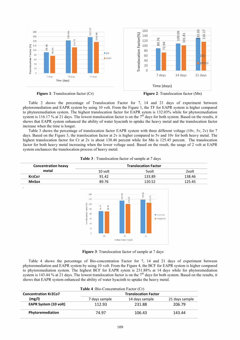
109

Figure 1: Translocation factor (Cr) Figure 2: Translocation factor (Mn) Table 2 shows the percentage of Translocation Factor for 7, 14 and 21 days of experiment between

phytoremediation and EAPR system by using 10 volt. From the Figure 1, the TF for EAPR system is higher compared to phytoremediation system. The highest translocation factor for EAPR sytem is 132.03% while for phytoremediation system is 116.17 % at 21 days. The lowest translocation factor is on the 7th days for both system. Based on the results, it shows that EAPR system enhanced the ability of water hyacinth to uptake the heavy metal and the translocation factor increase when the time is longer.

Table 3 shows the percentage of translocation factor EAPR system with three different voltage (10v, 5v, 2v) for 7 days. Based on the Figure 3, the translocation factor at 2v is higher compared to 5v and 10v for both heavy metal. The highest translocation factor for Cr at 2v is about 138.46 percent while for Mn is 125.45 percent. The translocation factor for both heavy metal increasing when the lower voltage used. Based on the result, the usage of 2 volt at EAPR system enchances the translocation process of heavy metal.

Table 3 : Translocation factor of sample at 7 days

.

Figure 3: Translocation factor of sample at 7 days

Table 4 shows the percentage of Bio-concentration Factor for 7, 14 and 21 days of experiment between phytoremediation and EAPR system by using 10 volt. From the Figure 4, the BCF for EAPR system is higher compared to phytoremediation system. The highest BCF for EAPR sytem is 231.88% at 14 days while for phytoremediation system is 143.44 % at 21 days. The lowest translocation factor is on the 7th days for both system. Based on the results, it shows that EAPR system enhanced the ability of water hyacinth to uptake the heavy metal.

Table 4 :Bio-Concentration Factor (Cr)

Concentration Kr2Co7 (mg/l)

Translocation Factor 7 days sample 14 days sample 21 days sample

EAPR System (10 volt) 112.93 231.88 206.79

Phytoremediation 74.97 106.43 143.44

89.7

6 109.

09

132.

03

72.9

4 101.

81

116.

17

020406080

100120140160

7 days 14 days 21 days

Tran

sloc

atio

n Fa

ctor

(%)

Time (days)

10v

phyto

Concentration heavy metal

Translocation Factor 10 volt 5volt 2volt

Kr2Co7 91.42 133.89 138.46 MnSo4 89.76 120.52 125.45

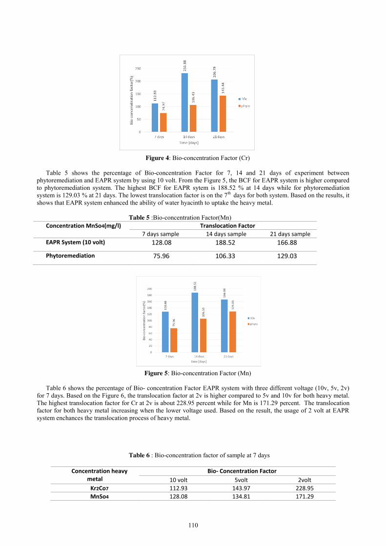
110

Figure 4: Bio-concentration Factor (Cr)

Table 5 shows the percentage of Bio-concentration Factor for 7, 14 and 21 days of experiment between phytoremediation and EAPR system by using 10 volt. From the Figure 5, the BCF for EAPR system is higher compared to phytoremediation system. The highest BCF for EAPR sytem is 188.52 % at 14 days while for phytoremediation system is 129.03 % at 21 days. The lowest translocation factor is on the 7th days for both system. Based on the results, it shows that EAPR system enhanced the ability of water hyacinth to uptake the heavy metal.

Table 5 :Bio-concentration Factor(Mn)

Concentration MnSo4(mg/l) Translocation Factor 7 days sample 14 days sample 21 days sample

EAPR System (10 volt) 128.08 188.52 166.88

Phytoremediation 75.96 106.33 129.03

Figure 5: Bio-concentration Factor (Mn)

Table 6 shows the percentage of Bio- concentration Factor EAPR system with three different voltage (10v, 5v, 2v)

for 7 days. Based on the Figure 6, the translocation factor at 2v is higher compared to 5v and 10v for both heavy metal. The highest translocation factor for Cr at 2v is about 228.95 percent while for Mn is 171.29 percent. The translocation factor for both heavy metal increasing when the lower voltage used. Based on the result, the usage of 2 volt at EAPR system enchances the translocation process of heavy metal.

Table 6 : Bio-concentration factor of sample at 7 days

Concentration heavy metal

Bio- Concentration Factor 10 volt 5volt 2volt

Kr2Co7 112.93 143.97 228.95 MnSo4 128.08 134.81 171.29

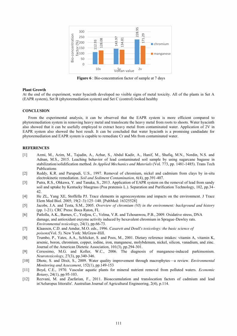
111

Figure 6 : Bio-concentration factor of sample at 7 days

Plant Growth At the end of the experiment, water hyacinth developed no visible signs of metal toxicity. All of the plants in Set A (EAPR system), Set B (phytoremediation system) and Set C (control) looked healthy

CONCLUSION

From the experimental analysis, it can be observed that the EAPR system is more efficient compared to phytoremediation system in removing heavy metal and translocate the heavy metal from roots to shoots. Water hyacinth also showed that it can be usefully employed to extract heavy metal from contaminated water. Application of 2V in EAPR system also showed the best result. It can be concluded that water hyacinth is a promising candiadate for phytoremediation and EAPR system is capable to remediate Cr and Mn from contaminated water.

REFERENCES [1] Azmi, M., Azim, M., Tajudin, A., Azhar, S., Abdul Kadir, A., Hanif, M., Shafiq, M.N., Nordin, N.S. and

Adnan, M.S., 2015. Leaching behavior of lead contaminated soil sample by using sugarcane bagasse in stabilization/solidification method. In Applied Mechanics and Materials (Vol. 773, pp. 1481-1485). Trans Tech Publications

[2] Reddy, K.R. and Parupudi, U.S., 1997. Removal of chromium, nickel and cadmium from clays by in‐situ electrokinetic remediation. Soil and Sediment Contamination, 6(4), pp.391-407.

[3] Putra, R.S., Ohkawa, Y. and Tanaka, S., 2013. Application of EAPR system on the removal of lead from sandy soil and uptake by Kentucky bluegrass (Poa pratensis L.). Separation and Purification Technology, 102, pp.34-42.

[4] He ZL, Yang XE, Stoffella PJ. Trace elements in agroecosystems and impacts on the environment. J Trace Elem Med Biol. 2005; 19(2–3):125–140. [PubMed: 16325528]

[5] Jacobs, J.A. and Testa, S.M., 2005. Overview of chromium (VI) in the environment: background and history (pp. 1-21). CRC Press: Boca Raton, FL

[6] Patlolla, A.K., Barnes, C., Yedjou, C., Velma, V.R. and Tchounwou, P.B., 2009. Oxidative stress, DNA damage, and antioxidant enzyme activity induced by hexavalent chromium in Sprague‐Dawley rats. Environmental toxicology, 24(1), pp.66-73. [7] Klaassen, C.D. and Amdur, M.O. eds., 1996. Casarett and Doull's toxicology: the basic science of

poisons(Vol. 5). New York: McGraw-Hill. [8] Trumbo, P., Yates, A.A., Schlicker, S. and Poos, M., 2001. Dietary reference intakes: vitamin A, vitamin K,

arsenic, boron, chromium, copper, iodine, iron, manganese, molybdenum, nickel, silicon, vanadium, and zinc. Journal of the American Dietetic Association, 101(3), pp.294-301.

[9] Cersosimo, M.G. and Koller, W.C., 2006. The diagnosis of manganese-induced parkinsonism. Neurotoxicology, 27(3), pp.340-346.

[10] Dhote, S. and Dixit, S., 2009. Water quality improvement through macrophytes—a review. Environmental Monitoring and Assessment, 152(1), pp.149-153

[11] Boyd, C.E., 1970. Vascular aquatic plants for mineral nutrient removal from polluted waters. Economic Botany, 24(1), pp.95-103.

[12] Rezvani, M. and Zaefarian, F., 2011. Bioaccumulation and translocation factors of cadmium and lead in'Aeluropus littoralis'. Australian Journal of Agricultural Engineering, 2(4), p.114.

112.

93

143.

97 22

8.95

128.

08

134.

81

171.

29

050

100150200250300

10v 5v 2vBi

o-co

ncen

trat

ion

fact

or (%

) Voltan value

chromium

manganese

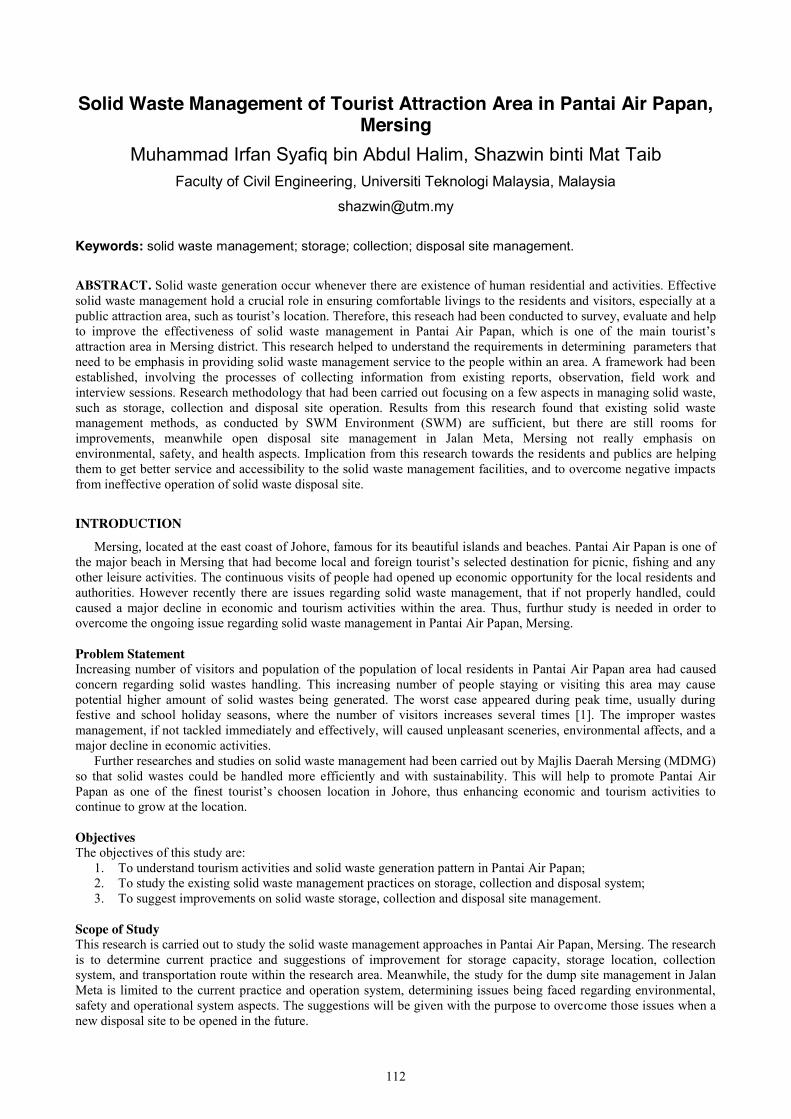
112

Solid Waste Management of Tourist Attraction Area in Pantai Air Papan, Mersing

Muhammad Irfan Syafiq bin Abdul Halim, Shazwin binti Mat Taib Faculty of Civil Engineering, Universiti Teknologi Malaysia, Malaysia

shazwin@utm.my

Keywords: solid waste management; storage; collection; disposal site management.

ABSTRACT. Solid waste generation occur whenever there are existence of human residential and activities. Effective solid waste management hold a crucial role in ensuring comfortable livings to the residents and visitors, especially at a public attraction area, such as tourist’s location. Therefore, this reseach had been conducted to survey, evaluate and help to improve the effectiveness of solid waste management in Pantai Air Papan, which is one of the main tourist’s attraction area in Mersing district. This research helped to understand the requirements in determining parameters that need to be emphasis in providing solid waste management service to the people within an area. A framework had been established, involving the processes of collecting information from existing reports, observation, field work and interview sessions. Research methodology that had been carried out focusing on a few aspects in managing solid waste, such as storage, collection and disposal site operation. Results from this research found that existing solid waste management methods, as conducted by SWM Environment (SWM) are sufficient, but there are still rooms for improvements, meanwhile open disposal site management in Jalan Meta, Mersing not really emphasis on environmental, safety, and health aspects. Implication from this research towards the residents and publics are helping them to get better service and accessibility to the solid waste management facilities, and to overcome negative impacts from ineffective operation of solid waste disposal site.

INTRODUCTION

Mersing, located at the east coast of Johore, famous for its beautiful islands and beaches. Pantai Air Papan is one of the major beach in Mersing that had become local and foreign tourist’s selected destination for picnic, fishing and any other leisure activities. The continuous visits of people had opened up economic opportunity for the local residents and authorities. However recently there are issues regarding solid waste management, that if not properly handled, could caused a major decline in economic and tourism activities within the area. Thus, furthur study is needed in order to overcome the ongoing issue regarding solid waste management in Pantai Air Papan, Mersing.

Problem Statement Increasing number of visitors and population of the population of local residents in Pantai Air Papan area had caused concern regarding solid wastes handling. This increasing number of people staying or visiting this area may cause potential higher amount of solid wastes being generated. The worst case appeared during peak time, usually during festive and school holiday seasons, where the number of visitors increases several times [1]. The improper wastes management, if not tackled immediately and effectively, will caused unpleasant sceneries, environmental affects, and a major decline in economic activities.

Further researches and studies on solid waste management had been carried out by Majlis Daerah Mersing (MDMG) so that solid wastes could be handled more efficiently and with sustainability. This will help to promote Pantai Air Papan as one of the finest tourist’s choosen location in Johore, thus enhancing economic and tourism activities to continue to grow at the location.

Objectives The objectives of this study are:

1. To understand tourism activities and solid waste generation pattern in Pantai Air Papan; 2. To study the existing solid waste management practices on storage, collection and disposal system; 3. To suggest improvements on solid waste storage, collection and disposal site management.

Scope of Study This research is carried out to study the solid waste management approaches in Pantai Air Papan, Mersing. The research is to determine current practice and suggestions of improvement for storage capacity, storage location, collection system, and transportation route within the research area. Meanwhile, the study for the dump site management in Jalan Meta is limited to the current practice and operation system, determining issues being faced regarding environmental, safety and operational system aspects. The suggestions will be given with the purpose to overcome those issues when a new disposal site to be opened in the future.

113

LITERATURE REVIEW

In Malaysia, the Solid Waste and Public Cleansing Management Act 2007 defined solid waste as any scrap material or other unwanted surplus substance or rejected products that arise as a result of human activity, but excluding scheduled wastes, sewage and radioactive wastes [2]. Meanwhile, The Environmental Act (1995) in the United Kingdom defined waste as any substance or object, which the holder discards or intends to discard. There are several type and classification of solid waste that includes residential waste, commercial waste, industrial waste, public solid waste, construction waste, imported waste and institutional waste, as classified by Solid Waste And Public Cleansing Corporation Management (SWCorp).

In order to plan a suitable management and disposal system of solid waste, it is important to study and understand the characteristics and composition of solid waste components. Within most Asian countries, municipal solid waste generated is highly biodegradable with high moisture contents. Some of the common examples are food waste, paper, plastic/foam, agriculture waste, rubber/leather, wood, glass, metal and textiles [3]. Meanwhile in Malaysia, the average composition of municipal solid waste, according to the largest categories consist of food waste at 45%, followed by plastic (24%), paper and iron at 7% and 6% respectively, and finally 3% for glass and others [4].

Tamudi et al. [5] stated that rapid increase in population, together with economic growth, urbanization and rise in community living standards lead to the increase in the rate of solid waste generation within an area. As a developing country, Malaysia is facing issues on municipal solid waste disposal due to increasing of solid waste generation rate. As the years passed, it becoming more challenging to carry out disposal process of these solid waste. Environment impact started to exists due to inadequate waste management, not environmental friendly disposal practice, tropical climate of our region and many other reasons [3].

Information on waste generation rate in Malaysia was limited as there were no specific or systematic analysis to record them until 1987. Only in May 1987, the first national compilation of waste generation and composition was carried out by the federal government, under the Ministry of Housing and Local Government (MHLG) [6]. Since then, more and more studies and surveys being carried out, at nationwide and state level. In 1978, a written report was produced on solid waste management, where a survey was conducted by a local non-government organization (NGO), Environmental Protection Society of Malaysia (EPSM). The survey was conducted in five municipalities within the Klang Valley [7]. The findings of the survey showed that three major problems in solid waste management were improper disposal manner, insufficient coverage of the collection systems, and inefficient collection methods.

On average, the municipal solid waste generation in Malaysia rised 2% annually and projected to reach 2.5%-3% due to increase of population and economic development during the Ninth Malaysia Plan (2006-2010) [4]. Ninth Malaysia Plan (2006-2010) stated that total municipal solid waste production in Malaysia increased significantly from 5.91 million tonnes in 2001 to 6.97 million tonnes in 2005, in the period of less than 5 years. Within the same period, average per capita waste generation also increased drastically from 0.67 kg/capita/day to 0.8 kg/capita/day. This figure was expected to continue to grow and reach double digits by the year 2020, in line with the population growth. This analysis and indicator made it clear that the quantity of solid waste generation is increasing and will continue to rise ith time, pointing a serious need for a far more efficient management system and disposal alternatives in the future.

Mersing, located at the east coast of Johore state, famous for their tourism activities, especially involving their beautiful nature of islands and beaches [8]. Some of their famous tourist attraction lacation includes Tioman Island, Rawa Island, Pantai Air Papan and Pantai Tanjung Leman. Tourism activities had generated potential economic growth for local residents and authorities for years. Tourisms had become one of the main revenue for the Mersing District Counsil (MDMG) and millions of Ringgit being invested to maintain and further develop the tourism in Mersing. Many tourism-related business activities being established by the local people such as food stalls, souvenir shops and accomodations such as hotel, chalet and homestay. There are not less than 27 resorts had been established in Mersing Islands while further 19 hotels and 37 resorts or chalet had been registered under MDMG within the Mersing district itself. Statistics conduted by MDMG also shown that from 2010-2016, there were a number of more than 1 million tourists had visited Mersing, averaging of almost 200 000 people annually.

Since years, Pantai Air Papan was one of the main tourist’s attraction area, well-known among local visitors for picnic purpose. Although this location only provide basic tourism facilities such as chalet, homestay, food stalls and souvenir shops, and not as advance as in Port Dickson, it is not stopping visitors from choosing Pantai Air Papan as their holiday destination due to its beautiful scenery and undisturbed nature [9]. Pantai Air Papan is a 3 km long beach, set in between the hills, about 12 km to the north away from the Mersing Town. Located at coordinate of 2.436428”N 103.831237”E, this beautiful beach located inside a village, named Kampung Air Papan. Information obtained from Mersing District Council (MDMG) shown that Kampung Air Papan have 41 unit of residential houses, with a population of about 460 people. Tourism’s facilities developed in Pantai Air Papan includes 7 resorts or chalet, 8 units of food stalls and anoher 3 souvenir stalls. There are several reasons of choosing Pantai Air Papan as the research area, due to the reasonable coverage area for the research period of six months, the status of Pantai Air Papan itself as one of the main attraction areain Mersing and the ongoing issue of solid waste management between the villagers and MDMG.

114

METHODOLOGY

The main objective of the research is to study solid waste management approaches in Pantai Air Papan. In addition, management and operation of solid waste, which includes the storage, collection and disposal site is analyse and suggested to be improved as well. This research methodology consisted of 4 key activities: on-site observation, field work, interview sessions, and data analysis. On-site Observation Physical visit to the location area had been conducted three (3) times throughout the research. The visits were on 12 Nov 2016, 6 May 2017 and 20 May 2017. The date was choosen as they were during weekend and school holiday season, where the number of visitors are expected to be high. The visit used to observe the number and location of solid waste storage facilities. The location of bins being marked with Global Positioning System (GPS) device. Other than that, the type of vehicle, methods and route used for collection purpose also being observed. Visit also being conducted at open dumping area at Jalan Meta, to observe the operation of the landfill. Interview Sessions Few interview sessions had been carried out to get clearer view on solid waste management in Pantai Air Papan. Each interview had different objective the people to be interviewed had been identified as the person or party that involved directly with solid waste operation in the research area. Some of the interviews were to determine: Effectiveness of existing solid waste management. Interview had been carried out with two different people, to obtain two different perspective on the issue. The respondent were supervisor of SWM and villager that live permanently at the area. The purpose of the interview was to determine on local people view, whether the existing facilities and management system being sufficient. There are also questions that looking for their opinion and recommendation on improving the solid waste management issue at Pantai Air Papan. Waste handling by chalet and stalls operators. The objective of this interview sessions were to study the approaches used by chalet and food stalls operators regarding solid waste management. The interviews gathered information on how they handle the waste from their premises. The interview also asked them about problems they faced about solid waste so that their perspective could be considered when making analysis and giving improvement suggestions. Collection of solid waste by SWM. This interview session was to ask and study the operation system practiced by SWM. The supervisor of SWM shared the type of vehicle used, the route of the vehicle within Pantai Air Papan and to the disposal land. Besides, the respondant also shared the vehicle registration system before they dispose their waste to the landfill and the capacity of the vehicle. Operation of open dump site. An interview also being conducted with staff of SWM on how they operate the open dumpsite in Jalan Meta, Mersing. Many information had been gathered on how the waste being handled, separation process at the landfill, and the environmental issues that faced at the landfill within its operation. Recycle Bins Location Simulation Rate of waste generation. Several location had been choosen based on some parameters. Set of dustbins had been placed at five (5) different locations along Pantai Air Papan. Observation had been made from 10am until 4pm to determine which area generated more waste based on the usage of the provided bins. The weighing being done at the end of the observation for analysis purpose. The observation also help to determine type of waste composition that being produced by the people. Waste separation participation and recycling awareness. Each set dustbins consists of three (3) different bins that had been labelled with recycleable materials, which are plastic, paper and glass/cans. The purpose of this method was to determine whether there are participation among people that are staying or visiting Pantai Air Papan on waste separation habit. The results of this observation being used to determine whether there are needs to provide recycling facilities at the research area to promote the 3R’s (Reduce, Reuse, Recycle) campaign. Data Analysis From data that being obtained from previous methods, analysis was conducted with five major outcomes, which were:

i) Determining areas that has the potential to generate different quantity of waste, and to relocate the storage facilities to fulfill the rate of generation needs and easy accessibility;

ii) Providing number of storage facilities that is sufficient to cater the generation needs without being over-supply;

iii) Determining locations that were suitable to be supplied with waste separation facilities; iv) Making slight adjustment to the transportation route so that the whole area of study being covered by

waste management operation, and;

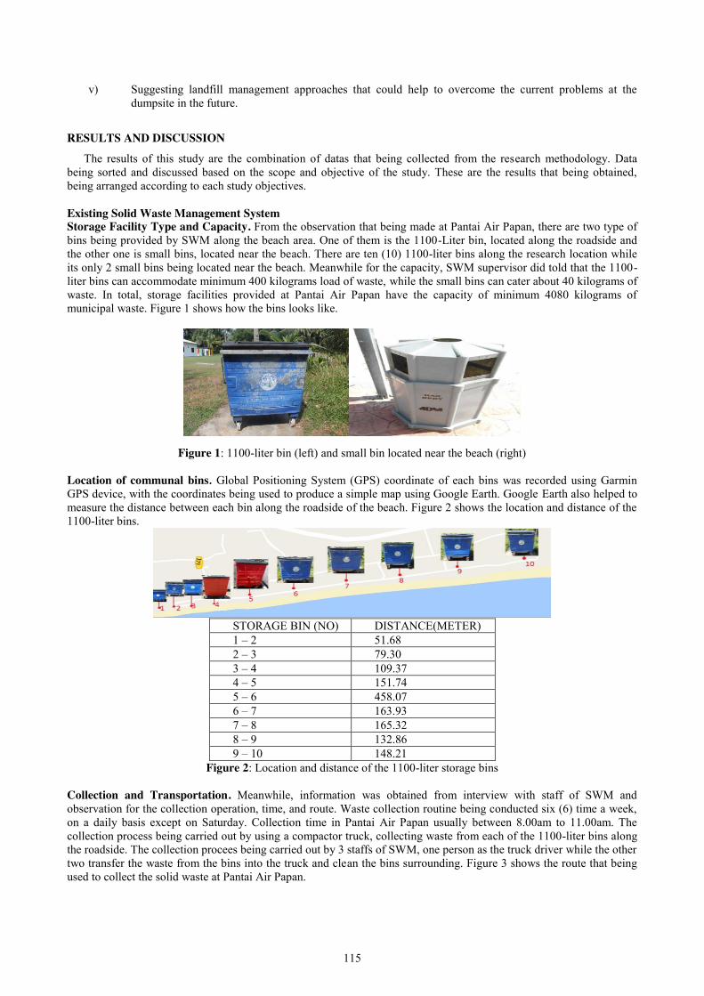
115

v) Suggesting landfill management approaches that could help to overcome the current problems at the dumpsite in the future.

RESULTS AND DISCUSSION

The results of this study are the combination of datas that being collected from the research methodology. Data being sorted and discussed based on the scope and objective of the study. These are the results that being obtained, being arranged according to each study objectives.

Existing Solid Waste Management System Storage Facility Type and Capacity. From the observation that being made at Pantai Air Papan, there are two type of bins being provided by SWM along the beach area. One of them is the 1100-Liter bin, located along the roadside and the other one is small bins, located near the beach. There are ten (10) 1100-liter bins along the research location while its only 2 small bins being located near the beach. Meanwhile for the capacity, SWM supervisor did told that the 1100-liter bins can accommodate minimum 400 kilograms load of waste, while the small bins can cater about 40 kilograms of waste. In total, storage facilities provided at Pantai Air Papan have the capacity of minimum 4080 kilograms of municipal waste. Figure 1 shows how the bins looks like.

Figure 1: 1100-liter bin (left) and small bin located near the beach (right)

Location of communal bins. Global Positioning System (GPS) coordinate of each bins was recorded using Garmin GPS device, with the coordinates being used to produce a simple map using Google Earth. Google Earth also helped to measure the distance between each bin along the roadside of the beach. Figure 2 shows the location and distance of the 1100-liter bins.

STORAGE BIN (NO) DISTANCE(METER) 1 – 2 51.68 2 – 3 79.30 3 – 4 109.37 4 – 5 151.74 5 – 6 458.07 6 – 7 163.93 7 – 8 165.32 8 – 9 132.86 9 – 10 148.21

Figure 2: Location and distance of the 1100-liter storage bins

Collection and Transportation. Meanwhile, information was obtained from interview with staff of SWM and observation for the collection operation, time, and route. Waste collection routine being conducted six (6) time a week, on a daily basis except on Saturday. Collection time in Pantai Air Papan usually between 8.00am to 11.00am. The collection process being carried out by using a compactor truck, collecting waste from each of the 1100-liter bins along the roadside. The collection procees being carried out by 3 staffs of SWM, one person as the truck driver while the other two transfer the waste from the bins into the truck and clean the bins surrounding. Figure 3 shows the route that being used to collect the solid waste at Pantai Air Papan.

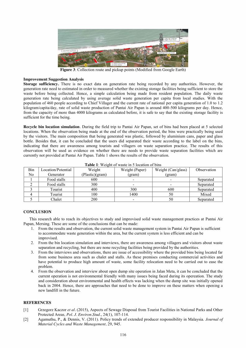
116

Figure 3: Collection route and pickup points (Modified from Google Earth)

Improvement Suggestion Analysis Storage sufficiency. There is no exact data on generation rate being recorded by any authorities. However, the generation rate need to estimated in order to measured whether the existing storage facilities being sufficient to store the waste before being collected. Hence, a simple calculation being made from resident population. The daily waste generation rate being calculated by using average solid waste generation per capita from local studies. With the population of 460 people according to Chief Villager and the current rate of national per capita generation of 1.0 to 1.2 kilogram/capita/day, rate of solid waste production of Pantai Air Papan is around 400-500 kilograms per day. Hence, from the capacity of more than 4000 kilograms as calculated before, it is safe to say that the existing storage facility is sufficient for the time being. Recycle bin location simulation. During the field trip to Pantai Air Papan, set of bins had been placed at 5 selected locations. When the observation being made at the end of the observation period, the bins were practically being used by the visitors. The main composition that being generated was plastic, followed by aluminium cans, paper and glass bottle. Besides that, it can be concluded that the users did separated their waste according to the label on the bins, indicating that there are awareness among tourists and villagers on waste separation practice. The results of this observation will be used as evidence on whether there are needs to provide waste separation facilities which are currently not provided at Pantai Air Papan. Table 1 shows the results of the observation.

Table 1: Weight of waste in 5 location of bins Bin No

Location/Potential Generator

Weight (Plastic)(gram)

Weight (Paper) (gram)

Weight (Can/glass) (gram)

Observation

1 Food stalls 600 - - Separated 2 Food stalls 300 - - Separated 3 Tourist 400 300 600 Separated 4 Tourist 100 1400 50 Mixed 5 Chalet 200 - 50 Separated

CONCLUSION

This research able to reach its objectives to study and improvised solid waste management practices at Pantai Air Papan, Mersing. These are some of the conclusions that can be made:

1. From the results and observation, the current solid waste management system in Pantai Air Papan is sufficient to accommodate waste generation within the area, but the current system is less efficient and can be improvised.

2. From the bin location simulation and interviews, there are awareness among villagers and visitors about waste separation and recycling, but there are none recycling facilities being provided by the authorities.

3. From the interviews and observations, there are issue of accessibility where the provided bins being located far from some business area such as chalet and stalls. As these premises conducting commercial activities and have potential to produce high amount of waste, some facility relocation need to be carried out to ease the problem.

4. From the observation and interview about open dump site operation in Jalan Meta, it can be concluded that the current operation is not environmental friendly with many issues being faced during its opereation. The study and consideration about environmental and health effects was lacking when the dump site was initially opened back in 2004. Hence, there are approaches that need to be done to improve on these matters when opening a new landfill in the future.

REFERENCES

[1] Grzegorz Kaczor et al. (2015), Aspects of Sewage Disposal from Tourist Facilities in National Parks and Other Protected Areas, Pol. J. Environ.Stud., 24(1), 107-114.

[2] Agamuthu, P., & Dennis, V. (2011). Policy trends of extended producer responsibility in Malaysia. Journal of Material Cycles and Waste Management, 29, 945.

117

[3] Visvanathan, C., O. Tubtimthai, and P. Kuruparan. 2004. Influence of Landfill Top Cover Design on Methane Oxidation: Pilot Scale Lysimeter Experiments under Tropical Conditions, 3rd Asia Pasific Landfill Symposium. Kitakyushu, Japan. Oct. 27–29.

[4] Government of Malaysia. 2006. Ninth Malaysia Plan (2006–2010). Putrajaya, Malaysia: Economic Planning Unit.

[5] Tarmudi, Z., Abdullah, M.L. and Tap, A.B.U.O. (2009). An overview of Municipal Solid Wastes Generation in Malaysia. Jurnal Teknologi, 51, 1-15.

[6] Nasir, M. H., A. R. Rakmi, T. C. Chong, Z. Zulina, and A. Muhamad. 2000. Waste Recycling in Malaysia: Problems and Prospects. Waste Management and Research. 18: 320–328.

[7] Juzhar, J. 2002. Improving Municipal Solid Waste Landfills of Peninsular Malaysia: Organisation and Structural Adjustments. PhD Thesis. University of Wisconsin-Madison.

[8] Rajak, R. H. A. (2016, November 24). Mersing lebih cantik dari Maldives. Sinar Harian. Retrieved May 2, 2017, from www.sinarharian.com.my

[9] Samsudin, M. et al. (2010). Warisan Sejarah dan Pelancongan Mersing Serta Kepulauan. In Mohamed, C. A. R. Penyelidikan Pantai Timur Johor: Mersing warisan terpelihara (pp. 57-70). Bangi: Universiti Kebangsaan Malaysia.

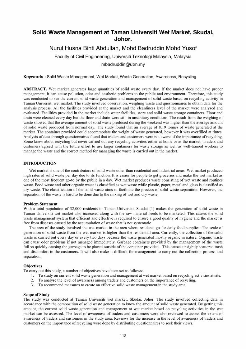
118

Solid Waste Management at Taman Universiti Wet Market, Skudai, Johor.

Nurul Husna Binti Abdullah, Mohd Badruddin Mohd Yusof Faculty of Civil Engineering, Universiti Teknologi Malaysia, Malaysia

mbadruddin@utm.my

Keywords : Solid Waste Management, Wet Market, Waste Generation, Awareness, Recycling

ABSTRACT. Wet market generates large quantities of solid waste every day. If the market does not have proper management, it can cause pollution, odor and aesthetic problems to the public and environment. Therefore, this study was conducted to see the current solid waste generation and management of solid waste based on recycling activity in Taman Universiti wet market. The study involved observation, weighing waste and questionnaires to obtain data for the analysis process. All the facilities provided at the market and the cleanliness level of the market were analysed and evaluated. Facilities provided in the market include water facilities, store and solid waste storage containers. Floor and drain were cleaned every day but the floor and drain were still in unsanitary conditions. The result from the weighing of waste showed that the average amount of solid waste produced during the weekend was higher than the average amount of solid waste produced from normal day. The study found that an average of 8.19 tonnes of waste generated at the market. The container provided could accommodate the weight of waste generated, however it was overfilled at times. Analysis of data through questionnaires found that traders and customers were not aware of the importance of recycling. Some knew about recycling but never carried out any recycling activities either at home or at the market. Traders and customers agreed with the future effort to use larger containers for waste storage as well as well-trained workers to manage the waste and the correct method for managing the waste is carried out in the market.

INTRODUCTION

Wet market is one of the contributors of solid waste other than residential and industrial areas. Wet market produced high rates of solid waste per day due to its function. It is easier for people to get groceries and make the wet market as one of the most frequent go-to by the public in a day. Wet market produces waste consisting of wet waste and routines waste. Food waste and other organic waste is classified as wet waste while plastic, paper, metal and glass is classified as dry waste. The classification of the solid waste aims to facilitate the process of solid waste separation. However, the separation of the waste is hard to be done due to the mixing of wet and dry waste. Problem Statement With a total population of 32,000 residents in Taman Universiti, Skudai [1] makes the generation of solid waste in Taman Universiti wet market also increased along with the raw material needs to be marketed. This causes the solid waste management system that efficient and effective is required to ensure a good quality of hygiene and the market is free from diseases caused by the accumulation of waste that is not systematic

The area of the study involved the wet market in the area where residents go for daily food supplies. The scale of generation of solid waste from the wet market is higher than the residential area. Currently, the collection of the solid waste is carried out every day or every two days because the waste generated mostly organic in nature. Organic waste can cause odor problems if not managed immediately. Garbage containers provided by the management of the waste full so quickly causing the garbage to be placed outside of the container provided. This causes unsightly scattered trash and discomfort to the customers. It will also make it difficult for management to carry out the collection process and separation. Objectives To carry out this study, a number of objectives have been set as follows:

1. To study on current solid waste generation and management at wet market based on recycling activities at site. 2. To analyse the level of awareness among traders and customers on the importance of recycling. 3. To recommend measures to create an effective solid waste management in the study area

Scope of Study The study was conducted at Taman Universiti wet market, Skudai, Johor. The study involved collecting data in accordance with the composition of solid waste generation to know the amount of solid waste generated. By getting this amount, the current solid waste generation and management at wet market based on recycling activities in the wet market can be assessed. The level of awareness of traders and customers were also reviewed to assess the extent of awareness of traders and customers in the study area. Reviews for the increase in the level of awareness of traders and customers on the importance of recycling were done by distributing questionnaires to seek their views.

119

LITERATURE REVIEW

Solid waste is commonly known as garbage or trash can be classified into several types of solid waste such as household solid waste, public solid waste, solid waste imports, special solid waste, solid waste institutions, commercial solid waste, solid waste and construction of industrial solid waste [2].

The commercial waste collection is the process of collecting solid wastes either bulky waste or solid waste that will be recycled from barrels per premises or from the source of solid waste is generated. The method of collection carried out in commercial areas such as wet markets is Communal Collection methods. Solid waste that had been collected from wet market will be sent to landfill. There are three methods of solid waste disposal can be used to dispose solid waste that keep rising from day to day especially in commercial and city area. The methods are landfill, incinerator and composting methods. For the solid waste management system to work out accordingly, the Solid Waste Management and Public Cleansing Act 2007 (Act 672) was enacted on August 30, 2007. Rules and act established to foster public awareness of sustainable waste management and public cleaning and also responsible for improving the recycling technology [3].

Malaysia's recycling rate is still far from the target of 22% by 2020 set by the government. The current rate is only 17.5% compared to other developed countries which have reached more than 40% [4]. Law and moral force of society is needed to reduce the amount of waste generated. Three initiatives are introduced to prevent the solid waste problem that is Reduce, Reuse and Recycle (3R). To foster a culture of 3R in society, it is important to train people to create awareness towards implementing the 3R initiative. Another one of the effective way to solve the solid waste problem is to change the attitude of society, especially the younger generations through education and awareness campaigns in schools across the country. Efforts to raise awareness should be implemented at all levels and the best method is to start at the nursery to the tertiary level.

Based on a previous study, the separated organic waste was recycled by composting the waste into organic fertilizer through large-scale composting method. The results of this study prove the probability to convert wet waste components from markets into organic fertilizer through composting methods will at least help to reduce about 60 percent the volume of solid waste [5].

Taman Universiti wet market has an area of approximately 2000 m2 located in the center of Taman Universiti. The wet market designed concept is open market. There are 76 traders who run their business at the market. The wet market operates every day except Mondays and the business activity starts at 7am and end at 2 pm. Opposites to the wet market building, there is a row of food and fruits stall which operates until late evening. Management of solid waste at Taman Universiti wet market is managed by the Majlis Perbandaran Johor Bahru Tengah (MPJBT). MPJBT provides business site and water source for the traders who conduct their business operation at the market. Storage facility also provided by MPJBT for the traders to store their raw materials that are not sold out. MPJBT also provides other facilities such as public toilets and garbage containers. Garbage container is managed by the Southern Waste Management Sdn Bhd (SWM). Cleanliness of the wet market is poor. The floor and the drain are cleaned every day after the operation and the waste is collected five times a week by SWM employee. However, the floor and the drain around the area are still in unsanitary conditions. It can be seen where the residual waste are trap in ‘sump’ and the floor are still cover with dirt. The wastewater from the market is channeled directly to the main drainage system at the area and subsequently flow to the treatment plant.

METHODOLOGY

The current solid waste generation and management at wet market were investigated by getting feedbacks from shop operators and their customers as well as the quantity of waste generation data. Waste was separated according to its composition Solid waste was weighed using a weighing scale with capacity of 40kg to obtain the quantity of waste generated and the weighing data were recorded. A site visit was conducted to find out the real situation in the wet market. The existing solid waste management system and the facilities provided in the wet market were observed and evaluated. A survey was also conducted through 110 respondents from the traders (50) and customers (60). The conducted survey was analyzed using the Statistical Package for Social Science (SPSS) to see the correlation between the data obtained. By using SPSS software, data from the survey of 110 sample questionnaires was calculated per frequency and the comparison between the findings of this study can be obtained. The Chi-Square Test technique was used and the result was obtained from the data.

RESULTS AND DISCUSSION

The result from weighing of waste and the data through questionnaire from 110 respondents in Taman Universiti wet market was obtained, analysed and discussed. Background of respondents The result from traders’ questionnaire analysis showed that there were more male (62%) than female (38%) respondents. The majority of traders were aged between 31 to 40 years and 41 to 50 years at 36% respectively. For the analysis of the type of business, those selling meat and fish formed 54% compared to others, selling vegetable (18%),

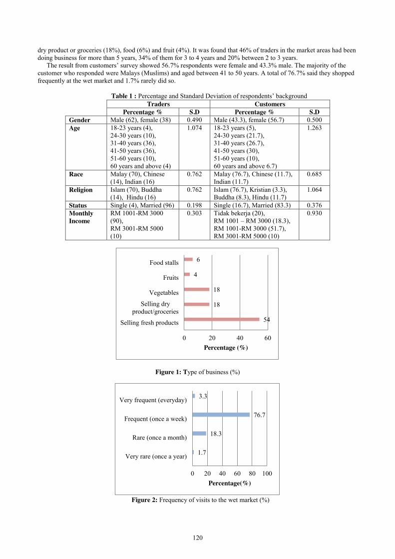
120

dry product or groceries (18%), food (6%) and fruit (4%). It was found that 46% of traders in the market areas had been doing business for more than 5 years, 34% of them for 3 to 4 years and 20% between 2 to 3 years.

The result from customers’ survey showed 56.7% respondents were female and 43.3% male. The majority of the customer who responded were Malays (Muslims) and aged between 41 to 50 years. A total of 76.7% said they shopped frequently at the wet market and 1.7% rarely did so.

Table 1 : Percentage and Standard Deviation of respondents’ background

Traders Customers Percentage % S.D Percentage % S.D

Gender Male (62), female (38) 0.490 Male (43.3), female (56.7) 0.500 Age 18-23 years (4),

24-30 years (10), 31-40 years (36), 41-50 years (36), 51-60 years (10), 60 years and above (4)

1.074 18-23 years (5), 24-30 years (21.7), 31-40 years (26.7), 41-50 years (30), 51-60 years (10), 60 years and above 6.7)

1.263

Race Malay (70), Chinese (14), Indian (16)

0.762 Malay (76.7), Chinese (11.7), Indian (11.7)

0.685

Religion Islam (70), Buddha (14), Hindu (16)

0.762 Islam (76.7), Kristian (3.3), Buddha (8.3), Hindu (11.7)

1.064

Status Single (4), Married (96) 0.198 Single (16.7), Married (83.3) 0.376 Monthly Income

RM 1001-RM 3000 (90), RM 3001-RM 5000 (10)

0.303 Tidak bekerja (20), RM 1001 – RM 3000 (18.3), RM 1001-RM 3000 (51.7), RM 3001-RM 5000 (10)

0.930

Figure 1: Type of business (%)

Figure 2: Frequency of visits to the wet market (%)

54

18

18

4

6

0 20 40 60

Selling fresh products

Selling dryproduct/groceries

Vegetables

Fruits

Food stalls

Percentage (%)

1.7

18.3

76.7

3.3

0 20 40 60 80 100

Very rare (once a year)

Rare (once a month)

Frequent (once a week)

Very frequent (everyday)

Percentage(%)

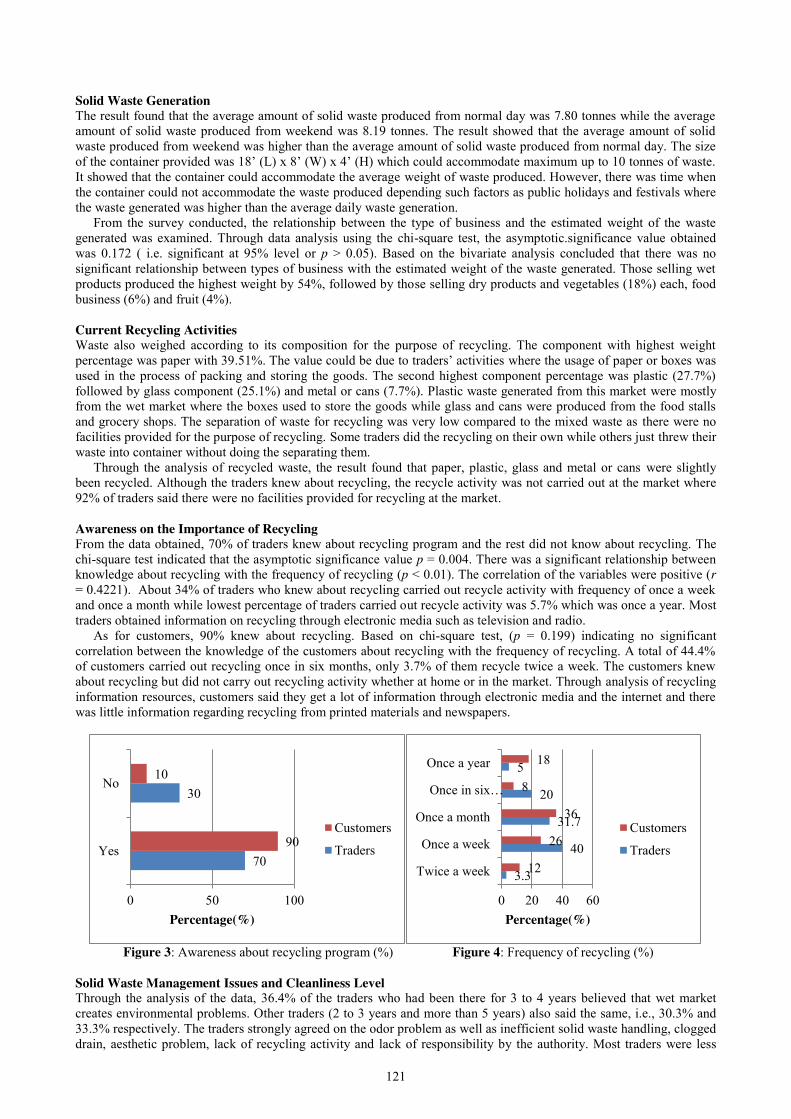
121

Solid Waste Generation The result found that the average amount of solid waste produced from normal day was 7.80 tonnes while the average amount of solid waste produced from weekend was 8.19 tonnes. The result showed that the average amount of solid waste produced from weekend was higher than the average amount of solid waste produced from normal day. The size of the container provided was 18’ (L) x 8’ (W) x 4’ (H) which could accommodate maximum up to 10 tonnes of waste. It showed that the container could accommodate the average weight of waste produced. However, there was time when the container could not accommodate the waste produced depending such factors as public holidays and festivals where the waste generated was higher than the average daily waste generation.

From the survey conducted, the relationship between the type of business and the estimated weight of the waste generated was examined. Through data analysis using the chi-square test, the asymptotic.significance value obtained was 0.172 ( i.e. significant at 95% level or p > 0.05). Based on the bivariate analysis concluded that there was no significant relationship between types of business with the estimated weight of the waste generated. Those selling wet products produced the highest weight by 54%, followed by those selling dry products and vegetables (18%) each, food business (6%) and fruit (4%). Current Recycling Activities Waste also weighed according to its composition for the purpose of recycling. The component with highest weight percentage was paper with 39.51%. The value could be due to traders’ activities where the usage of paper or boxes was used in the process of packing and storing the goods. The second highest component percentage was plastic (27.7%) followed by glass component (25.1%) and metal or cans (7.7%). Plastic waste generated from this market were mostly from the wet market where the boxes used to store the goods while glass and cans were produced from the food stalls and grocery shops. The separation of waste for recycling was very low compared to the mixed waste as there were no facilities provided for the purpose of recycling. Some traders did the recycling on their own while others just threw their waste into container without doing the separating them.

Through the analysis of recycled waste, the result found that paper, plastic, glass and metal or cans were slightly been recycled. Although the traders knew about recycling, the recycle activity was not carried out at the market where 92% of traders said there were no facilities provided for recycling at the market. Awareness on the Importance of Recycling From the data obtained, 70% of traders knew about recycling program and the rest did not know about recycling. The chi-square test indicated that the asymptotic significance value p = 0.004. There was a significant relationship between knowledge about recycling with the frequency of recycling (p < 0.01). The correlation of the variables were positive (r = 0.4221). About 34% of traders who knew about recycling carried out recycle activity with frequency of once a week and once a month while lowest percentage of traders carried out recycle activity was 5.7% which was once a year. Most traders obtained information on recycling through electronic media such as television and radio.

As for customers, 90% knew about recycling. Based on chi-square test, (p = 0.199) indicating no significant correlation between the knowledge of the customers about recycling with the frequency of recycling. A total of 44.4% of customers carried out recycling once in six months, only 3.7% of them recycle twice a week. The customers knew about recycling but did not carry out recycling activity whether at home or in the market. Through analysis of recycling information resources, customers said they get a lot of information through electronic media and the internet and there was little information regarding recycling from printed materials and newspapers.

Figure 3: Awareness about recycling program (%) Figure 4: Frequency of recycling (%)

Solid Waste Management Issues and Cleanliness Level Through the analysis of the data, 36.4% of the traders who had been there for 3 to 4 years believed that wet market creates environmental problems. Other traders (2 to 3 years and more than 5 years) also said the same, i.e., 30.3% and 33.3% respectively. The traders strongly agreed on the odor problem as well as inefficient solid waste handling, clogged drain, aesthetic problem, lack of recycling activity and lack of responsibility by the authority. Most traders were less

70

30

90

10

0 50 100

Yes

No

Percentage(%)

Customers

Traders

3.3

40

31.7

20

5

12

26

36

8

18

0 20 40 60

Twice a week

Once a week

Once a month

Once in six…

Once a year

Percentage(%)

Customers

Traders

122

concerned about the management of solid waste. For the health issues, traders stated that they did not agree that the management of solid waste and sanitary problem at the market was critical in its impact on human health.

From the data of customers’ survey analysis, it was found that 63.3% customers of the market agreed that the wet market contributed to environmental problems while 36.7% said otherwise. As for the waste management problem and hygiene, customers agreed that waste handling at the market was not efficient. The waste was scattered at some places causing aesthetic and odor problems as well as clogged drain. This showed that the level of cleanliness of the market at low and was unhygienic. Recycling was not carried out at the market, a contributor to problems or issues that arise in the market. Customers also disagreed about the health problems caused by inefficient solid waste management. Respondents Opinions and Suggested Measures From the analysis, majority of the respondents agreed that the solid waste management system carried out in the wet market was inefficient. The bins provided were insufficient to support waste generation in the market and there was a lack of cooperation amongst the traders and customers of the market in managing the wastes.

The respondents suggested that a larger container and sufficient number of bins be provided including recycling bins. This could help the traders and customers to throw the waste according to its composition and facilitate the management of the waste. Traders and customers also agreed that SWM provide trained workers to carry out waste management. Thus, the waste could be handled well and the cleaning processes run more effectively. In order to avoid odor problem, respondents agreed that if the traders could use plastic garbage bags, tie them properly and close the containers so the trash would not be scattered.

CONCLUSION The research achieved all the objectives set. For the first objective, the study found that the quantity of waste

generated from the market was high. The storage container could accommodate the quantity of waste generation on normal day but it failed to do so on certain days such as public holidays and during festivals. The maintenance work and the attitude of the public especially the residents nearby that threw their garbage into the market’s container were also caused the overflow of the container.

For the second objective, the research found that the traders did not carry out proper waste handling where all the waste generated was not being separate and only several traders who carried out recycling. Waste separated for recycling was very little. This could be due to an absence of facilities provided for the purpose of recycling. Several traders used their own initiative to carry out recycling. Customers also lacked the awareness about the importance of recycling, where they learned about recycling but did not carry out recycling activities either at home or at the market.

For the third objective, the study found a number of measures that could be carried out at wet market to create an effective waste management. The measures that could be undertaken include the provision of bigger or more numbers of containers and recycle bins nearby. Other than that, the management also needs to provide trained employee to manage waste so that the waste can be handle well and the cleaning process can be more effective. Traders are also advised to carry out correct method to manage waste by tying the plastic garbage bag properly and close the bins after using it.

REFERENCES [1] Jabatan Perangkaan Malaysia (2016 ). Siaran Akhbar, Anggaran Penduduk Semasa, Malaysia, 2014-2016. [2] Jabatan Pengurusan Sisa Pepejal Negara, JPSPN (2015). Laporan: Lab Pengurusan Sisa Pepejal 26 Mac - 13

April 2012. [3] Malaysia (2007). Solid Waste and Public Cleansing Management Act 2007. (Act 672). Solid Waste and Public

Cleansing Management Corporation Act 2007. (Act 673). Percetakan Nasional Malaysia Berhad (Appointed Printer to the Government of Malaysia).

[4] Pauze (2016). Integrated Solid Waste Management : Challenge and Future. Solid Waste and Public Cleansing Management Corporation (SWCorp).

[5] Agamuthu P., Fauziah S. H. (2007). Sustainable Management of Wet Market Waste. Proceedings of the International Conference on Sustainable Solid Waste Management, 5 - 7 September 2007, Chennai, India. pp.239-243.

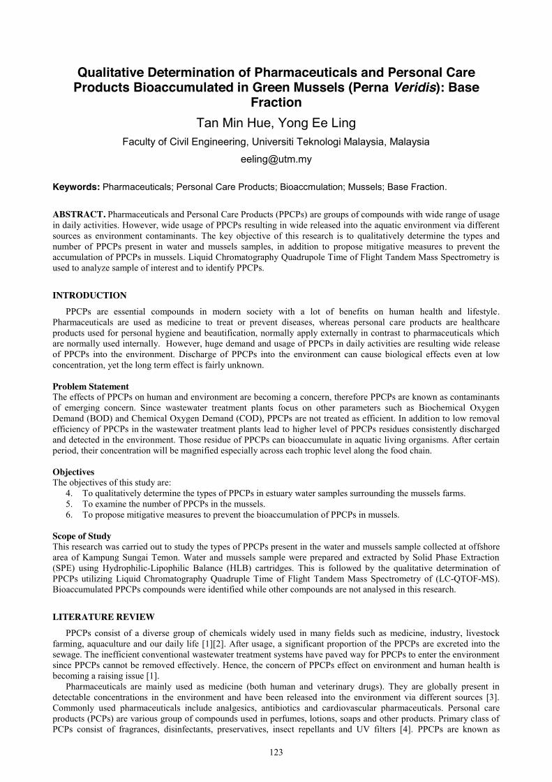
123

Qualitative Determination of Pharmaceuticals and Personal Care Products Bioaccumulated in Green Mussels (Perna Veridis): Base

Fraction Tan Min Hue, Yong Ee Ling

Faculty of Civil Engineering, Universiti Teknologi Malaysia, Malaysia

eeling@utm.my

Keywords: Pharmaceuticals; Personal Care Products; Bioaccmulation; Mussels; Base Fraction.

ABSTRACT. Pharmaceuticals and Personal Care Products (PPCPs) are groups of compounds with wide range of usage in daily activities. However, wide usage of PPCPs resulting in wide released into the aquatic environment via different sources as environment contaminants. The key objective of this research is to qualitatively determine the types and number of PPCPs present in water and mussels samples, in addition to propose mitigative measures to prevent the accumulation of PPCPs in mussels. Liquid Chromatography Quadrupole Time of Flight Tandem Mass Spectrometry is used to analyze sample of interest and to identify PPCPs.

INTRODUCTION

PPCPs are essential compounds in modern society with a lot of benefits on human health and lifestyle. Pharmaceuticals are used as medicine to treat or prevent diseases, whereas personal care products are healthcare products used for personal hygiene and beautification, normally apply externally in contrast to pharmaceuticals which are normally used internally. However, huge demand and usage of PPCPs in daily activities are resulting wide release of PPCPs into the environment. Discharge of PPCPs into the environment can cause biological effects even at low concentration, yet the long term effect is fairly unknown.

Problem Statement The effects of PPCPs on human and environment are becoming a concern, therefore PPCPs are known as contaminants of emerging concern. Since wastewater treatment plants focus on other parameters such as Biochemical Oxygen Demand (BOD) and Chemical Oxygen Demand (COD), PPCPs are not treated as efficient. In addition to low removal efficiency of PPCPs in the wastewater treatment plants lead to higher level of PPCPs residues consistently discharged and detected in the environment. Those residue of PPCPs can bioaccumulate in aquatic living organisms. After certain period, their concentration will be magnified especially across each trophic level along the food chain.

Objectives The objectives of this study are:

4. To qualitatively determine the types of PPCPs in estuary water samples surrounding the mussels farms. 5. To examine the number of PPCPs in the mussels. 6. To propose mitigative measures to prevent the bioaccumulation of PPCPs in mussels.

Scope of Study This research was carried out to study the types of PPCPs present in the water and mussels sample collected at offshore area of Kampung Sungai Temon. Water and mussels sample were prepared and extracted by Solid Phase Extraction (SPE) using Hydrophilic-Lipophilic Balance (HLB) cartridges. This is followed by the qualitative determination of PPCPs utilizing Liquid Chromatography Quadruple Time of Flight Tandem Mass Spectrometry of (LC-QTOF-MS). Bioaccumulated PPCPs compounds were identified while other compounds are not analysed in this research.

LITERATURE REVIEW

PPCPs consist of a diverse group of chemicals widely used in many fields such as medicine, industry, livestock farming, aquaculture and our daily life [1][2]. After usage, a significant proportion of the PPCPs are excreted into the sewage. The inefficient conventional wastewater treatment systems have paved way for PPCPs to enter the environment since PPCPs cannot be removed effectively. Hence, the concern of PPCPs effect on environment and human health is becoming a raising issue [1].

Pharmaceuticals are mainly used as medicine (both human and veterinary drugs). They are globally present in detectable concentrations in the environment and have been released into the environment via different sources [3]. Commonly used pharmaceuticals include analgesics, antibiotics and cardiovascular pharmaceuticals. Personal care products (PCPs) are various group of compounds used in perfumes, lotions, soaps and other products. Primary class of PCPs consist of fragrances, disinfectants, preservatives, insect repellants and UV filters [4]. PPCPs are known as

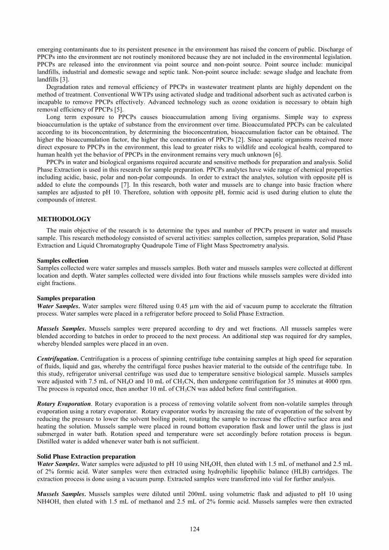
124

emerging contaminants due to its persistent presence in the environment has raised the concern of public. Discharge of PPCPs into the environment are not routinely monitored because they are not included in the environmental legislation. PPCPs are released into the environment via point source and non-point source. Point source include: municipal landfills, industrial and domestic sewage and septic tank. Non-point source include: sewage sludge and leachate from landfills [3].

Degradation rates and removal efficiency of PPCPs in wastewater treatment plants are highly dependent on the method of treatment. Conventional WWTPs using activated sludge and traditional adsorbent such as activated carbon is incapable to remove PPCPs effectively. Advanced technology such as ozone oxidation is necessary to obtain high removal efficiency of PPCPs [5].

Long term exposure to PPCPs causes bioaccumulation among living organisms. Simple way to express bioaccumulation is the uptake of substance from the environment over time. Bioaccumulated PPCPs can be calculated according to its bioconcentration, by determining the bioconcentration, bioaccumulation factor can be obtained. The higher the bioaccumulation factor, the higher the concentration of PPCPs [2]. Since aquatic organisms received more direct exposure to PPCPs in the environment, this lead to greater risks to wildlife and ecological health, compared to human health yet the behavior of PPCPs in the environment remains very much unknown [6].

PPCPs in water and biological organisms required accurate and sensitive methods for preparation and analysis. Solid Phase Extraction is used in this research for sample preparation. PPCPs analytes have wide range of chemical properties including acidic, basic, polar and non-polar compounds. In order to extract the analytes, solution with opposite pH is added to elute the compounds [7]. In this research, both water and mussels are to change into basic fraction where samples are adjusted to pH 10. Therefore, solution with opposite pH, formic acid is used during elution to elute the compounds of interest.

METHODOLOGY

The main objective of the research is to determine the types and number of PPCPs present in water and mussels sample. This research methodology consisted of several activities: samples collection, samples preparation, Solid Phase Extraction and Liquid Chromatography Quadrupole Time of Flight Mass Spectrometry analysis. Samples collection Samples collected were water samples and mussels samples. Both water and mussels samples were collected at different location and depth. Water samples collected were divided into four fractions while mussels samples were divided into eight fractions. Samples preparation Water Samples. Water samples were filtered using 0.45 Pm with the aid of vacuum pump to accelerate the filtration process. Water samples were placed in a refrigerator before proceed to Solid Phase Extraction. Mussels Samples. Mussels samples were prepared according to dry and wet fractions. All mussels samples were blended according to batches in order to proceed to the next process. An additional step was required for dry samples, whereby blended samples were placed in an oven. Centrifugation. Centrifugation is a process of spinning centrifuge tube containing samples at high speed for separation of fluids, liquid and gas, whereby the centrifugal force pushes heavier material to the outside of the centrifuge tube. In this study, refrigerator universal centrifuge was used due to temperature sensitive biological sample. Mussels samples were adjusted with 7.5 mL of NH4O and 10 mL of CH3CN, then undergone centrifugation for 35 minutes at 4000 rpm. The process is repeated once, then another 10 mL of CH3CN was added before final centrifugation. Rotary Evaporation. Rotary evaporation is a process of removing volatile solvent from non-volatile samples through evaporation using a rotary evaporator. Rotary evaporator works by increasing the rate of evaporation of the solvent by reducing the pressure to lower the solvent boiling point, rotating the sample to increase the effective surface area and heating the solution. Mussels sample were placed in round bottom evaporation flask and lower until the glass is just submerged in water bath. Rotation speed and temperature were set accordingly before rotation process is begun. Distilled water is added whenever water bath is not sufficient.

Solid Phase Extraction preparation Water Samples. Water samples were adjusted to pH 10 using NH4OH, then eluted with 1.5 mL of methanol and 2.5 mL of 2% formic acid. Water samples were then extracted using hydrophilic lipophilic balance (HLB) cartridges. The extraction process is done using a vacuum pump. Extracted samples were transferred into vial for further analysis. Mussels Samples. Mussels samples were diluted until 200mL using volumetric flask and adjusted to pH 10 using NH4OH, then eluted with 1.5 mL of methanol and 2.5 mL of 2% formic acid. Mussels samples were then extracted

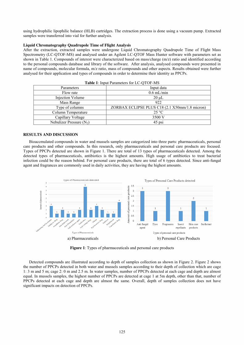
125

using hydrophilic lipophilic balance (HLB) cartridges. The extraction process is done using a vacuum pump. Extracted samples were transferred into vial for further analysis. Liquid Chromatography Quadrupole Time of Flight Analysis After the extraction, extracted samples were undergone Liquid Chromatography Quadrupole Time of Flight Mass Spectrometry (LC-QTOF-MS) and analysed under an Agilent LC-QTOF Mass Hunter software with parameters set as shown in Table 1. Compounds of interest were characterized based on mass/charge (m/z) ratio and identified according to the personal compounds database and library of the software. After analysis, analysed compounds were presented in name of compounds, molecular formula, m/z ratio, mass of compounds and other aspects. Results obtained were further analysed for their application and types of compounds in order to determine their identity as PPCPs.

Table 1: Input Parameters for LC-QTOF-MS Parameters Input data Flow rate 0.6 mL/min

Injection Volume 20 μL Mass Range 922

Type of columns ZORBAX ECLIPSE PLUS C18 (2.1 X50mm/1.8 micron) Column Temperature 25 °C

Capillary Voltage 3500 V Nebulizer Pressure (N2) 45 psi

RESULTS AND DISCUSSION

Bioaccmulated compounds in water and mussels samples are categorized into three parts: pharmaceuticals, personal care products and other compounds. In this research, only pharmaceuticals and personal care products are focused. Types of PPCPs detected are shown in Figure 1. There are total of 13 types of pharmaceuticals detected. Among the detected types of pharmaceuticals, antibiotics is the highest amounts. High usage of antibiotics to treat bacterial infection could be the reason behind. For personal care products, there are total of 6 types detected. Since anti-fungal agent and fragrances are commonly used in daily activities, they are having the highest amounts.

a) Pharmaceuticals b) Personal Care Products

Figure 1: Types of pharmaceuticals and personal care products

Detected compounds are illustrated according to depth of samples collection as shown in Figure 2. Figure 2 shows the number of PPCPs detected in both water and mussels samples according to their depth of collection which are cage 1: 3 m and 5 m; cage 2: 0 m and 2.5 m. In water samples, number of PPCPs detected at each cage and depth are almost equal. In mussels samples, the highest number of PPCPs are detected at cage 1 at 5m depth, other than that, number of PPCPs detected at each cage and depth are almost the same. Overall, depth of samples collection does not have significant impacts on detection of PPCPs.

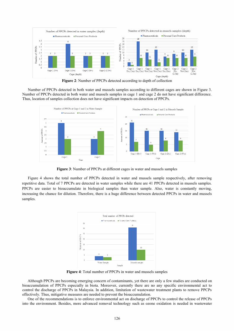
126

Figure 2: Number of PPCPs detected according to depth of collection

Number of PPCPs detected in both water and mussels samples according to different cages are shown in Figure 3.

Number of PPCPs detected in both water and mussels samples in cage 1 and cage 2 do not have significant difference. Thus, location of samples collection does not have significant impacts on detection of PPCPs.

Figure 3: Number of PPCPs at different cages in water and mussels samples

Figure 4 shows the total number of PPCPs detected in water and mussels sample respectively, after removing repetitive data. Total of 7 PPCPs are detected in water samples while there are 41 PPCPs detected in mussels samples. PPCPs are easier to bioaccumulate in biological samples than water sample. Also, water is constantly moving, increasing the chance for dilution. Therefore, there is a huge difference between detected PPCPs in water and mussels samples.

Figure 4: Total number of PPCPs in water and mussels samples

Although PPCPs are becoming emerging concern of contaminants, yet there are only a few studies are conducted on

bioaccumulation of PPCPs especially in biota. Moreover, currently there are no any specific environmental act to control the discharge of PPCPs in Malaysia. In addition, limitation of wastewater treatment plants to remove PPCPs effectively. Thus, mitigative measures are needed to prevent the bioaccumulation.

One of the recommendations is to enforce environmental act on discharge of PPCPs to control the release of PPCPs into the environment. Besides, more advanced removal technology such as ozone oxidation is needed in wastewater

127

treatment plants to remove PPCPs effectively. Other than that, biodegradable organic compounds based products should be introduced more to replaced PPCPs based products, in order to reduce the usage of PPCPs.

CONCLUSION

After conducting the laboratory experiment and analysis of compounds, there are PPCPs present in both water and mussels samples.

1. There are total of 13 types of pharmaceuticals and 6 types of personal care products detected. 2. Number of PPCPs detected in water samples are 7 while mussels samples detected total of 41 PPCPs.

There are a few mitigative measures can be taken to prevent bioaccumulation of PPCPs in aquatic living organisms. 1. Enforce specific environmental acts on PPCPs to control discharge of PPCPs into the environment. 2. Upgrade current removal technology to more advanced removal technology to remove PPCPs more

effectively. 3. Introduce biodegradable organic compounds based products to replace PPCPS based products.

REFERENCES

[1] Cortez, F. S., Pereira, C. D. S., Santos, A. R., Cesar, A., Choueri, R. B., De Assis Martini, G. & Bohrer-Morel, M. B. 2012. Biological Effects of Environmentally Relevant Concentrations of the Pharmaceutical Triclosan in the Marine Mussel Perna Perna (Linnaeus, 1758). Environmental Pollution, 168, 145-150.

[2] Zenker, A., Cicero, M. R., Prestinaci, F., Bottoni, P. & Carere, M. 2014. Bioaccumulation and Biomagnification Potential of Pharmaceuticals with a Focus to the Aquatic Environment. Journal of Environmental Management, 133, 378-387.

[3] Li, W. C. 2014. Occurrence, Sources, and Fate of Pharmaceuticals in Aquatic Environment and Soil. Environmental Pollution, 187, 193-201.

[4] Brausch, J. M. & Rand, G. M. 2011. A Review of Personal Care Products in the Aquatic Environment: Environmental Concentrations and Toxicity. Chemosphere, 82, 1518-1532.

[5] Wang, J. & Wang, S. 2016. Removal of Pharmaceuticals and Personal Care Products (PPCPs) from Wastewater: A Review. Journal of Environmental Management, 182, 620-640.

[6] Bayen, S., Zhang, H., Desai, M. M., Ooi, S. K. & Kelly, B. C. 2013. Occurrence and Distribution of Pharmaceutically Active and Endocrine Disrupting Compounds in Singapore's Marine Environment: Influence of Hydrodynamics and Physical–Chemical Properties. Environmental Pollution, 182, 1-8.

[7] Crawford_Scientific Sample Preparation Solid Phase Extraction.

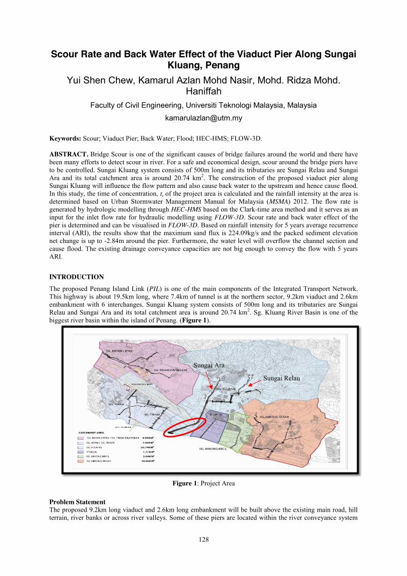
128

Scour Rate and Back Water Effect of the Viaduct Pier Along Sungai Kluang, Penang

Yui Shen Chew, Kamarul Azlan Mohd Nasir, Mohd. Ridza Mohd. Haniffah

Faculty of Civil Engineering, Universiti Teknologi Malaysia, Malaysia

kamarulazlan@utm.my

Keywords: Scour; Viaduct Pier; Back Water; Flood; HEC-HMS; FLOW-3D. ABSTRACT. Bridge Scour is one of the significant causes of bridge failures around the world and there have been many efforts to detect scour in river. For a safe and economical design, scour around the bridge piers have to be controlled. Sungai Kluang system consists of 500m long and its tributaries are Sungai Relau and Sungai Ara and its total catchment area is around 20.74 km2. The construction of the proposed viaduct pier along Sungai Kluang will influence the flow pattern and also cause back water to the upstream and hence cause flood. In this study, the time of concentration, tc of the project area is calculated and the rainfall intensity at the area is determined based on Urban Stormwater Management Manual for Malaysia (MSMA) 2012. The flow rate is generated by hydrologic modelling through HEC-HMS based on the Clark-time area method and it serves as an input for the inlet flow rate for hydraulic modelling using FLOW-3D. Scour rate and back water effect of the pier is determined and can be visualised in FLOW-3D. Based on rainfall intensity for 5 years average recurrence interval (ARI), the results show that the maximum sand flux is 224.09kg/s and the packed sediment elevation net change is up to -2.84m around the pier. Furthermore, the water level will overflow the channel section and cause flood. The existing drainage conveyance capacities are not big enough to convey the flow with 5 years ARI.

INTRODUCTION The proposed Penang Island Link (PIL) is one of the main components of the Integrated Transport Network. This highway is about 19.5km long, where 7.4km of tunnel is at the northern sector, 9.2km viaduct and 2.6km embankment with 6 interchanges. Sungai Kluang system consists of 500m long and its tributaries are Sungai Relau and Sungai Ara and its total catchment area is around 20.74 km2. Sg. Kluang River Basin is one of the biggest river basin within the island of Penang. (Figure 1).

Figure 1: Project Area

Problem Statement The proposed 9.2km long viaduct and 2.6km long embankment will be built above the existing main road, hill terrain, river banks or across river valleys. Some of these piers are located within the river conveyance system

Sungai Ara

Sungai Relau

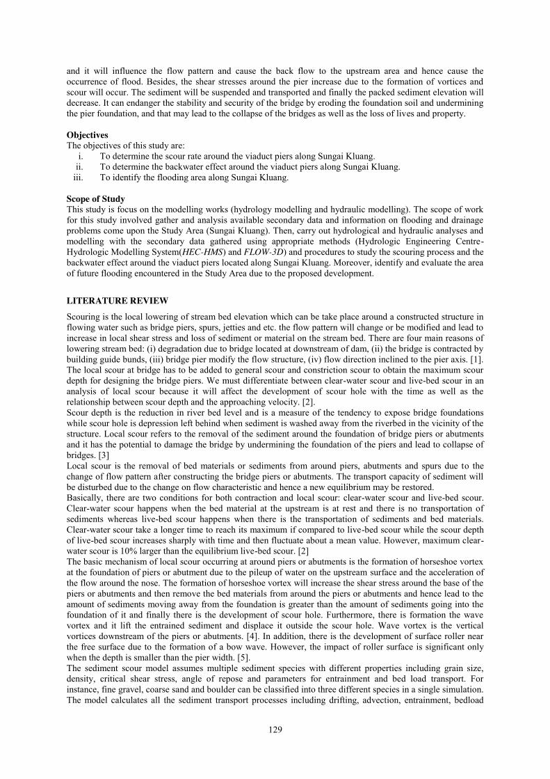
129

and it will influence the flow pattern and cause the back flow to the upstream area and hence cause the occurrence of flood. Besides, the shear stresses around the pier increase due to the formation of vortices and scour will occur. The sediment will be suspended and transported and finally the packed sediment elevation will decrease. It can endanger the stability and security of the bridge by eroding the foundation soil and undermining the pier foundation, and that may lead to the collapse of the bridges as well as the loss of lives and property. Objectives The objectives of this study are:

i. To determine the scour rate around the viaduct piers along Sungai Kluang. ii. To determine the backwater effect around the viaduct piers along Sungai Kluang.

iii. To identify the flooding area along Sungai Kluang. Scope of Study This study is focus on the modelling works (hydrology modelling and hydraulic modelling). The scope of work for this study involved gather and analysis available secondary data and information on flooding and drainage problems come upon the Study Area (Sungai Kluang). Then, carry out hydrological and hydraulic analyses and modelling with the secondary data gathered using appropriate methods (Hydrologic Engineering Centre-Hydrologic Modelling System(HEC-HMS) and FLOW-3D) and procedures to study the scouring process and the backwater effect around the viaduct piers located along Sungai Kluang. Moreover, identify and evaluate the area of future flooding encountered in the Study Area due to the proposed development.

LITERATURE REVIEW Scouring is the local lowering of stream bed elevation which can be take place around a constructed structure in flowing water such as bridge piers, spurs, jetties and etc. the flow pattern will change or be modified and lead to increase in local shear stress and loss of sediment or material on the stream bed. There are four main reasons of lowering stream bed: (i) degradation due to bridge located at downstream of dam, (ii) the bridge is contracted by building guide bunds, (iii) bridge pier modify the flow structure, (iv) flow direction inclined to the pier axis. [1]. The local scour at bridge has to be added to general scour and constriction scour to obtain the maximum scour depth for designing the bridge piers. We must differentiate between clear-water scour and live-bed scour in an analysis of local scour because it will affect the development of scour hole with the time as well as the relationship between scour depth and the approaching velocity. [2]. Scour depth is the reduction in river bed level and is a measure of the tendency to expose bridge foundations while scour hole is depression left behind when sediment is washed away from the riverbed in the vicinity of the structure. Local scour refers to the removal of the sediment around the foundation of bridge piers or abutments and it has the potential to damage the bridge by undermining the foundation of the piers and lead to collapse of bridges. [3] Local scour is the removal of bed materials or sediments from around piers, abutments and spurs due to the change of flow pattern after constructing the bridge piers or abutments. The transport capacity of sediment will be disturbed due to the change on flow characteristic and hence a new equilibrium may be restored. Basically, there are two conditions for both contraction and local scour: clear-water scour and live-bed scour. Clear-water scour happens when the bed material at the upstream is at rest and there is no transportation of sediments whereas live-bed scour happens when there is the transportation of sediments and bed materials. Clear-water scour take a longer time to reach its maximum if compared to live-bed scour while the scour depth of live-bed scour increases sharply with time and then fluctuate about a mean value. However, maximum clear-water scour is 10% larger than the equilibrium live-bed scour. [2] The basic mechanism of local scour occurring at around piers or abutments is the formation of horseshoe vortex at the foundation of piers or abutment due to the pileup of water on the upstream surface and the acceleration of the flow around the nose. The formation of horseshoe vortex will increase the shear stress around the base of the piers or abutments and then remove the bed materials from around the piers or abutments and hence lead to the amount of sediments moving away from the foundation is greater than the amount of sediments going into the foundation of it and finally there is the development of scour hole. Furthermore, there is formation the wave vortex and it lift the entrained sediment and displace it outside the scour hole. Wave vortex is the vertical vortices downstream of the piers or abutments. [4]. In addition, there is the development of surface roller near the free surface due to the formation of a bow wave. However, the impact of roller surface is significant only when the depth is smaller than the pier width. [5]. The sediment scour model assumes multiple sediment species with different properties including grain size, density, critical shear stress, angle of repose and parameters for entrainment and bed load transport. For instance, fine gravel, coarse sand and boulder can be classified into three different species in a single simulation. The model calculates all the sediment transport processes including drifting, advection, entrainment, bedload

130

transport, suspended load transport, entrainment and packing for each species. Drifting is the process when the suspended grains settle onto the packed bed due to the combined effect of gravity, buoyancy and also friction. Advection take place when the grains is carried along by the fluid while entrainment is the process when turbulent vortexes remove the grains from the top of the packed bed and pick up into fluid by either drifting or advecting. Entrainment occur when the bed shear stress exceeds a threshold value (critical shear stress). After entrained, the grains are carried by the water current within a certain height above the packed bed, known as the suspended load transport. Bedload transport defines the process of rolling, hopping and bouncing of grains along the packed bed surface in response to the shear stress applied by fluid flow without advecting. The grains solidify when it cannot move or transport is known as the process of packing. [6]

METHODOLOGY

This study involves hydrologic and hydraulic modelling using HEC-HMS and FLOW-3D software respectively. HEC-HMS and FLOW 3D model is using in this study to analyse the hydrologic and hydraulic behaviour of present catchment characteristics and to simulate the impacts of future development of PIL to the flooding problem along Sungai Kluang. Hydrologic Modelling The purpose of hydrologic modelling is to estimate flow hydrograph from tributary catchment for various ARI’s by using HEC-HMS model. The estimated flow hydrograph serves as the input to the hydraulic modelling of the study area. The development area is located near the downstream of Sungai Kluang. The catchment area is divided into 3 sub-catchments Time of Concentration. The design storm selected for this study depends on the time of concentration of the study area (tc). The tc (to + td) was estimated by using the overland flow time and drain flow time formulae. Storm Intensity. The derived tc serves as the storm duration for the design storm. The design storm intensity for the area can be calculated by Intensity Duration Frequency (IDF) equation. Kolam Takungan Air Hitam is located within the same river basin as the project development site and hence the IDF derived for it had been chosen for the simulation of surface runoff in this study. The temporal pattern used for this study is based on the Penang temporal pattern. Clark Time-area Method. The transformation of effective rainfall to the outlet area will be based on Clark time-area method. Time of concentration, tc and storage coefficient, R are used for the development of the synthetic unit hydrograph. In the absence of the observed hydrograph, the parameters can be determined from regression equations derived areas with gauged data. The regression equation used in this study is derived from a study in small rural watersheds in Illinois, USA. [7]. HEC-HMS. A new project file is created. A basin model which represent entire catchment area is created. In this study, runoff was modelled using initial and constant method, stream flow hydrograph by Clark Unit Hydrograph technique, base flow with constant monthly method and channel routing by Muskingum method. All the parameters were key in to each sub-basin according to the calculated values. The hydrologic losses for this study will be based on initial and continuing loss method. The initial loss is assumed to be 10 mm and the continuing loss is assumed to be 15 mm/hr. It is also assumed that the pre-development land cover consists of 10% impervious area, and the post-development consists of 80% impervious area. The transformation of effective rainfall to the outlet area will be based on Clark time-area method. The base flow for the area is assumed to be constant at 0.1 m3/sec. Hydraulic Modelling FLOW-3D. The purpose of hydrologic modelling is to determine the scour rate and back water effect around the piers. The sediment scour model is designed to be used with single fluid flow. If the two-fluid flow model is used, the model will still work, but the sediment will not advect or interact with the second fluid. The sediment scour model is sensitive to turbulence modelling, because the turbulence model directly affects the viscosity as computed in FLOW-3D, and this viscosity is needed to compute the local shear stress that is used to calculate the rates of entrainment and bed-load erosion. Renormalized Group model (RNG) model of turbulence is recommended to be used in this study. Furthermore, Figure 2 shows the model setup and is explained in detail below; Set Up Geometry. The sterolitography (stl) file is generated from AutoCAD 2016 in three-dimensional view and imported to FLOW-3D. The topography of the river and viaduct pier stl files are imported into 2 different components where the topography act as the packed sediment while the pier is solid. There are 2 sediment components to the topography file; one consists of boulder that is large in diameter and the other one is the packed sediment which consists of 100% sand with 5mm in diameter. The pier is circle in shape with 3m diameter. The units of the simulation are specified as System International (SI).

131

Meshing.The mesh defines the domain where the region in which fluid calculations will take place. The aim of meshing is to resolve the flow features and geometry adequately to obtain good results. In fact, finer meshes will generate more precise results but it takes a longer simulation time and also more memory. There is a limit to how fine the mesh should be where beyond the limit reducing the cell size does not improving the results. A convergence test is carried out to make sure the results are grid independent by conducting three sets of simulations with different mesh sizes. Three mesh block sizes were used in each simulation, with a finest mesh block near the piers and finer mesh block along the river and a large mesh block at the river reserve domain to reduce simulation time. Boundary. The inlet is specified as volumetric flow rate as generated from HEC-HMS while the downstream is specified as outflow where they do not transmit information back into the domain. The left and right boundaries along the river are specified as continuative; intended to represent a spatially steady flow condition where water can flow out and there is no acceleration. The top and bottom boundaries are specified as wall; no fluid flow across and no surface roughness. Initial Condition. An initial fluid to the simulation is needed to speed up the time to steady state because if there are no fluids, the simulation run will fill the empty domain first and takes a longer time to reach steady-state. Hydrostatic pressure is specified as the initial condition and the fluid elevation is set to 9m where it will fill the entire domain. Physics. The gravity physics is activated and set with Z component = -9.8m/s2. In this study, the sediment scour physics model has to be activated and the properties of the sediment has to be specified. There are 2 types of sediment which are sand and boulder. The bed sediment is assumed to be sand with 0.5mm diameter and 2100 kg/m3 in density. The angle of repose and critical shields is 31° and 0.033 respectively by referring approximate particle parameter guide in FLOW-3D manual. The bed load coefficient is set to 8 where there is the immediate transport of it while the entrainment coefficient is set to default of 0.0018. Besides, the river bank is assumed to be made of the boulders with 0.512m in diameter and 2400 kg/m3 in density. There is low transport of it and hence the bed load coefficient is set to 5.7.

Figure 2: Geometry, Meshing and Boundary Condition of FLOW-3D Model

RESULTS AND DISCUSSION

Hydrologic Modelling Time of concentration. The Horton’s roughness value for the surface, n is assumed to be 0.2 while the velocity of flow is assumed to be 1.0 m/s and the time of concentration ranges from 3 hours for pre-development condition. Rainfall Intensity. The adopted storm duration for this study is based on the longest time of concentration which is about 3 hours and with a value of 37.51 m3/hr. Temporal Pattern. The temporal pattern used for this study is based on the temporal pattern for Penang state and the rainfall depth. HEC-HMS. The flow rate of storm duration 5 years ARI is recorded for 10 hours with 15 minutes’ intervals. Figure 3 represent the hydrograph for 5 years ARI. Table 1 shows the comparison between the results from hydrologic modelling and the results of Japan International Cooperation Agency (JIPA) and Storm Water Management Model (SWMM).

ARI SWMM (m3/s)

JICA (m3/s)

Clark-Time Area Method

Volumetric flow rate continuative

outflow

wall

continuative

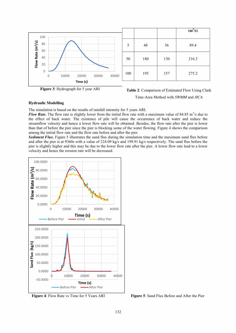
132

Figure 3: Hydrograph for 5 year ARI

Hydraulic Modelling

The simulation is based on the results of rainfall intensity for 5 years ARI. Flow Rate. The flow rate is slightly lower from the initial flow rate with a maximum value of 84.85 m3/s due to the effect of back water. The existence of pile will cause the occurrence of back water and reduce the streamflow velocity and hence a lower flow rate will be obtained. Besides, the flow rate after the pier is lower than that of before the pier since the pier is blocking some of the water flowing. Figure 4 shows the comparison among the initial flow rate and the flow rate before and after the pier. Sediment Flux. Figure 5 illustrates the sand flux during the simulation time and the maximum sand flux before and after the pier is at 9360s with a value of 224.09 kg/s and 199.91 kg/s respectively. The sand flux before the pier is slightly higher and this may be due to the lower flow rate after the pier. A lower flow rate lead to a lower velocity and hence the erosion rate will be decreased.

Figure 4: Flow Rate vs Time for 5 Years ARI Figure 5: Sand Flux Before and After the Pier

0

20

40

60

80

100

0 10000 20000 30000 40000

Flow

Rat

e (m

3 /s)

TIme (s)

0.0000

20.0000

40.0000

60.0000

80.0000

100.0000

0 10000 20000 30000 40000

Flow

Rat

e (m

3 /s)

Time (s) Before Pier Initial After Pier

-50.0000

0.0000

50.0000

100.0000

150.0000

200.0000

250.0000

0 10000 20000 30000 40000

Sand

Flu

x (k

g/s)

Time (s) Before Pier After Pier

(m3/s)

5 48 36 89.4

50 180 130 216.3

100 195 157 275.2

Table 2: Comparison of Estimated Flow Using Clark

Time-Area Method with SWMM and JICA

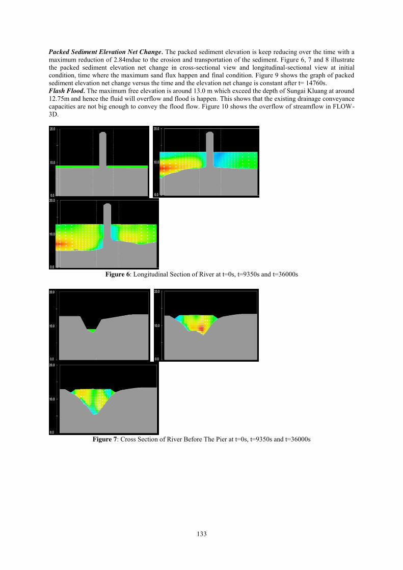
133

Packed Sediment Elevation Net Change. The packed sediment elevation is keep reducing over the time with a maximum reduction of 2.84mdue to the erosion and transportation of the sediment. Figure 6, 7 and 8 illustrate the packed sediment elevation net change in cross-sectional view and longitudinal-sectional view at initial condition, time where the maximum sand flux happen and final condition. Figure 9 shows the graph of packed sediment elevation net change versus the time and the elevation net change is constant after t= 14760s. Flash Flood. The maximum free elevation is around 13.0 m which exceed the depth of Sungai Kluang at around 12.75m and hence the fluid will overflow and flood is happen. This shows that the existing drainage conveyance capacities are not big enough to convey the flood flow. Figure 10 shows the overflow of streamflow in FLOW-3D.

Figure 6: Longitudinal Section of River at t=0s, t=9350s and t=36000s

Figure 7: Cross Section of River Before The Pier at t=0s, t=9350s and t=36000s

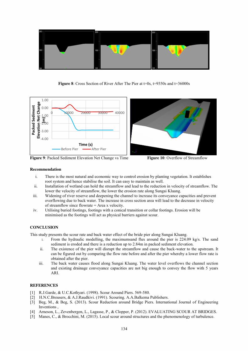
134

Figure 8: Cross Section of River After The Pier at t=0s, t=9350s and t=36000s

Figure 9: Packed Sediment Elevation Net Change vs Time Figure 10: Overflow of Streamflow

Recommendation

i. There is the most natural and economic way to control erosion by planting vegetation. It establishes root system and hence stabilise the soil. It can easy to maintain as well.

ii. Installation of wetland can hold the streamflow and lead to the reduction in velocity of streamflow. The lower the velocity of streamflow, the lower the erosion rate along Sungai Kluang.

iii. Widening of river reserve and deepening the channel to increase its conveyance capacities and prevent overflowing due to back water. The increase in cross section area will lead to the decrease in velocity of streamflow since flowrate = Area x velocity.

iv. Utilising buried footings, footings with a conical transition or collar footings. Erosion will be minimised as the footings will act as physical barriers against scour.

CONCLUSION

This study presents the scour rate and back water effect of the bride pier along Sungai Kluang. i. From the hydraulic modelling, the maximumsand flux around the pier is 224.09 kg/s. The sand

sediment is eroded and there is a reduction up to 2.84m in packed sediment elevation. ii. The existence of the pier will disrupt the streamflow and cause the back-water to the upstream. It

can be figured out by comparing the flow rate before and after the pier whereby a lower flow rate is obtained after the pier.

iii. The back water causes flood along Sungai Kluang. The water level overflows the channel section and existing drainage conveyance capacities are not big enough to convey the flow with 5 years ARI.

REFERENCES

[1] R.J.Garde, & U.C.Kothyari. (1998). Scour Around Piers. 569-580. [2] H.N.C.Breusers, & A.J.Raudkivi. (1991). Scouring. A.A.Balkema Publishers. [3] Beg, M., & Beg, S. (2013). Scour Reduction around Bridge Piers. International Journal of Engineering

Inventions , [4] Arneson, L., Zevenbergen, L., Lagasse, P., & Clopper, P. (2012). EVALUATING SCOUR AT BRIDGES. [5] Manes, C., & Brocchini, M. (2015). Local scour around structures and the phenomenology of turbulence.

-4.00

-3.00

-2.00

-1.00

0.00

1.00

0 10000 20000 30000 40000

Pack

ed S

edim

ent

Elev

atio

n N

et C

hang

e (m

)

Time (s) Before Pier After Pier

135

[6] Gengsheng Wei, J. B. (2014). Sedimentation Scour Model. [7] Straub, T. D., Melching, C. S., & Kocher, K. E. (2000). Equations for Estimating Clark Unit-Hydrograph

Parameters for Small Rural Watersheds in Illinois. U.S. DEPARTMENT OF THE INTERIOR. Urbana,Illinois: U.S. Geological Survey.

Impact of Impervious Surface on Peak Discharge and Discharge Volume of Sungai Lebir Catchment using HEC-HMS

Muhammad Faisal Amin Mat Ali, Noraliani Alias

noraliani@utm.my Keywords: Sungai Lebir catchment; HEC-HMS Modeling; Impervious Surface; Flood Forecasting. Abstract: Flood forecasting is one of the importance areas in hydrological studies. This study focused on the effect of changes in impervious surface to peak discharge and discharge volume readings on the hydrograph. Process modeling to forecast river flooding in Sungai Lebir, Kelantan performed using HEC-HMS 4.2. Rainfall data used for the calibration process was 27 December 2010 until 2 January 2011, while the data used for the validation process was 30 November 2013 until 6 December 2013. The loss parameter used is Initial and Constant, Clark UH for transformation parameter, Constant Monthly for base flow parameter and Muskingum for routing parameter. The values of these parameters obtained as a result of process simulation and calibration flood data. The accuracy of the simulation work was measured using Nash-Sutcliffe Efficiency (NSE). The rainfall data for case study simulation designed using methods available in the MSMA for 24-hour with 5, 10, 50 and 100 ARI. The data was simulated using parameters achieved to get the peak discharge and discharge volume at the outlet. Then, the percentage of impervious surface of each sub-catchment changed to 10%, 20%, 25% and 30% to compare the value of the peak discharge and discharge volume. INTRODUCTION

Floods are natural disasters that are often contributed to loss of life and destruction of property. As we

all know, floods caused by many factors, whether natural or the result of human activities. For example the development of the area and use of land without controls, drainage problems, increasing of population and so on. Construction of buildings, roads, concrete surfaces, housing and various other developments will increase the percentage of impervious surface at that area resulting in disruption to the runoff water. Consequently result in flood happening so fast there is not enough time for villagers to rescue their properties and themselves. Problem Statement The flooding phenomena in Malaysia are natural disasters that occur almost every year, especially in the east coast of the peninsular. Starting in October until February, this region will definitely badly hit by floods. Sungai Lebir and Sungai Galas are the main branch of Sungai Kelantan where both joined at the Kuala Krai before heading to Sungai Kelantan [1]. Catchment area alongside Sungai Lebir is a developing residential area especially at downstream area known as Kuala Krai. Therefore, it is important to determine the impact of impervious surface changes on peak discharge and discharge volume. Objective of Study There are several important objectives that led to this study as follows:

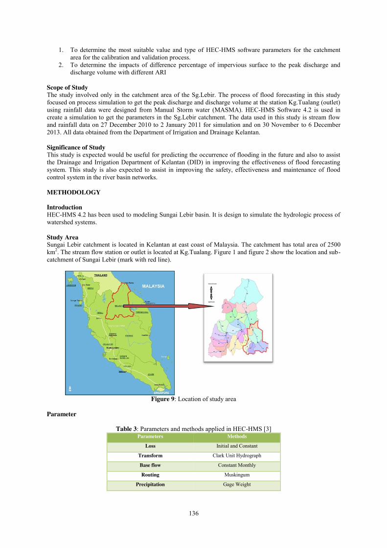
136

1. To determine the most suitable value and type of HEC-HMS software parameters for the catchment area for the calibration and validation process.

2. To determine the impacts of difference percentage of impervious surface to the peak discharge and discharge volume with different ARI

Scope of Study The study involved only in the catchment area of the Sg.Lebir. The process of flood forecasting in this study focused on process simulation to get the peak discharge and discharge volume at the station Kg.Tualang (outlet) using rainfall data were designed from Manual Storm water (MASMA). HEC-HMS Software 4.2 is used in create a simulation to get the parameters in the Sg.Lebir catchment. The data used in this study is stream flow and rainfall data on 27 December 2010 to 2 January 2011 for simulation and on 30 November to 6 December 2013. All data obtained from the Department of Irrigation and Drainage Kelantan. Significance of Study This study is expected would be useful for predicting the occurrence of flooding in the future and also to assist the Drainage and Irrigation Department of Kelantan (DID) in improving the effectiveness of flood forecasting system. This study is also expected to assist in improving the safety, effectiveness and maintenance of flood control system in the river basin networks. METHODOLOGY Introduction HEC-HMS 4.2 has been used to modeling Sungai Lebir basin. It is design to simulate the hydrologic process of watershed systems. Study Area Sungai Lebir catchment is located in Kelantan at east coast of Malaysia. The catchment has total area of 2500 km2. The stream flow station or outlet is located at Kg.Tualang. Figure 1 and figure 2 show the location and sub-catchment of Sungai Lebir (mark with red line).

Figure 9: Location of study area

Parameter

Table 3: Parameters and methods applied in HEC-HMS [3] Parameters Methods

Loss Initial and Constant

Transform Clark Unit Hydrograph

Base flow Constant Monthly

Routing Muskingum

Precipitation Gage Weight

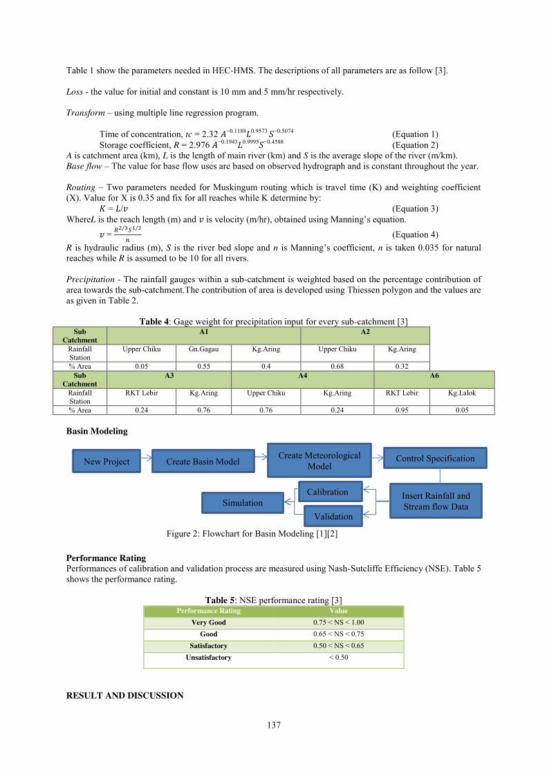
137

Table 1 show the parameters needed in HEC-HMS. The descriptions of all parameters are as follow [3]. Loss - the value for initial and constant is 10 mm and 5 mm/hr respectively. Transform – using multiple line regression program.

Time of concentration, tc = 2.32 𝐴−0.1188𝐿0.9573 𝑆−0.5074 (Equation 1) Storage coefficient, R = 2.976 𝐴−0.1943𝐿0.9995𝑆−0.4588 (Equation 2)

A is catchment area (km), L is the length of main river (km) and S is the average slope of the river (m/km). Base flow – The value for base flow uses are based on observed hydrograph and is constant throughout the year. Routing – Two parameters needed for Muskingum routing which is travel time (K) and weighting coefficient (X). Value for X is 0.35 and fix for all reaches while K determine by:

𝐾 = 𝐿/𝑣 (Equation 3) WhereL is the reach length (m) and 𝑣 is velocity (m/hr), obtained using Manning’s equation.

𝑣 = 𝑅2/3𝑆1/2

𝑛 (Equation 4)

R is hydraulic radius (m), S is the river bed slope and n is Manning’s coefficient, n is taken 0.035 for natural reaches while R is assumed to be 10 for all rivers. Precipitation - The rainfall gauges within a sub-catchment is weighted based on the percentage contribution of area towards the sub-catchment.The contribution of area is developed using Thiessen polygon and the values are as given in Table 2.

Table 4: Gage weight for precipitation input for every sub-catchment [3] Sub

Catchment A1 A2

Rainfall Station

Upper Chiku Gn.Gagau Kg.Aring Upper Chiku Kg.Aring

% Area 0.05 0.55 0.4 0.68 0.32 Sub

Catchment A3 A4 A6

Rainfall Station

RKT Lebir Kg.Aring Upper Chiku Kg.Aring RKT Lebir Kg.Lalok

% Area 0.24 0.76 0.76 0.24 0.95 0.05 Basin Modeling Performance Rating Performances of calibration and validation process are measured using Nash-Sutcliffe Efficiency (NSE). Table 5 shows the performance rating.

Table 5: NSE performance rating [3] Performance Rating Value

Very Good 0.75 < NS < 1.00 Good 0.65 < NS < 0.75

Satisfactory 0.50 < NS < 0.65 Unsatisfactory < 0.50

RESULT AND DISCUSSION

New Project Create Basin Model Create Meteorological

Model Control Specification

Insert Rainfall and Stream flow Data Simulation

Calibration

Validation

Figure 2: Flowchart for Basin Modeling [1][2]

138

Calibration The rainfall event chooses for calibration process is between 27 December 2010 and 2 January 2011. Figure 3(a) shows the calibrated model for the Kg.Tualang stream flow station. The efficiency index between observed and simulated stream flow is very high at 90%. It shows the hydrograph is look alike.Observed peak flow is 1291.1 m3/s on 31 December 2010 at 02:00 while simulated peak flow is 1040 m3/s on 30 December 2010 at 09:00. Validation For validation process, the rainfall event chooses are between 30 November 2013 and 6 December 2013. Figure 3(b) for validation model shows a slightly unwell match, but still within the good level of efficiency index which is 67%. Observed peak flow is 2559 m3/s on 05 December 2013 at 05:00 while simulated peak flow is 2419.7 m3/s on 04 December 2013 at 15:00.

(a) (b)

Figure 3: Sg.Lebir stream flow for Calibration and Validation

Table 6: Result for calibration and validation Calibration

Observed Peak Flow (m3s-1)

1291.1 Time 31-Dec-10 02:00

Simulated Peak Flow (m3s-1)

1040.0 Time 30-Dec-10 09:00

NSE 90 % accuracy Validation

Observed Peak Flow (m3s-1)

2559 Time 5-Dec-13 05:00

Simulated Peak Flow (m3s-1)

2419.7 Time 04-Dec-13 15:00

NSE 67 % accuracy

Table 4 shows the details for calibration and validation of Sg.Lebir. Both processes pass the satisfactory level of efficiency index. Peak discharge and time to peak also shows in the table.

0200400600800

100012001400

1:00

14:0

03:

0016

:00

5:00

18:0

07:

0020

:00

9:00

22:0

011

:00

24:0

013

:00

Flow

rate

(m3/

s)

Time

Calibration Hydrograph

Observe

Simulation

0

500

1000

1500

2000

2500

3000

1:00

12:0

023

:00

10:0

021

:00

8:00

19:0

06:

0017

:00

4:00

15:0

02:

0013

:00

24:0

011

:00

22:0

0

Flow

rate

(m3/

s)

Time

Validation Hydrograph

Observe

Simulation

139

Optimized Parameter Table 5 and 6 shows the optimized parameter used in HEC-HMS achieve from calibration and validation process. The value for all parameter is suitable and within the acceptable range [4].

Table 7: Optimized parameter for loss and transform Sub-

catchment Loss-initial & constant Clark Transform

Initial (mm)

Constant (mm/hr)

Impervious Time of concentration

(hr)

Storage coefficient

(hr) A1 10 1.5 2 22.48 21.29 A2 10 2.5 2 20.78 20.26 A3 10 2.5 5 51.03 45.61 A4 10 1.5 2 31.01 32.19 A6 10 2.5 4 20.01 18.61

Table 8: Optimized parameter for routing

Reach Muskingum Routing

Muskingum X Time Travel, K

R1 0.35 0.43

R2 0.35 0.15

Case Study

Kg.Aring rainfall station data was used for design 5, 10, 50 and 100 year ARI [4] to compare the impact of changes impervious surface percentage to the peak discharge and discharge volume of hydrograph. ARI data was calculated using method available in MASMA. The parameter used in this simulation gain from optimized parameter through calibration and validation process. Based on the observation of the simulated hydrograph, the results show increase in flow rate and volume each year. Table 7 shows the result of simulation.

Table 9: Result of simulation Imperviousness Qpeak (m3/s)

5 Year ARI 10 Year ARI 50 Year ARI 100 Year ARI 5% 2292.70 2669.70 3767.70 4355.30

10% 2323.80 2701.20 3799.90 4387.70 15% 2354.80 2732.70 3832.20 4420.20 20% 2385.90 2764.10 3864.40 4452.70

Imperviousness Volume (m3) 5 Year ARI 10 Year ARI 50 Year ARI 100 Year ARI

5% 379024.90 439360.60 615492.50 709903.50 10% 384510.60 444938.90 621240.90 715709.70 15% 389996.40 450517.20 626989.30 721516.00 20% 395482.10 456095.50 632737.70 727322.30

Figure 4 shows the hydrograph of simulation for different ARI. The difference of the hydrograph for impervious surface (5%, 10%, 15% and 20%) not quite clear because the value for peak discharge is too big and the changes in value is not much. But still peak discharge and discharge volume increase for increasing of impervious surface percentage.

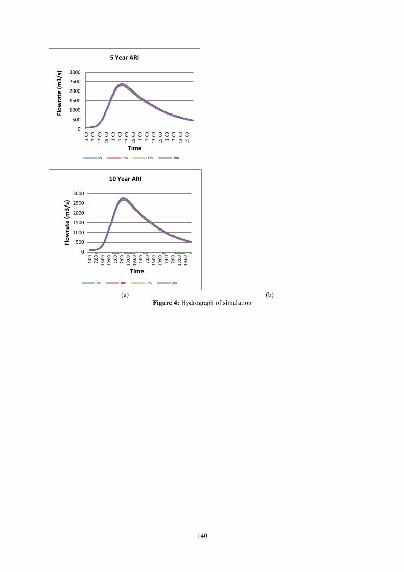
140

(a) (b)

Figure 4: Hydrograph of simulation

0

500

1000

1500

2000

2500

3000

1:00

7:00

13:0

019

:00

1:00

7:00

13:0

019

:00

1:00

7:00

13:0

019

:00

1:00

7:00

13:0

019

:00

Flow

rate

(m3/

s)

Time

5 Year ARI

5% 10% 15% 20%

0

500

1000

1500

2000

2500

3000

1:00

7:00

13:0

019

:00

1:00

7:00

13:0

019

:00

1:00

7:00

13:0

019

:00

1:00

7:00

13:0

019

:00

Flow

rate

(m3/

s)

Time

10 Year ARI

5% 10% 15% 20%

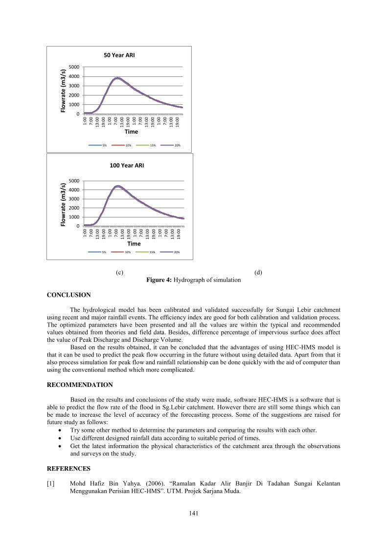
141

(c) (d)

Figure 4: Hydrograph of simulation CONCLUSION The hydrological model has been calibrated and validated successfully for Sungai Lebir catchment using recent and major rainfall events. The efficiency index are good for both calibration and validation process. The optimized parameters have been presented and all the values are within the typical and recommended values obtained from theories and field data. Besides, difference percentage of impervious surface does affect the value of Peak Discharge and Discharge Volume.

Based on the results obtained, it can be concluded that the advantages of using HEC-HMS model is that it can be used to predict the peak flow occurring in the future without using detailed data. Apart from that it also process simulation for peak flow and rainfall relationship can be done quickly with the aid of computer than using the conventional method which more complicated. RECOMMENDATION

Based on the results and conclusions of the study were made, software HEC-HMS is a software that is able to predict the flow rate of the flood in Sg.Lebir catchment. However there are still some things which can be made to increase the level of accuracy of the forecasting process. Some of the suggestions are raised for future study as follows:

x Try some other method to determine the parameters and comparing the results with each other. x Use different designed rainfall data according to suitable period of times. x Get the latest information the physical characteristics of the catchment area through the observations

and surveys on the study. REFERENCES [1] Mohd Hafiz Bin Yahya. (2006). “Ramalan Kadar Alir Banjir Di Tadahan Sungai Kelantan

Menggunakan Perisian HEC-HMS”. UTM. Projek Sarjana Muda.

0

1000

2000

3000

4000

5000

1:00

7:00

13:0

019

:00

1:00

7:00

13:0

019

:00

1:00

7:00

13:0

019

:00

1:00

7:00

13:0

019

:00

Flow

rate

(m3/

s)

Time

50 Year ARI

5% 10% 15% 20%

0

1000

2000

3000

4000

5000

1:00

7:00

13:0

019

:00

1:00

7:00

13:0

019

:00

1:00

7:00

13:0

019

:00

1:00

7:00

13:0

019

:00

Flow

rate

(m3/

s)

Time

100 Year ARI

5% 10% 15% 20%

142

[2] Mohd Latif Bin Ramli. (20010). “Simulasi Model Hujan-Air Larian Dengan Menggunakan Perisian HEC-HMS Bagi Kawasan Tadahan Sungai Padang Terap, Jitra Kedah”. UTM. Projek Sarjana Muda.

[3] M.R.M. Haniffah, K.A. Nasir (2015). “Hydrological Modelling at Upstream of Sg. Kelantan using HEC-HMS for Major Current Rainfall Events”. Jurnal Teknologi (Sciences & Engineering)

[4] Department of Irrigation and Drainage. (2012). “Urban Stormwater Management Manual for Malaysia (MSMA 2nd Edition)”. Department of Irrigation and Drainage.

Performance of Turbine’s Bio-Inspired Blade Subjected to Perpendicular Flow

Moses Ching Yu Keit, Mohd Ridza Bin Mohd Haniffah Faculty of Civil Engineering, Universiti Teknologi Malaysia, Malaysia

mridza@utm.my

Keywords: Bio-Inspired Blade; Hydrokinetic Turbine; FLOW-3D; CFD ABSTRACT. Hydrokinetic turbine is a good approach to produce renewable energy in Malaysia because of the abundance of water sources. A good design of turbine blade will produce high energy output and efficiency. The aim of this research is to computationally investigate performance of turbine blade for a single bio-inspired blade in river. The effects of tubercles on the blade’s performance in terms of hydrodynamics, such as the velocity field, flow circulation and drag force are analyzed. Bio-inspired blades with NACA 0012 airfoil profile are constructed using Solidworks. FLOW-3D, a Computational Fluid Dynamics (CFD) software will be applied to simulate the fluid flow perpendicular to the bio-inspired blade. Convergence test is done to make sure the simulation is grid independent. Larger water circulation induced by bio-inspired blade compared to flat blade without tubercles geometry. Bio-inspired blade with lower A/λ ratio generates larger water circulation. Higher

143

force was generated from the pressure difference between windward and leeward side of blade due to larger water circulation. Hence, higher energy can be generated by the turbine with bio-inspired blade and the performance of hydrokinetic turbine is improved.

INTRODUCTION

The bio-inspired blade is inspired by the rounded tubercles on the flipper of the humpback whale. The performance of the bio-inspired blade will increase when higher drag force is produced and thus increasing the blades rotation of the turbine. Hence, higher energy can be generated by the hydrokinetic turbine. FLOW-3D is a CFD software that can used to simulate fluid flow in a virtual environment and used in this study to carry out the simulation work.

Problem Statement

Energy is essential to economic and social development and improved quality of life in all countries. Much of the world’s energy, however, is being met from fossil fuels, which are limited and are reducing day by day. The most vital concerns today are ensuring sustainable existence of natural life and leaving a green environment for next generations. Renewable energy resources seem to be one of the most efficient and effective solutions for clean and sustainable energy development. Examples of renewable energies are hydro, wind, solar, biomass and geothermal energies. But for Malaysia, wind and wave might not be the best solution because amount of wind and wave energy in Malaysia is relatively small compared to other parts of the world such as the North Sea in Europe. Hence, hydropower seems to be the optimum choice for Malaysia.

Hydrokinetic turbine is a good approach to produce renewable energy in Malaysia. Therefore, a good design of turbine blade which is able to produce high energy output and high efficiency is required. This means the blade design should be able to increase the performance of blade in terms of the hydrodynamics when compared to the conventional blade design. A higher pressure difference between the windward and leeward side of the blade will increase the drag force. The higher drag force produced by the blade will help to increase the efficiency of the hydrokinetic turbine with higher blade rotation. Hence, in this study, the introduction of the tubercles geometry on the turbine blade is hoped to increase the performance of the hydrokinetic turbine.

Objectives

The aims is to improve the performance of turbine blade using computational modelling for a single bio-inspired blade in a river flow. The objectives of this study are:

7. To investigate the effects of tubercles geometry on blade’s performance in terms of the hydrodynamics. 8. To determine the effect of water circulation created by the flow through the tubercles towards the

pressur eat the leeward side of the blade. 9. To determine the relationship between the drag force and the created water circulation.

Scope of Study

This study is carried out using FLOW-3D software, it’s a Computational Fluid Dynamics (CFD) software which can be used to stimulate fluid flow in virtual environment. Hence, this study only focus on understanding the flow behavior, and does not include the structural behavior of the blade. This study is limited to model type of NACA 0012 blade design, which is a common design in wind and wave turbine. The flow is normal to the largest area of the blade instead of the existing literatures in which the flow is head on with the tubercles.

LITERATURE REVIEW Malaysia consists of 150 rivers in Peninsular Malaysia and 50 rivers in Sabah and Sarawak [1]. The average

annual rainfall of Malaysia is quite high compared to world's average annual rainfall which is 750 mm [2]. Thus, Malaysia has a significant potential for hydropower generation. Hydropower can further be categorized as large, medium or small scale. Electricity generated from large scale hydropower plants is supplied to main grid, on the other hand, electricity generated from small scale hydropower generators usually used only for rural and off-grid applications. Hence, small scale hydropower is essential to many developing countries, such as Malaysia [3]. Despite hydro-power technologies are preferable choices for energy generation in Malaysia, they have not been fully exploited yet due to some technical, economical, and institutional challenges [4]. Therefore, this study on the tubercles geometry on turbine runner blades can gives positive impact on the application of hydrokinetic turbine for rural electrification in Malaysia.

The name of “Bio-Inspired Blade” is inspired by the flipper of the humpback whale. The humpback whale had a wing-like shape flipper, which is long, narrow and thin. Flippers of humpback whales have rounded and blunt large tubercles along its leading edge. It was suggested that these leading edge tubercles somehow

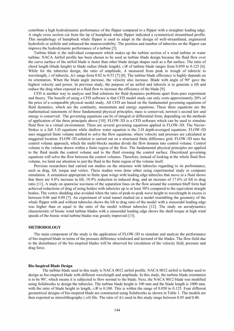
144

contribute a high hydrodynamic performance of the flipper compared to a flipper with a straighter leading edge. A single cross section cut from the tip of humpback whale flipper indicated a symmetrical streamlined profile. This morphology of humpback whale flipper is used to adapt in the design of well-streamlined, engineered hydrofoils or airfoils and enhanced the maneuverability. The position and number of tubercles on the flipper can improve the hydrodynamic performance of a turbine [5].

Turbine blade is the individual component which makes up the turbine section of a wind turbine or water turbine. NACA Airfoil profile has been chosen to be used as turbine blade design because the fluid flow over the curve surface of the airfoil blade is faster than other blade design shapes such as a flat surface. The ratio of chord length (blade height) to blade radius (blade length), c/R of turbine blade ranges from 0.050 to 0.125 [6]. While for the tubercles design, the ratio of amplitude, A measured from peak to trough of tubercle to wavelength, λ of tubercle, A/λ range from 0.02 to 0.53 [7] [8]. The turbine blade efficiency is highly depends on its orientation. When the blade angle increase, the velocity also increase. Blade with angle of 90° gave the highest velocity and power. In previous study, the purpose of an airfoil and tubercle is to generate a lift and reduce the drag when exposed to a fluid flow to increase the efficiency of the blade [9].

CFD is another way to analyze and find solutions for fluid dynamics problems apart from pure experiment and theory. The benefit of using a CFD software is that CFD model study can only costs approximately 20% of the price of a comparable physical model study. All CFD are based on the fundamental governing equations of fluid dynamics, which are the continuity, momentum and energy equations. These three equations are the mathematical statements of three fundamental physical principles; mass is conserved, newton’s second law and energy is conserved. The governing equations can be of integral or differential form, depending on the methods of application of the three principals above [10]. FLOW-3D is a CFD software which can be used to simulate fluid flow in a virtual environment. There are several governing equations applied in FLOW-3D. The Navier-Stokes is a full 3-D equations while shallow water equation is the 2-D depth-averaged equations. FLOW-3D uses staggered finite volume method to solve the flow equations, where velocity and pressure are calculated at staggered location. FLOW-3D solution is carried out on a structured finite difference grid. FLOW-3D uses the control volume approach, which the multi-blocks meshes divide the flow domain into control volume. Control volume is the volume drawn within a finite region of the flow. The fundamental physical principles are applied to the fluid inside the control volume and to the fluid crossing the control surface. Discretized governing equations will solve the flow between the control volumes. Therefore, instead of looking at the whole fluid flow volume, we limit our attention to just the fluid in the finite region of the volume itself.

Previous researchers had carried out studies on the structure with tubercles regarding to its performance, such as drag, lift, torque and vortex. These studies were done either using experimental study or computer simulation. A simulation appropriate to finite span wings with leading edge tubercles that move in a fluid shows that there are 4.8% increase in lift, 10.9% reduction in induced drag, and an increase of 17.6% of lift to drag ratio [11]. A study on spanwise waviness of the separation lines on the flow around the common bluff form had achieved reductions of drag of using bodies with tubercles up to at least 30% compared to the equivalent straight bodies. The vortex shedding also avoided when the ratio of peak-to-peak wave height to wavelength in excess is between 0.06 and 0.09 [7]. An experiment of wind tunnel studied on a model resembling the geometry of the whale flipper with and without tubercles shows the lift to drag ratio of the model with a sinusoidal leading edge was higher than or equal to the ratio of the model without tubercles [12]. The study on aerodynamics characteristic of bionic wind turbine blades with a sinusoidal leading edge shows the shaft torque at high wind speeds of the bionic wind turbine blades was greatly improved [13].

METHODOLOGY The main component of the study is the application of FLOW-3D to simulate and analyze the performance

of bio-inspired blade in terms of the pressure difference windward and leeward of the blades. The flow-field due to the disturbance of the bio-inspired blades will be observed for circulation of the velocity field, pressure and drag force.

Bio-Inspired Blade Design The turbine blade used in this study is NACA 0012 airfoil profile. NACA 0012 airfoil is further used to

design as bio-inspired blade with different wavelength and amplitude. In this study, the turbine blade orientation is to be 90°, which means it is subjected to flow normal to the blade. Next, the NACA 0012 blade was modified using Solidworks to design the tubercles. The turbine blade height is 100 mm and the blade length is 1000 mm, with the ratio of blade height to length, c/R is 0.100. This is within the range of 0.050 to 0.125. Four different geometrical designs of bio-inspired blade are constructed using Solidworks as shown in Table 1. The models are then exported as stereolithography (.stl) file. The ratio of A/λ used in this study range between 0.05 and 0.40.

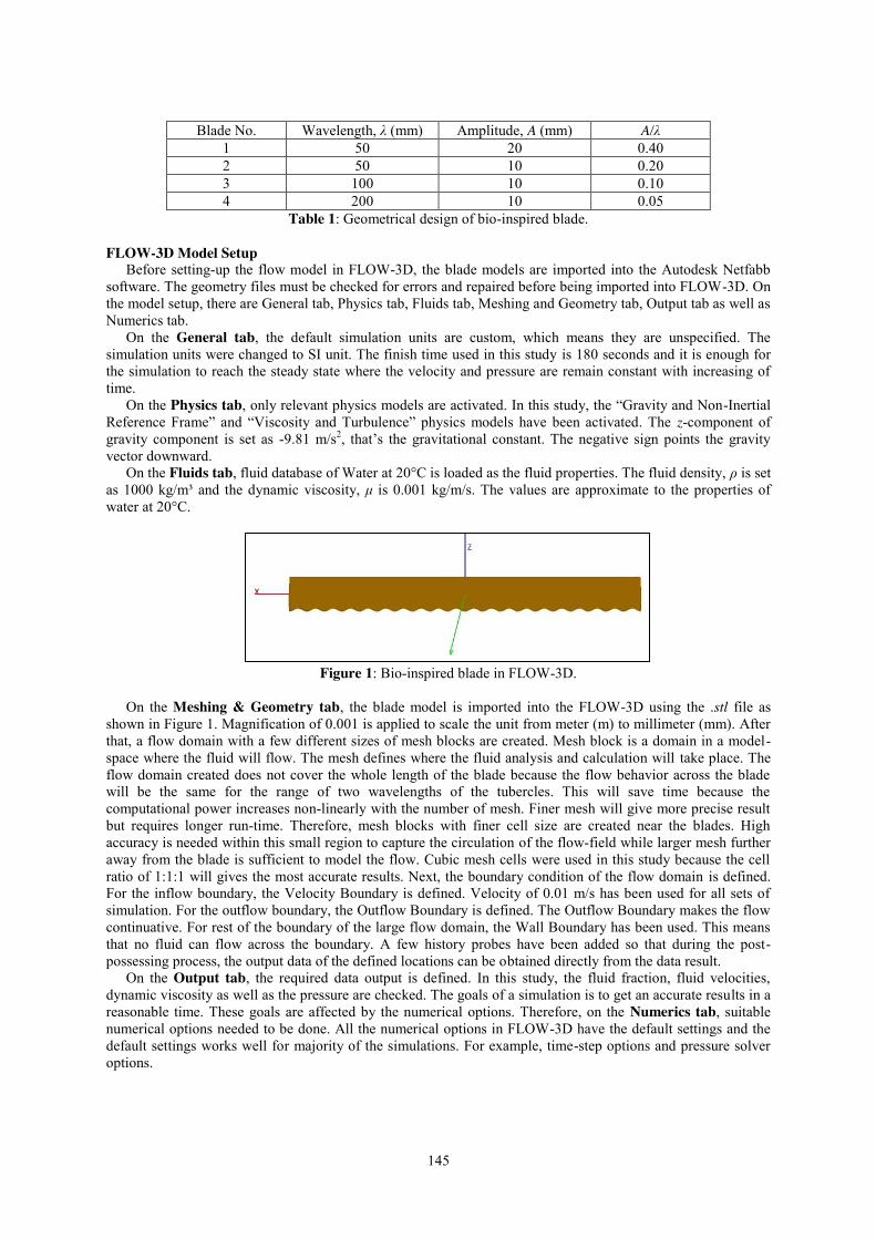
145

Blade No. Wavelength, λ (mm) Amplitude, A (mm) A/λ

1 50 20 0.40 2 50 10 0.20 3 100 10 0.10 4 200 10 0.05

Table 1: Geometrical design of bio-inspired blade. FLOW-3D Model Setup

Before setting-up the flow model in FLOW-3D, the blade models are imported into the Autodesk Netfabb software. The geometry files must be checked for errors and repaired before being imported into FLOW-3D. On the model setup, there are General tab, Physics tab, Fluids tab, Meshing and Geometry tab, Output tab as well as Numerics tab.

On the General tab, the default simulation units are custom, which means they are unspecified. The simulation units were changed to SI unit. The finish time used in this study is 180 seconds and it is enough for the simulation to reach the steady state where the velocity and pressure are remain constant with increasing of time.

On the Physics tab, only relevant physics models are activated. In this study, the “Gravity and Non-Inertial Reference Frame” and “Viscosity and Turbulence” physics models have been activated. The z-component of gravity component is set as -9.81 m/s2, that’s the gravitational constant. The negative sign points the gravity vector downward.

On the Fluids tab, fluid database of Water at 20°C is loaded as the fluid properties. The fluid density, ρ is set as 1000 kg/m³ and the dynamic viscosity, μ is 0.001 kg/m/s. The values are approximate to the properties of water at 20°C.

Figure 1: Bio-inspired blade in FLOW-3D.

On the Meshing & Geometry tab, the blade model is imported into the FLOW-3D using the .stl file as

shown in Figure 1. Magnification of 0.001 is applied to scale the unit from meter (m) to millimeter (mm). After that, a flow domain with a few different sizes of mesh blocks are created. Mesh block is a domain in a model-space where the fluid will flow. The mesh defines where the fluid analysis and calculation will take place. The flow domain created does not cover the whole length of the blade because the flow behavior across the blade will be the same for the range of two wavelengths of the tubercles. This will save time because the computational power increases non-linearly with the number of mesh. Finer mesh will give more precise result but requires longer run-time. Therefore, mesh blocks with finer cell size are created near the blades. High accuracy is needed within this small region to capture the circulation of the flow-field while larger mesh further away from the blade is sufficient to model the flow. Cubic mesh cells were used in this study because the cell ratio of 1:1:1 will gives the most accurate results. Next, the boundary condition of the flow domain is defined. For the inflow boundary, the Velocity Boundary is defined. Velocity of 0.01 m/s has been used for all sets of simulation. For the outflow boundary, the Outflow Boundary is defined. The Outflow Boundary makes the flow continuative. For rest of the boundary of the large flow domain, the Wall Boundary has been used. This means that no fluid can flow across the boundary. A few history probes have been added so that during the post-possessing process, the output data of the defined locations can be obtained directly from the data result.

On the Output tab, the required data output is defined. In this study, the fluid fraction, fluid velocities, dynamic viscosity as well as the pressure are checked. The goals of a simulation is to get an accurate results in a reasonable time. These goals are affected by the numerical options. Therefore, on the Numerics tab, suitable numerical options needed to be done. All the numerical options in FLOW-3D have the default settings and the default settings works well for majority of the simulations. For example, time-step options and pressure solver options.

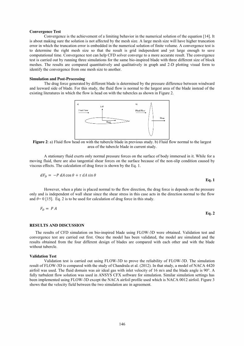
146

Convergence Test Convergence is the achievement of a limiting behavior in the numerical solution of the equation [14]. It

is about making sure the solution is not affected by the mesh size. A large mesh size will have higher truncation error in which the truncation error is embedded in the numerical solution of finite volume. A convergence test is to determine the right mesh size so that the result is grid independent and yet large enough to save computational time. Convergence test can help CFD solver converge to a more accurate result. The convergence test is carried out by running three simulations for the same bio-inspired blade with three different size of block meshes. The results are compared quantitatively and qualitatively in graph and 2-D plotting visual form to identify the convergence from one mesh size to another. Simulation and Post-Processing

The drag force generated by different blade is determined by the pressure difference between windward and leeward side of blade. For this study, the fluid flow is normal to the largest area of the blade instead of the existing literatures in which the flow is head on with the tubercles as shown in Figure 2.

Figure 2: a) Fluid flow head on with the tubercle blade in previous study. b) Fluid flow normal to the largest

area of the tubercle blade in current study.

A stationary fluid exerts only normal pressure forces on the surface of body immersed in it. While for a moving fluid, there are also tangential shear forces on the surface because of the non-slip condition caused by viscous effects. The calculation of drag force is shown by the Eq. 1.

𝑑𝐹𝐷 = −𝑃 𝑑𝐴 cos 𝜃 + 𝜏 𝑑𝐴 sin 𝜃

Eq. 1

However, when a plate is placed normal to the flow direction, the drag force is depends on the pressure only and is independent of wall shear since the shear stress in this case acts in the direction normal to the flow and 𝜃= 0 [15]. Eq. 2 is to be used for calculation of drag force in this study.

𝐹𝐷 = 𝑃 𝐴 Eq. 2

RESULTS AND DISCUSSION

The results of CFD simulation on bio-inspired blade using FLOW-3D were obtained. Validation test and convergence test are carried out first. Once the model has been validated, the model are simulated and the results obtained from the four different design of blades are compared with each other and with the blade without tubercle.

Validation Test

Validation test is carried out using FLOW-3D to prove the reliability of FLOW-3D. The simulation result of FLOW-3D is compared with the study of Chandrala et al. (2012). In that study, a model of NACA 4420 airfoil was used. The fluid domain was air ideal gas with inlet velocity of 16 m/s and the blade angle is 90°. A fully turbulent flow solution was used in ANSYS CFX software for simulation. Similar simulation settings has been implemented using FLOW-3D except the NACA airfoil profile used which is NACA 0012 airfoil. Figure 3 shows that the velocity field between the two simulation are in agreement.

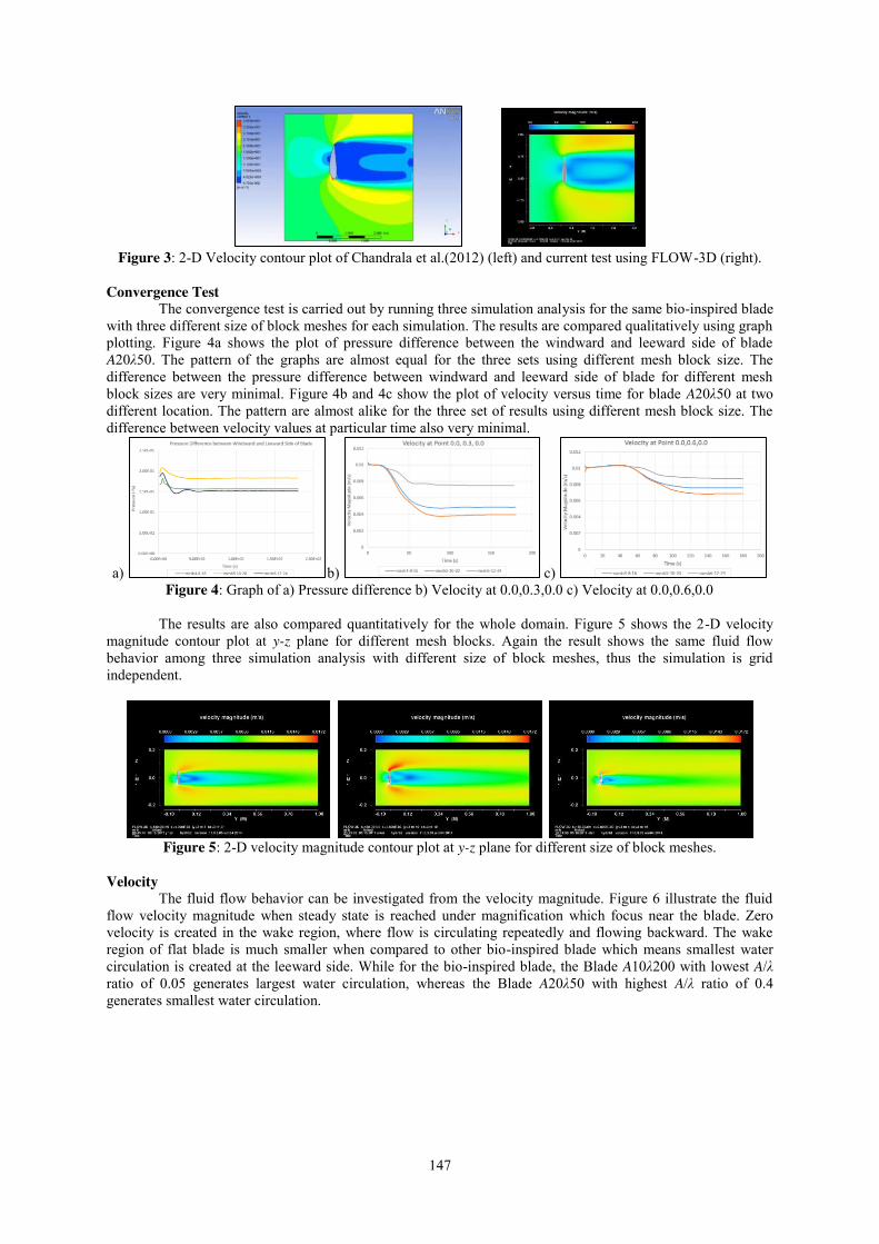
147

Figure 3: 2-D Velocity contour plot of Chandrala et al.(2012) (left) and current test using FLOW-3D (right).

Convergence Test

The convergence test is carried out by running three simulation analysis for the same bio-inspired blade with three different size of block meshes for each simulation. The results are compared qualitatively using graph plotting. Figure 4a shows the plot of pressure difference between the windward and leeward side of blade A20λ50. The pattern of the graphs are almost equal for the three sets using different mesh block size. The difference between the pressure difference between windward and leeward side of blade for different mesh block sizes are very minimal. Figure 4b and 4c show the plot of velocity versus time for blade A20λ50 at two different location. The pattern are almost alike for the three set of results using different mesh block size. The difference between velocity values at particular time also very minimal.

a) b) c) Figure 4: Graph of a) Pressure difference b) Velocity at 0.0,0.3,0.0 c) Velocity at 0.0,0.6,0.0

The results are also compared quantitatively for the whole domain. Figure 5 shows the 2-D velocity

magnitude contour plot at y-z plane for different mesh blocks. Again the result shows the same fluid flow behavior among three simulation analysis with different size of block meshes, thus the simulation is grid independent.

Figure 5: 2-D velocity magnitude contour plot at y-z plane for different size of block meshes.

Velocity

The fluid flow behavior can be investigated from the velocity magnitude. Figure 6 illustrate the fluid flow velocity magnitude when steady state is reached under magnification which focus near the blade. Zero velocity is created in the wake region, where flow is circulating repeatedly and flowing backward. The wake region of flat blade is much smaller when compared to other bio-inspired blade which means smallest water circulation is created at the leeward side. While for the bio-inspired blade, the Blade A10λ200 with lowest A/λ ratio of 0.05 generates largest water circulation, whereas the Blade A20λ50 with highest A/λ ratio of 0.4 generates smallest water circulation.

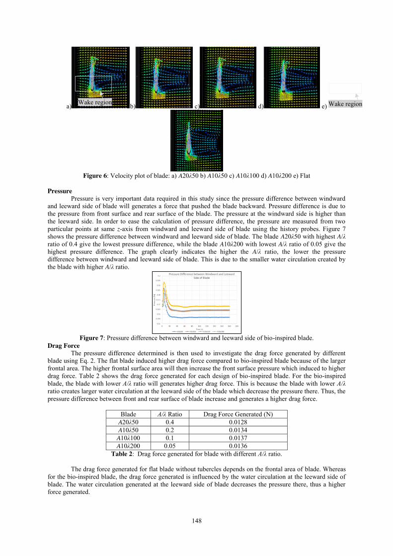
148

a) b) c) d) e)

Figure 6: Velocity plot of blade: a) A20λ50 b) A10λ50 c) A10λ100 d) A10λ200 e) Flat

Pressure

Pressure is very important data required in this study since the pressure difference between windward and leeward side of blade will generates a force that pushed the blade backward. Pressure difference is due to the pressure from front surface and rear surface of the blade. The pressure at the windward side is higher than the leeward side. In order to ease the calculation of pressure difference, the pressure are measured from two particular points at same z-axis from windward and leeward side of blade using the history probes. Figure 7 shows the pressure difference between windward and leeward side of blade. The blade A20λ50 with highest A/λ ratio of 0.4 give the lowest pressure difference, while the blade A10λ200 with lowest A/λ ratio of 0.05 give the highest pressure difference. The graph clearly indicates the higher the A/λ ratio, the lower the pressure difference between windward and leeward side of blade. This is due to the smaller water circulation created by the blade with higher A/λ ratio.

Figure 7: Pressure difference between windward and leeward side of bio-inspired blade.

Drag Force The pressure difference determined is then used to investigate the drag force generated by different

blade using Eq. 2. The flat blade induced higher drag force compared to bio-inspired blade because of the larger frontal area. The higher frontal surface area will then increase the front surface pressure which induced to higher drag force. Table 2 shows the drag force generated for each design of bio-inspired blade. For the bio-inspired blade, the blade with lower A/λ ratio will generates higher drag force. This is because the blade with lower A/λ ratio creates larger water circulation at the leeward side of the blade which decrease the pressure there. Thus, the pressure difference between front and rear surface of blade increase and generates a higher drag force.

Blade A/λ Ratio Drag Force Generated (N) A20λ50 0.4 0.0128 A10λ50 0.2 0.0134

A10λ100 0.1 0.0137 A10λ200 0.05 0.0136

Table 2: Drag force generated for blade with different A/λ ratio.

The drag force generated for flat blade without tubercles depends on the frontal area of blade. Whereas for the bio-inspired blade, the drag force generated is influenced by the water circulation at the leeward side of blade. The water circulation generated at the leeward side of blade decreases the pressure there, thus a higher force generated.

Wake region Wake region

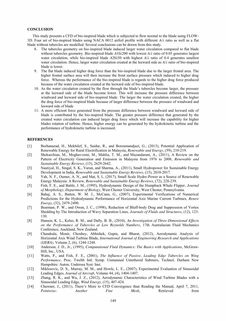
149

CONCLUSION

This study presents a CFD of bio-inspired blade which is subjected to flow normal to the blade using FLOW-3D. Four set of bio-inspired blades using NACA 0012 airfoil profile with different A/λ ratio as well as a flat blade without tubercles are modelled. Several conclusions can be drawn from this study.

8. The tubercles geometry on bio-inspired blade induced larger water circulation compared to flat blade without tubercles geometry. Bio-inspired blade A10λ200 with lowest A/λ ratio of 0.05 generates largest water circulation, while bio-inspired blade A20λ50 with highest A/λ ratio of 0.4 generates smallest water circulation. Hence, larger water circulation created at the leeward side as A/λ ratio of bio-inspired blade is lower.

9. The flat blade induced higher drag force than the bio-inspired blade due to the larger frontal area. The higher frontal surface area will then increase the front surface pressure which induced to higher drag force. Whereas the performance of the bio-inspired blade is regards to the higher drag force produced because of the water circulation created at the leeward side of bio-inspired blade.

10. As the water circulation created by the flow through the blade’s tubercles become larger, the pressure at the leeward side of the blade become lower. This will increase the pressure difference between windward and leeward side of bio-inspired blade. The larger the water circulation created, the higher the drag force of bio-inspired blade because of larger difference between the pressure of windward and leeward side of blade

11. A more efficient force generated from the pressure difference between windward and leeward side of blade is contributed by the bio-inspired blade. The greater pressure difference that generated by the created water circulation can induced larger drag force which will increase the capability for higher blades rotation of turbine. Hence, higher energy can be generated by the hydrokinetic turbine and the performance of hydrokinetic turbine is increased.

REFERENCES

[1] Borhanazad, H., Mekhilef, S., Saidur, R., and Boroumandjazi, G., (2013), Potential Application of Renewable Energy for Rural Electrification in Malaysia, Renewable and Energy, (59), 210-219.

[2] Shekarchian, M., Moghavvemi, M., Mahlia, T. M., and Mazandarani, A., (2011), A Review on the Pattern of Electricity Generation and Emission in Malaysia from 1976 to 2008, Renewable and Sustainable Energy Reviews, (15), 2629-2642.

[3] Nautiyal, H., Singal, S. K., Varun, and Sharma, A., (2011), Small Hydropower for Sustainable Energy Development in India, Renewable and Sustainable Energy Reviews, (15), 2010-2017.

[4] Yah, N. F., Oumer, A. N., and Mat, S. I., (2017), Small Scale Hydro-Power as a Source of Renewable Energy Malaysia: A Review, Renewable and Sustainable Energy Reviews, (72), 228-239.

[5] Fish, F. E., and Battle, J. M., (1995), Hydrodynamic Design of the Humpback Whale Flipper, Journal of Morphology, Department of Biology, West Chester University, West Chester, Pennsylvania.

[6] Bahaj, A. S., Batten, W. M. J., McCann, G., (2007), Experimental Verifications of Numerical Predictions for the Hydrodynamic Performance of Horizontal Axis Marine Current Turbines, Renew Energy, (32), 2479-2490.

[7] Bearman, P. W., and Owen, J. C., (1998), Reduction of Bluff-body Drag and Suppression of Vortex Shedding by The Introduction of Wavy Separation Lines, Journals of Fluids and Structures, (12), 123-130.

[8] Hansen, K. L., Kelso, R. M., and Dally, B. B., (2010), An Investigation of Three-Dimensional Effects on the Performance of Tubercles at Low Reynolds Numbers, 17th Australasian Fluid Mechanics Conference, Auckland, New Zealand.

[9] Chandrala, Monir, Choubey, Abhishek, Gupta, and Bharat, (2012), Aerodynamic Analysis of Horizontal Axis Wind Turbine Blade, International Journal of Engineering Research and Applications (IJERA), Volume 2, (6), 1244-1248.

[10] Anderson, J. D., Jr., (1995), Computational Fluid Dynamics: The Basics with Applications, McGraw-Hill, Inc., USA.

[11] Watts, P., and Fish, F. E., (2001), The Influence of Passive, Leading Edge Tubercles on Wing Performance, Proc. Twelth Intl. Symp. Unmanned Untethered Submers, Technol, Durham New Hampshire: Auton, Undersea Syst. Inst.

[12] Miklosovic, D. S., Murray, M. M., and Howle, L. E., (2007), Experimental Evaluation of Sinusoidal Leading Edges, Journal of Aircraft, Volume 44, (4), 1404-1407.

[13] Zhang, R. K., and Wu, J. Z., (2012), Aerodynamic Characteristics of Wind Turbine Blades with a Sinusoidal Leading Edge, Wind Energy, (15), 407-424.

[14] Chawner, J., (2011), There’s More to CFD Convergence than Reading the Manual, April 7, 2011, Pointwise: Another Fine Mesh, Retrieved from

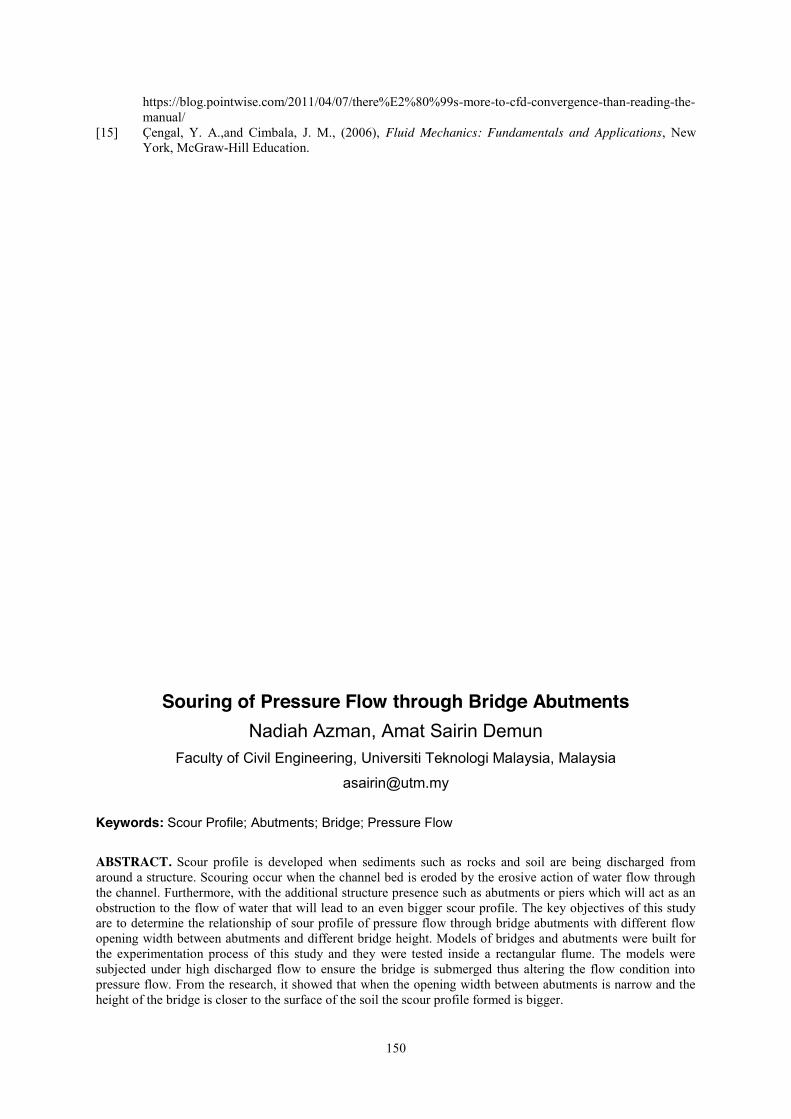
150

https://blog.pointwise.com/2011/04/07/there%E2%80%99s-more-to-cfd-convergence-than-reading-the-manual/

[15] Çengal, Y. A.,and Cimbala, J. M., (2006), Fluid Mechanics: Fundamentals and Applications, New York, McGraw-Hill Education.

Souring of Pressure Flow through Bridge Abutments Nadiah Azman, Amat Sairin Demun

Faculty of Civil Engineering, Universiti Teknologi Malaysia, Malaysia

asairin@utm.my

Keywords: Scour Profile; Abutments; Bridge; Pressure Flow

ABSTRACT. Scour profile is developed when sediments such as rocks and soil are being discharged from around a structure. Scouring occur when the channel bed is eroded by the erosive action of water flow through the channel. Furthermore, with the additional structure presence such as abutments or piers which will act as an obstruction to the flow of water that will lead to an even bigger scour profile. The key objectives of this study are to determine the relationship of sour profile of pressure flow through bridge abutments with different flow opening width between abutments and different bridge height. Models of bridges and abutments were built for the experimentation process of this study and they were tested inside a rectangular flume. The models were subjected under high discharged flow to ensure the bridge is submerged thus altering the flow condition into pressure flow. From the research, it showed that when the opening width between abutments is narrow and the height of the bridge is closer to the surface of the soil the scour profile formed is bigger.

151

INTRODUCTION

Scouring is a natural phenomenon occurred when the sediments on the channel bed are carried away by the flowing stream. This can be referred to as live bed scour. Clear water scour occurs when sediment is removed from the scour hole but not supplied by the approaching flow. Both type of scouring are known as local scour at abutments. However, due to continuous scouring around bridge structures such as abutments and piers many bridges had failed. When scouring keep on forming around the area of the structure, it will affect the stability and strength of the structure. This will result in possible failure of the structure such as the bridge that the piers or abutments were supporting will collapse.

Problem Statement

As scouring will lead to the failure of bridge mainly the failure of piers and abutment, it is very important to study more in this area to find out about the cause and effect of scouring at bridge abutments. However, if comparing these two structures, there had not been many research done on the scouring at bridge abutments but a number of studies were done on local scouring at piers. It can be said that scouring occur at piers is widely understood by hydraulics engineer but not in the case for scouring at abutments which still need to be discovered. Kandasamy and Melville (2010) were the first few that had tried to link between the behavior of the local scouring of piers with abutments. Before them there had been several that had tried to make a connection between the two structures. However, many of it only focus on relating local scouring at piers with a shape like abutments.

Furthermore, the study on scour profile under pressure flow is still lacking. According to United States Department of Transportation (2009), most study regarding the scour profile at bridge structures are usually assumed to be under the free flow condition. However, they stated that the flow of water can change to pressure flow when the lower deck of the bridge is submerged under water which this condition can usually be found during flooding.

Objectives This study is done to determine the relationship of the scour profile of pressure flow through bridge abutments with

1. Different flow opening width between abutments, w 2. Different bridge height, h

Scope of Study This study will include a laboratory experiment on the scour profile of pressure flow through bridge abutments that will be carried out at the Hydraulics and Hydrology Laboratory, Faculty of Civil Engineering UTM. The scope of this study will be limited to firstly, the flow of water in the channel under the bridge model would be under pressure flow. Next, the flow of water through bridge abutments can be monitored from outside as the abutments will be constructed by using Perspex. The shape of the bridge abutments are trapezoidal shaped with 45° wing wall. It is limited to a straight rectangular flume and he soil that will be using as the sediment bed is only non-cohesive soil.

LITERATURE REVIEW

The accuracy of prediction for scouring at bridge abutments is still considered as a big problem by bridge engineers as it is not widely studied yet by researches. Although there are some studies that had been done such as the one by Najafzadeh et. al. (2013) about the capability of the group method of data handling (GMDH) for the prediction of scour depth at abutments in cohesive soils. In their research, they stated that scour depth around a vertical abutment in cohesive soils actually relied upon the characteristics of the cohesive soils themselves. Furthermore, the shape of the abutments plays a big role as it will affect the scour depth around the abutments as well. Lastly, they said that the depth of the scour at abutments will be affected by the velocity of the approaching flow. Regarding the research done by Bressan et. al. (2011), they had managed to identify the effects of the dynamics of the turbulence under free flow condition on the local scour depth at 45° wing wall abutments through numerical method. They had analyzed the turbulence under three phases which were the beginning of the process, the logarithmic stage and the equilibrium stage. In their research, they also achieved a better understanding about how the geometry of the abutments and the existing local scour can give effect to the dynamics of the turbulence.

Furthermore, in the paper written by Maddison (2012), he mentioned that bridge failure due to scour will occurred in a sudden and the result will be disastrous as it can lead to loss of life. The bridge that carried the

152

Central Wales line over the River Towy was referred by Maddison as one of his case study. The bridge collapsed during heavy rain and flooding in 1987. After numerous investigation made by authorities, it was concluded that a local scour at the downstream end of the pier 3 was the primary reason that made the bridge collapsed. He also used the railway bridge at River Rother near Beighton as his case study for contraction scour. The bridge mentioned collapsed because the pier and the one of the span of the bridge had partially collapsed. Lin et. al. (2010) also described scour failure of bridges as sudden and without any warning. Thus, they suggested that particularly during flood season, bridges should be periodically monitored for the safety of the public.

As for the pressure flow, Lyn and Asce (2008) stated that it can occur when the water at the upstream of the bridge rise above the low chord of the bridge. They said this will increase the velocity of the flow making it increase in sediment transport. Based on the research done by the United States Department of Transportation (2009), numerical analyses had been done a couple of times on pressure flow scour however it still lacks the theoretical explanation for the mechanism. Furthermore, the input data obtained by the research done before this was not very accurate. They also failed to provide the information for the profile of the scour hole and their characteristics. It can be seen that the studies on scouring under pressure flow between bridge abutments are still very lacking as researches keep on doing a research on scouring under the free flow conditions.

METHODOLOGY

For the study of scouring of pressure flow between bridge abutments, it was decided that laboratory tests should be conducted. Before the experiments were conducted, there were several models and processes that needed to be followed for the preparation of the experiments. Firstly, a downsize model of a bridge should be created using plywood. The bridge will be used at five different heights. Next, the bridge abutments were to be produced using Perspex. For the bridge abutments, there will be five different widths as this study wants to determine the effect of the different flow opening width between abutments on the downward scour profile. Description of the Channel

The experiments for this study will be conducted on a rectangular section of 4.9m long with open channel. This section was already in place in the hydraulic laboratory thus the detail specification of the model can be set up in the section. The channel was built using fiberglass and it consisted of pipes, valve, pump, pump control, stilling tank and sump. In the section, two pieces of Perspex was placed to imitate the presence of abutments in the channel. Next, mixed grains was placed inside the section as the sediment bed. Experimental Set-up

According to the objectives stated before, one of it is to study the effect of different abutments opening on the downward scouring profile. On that account, the abutments mentioned will be modelled using Perspex with five different widths as the first variable. The width of the abutments is 4cm, 6cm, 8cm, 10cm and 12cm. After that, the abutments were set inside the rectangular section at 55cm from the upstream of the section. As for the second objective, it was to determine the effect of different height of bridge on the downward scouring profile of pressure flow between bridge abutments. To do so, the modelled bridge using plywood will be placed inside the rectangular section in between the abutments at five different heights which are 10.5cm, 11cm, 11.5cm, 12cm and 12.5cm. Abutment Model

As mentioned before, the abutments model will be constructed using Perspex. Complying to the scope of this study, the abutments used in this study is trapezoidal shaped abutments with only 45º angle wing wall. The reason of using Perspex as the material to construct the abutments is because when the scour profile is developed, it can be seen clearly from the outside of the rectangular flume section. There were 5 different widths of abutments that had been constructed to satisfy the first objective of this study which is to find the impact of different sizes of abutments’ width on the scouring profile of pressure flow between bridge abutments. Bridge Model

The bridge model that will be used in this experiment will be constructed by using plywood. There will be five bridge models to be constructed. This is because, the usage of this bridge model is to locate it in between the opening width between the abutments which varies. Thus, it is necessary to make sure that the bridge model can fit into the opening to carry on with the experiments. This will satisfy the third objective of this study which is to know how will the scouring profile of pressure flow between abutments will be affected with different height of bridges at 10.5cm, 11cm, 11.5cm, 12cm and 12.5cm from the bed of the rectangular section. The Experiment and Data Collection

153

Before the experiment was being conducted, the rectangular flume needed to be cleaned and the modeled abutments were glued onto the flume’s wall to ensure that there will be no water to flow into the abutments. If the water were to flow inside the abutments, then it will compromise the observation for determining the depth of the scour profile formed under the bridge. After that, a mixed grain of sediment was put inside the rectangular flume. It is layered flat until it reached the height of 10cm height which is uniform throughout the flume. Consequently, after layering the sediment onto the flume bed, the bridge modeled was placed in between the opening width of the abutments. The height of the bridge was adjusted until it reached the desired height thus to ensure the water will submerged it. This is crucial as it is needed for the pressure flow to occur during the experiment. The stop valve that control the flow of water inside the flume was set to open at maximum level and it wil be the same rate for all sets of the experiments. When the water had flow inside the flume and the scouring begin to occur stop watch was started and data collected which is the depth of the scour profile (ys) developed at several different points (x) inside the flume at initially at interval of 15 seconds until it reached 1 minute. After that, the data was collected at interval of 1 minute until it reached the 10-minute mark. The data of depth of scour profile (ys), the water level and the horizontal scale (x) were tabulated. Data inside the table was transformed into graphs with ys/y vs x/L where y is the height of sediment and L is representing the length of abutment.

RESULTS AND DISCUSSION

The results of this experiment were based from the depth of scour hole formed taken at different points along the rectangular flume, thus creating a scour profile. After that, the collected data was plotted into graph. The graph was plotted into dimensionless parameter where the y-axis is ys /y and the x-axis is x/L. Ys represent the scour depth and y is representing the height of sediment. In the x-axis, the distance of each points taken were expressed in the x term while L is the length of abutment, which in this case is 15 cm. Analysis of Data

The experiments were conducted under constant maximum flowrate which is 0.0021 m3/s. The duration of the experiments took 10 minutes long with 15 second interval initially until it reached one minute then continued with the interval of 1 minute until it reached 10 minutes. The main parameters that are required to be discussed are the effect of the opening width between bridge abutments and the effect of height of the bridge its connection with the depth of scour profile produced.

Based from the graphs obtained, it can be seen that the scour profile had developed into similar shape graph which is the inverted bell-shaped graph. Furthermore, the graphs were being analyzed in term of relation between the depth of scour profile with opening width between the bridge abutments and the height of the bridge. The Effect of Opening Width between Bridge Abutments.

To acquire the result of the effect of opening width between bridge abutments to the scour profile, the experiment was modified to vary the size of opening width into five different widths. The size of the opening width between abutments are 12 cm, 10 cm, 8 cm, 6 cm and 4 cm. In this case, a comparison is made between different size of opening between abutments with the same height of bridge thus allowing more clear perspective on the matter. From the graph in Figure 1 until Figure 5, it can be seen that the depth of the scour profile increases as the opening width between the bridge abutments decrease.

As to why the scour depth increases while the opening width between abutments decreases is because according to Kouchakzadeh (1996) when the water flow towards the abutments which is considered as interference in the path of the flow thus the flow will increase in acceleration while redirecting its direction towards the abutment ends. Moreover, the study also showed that the flow velocity increases up to 50% in the zone which give a large contribution to a deeper scour hole formed. As the opening width become smaller, the velocity will increase. Therefore, with an increase in velocity the sediment around the abutments will be eroded more than other parts of the channel. In addition to that, Barbhuiya and Dey (2004) also stated that with a decreased in opening width, the depth of scour hole will increase.

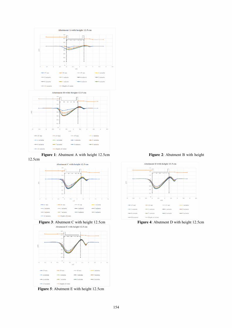
154

Figure 1: Abutment A with height 12.5cm Figure 2: Abutment B with height

12.5cm

Figure 3: Abutment C with height 12.5cm Figure 4: Abutment D with height 12.5cm

Figure 5: Abutment E with height 12.5cm

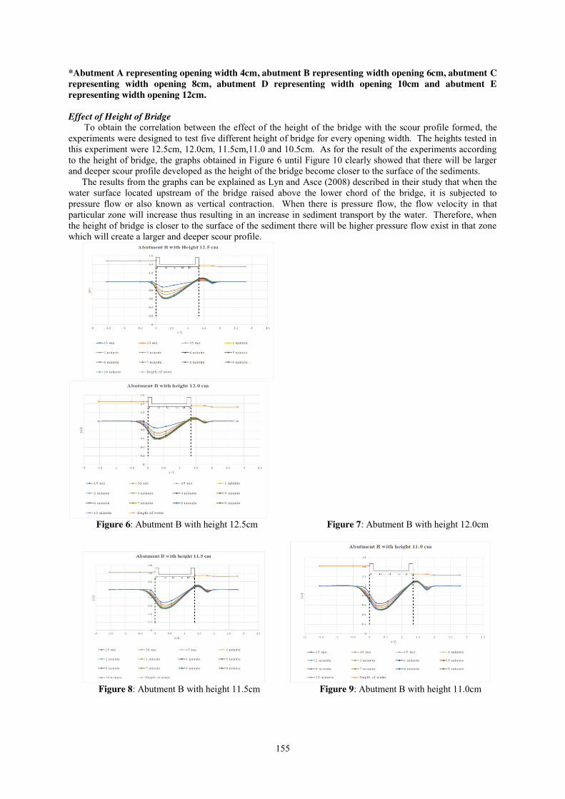
155

*Abutment A representing opening width 4cm, abutment B representing width opening 6cm, abutment C representing width opening 8cm, abutment D representing width opening 10cm and abutment E representing width opening 12cm. Effect of Height of Bridge

To obtain the correlation between the effect of the height of the bridge with the scour profile formed, the experiments were designed to test five different height of bridge for every opening width. The heights tested in this experiment were 12.5cm, 12.0cm, 11.5cm,11.0 and 10.5cm. As for the result of the experiments according to the height of bridge, the graphs obtained in Figure 6 until Figure 10 clearly showed that there will be larger and deeper scour profile developed as the height of the bridge become closer to the surface of the sediments.

The results from the graphs can be explained as Lyn and Asce (2008) described in their study that when the water surface located upstream of the bridge raised above the lower chord of the bridge, it is subjected to pressure flow or also known as vertical contraction. When there is pressure flow, the flow velocity in that particular zone will increase thus resulting in an increase in sediment transport by the water. Therefore, when the height of bridge is closer to the surface of the sediment there will be higher pressure flow exist in that zone which will create a larger and deeper scour profile.

Figure 6: Abutment B with height 12.5cm Figure 7: Abutment B with height 12.0cm

Figure 8: Abutment B with height 11.5cm Figure 9: Abutment B with height 11.0cm

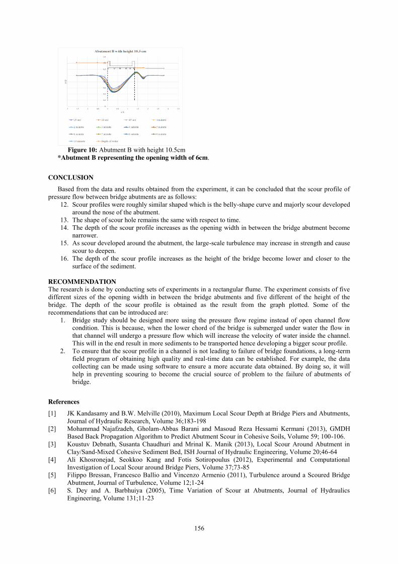
156

Figure 10: Abutment B with height 10.5cm *Abutment B representing the opening width of 6cm.

CONCLUSION

Based from the data and results obtained from the experiment, it can be concluded that the scour profile of pressure flow between bridge abutments are as follows:

12. Scour profiles were roughly similar shaped which is the belly-shape curve and majorly scour developed around the nose of the abutment.

13. The shape of scour hole remains the same with respect to time. 14. The depth of the scour profile increases as the opening width in between the bridge abutment become

narrower. 15. As scour developed around the abutment, the large-scale turbulence may increase in strength and cause

scour to deepen. 16. The depth of the scour profile increases as the height of the bridge become lower and closer to the

surface of the sediment. RECOMMENDATION The research is done by conducting sets of experiments in a rectangular flume. The experiment consists of five different sizes of the opening width in between the bridge abutments and five different of the height of the bridge. The depth of the scour profile is obtained as the result from the graph plotted. Some of the recommendations that can be introduced are:

1. Bridge study should be designed more using the pressure flow regime instead of open channel flow condition. This is because, when the lower chord of the bridge is submerged under water the flow in that channel will undergo a pressure flow which will increase the velocity of water inside the channel. This will in the end result in more sediments to be transported hence developing a bigger scour profile.

2. To ensure that the scour profile in a channel is not leading to failure of bridge foundations, a long-term field program of obtaining high quality and real-time data can be established. For example, the data collecting can be made using software to ensure a more accurate data obtained. By doing so, it will help in preventing scouring to become the crucial source of problem to the failure of abutments of bridge.

References

[1] JK Kandasamy and B.W. Melville (2010), Maximum Local Scour Depth at Bridge Piers and Abutments, Journal of Hydraulic Research, Volume 36;183-198

[2] Mohammad Najafzadeh, Gholam-Abbas Barani and Masoud Reza Hessami Kermani (2013), GMDH Based Back Propagation Algorithm to Predict Abutment Scour in Cohesive Soils, Volume 59; 100-106.

[3] Koustuv Debnath, Susanta Chaudhuri and Mrinal K. Manik (2013), Local Scour Around Abutment in Clay/Sand-Mixed Cohesive Sediment Bed, ISH Journal of Hydraulic Engineering, Volume 20;46-64

[4] Ali Khosronejad, Seokkoo Kang and Fotis Sotiropoulus (2012), Experimental and Computational Investigation of Local Scour around Bridge Piers, Volume 37;73-85

[5] Filippo Bressan, Francesco Ballio and Vincenzo Armenio (2011), Turbulence around a Scoured Bridge Abutment, Journal of Turbulence, Volume 12;1-24

[6] S. Dey and A. Barbhuiya (2005), Time Variation of Scour at Abutments, Journal of Hydraulics Engineering, Volume 131;11-23

157

[7] H. Azamathulla (2012), Gene-expression Programming to Predict Scour at a Bridge Abutment, Journal of Hydroinformatics, Volume 14;324-331

[8] Stephen E. Coleman, Christine S. Lauchlan and Bruce W. Melville (2003), Clear Water Scour Development at Bridge Abutments, Journal of Hydraulics Research, Volume 41;521-531From Experimental Testing of the In-Plane Capacity of Walls to Building Response Simulation. Journal of Earthquake Engineering (Vol. 15).

Hydraulic and Mechanic of Riparian Vegatated Natural Compound

Meandering River Muhammad Nazmi Akmal Bin Masri, Zulkiflee Bin Ibrahim

Faculty of Civil Engineering, Universiti Teknologi Malaysia, Malaysia

mienazmi094@gmail.com

Keywords: Flooding; Meandering Natural River; Riparian Vegatation; River Profile; Hydraulic Roughness. ABSTRACT. Flooding is a common disaster and no longer surprise in Malaysia. Mostly every year, this disaster will hit the Peninsular Malaysia or Borneo part at least once. Mostly river in Malaysia can be categorising as a meandering river. Therefore, the studies of this type of river become important to gain a better understanding to solve this problem. The key objectives of this research are to investigate the characteristic of meandering natural river; river profile and velocity along the channel, in addition, to studying the effect of riparian vegetation on the hydraulic roughness of the floodplain. 1:200 scale-downed main channel was built and performed using a rectangular flume in the Hydraulics Laboratory, Faculty of Civil Engineering, Universiti Teknologi Malaysia (UTM). From the result, it shown that the presences of riparian tress have a significant effect on river profile, flow velocity and roughness of channel. Result from this experiment was useful to study hydraulic and mechanic during flooding event in future.

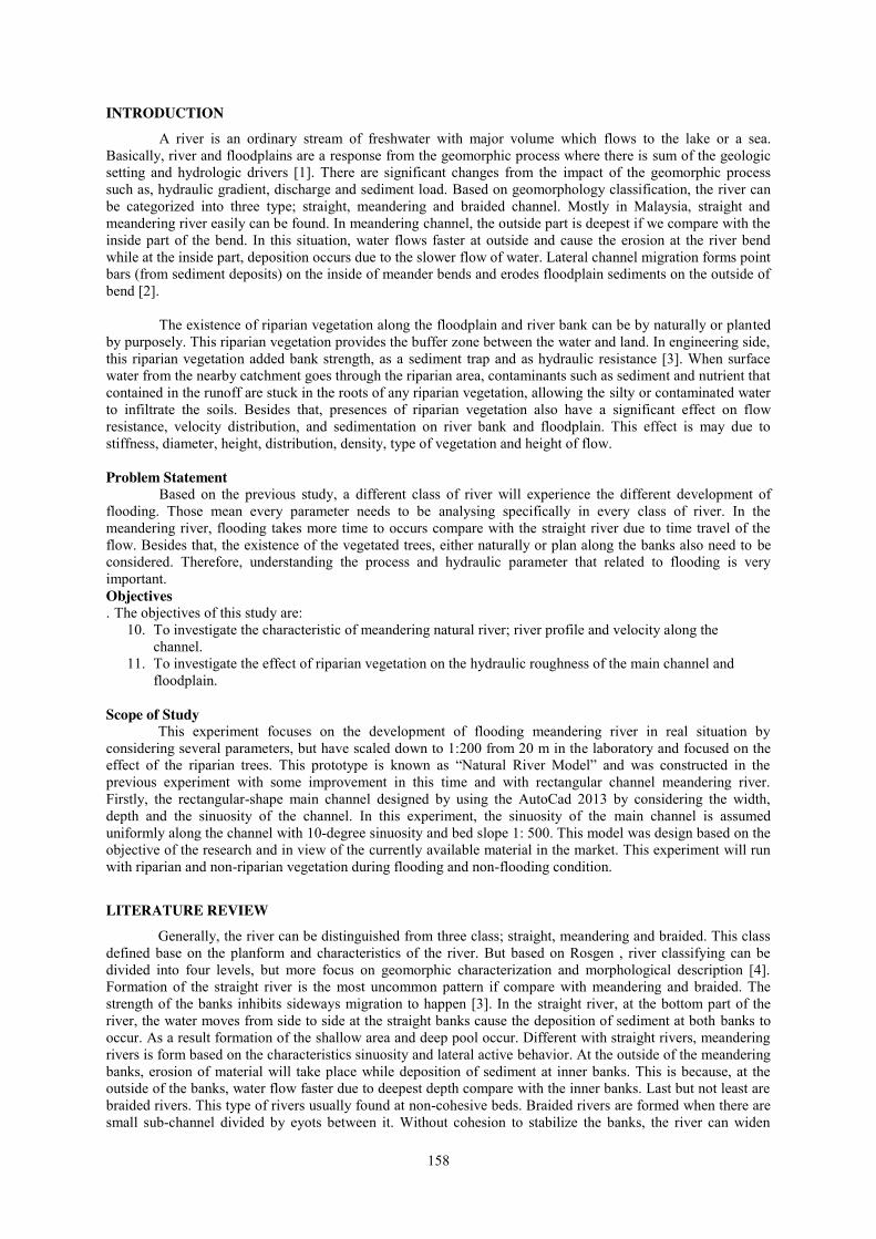
158

INTRODUCTION

A river is an ordinary stream of freshwater with major volume which flows to the lake or a sea. Basically, river and floodplains are a response from the geomorphic process where there is sum of the geologic setting and hydrologic drivers [1]. There are significant changes from the impact of the geomorphic process such as, hydraulic gradient, discharge and sediment load. Based on geomorphology classification, the river can be categorized into three type; straight, meandering and braided channel. Mostly in Malaysia, straight and meandering river easily can be found. In meandering channel, the outside part is deepest if we compare with the inside part of the bend. In this situation, water flows faster at outside and cause the erosion at the river bend while at the inside part, deposition occurs due to the slower flow of water. Lateral channel migration forms point bars (from sediment deposits) on the inside of meander bends and erodes floodplain sediments on the outside of bend [2].

The existence of riparian vegetation along the floodplain and river bank can be by naturally or planted

by purposely. This riparian vegetation provides the buffer zone between the water and land. In engineering side, this riparian vegetation added bank strength, as a sediment trap and as hydraulic resistance [3]. When surface water from the nearby catchment goes through the riparian area, contaminants such as sediment and nutrient that contained in the runoff are stuck in the roots of any riparian vegetation, allowing the silty or contaminated water to infiltrate the soils. Besides that, presences of riparian vegetation also have a significant effect on flow resistance, velocity distribution, and sedimentation on river bank and floodplain. This effect is may due to stiffness, diameter, height, distribution, density, type of vegetation and height of flow.

Problem Statement

Based on the previous study, a different class of river will experience the different development of flooding. Those mean every parameter needs to be analysing specifically in every class of river. In the meandering river, flooding takes more time to occurs compare with the straight river due to time travel of the flow. Besides that, the existence of the vegetated trees, either naturally or plan along the banks also need to be considered. Therefore, understanding the process and hydraulic parameter that related to flooding is very important. Objectives . The objectives of this study are:

10. To investigate the characteristic of meandering natural river; river profile and velocity along the channel.

11. To investigate the effect of riparian vegetation on the hydraulic roughness of the main channel and floodplain.

Scope of Study This experiment focuses on the development of flooding meandering river in real situation by

considering several parameters, but have scaled down to 1:200 from 20 m in the laboratory and focused on the effect of the riparian trees. This prototype is known as “Natural River Model” and was constructed in the previous experiment with some improvement in this time and with rectangular channel meandering river. Firstly, the rectangular-shape main channel designed by using the AutoCad 2013 by considering the width, depth and the sinuosity of the channel. In this experiment, the sinuosity of the main channel is assumed uniformly along the channel with 10-degree sinuosity and bed slope 1: 500. This model was design based on the objective of the research and in view of the currently available material in the market. This experiment will run with riparian and non-riparian vegetation during flooding and non-flooding condition.

LITERATURE REVIEW

Generally, the river can be distinguished from three class; straight, meandering and braided. This class defined base on the planform and characteristics of the river. But based on Rosgen , river classifying can be divided into four levels, but more focus on geomorphic characterization and morphological description [4]. Formation of the straight river is the most uncommon pattern if compare with meandering and braided. The strength of the banks inhibits sideways migration to happen [3]. In the straight river, at the bottom part of the river, the water moves from side to side at the straight banks cause the deposition of sediment at both banks to occur. As a result formation of the shallow area and deep pool occur. Different with straight rivers, meandering rivers is form based on the characteristics sinuosity and lateral active behavior. At the outside of the meandering banks, erosion of material will take place while deposition of sediment at inner banks. This is because, at the outside of the banks, water flow faster due to deepest depth compare with the inner banks. Last but not least are braided rivers. This type of rivers usually found at non-cohesive beds. Braided rivers are formed when there are small sub-channel divided by eyots between it. Without cohesion to stabilize the banks, the river can widen

159

itself by lateral erosion and form new channel [3]. In braided rivers, the discharge changes regularly cause a lot of sediment to form with a steep gradient.

During the flooding condition, the water will overflow from the channel or stream with the high

discharge to the surrounding area. This area is known as floodplains. Floodplain also can be defined as an area that is periodically inundated by the lateral overflow of river, lakes, direct precipitation or groundwater [5]. The deposited sediment at the floodplain area is known as alluvium. This alluvium is suitable for farmland because it contains very fertile soil. The width of the floodplain is affected by the sinuosity of the river and the lateral migration. The bigger meander migration erosion, the wider the floodplain area.

The open channel is a canal has a free surface of flow that exposed to the atmospheric pressure. The

open channel also can happen in close conduit in the condition the water only flowing partially full. It can be classified by man-made or presence by naturally. In the man-made channel, the channel characteristic is prismatic. Prismatic mean it has constant bed slope, cross section, and relative straight line while in the natural channel it characteristics are vice versa [6]. In open channel depth of flow, the discharge, and the slopes of the channel bottom and of the free surface are interdependent so it more difficult to analyse compare with close conduit [7]. To differentiate types of flow, it needs to consider the change of depth with respect to time and space. Under the change of depth with respect to the time there is two type of flow which is steady and unsteady flow. During steady flow, the depth of flow does not change with time, but in unsteady flow the depth change with time [7]. For flow under change of depth with respect to space also have two type of flow; uniform and non-uniform flow. Uniform flow means the depth of flow does not vary with distance, while non-uniform flow varies with time. Non-uniform flow also can be called as varied flow.

In open channel, the velocity always varies across the channel section due to the free surface and

friction. This friction is caused by the contact between the water flow and the boundary along the channel. Usually, the maximum velocity can be found just below the surface or in specific 0.05 to 0.25 of the depth from the surface [8]. The best explanation for this situation is the presence of resistance in the water or air interface and the secondary currents which are circulating from the boundaries toward the section center. This has been proving in the 3d simulation and in the laboratory. Permissible velocity can be divided into two; minimum and maximum. Minimum permissible velocity (Vmin) mean the lowest velocity that will prevent sedimentation and vegetative growth in the channel, while, maximum permissible velocity (Vmax) is the maximum velocity that allows the in the channel without causing scout or erosion of the channel material.

To estimate the flow resistance the most important parameter need to consider is velocity. For this

experiment, Manning equation was used to determine the flow resistance. Flow resistance is the product of velocity multiple by the area [6]. Based on Chow there are several factors that affecting the Manning’s roughness coefficient such as channel irregularity, channel alignment, silting and scouring, size and shape of the channel, stage, and discharge, obstruction, suspended material and bed load, seasonal change, vegetation, and surface roughness [7].

METHODOLOGY

The experiment was carried out on the previous rectangular flume with dimension 4.0 m long, 1.2 m width and 0.6 m high. This flume was modified from the previous study by maintaining the old soil. From the result it shows that, D50 for soil sample can be classified as a sand fraction for coarse sand [9]. From the British Standard Part 2, coarse sand range 0.6 mm to 2 mm. The improvement for this experiment was, the flume was provided by bracing. Bracing was provided to increase the strength to the wall caused by the hydrostatic pressure caused by the water flow in the flume. Besides that, the existence water pump also has been replaced by a new one. The main reason to replace the existence pump is to provide sufficient flow along the channel since the dimension of the main channel has been changed. The maximum discharge from the new pump was 5.71L/s compare with the existing pump only 0.67L/s. The longitudinal bed slope main channel for this experiment is 1:500 with sinuosity index 1.02. Therefore, surveying work needs to conduct first to levelling the bed slope. The equipment required in this levelling work such as levelling staff, tripod and theodolite. The compound channel consists of a meandering channel with a rectangular shape with double floodplain. The dimension of the main channel was 100 mm width and 75 mm depth along the channel. The rod with 0.5 cm diameter and 10 cm height was used represent as the vegetation on the floodplain. This steel rod was arranged with 2 cm (4d) spacing between each other as shown in Figure 2(b).

In this experiment, there are five selected chainage for collected the data which is CH785, CH1065, CH1315, CH1615 and CH1895. Since the bed profile was measured using point gauge, the reference point need to be decide. In this experiment, the reference point was set at the concrete at the upstream. Every measurement

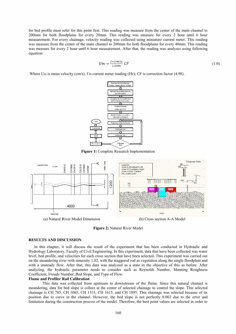
160

for bed profile must refer for this point first. This reading was measure from the center of the main channel to 200mm for both floodplains for every 20mm. This reading was measure for every 2 hour until 6 hour measurement. For every chainage, velocity reading was collected using miniature current meter. This reading was measure from the center of the main channel to 200mm for both floodplains for every 40mm. This reading was measure for every 2 hour until 6 hour measurement. After that, the reading was analyses using following equation:

𝑈𝑚 = 𝑓+3.90161.3399

𝐶𝐹 (1.0)

Where Um is mean velocity (cm/s); f is current meter reading (Hz); CF is correction factor (4.98).

Figure 1: Complete Research Implementation

(a) Natural River Model Dimension (b) Cross section A-A Model

Figure 2: Natural River Model

RESULTS AND DISCUSSION

In this chapter, it will discuss the result of the experiment that has been conducted in Hydraulic and Hydrology Laboratory, Faculty of Civil Engineering. In this experiment, data that have been collected was water level, bed profile, and velocities for each cross section that have been selected. This experiment was carried out on the meandering river with sinuosity 1.02, with the staggered rod as vegetation along the single floodplain and with a unsteady flow. After that, this data was analyzed as a state in the objective of this as before. After analyzing, the hydraulic parameter needs to consider such as Reynolds Number, Manning Roughness Coefficient, Froude Number, Bed Slope, and Type of Flow. Flume and Profiler Rail Calibration

This data was collected from upstream to downstream of the flume. Since this natural channel is meandering, data for bed slope is collect at the center of selected chainage to control the slope. This selected chainage is CH 785, CH 1065, CH 1315, CH 1615, and CH 1895. This chainage was selected because of its position due to curve in the channel. However, the bed slope is not perfectly 0.002 due to the error and limitation during the construction process of the model. Therefore, the best point values are selected in order to

161

obtain the channel bed slope values close to 0.002. Based on Figure 3, the channel bed slope is obtained through best fit line which generates a linear line.

Figure 3: Original Channel Bed Slope

Longitudinal Bed Profile

Figure 4 show the result of temporal changes in bed profile for each two hours. All channel bed level and cross section profile were measured using the point gauge. The original bed profile was set approximately to 1:500 and compares with the bed profile other bed profile for every two hours. Based on the result, it shows that temporal bed profile become steeper compare to the original bed profile. For the first two hours, the bed profile becomes steeper compared with the original bed slope with 47.62% changes while after six hours, the bed slope change with 71.42% . The summary of the bed slope can be simplified in Table 1 below. The process of slope changing shows there is the discrete particle that washes away by the water through the outlet channel.

Figure 4: Temporal changes on bed profile (So)

Mean Velocity

Based on the results shown in Figure 5, it follows the theoretically. Mean velocity higher at zone 1 due to increasing of water depth in the main channel compare to the both floodplain. While at floodplain zone 2 there are present of steel rod as riparian three, therefore the mean velocity at zone 2 little bit lower compare to zone 3 without any obstacle. Summarily, mean velocity at zone 1 was in range 0.19 m/s to 0.26 m/s, for zone 2 about 0.15 m/s to 0.20 m/s and for zone 3 about 0.17 m/s to 0.24 m/s.

y = -0.0021x + 30.299

242526272829

0 1000 2000 3000z

(mm

) CH. (mm)

y = -0.0021x + 30.299

y = -0.0031x + 32.904

y = -0.0029x + 32.497

y = -0.0036x + 34.091 22

24

26

28

30

32

34

36

0 500 1000 1500 2000 2500 3000

Z (m

m)

CH (mm)

Linear (0 Hr)

Linear (2 Hr)

Linear (4 Hr)

Linear (6 Hr)

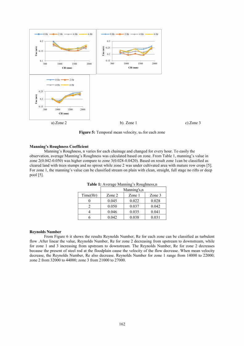
162

a).Zone 2 b). Zone 1 c).Zone 3

Figure 5: Temporal mean velocity, um for each zone

Manning’s Roughness Coefficient Manning’s Roughness, n varies for each chainage and changed for every hour. To easily the

observation, average Manning’s Roughness was calculated based on zone. From Table 1, manning’s value in zone 2(0.042-0.050) was higher compare to zone 3(0.028-0.0420). Based on result zone 1can be classified as cleared land with trees stumps and no sprout while zone 2 was under cultivated area with mature row crops [5]. For zone 1, the manning’s value can be classified stream on plain with clean, straight, full stage no rifts or deep pool [5].

Table 1: Average Manning’s Roughness,n

Manning's,n

Time(Hr) Zone 2 Zone 1 Zone 3 0 0.045 0.022 0.028 2 0.050 0.037 0.042 4 0.046 0.035 0.041 6 0.042 0.038 0.031

Reynolds Number From Figure 6 it shows the results Reynolds Number, Re for each zone can be classified as turbulent

flow .After linear the value, Reynolds Number, Re for zone 2 decreasing from upstream to downstream, while for zone 1 and 3 increasing from upstream to downstream. The Reynolds Number, Re for zone 2 decreases because the present of steel rod at the floodplain cause the velocity of the flow decrease. When mean velocity decrease, the Reynolds Number, Re also decrease. Reynolds Number for zone 1 range from 14000 to 22000; zone 2 from 32000 to 44000; zone 3 from 21000 to 27000.

0.1

0.15

0.2

500 1000 1500 2000

Um

(m/s)

CH (mm)

0 Hr 2 Hr 4 Hr 6 Hr

0.15

0.2

0.25

0.3

500 1000 1500 2000

Um

(m/s)

CH (mm)

0 Hr 2 Hr 4 Hr 6 Hr

0.15

0.2

0.25

500 1000 1500 2000

Um

(m/s)

CH (mm)

0 Hr 2 Hr

4 Hr 6 Hr

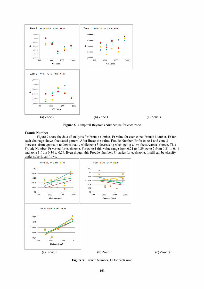
163

(a).Zone 2 (b).Zone 1 (c).Zone 3

Figure 6: Temporal Reynolds Number,Re for each zone

Froude Number Figure 7 show the data of analysis for Froude number, Fr value for each zone. Froude Number, Fr for

each chainage shows fluctuated pattern. After linear the value, Froude Number, Fr for zone 1 and zone 3 increases from upstream to downstream, while zone 3 decreasing when going down the stream as shown. This Froude Number, Fr varied for each zone. For zone 1 this value range from 0.21 to 0.29, zone 2 from 0.31 to 0.41 and zone 3 from 0.34 to 0.54. Even though this Froude Number, Fr varies for each zone, it still can be classify under subcritical flows.

(a). Zone 1 (b).Zone 2 (c).Zone 3

Figure 7: Froude Number, Fr for each zone

12000

14000

16000

18000

20000

22000

24000

500 1000 1500 2000

Re

CH (mm)

Zone 2 0 Hr 2 Hr 4 Hr 6 Hr

30000

34000

38000

42000

46000

500 1000 1500 2000

Re

CH (mm)

Zone 1 0 Hr 2 Hr 4 Hr 6 Hr

20000

22000

24000

26000

28000

30000

500 1000 1500 2000

Re

CH (mm)

Zone 3 0 Hr 2 Hr 4 Hr 6 Hr

0.2

0.22

0.24

0.26

0.28

0.3

500 1000 1500 2000

Fr

Chainage (mm)

0 Hr 2 Hr 4 Hr 6 Hr

0.3

0.32

0.34

0.36

0.38

0.4

0.42

500 1000 1500 2000

Fr

Chainage (mm)

0 Hr 2 Hr 4 Hr 6 Hr

0.34

0.39

0.44

0.49

0.54

500 1000 1500 2000

Fr

Chainage (mm)

0 Hr 2 Hr 4 Hr 6 Hr

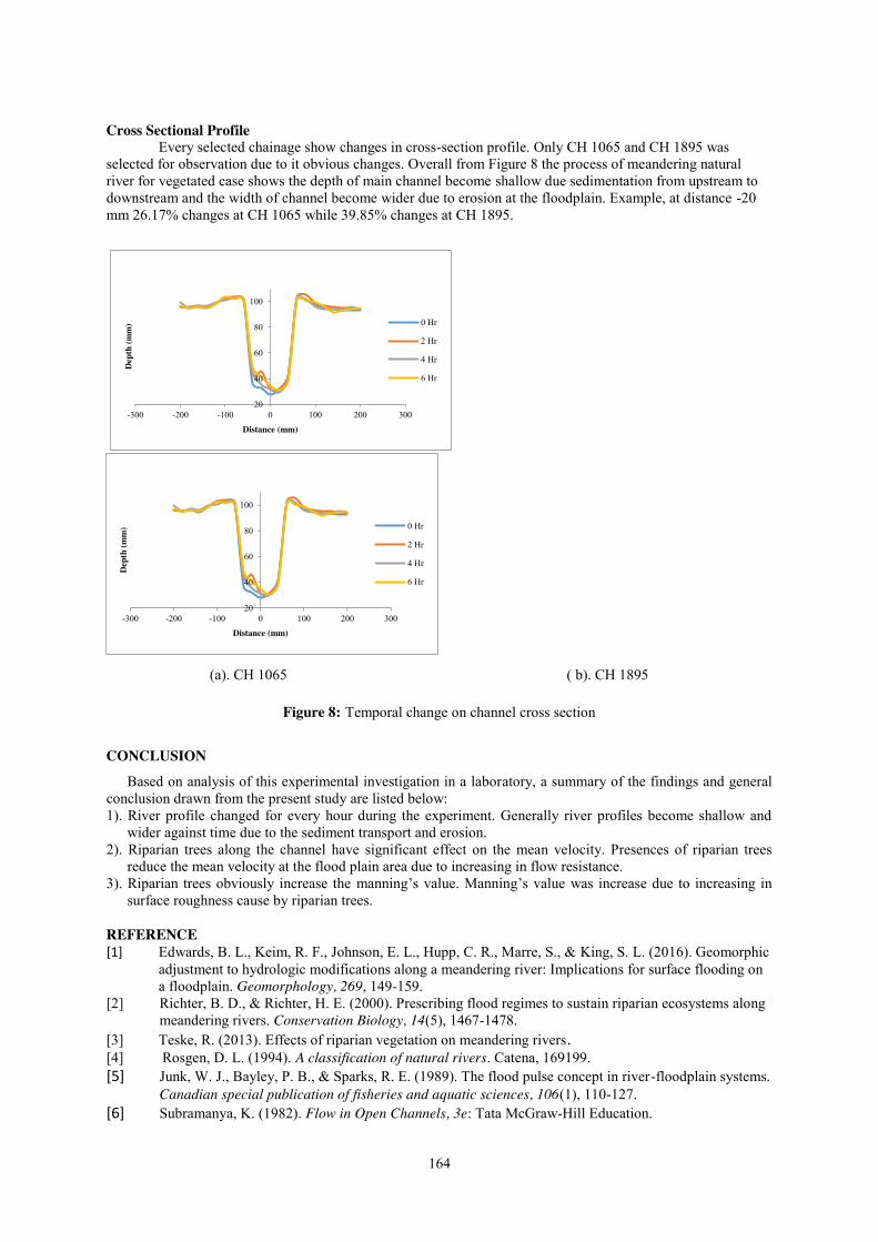
164

Cross Sectional Profile

Every selected chainage show changes in cross-section profile. Only CH 1065 and CH 1895 was selected for observation due to it obvious changes. Overall from Figure 8 the process of meandering natural river for vegetated case shows the depth of main channel become shallow due sedimentation from upstream to downstream and the width of channel become wider due to erosion at the floodplain. Example, at distance -20 mm 26.17% changes at CH 1065 while 39.85% changes at CH 1895.

(a). CH 1065 ( b). CH 1895

Figure 8: Temporal change on channel cross section

CONCLUSION

Based on analysis of this experimental investigation in a laboratory, a summary of the findings and general conclusion drawn from the present study are listed below: 1). River profile changed for every hour during the experiment. Generally river profiles become shallow and

wider against time due to the sediment transport and erosion. 2). Riparian trees along the channel have significant effect on the mean velocity. Presences of riparian trees

reduce the mean velocity at the flood plain area due to increasing in flow resistance. 3). Riparian trees obviously increase the manning’s value. Manning’s value was increase due to increasing in

surface roughness cause by riparian trees. REFERENCE [1] Edwards, B. L., Keim, R. F., Johnson, E. L., Hupp, C. R., Marre, S., & King, S. L. (2016). Geomorphic

adjustment to hydrologic modifications along a meandering river: Implications for surface flooding on a floodplain. Geomorphology, 269, 149-159.

[2] Richter, B. D., & Richter, H. E. (2000). Prescribing flood regimes to sustain riparian ecosystems along meandering rivers. Conservation Biology, 14(5), 1467-1478.

[3] Teske, R. (2013). Effects of riparian vegetation on meandering rivers. [4] Rosgen, D. L. (1994). A classification of natural rivers. Catena, 169199. [5] Junk, W. J., Bayley, P. B., & Sparks, R. E. (1989). The flood pulse concept in river-floodplain systems.

Canadian special publication of fisheries and aquatic sciences, 106(1), 110-127. [6] Subramanya, K. (1982). Flow in Open Channels, 3e: Tata McGraw-Hill Education.

20

40

60

80

100

-300 -200 -100 0 100 200 300

Dep

th (m

m)

Distance (mm)

0 Hr

2 Hr

4 Hr

6 Hr

20

40

60

80

100

-300 -200 -100 0 100 200 300

Dep

th (m

m)

Distance (mm)

0 Hr

2 Hr

4 Hr

6 Hr

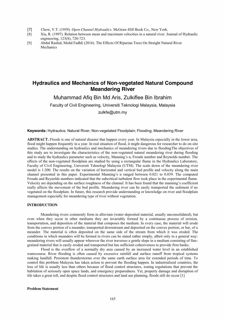
165

[7] Chow, V.T. (1959). Open Channel Hydraulics. McGraw-Hill Book Co., New York. [8] Xia, R. (1997). Relation between mean and maximum velocities in a natural river. Journal of Hydraulic

engineering, 123(8), 720-723. [9] Abdul Rashid, Mohd Fadhli (2016). The Effects Of Riparian Trees On Straight Natural River

Mechanics

Hydraulics and Mechanics of Non-vegetated Natural Compound Meandering River

Muhammad Afiq Bin Md Aris, Zulkiflee Bin Ibrahim Faculty of Civil Engineering, Universiti Teknologi Malaysia, Malaysia

zulkfe@utm.my

Keywords: Hydraulics; Natural River; Non-vegetated Floodplain; Flooding; Meandering River ABSTRACT. Floods is one of natural disaster that happen every year. In Malaysia especially in the lower area, flood might happen frequently in a year. In real situation of flood, it might dangerous for researcher to do on-site studies. The understanding on hydraulics and mechanics of meandering rivers due to floodingThe objectives of this study are to investigate the characteristics of the non-vegetated natural meandering river during flooding and to study the hydraulics parameter such as velocity, Manning’s n, Froude number and Reynolds number. The effects of the non-vegetated floodplain are studied by using a rectangular flume in the Hydraulics Laboratory, Faculty of Civil Engineering, Universiti Teknologi Malaysia (UTM). The scale down of the meandering river model is 1:200. The results on the variation of horizontal and vertical bed profile and velocity along the main channel presented in this paper. Experimental Manning’s n ranged between 0.021 to 0.039. The computed Froude and Reynolds numbers indicated that the subcritical turbulent flow took place in the experimental flume. Velocity are depending on the surface roughness of the channel. It has been found that the manning’s coefficient really affects the movement of the bed profile. Meandering river can be easily transported the sediment if no vegetated on the floodplain. In future, this research provide understanding or knowledge on river and floodplain management especially for meandering type of river without vegetation. INTRODUCTION

Meandering rivers commonly form in alluvium (water-deposited material, usually unconsolidated), but even when they occur in other mediums they are invariably formed by a continuous process of erosion, transportation, and deposition of the material that composes the medium. In every case, the material will erode from the convex portion of a meander, transported downstream and deposited on the convex portion, or bar, of a meander. The material is often deposited on the same side of the stream from which it was eroded. The conditions in which meanders will be formed in rivers can be stated rather simply, albeit only in a general way: meandering rivers will usually appear wherever the river traverses a gentle slope in a medium consisting of fine-grained material that is easily eroded and transported but has sufficient cohesiveness to provide firm banks.

Flood is the overflow of a normally dry area caused by an increased water level in an established watercourse. River flooding is often caused by excessive rainfall and surface runoff from tropical systems making landfall. Persistent thunderstorms over the same earth surface area for extended periods of time. To control this problem Malaysia has taken action to prevent the flooding happen. In industrialized countries, the loss of life is usually less than others because of flood control structures, zoning regulations that prevent the habitation of seriously open space lands, and emergency preparedness. Yet, property damage and disruption of life takes a great toll, and despite flood control structures and land use planning, floods still do occur [1]

Problem Statement

166

Lately, unexpected heavy rain resulted in two consecutive waves of flash floods hitting the southern and south-western coasts of Peninsular Malaysia. This is due to Malaysia have climate equator which is hot and humid year-round with higher an average annual rainfall. Other than that, human activities also contribute to flooding such as the development they were developed without a care about the environment and the vegetation around the river and forestry. Water flow has big destructive power. When a river overflows its banks or the sea drives inland, structures poorly equipped to withstand the water's strength are no match. Bridges, houses, trees, and cars can be picked up and carried off. The erosive force of moving water can drag dirt from under a building's foundation, causing it to crack and tumble.

A flood occurs when a river blasts its banks and the water spills onto the floodplain. Flooding has a tendency to be caused by heavy rain. The faster the rain drops reaches the river channel, the more likely it is to flood. The nature of the landscape around a river will influence how quickly rainwater reaches the channel. Every channel is surrounded by steep slopes cause fast surface run-off. Vegetation also important but because of human activities, floodplain area has no vegetation and it will lead to flooding. Case study on-site are very dangerous and take a long time. Lab-scale study can be considered to get the result. Objectives

This study is conducted to gain more understanding about the development of meandering river behavior from the same discharge vegetated and non-vegetated flood event. The aims of the study are to gather the information about the development of natural river behavior. The objective of the research are to study meandering river mechanics are as follows:

i. To study the temporal hydraulic parameters such as velocity, Reynolds Number, Froude Number and Manning’s Roughness Coefficient in the non-vegetated meandering river during a flooding event.

ii. To investigate the characteristic of meandering natural river; river profile along the channel Scope Of Study

This research is focussing more on experimental work in the laboratory and meandering natural river mechanics. Before that, based on a research study of previous researcher scope. After that making the improvement from previous research about the research and it is more to planning and design of channel model which is meandering river using AutoCad software. This studies will be conducted depending on a few hydraulics parameters such as the different discharge of vegetated and non-vegetated during flooding events. This study is carried out in the Hydraulics and Hydrology Laboratory Faculty of Civil Engineering Universiti Teknologi Malaysia, Johor Bahru, Johor. A physical Model is known as the “Natural River Model” was constructed in the laboratory. This model has been improvising from the previous researcher. Based on the objective to design the natural river mechanic model with AutoCAD 2013 with appropriate available material and apparatus that can be accessed in Peninsular Malaysia and provided space in Faculty of Civil Engineering Laboratory. Most of the material and apparatus is sure can be accessed but with improvement. The bed slope of this research used is approximately 1:500 ratio. The inflow discharge is constant with changes of time that is 5.71 l/s. The sinuosity index is also constant with value of 1.02 along the channel. For the data that will be collected, the depth of water and the level of channel bed are recorded to investigate the uniformity of the water flow. Velocity in the main channel is recorded at 4 cross-sections in the channel to determine the average water discharge. Graph bed morphologies and Manning’s n roughness coefficient within time are plotted.

LITERATURE REVIEW

Streams and rivers form an important link in the hydrological cycle and, in that capacity, provide freshwater for depletion and irrigation [2]. Through their watershed, they also gather, carry and distribute almost any substance that enters the water on land. Streams and rivers are thus main characteristics of environmental transport and fate. Natural river channels characteristically exhibit alternating pools or deep reaches and riffles or shallow reaches, regardless of the type of pattern [3].

Meandering river, the mechanics of formation of meanders is reasonably well understood. The meandering river has a curve which is happened to erode and sediment the river width. When flow enters a channel bed, a form of helix secondary current is set up that increases flow velocity and channel depth along the outer bank in proportion to bed curvature, which encourages bank erosion. The secondary current has a natural downstream scale related to low velocity and depth; this results in a gradual increase in bend amplitude and propagation of the meandering pattern upstream and downstream.

Sinuosity is one of the channel types that a stream may assume over all or part of its course. All streams are sinuous at some time in their geologic history over some part of their length. To compare, the straight channel sinuosity index must be less than 1.10. If more than 1.10 but less than 1.50 we can call the river is sinuous river. The sinuosity of a meandering stream has a tendency to approach a critical state at which the opposing forces which create and cut off meanders interact in such a way that sinuosity fluctuates around a

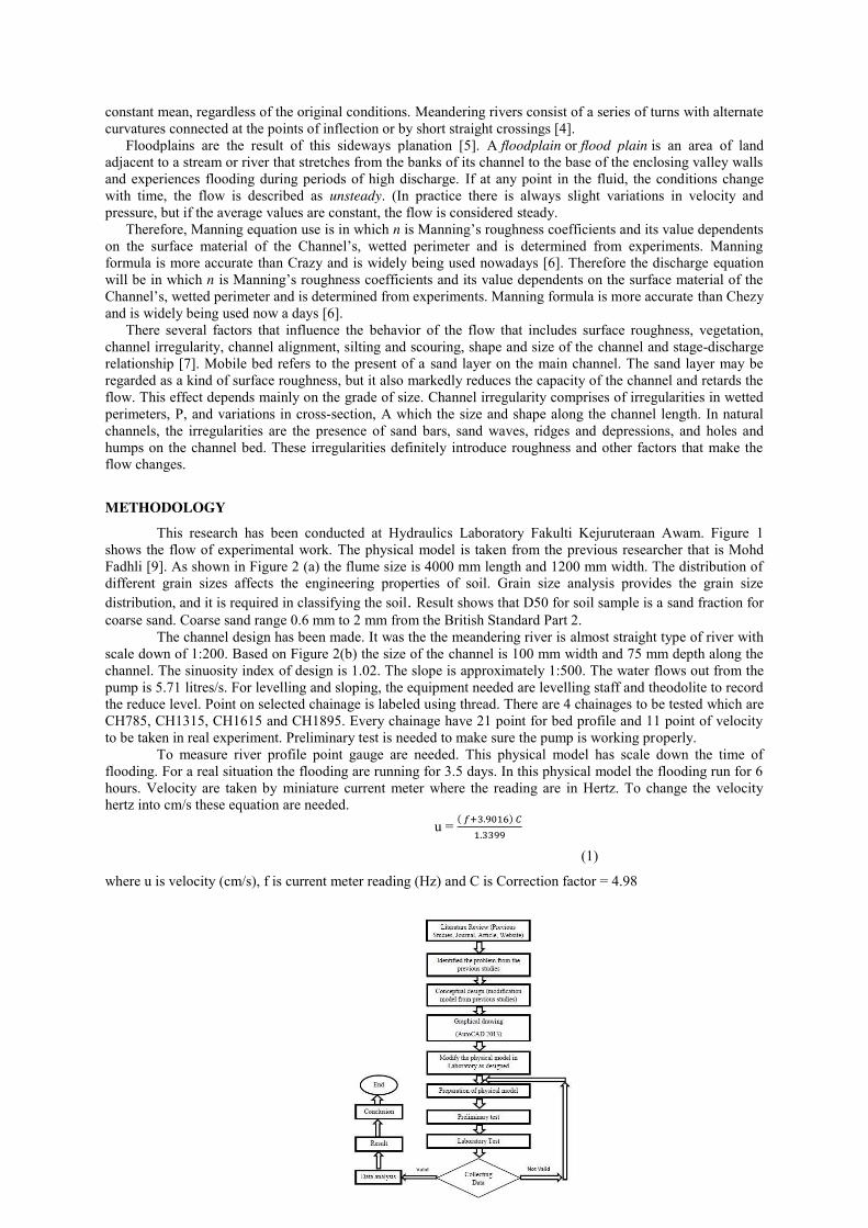
167

constant mean, regardless of the original conditions. Meandering rivers consist of a series of turns with alternate curvatures connected at the points of inflection or by short straight crossings [4].

Floodplains are the result of this sideways planation [5]. A floodplain or flood plain is an area of land adjacent to a stream or river that stretches from the banks of its channel to the base of the enclosing valley walls and experiences flooding during periods of high discharge. If at any point in the fluid, the conditions change with time, the flow is described as unsteady. (In practice there is always slight variations in velocity and pressure, but if the average values are constant, the flow is considered steady.

Therefore, Manning equation use is in which n is Manning’s roughness coefficients and its value dependents on the surface material of the Channel’s, wetted perimeter and is determined from experiments. Manning formula is more accurate than Crazy and is widely being used nowadays [6]. Therefore the discharge equation will be in which n is Manning’s roughness coefficients and its value dependents on the surface material of the Channel’s, wetted perimeter and is determined from experiments. Manning formula is more accurate than Chezy and is widely being used now a days [6].

There several factors that influence the behavior of the flow that includes surface roughness, vegetation, channel irregularity, channel alignment, silting and scouring, shape and size of the channel and stage-discharge relationship [7]. Mobile bed refers to the present of a sand layer on the main channel. The sand layer may be regarded as a kind of surface roughness, but it also markedly reduces the capacity of the channel and retards the flow. This effect depends mainly on the grade of size. Channel irregularity comprises of irregularities in wetted perimeters, P, and variations in cross-section, A which the size and shape along the channel length. In natural channels, the irregularities are the presence of sand bars, sand waves, ridges and depressions, and holes and humps on the channel bed. These irregularities definitely introduce roughness and other factors that make the flow changes.

METHODOLOGY

This research has been conducted at Hydraulics Laboratory Fakulti Kejuruteraan Awam. Figure 1 shows the flow of experimental work. The physical model is taken from the previous researcher that is Mohd Fadhli [9]. As shown in Figure 2 (a) the flume size is 4000 mm length and 1200 mm width. The distribution of different grain sizes affects the engineering properties of soil. Grain size analysis provides the grain size distribution, and it is required in classifying the soil. Result shows that D50 for soil sample is a sand fraction for coarse sand. Coarse sand range 0.6 mm to 2 mm from the British Standard Part 2.

The channel design has been made. It was the the meandering river is almost straight type of river with scale down of 1:200. Based on Figure 2(b) the size of the channel is 100 mm width and 75 mm depth along the channel. The sinuosity index of design is 1.02. The slope is approximately 1:500. The water flows out from the pump is 5.71 litres/s. For levelling and sloping, the equipment needed are levelling staff and theodolite to record the reduce level. Point on selected chainage is labeled using thread. There are 4 chainages to be tested which are CH785, CH1315, CH1615 and CH1895. Every chainage have 21 point for bed profile and 11 point of velocity to be taken in real experiment. Preliminary test is needed to make sure the pump is working properly.

To measure river profile point gauge are needed. This physical model has scale down the time of flooding. For a real situation the flooding are running for 3.5 days. In this physical model the flooding run for 6 hours. Velocity are taken by miniature current meter where the reading are in Hertz. To change the velocity hertz into cm/s these equation are needed.

u = ( 𝑓+3.9016) 𝐶1.3399

(1)

where u is velocity (cm/s), f is current meter reading (Hz) and C is Correction factor = 4.98

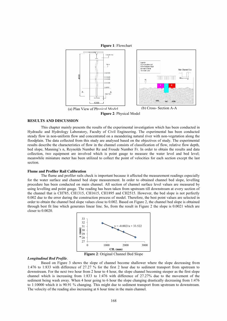
168

(a) Plan View of Physical Model (b) Cross- Section A-A Figure 2: Physical Model

Figure 1: Flowchart

RESULTS AND DISCUSSION This chapter mainly presents the results of the experimental investigation which has been conducted in

Hydraulic and Hydrology Laboratory, Faculty of Civil Engineering. The experimental has been conducted steady flow in non-uniform flow and concentrated on a meandering natural river with non-vegetation along the floodplain. The data collected from this study are analysed based on the objectives of study. The experimental results describe the characteristics of flow in the channel consists of classification of flow, relative flow depth, bed slope, Manning’s n, Reynolds Number Re and Froude Number Fr. In order to obtain the results and data collection, two equipment are involved which is point gauge to measure the water level and bed level; meanwhile miniature meter has been utilized to collect the point of velocities for each section except the last section. Flume and Profiler Rail Calibration

The flume and profiler rails check is important because it affected the measurement readings especially for the water surface and channel bed slope measurement. In order to obtained channel bed slope, levelling procedure has been conducted on main channel. All section of channel surface level values are measured by using levelling and point gauge. The reading has been taken from upstream till downstream at every section of the channel that is CH785, CH1315, CH1615, CH1895 and CH2515. However, the bed slope is not perfectly 0.002 due to the error during the construction process of model. Therefore, the best point values are selected in order to obtain the channel bed slope values close to 0.002. Based on Figure 2, the channel bed slope is obtained through best fit line which generates linear line. So, from the result in Figure 2 the slope is 0.0021 which are closer to 0.0020.

Figure 2: Original Channel Bed Slope

Longitudinal Bed Profile. Based on Figure 3 shows the slope of channel become shallower where the slope decreasing from

1:476 to 1:833 with difference of 27.27 % for the first 2 hour due to sediment transport from upstream to downstream. For the next two hour from 2 hour to 4 hour, the slope channel becoming steeper as the first slope channel which is increasing from 1:833 to 1:476 with difference of 27.27% due to the movement of the sediment being wash away. When 4 hour going to 6 hour the slope changing drastically decreasing from 1:476 to 1:10000 which it is 90.91 % changing. This might due to sediment transport from upstream to downstream. The velocity of the reading also increasing at 6 hour time in the main channel.

y = -0.0021x + 33.522

27282930313233

0 1000 2000 3000

z (m

m)

CH. (mm)

FPR MC FPL

169

0.15

0.17

0.19

0.21

0.23

0.25

600 1100 1600 2100

Vel

ocity

(m/s

)

CH (mm)

0 Hr 2 Hr

4 Hr 6 Hr

(c) Floodplain Left, FPL (a) Main Channel, MC (b) Floodplain Right, FPR

0.150.170.190.210.230.250.27

600 1100 1600 2100

Vel

ocity

(m/s

)

CH (mm)

0 Hr 2 Hr

4 Hr 6 Hr

Figure 3: Main Channel Bed Slope

Velocity From Figure 4 (a) average velocity during Hour 4 of running the laboratory test are higher at Zone FPL.

Hour 0 result shows that the starting velocity is lower compared to 2, 4 and 6 hours but overall results shows that at upstream have high velocity compare to downtream. Figure 4 (b) shows that Hour 6 average velocity at main channel are higher than other hour. It is also shows that upstream velocity become slower and the dowstream was starting high velocity. This is because of the main channel have occur the erosion of soil especially the curvature of the main channel. Nextly, Figure 4 (c) shows that average velocity during 6 hour of running the laboratory test are higher at Zone FPR. 0 Hour result shows that the starting velocity is lower compared to 2, 4 and 6 hours. FPR also shows that the velocity at upstream are lower than downstream. *FPR is Floodplain Right which is from centre the distance start from 50mm to 200mm. MC is Main Channel which is from centre the distance start from 0mm to 50mm and -50mm. FPL is Floodplain Left which is from centre the distance start from -50mm to -200mm *CH785 are located at upstream and the slope is approximately 1:500 until the chainage CH1895 which is located at downstream

Figure 4: Zonal Average Temporal Velocity

Manning Roughness Coefficient

Manning’s n value for non-vegetated case is increase then decrease within a time provided. From the Table 1 the result for manning’s n value should be increasing because the sediment transport from upstream to downstream cause the river become shallow in the main channel, MC and this value match with Clean, straight, full stage, no rifts or deep pools (0.025-0.033) on site experiment [8]. FPR Manning’s n becoming up and down and FPL Manning’s n are increasing with time and it can match the cultivated area with no crop (0.02-0.04) ) on site experiment [8].

Table 1: Zonal Average Temporal Manning Roughness Coefficient, n

Time (Hr)

Manning, n FPL MC FPR

y = -0.0021x + 33.522

y = -0.0012x + 32.864 y = -0.0021x + 34.416

y = -0.0001x + 31.652

2829303132333435

600 1100 1600 2100 2600 3100

Dep

th (m

m)

CH (mm)

0 Hr 2 Hr 4 Hr 6 Hr

0.15

0.17

0.19

0.21

0.23

600 1100 1600 2100

Vel

ocity

(m/s

)

CH (mm)

0 Hr 2 Hr

4 Hr 6 Hr

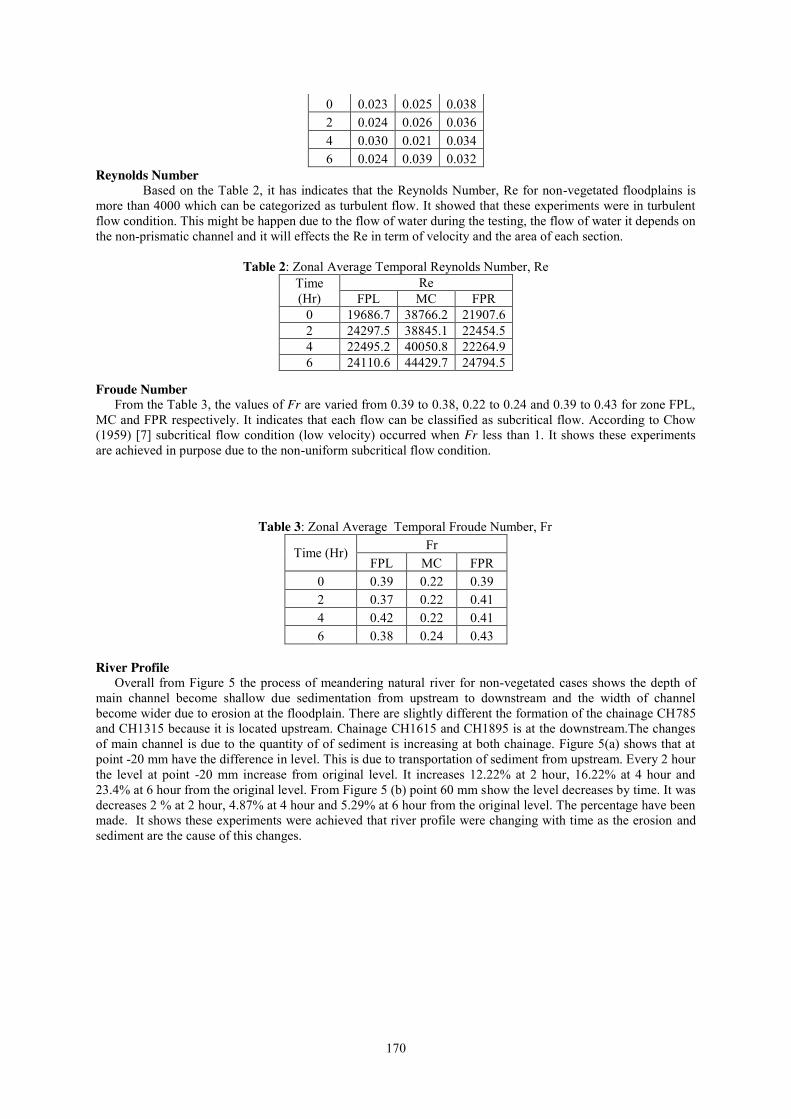
170

0 0.023 0.025 0.038 2 0.024 0.026 0.036 4 0.030 0.021 0.034 6 0.024 0.039 0.032

Reynolds Number Based on the Table 2, it has indicates that the Reynolds Number, Re for non-vegetated floodplains is

more than 4000 which can be categorized as turbulent flow. It showed that these experiments were in turbulent flow condition. This might be happen due to the flow of water during the testing, the flow of water it depends on the non-prismatic channel and it will effects the Re in term of velocity and the area of each section.

Table 2: Zonal Average Temporal Reynolds Number, Re

Froude Number

From the Table 3, the values of Fr are varied from 0.39 to 0.38, 0.22 to 0.24 and 0.39 to 0.43 for zone FPL, MC and FPR respectively. It indicates that each flow can be classified as subcritical flow. According to Chow (1959) [7] subcritical flow condition (low velocity) occurred when Fr less than 1. It shows these experiments are achieved in purpose due to the non-uniform subcritical flow condition.

Table 3: Zonal Average Temporal Froude Number, Fr

Time (Hr) Fr FPL MC FPR

0 0.39 0.22 0.39 2 0.37 0.22 0.41 4 0.42 0.22 0.41 6 0.38 0.24 0.43

River Profile

Overall from Figure 5 the process of meandering natural river for non-vegetated cases shows the depth of main channel become shallow due sedimentation from upstream to downstream and the width of channel become wider due to erosion at the floodplain. There are slightly different the formation of the chainage CH785 and CH1315 because it is located upstream. Chainage CH1615 and CH1895 is at the downstream.The changes of main channel is due to the quantity of of sediment is increasing at both chainage. Figure 5(a) shows that at point -20 mm have the difference in level. This is due to transportation of sediment from upstream. Every 2 hour the level at point -20 mm increase from original level. It increases 12.22% at 2 hour, 16.22% at 4 hour and 23.4% at 6 hour from the original level. From Figure 5 (b) point 60 mm show the level decreases by time. It was decreases 2 % at 2 hour, 4.87% at 4 hour and 5.29% at 6 hour from the original level. The percentage have been made. It shows these experiments were achieved that river profile were changing with time as the erosion and sediment are the cause of this changes.

Time (Hr)

Re FPL MC FPR

0 19686.7 38766.2 21907.6 2 24297.5 38845.1 22454.5 4 22495.2 40050.8 22264.9 6 24110.6 44429.7 24794.5

171

(a) Chainage CH1615 (b) Chainage CH1895

Figure 5: Temporal River Profile

CONCLUSION This research presents characteristic of meandering river for non-vegetated floodplain during flooding.

Based on analysis of experiments on flow characteristics in physical model which is investigated in a laboratory, a summary of the findings and general conclusion are drawn from the present study are listed.

17. The velocity at the upstream is higher than downstream when it is flow on FPL. Mean velocity at FPR and MC are higher at the downstream compare to upstream. Average velocity are changing with time.

18. Froude Number is less than 1 and it is shows that Fr<1 is subcritical flow and the Reynold Number is more than 4000 which it indicates the flow is turbulant.

19. Manning Roughness Coefficient show the value of main channel characteristic can match with natural river Clean, straight, full stage, no rifts or deep pools. For both floodplain the value shows it’s characteristic can match with floodplain where it is cultivated area with no crop.

20. The meandering river does affect the changing of river profile with it’s sinuosity, the erosion are happened at the edge of main channel as the water flow. Sediment transport from upstream to downstream also affect the river profile. River profile at each chainage are changing with time. Both floodplain and main channel have erossion and sediment transport from preceded area.

REFERENCES [1] Nelson, J. D. (1989). River Meandering. Evolution and Stability of Erodible Channel Beds, 321-377. [2] Chen, D., & Duan, J. G. (2006). Modeling width adjustment in meandering channels. Journal of

Hydrology, 321(1–4), 59–76. https://doi.org/10.1016/j.jhydrol.2005.07.034 [3] Leopold, L. B., & Maddock, T. J. (1953). The Hydraulic Geomtry of Stream Channels and Some

Physiographic Implications. Geological Survey Professional Paper 252, 57. [4] Subhasish, D. (2011). Fluvial Hydrodynamics. Sciences-New York. https://doi.org/10.1007/978-3-642-

19062-9 [5] Hancock, G. S., & Anderson, R. S. (2002). Numerical modelling of fluvial strath terrace formation in

response to oscillating climate. Geological Society of American Bulletin, 114(9), 1131–1142. https://doi.org/10.1130/0016-7606(2002)114<1131

[6] Naeem, R. K., & Mansoor, A. (2007). Scaling Aspects of Lyari River Flow Routing. Indus Journal of Management & Social Sciences, 1(2), 187–194.

[7] Chow, V.T. (1959). Open Channel Hydraulics. McGraw-Hill Book Co [8] Chow. (1959). Manning’s n values. Notes de cours.

0

20

40

60

80

100

120

-240 -200 -160 -120 -80 -40 0 40 80 120 160 200 240

Dep

th (m

m)

Distance (mm) 0 Hr 2 Hr 4 Hr 6 Hr

0

20

40

60

80

100

120

-240 -200 -160 -120 -80 -40 0 40 80 120 160 200 240

Dep

th (m

m)

Distance (mm) 0 Hr 2 Hr 4 Hr 6 Hr

172

[9] Abdul Rashid, Mohd Fadhli (2016). The Effects Of Riparian Trees On Straight Natural River Mechanics – Final Year Project

Modification and Testing of Bed Sediment Samplers Hamidah Abdul Hamid, Zulkiflee Ibrahim

173

Faculty of Civil Engineering, Universiti Teknologi Malaysia, Malaysia

zulkfe@utm.my

Keywords: Grab sediment sampler, sediment transport, accreation ABSTRACT: This study focussed on modification of an existing grab sediment sampler to improve its effectiveness. The design consideration of new grab sampler is improvement on the mechanism of sampler model with 45° opening angle. The performance of sampler model was tested in the laboratory for various parameters such as different flow condition, distance of sand bed scouring, water depth and reverse water flow. In addition, the sampler model was tested in the field to comparing the performance with the old sampler. The result of this study show that the performance of sampler model more effective compared to existing grab sampler with condition reverse water flow and several of distance bed scouring. Hence, the sampler model can be used widely in Malaysia as a new product of grab sampler. INTRODUCTION Erosion agent is a natural process by which land surface such as soil and rock materials is loosened and removed. This process is taken by natural action such as water, wind, ice and gravity that causes the land surface is transported from one location on the Earth’s crust to another location. Then, the deposition of soil particles that have been transported by flowing water or wind known as sedimentation process. It takes long period of time to allow the particles to settle down in water by effect of gravity. Construction by human activities can speed up the erosion dramatically by exposing the bigger area of top soil to rain and will causes running water. If this issues is not properly treated, it will give negative impact to the environment such as ecosystem wildlife affected, reduce the fresh water supplies, navigation, and recreation area [1].

Problem statement According to the previous studies that written by Mohd Apandi, N. 2016, new product of grab samplers has been developed since Malaysia had to import from another country to get this equipment for sampling sediment. However, this product need to get improvement to produce more efficient grab sediment samplers and it will give a better result of analysis. Therefore, the modification of this local product should be applied to get better understanding about the development of grab sampler and the performance towards in certain condition of sample. Objectives of the study The aim of this study is to modify the existing of grab sampler with improvement the performance and efficiency to grab the sediment. In addition, to develop economical grab sampler that suitable to be used widely in Malaysia. Here, the following are the objectives of this study:

1. To design new grab sampler with improvement in terms of the effectiveness of grab sampler. 2. To evaluate the performance of sampler model in different conditions including water flow and

directions of pulling the sediment sampler. 3. To compare the performance of existing grab sampler developed by Mohd Apandi, N. 2016 with the

present sampler model.

LITERATURE REVIEW In this study, there are several type of sources that were used as references such as article, website, journal and thesis. For this part are covered about the detailed information of sedimentation transport process including the formation and properties of sediment. Moreover, the type of sediment sampling equipment and selection of sampling site either in river or canal. Sedimentation Transport Process

The mixture of the soil particles with the different organic and inorganic materials during the process of erosion causes by natural forces such as wind, water, ice or gravity then, the sediment will be formed. In the other word, “sediments refer to organic and inorganic loose fragment of rocks or minerals broken off bedrock, shells or mineral precipitated directly out of the water”[2]. This process known as physical and chemical weathering that break the intact rock into smaller size with the present of physical agent such as wind, currents, waves and gravity move the material from time to time.

Next, it is important to get know about the natural transport of sediments because this process are related to human environment. Sedimentation can occur everywhere in nature such as in river, lakes, seas, or even in the air as well in form of dust or smoke. Also, it can be perform as objects in several of sizes which ranging from huge rocks to suspension of pollen particles. Sediment transport is divided into two part which is

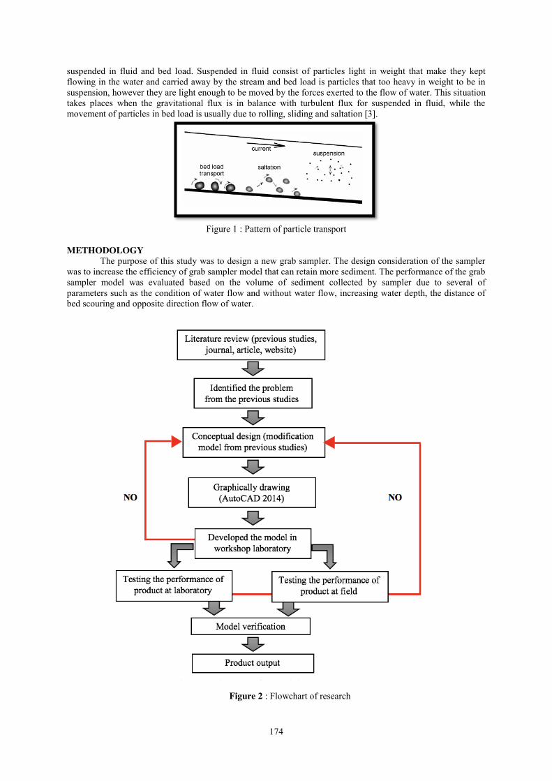
174

suspended in fluid and bed load. Suspended in fluid consist of particles light in weight that make they kept flowing in the water and carried away by the stream and bed load is particles that too heavy in weight to be in suspension, however they are light enough to be moved by the forces exerted to the flow of water. This situation takes places when the gravitational flux is in balance with turbulent flux for suspended in fluid, while the movement of particles in bed load is usually due to rolling, sliding and saltation [3].

Figure 1 : Pattern of particle transport

METHODOLOGY

The purpose of this study was to design a new grab sampler. The design consideration of the sampler was to increase the efficiency of grab sampler model that can retain more sediment. The performance of the grab sampler model was evaluated based on the volume of sediment collected by sampler due to several of parameters such as the condition of water flow and without water flow, increasing water depth, the distance of bed scouring and opposite direction flow of water.

Figure 2 : Flowchart of research

implementation

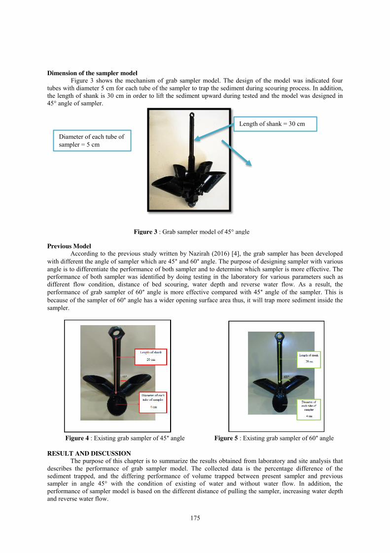
175

Dimension of the sampler model

Figure 3 shows the mechanism of grab sampler model. The design of the model was indicated four tubes with diameter 5 cm for each tube of the sampler to trap the sediment during scouring process. In addition, the length of shank is 30 cm in order to lift the sediment upward during tested and the model was designed in 45° angle of sampler.

Previous Model According to the previous study written by Nazirah (2016) [4], the grab sampler has been developed with different the angle of sampler which are 45° and 60° angle. The purpose of designing sampler with various angle is to differentiate the performance of both sampler and to determine which sampler is more effective. The performance of both sampler was identified by doing testing in the laboratory for various parameters such as different flow condition, distance of bed scouring, water depth and reverse water flow. As a result, the performance of grab sampler of 60° angle is more effective compared with 45° angle of the sampler. This is because of the sampler of 60° angle has a wider opening surface area thus, it will trap more sediment inside the sampler.

Figure 4 : Existing grab sampler of 45° angle Figure 5 : Existing grab sampler of 60° angle RESULT AND DISCUSSION The purpose of this chapter is to summarize the results obtained from laboratory and site analysis that describes the performance of grab sampler model. The collected data is the percentage difference of the sediment trapped, and the differing performance of volume trapped between present sampler and previous sampler in angle 45° with the condition of existing of water and without water flow. In addition, the performance of sampler model is based on the different distance of pulling the sampler, increasing water depth and reverse water flow.

Figure 3 : Grab sampler model of 45° angle

Length of shank = 30 cm

Diameter of each tube of sampler = 5 cm

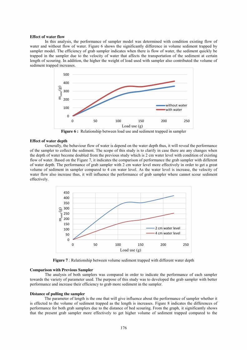
176

Effect of water flow

In this analysis, the performance of sampler model was determined with condition existing flow of water and without flow of water. Figure 6 shows the significantly difference in volume sediment trapped by sampler model. The efficiency of grab sampler indicates when there is flow of water, the sediment quickly be trapped in the sampler due to the velocity of water that affects the transportation of the sediment at certain length of scouring. In addition, the higher the weight of load used with sampler also contributed the volume of sediment trapped increases.

Figure 6 : Relationship between load use and sediment trapped in sampler

Effect of water depth

Generally, the behaviour flow of water is depend on the water depth thus, it will reveal the performance of the sampler to collect the sediment. The scope of this study is to clarify in case there are any changes when the depth of water become doubled from the previous study which is 2 cm water level with condition of existing flow of water. Based on the Figure 7, it indicates the comparison of performance the grab sampler with different of water depth. The performance of grab sampler with 2 cm water level more effectively in order to get a great volume of sediment in sampler compared to 4 cm water level. As the water level is increase, the velocity of water flow also increase thus, it will influence the performance of grab sampler where cannot scour sediment effectively.

Figure 7 : Relationship between volume sediment trapped with different water depth Comparison with Previous Sampler

The analysis of both samplers was compared in order to indicate the performance of each sampler towards the variety of parameter used. The purpose of this study was to developed the grab sampler with better performance and increase their efficiency to grab more sediment in the sampler. Distance of pulling the sampler The parameter of length is the one that will give influence about the performance of sampler whether it is effected to the volume of sediment trapped as the length is increases. Figure 8 indicates the differences of performance for both grab samplers due to the distance of bed scouring. From the graph, it significantly shows that the present grab sampler more effectively to get higher volume of sediment trapped compared to the

0

100

200

300

400

500

0 50 100 150 200 250

msa

nd (g

)

Load use (g)

without waterwith water

050

100150200250300350400450

0 50 100 150 200 250

msa

nd (g

)

Load use (g)

2 cm water level4 cm water level

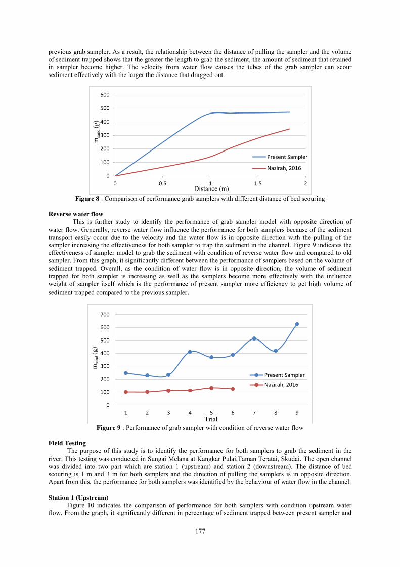
177

previous grab sampler. As a result, the relationship between the distance of pulling the sampler and the volume of sediment trapped shows that the greater the length to grab the sediment, the amount of sediment that retained in sampler become higher. The velocity from water flow causes the tubes of the grab sampler can scour sediment effectively with the larger the distance that dragged out.

Figure 8 : Comparison of performance grab samplers with different distance of bed scouring

Reverse water flow

This is further study to identify the performance of grab sampler model with opposite direction of water flow. Generally, reverse water flow influence the performance for both samplers because of the sediment transport easily occur due to the velocity and the water flow is in opposite direction with the pulling of the sampler increasing the effectiveness for both sampler to trap the sediment in the channel. Figure 9 indicates the effectiveness of sampler model to grab the sediment with condition of reverse water flow and compared to old sampler. From this graph, it significantly different between the performance of samplers based on the volume of sediment trapped. Overall, as the condition of water flow is in opposite direction, the volume of sediment trapped for both sampler is increasing as well as the samplers become more effectively with the influence weight of sampler itself which is the performance of present sampler more efficiency to get high volume of sediment trapped compared to the previous sampler.

Figure 9 : Performance of grab sampler with condition of reverse water flow

Field Testing The purpose of this study is to identify the performance for both samplers to grab the sediment in the river. This testing was conducted in Sungai Melana at Kangkar Pulai,Taman Teratai, Skudai. The open channel was divided into two part which are station 1 (upstream) and station 2 (downstream). The distance of bed scouring is 1 m and 3 m for both samplers and the direction of pulling the samplers is in opposite direction. Apart from this, the performance for both samplers was identified by the behaviour of water flow in the channel. Station 1 (Upstream) Figure 10 indicates the comparison of performance for both samplers with condition upstream water flow. From the graph, it significantly different in percentage of sediment trapped between present sampler and

0

100

200

300

400

500

600

0 0.5 1 1.5 2

msa

nd (g

)

Distance (m)

Present Sampler

Nazirah, 2016

0

100

200

300

400

500

600

700

1 2 3 4 5 6 7 8 9

msa

nd (g

)

Trial

Present SamplerNazirah, 2016

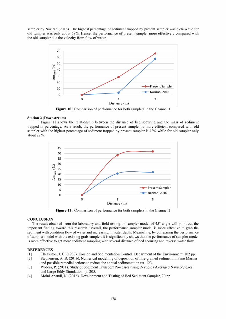
178

sampler by Nazirah (2016). The highest percentage of sediment trapped by present sampler was 67% while for old sampler was only about 58%. Hence, the performance of present sampler more effectively compared with the old sampler due the velocity from flow of water.

Figure 10 : Comparison of performance for both samplers in the Channel 1

Station 2 (Downstream) Figure 11 shows the relationship between the distance of bed scouring and the mass of sediment trapped in percentage. As a result, the performance of present sampler is more efficient compared with old sampler with the highest percentage of sediment trapped by present sampler is 42% while for old sampler only about 22%.

Figure 11 : Comparison of performance for both samplers in the Channel 2

CONCLUSION The result obtained from the laboratory and field testing on sampler model of 45° angle will point out the important finding toward this research. Overall, the performance sampler model is more effective to grab the sediment with condition flow of water and increasing in water depth. Meanwhile, by comparing the performance of sampler model with the existing grab sampler, it is significantly shows that the performance of sampler model is more effective to get more sediment sampling with several distance of bed scouring and reverse water flow. REFERENCES [1] Theakston, J. G. (1988). Erosion and Sedimentation Control. Department of the Environment, 102 pp. [2] Stephensen, A. B. (2016). Numerical modelling of deposition of fine-grained sediment in Fanø Marina

and possible remedial actions to reduce the annual sedimentation rat. 123. [3] Widera, P. (2011). Study of Sediment Transport Processes using Reynolds Averaged Navier-Stokes

and Large Eddy Simulation . p. 205. [4] Mohd Apandi, N. (2016). Development and Testing of Bed Sediment Sampler, 70 pp.

0

10

20

30

40

50

60

70

0 1 3

∆msa

nd (%

)

Distance (m)

Present Sampler

Nazirah, 2016

05

1015202530354045

0 1 3

∆msa

nd (%

)

Distance (m)

Present SamplerNazirah, 2016

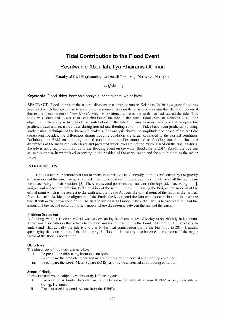
179

Tidal Contribution to the Flood Event

Rosalwanie Abdullah, Ilya Khairanis Othman

Faculty of Civil Engineering, Universiti Teknologi Malaysia, Malaysia

ilya@utm.my Keywords: Flood, tides, harmonic analysis, constituents, water level.

ABSTRACT. Flood is one of the natural disasters that often occurs in Kelantan. In 2014, a great flood has happened which had given rise to a variety of responses. Among them include a saying that the flood occurred due to the phenomenon of 'New Moon', which is positioned close to the earth that had caused the tide. This study was conducted to assess the contribution of the tide to the worse flood event at Kelantan 2014. The objective of the study is to predict the contribution of the tide by using harmonic analysis and compare the predicted tides and measured tides during normal and flooding condition. Tides have been predicted by using mathematical technique of the harmonic analysis. The analysis shows the amplitude and phase of the set tidal constituent. Besides, the differences during flooding condition are larger compared to the normal condition. Definitely, the RMS error during normal condition is smaller compared to flooding condition since the differences of the measured water level and predicted water level are not too much. Based on the final analysis, the tide is not a major contribution to the flooding event on the worst flood case in 2014. Surely, the tide can cause a huge rise in water level according to the position of the earth, moon and the sun, but not as the major factor

INTRODUCTION

Tide is a natural phenomenon that happens in our daily life. Generally, a tide is influenced by the gravity of the moon and the sun. The gravitational attraction of the earth, moon, and the sun will swell all the liquids on Earth according to their positions [3]. There are several positions that can cause the high tide. According to [4], perigee and apogee are referring to the position of the moon in the orbit. During the Perigee, the moon is at the orbital point which is the nearest to the earth and during the Apogee, the orbital point of the moon is the farthest from the earth. Besides, the alignment of the Earth, the Moon, and the Sun can also contribute to the extreme tide. It will occur in two conditions. The first condition is full moon, where the Earth is between the sun and the moon, and the second condition is new moon, where the moon is between the sun and the earth.

Problem Statement A flooding event in December 2014 was so devastating in several states of Malaysia specifically in Kelantan. There was a speculation that relates to the tide and its contribution to the flood. Therefore, it is necessary to understand what actually the tide is and clarify the tidal contribution during the big flood in 2014. Besides, quantifying the contribution of the tide during the flood at the estuary also becomes our concerns if the major factor of the flood is not the tide.

Objectives The objectives of this study are as follow:

i. To predict the tides using harmonic analysis. ii. To compare the predicted tides and measured tides during normal and flooding condition. iii. To compare the Roots-Mean-Square (RMS) error between normal and flooding condition.

Scope of Study In order to achieve the objectives, this study is focusing on:

I. The location is limited to Kelantan only. The measured tidal data from JUPEM is only available at Geting, Kelantan.

II. The data used is secondary data from the JUPEM.

180

III. The numerical modeling used to simulate the data is WORLD TIDES.

LITERATURE REVIEW

Basically, Tides are the rise and fall of the sea water level. The gravitational attraction of the earth, the moon and the sun affected the tides. The attraction between the centrifugal force and the gravitational force due to the Moon is called tide-generating force [2] As a result, the centrifugal forces exceed the gravitational force on the side of earth away from Moon and the gravitational forces exceed the centrifugal force on side Earth near to the Moon. There are variations of effect of the high tidal wave and hence the range of the tide [7]. Shortly after full or new Moon a locality will experience its highest high waters and lowest low waters of the lunar month, and tides in this period are called Spring Tides. Conversely, around the time of the first and last quarters of the Moon, the lowest high waters and the highest low waters of the lunar month will be experienced, at which period the tides are called Neap Tides.

Tidal constituent is a simple harmonic cosine curve which is demonstrating the tide-generation motions. The influence of tide to water level is referred to the constituents with conceiving the harmonic method of tidal analysis. By analyzing the measured tides and the tidal harmonic constituent, the tides can be predicted [6]. The tidal constituent can be described according to their tidal component, period, description and nature. According to the [1], there are five tidal constituents that will increase the accuracy of prediction which is M2, S2, N2, K1 and O1. Mathematic application is needed to represent the tidal constituent. From the input data, the time is given in an hour.

According to the (Hydrographic, 2006), harmonic analysis is the mathematical process by which the perceived tide or tidal current at any place is divided into simple harmonic constituents which are amplitude and phase. Again, the constituents are exclusively recognized by their frequencies. For this study, the least square method is used in tidal analysis and it can be viewed as a form of multiple linear regression [1]. However, the errors still have to refer the natural meteorological occurrences. The principal factors include atmospheric pressure and the winds acting on the sea surface to create storm surges [6]. Aim for the method of least square is to minimize the error[5]. By using the RMS error and percentage reduction in variance, the prediction will be closer. The definition of the RMS error is the square root of the mean square difference between observed and predicted water level. Ideally, the periodogram should result in a noticeable reduce in RMS error combine with and rise in %V_Var.

METHODOLOGY Generally, WORLD TIDE was written in the MATLAB programming language. It was presented in the

Graphical User Interface (GUI) that can accomplish both analysis and prediction. For this study, the focus is in the analysis.

181

Figure 1: Flow chart of the methodology

Nowadays, lots of software can be used in order to predict the tide. WORLD TIDES software performed in its Graphical User Interface (GUI) allows the separation of the time series of water level measurement into its tidal and non-tidal components using a selective least square harmonic reduction employing up to 35 tidal constituents. The prediction of the tide was performed after saving the tidal constants for the constituent selected during the analysis. Harmonic Analysis Method of Least Squares (HAMELS) is the method that used to analyze the water level.

1. Set up with m harmonic constituent to predict the astronomical tide height, h, at time needed t, relative to the h0,

h(t) = h0 + ∑ Hj cos (ωjt − ϕj)𝑚𝑘=𝑗=1 (1)

2. The observe water level, ht and the predicted tide, h(t), at each measurement time are the element of the sum of square different. The equation is as follow:

SSQ = Σn [ht – h(t)]2 (2) 3. The SSQ will become as small as possible. The root-mean-square (RMS) difference and the variance

become the parameter in order to judge how good the fit actually is.

The WORL TIDE input file is on the worksheet of a Microsoft Excel. The inquiry ration of the software receives only files of type .xls for data input. The water level data from the JUPEM is entered into the Excell worksheet using a simple three-column format. At first, choose the number of days to analyze, and check the constituents wanted. At first, use the 5 basic constituent which is M2, N2, S2, K1 and O1. Double-click the .xls file name in the list box. Analyze the file and

Start

Data Collection from JUPEM Date and time, Water level

(m)

Review and Interpretation of Available Data

Numerical Modelling WORLD TIDES

Select Constituents

Frequency Analysis

Conclusion

Analyse the RMS Error and %R_Var

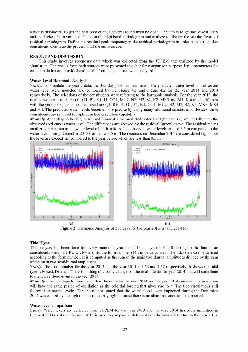
182

a plot is displayed. To get the best prediction, a several round must be done. The aim is to get the lowest RMS and the highest % in variance. Click on the high band periodogram and analyze to display the see the figure of residual periodogram. Define the residual peak frequency in the residual periodogram in order to select another constituent. Continue the process until the aim achieve.

RESULT AND DISCUSSION This study involves secondary data which was collected from the JUPEM and analyzed by the model

simulation. The results from both sources were presented together for comparison purpose. Input parameters for each simulation are provided and results from both sources were analyzed.

Water Level Harmonic Analysis Yearly. To simulate the yearly data, the 365-day plot has been used. The predicted water level and observed water level were modeled and compared by the Figure 4.1 and Figure 4.2 for the year 2013 and 2014 respectively. The selections of the constituents were referring to the harmonic analysis. For the year 2013, the tidal constituents used are Q1, O1, P1, K1, J1, OO1, MU2, N2, M2, S2, K2, MK3 and M4. Not much different with the year 2014, the constituent used are Q1, RHO1, O1, P1, K1, OO1, MU2, N2, M2, S2, K2, MK3, MS4 and M4. The predicted water levels become more precise by using many additional constituents. Besides, these constituents are required for optimum tide prediction capability. Monthly. According to the Figure 4.1 and Figure 4.2 the predicted water level (blue curve) are not tally with the observed (red curve) water level. The differences are showed by the residual (green) curve. The residual means another contribution to the water level other than tides. The observed water levels exceed 3.5 m compared to the water level during December 2013 that below 3.5 m. The residuals on December 2014 are considered high since the level are exceed 1m compared to the year before which are less than 0.5 m.

(a) (b)

Figure 2: Harmonic Analysis of 365 days for the year 2013 (a) and 2014 (b) Tidal Type The analysis has been done for every month in year the 2013 and year 2014. Referring to the four basic constituents which are K1, O1, M2 and S2, the form number (F) can be calculated. The tidal type can be defined according to the form number. It is computed as the sum of the main two diurnal amplitudes divided by the sum of the main two semidiurnal amplitudes. Yearly. The form number for the year 2013 and the year 2014 is 1.53 and 1.52 respectively. It shows the tidal type is Mixed, Diurnal. There is nothing obviously changes of the tidal tide for the year 2014 that will contribute to the worse flood event in the year 2014. Monthly. The tidal type for every month is the same for the year 2013 and the year 2014 since each cosine wave will have the same period of oscillation as the celestial forcing that gives rise to it. The tide circulations still follow their normal cycle. The speculation stated that the worse flood event happened during the December 2014 was caused by the high tide is not exactly right because there is no abnormal circulation happened.

Water level comparison Yearly. Water levels are collected from JUPEM for the year 2013 and the year 2014 has been simplified in Figure 4.2. The data on the year 2013 is used to compare with the data on the year 2014. During the year 2013,

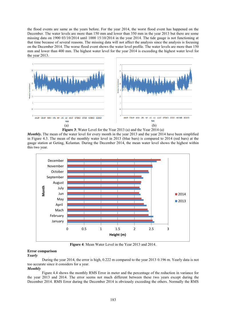
183

the flood events are same as the years before. For the year 2014, the worst flood event has happened on the December. The water levels are more than 150 mm and lower than 350 mm in the year 2013 but there are some missing data on 1900 03/10/2014 until 1000 15/10/2014 in the year 2014. The tide gauge is not functioning at that time because of several reasons. The missing data will not affect the analysis since the analysis is focusing on the December 2014. The worse flood event shows the water level profile. The water levels are more than 150 mm and lower than 400 mm. The highest water level for the year 2014 is exceeding the highest water level for the year 2013.

(a) (b)

Figure 3: Water Level for the Year 2013 (a) and the Year 2014 (a) Monthly. The mean of the water level for every month in the year 2013 and the year 2014 have been simplified in Figure 4.3. The mean of the monthly water level in 2013 (blue bars) is compared to 2014 (red bars) at the gauge station at Geting, Kelantan. During the December 2014, the mean water level shows the highest within this two year.

Figure 4: Mean Water Level in the Year 2013 and 2014.

Error comparison Yearly

During the year 2014, the error is high, 0.222 m compared to the year 2013 0.196 m. Yearly data is not too accurate since it considers for a year. Monthly

Figure 4.4 shows the monthly RMS Error in meter and the percentage of the reduction in variance for the year 2013 and 2014. The error seems not much different between these two years except during the December 2014. RMS Error during the December 2014 is obviously exceeding the others. Normally the RMS

0 0.5 1 1.5 2 2.5 3

JanuaryFebruary

MachAprilMayJunJuly

AugustSeptember

OctoberNovemberDecember

Height (m)

Mon

th

2014

2013

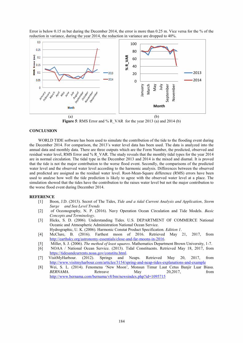
184

Error is below 0.15 m but during the December 2014, the error is more than 0.25 m. Vice versa for the % of the reduction in variance, during the year 2014, the reduction in variance are dropped to 40%.

(a) (b)

Figure 5: RMS Error and % R_VAR for the year 2013 (a) and 2014 (b)

CONCLUSION

WORLD TIDE software has been used to simulate the contribution of the tide to the flooding event during the December 2014. For comparison, the 2013’s water level data has been used. The data is analyzed into the annual data and monthly data. There are three outputs which are the Form Number, the predicted, observed and residual water level, RMS Error and % R_VAR. The study reveals that the monthly tidal types for the year 2014 are in normal circulation. The tidal type in the December 2013 and 2014 is the mixed and diurnal. It is proved that the tide is not the major contribution to the worse flood event. Secondly, the comparisons of the predicted water level and the observed water level according to the harmonic analysis. Differences between the observed and predicted are assigned as the residual water level. Root-Mean-Square difference (RMS) errors have been used to analzse how well the tide prediction is likely to agree with the observed water level at a place. The simulation showed that the tides have the contribution to the raises water level but not the major contribution to the worse flood event during December 2014.

REFERENCE [1] Boon, J.D. (2013). Secret of The Tides, Tide and a tidal Current Analysis and Application, Storm

Surge and Sea Level Trends [2] of Oceonography, N. P. (2016). Navy Operation Ocean Circulation and Tide Models. Basic

Concepts and Terminology. [3] Hicks, S. D. (2006). Understanding Tides. U.S. DEPARTMENT OF COMMERCE National

Oceanic and Atmospheric Administration National Ocean Service. Hydrographic, U. K. (2006). Harmonic Constat Product Specification. Edition 1. [4] McClure, B. (2016). Farthest moon of 2016. Retrieved May 21, 2017, from

http://earthsky.org/astronomy-essentials/close-and-far-moons-in-2016. [5] Miller, S. J. (2006). The method of least squares. Mathematics Department Brown University, 1-7. [6] NOAA / National Ocean Service. (2013). Tidal Constituents. Retrieved May 18, 2017, from

https://tidesandcurrents.noaa.gov/constitu.html. [7] VisitMyHarbour. (2012). Springs and Neaps. Retrieved May 20, 2017, from

http://www.visitmyharbour.com/articles/3154/spring-and-neap-tides-explanations-and-example [8] Wei, S. L. (2014). Fenomena ‘New Moon’, Monsun Timur Laut Cetus Banjir Luar Biasa.

BERNAMA. Retreave May 20,2017, from http://www.bernama.com/bernama/v8/bm/newsindex.php?id=1095715

0

20

40

60

80

100

Janu

ary

Mar

chM

ay July

Sept

embe

rN

ovem

ber

% R

_VAR

Month

2013

2014

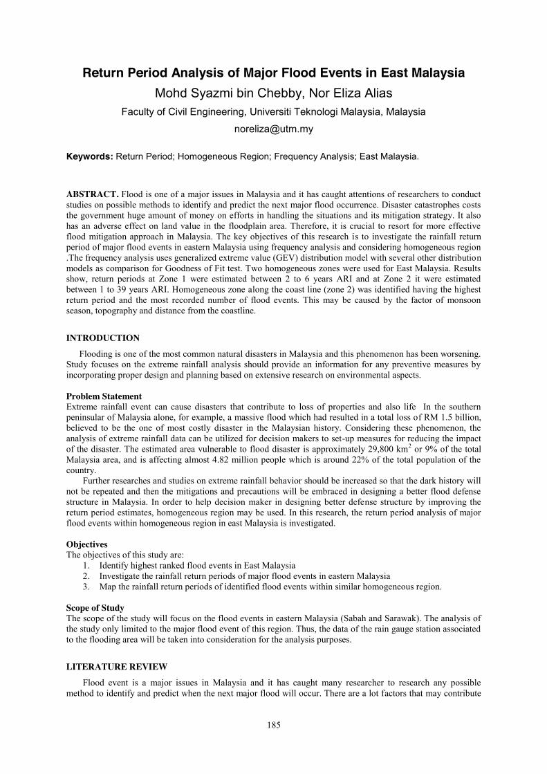
185

Return Period Analysis of Major Flood Events in East Malaysia Mohd Syazmi bin Chebby, Nor Eliza Alias

Faculty of Civil Engineering, Universiti Teknologi Malaysia, Malaysia

noreliza@utm.my

Keywords: Return Period; Homogeneous Region; Frequency Analysis; East Malaysia.

ABSTRACT. Flood is one of a major issues in Malaysia and it has caught attentions of researchers to conduct studies on possible methods to identify and predict the next major flood occurrence. Disaster catastrophes costs the government huge amount of money on efforts in handling the situations and its mitigation strategy. It also has an adverse effect on land value in the floodplain area. Therefore, it is crucial to resort for more effective flood mitigation approach in Malaysia. The key objectives of this research is to investigate the rainfall return period of major flood events in eastern Malaysia using frequency analysis and considering homogeneous region .The frequency analysis uses generalized extreme value (GEV) distribution model with several other distribution models as comparison for Goodness of Fit test. Two homogeneous zones were used for East Malaysia. Results show, return periods at Zone 1 were estimated between 2 to 6 years ARI and at Zone 2 it were estimated between 1 to 39 years ARI. Homogeneous zone along the coast line (zone 2) was identified having the highest return period and the most recorded number of flood events. This may be caused by the factor of monsoon season, topography and distance from the coastline.

INTRODUCTION

Flooding is one of the most common natural disasters in Malaysia and this phenomenon has been worsening. Study focuses on the extreme rainfall analysis should provide an information for any preventive measures by incorporating proper design and planning based on extensive research on environmental aspects.

Problem Statement Extreme rainfall event can cause disasters that contribute to loss of properties and also life In the southern peninsular of Malaysia alone, for example, a massive flood which had resulted in a total loss of RM 1.5 billion, believed to be the one of most costly disaster in the Malaysian history. Considering these phenomenon, the analysis of extreme rainfall data can be utilized for decision makers to set-up measures for reducing the impact of the disaster. The estimated area vulnerable to flood disaster is approximately 29,800 km2 or 9% of the total Malaysia area, and is affecting almost 4.82 million people which is around 22% of the total population of the country.

Further researches and studies on extreme rainfall behavior should be increased so that the dark history will not be repeated and then the mitigations and precautions will be embraced in designing a better flood defense structure in Malaysia. In order to help decision maker in designing better defense structure by improving the return period estimates, homogeneous region may be used. In this research, the return period analysis of major flood events within homogeneous region in east Malaysia is investigated.

Objectives The objectives of this study are:

1. Identify highest ranked flood events in East Malaysia 2. Investigate the rainfall return periods of major flood events in eastern Malaysia 3. Map the rainfall return periods of identified flood events within similar homogeneous region.

Scope of Study The scope of the study will focus on the flood events in eastern Malaysia (Sabah and Sarawak). The analysis of the study only limited to the major flood event of this region. Thus, the data of the rain gauge station associated to the flooding area will be taken into consideration for the analysis purposes.

LITERATURE REVIEW Flood event is a major issues in Malaysia and it has caught many researcher to research any possible

method to identify and predict when the next major flood will occur. There are a lot factors that may contribute

186

to a flood event. In Malaysia, Monsoon is an annual phenomena that cause many flood cases. In East Malaysia flood mainly affected by the Northeast Monsoon and the geographical characteristics. The study of return period analysis can be used as a tool for flood prediction in urban areas. This technique enables them to know when an event is expected to occur, be equalled, or be exceeded [1].

A monsoon is a seasonal prevailing wind which lasts for several months. Monsoons are caused by the larger amplitude of the seasonal cycle of land temperature compared to that of nearby oceans. The Northeast Monsoon season typically starts with a wet phase (December to January) followed by a dry phase (February to early March). The North-east monsoon usually brings heavy rainfall to the East-coast of the Malaysia every year contributing to flood. November, December and January is the month where the east coast states stricken by the east coast monsoon that resulting to the maximum rain while on June and July is the month is in the driest [2]. It was observed that both north-east and south-west monsoons produce the severe events in most of the states of the Peninsular Malaysia. However, for Sabah and Sarawak, such severe events occurred during the north-east monsoon as compared to the south-west monsoon due to the geological location of the states [3].

Extreme rainfall events are expected to occur each year at sites located in areas with tropical climate, which indirectly affected by the impact of monsoons. Most of the rainfall events in Malaysia are multi-days and this is the main cause of flooding. About 29,720 km2 or 9% of the total area in Malaysia is estimated to be exposed to flood, which indirectly affects 4.9 million people, i.e. about 21% of the total population [4].

Homogeneous regions are regions which has the similarities in meteorological condition such as similar exposure towards the same extreme rainfall conditions. Thus, all the stations with the same homogenous regions has its extreme rainfall distribution within the same frequency model or population group [5]. Regions are said to be meteorologically homogeneous if they have similar features of climate, identical topographic features, affected by the same moisture source and experience the same type of storms [3]. The identification of homogeneous region can be done by relocating isohyetal patterns of storm precipitation within a region that is homogeneous relative to terrain and meteorological features important to the particular storm rainfall under concern [3].

The best distribution model for hourly rainfall in Wilayah Persekutuan is Mixed-Exponential [6]. Generalized extreme value (GEV) is the most suitable to be used in Malaysia for annual maximum rainfall data [7]. The suitable distribution that describe the distribution at homogeneous region of Sarawak are generalized extreme value (GEV) and Generalized Logistic distribution [8].

For a better analysis of the data, data pooling also have been conducted. Pooling information at target site with that from other locations depicting similar characteristics of precipitation [9]. The proposed groups of sites should meet the requirement of homogeneity, that is, sites pooled together have to exhibit, except for a scaling factor, similar probability- distribution curves (growth curves) of extremes [10].

METHODOLOGY

The main objective of the research is to study the rainfall return period during major flood event within the homogeneous regions in east Malaysia. This research methodology consisted of 4 key activities: ranking of flood events, computing annual maximum rainfall data, frequency analysis and mapping of return period at homogeneous region. Ranking of flood event The historical rainfall data and annual flood report at east Malaysia were obtained from the Division of Flood Management, Department of Irrigation and Drainage Malaysia (DID). The flood report provided by DID are in PDF format, thus tabulation works has been done manually on excel. There are a total of 151 flood events recorded in Sabah (1986-2012) and a total of 133 flood events in Sarawak (1980-2012). Flood events were shortlisted and ranked based on the impact of a flood event on population (evacuated victim). The shortlisted flood events are considered as major flood event for this study. The ranking works are done by using Microsoft Excel. Rainfall Annual Maximum Data For the analysis of an extreme event, the return period of the rainfall are determined through frequency analysis. However, the daily data for the analysis need to be converted into Annual Maximum seres since the return period are determined in yearly basis and to represent extreme values data. This can be achieved by using computer programming such as FORTRAN language. Frequency Analysis by EasyFit Easyfit software was utilized for the analysis of the rainfall return period. EasyFit can help with uncertainty and make informed decisions by analysing the probability data and selecting the best fitting distribution. GEV distribution is selected for the evaluation since many studies have proven its suitability to represent the rainfall

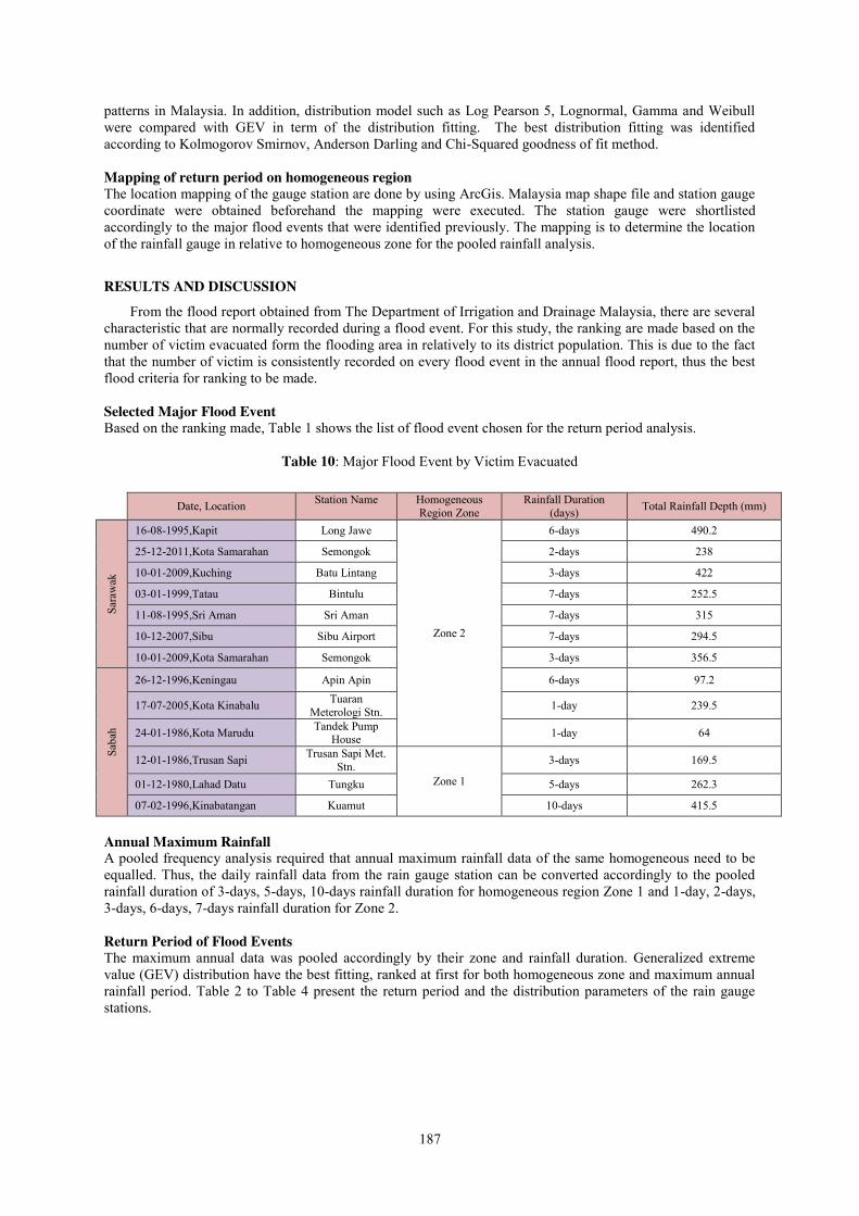
187

patterns in Malaysia. In addition, distribution model such as Log Pearson 5, Lognormal, Gamma and Weibull were compared with GEV in term of the distribution fitting. The best distribution fitting was identified according to Kolmogorov Smirnov, Anderson Darling and Chi-Squared goodness of fit method. Mapping of return period on homogeneous region The location mapping of the gauge station are done by using ArcGis. Malaysia map shape file and station gauge coordinate were obtained beforehand the mapping were executed. The station gauge were shortlisted accordingly to the major flood events that were identified previously. The mapping is to determine the location of the rainfall gauge in relative to homogeneous zone for the pooled rainfall analysis.

RESULTS AND DISCUSSION

From the flood report obtained from The Department of Irrigation and Drainage Malaysia, there are several characteristic that are normally recorded during a flood event. For this study, the ranking are made based on the number of victim evacuated form the flooding area in relatively to its district population. This is due to the fact that the number of victim is consistently recorded on every flood event in the annual flood report, thus the best flood criteria for ranking to be made.

Selected Major Flood Event Based on the ranking made, Table 1 shows the list of flood event chosen for the return period analysis.

Table 10: Major Flood Event by Victim Evacuated

Date, Location Station Name Homogeneous Region Zone

Rainfall Duration (days) Total Rainfall Depth (mm)

Sara

wak

16-08-1995,Kapit Long Jawe

Zone 2

6-days 490.2

25-12-2011,Kota Samarahan Semongok 2-days 238

10-01-2009,Kuching Batu Lintang 3-days 422

03-01-1999,Tatau Bintulu 7-days 252.5

11-08-1995,Sri Aman Sri Aman 7-days 315

10-12-2007,Sibu Sibu Airport 7-days 294.5

10-01-2009,Kota Samarahan Semongok 3-days 356.5

Saba

h

26-12-1996,Keningau Apin Apin 6-days 97.2

17-07-2005,Kota Kinabalu Tuaran Meterologi Stn. 1-day 239.5

24-01-1986,Kota Marudu Tandek Pump House 1-day 64

12-01-1986,Trusan Sapi Trusan Sapi Met. Stn.

Zone 1

3-days 169.5

01-12-1980,Lahad Datu Tungku 5-days 262.3

07-02-1996,Kinabatangan Kuamut 10-days 415.5

Annual Maximum Rainfall A pooled frequency analysis required that annual maximum rainfall data of the same homogeneous need to be equalled. Thus, the daily rainfall data from the rain gauge station can be converted accordingly to the pooled rainfall duration of 3-days, 5-days, 10-days rainfall duration for homogeneous region Zone 1 and 1-day, 2-days, 3-days, 6-days, 7-days rainfall duration for Zone 2. Return Period of Flood Events The maximum annual data was pooled accordingly by their zone and rainfall duration. Generalized extreme value (GEV) distribution have the best fitting, ranked at first for both homogeneous zone and maximum annual rainfall period. Table 2 to Table 4 present the return period and the distribution parameters of the rain gauge stations.

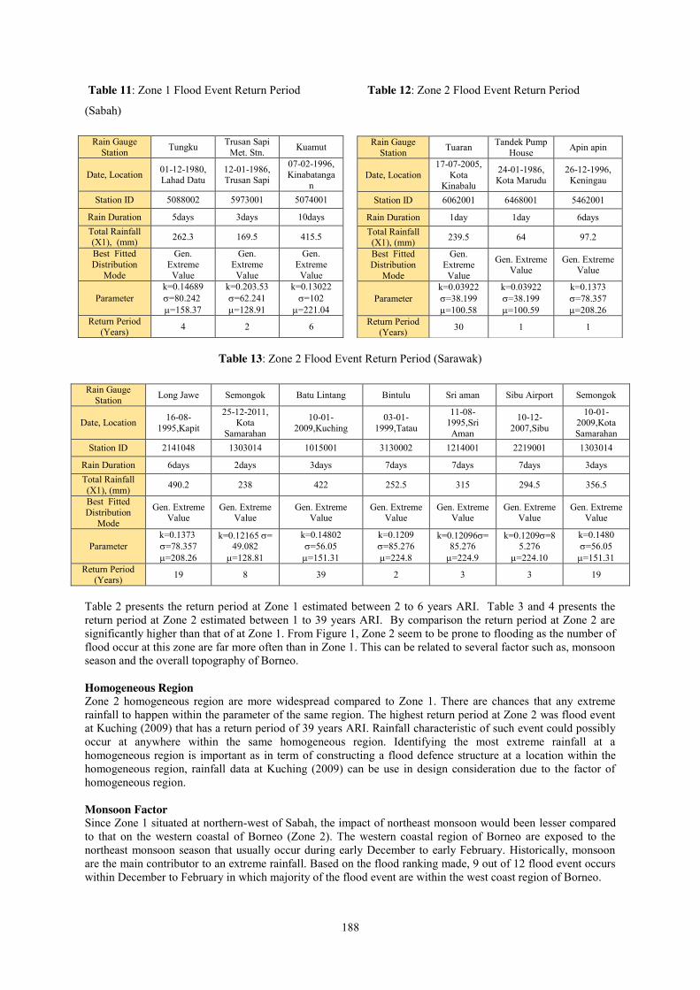
188

Table 11: Zone 1 Flood Event Return Period Table 12: Zone 2 Flood Event Return Period

(Sabah)

Rain Gauge Station Tungku Trusan Sapi

Met. Stn. Kuamut

Date, Location 01-12-1980, Lahad Datu

12-01-1986, Trusan Sapi

07-02-1996, Kinabatanga

n Station ID 5088002 5973001 5074001

Rain Duration 5days 3days 10days Total Rainfall (X1), (mm) 262.3 169.5 415.5

Best Fitted Distribution

Mode

Gen. Extreme Value

Gen. Extreme Value

Gen. Extreme Value

Parameter k=0.14689 V=80.242 P=158.37

k=0.203.53 V=62.241 P=128.91

k=0.13022 V=102

P=221.04 Return Period

(Years) 4 2 6

Table 13: Zone 2 Flood Event Return Period (Sarawak)

Rain Gauge Station Long Jawe Semongok Batu Lintang Bintulu Sri aman Sibu Airport Semongok

Date, Location 16-08-1995,Kapit

25-12-2011, Kota

Samarahan

10-01-2009,Kuching

03-01-1999,Tatau

11-08-1995,Sri Aman

10-12-2007,Sibu

10-01-2009,Kota Samarahan

Station ID 2141048 1303014 1015001 3130002 1214001 2219001 1303014

Rain Duration 6days 2days 3days 7days 7days 7days 3days Total Rainfall (X1), (mm) 490.2 238 422 252.5 315 294.5 356.5

Best Fitted Distribution

Mode

Gen. Extreme Value

Gen. Extreme Value

Gen. Extreme Value

Gen. Extreme Value

Gen. Extreme Value

Gen. Extreme Value

Gen. Extreme Value

Parameter k=0.1373 V=78.357 P=208.26

k=0.12165 V=49.082

P=128.81

k=0.14802 V=56.05 P=151.31

k=0.1209 V=85.276 P=224.8

k=0.12096V=85.276 P=224.9

k=0.1209V=85.276

P=224.10

k=0.1480 V=56.05 P=151.31

Return Period (Years) 19 8 39 2 3 3 19

Table 2 presents the return period at Zone 1 estimated between 2 to 6 years ARI. Table 3 and 4 presents the return period at Zone 2 estimated between 1 to 39 years ARI. By comparison the return period at Zone 2 are significantly higher than that of at Zone 1. From Figure 1, Zone 2 seem to be prone to flooding as the number of flood occur at this zone are far more often than in Zone 1. This can be related to several factor such as, monsoon season and the overall topography of Borneo. Homogeneous Region Zone 2 homogeneous region are more widespread compared to Zone 1. There are chances that any extreme rainfall to happen within the parameter of the same region. The highest return period at Zone 2 was flood event at Kuching (2009) that has a return period of 39 years ARI. Rainfall characteristic of such event could possibly occur at anywhere within the same homogeneous region. Identifying the most extreme rainfall at a homogeneous region is important as in term of constructing a flood defence structure at a location within the homogeneous region, rainfall data at Kuching (2009) can be use in design consideration due to the factor of homogeneous region. Monsoon Factor Since Zone 1 situated at northern-west of Sabah, the impact of northeast monsoon would been lesser compared to that on the western coastal of Borneo (Zone 2). The western coastal region of Borneo are exposed to the northeast monsoon season that usually occur during early December to early February. Historically, monsoon are the main contributor to an extreme rainfall. Based on the flood ranking made, 9 out of 12 flood event occurs within December to February in which majority of the flood event are within the west coast region of Borneo.

Rain Gauge Station Tuaran Tandek Pump

House Apin apin

Date, Location 17-07-2005,

Kota Kinabalu

24-01-1986, Kota Marudu

26-12-1996, Keningau

Station ID 6062001 6468001 5462001

Rain Duration 1day 1day 6days Total Rainfall (X1), (mm) 239.5 64 97.2

Best Fitted Distribution

Mode

Gen. Extreme Value

Gen. Extreme Value

Gen. Extreme Value

Parameter k=0.03922 V=38.199 P=100.58

k=0.03922 V=38.199 P=100.59

k=0.1373 V=78.357 P=208.26

Return Period (Years) 30 1 1

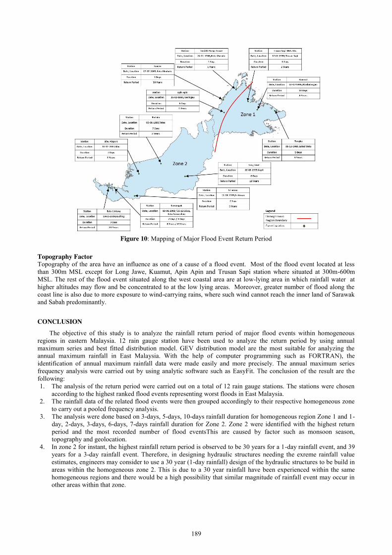
189

Figure 10: Mapping of Major Flood Event Return Period

Topography Factor Topography of the area have an influence as one of a cause of a flood event. Most of the flood event located at less than 300m MSL except for Long Jawe, Kuamut, Apin Apin and Trusan Sapi station where situated at 300m-600m MSL. The rest of the flood event situated along the west coastal area are at low-lying area in which rainfall water at higher altitudes may flow and be concentrated to at the low lying areas. Moreover, greater number of flood along the coast line is also due to more exposure to wind-carrying rains, where such wind cannot reach the inner land of Sarawak and Sabah predominantly.

CONCLUSION

The objective of this study is to analyze the rainfall return period of major flood events within homogeneous regions in eastern Malaysia. 12 rain gauge station have been used to analyze the return period by using annual maximum series and best fitted distribution model. GEV distribution model are the most suitable for analyzing the annual maximum rainfall in East Malaysia. With the help of computer programming such as FORTRAN), the identification of annual maximum rainfall data were made easily and more precisely. The annual maximum series frequency analysis were carried out by using analytic software such as EasyFit. The conclusion of the result are the following: 1. The analysis of the return period were carried out on a total of 12 rain gauge stations. The stations were chosen

according to the highest ranked flood events representing worst floods in East Malaysia. 2. The rainfall data of the related flood events were then grouped accordingly to their respective homogeneous zone

to carry out a pooled frequency analysis. 3. The analysis were done based on 3-days, 5-days, 10-days rainfall duration for homogeneous region Zone 1 and 1-

day, 2-days, 3-days, 6-days, 7-days rainfall duration for Zone 2. Zone 2 were identified with the highest return period and the most recorded number of flood eventsThis are caused by factor such as monsoon season, topography and geolocation.

4. In zone 2 for instant, the highest rainfall return period is observed to be 30 years for a 1-day rainfall event, and 39 years for a 3-day rainfall event. Therefore, in designing hydraulic structures needing the exreme rainfall value estimates, engineers may consider to use a 30 year (1-day rainfall) design of the hydraulic structures to be build in areas within the homogeneous zone 2. This is due to a 30 year rainfall have been experienced within the same homogeneous regions and there would be a high possibility that similar magnitude of rainfall event may occur in other areas within that zone.

190

Therefore, identifying the return period on a homogeneous region will benefits in hydraulic structure design. One of the major concern of designing a hydraulic structure is the rainfall ARI. By identifying the return period within the same homogeneous region, the critical return period can be known and taken into design consideration of a food defense structure to ensure a future and safety proof design.

REFERENCES

[1] Gobo, A.E., and T.K.S Abam. (2006). Return period analysis as a tool for urban flood prediction in the Niger Delta: A case study of Port Harcourt City, Nigeria. Journal of Environmental Hydrology, Vol. 14, Paper 12.

[2] Shaharuddin A., Noorazuan Md. H. (2016), Menganalisis pola dan arah aliran hujan di Negeri Sembilan menggunakan kaedah GIS poligon Thiessen dan kontur Isoyet, Geografia - Malaysian Journal of Society and Space 2; 105-113

[3] National Hydraulic Research Institute of Malaysia (NAHRIM) (2007), Nahrim Technical Research Publication (TRP) No. 1 – Derivation of Probable Maximum Precipitation for Design Floods In Malaysia

[4] Muhammad N. S., Akashah A.I., Abdullah J. (2016), Analysis of Extreme Rainfall Indices in Peninsular Malaysia, Universiti Kebangsaan Malaysia.

[5] Alias N. E. (2014), Improving Extreme Precipitation Estimates Considering Regional Frequency Analysis, Kyoto University.

[6] Fadhilah, Y., Zalina, M. D., Nguyen, V-T-V, Suhaila, S., Zulkifli, Y. (2007). Fitting the Best-Fit Distribution for the Hourly Rainfall Amount in the Wilayah Persekutuan. Jurnal Teknologi. 2007. 46(C): 49-58.

[7] Zalina, M. D., Amir, H. M. K., Mohd Nor Mohd Desa, Nguyen, V-T-V. (2002). Statistical analysis of at-site extreme rainfall processes in Penisular Malaysia. In Regional Hydrology: Bridging the Gap Between Research and Practice (Proceeding of the Fourth International FRIEND Conference, March. Cape Town, South Africa: FRIEND. 2002.

[8] Lim, Y. H. and Lye, L. M. (2003). Regional Flood Estimation for Ungauged Basins in Sarawak, Malaysia. Hydrological Science Journal. 48(1): 79-94

[9] Satyanarayana P and V. V. Srinivas, 2008. Regional frequency analysis of precipitation using large-scale atmospheric variables. J. Geophys.

[10] L. Gaál, J. Kyselý, J. Szolgay. (2007). Region-of-influence approach to a frequency analysis of heavy precipitation in Slovakia. Hydrology and Earth System Sciences Discussions, European Geosciences Union, 2008, 12 (3), pp.825-839.

191

Return Period Analysis of Major Flood Events in Peninsular Malaysia Mohamad Mahayuddin Bin Mohamad Tarmizi, Nor Eliza Binti Alias

Faculty of Civil Engineering, Universiti Teknologi Malaysia, Malaysia

noreliza@utm.my

Keywords: Frequency Analysis; Generalized Extreme Value; Homogeneous Region; Return Period

ABSTRACT. Extreme rainfall events are the main cause of flooding. Flood is one of a major issue in Malaysia and these phenomena have attracted many meteorologists and hydrologists in the world to investigate and predict when the next major flood will occur. The objectives of this research is to identify major flood events in Peninsular Malaysia and mapping the return period of identified flood event in extreme rainfall homogeneous region. The method of pooled frequency analysis was used to combine Annual Maximum Series (AMS) data in each homogeneous region and Generalized Extreme Value (GEV) were selected for distribution model based on highest rank in Kolmogrov Smirnov, Anderson Darling, and Chi-Squared. From the research, the highest return period at zone 1, zone 2, zone 3, and zone 4 are 50 years, 333 years, 500 years, and 20 years of Average Recurrance Interval (ARI).

INTRODUCTION

Flood is a yearly event in Malaysia but the major flood in Malaysia showed an increasing trend in every year which happen during the monsoon season and the most devastating natural disaster experienced in Malaysia [1]. Malaysia experience two categories of flood as been classified by the Department of Drainage and Irrigation, i.e. flash flood and monsoon floods (DID, 2000). Based on the hydrological perspectives, the clear difference between these two disasters is the period taken by the river flow to recede to the normal level. Flash floods take only some hours to return to the normal water level, while monsoon flood can last for a month [2].

Problem Statement It has terrible impacts on people, society and economics when floods occurred. Considering these phenomenon, the analysis of extreme rainfall data can be utilized for decision makers to set-up measures for reducing the impact of the disaster. Further reseaches and studies on extreme rainfall behavior should be increased so the dark history will not be repeated and then the mitigation and precautions will be embraced by designing better flood defense structures in Malaysia. In order to help decision makers in better designing flood defense structure, use of homogeneous region may be used to improve extreme rainfall estimates. In this research, the rainfall return periods analysis of major flood events within homogeneous region in peninsular Malaysia was investigated.

Objectives The objectives of this study are:

1. Identifying major flood events in Peninsular Malaysia. 2. Estimating the return period of rainfall during the major flood events. 3. Mapping the return period of identified flood event in extreme rainfall homogeneous region.

Scope of Study The scope of this study will focus on the flood events in peninsular Malaysia. The analysis of study only limited to the major flood events of this region. Thus, the data of the rain gauge station associated to the flooding area will be taken into consideration for the analysis purposes.

LITERATURE REVIEW In Malaysia, the weather mainly influenced by two monsoon regimes namely the Southwest Monsoon from late

May to September, and the Northeast Monsoon from November to March. The Northeast Monsoon brings heavy rainfall, particularly to the east coast states of Peninsular Malaysia and western Sarawak, whereas the Southwest Monsoon normally signifies relatively drier weather. In the past, widespread floods have occurred especially during the northeast monsoon season. Malaysia has always been complacent and perceived to be relatively free from major hydrometeorological and geological hazards [3]. With rapid development in high-rise buildings and other infrastructures, the occurrences of hydrometeorological and geological hazards have been increased [3]. These natural hazards include monsoon flood, flash flood in the cities, severe storms, storm surge, landslides, earthquakes and tsunami. The government has taken the initiatives to implement various projects and activities towards disaster prevention and mitigation in the country.

192

Extreme rainfall events are the main cause of flooding [4]. The changes in extreme rainfall events, such as heavy precipitation and major flood have attracted a lot of attention because of their devastating consequences on society and economics. Increasing frequency and intensity of extreme rainfall events have raised concern that human activity might have resulted in an alteration of the climate system. It is believed that rise in both frequency and intensity of extreme rainfall events are the major impacts of global warming [5].

In a frequency analysis, estimates of the probability of occurrence of future events are based on the analysis of historical rainfall records. Extreme rainfall events are considered as random variables in frequency analysis, which come from identical distribution and are assumed to be independent. The magnitude of the random variables can be related to their frequency of occurrence using probability distribution. There are two forms of probability distribution which is probability density function (PDF) and cumulative distribution function (CDF) [6]. PDF and CDF are described in the following equation;

𝒇(𝒙) = 𝑷[𝑿 ≤ 𝒙] Eq. 1 𝑭(𝒙) = ∫ 𝒇(𝒙)𝒅𝒙𝒙

−∞ Eq. 2

From equation, F(x) is the cumulative distribution function (CDF) and f(x) is the probability density function (PDF). The CDF is the probability distribution of a random variable x with a given probability, P found at a value less than or equal to x (Eq.1). It is also regarded as the non-exceedence probability. The CDF is also related to PDF as in Eq.2. A cumulative of the PDF produces the CDF. A proper fit of PDF is the best way to describe the random variables. This is to identify which frequency analysis model the random variables belongs to, afterwards the model is then used to predict the extreme values and its frequency of occurrence or return period, T (e.g., 10-year, 50-year, 100-year rainfall) [7].

From equation, F(x) is the cumulative distribution function (CDF) and f(x) is the probability density function (PDF). The CDF is the probability distribution of a random variable x with a given probability, P found at a value less than or equal to x (Eq.1). It is also regarded as the non-exceedence probability. The CDF is also related to PDF as in Eq.2. A cumulative of the PDF produces the CDF. A proper fit of PDF is the best way to describe the random variables. This is to identify which frequency analysis model the random variables belongs to, afterwards the model is then used to predict the extreme values and its frequency of occurrence or return period, T (e.g., 10-year, 50-year, 100-year rainfall) [7].

There are also several studies investigated on the distribution of rainfall, either hourly, daily or annually. Quantitative goodness of fit tests was done to determine the probability distribution most appropriate for describing annual maximum rainfall series in Peninsular Malaysia. Eight probability distributions were investigated as potential candidates to describe the annual extreme rainfall data of Peninsular Malaysia. They were the two-parameter Gumbel and gamma, the three-parameter generalized extreme value (GEV), generalized normal (GNO), generalized Pareto (GPA), Pearson type 3 (PE3) and Log-Pearson type 3 (LP3) and the five-parameter Wakeby. For annually maximum rainfall data in Peninsular Malaysia, the generalized extreme value (GEV) distribution is the most suitable to be used [8].

In order to overcome the lack of at-site observations, a regional approach to a frequency analysis that traded space for time was developed in the 1960s for the estimation of design floods. This approach, based on the index-flood method, has gained wider popularity [9]. The core idea of the regional approach is that one can obtain more reliable quantile estimates for a given site based on a multi-site analysis compared to a single site approach. The proposed groups of sites should meet the requirement of homogeneity that is sites pooled together have to exhibit, except for a scaling factor, similar probability distribution curves of extremes. Provided the groups of sites regions are homogeneous, the regional methods not only enhance the reliability of the at-site estimates at observing stations, but also allow for the estimation of design values at ungauged locations.

The most common means used in hydrology to show the probability of an event, is to assign a return period or recurrence interval to the event [10]. Return period is an annual maximum event that has a return period (or recurrence interval) of T years, if this value is equaled or exceeded once, on the average, every T year. The reciprocal of T is called the probability of the event or the probability the event is equaled or exceeded in any one year. For example, a 100-year flood has a probability, P =1/T = 1/100 = 0.01 or 1.0 % of being equaled or exceeded in any single year. Here, however, it is important to realize that the return period implies nothing about the actual time sequence of an event. The concept of a return period is usually found by analyzing a series of maximum annual floods, and rainfalls.

The homogeneous region is described as one in which a group of stations with similar at-site characteristics, such as mean annual precipitation (MAP), hydrologic, physiographic, climatic variables, and trend direction is gathered together [11]. This means that any areas within the homogeneous region are considered to have similar climatic exposure, conditions and source of extreme rainfalls. The regional homogeneity test is the first step to perform in obtaining regional probability distributions for annual maximum storm intensities and regionalized IDF. The regional homogeneity test is performed to determine whether a region or an area consisting of a few rainfall stations may be considered as a homogeneous region.

Pooling information at target site with that from other locations depicting similar characteristics of precipitation [12]. The proposed groups of sites should meet the requirement of homogeneity that is sites pooled together have to exhibit, except for a scaling factor, similar probability distribution curves of extremes [13].

193

METHODOLOGY

The main objective of the research is to study the return period rainfall during major flood event of homogeneous region in peninsular Malaysia. This research methodology consisted of 4 key activities; ranking of flood events, computing rainfall data, frequency analysis and mapping of return period on homogeneous region. Ranking of Flood Event The historical rainfall data and annual flood report at peninsular Malaysia were obtained from the Division of Flood Management, Department of Irrigation and Drainage Malaysia (DID). The report provided by DID are in PDF format, thus tabulations work has been done manually in excel. There are total of 249 flood events recorded in Kelantan (1965-2015), total of 130 flood events in Terengganu (1979-2014), total of 81 flood events in Pahang (1979-2014), total of 75 flood events in Johor (1979-2014), total of 35 flood events in Melaka (1984-2014), total of 128 flood events in Kedah (1984-2014), total of 58 flood events in Perlis (1983-2014), total of 37 flood events in Pulau Pinang (1983-2014), total of 88 flood events in Perak (1985-2014), total of 506 flood events in Selangor (1984-2014), total of 33 flood events in Kuala Lumpur (1984-2014),and total of 83 flood events in Negeri Sembilan (1984-2014). Homogeneous region in Peninsular Malaysia was divided into four zone, namely, East as zone 1, South as zone 2, North as zone 3, and West as zone 4. The North covers the state of Kedah, Perlis and Penang, while the South covers the state of Johor and Malacca. The East covers the state of Kelantan, Terengganu, and Pahang while the West covers the states of Perak, Selangor, Wilayah, and Negeri Sembilan. Flood events were shortlisted and ranked based on impact of a flood event on number of victim evacuated. The ranking works are done by using Microsoft Excel. Rainfall Annual Maximum Data For the analysis of an extreme event, the return period of the rainfall is determined through frequency analysis. However, the daily data for the analysis need to be converted into Annual Maximum data since the return period are determined in yearly basis and to represent extreme values series. The number of record years available at the rainfall stations selected are more than 25 years. The annual maximum data extraction were achieved by using FORTAN programming codes. Simply Fortran 2 was used as a platform for the FORTRAN program. Frequency Analysis by EasyFit EasyFit software were utilized for the analysis of the rainfall return period. EasyFit can help with uncertainty and make informed decisions by analyzing the probability data and selecting the best fitting distribution. GEV distribution were selected for the evaluation since many studies have proven its suitability to represent the rainfall patterns in Malaysia. In addition, distribution model such as Generalized Pareto (GPA), Gumbel, and Gamma were compared with GEV in term of the distribution fitting. The best distribution fitting according to Kolmogrov Smirnov, Anderson Darling and Chi-Squared goodness of fit method were used. Mapping of Return Period on Homogeneous Region The location mapping of the gauge station is done by using ArcGIS. Malaysia map shape file and station gauge coordinate were obtained. The station gauge was shortlisted accordingly to the major flood events that were identified previously. The mapping is to determine the location of the rainfall gauge in relative to homogeneous zone for the pooled rainfall analysis.

RESULTS AND DISCUSSION

From the flood report obtained from the Department of Irrigation and Drainage Malaysia, there are several characteristic that are normally recorded during flood event in their reports.

Selected Major Flood Events To identify the worst flood events, flood events in each zone are filtered to ensure highest rank is selected. The worst flood was analyzed based on number of victim evacuated, maximum rainfall, rainfall duration, flood duration, maximum flood depth and damages. The victim evacuated data are more complete compared to other data. Figure 1 and 2 shows the major flood events in each state and in each zone. The top six of worst flood events in zone 1 and 2, while top five worst flood events in zone 3 and 4 was chosen to be analyzed. Flood events at Tanah Merah as zone 1, Muar as zone 2, Kubang Pasu as zone 3, and Petaling as zone 4 was the highest rank based on number of victims evacuated.

194

Figure 1: Flood events in zone 1 and 2

Figure 2: Flood events in zone 3 and 4

Homogeneous Region The return period at Zone 1 estimated between 9-50 years, zone 2 estimated between 4-333 years, zone 3 estimated between 4-500 years, and zone 4 estimated between 7-20 years of ARI (Refer Figure 3). Zone 1 homogeneous region are the largest compared to zone 2, zone 3 and zone 4. The highest value of the return period of worst flood events in a zone means that the worst flood events can occur in any area within similar zone. Zone or homogenous region means that any areas within the homogeneous region are considered to have similar climatic exposure, conditions and source of extreme rainfalls. Identfying the most extreme rainfall at homogeneous region is important. As in term of constructing a hydraulic structure at a location within similar homogeneous region, the highest return period experienced within the zone may be used as a guideline for designing. Monsoon The Northeast monsoon is the major rainy season in the country. Occasionally, the northeast moonson brings heavy rain which may cause severe floods to east coast states of peninsular Malaysia during the months November till early March. As a result, zone 1 located at east coast was the highest rank in maximum rainfall, rainfall duration, flood duration and number of victim evacuated. Within zone 1, flood events at Tanah Merah (2014) was the highest rank in maximum rainfall and number of victim evacuated which is 1066 mm in 7-days rainfall duration and 42171 victims have been evacuated.

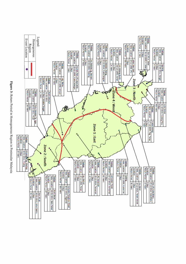
195

Figure 3: Return Period in H

omogeneous R

egion in Peninsular Malaysia

Hom

ogeneous R

egion

Event Location

Legend:

196

CONCLUSION

The objective of this study is to analyse the rainfall return period of major flood events on the homogeneous region at peninsular Malaysia. 22 rain gauge station have been used to analyse the return period by annual maximum series of a best fitted distribution model. GEV distribution model are the most suitable for analysing the annual maximum rainfall. With the help of computer programming such as FORTRAN, the sorting of cumulative maximum annual data were made easily and more precisely. The annual maximum series frequency analysis were carried out by using computer programming such as EasyFit. The conclusion of the result are the following;

1. The analysis of the return period were carried out on a total of 22 rain gauge station. The station were chosen according to the flood event that were ranked as the most severe based on number of victim evacuated.

2. The rainfall data of the selected flood events were then grouped accordingly to their respective homogeneous zone to carry out pooled frequency analysis.

3. The analysis were done based on 6-days, 7-days, 8-days, rainfall duration for homogeneous region zone 1, 4-days, 6-days rainfall duration for zone 2, 4-days, 5-days, 8-days rainfall duration for zone 3, and 3-days, 4-days, 7-days rainfall duration for zone 4.

4. In zone 1 for instant, the highest rainfall return period is observed to be 50 years for a 7-day rainfall event, and 20 years for a 5-day rainfall event. Therefore, in designing hydraulic structures needing the extreme rainfall value estimates, engineers may consider to use a 50 year (7-day rainfall) design of the hydraulic structures to be build in areas within the homogeneous zone 1. This is due to a 50 year rainfall have been experienced within the same homogeneous regions and there would be a high possibility that similar magnitude of rainfall event may occur in other areas within zone 1.

Therefore, identifying the return period on a homogeneous region will benefits in hydraulic structure design. The result from this study can be used for future relating to flood mitigation structure designs. The estimation of the return periods of each zone may be improved using regional frequency analysis which consider a scaling factor and including more analysis of return periods from other rainfall stations within the zone.

REFERENCES [1] Sani G. D/iya, Muhd BarzaniGasim, Mohd EkhwanToriman, Musa G. Abdullahi (2014), Floods in Malaysia

Historical Reviews, Causes, Effects and Mitigations Approach. International Journal of Interdisciplinary Research and Innovations, 2(4); 59-65

[2] Sulong Mohamad, Noorazuan Md Hashim, Kadaruddin Aiyub & M.E. Toriman (2012), Flash Flood and Community’s Response at Sg. Lembing, Pahang, Advances in Natural and Applied Sciences, 6(1); 19-25

[3] K.C. Low (2006), Application of Nowcasting Techniques Towards Strengthening National Warning Capabilities on Hydrometeorological and Landslides Hazards, Public Weather Services Workshop on Warning of Real-Time Hazards by Using Nowcasting Technology

[4] Syafrina, A.H., Zalina, M.D. & Juneng, L. (2015), Historical trend of hourly extreme rainfall in Peninsular Malaysia, Theoretical and Applied Climatology, 120(1); 259–285

[5] Sen Roy S (2009) A spatial analysis of extreme hourly precipitation patterns in India. Int J Climatol, 29 (3); 345–355 [6] Alias, N. E., & Takara, K. (2014). Incorporating extreme rainfall behaviors into flood risk management- an

assessment on probable maximum precipitation, trends and future predictions, DPRI Annual Meeting., Kyoto Univ. 27-28 February 2014.

[7] Yevjevich, V., 1972. Probability and Statistics in Hydrology. Water Resources Publications, Colorado. [8] Zalina, M. D., Amir, H. M. K., Mohd Nor Mohd Desa, Nguyen, V-T-V. Statistical analysis of at-site extreme

rainfall processes in Penisular Malaysia. In Regional Hydrology: Bridging the Gap Between Research and Practice (Proceeding of the Fourth International FRIEND Conference, March. Cape Town, South Africa: FRIEND. 2002.

[9] Hosking, J. R. M. and Wallis, J. R, (1993) Some statistics useful in regional frequency analysis, Water Resour. Res., 29; 271–281

[10] Bedient & Huber. Hydrology and Flooding Analysis. Addison Wesley Publishing Co (1948). [11] Adamowski K, Bougadis J (2003), Detection of trends in annual extreme rainfall, Hydrol Process, 17(18);

3547–3560 [12] P. Satyanarayana,V. V. Srinivas, (2008), Regional frequency analysis of precipitation using large-scale

atmospheric variables, Journal Of Geophysical Research, 113(D24) [13] L. Ga´al, J. Kysel´y, J. Szolgay, (2008), Region-of-influence approach to a frequency analysis of heavy

precipitation in Slovakia. Hydrology and Earth System Sciences Discussions, European Geosciences Union,12 (3); 825-839

197

The Relationship of Rainfall-Runoff within Putrajaya Catchment Area Nor Hanani binti Habsirun, Kamarul Azlan Mohd Nasir

Faculty of Civil Engineering, Universiti Teknologi Malaysia

kamarul.azlan@yahoo.com

Keywords: Putrajaya Catchment, Rainfall-Runoff, Hydrologic Model

ABSTRACT. Progressive development in Putrajaya from agricultural area to urban area brings significant problems such as overflow and poor water quality. In order to avoid problems during urbanization transformation, a series of Wetland and lakes is introduced. The Wetland, which covers an area of about 2km2, was artificially created to become the aesthetic centre of Putrajaya. Putrajaya Wetlands is the main and the biggest component of Putrajaya as the new Malaysian Government Adminitrative Centre. This study has been conducted to describe the relationships of rainfall-runoff in the study area. HEC-HMS modelling of study area has been implemented to determine the 100 years ARI. In this modelling, there are three basic stages that had to be done, they are calibration, validation, and simulation. A couple set of precipitation and discharge data were used in calibration and validation process. In the calibration process, precipitation data as at 7 May 2016 was used. The computed peak discharge was 7.8m3/s and the observed peak discharge was 2.4m3/s. As for validation process, precipitation data as at 13 December 2015 was used. The computed peak discharge was 1.2m3/s and the observed peak discharge was 1.4m3/s. The relationship of rainfall runoff within the catchment were established using simple linear model, the correlation coefficient, R2 obtained was 0.86 for calibration and 0.37 for validation respectively. In designing 100 years ARI, peak flow has been estimated by using same parameters in HEC-HMS. Based on the result, it shows value of the design rainfall in Putrajaya catchment area was 10m3/s which was higher than the channel capacity of 5m3/s. This shows that flood is likely to happen in Putrajaya.

INTRODUCTION

Progressive development in Putrajaya from agricultural area to urban area definitely brings significant problem such as overflow and poor water quality. Deforestation increases surface runoff and catchment response to rainfall is highly variable and unpredictable. (Hibbert, 1995). Deforestation almost invariably leads to higher stream flow while reforestation of open land generally reduces the overall stream flow. (Bosch and Hewlett, 1982). The land of urban area has less permeability, which causes storm water runoff increase.

Hydrologists are often required to predict stream flow for catchments with limited or no flow measurements. Particular aspects of the stream-flow hydrograph have been selected for regional analysis, for example, the median annual flood and associated flood frequency growth curve, or the flow-duration curve. However, for a range of flood and water resources studies, and increasingly for wider set of environmental studies, simulation of the rainfall-runoff relationship is desirable.

The knowledge of both the rainfall-runoff relationship and design of urban drainage networks is an essential tool in modelling. Moreover, as increasing urbanization makes the flow in drainage networks larger and urban catchments are usually designed to convey only medium intensity rainfall, it can be useful to perform fault detection and supervision and to design control systems for real-time storm effect management. In order to perform effective management of urban drainage networks, accurate models are needed, which must be capable of simulating and predicting the water flow in the main sections of the network.

Problem Statement Putrajaya was developed as the federal administrative centre of Malaysia. Most of the ministries’ offices were shifted from Kuala Lumpur to Putrajaya in 1999 due to overcrowding and congestion in Kuala Lumpur. In 2001, Putrajaya became Malaysia's third Federal Territory after Kuala Lumpur and Labuan. It plays an important role being the heart of the country as all ministries were moved there. Should Putrajaya flood, many government servants will face difficulty to continue their jobs and even important events held in Putrajaya will have to stop.

By introducing a wetland and lake to the city of Putrajaya, the problems may be curb. Putrajaya wetland and lake is located at the center of the city which is a very strategic area to protect and control the hydrological component of Putrajaya. With an area of high rapid developent, the risk of siltation and sedimentation which lead to flash flood is high. Surface runoff also increases and the precipitation might be unpredictable in volume and affect the downstream area since the cycle is disturbed. By having a wetland, the predicted problems can be controlled. Therefore, it is vital to analyze rainfall data to estimate total precipitation and discharge level to identify the effectiveness of the Putrajaya wetland and lake in balancing the hydrological component. Although Putrajaya experienced flood once on 7 May 2016, the management has since improvised the flood prevention system as to ensure that the catastrophe will not happen again.

198

Objectives The objectives of this study are:

1. To compare the peak flow rate between simulated hydrograph and observe hydrograph. 2. To design the rainfall of 100 years ARI for Putrajaya catchment and compare with channel capacity whether

that Putrajaya may be facing flood problem for the next 100 years.

Scope of Study This study is focusing on Putrajaya wetland and lakes as their catchment area. It consists of explanation about the steps to be taken and the process in conducting this study. It explains about the scope covered in conducting this project start from the beginning which is collating the data until the final process of getting the results. Scope of study that includes Putrajaya catchment area only. Data Collection: Data that are needed in this study such as rainfall and water level are obtained from Efektif Permai Sdn. Bhd. which is the contractor that monitored Putrajaya Wetland. Besides, data from Jabatan Pengairan dan Saliran (JPS) for several stations around Putrajaya are also complementary as comparison to identify the validity of the data. The information such as dimension of weir, losses rate and so on are also needed. All data are required for modelling and simulation process by using HEC-HMS. Analyze the Collection Data: The collated data must be analysed in order to determine the suitable data that will be used. This process is very important since it may affect the calculation and may produce bad result due to choosing wrong data. Rainfall Runoff Modelling: Through this process, the data of rainfall and runoff that has been analysed and chose will be modelled by using HEC-HMS in order to obtain the result, which is the peak flow. This software will produce the hydrograph unit. To produce such accurate and reliable result, there are other processes such as model calibration and model validation. Designing the Rainfall for 100 years ARI: This process is to predict whether Putrajaya will be facing flood problem for the next 100 years. The rainfall results obtained from this process will be used to find the capacity that can be supported by the existing basin for the next 100 years. The value of the capacity will be compared with the value of flow for the next 100 years. If the peak flow is higher than the capacity of the basin, than flood will occur. Conclusion: Summarise the result of modelling and simulation of rainfall and runoff data. This may include the explanation whether the basin will flood for the next 100 years and also the structures and works that can be done to overcome the flood problem.

LITERATURE REVIEW

Precipitation in arid and semi-arid zones results largely from convective cloud mechanisms producing storms typically of short duration, relatively high intensity and limited area extent. However, low intensity frontal-type rains are also experienced, usually in the winter season. When most precipitation occurs during winter, as in Jordan and in the Negev, relatively low-intensity rainfall may represent the greater part of annual rainfall.

When rain falls, the first drops of water are intercepted by the leaves and stems of the vegetation. This is usually referred to as interception storage. As the rain continues, water reaching the ground surface infiltrates into the soil until it reaches a stage where the rate of rainfall (intensity) exceeds the infiltration capacity of the soil. Thereafter, surface puddles, ditches, and other depressions are filled (depression storage), after which runoff is generated.

Storm analysis is an important aspect of rainfall evaluation. The rainfall-runoff relationship for any rainstorm depends on the dynamic interaction between rain intensity, soil infiltration and surface storage. Runoff occurs whenever rain intensity exceeds the infiltration capacity of the soil, provided that there are no physical obstructions to surface flow. Rainfall storm analysis should consider the sequence of intensive rain events as well as their magnitude.

Very often attention is focused on quite large hydrologic basins which often involves lakes and rivers, which is far away from hydraulic urban engineering interests. In hydraulic practice, the rainfall-runoff relationship is described trough physical- based models which is completely characterized by a set of design parameters. Good estimates of parameters for these models should be obtained through long-term surveys on existing network, which would be able to provide reliable parameter values in order to design networks on the basis of a previously assigned “design risk”. The design risk is defined on the basis of the network maximum acceptable peak discharge Q as a function of the so-called “return period”, the mean time interval, Tr which must pass between the occurrence of two flow peaks of intensity Q (Chow, Maidment & Mays, 1988).

METHODOLOGY

There are several works, procedures and considerations involved in determining the relationship of rainfall runoff in this study area. The methods and solutions that can be used for finding the peak flow rate and volume are able to

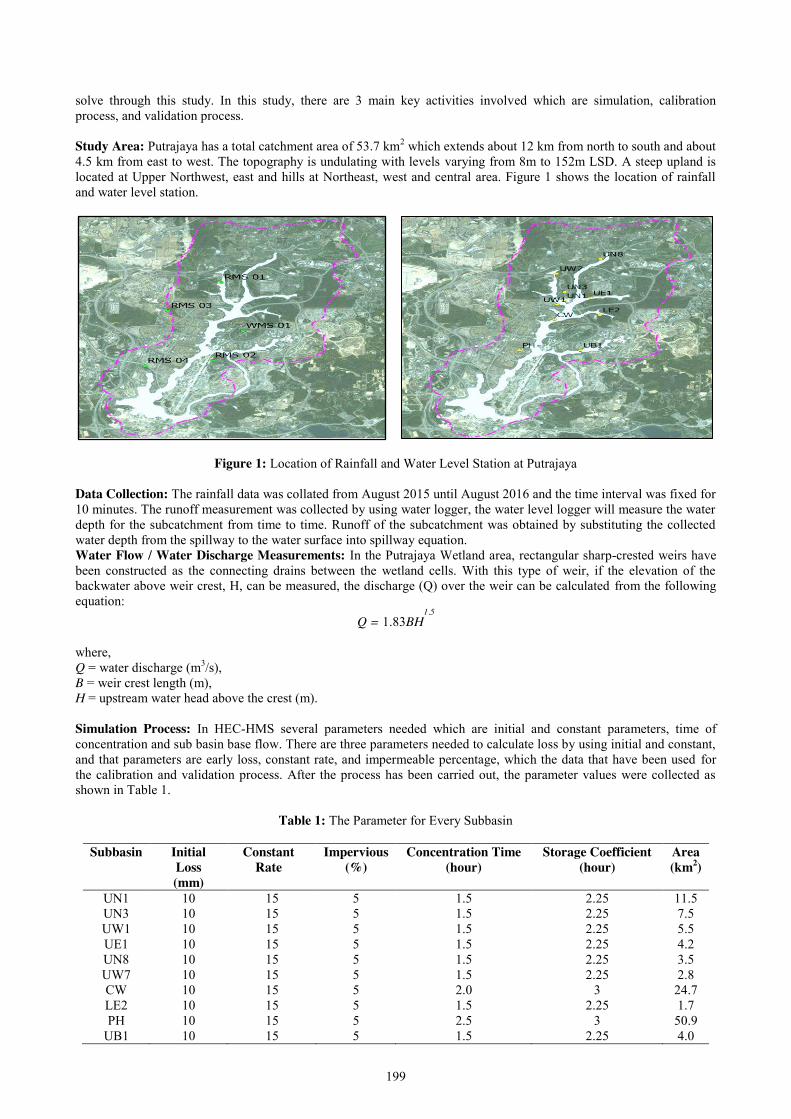
199

solve through this study. In this study, there are 3 main key activities involved which are simulation, calibration process, and validation process. Study Area: Putrajaya has a total catchment area of 53.7 km2 which extends about 12 km from north to south and about 4.5 km from east to west. The topography is undulating with levels varying from 8m to 152m LSD. A steep upland is located at Upper Northwest, east and hills at Northeast, west and central area. Figure 1 shows the location of rainfall and water level station.

Figure 1: Location of Rainfall and Water Level Station at Putrajaya

Data Collection: The rainfall data was collated from August 2015 until August 2016 and the time interval was fixed for 10 minutes. The runoff measurement was collected by using water logger, the water level logger will measure the water depth for the subcatchment from time to time. Runoff of the subcatchment was obtained by substituting the collected water depth from the spillway to the water surface into spillway equation. Water Flow / Water Discharge Measurements: In the Putrajaya Wetland area, rectangular sharp-crested weirs have been constructed as the connecting drains between the wetland cells. With this type of weir, if the elevation of the backwater above weir crest, H, can be measured, the discharge (Q) over the weir can be calculated from the following equation:

Q = 1.83BH1.5

where, Q = water discharge (m3/s), B = weir crest length (m), H = upstream water head above the crest (m). Simulation Process: In HEC-HMS several parameters needed which are initial and constant parameters, time of concentration and sub basin base flow. There are three parameters needed to calculate loss by using initial and constant, and that parameters are early loss, constant rate, and impermeable percentage, which the data that have been used for the calibration and validation process. After the process has been carried out, the parameter values were collected as shown in Table 1.

Table 1: The Parameter for Every Subbasin

Subbasin Initial Loss (mm)

Constant Rate

Impervious (%)

Concentration Time (hour)

Storage Coefficient (hour)

Area (km2)

UN1 10 15 5 1.5 2.25 11.5 UN3 10 15 5 1.5 2.25 7.5 UW1 10 15 5 1.5 2.25 5.5 UE1 10 15 5 1.5 2.25 4.2 UN8 10 15 5 1.5 2.25 3.5 UW7 10 15 5 1.5 2.25 2.8 CW 10 15 5 2.0 3 24.7 LE2 10 15 5 1.5 2.25 1.7 PH 10 15 5 2.5 3 50.9

UB1 10 15 5 1.5 2.25 4.0

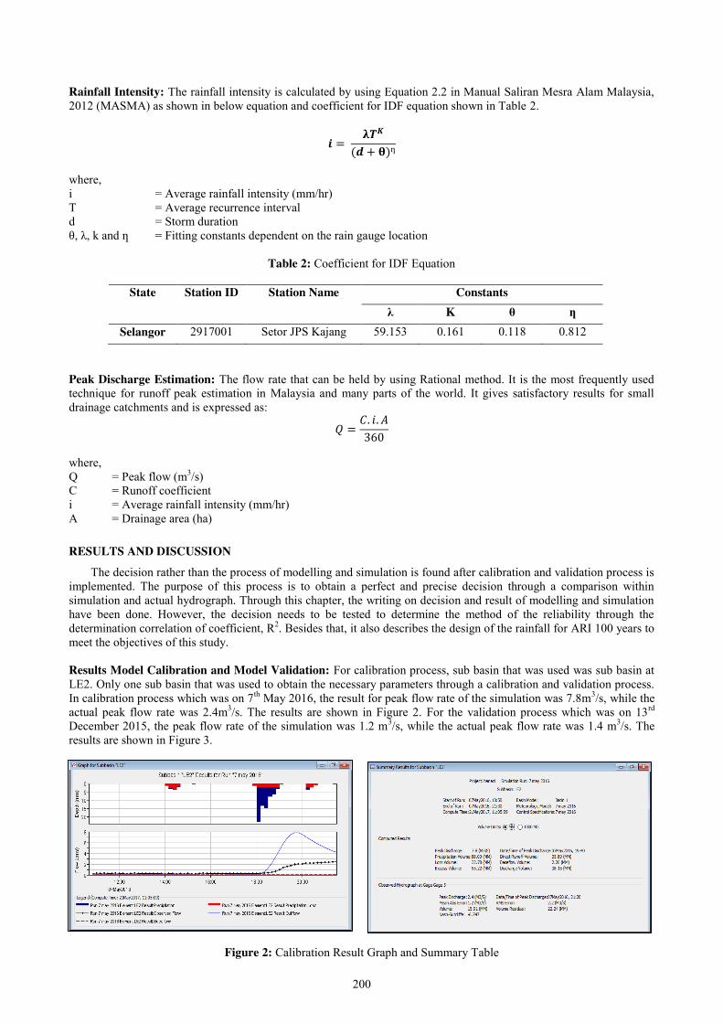
200

Rainfall Intensity: The rainfall intensity is calculated by using Equation 2.2 in Manual Saliran Mesra Alam Malaysia, 2012 (MASMA) as shown in below equation and coefficient for IDF equation shown in Table 2.

𝒊 = 𝛌𝑻𝑲

(𝒅 + 𝛉)ƞ

where, i = Average rainfall intensity (mm/hr) T = Average recurrence interval d = Storm duration θ, λ, k and ƞ = Fitting constants dependent on the rain gauge location

Table 2: Coefficient for IDF Equation

State Station ID Station Name Constants λ K θ ƞ

Selangor 2917001 Setor JPS Kajang 59.153 0.161 0.118 0.812 Peak Discharge Estimation: The flow rate that can be held by using Rational method. It is the most frequently used technique for runoff peak estimation in Malaysia and many parts of the world. It gives satisfactory results for small drainage catchments and is expressed as:

𝑄 =𝐶. 𝑖. 𝐴360

where, Q = Peak flow (m3/s) C = Runoff coefficient i = Average rainfall intensity (mm/hr) A = Drainage area (ha)

RESULTS AND DISCUSSION The decision rather than the process of modelling and simulation is found after calibration and validation process is

implemented. The purpose of this process is to obtain a perfect and precise decision through a comparison within simulation and actual hydrograph. Through this chapter, the writing on decision and result of modelling and simulation have been done. However, the decision needs to be tested to determine the method of the reliability through the determination correlation of coefficient, R2. Besides that, it also describes the design of the rainfall for ARI 100 years to meet the objectives of this study. Results Model Calibration and Model Validation: For calibration process, sub basin that was used was sub basin at LE2. Only one sub basin that was used to obtain the necessary parameters through a calibration and validation process. In calibration process which was on 7th May 2016, the result for peak flow rate of the simulation was 7.8m3/s, while the actual peak flow rate was 2.4m3/s. The results are shown in Figure 2. For the validation process which was on 13rd December 2015, the peak flow rate of the simulation was 1.2 m3/s, while the actual peak flow rate was 1.4 m3/s. The results are shown in Figure 3.

Figure 2: Calibration Result Graph and Summary Table

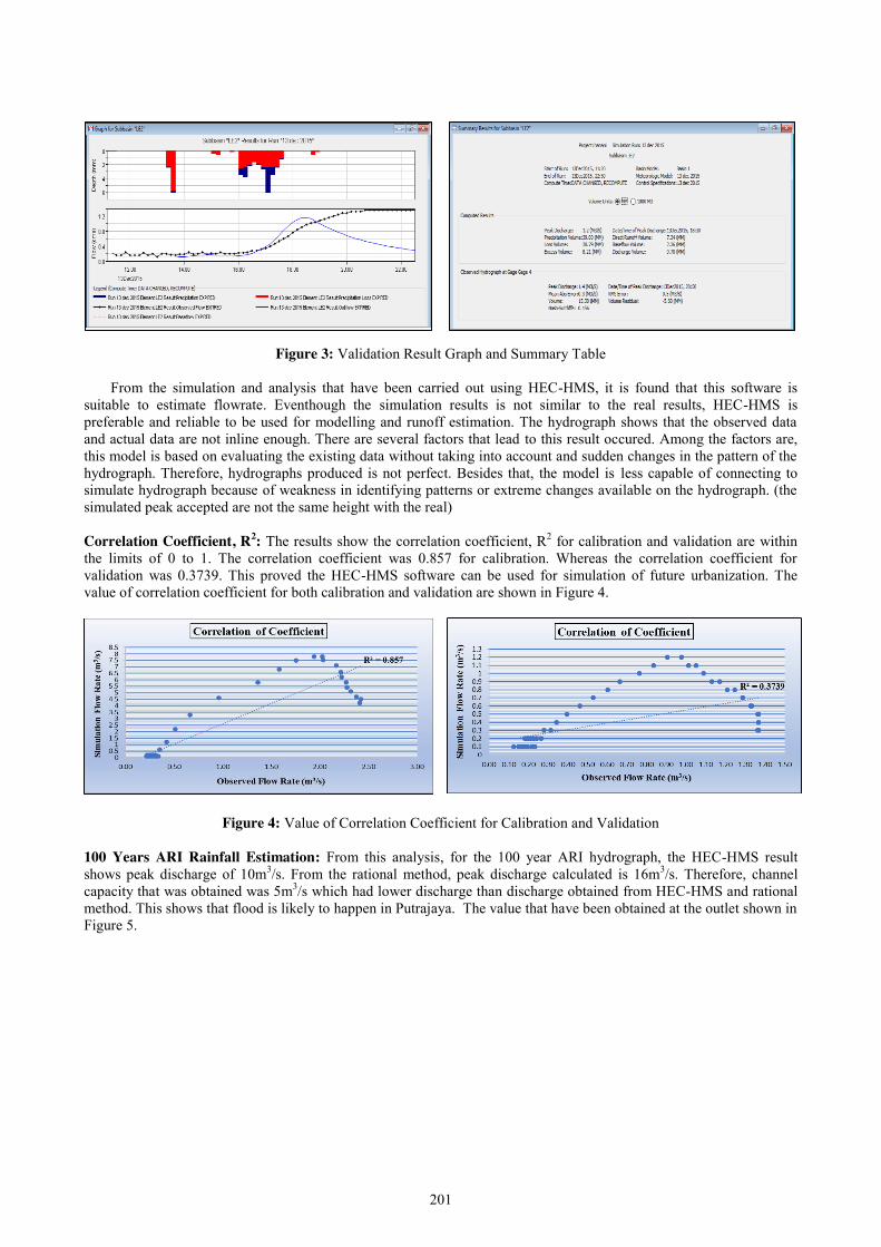
201

Figure 3: Validation Result Graph and Summary Table

From the simulation and analysis that have been carried out using HEC-HMS, it is found that this software is suitable to estimate flowrate. Eventhough the simulation results is not similar to the real results, HEC-HMS is preferable and reliable to be used for modelling and runoff estimation. The hydrograph shows that the observed data and actual data are not inline enough. There are several factors that lead to this result occured. Among the factors are, this model is based on evaluating the existing data without taking into account and sudden changes in the pattern of the hydrograph. Therefore, hydrographs produced is not perfect. Besides that, the model is less capable of connecting to simulate hydrograph because of weakness in identifying patterns or extreme changes available on the hydrograph. (the simulated peak accepted are not the same height with the real)

Correlation Coefficient, R2: The results show the correlation coefficient, R2 for calibration and validation are within the limits of 0 to 1. The correlation coefficient was 0.857 for calibration. Whereas the correlation coefficient for validation was 0.3739. This proved the HEC-HMS software can be used for simulation of future urbanization. The value of correlation coefficient for both calibration and validation are shown in Figure 4.

Figure 4: Value of Correlation Coefficient for Calibration and Validation

100 Years ARI Rainfall Estimation: From this analysis, for the 100 year ARI hydrograph, the HEC-HMS result shows peak discharge of 10m3/s. From the rational method, peak discharge calculated is 16m3/s. Therefore, channel capacity that was obtained was 5m3/s which had lower discharge than discharge obtained from HEC-HMS and rational method. This shows that flood is likely to happen in Putrajaya. The value that have been obtained at the outlet shown in Figure 5.

202

Figure 5: ARI 100 Years Result Graph and Summary Table

CONCLUSION

Process modelling and simulation of rainfall and runoff performed using HEC-HMS to get the peak flow rate in effect at the catchment area. From the rainfall runoff relationship graph, it shows flow rate increases as rainfall increases gradually. For calibration process, computed peak discharge was 7.8m3/s and time to concentration was on 7th May 2016, 19:40. While observed peak discharge was 2.4m3/s and time to concentration was on 7th May 2016, 21:20. For validation process, computed peak discharge was 1.2m3/s and time to concentration was on 13th December 2015, 18:30. While observed peak discharge was 1.4m3/s and time to concentration was 13th December 2015, 20:50. The relationship of rainfall runoff within the catchment were established using simple linear model, the correlation coefficient, R2 obtained was 0.857 for calibration and 0.3739 for validation resepectively.

This shows that Putrajaya is a good role model of sustainable development as it takes into account suitable mitigations as can be seen in Putrajaya wetland and lakes, which can be regarded as good model to control flood. There are a few recommendations that can be improved for further research such as:

1. The water level in Putrajaya Wetland should be relocated so that the data can be more accurate. 2. Maintenance regularly in rain station is needed to ensure the safekeeping of data.

REFERENCES

[1] Jonathan M. Harbor. (1994). “A Practical Method for Estimating the Impact of Land Use Change on Surface Runoff, Groundwater Recharge and Wetland Hydrology.” Journal of The American Planning Association, 60:1, 95-108, DOI: 10.1080/01944369408975555

[2] US Army Corps of Engineers, Hydrologic Engineering Center. (2000). “HEC-HMS Hydrology Modelling System – Technical Reference Manual.”

[3] US Army Corps of Engineers, Hydrologic Engineering Center. (2016). “HEC-RAS River Analysis System – Hydraulic Reference Manual Version 5.0.”

[4] Jabatan Pengairan dan Saliran (2012). “Manual Saliran Mesra Alam Malaysia, (MASMA)”. JPS Malaysia. [5] Viessman, Warren, JR., Gary L. Lewis, John W. Knapp (1989). “Introduction To Hydrology.” 3rd. ed. New

York: Happer & Row. , pp. 494-498. [6] Luna B. Leopold. (1968). “Hydrology for Urban Land Planning – A Guidebook on The Hydrologic Effects of

Urban Land Use.”

203

Estimation of Evapotranspiration at Putrajaya Wetland Ummu Najwa binti Ladzim, Kamarul Azlan Mohd Nasir Faculty of Civil Engineering, Universiti Teknologi Malaysia, Malaysia

kamarul.azlan@yahoo.com

Keywords: Evapotranspiration, Wetland, Hydrological Cycle, Penman Method, Water Balance Method

ABSTRACT. Evapotranspiration is one of component in hydrological cycle which really important in our daily life in order to get continuous water supply. Putrajaya is one of a develop area in Malaysia which before named Prang Besar. As land in Putrajaya is transformed from a forest into a city, it is definitely bringing a significance changes to the state of hydrological cycle in that particular area. To ensure there will be no problems encounter because of the changes, a lake and wetland is introduced. To study the effectiveness of the lake and wetland in quantity perspective, estimation of evapotranspiration (PET) is done. The estimation is based on Penman method and also water balance method and Penman method is act as benchmark. The PET rate between Penman method and water balance method is distinctive because of difference variables and also certain circumstances during data collection. .

INTRODUCTION

Water is the main component that really important to the lake and wetland ecological environment. Water state in a wetland reflects the ecosystem in that particular area. To ensure the lake and wetland are in proper state, the quantity of water loss through evaporation and evapotranspiration (ET) are essentials. Evapotranspiration is the combined loss of water by evaporation and transpiration by plants. Mainly in wetland, evapotranspiration is largely the cause of water loss. So, the water loss quantity need to be measured since it will affect water resources availability. Furthermore, evaporation and evapotranspiration (ET) are of the component in hydrological cycle which responsible for water balance in an area and parameters for water level and storage volume of a lake.

Problem Statement Putrajaya is one of developed area which is start operating in 1999 as federal administrative centre of Malaysia and Malaysia's third Federal Territory after Kuala Lumpur and Labuan. This development is to minimize the overcrowding in Kuala Lumpur. As land in Putrajaya is transformed from a forest into a city, it is definitely bring a significance changes to the state of hydrological cycle in that particular area. By introducing a lake and a wetland to the city of Putrajaya, the problems may be curb. Lake of Putrajaya and the wetland is located at the center of the city which is a very strategic area to protect and control the hydrological component of Putrajaya. With a very rapid development of the area, the risk of siltation and sedimentation which lead to flash flood is high. Surface runoff also increases and the precipitation might be unpredictable in volume and effect the downstream area since the cycle is disturbed. By having a wetland, the predicted problems could be controlled. Therefore, it is vital to analyze rainfall data to estimate total precipitation and discharge level to identify the effectiveness of the Putrajaya lake and Putrajaya wetland in balancing the hydrological component.

Objectives The objectives of this study are:

12. To estimate the evapotranspiration rate at Putrajaya Wetlands and lakes.

13. To study the relationship of meteorological variables and water level affect the evapotranspiration (ET) rate

Scope of Study This research is carried out to study the rate of evapotranspiration in Putrajaya Wetland to ensure that the hydrological system in that area is effective or not. Several data of a particular area are gathered such as rainfall data, evaporation data, meteorological data and also water level data. The data is used in the estimation process. Site visit to Putrajaya Wetland is needed to observe the condition of the wetland itself and get the picture what problems that might be happenned. The data collection then analyzed by using Penman formula and water balance method. The analyzing process is using Microsoft Excel. Evaporation data from DID is used as guidance and prove that weather in Malaysia is unpredictable.

204

LITERATURE REVIEW

Wetlands have several functions that could preserve the environment and ecosystem. Besides, it also influence on hydrological cycle since it might increase the rate of evapotranspiration and also evaporation. It regulates the flow of water within watersheds and in the global water cycle [1]. The uniqueness of it and also its function as terrestrial zone between two zones or more diversity made it the heart of the landscape [2].

Evapotranspiration is related to climate, groundwater and surface-water characteristics, as well as to the physiology of plants. Evaporation and transpiration are enhanced by meteorological conditions, such as solar radiation or surface temperature, that increase the value of the vapour pressure at the water surface, or by factors such as the decreased humidity or increased wind speed that decrease the vapour pressure of the surrounding air[1]. Among the environmental factors at work, light intensity, humidity and temperature are the climatic variables which most influence the transpiration rates in macrophytes [3]. While evaporation rate is directly proportional to the wind speed, emergent hydrophytes reduce evaporation by sheltering the water surface from the wind [3]. Because a supply of water is seldom considered limiting during the growing season in many types of wetlands, the theoretical atmospheric demand or potential evapotranspiration (PET) is used to approximate wetland evapotranspiration rates [1].

Energy must either be available or must be redistributed within the hydrologic system to cause the water to evaporate. The sources of this energy in the hydrologic system are the sun, heat carried into the region by wind, heat stored in land masses and also heat stored in water [4].

METHODOLOGY

This research involves the effectiveness of Putrajaya Wetland towards the water quality control and also as flood control device. The data of evapotranspiration will be taken from Jabatan Aliran dan Saliran of nearest rain station around Putrajaya and also from Efektif Permai Sdn. Bhd. which is the contractor that manage Putrajaya lake and wetland. From the data, we will compare it with the expected volume that will be calculated using suitable formulas. Research Area Putrajaya is a planned city located 25km south of Kuala Lumpur which is the capital of Malaysia. This area was originally part of the Selangor state. Both parties; Federal Government and Selangor State Government have been through a series of negotiations on the possibility of developing another Federal Territory in the mid-1990s. As a result, the Federal Government paid a substantial amount of money to Selangor for approximately 11,320 acres (45.8 km2) of land in Prang Besar, Selangor.

Putrajaya Lake Catchment. The Putrajaya Lake catchment area is 53.7 km2, which is small part of bigger 2530 km2 Sungai Langat catchment. The location of this catchment is within a fairly urbanized area with rapid development going on all around it, at the southern part of Kuala Lumpur. Topography. Putrajaya has a total catchment area of 53.7 km2 which extends about 12 km from north to south and about 4.5 km from east to west. The topography is undulating with levels varying from 8m to 152m LSD. A steep upland is located at Upper Northwest, east and hills at Northeast, west and central area. Figure 2.3 shows the topography map of the Putrajaya catchment. Putrajaya Lake and Wetland The wetlands have been designed as a quality control measure to enhance the water quality in the lake. It also acts as another natural landscape feature of the “Garden–in-a-city concept” of Putrajaya. They have been designed as secondary measures for the reduction of runoff pollutants into the lake. The Putrajaya Lake is at the southern part of the wetland. About 60% of the lake water flows from the wetland and the remaining 40% is the direct discharge from the bordering promenade. The 20 m- wide promenade is the buffer feature along the lake shorelines. The 400 hectares Putrajaya Lake was created by inundating the lower part of the valleys of Sungai Chua and Sungai Bisa. The construction was started in 1998 and fully completed in the year 2002. The total volume of the whole lake is about 23.5 million cubic meters (MCM) and the water depth is in the range of 3 to 14 meters.. Data Collection Data that are needed in this research such as solar radiation, daily evaporation, wind speed, air moisture water level and ambient temperature is obtained from Efektif Permai Sdn. Bhd. which is the contractor that monitored Putrajaya Lake and Wetland. Besides, data from Jabatan Pengairan dan Saliran (JPS) for several stations around Putrajaya also complementary as comparison to identify the validity of the data. Measurement of Evapotranspiration (PET) The measurement of evaporation loss from a vegetated land surface is even more complex than measurement of loss from an open water body. The mechanism of plant transpiration must take into considerations the water availability in the plant and the ability of the atmosphere to absorb and carry away the water vapour. However, similar approaches for measurement of Eo may be adopted, and the ET of a particular type of plant can be determined by establishing a water budget for a growing plant or group of plants.

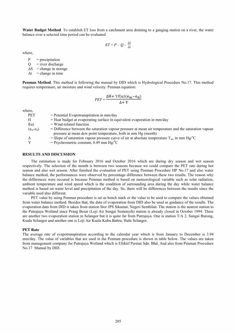
205

Water Budget Method. To establish ET loss from a catchment area draining to a gauging station on a river, the water balance over a selected time period can be evaluated

ET = P – Q - ∆𝑆∆𝑡

where,

P = precipitation Q = river discharge ΔS = change in storage Δt = change in time

Penman Method. This method is following the manual by DID which is Hydrological Procedure No.17. This method requires temperature, air moisture and wind velocity. Penman equation:

PET = ∆H+ Υf(u)(em−ed)

∆+ Υ

where,

PET = Potential Evapotranspiration in mm/day H = Heat budget at evaporating surface in equivalent evaporation in mm/day f(u) = Wind-related function (em-ed) = Difference between the saturation vapour pressure at mean air temperature and the saturation vapour

pressure at mean dew point temperature, both in mm Hg (month) Δ = Slope of saturation vapour pressure curve of air at absolute temperature Tm, in mm Hg/oC Υ = Psychrometric constant, 0.49 mm Hg/0C

RESULTS AND DISCUSSION

The estimation is made for February 2016 and October 2016 which are during dry season and wet season respectively. The selection of the month is between two seasons because we could compare the PET rate during hot season and also wet season. After finished the evaluation of PET using Penman Procedure HP No.17 and also water balance method, the performances were observed by percentage difference between these two results. The reason why the differences were occured is because Penman method is based on meteorological variable such as solar radiation, ambient temperature and wind speed which is the condition of surrounding area during the day while water balance method is based on water level and precipitation of the day. So, there will be differences between the results since the variable used also different.

PET value by using Penman procedure is set as bench mark or the value to be used to compare the values obtained from water balance method. Besides that, the data of evaporation from DID also be used as guidance of the results. The evaporation data from DID is taken from station Stor JPS Sikamat, Negeri Sembilan. The station is the nearest station to the Putrajaya Wetland since Prang Besar (Loji Air Sungai Semenyih) station is already closed in October 1994. There are another two evaporation station in Selangor but it is quite far from Putrajaya. One is station T/A 2, Sungai Burong, Kuala Selangor and another one is Loji Air Kuala Kubu Bahru, Hulu Selangor. PET Rate The average rate of evapotranspiration according to the calendar year which is from January to December is 3.94 mm/day. The value of variables that are used in the Penman procedure is shown in table below. The values are taken from management company for Putrajaya Wetland which is Efektif Permai Sdn. Bhd. And also from Penman Procedure No.17 Manual by DID.

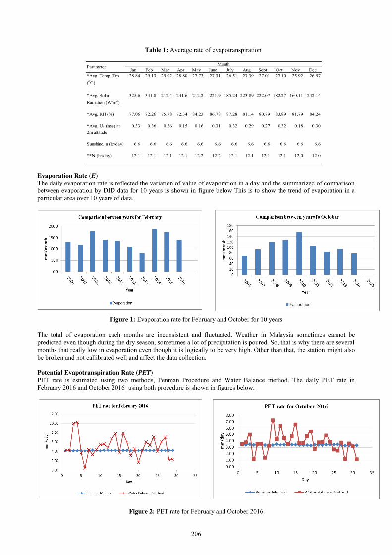
206

Table 1: Average rate of evapotranspiration

Evaporation Rate (E) The daily evaporation rate is reflected the variation of value of evaporation in a day and the summarized of comparison between evaporation by DID data for 10 years is shown in figure below This is to show the trend of evaporation in a particular area over 10 years of data.

Figure 1: Evaporation rate for February and October for 10 years

The total of evaporation each months are inconsistent and fluctuated. Weather in Malaysia sometimes cannot be predicted even though during the dry season, sometimes a lot of precipitation is poured. So, that is why there are several months that really low in evaporation even though it is logically to be very high. Other than that, the station might also be broken and not callibrated well and affect the data collection. Potential Evapotranspiration Rate (PET) PET rate is estimated using two methods, Penman Procedure and Water Balance method. The daily PET rate in February 2016 and October 2016 using both procedure is shown in figures below.

Figure 2: PET rate for February and October 2016

Jan Feb Mar Apr May June July Aug Sept Oct Nov Dec*Avg. Temp, Tm 28.84 29.13 29.02 28.80 27.73 27.31 26.51 27.39 27.01 27.10 25.92 26.97(oC)

*Avg. Solar 325.6 341.8 212.4 241.6 212.2 221.9 185.24 223.89 222.07 182.27 160.11 242.14Radiation (W/m2)

*Avg. RH (%) 77.06 72.26 75.78 72.34 84.23 86.78 87.28 81.14 80.79 83.89 81.79 84.24

*Avg. U2 (m/s) at 0.33 0.36 0.26 0.15 0.16 0.31 0.32 0.29 0.27 0.32 0.18 0.302m altitude

Sunshine, n (hr/day) 6.6 6.6 6.6 6.6 6.6 6.6 6.6 6.6 6.6 6.6 6.6 6.6

**N (hr/day) 12.1 12.1 12.1 12.1 12.2 12.2 12.1 12.1 12.1 12.1 12.0 12.0

Parameter Month

207

The difference between results of Penman and water balance is distinct. This could be because of the variables used in estimation using these two method is not the same. Penman is using meteorological variables such as ambient temperature, wind speed, and solar radiation while water balance is based on inflow and outflow of an area. The weather station and also water level gauge used by Efektif Permai Sdn. Bhd may not calibrated perfectly and affect the data taken. Some of the rain station is not functionally well because of several circumstances such as out of power source and also very near to the canopy which is reflected in the observed data. Water balance method is influenced by the water level, runoff and also precipitation of the day. The higher the water level is decreases, the higher the rate of PET.

The water level of the days is fluctuated and some of them are increasing and decreasing a lot between the days. These might be because of the precipitation and also the logging in and logging off of the weir at the water level station. Besides, the precipitation recorded are also not scattered well among the rain station around Putrajaya area. Some of the stations have a very high in precipitation and some are not. These could be because of the failure of rain gauge and the location of the rain gauge itself that near to the canopy.

CONCLUSION

The potential evapotranspiration rate (PET) is estimated using two methods which is Penman method and another one is water balance method. The performance between these two method is measured by percentage difference (%).The estimated value of PET for Putrajaya Wetland during February 2016 by Penman method is 121.01 mm and by using water balance method, PET value is 145.26 mm. While in October 2016, PET value is lesser because of wet season. So, the PET value when using Penman method and water balance method is 104.8 mm and 116.64 mm respectively. Based on the observation and estimation, the percentage difference between these two methods is distinctive because of unreliable observe data from water level station and also rainfall station.

The following recommendations were drawn for this study:

1. The evaporation station in Selangor should be increased to ease the scientific research on a particular area around Selangor because there are only two evaporation station located in Selangor which is very far from certain area.

2. The water level gauge for weir in Putrajaya wetland should be relocated so that a precise data could be taken for more accurate analyzing process

3. Rain station should be followed the specification that has been measured which is far from trees and building for certain distances. This is to ensure an accurate data collection could be taken

4. The climatic weather variables of the meteorological station should be observed frequently so that the values is logic and could be used for analysis process

REFERENCES [1] Richardson (1994), Mitsch and Gooselink 1993). Wetland Soils: Genesis, Hydrology, Landscapes, and

Classification. [2] William and James (1993). Defining Arizona’s Riparian Areas and Their Importance to the Landscape [3] David (2011). A simple method for estimating water loss by transpiration in wetlands [4] S.Supiah (2000). Hydrology Note Book Universiti Teknologi Malaysia

208

The Effectiveness of Sediment Removal within Putrajaya Wetlands and Lake

Nur Hidayah binti Mat Noor, Kamarul Azlan Mohd Nasir Faculty of Civil Engineering, Universiti Teknologi Malaysia

kamarul.azlan@yahoo.com

Keywords: Sediment Loading; HEC-HMS; USLE; MUSLE; Hydrology Analysis.

ABSTRACT. Sediment is the aftermath of construction that has taken place nearby the water bodies especially during earthwork stages. Putrajaya was constructed as a town but still preserve green area as to ensure sustainability of the mother-nature. However, construction of Putrajaya may have impacted land movement which may be aggravated by its natural high volume of rainfall which average at around 2307 mm per year, which sedimentation process occur more frequently. Besides that, Putrajaya also supports the flow coming from outside the catchment which made the area more prone to flood if not being controlled especially the amount of sediment in the wetlands and lake. Putrajaya management has applied their integrated management plan to combat the problem and to maintain water quality which includes bi-monthly sediment report and desilting activity to the required wetland cell. The objectives of this study are to estimate sediment loading per event and to assess the effectiveness of sediment removal in Putrajaya wetlands and lake. In order to obtain the targeted objective, data such as rainfall tip, water level, TSS concentration and weir dimension need to be gathered and to be systemized for further used. Water level data are used to estimate observed sediment loading at outflow of the cell. Meanwhile, rainfall data are keyed-in into HEC-HMS modelling to simulate peak discharge and runoff volume. The simulated data from HEC-HMS used in MUSLE equation to produce sediment yield at the inflow of the cell. For this study, the cell that was selected is UN3 due to complete data availability. For sediment yield at inflow of the cell shows that the sediment amount enters the wetland are quite high with the lowest amount 176 tonnes and the highest up to 8000 tonnes per event. However, the sediment loading at the outflow of cell shows significantly lower amount of sediment expel from the cell which the lowest only 6 tonnes per event and the highest was only 75 tonnes per event. Therefore, the cells are relatively effective in controlling sediment as 80% of the sediment are retained within the wetland and lake as monitored in November 2015 to March 2016. The finding of this study is important to provide additional information regarding wetland in Putrajaya specifically in sedimentation. Besides that, this study can act as a guideline for the authority regarding sediment loading in order to maintain the discharge capacity and water quality. INTRODUCTION

Sediment has become a normal composition in our water body due to rapid development in Putrajaya. When land disturbing activities occur, loose soil particle are transmitted into waterways by surface runoff and water movement. Since rainfall in Putrajaya is quite high ranging around 2307 mm per year, sedimentation process occur more frequently. Soil particles that are transmitted often end up in streams, lakes, and wetlands.Various impacts occur when pollutant enter water bodies as it changes the physical and aesthetical characteristic of water. Therefore it is important to maintain the sediment level so that wetland and lake can function fully. Problem Statement During 7th May 2016, with heavy rain (124 mm), Putrajaya area was flooded. The causes are believed due to unusual high amount of rainfall per event and also reduction conveyor capacity due to sedimentation and choke. The reduction of capacity is due to lack of maintenances in the area. Therefore, sedimentation is a critical problem that can reduce the capacity and cause damages to water intake. Apart from that, since Putrajaya is comprised of two components of different and distinct water-bodies, it is complex both in geographical location and hydrological functions to maintain the health of wetlands. Therefore, it is important to monitor and analyze the sedimentation loading to make sure the effectiveness of Putrajaya wetlands and lakes. Objectives The objectives of this study are:

14. To estimate sediment loading of the selected cell. 15. To assess the effectiveness of existing integrated management plan (wetlands and lake) to control sediment.

Scope of Study In order to estimate the effectiveness of Putrajaya wetlands and lake, it is essential to receive collation of data at selected locations in Putrajaya covering the parameters such as rainfall data from rainfall station, water level for each station and Total Suspended Solids (TSS) concentration from Effective Permai Sdn Bhd, which is the contractor

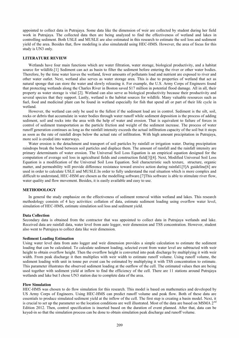
209

appointed to collect data in Putrajaya. Some data like the dimension of weir are collected by student during her field work in Putrajaya. The collected data then are being analyzed to find the effectiveness of wetland and lakes in controlling sediment. Both USLE and MUSLE are also estimated in this research to estimate the soil loss and sediment yield of the area. Besides that, flow modeling is also simulatedd using HEC-HMS. However, the area of focus for this study is UN3 only. LITERATURE REVIEW

Wetlands have four main functions which are water filtration, water storage, biological productivity, and a habitat source for wildlife.[1] Sediment can act as basin to filter the sediment before entering the river or other water bodies. Therefore, by the time water leaves the wetland, fewer amounts of pollutants load and nutrient are exposed to river and other water outlet. Next, wetland also serves as water storage area. This is due to properties of wetland that act as natural sponge that can store the water and slowly releasing it. For example, the U.S. Army Corps of Engineers found that protecting wetlands along the Charles River in Boston saved $17 million in potential flood damage. All in all, their property as water storage is vital [2]. Wetland can also serve as biological productivity because their productivity and several species that they support. Lastly, wetland is the habitat sources for wildlife. Many valuable resources such as fuel, food and medicinal plant can be found in wetland especially for fish that spend all or part of their life cycle in wetland.

However, the wetland can only be used to the fullest if the sediment load are in control. Sediment is the silt, soil, rocks or debris that accumulate in water bodies through water runoff while sediment deposition is the process of adding sediment, soil and rocks into the area with the help of water and erosion. That is equivalent to failure of forces in control of sediment transportation as the particle friction and weight of the sediment increase. The process of water runoff generation continues as long as the rainfall intensity exceeds the actual infiltration capacity of the soil but it stops as soon as the rate of rainfall drops below the actual rate of infiltration. With high amount precipitation in Putrajaya, more soil is eroded into waterways.

Water erosion is the detachment and transport of soil particles by rainfall or irrigation water. During precipitation raindrops break the bond between soil particles and displace them. The amount of rainfall and the rainfall intensity are primary determinants of water erosion. The Universal Soil Loss Equation is an empirical equation designed for the computation of average soil loss in agricultural fields and construction field[3][4]. Next, Modified Universal Soil Loss Equation is a modification of the Universal Soil Loss Equation. Soil characteristic such texture, structure, organic matter, and permeability will provide difference resistance toward erosive action during rainfall.[5]A guideline[6] are used in order to calculate USLE and MUSLE.In order to fully understand the real situation which is more complex and difficult to understand, HEC-HSM are chosen as the modelling software.[7]This software is able to stimulate river flow, water quality and flow movement. Besides, it is easily available and easy to use. METHODOLOGY

In general the study emphasize on the effectiveness of sediment removal within wetland and lakes. This research methodology consists of 4 key activities: collation of data, estimate sediment loading using overflow water level, simulation of HEC-HMS, estimate simulation soil loss and sediment yield. Data Collection Secondary data is obtained from the contractor that was appointed to collect data in Putrajaya wetlands and lake. Received data are rainfall data, water level from auto logger, weir dimension and TSS concentration. However, student also went to Putrajaya to collect data like weir dimension. Sediment Loading Estimation Using water level data from auto logger and weir dimension provides a simple calculation to estimate the sediment loading that can be calculated. To calculate sediment loading, selected event from water level are subtracted with weir height to obtain overflow height. Then the overflow height is converted into peak discharge by multiplying it with weir width. From peak discharge it then multiplies with weir width to estimate runoff volume. Using runoff volume, the sediment loading with unit in tonne per event can be estimated by multiplying it with TSS concentration to estimate. This parameter illustrates the observed sediment loading at the outflow of the cell. The estimated values then are being used together with sediment yield at inflow to find the efficiency of the cell. There are 11 stations around Putrajaya wetlands and lake but I chose UN3 station due to complete data of the area. Flow Simulation HEC-HMS was chosen to do flow simulation for this research. This model is based on mathematics and developed by US Army Corps of Engineers. Using HEC-HMS can predict runoff volume and peak flow. Both of these data are essentials to produce simulated sediment yield at the inflow of the cell. The first step is creating a basin model. Next, it is crucial to set up the parameter so the location conditions are well illustrated. Most of the data are based on MSMA 2nd Edition 2012. Then, control specification is inserted based on the duration of event planned. After that, data can be keyed-in so that the simulation process can be done to obtain simulation peak discharge and runoff volume.

210

Estimated Sediment Yield To estimate sediment yield, USLE and MUSLE equation are being used. By using runoff volume and peak flow from HEC-HMS, an estimated soil loss and simulated sediment yield can be calculated by multiplying to the factor underlying by the DID guideline. Both units are in tonnes/ha and tonnes respectively. In order to calculate soil loss using USLE, rainfall erosivity factor are multiplied with soil erodibility factor, topographic factor, cover factor and management practice factor. Meanwhile, to calculate MUSLE all factors from USLE except rainfall erosivity factor are multiplied to peak discharge and runoff volume. The peak discharge and runoff volume are used from HEC-HMS modelling. This data represents the sediment yield at inflow of the cell. This data are important to find the cell effectiveness of sediment removal.

Effectiveness of wetland cell Since the sediment loading at the inflow and outflow are known, the effectiveness of wetland cell to trap sediment can be estimated. To estimate sediment yield at inflow minus the sediment loading at outflow then divide by sediment yield at inflow. The unit in percent can be obtained.

RESULTS AND DISCUSSION

The data was obtained from August 2015 to July 2016. For the purpose of this study, the selected area of focus is at upper north catchment region of Putrajaya. The particular area was chosen as indications for the whole catchment as the area contain most reliable data. Result for sediment loading obtained from the observed peak discharge. Next, using simulated result from HEC-HMS, soil loss and sediment yield are also calculated. Then the efficiency of the cell is obtained by comparing sediment loading and sediment yield. Sediment Loading In order to estimate the sediment loading for UN3, data such as water level with interval 10 minutes is required alongside with details of weir at UN3. The details are as follow:

1. Weir height =1 m 2. Weir width =3.6 m 3. Time interval =10 min 4. TSS concentration =10 mg/l

Most of the weirs in Putrajaya are rectangular, sharp-crested weirs. The upstream water head (H) is uniquely related to the discharge over the crest of the structure. The discharge over the weir at critical condition can be calculated by empirical formula as follows:

Q = 1.83BH^1.5 Eq. 1 where: Q = water discharge (m3/s), B = weir crest length (m), and H = upstream water head above the crest (m)

When observed peak is known from the equation, volume can be calculated by multiplying the peak discharge to time interval which is ten minutes. The unit for volume is cubic meter. Lastly, the sediment loading can be calculated by multiplying volume and TSS concentration. The unit for sediment loading is tonne. By summing up the sediment loading from each interval, the sediment loading for the event is known. The results of sediment loading according to event are as follows:

Table 1: Result of sediment loading according to event

Month Sediment Loading, (tonne) November 2015 60 December 2015 75 January 2016 19 February 2016 45

March 2016 6 April 2016 74

As shown in Table 1, the sediment loading for each month differ. This situation occurs because the amount of

sediment increases when the volume and velocity of runoff increases. Since the runoff is related to amount of rainfall, the sediment loading are related to amount of rainfall. Based on rainfall data gathered from November 2015 to January 2016, it is shown that the amount of rainfall in that particular time are quite high which are 47.8 mm, 40.8 mm, 35.8 mm, and 24 mm respectively. For that reasons the amount of sediment loading are quite high during those month. As for February and March 2016, the amount of rainfalls are quite low which were only 10.6 mm and 18.4 mm respectively. Thus this explains why the sediment loading on those month were comparatively low. Lastly for April

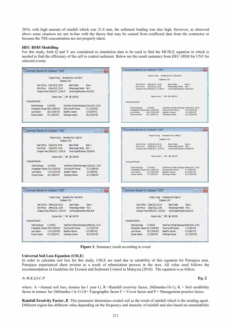
211

2016, with high amount of rainfall which was 21.8 mm, the sediment loading was also high. However, as observed above some situation are not in-line with the theory that may be caused from conflicted data from the contractor or because the TSS concentration are not properly taken. HEC-HMS Modelling For this study, both Q and V are considered as simulation data to be used to find the MUSLE equation in which is needed to find the efficiency of the cell to control sediment. Below are the result summary from HEC-HSM for UN3 for selected events:

Figure 1: Summary result according to event

Universal Soil Loss Equation (USLE) In order to calculate soil loss for this study, USLE are used due to suitability of this equation for Putrajaya area. Putrajaya experienced sheet erosion as a result of urbanisation process in the area. All value used follows the recommendation in Guideline for Erosion and Sediment Control in Malaysia (2010). The equation is as follow: A=R.K.LS.C.P Eq. 2 where: A =Annual soil loss, (tonnes ha-1 year-1), R =Rainfall erosivity factor, (MJmmha-1h-1), K = Soil erodibility factor in tonnes/ ha/ (MJmmha-1 h-1) LS= Topographic factor C = Cover factor and P = Management practice factor. Rainfall Erosivity Factor, R. This parameter determines eroded soil as the result of rainfall which is the eroding agent. Different region has different value depending on the frequency and intensity of rainfall and also based on sustainability

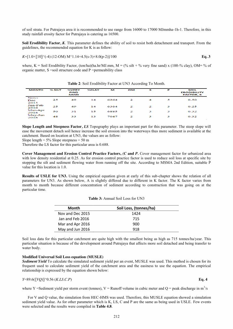
212

of soil strata. For Putrajaya area it is recommended to use range from 16000 to 17000 MJmmha-1h-1. Therefore, in this study rainfall erosity factor for Putrajaya is catering as 16500. Soil Erodibility Factor, K. This parameter defines the ability of soil to resist both detachment and transport. From the guidelines, the recommended equation for K is as follow: K=[1.0×〖10〗^(-4) (12-OM) M^1.14+4.5(s-3)+8.0(p-2)]/100 Eq. 3 where, K = Soil Erodibility Factor, (ton/ha)(ha.hr/MJ.mm, M = (% silt + % very fine sand) x (100-% clay), OM= % of organic matter, S =soil structure code and P =permeability class

Table 2: Soil Erodibility Factor at UN3 According To Month.

Slope Length and Steepness Factor, LS Topography plays an important part for this parameter. The steep slope will ease the movement detach soil hence increase the soil erosion into the waterways thus more sediment is available at the catchment. Based on location at UN3, the values are as follow: Slope length = 5% Slope steepness = 50 m Therefore the LS factor for this particular area is 0.688. Cover Management and Erosion Control Practice Factors, (C and P. Cover management factor for urbanized area with low density residential at 0.25. As for erosion control practice factor is used to reduce soil loss at specific site by stopping the silt and sediment flowing water from running off the site. According to MSMA 2nd Edition, suitable P value for this location is 1.0. Results of USLE for UN3. Using the empirical equation given at early of this sub-chapter shows the relation of all parameters for UN3. As shown below, A is slightly differed due to different in K factor. The K factor varies from month to month because different concentration of sediment according to construction that was going on at the particular time.

Table 3: Annual Soil Loss for UN3

Month Soil Loss, (tonnes/ha) Nov and Dec 2015 1424 Jan and Feb 2016 715 Mar and Apr 2016 900 May and Jun 2016 918

Soil loss data for this particular catchment are quite high with the smallest being as high as 715 tonnes/ha/year. This particular situation is because of the development around Putrajaya that affects more soil detached and being transfer to water body. Modified Universal Soil Loss equation (MUSLE) Sediment Yield To calculate the simulated sediment yield per an event, MUSLE was used. This method is chosen for its frequent used to calculate sediment yield of the catchment area and the easiness to use the equation. The empirical relationship is expressed by the equation shown below: Y=89.6(〖VQ)〗^0.56 (K.LS.C.P) Eq. 4 where Y =Sediment yield per storm event (tonnes), V = Runoff volume in cubic meter and Q = peak discharge in m3/s

For V and Q value, the simulation from HEC-HMS was used. Therefore, this MUSLE equation showed a simulation sediment yield value. As for other parameter which is K, LS, C and P are the same as being used in USLE. Few events were selected and the results were compiled in Table 4.8.

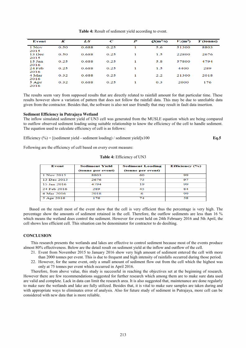
213

Table 4: Result of sediment yield according to event.

The results seem vary from supposed results that are directly related to rainfall amount for that particular time. These results however show a variation of pattern that does not follow the rainfall data. This may be due to unreliable data given from the contractor. Besides that, the software is also not user friendly that may result in fault data insertion. Sediment Efficiency in Putrajaya Wetland The inflow simulated sediment yield of UN3 cell was generated from the MUSLE equation which are being compared to outflow observed sediment loading using suitable relationship to know the efficiency of the cell to handle sediment. The equation used to calculate efficiency of cell is as follows: Efficiency (%) = [(sediment yield - sediment loading) / sediment yield]x100 Eq.5 Following are the efficiency of cell based on every event measure:

Table 4: Efficiency of UN3

Based on the result most of the event show that the cell is very efficient thus the percentage is very high. The percentage show the amounts of sediment retained in the cell. Therefore, the outflow sediments are less than 16 % which means the wetland does control the sediment. However for event held on 24th February 2016 and 5th April, the cell shows less efficient cell. This situation can be denominator for contractor to do desilting.

CONCLUSION

This research presents the wetlands and lakes are effective to control sediment because most of the events produce almost 80% effectiveness. Below are the detail result on sediment yield at the inflow and outflow of the cell.

21. Event from November 2015 to January 2016 show very high amount of sediment entered the cell with more than 2000 tonnes per event. This is due to frequent and high intensity of rainfalls occurred during those period.

22. However, for the same event, only a small amount of sediment flow out from the cell which the highest was only at 75 tonnes per event which occurred in April 2016.

Therefore, from above value, this study is successful in reaching the objectives set at the beginning of research. However there are few recommendations suggested for further research which among them are to make sure data used are valid and complete. Lack in data can limit the research area. It is also suggested that, maintenance are done regularly to make sure the wetlands and lake are fully utilized. Besides that, it is vital to make sure samples are taken during and with appropriate ways to eliminates error of analysis. Also for future study of sediment in Putrajaya, more cell can be considered with new data that is more reliable.

214

REFERENCES

[1] Tiffany B. (2013). Sediment Deposition in Wetlands and Effects on Near Shore Marine Ecosystems in Hawai‘i: An Analysis and Comparison to Wetlands Loss in Louisiana.

[2] United State Environmental Protection Agency (2011). Function and Values of Wetland. EPA 843-F-01-002c. [3] Musgrave G.W. (1947). The quantitative evaluation of factors in water erosion: a first approximation, Journal

of soil and water conservation, 2, pp.133-138. [4] Wischmeier, W.H. and Smith, D.D. (1978). Predicting rainfall erosion losses-A guide to conservation planning.

Agricultural HandbookNo.537. USDA, Washington, DC. [5] Williams J.R. (1975). Sediment routing for agricultural watersheds. Journal of the American Water Resources

Association, 11(5), pp. 965–974. [6] Department of Irrigation and Drainage or DID(2010). Guideline For Erosion And Sediment Control In

Malaysia-Chapter3-Soil Erosion and Sedimentation. [7] US Army Corp of Engineering (2013). Hydraulic Modelling System HEC-HMS: Manual. Version 4.0

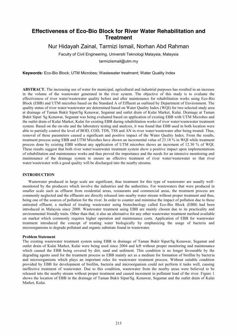
215

Effectiveness of Eco-Bio Block for River Water Rehabilitation and Treatment

Nur Hidayah Zainal, Tarmizi Ismail, Norhan Abd Rahman Faculty of Civil Engineering, Universiti Teknologi Malaysia, Malaysia

tarmiziismail@utm.my

Keywords: Eco-Bio Block; UTM Microbes; Wastewater treatment; Water Quality Index

ABSTRACT. The increasing use of water for municipal, agricultural and industrial purposes has resulted in an increase in the volume of the wastewater generated in the river system. The objective of this study is to evaluate the effectiveness of river water/wastewater quality before and after maintenance for rehabilitation works using Eco-Bio Block (EBB) and UTM microbes based on the Standard A of Effluent as outlined by Department of Environment. The quality status of river water/wastewater are determined based on Water Quality Index (WQI) for two selected study area at drainage of Taman Bukit Siput/Sg Kenawar, Segamat and outlet drain of Kulai Market, Kulai. Drainage at Taman Bukit Siput/ Sg Kenawar, Segamat was being evaluated based on application of existing EBB with UTM Microbes and the outlet drain of Kulai Market, Kulai for existing EBB during rehabilitation works of river water/wastewater treatment system. Based on the on-site and the laboratory testing and analysis, it was found that EBB used in both location were able to partially control the level of BOD, COD, TDS, TSS and AN in river water/wastewater after being treated. Thus, removal of these parameters caused a significant and positive impact of the Water Quality Index. From the results, treatment process using EBB and UTM Microbes have shown an incremental value of 23.18 % in WQI while treatment process done by existing EBB without any application of UTM microbes shows an increment of 12.30 % of WQI. These results suggest that both river water/wastewater treatment system show a positive impact upon implementations of rehabilitation and maintenance works and thus proved the importance and the needs for an intensive monitoring and maintenance of the drainage system to ensure an effective treatment of river water/wastewater so that river water/wastewater with a good quality will be discharged into the nearby streams.

INTRODUCTION Wastewater produced in large scale are significant, thus treatment for this type of wastewater are usually well-

monitored by the producers which involve the industries and the authorities. For wastewaters that were produced in smaller scale such as effluent from residential areas, restaurants and commercial areas, the treatment process are commonly neglected and the effluents are directly released into nearby water stream without proper treatment and thus, being one of the sources of pollution for the river. In order to counter and minimise the impact of pollution due to these untreated effluent, a method of treating wastewater using biotechnology called Eco-Bio Block (EBB) had been introduced in Malaysia since 2000. Wastewater treatment using EBB are mainly chosen due to its practicality and environmental friendly traits. Other than that, it also an alternative for any other wastewater treatment method available on market which commonly requires higher operation and maintenance costs. Application of EBB for wastewater treatment introduced the concept of treating water biologically by emphasizing the usage of bacteria and microorganisms to degrade pollutant and organic substrate found in wastewater. Problem Statement The existing wastewater treatment system using EBB in drainage of Taman Bukit Siput/Sg Kenawar, Segamat and outlet drain of Kulai Market, Kulai were being used since 2004 and left without proper monitoring and maintenance which caused the EBB being covered by dirt, sand and sediment. This condition is no longer favourable by the degrading agents used for the treatment process as EBB mainly act as a medium for formation of biofilm by bacteria and microorganisms which plays an important roles for wastewater treatment process. Without suitable condition provided by EBB for development of biofilm, bacteria and microorganism could not perform it tasks well, causing ineffective treatment of wastewater. Due to this condition, wastewater from the nearby areas were believed to be released into the nearby stream without proper treatment and caused increment in pollutant load of the river. Figure 1 shows the location of EBB in the drainage of Taman Bukit Siput/Sg. Kenawar, Segamat and the outlet drain of Kulai Market, Kulai.

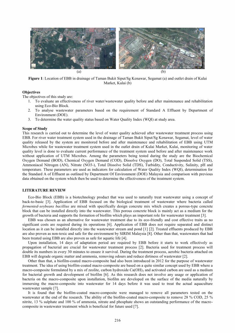
216

(a) (b)

Figure 1: Location of EBB in drainage of Taman Bukit Siput/Sg Kenawar, Segamat (a) and outlet drain of Kulai Market, Kulai (b)

Objectives The objectives of this study are:

1. To evaluate an effectiveness of river water/wastewater quality before and after maintenance and rehabilitation using Eco-Bio Block.

2. To analyse wastewater parameters based on the requirement of Standard A Effluent by Department of Environment (DOE).

3. To determine the water quality status based on Water Quality Index (WQI) at study area.

Scope of Study This research is carried out to determine the level of water quality achieved after wastewater treatment process using EBB. For river water treatment system used in the drainage of Taman Bukit Siput/Sg Kenawar, Segamat, level of water quality released by the system are monitored before and after maintenance and rehabilitation of EBB using UTM Microbes while for wastewater treatment system used in the outlet drain of Kulai Market, Kulai, monitoring of water quality level is done to evaluate current performance of the treatment system used before and after maintenance work without application of UTM Microbes. Among the parameters being tested during the study are the Biochemical Oxygen Demand (BOD), Chemical Oxygen Demand (COD), Dissolve Oxygen (DO), Total Suspended Solid (TSS), Ammoniacal Nitrogen (AN), Nitrate (NO3-), Total Dissolve Solid (TDS), Turbidity, Conductivity, Salinity, pH and temperature. These parameters are used as indicators for calculation of Water Quality Index (WQI), determination for the Standard A of Effluent as outlined by Department Of Environment (DOE) Malaysia and comparison with previous data obtained on the system which then be used to determine the effectiveness of the treatment system.

LITERATURE REVIEW

Eco-Bio Block (EBB) is a biotechnology product that was used to naturally treat wastewater using a concept of back-to-basic [3]. Application of EBB focused on the biological treatment of wastewater where bacteria called fermented-soybeans bacillius are mixed with specifically design concrete mix which creates a porous-type concrete block that can be installed directly into the wastewater. This porous concrete block is mainly act as a medium for the growth of bacteria and supports the formation of biofilm which plays an important role for wastewater treatment [3].

EBB was chosen as an alternative for wastewater treatment due to its eco-friendly and cost effective traits as no significant costs are required during its operations [6]. Application of EBB does not require separated and distinct location as it can be installed directly into the wastewater stream and pond [1] [2]. Treated effluents produced by EBB are also proven as non-toxic and safe for the environment by SIRIM Malaysia [8]. Other than that, wastewaters that had been treated using EBB are also proven as safe for aquatic life [4].

Upon installation, 14 days of adaptation period are required by EBB before it starts to work effectively as propagation of bacterial are crucial for wastewater treatment process [2]. Bacteria used for treatment process will double its numbers in every 30 minutes to ensure it survival. During the treatment process, aerobic bacteria attached on EBB will degrade organic matter and ammonia, removing odours and reduce dirtiness of wastewater [2].

Other than that, a biofilm-coated macro-composite had also been introduced in 2012 for the purpose of wastewater treatment. The idea of using biofilm-coated macro-composite are based on a quite similar concept used by EBB where a macro-composite formulated by a mix of zeolite, carbon hydroxide Ca(OH)2 and activated carbon are used as a medium for bacterial growth and development of biofilm [6]. As this research does not involve any usage or application of bacteria on the macro-composite upon installation, biofilm are developed on the surface of the media naturally by immersing the macro-composite into wastewater for 14 days before it was used to treat the actual aquaculture wastewater sample [7].

It is found that the biofilm-coated macro-composite were managed to remove all parameters tested on the wastewater at the end of the research. The ability of the biofilm-coated macro-composite to remove 28 % COD, 25 % nitrite, 13 % sulphate and 100 % of ammonia, nitrate and phosphate shows an outstanding performance of the macro-composite in wastewater treatment which is beneficial for future used [7].

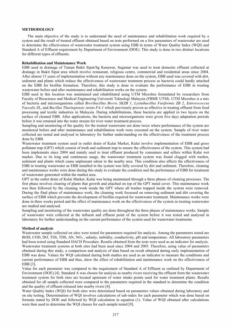
217

METHODOLOGY

The main objective of the study is to understand the need of maintenance and rehabilitation work required by a system and the result of treated effluent obtained based on tests performed on a few parameters of wastewater are used to determine the effectiveness of wastewater treatment system using EBB in terms of Water Quality Index (WQI) and Standard A of Effluent requirement by Department of Environment (DOE). This study is done in two distinct locations for different types of effluents. Rehabilitation and Maintenance Work EBB used in drainage of Taman Bukit Siput/Sg Kenawar, Segamat was used to treat domestic effluent collected at drainage in Bukit Siput area which involve restaurant, religious centre, commercial and residential areas since 2004. After almost 13 years of implementation without any maintenance done on the system, EBB used was covered with dirt, sediment and plants which reduce the effectiveness of wastewater treatment process as bacteria could hardly attached on the EBB for biofilm formation. Therefore, this study is done to evaluate the performance of EBB in treating wastewater before and after maintenance and rehabilitation works on the system. EBB used in this location was maintained and rehabilitated using UTM Microbes formulated by researchers from Faculty of Bioscience and Medical Engineering Universiti Teknologi Malaysia (FBME UTM). UTM Microbes is a mix of bacteria and microorganisms called Brevibacillus Brevis SKZB 1, Lysinibacillus Fusiformis ZB 2, Entrerococcus Faecalis ZL, and Bacillus Thuringiensis strain FA-1 which previously proven as effective in treating effluent from food processing and textile industries in Malaysia. During rehabilitations, these bacteria are applied in two layers on the surface of cleaned EBB. After applications, the bacteria and microorganisms were given five days adaptation periods before it was returned into the water stream for river water treatment process. Sampling and monitoring of the quality for the treated wastewater are done twice where performance of the system are monitored before and after maintenance and rehabilitation work were executed on the system. Sample of river water collected are tested and analysed in laboratory for further understanding on the effectiveness of the treatment process done by EBB. Wastewater treatment system used in outlet drain of Kulai Market, Kulai involve implementation of EBB and gross pollutant trap (GPT) which consist of trash and sediment trap to ensure the effectiveness of the system. This system had been implements since 2004 and mainly used to treat effluent produced by consumers and sellers within Kulai wet market. Due to its long and continuous usage, the wastewater treatment system was found clogged with trashes, sediment and plants which cause unpleasant odour to the nearby area. This condition also affects the effectiveness of EBB in treating wastewater as EBB installed in the system was fully covered by dirt and sediment. Therefore, cleaning and maintenance works were done during this study to evaluate the condition and the performance of EBB for treatment of wastewater generated within the market area. GPT in the outlet drain of Kulai Market, Kulai was being maintained through a three phases of cleaning processes. The first phase involves clearing of plants that growth and attached on top of the GPT metal cover. This maintenance work was then followed by the cleaning work inside the GPT where all trashes trapped inside the system were removed. During the final phase of maintenance work, the cleaning work focussed on removing sediment and dirt covering the surface of EBB which prevents the development of biofilm required for wastewater treatment. Maintenance works were done in three weeks period and the effect of maintenance work on the effectiveness of the system in treating wastewater are studied and analysed. Sampling and monitoring of the wastewater quality are done throughout the three phases of maintenance works. Sample of wastewater were collected at the influent and effluent point of the system before it was tested and analysed in laboratory for further understanding on the current performance of the system used for wastewater treatments.

Method of analysis Wastewater sample collected on sites were tested for parameters required for analysis. Among the parameters tested are BOD, COD, DO, TSS, TDS, AN, NO3

-, salinity, turbidity, conductivity, pH and temperature. All laboratory parameters had been tested using Standard HACH Procedure. Results obtained from the tests were used as an indicator for analysis. Wastewater treatment systems at both sites had been used since 2004 and 2005. Therefore, using value of parameters obtained during this study, a comparison and analysis of data based on result obtained during early implementation of EBB was done. Values for WQI calculated during both studies are used as an indicator to measure the conditions and current performance of EBB and thus, show the effect of rehabilitation and maintenance work on the effectiveness of EBB [3]. Value for each parameter was compared to the requirement of Standard A of Effluent as outlined by Department of Environment (DOE) [4]. Standard A was chosen for analysis as nearby rivers receiving the effluent form the wastewater treatment system for both sites are located upstream of water intake points used for water treatment plants. Results obtained for all sample collected were compared to the parameters required in the standard to determine the condition and the quality of effluent released into nearby rivers [4]. Water Quality Index (WQI) for both sites were determined based on parameters values obtained during laboratory and on site testing. Determination of WQI involves calculations of sub-index for each parameter which was done based on formula stated by DOE and followed by WQI calculation in equation (1). Value of WQI obtained after calculations were then used to determine the WQI classes for each sample tested [9].

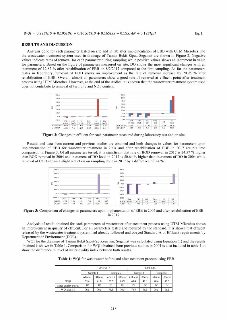
218

𝑊𝑄𝐼 = 0.22𝑆𝐼𝐷𝑂 + 0.19𝑆𝐼𝐵𝑂 + 0.16 𝑆𝐼𝐶𝑂𝐷 + 0.16𝑆𝐼𝑆𝑆 + 0.15𝑆𝐼𝐴𝑁 + 0.12𝑆𝐼𝑝𝐻 Eq. 1

RESULTS AND DISCUSSION

Analysis done for each parameter tested on site and in lab after implementation of EBB with UTM Microbes into the wastewater treatment system used in drainage of Taman Bukit Siput, Segamat are shown in Figure 2. Negative values indicate rates of removal for each parameter during sampling while positive values shows an increment in value for parameters. Based on the figure of parameters measured on site, DO shows the most significant changes with an increment of 12.82 % after rehabilitation of EBB on 8/2/2017 compared to the first sampling. As for the parameters testes in laboratory, removal of BOD shows an improvement as the rate of removal increase by 20.95 % after rehabilitation of EBB. Overall, almost all parameters show a good rate of removal at effluent point after treatment process using UTM Microbes. However, at the end of the studies, it is shown that the wastewater treatment system used does not contribute to removal of turbidity and NO3

- content.

Figure 2: Changes in effluent for each parameter measured during laboratory test and on site

Results and data from current and previous studies are obtained and both changes in values for parameters upon

implementation of EBB for wastewater treatment in 2004 and after rehabilitation of EBB in 2017 are put into comparison in Figure 3. Of all parameters tested, it is significant that rate of BOD removal in 2017 is 24.57 % higher than BOD removal in 2004 and increment of DO level in 2017 is 50.64 % higher than increment of DO in 2004 while removal of COD shows a slight reduction on sampling done in 2017 by a difference of 0.4 %.

Figure 3: Comparison of changes in parameters upon implementation of EBB in 2004 and after rehabilitation of EBB

in 2017

Analysis of result obtained for each parameters of wastewater after treatment process using UTM Microbes shows an improvement in quality of effluent. For all parameters tested and required by the standard, it is shown that effluent released by the wastewater treatment system had already followed and obeyed Standard A of Effluent requirements by Department of Environment (DOE).

WQI for the drainage of Taman Bukit Siput/Sg Kenawar, Segamat was calculated using Equation (1) and the results obtained is shown in Table 1. Comparison for WQI obtained from previous studies in 2004 is also included in table 1 to show the difference in level of water quality index between both results.

Table 1: WQI for wastewater before and after treatment process using EBB

influent effluent influent effluent influent effluent influent effluentWQI 35.4 41.0 53.5 65.9 40.4 42.0 40.4 47.3

water quality status IV IV III III IV IV IV IVWQI class II 76.5 76.5 76.5 76.5 76.5 76.5 76.5 76.5

2016/2017 2004/2005

Sample 1 Sample 2 Sampel 1 Sampel 2

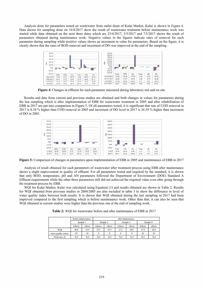
219

Analysis done for parameters tested on wastewater from outlet drain of Kulai Market, Kulai is shown in Figure 4. Data shown for sampling done on 16/4/2017 show the result of wastewater treatment before maintenance work was started while data obtained on the next three dates which are 23/4/2017, 3/5/2017 and 7/5/2017 shows the result of parameters obtained during maintenance work. Negative values in the figures indicate rates of removal for each parameter during sampling while positive values shows an increment in value for parameters. Based on the figure, it is clearly shown that the rates of BOD removal and increment of DO was improved at the end of the sampling.

Figure 4: Changes in effluent for each parameter measured during laboratory test and on site

Results and data from current and previous studies are obtained and both changes in values for parameters during

the last sampling which is after implementation of EBB for wastewater treatment in 2005 and after rehabilitation of EBB in 2017 are put into comparison in Figure 5. Of all parameters tested, it is significant that rate of COD removal in 2017 is 8.34 % higher than COD removal in 2005 and increment of DO level in 2017 is 36.39 % higher than increment of DO in 2005.

Figure 5: Comparison of changes in parameters upon implementation of EBB in 2005 and maintenance of EBB in 2017

Analysis of result obtained for each parameters of wastewater after treatment process using EBB after maintenance

shows a slight improvement in quality of effluent. For all parameters tested and required by the standard, it is shown that only BOD, temperature, pH and AN parameters followed the Department of Environment (DOE) Standard A Effluent requirements while the other three parameters still did not achieved the required value even after going through the treatment process by EBB.

WQI for Kulai Market, Kulai was calculated using Equation (1) and results obtained are shown in Table 2. Results for WQI obtained from previous studies in 2004/2005 are also included in table 3 to show the difference in level of water quality index between both results. It is shown that WQI obtained during the last sampling in 2017 had been improved compared to the first sampling which is before maintenance work. Other than that, it can also be seen that WQI obtained in current studies were higher than the previous one at the end of sampling work.

Table 2: WQI for wastewater before and after maintenance of EBB in 2017

influen efluen influen efluen influen efluen influen efluenWQI 40.4 33.5 27.1 27.5 27.2 28.6 37.4 42.0

water quality status IV IV V V V V IV IVWQI class II 76.5 76.5 76.5 76.5 76.5 76.5 76.5 76.5

before maintenance after maintenanceSample 1 Sample 2 Sample 3 Sample 4

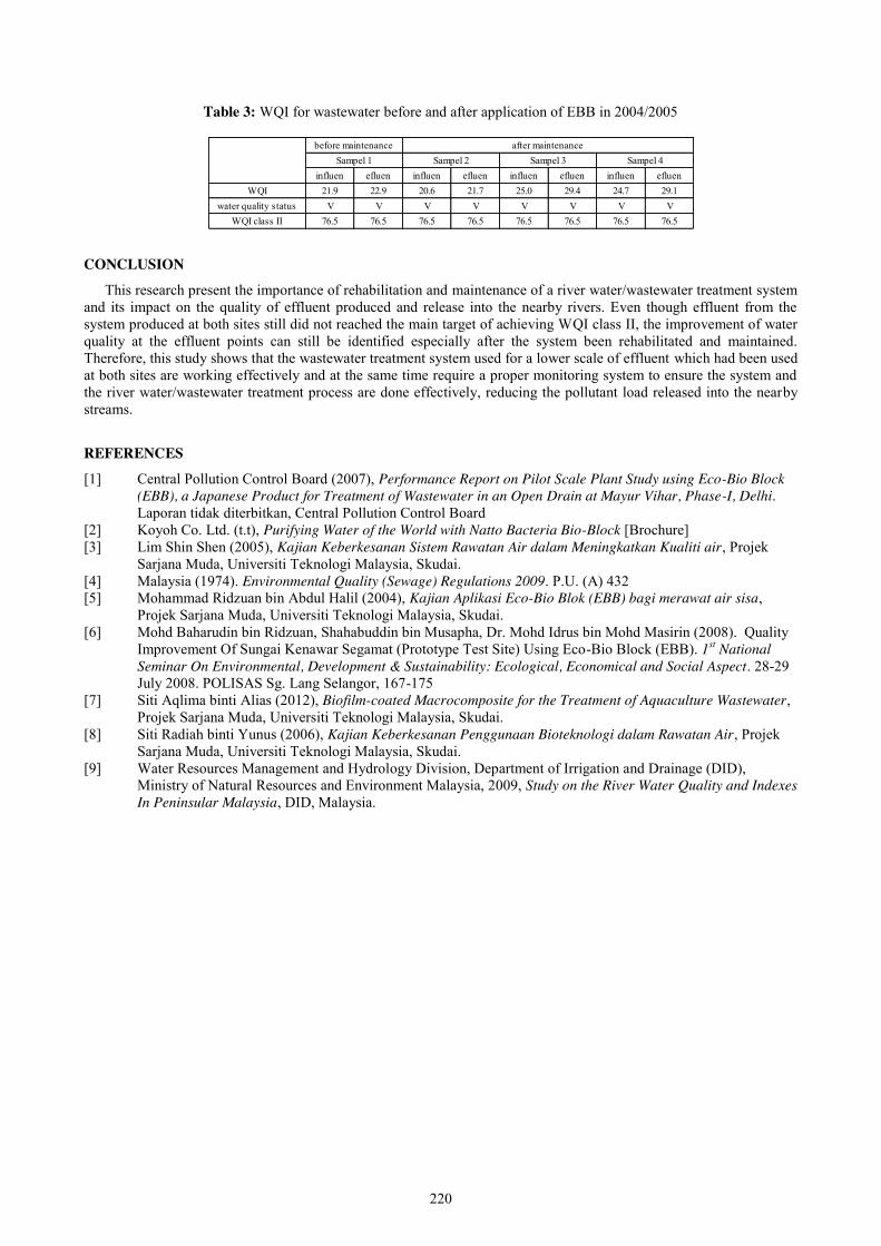
220

Table 3: WQI for wastewater before and after application of EBB in 2004/2005

CONCLUSION

This research present the importance of rehabilitation and maintenance of a river water/wastewater treatment system and its impact on the quality of effluent produced and release into the nearby rivers. Even though effluent from the system produced at both sites still did not reached the main target of achieving WQI class II, the improvement of water quality at the effluent points can still be identified especially after the system been rehabilitated and maintained. Therefore, this study shows that the wastewater treatment system used for a lower scale of effluent which had been used at both sites are working effectively and at the same time require a proper monitoring system to ensure the system and the river water/wastewater treatment process are done effectively, reducing the pollutant load released into the nearby streams.

REFERENCES

[1] Central Pollution Control Board (2007), Performance Report on Pilot Scale Plant Study using Eco-Bio Block (EBB), a Japanese Product for Treatment of Wastewater in an Open Drain at Mayur Vihar, Phase-I, Delhi. Laporan tidak diterbitkan, Central Pollution Control Board

[2] Koyoh Co. Ltd. (t.t), Purifying Water of the World with Natto Bacteria Bio-Block [Brochure] [3] Lim Shin Shen (2005), Kajian Keberkesanan Sistem Rawatan Air dalam Meningkatkan Kualiti air, Projek

Sarjana Muda, Universiti Teknologi Malaysia, Skudai. [4] Malaysia (1974). Environmental Quality (Sewage) Regulations 2009. P.U. (A) 432 [5] Mohammad Ridzuan bin Abdul Halil (2004), Kajian Aplikasi Eco-Bio Blok (EBB) bagi merawat air sisa,

Projek Sarjana Muda, Universiti Teknologi Malaysia, Skudai. [6] Mohd Baharudin bin Ridzuan, Shahabuddin bin Musapha, Dr. Mohd Idrus bin Mohd Masirin (2008). Quality

Improvement Of Sungai Kenawar Segamat (Prototype Test Site) Using Eco-Bio Block (EBB). 1st National Seminar On Environmental, Development & Sustainability: Ecological, Economical and Social Aspect. 28-29 July 2008. POLISAS Sg. Lang Selangor, 167-175

[7] Siti Aqlima binti Alias (2012), Biofilm-coated Macrocomposite for the Treatment of Aquaculture Wastewater, Projek Sarjana Muda, Universiti Teknologi Malaysia, Skudai.

[8] Siti Radiah binti Yunus (2006), Kajian Keberkesanan Penggunaan Bioteknologi dalam Rawatan Air, Projek Sarjana Muda, Universiti Teknologi Malaysia, Skudai.

[9] Water Resources Management and Hydrology Division, Department of Irrigation and Drainage (DID), Ministry of Natural Resources and Environment Malaysia, 2009, Study on the River Water Quality and Indexes In Peninsular Malaysia, DID, Malaysia.

influen efluen influen efluen influen efluen influen efluenWQI 21.9 22.9 20.6 21.7 25.0 29.4 24.7 29.1

water quality status V V V V V V V VWQI class II 76.5 76.5 76.5 76.5 76.5 76.5 76.5 76.5

before maintenance after maintenanceSampel 1 Sampel 2 Sampel 3 Sampel 4

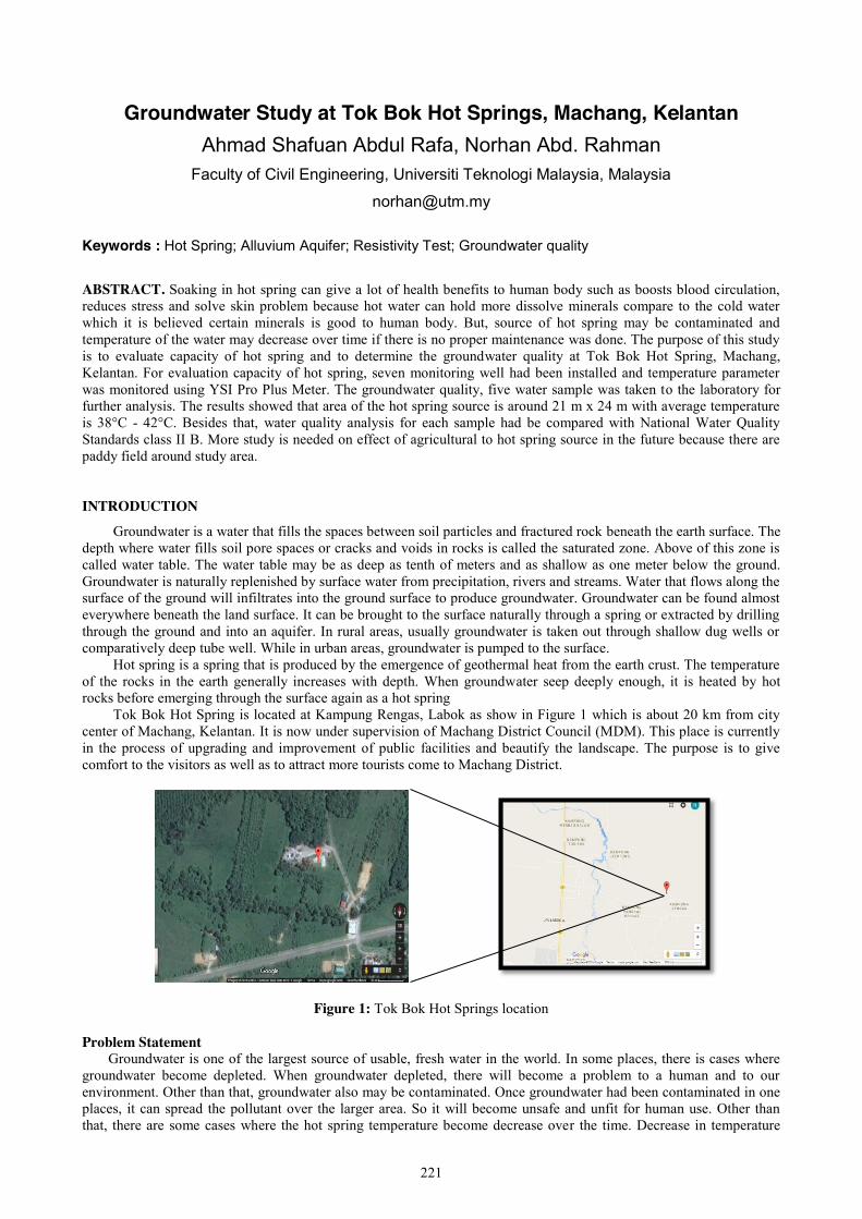
221

Groundwater Study at Tok Bok Hot Springs, Machang, Kelantan Ahmad Shafuan Abdul Rafa, Norhan Abd. Rahman

Faculty of Civil Engineering, Universiti Teknologi Malaysia, Malaysia

norhan@utm.my

Keywords : Hot Spring; Alluvium Aquifer; Resistivity Test; Groundwater quality

ABSTRACT. Soaking in hot spring can give a lot of health benefits to human body such as boosts blood circulation, reduces stress and solve skin problem because hot water can hold more dissolve minerals compare to the cold water which it is believed certain minerals is good to human body. But, source of hot spring may be contaminated and temperature of the water may decrease over time if there is no proper maintenance was done. The purpose of this study is to evaluate capacity of hot spring and to determine the groundwater quality at Tok Bok Hot Spring, Machang, Kelantan. For evaluation capacity of hot spring, seven monitoring well had been installed and temperature parameter was monitored using YSI Pro Plus Meter. The groundwater quality, five water sample was taken to the laboratory for further analysis. The results showed that area of the hot spring source is around 21 m x 24 m with average temperature is 38°C - 42°C. Besides that, water quality analysis for each sample had be compared with National Water Quality Standards class II B. More study is needed on effect of agricultural to hot spring source in the future because there are paddy field around study area. INTRODUCTION

Groundwater is a water that fills the spaces between soil particles and fractured rock beneath the earth surface. The depth where water fills soil pore spaces or cracks and voids in rocks is called the saturated zone. Above of this zone is called water table. The water table may be as deep as tenth of meters and as shallow as one meter below the ground. Groundwater is naturally replenished by surface water from precipitation, rivers and streams. Water that flows along the surface of the ground will infiltrates into the ground surface to produce groundwater. Groundwater can be found almost everywhere beneath the land surface. It can be brought to the surface naturally through a spring or extracted by drilling through the ground and into an aquifer. In rural areas, usually groundwater is taken out through shallow dug wells or comparatively deep tube well. While in urban areas, groundwater is pumped to the surface. Hot spring is a spring that is produced by the emergence of geothermal heat from the earth crust. The temperature of the rocks in the earth generally increases with depth. When groundwater seep deeply enough, it is heated by hot rocks before emerging through the surface again as a hot spring Tok Bok Hot Spring is located at Kampung Rengas, Labok as show in Figure 1 which is about 20 km from city center of Machang, Kelantan. It is now under supervision of Machang District Council (MDM). This place is currently in the process of upgrading and improvement of public facilities and beautify the landscape. The purpose is to give comfort to the visitors as well as to attract more tourists come to Machang District.

Figure 1: Tok Bok Hot Springs location Problem Statement

Groundwater is one of the largest source of usable, fresh water in the world. In some places, there is cases where groundwater become depleted. When groundwater depleted, there will become a problem to a human and to our environment. Other than that, groundwater also may be contaminated. Once groundwater had been contaminated in one places, it can spread the pollutant over the larger area. So it will become unsafe and unfit for human use. Other than that, there are some cases where the hot spring temperature become decrease over the time. Decrease in temperature

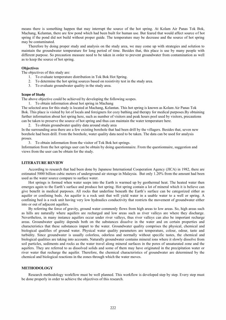
222

means there is something happen that may interrupt the source of the hot spring. At Kolam Air Panas Tok Bok, Machang, Kelantan, there are few pond which had been built for human use. But feared that would affect source of hot spring if the pond did not build without proper guide. The temperature may be decrease and the source of hot spring may be contaminated.

Therefore by doing proper study and analysis on the study area, we may come up with strategies and solution to maintain the groundwater temperature for long period of time. Besides that, this place is use by many people with different purpose. So precaution measure need to be taken in order to prevent groundwater from contamination as well as to keep the source of hot spring.

Objectives The objectives of this study are:

1. To evaluate temperature distribution in Tok Bok Hot Spring. 2. To determine the hot spring sources based on resistivity test in the study area. 3. To evaluate groundwater quality in the study area.

Scope of Study The above objective could be achieved by developing the following scopes.

1. To obtain information about hot spring in Machang The selected area for this study is located at Machang, Kelantan. This hot spring is known as Kolam Air Panas Tok Bok. This place is visited by lot of locals and foreigners for cozy bathing and therapy for medical purposes.By obtaining further information about hot spring here, such as number of visitors and peak hours pool used by visitors, precautions can be taken to preserve the source of hot spring and thus can maintain the water temperature here.

2. To obtain groundwater quality data around study area In the surrounding area there are a few existing borehole that had been drill by the villagers. Besides that, seven new borehole had been drill. From the borehole, water quality data need to be taken. The data can be used for analysis proses.

3. To obtain information from the visitor of Tok Bok hot springs. Information from the hot springs user can be obtain by doing questionnaire. From the questionnaire, suggestion and views from the user can be obtain for the study.

LITERATURE REVIEW According to research that had been done by Japanese International Cooperation Agency (JICA) in 1982, there are

estimated 5000 billion cubic meters of underground air storage in Malaysia. But only 1.20% from the amount had been used as the water source compare to surface water.

Hot springs is formed when water seeps into the Earth is warmed up by geothermal heat. The heated water then emerges again to the Earth’s surface and produce hot spring. Hot spring contain a lot of mineral which it is believe can give benefit in medical purposes. All rocks that underline beneath the Earth’s surface can be categorized either as aquifer or confining beds. An aquifer is a rock unit that will yield water in a usable water to a well or spring. A confining bed is a rock unit having very low hydraulics conductivity that restricts the movement of groundwater either into or out of adjacent aquifers.

By referring the force of gravity, ground water commonly flows from high areas to low areas. So, high areas such as hills are naturally where aquifers are recharged and low areas such as river valleys are where they discharge. Nevertheless, in many instance aquifers occur under river valleys, thus river valleys can also be important recharge areas. Groundwater quality depends both on the substances dissolve in the water and on certain properties and characteristics that these substances impart to the water. Groundwater quality comprises the physical, chemical and biological qualifies of ground water. Physical water quality parameters are temperature, colour, odour, taste and turbidity. Since groundwater is usually colorless, odorless and normally without specific tastes, the chemical and biological qualities are taking into accounts. Naturally groundwater contains mineral ions where it slowly dissolve from soil particles, sediments and rocks as the water travel along mineral surfaces in the pores of unsaturated zone and the aquifers. They are referred to as dissolved solids and some of them may have originated in the precipitation water or river water that recharge the aquifer. Therefore, the chemical characteristics of groundwater are determined by the chemical and biological reactions in the zones through which the water moves.

METHODOLOGY

Research methodology workflow must be well planned. This workflow is developed step by step. Every step must be done properly in order to achieve the objectives of this research.

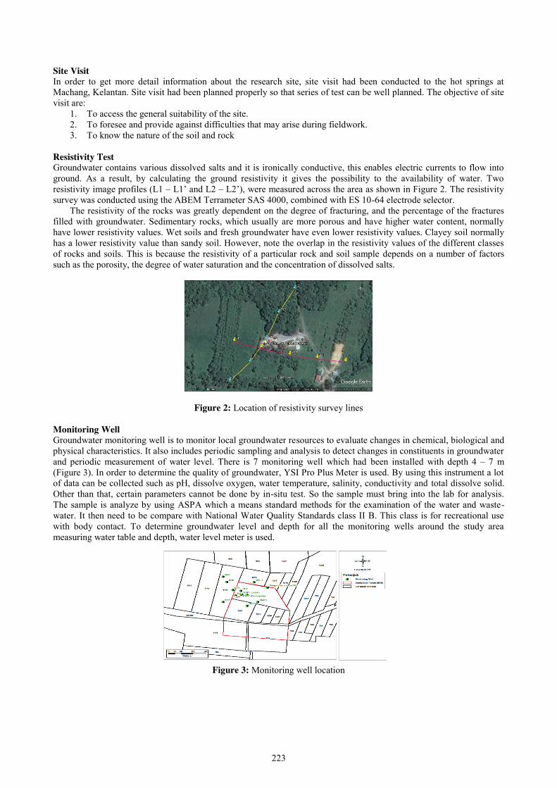
223

Site Visit In order to get more detail information about the research site, site visit had been conducted to the hot springs at Machang, Kelantan. Site visit had been planned properly so that series of test can be well planned. The objective of site visit are:

1. To access the general suitability of the site. 2. To foresee and provide against difficulties that may arise during fieldwork. 3. To know the nature of the soil and rock

Resistivity Test Groundwater contains various dissolved salts and it is ironically conductive, this enables electric currents to flow into ground. As a result, by calculating the ground resistivity it gives the possibility to the availability of water. Two resistivity image profiles (L1 – L1’ and L2 – L2’), were measured across the area as shown in Figure 2. The resistivity survey was conducted using the ABEM Terrameter SAS 4000, combined with ES 10-64 electrode selector.

The resistivity of the rocks was greatly dependent on the degree of fracturing, and the percentage of the fractures filled with groundwater. Sedimentary rocks, which usually are more porous and have higher water content, normally have lower resistivity values. Wet soils and fresh groundwater have even lower resistivity values. Clayey soil normally has a lower resistivity value than sandy soil. However, note the overlap in the resistivity values of the different classes of rocks and soils. This is because the resistivity of a particular rock and soil sample depends on a number of factors such as the porosity, the degree of water saturation and the concentration of dissolved salts.

Figure 2: Location of resistivity survey lines Monitoring Well Groundwater monitoring well is to monitor local groundwater resources to evaluate changes in chemical, biological and physical characteristics. It also includes periodic sampling and analysis to detect changes in constituents in groundwater and periodic measurement of water level. There is 7 monitoring well which had been installed with depth 4 – 7 m (Figure 3). In order to determine the quality of groundwater, YSI Pro Plus Meter is used. By using this instrument a lot of data can be collected such as pH, dissolve oxygen, water temperature, salinity, conductivity and total dissolve solid. Other than that, certain parameters cannot be done by in-situ test. So the sample must bring into the lab for analysis. The sample is analyze by using ASPA which a means standard methods for the examination of the water and waste-water. It then need to be compare with National Water Quality Standards class II B. This class is for recreational use with body contact. To determine groundwater level and depth for all the monitoring wells around the study area measuring water table and depth, water level meter is used.

Figure 3: Monitoring well location

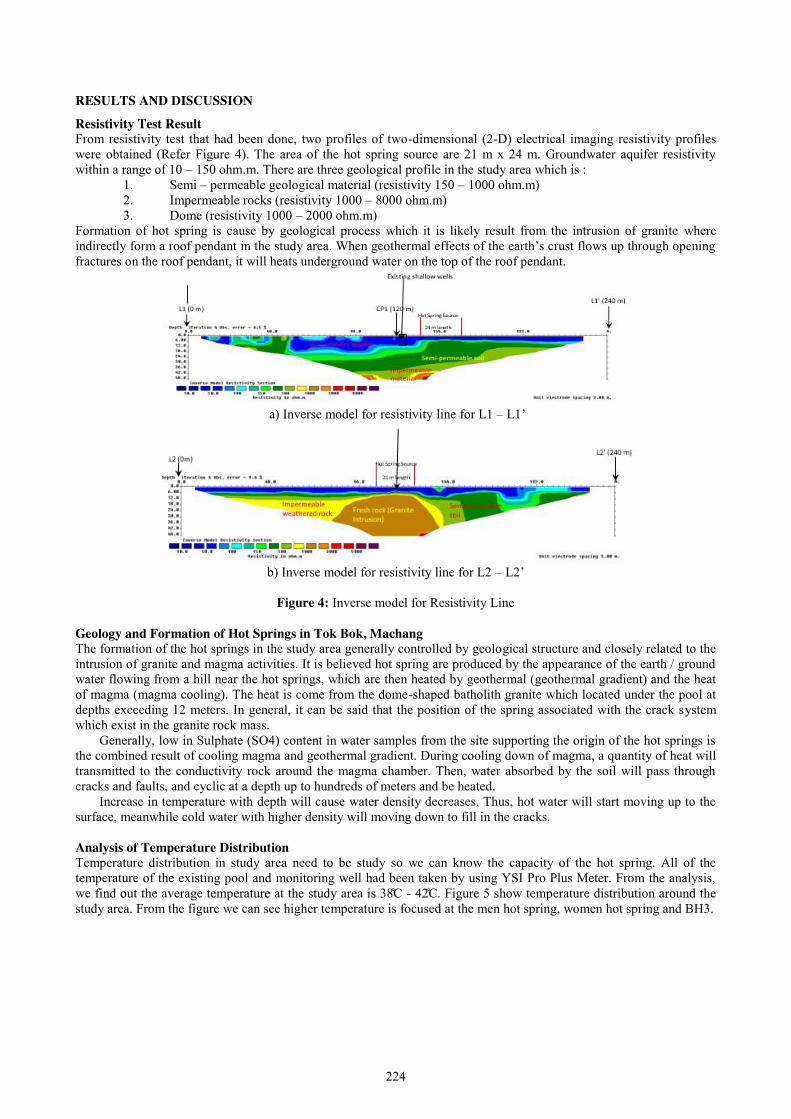
224

RESULTS AND DISCUSSION

Resistivity Test Result From resistivity test that had been done, two profiles of two-dimensional (2-D) electrical imaging resistivity profiles were obtained (Refer Figure 4). The area of the hot spring source are 21 m x 24 m. Groundwater aquifer resistivity within a range of 10 – 150 ohm.m. There are three geological profile in the study area which is :

1. Semi – permeable geological material (resistivity 150 – 1000 ohm.m) 2. Impermeable rocks (resistivity 1000 – 8000 ohm.m) 3. Dome (resistivity 1000 – 2000 ohm.m)

Formation of hot spring is cause by geological process which it is likely result from the intrusion of granite where indirectly form a roof pendant in the study area. When geothermal effects of the earth’s crust flows up through opening fractures on the roof pendant, it will heats underground water on the top of the roof pendant.

a) Inverse model for resistivity line for L1 – L1’

b) Inverse model for resistivity line for L2 – L2’

Figure 4: Inverse model for Resistivity Line

Geology and Formation of Hot Springs in Tok Bok, Machang The formation of the hot springs in the study area generally controlled by geological structure and closely related to the intrusion of granite and magma activities. It is believed hot spring are produced by the appearance of the earth / ground water flowing from a hill near the hot springs, which are then heated by geothermal (geothermal gradient) and the heat of magma (magma cooling). The heat is come from the dome-shaped batholith granite which located under the pool at depths exceeding 12 meters. In general, it can be said that the position of the spring associated with the crack system which exist in the granite rock mass.

Generally, low in Sulphate (SO4) content in water samples from the site supporting the origin of the hot springs is the combined result of cooling magma and geothermal gradient. During cooling down of magma, a quantity of heat will transmitted to the conductivity rock around the magma chamber. Then, water absorbed by the soil will pass through cracks and faults, and cyclic at a depth up to hundreds of meters and be heated.

Increase in temperature with depth will cause water density decreases. Thus, hot water will start moving up to the surface, meanwhile cold water with higher density will moving down to fill in the cracks. Analysis of Temperature Distribution Temperature distribution in study area need to be study so we can know the capacity of the hot spring. All of the temperature of the existing pool and monitoring well had been taken by using YSI Pro Plus Meter. From the analysis, we find out the average temperature at the study area is 38̊C - 42̊C. Figure 5 show temperature distribution around the study area. From the figure we can see higher temperature is focused at the men hot spring, women hot spring and BH3.

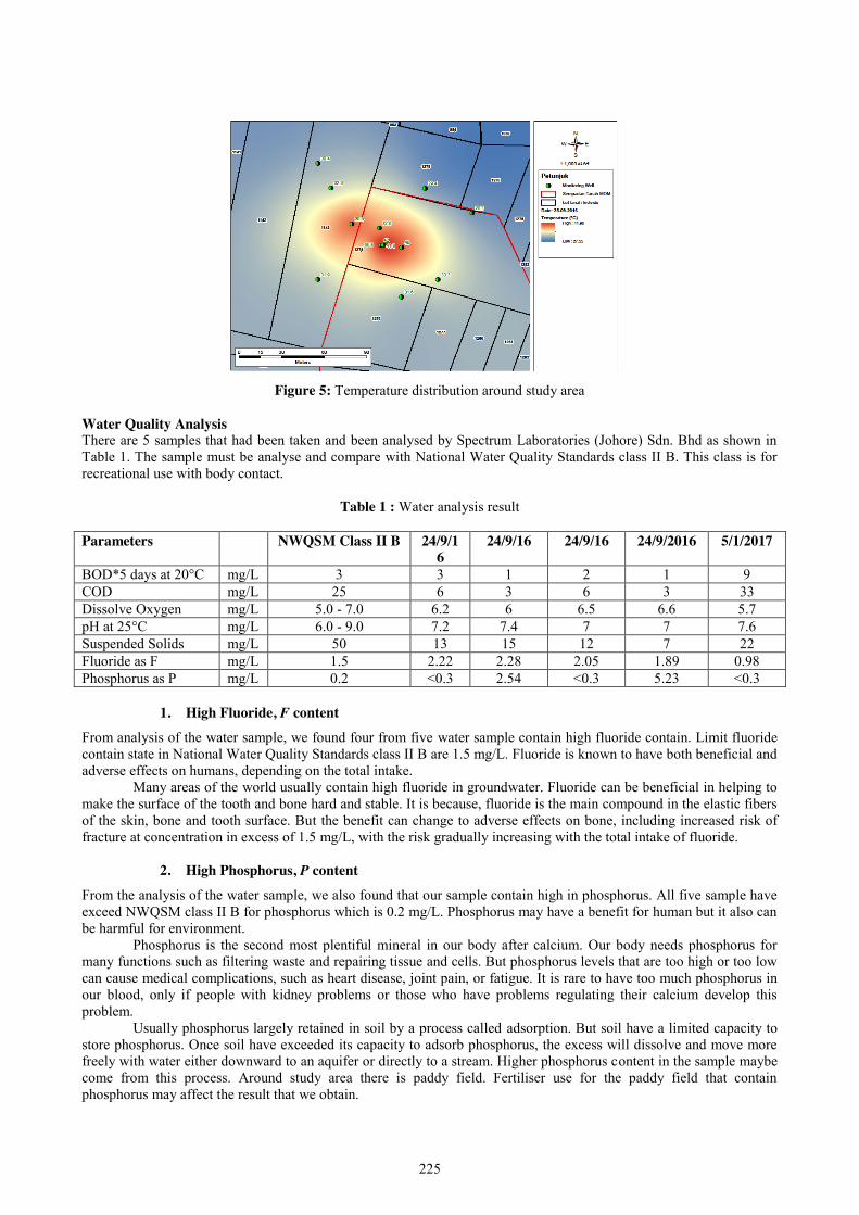
225

Figure 5: Temperature distribution around study area

Water Quality Analysis There are 5 samples that had been taken and been analysed by Spectrum Laboratories (Johore) Sdn. Bhd as shown in Table 1. The sample must be analyse and compare with National Water Quality Standards class II B. This class is for recreational use with body contact.

Table 1 : Water analysis result

Parameters NWQSM Class II B 24/9/16

24/9/16 24/9/16 24/9/2016 5/1/2017

BOD*5 days at 20°C mg/L 3 3 1 2 1 9 COD mg/L 25 6 3 6 3 33 Dissolve Oxygen mg/L 5.0 - 7.0 6.2 6 6.5 6.6 5.7 pH at 25°C mg/L 6.0 - 9.0 7.2 7.4 7 7 7.6 Suspended Solids mg/L 50 13 15 12 7 22 Fluoride as F mg/L 1.5 2.22 2.28 2.05 1.89 0.98 Phosphorus as P mg/L 0.2 <0.3 2.54 <0.3 5.23 <0.3

1. High Fluoride, F content From analysis of the water sample, we found four from five water sample contain high fluoride contain. Limit fluoride contain state in National Water Quality Standards class II B are 1.5 mg/L. Fluoride is known to have both beneficial and adverse effects on humans, depending on the total intake. Many areas of the world usually contain high fluoride in groundwater. Fluoride can be beneficial in helping to make the surface of the tooth and bone hard and stable. It is because, fluoride is the main compound in the elastic fibers of the skin, bone and tooth surface. But the benefit can change to adverse effects on bone, including increased risk of fracture at concentration in excess of 1.5 mg/L, with the risk gradually increasing with the total intake of fluoride.

2. High Phosphorus, P content From the analysis of the water sample, we also found that our sample contain high in phosphorus. All five sample have exceed NWQSM class II B for phosphorus which is 0.2 mg/L. Phosphorus may have a benefit for human but it also can be harmful for environment. Phosphorus is the second most plentiful mineral in our body after calcium. Our body needs phosphorus for many functions such as filtering waste and repairing tissue and cells. But phosphorus levels that are too high or too low can cause medical complications, such as heart disease, joint pain, or fatigue. It is rare to have too much phosphorus in our blood, only if people with kidney problems or those who have problems regulating their calcium develop this problem. Usually phosphorus largely retained in soil by a process called adsorption. But soil have a limited capacity to store phosphorus. Once soil have exceeded its capacity to adsorb phosphorus, the excess will dissolve and move more freely with water either downward to an aquifer or directly to a stream. Higher phosphorus content in the sample maybe come from this process. Around study area there is paddy field. Fertiliser use for the paddy field that contain phosphorus may affect the result that we obtain.

226

Data Survey Analysis Data survey had been conducted on April 5-6, 2017 at the study area. The questionnaire had been distributed to 40 person who is the user of the hot spring. From 40 persons who join the survey, 31 of them is male then the rest is female. Few factor less female come to this place is because the female pool is connect to the man pool with separate by a separator. Maybe some of them feel uncomfortable with the situation.

Next from the data, we found that the user of the hot spring comes from various age with the higher hot spring user is come from age 21-30 years old meanwhile the lowest is come from age 41-50 years old. Factor highest user is come from 21-30 years old because there is University Teknologi Mara (UiTM) nearby which located less than 20 KM. It can be proven by the employment data users show the highest occupation of the user is come from student.

Other than that, most of the visitor visit this place less than 5 times per week. But for each time they will soak in the pool for about 11-30 minutes. 30 out of 40 person say they feel comfortable using the pool provided. Maybe it is because there are person responsible to clean the pool once a week and also there is no fee for entry.

We also do survey on medical effect to the visitor. On the positive side, most of the data shows visitor feel fresher and some of them feel relaxing in mind. But on the negative side, some of them feel dizziness and sleepy. Hot bath may cause the blood pressure drops. So the user need to soak in the hot spring with a reasonable time.

CONCLUSION

All the findings from previous researches and results of the laboratory tests that have been analyzed to draw the following conclusions:

1. Average temperature capacity at the study area is 38̊C - 42C̊ with the area of the hot spring source are 21 m x 24 m. The hottest place is located at men hot spring and women hot spring. Also, BH3 also is the highest temperature that newly found.

2. Water quality analysis at the study area nearly meet the requirement for National Water Quality Standards class II B.

REFERENCES

[1] Hassan Mohamed Baioumy, Mohd Nawawi, Karl Wagner, Mohd Hariri Arifin. (2014). Geological Setting and Origin of Non-Volcanic Hot Springs in West Malaysia. [2] Ismail C. Mohamad, Mohammed Hatta Abd Karim (JMG). (2010). Groundwater Availability and Quality in Malaysia. [3] Daniel Ityel, (2011). Ground water: Dealing with iron contamination. [4] Ene Indermitte, Astrid Saava, Enn Karro. (2009). Exposure to High Fluoride Drinking Water and Risk of Dental Fluorosis in Estonia.

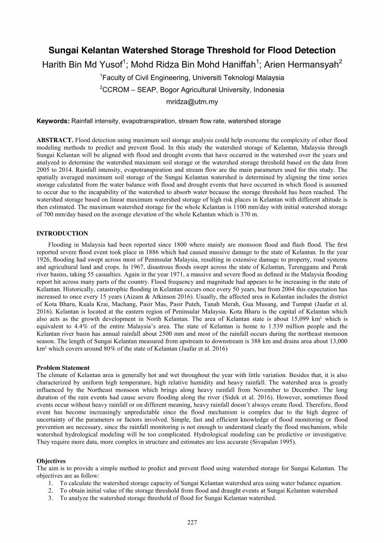
227

Sungai Kelantan Watershed Storage Threshold for Flood Detection Harith Bin Md Yusof1; Mohd Ridza Bin Mohd Haniffah1; Arien Hermansyah2

1Faculty of Civil Engineering, Universiti Teknologi Malaysia 2CCROM – SEAP, Bogor Agricultural University, Indonesia

mridza@utm.my

Keywords: Rainfall intensity, evapotranspiration, stream flow rate, watershed storage

ABSTRACT. Flood detection using maximum soil storage analysis could help overcome the complexity of other flood modeling methods to predict and prevent flood. In this study the watershed storage of Kelantan, Malaysia through Sungai Kelantan will be aligned with flood and drought events that have occurred in the watershed over the years and analyzed to determine the watershed maximum soil storage or the watershed storage threshold based on the data from 2005 to 2014. Rainfall intensity, evapotranspiration and stream flow are the main parameters used for this study. The spatially averaged maximum soil storage of the Sungai Kelantan watershed is determined by aligning the time series storage calculated from the water balance with flood and drought events that have occurred in which flood is assumed to occur due to the incapability of the watershed to absorb water because the storage threshold has been reached. The watershed storage based on linear maximum watershed storage of high risk places in Kelantan with different altitude is then estimated. The maximum watershed storage for the whole Kelantan is 1100 mm/day with initial watershed storage of 700 mm/day based on the average elevation of the whole Kelantan which is 370 m.

INTRODUCTION

Flooding in Malaysia had been reported since 1800 where mainly are monsoon flood and flash flood. The first reported severe flood event took place in 1886 which had caused massive damage to the state of Kelantan. In the year 1926, flooding had swept across most of Peninsular Malaysia, resulting in extensive damage to property, road systems and agricultural land and crops. In 1967, disastrous floods swept across the state of Kelantan, Terengganu and Perak river basins, taking 55 casualties. Again in the year 1971, a massive and severe flood as defined in the Malaysia flooding report hit across many parts of the country. Flood frequency and magnitude had appears to be increasing in the state of Kelantan. Historically, catastrophic flooding in Kelantan occurs once every 50 years, but from 2004 this expectation has increased to once every 15 years (Aizam & Atkinson 2016). Usually, the affected area in Kelantan includes the district of Kota Bharu, Kuala Krai, Machang, Pasir Mas, Pasir Puteh, Tanah Merah, Gua Musang, and Tumpat (Jaafar et al. 2016). Kelantan is located at the eastern region of Peninsular Malaysia. Kota Bharu is the capital of Kelantan which also acts as the growth development in North Kelantan. The area of Kelantan state is about 15,099 km² which is equivalent to 4.4% of the entire Malaysia’s area. The state of Kelantan is home to 1.539 million people and the Kelantan river basin has annual rainfall about 2500 mm and most of the rainfall occurs during the northeast monsoon season. The length of Sungai Kelantan measured from upstream to downstream is 388 km and drains area about 13,000 km² which covers around 80% of the state of Kelantan (Jaafar et al. 2016)

Problem Statement The climate of Kelantan area is generally hot and wet throughout the year with little variation. Besides that, it is also characterized by uniform high temperature, high relative humidity and heavy rainfall. The watershed area is greatly influenced by the Northeast monsoon which brings along heavy rainfall from November to December. The long duration of the rain events had cause severe flooding along the river (Sidek et al. 2016). However, sometimes flood events occur without heavy rainfall or on different meaning, heavy rainfall doesn’t always create flood. Therefore, flood event has become increasingly unpredictable since the flood mechanism is complex due to the high degree of uncertainty of the parameters or factors involved. Simple, fast and efficient knowledge of flood monitoring or flood prevention are necessary, since the rainfall monitoring is not enough to understand clearly the flood mechanism, while watershed hydrological modeling will be too complicated. Hydrological modeling can be predictive or investigative. They require more data, more complex in structure and estimates are less accurate (Sivapalan 1995).

Objectives The aim is to provide a simple method to predict and prevent flood using watershed storage for Sungai Kelantan. The objectives are as follow:

1. To calculate the watershed storage capacity of Sungai Kelantan watershed area using water balance equation. 2. To obtain initial value of the storage threshold from flood and draught events at Sungai Kelantan watershed 3. To analyze the watershed storage threshold of flood for Sungai Kelantan watershed.

228

Scope of Study This study will focus on Kelantan watershed to determine the watershed storage capacity by using simple bucket model equation based on water balance equation. The water balance equation does not take into account deep percolation/infiltration. Figure 1 shows the watershed area of Kelantan that will be analyzed based on stream flow station at Jambatan Guillemard. The stream flow station at Jambatan Guillemard roughly provides an overall area of Sungai Kelantan watershed and it is the most downstream stream flow station available in Sungai Kelantan. Main assumption is that the storage analysis is averaged throughout the whole Sungai Kelantan watershed. The historical data used is from 2005 to 2014.

Figure 11: Kelantan watershed area based on stream flow station at Jambatan Guillemard (the red triangle represent

Jambatan Guillemard) (Aizam & Atkinson 2016).

LITERATURE REVIEW Kelantan has an area of 15,099 km² in Malaysia and compromise of 10 districts which are Kota Bharu, Tumpat,

Machang, Pasir Puteh, Bachok, Jeli, Tanah Merah, Pasir Mas, Kuala Krai and Gua Musang. Kelantan has many flood prone river such as Sungai Nenggiri, Sungai Galas, Sungai Pergau, Sungai Kelantan, Sungai Golok, Sungai Kemasin, Sungai Pengkalan Chepa, Sungai Pengkalan Datu and Sungai Semerak. The monitoring of flood trends, rainfall intensity and stream flow rate in Kelantan is done by DID. Kelantan has heavy frequent rainfall with high intensity because of monsoon season. Hydrological flood events that have occurred are crucial for flood forecasting model. Hence, it is important to compile and analyze major hydrological extreme events which could serve as future references (Sidek et al. 2016).

Flood Modeling Methods Since the natural occurrence of floods cannot be represented appropriately by a single design floods, different hydrological scenarios are needed for sustainable design of flood protection structures such as flood control reservoirs and polders. A number of studies have been carried out on different aspects of floods, such as in Kelantan of Malaysia including flood vulnerability mapping (Pradhan 2009) and flood hydrological modeling (Adnan et al. 2014). Some researcher use complex mathematical approach to develop flood warning system such as multi stage probabilistic warning system for heavy precipitation event (Alfieri et al. 2011). Usage of different meteorological products resolution namely numerical weather prediction (NWP), radar NWP blending and probabilistic weather forecast. This method is suitable for detection for continental scale. On the other region, integration of hydrologic and hydraulic models for flood warning system was used for example in Iran (Matkan et al. 2009) in which the flood can be predicted as early as 22 to 30 hours before the occurrence. Watershed Storage as Flood Indicator However, most of the system used complex calculation and analysis of data which may not be suitable for flood warning and prevention. Instead of hydrological model or complex mathematical approach, watershed water storage was selected as simple indicator for flood warning indicator. Proposed setting up local flood warning system by monitoring sources of floods, predicting where and when flood will occur, identifying potential victim and strengthens management to overcome risk from flood. The whole watershed should be seen as an important system to better understand where all the water that causes flood comes from. When the watershed storage exceeds its maximum capacity, the excess water is spilled onto land area which will cause flood especially in the downstream area. Binahaan watershed of Leyte Province in Philippines was installed with this system (Salzer 2012). There are several key factors need to be taken consideration when applying watershed storage method such as methods used to define the watershed boundaries and the initial watershed capacity. By using this method, the upper Mustinka watershed can intercept around up to 42% of rainfall intensity and has potential to store around 4,706 ha-m of water. Linear regression analysis is used to determine the relationship between the elevation of land and watershed storage volume (Gleason et al. 2007). When threshold is exceed, runoff volume will flow to lower area which cause flood. Low intensity precipitation will only generate runoff in the lower portion of the watershed while high intensity precipitation would naturally produce flow in more channels (Wallace & Lane 1976). Stream flow had been revealed to be inconsistent in which it is increasing in the upstream in all the season but it is showing a decreasing trend downstream in the dry season. The

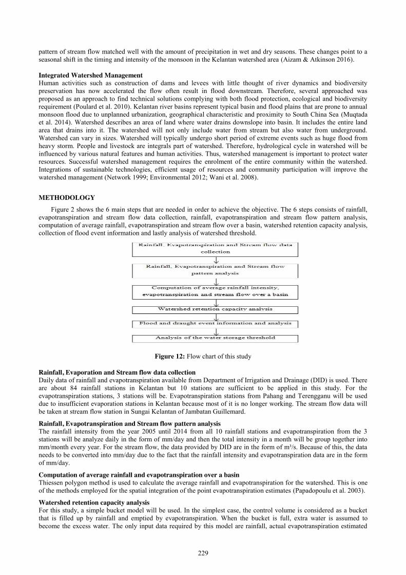
229

pattern of stream flow matched well with the amount of precipitation in wet and dry seasons. These changes point to a seasonal shift in the timing and intensity of the monsoon in the Kelantan watershed area (Aizam & Atkinson 2016). Integrated Watershed Management Human activities such as construction of dams and levees with little thought of river dynamics and biodiversity preservation has now accelerated the flow often result in flood downstream. Therefore, several approached was proposed as an approach to find technical solutions complying with both flood protection, ecological and biodiversity requirement (Poulard et al. 2010). Kelantan river basins represent typical basin and flood plains that are prone to annual monsoon flood due to unplanned urbanization, geographical characteristic and proximity to South China Sea (Muqtada et al. 2014). Watershed describes an area of land where water drains downslope into basin. It includes the entire land area that drains into it. The watershed will not only include water from stream but also water from underground. Watershed can vary in sizes. Watershed will typically undergo short period of extreme events such as huge flood from heavy storm. People and livestock are integrals part of watershed. Therefore, hydrological cycle in watershed will be influenced by various natural features and human activities. Thus, watershed management is important to protect water resources. Successful watershed management requires the enrolment of the entire community within the watershed. Integrations of sustainable technologies, efficient usage of resources and community participation will improve the watershed management (Network 1999; Environmental 2012; Wani et al. 2008).

METHODOLOGY

Figure 2 shows the 6 main steps that are needed in order to achieve the objective. The 6 steps consists of rainfall, evapotranspiration and stream flow data collection, rainfall, evapotranspiration and stream flow pattern analysis, computation of average rainfall, evapotranspiration and stream flow over a basin, watershed retention capacity analysis, collection of flood event information and lastly analysis of watershed threshold.

Figure 12: Flow chart of this study

Rainfall, Evaporation and Stream flow data collection Daily data of rainfall and evapotranspiration available from Department of Irrigation and Drainage (DID) is used. There are about 84 rainfall stations in Kelantan but 10 stations are sufficient to be applied in this study. For the evapotranspiration stations, 3 stations will be. Evapotranspiration stations from Pahang and Terengganu will be used due to insufficient evaporation stations in Kelantan because most of it is no longer working. The stream flow data will be taken at stream flow station in Sungai Kelantan of Jambatan Guillemard.

Rainfall, Evapotranspiration and Stream flow pattern analysis The rainfall intensity from the year 2005 until 2014 from all 10 rainfall stations and evapotranspiration from the 3 stations will be analyze daily in the form of mm/day and then the total intensity in a month will be group together into mm/month every year. For the stream flow, the data provided by DID are in the form of m³/s. Because of this, the data needs to be converted into mm/day due to the fact that the rainfall intensity and evapotranspiration data are in the form of mm/day.

Computation of average rainfall and evapotranspiration over a basin Thiessen polygon method is used to calculate the average rainfall and evapotranspiration for the watershed. This is one of the methods employed for the spatial integration of the point evapotranspiration estimates (Papadopoulu et al. 2003).

Watershed retention capacity analysis For this study, a simple bucket model will be used. In the simplest case, the control volume is considered as a bucket that is filled up by rainfall and emptied by evapotranspiration. When the bucket is full, extra water is assumed to become the excess water. The only input data required by this model are rainfall, actual evapotranspiration estimated

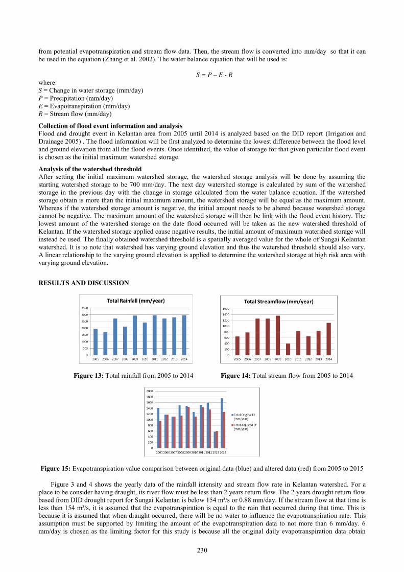
230

from potential evapotranspiration and stream flow data. Then, the stream flow is converted into mm/day so that it can be used in the equation (Zhang et al. 2002). The water balance equation that will be used is:

S = P – E - R where: S = Change in water storage (mm/day) P = Precipitation (mm/day) E = Evapotranspiration (mm/day) R = Stream flow (mm/day)

Collection of flood event information and analysis Flood and drought event in Kelantan area from 2005 until 2014 is analyzed based on the DID report (Irrigation and Drainage 2005) . The flood information will be first analyzed to determine the lowest difference between the flood level and ground elevation from all the flood events. Once identified, the value of storage for that given particular flood event is chosen as the initial maximum watershed storage.

Analysis of the watershed threshold After setting the initial maximum watershed storage, the watershed storage analysis will be done by assuming the starting watershed storage to be 700 mm/day. The next day watershed storage is calculated by sum of the watershed storage in the previous day with the change in storage calculated from the water balance equation. If the watershed storage obtain is more than the initial maximum amount, the watershed storage will be equal as the maximum amount. Whereas if the watershed storage amount is negative, the initial amount needs to be altered because watershed storage cannot be negative. The maximum amount of the watershed storage will then be link with the flood event history. The lowest amount of the watershed storage on the date flood occurred will be taken as the new watershed threshold of Kelantan. If the watershed storage applied cause negative results, the initial amount of maximum watershed storage will instead be used. The finally obtained watershed threshold is a spatially averaged value for the whole of Sungai Kelantan watershed. It is to note that watershed has varying ground elevation and thus the watershed threshold should also vary. A linear relationship to the varying ground elevation is applied to determine the watershed storage at high risk area with varying ground elevation.

RESULTS AND DISCUSSION

Figure 13: Total rainfall from 2005 to 2014 Figure 14: Total stream flow from 2005 to 2014

Figure 15: Evapotranspiration value comparison between original data (blue) and altered data (red) from 2005 to 2015

Figure 3 and 4 shows the yearly data of the rainfall intensity and stream flow rate in Kelantan watershed. For a place to be consider having draught, its river flow must be less than 2 years return flow. The 2 years drought return flow based from DID drought report for Sungai Kelantan is below 154 m³/s or 0.88 mm/day. If the stream flow at that time is less than 154 m³/s, it is assumed that the evapotranspiration is equal to the rain that occurred during that time. This is because it is assumed that when draught occurred, there will be no water to influence the evapotranspiration rate. This assumption must be supported by limiting the amount of the evapotranspiration data to not more than 6 mm/day. 6 mm/day is chosen as the limiting factor for this study is because all the original daily evapotranspiration data obtain

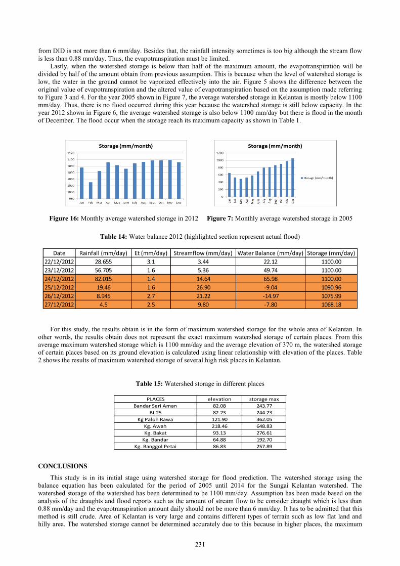
231

from DID is not more than 6 mm/day. Besides that, the rainfall intensity sometimes is too big although the stream flow is less than 0.88 mm/day. Thus, the evapotranspiration must be limited.

Lastly, when the watershed storage is below than half of the maximum amount, the evapotranspiration will be divided by half of the amount obtain from previous assumption. This is because when the level of watershed storage is low, the water in the ground cannot be vaporized effectively into the air. Figure 5 shows the difference between the original value of evapotranspiration and the altered value of evapotranspiration based on the assumption made referring to Figure 3 and 4. For the year 2005 shown in Figure 7, the average watershed storage in Kelantan is mostly below 1100 mm/day. Thus, there is no flood occurred during this year because the watershed storage is still below capacity. In the year 2012 shown in Figure 6, the average watershed storage is also below 1100 mm/day but there is flood in the month of December. The flood occur when the storage reach its maximum capacity as shown in Table 1.

Figure 16: Monthly average watershed storage in 2012 Figure 7: Monthly average watershed storage in 2005

Table 14: Water balance 2012 (highlighted section represent actual flood)

For this study, the results obtain is in the form of maximum watershed storage for the whole area of Kelantan. In other words, the results obtain does not represent the exact maximum watershed storage of certain places. From this average maximum watershed storage which is 1100 mm/day and the average elevation of 370 m, the watershed storage of certain places based on its ground elevation is calculated using linear relationship with elevation of the places. Table 2 shows the results of maximum watershed storage of several high risk places in Kelantan.

Table 15: Watershed storage in different places

CONCLUSIONS This study is in its initial stage using watershed storage for flood prediction. The watershed storage using the

balance equation has been calculated for the period of 2005 until 2014 for the Sungai Kelantan watershed. The watershed storage of the watershed has been determined to be 1100 mm/day. Assumption has been made based on the analysis of the draughts and flood reports such as the amount of stream flow to be consider draught which is less than 0.88 mm/day and the evapotranspiration amount daily should not be more than 6 mm/day. It has to be admitted that this method is still crude. Area of Kelantan is very large and contains different types of terrain such as low flat land and hilly area. The watershed storage cannot be determined accurately due to this because in higher places, the maximum

Date Rainfall (mm/day) Et (mm/day) Streamflow (mm/day) Water Balance (mm/day) Storage (mm/day)22/12/2012 28.655 3.1 3.44 22.12 1100.0023/12/2012 56.705 1.6 5.36 49.74 1100.0024/12/2012 82.015 1.4 14.64 65.98 1100.0025/12/2012 19.46 1.6 26.90 -9.04 1090.9626/12/2012 8.945 2.7 21.22 -14.97 1075.9927/12/2012 4.5 2.5 9.80 -7.80 1068.18

PLACES elevation storage maxBandar Seri Aman 82.08 243.77

Bt 25 82.23 244.23Kg Paloh Rawa 121.90 362.05

Kg. Awah 218.46 648.83Kg. Bakat 93.13 276.61

Kg. Bandar 64.88 192.70Kg. Banggol Petai 86.83 257.89

232

watershed storage is higher whereas in low elevation places the maximum amount of watershed storage is very low. Besides that, the flood event occurred in Kelantan were in different places with different elevation. As recommendations for future work, the study must be focus to a small area with the same elevation. The area with history of flood should be analyzing one by one its watershed storage.

REFERRENCE [1] Adnan, N.A., Basarudin, Z. & Omar, N.C., (2014). Variation in Hydrological Responses Estimation

Simulations due to Land Use Changes. [2] Aizam, N. & Atkinson, P.M., (2016). Exploring the impact of climate and land use change on stream trends in

a monsoon watershed. [3] Alfieri, L., Velasco, D. & Thielen, J. (2011). Flash flood detection through a multi-stage probabilistic warning

system for heavy precipitation events. Advances in Geosciences. pp.69–75. [4] Environmental, N.J.D. of, 2012. What's a watershed ? , p.8. [5] Gleason, R.A. et al., (2007). Estimating Water Storage Capacity of Existing and Potentially Restorable

Wetland Depressions in a Subbasin of the Red River of the North., p.45. [6] Department of Irrigation and Drainage, (2005). Drought Report of Peninsular Malaysia. [7] Jaafar, A.S., Sidek, L.M. & Basri, H., (2016). DID, pp.17–29. Available at:

http://link.springer.com/10.1007/978-981-10-0500-8. [8] Matkan, A. et al., (2009). Flood Early Warning with Integration of Hydrologic and Hydraulic Models , RS and

GIS (Case Study : Madarsoo basin , Iran ), 6(12), pp.1698–1704. [9] Muqtada, M. et al., (2014). Flood Impact Assessment in Kota Bharu , Malaysia : A Statistical Analysis Faculty

of Earth Science , Universiti Malaysia Kelantan , Jeli Campus , School of Quantitative Sciences , Universiti Utara Malaysia, 32(100), pp.626–634.

[10] Network, C.W., (1999). Watershed Definitions and Fundamentals. , p.18. [11] Papadopoulu, E. et al., (2003). Estimating Potential Evapotranspiration and Its Spatial Distribution In Greece

Using Empirical Methods, p.9. [12] Poulard, C. et al., (2010). Flood mitigation designs with respect to river ecosystem functions - A problem

orientated conceptual approach. Ecological engineering, 36, pp.69–77. [13] Pradhan, B., (2009). Journal of Spatial Hydrology Biswajeet Pradhan. Journal of Spatial Hydrology, 9(2),

p.18. [14] Salzer, W., (2012). LFEWS Local Flood Early Warning System. [15] Sidek, L.M., Mubin Jahari, N. & Jajarmizadeh, M., (2016). A Review on Flood Events for Kelantan River

Watershed in Malaysia for Last Decade, p.4. [16] Sivapalan, M., (1995). Scale issues in hydrological modelling : A review., p.42. [17] Wallace, D.E. & Lane, L.J., (1976). Geomorphic thresholds and their influence on surface runoff from small

semiarid watersheds. , pp.169–176. Available at: http://arizona.openrepository.com/arizona/handle/10150/300973.

[18] Wani, S. et al., (2008). Community watersheds for improved livelihoods through consortium approach in drought prone rain-fed areas. Journal of Hydrological Research and Development, 23, pp.55–77.

[19] Zhang, L., Walker, G.R. & Dawes, W.R., (2002). Water Balance Modelling : Concepts and Applications. , (84), pp.31–47.

233

Laboratory Study for Light Non-Aqueous Phase Liquid Migration in Double Porosity Soil with Vibration Effect

Z. A. Syakirin, A.R. Norhan, N. Ramli and L K Foong Faculty of Civil Engineering, Universiti Teknologi Malaysia

norhan@utm.my

Keywords: double porosity soil, migration, moisture content, vibration effect and LNAPL

ABSTRACT. The issue of environmental pollution that need to be addressed in ensuring the environmental is safe and sustainable. This paper aims to present the results and discusses on phenomenon of three soil moisture content for light non-aqueous phase liquid (LNAPL) migration in double porosity soil under vibration effect using image analysis. A physical experiment model was conducted to investigate phenomenon of LNAPL migration in fractured double-porosity soil. By the used of digital image processing technique, the digital images captured was transformed into hue-saturation-intensity (HSI) value and used for plotting of LNAPL migration pattern. The effect of distinct moisture content and vibration effect on aggregated kaolin were experimentally investigated. Test specimens consist of soil column, mirror, LNAPL and camera were prepared. It has been found that the migration of LNAPL was more rapidly as the moisture content increased. The moisture content reached the limit percentage at 35% where if moisture content exceeds the limits and it is too wet, the aggregated kaolin granule might be not form. Therefore, the digital image processing technique has provided detailed information and comprehensively understand the phenomenon of LNAPL migration that could be used to identify the remediation method and ensure sustainable of groundwater resorces. INTRODUCTION

Nowadays, the problem which related to groundwater contaminant become the most concern in our society. The source itself made people to curious about it since it involves the natural resource of water of human use. The detected chemical that has been the source, one of it is non-aqueous phase liquids (NAPL), an undissolved hydrocarbon in subsurface. The component of the NAPL show diverse possessions and comportment than the dissolved contaminant plumes. Bedient et. al., 1999 state that the NAPL is an observable to the naked eye, separated oily phase in the subsurface where the migration is by gravity capillary forces and buoyancy whereas the dissolved plumes are unobservable that foldaway with the groundwater flow. The NAPL conveyance is mostly in unsaturated zone as various phase involve throughout the migration. Furthermore, the structure of the soil also effects the migration of the contaminant. The soil that demonstrate of two different scales of porosity is double porosity soil. It shows different hydraulic properties that stand up from diverse characteristic pore size of the two dissimilar sub regions. Thus, the migration of NAPL in double porosity soil is the concern purpose of this study problem.

Problem Statement The plea of clean water resource is more as the population number is growths. The groundwater system is one of the water resource. The groundwater seep through the soil layer for natural filtration and been amass by aquifer. The place where the storage of water for usages is the aquifer itself. From the research done by some of the researcher detect that there are a lot of aquifer either deep or shallow aquifer has become polluted over the decades ago from many releases without we acknowledge them. From there, the issue of the groundwater contaminant become a serious issue to be concern. Once the hazardous contaminants are acquainting with the subsurface, they are likely to give risk to the huge amounts of groundwater. Consequently, the threat of unintentional leakage and spills to the soil is the result of the enlarged production of the chemicals in many of industries currently. Moreover, others main problems of the groundwater contaminants are improper manage of the hazardous waste and landfills. Bedient et. al., 1999 mentioned that the nature of the undissolved pollutants makes themselves travel through the double porosity soil. For that reason, this study will give more understanding or expose to the migration of the contaminants in double porosity soil with vibration effects.

Objectives The objectives of this study are:

1. To identify the soil properties for double porosity kaolin soil. 2. To produce the non-aqueous phase liquid (NAPL) migration patterns in vibrated double porosity soil by the

method of image analysis. 3. To distinguish the NAPL migration patterns in double porosity soil by using three distinctive soil moisture

content that are 27%, 29% and 31%.

234

Scope of Study The scope of this research is involved laboratory study of three 100mm tall soil columns of NAPL migration in double porosity soil aggregates kaolin samples which using DIPT Matlab procedure for image analysis aimed at measuring the flow of NAPL. The kaolin aggregates sample is prepared by mixing dry kaolin with water content of 27% and bring into being kaolin granules by the establish method applied (Saari et al., 2015: Loke et al., 2016 and 2017. Experiment was done in 300mm high acrylic cylinder with sealed base, 94mm inner diameter and 100mm outer diameter designed for observing the NAPL migration outlines in double porosity soil. The toluene is dyed red to enable the distinct visual observation before and after poured in the kaolin aggregates samples. For 29% and 31% of water contents, the same procedure was applied and repeated. LITERATURE REVIEW

In many countries around the world, groundwater is the major source of water supply either for domestics, industrials or agricultures and this resource increased tremendously due to population increased constantly and civilization grew rapidly. Furthermore, it is safer and more reliable for use than surface water because surface water is exposed to numerous pollutants than groundwater and degree of contamination cannot be easily detected due to pollution through the earth’s subsurface that caused serious problems and even more dangerous. This inestimable natural resource is so weak that contamination by only a few parts per billion of some chemical or crude oil can cause it not suitable for human consumption. Once a groundwater source is contaminated, it is very difficult and an arduous task to remove the contaminants. The very nature of the immiscible contaminants causes the contamination to migrate preferentially through the secondary porosity features of the double-porosity soil (Bedient et al., 1999).

In addition, the earthquakes that occurred have caused changes in soil characteristics and deformation of soil media. In Malaysia, earthquake events are regarded as very dangerous phenomena that must be addressed by both professionals and researches to ascertain the solution to ground vibration effect (Loke et al.,2017). The incident that occurred at Ranau, Sabah caused damage to underground water tanks and drainage pipes (Loke et al. 2016). Hence, this study essential needed for better understanding of immiscible contaminants migration from sources in double-porosity soils under vibrations with different moisture content which result will grant beneficial in sustainable use of groundwater resources and safeguard available groundwater resources. METHODOLOGY

The aim of this study is undertake to investigate on the phenomenon of light non-aqueous phase liquid (LNAPL) migration in double porosity soil structure under vibration effect using laboratory experimental. The materials used and the methods followed for conducting the tests are given in the following sections. Soil Sample Preparation The soil sample practiced is S300 kaolin that has the properties of double porosity medium. Particle size, particle density and Atterberg limits are tests that based on British standard BS 1377-2 to identify the properties of the kaolin. No change in properties of kaolin when LNAPL is poured, kaolin inhibits double porosity soil are case of hypothesis to be hold when conducting the experiment. Since the no biodegradation of LNAPL take place and the temperature of the room is reserved constant, there is no need to concern the temperature. When LNAPL is discharge to the kaolin aggregate, the evaporation of the LNAPL is insignificant. In preparing this sample, the method used is referring to three moiture content (i.e. 27%, 29%, 31%) of water were prepared and let to mix up with the same amount of three soil samples. Falling head method is used to find the average permeability of three distinctive moisture content samples. After thoroughly mixed up water and the sample, keep the mixture in the reseal-able plastic bag. It is then cure for minimum 24 hours in a room temperature and dark place for avoiding evaporation of the moisture content. Successively, the dried soil sample is sieved up to form kaolin granules of 2.36mm sieve plate. Aggregation process that produce inter and intra aggregate pores characterize the double porosity of the soil sample. Laboratory Experiment Setup and Procedure The kaolin granules then are taken to fill the acrylic soil column and let it compress until 100mm height is reached by using compression machine. The features of the acrylic soil column can display and spot the vicissitudes taking place in the entire space of circular column. A distinctive design of the acrylic soil column sealed base with dimension of 300mm high with 100mm outer diameter and 94mm inner diameter was fulfilled the laboratory experiments. The sample then is taking out to the vibratory table to vibrate the sample (Loke et al., 2016). Next, the model of double porosity soil structure is presented and image of it is taken. Mainly, all the process carried in this experiment is similar throughout the three sample, only their moisture is distinctive. To observe the migration in the soil samples, LNAPL is practiced. Image processing scheme was selected as technique to observe the migration of the NAPL over the soil. This technique provides a complete view of the LNAPL migration. The camera plays an important role for the image processing as it can capture the images at certain period of time as decided earlier. This imaging technique also known as the non-intrusive and non-destructive testing (Ngien et. al., 2012). Digital cameras placed in a ring surrounds the soil column would be the finest alternative in demand to capture the LNAPL migration from different angles meanwhile the columns are circular. Nikon D90 is camera with a sensor size of 15.04 mm by 10 mm with a pixel array of 3008 pixels

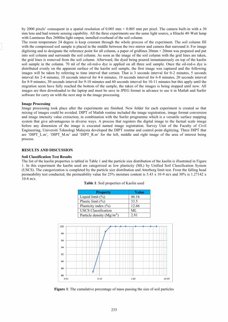
235

by 2000 pixels’ consequent in a spatial resolution of 0.005 mm × 0.005 mm per pixel. The camera built-in with a 30 mm lens and had remote sensing capability. All the three experiments use the same light source, a Hitachi 40-Watt lamp with Luminous flux 2600lm light output, installed overhead of the soil column. The room temperature 24 degree is keep constant through the whole process of the experiment. The soil column fill with the compressed soil sample is placed in the middle between the two mirror and camera that surround it. For image digitizing and to designate the reference point for all column, a paper of gridlines 20mm × 20mm was prepared and put into soil column and surrounds the soil column. As soon as the image of the soil column with the grid lines are taken, the grid lines is removed from the soil column. Afterward, the dyed being poured instantaneously on top of the kaolin soil sample in the column. 70 ml of the oil-red-o dye is applied on all three soil sample. Once the oil-red-o dye is distributed evenly on the apparent surface of the kaolin soil sample, the first image was captured and the following images will be taken by referring to time interval that certain. That is 3 seconds interval for 0-2 minutes, 5 seconds interval for 2-4 minutes, 10 seconds interval for 4-6 minutes, 10 seconds interval for 6-8 minutes, 20 seconds interval for 8-9 minutes, 30 seconds interval for 9-10 minutes and 60 seconds interval for 10-11 minutes but this apply until the migration seem have fully reached the bottom of the sample, the taken of the images is being stopped until now. All images are then downloaded to the laptop and must be save in JPEG format in advance to use it in Matlab and Surfer software for carry on with the next step in the image processing. Image Processing Image processing took place after the experiments are finished. New folder for each experiment is created so that mixing of images could be avoided. DIPT of Matlab routine included the image registration, image format conversion and image intensity value extraction, in combination with the Surfer programme which is a versatile surface mapping system that give advantageous in diverse ways. A process that registers the digital image to the factual scale image before any dimension of the image is executed named image registration. Survey Unit of the Faculty of Civil Engineering, Universiti Teknologi Malaysia developed the DIPT routine and control point digitizing. Three DIPT that are ‘DIPT_L.m’, ‘DIPT_M.m’ and ‘DIPT_R.m’ for the left, middle and right image of the area of interest being process.

RESULTS AND DISCUSSION

Soil Classification Test Results The list of the kaolin properties is tabled in Table 1 and the particle size distribution of the kaolin is illustrated in Figure 1. In this experiment the kaolin used are categorized as low plasticity (ML) by Unified Soil Classification System (USCS). The categorization is completed by the particle size distribution and Atterberg limit test. From the falling head permeability test conducted, the permeability value for 25% moisture content is 5.43 x 10-9 m/s and 30% is 1.27142 x 10-8 m/s.

Table 1: Soil properties of Kaolin used

Property Value Liquid limit (%) 46.16 Plastic limit (%) 33.5 Plasticity index (%) 12.66 USCS Classification ML Particle density (Mg/𝑚3) 2.81

Figure 1: The cumulative percentage of mass passing the size of soil particles

After shredding Before shredding

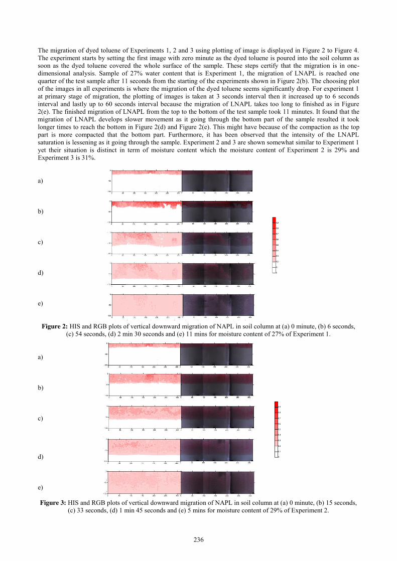
236

The migration of dyed toluene of Experiments 1, 2 and 3 using plotting of image is displayed in Figure 2 to Figure 4. The experiment starts by setting the first image with zero minute as the dyed toluene is poured into the soil column as soon as the dyed toluene covered the whole surface of the sample. These steps certify that the migration is in one-dimensional analysis. Sample of 27% water content that is Experiment 1, the migration of LNAPL is reached one quarter of the test sample after 11 seconds from the starting of the experiments shown in Figure 2(b). The choosing plot of the images in all experiments is where the migration of the dyed toluene seems significantly drop. For experiment 1 at primary stage of migration, the plotting of images is taken at 3 seconds interval then it increased up to 6 seconds interval and lastly up to 60 seconds interval because the migration of LNAPL takes too long to finished as in Figure 2(e). The finished migration of LNAPL from the top to the bottom of the test sample took 11 minutes. It found that the migration of LNAPL develops slower movement as it going through the bottom part of the sample resulted it took longer times to reach the bottom in Figure 2(d) and Figure 2(e). This might have because of the compaction as the top part is more compacted that the bottom part. Furthermore, it has been observed that the intensity of the LNAPL saturation is lessening as it going through the sample. Experiment 2 and 3 are shown somewhat similar to Experiment 1 yet their situation is distinct in term of moisture content which the moisture content of Experiment 2 is 29% and Experiment 3 is 31%. a) b) c) d) e)

Figure 2: HIS and RGB plots of vertical downward migration of NAPL in soil column at (a) 0 minute, (b) 6 seconds, (c) 54 seconds, (d) 2 min 30 seconds and (e) 11 mins for moisture content of 27% of Experiment 1.

a) b) c) d) e) Figure 3: HIS and RGB plots of vertical downward migration of NAPL in soil column at (a) 0 minute, (b) 15 seconds,

(c) 33 seconds, (d) 1 min 45 seconds and (e) 5 mins for moisture content of 29% of Experiment 2.

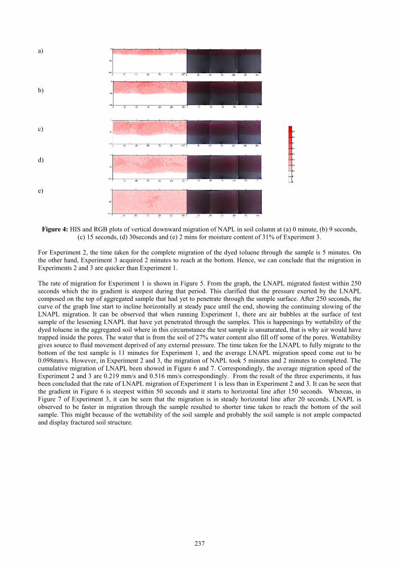
237

a) b) c) d) e)

Figure 4: HIS and RGB plots of vertical downward migration of NAPL in soil column at (a) 0 minute, (b) 9 seconds, (c) 15 seconds, (d) 30seconds and (e) 2 mins for moisture content of 31% of Experiment 3.

For Experiment 2, the time taken for the complete migration of the dyed toluene through the sample is 5 minutes. On the other hand, Experiment 3 acquired 2 minutes to reach at the bottom. Hence, we can conclude that the migration in Experiments 2 and 3 are quicker than Experiment 1. The rate of migration for Experiment 1 is shown in Figure 5. From the graph, the LNAPL migrated fastest within 250 seconds which the its gradient is steepest during that period. This clarified that the pressure exerted by the LNAPL composed on the top of aggregated sample that had yet to penetrate through the sample surface. After 250 seconds, the curve of the graph line start to incline horizontally at steady pace until the end, showing the continuing slowing of the LNAPL migration. It can be observed that when running Experiment 1, there are air bubbles at the surface of test sample of the lessening LNAPL that have yet penetrated through the samples. This is happenings by wettability of the dyed toluene in the aggregated soil where in this circumstance the test sample is unsaturated, that is why air would have trapped inside the pores. The water that is from the soil of 27% water content also fill off some of the pores. Wettability gives source to fluid movement deprived of any external pressure. The time taken for the LNAPL to fully migrate to the bottom of the test sample is 11 minutes for Experiment 1, and the average LNAPL migration speed come out to be 0.098mm/s. However, in Experiment 2 and 3, the migration of NAPL took 5 minutes and 2 minutes to completed. The cumulative migration of LNAPL been showed in Figure 6 and 7. Correspondingly, the average migration speed of the Experiment 2 and 3 are 0.219 mm/s and 0.516 mm/s correspondingly. From the result of the three experiments, it has been concluded that the rate of LNAPL migration of Experiment 1 is less than in Experiment 2 and 3. It can be seen that the gradient in Figure 6 is steepest within 50 seconds and it starts to horizontal line after 150 seconds. Whereas, in Figure 7 of Experiment 3, it can be seen that the migration is in steady horizontal line after 20 seconds. LNAPL is observed to be faster in migration through the sample resulted to shorter time taken to reach the bottom of the soil sample. This might because of the wettability of the soil sample and probably the soil sample is not ample compacted and display fractured soil structure.

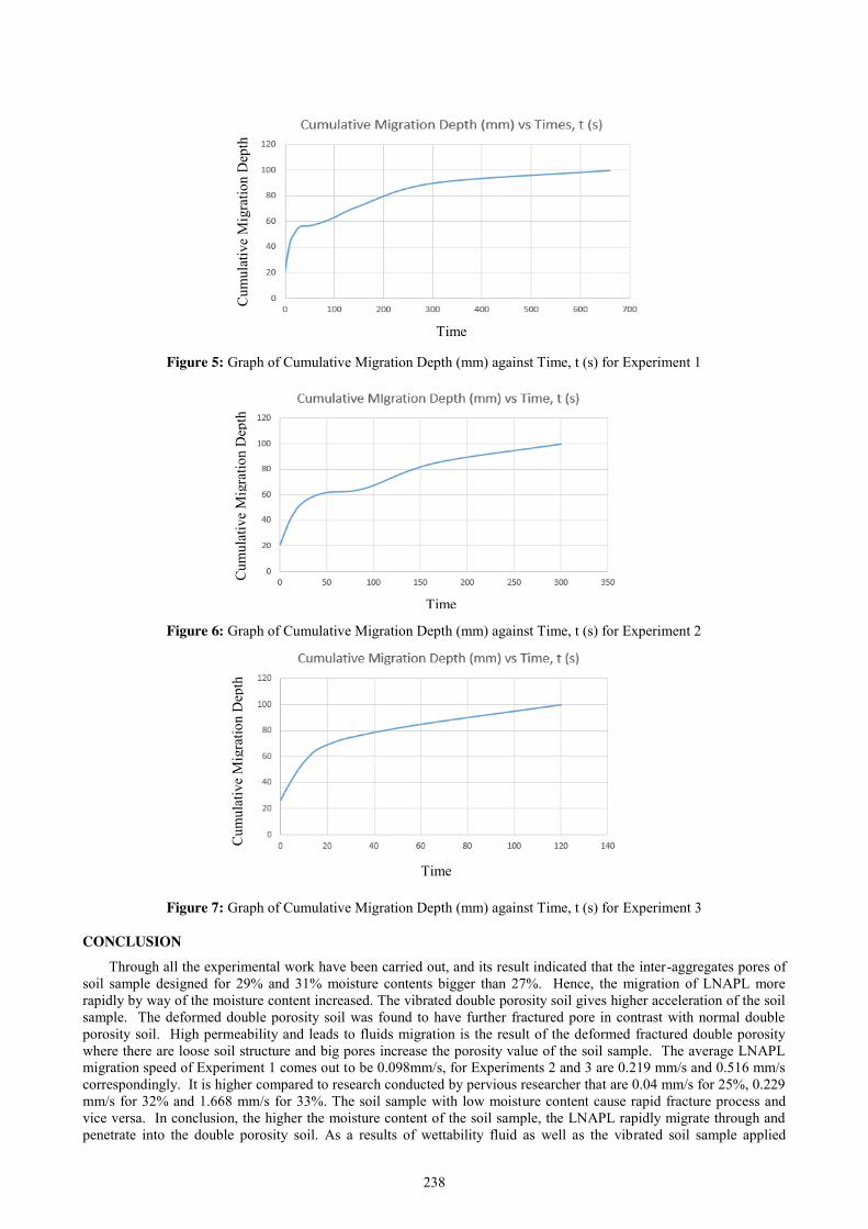
238

Time, t (s)

Cum

ulat

ive

Mig

ratio

n D

epth

(m

m)

Time, t (s)

Cum

ulat

ive

Mig

ratio

n D

epth

(m

m)

Figure 5: Graph of Cumulative Migration Depth (mm) against Time, t (s) for Experiment 1

Figure 6: Graph of Cumulative Migration Depth (mm) against Time, t (s) for Experiment 2

Figure 7: Graph of Cumulative Migration Depth (mm) against Time, t (s) for Experiment 3

CONCLUSION

Through all the experimental work have been carried out, and its result indicated that the inter-aggregates pores of soil sample designed for 29% and 31% moisture contents bigger than 27%. Hence, the migration of LNAPL more rapidly by way of the moisture content increased. The vibrated double porosity soil gives higher acceleration of the soil sample. The deformed double porosity soil was found to have further fractured pore in contrast with normal double porosity soil. High permeability and leads to fluids migration is the result of the deformed fractured double porosity where there are loose soil structure and big pores increase the porosity value of the soil sample. The average LNAPL migration speed of Experiment 1 comes out to be 0.098mm/s, for Experiments 2 and 3 are 0.219 mm/s and 0.516 mm/s correspondingly. It is higher compared to research conducted by pervious researcher that are 0.04 mm/s for 25%, 0.229 mm/s for 32% and 1.668 mm/s for 33%. The soil sample with low moisture content cause rapid fracture process and vice versa. In conclusion, the higher the moisture content of the soil sample, the LNAPL rapidly migrate through and penetrate into the double porosity soil. As a results of wettability fluid as well as the vibrated soil sample applied

Time, t (s)

Cum

ulat

ive

Mig

ratio

n D

epth

(m

m)

239

prompting the NAPL migration. The current model developed is more praticable as a contribution to future sustainable groundwater resources protection and remediation. REFERENCES [1] Loke Kok Foong, Norhan Abd Rahman and Ramli Nazir. 2017. Experimental study on double-porosity soil

phenomena under vibration effect, Jurnal Teknologi, Vol 79, No 4, May 2017 [2] Loke Kok Foong, Norhan Abd Rahman and Mohd Zamri Ramli. 2016. A laboratory study of vibration effect

for deformable double-porosity soil with different moisture content, Malaysian Journal of Civil Engineering, 28(3): 207-222.

[3] Saari, R., Rahman N.A., Abdul Latiff, H.N., Yusof Z.M., Kamaruddin,S.A., Ngien S. K., Mustaffar, M. and Hezmi M. A. (2015). Application of digital image processing technique in monitoring LNAPL migration in double porosity soil column, Jurnal Teknologi, Vol 72, N0. 3, DOI:http:/dx.doi.org/10.11113/jt.v72.4018

[4] S. K. Ngien, N. A. Rahman, K. Ahmad, R. W. Lewis. 2012. NAPL Contamination in Groundwater for Double-Porosity Featured Sub-Surface Systems.

[5] Bedient, P.B., Rifai, H.S., Newell, C.J. 1999. Ground Water Contamination—Transport and Remediation, 2nd edition. Prentice Hall, Upper Saddle River.

240

Erosion Rate in Rubber Plantation in Kelantan River Basin Muhamad Zul Izhar Zulkipli, K.V. Annammala, Muhammad Fahmi Ibrahim,

Nur Athirah Mohamad

Faculty of Civil Engineering, Universiti Teknologi Malaysia kogila@utm.com

Keywords: Soil erosion rates, Soil movement, Rubber Plantation ABSTRACT. Soil erosion is the movement of soil from its original place due to two main elements namely wind and water at a greater rate than it is normal formed. Soil erosion removes the top layer of soil which is rich in nutrients. When the nutrient from the rich layer is removed there will be less plant growth. The objectives of this research are to determine the erosion rate in rubber plantation, to carry out the erosion bridge method in order to measure rate of erosion, to compare erosion rate within various rubber plantation practices and sites; slope, canopy openess, bare ground, soil moisture, and make comparison erosion rate of rubber plantation with oil palm plantation from other research findings. The rates of soil erosion in rubber plantation near Kelantan river basin was measured using Remodeled-Erosion Bridge method. This method is a modified method from existing method with better accuracy. The collected data was analyzed using the Microsoft excel. Total of 36 sites of erosion bridges were installed in-which each sites will further derive 30 measurements within it. In total, there are 1080 points measured to deduce the erosion rate factor. Apart from measurement in ground level changes, measurement of slope and canopy openness (using densitometer) were also performed. Soil samples were also collected at this location to measure soil moisture and to calculate bulk density. Which is then used to calculate the erosion rates in year. Results shows that the erosion rates on this rubber plantation is approximately 1.02 tons/ha/year. Which is very much lower than reported rates within mature oil palm plantations in Malaysia which have a soil erosion rate of approximately 7.7-14 tons/ha/year. Although result is indicating that erosion rate within oil palm plantation in Malaysia is very much higher than the erosion rates in rubber plantation. Further longer term monitoring is suggested to be confirmed. Results from this study may be under-estimated as it was conducted for shorter term and extreme weather conditions were absent. INTRODUCTION

The word “soil” according to the 8th edition Oxford dictionary (2010) is the top layer of the earth in which plants grow. The term “soil erosion” in everyday parlance it can be described as one of the process in earth science that involved the movement of soil, rock or dissolved material from one location on the earth’s crust, then transport it away to another location. Soil erosion which also known as soil degradation is a natural process on the surface layer of soil and it is a slow process and the erosion of soil is a naturally occurring process on all land (Toy et al., 2002). However, according to Pierre et al. (2010), human activities have increased by 10 - 40 times the rate at which erosion is occurring globally (Julien, 2010). Kakembo et al. (2009) who stated that the intensive agriculture, deforestation, roads, anthropogenic climate change and urban sprawl are amongst the most significant human activities in regard to their effect on stimulating erosion (Kakembo et al., 2009).

Problem Statement Monitoring duration was done for 2 months, due to time constrain. Comparison of erosion rates on rubber plantation and oil palm plantation were conducted. The collection data includes four parameters namely; slope, canopy openess, ground cover and soil moisture. Objectives The objectives of this study are: To remodel and install and measure erosion rate in rubber plantation using the erosion bridge method. To compare erosion rate within rubber plantation practices and sites and also against slope, canopy openness, ground cover and soil moisture factors and finally to determine the erosion rate in rubber plantation in tons/ha/year. LITERATURE REVIEW

Soil erosion is the movement of soil from its original place due to the two element which is wind and water at a greater rate than it is normal formed (Toy et al., 2002). Water affects the soil erosion when the rains drops hits the soil which is not bonded by the root of tree and vegetation cover known as rainfall kinetics. The erosion process removes the first layer of soil also know as to soil which is essential in vegetation growth. When the nutrient from this rich layer is removed, there will be less plants re-growth. When the rich nutrients soil and plants is gone, the land becomes dessert like and cannot support the ecosystems (Poesen et al., 1994). There are two major agriculture plantation in Malaysia, which are rubber and palm oil plants. Since there have been many research focused and highlighting on palm oil plantation, this research will focus on rubber plantation which is also the largest agricultural plantation in Malaysia

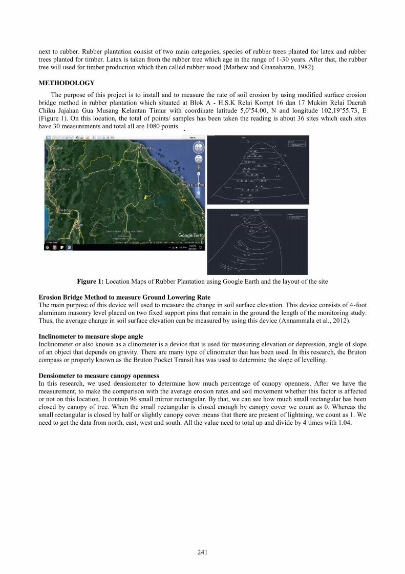
241

next to rubber. Rubber plantation consist of two main categories, species of rubber trees planted for latex and rubber trees planted for timber. Latex is taken from the rubber tree which age in the range of 1-30 years. After that, the rubber tree will used for timber production which then called rubber wood (Mathew and Gnanaharan, 1982). METHODOLOGY

The purpose of this project is to install and to measure the rate of soil erosion by using modified surface erosion bridge method in rubber plantation which situated at Blok A - H.S.K Relai Kompt 16 dan 17 Mukim Relai Daerah Chiku Jajahan Gua Musang Kelantan Timur with coordinate latitude 5,0’54.00, N and longitude 102,19’55.73, E (Figure 1). On this location, the total of points/ samples has been taken the reading is about 36 sites which each sites have 30 measurements and total all are 1080 points.

Figure 1: Location Maps of Rubber Plantation using Google Earth and the layout of the site

Erosion Bridge Method to measure Ground Lowering Rate The main purpose of this device will used to measure the change in soil surface elevation. This device consists of 4-foot aluminum masonry level placed on two fixed support pins that remain in the ground the length of the monitoring study. Thus, the average change in soil surface elevation can be measured by using this device (Annammala et al., 2012). Inclinometer to measure slope angle Inclinometer or also known as a clinometer is a device that is used for measuring elevation or depression, angle of slope of an object that depends on gravity. There are many type of clinometer that has been used. In this research, the Bruton compass or properly known as the Bruton Pocket Transit has was used to determine the slope of levelling. Densiometer to measure canopy openness In this research, we used densiometer to determine how much percentage of canopy openness. After we have the measurement, to make the comparison with the average erosion rates and soil movement whether this factor is affected or not on this location. It contain 96 small mirror rectangular. By that, we can see how much small rectangular has been closed by canopy of tree. When the small rectangular is closed enough by canopy cover we count as 0. Whereas the small rectangular is closed by half or slightly canopy cover means that there are present of lightning, we count as 1. We need to get the data from north, east, west and south. All the value need to total up and divide by 4 times with 1.04.

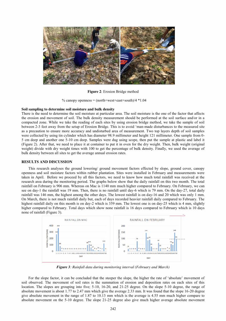
242

Figure 2: Erosion Bridge method

% canopy openness = (north+west+east+south)/4 *1.04 Soil sampling to determine soil moisture and bulk density There is the need to determine the soil moisture at particular area. The soil moisture is the one of the factor that affects the erosion and movement of soil. The bulk density measurement should be performed at the soil surface and/or in a compacted zone. While we take the reading of each sites by using erosion bridge method, we take the sample of soil between 2-3 feet away from the setup of Erosion Bridge. This is to avoid ‘man-made disturbances to the measured site as a precaution to ensure more accuracy and undisturbed area of measurement. Two top layers depth of soil samples were collected by using tin cylinder which has diameter 98.9 millimeter and height 121 millimeter. One sample from 0-5 cm deep and another one 5-10 cm deep. Samples were dug using scope, then put the sample at plastic and label it (Figure 2). After that, we need to place it at container to put it in oven for the dry weight. Then, bulk weight (original weight) divide with dry weight times with 100 to get the percentage of bulk density. Finally, we used the average of bulk density between all sites to get the average annual erosion rates. RESULTS AND DISCUSSION

This research analyses the ground lowering/ ground movement factors effected by slope, ground cover, canopy openness and soil moisture factors within rubber plantation. Sites were installed in February and measurements were taken in April. Before we proceed by all this factors, we need to know how much total rainfall was received at the research area during the monitoring period. The graphs below show that the daily rainfall on this two month. The total rainfall on February is 906 mm. Whereas on Mac is 1140 mm much higher compared to February. On February, we can see on day-1 the rainfall was 19 mm. Then, there is no rainfall until day-6 which is 79 mm. On the day-27, total daily rainfall was 146 mm, the highest among the other days. The lowest rainfall is on day-16 and 20 which was only 1 mm. On March, there is not much rainfall daily but, each of days recorded heavier rainfall daily compared to February. The highest rainfall daily on this month is on day-2 which is 359 mm. The lowest one is on day-25 which is 4 mm, slightly higher compared to February. Total days which show none rainfall is 16 days compared to February which is 10 days none of rainfall (Figure 3).

Figure 3: Rainfall data during monitoring interval (February and March)

For the slope factor, it can be concluded that the steeper the slope, the higher the rate of ‘absolute’ movement of

soil observed. The movement of soil rates is the summation of erosion and deposition rates on each sites of this location. The slopes are grouping into five; 5-10, 16-20, and 21-25 degree. On the slope 5-10 degree, the range of absolute movement is about 1.77 to 2.47 mm which give the average 2.33 mm. It was found that the slope 16-20 degree give absolute movement in the range of 1.87 to 10.13 mm which is the average is 4.55 mm much higher compare to absolute movement on the 5-10 degree. The slope 21-25 degree also give much higher average absolute movement

243

which is 4.67 mm compared to the groups of slope that had mention before. The minimum absolute movement on this group is 4.63 mm and the maximum is about 4.70 mm,

For the average erosion rates, we need to know that the ‘+’ value means erosion whereas ‘-’ value means deposition at the mentioned point/site. The slope 5-10 degree give the reading +0.742 mm. The range of erosion rates is within 1.1 to 1.3 mm. On this slope, it was found that only site S1 had deposition which is -1.47mm. Slope 16-20 degree give the reading -0.103 mm (average) which is we can said also that there is more deposition compare to erosion on this group’s slope. The higher deposition is on site A1 which is -3.31 mm and the higher erosion is on site F3 which is 2.933 mm. On the Slope 21-25 degree, there are consist only two sites; O1 and D2. These two sites give the erosion rates which is about 0.606 mm (average) and all of this sites give erosion rates. Site D2 give 4.63 mm and site O1 give 4.70 mm of erosion rates.

All of this factors need to investigate which one is the major problem that affect the erosion rates on this location. We can used the correlation value which is produced by the trend line from the graph of all this factors versus erosion rates. The higher the value of correlation, the higher relationship between the factors. For the slope factor, the correlation value is 0.0226. From the graph below we can see that 10 to 20 degree of slope, there is present of erosion and deposition rates. Sites at above 20 degree, erosion were recorded (Figure 4).

Canopy openness it can be concluded that the higher the percentage of canopy openness, the higher erosion and absolute movement rates of soil. The research have categories the percentage canopy openness into 3 group; 30-40 percent opened, 40-50 percent opened and above 50 percent not covered. On the 30-40 percent of canopy openness, the average of absolute movement regarding those sites is 4.58 mm whereas on the 40-50 percent of canopy openness, there is slightly lower on absolute movement which is 3.393 mm compared to 30-40 percent of canopy openness but still can consider the result is proportional with the theory. The obvious result we can see on group more than 50 percent which is has average absolute movement 6.54 mm much higher compared to group of canopy openness that mention before.

For the average erosion rates, the group of 30-40 percent canopy openess has 0.175 mm which is the erosion is on dominant compared to deposition. The range of erosion rates is within 0.1 to 2.2 mm. Only sites R1 has deposition value which is -2.1 mm. For the group 40-50 percent canopy openess, the average erosion rates is about 0.063 mm. The range of erosion rates is within 1.1 to 2.0 mm whereas the deposition rates is between -0.86 to -4.9 mm. Lastly for the group more than 50 percent canopy openess give the result 1.792 mm (average) and all sites on this group give erosion value which is on the range 0.6 to 2.9 mm.

For the canopy openness, the correlation value is 0.2328. From the graph, at 40 to 50 percent of canopy openness, there is present of deposition until above the 50 percent of canopy openness, there is only erosion rate would present (Figure 4).

For the ground cover factor, the theory said that if the percentage of ground cover is high, then the absolute movement and erosion rates of soil will be low due to vegetation agents (Torbert and Burger, 1994). The research have been analyzed the percentage of ground cover versus average erosion and absolute movement rates of soils. All of those sites have been grouped by 4 groups; (1) 0-25 percent covered, (2) 25-50 percent covered, (3)50-75 percent covered and (4)75-100 percent covered. The trend of average absolute movement will be going up from group (1) and (2). Then the average absolute movement decrease at group (3) and (4) percent.

On the group (1) of ground cover, the average absolute movement is 3.02 mm. The average erosion rates is 0.60 mm which means the erosion is more than deposition. The range of erosion is from 0.73 to 2.03 mm. Only site S1 has deposition value which is -1.47 mm. For group (2), the absolute movement is higher than group of (1) which is 4.816 mm. The average erosion rates is -0.126 mm which is the deposition is dominant here compared to erosion. The range of erosion rates on this group is about 0.1 to 2.9 mm and range of deposition from -2.9 to -4.9 mm.

Figure 4: graph of all sites of for slope and canopy openness results against erosion separately.

The group (3) gave higher of average absolute movement compared to group that mention before which is 4.47 mm. The average erosion rates is 0.70 mm. The range of erosion rates on this group from 0.8 to 2.2 mm. Only site D1 got deposition value which is -0.857 mm. Lastly, group (4) is less compared to group (2) and (3) but higher than group (1) of ground cover which is 3.76 mm. On this group, there is more deposition than erosion which is -0.225 mm. The range of erosion rates is from 0.4 to 0.5 mm. Only site A1 got deposition value which is -3.31 mm.

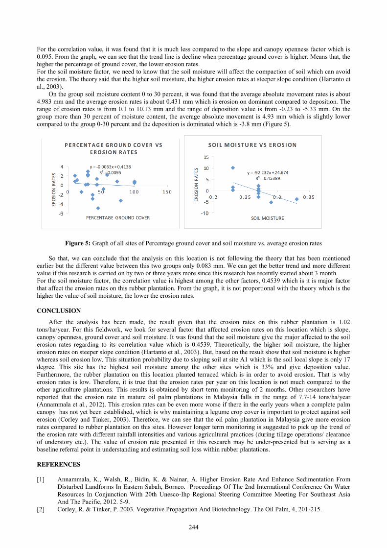
244

For the correlation value, it was found that it is much less compared to the slope and canopy openness factor which is 0.095. From the graph, we can see that the trend line is decline when percentage ground cover is higher. Means that, the higher the percentage of ground cover, the lower erosion rates. For the soil moisture factor, we need to know that the soil moisture will affect the compaction of soil which can avoid the erosion. The theory said that the higher soil moisture, the higher erosion rates at steeper slope condition (Hartanto et al., 2003).

On the group soil moisture content 0 to 30 percent, it was found that the average absolute movement rates is about 4.983 mm and the average erosion rates is about 0.431 mm which is erosion on dominant compared to deposition. The range of erosion rates is from 0.1 to 10.13 mm and the range of deposition value is from -0.23 to -5.33 mm. On the group more than 30 percent of moisture content, the average absolute movement is 4.93 mm which is slightly lower compared to the group 0-30 percent and the deposition is dominated which is -3.8 mm (Figure 5).

Figure 5: Graph of all sites of Percentage ground cover and soil moisture vs. average erosion rates

So that, we can conclude that the analysis on this location is not following the theory that has been mentioned earlier but the different value between this two groups only 0.083 mm. We can get the better trend and more different value if this research is carried on by two or three years more since this research has recently started about 3 month. For the soil moisture factor, the correlation value is highest among the other factors, 0.4539 which is it is major factor that affect the erosion rates on this rubber plantation. From the graph, it is not proportional with the theory which is the higher the value of soil moisture, the lower the erosion rates. CONCLUSION

After the analysis has been made, the result given that the erosion rates on this rubber plantation is 1.02 tons/ha/year. For this fieldwork, we look for several factor that affected erosion rates on this location which is slope, canopy openness, ground cover and soil moisture. It was found that the soil moisture give the major affected to the soil erosion rates regarding to its correlation value which is 0.4539. Theoretically, the higher soil moisture, the higher erosion rates on steeper slope condition (Hartanto et al., 2003). But, based on the result show that soil moisture is higher whereas soil erosion low. This situation probability due to sloping soil at site A1 which is the soil local slope is only 17 degree. This site has the highest soil moisture among the other sites which is 33% and give deposition value. Furthermore, the rubber plantation on this location planted terraced which is in order to avoid erosion. That is why erosion rates is low. Therefore, it is true that the erosion rates per year on this location is not much compared to the other agriculture plantations. This results is obtained by short term monitoring of 2 months. Other researchers have reported that the erosion rate in mature oil palm plantations in Malaysia falls in the range of 7.7-14 tons/ha/year (Annammala et al., 2012). This erosion rates can be even more worse if there in the early years when a complete palm canopy has not yet been established, which is why maintaining a legume crop cover is important to protect against soil erosion (Corley and Tinker, 2003). Therefore, we can see that the oil palm plantation in Malaysia give more erosion rates compared to rubber plantation on this sites. However longer term monitoring is suggested to pick up the trend of the erosion rate with different rainfall intensities and various agricultural practices (during tillage operations/ clearance of understory etc.). The value of erosion rate presented in this research may be under-presented but is serving as a baseline referral point in understanding and estimating soil loss within rubber plantations. REFERENCES [1] Annammala, K., Walsh, R., Bidin, K. & Nainar, A. Higher Erosion Rate And Enhance Sedimentation From

Disturbed Landforms In Eastern Sabah, Borneo. Proceedings Of The 2nd International Conference On Water Resources In Conjunction With 20th Unesco-Ihp Regional Steering Committee Meeting For Southeast Asia And The Pacific, 2012. 5-9.

[2] Corley, R. & Tinker, P. 2003. Vegetative Propagation And Biotechnology. The Oil Palm, 4, 201-215.

245

[3] Hartanto, H., Prabhu, R., Widayat, A. S. & Asdak, C. 2003. Factors Affecting Runoff And Soil Erosion: Plot-Level Soil Loss Monitoring For Assessing Sustainability Of Forest Management. Forest Ecology And Management, 180, 361-374.

[4] Julien, P. Y. 2010. Erosion And Sedimentation, Cambridge University Press. [5] Kakembo, V., Xanga, W. & Rowntree, K. 2009. Topographic Thresholds In Gully Development On The

Hillslopes Of Communal Areas In Ngqushwa Local Municipality, Eastern Cape, South Africa. Geomorphology, 110, 188-194.

[6] Mathew, G. & Gnanaharan, R. 1982. Preservative Treatment Of Rubber Wood (Hevea Brasiliensis). Kfri Research Report 15.

[7] Poesen, J., Torri, D. & Bunte, K. 1994. Effects Of Rock Fragments On Soil Erosion By Water At Different Spatial Scales: A Review. Catena, 23, 141-166.

[8] Sparovek, G. & Schnug, E. 2001. Temporal Erosion-Induced Soil Degradation And Yield Loss. Soil Science Society Of America Journal, 65, 1479-1486.

[9] Tomei, J. & Upham, P. 2009. Argentinean Soy-Based Biodiesel: An Introduction To Production And Impacts. Energy Policy, 37, 3890-3898.

[10] Torbert, J. L. & Burger, J. A. Influence Of Grading Intensity On Ground Cover Establishment, Erosion, And Tree Establishment On Steep Slopes. International Land Reclamation And Mine Drainage Conference And Third International Conference On The Abatement Of Acidic Drainage: Proceedings. Volume 3: Reclamation And Revegetation--Sp 06c-94, 1994.

[11] Toy, T. J., Foster, G. R. & Renard, K. G. 2002. Soil Erosion: Processes, Prediction, Measurement, And Control, John Wiley & Sons.

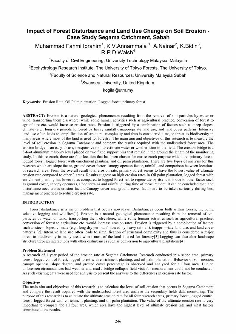
246

Impact of Forest Disturbance and Land Use Change on Soil Erosion - Case Study Segama Catchment, Sabah

Muhammad Fahmi Ibrahim1, K.V.Annammala 1, A.Nainar2, K.Bidin3, R.P.D.Walsh4

1Faculty of Civil Engineering, University Technology Malaysia, Malaysia 2Ecohydrology Research Institute, The University of Tokyo Forests, The University of Tokyo.

3Faculty of Science and Natural Resources, University Malaysia Sabah 4Swansea University, United Kingdom.

kogila@utm.my Keywords: Erosion Rate, Oil Palm plantation, Logged forest, primary forest ABSTRACT: Erosion is a natural geological phenomenon resulting from the removal of soil particles by water or wind, transporting them elsewhere, while some human activities such as agricultural practice, conversion of forest to agriculture etc. would increase erosion rates. Erosion is triggered by a combination of factors such as steep slopes, climate (e.g., long dry periods followed by heavy rainfall), inappropriate land use, and land cover patterns. Intensive land use often leads to simplification of structural complexity and thus is considered a major threat to biodiversity in many areas where most of the land is used for forestry. The main aim and objectives of this research is to measure the level of soil erosion in Segama Catchment and compare the results acquired with the undisturbed forest area. The erosion bridge is an easy-to-use, inexpensive tool to estimate water or wind erosion in the field. The erosion bridge is a 3-foot aluminum masonry level placed on two fixed support pins that remain in the ground the length of the monitoring study. In this research, there are four location that has been chosen for our research purpose which are, primary forest, logged forest, logged forest with enrichment planting, and oil palm plantation. There are five types of analysis for this research which are slope factor, ground cover factor, canopy openess factor, rainfall, and comparison between locations of research area. From the overall result total erosion rate, primary forest seems to have the lowest value of ultimate erosion rate compared to other 3 areas. Results suggest on high erosion rates in Oil palm plantation, logged forest with enrichment planting has lower rates compared to logged forest left to regenerate by itself. it is due to other factor such as ground cover, canopy openness, slope terrains and rainfall during time of measurement. It can be concluded that land disturbance accelerates erosion factor. Canopy cover and ground cover factor are to be taken seriously during best management practices to reduce erosion rate. INTRODUCTION

Forest disturbance is a major problem that occurs nowadays. Disturbances occur both within forests, including selective logging and wildfires[1]. Erosion is a natural geological phenomenon resulting from the removal of soil particles by water or wind, transporting them elsewhere, while some human activities such as agricultural practice, conversion of forest to agriculture etc. would increase erosion rates. Erosion is triggered by a combination of factors such as steep slopes, climate (e.g., long dry periods followed by heavy rainfall), inappropriate land use, and land cover patterns [2]. Intensive land use often leads to simplification of structural complexity and thus is considered a major threat to biodiversity in many areas where most of the land is used for forestry[3].Logging can also alter landscape structure through interactions with other disturbances such as conversion to agricultural plantations[4].

Problem Statement A research of 1 year period of the erosion rate at Segama Catchment. Research conducted in 4 scope area, primary forest, logged control forest, logged forest with enrichment planting, and oil palm plantation. Behavior of soil erosion, canopy openess, slope degree, and ground cover percentage is observed and analyzed for all four area. Due to unforeseen circumstances bad weather and road / bridge collapse field visit for measurement could not be conducted. As such existing data were used for analysis to present the answers to the differences in erosion rate factor. Objectives The main aim and objectives of this research is to calculate the level of soil erosion that occurs in Segama Catchment and compare the result acquired with the undisturbed forest area analyse the secondary fields data monitoring. The purpose of this research is to calculate the ultimate erosion rate for all four research areas, primary forest, logged control forest, logged forest with enrichment planting, and oil palm plantation. The value of the ultimate erosion rate is very important to compare the all four area, which area have the highest level of ultimate erosion rate and what factors contribute to the results.

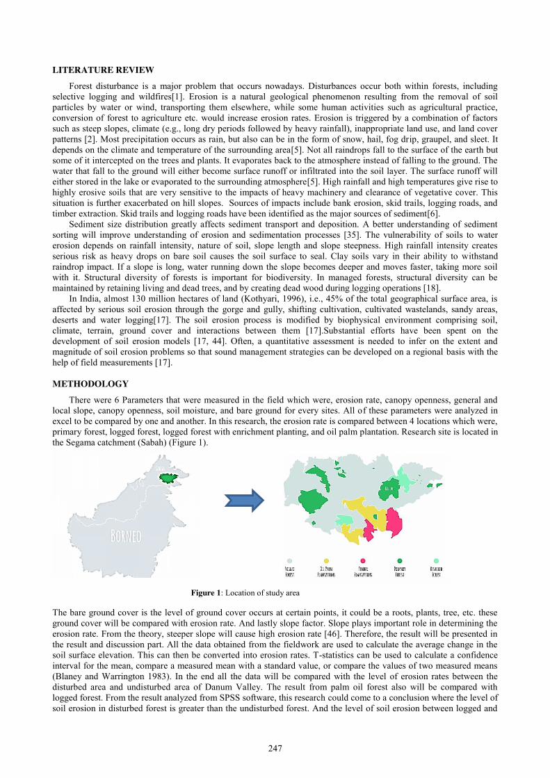
247

LITERATURE REVIEW

Forest disturbance is a major problem that occurs nowadays. Disturbances occur both within forests, including selective logging and wildfires[1]. Erosion is a natural geological phenomenon resulting from the removal of soil particles by water or wind, transporting them elsewhere, while some human activities such as agricultural practice, conversion of forest to agriculture etc. would increase erosion rates. Erosion is triggered by a combination of factors such as steep slopes, climate (e.g., long dry periods followed by heavy rainfall), inappropriate land use, and land cover patterns [2]. Most precipitation occurs as rain, but also can be in the form of snow, hail, fog drip, graupel, and sleet. It depends on the climate and temperature of the surrounding area[5]. Not all raindrops fall to the surface of the earth but some of it intercepted on the trees and plants. It evaporates back to the atmosphere instead of falling to the ground. The water that fall to the ground will either become surface runoff or infiltrated into the soil layer. The surface runoff will either stored in the lake or evaporated to the surrounding atmosphere[5]. High rainfall and high temperatures give rise to highly erosive soils that are very sensitive to the impacts of heavy machinery and clearance of vegetative cover. This situation is further exacerbated on hill slopes. Sources of impacts include bank erosion, skid trails, logging roads, and timber extraction. Skid trails and logging roads have been identified as the major sources of sediment[6].

Sediment size distribution greatly affects sediment transport and deposition. A better understanding of sediment sorting will improve understanding of erosion and sedimentation processes [35]. The vulnerability of soils to water erosion depends on rainfall intensity, nature of soil, slope length and slope steepness. High rainfall intensity creates serious risk as heavy drops on bare soil causes the soil surface to seal. Clay soils vary in their ability to withstand raindrop impact. If a slope is long, water running down the slope becomes deeper and moves faster, taking more soil with it. Structural diversity of forests is important for biodiversity. In managed forests, structural diversity can be maintained by retaining living and dead trees, and by creating dead wood during logging operations [18].

In India, almost 130 million hectares of land (Kothyari, 1996), i.e., 45% of the total geographical surface area, is affected by serious soil erosion through the gorge and gully, shifting cultivation, cultivated wastelands, sandy areas, deserts and water logging[17]. The soil erosion process is modified by biophysical environment comprising soil, climate, terrain, ground cover and interactions between them [17].Substantial efforts have been spent on the development of soil erosion models [17, 44]. Often, a quantitative assessment is needed to infer on the extent and magnitude of soil erosion problems so that sound management strategies can be developed on a regional basis with the help of field measurements [17].

METHODOLOGY

There were 6 Parameters that were measured in the field which were, erosion rate, canopy openness, general and local slope, canopy openness, soil moisture, and bare ground for every sites. All of these parameters were analyzed in excel to be compared by one and another. In this research, the erosion rate is compared between 4 locations which were, primary forest, logged forest, logged forest with enrichment planting, and oil palm plantation. Research site is located in the Segama catchment (Sabah) (Figure 1).

The bare ground cover is the level of ground cover occurs at certain points, it could be a roots, plants, tree, etc. these ground cover will be compared with erosion rate. And lastly slope factor. Slope plays important role in determining the erosion rate. From the theory, steeper slope will cause high erosion rate [46]. Therefore, the result will be presented in the result and discussion part. All the data obtained from the fieldwork are used to calculate the average change in the soil surface elevation. This can then be converted into erosion rates. T-statistics can be used to calculate a confidence interval for the mean, compare a measured mean with a standard value, or compare the values of two measured means (Blaney and Warrington 1983). In the end all the data will be compared with the level of erosion rates between the disturbed area and undisturbed area of Danum Valley. The result from palm oil forest also will be compared with logged forest. From the result analyzed from SPSS software, this research could come to a conclusion where the level of soil erosion in disturbed forest is greater than the undisturbed forest. And the level of soil erosion between logged and

Figure 1: Location of study area

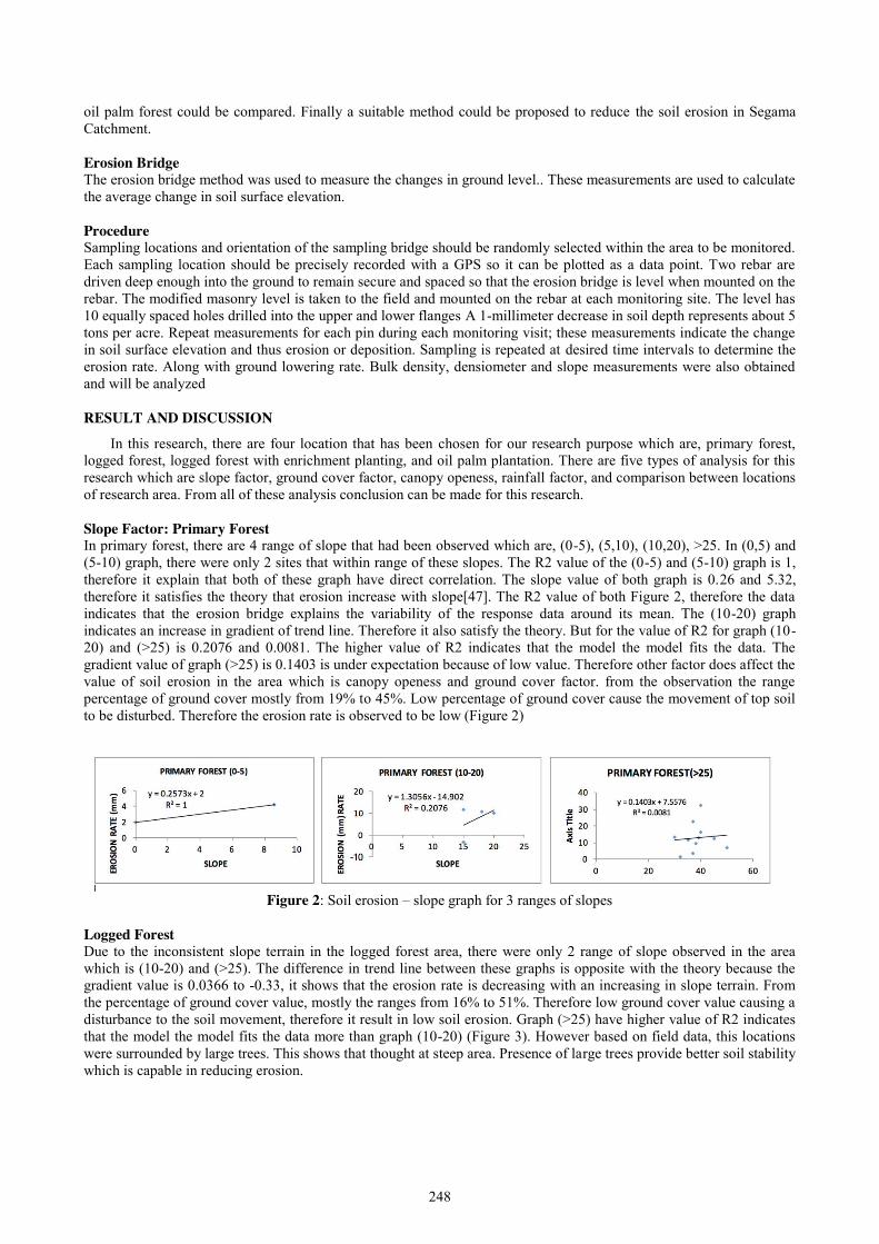
248

oil palm forest could be compared. Finally a suitable method could be proposed to reduce the soil erosion in Segama Catchment. Erosion Bridge The erosion bridge method was used to measure the changes in ground level.. These measurements are used to calculate the average change in soil surface elevation. Procedure Sampling locations and orientation of the sampling bridge should be randomly selected within the area to be monitored. Each sampling location should be precisely recorded with a GPS so it can be plotted as a data point. Two rebar are driven deep enough into the ground to remain secure and spaced so that the erosion bridge is level when mounted on the rebar. The modified masonry level is taken to the field and mounted on the rebar at each monitoring site. The level has 10 equally spaced holes drilled into the upper and lower flanges A 1-millimeter decrease in soil depth represents about 5 tons per acre. Repeat measurements for each pin during each monitoring visit; these measurements indicate the change in soil surface elevation and thus erosion or deposition. Sampling is repeated at desired time intervals to determine the erosion rate. Along with ground lowering rate. Bulk density, densiometer and slope measurements were also obtained and will be analyzed RESULT AND DISCUSSION

In this research, there are four location that has been chosen for our research purpose which are, primary forest, logged forest, logged forest with enrichment planting, and oil palm plantation. There are five types of analysis for this research which are slope factor, ground cover factor, canopy openess, rainfall factor, and comparison between locations of research area. From all of these analysis conclusion can be made for this research. Slope Factor: Primary Forest In primary forest, there are 4 range of slope that had been observed which are, (0-5), (5,10), (10,20), >25. In (0,5) and (5-10) graph, there were only 2 sites that within range of these slopes. The R2 value of the (0-5) and (5-10) graph is 1, therefore it explain that both of these graph have direct correlation. The slope value of both graph is 0.26 and 5.32, therefore it satisfies the theory that erosion increase with slope[47]. The R2 value of both Figure 2, therefore the data indicates that the erosion bridge explains the variability of the response data around its mean. The (10-20) graph indicates an increase in gradient of trend line. Therefore it also satisfy the theory. But for the value of R2 for graph (10-20) and (>25) is 0.2076 and 0.0081. The higher value of R2 indicates that the model the model fits the data. The gradient value of graph (>25) is 0.1403 is under expectation because of low value. Therefore other factor does affect the value of soil erosion in the area which is canopy openess and ground cover factor. from the observation the range percentage of ground cover mostly from 19% to 45%. Low percentage of ground cover cause the movement of top soil to be disturbed. Therefore the erosion rate is observed to be low (Figure 2)

Figure 2: Soil erosion – slope graph for 3 ranges of slopes

Logged Forest Due to the inconsistent slope terrain in the logged forest area, there were only 2 range of slope observed in the area which is (10-20) and (>25). The difference in trend line between these graphs is opposite with the theory because the gradient value is 0.0366 to -0.33, it shows that the erosion rate is decreasing with an increasing in slope terrain. From the percentage of ground cover value, mostly the ranges from 16% to 51%. Therefore low ground cover value causing a disturbance to the soil movement, therefore it result in low soil erosion. Graph (>25) have higher value of R2 indicates that the model the model fits the data more than graph (10-20) (Figure 3). However based on field data, this locations were surrounded by large trees. This shows that thought at steep area. Presence of large trees provide better soil stability which is capable in reducing erosion.

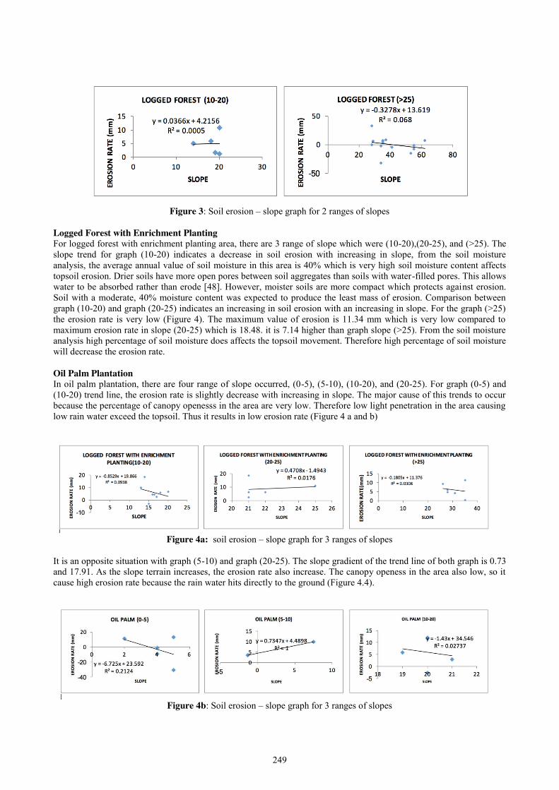
249

Figure 3: Soil erosion – slope graph for 2 ranges of slopes

Logged Forest with Enrichment Planting For logged forest with enrichment planting area, there are 3 range of slope which were (10-20),(20-25), and (>25). The slope trend for graph (10-20) indicates a decrease in soil erosion with increasing in slope, from the soil moisture analysis, the average annual value of soil moisture in this area is 40% which is very high soil moisture content affects topsoil erosion. Drier soils have more open pores between soil aggregates than soils with water-filled pores. This allows water to be absorbed rather than erode [48]. However, moister soils are more compact which protects against erosion. Soil with a moderate, 40% moisture content was expected to produce the least mass of erosion. Comparison between graph (10-20) and graph (20-25) indicates an increasing in soil erosion with an increasing in slope. For the graph (>25) the erosion rate is very low (Figure 4). The maximum value of erosion is 11.34 mm which is very low compared to maximum erosion rate in slope (20-25) which is 18.48. it is 7.14 higher than graph slope (>25). From the soil moisture analysis high percentage of soil moisture does affects the topsoil movement. Therefore high percentage of soil moisture will decrease the erosion rate. Oil Palm Plantation In oil palm plantation, there are four range of slope occurred, (0-5), (5-10), (10-20), and (20-25). For graph (0-5) and (10-20) trend line, the erosion rate is slightly decrease with increasing in slope. The major cause of this trends to occur because the percentage of canopy openesss in the area are very low. Therefore low light penetration in the area causing low rain water exceed the topsoil. Thus it results in low erosion rate (Figure 4 a and b)

Figure 4a: soil erosion – slope graph for 3 ranges of slopes

It is an opposite situation with graph (5-10) and graph (20-25). The slope gradient of the trend line of both graph is 0.73 and 17.91. As the slope terrain increases, the erosion rate also increase. The canopy openess in the area also low, so it cause high erosion rate because the rain water hits directly to the ground (Figure 4.4).

Figure 4b: Soil erosion – slope graph for 3 ranges of slopes

250

Ground cover In primary forest and logged forest, the trend line is more significant in primary forest because the R2 value gives greater than logged forest which is 0.1324 where the R2 value for logged forest is 0.003. Therefore low R2 value commits that there is no significant trends in logged forest. In logged forest graph there are 6 points of of negative erosion rate which indicates a deposition of soil in certain sites. This is because porous and low grip strength of soil after logging and low ground cover causing the movement of soil to be increase, thus deposition o soil will occur. In logged forest with enrichment planting area, the level of erosion rate is slightly low. It has maximum value of 18.48mm which is slightly low compared to the other four area. It is observed that logged forest with enrichment planting area has the lowest maximum erosion rate value which is 18.46 mm but the majority of ground cover percentage is the lowest which ranges from 3% to 20%. In this situation, the lower ground cover percentage will reduce the erosion rate of the area. The usual assumption is that erosion and sediment yield from a slope increases with decreasing vegetative cover until they reach a maximum when the ground is bare. However, it has been suggested that erosion rates are minimally affected by vegetation at some low value of vegetative cover. It has even been reported that as ground cover increases from zero, in some circumstances erosion and sediment yield will increase to a maximum at some low percentage of cover. The relation between sediment yield and percentage of ground cover has been reported to be both linear and exponential although most data have been obtained for surfaces with more than 20% cover [51]. Therefore in this research, it is proved that the percentage of ground cover does affect the erosion rate. As the percentage of ground cover increases, the erosion rate also will increase. The R2 value for both primary forest and oil palm plantation are 0.1931 and 0.1268. These data different with R2 value of logged forest and logged forest with enrichment planting area which are 0.0030 and 0.0047. Low value of coefficients of determination R2 indicates that the data shows imprecise trends. In this situation, this research assumed that soil behavior in logged forest affected the level of soil erosion due to porous and low grip strength of soil. Therefore, the results of soil erosion will be inconsistent. The result of inconsistent data behavior affected the gradient of regression line. It affected at both logged forest and logged forest with enrichment planting which the gradient are negative which is -0.0264 and 0.0047.

Figure 5: Soil erosion – ground-cover graph

Rainfall Factor In logged forest area, there are fluctuation trends that occur across the year. In March, the soil erosion rate are relatively small. The majority of them is commonly soil erosion but small value. The maximum erosion rate in March is -11.52 at site A13 which indicates a deposition. In October, the erosion rate is slightly higher than March, but the maximum erosion rate is 9.21 at site A13. Therefore site A13 has the highest soil movement from March to August based on the observation across all over the three months, the overall overview for all sites could be seen to be decrease with time. So base on the rainfall data analysis the rainfall is decreasing from March to October and there is no extreme event in October. Therefore conclusion can be made by saying that erosion rate will increase with rainfall frequency. . In logged forest with enrichment planting area the erosion rate is relatively small compared to logged forest. It is proved that enrichment planting helped in reducing the erosion rate. Most of the data over the three month, there are variations of data such as increase, decrease and fluctuation data across three month. The majority of the data recorded is increasing in value of erosion, but only small difference recorded. In March, there are 7 sites that have deposition but in august, the deposition value starts to decrease to 5 sites and in October only 3 sites that have deposition value (Figure 6). Therefore low rainfall rate thus decrease the erosion rate.

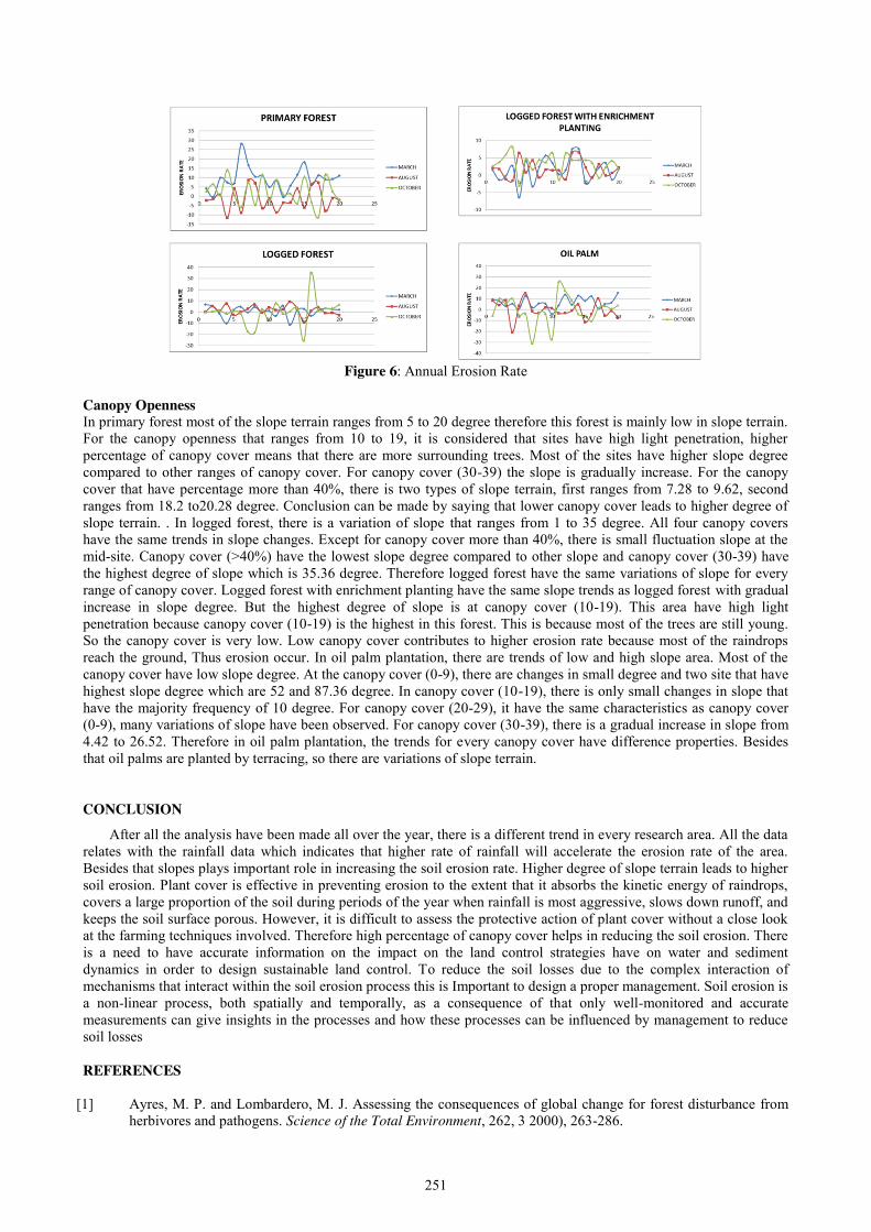
251

Figure 6: Annual Erosion Rate

Canopy Openness In primary forest most of the slope terrain ranges from 5 to 20 degree therefore this forest is mainly low in slope terrain. For the canopy openness that ranges from 10 to 19, it is considered that sites have high light penetration, higher percentage of canopy cover means that there are more surrounding trees. Most of the sites have higher slope degree compared to other ranges of canopy cover. For canopy cover (30-39) the slope is gradually increase. For the canopy cover that have percentage more than 40%, there is two types of slope terrain, first ranges from 7.28 to 9.62, second ranges from 18.2 to20.28 degree. Conclusion can be made by saying that lower canopy cover leads to higher degree of slope terrain. . In logged forest, there is a variation of slope that ranges from 1 to 35 degree. All four canopy covers have the same trends in slope changes. Except for canopy cover more than 40%, there is small fluctuation slope at the mid-site. Canopy cover (>40%) have the lowest slope degree compared to other slope and canopy cover (30-39) have the highest degree of slope which is 35.36 degree. Therefore logged forest have the same variations of slope for every range of canopy cover. Logged forest with enrichment planting have the same slope trends as logged forest with gradual increase in slope degree. But the highest degree of slope is at canopy cover (10-19). This area have high light penetration because canopy cover (10-19) is the highest in this forest. This is because most of the trees are still young. So the canopy cover is very low. Low canopy cover contributes to higher erosion rate because most of the raindrops reach the ground, Thus erosion occur. In oil palm plantation, there are trends of low and high slope area. Most of the canopy cover have low slope degree. At the canopy cover (0-9), there are changes in small degree and two site that have highest slope degree which are 52 and 87.36 degree. In canopy cover (10-19), there is only small changes in slope that have the majority frequency of 10 degree. For canopy cover (20-29), it have the same characteristics as canopy cover (0-9), many variations of slope have been observed. For canopy cover (30-39), there is a gradual increase in slope from 4.42 to 26.52. Therefore in oil palm plantation, the trends for every canopy cover have difference properties. Besides that oil palms are planted by terracing, so there are variations of slope terrain. CONCLUSION

After all the analysis have been made all over the year, there is a different trend in every research area. All the data relates with the rainfall data which indicates that higher rate of rainfall will accelerate the erosion rate of the area. Besides that slopes plays important role in increasing the soil erosion rate. Higher degree of slope terrain leads to higher soil erosion. Plant cover is effective in preventing erosion to the extent that it absorbs the kinetic energy of raindrops, covers a large proportion of the soil during periods of the year when rainfall is most aggressive, slows down runoff, and keeps the soil surface porous. However, it is difficult to assess the protective action of plant cover without a close look at the farming techniques involved. Therefore high percentage of canopy cover helps in reducing the soil erosion. There is a need to have accurate information on the impact on the land control strategies have on water and sediment dynamics in order to design sustainable land control. To reduce the soil losses due to the complex interaction of mechanisms that interact within the soil erosion process this is Important to design a proper management. Soil erosion is a non-linear process, both spatially and temporally, as a consequence of that only well-monitored and accurate measurements can give insights in the processes and how these processes can be influenced by management to reduce soil losses REFERENCES

[1] Ayres, M. P. and Lombardero, M. J. Assessing the consequences of global change for forest disturbance from herbivores and pathogens. Science of the Total Environment, 262, 3 2000), 263-286.

252

[2] Ganasri, B. and Ramesh, H. Assessment of soil erosion by RUSLE model using remote sensing and GIS-A case study of Nethravathi Basin. Geoscience Frontiers2015).

[3] Santaniello, F., Line, D. B., Ranius, T., Rudolphi, J., Widenfalk, O. and Weslien, J. Effects of partial cutting on logging productivity, economic returns and dead wood in boreal pine forest. Forest Ecology and Management, 3652016), 152-158.

[4] Lindenmayer, D. Interactions between Forest Resource Management and Landscape Structure. Current Landscape Ecology Reports2016), 1-9.

[5] Evaristo, J., Jasechko, S. and McDonnell, J. J. Global separation of plant transpiration from groundwater and streamflow. Nature, 525, 7567 2015), 91-94.

[6] Hartanto, H., Prabhu, R., Widayat, A. S. and Asdak, C. Factors affecting runoff and soil erosion: plot-level soil loss monitoring for assessing sustainability of forest management. Forest Ecology and Management, 180, 1 2003), 361-374.

253

Monitoring Shoreline Changes at Teluk Gorek Beach, Mersing, Johor Nur Azlin Baharudin, Radzuan Sa’ari, Muhammamad Azril Hezmi

Faculty of Civil Engineering, Universiti Teknologi Malaysia

radzuans@utm.my,

Keywords: Beach Profile changes, RTK GPS.

ABSTRACT. Beach profile changes are subjected to various parameters such as tides, currents and wave effect. This study conduct to monitor the coastal changes at Teluk Gorek Beach, Mersing and to evaluate the effect of soil density on beach sediment properties. The monitoring work involved the usage of Real Time Kinematik Global Positioning System (RTK-GPS) technique and to determine the beach sediment properties of Teluk Gorek. The objective of this study are to apply the tenhnique of RTK-GPS in obtaining the current beach profile and to compare the data between two measurements obtained between January and April 2017. A total of nine beach profile cross sections with offset 100 m apart were established to monitor the presence of erosion and accretion. While, a total of nine samples were collected and analyze to determine the coastal sediment properties. The findings of this study shows that the beach profiles have experienced both erosion and accretion during the period of study. The soil density change varies to the erosion and accretion process. As a conclusion, the beach is slightly changes during the period of study.

INTRODUCTION

Malaysia has a total coastline of 4.675km and Peninsular Malaysia has 2068km, while East Malaysia has 2607km of coastline. A large number of factors influence the shape of beach profile in nature. Approximately, 30% of Malaysia’s coastline is experiencing erosion (Rahman, 2000). It can be stated that the east coast state of Peninsular Malaysia is has experienced beach erosion along the coastline due to the large waves of the north east monsoon seasons. Beach erosion is a serious problem for coastal country in the world such as Australia, Poland and Belgium (Cheng, 2016). Beach erosion occurs when waves and currents remove sand from the beach normal condition and this losses of sand will change the beach to become narrower and lower in elevation. There are also cases of erosion due to the disturbance by mankind such as tourism activities. Activities conducted by mankind along the beach really give a big impact to the beach profile. The changing of beach elevation causes the changing of beach profile.

Problem Statement The windy criteria from the sea in South East of China as a factor of beach erosion in Peninsular Malaysia. The wind, wave propagation and tides could change the beach profile by disturbed the sediment at the coast. Then, the topography changes would occur due to the natural process of wave and tides. The changes would give negative impact to Telok Gorek beach especially when erosion happen. There are Teluk Gorek Chalet and Camp Site near the beach and it can effect the condition of the chalet. The topography changes would occur due to the natural process of waves and tides. The development of the study area are still in progress and the information about the beach area are important. Beach profiling is importance to monitor and planning action should be taken for a long-term prevention. Objectives The objectives of this study are:

16. To evaluate the beach profile changes at Teluk Gorek 17. To estimate the erosion and accreation at Teluk Gorek 18. To determine the beach sediment properties changes at Teluk Gorek (sediment classification and density)

Scope of Study This study had investigated the beach profile changes at Teluk Gorek Beach by comparing several beach profile cross-section obtain by using RTK GPS. The survey was conducted on 16th January 2017 for first data collection whereas the second data collection was collected on 25th April 2017. Both surveys were carried out during spring tide.This beach profiling survey was conducted to obtain the profile changes of the existing beach profiles. In addition, this study was conducted to estimate the erosion and accretion by comparing the results obtained from the analysed data. As the results, the changes of the beach profile were evaluated. Sediment samples were also collected from the study area for basic soil properties investigation. A total number of nine samples were taken from nine different points. The sample then had been analysed to determine the characteristics and physical properties of the sediment.

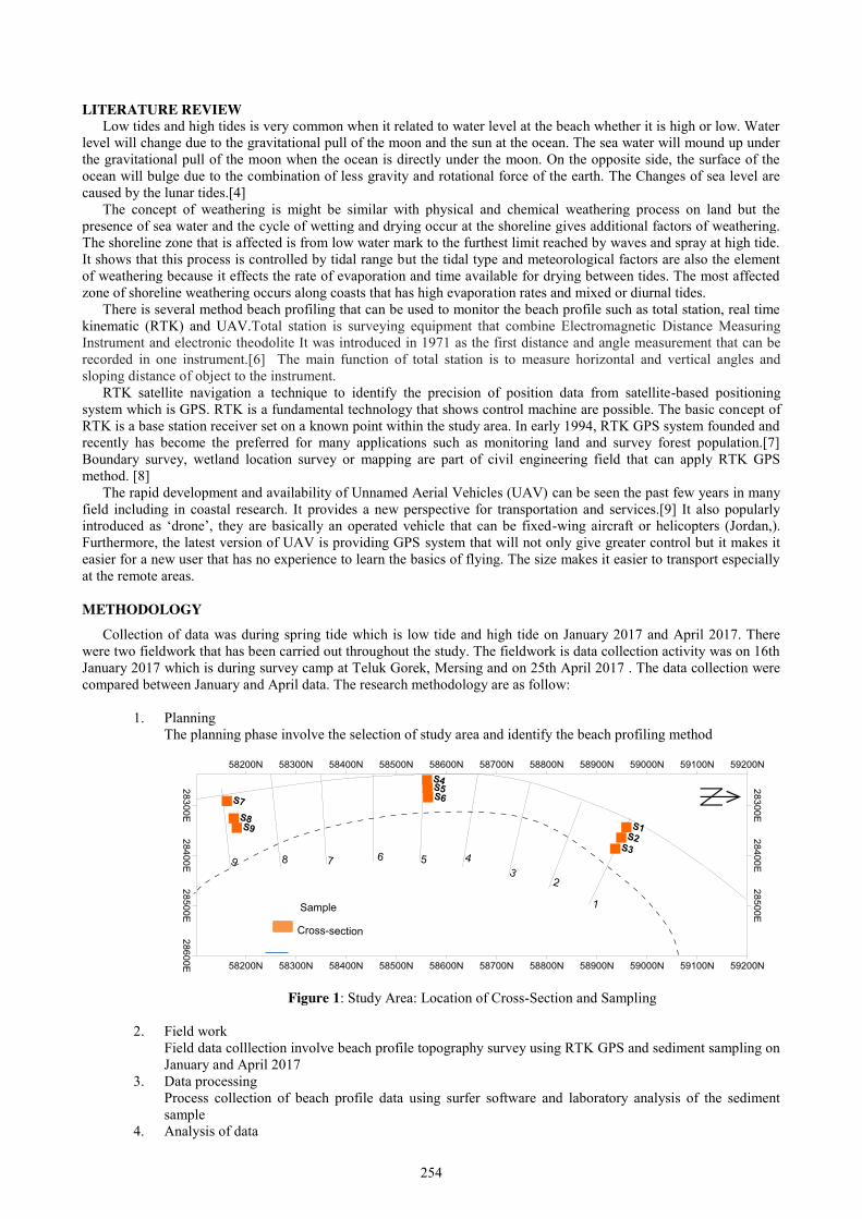
254

LITERATURE REVIEW Low tides and high tides is very common when it related to water level at the beach whether it is high or low. Water

level will change due to the gravitational pull of the moon and the sun at the ocean. The sea water will mound up under the gravitational pull of the moon when the ocean is directly under the moon. On the opposite side, the surface of the ocean will bulge due to the combination of less gravity and rotational force of the earth. The Changes of sea level are caused by the lunar tides.[4]

The concept of weathering is might be similar with physical and chemical weathering process on land but the presence of sea water and the cycle of wetting and drying occur at the shoreline gives additional factors of weathering. The shoreline zone that is affected is from low water mark to the furthest limit reached by waves and spray at high tide. It shows that this process is controlled by tidal range but the tidal type and meteorological factors are also the element of weathering because it effects the rate of evaporation and time available for drying between tides. The most affected zone of shoreline weathering occurs along coasts that has high evaporation rates and mixed or diurnal tides.

There is several method beach profiling that can be used to monitor the beach profile such as total station, real time kinematic (RTK) and UAV.Total station is surveying equipment that combine Electromagnetic Distance Measuring Instrument and electronic theodolite It was introduced in 1971 as the first distance and angle measurement that can be recorded in one instrument.[6] The main function of total station is to measure horizontal and vertical angles and sloping distance of object to the instrument.

RTK satellite navigation a technique to identify the precision of position data from satellite-based positioning system which is GPS. RTK is a fundamental technology that shows control machine are possible. The basic concept of RTK is a base station receiver set on a known point within the study area. In early 1994, RTK GPS system founded and recently has become the preferred for many applications such as monitoring land and survey forest population.[7] Boundary survey, wetland location survey or mapping are part of civil engineering field that can apply RTK GPS method. [8]

The rapid development and availability of Unnamed Aerial Vehicles (UAV) can be seen the past few years in many field including in coastal research. It provides a new perspective for transportation and services.[9] It also popularly introduced as ‘drone’, they are basically an operated vehicle that can be fixed-wing aircraft or helicopters (Jordan,). Furthermore, the latest version of UAV is providing GPS system that will not only give greater control but it makes it easier for a new user that has no experience to learn the basics of flying. The size makes it easier to transport especially at the remote areas. METHODOLOGY

Collection of data was during spring tide which is low tide and high tide on January 2017 and April 2017. There were two fieldwork that has been carried out throughout the study. The fieldwork is data collection activity was on 16th January 2017 which is during survey camp at Teluk Gorek, Mersing and on 25th April 2017 . The data collection were compared between January and April data. The research methodology are as follow:

1. Planning

The planning phase involve the selection of study area and identify the beach profiling method

Figure 1: Study Area: Location of Cross-Section and Sampling

2. Field work Field data colllection involve beach profile topography survey using RTK GPS and sediment sampling on January and April 2017

3. Data processing Process collection of beach profile data using surfer software and laboratory analysis of the sediment sample

4. Analysis of data

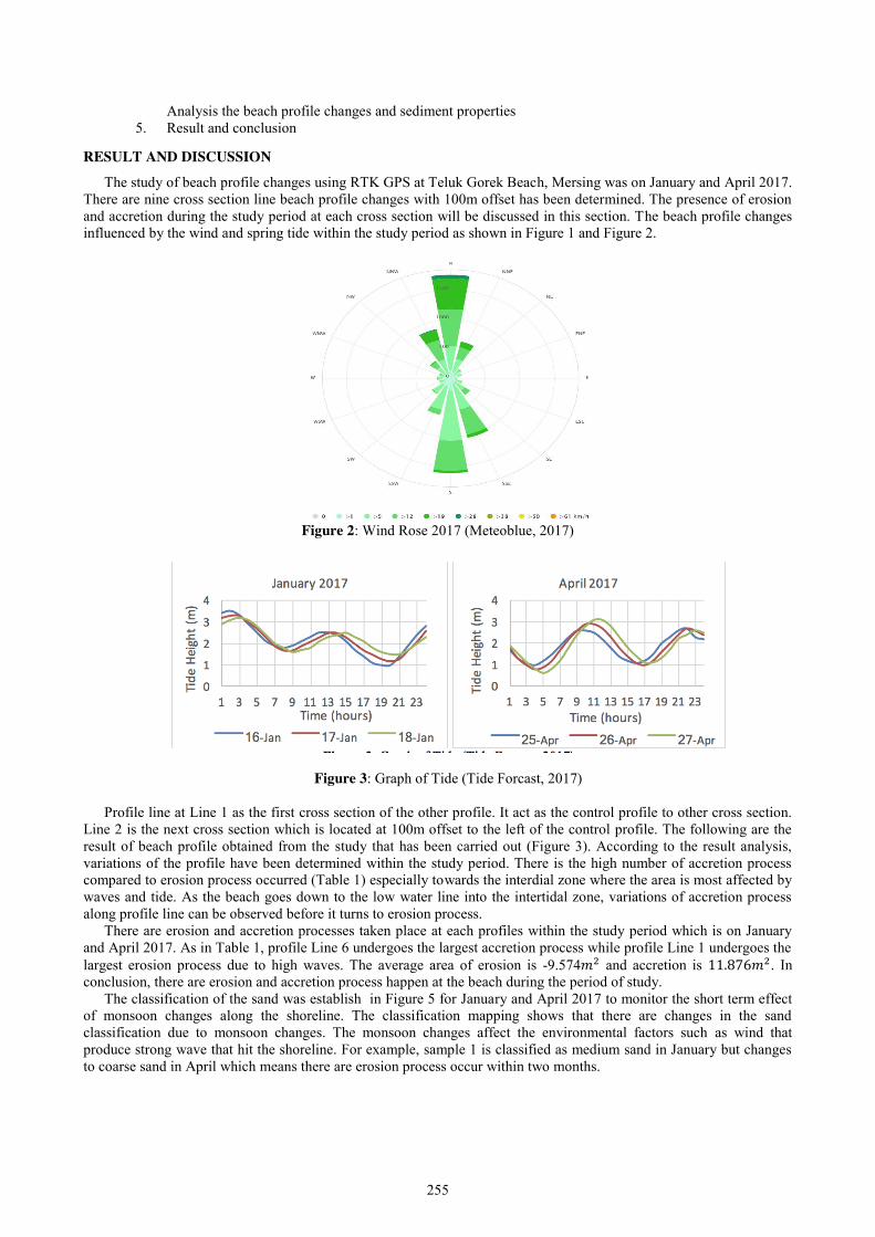
255

Analysis the beach profile changes and sediment properties 5. Result and conclusion

RESULT AND DISCUSSION

The study of beach profile changes using RTK GPS at Teluk Gorek Beach, Mersing was on January and April 2017. There are nine cross section line beach profile changes with 100m offset has been determined. The presence of erosion and accretion during the study period at each cross section will be discussed in this section. The beach profile changes influenced by the wind and spring tide within the study period as shown in Figure 1 and Figure 2.

Figure 2: Wind Rose 2017 (Meteoblue, 2017)

Figure 3: Graph of Tide (Tide Forcast, 2017) Profile line at Line 1 as the first cross section of the other profile. It act as the control profile to other cross section.

Line 2 is the next cross section which is located at 100m offset to the left of the control profile. The following are the result of beach profile obtained from the study that has been carried out (Figure 3). According to the result analysis, variations of the profile have been determined within the study period. There is the high number of accretion process compared to erosion process occurred (Table 1) especially towards the interdial zone where the area is most affected by waves and tide. As the beach goes down to the low water line into the intertidal zone, variations of accretion process along profile line can be observed before it turns to erosion process.

There are erosion and accretion processes taken place at each profiles within the study period which is on January and April 2017. As in Table 1, profile Line 6 undergoes the largest accretion process while profile Line 1 undergoes the largest erosion process due to high waves. The average area of erosion is -9.574𝑚2 and accretion is 11.876𝑚2. In conclusion, there are erosion and accretion process happen at the beach during the period of study.

The classification of the sand was establish in Figure 5 for January and April 2017 to monitor the short term effect of monsoon changes along the shoreline. The classification mapping shows that there are changes in the sand classification due to monsoon changes. The monsoon changes affect the environmental factors such as wind that produce strong wave that hit the shoreline. For example, sample 1 is classified as medium sand in January but changes to coarse sand in April which means there are erosion process occur within two months.

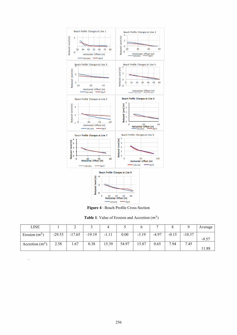
256

Figure 4 : Beach Profile Cross-Section

Table 1: Value of Erosion and Accretion (𝑚2)

LINE 1 2 3 4 5 6 7 8 9 Average

Erosion (𝑚2) -29.53 -17.65 -19.19 -1.11 0.00 -3.19 -4.97 -0.15 -10.37 -9.57

Accretion (𝑚2) 2.58 1.67 0.38 15.39 54.97 15.87 0.65 7.94 7.45 11.88

.

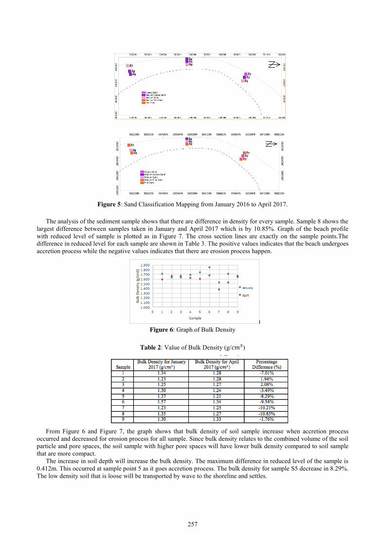
257

Figure 5: Sand Classification Mapping from January 2016 to April 2017.

The analysis of the sediment sample shows that there are difference in density for every sample. Sample 8 shows the

largest difference between samples taken in January and April 2017 which is by 10.85%. Graph of the beach profile with reduced level of sample is plotted as in Figure 7. The cross section lines are exactly on the sample points.The difference in reduced level for each sample are shown in Table 3. The positive values indicates that the beach undergoes accretion process while the negative values indicates that there are erosion process happen.

Figure 6: Graph of Bulk Density

Table 2: Value of Bulk Density (g/𝑐𝑚3)

From Figure 6 and Figure 7, the graph shows that bulk density of soil sample increase when accretion process

occurred and decreased for erosion process for all sample. Since bulk density relates to the combined volume of the soil particle and pore spaces, the soil sample with higher pore spaces will have lower bulk density compared to soil sample that are more compact.

The increase in soil depth will increase the bulk density. The maximum difference in reduced level of the sample is 0.412m. This occurred at sample point 5 as it goes accretion process. The bulk density for sample S5 decrease in 8.29%. The low density soil that is loose will be transported by wave to the shoreline and settles.

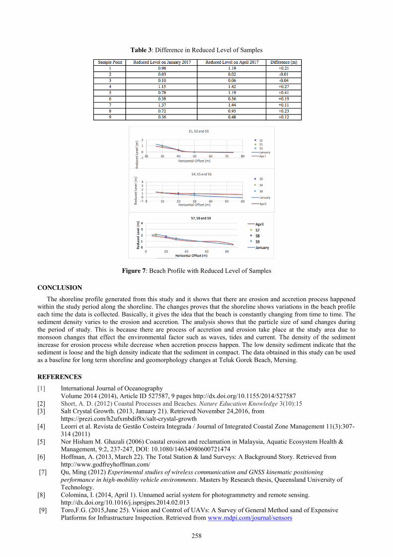
258

Table 3: Difference in Reduced Level of Samples

Figure 7: Beach Profile with Reduced Level of Samples CONCLUSION

The shoreline profile generated from this study and it shows that there are erosion and accretion process happened within the study period along the shoreline. The changes proves that the shoreline shows variations in the beach profile each time the data is collected. Basically, it gives the idea that the beach is constantly changing from time to time. The sediment density varies to the erosion and accretion. The analysis shows that the particle size of sand changes during the period of study. This is because there are process of accretion and erosion take place at the study area due to monsoon changes that effect the environmental factor such as waves, tides and current. The density of the sediment increase for erosion process while decrease when accretion process happen. The low density sediment indicate that the sediment is loose and the high density indicate that the sediment in compact. The data obtained in this study can be used as a baseline for long term shoreline and geomorphology changes at Teluk Gorek Beach, Mersing.

REFERENCES

[1] International Journal of Oceanography Volume 2014 (2014), Article ID 527587, 9 pages http://dx.doi.org/10.1155/2014/527587

[2] Short, A. D. (2012) Coastal Processes and Beaches. Nature Education Knowledge 3(10):15 [3] Salt Crystal Growth. (2013, January 21). Retrieved November 24,2016, from

https://prezi.com/h2ufxmbdif8x/salt-crystal-growth [4] Leorri et al. Revista de Gestão Costeira Integrada / Journal of Integrated Coastal Zone Management 11(3):307-

314 (2011) [5] Nor Hisham M. Ghazali (2006) Coastal erosion and reclamation in Malaysia, Aquatic Ecosystem Health &

Management, 9:2, 237-247, DOI: 10.1080/14634980600721474 [6] Hoffman, A. (2013, March 22). The Total Station & land Surveys: A Background Story. Retrieved from

http://www.godfreyhoffman.com/ [7] Qu, Ming (2012) Experimental studies of wireless communication and GNSS kinematic positioning

performance in high-mobility vehicle environments. Masters by Research thesis, Queensland University of Technology.

[8] Colomina, I. (2014, April 1). Unnamed aerial system for photogrammetry and remote sensing. http://dx.doi.org/10.1016/j.isprsjprs.2014.02.013

[9] Toro,F.G. (2015,June 25). Vision and Control of UAVs: A Survey of General Method sand of Expensive Platforms for Infrastructure Inspection. Retrieved from www.mdpi.com/journal/sensors