
2016DinardoPhd.pdf - University of Glasgow
229
Glasgow Theses Service http://theses.gla.ac.uk/ [email protected] Di Nardo, Antonello (2016) Phylodynamic modelling of foot-and-mouth disease virus sequence data. PhD thesis http://theses.gla.ac.uk/7558/ Copyright and moral rights for this thesis are retained by the author A copy can be downloaded for personal non-commercial research or study, without prior permission or charge This thesis cannot be reproduced or quoted extensively from without first obtaining permission in writing from the Author The content must not be changed in any way or sold commercially in any format or medium without the formal permission of the Author When referring to this work, full bibliographic details including the author, title, awarding institution and date of the thesis must be given.
-
Upload
khangminh22 -
Category
Documents
-
view
0 -
download
0
Transcript of 2016DinardoPhd.pdf - University of Glasgow

Glasgow Theses Service http://theses.gla.ac.uk/
Di Nardo, Antonello (2016) Phylodynamic modelling of foot-and-mouth disease virus sequence data. PhD thesis http://theses.gla.ac.uk/7558/ Copyright and moral rights for this thesis are retained by the author A copy can be downloaded for personal non-commercial research or study, without prior permission or charge This thesis cannot be reproduced or quoted extensively from without first obtaining permission in writing from the Author The content must not be changed in any way or sold commercially in any format or medium without the formal permission of the Author When referring to this work, full bibliographic details including the author, title, awarding institution and date of the thesis must be given.
© Antonello Di Nardo 2016
PHYLODYNAMIC MODELLING OF
FOOT-AND-MOUTH DISEASE VIRUS
SEQUENCE DATA
Antonello Di Nardo
DVM, MSc, MRCVS
Submitted in fulfilment of the requirements for the Degree of Doctor of Philosophy
Institute of Biodiversity, Animal Health and
Comparative Medicine
College of Medical, Veterinary and Life Sciences
University of Glasgow
5th September 2016


3
DECLARATION
I hereby declare that the research described within this thesis is my own work, unless
otherwise stated, and certify that it has never been submitted for any other degree or
professional qualification.
Antonello Di Nardo (DVM, MSc, MRCVS)
The Pirbright Institute
Ash Road
Pirbright, Woking
Surrey GU24 0NF


5
ACKNOWLEDGEMENT
Like Ulysses (or rather a Leopold Bloom), this journey starts back to a very
beginning phase of the discovery of the field of epidemiology which, from that time,
became my passion, my professional development and my pain. From Africa to
Scotland, I have been very privileged to meet and share friendship and job
collaboration with many interesting and peculiar characters, who have all contributed
to my career development with their ideas, ‘philosophies’ and works.
I am deeply indebted to my academic promoter and supervisor, Dan, for his
valuable guidance and critical analysis, motivating discussions (even with ‘dozens’ of
beers), and inspiring supervision. He has been of invaluable help in the development
of this project, of my thinking process, and of my career as a scientist. The very close
collaboration with Glasgow also gave me the opportunity to work with some amazing
and stimulating researchers, among all Paul and Richard. A much deserved price to the
infinite patience of Don, my Pirbright supervisor, who gave me the opportunity to dive
into this very challenging journey. I would also extend a special thanks to Nick who has
been handing down to me the knowledge and very detailed history of FMD molecular
epidemiology. I am also very lucky to have been working during the past 7 years in The
Pirbright Institute, my colleagues which has contributed to make me feeling at home. I
am grateful to Graham who has been behind the generation of the WGSs analysed in
chapter 6. I also would like to acknowledge the fruitful discussion during the viva with
my examiners, Rolf and Rowland.
I extend my gratitude to my family and friend both in Italy and London, I heartily
thanks above all my mother Maria and my father Tonino that have been continuing
kept faith, encourage, support and love.
6
ABSTRACT
The under-reporting of cases of infectious diseases is a substantial impediment
to the control and management of infectious diseases in both epidemic and endemic
contexts. Information about infectious disease dynamics can be recovered from
sequence data using time-varying coalescent approaches, and phylodynamic models
have been developed in order to reconstruct demographic changes of the numbers of
infected hosts through time. In this study I have demonstrated the general concordance
between empirically observed epidemiological incidence data and viral demography
inferred through analysis of foot-and-mouth disease virus VP1 coding sequences
belonging to the CATHAY topotype over large temporal and spatial scales. However a
more precise and robust relationship between the effective population size (𝑁𝑒) of a
virus population and the number of infected hosts (or ‘host units’) (𝑁) has proven
elusive. The detailed epidemiological data from the exhaustively-sampled UK 2001
foot-and-mouth (FMD) epidemic combined with extensive amounts of whole genome
sequence data from viral isolates from infected premises presents an excellent
opportunity to study this relationship in more detail. Using a combination of real and
simulated data from the outbreak I explored the relationship between 𝑁𝑒 , as estimated
through a Bayesian skyline analysis, and the empirical number of infected cases. I
investigated the nature of this scaling defining prevalence according to different
possible timings of FMD disease progression, and attempting to account for complex
variability in the population structure. I demonstrated that the variability in the
number of secondary cases per primary infection 𝑅𝑡 and the population structure
greatly impact on effective scaling of 𝑁𝑒 . I further explored how the demographic signal
carried by sequence data becomes imprecise and weaker when reducing the number
of samples are described, including how the extent of the size and structure of the
sampled dataset impact on the accuracy of a reconstructed viral demography at any
level of the transmission process. Methods drawn from phylodynamic inference
combine powerful epidemiological and population genetic tools which can provide
valuable insights into the dynamics of viral disease. However, the strict and sensitive
dependency of the majority of these models on their assumptions makes estimates
very fragile when these assumptions are violated. It is therefore essential that for these

Abstract
7
methods to be applied as reliable tools supporting control programs, more focused
theoretical research is undertaken to model the epidemiological dynamics of infected
populations using sequence data.


9
TABLE OF CONTENTS
DECLARATION 3
ACKNOWLEDGEMENT 5
ABSTRACT 6
TABLE OF CONTENTS 9
LIST OF TABLES 15
LIST OF FIGURES 19
ABBREVIATIONS 25
CHAPTER 1 29
FOOT-AND-MOUTH DISEASE AND PHYLODYNAMICS OF INFECTIOUS DISEASES
1.1 Foot-and-mouth disease 29
1.1.1 Foot-and-mouth disease virus 30
1.1.1.1 FMDV evolutionary patterns 33
1.1.2 FMDV genetic tracing 35
1.2 Phylodynamics of viral infectious diseases 38
1.2.1 Reconstructing the dynamics of viral epidemics 38
1.2.1.1 Coalescent theory 38
1.2.1.2 Effective population size 40
1.2.1.3 Modelling the demography of viral populations 42
1.2.1.4 Sampling genetic data 46
1.2.2 Integrating epidemiology with phylogenetics 48
1.3 Project rationale and scientific objectives 52
1.3.1 Thesis outline 54
CHAPTER 2 57
PHYLODYNAMIC RECONSTRUCTION OF O CATHAY TOPOTYPE FOOT-AND-
MOUTH DISEASE VIRUS EPIDEMICS IN THE PHILIPPINES
2.1 Abstract 57
2.2 Introduction 58
2.2.1 The O CATHAY FMDV topotype 58
2.2.2 FMDV in the Philippines 59
2.3 Materials and methods 60
2.3.1 Sample database 60

Table of Contents
10
2.3.2 Viral RNA detection and sequencing 60
2.3.3 Phylogenetic analysis 61
2.3.4 Statistical analysis 62
2.4 Results 63
2.4.1 O CATHAY FMDV country based phylodynamics: the Philippines 63
2.4.2 Global and regional phylodynamics of O CATHAY topotype FMDV 68
2.5 Discussion 73
CHAPTER 3 77
A MODEL FRAMEWORK FOR SIMULATING SPACE-TIME EPIDEMIOLOGICAL AND
GENETIC DATA
3.1 Rationale 77
3.2 Model Framework 78
3.2.1 Data 78
3.2.1.1 Epidemiological data 79
3.2.1.2 Genetic data 79
3.2.2 Transmission tree reconstruction 79
3.2.2.1 Spatial transmission 82
3.2.2.2 Prevalence and incidence estimation 82
3.2.2.3 Computing the generation time 83
3.2.3 Genetic simulation 85
3.2.3.1 Simulation of genetic mutations along the transmission tree 87
3.2.3.2 Evolutionary analysis of the UK 2001 FMDV WGS simulated alignment 88
3.2.4 Model implementation 89
3.3 Results 89
3.3.1 UK 2001 FMD transmission tree reconstruction 89
3.3.2 UK 2001 FMDV genetic simulation 93
3.3.2.1 UK 2001 FMDV evolutionary analysis using WGS data 95
3.3.2.2 UK 2001 FMDV evolutionary analysis using VP1 coding sequences 95
3.3.3 Validating simulation with field isolates 96
3.4 Discussion 97
CHAPTER 4 101
RECONSTRUCTING VIRUS POPULATIONS DYNAMICS OVER TIME
4.1 Rationale 101
4.2 Methodological process for scaling Ne to the actual infected population size
102

Table of Contents
11
4.2.1 Reconstructing Ne changes through time from a Bayesian Skyline analysis 103
4.2.2 Deriving infection prevalence N* 103
4.2.2.1 Reconstructing N* assuming variance in the number of secondary cases per
primary infection Rt 103
4.2.2.2 Reconstructing N* assuming the number of lineages as a function of time 104
4.2.2.3 Computation of infection prevalence N* using the UK 2001 FMD simulated WGS
105
4.2.3 Investigating the impact of changing var(Rt) on the recovery of the infection
prevalence N* 106
4.2.3.1 Computation of infection prevalence N* from the simulated FMD stationary system
107
4.3 Results 108
4.3.1 Average scaling approach 108
4.3.1.1 Skyline scaled effective population size Ne 110
4.3.1.2 Infection prevalence N* estimated using the var(Rt) scaling formulation 112
4.3.1.3 Infection prevalence N* estimated using the NLFT scaling formulation 113
4.3.2 Time-varying scaling approach 114
4.3.3 Viral demography reconstruction through simulations of a FMD stationary system
118
4.3.3.1 Skyline scaled effective population size Ne 119
4.3.3.2 Infection prevalence N* estimated using the var(Rt) scaling formulation 121
4.3.3.3 Infection prevalence N* estimated using the NLFT scaling formulation 123
4.4 Discussion 125
CHAPTER 5 129
OPTIMAL STRUCTURE OF INCOMPLETELY SAMPLED DATASETS
5.1 Rationale 129
5.2 Simple random sampling of genetic data 130
5.3 ‘Probability proportional to size’ sampling of genetic data 133
5.3.1 Sampling within genetic strata 135
5.3.1.1 Evolutionary duration ∆t 135
5.3.1.2 Epidemiological generation time τ 136
5.3.1.3 TN93 genetic distance 138
5.3.2 Sampling within spatial strata 139
5.3.2.1 Regional division 139
5.3.2.2 Spatial transmission distance 141
5.3.3 Sampling within temporal strata 143

Table of Contents
12
5.3.3.1 Month timing 143
5.3.3.2 Week timing 145
5.4 Sampling within epidemic phases 147
5.4.1 Exponential phase 148
5.4.2 Decline phase 150
5.4.3 Tail end phase 150
5.5 Conclusion 151
CHAPTER 6 155
PHYLODYNAMICS OF THE UK 2001 FMD EPIDEMIC USING AVAILABLE WGS DATA:
A PRELIMINARY ANALYSIS
6.1 Rationale 155
6.1.1 Brief description of the UK 2001 FMD epidemic event 156
6.2 Materials and methods 157
6.2.1 Generating the UK 2001 FMDV WGS 157
6.2.2 Data analysis 158
6.2.2.1 Recovery the evolutionary and demographic signal 158
6.3 Results 159
6.3.1 Evolutionary patterns 159
6.3.2 Demographic change of infected population size over time 160
6.4 Discussion 165
CHAPTER 7 169
FINAL DISCUSSION AND CONCLUDING REMARKS
APPENDICES 175
Appendix 1 175
Appendix 2 179
Appendix 3 185
Appendix 4 186
Appendix 5 189
Appendix 6 190
A6.1 Scaled Ne formulation 190
A6.1.1 Epidemiological generation time τ 190
A6.1.2 Serial case interval τc 191
A6.2 var(Rt) scaling formulation 192
A6.2.1 Epidemiological generation time τ 192
A6.1.2 Serial case interval τc 194

Table of Contents
13
A6.3 NLFT scaling formulation 196
Appendix 7 197
A7.1 Scaled Ne formulation 197
A7.1.1 Epidemiological generation time τ 197
A7.1.2 Serial case interval τc 198
A7.2 var(Rt) scaling formulation 199
A7.2.1 Epidemiological generation time τ 199
A7.1.2 Serial case interval τc 201
A7.3 NLFT scaling formulation 203
REFERENCES 204

15
LIST OF TABLES
Table 1-1 Comparison of substitution rates between transmission chains
extracted from FMDV sequences using a strict molecular evolutionary
clock model.
Table 1-2 Model-based tools for reconstructing demographic history from both
DNA and RNA virus sequence data (listed in chronological order of
development).
Table 2-1 Oligonucleotide primers used for either RT-PCR or cycle sequencing
of the VP1 coding region from the FMDV isolates.
Table 2-2 Genetic, time and geographical pairwise distances (with
corresponding standard deviation values) calculated for the within-
year Philippines O CATHAY FMDV isolates groups and for each of the
country based data from the earliest samples collected within the
specific group.
Table 3-1 Description of observed epidemiological variables with associated
symbols entered in the model.
Table 3-2 Description of parameters defined for the Tamura and Nei model of
nucleotide substitution (Tamura and Nei, 1993).
Table 3-3 Empirical prevalence 𝑃, incidence 𝐼, epidemiological generation time
𝜏, serial case interval τ𝑐, prevalence-to-incidence ratio 𝜏𝑝 and number
of secondary cases per primary infection 𝑅𝑡 with its variance 𝑣𝑎𝑟(𝑅𝑡)
estimated from the reconstructed transmission tree according to each
phase of the UK 2001 FMD epidemic.
Table 4-1 Comparison of scaling equations of effective population size 𝑁𝑒
derived from time-varying coalescent-based models for recovering
the infection prevalence 𝑁∗.
Table 4-2 Statistical parameters estimated from the pairwise correlation
between infection prevalence 𝑁∗ and the empirical prevalence data
extracted from the UK 2001 FMD epidemic using each of the three
scaling equations.
List of Tables
16
Table 4-3 Statistical parameters estimated from the correlation between
infection prevalence 𝑁∗ and the empirical prevalence data extracted
from the UK 2001 FMD epidemic using each of the three scaling
equations
Table 4-4 Overall and time specific number of infected cases estimated under 12
realisations of the UK 2001 FMD full IPs (𝑛=2026) epidemic dataset
from the empirical epidemiological data and the scaled 𝑁𝑒 recovered
from the BSP analysis
Table 4-5 Overall and time specific number of infected cases estimated under 12
realisations for the UK 2001 FMD full IPs (𝑛=2026) epidemic dataset
from the empirical epidemiological data and the scaled infection
prevalence 𝑁∗ estimated under the assumption of variance in 𝑅𝑡
[Koelle and Rasmussen (2012) parameterisation (§4.2.2.1)].
Table 4-6 Overall and time specific number of infected cases estimated under 12
realisations for the UK 2001 FMD full IPs (𝑛=2026) epidemic dataset
from the empirical epidemiological data and the scaled infection
prevalence 𝑁∗ estimated by expressing the phylogenetic structure by
NLFT.
Table 4-7 Epidemiological parameters estimated following natural spline
interpolations of the 12 realisations of the reconstructed UK 2001
FMD transmission tree.
Table 4-8 Epidemiological parameters estimated from the stationary FMD
simulation and using different dispersion parameters for generating
the number of IP daughters for each parent IP.
Table 4-9 Statistical parameters estimated from the correlation between scaled
𝑁𝑒 values based on the BSP and the empirical prevalence data
extracted from the simulated FMD stationary system under different
parameterisations of the dispersion parameter 𝑘.
Table 4-10 Statistical parameters estimated for the relationship between
infection prevalence 𝑁∗ estimated under the assumption of variance
in 𝑅𝑡 [Koelle and Rasmussen (2012) parameterisation] and the
empirical prevalence data extracted from the simulated stationary
List of Tables
17
system under different parameterisations of the dispersion
parameter 𝑘.
Table 4-11 Statistical parameters estimated for the relationship between
infection prevalence 𝑁∗ estimated under the assumption of a single
freely mixing population and the empirical prevalence data extracted
from the simulated stationary system under different
parameterisations of the dispersion parameter 𝑘.
Table 5-1 Time specific number of infected cases recovered from the infection
prevalence 𝑁∗ estimated from 12 realisations of the UK 2001 FMD full
IPs (𝑛=2026) epidemic scenario and resampled datasets at a
decreasing sampling proportion 𝑠 of 0.25.
Table 5-2 Time specific number of infected cases recovered from the infection
prevalence 𝑁∗ estimated from 12 realisation of the UK 2001 FMD full
IPs (𝑛=2026) epidemic scenario and resampled datasets at a
decreasing sampling proportion 𝑠 of 0.25.
Table 5-3 Time specific number of infected cases recovered from the infection
prevalence 𝑁∗ estimated from 12 realisation of the UK 2001 FMD full
IPs (𝑛=2026) epidemic scenario and resampled datasets at a
decreasing sampling proportion 𝑠 of 0.25.
Table 5-4 Time specific number of infected cases recovered from the infection
prevalence 𝑁∗ estimated from 12 realisations of the UK 2001 FMD full
IPs (𝑛=2026) epidemic scenario and resampled datasets at a
decreasing sampling proportion 𝑠 of 0.25.
Table 5-5 Time specific number of infected cases recovered from the infection
prevalence 𝑁∗ estimated from 12 realisation of the UK 2001 FMD full
IPs (𝑛=2026) epidemic scenario and resampled datasets at a
decreasing sampling proportion 𝑠 of 0.25.
Table 5-6 Time specific number of infected cases recovered from the infection
prevalence 𝑁∗ estimated from 12 realisation of the UK 2001 FMD full
IPs (𝑛=2026) epidemic scenario and resampled datasets at a
decreasing sampling proportion 𝑠 of 0.25.
Table 5-7 Time specific number of infected cases recovered from the infection
prevalence 𝑁∗ estimated from 12 realisations of the UK 2001 FMD full
List of Tables
18
IPs (𝑛=2026) epidemic scenario and resampled datasets at a
decreasing sampling proportion 𝑠 of 0.25.
Table 5-8 Time specific number of infected cases recovered from the infection
prevalence 𝑁∗ estimated from 12 realisations of the UK 2001 FMD full
IPs (𝑛=2026) epidemic scenario and resampled datasets at a
decreasing sampling proportion 𝑠 of 0.25
Table 5-9 Time specific number of infected cases estimated from 12 realisations
of FMDV WGS simulated database (𝑛=2026) and at a sampling rate 𝑠
of ~0.03
Table 5-10 Comparison of the empirical proportion 𝑠 of IPs reported during the
UK 2001 FMD epidemic according to each epidemic phase and the
corresponding sample probability 𝜌 obtained using 12 realisations of
the BDM (Stadler, 2009).
Table 6-1 Time specific number of infected cases estimated using the infection
prevalence 𝑁∗ recovered from the BSP analysis of the 𝑛=154 WGSs
generated from the clinical samples collected during the UK 2001
FMD epidemic.
Table 6-2 Time specific number of infected cases estimated using the infection
prevalence 𝑁∗ recovered from the BSP analysis of the simulated
𝑛=154 WGSs.
19
LIST OF FIGURES
Figure 1-1 Schematic representation of the FMDV genome structure
organisation showing the individual genomic regions described in
text.
Figure 1-2 Conjectured FMD status in 2015 with seven regional FMDV pools and
predominant serotype distribution at the global level.
Figure 1-3 Number of FMDV sequences submitted to GenBank at NCBI since
prior 1994.
Figure 1-4 Schematic representation of the coalescent process.
Figure 1-5 Inferring demographic history of virus population from reconstructed
phylogeny.
Figure 1-6 Schematic representation of multiple scale of virus evolution aimed at
reconstructing pathways of pathogens transmission and their
population dynamics.
Figure 2-1 Accumulation of nucleotide differences calculated from the putative
root (HKN/12/91 isolate) for the Philippines database with time
expressed in years.
Figure 2-2 Network extracted from the statistical parsimony analysis performed
in TCS for the Philippines isolates (𝑛=112).
Figure 2-3 Phylodynamic reconstruction of the O CATHAY FMDV epidemics in
the Philippines.
Figure 2-4 Maximum clade credibility tree for all the O CATHAY FMDV isolates
sequenced (𝑛=322).
Figure 2-5 BSP of log effective population size (𝑁𝑒𝜏) against time in years
estimated from the full O CATHAY FMDV database.
Figure 2-6 Chronological evolutionary trend and transmission ancestry of the O
CATHAY FMDV topotype in Southeast Asia.
Figure 3-1 FMDV transmission between a parent IP 𝑖 and a daughter IP 𝑘.
Figure 3-2 Gamma probability density function 𝛤(𝜅, 𝜃) for the latency time
variable.
Figure 3-3 Transmission tree model scheme and algorithm.
List of Figures
20
Figure 3-4 Genetic simulation model scheme and algorithm.
Figure 3-5 Evolutionary structure of the dependency between sampled lineages
along a reconstructed transmission tree.
Figure 3-6 Number of secondary cases per primary infection (𝑅𝑡, A), generation
time (𝜏, B), serial case interval (𝜏𝑐, C), and prevalence-to-incidence
ratio (𝜏𝑝, D) estimated for the UK 2001 FMD epidemic using the full
IPs dataset (𝑛=2026).
Figure 3-7 Transmission tree (top graph) and probability of parent-daughter
established links (bottom graph) reconstructed using the full IPs
dataset (𝑛=2026).
Figure 3-8 Accumulation of nucleotide differences estimated from the index IP
(IP4) for the full IPs UK 2001 FMDV WGS simulated alignment
(𝑛=2026) with time expressed in days.
Figure 3-9 Tree phylogenies reconstructed using the FMDV WGS simulated
alignment from the full IPs dataset (𝑛=2026).
Figure 3-10 Phylogenetic reconstruction of the 𝑛=39 UK 2001 FMDV WGS
generated from the field isolates (lower row) and simulated by the
model (upper row).
Figure 4-1 Dynamical model of FMDV transmission for a FMD stationary system
between a parent IP 𝑖 and a daughter IP 𝑘.
Figure 4-2 Scaled 𝑁𝑒 estimated from 12 realisations of the UK 2001 FMDV
simulated WGS data and reconstructed using the full IPs (𝑛=2026)
epidemic dataset.
Figure 4-3 Infection prevalence 𝑁∗ estimated from 12 realisations of the UK
2001 FMDV simulated WGS data and reconstructed using the full IPs
(𝑛=2026) epidemic dataset.
Figure 4-4 Infection prevalence 𝑁∗ estimated from 12 realisations of the UK
2001 FMDV simulated WGS data and reconstructed using the full IPs
(𝑛=2026) epidemic dataset.
Figure 4-5 Natural splines interpolation for time-varying epidemiological
parameters estimated from the empirical UK 2001 FMD epidemic
data.
List of Figures
21
Figure 4-6 Infection prevalence 𝑁∗ estimated from 12 realisations of the UK
2001 FMDV simulated WGS data and reconstructed using the full IPs
(𝑛=2026) epidemic dataset using the time-varying scaling approach.
Figure 4-7 Scaled 𝑁𝑒 estimated using the BSP from the WGS generated by the
stationary FMD simulation.
Figure 4-8 Infection prevalence 𝑁∗ estimated from the WGS generated by the
stationary FMD simulation.
Figure 4-9 Infection prevalence 𝑁∗ estimated from the WGS generated by the
stationary FMD simulation.
Figure 5-1 Molecular clocks (nt/site/day) estimated using BEAST 1.8.0 under the
assumption of a strict clock evolutionary model from 12 realisations
of the full UK 2001 FMDV WGS simulated database (𝑛=2026) and from
each of the resampled datasets at a decreasing sampling proportion
rate 𝑠 of 0.25.
Figure 5-2 Infection prevalence 𝑁∗ estimated from 12 realisations of the full UK
2001 FMDV WGS simulated database (𝑛=2026) and resampled
datasets at a decreasing sampling proportion rate 𝑠 of 0.25.
Figure 5-3 Empirical probability density functions of epidemiological and
genetic parameters estimated from the UK 2001 FMD epidemic using
a kernel density approach for sampling WGS data by a PPS scheme.
Figure 5-4 Infection prevalence 𝑁∗ estimated from 12 realisations of the full UK
2001 FMDV WGS simulated database (𝑛=2026) and resampled
datasets at a decreasing sampling proportion rate 𝑠 of 0.25.
Figure 5-5 Infection prevalence 𝑁∗ estimated from 12 realisations of the full UK
2001 FMDV WGS simulated database (𝑛=2026) and resampled
datasets at a decreasing sampling proportion rate 𝑠 of 0.25.
Figure 5-6 Infection prevalence 𝑁∗ estimated from 12 realisations of the full UK
2001 FMDV WGS simulated database (𝑛=2026) and from each of the
resampled datasets at a decreasing sampling proportion rate 𝑠 of 0.25.
Figure 5-7 Spatial proportion of IPs according to the affected UK counties as
reported during the UK 2001 FMD epidemic.
List of Figures
22
Figure 5-8 Infection prevalence 𝑁∗ estimated from 12 realisations of the full UK
2001 FMDV WGS simulated database (𝑛=2026) and resampled
datasets at a decreasing sampling proportion rate 𝑠 of 0.25.
Figure 5-9 Infection prevalence 𝑁∗ estimated from 12 realisations of the full UK
2001 FMDV WGS simulated database (𝑛=2026) and resampled
datasets at a decreasing sampling proportion rate 𝑠 of 0.25.
Figure 5-10 Total number of IP reported to be infected by FMDV during the UK
2001 FMD epidemic by month of reporting.
Figure 5-11 Infection prevalence 𝑁∗ estimated from 12 realisations of the full UK
2001 FMDV WGS simulated database (𝑛=2026) and resampled
datasets at a decreasing sampling proportion rate 𝑠 of 0.25.
Figure 5-12 Total number of IP reported to be infected by FMDV during the UK
2001 FMD epidemic by week of reporting.
Figure 5-13 Infection prevalence 𝑁∗ estimated from 12 realisations of the full UK
2001 FMDV WGS simulated database (𝑛=2026) and resampled
datasets at a decreasing sampling proportion rate 𝑠 of 0.25.
Figure 5-14 Epidemic size of the UK 2001 FMD exponential phase estimated from
10 realisations of FMDV WGS simulated database (𝑛=2026)
resampled at a rate 𝑠 of 0.03.
Figure 5-15 Epidemic size of the UK 2001 FMD decline phase estimated from 12
realisations of FMDV WGS simulated database (𝑛=2026) resampled at
a rate 𝑠 of 0.03.
Figure 5-16 Epidemic size of the UK 2001 FMD tail end phase estimated from 12
realisations of FMDV WGS simulated database (𝑛=2026) resampled at
a rate 𝑠 of 0.03.
Figure 6-1 Geographical location and frequency in time of the 𝑛=154 WGS
generated from the samples collected during the UK 2001 FMD
epidemic and analysed in this study.
Figure 6-2 Accumulation of nucleotide differences estimated from the index IP
(IP4) for the FMDV WGS alignment (𝑛=154) generated from the
clinical field samples collected during the UK 2001 FMD epidemic.
List of Figures
23
Figure 6-3 Demography of the UK 2001 infected viral population estimated from
the BSP and recovered using the infection prevalence 𝑁∗ scaling
formulations defined in §4.3.1.
Figure 6-4 Demography of the UK 2001 infected viral population estimated from
the simulated data and recovered using the infection prevalence 𝑁∗
scaling formulations defined in §4.3.1

25
ABBREVIATIONS
ABC Approximate Bayesian computation
BDM Birth-death model
BEAST Bayesian evolutionary analysis sampling trees
BF Bayes factor
BIC Bayesian information criterion
BSP Bayesian skyline plot
BSSVS Bayesian stochastic search variable selection
CI Confidence interval
CID Complexity invariant distance
CP Contagious to infected premise
CTMC Continuous time Markov chain
CV Coefficient of variation
DC Dangerous contact
DEFRA Department for Environment, Food and Rural Affairs
DNA Deoxyribonucleic acid
ERGM Exponential-family random graph model
EU European Union
FAO Food and Agriculture Organization of the United Nations
FMD Foot-and-mouth disease
FMDV Foot-and-mouth disease virus
GMRF Gaussian Markov random field
HPD High posterior density
INLA Integrated nested Laplace approximation
IP Infected premise
IRES Internal ribosome entry site
LTT Lineage through time
NCBI National Center for Biotechnology Information
NGS Next generation sequencing
NMB National movement ban
NSP Non-structural protein
Abbreviations
26
nt Nucleotide
MAFF Ministry of Agriculture, Fisheries and Food
MCC Maximum clade credibility
MCMC Markov chain Monte Carlo
MCP Multiple change point
MRCA Most recent common ancestor
NLFT Number of lineages as a function of time
OIE World Organisation for Animal Health
ORF Open reading frame
PDF Probability density function
PI Percentile interval
pk Posterior probability
PPS Probability proportional to size
RMSD Root-mean-square deviation
RNA Ribonucleic acid
RT-PCR Reverse transcription polymerase chain reaction
RTO Regression through the origin
SAT Southern African Territories
SEA Southeast Asia
SEIR Susceptible-Exposed-Infectious-Removed
SIR Susceptible infectious recovered
SIS Susceptible infectious susceptible
SMC Sequential Monte Carlo
SRS Simple random sampling
SSM State-space model
ssRNA Single-stranded ribonucleic acid
TMRCA Time to most recent common ancestor
TN93 Tamura and Nei evolutionary model
UK United Kingdom
UTR Untranslated region
VP Viral protein
WGS Whole genome sequence
WRLFMD World Reference Laboratory for Foot-and-Mouth Disease

27
to Giuseppina, Lucia and Mariarosa,
always there,
waiting for us…

29
CHAPTER 1
Foot-and-mouth disease and phylodynamics of
infectious diseases
1.1 Foot-and-mouth disease
Foot-and-mouth disease (FMD) is an economically devastating viral disease of
cloven-hoofed domestic and wild artiodactyls, causing an acute and highly contagious
vesicular disease, which can progress into a persistent infection (Alexandersen et al.,
2003). Vesicular lesions are mainly found in the epithelia of tongue, lips and feet but in
some cases lesions also occur in snout, muzzle, teats, skin and rumen. The disease is
characterised by a very short incubation period and high level of virus excretion,
particularly in pigs. Animals exposed to the FMD virus (FMDV) usually develop a
viraemia within 3 to 5 days of exposure, with clinical signs and lesions that usually last
for 1 to 2 weeks post-infection (Kitching, 2002, Kitching and Alexandersen, 2002,
Kitching and Hughes, 2002). However, hosts differ in susceptibility to infection and
disease according to animal breed and productivity, farming system and environment,
and the infecting virus strain (Rweyemamu et al., 2008). Although FMD does not
usually cause high mortality in susceptible animals (high mortality may be seen in
young animal due to acute fatal myocarditis) it decreases productivity, which in turn
impacts on farmers’ livelihoods. Since livestock constitute an important source of
livelihood and tradable commodity in the agricultural based economies and social
structure of many countries, FMD has a serious impact on food security, rural income
generation, and the national economy by impairing livestock trade (Forman et al.,
2009). The livestock sector has increased rapidly over the past decades, particularly in
developing countries, where the growing demand has been driven by economic and
population growth, rising per capita incomes and urbanisation (FAO, 2011). In
addition, a wide range of traditional livestock management systems have evolved to
optimise the use of resources, transformed by the implementation of more intensive
farming units overlaid on the top of the traditional small-scale systems (i.e. pastoralist
and/or smallholder production systems) (Di Nardo et al., 2011). However, the
Chapter 1 – FMD and Phylodynamics of Infectious Diseases
30
increasing demand for livestock products and modernisation of management systems
implies challenges in terms of efficient management of animal-health risks that have
not always been considered as a priority in most developing countries. Therefore, in
FMD endemic countries the lack of resources for an effective strategy to control disease
through the restriction of animal movements makes FMD a continuous threat for its
potential risk to spread at both the regional and global level. Nevertheless, the lack of
baseline FMD information from several endemic countries with limited reporting of
disease outbreaks provides less opportunity for the development of targeted policies
and programs aimed at improving animal health and prevention of the disease. In
recognising these constraints in endemic settings, in 2008 the Food and Agriculture
Organization of the United Nations (FAO) launched a pathway for the progressive
control of FMD which has been subsequently endorsed by the World Organisation for
Animal Health (OIE) and it is nowadays one of the tools for the implementation of an
integrated strategy for the global FMD control coordinated by the two Organisations
(Sumption et al., 2012). Therefore, in specific regions of the world the implementation
of regional roadmaps based on the circulating FMDV pools has greatly assisted in
identifying hotspots which may be considered potential sources of lineages that pose a
threat to neighbouring countries. Nevertheless, in the challenge of controlling FMD
which, eventually, would work towards its eradication, new tools are warranted to
enable a better characterisation on both molecular and epidemiological scales of the
signal that drives the evolutionary history of FMDV and which underpin its
transmission dynamics. Ultimately, a better understanding of the evolutionary
dynamics of FMDV has the potential to inform intervention strategies and control
policies to be risk-targeted.
1.1.1 Foot-and-mouth disease virus
FMDV is the prototypical member of the Aphthovirus genus, family
Picornaviridae, which also comprises three other species Bovine rhinitis A virus, Bovine
rhinitis B virus, and Equine rhinitis A virus (Knowles et al., 2011). The non-enveloped
virion is characterised by a single-stranded positive-sense ribonucleic acid (RNA)
(~8.4 kb in size), which is organised in: a 5' untranslated region (UTR) of ~1300 nt
[which contains a number of structures, such as the S-fragment, a poly(C) tract, a series
Chapter 1 – FMD and Phylodynamics of Infectious Diseases
31
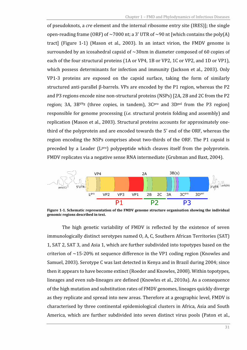
of pseudoknots, a cre element and the internal ribosome entry site (IRES)]; the single
open-reading frame (ORF) of ~7000 nt; a 3' UTR of ~90 nt [which contains the poly(A)
tract] (Figure 1-1) (Mason et al., 2003). In an intact virion, the FMDV genome is
surrounded by an icosahedral capsid of ~30nm in diameter composed of 60 copies of
each of the four structural proteins (1A or VP4, 1B or VP2, 1C or VP2, and 1D or VP1),
which possess determinants for infection and immunity (Jackson et al., 2003). Only
VP1-3 proteins are exposed on the capsid surface, taking the form of similarly
structured anti-parallel β-barrels. VPs are encoded by the P1 region, whereas the P2
and P3 regions encode nine non-structural proteins (NSPs) [2A, 2B and 2C from the P2
region; 3A, 3BVPg (three copies, in tandem), 3Cpro and 3Dpol from the P3 region]
responsible for genome processing (i.e. structural protein folding and assembly) and
replication (Mason et al., 2003). Structural proteins accounts for approximately one-
third of the polyprotein and are encoded towards the 5’ end of the ORF, whereas the
region encoding the NSPs comprises about two-thirds of the ORF. The P1 capsid is
preceded by a Leader (Lpro) polypeptide which cleaves itself from the polyprotein.
FMDV replicates via a negative sense RNA intermediate (Grubman and Baxt, 2004).
Figure 1-1. Schematic representation of the FMDV genome structure organisation showing the individual genomic regions described in text.
The high genetic variability of FMDV is reflected by the existence of seven
immunologically distinct serotypes named O, A, C, Southern African Territories (SAT)
1, SAT 2, SAT 3, and Asia 1, which are further subdivided into topotypes based on the
criterion of ~15-20% nt sequence difference in the VP1 coding region (Knowles and
Samuel, 2003). Serotype C was last detected in Kenya and in Brazil during 2004; since
then it appears to have become extinct (Roeder and Knowles, 2008). Within topotypes,
lineages and even sub-lineages are defined (Knowles et al., 2010a). As a consequence
of the high mutation and substitution rates of FMDV genomes, lineages quickly diverge
as they replicate and spread into new areas. Therefore at a geographic level, FMDV is
characterised by three continental epidemiological clusters in Africa, Asia and South
America, which are further subdivided into seven distinct virus pools (Paton et al.,
Chapter 1 – FMD and Phylodynamics of Infectious Diseases
32
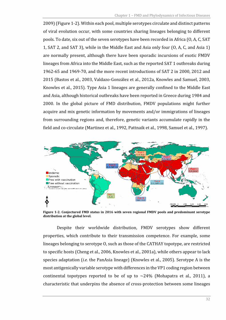
2009) (Figure 1-2). Within each pool, multiple serotypes circulate and distinct patterns
of viral evolution occur, with some countries sharing lineages belonging to different
pools. To date, six out of the seven serotypes have been recorded in Africa (O, A, C, SAT
1, SAT 2, and SAT 3), while in the Middle East and Asia only four (O, A, C, and Asia 1)
are normally present, although there have been sporadic incursions of exotic FMDV
lineages from Africa into the Middle East, such as the reported SAT 1 outbreaks during
1962-65 and 1969-70, and the more recent introductions of SAT 2 in 2000, 2012 and
2015 (Bastos et al., 2003, Valdazo-González et al., 2012a, Knowles and Samuel, 2003,
Knowles et al., 2015). Type Asia 1 lineages are generally confined to the Middle East
and Asia, although historical outbreaks have been reported in Greece during 1984 and
2000. In the global picture of FMD distribution, FMDV populations might further
acquire and mix genetic information by movements and/or immigrations of lineages
from surrounding regions and, therefore, genetic variants accumulate rapidly in the
field and co-circulate (Martinez et al., 1992, Pattnaik et al., 1998, Samuel et al., 1997).
Figure 1-2. Conjectured FMD status in 2016 with seven regional FMDV pools and predominant serotype distribution at the global level.
Despite their worldwide distribution, FMDV serotypes show different
properties, which contribute to their transmission competence. For example, some
lineages belonging to serotype O, such as those of the CATHAY topotype, are restricted
to specific hosts (Cheng et al., 2006, Knowles et al., 2001a), while others appear to lack
species adaptation (i.e. the PanAsia lineage) (Knowles et al., 2005). Serotype A is the
most antigenically variable serotype with differences in the VP1 coding region between
continental topotypes reported to be of up to ~24% (Mohapatra et al., 2011), a
characteristic that underpins the absence of cross-protection between some lineages
Chapter 1 – FMD and Phylodynamics of Infectious Diseases
33
(Klein et al., 2006, Knowles et al., 2009, Jamal et al., 2011c). In addition, the SAT
serotypes have been reported to have higher intraserotype nucleotide variation in
comparison to serotype O (Bastos et al., 2001, Bastos et al., 2003). Differently, the type
Asia 1 is considered to be the least diverse serotype both genetically and antigenically
when compared to the other FMDV serotypes (Ansell et al., 1994), although reports
highlight that field isolates belonging to the recently evolved Sindh-08 lineage causing
outbreaks in livestock vaccinated with the established Asia-1/Shamir and Asia-
1/Ind/8/79 vaccine strains (Jamal et al., 2011b). Therefore, FMDV populations can be
seen as showing extensive genetic and antigenic heterogeneity at both molecular and
geographic levels, driven by co-circulation of multiple lineages, heterogenic mixed host
populations, extensive animal movements and trade patterns (Di Nardo et al., 2011).
1.1.1.1 FMDV evolutionary patterns
Similarly to other single-stranded RNA viruses, the genetic evolution of FMDV
is mainly driven by the interplay of two mechanisms: 1) spontaneous mutation; 2)
recombination. Due to the error-prone RNA-dependent RNA polymerase (3D in Figure
1-1), ssRNA viruses are characterised by high mutation rates (in a range of 10-5 to 10-3
nt misincorporations/site/replication cycle) (Drake, 1993, Duffy et al., 2008), which
leads to evolution mainly through genetic drift (Domingo et al., 2005). At these rates of
mutation, replicated FMDV genomes would differ on average from their parent genome
by 0.1 to 10 base positions. A recent study reported that ssRNA are among those
viruses showing the highest average genome mutation rates of the order of 0.66±0.42
substitutions/nt site/cell infection (Sanjuan, 2012). In a study of viruses belonging to
the Picornaviridae family based on partial 3Dpol gene sequences, type A, O and C FMDV
lineages were reported as evolving significantly more slowly than enteroviruses, with
mean rate in the order of 1.45×10⁻³ nt substitutions/site/year estimated for type A and
O lineages (Hicks and Duffy, 2011). Although constrained by the sequences available in
Genbank, a review of evolutionary history based on VP1 coding sequences collected
between 1932 and 2001 identified similar rates of nt substitution for all of the seven
FMDV serotypes, with an average estimate of 2.48×10⁻³ nt substitutions/site/year
(which resulted in a range of 1.07×10⁻³ nt substitutions/site/year for SAT 2 to 6.50×10³
nt substitutions/site/year for SAT 1) (Tully and Fares, 2008). However, the mutation
Chapter 1 – FMD and Phylodynamics of Infectious Diseases
34
rate of FMDV is seen to vary according to the genome resolution and the transmission
level at which it is expressed. An experimental study conducted both in vivo and in vitro
and examining the whole-genome sequence (WGS) has shown that nt substitutions
occur randomly across the FMDV genome, as might be expected at the finest scale in
the absence of selection: within 20 serial passages only 2 nt substitutions out of 48
were recorded in the VP1 coding region recovered from infected pigs, and 4 out of 22
from cell cultures (Carrillo et al., 2007). Genome-wide mutation rate estimated from a
within-host study system and employing next-generation sequencing (NGS) fixed the
upper bound limit to 7.8×10⁻⁴ nt change/transcription event (Wright et al., 2011). In
an endemic system, FMDV reveals a rate of nt change per year in a range of 4.5×10⁻⁴ to
4×10⁻² based on VP1 coding sequences (Haydon et al., 2001, Bastos et al., 2003). In
addition, estimates derived from a SAT 2 phylogenetic study of VP1 coding sequences,
historically circulating in Africa and, more recently, in the Middle East reported an
average molecular clock of 2.45×10⁻³ substitution/site/year (Hall et al., 2013).
Enhancing the resolution of these analyses, WGSs of field samples collected during the
2001 United Kingdom (UK) epidemic estimated an average of nt changes per farm
transfer at 4.3±2.1, with the substitution rate set at 2.37×10⁻⁵ nt/site/day [re-
estimated from (Cottam et al., 2008a)], whilst the fully-resolved 2007 UK epidemic
reported estimates ranging between 2.51×10⁻⁵ and 3.09×10⁻⁵ nt/site/day (Orton et al.,
2013), with an average distance of 4.6 nt at source-to-recipient link levels (Valdazo-
González et al., 2015). In addition, WGSs extracted from clinical samples collected
during the 2011 Bulgaria epidemic revealed an evolutionary clock of 2.48×10⁻⁵
nt/site/day (Valdazo-González et al., 2012b). Table 1-1 presents a summary of the
most recent publications reporting estimates of the FMDV molecular clock from
sequence data based on either the WGS of the VP1 coding region and extracted from
either an epidemic or endemic setting. Remarkably, very similar estimates of the FMDV
evolutionary clock determined using WGS are reported, whilst a wider variability
(although with the largest difference in the order of 4×10⁻³ nt/site/year) is found
between estimates using VP1 data, with some results actually matching those of the
WGS. This finding would thus contribute to the hypothesis that FMDV evolutionary
dynamics are driven by a strict, stable and constant molecular clock.
Recombination is an important mechanism that contributes to the evolutionary
patterns of RNA viruses. Although the extent to which recombination might play a role
in the evolutionary dynamics of FMDV is not entirely understood, analysis of sequence
Chapter 1 – FMD and Phylodynamics of Infectious Diseases
35
data indicates that these events do indeed occur (Heath et al., 2006, Jackson et al.,
2007). Although rarely observed in the capsid proteins and more frequently in NSP
coding regions, intertypic recombination has been reported in sites belonging to either
the coding regions for NSPs (Domingo et al., 2003, Carrillo et al., 2005, Klein et al.,
2007) or structural proteins (Tosh et al., 2002, Haydon et al., 2004), where NSP
changes might lead to modification of the virulence (Klein et al., 2007). It is important
to note that recombination events occur more frequently between FMDV lineages in
regions where co-circulation of multiple serotypes and/or topotypes is present,
therefore suggesting that co-infection drives the exchange of genetic material (Li et al.,
2007, Lee et al., 2009, Wu et al., 2009, Balinda et al., 2010b, Jamal et al., 2011b, Chitray
et al., 2014, Klein et al., 2007).
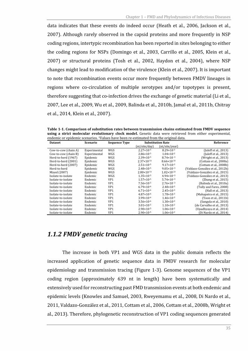
Table 1-1. Comparison of substitution rates between transmission chains estimated from FMDV sequence using a strict molecular evolutionary clock model. Genetic data were retrieved from either experimental, endemic or epidemic scenarios. †Values have been re-estimated from the original data.
Dataset Scenario Sequence Type Substitution Rate Reference (nt/site/day) (nt/site/year)
Cow-to-cow (chain A) Experimental WGS 2.27×10⁻⁵ 8.29×10⁻³ (Juleff et al., 2013) Cow-to-cow (chain B) Experimental WGS 2.86×10⁻⁵ 1.04×10⁻² (Juleff et al., 2013) Herd-to-herd (1967) Epidemic WGS 2.39×10⁻⁵ 8.74×10⁻³ (Wright et al., 2013) Herd-to-herd (2001) Epidemic WGS 2.37×10⁻⁵† 8.66×10⁻³† (Cottam et al., 2008a) Herd-to-herd (2007) Epidemic WGS 2.51×10⁻⁵ 9.17×10⁻³ (Cottam et al., 2008b) Herd-to-herd Epidemic WGS 2.48×10⁻⁵ 9.05×10⁻³ (Valdazo-González et al., 2012b) Mixed (2007) Epidemic WGS 2.80×10⁻⁵† 1.02×10⁻²† (Valdazo-González et al., 2015) Isolate-to-isolate Endemic WGS 1.35×10⁻⁵ 4.94×10⁻³ (Valdazo-González et al., 2013) Isolate-to-isolate Endemic VP1 1.57×10⁻⁵ 5.74×10⁻³ (Zhang et al., 2015) Isolate-to-isolate Endemic VP1 7.56×10⁻⁵ 2.76×10⁻³ (Balinda et al., 2010a) Isolate-to-isolate Endemic VP1 6.79×10⁻⁶ 2.48×10⁻³ (Tully and Fares, 2008) Isolate-to-isolate Endemic VP1 6.71×10⁻⁶ 2.45×10⁻³ (Hall et al., 2013) Isolate-to-isolate Endemic VP1 4.87×10⁻⁶ 1.78×10⁻³ (Mahapatra et al., 2015) Isolate-to-isolate Endemic VP1 3.99×10⁻⁶ 1.46×10⁻³ (Yoon et al., 2011b) Isolate-to-isolate Endemic VP1 3.56×10⁻⁶ 1.30×10⁻³ (Sangula et al., 2010) Isolate-to-isolate Endemic VP1 3.01×10⁻⁵ 1.10×10⁻² (de Carvalho et al., 2013) Isolate-to-isolate Endemic VP1 2.90×10⁻⁵ 1.06×10⁻² (Upadhyaya et al., 2014) Isolate-to-isolate Endemic VP1 2.90×10⁻⁵ 1.06×10⁻² (Di Nardo et al., 2014)
1.1.2 FMDV genetic tracing
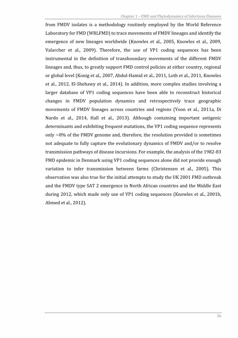
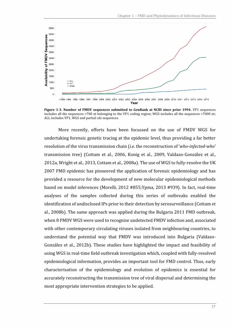
The increase in both VP1 and WGS data in the public domain reflects the
increased application of genetic sequence data in FMDV research for molecular
epidemiology and transmission tracing (Figure 1-3). Genome sequences of the VP1
coding region (approximately 639 nt in length) have been systematically and
extensively used for reconstructing past FMD transmission events at both endemic and
epidemic levels (Knowles and Samuel, 2003, Rweyemamu et al., 2008, Di Nardo et al.,
2011, Valdazo-González et al., 2011, Cottam et al., 2006, Cottam et al., 2008b, Wright et
al., 2013). Therefore, phylogenetic reconstruction of VP1 coding sequences generated
Chapter 1 – FMD and Phylodynamics of Infectious Diseases
36
from FMDV isolates is a methodology routinely employed by the World Reference
Laboratory for FMD (WRLFMD) to trace movements of FMDV lineages and identify the
emergence of new lineages worldwide (Knowles et al., 2005, Knowles et al., 2009,
Valarcher et al., 2009). Therefore, the use of VP1 coding sequences has been
instrumental in the definition of transboundary movements of the different FMDV
lineages and, thus, to greatly support FMD control policies at either country, regional
or global level (Konig et al., 2007, Abdul-Hamid et al., 2011, Loth et al., 2011, Knowles
et al., 2012, El-Shehawy et al., 2014). In addition, more complex studies involving a
larger database of VP1 coding sequences have been able to reconstruct historical
changes in FMDV population dynamics and retrospectively trace geographic
movements of FMDV lineages across countries and regions (Yoon et al., 2011a, Di
Nardo et al., 2014, Hall et al., 2013). Although containing important antigenic
determinants and exhibiting frequent mutations, the VP1 coding sequence represents
only ~8% of the FMDV genome and, therefore, the resolution provided is sometimes
not adequate to fully capture the evolutionary dynamics of FMDV and/or to resolve
transmission pathways of disease incursions. For example, the analysis of the 1982-83
FMD epidemic in Denmark using VP1 coding sequences alone did not provide enough
variation to infer transmission between farms (Christensen et al., 2005). This
observation was also true for the initial attempts to study the UK 2001 FMD outbreak
and the FMDV type SAT 2 emergence in North African countries and the Middle East
during 2012, which made only use of VP1 coding sequences (Knowles et al., 2001b,
Ahmed et al., 2012).
Chapter 1 – FMD and Phylodynamics of Infectious Diseases
37
Figure 1-3. Number of FMDV sequences submitted to GenBank at NCBI since prior 1994. VP1 sequences includes all the sequences <700 nt belonging to the VP1 coding region; WGS includes all the sequences >7000 nt; ALL includes VP1, WGS and partial cds sequences.
More recently, efforts have been focussed on the use of FMDV WGS for
undertaking forensic genetic tracing at the epidemic level, thus providing a far better
resolution of the virus transmission chain (i.e. the reconstruction of ‘who-infected-who’
transmission tree) (Cottam et al., 2006, Konig et al., 2009, Valdazo-González et al.,
2012a, Wright et al., 2013, Cottam et al., 2008a). The use of WGS to fully-resolve the UK
2007 FMD epidemic has pioneered the application of forensic epidemiology and has
provided a resource for the development of new molecular epidemiological methods
based on model inferences {Morelli, 2012 #855;Ypma, 2013 #939}. In fact, real-time
analyses of the samples collected during this series of outbreaks enabled the
identification of undisclosed IPs prior to their detection by serosurveillance (Cottam et
al., 2008b). The same approach was applied during the Bulgaria 2011 FMD outbreak,
when 8 FMDV WGS were used to recognise undetected FMDV infection and, associated
with other contemporary circulating viruses isolated from neighbouring countries, to
understand the potential way that FMDV was introduced into Bulgaria (Valdazo-
González et al., 2012b). These studies have highlighted the impact and feasibility of
using WGS in real-time field outbreak investigation which, coupled with fully-resolved
epidemiological information, provides an important tool for FMD control. Thus, early
characterisation of the epidemiology and evolution of epidemics is essential for
accurately reconstructing the transmission tree of viral dispersal and determining the
most appropriate intervention strategies to be applied.
Chapter 1 – FMD and Phylodynamics of Infectious Diseases
38
1.2 Phylodynamics of viral infectious diseases
Since the evolutionary rate of RNA viruses at nt level and their generation times
are fast enough to be measured in a short timescale, they offer an excellent system for
studying evolutionary processes that occur during transmission events (Drummond et
al., 2003, Duffy et al., 2008). Accordingly, genetic mutations carried by RNA viral
sequences enable the characterisation and reconstruction of on-going evolution
(Felsenstein, 2004). Therefore, molecular epidemiology and phylogenetics provide the
tools to understand the origin, evolutionary history, and transmission routes within
epidemics. Genealogies, moreover, contain information about historical demography
and processes that have acted to shape the diversity of populations. Given the same
time-frame, ecological dynamics can be integrated within the phylogenetic inference
to capture selective, ecological and demographic forces driving the evolution of
pathogens (Grenfell et al., 2004). This analytical framework, described as
phylodynamics, has the potential to bring together an estimation of genealogical
relationships and inferences on population sizes, structures and migration patterns,
thus enabling the reconstruction of detailed epidemiological dynamics and
transmission routes of viral system.
1.2.1 Reconstructing the dynamics of viral epidemics
1.2.1.1 Coalescent theory
Statistical methods in molecular epidemiology have significantly contributed to
the understanding of viral dynamics given the problem of data availability. One of the
most important advances in population genetics which provides the foundation of
phylodynamic inference is the formulation of the coalescent process first described by
Kingman (Kingman, 1982b, Kingman, 1982a). The coalescent model is, essentially, a
diffusion model of lines of descent which assumes a panmictic population governed by
the Wright-Fisher neutral model of genetic variation (Fisher, 1930, Wright, 1931).
Briefly, the Wright-Fisher model governs the evolution, at discrete time steps, of
population (here assumed to be haploid, as is the case for many pathogens) with
constant finite size, allowing each individual to randomly choose one parent from a
Chapter 1 – FMD and Phylodynamics of Infectious Diseases
39
previous generation and, thus, to adopt its type. Given this specification, the
assumptions constrained by the Wright-Fisher model are that the population is finite
and constant, the generations are not overlapping, the reproduction is a random
process, and no selection or recombination processes are allowed. With the coalescent
model, the ancestral lineages are traced back in time to the most recent common
ancestor (MRCA). The history of a sample of size 𝑛 comprises 𝑛 − 1 coalescent events,
with each of those decreasing the number of ancestral lineages by one. At each
coalescent event two of the lineages fuse into one common-ancestral lineage, with the
lineage remaining at the final coalescent event being the MRCA of the entire sample.
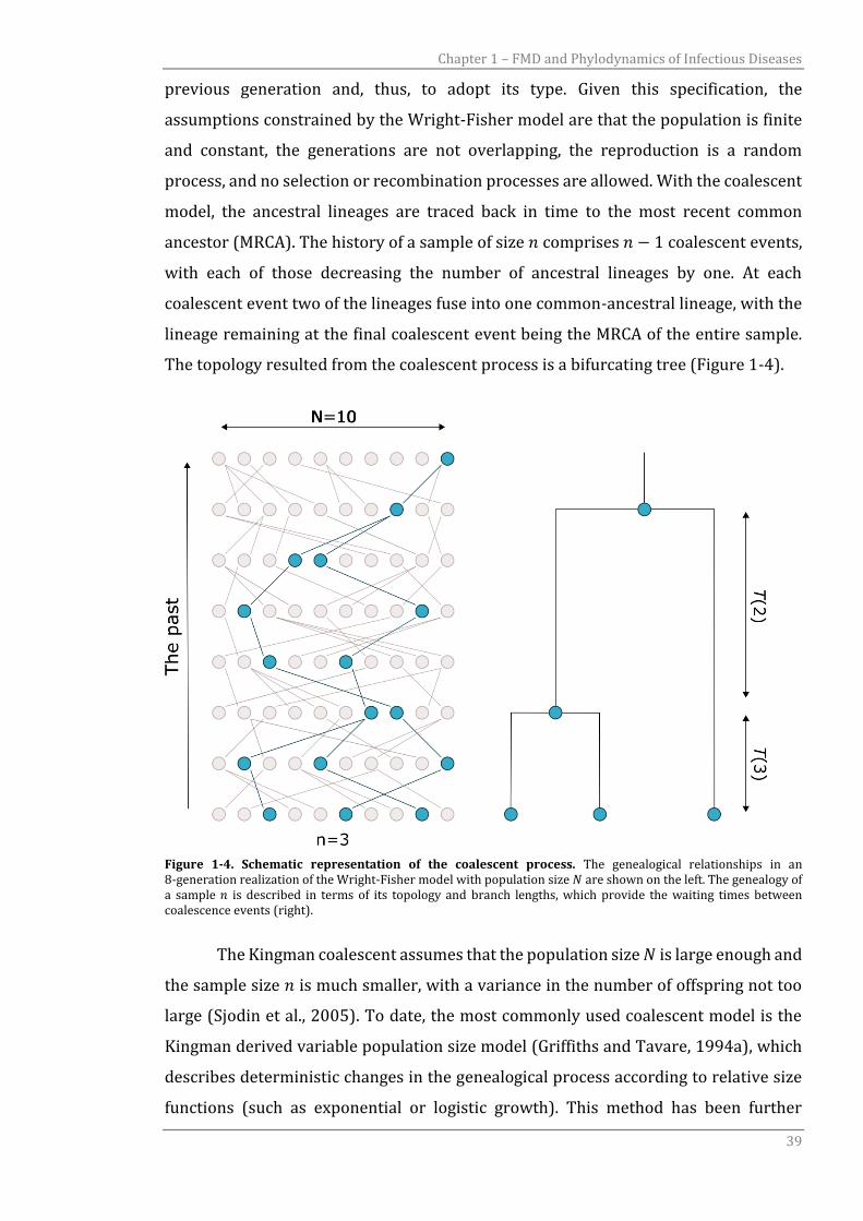
The topology resulted from the coalescent process is a bifurcating tree (Figure 1-4).
Figure 1-4. Schematic representation of the coalescent process. The genealogical relationships in an 8-generation realization of the Wright-Fisher model with population size 𝑁 are shown on the left. The genealogy of a sample 𝑛 is described in terms of its topology and branch lengths, which provide the waiting times between coalescence events (right).
The Kingman coalescent assumes that the population size 𝑁 is large enough and
the sample size 𝑛 is much smaller, with a variance in the number of offspring not too
large (Sjodin et al., 2005). To date, the most commonly used coalescent model is the
Kingman derived variable population size model (Griffiths and Tavare, 1994a), which
describes deterministic changes in the genealogical process according to relative size
functions (such as exponential or logistic growth). This method has been further
Chapter 1 – FMD and Phylodynamics of Infectious Diseases
40
extended to incorporate heterochronous sequences (Rodrigo and Felsenstein, 1999),
to deal with stochastically fluctuating population size (Kaj and Krone, 2003) and even
to apply the coalescent to spatially extended populations (Barton et al., 2002). In
addition, a more exact coalescent framework than the Kingman approximation of the
Wright-Fisher model has been recently developed, which enables the characterisation
of exhaustive sampling (i.e. of matching the size of the Wright-Fisher population) and
thus dealing with multiple coalescences at the same time (Fu, 2006).
1.2.1.2 Effective population size
Coalescence allows sampled sequences to be traced back in time within defined
ancestral lineages that eventually converge on a single MRCA. Under the coalescent
process, the shape and distribution of the phylogeny is reconstructed in terms of a
demographic parameter called the effective population size 𝑁𝑒 which corresponds to
the ideal Wright-Fisher population size 𝑁 (Charlesworth, 2009). The coalescent rate is,
nevertheless, affected by several demographic parameters, such as the population
structure and size, as well as genetic factors (i.e. reproductive forces) (Rosenberg and
Nordborg, 2002). For example, the larger the number of lineages the faster is the rate;
the larger the number of ancestors the slower is the rate. Moreover, the larger the
population size, the more genetic variability can be seen in the population and, thus,
the longer it takes for two lineages to coalesce. Therefore in its population genetic
formulation, 𝑁𝑒 provides an understanding of the observed extent and pattern of
retrospective genetic variability of a population, and is a key parameter to explain the
evolutionary mechanisms that drive the shape of variation in populations (Wang,
2005). From the initial theory of Wright (1931), the principle of 𝑁𝑒 has been extended
and applied to almost any evolutionary scenario, with several attempts to investigate
the nature of 𝑁𝑒 as an epidemiological measure in the field (Frost and Volz, 2010,
Magiorkinis et al., 2013, Volz et al., 2009, Drummond et al., 2005, Volz, 2012). To date,
studies have considered 𝑁𝑒 as equivalent to the number of infected individuals (Kouyos
et al., 2006). However, the direct relationship that exists between 𝑁𝑒 and the actual
number of infected individuals is not entirely clear, although this value is assumed to
be invariably less than the true number of infected individuals and often this is
attributed to heterogeneity in population structure (Luikart et al., 2010). In a recent
Chapter 1 – FMD and Phylodynamics of Infectious Diseases
41
study, Volz et al. (2009) demonstrated the direct relationship of the coalescent rate
with the transmission rate (i.e. incidence) but not with the measure of the number of
infected individuals (i.e. prevalence), and showed how the prevalence might influence
the shape of the phylogeny only through sampling effects. The authors reported the
coalescent rate to be proportional to the epidemic incidence and inversely
proportional to the square of the prevalence and, therefore, assuming that the rate is
high when the prevalence is low and the incidence is relatively high (i.e. during the
expansion phase of an epidemic). Frost and Volz (2010) further demonstrated that the
pattern of coalescence for an infectious disease is dominated by the transmission rate,
while the number of infected individuals is of secondary importance. Therefore,
defining the coalescent rate as a measure of incidence, incidence and prevalence are
expected to be out of phase, where peaks of incidence precede those of prevalence
(Frost and Volz, 2010). This evolutionary feature has been observed in studying the
phylodynamics of dengue virus serotype 4 in Puerto Rico, where fluctuating values of
both 𝑁𝑒 and case count over time were seen, although changes in 𝑁𝑒 preceded changes
in case count by months (Bennett et al., 2010). Since the timescale of the coalescent is
defined as a function of both 𝑁𝑒 and the generation time 𝜏 [here expressed with the
definition of serial case interval 𝜏𝑐 (Frost and Volz, 2010)], correlations between
increases in prevalence and corresponding increases in 𝑁𝑒𝜏𝑐 might be seen in a neutral
population showing absence of selection (Bedford et al., 2011). This has also been
shown in a study of hepatitis C virus, where a clear correlation in relative size of 𝑁𝑒
with the estimated number of infected individuals was reported (Magiorkinis et al.,
2013). It should be noted that although the Wright-Fisher model assumes that every
progeny is chosen at random from the parents according to a Poisson distribution, in
nature and often in viral dynamics few cases produce the majority of infections. This
variance in the number of progeny per parent can therefore increase the stochastic
effect and thus affects the 𝑁𝑒 estimate (Kouyos et al., 2006). The correlation between
𝑁𝑒 and the variance in the number of progeny per parent (𝑉𝑘) has been investigated for
several formulations of the coalescent process, thus defining different 𝑁𝑒 quantities
such as the inbreeding effective number (𝑁𝑒𝑖) and the variance effective number (𝑁𝑒𝑣
),
which account for uneven progeny structures (Kimura and Crow, 1963). This leads to
the assumption that 𝑁𝑒 is connected with the census population size 𝑁 and the variance
(𝜎2) in the reproductive success (Kingman, 1982b, Tavare et al., 1997) or, in a more
epidemiological definition, the variance in the number of secondary infections per
Chapter 1 – FMD and Phylodynamics of Infectious Diseases
42
primary infection [𝑣𝑎𝑟(𝑅𝑡)] (Koelle and Rasmussen, 2012). In addition, the ratio
between the number of infected individuals, 𝑁, and the effective population size, 𝑁𝑒 ,
(𝑁/𝑁𝑒) is formally described as being equal to the 𝑣𝑎𝑟(𝑅𝑡) when the genetic variability
within virus strains has no effect on their infectious potential (Kingman, 1982b,
Magiorkinis et al., 2013, Tavare et al., 1997).
Although the coalescent model is appropriate for making inferences about
population dynamics, in the context of viral transmission it is mainly used for its simple
mathematical formulation rather than its accuracy in defining the transmission
process. For example, the coalescent model can provide estimations of change in
population size but shows limitations as an estimator of epidemiological parameters.
Furthermore, it does not make use of information on sampling time. Stadler et al.
(2012) introduced the birth-death model (BDM) as an alternative to the coalescence
for the tree-generating process. The birth-death process generates, forward in time
and according to stochastic rates of birth and death, a tree with extinct and extant
lineages (i.e. the ‘complete tree’). The extinct and the not-sampled lineages are then
deleted producing the reconstructed tree of only sampled extant lineages. As
demonstrated, the BDM has the advantage of reflecting more accurately the process
underlying the transmission dynamic and, moreover, to estimate the total number of
infections caused by an individual over the course of the individuals infectious time (i.e.
the basic reproductive number 𝑅0). From their initial formulation, both the coalescent
and BDMs have been extended to account for heterogeneous structured populations
(Stadler and Bonhoeffer, 2013, Volz, 2012). In addition, several attempts have been
recently made towards the implementation of stochastic demographic processes into
a coalescent framework (Rasmussen et al., 2011, Rasmussen et al., 2014b)
1.2.1.3 Modelling the demography of viral populations
As presented in the previous section, the coalescent model defined by Kingman
describes the relationship between coalescent times and the population size under the
Wright-Fisher population model given a sampled genealogy. Given that 1/𝑁𝑒 is the
probability, under the coalescent assumptions, that two lineages descend from a
common ancestor at each generation and applying the derived probability distribution
to a phylogenetic tree, it is possible to estimate the change in Ne throughout the history
Chapter 1 – FMD and Phylodynamics of Infectious Diseases
43
of the population up to the MRCA. This feature of the coalescent enables quantification
of the rate at which the population loses or enhances its genetic diversity and,
therefore, the computation of historical patterns of viral population size provided by
genomic data (de Silva et al., 2012). In the last decade, several methods have been
developed for estimating the demography of populations from sequence data or an
estimated genealogy. However, most of these approaches constrain the population
history into continuous or piecewise parametric models, such as constant size,
exponential growth, logistic growth, and expansion growth, and therefore do not fully
capture the complex patterns of demographic changes (Kingman, 1982b, Slatkin and
Hudson, 1991, Tavare et al., 1997, Wilson and Balding, 1998, Griffiths and Tavare,
1994a). In addition, an a priori assumption of a population size history is usually not
possible and, therefore, simple population growth functions might not best describe
the population history of interest.
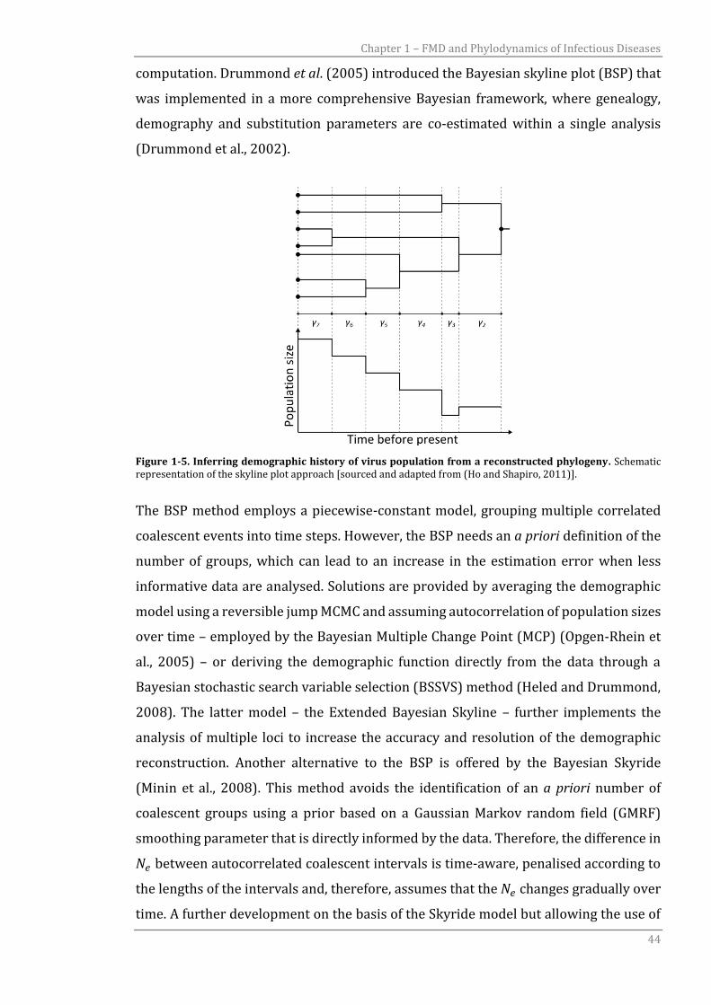
Building up from this problem, Nee et al. (1995) introduced the lineage-
through-time (LTT) plot that provides a graphical depiction of the accumulation of
lineages in a time scale derived from a time-stamped phylogeny. However, the initial
theoretical input of Pybus et al. (2000) with the introduction of the classic skyline plot
provided the basis to derive more precise computation of demographic history
reconstruction, thus giving rise to a family of so-called skyline plot methods (Table 1-
2). Skyline reconstruction assumes that under the coalescent the mean population size
for each coalescent interval can be estimated by the product of the interval size (𝛾𝑖)
and 𝑖(𝑖 − 2)/2, where 𝑖 is the number of lineages in the interval (Figure 1-5) and,
therefore, gives a non-parametric estimate of 𝑁𝑒 based on a piecewise method. The
limitation of the classical skyline plot is that it produces a noisy and stochastic
reconstruction resulting from the lack of coalescent error assessment provided by the
method, which is particularly evident when the genealogy contains a large number of
short internal branches and, therefore, the phylogenetic error is substantial. To
overcome this problem, the generalised skyline plot was developed (Strimmer and
Pybus, 2001). The main difference between the classical and generalised skyline plots
is that the latter overcomes the problem of the noisy estimates by grouping correlated
coalescent events and, thus, sampling events into time intervals of a certain length 𝜀.
However, the genealogy is still assumed to be estimated without error and does not
account for stochasticity in the coalescent process. Major improvements were
implemented estimating 𝑁𝑒 within a Bayesian Markov chain Monte Carlo (MCMC)
Chapter 1 – FMD and Phylodynamics of Infectious Diseases
44
computation. Drummond et al. (2005) introduced the Bayesian skyline plot (BSP) that
was implemented in a more comprehensive Bayesian framework, where genealogy,
demography and substitution parameters are co-estimated within a single analysis
(Drummond et al., 2002).
Figure 1-5. Inferring demographic history of virus population from a reconstructed phylogeny. Schematic representation of the skyline plot approach [sourced and adapted from (Ho and Shapiro, 2011)].
The BSP method employs a piecewise-constant model, grouping multiple correlated
coalescent events into time steps. However, the BSP needs an a priori definition of the
number of groups, which can lead to an increase in the estimation error when less
informative data are analysed. Solutions are provided by averaging the demographic
model using a reversible jump MCMC and assuming autocorrelation of population sizes
over time – employed by the Bayesian Multiple Change Point (MCP) (Opgen-Rhein et
al., 2005) – or deriving the demographic function directly from the data through a
Bayesian stochastic search variable selection (BSSVS) method (Heled and Drummond,
2008). The latter model – the Extended Bayesian Skyline – further implements the
analysis of multiple loci to increase the accuracy and resolution of the demographic
reconstruction. Another alternative to the BSP is offered by the Bayesian Skyride
(Minin et al., 2008). This method avoids the identification of an a priori number of
coalescent groups using a prior based on a Gaussian Markov random field (GMRF)
smoothing parameter that is directly informed by the data. Therefore, the difference in
𝑁𝑒 between autocorrelated coalescent intervals is time-aware, penalised according to
the lengths of the intervals and, therefore, assumes that the 𝑁𝑒 changes gradually over
time. A further development on the basis of the Skyride model but allowing the use of
Chapter 1 – FMD and Phylodynamics of Infectious Diseases
45
multiple unlinked genetic loci, as featured in the Extended Bayesian Skyline, is the
Bayesian Skygrid, which parameterises 𝑁𝑒 as a piecewise constant function smoothing
the trajectory by GMRF and allowing changes to the estimated trajectory at pre-
specified fixed points in real time (i.e. grid points) (Gill et al., 2013). A method for
calculating the 𝑁𝑒 based on an approximate Bayesian computation (ABC) algorithm has
also been proposed (Palacios and Minin, 2012). This method integrates Gaussian
process-based Bayesian nonparametric approaches into integrated nested Laplace
approximation (INLA) (Rue et al., 2009) without the need for complex MCMC
computation and, therefore, speeding up the calculation and improving the efficiency.
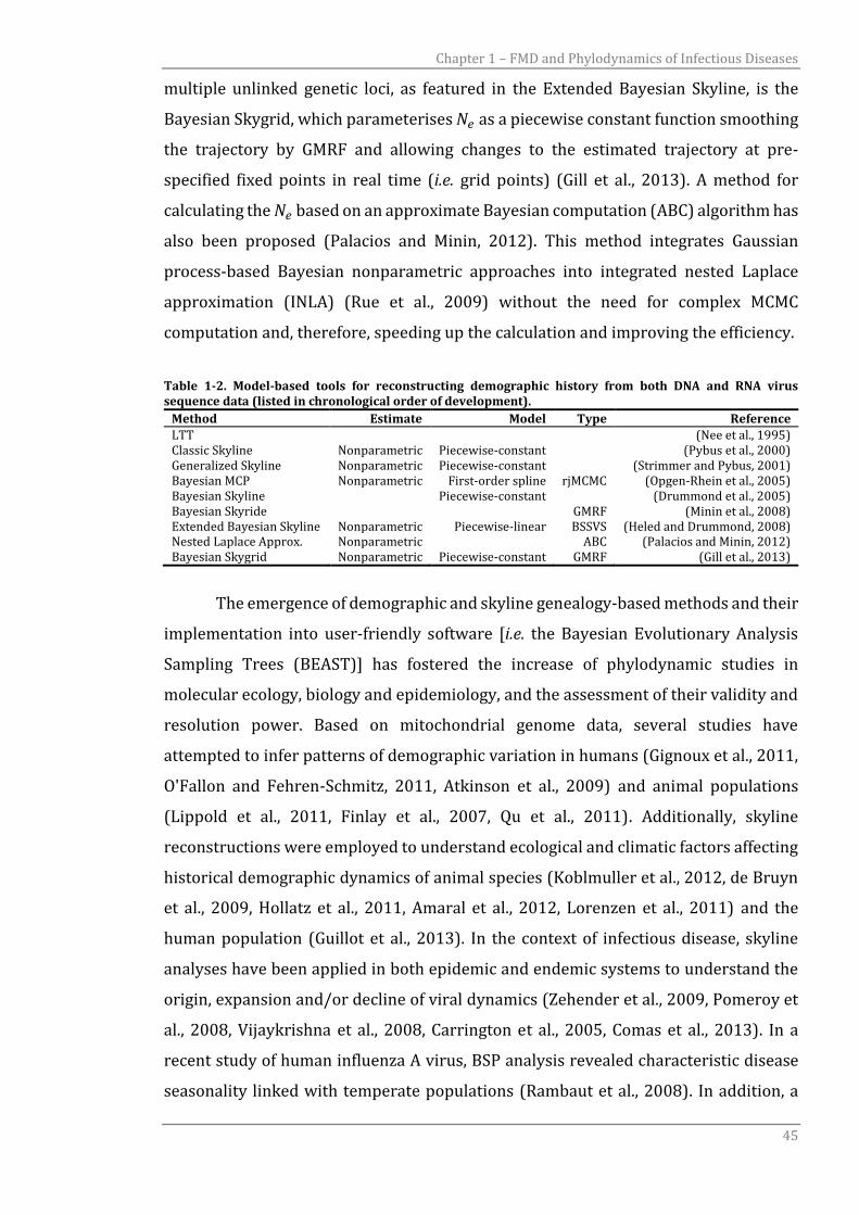
Table 1-2. Model-based tools for reconstructing demographic history from both DNA and RNA virus sequence data (listed in chronological order of development).
Method Estimate Model Type Reference
LTT (Nee et al., 1995) Classic Skyline Nonparametric Piecewise-constant (Pybus et al., 2000) Generalized Skyline Nonparametric Piecewise-constant (Strimmer and Pybus, 2001) Bayesian MCP Nonparametric First-order spline rjMCMC (Opgen-Rhein et al., 2005) Bayesian Skyline Piecewise-constant (Drummond et al., 2005) Bayesian Skyride GMRF (Minin et al., 2008) Extended Bayesian Skyline Nonparametric Piecewise-linear BSSVS (Heled and Drummond, 2008) Nested Laplace Approx. Nonparametric ABC (Palacios and Minin, 2012) Bayesian Skygrid Nonparametric Piecewise-constant GMRF (Gill et al., 2013)
The emergence of demographic and skyline genealogy-based methods and their
implementation into user-friendly software [i.e. the Bayesian Evolutionary Analysis
Sampling Trees (BEAST)] has fostered the increase of phylodynamic studies in
molecular ecology, biology and epidemiology, and the assessment of their validity and
resolution power. Based on mitochondrial genome data, several studies have
attempted to infer patterns of demographic variation in humans (Gignoux et al., 2011,
O'Fallon and Fehren-Schmitz, 2011, Atkinson et al., 2009) and animal populations
(Lippold et al., 2011, Finlay et al., 2007, Qu et al., 2011). Additionally, skyline
reconstructions were employed to understand ecological and climatic factors affecting
historical demographic dynamics of animal species (Koblmuller et al., 2012, de Bruyn
et al., 2009, Hollatz et al., 2011, Amaral et al., 2012, Lorenzen et al., 2011) and the
human population (Guillot et al., 2013). In the context of infectious disease, skyline
analyses have been applied in both epidemic and endemic systems to understand the
origin, expansion and/or decline of viral dynamics (Zehender et al., 2009, Pomeroy et
al., 2008, Vijaykrishna et al., 2008, Carrington et al., 2005, Comas et al., 2013). In a
recent study of human influenza A virus, BSP analysis revealed characteristic disease
seasonality linked with temperate populations (Rambaut et al., 2008). In addition, a
Chapter 1 – FMD and Phylodynamics of Infectious Diseases
46
three-stage process of host shift for rabies virus in bats was described for all different
virus lineages (Streicker et al., 2012). The use of BSP to assess impact of control policies
on viral diversity has been also applied in the context of hepatitis A virus with the
introduction of vaccination in France related to the time of decline observed in the
reconstructed skyline plot (Moratorio et al., 2007), whereas an exponential growth in
the 𝑁𝑒 of hepatitis C virus in Egypt was attributed to the introduction of parental
antischistosomal treatments (Pybus et al., 2003). In a review of skyline plot methods,
Ho and Shapiro (2011) tested five skyline models against two datasets generated via
simulation. Beside the classic and generalised skyline, the BSP largely matched the
trajectories of the simulated data although not full recovering the demography.
Simulating epidemic and evolutionary dynamics of biannual measles outbreaks by a
Time-Series SIR model, Stack et al. (2010) reported the failure of the BSP to reconstruct
the full biennial dynamics of measles epidemics over different long-term sampling sets.
This is relevant when populations undergo bottlenecks and the number of lineages is
substantially reduced from one epidemic season to the next. In another study carried
out with the aim of testing the BSP for reconstructing epidemic dynamics, data related
to the early exponential phase of an influenza A virus H1N1 epidemic were simulated
using a branching process model (de Silva et al., 2012). Results revealed biases in the
skyline estimates, incorrectly inferring a decrease in the 𝑁𝑒 in the last part of the
epidemic phase when the population was still growing. This problem was related to
the lack of genealogical information at later times, corresponding to the last coalescent
event and the flattening of the LTT plot; therefore, the authors suggested truncating
the BSP reconstruction behind the last coalescent event. In addition, some studies
highlighted the limitations of the BSP for reconstructing viral demography due to its
formulation being based on the coalescent, which approximates the population
dynamics assuming a small sample of the entire population (Stadler et al., 2013).
1.2.1.4 Sampling genetic data
Making an inference on evolution and population structures for a given
pathogen relies on adequate sampling which ideally should be based on knowledge of
pattern and extent of genetic diversity at a given spatio-temporal scale. Therefore, two
important questions might be raised in the context of sampling genetic data: 1) how
Chapter 1 – FMD and Phylodynamics of Infectious Diseases
47
does the temporal distribution of the samples affect the estimation of the population
size? and 2) can a sampling strategy be designed to optimise the reconstruction of
population histories? For coalescent-based methods to work optimally, samples should
be drawn from a well-defined scheme (Rosenberg and Nordborg, 2002) with
individuals randomly sampled from a panmictic population. When heterochronous
data are used, the random sampling is extended across geographical and temporal
ranges; sampled sequences are assumed to be orthologous, non-recombining and
neutrally evolving. It should be noted that, under the coalescent model, increasing the
sample size does not extend the accuracy of the estimates, because of the existence of
a single underlying genealogy (Rosenberg and Nordborg, 2002). However, sampling
biases at the genetic level could result in strongly unbalanced trees, even in the case of
a panmictic population (Mooers and Heard, 1997). Different opinions are expressed as
to whether demographic history is best reconstructed from a local or a pooled
sampling scheme when populations are geographically and genetically structured (St
Onge et al., 2012). The effect of population subdivision and structure has been reported
to impact on the reconstruction of population size changes (Peter et al., 2010, Chikhi et
al., 2010). Stadler et al. (2009) suggested that a scattered sampling might result in a
frequency polymorphism spectrum more similar to that expected in a neutral evolving
population. However, St Onge et al. (2012) concluded that the effect of sampling on the
site frequency spectrum is limited in many cases, such as populations that experience
large demographic changes or when migration is unlimited. In the context of
epidemics, using discrete-time simulations Stack et al. (2010) found that the bias in
prevalence reconstruction using BSP depended largely on how samples were
distributed over the course of the epidemic: the most reliable estimates could be
obtained by sampling sequences towards the end of an epidemic. Therefore, a
systematic approach based on serial sampling schemes should provide a broad view of
the epidemic dynamic (Stack et al., 2010). For example, sampling a higher fraction of
the infected population in a given time might result in trees with shorter terminal
branches (Volz et al., 2009). In a phylodynamics study of norovirus GII.4, although the
disease seasonality derived from the surveillance system was reconstructed using the
BSP, re-performing the analysis using a subset of the polymerase dataset drastically
reduced the resolution provided by the BSP, demonstrating that a high sampling
density is required to analyse population dynamics of viruses characterised by
seasonal variation interleaved by population bottlenecks (Siebenga et al., 2010). From
Chapter 1 – FMD and Phylodynamics of Infectious Diseases
48
a different prospective, an extension of the BDM has been developed to account for
incomplete sampling of the population (Stadler, 2010). The use of BDM has the
advantage that it can be applied to different sampling scenarios (i.e. sparse or dense
sampling schemes), since the sampling process is specified within the model (Stadler
et al., 2012). In addition within this process, the sampling rates can be relaxed to vary
through time by means of a step function (Stadler et al., 2013). However, one problem
of the BDM is that it requires a specification of the sampling process and, therefore, if
the testing system deviates from the theoretical formulation of the BDM the results
obtained might be highly biased (Volz and Frost, 2014). This has been seen with the
study of the recent Ebola virus epidemic in Sierra Leone (Stadler et al., 2014), where
the assumption of a constant sampling rate of the BD exposed-infected model used for
the analysis is violated by the sampling variability reported between collection periods
(Volz and Pond, 2014).
1.2.2 Integrating epidemiology with phylogenetics
One of the most challenging tasks to fully understand the dynamics of pathogen
dispersal is the integration of data based on epidemiological observations with
phylogenetic inferences. In fact, although the transmission pathways can be
reconstructed using either epidemiological (i.e. by the means of time, space or space-
time data) or genetic data alone, inferences based on these approaches are generally
biased and unreliable. Great robustness can be achieved by integrating these data types
together. With the increasing affordability and speed with which genomic data can be
generated, research on this topic has expanded in the last 5 years leading to a range of
different methodological approaches to try to resolve the complex structure defined by
the phylodynamic process (Grenfell et al., 2004). However, despite the increase in the
application of coalescent-based methods in molecular epidemiology, difficulties arise
when validating the obtained results through independent data. Biek et al. (2007)
demonstrated the detailed information which can be extracted when integrating
different types of data sources into the phylogenetic inference. In the context of viral
dynamics, phylogenetic reconstruction has been used to understand the complex virus
diversity within the inter-farm transmission dynamics of the H7N7 highly pathogenic
avian influenza virus outbreak recorded in The Netherlands in 2003 (Bataille et al.,
Chapter 1 – FMD and Phylodynamics of Infectious Diseases
49
2011). In addition, attempts to reconstruct the underlying transmission pathways of
viral dynamics include the integration of spatial and temporal data within the
phylogenetic reconstruction. Lemey et al. (2009a) provided the basis for an integrated
Bayesian phylogeography framework built on a BSSVS model using discrete location
states which helped in reconstructing the patterns of global spread of the H5N1
influenza A virus. This methodology was further tested analysing the process
underlying the geographical migration of the initial spread of the H1N1 human
influenza A virus pandemic (Lemey et al., 2009b). Further extensions enabled the use
of continuous data, such as geographical coordinates, through the implementation of
random walk diffusion models based on branch-specific variation in the dispersal rates
(Lemey et al., 2010). In the FMD context, phylogeography has been used for
characterising movement of lineages within a country (de Carvalho et al., 2013), within
a continent and across different species (Hall et al., 2013), and from a whole topotype
perspective (Di Nardo et al., 2014).
Differently, a set of studies were based on a previously developed parameter-
free method for estimating the history of transmission events in the course of an
epidemic, which reconstructs the temporal chain of transmission events (Haydon et al.,
2003). However, accurate and unbiased reconstruction of the so-called transmission
trees is likely to require a very good sampling of cases during an epidemic. Therefore,
studies have been focused on the potential integration of genetic information with
epidemiological data to enhance the resolution, which could be categorised into two
distinct computational approaches: the ‘transmission tree first’ when the transmission
tree is firstly reconstructed and then an evolutionary model is attached to the
transmission model; and the ‘phylogenetic first’ where the genetic data are used to
directly infer the transmission tree by augmenting some evolutionary model with
epidemiological information. Cottam et al. (2008a) studied a cluster from the UK 2001
FMD epidemic and developed a transmission tree analysis based on estimating likely
periods of infectiousness, constructing all plausible trees, and using genetic data to
identify and exclude unlikely transmission trees. Following this approach, in a study of
the H7N7 avian influenza A epidemic in The Netherlands in 2003 (Ypma et al., 2012),
genetic, geographical and temporal data were integrated in one single likelihood
function for estimating the infection events and the infectiousness of farms according
to their size and type. Furthermore, this methodology appropriately handled missing
data (i.e. cases for which no genetic data were available). A comprehensive analytical
Chapter 1 – FMD and Phylodynamics of Infectious Diseases
50
framework is also proposed by Rasmussen et al. (2011), who integrated genealogies
and time series data in a State-Space Model (SSM) parameter and population dynamics
using a particle filtering MCMC method. A detailed spatial epidemiological model of
transmission coupled with a simple evolutionary model has been proposed by Morelli
et al. (2012), an approach that attempts simultaneous inferences to be made on
epidemiological processes, the transmission chain and the mechanisms that shape the
evolutionary process. The Bayesian framework proposed pioneered the further
development of likelihood functions that integrated genetic distance and
epidemiological models for analysing disease outbreaks and thus estimating
transmission trees.
Moving from more classical phylogenetic approaches, Jombart et al. (2011)
developed a method based on graph theory (Lieberman et al., 2005) that derives
ancestries directly from the sampled isolates. This approach becomes relevant when
the phylogeny includes both the ancestor and descendants, as in the case of an
outbreak. Clearly, the structure of the contact network underlying epidemics impacts
on the spread of a pathogen (Keeling, 2005), leaving detectable genetic signatures and
providing evident correlations between genetic and epidemiological data (Welch et al.,
2011). In a study of a nosocomial outbreak of hepatitis C (Spada et al., 2004), a
Minimum Spanning Tree approach was used to reconstruct the transmission tree of
the epidemic combined with information on the contact patterns of the hosts. Gordo
and Campos (2007) studied the level and pattern of genetic diversity in viral
populations developing a population genetic model incorporating epidemiological
parameters based on SIS simulations on two different structures of the host contact
network. The utility of integrating genetic data with epidemiology has been
demonstrated by Lewis et al. (2008) who developed a Bayesian approach for
reconstructing transmission network of HIV patients. The effect of contact network on
phylogeny has been quantified in a recent study (Leventhal et al., 2012), where the
authors reported significant variation of the Sackin index (i.e. a measure of the tree
shape) according to different classes of contact structures tested.
A common assumption on which the relationship between transmission tree
and phylogeny is founded is that transmission events and time of ancestry are
equivalent and, therefore, transmission and phylogenetic trees are topologically
equivalent (Pybus and Rambaut, 2009). However, this might not be correct when a
substantial within-host (or even within-farm) evolutionary process potentially allows
Chapter 1 – FMD and Phylodynamics of Infectious Diseases
51
several individual lineages to be transmitted from the same source (Kao et al., 2014).
An initial attempt to include within-host genetic diversity linked a structured
transmission tree with a within-host evolutionary process to resolve the full
transmission history of epidemics (Ypma et al., 2013). However, problems arise since
estimates based on either fixed phylogenetic or transmission tree topology are not able
to fully capture the extent of the variability in the tree space (Vrancken et al., 2014).
Didelot et al. (2014) explored this issue introducing a model based on a coalescent
within-host evolutionary process, which accounted for uncertainty in the inferred
phylogeny, in order to reconstruct disease transmission history in a densely sampled
scenario and when multiple lineages might be passed to subsequent generations.
Further developments on this approach have been recently put into a more theoretical
framework (Hall and Rambaut, 2014). However, one limitation of all the above
methods is that they require that all infected cases have been observed and, therefore,
the trees should contain a tip from every case involved in the transmission chain.
Although epidemiological data extracted from fully-resolved epidemics can be
informative about unsampled genetic data, this would not always be the case in
endemic settings where surveillance is unlikely to be exhaustive or when infections are
characterised by a subclinical form. Studies have started to investigate space-time-
genetic SEIR approaches (Mollentze et al., 2014, Soubeyrand, 2014) or a simpler
discrete-time stochastic model (Jombart et al., 2014) that would enable the
characterisation of missed or unsampled cases and the existence of polyphyletic
systems. On a multi-scale perspective whether investigating small scale epidemics,
disease spread at continental level or viral population structure (Figure 1-6), this
highlights the important source of information that epidemiological data provides to
the reliable reconstruction of transmission chains based on phylogenetic methods.
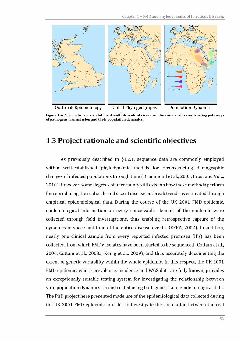
Chapter 1 – FMD and Phylodynamics of Infectious Diseases
52
Figure 1-6. Schematic representation of multiple scale of virus evolution aimed at reconstructing pathways of pathogens transmission and their population dynamics.
1.3 Project rationale and scientific objectives
As previously described in §1.2.1, sequence data are commonly employed
within well-established phylodynamic models for reconstructing demographic
changes of infected populations through time (Drummond et al., 2005, Frost and Volz,
2010). However, some degrees of uncertainty still exist on how these methods perform
for reproducing the real scale and size of disease outbreak trends as estimated through
empirical epidemiological data. During the course of the UK 2001 FMD epidemic,
epidemiological information on every conceivable element of the epidemic were
collected through field investigations, thus enabling retrospective capture of the
dynamics in space and time of the entire disease event (DEFRA, 2002). In addition,
nearly one clinical sample from every reported infected premises (IPs) has been
collected, from which FMDV isolates have been started to be sequenced (Cottam et al.,
2006, Cottam et al., 2008a, Konig et al., 2009), and thus accurately documenting the
extent of genetic variability within the whole epidemic. In this respect, the UK 2001
FMD epidemic, where prevalence, incidence and WGS data are fully known, provides
an exceptionally suitable testing system for investigating the relationship between
viral population dynamics reconstructed using both genetic and epidemiological data.
The PhD project here presented made use of the epidemiological data collected during
the UK 2001 FMD epidemic in order to investigate the correlation between the real
Chapter 1 – FMD and Phylodynamics of Infectious Diseases
53
count of infected cases (derived from either prevalence or incidence data) and the viral
demographic history inferred by sequence variability that is recorded from time-
stamped WGSs extracted from the field isolates. At the time of starting this PhD
research, the Epi-SEQ EMIDA-ERA NET funded project
(www.episeq.eu/index_files/Page1077.htm) was focused on the genetic
characterisation of the entire UK 2001 FMD collection of clinical samples stored at the
WRLFMD, The Pirbright Institute - UK, which theoretically would have been sequenced
within the timeframe of this PhD project. Unfortunately, delays have meant that some
of the results obtained from this PhD project can only be validated sometime after its
completion, when the full dataset of UK 2001 FMDV WGSs will be available. Therefore,
the observations and research findings grounded on the results here presented were
generated through an evolutionary simulation framework of the whole UK 2001 FMD
epidemic, which has been informed by the space-time dynamics of the transmission
events as reconstructed using the fully resolved epidemiological data. Hence, the
overall aim of this PhD project was to test the hypothesis that inferences on the true
number of infected cases can be drawn from patterns of mutation accumulating in
sequence data recovered from observed cases, as estimated by transformations of the
effective population size 𝑁𝑒 . Accordingly, the work here presented attempts to
disentangle some key questions in the field of phylodynamics of viral infectious
disease, namely:
Can the effective population size 𝑁𝑒 derived from the BSP be scaled to
some epidemiological relevant measure of prevalence?
How does the sampling design affect the estimation of virus evolution and
population demography?
Can sequence data be used to infer unobserved disease events?
Results from this project may have particular relevance in FMD endemic settings
where comprehensive sampling is not usually possible and official reporting of
outbreaks limited. In this context, a clear understanding of the disease burden is
therefore needed, which might be derived from the estimation of the viral population
size as a proxy of disease prevalence. In addition, inferences about evolutionary
changes on timescales enable the dating of epidemiologically important events and,
therefore, independently validating against surveillance data to understand the impact
of control measures imposed. Thus, reconstructing and predicting epidemiological
dynamics and transmission routes during epidemic events or in an endemic setting
Chapter 1 – FMD and Phylodynamics of Infectious Diseases
54
have the potential to inform intervention strategies and control policies In addition,
the outcomes derived from this project have many potential and valuable applications
not only for FMD but may also be generalised to other RNA viral diseases.
1.3.1 Thesis outline
The work produced in this thesis is structured into seven chapters, which are
sequentially presented in a logical consecutio. Following this introductory chapter
which reviews the studies published in the literature on the topics of FMD and
phylodynamics of infectious diseases, Chapter 2 describes a practical example of the
use of phylogenetic methods currently employed for reconstructing evolutionary
history, demographic signal and the dispersal process of viruses. This study, based on
the generation of new sequence data and analyses of 322 VP1 coding sequences,
produced a comprehensive phylodynamics picture of the serotype O CATHAY FMDV
topotype and its evolutionary adaptation into the Southeast Asia ecosystem. In
addition, a detailed historical reconstruction of the FMDV epidemic events reported in
the Philippines during 1994 and 2005 has been performed analysing the genetic signal
carried by 112 VP1 coding sequences. Results generated from Chapter 2 have been
already published in the peer-reviewed journal Veterinary Research (Di Nardo et al.,
2014).
Chapter 3 presents the model framework that has been developed with the aim
of reconstructing the transmission tree of the UK 2001 FMD epidemic and simulating
the entire FMDV alignment of the epidemic, thus generating one WGS for each of the
IPs reported to be infected during the outbreak. The metrics of the reconstructed
epidemic are presented along with the estimation of its demographic size, as either
prevalence or incidence estimation. In addition and as a preliminary attempt to
validate the WGS simulation, the metrics of the simulated genetic data with the 39
already characterised WGS isolates (Cottam et al., 2006, Cottam et al., 2008a, Konig et
al., 2009) have been compared.
Chapter 4 has been fully devoted to the relationship between the real number
of infected cases (as estimated by prevalence or incidence data) and 𝑁𝑒 . Using the WGS
data derived from the simulation model presented in the previous chapter, the concept
of the infection prevalence 𝑁∗ has been explored to investigate a likely scaling
Chapter 1 – FMD and Phylodynamics of Infectious Diseases
55
approach which could potentially link 𝑁𝑒 with the real infected population size and,
therefore, empowering the conceptualization of genetic data as a proxy for a
prevalence measure. For this purpose, empirical prevalence and incidence data
extracted from the UK 2001 FMD epidemic have been correlated with the demographic
signal carried by the 𝑁𝑒 and extracted from the BSP analysis of the WGS simulated data.
In addition, further FMDV stationary demographic scenarios, simulated at different
degree of population structure, have been tested in order to assess the impact of the
variance in the population structure [i.e. 𝑣𝑎𝑟(𝑅𝑡)] on the accuracy of the BSP-derived
𝑁𝑒 estimates.
Chapter 5 examines the effect of sampling size on the reconstruction of viral
demography further using the UK 2001 FMDV WGS simulated data and the 𝑁𝑒 scaling
formulations derived from Chapter 4. For this purpose, different sampling schemes
have been tested from the simple realisation of a random process to more
epidemiologically structured schemes, based on the probability proportional to size
sampling theory. In addition, estimates extracted from the incomplete sampling BDM
have been compared with their coalescent derivation.
Chapter 6 presents a preliminary characterisation of the whole UK 2001 FMD
epidemic using an initial set of the WGS (n=154) that have been generated from the
archive of clinical samples collected at the time of the outbreak (n=1404). These real
data allow us to test the hypotheses derived from the results obtained from the
analyses of the simulated data presented in Chapters 3 to 5 and, therefore, to initially
validate their assumptions with a relatively small subset of the real WGS data (~11%).
In addition, the results here presented attempt to draw the first sensu scricto
phylodynamic inference from the fully-resolved epidemiological and genetic data of
the UK 2001 FMD epidemic.
The final discussion and concluding remarks are then presented in Chapter 7.


57
CHAPTER 2
2.1 Abstract
Reconstructing the evolutionary history, demographic signal and dispersal
processes from viral genome sequences contributes to our understanding of the
epidemiological dynamics underlying epizootic events. In this study, a Bayesian
phylogenetic framework was used to explore the phylodynamics and spatio-temporal
dispersion of the O CATHAY topotype of foot-and-mouth disease virus (FMDV) that
caused epidemics in the Philippines between 1994 and 2005. Sequences of the FMDV
genome encoding the VP1 showed that the O CATHAY FMD epizootic in the Philippines
resulted from a single introduction and was characterised by three main transmission
hubs in Rizal, Bulacan and Manila Provinces. From a wider regional perspective,
phylogenetic reconstruction of all available O CATHAY VP1 nucleotide sequences
identified three distinct sub-lineages associated with country-based clusters
originating in Hong Kong Special Administrative Region (SAR), the Philippines and
Taiwan. The root of this phylogenetic tree was located in Hong Kong SAR, representing
the most likely source for the introduction of this lineage into the Philippines and
Taiwan. The reconstructed O CATHAY phylodynamics revealed three chronologically
distinct evolutionary phases, culminating in a reduction in viral diversity over the final
10 years. The analysis suggests that viruses from the O CATHAY topotype have been
continually maintained within swine industries close to Hong Kong SAR, following the
extinction of virus lineages from the Philippines and the reduced number of FMD cases
in Taiwan.
Chapter 2 – Phylodynamic Reconstruction of O CATHAY Topotype FMDV Epidemics in the Philippines
58
2.2 Introduction
Foot-and-mouth disease is an economically devastating transboundary disease
of cloven-hoofed domestic and wild ruminants, causing an acute and highly contagious
vesicular disease which can develop into a persistent infection. The aetiological agent
is FMDV, a single-stranded RNA virus belonging to the Aphthovirus genus, family
Picornaviridae. FMDV is characterised by high genetic variability and exists as seven
different serotypes named as O, A, C, Asia 1, SAT 1, SAT 2, and SAT 3 (Knowles and
Samuel, 2003). As a consequence of their high mutation rate, FMDV lineages quickly
diverge as they replicate and spread into new areas. Therefore, transmission of the
virus through space and time directly defines the evolutionary patterns observed
between related FMDV strains (Knowles et al., 2010b). In addition to the accumulation
of nucleotide substitutions through errors, large block of sequence changes can be
mediated via recombination between different FMDV genomes, further expanding its
evolutionary repertoire. In this context, FMDV populations often exhibit extensive
genetic and antigenic heterogeneity at both the molecular and geographical level,
driven by co-circulation of multiple lineages, heterogenic mixed host populations,
extensive animal movements and trade patterns (Di Nardo et al., 2011). FMDV
serotypes have evolved independently in different geographical regions to give rise to
distinct genetic lineages, designated topotypes. Eleven topotypes have been defined for
serotype O, based on phylogenetic relationships between available sequence data and
a value of ~15% of nt sequence difference in the VP1 coding region (Knowles et al.,
2010a, Samuel and Knowles, 2001).
2.2.1 The O CATHAY FMDV topotype
The first FMDV strain belonging to the O CATHAY topotype was isolated from
Hong Kong SAR from pig samples collected during 1970 (HKN/21/70, GenBank
accession no. AJ294911) and was characterised by a 93-102 nt deletion within the 3A
coding region that is associated with the atypical porcinophilic phenotype of this FMDV
lineage (Knowles et al., 2001a). Subsequently, O CATHAY isolates have been confirmed
in several Southeast and East Asian countries (including Malaysia, the Philippines,
Taiwan, Thailand and Vietnam), although since 1970, the majority of field cases due to
Chapter 2 – Phylodynamic Reconstruction of O CATHAY Topotype FMDV Epidemics in the Philippines
59
this topotype have been reported in Hong Kong SAR and China (Gleeson, 2002,
Knowles et al., 2005, Cao et al., 2014). The O CATHAY FMD outbreak in Taiwan which
began during 1997 resulted in the stamping-out of more than 4 million pigs and
generated economic losses of over 6 billion US dollars (Yang et al., 1999). Outside of
Asia, viruses belonging to the O CATHAY topotype have been responsible for isolated
FMD outbreaks that occurred in Europe in 1981 (Thalheim, Austria), 1982 (Wuppertal,
Germany) and 1995 (Moscow, Russia). In the last ten years, O CATHAY FMDV strains
causing epizootics have been collected in Hong Kong SAR on a yearly basis, where the
last reported outbreak occurred during March 2014. However, FMD viruses belonging
to the type O CATHAY topotype are sampled on a more sporadic basis from countries
in Southeast Asia, and it is currently unclear where this topotype is maintained and/or
how it is dispersed.
2.2.2 FMDV in the Philippines
The introduction of FMD into the Philippines can be dated back to 1902 as a
result of the importation of infected cattle from Hong Kong SAR to Manila. Following
large epidemics reported in Sorsogon and Bukidnon Provinces in 1920, FMD became
widespread in the entire Philippines. FMDV lineages belonging to serotypes A, O and C
were identified in samples collected from outbreaks occurring in the Philippines
during the period between 1954 and 2005. Major epidemics were caused by type O
(from 1972 to 1991), type A (from 1975 to 1983) and type C (from 1976 to 1995)
strains (Randolph et al., 2002). The O CATHAY topotype was first detected in August
1994 in a backyard piggery located in Rizal Province. More recently, this FMDV
topotype has been the sole lineage responsible for epidemics in the Philippines until
December 2005, when the last detected case was confirmed in Quezon Province. The
majority of the cases due to O CATHAY were located on Luzon Island, from where FMD
spread to 27 provinces. It has been estimated that wholesale market prices of both pork
and even chicken in Central Luzon dropped significantly following the start of the
epidemic in 1995, highlighting the economic impact of FMD across the entire supply
chain (Abao et al., 2014). Since June 2011, the Philippines have been officially declared
as FMD-free (without vaccination).
Chapter 2 – Phylodynamic Reconstruction of O CATHAY Topotype FMDV Epidemics in the Philippines
60
This study explored the phylodynamics of these O CATHAY outbreaks
reconstructed through molecular epidemiological analyses of VP1 coding sequences
(𝑛 = 112) collected between 1994 and 2005. In addition, a wider picture of the O
CATHAY topotype phylogenetics was determined from a larger database of currently
available VP1 coding sequences (𝑛 = 322) to enable the characterisation of
geographical movements of this FMDV lineage across historically affected countries of
Southeast and East Asia.
2.3 Materials and methods
2.3.1 Sample database
This study accessed archived vesicular fluid and/or epithelium samples
(n = 112) from the FAO WRLFMD at The Pirbright Institute, UK, which had been stored
at −20 °C in 0.04 M phosphate buffer (M25; disodium hydrogen phosphate, potassium
dihydrogen phosphate, pH 7.5) and 50% (vol/vol) glycerol. This dataset represented
clinical samples collected in the Philippines from 22 provinces in the period between
1994 and 2005 (Appendix 1). In addition, a further 210 VP1 coding region sequences
and representing isolates collected from Austria, China, Germany, Hong Kong SAR,
Malaysia, Russia, Taiwan, Thailand and Vietnam (Abdul-Hamid et al., 2011, Beard and
Mason, 2000, Carrillo et al., 2005, Hui and Leung, 2012, Knowles et al., 2001b, Knowles
et al., 2005, Tsai et al., 2000) were retrieved from both GenBank at NCBI (Benson et al.,
2013) and the WRLFMD sequence archive and, then, integrated with the Philippines
collection to comprise a total dataset of 322 VP1 coding sequences (Appendix 2) These
VP1 coding region sequences have been submitted to GenBank and have been assigned
the following accession numbers: KM243030-KM243172.
2.3.2 Viral RNA detection and sequencing
Clinical samples were processed in order to obtain the FMDV VP1 coding
sequences (639 nt length, ~8% of the full genome length). Viral RNA for each sample
was extracted from virus suspensions using the RNeasy® Mini Kit (QIAGEN® Ltd., UK),

Chapter 2 – Phylodynamic Reconstruction of O CATHAY Topotype FMDV Epidemics in the Philippines
61
according to the manufacturer’s protocol. One-step Reverse Transcription Polymerase
Chain Reaction (RT-PCR) to amplify the VP1 region of FMDV was carried out as
previously described (Knowles et al., 2009). Primers used for the RT-PCR step were O-
1C244F and O-1C272F for the forward, and EUR-2B52R for the reverse orientations
(Table 2-1). PCR products were cleaned up using the Illustra GFX™ PCR DNA and Gel
Band Purification Kit (GE Healthcare Ltd., UK), and were then cycle-sequenced using
the BigDye® Terminator v3.1 Cycle Sequencing Kit (Applied Biosystems, UK). A set of
forward and reverse primers was employed to ensure the complete coverage of the
VP1 coding region (Table 2-1). Sequencing reactions were analysed using the ABI 3730
DNA Analyzer (Applied Biosystems, USA). Raw data files were assembled into a contig
and edited using SeqMan Pro™ 12 (DNASTAR, Inc.), then aligned using Clustal Omega
1.2.0 (Sievers et al., 2011).
Table 2-1. Oligonucleotide primers used for either RT-PCR or cycle sequencing of the VP1 coding region from the FMDV isolates. Start and end locations have been mapped against the Kaufbeuren/FRG/66 type O FMDV isolate (GenBank accession no. X00871) (Forss et al., 1984).
Primer Designation Primer Sequence (5΄ to 3΄) Start - End
Reverse Primers NK72 GAAGGGCCCAGGGTTGGACTC 3558 – 3578
EUR-2B52R GACATGTCCTCCTGCATCTGGTTGAT 3624 – 3649 O-1D487gR TAATGGCACCRAAGTTGAA 3372 – 3390
O-1D628R GTTGGGTTGGTGGTGTTGT 3181 – 3199
Forward Primers O-1C244F GCAGCAAAACACATGTCAAACACCTT 2469 – 2494 O-1C272F TBGCRGGNCTYGCCCAGTACTAC 2497 – 2519 O-1C283F GCCCAGTACTACACACAGTACAG 2508 – 2530 O-1D296F ACAACACCACCAACCCAAC 3181 – 3199 O-1C499F TACGCGTACACCGCGTC 2724 – 2740
O-1C605hF TGGCCAGTGCCGGTAAGGACTTTGAC 2830 – 2855 O-1C605nF TGGCTAGTGCTGGCAAAGACTTTGAC 2830 – 2855
2.3.3 Phylogenetic analysis
Before performing the phylogenetic reconstruction, jModelTest 2.1.6 analysis
(Darriba et al., 2012, Guindon and Gascuel, 2003) was undertaken to determine the
best fitting nucleotide substitution model using the Bayesian Information Criterion
(BIC) (Posada and Buckley, 2004). Statistical parsimony (Templeton et al., 1992) was
used for reconstructing the genealogical networks as implemented in the TCS 1.21
program (Clement et al., 2000). The network generated was then edited and plotted in
yEd Graph Editor 3.13.

Chapter 2 – Phylodynamic Reconstruction of O CATHAY Topotype FMDV Epidemics in the Philippines
62
A Bayesian analysis framework was employed for phylogenetic and demographic
inferences using a MCMC method implemented in the BEAST 1.8.0 package
(Drummond et al., 2012). The analysis was performed using the Hasegawa-Kishino-
Yano substitution model plus gamma-distributed rates (HKY85+Γ4), and the relaxed
uncorrelated lognormal molecular clock model (Drummond et al., 2006, Hasegawa et
al., 1985). Demographic reconstruction was employed using the BSP (Drummond et al.,
2005). Spatial patterns of FMDV dispersal were estimated through a probabilistic
discrete asymmetric diffusion model using a continuous-time Markov chain process,
adopting a BSSVS procedure to select among all possible migration pathways (Lemey
et al., 2009a). Nonzero rates of virus movement between countries were judged to be
supported when the associated Bayes Factor (BF) exceeded 3. The MCMCs were run
for 150 million iterations, sub-sampling every 15 000 states. Convergence of the chain
was assessed using Tracer 1.5 removing the initial 10% of the chain as burn-in. The
Maximum Clade Credibility (MCC) tree was summarised using TreeAnnotator 1.8.0 and
constructed using FigTree 1.4.1. Phylogeographic maps were constructed using ArcGIS
10.2.2 (Environmental Systems Research Institute, Inc.).
2.3.4 Statistical analysis
The epidemic curve was constructed using the Handistatus II data for the
Philippines retrieved from the OIE website (OIE, 2014). Statistical computations were
performed in R 3.1.1 (R Core Team, 2015) and graphs were plotted using the ggplot2
package for R (Wickham, 2009), whereas complex vector images were rendered using
Inkscape 0.48.5. To determine the potential extent of recombination in the genetic
structuring of the virus population, ratios of per-site recombination rate to the per-site
mutation rate (r) were estimated using LAMARC 2.1.9 (Kuhner, 2006).
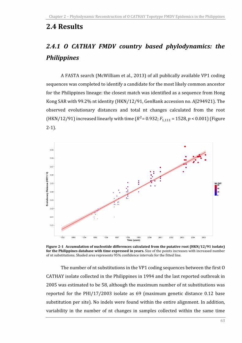
Chapter 2 – Phylodynamic Reconstruction of O CATHAY Topotype FMDV Epidemics in the Philippines
63
2.4 Results
2.4.1 O CATHAY FMDV country based phylodynamics: the
Philippines
A FASTA search (McWilliam et al., 2013) of all publically available VP1 coding
sequences was completed to identify a candidate for the most likely common ancestor
for the Philippines lineage: the closest match was identified as a sequence from Hong
Kong SAR with 99.2% nt identity (HKN/12/91, GenBank accession no. AJ294921). The
observed evolutionary distances and total nt changes calculated from the root
(HKN/12/91) increased linearly with time (𝑅2= 0.932; 𝐹1,111 = 1528, 𝑝 < 0.001) (Figure
2-1).
Figure 2-1 Accumulation of nucleotide differences calculated from the putative root (HKN/12/91 isolate) for the Philippines database with time expressed in years. Size of the points increases with increased number of nt substitutions. Shaded area represents 95% confidence intervals for the fitted line.
The number of nt substitutions in the VP1 coding sequences between the first O
CATHAY isolate collected in the Philippines in 1994 and the last reported outbreak in
2005 was estimated to be 58, although the maximum number of nt substitutions was
reported for the PHI/17/2003 isolate as 69 (maximum genetic distance 0.12 base
substitution per site). No indels were found within the entire alignment. In addition,
variability in the number of nt changes in samples collected within the same time
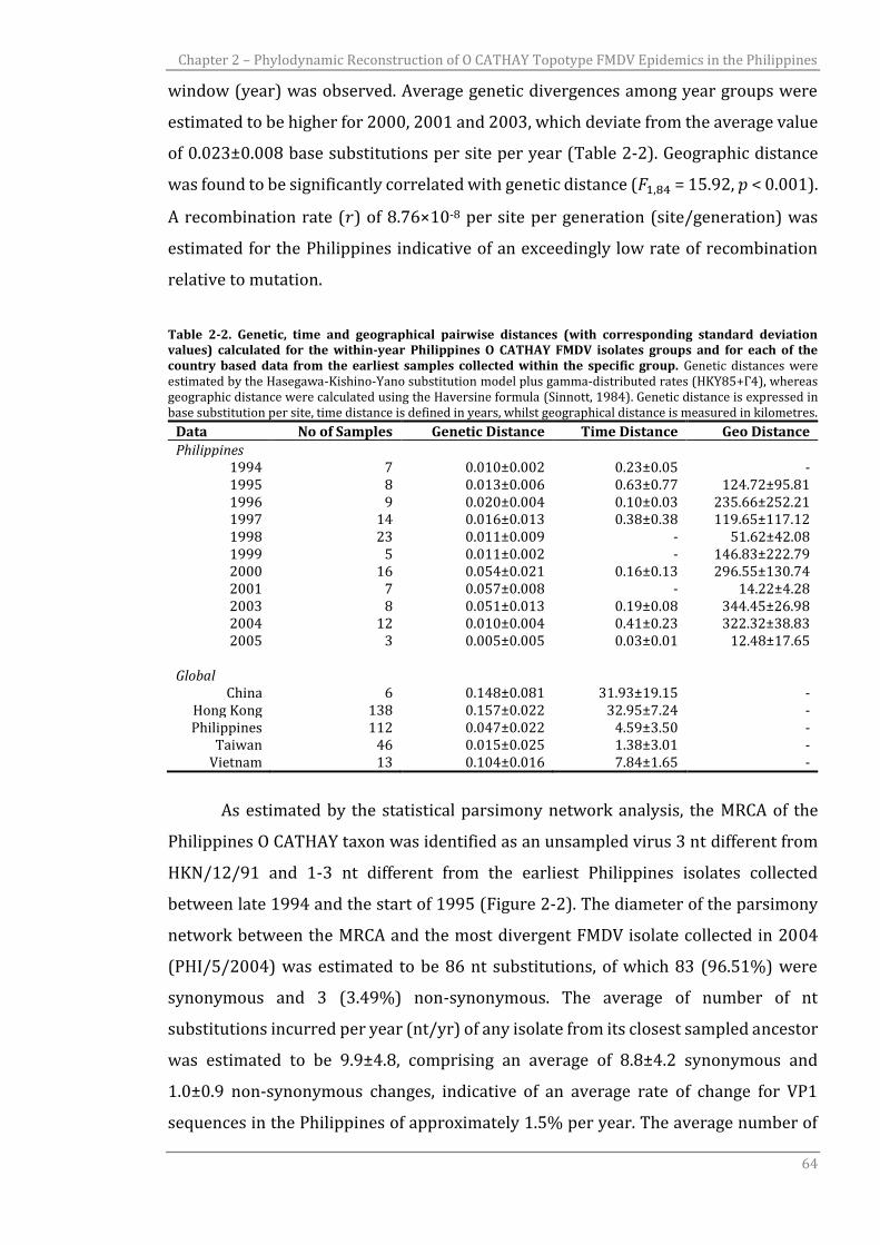
Chapter 2 – Phylodynamic Reconstruction of O CATHAY Topotype FMDV Epidemics in the Philippines
64
window (year) was observed. Average genetic divergences among year groups were
estimated to be higher for 2000, 2001 and 2003, which deviate from the average value
of 0.023±0.008 base substitutions per site per year (Table 2-2). Geographic distance
was found to be significantly correlated with genetic distance (𝐹1,84 = 15.92, 𝑝 < 0.001).
A recombination rate (𝑟) of 8.76×10⁻⁸ per site per generation (site/generation) was
estimated for the Philippines indicative of an exceedingly low rate of recombination
relative to mutation.
Table 2-2. Genetic, time and geographical pairwise distances (with corresponding standard deviation values) calculated for the within-year Philippines O CATHAY FMDV isolates groups and for each of the country based data from the earliest samples collected within the specific group. Genetic distances were estimated by the Hasegawa-Kishino-Yano substitution model plus gamma-distributed rates (HKY85+Γ4), whereas geographic distance were calculated using the Haversine formula (Sinnott, 1984). Genetic distance is expressed in base substitution per site, time distance is defined in years, whilst geographical distance is measured in kilometres.
Data No of Samples Genetic Distance Time Distance Geo Distance
Philippines 1994 7 0.010±0.002 0.23±0.05 - 1995 8 0.013±0.006 0.63±0.77 124.72±95.81 1996 9 0.020±0.004 0.10±0.03 235.66±252.21 1997 14 0.016±0.013 0.38±0.38 119.65±117.12 1998 23 0.011±0.009 - 51.62±42.08 1999 5 0.011±0.002 - 146.83±222.79 2000 16 0.054±0.021 0.16±0.13 296.55±130.74 2001 7 0.057±0.008 - 14.22±4.28 2003 8 0.051±0.013 0.19±0.08 344.45±26.98 2004 12 0.010±0.004 0.41±0.23 322.32±38.83 2005 3 0.005±0.005 0.03±0.01 12.48±17.65
Global
China 6 0.148±0.081 31.93±19.15 - Hong Kong 138 0.157±0.022 32.95±7.24 - Philippines 112 0.047±0.022 4.59±3.50 -
Taiwan 46 0.015±0.025 1.38±3.01 - Vietnam 13 0.104±0.016 7.84±1.65 -
As estimated by the statistical parsimony network analysis, the MRCA of the
Philippines O CATHAY taxon was identified as an unsampled virus 3 nt different from
HKN/12/91 and 1-3 nt different from the earliest Philippines isolates collected
between late 1994 and the start of 1995 (Figure 2-2). The diameter of the parsimony
network between the MRCA and the most divergent FMDV isolate collected in 2004
(PHI/5/2004) was estimated to be 86 nt substitutions, of which 83 (96.51%) were
synonymous and 3 (3.49%) non-synonymous. The average of number of nt
substitutions incurred per year (nt/yr) of any isolate from its closest sampled ancestor
was estimated to be 9.9±4.8, comprising an average of 8.8±4.2 synonymous and
1.0±0.9 non-synonymous changes, indicative of an average rate of change for VP1
sequences in the Philippines of approximately 1.5% per year. The average number of
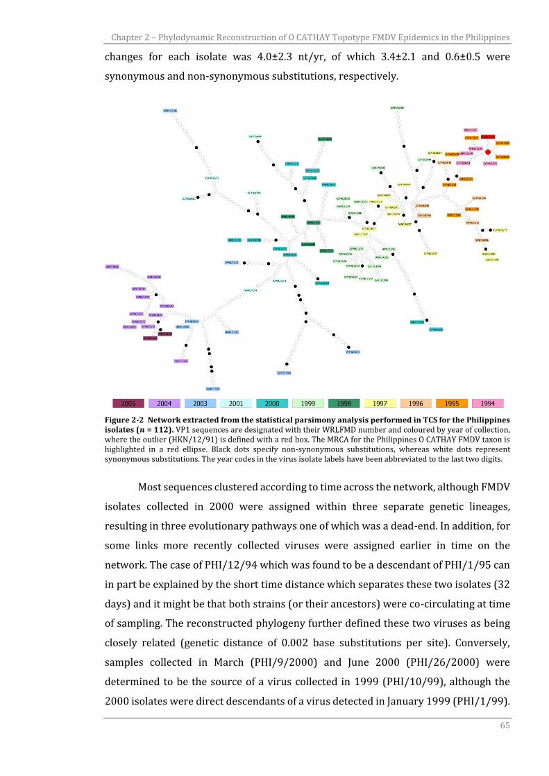
Chapter 2 – Phylodynamic Reconstruction of O CATHAY Topotype FMDV Epidemics in the Philippines
65
changes for each isolate was 4.0±2.3 nt/yr, of which 3.4±2.1 and 0.6±0.5 were
synonymous and non-synonymous substitutions, respectively.
Figure 2-2 Network extracted from the statistical parsimony analysis performed in TCS for the Philippines isolates (𝒏 = 112). VP1 sequences are designated with their WRLFMD number and coloured by year of collection, where the outlier (HKN/12/91) is defined with a red box. The MRCA for the Philippines O CATHAY FMDV taxon is highlighted in a red ellipse. Black dots specify non-synonymous substitutions, whereas white dots represent synonymous substitutions. The year codes in the virus isolate labels have been abbreviated to the last two digits.
Most sequences clustered according to time across the network, although FMDV
isolates collected in 2000 were assigned within three separate genetic lineages,
resulting in three evolutionary pathways one of which was a dead-end. In addition, for
some links more recently collected viruses were assigned earlier in time on the
network. The case of PHI/12/94 which was found to be a descendant of PHI/1/95 can
in part be explained by the short time distance which separates these two isolates (32
days) and it might be that both strains (or their ancestors) were co-circulating at time
of sampling. The reconstructed phylogeny further defined these two viruses as being
closely related (genetic distance of 0.002 base substitutions per site). Conversely,
samples collected in March (PHI/9/2000) and June 2000 (PHI/26/2000) were
determined to be the source of a virus collected in 1999 (PHI/10/99), although the
2000 isolates were direct descendants of a virus detected in January 1999 (PHI/1/99).
Chapter 2 – Phylodynamic Reconstruction of O CATHAY Topotype FMDV Epidemics in the Philippines
66
Looking in detail at this case, the phylogeny found descent of PHI/10/99, PHI/9/2000
and PHI/26/2000 from the same common ancestor. These samples were collected
from the same region (Central Luzon) within an area of ~40 km of radius, potentially
explaining the inconsistent result provided by the TCS analysis to have arisen from
sampling bias. The discrete states analysis resolved the relationship of the PHI/10/99,
PHI/9/2000 and PHI/26/2000 isolates rooting those from a common ancestor that
descends in turn from an unsampled virus source both seeded from Bulacan Province,
which includes the PHI/1/99 sample (Figure 2-3).
Figure 2-3 Phylodynamic reconstruction of the O CATHAY FMDV epidemics in the Philippines. Maximum clade credibility tree branches are coloured according to the most likely transmission source as reconstructed from the discrete states model. Nodes with a posterior probability value ≥0.7 are shown. FMDV demography is expressed by log Effective Population Size (𝑁𝑒𝜏) as estimated from the BSP along with the monthly epidemic curve reconstructed from the data retrieved from the OIE Handistatus II database (OIE, 2014).
The molecular clock for the O CATHAY Philippines lineage was estimated to be
1.25×10⁻² nt/site/yr (95%HPD 9.47×10⁻³ to 1.57×10⁻²) with a standard deviation of
0.70 (95%HPD 0.49 to 0.91). No evidence of autocorrelation of rates in the
reconstructed phylogeny was provided by the covariance value of 2.65×10⁻³. The
introduction date, the TMRCA, of the type O CATHAY topotype FMDV lineage into the
Philippines was calculated to be the 30th of March 1994 (95%HPD 07/08/1993 to
08/08/1994, a time interval which included the date of the first officially reported
case).
Chapter 2 – Phylodynamic Reconstruction of O CATHAY Topotype FMDV Epidemics in the Philippines
67
The reconstructed FMDV population dynamics from the skyline plot (Figure 2-
3) describes a demographic history characterised by three phases. In the first phase,
after an initial exponential increase from mid-1994 until late 1997 at a rate that
decreased from late 1996, a sudden and short period of decline was observed, resulting
in a population bottleneck. Since genetic bottlenecks correspond to significant
reductions in population size, these changes in the O CATHAY population dynamics in
the Philippines probably link to the launch of an extensive control plan in 1996 that
was successful in limiting the further spread of FMD and thereby reducing the number
of outbreaks (Randolph et al., 2002). However, during 1999 a new FMD outbreak
occurred within an already declared FMD-free zone, the Panay region. Therefore in the
second phase, the skyline trajectory recorded a second rapidly increasing viral
population size starting in mid-1998 and lasting up to the first months of 1999, which
resulted in a diversification of viral lineages. In the third phase, the viral population
size reached a plateau until late 2002, when further control policies resulted in a steady
decline in FMD prevalence until eradication.
The epidemic curve drawn from the field epidemiological data from the OIE for
the period 1995-2005 (OIE, 2014) described an oscillatory trend in the number of FMD
outbreaks reported in the Philippines, with times of high epidemic peaks interleaved
by low-level FMD circulation. The frequency of these oscillations was higher between
1997 and the beginning of 2000 (a monthly average of 37.9 FMD outbreaks), after
which the number of FMD outbreaks started to decline following periods of low
reporting (with a monthly average of 19.8 FMD outbreaks). However, the reported
epidemic trend did not overlap with the skyline plot trajectory, although the epidemic
window from mid-2000 to 2005 characterised by a reduced number of outbreaks could
be evinced by the plateauing and subsequent decrease in the genetic diversity of the
skyline plot. It should be noted that although more than 300 outbreaks were officially
reported through OIE during 2002, no clinical samples (and thus genetic information)
were collected within that time window.
According to the results obtained by the discrete states phylogeography
analysis, the root of the Philippines taxon was found to be from Rizal Province,
consistent with the location of the first officially reported cases of O CATHAY topotype
in the Philippines during August 1994 (Figure 2-3). Three main epidemic hubs could
be identified from the analysis: the first from the beginning of the epizootic up to mid-
1996, where outbreaks were found to be seeded from Rizal Province; the second
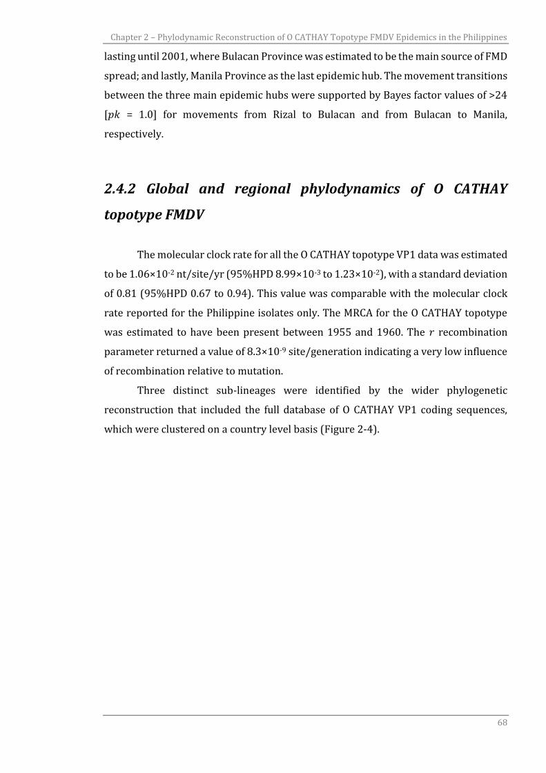
Chapter 2 – Phylodynamic Reconstruction of O CATHAY Topotype FMDV Epidemics in the Philippines
68
lasting until 2001, where Bulacan Province was estimated to be the main source of FMD
spread; and lastly, Manila Province as the last epidemic hub. The movement transitions
between the three main epidemic hubs were supported by Bayes factor values of >24
[𝑝𝑘 = 1.0] for movements from Rizal to Bulacan and from Bulacan to Manila,
respectively.
2.4.2 Global and regional phylodynamics of O CATHAY
topotype FMDV
The molecular clock rate for all the O CATHAY topotype VP1 data was estimated
to be 1.06×10⁻² nt/site/yr (95%HPD 8.99×10⁻³ to 1.23×10⁻²), with a standard deviation
of 0.81 (95%HPD 0.67 to 0.94). This value was comparable with the molecular clock
rate reported for the Philippine isolates only. The MRCA for the O CATHAY topotype
was estimated to have been present between 1955 and 1960. The 𝑟 recombination
parameter returned a value of 8.3×10⁻⁹ site/generation indicating a very low influence
of recombination relative to mutation.
Three distinct sub-lineages were identified by the wider phylogenetic
reconstruction that included the full database of O CATHAY VP1 coding sequences,
which were clustered on a country level basis (Figure 2-4).

Chapter 2 – Phylodynamic Reconstruction of O CATHAY Topotype FMDV Epidemics in the Philippines
69
Figure 2-4 Maximum clade credibility tree for all the O CATHAY FMDV isolates sequenced (𝒏 = 322). Nodes with a posterior probability value ≥0.7 are shown. Branches are coloured according to the most probable country of the node from which they descended as estimated from the discrete state phylogeographic Bayesian model. Geographical links between countries identified by the BSSVS analysis are coloured by the corresponding BF value. The year codes in virus isolate labels have been abbreviated to the last two digits. The geographical locations are defined with the country centroid.

Chapter 2 – Phylodynamic Reconstruction of O CATHAY Topotype FMDV Epidemics in the Philippines
70
The FMDV strains circulating in the Philippines were found to have descended
from a common ancestor that was shared with the Taiwanese isolates, in line with what
was proposed to be the source of introduction of the O CATHAY virus into the
Philippines in 1994 (Knowles et al., 2005). In turn, the Taiwanese cluster descended
from an unsampled virus closely related to a FMDV isolate collected from China in
2000. The Hong Kong SAR isolates were defined in a separate phylogenetic cluster
along with FMDV samples collected from countries in mainland Southeast Asia
(Malaysia, Thailand and Vietnam). This finding is in contrast to that previously
reported (Hui and Leung, 2012), which designated the Taiwanese lineages descending
from a common ancestor with the Hong Kong SAR isolates, and identified the
Philippines lineages as a distinct phylogenetic cluster. Hui and Leung (2012) inferred
the phylogenetic relationship employing a Neighbor-joining method; nevertheless,
estimating the phylogeny using a maximum-likelihood method (Guindon et al., 2010)
did not alter the shape of the reconstructed phylogeny [data not shown]. The three
phylogenetic clusters shared a common ancestor related to a FMDV strain collected in
Hong Kong SAR in 1991 (HKN/12/91), which was in turn a descendent from other
Hong Kong SAR isolates related to more recent samples obtained from Russia (1995),
Hong Kong SAR (1996) and China (2003). FMDV isolates collected from countries of
mainland Southeast Asia were phylogenetically grouped into two distinct clusters: the
first (MRCA dated 1997) including the first O CATHAY virus isolate from Vietnam in
1997 from which viruses were collected in 2005-06 and 2008, and the only isolate from
Malaysia (2005) was sourced; the second (MRCA dated 1998) associated with a later
introduction of an O CATHAY strain in Vietnam in 2002, from which viruses isolated in
2004-05, and FMDV sequences from Thailand (2005) were related. The FMDV ancestor
of the first mainland Southeast Asia sublineage was dated circa mid-1993, directly
descending from the oldest MRCA of the Hong Kong SAR cluster, whereas the second
sublineage was circulating in late 1998 and closely related to a virus collected in Hong
Kong SAR in 2002. This phylogenetic picture supports two potential introductions of
the O CATHAY FMDV lineage into Vietnam from Hong Kong SAR.
The MRCA shared between the Philippines and Taiwanese phylogenetic clusters
was estimated to have been circulating in 1993 (95%HPD 1992 to 1994), whereas the
origin of the MRCA for the more recent O CATHAY FMD epidemics in the Southeast and
East Asia regions was dated 1991 (95%HPD 1990 to 1992). No other virus introduction
or escape was ascribed to the Philippines O CATHAY FMD epidemic history, suggesting

Chapter 2 – Phylodynamic Reconstruction of O CATHAY Topotype FMDV Epidemics in the Philippines
71
the Philippines sub-lineage to be monophyletic. In contrast, Hui and Leung (2012)
described two different FMDV introductions into the Philippines, assigning the
PHI/5/95 isolates within the phylogenetic cluster which includes the Taiwanese
isolates. However, the tree node that governed this inclusion had a bootstrap value of
<70, suggesting uncertainty in the assignment of these descendants.
As estimated by the discrete phylogeography model, the root of the entire
phylogenetic tree was reported to be in Hong Kong SAR and, therefore, representing a
likely source for the introduction of the O CATHAY lineage into the Philippines and
Taiwan. This is confirmed by the estimated BSSVS parameters, for which China and
Hong Kong SAR were assessed as the main hubs of FMDV spread between countries
(Figure 2-4): China was found to be the source for Hong Kong SAR (BF = 5.6, 𝑝𝑘 = 0.60),
Taiwan (BF = 5.07, 𝑝𝑘 = 0.58) and Russia (BF = 4.33, 𝑝𝑘 = 0.54), whilst Hong Kong SAR
was identified as the source of FMD transmission to Vietnam (BF = 6.75, 𝑝𝑘 = 0.65) and
the Philippines (BF = 3.16, 𝑝𝑘 = 0.46). The link found between China and Russia
reinforces the hypothesis that Chinese pork shipments were responsible for the
introduction of the O CATHAY lineage into Moscow, Russia during 1995 [6]. Vietnam
was estimated as a recipient of viruses moving from Malaysia (BF = 23.25, 𝑝𝑘 = 0.86),
Thailand (BF = 12.55, 𝑝𝑘 = 0.77) and Hong Kong SAR (BF = 6.75, 𝑝𝑘 = 0.65). The most
likely routes of chronological introduction of the FMDV O CATHAY lineage into Europe
were identified to be from Hong Kong SAR to Austria (BF = 3.14, 𝑝𝑘 = 0.27). The virus
movement within Europe has been identified from Austria to Germany (BF = 5.15, 𝑝𝑘
= 0.58). Thus supported by the Bayesian phylogenetic and BSSVS analyses, the
historical movement of the FMDV type O CATHAY lineage across Asia might be
temporally and spatially reconstructed as represented in Figure 2-6.
The historical phylodynamics of the FMDV O CATHAY lineage, as reconstructed
by the skyline model using the full currently available VP1 coding sequences database
(Figure 2-5), underwent three distinct and chronologically consequent evolutionary
stages.
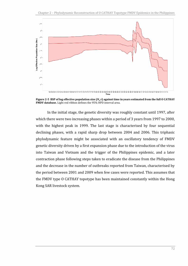
Chapter 2 – Phylodynamic Reconstruction of O CATHAY Topotype FMDV Epidemics in the Philippines
72
Figure 2-5 BSP of log effective population size (𝑵𝒆𝝉) against time in years estimated from the full O CATHAY FMDV database. Light red ribbon defines the 95% HPD interval area.
In the initial stage, the genetic diversity was roughly constant until 1997, after
which there were two increasing phases within a period of 3 years from 1997 to 2000,
with the highest peak in 1999. The last stage is characterised by four sequential
declining phases, with a rapid sharp drop between 2004 and 2006. This triphasic
phylodynamic feature might be associated with an oscillatory tendency of FMDV
genetic diversity driven by a first expansion phase due to the introduction of the virus
into Taiwan and Vietnam and the trigger of the Philippines epidemic, and a later
contraction phase following steps taken to eradicate the disease from the Philippines
and the decrease in the number of outbreaks reported from Taiwan, characterised by
the period between 2001 and 2009 when few cases were reported. This assumes that
the FMDV type O CATHAY topotype has been maintained constantly within the Hong
Kong SAR livestock system.
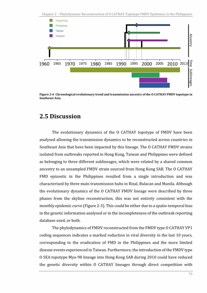
Chapter 2 – Phylodynamic Reconstruction of O CATHAY Topotype FMDV Epidemics in the Philippines
73
Figure 2-6 Chronological evolutionary trend and transmission ancestry of the O CATHAY FMDV topotype in Southeast Asia.
2.5 Discussion
The evolutionary dynamics of the O CATHAY topotype of FMDV have been
analysed allowing the transmission dynamics to be reconstructed across countries in
Southeast Asia that have been impacted by this lineage. The O CATHAY FMDV strains
isolated from outbreaks reported in Hong Kong, Taiwan and Philippines were defined
as belonging to three different sublineages, which were related by a shared common
ancestry to an unsampled FMDV strain sourced from Hong Kong SAR. The O CATHAY
FMD epizootic in the Philippines resulted from a single introduction and was
characterised by three main transmission hubs in Rizal, Bulacan and Manila. Although
the evolutionary dynamics of the O CATHAY FMDV lineage were described by three
phases from the skyline reconstruction, this was not entirely consistent with the
monthly epidemic curve (Figure 2-3). This could be either due to a spatio-temporal bias
in the genetic information analysed or in the incompleteness of the outbreak reporting
database used, or both.
The phylodynamics of FMDV reconstructed from the FMDV type O CATHAY VP1
coding sequences indicates a marked reduction in viral diversity in the last 10 years,
corresponding to the eradication of FMD in the Philippines and the more limited
disease events experienced in Taiwan. Furthermore, the introduction of the FMDV type
O SEA topotype Mya-98 lineage into Hong Kong SAR during 2010 could have reduced
the genetic diversity within O CATHAY lineages through direct competition with
Chapter 2 – Phylodynamic Reconstruction of O CATHAY Topotype FMDV Epidemics in the Philippines
74
available hosts, as well as the presence of cross-protective antibodies in convalescent
animals. These findings indicate that the O CATHAY topotype is maintained in the Hong
Kong SAR ecosystem and sporadically spread from there to other Southeast Asian
countries, as would be the case for the Philippines in 1994 and Vietnam in 1997.
However, few O CATHAY FMDV strains have been reported from mainland China,
which has the largest swine production industry in the world (representing over 51%
of the world’s pig population). These few isolates were collected in 1986, 2000, 2001
and 2003, therefore sampling bias or underreporting of epidemic events occurring in
China would likely have an impact on assessing the geographical movements of the
FMDV type O CATHAY topotype. It is, nevertheless, clear from the analysis that a
transmission link exists between China and Hong Kong SAR, thus indicating a
historically southward movement of the O CATHAY FMDV lineage.
The molecular clock estimated here for the O CATHAY topotype is at the high
end of evolutionary rate estimates for FMDV. Previously estimates reported an average
evolutionary rate across all FMDV serotype of 2.48×10⁻³ nt/site/yr (Tully and Fares,
2008), while rates of 3.14×10⁻³, 1.3×10⁻³ and 4.8×10⁻³ nt/site/yr were reported for
serotype O (Tully and Fares, 2008, Yoon et al., 2011a, Jenkins et al., 2002). In addition,
lineage-based FMDV molecular clock rates of 2.8×10⁻³, 6.65×10⁻³, 7.81×10⁻³ and
2.7×10⁻³ nt/site/yr were previously estimated for the O-PanAsia lineage in India, O-
PanAsia-2 sublineage in Pakistan and Afghanistan, and type O in East Africa,
respectively (Balinda et al., 2010a, Hemadri et al., 2002, Jamal et al., 2011a). The higher
rate of FMDV evolution reported for the A Iran-05 FMDV lineage in Afghanistan and
Pakistan (1.2×10⁻² nt/site/yr) (Jamal et al., 2011c) was similar to the molecular clock
for the O CATHAY topotype estimated by this study. Therefore, genotypically and
regionally variable evolutionary rates may in fact reflect real differences in the
epidemiological dynamics and host-interaction of FMDV.
Although using a large database of FMDV isolates and generating a
comprehensive picture of the O CATHAY topotype evolutionary history, this study has
some limitations largely derived from the nature of the genetic data used for the
analysis. The VP1 coding region, although defining only ~8% (639 nt of length) of the
complete FMDV genome, is the most variable section of the FMDV genome and is
historically used for tracing the movement and spread of FMD globally (Knowles and
Samuel, 2003, Samuel and Knowles, 2001) and, furthermore, provides the basis for
FMDV genotype definition (Knowles et al., 2010a). Analysing a larger part of the FMDV

Chapter 2 – Phylodynamic Reconstruction of O CATHAY Topotype FMDV Epidemics in the Philippines
75
genome, such as the whole capsid region or the full-length genome, would produce
results with a higher resolution (Cottam et al., 2006, Cottam et al., 2008b). However, it
should be noted that recombination events seem to be more widespread in other part
of the genome (Carrillo et al., 2005, Jackson et al., 2007, Wright et al., 2013), thus
representing a limitation in interpreting results based on full-length genome analysis
of large scale FMDV evolutionary studies. The ratio of per-site recombination to
mutation rate here estimated from the full currently available FMDV type O CATHAY
topotype VP1 coding sequences database is very low indicating that these results are
not influenced by the process of recombination.

77
CHAPTER 3
A model framework for simulating space-time
epidemiological and genetic data
3.1 Rationale
As reviewed in Chapter 1, an extensive literature has been devoted to the topic
of phylodynamics for linking the population genetic concept of effective population size
𝑁𝑒 with the evolutionary dynamics of virus transmission in space and time. However,
studies published on this topic had rather limited focus on trying to disentangle the
relationship of 𝑁𝑒 with the actual number of infected cases. In addition, no studies have
endeavoured to compare viral population dynamics derived from genetic sequences
with empirical data observed from a completely sampled large epidemic where either
prevalence or incidence are accurately observed through time. One exceptional
example of a fully-resolved real disease epidemic is the UK 2001 FMD event, which is
currently the largest and most completely sampled virus disease epidemic. To study
the relationship between the dynamics as reconstructed from viral sequences and the
actual count of infected cases over time, a thorough investigation of the fully-resolved
UK 2001 FMD epidemic making use of the epidemiological data extracted at the time
from the field outbreak investigation was undertaken. As discussed in §1.3, the genetic
component of the epidemic was fully simulated for the entire epidemic using an
evolutionary model parameterised from the 39 already characterised sequence data
(Cottam et al., 2006, Cottam et al., 2008a, Konig et al., 2009). In order to generate a
complete epidemiological and genetic dataset in which prevalence, incidence and WGS
are linked to the fully-resolved transmission tree, a model framework has been built
for:
Reconstructing the transmission tree underlying the UK 2001 FMD epidemic
using the epidemiological data and, therefore, providing a who-infected-who
transmission network;
Chapter 3 – A Model Framework for Simulating Space-Time Epidemiological and Genetic Data
78
Using the transmission tree as a backbone for simulating an FMDV WGS for
each IP generated from a Markovian evolutionary model informed with data
extracted from prior FMDV genetic analyses;
Estimating the virus demographic history from the simulated WGS using the
BSP and comparing this with the empirical prevalence and incidence data
extracted from the UK 2001 FMD epidemiological data.
The model framework here described constitutes the mainstay algorithm for
generating the WGS data that will be used in subsequent chapters for investigating in
detail the influence of sampling and population structure in the relationship between
reconstructed demographic history from sequence data and the actual count of
infected cases, and its scaling formulations.
3.2 Model Framework
3.2.1 Data
The FMD epidemic affecting the UK in 2001, was caused by a virus belonging to
the FMDV type O PanAsia lineage (Knowles et al., 2001b), and 2026 farms were
confirmed at the time of the epidemic event as IPs. The introduction of FMDV into UK
has been attributed to the illegal importation of infected or contaminated meat or meat
products which were consumed as swill feed to pigs reared at Burnside Farm, Heddon-
on-the-Wall (IP04) (DEFRA, 2002). The movement of the pigs from IP04 to the Essex
abattoir (IP01) was the trigger and spread of the first phase of the epidemic in Essex
and Kent, which started on the 19th of February (Gibbens et al., 2001). A second phase
of the epidemic that was country wide was attributed to the airborne spread of FMDV
from IP04 to sheep at Prestwick Hall Farm, Callerton (IP06), from where infected sheep
were moved and sold in markets located in Hexham (Northumberland) and Longtown
(Cumbria) thus resulting in the dissemination of the disease in multiple clusters
throughout England and Wales (Gloster et al., 2005, Konig et al., 2009). In order to
control the outbreak, a national ban on animal movements along with the culling of all
susceptible animals on confirmed IPs and Direct Contacts (DCs) was introduced on the
23rd of February; thereafter, the control (‘stamping out’) measures were intensified
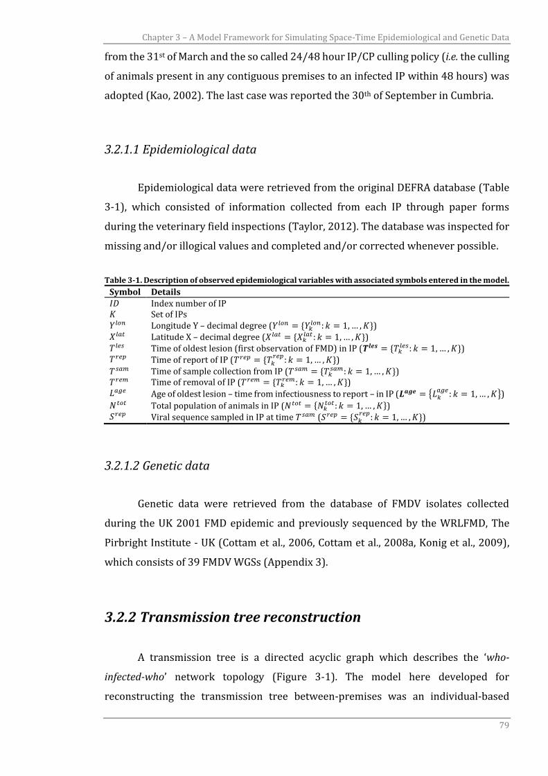
Chapter 3 – A Model Framework for Simulating Space-Time Epidemiological and Genetic Data
79
from the 31st of March and the so called 24/48 hour IP/CP culling policy (i.e. the culling
of animals present in any contiguous premises to an infected IP within 48 hours) was
adopted (Kao, 2002). The last case was reported the 30th of September in Cumbria.
3.2.1.1 Epidemiological data
Epidemiological data were retrieved from the original DEFRA database (Table
3-1), which consisted of information collected from each IP through paper forms
during the veterinary field inspections (Taylor, 2012). The database was inspected for
missing and/or illogical values and completed and/or corrected whenever possible.
Table 3-1. Description of observed epidemiological variables with associated symbols entered in the model.
Symbol Details 𝐼𝐷 Index number of IP 𝐾 Set of IPs 𝑌𝑙𝑜𝑛 Longitude Y – decimal degree (𝑌𝑙𝑜𝑛 = {𝑌𝑘
𝑙𝑜𝑛: 𝑘 = 1, … , 𝐾}) 𝑋𝑙𝑎𝑡 Latitude X – decimal degree (𝑋𝑙𝑎𝑡 = {𝑋𝑘
𝑙𝑎𝑡: 𝑘 = 1, … , 𝐾}) 𝑇𝑙𝑒𝑠 Time of oldest lesion (first observation of FMD) in IP (𝑻𝒍𝒆𝒔 = {𝑇𝑘
𝑙𝑒𝑠: 𝑘 = 1, … , 𝐾}) 𝑇𝑟𝑒𝑝 Time of report of IP (𝑇𝑟𝑒𝑝 = {𝑇𝑘
𝑟𝑒𝑝: 𝑘 = 1, … , 𝐾})
𝑇𝑠𝑎𝑚 Time of sample collection from IP (𝑇𝑠𝑎𝑚 = {𝑇𝑘𝑠𝑎𝑚: 𝑘 = 1, … , 𝐾})
𝑇𝑟𝑒𝑚 Time of removal of IP (𝑇𝑟𝑒𝑚 = {𝑇𝑘𝑟𝑒𝑚: 𝑘 = 1, … , 𝐾})
𝐿𝑎𝑔𝑒 Age of oldest lesion – time from infectiousness to report – in IP (𝑳𝒂𝒈𝒆 = {𝐿𝑘𝑎𝑔𝑒
: 𝑘 = 1, … , 𝐾})
𝑁𝑡𝑜𝑡 Total population of animals in IP (𝑁𝑡𝑜𝑡 = {𝑁𝑘𝑡𝑜𝑡: 𝑘 = 1, … , 𝐾})
𝑆𝑟𝑒𝑝 Viral sequence sampled in IP at time 𝑇𝑠𝑎𝑚 (𝑆𝑟𝑒𝑝 = {𝑆𝑘𝑟𝑒𝑝
: 𝑘 = 1, … , 𝐾})
3.2.1.2 Genetic data
Genetic data were retrieved from the database of FMDV isolates collected
during the UK 2001 FMD epidemic and previously sequenced by the WRLFMD, The
Pirbright Institute - UK (Cottam et al., 2006, Cottam et al., 2008a, Konig et al., 2009),
which consists of 39 FMDV WGSs (Appendix 3).
3.2.2 Transmission tree reconstruction
A transmission tree is a directed acyclic graph which describes the ‘who-
infected-who’ network topology (Figure 3-1). The model here developed for
reconstructing the transmission tree between-premises was an individual-based
Chapter 3 – A Model Framework for Simulating Space-Time Epidemiological and Genetic Data
80
model of disease transmission, which provided a representation of the FMD infection
dynamics that takes into account the timing and location of cases (Figure 3-1), and was
constructed on a farm level (i.e. farms are considered as single epidemiological units),
therefore omitting the potential impact of within-farm epidemic dynamics. Hence, for
the purposes of these models it was assumed that FMD spread within a farm is
instantaneous with all the animals that contribute to the transmission network
becoming infected and subsequently infectious together. In addition, this model
considered a single homogeneous virus population that was introduced on to each new
farm and, following possible mutation, a single homogenous virus population
transmitted onward. All but one premises started as susceptible, where the first
infected premises is assumed to have been infected from an external source. FMD has
a staged progression in time and, therefore, can be represented in a series of successive
disease stages. These stages can be described as infected, infectious, reported and
removed. Consider a set of 𝐾 infected premises and let 𝐽 be a function defining the
transmission tree, a premise 𝑘 at location (𝑋𝑘𝑙𝑎𝑡, 𝑌𝑘
𝑙𝑜𝑛) is infected at time 𝑇𝑘𝑒𝑥𝑝 by a
source 𝑖. Following a latency period 𝑇𝑘𝑙𝑎𝑡, 𝑘 becomes infectious at time 𝑇𝑘
𝑙𝑒𝑠 (the time at
which the oldest lesion would have first become apparent), is reported at time 𝑇𝑘𝑟𝑒𝑝,
and is removed from the susceptible population at time 𝑇𝑘𝑟𝑒𝑚. During the reporting of
IP 𝑘, the interval between becoming infectious and reporting is assessed in the field by
experts based on the ageing of the oldest clinical lesion 𝐿𝑘𝑎𝑔𝑒
observed on the premise.
The clinical sample is collected at time 𝑇𝑘𝑠𝑎𝑚, thus, also defining the time a viral
sequence 𝑆𝑘𝑟𝑒𝑝 is obtained.
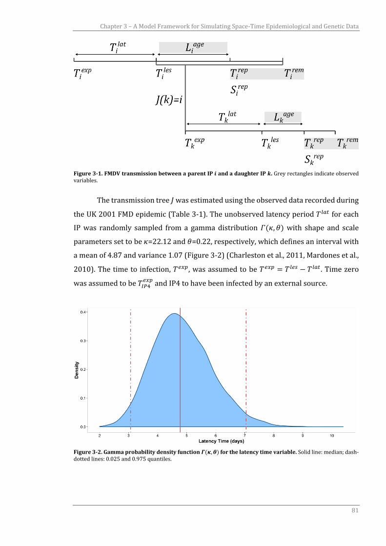
Chapter 3 – A Model Framework for Simulating Space-Time Epidemiological and Genetic Data
81
Figure 3-1. FMDV transmission between a parent IP 𝒊 and a daughter IP 𝒌. Grey rectangles indicate observed variables.
The transmission tree 𝐽 was estimated using the observed data recorded during
the UK 2001 FMD epidemic (Table 3-1). The unobserved latency period 𝑇𝑙𝑎𝑡 for each
IP was randomly sampled from a gamma distribution 𝛤(𝜅, 𝜃) with shape and scale
parameters set to be 𝜅=22.12 and 𝜃=0.22, respectively, which defines an interval with
a mean of 4.87 and variance 1.07 (Figure 3-2) (Charleston et al., 2011, Mardones et al.,
2010). The time to infection, 𝑇𝑒𝑥𝑝, was assumed to be 𝑇𝑒𝑥𝑝 = 𝑇𝑙𝑒𝑠 − 𝑇𝑙𝑎𝑡. Time zero
was assumed to be 𝑇𝐼𝑃4𝑒𝑥𝑝 and IP4 to have been infected by an external source.
Figure 3-2. Gamma probability density function 𝜞(𝜿, 𝜽) for the latency time variable. Solid line: median; dash-dotted lines: 0.025 and 0.975 quantiles.
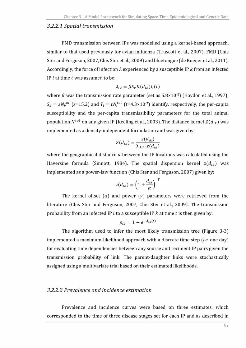
Chapter 3 – A Model Framework for Simulating Space-Time Epidemiological and Genetic Data
82
3.2.2.1 Spatial transmission
FMD transmission between IPs was modelled using a kernel-based approach,
similar to that used previously for avian influenza (Truscott et al., 2007), FMD (Chis
Ster and Ferguson, 2007, Chis Ster et al., 2009) and bluetongue (de Koeijer et al., 2011).
Accordingly, the force of infection 𝜆 experienced by a susceptible IP 𝑘 from an infected
IP 𝑖 at time 𝑡 was assumed to be:
𝜆𝑖𝑘 = 𝛽𝑆𝑘𝐾(𝑑𝑖𝑘)𝐼𝑖(𝑡)
where 𝛽 was the transmission rate parameter (set as 5.8×10⁻⁵) (Haydon et al., 1997);
𝑆𝑘 = 𝑠𝑁𝑘𝑡𝑜𝑡 (𝑠=15.2) and 𝑇𝑖 = 𝑡𝑁𝑖
𝑡𝑜𝑡 (𝑡=4.3×10⁻⁷) identify, respectively, the per-capita
susceptibility and the per-capita transmissibility parameters for the total animal
population 𝑁𝑡𝑜𝑡 on any given IP (Keeling et al., 2003). The distance kernel 𝑍(𝑑𝑖𝑘) was
implemented as a density-independent formulation and was given by:
𝑍(𝑑𝑖𝑘) =𝑧(𝑑𝑖𝑘)
∑ 𝑧(𝑑𝑖𝑘)𝑘≠𝑖
where the geographical distance 𝑑 between the IP locations was calculated using the
Haversine formula (Sinnott, 1984). The spatial dispersion kernel 𝑧(𝑑𝑖𝑘) was
implemented as a power-law function (Chis Ster and Ferguson, 2007) given by:
𝑧(𝑑𝑖𝑘) = (1 +𝑑𝑖𝑘
𝛼)
−𝛾
The kernel offset (𝛼) and power (𝛾) parameters were retrieved from the
literature (Chis Ster and Ferguson, 2007, Chis Ster et al., 2009). The transmission
probability from an infected IP 𝑖 to a susceptible IP 𝑘 at time 𝑡 is then given by:
𝑝𝑖𝑘 = 1 − 𝑒−𝜆𝑖𝑘(𝑡)
The algorithm used to infer the most likely transmission tree (Figure 3-3)
implemented a maximum-likelihood approach with a discrete time step (i.e. one day)
for evaluating time dependencies between any source and recipient IP pairs given the
transmission probability of link. The parent-daughter links were stochastically
assigned using a multivariate trial based on their estimated likelihoods.
3.2.2.2 Prevalence and incidence estimation
Prevalence and incidence curves were based on three estimates, which
corresponded to the time of three disease stages set for each IP and as described in
Chapter 3 – A Model Framework for Simulating Space-Time Epidemiological and Genetic Data
83
§3.2.2. The 𝑃𝑒𝑥𝑝 prevalence assumes infection to be defined over the interval from
exposed to culled. The 𝑃𝑙𝑒𝑠 assumes infection to be defined over the interval from the
appearance of lesions to culled. The 𝑃𝑟𝑒𝑝 assumes infection is defined over the interval
from reporting to culled, and in each case prevalence at any point is the number of
farms infected when infection is defined by these different ways. The 𝐼𝑒𝑥𝑝 incidence
estimates the number of new exposed IPs at each time (expressed in days) over the
entire duration of the epidemic; the 𝐼𝑙𝑒𝑠 incidence estimates the number of new IPs
showing lesions at each day; 𝐼𝑟𝑒𝑝 incidence estimates the number of new IPs being
reported each day over the entire course of the epidemic. These measures could be
arbitrarily classified as exposure prevalence/incidence (e.g. 𝑃𝑒𝑥𝑝 prevalence),
infectious prevalence/incidence (e.g. 𝑃𝑙𝑒𝑠 prevalence) and reporting
prevalence/incidence (e.g. 𝑃𝑟𝑒𝑝 prevalence).
3.2.2.3 Computing the generation time
Several definitions of generation time are present in the literature. The
epidemiological generation time is the time interval between sequential cases, which
is assumed to be equal to the duration of infectiousness (Fine, 2003, Svensson, 2007,
Pomeroy et al., 2008, van Ballegooijen et al., 2009). However, Kenah et al. (2008) refer
to the above epidemiological quantity as the generation interval, where the generation
time is recognised to be the average duration of infection, which is longer than the
generation interval during the exponential phase of an epidemic and shorter in the
decline phase (Koelle and Rasmussen, 2012). Others studies describe the generation
time as the prevalence-to-incidence ratio (Frost and Volz, 2013, White et al., 2006) or
the expected time before an infected individual transmits the infection (Frost and Volz,
2010). Although in population biology a plethora of generation time definitions exist
(Steiner et al., 2014), the common definition of intergeneration interval or time
between two consecutive generations within a population (i.e. the parent-daughter
interval) (Bienvenu and Legendre, 2015) would essentially overlap with the first
epidemiological definition of generation time given above. In coalescent-based
approaches, however, the generation time might be also described as the time between
transmission events (Kuhnert et al., 2011). For the purpose of this study, three
formulations of the generation time have been investigated.
Chapter 3 – A Model Framework for Simulating Space-Time Epidemiological and Genetic Data
84
Generation time 𝜏
The first formulation defines the generation time with its common
epidemiological definition of time interval between sequential cases (Fine, 2003,
Svensson, 2007, Pomeroy et al., 2008, van Ballegooijen et al., 2009), which has been
computed from the reconstructed UK 2001 transmission tree as 𝜏 = 𝑇𝑘𝑒𝑥𝑝 − 𝑇𝑖
𝑒𝑥𝑝,
where 𝑖 is the parent IP and 𝑘 is the daughter. This formulation will be referred in this
text as the epidemiological generation time 𝜏.
Generation time 𝜏𝑐
The second formulation defines the generation time as the time interval
between epidemiologically unrelated cases, or the serial cases interval (Frost and Volz,
2010). This parameterisation has been computed from the UK 2001 epidemiological
data as 𝜏𝑐 = ∑𝐶𝑡
𝑇𝑇𝑡=0 , where 𝐶𝑡 is the actual count of infected cases at time 𝑡. This
definition of generation time will be referred in text as the serial case interval 𝜏𝑐.
Generation time 𝜏𝑝
The last formulation of the generation time is defined as the average time
between infections at a given time at the population level. This has been computed
using the inverse of the incidence-to-prevalence ratio (White et al., 2006, Frost and
Volz, 2013). Thus it can be derived from the empirical epidemiological data at each
time 𝑡 of the UK 2001 FMD epidemic as 𝑃𝑡
𝑒𝑥𝑝
𝐼𝑡𝑒𝑥𝑝 . This definition will be referred to in the
text as the prevalence-to-incidence ratio 𝜏𝑝.
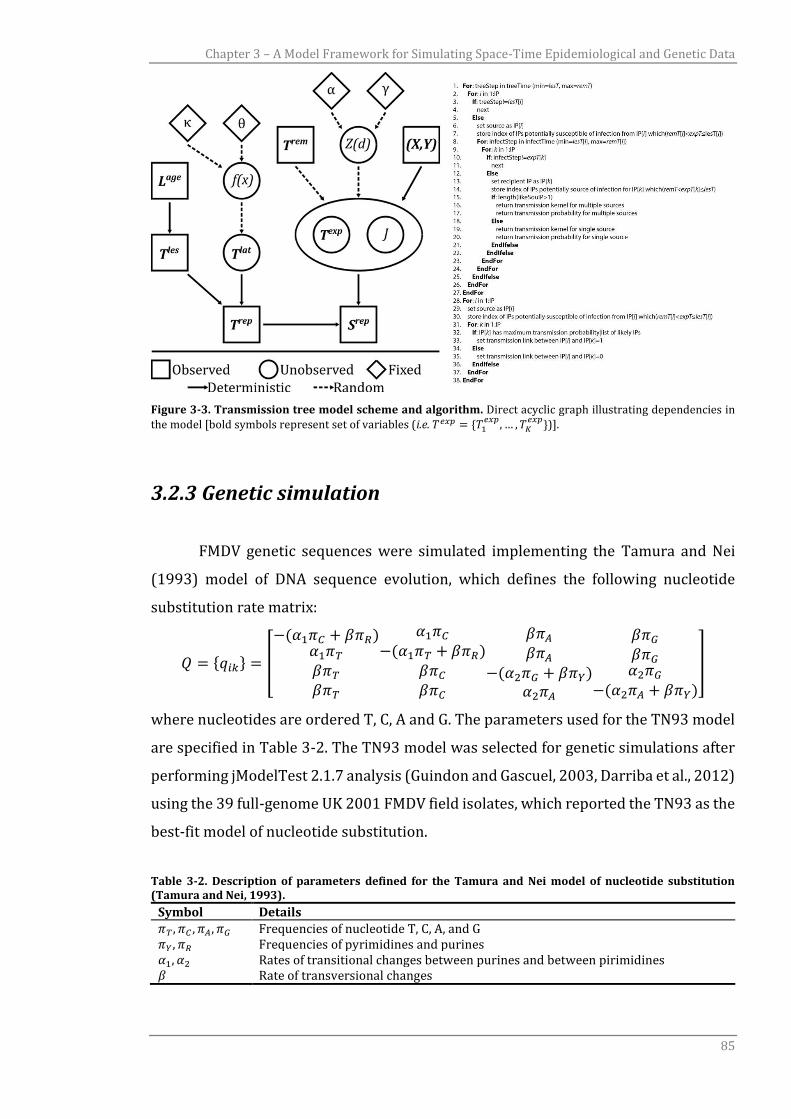
Chapter 3 – A Model Framework for Simulating Space-Time Epidemiological and Genetic Data
85
Figure 3-3. Transmission tree model scheme and algorithm. Direct acyclic graph illustrating dependencies in the model [bold symbols represent set of variables (i.e. 𝑇𝑒𝑥𝑝 = {𝑇1
𝑒𝑥𝑝, … , 𝑇𝐾
𝑒𝑥𝑝})].
3.2.3 Genetic simulation
FMDV genetic sequences were simulated implementing the Tamura and Nei
(1993) model of DNA sequence evolution, which defines the following nucleotide
substitution rate matrix:
𝑄 = {𝑞𝑖𝑘} = [
−(𝛼1𝜋𝐶 + 𝛽𝜋𝑅)𝛼1𝜋𝑇
𝛽𝜋𝑇
𝛽𝜋𝑇
𝛼1𝜋𝐶
−(𝛼1𝜋𝑇 + 𝛽𝜋𝑅)𝛽𝜋𝐶
𝛽𝜋𝐶
𝛽𝜋𝐴
𝛽𝜋𝐴
−(𝛼2𝜋𝐺 + 𝛽𝜋𝑌)𝛼2𝜋𝐴
𝛽𝜋𝐺
𝛽𝜋𝐺𝛼2𝜋𝐺
−(𝛼2𝜋𝐴 + 𝛽𝜋𝑌)
]
where nucleotides are ordered T, C, A and G. The parameters used for the TN93 model
are specified in Table 3-2. The TN93 model was selected for genetic simulations after
performing jModelTest 2.1.7 analysis (Guindon and Gascuel, 2003, Darriba et al., 2012)
using the 39 full-genome UK 2001 FMDV field isolates, which reported the TN93 as the
best-fit model of nucleotide substitution.
Table 3-2. Description of parameters defined for the Tamura and Nei model of nucleotide substitution (Tamura and Nei, 1993).
Symbol Details 𝜋𝑇 , 𝜋𝐶 , 𝜋𝐴, 𝜋𝐺 Frequencies of nucleotide T, C, A, and G 𝜋𝑌 , 𝜋𝑅 Frequencies of pyrimidines and purines 𝛼1, 𝛼2 Rates of transitional changes between purines and between pirimidines 𝛽 Rate of transversional changes

Chapter 3 – A Model Framework for Simulating Space-Time Epidemiological and Genetic Data
86
A previously sequenced FMDV isolate collected from the outbreak source IP
(IP4) during the UK 2001 FMD epidemic (Appendix 3) was used for setting the initial
virus genome from which the sequences of IPs were generated according to the
previously reconstructed transmission tree network. FMDV was defined to evolve at a
molecular clock rate 𝜇 equal to 2.37×10⁻⁵ nt/site/day (Orton et al., 2013), as
parameterised using BEAST 1.8.0 (Drummond and Rambaut, 2007, Drummond et al.,
2012). For each transmission link, the number of nucleotides by which a virus genome
sampled on farm 𝑘 differed from that on the farm from which it was infected (farm 𝑖)
was randomly sampled from a Poisson distribution 𝑃𝑜𝑖𝑠(𝜆) setting the mean to be 𝜆 =
𝜇𝑀∆𝑡, where 𝑀 was the length of the FMDV complete genome [for the UK 2001 FMD
epidemic 𝑀 is equal to 8196 nucleotides, as estimated from the field isolates (Cottam
et al., 2006)] and ∆𝑡 is the evolutionary duration (the sum of the time intervals
computed along the transmission tree – refer to 3.2.3.1). The algorithm used to
simulate FMDV sequences implemented a discrete-time Markov chain model of first
order (Rios Insua et al., 2012) to derive nucleotide changes in the recipient genome
which depended on the nucleotide state of the source genome (Figure 3-5). In this
inference scheme, the Markov transition probability matrix 𝑃(𝑡) = {𝑝𝑖𝑘} = 𝑒𝑄(𝑡) over
time 𝑡 estimated from the source genome using the TN93 model provided the
probability of selecting any of the four nucleotides to be changed at the randomly
selected site in the recipient genome determined chosen from a discrete uniform
distribution 𝑈(1, 𝑀). The 𝛼1, 𝛼2, 𝛽 parameters used to derive 𝑃(𝑡) were estimated from
the available UK 2001 FMDV full-genome sequences (Appendix 3), resulting in values
of 11.325, 23.281 and 3.7, respectively.
Figure 3-4. Genetic simulation model scheme and algorithm. Nucleotide substitution probabilities set under the discrete-time Markov chain model of first order.
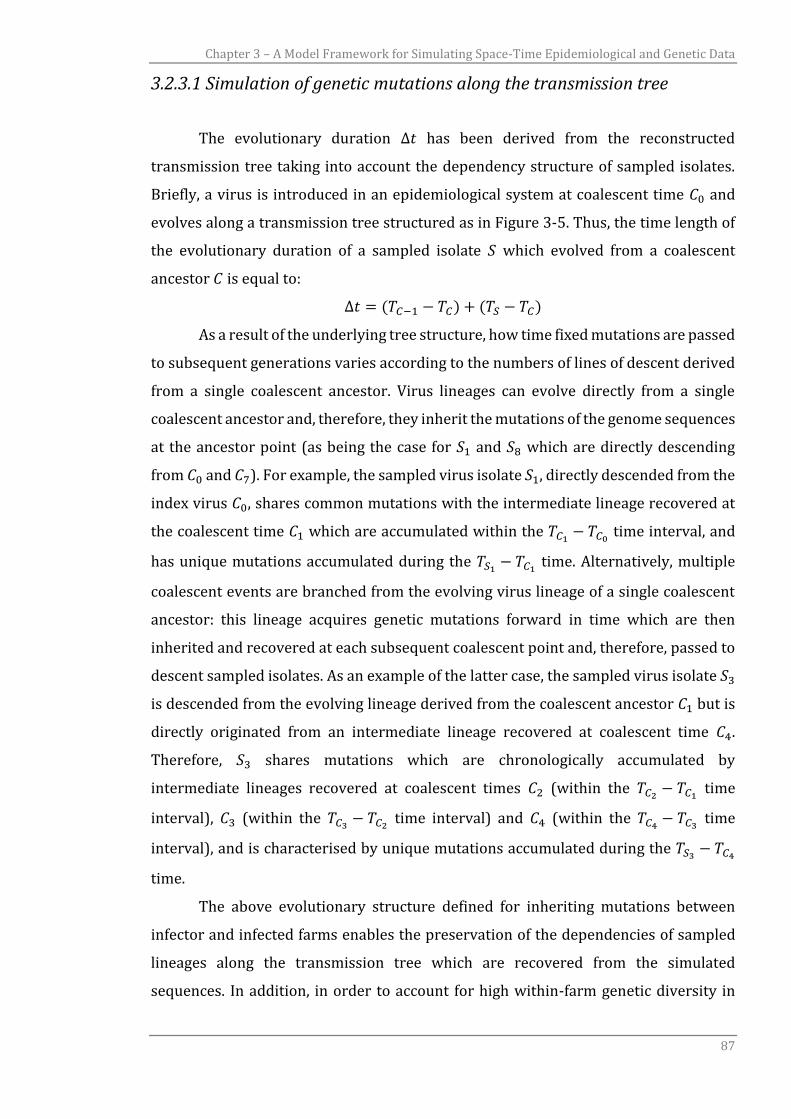
Chapter 3 – A Model Framework for Simulating Space-Time Epidemiological and Genetic Data
87
3.2.3.1 Simulation of genetic mutations along the transmission tree
The evolutionary duration ∆𝑡 has been derived from the reconstructed
transmission tree taking into account the dependency structure of sampled isolates.
Briefly, a virus is introduced in an epidemiological system at coalescent time 𝐶0 and
evolves along a transmission tree structured as in Figure 3-5. Thus, the time length of
the evolutionary duration of a sampled isolate 𝑆 which evolved from a coalescent
ancestor 𝐶 is equal to:
∆𝑡 = (𝑇𝐶−1 − 𝑇𝐶) + (𝑇𝑆 − 𝑇𝐶)
As a result of the underlying tree structure, how time fixed mutations are passed
to subsequent generations varies according to the numbers of lines of descent derived
from a single coalescent ancestor. Virus lineages can evolve directly from a single
coalescent ancestor and, therefore, they inherit the mutations of the genome sequences
at the ancestor point (as being the case for 𝑆1 and 𝑆8 which are directly descending
from 𝐶0 and 𝐶7). For example, the sampled virus isolate 𝑆1, directly descended from the
index virus 𝐶0, shares common mutations with the intermediate lineage recovered at
the coalescent time 𝐶1 which are accumulated within the 𝑇𝐶1− 𝑇𝐶0
time interval, and
has unique mutations accumulated during the 𝑇𝑆1− 𝑇𝐶1
time. Alternatively, multiple
coalescent events are branched from the evolving virus lineage of a single coalescent
ancestor: this lineage acquires genetic mutations forward in time which are then
inherited and recovered at each subsequent coalescent point and, therefore, passed to
descent sampled isolates. As an example of the latter case, the sampled virus isolate 𝑆3
is descended from the evolving lineage derived from the coalescent ancestor 𝐶1 but is
directly originated from an intermediate lineage recovered at coalescent time 𝐶4.
Therefore, 𝑆3 shares mutations which are chronologically accumulated by
intermediate lineages recovered at coalescent times 𝐶2 (within the 𝑇𝐶2− 𝑇𝐶1
time
interval), 𝐶3 (within the 𝑇𝐶3− 𝑇𝐶2
time interval) and 𝐶4 (within the 𝑇𝐶4− 𝑇𝐶3
time
interval), and is characterised by unique mutations accumulated during the 𝑇𝑆3− 𝑇𝐶4
time.
The above evolutionary structure defined for inheriting mutations between
infector and infected farms enables the preservation of the dependencies of sampled
lineages along the transmission tree which are recovered from the simulated
sequences. In addition, in order to account for high within-farm genetic diversity in
Chapter 3 – A Model Framework for Simulating Space-Time Epidemiological and Genetic Data
88
systems where multiple animals are infected within a farm (as being the case for the
UK 2001 FMD outbreak), the coalescent event for multiple evolving lineages was let to
be early in infection, backward in time of the first related coalescent ancestor (i.e. the
infection time of the infector farm rather than the infection time of the infected farm).
Figure 3-5. Evolutionary structure of the dependency between sampled lineages along a reconstructed transmission tree. Red nodes represent coalescent ancestors; orange nodes represent coalescent events of single lineages, whilst green tips represent sampled virus isolates.
3.2.3.2 Evolutionary analysis of the UK 2001 FMDV WGS simulated
alignment
Evolutionary analyses were performed using BEAST 1.8.0 package (Drummond
et al., 2012, Drummond and Rambaut, 2007). The analysis was executed with the TN93
substitution model and the strict clock evolutionary model, setting the molecular clock
used for the simulation (2.30×10⁻⁵) as the substitution rate defined by a gamma
distribution 𝛤(𝜅, 𝜃) prior of 𝜅=0.0084 and 𝜃=1000.0. A piecewise constant Bayesian
skyline model with 10 groups was used as tree prior (Drummond et al., 2005). Other
priors were set with the defaults parameters. Additional comparisons using only VP1
coding sequences were also undertaken.
Chapter 3 – A Model Framework for Simulating Space-Time Epidemiological and Genetic Data
89
3.2.4 Model implementation
The model was coded in the R programming language (R Core Team, 2015).
Running the transmission tree reconstruction for the full UK 2001 FMD outbreak (2026
IPs) and simulating the corresponding genetic component took about 15 minutes using
R 3.2.1 on an Intel i7 Quad Core processor with clock speed 3.40 GHz and 16 Gb of RAM
memory.
3.3 Results
Three different epidemic datasets were constructed from the overall UK 2001
FMD database: the first, used the entire set of IPs described by DEFRA at the time of
the epidemic (𝑛=2026); the second excluded IPs that were at a later stage re-assessed
as negative premises based on the laboratory analysis of collected samples, and those
with missing results (𝑛=1428); the third included only the confirmed IPs and those
with missing results (𝑛=1616) (Ferris et al., 2006, Taylor, 2012). For each of these
datasets a transmission tree was estimated and corresponding WGSs simulated. All
parameters are reported together with their standard deviations.
3.3.1 UK 2001 FMD transmission tree reconstruction
From the reconstructed transmission tree, epidemiological parameters were
estimated according to two points in time of the UK 2001 FMD epidemic. These
corresponded to the introduction of the national movement ban (NMB) (5th day from
the start of the epidemic) and the subsequent 24/48 hour IP/CP culling policy (41st day
from the start of the epidemic). The average number of secondary cases (𝑅𝑡) generated
from a single IP across the entire outbreak is constrained to be equal to 𝑁−1
𝑁 (Figure 3-
5). The 𝑅𝑡 mean estimates were shown to increase for the period before the
introduction of the NMB (5.5) and to decrease following the implementation of the
24/48 hour IP/CP culling policy (0.8).
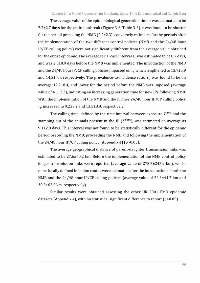
Chapter 3 – A Model Framework for Simulating Space-Time Epidemiological and Genetic Data
90
The average value of the epidemiological generation time 𝜏 was estimated to be
7.2±2.7 days for the entire outbreak (Figure 3-6, Table 3-3). 𝜏 was found to be shorter
for the period preceding the NMB (2.2±2.3), conversely estimates for the periods after
the implementation of the two different control policies (NMB and the 24/48 hour
IP/CP culling policy) were not significantly different from the average value obtained
for the entire epidemic. The average serial case interval 𝜏𝑐 was estimated to be 8.7 days,
and was 2.5±0.9 days before the NMB was implemented. The introduction of the NMB
and the 24/48 hour IP/CP culling policies impacted on 𝜏𝑐 which lengthened to 13.7±5.9
and 14.3±4.4, respectively. The prevalence-to-incidence ratio 𝜏𝑝 was found to be on
average 12.2±8.4, and lower for the period before the NMB was imposed (average
value of 4.1±2.2), indicating an increasing generation time for new IPs following NMB.
With the implementation of the NMB and the further 24/48 hour IP/CP culling policy
𝜏𝑝 increased to 9.2±3.2 and 13.5±8.9, respectively.
The culling time, defined by the time interval between exposure 𝑇𝑒𝑥𝑝 and the
stamping-out of the animals present in the IP (𝑇𝑟𝑒𝑚), was estimated on average as
9.1±2.8 days. This interval was not found to be statistically different for the epidemic
period preceding the NMB, proceeding the NMB and following the implementation of
the 24/48 hour IP/CP culling policy (Appendix 4) (𝑝>0.05).
The average geographical distance of parent-daughter transmission links was
estimated to be 27.6±60.2 km. Before the implementation of the NMB control policy
longer transmission links were reported (average value of 273.7±245.9 km), whilst
more locally defined infection routes were estimated after the introduction of both the
NMB and the 24/48 hour IP/CP culling policies (average value of 22.3±44.7 km and
30.5±62.5 km, respectively).
Similar results were obtained assessing the other UK 2001 FMD epidemic
datasets (Appendix 4), with no statistical significant difference to report (𝑝>0.05).
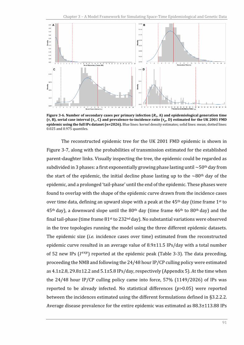
Chapter 3 – A Model Framework for Simulating Space-Time Epidemiological and Genetic Data
91
Figure 3-6. Number of secondary cases per primary infection (𝑹𝒕, A) and epidemiological generation time (𝝉, B), serial case interval (𝝉𝒄, C) and prevalence-to-incidence ratio (𝝉𝒑, D) estimated for the UK 2001 FMD
epidemic using the full IPs dataset (𝒏=2026). Blue lines: kernel density estimates; solid lines: mean; dotted lines: 0.025 and 0.975 quantiles.
The reconstructed epidemic tree for the UK 2001 FMD epidemic is shown in
Figure 3-7, along with the probabilities of transmission estimated for the established
parent-daughter links. Visually inspecting the tree, the epidemic could be regarded as
subdivided in 3 phases: a first exponentially growing phase lasting until ~50th day from
the start of the epidemic, the initial decline phase lasting up to the ~80th day of the
epidemic, and a prolonged ‘tail-phase’ until the end of the epidemic. These phases were
found to overlap with the shape of the epidemic curve drawn from the incidence cases
over time data, defining an upward slope with a peak at the 45th day (time frame 1st to
45th day), a downward slope until the 80th day (time frame 46th to 80th day) and the
final tail-phase (time frame 81st to 232nd day). No substantial variations were observed
in the tree topologies running the model using the three different epidemic datasets.
The epidemic size (i.e. incidence cases over time) estimated from the reconstructed
epidemic curve resulted in an average value of 8.9±11.5 IPs/day with a total number
of 52 new IPs (𝐼𝑒𝑥𝑝) reported at the epidemic peak (Table 3-3). The data preceding,
proceeding the NMB and following the 24/48 hour IP/CP culling policy were estimated
as 4.1±2.8, 29.8±12.2 and 5.1±5.8 IPs/day, respectively (Appendix 5). At the time when
the 24/48 hour IP/CP culling policy came into force, 57% (1149/2026) of IPs was
reported to be already infected. No statistical differences (𝑝>0.05) were reported
between the incidences estimated using the different formulations defined in §3.2.2.2.
Average disease prevalence for the entire epidemic was estimated as 88.3±113.88 IPs
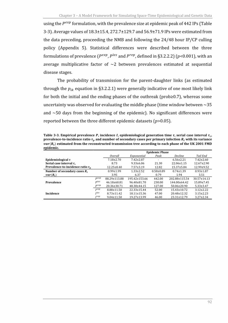
Chapter 3 – A Model Framework for Simulating Space-Time Epidemiological and Genetic Data
92
using the 𝑃𝑒𝑥𝑝 formulation, with the prevalence size at epidemic peak of 442 IPs (Table
3-3). Average values of 18.3±15.4, 272.7±129.7 and 56.9±71.9 IPs were estimated from
the data preceding, proceeding the NMB and following the 24/48 hour IP/CP culling
policy (Appendix 5). Statistical differences were described between the three
formulations of prevalence (𝑃𝑒𝑥𝑝, 𝑃𝑙𝑒𝑠 and 𝑃𝑟𝑒𝑝, defined in §3.2.2.2) (𝑝<0.001), with an
average multiplicative factor of ~2 between prevalences estimated at sequential
disease stages.
The probability of transmission for the parent-daughter links (as estimated
through the 𝑝𝑖𝑘 equation in §3.2.2.1) were generally indicative of one most likely link
for both the initial and the ending phases of the outbreak (prob≥0.7), whereas some
uncertainty was observed for evaluating the middle phase (time window between ~35
and ~50 days from the beginning of the epidemic). No significant differences were
reported between the three different epidemic datasets (𝑝>0.05).
Table 3-3. Empirical prevalence 𝑷, incidence 𝑰, epidemiological generation time 𝝉, serial case interval 𝝉𝒄, prevalence-to-incidence ratio 𝝉𝒑 and number of secondary cases per primary infection 𝑹𝒕 with its variance
𝒗𝒂𝒓(𝑹𝒕) estimated from the reconstructed transmission tree according to each phase of the UK 2001 FMD epidemic.
Epidemic Phase Overall Exponential Peak Decline Tail End
Epidemiological 𝝉 7.18±2.70 7.42±2.87 - 6.56±2.21 7.42±2.60 Serial case interval 𝝉𝒄 8.73 9.33±6.06 21.30 22.06±1.15 12.67±2.90 Prevalence-to-incidence ratio 𝝉𝒑 12.25±8.40 7.57±3.19 12.82 15.37±5.84 12.99±9.52
Number of secondary cases 𝑹𝒕 0.99±1.99 1.33±2.52 0.58±0.89 0.74±1.39 0.93±1.87 𝒗𝒂𝒓(𝑹𝒕) 3.95 6.37 0.79 1.94 3.51
Prevalence 𝑃𝑒𝑥𝑝 88.29±113.88 195.42±153.66 442.00 202.88±115.54 30.57±14.13 𝑃𝑙𝑒𝑠 46.18±60.81 96.40±81.70 230.00 144.00±64.42 15.89±7.45 𝑃𝑟𝑒𝑝 20.36±30.71 48.38±44.15 127.00 50.06±20.90 5.33±3.47
Incidence 𝐼𝑒𝑥𝑝 8.88±11.50 22.33±15.44 52.00 15.43±10.72 3.12±2.22 𝐼𝑙𝑒𝑠 8.73±11.42 18.11±15.36 47.00 20.48±12.32 3.15±2.23 𝐼𝑟𝑒𝑝 9.04±11.50 19.27±13.99 46.00 23.31±12.79 3.27±2.34
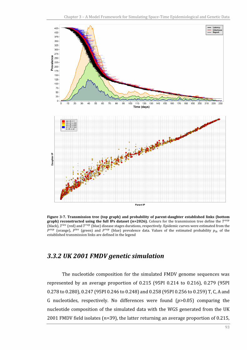
Chapter 3 – A Model Framework for Simulating Space-Time Epidemiological and Genetic Data
93
Figure 3-7. Transmission tree (top graph) and probability of parent-daughter established links (bottom graph) reconstructed using the full IPs dataset (𝒏=2026). Colours for the transmission tree define the 𝑇𝑒𝑥𝑝 (black), 𝑇𝑙𝑒𝑠 (red) and 𝑇𝑟𝑒𝑝 (blue) disease stages durations, respectively. Epidemic curves were estimated from the 𝑃𝑒𝑥𝑝 (orange), 𝑃𝑙𝑒𝑠 (green) and 𝑃𝑟𝑒𝑝 (blue) prevalence data. Values of the estimated probability 𝑝𝑖𝑘 of the established transmission links are defined in the legend
3.3.2 UK 2001 FMDV genetic simulation
The nucleotide composition for the simulated FMDV genome sequences was
represented by an average proportion of 0.215 (95PI 0.214 to 0.216), 0.279 (95PI
0.278 to 0.280), 0.247 (95PI 0.246 to 0.248) and 0.258 (95PI 0.256 to 0.259) T, C, A and
G nucleotides, respectively. No differences were found (𝑝>0.05) comparing the
nucleotide composition of the simulated data with the WGS generated from the UK
2001 FMDV field isolates (𝑛=39), the latter returning an average proportion of 0.215,
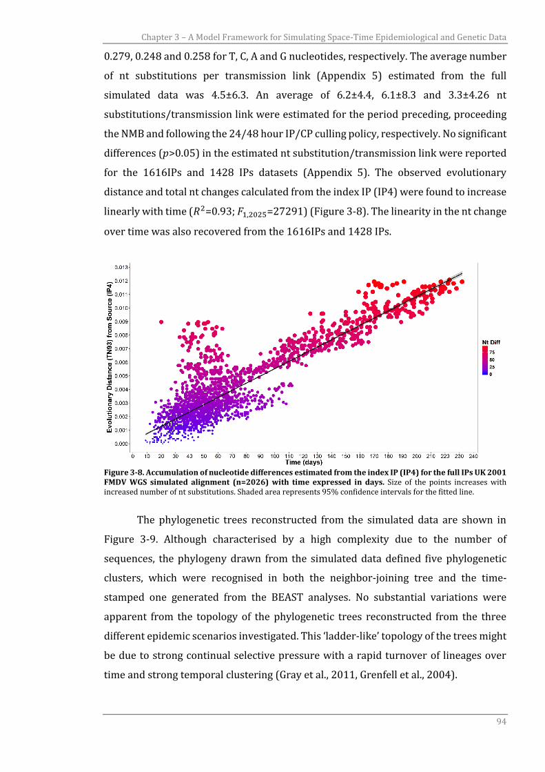
Chapter 3 – A Model Framework for Simulating Space-Time Epidemiological and Genetic Data
94
0.279, 0.248 and 0.258 for T, C, A and G nucleotides, respectively. The average number
of nt substitutions per transmission link (Appendix 5) estimated from the full
simulated data was 4.5±6.3. An average of 6.2±4.4, 6.1±8.3 and 3.3±4.26 nt
substitutions/transmission link were estimated for the period preceding, proceeding
the NMB and following the 24/48 hour IP/CP culling policy, respectively. No significant
differences (𝑝>0.05) in the estimated nt substitution/transmission link were reported
for the 1616IPs and 1428 IPs datasets (Appendix 5). The observed evolutionary
distance and total nt changes calculated from the index IP (IP4) were found to increase
linearly with time (𝑅2=0.93; 𝐹1,2025=27291) (Figure 3-8). The linearity in the nt change
over time was also recovered from the 1616IPs and 1428 IPs.
Figure 3-8. Accumulation of nucleotide differences estimated from the index IP (IP4) for the full IPs UK 2001 FMDV WGS simulated alignment (n=2026) with time expressed in days. Size of the points increases with increased number of nt substitutions. Shaded area represents 95% confidence intervals for the fitted line.
The phylogenetic trees reconstructed from the simulated data are shown in
Figure 3-9. Although characterised by a high complexity due to the number of
sequences, the phylogeny drawn from the simulated data defined five phylogenetic
clusters, which were recognised in both the neighbor-joining tree and the time-
stamped one generated from the BEAST analyses. No substantial variations were
apparent from the topology of the phylogenetic trees reconstructed from the three
different epidemic scenarios investigated. This ‘ladder-like’ topology of the trees might
be due to strong continual selective pressure with a rapid turnover of lineages over
time and strong temporal clustering (Gray et al., 2011, Grenfell et al., 2004).

Chapter 3 – A Model Framework for Simulating Space-Time Epidemiological and Genetic Data
95
Figure 3-9. Tree phylogenies reconstructed using the FMDV WGS simulated from the full IPs dataset (𝒏=2026). The phylogenetic trees were computed using the neighbor-joining method in MEGA 6.06 (A), and time-stamped from the BEAST analyses (B). All the trees were rooted from the outbreak source (IP4).
3.3.2.1 UK 2001 FMDV evolutionary analysis using WGS data
The average evolutionary duration (∆𝑡) was estimated as 14.8±3.7 days for the
full outbreak time window, with the periods preceding, proceeding the NMB and the
24/48 hour IP/CP culling policy were comparable with the average value estimated for
the entire epidemic. No significant variation (𝑝>0.5) in the ∆𝑡 estimates were obtained
running the simulation model for the three different epidemic datasets and for each of
the time-period assessed (Appendix 5).
The molecular clock reconstructed from BEAST resulted in a value of 2.05×10⁻⁵
nt/site/day (95%HPD 1.97×10⁻⁵ to 2.14×10⁻⁵), with no statistical difference observed
for the other epidemic datasets (𝑝>0.05). These results were comparable with those
estimated from the 39 previously sequenced UK 2001 FMDV field isolates [2.26×10⁻⁵
nt/site/day, using a relaxed-exponential clock model (Cottam et al., 2006); 2.08×10⁻⁵
nt/site/day, using a relaxed-constant clock model (Cottam et al., 2008a); 2.33×10⁻⁵
nt/site/day here re-estimated using the same strict clock model assumed for
simulating the WGSs].
3.3.2.2 UK 2001 FMDV evolutionary analysis using VP1 coding sequences
A molecular clock reconstructed from BEAST using the VP1 coding sequences
extracted from the simulated data for the full epidemic dataset (𝑛=2026) resulted in a
value of 2.36×10⁻⁵ (95%HPD 1.94×10⁻⁵ to 2.54×10⁻⁵), which was comparable with
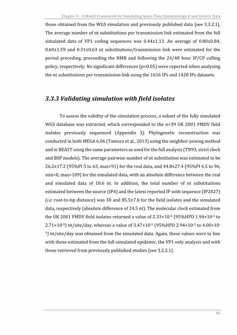
Chapter 3 – A Model Framework for Simulating Space-Time Epidemiological and Genetic Data
96
those obtained from the WGS simulation and previously published data [see 3.3.2.1].
The average number of nt substitutions per transmission link estimated from the full
simulated data of VP1 coding sequences was 0.44±1.13. An average of 0.80±0.84,
0.60±1.59 and 0.31±0.63 nt substitutions/transmission link were estimated for the
period preceding, proceeding the NMB and following the 24/48 hour IP/CP culling
policy, respectively. No significant differences (𝑝>0.05) were reported when analysing
the nt substitutions per transmission link using the 1616 IPs and 1428 IPs datasets.
3.3.3 Validating simulation with field isolates
To assess the validity of the simulation process, a subset of the fully simulated
WGS database was extracted, which corresponded to the 𝑛=39 UK 2001 FMDV field
isolates previously sequenced (Appendix 3). Phylogenetic reconstruction was
conducted in both MEGA 6.06 (Tamura et al., 2013) using the neighbor-joining method
and in BEAST using the same parameters as used for the full analysis (TN93, strict clock
and BSP models). The average pairwise number of nt substitution was estimated to be
26.2±17.2 (95%PI 5 to 63, max=91) for the real data, and 44.8±27.4 (95%PI 6.5 to 96,
min=0, max=109) for the simulated data, with an absolute difference between the real
and simulated data of 18.6 nt. In addition, the total number of nt substitutions
estimated between the source (IP4) and the latest reported IP with sequence (IP2027)
(i.e. root-to-tip distance) was 50 and 85.5±7.0 for the field isolates and the simulated
data, respectively (absolute difference of 24.5 nt). The molecular clock estimated from
the UK 2001 FMDV field isolates returned a value of 2.33×10⁻⁵ (95%HPD 1.94×10⁻⁵ to
2.71×10⁻⁵) nt/site/day, whereas a value of 3.47×10⁻⁵ (95%HPD 2.94×10⁻⁵ to 4.00×10-
5) nt/site/day was obtained from the simulated data. Again, these values were in line
with those estimated from the full-simulated epidemic, the VP1 only analysis and with
those retrieved from previously published studies [see 3.2.2.1].
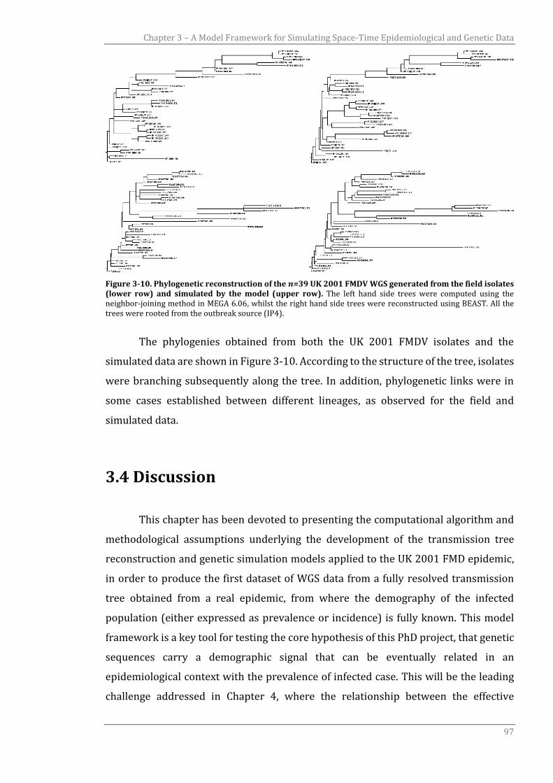
Chapter 3 – A Model Framework for Simulating Space-Time Epidemiological and Genetic Data
97
Figure 3-10. Phylogenetic reconstruction of the 𝒏=39 UK 2001 FMDV WGS generated from the field isolates (lower row) and simulated by the model (upper row). The left hand side trees were computed using the neighbor-joining method in MEGA 6.06, whilst the right hand side trees were reconstructed using BEAST. All the trees were rooted from the outbreak source (IP4).
The phylogenies obtained from both the UK 2001 FMDV isolates and the
simulated data are shown in Figure 3-10. According to the structure of the tree, isolates
were branching subsequently along the tree. In addition, phylogenetic links were in
some cases established between different lineages, as observed for the field and
simulated data.
3.4 Discussion
This chapter has been devoted to presenting the computational algorithm and
methodological assumptions underlying the development of the transmission tree
reconstruction and genetic simulation models applied to the UK 2001 FMD epidemic,
in order to produce the first dataset of WGS data from a fully resolved transmission
tree obtained from a real epidemic, from where the demography of the infected
population (either expressed as prevalence or incidence) is fully known. This model
framework is a key tool for testing the core hypothesis of this PhD project, that genetic
sequences carry a demographic signal that can be eventually related in an
epidemiological context with the prevalence of infected case. This will be the leading
challenge addressed in Chapter 4, where the relationship between the effective
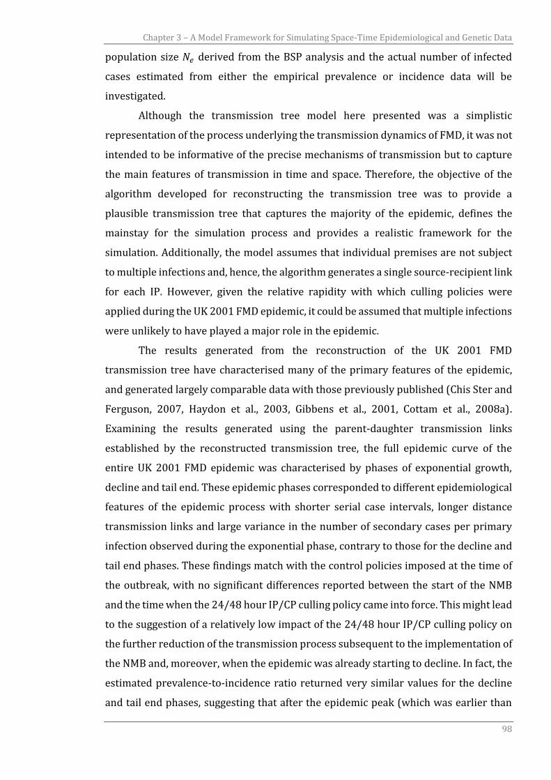
Chapter 3 – A Model Framework for Simulating Space-Time Epidemiological and Genetic Data
98
population size 𝑁𝑒 derived from the BSP analysis and the actual number of infected
cases estimated from either the empirical prevalence or incidence data will be
investigated.
Although the transmission tree model here presented was a simplistic
representation of the process underlying the transmission dynamics of FMD, it was not
intended to be informative of the precise mechanisms of transmission but to capture
the main features of transmission in time and space. Therefore, the objective of the
algorithm developed for reconstructing the transmission tree was to provide a
plausible transmission tree that captures the majority of the epidemic, defines the
mainstay for the simulation process and provides a realistic framework for the
simulation. Additionally, the model assumes that individual premises are not subject
to multiple infections and, hence, the algorithm generates a single source-recipient link
for each IP. However, given the relative rapidity with which culling policies were
applied during the UK 2001 FMD epidemic, it could be assumed that multiple infections
were unlikely to have played a major role in the epidemic.
The results generated from the reconstruction of the UK 2001 FMD
transmission tree have characterised many of the primary features of the epidemic,
and generated largely comparable data with those previously published (Chis Ster and
Ferguson, 2007, Haydon et al., 2003, Gibbens et al., 2001, Cottam et al., 2008a).
Examining the results generated using the parent-daughter transmission links
established by the reconstructed transmission tree, the full epidemic curve of the
entire UK 2001 FMD epidemic was characterised by phases of exponential growth,
decline and tail end. These epidemic phases corresponded to different epidemiological
features of the epidemic process with shorter serial case intervals, longer distance
transmission links and large variance in the number of secondary cases per primary
infection observed during the exponential phase, contrary to those for the decline and
tail end phases. These findings match with the control policies imposed at the time of
the outbreak, with no significant differences reported between the start of the NMB
and the time when the 24/48 hour IP/CP culling policy came into force. This might lead
to the suggestion of a relatively low impact of the 24/48 hour IP/CP culling policy on
the further reduction of the transmission process subsequent to the implementation of
the NMB and, moreover, when the epidemic was already starting to decline. In fact, the
estimated prevalence-to-incidence ratio returned very similar values for the decline
and tail end phases, suggesting that after the epidemic peak (which was earlier than
Chapter 3 – A Model Framework for Simulating Space-Time Epidemiological and Genetic Data
99
the beginning of the 24/48 hour IP/CP culling policy) new IPs are generated in direct
proportion to the existing prevalence (i.e. 𝑅𝑡 is constant and slightly less than 1).
The molecular clock recovered from the fully-simulated FMDV WGS data was
found to be similar to the one estimated from the 39 WGS generated from the field
isolates, which provides confidence around the robustness and validity of the
simulation process. The differences observed in comparing the UK 2001 FMDV field
isolates and the corresponding simulated lineages are likely to be mostly explained by
the space-time process for generating the transmission tree which, as already
discussed, might not be entirely accurate in establishing the actual transmission links
observed during the UK 2001 FMD epidemic. However, this would likely have a limited
influence on the simulation of the evolutionary process, and the reconstruction of the
underlying phylogenetic trees. Similar results were obtained performing the analyses
with only the VP1 coding region sequences, although with an expected greater degree
of uncertainty given by the wider confidence intervals of the estimated parameters
relative to those obtained using the WGS. This can be easily linked to the lower
resolution provided by the VP1 coding region sequences, which represents only 8% of
the complete FMDV genome.
The average number of nt substitutions per transmission links estimated from
the WGS simulated alignment was very similar in comparison to that previously
reported (Cottam et al., 2008a), even matching the difference reported between the
mean number of substitutions per transmission link when partitioned into
transmission events preceding and proceeding the NMB. However, comparing the
extracted 39 simulated sequences with the corresponding field isolates, a relative
difference was apparent between observed and simulated sequences for the average
nt substitutions recovered over the root-to-tip distances, which were higher for the
simulated WGS. It should be noted that the former estimate was established using only
20 WGSs generated from the Darlington cluster, which potentially might not be
generalised to the evolutionary process underlying the full epidemic event. In a real
epidemic, genetic change might acquire from within-farm evolutionary processes, for
which multiple cycles of infection might be present on each IP. The process here
developed for simulating the virus evolution does consider, although in a very crude
form, the within-farm process, which contribute to the genetic diversity observed
between the sequences recovered from each IP. For example, coalescent models
assume that the transmission event is coincident with the coalescent event, which

Chapter 3 – A Model Framework for Simulating Space-Time Epidemiological and Genetic Data
100
might be not the case when significant variation is seen at the within-farm evolutionary
scale. However, the impact of the within-farm evolutionary dynamics on the short
timescale considered for an epidemic event could be regarded as limited and unlikely
to add significant variation over and above that observed at consensus level (King et
al., unpublished data).
101
CHAPTER 4
Reconstructing virus populations dynamics
over time
4.1 Rationale
In population genetics, factors that cause differences between 𝑁𝑒 and the census
population size 𝑁 have been well studied. As already reviewed in Chapter 1, 𝑁𝑒 is
defined as ‘the size of an idealised population experiencing the same rate of random
genetic change over time as the real population under consideration’ (Wright, 1931,
Wright, 1938), assuming that these two populations have the same properties under
neutral selection (i.e. for the Wright-Fisher model 𝑁𝑒 ≅ 𝑁). However, violations of the
assumptions underlying the Wright-Fisher model leads to a reduction in 𝑁𝑒 relative to
𝑁, and the ratio 𝑁𝑒
𝑁 assesses the departure from the assumption of the idealised model
(Felsenstein, 1971, Kimura and Crow, 1963). 𝑁𝑒 can be assumed to scale to the genetic
diversity of the population as measured by the population genetic parameter 𝜃, and by
making various assumptions it is possible to identify additional scaling factors that
relate 𝑁𝑒 to the census population size 𝑁 (Magiorkinis et al., 2013). The challenge in
this chapter is to identify and empirically test the performance of different scaling
factors that can be used to relate 𝑁𝑒 to the census population size in an epidemiological
context.
In epidemiology, the census population size relates to the actual numbers of
infected cases measured as an estimate of prevalence, or possibly incidence. The
correlation between 𝑁𝑒 and the actual numbers of infected cases has been studied
under the assumption of a time-varying coalescent model (Griffiths and Tavare,
1994a), and suggests that no simple relationship or clear transformation exists
between these two quantities (Frost and Volz, 2010, Volz et al., 2009). The lack of a
clear relationship between the effective and actual population size has been attributed
to the variable nature of the serial case interval 𝜏𝑐. The serial case interval will vary
over the course of an epidemic (e.g. shortening during the exponential phase when the
full population is susceptible and expanding when the susceptible population becomes
Chapter 4 – Reconstructing viral populations dynamics over time
102
depleted – i.e. during the decline and/or tail end phases), causing variation in the
relationship between transmission rate and the number of infected individuals.
Bedford et al. (2011) found 𝜏𝑐 to be inversely proportional to the contact rate during
the expansion phase of an epidemic, whilst 𝜏𝑐 was estimated to be inversely
proportional to the rate of recovery when at equilibrium. However, during the
exponential phase of an epidemic or within a steady endemic state where 𝜏𝑐 is roughly
constant, a direct transformation might be found (Koelle and Rasmussen, 2012), hence
𝑁𝑒 estimates would be proportional to the prevalence of infection (Frost and Volz,
2010). It should be noted that at steady state, prevalence is also proportional to
incidence. The fact that the 𝜏𝑐 varies over the course of an epidemic implies that it
might not be straightforward to estimate 𝑁𝑒 at a given time (de Silva et al., 2012).
4.2 Methodological process for scaling 𝑵𝒆 to the actual
infected population size
This chapter reports studies of the viral population demography estimated from
the genetic data simulated using the model described in Chapter 3. The aim is to
investigate the relationship between 𝑁𝑒 and the actual numbers of infected cases (cases
here are defined as numbers of IPs) derived from the 𝑃𝑒𝑥𝑝 prevalence data, and
estimated from a fully-resolved epidemic, the UK 2001 FMD epidemic. In order to
investigate the correlation between estimates of 𝑁𝑒 derived from the BSP and the real
numbers of infected cases, three scaling formulations were examined, which also
accounted for the variability in the generation time within the time frame of an
epidemic. Account has also been taken of the definition of generation time provided in
§3.2.2.3. The resulting prediction estimate from the 𝑁𝑒scaling should be considered as
a proxy of prevalence measure, therefore it has been termed as the ‘infection
prevalence’ 𝑁∗. The final derivation of the different scaling equations for estimating 𝑁∗
is summarised in Table 4-1.
Chapter 4 – Reconstructing viral populations dynamics over time
103
4.2.1 Reconstructing 𝑵𝒆 changes through time from a
Bayesian Skyline analysis
As detailed in §1.2.1 and §4.1, the parameter 𝜃 can be equated to the product
𝑁𝑒𝜏 (Drummond et al., 2002). Rearranging for 𝑁𝑒 , the latter equation results in 𝑁𝑒 =𝜃
𝜏,
that is the skyline-derived effective population size 𝑁𝑒 . This value is easily computed
using the BSP-derived 𝜃 and the generation time estimated from the UK 2001 FMD
data, for which both the 𝜏 and 𝜏𝑐 definitions have been used (see §3.2.2.3). The above
formulation has been referred to in the text as the ‘scaled 𝑁𝑒 formulation’ and has been
used for assessing the potential of using 𝑁𝑒 estimates for predicting the actual
demography of an infected population.
4.2.2 Deriving infection prevalence 𝑵∗
4.2.2.1 Reconstructing 𝑁∗ assuming variance in the number of secondary
cases per primary infection 𝑅𝑡
The ratio between the effective and actual population size 𝑁𝑒
𝑁 has been related
to the variance in the reproduction success 𝜎2 (Kingman, 1982b, Tavare et al., 1997) in
the following way: 𝑁𝑒 =𝑁
𝜎2. The variance in the reproduction success 𝜎2 in an
epidemiological context is the variance in the number of secondary infections per
primary infections [i.e. 𝑣𝑎𝑟(𝑅𝑡)] or by the alternative form 𝑣𝑎𝑟(𝑅𝑡)
𝐸(𝑅𝑡)2 + 1, which accounts
for the fraction of the host population that is susceptible to infection (Koelle and
Rasmussen, 2012)]. These two formulations lead to the following expressions for the
derived infection prevalence: 𝑁∗ =𝜃𝑣𝑎𝑟(𝑅𝑡)
𝜏 and 𝑁∗ =
𝜃(𝑣𝑎𝑟(𝑅𝑡)+𝐸(𝑅𝑡)2)
𝜏𝐸(𝑅𝑡)2 . This scaling
formulation has been termed the ‘𝑣𝑎𝑟(𝑅𝑡) scaling formulation’, referring to Tavare et
al. (1997) or Koelle and Rasmussen (2012) for differentiating between the two 𝑣𝑎𝑟(𝑅𝑡)
derivation forms. Both 𝜏 and 𝜏𝑐 definitions of generation time have been used within
the context of the above scaling formulations (see §3.2.2.3).
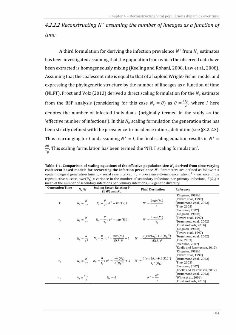
Chapter 4 – Reconstructing viral populations dynamics over time
104
4.2.2.2 Reconstructing 𝑁∗ assuming the number of lineages as a function of
time
A third formulation for deriving the infection prevalence 𝑁∗ from 𝑁𝑒 estimates
has been investigated assuming that the population from which the observed data have
been extracted is homogeneously mixing (Keeling and Rohani, 2008, Law et al., 2008).
Assuming that the coalescent rate is equal to that of a haploid Wright-Fisher model and
expressing the phylogenetic structure by the number of lineages as a function of time
(NLFT), Frost and Volz (2013) derived a direct scaling formulation for the 𝑁𝑒 estimate
from the BSP analysis (considering for this case 𝑁𝑒 = 𝜃) as 𝜃 =𝐼𝜏𝑝
2, where 𝐼 here
denotes the number of infected individuals (originally termed in the study as the
‘effective number of infections’). In this 𝑁𝑒 scaling formulation the generation time has
been strictly defined with the prevalence-to-incidence ratio 𝜏𝑝 definition (see §3.2.2.3).
Thus rearranging for 𝐼 and assuming 𝑁∗ ≈ 𝐼, the final scaling equation results in 𝑁∗ =
2𝜃
𝜏𝑝. This scaling formulation has been termed the ‘NFLT scaling formulation’.
Table 4-1. Comparison of scaling equations of the effective population size 𝑵𝒆 derived from time-varying coalescent based models for recovering the infection prevalence 𝑵∗. Parameters are defined as follow: 𝜏 = epidemiological generation time, 𝜏𝑐= serial case interval, 𝜏𝑝 = prevalence-to-incidence ratio, 𝜎2 = variance in the
reproductive success, 𝑣𝑎𝑟(𝑅𝑡) = variance in the number of secondary infections per primary infections, 𝐸(𝑅𝑡) = mean of the number of secondary infections per primary infections, 𝜃 = genetic diversity.
Generation Time 𝑵𝒆/𝑵
Scaling Factor Relating 𝜽 (BSP) and 𝑵𝒆
Final Derivation Reference
𝜏 𝑁𝑒 =𝑁
𝜎2 𝑁𝑒 =
𝜃
𝜏; 𝜎2 = 𝑣𝑎𝑟(𝑅𝑡) 𝑁∗ =
𝜃𝑣𝑎𝑟(𝑅𝑡)
𝜏
(Kingman, 1982b) (Tavare et al., 1997) (Drummond et al., 2002) (Fine, 2003) (Svensson, 2007)
𝜏𝑐 𝑁𝑒 =𝑁
𝜎2 𝑁𝑒 =
𝜃
𝜏𝑐
; 𝜎2 = 𝑣𝑎𝑟(𝑅𝑡) 𝑁∗ =𝜃𝑣𝑎𝑟(𝑅𝑡)
𝜏𝑐
(Kingman, 1982b) (Tavare et al., 1997) (Drummond et al., 2002) (Frost and Volz, 2010)
𝜏 𝑁𝑒 =𝑁
𝜎2 𝑁𝑒 =
𝜃
𝜏; 𝜎2 =
𝑣𝑎𝑟(𝑅𝑡)
𝐸(𝑅𝑡)2+ 1 𝑁∗ =
𝜃(𝑣𝑎𝑟(𝑅𝑡) + 𝐸(𝑅𝑡)2)
𝜏𝐸(𝑅𝑡)2
(Kingman, 1982b) (Tavare et al., 1997) (Drummond et al., 2002) (Fine, 2003) (Svensson, 2007) (Koelle and Rasmussen, 2012)
𝜏𝑐 𝑁𝑒 =𝑁
𝜎2 𝑁𝑒 =
𝜃
𝜏𝑐
; 𝜎2 =𝑣𝑎𝑟(𝑅𝑡)
𝐸(𝑅𝑡)2+ 1 𝑁∗ =
𝜃(𝑣𝑎𝑟(𝑅𝑡) + 𝐸(𝑅𝑡)2)
𝜏𝑐𝐸(𝑅𝑡)2
(Kingman, 1982b) (Tavare et al., 1997) (Drummond et al., 2002) (Fine, 2003) (Svensson, 2007) (Koelle and Rasmussen, 2012)
𝜏𝑝 𝑁𝑒 =𝐼𝜏𝑝
2 𝑁𝑒 = 𝜃 𝑁∗ =
2𝜃
𝜏𝑝
(Drummond et al., 2002) (White et al., 2006) (Frost and Volz, 2013)
Chapter 4 – Reconstructing viral populations dynamics over time
105
4.2.2.3 Computation of infection prevalence 𝑁∗ using the UK 2001 FMD
simulated WGS
Twelve realisations of the UK 2001 FMD transmission tree reconstruction and
genetic simulation generated full WGS datasets (𝑛=2026 IPs) as detailed in §3.3. For
each simulated alignment, BEAST 1.8.0 package (Drummond et al., 2012, Drummond
and Rambaut, 2007) was employed to reconstruct the demography of the FMDV
population from the simulated data using the BSP model (Drummond et al., 2005). The
analysis was undertaken with the TN93 substitution model and the strict clock
evolutionary model, the average rate of the fixed clock model as the one used for the
simulation (2.33×10⁻⁵ nt/site/day) and defining a gamma distribution 𝛤(𝜅, 𝜃) of
𝜅=0.0084 and 𝜃=1000.0 for the substitution rate prior. Other priors were set with the
default values. Furthermore, epidemiological parameters used for formulating the
scaling equations presented in Table 4-1 (i.e. 𝜏, 𝜏𝑐, 𝜏𝑝, 𝑣𝑎𝑟(𝑅𝑡), 𝐸(𝑅𝑡)) have been either
estimated by averaging over the time course of the epidemic or estimated as changing
through time, leading to two different scaling approaches, namely average and time-
varying. Thus, the time-varying scaling approach takes into account the variability in
time of the UK 2001 FMD epidemic and, therefore, of each epidemiological parameter
used to derive the infection prevalence 𝑁∗. Natural splines (Harrell, 2001) were fitted
to time-varying data and used to smooth and interpolate the required data for each
time point. Fitting procedures have been performed in R 3.2.1 using the splines
package (R Core Team, 2015). The 𝜏𝑡 generation time has not been smoothed since it
can be easily estimated in continuous time from the UK 2001 FMD empirical data.
The root-mean-squared deviation (RMSD) was used for estimating the
numerical departure of the recovered 𝑁∗ from the empirical count of infected cases,
expressed as prevalence. This statistical parameter is a scale-dependent accuracy
measure based on the absolute squared error, which provides an indication of the
difference between values predicted by a given model and the actual data (Hyndman
and Koehler, 2006). For the scaling study, this can be estimated as 𝑅𝑀𝑆𝐷(𝑁∗) =
√𝐸((𝑁𝑡∗ − 𝑁𝑡)2), where 𝑁 can denote prevalence or incidence estimated at time 𝑡. The
RMSD returns a value of zero if the correlated time-series are perfectly matching 𝑁∗ ≅
𝑁 = 0.
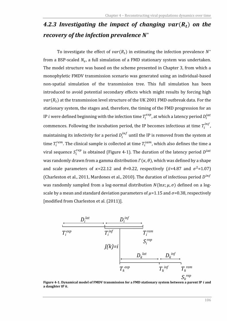
Chapter 4 – Reconstructing viral populations dynamics over time
106
4.2.3 Investigating the impact of changing 𝒗𝒂𝒓(𝑹𝒕) on the
recovery of the infection prevalence 𝑵∗
To investigate the effect of 𝑣𝑎𝑟(𝑅𝑡) in estimating the infection prevalence 𝑁∗
from a BSP-scaled 𝑁𝑒 , a full simulation of a FMD stationary system was undertaken.
The model structure was based on the scheme presented in Chapter 3, from which a
monophyletic FMDV transmission scenario was generated using an individual-based
non-spatial simulation of the transmission tree. This full simulation has been
introduced to avoid potential secondary effects which might results by forcing high
𝑣𝑎𝑟(𝑅𝑡) at the transmission level structure of the UK 2001 FMD outbreak data. For the
stationary system, the stages and, therefore, the timing of the FMD progression for an
IP 𝑖 were defined beginning with the infection time 𝑇𝑖𝑒𝑥𝑝, at which a latency period 𝐷𝑖
𝑙𝑎𝑡
commences. Following the incubation period, the IP becomes infectious at time 𝑇𝑖𝑖𝑛𝑓
,
maintaining its infectivity for a period 𝐷𝑖𝑖𝑛𝑓
until the IP is removed from the system at
time 𝑇𝑖𝑟𝑒𝑚. The clinical sample is collected at time 𝑇𝑖
𝑠𝑎𝑚, which also defines the time a
viral sequence 𝑆𝑖𝑟𝑒𝑝 is obtained (Figure 4-1). The duration of the latency period 𝐷𝑙𝑎𝑡
was randomly drawn from a gamma distribution 𝛤(𝜅, 𝜃), which was defined by a shape
and scale parameters of 𝜅=22.12 and 𝜃=0.22, respectively (�̅�=4.87 and 𝜎2=1.07)
(Charleston et al., 2011, Mardones et al., 2010). The duration of infectious period 𝐷𝑖𝑛𝑓
was randomly sampled from a log-normal distribution 𝑁(ln𝑥; 𝜇, 𝜎) defined on a log-
scale by a mean and standard deviation parameters of 𝜇=1.15 and 𝜎=0.38, respectively
[modified from Charleston et al. (2011)].
Figure 4-1. Dynamical model of FMDV transmission for a FMD stationary system between a parent IP 𝒊 and a daughter IP 𝒌.
Chapter 4 – Reconstructing viral populations dynamics over time
107
The negative binomial distribution has been previously used to model the
variation in the number of progenies per individual parent. Low values of the
dispersion parameter 𝑘 describes the situation when only a small proportion of IPs go
on to transmit the infection, whilst large values of the dispersion parameter indicates
that the infected population contributes more uniformly to the future transmission
(Lloyd-Smith, 2007, Lloyd-Smith et al., 2005, Garske and Rhodes, 2008). Following the
methods provided by the above studies, the number of daughter IPs to be infected by
each parent IP were randomly generated through a negative binomial distribution
𝑁𝐵(𝑘, 𝜇) defined by a mean 𝜇 which was made dependent on the ratio of the required
‘target’ prevalence 𝑃 at endemic equilibrium and the current simulated prevalence
𝑃𝑡𝑒𝑥𝑝 (𝜇=𝑃/𝑃𝑡
𝑒𝑥𝑝). The dispersion parameter 𝑘 was set at different values (i.e. 0.01, 0.1,
0.5, 1, 10, 50, and 100) thus investigating the influence of varying 𝑣𝑎𝑟(𝑅𝑡) on 𝑁∗. The
computational approach implemented allowed maintaining the 𝑅𝑡 parameter constant
throughout the simulation at an average value ~1 while varying its variance. The
simulation of the genetic sequences sampled at time 𝑇𝑠𝑎𝑚 was processed under the
Markovian evolutionary model presented in Chapter 3, where the ∆𝑡 evolutionary
duration was estimated along the simulated transmission tree according to the
methodology described in §3.2.3.1.
The molecular clock for simulating FMDV WGS data was set at 2.33×10⁻⁵
nt/site/day, matching the one used for the UK 2001 FMD simulation. The simulation
was run until 10000 IPs had been generated, but only a random sample of 1000 IPs and
corresponding FMDV WGSs were extracted from the full dataset. This random sample
was obtained only when the simulation reached its stationary prevalence equilibrium
(i.e. at the predefined 𝑃 value).
4.2.3.1 Computation of infection prevalence 𝑁∗ from the simulated FMD
stationary system
BEAST 1.8.0 analysis were performed for reconstructing the BSP plot
(Drummond et al., 2005, Drummond et al., 2012) using the same settings previously
described for the UK 2001 FMD epidemic: TN93 substitution model, strict clock
evolutionary model and using the molecular clock inputted for the simulation as the
substitution rate prior. Infected population size curves extracted from the prevalence
Chapter 4 – Reconstructing viral populations dynamics over time
108
data of the entire simulated database (𝑛=10000) (for the prevalence computation refer
to §3.2.2.2) were compared with both the effective population size 𝑁𝑒 and the
recovered infection prevalence 𝑁∗ derived from the BSP estimates using the average
scaling approach as previously described in §4.2.2.3. The results obtained with this
approach were analysed with the same methodology described above for the UK 2001
FMD epidemic reconstruction and using the scaling equations presented in Table 4-1
4.3 Results
4.3.1 Average scaling approach
From the infection prevalence 𝑁∗ estimates derived from each of the scaling
equations provided in Table 4-1, seven pairwise correlation analyses were undertaken
for assessing the similarity between the 𝑁∗ curves with the real epidemic curves
obtained from the 𝑃𝑒𝑥𝑝 prevalence measure (as detailed in §3.2.2.2). The results
produced for the 7 comparisons are presented in Table 4-2 and ranked in descending
order from the best fit to the poorest one according to the RMSD parameters estimated.
All parameters are reported together with their standard deviations.
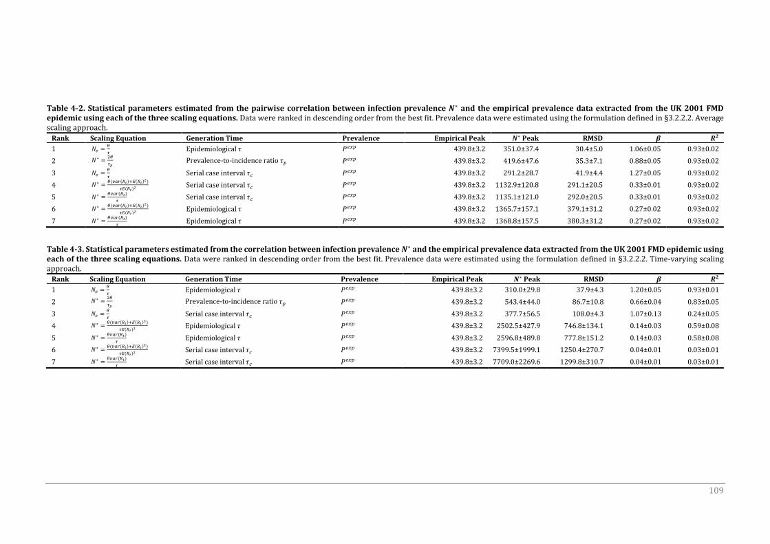
109
Table 4-2. Statistical parameters estimated from the pairwise correlation between infection prevalence 𝑵∗ and the empirical prevalence data extracted from the UK 2001 FMD epidemic using each of the three scaling equations. Data were ranked in descending order from the best fit. Prevalence data were estimated using the formulation defined in §3.2.2.2. Average scaling approach.
Rank Scaling Equation Generation Time Prevalence Empirical Peak 𝑵∗ Peak RMSD 𝜷 𝑹𝟐
1 𝑁𝑒 =𝜃
𝜏 Epidemiological 𝜏 𝑃𝑒𝑥𝑝 439.8±3.2 351.0±37.4 30.4±5.0 1.06±0.05 0.93±0.02
2 𝑁∗ =2𝜃
𝜏𝑝 Prevalence-to-incidence ratio 𝜏𝑝 𝑃𝑒𝑥𝑝 439.8±3.2 419.6±47.6 35.3±7.1 0.88±0.05 0.93±0.02
3 𝑁𝑒 =𝜃
𝜏 Serial case interval 𝜏𝑐 𝑃𝑒𝑥𝑝 439.8±3.2 291.2±28.7 41.9±4.4 1.27±0.05 0.93±0.02
4 𝑁∗ =𝜃(𝑣𝑎𝑟(𝑅𝑡)+𝐸(𝑅𝑡)2)
𝜏𝐸(𝑅𝑡)2 Serial case interval 𝜏𝑐 𝑃𝑒𝑥𝑝 439.8±3.2 1132.9±120.8 291.1±20.5 0.33±0.01 0.93±0.02
5 𝑁∗ =𝜃𝑣𝑎𝑟(𝑅𝑡)
𝜏 Serial case interval 𝜏𝑐 𝑃𝑒𝑥𝑝 439.8±3.2 1135.1±121.0 292.0±20.5 0.33±0.01 0.93±0.02
6 𝑁∗ =𝜃(𝑣𝑎𝑟(𝑅𝑡)+𝐸(𝑅𝑡)2)
𝜏𝐸(𝑅𝑡)2 Epidemiological 𝜏 𝑃𝑒𝑥𝑝 439.8±3.2 1365.7±157.1 379.1±31.2 0.27±0.02 0.93±0.02
7 𝑁∗ =𝜃𝑣𝑎𝑟(𝑅𝑡)
𝜏 Epidemiological 𝜏 𝑃𝑒𝑥𝑝 439.8±3.2 1368.8±157.5 380.3±31.2 0.27±0.02 0.93±0.02
Table 4-3. Statistical parameters estimated from the correlation between infection prevalence 𝑵∗ and the empirical prevalence data extracted from the UK 2001 FMD epidemic using each of the three scaling equations. Data were ranked in descending order from the best fit. Prevalence data were estimated using the formulation defined in §3.2.2.2. Time-varying scaling approach.
Rank Scaling Equation Generation Time Prevalence Empirical Peak 𝑵∗ Peak RMSD 𝜷 𝑹𝟐
1 𝑁𝑒 =𝜃
𝜏 Epidemiological 𝜏 𝑃𝑒𝑥𝑝 439.8±3.2 310.0±29.8 37.9±4.3 1.20±0.05 0.93±0.01
2 𝑁∗ =2𝜃
𝜏𝑝 Prevalence-to-incidence ratio 𝜏𝑝 𝑃𝑒𝑥𝑝 439.8±3.2 543.4±44.0 86.7±10.8 0.66±0.04 0.83±0.05
3 𝑁𝑒 =𝜃
𝜏 Serial case interval 𝜏𝑐 𝑃𝑒𝑥𝑝 439.8±3.2 377.7±56.5 108.0±4.3 1.07±0.13 0.24±0.05
4 𝑁∗ =𝜃(𝑣𝑎𝑟(𝑅𝑡)+𝐸(𝑅𝑡)2)
𝜏𝐸(𝑅𝑡)2 Epidemiological 𝜏 𝑃𝑒𝑥𝑝 439.8±3.2 2502.5±427.9 746.8±134.1 0.14±0.03 0.59±0.08
5 𝑁∗ =𝜃𝑣𝑎𝑟(𝑅𝑡)
𝜏 Epidemiological 𝜏 𝑃𝑒𝑥𝑝 439.8±3.2 2596.8±489.8 777.8±151.2 0.14±0.03 0.58±0.08
6 𝑁∗ =𝜃(𝑣𝑎𝑟(𝑅𝑡)+𝐸(𝑅𝑡)2)
𝜏𝐸(𝑅𝑡)2 Serial case interval 𝜏𝑐 𝑃𝑒𝑥𝑝 439.8±3.2 7399.5±1999.1 1250.4±270.7 0.04±0.01 0.03±0.01
7 𝑁∗ =𝜃𝑣𝑎𝑟(𝑅𝑡)
𝜏 Serial case interval 𝜏𝑐 𝑃𝑒𝑥𝑝 439.8±3.2 7709.0±2269.6 1299.8±310.7 0.04±0.01 0.03±0.01
Chapter 4
110
The best fit was obtained by the simple derivation of 𝑁𝑒 from the BSP scaled
using the epidemiological generation time 𝜏 (RMSD=30.4±5.0). The scaling formulation
ranked second was the ‘NLFT scaling formulation’ (RMSD=35.3±7.1), which also
produced the closest match with the empirical epidemic peak (average difference of
20.2 IPs). The third ranked 𝑁∗ was obtained scaling the BSP using the serial case
interval 𝜏𝑐 (RMSD=41.9±4.4). The results produced using the first two ranked scaling
formulations and the one derived from the ‘𝑣𝑎𝑟(𝑅𝑡) scaling formulation’ [assuming the
Koelle and Rasmussen (2012) derivation of 𝑣𝑎𝑟(𝑅𝑡) and the serial case interval 𝜏𝑐]
have been further analysed within this chapter, whilst 𝑁∗ curves and analyses gathered
from the remaining 4 pairwise comparisons are presented in Appendix 6. Incidence
was found to be invariably lower than the infection prevalence 𝑁∗ recovered from each
of the 7 scaling correlation matrices, showing high deviance values and low similarity
(RMSD>150). Therefore, this relationship has not been investigated further in the
study.
4.3.1.1 Skyline scaled effective population size 𝑁𝑒
Assuming the generation time with its epidemiological definition (§3.2.2.3), the
𝑁𝑒 curves derived using the skyline scaling formulation are shown in Figure 4-2. A high
level of consistency was produced across the 12 realisations of the UK 2001 FMDV
simulated WGS, with the shape and the structure of the 𝑁𝑒 trajectory largely preserved.
Visually inspecting the 𝑁𝑒 curve generated from the 𝑛=2026 IPs dataset, the epidemic
phases characterising the shape of the epidemic curve could be identified from the
skyline trajectories, albeit some variabilities observed between runs. Dissecting the
epidemic curve into the three subsequent phases (as define in §3.3.1) the correlation
of the actual number of infected cases from 𝑃𝑒𝑥𝑝 and scaled 𝑁𝑒 values are presented in
Table 4-4. The correlation between 𝑁𝑒 and 𝑃𝑒𝑥𝑝 was described to be highly linearly
correlated (average 𝑅2 value of 0.93±0.02), thus resulting in very low deviance
(RMSD=30.4±5.0) estimate (Table 4-4). The average 𝑁𝑒 estimated for the full epidemic
dataset (𝑛=2026) was found to be 77.7±3.5 cases/day, whilst the average data
estimated for the exponential, peak, decline and tail end phases were 155.9±10.4,
351.0±37.4, 149.6±6.0 and 24.2±1.3 cases/day. To define the numerical size gap
between 𝑁𝑒 and prevalence, the count lag of the two quantities has been assessed
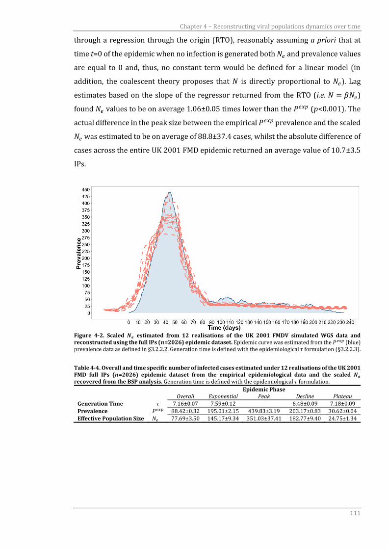
Chapter 4 – Reconstructing viral populations dynamics over time
111
through a regression through the origin (RTO), reasonably assuming a priori that at
time t=0 of the epidemic when no infection is generated both 𝑁𝑒 and prevalence values
are equal to 0 and, thus, no constant term would be defined for a linear model (in
addition, the coalescent theory proposes that 𝑁 is directly proportional to 𝑁𝑒). Lag
estimates based on the slope of the regressor returned from the RTO (i.e. 𝑁 = 𝛽𝑁𝑒)
found 𝑁𝑒 values to be on average 1.06±0.05 times lower than the 𝑃𝑒𝑥𝑝 (𝑝<0.001). The
actual difference in the peak size between the empirical 𝑃𝑒𝑥𝑝 prevalence and the scaled
𝑁𝑒 was estimated to be on average of 88.8±37.4 cases, whilst the absolute difference of
cases across the entire UK 2001 FMD epidemic returned an average value of 10.7±3.5
IPs.
Figure 4-2. Scaled 𝑵𝒆 estimated from 12 realisations of the UK 2001 FMDV simulated WGS data and reconstructed using the full IPs (𝒏=2026) epidemic dataset. Epidemic curve was estimated from the 𝑃𝑒𝑥𝑝 (blue) prevalence data as defined in §3.2.2.2. Generation time is defined with the epidemiological 𝜏 formulation (§3.2.2.3).
Table 4-4. Overall and time specific number of infected cases estimated under 12 realisations of the UK 2001 FMD full IPs (𝒏=2026) epidemic dataset from the empirical epidemiological data and the scaled 𝑵𝒆 recovered from the BSP analysis. Generation time is defined with the epidemiological 𝜏 formulation.
Epidemic Phase Overall Exponential Peak Decline Plateau
Generation Time 𝜏 7.16±0.07 7.59±0.12 - 6.48±0.09 7.18±0.09
Prevalence 𝑃𝑒𝑥𝑝 88.42±0.32 195.01±2.15 439.83±3.19 203.17±0.83 30.62±0.04
Effective Population Size 𝑁𝑒 77.69±3.50 145.17±9.34 351.03±37.41 182.77±9.40 24.75±1.34
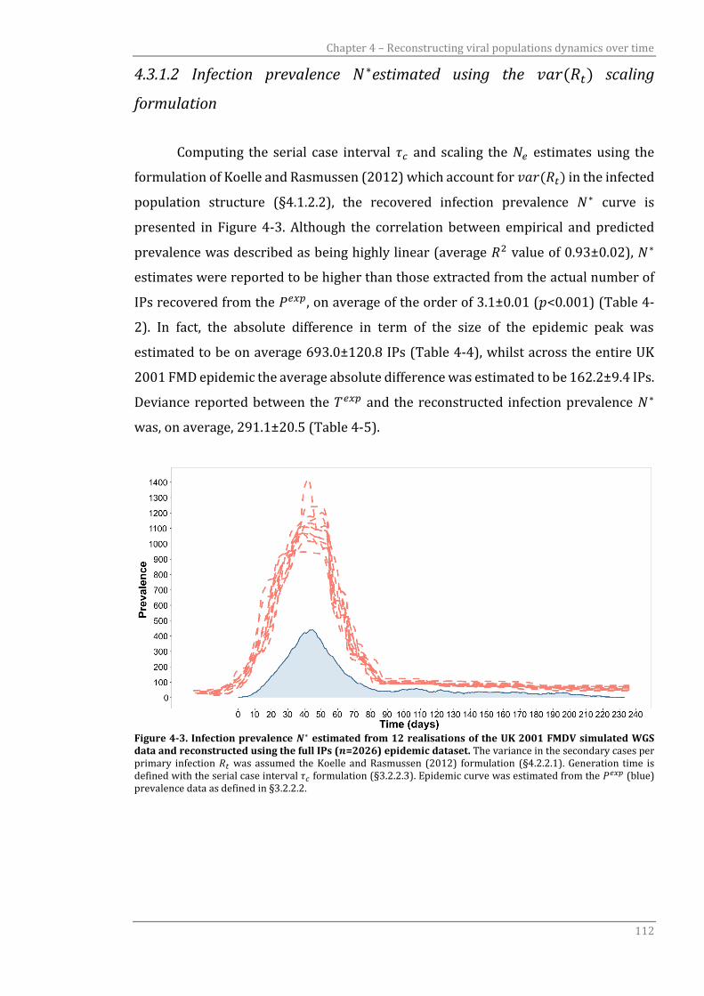
Chapter 4 – Reconstructing viral populations dynamics over time
112
4.3.1.2 Infection prevalence 𝑁∗estimated using the 𝑣𝑎𝑟(𝑅𝑡) scaling
formulation
Computing the serial case interval 𝜏𝑐 and scaling the 𝑁𝑒 estimates using the
formulation of Koelle and Rasmussen (2012) which account for 𝑣𝑎𝑟(𝑅𝑡) in the infected
population structure (§4.1.2.2), the recovered infection prevalence 𝑁∗ curve is
presented in Figure 4-3. Although the correlation between empirical and predicted
prevalence was described as being highly linear (average 𝑅2 value of 0.93±0.02), 𝑁∗
estimates were reported to be higher than those extracted from the actual number of
IPs recovered from the 𝑃𝑒𝑥𝑝, on average of the order of 3.1±0.01 (𝑝<0.001) (Table 4-
2). In fact, the absolute difference in term of the size of the epidemic peak was
estimated to be on average 693.0±120.8 IPs (Table 4-4), whilst across the entire UK
2001 FMD epidemic the average absolute difference was estimated to be 162.2±9.4 IPs.
Deviance reported between the 𝑇𝑒𝑥𝑝 and the reconstructed infection prevalence 𝑁∗
was, on average, 291.1±20.5 (Table 4-5).
Figure 4-3. Infection prevalence 𝑵∗ estimated from 12 realisations of the UK 2001 FMDV simulated WGS data and reconstructed using the full IPs (𝒏=2026) epidemic dataset. The variance in the secondary cases per primary infection 𝑅𝑡 was assumed the Koelle and Rasmussen (2012) formulation (§4.2.2.1). Generation time is defined with the serial case interval 𝜏𝑐 formulation (§3.2.2.3). Epidemic curve was estimated from the 𝑃𝑒𝑥𝑝 (blue) prevalence data as defined in §3.2.2.2.
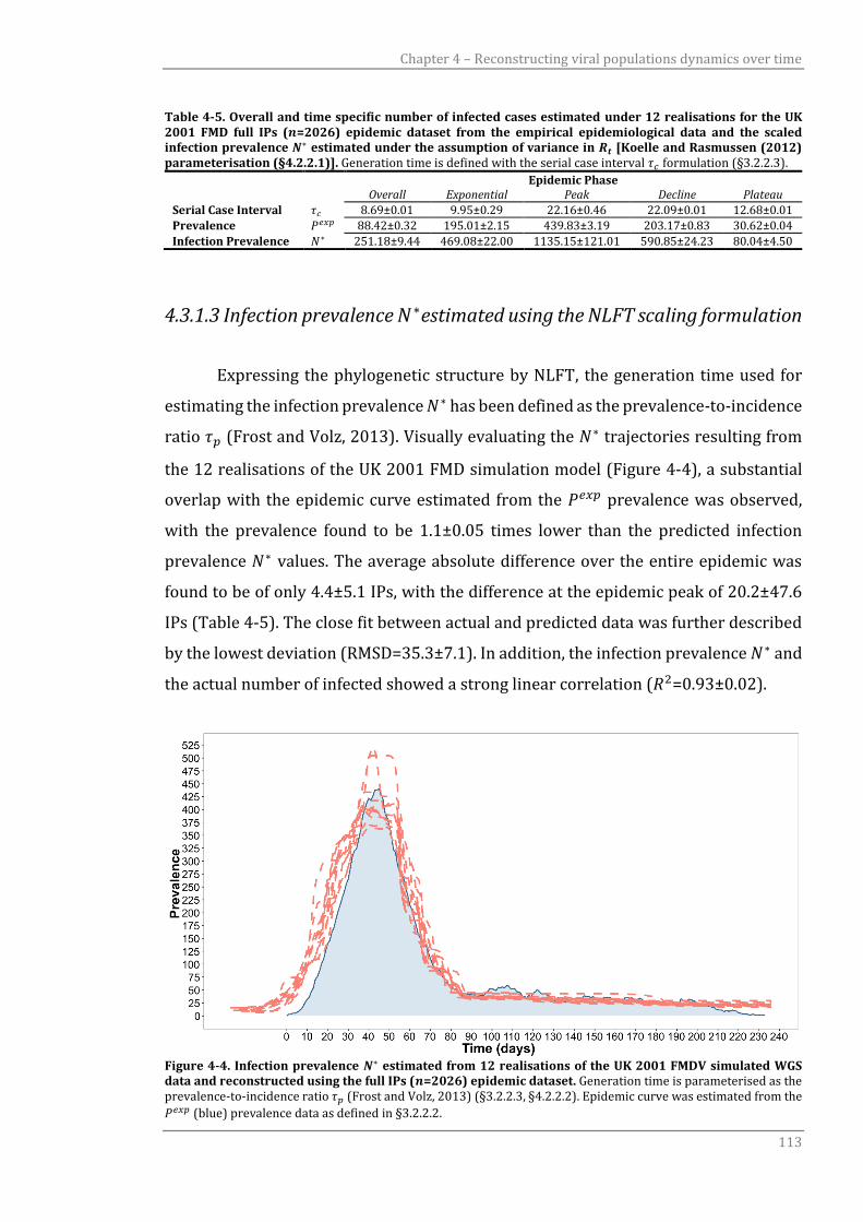
Chapter 4 – Reconstructing viral populations dynamics over time
113
Table 4-5. Overall and time specific number of infected cases estimated under 12 realisations for the UK 2001 FMD full IPs (𝒏=2026) epidemic dataset from the empirical epidemiological data and the scaled infection prevalence 𝑵∗ estimated under the assumption of variance in 𝑹𝒕 [Koelle and Rasmussen (2012) parameterisation (§4.2.2.1)]. Generation time is defined with the serial case interval 𝜏𝑐 formulation (§3.2.2.3).
Epidemic Phase Overall Exponential Peak Decline Plateau
Serial Case Interval 𝜏𝑐 8.69±0.01 9.95±0.29 22.16±0.46 22.09±0.01 12.68±0.01
Prevalence 𝑃𝑒𝑥𝑝 88.42±0.32 195.01±2.15 439.83±3.19 203.17±0.83 30.62±0.04
Infection Prevalence 𝑁∗ 251.18±9.44 469.08±22.00 1135.15±121.01 590.85±24.23 80.04±4.50
4.3.1.3 Infection prevalence 𝑁∗estimated using the NLFT scaling formulation
Expressing the phylogenetic structure by NLFT, the generation time used for
estimating the infection prevalence 𝑁∗ has been defined as the prevalence-to-incidence
ratio 𝜏𝑝 (Frost and Volz, 2013). Visually evaluating the 𝑁∗ trajectories resulting from
the 12 realisations of the UK 2001 FMD simulation model (Figure 4-4), a substantial
overlap with the epidemic curve estimated from the 𝑃𝑒𝑥𝑝 prevalence was observed,
with the prevalence found to be 1.1±0.05 times lower than the predicted infection
prevalence 𝑁∗ values. The average absolute difference over the entire epidemic was
found to be of only 4.4±5.1 IPs, with the difference at the epidemic peak of 20.2±47.6
IPs (Table 4-5). The close fit between actual and predicted data was further described
by the lowest deviation (RMSD=35.3±7.1). In addition, the infection prevalence 𝑁∗ and
the actual number of infected showed a strong linear correlation (𝑅2=0.93±0.02).
Figure 4-4. Infection prevalence 𝑵∗ estimated from 12 realisations of the UK 2001 FMDV simulated WGS data and reconstructed using the full IPs (𝒏=2026) epidemic dataset. Generation time is parameterised as the prevalence-to-incidence ratio 𝜏𝑝 (Frost and Volz, 2013) (§3.2.2.3, §4.2.2.2). Epidemic curve was estimated from the
𝑃𝑒𝑥𝑝 (blue) prevalence data as defined in §3.2.2.2.
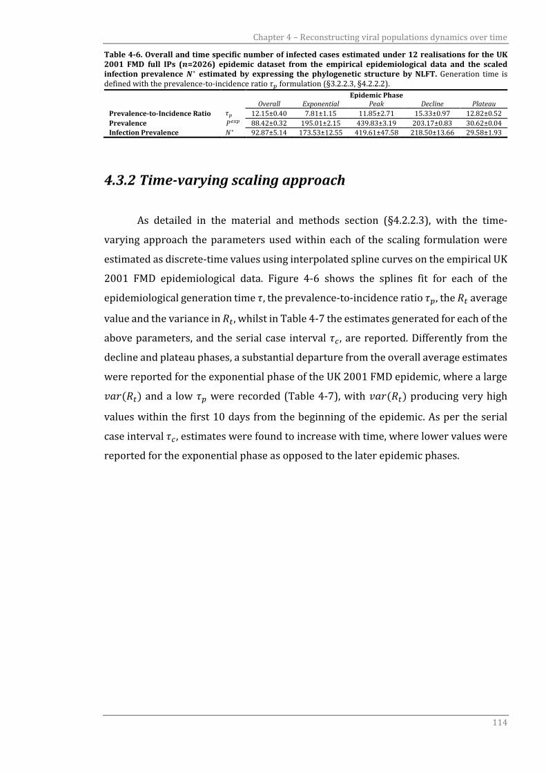
Chapter 4 – Reconstructing viral populations dynamics over time
114
Table 4-6. Overall and time specific number of infected cases estimated under 12 realisations for the UK 2001 FMD full IPs (𝒏=2026) epidemic dataset from the empirical epidemiological data and the scaled infection prevalence 𝑵∗ estimated by expressing the phylogenetic structure by NLFT. Generation time is defined with the prevalence-to-incidence ratio 𝜏𝑝 formulation (§3.2.2.3, §4.2.2.2).
Epidemic Phase Overall Exponential Peak Decline Plateau
Prevalence-to-Incidence Ratio 𝜏𝑝 12.15±0.40 7.81±1.15 11.85±2.71 15.33±0.97 12.82±0.52
Prevalence 𝑃𝑒𝑥𝑝 88.42±0.32 195.01±2.15 439.83±3.19 203.17±0.83 30.62±0.04
Infection Prevalence 𝑁∗ 92.87±5.14 173.53±12.55 419.61±47.58 218.50±13.66 29.58±1.93
4.3.2 Time-varying scaling approach
As detailed in the material and methods section (§4.2.2.3), with the time-
varying approach the parameters used within each of the scaling formulation were
estimated as discrete-time values using interpolated spline curves on the empirical UK
2001 FMD epidemiological data. Figure 4-6 shows the splines fit for each of the
epidemiological generation time 𝜏, the prevalence-to-incidence ratio 𝜏𝑝, the 𝑅𝑡 average
value and the variance in 𝑅𝑡, whilst in Table 4-7 the estimates generated for each of the
above parameters, and the serial case interval 𝜏𝑐, are reported. Differently from the
decline and plateau phases, a substantial departure from the overall average estimates
were reported for the exponential phase of the UK 2001 FMD epidemic, where a large
𝑣𝑎𝑟(𝑅𝑡) and a low 𝜏𝑝 were recorded (Table 4-7), with 𝑣𝑎𝑟(𝑅𝑡) producing very high
values within the first 10 days from the beginning of the epidemic. As per the serial
case interval 𝜏𝑐, estimates were found to increase with time, where lower values were
reported for the exponential phase as opposed to the later epidemic phases.
Chapter 4 – Reconstructing viral populations dynamics over time
115
Figure 4-5. Natural splines interpolation for time-varying epidemiological parameters estimated from the empirical UK 2001 FMD epidemic data. Generation time 𝜏 (A), prevalence-to-incidence ratio 𝜏𝑝 (B), average
number of secondary cases per primary infection 𝑅𝑡 (C), variance in the number of secondary cases per primary infection 𝑣𝑎𝑟(𝑅𝑡).
Table 4-7. Epidemiological parameters estimated following natural spline interpolations of the 12 realisations of the reconstructed UK 2001 FMD transmission tree.
Epidemic Phase Overall Exponential Peak Decline Plateau
Epidemiological Generation Time (𝝉) 5.91±0.10 7.57±0.11 5.91±0.10 6.93±0.07 5.35±0.67 Serial Case Interval (𝝉𝒄) 8.73 9.42±0.38 21.40±0.68 22.06±0.05 12.68±0.01 Prevalence-to-Incidence Ratio (𝝉𝒑) 11.63±0.21 8.07±0.21 11.64±0.21 11.71±0.4 12.70±0.26 𝑹𝒕 Variance 4.28±0.45 12.18±2.25 4.28±0.45 2.75±0.52 2.23±0.19 𝑹𝒕 Mean 0.99±0.04 2.04±0.26 1.16±0.07 1.09±0.05 0.98±0.04
Similarly to that reported for the average scaling approach, spline fitted values
were then used to investigate the effect of the time-varying scaling approach for
deriving the 𝑁𝑒 estimates and, thus, the infection prevalence 𝑁∗ curve. Therefore,
twenty one pairwise correlation analyses were also undertaken between the 𝑁∗
estimates derived by using the time-varying parameter estimates for each of the
scaling equations provided in Table 4-1 and the 𝑃𝑒𝑥𝑝 prevalence estimate (as detailed
in §3.2.2.2). The results produced are presented in Table 4-3 and ranked in descending
order from the best fit to the poorest according to the RMSD estimates. The full details
of the results generated from each of the scaling formulation are presented in Appendix
7.
As observed with the average scaling approach, the best fit was still obtained
with the scaling formulation consisting of the simple derivation of 𝑁𝑒 from the BSP
scaled using the serial case interval 𝜏, although returning relatively higher deviance
estimates (RMSD=37.9±4.3) (Table 4-3). With the time-varying scaling approach, the
absolute difference in size of the entire epidemic between predicted and actual data
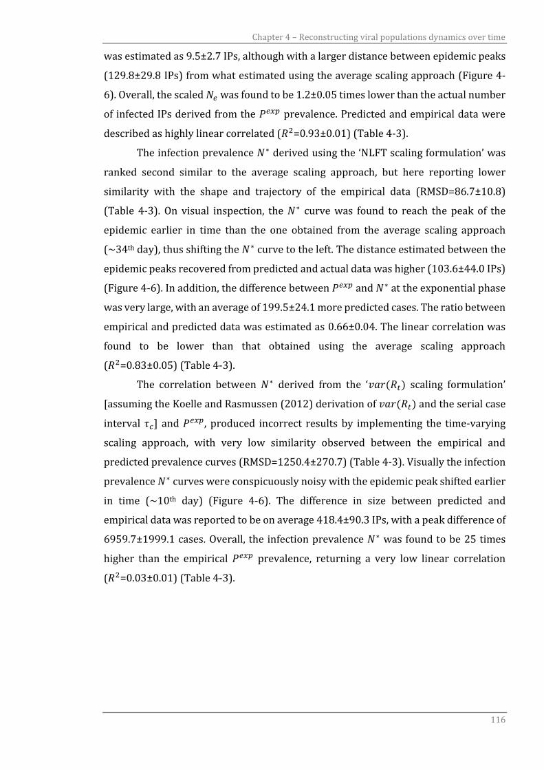
Chapter 4 – Reconstructing viral populations dynamics over time
116
was estimated as 9.5±2.7 IPs, although with a larger distance between epidemic peaks
(129.8±29.8 IPs) from what estimated using the average scaling approach (Figure 4-
6). Overall, the scaled 𝑁𝑒 was found to be 1.2±0.05 times lower than the actual number
of infected IPs derived from the 𝑃𝑒𝑥𝑝 prevalence. Predicted and empirical data were
described as highly linear correlated (𝑅2=0.93±0.01) (Table 4-3).
The infection prevalence 𝑁∗ derived using the ‘NLFT scaling formulation’ was
ranked second similar to the average scaling approach, but here reporting lower
similarity with the shape and trajectory of the empirical data (RMSD=86.7±10.8)
(Table 4-3). On visual inspection, the 𝑁∗ curve was found to reach the peak of the
epidemic earlier in time than the one obtained from the average scaling approach
(~34th day), thus shifting the 𝑁∗ curve to the left. The distance estimated between the
epidemic peaks recovered from predicted and actual data was higher (103.6±44.0 IPs)
(Figure 4-6). In addition, the difference between 𝑃𝑒𝑥𝑝 and 𝑁∗ at the exponential phase
was very large, with an average of 199.5±24.1 more predicted cases. The ratio between
empirical and predicted data was estimated as 0.66±0.04. The linear correlation was
found to be lower than that obtained using the average scaling approach
(𝑅2=0.83±0.05) (Table 4-3).
The correlation between 𝑁∗ derived from the ‘𝑣𝑎𝑟(𝑅𝑡) scaling formulation’
[assuming the Koelle and Rasmussen (2012) derivation of 𝑣𝑎𝑟(𝑅𝑡) and the serial case
interval 𝜏𝑐] and 𝑃𝑒𝑥𝑝, produced incorrect results by implementing the time-varying
scaling approach, with very low similarity observed between the empirical and
predicted prevalence curves (RMSD=1250.4±270.7) (Table 4-3). Visually the infection
prevalence 𝑁∗ curves were conspicuously noisy with the epidemic peak shifted earlier
in time (~10th day) (Figure 4-6). The difference in size between predicted and
empirical data was reported to be on average 418.4±90.3 IPs, with a peak difference of
6959.7±1999.1 cases. Overall, the infection prevalence 𝑁∗ was found to be 25 times
higher than the empirical 𝑃𝑒𝑥𝑝 prevalence, returning a very low linear correlation
(𝑅2=0.03±0.01) (Table 4-3).
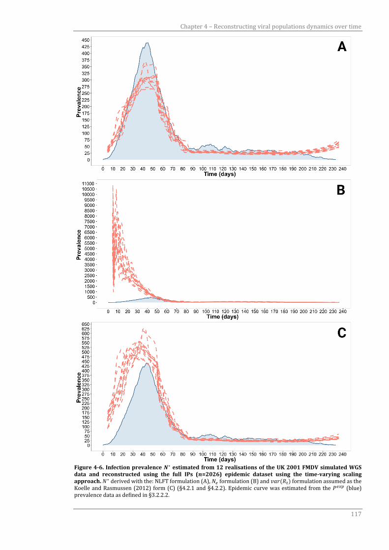
Chapter 4 – Reconstructing viral populations dynamics over time
117
Figure 4-6. Infection prevalence 𝑵∗ estimated from 12 realisations of the UK 2001 FMDV simulated WGS data and reconstructed using the full IPs (𝒏=2026) epidemic dataset using the time-varying scaling approach. 𝑁∗ derived with the: NLFT formulation (A), 𝑁𝑒 formulation (B) and 𝑣𝑎𝑟(𝑅𝑡) formulation assumed as the Koelle and Rasmussen (2012) form (C) (§4.2.1 and §4.2.2). Epidemic curve was estimated from the 𝑃𝑒𝑥𝑝 (blue) prevalence data as defined in §3.2.2.2.
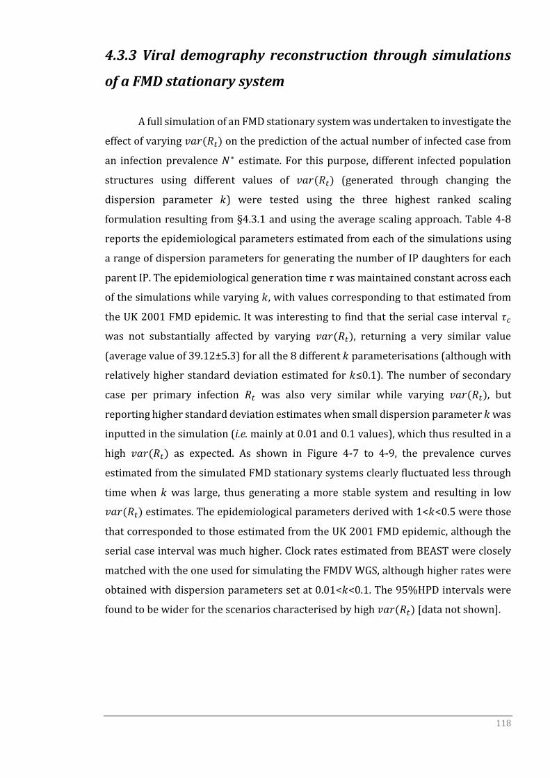
118
4.3.3 Viral demography reconstruction through simulations
of a FMD stationary system
A full simulation of an FMD stationary system was undertaken to investigate the
effect of varying 𝑣𝑎𝑟(𝑅𝑡) on the prediction of the actual number of infected case from
an infection prevalence 𝑁∗ estimate. For this purpose, different infected population
structures using different values of 𝑣𝑎𝑟(𝑅𝑡) (generated through changing the
dispersion parameter 𝑘) were tested using the three highest ranked scaling
formulation resulting from §4.3.1 and using the average scaling approach. Table 4-8
reports the epidemiological parameters estimated from each of the simulations using
a range of dispersion parameters for generating the number of IP daughters for each
parent IP. The epidemiological generation time 𝜏 was maintained constant across each
of the simulations while varying 𝑘, with values corresponding to that estimated from
the UK 2001 FMD epidemic. It was interesting to find that the serial case interval 𝜏𝑐
was not substantially affected by varying 𝑣𝑎𝑟(𝑅𝑡), returning a very similar value
(average value of 39.12±5.3) for all the 8 different 𝑘 parameterisations (although with
relatively higher standard deviation estimated for 𝑘≤0.1). The number of secondary
case per primary infection 𝑅𝑡 was also very similar while varying 𝑣𝑎𝑟(𝑅𝑡), but
reporting higher standard deviation estimates when small dispersion parameter 𝑘 was
inputted in the simulation (i.e. mainly at 0.01 and 0.1 values), which thus resulted in a
high 𝑣𝑎𝑟(𝑅𝑡) as expected. As shown in Figure 4-7 to 4-9, the prevalence curves
estimated from the simulated FMD stationary systems clearly fluctuated less through
time when 𝑘 was large, thus generating a more stable system and resulting in low
𝑣𝑎𝑟(𝑅𝑡) estimates. The epidemiological parameters derived with 1<𝑘<0.5 were those
that corresponded to those estimated from the UK 2001 FMD epidemic, although the
serial case interval was much higher. Clock rates estimated from BEAST were closely
matched with the one used for simulating the FMDV WGS, although higher rates were
obtained with dispersion parameters set at 0.01<𝑘<0.1. The 95%HPD intervals were
found to be wider for the scenarios characterised by high 𝑣𝑎𝑟(𝑅𝑡) [data not shown].
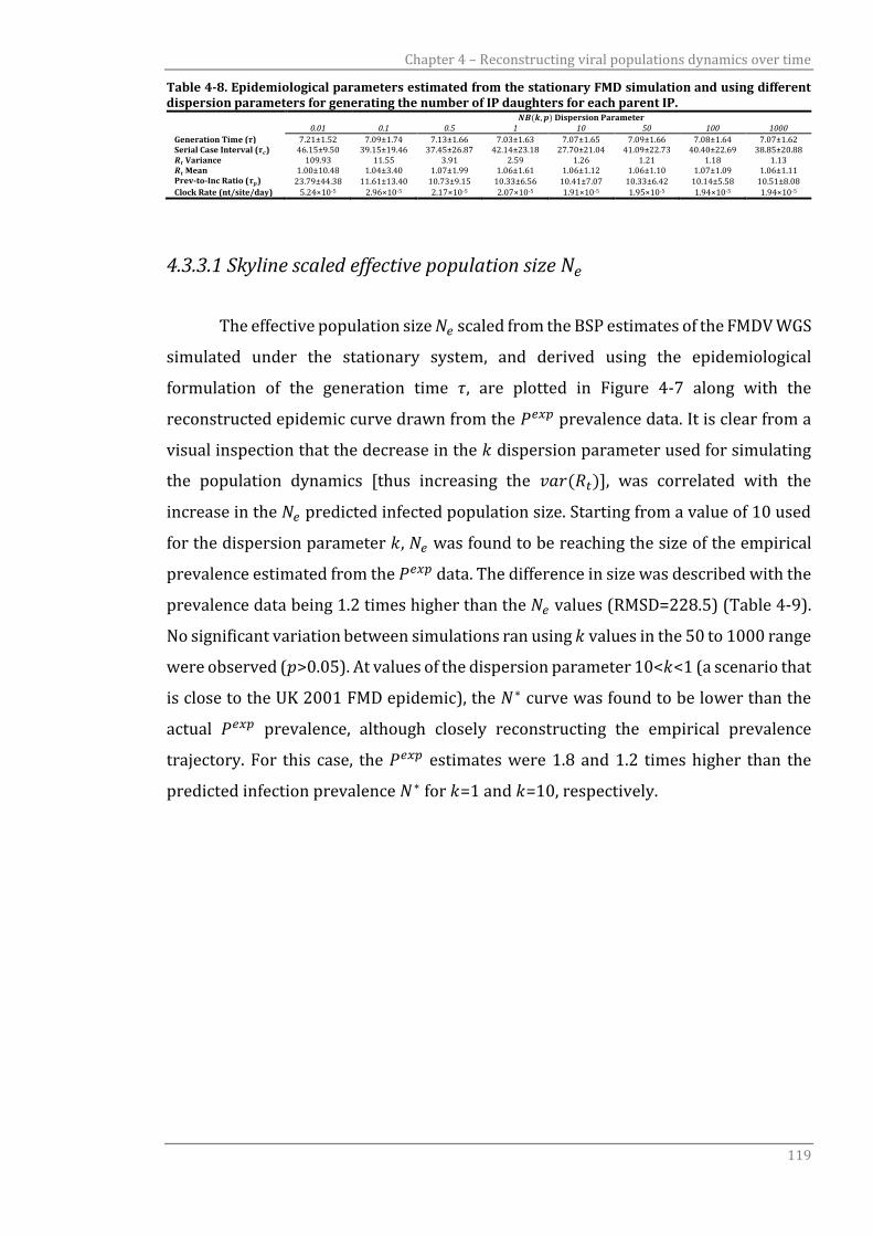
Chapter 4 – Reconstructing viral populations dynamics over time
119
Table 4-8. Epidemiological parameters estimated from the stationary FMD simulation and using different dispersion parameters for generating the number of IP daughters for each parent IP.
𝑵𝑩(𝒌, 𝒑) Dispersion Parameter 0.01 0.1 0.5 1 10 50 100 1000
Generation Time (𝝉) 7.21±1.52 7.09±1.74 7.13±1.66 7.03±1.63 7.07±1.65 7.09±1.66 7.08±1.64 7.07±1.62 Serial Case Interval (𝝉𝒄) 46.15±9.50 39.15±19.46 37.45±26.87 42.14±23.18 27.70±21.04 41.09±22.73 40.40±22.69 38.85±20.88 𝑹𝒕 Variance 109.93 11.55 3.91 2.59 1.26 1.21 1.18 1.13 𝑹𝒕 Mean 1.00±10.48 1.04±3.40 1.07±1.99 1.06±1.61 1.06±1.12 1.06±1.10 1.07±1.09 1.06±1.11 Prev-to-Inc Ratio (𝝉𝒑) 23.79±44.38 11.61±13.40 10.73±9.15 10.33±6.56 10.41±7.07 10.33±6.42 10.14±5.58 10.51±8.08 Clock Rate (nt/site/day) 5.24×10⁻⁵ 2.96×10⁻⁵ 2.17×10⁻⁵ 2.07×10⁻⁵ 1.91×10⁻⁵ 1.95×10⁻⁵ 1.94×10⁻⁵ 1.94×10⁻⁵
4.3.3.1 Skyline scaled effective population size 𝑁𝑒
The effective population size 𝑁𝑒 scaled from the BSP estimates of the FMDV WGS
simulated under the stationary system, and derived using the epidemiological
formulation of the generation time 𝜏, are plotted in Figure 4-7 along with the
reconstructed epidemic curve drawn from the 𝑃𝑒𝑥𝑝 prevalence data. It is clear from a
visual inspection that the decrease in the 𝑘 dispersion parameter used for simulating
the population dynamics [thus increasing the 𝑣𝑎𝑟(𝑅𝑡)], was correlated with the
increase in the 𝑁𝑒 predicted infected population size. Starting from a value of 10 used
for the dispersion parameter 𝑘, 𝑁𝑒 was found to be reaching the size of the empirical
prevalence estimated from the 𝑃𝑒𝑥𝑝 data. The difference in size was described with the
prevalence data being 1.2 times higher than the 𝑁𝑒 values (RMSD=228.5) (Table 4-9).
No significant variation between simulations ran using 𝑘 values in the 50 to 1000 range
were observed (𝑝>0.05). At values of the dispersion parameter 10<𝑘<1 (a scenario that
is close to the UK 2001 FMD epidemic), the 𝑁∗ curve was found to be lower than the
actual 𝑃𝑒𝑥𝑝 prevalence, although closely reconstructing the empirical prevalence
trajectory. For this case, the 𝑃𝑒𝑥𝑝 estimates were 1.8 and 1.2 times higher than the
predicted infection prevalence 𝑁∗ for 𝑘=1 and 𝑘=10, respectively.
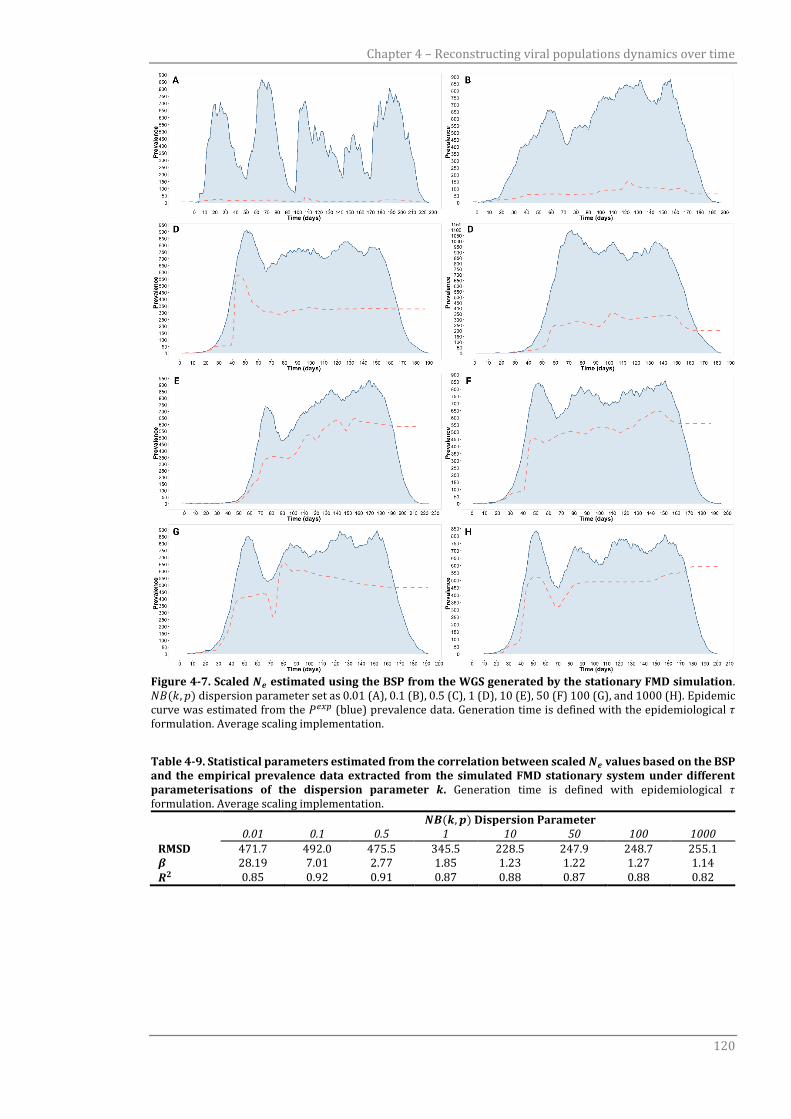
Chapter 4 – Reconstructing viral populations dynamics over time
120
Figure 4-7. Scaled 𝑵𝒆 estimated using the BSP from the WGS generated by the stationary FMD simulation. 𝑁𝐵(𝑘, 𝑝) dispersion parameter set as 0.01 (A), 0.1 (B), 0.5 (C), 1 (D), 10 (E), 50 (F) 100 (G), and 1000 (H). Epidemic curve was estimated from the 𝑃𝑒𝑥𝑝 (blue) prevalence data. Generation time is defined with the epidemiological 𝜏 formulation. Average scaling implementation.
Table 4-9. Statistical parameters estimated from the correlation between scaled 𝑵𝒆 values based on the BSP and the empirical prevalence data extracted from the simulated FMD stationary system under different parameterisations of the dispersion parameter 𝒌. Generation time is defined with epidemiological 𝜏 formulation. Average scaling implementation.
𝑵𝑩(𝒌, 𝒑) Dispersion Parameter 0.01 0.1 0.5 1 10 50 100 1000
RMSD 471.7 492.0 475.5 345.5 228.5 247.9 248.7 255.1 𝜷 28.19 7.01 2.77 1.85 1.23 1.22 1.27 1.14 𝑹𝟐 0.85 0.92 0.91 0.87 0.88 0.87 0.88 0.82
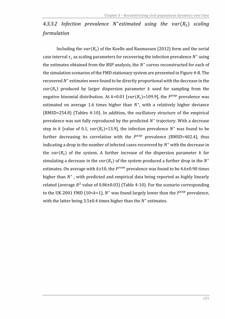
Chapter 4 – Reconstructing viral populations dynamics over time
121
4.3.3.2 Infection prevalence 𝑁∗estimated using the 𝑣𝑎𝑟(𝑅𝑡) scaling
formulation
Including the 𝑣𝑎𝑟(𝑅𝑡) of the Koelle and Rasmussen (2012) form and the serial
case interval 𝜏𝑐 as scaling parameters for recovering the infection prevalence 𝑁∗ using
the estimates obtained from the BSP analysis, the 𝑁∗ curves reconstructed for each of
the simulation scenarios of the FMD stationary system are presented in Figure 4-8. The
recovered 𝑁∗ estimates were found to be directly proportional with the decrease in the
𝑣𝑎𝑟(𝑅𝑡) produced by larger dispersion parameter 𝑘 used for sampling from the
negative binomial distribution. At 𝑘=0.01 [𝑣𝑎𝑟(𝑅𝑡)=109.9], the 𝑃𝑒𝑥𝑝 prevalence was
estimated on average 1.6 times higher than 𝑁∗, with a relatively higher deviance
(RMSD=254.8) (Tables 4-10). In addition, the oscillatory structure of the empirical
prevalence was not fully reproduced by the predicted 𝑁∗ trajectory. With a decrease
step in 𝑘 [value of 0.1, 𝑣𝑎𝑟(𝑅𝑡)=13.9], the infection prevalence 𝑁∗ was found to be
further decreasing its correlation with the 𝑃𝑒𝑥𝑝 prevalence (RMSD=402.4), thus
indicating a drop in the number of infected cases recovered by 𝑁∗ with the decrease in
the 𝑣𝑎𝑟(𝑅𝑡) of the system. A further increase of the dispersion parameter 𝑘 for
simulating a decrease in the 𝑣𝑎𝑟(𝑅𝑡) of the system produced a further drop in the 𝑁∗
estimates. On average with 𝑘≥10, the 𝑃𝑟𝑒𝑚 prevalence was found to be 4.6±0.90 times
higher than 𝑁∗ , with predicted and empirical data being reported as highly linearly
related (average 𝑅2 value of 0.86±0.03) (Table 4-10). For the scenario corresponding
to the UK 2001 FMD (10<𝑘<1), 𝑁∗ was found largely lower than the 𝑃𝑒𝑥𝑝 prevalence,
with the latter being 3.5±0.4 times higher than the 𝑁∗ estimates.
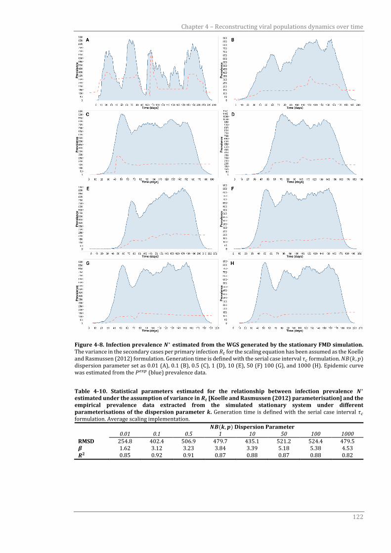
Chapter 4 – Reconstructing viral populations dynamics over time
122
Figure 4-8. Infection prevalence 𝑵∗ estimated from the WGS generated by the stationary FMD simulation. The variance in the secondary cases per primary infection 𝑅𝑡 for the scaling equation has been assumed as the Koelle and Rasmussen (2012) formulation. Generation time is defined with the serial case interval 𝜏𝑐 formulation. 𝑁𝐵(𝑘, 𝑝) dispersion parameter set as 0.01 (A), 0.1 (B), 0.5 (C), 1 (D), 10 (E), 50 (F) 100 (G), and 1000 (H). Epidemic curve was estimated from the 𝑃𝑒𝑥𝑝 (blue) prevalence data.
Table 4-10. Statistical parameters estimated for the relationship between infection prevalence 𝑵∗ estimated under the assumption of variance in 𝑹𝒕 [Koelle and Rasmussen (2012) parameterisation] and the empirical prevalence data extracted from the simulated stationary system under different parameterisations of the dispersion parameter 𝒌. Generation time is defined with the serial case interval 𝜏𝑐 formulation. Average scaling implementation.
𝑵𝑩(𝒌, 𝒑) Dispersion Parameter 0.01 0.1 0.5 1 10 50 100 1000
RMSD 254.8 402.4 506.9 479.7 435.1 521.2 524.4 479.5 𝜷 1.62 3.12 3.23 3.84 3.39 5.18 5.38 4.53 𝑹𝟐 0.85 0.92 0.91 0.87 0.88 0.87 0.88 0.82
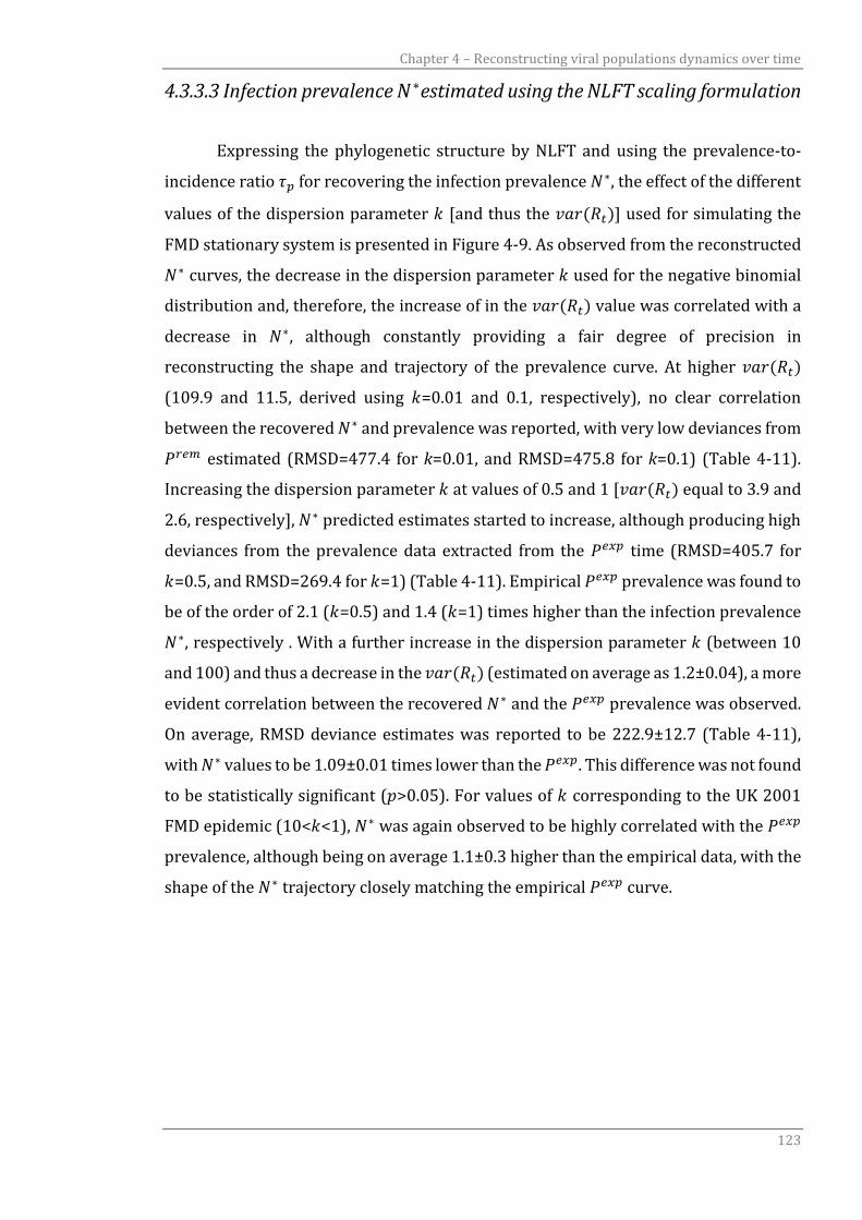
Chapter 4 – Reconstructing viral populations dynamics over time
123
4.3.3.3 Infection prevalence 𝑁∗estimated using the NLFT scaling formulation
Expressing the phylogenetic structure by NLFT and using the prevalence-to-
incidence ratio 𝜏𝑝 for recovering the infection prevalence 𝑁∗, the effect of the different
values of the dispersion parameter 𝑘 [and thus the 𝑣𝑎𝑟(𝑅𝑡)] used for simulating the
FMD stationary system is presented in Figure 4-9. As observed from the reconstructed
𝑁∗ curves, the decrease in the dispersion parameter 𝑘 used for the negative binomial
distribution and, therefore, the increase of in the 𝑣𝑎𝑟(𝑅𝑡) value was correlated with a
decrease in 𝑁∗, although constantly providing a fair degree of precision in
reconstructing the shape and trajectory of the prevalence curve. At higher 𝑣𝑎𝑟(𝑅𝑡)
(109.9 and 11.5, derived using 𝑘=0.01 and 0.1, respectively), no clear correlation
between the recovered 𝑁∗ and prevalence was reported, with very low deviances from
𝑃𝑟𝑒𝑚 estimated (RMSD=477.4 for k=0.01, and RMSD=475.8 for k=0.1) (Table 4-11).
Increasing the dispersion parameter 𝑘 at values of 0.5 and 1 [𝑣𝑎𝑟(𝑅𝑡) equal to 3.9 and
2.6, respectively], 𝑁∗ predicted estimates started to increase, although producing high
deviances from the prevalence data extracted from the 𝑃𝑒𝑥𝑝 time (RMSD=405.7 for
𝑘=0.5, and RMSD=269.4 for 𝑘=1) (Table 4-11). Empirical 𝑃𝑒𝑥𝑝 prevalence was found to
be of the order of 2.1 (𝑘=0.5) and 1.4 (𝑘=1) times higher than the infection prevalence
𝑁∗, respectively . With a further increase in the dispersion parameter 𝑘 (between 10
and 100) and thus a decrease in the 𝑣𝑎𝑟(𝑅𝑡) (estimated on average as 1.2±0.04), a more
evident correlation between the recovered 𝑁∗ and the 𝑃𝑒𝑥𝑝 prevalence was observed.
On average, RMSD deviance estimates was reported to be 222.9±12.7 (Table 4-11),
with 𝑁∗ values to be 1.09±0.01 times lower than the 𝑃𝑒𝑥𝑝. This difference was not found
to be statistically significant (𝑝>0.05). For values of 𝑘 corresponding to the UK 2001
FMD epidemic (10<𝑘<1), 𝑁∗ was again observed to be highly correlated with the 𝑃𝑒𝑥𝑝
prevalence, although being on average 1.1±0.3 higher than the empirical data, with the
shape of the 𝑁∗ trajectory closely matching the empirical 𝑃𝑒𝑥𝑝 curve.
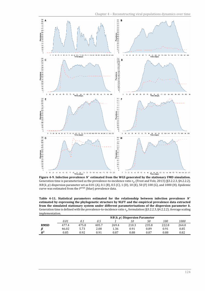
Chapter 4 – Reconstructing viral populations dynamics over time
124
Figure 4-9. Infection prevalence 𝑵∗ estimated from the WGS generated by the stationary FMD simulation. Generation time is parameterised as the prevalence-to-incidence ratio 𝜏𝑝 (Frost and Volz, 2013) (§3.2.2.3, §4.2.2.2).
𝑁𝐵(𝑘, 𝑝) dispersion parameter set as 0.01 (A), 0.1 (B), 0.5 (C), 1 (D), 10 (E), 50 (F) 100 (G), and 1000 (H). Epidemic curve was estimated from the 𝑃𝑒𝑥𝑝 (blue) prevalence data.
Table 4-11. Statistical parameters estimated for the relationship between infection prevalence 𝑵∗ estimated by expressing the phylogenetic structure by NLFT and the empirical prevalence data extracted from the simulated stationary system under different parameterisations of the dispersion parameter 𝒌. Generation time is defined with the prevalence-to-incidence ratio 𝜏𝑝 formulation (§3.2.2.3, §4.2.2.2). Average scaling
implementation.
𝑵𝑩(𝒌, 𝒑) Dispersion Parameter 0.01 0.1 0.5 1 10 50 100 1000
RMSD 477.4 475.8 405.7 269.4 210.3 235.8 222.8 264.0 𝜷 46.02 5.73 2.08 1.36 0.91 0.89 0.91 0.85 𝑹𝟐 0.85 0.92 0.91 0.87 0.88 0.87 0.88 0.82
Chapter 4 – Reconstructing viral populations dynamics over time
125
4.4 Discussion
In this chapter, a thorough investigation of the relationship that exists between
the effective population size 𝑁𝑒 extracted from the BSP and the actual number of
infected cases has been presented. The aim was to attempt to identify a valid
formulation which can be used to scale 𝑁𝑒 to a proxy measure of empirical prevalence
data, here termed the infection prevalence 𝑁∗. Three formulations derived from 𝑁𝑒
𝑁
equations (as in Table 4-1) were tested with two different scaling approaches, namely
average and time-varying, describing the potential epidemiological and/or
evolutionary factors associated with the relationship of these two quantities, from a
simple linear scaling of generation time to the account of complex variabilities in the
population structure under study. The uniqueness of this study relies in the data which,
albeit simulated for its genetic component, have been obtained from a single
exhaustive and fully-resolved epidemic (i.e. the UK 2001 FMD epidemic) where the
demography of the infected population is fully known, thus enabling measurement of
a direct correlation in time between the real epidemic size and the recovered infection
prevalence 𝑁∗.
Although the shape and trajectory of the scaled 𝑁∗ curve followed with
precision the epidemic curve generated from the prevalence data and a strong linear
relationship has been established (𝑅2 value of up to 0.93), the exact match varied
considerably according to the scaling formulation used. Thus, defining prevalence data
according to the timing of the FMD disease progression (as previously described in
§3.2.2.2), different correlations exist between the infection prevalence 𝑁∗ and the
prevalence data extracted from each of the time-related FMD stages. It is evident that,
using 𝑁𝑒 estimated directly from the BSP and scaling this quantity using the
epidemiological definition of generation time 𝜏, a clear correlation with the prevalence
extracted from the 𝑃𝑒𝑥𝑝 is observed. Expressing the phylogenetic structure by NLFT
and using the prevalence-to-incidence ratio 𝜏𝑝 for deriving the infection prevalence 𝑁∗,
this quantity effectively resolves the shape and trajectory of the prevalence computed
from the 𝑃𝑒𝑥𝑝 data. On the other hand, accounting for the variability in the number of
progeny per single IP generated across the different phases of the epidemic and using
the Koelle and Rasmussen (2012) form of 𝑣𝑎𝑟(𝑅𝑡) along with the serial case interval 𝜏𝑐
for recovering 𝑁∗, estimates were observed to not correlate with the infected
Chapter 4 – Reconstructing viral populations dynamics over time
126
population size derived from the 𝑃𝑒𝑥𝑝 prevalence data, where the predicted 𝑁∗ was
found to be considerably higher than the empirical prevalence. This finding indicates
that, for correctly scaling an estimate of 𝑁𝑒 to the actual number of infected cases
(expressed as prevalence), the generation time should be measured by as the
prevalence to incidence ratio 𝜏𝑝, and scaling should express the phylogenetic structure
by the number of lineages as a function of time.
Investigating the effect of the 𝑣𝑎𝑟(𝑅𝑡) on the estimation of the infected
population demography and examining the results obtained from the analysis of the
stationary FMD simulation, it is evident that the variability in the number of secondary
cases per primary infection 𝑅𝑡 greatly impacts on the BSP reconstruction of the actual
number of infected cases and, although accurately describing the shape of the
demographic curve and its trajectory, the increase in the stochastic reproduction of the
infected population [i.e. 𝑣𝑎𝑟(𝑅𝑡)] significantly reduces the BSP accuracy. This outcome
has been consistently observed for every formulation used to scale the BSP estimates
to either the effective population size 𝑁𝑒 or the infection prevalence 𝑁∗, even those that
include the variance in the number of secondary cases per primary infection explicitly
in the formulation of the scaling equation. On the other hand when 𝑣𝑎𝑟(𝑅𝑡) is reduced
by increasing the dispersion parameter 𝑘, the infection prevalence 𝑁∗ matches the 𝑃𝑒𝑥𝑝
prevalence, although the precise relationship varies according to the formulation used
for scaling the BSP data and, therefore, the model assumptions. For example, the fit
from the scaling equation that considers the phylogenetic structure by NLFT suggests
that in a more homogeneous FMD system [i.e. with 𝑘≥10 and 𝑣𝑎𝑟(𝑅𝑡)≈1] the predicted
infection prevalence 𝑁∗ is a good approximation to the empirical IP count (𝑃𝑒𝑥𝑝
derived). This means that every IP in the system has the same chance of transmitting
infection to subsequent generations and, therefore, the average time between
infections is the only possible scaling factor and is constant.
Assuming a more stochastic disease system in which the presence of
‘superspreaders’ is not solely driving the transmission process [i.e. 0.5<𝑘<10 and
2≲𝑣𝑎𝑟(𝑅𝑡)≲3], estimates of infection prevalence 𝑁∗ provided by the scaling
transformation of 𝑁𝑒 which account for 𝑣𝑎𝑟(𝑅𝑡), closely match with the empirical
infected population size (𝑃𝑟𝑒𝑝 derived), maintaining or even increasing its accuracy
when the system is structured as being more homogeneous [i.e. with 𝑘≥10 and
𝑣𝑎𝑟(𝑅𝑡)≈1]. When 10<𝑘<1, the FMD stationary system returns very similar estimates
of epidemiological parameters (i.e. 𝜏𝑒 , 𝑣𝑎𝑟(𝑅𝑡), 𝐸(𝑅𝑡), 𝜏𝑝) to those obtained from the

Chapter 4 – Reconstructing viral populations dynamics over time
127
UK 2001 FMD empirical data, with a further similarity on the correlation between the
infection prevalence 𝑁∗ recovered using the NLFT scaling formulation and the 𝑃𝑒𝑥𝑝
prevalence data. The 𝛽 parameters extracted from the two analyses were also very
close (0.88 and 0.91 for the UK 2001 FMD epidemic and the FMD stationary system,
respectively). However, the effect of the serial case interval 𝜏𝑐 within the FMD
stationary system on recovering the empirical prevalence using the 𝑁∗ estimator needs
to be further clarified.
Magiorkinis et al. (2013) describe how the 𝑁/𝑁𝑒 ratio (i.e. the prevalence to the
effective number of infections ratio) is equal to 𝑣𝑎𝑟(𝑅𝑡) when the genetic variability
between strains has a negligible effect on their infection potential, with the 𝑣𝑎𝑟(𝑅𝑡)/𝜏
being termed the phylodynamic transmission parameter (PTP). Theoretically, the PTP
is assessed through linearly correlating 𝑁 with 𝑁𝑒 and obtaining the estimates from the
slope 𝛽 of the regressor (i.e. 𝑁 = 𝛽𝑁𝑒). The results provided by the UK 2001 FMD
epidemic (using the epidemiological generation time 𝜏 corresponding to the definition
the authors described in their study) do not support this hypothesis, since the 𝛽 is
calculated to be 1.1±0.05 whilst the 𝑣𝑎𝑟(𝑅𝑡) extracted from the epidemiological data is
estimated to be 3.9±0.1. This relationship does not converge even when recovering the
𝑁𝑒 using the serial case interval 𝜏𝑐 (𝛽=1.3±0.05). Looking at the results generated from
the FMD stationary system, the recovery of the 𝑣𝑎𝑟(𝑅𝑡) from 𝛽 estimates seems to be
possible with large values used for the dispersion parameter of the negative binomial
distribution (for 𝑘≥10), which thus defines systems with lower variability in the
population structure (i.e. where all the IPs are contributing on average equally to the
transmission process and no ‘superspreaders’ would be defined). This finding would
indicate that the recovery of the infection prevalence 𝑁∗ from a simple linear
relationship between the real infected population size 𝑁 and the effective population
size 𝑁𝑒 in a really complex system would be in some way difficult. Nevertheless, it has
been demonstrated here that in a more homogeneous epidemiological system, such as
the UK 2001 FMD epidemic, the empirical prevalence 𝑃𝑒𝑥𝑝 and the infection prevalence
𝑁∗ are very closely related in relative size.
It is interesting to note that although the number of infected cases estimated by
the UK 2001 FMD epidemic or the simulated FMD stationary systems are dying out in
the tail end phase, and thus leading to the end of the infection, the BSP still continue to
record infections. For example, at day 232 from the start of the UK 2001 FMD epidemic
(i.e. the last day of the epidemic) the 𝑁𝑒 estimated by the BSP still recorded an average

Chapter 4 – Reconstructing viral populations dynamics over time
128
of 17 active cases, whilst the prevalence is equal to 1 and the incidence is zero. The BSP
issue in the estimation of the last phase of a datum system has been already reported
as due to a lack of genealogical information at later times (de Silva et al., 2012).
Although this would not be an issue while retrospectively analysing viral disease
demography though generally biasing the results, it might lead to incorrect forecasts if
using the BSP to monitor the infection trend in real time during an epidemic.
129
CHAPTER 5
Optimal structure of incompletely sampled
datasets
5.1 Rationale
In Chapter 4, it was demonstrated that the infection prevalence 𝑁∗ scaled from
𝑁𝑒 estimated from genetic data collected from a fully resolved epidemic system might
be equated to the actual number of infected cases, although there was inherited
complexity and variability in matching a single prevalence estimate. It was also
observed that when expressing the phylogenetic structure by NLFT and scaling 𝑁𝑒
using the prevalence-to-incidence ratio 𝜏𝑝, the correlation between the predicted 𝑁∗
and the empirical infected population size is close to 𝑃𝑒𝑥𝑝. This finding was been also
reproduced at a simulated steady state, when the variance in the reproductive number
of the IPs is set equal to that of the UK 2001 FMD epidemic. It should be noted that the
𝑁∗ demographic signal recovered from the UK 2001 FMD epidemic resulted from a
large and fully observed and sequenced outbreak (albeit simulated), whilst the
simulated steady state was derived from a more poorly sampled but relatively large
population. However, in more common epidemic or endemic scenarios, it would often
be the case that representative field samples would not be collected from all of the
reported IPs. Therefore, the actual sampling rate would vary and this could directly
impact on the accuracy of reconstructed population dynamics.
The coalescent model, from which the BSP is derived, assumes that the samples
are randomly collected from a homogeneous population (Griffiths and Tavare, 1994b),
a criterion which in a real scenario would not be always satisfied. Most importantly,
increasing the sample size 𝑠 does not improve the accuracy of estimates in a manner
that is typically observed in conventional statistical analysis. For example, in the
standard coalescent model the variance of estimators of the scaled mutation rate 𝜃 =
4𝑁𝑢 decreases at a rate 1/ log 𝑠, rather than 1/𝑠 (Rosenberg and Nordborg, 2002).
Sampling bias represents an important issue for coalescent-based demographic
reconstruction methods. In recent years, there has been a substantial expansion in the
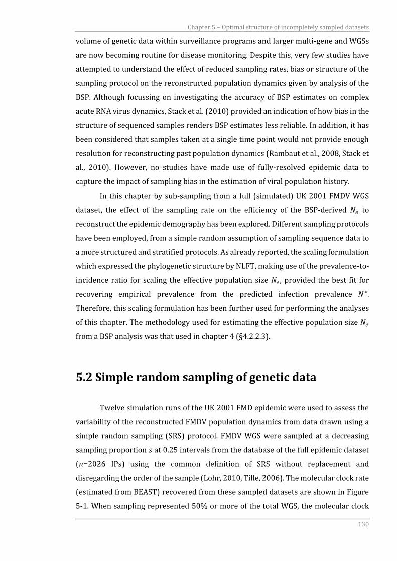
Chapter 5 – Optimal structure of incompletely sampled datasets
130
volume of genetic data within surveillance programs and larger multi-gene and WGSs
are now becoming routine for disease monitoring. Despite this, very few studies have
attempted to understand the effect of reduced sampling rates, bias or structure of the
sampling protocol on the reconstructed population dynamics given by analysis of the
BSP. Although focussing on investigating the accuracy of BSP estimates on complex
acute RNA virus dynamics, Stack et al. (2010) provided an indication of how bias in the
structure of sequenced samples renders BSP estimates less reliable. In addition, it has
been considered that samples taken at a single time point would not provide enough
resolution for reconstructing past population dynamics (Rambaut et al., 2008, Stack et
al., 2010). However, no studies have made use of fully-resolved epidemic data to
capture the impact of sampling bias in the estimation of viral population history.
In this chapter by sub-sampling from a full (simulated) UK 2001 FMDV WGS
dataset, the effect of the sampling rate on the efficiency of the BSP-derived 𝑁𝑒 to
reconstruct the epidemic demography has been explored. Different sampling protocols
have been employed, from a simple random assumption of sampling sequence data to
a more structured and stratified protocols. As already reported, the scaling formulation
which expressed the phylogenetic structure by NLFT, making use of the prevalence-to-
incidence ratio for scaling the effective population size 𝑁𝑒 , provided the best fit for
recovering empirical prevalence from the predicted infection prevalence 𝑁∗.
Therefore, this scaling formulation has been further used for performing the analyses
of this chapter. The methodology used for estimating the effective population size 𝑁𝑒
from a BSP analysis was that used in chapter 4 (§4.2.2.3).
5.2 Simple random sampling of genetic data
Twelve simulation runs of the UK 2001 FMD epidemic were used to assess the
variability of the reconstructed FMDV population dynamics from data drawn using a
simple random sampling (SRS) protocol. FMDV WGS were sampled at a decreasing
sampling proportion 𝑠 at 0.25 intervals from the database of the full epidemic dataset
(𝑛=2026 IPs) using the common definition of SRS without replacement and
disregarding the order of the sample (Lohr, 2010, Tille, 2006). The molecular clock rate
(estimated from BEAST) recovered from these sampled datasets are shown in Figure
5-1. When sampling represented 50% or more of the total WGS, the molecular clock
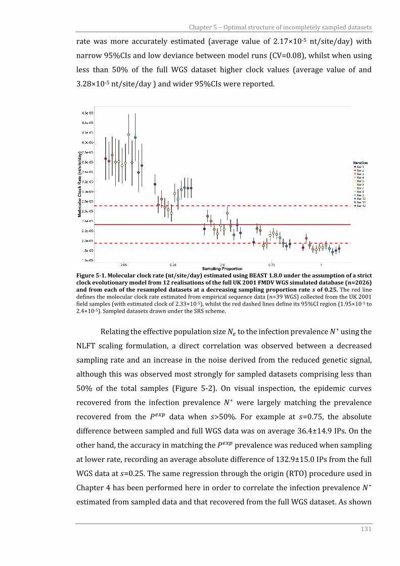
Chapter 5 – Optimal structure of incompletely sampled datasets
131
rate was more accurately estimated (average value of 2.17×10⁻⁵ nt/site/day) with
narrow 95%CIs and low deviance between model runs (CV=0.08), whilst when using
less than 50% of the full WGS dataset higher clock values (average value of and
3.28×10⁻⁵ nt/site/day ) and wider 95%CIs were reported.
Figure 5-1. Molecular clock rate (nt/site/day) estimated using BEAST 1.8.0 under the assumption of a strict clock evolutionary model from 12 realisations of the full UK 2001 FMDV WGS simulated database (𝒏=2026) and from each of the resampled datasets at a decreasing sampling proportion rate 𝒔 of 0.25. The red line defines the molecular clock rate estimated from empirical sequence data (𝑛=39 WGS) collected from the UK 2001 field samples (with estimated clock of 2.33×10⁻⁵), whilst the red dashed lines define its 95%CI region (1.95×10⁻⁵ to 2.4×10⁻⁵). Sampled datasets drawn under the SRS scheme.
Relating the effective population size 𝑁𝑒 to the infection prevalence 𝑁∗ using the
NLFT scaling formulation, a direct correlation was observed between a decreased
sampling rate and an increase in the noise derived from the reduced genetic signal,
although this was observed most strongly for sampled datasets comprising less than
50% of the total samples (Figure 5-2). On visual inspection, the epidemic curves
recovered from the infection prevalence 𝑁∗ were largely matching the prevalence
recovered from the 𝑃𝑒𝑥𝑝 data when 𝑠>50%. For example at 𝑠=0.75, the absolute
difference between sampled and full WGS data was on average 36.4±14.9 IPs. On the
other hand, the accuracy in matching the 𝑃𝑒𝑥𝑝 prevalence was reduced when sampling
at lower rate, recording an average absolute difference of 132.9±15.0 IPs from the full
WGS data at 𝑠=0.25. The same regression through the origin (RTO) procedure used in
Chapter 4 has been performed here in order to correlate the infection prevalence 𝑁∗
estimated from sampled data and that recovered from the full WGS dataset. As shown
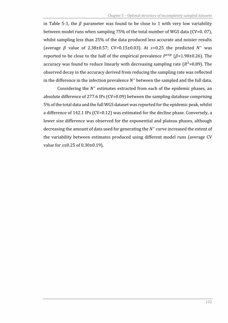
Chapter 5 – Optimal structure of incompletely sampled datasets
132
in Table 5-1, the 𝛽 parameter was found to be close to 1 with very low variability
between model runs when sampling 75% of the total number of WGS data (CV=0. 07),
whilst sampling less than 25% of the data produced less accurate and noisier results
(average 𝛽 value of 2.38±0.57; CV=0.15±0.03). At 𝑠=0.25 the predicted 𝑁∗ was
reported to be close to the half of the empirical prevalence 𝑃𝑒𝑥𝑝 (𝛽=1.98±0.26). The
accuracy was found to reduce linearly with decreasing sampling rate (𝑅2=0.89). The
observed decay in the accuracy derived from reducing the sampling rate was reflected
in the difference in the infection prevalence 𝑁∗ between the sampled and the full data.
Considering the 𝑁∗ estimates extracted from each of the epidemic phases, an
absolute difference of 277.6 IPs (CV=0.09) between the sampling database comprising
5% of the total data and the full WGS dataset was reported for the epidemic peak, whilst
a difference of 142.1 IPs (CV=0.12) was estimated for the decline phase. Conversely, a
lower size difference was observed for the exponential and plateau phases, although
decreasing the amount of data used for generating the 𝑁∗ curve increased the extent of
the variability between estimates produced using different model runs (average CV
value for 𝑠≤0.25 of 0.30±0.19).

Chapter 5 – Optimal structure of incompletely sampled datasets
133
Figure 5-2. Infection prevalence 𝑵∗ estimated from 12 realisations of the full UK 2001 FMDV WGS simulated database (𝒏=2026) and resampled datasets at a decreasing sampling proportion rate 𝒔 of 0.25. Epidemic curve was estimated from the 𝑃𝑒𝑥𝑝 (blue) prevalence data as defined in §3.2.2.2. Datasets were sampled under the SRS scheme.
Table 5-1. Time specific number of infected cases recovered from the infection prevalence 𝑵∗ estimated from 12 realisations of the UK 2001 FMD full IPs (𝒏=2026) epidemic scenario and resampled datasets at a decreasing sampling proportion 𝒔 of 0.25. 𝛽 parameter designates the slope of the regressor of the RTO analysis. Datasets were sampled under the SRS scheme.
Epidemic Phase
Sample proportion 𝛽 Exponential Peak Decline Plateau
𝑃𝑒𝑥𝑝 195.01±2.15 439.83±3.19 203.17±0.83 30.62±0.04 1 (𝑛=2026) Ref. 173.53±12.55 419.61±47.58 218.50±13.66 29.58±1.93
0.75 (𝑛=1519) 1.16±0.08 162.19±19.28 364.81±43.26 156.70±13.82 26.94±3.54 0.5 (𝑛=1013) 1.42±0.09 137.06±16.12 281.72±33.55 134.48±14.53 26.42±4.39 0.25 (𝑛=506) 1.98±0.26 98.05±14.02 207.80±40.21 109.09±19.55 19.51±4.00 0.05 (𝑛=101) 2.78±0.48 71.86±10.52 141.95±26.60 76.34±17.64 19.61±5.36
5.3 ‘Probability proportional to size’ sampling of
genetic data
To account for the structure of the genetic signal carried by WGS data within a
partially sampled scenario, a ‘probability proportional to size’ (PPS) sampling scheme
(Lohr, 2010) was applied to sample from the simulated UK 2001 FMDV WGS full
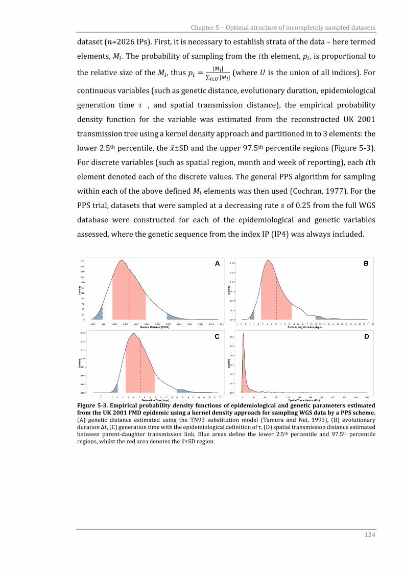
Chapter 5 – Optimal structure of incompletely sampled datasets
134
dataset (𝑛=2026 IPs). First, it is necessary to establish strata of the data – here termed
elements, 𝑀𝑖 . The probability of sampling from the 𝑖th element, 𝑝𝑖, is proportional to
the relative size of the 𝑀𝑖 , thus 𝑝𝑖 =|𝑀𝑖|
∑ |𝑀𝑖|𝑖∈𝑈 (where 𝑈 is the union of all indices). For
continuous variables (such as genetic distance, evolutionary duration, epidemiological
generation time 𝜏 , and spatial transmission distance), the empirical probability
density function for the variable was estimated from the reconstructed UK 2001
transmission tree using a kernel density approach and partitioned in to 3 elements: the
lower 2.5th percentile, the �̅�±SD and the upper 97.5th percentile regions (Figure 5-3).
For discrete variables (such as spatial region, month and week of reporting), each 𝑖th
element denoted each of the discrete values. The general PPS algorithm for sampling
within each of the above defined 𝑀𝑖 elements was then used (Cochran, 1977). For the
PPS trial, datasets that were sampled at a decreasing rate 𝑠 of 0.25 from the full WGS
database were constructed for each of the epidemiological and genetic variables
assessed, where the genetic sequence from the index IP (IP4) was always included.
Figure 5-3. Empirical probability density functions of epidemiological and genetic parameters estimated from the UK 2001 FMD epidemic using a kernel density approach for sampling WGS data by a PPS scheme. (A) genetic distance estimated using the TN93 substitution model (Tamura and Nei, 1993), (B) evolutionary duration ∆𝑡, (C) generation time with the epidemiological definition of 𝜏, (D) spatial transmission distance estimated between parent-daughter transmission link. Blue areas define the lower 2.5th percentile and 97.5th percentile regions, whilst the red area denotes the �̅�±SD region.
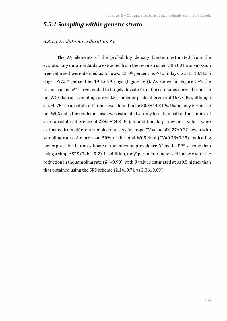
Chapter 5 – Optimal structure of incompletely sampled datasets
135
5.3.1 Sampling within genetic strata
5.3.1.1 Evolutionary duration ∆𝑡
The 𝑀𝑖 elements of the probability density function estimated from the
evolutionary duration ∆𝑡 data extracted from the reconstructed UK 2001 transmission
tree returned were defined as follows: <2.5th percentile, 4 to 5 days; �̅�±SD, 10.1±3.5
days; >97.5th percentile, 19 to 29 days (Figure 5-3). As shown in Figure 5-4, the
reconstructed 𝑁∗ curve tended to largely deviate from the estimates derived from the
full WGS data at a sampling rate 𝑠<0.5 (epidemic peak difference of 153.7 IPs), although
at 𝑠=0.75 the absolute difference was found to be 50.3±14.8 IPs. Using only 5% of the
full WGS data, the epidemic peak was estimated at only less than half of the empirical
size (absolute difference of 288.0±24.3 IPs). In addition, large deviance values were
estimated from different sampled datasets (average CV value of 0.27±0.22), even with
sampling rates of more than 50% of the total WGS data (CV=0.38±0.25), indicating
lower precision in the estimate of the infection prevalence 𝑁∗ by the PPS scheme than
using a simple SRS (Table 5-2). In addition, the 𝛽 parameter increased linearly with the
reduction in the sampling rate (𝑅2=0.90), with 𝛽 values estimated at 𝑠≤0.5 higher than
that obtained using the SRS scheme (2.14±0.71 vs 2.06±0.69).
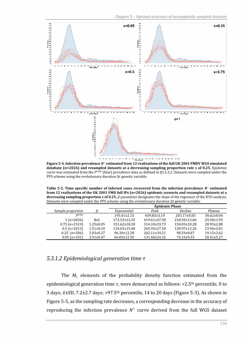
Chapter 5 – Optimal structure of incompletely sampled datasets
136
Figure 5-4. Infection prevalence 𝑵∗ estimated from 12 realisations of the full UK 2001 FMDV WGS simulated database (𝒏=2026) and resampled datasets at a decreasing sampling proportion rate 𝒔 of 0.25. Epidemic curve was estimated from the 𝑃𝑒𝑥𝑝 (blue) prevalence data as defined in §3.2.2.2. Datasets were sampled under the PPS scheme using the evolutionary duration ∆𝑡 genetic variable.
Table 5-2. Time specific number of infected cases recovered from the infection prevalence 𝑵∗ estimated from 12 realisations of the UK 2001 FMD full IPs (𝒏=2026) epidemic scenario and resampled datasets at a decreasing sampling proportion 𝒔 of 0.25. 𝛽 parameter designates the slope of the regressor of the RTO analysis. Datasets were sampled under the PPS scheme using the evolutionary duration ∆𝑡 genetic variable.
Epidemic Phase
Sample proportion 𝛽 Exponential Peak Decline Plateau
𝑃𝑒𝑥𝑝 195.01±2.15 439.83±3.19 203.17±0.83 30.62±0.04 1 (𝑛=2026) Ref. 173.53±12.55 419.61±47.58 218.50±13.66 29.58±1.93
0.75 (𝑛=1519) 1.25±0.05 151.62±18.20 314.10±33.73 150.03±10.28 28.95±2.88 0.5 (𝑛=1013) 1.51±0.10 124.03±15.68 265.93±27.50 128.97±12.26 23.96±2.81 0.25 (𝑛=506) 2.03±0.27 96.30±12.28 202.11±34.51 98.59±8.87 19.15±3.62 0.05 (𝑛=101) 2.91±0.47 66.83±12.50 131.60±24.32 74.15±9.33 20.41±5.27
5.3.1.2 Epidemiological generation time 𝜏
The 𝑀𝑖 elements of the probability density function estimated from the
epidemiological generation time 𝜏, were demarcated as follows: <2.5th percentile, 0 to
3 days; �̅�±SD, 7.2±2.7 days; >97.5th percentile, 14 to 20 days (Figure 5-3). As shown in
Figure 5-5, as the sampling rate decreases, a corresponding decrease in the accuracy of
reproducing the infection prevalence 𝑁∗ curve derived from the full WGS dataset
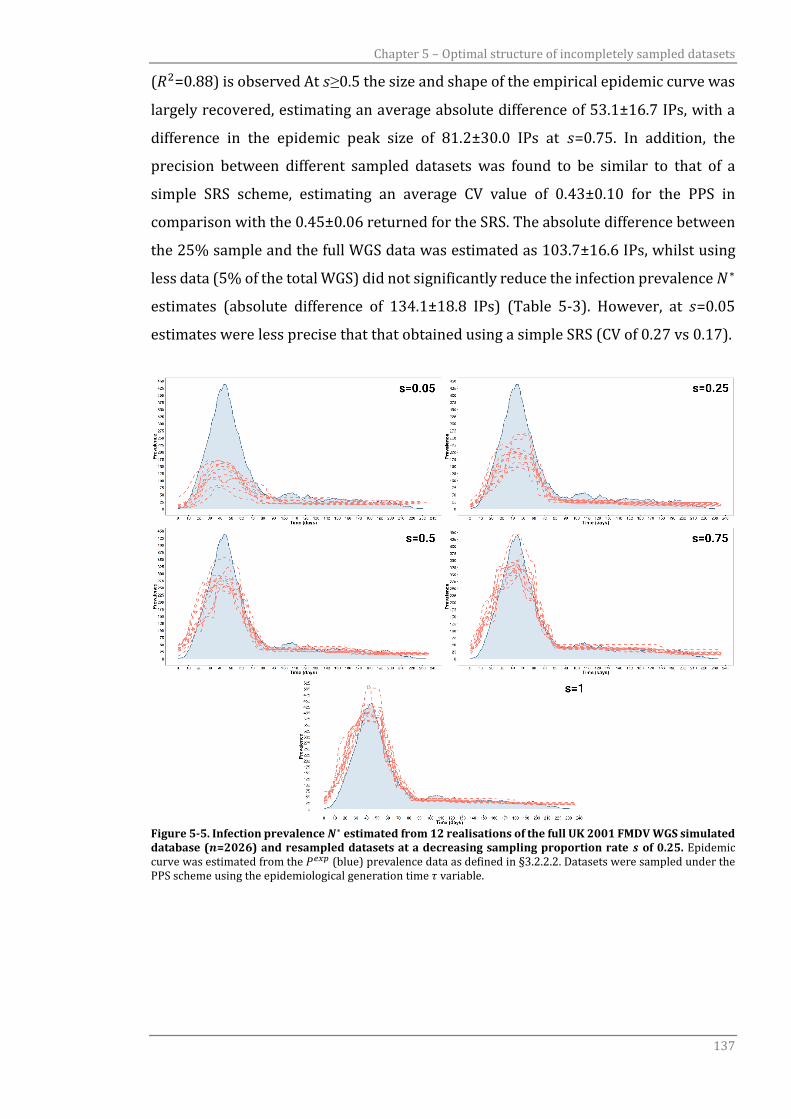
Chapter 5 – Optimal structure of incompletely sampled datasets
137
(𝑅2=0.88) is observed At 𝑠≥0.5 the size and shape of the empirical epidemic curve was
largely recovered, estimating an average absolute difference of 53.1±16.7 IPs, with a
difference in the epidemic peak size of 81.2±30.0 IPs at 𝑠=0.75. In addition, the
precision between different sampled datasets was found to be similar to that of a
simple SRS scheme, estimating an average CV value of 0.43±0.10 for the PPS in
comparison with the 0.45±0.06 returned for the SRS. The absolute difference between
the 25% sample and the full WGS data was estimated as 103.7±16.6 IPs, whilst using
less data (5% of the total WGS) did not significantly reduce the infection prevalence 𝑁∗
estimates (absolute difference of 134.1±18.8 IPs) (Table 5-3). However, at 𝑠=0.05
estimates were less precise that that obtained using a simple SRS (CV of 0.27 vs 0.17).
Figure 5-5. Infection prevalence 𝑵∗ estimated from 12 realisations of the full UK 2001 FMDV WGS simulated database (𝒏=2026) and resampled datasets at a decreasing sampling proportion rate 𝒔 of 0.25. Epidemic curve was estimated from the 𝑃𝑒𝑥𝑝 (blue) prevalence data as defined in §3.2.2.2. Datasets were sampled under the PPS scheme using the epidemiological generation time 𝜏 variable.
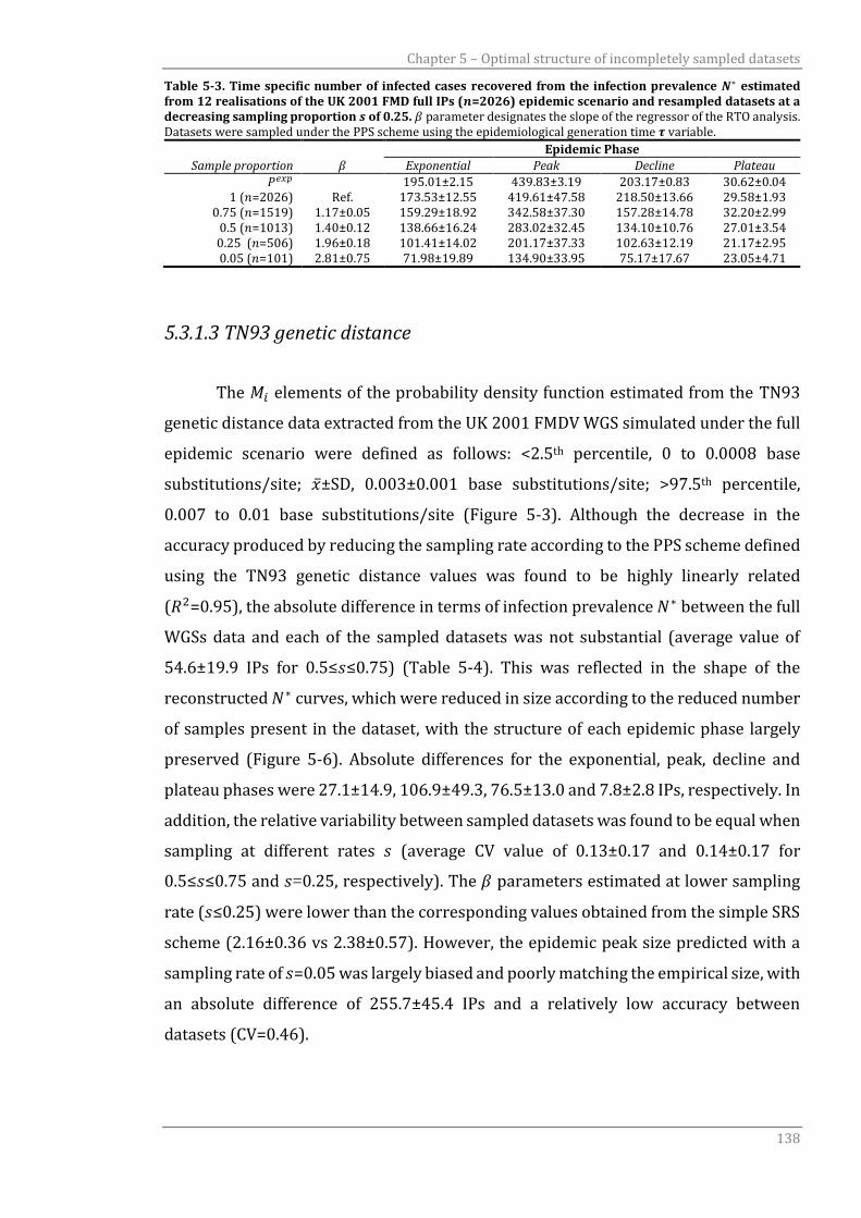
Chapter 5 – Optimal structure of incompletely sampled datasets
138
Table 5-3. Time specific number of infected cases recovered from the infection prevalence 𝑵∗ estimated from 12 realisations of the UK 2001 FMD full IPs (𝒏=2026) epidemic scenario and resampled datasets at a decreasing sampling proportion 𝒔 of 0.25. 𝛽 parameter designates the slope of the regressor of the RTO analysis. Datasets were sampled under the PPS scheme using the epidemiological generation time 𝝉 variable.
Epidemic Phase
Sample proportion 𝛽 Exponential Peak Decline Plateau
𝑃𝑒𝑥𝑝 195.01±2.15 439.83±3.19 203.17±0.83 30.62±0.04 1 (𝑛=2026) Ref. 173.53±12.55 419.61±47.58 218.50±13.66 29.58±1.93
0.75 (𝑛=1519) 1.17±0.05 159.29±18.92 342.58±37.30 157.28±14.78 32.20±2.99 0.5 (𝑛=1013) 1.40±0.12 138.66±16.24 283.02±32.45 134.10±10.76 27.01±3.54 0.25 (𝑛=506) 1.96±0.18 101.41±14.02 201.17±37.33 102.63±12.19 21.17±2.95 0.05 (𝑛=101) 2.81±0.75 71.98±19.89 134.90±33.95 75.17±17.67 23.05±4.71
5.3.1.3 TN93 genetic distance
The 𝑀𝑖 elements of the probability density function estimated from the TN93
genetic distance data extracted from the UK 2001 FMDV WGS simulated under the full
epidemic scenario were defined as follows: <2.5th percentile, 0 to 0.0008 base
substitutions/site; �̅�±SD, 0.003±0.001 base substitutions/site; >97.5th percentile,
0.007 to 0.01 base substitutions/site (Figure 5-3). Although the decrease in the
accuracy produced by reducing the sampling rate according to the PPS scheme defined
using the TN93 genetic distance values was found to be highly linearly related
(𝑅2=0.95), the absolute difference in terms of infection prevalence 𝑁∗ between the full
WGSs data and each of the sampled datasets was not substantial (average value of
54.6±19.9 IPs for 0.5≤𝑠≤0.75) (Table 5-4). This was reflected in the shape of the
reconstructed 𝑁∗ curves, which were reduced in size according to the reduced number
of samples present in the dataset, with the structure of each epidemic phase largely
preserved (Figure 5-6). Absolute differences for the exponential, peak, decline and
plateau phases were 27.1±14.9, 106.9±49.3, 76.5±13.0 and 7.8±2.8 IPs, respectively. In
addition, the relative variability between sampled datasets was found to be equal when
sampling at different rates 𝑠 (average CV value of 0.13±0.17 and 0.14±0.17 for
0.5≤𝑠≤0.75 and 𝑠=0.25, respectively). The 𝛽 parameters estimated at lower sampling
rate (𝑠≤0.25) were lower than the corresponding values obtained from the simple SRS
scheme (2.16±0.36 vs 2.38±0.57). However, the epidemic peak size predicted with a
sampling rate of 𝑠=0.05 was largely biased and poorly matching the empirical size, with
an absolute difference of 255.7±45.4 IPs and a relatively low accuracy between
datasets (CV=0.46).
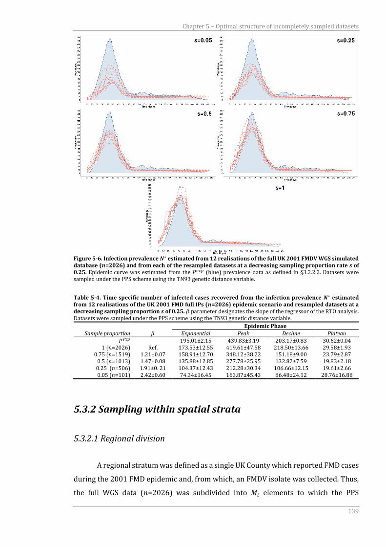
Chapter 5 – Optimal structure of incompletely sampled datasets
139
Figure 5-6. Infection prevalence 𝑵∗ estimated from 12 realisations of the full UK 2001 FMDV WGS simulated database (𝒏=2026) and from each of the resampled datasets at a decreasing sampling proportion rate 𝒔 of 0.25. Epidemic curve was estimated from the 𝑃𝑒𝑥𝑝 (blue) prevalence data as defined in §3.2.2.2. Datasets were sampled under the PPS scheme using the TN93 genetic distance variable.
Table 5-4. Time specific number of infected cases recovered from the infection prevalence 𝑵∗ estimated from 12 realisations of the UK 2001 FMD full IPs (𝒏=2026) epidemic scenario and resampled datasets at a decreasing sampling proportion 𝒔 of 0.25. 𝛽 parameter designates the slope of the regressor of the RTO analysis. Datasets were sampled under the PPS scheme using the TN93 genetic distance variable.
Epidemic Phase
Sample proportion 𝛽 Exponential Peak Decline Plateau
𝑃𝑒𝑥𝑝 195.01±2.15 439.83±3.19 203.17±0.83 30.62±0.04 1 (𝑛=2026) Ref. 173.53±12.55 419.61±47.58 218.50±13.66 29.58±1.93
0.75 (𝑛=1519) 1.21±0.07 158.91±12.70 348.12±38.22 151.18±9.00 23.79±2.87 0.5 (𝑛=1013) 1.47±0.08 135.88±12.85 277.78±25.95 132.82±7.59 19.83±2.18 0.25 (𝑛=506) 1.91±0. 21 104.37±12.43 212.28±30.34 106.66±12.15 19.61±2.66 0.05 (𝑛=101) 2.42±0.60 74.34±16.45 163.87±45.43 86.48±24.12 28.76±16.88
5.3.2 Sampling within spatial strata
5.3.2.1 Regional division
A regional stratum was defined as a single UK County which reported FMD cases
during the 2001 FMD epidemic and, from which, an FMDV isolate was collected. Thus,
the full WGS data (𝑛=2026) was subdivided into 𝑀𝑖 elements to which the PPS

Chapter 5 – Optimal structure of incompletely sampled datasets
140
sampling scheme has been applied. This spatial allocation was based on the spatial
connections between the geographical coordinates of each reported IPs and the spatial
UK county layer, which defines the county borders (according to 2009 boundaries)
(Figure 5-7).
Figure 5-7. Spatial proportion of IPs according to the affected UK counties as reported during the UK 2001 FMD epidemic. The spatial layer defines the UK counties based on the 2009 boundaries.
Results for the estimated infection prevalence 𝑁∗ curves are shown in Figure 5-
8. Although the relative variability between sampled datasets was reported to produce
no substantial difference at higher and lower rates of 𝑠 (average CV value of 0.11±0.01
and 0.18±0.06 for 0.5≤𝑠≤0.75 and 0.05≤𝑠≤0.25, respectively), reducing the sample size
greatly impacted on the accuracy of matching the estimates obtained with the full WGS
data. Using only 5% of the total data, an absolute difference of 102.6±18.6, 272.1±42.4
and 139.0±14.3 IPs was estimated for the exponential, peak and decline phases,
respectively, whilst averages of 24.8±12.2, 95.8±34.0 and 74.6±16.7 IPs were
calculated with datasets sampled at a rate of 0.5≤𝑠≤0.75 (Table 5-5). However, the
reduced accuracy of the PPS at a sampling rate 𝑠=0.05 was similar to the estimates
obtained using a simple SRS scheme (absolute difference values of 0.9, 5.6 and 3.1 IPs
for the exponential, peak and decline phases, respectively). The 𝛽 parameter estimated
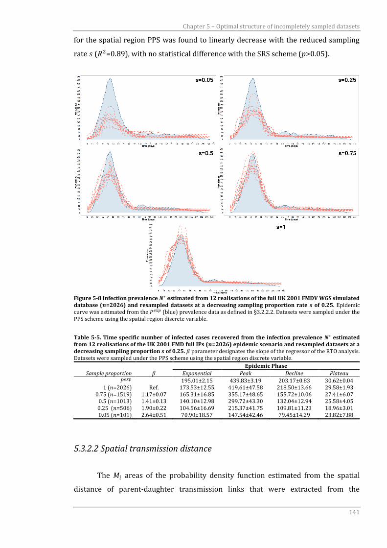
Chapter 5 – Optimal structure of incompletely sampled datasets
141
for the spatial region PPS was found to linearly decrease with the reduced sampling
rate 𝑠 (𝑅2=0.89), with no statistical difference with the SRS scheme (𝑝>0.05).
Figure 5-8 Infection prevalence 𝑵∗ estimated from 12 realisations of the full UK 2001 FMDV WGS simulated database (𝒏=2026) and resampled datasets at a decreasing sampling proportion rate 𝒔 of 0.25. Epidemic curve was estimated from the 𝑃𝑒𝑥𝑝 (blue) prevalence data as defined in §3.2.2.2. Datasets were sampled under the PPS scheme using the spatial region discrete variable.
Table 5-5. Time specific number of infected cases recovered from the infection prevalence 𝑵∗ estimated from 12 realisations of the UK 2001 FMD full IPs (𝒏=2026) epidemic scenario and resampled datasets at a decreasing sampling proportion 𝒔 of 0.25. 𝛽 parameter designates the slope of the regressor of the RTO analysis. Datasets were sampled under the PPS scheme using the spatial region discrete variable.
Epidemic Phase
Sample proportion 𝛽 Exponential Peak Decline Plateau
𝑃𝑒𝑥𝑝 195.01±2.15 439.83±3.19 203.17±0.83 30.62±0.04 1 (𝑛=2026) Ref. 173.53±12.55 419.61±47.58 218.50±13.66 29.58±1.93
0.75 (𝑛=1519) 1.17±0.07 165.31±16.85 355.17±48.65 155.72±10.06 27.41±6.07 0.5 (𝑛=1013) 1.41±0.13 140.10±12.98 299.72±43.30 132.04±12.94 25.58±4.05 0.25 (𝑛=506) 1.90±0.22 104.56±16.69 215.37±41.75 109.81±11.23 18.96±3.01 0.05 (𝑛=101) 2.64±0.51 70.90±18.57 147.54±42.46 79.45±14.29 23.82±7.88
5.3.2.2 Spatial transmission distance
The 𝑀𝑖 areas of the probability density function estimated from the spatial
distance of parent-daughter transmission links that were extracted from the
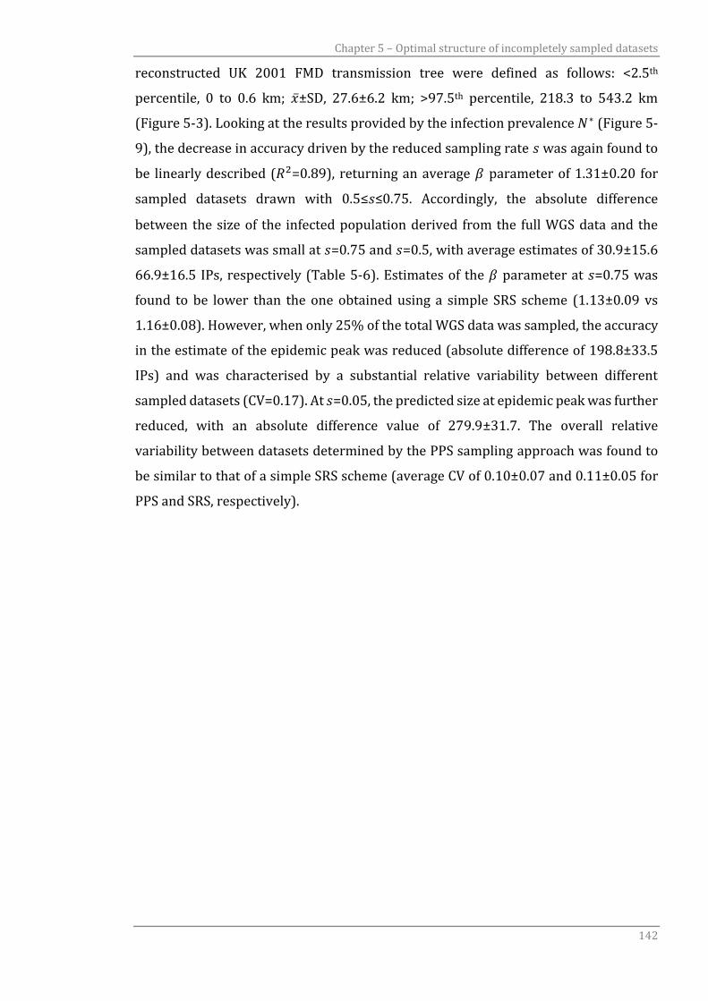
Chapter 5 – Optimal structure of incompletely sampled datasets
142
reconstructed UK 2001 FMD transmission tree were defined as follows: <2.5th
percentile, 0 to 0.6 km; �̅�±SD, 27.6±6.2 km; >97.5th percentile, 218.3 to 543.2 km
(Figure 5-3). Looking at the results provided by the infection prevalence 𝑁∗ (Figure 5-
9), the decrease in accuracy driven by the reduced sampling rate 𝑠 was again found to
be linearly described (𝑅2=0.89), returning an average 𝛽 parameter of 1.31±0.20 for
sampled datasets drawn with 0.5≤𝑠≤0.75. Accordingly, the absolute difference
between the size of the infected population derived from the full WGS data and the
sampled datasets was small at 𝑠=0.75 and 𝑠=0.5, with average estimates of 30.9±15.6
66.9±16.5 IPs, respectively (Table 5-6). Estimates of the 𝛽 parameter at 𝑠=0.75 was
found to be lower than the one obtained using a simple SRS scheme (1.13±0.09 vs
1.16±0.08). However, when only 25% of the total WGS data was sampled, the accuracy
in the estimate of the epidemic peak was reduced (absolute difference of 198.8±33.5
IPs) and was characterised by a substantial relative variability between different
sampled datasets (CV=0.17). At 𝑠=0.05, the predicted size at epidemic peak was further
reduced, with an absolute difference value of 279.9±31.7. The overall relative
variability between datasets determined by the PPS sampling approach was found to
be similar to that of a simple SRS scheme (average CV of 0.10±0.07 and 0.11±0.05 for
PPS and SRS, respectively).
Chapter 5 – Optimal structure of incompletely sampled datasets
143
Figure 5-9. Infection prevalence 𝑵∗ estimated from 12 realisations of the full UK 2001 FMDV WGS simulated database (𝒏=2026) and resampled datasets at a decreasing sampling proportion rate 𝒔 of 0.25. Epidemic curve was estimated from the 𝑃𝑒𝑥𝑝 (blue) prevalence data as defined in §3.2.2.2. Datasets were sampled under the PPS scheme using the spatial transmission distance epidemiological variable.
Table 5-6. Time specific number of infected cases recovered from the infection prevalence 𝑵∗ estimated from 12 realisations of the UK 2001 FMD full IPs (𝒏=2026) epidemic scenario and resampled datasets at a decreasing sampling proportion 𝒔 of 0.25. 𝛽 parameter designates the slope of the regressor of the RTO analysis. Datasets were sampled under the PPS scheme using the spatial transmission distance epidemiological variable.
Epidemic Phase
Sample proportion 𝛽 Exponential Peak Decline Plateau
𝑃𝑒𝑥𝑝 195.01±2.15 439.83±3.19 203.17±0.83 30.62±0.04 1 (𝑛=2026) Ref. 173.53±12.55 419.61±47.58 218.50±13.66 29.58±1.93
0.75 (𝑛=1519) 1.13±0.06 161.66±14.02 370.81±39.62 163.75±15.18 30.37±2.62 0.5 (𝑛=1013) 1.45±0.08 134.21±12.48 280.22±39.54 135.295±12.32 23.90±1.74 0.25 (𝑛=506) 1.93±0.17 98.57±13.97 220.77±33.50 107.07±12.60 20.22±2.99 0.05 (𝑛=101) 2.77±0.60 71.92±12.66 139.69±31.67 81.75±26.69 22.31±8.32
5.3.3 Sampling within temporal strata
5.3.3.1 Month timing
The strata for the PPS sampling scheme using the month of IP reporting were
estimated from the UK 2001 FMD epidemic records, which returned a total of 8 𝑀
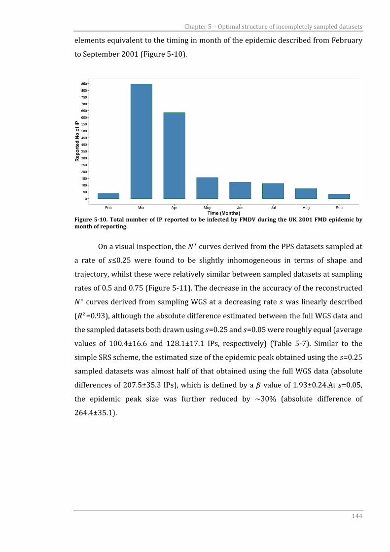
Chapter 5 – Optimal structure of incompletely sampled datasets
144
elements equivalent to the timing in month of the epidemic described from February
to September 2001 (Figure 5-10).
Figure 5-10. Total number of IP reported to be infected by FMDV during the UK 2001 FMD epidemic by month of reporting.
On a visual inspection, the 𝑁∗ curves derived from the PPS datasets sampled at
a rate of 𝑠≤0.25 were found to be slightly inhomogeneous in terms of shape and
trajectory, whilst these were relatively similar between sampled datasets at sampling
rates of 0.5 and 0.75 (Figure 5-11). The decrease in the accuracy of the reconstructed
𝑁∗ curves derived from sampling WGS at a decreasing rate 𝑠 was linearly described
(𝑅2=0.93), although the absolute difference estimated between the full WGS data and
the sampled datasets both drawn using 𝑠=0.25 and 𝑠=0.05 were roughly equal (average
values of 100.4±16.6 and 128.1±17.1 IPs, respectively) (Table 5-7). Similar to the
simple SRS scheme, the estimated size of the epidemic peak obtained using the 𝑠=0.25
sampled datasets was almost half of that obtained using the full WGS data (absolute
differences of 207.5±35.3 IPs), which is defined by a 𝛽 value of 1.93±0.24.At 𝑠=0.05,
the epidemic peak size was further reduced by ~30% (absolute difference of
264.4±35.1).
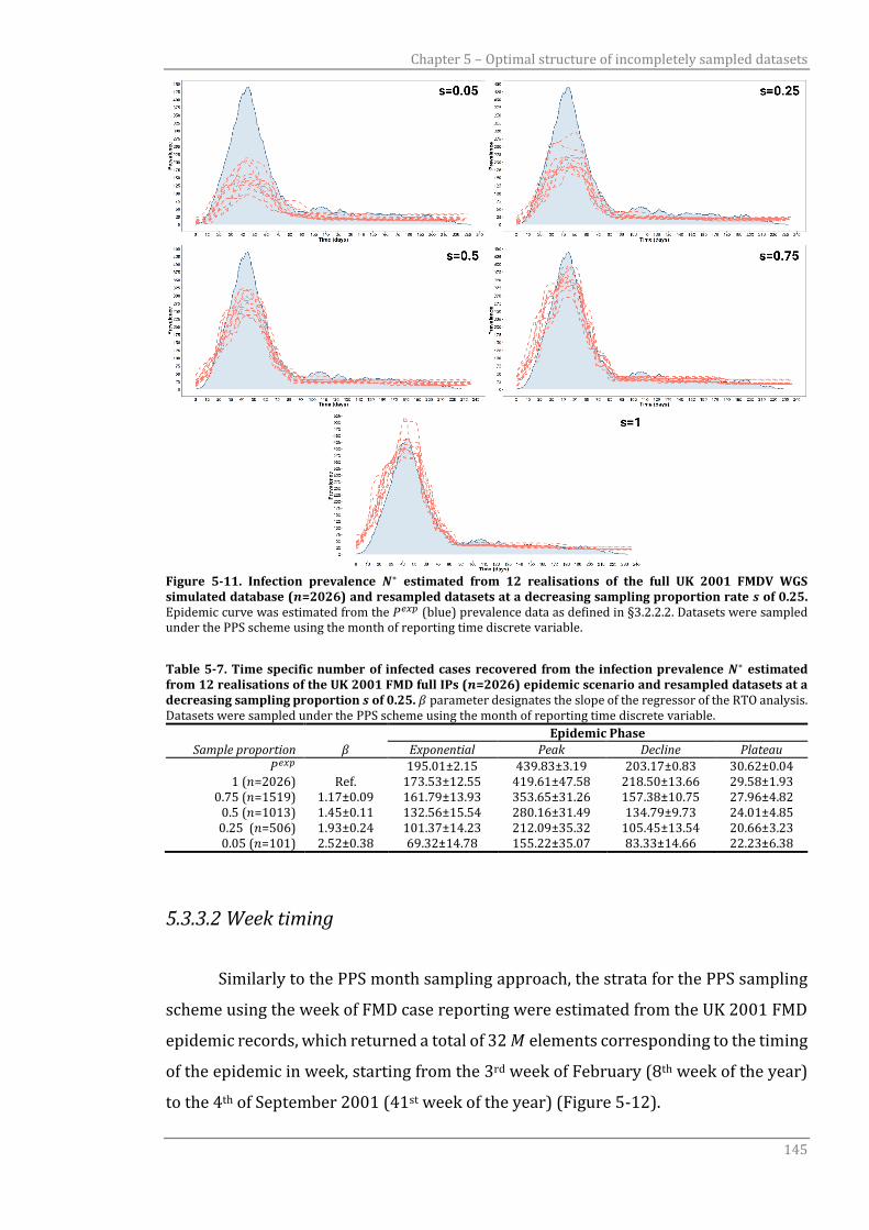
Chapter 5 – Optimal structure of incompletely sampled datasets
145
Figure 5-11. Infection prevalence 𝑵∗ estimated from 12 realisations of the full UK 2001 FMDV WGS simulated database (𝒏=2026) and resampled datasets at a decreasing sampling proportion rate 𝒔 of 0.25. Epidemic curve was estimated from the 𝑃𝑒𝑥𝑝 (blue) prevalence data as defined in §3.2.2.2. Datasets were sampled under the PPS scheme using the month of reporting time discrete variable.
Table 5-7. Time specific number of infected cases recovered from the infection prevalence 𝑵∗ estimated from 12 realisations of the UK 2001 FMD full IPs (𝒏=2026) epidemic scenario and resampled datasets at a decreasing sampling proportion 𝒔 of 0.25. 𝛽 parameter designates the slope of the regressor of the RTO analysis. Datasets were sampled under the PPS scheme using the month of reporting time discrete variable.
Epidemic Phase
Sample proportion 𝛽 Exponential Peak Decline Plateau
𝑃𝑒𝑥𝑝 195.01±2.15 439.83±3.19 203.17±0.83 30.62±0.04 1 (𝑛=2026) Ref. 173.53±12.55 419.61±47.58 218.50±13.66 29.58±1.93
0.75 (𝑛=1519) 1.17±0.09 161.79±13.93 353.65±31.26 157.38±10.75 27.96±4.82 0.5 (𝑛=1013) 1.45±0.11 132.56±15.54 280.16±31.49 134.79±9.73 24.01±4.85 0.25 (𝑛=506) 1.93±0.24 101.37±14.23 212.09±35.32 105.45±13.54 20.66±3.23 0.05 (𝑛=101) 2.52±0.38 69.32±14.78 155.22±35.07 83.33±14.66 22.23±6.38
5.3.3.2 Week timing
Similarly to the PPS month sampling approach, the strata for the PPS sampling
scheme using the week of FMD case reporting were estimated from the UK 2001 FMD
epidemic records, which returned a total of 32 𝑀 elements corresponding to the timing
of the epidemic in week, starting from the 3rd week of February (8th week of the year)
to the 4th of September 2001 (41st week of the year) (Figure 5-12).
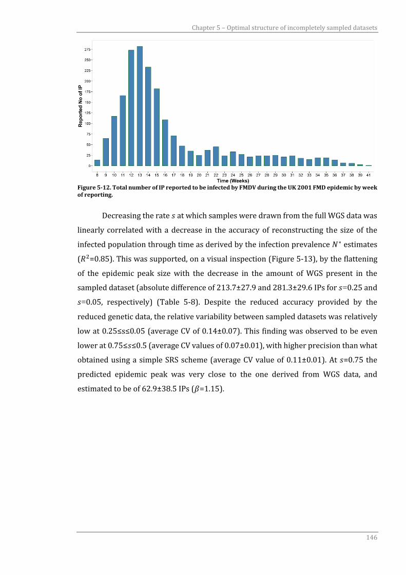
Chapter 5 – Optimal structure of incompletely sampled datasets
146
Figure 5-12. Total number of IP reported to be infected by FMDV during the UK 2001 FMD epidemic by week of reporting.
Decreasing the rate 𝑠 at which samples were drawn from the full WGS data was
linearly correlated with a decrease in the accuracy of reconstructing the size of the
infected population through time as derived by the infection prevalence 𝑁∗ estimates
(𝑅2=0.85). This was supported, on a visual inspection (Figure 5-13), by the flattening
of the epidemic peak size with the decrease in the amount of WGS present in the
sampled dataset (absolute difference of 213.7±27.9 and 281.3±29.6 IPs for 𝑠=0.25 and
𝑠=0.05, respectively) (Table 5-8). Despite the reduced accuracy provided by the
reduced genetic data, the relative variability between sampled datasets was relatively
low at 0.25≤s≤0.05 (average CV of 0.14±0.07). This finding was observed to be even
lower at 0.75≤𝑠≤0.5 (average CV values of 0.07±0.01), with higher precision than what
obtained using a simple SRS scheme (average CV value of 0.11±0.01). At 𝑠=0.75 the
predicted epidemic peak was very close to the one derived from WGS data, and
estimated to be of 62.9±38.5 IPs (𝛽=1.15).
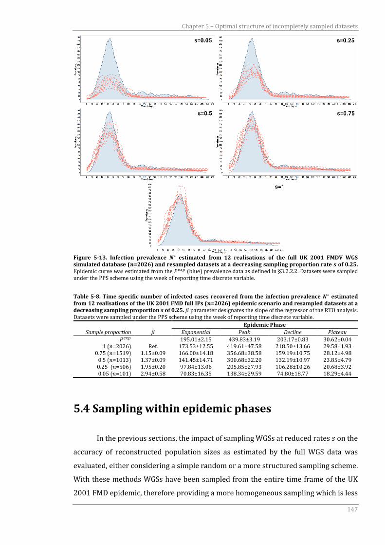
Chapter 5 – Optimal structure of incompletely sampled datasets
147
Figure 5-13. Infection prevalence 𝑵∗ estimated from 12 realisations of the full UK 2001 FMDV WGS simulated database (𝒏=2026) and resampled datasets at a decreasing sampling proportion rate 𝒔 of 0.25. Epidemic curve was estimated from the 𝑃𝑒𝑥𝑝 (blue) prevalence data as defined in §3.2.2.2. Datasets were sampled under the PPS scheme using the week of reporting time discrete variable.
Table 5-8. Time specific number of infected cases recovered from the infection prevalence 𝑵∗ estimated from 12 realisations of the UK 2001 FMD full IPs (𝒏=2026) epidemic scenario and resampled datasets at a decreasing sampling proportion 𝒔 of 0.25. 𝛽 parameter designates the slope of the regressor of the RTO analysis. Datasets were sampled under the PPS scheme using the week of reporting time discrete variable.
Epidemic Phase
Sample proportion 𝛽 Exponential Peak Decline Plateau
𝑃𝑒𝑥𝑝 195.01±2.15 439.83±3.19 203.17±0.83 30.62±0.04 1 (𝑛=2026) Ref. 173.53±12.55 419.61±47.58 218.50±13.66 29.58±1.93
0.75 (𝑛=1519) 1.15±0.09 166.00±14.18 356.68±38.58 159.19±10.75 28.12±4.98 0.5 (𝑛=1013) 1.37±0.09 141.45±14.71 300.68±32.20 132.19±10.97 23.85±4.79 0.25 (𝑛=506) 1.95±0.20 97.84±13.06 205.85±27.93 106.28±10.26 20.68±3.92 0.05 (𝑛=101) 2.94±0.58 70.83±16.35 138.34±29.59 74.80±18.77 18.29±4.44
5.4 Sampling within epidemic phases
In the previous sections, the impact of sampling WGSs at reduced rates 𝑠 on the
accuracy of reconstructed population sizes as estimated by the full WGS data was
evaluated, either considering a simple random or a more structured sampling scheme.
With these methods WGSs have been sampled from the entire time frame of the UK
2001 FMD epidemic, therefore providing a more homogeneous sampling which is less
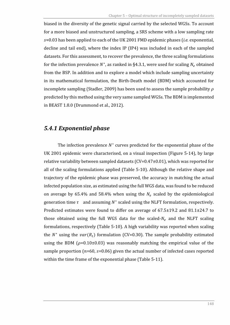
Chapter 5 – Optimal structure of incompletely sampled datasets
148
biased in the diversity of the genetic signal carried by the selected WGSs. To account
for a more biased and unstructured sampling, a SRS scheme with a low sampling rate
𝑠≈0.03 has been applied to each of the UK 2001 FMD epidemic phases (i.e. exponential,
decline and tail end), where the index IP (IP4) was included in each of the sampled
datasets. For this assessment, to recover the prevalence, the three scaling formulations
for the infection prevalence 𝑁∗, as ranked in §4.3.1, were used for scaling 𝑁𝑒 obtained
from the BSP. In addition and to explore a model which include sampling uncertainty
in its mathematical formulation, the Birth-Death model (BDM) which accounted for
incomplete sampling (Stadler, 2009) has been used to assess the sample probability 𝜌
predicted by this method using the very same sampled WGSs. The BDM is implemented
in BEAST 1.8.0 (Drummond et al., 2012).
5.4.1 Exponential phase
The infection prevalence 𝑁∗ curves predicted for the exponential phase of the
UK 2001 epidemic were characterised, on a visual inspection (Figure 5-14), by large
relative variability between sampled datasets (CV=0.47±0.01), which was reported for
all of the scaling formulations applied (Table 5-10). Although the relative shape and
trajectory of the epidemic phase was preserved, the accuracy in matching the actual
infected population size, as estimated using the full WGS data, was found to be reduced
on average by 65.4% and 58.4% when using the 𝑁𝑒 scaled by the epidemiological
generation time 𝜏 and assuming 𝑁∗ scaled using the NLFT formulation, respectively.
Predicted estimates were found to differ on average of 67.5±19.2 and 81.1±24.7 to
those obtained using the full WGS data for the scaled-𝑁𝑒 and the NLFT scaling
formulations, respectively (Table 5-10). A high variability was reported when scaling
the 𝑁∗ using the 𝑣𝑎𝑟(𝑅𝑡) formulation (CV=0.30). The sample probability estimated
using the BDM (𝜌=0.10±0.03) was reasonably matching the empirical value of the
sample proportion (𝑛=60, 𝑠=0.06) given the actual number of infected cases reported
within the time frame of the exponential phase (Table 5-11).
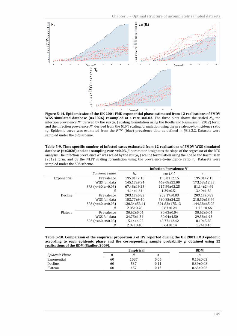
Chapter 5 – Optimal structure of incompletely sampled datasets
149
Figure 5-14. Epidemic size of the UK 2001 FMD exponential phase estimated from 12 realisations of FMDV WGS simulated database (𝒏=2026) resampled at a rate 𝒔≈0.03. The three plots shows the scaled 𝑁𝑒 , the infection prevalence 𝑁∗ derived by the 𝑣𝑎𝑟(𝑅𝑡) scaling formulation using the Koelle and Rasmussen (2012) form, and the infection prevalence 𝑁∗ derived from the NLFT scaling formulation using the prevalence-to-incidence ratio 𝜏𝑝. Epidemic curve was estimated from the 𝑃𝑒𝑥𝑝 (blue) prevalence data as defined in §3.2.2.2. Datasets were
sampled under the SRS scheme.
Table 5-9. Time specific number of infected cases estimated from 12 realisations of FMDV WGS simulated database (𝒏=2026) and at a sampling rate 𝒔≈0.03. 𝛽 parameter designates the slope of the regressor of the RTO analysis. The infection prevalence 𝑁∗ was scaled by the 𝑣𝑎𝑟(𝑅𝑡) scaling formulation using the Koelle and Rasmussen (2012) form, and by the NLFT scaling formulation using the prevalence-to-incidence ratio 𝜏𝑝. Datasets were
sampled under the SRS scheme.
Infection Prevalence 𝑵∗
Epidemic Phase 𝑁𝑒 𝑣𝑎𝑟(𝑅𝑡) 𝜏𝑝
Exponential Prevalence 195.01±2.15 195.01±2.15 195.01±2.15 WGS full data 145.17±9.34 469.08±22.00 173.53±12.55 SRS (𝑛=60, 𝑠≈0.03) 67.48±19.23 217.89±63.25 81.14±24.69 𝛽 4.14±1.64 1.29±0.51 3.49±1.38
Decline Prevalence 203.17±0.83 203.17±0.83 203.17±0.83 WGS full data 182.77±9.40 590.85±24.23 218.50±13.66 SRS (𝑛=60, 𝑠≈0.03) 120.34±53.41 391.82±175.13 144.38±65.08 𝛽 2.05±0.78 0.63±0.24 1.72 ±0.66
Plateau Prevalence 30.62±0.04 30.62±0.04 30.62±0.04 WGS full data 24.75±1.34 80.04±4.50 29.58±1.93 SRS (𝑛=60, 𝑠≈0.03) 15.14±4.02 48.77±12.42 8.19±5.28 𝛽 2.07±0.48 0.64±0.14 1.74±0.43
Table 5-10. Comparison of the empirical proportion 𝒔 of IPs reported during the UK 2001 FMD epidemic according to each epidemic phase and the corresponding sample probability 𝝆 obtained using 12 realisations of the BDM (Stadler, 2009).
Empirical BDM
Epidemic Phase 𝑛 𝑁 𝑠 𝜌
Exponential 60 1037 0.06 0.10±0.03 Decline 60 537 0.11 0.39±0.08 Plateau 60 457 0.13 0.63±0.05
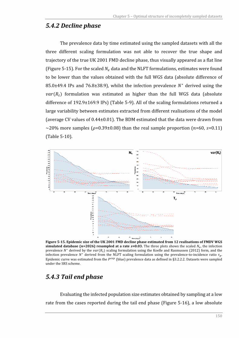
Chapter 5 – Optimal structure of incompletely sampled datasets
150
5.4.2 Decline phase
The prevalence data by time estimated using the sampled datasets with all the
three different scaling formulation was not able to recover the true shape and
trajectory of the true UK 2001 FMD decline phase, thus visually appeared as a flat line
(Figure 5-15). For the scaled 𝑁𝑒 data and the NLFT formulations, estimates were found
to be lower than the values obtained with the full WGS data (absolute difference of
85.0±49.4 IPs and 76.8±38.9), whilst the infection prevalence 𝑁∗ derived using the
𝑣𝑎𝑟(𝑅𝑡) formulation was estimated as higher than the full WGS data (absolute
difference of 192.9±169.9 IPs) (Table 5-9). All of the scaling formulations returned a
large variability between estimates extracted from different realisations of the model
(average CV values of 0.44±0.01). The BDM estimated that the data were drawn from
~20% more samples (𝜌=0.39±0.08) than the real sample proportion (𝑛=60, 𝑠=0.11)
(Table 5-10).
Figure 5-15. Epidemic size of the UK 2001 FMD decline phase estimated from 12 realisations of FMDV WGS simulated database (𝒏=2026) resampled at a rate 𝒔≈0.03. The three plots shows the scaled 𝑁𝑒 , the infection prevalence 𝑁∗ derived by the 𝑣𝑎𝑟(𝑅𝑡) scaling formulation using the Koelle and Rasmussen (2012) form, and the infection prevalence 𝑁∗ derived from the NLFT scaling formulation using the prevalence-to-incidence ratio 𝜏𝑝.
Epidemic curve was estimated from the 𝑃𝑒𝑥𝑝 (blue) prevalence data as defined in §3.2.2.2. Datasets were sampled under the SRS scheme.
5.4.3 Tail end phase
Evaluating the infected population size estimates obtained by sampling at a low
rate from the cases reported during the tail end phase (Figure 5-16), a low absolute

Chapter 5 – Optimal structure of incompletely sampled datasets
151
difference between the sampled datasets and the full WGS estimates was described for
all the scaling formulations (average value of 15.3±2.9), with the WGS data being higher
than the scaled 𝑵𝒆 data and the freely mixing formulations. However, a high relative
variability between datasets was observed, estimated in an average CV value of
0.27±0.02 (Table 5-9). It should be noted that, as already described in Chapter 4, the
BSP reported an increased number of infected cases in the last weeks, failing to
describe the actual fading out of the epidemic. The BDM analysis returned a sample
probability 𝝆 of 0.63±0.05 (Table 5-10), which was higher than the real sample
proportion drawn from the list of reported cases within the time frame of the tail end
phase (𝒏=60, 𝒔=0.13).
Figure 5-16. Epidemic size of the UK 2001 FMD tail end phase estimated from 12 realisations of FMDV WGS simulated database (𝒏=2026) resampled at a rate 𝒔≈0.03. The three plots shows the scaled 𝑁𝑒 , the infection prevalence 𝑁∗ derived by the 𝑣𝑎𝑟(𝑅𝑡) scaling formulation using the Koelle and Rasmussen (2012) form, and the infection prevalence 𝑁∗ derived from the NLFT scaling formulation using the prevalence-to-incidence ratio 𝜏𝑝.
Epidemic curve was estimated from the 𝑃𝑒𝑥𝑝 (blue) prevalence data as defined in §3.2.2.2. Datasets were sampled under the SRS scheme.
5.5 Conclusion
This chapter analysed the impact of the size and structure of the sampled
dataset on the accuracy of the reconstructed viral demographies. The results generated
should provide information on how the demographic signal carried by sequence data
becomes imprecise and weaker when reducing the number of samples. Using a simple
random sampling protocol (SRS scheme) to generate WGS sub-datasets from the
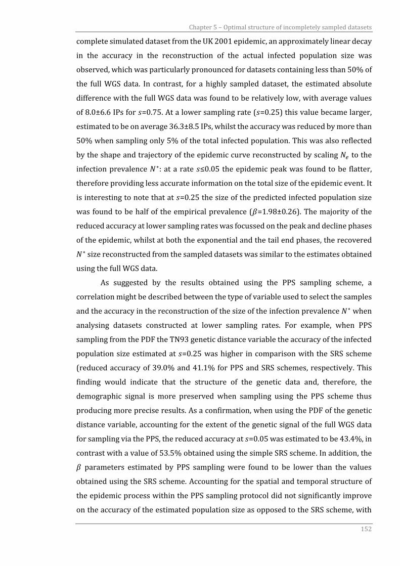
Chapter 5 – Optimal structure of incompletely sampled datasets
152
complete simulated dataset from the UK 2001 epidemic, an approximately linear decay
in the accuracy in the reconstruction of the actual infected population size was
observed, which was particularly pronounced for datasets containing less than 50% of
the full WGS data. In contrast, for a highly sampled dataset, the estimated absolute
difference with the full WGS data was found to be relatively low, with average values
of 8.0±6.6 IPs for 𝑠=0.75. At a lower sampling rate (𝑠=0.25) this value became larger,
estimated to be on average 36.3±8.5 IPs, whilst the accuracy was reduced by more than
50% when sampling only 5% of the total infected population. This was also reflected
by the shape and trajectory of the epidemic curve reconstructed by scaling 𝑁𝑒 to the
infection prevalence 𝑁∗: at a rate 𝑠≤0.05 the epidemic peak was found to be flatter,
therefore providing less accurate information on the total size of the epidemic event. It
is interesting to note that at 𝑠=0.25 the size of the predicted infected population size
was found to be half of the empirical prevalence (𝛽=1.98±0.26). The majority of the
reduced accuracy at lower sampling rates was focussed on the peak and decline phases
of the epidemic, whilst at both the exponential and the tail end phases, the recovered
𝑁∗ size reconstructed from the sampled datasets was similar to the estimates obtained
using the full WGS data.
As suggested by the results obtained using the PPS sampling scheme, a
correlation might be described between the type of variable used to select the samples
and the accuracy in the reconstruction of the size of the infection prevalence 𝑁∗ when
analysing datasets constructed at lower sampling rates. For example, when PPS
sampling from the PDF the TN93 genetic distance variable the accuracy of the infected
population size estimated at 𝑠=0.25 was higher in comparison with the SRS scheme
(reduced accuracy of 39.0% and 41.1% for PPS and SRS schemes, respectively. This
finding would indicate that the structure of the genetic data and, therefore, the
demographic signal is more preserved when sampling using the PPS scheme thus
producing more precise results. As a confirmation, when using the PDF of the genetic
distance variable, accounting for the extent of the genetic signal of the full WGS data
for sampling via the PPS, the reduced accuracy at 𝑠=0.05 was estimated to be 43.4%, in
contrast with a value of 53.5% obtained using the simple SRS scheme. In addition, the
𝛽 parameters estimated by PPS sampling were found to be lower than the values
obtained using the SRS scheme. Accounting for the spatial and temporal structure of
the epidemic process within the PPS sampling protocol did not significantly improve
on the accuracy of the estimated population size as opposed to the SRS scheme, with
Chapter 5 – Optimal structure of incompletely sampled datasets
153
the reconstructed epidemic peak largely flattening at low sampling rates. At 𝑠=0.05, the
accuracy was reduced on average by 49.8±11.5%, 50.7±13.5%, 50.7±0.06% and
55.4±10.0% for the regional, spatial transmission, month and week samplings,
respectively, also reporting larger 𝛽 estimates. In addition, as already observed for the
continuous genetic variables, the precision of the population size estimates between
different sampled datasets were higher in comparison to the SRS scheme
(CV=0.15±0.03), returning average CV values of 0.26, 0.24, 0.21 and 0.20 for the
regional, spatial transmission, month and week samplings, respectively.
Analysis of each UK 2001 FMD epidemic phases when using very small (𝑠≈0.03)
and relatively biased sampled datasets confirmed what was already observed with a
larger sample size. For the exponential phase, the population size estimates produced
using the SRS sampled data were reported to be relatively inaccurate, with a reduced
accuracy of 53.2±14.2% estimated using the NLFT scaling formulation, and producing
nosier (CV=0.27) curves compared with the full WGS data (CV=0.18). The infection
prevalence 𝑁∗ curve obtained for the decline phase using the sampling data was akin
to a flat line, thus not capturing the real trend of the prevalence data extracted from the
empirical infected population size, a feature that was also described for the tail end
phase analysis, although the latter produced the oscillatory trend observed during the
last three months of the epidemic fadeout. These findings were unexpected considering
that a constant linear transformation between scaled 𝑁𝑒 estimates and the real infected
population size during an exponential epidemic phase, or a steady endemic state has
been previously described (Koelle and Rasmussen, 2012, Magiorkinis et al., 2013),
assuming that the generation time 𝜏 is constant through time. Although this holds true,
visually inspecting and comparing both the reconstructed and the empirical epidemic
curves, it is not valid when comparing the size of both the 𝑁𝑒 or the infection prevalence
𝑁∗ with the real number of infected cases. It should be noted that, as already described
in Chapter 4, the BSP reported an increased number of infected cases in the last weeks
of the tail end epidemic phase, failing to describe the actual fading out of the epidemic.
The BDM computed for estimating the sample probability 𝜌 was able to detect,
albeit slightly higher, the number of IPs reported only for the exponential phase
(𝜌=0.10±0.03, 𝑠=0.06), whilst was failing to recover the true data for both the decline
and the tail end phases. When sampling 50% of the full WGS data regardless of the
epidemic phase, the BDM estimated a 𝜌=0.32, lower than the empirical value although
it was included within the 95% confidence interval (95%HPD 0.07 to 0.54). In addition,
Chapter 5 – Optimal structure of incompletely sampled datasets
154
estimates of the sampling probability 𝜌 obtained using the BD Skyline model (Stadler
et al., 2013) or the BDSIR model implemented in BEAST 2.3.0 software (Bouckaert et
al., 2014) were not significantly different from those presented here [data not shown].
Although it would be difficult to detect deviation of the sampling process from the BDM
form in a real world scenario, one of the assumptions of the BDM is that the sampling
rate should be constant through time (Boskova et al., 2014), which should hold true in
the case of the SRS scheme here adopted for homogeneous sampling from each phase
of the UK 2001 FMD epidemic. Therefore, as previously demonstrated and the results
here confirmed (Stadler et al., 2015), the BDM correctly reflects the real sampled
proportion of infected population only during an exponential growing phase with a
constant sampling rate, whilst for other scenario its estimates might be largely biased
by the misspecification of the sampling process formulated by the BDM (Volz and Frost,
2014).
Lastly, comparing the coalescent-based method (i.e. scaled 𝑁𝑒 estimated
obtained using the BSP plot) with the BDM for reconstructing the real infected
population size from partially sampled sequence data, pro and cons of both methods
might be perceived. Although the accuracy and precision of the BDM estimate was
largely high when investigating the exponential phase of an epidemic when the
coalescent-based approach failed to provide an accurate picture, the coalescent
approach performed better in assessing the real infected population size of the entire
epidemic (as evaluated using the SRS scheme). It has been observed that
epidemiological dynamics reconstructed using both the coalescent-based approach
and BDM might be largely biased when assessing epidemic with 𝑅0 value close to 1 or
with small effective susceptible populations (Popinga et al., 2015), which might be the
case for the UK 2001 FMD epidemic.
155
CHAPTER 6
Phylodynamics of the UK 2001 FMD epidemic
using available WGS data: a preliminary analysis
6.1 Rationale
Throughout the studies presented in this thesis, the research focus has been on
investigating the relationship between the empirical epidemic size and the
corresponding predicted infection prevalence 𝑁∗ recovered solely from genetic data. It
has been also observed how this relationship might be less accurately established
when improperly structured samples of genetic data are used. The complex
relationship between the empirical epidemic size and the predicted infection
prevalence 𝑁∗ has been studied in silico from the UK 2001 FMD epidemic where the
demography of the infected population is well understood. An evolutionary simulation
framework of the whole UK 2001 FMD epidemic has been developed, which has been
informed by the space-time dynamics of the transmission events as reconstructed
using the fully resolved epidemiological data. However, some of the results obtained
from this project can only be validated sometime after its completion, when the full
dataset of UK 2001 FMDV WGSs will be available. At the time of writing, an initial set
of the WGS (n=154) is available that have been generated from the archive of clinical
samples collected at the time of the outbreak (n=1404) by the Epi-SEQ EMIDA-ERA
NET funded project (www.episeq.eu/index_files/Page1077.htm). Accordingly, this
chapter presents a preliminary characterisation of the UK 2001 FMD epidemic based
on these real data, enabling testing of the hypotheses suggested by the results obtained
from the analyses of the simulated data presented in Chapters 4 and 5 and, therefore,
to initially validate their assumptions with a relatively small subset of the real WGS
data [~11% of the total clinical samples collected at the time of the outbreak (𝑛=1404),
~8% of the total number of reported IPs (𝑛=2026)]. In addition, a random subset of
the simulated data representative of the sample of the 𝑛=154 real WGSs was obtained
to compare the population dynamics recovered from the real data with that derived in
silico.
Chapter 6 – Phylodynamics of the UK 2001 FMD Epidemic
156
6.1.1 Brief description of the UK 2001 FMD epidemic event
Between February and September 2001, a total of 2026 IPs were reported to be
infected by FMD in UK, defining the largest FMD epidemic recorded following the
eradication of the disease from Europe. It has been estimated that during the seven
months of the epidemic almost 6.5 million animals were culled to control the outbreak,
with a total financial cost of about £8 billion shared between the private and public
sectors (Donaldson et al., 2006). On 19th February 2001 suspect cases of FMD were
reported to the MAFF (later re-organised as DEFRA) from an official veterinary
inspection at an abattoir in Essex (IP01), southeast England. The causative agent was
confirmed as type O PanAsia FMDV strain by the WRLFMD at the Institute for Animal
Health, Pirbright, on the 20th of February (Gibbens et al., 2001, Knowles et al., 2001b).
Infected pigs were delivered to the abattoir from farms in southeast and northern
England. Forensic tracing and inspecting farms which supplied livestock to the Essex
abattoir found clinical signs of FMD in pigs fed unprocessed waste food (swill) at the
index premise in Heddon-on-the-Wall (IP04), Newcastle-upon-Tyne, northeast
England (DEFRA, 2002). It has been allegedly attributed that illegal import of FMDV
contaminated pork products from Asia has been the likely way by which FMD was
introduced into UK, although tests performed failed to recover the virus. The initial
expansion phase of the epidemic was driven by three main events: the infection via
airborne route to Prestwick Hall Farm, Callerton, (IP06) 5km away from the index case
(Gloster et al., 2003); the movement of infected sheep from IP06 to the Hexham
livestock auction market in Northumberland; the movement of infected sheep bought
at the Hexham market to Longtown market in Cumbria before entering into the
national sheep marketing system. It has been reconstructed through epidemiological
investigations that the sheep moved from Longtown market were disseminated to 10
of the 12 geographical IP clusters that were identified during the epidemic before the
first case was reported the 19th of February (Gibbens et al., 2001, Mansley et al., 2003).
The trigger of the exponential phase of the epidemic was thus mainly due to the
dissemination of infected sheep through the marketing network across the country and
then to local spread across clusters of IPs within each affected geographical area
(Mansley et al., 2011). Within the first 10 weeks from the beginning of the epidemic
~1600 IPs were reported, reaching a peak between the 27th and 29th of March. In the
20 weeks of the tail end phase of the epidemic (from May to September), 400 farms
Chapter 6 – Phylodynamics of the UK 2001 FMD Epidemic
157
were reported as infected, with the last case confirmed on the 30th of September in
Cumbria. These last cases were identified in previously unaffected and widely
separated areas and mainly characterised by local spread (Mansley et al., 2011).
Although the overall picture of the UK 2001 FMD epidemic has been largely
reconstructed through epidemiological analysis of data generated through field
investigations, the source for the majority of the IPs remains unidentified.
6.2 Materials and methods
6.2.1 Generating the UK 2001 FMDV WGS
The 154 FMDV WGSs analysed in this study were partially obtained from the
WRLFMD database of already published WGS of the UK 2001 FMD epidemic (𝑛=39)
(Cottam et al., 2006, Cottam et al., 2008a, Konig et al., 2009), with further 115 WGS
newly generated from the Epi-SEQ EMIDA-ERA NET funded project
(www.episeq.eu/index_files/Page1077.htm), which is focused on the genetic
characterisation of the entire UK 2001 FMD collection of clinical samples stored at the
WRLFMD, The Pirbright Institute – UK. For the samples, sequencing was performed on
an Illumina MiSeq NGS sequencer using a 12.5pM pool in a 2×250-2×300 cycle
sequencing reaction using a 600 cycle v.3 cartridge. The protocol that has been used
for generating the consensus level sequences from FMDV clinical samples has been
previously published (Logan et al., 2014). The geographical locations and frequency of
the time of collection for the 154 WGSs used in this study are detailed in Figure 6-1.

Chapter 6 – Phylodynamics of the UK 2001 FMD Epidemic
158
Figure 6-1. Geographical location and frequency in time of the 𝒏=154 WGS generated from the samples collected during the UK 2001 FMD epidemic and analysed in this study. Counties are coloured according to the total number of samples present.
6.2.2 Data analysis
6.2.2.1 Recovery the evolutionary and demographic signal
BEAST 1.8.0 package (Drummond et al., 2012, Drummond and Rambaut, 2007)
was employed to estimate the evolutionary clock rate of the UK 2001 FMD epidemic
and to reconstruct the demography of the infected population. The analysis was
undertaken with the TN93 substitution model and testing both the strict and random
local clock evolutionary models (Drummond and Suchard, 2010). The average rate of
the clock model was fixed as the one previously estimated from the 𝑛=39 already
published FMDV WGS (2.33×10⁻⁵ nt/site/day) and defining a gamma distribution
𝛤(𝜅, 𝜃) of 𝜅=0.0086 and 𝜃=1000.0 for the substitution rate prior. A piecewise constant
Bayesian skyline model with 10 groups was used as tree prior (Drummond et al., 2005).
Other priors were set with the defaults parameters. The MCMC chain was run for 100
million iterations, sub-sampling every 10000 states. Convergence of the chain was
assessed using Tracer 1.5 removing the initial 10% of the chain as burn-in. The MCC
tree was summarised using TreeAnnotator 1.8.0 and constructed using FigTree 1.4.2.
To reconstruct the demography of the FMDV population from the real 154 FMDV WGSs
data, the scaling formulations previously tested and which produced the highest fit (as
Chapter 6 – Phylodynamics of the UK 2001 FMD Epidemic
159
reported in §4.3.1) were here used to recover the infection prevalence 𝑁∗ from the 𝑁𝑒
estimated from the BSP. These were the scaled 𝑁𝑒 formulation, the 𝑣𝑎𝑟(𝑅𝑡)
formulation using the Koelle and Rasmussen (2012) form, and the one assuming a
freely mixing population (Frost and Volz, 2013). This methodology was used for both
the real and simulated WGSs.
6.3 Results
6.3.1 Evolutionary patterns
The observed evolutionary distances and total nt changes calculated from the
root (IP04) increased linearly with time (𝑅2=0.93; 𝐹1,153=1993, 𝑝<0.001) (Figure 6-2).
The root-to-tip distance of substitutions between the index IP04 and the latest
reported IP2027 was estimated to be 50 nt, although the maximum number of nt
substitutions across all the WGSs was 78 nt between IP1945 and IP2027 (maximum
genetic distance 0.01 base substitution per site). It is interesting to note that these two
IPs were located in two separate geographical clusters and phylogenetically not related
(IP1945 collected in Powys, Wales, and IP2027 in Cumbria), thus defined within two
different evolutionary chains. In addition, two pairs of identical sequences were
observed, namely IP28/IP536 and IP44/IP96.
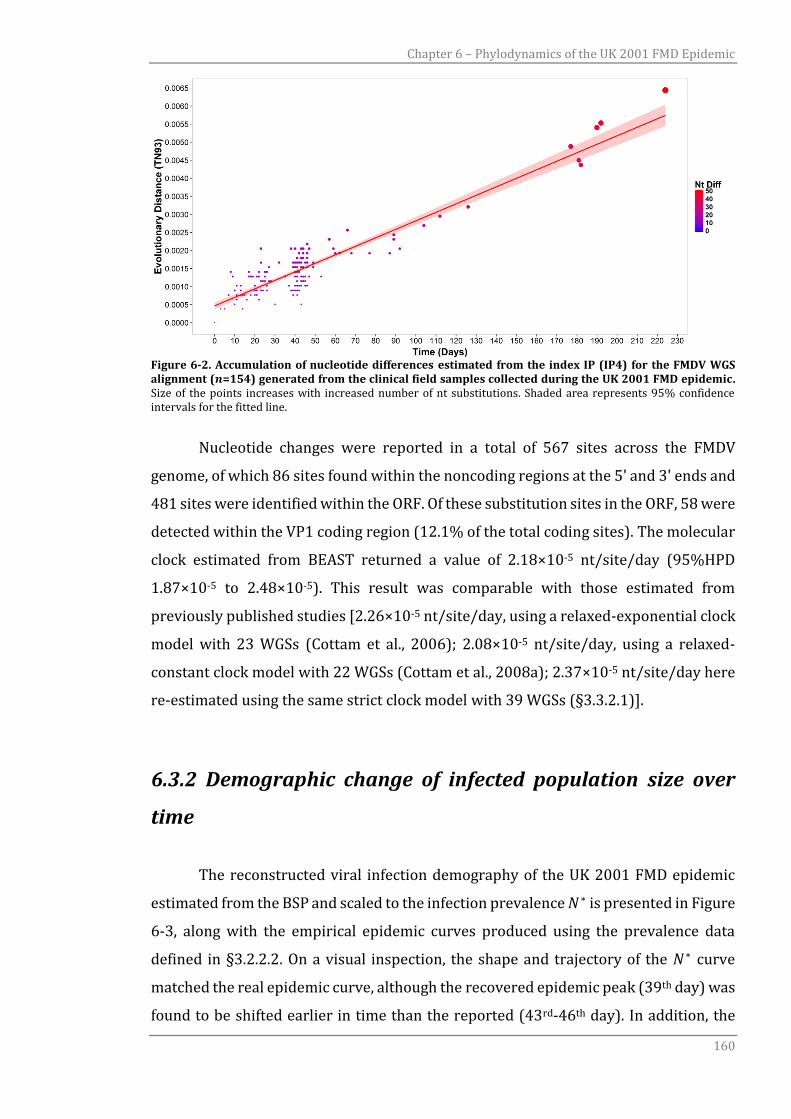
Chapter 6 – Phylodynamics of the UK 2001 FMD Epidemic
160
Figure 6-2. Accumulation of nucleotide differences estimated from the index IP (IP4) for the FMDV WGS alignment (𝒏=154) generated from the clinical field samples collected during the UK 2001 FMD epidemic. Size of the points increases with increased number of nt substitutions. Shaded area represents 95% confidence intervals for the fitted line.
Nucleotide changes were reported in a total of 567 sites across the FMDV
genome, of which 86 sites found within the noncoding regions at the 5' and 3' ends and
481 sites were identified within the ORF. Of these substitution sites in the ORF, 58 were
detected within the VP1 coding region (12.1% of the total coding sites). The molecular
clock estimated from BEAST returned a value of 2.18×10⁻⁵ nt/site/day (95%HPD
1.87×10⁻⁵ to 2.48×10⁻⁵). This result was comparable with those estimated from
previously published studies [2.26×10⁻⁵ nt/site/day, using a relaxed-exponential clock
model with 23 WGSs (Cottam et al., 2006); 2.08×10⁻⁵ nt/site/day, using a relaxed-
constant clock model with 22 WGSs (Cottam et al., 2008a); 2.37×10⁻⁵ nt/site/day here
re-estimated using the same strict clock model with 39 WGSs (§3.3.2.1)].
6.3.2 Demographic change of infected population size over
time
The reconstructed viral infection demography of the UK 2001 FMD epidemic
estimated from the BSP and scaled to the infection prevalence 𝑁∗ is presented in Figure
6-3, along with the empirical epidemic curves produced using the prevalence data
defined in §3.2.2.2. On a visual inspection, the shape and trajectory of the 𝑁∗ curve
matched the real epidemic curve, although the recovered epidemic peak (39th day) was
found to be shifted earlier in time than the reported (43rd-46th day). In addition, the
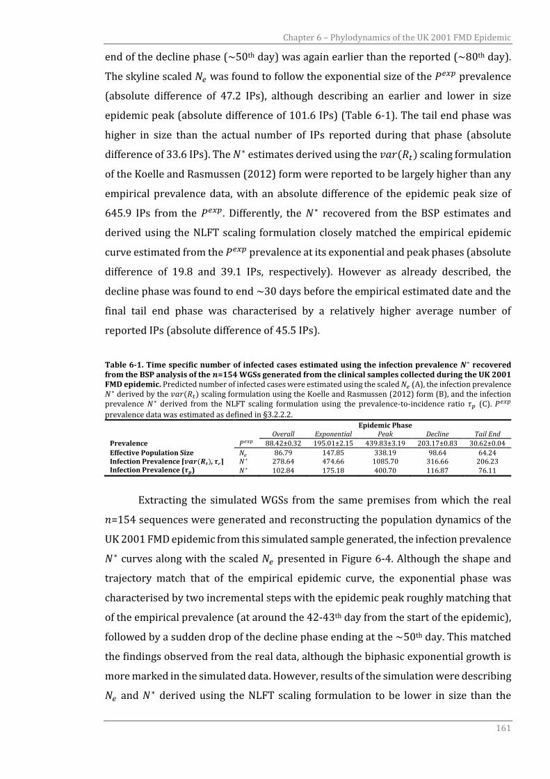
Chapter 6 – Phylodynamics of the UK 2001 FMD Epidemic
161
end of the decline phase (~50th day) was again earlier than the reported (~80th day).
The skyline scaled 𝑁𝑒 was found to follow the exponential size of the 𝑃𝑒𝑥𝑝 prevalence
(absolute difference of 47.2 IPs), although describing an earlier and lower in size
epidemic peak (absolute difference of 101.6 IPs) (Table 6-1). The tail end phase was
higher in size than the actual number of IPs reported during that phase (absolute
difference of 33.6 IPs). The 𝑁∗ estimates derived using the 𝑣𝑎𝑟(𝑅𝑡) scaling formulation
of the Koelle and Rasmussen (2012) form were reported to be largely higher than any
empirical prevalence data, with an absolute difference of the epidemic peak size of
645.9 IPs from the 𝑃𝑒𝑥𝑝. Differently, the 𝑁∗ recovered from the BSP estimates and
derived using the NLFT scaling formulation closely matched the empirical epidemic
curve estimated from the 𝑃𝑒𝑥𝑝 prevalence at its exponential and peak phases (absolute
difference of 19.8 and 39.1 IPs, respectively). However as already described, the
decline phase was found to end ~30 days before the empirical estimated date and the
final tail end phase was characterised by a relatively higher average number of
reported IPs (absolute difference of 45.5 IPs).
Table 6-1. Time specific number of infected cases estimated using the infection prevalence 𝑵∗ recovered from the BSP analysis of the 𝒏=154 WGSs generated from the clinical samples collected during the UK 2001 FMD epidemic. Predicted number of infected cases were estimated using the scaled 𝑁𝑒 (A), the infection prevalence 𝑁∗ derived by the 𝑣𝑎𝑟(𝑅𝑡) scaling formulation using the Koelle and Rasmussen (2012) form (B), and the infection prevalence 𝑁∗ derived from the NLFT scaling formulation using the prevalence-to-incidence ratio 𝜏𝑝 (C). 𝑃𝑒𝑥𝑝
prevalence data was estimated as defined in §3.2.2.2.
Epidemic Phase Overall Exponential Peak Decline Tail End
Prevalence 𝑃𝑒𝑥𝑝 88.42±0.32 195.01±2.15 439.83±3.19 203.17±0.83 30.62±0.04
Effective Population Size 𝑁𝑒 86.79 147.85 338.19 98.64 64.24 Infection Prevalence [𝒗𝒂𝒓(𝑹𝒕), 𝝉𝒄] 𝑁∗ 278.64 474.66 1085.70 316.66 206.23 Infection Prevalence (𝝉𝒑) 𝑁∗ 102.84 175.18 400.70 116.87 76.11
Extracting the simulated WGSs from the same premises from which the real
𝑛=154 sequences were generated and reconstructing the population dynamics of the
UK 2001 FMD epidemic from this simulated sample generated, the infection prevalence
𝑁∗ curves along with the scaled 𝑁𝑒 presented in Figure 6-4. Although the shape and
trajectory match that of the empirical epidemic curve, the exponential phase was
characterised by two incremental steps with the epidemic peak roughly matching that
of the empirical prevalence (at around the 42-43th day from the start of the epidemic),
followed by a sudden drop of the decline phase ending at the ~50th day. This matched
the findings observed from the real data, although the biphasic exponential growth is
more marked in the simulated data. However, results of the simulation were describing
𝑁𝑒 and 𝑁∗ derived using the NLFT scaling formulation to be lower in size than the
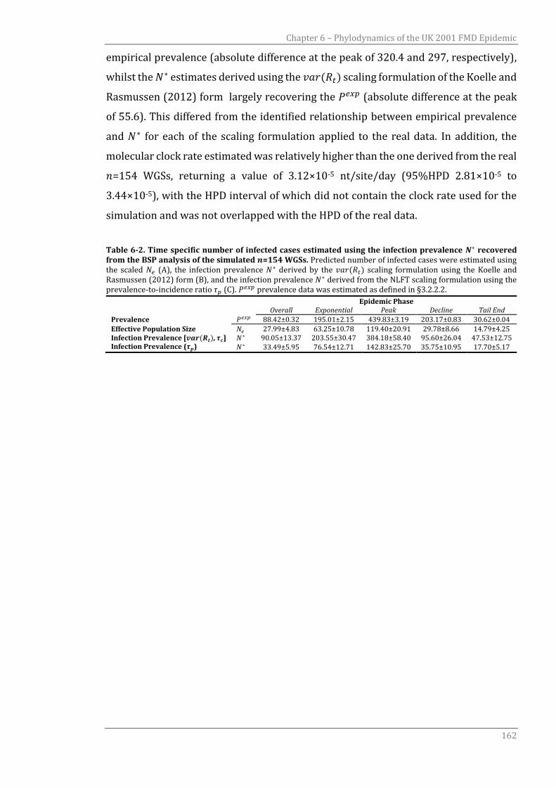
Chapter 6 – Phylodynamics of the UK 2001 FMD Epidemic
162
empirical prevalence (absolute difference at the peak of 320.4 and 297, respectively),
whilst the 𝑁∗ estimates derived using the 𝑣𝑎𝑟(𝑅𝑡) scaling formulation of the Koelle and
Rasmussen (2012) form largely recovering the 𝑃𝑒𝑥𝑝 (absolute difference at the peak
of 55.6). This differed from the identified relationship between empirical prevalence
and 𝑁∗ for each of the scaling formulation applied to the real data. In addition, the
molecular clock rate estimated was relatively higher than the one derived from the real
𝑛=154 WGSs, returning a value of 3.12×10⁻⁵ nt/site/day (95%HPD 2.81×10⁻⁵ to
3.44×10⁻⁵), with the HPD interval of which did not contain the clock rate used for the
simulation and was not overlapped with the HPD of the real data.
Table 6-2. Time specific number of infected cases estimated using the infection prevalence 𝑵∗ recovered from the BSP analysis of the simulated 𝒏=154 WGSs. Predicted number of infected cases were estimated using the scaled 𝑁𝑒 (A), the infection prevalence 𝑁∗ derived by the 𝑣𝑎𝑟(𝑅𝑡) scaling formulation using the Koelle and Rasmussen (2012) form (B), and the infection prevalence 𝑁∗ derived from the NLFT scaling formulation using the prevalence-to-incidence ratio 𝜏𝑝 (C). 𝑃𝑒𝑥𝑝 prevalence data was estimated as defined in §3.2.2.2.
Epidemic Phase Overall Exponential Peak Decline Tail End
Prevalence 𝑃𝑒𝑥𝑝 88.42±0.32 195.01±2.15 439.83±3.19 203.17±0.83 30.62±0.04
Effective Population Size 𝑁𝑒 27.99±4.83 63.25±10.78 119.40±20.91 29.78±8.66 14.79±4.25 Infection Prevalence [𝒗𝒂𝒓(𝑹𝒕), 𝝉𝒄] 𝑁∗ 90.05±13.37 203.55±30.47 384.18±58.40 95.60±26.04 47.53±12.75 Infection Prevalence (𝝉𝒑) 𝑁∗ 33.49±5.95 76.54±12.71 142.83±25.70 35.75±10.95 17.70±5.17
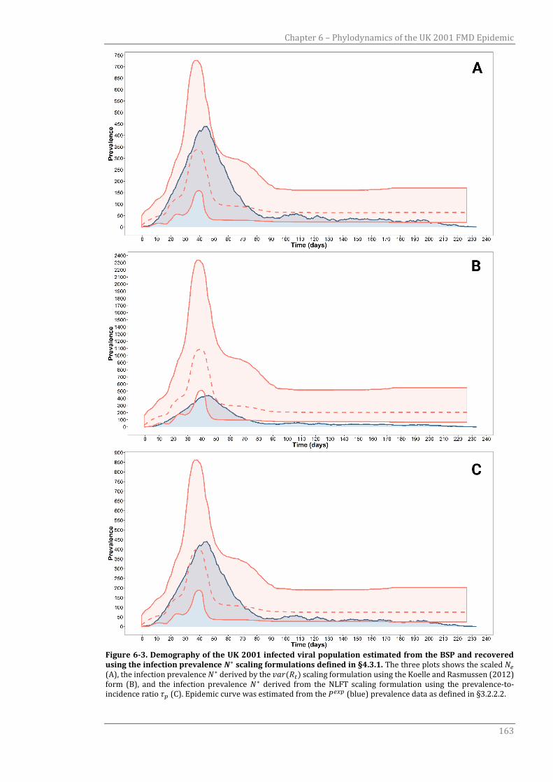
Chapter 6 – Phylodynamics of the UK 2001 FMD Epidemic
163
Figure 6-3. Demography of the UK 2001 infected viral population estimated from the BSP and recovered using the infection prevalence 𝑵∗ scaling formulations defined in §4.3.1. The three plots shows the scaled 𝑁𝑒 (A), the infection prevalence 𝑁∗ derived by the 𝑣𝑎𝑟(𝑅𝑡) scaling formulation using the Koelle and Rasmussen (2012) form (B), and the infection prevalence 𝑁∗ derived from the NLFT scaling formulation using the prevalence-to-incidence ratio 𝜏𝑝 (C). Epidemic curve was estimated from the 𝑃𝑒𝑥𝑝 (blue) prevalence data as defined in §3.2.2.2.

Chapter 6 – Phylodynamics of the UK 2001 FMD Epidemic
164
Figure 6-4. Demography of the UK 2001 infected viral population estimated from the simulated data and recovered using the infection prevalence 𝑵∗ scaling formulations defined in §4.3.1. The three plots shows the scaled 𝑁𝑒 (A), the infection prevalence 𝑁∗ derived by the 𝑣𝑎𝑟(𝑅𝑡) scaling formulation using the Koelle and Rasmussen (2012) form (B), and the infection prevalence 𝑁∗ derived from the NLFT scaling formulation using the prevalence-to-incidence ratio 𝜏𝑝 (C). Epidemic curve was estimated from the 𝑃𝑒𝑥𝑝 (blue) prevalence data as defined
in §3.2.2.2.
Chapter 6 – Phylodynamics of the UK 2001 FMD Epidemic
165
6.4 Discussion
This chapter undertakes preliminary analyses to combining epidemiological
and genetic data to recover the phylodynamics of the UK 2001 FMD epidemic.
Previously, studies have investigated the temporal and spatial dispersal of FMDV
across the UK 2001 FMD epidemic using WGSs generated from the clinical samples
collected from each IPs, although only focusing on dissecting the evolutionary patterns
of the virus (Cottam et al., 2006), and investigating transmission links within
epidemiologically isolated clusters (Cottam et al., 2008a, Konig et al., 2009). However,
these studies used less than ~2% of the total number of reported IPs, which limits
generalisation to the full epidemic event. In this study a larger database of WGSs
(𝑛=154, ~8% of the total number of reported IPs, and ~11% of the collected clinical
samples) have been used, with the aim of recovering the infected population dynamics
of the UK 2001 FMD epidemic. This has been achieved by employing a phylodynamic
method (the BSP) and using those scaling formulations identified from chapter 4 to be
effective in recovering the empirical prevalence. It should be noted that this initial
dataset was primarily extracted from the full collection of clinical samples of the UK
2001 FMD epidemic with the main purpose of testing and validating the protocol for
generating the consensus level sequence from NGS reads, providing confidence in the
accuracy of the sequences. Therefore, samples were not selected for sequencing at
random, and this is likely to bias the demographic signal derived from the sequence
data.
The reconstruction in time of the infected population demography using the 𝑁𝑒
estimated from the BSP produced results different to those anticipated and based on
studies reported in chapter 4. Every scaling formulation used for recovering the
infection prevalence 𝑁∗ produced results that differed from those reconstructed from
the simulated WGSs. The highest ranked scaling formulation derived from §4.3.1
(which expresses the phylogenetic structure by NLFT and use the prevalence-to-
incidence ratio 𝜏𝑝) was found using the real data to closely match the prevalence
estimated from the 𝑃𝑒𝑥𝑝 data. However, it is visually clear that this relationship is
almost perfectly observed for the exponential phase of the epidemic, whilst the
infected population size of the later phases was not recovered. The 𝑁∗ curve drops
more rapidly after the peak than that reported form the empirical prevalence data,
Chapter 6 – Phylodynamics of the UK 2001 FMD Epidemic
166
producing an earlier tail end phase which was also overestimated in size. This
behaviour of the 𝑁∗ curve has been also recovered from the simulated data, and
therefore could be due to the structure of the sample dataset thus biasing the estimates
obtained from both the real and the simulated datasets. As previously described, the
sampled dataset here used for analysing the UK 2001 FMD epidemic has not been
randomly selected. In fact, 85% of the total WGSs were from IPs reported between the
first two months (February and March) of the epidemic, which might substantially bias
the genetic diversity recovered over time. As observed from chapter 5, reducing the
amount of samples and biasing the collection in time and space could substantially
affect the estimates produced by the BSP analysis and, thus, the recovered infection
prevalence 𝑁∗ by any scaling formulation.
A more speculative and critical discussion should be devoted to questioning the
reason for the lack of fit between the simulated and real data. It might be argued that
the genetic mutations (estimated as root-to-tip distance) raised from the simulation
are produced with an error. However, 50 and 84.5±7.5 nt changes at the root-to-tip
level (from IP04 to IP2027) have been estimated for the field isolates and the simulated
data, respectively (absolute difference of 14.5±7.5 nt). Therefore, the higher number of
changes obtained from the simulation would have led to increased genetic diversity,
differently to what reported. This comment might be also valid to explain the observed
difference in the clock rate recovered from the real and simulated data, estimated at
values of 2.18×10⁻⁵ and 3.12×10⁻⁵ nt/site/day, respectively.
As already discussed in chapter 3, the substantially different behaviour
observed between the real and simulated data might be due to the effect of within-farm
evolutionary processes. In a real epidemic, genetic change might accrue from within-
farm evolutionary processes, for which multiple cycles of infection might be present on
each IP. Genetic diversity derived from the swarm of unsampled genome at the within-
farm level might contribute to the size of the ‘effective population’, although at
consensus level this variability could not be recovered. However, the process
developed for simulating the virus evolution does consider, although using a very
simplified algorithmic implementation, the characterisation of the within-farm
dynamics, which might contribute to the genetic diversity observed between the
sequences recovered from each IP. On this line, it would be interesting to see if the
observed nt change per farm transfer estimated from the real data (if the real
Chapter 6 – Phylodynamics of the UK 2001 FMD Epidemic
167
transmission tree would ever be resolved) would match with the value obtained from
the simulated data.
Another explanation could be that the reconstruction of the transmission tree
that has been used as a backbone for the Markovian evolutionary simulation differed
importantly from the real one. However very similar results were obtained running
different realisations of the transmission tree reconstruction model (as could be
evinced from §4.3) and, in addition, the bias in the structure of the 𝑛=154 in estimating
the real shape of the epidemic curve (peak and decline phase) have been observed
similarly with the simulated data, thus suggesting that the underling transmission tree
has been largely recovered. It is, thus, clear that despite attempts in explaining this
unresolved and unexpected behaviour, it merits further investigations.
The effective control of FMD, and any other infectious disease, relies on a close
epidemiological investigation of the spatio-temporal dynamics of pathogen dispersal,
along with the understanding of the evolutionary drives which contributes to the
transmission process. Although this initial investigation made use of a small and not
uniformly structured dataset, it can preliminarily define the potential resolution which
the UK 2001 FMD epidemic might provide for contributing to seminal works on the
development of new epidemiological tools which can be used to further enhance our
ability in predicting and controlling future outbreaks.

169
CHAPTER 7
Final Discussion and Concluding Remarks
With the development of the discipline of ‘phylodynamics’ (Grenfell et al., 2004),
seminal studies from several research groups have contributed to our understanding
of how epidemiological dynamics can be recovered from an estimated phylogeny
(Drummond et al., 2002, Lemey et al., 2009a, Stadler et al., 2012). Population genetic
models have also provided the substrate to augment the information derived from the
ancestral relationship of sampled lineages with population dynamics inference, to
derive a more detailed representation of how the genetic diversity (and the
corresponding concept of ‘effective population size’ 𝑁𝑒) leaves imprints in genetic
sequences about past population dynamics. This theory reminds us how
epidemiological and evolutionary forces act within the same time frame, and why
genetic data sampled from infected hosts can reveal the dynamics of disease spread
(Drummond and Rambaut, 2007, Frost and Volz, 2010, Kuhnert et al., 2014). Scholars
have shown how the demographic history of infectious disease reconstructed from
genome sequences follow in relative size the observed disease dynamics (Rambaut et
al., 2008). However, evolutionary dynamics accruing from high population complexity,
which is often the case for infectious disease of viral origin, could challenge the ability
of analytical approaches used in phylodynamic inference to produce robust estimates
(Bennett et al., 2010, Siebenga et al., 2010, Rasmussen et al., 2014a). Degrees of
uncertainty still exist on how these methods perform for reproducing the real scale and
size of disease outbreak trends as estimated through empirical epidemiological data.
Our ability to genetically characterise pathogens has increased exponentially in the last
ten years, driven by the advance in high-throughput sequencing technology and the
ability to rapidly generate WGSs at low costs, enabling genetic sequences to be
provided from each individual in an infected population and thus leading to really
large-scale and high resolution population genetic studies for the first time.
In this thesis the exhaustively-sampled UK 2001 FMD epidemic has been used
to investigate how established phylodynamic methods based on a coalescent model [i.e.
the Bayesian skyline plot (Drummond et al., 2005)] perform to recover the
demographic history estimated from time series of case reports, thus enabling capture
Chapter 7 – Final Discussion and Concluding Remarks
170
of the real dynamic of the infected population. Although in viral systems 𝑁𝑒 has often
been interpreted in an epidemiological sense as the effective size of an infected
population, previously it has been shown that coalescent rates are governed by both
incidence and prevalence, so that BSP estimates might not accurately be used to infer
prevalence alone (Frost and Volz, 2010, Volz 2012). The aim of this study was to
attempt to identify a valid formulation which can be used to scale the population
genetics parameter 𝑁𝑒 (derived from the BSP) to a measure of empirical prevalence
data, here termed the infection prevalence 𝑁∗. This theoretical relation has been
investigated defining prevalence data according to the timing of FMD disease
progression, and attempting to account for complex variabilities in the population
structure under study. I conclude, that different relationships can be established
between the infection prevalence 𝑁∗ and the prevalence data. The best fit between 𝑁∗
and the empirical prevalence was found by expressing the phylogenetic structure by
the number of lineages as a function of time and using the prevalence-to-incidence
ratio 𝜏𝑝 (Frost and Volz, 2013). I here demonstrated, albeit in silico, how this quantity
effectively resolves the shape and trajectory of the prevalence computed from the 𝑃𝑒𝑥𝑝
prevalence data, where infected cases are defined to exist over the time interval from
exposed to being culled. This result provides further insights in how the relationship
between 𝑁𝑒 and prevalence can be defined in a closed viral epidemic system, although
this might be not so straightforward. In fact, it has also been established here that the
variability in the number of secondary cases per primary infection 𝑅𝑡 greatly impacts
on the ability of the BSP to recover the real number of infected cases: increasing the
variance in the reproduction number of the infected population [i.e. 𝑣𝑎𝑟(𝑅𝑡)]
significantly impacts on the accuracy of the estimator. This is in line with the
theoretical definition of the BSP model, which assumes that viral lineages are sampled
from a single, freely mixing population. Therefore it is clear that this assumption can
always be violated in practice and, thus, be invalid in complex epidemiological systems.
Thus, accounting for the effect of the variance in the reproductive success [i.e. 𝑣𝑎𝑟(𝑅𝑡)]
in scaling 𝑁𝑒 , 𝑁∗ estimates were observed to correlate with the infected population size
derived from the 𝑃𝑒𝑥𝑝 prevalence data at a very high level of population structure (i.e.
in a system with a high value of 𝑣𝑎𝑟(𝑅𝑡) and presence of ‘super-spreaders’). In addition,
the fit from the scaling equation, that expresses the phylogenetic structure by the
number of lineages as a function of time, suggests that in a more homogeneous FMD
system [i.e. when 𝑣𝑎𝑟(𝑅𝑡)≈1] the predicted infection prevalence 𝑁∗ is a good
Chapter 7 – Final Discussion and Concluding Remarks
171
approximation to the empirical IP count (𝑃𝑒𝑥𝑝 derived). This stands as a demonstration
that because every IP in a homogenous system has the same chance of transmitting
infection to subsequent generations and, therefore, the average time between
infections (i.e. the serial case interval) is the only possible scaling factor that is
maintained constant through the system. It is therefore clear that the results generated
provide further supporting evidence that the population structure greatly impacts on
estimation of demographic dynamics (Frost and Volz, 2010, Frost and Volz, 2013,
Rasmussen et al., 2014a, Pybus et al., 2012). Although structured coalescent models
define population structures within its model definition, current phylogenetic
implementation (Vaughan et al., 2014) might not be able to fully capture heterogeneity
in contacts and transmission among infected individuals. It might be, therefore,
essential to account for variability in the infected population structure within the
model specification for population size estimates to be more accurate.
A unique feature of the evolutionary process implemented here for generating
the genetic variability of the UK 2001 FMD simulated epidemic is that the virus is
constrained to evolve along a well-reconstructed transmission tree, thus enabling the
preservation of the dependencies of sampled lineages along the transmission tree
which are then recovered from the simulated sequences. In addition, in order to
account for high within-farm genetic diversity, the coalescent event was set to be early
in infection, backward in time of the first related coalescent ancestor (i.e. the infection
time of the infector farm rather than the infection time of the infected farm). Most
phylodynamic models assume that the timing of coalescent events in the phylogeny
coincides with the timing of the transmission events. This is obviously not the case
when a significant genetic variation exists at the within-host and/or within-farm level
as, for examples, in the case of highly population structured infectious disease
epidemics. It has been previously reported how the within-farm genetic diversity can
contribute to the genetic diversity observed between sampled sequences (Ypma et al.,
2013) and, therefore, ignoring this aspect could have led to false estimates of the
population size.
Traditionally, methods used for measuring, quantitatively and qualitatively, the
burden of pathogen spread within populations rely on surveillance data collected
through either disease monitoring programs or during epidemics. As already
discussed, in recent years there has been a substantial expansion in the volume of
genetic data generated within surveillance programs and larger multi-gene sequences
Chapter 7 – Final Discussion and Concluding Remarks
172
and WGS are now becoming routine for disease monitoring. Therefore, the potential
utility of using molecular methods for estimating infected population dynamics is to
support surveillance programs or more conventional control practices. Although in
practice this would require less field effort than conventional serosurveillance studies
and the deployment of fewer economic resources, sensitivity of the analyses generated
through the use of phylodynamics tools to non-random sampling is a widely recognised
problem (St Onge et al., 2012, Stack et al., 2010, Volz and Frost, 2014). It is often the
case that collected samples would not be representative of the entire infected
population, introducing on in the efficacy by which population-level information is
extracted and, thus, impacting on the accuracy of reconstructed population dynamics.
This might be more relevant when considering endemic disease affecting developing
countries with poor health infrastructure. In these setting the availability of less-
intensive and more error prone sampled data challenges the evaluation of the health
status and, thus, the design of effective control policies. Considering FMD as an
example, analysis of sequence data based on the VP1 coding regions collected from
Southeast Asian countries revealed the potential impact of undisclosed cases (and
potentially misreported disease events) on the maintenance of the disease within an
endemic setting (Knowles et al., 2012). This leads to the inability of the FMD research
community to capture the real burden of the disease and, thus, to generate the
necessary resources to control FMD in these ecosystems.
The effect of sampling strategies on phylodynamic inferences and, thus, on the
reconstructed temporal dynamics of viral populations has not been exhaustively
explored and, moreover, no attempts have been put forward the assessment of the
impact of population structures in an infectious disease context (Chikhi et al. 2010,
Stack et al., 2010, de Silva, Ferguson and Fraser, 2012). Results reported within this
thesis provides further information on how the demographic signal carried by
sequence data becomes imprecise and weaker when reducing the number of samples.
In order to address this research question, scenarios from the UK 2001 FMD simulation
were intended to represent sampling for the population of an epidemic virus across
multiple spatial, temporal and genetic structures. It has been shown that, when
sampling at a rate of less than 50% of the total infected population, the 𝑁∗ curve was
reported to generate underestimates of the infectious prevalence and, more
understandably, more variable estimates with greater standard errors. In addition,
with a sample of only 25% of the total infected population the predicted infection
Chapter 7 – Final Discussion and Concluding Remarks
173
prevalence 𝑁∗ was found to be half of the empirical prevalence. It has been also
observed how accounting for the spatial and temporal structure of the transmission
process within the sampling protocol does not significantly improve the accuracy of
the estimated population size at very low sampling rates, in contrast to more
evolutionary based sampling approaches which represent the extent of the genetic
signal (i.e. accounting for the length of the evolutionary process generated between
serial cases or the observed genetic distance between sequences). It should be further
noted from the analysis of these results that sampling methods designed in a more
biased and unstructured fashion (i.e. strictly sampling from some infected populations
and not others) can falsely suggest population dynamics trends (spurious temporal
variation in the BSP reconstruction as, for example, population declines), which would
in fact be entirely sampling artefacts and, therefore, not truly reflecting the real
demography of the infected population. This leads to the conclusion that the impact of
the size and structure of the sampled dataset on the accuracy of the reconstructed viral
demographies is relevant at any scale of the transmission process and, therefore, the
results derived from this study can provide relevant material to be used in order to
inform sampling strategies designed to investigate disease dynamics at endemic level.
For example, undisclosed (i.e. unsampled) cases maintain endemicity at a fixed level,
which could be difficult to account for when the structure of the sampled population is
biased. As already discussed, the coalescent model, from which the BSP is derived,
assumes that the samples are randomly collected from a homogeneous population
(Griffiths and Tavare, 1994b), a criterion which in a real scenario would not be always
satisfied. In addition, the BSP model does not specifically account for the sampling
process, resulting in more biased estimates when the population is not randomly
sampled (Popinga et al., 2015). Therefore, estimates of population dynamics based on
coalescent based methods would benefit from the further integration of surveillance
information for the specification of the sampling process, which would lead to
reduction in the bias of the inference methods. In fact, time series of sequence data can
be effectively used for recovering the population size through time if the sampling
process can be correctly specified (Volz and Frost, 2014).
It has been already demonstrated how genetic data carries signal on
evolutionary forces, demographic size and structure of populations. However, the
challenge here lies in how to rigorously make these estimations accurate and unbiased.
A further unresolved question is how genome sequences must be examined for

Chapter 7 – Final Discussion and Concluding Remarks
174
epidemiological characterisation. Methods drawn from phylodynamic inference
combine powerful epidemiological and population genetics tools that can provide
valuable insights into the dynamics of viral disease. However, the sensitivity of the
majority of these models on their assumptions makes estimates less reliable when
these are violated, as it has been here reported. Therefore, to be applied as reliable
tools supporting control programs, more focused theoretical research is required to
model with much more details the processes driving the evolutionary shape of a
natural population. This could take into account the structural inhomogeneity of the
infected population, the non-random effect derived from partial sampling, the
evolutionary interplay driven by coexisting lineages (as in the FMD case) within an
ecosystem and the sample size at which the phylodynamic inference starts to be
reliable. The further development of phylodynamics methods which integrate
inferences of both genetic and epidemiological processes would thus likely provide a
promising framework to address these challenges.
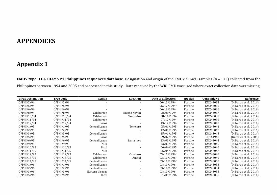
APPENDICES
Appendix 1
FMDV type O CATHAY VP1 Philippines sequences database. Designation and origin of the FMDV clinical samples (n = 112) collected from the
Philippines between 1994 and 2005 and processed in this study. †Date received by the WRLFMD was used where exact collection date was missing.
Virus Designation Tree Code Region Location Date of Collection† Species GenBank No Reference
O/PHI/2/94 O/PHI/2/94 - - 06/12/1994† Porcine KM243034 (Di Nardo et al., 2014) O/PHI/5/94 O/PHI/5/94 - - 06/12/1994† Porcine KM243035 (Di Nardo et al., 2014) O/PHI/6/94 O/PHI/6/94 - - 06/12/1994† Porcine KM243036 (Di Nardo et al., 2014) O/PHI/8/94 O/PHI/8/94 Calabarzon Bagong Nayon 08/09/1994 Porcine KM243037 (Di Nardo et al., 2014) O/PHI/10/94 O/PHI/10/94 Calabarzon San Isidro 28/10/1994 Porcine KM243038 (Di Nardo et al., 2014) O/PHI/11/94 O/PHI/11/94 Calabarzon - 07/12/1994 Porcine KM243039 (Di Nardo et al., 2014) O/PHI/12/94 O/PHI/12/94 Ilocos - 13/12/1994 Porcine KM243040 (Di Nardo et al., 2014) O/PHI/1/95 O/PHI/1/95 Central Luzon Tenejero 05/01/1995 Porcine KM243041 (Di Nardo et al., 2014) O/PHI/2/95 O/PHI/2/95 Ilocos - 12/01/1995 Porcine KM243042 (Di Nardo et al., 2014) O/PHI/3/95 O/PHI/3/95 Central Luzon - 15/01/1995 Porcine KM243043 (Di Nardo et al., 2014) O/PHI/5/95 O/PHI/5/95 Ilocos - 09/02/1995 Porcine DQ164946 (Knowles et al., 2005) O/PHI/6/95 O/PHI/6/95 Central Luzon Santa Ines 23/03/1995 Porcine KM243044 (Di Nardo et al., 2014) O/PHI/9/95 O/PHI/9/95 NCR - 23/03/1995 Porcine KM243045 (Di Nardo et al., 2014) O/PHI/10/95 O/PHI/10/95 Bicol - 06/04/1995 Porcine KM243046 (Di Nardo et al., 2014) O/PHI/11/95 O/PHI/11/95 NCR - 06/04/1995 Porcine KM243047 (Di Nardo et al., 2014) O/PHI/12/95 O/PHI/12/95 Calabarzon Calabuso 03/10/1996† Porcine KM243048 (Di Nardo et al., 2014) O/PHI/13/95 O/PHI/13/95 Calabarzon Ampid 03/10/1996† Porcine KM243049 (Di Nardo et al., 2014) O/PHI/14/95 O/PHI/14/95 Central Luzon - 03/10/1996† Porcine KM243050 (Di Nardo et al., 2014) O/PHI/1/96 O/PHI/1/96 Central Luzon - 03/10/1996† Porcine KM243053 (Di Nardo et al., 2014) O/PHI/2/96 O/PHI/2/96 Central Luzon - 03/10/1996† Porcine KM243054 (Di Nardo et al., 2014) O/PHI/3/96 O/PHI/3/96 Eastern Visayas - 03/10/1996† Porcine KM243055 (Di Nardo et al., 2014) O/PHI/5/96 O/PHI/5/96 Bicol - 01/09/1996 Porcine KM243056 (Di Nardo et al., 2014)
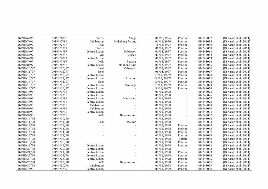
O/PHI/6/96 O/PHI/6/96 Ilocos Aliaga 01/10/1996 Porcine KM243057 (Di Nardo et al., 2014) O/PHI/7/96 O/PHI/7/96 Calabarzon Mahabang Parang 01/11/1996 Porcine KM243058 (Di Nardo et al., 2014) O/PHI/2/97 O/PHI/2/97 NCR - 16/01/1997 Porcine KM243059 (Di Nardo et al., 2014) O/PHI/3/97 O/PHI/3/97 Ilocos - 01/01/1997 Porcine KM243060 (Di Nardo et al., 2014) O/PHI/4/97 O/PHI/4/97 Central Luzon Poblacion 01/02/1997 Porcine KM243061 (Di Nardo et al., 2014) O/PHI/5/97 O/PHI/5/97 CAR Guisad 01/02/1997 Porcine KM243062 (Di Nardo et al., 2014) O/PHI/6/97 O/PHI/6/97 Central Luzon - 01/03/1997 Porcine KM243063 (Di Nardo et al., 2014) O/PHI/7/97 O/PHI/7/97 NCR Payatas 01/03/1997 Porcine KM243064 (Di Nardo et al., 2014) O/PHI/8/97 O/PHI/8/97 Central Luzon Malibong Bata 01/03/1997 Porcine KM243065 (Di Nardo et al., 2014) O/PHI/10/97 O/PHI/10/97 Bicol Cabangan 01/03/1997 Porcine KM243066 (Di Nardo et al., 2014) O/PHI/11/97 O/PHI/11/97 Bicol - 06/04/1997 Porcine KM243067 (Di Nardo et al., 2014) O/PHI/12/97 O/PHI/12/97 Central Luzon - 19/11/1997† Porcine KM243070 (Di Nardo et al., 2014) O/PHI/13/97 O/PHI/13/97 Central Luzon Balatong 19/11/1997† Porcine KM243071 (Di Nardo et al., 2014) O/PHI/14/97 O/PHI/14/97 Bicol - 19/11/1997† Porcine KM243072 (Di Nardo et al., 2014) O/PHI/15/97 O/PHI/15/97 Central Luzon Sampaga 19/11/1997† Porcine KM243073 (Di Nardo et al., 2014) O/PHI/16/97 O/PHI/16/97 Central Luzon - 19/11/1997† Porcine KM243074 (Di Nardo et al., 2014) O/PHI/1/98 O/PHI/1/98 Central Luzon - 01/01/1998 - KM243075 (Di Nardo et al., 2014) O/PHI/2/98 O/PHI/2/98 Central Luzon - 01/01/1998 - KM243076 (Di Nardo et al., 2014) O/PHI/3/98 O/PHI/3/98 Central Luzon Matatalaib 01/01/1998 - KM243077 (Di Nardo et al., 2014) O/PHI/4/98 O/PHI/4/98 Central Luzon - 01/01/1998 - KM243078 (Di Nardo et al., 2014) O/PHI/5/98 O/PHI/5/98 Calabarzon - 01/01/1998 - KM243079 (Di Nardo et al., 2014) O/PHI/6/98 O/PHI/6/98 Calabarzon - 01/01/1998 - KM243080 (Di Nardo et al., 2014) O/PHI/8/98 O/PHI/8/98 Central Luzon - 01/01/1998 - KM243081 (Di Nardo et al., 2014) O/PHI/9/98 O/PHI/9/98 NCR Nepomuceno 01/01/1998 - KM243082 (Di Nardo et al., 2014) O/PHI/10/98 O/PHI/10/98 - - 01/01/1998 - KM243083 (Di Nardo et al., 2014) O/PHI/11/98 O/PHI/11/98 NCR Malinta 01/01/1998 - KM243084 (Di Nardo et al., 2014) O/PHI/12/98 O/PHI/12/98 - - 01/01/1998 Porcine KM243085 (Di Nardo et al., 2014) O/PHI/13/98 O/PHI/13/98 - - 01/01/1998 Porcine KM243086 (Di Nardo et al., 2014) O/PHI/14/98 O/PHI/14/98 - - 01/01/1998 Porcine KM243087 (Di Nardo et al., 2014) O/PHI/15/98 O/PHI/15/98 - - 01/01/1998 Porcine KM243088 (Di Nardo et al., 2014) O/PHI/16/98 O/PHI/16/98 - - 01/01/1998 Buffalo KM243089 (Di Nardo et al., 2014) O/PHI/18/98 O/PHI/18/98 - - 01/01/1998 Porcine KM243090 (Di Nardo et al., 2014) O/PHI/19/98 O/PHI/19/98 Central Luzon - 01/01/1998 Porcine KM243091 (Di Nardo et al., 2014) O/PHI/20/98 O/PHI/20/98 Central Luzon - 01/01/1998 - KM243092 (Di Nardo et al., 2014) O/PHI/21/98 O/PHI/21/98 Central Luzon - 01/01/1998 Porcine KM243093 (Di Nardo et al., 2014) O/PHI/22/98 O/PHI/22/98 Central Luzon - 01/01/1998 Porcine KM243094 (Di Nardo et al., 2014) O/PHI/23/98 O/PHI/23/98 Central Luzon - 01/01/1998 Porcine KM243095 (Di Nardo et al., 2014) O/PHI/25/98 O/PHI/25/98 NCR Nepomuceno 01/01/1998 Porcine KM243096 (Di Nardo et al., 2014) O/PHI/30/98 O/PHI/30/98 Calabarzon - 01/01/1998 Porcine KM243097 (Di Nardo et al., 2014) O/PHI/1/99 O/PHI/1/99 Central Luzon - 01/01/1999 Porcine KM243098 (Di Nardo et al., 2014)
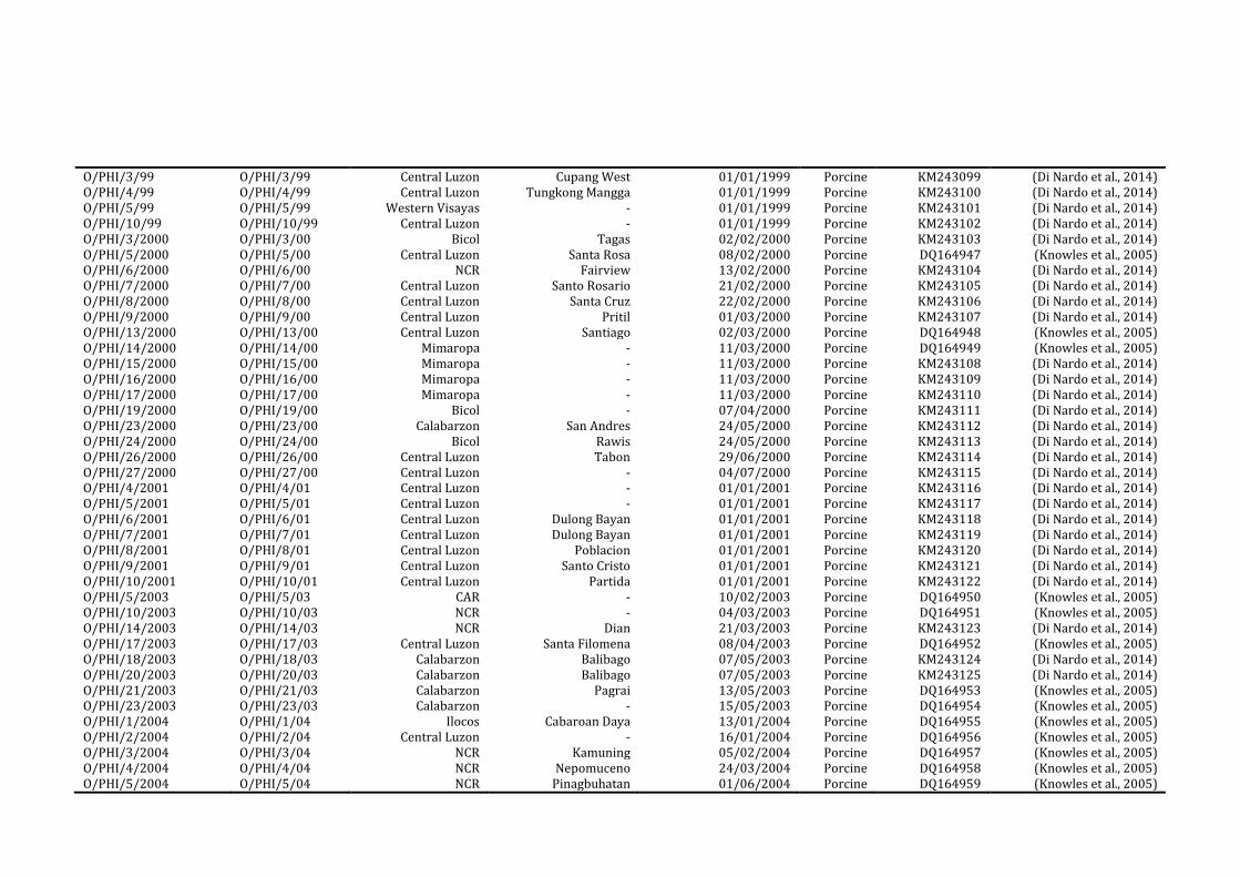
O/PHI/3/99 O/PHI/3/99 Central Luzon Cupang West 01/01/1999 Porcine KM243099 (Di Nardo et al., 2014) O/PHI/4/99 O/PHI/4/99 Central Luzon Tungkong Mangga 01/01/1999 Porcine KM243100 (Di Nardo et al., 2014) O/PHI/5/99 O/PHI/5/99 Western Visayas - 01/01/1999 Porcine KM243101 (Di Nardo et al., 2014) O/PHI/10/99 O/PHI/10/99 Central Luzon - 01/01/1999 Porcine KM243102 (Di Nardo et al., 2014) O/PHI/3/2000 O/PHI/3/00 Bicol Tagas 02/02/2000 Porcine KM243103 (Di Nardo et al., 2014) O/PHI/5/2000 O/PHI/5/00 Central Luzon Santa Rosa 08/02/2000 Porcine DQ164947 (Knowles et al., 2005) O/PHI/6/2000 O/PHI/6/00 NCR Fairview 13/02/2000 Porcine KM243104 (Di Nardo et al., 2014) O/PHI/7/2000 O/PHI/7/00 Central Luzon Santo Rosario 21/02/2000 Porcine KM243105 (Di Nardo et al., 2014) O/PHI/8/2000 O/PHI/8/00 Central Luzon Santa Cruz 22/02/2000 Porcine KM243106 (Di Nardo et al., 2014) O/PHI/9/2000 O/PHI/9/00 Central Luzon Pritil 01/03/2000 Porcine KM243107 (Di Nardo et al., 2014) O/PHI/13/2000 O/PHI/13/00 Central Luzon Santiago 02/03/2000 Porcine DQ164948 (Knowles et al., 2005) O/PHI/14/2000 O/PHI/14/00 Mimaropa - 11/03/2000 Porcine DQ164949 (Knowles et al., 2005) O/PHI/15/2000 O/PHI/15/00 Mimaropa - 11/03/2000 Porcine KM243108 (Di Nardo et al., 2014) O/PHI/16/2000 O/PHI/16/00 Mimaropa - 11/03/2000 Porcine KM243109 (Di Nardo et al., 2014) O/PHI/17/2000 O/PHI/17/00 Mimaropa - 11/03/2000 Porcine KM243110 (Di Nardo et al., 2014) O/PHI/19/2000 O/PHI/19/00 Bicol - 07/04/2000 Porcine KM243111 (Di Nardo et al., 2014) O/PHI/23/2000 O/PHI/23/00 Calabarzon San Andres 24/05/2000 Porcine KM243112 (Di Nardo et al., 2014) O/PHI/24/2000 O/PHI/24/00 Bicol Rawis 24/05/2000 Porcine KM243113 (Di Nardo et al., 2014) O/PHI/26/2000 O/PHI/26/00 Central Luzon Tabon 29/06/2000 Porcine KM243114 (Di Nardo et al., 2014) O/PHI/27/2000 O/PHI/27/00 Central Luzon - 04/07/2000 Porcine KM243115 (Di Nardo et al., 2014) O/PHI/4/2001 O/PHI/4/01 Central Luzon - 01/01/2001 Porcine KM243116 (Di Nardo et al., 2014) O/PHI/5/2001 O/PHI/5/01 Central Luzon - 01/01/2001 Porcine KM243117 (Di Nardo et al., 2014) O/PHI/6/2001 O/PHI/6/01 Central Luzon Dulong Bayan 01/01/2001 Porcine KM243118 (Di Nardo et al., 2014) O/PHI/7/2001 O/PHI/7/01 Central Luzon Dulong Bayan 01/01/2001 Porcine KM243119 (Di Nardo et al., 2014) O/PHI/8/2001 O/PHI/8/01 Central Luzon Poblacion 01/01/2001 Porcine KM243120 (Di Nardo et al., 2014) O/PHI/9/2001 O/PHI/9/01 Central Luzon Santo Cristo 01/01/2001 Porcine KM243121 (Di Nardo et al., 2014) O/PHI/10/2001 O/PHI/10/01 Central Luzon Partida 01/01/2001 Porcine KM243122 (Di Nardo et al., 2014) O/PHI/5/2003 O/PHI/5/03 CAR - 10/02/2003 Porcine DQ164950 (Knowles et al., 2005) O/PHI/10/2003 O/PHI/10/03 NCR - 04/03/2003 Porcine DQ164951 (Knowles et al., 2005) O/PHI/14/2003 O/PHI/14/03 NCR Dian 21/03/2003 Porcine KM243123 (Di Nardo et al., 2014) O/PHI/17/2003 O/PHI/17/03 Central Luzon Santa Filomena 08/04/2003 Porcine DQ164952 (Knowles et al., 2005) O/PHI/18/2003 O/PHI/18/03 Calabarzon Balibago 07/05/2003 Porcine KM243124 (Di Nardo et al., 2014) O/PHI/20/2003 O/PHI/20/03 Calabarzon Balibago 07/05/2003 Porcine KM243125 (Di Nardo et al., 2014) O/PHI/21/2003 O/PHI/21/03 Calabarzon Pagrai 13/05/2003 Porcine DQ164953 (Knowles et al., 2005) O/PHI/23/2003 O/PHI/23/03 Calabarzon - 15/05/2003 Porcine DQ164954 (Knowles et al., 2005) O/PHI/1/2004 O/PHI/1/04 Ilocos Cabaroan Daya 13/01/2004 Porcine DQ164955 (Knowles et al., 2005) O/PHI/2/2004 O/PHI/2/04 Central Luzon - 16/01/2004 Porcine DQ164956 (Knowles et al., 2005) O/PHI/3/2004 O/PHI/3/04 NCR Kamuning 05/02/2004 Porcine DQ164957 (Knowles et al., 2005) O/PHI/4/2004 O/PHI/4/04 NCR Nepomuceno 24/03/2004 Porcine DQ164958 (Knowles et al., 2005) O/PHI/5/2004 O/PHI/5/04 NCR Pinagbuhatan 01/06/2004 Porcine DQ164959 (Knowles et al., 2005)

O/PHI/6/2004 O/PHI/6/04 NCR Dagat-Dagatan 21/06/2004 Porcine DQ164960 (Knowles et al., 2005) O/PHI/7/2004 O/PHI/7/04 Central Luzon Ayson 29/06/2004 Porcine DQ164961 (Knowles et al., 2005) O/PHI/8/2004 O/PHI/8/04 Central Luzon - 14/07/2004 Porcine DQ164962 (Knowles et al., 2005) O/PHI/9/2004 O/PHI/9/04 Calabarzon Mayamot 21/07/2004 Porcine DQ164963 (Knowles et al., 2005) O/PHI/10/2004 O/PHI/10/04 NCR Project 8 04/08/2004 Porcine DQ164964 (Knowles et al., 2005) O/PHI/11/2004 O/PHI/11/04 NCR - 03/09/2004 Porcine DQ164965 (Knowles et al., 2005) O/PHI/12/2004 O/PHI/12/04 Calabarzon Calabuso 29/09/2004 Porcine DQ164966 (Knowles et al., 2005) O/PHI/1/2005 O/PHI/1/05 NCR La Loma 16/02/2005 Porcine KM243127 (Di Nardo et al., 2014) O/PHI/2/2005 O/PHI/2/05 NCR - 23/02/2005 Porcine KM243128 (Di Nardo et al., 2014) O/PHI/3/2005 O/PHI/3/05 NCR La Loma 03/03/2005 Porcine KM243131 (Di Nardo et al., 2014)
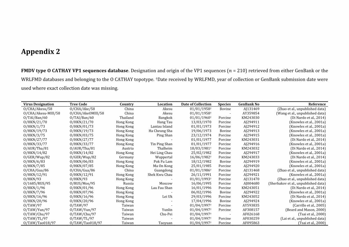
Appendix 2
FMDV type O CATHAY VP1 sequences database. Designation and origin of the VP1 sequences (𝑛 = 210) retrieved from either GenBank or the
WRLFMD databases and belonging to the O CATHAY topotype. †Date received by WRLFMD, year of collection or GenBank submission date were
used where exact collection date was missing.
Virus Designation Tree Code Country Location Date of Collection Species GenBank No Reference
O/CHA/Akesu/58 O/CHA/Ake/58 China Akesu 01/01/1958† Bovine AJ131469 (Zhao et al., unpublished data) O/CHA/Akesu-MIII/58 O/CHA/AkeOMIII/58 China Akesu 01/01/1958† - AY359854 (Wang et al., unpublished data) O/TAI/Ban/60 O/TAI/Ban/60 Thailand Bangkok 01/01/1960† Porcine KM243030 (Di Nardo et al., 2014) O/HKN/21/70 O/HKN/21/70 Hong Kong Hang Tau 13/03/1970 Porcine AJ294911 (Knowles et al., 2001a) O/HKN/1/73 O/HKN/01/73 Hong Kong Lantau Island 01/01/1973 Porcine AJ294912 (Knowles et al., 2001a) O/HKN/19/73 O/HKN/19/73 Hong Kong Ha Cheung Sha 19/06/1973 Bovine AJ294913 (Knowles et al., 2001a) O/HKN/3/75 O/HKN/03/75 Hong Kong Ping Shan 23/12/1974 Porcine AJ294915 (Knowles et al., 2001a) O/HKN/27/77 O/HKN/27/77 Hong Kong - 01/01/1977 Porcine KM243031 (Di Nardo et al., 2014) O/HKN/33/77 O/HKN/33/77 Hong Kong Tin Ping Shan 01/01/1977 Porcine AJ294916 (Knowles et al., 2001a) O/AUR/Tha/81 O/AUR/Tha/81 Austria Thalheim 18/03/1981† Porcine KM243032 (Di Nardo et al., 2014) O/HKN/14/82 O/HKN/14/82 Hong Kong Hei Ling Chau 25/02/1982 Porcine AJ294917 (Knowles et al., 2001a) O/GER/Wup/82 O/GER/Wup/82 Germany Wuppertal 16/06/1982† Porcine KM243033 (Di Nardo et al., 2014) O/HKN/6/83 O/HKN/06/83 Hong Kong Pok Fu Lam 18/12/1982 Bovine AJ294919 (Knowles et al., 2001a) O/HKN/7/85 O/HKN/07/85 Hong Kong Ma On Kong 25/01/1985 Porcine AJ294920 (Knowles et al., 2001a) O/CHA/Gua/86 O/CHA/Gua/86 China Guangdong 01/01/1986† Porcine AJ131468 (Zhao et al., unpublished data) O/HKN/12/91 O/HKN/12/91 Hong Kong Shek Kwu Chau 26/11/1991 Porcine AJ294921 (Knowles et al., 2001a) O/HKN/93 O/HKN/93 Hong Kong - 01/01/1993† Porcine AJ131470 (Zhao et al., unpublished data) O/1685/RUS/95 O/RUS/Mos/95 Russia Moscow 16/06/1995 Porcine AJ004680 (Sherbakov et al., unpublished data) O/HKN/1/96 O/HKN/01/96 Hong Kong Lau Fau Shan 16/01/1996 Porcine KM243051 (Di Nardo et al., 2014) O/HKN/7/96 O/HKN/07/96 Hong Kong - 06/02/1996 Bovine AJ294922 (Knowles et al., 2001a) O/HKN/16/96 O/HKN/16/96 Hong Kong Lei Uk 29/03/1996 Porcine KM243052 (Di Nardo et al., 2014) O/HKN/20/96 O/HKN/20/96 Hong Kong - 17/04/1996 Bovine AJ294924 (Knowles et al., 2001a) O/TAW/97 O/TAW/97 Taiwan - 01/04/1997† Porcine AY593835 (Carrillo et al., 2005) O/TAW/Yun/97 O/TAW/Yun/97 Taiwan Yunlin 01/04/1997† Porcine AF308157 (Beard and Mason, 2000) O/TAW/Chu/97 O/TAW/Chu/97 Taiwan Chu-Pei 01/04/1997† - AF026168 (Tsai et al., 2000) O/TAW/TL/97 O/TAW/TL/97 Taiwan - 01/04/1997† Porcine AF030259 (Lai et al., unpublished data) O/TAW/Tao018/97 O/TAW/Tao018/97 Taiwan Taoyuan 01/04/1997† Porcine AF095863 (Tsai et al., 2000)
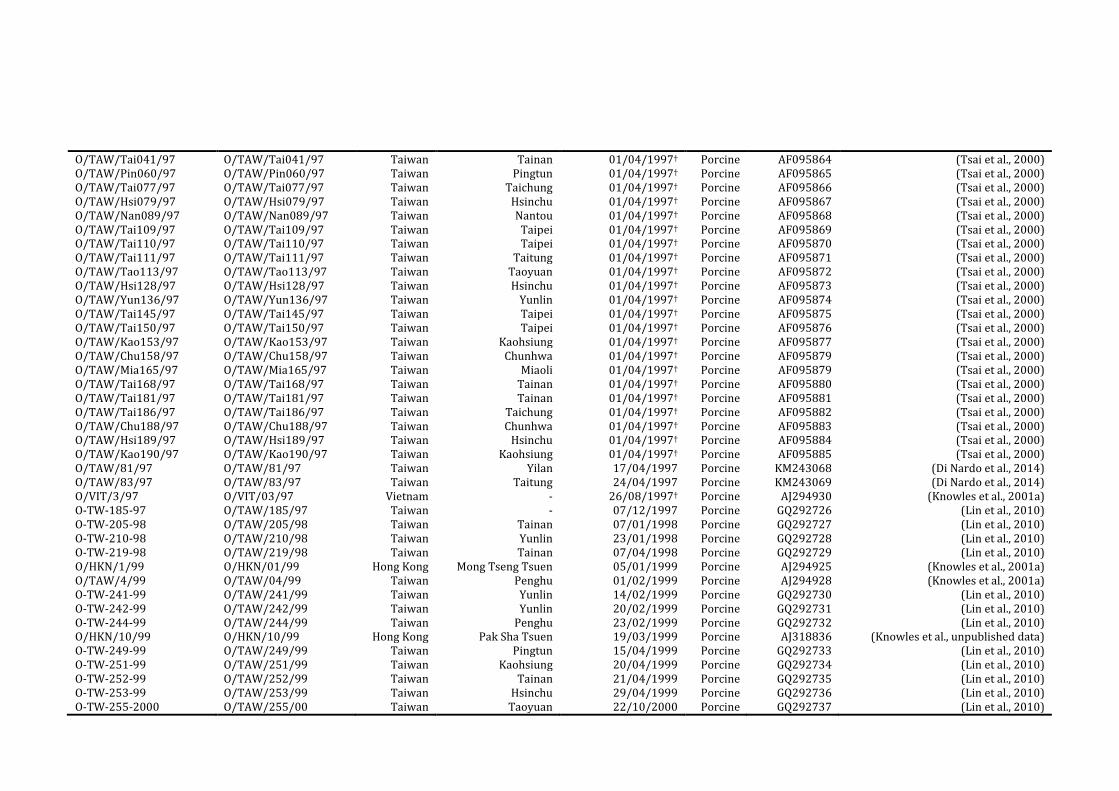
O/TAW/Tai041/97 O/TAW/Tai041/97 Taiwan Tainan 01/04/1997† Porcine AF095864 (Tsai et al., 2000) O/TAW/Pin060/97 O/TAW/Pin060/97 Taiwan Pingtun 01/04/1997† Porcine AF095865 (Tsai et al., 2000) O/TAW/Tai077/97 O/TAW/Tai077/97 Taiwan Taichung 01/04/1997† Porcine AF095866 (Tsai et al., 2000) O/TAW/Hsi079/97 O/TAW/Hsi079/97 Taiwan Hsinchu 01/04/1997† Porcine AF095867 (Tsai et al., 2000) O/TAW/Nan089/97 O/TAW/Nan089/97 Taiwan Nantou 01/04/1997† Porcine AF095868 (Tsai et al., 2000) O/TAW/Tai109/97 O/TAW/Tai109/97 Taiwan Taipei 01/04/1997† Porcine AF095869 (Tsai et al., 2000) O/TAW/Tai110/97 O/TAW/Tai110/97 Taiwan Taipei 01/04/1997† Porcine AF095870 (Tsai et al., 2000) O/TAW/Tai111/97 O/TAW/Tai111/97 Taiwan Taitung 01/04/1997† Porcine AF095871 (Tsai et al., 2000) O/TAW/Tao113/97 O/TAW/Tao113/97 Taiwan Taoyuan 01/04/1997† Porcine AF095872 (Tsai et al., 2000) O/TAW/Hsi128/97 O/TAW/Hsi128/97 Taiwan Hsinchu 01/04/1997† Porcine AF095873 (Tsai et al., 2000) O/TAW/Yun136/97 O/TAW/Yun136/97 Taiwan Yunlin 01/04/1997† Porcine AF095874 (Tsai et al., 2000) O/TAW/Tai145/97 O/TAW/Tai145/97 Taiwan Taipei 01/04/1997† Porcine AF095875 (Tsai et al., 2000) O/TAW/Tai150/97 O/TAW/Tai150/97 Taiwan Taipei 01/04/1997† Porcine AF095876 (Tsai et al., 2000) O/TAW/Kao153/97 O/TAW/Kao153/97 Taiwan Kaohsiung 01/04/1997† Porcine AF095877 (Tsai et al., 2000) O/TAW/Chu158/97 O/TAW/Chu158/97 Taiwan Chunhwa 01/04/1997† Porcine AF095879 (Tsai et al., 2000) O/TAW/Mia165/97 O/TAW/Mia165/97 Taiwan Miaoli 01/04/1997† Porcine AF095879 (Tsai et al., 2000) O/TAW/Tai168/97 O/TAW/Tai168/97 Taiwan Tainan 01/04/1997† Porcine AF095880 (Tsai et al., 2000) O/TAW/Tai181/97 O/TAW/Tai181/97 Taiwan Tainan 01/04/1997† Porcine AF095881 (Tsai et al., 2000) O/TAW/Tai186/97 O/TAW/Tai186/97 Taiwan Taichung 01/04/1997† Porcine AF095882 (Tsai et al., 2000) O/TAW/Chu188/97 O/TAW/Chu188/97 Taiwan Chunhwa 01/04/1997† Porcine AF095883 (Tsai et al., 2000) O/TAW/Hsi189/97 O/TAW/Hsi189/97 Taiwan Hsinchu 01/04/1997† Porcine AF095884 (Tsai et al., 2000) O/TAW/Kao190/97 O/TAW/Kao190/97 Taiwan Kaohsiung 01/04/1997† Porcine AF095885 (Tsai et al., 2000) O/TAW/81/97 O/TAW/81/97 Taiwan Yilan 17/04/1997 Porcine KM243068 (Di Nardo et al., 2014) O/TAW/83/97 O/TAW/83/97 Taiwan Taitung 24/04/1997 Porcine KM243069 (Di Nardo et al., 2014) O/VIT/3/97 O/VIT/03/97 Vietnam - 26/08/1997† Porcine AJ294930 (Knowles et al., 2001a) O-TW-185-97 O/TAW/185/97 Taiwan - 07/12/1997 Porcine GQ292726 (Lin et al., 2010) O-TW-205-98 O/TAW/205/98 Taiwan Tainan 07/01/1998 Porcine GQ292727 (Lin et al., 2010) O-TW-210-98 O/TAW/210/98 Taiwan Yunlin 23/01/1998 Porcine GQ292728 (Lin et al., 2010) O-TW-219-98 O/TAW/219/98 Taiwan Tainan 07/04/1998 Porcine GQ292729 (Lin et al., 2010) O/HKN/1/99 O/HKN/01/99 Hong Kong Mong Tseng Tsuen 05/01/1999 Porcine AJ294925 (Knowles et al., 2001a) O/TAW/4/99 O/TAW/04/99 Taiwan Penghu 01/02/1999 Porcine AJ294928 (Knowles et al., 2001a) O-TW-241-99 O/TAW/241/99 Taiwan Yunlin 14/02/1999 Porcine GQ292730 (Lin et al., 2010) O-TW-242-99 O/TAW/242/99 Taiwan Yunlin 20/02/1999 Porcine GQ292731 (Lin et al., 2010) O-TW-244-99 O/TAW/244/99 Taiwan Penghu 23/02/1999 Porcine GQ292732 (Lin et al., 2010) O/HKN/10/99 O/HKN/10/99 Hong Kong Pak Sha Tsuen 19/03/1999 Porcine AJ318836 (Knowles et al., unpublished data) O-TW-249-99 O/TAW/249/99 Taiwan Pingtun 15/04/1999 Porcine GQ292733 (Lin et al., 2010) O-TW-251-99 O/TAW/251/99 Taiwan Kaohsiung 20/04/1999 Porcine GQ292734 (Lin et al., 2010) O-TW-252-99 O/TAW/252/99 Taiwan Tainan 21/04/1999 Porcine GQ292735 (Lin et al., 2010) O-TW-253-99 O/TAW/253/99 Taiwan Hsinchu 29/04/1999 Porcine GQ292736 (Lin et al., 2010) O-TW-255-2000 O/TAW/255/00 Taiwan Taoyuan 22/10/2000 Porcine GQ292737 (Lin et al., 2010)
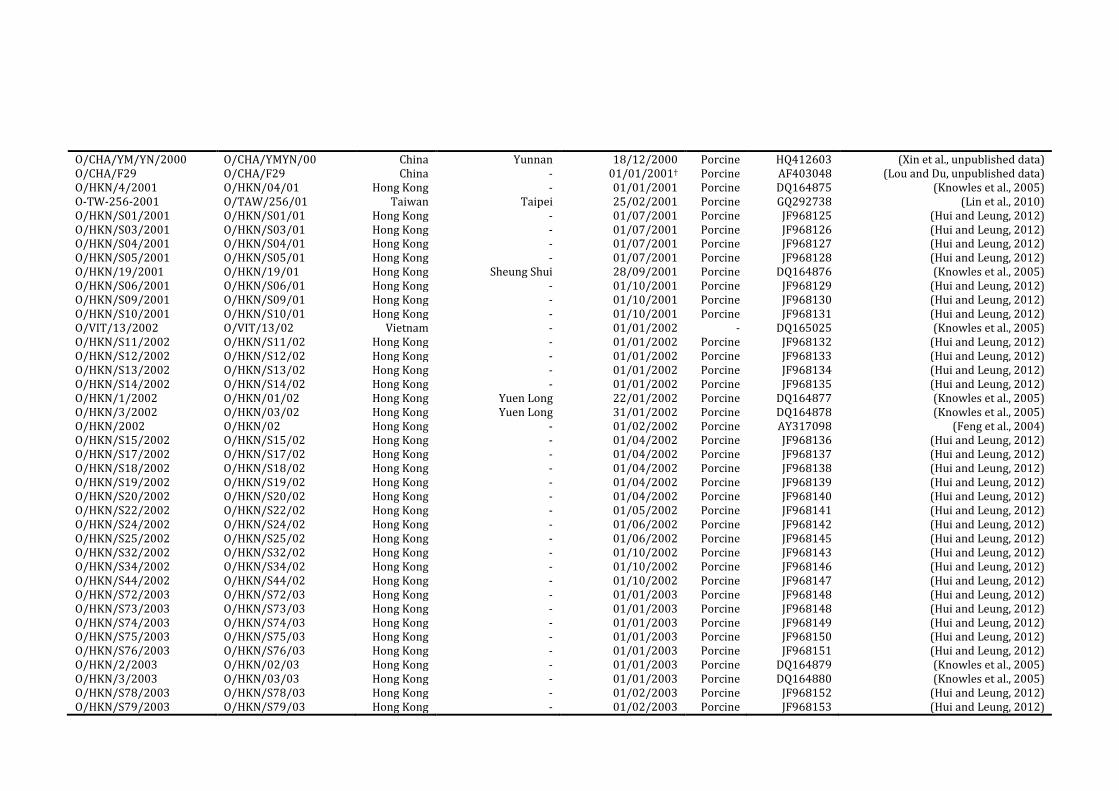
O/CHA/YM/YN/2000 O/CHA/YMYN/00 China Yunnan 18/12/2000 Porcine HQ412603 (Xin et al., unpublished data) O/CHA/F29 O/CHA/F29 China - 01/01/2001† Porcine AF403048 (Lou and Du, unpublished data) O/HKN/4/2001 O/HKN/04/01 Hong Kong - 01/01/2001 Porcine DQ164875 (Knowles et al., 2005) O-TW-256-2001 O/TAW/256/01 Taiwan Taipei 25/02/2001 Porcine GQ292738 (Lin et al., 2010) O/HKN/S01/2001 O/HKN/S01/01 Hong Kong - 01/07/2001 Porcine JF968125 (Hui and Leung, 2012) O/HKN/S03/2001 O/HKN/S03/01 Hong Kong - 01/07/2001 Porcine JF968126 (Hui and Leung, 2012) O/HKN/S04/2001 O/HKN/S04/01 Hong Kong - 01/07/2001 Porcine JF968127 (Hui and Leung, 2012) O/HKN/S05/2001 O/HKN/S05/01 Hong Kong - 01/07/2001 Porcine JF968128 (Hui and Leung, 2012) O/HKN/19/2001 O/HKN/19/01 Hong Kong Sheung Shui 28/09/2001 Porcine DQ164876 (Knowles et al., 2005) O/HKN/S06/2001 O/HKN/S06/01 Hong Kong - 01/10/2001 Porcine JF968129 (Hui and Leung, 2012) O/HKN/S09/2001 O/HKN/S09/01 Hong Kong - 01/10/2001 Porcine JF968130 (Hui and Leung, 2012) O/HKN/S10/2001 O/HKN/S10/01 Hong Kong - 01/10/2001 Porcine JF968131 (Hui and Leung, 2012) O/VIT/13/2002 O/VIT/13/02 Vietnam - 01/01/2002 - DQ165025 (Knowles et al., 2005) O/HKN/S11/2002 O/HKN/S11/02 Hong Kong - 01/01/2002 Porcine JF968132 (Hui and Leung, 2012) O/HKN/S12/2002 O/HKN/S12/02 Hong Kong - 01/01/2002 Porcine JF968133 (Hui and Leung, 2012) O/HKN/S13/2002 O/HKN/S13/02 Hong Kong - 01/01/2002 Porcine JF968134 (Hui and Leung, 2012) O/HKN/S14/2002 O/HKN/S14/02 Hong Kong - 01/01/2002 Porcine JF968135 (Hui and Leung, 2012) O/HKN/1/2002 O/HKN/01/02 Hong Kong Yuen Long 22/01/2002 Porcine DQ164877 (Knowles et al., 2005) O/HKN/3/2002 O/HKN/03/02 Hong Kong Yuen Long 31/01/2002 Porcine DQ164878 (Knowles et al., 2005) O/HKN/2002 O/HKN/02 Hong Kong - 01/02/2002 Porcine AY317098 (Feng et al., 2004) O/HKN/S15/2002 O/HKN/S15/02 Hong Kong - 01/04/2002 Porcine JF968136 (Hui and Leung, 2012) O/HKN/S17/2002 O/HKN/S17/02 Hong Kong - 01/04/2002 Porcine JF968137 (Hui and Leung, 2012) O/HKN/S18/2002 O/HKN/S18/02 Hong Kong - 01/04/2002 Porcine JF968138 (Hui and Leung, 2012) O/HKN/S19/2002 O/HKN/S19/02 Hong Kong - 01/04/2002 Porcine JF968139 (Hui and Leung, 2012) O/HKN/S20/2002 O/HKN/S20/02 Hong Kong - 01/04/2002 Porcine JF968140 (Hui and Leung, 2012) O/HKN/S22/2002 O/HKN/S22/02 Hong Kong - 01/05/2002 Porcine JF968141 (Hui and Leung, 2012) O/HKN/S24/2002 O/HKN/S24/02 Hong Kong - 01/06/2002 Porcine JF968142 (Hui and Leung, 2012) O/HKN/S25/2002 O/HKN/S25/02 Hong Kong - 01/06/2002 Porcine JF968145 (Hui and Leung, 2012) O/HKN/S32/2002 O/HKN/S32/02 Hong Kong - 01/10/2002 Porcine JF968143 (Hui and Leung, 2012) O/HKN/S34/2002 O/HKN/S34/02 Hong Kong - 01/10/2002 Porcine JF968146 (Hui and Leung, 2012) O/HKN/S44/2002 O/HKN/S44/02 Hong Kong - 01/10/2002 Porcine JF968147 (Hui and Leung, 2012) O/HKN/S72/2003 O/HKN/S72/03 Hong Kong - 01/01/2003 Porcine JF968148 (Hui and Leung, 2012) O/HKN/S73/2003 O/HKN/S73/03 Hong Kong - 01/01/2003 Porcine JF968148 (Hui and Leung, 2012) O/HKN/S74/2003 O/HKN/S74/03 Hong Kong - 01/01/2003 Porcine JF968149 (Hui and Leung, 2012) O/HKN/S75/2003 O/HKN/S75/03 Hong Kong - 01/01/2003 Porcine JF968150 (Hui and Leung, 2012) O/HKN/S76/2003 O/HKN/S76/03 Hong Kong - 01/01/2003 Porcine JF968151 (Hui and Leung, 2012) O/HKN/2/2003 O/HKN/02/03 Hong Kong - 01/01/2003 Porcine DQ164879 (Knowles et al., 2005) O/HKN/3/2003 O/HKN/03/03 Hong Kong - 01/01/2003 Porcine DQ164880 (Knowles et al., 2005) O/HKN/S78/2003 O/HKN/S78/03 Hong Kong - 01/02/2003 Porcine JF968152 (Hui and Leung, 2012) O/HKN/S79/2003 O/HKN/S79/03 Hong Kong - 01/02/2003 Porcine JF968153 (Hui and Leung, 2012)
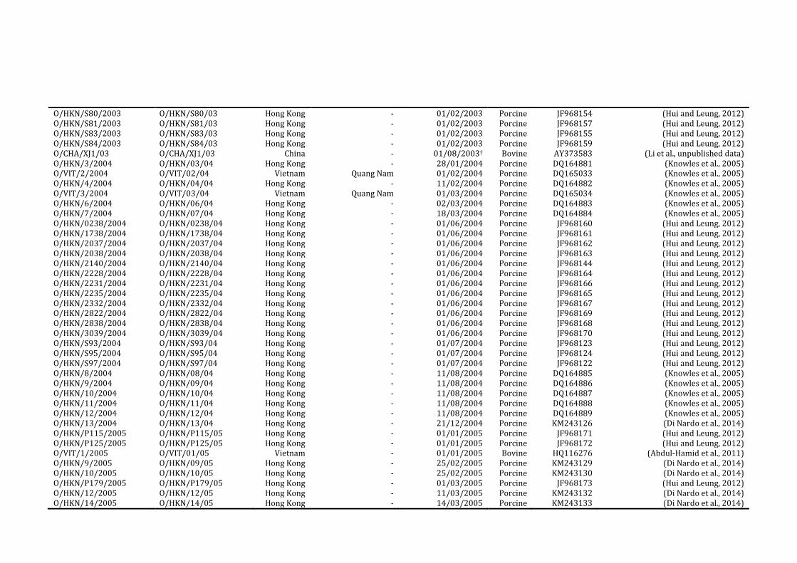
O/HKN/S80/2003 O/HKN/S80/03 Hong Kong - 01/02/2003 Porcine JF968154 (Hui and Leung, 2012) O/HKN/S81/2003 O/HKN/S81/03 Hong Kong - 01/02/2003 Porcine JF968157 (Hui and Leung, 2012) O/HKN/S83/2003 O/HKN/S83/03 Hong Kong - 01/02/2003 Porcine JF968155 (Hui and Leung, 2012) O/HKN/S84/2003 O/HKN/S84/03 Hong Kong - 01/02/2003 Porcine JF968159 (Hui and Leung, 2012) O/CHA/XJ1/03 O/CHA/XJ1/03 China - 01/08/2003† Bovine AY373583 (Li et al., unpublished data) O/HKN/3/2004 O/HKN/03/04 Hong Kong - 28/01/2004 Porcine DQ164881 (Knowles et al., 2005) O/VIT/2/2004 O/VIT/02/04 Vietnam Quang Nam 01/02/2004 Porcine DQ165033 (Knowles et al., 2005) O/HKN/4/2004 O/HKN/04/04 Hong Kong - 11/02/2004 Porcine DQ164882 (Knowles et al., 2005) O/VIT/3/2004 O/VIT/03/04 Vietnam Quang Nam 01/03/2004 Porcine DQ165034 (Knowles et al., 2005) O/HKN/6/2004 O/HKN/06/04 Hong Kong - 02/03/2004 Porcine DQ164883 (Knowles et al., 2005) O/HKN/7/2004 O/HKN/07/04 Hong Kong - 18/03/2004 Porcine DQ164884 (Knowles et al., 2005) O/HKN/0238/2004 O/HKN/0238/04 Hong Kong - 01/06/2004 Porcine JF968160 (Hui and Leung, 2012) O/HKN/1738/2004 O/HKN/1738/04 Hong Kong - 01/06/2004 Porcine JF968161 (Hui and Leung, 2012) O/HKN/2037/2004 O/HKN/2037/04 Hong Kong - 01/06/2004 Porcine JF968162 (Hui and Leung, 2012) O/HKN/2038/2004 O/HKN/2038/04 Hong Kong - 01/06/2004 Porcine JF968163 (Hui and Leung, 2012) O/HKN/2140/2004 O/HKN/2140/04 Hong Kong - 01/06/2004 Porcine JF968144 (Hui and Leung, 2012) O/HKN/2228/2004 O/HKN/2228/04 Hong Kong - 01/06/2004 Porcine JF968164 (Hui and Leung, 2012) O/HKN/2231/2004 O/HKN/2231/04 Hong Kong - 01/06/2004 Porcine JF968166 (Hui and Leung, 2012) O/HKN/2235/2004 O/HKN/2235/04 Hong Kong - 01/06/2004 Porcine JF968165 (Hui and Leung, 2012) O/HKN/2332/2004 O/HKN/2332/04 Hong Kong - 01/06/2004 Porcine JF968167 (Hui and Leung, 2012) O/HKN/2822/2004 O/HKN/2822/04 Hong Kong - 01/06/2004 Porcine JF968169 (Hui and Leung, 2012) O/HKN/2838/2004 O/HKN/2838/04 Hong Kong - 01/06/2004 Porcine JF968168 (Hui and Leung, 2012) O/HKN/3039/2004 O/HKN/3039/04 Hong Kong - 01/06/2004 Porcine JF968170 (Hui and Leung, 2012) O/HKN/S93/2004 O/HKN/S93/04 Hong Kong - 01/07/2004 Porcine JF968123 (Hui and Leung, 2012) O/HKN/S95/2004 O/HKN/S95/04 Hong Kong - 01/07/2004 Porcine JF968124 (Hui and Leung, 2012) O/HKN/S97/2004 O/HKN/S97/04 Hong Kong - 01/07/2004 Porcine JF968122 (Hui and Leung, 2012) O/HKN/8/2004 O/HKN/08/04 Hong Kong - 11/08/2004 Porcine DQ164885 (Knowles et al., 2005) O/HKN/9/2004 O/HKN/09/04 Hong Kong - 11/08/2004 Porcine DQ164886 (Knowles et al., 2005) O/HKN/10/2004 O/HKN/10/04 Hong Kong - 11/08/2004 Porcine DQ164887 (Knowles et al., 2005) O/HKN/11/2004 O/HKN/11/04 Hong Kong - 11/08/2004 Porcine DQ164888 (Knowles et al., 2005) O/HKN/12/2004 O/HKN/12/04 Hong Kong - 11/08/2004 Porcine DQ164889 (Knowles et al., 2005) O/HKN/13/2004 O/HKN/13/04 Hong Kong - 21/12/2004 Porcine KM243126 (Di Nardo et al., 2014) O/HKN/P115/2005 O/HKN/P115/05 Hong Kong - 01/01/2005 Porcine JF968171 (Hui and Leung, 2012) O/HKN/P125/2005 O/HKN/P125/05 Hong Kong - 01/01/2005 Porcine JF968172 (Hui and Leung, 2012) O/VIT/1/2005 O/VIT/01/05 Vietnam - 01/01/2005 Bovine HQ116276 (Abdul-Hamid et al., 2011) O/HKN/9/2005 O/HKN/09/05 Hong Kong - 25/02/2005 Porcine KM243129 (Di Nardo et al., 2014) O/HKN/10/2005 O/HKN/10/05 Hong Kong - 25/02/2005 Porcine KM243130 (Di Nardo et al., 2014) O/HKN/P179/2005 O/HKN/P179/05 Hong Kong - 01/03/2005 Porcine JF968173 (Hui and Leung, 2012) O/HKN/12/2005 O/HKN/12/05 Hong Kong - 11/03/2005 Porcine KM243132 (Di Nardo et al., 2014) O/HKN/14/2005 O/HKN/14/05 Hong Kong - 14/03/2005 Porcine KM243133 (Di Nardo et al., 2014)
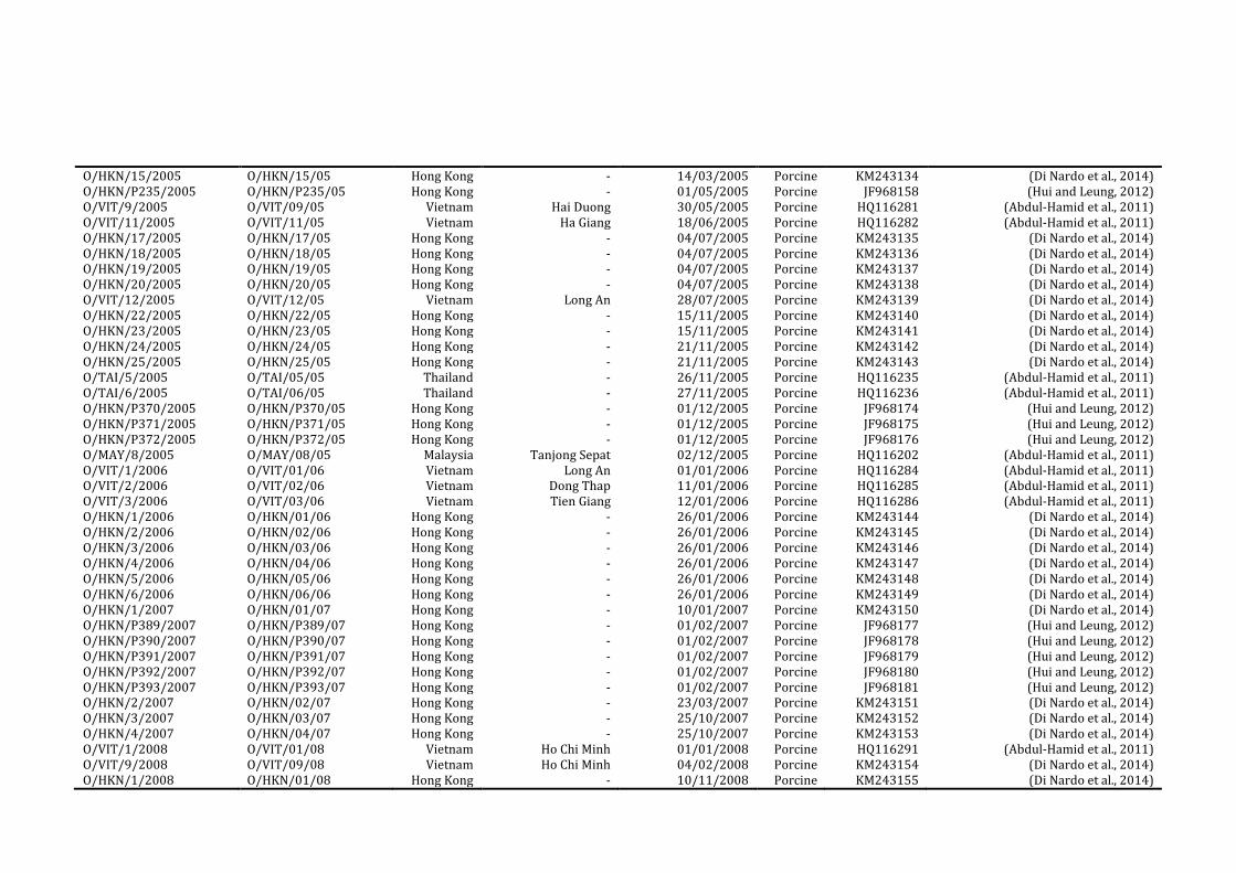
O/HKN/15/2005 O/HKN/15/05 Hong Kong - 14/03/2005 Porcine KM243134 (Di Nardo et al., 2014) O/HKN/P235/2005 O/HKN/P235/05 Hong Kong - 01/05/2005 Porcine JF968158 (Hui and Leung, 2012) O/VIT/9/2005 O/VIT/09/05 Vietnam Hai Duong 30/05/2005 Porcine HQ116281 (Abdul-Hamid et al., 2011) O/VIT/11/2005 O/VIT/11/05 Vietnam Ha Giang 18/06/2005 Porcine HQ116282 (Abdul-Hamid et al., 2011) O/HKN/17/2005 O/HKN/17/05 Hong Kong - 04/07/2005 Porcine KM243135 (Di Nardo et al., 2014) O/HKN/18/2005 O/HKN/18/05 Hong Kong - 04/07/2005 Porcine KM243136 (Di Nardo et al., 2014) O/HKN/19/2005 O/HKN/19/05 Hong Kong - 04/07/2005 Porcine KM243137 (Di Nardo et al., 2014) O/HKN/20/2005 O/HKN/20/05 Hong Kong - 04/07/2005 Porcine KM243138 (Di Nardo et al., 2014) O/VIT/12/2005 O/VIT/12/05 Vietnam Long An 28/07/2005 Porcine KM243139 (Di Nardo et al., 2014) O/HKN/22/2005 O/HKN/22/05 Hong Kong - 15/11/2005 Porcine KM243140 (Di Nardo et al., 2014) O/HKN/23/2005 O/HKN/23/05 Hong Kong - 15/11/2005 Porcine KM243141 (Di Nardo et al., 2014) O/HKN/24/2005 O/HKN/24/05 Hong Kong - 21/11/2005 Porcine KM243142 (Di Nardo et al., 2014) O/HKN/25/2005 O/HKN/25/05 Hong Kong - 21/11/2005 Porcine KM243143 (Di Nardo et al., 2014) O/TAI/5/2005 O/TAI/05/05 Thailand - 26/11/2005 Porcine HQ116235 (Abdul-Hamid et al., 2011) O/TAI/6/2005 O/TAI/06/05 Thailand - 27/11/2005 Porcine HQ116236 (Abdul-Hamid et al., 2011) O/HKN/P370/2005 O/HKN/P370/05 Hong Kong - 01/12/2005 Porcine JF968174 (Hui and Leung, 2012) O/HKN/P371/2005 O/HKN/P371/05 Hong Kong - 01/12/2005 Porcine JF968175 (Hui and Leung, 2012) O/HKN/P372/2005 O/HKN/P372/05 Hong Kong - 01/12/2005 Porcine JF968176 (Hui and Leung, 2012) O/MAY/8/2005 O/MAY/08/05 Malaysia Tanjong Sepat 02/12/2005 Porcine HQ116202 (Abdul-Hamid et al., 2011) O/VIT/1/2006 O/VIT/01/06 Vietnam Long An 01/01/2006 Porcine HQ116284 (Abdul-Hamid et al., 2011) O/VIT/2/2006 O/VIT/02/06 Vietnam Dong Thap 11/01/2006 Porcine HQ116285 (Abdul-Hamid et al., 2011) O/VIT/3/2006 O/VIT/03/06 Vietnam Tien Giang 12/01/2006 Porcine HQ116286 (Abdul-Hamid et al., 2011) O/HKN/1/2006 O/HKN/01/06 Hong Kong - 26/01/2006 Porcine KM243144 (Di Nardo et al., 2014) O/HKN/2/2006 O/HKN/02/06 Hong Kong - 26/01/2006 Porcine KM243145 (Di Nardo et al., 2014) O/HKN/3/2006 O/HKN/03/06 Hong Kong - 26/01/2006 Porcine KM243146 (Di Nardo et al., 2014) O/HKN/4/2006 O/HKN/04/06 Hong Kong - 26/01/2006 Porcine KM243147 (Di Nardo et al., 2014) O/HKN/5/2006 O/HKN/05/06 Hong Kong - 26/01/2006 Porcine KM243148 (Di Nardo et al., 2014) O/HKN/6/2006 O/HKN/06/06 Hong Kong - 26/01/2006 Porcine KM243149 (Di Nardo et al., 2014) O/HKN/1/2007 O/HKN/01/07 Hong Kong - 10/01/2007 Porcine KM243150 (Di Nardo et al., 2014) O/HKN/P389/2007 O/HKN/P389/07 Hong Kong - 01/02/2007 Porcine JF968177 (Hui and Leung, 2012) O/HKN/P390/2007 O/HKN/P390/07 Hong Kong - 01/02/2007 Porcine JF968178 (Hui and Leung, 2012) O/HKN/P391/2007 O/HKN/P391/07 Hong Kong - 01/02/2007 Porcine JF968179 (Hui and Leung, 2012) O/HKN/P392/2007 O/HKN/P392/07 Hong Kong - 01/02/2007 Porcine JF968180 (Hui and Leung, 2012) O/HKN/P393/2007 O/HKN/P393/07 Hong Kong - 01/02/2007 Porcine JF968181 (Hui and Leung, 2012) O/HKN/2/2007 O/HKN/02/07 Hong Kong - 23/03/2007 Porcine KM243151 (Di Nardo et al., 2014) O/HKN/3/2007 O/HKN/03/07 Hong Kong - 25/10/2007 Porcine KM243152 (Di Nardo et al., 2014) O/HKN/4/2007 O/HKN/04/07 Hong Kong - 25/10/2007 Porcine KM243153 (Di Nardo et al., 2014) O/VIT/1/2008 O/VIT/01/08 Vietnam Ho Chi Minh 01/01/2008 Porcine HQ116291 (Abdul-Hamid et al., 2011) O/VIT/9/2008 O/VIT/09/08 Vietnam Ho Chi Minh 04/02/2008 Porcine KM243154 (Di Nardo et al., 2014) O/HKN/1/2008 O/HKN/01/08 Hong Kong - 10/11/2008 Porcine KM243155 (Di Nardo et al., 2014)
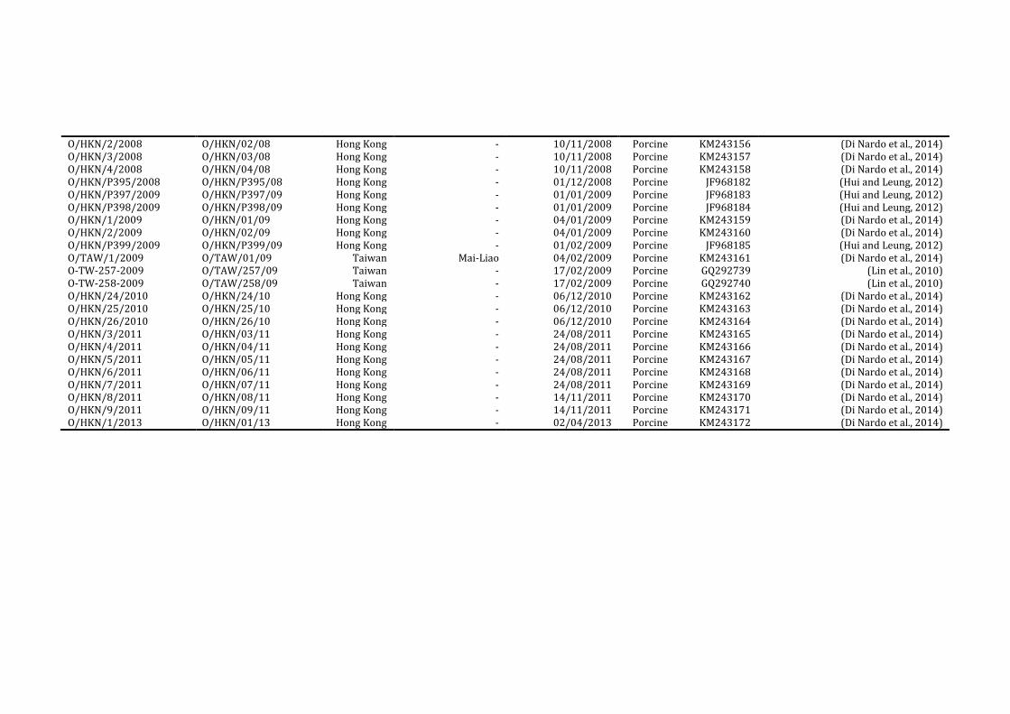
O/HKN/2/2008 O/HKN/02/08 Hong Kong - 10/11/2008 Porcine KM243156 (Di Nardo et al., 2014) O/HKN/3/2008 O/HKN/03/08 Hong Kong - 10/11/2008 Porcine KM243157 (Di Nardo et al., 2014) O/HKN/4/2008 O/HKN/04/08 Hong Kong - 10/11/2008 Porcine KM243158 (Di Nardo et al., 2014) O/HKN/P395/2008 O/HKN/P395/08 Hong Kong - 01/12/2008 Porcine JF968182 (Hui and Leung, 2012) O/HKN/P397/2009 O/HKN/P397/09 Hong Kong - 01/01/2009 Porcine JF968183 (Hui and Leung, 2012) O/HKN/P398/2009 O/HKN/P398/09 Hong Kong - 01/01/2009 Porcine JF968184 (Hui and Leung, 2012) O/HKN/1/2009 O/HKN/01/09 Hong Kong - 04/01/2009 Porcine KM243159 (Di Nardo et al., 2014) O/HKN/2/2009 O/HKN/02/09 Hong Kong - 04/01/2009 Porcine KM243160 (Di Nardo et al., 2014) O/HKN/P399/2009 O/HKN/P399/09 Hong Kong - 01/02/2009 Porcine JF968185 (Hui and Leung, 2012) O/TAW/1/2009 O/TAW/01/09 Taiwan Mai-Liao 04/02/2009 Porcine KM243161 (Di Nardo et al., 2014) O-TW-257-2009 O/TAW/257/09 Taiwan - 17/02/2009 Porcine GQ292739 (Lin et al., 2010) O-TW-258-2009 O/TAW/258/09 Taiwan - 17/02/2009 Porcine GQ292740 (Lin et al., 2010) O/HKN/24/2010 O/HKN/24/10 Hong Kong - 06/12/2010 Porcine KM243162 (Di Nardo et al., 2014) O/HKN/25/2010 O/HKN/25/10 Hong Kong - 06/12/2010 Porcine KM243163 (Di Nardo et al., 2014) O/HKN/26/2010 O/HKN/26/10 Hong Kong - 06/12/2010 Porcine KM243164 (Di Nardo et al., 2014) O/HKN/3/2011 O/HKN/03/11 Hong Kong - 24/08/2011 Porcine KM243165 (Di Nardo et al., 2014) O/HKN/4/2011 O/HKN/04/11 Hong Kong - 24/08/2011 Porcine KM243166 (Di Nardo et al., 2014) O/HKN/5/2011 O/HKN/05/11 Hong Kong - 24/08/2011 Porcine KM243167 (Di Nardo et al., 2014) O/HKN/6/2011 O/HKN/06/11 Hong Kong - 24/08/2011 Porcine KM243168 (Di Nardo et al., 2014) O/HKN/7/2011 O/HKN/07/11 Hong Kong - 24/08/2011 Porcine KM243169 (Di Nardo et al., 2014) O/HKN/8/2011 O/HKN/08/11 Hong Kong - 14/11/2011 Porcine KM243170 (Di Nardo et al., 2014) O/HKN/9/2011 O/HKN/09/11 Hong Kong - 14/11/2011 Porcine KM243171 (Di Nardo et al., 2014) O/HKN/1/2013 O/HKN/01/13 Hong Kong - 02/04/2013 Porcine KM243172 (Di Nardo et al., 2014)
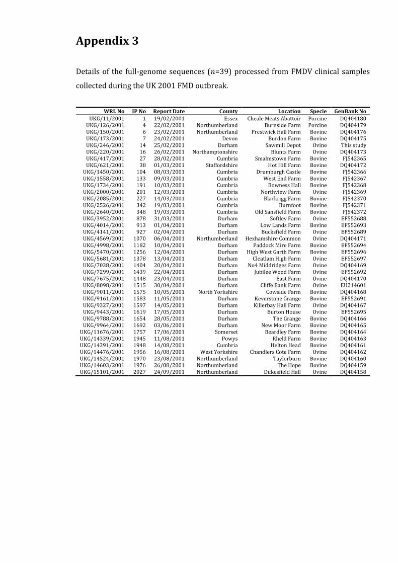
Appendix 3
Details of the full-genome sequences (𝑛=39) processed from FMDV clinical samples
collected during the UK 2001 FMD outbreak.
WRL No IP No Report Date County Location Specie GenBank No
UKG/11/2001 1 19/02/2001 Essex Cheale Meats Abattoir Porcine DQ404180 UKG/126/2001 4 22/02/2001 Northumberland Burnside Farm Porcine DQ404179 UKG/150/2001 6 23/02/2001 Northumberland Prestwick Hall Farm Bovine DQ404176 UKG/173/2001 7 24/02/2001 Devon Burdon Farm Bovine DQ404175 UKG/246/2001 14 25/02/2001 Durham Sawmill Depot Ovine This study UKG/220/2001 16 26/02/2001 Northamptonshire Blunts Farm Ovine DQ404173 UKG/417/2001 27 28/02/2001 Cumbria Smalmstown Farm Bovine FJ542365 UKG/621/2001 38 01/03/2001 Staffordshire Hot Hill Farm Bovine DQ404172
UKG/1450/2001 104 08/03/2001 Cumbria Drumburgh Castle Bovine FJ542366 UKG/1558/2001 133 09/03/2001 Cumbria West End Farm Bovine FJ542367 UKG/1734/2001 191 10/03/2001 Cumbria Bowness Hall Bovine FJ542368 UKG/2000/2001 201 12/03/2001 Cumbria Northview Farm Ovine FJ542369 UKG/2085/2001 227 14/03/2001 Cumbria Blackrigg Farm Bovine FJ542370 UKG/2526/2001 342 19/03/2001 Cumbria Burnfoot Bovine FJ542371 UKG/2640/2001 348 19/03/2001 Cumbria Old Sansfield Farm Bovine FJ542372 UKG/3952/2001 878 31/03/2001 Durham Softley Farm Ovine EF552688 UKG/4014/2001 913 01/04/2001 Durham Low Lands Farm Bovine EF552693 UKG/4141/2001 927 02/04/2001 Durham Bucksfield Farm Ovine EF552689 UKG/4569/2001 1070 06/04/2001 Northumberland Hexhamshire Common Ovine DQ404171 UKG/4998/2001 1182 10/04/2001 Durham Paddock Mire Farm Bovine EF552694 UKG/5470/2001 1256 12/04/2001 Durham High West Garth Farm Bovine EF552696 UKG/5681/2001 1378 13/04/2001 Durham Cleatlam High Farm Ovine EF552697 UKG/7038/2001 1404 20/04/2001 Durham No4 Middridges Farm Ovine DQ404169 UKG/7299/2001 1439 22/04/2001 Durham Jubilee Wood Farm Ovine EF552692 UKG/7675/2001 1448 23/04/2001 Durham East Farm Ovine DQ404170 UKG/8098/2001 1515 30/04/2001 Durham Cliffe Bank Farm Ovine EU214601 UKG/9011/2001 1575 10/05/2001 North Yorkshire Cowside Farm Bovine DQ404168 UKG/9161/2001 1583 11/05/2001 Durham Keverstone Grange Bovine EF552691 UKG/9327/2001 1597 14/05/2001 Durham Killerbay Hall Farm Ovine DQ404167 UKG/9443/2001 1619 17/05/2001 Durham Burton House Ovine EF552695 UKG/9788/2001 1654 28/05/2001 Durham The Grange Bovine DQ404166 UKG/9964/2001 1692 03/06/2001 Durham New Moor Farm Bovine DQ404165
UKG/11676/2001 1757 17/06/2001 Somerset Beardley Farm Bovine DQ404164 UKG/14339/2001 1945 11/08/2001 Powys Rheld Farm Bovine DQ404163 UKG/14391/2001 1948 14/08/2001 Cumbria Helton Head Bovine DQ404161 UKG/14476/2001 1956 16/08/2001 West Yorkshire Chandlers Cote Farm Ovine DQ404162 UKG/14524/2001 1970 23/08/2001 Northumberland Taylorburn Bovine DQ404160 UKG/14603/2001 1976 26/08/2001 Northumberland The Hope Bovine DQ404159 UKG/15101/2001 2027 24/09/2001 Northumberland Dukesfield Hall Ovine DQ404158
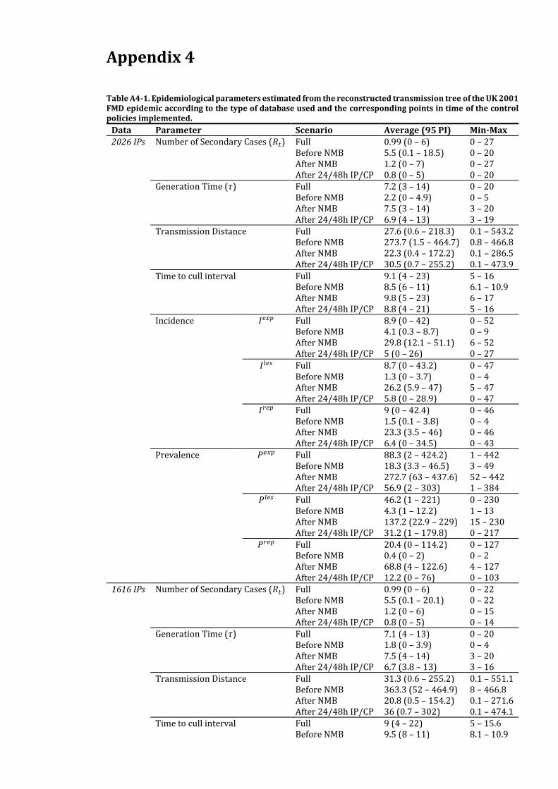
Appendix 4
Table A4-1. Epidemiological parameters estimated from the reconstructed transmission tree of the UK 2001 FMD epidemic according to the type of database used and the corresponding points in time of the control policies implemented.
Data Parameter Scenario Average (95 PI) Min-Max
2026 IPs Number of Secondary Cases (𝑅𝑡) Full 0.99 (0 – 6) 0 – 27 Before NMB 5.5 (0.1 – 18.5) 0 – 20 After NMB 1.2 (0 – 7) 0 – 27 After 24/48h IP/CP 0.8 (0 – 5) 0 – 20 Generation Time (𝜏) Full 7.2 (3 – 14) 0 – 20 Before NMB 2.2 (0 – 4.9) 0 – 5 After NMB 7.5 (3 – 14) 3 – 20 After 24/48h IP/CP 6.9 (4 – 13) 3 – 19
Transmission Distance Full 27.6 (0.6 – 218.3) 0.1 – 543.2 Before NMB 273.7 (1.5 – 464.7) 0.8 – 466.8 After NMB 22.3 (0.4 – 172.2) 0.1 – 286.5 After 24/48h IP/CP 30.5 (0.7 – 255.2) 0.1 – 473.9
Time to cull interval Full 9.1 (4 – 23) 5 – 16 Before NMB 8.5 (6 – 11) 6.1 – 10.9 After NMB 9.8 (5 – 23) 6 – 17 After 24/48h IP/CP 8.8 (4 – 21) 5 – 16
Incidence 𝐼𝑒𝑥𝑝 Full 8.9 (0 – 42) 0 – 52 Before NMB 4.1 (0.3 – 8.7) 0 – 9 After NMB 29.8 (12.1 – 51.1) 6 – 52 After 24/48h IP/CP 5 (0 – 26) 0 – 27
𝐼𝑙𝑒𝑠 Full 8.7 (0 – 43.2) 0 – 47 Before NMB 1.3 (0 – 3.7) 0 – 4 After NMB 26.2 (5.9 – 47) 5 – 47 After 24/48h IP/CP 5.8 (0 – 28.9) 0 – 47
𝐼𝑟𝑒𝑝 Full 9 (0 – 42.4) 0 – 46 Before NMB 1.5 (0.1 – 3.8) 0 – 4 After NMB 23.3 (3.5 – 46) 0 – 46 After 24/48h IP/CP 6.4 (0 – 34.5) 0 – 43
Prevalence 𝑃𝑒𝑥𝑝 Full 88.3 (2 – 424.2) 1 – 442 Before NMB 18.3 (3.3 – 46.5) 3 – 49 After NMB 272.7 (63 – 437.6) 52 – 442 After 24/48h IP/CP 56.9 (2 – 303) 1 – 384
𝑃𝑙𝑒𝑠 Full 46.2 (1 – 221) 0 – 230 Before NMB 4.3 (1 – 12.2) 1 – 13 After NMB 137.2 (22.9 – 229) 15 – 230 After 24/48h IP/CP 31.2 (1 – 179.8) 0 – 217
𝑃𝑟𝑒𝑝 Full 20.4 (0 – 114.2) 0 – 127 Before NMB 0.4 (0 – 2) 0 – 2 After NMB 68.8 (4 – 122.6) 4 – 127 After 24/48h IP/CP 12.2 (0 – 76) 0 – 103
1616 IPs Number of Secondary Cases (𝑅𝑡) Full 0.99 (0 – 6) 0 – 22 Before NMB 5.5 (0.1 – 20.1) 0 – 22 After NMB 1.2 (0 – 6) 0 – 15 After 24/48h IP/CP 0.8 (0 – 5) 0 – 14
Generation Time (𝜏) Full 7.1 (4 – 13) 0 – 20 Before NMB 1.8 (0 – 3.9) 0 – 4 After NMB 7.5 (4 – 14) 3 – 20 After 24/48h IP/CP 6.7 (3.8 – 13) 3 – 16
Transmission Distance Full 31.3 (0.6 – 255.2) 0.1 – 551.1 Before NMB 363.3 (52 – 464.9) 8 – 466.8 After NMB 20.8 (0.5 – 154.2) 0.1 – 271.6 After 24/48h IP/CP 36 (0.7 – 302) 0.1 – 474.1
Time to cull interval Full 9 (4 – 22) 5 – 15.6 Before NMB 9.5 (8 – 11) 8.1 – 10.9
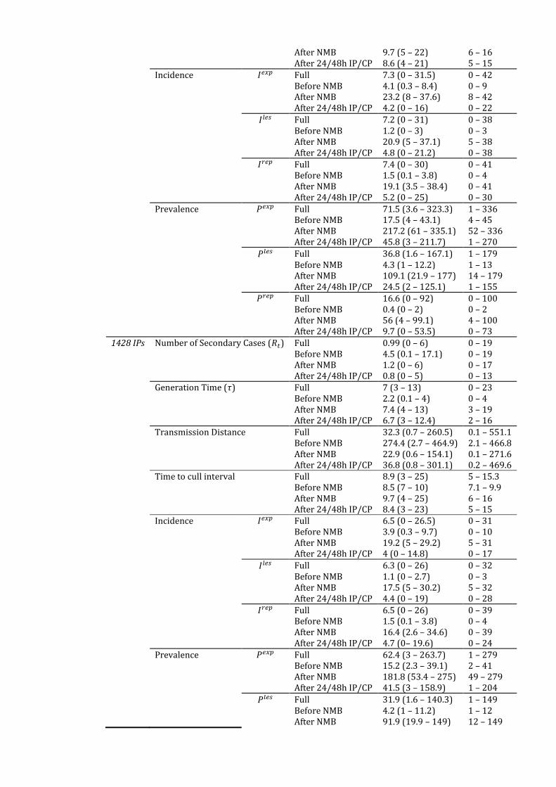
After NMB 9.7 (5 – 22) 6 – 16 After 24/48h IP/CP 8.6 (4 – 21) 5 – 15
Incidence 𝐼𝑒𝑥𝑝 Full 7.3 (0 – 31.5) 0 – 42 Before NMB 4.1 (0.3 – 8.4) 0 – 9 After NMB 23.2 (8 – 37.6) 8 – 42 After 24/48h IP/CP 4.2 (0 – 16) 0 – 22
𝐼𝑙𝑒𝑠 Full 7.2 (0 – 31) 0 – 38 Before NMB 1.2 (0 – 3) 0 – 3 After NMB 20.9 (5 – 37.1) 5 – 38 After 24/48h IP/CP 4.8 (0 – 21.2) 0 – 38
𝐼𝑟𝑒𝑝 Full 7.4 (0 – 30) 0 – 41 Before NMB 1.5 (0.1 – 3.8) 0 – 4 After NMB 19.1 (3.5 – 38.4) 0 – 41 After 24/48h IP/CP 5.2 (0 – 25) 0 – 30
Prevalence 𝑃𝑒𝑥𝑝 Full 71.5 (3.6 – 323.3) 1 – 336 Before NMB 17.5 (4 – 43.1) 4 – 45 After NMB 217.2 (61 – 335.1) 52 – 336 After 24/48h IP/CP 45.8 (3 – 211.7) 1 – 270
𝑃𝑙𝑒𝑠 Full 36.8 (1.6 – 167.1) 1 – 179 Before NMB 4.3 (1 – 12.2) 1 – 13 After NMB 109.1 (21.9 – 177) 14 – 179 After 24/48h IP/CP 24.5 (2 – 125.1) 1 – 155
𝑃𝑟𝑒𝑝 Full 16.6 (0 – 92) 0 – 100 Before NMB 0.4 (0 – 2) 0 – 2 After NMB 56 (4 – 99.1) 4 – 100 After 24/48h IP/CP 9.7 (0 – 53.5) 0 – 73
1428 IPs Number of Secondary Cases (𝑅𝑡) Full 0.99 (0 – 6) 0 – 19 Before NMB 4.5 (0.1 – 17.1) 0 – 19 After NMB 1.2 (0 – 6) 0 – 17 After 24/48h IP/CP 0.8 (0 – 5) 0 – 13
Generation Time (𝜏) Full 7 (3 – 13) 0 – 23 Before NMB 2.2 (0.1 – 4) 0 – 4 After NMB 7.4 (4 – 13) 3 – 19 After 24/48h IP/CP 6.7 (3 – 12.4) 2 – 16
Transmission Distance Full 32.3 (0.7 – 260.5) 0.1 – 551.1 Before NMB 274.4 (2.7 – 464.9) 2.1 – 466.8 After NMB 22.9 (0.6 – 154.1) 0.1 – 271.6 After 24/48h IP/CP 36.8 (0.8 – 301.1) 0.2 – 469.6 Time to cull interval Full 8.9 (3 – 25) 5 – 15.3 Before NMB 8.5 (7 – 10) 7.1 – 9.9 After NMB 9.7 (4 – 25) 6 – 16 After 24/48h IP/CP 8.4 (3 – 23) 5 – 15 Incidence 𝐼𝑒𝑥𝑝 Full 6.5 (0 – 26.5) 0 – 31 Before NMB 3.9 (0.3 – 9.7) 0 – 10 After NMB 19.2 (5 – 29.2) 5 – 31 After 24/48h IP/CP 4 (0 – 14.8) 0 – 17
𝐼𝑙𝑒𝑠 Full 6.3 (0 – 26) 0 – 32 Before NMB 1.1 (0 – 2.7) 0 – 3 After NMB 17.5 (5 – 30.2) 5 – 32 After 24/48h IP/CP 4.4 (0 – 19) 0 – 28
𝐼𝑟𝑒𝑝 Full 6.5 (0 – 26) 0 – 39 Before NMB 1.5 (0.1 – 3.8) 0 – 4 After NMB 16.4 (2.6 – 34.6) 0 – 39 After 24/48h IP/CP 4.7 (0– 19.6) 0 – 24
Prevalence 𝑃𝑒𝑥𝑝 Full 62.4 (3 – 263.7) 1 – 279 Before NMB 15.2 (2.3 – 39.1) 2 – 41 After NMB 181.8 (53.4 – 275) 49 – 279 After 24/48h IP/CP 41.5 (3 – 158.9) 1 – 204
𝑃𝑙𝑒𝑠 Full 31.9 (1.6 – 140.3) 1 – 149 Before NMB 4.2 (1 – 11.2) 1 – 12 After NMB 91.9 (19.9 – 149) 12 – 149

After 24/48h IP/CP 21.7 (2 – 90.9) 1 – 112
𝑃𝑟𝑒𝑝 Full 14.7 (0 – 80) 0 – 88 Before NMB 0.4 (0 – 2) 0 – 2 After NMB 49.2 (4 – 88) 4 – 88 After 24/48h IP/CP 8.8 (0 – 45.5) 0 – 60
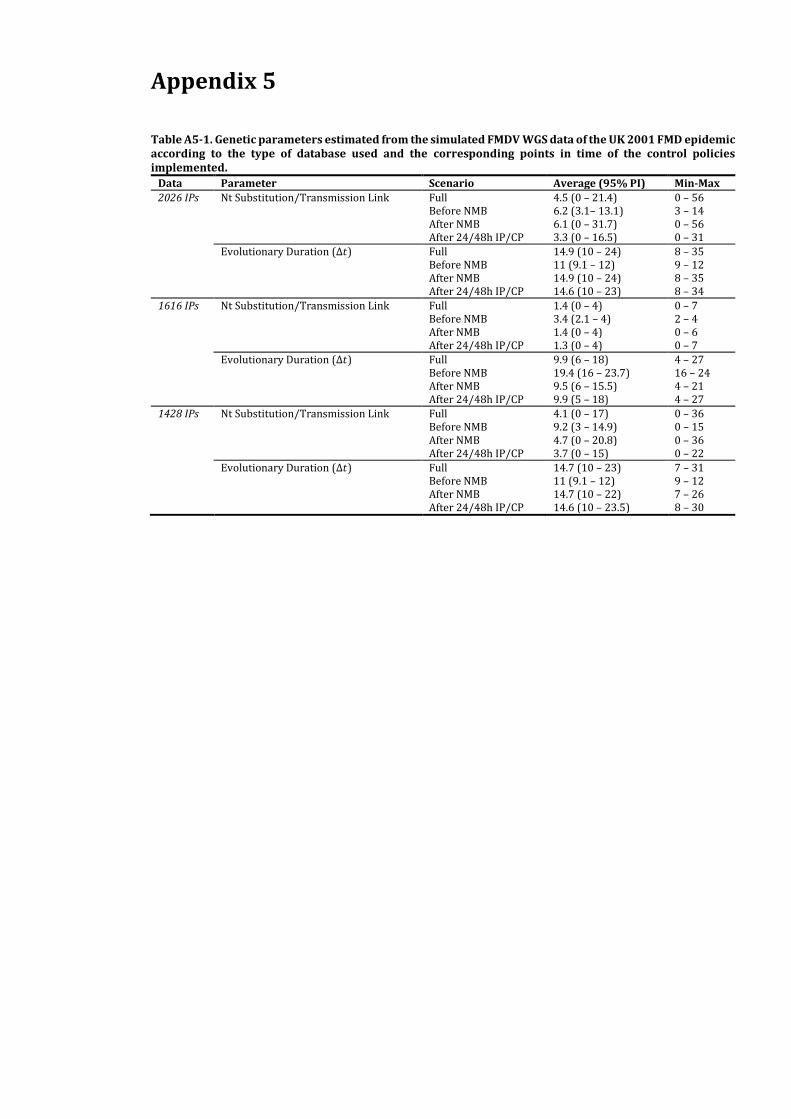
Appendix 5
Table A5-1. Genetic parameters estimated from the simulated FMDV WGS data of the UK 2001 FMD epidemic according to the type of database used and the corresponding points in time of the control policies implemented.
Data Parameter Scenario Average (95% PI) Min-Max
2026 IPs Nt Substitution/Transmission Link Full 4.5 (0 – 21.4) 0 – 56 Before NMB 6.2 (3.1– 13.1) 3 – 14 After NMB 6.1 (0 – 31.7) 0 – 56 After 24/48h IP/CP 3.3 (0 – 16.5) 0 – 31
Evolutionary Duration (∆𝑡) Full 14.9 (10 – 24) 8 – 35 Before NMB 11 (9.1 – 12) 9 – 12 After NMB 14.9 (10 – 24) 8 – 35 After 24/48h IP/CP 14.6 (10 – 23) 8 – 34
1616 IPs Nt Substitution/Transmission Link Full 1.4 (0 – 4) 0 – 7 Before NMB 3.4 (2.1 – 4) 2 – 4 After NMB 1.4 (0 – 4) 0 – 6 After 24/48h IP/CP 1.3 (0 – 4) 0 – 7
Evolutionary Duration (∆𝑡) Full 9.9 (6 – 18) 4 – 27 Before NMB 19.4 (16 – 23.7) 16 – 24 After NMB 9.5 (6 – 15.5) 4 – 21 After 24/48h IP/CP 9.9 (5 – 18) 4 – 27
1428 IPs Nt Substitution/Transmission Link Full 4.1 (0 – 17) 0 – 36 Before NMB 9.2 (3 – 14.9) 0 – 15 After NMB 4.7 (0 – 20.8) 0 – 36 After 24/48h IP/CP 3.7 (0 – 15) 0 – 22
Evolutionary Duration (∆𝑡) Full 14.7 (10 – 23) 7 – 31 Before NMB 11 (9.1 – 12) 9 – 12 After NMB 14.7 (10 – 22) 7 – 26 After 24/48h IP/CP 14.6 (10 – 23.5) 8 – 30
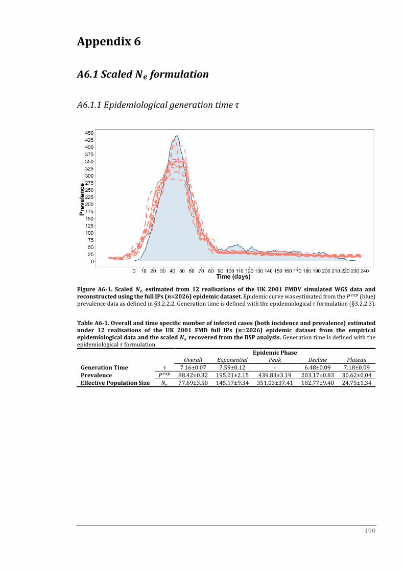
190
Appendix 6
A6.1 Scaled 𝑵𝒆 formulation
A6.1.1 Epidemiological generation time 𝜏
Figure A6-1. Scaled 𝑵𝒆 estimated from 12 realisations of the UK 2001 FMDV simulated WGS data and reconstructed using the full IPs (𝒏=2026) epidemic dataset. Epidemic curve was estimated from the 𝑃𝑒𝑥𝑝 (blue) prevalence data as defined in §3.2.2.2. Generation time is defined with the epidemiological 𝜏 formulation (§3.2.2.3).
Table A6-1. Overall and time specific number of infected cases (both incidence and prevalence) estimated under 12 realisations of the UK 2001 FMD full IPs (𝒏=2026) epidemic dataset from the empirical epidemiological data and the scaled 𝑵𝒆 recovered from the BSP analysis. Generation time is defined with the epidemiological 𝜏 formulation.
Epidemic Phase Overall Exponential Peak Decline Plateau
Generation Time 𝜏 7.16±0.07 7.59±0.12 - 6.48±0.09 7.18±0.09
Prevalence 𝑃𝑒𝑥𝑝 88.42±0.32 195.01±2.15 439.83±3.19 203.17±0.83 30.62±0.04
Effective Population Size 𝑁𝑒 77.69±3.50 145.17±9.34 351.03±37.41 182.77±9.40 24.75±1.34
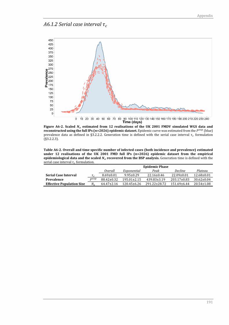
Appendix
191
A6.1.2 Serial case interval 𝜏𝑐
Figure A6-2. Scaled 𝑵𝒆 estimated from 12 realisations of the UK 2001 FMDV simulated WGS data and reconstructed using the full IPs (𝒏=2026) epidemic dataset. Epidemic curve was estimated from the 𝑃𝑒𝑥𝑝 (blue) prevalence data as defined in §3.2.2.2. Generation time is defined with the serial case interval 𝜏𝑐 formulation (§3.2.2.3).
Table A6-2. Overall and time specific number of infected cases (both incidence and prevalence) estimated under 12 realisations of the UK 2001 FMD full IPs (𝒏=2026) epidemic dataset from the empirical epidemiological data and the scaled 𝑵𝒆 recovered from the BSP analysis. Generation time is defined with the serial case interval 𝜏𝑐 formulation.
Epidemic Phase Overall Exponential Peak Decline Plateau
Serial Case Interval 𝜏𝑐 8.69±0.01 9.95±0.29 22.16±0.46 22.09±0.01 12.68±0.01
Prevalence 𝑃𝑒𝑥𝑝 88.42±0.32 195.01±2.15 439.83±3.19 203.17±0.83 30.62±0.04
Effective Population Size 𝑁𝑒 64.47±2.16 120.45±6.26 291.22±28.72 151.69±6.44 20.54±1.08
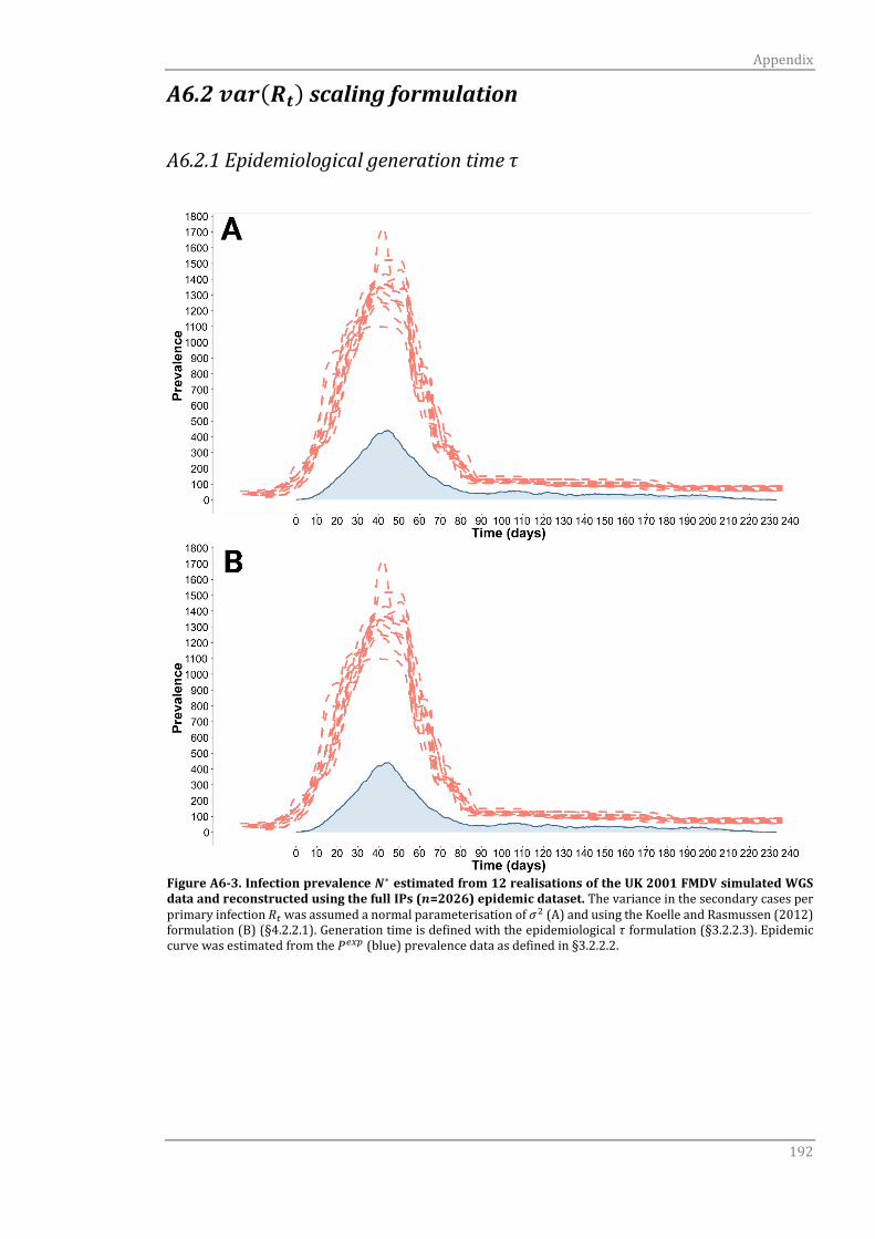
Appendix
192
A6.2 𝒗𝒂𝒓(𝑹𝒕) scaling formulation
A6.2.1 Epidemiological generation time 𝜏
Figure A6-3. Infection prevalence 𝑵∗ estimated from 12 realisations of the UK 2001 FMDV simulated WGS data and reconstructed using the full IPs (𝒏=2026) epidemic dataset. The variance in the secondary cases per primary infection 𝑅𝑡 was assumed a normal parameterisation of 𝜎2 (A) and using the Koelle and Rasmussen (2012) formulation (B) (§4.2.2.1). Generation time is defined with the epidemiological 𝜏 formulation (§3.2.2.3). Epidemic curve was estimated from the 𝑃𝑒𝑥𝑝 (blue) prevalence data as defined in §3.2.2.2.

Appendix
193
Table A6-3. Overall and time specific number of infected cases (both incidence and prevalence) estimated under 12 realisations for the UK 2001 FMD full IPs (𝒏=2026) epidemic dataset from the empirical epidemiological data and the scaled infection prevalence 𝑵∗ estimated under the assumption of variance in 𝑹𝒕 [𝝈𝟐 parameterisation (§4.2.2.1)]. Generation time is defined with the epidemiological 𝜏 formulation (§3.2.2.3).
Epidemic Phase Overall Exponential Peak Decline Plateau
Generation Time 𝜏 7.16±0.07 7.59±0.12 - 6.48±0.09 7.18±0.09
𝑹𝒕 Variance 𝜎2 3.91±0.1 6.49±0.25 0.9±0.19 1.88±0.12 3.28±0.18
Prevalence 𝑃𝑒𝑥𝑝 88.42±0.32 195.01±2.15 439.83±3.19 203.17±0.83 30.62±0.04
Infection Prevalence 𝑁∗ 302.76±15.48 565.55±35.19 1368.77±157.52 712.17±37.69 96.44±5.87
Table A6-4. Overall and time specific number of infected cases (both incidence and prevalence) estimated under 12 realisations for the UK 2001 FMD full IPs (𝒏=2026) epidemic dataset from the empirical epidemiological data and the scaled infection prevalence 𝑵∗ estimated under the assumption of variance in 𝑹𝒕 [Koelle and Rasmussen (2012) parameterisation (§4.2.2.1)]. Generation time is defined with the epidemiological 𝜏 formulation (§3.2.2.3).
Epidemic Phase Overall Exponential Peak Decline Plateau
Generation Time 𝜏 7.16±0.07 7.59±0.12 - 6.48±0.09 7.18±0.09
𝑹𝒕 Variance 𝑣𝑎𝑟(𝑅𝑡) 3.91±0.1 6.49±0.25 0.9±0.19 1.88±0.12 3.28±0.18
Prevalence 𝑃𝑒𝑥𝑝 88.42±0.32 195.01±2.15 439.83±3.19 203.17±0.83 30.62±0.04
Infection Prevalence 𝑁∗ 302.10±15.46 564.31±35.21 1365.73±157.14 710.59±37.56 96.24±5.86
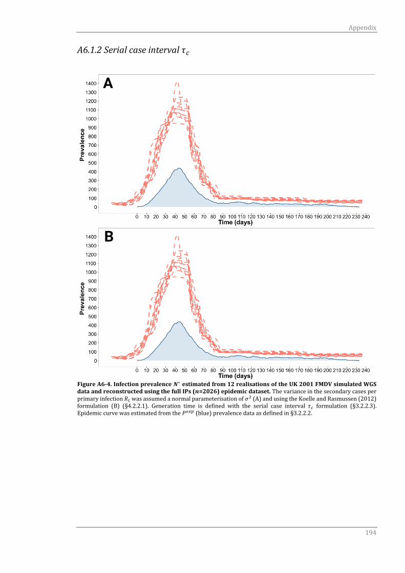
Appendix
194
A6.1.2 Serial case interval 𝜏𝑐
Figure A6-4. Infection prevalence 𝑵∗ estimated from 12 realisations of the UK 2001 FMDV simulated WGS data and reconstructed using the full IPs (𝒏=2026) epidemic dataset. The variance in the secondary cases per primary infection 𝑅𝑡 was assumed a normal parameterisation of 𝜎2 (A) and using the Koelle and Rasmussen (2012) formulation (B) (§4.2.2.1). Generation time is defined with the serial case interval 𝜏𝑐 formulation (§3.2.2.3). Epidemic curve was estimated from the 𝑃𝑒𝑥𝑝 (blue) prevalence data as defined in §3.2.2.2.

Appendix
195
Table A6-5. Overall and time specific number of infected cases (both incidence and prevalence) estimated under 12 realisations for the UK 2001 FMD full IPs (𝒏=2026) epidemic dataset from the empirical epidemiological data and the scaled infection prevalence 𝑵∗ estimated under the assumption of variance in 𝑹𝒕 [𝝈𝟐 parameterisation (§4.2.2.1)]. Generation time is defined with the serial case interval 𝜏𝑐 formulation (§3.2.2.3).
Epidemic Phase Overall Exponential Peak Decline Plateau
Serial Case Interval 𝜏𝑐 8.69±0.01 9.95±0.29 22.16±0.46 22.09±0.01 12.68±0.01
Prevalence 𝑃𝑒𝑥𝑝 88.42±0.32 195.01±2.15 439.83±3.19 203.17±0.83 30.62±0.04
Infection Prevalence 𝑁∗ 251.18±9.44 469.08±22.00 1135.15±121.01 590.85±24.23 80.04±4.50
Table A6-5. Overall and time specific number of infected cases (both incidence and prevalence) estimated under 12 realisations for the UK 2001 FMD full IPs (𝒏=2026) epidemic dataset from the empirical epidemiological data and the scaled infection prevalence 𝑵∗ estimated under the assumption of variance in 𝑹𝒕 [Koelle and Rasmussen (2012) parameterisation (§4.2.2.1)]. Generation time is defined with the serial case interval 𝜏𝑐 formulation (§3.2.2.3).
Epidemic Phase Overall Exponential Peak Decline Plateau
Serial Case Interval 𝜏𝑐 8.69±0.01 9.95±0.29 22.16±0.46 22.09±0.01 12.68±0.01
Prevalence 𝑃𝑒𝑥𝑝 88.42±0.32 195.01±2.15 439.83±3.19 203.17±0.83 30.62±0.04
Infection Prevalence 𝑁∗ 250.68±9.42 468.14±21.96 1132.88±120.76 589.67±24.18 79.88±4.49
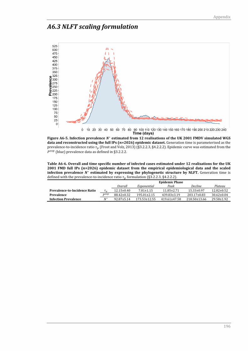
Appendix
196
A6.3 NLFT scaling formulation
Figure A6-5. Infection prevalence 𝑵∗ estimated from 12 realisations of the UK 2001 FMDV simulated WGS data and reconstructed using the full IPs (𝒏=2026) epidemic dataset. Generation time is parameterised as the prevalence-to-incidence ratio 𝜏𝑝 (Frost and Volz, 2013) (§3.2.2.3, §4.2.2.2). Epidemic curve was estimated from the
𝑃𝑒𝑥𝑝 (blue) prevalence data as defined in §3.2.2.2.
Table A6-6. Overall and time specific number of infected cases estimated under 12 realisations for the UK 2001 FMD full IPs (𝒏=2026) epidemic dataset from the empirical epidemiological data and the scaled infection prevalence 𝑵∗ estimated by expressing the phylogenetic structure by NLFT. Generation time is defined with the prevalence-to-incidence ratio 𝜏𝑝 formulation (§3.2.2.3, §4.2.2.2).
Epidemic Phase Overall Exponential Peak Decline Plateau
Prevalence-to-Incidence Ratio 𝜏𝑝 12.15±0.40 7.81±1.15 11.85±2.71 15.33±0.97 12.82±0.52
Prevalence 𝑃𝑒𝑥𝑝 88.42±0.32 195.01±2.15 439.83±3.19 203.17±0.83 30.62±0.04
Infection Prevalence 𝑁∗ 92.87±5.14 173.53±12.55 419.61±47.58 218.50±13.66 29.58±1.92
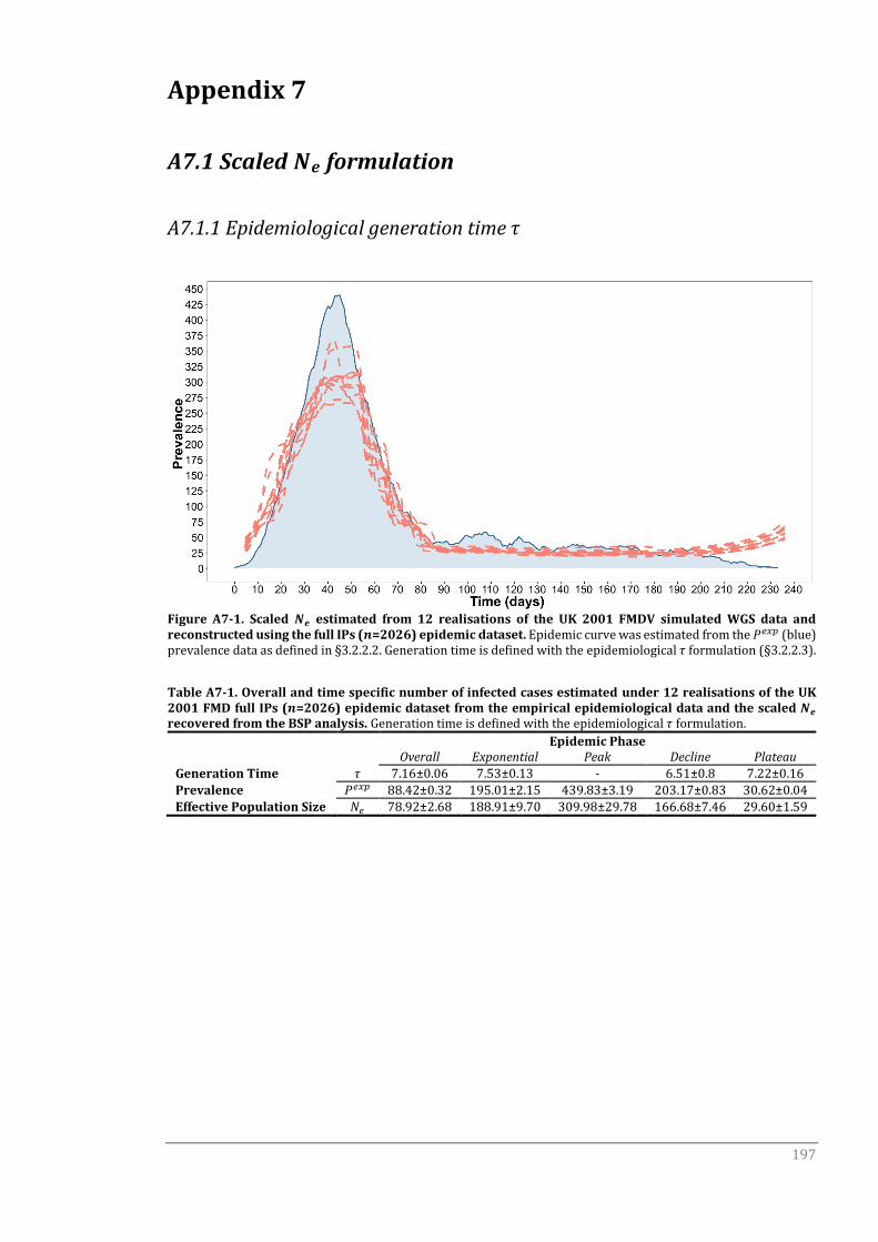
197
Appendix 7
A7.1 Scaled 𝑵𝒆 formulation
A7.1.1 Epidemiological generation time 𝜏
Figure A7-1. Scaled 𝑵𝒆 estimated from 12 realisations of the UK 2001 FMDV simulated WGS data and reconstructed using the full IPs (𝒏=2026) epidemic dataset. Epidemic curve was estimated from the 𝑃𝑒𝑥𝑝 (blue) prevalence data as defined in §3.2.2.2. Generation time is defined with the epidemiological 𝜏 formulation (§3.2.2.3).
Table A7-1. Overall and time specific number of infected cases estimated under 12 realisations of the UK 2001 FMD full IPs (𝒏=2026) epidemic dataset from the empirical epidemiological data and the scaled 𝑵𝒆 recovered from the BSP analysis. Generation time is defined with the epidemiological 𝜏 formulation.
Epidemic Phase Overall Exponential Peak Decline Plateau
Generation Time 𝜏 7.16±0.06 7.53±0.13 - 6.51±0.8 7.22±0.16
Prevalence 𝑃𝑒𝑥𝑝 88.42±0.32 195.01±2.15 439.83±3.19 203.17±0.83 30.62±0.04
Effective Population Size 𝑁𝑒 78.92±2.68 188.91±9.70 309.98±29.78 166.68±7.46 29.60±1.59

Appendix
198
A7.1.2 Serial case interval 𝜏𝑐
Figure A7-2. Scaled 𝑵𝒆 estimated from 12 realisations of the UK 2001 FMDV simulated WGS data and reconstructed using the full IPs (𝒏=2026) epidemic dataset. Epidemic curve was estimated from the 𝑃𝑒𝑥𝑝 (blue) prevalence data as defined in §3.2.2.2. Generation time is defined with the serial case intarval 𝜏𝑐 formulation (§3.2.2.3).
Table A7-2. Overall and time specific number of infected cases (both incidence and prevalence) estimated under 12 realisations of the UK 2001 FMD full IPs (𝒏=2026) epidemic dataset from the empirical epidemiological data and the scaled 𝑵𝒆 recovered from the BSP analysis. Generation time is defined with the serial case interval 𝜏𝑐 formulation.
Epidemic Phase Overall Exponential Peak Decline Plateau
Serial Case Interval 𝜏𝑐 5.91±0.1 7.57±0.11 5.91±0.1 6.93±0.07 5.35±0.67
Prevalence 𝑃𝑒𝑥𝑝 88.42±0.32 195.01±2.15 439.83±3.19 203.17±0.83 30.62±0.04
Effective Population Size 𝑁𝑒 53.05±2.58 194.83±13.77 377.68±56.53 57.50±2.41 13.92±0.76
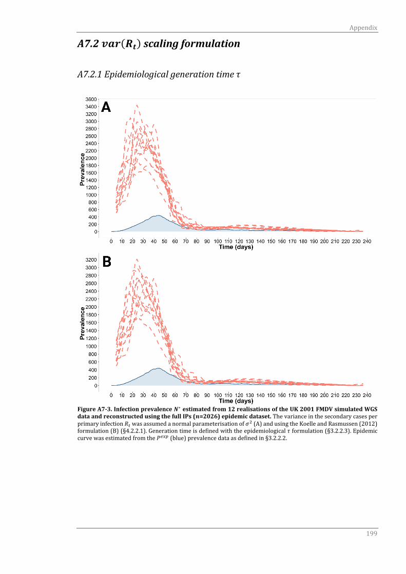
Appendix
199
A7.2 𝒗𝒂𝒓(𝑹𝒕) scaling formulation
A7.2.1 Epidemiological generation time 𝜏
Figure A7-3. Infection prevalence 𝑵∗ estimated from 12 realisations of the UK 2001 FMDV simulated WGS data and reconstructed using the full IPs (𝒏=2026) epidemic dataset. The variance in the secondary cases per primary infection 𝑅𝑡 was assumed a normal parameterisation of 𝜎2 (A) and using the Koelle and Rasmussen (2012) formulation (B) (§4.2.2.1). Generation time is defined with the epidemiological 𝜏 formulation (§3.2.2.3). Epidemic curve was estimated from the 𝑃𝑒𝑥𝑝 (blue) prevalence data as defined in §3.2.2.2.
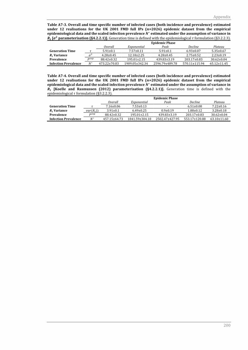
Appendix
200
Table A7-3. Overall and time specific number of infected cases (both incidence and prevalence) estimated under 12 realisations for the UK 2001 FMD full IPs (𝒏=2026) epidemic dataset from the empirical epidemiological data and the scaled infection prevalence 𝑵∗ estimated under the assumption of variance in 𝑹𝒕 [𝝈𝟐 parameterisation (§4.2.2.1)]. Generation time is defined with the epidemiological 𝜏 formulation (§3.2.2.3).
Epidemic Phase Overall Exponential Peak Decline Plateau
Generation Time 𝜏 5.91±0.1 7.57±0.11 5.91±0.1 6.93±0.07 5.35±0.67
𝑹𝒕 Variance 𝜎2 4.28±0.45 12.18±2.25 4.28±0.45 2.75±0.52 2.23±0.19
Prevalence 𝑃𝑒𝑥𝑝 88.42±0.32 195.01±2.15 439.83±3.19 203.17±0.83 30.62±0.04
Infection Prevalence 𝑁∗ 473.22±70.83 1909.05±342.34 2596.79±489.78 570.11±115.94 65.12±11.45
Table A7-4. Overall and time specific number of infected cases (both incidence and prevalence) estimated under 12 realisations for the UK 2001 FMD full IPs (𝒏=2026) epidemic dataset from the empirical epidemiological data and the scaled infection prevalence 𝑵∗ estimated under the assumption of variance in 𝑹𝒕 [Koelle and Rasmussen (2012) parameterisation (§4.2.2.1)]. Generation time is defined with the epidemiological 𝜏 formulation (§3.2.2.3).
Epidemic Phase Overall Exponential Peak Decline Plateau
Generation Time 𝜏 7.16±0.06 7.53±0.13 - 6.51±0.08 7.22±0.16
𝑹𝒕 Variance 𝑣𝑎𝑟(𝑅𝑡)) 3.91±0.1 6.49±0.25 0.9±0.19 1.88±0.12 3.28±0.18
Prevalence 𝑃𝑒𝑥𝑝 88.42±0.32 195.01±2.15 439.83±3.19 203.17±0.83 30.62±0.04
Infection Prevalence 𝑁∗ 457.15±64.73 1841.59±304.18 2502.47±427.95 553.17±120.88 63.10±11.60
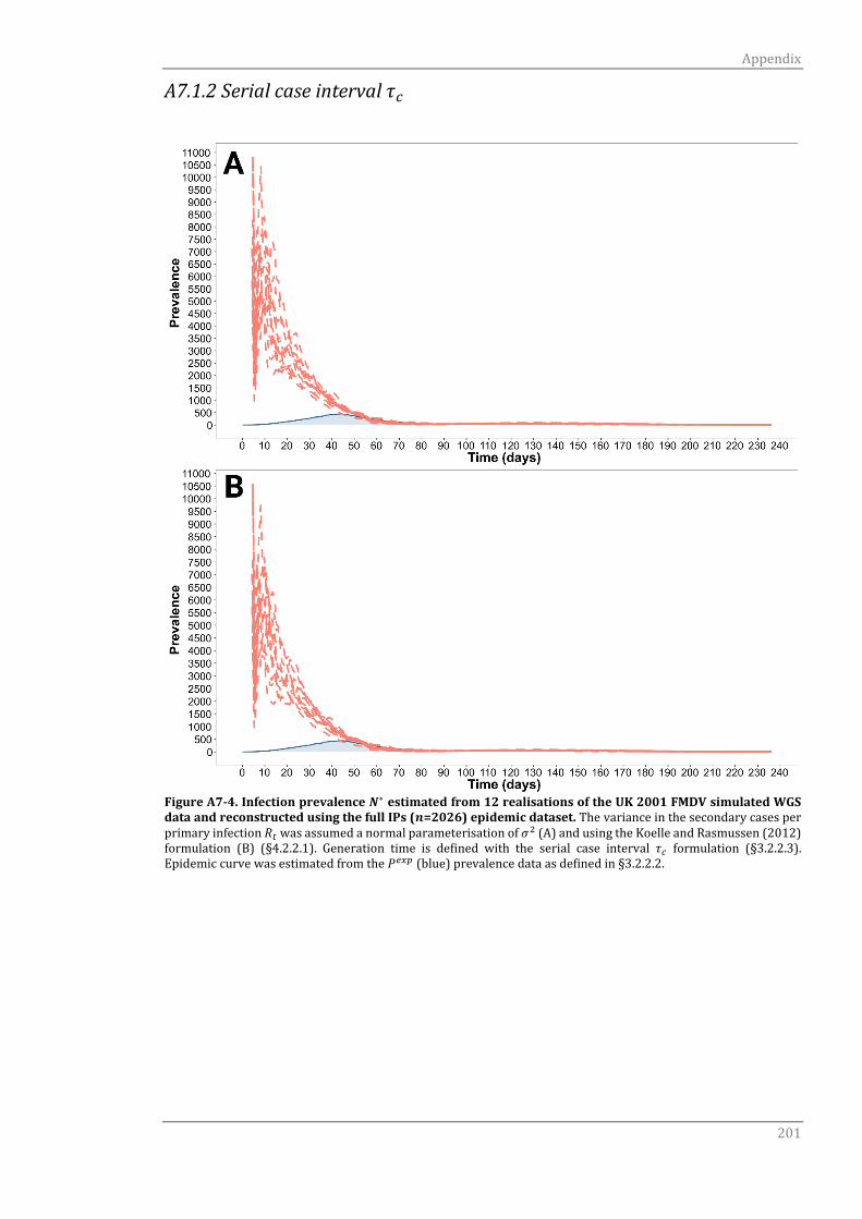
Appendix
201
A7.1.2 Serial case interval 𝜏𝑐
Figure A7-4. Infection prevalence 𝑵∗ estimated from 12 realisations of the UK 2001 FMDV simulated WGS data and reconstructed using the full IPs (𝒏=2026) epidemic dataset. The variance in the secondary cases per primary infection 𝑅𝑡 was assumed a normal parameterisation of 𝜎2 (A) and using the Koelle and Rasmussen (2012) formulation (B) (§4.2.2.1). Generation time is defined with the serial case interval 𝜏𝑐 formulation (§3.2.2.3). Epidemic curve was estimated from the 𝑃𝑒𝑥𝑝 (blue) prevalence data as defined in §3.2.2.2.
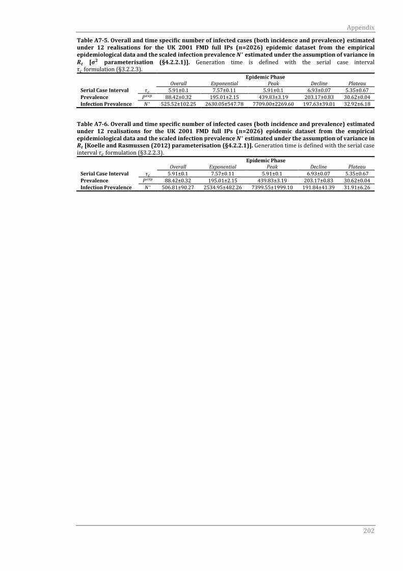
Appendix
202
Table A7-5. Overall and time specific number of infected cases (both incidence and prevalence) estimated under 12 realisations for the UK 2001 FMD full IPs (𝒏=2026) epidemic dataset from the empirical epidemiological data and the scaled infection prevalence 𝑵∗ estimated under the assumption of variance in 𝑹𝒕 [𝝈𝟐 parameterisation (§4.2.2.1)]. Generation time is defined with the serial case interval 𝜏𝑐 formulation (§3.2.2.3).
Epidemic Phase Overall Exponential Peak Decline Plateau
Serial Case Interval 𝜏𝑐 5.91±0.1 7.57±0.11 5.91±0.1 6.93±0.07 5.35±0.67
Prevalence 𝑃𝑒𝑥𝑝 88.42±0.32 195.01±2.15 439.83±3.19 203.17±0.83 30.62±0.04
Infection Prevalence 𝑁∗ 525.52±102.25 2630.05±547.78 7709.00±2269.60 197.63±39.01 32.92±6.18
Table A7-6. Overall and time specific number of infected cases (both incidence and prevalence) estimated under 12 realisations for the UK 2001 FMD full IPs (𝒏=2026) epidemic dataset from the empirical epidemiological data and the scaled infection prevalence 𝑵∗ estimated under the assumption of variance in 𝑹𝒕 [Koelle and Rasmussen (2012) parameterisation (§4.2.2.1)]. Generation time is defined with the serial case interval 𝜏𝑐 formulation (§3.2.2.3).
Epidemic Phase Overall Exponential Peak Decline Plateau
Serial Case Interval 𝜏𝑐 5.91±0.1 7.57±0.11 5.91±0.1 6.93±0.07 5.35±0.67
Prevalence 𝑃𝑒𝑥𝑝 88.42±0.32 195.01±2.15 439.83±3.19 203.17±0.83 30.62±0.04
Infection Prevalence 𝑁∗ 506.81±90.27 2534.95±482.26 7399.55±1999.10 191.84±41.39 31.91±6.26
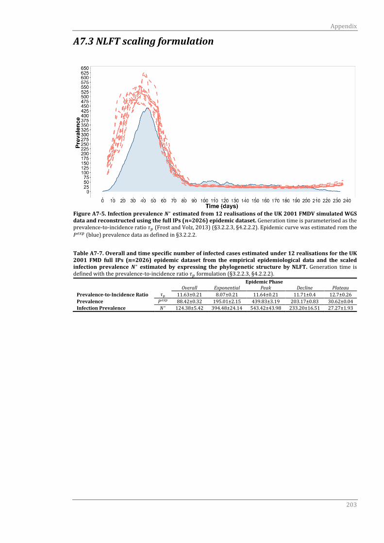
Appendix
203
A7.3 NLFT scaling formulation
Figure A7-5. Infection prevalence 𝑵∗ estimated from 12 realisations of the UK 2001 FMDV simulated WGS data and reconstructed using the full IPs (𝒏=2026) epidemic dataset. Generation time is parameterised as the prevalence-to-incidence ratio 𝜏𝑝 (Frost and Volz, 2013) (§3.2.2.3, §4.2.2.2). Epidemic curve was estimated rom the
𝑃𝑒𝑥𝑝 (blue) prevalence data as defined in §3.2.2.2.
Table A7-7. Overall and time specific number of infected cases estimated under 12 realisations for the UK 2001 FMD full IPs (𝒏=2026) epidemic dataset from the empirical epidemiological data and the scaled infection prevalence 𝑵∗ estimated by expressing the phylogenetic structure by NLFT. Generation time is defined with the prevalence-to-incidence ratio 𝜏𝑝 formulation (§3.2.2.3, §4.2.2.2).
Epidemic Phase Overall Exponential Peak Decline Plateau
Prevalence-to-Incidence Ratio 𝜏𝑝 11.63±0.21 8.07±0.21 11.64±0.21 11.71±0.4 12.7±0.26
Prevalence 𝑃𝑒𝑥𝑝 88.42±0.32 195.01±2.15 439.83±3.19 203.17±0.83 30.62±0.04
Infection Prevalence 𝑁∗ 124.38±5.42 394.48±24.14 543.42±43.98 233.20±16.51 27.27±1.93

204
REFERENCES
ABAO, L. N., KONO, H., GUNARATHNE, A., PROMENTILLA, R. R. & GAERLAN, M. Z. 2014.
Impact of foot-and-mouth disease on pork and chicken prices in Central Luzon,
Philippines. Prev Vet Med, 113, 398-406.
ABDUL-HAMID, N. F., HUSSEIN, N. M., WADSWORTH, J., RADFORD, A. D., KNOWLES, N.
J. & KING, D. P. 2011. Phylogeography of foot-and-mouth disease virus types O
and A in Malaysia and surrounding countries. Infect Genet Evol, 11, 320-8.
AHMED, H. A., SALEM, S. A., HABASHI, A. R., ARAFA, A. A., AGGOUR, M. G., SALEM, G. H.,
GABER, A. S., SELEM, O., ABDELKADER, S. H., KNOWLES, N. J., MADI, M.,
VALDAZO-GONZALEZ, B., WADSWORTH, J., HUTCHINGS, G. H., MIOULET, V.,
HAMMOND, J. M. & KING, D. P. 2012. Emergence of foot-and-mouth disease virus
SAT 2 in Egypt during 2012. Transbound Emerg Dis, 59, 476-81.
ALEXANDERSEN, S., ZHANG, Z., DONALDSON, A. I. & GARLAND, A. J. 2003. The
pathogenesis and diagnosis of foot-and-mouth disease. J Comp Pathol, 129, 1-
36.
AMARAL, A. R., BEHEREGARAY, L. B., BILGMANN, K., FREITAS, L., ROBERTSON, K. M.,
SEQUEIRA, M., STOCKIN, K. A., COELHO, M. M. & MOLLER, L. M. 2012. Influences
of past climatic changes on historical population structure and demography of
a cosmopolitan marine predator, the common dolphin (genus Delphinus). Mol
Ecol, 21, 4854-71.
ANSELL, D. M., SAMUEL, A. R., CARPENTER, W. C. & KNOWLES, N. J. 1994. Genetic
relationships between foot-and-mouth disease type Asia 1 viruses. Epidemiol
Infect, 112, 213-24.
ATKINSON, Q. D., GRAY, R. D. & DRUMMOND, A. J. 2009. Bayesian coalescent inference
of major human mitochondrial DNA haplogroup expansions in Africa. Proc Biol
Sci, 276, 367-73.
BALINDA, S. N., SANGULA, A. K., HELLER, R., MUWANIKA, V. B., BELSHAM, G. J.,
MASEMBE, C. & SIEGISMUND, H. R. 2010a. Diversity and transboundary
mobility of serotype O foot-and-mouth disease virus in East Africa: Implications
for vaccination policies. Infection Genetics and Evolution, 10, 1058-1065.
References
205
BALINDA, S. N., SIEGISMUND, H. R., MUWANIKA, V. B., SANGULA, A. K., MASEMBE, C.,
AYEBAZIBWE, C., NORMANN, P. & BELSHAM, G. J. 2010b. Phylogenetic analyses
of the polyprotein coding sequences of serotype O foot-and-mouth disease
viruses in East Africa: evidence for interserotypic recombination. Virol J, 7, 199.
BARTON, N. H., DEPAULIS, F. & ETHERIDGE, A. M. 2002. Neutral evolution in spatially
continuous populations. Theor Popul Biol, 61, 31-48.
BASTOS, A. D., HAYDON, D. T., FORSBERG, R., KNOWLES, N. J., ANDERSON, E. C., BENGIS,
R. G., NEL, L. H. & THOMSON, G. R. 2001. Genetic heterogeneity of SAT-1 type
foot-and-mouth disease viruses in southern Africa. Arch Virol, 146, 1537-51.
BASTOS, A. D., HAYDON, D. T., SANGARE, O., BOSHOFF, C. I., EDRICH, J. L. & THOMSON,
G. R. 2003. The implications of virus diversity within the SAT 2 serotype for
control of foot-and-mouth disease in sub-Saharan Africa. J Gen Virol, 84, 1595-
606.
BATAILLE, A., VAN DER MEER, F., STEGEMAN, A. & KOCH, G. 2011. Evolutionary
analysis of inter-farm transmission dynamics in a highly pathogenic avian
influenza epidemic. PLoS Pathog, 7, e1002094.
BATISTA, G. E. A. P. A., KEOGH, E. J., TATAW, O. M. & DE SOUZA, V. M. A. 2014. CID: an
efficient complexity-invariant distance for time series. Data Mining and
Knowledge Discovery, 28, 634-669.
BEARD, C. W. & MASON, P. W. 2000. Genetic determinants of altered virulence of
Taiwanese foot-and-mouth disease virus. J Virol, 74, 987-91.
BEDFORD, T., COBEY, S. & PASCUAL, M. 2011. Strength and tempo of selection revealed
in viral gene genealogies. BMC Evol Biol, 11, 220.
BENNETT, S. N., DRUMMOND, A. J., KAPAN, D. D., SUCHARD, M. A., MUNOZ-JORDAN, J.
L., PYBUS, O. G., HOLMES, E. C. & GUBLER, D. J. 2010. Epidemic dynamics
revealed in dengue evolution. Mol Biol Evol, 27, 811-8.
BENSON, D. A., CAVANAUGH, M., CLARK, K., KARSCH-MIZRACHI, I., LIPMAN, D. J.,
OSTELL, J. & SAYERS, E. W. 2013. GenBank. Nucleic Acids Res, 41, D36-42.
BIEK, R., HENDERSON, J. C., WALLER, L. A., RUPPRECHT, C. E. & REAL, L. A. 2007. A
high-resolution genetic signature of demographic and spatial expansion in
epizootic rabies virus. Proc Natl Acad Sci U S A, 104, 7993-8.
BIENVENU, F. & LEGENDRE, S. 2015. A new approach to the generation time in matrix
population models. Am Nat, 185, 834-43.
References
206
BOSKOVA, V., BONHOEFFER, S. & STADLER, T. 2014. Inference of epidemiological
dynamics based on simulated phylogenies using birth-death and coalescent
models. PLoS Comput Biol, 10, e1003913.
BOUCKAERT, R., HELED, J., KUHNERT, D., VAUGHAN, T., WU, C. H., XIE, D., SUCHARD,
M. A., RAMBAUT, A. & DRUMMOND, A. J. 2014. BEAST 2: a software platform for
Bayesian evolutionary analysis. PLoS Comput Biol, 10, e1003537.
CAO, Y. M., LU, Z. J., LI, D., FAN, P. J., SUN, P., BAO, H. F., FU, Y. F., LI, P. H., BAI, X. W.,
CHEN, Y. L., XIE, B. X. & LIU, Z. X. 2014. Evaluation of cross-protection against
three topotypes of serotype O foot-and-mouth disease virus in pigs vaccinated
with multi-epitope protein vaccine incorporated with poly(I:C). Veterinary
Microbiology, 168, 294-301.
CARRILLO, C., LU, Z., BORCA, M. V., VAGNOZZI, A., KUTISH, G. F. & ROCK, D. L. 2007.
Genetic and phenotypic variation of foot-and-mouth disease virus during serial
passages in a natural host. J Virol, 81, 11341-51.
CARRILLO, C., TULMAN, E. R., DELHON, G., LU, Z., CARRENO, A., VAGNOZZI, A., KUTISH,
G. F. & ROCK, D. L. 2005. Comparative genomics of foot-and-mouth disease virus.
J Virol, 79, 6487-504.
CARRINGTON, C. V., FOSTER, J. E., PYBUS, O. G., BENNETT, S. N. & HOLMES, E. C. 2005.
Invasion and maintenance of dengue virus type 2 and type 4 in the Americas. J
Virol, 79, 14680-7.
CHARLESTON, B., BANKOWSKI, B. M., GUBBINS, S., CHASE-TOPPING, M. E., SCHLEY, D.,
HOWEY, R., BARNETT, P. V., GIBSON, D., JULEFF, N. D. & WOOLHOUSE, M. E.
2011. Relationship between clinical signs and transmission of an infectious
disease and the implications for control. Science, 332, 726-9.
CHARLESWORTH, B. 2009. Effective population size and patterns of molecular
evolution and variation. Nat Rev Genet, 10, 195-205.
CHENG, I. C., LIANG, S. M., TU, W. J., CHEN, C. M., LAI, S. Y., CHENG, Y. C., LEE, F., HUANG,
T. S. & JONG, M. H. 2006. Study on the porcinophilic foot-and-mouth disease
virus I. production and characterization of monoclonal antibodies against VP1.
J Vet Med Sci, 68, 859-64.
CHIKHI, L., SOUSA, V. C., LUISI, P., GOOSSENS, B. & BEAUMONT, M. A. 2010. The
confounding effects of population structure, genetic diversity and the sampling
scheme on the detection and quantification of population size changes. Genetics,
186, 983-95.
References
207
CHIS STER, I. & FERGUSON, N. M. 2007. Transmission parameters of the 2001 foot and
mouth epidemic in Great Britain. PLoS One, 2, e502.
CHIS STER, I., SINGH, B. K. & FERGUSON, N. M. 2009. Epidemiological inference for
partially observed epidemics: the example of the 2001 foot and mouth epidemic
in Great Britain. Epidemics, 1, 21-34.
CHITRAY, M., DE BEER, T. A., VOSLOO, W. & MAREE, F. F. 2014. Genetic heterogeneity
in the leader and P1-coding regions of foot-and-mouth disease virus serotypes
A and O in Africa. Arch Virol, 159, 947-61.
CHRISTENSEN, L. S., NORMANN, P., THYKIER-NIELSEN, S., SORENSEN, J. H., DE
STRICKER, K. & ROSENORN, S. 2005. Analysis of the epidemiological dynamics
during the 1982-1983 epidemic of foot-and-mouth disease in Denmark based
on molecular high-resolution strain identification. J Gen Virol, 86, 2577-84.
CLEMENT, M., POSADA, D. & CRANDALL, K. A. 2000. TCS: a computer program to
estimate gene genealogies. Mol Ecol, 9, 1657-9.
COCHRAN, W. G. 1977. Sampling techniques, New York, John Wiley & Sons, Inc.
COMAS, I., COSCOLLA, M., LUO, T., BORRELL, S., HOLT, K. E., KATO-MAEDA, M.,
PARKHILL, J., MALLA, B., BERG, S., THWAITES, G., YEBOAH-MANU, D.,
BOTHAMLEY, G., MEI, J., WEI, L., BENTLEY, S., HARRIS, S. R., NIEMANN, S., DIEL,
R., ASEFFA, A., GAO, Q., YOUNG, D. & GAGNEUX, S. 2013. Out-of-Africa migration
and Neolithic coexpansion of Mycobacterium tuberculosis with modern
humans. Nat Genet, 45, 1176-82.
COTTAM, E. M., HAYDON, D. T., PATON, D. J., GLOSTER, J., WILESMITH, J. W., FERRIS, N.
P., HUTCHINGS, G. H. & KING, D. P. 2006. Molecular epidemiology of the foot-
and-mouth disease virus outbreak in the United Kingdom in 2001. J Virol, 80,
11274-82.
COTTAM, E. M., THEBAUD, G., WADSWORTH, J., GLOSTER, J., MANSLEY, L., PATON, D.
J., KING, D. P. & HAYDON, D. T. 2008a. Integrating genetic and epidemiological
data to determine transmission pathways of foot-and-mouth disease virus. Proc
Biol Sci, 275, 887-95.
COTTAM, E. M., WADSWORTH, J., SHAW, A. E., ROWLANDS, R. J., GOATLEY, L., MAAN,
S., MAAN, N. S., MERTENS, P. P., EBERT, K., LI, Y., RYAN, E. D., JULEFF, N., FERRIS,
N. P., WILESMITH, J. W., HAYDON, D. T., KING, D. P., PATON, D. J. & KNOWLES, N.
J. 2008b. Transmission pathways of foot-and-mouth disease virus in the United
Kingdom in 2007. PLoS Pathog, 4, e1000050.
References
208
DARRIBA, D., TABOADA, G. L., DOALLO, R. & POSADA, D. 2012. jModelTest 2: more
models, new heuristics and parallel computing. Nat Methods, 9, 772.
DE BRUYN, M., HALL, B. L., CHAUKE, L. F., BARONI, C., KOCH, P. L. & HOELZEL, A. R.
2009. Rapid response of a marine mammal species to holocene climate and
habitat change. PLoS Genet, 5, e1000554.
DE CARVALHO, L. M., SANTOS, L. B., FARIA, N. R. & DE CASTRO SILVEIRA, W. 2013.
Phylogeography of foot-and-mouth disease virus serotype O in Ecuador. Infect
Genet Evol, 13, 76-88.
DE KOEIJER, A. A., BOENDER, G. J., NODELIJK, G., STAUBACH, C., MEROC, E. & ELBERS,
A. R. 2011. Quantitative analysis of transmission parameters for bluetongue
virus serotype 8 in Western Europe in 2006. Vet Res, 42, 53.
DE SILVA, E., FERGUSON, N. M. & FRASER, C. 2012. Inferring pandemic growth rates
from sequence data. J R Soc Interface, 9, 1797-808.
DEFRA 2002. Origins of the UK foot-and-mouth disease epidemic in 2001. London:
Department for Environment, Food & Rural Affairs.
DI NARDO, A., KNOWLES, N. J. & PATON, D. J. 2011. Combining livestock trade patterns
with phylogenetics to help understand the spread of foot and mouth disease in
sub-Saharan Africa, the Middle East and Southeast Asia. Rev Sci Tech, 30, 63-85.
DI NARDO, A., KNOWLES, N. J., WADSWORTH, J., HAYDON, D. T. & KING, D. P. 2014.
Phylodynamic reconstruction of O CATHAY topotype foot-and-mouth disease
virus epidemics in the Philippines. Veterinary Research, 45, 90.
DIDELOT, X., GARDY, J. & COLIJN, C. 2014. Bayesian inference of infectious disease
transmission from whole-genome sequence data. Mol Biol Evol, 31, 1869-79.
DOMINGO, E., ESCARMIS, C., BARANOWSKI, E., RUIZ-JARABO, C. M., CARRILLO, E.,
NUNEZ, J. I. & SOBRINO, F. 2003. Evolution of foot-and-mouth disease virus.
Virus Res, 91, 47-63.
DOMINGO, E., GONZALEZ-LOPEZ, C., PARIENTE, N., AIRAKSINEN, A. & ESCARMIS, C.
2005. Population dynamics of RNA viruses: the essential contribution of mutant
spectra. Arch Virol Suppl, 59-71.
DONALDSON, A., LEE, R., WARD, N. & WILKINSON, K. 2006. Foot and mouth - five years
on: the legacy of the 2001 foot and mouth disease crisis for farming and the
British countryside Center for Rural Economy Discussion Paper Series No 6.
Newcastle upon Tyne: University of Newcastle upon Tyne.
References
209
DONNELLY, P. & TAVARE, S. 1995. Coalescents and genealogical structure under
neutrality. Annu Rev Genet, 29, 401-21.
DRAKE, J. W. 1993. Rates of spontaneous mutation among RNA viruses. Proc Natl Acad
Sci U S A, 90, 4171-5.
DRUMMOND, A. J., HO, S. Y., PHILLIPS, M. J. & RAMBAUT, A. 2006. Relaxed
phylogenetics and dating with confidence. PLoS Biol, 4, e88.
DRUMMOND, A. J., NICHOLLS, G. K., RODRIGO, A. G. & SOLOMON, W. 2002. Estimating
mutation parameters, population history and genealogy simultaneously from
temporally spaced sequence data. Genetics, 161, 1307-20.
DRUMMOND, A. J., PYBUS, O. G., RAMBAUT, A., FORSBERG, R. & RODRIGO, A. G. 2003.
Measurably evolving populations. Trends Ecol Evol, 18, 481-88.
DRUMMOND, A. J. & RAMBAUT, A. 2007. BEAST: Bayesian evolutionary analysis by
sampling trees. BMC Evol Biol, 7, 214.
DRUMMOND, A. J., RAMBAUT, A., SHAPIRO, B. & PYBUS, O. G. 2005. Bayesian coalescent
inference of past population dynamics from molecular sequences. Mol Biol Evol,
22, 1185-92.
DRUMMOND, A. J. & SUCHARD, M. A. 2010. Bayesian random local clocks, or one rate
to rule them all. BMC Biol, 8, 114.
DRUMMOND, A. J., SUCHARD, M. A., XIE, D. & RAMBAUT, A. 2012. Bayesian
phylogenetics with BEAUti and the BEAST 1.7. Mol Biol Evol, 29, 1969-73.
DUFFY, S., SHACKELTON, L. A. & HOLMES, E. C. 2008. Rates of evolutionary change in
viruses: patterns and determinants. Nat Rev Genet, 9, 267-76.
EL-SHEHAWY, L. I., ABU-ELNAGA, H. I., RIZK, S. A., ABD EL-KREEM, A. S., MOHAMED, A.
A. & FAWZY, H. G. 2014. Molecular differentiation and phylogenetic analysis of
the Egyptian foot-and-mouth disease virus SAT2. Arch Virol, 159, 437-43.
FAO 2011. World livestock 2011 - livestock in food security, Rome, Italy, Food and
Agriculture Organization of the United Nations.
FELSENSTEIN, J. 1971. Inbreeding and variance effective numbers in populations with
overlapping generations. Genetics, 68, 581-97.
FELSENSTEIN, J. 2004. Inferring phylogenies, Sunderland, Mass., Sinauer Associates.
FENG, Q., YU, H., LIU, Y., HE, C., HU, J., SANG, H., DING, N., DING, M., FUNG, Y. W., LAU, L.
T., YU, A. C. & CHEN, J. 2004. Genome comparison of a novel foot-and-mouth
disease virus with other FMDV strains. Biochem Biophys Res Commun, 323, 254-
63.
References
210
FERRIS, N. P., KING, D. P., REID, S. M., SHAW, A. E. & HUTCHINGS, G. H. 2006.
Comparisons of original laboratory results and retrospective analysis by real-
time reverse transcriptase-PCR of virological samples collected from confirmed
cases of foot-and-mouth disease in the UK in 2001. Vet Rec, 159, 373-8.
FINE, P. E. M. 2003. The interval between successive cases of an infectious disease.
American Journal of Epidemiology, 158, 1039-1047.
FINLAY, E. K., GAILLARD, C., VAHIDI, S. M., MIRHOSEINI, S. Z., JIANLIN, H., QI, X. B., EL-
BARODY, M. A., BAIRD, J. F., HEALY, B. C. & BRADLEY, D. G. 2007. Bayesian
inference of population expansions in domestic bovines. Biol Lett, 3, 449-52.
FISHER, R. A. S. 1930. The genetical theory of natural selection, Oxford, Clarendon Press.
FORMAN, S., LE GALL, F., BELTON, D., EVANS, B., FRANCOIS, J. L., MURRAY, G.,
SHEESLEY, D., VANDERSMISSEN, A. & YOSHIMURA, S. 2009. Moving towards
the global control of foot and mouth disease: an opportunity for donors. Rev Sci
Tech, 28, 883-96.
FORSS, S., STREBEL, K., BECK, E. & SCHALLER, H. 1984. Nucleotide sequence and
genome organization of foot-and-mouth disease virus. Nucleic Acids Res, 12,
6587-601.
FROST, S. D. & VOLZ, E. M. 2010. Viral phylodynamics and the search for an 'effective
number of infections'. Philos Trans R Soc Lond B Biol Sci, 365, 1879-90.
FROST, S. D. & VOLZ, E. M. 2013. Modelling tree shape and structure in viral
phylodynamics. Philos Trans R Soc Lond B Biol Sci, 368, 20120208.
FU, Y. X. 2006. Exact coalescent for the Wright-Fisher model. Theor Popul Biol, 69, 385-
94.
GARSKE, T. & RHODES, C. J. 2008. The effect of superspreading on epidemic outbreak
size distributions. J Theor Biol, 253, 228-37.
GIBBENS, J. C., SHARPE, C. E., WILESMITH, J. W., MANSLEY, L. M., MICHALOPOULOU, E.,
RYAN, J. B. & HUDSON, M. 2001. Descriptive epidemiology of the 2001 foot-and-
mouth disease epidemic in Great Britain: the first five months. Vet Rec, 149, 729-
43.
GIGNOUX, C. R., HENN, B. M. & MOUNTAIN, J. L. 2011. Rapid, global demographic
expansions after the origins of agriculture. Proc Natl Acad Sci U S A, 108, 6044-
9.
References
211
GILL, M. S., LEMEY, P., FARIA, N. R., RAMBAUT, A., SHAPIRO, B. & SUCHARD, M. A. 2013.
Improving Bayesian population dynamics inference: a coalescent-based model
for multiple loci. Mol Biol Evol, 30, 713-24.
GLEESON, L. J. 2002. A review of the status of foot and mouth disease in South-East Asia
and approaches to control and eradication. Rev Sci Tech, 21, 465-75.
GLOSTER, J., CHAMPION, H. J., MANSLEY, L. M., ROMERO, P., BROUGH, T. & RAMIREZ,
A. 2005. The 2001 epidemic of foot-and-mouth disease in the United Kingdom:
epidemiological and meteorological case studies. Vet Rec, 156, 793-803.
GLOSTER, J., CHAMPION, H. J., SORENSEN, J. H., MIKKELSEN, T., RYALL, D. B., ASTRUP,
P., ALEXANDERSEN, S. & DONALDSON, A. I. 2003. Airborne transmission of foot-
and-mouth disease virus from Burnside Farm, Heddon-on-the-Wall,
Northumberland, during the 2001 epidemic in the United Kingdom. Vet Rec,
152, 525-33.
GORDO, I. & CAMPOS, P. R. 2007. Patterns of genetic variation in populations of
infectious agents. BMC Evol Biol, 7, 116.
GRAY, R. R., PYBUS, O. G. & SALEMI, M. 2011. Measuring the Temporal Structure in
Serially-Sampled Phylogenies. Methods Ecol Evol, 2, 437-445.
GRENFELL, B. T., PYBUS, O. G., GOG, J. R., WOOD, J. L., DALY, J. M., MUMFORD, J. A. &
HOLMES, E. C. 2004. Unifying the epidemiological and evolutionary dynamics of
pathogens. Science, 303, 327-32.
GRIFFITHS, R. C. & TAVARE, S. 1994a. Ancestral inference in population genetics.
Statistical Science, 9, 307-319.
GRIFFITHS, R. C. & TAVARE, S. 1994b. Sampling theory for neutral alleles in a varying
environment. Philos Trans R Soc Lond B Biol Sci, 344, 403-10.
GRUBMAN, M. J. & BAXT, B. 2004. Foot-and-mouth disease. Clin Microbiol Rev, 17, 465-
93.
GUILLOT, E. G., TUMONGGOR, M. K., LANSING, S. J., SUDOYO, H. & COX, M. P. 2013.
Climate change influenced fenale population sizes through time across the
Indonesian Archipelago. Human Biology, 85, 135-152.
GUINDON, S., DUFAYARD, J. F., LEFORT, V., ANISIMOVA, M., HORDIJK, W. & GASCUEL,
O. 2010. New algorithms and methods to estimate maximum-likelihood
phylogenies: assessing the performance of PhyML 3.0. Syst Biol, 59, 307-21.
GUINDON, S. & GASCUEL, O. 2003. A simple, fast, and accurate algorithm to estimate
large phylogenies by maximum likelihood. Syst Biol, 52, 696-704.
References
212
HALL, M. & RAMBAUT, A. 2014. Epidemic reconstruction in a phylogenetics
framework: transmission trees as partitions. ArXiv e-prints, 1406.0428.
HALL, M. D., KNOWLES, N. J., WADSWORTH, J., RAMBAUT, A. & WOOLHOUSE, M. E.
2013. Reconstructing geographical movements and host species transitions of
foot-and-mouth disease virus serotype SAT 2. mBio, 4, e00591-13.
HARRELL, F. E. 2001. Regression modeling strategies: with applications to linear models,
logistic regression, and survival analysis, London, Springer.
HASEGAWA, M., KISHINO, H. & YANO, T. 1985. Dating of the human-ape splitting by a
molecular clock of mitochondrial DNA. J Mol Evol, 22, 160-74.
HAYDON, D. T., BASTOS, A. D. & AWADALLA, P. 2004. Low linkage disequilibrium
indicative of recombination in foot-and-mouth disease virus gene sequence
alignments. J Gen Virol, 85, 1095-100.
HAYDON, D. T., CHASE-TOPPING, M., SHAW, D. J., MATTHEWS, L., FRIAR, J. K.,
WILESMITH, J. & WOOLHOUSE, M. E. 2003. The construction and analysis of
epidemic trees with reference to the 2001 UK foot-and-mouth outbreak. Philos
Trans R Soc Lond B Biol Sci, 270, 121-7.
HAYDON, D. T., SAMUEL, A. R. & KNOWLES, N. J. 2001. The generation and persistence
of genetic variation in foot-and-mouth disease virus. Prev Vet Med, 51, 111-24.
HAYDON, D. T., WOOLHOUSE, M. E. & KITCHING, R. P. 1997. An analysis of foot-and-
mouth-disease epidemics in the UK. IMA J Math Appl Med Biol, 14, 1-9.
HEATH, L., VAN DER WALT, E., VARSANI, A. & MARTIN, D. P. 2006. Recombination
patterns in aphthoviruses mirror those found in other picornaviruses. J Virol,
80, 11827-32.
HELED, J. & DRUMMOND, A. J. 2008. Bayesian inference of population size history from
multiple loci. BMC Evol Biol, 8, 289.
HEMADRI, D., TOSH, C., SANYAL, A. & VENKATARAMANAN, R. 2002. Emergence of a
new strain of type O foot-and-mouth disease virus: Its phylogenetic and
evolutionary relationship with the PanAsia pandemic strain. Virus Genes, 25, 23-
34.
HICKS, A. L. & DUFFY, S. 2011. Genus-specific substitution rate variability among
picornaviruses. J Virol, 85, 7942-7.
HO, S. Y. & SHAPIRO, B. 2011. Skyline-plot methods for estimating demographic history
from nucleotide sequences. Mol Ecol Resour, 11, 423-34.
References
213
HOLLATZ, C., VILACA, S. T., REDONDO, R. A. F., MARMONTEL, M., BAKER, C. S. &
SANTOS, F. R. 2011. The Amazon River system as an ecological barrier driving
genetic differentiation of the pink dolphin (Inia geoffrensis). Biol J Linn Soc, 102,
812-27.
HUI, R. K. & LEUNG, F. C. 2012. Evolutionary trend of foot-and-mouth disease virus in
Hong Kong. Vet Microbiol, 159, 221-9.
HYNDMAN, R. J. & KOEHLER, A. B. 2006. Another look at measures of forecast accuracy.
International Journal of Forecasting, 22, 679-688.
JACKSON, A. L., O'NEILL, H., MAREE, F., BLIGNAUT, B., CARRILLO, C., RODRIGUEZ, L. &
HAYDON, D. T. 2007. Mosaic structure of foot-and-mouth disease virus
genomes. J Gen Virol, 88, 487-92.
JACKSON, T., KING, A. M., STUART, D. I. & FRY, E. 2003. Structure and receptor binding.
Virus Res, 91, 33-46.
JAMAL, S. M., FERRARI, G., AHMED, S., NORMANN, P. & BELSHAM, G. J. 2011a. Genetic
diversity of foot-and-mouth disease virus serotype O in Pakistan and
Afghanistan, 1997-2009. Infection Genetics and Evolution, 11, 1229-1238.
JAMAL, S. M., FERRARI, G., AHMED, S., NORMANN, P. & BELSHAM, G. J. 2011b. Molecular
characterization of serotype Asia-1 foot-and-mouth disease viruses in Pakistan
and Afghanistan; emergence of a new genetic Group and evidence for a novel
recombinant virus. Infect Genet Evol, 11, 2049-62.
JAMAL, S. M., FERRARI, G., AHMED, S., NORMANN, P., CURRY, S. & BELSHAM, G. J. 2011c.
Evolutionary analysis of serotype A foot-and-mouth disease viruses circulating
in Pakistan and Afghanistan during 2002-2009. Journal of General Virology, 92,
2849-2864.
JENKINS, G. M., RAMBAUT, A., PYBUS, O. G. & HOLMES, E. C. 2002. Rates of molecular
evolution in RNA viruses: a quantitative phylogenetic analysis. J Mol Evol, 54,
156-65.
JOMBART, T., CORI, A., DIDELOT, X., CAUCHEMEZ, S., FRASER, C. & FERGUSON, N. 2014.
Bayesian reconstruction of disease outbreaks by combining epidemiologic and
genomic data. PLoS Comput Biol, 10, e1003457.
JOMBART, T., EGGO, R. M., DODD, P. J. & BALLOUX, F. 2011. Reconstructing disease
outbreaks from genetic data: a graph approach. Heredity (Edinb), 106, 383-90.
JULEFF, N., VALDAZO-GONZÁLEZ, B., WADSWORTH, J., WRIGHT, C. F., CHARLESTON,
B., PATON, D. J., KING, D. P. & KNOWLES, N. J. 2013. Accumulation of nucleotide

References
214
substitutions occurring during experimental transmission of foot-and-mouth
disease virus. J Gen Virol, 94, 108-19.
KAJ, I. & KRONE, S. M. 2003. The coalescent process in a population with stochastically
varying size. J Appl Prob, 40, 33-48.
KAO, R. R. 2002. The role of mathematical modelling in the control of the 2001 FMD
epidemic in the UK. Trends Microbiol, 10, 279-86.
KAO, R. R., HAYDON, D. T., LYCETT, S. J. & MURCIA, P. R. 2014. Supersize me: how
whole-genome sequencing and big data are transforming epidemiology. Trends
Microbiol, 22, 282-91.
KEELING, M. 2005. The implications of network structure for epidemic dynamics.
Theor Popul Biol, 67, 1-8.
KEELING, M. J. & ROHANI, P. 2008. Modeling infectious diseases in humans and animals,
Princeton, N.J. ; Woodstock, Princeton University Press.
KEELING, M. J., WOOLHOUSE, M. E., MAY, R. M., DAVIES, G. & GRENFELL, B. T. 2003.
Modelling vaccination strategies against foot-and-mouth disease. Nature, 421,
136-42.
KENAH, E., LIPSITCH, M. & ROBINS, J. M. 2008. Generation interval contraction and
epidemic data analysis. Math Biosci, 213, 71-9.
KIMURA, M. & CROW, J. F. 1963. The measurement of effective population number.
Evolution, 17, 279-288.
KINGMAN, J. F. 1982a. The coalescent. Stochast Proc Appl, 13, 235-48.
KINGMAN, J. F. 1982b. On the genealogy of large population. J Appl Prob, 19A, 27-43.
KITCHING, R. P. 2002. Clinical variation in foot and mouth disease: cattle. Rev Sci Tech,
21, 499-504.
KITCHING, R. P. & ALEXANDERSEN, S. 2002. Clinical variation in foot and mouth
disease: pigs. Rev Sci Tech, 21, 513-8.
KITCHING, R. P. & HUGHES, G. J. 2002. Clinical variation in foot and mouth disease:
sheep and goats. Rev Sci Tech, 21, 505-12.
KLEIN, J., HUSSAIN, M., AHMAD, M., NORMANN, P., AFZAL, M. & ALEXANDERSEN, S.
2007. Genetic characterisation of the recent foot-and-mouth disease virus
subtype A/IRN/2005. Virol J, 4, 122.
KLEIN, J., PARLAK, U., OZYORUK, F. & CHRISTENSEN, L. S. 2006. The molecular
epidemiology of foot-and-mouth disease virus serotypes A and O from 1998 to
2004 in Turkey. BMC Vet Res, 2, 35.
References
215
KNOWLES, N. J., BACHANEK-BANKOWSKA, K. & WADSWORTH, J. 2015.
WRLFMD/2015/00007 Genotyping Report - Sultanate of Oman. World
Reference Laboratory for Foot-and-Mouth Disease.
KNOWLES, N. J., DAVIES, P. R., HENRY, T., O'DONNELL, V., PACHECO, J. M. & MASON, P.
W. 2001a. Emergence in Asia of foot-and-mouth disease viruses with altered
host range: characterization of alterations in the 3A protein. J Virol, 75, 1551-6.
KNOWLES, N. J., HE, J., SHANG, Y., WADSWORTH, J., VALDAZO-GONZÁLEZ, B.,
ONOSATO, H., FUKAI, K., MORIOKA, K., YOSHIDA, K., CHO, I. S., KIM, S. M., PARK,
J. H., LEE, K. N., LUK, G., BORISOV, V., SCHERBAKOV, A., TIMINA, A., BOLD, D.,
NGUYEN, T., PATON, D. J., HAMMOND, J. M., LIU, X. & KING, D. P. 2012. Southeast
Asian foot-and-mouth disease viruses in Eastern Asia. Emerg Infect Dis, 18, 499-
501.
KNOWLES, N. J., HOVI, T., HYYPIÄ, T., KING, A. M. Q., LINDBERG, A. M., PALLANSCH, M.
A., PALMENBERG, A. C., SIMMONDS, P., SKERN, T., STANWAY, G., YAMASHITA,
T. & ZELL, R. 2011. Picornaviridae. In: KING, A. M. Q., LEFKOWITZ, E. J., ADAMS,
M. J. & CARSTENS, E. B. (eds.) Virus Taxonomy. Classification and Nomenclature
of Viruses: Ninth Report of the International Committee on Taxonomy of Viruses.
San Diego: Elsevier.
KNOWLES, N. J., NAZEM SHIRAZI, M. H., WADSWORTH, J., SWABEY, K. G., STIRLING, J.
M., STATHAM, R. J., LI, Y., HUTCHINGS, G. H., FERRIS, N. P., PARLAK, U.,
OZYORUK, F., SUMPTION, K. J., KING, D. P. & PATON, D. J. 2009. Recent spread of
a new strain (A-Iran-05) of foot-and-mouth disease virus type A in the Middle
East. Transbound Emerg Dis, 56, 157-69.
KNOWLES, N. J. & SAMUEL, A. R. 2003. Molecular epidemiology of foot-and-mouth
disease virus. Virus Res, 91, 65-80.
KNOWLES, N. J., SAMUEL, A. R., DAVIES, P. R., KITCHING, R. P. & DONALDSON, A. I.
2001b. Outbreak of foot-and-mouth disease virus serotype O in the UK caused
by a pandemic strain. Vet Rec, 148, 258-9.
KNOWLES, N. J., SAMUEL, A. R., DAVIES, P. R., MIDGLEY, R. J. & VALARCHER, J. F. 2005.
Pandemic strain of foot-and-mouth disease virus serotype O. Emerg Infect Dis,
11, 1887-93.
KNOWLES, N. J., WADSWORTH, J., HAMMOND, J. M. & KING, D. P. 2010. Foot-and-mouth
disease virus geontype definitions and nomenclature. Open Session of the
References
216
European Commission for the Control of Foot-and-Mouth Disease Standing
Technical Committee, 28 September - 1 October 2010a Vienna, Austria.
KNOWLES, N. J., WADSWORTH, J., PARLAK, U., OZYORUK, F., NAZEM SHIRAZI, M. H.,
FERRIS, N. P., HUTCHINGS, G. H., STIRLING, J. M., HAMMOND, J. M. & KING, D. P.
Recent events in the evolution of foot-and-mouth disease in the Middle East.
Open Session of the European Commission for the Control of Foot-and-Mouth
Disease Standing Technical Committee, 28 September - 1 October 2010b
Vienna.
KOBLMULLER, S., WAYNE, R. K. & LEONARD, J. A. 2012. Impact of Quaternary climatic
changes and interspecific competition on the demographic history of a highly
mobile generalist carnivore, the coyote. Biol Lett, 8, 644-7.
KOELLE, K. & RASMUSSEN, D. A. 2012. Rates of coalescence for common
epidemiological models at equilibrium. J R Soc Interface, 9, 997-1007.
KONIG, G. A., COTTAM, E. M., UPADHYAYA, S., GLOSTER, J., MANSLEY, L. M., HAYDON,
D. T. & KING, D. P. 2009. Sequence data and evidence of possible airborne spread
in the 2001 foot-and-mouth disease epidemic in the UK. Vet Rec, 165, 410-1.
KONIG, G. A., PALMA, E. L., MARADEI, E. & PICCONE, M. E. 2007. Molecular
epidemiology of foot-and-mouth disease virus types A and O isolated in
Argentina during the 2000-2002 epizootic. Vet Microbiol, 124, 1-15.
KOUYOS, R. D., ALTHAUS, C. L. & BONHOEFFER, S. 2006. Stochastic or deterministic:
what is the effective population size of HIV-1? Trends Microbiol, 14, 507-11.
KUHNER, M. K. 2006. LAMARC 2.0: maximum likelihood and Bayesian estimation of
population parameters. Bioinformatics, 22, 768-70.
KUHNERT, D., STADLER, T., VAUGHAN, T. G. & DRUMMOND, A. J. 2014. Simultaneous
reconstruction of evolutionary history and epidemiological dynamics from viral
sequences with the birth-death SIR model. J R Soc Interface, 11, 20131106.
KUHNERT, D., WU, C. H. & DRUMMOND, A. J. 2011. Phylogenetic and epidemic modeling
of rapidly evolving infectious diseases. Infect Genet Evol, 11, 1825-41.
LAW, G. R., FELTBOWER, R. G., TAYLOR, J. C., PARSLOW, R. C., GILTHORPE, M. S., BOYLE,
P. & MCKINNEY, P. A. 2008. What do epidemiologists mean by 'population
mixing'? Pediatr Blood Cancer, 51, 155-60.
LEE, K. N., OEM, J. K., PARK, J. H., KIM, S. M., LEE, S. Y., TSERENDORJ, S.,
SODNOMDARJAA, R., JOO, Y. S. & KIM, H. 2009. Evidence of recombination in a
References
217
new isolate of foot-and-mouth disease virus serotype Asia 1. Virus Res, 139, 117-
21.
LEMEY, P., RAMBAUT, A., DRUMMOND, A. J. & SUCHARD, M. A. 2009a. Bayesian
phylogeography finds its roots. PLoS Comput Biol, 5, e1000520.
LEMEY, P., RAMBAUT, A., WELCH, J. J. & SUCHARD, M. A. 2010. Phylogeography takes a
relaxed random walk in continuous space and time. Mol Biol Evol, 27, 1877-85.
LEMEY, P., SUCHARD, M. & RAMBAUT, A. 2009b. Reconstructing the initial global
spread of a human influenza pandemic: A Bayesian spatial-temporal model for
the global spread of H1N1pdm. PLoS Curr, 1, RRN1031.
LEVENTHAL, G. E., KOUYOS, R., STADLER, T., WYL, V., YERLY, S., BONI, J., CELLERAI, C.,
KLIMKAIT, T., GUNTHARD, H. F. & BONHOEFFER, S. 2012. Inferring epidemic
contact structure from phylogenetic trees. PLoS Comput Biol, 8, e1002413.
LEWIS, F., HUGHES, G. J., RAMBAUT, A., POZNIAK, A. & LEIGH BROWN, A. J. 2008.
Episodic sexual transmission of HIV revealed by molecular phylodynamics.
PLoS Med, 5, e50.
LI, D., SHANG, Y. J., LIU, Z. X., LIU, X. T. & CAI, X. P. 2007. Molecular relationships between
type Asia 1 new strain from China and type O Panasia strains of foot-and-mouth-
disease virus. Virus Genes, 35, 273-9.
LIEBERMAN, E., HAUERT, C. & NOWAK, M. A. 2005. Evolutionary dynamics on graphs.
Nature, 433, 312-6.
LIN, Y. L., JONG, M. H., HUANG, C. C., SHIEH, H. K. & CHANG, P. C. 2010. Genetic and
antigenic characterization of foot-and-mouth disease viruses isolated in Taiwan
between 1998 and 2009. Veterinary Microbiology, 145, 34-40.
LIPPOLD, S., MATZKE, N. J., REISSMANN, M. & HOFREITER, M. 2011. Whole
mitochondrial genome sequencing of domestic horses reveals incorporation of
extensive wild horse diversity during domestication. BMC Evol Biol, 11, 328.
LLOYD-SMITH, J. O. 2007. Maximum likelihood estimation of the negative binomial
dispersion parameter for highly overdispersed data, with applications to
infectious diseases. PLoS One, 2, e180.
LLOYD-SMITH, J. O., SCHREIBER, S. J., KOPP, P. E. & GETZ, W. M. 2005. Superspreading
and the effect of individual variation on disease emergence. Nature, 438, 355-9.
LOGAN, G., FREIMANIS, G. L., KING, D. J., VALDAZO-GONZALEZ, B., BACHANEK-
BANKOWSKA, K., SANDERSON, N. D., KNOWLES, N. J., KING, D. P. & COTTAM, E.
M. 2014. A universal protocol to generate consensus level genome sequences
References
218
for foot-and-mouth disease virus and other positive-sense polyadenylated RNA
viruses using the Illumina MiSeq. BMC Genomics, 15, 828.
LOHR, S. L. 2010. Sampling: design and analysis, London, Duxbury Press.
LORENZEN, E. D., NOGUES-BRAVO, D., ORLANDO, L., WEINSTOCK, J., BINLADEN, J.,
MARSKE, K. A., UGAN, A., BORREGAARD, M. K., GILBERT, M. T., NIELSEN, R., HO,
S. Y., GOEBEL, T., GRAF, K. E., BYERS, D., STENDERUP, J. T., RASMUSSEN, M.,
CAMPOS, P. F., LEONARD, J. A., KOEPFLI, K. P., FROESE, D., ZAZULA, G.,
STAFFORD, T. W., JR., AARIS-SORENSEN, K., BATRA, P., HAYWOOD, A. M.,
SINGARAYER, J. S., VALDES, P. J., BOESKOROV, G., BURNS, J. A., DAVYDOV, S. P.,
HAILE, J., JENKINS, D. L., KOSINTSEV, P., KUZNETSOVA, T., LAI, X., MARTIN, L.
D., MCDONALD, H. G., MOL, D., MELDGAARD, M., MUNCH, K., STEPHAN, E.,
SABLIN, M., SOMMER, R. S., SIPKO, T., SCOTT, E., SUCHARD, M. A., TIKHONOV,
A., WILLERSLEV, R., WAYNE, R. K., COOPER, A., HOFREITER, M., SHER, A.,
SHAPIRO, B., RAHBEK, C. & WILLERSLEV, E. 2011. Species-specific responses of
Late Quaternary megafauna to climate and humans. Nature, 479, 359-64.
LOTH, L., OSMANI, M. G., KALAM, M. A., CHAKRABORTY, R. K., WADSWORTH, J.,
KNOWLES, N. J., HAMMOND, J. M. & BENIGNO, C. 2011. Molecular
characterization of foot-and-mouth disease virus: implications for disease
control in Bangladesh. Transbound Emerg Dis, 58, 240-6.
LUIKART, G., RYMAN, N., TALLMON, D. A., SCHWARTZ, M. K. & ALLENDORF, F. W. 2010.
Estimation of census and effective population sizes: the increasing usefulness of
DNA-based approaches. Conserv Genet, 11, 355-73.
MAGIORKINIS, G., SYPSA, V., MAGIORKINIS, E., PARASKEVIS, D., KATSOULIDOU, A.,
BELSHAW, R., FRASER, C., PYBUS, O. G. & HATZAKIS, A. 2013. Integrating
phylodynamics and epidemiology to estimate transmission diversity in viral
epidemics. PLoS Comput Biol, 9, e1002876.
MAHAPATRA, M., YUVARAJ, S., MADHANMOHAN, M., SUBRAMANIAM, S., PATTNAIK,
B., PATON, D. J., SRINIVASAN, V. A. & PARIDA, S. 2015. Antigenic and genetic
comparison of foot-and-mouth disease virus serotype O Indian vaccine strain,
O/IND/R2/75 against currently circulating viruses. Vaccine, 33, 693-700.
MANSLEY, L. M., DONALDSON, A. I., THRUSFIELD, M. V. & HONHOLD, N. 2011.
Destructive tension: mathematics versus experience--the progress and control
of the 2001 foot and mouth disease epidemic in Great Britain. Rev Sci Tech, 30,
483-98.
References
219
MANSLEY, L. M., DUNLOP, P. J., WHITESIDE, S. M. & SMITH, R. G. 2003. Early
dissemination of foot-and-mouth disease virus through sheep marketing in
February 2001. Vet Rec, 153, 43-50.
MARDONES, F., PEREZ, A., SANCHEZ, J., ALKHAMIS, M. & CARPENTER, T. 2010.
Parameterization of the duration of infection stages of serotype O foot-and-
mouth disease virus: an analytical review and meta-analysis with application to
simulation models. Vet Res, 41, 45.
MARTINEZ, M. A., DOPAZO, J., HERNANDEZ, J., MATEU, M. G., SOBRINO, F., DOMINGO,
E. & KNOWLES, N. J. 1992. Evolution of the capsid protein genes of foot-and-
mouth disease virus: antigenic variation without accumulation of amino acid
substitutions over six decades. J Virol, 66, 3557-65.
MASON, P. W., GRUBMAN, M. J. & BAXT, B. 2003. Molecular basis of pathogenesis of
FMDV. Virus Res, 91, 9-32.
MCWILLIAM, H., LI, W., ULUDAG, M., SQUIZZATO, S., PARK, Y. M., BUSO, N., COWLEY, A.
P. & LOPEZ, R. 2013. Analysis Tool Web Services from the EMBL-EBI. Nucleic
Acids Res, 41, W597-600.
MININ, V. N., BLOOMQUIST, E. W. & SUCHARD, M. A. 2008. Smooth skyride through a
rough skyline: Bayesian coalescent-based inference of population dynamics.
Mol Biol Evol, 25, 1459-71.
MOHAPATRA, J. K., SUBRAMANIAM, S., PANDEY, L. K., PAWAR, S. S., DE, A., DAS, B.,
SANYAL, A. & PATTNAIK, B. 2011. Phylogenetic structure of serotype A foot-
and-mouth disease virus: global diversity and the Indian perspective. J Gen Virol,
92, 873-9.
MOLLENTZE, N., NEL, L. H., TOWNSEND, S., LE ROUX, K., HAMPSON, K., HAYDON, D. T.
& SOUBEYRAND, S. 2014. A Bayesian approach for inferring the dynamics of
partially observed endemic infectious diseases from space-time-genetic data.
Proc Biol Sci, 281, 20133251.
MOOERS, A. O. & HEARD, S. B. 1997. Inferring evolutionary process from phylogenetic
tree shape. Q Rev Biol, 72, 31-54.
MORATORIO, G., COSTA-MATTIOLI, M., PIOVANI, R., ROMERO, H., MUSTO, H. &
CRISTINA, J. 2007. Bayesian coalescent inference of hepatitis A virus
populations: evolutionary rates and patterns. J Gen Virol, 88, 3039-42.
References
220
MORELLI, M. J., THEBAUD, G., CHADŒUF, J., KING, D. P., HAYDON, D. T. & SOUBEYRAND,
S. 2012. A bayesian inference framework to reconstruct transmission trees
using epidemiological and genetic data. PLoS Comput Biol, 8, e1002768.
NEE, S., HOLMES, E. C., RAMBAUT, A. & HARVEY, P. H. 1995. Inferring population
history from molecular phylogenies. Philos Trans R Soc Lond B Biol Sci, 349, 25-
31.
O'FALLON, B. D. & FEHREN-SCHMITZ, L. 2011. Native Americans experienced a strong
population bottleneck coincident with European contact. Proc Natl Acad Sci U S
A, 108, 20444-8.
OIE 2014. Animal Health Data (Handistatus II). World Organisation for Animal Health.
OPGEN-RHEIN, R., FAHRMEIR, L. & STRIMMER, K. 2005. Inference of demographic
history from genealogical trees using reversible jump Markov chain Monte
Carlo. BMC Evol Biol, 5, 6.
ORTON, R. J., WRIGHT, C. F., MORELLI, M. J., JULEFF, N., THEBAUD, G., KNOWLES, N. J.,
VALDAZO-GONZÁLEZ, B., PATON, D. J., KING, D. P. & HAYDON, D. T. 2013.
Observing micro-evolutionary processes of viral populations at multiple scales.
Philos Trans R Soc Lond B Biol Sci, 368, 20120203.
PALACIOS, J. A. & MININ, V. N. Integrated nested laplace approximation for bayesian
nonparametric phylodynamics. Conference on Uncertainity in Artificial
Intelligence, August 15-17 2012 2012 Catalina Island, CA, USA.
PATON, D. J., SUMPTION, K. J. & CHARLESTON, B. 2009. Options for control of foot-and-
mouth disease: knowledge, capability and policy. Philos Trans R Soc Lond B Biol
Sci, 364, 2657-67.
PATTNAIK, B., VENKATARAMANAN, R., TOSH, C., SANYAL, A., HEMADRI, D., SAMUEL,
A. R., KNOWLES, N. J. & KITCHING, R. P. 1998. Genetic heterogeneity of Indian
field isolates of foot-and-mouth disease virus serotype O as revealed by partial
sequencing of 1D gene. Virus Res, 55, 115-27.
PETER, B. M., WEGMANN, D. & EXCOFFIER, L. 2010. Distinguishing between population
bottleneck and population subdivision by a Bayesian model choice procedure.
Mol Ecol, 19, 4648-60.
POMEROY, L. W., BJORNSTAD, O. N. & HOLMES, E. C. 2008. The evolutionary and
epidemiological dynamics of the paramyxoviridae. J Mol Evol, 66, 98-106.
References
221
POPINGA, A., VAUGHAN, T., STADLER, T. & DRUMMOND, A. J. 2015. Inferring
epidemiological dynamics with Bayesian coalescent inference: the merits of
deterministic and stochastic models. Genetics, 199, 595-607.
POSADA, D. & BUCKLEY, T. R. 2004. Model selection and model averaging in
phylogenetics: advantages of akaike information criterion and bayesian
approaches over likelihood ratio tests. Syst Biol, 53, 793-808.
PYBUS, O. G., DRUMMOND, A. J., NAKANO, T., ROBERTSON, B. H. & RAMBAUT, A. 2003.
The epidemiology and iatrogenic transmission of hepatitis C virus in Egypt: a
Bayesian coalescent approach. Mol Biol Evol, 20, 381-7.
PYBUS, O. G. & RAMBAUT, A. 2009. Evolutionary analysis of the dynamics of viral
infectious disease. Nat Rev Genet, 10, 540-50.
PYBUS, O. G., RAMBAUT, A. & HARVEY, P. H. 2000. An integrated framework for the
inference of viral population history from reconstructed genealogies. Genetics,
155, 1429-37.
PYBUS, O. G., SUCHARD, M. A., LEMEY, P., BERNARDIN, F. J., RAMBAUT, A., CRAWFORD,
F. W., GRAY, R. R., ARINAMINPATHY, N., STRAMER, S. L., BUSCH, M. P. &
DELWART, E. L. 2012. Unifying the spatial epidemiology and molecular
evolution of emerging epidemics. Proc Natl Acad Sci U S A, 109, 15066-71.
QU, Y., LUO, X., ZHANG, R., SONG, G., ZOU, F. & LEI, F. 2011. Lineage diversification and
historical demography of a montane bird Garrulax elliotii--implications for the
Pleistocene evolutionary history of the eastern Himalayas. BMC Evol Biol, 11,
174.
R CORE TEAM 2015. R: A language and environment for statistical computing. R
Foundation For Statistical Computing. Vienna, Austria.
RAMBAUT, A., PYBUS, O. G., NELSON, M. I., VIBOUD, C., TAUBENBERGER, J. K. &
HOLMES, E. C. 2008. The genomic and epidemiological dynamics of human
influenza A virus. Nature, 453, 615-9.
RANDOLPH, T. F., PERRY, B. D., BENIGNO, C. C., SANTOS, I. J., AGBAYANI, A. L.,
COLEMAN, P., WEBB, R. & GLEESON, L. J. 2002. The economic impact of foot and
mouth disease control and eradication in the Philippines. Rev Sci Tech, 21, 645-
61.
RASMUSSEN, D. A., BONI, M. F. & KOELLE, K. 2014a. Reconciling phylodynamics with
epidemiology: the case of dengue virus in southern Vietnam. Mol Biol Evol, 31,
258-71.
References
222
RASMUSSEN, D. A., RATMANN, O. & KOELLE, K. 2011. Inference for nonlinear
epidemiological models using genealogies and time series. PLoS Comput Biol, 7,
e1002136.
RASMUSSEN, D. A., VOLZ, E. M. & KOELLE, K. 2014b. Phylodynamic inference for
structured epidemiological models. PLoS Comput Biol, 10, e1003570.
RIOS INSUA, D., RUGGERI, F. & WIPER, M. P. 2012. Discrete Time Markov Chains and
Extensions. Bayesian Analysis of Stochastic Process Models. John Wiley & Sons,
Ltd.
RODRIGO, A. G. & FELSENSTEIN, J. 1999. Coalescent approach to HIV population
genetics. In: CRANDALL, K. A. (ed.) Molecular evolution of HIV. Baltimore: Johns
Hopkins University Press.
ROEDER, P. L. & KNOWLES, N. J. Foot-and-mouth disease virus type C situation: the first
target for eradication? Open Session of the European Commission for the
Control of Foot-and-Mouth Disease Standing Technical Committee, 14-17
October 2008 Erice, Italy.
ROSENBERG, N. A. & NORDBORG, M. 2002. Genealogical trees, coalescent theory and
the analysis of genetic polymorphisms. Nat Rev Genet, 3, 380-90.
RUE, H., MARTINO, S. & CHOPIN, N. 2009. Approximate Bayesian inference for latent
Gaussian models by using integrated nested Laplace approximations. J Roy Stat
Soc Ser B (Stat Method), 71, 319-92.
RWEYEMAMU, M., ROEDER, P., MACKAY, D., SUMPTION, K., BROWNLIE, J., LEFORBAN,
Y., VALARCHER, J. F., KNOWLES, N. J. & SARAIVA, V. 2008. Epidemiological
patterns of foot-and-mouth disease worldwide. Transbound Emerg Dis, 55, 57-
72.
SAMUEL, A. R. & KNOWLES, N. J. 2001. Foot-and-mouth disease type O viruses exhibit
genetically and geographically distinct evolutionary lineages (topotypes). J Gen
Virol, 82, 609-21.
SAMUEL, A. R., KNOWLES, N. J., KITCHING, R. P. & HAFEZ, S. M. 1997. Molecular analysis
of foot-and-mouth disease type O viruses isolated in Saudi Arabia between 1983
and 1995. Epidemiol Infect, 119, 381-9.
SANGULA, A. K., BELSHAM, G. J., MUWANIKA, V. B., HELLER, R., BALINDA, S. N.,
MASEMBE, C. & SIEGISMUND, H. R. 2010. Evolutionary analysis of foot-and-
mouth disease virus serotype SAT 1 isolates from east Africa suggests two
independent introductions from southern Africa. BMC Evol Biol, 10, 371.
References
223
SANJUAN, R. 2012. From molecular genetics to phylodynamics: evolutionary relevance
of mutation rates across viruses. PLoS Pathog, 8, e1002685.
SIEBENGA, J. J., LEMEY, P., KOSAKOVSKY POND, S. L., RAMBAUT, A., VENNEMA, H. &
KOOPMANS, M. 2010. Phylodynamic reconstruction reveals norovirus GII.4
epidemic expansions and their molecular determinants. PLoS Pathog, 6,
e1000884.
SIEVERS, F., WILM, A., DINEEN, D., GIBSON, T. J., KARPLUS, K., LI, W., LOPEZ, R.,
MCWILLIAM, H., REMMERT, M., SODING, J., THOMPSON, J. D. & HIGGINS, D. G.
2011. Fast, scalable generation of high-quality protein multiple sequence
alignments using Clustal Omega. Mol Syst Biol, 7, 539.
SINNOTT, R. W. 1984. Virtues of the Haversine. Sky and Telescope, 68, 159-59.
SJODIN, P., KAJ, I., KRONE, S., LASCOUX, M. & NORDBORG, M. 2005. On the meaning and
existence of an effective population size. Genetics, 169, 1061-70.
SLATKIN, M. & HUDSON, R. R. 1991. Pairwise comparisons of mitochondrial DNA
sequences in stable and exponentially growing populations. Genetics, 129, 555-
62.
SOUBEYRAND, S. 2014. Construction of semi-Markov genetic-space-time SEIR models
and inference HAL, 01090675.
SPADA, E., SAGLIOCCA, L., SOURDIS, J., GARBUGLIA, A. R., POGGI, V., DE FUSCO, C. &
MELE, A. 2004. Use of the minimum spanning tree model for molecular
epidemiological investigation of a nosocomial outbreak of hepatitis C virus
infection. J Clin Microbiol, 42, 4230-6.
ST ONGE, K. R., PALME, A. E., WRIGHT, S. I. & LASCOUX, M. 2012. Impact of sampling
schemes on demographic inference: an empirical study in two species with
different mating systems and demographic histories. G3 (Bethesda), 2, 803-14.
STACK, J. C., WELCH, J. D., FERRARI, M. J., SHAPIRO, B. U. & GRENFELL, B. T. 2010.
Protocols for sampling viral sequences to study epidemic dynamics. J R Soc
Interface, 7, 1119-27.
STADLER, T. 2009. On incomplete sampling under birth-death models and connections
to the sampling-based coalescent. J Theor Biol, 261, 58-66.
STADLER, T. 2010. Sampling-through-time in birth-death trees. J Theor Biol, 267, 396-
404.
References
224
STADLER, T. & BONHOEFFER, S. 2013. Uncovering epidemiological dynamics in
heterogeneous host populations using phylogenetic methods. Philos Trans R Soc
Lond B Biol Sci, 368, 20120198.
STADLER, T., HAUBOLD, B., MERINO, C., STEPHAN, W. & PFAFFELHUBER, P. 2009. The
impact of sampling schemes on the site frequency spectrum in nonequilibrium
subdivided populations. Genetics, 182, 205-16.
STADLER, T., KOUYOS, R., VON WYL, V., YERLY, S., BONI, J., BURGISSER, P., KLIMKAIT,
T., JOOS, B., RIEDER, P., XIE, D., GUNTHARD, H. F., DRUMMOND, A. J. &
BONHOEFFER, S. 2012. Estimating the basic reproductive number from viral
sequence data. Mol Biol Evol, 29, 347-57.
STADLER, T., KUHNERT, D., BONHOEFFER, S. & DRUMMOND, A. J. 2013. Birth-death
skyline plot reveals temporal changes of epidemic spread in HIV and hepatitis C
virus (HCV). Proc Natl Acad Sci U S A, 110, 228-33.
STADLER, T., KUHNERT, D., RASMUSSEN, D. A. & DU PLESSIS, L. 2014. Insights into the
early epidemic spread of ebola in sierra leone provided by viral sequence data.
PLoS Curr, 6.
STADLER, T., VAUGHAN, T. G., GAVRYUSHKIN, A., GUINDON, S., KUHNERT, D.,
LEVENTHAL, G. E. & DRUMMOND, A. J. 2015. How well can the exponential-
growth coalescent approximate constant-rate birth-death population
dynamics? Philos Trans R Soc Lond B Biol Sci, 282, 20150420.
STEINER, U. K., TULJAPURKAR, S. & COULSON, T. 2014. Generation time, net
reproductive rate, and growth in stage-age-structured populations. Am Nat,
183, 771-83.
STREICKER, D. G., ALTIZER, S. M., VELASCO-VILLA, A. & RUPPRECHT, C. E. 2012.
Variable evolutionary routes to host establishment across repeated rabies virus
host shifts among bats. Proceedings of the National Academy of Sciences of the
United States of America, 109, 19715-19720.
STRIMMER, K. & PYBUS, O. G. 2001. Exploring the demographic history of DNA
sequences using the generalized skyline plot. Mol Biol Evol, 18, 2298-305.
SUMPTION, K., DOMENECH, J. & FERRARI, G. 2012. Progressive control of FMD on a
global scale. Vet Rec, 170, 637-9.
SVENSSON, A. 2007. A note on generation times in epidemic models. Math Biosci, 208,
300-11.
References
225
TAMURA, K. & NEI, M. 1993. Estimation of the number of nucleotide substitutions in
the control region of mitochondrial DNA in humans and chimpanzees. Mol Biol
Evol, 10, 512-26.
TAMURA, K., STECHER, G., PETERSON, D., FILIPSKI, A. & KUMAR, S. 2013. MEGA6:
Molecular Evolutionary Genetics Analysis version 6.0. Mol Biol Evol, 30, 2725-9.
TAVARE, S., BALDING, D. J., GRIFFITHS, R. C. & DONNELLY, P. 1997. Inferring
coalescence times from DNA sequence data. Genetics, 145, 505-18.
TAYLOR, N. M. 2012. RE: Foot-and-mouth disease UK 2001 outbreak database. Type to
DI NARDO, A.
TEMPLETON, A. R., CRANDALL, K. A. & SING, C. F. 1992. A cladistic analysis of
phenotypic associations with haplotypes inferred from restriction
endonuclease mapping and DNA sequence data. III. Cladogram estimation.
Genetics, 132, 619-33.
TILLE, Y. 2006. Sampling algorithms, New York, Springer.
TOSH, C., HEMADRI, D. & SANYAL, A. 2002. Evidence of recombination in the capsid-
coding region of type A foot-and-mouth disease virus. J Gen Virol, 83, 2455-60.
TRUSCOTT, J., GARSKE, T., CHIS-STER, I., GUITIAN, J., PFEIFFER, D., SNOW, L.,
WILESMITH, J., FERGUSON, N. M. & GHANI, A. C. 2007. Control of a highly
pathogenic H5N1 avian influenza outbreak in the GB poultry flock. Philos Trans
R Soc Lond B Biol Sci, 274, 2287-95.
TSAI, C. P., PAN, C. H., LIU, M. Y., LIN, Y. L., CHEN, C. M., HUANG, T. S., CHENG, I. C., JONG,
M. H. & YANG, P. C. 2000. Molecular epidemiological studies on foot-and-mouth
disease type O Taiwan viruses from the 1997 epidemic. Vet Microbiol, 74, 207-
16.
TULLY, D. C. & FARES, M. A. 2008. The tale of a modern animal plague: tracing the
evolutionary history and determining the time-scale for foot and mouth disease
virus. Virology, 382, 250-6.
UPADHYAYA, S., AYELET, G., PAUL, G., KING, D. P., PATON, D. J. & MAHAPATRA, M. 2014.
Genetic basis of antigenic variation in foot-and-mouth disease serotype A
viruses from the Middle East. Vaccine, 32, 631-8.
VALARCHER, J. F., KNOWLES, N. J., ZAKHAROV, V., SCHERBAKOV, A., ZHANG, Z., SHANG,
Y. J., LIU, Z. X., LIU, X. T., SANYAL, A., HEMADRI, D., TOSH, C., RASOOL, T. J.,
PATTNAIK, B., SCHUMANN, K. R., BECKHAM, T. R., LINCHONGSUBONGKOCH,
W., FERRIS, N. P., ROEDER, P. L. & PATON, D. J. 2009. Multiple origins of foot-
References
226
and-mouth disease virus serotype Asia 1 outbreaks, 2003-2007. Emerg Infect
Dis, 15, 1046-51.
VALDAZO-GONZÁLEZ, B., KIM, J. T., SOUBEYRAND, S., WADSWORTH, J., KNOWLES, N.
J., HAYDON, D. T. & KING, D. P. 2015. The impact of within-herd genetic variation
upon inferred transmission trees for foot-and-mouth disease virus. Infect Genet
Evol, 32, 440-8.
VALDAZO-GONZÁLEZ, B., KNOWLES, N. J., HAMMOND, J. & KING, D. P. 2012a. Genome
Sequences of SAT 2 Foot-and-Mouth Disease Viruses from Egypt and Palestinian
Autonomous Territories (Gaza Strip). J Virol, 86, 8901-2.
VALDAZO-GONZÁLEZ, B., KNOWLES, N. J., WADSWORTH, J., KING, D. P., HAMMOND, J.
M., OZYORUK, F., FIRAT-SARAC, M., PARLAK, U., POLYHRONOVA, L. &
GEORGIEV, G. K. 2011. Foot-and-mouth disease in Bulgaria. Vet Rec, 168, 247.
VALDAZO-GONZÁLEZ, B., POLIHRONOVA, L., ALEXANDROV, T., NORMANN, P.,
KNOWLES, N. J., HAMMOND, J. M., GEORGIEV, G. K., OZYORUK, F., SUMPTION, K.
J., BELSHAM, G. J. & KING, D. P. 2012b. Reconstruction of the transmission
history of RNA virus outbreaks using full genome sequences: foot-and-mouth
disease virus in Bulgaria in 2011. PLoS One, 7, e49650.
VALDAZO-GONZÁLEZ, B., TIMINA, A., SCHERBAKOV, A., ABDUL-HAMID, N. F.,
KNOWLES, N. J. & KING, D. P. 2013. Multiple introductions of serotype O foot-
and-mouth disease viruses into East Asia in 2010-2011. Vet Res, 44, 76.
VAN BALLEGOOIJEN, W. M., VAN HOUDT, R., BRUISTEN, S. M., BOOT, H. J., COUTINHO,
R. A. & WALLINGA, J. 2009. Molecular sequence data of hepatitis B virus and
genetic diversity after vaccination. Am J Epidemiol, 170, 1455-63.
VAUGHAN, T. G., KÜNERTH, D., POPINGA, A., WELCH, D. & DRUMMOND A. J. 2014.
Efficient Bayesian inference under the structured coalescent. Bioinformatics, 30,
2272-9.
VIJAYKRISHNA, D., BAHL, J., RILEY, S., DUAN, L., ZHANG, J. X., CHEN, H., PEIRIS, J. S.,
SMITH, G. J. & GUAN, Y. 2008. Evolutionary dynamics and emergence of
panzootic H5N1 influenza viruses. PLoS Pathog, 4, e1000161.
VOLZ, E. & POND, S. 2014. Phylodynamic analysis of ebola virus in the 2014 sierra leone
epidemic. PLoS Curr, 6.
VOLZ, E. M. 2012. Complex population dynamics and the coalescent under neutrality.
Genetics, 190, 187-201.
References
227
VOLZ, E. M. & FROST, S. D. W. 2014. Sampling through time and phylodynamic inference
with coalescent and birth-death models. ArXiv e-prints, 1408.6694.
VOLZ, E. M., KOSAKOVSKY POND, S. L., WARD, M. J., LEIGH BROWN, A. J. & FROST, S. D.
2009. Phylodynamics of infectious disease epidemics. Genetics, 183, 1421-30.
VRANCKEN, B., RAMBAUT, A., SUCHARD, M. A., DRUMMOND, A., BAELE, G.,
DERDELINCKX, I., VAN WIJNGAERDEN, E., VANDAMME, A. M., VAN LAETHEM,
K. & LEMEY, P. 2014. The genealogical population dynamics of HIV-1 in a large
transmission chain: bridging within and among host evolutionary rates. PLoS
Comput Biol, 10, e1003505.
WANG, J. 2005. Estimation of effective population sizes from data on genetic markers.
Philos Trans R Soc Lond B Biol Sci, 360, 1395-409.
WELCH, D., BANSAL, S. & HUNTER, D. R. 2011. Statistical inference to advance network
models in epidemiology. Epidemics, 3, 38-45.
WHITE, P. J., WARD, H. & GARNETT, G. P. 2006. Is HIV out of control in the UK? An
example of analysing patterns of HIV spreading using incidence-to-prevalence
ratios. AIDS, 20, 1898-901.
WICKHAM, H. 2009. Ggplot2: elegant graphics for data analysis, New York, Springer.
WILSON, I. J. & BALDING, D. J. 1998. Genealogical inference from microsatellite data.
Genetics, 150, 499-510.
WRIGHT, C. F., KNOWLES, N. J., DI NARDO, A., PATON, D. J., HAYDON, D. T. & KING, D. P.
2013. Reconstructing the origin and transmission dynamics of the 1967-68
foot-and-mouth disease epidemic in the United Kingdom. Infect Genet Evol, 20,
230-8.
WRIGHT, C. F., MORELLI, M. J., THEBAUD, G., KNOWLES, N. J., HERZYK, P., PATON, D. J.,
HAYDON, D. T. & KING, D. P. 2011. Beyond the consensus: dissecting within-host
viral population diversity of foot-and-mouth disease virus by using next-
generation genome sequencing. J Virol, 85, 2266-75.
WRIGHT, S. 1931. Evolution in Mendelian Populations. Genetics, 16, 97-159.
WRIGHT, S. 1938. Size of a population and breeding structure in relation to evolution.
Science, 87, 430-431.
WU, Z. Y., HE, C. Q., LIU, Y. Y., FENG, Q., TENG, J. L. & CHEN, J. G. 2009. A study of
homologous recombination in foot-and-mouth disease virus in china. Progr
Biochem Biophys, 36, 689-95.
References
228
YANG, P. C., CHU, R. M., CHUNG, W. B. & SUNG, H. T. 1999. Epidemiological
characteristics and financial costs of the 1997 foot-and-mouth disease epidemic
in Taiwan. Vet Rec, 145, 731-4.
YOON, S. H., LEE, K. N., PARK, J. H. & KIM, H. 2011a. Molecular epidemiology of foot-
and-mouth disease virus serotypes A and O with emphasis on Korean isolates:
temporal and spatial dynamics. Arch Virol, 156, 817-26.
YOON, S. H., PARK, W., KING, D. P. & KIM, H. 2011b. Phylogenomics and molecular
evolution of foot-and-mouth disease virus. Mol Cells, 31, 413-21.
YPMA, R. J., BATAILLE, A. M., STEGEMAN, A., KOCH, G., WALLINGA, J. & VAN
BALLEGOOIJEN, W. M. 2012. Unravelling transmission trees of infectious
diseases by combining genetic and epidemiological data. Philos Trans R Soc Lond
B Biol Sci, 279, 444-50.
YPMA, R. J., VAN BALLEGOOIJEN, W. M. & WALLINGA, J. 2013. Relating phylogenetic
trees to transmission trees of infectious disease outbreaks. Genetics, 195, 1055-
62.
ZEHENDER, G., BERNINI, F., DELOGU, M., CUSI, M. G., REZZA, G., GALLI, M. & CICCOZZI,
M. 2009. Bayesian skyline plot inference of the Toscana virus epidemic: a
decline in the effective number of infections over the last 30 years. Infect Genet
Evol, 9, 562-6.
ZHANG, Q., LIU, X., FANG, Y., PAN, L., LV, J., ZHANG, Z., ZHOU, P., DING, Y., CHEN, H.,
SHAO, J., ZHAO, F., LIN, T., CHANG, H., ZHANG, J., WANG, Y. & ZHANG, Y. 2015.
Evolutionary analysis of structural protein gene VP1 of foot-and-mouth disease
virus serotype Asia 1. The Scientific World Journal, 2015, 734253.