Accepted Manuscript

Uncertainty quantification through Monte Carlo method in a cloudcomputing setting

Americo Cunha Jr, Rafael Nasser, Rubens Sampaio, Helio Lopes,Karin Breitman

PII: S0010-4655(14)00019-8DOI: http://dx.doi.org/10.1016/j.cpc.2014.01.006Reference: COMPHY 5237

To appear in: Computer Physics Communications

Received date: 16 April 2013Revised date: 28 November 2013Accepted date: 14 January 2014

Please cite this article as: A. Cunha Jr, R. Nasser, R. Sampaio, H. Lopes, K. Breitman,Uncertainty quantification through Monte Carlo method in a cloud computing setting,Computer Physics Communications (2014), http://dx.doi.org/10.1016/j.cpc.2014.01.006

This is a PDF file of an unedited manuscript that has been accepted for publication. As aservice to our customers we are providing this early version of the manuscript. The manuscriptwill undergo copyediting, typesetting, and review of the resulting proof before it is published inits final form. Please note that during the production process errors may be discovered whichcould affect the content, and all legal disclaimers that apply to the journal pertain.

1 2 3 4 5 6 7 8 9 10 11 12 13 14 15 16 17 18 19 20 21 22 23 24 25 26 27 28 29 30 31 32 33 34 35 36 37 38 39 40 41 42 43 44 45 46 47 48 49 50 51 52 53 54 55 56 57 58 59 60 61 62 63 64 65

Uncertainty quantification through Monte Carlo

method in a cloud computing setting

Americo Cunha Jra, Rafael Nasserb,Rubens Sampaioa, Helio Lopesb,∗, Karin Breitmanb

aDepartment of Mechanical Engineering, PUC–RioRua Marques de Sao Vicente, 225, Gavea, Rio de Janeiro - RJ, Brazil - 22453-900

bDepartment of Informatics, PUC–RioRua Marques de Sao Vicente, 225, Gavea, Rio de Janeiro - RJ, Brazil - 22453-900

Abstract

The Monte Carlo (MC) method is the most common technique used for un-certainty quantification, due to its simplicity and good statistical results.However, its computational cost is extremely high, and, in many cases, pro-hibitive. Fortunately, the MC algorithm is easily parallelizable, which allowsits use in simulations where the computation of a single realization is verycostly. This work presents a methodology for the parallelization of the MCmethod, in the context of cloud computing. This strategy is based on theMapReduce paradigm, and allows an efficient distribution of tasks in thecloud. This methodology is illustrated on a problem of structural dynamicsthat is subject to uncertainties. The results show that the technique is ca-pable of producing good results concerning statistical moments of low order.It is shown that even a simple problem may require many realizations forconvergence of histograms, which makes the cloud computing strategy veryattractive (due to its high scalability capacity and low-cost). Additionally,the results regarding the time of processing and storage space usage allowone to qualify this new methodology as a solution for simulations that requirea number of MC realizations beyond the standard.

Keywords: uncertainty quantification, cloud computing, Monte Carlomethod, parallel algorithm, MapReduce

∗Corresponding author. Tel.:+55-21-3527-1500; e-mail: lopes@inf.puc-rio.br

Preprint submitted to Computer Physics Communications November 28, 2013

*Manuscript

1 2 3 4 5 6 7 8 9 10 11 12 13 14 15 16 17 18 19 20 21 22 23 24 25 26 27 28 29 30 31 32 33 34 35 36 37 38 39 40 41 42 43 44 45 46 47 48 49 50 51 52 53 54 55 56 57 58 59 60 61 62 63 64 65

1. Introduction

Most of the predictions that are necessary for decision making in engineer-ing, economics, actuarial sciences, and so on., are made based on computermodels. These models are based on assumptions that may or may not be inaccordance with reality. Thus, a model can have uncertainties on its predic-tions, due to possible wrong assumptions made during its conception. Thissource of variability on the response of a model is called model uncertainty[1]. In addition to modeling errors, the response of a model is also subject tovariabilities due to uncertainties on model parameters, which may be due tomeasurement errors, imperfections in the manufacturing process, and otherfactors. This second source of randomness on the models response is calleddata uncertainty [1].

One way to take into account these uncertainties is to use the theory ofprobability, to describe the uncertain parameters as random variables, ran-dom processes, and/or random fields. This approach allows one to obtaina model where it is possible to quantify the variability of the response. Forinstance, the reader can see from [2, 3] where techniques of stochastic model-ing are applied to describe the dynamics of a drillstring. Other applicationsin structural dynamics can be seen in [4, 5]. It is also worth mentioning thecontributions of [6], in the context of hydraulic fracturing, [7], for estimationof financial reserves, and in [8] for the analysis of structures built by heteroge-neous hyperelastic materials. For a deeper insight into stochastic modeling,with an emphasis in structural dynamics, the reader is encouraged to read[1, 9, 10].

To compute the propagation of uncertainties of the random parametersthrough the model, the most used technique in the literature is the MonteCarlo (MC) method [11]. This technique generates several realizations (sam-ples) of the random parameters according to their distributions (stochasticmodel). Each of these realizations defines a deterministic problem, which issolved (processing) using a deterministic technique, generating an amountof data. Then, all of these data are combined through statistics to accessthe response of the random system under analysis [12, 13, 14]. A generaloverview of the MC algorithm can be seen in the Figure 1.

The MC method does not require that one implements a new computercode to simulate a stochastic model. If a deterministic code to simulate asimilar deterministic model is available, the stochastic simulation can be per-formed by running the deterministic program several times, changing only the

2

1 2 3 4 5 6 7 8 9 10 11 12 13 14 15 16 17 18 19 20 21 22 23 24 25 26 27 28 29 30 31 32 33 34 35 36 37 38 39 40 41 42 43 44 45 46 47 48 49 50 51 52 53 54 55 56 57 58 59 60 61 62 63 64 65

Monte Carlo method

samplesgeneration

stochasticmodel

processing

deterministicmodel

outputdata statistics

response

Figure 1: General overview of Monte Carlo algorithm.

parameters that are randomly generated. This nonintrusive characteristic isa great advantage of MC when compared with other methods for uncertaintyquantification, such as generalized Polynomial Chaos (gPC), [15], which de-mands a new code for each new random system that one wants to simulate.Additionally, if the MC simulation is performed for a large number of sam-ples, it completely describes the statistical behavior of the random system.Unfortunately, MC is a very time-consuming method, which makes unfea-sible its use for complex simulations, when the processing time of a singlerealization is very large or the number of realizations to an accurate result ishuge [12, 13, 14].

Meanwhile, the MC method algorithm can easily be parallelized becauseeach realization can be done separately and then aggregated to calculate thestatistics. The parallelization of the MC algorithm allows one to obtain sig-nificant gains in terms of processing time, which can enable the use of theMC method in complex simulations. In this context, cloud computing canbe a very fruitful tool to enable the use of the MC method to access complexstochastic models because it is a natural environment for implementation ofparallelization strategies. Moreover, in theory, cloud computing offers almostinfinite scalability in terms of storage space, memory and processing capa-bility, with a financial cost significantly lower than the one that is necessaryto acquire a traditional cluster with the same capacity.

In this spirit, this work presents a methodology for implementing the MCmethod in a cloud computing setting, which is inspired by the MapReduce

3

1 2 3 4 5 6 7 8 9 10 11 12 13 14 15 16 17 18 19 20 21 22 23 24 25 26 27 28 29 30 31 32 33 34 35 36 37 38 39 40 41 42 43 44 45 46 47 48 49 50 51 52 53 54 55 56 57 58 59 60 61 62 63 64 65

paradigm [16]. This approach consists of splitting, among several instancesof the cloud environment, the MC calculation, processing each one of thesetasks in parallel, and finally merging the results into a single instance tocompute the statistics. As an example, the methodology is applied to asimple problem of stochastic structural dynamics. The use of cloud in notnew in the context of engineering and sciences [17]. We would like to mentionthe work of Ari and Muhtaroglu [18] that proposes a cloud computing servicefor finite element analysis, the work of Jorissen et al. [19] that proposes ascientific cloud computing platform that offers high performance computationcapability for materials simulations, and the work of Wang et al. [20] thatdiscusses the Cumulus cloud based project with its applications to scientificcomputing, just to cite a few.

This paper is organized as follows. Section 2 makes a brief presentation ofthe cloud computing concept. Section 3 presents a parallelization strategy forthe MC method in the context of cloud computing. Section 4 describes thecase of study in which the proposed methodology is exemplified. Section 5presents and discusses the statistics done with the data and the convergenceof the results. Finally, section 6 presents the conclusions and highlights themain contribution of this work.

2. Cloud computing

Traditionally, the term cloud is a metaphor about the way the Internetis usually represented in network diagrams. In these diagrams, the icon ofthe cloud represents all the technologies that make the Internet work, ignor-ing the infrastructure and complexity that it includes. Likewise, the termcloud has been used as an abstraction for a combination of various computertechnologies and paradigms, e.g., virtualization, utility computing, grid com-puting, service-oriented architecture and others, which together provide com-putational resources on demand, such as storage, database, bandwidth andprocessing [21].

Therefore, cloud computing can be understood as a style of computingwhere information technology capabilities are elastic, scalable, and are pro-vided as services to the users via the Internet [22, 23]. In this style of comput-ing, the computational resources are provided for the users on demand, as apay-as-you-go business model, where they only need to pay for the resourcesthat were effectively used. Due to its great potential for solving practicalproblems of computing, it is recognized as one of the top five emerging tech-

4

1 2 3 4 5 6 7 8 9 10 11 12 13 14 15 16 17 18 19 20 21 22 23 24 25 26 27 28 29 30 31 32 33 34 35 36 37 38 39 40 41 42 43 44 45 46 47 48 49 50 51 52 53 54 55 56 57 58 59 60 61 62 63 64 65

nologies that will have a major impact on the quality of science and societyover the next 20 years [24].

The reader can see from [25] a detailed comparison between three cloudproviders (Amazon EC2, Microsoft Azure and Rackspace) and a traditionalcluster of machines. These experiments were done using the well-known NASparallel benchmarks as an example of general scientific application. Thatarticle demonstrates that the cloud can have a higher performance and costefficiency than a traditional cluster.

Furthermore, a traditional cluster require huge investments in hardwareand in their maintenance and one can not “turn off resources contracts”,while they are unnecessary, to save money. Then, traditional clusters arealmost prohibitive for scientific research without large financial resources.

In a cloud computing environment one pays only per hour of use of onevirtual machine. Other costs of this platform are the shared/redundant stor-age and data transfers. For the data transfer, all inbound data transfers (i.e.,data going to the cloud) are free and the price for outbound data transfers(i.e., data going out of the cloud) is a small cost that depends on the volumeof data transferred.

Given these characteristics, it is easy to imagine a situation where compu-tational resources can be turned on and off according to demand, providingunprecedented savings compared with acquisition and maintenance of a tra-ditional cluster. In addition, if it is possible to parallelize the execution, thetotal duration of the process can be minimized using more virtual machinesof the cloud.

3. Parallelization of Monte Carlo method in the cloud

The strategy to run the MC algorithm in parallel, as proposed in thiswork is influenced by the MapReduce paradigm [16], which was originallypresented to support the processing of large collections of data in paralleland distributed environments. This paradigm consists in two phases: thefirst (Map) divides the computational job into several partitions and eachpartition is executed in parallel by different machines; the second phase (Re-duce) collects the partial results returned by each machine, aggregates partialresults and computes a response to the computational job.

We propose a MapReduce strategy for parallel execution in the cloud ofthe MC method that is composed of three steps: split, process, and merge.The split and the process steps correspond to the Map, while the merge

5

1 2 3 4 5 6 7 8 9 10 11 12 13 14 15 16 17 18 19 20 21 22 23 24 25 26 27 28 29 30 31 32 33 34 35 36 37 38 39 40 41 42 43 44 45 46 47 48 49 50 51 52 53 54 55 56 57 58 59 60 61 62 63 64 65

corresponds to the Reduce step. This strategy of parallelization was im-plemented in a cloud computing setting called McCloud [26, 27], which runson the Microsoft Windows Azure platform (http://www.windowsazure.com).A general overview of the strategy can be seen in Figure 2, and a detaileddescription of each step is made below.

Figure 2: General overview of Monte Carlo parallelization strategy in the cloud.

3.1. Split

First of all, the split step establishes the number of cloud virtual machinesto be used and turns then on. Then, it divides a MC simulation with NMC

realizations into tasks and puts them into a queue. Each one of these tasksis composed of an ensemble of Nserial realizations to be simulated. Thus,it is necessary to process a number of tasks equal to Ntasks = NMC/Nserial.These tasks are distributed in a uniform manner (approximately) among thevirtual machines [26, 27]. It is important to note that the number of tasksand virtual machines influences directly in the total simulation processingtime and the financial expenses of the cloud computing service.

In the simulations above, the realizations of the random parameters areobtained by the use of a pseudorandom numbers generator. This generatordeterministically constructs sequences of numbers indexed by the value ofa seed, which emulates a set of random numbers. It happens that, if twoinstances of tasks have the same seed, they will generate the same sequenceof random numbers. In this case, part of these results will be redundant atthe end of the simulation.

To avoid the possibility of repeated seeds, it is necessary to adopt astrategy of seed distribution among the virtual machines. This strategy must

6

1 2 3 4 5 6 7 8 9 10 11 12 13 14 15 16 17 18 19 20 21 22 23 24 25 26 27 28 29 30 31 32 33 34 35 36 37 38 39 40 41 42 43 44 45 46 47 48 49 50 51 52 53 54 55 56 57 58 59 60 61 62 63 64 65

generate one seed for each virtual machine, and guarantee that the sequenceof random numbers generated in each one of these machines is different fromthe sequences generated on the other machines. There are several ways todefine a distribution strategy and we will not discuss this in detail becauseit is quite simple. To see the strategy adopted in the example of section 5,the reader may consult [26, 27].

3.2. Process

The process step uses the available virtual machines to pick and process,in an asynchronous way, task by task in the queue. Thus, in theory, theexecution is as fast as the number of virtual machines used. In practice,there is a limit to efficiency gain because of the existence of overhead, suchas input/output of data and managing parallelization. Thus, one of thechallenges that must be solved for an efficient simulation, at a low-cost,is the determination of an optimal number of virtual machines to be used[26, 27]. Currently, this optimization process occurs empirically. However,in future works, we will seek to rationalize it, according to the nature of thesimulations involved.

At this step, there is a criterion of tolerance against failures. When atask is caught from the queue by a virtual machine, it has a time limit to beexecuted. If it is not performed in this time, it is put back into the queuefor another virtual machine to try and run it. Thus, a hardware or machinecommunication problem does not overtake the execution of MC simulation.

The output data generated by each executed task is saved onto the harddisk for subsequent post-processing. The total amount of storage space usedby a MC simulation is proportional to the number of realizations. Therefore,this step also requires attention in terms of storage space usage because thedemand for hard disk space may become unfeasible for a simulation with alarge number of realizations.

To reduce the storage space usage in the example of section 5, we choseto calculate the mean and standard deviation using the strategy of pair-wise parallel and incremental updates of the statistical moments describedin [28], which uses the Welford-Knuth algorithm [29, 30]. Thus, for eachexecuted task, instead of saving all the simulation data for subsequent cal-culation of the statistical moments, we save only the mean and the centeredsum of squares. For the calculation of the histograms, the random variablesof interest were identified before the processing step, and their realizations

7

1 2 3 4 5 6 7 8 9 10 11 12 13 14 15 16 17 18 19 20 21 22 23 24 25 26 27 28 29 30 31 32 33 34 35 36 37 38 39 40 41 42 43 44 45 46 47 48 49 50 51 52 53 54 55 56 57 58 59 60 61 62 63 64 65

were saved for being used in the histogram construction, during the post-processing step. This strategy is exemplified in Figure 3, which shows theparallelization of a MC simulation, with 16 realizations, that aims to calcu-late the square of an integer random number between 0 and 9.

Figure 3: Exemplification of the strategy for parallel calculation of statistics.

3.3. Merge

The merge step starts when the last task in a virtual machine finishes.This can occur in any virtual machine. This step reads, from the hard disk,all the information contained in the output data from the simulations, andcombines them through statistics to obtain relevant information about theproblem under analysis. At the end of this stage, the saved data are discardedand only the merged result is stored, to reduce future costs of data storage.

8

1 2 3 4 5 6 7 8 9 10 11 12 13 14 15 16 17 18 19 20 21 22 23 24 25 26 27 28 29 30 31 32 33 34 35 36 37 38 39 40 41 42 43 44 45 46 47 48 49 50 51 52 53 54 55 56 57 58 59 60 61 62 63 64 65

4. Case of study

4.1. Physical system

The system of interest in this study case is an elastic bar fixed at a rigidwall, on the left side, and attached to a lumped mass and two springs (onelinear and one nonlinear), on the right side, such as illustrated in Figure 4.The stochastic nonlinear dynamics of this system was investigated in [31, 32,33, 34], where the reader can see more details about the modeling procedurepresented below. For simplicity, from now on, this system will be called thefixed-mass-spring bar or simply the bar.

x

u(x, t)

L

k

kNL

m

Figure 4: Sketch of a bar fixed at one end and attached to two springs and a mass on theother end.

4.2. Model equation

The physical quantity of interest is the bar displacement field u, whichdepends on the position x and the time t, and evolves, for all (x, t) ∈ (0, L)×(0, T ), according to the following hyperbolic partial differential equation

ρA∂2u

∂t2+ c

∂u

∂t=

∂

∂x

(EA

∂u

∂x

)+ f(x, t), (1)

where ρ is mass density, A is the cross section area, c is the damping coeffi-cient, E is the elastic modulus, and f is a distributed external force, whichdepends on x and t.

The boundary conditions for this problem are given by

9

1 2 3 4 5 6 7 8 9 10 11 12 13 14 15 16 17 18 19 20 21 22 23 24 25 26 27 28 29 30 31 32 33 34 35 36 37 38 39 40 41 42 43 44 45 46 47 48 49 50 51 52 53 54 55 56 57 58 59 60 61 62 63 64 65

u(0, t) = 0, (2)

and

EA∂u

∂x(L, t) = −ku(L, t)− kNL

(u(L, t)

)3 −m ∂2u

∂t2(L, t), (3)

where k is the stiffness of the linear spring, kNL is the stiffness of the nonlinearspring, and m is the lumped mass.

The initial position and the initial velocity of the bar are

u(x, 0) = u0(x), (4)

and

∂u

∂t(x, 0) = v0(x), (5)

where u0 and v0 are known functions of x, defined for 0 ≤ x ≤ L.

4.3. Discretization of the model equation

To approximate the solution of the initial/boundary value problem givenby Eqs.(1) to (5), we employ the Galerkin method [35]. This results in thefollowing system of ordinary differential equations

[M ] u(t) + [C] u(t) + [K] u(t) = f(t) + fNL

(u(t)

), (6)

supplemented by the following pair of initial conditions

u(0) = u0 and u(0) = v0, (7)

where u(t) is the vector of RN in which the n-th component is the un(t),[M ] is the mass matrix, [C] is the damping matrix, and [K] is the stiffnessmatrix. Additionally, f(t), fNL

(u(t)

), u0, and v0 are vectors of RN , which

respectively represent the external force, the nonlinear force, the initial po-sition, and the initial velocity. The initial value problem defined by Eqs.(6)and (7) has its solution approximated by the Newmark method [36, 35].

10

1 2 3 4 5 6 7 8 9 10 11 12 13 14 15 16 17 18 19 20 21 22 23 24 25 26 27 28 29 30 31 32 33 34 35 36 37 38 39 40 41 42 43 44 45 46 47 48 49 50 51 52 53 54 55 56 57 58 59 60 61 62 63 64 65

4.4. Stochastic model

To introduce randomness in the bar model, we assume that the externalforce f is a random field proportional to a normalized Gaussian white noise.Moreover, the elastic modulus is assumed to be a random variable.

The probability distribution of E is characterized by its probability den-sity function (PDF) pE : (0,∞) → R, which is specified, based only on theknown information about this parameter, by the maximum entropy principle[37, 38, 39, 40].

The maximum entropy principle says that, among all the probabilitydistributions consistent with the current known information of E, to choosethe one that maximizes its entropy. Thus, to specify pE, it is necessary tomaximize the entropy function

S [pE] = −∫ ∞

0

pE(ξ) ln(pE(ξ)

)dξ, (8)

subjected to the constraints (known information) imposed by

∫ ∞

0

pE(ξ)dξ = 1, (9)

E [E] = µE <∞, (10)

and

E[ln (E)

]<∞, (11)

where E [·] is the expected value operator, and µE is the mean value of E.Regarding the known information, the Eq.(9) is the normalization condi-

tion of the random variable, the Eq.(10) means that the mean value of E isknown, and the Eq.(11) is a sufficient condition to ensure that U have finitevariance [37].

The desired distribution is the gamma, whose PDF is given by

pE(ξ) = 1(0,∞)1

µE

(1

δ2E

)(

1

δ2E

)

1

Γ(1/δ2E)

(ξ

µE

)(

1

δ2E

− 1

)

exp

(− ξ

δ2EµE

),

(12)

11

1 2 3 4 5 6 7 8 9 10 11 12 13 14 15 16 17 18 19 20 21 22 23 24 25 26 27 28 29 30 31 32 33 34 35 36 37 38 39 40 41 42 43 44 45 46 47 48 49 50 51 52 53 54 55 56 57 58 59 60 61 62 63 64 65

where the symbol 1(0,∞) denotes the indicator function of the interval (0,∞),δE is a dispersion factor, and the Γ indicates the gamma function.

Due to the randomness of F and E, the displacement of the bar becomesa random field U , which evolves according to the following stochastic partialdifferential equation

ρA∂2U

∂t2+ c

∂U

∂t=

∂

∂x

(E(θ)A

∂U

∂x

)+ F (x, t, θ). (13)

The boundary conditions now read as

U(0, t, θ) = 0, (14)

and

EA∂U

∂x(L, t, θ) = −kU(L, t, θ)− kNL

(U(L, t, θ)

)3 −m ∂2U

∂t2(L, t, θ), (15)

for 0 < t < T and θ ∈ Θ, while the initial conditions are

U(x, 0, θ) = u0(x), (16)

and

∂U

∂t(x, 0, θ) = v0(x), (17)

for 0 ≤ x ≤ L and θ ∈ Θ, where Θ denotes the sample space in which weare working.

5. Numerical experiments

We employ the MC method in the cloud to approximate the solution ofthe stochastic initial/boundary value problem defined by Eqs.(13) to (17).This procedure uses a sampling strategy with the number of realizationsalways being equal to a power of four. In this procedure, each realization ofthe random parameters defines a new initial value problem given by Eqs.(6)and (7), which is solved deterministically as described in section 4.3. Then,these results are combined through statistics.

The implementation of the MC method was conducted in MATLAB, withthe aid of two executable files. The first one, which is executed in each one

12

1 2 3 4 5 6 7 8 9 10 11 12 13 14 15 16 17 18 19 20 21 22 23 24 25 26 27 28 29 30 31 32 33 34 35 36 37 38 39 40 41 42 43 44 45 46 47 48 49 50 51 52 53 54 55 56 57 58 59 60 61 62 63 64 65

of the virtual machines, generates realizations of the random parametersand performs the determinist calculations to solve the associated variationalproblem. The other executable computes the statistics of the output datagenerated by the first executable.

5.1. Probability density function

A random variable is completely characterized by its PDF. The knowledgeof the PDF allows us to obtain all the statistical moments of the randomvariable and to calculate the probability of any event associated with it. So,we start our analysis with the PDF estimation.

The estimations for the PDF of the (normalized1) bar right extreme dis-placement for a fixed instant of time, is shown in Figure 5 for different valuesof the total number of realizations in MC simulations. We can note that asthe number of samples in the MC simulation increases, small differences maybe noted on the peaks of successive estimations of the PDF.

We use a convergence criterion based on a residue of the random vari-able U(L, T, θ), defined as the absolute value of the difference between twosuccessive approximations of pU(L,T,·), i.e.,

RU(L,T,·) =∣∣∣p4n

U(L,T,·) − pnU(L,T,·)

∣∣∣ , (18)

where the superscript n indicates the number of realizations in the MC sim-ulation. In this case, we say that the MC simulation reached a satisfactoryresult if this residue is less than a prescribed tolerance ε, i.e., RU(L,T,·) < εfor all θ ∈ Θ. For instance, ε = 0.05.

The reader can observe the distribution of the residue of U(L, T, θ), forseveral values of MC realizations, in the Figure 6. Note that although theresidue decreases with the increase of the MC realizations, only one simula-tion with 1, 048, 576 samples was able to fulfill the convergence criterion.

Therefore, despite the number of samples used in the MC simulation isvery high and the problem is relatively simple, the tolerance achieved wasrelatively low. It is common to observe in the literature some works thatanalyze problems much more complex, for instance [41, 42, 43], among manyothers, using some hundreds of samples.

This example leads us to reflect about the number of realizations requiredto obtain statistical independence of the results. In this context, the use of

1By normalized we mean a random variable with zero mean and unit standard deviation

13

1 2 3 4 5 6 7 8 9 10 11 12 13 14 15 16 17 18 19 20 21 22 23 24 25 26 27 28 29 30 31 32 33 34 35 36 37 38 39 40 41 42 43 44 45 46 47 48 49 50 51 52 53 54 55 56 57 58 59 60 61 62 63 64 65

−4 −2 0 2 40

0.2

0.4

0.6

0.8

1

norm. displacement at x = L and t = T

prob

abilit

yde

nsit

yfu

ncti

on

(a) 16, 384 realizations

−4 −2 0 2 40

0.2

0.4

0.6

0.8

1

norm. displacement at x = L and t = T

prob

abilit

yde

nsit

yfu

ncti

on(b) 65, 536 realizations

−4 −2 0 2 40

0.2

0.4

0.6

0.8

1

norm. displacement at x = L and t = T

prob

abilit

yde

nsit

yfu

ncti

on

(c) 262, 144 realizations

−4 −2 0 2 40

0.2

0.4

0.6

0.8

1

norm. displacement at x = L and t = T

prob

abilit

yde

nsit

yfu

ncti

on

(d) 1, 048, 576 realizations

Figure 5: This Figure illustrates estimations for the PDF of the (normalized) random vari-able U(L, T, ·), for different values of the total number of realizations in MC simulations:(a) 16, 384 realizations, (b) 65, 536 realizations, (c) 262, 144 realizations and (d) 1, 048, 576realizations.

MC in a cloud computing setting appears to be a viable solution, able tomake the work feasible at a low-cost.

5.2. Mean and standard deviation

Figure 7 shows the evolution of the bar right extreme displacement mean(blue line) and an envelope of reliability (grey shadow) around it, obtained byadding and subtracting one standard deviation around the mean. This figureshows these graphs for different values of the total number of realizations inMC simulations.

The first conclusion we can draw from these results is that the low-orderstatistics, from the qualitative point of view, do not undergo major changes

14

1 2 3 4 5 6 7 8 9 10 11 12 13 14 15 16 17 18 19 20 21 22 23 24 25 26 27 28 29 30 31 32 33 34 35 36 37 38 39 40 41 42 43 44 45 46 47 48 49 50 51 52 53 54 55 56 57 58 59 60 61 62 63 64 65

−4 −2 0 2 40

0.05

0.1

0.15

0.2

0.25

0.3

norm. disp. at x = L and t = T

resi

due

ofdi

spl.

PD

F

65 536

262 1441 048 576

Figure 6: This figure illustrates the residue of the U(L, T, ·) PDF.

when the total number of realizations is higher than 16, 384. However, basedon a purely visual analysis, we can not conclude anything quantitatively.

To investigate the quantitative differences on the results, we define theresidue of U(L, ·, ·) mean or standard deviation similarly to the one defined toEq.(18), by changing the PDF for the mean or standard deviation of U(L, ·, ·)only.

Figure 8 illustrates the evolution of several residues of the U(L, ·, ·) mean,and Figure 9 illustrates the evolution of several residues of the U(L, ·, ·) stan-dard deviation. We note that, the logarithm of the mean value residues arealmost always less than O(10−6), for the case of statistics with larger sam-ples, and presents an alternate behavior between large drops and climbs, (asseen in Figure 8). On the other hand, the logarithm of the standard devi-ation residue is greater than O(10−6) in the initial instants. This behavioris not maintained after 2 ms, when the residue curves keep their alternatebehavior, but almost always below O(10−6), as shown in Figure 9. Theseresults show that statistics of first and second order may be obtained withgreat accuracy using the methodology presented in this work.

5.3. Costs analysis for the processing time

In what follows we will present an evaluation of the time spent by MCsimulations based on the number of realizations. All the simulations wereperformed only once, without discarding any samples. Also, 20 virtual ma-

15

1 2 3 4 5 6 7 8 9 10 11 12 13 14 15 16 17 18 19 20 21 22 23 24 25 26 27 28 29 30 31 32 33 34 35 36 37 38 39 40 41 42 43 44 45 46 47 48 49 50 51 52 53 54 55 56 57 58 59 60 61 62 63 64 65

0 2 4 6 8 10−600

−400

−200

0

200

400

600

time (ms)

disp

lace

men

tat

x=

L(µ

m)

mean valuemean ± std. dev.

(a) 16, 384 realizations

0 2 4 6 8 10−600

−400

−200

0

200

400

600

time (ms)

disp

lace

men

tat

x=

L(µ

m)

mean valuemean ± std. dev.

(b) 65, 536 realizations

0 2 4 6 8 10−600

−400

−200

0

200

400

600

time (ms)

disp

lace

men

tat

x=

L(µ

m)

mean valuemean ± std. dev.

(c) 262, 144 realizations

0 2 4 6 8 10−600

−400

−200

0

200

400

600

time (ms)

disp

lace

men

tat

x=

L(µ

m)

mean valuemean ± std. dev.

(d) 1, 048, 576 realizations

Figure 7: This Figure illustrates the mean value (blue line) and a confidence interval (greyshadow) with one standard deviation, of the random process U(L, ·, ·), for different valuesof the total number of realizations in MC simulations: : (a) 16, 384 realizations, (b) 65, 536realizations, (c) 262, 144 realizations and (d) 1, 048, 576 realizations.

chines were used for the experiment, one for control and the other 19 forprocessing. Each task runned uses Nserial = 256.

A comparison between the computational time spent by each one of theMC simulations in the cloud, and the corresponding speed-up factors com-pared with a serial simulation can be seen in the Table 1. In this table thecolumn NMC represents the total number of realizations of the experiment;the column tasks represents the number of tasks to be processed; the columnssplit, process and merge represent the time, in milliseconds, consumed in eachstage of our parallelization strategy; the column total represents, in minutes,the total time spent by the parallel MC simulation (split + process + merge);the column serial shows, in minutes, the processing time of a MC simulation

16

1 2 3 4 5 6 7 8 9 10 11 12 13 14 15 16 17 18 19 20 21 22 23 24 25 26 27 28 29 30 31 32 33 34 35 36 37 38 39 40 41 42 43 44 45 46 47 48 49 50 51 52 53 54 55 56 57 58 59 60 61 62 63 64 65

0 2 4 6 8 1010

−12

10−10

10−8

10−6

10−4

time (ms)

resi

due

ofdi

sp.

mea

n

65 536

262 1441 048 576

Figure 8: This figure illustrates the evolution of residue of the U(L, ·, ·) mean.

0 2 4 6 8 1010

−12

10−10

10−8

10−6

10−4

time (ms)

resi

due

ofdi

sp.

std.

dev.

65 536

262 1441 048 576

Figure 9: This figure illustrates the evolution of the residue of the U(L, ·, ·) standarddeviation.

for the same problem executed in serial; and the column speed-up shows ametric of the parallel simulation performance, defined as the ratio betweenthe serial and the total time of simulation.

Before discussing the analysis of the results, we should indicate that theserial time, shown in the first line of the Table 1, was obtained by extrapola-tion of the average processing time spent to run a single task in two virtualmachines of the cloud. To obtain this average time the task was repeated 10times (5 times in each VM).

17

1 2 3 4 5 6 7 8 9 10 11 12 13 14 15 16 17 18 19 20 21 22 23 24 25 26 27 28 29 30 31 32 33 34 35 36 37 38 39 40 41 42 43 44 45 46 47 48 49 50 51 52 53 54 55 56 57 58 59 60 61 62 63 64 65

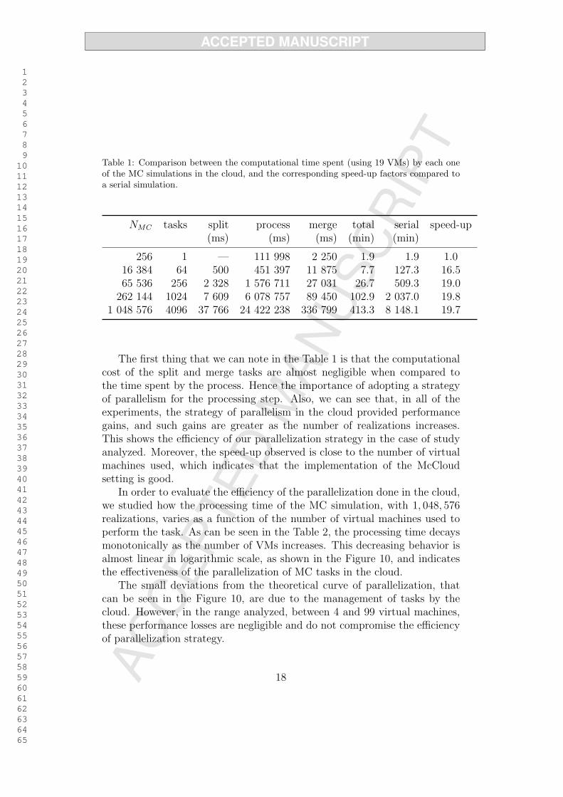
Table 1: Comparison between the computational time spent (using 19 VMs) by each oneof the MC simulations in the cloud, and the corresponding speed-up factors compared toa serial simulation.

NMC tasks split process merge total serial speed-up(ms) (ms) (ms) (min) (min)

256 1 — 111 998 2 250 1.9 1.9 1.016 384 64 500 451 397 11 875 7.7 127.3 16.565 536 256 2 328 1 576 711 27 031 26.7 509.3 19.0

262 144 1024 7 609 6 078 757 89 450 102.9 2 037.0 19.81 048 576 4096 37 766 24 422 238 336 799 413.3 8 148.1 19.7

The first thing that we can note in the Table 1 is that the computationalcost of the split and merge tasks are almost negligible when compared tothe time spent by the process. Hence the importance of adopting a strategyof parallelism for the processing step. Also, we can see that, in all of theexperiments, the strategy of parallelism in the cloud provided performancegains, and such gains are greater as the number of realizations increases.This shows the efficiency of our parallelization strategy in the case of studyanalyzed. Moreover, the speed-up observed is close to the number of virtualmachines used, which indicates that the implementation of the McCloudsetting is good.

In order to evaluate the efficiency of the parallelization done in the cloud,we studied how the processing time of the MC simulation, with 1, 048, 576realizations, varies as a function of the number of virtual machines used toperform the task. As can be seen in the Table 2, the processing time decaysmonotonically as the number of VMs increases. This decreasing behavior isalmost linear in logarithmic scale, as shown in the Figure 10, and indicatesthe effectiveness of the parallelization of MC tasks in the cloud.

The small deviations from the theoretical curve of parallelization, thatcan be seen in the Figure 10, are due to the management of tasks by thecloud. However, in the range analyzed, between 4 and 99 virtual machines,these performance losses are negligible and do not compromise the efficiencyof parallelization strategy.

18

1 2 3 4 5 6 7 8 9 10 11 12 13 14 15 16 17 18 19 20 21 22 23 24 25 26 27 28 29 30 31 32 33 34 35 36 37 38 39 40 41 42 43 44 45 46 47 48 49 50 51 52 53 54 55 56 57 58 59 60 61 62 63 64 65

Table 2: Comparison between the computational time spent (using 19 VMs) by each oneof the MC simulations in the cloud, and the corresponding speed-up factors compared toa serial simulation.

VMs split process merge total speed-up cost(ms) (ms) (ms) (min) (US$)

4 37 734 117 637 861 431 691 1968.5 4.0 17.155 34 062 99 041 631 354 791 1657.2 4.7 18.236 37 923 78 040 047 343 105 1307.0 6.0 17.397 36 982 66 989 658 348 603 1122.9 7.0 17.638 27 390 58 431 244 349 099 980.1 8.0 18.119 29 407 51 818 238 343 720 869.9 9.0 18.11

10 28 015 46 564 270 332 119 782.1 10.0 18.8311 28 734 42 192 535 334 432 709.3 11.0 17.9912 27 687 38 611 499 341 308 649.7 12.0 18.1113 34 874 36 039 896 334 806 606.8 12.9 19.5514 36 359 33 412 517 338 696 563.1 13.9 19.3115 36 499 31 199 806 343 874 526.3 14.8 18.8316 38 576 29 215 641 338 014 493.2 15.8 20.0317 40 484 27 406 752 340 522 463.1 16.8 19.1918 39 015 25 800 653 335 214 436.3 17.9 20.2719 37 766 24 422 238 336 799 413.3 18.9 19.0729 29 282 16 000 466 343 036 272.9 28.6 21.7139 29 547 11 927 263 346 594 205.1 38.0 24.2360 31 547 7 891 904 327 392 137.5 56.7 29.6380 25 328 5 900 347 33 709 99.3 78.5 29.6399 29 578 4 834 623 340 015 86.7 89.9 36.47

Table 2 also shows that the speed-up increases monotonically as the num-ber of VMs grows. This behavior can be better appreciated in the Figure 11,where the reader can verify that the values obtained for the speed-up arevery close to the theoretical values, that would be obtained if there were nodelays due to cloud management. The reader can note, also, that the mea-sured values The corresponding to larger numbers of VMs (60, 80 and 99) arefarther away from the theoretical reference. This occurs by the accumulation

19

1 2 3 4 5 6 7 8 9 10 11 12 13 14 15 16 17 18 19 20 21 22 23 24 25 26 27 28 29 30 31 32 33 34 35 36 37 38 39 40 41 42 43 44 45 46 47 48 49 50 51 52 53 54 55 56 57 58 59 60 61 62 63 64 65

100 101 102101

102

103

104

number of virtual machines

CP

Uti

me

(min

)

cloudtheoretical

Figure 10: CPU time of a MC simulation, with 1 048 576 realizations, as function of thenumbers of virtual machines.

of management delays, which are larger for a higher amount of VMs.

5.4. Costs analysis for the storage space

A comparison between the storage space used by each one of the MC sim-ulations in the cloud, and the financial cost associated with each simulationcan be seen in Table 3. In this table the column space represents the totalstorage space, in MB, temporarily used by the simulation, and the columncost represents the cost of this experiment in US dollars.

Observing the data in Table 3 we can see that our parallelization strategyused fairly little storage space, even for a large number of MC realizations.Additionally, the financial cost, even for the most complex simulation, is verysmall; which is a major advantage when compared to the costs of acquiringand maintaining a traditional cluster.

20

1 2 3 4 5 6 7 8 9 10 11 12 13 14 15 16 17 18 19 20 21 22 23 24 25 26 27 28 29 30 31 32 33 34 35 36 37 38 39 40 41 42 43 44 45 46 47 48 49 50 51 52 53 54 55 56 57 58 59 60 61 62 63 64 65

100 101 102100

101

102

number of virtual machines

Spee

d-up

measuredtheoretical

Figure 11: Speed-up of a MC simulation, with 1 048 576 realizations, as function of thenumbers of virtual machines.

Table 3: Comparison between the storage space used by each one of the MC simulationsin the cloud, and the financial cost associated with each simulation.

NMC space cost(MB) (US$)

16 384 12.4 5.3965 536 49.0 5.39

262 144 195.2 7.671 048 576 780.8 19.07

6. Concluding remarks

We present a strategy for parallelizing the Monte Carlo method in thecontext of cloud computing, using the fundamental idea of the MapReduce

21

1 2 3 4 5 6 7 8 9 10 11 12 13 14 15 16 17 18 19 20 21 22 23 24 25 26 27 28 29 30 31 32 33 34 35 36 37 38 39 40 41 42 43 44 45 46 47 48 49 50 51 52 53 54 55 56 57 58 59 60 61 62 63 64 65

paradigm. This strategy is described in detail and illustrated in the simula-tion of a simple problem of stochastic structural dynamics. The simulationresults show good accuracy for low-order statistics, low storage space usage,and that the performance gains increase with the number of Monte Carlorealizations. It was also illustrated that even a simple problem can requiremany realizations for the convergence of histograms, which makes the cloudcomputing strategy very attractive, due to its high scalability capacity andlow-cost. Thus, this article demonstrates that the advent of cloud comput-ing can become an important enabler for the adoption of the MC method tocompute the propagation of uncertainty in complex stochastic models.

Acknowledgments

The authors are indebted to the Brazilian agencies CNPq, CAPES, andFAPERJ for the financial support given to this research. By the free useof the Windows Azure platform, the authors are very grateful to MicrosoftCorporation. Also, they wish to thank the anonymous referee, for usefulcomments and suggestions.

References

[1] C. Soize, Random matrix theory for modeling uncertainties in com-putational mechanics, Computer Methods in Applied Mechanics andEngineering 194 (2005) 1333–1366. doi:10.1016/j.cma.2004.06.038.

[2] T. G. Ritto, R. Sampaio, Stochastic drill-string dynamics with un-certainty on the imposed speed and on the bit-rock parameters, In-ternational Journal for Uncertainty Quantification 2 (2012) 111–124.doi:10.1615/Int.J.UncertaintyQuantification.v2.i2.

[3] T. G. Ritto, M. R. Escalante, R. Sampaio, M. B. Rosales, Drill-stringhorizontal dynamics with uncertainty on the frictional force, Journal ofSound and Vibration 332 (2013) 145–153. doi:10.1016/j.jsv.2012.08.007.

[4] T. G. Ritto, C. Soize, R. Sampaio, Non-linear dynamics of adrill-string with uncertain model of the bit rock interaction, In-ternational Journal of Non-Linear Mechanics 44 (2009) 865–876.doi:10.1016/j.ijnonlinmec.2009.06.003.

22

1 2 3 4 5 6 7 8 9 10 11 12 13 14 15 16 17 18 19 20 21 22 23 24 25 26 27 28 29 30 31 32 33 34 35 36 37 38 39 40 41 42 43 44 45 46 47 48 49 50 51 52 53 54 55 56 57 58 59 60 61 62 63 64 65

[5] T. G. Ritto, R. Sampaio, F. Rochinha, Model uncertainties of flexiblestructures vibrations induced by internal flows, Journal of the Brazil-ian Society of Mechanical Sciences and Engineering 33 (2011) 373–380.doi:10.1590/S1678-58782011000300014.

[6] S. Zio, F. Rochinha, A stochastic collocation approach for uncer-tainty quantification in hydraulic fracture numerical simulation, In-ternational Journal for Uncertainty Quantification 2 (2012) 145–160.doi:10.1615/Int.J.UncertaintyQuantification.v2.i2.

[7] H. Lopes, J. Barcellos, J. Kubrusly, C. Fernandes, A non-parametricmethod for incurred but not reported claim reserve estimation, In-ternational Journal for Uncertainty Quantification 2 (2012) 39–51.doi:10.1615/Int.J.UncertaintyQuantification.v2.i1.40.

[8] A. Clement, C. Soize, J. Yvonnet, Uncertainty quantification in com-putational stochastic multiscale analysis of nonlinear elastic materials,Computer Methods in Applied Mechanics and Engineering 254 (2013)61–82. doi:10.1016/j.cma.2012.10.016.

[9] C. Soize, A comprehensive overview of a non-parametric probabilis-tic approach of model uncertainties for predictive models in struc-tural dynamics, Journal of Sound and Vibration 288 (2005) 623–652.doi:10.1016/j.jsv.2005.07.009.

[10] C. Soize, Stochastic modeling of uncertainties in computational struc-tural dynamics - Recent theoretical advances, Journal of Sound andVibration 332 (2013) 2379–2395. doi:10.1016/j.jsv.2011.10.010.

[11] N. Metropolis, S. Ulam, The Monte Carlo Method, Journal of the Amer-ican Statistical Association 44 (1949) 335–341. doi:10.2307/2280232.

[12] J. S. Liu, Monte Carlo Strategies in Scientific Computing, Springer,New York, 2001.

[13] R. W. Shonkwiler, F. Mendivil, Explorations in Monte Carlo Methods,Springer, New York, 2009.

[14] C. P. Robert, G. Casella, Monte Carlo Statistical Methods, Springer,New York, 2010.

23

1 2 3 4 5 6 7 8 9 10 11 12 13 14 15 16 17 18 19 20 21 22 23 24 25 26 27 28 29 30 31 32 33 34 35 36 37 38 39 40 41 42 43 44 45 46 47 48 49 50 51 52 53 54 55 56 57 58 59 60 61 62 63 64 65

[15] D. Xiu, G. E. Karniadakis, The Wiener-Askey Polynomial Chaos forstochastic differential equations, SIAM Journal on Scientific Computing24 (2002) 619–644. doi:10.1137/S1064827501387826.

[16] J. Dean, S. Ghemawat, MapReduce: Simplified data processing on largeclusters, in: OSDI, 2004.

[17] J. Shiers, Grid today, clouds on the horizon, Computer Physics Com-munications 180 (2009) 559–563. doi:10.1016/j.cpc.2008.11.027.

[18] I. Ari, N. Muhtaroglu, Design and implementation of a cloud computingservice for finite element analysis, Advances in Engineering Software 60-61 (2013) 122–135. doi:10.1016/j.advengsoft.2012.10.003.

[19] K. Jorissen, F. Vila, J. J. Rehr, A high performance scientific cloud com-puting environment for materials simulations, Computer Physics Com-munications 183 (2012) 1911–1919. doi:10.1016/j.cpc.2012.04.010.

[20] L. Wang, M. Kunze, J. Tao, G. von Laszewski, Towards building a cloudfor scientific applications, Advances in Engineering Software 42 (2011)714–722. doi:10.1016/j.advengsoft.2011.05.007.

[21] T. Velte, A. Velte, R. Elsenpeter, Cloud Computing, A Practical Ap-proach, McGraw-Hill Osborne Media, New York, 2009.

[22] D. Cearley, Hype Cycle for Application Development, Tech. Rep.G00147982, Gartner Group (2009).

[23] L. M. Vaquero, L. Rodero-Merino, J. Caceres, M. Lindner, A breakin the clouds: towards a cloud definition, Computer CommunicationReview 39 (2008) 50–55.

[24] R. Buyya, J. Broberg, A. M. Goscinski, Cloud computing: Principlesand paradigms.

[25] E. Roloff, M. Diener, A. Carissimi, P. O. A. Navaux, High perfor-mance computing in the cloud: Deployment, performance and costefficiency, in: Cloud Computing Technology and Science (Cloud-Com), 2012 IEEE 4th International Conference on, 2012, pp. 371–378.doi:10.1109/CloudCom.2012.6427549.

24

1 2 3 4 5 6 7 8 9 10 11 12 13 14 15 16 17 18 19 20 21 22 23 24 25 26 27 28 29 30 31 32 33 34 35 36 37 38 39 40 41 42 43 44 45 46 47 48 49 50 51 52 53 54 55 56 57 58 59 60 61 62 63 64 65

[26] R. Nasser, McCloud Service Framework: Development Services of MonteCarlo Simulation in the Cloud, M.Sc. Dissertation, Pontifıcia Universi-dade Catolica do Rio de Janeiro, Rio de Janeiro, (in portuguese) (2012).

[27] R. Nasser, A. Cunha Jr, H. Lopes, K. Breitman, R. Sampaio, McCloud:Easy and quick way to run Monte Carlo simulations in the cloud, (sub-mitted for publication) (2013).

[28] J. Bennett, R. Grout, P. Pebay, D. Roe, D. Thompson, Numericallystable, single-pass, parallel statistics algorithms, in: IEEE Interna-tional Conference on Cluster Computing and Workshops 2009, 2009.doi:10.1109/CLUSTR.2009.5289161.

[29] B. P. Welford, Note on a method for calculating correctedsums of squares and products, Technometric 4 (1962) 419–420.doi:10.1080/00401706.1962.10490022.

[30] D. E. Knuth, The Art of Computer Programming, volume 2: Seminu-merical Algorithms, 3rd Edition, Addison-Wesley, Boston, 1998.

[31] A. Cunha Jr, R. Sampaio, Effect of an attached end mass in the dy-namics of uncertainty nonlinear continuous random system, MecanicaComputacional 31 (2012) 2673–2683.

[32] A. Cunha Jr, R. Sampaio, Uncertainty propagation in the dynamicsof a nonlinear random bar, in: Proceedings of the XV InternationalSymposium on Dynamic Problems of Mechanics, 2013.

[33] A. Cunha Jr, R. Sampaio, Analysis of the nonlinear stochastic dynamicsof an elastic bar with an attached end mass, in: Proceedings of the IIISouth-East Conference on Computational Mechanics, 2013.

[34] A. Cunha Jr, R. Sampaio, On the nonlinear stochastic dynamics ofa continuous system with discrete attached elements, (submitted forpublication) (2013).

[35] T. J. R. Hughes, The Finite Element Method, Dover Publications,New York, 2000.

[36] N. Newmark, A method of computation for structural dynamics, Journalof the Engineering Mechanics Division 85 (1959) 67–94.

25

1 2 3 4 5 6 7 8 9 10 11 12 13 14 15 16 17 18 19 20 21 22 23 24 25 26 27 28 29 30 31 32 33 34 35 36 37 38 39 40 41 42 43 44 45 46 47 48 49 50 51 52 53 54 55 56 57 58 59 60 61 62 63 64 65

[37] C. Soize, A nonparametric model of random uncertainties for reducedmatrix models in structural dynamics, Probabilistic Engineering Me-chanics 15 (2000) 277 – 294. doi:10.1016/S0266-8920(99)00028-4.

[38] C. Shannon, A mathematical theory of communication, Bell SystemTechnical Journal 27 (1948) 379– 423.

[39] E. T. Jaynes, Information theory and statistical mechanics, PhysicalReview Series II 106 (1957) 620–630. doi:10.1103/PhysRev.106.620.

[40] E. T. Jaynes, Information theory and statistical mechanics II, PhysicalReview Series II 108 (1957) 171–190. doi:10.1103/PhysRev.108.171.

[41] P. Spanos, A. Kontsos, A multiscale Monte Carlo finite elementmethod for determining mechanical properties of polymer nanocom-posites, Probabilistic Engineering Mechanics 23 (2008) 456–470.doi:10.1016/j.probengmech.2007.09.002.

[42] B. Liang, S. Mahadevan, Error and uncertainty quantification andsensitivity analysis in mechanics computational models, Interna-tional Journal for Uncertainty Quantification 1 (2011) 147–161.doi:10.1615/IntJUncertaintyQuantification.v1.i2.30.

[43] S. Murugan, R. Chowdhury, S. Adhikari, M. Friswell, Helicopter aeroe-lastic analysis with spatially uncertain rotor blade properties, AerospaceScience and Technology 16 (2012) 29 –39. doi:10.1016/j.ast.2011.02.004.

26