(2013) Andean-scale highlands in the Late Cretaceous Cordillera of the North American western margin

(This is a sample cover image for this issue. The actual cover is not yet available at this time.)

This article appeared in a journal published by Elsevier. The attachedcopy is furnished to the author for internal non-commercial researchand education use, including for instruction at the authors institution

and sharing with colleagues.

Other uses, including reproduction and distribution, or selling orlicensing copies, or posting to personal, institutional or third party

websites are prohibited.

In most cases authors are permitted to post their version of thearticle (e.g. in Word or Tex form) to their personal website orinstitutional repository. Authors requiring further information

regarding Elsevier’s archiving and manuscript policies areencouraged to visit:

http://www.elsevier.com/copyright

http://www.elsevier.com/copyright

Author's personal copy

Andean-scale highlands in the Late Cretaceous Cordillera of the NorthAmerican western margin

Jacob O. Sewall a,n, Henry C. Fricke b

a Department of Physical Sciences, Kutztown University, Kutztown, PA 19530, USAb Department of Geology, Colorado College, Colorado Springs, CO 80903, USA

a r t i c l e i n f o

Article history:

Received 5 January 2012

Received in revised form

20 November 2012

Accepted 1 December 2012

Editor: J. Lynch-Stieglitz

Keywords:

North American Cordillera

paleoelevation

Campanian

Sevier

Cretaceous

climate modeling

a b s t r a c t

From the Late Jurassic through the Cretaceous, collision between the North American and Farallon

plates drove extensive thin-skinned thrusting and crustal shortening that resulted in substantial relief

in the North American Cordillera. The elevation history of this region is tightly linked to the tectonic,

climatic and landscape evolution of western North America but is not well constrained. Here we use an

atmospheric general circulation model with integrated oxygen isotope tracers (isoCAM3) to predict

how isotope ratios of precipitation would change along the North American Cordillera as the mean

elevation of orogenic highlands increased from 1200 m to 3975 m. With increases in mean elevation,

highland temperatures fall, monsoonal circulation along the eastern front of the Cordillera is enhanced,

and wet season (generally spring and summer) precipitation increases. Simulated oxygen isotopic

ratios in that precipitation are compared to those obtained from geologic materials (e.g. fossil bivalves,

authigenic minerals). Quantification of match between model and data-derived d18O values suggests

that during the Late Cretaceous, the best approximation of regional paleoelevation in western North

America is a large orogen on the scale of the modern Andes Mountains with a mean elevation

approaching 4000 m and a north-south extent of at least 151 of latitude.

& 2012 Elsevier B.V. All rights reserved.

1. Introduction

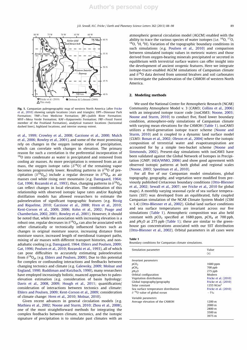
Throughout the Cretaceous, subduction of the Farallon plateunder North America drove broad regional folding and thrusting inthe western craton (DeCelles, 2004). This prolonged deformationalevent is termed the Sevier orogeny; it was characterized by crustalshortening of up to 75% (DeCelles and Coogan, 2006) and producednorth-south trending structures and topography along the westernmargin of North America from Alaska to Mexico (DeCelles, 2004).By the Campanian (�75 Ma), fluvial transport and deposition ofsediments from the growing orogeny had resulted in extensiveforeland basin filling and development of a broad, low-reliefcoastal plain separating the highlands in the west from theWestern Interior Seaway to the east (Aschoff and Steel, 2011;DeCelles, 2004; Roberts and Kirschbaum, 1995; Fig. 1).

While the deformation style, regional extent and horizontaltranslation of crustal material in the Cordilleran (Sevier) fold andthrust belt are relatively well documented (e.g. Burchfiel andDavis, 1972; Currie, 2002; DeCelles and Coogan, 2006; DeCelles,2004; Elison; 1991; Friedrich and Bartley, 2003; Hudec and Davis,1989; Weil et al., 2010), the actual elevation of the resulting

Campanian-age orogenic highlands (hereafter CAMOH) and theareal extent of the CAMOH are less well-constrained. Never-theless, it is crucial to obtain such information because of theinfluence that the elevation of this orogen may have had on theclimatic, tectonic, and landscape evolution of the North AmericanCordillera.

At a global or hemispheric scale, increased elevation can resultin changes in the planetary wave pattern or albedo and significantreorganizations of climate (e.g. Broccoli and Manabe, 1992;Ruddiman and Kutzbach, 1989). At local and regional scales,increased elevation results in surface cooling as a result of theadiabatic lapse rate and changes in net moisture balance as aresult of disrupted atmospheric circulation and/or the develop-ment of rain shadows and enhanced orographic precipitation (e.g.Drummond et al., 1996; Ehlers and Poulsen, 2009; Fricke et al.,2010; Poulsen et al., 2010; Zaleha, 2006) as well as a host of other,resultant feedbacks (e.g. increased albedo of higher, colder, dryer,less-vegetated surfaces). In turn, climatic conditions may influ-ence rates of uplift and rock exhumation (e.g. Reiners et al. 2003;Wobus et al., 2003) and foreland basin subsidence and infilling(e.g. Zaleha, 2006).

A number of different methods have been developed to studythe paleoelevation of ancient mountain belts (e.g. rock mechanics:DeCelles and Coogan, 2006; leaf physiognomy: Gregory and Chase,1992; Wolfe et al., 1998; stable isotope paleoaltimetry: Chamberlain

Contents lists available at SciVerse ScienceDirect

journal homepage: www.elsevier.com/locate/epsl

Earth and Planetary Science Letters

0012-821X/$ - see front matter & 2012 Elsevier B.V. All rights reserved.

http://dx.doi.org/10.1016/j.epsl.2012.12.002

n Corresponding author. Tel.: þ1 484 646 5864; fax: þ1 610 683 1352.

E-mail address: [email protected] (J.O. Sewall).

Earth and Planetary Science Letters 362 (2013) 88–98


et al., 1999; Crowley et al., 2008; Garzione et al., 2000; Mulchet al., 2006; Rowley et al., 2001), and some of the most promisingrely on changes in the oxygen isotope ratios of precipitation,which can correlate with changes in elevation. The primaryreason for such a correlation is the preferential incorporation of18O into condensate as water is precipitated and removed fromcooling air masses. As more precipitation is removed from an airmass, the oxygen isotope ratio (d18O) of the remaining vaporbecomes progressively lower. Resulting patterns in d18O of pre-cipitation (d18Opt) include a regular decrease in d18Opt as airmasses cool while rising over mountains (e.g. Dansgaard, 1964;Gat, 1996; Rozanski et al., 1993), thus, changing patterns in d18Opt

can reflect changes in local elevation. The combination of thisrelationship with observed isotopic lapse rates and/or Rayleighdistillation models has allowed researchers to estimate thepaleoelevation of significant topographic features (e.g. Bissigand Riquelme, 2010; Garzione et al., 2008; Hren et al., 2010;Kent-Corson et al., 2009, 2006; Kohn et al., 2002; Poage andChamberlain, 2002, 2001; Rowley et al., 2001). However, it shouldbe noted that, while the association with increasing elevation is arobust one, regular decreases in d18Opt can also be associated withother climatically or tectonically influenced factors such aschanges in original moisture source, increasing distance frommoisture source, increased length of meridional transport paths,mixing of air masses with different transport histories, and non-adiabatic cooling (e.g. Dansgaard, 1964; Ehlers and Poulsen, 2009;Gat, 1996; Poulsen et al., 2010; Rozanski et al., 1993), all of whichcan pose difficulties to accurately estimating paleoelevationfrom d18Opt (e.g. Ehlers and Poulsen, 2009). Due to this potentialfor complex or confounding interactions and feedbacks betweenchanging tectonics and climate (e.g. Galewsky, 2009; Molnar andEngland, 1990; Ruddiman and Kutzbach, 1990), many researchershave employed increasingly holistic, nuanced approaches to paleo-elevation estimation (e.g. consideration of basin hydrology:Davis et al., 2008, 2009; Hough et al., 2011; quantification/consideration of interactions between tectonics and climate:Ehlers and Poulsen, 2009; Kent-Corson et al., 2009; considerationof climate change: Hren et al., 2010; Molnar, 2010).

Given recent advances in general circulation models (e.g.Mathieu et al., 2002; Noone and Sturm, 2010; Zhou et al., 2008),one of the most straightforward methods for integrating thecomplex feedbacks between climate, tectonics, and the isotopicsignature of precipitation is to simulate past climates with an

atmospheric general circulation model (AGCM) enabled with theability to trace the various species of water isotopes (i.e. 16O, 17O,18O, 1H, 2H). Variation of the topographic boundary conditions insuch simulations (e.g. Poulsen et al., 2010) and comparisonbetween simulated isotopic values in meteoric waters and thosederived from oxygen-bearing minerals precipitated or secreted inequilibrium with terrestrial surface waters can offer insight intothe development of ancient orogenic features. Here we integrateisotope-tracer-enabled AGCM simulations of Campanian climateand d18O data derived from unionid bivalves and soil carbonatesto investigate the paleoelevation of the CAMOH of western NorthAmerica.

2. Modeling methods

We used the National Center for Atmospheric Research (NCAR)Community Atmosphere Model v. 3 (CAM3; Collins et al., 2006)with an integrated isotope tracer code (isoCAM3; Noone, 2003;Noone and Sturm, 2010) to conduct five, fixed lower boundarycondition, atmosphere-only simulations of Campanian climatewith varying mean elevations for the CAMOH (Table 1). isoCAM3utilizes a third-generation isotope tracer scheme (Noone andSturm, 2010) and is coupled to a dynamic land surface model(CLM3: Bonan et al., 2002; Oleson et al., 2004) where the isotopiccomposition of terrestrial water and evapotranspiration areaccounted for by a simple two-bucket scheme (Noone andSimmonds, 2002). Present-day simulations with isoCAM3 havebeen validated against the Global Network of Isotopes in Precipi-tation (GNIP; IAEA/WMO, 2006) and show good agreement withobserved isotopic patterns at both global and regional scales(Noone, 2003; Speelman et al., 2010).

For all five of our Campanian model simulations, globaltopography, geography, and vegetation were modified from pre-viously published Cretaceous boundary conditions (Otto-Bliesneret al., 2002; Sewall et al., 2007; see Fricke et al., 2010 for globalmaps). A monthly varying seasonal cycle of sea surface tempera-tures (SST) was developed from an equilibrated, fully coupledCampanian simulation of the NCAR Climate System Model (CSMv. 1.4) (Otto-Bliesner et al., 2002). Global land surface conditionsand sea surface temperatures are invariant across our fivesimulations (Table 1). Atmospheric composition was also heldconstant with pCO2 specified at 1680 ppm, pCH4 at 700 ppb,and pN2O at 275 ppb (Table 1); these are similar to the green-house gas concentrations associated with our SST distribution(Otto-Bliesner et al., 2002). Orbital parameters in all cases were

Fig. 1. Campanian paleogeographic map of western North America (after Fricke

et al., 2010) showing sample locations (stars and triangles; DPF¼Dinosaur Park

Formation; TMF¼Two Medicine Formation; JRF¼ Judith River Formation;

MVF¼Mesa Verde Formation; KAF¼Kaiparowits Formation; FRF¼Fossil Forest

member of the Fruitland Formation), analytical transect locations (horizontal

dashed lines), highland locations, and interior seaway extent.

Table 1Boundary conditions for Campanian climate simulations.

Simulation parameter Value

(s)

Invariant parameters

pCO2 1680 ppm

pCH4 700 ppb

pN2O 275 ppb

Orbital configuration Modern

Vegetation distribution Fricke et al. (2010)

Global topography/geography Fricke et al. (2010)

Solar constant 1355 W/m2

Sea surface temperature distribution Fricke et al. (2010)

d 18O value of global ocean �1%

Variable parameters

Average elevation of the CAMOH 1200 m

2000 m

2800 m

3500 m

3975 m

J.O. Sewall, H.C. Fricke / Earth and Planetary Science Letters 362 (2013) 88–98 89


specified at modern values and the solar constant was reduced to1355 W/m2 (Table 1). isoCAM3 was set up to simulate the H2Oand H2

18O content in both precipitation and water vapor with afixed, ice-free global ocean value of �1% d18O for all simulations(Table 1). All simulations were conducted with 26 vertical levelsin the atmosphere and a horizontal resolution of spectral T42(�2.81 latitude�2.81 longitude).

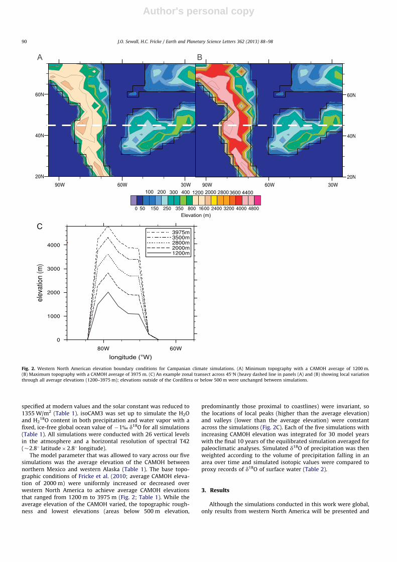
The model parameter that was allowed to vary across our fivesimulations was the average elevation of the CAMOH betweennorthern Mexico and western Alaska (Table 1). The base topo-graphic conditions of Fricke et al. (2010; average CAMOH eleva-tion of 2000 m) were uniformly increased or decreased overwestern North America to achieve average CAMOH elevationsthat ranged from 1200 m to 3975 m (Fig. 2; Table 1). While theaverage elevation of the CAMOH varied, the topographic rough-ness and lowest elevations (areas below 500 m elevation,

predominantly those proximal to coastlines) were invariant, sothe locations of local peaks (higher than the average elevation)and valleys (lower than the average elevation) were constantacross the simulations (Fig. 2C). Each of the five simulations withincreasing CAMOH elevation was integrated for 30 model yearswith the final 10 years of the equilibrated simulation averaged forpaleoclimatic analyses. Simulated d18O of precipitation was thenweighted according to the volume of precipitation falling in anarea over time and simulated isotopic values were compared toproxy records of d18O of surface water (Table 2).

3. Results

Although the simulations conducted in this work were global,only results from western North America will be presented and

Fig. 2. Western North American elevation boundary conditions for Campanian climate simulations. (A) Minimum topography with a CAMOH average of 1200 m.

(B) Maximum topography with a CAMOH average of 3975 m. (C) An example zonal transect across 451N (heavy dashed line in panels (A) and (B) showing local variation

through all average elevations (1200–3975 m); elevations outside of the Cordillera or below 500 m were unchanged between simulations.

J.O. Sewall, H.C. Fricke / Earth and Planetary Science Letters 362 (2013) 88–9890


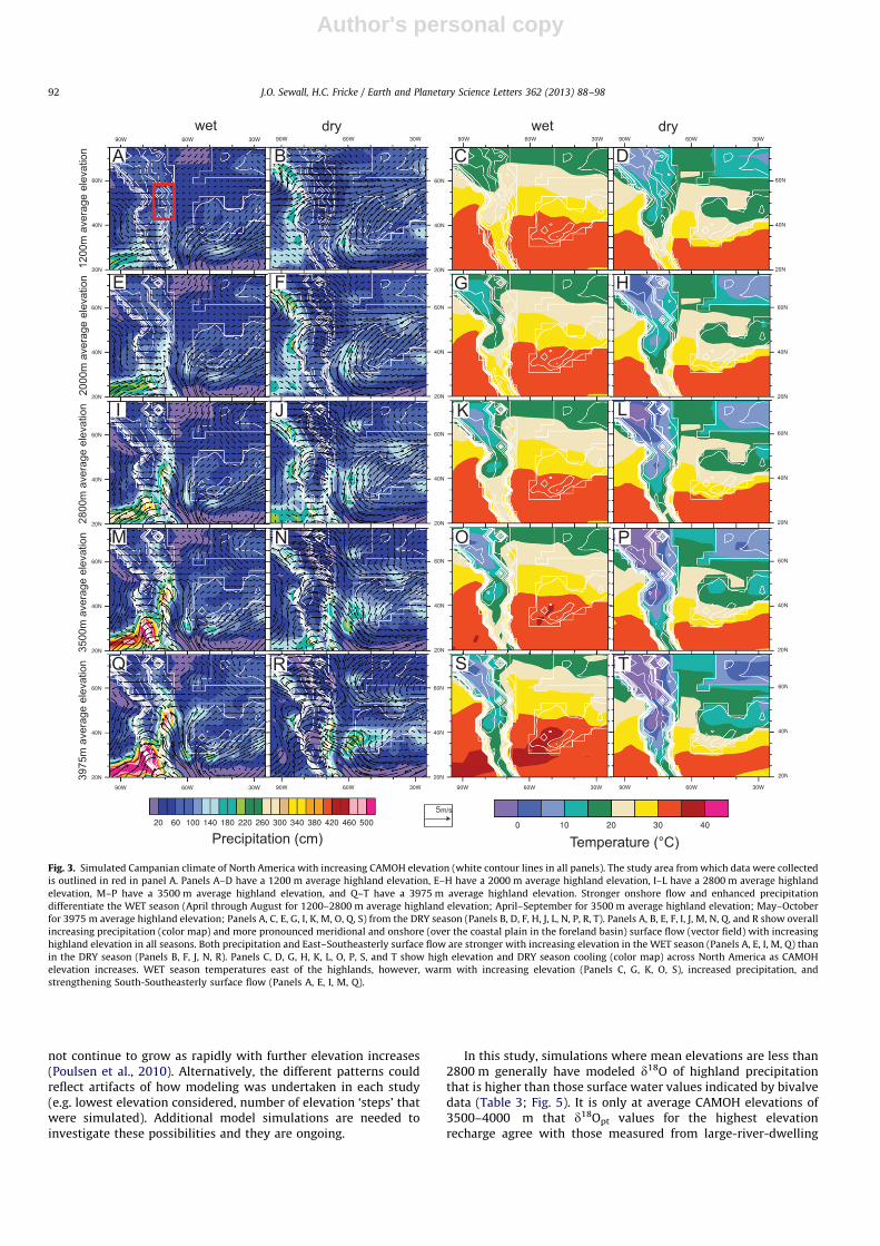
discussed here (see inset boxes in Figs. 3A and 4). Furthermore, asthe study region exhibited pronounced precipitation seasonalityin all simulations, we present not only annual averaged results,but also wet and dry season averages. The wet season is definedas all individual months during which 48% of the annualprecipitation falls and is associated with generally onshore atmo-spheric flow of water-laden air masses from the interior seawaytoward the foreland (Fig. 3). The dry season, associated withgenerally offshore atmospheric flow, constitutes the remainder ofthe year. With increasing CAMOH elevation, the duration andintensity of this seasonally reversing (i.e. monsoonal) circulationincreased while the time of the year at which the seasonalreversal took place gradually became later (Fig. 3).

In addition to affecting the duration, intensity, and timing ofthe regional monsoon, increasing highland elevation causedtemperatures over the highlands to fall from �22 to �15 1Cduring the wet season and from �15 to �0 1C during the dryseason (Fig. 3). Coastal plain temperatures, however, change onlyslightly from �22 to �27 1C as highland elevations increase(Fig. 3). Rising highlands also lead to an increase in precipitation,particularly during the wet season, with amounts along theeastern CAMOH front increasing from as little as 60 cm to over400 cm (Fig. 3) over the entire foreland basin.

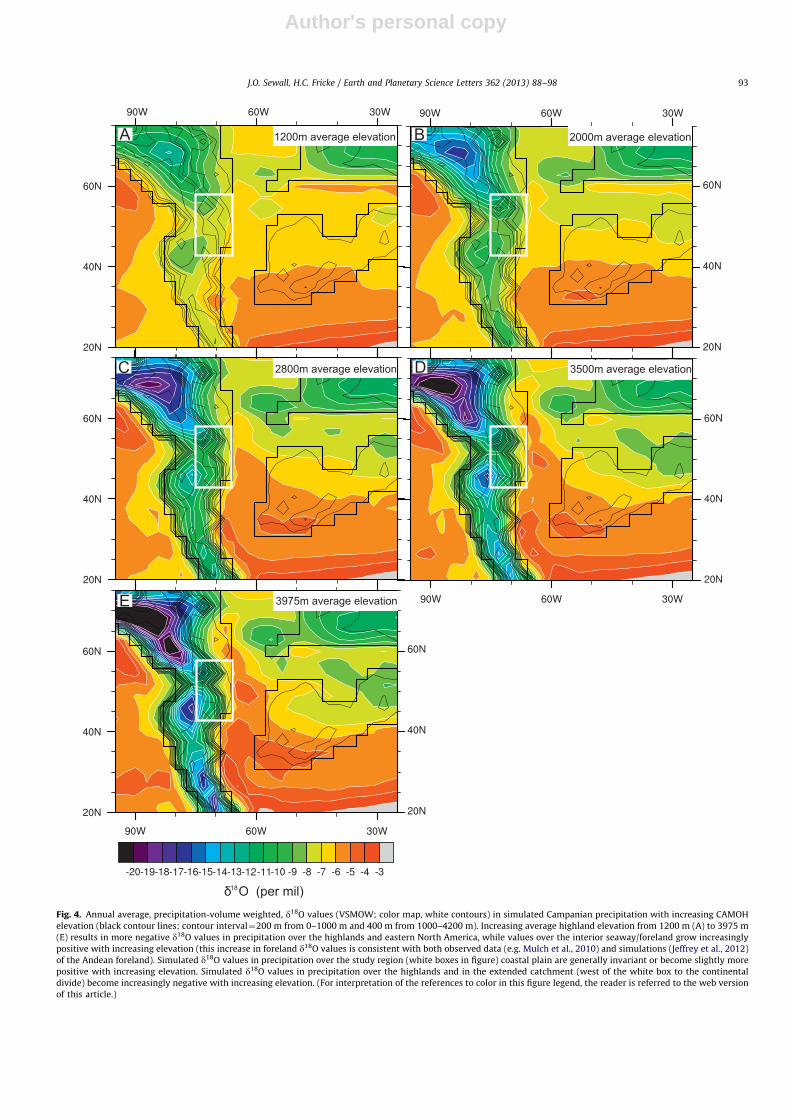
Annual average simulated d18O values (VSMOW) for precipita-tion are presented in map view in Fig. 4 and as latitudinaltransects in Fig. 5. As highland elevation increases, d18O ofprecipitation falling in or feeding into highland areas of the studyregion becomes lighter, moving from ��8% (Figs. 4A; 5; Table 3)to as low as �18% (Figs. 4E; 5; Table 3). d18O of precipitationin coastal regions o500 m in elevation is ��7.5% and onlyvaries 7�1% in response to changes in highland elevations(Figs. 4 and 5; Table 3). Similar elevation-related changes in d18Oof precipitation are simulated for wet and dry seasons, with d18Ovalues during the wet season being more positive than the annualaverage, and d18O of precipitation during the dry season beingsomewhat more negative (Table 3).

4. Discussion

Modeled d18O of precipitation varies over a wide region inresponse to increasing mean elevation of the CAMOH. Integratingthese variations with an isotopic record of Late Cretaceousprecipitation from the study area allows us to investigate thepaleotopography of the CAMOH. Proxy records of d18O of surface

water are available for a number of Campanian foreland basinlocalities that span paleolatitudes from 42–571N (Fig. 1), but thefocus of our analysis is on three latitudinal transects (45, 54 and56.51N) where the most oxygen isotope data are available. At eachlocality, bulk samples of unionid bivalves and soil carbonateswere taken, and estimates of d18O of associated surface waterswere made (Dettman and Lohmann, 2000; Fricke et al., 2010).Paleosol nodules and bivalves from ponds and small streamsproduce estimates of surface water d18O with mean valuesof��8% (Table 2; Fig. 5), and these waters are interpreted torepresent small, coastal plain catchments that were recharged bylocal precipitation from air masses that had not traveled far fromthe moisture source (the interior seaway). In contrast, bivalvesfound in large river deposits cluster at a much lower mean valueof ��17% (Table 2; Fig. 5), indicating a larger degree of isotopicrainout and suggesting that high elevation catchments were thedominant source of recharge for major river systems crossing theforeland basin (e.g. Fricke et al., 2010). The relatively constantoffset of�9% between the estimated d18O of coastal plain surfacewaters and those from higher elevations is compared to simulatedvalues to provide constraints on the elevation and extent ofthe CAMOH.

4.1. Model-data comparisons and paleoelevation

As noted above, we focus our analysis on three latitudinaltransects that cover the area where carbonate data were obtained.We also focus on annual d18Opt simulated by the model becauseof the strong relationship between the mean d18O of fluvialwaters and d18O from bulk samples of unionid bivalve shells(Kohn and Dettman, 2007).

Along the coastal plain (o500 m,�671W), where orography isconstant and wet season air masses move primarily from east towest in all simulations (Fig. 3), modeled d18Opt is relativelyinvariant regardless of latitude or elevation of the adjacent high-lands and matches d18O of surface waters inferred from bivalvesand soil carbonates relatively well (Table 3; Fig. 5). Modeledd18Opt values for high elevation precipitation, however, decreasesteadily with increasing highland elevation. The magnitude of thisdecrease is not regionally constant, with greater decreases in d18Oof precipitation occurring along transects with the highest aver-age elevation (Fig. 5). This pattern emphasizes the role of eleva-tion in cooling air masses, initiating precipitation (precipitation[total, large-scale, and convective] increases linearly [r2

¼0.97]with increasing elevation [not shown]), and progressively remov-ing 18O from the atmosphere. Although we do find the greatestchanges in d18Opt when CAMOH elevations reach 72000m(Fig. 5) and find that the particular elevation gain that engendersthe greatest change in d18Opt varies meridionally along themountain belt (e.g. Fig. 5A and C), our results suggest a moreuniform decrease in d18Opt with increasing elevation than thatobserved in similar modeling studies of the Andes Mountains(Insel et al., 2012; Poulsen et al., 2010). The different patternssimulated in these two regions could reflect real differences inhow climate, d18Opt, and topography relate in these two differentsituations. For example, the progressive increases in precipitationand consequent reduction in d18Opt that we simulate mayindicate stable atmospheric conditions where only forced liftingand cooling of air masses at the local lapse rate contributes toincreased precipitation. Given the approximately linear tropo-spheric lapse rate, this would result in a linear precipitationresponse. Conversely, thresholded behavior in Andean simula-tions (Insel et al., 2012; Poulsen et al., 2010) could reflect moreunstable atmospheric conditions where imposed elevationincreases can force air parcels above the level of free convectionand drive sudden, non-linear increases in precipitation that do

Table 2

Proxy-derived estimates of Campanian surface water d18O (VSMOW scale) in

Western North America (after Fricke et al., 2010).

Formationa Depositional

environment

Sample

size

Mean Median Range

(max/min)

(%) (%) (%)

DPFb,c Large river 128 �17.272.8 �17.0 �14.8/ �21.3

TMFb Stream 7 �8.671.5 �8.8 �7.6/ �9.7

TMFb Soil (at 24 1C) 13 �8.271.1 �8.1 �7.0/ �9.1

JRFb Pond 6 �7.671.0 �7.4 �7.2/ �8.3

JRFb Large river 19 �16.272.8 �16.2 �13.5/ �18.7

MVFb Stream 3 �14.771.5 �14.7 �14.0/ �15.5

KAFb Pond 6 �8.270.9 �8.0 �7.8/ �8.9

KAFb Large river 8 �16.270.5 �16.2 �16.0/ �16.7

FRFd Stream 11 �7.671.7 �7.6 �4.5/ �9.8

a See Fig. 1 for formation abbreviations.b Information presented in Fricke et al. (2010).c Includes bivalve data originally presented in Dettman and Lohmann (2000).d Bulk samples of unionid bivalves. d18O of surface water calculated as in Fricke

et al. (2010).



not continue to grow as rapidly with further elevation increases(Poulsen et al., 2010). Alternatively, the different patterns couldreflect artifacts of how modeling was undertaken in each study(e.g. lowest elevation considered, number of elevation ‘steps’ thatwere simulated). Additional model simulations are needed toinvestigate these possibilities and they are ongoing.

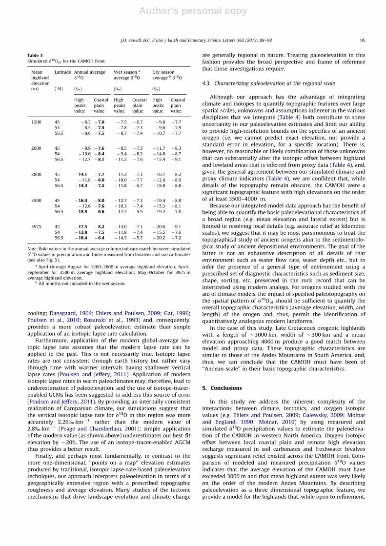
In this study, simulations where mean elevations are less than2800 m generally have modeled d18O of highland precipitationthat is higher than those surface water values indicated by bivalvedata (Table 3; Fig. 5). It is only at average CAMOH elevations of3500–4000 m that d18Opt values for the highest elevationrecharge agree with those measured from large-river-dwelling

Fig. 3. Simulated Campanian climate of North America with increasing CAMOH elevation (white contour lines in all panels). The study area from which data were collected

is outlined in red in panel A. Panels A–D have a 1200 m average highland elevation, E–H have a 2000 m average highland elevation, I–L have a 2800 m average highland

elevation, M–P have a 3500 m average highland elevation, and Q–T have a 3975 m average highland elevation. Stronger onshore flow and enhanced precipitation

differentiate the WET season (April through August for 1200–2800 m average highland elevation; April–September for 3500 m average highland elevation; May–October

for 3975 m average highland elevation; Panels A, C, E, G, I, K, M, O, Q, S) from the DRY season (Panels B, D, F, H, J, L, N, P, R, T). Panels A, B, E, F, I, J, M, N, Q, and R show overall

increasing precipitation (color map) and more pronounced meridional and onshore (over the coastal plain in the foreland basin) surface flow (vector field) with increasing

highland elevation in all seasons. Both precipitation and East–Southeasterly surface flow are stronger with increasing elevation in the WET season (Panels A, E, I, M, Q) than

in the DRY season (Panels B, F, J, N, R). Panels C, D, G, H, K, L, O, P, S, and T show high elevation and DRY season cooling (color map) across North America as CAMOH

elevation increases. WET season temperatures east of the highlands, however, warm with increasing elevation (Panels C, G, K, O, S), increased precipitation, and

strengthening South-Southeasterly surface flow (Panels A, E, I, M, Q).



Fig. 4. Annual average, precipitation-volume weighted, d18O values (VSMOW; color map, white contours) in simulated Campanian precipitation with increasing CAMOH

elevation (black contour lines; contour interval¼200 m from 0–1000 m and 400 m from 1000–4200 m). Increasing average highland elevation from 1200 m (A) to 3975 m

(E) results in more negative d18O values in precipitation over the highlands and eastern North America, while values over the interior seaway/foreland grow increasingly

positive with increasing elevation (this increase in foreland d18O values is consistent with both observed data (e.g. Mulch et al., 2010) and simulations (Jeffrey et al., 2012)

of the Andean foreland). Simulated d18O values in precipitation over the study region (white boxes in figure) coastal plain are generally invariant or become slightly more

positive with increasing elevation. Simulated d18O values in precipitation over the highlands and in the extended catchment (west of the white box to the continental

divide) become increasingly negative with increasing elevation. (For interpretation of the references to color in this figure legend, the reader is referred to the web version

of this article.)



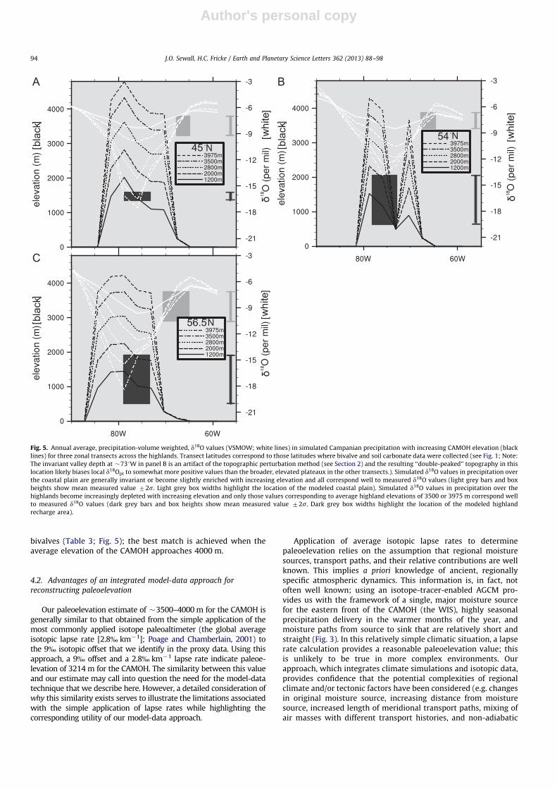
bivalves (Table 3; Fig. 5); the best match is achieved when theaverage elevation of the CAMOH approaches 4000 m.

4.2. Advantages of an integrated model-data approach for

reconstructing paleoelevation

Our paleoelevation estimate of �3500–4000 m for the CAMOH isgenerally similar to that obtained from the simple application of themost commonly applied isotope paleoaltimeter (the global averageisotopic lapse rate [2.8% km�1]; Poage and Chamberlain, 2001) tothe 9% isotopic offset that we identify in the proxy data. Using thisapproach, a 9% offset and a 2.8% km�1 lapse rate indicate paleoe-levation of 3214 m for the CAMOH. The similarity between this valueand our estimate may call into question the need for the model-datatechnique that we describe here. However, a detailed consideration ofwhy this similarity exists serves to illustrate the limitations associatedwith the simple application of lapse rates while highlighting thecorresponding utility of our model-data approach.

Application of average isotopic lapse rates to determinepaleoelevation relies on the assumption that regional moisturesources, transport paths, and their relative contributions are wellknown. This implies a priori knowledge of ancient, regionallyspecific atmospheric dynamics. This information is, in fact, notoften well known; using an isotope-tracer-enabled AGCM pro-vides us with the framework of a single, major moisture sourcefor the eastern front of the CAMOH (the WIS), highly seasonalprecipitation delivery in the warmer months of the year, andmoisture paths from source to sink that are relatively short andstraight (Fig. 3). In this relatively simple climatic situation, a lapserate calculation provides a reasonable paleoelevation value; thisis unlikely to be true in more complex environments. Ourapproach, which integrates climate simulations and isotopic data,provides confidence that the potential complexities of regionalclimate and/or tectonic factors have been considered (e.g. changesin original moisture source, increasing distance from moisturesource, increased length of meridional transport paths, mixing ofair masses with different transport histories, and non-adiabatic

Fig. 5. Annual average, precipitation-volume weighted, d18O values (VSMOW; white lines) in simulated Campanian precipitation with increasing CAMOH elevation (black

lines) for three zonal transects across the highlands. Transect latitudes correspond to those latitudes where bivalve and soil carbonate data were collected (see Fig. 1; Note:

The invariant valley depth at �731W in panel B is an artifact of the topographic perturbation method (see Section 2) and the resulting ‘‘double-peaked’’ topography in this

location likely biases local d18Opt to somewhat more positive values than the broader, elevated plateaux in the other transects.). Simulated d18O values in precipitation over

the coastal plain are generally invariant or become slightly enriched with increasing elevation and all correspond well to measured d18O values (light grey bars and box

heights show mean measured value 72s. Light grey box widths highlight the location of the modeled coastal plain). Simulated d18O values in precipitation over the

highlands become increasingly depleted with increasing elevation and only those values corresponding to average highland elevations of 3500 or 3975 m correspond well

to measured d18O values (dark grey bars and box heights show mean measured value 72s. Dark grey box widths highlight the location of the modeled highland

recharge area).



cooling; Dansgaard, 1964; Ehlers and Poulsen, 2009; Gat, 1996;Poulsen et al., 2010; Rozanski et al., 1993) and, consequently,provides a more robust paleoelevation estimate than simpleapplication of an isotopic lapse rate calculation.

Furthermore, application of the modern global-average iso-topic lapse rate assumes that the modern lapse rate can beapplied to the past. This is not necessarily true. Isotopic lapserates are not consistent through earth history but rather varythrough time with warmer intervals having shallower verticallapse rates (Poulsen and Jeffery, 2011). Application of modernisotopic lapse rates in warm paleoclimates may, therefore, lead tounderestimation of paleoelevation, and the use of isotope-tracer-enabled GCMs has been suggested to address this source of error(Poulsen and Jeffery, 2011). By providing an internally consistentrealization of Campanian climate, our simulations suggest thatthe vertical isotopic lapse rate for d18O in this region was moreaccurately 2.26% km�1 rather than the modern value of2.8% km�1 (Poage and Chamberlain, 2001); simple applicationof the modern value (as shown above) underestimates our best-fitelevation by �20%. The use of an isotope-tracer-enabled AGCMthus provides a better result.

Finally, and perhaps most fundamentally, in contrast to themore one-dimensional, ‘‘points on a map’’ elevation estimatesproduced by traditional, isotopic lapse-rate-based paleoelevationtechniques, our approach interprets paleoelevation in terms of ageographically extensive region with a prescribed topographicroughness and average elevation. Many studies of the tectonicmechanisms that drive landscape evolution and climate change

are generally regional in nature. Treating paleoelevation in thisfashion provides the broad perspective and frame of referencethat those investigations require.

4.3. Characterizing paleoelevation at the regional scale

Although our approach has the advantage of integratingclimate and isotopes to quantify topographic features over largespatial scales, unknowns and assumptions inherent in the variousdisciplines that we integrate (Table 4) both contribute to someuncertainty in our paleoelevation estimates and limit our abilityto provide high-resolution bounds on the specifics of an ancientorogen (i.e. we cannot predict exact elevation, nor provide astandard error in elevation, for a specific location). There is,however, no reasonable or likely combination of those unknownsthat can substantially alter the isotopic offset between highlandand lowland areas that is inferred from proxy data (Table 4), and,given the general agreement between our simulated climate andproxy climate indicators (Table 4), we are confident that, whiledetails of the topography remain obscure, the CAMOH were asignificant topographic feature with high elevations on the orderof at least 3500–4000 m.

Because our integrated model-data approach has the benefit ofbeing able to quantify the basic paleoelevational characteristics ofa broad region (e.g. mean elevation and lateral extent) but islimited in resolving local details (e.g. accurate relief at kilometerscales), we suggest that it may be most parsimonious to treat thetopographical study of ancient orogens akin to the sedimentolo-gical study of ancient depositional environments. The goal of thelatter is not an exhaustive description of all details of thatenvironment such as water flow rate, water depth etc., but toinfer the presence of a general type of environment using aprescribed set of diagnostic characteristics such as sediment size,shape, sorting, etc. preserved in the rock record that can beinterpreted using modern analogs. For orogens studied with theaid of climate models, the impact of specified paleotopography onthe spatial pattern of d18Opt should be sufficient to quantify theoverall topographic characteristics (average elevation, width, andlength) of the orogen and, thus, permit the identification ofquantitatively analogous modern landforms.

In the case of this study, Late Cretaceous orogenic highlandswith a length of �3000 km, width of �300 km and a meanelevation approaching 4000 m produce a good match betweenmodel and proxy data. These topographic characteristics aresimilar to those of the Andes Mountains in South America, and,thus, we can conclude that the CAMOH must have been of‘‘Andean-scale’’ in their basic topographic characteristics.

5. Conclusions

In this study we address the inherent complexity of theinteractions between climate, tectonics, and oxygen isotopicvalues (e.g. Ehlers and Poulsen, 2009; Galewsky, 2009; Molnarand England, 1990; Molnar, 2010) by using measured andsimulated d18O precipitation values to estimate the paleoeleva-tion of the CAMOH in western North America. Oxygen isotopicoffset between local coastal plain and remote high elevationrecharge measured in soil carbonates and freshwater bivalvessuggests significant relief existed across the CAMOH front. Com-parison of modeled and measured precipitation d18O valuesindicates that the average elevation of the CAMOH must haveexceeded 3000 m and that mean highland extent was very likelyon the order of the modern Andes Mountains. By describingpaleoelevation as a three dimensional topographic feature, weprovide a model for the highlands that, while open to refinement,

Table 3

Simulated d18Opt for the CAMOH front.

Mean

highland

elevation

Latitude Annual average

d18O

Wet season a

average d18O

Dry season

average b d18O

(m) (1N) (%) (%) (%)

High

peaks

value

Coastal

plain

value

High

peaks

value

Coastal

plain

value

High

peaks

value

Coastal

plain

value

1200 45 �8.3 �7.0 �7.5 �6.7 �9.8 �7.7

54 �8.5 �7.5 �7.8 �7.3 �9.6 �7.9

56.5 �9.6 �7.5 �8.7 �7.4 �10.7 �7.7

2000 45 �9.9 �7.6 �8.5 �7.3 �11.7 �8.3

54 �10.6 �8.4 �9.4 �8.2 �14.6 �8.7

56.5 �12.7 �8.1 �11.2 �7.6 �15.4 �9.1

2800 45 �14.1 �7.7 �11.2 �7.3 �16.1 �8.2

54 �11.8 �8.0 �10.0 �7.7 �12.4 �8.9

56.5 �14.3 �7.5 �11.8 �6.7 �18.0 �8.8

3500 45 �16.4 �8.0 �12.7 �7.3 �19.4 �8.8

54 �12.6 �7.6 �10.3 �7.4 �15.3 �8.1

56.5 �15.5 �6.6 �12.2 �5.9 �19.2 �7.8

3975 45 �17.5 �8.2 �14.0 �7.1 �20.6 �9.1

54 �13.8 �7.5 �11.8 �7.4 �15.5 �7.6

56.5 �18.4 �6.4 �14.3 �5.7 �20.2 �7.2

Note: Bold values in the annual average column indicate match between simulated

d18O values in precipitation and those measured from bivalves and soil carbonates

(see also Fig. 5).a April through August for 1200–2800 m average highland elevation; April–

September for 3500 m average highland elevation; May–October for 3975 m

average highland elevation.b All months not included in the wet season.



is intuitively and effectively functional in terms of investigatingand understanding climatic and landscape evolution of the region.We believe that both this integrated research strategy and the

description of paleoelevation in terms of threshold, scale andmodern analog has substantial utility for deep-time investigationof tectonic and orogenic histories.

Table 4Sources of uncertainty in paleotopographic quantification.

Source of uncertainty Potential impact on paleotopographic quantification

Prescribed d18O of the interior seaway Changes in seaway d18O would impact absolute simulated values for d18Opt but not the offset

between highlands and lowlands. Furthermore, geochemical constraints (e.g. Fisher and

Arthur, 2002; Cochran et al., 2003; He et al., 2005) suggest that the d18O of the seaway could

be no more than 2.5% lower than our prescribed value, and decreases greater than this

would result in no agreement between simulated and measured d18O values for coastal plain

ponds, soils, and streams.

Averaging of upstream precipitation signatures in bulk fluvial d18O

values

Averaging of lighter high elevation precipitation and heavier low elevation precipitation

would make bulk fluvial d18O higher than the highest elevation precipitation and, thus, result

in underestimates of paleoelevation.

Precise temperature and seasonal timing of soil carbonate and bivalve

shell formation is unknown

If bivalve shell values represent seasonal precipitation rather than annual average, elevation

estimates could be either slightly lower (dry season bias) or higher (wet season bias). Given

that the wet season comprises 60–70% of regional precipitation, a wet season bias seems

more likely. If bivalve shells formed at temperatures other than the specified optimal

temperature of 21 1C (Kohn and Dettman, 2007), then elevation estimates could also be

either lower (formation at warmer temperatures) or higher (formation at cooler

temperatures). Given the available information on bivalve growth with respect to water

temperature (Kohn and Dettman, 2007), it is difficult to identify which of these biases, if

either, might be at play in this study. Finally, if soil carbonates formed at modeled soil

temperatures (27 1C—not shown) rather than the assumed 24 1C temperature (Table 1), the

d18O values presented in Table 1 would decrease by 0.9%; the resulting values (��8 to

�10%) would still be in line with the other measured coastal plain values and, therefore,

have little impact on our paleoelevation estimates.

Model spatial resolution is coarser than that of proxy data and proxy

data spatial coverage is limited compared to model results

The scale mismatch between model and proxy data makes direct, local comparisons difficult.

However, changes in such local details are unlikely to influence the regional climate signal

that requires 73975 m CAMOH to produce an annual average highland/lowland offset in

d18Opt of �9%.

Simulated Campanian climate It has recently been shown that under different climate regimes, the vertical lapse rate of

d18Ov changes, with warmer climates having shallower vertical lapse rates (Poulsen and

Jeffery, 2011). Simulated climates that are too warm or too cold will, thus, result in incorrect

isotopic gradients in the model and paleoelevation estimates that are too high or low,

respectively. Comparison of our simulated climate to proxy climate indicators suggests that

our simulation produces the Campanian climate of western North America reasonably well.

Sedimentological and isotopic evidence indicate a warm, wet climate with seasonal aridity or

episodic precipitation (Roberts, 2007; Straight et al., 2004) similar to that in our simulations

(Fig. 3A, B, E, F, I, J, M, N, Q, R). Our modeled mean annual temperatures (MAT) of 17–27 1C in

the coastal plain of the study region (not shown) agree well with both faunal (Markwick,

1998) and floral (Saward, 1992; Vakhrameev, 1991; Wolfe and Upchurch, 1987) estimates

that suggest Campanian MAT in this region exceeded �15 1C. Cold (dry) season temperatures

of 5–20 1C (Fig. 3D, H, L, P, T) agree well with faunal indicators of cold month mean

temperatures (CMM)45.5 1C (Markwick, 1998). Warm (wet) season temperatures of

15–30 1C (Fig. 3C, G, K, O, S) are, however, somewhat cooler than recent clumped isotope

estimates of 30–40 1C just east of the Sevier front (Snell, 2011), although the latter may be

overestimates (Snell et al., in press). Given that the largest discrepancy between our

simulated climate and the available proxy data is a somewhat cool bias in the warm (wet)

season (Snell, 2011), our paleoelevation estimate for the CAMOH could be low. However,

general agreement between modeled and proxy-derived MAT and CMM suggests that any

elevation underestimate resulting from a climate bias in our simulations is likely small.

Estimates of Campanian pCO2 Uncertainty in estimates of Campanian pCO2 (filtered through resulting differences in

Campanian climate, see above) could result in over or underestimates of CAMOH elevation

(Poulsen and Jeffery, 2011). Although recent estimates for pCO2 continue to suggest a broad

range of possibilities for the Late Cretaceous (�0–3000 ppm; Breecker et al., 2010), it is more

likely that Campanian pCO2 fell between �500 and 1200 ppm (Fletcher et al., 2008; Quan

et al., 2009; Royer, 2010). This places our imposed concentration of 1680 ppm pCO2 as

slightly high and would result in our simulated climate being too warm and our elevation

estimates for the CAMOH being too high. However, recent modeling by Beerling et al. (2011)

indicates that under elevated pCO2 similar to the range expected for the Campanian, elevated

fluxes and concentrations of trace greenhouse gasses (methane, nitrous oxide, tropospheric

ozone) result in increased radiative forcing of 1.7–2.3 W m�2. This is similar to the radiative

forcing difference of �2 W m�2 (Ramaswamy et al., 2001) between our specified pCO2 of

1680 ppm and a more moderate estimate of 1120 ppm. Given that we specify modern trace

greenhouse gas concentrations (Table 1) much lower than those simulated by Beerling et al.

(2011) and our simulated climate agrees well with or is cooler than the available proxies

indicate (see above), it seems likely that, while our greenhouse gas distribution may not

exactly match that of the Campanian, our total radiative forcing and resultant climate are

close to that of the Campanian and no substantial error in paleoelevation estimate is being

induced by the slightly elevated pCO2 imposed in our simulations.



Acknowledgments

We thank David Noone for developing and making isoCAM3available for the simulations described here and Carmala Gar-zione and two anonymous reviewers for constructive comments.

References

Aschoff, J.L., Steel, R.J., 2011. Anatomy and development of a low-accommodationclastic wedge, upper Cretaceous, Cordilleran Foreland Basin, USA. Sediment.Geol. 236, 1–24.

Beerling, D.J., Fox, A., Stevenson, D.S., Valdes, P.J., 2011. Enhanced chemistry-climate feedbacks in past greenhouse worlds. Proc. Natl. Acad. Sci. 108,9770–9775.

Bissig, T., Riquelme, R., 2010. Andean uplift and climate evolution in the southernAtacama Desert deduced from geomorphology and supergene alunite-groupminerals. Earth Planet. Sci. Lett. 299, 447–457.

Bonan, G.B., Oleson, K.W., Vertenstein, M., Levis, S., Zeng, X.B., Dai, Y.J., Dickinson,R.E., Yang, Z.L., 2002. The land surface climatology of the community landmodel coupled to the NCAR community climate model. J. Clim. 15, 3123–3149.

Breecker, D.O., Sharp, Z.D., McFadden, L.D., 2010. Atmospheric CO2 concentrationsduring ancient greenhouse climates were similar to those predicted for A.D.2100. Proc. Natl. Acad. Sci. 107, 576–580.

Broccoli, A.J., Manabe, S., 1992. The effects of orography on midlatitude northernhemisphere dry climates. J. Clim. 5, 1181–1201.

Burchfiel, B.C., Davis, G.A., 1972. Structural framework and evolution of thesouthern part of the Cordilleran orogen, western United States. Am. J. Sci.272, 97–118.

Chamberlain, C.P., Poage, M.A., Craw, D., Reynolds, R.C., 1999. Topographicdevelopment of the Southern Alps recorded by the isotopic composition ofauthigenic clay minerals, South Island, New Zealand. Chem. Geol. 155,279–294.

Cochran, J.K., Landman, N.H., Turekian, K.K., Michard, A., Schrag, D.P., 2003.Paleoceanography of the Late Cretaceous (Maastrichtian) Western InteriorSeaway of North America: evidence from Sr and O isotopes. Palaeogeogr.Palaeoclimatol. Palaeoecol. 191, 45–64.

Collins, W.D., Rasch, P.J., Boville, B.A., Hack, J.J., McCaa, J.R., Williamson, D.L.,Briegleb, B.P., Bitz, C.M., Lin, S.J., Zhang, M.H., 2006. The formulation andatmospheric simulation of the Community Atmosphere Model version 3(CAM3). J. Clim. 19, 2144–2161.

Crowley, B.E., Koch, P.L., Davis, E.B., 2008. Stable isotope constraints on theelevation history of the Sierra Nevada Mountains, California. Geol. Soc. Am.Bull. 120, 588–598.

Currie, B.S., 2002. Structural configuration of the early Cretaceous CordilleranForeland-basin system and Sevier thrust belt, Utah and Colorado. J. Geol. 110,697–718.

Dansgaard, W., 1964. Stable isotopes in precipitation. Tellus 16, 436–468.Davis, S.J., Mulch, A., Carroll, A.R., Horton, T.W., Chamberlain, C.P., 2009. Paleogene

landscape evolution of the central North American Cordillera: developingtopography and hydrology in the Laramide foreland. Geol. Soc. Am. Bull. 121,100–116.

Davis, S.J., Wiegand, B.A., Carroll, A.R., Chamberlain, C.P., 2008. The effect ofdrainage reorganization on paleoaltimetry studies: an example from thePaleogene Laramide foreland. Earth Planet. Sci. Lett. 275, 258–268.

DeCelles, P.G., 2004. Late Jurassic to Eocene evolution of the Cordilleran thrust beltand foreland basin system, western U.S.A. Am. J. Sci 304, 105–168.

DeCelles, P.G., Coogan, J.C., 2006. Regional structure and kinematic history of theSevier fold-and-thrust belt, central Utah. Geol. Soc. Am. Bull. 118, 841–864.

Dettman, D.L., Lohmann, K., 2000. Oxygen isotope evidence for high-altitude snowin the laramide Rocky Mountains of North America during the Late Cretaceousand Paleogene. Geology 28, 243–246.

Drummond, C.N., Wilkinson, B.H., Lohmann, K.C., 1996. Climatic control of fluvial-lacustrine cyclicity in the Cretaceous Cordilleran Foreland Basin, westernUnited States. Sedimentology 43, 677–689.

Ehlers, T.A., Poulsen, C.J., 2009. Influence of Andean uplift on climate andpaleoaltimetry estimates. Earth Planet. Sci. Lett. 281, 238–248.

Elison, M.W., 1991. Intracontinental contraction in western North America:continuity and episodicity. Geol. Soc. Am. Bull. 103, 1226–1238.

Fisher, C.G., Arthur, M.A., 2002. Water mass characteristics in the Cenomanian USWestern Interior seaway as indicated by stable isotopes of calcareous organ-isms. Palaeogeogr. Palaeoclimatol. Palaeoecol. 188, 189–213.

Fletcher, B.J., Brentnall, S.J., Anderson, C.W., Berner, R.A., Beerling, D.J., 2008.Atmospheric carbon dioxide linked with Mesozoic and early Cenozoic climatechange. Nat. Geosci. 1, 43–48.

Fricke, H.C., Foreman, B.Z., Sewall, J.O., 2010. Integrated climate model-oxygenisotope evidence for a North American monsoon during the Late Cretaceous.Earth Planet. Sci. Lett. 289, 11–21.

Friedrich, A.M., Bartley, J.M., 2003. Three-dimensional structural reconstruction ofa thrust system overprinted by postorogenic extension, Wah Wah thrust zone,southwestern Utah. Geol. Soc. Am. Bull. 115, 1473–1491.

Galewsky, J., 2009. Orographic precipitation isotopic ratios in stratified atmo-spheric flows: implications for paleo-elevation studies. Geology 37, 791–794.

Garzione, C.N., Quade, J., DeCelles, P.G., English, N.B., 2000. Predicting paleoeleva-tion of Tibet and the Himalaya from d18O vs. altitude gradients of meteoricwater across the Nepal Himalaya. Earth Planet. Sci. Lett. 183, 215–229.

Garzione, C.N., Hoke, G.D., Libarkin, J.C., Withers, S., MacFadden, B.J., Eiler, J.M.,Ghosh, P., Mulch, A., 2008. Rise of the Andes. Science 320, 1304–1307.

Gat, J.R., 1996. Oxygen and hydrogen isotopes in the hydrologic cycle. Annu. Rev.Earth Planet. Sci. 24, 225–262.

Gregory, K.M., Chase, C.G., 1992. Tectonic significance of paleobotanically esti-mated climate and altitude of the late Eocene erosion surface, Colorado.Geology 20, 581–585.

He, S., Kyser, T.K., Caldwell, W.G.E., 2005. Paleoenvironment of the WesternInterior Seaway inferred from d18O and d13C values of molluscs from theCretaceous Bearpaw marine cyclothem. Palaeogeogr. Palaeoclimatol. Palaeoe-col. 217, 67–85.

Hough, B.G., Garzione, C.N., Wang, Z., Lease, R.O., Burbank, D.W., Yuan, D., 2011.Stable isotope evidence for topographic growth and basin segmentation:implications for the evolution of the NE Tibetan Plateau. Geol. Soc. Am. Bull.123, 168–185.

Hren, M.T., Pagani, M., Erwin, D.M., Brandon, M., 2010. Biomarker reconstructionof the early Eocene paleotopography and paleoclimate of the northern SierraNevada. Geology 38, 7–10.

Hudec, M.R., Davis, G.A., 1989. Out-of-sequence thrust faulting and duplexformation in the Lewis thrust system, Spot Mountain, southeastern GlacierNational Park, Montana. Can. J. Earth Sci. 26, 2356–2364.

IAEA/WMO, 2006. Global network of isotopes in precipitation. The GNIP Database.Accessible from: /http://www.isohis.iaea.orgS.

Insel, N., Poulsen, C.J., Ehlers, T.A., Sturm, C., 2012. Response of meteoric d18O tosurface uplift—implications for Cenozoic Andean Plateau growth. Earth Planet.Sci. Lett. 317–318, 262–272.

Jeffrey, M.L., Poulsen, C.J., Ehlers, T.A., 2012. Impacts of Cenozoic global cooling,surface uplift, and an inland seaway on South American paleoclimate andprecipitation d18O. Geol. Soc. Am. Bull. 124, 335–351.

Kent-Corson, M.L., Ritts, B.D., Zhuang, G., Bovet, P.M., Graham, S.A., Chamerlain,C.P., 2009. Stable isotopic constraints on the tectonic, topographic, andclimatic evolution of the northern margin of the Tibetan Plateau. Earth Planet.Sci. Lett. 282, 158–166.

Kent-Corson, M.L., Sherman, L.S., Mulch, A., Chamberlain, C.P., 2006. Cenozoictopographic and climatic response to changing tectonic boundary conditionsin Western North America. Earth Planet. Sci. Lett. 252, 453–466.

Kohn, M., Dettman, D.L., 2007. Paleoaltimetry from stable isotope compositions offossils. In: Kohn, M. (Ed.), Paleoaltimetry: Geochemical and thermodynamicapproaches. Reviews in Mineralogy and Geochemistry, vol. 66. MineralogicalSociety of America, Chantilly, VA, USA, pp. 119–154.

Kohn, M.J., Miselis, J.L., Fremd, T.J., 2002. Oxygen isotope evidence for progressiveuplift of the Cascade Range, Oregon. Earth Planet. Sci. Lett. 204, 151–165.

Markwick, P.J., 1998. Fossil crocodilians as indicators of Late Cretaceous andCenozoic climates: implications for using palaeontological data in reconstruct-ing palaeoclimate. Palaeogeogr. Palaeoclimatol. Palaeoecol. 137, 205–271.

Mathieu, R.D., Pollard, D., Cole, J.E., White, J.W.C., Webb, R.S., Thompson, S.L., 2002.Simulation of stable water isotope variations by the GENESIS GCM for modernconditions. J. Geophys. Res., 107, http://dx.doi.org/10.1029/2001JD900255.

Molnar, P., 2010. Deuterium and oxygen isotopes, paleoelevations of the SierraNevada, and Cenozoic climate. Geol. Soc. Am. Bull. 122, 1106–1115.

Molnar, P., England, P., 1990. Late Cenozoic uplift of mountain ranges and globalclimate change: chicken or egg? Nature 346, 29–34.

Mulch, A., Graham, S.A., Chamberlain, C.P., 2006. Hydrogen isotopes in Eoceneriver gravels and paleoelevation of the Sierra Nevada. Science 313, 87–89.

Mulch, A., Uba, C.E., Strecker, M.R., Schoenberg, R., Chamberlain, C.P., 2010. LateMiocene climate variability and surface elevation in the central Andes. EarthPlanet. Sci. Lett. 290, 173–182.

Noone, D., 2003. Water isotopes in CCSM for studying water cycles in the climatesystem. In: Proceedings of the 8th Annual CCSM Workshop, Breckenridge,Colorado.

Noone, D., Simmonds, I., 2002. Associations between d18O of water and climateparameters in a simulation of atmospheric circulation for 1979–95. J. Clim. 15,3150–3169.

Noone, D., Sturm, C., 2010. Comprehensive dynamical models of global andregional water isotope distributions. In: West, J., Bowen, G., Dawson, T., Tu,K. (Eds.), Isoscapes: Understanding Movement, Patterns, and Process on Earththrough Isotope Mapping. Springer, Dordrecht Heidelberg, London New York,pp. 195–219.

Oleson, K.W., Dai, Y., Bonan, G., Bosilovich, M., Dickinson, R., Dirmeyer, P.,Hoffman, F., Houser, P., Levis, S., Niu, G.Y., Thornton, P., Vertenstein, M., Yang,Z.L., Zeng, X., 2004. Technical description of the Community Land Model(CLM). NCAR/TN-461þSTR, 186 p.

Otto-Bliesner, B.L., Brady, E.C., Shields, C., 2002. Late Cretaceous ocean: coupledsimulations with the National Center for Atmospheric Research ClimateSystem Model. J. Geophys. Res.-Atmos. 107 (10) 1029/2001JD000821.

Poage, M.A., Chamberlain, C.P., 2001. Empirical relationships between elevationand the stable isotope composition of precipitation and surface waters:considerations for studies of paleoelevation change. Am. J. Sci. 301, 1–15.

Poage, M.A., Chamberlain, C.P., 2002. Stable isotopic evidence for a pre-middleMiocene rain shadow in the western Basin and Range: implication for thepaleo-topography of the Sierra Nevada. Tectonics, 21, http://dx.doi.org/10.1029/2001TC001303.



Poulsen, C.J., Ehlers, T.A., Insel, N., 2010. Onset of convective rainfall during graduallate Miocene rise of the Central Andes. Science 328, 490–493.

Poulsen, C.J., Jeffery, M.L., 2011. Climate change imprinting on stable isotopiccompositions of high-elevation meteoric water cloaks past surface elevationsof major orogens. Geology 39, 595–598, http://dx.doi.org/10.1130/G32052.1.

Quan, C., Sun, C., Sun, Y., Sun, G., 2009. High resolution estimates of paleo-CO2

levels through the Campanian (Late Cretaceous) based on Ginkgo cuticles.Cretac. Res. 30, 424–428.

Ramaswamy, V., et al., 2001. Radiative forcing of climate change. In: Houghton,J.T., Ding, Y., Griggs, D.J., Noguer, M., van der Linden, P.J., Da, X., Maskell, K.,Johnson, C.A. (Eds.), Climate Change 2001: The Scientific Basis. Contribution ofWorking Group I to the Third Assessment Report of The IntergovernmentalPanel on Climate Change. Cambridge University Press, Cambridge, UnitedKingdom and New York, NY, USA, pp. 349–416.

Reiners, P.W., Ehlers, T.A., Mitchell, S.G., Montgomery, D.R., 2003. Coupled spatialvariations in precipitation and long-term erosion rates across the WashingtonCascades. Nature 426, 645–647.

Roberts, L.N.R., Kirschbaum M.A., 1995. Paleogeography of the Late Cretaceous ofthe Western Interior of Middle North America—coal distribution and sedimentaccumulation. United States Geological Survey, Professional Paper 1561, 115 p.

Roberts, E.M., 2007. Facies architecture and depositional environments of theUpper Cretaceous Kaiparowits Formation, southern Utah. Sediment. Geol. 197,207–233.

Rowley, D.B., Pierrehumbert, R.T., Currie, B.S., 2001. A new approach to stableisotope-based paleoaltimetry: implications for paleoaltimetry and paleohyp-sometry of the High Himalaya since the Late Miocene. Earth Planet. Sci. Lett.188, 253–268.

Royer, D.L., 2010. Fossil soils constrain ancient climate sensitivity. Proc. Natl. Acad.Sci. 107, 517–518.

Rozanski, K., Araguas-Araguas, L., Gonfiantini, R., 1993. Isotopic patterns inmodern global precipitation. In: Swart, P.K., Lohmann, K.C., McKenzie, J.,Savings, S. (Eds.), Climate Change in the Continental Isotopic Records. Amer-ican Geophysical Union, Washington, DC, USA, pp. 1–36.

Ruddiman, W.F., Kutzbach, J.E., 1989. Forcing of late Cenozoic Northern Hemi-sphere climate by plateau uplift in southern Asia and the American west.J. Geophys. Res.-Atmos. 94, 18409–18427.

Ruddiman, W.F., Kutzbach, J.E., 1990. Late Cenozoic plateau uplift and climatechange. Trans. R. Soc. Edinburgh Earth Sci. 81, 301–314.

Saward, S.A., 1992. A global view of Cretaceous vegetation patterns. In: McCabe,P.J., Parrish, J.T. (Eds.), Controls on the Distribution and Quality of CretaceousCoals. Geological Society of America Special Paper 267. Geological Society ofAmerica, pp. 17–35.

Sewall, J.O., van de Wal, R.S.W., van der Zwan, K., van Oosterhout, C., Dijkstra, H.A.,Scotese, C.R., 2007. Climate model boundary conditions for four Cretaceoustime slices. Clim. Past 3, 647–657.

Snell, K.E., 2011. Paleoclimate and paleoelevation of the western Cordillera in theUnited States. Ph.D. Dissertation. University of California at Santa Cruz, SantaCruz, California, 213 p.

Snell, K.E., Thrasher, B.L., Eiler, J.M., Koch, P.L., Sloan, L.C., Tabor, N.J. Hot summersin the Bighorn Basin during the early Paleogene. Geology, G33567, http://dx.doi.org/10.1130/G33567.1, in press.

Speelman, E.N., Sewall, J.O., Noone, D., Huber, M., von der Heydt, A., SinningheDamste, J., Reichart, G.-J., 2010. Modeling the influence of a reduced equator-to-pole temperature gradient on the distribution of water isotopes in theEarly/Middle Eocene. Earth Planet. Sci. Lett. 298, 57–65.

Straight, W.H., Barrick, R.E., Eberth, D.A., 2004. Reflections of surface water,seasonality, and climate in stable oxygen isotopes from tyrannosaurid toothenamel. Palaeogeogr. Palaeoclimatol. Palaeoecol. 206, 239–256.

Vakhrameev, V.A., 1991. Jurassic and Cretaceous Floras and Climate of the Earth.Cambridge University Press, Cambridge, Great Britain 269.

Weil, A.B., Yonkee, A., Sussman, A., 2010. Reconstructing the kinematic evolutionof curved mountain belts: a paleomagnetic study of Triassic red beds from theWyoming salient, Sevier thrust belt, USA. Geol. Soc. Am. Bull. 122, 3–23.

Wobus, C.W., Hodges, K.V., Whipple, K.X., 2003. Has focused denudation sustainedactive thrusting at the Himalayan topographic front? Geology 31, 861–864.

Wolfe, J.A., Forest, C.E., Molnar, P., 1998. Paleobotanical evidence of Eocene andOligocene paleoaltitudes in midlatitude western North America. Geol. Soc. Am.Bull. 110, 664–678.

Wolfe, J.A., Upchurch Jr., G.R., 1987. North American nonmarine climates andvegetation during the Late Cretaceous. Palaeogeogr. Palaeoclimatol. Palaeoe-col. 61, 33–77.

Zaleha, M.J., 2006. Sevier orogenesis and nonmarine basin filling: implications ofnew stratigraphic correlations of Lower Cretaceous strata throughout Wyom-ing. Geol. Soc. Am. Bull. 118, 886–896.

Zhou, J., Poulsen, C.P., Pollard, D., White, T.S., 2008. Simulation of modern andmiddle Cretaceous marine d18O with an ocean–atmosphere general circulationmodel. Paleoceanography, 23, http://dx.doi.org/10.1029/2008PA001596.


(2013) Andean-scale highlands in the Late Cretaceous Cordillera of the North American western margin

Documents

Transcript of (2013) Andean-scale highlands in the Late Cretaceous Cordillera of the North American western margin