2-view Geometry - 16-720: Computer Vision

Two-view geometry

Multi-view geometry

(i) Correspondence geometry: Given an image point x in the first view, how does this constrain the position of the corresponding point x’ in the second image?

(ii) Camera geometry (motion): Given a set of corresponding image points {xi ↔x’i}, i=1,…,n, what are the cameras P and P’ for the two views?

(iii) Scene geometry (structure): Given corresponding image points xi ↔x’i and cameras P, P’, what is the position of (their pre-image) X in space?

Three questions:

Recall perspective projection

COP

(X,Y,Z)(x,y,1)

�

2

4x

y

1

3

5 =

2

4X

Y

Z

3

5

Assume calibrated camera with known intrinsics (f = 1)

Goal: let’s build intuition with pictures rather than math

Two-view (stereo)

Given 2 corresponding points in 2 cameras, see where the cast rays meet

Much of basics can be derived from this picture

Goal: let’s get the geometric intuition before the math

What to do when ray’s don’t intersect?

An annoying “detail”

Find 3D point closest to 2 rays Find 3D point with low reprojection error

Which makes sense?

Possible solns

Numerical stability

Which setup produces noisier estimates of depth (as a function of image noise)?

Which setup will produce points that are easier to match?

Questions

Given a point in left view, what is the set of points it could project to in right view?

Questions

Given a point in left view, what is the set of points it could project to in right view?

Implies that for known camera geometry, we need search for correspondence only over 1D line

Epipolar geometry

R,t

f1 f2

www.ai.sri.com/~luong/research/Meta3DViewer/EpipolarGeo.html

Epipolar geometry describes the set of candidate correspondences across 2 views as a function of camera extrinsics (R,t) and intrinsics (f)

Epipolar geometry is not a function of the 3D scene

http://www.ai.sri.com/~luong/research/Meta3DViewer/EpipolarGeo.html

Definitions

Epipolar plane: plane defined by 2 camera centers & candidate 3D point (green)

…but didn’t we just state that epipolar geometry doesn’t depend on the 3D scene?

Definitions

Epipolar plane: plane defined by 2 camera centers & candidate 3D point (green)(formally defined by 2 camera centers any 1 point in either image plane;

for convenience, we’ll draw the triangle connecting to 3D point)

How does epipolar plane change when we double distance between two cameras?

Definitions


How large is the family of epipolar planes?

We’ll show a neat way to index this family in a few slides

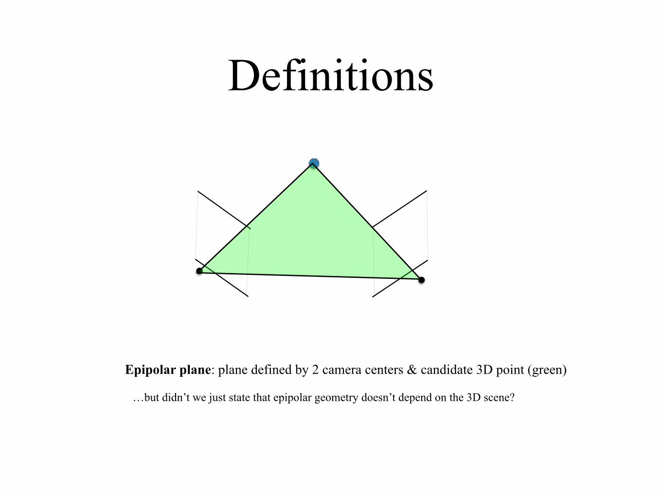
Definitions


Epipolar lines: intersection of epipolar plane and image planes (red)

Definitions



Epipoles: projection of camera center 1 in camera 2 (& vice versa) (orange)

(also defined by 2 camera centers any 1 points in either image plane)

Definitions





(set of all epipolar lines intersect at the epipoles)

R,t

What happens if we scale translation vector?

(imples set of all epipolar planes can be indexed by 2D angle)

Definitions





(set of all epipolar lines intersect at the epipoles)

Parallel, offset cameras

Special case (I)

What would epipolar lines look like?

Epipolar lines don’t intersect (are parallel) Epipoles are at infinity (derive by rotating image planes)

What happens to epipolar lines when we double the distance between two camera views?

11.1 Epipolar geometry 539

(a) (b)

(c) (d)

Figure 11.4 The multi-stage stereo rectification algorithm of Loop and Zhang (1999) c�

1999 IEEE. (a) Original image pair overlaid with several epipolar lines; (b) images trans-formed so that epipolar lines are parallel; (c) images rectified so that epipolar lines are hori-zontal and in vertial correspondence; (d) final rectification that minimizes horizontal distor-tions.

perpendicular to the camera center line. This ensures that corresponding epipolar lines arehorizontal and that the disparity for points at infinity is 0. Finally, re-scale the images, if nec-essary, to account for different focal lengths, magnifying the smaller image to avoid aliasing.(The full details of this procedure can be found in Fusiello, Trucco, and Verri (2000) and Ex-ercise 11.1.) Note that in general, it is not possible to rectify an arbitrary collection of imagessimultaneously unless their optical centers are collinear, although rotating the cameras so thatthey all point in the same direction reduces the inter-camera pixel movements to scalings andtranslations.

The resulting standard rectified geometry is employed in a lot of stereo camera setups andstereo algorithms, and leads to a very simple inverse relationship between 3D depths Z anddisparities d,

d = fB

Z, (11.1)

where f is the focal length (measured in pixels), B is the baseline, and

x0 = x + d(x, y), y0 = y (11.2)

describes the relationship between corresponding pixel coordinates in the left and right im-ages (Bolles, Baker, and Marimont 1987; Okutomi and Kanade 1993; Scharstein and Szeliski

Stereo Pair


(a) (b)

(c) (d)





d = fB

Z, (11.1)


x0 = x + d(x, y), y0 = y (11.2)



(a) (b)

(c) (d)





d = fB

Z, (11.1)


x0 = x + d(x, y), y0 = y (11.2)


Stereo Pair Rectified Stereo Pair

Aside: what kind of transformation is this?

Rotate image plane about fixed camera centers


(a) (b)

(c) (d)





d = fB

Z, (11.1)


x0 = x + d(x, y), y0 = y (11.2)



(a) (b)

(c) (d)





d = fB

Z, (11.1)


x0 = x + d(x, y), y0 = y (11.2)


Stereo Pair Rectified Stereo Pair

Question: do the epipolar lines depend on scene structure, cameras, or both?

Epipolar geometry is purely determined by camera extrinsics and camera instrinics

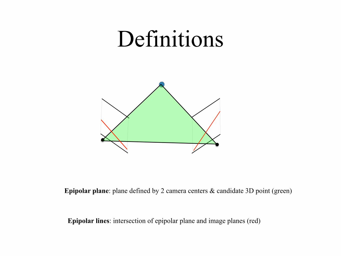
Forward camera motion

Special case (II)

What would epipolar lines look like?

Forward camera motion

Special case (II)

Mathematical formulation

Goal: given point in left image, we want to compute the equation of the line on the right image

Recall: camera projection

3D point in world coordinates

Camera extrinsics (rotation and translation)

Camera instrinsic matrix K (can include skew & non-square pixel size)

�

2

4x

y

1

3

5 =

2

4f 0 00 f 00 0 1

3

5

2

4r11 r12 r13 t

x

r21 r22 r23 t

y

r31 r32 r33 t

z

3

5

2

664

X

Y

Z

1

3

775

camera

world coordinate frame

r1

r2

r3

T

Recall notation

�

2

4x

y

1

3

5 =

2

4fs

x

fs

✓

o

x

0 fs

y

o

y

0 0 1

3

5

2

4r11 r12 r13 t

x

r21 r22 r23 t

y

r31 r32 r33 t

z

3

5

2

664

X

Y

Z

1

3

775

= K3⇥3

⇥R3⇥3 T3⇥1

⇤

2

664

X

Y

Z

1

3

775

= M3⇥4

2

664

X

Y

Z

1

3

775

[Using Matlab’s rows x columns]

Normalized coordinatesAssume camera intrinsics K = Identity (focal length of 1)

If K is known, compute warped image 2

4x

0

y

0

1

3

5 = K

�1

2

4x

y

1

3

5

�

2

4x

y

1

3

5 =

2

4fs

x

fs

✓

o

x

0 fs

y

o

y

0 0 1

3

5

2

4r11 r12 r13 t

x

r21 r22 r23 t

y

r31 r32 r33 t

z

3

5

2

664

X

Y

Z

1

3

775

= K3⇥3

⇥R3⇥3 T3⇥1

⇤

2

664

X

Y

Z

1

3

775

= M3⇥4

2

664

X

Y

Z

1

3

775

COP

(X,Y,Z)(x,y,1)

Normalized coordinates

�

2

4x

y

1

3

5 =

2

4X

Y

Z

3

5

�x = X

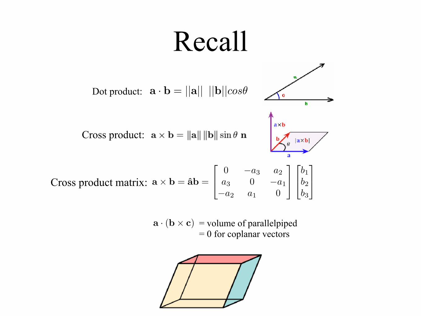
RecallDot product:

Cross product:

a · b = ||a|| ||b||cos✓

Cross product matrix:

Important property (skew symmetric):

a⇥ b =

2

4a2b3 � a3b2a3b1 � a1b3a1b2 � a2b1

3

5 =

2

40 �a3 a2a3 0 �a1�a2 a1 0

3

5

2

4b1b2b3

3

5 ⌘ ab

aT = �a

RecallDot product:

Cross product:

a · b = ||a|| ||b||cos✓

Cross product matrix: a⇥ b = ab =

2

40 �a3 a2a3 0 �a1�a2 a1 0

3

5

2

4b1b2b3

3

5

= volume of parallelpiped = 0 for coplanar vectors

a · (b⇥ c)

4 SERGE BELONGIE, CS 6670: COMPUTER VISION

• We will not handle the case of the conic being underdetermined (n <

5).

From the SVD we take the “right singular vector” (a column from V )which corresponds to the smallest singular value, �6. This is the solution,c, which contains the coe�cients of the conic that best fits the points. Wereshape this into the matrix C, and form the equation x

>Cx = 0.

To recap, note that although the expression for a conic looks nonlinear,it is only the known variables (the coordinates of the xi’s) that appear non-linearly; we were able to write the problem in homogeneous least squaresform since the coe�cients appear linearly.

3.3. Two View Geometry

We now consider the geometry of two calibrated cameras viewing a scene.We assume that the cameras are related by a rigid body motion (R,T ).(Figure from MaSKS Ch. 5.)

Since the cameras are calibrated, we have K1 = K2 = I. The cameras arecentered at o1 and o2, respectively. The vectors e1 and e2 are the epipoles,and can be intuitively thought of as any of the following:

• The points where the baseline pierces the image planes• The projection of the other camera’s optical center onto each imageplane

• The translation vector T (up to a scale factor)• The direction of travel (focus of expansion)

LECTURE 3. TWO VIEW GEOMETRY 5

The lines l1 and l2 are the epipolar lines. The plane spanned by o1, o2 andp is called the epipolar plane, and the epipolar lines are the intersections ofthe epipolar plane with the image planes.

3.3.1. Special Case: Rectified Stereo

Rectified stereo is the simplest case of two-view geometry in which we havetwo cameras that are aimed straight forward and translated horizontallyw.r.t. each other, as if your eyes were looking straight ahead at somethinginfinitely far away. In this case, the epipolar lines are horizontal, and pointsin one image plane map to the horizontal scan line with the same y coordinateon the other image plane.

If the cameras are not rectified in this way, how can we find correspondingpoints in the second image? It turns out we will still have a one-dimensionalsearch, it just won’t be as simple as being on corresponding horizontal scanlines.

3.3.2. General Two View Geometry

We specify the pose of the two cameras, g1 and g2 as follows:

g1 = (I,0)

g2 = (R,T ) 2 SE(3)

Without loss of generality for g1, we let its rotation and translation be theidentity matrix and zero vector, respectively. For g2, R is any rotation matrixand T is the translation vector.

A 3D point p will have coordinates X1 and X2 when viewed from g1

and g2 respectively. The following equation relates coordinate systems fromcamera 1 and camera 2.

(3.7) X2 = RX1 + T

3.3.3. The Epipolar Constraint and the Essential Matrix

We now want to find a relation between a point on one image and its possiblelocations on the other image. We begin by converting the image points intohomogeneous coordinates.

For some depths �i we have

X1 = �1x1, X2 = �2x2

which means�2x2 = R�1x1 + T

but �1,�2 are unknown. To solve this problem, Longuet-Higgins eliminatedthese depths algebraically as follows.

X2: postion of 3D point in camera 2’s coordinate systemX1: postion of 3D point in camera 1’s coordinate system

Calibrated 2-view geometry



5).


>Cx = 0.














g1 = (I,0)

g2 = (R,T ) 2 SE(3)




(3.7) X2 = RX1 + T




X1 = �1x1, X2 = �2x2










g1 = (I,0)

g2 = (R,T ) 2 SE(3)




(3.7) X2 = RX1 + T




X1 = �1x1, X2 = �2x2



Calibrated 2-view geometry

Epipolar geometry








g1 = (I,0)

g2 = (R,T ) 2 SE(3)




(3.7) X2 = RX1 + T




X1 = �1x1, X2 = �2x2










g1 = (I,0)

g2 = (R,T ) 2 SE(3)




(3.7) X2 = RX1 + T




X1 = �1x1, X2 = �2x2










g1 = (I,0)

g2 = (R,T ) 2 SE(3)




(3.7) X2 = RX1 + T




X1 = �1x1, X2 = �2x2


but �1,�2 are unknown. To solve this problem, Longuet-Higgins eliminatedthese depths algebraically as follows.(On board)

1. Take (left) cross product of both sides with T 2. Take (left) dot product of both sides with x2


Take the cross product of both sides with T ,

�2bTx2 = b

TR�1x1 + bTT|{z}=0

and take the inner product with x2,

�2x>2bTx2| {z }=0

= x

>2bTR�1x1

x

>2bTRx1 = 0

(3.8) x

>2 Ex1 = 0

Here we have used the facts that (a) any vector crossed with itself returns thezero vector and (b) a triple product a

>b⇥ c returns zero if any two vectors

are repeated. Equation 3.8 is a bilinear form and is called the essential

constraint or epipolar constraint. It gives us a line in the image plane ofcamera 2 for a point in the image plane of camera 1, and vice versa.

The essential matrix E = bTR 2 R3⇥3 compactly encodes the relative

camera pose g = (R,T ). (How to get back T and R from E is another story,which we’ll address next lecture.)

Thus to map a point in one image to a line in the other using the essentialmatrix, we apply the following equations:

l2 ⇠ Ex1

(3.9) x

>2 l2 = 0

Alternatively, you can go the other way:

l1 ⇠ E

>x2

(3.10) x

>1 l1 = 0

where l1, l2 are epipolar lines (specified in homogeneous coordinates).

3.3.4. Extracting the Epipoles From the Essential Matrix

Note that all epipolar lines in an image plane intersect at the epipole.Equivalently, the epipole has a distance of zero from every epipolar line:e

>2 l2 = 0, 8x1, and similarly e

>1 l1 = 0, 8x2.

For this to hold true, e>2 E and Ee1 must be zero vectors, i.e.,

e

>2 E = 0, Ee1 = 0

Thus e1 and e2 are vectors in the right and left null space of E, re-spectively, i.e., the left and right singular vectors of E with singular value0.



�2bTx2 = b

TR�1x1 + bTT|{z}=0


�2x>2bTx2| {z }=0

= x

>2bTR�1x1

x

>2bTRx1 = 0

(3.8) x

>2 Ex1 = 0








l2 ⇠ Ex1

(3.9) x

>2 l2 = 0


l1 ⇠ E

>x2

(3.10) x

>1 l1 = 0





>1 l1 = 0, 8x2.


e

>2 E = 0, Ee1 = 0




�2bTx2 = b

TR�1x1 + bTT|{z}=0


�2x>2bTx2| {z }=0

= x

>2bTR�1x1

x

>2bTRx1 = 0

(3.8) x

>2 Ex1 = 0








l2 ⇠ Ex1

(3.9) x

>2 l2 = 0


l1 ⇠ E

>x2

(3.10) x

>1 l1 = 0





>1 l1 = 0, 8x2.


e

>2 E = 0, Ee1 = 0


Epipolar geometry



�2bTx2 = b

TR�1x1 + bTT|{z}=0


�2x>2bTx2| {z }=0

= x

>2bTR�1x1

x

>2bTRx1 = 0

(3.8) x

>2 Ex1 = 0








l2 ⇠ Ex1

(3.9) x

>2 l2 = 0


l1 ⇠ E

>x2

(3.10) x

>1 l1 = 0





>1 l1 = 0, 8x2.


e

>2 E = 0, Ee1 = 0


Epipolar geometry

x2 · (T⇥Rx1) = 0



5).


>Cx = 0.







Simply the coplanar constraint applied to 3 vectors from camera 2’s coordinate system



�2bTx2 = b

TR�1x1 + bTT|{z}=0


�2x>2bTx2| {z }=0

= x

>2bTR�1x1

x

>2bTRx1 = 0

(3.8) x

>2 Ex1 = 0








l2 ⇠ Ex1

(3.9) x

>2 l2 = 0


l1 ⇠ E

>x2

(3.10) x

>1 l1 = 0





>1 l1 = 0, 8x2.


e

>2 E = 0, Ee1 = 0


E is known as the essential matrix

Epipolar geometry



�2bTx2 = b

TR�1x1 + bTT|{z}=0


�2x>2bTx2| {z }=0

= x

>2bTR�1x1

x

>2bTRx1 = 0

(3.8) x

>2 Ex1 = 0








l2 ⇠ Ex1

(3.9) x

>2 l2 = 0


l1 ⇠ E

>x2

(3.10) x

>1 l1 = 0





>1 l1 = 0, 8x2.


e

>2 E = 0, Ee1 = 0


Essential matrix

Maps a (x1,y1) point from left image to line in right image (and vice versa)

2

4a

b

c

3

5 = E

2

4x1

y1

1

3

5

ax2 + by2 + c = 0

But how is this different from a Homography (also a 3X3 matrix)?

Epipoles



�2bTx2 = b

TR�1x1 + bTT|{z}=0


�2x>2bTx2| {z }=0

= x

>2bTR�1x1

x

>2bTRx1 = 0

(3.8) x

>2 Ex1 = 0








l2 ⇠ Ex1

(3.9) x

>2 l2 = 0


l1 ⇠ E

>x2

(3.10) x

>1 l1 = 0





>1 l1 = 0, 8x2.


e

>2 E = 0, Ee1 = 0


We’ll write epipolar lines as 3-vectors:



�2bTx2 = b

TR�1x1 + bTT|{z}=0


�2x>2bTx2| {z }=0

= x

>2bTR�1x1

x

>2bTRx1 = 0

(3.8) x

>2 Ex1 = 0








l2 ⇠ Ex1

(3.9) x

>2 l2 = 0


l1 ⇠ E

>x2

(3.10) x

>1 l1 = 0





>1 l1 = 0, 8x2.


e

>2 E = 0, Ee1 = 0


l2 = Ex1

Uncalibrated case



�2bTx2 = b

TR�1x1 + bTT|{z}=0


�2x>2bTx2| {z }=0

= x

>2bTR�1x1

x

>2bTRx1 = 0

(3.8) x

>2 Ex1 = 0








l2 ⇠ Ex1

(3.9) x

>2 l2 = 0


l1 ⇠ E

>x2

(3.10) x

>1 l1 = 0





>1 l1 = 0, 8x2.


e

>2 E = 0, Ee1 = 0


x2TK2

�T TRK�11 x1 = 0

x2TFx1 = 0

�1x1 = K1X1

�2x2 = K2X2








g1 = (I,0)

g2 = (R,T ) 2 SE(3)




(3.7) X2 = RX1 + T




X1 = �1x1, X2 = �2x2



Fundamental matrix

E = TR

F = K2�TEK�1

1

(Faugeras and Luong, 1992)

Next lecture

• 2-view geometry

• essential matrix, fundamental matrix

• properties

• estimation

Next lecture

• Properties of F,E

• Estimating F,E from correspondences

• Recovering T,R,K from estimated F,E

2-view Geometry - 16-720: Computer Vision

Documents

Transcript of 2-view Geometry - 16-720: Computer Vision