1 23

Arabian Journal of Geosciences ISSN 1866-7511 Arab J GeosciDOI 10.1007/s12517-011-0418-0

The use of minimum curvature surfacetechnique in geoid computation processingof Egypt

M. Rabah & M. Kaloop

1 23

Your article is protected by copyright and all

rights are held exclusively by Saudi Society

for Geosciences. This e-offprint is for personal

use only and shall not be self-archived in

electronic repositories. If you wish to self-

archive your work, please use the accepted

author’s version for posting to your own

website or your institution’s repository. You

may further deposit the accepted author’s

version on a funder’s repository at a funder’s

request, provided it is not made publicly

available until 12 months after publication.

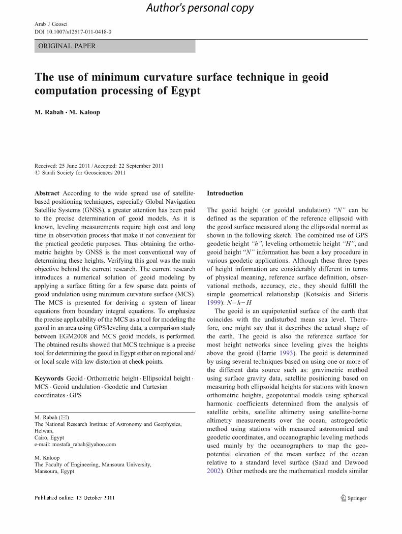
ORIGINAL PAPER

The use of minimum curvature surface technique in geoidcomputation processing of Egypt

M. Rabah & M. Kaloop

Received: 25 June 2011 /Accepted: 22 September 2011# Saudi Society for Geosciences 2011

Abstract According to the wide spread use of satellite-based positioning techniques, especially Global NavigationSatellite Systems (GNSS), a greater attention has been paidto the precise determination of geoid models. As it isknown, leveling measurements require high cost and longtime in observation process that make it not convenient forthe practical geodetic purposes. Thus obtaining the ortho-metric heights by GNSS is the most conventional way ofdetermining these heights. Verifying this goal was the mainobjective behind the current research. The current researchintroduces a numerical solution of geoid modeling byapplying a surface fitting for a few sparse data points ofgeoid undulation using minimum curvature surface (MCS).The MCS is presented for deriving a system of linearequations from boundary integral equations. To emphasizethe precise applicability of the MCS as a tool for modeling thegeoid in an area using GPS/leveling data, a comparison studybetween EGM2008 and MCS geoid models, is performed.The obtained results showed that MCS technique is a precisetool for determining the geoid in Egypt either on regional and/or local scale with law distortion at check points.

Keywords Geoid . Orthometric height . Ellipsoidal height .

MCS . Geoid undulation . Geodetic and Cartesiancoordinates . GPS

Introduction

The geoid height (or geoidal undulation) “N” can bedefined as the separation of the reference ellipsoid withthe geoid surface measured along the ellipsoidal normal asshown in the following sketch. The combined use of GPSgeodetic height “h”, leveling orthometric height “H”, andgeoid height “N” information has been a key procedure invarious geodetic applications. Although these three typesof height information are considerably different in termsof physical meaning, reference surface definition, obser-vational methods, accuracy, etc., they should fulfill thesimple geometrical relationship (Kotsakis and Sideris1999): N=h−H

The geoid is an equipotential surface of the earth thatcoincides with the undisturbed mean sea level. There-fore, one might say that it describes the actual shape ofthe earth. The geoid is also the reference surface formost height networks since leveling gives the heightsabove the geoid (Harrie 1993). The geoid is determinedby using several techniques based on using one or more ofthe different data source such as: gravimetric methodusing surface gravity data, satellite positioning based onmeasuring both ellipsoidal heights for stations with knownorthometric heights, geopotential models using sphericalharmonic coefficients determined from the analysis ofsatellite orbits, satellite altimetry using satellite-bornealtimetry measurements over the ocean, astrogeodeticmethod using stations with measured astronomical andgeodetic coordinates, and oceanographic leveling methodsused mainly by the oceanographers to map the geo-potential elevation of the mean surface of the oceanrelative to a standard level surface (Saad and Dawood2002). Other methods are the mathematical models similar

M. Rabah (*)The National Research Institute of Astronomy and Geophysics,Helwan,Cairo, Egypte-mail: mostafa_rabah@yahoo.com

M. KaloopThe Faculty of Engineering, Mansoura University,Mansoura, Egypt

Arab J GeosciDOI 10.1007/s12517-011-0418-0

Author's personal copy

to that used in this paper using minimum curvature surface(MCS) method.

Sketch illustrates the relation between ellipsoid height & Elevation

In this paper, precise local geoid determination will beconsidered according to geometric method using GPS/leveling data. First of all, an overview of the most recentGlobal Geoidal Model is reviewed. The mathematicalapproach of MCS technique is introduced. The data thatare used in computing the geoid over Egypt are describedas well as the two sets of data points that are used in theevaluation process of the MCS. The next section demon-strated a comparison between the results of the EGM2008model and MCS are presented and discussed. Finally, theconclusions are drawn.

EGM2008 geoidal model

The recent release of the new Earth Gravitational ModelEGM2008 by the US national Geospatial-IntelligenceAgency (Pavlis et al. 2008) is undoubtedly a major

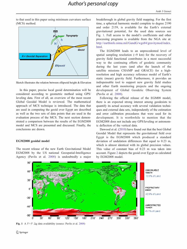
breakthrough in global gravity field mapping. For the firsttime, a spherical harmonic model complete to degree 2190and order 2159, is available for the Earth’s externalgravitational potential, for the used data sources seeFig. 1. Full access to the model’s coefficients and otherprocessing programs is available from the NGA site at:http://earthinfo.nima.mil/GandG/wgs84/gravitymod/index.html.

The EGM2008 leads to an unprecedented level ofspatial sampling resolution (∼9 km) for the recovery ofgravity field functional contributes in a most successfulway to the continuing efforts of geodetic communityduring the last years (and after the launch of thesatellite missions CHAMP and GRACE) for a high-resolution and high accuracy reference model of Earth’sstatic (mean) gravity field. Furthermore, it provides anindispensable tool to support new gravity field studiesand other Earth monitoring projects and the ongoingdevelopment of Global Geodetic Observing System(Pavlis et al. 2008).

Following the official release of the EGM08 model,there is an expected strong interest among geodesists toquantify its actual accuracy with several validation techni-ques and external data sets, independently of the estimationand error calibration procedures that were used for itsdevelopment. It is worthwhile to mention that theEGM2008 does not include any GPS/leveling or astronom-ic deflection of the vertical data.

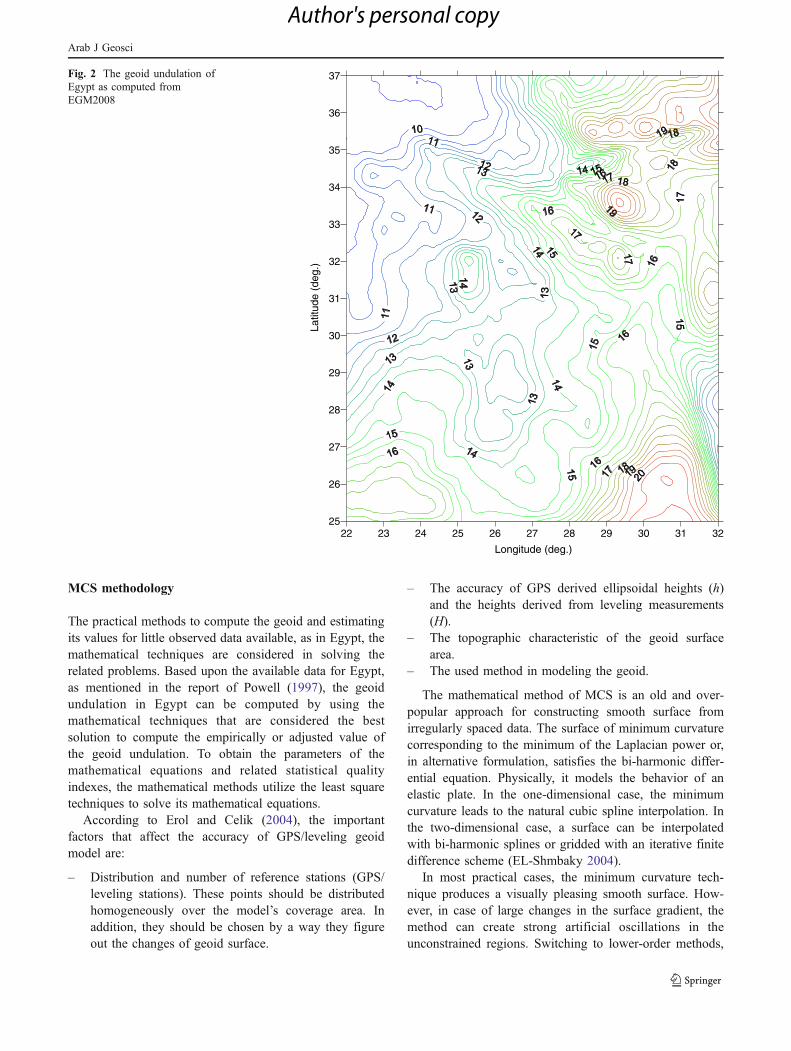
Dawood et al. (2010) have found out that the best GlobalGeoidal Model that represents the gravitational field overEgypt is the EGM2008 which produced a standarddeviation of undulation differences that equal to 0.23 m,which is almost identical with its global precision values.This value of constant bias of 0.23 m was taken intoaccount. Figure 2 depicts the geoid over Egypt as calculatedby EGM2008 model.

Fig. 1 A 5′×5′ Δg data availability (source: Pavlis et al. 2008)

Arab J Geosci

Author's personal copy

MCS methodology

The practical methods to compute the geoid and estimatingits values for little observed data available, as in Egypt, themathematical techniques are considered in solving therelated problems. Based upon the available data for Egypt,as mentioned in the report of Powell (1997), the geoidundulation in Egypt can be computed by using themathematical techniques that are considered the bestsolution to compute the empirically or adjusted value ofthe geoid undulation. To obtain the parameters of themathematical equations and related statistical qualityindexes, the mathematical methods utilize the least squaretechniques to solve its mathematical equations.

According to Erol and Celik (2004), the importantfactors that affect the accuracy of GPS/leveling geoidmodel are:

– Distribution and number of reference stations (GPS/leveling stations). These points should be distributedhomogeneously over the model’s coverage area. Inaddition, they should be chosen by a way they figureout the changes of geoid surface.

– The accuracy of GPS derived ellipsoidal heights (h)and the heights derived from leveling measurements(H).

– The topographic characteristic of the geoid surfacearea.

– The used method in modeling the geoid.

The mathematical method of MCS is an old and over-popular approach for constructing smooth surface fromirregularly spaced data. The surface of minimum curvaturecorresponding to the minimum of the Laplacian power or,in alternative formulation, satisfies the bi-harmonic differ-ential equation. Physically, it models the behavior of anelastic plate. In the one-dimensional case, the minimumcurvature leads to the natural cubic spline interpolation. Inthe two-dimensional case, a surface can be interpolatedwith bi-harmonic splines or gridded with an iterative finitedifference scheme (EL-Shmbaky 2004).

In most practical cases, the minimum curvature tech-nique produces a visually pleasing smooth surface. How-ever, in case of large changes in the surface gradient, themethod can create strong artificial oscillations in theunconstrained regions. Switching to lower-order methods,

22 23 24 25 26 27 28 29 30 31 32

Longitude (deg.)

25

26

27

28

29

30

31

32

33

34

35

36

37

Latit

ude

(deg

.)

Fig. 2 The geoid undulation ofEgypt as computed fromEGM2008

Arab J Geosci

Author's personal copy

such minimizing the power of the gradient, solves theproblem of extraneous inflections. On the other hand, italso removes the smoothness constraint and leads togradient discontinuities (EL-Shmbaky 2004).

The mathematical formula for (MCS) is seeking for atwo-dimensional surface f(x, y) in region D, which iscorresponding to the minimum of the Laplacian power:ZD

Zr2f x; yð Þ�� ��2dxdy ð1Þ

Where r2 denotes the Laplacian operator r2 ¼ @2

@x2 þ @2

@y2

Alternatively, seeking f(x, y) as the solution of the bi-harmonic differential equation:

r2� �2

f x; yð Þ ¼ 0 ð2ÞEquation 1 corresponding to the normal system of

equations in the least square optimization problem (Drakos1997). On the other hand, Poisson equation can beexpressed as follows:

ðr2Þ2f ðx; yÞ ¼ f ðx; yÞ ð3ÞThe solution of this differential equation can be solved

as follows:

If y=f(x) is a function of one variable, then by Taylortheorem:

y1 ¼ y0 þ hy00 þ h2

2! y0 00 þ h3

3! y0 0 00 þ . . .

y3 ¼ y0 � hy00 þ h2

2! y0 00 � h3

3! y0 0 00 þ . . .

As shown in Fig. 2, by adding the two equations andneglecting the higher orders one can get y1 þ y3 ¼ 2y0 þ h2y

0 00

with an error of less than h4y0 0 0 00 Þ=12� ���� . y

0 00 ¼ 1

h2 y1 þ y3�½2y0� or in other format: d

2ydx2 ¼ 1

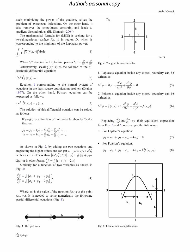
h2 y1 þ y3 � 2y0½ �Similarly for a function of two variables as shown in

Fig. 3:

d28dx2 ¼ 1

h2 8 1 þ 8 3 � 28 0½ �d28dy2 ¼ 1

h2 8 2 þ 8 4 � 28 0½ �

)ð4Þ

Where: 80 is the value of the function f(x, y) at the point(x0, y0). It is needed to solve numerically the followingpartial differential equations (Fig. 4):

1. Laplace’s equation inside any closed boundary can bewritten as:

r28 ¼ 0; i:e:;@28

@x2þ @28

@y2¼ 0 ð5Þ

2. Poisson’s equation inside any closed boundary can bewritten as:

r28 ¼ f x; yð Þ; i:e:; @28

@x2þ @28

@y2¼ f x; yð Þ ð6Þ

Replacing @28@x2 and

@28@y2 by their equivalent expression

from Eqs. 5 and 6, one can get the following:

& For Laplace’s equation:

8 1 þ 8 2 þ 8 3 þ 8 4 � 48 0 ¼ 0 ð7Þ& For Poisson’s equation:

8 1 þ 8 2 þ 8 3 þ 8 4 � 48 0 ¼ h2f x0; y0ð Þ ð8Þ

l1

h

K2K1

b

ac

4

2

13

Fig. 5 Case of non-completed arms

03h

y

1h

4

h

x

2

h

Fig. 4 The grid for two variables

x3 x0 x1

y3y0 y1

hh

Fig. 3 The grid arms

Arab J Geosci

Author's personal copy

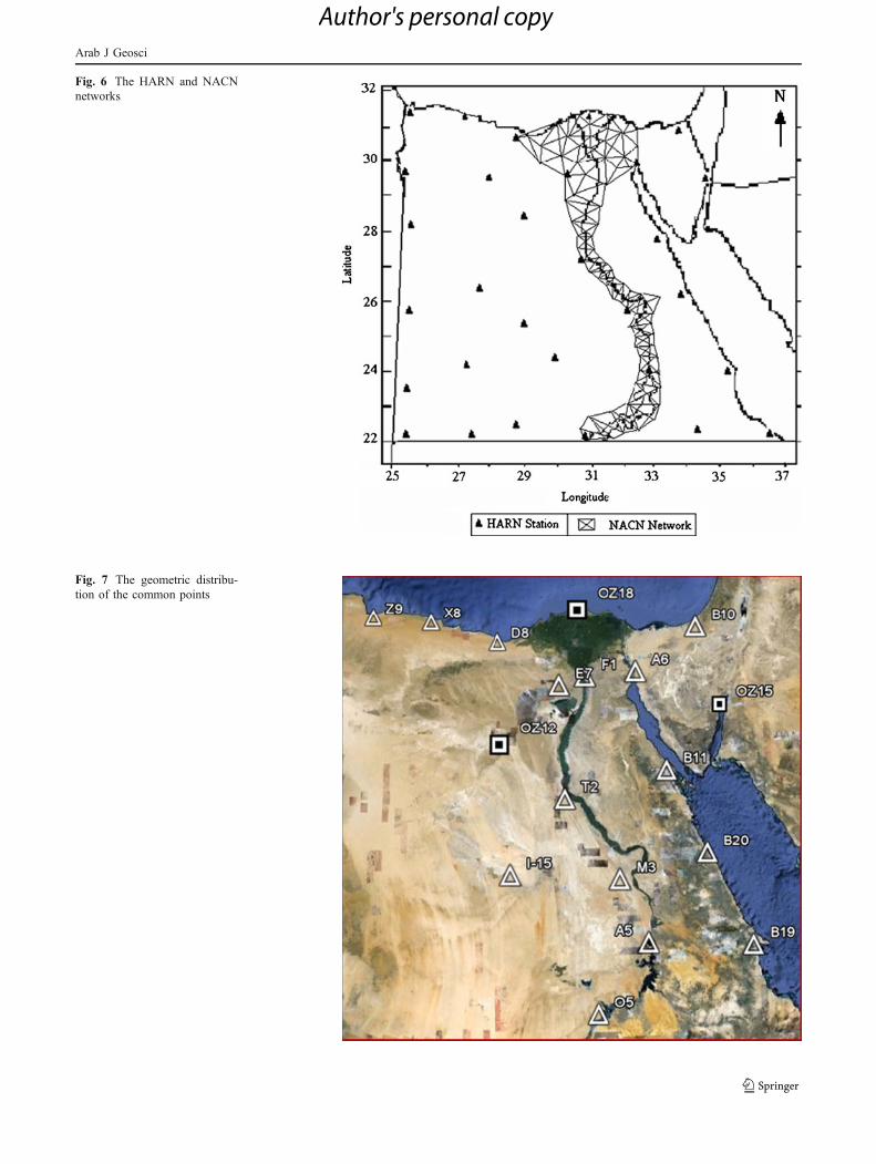
Fig. 7 The geometric distribu-tion of the common points

Fig. 6 The HARN and NACNnetworks

Arab J Geosci

Author's personal copy

The four arms about the nodes may be not completed.So, the two Eqs. 7 and 8 can be rearranged as follows:

28 a

k1 k1 þ k2ð Þ þ28 c

k1 k1 þ k2ð Þ þ28 b

l1 l1 þ l2ð Þ þ28 4

l1 l1 þ l2ð Þ� ð 2

l1l2ð Þ þ2

k1k2ð Þ�f0 ¼ 0;Laplac

h2f0; Poisson

� ð9Þ

Where:

k1, k2, l1, and l2 are the ratio from the complete gridarm (h) shown in Fig. 5, and f0 is a function ofunknown value 80.

Now, the area inside the boundaries can be divided into anetwork or lattice of squares of side (h). The corners of thesesquares are called nodes of the network. The two differenceEqs. 7 and 8 are written according to the considered problemfor each node. These linear equations can then be solved byleast square adjustment. The parametric least square can beapplied to system of equations with Laplace equation as:

A n;mð ÞV m;1ð Þ ¼ F n;1ð Þ ð10Þ

Where:

N The number of equationsM The number of unknown and known stationF The vector equal to observation differenceV The vector of unknown nods and no. of difference

coordinates for known stations

The values of φ(x, y) at the boundaries should be knownto solve the considered problem (Sedeek 1992).

The used data

In 1995, two national GPS geodetic control networks havebeen established, by the Egyptian Survey Authority, tofurnish a nationwide GPS skeleton for surveying and

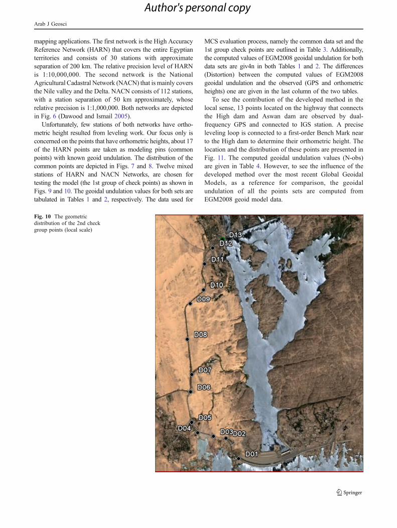
Fig. 9 The geometric distribu-tion of the 1st check grouppoints (regional scale)

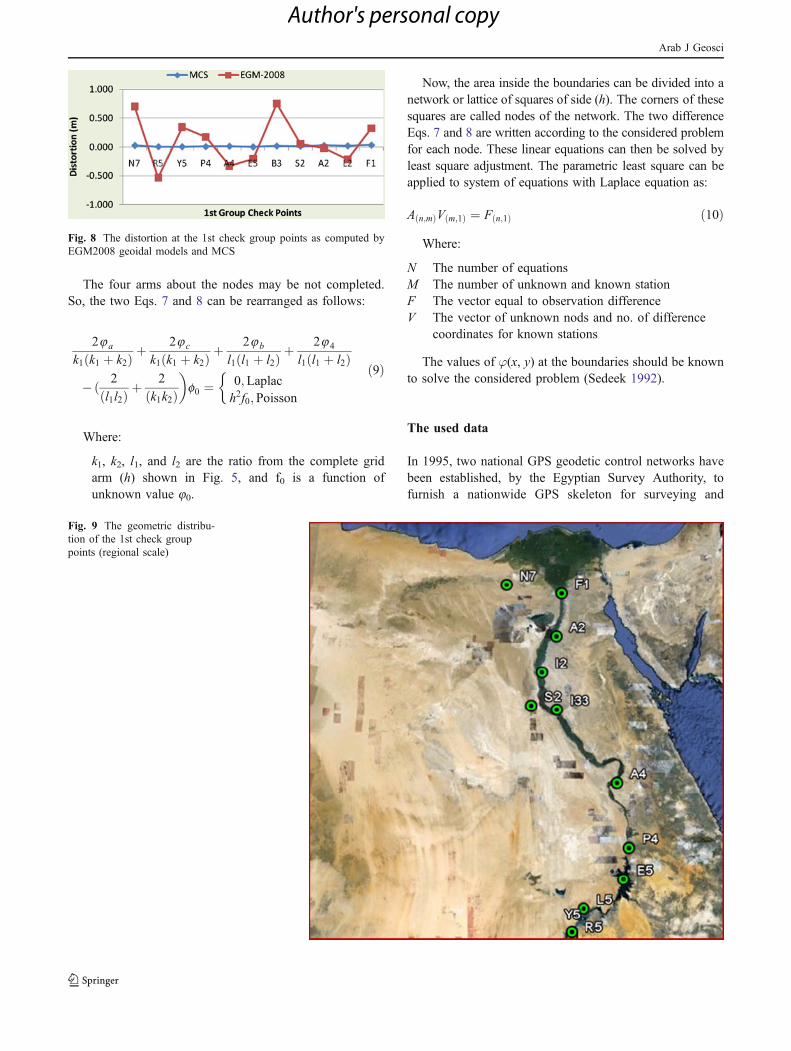
Fig. 8 The distortion at the 1st check group points as computed byEGM2008 geoidal models and MCS

Arab J Geosci

Author's personal copy

mapping applications. The first network is the High AccuracyReference Network (HARN) that covers the entire Egyptianterritories and consists of 30 stations with approximateseparation of 200 km. The relative precision level of HARNis 1:10,000,000. The second network is the NationalAgricultural Cadastral Network (NACN) that is mainly coversthe Nile valley and the Delta. NACN consists of 112 stations,with a station separation of 50 km approximately, whoserelative precision is 1:1,000,000. Both networks are depictedin Fig. 6 (Dawood and Ismail 2005).

Unfortunately, few stations of both networks have ortho-metric height resulted from leveling work. Our focus only isconcerned on the points that have orthometric heights, about 17of the HARN points are taken as modeling pins (commonpoints) with known geoid undulation. The distribution of thecommon points are depicted in Figs. 7 and 8. Twelve mixedstations of HARN and NACN Networks, are chosen fortesting the model (the 1st group of check points) as shown inFigs. 9 and 10. The geoidal undulation values for both sets aretabulated in Tables 1 and 2, respectively. The data used for

MCS evaluation process, namely the common data set and the1st group check points are outlined in Table 3. Additionally,the computed values of EGM2008 geoidal undulation for bothdata sets are giv4n in both Tables 1 and 2. The differences(Distortion) between the computed values of EGM2008geoidal undulation and the observed (GPS and orthometricheights) one are given in the last column of the two tables.

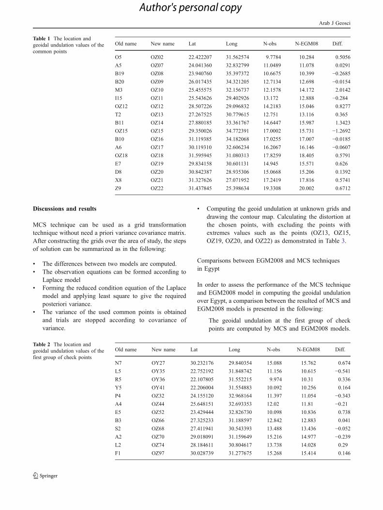
To see the contribution of the developed method in thelocal sense, 13 points located on the highway that connectsthe High dam and Aswan dam are observed by dual-frequency GPS and connected to IGS station. A preciseleveling loop is connected to a first-order Bench Mark nearto the High dam to determine their orthometric height. Thelocation and the distribution of these points are presented inFig. 11. The computed geoidal undulation values (N-obs)are given in Table 4. However, to see the influence of thedeveloped method over the most recent Global GeoidalModels, as a reference for comparison, the geoidalundulation of all the points sets are computed fromEGM2008 geoid model data.

Fig. 10 The geometricdistribution of the 2nd checkgroup points (local scale)

Arab J Geosci

Author's personal copy

Discussions and results

MCS technique can be used as a grid transformationtechnique without need a priori variance covariance matrix.After constructing the grids over the area of study, the stepsof solution can be summarized as in the following:

& The differences between two models are computed.& The observation equations can be formed according to

Laplace model& Forming the reduced condition equation of the Laplace

model and applying least square to give the requiredposteriori variance.

& The variance of the used common points is obtainedand trials are stopped according to covariance ofvariance.

& Computing the geoid undulation at unknown grids anddrawing the contour map. Calculating the distortion atthe chosen points, with excluding the points withextremes values such as the points (OZ13, OZ15,OZ19, OZ20, and OZ22) as demonstrated in Table 3.

Comparisons between EGM2008 and MCS techniquesin Egypt

In order to assess the performance of the MCS techniqueand EGM2008 model in computing the geoidal undulationover Egypt, a comparison between the resulted of MCS andEGM2008 models is presented in the following:

The geoidal undulation at the first group of checkpoints are computed by MCS and EGM2008 models.

Table 2 The location andgeoidal undulation values of thefirst group of check points

Old name New name Lat Long N-obs N-EGM08 Diff.

N7 OY27 30.232176 29.840354 15.088 15.762 0.674

L5 OY35 22.752192 31.848742 11.156 10.615 −0.541R5 OY36 22.107805 31.552215 9.974 10.31 0.336

Y5 OY41 22.206004 31.554883 10.092 10.256 0.164

P4 OZ32 24.155120 32.968164 11.397 11.054 −0.343A4 OZ44 25.648151 32.693353 12.02 11.81 −0.21E5 OZ52 23.429444 32.826730 10.098 10.836 0.738

B3 OZ66 27.325233 31.188597 12.842 12.883 0.041

S2 OZ68 27.411941 30.543393 13.488 13.436 −0.052A2 OZ70 29.018091 31.159649 15.216 14.977 −0.239L2 OZ74 28.184611 30.804617 13.738 14.028 0.29

F1 OZ97 30.028739 31.277675 15.268 15.414 0.146

Table 1 The location andgeoidal undulation values of thecommon points

Old name New name Lat Long N-obs N-EGM08 Diff.

O5 OZ02 22.422207 31.562574 9.7784 10.284 0.5056

A5 OZ07 24.041360 32.832799 11.0489 11.078 0.0291

B19 OZ08 23.940760 35.397372 10.6675 10.399 −0.2685B20 OZ09 26.017435 34.321205 12.7134 12.698 −0.0154M3 OZ10 25.455575 32.156737 12.1578 14.172 2.0142

I15 OZ11 25.543626 29.402926 13.172 12.888 −0.284OZ12 OZ12 28.507226 29.096832 14.2183 15.046 0.8277

T2 OZ13 27.267525 30.779615 12.751 13.116 0.365

B11 OZ14 27.880185 33.361767 14.6447 15.987 1.3423

OZ15 OZ15 29.350026 34.772391 17.0002 15.731 −1.2692B10 OZ16 31.119385 34.182068 17.0255 17.007 −0.0185A6 OZ17 30.119310 32.606234 16.2067 16.146 −0.0607OZ18 OZ18 31.595945 31.080313 17.8259 18.405 0.5791

E7 OZ19 29.834158 30.601131 14.945 15.571 0.626

D8 OZ20 30.842387 28.935306 15.0668 15.206 0.1392

X8 OZ21 31.327626 27.071952 17.2419 17.816 0.5741

Z9 OZ22 31.437845 25.398634 19.3308 20.002 0.6712

Arab J Geosci

Author's personal copy

The value of distortion of both models over theobserved values (the true values) is computed byfinding the differences between the computed andobserved geoidal undulation. The value of distortion ofboth models, maximum and minimum distortion andthe standard deviation of distortion are shown inTable 4. The value of distortion of both models aredepicted in Figs. 7 and 8.

As indicated in Table 4 and Figs. 7 and 8, it is obviousthat the MCS technique gives the best values of distortion

Table 3 The distortion at common and 1st check points groups byMCS

Point Distortion (m)

Common points

O5 0.077

A5 0.003

B19 −0.229B20 0.053

M3 −0.603I15 0.773

OZ12 −0.702T2 −1.079B11 0.353

OZ15 1.493

B10 0.006

A6 −0.003OZ18 0.329

E7 −1.068D8 −1.839X8 −0.118Z9 1.084

1st group check points

N7 0.031

R5 0.009

Y5 0.008

P4 0.010

A4 0.017

E5 0.005

B3 0.020

S2 0.017

A2 0.029

L2 0.023

F1 0.036

Max. value 0.036

Min. value 0.005

Average 0.019

SD 0.010

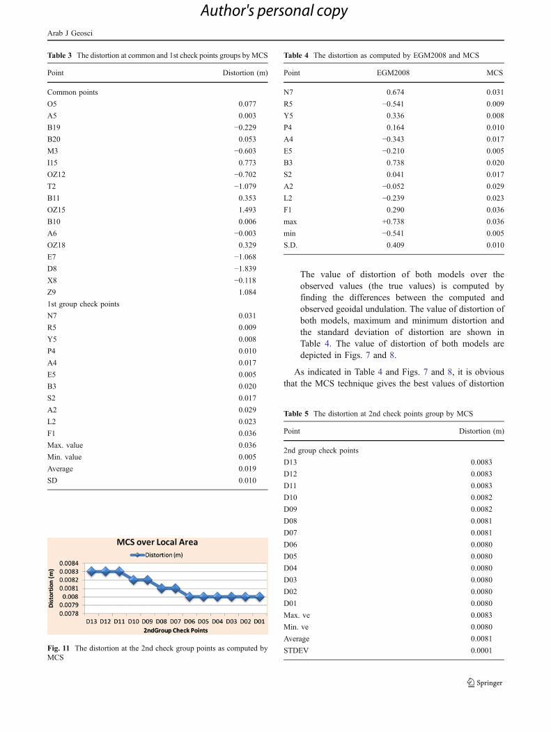
Fig. 11 The distortion at the 2nd check group points as computed byMCS

Table 4 The distortion as computed by EGM2008 and MCS

Point EGM2008 MCS

N7 0.674 0.031

R5 −0.541 0.009

Y5 0.336 0.008

P4 0.164 0.010

A4 −0.343 0.017

E5 −0.210 0.005

B3 0.738 0.020

S2 0.041 0.017

A2 −0.052 0.029

L2 −0.239 0.023

F1 0.290 0.036

max +0.738 0.036

min −0.541 0.005

S.D. 0.409 0.010

Table 5 The distortion at 2nd check points group by MCS

Point Distortion (m)

2nd group check points

D13 0.0083

D12 0.0083

D11 0.0083

D10 0.0082

D09 0.0082

D08 0.0081

D07 0.0081

D06 0.0080

D05 0.0080

D04 0.0080

D03 0.0080

D02 0.0080

D01 0.0080

Max. ve 0.0083

Min. ve 0.0080

Average 0.0081

STDEV 0.0001

Arab J Geosci

Author's personal copy

(minimum values) over Egypt where the computed dis-tortions are ranged between 5 mm to 3.6 cm whileEGM2008 distortion values ranged between 73.8 and54.1 cm. Hence, it is easy to see that the geoid undulationcomputed by MCS has the highest accuracy.

To see the performance of the MCS technique incomputing the geoidal undulation over a local area, thesecond group of check points was utilized. The geoidalundulation of the thirteen points of the check set is computedby the MCS. The distortion values of checked points over theobserved geoidal undulation values (the true values) can befound by computing the differences between the computedand observed values. The resulted value of distortion,maximum and minimum distortion and the standard deviationof distortion are shown in Table 5. The value of distortion ofboth models are illustrated in Figs. 9 and 10.

As it is shown in Table 5 and Figs. 9 and 10, the differencesin the geoid undulation of the 2nd group check points arevaried between 8.3 and 8 mm. The results of the 2nd groupconfirm again the precise applicability of MCS technique incomputing the geoidal undulation over local areas.

Conclusion

Based on the previous analysis and the obtained numericalresults, the following conclusions can be drawn:

& Among available data and techniques, GPS/Levelingwith MCS technique might be the most appropriatecombination for geoid model precise outputs in Egypt.

& The MCS technique gives a best geoid undulation overthe EGM2008 geoid models in Egypt and it is

recommend to use MCS technique to compute thegeoid undulation in Egypt.

References

Erol and Celik (2004) “Precise local geoid determination to make GPStechnique more effective in practical applications of geodesy”FIG Work 2004, Athens, Greece, 22–27 May 2004

Dawood GM and Ismail SS (2005) “Enhancing the integrity of thenational geodetic data bases in Egypt”. In: Proceeding of FIGWorking Week 2005 and GSDI-8 Cairo, Egypt, 16–21 April2005

Dawood GM, Mohamed HF, Ismail SS (2010) Evaluation andadaptation of the EGM2008 Geopotential model along theNorthern Nile Valley, Egypt: case study. J Surv Eng 136:36–40

Drakos N (1997) “Regularizing smooth data with splines in tension.”Computer Based Learning Unit, University of Leads

EL-Shmbaky H (2004) “Development and Improvement the transforma-tion parameters for Egyptian coordinates”, Public Works Depart-ment, Faculty of Engineering, EL-Mansoura University, Egypt

Harrie L (1993) Some specific problems in geoid determination.Department of Geodesy and Photogrammetry Royal Institute ofTechnology, Sweden

Kotsakis C, Sideris MG (1999) On the adjustment of combined GPS/levelling/geoid networks. J Geod 73(8):412–421

Pavlis N, Holmes S, Kenyon S and Factor J (2008) An earth gravitationalmodel to degree 2160: EGM2008. Presented at the 2008 GeneralAssembly of the European Geosciences Union, Vienna, Austria,April 13–18. Available from: http://earthinfo.nima.mil/GandG/wgs84/gravitymod/egm2008/NPavlis&al_EGU2008.ppt

Powell S (1997) Results of the final adjustment of the new nationalgeodetic network. The Egyptian Survey Authority

Saad AA and Dawood GM (2002) A precise integrated GPS/Gravitygeoid model for Egypt, V. 24, no. 1. Civil Engineering ResearchMagazine (CERM), Al-Azhar University, pp. 391–405

Sedeek A (1992) Engineering mathematics literature notes. Faculty ofEngineering, Mansoura University

Arab J Geosci

Author's personal copy