Geoid Modelling in the Sultanate of

Oman

Patrick Lasagna

A THESIS SUBMITTED TO

THE FACULTY OF GRADUATE STUDIES

IN PARTIAL FULFILLMENT OF THE REQUIREMENTS

FOR THE DEGREE OF MASTER OF SCIENCE

GRADUATE PROGRAM IN EARTH AND SPACE SCIENCE

YORK UNIVERSITY

TORONTO, ONTARIO

April, 2017

© Patrick Lasagna 2017

ii

Abstract

This thesis covers the process taken to complete the Oman National Geoid Model

(ONGM) project for the Sultanate of Oman. The steps taken to repair poor quality and badly

referenced gravity data are explained. Each observation point was assigned a new orthometric

height, its position was updated to geodetic coordinates, and its “observed” gravity was inversely

calculated. The major biases that existed in the ground dataset were fixed using airborne free air

anomalies at altitude. The ground data was merged with downward continued airborne gravity

and the merged dataset was used to calculate the gravimetric geoid using the remove-compute-

restore (RCR) method. The remove step was completed using the residual terrain model

modelling technique (RTM), a General Bathymetric Chart of the Oceans (GEBCO) model mixed

with a 30” NASA Shuttle Radar Topography Mission (SRTM) digital terrain model (DTM), and an

expansion of the EGM08 Global Geopotential Model (GGM) to degree and order 360. The

“residual anomalies” were run through the Stokes integral with Wong Gore Tapering using the

GRAVSOFT software package, the effects were restored to calculate the quasigeoid. The

gravimetric geoid was computed by adding the 𝑁 − 𝜁 separation term to the quasigeoid and was

fitted to the GPS-on-benchmarks provided by Oman. The external accuracy of the computed

gravimetric geoid is 14 cm below mean sea level (MSL) with a standard deviation of ±30 cm.

iii

Acknowledgements

The process of earning a master’s degree is long and arduous and is certainly not done

singlehandedly. This thesis became a reality with the kind support and help of many individuals.

I would like to extend my sincere thanks to all of them.

I am highly indebted to Professor Spiros Pagiatakis; professor, mentor, and thesis advisor

extraordinaire. He has the attitude and substance of a genius! He continually and convincingly

conveys a spirit of adventure in regard to research, and expresses intense passion and

excitement with respect to teaching. He provided indispensable advice, insightful comments and

feedback that were instrumental in the development of this project. He was always available for

my questions, and gave generously of his time and vast knowledge. He always knew where to

look for the answers to obstacles while leading me to the right source, theory, and perspective.

Thank you for imparting your knowledge and expertise in this study, and for your unequivocal,

invaluable support, inspiration, and motivation throughout my entire university studies.

I would like to acknowledge the advice, support and insights from my secondary

supervisory committee member, Professor Sunil Bisnath. Your input on an academic level has

been exceptional; your wit is refreshing and I am extremely grateful for your part in helping me to

achieve my educational goals, as you patiently encouraged me to explore beyond my comfort

zone.

Many thanks to the National Survey Authority of Oman and IIC technologies for their

gracious permission to utilize the proprietary data in my research. This thesis would not have

been possible without their support. A special thank you to Pavel Novak, for his assistance in

downward continuing of airborne data, which was fundamental to my project.

My thanks and appreciation go out to all my friends and colleagues. I would like to thank

Athina, Sinem, and Franck for being great office mates; their continuous support, guidance,

friendship, encouragement, and understanding during my graduate studies was invaluable. To

Evan, River, Dennis, Sonal, Younis, Ben, Agata, and all other friends, your support and

encouragement was worth more than I can express on paper; you were always there with a word

of reassurance, an occasional distraction, and a listening ear; even when I was just complaining.

iv

Last, but not least, I am thankful to my parents Rosie and Peter, my sister Sarah, and the

rest of my extended family, who have given their continuous and endless love, unceasing

encouragement, patience, and support my entire life regardless of the circumstances. My parents

always encouraged me to ask questions and to be curious about how things work. They taught

me the value of hard work and an education. All the support they have given me over the years

is the greatest gift one can receive. This journey would not have been possible if not for them.

v

Table of contents

Abstract....................................................................................................................................... ii

Acknowledgements .................................................................................................................... iii

Table of contents ........................................................................................................................ v

List of tables ............................................................................................................................. viii

List of figures ............................................................................................................................. ix

List of acronyms ........................................................................................................................ xii

List of Symbols......................................................................................................................... xiv

1 Introduction ......................................................................................................................... 1

1.1 The Oman National Geoid Model project ..................................................................... 2

1.2 Objective of work ......................................................................................................... 2

1.3 Thesis contributions ..................................................................................................... 2

1.4 Overview of methods ................................................................................................... 3

1.5 Layout of thesis ............................................................................................................ 3

2 Theory of geoid modelling ................................................................................................... 4

2.1 Attraction and potential ................................................................................................ 4

2.2 Geodetic boundary-value problems ............................................................................. 5

2.3 Gravity and level surfaces ............................................................................................ 6

2.4 Anomalous potential and gravity anomalies ................................................................. 8

2.5 The fundamental equation of physical geodesy ........................................................... 9

2.6 The geoid ....................................................................................................................11

2.7 Gravity anomalies .......................................................................................................13

2.8 The quasigeoid and the theory of Molodenskij ............................................................14

2.9 Spirit levelling and gravity ...........................................................................................16

2.10 The “frequency” of a surface .......................................................................................18

vi

2.11 Oman Gravity Base Network (OBGN) .........................................................................19

2.12 Geoid computation in practice .....................................................................................20

2.13 Summary ....................................................................................................................23

3 Ground gravity repair .........................................................................................................24

3.1 The Oman gravity dataset ...........................................................................................24

3.2 Coordinate transformation from PSD93 to WGS84 .....................................................27

3.3 Standardization of observation point orthometric heights ............................................28

3.4 Inverse calculation of “observed” gravity .....................................................................31

3.5 Augmenting of the old data with new gravity points .....................................................36

3.6 Initial determinations of gravity anomalies ...................................................................38

3.7 Summary ....................................................................................................................39

4 Ground gravity bias repair and gridding .............................................................................40

4.1 Ground gravity bias repair ...........................................................................................40

4.2 Gridding of gravity anomalies ......................................................................................49

4.3 Summary ....................................................................................................................55

5 Airborne data and ground-airborne data integration ...........................................................56

5.1 Airborne gravity dataset ..............................................................................................56

5.2 Downward continuation of airborne gravity anomalies ................................................58

5.3 Ground-airborne geoid comparison .............................................................................59

5.4 Ground-airborne data integration ................................................................................61

5.5 Verifying free air anomalies with a global geopotential model .....................................66

5.6 Summary ....................................................................................................................68

6 Geoid calculations ..............................................................................................................69

6.1 Remove-compute-restore technique ...........................................................................69

6.2 Remove step ...............................................................................................................69

6.3 Remove step workflow ................................................................................................72

6.4 Compute step .............................................................................................................73

vii

6.5 Compute step workflow ...............................................................................................74

6.6 Restore step ...............................................................................................................75

6.7 Restore step workflow .................................................................................................75

6.8 Gravimetric geoid step ................................................................................................76

6.9 Gravimetric geoid workflow .........................................................................................77

6.10 Fitting the gravimetric geoid model to GPS-on-benchmarks ........................................77

6.11 Geoid fitting step workflow ..........................................................................................78

6.12 Summary ....................................................................................................................78

7 Final Results ......................................................................................................................79

7.1 Geoid fit testing ...........................................................................................................79

7.2 Comparison of the Oman gravimetric geoid to GOCO05S global geopotential model .83

7.3 Important remarks on the accuracy of the Oman gravimetric geoid model ..................84

8 Conclusions and recommendations ...................................................................................85

8.1 Summary and conclusions ..........................................................................................85

8.2 Recommendations ......................................................................................................88

References ...............................................................................................................................89

viii

List of tables

Table 3-1. PSD93 to WGS84 transformation parameters ..........................................................27

Table 3-2. PSD93 pyproj paramaters ........................................................................................27

Table 6-1. Remove step software workflow ...............................................................................72

Table 6-2. Compute step workflow ............................................................................................74

Table 6-3. Restore step workflow ..............................................................................................75

Table 6-4. Compute gravimetric geoid workflow ........................................................................77

Table 6-5. Fitting of gravimetric geoid workflow .........................................................................78

ix

List of figures

Figure 2-1. Boundary-value problems ........................................................................................ 6

Figure 2-2. Level surfaces .......................................................................................................... 8

Figure 2-3. Geoid and reference normal ellipsoid ....................................................................... 9

Figure 2-4. Stokes function 𝑆𝜓 ..................................................................................................11

Figure 2-5. Spherical distance in spherical coordinates .............................................................11

Figure 2-6. Relationship between the terrain, a reference ellipsoid, and the geoid ....................12

Figure 2-7. Relation between classical surfaces in geodesy and Molodenskij surfaces .............14

Figure 2-8. A spirit levelling setup .............................................................................................16

Figure 2-9. Height systems .......................................................................................................18

Figure 2-10. Low frequency (left) versus high frequency (right) datasets ...................................19

Figure 2-11. Oman gravity base network...................................................................................20

Figure 3-1. Map of legacy Oman ground gravity dataset. ..........................................................25

Figure 3-2. Ground gravity observation points with supplied elevation information ....................29

Figure 3-3. Illustration of datum shifting the SRTM dataset from EGM96 to EGM08 .................30

Figure 3-4. SRTM augmented with bathymetry dataset .............................................................31

Figure 3-5. Ground gravity observation points with supplied observed gravity values ...............34

Figure 3-6. Differences between given gravity and inversely computed gravity values ..............35

Figure 3-7. Differences between given gravity and inversely computed gravity for left peak of

Figure 3-6 .................................................................................................................................35

Figure 3-8. Differences between given gravity and inversely computed gravity for right peak of

Figure 3-6 .................................................................................................................................36

Figure 3-9. New gravity observation points with respect to the legacy dataset with no points

removed ....................................................................................................................................37

Figure 3-10. Original biased ground free air anomalies .............................................................39

Figure 4-1. Comparison of ground gravity anomalies (upper panel) and their equivalent airborne

gravity anomalies (lower panel) of survey points in Line L68 indicated by the colored dots .......42

Figure 4-2. Histogram of ground gravity anomalies (upper panel) and their equivalent airborne

gravity anomalies (lower panel) of survey points in Line L68 .....................................................43

Figure 4-3. Comparison of ground gravity anomalies (upper panel) and their equivalent airborne

gravity anomalies (lower panel) of survey points in Line L79 indicated by the colored dotes .....44

x

Figure 4-4. Histogram of ground gravity anomalies (upper panel) and their equivalent airborne

gravity anomalies (lower panel) of survey points in Line L79 .....................................................45

Figure 4-5. Histogram of all biases ............................................................................................45

Figure 4-6. Color-coded biases of each ground survey line .......................................................46

Figure 4-7. Comparison of ground gravity anomalies (upper panel) and their equivalent airborne

gravity anomalies (lower panel) of survey points in Line L4A ....................................................47

Figure 4-8. Histogram of ground gravity anomalies (upper panel) and equivalent airborne gravity

anomalies (lower panel) of survey points in Line L4A ................................................................47

Figure 4-9. Example of the biases remaining in line L4B after bias repair .................................48

Figure 4-10. Comparison of ground gravity anomalies (left panel) and their equivalent airborne

gravity anomalies (right panel) of survey points in Line L4B ......................................................48

Figure 4-11. Histogram of ground gravity anomalies (upper panel) and their equivalent airborne

gravity anomalies (lower panel) of survey points in Line L4B ....................................................49

Figure 4-12. Roughness terrain correction ................................................................................51

Figure 4-13. Terrain roughness corrections for northern Oman .................................................53

Figure 4-14. Bias-free ground free air anomalies ......................................................................54

Figure 5-1. Free air anomalies at altitude ..................................................................................57

Figure 5-2. Downward continued airborne free air anomalies ....................................................59

Figure 5-3. Preliminary ground geoid minus preliminary airborne geoid ....................................60

Figure 5-4. Histogram of the differences between the preliminary ground geoid and the preliminary

airborne geoid ...........................................................................................................................61

Figure 5-5. Downward continued airborne free air anomalies filtered with an isometric Gaussian

filter in the spatial domain .........................................................................................................63

Figure 5-6. High frequency free air anomaly computed from the ground free air anomalies by

Gaussian filtering ......................................................................................................................64

Figure 5-7. Final ground gravity free air anomalies created from airborne free air anomalies

(downward continued and filtered) merged with ground free air anomalies (filtered) .................65

Figure 5-8. Simple Bouguer anomalies derived from final ground gravity free air anomalies .....66

Figure 5-9.GOCO05s minus final free air anomalies .................................................................67

Figure 5-10. Histogram of differences between GOCO05s free air anomalies and final free air

anomalies .................................................................................................................................68

Figure 6-1. RTM terrain effect theory ........................................................................................70

Figure 6-2. RTM terrain effects .................................................................................................71

Figure 6-3. Wong-Gore Tapering kernel ....................................................................................74

xi

Figure 6-4. Unfitted gravimetric geoid .......................................................................................76

Figure 7-1. Benchmark locations ...............................................................................................80

Figure 7-2. Benchmark residuals from -1 m to 1 m ....................................................................81

Figure 7-3. Histogram of geoid benchmark residuals ................................................................82

Figure 7-4. Histogram of differences between GPS-on benchmarks and the fitted gravimetric

geoid .........................................................................................................................................82

Figure 7-5. Difference between GOCO05S GGM and the gravimetric geoid .............................83

Figure 7-6. Histogram of differences between GOCO05S and the gravimetric geoid ................84

xii

List of acronyms

Acronyms are listed in the order they appear in the thesis.

ONGM – Oman National Geoid Model

RCR – Remove Compute Restore

RTM – Residual Terrain Model

GEBCO - General Bathymetric Chart of the Oceans

NASA - National Aeronautics and Space Administration

SRTM - Shuttle Radar Topography Mission

DTM – Digital Terrain Model

EGM08 - Earth Gravitational Model 2008

GGM - Global Geopotential Model

GPS – Global Positioning System

MSL – Mean Sea Level

PDO - Petroleum Development of Oman

NSA - National Survey Authority

UTM - Universal Transverse Mercator

WGS84 - World Geodetic System 1984

3D – Three Dimensional

BVP – Boundary Value Problem

FEPG – Fundamental Equation of Physical Geodesy

GOCO05S - Gravity Observation Combination Model 5S

OGBN - The Oman Gravity Base Network

IAGBN - International Absolute Gravity Base Network

xiii

IGSN71 - International Gravity Standardization Network of 1971

PSD93 - PDO Survey Datum of 93

GRS67 - Geodetic Reference System 1967

EGM96 - Earth Gravitational Model 1993

RET – Rock Equivalent Topography

GFZ - German Research Centre for Geosciences

ICGEM - International Center for Global Earth Models

FFT – Fast Fourier Transform

GNSS - Global Navigation Satellite System

SST – Sea Surface Topography

xiv

List of symbols

Symbols are listed in the order they appear in the thesis.

𝐹 Attractive force between two masses

𝑚1, 𝑚2 Masses that Attract each other

ℓ Euclidian distance between the two masses

𝐺 Newton’s Gravitational Constant

𝐹𝑋 , 𝐹𝑌, 𝐹𝑍 Force components in the X,Y, and Z direction

𝑉 Potential of Gravitation

𝜕𝑉

𝜕𝑛

First normal derivation of potential of gravitation

𝑆 Surface that 𝑉 is available above or below

Δ Laplacian operator

𝑉𝑒 Exterior potential outside 𝑆

𝑊 Gravity potential

𝜕𝑊 Change of potential

𝑔 Gravity Vector

𝑈0 Normal potential

𝑊0 The geoid’s constant geopotential value

𝐻 Orthometric height

𝑃 Terrain observation point

𝑑𝐻 Change in orthometric height along the plumbline

𝑁 Geoid undulation

𝑈 Normal Potential

xv

𝑇 Anomalous Potential

𝛾 Theoretical gravity on reference ellipsoid

Δ𝑔 Gravity anomaly

𝑔𝑃 Gravity observed on the terrain

𝑄 Point on reference ellipsoid beneath 𝑃

𝛾𝑄 Normal gravity on reference ellipsoid

𝑅 Mean radius of the earth

𝜎 Integration over the surface of the earth

𝑆(𝜓) Stokes Function

𝜓 Spherical Distance

(𝜃, 𝜆) Computation point spherical coordinates

(𝜃′, 𝜆′) Running point spherical coordinates

ℎ Geodetic height of a point above the reference ellipsoid

Δ𝑔𝑓𝑎 Free Air gravity anomaly

𝑔𝐺 Gravity measured on the ground

Δ𝑔𝑏𝑎 Bouguer gravity anomaly

𝜌 Density; taken as 2.67 𝑔/𝑐𝑚3

𝜁 Height Anomaly

ℎ∗ Normal height

∆�̃� Molodenskij gravity anomaly

𝐺1 Molodenskij correction to the Stokes function

𝐶𝑖 Geopotential number

𝛿𝑆 Transformation Scale factor

𝑅𝑋, 𝑅𝑌, 𝑅𝑧 Transformation Rotation Factors

xvi

Δ𝑥, Δ𝑦, Δ𝑧 Transformation Translation Factors

(Φ, 𝜆) Geodetic coordinates (latitude and longitude)

Δ𝑔𝑏𝑎_𝑐𝑜𝑚𝑝𝑙𝑒𝑡𝑒 Complete Bouguer gravity anomaly

𝑐𝑝 Classical Roughness term for a point

𝛿𝑔 Gravity Disturbance

𝐾 Observation point at altitude

𝑔𝐾 Observed gravity at altitude

𝛾𝐾 Normal gravity at altitude

𝐻𝑎 Orthometric height of airborne observation point

Δ𝑔(𝑟, Ω) Downward Continued gravity anomaly

𝐺(𝜙, 𝜆) Gaussian filter

𝑑 Spatial distance of Guassian filter

𝜎𝑘𝑚 Gaussian filter cutoff frequency

Δ𝑔𝑡𝑒𝑟 Terrain effects on gravity anomalies

𝐻𝑟𝑒𝑓 Reference height surface

𝑆𝑅𝑇𝑀[3"×3"] 3" × 3" gridded SRTM dataset

𝑆𝑅𝑇𝑀[30"×30"] 30" × 30" gridded SRTM dataset

𝑆𝑅𝑇𝑀𝑟𝑒𝑓[30"×30"] 30" × 30" gridded reference SRTM dataset

Δ𝑔𝑓𝑎[30"×30"] 30" × 30" gridded free air anomalies

𝑐𝑝[30"×30"] 30" × 30" gridded roughness correction terms

Δ𝐵𝐴[30"×30"] 30" × 30" gridded bouguer slab differences

Δ𝑔𝑡𝑒𝑟[30"×30"] 30" × 30" gridded terrain effects

Δ𝑔𝑒𝑔𝑚08[30"×30"] 30" × 30" gridded EGM08 gravity anomalies

xvii

Δ𝑔𝑟𝑒𝑠[30"×30"] 30" × 30" gridded residual gravity anomalies

𝑆𝑚𝑜𝑑(ψ) Stokes function modified with Wong-Gore tapering effects

𝜁Δ𝑔𝑟𝑒𝑠 [30"×30"] 30" × 30" gridded height anomalies from residual gravity anomalies

𝜁𝑒𝑔𝑚08[30"×30"] 30" × 30" gridded EGM08 height anomalies

𝜁Δ𝑔𝑡𝑒𝑟[30"×30"] 30" × 30" gridded height anomalies from terrain effects

𝜁[30"×30"] 30" × 30" gridded height anomalies

Δ𝑔𝑠𝑏𝑔[30"×30"] 30" × 30" gridded simple bouguer anomalies

(𝑁 − 𝜁)[30"×30"] 30" × 30" gridded geoid-height anomaly separation

𝑁[30"×30"] 30" × 30" gridded geoid

Δ𝑁 Difference between geometric and gravimetric geoid

𝑁𝑓𝑖𝑡𝑡𝑒𝑑[30"×30"] 30" × 30" gridded fitted geoid

1

1 Introduction

The fundamental task of geodesy is to study the varying shape, size, and gravity field of

the Earth. While mathematical approximations of Earth’s shape exist in the form of reference

ellipsoids, a physically defined surface describing its shape is required. The geoid takes into

account all masses and mass distributions present, and best describes the physical shape of the

Earth.

Observed gravity and terrain elevations are the fundamental quantities required to

calculate the geoid. The gravity observations and computed gravity anomalies with respect to a

model Earth, allow for the characterization of mass distribution that might not otherwise be

observable. The geoid is calculated using Stokes integral (Hofmann-Wellenhof & Moritz, 2006)

as a low-pass convolution filter of gravity anomalies over the entire surface of the Earth. The result

is an equipotential surface that approximates mean sea level globally. If precise gravity

measurements are collected over the surface of the Earth, and the topographic masses above

the geoid are mathematically or physically removed, then computing the geoid is a straightforward

application of the Stokes integral.

In addition to characterizing the shape of the Earth, the geoid also functions as a level

surface to which orthometric heights refer. To transfer elevation from one point to another, spirit

levelling is most commonly used; the difference in heights is measured using a level instrument

and two levelling rods. When spirit levelling is carried out over large distances, multiple setups

must be made to transfer elevation from a point on the coast at mean sea level, to a point

thousands of kilometers away. To take into consideration the varying mass distribution of the

topographic masses, spirit levelling must always be combined with gravity measurements to

establish orthometric heights. This is a time consuming and costly endeavor.

With the advent of high accuracy global positioning system (GPS) measurements, the

geoid can also be used as an alternative to spirit levelling. Since geodetic heights (GPS, or

ellipsoidal heights) relate the terrain to the reference ellipsoid, and the geoid deviates from the

reference ellipsoid, the height between the geoid and the terrain (orthometric height) can be

determined without levelling. This method of geometrically determining orthometric heights is an

attractive alternative to spirit levelling, despite the additional gravity observations and calculations

required to compute the geoid.

2

1.1 The Oman National Geoid Model project

In 2013, the Sultanate of Oman desired a national geoid model, initiating the Oman

National Geoid Model (ONGM) Project. A legacy ground gravity dataset was available from the

National Survey Authority (NSA) of Oman, with approximately 230 000 point gravity observations

divided into 82 survey lines. In addition, a newly observed ground gravity dataset of 6000 points,

a newly observed airborne dataset with countrywide coverage (Géophysique GPR I’ntl Inc.,

2015), and a set of GPS observations on Oman’s current leveled benchmarks were available from

the Sultanate of Oman for the development of their national geoid model.

1.2 Objective of work

The calculation of a geoid model requires the availability of a digital terrain model, and a

reliable and accurate gravity dataset. The initial Oman ground gravity dataset was not sufficient

for geoid computation. It was observed over a period of at least fifty years and critical metadata

were not available. The dataset as a whole was incomplete; each point contained a Universal

Transverse Mercator (UTM) northing and easting coordinate, several previously calculated

Bouguer anomalies of different kinds, and the point’s survey line (survey project) identification.

However, not all points had a supplied elevation, or sufficiently accurate latitude and longitude.

More importantly, only 25 percent of the points were supplied with an observed gravity value,

which is essential for the calculation of gravity anomalies necessary for the geoid computation. In

addition to the above, the gravity data were referenced to both the old horizontal (ellipsoid) and

gravity datums that are incompatible with new modern reference systems. These issues do not

allow for the merging of ground gravity observations with airborne measurements to fully

characterize the Earth’s gravity field, and furthermore, prevent the calculation of an accurate

complete geoid.

This thesis undertakes the steps required to complete the ONGM project. This process

involves the repair of biased ground gravity data, its integration with an airborne gravity dataset

using spatial filtering, the calculation of the gravimetric geoid using the remove-compute-restore

method, and the subsequent fitting of the geoid to the GPS-on-benchmarks.

1.3 Thesis contributions

The major contribution of this thesis is the workflow to resolve the deficiencies in the

ground gravity dataset presented above to get the ground gravity dataset to a reasonable

accuracy level, so that it can be merged with airborne gravity measurements for a complete geoid

3

model calculation. This workflow can be applied to other biased, low quality, ground gravity

datasets in other countries. In addition to the reclamation process of the low-quality gravity

dataset, other contributions of this thesis include: creation of automated geoid calculation

workflows, a rigorous geoid solution testing scheme, the fitting of a geoid solution to GPS-on-

benchmarks; Python software development related to gravity grid merging, gravity and vertical

datum shifts, integration of gridded results in multiple formats from multiple sources, and gravity

observation line bias detection.

1.4 Overview of methods

In this research, the following methodology is used to repair the deficiencies of the ground

gravity data. The observation points are transformed from their supplied Universal Transverse

Mercator (UTM) coordinates on Clarke 1880 ellipsoid to their geodetic coordinates and UTM

coordinates referenced to the World Geodetic System 1984 (WGS84). Then, the orthometric

height for each point is replaced with an interpolated orthometric height from the NASA Shuttle

Radar Topography Mission (SRTM) digital terrain model. The observed gravity is then inversely

calculated from the corresponding Bouguer gravity anomaly provided at each observation point

by making assumptions about the crustal density. Finally, the heavily biased gravity values that

were apparently referenced to gravity benchmarks with arbitrary gravity values are repaired using

the airborne data, in the gravity anomaly space resulting in an unbiased ground free air gravity

anomaly dataset, covering the entire country.

1.5 Layout of thesis

This thesis elaborates on the steps required to transform poor quality ground gravity data

and airborne gravity measurements into an unbiased and consistent dataset. Chapter 2 presents

the basic background theory pertaining to the Oman geoid modelling process, as well as a

literature review on the most common methods of calculating the geoid in practice is introduced.

Chapters 3 to 5 detail the steps taken to repair the ground data, remove their biases, and integrate

them with the airborne measurements, to obtain free air gravity anomalies that are used to

calculate the Oman geoid model. In Chapter 6, the software workflow used to calculate the geoid

using Python and the GRAVSOFT software package (Forsberg & Tscherning, GRAVSOFT, 2008)

is presented and explained. Lastly, the results of the calculations as well as recommendations for

future work are presented in Chapters 7 and 8, respectively.

4

2 Theory of geoid modelling

2.1 Attraction and potential

Newton’s law of gravitation states that two objects with point masses 𝑚1 and 𝑚2 seperated

by a distance ℓ will be attracted to each other with a force equal to (Hofmann-Wellenhof & Moritz,

2006):

𝐹 = 𝐺𝑚1𝑚2

ℓ2

(2.1)

where 𝐺 is the Newton’s gravitational constant. When one mass is significantly larger than the

other (e.g. 𝑚1 ≫ 𝑚2), then it is convenient to call the smaller mass the attracted mass and set it

equal to unity. In a 3D-Cartesian system (𝑥, 𝑦, 𝑧), the force between the attracting mass

𝑃(𝑥𝑃 , 𝑦𝑃 , 𝑧𝑃), and the attracted mass 𝑄(𝑥𝑄 , 𝑦𝑄 , 𝑧𝑄) can be given in component form by:

𝐹𝑋 = −𝐺𝑚

ℓ2

𝑥𝑃 − 𝑥𝑄

ℓ

(2.2)

𝐹𝑌 = −𝐺𝑚

ℓ2

𝑦𝑃 − 𝑦𝑄

ℓ

(2.3)

𝐹𝑍 = −𝐺𝑚

ℓ2

𝑧𝑃 − 𝑧𝑄

ℓ

(2.4)

where ℓ is the Euclidian distance between 𝑃 and 𝑄. The scalar function 𝑉, called the potential of

gravitation can be expressed with Equation (2.5).

𝑉 =𝐺𝑚

ℓ

(2.5)

Equations (2.2), (2.3), and (2.4) can be expressed as partial derivatives of 𝑉 with respect

to the coordinate axes 𝑥, 𝑦, and 𝑧.

𝐹𝑋 =𝜕𝑉

𝜕𝑥, 𝐹𝑌 =

𝜕𝑉

𝜕𝑦, 𝐹𝑍 =

𝜕𝑉

𝜕𝑧

(2.6)

The potential of gravitation is used to represent the components 𝐹𝑋 , 𝐹𝑌, and 𝐹𝑍 using a

single function.

5

2.2 Geodetic boundary-value problems

The three boundary-value problems (BVP) used in physical geodesy provide a way of

relating the scalar potential function 𝑉, or its first normal derivative 𝜕𝑉

𝜕𝑛, or a linear combination of

both given as boundary values on a surface 𝑆, to values of 𝑉 at other locations. Their primary

purpose is to determine the harmonic potential function 𝑉 in a region of space inside or outside

the surface 𝑆 as a function of the given boundary values (Hofmann-Wellenhof & Moritz, 2006).

A function is harmonic in a region if it satisfies Laplace’s equation at every point of the

region. Laplace’s equation is shown below in Equation (2.7) (Hofmann-Wellenhof & Moritz, 2006),

Δ𝑉 =𝜕2𝑉

𝜕𝑥2+

𝜕2𝑉

𝜕𝑦2+

𝜕2𝑉

𝜕𝑧2= 0

(2.7)

where 𝑉 is the harmonic function of interest, and Δ is the Laplacian operator.

In addition to the Laplace equation above, if the region is a closed surface 𝑆, then the

harmonic function should approach zero proportionally to 1/ℓ as ℓ approaches infinity (Hofmann-

Wellenhof & Moritz, 2006).

The first BVP is also known as Dirichlet’s problem. Given any function 𝑉 on a surface 𝑆,

find a function 𝑉′ that is harmonic either inside or outside 𝑆 that satisfies the boundary values 𝑉

on 𝑆 (Heiskanen & Moritz, 1967). Dirichlet’s problem applied to gravitational potential is as follows:

given the value(s) of the gravitational potential function 𝑉 at a boundary surface 𝑆, find the

potential in the interior 𝑉𝑖 and exterior 𝑉𝑒 of the boundary surface. Of particular interest to geodesy

is the gravitational potential outside the boundary, which is solved in closed form using Poisson’s

integral.

The second BVP is known as Neumann’s problem. In contrast to the first BVP, instead of

a function 𝑉 on the surface 𝑆, its first normal derivative 𝜕𝑉

𝜕𝑛 on the surface is provided. The first

normal derivative is perpendicular to and directed outwards from 𝑆 as demonstrated in Figure 2-1.

The goal is the same as the 1st BVP: find the harmonic function 𝑉 inside or outside 𝑆 that satisfies

the boundary values 𝜕𝑉

𝜕𝑛 on 𝑆. Finding a harmonic function for the exterior problem 𝑉𝑒, is particularly

important to geodesy.

The third BVP, also known as the boundary-value problem of physical geodesy, combines

the first and second BVP’s. Given a linear combination of the function 𝑉 and its first normal

derivative 𝜕𝑉

𝜕𝑛 on the boundary surface 𝑆, find the harmonic function 𝑉 inside or outside 𝑆 that also

6

satisfies the boundary values on 𝑆. The third BVP is extremely important because its solution for

the exterior potential 𝑉𝑒, the Stokes integral, allows for the determination of the geoid undulations

from a reference ellipsoid (Hofmann-Wellenhof & Moritz, 2006).

Figure 2-1. Boundary-value problems. This figure displays the third BVP. The dotted red surface denoted by 𝑉𝑒 is the

value of 𝑉 outside the blue boundary surface 𝑆.The linear combination of 𝑉 and its first normal derivative 𝜕𝑉

𝜕𝑁 are available

as boundary values on the surface, denoted by the black arrows and black dots respectively.

2.3 Gravity and level surfaces

The total force acting on a point mass at rest on the Earth’s surface is the sum of the

gravitational attraction from the Earth’s mass and the centrifugal force from the Earth’s rotation.

This force results in acceleration called gravity and is represented by the gravity vector 𝑔, and its

potential field is represented by the geopotential 𝑊 (Hofmann-Wellenhof & Moritz, 2006).

A surface on which the gravity potential 𝑊 is equal to a constant value is called an

equipotential or level surface. The downward gradient of the gravity potential, the gravity vector,

is orthogonal to the equipotential surface passing through the same point (Hofmann-Wellenhof &

Moritz, 2006). The change in potential 𝜕𝑊 with respect to the normal vector 𝑛, the negative

vertical gradient, is given by Equation (2.8),

𝜕𝑊

𝜕𝑛= −𝑔

(2.8)

where 𝑔 is the gravity vector, and 𝑛 is the normal vector to the equipotential surface.

An ellipsoid of rotation is a common mathematical approximation for the shape of the

Earth. The surface of this ellipsoid is an equipotential surface of normal potential 𝑈0 when the

ellipsoid includes in it the total mass of the solid earth, oceans, and atmosphere, and spins with

angular velocity 𝜔 equal to Earth’s spin.

𝑉𝑒

𝑆

𝑉 𝜕𝑉

𝜕𝑁

7

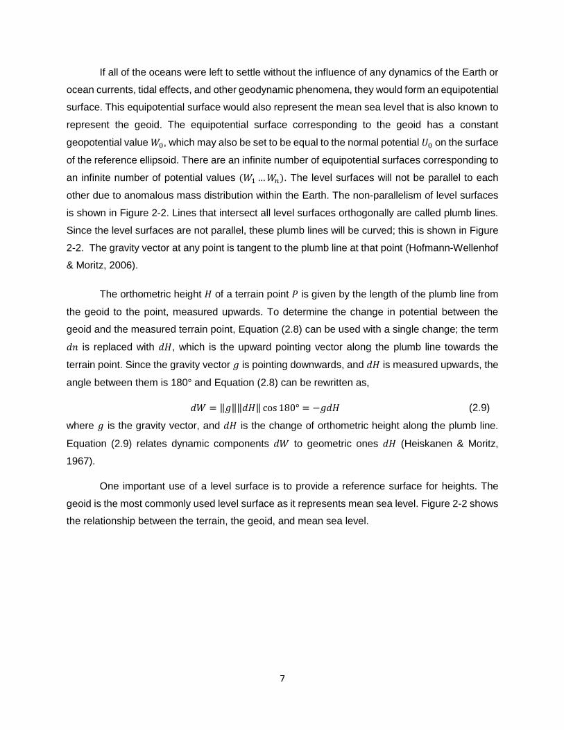
If all of the oceans were left to settle without the influence of any dynamics of the Earth or

ocean currents, tidal effects, and other geodynamic phenomena, they would form an equipotential

surface. This equipotential surface would also represent the mean sea level that is also known to

represent the geoid. The equipotential surface corresponding to the geoid has a constant

geopotential value 𝑊0, which may also be set to be equal to the normal potential 𝑈0 on the surface

of the reference ellipsoid. There are an infinite number of equipotential surfaces corresponding to

an infinite number of potential values (𝑊1 … 𝑊𝑛). The level surfaces will not be parallel to each

other due to anomalous mass distribution within the Earth. The non-parallelism of level surfaces

is shown in Figure 2-2. Lines that intersect all level surfaces orthogonally are called plumb lines.

Since the level surfaces are not parallel, these plumb lines will be curved; this is shown in Figure

2-2. The gravity vector at any point is tangent to the plumb line at that point (Hofmann-Wellenhof

& Moritz, 2006).

The orthometric height 𝐻 of a terrain point 𝑃 is given by the length of the plumb line from

the geoid to the point, measured upwards. To determine the change in potential between the

geoid and the measured terrain point, Equation (2.8) can be used with a single change; the term

𝑑𝑛 is replaced with 𝑑𝐻, which is the upward pointing vector along the plumb line towards the

terrain point. Since the gravity vector 𝑔 is pointing downwards, and 𝑑𝐻 is measured upwards, the

angle between them is 180° and Equation (2.8) can be rewritten as,

𝑑𝑊 = ‖𝑔‖‖𝑑𝐻‖ cos 180° = −𝑔𝑑𝐻 (2.9)

where 𝑔 is the gravity vector, and 𝑑𝐻 is the change of orthometric height along the plumb line.

Equation (2.9) relates dynamic components 𝑑𝑊 to geometric ones 𝑑𝐻 (Heiskanen & Moritz,

1967).

One important use of a level surface is to provide a reference surface for heights. The

geoid is the most commonly used level surface as it represents mean sea level. Figure 2-2 shows

the relationship between the terrain, the geoid, and mean sea level.

8

Figure 2-2. Level surfaces. Level surfaces with different values of W will not be parallel to each other. This is due to the anomalous mass distributions in Earth’s interior. The plumb line is orthogonal to every level surface and as a result, it will have a slight curve. The gravity vector 𝑔 at a level surface 𝑛 is orthogonal to 𝑊𝑛 and tangent to the plumb line at

the point where it crosses 𝑊𝑛.

2.4 Anomalous potential and gravity anomalies

The reference ellipsoid is a relatively close assumption (± 100 𝑚) to the true shape of the

Earth, the geoid. The gravity potential on the geoid is usually set to be identical to the normal

potential on the reference ellipsoid, that is, 𝑊0 = 𝑈0. Therefore, it is mathematically convenient to

represent the geoid, as the normal ellipsoid plus the geoid undulation 𝑁, and the gravity potential

𝑊, as the normal potential 𝑈 plus the anomalous potential 𝑇. The geoid and reference ellipsoid

are compared in Figure 2-3. Using Bruns formula (Hofmann-Wellenhof & Moritz, 2006), the geoid

undulation 𝑁 is related to the anomalous potential 𝑇 on the geoid and normal gravity 𝛾 (theoretical

gravity) on the reference ellipsoid using Equation (2.10).

𝑁 =𝑇

𝛾

(2.10)

The gravity vector on the geoid can also be defined as the systematic normal gravity vector

on the ellipsoid plus a correction term called the gravity anomaly vector Δ𝑔. In practice, however,

the magnitude of gravity anomaly is expressed using Equation (2.11). It is the difference between

the magnitude of the gravity vector on the geoid 𝑔𝑝 at point 𝑃, and the magnitude of normal gravity

𝛾𝑄 on the reference ellipsoid at point 𝑄.

Δ𝑔 = 𝑔𝑃 − 𝛾𝑄 (2.11)

The difference in direction of vectors 𝑔𝑝 and 𝛾𝑄 in Equation (2.11) is called the deflection of

the vertical; it is often very small and it is outside the scope of this thesis, because its effect on

Geoid, 𝑊0

Terrain 𝑊𝑛

𝑊1

𝑊𝑛

𝐻

Plumb Line

Plumb Line

𝑔 𝑔

𝑃

𝑃

𝑊2

9

gravity anomalies is very small so it will not have a measurable effect on the geoid. Figure 2-3

shows the gravity vector 𝑔𝑝 on the geoid with normal 𝑛, and the normal gravity vector 𝛾𝑄 on the

ellipsoid with normal 𝑛′.

Figure 2-3. Geoid and reference normal ellipsoid.

2.5 The fundamental equation of physical geodesy

The fundamental equation of physical geodesy (FEPG), shown in Equation (2.12), is the

fundamental partial differential equation that relates the unknown anomalous potential 𝑇 and its

normal derivative to a measureable quantity Δ𝑔 (Hofmann-Wellenhof & Moritz, 2006).

𝜕𝑇

𝜕ℎ−

1

𝛾

𝜕𝛾

𝜕ℎ𝑇 + Δ𝑔 = 0

(2.12)

Since Δ𝑔 is not known throughout space, Equation (2.12) has no solution; however, if Δ𝑔

is known over the boundary surface of the geoid, then the partial differential equation in Equation

(2.12) can be used as a boundary value condition when solving the third BVP for the anomalous

(disturbing) potential 𝑇.

If no masses exist above the geoid, then the anomalous potential 𝑇 is harmonic outside

the geoid and satisfies Laplace’s equation (Δ𝑇 = 0). Therefore,

Δ𝑇 ≡𝜕2𝑇

𝜕𝑥2+

𝜕2𝑇

𝜕𝑦2+

𝜕2𝑇

𝜕𝑧2= 0

(2.13)

is solvable for 𝑇 at every point outside the geoid, subject to the boundary condition given by the

FEPG in Equation (2.12) (Hofmann-Wellenhof & Moritz, 2006).

𝑃 𝑃

𝑄 𝑄

𝑁

𝛾𝑄

𝑔𝑝

𝑛′

𝑛

Geoid, 𝑊 = 𝑊0

Reference Ellipsoid,

𝑈 = 𝑈0

10

If Δ𝑔 is known (given) over the entire surface of the geoid, then a linear combination of 𝑇

and its first normal derivative 𝜕𝑇

𝜕ℎ is known on the boundary surface 𝑆, here the geoid (cf. Equation

(2.12)). Therefore, the solution of Equation (2.13) outside 𝑆 can be achieved using Equation (2.12)

as a boundary condition, leading to the third boundary-value problem of potential theory

(Hofmann-Wellenhof & Moritz, 2006).

On the geoid, the solution for 𝑇 at a point is given by Stokes formula (Hofmann-Wellenhof

& Moritz, 2006), and is shown in Equation (2.14),

𝑇 =𝑅

4𝜋∬ 𝛥𝑔 𝑆(𝜓)𝑑𝜎

𝜎

(2.14)

where 𝑅 is the mean radius of the Earth, and 𝛥𝑔 are gravity anomalies that refer to the geoid with

no masses above it. The double integral limit is carried over the entire globe 𝜎 and the gravity

anomaly varies with the moving point 𝑝′ on the sphere. 𝑆(𝜓) is the Stokes function at the spherical

distance 𝜓 between points 𝑝 and 𝑝′ and is given by Equation (2.15),

𝑆(𝜓) =1

𝑠𝑖𝑛(𝜓/2)− 6 𝑠𝑖𝑛 (

𝜓

2) + 1 − 5𝑐𝑜𝑠𝜓 − 3𝑐𝑜𝑠𝜓 𝑙𝑛 (𝑠𝑖𝑛 (

𝜓

2) + 𝑠𝑖𝑛 (

𝜓

2)

2

)

(2.15)

where 𝜓 is the spherical distance between the vectors taken from the center of the Earth to the

running point (𝜃′, 𝜆′) being iterated over 𝜎, and the point of computation at (𝜃, 𝜆). 𝑆(𝜓) acts as a

weighting function for the gravity anomalies in Equation (2.14) and is plotted in Figure 2-4.

The formula to calculate the spherical distance 𝜓 between points 𝑝(𝜃, 𝜆) and 𝑝′(𝜃′, 𝜆′) in

polar coordinates is given by Equation (2.16), and Figure 2-5 displays the spherical distance 𝜓

between the two points 𝑝 and 𝑝′.

𝜓 = 𝑐𝑜𝑠−1(𝑠𝑖𝑛𝜃𝑠𝑖𝑛𝜃′ + 𝑐𝑜𝑠𝜃𝑐𝑜𝑠𝜃′ 𝑐𝑜𝑠(𝜆′ − 𝜆)) (2.16)

11

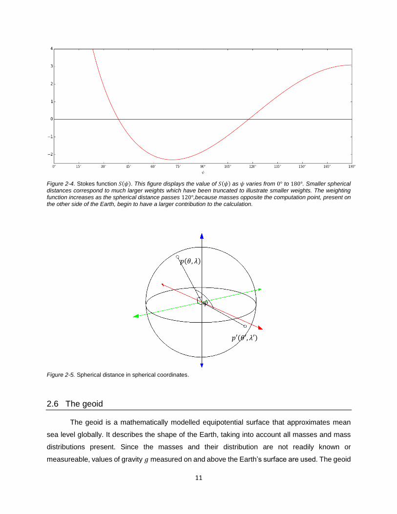
Figure 2-4. Stokes function 𝑆(𝜓). This figure displays the value of 𝑆(𝜓) as 𝜓 varies from 0° to 180°. Smaller spherical distances correspond to much larger weights which have been truncated to illustrate smaller weights. The weighting function increases as the spherical distance passes 120°,because masses opposite the computation point, present on the other side of the Earth, begin to have a larger contribution to the calculation.

Figure 2-5. Spherical distance in spherical coordinates.

2.6 The geoid

The geoid is a mathematically modelled equipotential surface that approximates mean

sea level globally. It describes the shape of the Earth, taking into account all masses and mass

distributions present. Since the masses and their distribution are not readily known or

measureable, values of gravity 𝑔 measured on and above the Earth’s surface are used. The geoid

𝑝(𝜃, 𝜆)

𝑝′(𝜃′, 𝜆′)

𝜓

12

can be calculated from gravity anomalies and a digital terrain model (DTM) using the Stokes

integral, which is derived by substituting Equation (2.14) into Bruns formula (2.10) and is shown

below in Equation (2.17). The Stokes integral is a low-pass filter (convolution integral) over the

entire surface of the Earth that is used to compute the geoid undulation 𝑁 for a single computation

point 𝑃. Unless stated otherwise, all equations are from Hofmann-Wellenhof & Moritz (2006).

𝑁 =𝑅

4𝜋𝛾0∬ 𝛥𝑔 𝑆(𝜓)𝑑𝜎

𝜎

(2.17)

𝑁 is the geoid undulation, the height of the geoid from a reference ellipsoid and 𝛾0 is the

normal gravity on the reference ellipsoid 𝑄 corresponding to point 𝑃 where the geoid undulation

is being calculated. The geometry of the problem can be seen in Figure 2-6.

Figure 2-6. Relationship between the terrain, a reference ellipsoid, and the geoid. The geodetic height h plus the geoid undulation N equals the orthometric height H.

The integral limit in Equation (2.17) is of extreme importance, as gravity anomalies are

required all over the surface of the Earth to properly determine 𝑁. In practice, one might have

access to gravity anomaly grids at high or medium spatial resolution (i.e. 30” or better for the area

of interest), but not for the rest of the Earth. To deal with this lack of gravity information, gravity is

approximated outside the area using a global gravity model, such as EGM08 or GOCO05s.

The Stokes integral has two requirements that must be fulfilled for the results to be correct.

First, as the solution to the geodetic boundary-value problem, the Stokes integral requires the

gravity anomalies to represent the boundary-values on the geoid. That is, 𝑔𝑃 must refer to the

geoid. Second, there must be no masses present outside the geoid, ensuring that 𝑔 on the geoid

truly is the boundary surface (Hofmann-Wellenhof & Moritz, 2006), as the BVP’s used in physical

geodesy are the solution to Laplace’s Equation, and Δ𝑉 ≠ 0 if masses exist above 𝑆.

Terrain

Reference Ellipsoid

Geoid

𝑃

𝑃0

𝑄

𝐻

ℎ

𝑁

𝑃

𝑃0

𝑄

13

2.7 Gravity anomalies

The gravity anomalies required as input for Stoke’s formula or integral are given by

Equation (2.11). The gravity on the geoid 𝑔𝑝 and the gravity on the reference ellipsoid 𝛾𝑄 must be

defined, such that there are no masses present above the geoid, to satisfy the requirements of

the boundary value problems. Since gravity cannot be measured on the geoid, gravity measured

on or above the Earth’s surface must be reduced to the geoid. Furthermore, even if gravity could

be measured at the geoid, all the mass on Earth above the geoid would have to be removed. This

changes the mass distribution of the Earth, making it impossible to determine the actual geoid.

If the masses above the geoid are ignored, then gravity measured on the ground (terrain)

𝑔𝐺 can be reduced to the geoid to acquire 𝑔𝑝 using a free air gradient in Equation (2.18). The

resultant gravity anomaly computed with Equation (2.11) is called a free air anomaly Δ𝑔𝑓𝑎.

Δ𝑔𝑓𝑎 = 𝑔𝐺 + 0.3086𝐻 − 𝛾𝑄 (2.18)

The free air gradient present in the second term on the right-hand-side assumes that the

point is floating in space, and is downward continued to the geoid through the “free air”. The

gravity value increases as a result of its observation point being moved closer to the center of

mass of the Earth.

Bouguer anomalies deal with the terrain that is ignored by the free air gradient. There are

two types of Bouguer anomalies, simple and complete. The complete Bouguer anomaly will be

mentioned in Chapter 4. Equation (2.19) shows the calculation of a simple Bouguer anomaly

Δ𝑔𝑏𝑎 = Δ𝑔𝑓𝑎 − 2𝜋𝐺𝜌𝐻 (2.19)

where 𝐺 is the universal constant of gravity, 𝜌 is the density of the slab, generally taken with mean

rock density (2.67𝑔/𝑐𝑚3), and 𝐻 remains the orthometric height of the point.

The Bouguer anomaly is the free air anomaly corrected by the simple Bouguer reduction

term. The term corresponds to the gravitational attraction of an infinite (area) slab of density 𝜌

and height 𝐻, over the computation point. The correction is subtracted from the free air anomaly,

representing the “restoring” of the attraction provided by the infinite slab, away from the center of

mass of the Earth.

14

2.8 The quasigeoid and the theory of Molodenskij

To bypass the second constraint of the Stokes integral, the theory of Molodenskij is used.

The terrain replaces the geoid as the boundary surface, and the result of the Stokes integral is

the quasigeoid, instead of the geoid. While the quasigeoid is approximately equivalent to the geoid

in terms of shape, unlike the geoid, it has no physical meaning and is merely a mathematical

surface of convenience (Vanicek, 1974). Figure 2-7 shows the relationship between the terrain,

the reference ellipsoid, the quasigeoid, and a new surface, the telluroid.

Figure 2-7. Relation between classical surfaces in geodesy and Molodenskij surfaces. The telluroid, terrain, and reference ellipsoid are related in a similar way to the terrain, the reference ellipsoid, and the geoid. When dealing with Molodenskij surfaces, the geodetic height ℎ is equal to the sum of the normal height ℎ∗ and the height anomaly 𝜁. By comparison, the orthometric height can be determined by adding the geoid undulation from the reference ellipsoid N, to the geodetic height h.

The difference between the geodetic height ℎ and the normal height ℎ∗ defines the height

anomaly 𝜁, which is numerically close to the geoid undulation 𝑁. Similar to the concept of the

geoid undulation 𝑁, with respect to the reference ellipsoid, the height anomaly can also be used

as a deviation of another surface from the reference ellipsoid, namely the quasigeoid or it can be

seen as a deviation of another surface from the terrain known as the telluroid surface. The height

anomaly 𝜁 is the result of Molodenskij’s equivalent to the Stokes integral shown in Equation (2.20)

(Vanicek, 1974),

𝜁 =𝑅

4𝜋𝛾0∬(∆�̃� + 𝐺1) 𝑆(𝜓)𝑑𝜎

𝜎

(2.20)

where 𝛾0 is the normal gravity on the telluroid, and Δ�̃� are not the free air anomalies mentioned

in Equation (2.11); rather, the ones expressed using Equation (2.21),

∆�̃� = 𝑔𝑃 − 𝛾𝑄 (2.21)

Terrain

Telluroid

Ellipsoid

Quasigeoid

Geoid

𝜁

𝜁 𝑄

𝑃

ℎ∗ ℎ

15

where 𝑃 is a point on the terrain and 𝑄 is its corresponding point on the telluroid. The additional

component inside the integral 𝐺1 is the Molodenskij correction term to the Stokes function, and is

shown in Equation (2.22) (Vanicek, 1974),

G1 =𝑅2

2𝜋∬

𝐻′ − 𝐻

𝜌3(∆�̃� +

3𝛾0

2𝑅𝜁0) 𝑑𝜎

𝜎

(2.22)

where 𝐻 is the orthometric height of the computation point, 𝐻’ is the orthometric height of the

moving point in the integral, 𝜌 is the standard mean rock density of 2.67𝑔/𝑐𝑚3, ∆�̃� and 𝛾0 remain

the same as in Equation (2.20), and 𝜁0 is the result of Equation (2.20) ignoring 𝐺1.The 𝐺1 term is

very small compared the value of 𝜁0, and is often neglected (Vanicek, 1974).

This thesis makes use of the method of Molodenskij to calculate the quasigeoid, but

neglects the 𝐺1 term from Equation (2.22) based on (Vanicek, 1974), and uses the classical free

air gravity anomalies defined using Equation (2.11) instead of the gravity anomalies defined by

Equation (2.21) i.e ∆𝑔 ≅ ∆�̃� because thetwo gravity anomalies are numerically similar (see

below).

Classical free air gravity anomalies are calculated using gravity measured on the ground

downward continued in the free air a distance 𝐻 to the geoid using the free air gradient acquired

from Brun’s generalized formula by setting 𝜌 = 0, calculating 𝑔 from the Somigliana-Pizzetti

normal field (Heiskanen & Moritz, 1967), and taking 𝐽 as the mean curvature of the equipotential

surface of the normal gravity field. Molodenskij free air gravity anomalies use normal gravity on

the ellipsoid upward continued a distance ℎ∗ from the ellipsoid to the telluroid using the accurately

determined free air gradient of Molodenskij, which, on average, has the same value as the normal

gravity gradient calculated from Brun’s formula mentioned above. The two gravity anomalies differ

by the following:

0.3086 × (𝐻 − ℎ∗) 𝑚𝐺𝑎𝑙 (2.23)

The difference between 𝐻 and ℎ∗ is the same as 𝑁 and 𝜁 and is negligible when dealing

with gravity anomalies. In an exaggerated case, if the difference between the two heights is equal

to 2m, then the difference in gravity anomalies will be ~ 0.6 mGal; insignificant when calculating

the geoid. From the above, ∆𝑔 is calculated from the downward continuation of terrain gravity and

it is by nature numerically unstable and perhaps theoretically impossible to achieve, whereas ∆�̃�

is the upward continuation of normal gravity on the ellipsoid, an operation that is numerically

16

stable and theoretically correct. Therefore, it is physically and numerically more meaningful to use

∆�̃� (surface gravity anomaly) and Molodenskij’s theory to calculate 𝜁 and subsequently 𝑁, rather

than using ∆𝑔 assuming that it is defined on the geoid and Stokes’ integral to calculate the geoid.

Molodneskij’s theory is therefore adopted in the research.

Since Equation (2.20) computes the quasigeoid instead of the geoid, an additional

correction namely 𝑁 − 𝜁 separation term must be added to it. It is given by Heiskanen & Moritz

(1967) in Equation (2.24).

𝑁 − 𝜁 ≈Δ𝑔𝑏𝑎𝐻

�̅�

(2.24)

The term is estimated by using the simple Bouguer anomalies Δ𝑔𝑏𝑎 (Equation (2.19)), the

orthometric height 𝐻, and mean normal gravity �̅�, which is 9.81 𝑚/𝑠2.

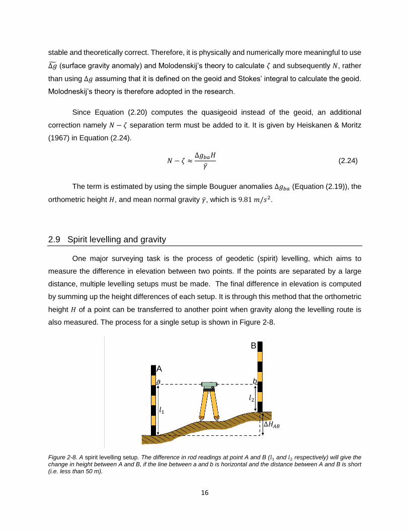
2.9 Spirit levelling and gravity

One major surveying task is the process of geodetic (spirit) levelling, which aims to

measure the difference in elevation between two points. If the points are separated by a large

distance, multiple levelling setups must be made. The final difference in elevation is computed

by summing up the height differences of each setup. It is through this method that the orthometric

height 𝐻 of a point can be transferred to another point when gravity along the levelling route is

also measured. The process for a single setup is shown in Figure 2-8.

Figure 2-8. A spirit levelling setup. The difference in rod readings at point A and B (𝑙1 and 𝑙2 respectively) will give the change in height between A and B, if the line between a and b is horizontal and the distance between A and B is short (i.e. less than 50 m).

A

a

B

b

𝑙1

𝑙2

Δ𝐻𝐴𝐵

17

If perfectly observed height differences for each setup in a closed levelling loop are added

together, the sum will not be rigorously zero (Hofmann-Wellenhof & Moritz, 2006). In addition, if

an alternate path is taken to complete the levelling loop, the sum of the levelled differences will

not be zero and will not be the same if another arbitrary path is followed. This path-dependence

is due to the non-parallelism of level surfaces mentioned previously; the geometric, observed

height difference for a setup is not the same as the physical, orthometric height difference. The

inconsistency between the two height differences can only be eliminated if Earth’s gravity field is

accounted for.

The Helmert orthometric height at a point 𝑃𝑖 on the terrain is defined by Equation (2.25)

(Hofmann-Wellenhof & Moritz, 2006),

𝐻𝑖 ≈𝐶𝑖

𝑔𝑖 + 0.0424ℓ

(2.25)

where 𝐶𝑖 is the geopotential number, 𝑔𝑖 is the measured gravity and ℓ is the leveled height, all at

point 𝑃𝑖. The geopotential number is determined by measuring levelled height differences and

gravity along the levelling path (see Equation (2.26)), and the coefficient 0.0424 is one-half of the

Poincaré-Prey gravity gradient in mGal/m along the plumb line at 𝑃𝑖. The Poincaré-Prey gradient

is an approximate value highly dependent on the crustal density in the vicinity of 𝑃𝑖.

The geopotential number 𝑃𝑖 is calculated as follows:

𝐶𝑖 = ∑ �̅�𝑘𝛿ℓ𝑘

𝑛

𝑘=1

(2.26)

where 𝑘 denotes the levelling segment of measured height difference 𝛿ℓ𝑘, and �̅�𝑘 is the mean

observed surface gravity within the levelling segment.

The above levelling process is costly and time consuming, especially so, if gravity and

height differences must be observed to get the orthometric height of a point. The geoid provides

a cheaper, more efficient alternative to levelling by mathematically relating the geodetic height

observed by GPS to orthometric height. Figure 2-9 shows the relationship between the two

heights and the geoid.

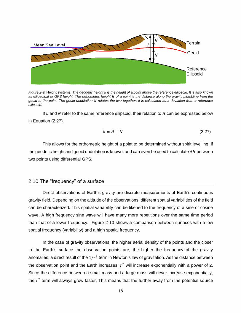
18

Figure 2-9. Height systems. The geodetic height ℎ is the height of a point above the reference ellipsoid. It is also known as ellipsoidal or GPS height. The orthometric height 𝐻 of a point is the distance along the gravity plumbline from the

geoid to the point. The geoid undulation 𝑁 relates the two together; it is calculated as a deviation from a reference ellipsoid.

If ℎ and 𝑁 refer to the same reference ellipsoid, their relation to 𝐻 can be expressed below

in Equation (2.27).

ℎ = 𝐻 + 𝑁 (2.27)

This allows for the orthometric height of a point to be determined without spirit levelling, if

the geodetic height and geoid undulation is known, and can even be used to calculate Δ𝐻 between

two points using differential GPS.

2.10 The “frequency” of a surface

Direct observations of Earth’s gravity are discrete measurements of Earth’s continuous

gravity field. Depending on the altitude of the observations, different spatial variabilities of the field

can be characterized. This spatial variability can be likened to the frequency of a sine or cosine

wave. A high frequency sine wave will have many more repetitions over the same time period

than that of a lower frequency. Figure 2-10 shows a comparison between surfaces with a low

spatial frequency (variability) and a high spatial frequency.

In the case of gravity observations, the higher aerial density of the points and the closer

to the Earth’s surface the observation points are, the higher the frequency of the gravity

anomalies, a direct result of the 1/𝑟2 term in Newton’s law of gravitation. As the distance between

the observation point and the Earth increases, 𝑟2 will increase exponentially with a power of 2.

Since the difference between a small mass and a large mass will never increase exponentially,

the 𝑟2 term will always grow faster. This means that the further away from the potential source

Mean Sea Level

Geoid

Terrain

Reference Ellipsoid

𝐻

𝑁

ℎ

19

the measurements are taken, the more uniform the potential will appear as the effects from

masses merge together. For example, the Earth’s gravity field will appear uniform if measured

from the surface of Mars as 𝑟 increases, and will be highly dependent on terrain if measured on

the surface of Earth as 𝑟 decreases.

Spatially, terrestrial gravity observations exhibit the higher frequencies of the Earth’s

gravity field, characterizing the rapid transitions between gravity values over shorter distances.

Airborne measurements characterize the medium frequency components of the gravity field and

will also show the general trends present in the field over much longer distances than the

terrestrial data. Finally, satellite observations characterize the low frequency components of the

field, and show trends present on a global scale.

Figure 2-10. Low frequency (left) versus high frequency (right) datasets.

2.11 Oman Gravity Base Network (OBGN)

The Oman Gravity Base Network (OGBN) is composed of 39 ground gravity base stations,

two of which were determined using absolute gravimetry in 1993 (Liard & Gagnon, 1993). The

two stations are located in Rustaq and Sayq, and were used in 1994 as reference (base) stations

for tying in the remainder of the base stations to the International Absolute Gravity Base Network

(IAGBN) at epoch 1993. Figure 2-11 shows the currently established gravity base network.

Before the establishment of the OBGN in 1994, Oman’s gravity datum was defined using

the International Gravity Standardization Network of 1971 (IGSN71); so any gravity

measurements taken before the OBGN readjustment in 1994 refer to a different gravity datum,

and are not fully compatible with newer gravity measurements (Ravaout, 1996).

The gravity stations were adjusted for the last time in May 1996; both absolute reference

stations were kept fixed, and the resultant gravity network is compatible with IAGBN at epoch

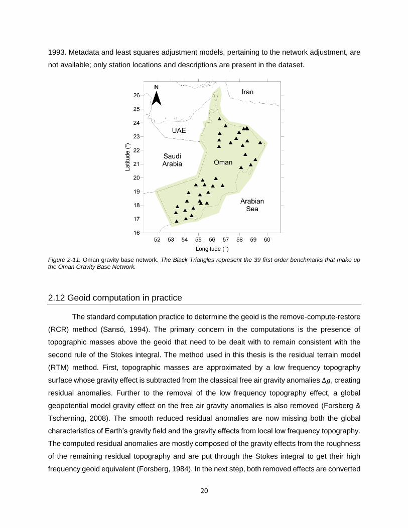
20

1993. Metadata and least squares adjustment models, pertaining to the network adjustment, are

not available; only station locations and descriptions are present in the dataset.

Figure 2-11. Oman gravity base network. The Black Triangles represent the 39 first order benchmarks that make up the Oman Gravity Base Network.

2.12 Geoid computation in practice

The standard computation practice to determine the geoid is the remove-compute-restore

(RCR) method (Sansó, 1994). The primary concern in the computations is the presence of

topographic masses above the geoid that need to be dealt with to remain consistent with the

second rule of the Stokes integral. The method used in this thesis is the residual terrain model

(RTM) method. First, topographic masses are approximated by a low frequency topography

surface whose gravity effect is subtracted from the classical free air gravity anomalies Δ𝑔, creating

residual anomalies. Further to the removal of the low frequency topography effect, a global

geopotential model gravity effect on the free air gravity anomalies is also removed (Forsberg &

Tscherning, 2008). The smooth reduced residual anomalies are now missing both the global

characteristics of Earth’s gravity field and the gravity effects from local low frequency topography.

The computed residual anomalies are mostly composed of the gravity effects from the roughness

of the remaining residual topography and are put through the Stokes integral to get their high

frequency geoid equivalent (Forsberg, 1984). In the next step, both removed effects are converted

21

to their quasigeoid equivalents, and are then added back to get the quasigeoid. The geoid is then

calculated from the quasigeoid by adding a correction that is a function of the simple Bouguer

anomalies as described in the previous section, and in Heiskanen & Moritz (1967).

Sjöberg (2005) discusses the practical implementation of the remove-compute-restore

method. In addition to describing the RCR method in detail, the paper discusses the

approximations made when using it, and provides a few recommendations to increase the solution

quality. The most important recommendation is that if residual anomalies were computed by

removing the low frequency effects of a global geopotential model, they should be run through a

modified stokes kernel with the same frequency effects removed.

The RCR method has been used in several large-scale geoid models, including the Andes

Mountains (Tocho et al., 2005), the Baltic and Nordic region (Omang & Forsberg, 2000), Japan

(Fukuda & Segawa, 1990), and the Konya Closed Basin in Turkey (Alpay Abbak et al., 2012).

The Andes geoid project was a preliminary analysis of a variety of gravity reduction

techniques in preparation for the determination of a national Argentinian geoid. The area of

interest of the study was the most rugged part of Argentina; therefore, whatever method worked

best there, would be effective elsewhere in the country. The residual terrain model (RTM)

(Forsberg, 1984), Rudzki’s inversion, Airy-Heiskanen topographic-isostatic reduction, and

Helmert’s second condensation methods were examined (Heiskanen & Moritz, 1967; Bajracharya

et al., 2001). Tocho et al. (2005) found that Rudzki’s inversion method provided the best

gravimetric geoid results with respect to the geometrically determined geoid; however, it is not a

commonly used computation method due to its treatment of topography (Tocho et al., 2005).

According to Heiskanen & Moritz (2006), although being conceptually important, the Rudzki

reduction does not correspond to a geophysically meaningful model, and highly discourages its

use in practice (Heiskanen & Moritz, 1967).

The Baltic and Nordic geoid was calculated using three separate terrain reduction

techniques. The RTM (Forsberg, 1984), Helmert condensation (Heiskanen & Moritz, 1967), and

a combination of the RTM and Helmert methods (Forsberg et al., 1996) were compared. All three

methods were implemented using the RCR technique. The RTM method utilizes a very smooth

reference surface, along with a roughness correction, to compute the terrain effects that are

removed. The Helmert method does not remove masses; instead it shifts them down to the geoid

using the same roughness correction as the RTM method, resulting in Faye anomalies. The

indirect effect on the gravity anomalies that occurs when masses are shifted is also compensated

22

for (Sideris & She, 1995), but is often small enough to neglect. The RTM/Helmert method removes

the RTM terrain effect from the gravity anomalies, grids them, and then adds them back before

applying the compute state of the RCR technique. The compute step was completed using the

standard Stokes integral (see Equation (2.17)) implemented with FFT. Omang & Forsberg (2000)

found that the RTM/Helmert combination produced slightly better results with respect to GPS-on-

benchmarks. They concluded that this was most likely a result of gridding the smoothest RTM

anomalies, and restoring the Faye anomalies to avoid linear approximations in the RTM method.

The results were not applicable to this thesis or the computation of Oman’s geoid. The advantage

of gridding the smoothest gravity anomalies in the RTM/Helmert method had little relevance to

the Oman project; the byproduct of merging the bias repaired ground gravity data and downward

continued airborne measurements already resulted in pre-gridded data prior to the initiation of the

RCR method. With respect to the pure Helmert method, the GRAVSOFT GCOMB function used

by Omang & Forsberg (2000) to compute and apply the indirect effect was not adequately

documented, and its results may be questionable.

The Japanese geoid project was an extension to a previously determined gravimetric

geoid model (Ganeko, 1983), that was computed exclusively with the Stokes integral and gravity

data. Fukada and Segawa (1990) suggest that with the advent of satellite altimetry and new

terrestrial gravity measurements, an improved geoid is possible. Their paper detailed the steps

taken to compute the geoid using multiple combinations of terrestrially observed gravity and

satellite altimeter data: gravity data only, altimeter data only, gravity data augmented with

altimeter data, and altimeter data augmented with gravity data. The RCR method was

implemented to calculate the geoid for each case. In the remove step, the effects of the terrain

were calculated using the RTM method, due to topographic data being more reliable than crustal

information required by other methods, as noted by Fukada and Segawa (1990). Instead of using

the Stokes integral on the resulting residual anomalies, least squares collocation was used to

estimate their geoidal effects. Fukada and Segawa (1990) found that using terrestrial gravity with

altimeter data in places where gravity data were not available provided the most reliable geoid

solution. The least squares collocation method optimally determines the value of the geoid at

each point based on nearby observation points using a covariance function. This method will not

work for Oman, because an optimal least squares solution requires the observations to have no

systematic biases; Oman’s ground gravity data will always have small biases, even after repair.

In addition, the empirical covariance function is often difficult to determine and requires properly

referenced unbiased gravity data; which is not available.

23

Lastly, the Turkish Konya Closed Basin geoid was computed as a way to compare the

RCR method and the stochastic KTH method (Alpay Abbak et al., 2012). The KTH method utilizes

a least squares stochastic modification of the Stokes integral by taking into account errors present

in the GGM and terrestrial data, and applies additional additive corrections related to: topographic

corrections, indirect effects, downward continuation effects, and atmospheric effects (Sjöberg,

1984, 1991, 2003) . Alpay Abbak et al., (2012) found that for mountainous regions with limited

terrestrial observations, the KTH method had an absolute accuracy that was 3 centimeters better

than the RCR method (Alpay Abbak et al., 2012). By merging the limited terrestrial observations

in mountainous regions with comprehensive airborne measurements, the final Oman dataset will

adequately characterize the gravity field in mountains, eliminating the need for the KTH method.

In addition, the least squares component of the KTH method requires a-priori estimations of the

errors of the gravity data, which were not rigorously provided in the initial Oman gravity dataset,

and would require approximate estimation.

The RTM method (Forsberg, 1984) was chosen in this research for the remove step of the

process, as it is the simplest conceptually to compute. Most importantly, it is highly dependent on

terrain, making it easily computable and verifiable when a digital terrain model (DTM) is available.

In addition, the RTM method requires a digital terrain model to compute, and topographic data

are more reliably acquired than Earth’s other crustal information (Fukuda & Segawa, 1990).

2.13 Summary

This chapter introduced several fundamental concepts that are essential to presenting the

rest of the thesis. First, the geodetic boundary value problems and their application to geodesy

were discussed. The concept of a level surface, anomalous potential, gravity anomalies, the

fundamental equation of physical geodesy, and their relations to each other, were presented and

discussed. The mathematically defined physical surface, the geoid, and the mathematical surface,

the quasigeoid, were described. The surveying technique of spirit levelling, and the application of

the geoid as an alternative were presented. The idea of the “frequency” of a surface was explained

and the current state of the Oman Gravity Base Network was explored. Finally, detailed

descriptions and comparisons of the methods currently used to calculate the geoid in other

countries were provided, in an effort to determine the optimal technique best suited for the ONGM

project.

24

3 Ground gravity repair

3.1 The Oman gravity dataset

The Oman gravity dataset contains the bulk of Oman’s ground gravity observations. It

consists of 229 298 observation points separated over 82 survey lines, shown in Figure 3-1. The

average point density is one observation per 1.35 𝑘𝑚2.

Some lines appear to be an amalgamation of several gravity surveys taken for different

purposes, while other measurement campaigns appear to have been artificially split into multiple

lines. The large vertical green block of gravity points running through the center of the country in

Figure 3-1 likely depicts a combination of exploration and gravity observation surveys, while

several other multicolored areas are separated unnaturally, possibly corresponding to the various

districts of Oman, or the border between UTM zones 39 and 40.

The arbitrary grouping of observation points into survey lines, illustrated in Figure 3-1, and the

lack of additional information about them made finding critical metadata about the ground

observation points difficult.

A thorough examination of the available technical reports and survey documents did not

provide any additional information. In particular, the following important pieces of metadata

pertaining to the gravity data necessary to compute the geoid were not found:

1.) Information pertaining to the national gravity network each line or observation refers to.

2.) Specific information about the reduction methods used to compute the provided gravity

anomalies, primarily the density used in the Bouguer reduction, and whether the terrain

roughness effect was removed from the gravity observations.

3.) Explicit information on the type of height provided; how it was acquired, and its accuracy.

4.) Information pertaining to how each Bouguer anomaly column of the provided gravity

dataset was calculated.

25

Figure 3-1. Map of legacy Oman ground gravity dataset. Each color represents one of the 82 “survey” lines denoted in the initial ground gravity dataset. Some lines appear to be an amalgamation of several observation campaigns, namely the large vertical green block of gravity points running through the center of the country. Not included are the ~6000 new points observed in 2015.

26

In addition to the lack of metadata, the actual data were incomplete and not in an adequate

form to calculate the geoid. The list below briefly outlines where the gravity dataset was deficient,

and the steps required to make it usable. A more detailed explanation is provided in the chapters

and sections that follow.

1.) The observation points were given as Eastings and Northings in Oman’s PDO Survey

Datum of 93 (PSD93), and were converted to Latitude and Longitude in the WGS84

system.

2.) Not all observation points came with a height value, additionally, it was unknown whether

the supplied heights were orthometric heights, and whether they referred to the correct

global geopotential model. The heights for all points were taken from a consistent source

with known properties and accuracies, such as NASA’s Shuttle Radar Topography

Mission (SRTM) model.

3.) Not all observation points came with the observed gravity value 𝑔. While all observation

points came with some form of Bouguer anomaly (e.g., BOUGUER_26), it was not clear

how it was calculated, i.e., what crustal density was used in the calculations. The observed

𝑔 was inversely computed from the supplied gravity anomalies.

4.) New gravity observations taken for the purpose of this project were merged with the legacy

ground gravity dataset.

5.) Free air and simple Bouguer anomalies were calculated from observed gravity at each

observation point using a consistent formula.

6.) The free air and Bouguer anomalies were adjusted on a line-by-line basis to remove the

sizeable biases arising from reference points of arbitrary gravity value. This bias repair

was done using the medium frequency airborne gravity dataset. After the bias shifts,

observation lines that still contained large outliers were also removed.

7.) To apply the Stokes integral, the bias shifted gravity anomalies were gridded. They were

converted to complete Bouguer anomalies to be as smooth as possible, and then were

gridded and converted back to free air anomalies.

8.) The medium frequency airborne gravity data and the high frequency ground gravity data

were combined into one dataset with minimal frequency overlap between the two. This

was done by low-pass filtering of the airborne data with an isometric Gaussian filter, and

high-pass filtering the ground data using the inverse of the same filter; then adding the

medium and high frequency components together.

27

3.2 Coordinate transformation from PSD93 to WGS84

The Oman gravity dataset is transformed from the PSD93 datum to the WGS84 datum. This

process involves transforming from the non-geocentric Clarke 1880 ellipsoid to the geocentric

WGS84 ellipsoid. First, the gravity survey points are transformed from UTM Zone 40 Easting and

Northing coordinates to an (XYZ) Cartesian coordinate system with respect to the Clarke 1880

ellipsoid. Then the coordinates are transferred to the (XYZ) Cartesian coordinate system

associated with the WGS84 ellipsoid using a seven parameter transformation. Table 3-1

describes the transformation parameters found in a report provided by Oman’s National Survey

Authority (NSA) (NSA, 1993).

Table 3-1. PSD93 to WGS84 transformation parameters

From

To

Transformation Parameters

Scale

Factor

Rotation Factors

Translation Factors

PSD93 WGS84 𝜹𝑺 (𝒑𝒑𝒎) 𝑹𝒙(") 𝑹𝒚 (") 𝑹𝒛 (") 𝚫𝒙 (𝒎) 𝚫𝒚 (𝒎) 𝚫𝒛 (𝒎)

(XYZ) (XYZ) +16.867 -0.616 -1.655 +8.378 -182.046 -225.604 +173.384

Finally, the WGS84 (XYZ) coordinates are converted to geodetic latitude (𝜙) and

longitude (𝜆) in the WGS84 system. The entire transformation process is carried out using the

pyproj.transform method from the Python software package pyproj (Whitaker, 2016). A custom

defined datum with parameters identical to the PSD93 datum is converted to the standard WGS84

datum (EPSG No. 4326). The custom paramaters for the pyprojProj object are given in Table 3-1:

Table 3-2. PSD93 pyproj paramaters

Projection String

"+proj= utm +a= 6378249.202 +rf= 293.466 +towgs84= -182.046, -225.604, 173.384, -0.616, -1.655, 8.378, 16.867 +zone= 40N +ellps= clrk80 +units= m"

This conversion is necessary to bring all the data to a common reference coordinate

system. Geodetic latitude and longitude will allow the heights of the gravity points to be estimated

from the SRTM, ensuring that a gridded gravity anomaly dataset will be spatially compatible with

the EGM08 global geopotential model.

28

3.3 Standardization of observation point orthometric heights

To compute gravity anomalies of any type, the orthometric height of the computation point

is required. The geodetic height observed with GPS relative to the reference ellipsoid is not

sufficient because it is not measured with respect to the geoid.

Only about 54 percent of gravity observation points supplied included a corresponding

height measurement, shown in red, in Figure 3-2. The technical and survey reports did not clarify

the source of the provided heights (e.g. spirit levelling, GPS measurements, altimetry, scaling off

a topographic map, etc.). Additionally, no height accuracy estimates were provided.

Ultimately, it will be better for long-term calculation consistency if all heights come from a

single source with a known vertical datum and accuracy level. The source of heights chosen is

NASA’s Shuttle Radar Topography Mission (SRTM) (NASA, 2016), which refers to the geoid

defined by the EGM96 (D/O 360) global geopotential model. The official absolute mean error of

the SRTM is at the 16 meter level, but independent studies have put it in the range of 4-8 meters

(Gorokhovich & Voustianiouk, 2006) with a standard deviation of ± 15-30m depending on the

region and topography. This is sufficient for the ONGM project. The SRTM’s datum is transformed

from EGM96 (D/O 360) to EGM08 (D/O 2190) to make it consistent with the global geopotential

model that will be used to calculate the geoid. Figure 3-3 illustrates the steps required to shift the

EGM96 SRTM to EGM08.

Additionally, any negative and zero SRTM values corresponding to locations at or below

sea level are replaced with values from the 30" × 30" General Bathymetric Chart of the Oceans

(GEBCO) dataset (BODC, 2016).

Any subsequent calculations that require a Digital Terrain Model (DTM), are carried out

by using various resampled spatial resolutions of the EGM08 shifted SRTM with bathymetry DTM.

The Orthometric height of each gravity observation point is determined by nearest neighbor

interpolation from a 3” (~100m) spatial resolution SRTM, which is a reasonable compromise

between accuracy and complexity, as the resampled SRTM has a spatial resolution of nearly

eight times the resolution of the ground gravity dataset. Figure 3-4 shows the SRTM dataset.

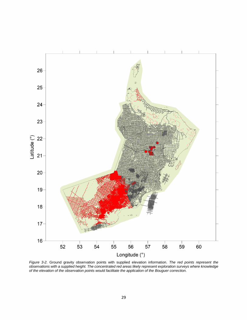
29

Figure 3-2. Ground gravity observation points with supplied elevation information. The red points represent the observations with a supplied height. The concentrated red areas likely represent exploration surveys where knowledge of the elevation of the observation points would facilitate the application of the Bouguer correction.

30

Figure 3-3. Illustration of datum shifting the SRTM dataset from EGM96 to EGM08. Panel (1) Compute the EGM96 and EGM08 model geoid to EGM96’s maximum degree and order of 360, represented by the blue and red dashed line in Panel 1 respectively, (2) Add their difference to the SRTM model to account for the datum difference up to degree and order 360. (3) Add the contribution of EGM08 from degree and order 361 to 2190 to the SRTM. This adds the additional effects of EGM08 not accounted for in EGM96. (4) Shows the complete total correction in blue, compared to the incomplete low order correction in dotted red.

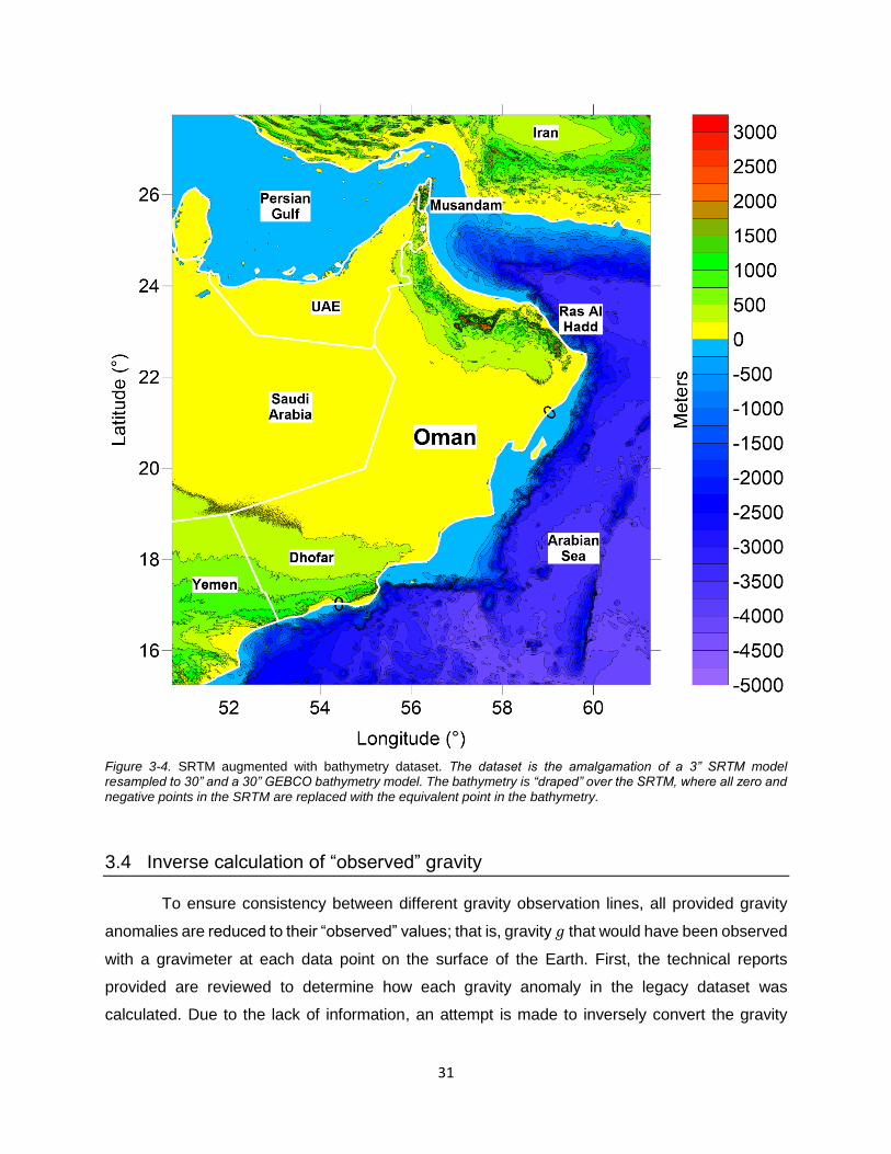
31

Figure 3-4. SRTM augmented with bathymetry dataset. The dataset is the amalgamation of a 3” SRTM model resampled to 30” and a 30” GEBCO bathymetry model. The bathymetry is “draped” over the SRTM, where all zero and negative points in the SRTM are replaced with the equivalent point in the bathymetry.

3.4 Inverse calculation of “observed” gravity

To ensure consistency between different gravity observation lines, all provided gravity

anomalies are reduced to their “observed” values; that is, gravity 𝑔 that would have been observed

with a gravimeter at each data point on the surface of the Earth. First, the technical reports

provided are reviewed to determine how each gravity anomaly in the legacy dataset was

calculated. Due to the lack of information, an attempt is made to inversely convert the gravity

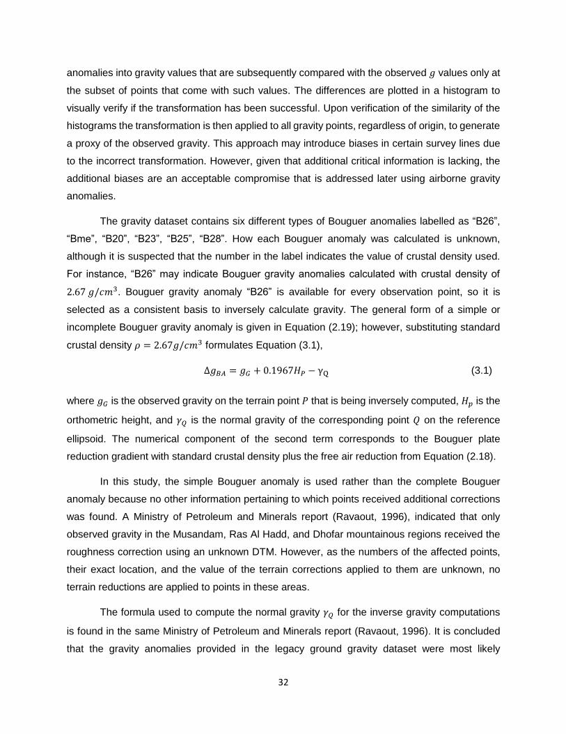
32

anomalies into gravity values that are subsequently compared with the observed 𝑔 values only at

the subset of points that come with such values. The differences are plotted in a histogram to

visually verify if the transformation has been successful. Upon verification of the similarity of the

histograms the transformation is then applied to all gravity points, regardless of origin, to generate

a proxy of the observed gravity. This approach may introduce biases in certain survey lines due

to the incorrect transformation. However, given that additional critical information is lacking, the

additional biases are an acceptable compromise that is addressed later using airborne gravity

anomalies.

The gravity dataset contains six different types of Bouguer anomalies labelled as “B26”,

“Bme”, “B20”, “B23”, “B25”, “B28”. How each Bouguer anomaly was calculated is unknown,

although it is suspected that the number in the label indicates the value of crustal density used.

For instance, “B26” may indicate Bouguer gravity anomalies calculated with crustal density of

2.67 𝑔/𝑐𝑚3. Bouguer gravity anomaly “B26” is available for every observation point, so it is

selected as a consistent basis to inversely calculate gravity. The general form of a simple or

incomplete Bouguer gravity anomaly is given in Equation (2.19); however, substituting standard

crustal density 𝜌 = 2.67𝑔/𝑐𝑚3 formulates Equation (3.1),

Δ𝑔𝐵𝐴 = 𝑔𝐺 + 0.1967𝐻𝑃 − γQ (3.1)

where 𝑔𝐺 is the observed gravity on the terrain point 𝑃 that is being inversely computed, 𝐻𝑝 is the

orthometric height, and 𝛾𝑄 is the normal gravity of the corresponding point 𝑄 on the reference

ellipsoid. The numerical component of the second term corresponds to the Bouguer plate

reduction gradient with standard crustal density plus the free air reduction from Equation (2.18).

In this study, the simple Bouguer anomaly is used rather than the complete Bouguer

anomaly because no other information pertaining to which points received additional corrections

was found. A Ministry of Petroleum and Minerals report (Ravaout, 1996), indicated that only

observed gravity in the Musandam, Ras Al Hadd, and Dhofar mountainous regions received the

roughness correction using an unknown DTM. However, as the numbers of the affected points,

their exact location, and the value of the terrain corrections applied to them are unknown, no

terrain reductions are applied to points in these areas.

The formula used to compute the normal gravity 𝛾𝑄 for the inverse gravity computations

is found in the same Ministry of Petroleum and Minerals report (Ravaout, 1996). It is concluded

that the gravity anomalies provided in the legacy ground gravity dataset were most likely

33

calculated using the Geodetic Reference System 1967 (GRS67) gravity formula, which is shown

in Equation (3.2)

𝛾𝐺𝑅𝑆67 = 978031.846(1 + 0.005278895 𝑠𝑖𝑛2 𝜙 + 0.000023462 𝑠𝑖𝑛4 𝜙) (3.2)

where 𝜙 is the geodetic latitude of the desired point.

Further supporting this normal gravity formula is the fact that the Oman Gravity Base

Network and its parent datum, the International IGSN71 gravity network, are fully compatible

with the GRS67 gravity formula.

Before the inverse calculations are finalized, several tests are conducted using the

available points with supplied observed gravity values. The two parameters of the inverse gravity

calculation namely, the crustal density of the Bouguer plate and the Bouguer gravity anomaly

column, were varied. Of the ~230 000 points, only about 25 percent (56 500) had measured

gravity values. All of the observations were assumed to have been corrected for tides; it is

standard practice in any gravity survey and it is highly unlikely they were not applied. They are

mostly situated in the southern part of the country, with a few thousand in central Oman. The

locations of the points can be seen in Figure 3-5.

Upon computing the inverse gravity values using Equations (3.1) and (3.2) for each point

where observed gravity is provided, a histogram of the differences defined by Equation (3.3), is

created.

𝛿𝑔 = 𝑔𝑂𝑏𝑠𝑒𝑟𝑣𝑒𝑑 − 𝑔𝑖𝑛𝑣𝑒𝑟𝑠𝑒 (3.3)

The purpose of this exercise is to determine whether the differences are small enough for

the inverse computation to be valid for the rest of the gravity points using the same process.

Figure 3-6 shows the initial histogram, which is bi-modally distributed. Each peak possibly

corresponds to a survey(s) taken with respect to different gravity reference points. For easier

viewing and decision-making, the two peaks are separated into two histograms and any visible

outliers are removed, resulting in Figure 3-7 and Figure 3-8. The bin sizes of the three histograms

were determined using ⌈√𝑛⌉, where 𝑛 is the number of differences.

34

Figure 3-5. Ground gravity observation points with supplied observed gravity values. The red points represent the observations that came with a supplied observed gravity (g) value. The concentrated red areas likely represent exploration surveys, where the gravity value was kept in addition to any number of Bouguer anomalies.

35

Figure 3-6. Differences between given gravity and inversely computed gravity values. Two distinct peaks are present; the “shortness” of the left peak indicates that the outliers are probably part of one or two survey lines. The majority of differences are in the peak centered around 0 mGal. The mean of the dataset is -6.9 mGal and the standard deviation is 29.4 mGal, which are a direct result of the “outliers” present in the left peak.

Figure 3-7. Differences between given gravity and inversely computed gravity for left peak of Figure 3-6. The left peak is negatively skewed; the reason for this is unknown. The data is shifted by a -133.5 mGal bias that may have resulted from the use of a gravity benchmark with an arbitrary gravity value to tie the points, or the use of another unknown normal gravity value different from 𝛾𝐺𝑅𝑆67. Regardless of the source, this bias issue is corrected in the following chapter.

The standard deviation is ± 3.82 mGal.

36

Figure 3-8. Differences between given gravity and inversely computed gravity for right peak of Figure 3-6. The right peak appear to be normally distributed around -0.08 mGal with a standard deviation of ± 0.65 mGal, but has a small bump around the -1.7 mGal mark. This bump is due to one or more survey lines that were slightly biased from an unknown source. Much like the points in Figure 3-7, the biases are compensated for in the following chapter. The

majority of points that were supplied with gravity observations (52 671) lie within ± 3𝜎 of the mean value, meaning the inverse calculation provides acceptable gravity values for 93.2 percent of the points.

3.5 Augmenting of the old data with new gravity points

The 6506 new gravity points that were measured in 2015 (Géophysique GPR I’ntl Inc.,

2015) need to be integrated to the inversely calculated gravity values computed in the previous

section. The new points were observed in the mountainous and populous areas of the country to

better characterize the regions where terrain would affect the measurements the most, and thus

the resolution and accuracy of the geoid model where it would be used the most. The locations

of the newly observed points relative to the legacy ground gravity dataset can be seen in Figure

3-9 (red dots).

To prevent the new gravity points from being obscured by possibly biased measurements

present in the legacy ground gravity dataset, all legacy data points within 33" (~1000 km) of a

newly observed point were removed. Approximately 4000 points were removed. The new gravity

points were assigned four “survey lines” that can be used to separate them from the legacy

dataset, where each line corresponds to a different observation location. The points can be seen

in Figure 3-9.

37

Figure 3-9. New gravity observation points with respect to the legacy dataset with no points removed. The red points in the northern mountainous region (Al Hajar Mountains) are assigned line number NU01. The purple points in the separated northern part (Ruus al Jibal) are assigned line number NU02. The blue points in the southern part of the country (Salalah) are assigned line number NU03. The green points in the eastern part (Duqm) are assigned line

number NU04. The 33” cutoff compliments the spacing of the final free air anomalies (30” × 30").

38

3.6 Initial determinations of gravity anomalies

The next stage includes the computation of the two types of gravity anomalies required to

calculate the geoid. The free air and simple Bouguer anomalies are calculated using the ground

gravity dataset created in the previous two sections. This stage is initially conducted without taking

into consideration the expected very large biases present in the ground gravity anomaly dataset.

These biases will be addressed using an airborne gravity dataset in following chapter.

For the WGS84 ellipsoid, the normal gravity 𝛾𝑄 can be calculated using Equation (3.4)

(DMA, 1987)

𝛾𝑄 = 978032.67714 1 + 0.00193185138639 sin2 𝜙

√1 − 0.0066943799901 sin2 𝜙 𝑚𝐺𝑎𝑙

(3.4)

where, similarly to Equation (3.2), 𝜙 is the geodetic latitude of the computation point.

The initial calculations of the free air anomaly grid appears to exhibit severe biases in

several locations. A plot of the biased free air anomalies can be seen in Figure 3-10. The largest

biases are shaded purple and highlighted in the southern part of the country. They have a bias

magnitude of about 90 mGal. Other biases exist elsewhere in the country but they are much

smaller in scale (e.g. small area circled in white in the center of the country).

In addition to the biases, there are two other deficiencies present in the gridded free air

gravity anomalies in Figure 3-10. Firstly, the gravity data exhibit traits that free air anomalies are

not expected to have, such as the high frequency noise in the dashed white ellipse located in the

northern part of the country. Secondly, the free air gravity anomalies do not characterize all the

terrain features, even though they should be highly correlated to the terrain. The northern-most

solid white circled area should have a similar shape to the part of the mountains that can be seen

in the same area in Figure 3-4, but it does not.

39

Figure 3-10. Original biased ground free air anomalies. In general, any bias or error in the free air anomalies will negatively affect the quality of geoid and corrections need to be considered. Solutions specific to the inconsistencies highlighted in this diagram will be discussed in the following chapters.

3.7 Summary

This chapter explained the steps taken to establish a preliminary ground gravity dataset

from the legacy gravity dataset. Gravity anomalies were first transformed from the PSD93 UTM

datum to the geodetic WGS84 datum. New orthometric elevations for each observation point were

taken from the SRTM dataset that was datum shifted vertically from EGM96 to EGM08. Bouguer

gravity anomalies taken form the legacy gravity dataset were used to inversely calculate

“observed” gravity 𝑔, and the new gravity observation points from 2015 were integrated into the

legacy gravity dataset. Free air gravity anomalies were computed for the entire gravity dataset;

however, components of the gravity anomaly dataset were biased by up to about 90 mGal and

will be repaired in the following chapter.

40

4 Ground gravity bias repair and gridding

Figure 3-10 shows several significant biases in the free air anomalies that are the result

of inadequately computed inverse gravity values or arbitrarily referenced gravity measurements,

due to the exploratory nature of the legacy gravity dataset. It was mostly populated from

geophysical exploration surveys, where tying in gravity survey lines to the existing gravity network

is not necessary. The lack of reference to a national gravity network means that each survey was

internally consistent, but would be biased relative to surveys conducted elsewhere in the country.

Any biases present in the free air anomaly dataset, even small ones, would improperly

bias the final geoid model. The biased lines could have been disregarded, but that would eliminate

a large portion of valuable high frequency ground gravity data. Therefore, it is very important to

reclaim as much of the problematic data as possible.

4.1 Ground gravity bias repair

The 82 original legacy survey lines and the four new additions are first split into 124 smaller

segments where visible groupings of points existed. For example, one original survey line with

discernable clusters of points in the northern and southern part of the country (cf., Figure 3-1) is

split into two separate survey segments.

It is then postulated that the free air anomalies contained in each individual survey line

and their equivalent interpolated free air anomalies from an alternate known reliable free air

gravity dataset (e.g., airborne), from the same region, would have similarly shaped histograms

offset by a bias value. This bias value would be equal to the difference in the simple mean of each

dataset, given by Equation (4.1), and would be the offset in milligals required to un-bias the gravity

anomalies.

𝑏𝑖𝑎𝑠 = 𝜇𝑘𝑛𝑜𝑤𝑛 − 𝜇𝑏𝑖𝑎𝑠𝑒𝑑 (4.1)

The first order statistic 𝜇 is the only statistic that can be applied from the known dataset.

The ground gravity dataset characterizes what is essentially an “infinite” frequency. It is the

closest point to the center of mass of the Earth that gravity can be measured. Any other dataset,

be it airborne, downward continued airborne, or satellite, cannot fully characterize the same

41

frequency in its histogram. Thus, the conventional image processing techniques of histogram

equalization or histogram matching is not applicable; the two histograms will express different

frequency components. Shifting the biased ground free air anomalies by the difference in

histogram means is the extent of the bias repair that can be conducted without the introduction of

additional frequency related biases.

The known gravity dataset that is used here for the repair of biases is the set of airborne

free air gravity anomalies downward continued to the geoid. The downward continuation process

adds additional higher frequency components to the medium frequency airborne gravity

anomalies that are the best estimates of the anomalies determined from ground gravity

observations. Note that the downward continuation of the airborne free air gravity anomalies is

discussed extensively in the next chapter. The difference in the mean values between the two

datasets in a region is used to un-bias the free air anomalies determined from ground gravity

observations, hereafter called ground gravity anomalies.

For every point in each survey line, the downward continued airborne gravity anomaly is

estimated using the nearest neighbor interpolation method. The histograms of the two sets of

gravity anomalies (ground and airborne) are then plotted and their means are differenced. The

histograms are used to check the similarity of the distributions before the difference of their mean

is used to remove the bias from the gravity anomalies determined from ground observations.

Figure 4-1 illustrates an extreme case of bias, and the corresponding histograms for each

are shown in Figure 4-2. Figure 4-3 shows a case in which bias shifting is not justifiable, along

with the equivalent histograms in Figure 4-4. Figure 4-5 shows a histogram of all the biases that

are computed for all survey lines, and Figure 4-6 shows each line with its bias.

The steps taken thus far do not fully eliminate all biases present on a line-to-line basis.

Lines L4A and L4B are removed because they appear to be visibly biased even after being bias

shifted (see Figure 4-9). A ground-to-airborne comparison plot and the associated histogram for

each line is shown below (L4A: Figure 4-7, Figure 4-10, L4B: Figure 4-8, Figure 4-11). These lines

are located in the oceans surrounding Oman and represent a portion of the seaborne gravity

measurements available. The postulation about the similarity of the histograms of ground and

airborne gravity anomalies is not valid in either survey lines’ case. The cause for this issue is

unknown, but it may have something to do with the surrounding terrain or the method of

observation of the seaborne gravity measurements. Approximately 4000 points are removed

altogether; representing less than 2 percent of the ground dataset.

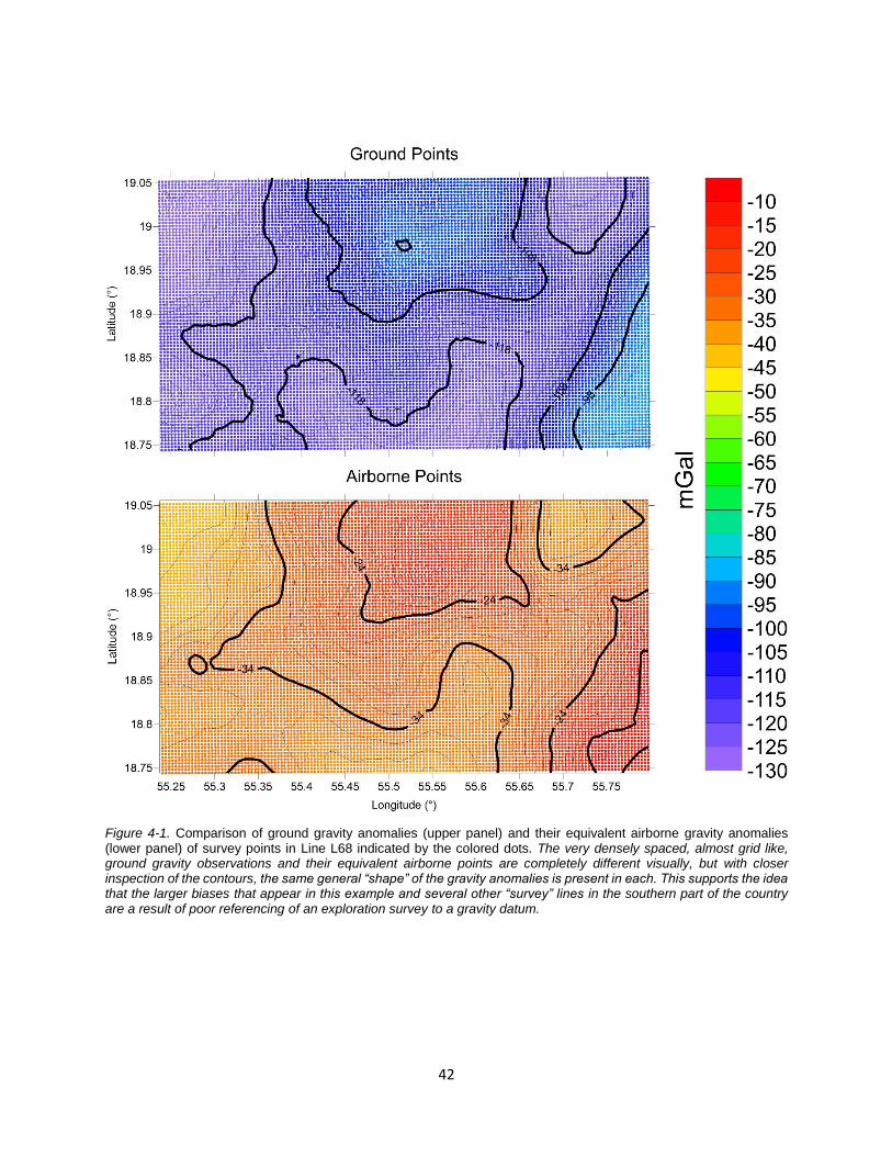
42

Figure 4-1. Comparison of ground gravity anomalies (upper panel) and their equivalent airborne gravity anomalies (lower panel) of survey points in Line L68 indicated by the colored dots. The very densely spaced, almost grid like, ground gravity observations and their equivalent airborne points are completely different visually, but with closer inspection of the contours, the same general “shape” of the gravity anomalies is present in each. This supports the idea that the larger biases that appear in this example and several other “survey” lines in the southern part of the country are a result of poor referencing of an exploration survey to a gravity datum.

43

Figure 4-2. Histogram of ground gravity anomalies (upper panel) and their equivalent airborne gravity anomalies (lower panel) of survey points in Line L68. The histograms are very similar, are positively skewed and have very similar variance and range. Their means however are offset by 80 mGal (bias).

44

Figure 4-3. Comparison of ground gravity anomalies (upper panel) and their equivalent airborne gravity anomalies (lower panel) of survey points in Line L79 indicated by the colored dotes. The ground line and the equivalent airborne line are extremely similar; they are probably referenced to the same gravity network. This was the normal case for very large “survey” lines, most of which were present in the northern part of the country. The grid pattern present in these larger observation lines suggests that they were not conducted for exploration surveys, and are more likely to be properly referenced to the national gravity network

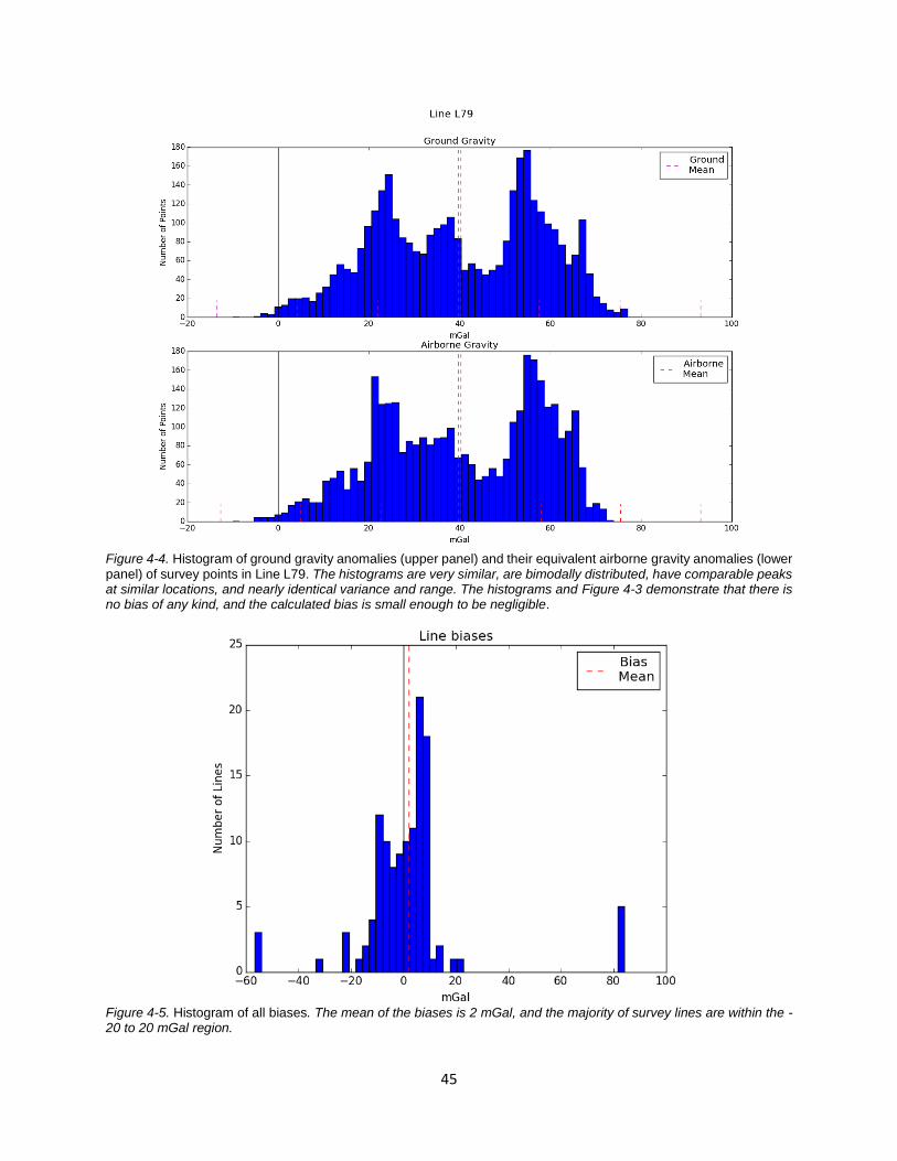
45

Figure 4-4. Histogram of ground gravity anomalies (upper panel) and their equivalent airborne gravity anomalies (lower panel) of survey points in Line L79. The histograms are very similar, are bimodally distributed, have comparable peaks at similar locations, and nearly identical variance and range. The histograms and Figure 4-3 demonstrate that there is no bias of any kind, and the calculated bias is small enough to be negligible.

Figure 4-5. Histogram of all biases. The mean of the biases is 2 mGal, and the majority of survey lines are within the -20 to 20 mGal region.

46

Figure 4-6. Color-coded biases of each ground survey line. Part of the lines (L4A and L4B) circled in black were removed as outliers.

47

Figure 4-7. Comparison of ground gravity anomalies (upper panel) and their equivalent airborne gravity anomalies (lower panel) of survey points in Line L4A. Unlike Figure 4-1 and Figure 4-3, there does not appear to be any visual correlation between the ground and airborne points. The distinctly different ground and airborne contours in each map also support this. There is no information on how or where the seaborne gravity was observed, whether it was filtered, etc.

Figure 4-8. Histogram of ground gravity anomalies (upper panel) and equivalent airborne gravity anomalies (lower panel) of survey points in Line L4A. The noticeable difference in histograms demonstrates that the initial postulation made to allow bias shifting is false in Line L4A.

48

Figure 4-9. Example of the biases remaining in line L4B after bias repair. The noticeable straight lines remaining after bias repair demonstrate that for this line in particular, bias shifting was not effective. The gridded gravity anomalies characterize features (e.g. “scratches”) that cannot exist in earth’s gravity field.

Figure 4-10. Comparison of ground gravity anomalies (left panel) and their equivalent airborne gravity anomalies (right panel) of survey points in Line L4B. Similar to Line L4A, the contours of the “ground” gravity points bear no resemblance to their airborne counterparts. Colors signify the value of the gravity anomaly indicated on the side color scale bar.

49

Figure 4-11. Histogram of ground gravity anomalies (upper panel) and their equivalent airborne gravity anomalies (lower panel) of survey points in Line L4B. Similar to Line L4A, there is a noticeable difference between the ground and airborne histograms that invalidates the histogram postulation.

In addition to the outliers (L4A, L4B) that were removed previously, inconsistencies

between different survey lines at their borders with other lines existed. Some survey lines, such

as line L79 in Figure 4-3, contain tens of thousands of points spread over large regions of the

country. While Figure 4-3 demonstrates that the airborne and ground datasets are visually almost

identical, very small but undefined biases still exist. In addition, several of the lines containing

newly observed and properly referenced gravity data, that were previously assumed to be correct

and un-biased, due to being observed relative to Oman’s current gravity datum, were found to

have rather large biases. It is still unclear whether the biases in these new observations were a

result of poorly referenced gravity measurements, bias errors from the downward continuation of

the airborne gravity anomalies in the mountainous areas, or related to other unknown effects of

the histogram postulation.

4.2 Gridding of gravity anomalies

The bias repaired, point gravity anomalies need to be gridded in order to be merged with

the airborne gravity anomalies. When gridding point values with least squares collocation

(Kriging), the best results are attained when the values to be gridded are as smooth as possible.

50

An adequately smooth point dataset has minimal high frequency variation. Of all the gravity

anomalies, complete Bouguer anomalies are the “smoothest”, and therefore, the most desirable

set of values to grid. A complete Bouguer anomaly, shown in Equation (4.2), was calculated for

the entire Oman territory, by adding an additional terrain roughness term to Equation (2.19).

Δ𝑔𝑏𝑎_𝑐𝑜𝑚𝑝𝑙𝑒𝑡𝑒 = Δ𝑔𝑓𝑎 − 2𝜋𝐺𝜌𝐻 + 𝑐𝑝 (4.2)

The additional terrain roughness term, 𝑐𝑝 is known as the classical terrain correction term.

It is always positive, and takes into account the deviation of the topography from the Bouguer

plate correction applied to the free air anomalies in Equation (2.19), and is given by Equation (4.3)

(Tocho et al., 2005).

𝑐𝑃 = 𝐺 ∬ ∫𝜌(𝑥, 𝑦, 𝑧)(𝐻𝑃 − 𝑧)

(√(𝑥𝑃 − 𝑥)2 + (𝑦𝑃 − 𝑦)2 + (𝐻𝑝 − 𝑧)2

)

3

𝐻

𝐻𝑃𝐸

𝑑𝑥𝑑𝑦𝑑𝑧

(4.3)

The first integral limit is given by 𝐸 and represents the integration over the entire surface

of the Earth. The second integral limit from 𝐻𝑃 to 𝐻 represents integration over the height from

the terrain at 𝐻𝑃 downwards to the height 𝐻 of the integration point. The denominator of the

quantity inside the integral is the Euclidian distance between the integration point and the location

of the terrain correction. The coordinates 𝑥, 𝑦, and 𝑧 are the variables of the integration. The

location of the point where the terrain correction is being computed, is represented by the

variables 𝑥𝑃 , 𝑦𝑃, and 𝐻𝑃.

The always positive nature of the roughness correction term is a result of the interaction

between the computation point 𝑃 and masses above and below it (Hofmann-Wellenhof & Moritz,

2006). Mass surpluses from the terrain, present above the Bouguer plate at point 𝑃, attract 𝑃 in a

direction opposite to gravity. Removing the mass surpluses will increase the value of 𝑔 at point 𝑃

because their attraction is no longer competing against gravity. Mass deficiencies, which are

areas with assumed zero mass, below the Bouguer plate, will not have an attractive force on 𝑃.

Filling in the deficiencies will add more mass below 𝑃 and will also increase 𝑔 at point 𝑃. Since

the roughness term characterizes the high frequency deviations from the Bouguer plate, the

greater the variation of the terrain surrounding point 𝑃, the larger the correction term will be. A

diagram showing how the roughness of the terrain contributes to 𝑐𝑝 at a calculation point can be

seen in Figure 4-12.

51

Figure 4-12. Roughness terrain correction. Mass surpluses are shown in blue and mass deficiencies are shown in red. Mass surpluses are removed to eliminate the attraction opposite the gravity vector; increasing the value of 𝑔 at point

𝑃. Empty mass deficiencies with zero attraction to 𝑃 are filled in to increase the value of 𝑔 at point 𝑃.

The triple integral required to compute the roughness term is simplified when detailed

density information is unknown. The density 𝜌 is taken as the mean rock density of 2.67 𝑔/𝑐𝑚3

and the second integral limit is removed entirely; replacing the 𝑧 variable with the orthometric

height of each moving point designated by the double integral limit over the surface of the Earth.

Due to the insignificant contributions to the terrain correction term from distant masses, the first

integral limit is often simplified to a specific neighborhood around the computation point extending

to about 100 km in radius, depending on the roughness of the terrain.

The terrain roughness correction is calculated for every ground gravity observation point

with a 100 km calculation radius using GRAVSOFT’s TC function; however, a modification was

made to the SRTM with bathymetry DTM. Due to the software’s inconsistent and poorly

documented method of handling negative elevations, the bathymetry component of the SRTM

was converted to its rock equivalent topography (RET) form (Kuhn & Hirt, 2016). RET

approximately condenses the masses of the ocean water and the ocean bottom topography (rock)

to their equivalent mass in rock (Kuhn & Hirt, 2016). Since the average rock density is about 2.5

times greater than the density of water, it will take less volume of rock to have the same effect as

the volume of water associated with the SRTM’s bathymetry. For example, 1000 m of water will

be equivalent to ~400 m of rock, so the -1000 m elevation in the SRTM with bathymetry dataset

will be reduced to about -400 m in the RET SRTM dataset, and the roughness correction algorithm

with density 𝜌 = 2.67𝑔/𝑐𝑚3 can be applied in the oceanic regions where bathymetry is available.

The RET SRTM keeps the densities between land and sea consistent at 2.67𝑔/𝑐𝑚3.

Several functions in the GRAVSOFT software package make a distinction for negative

elevation in input DTM files. In most cases, the grid cells with negative elevations are treated as

being filled with sea water instead of material with density 𝜌. However, in practice, when dealing

Bouguer Plate

Terrain

𝑃

52

with negative DTM elevations, the performance of the GRAVSOFT functions is not consistent with

its documentation.

Since RET produces negative elevations that need to be treated with a density of 𝜌 =

2.67𝑔/𝑐𝑚3, a constant value equal to the inverse of the deepest elevation is added to the dataset,

resulting in a minimum of zero and removes any confusion with respect to negative elevations.

The effects of the constant term are removed at the end of the roughness calculations. The terrain

roughness corrections for northern Oman can be seen in Figure 4-13.

After the terrain roughness is calculated the complete Bouguer anomalies are computed

and gridded to 30" × 30" using Golden Sun Software’s SURFER program. After gridding, they are

converted back to free air anomalies that are now reliably gridded and can be merged with the

downward continued airborne data.

The “inverse” corrections that convert complete Bouguer to free air anomalies are

performed at each grid cell using values of 𝐻 from the SRTM. Since it is not advisable to grid data

with high variability, the high frequency roughness terms computed for the 230 000 gravity points

cannot be used to reclaim simple Bouguer anomalies from complete Bouguer anomalies. To

compensate for this, the roughness term is computed for every grid cell’s latitude and longitude

inside Oman’s borders; then the points are arranged into an array, providing a “gridded”

roughness term.

The gridded free air anomalies have a strong dependence on terrain, a result of using 𝐻

provided by the SRTM to inversely compute them from complete Bouguer anomalies. The final

ground free air anomalies are shown in Figure 4-14.

The free air anomalies also characterize gravity features that were not directly observed,

such as the tops of mountains, or any large areas that have not been surveyed. Depending on

the interpolation distance and spatial location, the interpolated values for these areas can be

unreliable; they are highly dependent on measurements taken nearby. Gravity is often observed

at the base or valleys of mountains. Gridding these observed values can incorrectly skew the

gridded values at the peaks of the mountains. When dealing with gaps in ground gravity coverage,

such as the empty area in the southern part of Oman in Figure 3-1, points interpolated very far

away from measured points have a much higher cumulated gridding error and are less

dependable. While the ground gravity dataset characterizes much of the high frequency

components in the gravity field, it still has gaps in its medium frequency coverage. The steps

taken to compensate for this shortcoming will be discussed in the next chapter.

53

Figure 4-13. Terrain roughness corrections for northern Oman. There is a strong correlation between the magnitude of the roughness correction and the elevation of nearby terrain features. The only other non-zero correction term, not shown here, is located in the southern mountains in the Dhofar region.

54

Figure 4-14. Bias-free ground free air anomalies. The free air anomalies also show features that were not present in previous plots of free air anomalies, especially in areas where gaps in the gravity coverage that appear in Figure 3-1 are present.

55

4.3 Summary

This chapter detailed the steps taken to un-bias the ground gravity anomaly dataset and

prepare it for merging with the airborne dataset. Each gravity survey line was biased relative to

the airborne free air anomaly dataset. The difference of the mean of the free air gravity anomalies

of each survey line and its equivalent downward continued airborne free air anomalies was added

to the survey line to un-bias it. Survey lines L4A and L4B, containing shipborne data, were

removed and the reasons for their removal were discussed in detail. Lastly, the ground free air

gravity anomalies were provided in a gridded format by first transforming them to complete

Bouguer anomalies, gridding the smooth complete Bouguer anomalies and transforming them

back.

56

5 Airborne data and ground-airborne data

integration

5.1 Airborne gravity dataset

A large airborne gravity dataset with ~1.4 million points was observed over the entire

country in the summer of 2015 (Géophysique GPR I’ntl Inc., 2015). It was observed over four

measurement campaigns, with a traverse line spacing of 5 km in the mountainous and coastal

region, and 10 km in the flat desert region. Its average altitude was ~900 m above the geoid, with

the aircraft remaining about 600 m above the terrain at all times (Géophysique GPR I’ntl Inc.,

2015). The dataset originally contained gravity disturbances 𝛿𝑔, the formula for which is given in

Equation (5.1).

𝛿𝑔 = 𝑔𝐾 − 𝛾𝐾 (5.1)

The equation for 𝛿𝑔 is different from the formula for free air anomalies given in Equation

(2.11). While free air anomalies are the difference between measured gravity and normal gravity

on two different surfaces, gravity disturbances are the difference between measured gravity 𝑔𝐾

and normal gravity 𝛾𝐾 on the same surface (at the same point). In the case of the airborne data,

where 𝐾 is the observation point in the air, the standard free air anomaly given by Equation (2.11)

can also be re-written as a function of observations at 𝐾, as shown in Equation (5.2) (Hofmann-

Wellenhof & Moritz, 2006),

𝛥𝑔𝑓𝑎 = (𝑔𝐾 + 0.3086𝐻𝑎) − (𝛾𝐾 + 0.3086(𝐻𝑎 + 𝑁)) (5.2)

where 𝐻𝑎 is the orthometric height of the airborne observation point, 𝐻𝑎 + 𝑁 is the geodetic height

of the observation point, and 𝑁 is the geoid undulation of the terrain point corresponding to the

airborne point. The first term in Equation (5.2) shows that gravity on the geoid 𝑔𝑝 is equivalent to

𝑔𝐾 measured at point 𝐾 plus a free air reduction to the geoid. The second term in Equation (5.2)

shows that normal gravity on the reference ellipsoid 𝛾𝑄 is equivalent to normal gravity 𝛾𝐾 at point

𝐾 plus a free air reduction to the reference ellipsoid. Therefore, Equation (5.2) can be used to

convert observed gravity at point 𝐾 to free air anomalies at altitude.

57

Since gravity disturbances, not observed gravity, were provided in the airborne dataset,

Equation (5.2) can be simplified by cancelling the +0.3086𝐻𝑎 free air gradient term and

expanding the remaining terms. Equation (5.3) shows that taking away 0.3086𝑁 from the gravity

disturbances will give the free air anomaly at altitude.

𝛥𝑔𝑓𝑎 = 𝑔𝐾 − (𝛾𝐾 + 0.3086𝑁) = 𝑔𝐾 − 𝛾𝐾 − 0.3086𝑁 = 𝛿𝑔 − 0.3086𝑁 (5.3)

The free air anomalies at altitude can be seen in Figure 5-1. No additional steps were

taken to smooth the free air anomalies before gridding, as airborne measurements lack high

frequency measurements and are already smooth.

Figure 5-1. Free air anomalies at altitude. Free air gravity anomalies at flight altitude, derived from airborne gravity disturbance measurements. The airborne free air gravity anomalies characterize the medium frequency components of Earth’s gravity field, and capture features in the northern mountainous region’s gravity field not present in Figure 3-10, due to the ineffective sampling in Figure 3-1.

58

5.2 Downward continuation of airborne gravity anomalies

To downward continue airborne gravity anomalies to the geoid, the inverse Poisson

integral must be used. As mentioned previously, the Poisson integral is the solution to the 1st BVP

for the exterior gravity potential 𝑉𝑒, outside a boundary surface 𝑆, given the gravity potential 𝑉 on

𝑆. The inverse problem starts with 𝑉𝑒 outside 𝑆, and attempts to solve for 𝑉 on 𝑆. As with all inverse

problems, the solution is inexact and unstable.

The free air gravity anomalies at altitude are downward continued with the following Poisson

integral formulas (Novak & Heck, 2002),

Δ𝑔(𝑟, Ω) =𝑅

4𝜋𝑟∫ Δ𝑔(𝑟, Ω′)𝐾(𝑡, 𝑢)𝑑Ω′

Ω

where

𝐾(𝑡, 𝑢) =𝑡(1 − 𝑡2)

(√1 − 2𝑡𝑢 + 𝑡2)3/2

and

𝑡 =𝑅

𝑟

𝑢 = 𝑐𝑜𝑠𝜓

(5.4)

(5.5)

(5.6)

(5.7)

The solution to determine the downward continued gravity anomalies is the inverse to the

above equations. To facilitate this, the equations are stabilized with the Tikhonov-Phillips

regularization (Novak & Heck, 2002). Downward continuing the airborne anomalies injects high

frequency components into the medium frequency dataset. It attempts to transform the data

measured at altitude, to what it would look like if measured on the ground.

The downward continuation of gravity anomalies is not within the scope of this thesis. The

gravity anomalies at altitude were downward continued using the inverse Poisson integral by P.

Novak via personal communication using proprietary software. The 1′ × 1′ gridded free air

anomalies at altitude were downward continued to the geoid determined from the global

geopotential model EGM08. To facilitate the estimation of over 350 000 points, the airborne

survey area was split into 30 quadrangles with no more than 20 000 points each. Each

quadrangle’s area was extended by 10 arc minutes, to prevent any edge effects from occurring

between quadrangles when merging the results together. The results of the downward

continuation can be seen below in Figure 5-2.

59

Figure 5-2. Downward continued airborne free air anomalies. The large magnitude high frequency noisy components in the northern part of the country are artifacts from the inverse algorithm used to calculate the gravity anomalies on the geoid. The high frequency components over the mountainous regions are believed to be artifacts and are removed by low-pass filtering (see section 5.4).

5.3 Ground-airborne geoid comparison

To verify that the ground gravity data were correctly bias repaired and the airborne data

were correctly downward continued, preliminary geoids were calculated for each dataset using

the methodology outlined in Chapter 6. This was done to verify that no apparent biases exist in

either of the datasets and that the two datasets are compatible with each other and are

therefore suitable for merging. Figure 5-3 shows the differences between the two geoids and

Figure 5-4 shows the histogram of the differences.

60

Figure 5-3. Preliminary ground geoid minus preliminary airborne geoid. The two geoids are very similar, with sub 20-centimeter agreements throughout the entire country. The majority of the differences appear smooth with the exception of the mountainous region in the northern part of the country. This area is better characterized by the ground observations and the geoid reflects this.

61

Figure 5-4. Histogram of the differences between the preliminary ground geoid and the preliminary airborne geoid. The average of the differences (ground geoid – airborne geoid) is 0 m and the standard deviation is 1 cm.

5.4 Ground-airborne data integration

Merging the adjusted ground gravity dataset with the downward continued airborne free

air anomaly dataset allows the frequency content of each to be combined into one cohesive

dataset. The merging is done by low-pass filtering the downward continued airborne gravity

anomalies with an isometric Gaussian filter, and high-pass filtering the ground gravity anomalies

using the complement Gaussian of the same cutoff frequency. The medium (airborne) and high

(ground) frequency components of the gravity anomalies, are then added together, with no

overlap in the frequency content.

The 1’ × 1’ downward continued airborne free air gravity anomalies are resampled to 30“ ×

30” to have the same spacing and coverage as the ground free air gravity anomalies. Both

datasets are padded with zeros to increase the physical coverage of the grid. The ground and

downward continued airborne free air gravity anomalies are filtered with an isometric 2-D

Gaussian filter in the space domain, shown in Equation (5.8),

𝐺(𝜙, 𝜆) =1

2𝜋𝜎𝑘𝑚2 exp (−

𝑑2

2𝜎𝑘𝑚2 )

(5.8)

where 𝜎 is the standard deviation of the filter, and 𝑑 is the spatial distance between the point that

is being filtered and the running point. When working in spherical coordinates, the spatial distance

is given by Equation (5.9),

62

𝑑2 = 𝑅2(𝛿𝜙2 + cos2 𝜙𝛿𝜆2) (5.9)

where 𝑅 is the mean radius of the Earth and is equal to 6371 km, 𝜙 is the geodetic latitude of the

computation point, and 𝛿𝜙 and 𝛿𝜆 are the differences in radians between the filtered point and

the running point in latitude and longitude, respectively. The distance is computed using spherical

geodetic coordinates instead of Cartesian coordinates, because the linear length (km) per one

arc degree of longitude decreases towards the poles.

To determine the standard deviation 𝜎 that defines the cutoff frequency of the Gaussian

filter in Equation (5.8), we use Equation (5.10),

𝜎𝑘𝑚 =1

2𝜋

𝐷𝑐

√2 ln(2)≈

𝐷𝑐

7.398

(5.10)

where 𝐷𝑐 is the cutoff wavelength; the point where 50 percent of the signal power is attenuated.

When working in the space domain, 𝐷𝑐 corresponds to the spatial wavelength required. For

example, if the desired spatial resolution is 𝐷𝑐 = 100 km, or 1° × 1° in longitude (D/O 360 in

spherical harmonics), 𝜎 will equal 13.5 km. For efficient computations, only points up to 3.2𝜎 away

from the point of interest should be filtered, to ensure that 99.5 percent of points with a meaningful

contribution are filtered (3𝜎), plus a slight increase for redundancy. For example, for a spatial

resolution of 100 km, the Gaussian kernel search radius should be 43.2 km. Since the highest

airborne resolution is 20 km, that is, 2 times the 10 km line spacing, then the cutoff spacing for

the ground data should be 𝜎 =20

7.398 = 3 km, and the kernel value should be computed for a 3.2×3

= 10 km radius.

The downward continued airborne and the ground free air gravity anomalies are low-pass

filtered with a 3 km Gaussian filter. The low-pass filtered ground free air anomalies are subtracted

from the initial unfiltered ground free air anomalies, leaving the high frequency component to be

merged to the airborne anomalies (Figure 5-6). At this point, the medium (Figure 5-5) and high

(Figure 5-6) frequency components are added together to make the final free air gravity anomaly

dataset (Figure 5-7), and the simple Bouguer anomaly dataset (Figure 5-8) that will be used to

compute the geoid.

63

Figure 5-5. Downward continued airborne free air anomalies filtered with an isometric Gaussian filter in the spatial domain. The airborne dataset displays the medium frequency components of Earth’s gravity field after the application of the Gaussian filter.

64

Figure 5-6. High frequency free air anomaly computed from the ground free air anomalies by Gaussian filtering.

65

Figure 5-7. Final ground gravity free air anomalies created from airborne free air anomalies (downward continued and filtered) merged with ground free air anomalies (filtered).

66

Figure 5-8. Simple Bouguer anomalies derived from final ground gravity free air anomalies.

5.5 Verifying free air anomalies with a global geopotential model

For quality control purposes, the free air anomalies in Figure 5-7 were compared to a pure,

satellite determined, global geopotential model. While the satellite model would not characterize

the high and medium frequencies of the free air anomalies, it would demonstrate whether any

significant low frequency biases remain in the anomalies. The low-pass Stokes integral would not

remove the low frequency biases, and they would persist throughout the entire remove-compute-

restore process, biasing the final gravimetric geoid.

67

The pure, satellite determined, global geopotential model selected is the GOCO05s GGM

to D/O 280, from the German Research Centre for Geosciences (GFZ) (Mayer-Gürr et al., 2015).

It is generated using the International Center for Global Earth Models (ICGEM) online computation

service. Figure 5-9 shows the difference between the two free air anomaly maps. Figure 5-10

shows the histogram of differences seen in Figure 5-9 within the country’s borders. The

differences in Figure 5-9, are expected since the GOCO05S satellite model is not capable of

characterizing the high frequency variation of the ground gravity dataset. The final ground gravity

dataset is acceptable because it appears that there are no longer any biases in the ground gravity

dataset

Figure 5-9.GOCO05s minus final free air anomalies. The large differences in the mountainous and coastal regions are expected due to the high frequency components present in the free air anomalies. The low degree and order of the satellite model (280) cannot characterize the ground data at these high frequencies.

68

The histogram in Figure 5-10 appears to be nearly normally distributed but positively

skewed. The peak around -15 mGal represents the medium and high frequency components

present in the mountainous areas of Oman that the satellite model cannot adequately

characterize. The larger differences that are 80 to 100 mGal represent the high frequency

components present in the tallest mountains that the satellite is unable to characterize.

Figure 5-10. Histogram of differences between GOCO05s free air anomalies and final free air anomalies. The average of the differences (GOCO05s – Final Free Air Anomalies) is -3.25 mGal and the standard deviation is 27.2 mGal.

5.6 Summary

This chapter explained the steps required to create the final free air gravity anomaly

dataset that will be used to calculate the geoid. First, the airborne free air gravity anomalies at

altitude were downward continued to the geoid using the inverse Poisson integral. Next, using an

isometric Gaussian filter, the airborne and ground free air anomaly grids were low-pass and high-

pass filtered, respectively, in order to extract the low and high frequency components of the gravity

field. The sum of the two frequency components are the final free air gravity anomalies, which

were verified against the pure, satellite determined, global geopotential model GOCO05s.

69

6 Geoid calculations

6.1 Remove-compute-restore technique

The method used to calculate the geoid in Oman is the remove-compute-restore (RCR)

methodology. According to this methodology, the contribution of the gravitational attraction of the

topographic masses to the gravity anomalies is removed as much as possible to render them

smooth. The smooth residual gravity anomalies are then convolved with the Stokes integral to

compute the high frequency component of the quasigeoid. Finally, the removed effects are

restored after being converted to their corresponding quasigeoid components and are added to

the high frequency quasigeoid to determine the full quasigeoid. As a last step, the quasigeoid is

transformed to the geoid using simple Bouguer anomalies and a DTM.

6.2 Remove step

The purpose of the remove step is to make the gravity anomalies smooth and easy to grid

by removing as much information as possible. The global gravity signal is removed to eliminate

the long wavelength components not adequately characterized by the discrete computation

neighborhood, while the high frequency terrain effects are removed from the gravity anomalies to

eliminate any short wavelength biases in the gravity anomalies from the local terrain.

The general mathematical process of the remove step is given in Equation (6.1). The long

wavelength gravitational effects of a global geopotential model Δ𝑔𝑒𝑔𝑚, such as EGM08, and the

high frequency local terrain effects Δ𝑔𝑡𝑒𝑟, (i.e., the gravitational effects of the roughness of the

topography with respect to a smooth representation of the actual topography, such as a mean

height reference surface), are removed from the free air anomalies Δ𝑔𝑓𝑎, leaving behind smooth

residual gravity anomalies Δ𝑔𝑟𝑒𝑠.

Δ𝑔𝑟𝑒𝑠 = Δ𝑔𝑓𝑎 − Δ𝑔𝑒𝑔𝑚 − Δ𝑔𝑡𝑒𝑟 (6.1)

In this research, Δ𝑔𝑒𝑔𝑚 is calculated from the EGM08 global geopotential model to D/O

360, using the International Center for Global Earth Models (ICGEM) online computation service.

The effects of the terrain Δ𝑔𝑡𝑒𝑟 are computed using the RTM approach (Forsberg & Tscherning,

70

1981) by using a smooth height reference surface created by low-pass filtering of the actual

topography (see below in Figure 6-1).

The RTM method considers only the short and medium wavelength gravitational effects

of the topography. The linear approximation of Δ𝑔𝑡𝑒𝑟 for the RTM effect at a single point 𝑃 is

expressed in Equation (6.2) (Forsberg, 1984),

Δ𝑔𝑡𝑒𝑟 = 2𝜋𝐺𝜌(𝐻 − 𝐻𝑟𝑒𝑓) − 𝑐𝑝 (6.2)

which has some similarities to the terms added to free air anomalies when computing complete

Bouguer anomalies. However, an additional smooth reference surface is utilized; 𝐻 is the height

of the computation point, 𝐻𝑟𝑒𝑓 is the height of the smooth reference surface at the same

computation point, and 𝑐𝑝 is the classical terrain correction that characterizes roughness,

mentioned previously in Equation (4.3).

In essence, the first component of Equation (6.2) is the difference between two Bouguer

reductions. The gravitational effects of the actual topography 2𝜋𝑔𝜌𝐻 (with respect to the geoid)

are removed from the free air anomalies, and the effects of the smooth topography 2𝜋𝑔𝜌𝐻𝑟𝑒𝑓 are

added back, this is illustrated in Figure 6-1.

Figure 6-1. RTM terrain effect theory. The blue hatched areas above the reference surface show the removal of the actual topography. The red hatched areas below the reference surface show the effects of the smooth topography that are added back. The empty region below the reference surface is consistent between both Bouguer reductions.

If the smooth topography is created from a low-pass filter, the RTM reduction corresponds

to an isostatic reduction (Moritz, 1968), which characterizes the medium frequency components

of topography. A 100 km low-pass spatial filter is chosen for this purpose, and the mean reference

surface is computed using GRAVSOFT’s TCGRID function. The TCGRID function takes an input

grid file and low-pass filters it based on a moving average window specified by the user.

The gridded values of Δ𝑔𝑡𝑒𝑟 are computed in Python with simple grid mathematics using

the SRTM with RET bathymetry model to create the smooth reference surface over land and

𝐻 − 𝐻𝑟𝑒𝑓

Terrain

Reference Surface

𝑃

71

oceans. The final terrain effects are shown in Figure 6-2. The classical roughness term 𝑐𝑝 is

provided by the gridded corrections computed by TC in Chapter 4. The global geopotential effects

Δ𝑔𝑒𝑔𝑚 and local terrain effects Δ𝑔𝑡𝑒𝑟 are subtracted from the free air anomaly dataset with

GRAVSOFT’s GEOIP function, which adds or subtracts differently spaced grids. The resultant

residual gravity anomaly dataset is now ready to input into the Stokes integral in the compute

step.

Figure 6-2. RTM terrain effects. The purpose of creating the residual anomalies is to remove as much information as possible from the free air anomalies to make them smooth. The low frequency EGM component and the high frequency terrain effects are removed, leaving behind a smooth medium frequency surface.

72

6.3 Remove step workflow

Table 6-1 shows the GRAVSOFT and Python software required to complete the remove

step. Unless explicitly stated, the spatial extent of any datasets are 𝜙 [15.25°, 27.75°] and

𝜆 [50.75°, 61.25°]. The SRTM contains RET corrected bathymetry, and the entire dataset has a

constant added to avoid negative elevations in the oceans. The computation of the roughness

term 𝑐𝑝 in step 2A does not require any software modification to remove the constant because

the roughness calculation for a point is relative to that point’s elevation, instead of the dataset as

a whole. The constant must be removed when computing the difference in Bouguer slabs in the

Python software in step 2B.

Table 6-1. Remove step software workflow

Description Input Software Output

DTM setup

1A Resample SRTM

𝑺𝑹𝑻𝑴[3"×3"]

𝜙𝜆

[14° 28°48° 62°

]

SELECT 𝑺𝑹𝑻𝑴[30"×30"]

1B Get Reference Surface (~100 Km)

𝑺𝑹𝑻𝑴[30"×30"] TCGRID 𝑺𝑹𝑻𝑴𝒓𝒆𝒇[30"×30"]

Calculate 𝛥𝑔𝑡𝑒𝑟

2A Compute 𝑐𝑝 List of Point Free Air anomalies from

𝚫𝒈𝒇𝒂[30"×30"]

𝑺𝑹𝑻𝑴[30"×30"]

𝑺𝑹𝑻𝑴𝒓𝒆𝒇[30"×30"]

TC1

in mode 3 𝒄𝒑[30"×30"]

2B Compute

2𝜋𝐺𝜌(𝐻 − 𝐻𝑟𝑒𝑓) (Difference in Bouguer

Slabs)

𝝆 = 2.67 𝑺𝑹𝑻𝑴[30"×30"]

𝑺𝑹𝑻𝑴𝒓𝒆𝒇[30"×30"]

TC1

in mode 4

𝚫𝑩𝑨[30"×30"]

2C Calculate Δ𝑔𝑡𝑒𝑟 𝚫𝑩𝑨[30"×30"]

𝒄𝒑[30"×30"]

GCOMB in mode 1

𝚫𝒈𝒕𝒆𝒓[30"×30"]

Calculate 𝛥𝑔𝑟𝑒𝑠

3A Subtract Δ𝑒𝑔𝑚08 D/O

360 from Δ𝑔𝑓𝑎

𝚫𝒈𝒇𝒂[30"×30"]

𝚫𝒈𝒆𝒈𝒎𝟎𝟖[30"×30"]

GCOMB in mode 1

𝚫𝒈𝒕𝒆𝒎𝒑[30"×30"]

3B Compute Δ𝑔𝑟𝑒𝑠 by

subtracting Δ𝑔𝑡𝑒𝑟 from Δ𝑔𝑡𝑒𝑚𝑝

𝚫𝒈𝒕𝒆𝒎𝒑[30"×30"]

𝚫𝒈𝒕𝒆𝒓[30"×30"]

GCOMB in mode 1

𝚫𝒈𝒓𝒆𝒔[30"×30"]

1Modified for large datasets

73

6.4 Compute step

The Stokes integral is applied to the residual gravity anomalies Δ𝑔𝑟𝑒𝑠 to generate 𝜁Δ𝑔𝑟𝑒𝑠,

the residual height anomaly (residual quasigeoid height) according to the Molodenskij approach

since all gravity anomalies used in the calculations refer to the topography and not to the geoid.

For this calculation, the FFT implementation of GRAVSOFT’s SPFOUR (Forsberg, 2002) function

is used, with Wong-Gore tapering of the Stokes Function and 100% zero padding of the input

residual gravity anomalies. Equation (6.3) shows the modified Stokes function that is used to

suppress the effects of any remaining long wavelength harmonics.

𝑆𝑚𝑜𝑑(ψ) = 𝑆(𝜓) − ∑ 𝛼(𝑛)

𝑁

𝑛=2

2𝑛 + 1

𝑛 − 1𝑃𝑛𝑐𝑜𝑠𝜓

(6.3)

Each term of the summation is the value of the harmonic component corresponding to

degree 𝑛. The tapering coefficient 𝛼(𝑛) controls any Gibbs phenomenon that may arise from the

“sharp” truncation of the special harmonics to degree 𝑁. The value of the summation for degree

𝑛 is multiplied by the tapering coefficient, and is subtracted from the Stokes function.

When 2 ≤ 𝑛 ≤ 𝑁1, the function 𝛼(𝑛) is equal to 1, and the corresponding summation element is

removed from the Stokes function. When 𝑁1 < 𝑛 ≤ 𝑁2 , the function 𝛼(𝑛) is tapered down linearly

from 0.99̅ to 0. When 𝑛 > 𝑁2, the function 𝛼(𝑛) is equal to 0, and the summation components are

not removed. Figure 6-3 shows this tapering process.

The tapering is done to remove the same low frequency effects in the Stokes integral

previously removed in the remove step in case there are still some low order harmonics present

after the removal of the EGM08 of D/O 360. The Wong-Gore tapering is done to degree and order

360 because EGM08 D/O 360 has been removed; resulting in 𝑁1 = 360 and 𝑁2 = 365 to provide

a smooth transition.

74

Figure 6-3. Wong-Gore Tapering kernel. This plot illustrates the behavior of the factor 𝑎(𝑛) depending on the

parameters chosen for degree and order. Every component up to 𝑁1 is removed, components between 𝑁1 and 𝑁2 are

removed linearly, and components after 𝑁2 are not removed.

6.5 Compute step workflow

Table 6-2 shows the GRAVSOFT software required to complete the compute step. The

spatial extent of all datasets are 𝜙 [15.25°, 27.75°] and 𝜆 [50.75°, 61.25°].

Table 6-2. Compute step workflow

Description Input Software Output

1 Calculate 𝜁Δ𝑔𝑟𝑒𝑠 𝚫𝒈𝒓𝒆𝒔[30"×30"]

SPFOUR1 with Wong-Gore

Kernel Modification

𝜻𝚫𝒈𝒓𝒆𝒔 [30"×30"]

1Modified for large datasets

75

6.6 Restore step

The components removed from the free air anomalies to create the residual anomalies

Δ𝑔𝑟𝑒𝑠 need to be restored back to the residual height anomaly 𝜁𝑟𝑒𝑠, in the form of height anomalies

𝜁𝑒𝑔𝑚 and 𝜁𝑡𝑒𝑟. This process is shown in equation (6.4),

𝜁 = 𝜁𝑒𝑔𝑚 + 𝜁Δ𝑔 + 𝜁𝑡𝑒𝑟 (6.4)

where 𝜁𝑒𝑔𝑚 is the height anomaly computed from the EGM08 global geopotential model to D/O

360, using the ICGEM online computation service, and 𝜁𝑡𝑒𝑟 is the height anomaly due to the terrain

effect, calculated by running the terrain effects Δ𝑔𝑡𝑒𝑟 through the Stokes integral without the

Wong-Gore tapering. The grids holding each quantity on the right-hand side of the equation are

added together using GRAVSOFT’s GCOMB function, which can add or subtract grids with equal

spacing and limits.

6.7 Restore step workflow

Table 6-3 shows the GRAVSOFT software required to complete the restore step. The

spatial extent of all datasets are 𝜙 [15.25°, 27.75°] and 𝜆 [50.75°, 61.25°].

Table 6-3. Restore step workflow

Description Input Software Output

Calculate Quasi-Geoid

1A Add 𝑁𝑒𝑔𝑚08 D/O 360 to

𝜁Δ𝑔𝑟𝑒𝑠

𝜻𝚫𝒈𝒓𝒆𝒔 [30"×30"]

𝜻𝒆𝒈𝒎𝟎𝟖[30"×30"]

GCOMB in mode 2

𝜻𝒕𝒆𝒎𝒑[30"×30"]

1B Calculate 𝜁𝑡𝑒𝑟 𝚫𝒈𝒕𝒆𝒓[30"×30"] SPFOUR1 𝜻𝚫𝒈𝒕𝒆𝒓 [30"×30"]

1C Add 𝜁Δ𝑔𝑡𝑒𝑟 to 𝑁𝑡𝑒𝑚𝑝 𝜻𝒕𝒆𝒎𝒑[30"×30"]

𝜻𝚫𝒈𝒕𝒆𝒓 [30"×30"]

GCOMB in mode 2

𝜻[30"×30"]

1Modified for large datasets

76

6.8 Gravimetric geoid step

The computation of the gravimetric geoid 𝑁 from the quasigeoid (height anomaly) 𝜁 can

be done by calculating the 𝑁 − 𝜁 separation term, mentioned previously in Equation (2.24). The

𝑁 − 𝜁 correction is calculated using GCOMB in mode 9, and is added to the quasigeoid computed

in Equation (6.4) to get the gravimetric geoid using GCOMB in mode 2. Figure 6-4 shows the

unfitted gravimetric geoid.

Figure 6-4. Unfitted gravimetric geoid.

77

6.9 Gravimetric geoid workflow

Table 6-4 shows the GRAVSOFT software required to compute the gravimetric geoid

undulations from the height anomalies. The spatial extent of all datasets is 𝜙 [15.25°, 27.75°] and

𝜆 [50.75°, 61.25°].

Table 6-4. Compute gravimetric geoid workflow

Description Input Software Output

Calculate Gravimetric Geoid

1A Compute (𝑁 − 𝜁) corrections

𝚫𝒈𝒔𝒃𝒈[30"×30"]

𝑺𝑹𝑻𝑴[30"×30"]

GCOMB in mode 9

(𝑵 − 𝜻)[30"×30"]

1B Compute Geoid 𝜻[30"×30"]

(𝑵 − 𝜻)[30"×30"]

GCOMB in mode 2

𝑵[30"×30"]

6.10 Fitting the gravimetric geoid model to GPS-on-benchmarks

The main application of the geoid for surveying is the acquisition of the orthometric height

of a point, without measuring height differences and gravity in geodetic (spirit) levelling. Due to

datum inconsistencies (tide gauge datum), errors embedded in the Orthometric heights 𝐻

determined by geodetic levelling, errors in the Global Navigation Satellite System (GNSS)

geodetic height ℎ, and undoubtedly errors in the gravimetric geoid height 𝑁; it is often useful to fit

the gravimetric geoid model to the geometric geoid model determined from the well-known

relationship shown in Equation (2.27) at selected high precision benchmarks across the country.

Such benchmarks are often called “GPS-on-benchmarks” that define the height reference frame

in the country. The fitting of the gravimetric geoid to such benchmarks will allow users to determine

orthometric heights from GNSS observations and the fitted geoid that are compatible with the

national height system.

In addition to providing consistency to surveyors and engineers, the results of the fitting

can be used to assess the external accuracy of the gravimetric geoid model. If it is assumed that

the GPS-on-benchmarks and their associated orthometric heights are of good quality, then the

geometric geoid can be computed using Equation (2.27). The geometric geoid can be used to

determine the quality of the gravimetric geoid model by calculating the difference in geoid

undulation 𝑁 for each benchmark. The differences Δ𝑁 are calculated using Equation (6.5).

Δ𝑁 = 𝑁𝑔𝑒𝑜𝑚 − 𝑁𝑔𝑟𝑎𝑣 (6.5)

78

Gridding the calculated differences will result in a surface that can be added to the

gravimetric geoid to create the “fitted geoid” on GPS-on-benchmarks.

6.11 Geoid fitting step workflow

Table 6-5 shows the Surfer software required to fit the gravimetric geoid to the GPS-on-

benchmarks. The spatial extent of all datasets are 𝜙 [15.25°, 27.75°] and 𝜆 [50.75°, 61.25°].

Table 6-5. Fitting of gravimetric geoid workflow

Description Input Software Output

Fitting Gravimetric Geoid to GPS-on-Benchmarks

1A Compute GPS-On-benchmark residuals

𝑵[30"×30"]

Geometric Geoid for each GPS-On

Benchmark

Surfer Grid|Residuals

Residual2 for each GPS-On-

Benchmark

1B Grid Residuals Residual2 for each GPS-On

Benchmark

Surfer Grid|Data

𝑮𝒓𝒊𝒅𝒅𝒆𝒅 𝑹𝒆𝒔𝒊𝒅𝒖𝒂𝒍𝒔[30"×30"]

1C Fit Geoid 𝑵[30"×30"]

𝑮𝒓𝒊𝒅𝒅𝒆𝒅 𝑹𝒆𝒔𝒊𝒅𝒖𝒂𝒍𝒔[30"×30"]

Surfer Grid|Math (add)

𝑵𝒇𝒊𝒕𝒕𝒆𝒅[30"×30"]

2 Surfer defines residuals as 𝑁𝑔𝑒𝑜𝑚 − 𝑁𝑔𝑟𝑖𝑑

6.12 Summary

This chapter presented in detail the remove-compute-restore (RCR) method and how it

was applied to calculate the gravimetric quasigeoid. The workflow for each step in the process

was also included. In addition to the RCR method, the conversion from the quasi-geoid to the

gravimetric geoid was presented along with the steps required to fit the gravimetric geoid to the

geometric geoid using GPS-on-benchmarks.

79

7 Final Results

7.1 Geoid fit testing

To test the gravimetric geoid model, and subsequently fit it to GPS-on-benchmarks, 370

GPS-on-benchmarks are used; however, not all are considered for fitting the gravimetric geoid.

Of the 370 points, 39 are 1st order, 284 are 2nd order, and 47 were specifically observed for the

ONGM project. The location of the benchmarks and their gridded residuals with respect to the

gravimetric geoid model are shown in Figure 7-1.

Nine benchmarks have relatively large residuals greater than ± 1 m, and are designated

gross outliers, and removed. The large difference is likely a result of a combination of poorly

observed geodetic and orthometric heights, as it is highly unlikely that the geoid would differ from

the benchmarks to that level. These large residuals also appeared when comparing the GPS-on-

benchmarks to full expansion EGM08 and GOCO05s geoid models, further supporting the claim

that the height measurements have errors.

The remaining benchmarks are then used to produce the updated difference map shown

in Figure 7-2 with their histogram in Figure 7-3. There are still multiple locations with large

residuals (>± 25 cm) that are inconsistent, relative to their surroundings. These are circled and

numbered in Figure 7-2. The first six circles include one or two outlier points (8 in total) with large

residuals situated in an area with comparatively smaller ones. The geoid is a smooth surface in

these regions, and cannot explain abrupt residual changes for single point(s) on a levelling line.

Neighboring the large residuals there exist benchmarks with very small residuals. Since all

levelling lines are consistent with the reference benchmarks and exhibit misclosures at the sub-

centimeter level, it is highly unlikely that only one benchmark in the levelling line is off by up to

several decimeters. It is highly possible that the geodetic height used to calculate the geometric

geoid at such benchmarks contain a large systematic error, likely due to adverse atmospheric

conditions, poor field procedures, and/or severe multipath, or the observed orthometric height at

each benchmark was not determined correctly (e.g. no gravity measurements). Furthermore, the

benchmarks with larger residuals also had the same problem when testing them with other

independent geoid models, such as GOCO05s and EGM08. As a result, the eight outlier

benchmarks are removed leaving 347 points available to fit the geoid.

80

The larger discrepancies in regions seven and eight are also examined. The benchmarks

in each region that reach +60 cm and –60 cm, respectively, belong to the same levelling line.

Since in these regions the geoid is relatively flat (see Figure 6-4) and over a flat topography (see

Figure 3-4), EGM08 and GOCO05s GGMs can also be used to test the geometric geoid. As a

result of these tests, the said large discrepancies remain. Since the computed gravimetric geoid

model differs from the two reference models by a few centimeters at most in these regions, the

geodetic height of these benchmarks is likely the cause of discrepancies. Unlike the problems in

the first six regions, which span small areas, these benchmarks are not removed as they cover

extended areas rather than being single benchmarks. Until new high precision GNSS or

orthometric height measurements become available, the fitted geoid in these regions will be

biased by a few decimeters.

Figure 7-1. Benchmark locations. The white circles are the primary 1st order benchmarks, the black triangles are the 2nd order points referenced to the 1st order benchmarks, and the new observation points are the red diamonds referenced to both 1st and 2nd order points. The background map shows the gridded residuals of all benchmarks.

1 2 New

81

Figure 7-2. Benchmark residuals from -1 m to 1 m. The large differences in the circled areas are discussed in the text above.

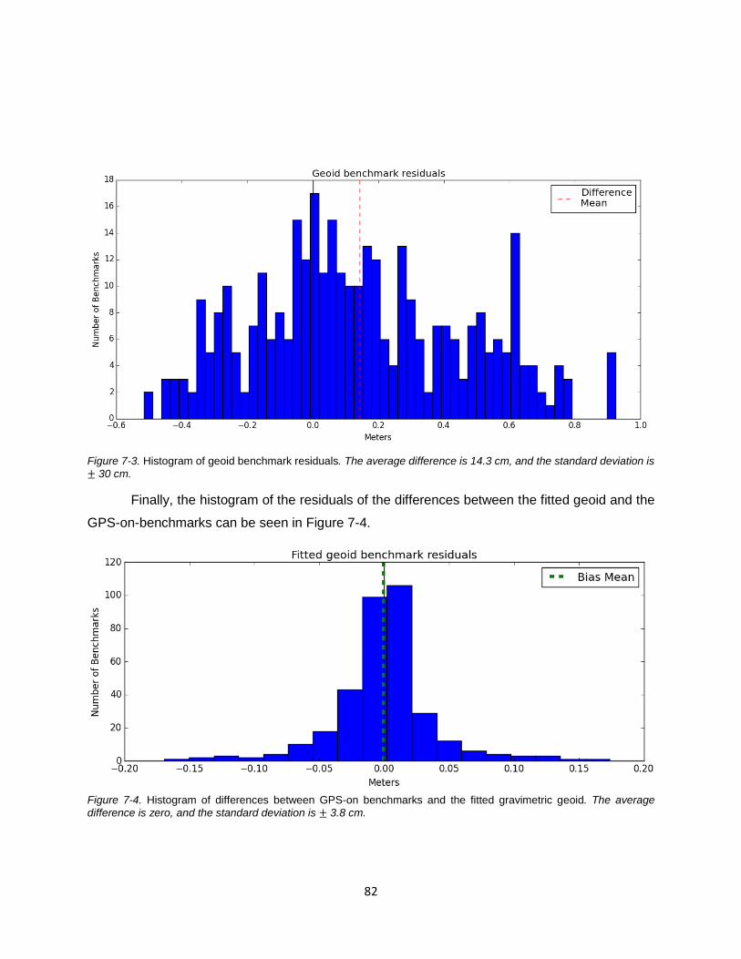
82

Figure 7-3. Histogram of geoid benchmark residuals. The average difference is 14.3 cm, and the standard deviation is

± 30 cm.

Finally, the histogram of the residuals of the differences between the fitted geoid and the

GPS-on-benchmarks can be seen in Figure 7-4.

Figure 7-4. Histogram of differences between GPS-on benchmarks and the fitted gravimetric geoid. The average

difference is zero, and the standard deviation is ± 3.8 cm.

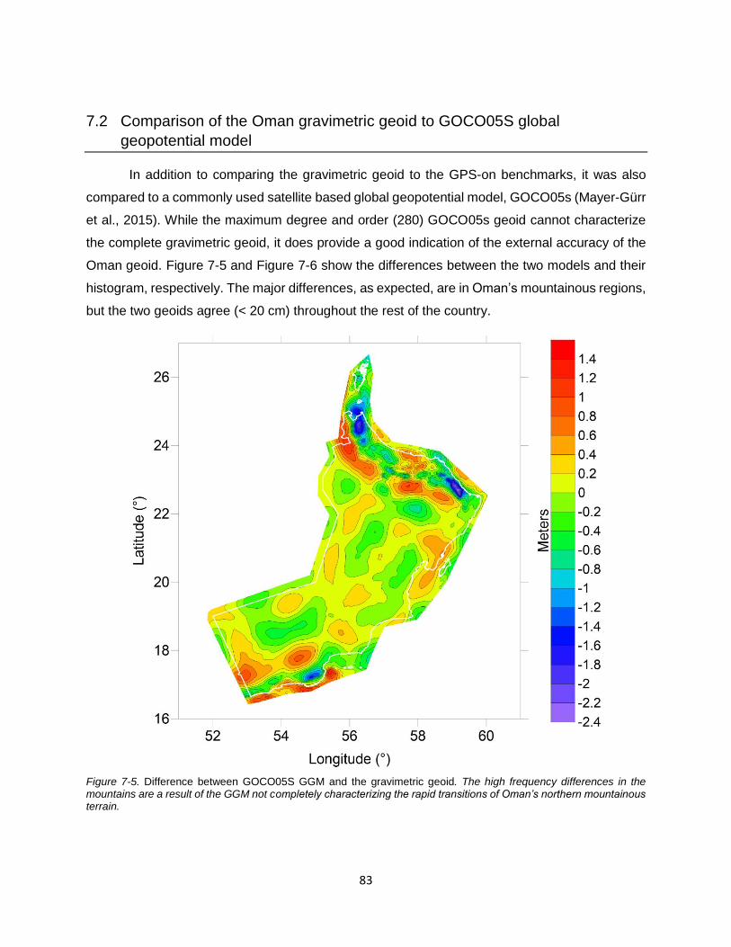
83

7.2 Comparison of the Oman gravimetric geoid to GOCO05S global

geopotential model

In addition to comparing the gravimetric geoid to the GPS-on benchmarks, it was also

compared to a commonly used satellite based global geopotential model, GOCO05s (Mayer-Gürr

et al., 2015). While the maximum degree and order (280) GOCO05s geoid cannot characterize

the complete gravimetric geoid, it does provide a good indication of the external accuracy of the

Oman geoid. Figure 7-5 and Figure 7-6 show the differences between the two models and their

histogram, respectively. The major differences, as expected, are in Oman’s mountainous regions,

but the two geoids agree (< 20 cm) throughout the rest of the country.

Figure 7-5. Difference between GOCO05S GGM and the gravimetric geoid. The high frequency differences in the mountains are a result of the GGM not completely characterizing the rapid transitions of Oman’s northern mountainous terrain.

84

Figure 7-6. Histogram of differences between GOCO05S and the gravimetric geoid. The average difference is 2.2 cm, with a standard deviation of ± 37.8 cm. The large peak on the right side of the histogram signifies the difference in frequency between the medium frequency gravimetric geoid and the low frequency satellite determined geoid.

7.3 Important remarks on the accuracy of the Oman gravimetric geoid model

The unfitted gravimetric geoid model is on average 14 cm lower than the mean sea level

(MSL) defined by the levelled heights (MSL) at all test benchmarks discussed in the previous

section. This agrees well with the sea surface topography (SST) in the region as determined by

satellite altimetry (Andersen & Knudsen, 2009).

One of the reasons for the gravimetric geoid misfit in certain regions of limited extent, and

also at single benchmarks, is most probably due to errors in the geodetic heights. Verification of

the accuracy of the GPS-on-benchmarks from the GPS perspective is required. The questionable

benchmarks found to be incompatible with the geoid model could be re-observed with minimal

effort to verify their geodetic and orthometric heights.

It is unclear whether the height network in Oman is in an orthometric height system. From

careful examination of various technical reports, it is suspected that the heights of the benchmarks

provided are in some normal height system. This might have introduced additional discrepancies

between the gravimetric geoid and the GPS-on-benchmarks. For the 1st and 2nd order

benchmarks, verification of reductions and calculations must be revisited and a readjustment of

the height network of Oman must be performed.

85

8 Conclusions and recommendations

8.1 Summary and conclusions

In this research, the task of developing the Oman National Geoid Model (ONGM) was

undertaken. A legacy ground gravity dataset was available from the National Survey Authority

(NSA) of Oman, with approximately 230 000 point gravity observations. In addition, a newly

observed ground gravity dataset of about 6000 points, a newly observed airborne dataset with

countrywide coverage, and a set of GPS observations on Oman’s current leveled benchmarks

were available for this research.

The main challenges for completing this work were concentrated on the quality of the

available datasets and in particular the legacy ground gravity dataset that was observed over a

period of at least fifty years using various techniques, instruments and data processing

methodologies whose description (metadata) was not available. In addition, the scope under

which the observations were collected and the reduction methods used were for natural resource

exploration and may not be suitable for the determination of the geoid model of Oman at the

centimetre level of accuracy. Moreover, over the long period of the data collection, the geodetic

reference systems used for processing the observations have become obsolete for modern geoid

computations.

Ground gravity observations provide the high frequency components of a geoid model,

that is, they make possible the calculation of the detailed short wavelength geoid structure that is

indispensable for accurate GNSS levelling. As such, the legacy gravity dataset, despite its

inherent problems and inconsistencies, was deemed very important for the ONGM, and a

necessary addition to the recent airborne and limited new ground gravity measurements. The

main contribution of this thesis was the launching and completion of a very long forensic

investigation of the legacy gravity data, in complete absence of critical metadata, to render them

useful and suitable for integration with the airborne data for the ONGM.

The investigation and subsequent repair of the data included the following main

contributions that are described in detail in Chapters 3, 4, and 5:

1.) Identification and verification of the geodetic reference system used to provide positional

information for the point gravity observations.

86

2.) Identification of the type of the original data, such as the type of gravity anomalies

provided, which were missing in the vast majority of original gravity observations and had

unknown reduction methods.

3.) Developing algorithms for the transformation of the old geodetic reference systems, such

as from PDO Survey Datum of 93 (PSD93), to the modern WGS84 reference system.

4.) Development of inverse calculation algorithms to recover proxy gravity values for about

75 percent of the observations.

5.) Removing significant biases from the gravity anomalies using many different approaches,

including the use of the airborne gravity anomalies. These methodologies are very useful

for many other countries that hold legacy data with referencing problems.

6.) Developing spatial filtering methodologies for ground and airborne gravity anomalies for

their correct integration with no frequency overlap.

7.) Deciphering the inner workings of the GRAVSOFT software package from very limited

and vague documentation, including thorough testing of the functions used in this thesis.

8.) Developing software modules with Python to achieve integration of various data types, file

formats, and software such as GRAVSOFT and Surfer, with minimal user input.

9.) Developing clear and well-documented automated processes on the use of GRAVSOFT

for future geoid modelling work.

In summary, the following tasks were completed successfully:

1.) An inversely computed ground gravity dataset was created from ~230 000 previously

observed Bouguer anomalies. Each point was assigned a new orthometric height based

on NASA’s SRTM using its newly converted latitude and longitude values from the PSD93

datum. The free air anomalies calculated from the dataset were biased, at most, by 100

milligals with respect to airborne free air anomalies at altitude. Attempts were made to

rectify this by utilizing all available survey documentation and field notes with minimal

success.

2.) The biased ground free air anomalies were repaired using airborne free air anomalies at

altitude. It was postulated that the histograms of the short wavelength component of the

unbiased ground data and the airborne data were the same. The difference between the

means of each pair of histograms was added to the biased gravity to repair it.

3.) The unbiased free air anomalies were converted to complete Bouguer anomalies, gridded,

then converted back to free air anomalies. This process injected the high frequency

87

component arising from the roughness of the terrain, into the ground free air anomaly

dataset.

4.) The ground free air anomalies were high-pass filtered to extract their medium to high

frequency components, which were then added to low-pass filtered downward continued

airborne free air anomalies. This created the final free air anomaly dataset. The final

dataset was compared to a full expansion GOCO05s GGM. The two models agreed on

the low to medium frequencies, but differed in the high frequency. The mean of the

differences between the two models was -3.25 mGal, with the majority of differences

present in the mountainous regions of the country.

5.) The geoid was computed using the remove-compute-restore method. The RTM method

was used to characterize the terrain effects for the remove step. It was computed using a

GEBCO bathymetry model mixed with a 30” NASA SRTM DTM. The harmonic component

removed was a D/O 360 expansion of the EGM08 GGM. The resultant “residual”

anomalies were run through GRAVSOFT’s implementation of the Stokes integral using

Wong-Gore Tapering to remove effects below D/O 360. The gravimetric quasigeoid was

computed by restoring the geoidal equivalents of both removed effects, and was then

converted to the gravimetric geoid by adding the 𝑁 − 𝜁 effects to it. The gravimetric geoid

was compared to a full expansion GOCO05s GGM geoid, and the two were approximately

equal everywhere, except in Oman’s mountainous regions. The mean of the differences

was 2.2 cm.

6.) The gravimetric geoid was fitted to GPS-on-benchmarks to provide an estimate of the

external accuracy of the geoid. The initial fit had a mean residual (geometric geoid –

gravimetric geoid) of ~17 cm, but had nine gross outlier points with residuals greater than

± 1 m, which were removed. After removing a few more discontinuous outlier points, the

remaining points had a mean of ~14 cm that agreed with the sea surface topography in

the region. The final fitted gravimetric geoid had a mean residual of zero centimeters, with

a standard deviation of ± 3.8 cm.

88

8.2 Recommendations

The following recommendations can be made with respect to the Oman National Geoid Model

project and future geoid modeling research.

1. The accuracy of the geodetic height measurements of the GPS-on-benchmarks need to

be verified, as the majority of the very large outlier benchmark residuals were due to

improperly measured geodetic heights. In the future, detailed notes about the

measurement practices and corrections applied to each measurement must be archived.

2. The spirit levelled heights need to be properly converted from height differences to

orthometric heights using observed gravity. The current height measurements labelled as

orthometric heights are not theoretically correct.

3. Measuring of the crustal mass density will contribute to more accurate orthometric heights

as well as making it possible to have centimeter level geoid accuracy (Huang et al., 2001).

The density will be used to better characterize the topography when dealing with the

remove step of geoid calculation, or when computing any type of Bouguer anomaly.

4. The coverage of the legacy ground gravity dataset can be increased in areas where

sparse gravity information is currently available. Prime locations for this extra coverage

are the mountainous regions in northern Oman, and other areas in the southwestern part

of the country. In addition, gravity can be observed at key locations in the gravity

observation lines that were found to have large biases, but different shapes, to provide a

secondary method of repairing heavily biased observation lines.

5. The gravity dataset can be augmented outside of Oman’s borders; either using a full

expansion high frequency GGM, or by collaborating with neighboring countries. This

augmentation will increase the accuracy of the geoid near the country’s borders.

89

References

Alpay Abbak, R., Erol, B., & Ustun, A. (2012). Comparison of the KTH and remove-compute-

restore techniques to geoid modelling in a mountainous area. Computers and

Geosciences.

Andersen, O. B., & Knudsen, P. (2009). DNSC08 mean sea surface and mean dynamic

topography models. Journal of Geophysical Research.

Bajracharya, S., Kotsakis, C., & Sideris, M. G. (2001). Geoid Determination Using Different

Gravity Reduction Techniques. Presented in IAG meeting. Budapest.

BODC, B. O. (2016). The General Bathymetric Chart of the Oceans.

DMA, D. M. (1987). DMA TECHNICAL REPORT TR8350.2-a.

Forsberg, R. (1984). A study of terrain reductions, density anomalies and geophysical inversion

methods in gravity field modelling. Ohio State University.

Forsberg, R. (2002). GRAVSOFT subroutine SPFOUR [Computer Software].

Forsberg, R., & Tscherning, C. (1981). The use of height data in gravity field approximation by

collocation.

Forsberg, R., & Tscherning, C. (2008). GRAVSOFT.

Forsberg, R., Solheim, D., & Kaminskis, J. (1996). Geoid of the Nordic and Baltic Region from

Gravimetry and Satellite Altimetry. International Symposium of Gravity, Geoid and Marine

Geoidesy (GRAGEOMAR) (pp. 540-547). Tokyo: Springer.

Fukuda, Y., & Segawa, J. (1990). Derivation of the Most Reliable Geoid in the Area of Japan and

Some Comments on the Variability of Sea Surface Topography. Determination of the

Geoid: Present and Future, (pp. 191-199). Milan.

Ganeko, Y. (1983). A 10'x10' Detailed Gravimetric Geoid Around Japan. Marine Geoid 7, 291-

314.

Géophysique GPR I’ntl Inc. (2015). GT-1A airborne gravity project filed operations and data

processing. Report on the Establishment of Oman National Geoid Model (ONGM) for the

Sultanate of Oman - Ministry of Defence GT-1A Airborne Gravity Survey.

90

Gorokhovich, Y., & Voustianiouk, A. (2006). Accuracy assessment of the processed SRTM-based

elevation data by CGIAR using field data from USA and Thailand and its relation to the

terrain characteristics. Remote Sensing of Environment, 409-415.

Heiskanen, W., & Moritz, H. (1967). Physical Geodesy. Institute of Physical Geodesy.

Hofmann-Wellenhof, B., & Moritz, H. (2006). Physical Geodesy.

Huang, J., Vaníček, P., Pagiatakis, S. D., & Brink, W. (2001). Effect of topographical density on

geoid in the Canadian Rocky Mountains. Journal of Geodesy, 805-815.

Kuhn, M., & Hirt, C. (2016). Examination of approximation errors caused by Rock-Equivalent

Topography (RET) for the topographic gravitational potential and its first and second

derivatives.

Liard, J., & Gagnon, C. (1993). Absolute Gravity Survey in theSultanate of Oman. Geological

Survey of Canada. Natural Resources Canada.

Mayer-Gürr, T., & et al. (2015). The combined satellite gravity field model GOCO05s. European

Geosciences Union. Vienna.

Moritz, H. (1968). On the use of the terrain correction in solving Molodensky’s problem.

Department of Geodetic Science.

NASA, N. A. (2016). Shuttle Radar Topography Mission.

Novak, P., & Heck, B. (2002). Downward continuation and geoid determination based on band-

limited airborne gravity data. Journal of Geodesy, 76, 269-278. doi:10.1007/s00190-002-

0252-y

NSA. (1993). Establishment of Oman National Geodetic Datum. National Survey Authority,

Ministry of Defense, Sultanate of Oman.

Omang, O., & Forsberg, R. (2000). How to handle topography in practical geoid determination:

three examples. Journal of Geodesy.

Ravaout, P. (1996). The Bouguer Anomaly Map of Oman. A synthesis of existing gravity data.

Ministry of Petroleum and Minerals. National Survey Authority.

Sansó, F. (1994). Lecture notes, International School for the Determination and Use of the Geoid.

Milan: International Geoid Service, DIIAR- Politechnico di Milano.

91

Sideris, M. G., & She, B. B. (1995). A new, High-resolution geoid for Canada and part of the U.S

by the 1D-FFT method. Bull Géod 69, 92-108.

Sjöberg, L. (1984). Least Squares Modification of Stokes and Venning-Meinesz Formulas by

Accounting for Errors of Truncation, Potential Coefficients and Gravity Data. Institude of

Geophysics, University of Uppsala, Department of Geodesy.

Sjöberg, L. (1991). Refined Least Squares Modification of Stokes Formula. Manuscripta

Geodaetica 16, 367-375.

Sjöberg, L. (2003). A General Model of Modifying Stokes Formula and its Least Squares Solution.

Journal of Geodesy, 790-804.

Sjöberg, L. (2005). A discussion on the approximations made in the practical implementation of

the remove-compute-restore technique in regional geoid modelling. Journal of Geodesy.

Tocho, C., Font, G., & Sideris, M. (2005). Gravimetric Geoid Determination in the Andes.

Vanicek, P. (1974). Brief Outline of the Molodenskij Theory. Lecture Notes, UNB, Geodesy and

Geomatics Engineering.

Whitaker, J. (2016). pyproj: Python interface to PROJ.4 library. Retrieved from

https://pypi.python.org/pypi/pyproj