1990-2020 – Industrial Processes and Product Use
165
Industrial Processes and Product Use 4-1 4. Industrial Processes and Product Use The Industrial Processes and Product Use (IPPU) chapter includes greenhouse gas emissions occurring from industrial processes and from the use of greenhouse gases in products. The industrial processes and product use categories included in this chapter are presented in Figure 4-1 and Figure 4-2. Greenhouse gas emissions from industrial processes can occur in two different ways. First, they may be generated and emitted as the byproducts of various non-energy-related industrial activities. Second, they may be emitted due to their use in manufacturing processes or by end-consumers. Combustion-related energy use emissions from industry are reported in Chapter 3, Energy. In the case of byproduct emissions, the emissions are generated by an industrial process itself and are not directly a result of energy consumed during the process. For example, raw materials can be chemically or physically transformed from one state to another. This transformation can result in the release of greenhouse gases such as carbon dioxide (CO2), methane (CH4), nitrous oxide (N2O), and fluorinated greenhouse gases (e.g., HFC-23). The greenhouse gas byproduct generating processes included in this chapter include iron and steel production and metallurgical coke production, cement production, petrochemical production, ammonia production, lime production, other process uses of carbonates (e.g., flux stone, flue gas desulfurization, and soda ash consumption not associated with glass manufacturing), nitric acid production, adipic acid production, urea consumption for non- agricultural purposes, aluminum production, HCFC-22 production, glass production, soda ash production, ferroalloy production, titanium dioxide production, caprolactam production, zinc production, phosphoric acid production, lead production, and silicon carbide production and consumption. Greenhouse gases that are used in manufacturing processes or by end-consumers include man-made compounds such as hydrofluorocarbons (HFCs), perfluorocarbons (PFCs), sulfur hexafluoride (SF6), and nitrogen trifluoride (NF3). The present contribution of HFCs, PFCs, SF6, and NF3 gases to the radiative forcing effect of all anthropogenic greenhouse gases is small; however, because of their extremely long lifetimes, many of them will continue to persist in the atmosphere long after they were first released. In addition, many of these gases have high global warming potentials; SF6 is the most potent greenhouse gas the Intergovernmental Panel on Climate Change (IPCC) has evaluated. Use of HFCs is growing rapidly since they are the primary substitutes for ozone depleting substances (ODS), which are being phased-out under the Montreal Protocol on Substances that Deplete the Ozone Layer. Hydrofluorocarbons, PFCs, SF6, and NF3 are employed and emitted by a number of other industrial sources in the United States, such as electronics industry, electric power transmission and distribution, aluminum production, and magnesium metal production and processing. Carbon dioxide is also consumed and emitted through various end-use applications. In addition, nitrous oxide is used in and emitted by the electronics industry and anesthetic and aerosol applications. In 2020, IPPU generated emissions of 376.4 million metric tons of CO2 equivalent (MMT CO2 Eq.), or 6.3 percent of total U.S. greenhouse gas emissions. 1 Carbon dioxide emissions from all industrial processes were 163.6 MMT CO2 1 Emissions reported in the IPPU chapter include those from all 50 states, including Hawaii and Alaska, as well as from U.S. Territories to the extent of which industries are occurring.
-
Upload
khangminh22 -
Category
Documents
-
view
1 -
download
0
Transcript of 1990-2020 – Industrial Processes and Product Use

Industrial Processes and Product Use 4-1
4. Industrial Processes and Product Use The Industrial Processes and Product Use (IPPU) chapter includes greenhouse gas emissions occurring from industrial processes and from the use of greenhouse gases in products. The industrial processes and product use categories included in this chapter are presented in Figure 4-1 and Figure 4-2. Greenhouse gas emissions from industrial processes can occur in two different ways. First, they may be generated and emitted as the byproducts of various non-energy-related industrial activities. Second, they may be emitted due to their use in manufacturing processes or by end-consumers. Combustion-related energy use emissions from industry are reported in Chapter 3, Energy.
In the case of byproduct emissions, the emissions are generated by an industrial process itself and are not directly a result of energy consumed during the process. For example, raw materials can be chemically or physically transformed from one state to another. This transformation can result in the release of greenhouse gases such as carbon dioxide (CO2), methane (CH4), nitrous oxide (N2O), and fluorinated greenhouse gases (e.g., HFC-23). The greenhouse gas byproduct generating processes included in this chapter include iron and steel production and metallurgical coke production, cement production, petrochemical production, ammonia production, lime production, other process uses of carbonates (e.g., flux stone, flue gas desulfurization, and soda ash consumption not associated with glass manufacturing), nitric acid production, adipic acid production, urea consumption for non-agricultural purposes, aluminum production, HCFC-22 production, glass production, soda ash production, ferroalloy production, titanium dioxide production, caprolactam production, zinc production, phosphoric acid production, lead production, and silicon carbide production and consumption.
Greenhouse gases that are used in manufacturing processes or by end-consumers include man-made compounds such as hydrofluorocarbons (HFCs), perfluorocarbons (PFCs), sulfur hexafluoride (SF6), and nitrogen trifluoride (NF3). The present contribution of HFCs, PFCs, SF6, and NF3 gases to the radiative forcing effect of all anthropogenic greenhouse gases is small; however, because of their extremely long lifetimes, many of them will continue to persist in the atmosphere long after they were first released. In addition, many of these gases have high global warming potentials; SF6 is the most potent greenhouse gas the Intergovernmental Panel on Climate Change (IPCC) has evaluated. Use of HFCs is growing rapidly since they are the primary substitutes for ozone depleting substances (ODS), which are being phased-out under the Montreal Protocol on Substances that Deplete the Ozone Layer. Hydrofluorocarbons, PFCs, SF6, and NF3 are employed and emitted by a number of other industrial sources in the United States, such as electronics industry, electric power transmission and distribution, aluminum production, and magnesium metal production and processing. Carbon dioxide is also consumed and emitted through various end-use applications. In addition, nitrous oxide is used in and emitted by the electronics industry and anesthetic and aerosol applications.
In 2020, IPPU generated emissions of 376.4 million metric tons of CO2 equivalent (MMT CO2 Eq.), or 6.3 percent of
total U.S. greenhouse gas emissions.1 Carbon dioxide emissions from all industrial processes were 163.6 MMT CO2
1 Emissions reported in the IPPU chapter include those from all 50 states, including Hawaii and Alaska, as well as from U.S. Territories to the extent of which industries are occurring.

4-2 Inventory of U.S. Greenhouse Gas Emissions and Sinks: 1990–2020
Eq. (163,571 kt CO2) in 2020, or 3.5 percent of total U.S. CO2 emissions. Methane emissions from industrial processes resulted in emissions of approximately 0.3 MMT CO2 Eq. (14 kt CH4) in 2020, which was 0.1 percent of U.S. CH4 emissions. Nitrous oxide emissions from IPPU were 23.3 MMT CO2 Eq. (78 kt N2O) in 2020, or 5.5 percent of total U.S. N2O emissions. In 2020 combined emissions of HFCs, PFCs, SF6, and NF3 totaled 189.2 MMT CO2 Eq. Total emissions from IPPU in 2020 were 8.7 percent more than 1990 emissions. Total emissions from IPPU remained relatively constant between 2019 and 2020, decreasing by 0.8 percent due to offsetting trends within the sector. Some industrial processes and product use categories experienced decreases due to impacts from the coronavirus (COVID-19) pandemic (e.g., iron and steel production and lime production), while other categories experienced increases in emissions from 2019 to 2020 (e.g., ammonia production and the substitution of ozone depleting substances). More information on emissions of greenhouse gas precursors emissions that also result from IPPU are presented in Section 4.27 of this chapter.
Figure 4-1: 2020 Industrial Processes and Product Use Sector Greenhouse Gas Sources
The increase in overall IPPU emissions since 1990 reflects a range of emission trends among the emission sources, as shown in Figure 4-2. Emissions resulting from most types of metal production have declined significantly since 1990, largely due to production shifting to other countries, but also due to transitions to less-emissive methods of production (in the case of iron and steel) and to improved practices (in the case of PFC emissions from aluminum production). Carbon dioxide and CH4 emissions from many chemical production sources have either decreased or not changed significantly since 1990, with the exception of petrochemical production, ammonia production, urea consumption for non-agricultural purposes, and carbon dioxide consumption, which has steadily increased. Emissions from mineral sources have either increased (e.g., cement production) or not changed significantly (e.g., glass and lime production) since 1990 but largely follow economic cycles. Hydrofluorocarbon emissions from the substitution of ODS have increased drastically since 1990 and are the largest source of IPPU emissions (46.8 percent in 2020), while the emissions of HFCs, PFCs, SF6, and NF3 from other sources have generally declined. Nitrous oxide emissions from the production of nitric acid have decreased. Some emission sources (e.g., adipic acid) exhibit varied interannual trends. Trends are explained further within each emission source category throughout the chapter.

Industrial Processes and Product Use 4-3
Figure 4-2: Trends in Industrial Processes and Product Use Sector Greenhouse Gas Sources
Table 4-1 summarizes emissions for the IPPU chapter in MMT CO2 Eq. using IPCC Fourth Assessment Report (AR4) GWP values, following the requirements of the current United Nations Framework Convention on Climate Change
(UNFCCC) reporting guidelines for national inventories (IPCC 2007).2 Unweighted native gas emissions in kt are also provided in Table 4-2. The source descriptions that follow in the chapter are presented in the order as reported to the UNFCCC in the Common Reporting Format (CRF) tables, corresponding generally to: mineral products, chemical production, metal production, and emissions from the uses of HFCs, PFCs, SF6, and NF3.
Each year, some emission and sink estimates in the IPPU sector of the Inventory are recalculated and revised with improved methods and/or data. In general, recalculations are made to the U.S. greenhouse gas emission estimates either to incorporate new methodologies or, most commonly, to update recent historical data. These improvements are implemented consistently across the previous Inventory’s time series (i.e., 1990 to 2019) to ensure that the trend is accurate. Key updates to this year’s inventory include revisions to the Glass Production methodology to use more complete GHGRP activity data for the years 2010 through 2020; updated activity data for Iron and Steel Production (e.g., updated coke production values, updated scrap steel consumption for EAF steel production, scrap steel consumption for BOF steel production, and pellet consumption in blast furnace); updates to emission estimates from Urea Consumption for Non-Agricultural purposes driven by revisions to quantities of urea applied, urea imports, and urea exports; and revisions to CO2 from Magnesium Production and Processing (e.g., the inclusion of CO2 emissions from permanent mold, wrought, and anode production for the time series, the inclusion of CO2 emissions from sand casting for the years 1990 through 2010) and Other Process Use of Carbonates (e.g., moving CO2 emissions from the use of dolomite in primary magnesium metal production from Other Process Uses of Carbonates to Magnesium Production and Processing). Together, these updates increased greenhouse gas emissions an average of 0.7 MMT CO2 Eq. (0.2 percent) across the time series.
2 See http://unfccc.int/resource/docs/2013/cop19/eng/10a03.pdf.
4-4 Inventory of U.S. Greenhouse Gas Emissions and Sinks: 1990–2020
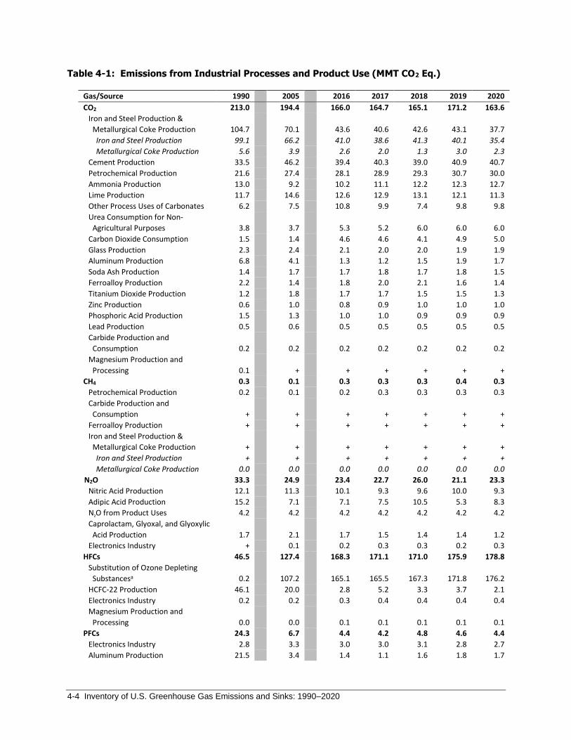
Table 4-1: Emissions from Industrial Processes and Product Use (MMT CO2 Eq.)
Gas/Source 1990 2005 2016 2017 2018 2019 2020
CO2 213.0 194.4 166.0 164.7 165.1 171.2 163.6
Iron and Steel Production &
Metallurgical Coke Production 104.7 70.1 43.6 40.6 42.6 43.1 37.7
Iron and Steel Production 99.1 66.2 41.0 38.6 41.3 40.1 35.4
Metallurgical Coke Production 5.6 3.9 2.6 2.0 1.3 3.0 2.3
Cement Production 33.5 46.2 39.4 40.3 39.0 40.9 40.7
Petrochemical Production 21.6 27.4 28.1 28.9 29.3 30.7 30.0
Ammonia Production 13.0 9.2 10.2 11.1 12.2 12.3 12.7
Lime Production 11.7 14.6 12.6 12.9 13.1 12.1 11.3
Other Process Uses of Carbonates 6.2 7.5 10.8 9.9 7.4 9.8 9.8
Urea Consumption for Non-
Agricultural Purposes 3.8 3.7 5.3 5.2 6.0 6.0 6.0
Carbon Dioxide Consumption 1.5 1.4 4.6 4.6 4.1 4.9 5.0
Glass Production 2.3 2.4 2.1 2.0 2.0 1.9 1.9
Aluminum Production 6.8 4.1 1.3 1.2 1.5 1.9 1.7
Soda Ash Production 1.4 1.7 1.7 1.8 1.7 1.8 1.5
Ferroalloy Production 2.2 1.4 1.8 2.0 2.1 1.6 1.4
Titanium Dioxide Production 1.2 1.8 1.7 1.7 1.5 1.5 1.3
Zinc Production 0.6 1.0 0.8 0.9 1.0 1.0 1.0
Phosphoric Acid Production 1.5 1.3 1.0 1.0 0.9 0.9 0.9
Lead Production 0.5 0.6 0.5 0.5 0.5 0.5 0.5
Carbide Production and
Consumption 0.2 0.2 0.2 0.2 0.2 0.2 0.2
Magnesium Production and
Processing 0.1 + + + + + +
CH4 0.3 0.1 0.3 0.3 0.3 0.4 0.3
Petrochemical Production 0.2 0.1 0.2 0.3 0.3 0.3 0.3
Carbide Production and
Consumption + + + + + + +
Ferroalloy Production + + + + + + +
Iron and Steel Production &
Metallurgical Coke Production + + + + + + +
Iron and Steel Production + + + + + + +
Metallurgical Coke Production 0.0 0.0 0.0 0.0 0.0 0.0 0.0
N2O 33.3 24.9 23.4 22.7 26.0 21.1 23.3
Nitric Acid Production 12.1 11.3 10.1 9.3 9.6 10.0 9.3
Adipic Acid Production 15.2 7.1 7.1 7.5 10.5 5.3 8.3
N₂O from Product Uses 4.2 4.2 4.2 4.2 4.2 4.2 4.2
Caprolactam, Glyoxal, and Glyoxylic
Acid Production 1.7 2.1 1.7 1.5 1.4 1.4 1.2
Electronics Industry + 0.1 0.2 0.3 0.3 0.2 0.3
HFCs 46.5 127.4 168.3 171.1 171.0 175.9 178.8
Substitution of Ozone Depleting
Substancesa 0.2 107.2 165.1 165.5 167.3 171.8 176.2
HCFC-22 Production 46.1 20.0 2.8 5.2 3.3 3.7 2.1
Electronics Industry 0.2 0.2 0.3 0.4 0.4 0.4 0.4
Magnesium Production and
Processing 0.0 0.0 0.1 0.1 0.1 0.1 0.1
PFCs 24.3 6.7 4.4 4.2 4.8 4.6 4.4
Electronics Industry 2.8 3.3 3.0 3.0 3.1 2.8 2.7
Aluminum Production 21.5 3.4 1.4 1.1 1.6 1.8 1.7

Industrial Processes and Product Use 4-5
Substitution of Ozone Depleting
Substances 0.0 + + + 0.1 0.1 0.1
Electrical Transmission and
Distribution 0.0 + + + 0.0 + +
SF6 28.8 11.8 6.0 5.9 5.7 5.9 5.4
Electrical Transmission and
Distribution 23.2 8.3 4.1 4.2 3.8 4.2 3.8
Magnesium Production and
Processing 5.2 2.7 1.1 1.0 1.0 0.9 0.9
Electronics Industry 0.5 0.7 0.8 0.7 0.8 0.8 0.7
NF3 + 0.5 0.6 0.6 0.6 0.6 0.6
Electronics Industry + 0.5 0.6 0.6 0.6 0.6 0.6
Total 346.2 365.9 369.0 369.4 373.4 379.5 376.4
Note: Totals may not sum due to independent rounding. + Does not exceed 0.05 MMT CO2 Eq. a Small amounts of PFC emissions also result from this source.
Table 4-2: Emissions from Industrial Processes and Product Use (kt)
Gas/Source 1990 2005 2016 2017 2018 2019 2020
CO2 213,017 194,389 165,969 164,660 165,086 171,154 163,571
Iron and Steel Production &
Metallurgical Coke Production 104,737 70,076 43,621 40,566 42,627 43,090 37,731
Iron and Steel Production 99,129 66,156 40,979 38,587 41,345 40,084 35,407
Metallurgical Coke Production 5,608 3,921 2,643 1,978 1,282 3,006 2,324
Cement Production 33,484 46,194 39,439 40,324 38,971 40,896 40,688
Petrochemical Production 21,611 27,383 28,110 28,890 29,314 30,702 30,011
Ammonia Production 13,047 9,177 10,245 11,112 12,163 12,272 12,717
Lime Production 11,700 14,552 12,630 12,882 13,106 12,112 11,299
Other Process Uses of
Carbonates 6,233 7,459 10,813 9,869 7,351 9,848 9,794
Urea Consumption for Non-
Agricultural Purposes 3,784 3,653 5,330 5,182 6,030 6,044 5,983
Carbon Dioxide Consumption 1,472 1,375 4,640 4,580 4,130 4,870 4,970
Glass Production 2,291 2,432 2,119 2,011 1,989 1,938 1,857
Aluminum Production 6,831 4,142 1,334 1,205 1,451 1,880 1,748
Soda Ash Production 1,431 1,655 1,723 1,753 1,714 1,792 1,461
Ferroalloy Production 2,152 1,392 1,796 1,975 2,063 1,598 1,377
Titanium Dioxide Production 1,195 1,755 1,662 1,688 1,541 1,474 1,340
Zinc Production 632 1,030 838 900 999 1,026 1,008
Phosphoric Acid Production 1,529 1,342 998 1,025 937 909 938
Lead Production 516 553 500 513 513 527 495
Carbide Production and
Consumption 243 213 170 181 184 175 154
Magnesium Production and
Processing 129 3 3 3 2 1 1
CH4 11 4 11 11 13 15 14
Petrochemical Production 9 3 10 10 12 13 13
Carbide Production and
Consumption 1 + + + + + +
Ferroalloy Production 1 + 1 1 1 + +
Iron and Steel Production &
Metallurgical Coke Production 1 1 + + + + +
Iron and Steel Production 1 1 + + + + +
Metallurgical Coke Production 0 0 0 0 0 0 0

4-6 Inventory of U.S. Greenhouse Gas Emissions and Sinks: 1990–2020
N2O 112 84 79 76 87 71 78
Nitric Acid Production 41 38 34 31 32 34 31
Adipic Acid Production 51 24 24 25 35 18 28
N₂O from Product Uses 14 14 14 14 14 14 14
Caprolactam, Glyoxal, and
Glyoxylic Acid Production 6 7 6 5 5 5 4
Electronics Industry + + 1 1 1 1 1
HFCs M M M M M M M
Substitution of Ozone Depleting
Substancesa M M M M M M M
HCFC-22 Production 3 1 + + + + +
Electronics Industry M M M M M M M
Magnesium Production and
Processing NO NO + + + + +
PFCs M M M M M M M
Electronics Industry M M M M M M M
Aluminum Production M M M M M M M
Substitution of Ozone Depleting
Substances NO + + + + + +
Electrical Transmission and
Distribution NO + + + NO + +
SF6 1 1 + + + + +
Electrical Transmission and
Distribution 1 + + + + + +
Magnesium Production and
Processing + + + + + + +
Electronics Industry + + + + + + +
NF3 + + + + + + +
Electronics Industry + + + + + + +
+ Does not exceed 0.5 kt. M (Mixture of gases) NO (Not Occurring) a Small amounts of PFC emissions also result from this source. Note: Totals may not sum due to independent rounding.
This chapter presents emission estimates calculated in accordance with the 2006 IPCC Guidelines for National Greenhouse Gas Inventories (2006 IPCC Guidelines) and its refinements. For additional detail on IPPU sources that are not included in this Inventory report, please review Annex 5, Assessment of the Sources and Sinks of Greenhouse Gas Emissions Not Included. These sources are not included due to various national circumstances, such as that emissions from a source may not currently occur in the United States, data are not currently available for those emission sources (e.g., ceramics, non-metallurgical magnesium production, glyoxal and glyoxylic acid production, CH4 from direct reduced iron production), emissions are included elsewhere within the Inventory report, or data suggest that emissions are not significant (e.g., other various fluorinated gas emissions from other product uses). In terms of geographic scope, emissions reported in the IPPU chapter include those from all 50 states, including Hawaii and Alaska, as well as from District of Columbia and U.S. Territories to the extent to which industries are occurring. While most IPPU sources do not occur in U.S. Territories (e.g., electronics manufacturing does not occur in U.S. Territories), they are estimated and accounted for where they are known to occur (e.g., cement production, lime production, and electrical transmission and distribution). EPA will review this on an ongoing basis to ensure emission sources are included across all geographic areas if they occur. Information on planned improvements for specific IPPU source categories can be found in the Planned Improvements section of the individual source category.
In addition, as mentioned in the Energy chapter of this report (Box 3-5), fossil fuels consumed for non-energy uses for primary purposes other than combustion for energy (including lubricants, paraffin waxes, bitumen asphalt, and solvents) are reported in the Energy chapter. According to the 2006 IPCC Guidelines, these non-energy uses of

Industrial Processes and Product Use 4-7
fossil fuels are to be reported under the IPPU, rather than the Energy sector; however, due to national circumstances regarding the allocation of energy statistics and carbon balance data, the United States reports these non-energy uses in the Energy chapter of this Inventory. Although emissions from these non-energy uses are reported in the Energy chapter, the methodologies used to determine emissions are compatible with the 2006 IPCC Guidelines and are well documented and scientifically based. The methodologies used are described in Section 3.2, Carbon Emitted from Non-Energy Uses of Fossil Fuels and Annex 2.3, Methodology for Estimating Carbon Emitted from Non-Energy Uses of Fossil Fuels. The emissions are reported under the Energy chapter to improve transparency, report a more complete carbon balance, and avoid double counting. For example, only the emissions from the first use of lubricants and waxes are to be reported under the IPPU sector, and emissions from use of lubricants in 2-stroke engines and emissions from secondary use of lubricants and waxes in waste incineration with energy recovery are to be reported under the Energy sector. Reporting non-energy use emissions from only first use of lubricants and waxes under IPPU would involve making artificial adjustments to the non-energy use carbon balance and could potentially result in double counting of emissions. These artificial adjustments would also be required for asphalt and road oil and solvents (which are captured as part of petrochemical feedstock emissions) and could also potentially result in double counting of emissions. For more information, see the Methodology discussion in Section 3.1, CO2 from Fossil Fuel Combustion, Section 3.2, Carbon Emitted from Non-Energy Uses of Fossil Fuels and Annex 2.3, Methodology for Estimating Carbon Emitted from Non-Energy Uses of Fossil Fuels.
Finally, as stated in the Energy chapter, portions of the fuel consumption data for seven fuel categories—coking coal, distillate fuel, industrial other coal, petroleum coke, natural gas, residual fuel oil, and other oil—are reallocated to the IPPU chapter, as they are consumed during non-energy related industrial process activity. Emissions from uses of fossil fuels as feedstocks or reducing agents (e.g., petrochemical production, aluminum production, titanium dioxide, zinc production) are reported in the IPPU chapter, unless otherwise noted due to specific national circumstances. This approach is compatible with the 2006 IPCC Guidelines and is well documented and scientifically based. The emissions from these feedstocks and reducing agents are reported under the IPPU chapter to improve transparency and to avoid double counting of emissions under both the Energy and IPPU sectors. More information on the methodology to adjust for these emissions within the Energy chapter is described in the Methodology section of CO2 from Fossil Fuel Combustion (3.1 Fossil Fuel Combustion [CRF Source Category 1A]) and Annex 2.1, Methodology for Estimating Emissions of CO2 from Fossil Fuel Combustion. Additional information is listed within each IPPU emission source in which this approach applies.
Box 4-1: Methodological Approach for Estimating and Reporting U.S. Emissions and Removals
In following the United Nations Framework Convention on Climate Change (UNFCCC) requirement under Article 4.1 to develop and submit national greenhouse gas emission inventories, the emissions and removals presented in this report and this chapter are organized by source and sink categories and calculated using internationally accepted methods provided by the Intergovernmental Panel on Climate Change (IPCC) in the 2006 IPCC Guidelines for National Greenhouse Gas Inventories (2006 IPCC Guidelines) and its supplements and refinements. Additionally, the calculated emissions and removals in a given year for the United States are presented in a common format in line with the UNFCCC reporting guidelines for the reporting of inventories under this international agreement. The use of consistent methods to calculate emissions and removals by all nations providing their inventories to the UNFCCC ensures that these reports are comparable. The presentation of emissions and removals provided in the IPPU chapter do not preclude alternative examinations, but rather, this chapter presents emissions and removals in a common format consistent with how countries are to report Inventories under the UNFCCC. The report itself, and this chapter, follows this standardized format, and provides an explanation of the application of methods used to calculate emissions and removals from industrial processes and from the use of greenhouse gases in products.

4-8 Inventory of U.S. Greenhouse Gas Emissions and Sinks: 1990–2020
QA/QC and Verification Procedures For IPPU sources, a detailed QA/QC plan was developed and implemented for specific categories. This plan is consistent with the U.S. Inventory QA/QC plan outlined in Annex 8 but tailored to include specific procedures recommended for these sources. The IPPU QA/QC Plan does not replace the Inventory QA/QC Plan, but rather provides more context for the IPPU sector. The IPPU QA/QC Plan provides the completed QA/QC forms for each inventory reports, as well as, for certain source categories (e.g., key categories), more detailed documentation of quality control checks and recalculations due to methodological changes.
Two types of checks were performed using this plan: (1) general (Tier 1) procedures consistent with Volume 1, Chapter 6 of the 2006 IPCC Guidelines that focus on annual procedures and checks to be used when gathering, maintaining, handling, documenting, checking, and archiving the data, supporting documents, and files; and (2) source category-specific (Tier 2) procedures that focus on checks and comparisons of the emission factors, activity data, and methodologies used for estimating emissions from the relevant industrial process and product use sources. Examples of these procedures include: checks to ensure that activity data and emission estimates are consistent with historical trends to identify significant changes; that, where possible, consistent and reputable data sources are used and specified across sources; that interpolation or extrapolation techniques are consistent across sources; and that common datasets, units, and conversion factors are used where applicable. The IPPU QA/QC plan also checked for transcription errors in data inputs required for emission calculations, including activity data and emission factors; and confirmed that estimates were calculated and reported for all applicable and able portions of the source categories for all years.
For sources that use data from EPA’s Greenhouse Gas Reporting Program (GHGRP), EPA verifies annual facility-level reports through a multi-step process (e.g., including a combination of pre-and post-submittal electronic checks and manual reviews by staff) to identify potential errors and ensure that data submitted to EPA are
accurate, complete, and consistent.3 Based on the results of the verification process, EPA follows up with facilities to resolve mistakes that may have occurred. The post-submittals checks are consistent with a number of general and category-specific QC procedures, including: range checks, statistical checks, algorithm checks, and year-to-year checks of reported data and emissions. See Box 4-2 below for more information on use of GHGRP data in this chapter.
General QA/QC procedures (Tier 1) and calculation-related QC (category-specific, Tier 2) have been performed for all IPPU sources. Consistent with the 2006 IPCC Guidelines, additional category-specific QC procedures were performed for more significant emission categories (such as the comparison of reported consumption with modeled consumption using EPA’s Greenhouse Gas Reporting Program (GHGRP) data within Substitution of Ozone Depleting Substances) or sources where significant methodological and data updates have taken place. The QA/QC implementation did not reveal any significant inaccuracies, and all errors identified were documented and corrected. Application of these procedures, specifically category-specific QC procedures and updates/improvements as a result of QA processes (expert, public, and UNFCCC technical expert reviews), are described further within respective source categories, in the Recalculations Discussion and Planned Improvement sections.
For most IPPU categories, activity data are obtained via aggregation of facility-level data from EPA’s GHGRP (see Box 4-2 below and Annex 9), national commodity surveys conducted by U.S. Geological Survey National Minerals Information Center, U.S. Department of Energy (DOE), U.S. Census Bureau, and industry associations such as Air-Conditioning, Heating, and Refrigeration Institute (AHRI), American Chemistry Council (ACC), and American Iron and Steel Institute (AISI) (specified within each source category). The emission factors used include those derived from the EPA’s GHGRP and application of IPCC default factors. Descriptions of uncertainties and assumptions for activity data and emission factors are included within the uncertainty discussion sections for each IPPU source category.
3 See https://www.epa.gov/sites/production/files/2015-07/documents/ghgrp_verification_factsheet.pdf.

Industrial Processes and Product Use 4-9
Box 4-2: Industrial Process and Product Use Data from EPA’s Greenhouse Gas Reporting Program
EPA collects greenhouse gas emissions data from individual facilities and suppliers of certain fossil fuels and industrial gases through its Greenhouse Gas Reporting Program (GHGRP). The GHGRP applies to direct greenhouse gas emitters, fossil fuel suppliers, industrial gas suppliers, and facilities that inject CO2 underground for sequestration or other reasons and requires reporting by sources or suppliers in 41 industrial categories. Annual reporting is at the facility level, except for certain suppliers of fossil fuels and industrial greenhouse gases.
In general, the threshold for reporting is 25,000 metric tons or more of CO2 Eq. per year, but reporting is required for all facilities in some industries. Calendar year 2010 was the first year for which data were collected for facilities subject to 40 CFR Part 98, though some source categories first collected data for calendar year 2011. For more information, see Annex 9, Use of EPA Greenhouse Gas Reporting Program in Inventory.
EPA uses annual GHGRP data in a number of categories to improve the national estimates presented in this Inventory, consistent with IPCC guidelines (e.g., minerals, chemicals, product uses). Methodologies used in EPA’s GHGRP are consistent with IPCC guidelines, including higher tier methods; however, it should be noted that the coverage and definitions for source categories (e.g., allocation of energy and IPPU emissions) in EPA’s GHGRP may differ from those used in this Inventory in meeting the UNFCCC reporting guidelines (IPCC 2011) and is an important consideration when incorporating GHGRP data in the Inventory. In line with the UNFCCC reporting guidelines, the Inventory is a comprehensive accounting of all emissions from source categories identified in the 2006 IPCC Guidelines. EPA has paid particular attention to ensuring both completeness and time-series consistency for major recalculations that have occurred from the incorporation of GHGRP data into these categories, consistent with 2006 IPCC Guidelines and IPCC Technical Bulletin on Use of Facility-Specific
Data in National GHG Inventories.4
For certain source categories in this Inventory (e.g., nitric acid production, lime production, cement production, petrochemical production, carbon dioxide consumption, ammonia production, and urea consumption for non-agricultural purposes), EPA has integrated data values that have been calculated by aggregating GHGRP data that are considered confidential business information (CBI) at the facility level. EPA, with industry engagement, has put forth criteria to confirm that a given data aggregation shields underlying CBI from public disclosure. EPA
is only publishing data values that meet these aggregation criteria.5 Specific uses of aggregated facility-level data are described in the respective methodological sections (e.g., including other sources using GHGRP data that is not aggregated CBI, such as aluminum, electronics industry, electrical transmission and distribution, HCFC-22 production, and magnesium production and processing.). For other source categories in this chapter,
as indicated in the respective planned improvements sections,6 EPA is continuing to analyze how facility-level GHGRP data may be used to improve the national estimates presented in this Inventory, giving particular consideration to ensuring time-series consistency and completeness.
Additionally, EPA’s GHGRP has and will continue to enhance QA/QC procedures and assessment of uncertainties within the IPPU categories (see those categories for specific QA/QC details regarding the use of GHGRP data).
4 See http://www.ipcc-nggip.iges.or.jp/public/tb/TFI_Technical_Bulletin_1.pdf. 5 U.S. EPA Greenhouse Gas Reporting Program. Developments on Publication of Aggregated Greenhouse Gas Data, November 25, 2014. See http://www.epa.gov/ghgreporting/confidential-business-information-ghg-reporting. 6 Ammonia Production, Glass Production, Lead Production, and Other Fluorinated Gas Production.

4-10 Inventory of U.S. Greenhouse Gas Emissions and Sinks: 1990–2020
4.1 Cement Production (CRF Source Category 2A1)
Cement production is an energy- and raw material-intensive process that results in the generation of carbon dioxide (CO2) both from the energy consumed in making the clinker precursor to cement and from the chemical process to make the clinker. Emissions from fuels consumed for energy purposes during the production of cement are accounted for in the Energy chapter.
During the clinker production process, the key reaction occurs when calcium carbonate (CaCO3), in the form of limestone or similar rocks or in the form of cement kiln dust (CKD), is heated in a cement kiln at a temperature range of about 700 to 1,000 degrees Celsius (1,300 to 1,800 degrees Fahrenheit) to form lime (i.e., calcium oxide, or CaO) and CO2 in a process known as calcination or calcining. The quantity of CO2 emitted during clinker production is directly proportional to the lime content of the clinker. During calcination, each mole of CaCO3 heated in the clinker kiln forms one mole of CaO and one mole of CO2. The CO2 is vented to the atmosphere as part of the kiln exhaust:
𝐶𝑎𝐶𝑂3 + ℎ𝑒𝑎𝑡 → 𝐶𝑎𝑂 + 𝐶𝑂2
Next, over a temperature range of 1000 to 1450 degrees Celsius, the CaO combines with alumina, iron oxide and silica that are also present in the clinker raw material mix to form hydraulically reactive compounds within white-hot semifused (sintered) nodules of clinker. Because these “sintering” reactions are highly exothermic, they produce few CO2 process emissions. The clinker is then rapidly cooled to maintain quality and then very finely ground with a small amount of gypsum and potentially other materials (e.g., ground granulated blast furnace slag, etc.) to make portland and similar cements.
Masonry cement consists of plasticizers (e.g., ground limestone, lime, etc.) and portland cement, and the amount of portland cement used accounts for approximately 3 percent of total clinker production (USGS 2020). No additional emissions are associated with the production of masonry cement. Carbon dioxide emissions that result from the production of lime used to produce portland and masonry cement are included in Section 4.2 Lime Production (CRF Source Category 2A2).
Carbon dioxide emitted from the chemical process of cement production is the second largest source of industrial CO2 emissions in the United States. Cement is produced in 34 states and Puerto Rico. Texas, California, Missouri, and Florida were the leading cement-producing states in 2020 and accounted for almost 45 percent of total U.S. production (USGS 2021). Clinker production in 2020 remained at relatively flat levels, compared to 2019 (EPA 2020; USGS 2021). In 2020, shipments of cement were essentially unchanged from 2019, and imports increased by about 7 percent compared to 2019. In 2020, U.S. clinker production totaled 78,200 kilotons (EPA 2021). The resulting CO2 emissions were estimated to be 40.7 MMT CO2 Eq. (40,688 kt) (see Table 4-3). In 2020 due to the COVID-19 pandemic, production of cement was temporarily idled in many localities and countries in response to the lockdowns imposed to limit the spread of COVID-19. Disruptions in the construction industry affected cement demand, and several plant openings and expansions were delayed due to the COVID-19 pandemic. The U.S. cement industry, however, showed no prolonged or widespread negative effects from the COVID-19 pandemic (USGS 2021).

Industrial Processes and Product Use 4-11
Table 4-3: CO2 Emissions from Cement Production (MMT CO2 Eq. and kt)
Year MMT CO2 Eq. kt
1990 33.5 33,484
2005 46.2 46,194
2016 39.4 39,439
2017 40.3 40,324
2018 39.0 38,971
2019 40.9 40,896
2020 40.7 40,688
Greenhouse gas emissions from cement production, which are primarily driven by production levels, increased every year from 1991 through 2006 but decreased in the following years until 2009. Since 1990, emissions have increased by 22 percent. Emissions from cement production were at their lowest levels in 2009 (2009 emissions are approximately 28 percent lower than 2008 emissions and 12 percent lower than 1990) due to the economic recession and the associated decrease in demand for construction materials. Since 2010, emissions have increased by about 30 percent, due to increasing demand for cement. Cement continues to be a critical component of the construction industry; therefore, the availability of public and private construction funding, as well as overall economic conditions, have considerable impact on the level of cement production.
Methodology and Time-Series Consistency Carbon dioxide emissions from cement production were estimated using the Tier 2 methodology from the 2006 IPCC Guidelines as this is a key category. The Tier 2 methodology was used because detailed and complete data
(including weights and composition) for carbonate(s) consumed in clinker production are not available,7 and thus a rigorous Tier 3 approach is impractical. Tier 2 specifies the use of aggregated plant or national clinker production data and an emission factor, which is the product of the average lime fraction for clinker of 65 percent and a constant reflecting the mass of CO2 released per unit of lime. The U.S. Geological Survey (USGS) mineral commodity expert for cement has confirmed that this is a reasonable assumption for the United States (Van Oss 2013a). This calculation yields an emission factor of 0.510 tons of CO2 per ton of clinker produced, which was determined as follows:
Equation 4-1: 2006 IPCC Guidelines Tier 1 Emission Factor for Clinker (precursor to Equation
2.4)
EFclinker = 0.650 CaO × [(44.01 g/mole CO2) ÷ (56.08 g/mole CaO)] = 0.510 tons CO2/ton clinker
During clinker production, some of the raw materials, partially reacted raw materials, and clinker enters the kiln line’s exhaust system as non-calcinated, partially calcinated, or fully calcinated cement kiln dust (CKD). To the degree that the CKD contains carbonate raw materials which are then calcined, there are associated CO2 emissions. At some plants, essentially all CKD is directly returned to the kiln, becoming part of the raw material feed, or is likewise returned to the kiln after first being removed from the exhaust. In either case, the returned CKD becomes a raw material, thus forming clinker, and the associated CO2 emissions are a component of those calculated for the clinker overall. At some plants, however, the CKD cannot be returned to the kiln because it is chemically unsuitable as a raw material or chemical issues limit the amount of CKD that can be so reused. Any clinker that cannot be returned to the kiln is either used for other (non-clinker) purposes or is landfilled. The CO2 emissions attributable
7 As discussed further under “Planned Improvements,” most cement-producing facilities that report their emissions to the GHGRP use CEMS to monitor combined process and fuel combustion emissions for kilns, making it difficult to quantify the process emissions on a facility-specific basis. In 2019, the percentage of facilities not using CEMS was 8 percent.

4-12 Inventory of U.S. Greenhouse Gas Emissions and Sinks: 1990–2020
to the non-returned calcinated portion of the CKD are not accounted for by the clinker emission factor and thus a CKD correction factor should be applied to account for those emissions. The USGS reports the amount of CKD used
to produce clinker, but no information is currently available on the total amount of CKD produced annually.8 Because data are not currently available to derive a country-specific CKD correction factor, a default correction
factor of 1.02 (2 percent) was used to account for CKD CO2 emissions, as recommended by the IPCC (IPCC 2006).9 Total cement production emissions were calculated by adding the emissions from clinker production and the emissions assigned to CKD.
Small amounts of impurities (i.e., not calcium carbonate) may exist in the raw limestone used to produce clinker. The proportion of these impurities is generally minimal, although a small amount (1 to 2 percent) of magnesium oxide (MgO) may be desirable as a flux. Per the IPCC Tier 2 methodology, a correction for MgO is not used, since the amount of MgO from carbonate is likely very small and the assumption of a 100 percent carbonate source of CaO already yields an overestimation of emissions (IPCC 2006).
The 1990 through 2012 activity data for clinker production were obtained from USGS (Van Oss 2013a, Van Oss 2013b). Clinker production data for 2013 were also obtained from USGS (USGS 2014). USGS compiled the data (to the nearest ton) through questionnaires sent to domestic clinker and cement manufacturing plants, including facilities in Puerto Rico. Clinker production values in the current Inventory report utilize GHGRP data for the years 2014 through 2020 (EPA 2021). Clinker production data are summarized in Table 4-4. Details on how this GHGRP data compares to USGS reported data can be found in the section on QA/QC and Verification.
Table 4-4: Clinker Production (kt)
Year Clinker
1990 64,355
2005 88,783
2016 75,800
2017 77,500
2018 74,900
2019 78,600
2020 78,200
Notes: Clinker production from 1990
through 2020 includes Puerto Rico
(relevant U.S. Territories).
Methodological approaches were applied to the entire time series to ensure time-series consistency from 1990 through 2020. The methodology for cement production spliced activity data from two different sources: USGS for 1990 through 2013 and GHGRP starting in 2014. Consistent with the 2006 IPCC Guidelines, the overlap technique was applied to compare the two data sets for years where there was overlap, with findings that the data sets were consistent and adjustments were not needed.
8 The USGS Minerals Yearbook: Cement notes that CKD values used for clinker production are likely underreported. 9 As stated on p. 2.12 of the 2006 IPCC Guidelines, Vol. 3, Chapter 2: “…As data on the amount of CKD produced may be scarce (except possibly for plant-level reporting), estimating emissions from lost CKD based on a default value can be considered good practice. The amount of CO2 from lost CKD can vary, but ranges typically from about 1.5 percent (additional CO2 relative to that calculated for clinker) for a modern plant to about 20 percent for a plant losing a lot of highly calcinated CKD (van Oss 2005). In the absence of data, the default CKD correction factor (CFckd) is 1.02 (i.e., add 2 percent to the CO2 calculated for clinker). If no calcined CKD is believed to be lost to the system, the CKD correction factor will be 1.00 (van Oss 2005)…”
Industrial Processes and Product Use 4-13
Uncertainty The uncertainties contained in these estimates are primarily due to uncertainties in the lime content of clinker and in the percentage of CKD recycled inside the cement kiln. Uncertainty is also associated with the assumption that all calcium-containing raw materials are CaCO3, when a small percentage likely consists of other carbonate and non-carbonate raw materials. The lime content of clinker varies from 60 to 67 percent; 65 percent is used as a representative value (Van Oss 2013a). This contributes to the uncertainty surrounding the emission factor for clinker which has an uncertainty range of ±5 percent with uniform densities (Van Oss 2013b). The amount of CO2 from CKD loss can range from 1.5 to 8 percent depending upon plant specifications, and uncertainty was estimated at ±3 percent with uniform densities (Van Oss 2013b). Additionally, some amount of CO2 is reabsorbed when the cement is used for construction. As cement reacts with water, alkaline substances such as calcium hydroxide are formed. During this curing process, these compounds may react with CO2 in the atmosphere to create calcium carbonate. This reaction only occurs in roughly the outer 0.2 inches of the total thickness. Because the amount of CO2 reabsorbed is thought to be minimal, it was not estimated. EPA assigned default uncertainty bounds of ±3 percent for clinker production, based on expert judgment (Van Oss 2013b).
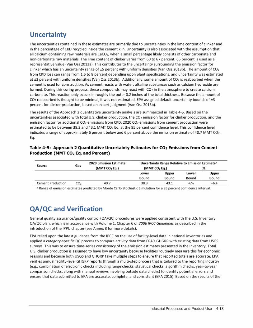
The results of the Approach 2 quantitative uncertainty analysis are summarized in Table 4-5. Based on the uncertainties associated with total U.S. clinker production, the CO2 emission factor for clinker production, and the emission factor for additional CO2 emissions from CKD, 2020 CO2 emissions from cement production were estimated to be between 38.3 and 43.1 MMT CO2 Eq. at the 95 percent confidence level. This confidence level indicates a range of approximately 6 percent below and 6 percent above the emission estimate of 40.7 MMT CO2 Eq.
Table 4-5: Approach 2 Quantitative Uncertainty Estimates for CO2 Emissions from Cement
Production (MMT CO2 Eq. and Percent)
QA/QC and Verification General quality assurance/quality control (QA/QC) procedures were applied consistent with the U.S. Inventory QA/QC plan, which is in accordance with Volume 1, Chapter 6 of 2006 IPCC Guidelines as described in the introduction of the IPPU chapter (see Annex 8 for more details).
EPA relied upon the latest guidance from the IPCC on the use of facility-level data in national inventories and applied a category-specific QC process to compare activity data from EPA’s GHGRP with existing data from USGS surveys. This was to ensure time-series consistency of the emission estimates presented in the Inventory. Total U.S. clinker production is assumed to have low uncertainty because facilities routinely measure this for economic reasons and because both USGS and GHGRP take multiple steps to ensure that reported totals are accurate. EPA verifies annual facility-level GHGRP reports through a multi-step process that is tailored to the reporting industry (e.g., combination of electronic checks including range checks, statistical checks, algorithm checks, year-to-year comparison checks, along with manual reviews involving outside data checks) to identify potential errors and ensure that data submitted to EPA are accurate, complete, and consistent (EPA 2015). Based on the results of the
Source Gas
2020 Emission Estimate Uncertainty Range Relative to Emission Estimatea
(MMT CO2 Eq.) (MMT CO2 Eq.) (%)
Lower
Bound
Upper
Bound
Lower
Bound
Upper
Bound
Cement Production CO2 40.7 38.3 43.1 -6% +6%
a Range of emission estimates predicted by Monte Carlo Stochastic Simulation for a 95 percent confidence interval.

4-14 Inventory of U.S. Greenhouse Gas Emissions and Sinks: 1990–2020
verification process, EPA follows up with facilities to resolve mistakes that may have occurred.10 Facilities are also required to monitor and maintain records of monthly clinker production per section 98.84 of the GHGRP regulation (40 CFR 98.84).
EPA’s GHGRP requires all facilities producing Portland cement to report greenhouse gas emissions, including CO2 process emissions from each kiln, CO2 combustion emissions from each kiln, CH4 and N2O combustion emissions from each kiln, and CO2, CH4, and N2O emissions from each stationary combustion unit other than kilns (40 CFR Part 98 Subpart H). Source-specific quality control measures for the Cement Production category are included in section 98.84, Monitoring and QA/QC Requirements.
As mentioned above, EPA compares GHGRP clinker production data to the USGS clinker production data. For the year 2014 and 2020, USGS and GHGRP clinker production data showed a difference of approximately 1 percent. In 2018, the difference was approximately 3 percent. In 2015, 2016, 2017, and 2019, that difference was less than 1 percent between the two sets of activity data. This difference resulted in a difference in emissions compared to USGS data of about 0.1 MMT CO2 Eq. in 2015, 2016, 2017, and 2019. The information collected by the USGS National Minerals Information Center surveys continue to be an important data source.
Recalculations Discussion No recalculations were performed for the 1990 through 2019 portion of the time series.
Planned Improvements EPA is continuing to evaluate and analyze data reported under EPA’s GHGRP that would be useful to improve the emission estimates for the Cement Production source category. Most cement production facilities reporting under EPA’s GHGRP use Continuous Emission Monitoring Systems (CEMS) to monitor and report CO2 emissions, thus reporting combined process and combustion emissions from kilns. In implementing further improvements and integration of data from EPA’s GHGRP, the latest guidance from the IPCC on the use of facility-level data in national inventories will be relied upon, in addition to category-specific QC methods recommended by the 2006 IPCC
Guidelines.11 EPA’s long-term improvement plan includes continued assessment of the feasibility of using additional GHGRP information beyond aggregation of reported facility-level clinker data, in particular disaggregating the combined process and combustion emissions reported using CEMS, to separately present national process and combustion emissions streams consistent with IPCC and UNFCCC guidelines. This long-term planned analysis is still in development and has not been applied for this current Inventory.
Finally, in response to feedback from Portland Cement Association (PCA) during the Public Review comment period of a previous Inventory, EPA plans to work with PCA to discuss additional long-term improvements to review methods and data used to estimate CO2 emissions from cement production to account for organic material in the raw material and to discuss the carbonation that occurs across the duration of the cement product. Work includes identifying data and studies on the average carbon content for organic materials in kiln feed in the United States and CO2 reabsorption rates via carbonation for various cement products. This information is not reported by facilities subject to GHGRP reporting.
10 See GHGRP Verification Fact Sheet https://www.epa.gov/sites/production/files/2015-07/documents/ghgrp_verification_factsheet.pdf. 11 See IPCC Technical Bulletin on Use of Facility-Specific Data in National Greenhouse Gas Inventories http://www.ipcc-nggip.iges.or.jp/public/tb/TFI_Technical_Bulletin_1.pdf.

Industrial Processes and Product Use 4-15
4.2 Lime Production (CRF Source Category 2A2 and 2H3)
Lime is an important manufactured product with many industrial, chemical, and environmental applications. Lime production involves three main processes: stone preparation, calcination, and hydration. Carbon dioxide (CO2) is generated during the calcination stage, when limestone—consisting of calcium (CaCO3) and/or magnesium (MgCO3) carbonate—is roasted at high temperatures in a kiln to produce calcium oxide (CaO) and CO2. The CO2 is given off as a gas and is normally emitted to the atmosphere.
𝐶𝑎𝐶𝑂3 → 𝐶𝑎𝑂 + 𝐶𝑂2
Some facilities, however, recover CO2 generated during the production process for use in sugar refining and
precipitated calcium carbonate (PCC) production.12 PCC is used as a filler or coating in the paper, food, and plastic industries and is derived from reacting hydrated high-calcium quicklime with CO2, a production process that does not result in net emissions of CO2 to the atmosphere. Emissions from fuels consumed for energy purposes during the production of lime are included in the Energy chapter.
For U.S. operations, the term “lime” actually refers to a variety of chemical compounds. These include CaO, or high-calcium quicklime; calcium hydroxide (Ca(OH)2), or hydrated lime; dolomitic quicklime ([CaO•MgO]); and dolomitic hydrate ([Ca(OH)2•MgO] or [Ca(OH)2•Mg(OH)2]).
The current lime market is approximately distributed across five end-use categories, as follows: metallurgical uses, 34 percent; environmental uses, 30 percent; chemical and industrial uses, 21 percent; construction uses, 11 percent; and refractory dolomite, 1 percent (USGS 2020b). The major uses are in steel making, flue gas desulfurization (FGD) systems at coal-fired electric power plants, construction, and water treatment, as well as uses in mining, pulp and paper and precipitated calcium carbonate manufacturing. Lime is also used as a CO2 scrubber, and there has been experimentation on the use of lime to capture CO2 from electric power plants. Both lime (CaO) and limestone (CaCO3) can be used as a sorbent for FGD systems. Emissions from limestone consumption for FGD systems are reported under Section 4.4 Other Process Uses of Carbonate Production (CRF Source Category 2A4).
Emissions from lime production have increased and decreased over the time series depending on lime end-use markets – primarily the steel making industry and FGD systems for utility and industrial plants – and also energy costs. One significant change to lime end-use since 1990 has been the increase in demand for lime for FGD at coal-fired electric power plants, which can be attributed to compliance with sulfur dioxide (SO2) emission regulations of the Clean Air Act Amendments of 1990. Phase I went into effect on January 1, 1995, followed by Phase II on January 1, 2000. To supply lime for the FGD market, the lime industry installed more than 1.8 million tons per year of new capacity by the end of 1995 (USGS 1996). The need for air pollution controls continued to drive the FGD lime market, which had doubled between 1990 and 2019 (USGS 1991 and 2020d).
The U.S. lime industry temporarily shut down some individual gas-fired kilns and, in some case, entire lime plants during 2000 and 2001, due to significant increases in the price of natural gas. Lime production continued to decrease in 2001 and 2002, a result of lower demand from the steel making industry, lime’s largest end-use market, when domestic steel producers were affected by low priced imports and slowing demand (USGS 2002).
Emissions from lime production increased and then peaked in 2006 at approximately 30.3 percent above 1990 levels, due to strong demand from the steel and construction markets (road and highway construction projects), before dropping to its lowest level in 2009 at approximately 2.5 percent below 1990 emissions, driven by the economic recession and downturn in major markets including construction, mining, and steel (USGS 2007, 2008,
12 The amount of CO2 captured for sugar refining and PCC production is reported within the CRF tables under CRF Source Category 2H3, but within this report, they are included in this chapter.

4-16 Inventory of U.S. Greenhouse Gas Emissions and Sinks: 1990–2020
2010). In 2010, the lime industry began to recover as the steel, FGD, and construction markets also recovered (USGS 2011 and 2012). Fluctuation in lime production since 2015 has been driven largely by demand from the steel making industry (USGS 2018b, 2019, 2020b, 2020c). In 2020, annual domestic lime production decreased due to temporary plant closures as a result of the COVID-19 pandemic (USGS 2021c).
Lime production in the United States—including Puerto Rico—was reported to be 15,862 kilotons in 2020, a decrease of about 6.1 percent compared to 2019 levels (USGS 2021b). Compared to 1990, lime production increased by about 0.1 percent. At year-end 2020, 74 primary lime plants were operating in the United States,
including Puerto Rico according to the USGS MCS (USGS 2021a).13 Principal lime producing states were Missouri, Alabama, Ohio, Texas, and Kentucky (USGS 2021a).
U.S. lime production resulted in estimated net CO2 emissions of 11.3 MMT CO2 Eq. (11,299 kt) (see Table 4-6 and Table 4-7). Carbon dioxide emissions from lime production decreased by about 6.7 percent compared to 2019 levels. Compared to 1990, CO2 emissions have decreased by about 3.4 percent. The trends in CO2 emissions from lime production are directly proportional to trends in production, which are described above.
Table 4-6: CO2 Emissions from Lime Production (MMT CO2 Eq. and kt)
Year MMT CO2 Eq. kt
1990 11.7 11,700
2005 14.6 14,552
2016 12.6 12,630
2017 12.9 12,882
2018 13.1 13,106
2019 12.1 12,112
2020 11.3 11,299
Table 4-7: Gross, Recovered, and Net CO2 Emissions from Lime Production (kt)
Year Gross Recovereda Net Emissions
1990 11,959 259 11,700
2005 15,074 522 14,552
2016 13,000 370 12,630
2017 13,283 401 12,882
2018 13,609 503 13,106
2019 12,676 564 12,112
2020 11,875 576 11,299
Note: Totals may not sum due to independent rounding. a For sugar refining and PCC production.
Methodology and Time-Series Consistency To calculate emissions, the amounts of high-calcium and dolomitic lime produced were multiplied by their respective emission factors using the Tier 2 approach from the 2006 IPCC Guidelines. The emission factor is the product of the stoichiometric ratio between CO2 and CaO, and the average CaO and MgO content for lime. The
13 In 2020, 71 operating primary lime facilities in the United States reported to the EPA Greenhouse Gas Reporting Program, including three facilities that reported emission values of zero.

Industrial Processes and Product Use 4-17
CaO and MgO content for lime is assumed to be 95 percent for both high-calcium and dolomitic lime (IPCC 2006). The emission factors were calculated as follows:
Equation 4-2: 2006 IPCC Guidelines Tier 2 Emission Factor for Lime Production, High-
Calcium Lime (Equation 2.9)
EFHigh-Calcium Lime = [(44.01 g/mole CO2) ÷ (56.08 g/mole CaO)] × (0.9500 CaO/lime) = 0.7455 g CO2/g lime
Equation 4-3: 2006 IPCC Guidelines Tier 2 Emission Factor for Lime Production, Dolomitic Lime (Equation 2.9)
EFDolomitic Lime = [(88.02 g/mole CO2) ÷ (96.39 g/mole CaO)] × (0.9500 CaO/lime) = 0.8675 g CO2/g lime
Production was adjusted to remove the mass of chemically combined water found in hydrated lime, determined according to the molecular weight ratios of H2O to (Ca(OH)2 and [Ca(OH)2•Mg(OH)2]) (IPCC 2006). These factors set the chemically combined water content to 27 percent for high-calcium hydrated lime, and 30 percent for dolomitic hydrated lime.
The 2006 IPCC Guidelines (Tier 2 method) also recommends accounting for emissions from lime kiln dust (LKD) through application of a correction factor. LKD is a byproduct of the lime manufacturing process typically not recycled back to kilns. LKD is a very fine-grained material and is especially useful for applications requiring very small particle size. Most common LKD applications include soil reclamation and agriculture. Emissions from the application of lime for agricultural purposes are reported in the Agriculture chapter under 5.5 Liming (CRF Source Category 3G). Currently, data on annual LKD production is not readily available to develop a country-specific correction factor. Lime emission estimates were multiplied by a factor of 1.02 to account for emissions from LKD (IPCC 2006). See the Planned Improvements section associated with efforts to improve uncertainty analysis and emission estimates associated with LKD.
Lime emission estimates were further adjusted to account for the amount of CO2 captured for use in on-site processes. All the domestic lime facilities are required to report these data to EPA under its GHGRP. The total national-level annual amount of CO2 captured for on-site process use was obtained from EPA’s GHGRP (EPA 2021) based on reported facility-level data for years 2010 through 2020. The amount of CO2 captured/recovered for on-site process use is deducted from the total gross emissions (i.e., from lime production and LKD). The net lime emissions are presented in Table 4-6 and Table 4-7. GHGRP data on CO2 removals (i.e., CO2 captured/recovered) was available only for 2010 through 2020. Since GHGRP data are not available for 1990 through 2009, IPCC “splicing” techniques were used as per the 2006 IPCC Guidelines on time-series consistency (IPCC 2006, Volume 1, Chapter 5).
Lime production data by type (i.e., high-calcium and dolomitic quicklime, high-calcium and dolomitic hydrated lime, and dead-burned dolomite) for 1990 through 2020 (see Table 4-8) were obtained from U.S. Geological Survey (USGS) Minerals Yearbook (USGS 1992 through 2021b) and are compiled by USGS to the nearest ton. Dead-burned dolomite data are additionally rounded by USGS to no more than one significant digit to avoid disclosing company proprietary data. Natural hydraulic lime, which is produced from CaO and hydraulic calcium silicates, is not manufactured in the United States (USGS 2018a). Total lime production was adjusted to account for the water content of hydrated lime by converting hydrate to oxide equivalent based on recommendations from the IPCC and using the water content values for high-calcium hydrated lime and dolomitic hydrated lime mentioned above, and is presented in Table 4-9 (IPCC 2006). The CaO and CaO•MgO contents of lime, both 95 percent, were obtained from the IPCC (IPCC 2006). Since data for the individual lime types (high calcium and dolomitic) were not provided prior to 1997, total lime production for 1990 through 1996 was calculated according to the three-year distribution from 1997 to 1999.

4-18 Inventory of U.S. Greenhouse Gas Emissions and Sinks: 1990–2020
Table 4-8: High-Calcium- and Dolomitic-Quicklime, High-Calcium- and Dolomitic-Hydrated, and Dead-Burned-Dolomite Lime Production (kt)
Year
High-Calcium
Quicklime
Dolomitic
Quicklime
High-Calcium
Hydrated
Dolomitic
Hydrated
Dead-Burned
Dolomite
1990 11,166 2,234 1,781 319 342
2005 14,100 2,990 2,220 474 200
2016 12,100 2,420 2,350 280 200
2017 12,200 2,650 2,360 276 200
2018 12,400 2,810 2,430 265 200
2019 11,300 2,700 2,430 267 200
2020 10,700 2,390 2,320 252 200
Table 4-9: Adjusted Lime Production (kt)
Year High-Calcium Dolomitic
1990 12,466 2,800
2005 15,721 3,522
2016 13,816 2,816
2017 13,923 3,043
2018 14,174 3,196
2019 13,074 3,087
2020 12,394 2,766
Note: Minus water content of hydrated lime.
Methodological approaches were applied to the entire time series to ensure consistency in emissions from 1990 through 2020.
Uncertainty The uncertainties contained in these estimates can be attributed to slight differences in the chemical composition of lime products and CO2 recovery rates for on-site process use over the time series. Although the methodology accounts for various formulations of lime, it does not account for the trace impurities found in lime, such as iron oxide, alumina, and silica. Due to differences in the limestone used as a raw material, a rigid specification of lime material is impossible. As a result, few plants produce lime with exactly the same properties.
In addition, a portion of the CO2 emitted during lime production will actually be reabsorbed when the lime is consumed, especially at captive lime production facilities. As noted above, lime has many different chemical, industrial, environmental, and construction applications. In many processes, CO2 reacts with the lime to create calcium carbonate (e.g., water softening). Carbon dioxide reabsorption rates vary, however, depending on the application. For example, 100 percent of the lime used to produce precipitated calcium carbonate reacts with CO2, whereas most of the lime used in steel making reacts with impurities such as silica, sulfur, and aluminum compounds. Quantifying the amount of CO2 that is reabsorbed would require a detailed accounting of lime use in the United States and additional information about the associated processes where both the lime and byproduct CO2 are “reused.” Research conducted thus far has not yielded the necessary information to quantify CO2

Industrial Processes and Product Use 4-19
reabsorption rates.14 Some additional information on the amount of CO2 consumed on site at lime facilities, however, has been obtained from EPA’s GHGRP.
In some cases, lime is generated from calcium carbonate byproducts at pulp mills and water treatment plants.15 The lime generated by these processes is included in the USGS data for commercial lime consumption. In the pulping industry, mostly using the Kraft (sulfate) pulping process, lime is consumed in order to causticize a process liquor (green liquor) composed of sodium carbonate and sodium sulfide. The green liquor results from the dilution of the smelt created by combustion of the black liquor where biogenic carbon (C) is present from the wood. Kraft mills recover the calcium carbonate “mud” after the causticizing operation and calcine it back into lime—thereby generating CO2—for reuse in the pulping process. Although this re-generation of lime could be considered a lime manufacturing process, the CO2 emitted during this process is mostly biogenic in origin and therefore is not included in the industrial processes totals (Miner and Upton 2002). In accordance with IPCC methodological guidelines, any such emissions are calculated by accounting for net C fluxes from changes in biogenic C reservoirs in wooded or crop lands (see the Land Use, Land-Use Change, and Forestry chapter).
In the case of water treatment plants, lime is used in the softening process. Some large water treatment plants may recover their waste calcium carbonate and calcine it into quicklime for reuse in the softening process. Further research is necessary to determine the degree to which lime recycling is practiced by water treatment plants in the United States.
Another uncertainty is the assumption that calcination emissions for LKD are around 2 percent. The National Lime Association (NLA) has commented that the estimates of emissions from LKD in the United States could be closer to 6 percent. They also note that additional emissions (approximately 2 percent) may also be generated through production of other byproducts/wastes (off-spec lime that is not recycled, scrubber sludge) at lime plants (Seeger 2013). Publicly available data on LKD generation rates, total quantities not used in cement production, and types of other byproducts/wastes produced at lime facilities are limited. NLA compiled and shared historical emissions information and quantities for some waste products reported by member facilities associated with generation of total calcined byproducts and LKD, as well as methodology and calculation worksheets that member facilities complete when reporting. There is uncertainty regarding the availability of data across the time series needed to generate a representative country-specific LKD factor. Uncertainty of the activity data is also a function of the reliability and completeness of voluntarily reported plant-level production data. Further research, including outreach and discussion with NLA, and data is needed to improve understanding of additional calcination emissions to consider revising the current assumptions that are based on IPCC guidelines. More information can be found in the Planned Improvements section below.
The results of the Approach 2 quantitative uncertainty analysis are summarized in Table 4-10. Lime CO2 emissions for 2020 were estimated to be between 11.1 and 11.5 MMT CO2 Eq. at the 95 percent confidence level. This confidence level indicates a range of approximately 2 percent below and 2 percent above the emission estimate of 11.3 MMT CO2 Eq.
14 Representatives of the National Lime Association estimate that CO2 reabsorption that occurs from the use of lime may offset as much as a quarter of the CO2 emissions from calcination (Males 2003). 15 Some carbide producers may also regenerate lime from their calcium hydroxide byproducts, which does not result in emissions of CO2. In making calcium carbide, quicklime is mixed with coke and heated in electric furnaces. The regeneration of lime in this process is done using a waste calcium hydroxide (hydrated lime) [CaC2 + 2H2O → C2H2 + Ca(OH) 2], not calcium carbonate [CaCO3]. Thus, the calcium hydroxide is heated in the kiln to simply expel the water [Ca(OH)2 + heat → CaO + H2O], and no CO2 is released.

4-20 Inventory of U.S. Greenhouse Gas Emissions and Sinks: 1990–2020
Table 4-10: Approach 2 Quantitative Uncertainty Estimates for CO2 Emissions from Lime Production (MMT CO2 Eq. and Percent)
Source Gas
2020 Emission Estimate Uncertainty Range Relative to Emission Estimatea
(MMT CO2 Eq.) (MMT CO2 Eq.) (%)
Lower
Bound
Upper
Bound
Lower
Bound
Upper
Bound
Lime Production CO2 11.3 11.1 11.5 -2% +2%
a Range of emission estimates predicted by Monte Carlo Stochastic Simulation for a 95 percent confidence interval.
QA/QC and Verification General quality assurance/quality control (QA/QC) procedures were applied consistent with the U.S. Inventory QA/QC plan, which is in accordance with Volume 1, Chapter 6 of 2006 IPCC Guidelines as noted in the introduction of the IPPU chapter (see Annex 8 for more details).
More details on the greenhouse gas calculation, monitoring and QA/QC methods associated with reporting on CO2 captured for onsite use applicable to lime manufacturing facilities can be found under Subpart S (Lime Manufacturing) of the GHGRP regulation (40 CFR Part 98).16 EPA verifies annual facility-level GHGRP reports through a multi-step process (e.g., combination of electronic checks and manual reviews) to identify potential errors and ensure that data submitted to EPA are accurate, complete, and consistent (EPA 2020).17 Based on the results of the verification process, EPA follows up with facilities to resolve mistakes that may have occurred. The post-submittals checks are consistent with a number of general and category-specific QC procedures, including: range checks, statistical checks, algorithm checks, and year-to-year checks of reported data and emissions.
Recalculations Discussion No recalculations were performed for the 1990 through 2019 portion of the time series.
Planned Improvements EPA plans to review GHGRP emissions and activity data reported to EPA under Subpart S of the GHGRP regulation (40 CFR Part 98), and aggregated activity data on lime production by type in particular. In addition, initial review of data has identified that several facilities use CEMS to report emissions. Under Subpart S, if a facility is using a CEMS, they are required to report combined combustion emissions and process emissions. EPA continues to review how best to incorporate GHGRP and notes that particular attention will be made to also ensuring time-series consistency of the emissions estimates presented in future Inventory reports, consistent with IPCC and UNFCCC guidelines. This is required because the facility-level reporting data from EPA’s GHGRP, with the program’s initial requirements for reporting of emissions in calendar year 2010, are not available for all inventory years (i.e., 1990 through 2009) as required for this Inventory. In implementing improvements and integration of data from EPA’s GHGRP, the latest guidance from the IPCC on the use of facility-level data in national inventories will be
relied upon.18
Future improvements involve improving and/or confirming the representativeness of current assumptions associated with emissions from production of LKD and other byproducts/wastes as discussed in the Uncertainty section, per comments from the NLA provided during a prior Public Review comment period for a previous Inventory (i.e., 1990 through 2018) . EPA met with NLA in summer of 2020 for clarification on data needs and
16 See http://www.ecfr.gov/cgi-bin/text-idx?tpl=/ecfrbrowse/Title40/40cfr98_main_02.tpl. 17 See https://www.epa.gov/sites/production/files/2015-07/documents/ghgrp_verification_factsheet.pdf. 18 See http://www.ipcc-nggip.iges.or.jp/public/tb/TFI_Technical_Bulletin_1.pdf.

Industrial Processes and Product Use 4-21
available data and to discuss planned research into GHGRP data. Previously, EPA met with NLA in spring of 2015 to outline specific information required to apply IPCC methods to develop a country-specific correction factor to more accurately estimate emissions from production of LKD. In 2016, NLA compiled and shared historical emissions information reported by member facilities on an annual basis under voluntary reporting initiatives from 2002 through 2011 associated with generation of total calcined byproducts and LKD. Reporting of LKD was only differentiated for the years 2010 and 2011. This emissions information was reported on a voluntary basis consistent with NLA’s facility-level reporting protocol, which was also provided to EPA. To reflect information provided by NLA, EPA updated the qualitative description of uncertainty. At the time of this Inventory, this planned improvement is in process and has not been incorporated into this current Inventory report.
4.3 Glass Production (CRF Source Category 2A3)
Glass production is an energy and raw-material intensive process that results in the generation of carbon dioxide (CO2) from both the energy consumed in making glass and the glass production process itself. Emissions from fuels consumed for energy purposes during the production of glass are included in the Energy sector.
Glass production employs a variety of raw materials in a glass-batch. These include formers, fluxes, stabilizers, and sometimes colorants. The major raw materials (i.e., fluxes and stabilizers) that emit process-related CO2 emissions during the glass melting process are limestone, dolomite, and soda ash. The main former in all types of glass is silica (SiO2). Other major formers in glass include feldspar and boric acid (i.e., borax). Fluxes are added to lower the temperature at which the batch melts. Most commonly used flux materials are soda ash (sodium carbonate, Na2CO3) and potash (potassium carbonate, K2O). Stabilizers make glass more chemically stable and keep the finished glass from dissolving and/or falling apart. Commonly used stabilizing agents in glass production are limestone (CaCO3), dolomite (CaCO3MgCO3), alumina (Al2O3), magnesia (MgO), barium carbonate (BaCO3), strontium carbonate (SrCO3), lithium carbonate (Li2CO3), and zirconia (ZrO2) (DOE 2002). Glass makers also use a certain amount of recycled scrap glass (cullet), which comes from in-house return of glassware broken in the production process or other glass spillage or retention, such as recycling or from cullet broker services.
The raw materials (primarily soda ash, limestone, and dolomite) release CO2 emissions in a complex high-temperature chemical reaction during the glass melting process. This process is not directly comparable to the calcination process used in lime manufacturing, cement manufacturing, and process uses of carbonates (i.e., limestone/dolomite use) but has the same net effect in terms of CO2 emissions (IPCC 2006).
The U.S. glass industry can be divided into four main categories: containers, flat (window) glass, fiber glass, and specialty glass. The majority of commercial glass produced is container and flat glass (EPA 2009). The United States is one of the major global exporters of glass. Domestically, demand comes mainly from the construction, auto, bottling, and container industries. There are more than 1,700 facilities that manufacture glass in the United States,
with the largest companies being Corning, Guardian Industries, Owens-Illinois, and PPG Industries.19
The glass container sector is one of the leading soda ash consuming sectors in the United States. In 2020, glass production accounted for 48 percent of total domestic soda ash consumption (USGS 2021). Emissions from soda ash production are reported in 4.12 Soda Ash Production (CRF Source Category 2B7).
In 2020, 2,130 kilotons of soda ash, 1,334 kilotons of limestone, and 824 kilotons of dolomite were consumed for glass production (USGS 2021; EPA 2021). Use of soda ash, limestone, and dolomite in glass production resulted in aggregate CO2 emissions of 1.9 MMT CO2 Eq. (1,857 kt) (see Table 4-11). Overall, emissions have decreased by 19
19 Excerpt from Glass & Glass Product Manufacturing Industry Profile, First Research. Available online at: http://www.firstresearch.com/Industry-Research/Glass-and-Glass-Product-Manufacturing.html.

4-22 Inventory of U.S. Greenhouse Gas Emissions and Sinks: 1990–2020
percent compared to 1990. Glass production and emissions decreased by about 4 percent compared to 2019 levels.
Emissions from glass production have remained relatively constant over the time series with some fluctuations since 1990. In general, these fluctuations were related to the behavior of the export market and the U.S. economy. Specifically, the extended downturn in residential and commercial construction and automotive industries between 2008 and 2010 resulted in reduced consumption of glass products, causing a drop in global demand for limestone/dolomite and soda ash and resulting in lower emissions. Some commercial food and beverage package manufacturers are shifting from glass containers towards lighter and more cost-effective polyethylene terephthalate (PET) based containers, putting downward pressure on domestic consumption of soda ash (USGS 1995 through 2015b). Due to the COVID-19 pandemic, glass production dropped in the spring of 2020 but mostly rebounded by the end of the year (Federal Reserve 2021).
Table 4-11: CO2 Emissions from Glass Production (MMT CO2 Eq. and kt)
Year MMT CO2 Eq. kt
1990 2.3 2,291
2005 2.4 2,432
2016 2.1 2,119
2017 2.0 2,011
2018 2.0 1,989
2019 1.9 1,938
2020 1.9 1,857
Methodology and Time-Series Consistency Carbon dioxide emissions were calculated based on the 2006 IPCC Guidelines Tier 3 method by multiplying the quantity of input carbonates (limestone, dolomite, and soda ash) by the IPCC default carbonate-based emission factor (in metric tons CO2/metric ton carbonate).
The methodology for estimating CO2 emissions from the use of soda ash for glass production remains unchanged for 1990 to 2020. This methodology continues to assume that soda ash contains 100 percent sodium carbonate (Na2CO3), consistent with 2006 IPCC Guidelines and the previous methodology. For 1990 through 2020, data on soda ash used for glass manufacturing were obtained from the U.S. Bureau of Mines (1991 and 1993a), the USGS Minerals Yearbook: Soda Ash Annual Report (USGS 1995 through 2015b), and USGS Mineral Industry Surveys for Soda Ash (USGS 2017 through 2021).
2010 through 2020
For this Inventory, the methodology for estimating CO2 emissions from the use of limestone and dolomite for glass production for years 2010 through 2020 has changed to use new activity data reported to the U.S. EPA Greenhouse Gas Reporting Program (GHGRP) on the quantities of limestone and dolomite used for glass production (EPA 2021). USGS data on the quantity of soda ash used for glass production continues to be used because it was obtained directly from the soda ash producers and includes use by smaller artisanal glass operations, which are excluded in the GHGRP data.
GHGRP collects data from glass production facilities with greenhouse gas emissions greater than 25,000 metric tons CO2 Eq. The reporting threshold is used to exclude artisanal glass operations that are expected to have much lower greenhouse gas emissions than the threshold. These smaller facilities have not been accounted for yet for this portion of the time series due to limited data. Facilities report the total quantity of each type of carbonate (e.g., limestone, dolomite, soda ash) used in glass production each year to GHGRP, with data collection starting in 2010 (EPA 2021).

Industrial Processes and Product Use 4-23
Using the total quantities of each carbonate, EPA calculated the metric tons of emissions resulting from glass production by multiplying the quantity of input carbonates (i.e., limestone, dolomite, and soda ash) by IPCC default carbonate-based emission factors (in metric tons CO2/metric ton carbonate): limestone, 0.43971; dolomite, 0.47732; and soda ash, 0.41492 and by the average carbonate-based mineral mass fraction for each year. The average carbonate-based mineral mass fractions from the GHGRP, averaged across 2010 through 2020, indicate that the limestone used in glass production contained 98.6 percent calcium carbonate (CaCO3) and dolomite contained 98.5 percent calcium magnesium carbonate (CaMg(CO3)2). The previous methodology assumed that limestone contained 100 percent CaCO3 and dolomite contained 100 percent CaMg(CO3)2. This methodology continues to assume that soda ash contains 100 percent sodium carbonate (Na2CO3), consistent with 2006 IPCC Guidelines and the previous methodology.
1990 through 2009
Data from GHGRP on the quantity of limestone and dolomite used in glass production is not available for 1990 through 2009. USGS and GHGRP datasets for 2010 through 2020 showed inconsistent overlap, and using USGS data for 1990 through 2009 would have introduced inconsistencies over the time series.
To address time-series consistency, total emissions from 1990 to 2009 were calculated using the Federal Reserve Industrial Production Index for glass production in the United States as a surrogate for the total quantity of carbonates used in glass production. The production index measures real output expressed as a percentage of real output in a base year, which is currently 2017 (Federal Reserve 2021). Since January 1971, the Federal Reserve has released the monthly glass production index for NAICS code 3272 (Glass and Glass Product Manufacturing) as part of release G.17, “Industrial Production and Capacity Utilization” (Federal Reserve 2021). The monthly index values for each year were averaged to calculate an average annual glass production index value. Total annual emissions were calculated by taking a ratio of the average annual glass production index for each year, with a base year of 2017, and the calculated 2017 emissions based on GHGRP data.
Emissions from limestone and dolomite consumption were disaggregated from total annual emissions, using the average percent contribution of each carbonate to total annual emissions for 2010 through 2020 based on GHGRP data: 32.1 percent limestone and 19.0 percent dolomite. A comparison of the 1990 to 2009 methodology applied to 2010 to 2020 and the calculated emissions based on GHGRP data of quantities of carbonates consumed for glass production for 2010 to 2020 showed that these two methods are closely correlated. The methodology for estimating CO2 emissions from the use of soda ash for glass production and data sources for the amount of soda ash used in glass production are described above.
The amount of limestone, dolomite, and soda ash used in glass production each year and the annual average Federal Reserve production indices for glass production are shown in Table 4-12.
Table 4-12: Limestone, Dolomite, and Soda Ash Used in Glass Production (kt) and Average
Annual Production Index for Glass and Glass Product Manufacturing
Activity 1990 2005 2016 2017 2018 2019 2020
Limestone 1,391 1,668 1,560 1,488 1,442 1,370 1,334
Dolomite 757 908 836 806 871 883 824
Soda Ash 3,177 3,050 2,510 2,360 2,280 2,220 2,130
Total 5,325 5,626 4,906 4,653 4,593 4,473 4,287
Production Indexa 94.3 113.1 102.6 100 102.5 100 91.1
a Average Annual Production Index uses 2017 as the base year. Note: Totals may not sum due to independent rounding.
As discussed above, methodological approaches were applied to the entire time series to ensure consistency in emissions from 1990 through 2020. Consistent with the 2006 IPCC Guidelines, the overlap technique was applied to compare USGS and GHGRP data sets for 2010 through 2020. To address the inconsistencies, adjustments were made as described above.
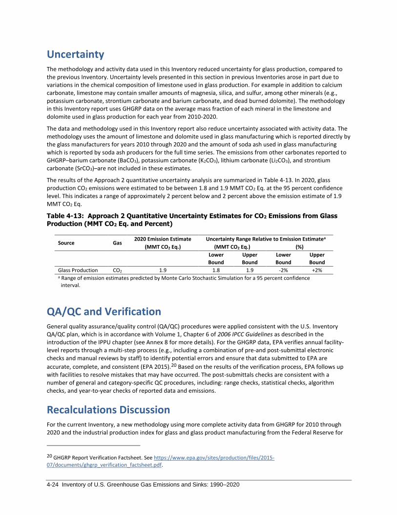
4-24 Inventory of U.S. Greenhouse Gas Emissions and Sinks: 1990–2020
Uncertainty The methodology and activity data used in this Inventory reduced uncertainty for glass production, compared to the previous Inventory. Uncertainty levels presented in this section in previous Inventories arose in part due to variations in the chemical composition of limestone used in glass production. For example in addition to calcium carbonate, limestone may contain smaller amounts of magnesia, silica, and sulfur, among other minerals (e.g., potassium carbonate, strontium carbonate and barium carbonate, and dead burned dolomite). The methodology in this Inventory report uses GHGRP data on the average mass fraction of each mineral in the limestone and dolomite used in glass production for each year from 2010-2020.
The data and methodology used in this Inventory report also reduce uncertainty associated with activity data. The methodology uses the amount of limestone and dolomite used in glass manufacturing which is reported directly by the glass manufacturers for years 2010 through 2020 and the amount of soda ash used in glass manufacturing which is reported by soda ash producers for the full time series. The emissions from other carbonates reported to GHGRP–barium carbonate (BaCO3), potassium carbonate (K2CO3), lithium carbonate (Li2CO3), and strontium carbonate (SrCO3)–are not included in these estimates.
The results of the Approach 2 quantitative uncertainty analysis are summarized in Table 4-13. In 2020, glass production CO2 emissions were estimated to be between 1.8 and 1.9 MMT CO2 Eq. at the 95 percent confidence level. This indicates a range of approximately 2 percent below and 2 percent above the emission estimate of 1.9 MMT CO2 Eq.
Table 4-13: Approach 2 Quantitative Uncertainty Estimates for CO2 Emissions from Glass
Production (MMT CO2 Eq. and Percent)
Source Gas
2020 Emission Estimate Uncertainty Range Relative to Emission Estimatea
(MMT CO2 Eq.) (MMT CO2 Eq.) (%)
Lower
Bound
Upper
Bound
Lower
Bound
Upper
Bound
Glass Production CO2 1.9 1.8 1.9 -2% +2%
a Range of emission estimates predicted by Monte Carlo Stochastic Simulation for a 95 percent confidence interval.
QA/QC and Verification General quality assurance/quality control (QA/QC) procedures were applied consistent with the U.S. Inventory QA/QC plan, which is in accordance with Volume 1, Chapter 6 of 2006 IPCC Guidelines as described in the introduction of the IPPU chapter (see Annex 8 for more details). For the GHGRP data, EPA verifies annual facility-level reports through a multi-step process (e.g., including a combination of pre-and post-submittal electronic checks and manual reviews by staff) to identify potential errors and ensure that data submitted to EPA are
accurate, complete, and consistent (EPA 2015).20 Based on the results of the verification process, EPA follows up with facilities to resolve mistakes that may have occurred. The post-submittals checks are consistent with a number of general and category-specific QC procedures, including: range checks, statistical checks, algorithm checks, and year-to-year checks of reported data and emissions.
Recalculations Discussion For the current Inventory, a new methodology using more complete activity data from GHGRP for 2010 through 2020 and the industrial production index for glass and glass product manufacturing from the Federal Reserve for
20 GHGRP Report Verification Factsheet. See https://www.epa.gov/sites/production/files/2015-07/documents/ghgrp_verification_factsheet.pdf.

Industrial Processes and Product Use 4-25
1990 through 2009 to address time-series consistency were implemented and is described under the Methodology and Time-Series Consistency section. The revised values for 1990 through 2019 resulted in increased emissions estimates for all years. Across the time series, emissions increased by an average of 52 percent compared to the previous Inventory. Annual emission increases during the time series ranged from an 18 percent increase in 2006 (373 kt) to a 91 percent increase in 1999 (1,238 kt).
Planned Improvements EPA incorporated data from GHGRP on limestone and dolomite used for glass production into the emissions estimates for the Glass Production source category for 1990 through 2020. EPA continues to evaluate and analyze data reported under GHGRP that would be useful to improve the emission estimates for the Glass Production source category, particularly the use of barium carbonate, potassium carbonate, lithium carbonate, and strontium carbonate for glass production. EPA will also evaluate updates to uncertainty levels for the activity data and mineral mass fraction values from EPA’s GHGRP. This is a near-term planned improvement.
Some glass producing facilities in the United States do not report to EPA’s GHGRP because they fall below the reporting threshold for this industry. EPA will continue ongoing research on the availability of data to better assess the completeness of emission estimates from glass production and assess how to refine the methodology to ensure complete national coverage of this category. Research will include reassessing previous assessments of GHGRP industry coverage using the reporting threshold of 25,000 metric tons CO2 Eq. This is a medium-term planned improvement.
4.4 Other Process Uses of Carbonates (CRF Source Category 2A4)
Limestone (CaCO3), dolomite (CaCO3MgCO3),21 and other carbonates such as soda ash, magnesite, and siderite are basic materials used by a wide variety of industries, including construction, agriculture, chemical, metallurgy, glass production, and environmental pollution control. This section addresses only limestone, dolomite, and soda ash use. For industrial applications, carbonates such as limestone and dolomite are heated sufficiently enough to calcine the material and generate CO2 as a byproduct.
𝐶𝑎𝐶𝑂3 → 𝐶𝑎𝑂 + 𝐶𝑂2
𝑀𝑔𝐶𝑂3 → 𝑀𝑔𝑂 + 𝐶𝑂2
Examples of such applications include limestone used as a flux or purifier in metallurgical furnaces, as a sorbent in flue gas desulfurization (FGD) systems for utility and industrial plants, and as a raw material for the production of glass, lime, and cement. Emissions from limestone and dolomite used in the production of cement, lime, glass, and iron and steel are excluded from the Other Process Uses of Carbonates category and reported under their respective source categories (e.g., Section 4.2, Glass Production). Emissions from soda ash production are reported under Section 4.12 Soda Ash Production (CRF Source Category 2B7). Emissions from soda ash consumption associated with glass manufacturing are reported under Section 4.2 Glass Production (CRF Source Category 2A3). Emissions from the use of limestone and dolomite in liming of agricultural soils are included in the Agriculture chapter under Liming (CRF Source Category 3G). Emissions from fuels consumed for energy purposes during these processes are accounted for in the Energy chapter under Section 3.1 Fossil Fuel Combustion (CRF Source Category 1A). Both lime (CaO) and limestone (CaCO3) can be used as a sorbent for FGD systems. Emissions from lime consumption for FGD systems and from sugar refining are reported under Section 4.3 Lime Production (CRF Source Category 2A2).
21 Limestone and dolomite are collectively referred to as limestone by the industry, and intermediate varieties are seldom distinguished.

4-26 Inventory of U.S. Greenhouse Gas Emissions and Sinks: 1990–2020
Emissions from the use of dolomite in primary magnesium metal production are reported under Section 4.20 Magnesium Production and Processing (CRF Source Category 2C4).
Limestone and dolomite are widely distributed throughout the world in deposits of varying sizes and degrees of purity. Large deposits of limestone occur in nearly every state in the United States, and significant quantities are extracted for industrial applications. In 2017, the leading limestone producing states were Texas, Florida, Missouri, Ohio, and Pennsylvania, which contributed 44 percent of the total U.S. output (USGS 2021a). Dolomite deposits are found in the United States, Canada, Mexico, Europe, Africa, and Brazil. In the United States, the leading dolomite producing states are Pennsylvania, New York, and Utah which currently contribute more than a third of the total U.S. output (USGS 2021a). Internationally, two types of soda ash are produced: natural and synthetic. In 2019, 93 percent of the global soda ash production came from China, the United States, Russia, Germany, India, Turkey, Poland, and France. The United States only produces natural soda ash and only in two states: Wyoming and California (USGS 2021c).
In 2020, 15,346 kilotons (kt) of limestone, 4,374 kt of dolomite, and 2,310 kt of soda ash were consumed for these emissive applications, which excludes consumption for the production of cement, lime, glass, and iron and steel (Willett 2021, USGS 2021d). Limestone and dolomite consumption data for 2020 were not available in time for publication and were estimated using 2019 values, as described in the Methodology and Time-Series Consistency section below. Usage of limestone, dolomite and soda ash resulted in aggregate CO2 emissions of 9.8 MMT CO2 Eq. (9,794 kt) (see Table 4-14 and Table 4-15). The 2019 and 2020 emissions increased over 30 percent compared to 2018, primarily as a result of increased limestone consumption attributed to sulfur oxide removal usage for FGD systems and dolomite consumption attributed to flux stone. Disruptions in the mining and construction industries associated with the COVID-19 pandemic led to decreased consumption of crushed stone in 2020; however, the impacts on emissions from limestone and dolomite consumption are not able to be quantified without more detailed information on consumption from the emissive sources in 2020 (USGS 2021b). Overall emissions have increased 57 percent from 1990 through 2020.
Table 4-14: CO2 Emissions from Other Process Uses of Carbonates (MMT CO2 Eq.)
Year
Flux
Stone FGD
Soda Ash
Consumptiona
Other
Miscellaneous
Usesb Total
1990 2.6 1.4 1.4 0.8 6.2
2005 2.6 3.0 1.3 0.5 7.5
2016 2.6 6.2 1.1 1.0 10.8
2017 2.4 5.6 1.1 0.8 9.9
2018 2.8 2.2 1.1 1.3 7.4
2019 4.8 3.5 1.0 0.5 9.8
2020 4.8 3.5 1.0 0.5 9.8
a Soda ash consumption not associated with glass manufacturing.
b “Other miscellaneous uses” include chemical stone, mine dusting or acid water treatment, and acid neutralization.
Note: Totals may not sum due to independent rounding.

Industrial Processes and Product Use 4-27
Table 4-15: CO2 Emissions from Other Process Uses of Carbonates (kt)
Year
Flux
Stone FGD
Soda Ash
Consumptiona
Other
Miscellaneous
Usesb Total
1990 2,592 1,432 1,390 819 6,233
2005 2,649 2,973 1,305 533 7,459
2016 2,585 6,164 1,082 981 10,813
2017 2,441 5,598 1,058 771 9,869
2018 2,795 2,229 1,069 1,259 7,351
2019 4,811 3,537 1,036 463 9,848
2020 4,835 3,537 958 463 9,794
a Soda ash consumption not associated with glass manufacturing. b “Other miscellaneous uses” include chemical stone, mine dusting or acid water
treatment, and acid neutralization. Note: Totals may not sum due to independent rounding.
Methodology and Time-Series Consistency Carbon dioxide emissions were calculated based on the 2006 IPCC Guidelines Tier 2 method by multiplying the quantity of limestone or dolomite consumed by the emission factor for limestone or dolomite calcination, respectively: 0.43971 metric ton CO2/metric ton carbonate for limestone and 0.47732 metric ton CO2/metric ton
carbonate for dolomite.22 This methodology was used for flux stone, flue gas desulfurization systems, chemical stone, mine dusting or acid water treatment, and acid neutralization. Flux stone used during the production of iron and steel was deducted from the Other Process Uses of Carbonates source category estimate and attributed to the Iron and Steel Production source category estimate. Similarly, limestone and dolomite consumption for glass manufacturing, cement, and lime manufacturing are excluded from this category and attributed to their respective categories.
Consumption data for 1990 through 2019 of limestone and dolomite used for flux stone, flue gas desulfurization systems, chemical stone, mine dusting or acid water treatment, and acid neutralization (see Table 4-16) were obtained from the U.S. Geological Survey (USGS) Minerals Yearbook: Crushed Stone Annual Report (1995a through 2017, 2020a, 2020c), preliminary data for 2019 from USGS Crushed Stone Commodity Expert (Willett 2021), American Iron and Steel Institute limestone and dolomite consumption data (AISI 2018 through 2020), and the U.S. Bureau of Mines (1991 and 1993a), which are reported to the nearest ton. Limestone and dolomite consumption data for 2020 were not available at the time of publication and were estimated using 2019 values. In addition, the estimated values for limestone and dolomite consumption for flux stone used during the production of iron and steel were adjusted down, using emissions data from the EPA’s Greenhouse Gas Reporting Program (GHGRP) subpart Q for the iron and steel sector to account for the impacts of the COVID-19 pandemic in 2020. GHGRP process emissions data decreased by approximately 14 percent from 2019 to 2020 (EPA 2021). This adjustment method is consistent with the method used in Section 4.17 (CRF Source Category 2C1) and Metallurgical Coke Production. Similar data on 2020 emissions trends were not available for the other process uses included in this section, which prevented the use of a similar approach.
During 1990 and 1992, the USGS did not conduct a detailed survey of limestone and dolomite consumption by end-use; therefore, data on consumption by end use for 1990 was estimated by applying the 1991 ratios of total limestone and dolomite consumption by end use to total 1990 limestone and dolomite consumption values. Similarly, the 1992 consumption figures were approximated by applying an average of the 1991 and 1993 ratios of total limestone and dolomite use by end uses to the 1992 total values.
22 2006 IPCC Guidelines, Volume 3: Chapter 2, Table 2.1.

4-28 Inventory of U.S. Greenhouse Gas Emissions and Sinks: 1990–2020
In 1991, the U.S. Bureau of Mines, now known as the USGS, began compiling production and end use information through surveys of crushed stone manufacturers. Manufacturers provided different levels of detail in survey responses, so information was divided into three categories: (1) production by end-use, as reported by manufacturers (i.e., “specified” production); (2) production reported by manufacturers without end-uses specified (i.e., “unspecified-reported” production); and (3) estimated additional production by manufacturers who did not respond to the survey (i.e., “unspecified-estimated” production). Additionally, each year the USGS withholds data on certain limestone and dolomite end-uses due to confidentiality agreements regarding company proprietary data. For the purposes of this analysis, emissive end-uses that contained withheld data were estimated using one of the following techniques: (1) the value for all the withheld data points for limestone or dolomite use was distributed evenly to all withheld end-uses; (2) the average percent of total limestone or dolomite for the withheld end-use in the preceding and succeeding years; or (3) the average fraction of total limestone or dolomite for the end-use over the entire time period.
A large quantity of crushed stone was reported to the USGS under the category “unspecified uses.” A portion of this consumption is believed to be limestone or dolomite used for emissive end uses. The quantity listed for “unspecified uses” was, therefore, allocated to all other reported end-uses according to each end-use’s fraction of
total consumption in that year.23
Table 4-16: Limestone and Dolomite Consumption (kt)
Activity 1990 2005 2016 2017 2018 2019 2020
Flux Stone 5,842 5,745 5,686 5,447 6,242 10,570 10,622
Limestone 5,237 2,492 3,415 4,216 4,891 6,222 6,248
Dolomite 605 3,254 2,270 1,230 1,351 4,348 4,374
FGD 3,258 6,761 14,019 12,732 5,068 8,045 8,045
Other Miscellaneous Uses 1,835 1,212 2,231 1,754 2,862 1,054 1,054
Total 10,935 13,719 21,935 19,932 14,172 19,668 19,720
Note: Totals may not sum due to independent rounding.
Excluding glass manufacturing which is reported under Section 4.2 Glass Production (CRF Source Category 2A3), most soda ash is consumed in chemical production, with minor amounts used in soap production, pulp and paper, flue gas desulfurization, and water treatment. As soda ash is consumed for these purposes, CO2 is usually emitted. In these applications, it is assumed that one mole of carbon is released for every mole of soda ash used. Thus, approximately 0.113 metric tons of carbon (or 0.415 metric tons of CO2) are released for every metric ton of soda ash consumed. The activity data for soda ash consumption for 1990 to 2020 (see Table 4-17) were obtained from the U.S. Geological Survey (USGS) Minerals Yearbook for Soda Ash (1994 through 2015b) and USGS Mineral Industry Surveys for Soda Ash (USGS 2017a, 2018, 2019, 2020b, 2021d). Soda ash consumption data were collected by the USGS from voluntary surveys of the U.S. soda ash industry.
Table 4-17: Soda Ash Consumption Not Associated with Glass Manufacturing (kt)
Activity 1990 2005 2016 2017 2018 2019 2020
Soda Asha 3,351 3,144 2,608 2,550 2,576 2,497 2,310
a Soda ash consumption is sales reported by producers which exclude imports. Historically, imported soda ash is less than 1 percent of the total U.S. consumption (Kostick 2012).
Methodological approaches were applied to the entire time series to ensure consistency in emissions from 1990 through 2020.
23 This approach was recommended by USGS, the data collection agency.

Industrial Processes and Product Use 4-29
Uncertainty The uncertainty levels presented in this section account for uncertainty associated with activity data. Data on limestone and dolomite consumption are collected by USGS through voluntary national surveys. USGS contacts the mines (i.e., producers of various types of crushed stone) for annual sales data. Data on other carbonate consumption are not readily available. The producers report the annual quantity sold to various end-users and industry types. USGS estimates the historical response rate for the crushed stone survey to be approximately 70 percent, and the rest is estimated by USGS. Large fluctuations in reported consumption exist, reflecting year-to-year changes in the number of survey responders. The uncertainty resulting from a shifting survey population is exacerbated by the gaps in the time series of reports. The accuracy of distribution by end use is also uncertain because this value is reported by the producer/mines and not the end user. Additionally, there is significant inherent uncertainty associated with estimating withheld data points for specific end uses of limestone and dolomite. Lastly, much of the limestone consumed in the United States is reported as “other unspecified uses;” therefore, it is difficult to accurately allocate this unspecified quantity to the correct end-uses. EPA contacted the USGS National Minerals Information Center Crushed Stone commodity expert to assess the current uncertainty ranges associated with the limestone and dolomite consumption data compiled and published by USGS. During this discussion, the expert confirmed that EPA’s range of uncertainty was still reasonable (Willett 2017).
Uncertainty in the estimates also arises in part due to variations in the chemical composition of limestone. In addition to calcium carbonate, limestone may contain smaller amounts of magnesia, silica, and sulfur, among other minerals. The exact specifications for limestone or dolomite used as flux stone vary with the pyrometallurgical process and the kind of ore processed.
For emissions from soda ash consumption, the primary source of uncertainty results from the fact that these emissions are dependent upon the type of processing employed by each end-use. Specific emission factors for each end-use are not available, so a Tier 1 default emission factor is used for all end-uses. Therefore, there is uncertainty surrounding the emission factors from the consumption of soda ash. Additional uncertainty comes from the reported consumption and allocation of consumption within sectors that is collected on a quarterly basis by the USGS. Efforts have been made to categorize company sales within the correct end-use sector.
The results of the Approach 2 quantitative uncertainty analysis are summarized in Table 4-18. Carbon dioxide emissions from other process uses of carbonates in 2020 were estimated to be between 8.2 and 12.9 MMT CO2 Eq. at the 95 percent confidence level. This indicates a range of approximately 19 percent below and 28 percent above the emission estimate of 9.8 MMT CO2 Eq.
Table 4-18: Approach 2 Quantitative Uncertainty Estimates for CO2 Emissions from Other Process Uses of Carbonates (MMT CO2 Eq. and Percent)
Source Gas
2020 Emission
Estimate Uncertainty Range Relative to Emission Estimatea
(MMT CO2 Eq.) (MMT CO2 Eq.) (%)
Lower
Bound
Upper
Bound
Lower
Bound
Upper
Bound
Other Process Uses
of Carbonates CO2 9.8 8.2 12.9 -19% +28%
a Range of emission estimates predicted by Monte Carlo Stochastic Simulation for a 95 percent confidence interval.
QA/QC and Verification General quality assurance/quality control (QA/QC) procedures were applied consistent with the U.S. Inventory QA/QC plan, which is in accordance with Volume 1, Chapter 6 of 2006 IPCC Guidelines as described in the introduction of the IPPU chapter (see Annex 8 for more details).

4-30 Inventory of U.S. Greenhouse Gas Emissions and Sinks: 1990–2020
Recalculations Discussion Emissions from carbonate consumption for magnesium metal production previously included in this chapter have been moved from Other Process Uses of Carbonates to Section 4.20 Magnesium Production and Processing (CRF Source Category 2C4) in the current Inventory, consistent with the 2006 IPCC Guidelines. Emissions were removed from this chapter for 1990 through 2001, resulting in approximately 50 to 70 kt CO2 reduction for these years.
Emissions previously included in this chapter for limestone consumption for sugar refining have been removed in the current inventory, as it was determined that these emissions are already accounted for in the Lime Production source category emissions. Emissions were removed from this chapter for 1990 through 2019, resulting in a range of 0 to 1,500 kt CO2 reduction for these years.
Additionally, for the current Inventory, updated USGS data on limestone and dolomite consumption was available for 2019, resulting in updated emissions estimates for that year. Compared to the previous Inventory, emissions for 2019 increased by 32 percent (2,391 kt CO2 Eq.).
Planned Improvements In response to comments received during previous Inventory reports from the UNFCCC, EPA has inquired to the availability of ceramics and non-metallurgical magnesia data. The USGS notes that this data is not currently reported by survey respondents. EPA continues to conduct outreach with other entities, but at this time, the research has not yielded any alternative data on national levels of carbonates. This improvement remains ongoing, and EPA plans to continue to update this Planned Improvements section in future reports as more information becomes available.
EPA also plans to continue dialogue with USGS to assess uncertainty ranges for activity data used to estimate emissions from other process use of carbonates. This planned improvement is currently planned as a medium-term improvement.
4.5 Ammonia Production (CRF Source Category 2B1)
Emissions of carbon dioxide (CO2) occur during the production of synthetic ammonia (NH3), primarily through the use of natural gas, petroleum coke, or naphtha as a feedstock. The natural gas-, naphtha-, and petroleum coke-based processes produce CO2 and hydrogen (H2), the latter of which is used in the production of ammonia. The brine electrolysis process for production of ammonia does not lead to process-based CO2 emissions. Due to national circumstances, emissions from fuels consumed for energy purposes during the production of ammonia are accounted for in the Energy chapter. More information on this approach can be found in the Methodology section below.
Ammonia production requires a source of nitrogen (N) and hydrogen (H). Nitrogen is obtained from air through liquid air distillation or an oxidative process where air is burnt and the residual nitrogen is recovered. In the United States, the majority of ammonia is produced using a natural gas feedstock as the hydrogen source. One synthetic ammonia production plant located in Kansas is producing ammonia from petroleum coke feedstock. In some U.S. plants, some of the CO2 produced by the process is captured and used to produce urea rather than being emitted to the atmosphere. In 2020, 16 companies operated 35 ammonia producing facilities in 16 states. Approximately 60 percent of domestic ammonia production capacity is concentrated in Louisiana, Oklahoma, and Texas (USGS 2021).
Synthetic ammonia production from natural gas feedstock consists of five principal process steps. The primary reforming step converts methane (CH4) to CO2, carbon monoxide (CO), and hydrogen (H2) in the presence of a
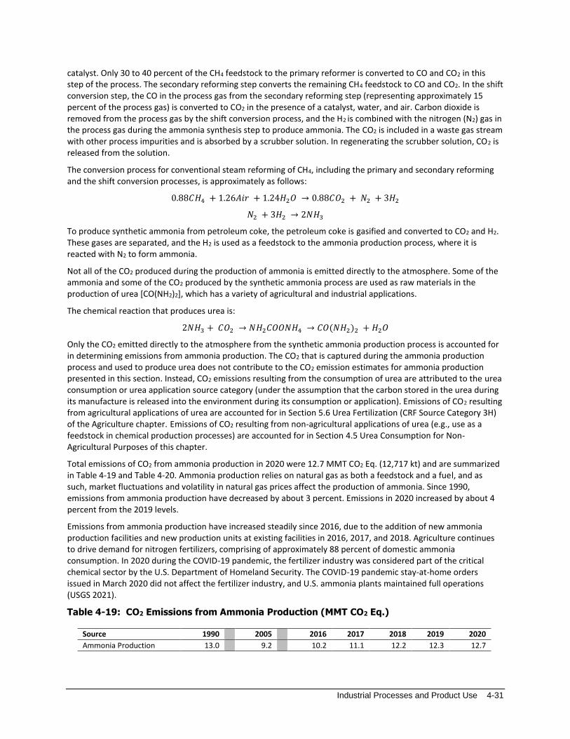
Industrial Processes and Product Use 4-31
catalyst. Only 30 to 40 percent of the CH4 feedstock to the primary reformer is converted to CO and CO2 in this step of the process. The secondary reforming step converts the remaining CH4 feedstock to CO and CO2. In the shift conversion step, the CO in the process gas from the secondary reforming step (representing approximately 15 percent of the process gas) is converted to CO2 in the presence of a catalyst, water, and air. Carbon dioxide is removed from the process gas by the shift conversion process, and the H2 is combined with the nitrogen (N2) gas in the process gas during the ammonia synthesis step to produce ammonia. The CO2 is included in a waste gas stream with other process impurities and is absorbed by a scrubber solution. In regenerating the scrubber solution, CO2 is released from the solution.
The conversion process for conventional steam reforming of CH4, including the primary and secondary reforming and the shift conversion processes, is approximately as follows:
0.88𝐶𝐻4 + 1.26𝐴𝑖𝑟 + 1.24𝐻2𝑂 → 0.88𝐶𝑂2 + 𝑁2 + 3𝐻2
𝑁2 + 3𝐻2 → 2𝑁𝐻3
To produce synthetic ammonia from petroleum coke, the petroleum coke is gasified and converted to CO2 and H2. These gases are separated, and the H2 is used as a feedstock to the ammonia production process, where it is reacted with N2 to form ammonia.
Not all of the CO2 produced during the production of ammonia is emitted directly to the atmosphere. Some of the ammonia and some of the CO2 produced by the synthetic ammonia process are used as raw materials in the production of urea [CO(NH2)2], which has a variety of agricultural and industrial applications.
The chemical reaction that produces urea is:
2𝑁𝐻3 + 𝐶𝑂2 → 𝑁𝐻2𝐶𝑂𝑂𝑁𝐻4 → 𝐶𝑂(𝑁𝐻2)2 + 𝐻2𝑂
Only the CO2 emitted directly to the atmosphere from the synthetic ammonia production process is accounted for in determining emissions from ammonia production. The CO2 that is captured during the ammonia production process and used to produce urea does not contribute to the CO2 emission estimates for ammonia production presented in this section. Instead, CO2 emissions resulting from the consumption of urea are attributed to the urea consumption or urea application source category (under the assumption that the carbon stored in the urea during its manufacture is released into the environment during its consumption or application). Emissions of CO2 resulting from agricultural applications of urea are accounted for in Section 5.6 Urea Fertilization (CRF Source Category 3H) of the Agriculture chapter. Emissions of CO2 resulting from non-agricultural applications of urea (e.g., use as a feedstock in chemical production processes) are accounted for in Section 4.5 Urea Consumption for Non-Agricultural Purposes of this chapter.
Total emissions of CO2 from ammonia production in 2020 were 12.7 MMT CO2 Eq. (12,717 kt) and are summarized in Table 4-19 and Table 4-20. Ammonia production relies on natural gas as both a feedstock and a fuel, and as such, market fluctuations and volatility in natural gas prices affect the production of ammonia. Since 1990, emissions from ammonia production have decreased by about 3 percent. Emissions in 2020 increased by about 4 percent from the 2019 levels.
Emissions from ammonia production have increased steadily since 2016, due to the addition of new ammonia production facilities and new production units at existing facilities in 2016, 2017, and 2018. Agriculture continues to drive demand for nitrogen fertilizers, comprising of approximately 88 percent of domestic ammonia consumption. In 2020 during the COVID-19 pandemic, the fertilizer industry was considered part of the critical chemical sector by the U.S. Department of Homeland Security. The COVID-19 pandemic stay-at-home orders issued in March 2020 did not affect the fertilizer industry, and U.S. ammonia plants maintained full operations (USGS 2021).
Table 4-19: CO2 Emissions from Ammonia Production (MMT CO2 Eq.)
Source 1990 2005 2016 2017 2018 2019 2020
Ammonia Production 13.0 9.2 10.2 11.1 12.2 12.3 12.7

4-32 Inventory of U.S. Greenhouse Gas Emissions and Sinks: 1990–2020
Table 4-20: CO2 Emissions from Ammonia Production (kt)
Source 1990 2005 2016 2017 2018 2019 2020
Ammonia Production 13,047 9,177 10,245 11,112 12,163 12,272 12,717
Methodology and Time-Series Consistency For this Inventory, CO2 emissions from the production of synthetic ammonia from natural gas feedstock are estimated using a country-specific approach modified from the 2006 IPCC Guidelines (IPCC 2006) Tier 1 and 2 methods. In the country-specific approach, emissions are not based on total fuel requirement per the 2006 IPCC Guidelines due to data disaggregation limitations of energy statistics provided by the Energy Information Administration (EIA). Data on total fuel use (including fuel used for ammonia feedstock and fuel used for energy) for ammonia production are not known in the United States. EIA does not provide data broken out by industrial category, only at the broad industry sector level. To estimate emissions, a country-specific emission factor is developed and applied to national ammonia production to estimate ammonia-production emissions from feedstock fuel use. Emissions from fuel used for energy at ammonia plants are included in the overall EIA Industrial sector energy use and accounted for in the Energy chapter.
The country-specific approach uses a CO2 emission factor of 1.2 metric tons CO2/metric ton NH3, which is published by the European Fertilizer Manufacturers Association (EFMA) and is based on natural gas-based ammonia production technologies that are similar to those employed in the United States (EFMA 2000a). The EFMA reported an emission factor range of 1.15 to 1.30 metric tons CO2 per metric ton NH3, with 1.2 metric tons CO2 per metric ton NH3 as a typical value (EFMA 2000a). Technologies (e.g., catalytic reforming process, etc.) associated with this factor are found to closely resemble those employed in the United States for use of natural gas as a feedstock. The EFMA reference also indicates that more than 99 percent of the CH4 feedstock to the catalytic reforming process is ultimately converted to CO2. This country-specific approach is compatible with the 2006 IPCC Guidelines as it is based on the same scientific approach that the carbon in the fuel used to produce ammonia is released as CO2. The CO2 emission factor is applied to the percent of total annual domestic ammonia production from natural gas feedstock.
Emissions of CO2 from ammonia production are then adjusted to account for the use of some of the CO2 produced from ammonia production as a raw material in the production of urea. The CO2 emissions reported for ammonia production are reduced by a factor of 0.733 multiplied by total annual domestic urea production. This corresponds to a stoichiometric CO2/urea factor of 44/60, assuming complete conversion of ammonia (NH3) and CO2 to urea (IPCC 2006; EFMA 2000b).
All synthetic ammonia production and subsequent urea production are assumed to be from the same process—conventional catalytic reforming of natural gas feedstock, with the exception of ammonia production from petroleum coke feedstock at one plant located in Kansas. Annual ammonia and urea production are shown in Table 4-21.
The implied CO2 emission factor for total ammonia production is a combination of the emission factors for ammonia production from natural gas and from petroleum coke. Changes in the relative production of ammonia from natural gas and petroleum coke will impact overall emissions and emissions per ton of total ammonia produced. For example, between 2000 and 2001 there were increases in the amount of ammonia produced from petroleum coke which caused increases in the implied emission factor across those years.
The CO2 emission factor for petroleum coke feedstock is 3.52 metric tons of CO2 per metric ton of NH3 and is applied to the percent of total annual domestic ammonia production from petroleum coke feedstock. The CO2 emission factor is based on an average of the ratio of ammonia production from petroleum coke for years 2010 through 2015 (ACC 2020) and the facility-specific CO2 emissions from the one ammonia production plant located in Kansas that is manufacturing ammonia from petroleum coke feedstock for years 2010 through 2015 (EPA 2021b). Ammonia and urea are assumed to be manufactured in the same manufacturing complex, as both the raw materials needed for urea production are produced by the ammonia production process.

Industrial Processes and Product Use 4-33
The methodology for ammonia produced from petroleum coke shifts in 2016 when the parent company of the facility manufacturing ammonia from petroleum coke feedstock, CVR Energy, acquired a second plant that uses natural gas as a feedstock. The amount of ammonia production reported by CVR Energy was no longer specific to the use of petroleum coke as a feedstock. To adjust for this, beginning in 2016, the amount of CO2 from the ammonia production plant located in Kansas that manufactured ammonia from petroleum coke feedstock (as reported under EPA 2021b) is now being used, along with the emission factor of 3.52 metric tons of CO2 per metric ton of NH3 to back-calculate the amount of ammonia produced through the use of petroleum coke as feedstock.
The consumption of natural gas and petroleum coke as fossil fuel feedstocks for NH3 production are adjusted for within the Energy chapter as these fuels were consumed during non-energy related activities. More information on this methodology is described in Annex 2.1, Methodology for Estimating Emissions of CO2 from Fossil Fuel Combustion. See the Planned Improvements section on improvements of reporting fuel and feedstock CO2 emissions utilizing EPA’s GHGRP data to improve consistency with 2006 IPCC Guidelines.
Total ammonia production data for 2011 through 2020 were obtained from American Chemistry Council (ACC 2021). For years before 2011, ammonia production data (see Table 4-21) were obtained from Coffeyville Resources (Coffeyville 2005, 2006, 2007a, 2007b, 2009, 2010, 2011, and 2012) and the Census Bureau of the U.S. Department of Commerce (U.S. Census Bureau 1991 through 1994, 1998 through 2011) as reported in Current Industrial Reports Fertilizer Materials and Related Products annual and quarterly reports. Urea-ammonia nitrate production from petroleum coke for 1990 through 2011 was obtained from Coffeyville Resources (Coffeyville 2005, 2006, 2007a, 2007b, 2009, 2010, 2011, and 2012) and from CVR Energy, Inc. Annual Report (CVR 2012 through 2015) for 2012 through 2015. Urea production data for 1990 through 2008 were obtained from the Minerals Yearbook: Nitrogen (USGS 1994 through 2009). Urea production data for 2009 through 2010 were obtained from the U.S. Census Bureau (U.S. Census Bureau 2010 and 2011). The U.S. Census Bureau ceased collection of urea production statistics in 2011. Urea production values for the years 2011 through 2020 utilize GHGRP data (EPA 2018; EPA 2021a).
Table 4-21: Ammonia Production, Recovered CO2 Consumed for Urea Production, and Urea
Production (kt)
Year Ammonia Production
Total CO2 Consumption
for Urea Production Urea Production
1990 15,425 5,463 7,450
2005 10,143 3,865 5,270
2016 12,305 5,419 7,390
2017 14,070 6,622 9,030
2018 16,010 7,847 10,700
2019
2020
16,410
16,855
8,360
8,433
11,400
11,500
Methodological approaches were applied to the entire time series to ensure consistency in emissions from 1990 through 2020. The methodology for ammonia production spliced activity data from different sources: U. S. Census Bureau data for 1990 through 2010, and ACC data beginning in 2011. Consistent with the 2006 IPCC Guidelines, the overlap technique was applied to compare the two data sets for years where there was overlap, with findings that the data sets were consistent and adjustments were not needed.
Uncertainty
The uncertainties presented in this section are primarily due to how accurately the emission factor used represents an average across all ammonia plants using natural gas feedstock. Uncertainties are also associated with ammonia production estimates and the assumption that all ammonia production and subsequent urea production was from

4-34 Inventory of U.S. Greenhouse Gas Emissions and Sinks: 1990–2020
the same process—conventional catalytic reforming of natural gas feedstock, with the exception of one ammonia production plant located in Kansas that is manufacturing ammonia from petroleum coke feedstock. Uncertainty is also associated with the representativeness of the emission factor used for the petroleum coke-based ammonia process. It is also assumed that ammonia and urea are produced at co-located plants from the same natural gas raw material. The uncertainty of the total urea production activity data, based on USGS Minerals Yearbook: Nitrogen data, is a function of the reliability of reported production data and is influenced by the completeness of the survey responses. EPA assigned a default uncertainty range of ±5 percent for both ammonia production and the emission factor used for the petroleum coke-based ammonia process, consistent with the ranges in Section 3.2.3.2 of the 2006 IPCC Guidelines, and ±10 percent for urea production, based on expert judgment.
Recovery of CO2 from ammonia production plants for purposes other than urea production (e.g., commercial sale, etc.) has not been considered in estimating the CO2 emissions from ammonia production, as data concerning the disposition of recovered CO2 are not available. Such recovery may or may not affect the overall estimate of CO2 emissions depending upon the end use to which the recovered CO2 is applied. Further research is required to determine whether byproduct CO2 is being recovered from other ammonia production plants for application to end uses that are not accounted for elsewhere; however, for reporting purposes, CO2 consumption for urea production is provided in this chapter.
The results of the Approach 2 quantitative uncertainty analysis are summarized in Table 4-22. Carbon dioxide emissions from ammonia production in 2020 were estimated to be between 11.4 and 14.1 MMT CO2 Eq. at the 95 percent confidence level. This indicates a range of approximately 10 percent below and 11 percent above the emission estimate of 12.7 MMT CO2 Eq.
Table 4-22: Approach 2 Quantitative Uncertainty Estimates for CO2 Emissions from
Ammonia Production (MMT CO2 Eq. and Percent)
Source Gas 2020 Emission Estimate Uncertainty Range Relative to Emission Estimatea
(MMT CO2 Eq.) (MMT CO2 Eq.) (%)
Lower
Bound
Upper
Bound
Lower
Bound
Upper
Bound
Ammonia Production CO2 12.7 11.4 14.1 -10% +11% a Range of emission estimates predicted by Monte Carlo Stochastic Simulation for a 95 percent confidence interval.
QA/QC and Verification General quality assurance/quality control (QA/QC) procedures were applied to ammonia production emission estimates consistent with the U.S. Inventory QA/QC plan, which is in accordance with Volume 1, Chapter 6 of 2006 IPCC Guidelines as described in the introduction of the IPPU chapter (see Annex 8 for more details). More details on the greenhouse gas calculation, monitoring and QA/QC methods applicable to ammonia facilities can be found under Subpart G (Ammonia Production) of the regulation (40 CFR Part 98).24 EPA verifies annual facility-level GHGRP reports through a multi-step process (e.g., combination of electronic checks and manual reviews) to identify potential errors and ensure that data submitted to EPA are accurate, complete, and consistent.25 Based on the results of the verification process, EPA follows up with facilities to resolve mistakes that may have occurred. The post-submittals checks are consistent with a number of general and category-specific QC procedures, including range checks, statistical checks, algorithm checks, and year-to-year checks of reported data and emissions.
More details on the greenhouse gas calculation, monitoring and QA/QC methods applicable to reporting of urea produced at ammonia production facilities can be found under Section 4.5 Urea Consumption for Non-Agricultural Purposes.
24 See http://www.ecfr.gov/cgi-bin/text-idx?tpl=/ecfrbrowse/Title40/40cfr98_main_02.tpl. 25 See https://www.epa.gov/sites/production/files/2015-07/documents/ghgrp_verification_factsheet.pdf.

Industrial Processes and Product Use 4-35
Planned Improvements Future improvements involve continuing to evaluate and analyze data reported under EPA’s GHGRP to improve the emission estimates for the Ammonia Production source category, in particular new facility-level reporting data from updated reporting requirements finalized in October of 2014 (79 FR 63750) and December 2016 (81 FR
89188)26 that include facility-level ammonia production data and feedstock consumption. The data were first reported by facilities in 2018 and available post-verification in 2019 to assess for use in future Inventories, if the data meet GHGRP CBI aggregation criteria. The data are still being evaluated and will be incorporated in future Inventory reports, if possible. Particular attention will be made to ensure time-series consistency of the emission estimates presented in future Inventory reports, along with application of appropriate category-specific QC procedures consistent with IPCC and UNFCCC guidelines. For example, data reported in 2018 will reflect activity in 2017 and may not be representative of activity in prior years of the time series. This assessment is required as the new GHGRP data associated with new requirements are only applicable starting with reporting for calendar year 2017, and thus are not available for all inventory years (i.e., 1990 through 2016) as required for this Inventory.
In implementing improvements and integration of data from EPA’s GHGRP, the latest guidance from the IPCC on
the use of facility-level data in national inventories will be relied upon.27 Specifically, the planned improvements include assessing the anticipated new data to update the emission factors to include both fuel and feedstock CO2 emissions to improve consistency with 2006 IPCC Guidelines, in addition to reflecting CO2 capture and storage practices (beyond use of CO2 for urea production). Methodologies will also be updated if additional ammonia production plants are found to use hydrocarbons other than natural gas for ammonia production. Due to limited resources and ongoing data collection efforts, this planned improvement is still in development and is not incorporated into this Inventory. This is a long-term planned improvement.
4.6 Urea Consumption for Non-Agricultural Purposes
Urea is produced using ammonia (NH3) and carbon dioxide (CO2) as raw materials. All urea produced in the United States is assumed to be produced at ammonia production facilities where both ammonia and CO2 are generated. There were 35 plants producing ammonia in the United States in 2020, with two additional plants sitting idle for the entire year (USGS 2021).
The chemical reaction that produces urea is:
2𝑁𝐻3 + 𝐶𝑂2 → 𝑁𝐻2𝐶𝑂𝑂𝑁𝐻4 → 𝐶𝑂(𝑁𝐻2)2 + 𝐻2𝑂
This section accounts for CO2 emissions associated with urea consumed exclusively for non-agricultural purposes. Emissions of CO2 resulting from agricultural applications of urea are accounted for in Section 5.6 Urea Fertilization (CRF Source Category 3H) of the Agriculture chapter.
The industrial applications of urea include its use in adhesives, binders, sealants, resins, fillers, analytical reagents, catalysts, intermediates, solvents, dyestuffs, fragrances, deodorizers, flavoring agents, humectants and dehydrating agents, formulation components, monomers, paint and coating additives, photosensitive agents, and surface treatments agents. In addition, urea is used for abating nitrogen oxide (NOx) emissions from coal-fired power plants and diesel transportation motors.
Emissions of CO2 from urea consumed for non-agricultural purposes in 2020 were estimated to be 6.0 MMT CO2 Eq. (5,983 kt) and are summarized in Table 4-23 and Table 4-24. Net CO2 emissions from urea consumption for
26 See https://www.epa.gov/ghgreporting/historical-rulemakings. 27 See http://www.ipcc-nggip.iges.or.jp/public/tb/TFI_Technical_Bulletin_1.pdf.

4-36 Inventory of U.S. Greenhouse Gas Emissions and Sinks: 1990–2020
non-agricultural purposes have increased by approximately 58 percent from 1990 to 2020 and decreased by approximately 1.0 percent from 2019 to 2020.
Table 4-23: CO2 Emissions from Urea Consumption for Non-Agricultural Purposes (MMT CO2
Eq.)
Source 1990 2005 2016 2017 2018 2019 2020
Urea Consumption 3.8 3.7 5.3 5.2 6.0 6.0 6.0
Table 4-24: CO2 Emissions from Urea Consumption for Non-Agricultural Purposes (kt)
Source 1990 2005 2016 2017 2018 2019 2020
Urea Consumption 3,784 3,653 5,330 5,182 6,030 6,044 5,983
Methodology and Time-Series Consistency Emissions of CO2 resulting from urea consumption for non-agricultural purposes are estimated by multiplying the amount of urea consumed in the United States for non-agricultural purposes by a factor representing the amount of CO2 used as a raw material to produce the urea. This method is based on the assumption that all of the carbon in urea is released into the environment as CO2 during use, consistent with the Tier 1 method used to estimate emissions from ammonia production in the 2006 IPCC Guidelines (IPCC 2006) which states that the “CO2 recovered [from ammonia production] for downstream use can be estimated from the quantity of urea produced where CO2 is estimated by multiplying urea production by 44/60, the stoichiometric ratio of CO2 to urea.”
The amount of urea consumed for non-agricultural purposes in the United States is estimated by deducting the quantity of urea fertilizer applied to agricultural lands, which is obtained directly from the Agriculture chapter (see Table 5-25), from the total domestic supply of urea as reported in Table 4-25. The domestic supply of urea is estimated based on the amount of urea produced plus urea imports and minus urea exports. A factor of 0.733 tons of CO2 per ton of urea consumed is then applied to the resulting supply of urea for non-agricultural purposes to estimate CO2 emissions from the amount of urea consumed for non-agricultural purposes. The 0.733 tons of CO2 per ton of urea emission factor is based on the stoichiometry of carbon in urea. This corresponds to a stoichiometric CO2 to urea factor of 44/60, assuming complete conversion of carbon in urea to CO2 (IPCC 2006; EFMA 2000).
Urea production data for 1990 through 2008 were obtained from the U.S. Geological Survey (USGS) Minerals Yearbook: Nitrogen (USGS 1994 through 2009a). Urea production data for 2009 through 2010 were obtained from the U.S. Census Bureau (2011). The U.S. Census Bureau ceased collection of urea production statistics in 2011. Starting with the 1990 through 2017 Inventory report, EPA began utilizing urea production data from EPA’s GHGRP to estimate emissions. Urea production values in the current Inventory report utilize GHGRP data for the years 2011 through 2020 (EPA 2018; EPA 2021a; EPA 2021b).
Urea import data for 2020 were not available at the time of publication and were estimated using 2019 values. Urea import data for 2013 to 2019 were obtained from the USGS Minerals Yearbook: Nitrogen (USGS 2021a). Urea import data for 2011 and 2012 were taken from U.S. Fertilizer Import/Exports from the United States Department of Agriculture (USDA) Economic Research Service Data Sets (U.S. Department of Agriculture 2012). USDA suspended updates to this data after 2012. Urea import data for the previous years were obtained from the U.S. Census Bureau Current Industrial Reports Fertilizer Materials and Related Products annual and quarterly reports for 1997 through 2010 (U.S. Census Bureau 2001 through 2011), The Fertilizer Institute (TFI 2002) for 1993 through 1996, and the United States International Trade Commission Interactive Tariff and Trade DataWeb (U.S. ITC 2002) for 1990 through 1992 (see Table 4-25).
Urea export data for 2020 were not available at the time of publication and were estimated using 2019 values. Urea export data for 2013 to 2019 were obtained from the USGS Minerals Yearbook: Nitrogen (USGS 2021a). Urea

Industrial Processes and Product Use 4-37
export data for 1990 through 2012 were taken from U.S. Fertilizer Import/Exports from USDA Economic Research Service Data Sets (U.S. Department of Agriculture 2012). USDA suspended updates to this data after 2012.
Table 4-25: Urea Production, Urea Applied as Fertilizer, Urea Imports, and Urea Exports (kt)
Year
Urea
Production
Urea Applied
as Fertilizer
Urea
Imports
Urea
Exports
Urea Consumed for Non-
Agricultural Purposes
1990 7,450 3,296 1,860 854 5,160
2005 5,270 4,779 5,026 536 4,981
2016 7,390 6,381 6,580 321 7,268
2017 9,030 6,678 5,510 795 7,067
2018 10,700 6,844 5,110 743 8,223
2019 11,400 7,009 4,410 559 8,242
2020 11,500 7,193 4,410 559 8,158
Methodological approaches were applied to the entire time series to ensure consistency in emissions from 1990 through 2020. The methodology for urea consumption for non-agricultural purposes spliced activity data from different sources: USGS data for 1990 through 2008, U. S. Census Bureau data for 2009 and 2010, and GHGRP data beginning in 2011. Consistent with the 2006 IPCC Guidelines, the overlap technique was applied to compare the data sets for years where there was overlap, with findings that the data sets were consistent and adjustments were not needed.
Uncertainty There is limited publicly available data on the quantities of urea produced and consumed for non-agricultural purposes. Therefore, the amount of urea used for non-agricultural purposes is estimated based on a balance that relies on estimates of urea production, urea imports, urea exports, and the amount of urea used as fertilizer. The primary uncertainties associated with this source category are associated with the accuracy of these estimates as well as the fact that each estimate is obtained from a different data source. Because urea production estimates are no longer available from the USGS, there is additional uncertainty associated with urea produced beginning in 2011. There is also uncertainty associated with the assumption that all of the carbon in urea is released into the environment as CO2 during use.
The results of the Approach 2 quantitative uncertainty analysis are summarized in Table 4-26. Carbon dioxide emissions associated with urea consumption for non-agricultural purposes during 2020 were estimated to be between 5.1 and 6.8 MMT CO2 Eq. at the 95 percent confidence level. This indicates a range of approximately 14 percent below and 14 percent above the emission estimate of 6.0 MMT CO2 Eq.
Table 4-26: Approach 2 Quantitative Uncertainty Estimates for CO2 Emissions from Urea
Consumption for Non-Agricultural Purposes (MMT CO2 Eq. and Percent)
Source Gas 2020 Emission Estimate Uncertainty Range Relative to Emission Estimatea
(MMT CO2 Eq.) (MMT CO2 Eq.) (%)
Lower
Bound
Upper
Bound
Lower
Bound
Upper
Bound
Urea Consumption
for Non-Agricultural
Purposes
CO2 6.0 5.1 6.8 -14% +14%
a Range of emission estimates predicted by Monte Carlo Stochastic Simulation for a 95 percent confidence interval.

4-38 Inventory of U.S. Greenhouse Gas Emissions and Sinks: 1990–2020
QA/QC and Verification General quality assurance/quality control (QA/QC) procedures were applied consistent with the U.S. Inventory QA/QC plan, which is in accordance with Volume 1, Chapter 6 of 2006 IPCC Guidelines as described in the introduction of the IPPU chapter (see Annex 8 for more details).
More details on the greenhouse gas calculation, monitoring and QA/QC methods applicable to reporting of urea production occurring at ammonia facilities can be found under Subpart G (Ammonia Manufacturing) of the regulation (40 CFR Part 98).28 EPA verifies annual facility-level GHGRP reports through a multi-step process (e.g., combination of electronic checks and manual reviews) to identify potential errors and ensure that data submitted to EPA are accurate, complete, and consistent.29 Based on the results of the verification process, EPA follows up with facilities to resolve mistakes that may have occurred. The post-submittals checks are consistent with a number of general and category-specific QC procedures, including range checks, statistical checks, algorithm checks, and year-to-year checks of reported data and emissions. EPA also conducts QA checks of GHGRP reported urea production data against external datasets including the USGS Minerals Yearbook data. The comparison shows consistent trends in urea production over time.
Recalculations Discussion Based on updated quantities of urea applied for agricultural uses for 2014-2019, updated urea imports from USGS for 2018 and 2019, and updated urea exports from USGS for 2018 and 2019, recalculations were performed for 2014 through 2019. Compared to the previous Inventory, CO2 emissions from urea consumption for non-agricultural purposes increased by less than 1 percent (2 kt CO2) for 2014, 1.6 percent (73 kt CO2) for 2015, 3.9 percent (198 kt CO2) for 2016, 3.1 percent (154 kt CO2) for 2017, and 3.0 percent (173 kt CO2) for 2018 and decreased by 2.9 percent (178 kt CO2) for 2019.
Recalculations Discussion No recalculations were performed for the 1990 through 2019 portion of the time series.
4.7 Nitric Acid Production (CRF Source Category 2B2)
Nitrous oxide (N2O) is emitted during the production of nitric acid (HNO3), an inorganic compound used primarily to make synthetic commercial fertilizers. Nitric acid is also a major component in the production of adipic acid—a feedstock for nylon—and explosives. Virtually all of the nitric acid produced in the United States is manufactured by the high-temperature catalytic oxidation of ammonia (EPA 1998). There are two different nitric acid production methods: weak nitric acid and high-strength nitric acid. The first method utilizes oxidation, condensation, and absorption to produce nitric acid at concentrations between 30 and 70 percent nitric acid. High-strength acid (90 percent or greater nitric acid) can be produced from dehydrating, bleaching, condensing, and absorption of the weak nitric acid. Most U.S. plants were built between 1960 and 2000. As of 2020, there were 32 active nitric acid production plants, including one high-strength nitric acid production plant in the United States (EPA 2010; EPA 2021).
28 See http://www.ecfr.gov/cgi-bin/text-idx?tpl=/ecfrbrowse/Title40/40cfr98_main_02.tpl. 29 See https://www.epa.gov/sites/production/files/2015-07/documents/ghgrp_verification_factsheet.pdf.

Industrial Processes and Product Use 4-39
The basic process technology for producing nitric acid has not changed significantly over time. During this process, N2O is formed as a byproduct and is released from reactor vents into the atmosphere. Emissions from fuels consumed for energy purposes during the production of nitric acid are included in the Energy chapter.
Nitric acid is made from the reaction of ammonia (NH3) with oxygen (O2) in two stages. The overall reaction is:
4𝑁𝐻3 + 8𝑂2 → 4𝐻𝑁𝑂3 + 4𝐻2
Currently, the nitric acid industry in the United States controls emissions of NO and NO2 (i.e., NOx), using a combination of non-selective catalytic reduction (NSCR) and selective catalytic reduction (SCR) technologies. In the process of destroying NOx, NSCR systems are also very effective at destroying N2O. Five nitric acid plants had NSCR systems installed between 1964 and 1977, over half due to the finalization of the Nitric Acid Plant New Source Performance Standards (NSPS) which went into effect in 1971. Four additional nitric acid plants had NSCR systems installed between 2016 and 2018, as a result of EPA Consent Decrees to control NOX emissions more effectively. NSCR systems are used in approximately one-third of the weak acid production plants. For N2O abatement, U.S. facilities are using both tertiary (i.e., NSCR and SCR) and secondary controls (i.e., catalysts added to the ammonia reactor to lessen potential N2O production).
Emissions from the production of nitric acid are generally directly proportional to the annual amount of nitric acid produced because emissions are calculated as the product of the total annual production and plant-specific emission factors. There are a few instances, however, where that relationship has not been directly proportional. For example, in 2015 and 2019, nitric acid production decreased and emissions increased, compared to the respective preceding years. N2O emissions for those years are calculated based on data from the GHGRP as discussed in the Methodology section below. According to data from plants reporting to GHGRP, plant-specific operations can affect the emission factor used, including: (1) site-specific fluctuations in ambient temperature and humidity, (2) catalyst age and condition, (3) process changes, (4) the addition or removal of abatement technologies, and (5) the number of nitric acid trains. Changes in those operating conditions for the years in question (2015 and 2018) caused changes in emission factors and, therefore, the emissions to change disproportionally to production in those years.
Nitrous oxide emissions from this source were estimated to be 9.3 MMT CO2 Eq. (31 kt of N2O) in 2020 (see Table 4-27). Emissions from nitric acid production have decreased by 23 percent since 1990, while production has increased by 11 percent over the same time period (see Table 4-27). Emissions have decreased by 36 percent since 1997, the highest year of production in the time series. The primary use of nitric acid is to produce synthetic fertilizers, and in 2020, the fertilizer industry was considered part of the critical chemical sector by the U.S. Department of Homeland Security, which minimized the impact of the COVID-19 pandemic on nitric acid production and emissions (USGS 2021).
Table 4-27: N2O Emissions from Nitric Acid Production (MMT CO2 Eq. and kt N2O)
Year MMT CO2 Eq. kt N2O
1990 12.1 41
2005 11.3 38
2016 10.1 34
2017 9.3 31
2018 9.6 32
2019 10.0 34
2020 9.3 31
Methodology and Time-Series Consistency Emissions of N2O were calculated using the estimation methods provided by the 2006 IPCC Guidelines and a country-specific method utilizing EPA’s GHGRP. The 2006 IPCC Guidelines Tier 2 method was used to estimate
4-40 Inventory of U.S. Greenhouse Gas Emissions and Sinks: 1990–2020
emissions from nitric acid production for 1990 through 2009, and a country-specific approach similar to the IPCC Tier 3 method was used to estimate N2O emissions for 2010 through 2020.
For this Inventory, EPA reviewed GHGRP facility-level information on the installation date of all N2O abatement equipment (EPA 2021). Revisions to GHGRP reporting requirements were finalized in December 2016, and this information was first reported by facilities in 2018 and available post-verification in 2019. EPA verified that all reported N2O abatement equipment had already been incorporated into the estimation of N2O emissions from nitric acid production over the full time series.
2010 through 2020
Process N2O emissions and nitric acid production data were obtained directly from EPA’s GHGRP for 2010 through 2020 by aggregating reported facility-level data (EPA 2021).
Since 2010, in the United States, all nitric acid facilities that produce weak nitric acid (30 to 70 percent) have been required to report annual greenhouse gas emissions data to EPA as per the requirements of the GHGRP (Subpart V). Beginning with 2018, the rule was changed to include facilities that produce nitric acid of any strength. The only facility that produces high-strength nitric acid also produces weak nitric acid. All greenhouse gas emissions from nitric acid production originate from the production of weak nitric acid.
Process emissions and nitric acid production reported to the GHGRP provide complete estimates of greenhouse gas emissions for the United States because there are no reporting thresholds. While facilities are allowed to stop reporting to the GHGRP if the total reported emissions from nitric acid production are less than 25,000 metric tons CO2 Eq. per year for five consecutive years or less than 15,000 metric tons CO2 Eq. per year for three consecutive
years, no facilities have stopped reporting as a result of these provisions.30 All nitric acid facilities are required to calculate process emissions using a site-specific emission factor that is the average of the emission factor determined through annual performance tests for each nitric acid train under typical operating conditions or by
directly measuring N2O emissions using monitoring equipment.31
Emissions from facilities vary from year to year, depending on the amount of nitric acid produced with and without abatement technologies and other conditions affecting the site-specific emission factor. To maintain consistency across the time series and with the rounding approaches taken by other data sets, GHGRP nitric acid data are rounded for consistency and are shown in Table 4-28.
1990 through 2009
Using GHGRP data for 2010,32 country-specific N2O emission factors were calculated for nitric acid production with abatement and without abatement (i.e., controlled and uncontrolled emission factors). The following 2010 emission factors were derived for production with abatement and without abatement: 3.3 kg N2O/metric ton HNO3 produced at plants using abatement technologies (e.g., tertiary systems such as NSCR systems) and 5.99 kg N2O/metric ton HNO3 produced at plants not equipped with abatement technology. Country-specific weighted emission factors were derived by weighting these emission factors by percent production with abatement and without abatement over time periods 1990 through 2008 and 2009. These weighted emission factors were used to estimate N2O emissions from nitric acid production for years prior to the availability of GHGRP data (i.e., 1990 through 2008 and 2009). A separate weighted emission factor is included for 2009 due to data availability for that year. At that time, EPA had initiated compilation of a nitric acid database to improve estimation of emissions from
30 See 40 CFR 98.2(i)(1) and 40 CFR 98.2(i)(2) for more information about these provisions. 31 Facilities must use standard methods, either EPA Method 320 or ASTM D6348-03 for annual performance tests, and must follow associated QA/QC procedures consistent with category-specific QC of direct emission measurements during these performance tests. 32 National N2O process emissions, national production, and national share of nitric acid production with abatement and without abatement technology was aggregated from the GHGRP facility-level data for 2010 to 2017 (i.e., percent production with and without abatement).

Industrial Processes and Product Use 4-41
this industry and obtained updated information on application of controls via review of permits and outreach with facilities and trade associations. The research indicated recent installation of abatement technologies at additional facilities.
Based on the available data, it was assumed that emission factors for 2010 would be more representative of operating conditions in 1990 through 2009 than more recent years. Initial review of historical data indicates that percent production with and without abatement can change over time and from year to year due to changes in application of facility-level abatement technologies, maintenance of abatement technologies, and plant closures and start-ups (EPA 2012, 2013; Desai 2012; CAR 2013). In this Inventory, EPA verified the installation dates of N2O abatement technologies for all facilities based on GHGRP facility-level information (EPA 2021), as noted above. Due to the lack of information on abatement equipment utilization, it is assumed that once abatement technology was installed in facilities, the equipment was consistently operational for the duration of the time series considered in this report (especially NSCRs).
The country-specific weighted N2O emission factors were used in conjunction with annual production to estimate N2O emissions for 1990 through 2009, using the following equations:
Equation 4-4: 2006 IPCC Guidelines Tier 3: N2O Emissions From Nitric Acid Production (Equation 3.6)
𝐸𝑖 = 𝑃𝑖 × 𝐸𝐹𝑤𝑒𝑖𝑔ℎ𝑡𝑒𝑑,𝑖
𝐸𝐹𝑤𝑒𝑖𝑔ℎ𝑡𝑒𝑑,𝑖 = ⌊(%𝑃𝑐,𝑖 × 𝐸𝐹𝑐) + (%𝑃𝑢𝑛𝑐,𝑖 × 𝐸𝐹𝑢𝑛𝑐)⌋
where,
Ei = Annual N2O Emissions for year i (kg/yr) Pi = Annual nitric acid production for year i (metric tons HNO3) EFweighted,i = Weighted N2O emission factor for year i (kg N2O/metric ton HNO3) %Pc,i = Percent national production of HNO3 with N2O abatement technology (%) EFc = N2O emission factor, with abatement technology (kg N2O/metric ton HNO3) %Punc,i = Percent national production of HNO3 without N2O abatement technology (%) EFunc = N2O emission factor, without abatement technology (kg N2O/metric ton HNO3) i = year from 1990 through 2009
• For 2009: Weighted N2O emission factor = 5.46 kg N2O/metric ton HNO3.
• For 1990 through 2008: Weighted N2O emission factor = 5.66 kg N2O/metric ton HNO3. Nitric acid production data for the United States for 1990 through 2009 were obtained from the U.S. Census Bureau (U.S. Census Bureau 2008, 2009, 2010a, 2010b) (see Table 4-28). Publicly available information on plant-level abatement technologies was used to estimate the shares of nitric acid production with and without abatement for 2008 and 2009 (EPA 2012, 2013; Desai 2012; CAR 2013). In previous Inventory reports, EPA conducted a review of operating permits to obtain more information on the use or installation of abatement technologies for 1990 through 2007; therefore, the share of national production with and without abatement for 2008 was assumed to be constant for 1990 through 2007. As noted above, EPA used GHGRP facility-level information to verify that all reported N2O abatement equipment had already been incorporated into the estimation of N2O emissions from nitric acid production over the full time series (EPA 2021).

4-42 Inventory of U.S. Greenhouse Gas Emissions and Sinks: 1990–2020
Table 4-28: Nitric Acid Production (kt)
Year kt
1990 7,200
2005 6,710
2016 7,810
2017 7,780
2018 8,210
2019
2020
8,080
7,970
Methodological approaches were applied to the entire time series to ensure consistency in emissions from 1990 through 2020. The methodology for nitric acid production spliced activity data from two different sources: U. S. Census Bureau production data for 1990 through 2009 and GHGRP production data starting in 2010. Consistent with the 2006 IPCC Guidelines, the overlap technique was applied to compare the two data sets for years where there was overlap, with findings that the data sets were consistent and adjustments were not needed.
Uncertainty Uncertainty associated with the parameters used to estimate N2O emissions includes the share of U.S. nitric acid production attributable to each emission abatement technology over the time series (especially prior to 2010), and the associated emission factors applied to each abatement technology type. While some information has been obtained through outreach with industry associations, limited information is available over the time series (especially prior to 2010) for a variety of facility level variables, including plant-specific production levels, plant production technology (e.g., low, high pressure, etc.), and abatement technology destruction and removal efficiency rates. Production data prior to 2010 were obtained from National Census Bureau, which does not provide uncertainty estimates with their data. Facilities reporting to EPA’s GHGRP must measure production using equipment and practices used for accounting purposes. While emissions are often directly proportional to production, the emission factor for individual facilities can vary significantly from year to year due to site-specific fluctuations in ambient temperature and humidity, catalyst age and condition, nitric acid production process changes, the addition or removal of abatement technologies, and the number of nitric acid trains at the facility. At this time, EPA does not estimate uncertainty of the aggregated facility-level information. As noted in the QA/QC and verification section below, EPA verifies annual facility-level reports through a multi-step process (e.g., combination of electronic checks and manual reviews by staff) to identify potential errors and ensure that data submitted to EPA are accurate, complete, and consistent. The annual production reported by each nitric acid facility under EPA’s GHGRP and then aggregated to estimate national N2O emissions is assumed to have low uncertainty. EPA assigned an uncertainty range of ±5 percent for facility-reported N2O emissions, consistent with section 3.4.3.1 of the 2006 IPCC Guidelines, and ±2 percent for nitric acid production, consistent with section 3.3.3.2 of the 2006 IPCC Guidelines.
The results of this Approach 2 quantitative uncertainty analysis are summarized in Table 4-29. Nitrous oxide emissions from nitric acid production were estimated to be between 8.8 and 9.8 MMT CO2 Eq. at the 95 percent confidence level. This indicates a range of approximately 5 percent below to 5 percent above the 2020 emissions estimate of 9.3 MMT CO2 Eq.
Table 4-29: Approach 2 Quantitative Uncertainty Estimates for N2O Emissions from Nitric Acid Production (MMT CO2 Eq. and Percent)
Source Gas 2020 Emission Estimate Uncertainty Range Relative to Emission Estimatea
(MMT CO2 Eq.) (MMT CO2 Eq.) (%)

Industrial Processes and Product Use 4-43
Lower Bound
Upper Bound
Lower Bound
Upper Bound
Nitric Acid Production N2O 9.3 8.8 9.8 -5% +5% a Range of emission estimates predicted by Monte Carlo Stochastic Simulation for a 95 percent confidence interval.
QA/QC and Verification General quality assurance/quality control (QA/QC) procedures were applied consistent with the U.S. Inventory QA/QC plan, which is in accordance with Volume 1, Chapter 6 of the 2006 IPCC Guidelines as described in the introduction of the IPPU chapter (see Annex 8 for more details). More details on the greenhouse gas calculation, monitoring and QA/QC methods applicable to nitric acid facilities can be found under Subpart V: Nitric Acid
Production of the GHGRP regulation (40 CFR Part 98).33
The main QA/QC activities are related to annual performance testing, which must follow either EPA Method 320 or ASTM D6348-03. EPA verifies annual facility-level GHGRP reports through a multi-step process that is tailored to the Subpart (e.g., combination of electronic checks including range checks, statistical checks, algorithm checks, year-to-year comparison checks, along with manual reviews) to identify potential errors and ensure that data submitted to EPA are accurate, complete, and consistent. Based on the results of the verification process, EPA
follows up with facilities to resolve mistakes that may have occurred (EPA 2015).34 EPA’s review of observed trends noted that while emissions have generally mirrored production, in 2015 and 2019 nitric acid production decreased compared to the previous year and emissions increased. While review is ongoing, based on feedback from the verification process to date, these changes are due to facility-specific changes (e.g., in the nitric production process and management of abatement equipment).
Recalculations Discussion No recalculations were performed for the 1990 through 2019 portion of the time series.
Planned Improvements Pending resources, EPA is considering a near-term improvement to estimates and associated characterization of uncertainty. In the short-term, with 10 years of EPA’s GHGRP data, EPA anticipates completing updates of category-specific QC procedures. EPA also anticipates making improvements to both qualitative and quantitative uncertainty estimates.
4.8 Adipic Acid Production (CRF Source Category 2B3)
Adipic acid is produced through a two-stage process during which nitrous oxide (N2O) is generated in the second stage. Emissions from fuels consumed for energy purposes during the production of adipic acid are accounted for in the Energy chapter. The first stage of manufacturing usually involves the oxidation of cyclohexane to form a cyclohexanone/cyclohexanol mixture. The second stage involves oxidizing this mixture with nitric acid to produce
33 See Subpart V monitoring and reporting regulation http://www.ecfr.gov/cgi-bin/text-idx?tpl=/ecfrbrowse/Title40/40cfr98_main_02.tpl. 34 See GHGRP Verification Factsheet https://www.epa.gov/sites/production/files/2015-07/documents/ghgrp_verification_factsheet.pdf.

4-44 Inventory of U.S. Greenhouse Gas Emissions and Sinks: 1990–2020
adipic acid. Nitrous oxide is generated as a byproduct of the nitric acid oxidation stage and is emitted in the waste gas stream (Thiemens and Trogler 1991). The second stage is represented by the following chemical reaction:
(𝐶𝐻2)5𝐶𝑂(𝑐𝑦𝑐𝑙𝑜ℎ𝑒𝑥𝑎𝑛𝑜𝑛𝑒) + (𝐶𝐻2)5𝐶𝐻𝑂𝐻(𝑐𝑦𝑐𝑙𝑜ℎ𝑒𝑥𝑎𝑛𝑜𝑙) + 𝑤𝐻𝑁𝑂3 → 𝐻𝑂𝑂𝐶(𝐶𝐻2)4𝐶𝑂𝑂𝐻(𝑎𝑑𝑖𝑝𝑖𝑐 𝑎𝑐𝑖𝑑) + 𝑥𝑁2𝑂 + 𝑦𝐻2𝑂
Process emissions from the production of adipic acid vary with the types of technologies and level of emission controls employed by a facility. In 1990, two major adipic acid-producing plants had N2O abatement technologies in place and, as of 1998, three major adipic acid production facilities had control systems in place (Reimer et al. 1999). In 2020, catalytic reduction, non-selective catalytic reduction (NSCR), and thermal reduction abatement technologies were applied as N2O abatement measures at adipic acid facilities (EPA 2021).
Worldwide, only a few adipic acid plants exist. The United States, Europe, and China are the major producers, with the United States accounting for the largest share of global adipic acid production capacity in recent years. In 2020, the United States had two companies with a total of two adipic acid production facilities (one in Texas and one in Florida), following the ceased operations of a third major production facility at the end of 2015 (EPA 2021).
Adipic acid is a white crystalline solid used in the manufacture of synthetic fibers, plastics, coatings, urethane foams, elastomers, and synthetic lubricants. Commercially, it is the most important of the aliphatic dicarboxylic acids, which are used to manufacture polyesters. Eighty-four percent of all adipic acid produced in the United States is used in the production of nylon 6,6; 9 percent is used in the production of polyester polyols; 4 percent is used in the production of plasticizers; and the remaining 4 percent is accounted for by other uses, including unsaturated polyester resins and food applications (ICIS 2007). Food grade adipic acid is used to provide some foods with a “tangy” flavor (Thiemens and Trogler 1991).
National adipic acid production has decreased by approximately 7 percent over the period of 1990 through 2020, to approximately 700,000 metric tons (ACC 2021). Nitrous oxide emissions from adipic acid production were estimated to be 8.3 MMT CO2 Eq. (28 kt N2O) in 2020 (see Table 4-30). Over the period 1990 through 2020, facilities have reduced emissions by 45 percent due to the widespread installation of pollution control measures in the late 1990s. The COVID-19 pandemic may have partially influenced the decrease in adipic acid production between 2019 and 2020.
Significant changes in the amount of time that the N2O abatement device at one facility was in operation has been the main cause of fluctuating emissions in recent years. These fluctuations are most evident for years where trends in emissions and adipic acid production were not directly proportional: (1) between 2016 and 2017, (2) between 2017 and 2018, and (3) between 2019 and 2020. As noted above, changes in control measures and abatement technologies at adipic acid production facilities, including maintenance of equipment, can result in annual emission fluctuations. Little additional information is available on drivers of trends, and the amount of adipic acid produced is not reported under EPA’s GHGRP.
Table 4-30: N2O Emissions from Adipic Acid Production (MMT CO2 Eq. and kt N2O)
Year MMT CO2 Eq. kt N2O
1990 15.2 51
2005 7.1 24
2016 7.1 24
2017 7.5 25
2018 10.5 35
2019 5.3 18
2020 8.3 28

Industrial Processes and Product Use 4-45
Methodology and Time-Series Consistency Emissions are estimated using both Tier 2 and Tier 3 methods consistent with the 2006 IPCC Guidelines. Due to confidential business information (CBI), plant names are not provided in this section; therefore, the four adipic acid-producing facilities that have operated over the time series will be referred to as Plants 1 through 4. Overall, as noted above, the two currently operating facilities use catalytic reduction, NSCR, and thermal reduction abatement technologies.
2010 through 2020
All emission estimates for 2010 through 2020 were obtained through analysis of GHGRP data (EPA 2010 through 2021), which is consistent with the 2006 IPCC Guidelines Tier 3 method. Facility-level greenhouse gas emissions data were obtained from EPA’s GHGRP for the years 2010 through 2020 (EPA 2010 through 2021) and aggregated to national N2O emissions. Consistent with IPCC Tier 3 methods, all adipic acid production facilities are required to either calculate N2O emissions using a facility-specific emission factor developed through annual performance
testing under typical operating conditions or directly measure N2O emissions using monitoring equipment.35
1990 through 2009
For years 1990 through 2009, which were prior to EPA’s GHGRP reporting, for both Plants 1 and 2, emission estimates were obtained directly from the plant engineers and account for reductions due to control systems in place at these plants during the time series. These prior estimates are considered CBI and hence are not published (Desai 2010, 2011). These estimates were based on continuous process monitoring equipment installed at the two facilities.
For Plant 4, 1990 through 2009 N2O emissions were estimated using the following Tier 2 equation from the 2006 IPCC Guidelines:
Equation 4-5: 2006 IPCC Guidelines Tier 2: N2O Emissions From Adipic Acid Production (Equation 3.8)
𝐸𝑎𝑎 = 𝑄𝑎𝑎 × 𝐸𝐹𝑎𝑎 × (1 − [𝐷𝐹 × 𝑈𝐹])
where,
Eaa = N2O emissions from adipic acid production, metric tons Qaa = Quantity of adipic acid produced, metric tons EFaa = Emission factor, metric ton N2O/metric ton adipic acid produced DF = N2O destruction factor UF = Abatement system utility factor
The adipic acid production is multiplied by an emission factor (i.e., N2O emitted per unit of adipic acid produced), which has been estimated to be approximately 0.3 metric tons of N2O per metric ton of product (IPCC 2006). The “N2O destruction factor” in the equation represents the percentage of N2O emissions that are destroyed by the installed abatement technology. The “abatement system utility factor” represents the percentage of time that the abatement equipment operates during the annual production period. Plant-specific production data for Plant 4 were obtained across the time series through personal communications (Desai 2010, 2011). The plant-specific production data were then used for calculating emissions as described above.
For Plant 3, 2005 through 2009 emissions were obtained directly from the plant (Desai 2010, 2011). For 1990 through 2004, emissions were estimated using plant-specific production data and the IPCC factors as described
35 Facilities must use standard methods, either EPA Method 320 or ASTM D6348-03 for annual performance testing, and must follow associated QA/QC procedures during these performance tests consistent with category-specific QC of direct emission measurements.
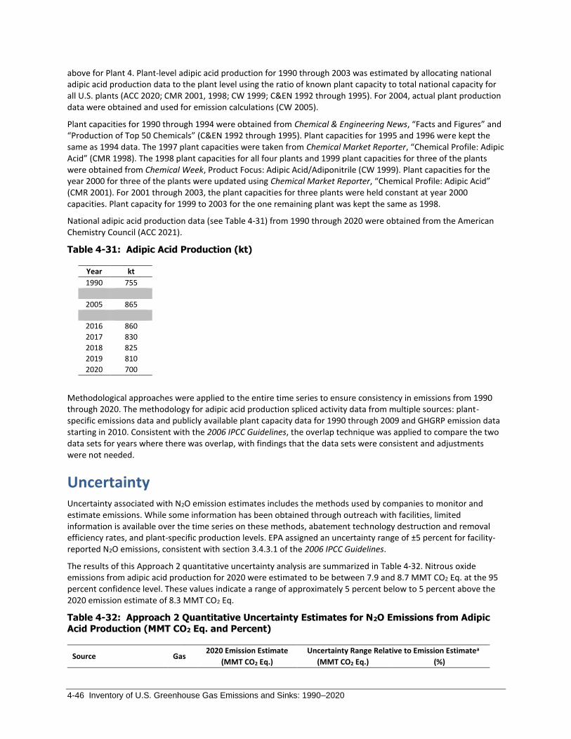
4-46 Inventory of U.S. Greenhouse Gas Emissions and Sinks: 1990–2020
above for Plant 4. Plant-level adipic acid production for 1990 through 2003 was estimated by allocating national adipic acid production data to the plant level using the ratio of known plant capacity to total national capacity for all U.S. plants (ACC 2020; CMR 2001, 1998; CW 1999; C&EN 1992 through 1995). For 2004, actual plant production data were obtained and used for emission calculations (CW 2005).
Plant capacities for 1990 through 1994 were obtained from Chemical & Engineering News, “Facts and Figures” and “Production of Top 50 Chemicals” (C&EN 1992 through 1995). Plant capacities for 1995 and 1996 were kept the same as 1994 data. The 1997 plant capacities were taken from Chemical Market Reporter, “Chemical Profile: Adipic Acid” (CMR 1998). The 1998 plant capacities for all four plants and 1999 plant capacities for three of the plants were obtained from Chemical Week, Product Focus: Adipic Acid/Adiponitrile (CW 1999). Plant capacities for the year 2000 for three of the plants were updated using Chemical Market Reporter, “Chemical Profile: Adipic Acid” (CMR 2001). For 2001 through 2003, the plant capacities for three plants were held constant at year 2000 capacities. Plant capacity for 1999 to 2003 for the one remaining plant was kept the same as 1998.
National adipic acid production data (see Table 4-31) from 1990 through 2020 were obtained from the American Chemistry Council (ACC 2021).
Table 4-31: Adipic Acid Production (kt)
Year kt
1990 755
2005 865
2016 860
2017 830
2018 825
2019 810
2020 700
Methodological approaches were applied to the entire time series to ensure consistency in emissions from 1990 through 2020. The methodology for adipic acid production spliced activity data from multiple sources: plant-specific emissions data and publicly available plant capacity data for 1990 through 2009 and GHGRP emission data starting in 2010. Consistent with the 2006 IPCC Guidelines, the overlap technique was applied to compare the two data sets for years where there was overlap, with findings that the data sets were consistent and adjustments were not needed.
Uncertainty Uncertainty associated with N2O emission estimates includes the methods used by companies to monitor and estimate emissions. While some information has been obtained through outreach with facilities, limited information is available over the time series on these methods, abatement technology destruction and removal efficiency rates, and plant-specific production levels. EPA assigned an uncertainty range of ±5 percent for facility-reported N2O emissions, consistent with section 3.4.3.1 of the 2006 IPCC Guidelines.
The results of this Approach 2 quantitative uncertainty analysis are summarized in Table 4-32. Nitrous oxide emissions from adipic acid production for 2020 were estimated to be between 7.9 and 8.7 MMT CO2 Eq. at the 95 percent confidence level. These values indicate a range of approximately 5 percent below to 5 percent above the 2020 emission estimate of 8.3 MMT CO2 Eq.
Table 4-32: Approach 2 Quantitative Uncertainty Estimates for N2O Emissions from Adipic Acid Production (MMT CO2 Eq. and Percent)
Source Gas 2020 Emission Estimate Uncertainty Range Relative to Emission Estimatea
(MMT CO2 Eq.) (MMT CO2 Eq.) (%)

Industrial Processes and Product Use 4-47
Lower
Bound
Upper
Bound
Lower
Bound
Upper
Bound
Adipic Acid Production N2O 8.3 7.9 8.7 -5% +5% a Range of emission estimates predicted by Monte Carlo Stochastic Simulation for a 95 percent confidence interval.
QA/QC and Verification General quality assurance/quality control (QA/QC) procedures were applied consistent with the U.S. Inventory QA/QC plan, which is in accordance with Volume 1, Chapter 6 of the 2006 IPCC Guidelines as described in the introduction of the IPPU chapter (see Annex 8 for more details).
More details on the greenhouse gas calculation, monitoring and QA/QC methods applicable to adipic acid facilities can be found under Subpart E (Adipic Acid Production) of the GHGRP regulation (40 CFR Part 98).36 The main QA/QC activities are related to annual performance testing, which must follow either EPA Method 320 or ASTM D6348-03. EPA verifies annual facility-level GHGRP reports through a multi-step process (e.g., combination of electronic checks and manual reviews) to identify potential errors and ensure that data submitted to EPA are accurate, complete, and consistent (EPA 2015).37 Based on the results of the verification process, EPA follows up with facilities to resolve mistakes that may have occurred. The post-submittals checks are consistent with a number of general and category-specific QC procedures, including range checks, statistical checks, algorithm checks, and year-to-year comparisons of reported data.
Recalculations Discussion Recalculations of adipic acid emissions were performed for the 2016 through 2019 portion of the time series due to GHGRP resubmittals for those years. For years 2016 through 2018, the emissions increased by 0.4 MMT CO2 Eq. (1.6 percent), 0.3 MMT CO2 Eq. (1.2 percent), and 0.6 MMT CO2 Eq. (1.8 percent), respectively. For year 2019, the emissions decreased by 0.1 MMT CO2 Eq. (0.3 percent).
Planned Improvements EPA plans to review GHGRP facility reported information on the date of abatement technology installation in order to better reflect trends and changes in emissions abatement within the industry across the time series. To date, the facility using the facility-specific emission factor developed through annual performance testing has reported no utilization of N2O abatement technology. The facility using direct measurement of N2O emissions has reported the use of N2O abatement technology but is not required to report the date of installation.
4.9 Caprolactam, Glyoxal and Glyoxylic Acid Production (CRF Source Category 2B4)
Caprolactam
Caprolactam (C6H11NO) is a colorless monomer produced for nylon-6 fibers and plastics. A substantial proportion of the fiber is used in carpet manufacturing. Most commercial processes used for the manufacture of caprolactam
36 See http://www.ecfr.gov/cgi-bin/text-idx?tpl=/ecfrbrowse/Title40/40cfr98_main_02.tpl. 37 See https://www.epa.gov/sites/production/files/2015-07/documents/ghgrp_verification_factsheet.pdf.

4-48 Inventory of U.S. Greenhouse Gas Emissions and Sinks: 1990–2020
begin with benzene, but toluene can also be used. The production of caprolactam can give rise to significant emissions of nitrous oxide (N2O).
During the production of caprolactam, emissions of N2O can occur from the ammonia oxidation step, emissions of carbon dioxide (CO2) from the ammonium carbonate step, emissions of sulfur dioxide (SO2) from the ammonium bisulfite step, and emissions of non-methane volatile organic compounds (NMVOCs). Emissions of CO2, SO2 and NMVOCs from the conventional process are unlikely to be significant in well-managed plants. Modified caprolactam production processes are primarily concerned with elimination of the high volumes of ammonium sulfate that are produced as a byproduct of the conventional process (IPCC 2006).
In the most commonly used process where caprolactam is produced from benzene, benzene is hydrogenated to cyclohexane which is then oxidized to produce cyclohexanone (C6H10O). The classical route (Raschig process) and basic reaction equations for production of caprolactam from cyclohexanone are (IPCC 2006):
𝑂𝑥𝑖𝑑𝑎𝑡𝑖𝑜𝑛 𝑜𝑓 𝑁𝐻3 𝑡𝑜 𝑁𝑂/𝑁𝑂2 ↓
𝑁𝐻3 𝑟𝑒𝑎𝑐𝑡𝑒𝑑 𝑤𝑖𝑡ℎ 𝐶𝑂2/𝐻2𝑂 𝑡𝑜 𝑦𝑖𝑒𝑙𝑑 𝑎𝑚𝑚𝑜𝑛𝑖𝑢𝑚 𝑐𝑎𝑟𝑏𝑜𝑛𝑎𝑡𝑒 (𝑁𝐻4)2𝐶𝑂3
↓
(𝑁𝐻4)2𝐶𝑂3 𝑟𝑒𝑎𝑐𝑡𝑒𝑑 𝑤𝑖𝑡ℎ 𝑁𝑂/𝑁𝑂2 (𝑓𝑟𝑜𝑚 𝑁𝐻3 𝑜𝑥𝑖𝑑𝑎𝑡𝑖𝑜𝑛) 𝑡𝑜 𝑦𝑖𝑒𝑙𝑑 𝑎𝑚𝑚𝑜𝑛𝑖𝑢𝑚 𝑛𝑖𝑡𝑟𝑖𝑡𝑒 (𝑁𝐻4𝑁𝑂2)
↓
𝑁𝐻3 𝑟𝑒𝑎𝑐𝑡𝑒𝑑 𝑤𝑖𝑡ℎ 𝑆𝑂2/𝐻2𝑂 𝑡𝑜 𝑦𝑖𝑒𝑙𝑑 𝑎𝑚𝑚𝑜𝑛𝑖𝑢𝑚 𝑏𝑖𝑠𝑢𝑙𝑝ℎ𝑖𝑡𝑒 (𝑁𝐻4𝐻𝑆𝑂3)
↓
𝑁𝐻4𝑁𝑂2 𝑎𝑛𝑑 (𝑁𝐻4𝐻𝑆𝑂3) 𝑟𝑒𝑎𝑐𝑡𝑒𝑑 𝑡𝑜 𝑦𝑖𝑒𝑙𝑑 ℎ𝑦𝑑𝑟𝑜𝑥𝑦𝑙𝑎𝑚𝑖𝑛𝑒 𝑑𝑖𝑠𝑢𝑙𝑝ℎ𝑜𝑛𝑎𝑡𝑒 (𝑁𝑂𝐻(𝑆𝑂3𝑁𝐻4)2)
↓ (𝑁𝑂𝐻(𝑆𝑂3𝑁𝐻4)2) ℎ𝑦𝑑𝑟𝑜𝑙𝑖𝑠𝑒𝑑 𝑡𝑜 𝑦𝑖𝑒𝑙𝑑 ℎ𝑦𝑑𝑟𝑜𝑥𝑦𝑙𝑎𝑚𝑖𝑛𝑒 𝑠𝑢𝑙𝑝ℎ𝑎𝑡𝑒 ((𝑁𝐻2𝑂𝐻)2. 𝐻2𝑆𝑂4) 𝑎𝑛𝑑
𝑎𝑚𝑚𝑜𝑛𝑖𝑢𝑚 𝑠𝑢𝑙𝑝ℎ𝑎𝑡𝑒 ((𝑁𝐻4)2𝑆𝑂4) ↓
𝐶𝑦𝑙𝑜ℎ𝑒𝑥𝑎𝑛𝑜𝑛𝑒 𝑟𝑒𝑎𝑐𝑡𝑖𝑜𝑛:
𝐶6𝐻10𝑂 +1
2(𝑁𝐻2𝑂𝐻)2. 𝐻2𝑆𝑂4(+𝑁𝐻3 𝑎𝑛𝑑 𝐻2𝑆𝑂4) → 𝐶6𝐻10𝑁𝑂𝐻 + (𝑁𝐻4)2𝑆𝑂4 + 𝐻2𝑂
↓ 𝐵𝑒𝑐𝑘𝑚𝑎𝑛𝑛 𝑟𝑒𝑎𝑟𝑟𝑎𝑛𝑔𝑒𝑚𝑒𝑛𝑡:
𝐶6𝐻10𝑁𝑂𝐻 (+𝐻2𝑆𝑂4 𝑎𝑛𝑑 𝑆𝑂2) → 𝐶6𝐻11𝑁𝑂. 𝐻2𝑆𝑂4 (+4𝑁𝐻3 𝑎𝑛𝑑 𝐻2𝑂) → 𝐶6𝐻11𝑁𝑂 + 2(𝑁𝐻4)2𝑆𝑂4
In 2004, three facilities produced caprolactam in the United States (ICIS 2004). Another facility, Evergreen Recycling, was in operation from 2000 to 2001 (ICIS 2004; Textile World 2000) and from 2007 through 2015 (DOE 2011; Shaw 2015). Caprolactam production at Fibrant LLC (formerly DSM Chemicals) in Georgia ceased in 2018 (Cline 2019). As of 2020, two companies in the United States produced caprolactam at two facilities: AdvanSix (formerly Honeywell) in Virginia (AdvanSix 2021) and BASF in Texas (BASF 2021).
Nitrous oxide emissions from caprolactam production in the United States were estimated to be 1.2 MMT CO2 Eq. (4 kt N2O) in 2020 (see Table 4-33). National emissions from caprolactam production decreased by approximately 28 percent over the period of 1990 through 2020. Emissions in 2020 decreased by approximately 13 percent from the 2019 levels. While this decrease could be related to the COVID-19 pandemic, caprolactam production has been declining since 2013, with the largest decrease of 15 percent happening between 2016 and 2017.

Industrial Processes and Product Use 4-49
Table 4-33: N2O Emissions from Caprolactam Production (MMT CO2 Eq. and kt N2O)
Year MMT CO2 Eq. kt N2O
1990 1.7 6
2005 2.1 7
2016 1.7 6
2017 1.5 5
2018 1.4 5
2019 1.4 5
2020 1.2 4
Glyoxal
Glyoxal is mainly used as a crosslinking agent for vinyl acetate/acrylic resins, disinfectant, gelatin hardening agent, textile finishing agent (permanent-press cotton, rayon fabrics), and wet-resistance additive (paper coatings) (IPCC 2006). It is also used for enhanced oil-recovery. It is produced from oxidation of acetaldehyde with concentrated nitric acid, or from the catalytic oxidation of ethylene glycol, and N2O is emitted in the process of oxidation of acetaldehyde.
Glyoxal (ethanedial) (C2H2O2) is produced from oxidation of acetaldehyde (ethanal) (C2H4O) with concentrated nitric acid (HNO3). Glyoxal can also be produced from catalytic oxidation of ethylene glycol (ethanediol) (CH2OHCH2OH).
Glyoxylic Acid
Glyoxylic acid is produced by nitric acid oxidation of glyoxal. Glyoxylic acid is used for the production of synthetic aromas, agrochemicals, and pharmaceutical intermediates (IPCC 2006).
EPA does not currently estimate the emissions associated with the production of Glyoxal and Glyoxylic Acid due to a lack of publicly available information on the industry in the United States. See Annex 5 for additional information.
Methodology and Time-Series Consistency Emissions of N2O from the production of caprolactam were calculated using the estimation methods provided by the 2006 IPCC Guidelines. The 2006 IPCC Guidelines Tier 1 method was used to estimate emissions from caprolactam production for 1990 through 2020, as shown in this formula:
Equation 4-6: 2006 IPCC Guidelines Tier 1: N2O Emissions From Caprolactam Production
(Equation 3.9)
𝐸𝑁2𝑂 = 𝐸𝐹 𝑥 𝐶𝑃
where,
EN2O = Annual N2O Emissions (kg) EF = N2O emission factor (default) (kg N2O/metric ton caprolactam produced) CP = Caprolactam production (metric tons)
During the caprolactam production process, N2O is generated as a byproduct of the high temperature catalytic oxidation of ammonia (NH3), which is the first reaction in the series of reactions to produce caprolactam. The amount of N2O emissions can be estimated based on the chemical reaction shown above. Based on this formula, which is consistent with an IPCC Tier 1 approach, approximately 111.1 metric tons of caprolactam are required to generate one metric ton of N2O, resulting in an emission factor of 9.0 kg N2O per metric ton of caprolactam (IPCC

4-50 Inventory of U.S. Greenhouse Gas Emissions and Sinks: 1990–2020
2006). When applying the Tier 1 method, the 2006 IPCC Guidelines state that it is good practice to assume that there is no abatement of N2O emissions and to use the highest default emission factor available in the guidelines. In addition, EPA did not find support for the use of secondary catalysts to reduce N2O emissions, such as those employed at nitric acid plants.
The activity data for caprolactam production (see Table 4-34) from 1990 to 2020 were obtained from the American Chemistry Council’s Guide to the Business of Chemistry (ACC 2021). EPA will continue to analyze and assess alternative sources of production data as a quality control measure.
Table 4-34: Caprolactam Production (kt)
Year kt
1990 626
2005 795
2016 640
2017 545
2018 530
2019 515
2020 450
Carbon dioxide and methane (CH4) emissions may also occur from the production of caprolactam, but currently the IPCC does not have methodologies for calculating these emissions associated with caprolactam production.
Methodological approaches, consistent with IPCC guidelines, have been applied to the entire time series to ensure consistency in emissions from 1990 through 2020.
Uncertainty Estimation of emissions of N2O from caprolactam production can be treated as analogous to estimation of emissions of N2O from nitric acid production. Both production processes involve an initial step of NH3 oxidation, which is the source of N2O formation and emissions (IPCC 2006). Therefore, uncertainties for the default emission factor values in the 2006 IPCC Guidelines are an estimate based on default values for nitric acid plants. In general, default emission factors for gaseous substances have higher uncertainties because mass values for gaseous substances are influenced by temperature and pressure variations and gases are more easily lost through process leaks. The default values for caprolactam production have a relatively high level of uncertainty due to the limited information available (IPCC 2006).
The results of this Approach 2 quantitative uncertainty analysis are summarized in Table 4-35. Nitrous oxide emissions from Caprolactam, Glyoxal and Glyoxylic Acid Production for 2020 were estimated to be between 0.8 and 1.6 MMT CO2 Eq. at the 95 percent confidence level. These values indicate a range of approximately 31 percent below to 32 percent above the 2020 emission estimate of 1.2 MMT CO2 Eq.

Industrial Processes and Product Use 4-51
Table 4-35: Approach 2 Quantitative Uncertainty Estimates for N2O Emissions from Caprolactam, Glyoxal and Glyoxylic Acid Production (MMT CO2 Eq. and Percent)
Source Gas 2020 Emission Estimate Uncertainty Range Relative to Emission Estimatea
(MMT CO2 Eq.) (MMT CO2 Eq.) (%)
Lower
Bound
Upper
Bound
Lower
Bound
Upper
Bound
Caprolactam Production N2O 1.2 0.8 1.6 -31% +32% a Range of emission estimates predicted by Monte Carlo Stochastic Simulation for a 95 percent confidence interval.
QA/QC and Verification General quality assurance/quality control (QA/QC) procedures were applied consistent with the U.S. Inventory QA/QC plan, which is in accordance with Volume 1, Chapter 6 of the 2006 IPCC Guidelines as described in the introduction of the IPPU chapter (see Annex 8 for more details).
Recalculations Discussion No recalculations were performed for the 1990 through 2019 portion of the time series.
Planned Improvements Pending resources, EPA will research other available datasets for caprolactam production and industry trends, including facility-level data. EPA continues to research the production process and emissions associated with the production of glyoxal and glyoxylic acid. Preliminary data suggests that glyoxal and glyoxylic acid may no longer be produced domestically and are largely imported to the United States. EPA is working to identify historical data to understand if any production of these chemicals has occurred since 1990. EPA plans to share latest findings from ongoing research for feedback during the next Inventory expert review cycle. During the Expert Review period for the current Inventory report, EPA continued to seek expert solicitation on data available for these emission source categories. This planned improvement is subject to data availability and will be implemented in the medium- to long-term.
4.10 Carbide Production and Consumption (CRF Source Category 2B5)
Carbon dioxide (CO2) and methane (CH4) are emitted from the production of silicon carbide (SiC), a material used for industrial abrasive applications as well as metallurgical and other non-abrasive applications in the United States. Emissions from fuels consumed for energy purposes during the production of silicon carbide are accounted for in the Energy chapter. Additionally, some metallurgical and non-abrasive applications of SiC are emissive, and while emissions should be accounted for where they occur based on 2006 IPCC Guidelines, emissions from SiC consumption are accounted for here until additional data on SiC consumption by end-use are available.
To produce SiC, silica sand or quartz (SiO2) is reacted with carbon (C) in the form of petroleum coke. A portion (about 35 percent) of the carbon contained in the petroleum coke is retained in the SiC. The remaining C is emitted as CO2, CH4, or carbon monoxide (CO). The overall reaction is shown below, but in practice, it does not proceed according to stoichiometry:
𝑆𝑖𝑂2 + 3𝐶 → 𝑆𝑖𝐶 + 2𝐶𝑂 (+ 𝑂2 → 2𝐶𝑂2)

4-52 Inventory of U.S. Greenhouse Gas Emissions and Sinks: 1990–2020
Carbon dioxide and CH4 are also emitted during the production of calcium carbide, a chemical used to produce acetylene. Carbon dioxide is implicitly accounted for in the storage factor calculation for the non-energy use of petroleum coke in the Energy chapter. As noted in Annex 5 to this report, CH4 emissions from calcium carbide production are not estimated because data are not available. EPA is continuing to investigate the inclusion of these emissions in future Inventory reports.
Markets for manufactured abrasives, including SiC, are heavily influenced by activity in the U.S. manufacturing sector, especially in the aerospace, automotive, furniture, housing, and steel manufacturing sectors. Specific applications of abrasive-grade SiC in 2017 included antislip abrasives, blasting abrasives, bonded abrasives, coated abrasives, polishing and buffing compounds, tumbling media, and wire-sawing abrasives. Approximately 50 percent of SiC is used in metallurgical applications, which include primarily iron and steel production, and other non-abrasive applications, which include use in advanced or technical ceramics and refractories (USGS 1991a through 2020, Washington Mills 2021).
As a result of the economic downturn in 2008 and 2009, demand for SiC decreased in those years. Low-cost imports, particularly from China, combined with high relative operating costs for domestic producers, continue to put downward pressure on the production of SiC in the United States. Consumption of SiC in the United States has recovered somewhat from its low in 2009 (USGS 1991b through 2020).
Silicon carbide was manufactured by two facilities in the United States, one of which produced primarily non-abrasive SiC (USGS 2020). USGS production values for the United States consists of SiC used for abrasives and for metallurgical and other non-abrasive applications (USGS 2020). During the COVID-19 pandemic in 2020, the U.S. Department of Homeland Security considered abrasives manufacturing part of the critical manufacturing sector, and as a result, pandemic “stay-at-home” orders issued in March 2020 did not affect the abrasives manufacturing industry. These plants remained at full operation (USGS 2021). Consumption of SiC, however, decreased by approximately 25 percent due to a sharp decline in imports (U.S. Census Bureau 2005 through 2021).
Carbon dioxide emissions from SiC production and consumption in 2020 were 0.2 MMT CO2 Eq. (154 kt CO2), which are about 40 percent lower than emissions in 1990 (243 kt) (see Table 4-36 and Table 4-37). Approximately 59 percent of these emissions resulted from SiC production, while the remainder resulted from SiC consumption. Methane emissions from SiC production in 2020 were 0.01 MMT CO2 Eq. (0.4 kt CH4) (see Table 4-36 and Table 4-37). Emissions have not fluctuated greatly in recent years.
Table 4-36: CO2 and CH4 Emissions from Silicon Carbide Production and Consumption (MMT CO2 Eq.)
Year 1990 2005 2016 2017 2018 2019 2020
Production
CO2 0.2 0.1 0.1 0.1 0.1 0.1 0.1
CH4 + + + + + + +
Consumption
CO2 0.1 0.1 0.1 0.1 0.1 0.1 0.1
Total 0.3 0.2 0.2 0.2 0.2 0.2 0.2
+ Does not exceed 0.05 MMT CO2 Eq.
Note: Totals may not sum due to independent rounding.
Table 4-37: CO2 and CH4 Emissions from Silicon Carbide Production and Consumption (kt)
Year 1990 2005 2016 2017 2018 2019 2020
Production
CO2 170 92 92 92 92 92 92
CH4 1 + + + + + +
Consumption
CO2 73 121 78 90 93 84 62
+ Does not exceed 0.5 kt
Industrial Processes and Product Use 4-53
Methodology and Time-Series Consistency Emissions of CO2 and CH4 from the production of SiC were calculated using the Tier 1 method provided by the 2006 IPCC Guidelines. Annual estimates of SiC production were multiplied by the default emission factors, as shown below:
Equation 4-7: 2006 IPCC Guidelines Tier 1: Emissions from Carbide Production (Equation 3.11)
𝐸𝑠𝑐,𝐶𝑂2 = 𝐸𝐹𝑠𝑐,𝐶𝑂2 × 𝑄𝑠𝑐
𝐸𝑠𝑐,𝐶𝐻4 = 𝐸𝐹𝑠𝑐,𝐶𝐻4 × 𝑄𝑠𝑐 × (1 𝑚𝑒𝑡𝑟𝑖𝑐 𝑡𝑜𝑛
1000 𝑘𝑔)
where,
Esc,CO2 = CO2 emissions from production of SiC, metric tons EFsc,CO2 = Emission factor for production of SiC, metric ton CO2/metric ton SiC Qsc = Quantity of SiC produced, metric tons Esc,CH4 = CH4 emissions from production of SiC, metric tons EFsc,CH4 = Emission factor for production of SiC, kilogram CH4/metric ton SiC
Emission factors were taken from the 2006 IPCC Guidelines:
• 2.62 metric tons CO2/metric ton SiC
• 11.6 kg CH4/metric ton SiC
Production data for metallurgical and other non-abrasive applications of SiC are not available; therefore, both CO2 and CH4 estimates for SiC are based solely upon production data for SiC for industrial abrasive applications.
Silicon carbide industrial abrasives production data for 1990 through 2017 were obtained from the U.S. Geological Survey (USGS) Minerals Yearbook: Manufactured Abrasives (USGS 1991a through 2017). Production data for 2018 through 2020 were obtained from the Mineral Commodity Summaries: Abrasives (Manufactured) (USGS 2021). Silicon carbide production data published by USGS have been rounded to the nearest 5,000 metric tons to avoid disclosing company proprietary data. For the period 1990 through 2001, reported USGS production data include production from a facility located in Canada that ceased operations in 2001. Using SiC data from Canada (UNFCCC GHG Data Interface 2021), U.S. SiC production for 1990 through 2001 was revised to reflect only U.S. production. SiC consumption for the entire time series is estimated using USGS consumption data (USGS 1991b through 2020) and data from the U.S. International Trade Commission (USITC) database on net imports and exports of SiC(U.S. Census Bureau 2005 through 2021) (see Table 4-38). Total annual SiC consumption (utilization) was estimated by subtracting annual exports of SiC from the annual total of national SiC production and net imports.
Emissions of CO2 from SiC consumption for metallurgical uses were calculated by multiplying the annual utilization of SiC for metallurgical uses (reported annually in the USGS Minerals Yearbook: Silicon) by the carbon content of SiC (30.0 percent), which was determined according to the molecular weight ratio of SiC. Because USGS withheld consumption data for metallurgical uses from publication for 2017 and 2018 due to concerns of disclosing company-specific sensitive information, SiC consumption for 2017 and 2018 were estimated using 2016 values.
Emissions of CO2 from SiC consumption for other non-abrasive uses were calculated by multiplying the annual SiC consumption for non-abrasive uses by the carbon content of SiC (30 percent). The annual SiC consumption for non-abrasive uses was calculated by multiplying the annual SiC consumption (production plus net imports) by the percentage used in metallurgical and other non-abrasive uses (50 percent) (USGS 1991a through 2017) and then subtracting the SiC consumption for metallurgical use.
The petroleum coke portion of the total CO2 process emissions from silicon carbide production is adjusted for within the Energy chapter, as these fuels were consumed during non-energy related activities. Additional information on the adjustments made within the Energy sector for Non-Energy Use of Fuels is described in both

4-54 Inventory of U.S. Greenhouse Gas Emissions and Sinks: 1990–2020
the Methodology section of CO2 from Fossil Fuel Combustion (Section 3.1) and Annex 2.1, Methodology for Estimating Emissions of CO2 from Fossil Fuel Combustion.
Table 4-38: Production and Consumption of Silicon Carbide (Metric Tons)
Year Production Consumption
1990 65,000 132,465
2005 35,000 220,149
2016 35,000 142,104
2017 35,000 163,492
2018 35,000 168,526
2019 35,000 152,410
2020 35,000 113,736
Methodological approaches were applied to the entire time series to ensure consistency in emissions from 1990 through 2020.
Uncertainty There is uncertainty associated with the emission factors used because they are based on stoichiometry as opposed to monitoring of actual SiC production plants. An alternative is to calculate emissions based on the quantity of petroleum coke used during the production process rather than on the amount of silicon carbide produced. However, these data were not available. For CH4, there is also uncertainty associated with the hydrogen-containing volatile compounds in the petroleum coke (IPCC 2006). There is also uncertainty associated with the use or destruction of CH4 generated from the process, in addition to uncertainty associated with levels of production, net imports, consumption levels, and the percent of total consumption that is attributed to metallurgical and other non-abrasive uses.
The results of the Approach 2 quantitative uncertainty analysis are summarized in Table 4-39. Silicon carbide production and consumption CO2 emissions from 2020 were estimated to be between 9 percent below and 9 percent above the emission estimate of 0.15 MMT CO2 Eq. at the 95 percent confidence level. Silicon carbide production CH4 emissions were estimated to be between 9 percent below and 9 percent above the emission estimate of 0.01 MMT CO2 Eq. at the 95 percent confidence level.
Table 4-39: Approach 2 Quantitative Uncertainty Estimates for CH4 and CO2 Emissions from Silicon Carbide Production and Consumption (MMT CO2 Eq. and Percent)
Source Gas 2020 Emission Estimate Uncertainty Range Relative to Emission Estimatea
(MMT CO2 Eq.) (MMT CO2 Eq.) (%)
Lower
Bound
Upper
Bound
Lower
Bound
Upper
Bound
Silicon Carbide Production
and Consumption CO2 0.15 0.14 0.17 -9% +9%
Silicon Carbide Production CH4 + + + -9% +9%
+ Does not exceed 0.05 MMT CO2 Eq. a Range of emission estimates predicted by Monte Carlo Stochastic Simulation for a 95 percent confidence interval.
QA/QC and Verification General quality assurance/quality control (QA/QC) procedures were applied consistent with the U.S. Inventory QA/QC plan, which is in accordance with Volume 1, Chapter 6 of 2006 IPCC Guidelines as described in the introduction of the IPPU chapter (see Annex 8 for more details).

Industrial Processes and Product Use 4-55
Recalculations Discussion For the period 1990 through 2001, reported USGS production data included production from two facilities located
in Canada. Using SiC data from Canada (UNFCCC GHG Data Interface 2021),38 U.S. SiC production for 1990 through 2001 was recalculated to reflect only U.S. production. Using the recalculated production values, CO2 emissions decreased by 25 to 127 kt CO2 per year, a decrease in emissions of between about 10 percent and 45 percent. Estimates for CH4 emissions decreased by about 0.1 to 0.5 kt per year, a decrease of between 20 percent and 50 percent.
Planned Improvements EPA is initiating research for data on SiC consumption by end-use for consideration in updating emissions estimates from SiC consumption and to account for emissions where they occur. This planned improvement is subject to data availability and will be implemented in the medium- to long-term.
EPA has not integrated aggregated facility-level GHGRP information to inform estimates of CO2 and CH4 from SiC production and consumption. The aggregated information (e.g., activity data and emissions) associated with silicon carbide did not meet criteria to shield underlying confidential business information (CBI) from public disclosure. EPA plans to examine the use of GHGRP silicon carbide emissions data for possible use in emission estimates consistent with both Volume 1, Chapter 6 of the 2006 IPCC Guidelines and the latest IPCC guidance on the use of facility-level data in national inventories. This planned improvement is ongoing and has not been incorporated into this Inventory report. This is a long-term planned improvement.
4.11 Titanium Dioxide Production (CRF Source Category 2B6)
Titanium dioxide (TiO2) is manufactured using one of two processes: the chloride process and the sulfate process. The chloride process uses petroleum coke and chlorine as raw materials and emits process-related carbon dioxide (CO2). Emissions from fuels consumed for energy purposes during the production of titanium dioxide are accounted for in the Energy chapter. The sulfate process does not use petroleum coke or other forms of carbon as a raw material and does not emit CO2. The chloride process is based on the following chemical reactions and does emit CO2:
2𝐹𝑒𝑇𝑖𝑂3 + 7𝐶𝑙2 + 3𝐶 → 2𝑇𝑖𝐶𝑙4 + 2𝐹𝑒𝐶𝑙3 + 3𝐶𝑂2
2𝑇𝑖𝐶𝑙4 + 2𝑂2 → 2𝑇𝑖𝑂2 + 4𝐶𝑙2
The carbon in the first chemical reaction is provided by petroleum coke, which is oxidized in the presence of the chlorine and FeTiO3 (rutile ore) to form CO2. Since 2004, all TiO2 produced in the United States has been produced using the chloride process, and a special grade of “calcined” petroleum coke is manufactured specifically for this purpose.
The principal use of TiO2 is as a white pigment in paint, lacquers, and varnishes. It is also used as a pigment in the manufacture of plastics, paper, and other products. In 2020, U.S. TiO2 production totaled 1,000,000 metric tons (USGS 2021a). Five plants produced TiO2 in the United States in 2020.
Emissions of CO2 from titanium dioxide production in 2020 were estimated to be 1.3 MMT CO2 Eq. (1,340 kt CO2), which represents an increase of 12 percent since 1990 (see Table 4-40). Compared to 2019, emissions from titanium dioxide production decreased by 9 percent in 2020, due to a 9 percent decrease in production. Demand
38 The data were confirmed with Environment and Climate Change Canada.

4-56 Inventory of U.S. Greenhouse Gas Emissions and Sinks: 1990–2020
for TiO2 pigments decreased during the first half of 2020 due to restrictions implemented during the COVID-19 pandemic (USGS 2021a).
Table 4-40: CO2 Emissions from Titanium Dioxide (MMT CO2 Eq. and kt)
Year MMT CO2 Eq. kt
1990 1.2 1,195
2005 1.8 1,755
2016 1.7 1,662
2017 1.7 1,688
2018 1.5 1,541
2019 1.5 1,474
2020 1.3 1,340
Methodology and Time-Series Consistency Emissions of CO2 from TiO2 production were calculated by multiplying annual national TiO2 production by chloride process-specific emission factors using a Tier 1 approach provided in 2006 IPCC Guidelines. The Tier 1 equation is as follows:
Equation 4-8: 2006 IPCC Guidelines Tier 1: CO2 Emissions from Titanium Production
(Equation 3.12)
𝐸𝑡𝑑 = 𝐸𝐹𝑡𝑑 × 𝑄𝑡𝑑
where,
Etd = CO2 emissions from TiO2 production, metric tons EFtd = Emission factor (chloride process), metric ton CO2/metric ton TiO2 Qtd = Quantity of TiO2 produced, metric tons
The petroleum coke portion of the total CO2 process emissions from TiO2 production is adjusted for within the Energy chapter as these fuels were consumed during non-energy related activities. Additional information on the adjustments made within the Energy sector for Non-Energy Use of Fuels is described in both the Methodology section of CO2 from Fossil Fuel Combustion (Section 3.1 Fossil Fuel Combustion) and Annex 2.1, Methodology for Estimating Emissions of CO2 from Fossil Fuel Combustion.
Data were obtained for the total amount of TiO2 produced each year. For years prior to 2004, it was assumed that TiO2 was produced using the chloride process and the sulfate process in the same ratio as the ratio of the total U.S. production capacity for each process. As of 2004, the last remaining sulfate process plant in the United States closed; therefore, 100 percent of production since 2004 used the chloride process (USGS 2005). An emission factor of 1.34 metric tons CO2/metric ton TiO2 was applied to the estimated chloride-process production (IPCC 2006). It was assumed that all TiO2 produced using the chloride process was produced using petroleum coke, although some TiO2 may have been produced with graphite or other carbon inputs.
The emission factor for the TiO2 chloride process was taken from the 2006 IPCC Guidelines. Titanium dioxide production data and the percentage of total TiO2 production capacity that is chloride process for 1990 through 2017 (see Table 4-41) were obtained through the U.S. Geological Survey (USGS) Minerals Yearbook: Titanium (USGS 1991 through 2020). Production data for 2018 through 2019 were obtained from the USGS Minerals Yearbook: Titanium, advanced data release of the 2019 tables (USGS 2021b). Production data for 2020 were

Industrial Processes and Product Use 4-57
obtained from the Minerals Commodity Summaries: Titanium and Titanium Dioxide (USGS 2021a).39 Data on the percentage of total TiO2 production capacity that is chloride process were not available for 1990 through 1993, so data from the 1994 USGS Minerals Yearbook were used for these years. Because a sulfate process plant closed in September 2001, the chloride process percentage for 2001 was estimated based on a discussion with Joseph Gambogi (Gambogi 2002). By 2002, only one sulfate process plant remained online in the United States, and this plant closed in 2004 (USGS 2005).
Table 4-41: Titanium Dioxide Production (kt)
Year kt
1990 979
2005 1,310
2016 1,240
2017 1,260
2018 1,150
2019 1,100
2020 1,000
Methodological approaches were applied to the entire time series to ensure consistency in emissions from 1990 through 2020.
Uncertainty Each year, the USGS collects titanium industry data for titanium mineral and pigment production operations. If TiO2 pigment plants do not respond, production from the operations is estimated based on prior year production levels and industry trends. Variability in response rates fluctuates from 67 to 100 percent of TiO2 pigment plants over the time series.
Although some TiO2 may be produced using graphite or other carbon inputs, information and data regarding these practices were not available. Titanium dioxide produced using graphite inputs, for example, may generate differing amounts of CO2 per unit of TiO2 produced as compared to that generated using petroleum coke in production. While the most accurate method to estimate emissions would be to base calculations on the amount of reducing agent used in each process rather than on the amount of TiO2 produced, sufficient data were not available to do so.
As of 2004, the last remaining sulfate-process plant in the United States closed. Since annual TiO2 production was not reported by USGS by the type of production process used (chloride or sulfate) prior to 2004 and only the percentage of total production capacity by process was reported, the percent of total TiO2 production capacity that was attributed to the chloride process was multiplied by total TiO2 production to estimate the amount of TiO2 produced using the chloride process. Finally, the emission factor was applied uniformly to all chloride-process production, and no data were available to account for differences in production efficiency among chloride-process plants. In calculating the amount of petroleum coke consumed in chloride-process TiO2 production, literature data were used for petroleum coke composition. Certain grades of petroleum coke are manufactured specifically for use in the TiO2 chloride process; however, this composition information was not available.
The results of the Approach 2 quantitative uncertainty analysis are summarized in Table 4-42. Titanium dioxide consumption CO2 emissions from 2020 were estimated to be between 1.2 and 1.5 MMT CO2 Eq. at the 95 percent
39 EPA has not integrated aggregated facility-level GHGRP information for Titanium Dioxide production facilities (40 CFR Part 98 Subpart EE). The relevant aggregated information (activity data, emission factor) from these facilities did not meet criteria to shield underlying CBI from public disclosure.

4-58 Inventory of U.S. Greenhouse Gas Emissions and Sinks: 1990–2020
confidence level. This indicates a range of approximately 13 percent below and 13 percent above the emission estimate of 1.3 MMT CO2 Eq.
Table 4-42: Approach 2 Quantitative Uncertainty Estimates for CO2 Emissions from Titanium
Dioxide Production (MMT CO2 Eq. and Percent)
Source Gas 2020 Emission Estimate Uncertainty Range Relative to Emission Estimatea
(MMT CO2 Eq.) (MMT CO2 Eq.) (%)
Lower
Bound
Upper
Bound
Lower
Bound
Upper
Bound
Titanium Dioxide Production CO2 1.3 1.2 1.5 -13% +13% a Range of emission estimates predicted by Monte Carlo Stochastic Simulation for a 95 percent confidence interval.
QA/QC and Verification General quality assurance/quality control (QA/QC) procedures were applied consistent with the U.S. Inventory QA/QC plan, which is in accordance with Volume 1, Chapter 6 of the 2006 IPCC Guidelines as described in the introduction of the IPPU chapter (see Annex 8 for more details).
Recalculations Discussion No recalculations were performed for the 1990 through 2019 portion of the time series.
Planned Improvements EPA plans to examine the use of GHGRP titanium dioxide emissions and other data for possible use in emission estimates consistent with both Volume 1, Chapter 6 of the 2006 IPCC Guidelines and the latest IPCC guidance on
the use of facility-level data in national inventories.40 This planned improvement is ongoing and has not been incorporated into this Inventory report. This is a long-term planned improvement.
4.12 Soda Ash Production (CRF Source Category 2B7)
Carbon dioxide (CO2) is generated as a byproduct of calcining trona ore to produce soda ash and is eventually emitted into the atmosphere. In addition, CO2 may also be released when soda ash is consumed. Emissions from soda ash consumption not associated with glass production are reported under Section 4.4 Other Process Uses of Carbonates (CRF Category 2A4), and emissions from fuels consumed for energy purposes during the production and consumption of soda ash are accounted for in the Energy chapter.
Calcining involves placing crushed trona ore into a kiln to convert sodium bicarbonate into crude sodium carbonate that will later be filtered into pure soda ash. The emission of CO2 during trona-based production is based on the following reaction:
2𝑁𝑎2𝐶𝑂3 · 𝑁𝑎𝐻𝐶𝑂3 · 2𝐻2𝑂(𝑇𝑟𝑜𝑛𝑎) → 3𝑁𝑎2𝐶𝑂3(𝑆𝑜𝑑𝑎 𝐴𝑠ℎ) + 5𝐻2𝑂 + 𝐶𝑂2
40 See http://www.ipcc-nggip.iges.or.jp/public/tb/TFI_Technical_Bulletin_1.pdf.

Industrial Processes and Product Use 4-59
Soda ash (sodium carbonate, Na2CO3) is a white crystalline solid that is readily soluble in water and strongly alkaline. Commercial soda ash is used as a raw material in a variety of industrial processes and in many familiar consumer products such as glass, soap and detergents, paper, textiles, and food. The largest use of soda ash is for glass manufacturing. Emissions from soda ash used in glass production are reported under Section 4.2, Glass Production (CRF Source Category 2A3). In addition, soda ash is used primarily to manufacture many sodium-based inorganic chemicals, including sodium bicarbonate, sodium chromates, sodium phosphates, and sodium silicates (USGS 2018b). Internationally, two types of soda ash are produced: natural and synthetic. The United States produces only natural soda ash and is second only to China in total soda ash production. Trona is the principal ore from which natural soda ash is made.
The United States represents about one-fifth of total world soda ash output (USGS 2021a). Only two states produce natural soda ash: Wyoming and California. Of these two states, net emissions of CO2 from soda ash production were only calculated for Wyoming, due to specifics regarding the production processes employed in
the state.41 Based on 2020 reported data, the estimated distribution of soda ash by end-use in 2020 (excluding glass production) was chemical production, 54 percent; other uses, 15 percent; soap and detergent manufacturing, 11 percent; wholesale distributors (e.g., for use in agriculture, water treatment, and grocery wholesale), 10 percent; flue gas desulfurization, 6 percent; water treatment, 2 percent; and pulp and paper production, 2 percent
(USGS 2021b).42
U.S. natural soda ash is competitive in world markets because it is generally considered a better-quality raw material than synthetically produced soda ash, and the majority of the world output of soda ash is made synthetically. Although the United States continues to be a major supplier of soda ash, China surpassed the United States in soda ash production in 2003, becoming the world’s leading producer.
In 2020, CO2 emissions from the production of soda ash from trona ore were 1.5 MMT CO2 Eq. (1,461 kt CO2) (see Table 4-43). Total emissions from soda ash production in 2020 decreased by approximately 18 percent compared to emissions in 2019 primarily due to decreased global demand associated with the COVID-19 pandemic and have increased by approximately 2 percent from 1990 levels.
Other than the significant decrease observed in 2020, emissions have remained relatively constant over the time series with some fluctuations since 1990. In general, these fluctuations were related to the behavior of the export market and the U.S. economy. The U.S. soda ash industry had continued a trend of increased production and value through 2019 since experiencing a decline in domestic and export sales caused by adverse global economic conditions in 2009.
Table 4-43: CO2 Emissions from Soda Ash Production (MMT CO2 Eq. and kt CO2)
Year MMT CO2 Eq. kt CO2
1990 1.4 1,431
2005 1.7 1,655
2016 1.7 1,723
2017 1.8 1,753
41 In California, soda ash is manufactured using sodium carbonate-bearing brines instead of trona ore. To extract the sodium carbonate, the complex brines are first treated with CO2 in carbonation towers to convert the sodium carbonate into sodium bicarbonate, which then precipitates from the brine solution. The precipitated sodium bicarbonate is then calcined back into sodium carbonate. Although CO2 is generated as a byproduct, the CO2 is recovered and recycled for use in the carbonation stage and is not emitted. A facility in a third state, Colorado, produced soda ash until the plant was idled in 2004. The lone producer of sodium bicarbonate no longer mines trona ore in the state. For a brief time, sodium bicarbonate was produced using soda ash feedstocks mined in Wyoming and shipped to Colorado. Prior to 2004, because the trona ore was mined in Wyoming, the production numbers given by the USGS included the feedstocks mined in Wyoming and shipped to Colorado. In this way, the sodium bicarbonate production that took place in Colorado was accounted for in the Wyoming numbers. 42 Percentages may not add up to 100 percent due to independent rounding.
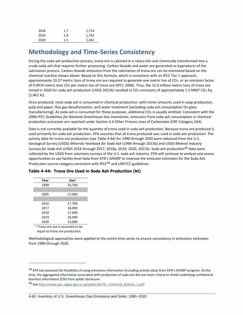
4-60 Inventory of U.S. Greenhouse Gas Emissions and Sinks: 1990–2020
2018 1.7 1,714
2019 1.8 1,792
2020 1.5 1,461
Methodology and Time-Series Consistency During the soda ash production process, trona ore is calcined in a rotary kiln and chemically transformed into a crude soda ash that requires further processing. Carbon dioxide and water are generated as byproducts of the calcination process. Carbon dioxide emissions from the calcination of trona ore can be estimated based on the chemical reaction shown above. Based on this formula, which is consistent with an IPCC Tier 1 approach, approximately 10.27 metric tons of trona ore are required to generate one metric ton of CO2, or an emission factor of 0.0974 metric tons CO2 per metric ton of trona ore (IPCC 2006). Thus, the 15.0 million metric tons of trona ore mined in 2020 for soda ash production (USGS 2021b) resulted in CO2 emissions of approximately 1.5 MMT CO2 Eq. (1,461 kt).
Once produced, most soda ash is consumed in chemical production, with minor amounts used in soap production, pulp and paper, flue gas desulfurization, and water treatment (excluding soda ash consumption for glass manufacturing). As soda ash is consumed for these purposes, additional CO2 is usually emitted. Consistent with the 2006 IPCC Guidelines for National Greenhouse Gas Inventories, emissions from soda ash consumption in chemical production processes are reported under Section 4.4 Other Process Uses of Carbonates (CRF Category 2A4).
Data is not currently available for the quantity of trona used in soda ash production. Because trona ore produced is used primarily for soda ash production, EPA assumes that all trona produced was used in soda ash production. The activity data for trona ore production (see Table 4-44) for 1990 through 2020 were obtained from the U.S. Geological Survey (USGS) Minerals Yearbook for Soda Ash (1994 through 2015b) and USGS Mineral Industry
Surveys for Soda Ash (USGS 2016 through 2017, 2018a, 2019, 2020, 2021b). Soda ash production43 data were collected by the USGS from voluntary surveys of the U.S. soda ash industry. EPA will continue to analyze and assess opportunities to use facility-level data from EPA’s GHGRP to improve the emission estimates for the Soda Ash
Production source category consistent with IPCC44 and UNFCCC guidelines.
Table 4-44: Trona Ore Used in Soda Ash Production (kt)
Year Usea
1990 14,700
2005 17,000
2016 17,700
2017 18,000
2018 17,600
2019 18,400
2020 15,000
a Trona ore use is assumed to be
equal to trona ore production.
Methodological approaches were applied to the entire time series to ensure consistency in emissions estimates from 1990 through 2020.
43 EPA has assessed the feasibility of using emissions information (including activity data) from EPA’s GHGRP program. At this time, the aggregated information associated with production of soda ash did not meet criteria to shield underlying confidential business information (CBI) from public disclosure. 44 See http://www.ipcc-nggip.iges.or.jp/public/tb/TFI_Technical_Bulletin_1.pdf.

Industrial Processes and Product Use 4-61
Uncertainty Emission estimates from soda ash production have relatively low associated uncertainty levels because reliable and accurate data sources are available for the emission factor and activity data for trona-based soda ash production. One source of uncertainty is the purity of the trona ore used for manufacturing soda ash. The emission factor used for this estimate assumes the ore is 100 percent pure and likely overestimates the emissions from soda ash manufacture. The average water-soluble sodium carbonate-bicarbonate content for ore mined in Wyoming ranges from 85.5 to 93.8 percent (USGS 1995c).
EPA is aware of one facility producing soda ash from a liquid alkaline feedstock process, based on EPA’s GHGRP. Soda ash production data was collected by the USGS from voluntary surveys. A survey request was sent to each of the five soda ash producers, all of which responded, representing 100 percent of the total production data (USGS 2020b).
The results of the Approach 2 quantitative uncertainty analysis are summarized in Table 4-45. Soda ash production CO2 emissions for 2020 were estimated to be between 1.3 and 1.5 MMT CO2 Eq. at the 95 percent confidence level. This indicates a range of approximately 9 percent below and 8 percent above the emission estimate of 1.5 MMT CO2 Eq.
Table 4-45: Approach 2 Quantitative Uncertainty Estimates for CO2 Emissions from Soda Ash Production (MMT CO2 Eq. and Percent)
QA/QC and Verification General quality assurance/quality control (QA/QC) procedures were applied consistent with the U.S. Inventory QA/QC plan, which is in accordance with Volume 1, Chapter 6 of 2006 IPCC Guidelines as described in the introduction of the IPPU chapter (see Annex 8 for more details).
Recalculations Discussion No recalculations were performed for the 1990 through 2019 portion of the time series.
4.13 Petrochemical Production (CRF Source Category 2B8)
The production of some petrochemicals results in the release of carbon dioxide (CO2) and methane (CH4) emissions. Petrochemicals are chemicals isolated or derived from petroleum or natural gas. Carbon dioxide emissions from the production of acrylonitrile, carbon black, ethylene, ethylene dichloride, ethylene oxide, and methanol, and CH4 emissions from the production of methanol and acrylonitrile are presented here and reported under IPCC Source Category 2B8. The petrochemical industry uses primary fossil fuels (i.e., natural gas, coal, petroleum, etc.) for non-fuel purposes in the production of carbon black and other petrochemicals. Emissions from fuels and feedstocks transferred out of the system for use in energy purposes (e.g., indirect or direct process heat
Source Gas 2020 Emission Estimate Uncertainty Range Relative to Emission Estimatea
(MMT CO2 Eq.) (MMT CO2 Eq.) (%)
Lower
Bound
Upper
Bound
Lower
Bound
Upper
Bound
Soda Ash Production CO2 1.5 1.3 1.5 -9% +8% a Range of emission estimates predicted by Monte Carlo Stochastic Simulation for a 95 percent confidence interval.

4-62 Inventory of U.S. Greenhouse Gas Emissions and Sinks: 1990–2020
or steam production) are currently accounted for in the Energy sector. The allocation and reporting of emissions from feedstocks transferred out of the system for use in energy purposes to the Energy chapter is consistent with the 2006 IPCC Guidelines.
Worldwide, more than 90 percent of acrylonitrile (vinyl cyanide, C3H3N) is made by way of direct ammoxidation of propylene with ammonia (NH3) and oxygen over a catalyst. This process is referred to as the SOHIO process, named after the Standard Oil Company of Ohio (SOHIO) (IPCC 2006). The primary use of acrylonitrile is as the raw material for the manufacture of acrylic and modacrylic fibers. Other major uses include the production of plastics (acrylonitrile-butadiene-styrene [ABS] and styrene-acrylonitrile [SAN]), nitrile rubbers, nitrile barrier resins, adiponitrile, and acrylamide. All U.S. acrylonitrile facilities use the SOHIO process (AN 2014). The SOHIO process involves a fluidized bed reaction of chemical-grade propylene, ammonia, and oxygen over a catalyst. The process produces acrylonitrile as its primary product, and the process yield depends on the type of catalyst used and the process configuration. The ammoxidation process produces byproduct CO2, carbon monoxide (CO), and water from the direct oxidation of the propylene feedstock and produces other hydrocarbons from side reactions.
Carbon black is a black powder generated by the incomplete combustion of an aromatic petroleum- or coal-based feedstock at a high temperature. Most carbon black produced in the United States is added to rubber to impart strength and abrasion resistance, and the tire industry is by far the largest consumer. The other major use of carbon black is as a pigment. The predominant process used in the United States to produce carbon black is the furnace black (or oil furnace) process. In the furnace black process, carbon black oil (a heavy aromatic liquid) is continuously injected into the combustion zone of a natural gas-fired furnace. Furnace heat is provided by the natural gas and a portion of the carbon black feedstock; the remaining portion of the carbon black feedstock is pyrolyzed to carbon black. The resultant CO2 and uncombusted CH4 emissions are released from thermal incinerators used as control devices, process dryers, and equipment leaks. Three facilities in the United States use other types of carbon black processes. Specifically, one facility produces carbon black by the thermal cracking of acetylene-containing feedstocks (i.e., acetylene black process), a second facility produces carbon black by the thermal cracking of other hydrocarbons (i.e., thermal black process), and a third facility produces carbon black by the open burning of carbon black feedstock (i.e., lamp black process) (EPA 2000).
Ethylene (C2H4) is consumed in the production processes of the plastics industry including polymers such as high, low, and linear low density polyethylene (HDPE, LDPE, LLDPE); polyvinyl chloride (PVC); ethylene dichloride; ethylene oxide; and ethylbenzene. Virtually all ethylene is produced from steam cracking of ethane, propane, butane, naphtha, gas oil, and other feedstocks. The representative chemical equation for steam cracking of ethane to ethylene is shown below:
𝐶2𝐻6 → 𝐶2𝐻4 + 𝐻2
Small amounts of CH4 are also generated from the steam cracking process. In addition, CO2 and CH4 emissions are also generated from combustion units.
Ethylene dichloride (C2H4Cl2) is used to produce vinyl chloride monomer, which is the precursor to polyvinyl chloride (PVC). Ethylene dichloride was also used as a fuel additive until 1996 when leaded gasoline was phased out. Ethylene dichloride is produced from ethylene by either direct chlorination, oxychlorination, or a combination of the two processes (i.e., the “balanced process”); most U.S. facilities use the balanced process. The direct chlorination and oxychlorination reactions are shown below:
𝐶2𝐻4 + 𝐶𝑙2 → 𝐶2𝐻4𝐶𝑙2 (direct chlorination)
𝐶2𝐻4 + 1
2𝑂2 + 2𝐻𝐶𝑙 → 𝐶2𝐻4𝐶𝑙2 + 2𝐻2𝑂 (oxychlorination)
𝐶2𝐻4 + 3𝑂2 → 2𝐶𝑂2 + 2𝐻2𝑂 (direct oxidation of ethylene during oxychlorination)
In addition to the byproduct CO2 produced from the direction oxidation of the ethylene feedstock, CO2 and CH4
emissions are also generated from combustion units.
Ethylene oxide (C2H4O) is used in the manufacture of glycols, glycol ethers, alcohols, and amines. Approximately 70 percent of ethylene oxide produced worldwide is used in the manufacture of glycols, including monoethylene glycol. Ethylene oxide is produced by reacting ethylene with oxygen over a catalyst. The oxygen may be supplied to

Industrial Processes and Product Use 4-63
the process through either an air (air process) or a pure oxygen stream (oxygen process). The byproduct CO2 from the direct oxidation of the ethylene feedstock is removed from the process vent stream using a recycled carbonate solution, and the recovered CO2 may be vented to the atmosphere or recovered for further utilization in other sectors, such as food production (IPCC 2006). The combined ethylene oxide reaction and byproduct CO2 reaction is exothermic and generates heat, which is recovered to produce steam for the process. The ethylene oxide process also produces other liquid and off-gas byproducts (e.g., ethane that may be burned for energy recovery within the process. Almost all facilities, except one in Texas, use the oxygen process to manufacture ethylene oxide (EPA 2008).
Methanol (CH3OH) is a chemical feedstock most often converted into formaldehyde, acetic acid and olefins. It is also an alternative transportation fuel, as well as an additive used by municipal wastewater treatment facilities in the denitrification of wastewater. Methanol is most commonly synthesized from a synthesis gas (i.e., “syngas” – a mixture containing H2, CO, and CO2) using a heterogeneous catalyst. There are a number of process techniques that can be used to produce syngas. Worldwide, steam reforming of natural gas is the most common method; most methanol producers in the United States also use steam reforming of natural gas to produce syngas. Other syngas production processes in the United States include partial oxidation of natural gas and coal gasification.
Emissions of CO2 and CH4 from petrochemical production in 2020 were 30.0 MMT CO2 Eq. (30,011 kt CO2) and 0.3 MMT CO2 Eq. (13 kt CH4), respectively (see Table 4-46 and Table 4-47). Carbon dioxide emissions from petrochemical production are driven primarily from ethylene production, while CH4 emissions are almost entirely from methanol production. Since 1990, total CO2 emissions from petrochemical production increased by 39 percent, and CH4 emissions increased by 43 percent. Emissions of CO2 in 2020 are 7 percent below the peak in 1999, and CH4 emissions in 2020 are 9 percent below the peak in 1997. Compared to 2019, CO2 emissions decreased 2 percent in 2020, and CH4 emissions decreased 5 percent. This decrease in emissions is due in part to lower production as a result of the COVID-19 pandemic reducing demand and also a strong hurricane season that temporarily shut down operations in Texas and Louisiana in 2020.
Table 4-46: CO2 and CH4 Emissions from Petrochemical Production (MMT CO2 Eq.)
Year 1990 2005 2016 2017 2018 2019 2020
CO2 21.6 27.4 28.1 28.9 29.3 30.7 30.0
Carbon Black 3.4 4.3 3.2 3.3 3.4 3.3 2.6
Ethylene 13.1 19.0 19.6 20.0 19.4 20.7 20.7
Ethylene Dichloride 0.3 0.5 0.4 0.4 0.4 0.5 0.5
Ethylene Oxide 1.1 1.5 1.1 1.3 1.3 1.4 1.7
Acrylonitrile 1.2 1.3 1.0 1.0 1.3 1.0 0.9
Methanol 2.5 0.8 2.8 2.9 3.5 3.8 3.6
CH4 0.2 0.1 0.2 0.3 0.3 0.3 0.3
Acrylonitrile + + + + + + +
Methanol 0.2 0.1 0.2 0.2 0.3 0.3 0.3
Total 21.8 27.5 28.4 29.1 29.6 31.0 30.3
+ Does not exceed 0.05 MMT CO2 Eq. Note: Totals may not sum due to independent rounding.
Table 4-47: CO2 and CH4 Emissions from Petrochemical Production (kt)
Year 1990 2005 2016 2017 2018 2019 2020
CO2 21,611 27,383 28,110 28,890 29,314 30,702 30,011
Carbon Black 3,381 4,269 3,160 3,310 3,440 3,300 2,610
Ethylene 13,126 19,024 19,600 20,000 19,400 20,700 20,700
Ethylene Dichloride 254 455 447 412 440 503 456
Ethylene Oxide 1,123 1,489 1,100 1,250 1,300 1,370 1,680
Acrylonitrile 1,214 1,325 955 1,040 1,250 990 930
Methanol 2,513 821 2,848 2,878 3,484 3,839 3,635
CH4 9 3 10 10 12 13 13

4-64 Inventory of U.S. Greenhouse Gas Emissions and Sinks: 1990–2020
Acrylonitrile + + + + + + +
Methanol 9 3 10 10 12 13 12
+ Does not exceed 0.5 kt CH4. Note: Totals may not sum due to independent rounding.
Methodology and Time-Series Consistency Emissions of CO2 and CH4 were calculated using the estimation methods provided by the 2006 IPCC Guidelines and country-specific methods from EPA’s GHGRP. The 2006 IPCC Guidelines Tier 1 method was used to estimate CO2
and CH4 emissions from production of acrylonitrile and methanol,45 and a country-specific approach similar to the IPCC Tier 2 method was used to estimate CO2 emissions from production of carbon black, ethylene oxide, ethylene, and ethylene dichloride. The Tier 2 method for petrochemicals is a total feedstock carbon (C) mass balance method used to estimate total CO2 emissions, but it is not applicable for estimating CH4 emissions.
As noted in the 2006 IPCC Guidelines, the total feedstock C mass balance method (Tier 2) is based on the assumption that all of the C input to the process is converted either into primary and secondary products or into CO2. Further, the guideline states that while the total C mass balance method estimates total C emissions from the process, it does not directly provide an estimate of the amount of the total C emissions emitted as CO2, CH4, or non-CH4 volatile organic compounds (NMVOCs). This method accounts for all the C as CO2, including CH4.
Note, a small subset of facilities reporting under EPA’s GHGRP use Continuous Emission Monitoring Systems (CEMS) to monitor CO2 emissions from process vents and/or stacks from stationary combustion units, these facilities are required to also report CO2, CH4 and N2O emissions from combustion of process off-gas in flares. The CO2 from flares are included in aggregated CO2 results. Preliminary analysis of aggregated annual reports shows that flared CH4 and N2O emissions are less than 500 kt CO2 Eq./year. EPA’s GHGRP team is still reviewing these data across reported years, and EPA plans to address this more completely in future reports.
Carbon Black, Ethylene, Ethylene Dichloride, and Ethylene Oxide
2010 through 2020
Carbon dioxide emissions and national production were aggregated directly from EPA’s GHGRP dataset for 2010 through 2020 (EPA 2021). In 2020, data reported to the GHGRP included CO2 emissions of 2,610,000 metric tons from carbon black production; 20,700,000 metric tons of CO2 from ethylene production; 456,000 metric tons of CO2 from ethylene dichloride production; and 1,680,000 metric tons of CO2 from ethylene oxide production. These emissions reflect application of a country-specific approach similar to the IPCC Tier 2 method and were used to estimate CO2 emissions from the production of carbon black, ethylene, ethylene dichloride, and ethylene oxide.
Since 2010, EPA’s GHGRP, under Subpart X, requires all domestic producers of petrochemicals to report annual emissions and supplemental emissions information (e.g., production data, etc.) to facilitate verification of reported emissions. Under EPA’s GHGRP, most petrochemical production facilities are required to use either a mass balance approach or CEMS to measure and report emissions for each petrochemical process unit to estimate facility-level process CO2 emissions; ethylene production facilities also have a third option. The mass balance method is used by
most facilities46 and assumes that all the carbon input is converted into primary and secondary products, byproducts, or is emitted to the atmosphere as CO2. To apply the mass balance, facilities must measure the volume or mass of each gaseous and liquid feedstock and product, mass rate of each solid feedstock and product, and carbon content of each feedstock and product for each process unit and sum for their facility. To apply the
45 EPA has not integrated aggregated facility-level GHGRP information for acrylonitrile and methanol production. The aggregated information associated with production of these petrochemicals did not meet criteria to shield underlying CBI from public disclosure.
46 A few facilities producing ethylene dichloride, ethylene, and methanol used CO2 CEMS; those CO2 emissions have been included in the aggregated GHGRP emissions presented here.

Industrial Processes and Product Use 4-65
optional combustion methodology, ethylene production facilities must measure the quantity, carbon content, and molecular weight of the fuel to a stationary combustion unit when that fuel includes any ethylene process off-gas. These data are used to calculate the total CO2 emissions from the combustion unit. The facility must also estimate the fraction of the emissions that is attributable to burning the ethylene process off-gas portion of the fuel. This fraction is multiplied by the total emissions to estimate the emissions from ethylene production. The QA/QC and Verification section below has a discussion of non-CO2 emissions from ethylene production facilities.
All non-energy uses of residual fuel and some non-energy uses of "other oil" are assumed to be used in the production of carbon black; therefore, consumption of these fuels is adjusted for within the Energy chapter to avoid double-counting of emissions from fuel used in the carbon black production presented here within IPPU sector. Additional information on the adjustments made within the Energy sector for Non-Energy Use of Fuels is described in both the Methodology section of CO2 from Fossil Fuel Combustion (3.1 Fossil Fuel Combustion (IPCC Source Category 1A)) and Annex 2.1, Methodology for Estimating Emissions of CO2 from Fossil Fuel Combustion.
1990 through 2009
Prior to 2010, for each of these 4 types of petrochemical processes, an average national CO2 emission factor was calculated based on the GHGRP data and applied to production for earlier years in the time series (i.e., 1990 through 2009) to estimate CO2 emissions from carbon black, ethylene, ethylene dichloride, and ethylene oxide production. For carbon black, ethylene, ethylene dichloride, and ethylene oxide carbon dioxide emission factors were derived from EPA’s GHGRP data by dividing annual CO2 emissions for petrochemical type “i” with annual production for petrochemical type “i” and then averaging the derived emission factors obtained for each calendar year 2010 through 2013 (EPA 2019). The years 2010 through 2013 were used in the development of carbon dioxide emission factors as these years are more representative of operations in 1990 through 2009 for these facilities. The average emission factors for each petrochemical type were applied across all prior years because petrochemical production processes in the United States have not changed significantly since 1990, though some operational efficiencies have been implemented at facilities over the time series.
The average country-specific CO2 emission factors that were calculated from the GHGRP data are as follows:
• 2.59 metric tons CO2/metric ton carbon black produced
• 0.79 metric tons CO2/metric ton ethylene produced
• 0.040 metric tons CO2/metric ton ethylene dichloride produced
• 0.46 metric tons CO2/metric ton ethylene oxide produced Annual production data for carbon black for 1990 through 2009 were obtained from the International Carbon Black Association (Johnson 2003 and 2005 through 2010). Annual production data for ethylene, ethylene dichloride, and ethylene oxide for 1990 through 2009 were obtained from the American Chemistry Council’s (ACC’s) Business of Chemistry (ACC 2021).
Acrylonitrile
Carbon dioxide and methane emissions from acrylonitrile production were estimated using the Tier 1 method in the 2006 IPCC Guidelines. Annual acrylonitrile production data were used with IPCC default Tier 1 CO2 and CH4 emission factors to estimate emissions for 1990 through 2019. Emission factors used to estimate acrylonitrile production emissions are as follows:
• 0.18 kg CH4/metric ton acrylonitrile produced
• 1.00 metric tons CO2/metric ton acrylonitrile produced
Annual acrylonitrile production data for 1990 through 2020 were obtained from ACC’s Business of Chemistry (ACC 2021). EPA is not able to apply the aggregated facility-level GHGRP information for acrylonitrile production needed for a Tier 2 approach. The aggregated information associated with production of these petrochemicals did not meet criteria to shield underlying CBI from public disclosure.
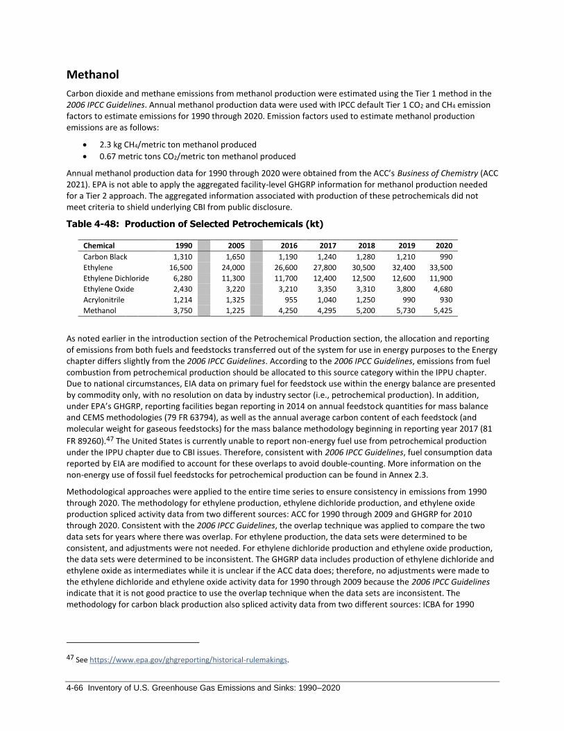
4-66 Inventory of U.S. Greenhouse Gas Emissions and Sinks: 1990–2020
Methanol
Carbon dioxide and methane emissions from methanol production were estimated using the Tier 1 method in the 2006 IPCC Guidelines. Annual methanol production data were used with IPCC default Tier 1 CO2 and CH4 emission factors to estimate emissions for 1990 through 2020. Emission factors used to estimate methanol production emissions are as follows:
• 2.3 kg CH4/metric ton methanol produced
• 0.67 metric tons CO2/metric ton methanol produced
Annual methanol production data for 1990 through 2020 were obtained from the ACC’s Business of Chemistry (ACC 2021). EPA is not able to apply the aggregated facility-level GHGRP information for methanol production needed for a Tier 2 approach. The aggregated information associated with production of these petrochemicals did not meet criteria to shield underlying CBI from public disclosure.
Table 4-48: Production of Selected Petrochemicals (kt)
Chemical 1990 2005 2016 2017 2018 2019 2020
Carbon Black 1,310 1,650 1,190 1,240 1,280 1,210 990
Ethylene 16,500 24,000 26,600 27,800 30,500 32,400 33,500
Ethylene Dichloride 6,280 11,300 11,700 12,400 12,500 12,600 11,900
Ethylene Oxide 2,430 3,220 3,210 3,350 3,310 3,800 4,680
Acrylonitrile 1,214 1,325 955 1,040 1,250 990 930
Methanol 3,750 1,225 4,250 4,295 5,200 5,730 5,425
As noted earlier in the introduction section of the Petrochemical Production section, the allocation and reporting of emissions from both fuels and feedstocks transferred out of the system for use in energy purposes to the Energy chapter differs slightly from the 2006 IPCC Guidelines. According to the 2006 IPCC Guidelines, emissions from fuel combustion from petrochemical production should be allocated to this source category within the IPPU chapter. Due to national circumstances, EIA data on primary fuel for feedstock use within the energy balance are presented by commodity only, with no resolution on data by industry sector (i.e., petrochemical production). In addition, under EPA’s GHGRP, reporting facilities began reporting in 2014 on annual feedstock quantities for mass balance and CEMS methodologies (79 FR 63794), as well as the annual average carbon content of each feedstock (and molecular weight for gaseous feedstocks) for the mass balance methodology beginning in reporting year 2017 (81
FR 89260).47 The United States is currently unable to report non-energy fuel use from petrochemical production under the IPPU chapter due to CBI issues. Therefore, consistent with 2006 IPCC Guidelines, fuel consumption data reported by EIA are modified to account for these overlaps to avoid double-counting. More information on the non-energy use of fossil fuel feedstocks for petrochemical production can be found in Annex 2.3.
Methodological approaches were applied to the entire time series to ensure consistency in emissions from 1990 through 2020. The methodology for ethylene production, ethylene dichloride production, and ethylene oxide production spliced activity data from two different sources: ACC for 1990 through 2009 and GHGRP for 2010 through 2020. Consistent with the 2006 IPCC Guidelines, the overlap technique was applied to compare the two data sets for years where there was overlap. For ethylene production, the data sets were determined to be consistent, and adjustments were not needed. For ethylene dichloride production and ethylene oxide production, the data sets were determined to be inconsistent. The GHGRP data includes production of ethylene dichloride and ethylene oxide as intermediates while it is unclear if the ACC data does; therefore, no adjustments were made to the ethylene dichloride and ethylene oxide activity data for 1990 through 2009 because the 2006 IPCC Guidelines indicate that it is not good practice to use the overlap technique when the data sets are inconsistent. The methodology for carbon black production also spliced activity data from two different sources: ICBA for 1990
47 See https://www.epa.gov/ghgreporting/historical-rulemakings.
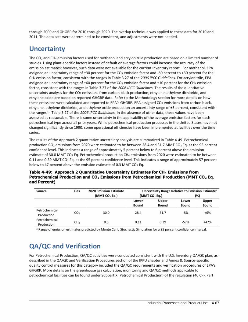
Industrial Processes and Product Use 4-67
through 2009 and GHGRP for 2010 through 2020. The overlap technique was applied to these data for 2010 and 2011. The data sets were determined to be consistent, and adjustments were not needed.
Uncertainty The CO2 and CH4 emission factors used for methanol and acrylonitrile production are based on a limited number of studies. Using plant-specific factors instead of default or average factors could increase the accuracy of the emission estimates; however, such data were not available for the current Inventory report. For methanol, EPA assigned an uncertainty range of ±30 percent for the CO2 emission factor and -80 percent to +30 percent for the CH4 emission factor, consistent with the ranges in Table 3.27 of the 2006 IPCC Guidelines. For acrylonitrile, EPA assigned an uncertainty range of ±60 percent for the CO2 emission factor and ±10 percent for the CH4 emission factor, consistent with the ranges in Table 3.27 of the 2006 IPCC Guidelines. The results of the quantitative uncertainty analysis for the CO2 emissions from carbon black production, ethylene, ethylene dichloride, and ethylene oxide are based on reported GHGRP data. Refer to the Methodology section for more details on how these emissions were calculated and reported to EPA’s GHGRP. EPA assigned CO2 emissions from carbon black, ethylene, ethylene dichloride, and ethylene oxide production an uncertainty range of ±5 percent, consistent with the ranges in Table 3.27 of the 2006 IPCC Guidelines. In the absence of other data, these values have been assessed as reasonable. There is some uncertainty in the applicability of the average emission factors for each petrochemical type across all prior years. While petrochemical production processes in the United States have not changed significantly since 1990, some operational efficiencies have been implemented at facilities over the time series.
The results of the Approach 2 quantitative uncertainty analysis are summarized in Table 4-49. Petrochemical production CO2 emissions from 2020 were estimated to be between 28.4 and 31.7 MMT CO2 Eq. at the 95 percent confidence level. This indicates a range of approximately 5 percent below to 6 percent above the emission estimate of 30.0 MMT CO2 Eq. Petrochemical production CH4 emissions from 2020 were estimated to be between 0.11 and 0.39 MMT CO2 Eq. at the 95 percent confidence level. This indicates a range of approximately 57 percent below to 47 percent above the emission estimate of 0.3 MMT CO2 Eq.
Table 4-49: Approach 2 Quantitative Uncertainty Estimates for CH4 Emissions from
Petrochemical Production and CO2 Emissions from Petrochemical Production (MMT CO2 Eq. and Percent)
Source Gas 2020 Emission Estimate Uncertainty Range Relative to Emission Estimatea
(MMT CO2 Eq.) (MMT CO2 Eq.) (%)
Lower
Bound
Upper
Bound
Lower
Bound
Upper
Bound
Petrochemical
Production CO2 30.0 28.4 31.7 -5% +6%
Petrochemical
Production CH4 0.3 0.11 0.39 -57% +47%
a Range of emission estimates predicted by Monte Carlo Stochastic Simulation for a 95 percent confidence interval.
QA/QC and Verification For Petrochemical Production, QA/QC activities were conducted consistent with the U.S. Inventory QA/QC plan, as described in the QA/QC and Verification Procedures section of the IPPU chapter and Annex 8. Source-specific quality control measures for this category included the QA/QC requirements and verification procedures of EPA’s GHGRP. More details on the greenhouse gas calculation, monitoring and QA/QC methods applicable to petrochemical facilities can be found under Subpart X (Petrochemical Production) of the regulation (40 CFR Part
4-68 Inventory of U.S. Greenhouse Gas Emissions and Sinks: 1990–2020
98).48 EPA verifies annual facility-level GHGRP reports through a multi-step process (e.g., combination of electronic checks and manual reviews) to identify potential errors and ensure that data submitted to EPA are accurate,
complete, and consistent (EPA 2015).49 Based on the results of the verification process, EPA follows up with facilities to resolve mistakes that may have occurred. The post-submittals checks are consistent with a number of general and category-specific QC procedures, including range checks, statistical checks, algorithm checks, and year-to-year checks of reported data and emissions. EPA also conducts QA checks of GHGRP reported production data by petrochemical type against external datasets.
For ethylene, ethylene dichloride, and ethylene oxide, it is possible to compare CO2 emissions calculated using the GHGRP data to the CO2 emissions that would have been calculated using the Tier 1 approach if GHGRP data were not available. For ethylene, the GHGRP emissions were within 5 percent of the emissions calculated using the Tier 1 approach prior to 2018; in 2018 through 2020, the GHGRP emissions have been about 20 percent lower than what would be calculated using the Tier 1 approach. For ethylene dichloride, the GHGRP emissions are typically higher than the Tier 1 emissions by up to 25 percent. For ethylene oxide, GHGRP emissions vary from 17 percent less than the Tier 1 emissions to 20 percent more than the Tier 1 emissions, depending on the year.
EPA’s GHGRP mandates that all petrochemical production facilities report their annual emissions of CO2, CH4, and N2O from each of their petrochemical production processes. Source-specific quality control measures for the Petrochemical Production category included the QA/QC requirements and verification procedures of EPA’s GHGRP. The QA/QC requirements differ depending on the calculation methodology used.
As part of a planned improvement effort, EPA has assessed the potential of using GHGRP data to estimate CH4 emissions from ethylene production. As discussed in the Methodology section above, CO2 emissions from ethylene production in this chapter are based on data reported under the GHGRP, and these emissions are calculated using a Tier 2 approach that assumes all of the carbon in the fuel (i.e., ethylene process off-gas) is converted to CO2. Ethylene production facilities also calculate and report CH4 emissions under the GHGRP when they use the optional combustion methodology. The facilities calculate CH4 emissions from each combustion unit that burns off-gas from an ethylene production process unit using a Tier 1 approach based on the total quantity of fuel burned, a default higher heating value, and a default emission factor. Because multiple other types of fuel in addition to the ethylene process unit off-gas may be burned in these combustion units, the facilities also report an estimate of the fraction of emissions that is due to burning the ethylene process off-gas component of the total fuel. Multiplying the total emissions by the estimated fraction provides an estimate of the CH4 emissions from the ethylene production process unit. These ethylene production facilities also calculate CH4 emissions from flares that burn process vent emissions from ethylene processes. The emissions are calculated using either a Tier 2 approach based on measured gas volumes and measured carbon content or higher heating value, or a Tier 1 approach based on the measured gas flow and a default emission factor. Nearly all ethylene production facilities use the optional combustion methodology under the GHGRP, and the sum of reported CH4 emissions from combustion in stationary combustion units and flares at all of these facilities is on the same order of magnitude as the combined CH4 emissions presented in this chapter from methanol and acrylonitrile production. The CH4 emissions from ethylene production under the GHGRP have not been included in this chapter because this approach double counts carbon (i.e., all of the carbon in the CH4 emissions is also included in the CO2 emissions from the ethylene process units). EPA continues to assess the GHGRP data for ways to better disaggregate the data and incorporate it into the inventory.
These facilities are also required to report emissions of N2O from combustion of ethylene process off-gas in both stationary combustion units and flares. Facilities using CEMS (consistent with a Tier 3 approach) are also required to report emissions of CH4 and N2O from combustion of petrochemical process-off gases in flares. Preliminary analysis of the aggregated reported CH4 and N2O emissions from facilities using CEMS and N2O emissions from facilities using the optional combustion methodology suggests that these annual emissions are less than 500 kt/yr,
48 See http://www.ecfr.gov/cgi-bin/text-idx?tpl=/ecfrbrowse/Title40/40cfr98_main_02.tpl. 49 See https://www.epa.gov/sites/production/files/2015-07/documents/ghgrp_verification_factsheet.pdf.

Industrial Processes and Product Use 4-69
which is not significant enough to prioritize for inclusion in the report at this time. Pending resources and significance, EPA may include these N2O emissions in future reports to enhance completeness.
Future QC efforts to validate the use of Tier 1 default emission factors and report on the comparison of Tier 1 emission estimates and GHGRP data are described below in the Planned Improvements section.
Recalculations Discussion The acrylonitrile production quantity for 2019 was updated with the revised value in ACC’s Business of Chemistry (ACC 2021). This change resulted in less than a 0.3 percent (90 kt) decrease in total petrochemical emissions for 2019, compared to the previous Inventory.
Emissions from ethylene production in 2016 and emissions from carbon black production in 2017 were updated and reduced slightly to be consistent with updated GHGRP data (EPA 2021). These changes resulted in a 0.7 percent (200 kt) decrease in total emissions from petrochemical production for 2016 and a 0.07 percent (20 kt) decrease in total emissions from petrochemical production for 2017, compared to the previous Inventory.
Planned Improvements Improvements include completing category-specific QC of activity data and emission factors, along with further assessment of CH4 and N2O emissions to enhance completeness in reporting of emissions from U.S. petrochemical production, pending resources, significance and time-series consistency considerations. For example, EPA is planning additional assessment of ways to use CH4 data from the GHGRP in the Inventory. One possible approach EPA is assessing would be to adjust the CO2 emissions from the GHGRP downward by subtracting the carbon that is also included in the reported CH4 emissions, per the discussion in the Petrochemical Production QA/QC and Verification section, above. As of this current report, timing and resources have not allowed EPA to complete this analysis of activity data, emissions, and emission factors and remains a priority improvement within the IPPU chapter.
Pending resources, a secondary potential improvement for this source category would focus on continuing to analyze the fuel and feedstock data from EPA’s GHGRP to better disaggregate energy-related emissions and allocate them more accurately between the Energy and IPPU sectors of the Inventory. It is important to ensure no double counting of emissions between fuel combustion, non-energy use of fuels, and industrial process emissions. For petrochemical feedstock production, EPA review of the categories suggests this is not a significant issue since the non-energy use industrial release data includes different categories of sources and sectors than those included in the IPPU emissions category for petrochemicals. As noted previously in the methodology section, data integration is not available at this time because feedstock data from the EIA used to estimate non-energy uses of fuels are aggregated by fuel type, rather than disaggregated by both fuel type and particular industries. Also, GHGRP-reported data on quantities of fuel consumed as feedstocks by petrochemical producers are unable to be used due to the data failing GHGRP CBI aggregation criteria. EPA will continue to look for ways to incorporate this data into future Inventories to will allow for easier data integration between the non-energy uses of fuels category and the petrochemicals category presented in this chapter. This planned improvement is still under development and has not been completed to report on progress in this current Inventory.
EPA plans to review USGS data to improve use of activity data to estimate emissions, consistent with the methodological decision trees in 2006 IPCC Guidelines. EPA also plans to review GHGRP emissions data for possible use in estimates, consistent with both Volume 1, Chapter 6 of the 2006 IPCC Guidelines and the latest IPCC
guidance on the use of facility-level data in national inventories.50 This planned improvement is ongoing and has not been incorporated into this Inventory report. This is a medium-term planned improvement and expected to be completed by the next (i.e., 2023) Inventory submission.
50 See http://www.ipcc-nggip.iges.or.jp/public/tb/TFI_Technical_Bulletin_1.pdf.

4-70 Inventory of U.S. Greenhouse Gas Emissions and Sinks: 1990–2020
4.14 HCFC-22 Production (CRF Source Category 2B9a)
Trifluoromethane (HFC-23 or CHF3) is generated as a byproduct during the manufacture of chlorodifluoromethane (HCFC-22), which is primarily employed in refrigeration and air conditioning systems and as a chemical feedstock for manufacturing synthetic polymers. Between 1990 and 2000, U.S. production of HCFC-22 increased significantly as HCFC-22 replaced chlorofluorocarbons (CFCs) in many applications. Between 2000 and 2007, U.S. production fluctuated but generally remained above 1990 levels. In 2008 and 2009, U.S. production declined markedly and has remained near 2009 levels since. Because HCFC-22 depletes stratospheric ozone, its production for non-feedstock uses was phased out in 2020 under the U.S. Clean Air Act.51 Feedstock production, however, is permitted to continue indefinitely.
HCFC-22 is produced by the reaction of chloroform (CHCl3) and hydrogen fluoride (HF) in the presence of a catalyst, SbCl5. The reaction of the catalyst and HF produces SbClxFy, (where x + y = 5), which reacts with chlorinated hydrocarbons to replace chlorine atoms with fluorine. The HF and chloroform are introduced by submerged piping into a continuous-flow reactor that contains the catalyst in a hydrocarbon mixture of chloroform and partially fluorinated intermediates. The vapors leaving the reactor contain HCFC-21 (CHCl2F), HCFC-22 (CHClF2), HFC-23 (CHF3), HCl, chloroform, and HF. The under-fluorinated intermediates (HCFC-21) and chloroform are then condensed and returned to the reactor, along with residual catalyst, to undergo further fluorination. The final vapors leaving the condenser are primarily HCFC-22, HFC-23, HCl and residual HF. The HCl is recovered as a useful byproduct, and the HF is removed. Once separated from HCFC-22, the HFC-23 may be released to the atmosphere, recaptured for use in a limited number of applications, or destroyed.
Two facilities produced HCFC-22 in the United States in 2020. Emissions of HFC-23 from this activity in 2020 were estimated to be 2.1 MMT CO2 Eq. (0.1 kt) (see Table 4-50). This quantity represents a 43 percent decrease from 2019 emissions and a 95 percent decrease from 1990 emissions. The decrease from 1990 emissions was caused primarily by changes in the HFC-23 emission rate (kg HFC-23 emitted/kg HCFC-22 produced). The decrease from 2019 emissions was caused by both a decrease in the HFC-23 emission rate at one plant and a decrease in the total quantity of HCFC-22 produced. The long-term decrease in the emission rate is primarily attributable to six factors: (a) five plants that did not capture and destroy the HFC-23 generated have ceased production of HCFC-22 since 1990; (b) one plant that captures and destroys the HFC-23 generated began to produce HCFC-22; (c) one plant implemented and documented a process change that reduced the amount of HFC-23 generated; (d) the same plant began recovering HFC-23, primarily for destruction and secondarily for sale; (e) another plant began destroying HFC-23; and (f) the same plant, whose emission rate was higher than that of the other two plants, ceased production of HCFC-22 in 2013.
51 As construed, interpreted, and applied in the terms and conditions of the Montreal Protocol on Substances that Deplete the Ozone Layer [42 U.S.C. §7671m(b), CAA §614].

Industrial Processes and Product Use 4-71
Table 4-50: HFC-23 Emissions from HCFC-22 Production (MMT CO2 Eq. and kt HFC-23)
Year MMT CO2 Eq. kt HFC-23
1990 46.1 3
2005 20.0 1
2016 2.8 0.2
2017 5.2 0.3
2018 3.3 0.2
2019 3.7 0.3
2020 2.1 0.1
Methodology and Time-Series Consistency To estimate HFC-23 emissions for five of the eight HCFC-22 plants that have operated in the United States since 1990, methods comparable to the Tier 3 methods in the 2006 IPCC Guidelines (IPCC 2006) were used throughout the time series. Emissions for 2010 through 2020 were obtained through reports submitted by U.S. HCFC-22 production facilities to EPA’s Greenhouse Gas Reporting Program (GHGRP). EPA’s GHGRP mandates that all HCFC-22 production facilities report their annual emissions of HFC-23 from HCFC-22 production processes and HFC-23 destruction processes. Previously, data were obtained by EPA through collaboration with an industry association that received voluntarily reported HCFC-22 production and HFC-23 emissions annually from all U.S. HCFC-22 producers from 1990 through 2009. These emissions were aggregated and reported to EPA on an annual basis.
For the other three plants, the last of which closed in 1993, methods comparable to the Tier 1 method in the 2006 IPCC Guidelines were used. Emissions from these three plants have been calculated using the recommended emission factor for unoptimized plants operating before 1995 (0.04 kg HCFC-23/kg HCFC-22 produced).
The five plants that have operated since 1994 measure (or, for the plants that have since closed, measured) concentrations of HFC-23 as well as mass flow rates of process streams to estimate their generation of HFC-23. Plants using thermal oxidation to abate their HFC-23 emissions monitor the performance of their oxidizers to verify that the HFC-23 is almost completely destroyed. One plant that releases a small fraction of its byproduct HFC-23 periodically measures HFC-23 concentrations at process vents using gas chromatography. This information is combined with information on quantities of products (e.g., HCFC-22) to estimate HFC-23 emissions.
To estimate 1990 through 2009 emissions, reports from an industry association were used that aggregated HCFC-22 production and HFC-23 emissions from all U.S. HCFC-22 producers and reported them to EPA (ARAP 1997, 1999, 2000, 2001, 2002, 2003, 2004, 2005, 2006, 2007, 2008, 2009, and 2010). To estimate 2010 through 2020 emissions, facility-level data (including both HCFC-22 production and HFC-23 emissions) reported through EPA’s GHGRP were analyzed. In 1997 and 2008, comprehensive reviews of plant-level estimates of HFC-23 emissions and HCFC-22 production were performed (RTI 1997; RTI 2008). The 1997 and 2008 reviews enabled U.S. totals to be reviewed, updated, and where necessary, corrected, and also for plant-level uncertainty analyses (Monte-Carlo simulations) to be performed for 1990, 1995, 2000, 2005, and 2006. Estimates of annual U.S. HCFC-22 production are presented in Table 4-51.

4-72 Inventory of U.S. Greenhouse Gas Emissions and Sinks: 1990–2020
Table 4-51: HCFC-22 Production (kt)
Year kt
1990 139
2005 156
2012 96
2013-2020 C
C (CBI)
Note: HCFC-22 production in 2013
through 2020 is considered
Confidential Business Information
(CBI) as there were only two
producers of HCFC-22 in those years.
Uncertainty The uncertainty analysis presented in this section was based on a plant-level Monte Carlo Stochastic Simulation for 2006. The Monte Carlo analysis used estimates of the uncertainties in the individual variables in each plant’s estimating procedure. This analysis was based on the generation of 10,000 random samples of model inputs from the probability density functions for each input. A normal probability density function was assumed for all measurements and biases except the equipment leak estimates for one plant; a log-normal probability density function was used for this plant’s equipment leak estimates. The simulation for 2006 yielded a 95-percent confidence interval for U.S. emissions of 6.8 percent below to 9.6 percent above the reported total.
The relative errors yielded by the Monte Carlo Stochastic Simulation for 2006 were applied to the U.S. emission estimate for 2020. The resulting estimates of absolute uncertainty are likely to be reasonably accurate because (1) the methods used by the two remaining plants to estimate their emissions are not believed to have changed significantly since 2006, and (2) although the distribution of emissions among the plants has changed between 2006 and 2020 (because one plant has closed), the plant that currently accounts for most emissions had a relative uncertainty in its 2006 (as well as 2005) emissions estimate that was similar to the relative uncertainty for total U.S. emissions. Thus, the closure of one plant is not likely to have a large impact on the uncertainty of the national emission estimate.
The results of the Approach 2 quantitative uncertainty analysis are summarized in Table 4-52. HFC-23 emissions from HCFC-22 production were estimated to be between 2.0 and 2.3 MMT CO2 Eq. at the 95 percent confidence level. This indicates a range of approximately 7 percent below and 10 percent above the emission estimate of 2.1 MMT CO2 Eq.
Table 4-52: Approach 2 Quantitative Uncertainty Estimates for HFC-23 Emissions from HCFC-22 Production (MMT CO2 Eq. and Percent)
Source Gas
2020 Emission Estimate Uncertainty Range Relative to Emission Estimatea
(MMT CO2 Eq.) (MMT CO2 Eq.) (%)
Lower
Bound
Upper
Bound
Lower
Bound
Upper
Bound
HCFC-22 Production HFC-23 2.1 2.0 2.3 -7% +10%
a Range of emissions reflects a 95 percent confidence interval.
QA/QC and Verification General quality assurance/quality control (QA/QC) procedures were applied consistent with the U.S. Inventory QA/QC plan, which is in accordance with Volume 1, Chapter 6 of 2006 IPCC Guidelines as described in the

Industrial Processes and Product Use 4-73
introduction of the IPPU chapter (see Annex 8 for more details). Under the GHGRP, EPA verifies annual facility-level reports through a multi-step process (e.g., including a combination of pre-and post-submittal electronic checks and manual reviews by staff) to identify potential errors and ensure that data submitted to EPA are accurate,
complete, and consistent (EPA 2015).52 Based on the results of the verification process, EPA follows up with facilities to resolve mistakes that may have occurred. The post-submittals checks are consistent with a number of general and category-specific QC procedures, including: range checks, statistical checks, algorithm checks, and year-to-year checks of reported data and emissions.
The GHGRP also requires source-specific quality control measures for the HCFC-22 Production category. Under EPA’s GHGRP, HCFC-22 producers are required to (1) measure concentrations of HFC-23 and HCFC-22 in the product stream at least weekly using equipment and methods (e.g., gas chromatography) with an accuracy and precision of 5 percent or better at the concentrations of the process samples, (2) measure mass flows of HFC-23 and HCFC-22 at least weekly using measurement devices (e.g., flowmeters) with an accuracy and precision of 1 percent of full scale or better, (3) calibrate mass measurement devices at the frequency recommended by the manufacturer using traceable standards and suitable methods published by a consensus standards organization, (4) calibrate gas chromatographs at least monthly through analysis of certified standards, and (5) document these calibrations.
Recalculations The emissions estimate for 2011 was revised to exclude HFC-23 emissions from one plant that did not produce HCFC-22. This revision resulted in a decrease in 2011 emissions of 459 kg HFC-23, about 0.07 percent of the previous estimate.
4.15 Carbon Dioxide Consumption (CRF Source Category 2B10)
Carbon dioxide (CO2) is used for a variety of commercial applications, including food processing, chemical production, carbonated beverage production, and refrigeration, and is also used in petroleum production for enhanced oil recovery (EOR). CO2 used for EOR is injected underground to enable additional petroleum to be produced. For the purposes of this analysis, CO2 used in commercial applications other than EOR is assumed to be emitted to the atmosphere. A further discussion of CO2 used in EOR is described in the Energy chapter in Box 3-6 titled “Carbon Dioxide Transport, Injection, and Geological Storage” and is not included in this section.
Carbon dioxide is produced from naturally-occurring CO2 reservoirs, as a byproduct from the energy and industrial production processes (e.g., ammonia production, fossil fuel combustion, ethanol production), and as a byproduct from the production of crude oil and natural gas, which contain naturally occurring CO2 as a component.
In 2020, the amount of CO2 produced and captured for commercial applications and subsequently emitted to the atmosphere was 5.0 MMT CO2 Eq. (4,970 kt) (see Table 4-53). This is a 2 percent increase (100 kt) from 2019 levels and is an increase of approximately 238 percent since 1990.
Table 4-53: CO2 Emissions from CO2 Consumption (MMT CO2 Eq. and kt)
Year MMT CO2 Eq. kt
1990 1.5 1,472
52 EPA (2015). Greenhouse Gas Reporting Program Report Verification. Available online at: https://www.epa.gov/sites/production/files/2015-07/documents/ghgrp_verification_factsheet.pdf.
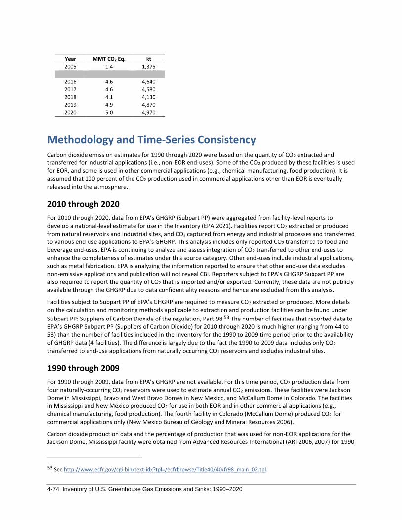
4-74 Inventory of U.S. Greenhouse Gas Emissions and Sinks: 1990–2020
Year MMT CO2 Eq. kt
2005 1.4 1,375
2016 4.6 4,640
2017 4.6 4,580
2018 4.1 4,130
2019 4.9 4,870
2020 5.0 4,970
Methodology and Time-Series Consistency Carbon dioxide emission estimates for 1990 through 2020 were based on the quantity of CO2 extracted and transferred for industrial applications (i.e., non-EOR end-uses). Some of the CO2 produced by these facilities is used for EOR, and some is used in other commercial applications (e.g., chemical manufacturing, food production). It is assumed that 100 percent of the CO2 production used in commercial applications other than EOR is eventually released into the atmosphere.
2010 through 2020
For 2010 through 2020, data from EPA’s GHGRP (Subpart PP) were aggregated from facility-level reports to develop a national-level estimate for use in the Inventory (EPA 2021). Facilities report CO2 extracted or produced from natural reservoirs and industrial sites, and CO2 captured from energy and industrial processes and transferred to various end-use applications to EPA’s GHGRP. This analysis includes only reported CO2 transferred to food and beverage end-uses. EPA is continuing to analyze and assess integration of CO2 transferred to other end-uses to enhance the completeness of estimates under this source category. Other end-uses include industrial applications, such as metal fabrication. EPA is analyzing the information reported to ensure that other end-use data excludes non-emissive applications and publication will not reveal CBI. Reporters subject to EPA’s GHGRP Subpart PP are also required to report the quantity of CO2 that is imported and/or exported. Currently, these data are not publicly available through the GHGRP due to data confidentiality reasons and hence are excluded from this analysis.
Facilities subject to Subpart PP of EPA’s GHGRP are required to measure CO2 extracted or produced. More details on the calculation and monitoring methods applicable to extraction and production facilities can be found under
Subpart PP: Suppliers of Carbon Dioxide of the regulation, Part 98.53 The number of facilities that reported data to EPA’s GHGRP Subpart PP (Suppliers of Carbon Dioxide) for 2010 through 2020 is much higher (ranging from 44 to 53) than the number of facilities included in the Inventory for the 1990 to 2009 time period prior to the availability of GHGRP data (4 facilities). The difference is largely due to the fact the 1990 to 2009 data includes only CO2 transferred to end-use applications from naturally occurring CO2 reservoirs and excludes industrial sites.
1990 through 2009
For 1990 through 2009, data from EPA’s GHGRP are not available. For this time period, CO2 production data from four naturally-occurring CO2 reservoirs were used to estimate annual CO2 emissions. These facilities were Jackson Dome in Mississippi, Bravo and West Bravo Domes in New Mexico, and McCallum Dome in Colorado. The facilities in Mississippi and New Mexico produced CO2 for use in both EOR and in other commercial applications (e.g., chemical manufacturing, food production). The fourth facility in Colorado (McCallum Dome) produced CO2 for commercial applications only (New Mexico Bureau of Geology and Mineral Resources 2006).
Carbon dioxide production data and the percentage of production that was used for non-EOR applications for the Jackson Dome, Mississippi facility were obtained from Advanced Resources International (ARI 2006, 2007) for 1990
53 See http://www.ecfr.gov/cgi-bin/text-idx?tpl=/ecfrbrowse/Title40/40cfr98_main_02.tpl.

Industrial Processes and Product Use 4-75
to 2000, and from the Annual Reports of Denbury Resources (Denbury Resources 2002 through 2010) for 2001 to 2009 (see Table 4-54). Denbury Resources reported the average CO2 production in units of MMCF CO2 per day for 2001 through 2009 and reported the percentage of the total average annual production that was used for EOR. Production from 1990 to 1999 was set equal to 2000 production, due to lack of publicly available production data for 1990 through 1999. Carbon dioxide production data for the Bravo Dome and West Bravo Dome were obtained from ARI for 1990 through 2009 (ARI 1990 to 2010). Data for the West Bravo Dome facility were only available for 2009. The percentage of total production that was used for non-EOR applications for the Bravo Dome and West Bravo Dome facilities for 1990 through 2009 were obtained from New Mexico Bureau of Geology and Mineral Resources (Broadhead 2003; New Mexico Bureau of Geology and Mineral Resources 2006). Production data for the McCallum Dome (Jackson County), Colorado facility were obtained from the Colorado Oil and Gas Conservation Commission (COGCC) for 1999 through 2009 (COGCC 2014). Production data for 1990 to 1998 and percentage of production used for EOR were assumed to be the same as for 1999, due to lack of publicly available data.
Table 4-54: CO2 Production (kt CO2) and the Percent Used for Non-EOR Applications
Year
Jackson Dome,
MS
CO2 Production
(kt) (% Non-EOR)
Bravo Dome,
NM
CO2 Production
(kt) (% Non-EOR)
West Bravo Dome,
NM
CO2 Production
(kt) (% Non-EOR)
McCallum Dome,
CO
CO2 Production
(kt) (% Non-EOR)
Total CO2
Production
from Extraction
and Capture
Facilities (kt)
%
Non-
EORa
1990 1,344 (100%) 63 (1%) + 65 (100%) NA NA
2005 1,254 (27%) 58 (1%) + 63 (100%) NA NA
2016 NA NA NA NA 55,900b 8%
2017 NA NA NA NA 59,900b 8%
2018 NA NA NA NA 58,400b 7%
2019 NA NA NA NA 61,300b 8%
2020 NA NA NA NA 44,700b 11%
+ Does not exceed 0.5 percent.
NA (Not Available)
a Includes only food and beverage applications. b For 2010 through 2020, the publicly available GHGRP data were aggregated at the national level based on GHGRP CBI
criteria.
Methodological approaches were applied to the entire time series to ensure consistency in emissions from 1990 through 2020. The methodology for CO2 consumption spliced activity data from two different sources: Industry data for 1990 through 2009 and GHGRP data starting in 2010. Consistent with the 2006 IPCC Guidelines, the overlap technique was applied to compare the two data dets for years where there was overlap. The data sets were determined to be inconsistent; the GHGRP data includes CO2 from industrial sources while the industry data does not. No adjustments were made to the activity data for 1990 through 2009 because the 2006 IPCC Guidelines indicate that it is not good practice to use the overlap technique when the data sets are inconsistent.
Uncertainty There is uncertainty associated with the data reported through EPA’s GHGRP. Specifically, there is uncertainty associated with the amount of CO2 consumed for food and beverage applications, given the GHGRP does have provisions that Subpart PP reporters are not required to report to the GHGRP if their emissions fall below certain thresholds, in addition to the exclusion of the amount of CO2 transferred to all other end-use categories. This latter category might include CO2 quantities that are being used for non-EOR industrial applications such as firefighting. Second, uncertainty is associated with the exclusion of imports/exports data for CO2 suppliers. Currently these data are not publicly available through EPA’s GHGRP and hence are excluded from this analysis. EPA verifies annual facility-level reports through a multi-step process (e.g., combination of electronic checks and manual reviews by staff) to identify potential errors and ensure that data submitted to EPA are accurate, complete, and consistent.
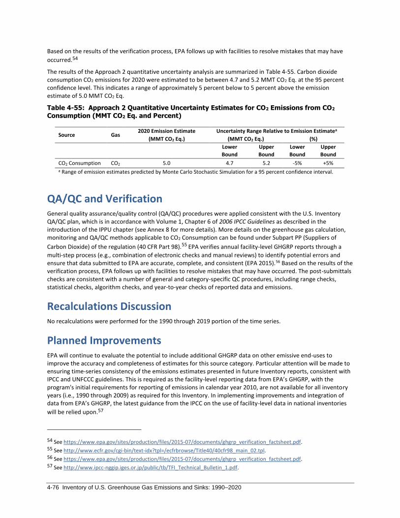
4-76 Inventory of U.S. Greenhouse Gas Emissions and Sinks: 1990–2020
Based on the results of the verification process, EPA follows up with facilities to resolve mistakes that may have
occurred.54
The results of the Approach 2 quantitative uncertainty analysis are summarized in Table 4-55. Carbon dioxide consumption CO2 emissions for 2020 were estimated to be between 4.7 and 5.2 MMT CO2 Eq. at the 95 percent confidence level. This indicates a range of approximately 5 percent below to 5 percent above the emission estimate of 5.0 MMT CO2 Eq.
Table 4-55: Approach 2 Quantitative Uncertainty Estimates for CO2 Emissions from CO2
Consumption (MMT CO2 Eq. and Percent)
Source Gas
2020 Emission Estimate Uncertainty Range Relative to Emission Estimatea
(MMT CO2 Eq.) (MMT CO2 Eq.) (%)
Lower
Bound
Upper
Bound
Lower
Bound
Upper
Bound
CO2 Consumption CO2 5.0 4.7 5.2 -5% +5%
a Range of emission estimates predicted by Monte Carlo Stochastic Simulation for a 95 percent confidence interval.
QA/QC and Verification General quality assurance/quality control (QA/QC) procedures were applied consistent with the U.S. Inventory QA/QC plan, which is in accordance with Volume 1, Chapter 6 of 2006 IPCC Guidelines as described in the introduction of the IPPU chapter (see Annex 8 for more details). More details on the greenhouse gas calculation, monitoring and QA/QC methods applicable to CO2 Consumption can be found under Subpart PP (Suppliers of
Carbon Dioxide) of the regulation (40 CFR Part 98).55 EPA verifies annual facility-level GHGRP reports through a
multi-step process (e.g., combination of electronic checks and manual reviews) to identify potential errors and ensure that data submitted to EPA are accurate, complete, and consistent (EPA 2015).56 Based on the results of the verification process, EPA follows up with facilities to resolve mistakes that may have occurred. The post-submittals checks are consistent with a number of general and category-specific QC procedures, including range checks, statistical checks, algorithm checks, and year-to-year checks of reported data and emissions.
Recalculations Discussion No recalculations were performed for the 1990 through 2019 portion of the time series.
Planned Improvements EPA will continue to evaluate the potential to include additional GHGRP data on other emissive end-uses to improve the accuracy and completeness of estimates for this source category. Particular attention will be made to ensuring time-series consistency of the emissions estimates presented in future Inventory reports, consistent with IPCC and UNFCCC guidelines. This is required as the facility-level reporting data from EPA’s GHGRP, with the program's initial requirements for reporting of emissions in calendar year 2010, are not available for all inventory years (i.e., 1990 through 2009) as required for this Inventory. In implementing improvements and integration of data from EPA’s GHGRP, the latest guidance from the IPCC on the use of facility-level data in national inventories
will be relied upon.57
54 See https://www.epa.gov/sites/production/files/2015-07/documents/ghgrp_verification_factsheet.pdf. 55 See http://www.ecfr.gov/cgi-bin/text-idx?tpl=/ecfrbrowse/Title40/40cfr98_main_02.tpl. 56 See https://www.epa.gov/sites/production/files/2015-07/documents/ghgrp_verification_factsheet.pdf. 57 See http://www.ipcc-nggip.iges.or.jp/public/tb/TFI_Technical_Bulletin_1.pdf.

Industrial Processes and Product Use 4-77
These improvements are still in process and will be incorporated into future Inventory reports. These are near-to medium-term improvements.
4.16 Phosphoric Acid Production (CRF Source Category 2B10)
Phosphoric acid (H3PO4) is a basic raw material used in the production of phosphate-based fertilizers. Phosphoric acid production from natural phosphate rock is a source of carbon dioxide (CO2) emissions, due to the chemical reaction of the inorganic carbon (calcium carbonate) component of the phosphate rock.
Phosphate rock is mined in Florida and North Carolina, which account for more than 75 percent of total domestic output, and in Idaho and Utah (USGS 2021a). It is used primarily as a raw material for wet-process phosphoric acid production. The composition of natural phosphate rock varies, depending on the location where it is mined. Natural phosphate rock mined in the United States generally contains inorganic carbon in the form of calcium carbonate (limestone) and may also contain organic carbon.
The phosphoric acid production process involves chemical reaction of the calcium phosphate (Ca3(PO4)2) component of the phosphate rock with sulfuric acid (H2SO4) and recirculated phosphoric acid (H3PO4) (EFMA 2000). The generation of CO2, however, is due to the associated limestone-sulfuric acid reaction, as shown below:
𝐶𝑎𝐶𝑂3 + 𝐻2𝑆𝑂4 + 𝐻2𝑂 → 𝐶𝑎𝑆𝑂4 · 2𝐻2𝑂 + 𝐶𝑂2
Total U.S. phosphate rock production used in 2020 was an estimated 24.0 million metric tons (USGS 2021a). Total imports of phosphate rock to the United States in 2020 were 2.3 million metric tons (USGS 2021a). Between 2016 and 2019, most of the imported phosphate rock (85 percent) came from Peru, with 15 percent from Morocco (USGS 2021a). All phosphate rock mining companies in the United States are vertically integrated with fertilizer plants that produce phosphoric acid located near the mines. The phosphoric acid production facilities that use imported phosphate rock are located in Louisiana.
Over the 1990 to 2020 period, domestic phosphate rock production has decreased by nearly 52 percent. Total CO2 emissions from phosphoric acid production were 0.9 MMT CO2 Eq. (938 kt CO2) in 2020 (see Table 4-56). Domestic consumption of phosphate rock in 2020 was estimated to have increased 3 percent relative to 2019 levels. The COVID-19 pandemic did not have a major effect on the domestic phosphate rock market as both the fertilizer industry and related agricultural businesses were considered essential industries (USGS 2021a).
Table 4-56: CO2 Emissions from Phosphoric Acid Production (MMT CO2 Eq. and kt)
Year MMT CO2 Eq. kt
1990 1.5 1,529
2005 1.3 1,342
2016 1.0 998
2017 1.0 1,025
2018 0.9 937
2019 0.9 909
2020 0.9 938

4-78 Inventory of U.S. Greenhouse Gas Emissions and Sinks: 1990–2020
Methodology and Time-Series Consistency The United States uses a country-specific methodology consistent with an IPCC Tier 1 approach to calculate
emissions from production of phosphoric acid from phosphate rock.58 Carbon dioxide emissions from production of phosphoric acid from phosphate rock are estimated by multiplying the average amount of inorganic carbon (expressed as CO2) contained in the natural phosphate rock as calcium carbonate by the amount of phosphate rock that is used annually to produce phosphoric acid, accounting for domestic production and net imports for consumption. The estimation methodology is as follows:
Equation 4-9: CO2 Emissions from Phosphoric Acid Production
𝐸𝑝𝑎 = 𝐶𝑝𝑟 × 𝑄𝑝𝑟
where,
Epa = CO2 emissions from phosphoric acid production, metric tons Cpr = Average amount of carbon (expressed as CO2) in natural phosphate rock, metric ton
CO2/ metric ton phosphate rock Qpr = Quantity of phosphate rock used to produce phosphoric acid
The CO2 emissions calculation methodology assumes that all of the inorganic C (calcium carbonate) content of the phosphate rock reacts to produce CO2 in the phosphoric acid production process and is emitted with the stack gas. The methodology also assumes that none of the organic C content of the phosphate rock is converted to CO2 and that all of the organic C content remains in the phosphoric acid product.
From 1993 to 2004, the U.S. Geological Survey (USGS) Mineral Yearbook: Phosphate Rock disaggregated phosphate rock mined annually in Florida and North Carolina from phosphate rock mined annually in Idaho and Utah, and reported the annual amounts of phosphate rock exported and imported for consumption (see Table 4-57). For the years 1990 through 1992, and 2005 through 2019, only nationally aggregated mining data was reported by USGS. For the years 1990, 1991, and 1992, the breakdown of phosphate rock mined in Florida and North Carolina, and the amount mined in Idaho and Utah, are approximated using data reported by USGS for the average share of U.S. production in those states from 1993 to 2004. For the years 2005 through 2016 and years 2017 through 2020, the same approximation method is used, but the share of U.S. production based on production capacity in those states were obtained from the USGS commodity specialist for phosphate rock (USGS 2012; USGS 2021b). Data for domestic sales or consumption of phosphate rock, exports of phosphate rock (primarily from Florida and North Carolina), and imports of phosphate rock for consumption for 1990 through 2010 were obtained from USGS Minerals Yearbook: Phosphate Rock (USGS 1994 through 2015b), and from USGS Minerals Commodity Summaries: Phosphate Rock (USGS 2016 through 2021a). From 2004 through 2019, the USGS reported no exports of phosphate rock from U.S. producers (USGS 2021a).
The carbonate content of phosphate rock varies depending upon where the material is mined. Composition data for domestically mined and imported phosphate rock were provided by the Florida Institute of Phosphate Research, now known as the Florida Industrial and Phosphate Research Institute (FIPR 2003a). Phosphate rock mined in Florida contains approximately 1 percent inorganic C, and phosphate rock imported from Morocco contains approximately 1.46 percent inorganic C. Calcined phosphate rock mined in North Carolina and Idaho contains approximately 0.41 percent and 0.27 percent inorganic C, respectively (see Table 4-58). Similar to the phosphate rock mined in Morocco, phosphate rock mined in Peru contains approximately 5 percent CO2 (Golder Associates and M3 Engineering 2016).
Carbonate content data for phosphate rock mined in Florida are used to calculate the CO2 emissions from consumption of phosphate rock mined in Florida and North Carolina (more than 75 percent of domestic production), and carbonate content data for phosphate rock mined in Morocco and Peru are used to calculate CO2 emissions from consumption of imported phosphate rock. The CO2 emissions calculation assumes that all of the
58 The 2006 IPCC Guidelines do not provide a method for estimating process emissions (CO2) from Phosphoric Acid Production.

Industrial Processes and Product Use 4-79
domestic production of phosphate rock is used in uncalcined form. As of 2006, the USGS noted that one phosphate rock producer in Idaho produces calcined phosphate rock; however, no production data were available for this single producer (USGS 2006). The USGS confirmed that no significant quantity of domestic production of phosphate rock is in the calcined form (USGS 2012).
Table 4-57: Phosphate Rock Domestic Consumption, Exports, and Imports (kt)
Location/Year 1990 2005 2016 2017 2018 2019 2020
U.S. Domestic Consumption 49,800 35,200 26,700 26,300 23,300 23,400 24,000
FL and NC 42,494 28,160 21,360 20,510 18,170 18,250 18,720
ID and UT 7,306 7,040 5,340 5,790 5,130 5,150 5,280
Exports—FL and NC 6,240 0 0 0 0 0 0
Imports 451 2,630 1,590 2,470 2,770 2,140 2,300
Total U.S. Consumption 44,011 37,830 28,290 28,770 26,070 25,540 26,300
Note: Totals may not sum due to independent rounding.
Table 4-58: Chemical Composition of Phosphate Rock (Percent by Weight)
Composition
Central
Florida
North
Florida
North
Carolina
(calcined)
Idaho
(calcined) Morocco Peru
Total Carbon (as C) 1.60 1.76 0.76 0.60 1.56 NA
Inorganic Carbon (as C) 1.00 0.93 0.41 0.27 1.46 NA
Organic Carbon (as C) 0.60 0.83 0.35 0.00 0.10 NA
Inorganic Carbon (as CO2) 3.67 3.43 1.50 1.00 5.00 5.00
NA (Not Available) Sources: FIPR (2003a), Golder Associates and M3 Engineering (2016)
Methodological approaches were applied to the entire time series to ensure consistency in emissions estimates from 1990 through 2020.
Uncertainty Phosphate rock production data used in the emission calculations were developed by the USGS through monthly and semiannual voluntary surveys of the active phosphate rock mines during 2019. Prior to 2006, USGS provided the data disaggregated regionally; however, beginning in 2006, only total U.S. phosphate rock production was reported. Regional production for 2020 was estimated based on regional production data from 2017 to 2020 and multiplied by regionally-specific emission factors. There is uncertainty associated with the degree to which the estimated 2019 regional production data represents actual production in those regions. Total U.S. phosphate rock production data are not considered to be a significant source of uncertainty because all the domestic phosphate rock producers report their annual production to the USGS. Data for exports of phosphate rock used in the emission calculations are reported to the USGS by phosphate rock producers and are not considered to be a significant source of uncertainty. Data for imports for consumption are based on international trade data collected by the U.S. Census Bureau. These U.S. government economic data are not considered to be a significant source of uncertainty.
An additional source of uncertainty in the calculation of CO2 emissions from phosphoric acid production is the carbonate composition of phosphate rock, as the composition of phosphate rock varies depending upon where the material is mined and may also vary over time. The Inventory relies on one study (FIPR 2003a) of chemical composition of the phosphate rock; limited data are available beyond this study. Another source of uncertainty is the disposition of the organic carbon content of the phosphate rock. A representative of FIPR indicated that in the phosphoric acid production process the organic C content of the mined phosphate rock generally remains in the phosphoric acid product, which is what produces the color of the phosphoric acid product (FIPR 2003b). Organic carbon is therefore not included in the calculation of CO2 emissions from phosphoric acid production.

4-80 Inventory of U.S. Greenhouse Gas Emissions and Sinks: 1990–2020
A third source of uncertainty is the assumption that all domestically-produced phosphate rock is used in phosphoric acid production and used without first being calcined. Calcination of the phosphate rock would result in conversion of some of the organic C in the phosphate rock into CO2. However, according to air permit information available to the public, at least one facility has calcining units permitted for operation (NCDENR 2013).
Finally, USGS indicated that in 2020 less than 5 percent of domestically-produced phosphate rock was used to manufacture elemental phosphorus and other phosphorus-based chemicals, rather than phosphoric acid (USGS 2021a). According to USGS, there is only one domestic producer of elemental phosphorus, in Idaho, and no data were available concerning the annual production of this single producer. Elemental phosphorus is produced by reducing phosphate rock with coal coke, and it is therefore assumed that 100 percent of the carbonate content of the phosphate rock will be converted to CO2 in the elemental phosphorus production process. The calculation for CO2 emissions assumes that phosphate rock consumption, for purposes other than phosphoric acid production, results in CO2 emissions from 100 percent of the inorganic carbon content in phosphate rock, but none from the organic carbon content.
The results of the Approach 2 quantitative uncertainty analysis are summarized in Table 4-59. 2020 phosphoric acid production CO2 emissions were estimated to be between 0.8 and 1.2 MMT CO2 Eq. at the 95 percent confidence level. This indicates a range of approximately 18 percent below and 20 percent above the emission estimate of 0.9 MMT CO2 Eq.
Table 4-59: Approach 2 Quantitative Uncertainty Estimates for CO2 Emissions from
Phosphoric Acid Production (MMT CO2 Eq. and Percent)
Source Gas 2020 Emission Estimate Uncertainty Range Relative to Emission Estimatea
(MMT CO2 Eq.) (MMT CO2 Eq.) (%)
Lower
Bound
Upper
Bound
Lower
Bound
Upper
Bound
Phosphoric Acid Production CO2 0.9 0.8 1.2 -18% +20% a Range of emission estimates predicted by Monte Carlo Stochastic Simulation for a 95 percent confidence interval.
QA/QC and Verification For more information on the general QA/QC process applied to this source category, consistent with the U.S. Inventory QA/QC plan, which is in accordance with Volume 1, Chapter 6 of 2006 IPCC Guidelines as described in the introduction of the IPPU chapter (see Annex 8 for more details).
Recalculations Discussion Recalculations were performed for the 2017 through 2019 portion of the time series to reflect an updated breakdown of phosphate rock mined in Florida and North Carolina and the amount mined in Idaho and Utah as provided by the USGS commodity specialist. Additionally, the 2019 value for the total U.S. production of phosphate rock was updated based on updated USGS data. These updates resulted in minor decreases of 3 kt CO2 in both 2017 and 2018 and an increase of 18 kt CO2 in 2019.
Planned Improvements EPA continues to evaluate potential improvements to the Inventory estimates for this source category, which include direct integration of EPA’s GHGRP data for 2010 through 2020 along with assessing applicability of reported GHGRP data to update the inorganic C content of phosphate rock for prior years to ensure time-series consistency. Specifically, EPA would need to assess that averaged inorganic C content data (by region or other approaches) meets GHGRP confidential business information (CBI) screening criteria. EPA would then need to assess the applicability of GHGRP data for the averaged inorganic C content (by region or other approaches) from 2010 through 2020, along with other information to inform estimates in prior years in the required time series

Industrial Processes and Product Use 4-81
(1990 through 2009) based on the sources of phosphate rock used in production of phosphoric acid over time. In implementing improvements and integration of data from EPA’s GHGRP, the latest guidance from the IPCC on the
use of facility-level data in national inventories will be relied upon.59 These long-term planned improvements are still in development by EPA and have not been implemented into the current Inventory report.
4.17 Iron and Steel Production (CRF Source Category 2C1) and Metallurgical Coke Production
Iron and steel production is a multi-step process that generates process-related emissions of carbon dioxide (CO2)
and methane (CH4) as raw materials are refined into iron and then transformed into crude steel. Emissions from conventional fuels (e.g., natural gas, fuel oil) consumed for energy purposes during the production of iron and steel are accounted for in the Energy chapter.
Iron and steel production includes seven distinct production processes: metallurgical coke production, sinter
production, direct reduced iron (DRI) production, pellet production, pig iron60 production, electric arc furnace (EAF) steel production, and basic oxygen furnace (BOF) steel production. The number of production processes at a particular plant is dependent upon the specific plant configuration. Most process CO2 generated from the iron and steel industry is a result of the production of crude iron.
In addition to the production processes mentioned above, CO2 is also generated at iron and steel mills through the consumption of process byproducts (e.g., blast furnace gas, coke oven gas) used for various purposes including heating, annealing, and electricity generation. Process byproducts sold off-site for use as synthetic natural gas are also accounted for in these calculations. In general, CO2 emissions are generated in these production processes through the reduction and consumption of various carbon-containing inputs (e.g., ore, scrap, flux, coke byproducts). Fugitive CH4 emissions can also be generated from these processes, as well as from sinter, direct iron, and pellet production.
In 2020, approximately eleven integrated iron and steel steelmaking facilities utilized BOFs to refine and produce steel from iron, and raw steel was produced at 98 facilities across the United States. Approximately 30 percent of steel production was attributed to BOFs and 70 percent to EAFs (USGS 2021). The trend in the United States for integrated facilities has been a shift towards fewer BOFs and more EAFs. EAFs use scrap steel as their main input and use significantly less energy than BOFs. There are also 14 cokemaking facilities, of which 3 facilities are co-located with integrated iron and steel facilities (ACCCI 2021). In the United States, 6 states account for roughly 51 percent of total raw steel production: Indiana, Alabama, Tennessee, Kentucky, Mississippi, and Arkansas (AISI 2021).
Total annual production of crude steel in the United States was fairly constant between 2000 and 2008 and ranged from a low of 99,320,000 tons to a high of 109,880,000 tons (2001 and 2004, respectively). Due to the decrease in demand caused by the global economic downturn (particularly from the automotive industry), crude steel production in the United States sharply decreased to 65,459,000 tons in 2009. Crude steel production was fairly constant from 2011 through 2014, and after a dip in production from 2014 to 2015, crude steel production has slowly and steadily increased for the past few years. The United States was the fourth largest producer of raw steel
59 See http://www.ipcc-nggip.iges.or.jp/public/tb/TFI_Technical_Bulletin_1.pdf. 60 Pig iron is the common industry term to describe what should technically be called crude iron. Pig iron is a subset of crude iron that has lost popularity over time as industry trends have shifted. Throughout this report, pig iron will be used interchangeably with crude iron, but it should be noted that in other data sets or reports pig iron and crude iron may not be used interchangeably and may provide different values.

4-82 Inventory of U.S. Greenhouse Gas Emissions and Sinks: 1990–2020
in the world, behind China, India and Japan, accounting for approximately 3.9 percent of world production in 2020 (AISI 2004 through 2021).
The majority of CO2 emissions from the iron and steel production process come from the use of metallurgical coke in the production of pig iron and from the consumption of other process byproducts, with lesser amounts emitted from the use of carbon-containing flux and from the removal of carbon from pig iron used to produce steel.
According to the 2006 IPCC Guidelines, the production of metallurgical coke from coking coal is considered to be an energy use of fossil fuel, and the use of coke in iron and steel production is considered to be an industrial process source. The 2006 IPCC Guidelines suggest that emissions from the production of metallurgical coke should be reported separately in the Energy sector, while emissions from coke consumption in iron and steel production should be reported in the Industrial Processes and Product Use sector. The approaches and emission estimates for both metallurgical coke production and iron and steel production, however, are presented here because much of the relevant activity data is used to estimate emissions from both metallurgical coke production and iron and steel production. For example, some byproducts (e.g., coke oven gas) of the metallurgical coke production process are consumed during iron and steel production, and some byproducts of the iron and steel production process (e.g., blast furnace gas) are consumed during metallurgical coke production. Emissions associated with the consumption of these byproducts are attributed at the point of consumption. Emissions associated with the use of conventional fuels (e.g., natural gas, fuel oil) for electricity generation, heating and annealing, or other miscellaneous purposes downstream of the iron and steelmaking furnaces are reported in the Energy chapter.
Metallurgical Coke Production
Emissions of CO2 from metallurgical coke production in 2020 were 2.3 MMT CO2 Eq. (2,324 kt CO2) (see Table 4-60 and Table 4-61). Emissions decreased by 23 percent from 2019 to 2020 and have decreased by 59 percent since 1990. Coke production in 2020 was about 20 percent lower than in 2019 and 63 percent below 1990 (EIA 2021, AISI 2021).
Significant activity data for 2020 were not available in time for publication of this report and were estimated using 2019 values adjusted based on GHGRP emissions data, as described in the Methodology and Time-Series Consistency section below.
Table 4-60: CO2 Emissions from Metallurgical Coke Production (MMT CO2 Eq.)
Gas 1990 2005 2016 2017 2018 2019 2020
CO2 5.6 3.9 2.6 2.0 1.3 3.0 2.3
Table 4-61: CO2 Emissions from Metallurgical Coke Production (kt)
Gas 1990 2005 2016 2017 2018 2019 2020
CO2 5,608 3,921 2,643 1,978 1,282 3,006 2,324
Iron and Steel Production
Emissions of CO2 and CH4 from iron and steel production in 2020 were 35.4 MMT CO2 Eq. (35,386 kt) and 0.0066 MMT CO2 Eq. (0.3 kt CH4), respectively (see Table 4-62 through Table 4-65), totaling 35.4 MMT CO2 Eq. Emissions from iron and steel production decreased by 12 percent from 2019 to 2020 and have decreased by 64 percent since 1990, due to restructuring of the industry, technological improvements, and increased scrap steel utilization. Carbon dioxide emission estimates include emissions from the consumption of carbonaceous materials in the blast furnace, EAF, and BOF, as well as blast furnace gas and coke oven gas consumption for other activities at the steel mill.
Significant activity data for 2020 were not available in time for publication of this report and were estimated using 2019 values adjusted based on GHGRP emissions data, as described in the Methodology and Time-Series Consistency section below.

Industrial Processes and Product Use 4-83
In 2020, domestic production of pig iron decreased by 18 percent from 2019 levels. Overall, domestic pig iron production has declined since the 1990s. Pig iron production in 2020 was 62 percent lower than in 2000 and 63 percent below 1990. Carbon dioxide emissions from iron production have decreased by 82 percent (37.3 MMT CO2 Eq.) since 1990. Carbon dioxide emissions from steel production have decreased by 29 percent (2.3 MMT CO2 Eq.) since 1990, while overall CO2 emissions from iron and steel production have declined by 64 percent (63.7 MMT CO2 Eq.) from 1990 to 2020.
Table 4-62: CO2 Emissions from Iron and Steel Production (MMT CO2 Eq.)
Source/Activity Data 1990 2005 2016 2017 2018 2019 2020
Sinter Production 2.4 1.7 0.9 0.9 0.9 0.9 0.8
Iron Production 45.7 17.7 9.9 8.2 9.6 9.4 8.4
Pellet Production 1.8 1.5 0.9 0.9 0.9 0.9 0.8
Steel Production 8.0 9.4 6.9 6.2 5.8 5.8 5.6
Other Activitiesa 41.2 35.9 22.5 22.4 24.1 23.2 19.8
Total 99.1 66.2 41.0 38.6 41.3 40.1 35.4
a Includes emissions from blast furnace gas and coke oven gas combustion for activities at the steel mill other than consumption in blast furnace, EAFs, or BOFs.
Note: Totals may not sum due to independent rounding.
Table 4-63: CO2 Emissions from Iron and Steel Production (kt)
Source/Activity Data 1990 2005 2016 2017 2018 2019 2020
Sinter Production 2,448 1,663 877 869 937 876 750
Iron Production 45,706 17,661 9,928 8,237 9,581 9,360 8,416
Pellet Production 1,817 1,503 869 867 924 878 752
Steel Production 7,964 9,395 6,854 6,218 5,754 5,812 5,650
Other Activities a 41,194 35,934 22,451 22,396 24,149 23,158 19,838
Total 99,129 66,156 40,979 38,587 41,345 40,084 35,407 a Includes emissions from blast furnace gas and coke oven gas combustion for activities at the steel mill
other than consumption in blast furnace, EAFs, or BOFs. Note: Totals may not sum due to independent rounding.
Table 4-64: CH4 Emissions from Iron and Steel Production (MMT CO2 Eq.)
Source/Activity Data 1990 2005 2016 2017 2018 2019 2020
Sinter Production + + + + + + +
+ Does not exceed 0.05 MMT CO2 Eq.
Table 4-65: CH4 Emissions from Iron and Steel Production (kt)
Source/Activity Data 1990 2005 2016 2017 2018 2019 2020
Sinter Production 0.9 0.6 0.3 0.3 0.3 0.3 0.3
Methodology and Time-Series Consistency Emission estimates presented in this chapter utilize a country-specific approach based on Tier 2 methodologies provided by the 2006 IPCC Guidelines. These Tier 2 methodologies call for a mass balance accounting of the carbonaceous inputs and outputs during the iron and steel production process and the metallurgical coke production process. Tier 1 methods are used for certain iron and steel production processes (i.e., sinter production, pellet production and DRI production) for which available data are insufficient to apply a Tier 2

4-84 Inventory of U.S. Greenhouse Gas Emissions and Sinks: 1990–2020
method (e.g., country-specific carbon contents of inputs and outputs are not known). The majority of emissions are captured with higher tier methods, as sinter production, pellet production, and DRI production only account for roughly 8 percent of total iron and steel production emissions.
The Tier 2 methodology equation is as follows:
Equation 4-10: CO2 Emissions from Coke, Pig Iron, EAF Steel, and BOF Steel Production,
based on 2006 IPCC Guidelines Tier 2 Methodologies
𝐸𝐶𝑂2= [∑(𝑄𝑎 × 𝐶𝑎)
𝑎
− ∑(𝑄𝑏 × 𝐶𝑏)
𝑏
] ×44
12
where, ECO2 = Emissions from coke, pig iron, EAF steel, or BOF steel production, metric tons a = Input material a b = Output material b Qa = Quantity of input material a, metric tons Ca = Carbon content of input material a, metric tons C/metric ton material Qb = Quantity of output material b, metric tons Cb = Carbon content of output material b, metric tons C/metric ton material 44/12 = Stoichiometric ratio of CO2 to C
The Tier 1 methodology equations are as follows:
Equation 4-11: 2006 IPCC Guidelines Tier 1: Emissions from Sinter, Direct Reduced Iron, and
Pellet Production (Equations 4.6, 4.7, and 4.8)
𝐸𝑠,𝑝 = 𝑄𝑠 × 𝐸𝐹𝑠,𝑝
𝐸𝑑,𝐶𝑂2 = 𝑄𝑑 × 𝐸𝐹𝑑,𝐶𝑂2
𝐸𝑝,𝐶𝑂2 = 𝑄𝑝 × 𝐸𝐹𝑝,𝐶𝑂2
where, Es,p = Emissions from sinter production process for pollutant p (CO2 or CH4), metric ton Qs = Quantity of sinter produced, metric tons EFs,p = Emission factor for pollutant p (CO2 or CH4), metric ton p/metric ton sinter Ed,CO2 = Emissions from DRI production process for CO2, metric ton Qd = Quantity of DRI produced, metric tons EFd,CO2 = Emission factor for CO2, metric ton CO2/metric ton DRI Ep,CO2 = Emissions from pellet production process for CO2, metric ton Qp = Quantity of pellets produced, metric tons EFp,CO2 = Emission factor for CO2, metric ton CO2/metric ton pellets produced
A significant number of activity data that serve as inputs to emissions calculations were unavailable for 2020 at the time of publication and were estimated using 2019 values. In addition, to account for the impacts of the COVID-19 pandemic in 2020, the EPA used process emissions data from the EPA’s Greenhouse Gas Reporting Program (GHGRP) subpart Q for the iron and steel sector to adjust the estimated values. GHGRP process emissions data decreased by approximately 14 percent from 2019 to 2020 (EPA 2021), and this percentage decrease was applied to all 2020 activity data estimated with 2019 values.
Metallurgical Coke Production
Coking coal is used to manufacture metallurgical coke which is used primarily as a reducing agent in the production of iron and steel but is also used in the production of other metals including zinc and lead (see Zinc Production and Lead Production sections of this chapter). Emissions associated with producing metallurgical coke from coking coal

Industrial Processes and Product Use 4-85
are estimated and reported separately from emissions that result from the iron and steel production process. To estimate emissions from metallurgical coke production, a Tier 2 method provided by the 2006 IPCC Guidelines was utilized. The amount of carbon contained in materials produced during the metallurgical coke production process (i.e., coke, coke breeze and coke oven gas) is deducted from the amount of carbon contained in materials consumed during the metallurgical coke production process (i.e., natural gas, blast furnace gas, and coking coal). For calculations, activity data for these inputs, including natural gas, blast furnace gas, and coking coke consumed for metallurgical coke production, are in units consistent with the carbon content values. Light oil, which is produced during the metallurgical coke production process, is excluded from the deductions due to data limitations. The amount of carbon contained in these materials is calculated by multiplying the material-specific carbon content by the amount of material consumed or produced (see Table 4-66). The amount of coal tar produced was approximated using a production factor of 0.03 tons of coal tar per ton of coking coal consumed. The amount of coke breeze produced was approximated using a production factor of 0.075 tons of coke breeze per ton of coking coal consumed (Steiner 2008; DOE 2000). Data on the consumption of carbonaceous materials (other than coking coal) as well as coke oven gas production were available for integrated steel mills only (i.e., steel mills with co-located coke plants); therefore, carbonaceous material (other than coking coal) consumption and coke oven gas production were excluded from emission estimates for merchant coke plants. Carbon contained in coke oven gas used for coke-oven underfiring was not included in the deductions to avoid double-counting.
Table 4-66: Material Carbon Contents for Metallurgical Coke Production
Material kg C/kg
Coal Tara 0.62
Cokea 0.83
Coke Breezea 0.83
Coking Coalb 0.75
Material kg C/GJ
Coke Oven Gasc 12.1
Blast Furnace Gasc 70.8
a Source: IPCC (2006), Vol. 3 Chapter 4, Table 4.3 b Source: EIA (2017b) c Source: IPCC (2006), Vol. 2 Chapter 1, Table 1.3
Although the 2006 IPCC Guidelines provide a Tier 1 CH4 emission factor for metallurgical coke production (i.e., 0.1 g CH4 per metric ton of coke production), it is not appropriate to use because CO2 emissions were estimated using the Tier 2 mass balance methodology. The mass balance methodology makes a basic assumption that all carbon that enters the metallurgical coke production process either exits the process as part of a carbon-containing output or as CO2 emissions. This is consistent with a preliminary assessment of aggregated facility-level greenhouse gas CH4 emissions reported by coke production facilities under EPA’s GHGRP. The assessment indicates that CH4 emissions from coke production are insignificant and below 500 kt or 0.05 percent of total national emissions. Pending resources and significance, EPA continues to assess the possibility of including these emissions in future Inventories to enhance completeness but has not incorporated these emissions into this report.
Data relating to the mass of coking coal consumed at metallurgical coke plants and the mass of metallurgical coke produced at coke plants were taken from the Energy Information Administration (EIA) Quarterly Coal Report: October through December (EIA 1998 through 2019) and EIA Quarterly Coal Report: January through March (EIA 2021) (see Table 4-67). Data on the volume of natural gas consumption, blast furnace gas consumption, and coke oven gas production for metallurgical coke production at integrated steel mills were obtained from the American Iron and Steel Institute (AISI) Annual Statistical Report (AISI 2004 through 2021) and through personal communications with AISI (Steiner 2008) (see Table 4-68). Coke plant consumption and production data from the AISI Annual Statistical Report were withheld for 2020, so the 2019 values were used as estimated data for the missing 2020 values and adjusted using GHGRP emissions data, as described earlier in this Methodology and Time-Series Consistency section.
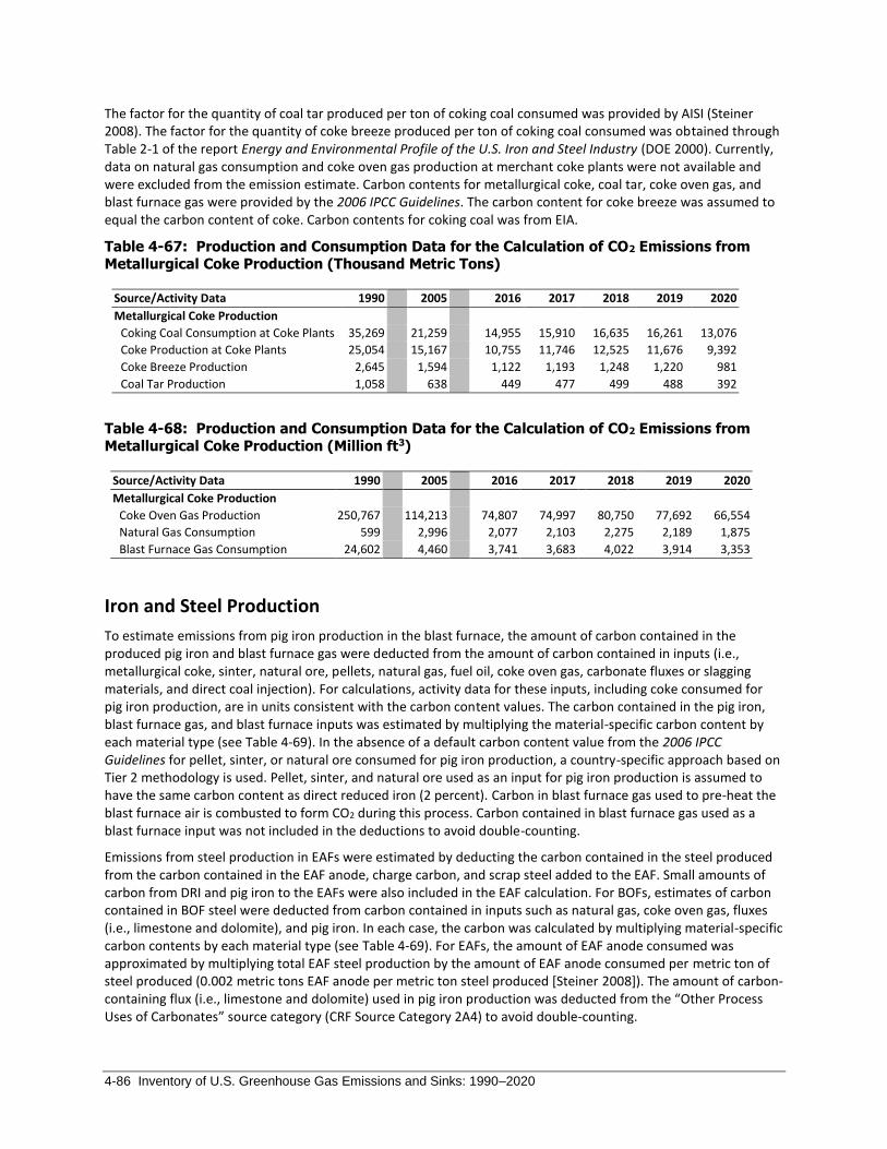
4-86 Inventory of U.S. Greenhouse Gas Emissions and Sinks: 1990–2020
The factor for the quantity of coal tar produced per ton of coking coal consumed was provided by AISI (Steiner 2008). The factor for the quantity of coke breeze produced per ton of coking coal consumed was obtained through Table 2-1 of the report Energy and Environmental Profile of the U.S. Iron and Steel Industry (DOE 2000). Currently, data on natural gas consumption and coke oven gas production at merchant coke plants were not available and were excluded from the emission estimate. Carbon contents for metallurgical coke, coal tar, coke oven gas, and blast furnace gas were provided by the 2006 IPCC Guidelines. The carbon content for coke breeze was assumed to equal the carbon content of coke. Carbon contents for coking coal was from EIA.
Table 4-67: Production and Consumption Data for the Calculation of CO2 Emissions from Metallurgical Coke Production (Thousand Metric Tons)
Source/Activity Data 1990 2005 2016 2017 2018 2019 2020
Metallurgical Coke Production
Coking Coal Consumption at Coke Plants 35,269 21,259 14,955 15,910 16,635 16,261 13,076
Coke Production at Coke Plants 25,054 15,167 10,755 11,746 12,525 11,676 9,392
Coke Breeze Production 2,645 1,594 1,122 1,193 1,248 1,220 981
Coal Tar Production 1,058 638 449 477 499 488 392
Table 4-68: Production and Consumption Data for the Calculation of CO2 Emissions from Metallurgical Coke Production (Million ft3)
Source/Activity Data 1990 2005 2016 2017 2018 2019 2020
Metallurgical Coke Production
Coke Oven Gas Production 250,767 114,213 74,807 74,997 80,750 77,692 66,554
Natural Gas Consumption 599 2,996 2,077 2,103 2,275 2,189 1,875
Blast Furnace Gas Consumption 24,602 4,460 3,741 3,683 4,022 3,914 3,353
Iron and Steel Production
To estimate emissions from pig iron production in the blast furnace, the amount of carbon contained in the produced pig iron and blast furnace gas were deducted from the amount of carbon contained in inputs (i.e., metallurgical coke, sinter, natural ore, pellets, natural gas, fuel oil, coke oven gas, carbonate fluxes or slagging materials, and direct coal injection). For calculations, activity data for these inputs, including coke consumed for pig iron production, are in units consistent with the carbon content values. The carbon contained in the pig iron, blast furnace gas, and blast furnace inputs was estimated by multiplying the material-specific carbon content by each material type (see Table 4-69). In the absence of a default carbon content value from the 2006 IPCC Guidelines for pellet, sinter, or natural ore consumed for pig iron production, a country-specific approach based on Tier 2 methodology is used. Pellet, sinter, and natural ore used as an input for pig iron production is assumed to have the same carbon content as direct reduced iron (2 percent). Carbon in blast furnace gas used to pre-heat the blast furnace air is combusted to form CO2 during this process. Carbon contained in blast furnace gas used as a blast furnace input was not included in the deductions to avoid double-counting.
Emissions from steel production in EAFs were estimated by deducting the carbon contained in the steel produced from the carbon contained in the EAF anode, charge carbon, and scrap steel added to the EAF. Small amounts of carbon from DRI and pig iron to the EAFs were also included in the EAF calculation. For BOFs, estimates of carbon contained in BOF steel were deducted from carbon contained in inputs such as natural gas, coke oven gas, fluxes (i.e., limestone and dolomite), and pig iron. In each case, the carbon was calculated by multiplying material-specific carbon contents by each material type (see Table 4-69). For EAFs, the amount of EAF anode consumed was approximated by multiplying total EAF steel production by the amount of EAF anode consumed per metric ton of steel produced (0.002 metric tons EAF anode per metric ton steel produced [Steiner 2008]). The amount of carbon-containing flux (i.e., limestone and dolomite) used in pig iron production was deducted from the “Other Process Uses of Carbonates” source category (CRF Source Category 2A4) to avoid double-counting.

Industrial Processes and Product Use 4-87
Carbon dioxide emissions from the consumption of blast furnace gas and coke oven gas for other activities occurring at the steel mill were estimated by multiplying the amount of these materials consumed for these purposes by the material-specific carbon content (see Table 4-69).
Table 4-69: Material Carbon Contents for Iron and Steel Production
Material kg C/kg
Coke 0.83
Direct Reduced Iron 0.02
Dolomite 0.13
EAF Carbon Electrodes 0.82
EAF Charge Carbon 0.83
Limestone 0.12
Pig Iron 0.04
Steel 0.01
Material kg C/GJ
Coke Oven Gas 12.1
Blast Furnace Gas 70.8
Source: IPCC (2006), Table 4.3. Coke Oven Gas and Blast Furnace Gas, Table 1.3.
Carbon dioxide emissions associated with sinter production, direct reduced iron production, pellet production, pig iron production, steel production, and other steel mill activities were summed to calculate the total CO2 emissions from iron and steel production (see Table 4-62 and Table 4-63).
The sinter production process results in fugitive emissions of CH4, which are emitted via leaks in the production equipment, rather than through the emission stacks or vents of the production plants. The fugitive emissions were calculated by applying Tier 1 emission factors taken from the 2006 IPCC Guidelines for sinter production (see Table 4-70). Although the 2006 IPCC Guidelines also provide a Tier 1 methodology for CH4 emissions from pig iron production, it is not appropriate to use because CO2 emissions for pig iron production are estimated using the Tier 2 mass balance methodology. The mass balance methodology makes a basic assumption that all carbon that enters the pig iron production process either exits the process as part of a carbon-containing output or as CO2 emissions; the estimation of CH4 emissions is precluded. Annual analysis of facility-level emissions reported during iron production further supports this assumption and indicates that CH4 emissions are below 500 kt CO2 Eq. and well below 0.05 percent of total national emissions. The production of direct reduced iron could also result in emissions of CH4 through the consumption of fossil fuels (e.g., natural gas, etc.); however, these emission estimates are excluded due to data limitations. Pending further analysis and resources, EPA may include these emissions in future reports to enhance completeness. EPA is still assessing the possibility of including these emissions in future reports and have not included this data in the current report.
Table 4-70: CH4 Emission Factors for Sinter and Pig Iron Production
Material Produced Factor Unit
Sinter 0.07 kg CH4/metric ton
Source: IPCC (2006), Table 4.2.
Emissions of CO2 from sinter production, direct reduced iron production, and pellet production were estimated by multiplying total national sinter production, total national direct reduced iron production, and total national pellet production by Tier 1 CO2 emission factors (see Table 4-71). Because estimates of sinter production, direct reduced iron production, and pellet production were not available, production was assumed to equal consumption.

4-88 Inventory of U.S. Greenhouse Gas Emissions and Sinks: 1990–2020
Table 4-71: CO2 Emission Factors for Sinter Production, Direct Reduced Iron Production, and Pellet Production
Material Produced
Metric Ton CO2/Metric
Ton
Sinter 0.2
Direct Reduced Iron 0.7
Pellet Production 0.03
Source: IPCC (2006), Table 4.1.
The consumption of coking coal, natural gas, distillate fuel, and coal used in iron and steel production are adjusted for within the Energy chapter to avoid double-counting of emissions reported within the IPPU chapter as these fuels were consumed during non-energy related activities. More information on this methodology and examples of adjustments made between the IPPU and Energy chapters are described in Annex 2.1, Methodology for Estimating Emissions of CO2 from Fossil Fuel Combustion.
Sinter consumption and pellet consumption data for 1990 through 2020 were obtained from AISI’s Annual Statistical Report (AISI 2004 through 2021) and through personal communications with AISI (Steiner 2008) (see
Table 4-72). Data from the AISI Annual Statistical Report were withheld for 2020, so the 2019 values were used as estimated data for the missing 2020 values and adjusted using GHGRP emissions data, as described earlier in this Methodology and Time-Series Consistency section.
In general, direct reduced iron (DRI) consumption data were obtained from the U.S. Geological Survey (USGS) Minerals Yearbook – Iron and Steel Scrap (USGS 1991 through 2020) and personal communication with the USGS Iron and Steel Commodity Specialist (Tuck 2020); however, data for DRI consumed in EAFs were not available for the years 1990 and 1991. EAF DRI consumption in 1990 and 1991 was calculated by multiplying the total DRI consumption for all furnaces by the EAF share of total DRI consumption in 1992. Also, data for DRI consumed in BOFs were not available for the years 1990 through 1993. BOF DRI consumption in 1990 through 1993 was calculated by multiplying the total DRI consumption for all furnaces (excluding EAFs and cupola) by the BOF share of total DRI consumption (excluding EAFs and cupola) in 1994.
The Tier 1 CO2 emission factors for sinter production, direct reduced iron production and pellet production were obtained through the 2006 IPCC Guidelines (IPCC 2006). Time-series data for pig iron production, coke, natural gas, fuel oil, sinter, and pellets consumed in the blast furnace; pig iron production; and blast furnace gas produced at the iron and steel mill and used in the metallurgical coke ovens and other steel mill activities were obtained from AISI’s Annual Statistical Report (AISI 2004 through 2021) and through personal communications with AISI (Steiner 2008) (see Table 4-72 and Table 4-73). Some data from the AISI Annual Statistical Report were withheld for 2020, so the 2019 values were used as estimated data for the missing 2020 values and adjusted using GHGRP emissions data, as described earlier in this Methodology and Time-Series Consistency section.
Data for EAF steel production, carbon-containing flux, EAF charge carbon, and natural gas consumption were obtained from AISI’s Annual Statistical Report (AISI 2004 through 2021) and through personal communications with AISI (AISI 2006 through 2016, Steiner 2008). The factor for the quantity of EAF anode consumed per ton of EAF steel produced was provided by AISI (Steiner 2008). Data for BOF steel production, carbon-containing flux, natural gas, natural ore, pellet, sinter consumption as well as BOF steel production were obtained from AISI’s Annual Statistical Report (AISI 2004 through 2021) and through personal communications with AISI (Steiner 2008). Data for EAF and BOF scrap steel, pig iron, and DRI consumption were obtained from the USGS Minerals Yearbook – Iron and Steel Scrap (USGS 1991 through 2020). Data on coke oven gas and blast furnace gas consumed at the iron and steel mill (other than in the EAF, BOF, or blast furnace) were obtained from AISI’s Annual Statistical Report (AISI 2004 through 2021) and through personal communications with AISI (Steiner 2008). Some data from the AISI Annual Statistical Report on natural gas consumption were withheld for 2020, so the 2019 values were used as
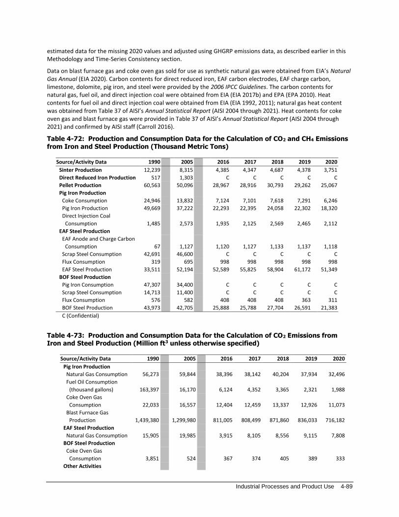
Industrial Processes and Product Use 4-89
estimated data for the missing 2020 values and adjusted using GHGRP emissions data, as described earlier in this Methodology and Time-Series Consistency section.
Data on blast furnace gas and coke oven gas sold for use as synthetic natural gas were obtained from EIA’s Natural Gas Annual (EIA 2020). Carbon contents for direct reduced iron, EAF carbon electrodes, EAF charge carbon, limestone, dolomite, pig iron, and steel were provided by the 2006 IPCC Guidelines. The carbon contents for natural gas, fuel oil, and direct injection coal were obtained from EIA (EIA 2017b) and EPA (EPA 2010). Heat contents for fuel oil and direct injection coal were obtained from EIA (EIA 1992, 2011); natural gas heat content was obtained from Table 37 of AISI’s Annual Statistical Report (AISI 2004 through 2021). Heat contents for coke oven gas and blast furnace gas were provided in Table 37 of AISI’s Annual Statistical Report (AISI 2004 through 2021) and confirmed by AISI staff (Carroll 2016).
Table 4-72: Production and Consumption Data for the Calculation of CO2 and CH4 Emissions from Iron and Steel Production (Thousand Metric Tons)
Source/Activity Data 1990 2005 2016 2017 2018 2019 2020
Sinter Production 12,239 8,315 4,385 4,347 4,687 4,378 3,751
Direct Reduced Iron Production 517 1,303 C C C C C
Pellet Production 60,563 50,096 28,967 28,916 30,793 29,262 25,067
Pig Iron Production
Coke Consumption 24,946 13,832 7,124 7,101 7,618 7,291 6,246
Pig Iron Production 49,669 37,222 22,293 22,395 24,058 22,302 18,320 Direct Injection Coal
Consumption 1,485 2,573
1,935 2,125
2,569
2,465 2,112
EAF Steel Production
EAF Anode and Charge Carbon
Consumption 67 1,127 1,120 1,127
1,133
1,137 1,118
Scrap Steel Consumption 42,691 46,600 C C C C C
Flux Consumption 319 695 998 998 998 998 998
EAF Steel Production 33,511 52,194 52,589 55,825 58,904 61,172 51,349
BOF Steel Production
Pig Iron Consumption 47,307 34,400 C C C C C
Scrap Steel Consumption 14,713 11,400 C C C C C
Flux Consumption 576 582 408 408 408 363 311
BOF Steel Production 43,973 42,705 25,888 25,788 27,704 26,591 21,383
C (Confidential)
Table 4-73: Production and Consumption Data for the Calculation of CO2 Emissions from Iron and Steel Production (Million ft3 unless otherwise specified)
Source/Activity Data 1990 2005 2016 2017 2018 2019 2020
Pig Iron Production
Natural Gas Consumption 56,273 59,844 38,396 38,142 40,204 37,934 32,496
Fuel Oil Consumption
(thousand gallons) 163,397 16,170
6,124 4,352
3,365
2,321 1,988
Coke Oven Gas
Consumption 22,033 16,557 12,404 12,459 13,337 12,926 11,073
Blast Furnace Gas
Production 1,439,380 1,299,980 811,005 808,499 871,860 836,033 716,182
EAF Steel Production
Natural Gas Consumption 15,905 19,985 3,915 8,105 8,556 9,115 7,808
BOF Steel Production
Coke Oven Gas
Consumption 3,851 524 367 374 405 389 333
Other Activities

4-90 Inventory of U.S. Greenhouse Gas Emissions and Sinks: 1990–2020
Coke Oven Gas
Consumption 224,883 97,132 62,036 62,164 67,008 64,377 55,148
Blast Furnace Gas
Consumption 1,414,778 1,295,520 807,264 804,816 867,838 832,119 712,829
Methodological approaches were applied to the entire time series to ensure consistency in emissions from 1990 through 2020.
Uncertainty The estimates of CO2 emissions from metallurgical coke production are based on assessing uncertainties in material production and consumption data and average carbon contents. Uncertainty is associated with the total U.S. coking coal consumption, total U.S. coke production, and materials consumed during this process. Data for coking coal consumption and metallurgical coke production are from different data sources (EIA) than data for other carbonaceous materials consumed at coke plants (AISI), which does not include data for merchant coke plants. There is uncertainty associated with the fact that coal tar and coke breeze production were estimated based on coke production because coal tar and coke breeze production data were not available. Since merchant coke plant data is not included in the estimate of other carbonaceous materials consumed at coke plants, the mass balance equation for CO2 from metallurgical coke production cannot be reasonably completed; therefore, for the purpose of this analysis, uncertainty parameters are applied to primary data inputs to the calculation (i.e., coking coal consumption and metallurgical coke production) only.
The estimates of CO2 emissions from iron and steel production are based on material production and consumption data and average carbon contents. There is uncertainty associated with the assumption that pellet production, direct reduced iron and sinter consumption are equal to production. There is uncertainty with the representativeness of the associated IPCC default emission factors. There is uncertainty associated with the assumption that all coal used for purposes other than coking coal is for direct injection coal. There is also uncertainty associated with the carbon contents for pellets, sinter, and natural ore, which are assumed to equal the carbon contents of direct reduced iron, when consumed in the blast furnace. There is uncertainty associated with the consumption of natural ore under current industry practices. For EAF steel production, there is uncertainty associated with the amount of EAF anode and charge carbon consumed due to inconsistent data throughout the time series. Also for EAF steel production, there is uncertainty associated with the assumption that 100 percent of the natural gas attributed to “steelmaking furnaces” by AISI is process-related and nothing is combusted for energy purposes. Uncertainty is also associated with the use of process gases such as blast furnace gas and coke oven gas. Data are not available to differentiate between the use of these gases for processes at the steel mill versus for energy generation (i.e., electricity and steam generation); therefore, all consumption is attributed to iron and steel production. These data and carbon contents produce a relatively accurate estimate of CO2 emissions; however, there are uncertainties associated with each.
For calculating the emissions estimates from iron and steel and metallurgical coke production, EPA utilizes a number of data points taken from the AISI Annual Statistical Report (ASR). This report serves as a benchmark for information on steel companies in United States, regardless if they are a member of AISI, which represents integrated producers (i.e., blast furnace and EAF). During the compilation of the 1990 through 2016 Inventory report EPA initiated conversation with AISI to better understand and update the qualitative and quantitative uncertainty metrics associated with AISI data elements. AISI estimates their data collection response rate to range from 75 to 90 percent, with certain sectors of the iron and steel industry not being covered by the ASR; therefore, there is some inherent uncertainty in the values provided in the AISI ASR, including material production and consumption data. There is also some uncertainty to which materials produced are exported to Canada. As indicated in the introduction to this section, the trend for integrated facilities has moved to more use of EAFs and fewer BOFs. This trend may not be completely captured in the current data which also increases uncertainty. EPA currently uses an uncertainty range of ±10 percent for the primary data inputs (e.g., consumption and production values for each production process, heat and carbon content values) to calculate overall uncertainty from iron and steel production, consistent with the ranges in Table 4.4 of the 2006 IPCC Guidelines. During EPA’s discussion with

Industrial Processes and Product Use 4-91
AISI, AISI noted that an uncertainty range of ±5 percent would be a more appropriate approximation to reflect their coverage of integrated steel producers in the United States. EPA will continue to assess the best range of uncertainty for these values. Consistent with the ranges in Table 4.4 of the 2006 IPCC Guidelines, EPA assigned an uncertainty range of ±25 percent for the Tier 1 CO2 emission factors for the sinter, direct reduced iron, and pellet production processes.
The results of the Approach 2 quantitative uncertainty analysis are summarized in Table 4-74 for metallurgical coke production and iron and steel production. Total CO2 emissions from metallurgical coke production and iron and steel production for 2020 were estimated to be between 31.4 and 44.2 MMT CO2 Eq. at the 95 percent confidence level. This indicates a range of approximately 17 percent below and 17 percent above the emission estimate of 35.4 MMT CO2 Eq. Total CH4 emissions from metallurgical coke production and iron and steel production for 2020 were estimated to be between 0.005 and 0.008 MMT CO2 Eq. at the 95 percent confidence level. This indicates a range of approximately 21 percent below and 23 percent above the emission estimate of 0.007 MMT CO2 Eq.
Table 4-74: Approach 2 Quantitative Uncertainty Estimates for CO2 and CH4 Emissions from
Iron and Steel Production and Metallurgical Coke Production (MMT CO2 Eq. and Percent)
Source Gas 2020 Emission Estimate Uncertainty Range Relative to Emission Estimatea
(MMT CO2 Eq.) (MMT CO2 Eq.) (%)
Lower
Bound
Upper
Bound
Lower
Bound
Upper
Bound
Metallurgical Coke & Iron
and Steel Production CO2 35.4 31.4 44.2 -17% +17%
Metallurgical Coke & Iron
and Steel Production CH4 + + + -21% +23%
+ Does not exceed 0.05 MMT CO2 Eq. a Range of emission estimates predicted by Monte Carlo Stochastic Simulation for a 95 percent confidence interval.
QA/QC and Verification For more information on the general QA/QC process applied to this source category, consistent with Volume 1, Chapter 6 of the 2006 IPCC Guidelines, see the QA/QC and Verification Procedures section in the introduction of the IPPU chapter.
Recalculations Discussion Recalculations were performed for the year 2019 with updated values for coke production at coke plants, scrap steel consumption for EAF steel production, scrap steel consumption for BOF steel production, and pellet consumption in blast furnaces from EIA, USGS, and AISI. These updates resulted in emissions increases of 114 percent from metallurgical coke production (1.6 MMT CO2), less than 1 percent from iron production (87 kt CO2), 1.2 percent from pellet production (11 kt CO2), and less than 1 percent from steel production (42 kt CO2).
Planned Improvements Significant activity data for 2020 were not available for this report and were estimated using 2019 values and adjusted using GHGRP emissions data. EPA will continue to explore sources of 2020 data and other estimation approaches if 2020 data is not available for the next Inventory report. EPA will update the calculations for the 2023 Inventory submission if new data becomes available.
Future improvements involve improving activity data and emission factor sources for CO2 and CH4 emissions estimations from pellet production. EPA will also evaluate and analyze data reported under EPA’s GHGRP to improve the emission estimates for this and other Iron and Steel Production process categories. Particular attention will be made to ensure time-series consistency of the emissions estimates presented in future Inventory reports, consistent with IPCC and UNFCCC guidelines. This is required as the facility-level reporting data from EPA’s

4-92 Inventory of U.S. Greenhouse Gas Emissions and Sinks: 1990–2020
GHGRP, with the program's initial requirements for reporting of emissions in calendar year 2010, are not available for all inventory years (i.e., 1990 through 2009) as required for this Inventory. In implementing improvements and integration of data from EPA’s GHGRP, the latest guidance from the IPCC on the use of facility-level data in national
inventories will be relied upon.61 This remains a medium-term improvement, and per preliminary work, EPA estimates that the earliest this improvement could be incorporated is the 2024 Inventory submission.
Additional improvements include accounting for emission estimates for the production of metallurgical coke in the Energy chapter as well as identifying the amount of carbonaceous materials, other than coking coal, consumed at merchant coke plants. Other potential improvements include identifying the amount of coal used for direct injection and the amount of coke breeze, coal tar, and light oil produced during coke production. Efforts will also be made to identify information to better characterize emissions from the use of process gases and fuels within the Energy and IPPU chapters. Additional efforts will be made to improve the reporting between the IPPU and Energy chapters, particularly the inclusion of a quantitative summary of the carbon balance in the United States. This planned improvement is a long-term improvement and is still in development. It is not included in this current Inventory report and is not expected until a future (i.e., 2024) Inventory submission.
EPA also received comments during the Expert Review cycle of a previous (i.e., 1990 through 2016) Inventory on recommendations to improve the description of the iron and steel industry and emissive processes. EPA began incorporating some of these recommendations into a previous Inventory (i.e., 1990 through 2016) and will require some additional time to implement other substantive changes.
4.18 Ferroalloy Production (CRF Source Category 2C2)
Carbon dioxide (CO2) and methane (CH4) are emitted from the production of several ferroalloys. Ferroalloys are composites of iron (Fe) and other elements such as silicon (Si), manganese (Mn), and chromium (Cr). Emissions from fuels consumed for energy purposes during the production of ferroalloys are accounted for in the Energy chapter. Emissions from the production of two types of ferrosilicon (25 to 55 percent and 56 to 95 percent silicon), silicon metal (96 to 99 percent silicon), and miscellaneous alloys (32 to 65 percent silicon) have been calculated.
Emissions from the production of ferrochromium and ferromanganese are not included because of the small number of manufacturers of these materials in the United States. Government information disclosure rules prevent the publication of production data for these production facilities. Additionally, production of ferrochromium in the United States ceased in 2009 (USGS 2013).
Similar to emissions from the production of iron and steel, CO2 is emitted when metallurgical coke is oxidized during a high-temperature reaction with iron and the selected alloying element. Due to the strong reducing environment, CO is initially produced and eventually oxidized to CO2. A representative reaction equation for the production of 50 percent ferrosilicon (FeSi) is given below:
Fe2O3 + 2SiO2 + 7C → 2FeSi + 7CO
While most of the carbon contained in the process materials is released to the atmosphere as CO2, a percentage is also released as CH4 and other volatiles. The amount of CH4 that is released is dependent on furnace efficiency, operation technique, and control technology.
Ferroalloys are used to alter the material properties of the steel. Ferroalloys are produced in conjunction with the iron and steel industry, often at co-located facilities, and production trends closely follow that of the iron and steel industry. As of 2018, 11 facilities in the United States produce ferroalloys (USGS 2021b). Emissions of CO2 from ferroalloy production in 2020 were 1.4 MMT CO2 Eq. (1,377 kt CO2) (see Table 4-75 and Table 4-76), which is a 36
61 See http://www.ipcc-nggip.iges.or.jp/public/tb/TFI_Technical_Bulletin_1.pdf.

Industrial Processes and Product Use 4-93
percent reduction since 1990. Emissions of CH4 from ferroalloy production in 2020 were 0.01 MMT CO2 Eq. (0.4 kt CH4), which is a 43 percent decrease since 1990. The decrease in emissions since 1990 can largely be attributed to two facility shutdowns in 2018 and one facility shutdown in 2020. Additionally, the COVID-19 pandemic and lower priced imported ferrosilicon had an impact on ferroalloy production in 2020 (USGS 2021a).
Table 4-75: CO2 and CH4 Emissions from Ferroalloy Production (MMT CO2 Eq.)
Gas 1990 2005 2016 2017 2018 2019 2020
CO2 2.2 1.4 1.8 2.0 2.1 1.6 1.4
CH4 + + + + + + +
Total 2.2 1.4 1.8 2.0 2.1 1.6 1.4 + Does not exceed 0.05 MMT CO2 Eq.
Table 4-76: CO2 and CH4 Emissions from Ferroalloy Production (kt)
Gas 1990 2005 2016 2017 2018 2019 2020
CO2 2,152 1,392 1,796 1,975 2,063 1,598 1,377
CH4 1 + 1 1 1 + +
+ Does not exceed 0.5 kt
Methodology and Time-Series Consistency
Emissions of CO2 and CH4 from ferroalloy production were calculated62 using a Tier 1 method from the 2006 IPCC Guidelines by multiplying annual ferroalloy production by material-specific default emission factors provided by IPCC (IPCC 2006). The Tier 1 equations for CO2 and CH4 emissions are as follows:
Equation 4-12: 2006 IPCC Guidelines Tier 1: CO2 Emissions for Ferroalloy Production
(Equation 4.15)
𝐸𝐶𝑂2= ∑(𝑀𝑃𝑖 × 𝐸𝐹𝑖)
𝑖
where,
ECO2 = CO2 emissions, metric tons MPi = Production of ferroalloy type i, metric tons EFi = Generic emission factor for ferroalloy type i, metric tons CO2/metric ton specific
ferroalloy product
Equation 4-13: 2006 IPCC Guidelines Tier 1: CH4 Emissions for Ferroalloy Production (Equation 4.18)
𝐸𝐶𝐻4= ∑(𝑀𝑃𝑖 × 𝐸𝐹𝑖)
𝑖
where,
ECH4 = CH4 emissions, kg MPi = Production of ferroalloy type i, metric tons EFi = Generic emission factor for ferroalloy type i, kg CH4/metric ton specific ferroalloy product
62 EPA has not integrated aggregated facility-level GHGRP information to inform these estimates. The aggregated information (e.g., activity data and emissions) associated with production of ferroalloys did not meet criteria to shield underlying confidential business information (CBI) from public disclosure.

4-94 Inventory of U.S. Greenhouse Gas Emissions and Sinks: 1990–2020
Default emission factors were used because country-specific emission factors are not currently available. The following emission factors were used to develop annual CO2 and CH4 estimates:
• Ferrosilicon, 25 to 55 percent Si and Miscellaneous Alloys, 32 to 65 percent Si: 2.5 metric tons CO2/metric ton of alloy produced, 1.0 kg CH4/metric ton of alloy produced.
• Ferrosilicon, 56 to 95 percent Si: 4.0 metric tons CO2/metric ton alloy produced, 1.0 kg CH4/metric ton of alloy produced.
• Silicon Metal: 5.0 metric tons CO2/metric ton metal produced, 1.2 kg CH4/metric ton metal produced.
It was assumed that 100 percent of the ferroalloy production was produced using petroleum coke in an electric arc furnace process (IPCC 2006), although some ferroalloys may have been produced with coking coal, wood, other biomass, or graphite carbon inputs. The amount of petroleum coke consumed in ferroalloy production was calculated assuming that the petroleum coke used is 90 percent carbon (C) and 10 percent inert material (Onder and Bagdoyan 1993).
The use of petroleum coke for ferroalloy production is adjusted for within the Energy chapter as this fuel was consumed during non-energy related activities. Additional information on the adjustments made within the Energy sector for Non-Energy Use of Fuels is described in both the Methodology section of CO2 from Fossil Fuel Combustion (3.1 Fossil Fuel Combustion [CRF Source Category 1A]) and Annex 2.1, Methodology for Estimating Emissions of CO2 from Fossil Fuel Combustion.
Ferroalloy production data for 1990 through 2020 (see Table 4-77) were obtained from the U.S. Geological Survey (USGS) through the Minerals Yearbook: Silicon (USGS 1996 through 2013, 2021c) and the Mineral Industry Surveys: Silicon (USGS 2014, 2015, 2016b, 2017, 2018b, 2019, 2020). The following data were available from the USGS publications for the time series:
• Ferrosilicon, 25 to 55 percent Si: Annual production data were available from 1990 through 2010.
• Ferrosilicon, 56 to 95 percent Si: Annual production data were available from 1990 through 2010.
• Silicon Metal: Annual production data were available from 1990 through 2005. Production data for 2005 were used as estimates for 2006 through 2010 because data for these years were not available due to government information disclosure rules.
• Miscellaneous Alloys, 32 to 65 percent Si: Annual production data were available from 1990 through 1998. Starting 1999, USGS reported miscellaneous alloys and ferrosilicon containing 25 to 55 percent silicon as a single category.
Starting with the 2011 publication, USGS ceased publication of production quantity by ferroalloy product and began reporting all the ferroalloy production data as a single category (i.e., Total Silicon Materials Production). This is due to the small number of ferroalloy manufacturers in the United States and government information disclosure rules. Ferroalloy product shares developed from the 2010 production data (i.e., ferroalloy product production/total ferroalloy production) were used with the total silicon materials production quantity to estimate the production quantity by ferroalloy product type for 2011 through 2020 (USGS 2017, 2018b, 2019, 2020, 2021c).
Table 4-77: Production of Ferroalloys (Metric Tons)
Year Ferrosilicon
25%-55%
Ferrosilicon
56%-95%
Silicon Metal Misc. Alloys
32-65%
1990 321,385 109,566 145,744 72,442
2005 123,000 86,100 148,000 NA
2016 165,282 145,837 159,881 NA
2017 181,775 160,390 175,835 NA
2018 189,846 167,511 183,642 NA
2019 147,034 129,736 142,229 NA
2020 126,681 111,778 122,541 NA
NA (Not Available) for product type, aggregated along with ferrosilicon (25-55% Si)

Industrial Processes and Product Use 4-95
Methodological approaches were applied to the entire time series to ensure consistency in emissions from 1990 through 2020.
Uncertainty Annual ferroalloy production was reported by the USGS in three broad categories until the 2010 publication: ferroalloys containing 25 to 55 percent silicon (including miscellaneous alloys), ferroalloys containing 56 to 95 percent silicon, and silicon metal (through 2005 only, 2005 value used as an estimate for 2006 through 2010). Starting with the 2011 Minerals Yearbook, USGS started reporting all the ferroalloy production under a single category: total silicon materials production. The total silicon materials quantity was allocated across the three categories, based on the 2010 production shares for the three categories. Refer to the Methodology section for further details. Additionally, production data for silvery pig iron (alloys containing less than 25 percent silicon) are not reported by the USGS to avoid disclosing proprietary company data. Emissions from this production category, therefore, were not estimated.
Some ferroalloys may be produced using wood or other biomass as a primary or secondary carbon source (carbonaceous reductants); however, information and data regarding these practices were not available. Emissions from ferroalloys produced with wood or other biomass would not be counted under this source because wood-
based carbon is of biogenic origin.63 Even though emissions from ferroalloys produced with coking coal or graphite inputs would be counted in national trends, they may be generated with varying amounts of CO2 per unit of ferroalloy produced. The most accurate method for these estimates would be to base calculations on the amount of reducing agent used in the process, rather than the amount of ferroalloys produced. These data, however, were not available, and are also often considered confidential business information.
Emissions of CH4 from ferroalloy production will vary depending on furnace specifics, such as type, operation technique, and control technology. Higher heating temperatures and techniques such as sprinkle charging would reduce CH4 emissions; however, specific furnace information was not available or included in the CH4 emission estimates.
The results of the Approach 2 quantitative uncertainty analysis are summarized in Table 4-78. Ferroalloy production CO2 emissions from 2020 were estimated to be between 1.2 and 1.6 MMT CO2 Eq. at the 95 percent confidence level. This indicates a range of approximately 13 percent below and 13 percent above the emission estimate of 1.4 MMT CO2 Eq. Ferroalloy production CH4 emissions were estimated to be between a range of approximately 12 percent below and 13 percent above the emission estimate of 0.01 MMT CO2 Eq.
Table 4-78: Approach 2 Quantitative Uncertainty Estimates for CO2 Emissions from
Ferroalloy Production (MMT CO2 Eq. and Percent)
Source Gas
2020 Emission Estimate Uncertainty Range Relative to Emission Estimatea
(MMT CO2 Eq.) (MMT CO2 Eq.) (%)
Lower
Bound
Upper
Bound
Lower
Bound
Upper
Bound
Ferroalloy Production CO2 1.4 1.2 1.6 -13% +13%
Ferroalloy Production CH4 + + + -12% +13%
+ Does not exceed 0.05 MMT CO2 Eq.
a Range of emission estimates predicted by Monte Carlo Stochastic Simulation for a 95 percent confidence interval.
63 Emissions and sinks of biogenic carbon are accounted for in the Land Use, Land-Use Change, and Forestry chapter.
4-96 Inventory of U.S. Greenhouse Gas Emissions and Sinks: 1990–2020
QA/QC and Verification For more information on the general QA/QC process applied to this source category, consistent with Volume 1, Chapter 6 of the 2006 IPCC Guidelines, see the QA/QC and Verification Procedures section in the introduction of the IPPU chapter and Annex 8.
Recalculations Discussion No recalculations were performed for the 1990 through 2019 portion of the time series.
Planned Improvements Pending available resources and prioritization of improvements for more significant sources, EPA will continue to evaluate and analyze data reported under EPA’s GHGRP that would be useful to improve the emission estimates and category-specific QC procedures for the Ferroalloy Production source category. Given the small number of facilities and reporting thresholds, particular attention will be made to ensure completeness and time-series consistency of the emissions estimates presented in future Inventory reports, consistent with IPCC and UNFCCC guidelines. This is required as the facility-level reporting data from EPA’s GHGRP, with the program's initial requirements for reporting of emissions in calendar year 2010, are not available for all inventory years (i.e., 1990 through 2009) as required for this Inventory. In implementing improvements and integration of data from EPA’s GHGRP, the latest guidance from the IPCC on the use of facility-level data in national inventories will be relied
upon.64 This is a long-term planned improvement, and EPA is still assessing the possibility of incorporating this improvement into the Inventory. This improvement has not been included in the current Inventory report.
4.19 Aluminum Production (CRF Source Category 2C3)
Aluminum is a lightweight, malleable, and corrosion-resistant metal that is used in many manufactured products, including aircraft, automobiles, bicycles, and kitchen utensils. As of recent reporting, the United States was the
ninth65 largest producer of primary aluminum, with approximately 1.5 percent of the world total production (USGS 2020). The United States was also a major importer of primary aluminum. The production of primary aluminum—in addition to consuming large quantities of electricity—results in process-related emissions of carbon dioxide (CO2) and two perfluorocarbons (PFCs): perfluoromethane (CF4) and perfluoroethane (C2F6).
Carbon dioxide is emitted during the aluminum smelting process when alumina (aluminum oxide, Al2O3) is reduced to aluminum using the Hall-Héroult reduction process. The reduction of the alumina occurs through electrolysis in a molten bath of natural or synthetic cryolite (Na3AlF6). The reduction cells contain a carbon (C) lining that serves as the cathode. Carbon is also contained in the anode, which can be a C mass of paste, coke briquettes, or prebaked C blocks from petroleum coke. During reduction, most of this C is oxidized and released to the atmosphere as CO2.
Process emissions of CO2 from aluminum production were estimated to be 1.7 MMT CO2 Eq. (1,748 kt) in 2020 (see Table 4-79). The C anodes consumed during aluminum production consist of petroleum coke and, to a minor extent, coal tar pitch. The petroleum coke portion of the total CO2 process emissions from aluminum production is
64 See http://www.ipcc-nggip.iges.or.jp/public/tb/TFI_Technical_Bulletin_1.pdf. 65 Based on the U.S. USGS (2020) Aluminum factsheet, assuming all countries grouped under the “other countries” categories all have lower production than the U.S. Available at: https://pubs.usgs.gov/periodicals/mcs2021/mcs2021-aluminum.pdf
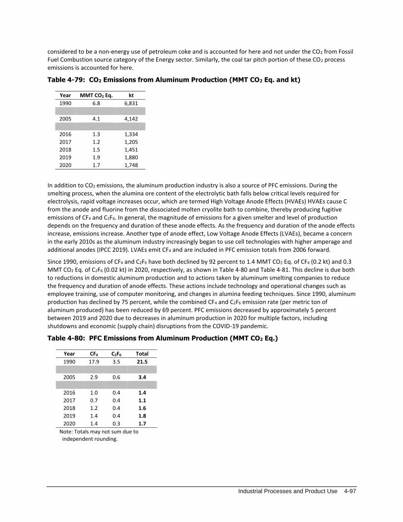
Industrial Processes and Product Use 4-97
considered to be a non-energy use of petroleum coke and is accounted for here and not under the CO2 from Fossil Fuel Combustion source category of the Energy sector. Similarly, the coal tar pitch portion of these CO2 process emissions is accounted for here.
Table 4-79: CO2 Emissions from Aluminum Production (MMT CO2 Eq. and kt)
Year MMT CO2 Eq. kt
1990 6.8 6,831
2005 4.1 4,142
2016 1.3 1,334
2017 1.2 1,205
2018 1.5 1,451
2019 1.9 1,880
2020 1.7 1,748
In addition to CO2 emissions, the aluminum production industry is also a source of PFC emissions. During the smelting process, when the alumina ore content of the electrolytic bath falls below critical levels required for electrolysis, rapid voltage increases occur, which are termed High Voltage Anode Effects (HVAEs) HVAEs cause C from the anode and fluorine from the dissociated molten cryolite bath to combine, thereby producing fugitive emissions of CF4 and C2F6. In general, the magnitude of emissions for a given smelter and level of production depends on the frequency and duration of these anode effects. As the frequency and duration of the anode effects increase, emissions increase. Another type of anode effect, Low Voltage Anode Effects (LVAEs), became a concern in the early 2010s as the aluminum industry increasingly began to use cell technologies with higher amperage and additional anodes (IPCC 2019). LVAEs emit CF4 and are included in PFC emission totals from 2006 forward.
Since 1990, emissions of CF4 and C2F6 have both declined by 92 percent to 1.4 MMT CO2 Eq. of CF4 (0.2 kt) and 0.3 MMT CO2 Eq. of C2F6 (0.02 kt) in 2020, respectively, as shown in Table 4-80 and Table 4-81. This decline is due both to reductions in domestic aluminum production and to actions taken by aluminum smelting companies to reduce the frequency and duration of anode effects. These actions include technology and operational changes such as employee training, use of computer monitoring, and changes in alumina feeding techniques. Since 1990, aluminum production has declined by 75 percent, while the combined CF4 and C2F6 emission rate (per metric ton of aluminum produced) has been reduced by 69 percent. PFC emissions decreased by approximately 5 percent between 2019 and 2020 due to decreases in aluminum production in 2020 for multiple factors, including shutdowns and economic (supply chain) disruptions from the COVID-19 pandemic.
Table 4-80: PFC Emissions from Aluminum Production (MMT CO2 Eq.)
Year CF4 C2F6 Total
1990 17.9 3.5 21.5
2005 2.9 0.6 3.4
2016 1.0 0.4 1.4
2017 0.7 0.4 1.1
2018 1.2 0.4 1.6
2019 1.4 0.4 1.8
2020 1.4 0.3 1.7
Note: Totals may not sum due to
independent rounding.

4-98 Inventory of U.S. Greenhouse Gas Emissions and Sinks: 1990–2020
Table 4-81: PFC Emissions from Aluminum Production (kt)
Year CF4 C2F6
1990 2.4 0.29
2005 0.4 0.05
2016 0.1 0.04
2017 0.1 0.03
2018 0.2 0.03
2019 0.2 0.03
2020 0.2 0.02
In 2020, U.S. primary aluminum production totaled approximately 1.012 million metric tons, a 4 percent decrease from 2019 production levels (USGS 2021). In 2020, three companies managed production at seven operational primary aluminum smelters in six states. Two smelters operated at full capacity during 2020, while four smelters operated at reduced capacity (USGS 2021). One smelter operated at reduced capacity until it was idled in July. Domestic smelters were operating at about 49 percent of capacity of 1.79 million tons per year at year end 2020 (USGS 2021).
The COVID-19 pandemic impacted domestic aluminum production and imports indirectly and directly, and neither USGS nor USAA sources have stated projections for the production year 2021.
Methodology and Time-Series Consistency Process CO2 and PFC (i.e., CF4 and C2F6) emission estimates from primary aluminum production for 2010 through 2020 are available from EPA’s GHGRP Subpart F (Aluminum Production) (EPA 2021). Under EPA’s GHGRP, facilities began reporting primary aluminum production process emissions (for 2010) in 2011; as a result, GHGRP data (for 2010 through 2020) are available to be incorporated into the Inventory. EPA’s GHGRP mandates that all facilities that contain an aluminum production process must report: CF4 and C2F6 emissions from anode effects in all prebake and Søderberg electrolysis cells, CO2 emissions from anode consumption during electrolysis in all prebake and Søderberg cells, and all CO2 emissions from onsite anode baking. To estimate the process emissions, EPA’s
GHGRP uses the process-specific equations detailed in Subpart F (aluminum production).66 These equations are based on the Tier 2/Tier 3 IPCC (2006) methods for primary aluminum production, and Tier 1 methods when estimating missing data elements. It should be noted that the same methods (i.e., 2006 IPCC Guidelines) were used for estimating the emissions prior to the availability of the reported GHGRP data in the Inventory. Prior to 2010, aluminum production data were provided through EPA’s Voluntary Aluminum Industrial Partnership (VAIP).
As previously noted, the use of petroleum coke for aluminum production is adjusted for within the Energy chapter as this fuel was consumed during non-energy related activities. Additional information on the adjustments made within the Energy sector for Non-Energy Use of Fuels is described in both the Methodology section of CO2 from Fossil Fuel Combustion (3.1 Fossil Fuel Combustion [CRF Source Category 1A]) and Annex 2.1, Methodology for Estimating Emissions of CO2 from Fossil Fuel Combustion.
Process CO2 Emissions from Anode Consumption and Anode Baking
Carbon dioxide emission estimates for the years prior to the introduction of EPA’s GHGRP in 2010 were estimated using 2006 IPCC Guidelines methods, but individual facility reported data were combined with process-specific
66 Code of Federal Regulations, Title 40: Protection of Environment, Part 98: Mandatory Greenhouse Gas Reporting, SubpartF—Aluminum Production. See https://www.ecfr.gov/cgi-bin/text-idx?SID=24a41781dfe4218b339e914de03e8727&mc=true&node=pt40.23.98&rgn=div5#sp40.23.98.f.

Industrial Processes and Product Use 4-99
emissions modeling. These estimates were based on information previously gathered from EPA’s Voluntary Aluminum Industrial Partnership (VAIP) program, U.S. Geological Survey (USGS) Mineral Commodity reviews, and The Aluminum Association (USAA) statistics, among other sources. Since pre- and post-GHGRP estimates use the same methodology, emission estimates are comparable across the time series.
Most of the CO2 emissions released during aluminum production occur during the electrolysis reaction of the C anode, as described by the following reaction:
2Al2O3 + 3C → 4Al + 3CO2
For prebake smelter technologies, CO2 is also emitted during the anode baking process. These emissions can account for approximately 10 percent of total process CO2 emissions from prebake smelters.
Depending on the availability of smelter-specific data, the CO2 emitted from electrolysis at each smelter was estimated from: (1) the smelter’s annual anode consumption, (2) the smelter’s annual aluminum production and rate of anode consumption (per ton of aluminum produced) for previous and/or following years, or (3) the smelter’s annual aluminum production and IPCC default CO2 emission factors. The first approach tracks the consumption and carbon content of the anode, assuming that all C in the anode is converted to CO2. Sulfur, ash, and other impurities in the anode are subtracted from the anode consumption to arrive at a C consumption figure. This approach corresponds to either the IPCC Tier 2 or Tier 3 method, depending on whether smelter-specific data on anode impurities are used. The second approach interpolates smelter-specific anode consumption rates to estimate emissions during years for which anode consumption data are not available. This approach avoids substantial errors and discontinuities that could be introduced by reverting to Tier 1 methods for those years. The last approach corresponds to the IPCC Tier 1 method (IPCC 2006) and is used in the absence of present or historic anode consumption data.
The equations used to estimate CO2 emissions in the Tier 2 and 3 methods vary depending on smelter type (IPCC 2006). For Prebake cells, the process formula accounts for various parameters, including net anode consumption, and the sulfur, ash, and impurity content of the baked anode. For anode baking emissions, the formula accounts for packing coke consumption, the sulfur and ash content of the packing coke, as well as the pitch content and weight of baked anodes produced. For Søderberg cells, the process formula accounts for the weight of paste consumed per metric ton of aluminum produced, and pitch properties, including sulfur, hydrogen, and ash content.
Through the VAIP, anode consumption (and some anode impurity) data have been reported for 1990, 2000, 2003, 2004, 2005, 2006, 2007, 2008, and 2009. Where available, smelter-specific process data reported under the VAIP were used; however, if the data were incomplete or unavailable, information was supplemented using industry average values recommended by IPCC (2006). Smelter-specific CO2 process data were provided by 18 of the 23 operating smelters in 1990 and 2000, by 14 out of 16 operating smelters in 2003 and 2004, 14 out of 15 operating smelters in 2005, 13 out of 14 operating smelters in 2006, 5 out of 14 operating smelters in 2007 and 2008, and 3 out of 13 operating smelters in 2009. For years where CO2 emissions data or CO2 process data were not reported by these companies, estimates were developed through linear interpolation, and/or assuming representative (e.g., previously reported or industry default) values.
In the absence of any previous historical smelter-specific process data (i.e., 1 out of 13 smelters in 2009; 1 out of 14 smelters in 2006, 2007, and 2008; 1 out of 15 smelters in 2005; and 5 out of 23 smelters between 1990 and 2003), CO2 emission estimates were estimated using Tier 1 Søderberg and/or Prebake emission factors (metric ton of CO2 per metric ton of aluminum produced) from IPCC (2006).
Process PFC Emissions from Anode Effects
High Voltage Anode Effects
Smelter-specific PFC emissions from aluminum production for 2010 through 2020 were reported to EPA under its GHGRP. To estimate their PFC emissions from HVAEs and report them under EPA’s GHGRP, smelters use an approach identical to the Tier 3 approach in the 2006 IPCC Guidelines (IPCC 2006). Specifically, they use a smelter-

4-100 Inventory of U.S. Greenhouse Gas Emissions and Sinks: 1990–2020
specific slope coefficient as well as smelter-specific operating data to estimate an emission factor using the following equation:
𝑃𝐹𝐶 = 𝑆 × 𝐴𝐸
𝐴𝐸 = 𝐹 × 𝐷
where,
PFC = CF4 or C2F6, kg/MT aluminum S = Slope coefficient, PFC/AE AE = Anode effect, minutes/cell-day F = Anode effect frequency per cell-day D = Anode effect duration, minutes
They then multiply this emission factor by aluminum production to estimate PFC emissions from HVAEs. All U.S. aluminum smelters are required to report their emissions under EPA’s GHGRP.
Perfluorocarbon emissions for the years prior to 2010 were estimated using the same equation, but the slope-factor used for some smelters was technology-specific rather than smelter-specific, making the method a Tier 2 rather than a Tier 3 approach for those smelters. Emissions and background data were reported to EPA under the VAIP. For 1990 through 2009, smelter-specific slope coefficients were available and were used for smelters representing between 30 and 94 percent of U.S. primary aluminum production. The percentage changed from year to year as some smelters closed or changed hands and as the production at remaining smelters fluctuated. For smelters that did not report smelter-specific slope coefficients, IPCC technology-specific slope coefficients were applied (IPCC 2006). The slope coefficients were combined with smelter-specific anode effect data collected by aluminum companies and reported under the VAIP to estimate emission factors over time. For 1990 through 2009, smelter-specific anode effect data were available for smelters representing between 80 and 100 percent of U.S. primary aluminum production. Where smelter-specific anode effect data were not available, representative values (e.g., previously reported or industry averages) were used.
For all smelters, emission factors were multiplied by annual production to estimate annual emissions at the smelter level. For 1990 through 2009, smelter-specific production data were available for smelters representing between 30 and 100 percent of U.S. primary aluminum production. (For the years after 2000, this percentage was near the high end of the range.) Production at non-reporting smelters was estimated by calculating the difference between the production reported under VAIP and the total U.S. production supplied by USGS or USAA, and then allocating this difference to non-reporting smelters in proportion to their production capacity. Emissions were then aggregated across smelters to estimate national emissions.
Table 4-82: Summary of HVAE Emissions
Year MMT CO2 Eq.
1990 21.5
2005 3.4
2016 1.4
2017 1.0
2018 1.6
2019 1.7
2020 1.6

Industrial Processes and Product Use 4-101
Low Voltage Anode Effects
LVAE emissions of CF4 were estimated for 2006 through 2020 based on the Tier 1 (technology-specific, production-based) method in the 2019 Refinement to the 2006 IPCC Guidelines for National Greenhouse Gas Inventories (IPCC
2019). Prior to 2006, LVAE emissions are believed to have been negligible.67 The following equation was used to estimate LVAE PFC emissions:
Equation 4-14: CF4 Emissions Resulting from Low Voltage Anode Effects
𝐿𝑉𝐴𝐸 𝐸𝐶𝐹4 = 𝐿𝑉𝐴𝐸 𝐸𝐹𝐶𝐹4 × 𝑀𝑃
where,
LVAE ECF4 = LVAE emissions of CF4 from aluminum production, kg CF4 LVAE EFCF4 = LVAE emission factor for CF4 (default by cell technology type) MP = metal production by cell technology type, tons Al.
Once LVAE emissions were estimated, they were then combined with HVAE emissions estimates to calculate total PFC emissions from aluminum production.
Table 4-83: Summary of LVAE Emissions
Year MMT CO2 Eq.
2006 0.1
2016 0.1
2017 0.1
2018 0.1
2019 0.1
2020 0.1
Production Data
Between 1990 and 2009, production data were provided under the VAIP by 21 of the 23 U.S. smelters that operated during at least part of that period. For the non-reporting smelters, production was estimated based on the difference between reporting smelters and national aluminum production levels as reported to USGS, with allocation to specific smelters based on reported production capacities (USGS 1990 through 2009).
National primary aluminum production data for 2020, 2019, and 2018 were obtained via the 2020 USGS Mineral Industry Surveys, and the 2021 USGS Mineral Commodity Summaries. For 1990 through 2001, and 2006 (see Table 4-84) data were obtained from USGS Mineral Industry Surveys: Aluminum Annual Report (USGS 1995, 1998, 2000, 2001, 2002, 2007). For 2002 through 2005, and 2007 through 2017, national aluminum production data were obtained from the USAA’s Primary Aluminum Statistics (USAA 2004 through 2006, 2008 through 2017).
67 The 2019 Refinement states, “Since 2006, the global aluminum industry has undergone changes in technology and operating conditions that make LVAE emissions much more prevalent12; these changes have occurred not only through uptake of newer technologies (e.g., PFPBL to PFPBM) but also during upgrades within the same technology in order to maximize productivity and reduce energy use” (IPCC 2019). Footnote #12 uses the example of PFPBL, which is prevalent in the United States, as an older technology that has been upgraded.

4-102 Inventory of U.S. Greenhouse Gas Emissions and Sinks: 1990–2020
Table 4-84: Production of Primary Aluminum (kt)
Year kt
1990 4,048
2005 2,478
2016 818
2017 741
2018 891
2019 1,093
2020 1,012
Methodological approaches were applied to the entire time-series to ensure time-series consistency from 1990 through 2020.
Uncertainty
Uncertainty was estimated for the CO2, CF4, and C2F6 emission values reported by each individual facility to EPA’s GHGRP, taking into consideration the uncertainties associated with aluminum production, anode effect minutes, and slope factors. The uncertainty bounds used for these parameters were established based on information collected under the VAIP and held constant through 2020. Uncertainty surrounding the reported CO2, CF4, and C2F6 emission values were determined to have a normal distribution with uncertainty ranges of approximately 6 percent below to 6 percent above, 16 percent below to 16 percent above, and 20 percent below to 20 percent above their 2020 emission estimates, respectively.
For LVAE, since emission values were not reported through EPA’s GHGRP but estimated instead through a Tier 1 methodology, the uncertainty analysis examined uncertainty associated with primary capacity data as well as technology-specific emission factors. Uncertainty for each facility’s primary capacity, reported in the USGS Yearbook, was estimated to have a Pert Beta distribution with an uncertainty range of 10 percent below to 7 percent above the capacity estimates based on the uncertainty of reported capacity data, the number of years since the facility reported new capacity data, and uncertainty in capacity utilization. Uncertainty was applied to LVAE emission factors according to technology using the uncertainty ranges provided in the 2019 Refinement to the 2006 IPCC Guidelines. An uncertainty range for Horizontal Stud Søderberg (HSS) technology was not provided in the 2019 Refinement to the 2006 IPCC Guidelines due to insufficient data, so a normal distribution and uncertainty range of ±99 percent was applied for that technology based on expert judgment. A Monte Carlo analysis was applied to estimate the overall uncertainty of the CO2, CF4, and C2F6 emission estimates for the U.S. aluminum industry as a whole, and the results are provided below.
The results of this Approach 2 quantitative uncertainty analysis are summarized in Table 4‑85. Aluminum production-related CO2 emissions were estimated to be between 1.71 and 1.79 MMT CO2 Eq. at the 95 percent confidence level. This indicates a range of approximately 2 percent below to 2 percent above the emission estimate of 1.75 MMT CO2 Eq. Also, production-related CF4 emissions were estimated to be between 1.29 and 1.50 MMT CO2 Eq. at the 95 percent confidence level. This indicates a range of approximately 7 percent below to 8 percent above the emission estimate of 1.39 MMT CO2 Eq. Aluminum production-related C2F6 emissions were estimated to be between 0.25 and 0.32 MMT CO2 Eq. at the 95 percent confidence level. This indicates a range of approximately 11 percent below to 11 percent above the emission estimate of 0.29 MMT CO2 Eq. Finally, Aluminum production-related aggregated PFCs emissions were estimated to be between 1.57 and 1.79 MMT CO2 Eq. at the 95 percent confidence level. This indicates a range of approximately 6 percent below to 7 percent above the emission estimate of 1.68 MMT CO2 Eq.
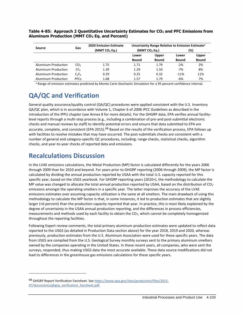
Industrial Processes and Product Use 4-103
Table 4-85: Approach 2 Quantitative Uncertainty Estimates for CO2 and PFC Emissions from Aluminum Production (MMT CO2 Eq. and Percent)
Source Gas
2020 Emission Estimate Uncertainty Range Relative to Emission Estimatea
(MMT CO2 Eq.) (MMT CO2 Eq.) (%)
Lower
Bound
Upper
Bound
Lower
Bound
Upper
Bound
Aluminum Production CO2 1.75 1.71 1.79 -2% 2%
Aluminum Production CF4 1.39 1.29 1.50 -7% 8%
Aluminum Production C2F6 0.29 0.25 0.32 -11% 11%
Aluminum Production PFCs 1.68 1.57 1.79 -6% 7%
a Range of emission estimates predicted by Monte Carlo Stochastic Simulation for a 95 percent confidence interval.
QA/QC and Verification General quality assurance/quality control (QA/QC) procedures were applied consistent with the U.S. Inventory QA/QC plan, which is in accordance with Volume 1, Chapter 6 of 2006 IPCC Guidelines as described in the introduction of the IPPU chapter (see Annex 8 for more details). For the GHGRP data, EPA verifies annual facility-level reports through a multi-step process (e.g., including a combination of pre-and post-submittal electronic checks and manual reviews by staff) to identify potential errors and ensure that data submitted to EPA are
accurate, complete, and consistent (EPA 2015).68 Based on the results of the verification process, EPA follows up with facilities to resolve mistakes that may have occurred. The post-submittals checks are consistent with a number of general and category-specific QC procedures, including: range checks, statistical checks, algorithm checks, and year-to-year checks of reported data and emissions.
Recalculations Discussion In the LVAE emissions calculations, the Metal Production (MP) factor is calculated differently for the years 2006 through 2009 than for 2010 and beyond. For years prior to GHGRP reporting (2006 through 2009), the MP factor is calculated by dividing the annual production reported by USAA with the total U.S. capacity reported for this specific year, based on the USGS yearbook. For GHGRP reporting years (2010+), the methodology to calculate the MP value was changed to allocate the total annual production reported by USAA, based on the distribution of CO2 emissions amongst the operating smelters in a specific year. The latter improves the accuracy of the LVAE emissions estimates over assuming capacity utilization is the same at all smelters. The main drawback of using this methodology to calculate the MP factor is that, in some instances, it led to production estimates that are slightly larger (<6 percent) than the production capacity reported that year. In practice, this is most likely explained by the degree of uncertainty in the USAA annual production reporting, and the differences in process efficiencies, measurements and methods used by each facility to obtain the CO2, which cannot be completely homogenized throughout the reporting facilities.
Following Expert review comments, the total primary aluminum production estimates were updated to reflect data reported to the USGS (as detailed in Production Data section above) for the year 2018, 2019 and 2020, whereas previously, production estimates from the U.S. Aluminum Association were used for these specific years. The data from USGS are compiled from the U.S. Geological Survey monthly surveys sent to the primary aluminum smelters owned by the companies operating in the United States. In these recent years, all companies, who were sent the surveys, responded, thus making USGS data the most accurate available. These data source modifications did not lead to differences in the greenhouse gas emissions calculations for these specific years.
68 GHGRP Report Verification Factsheet. See https://www.epa.gov/sites/production/files/2015-07/documents/ghgrp_verification_factsheet.pdf.

4-104 Inventory of U.S. Greenhouse Gas Emissions and Sinks: 1990–2020
Planned Improvements EPA will further investigate the sources of historical total primary aluminum production estimates for the earlier years in the timeseries and potentially update historical estimates to aim for increased consistency throughout the timeseries. As part of this planned improvement, EPA will review whether historical estimates are broken down into smelter specific production estimates, which are the basis for calculating smelter PFC (for non-partners) and CO2 emissions (for all facilities) for the 1990 through 2009 time series (years preceding GHGRP reporting).
4.20 Magnesium Production and Processing (CRF Source Category 2C4)
The magnesium metal production and casting industry uses sulfur hexafluoride (SF6) as a cover gas to prevent the rapid oxidation of molten magnesium in the presence of air. Sulfur hexafluoride has been used in this application around the world for more than thirty years. A dilute gaseous mixture of SF6 with dry air and/or carbon dioxide (CO2) is blown over molten magnesium metal to induce and stabilize the formation of a protective crust. A small portion of the SF6 reacts with the magnesium to form a thin molecular film of mostly magnesium oxide and magnesium fluoride. The amount of SF6 reacting in magnesium production and processing is considered to be negligible and thus all SF6 used is assumed to be emitted into the atmosphere. Alternative cover gases, such as AM-cover™ (containing HFC-134a), Novec™ 612 (FK-5-1-12) and dilute sulfur dioxide (SO2) systems can and are being used by some facilities in the United States. However, many facilities in the United States are still using traditional SF6 cover gas systems. Carbon dioxide is also released during primary magnesium production if carbonate based raw materials, such as dolomite, are used. During the processing of these raw materials to produce magnesium, calcination occurs which results in a release of CO2 emissions.
The magnesium industry emitted 0.9 MMT CO2 Eq. (0.04 kt) of SF6, 0.1 MMT CO2 Eq. (0.04 kt) of HFC-134a, and 0.001 MMT CO2 Eq. (0.9 kt) of CO2 in 2020. This represents a decrease of approximately 2 percent from total 2019 emissions (see Table 4-86 and Table 4-87) and a decrease in SF6 emissions by 1 percent. In 2020, total HFC-134a emissions decreased from 0.066 MMT CO2 Eq. to 0.058 MMT CO2 Eq., or a 13 percent decrease as compared to 2019 emissions. FK 5-1-12 emissions in 2020 were consistent with 2019. The emissions of the carrier gas, CO2, decreased from 1.40 kt in 2019 to 0.94 kt in 2020, or 33 percent. These decreases are likely attributed to decreasing production levels between 2019 and 2020. For the first time this year CO2 emissions from the use of dolomite in primary production are included under Magnesium Production and Processing. Previously, these emissions had been included under Other Process Uses of Carbonates. This inclusion resulted in a significant increase in CO2 emissions from 1990 through 2001, the time period during which it is known that dolomite was used in primary production, as compared to previously compiled Inventories. Additional information related to this update is provided below.
Table 4-86: SF6, HFC-134a, FK 5-1-12 and CO2 Emissions from Magnesium Production and Processing (MMT CO2 Eq.)
Year 1990 2005 2016 2017 2018 2019 2020
SF6 5.2 2.7 1.1 1.0 1.0 0.9 0.9
HFC-134a 0.0 0.0 0.1 0.1 0.1 0.1 0.1
CO2 0.1 + + + + + +
FK 5-1-12a 0.0 0.0 + + + + +
Total 5.3 2.7 1.2 1.1 1.1 0.9 0.9
+ Does not exceed 0.05 MMT CO2 Eq. a
Emissions of FK 5-1-12 are not included in totals.

Industrial Processes and Product Use 4-105
Table 4-87: SF6, HFC-134a, FK 5-1-12 and CO2 Emissions from Magnesium Production and Processing (kt)
Year 1990 2005 2016 2017 2018 2019 2020
SF6 0.2 0.1 + + + + +
HFC-134a 0.0 0.0 0.1 0.1 0.1 + +
CO2 128.5 3.3 2.8 3.3 1.6 1.4 0.9
FK 5-1-12 a 0.0 0.0 + + + + +
+ Does not exceed 0.05 kt a Emissions of FK 5-1-12 are not included in totals.
Methodology and Time-Series Consistency Emission estimates for the magnesium industry incorporate information provided by industry participants in EPA’s SF6 Emission Reduction Partnership for the Magnesium Industry as well as emissions data reported through Subpart T (Magnesium Production and Processing) of EPA’s GHGRP. The Partnership started in 1999 and, in 2010, participating companies represented 100 percent of U.S. primary and secondary production and 16 percent of the casting sector production (i.e., die, sand, permanent mold, wrought, and anode casting). SF6 emissions for 1999 through 2010 from primary production, secondary production (i.e., recycling), and die casting were generally reported by Partnership participants. Partners reported their SF6 consumption, which is assumed to be equivalent to emissions. Along with SF6, some Partners reported their HFC-134a and FK 5-1-12 consumed, which is also assumed to be equal to emissions. The last reporting year under the Partnership was 2010. Emissions data for 2011 through 2020 are obtained through EPA’s GHGRP. Under the program, owners or operators of facilities that have a magnesium production or casting process must report emissions from use of cover or carrier gases, which include SF6, HFC-134a, FK 5-1-12 and CO2. Consequently, cover and carrier gas emissions from magnesium production and processing were estimated for three time periods, depending on the source of the emissions data: 1990 through 1998 (pre-EPA Partnership), 1999 through 2010 (EPA Partnership), and 2011 through 2020 (EPA GHGRP). The methodologies described below also make use of magnesium production data published by the U.S. Geological Survey (USGS) as available.
1990 through 1998
To estimate emissions for 1990 through 1998, industry SF6 emission factors were multiplied by the corresponding metal production and consumption (casting) statistics from USGS. For this period, it was assumed that there was no use of HFC-134a or FK 5-1-12 cover gases, and hence emissions were not estimated for these alternatives.
Sulfur hexafluoride emission factors from 1990 through 1998 were based on a number of sources and assumptions. Emission factors for primary production were available from U.S. primary producers for 1994 and 1995. The primary production emission factors were 1.2 kg SF6 per metric ton for 1990 through 1993, and 1.1 kg SF6 per metric ton for 1994 through 1997. The emission factor for secondary production from 1990 through 1998 was assumed to be constant at the 1999 average Partner value. An emission factor for die casting of 4.1 kg SF6 per metric ton, which was available for the mid-1990s from an international survey (Gjestland and Magers 1996), was used for years 1990 through 1996. For 1996 through 1998, the emission factor for die casting was assumed to decline linearly to the level estimated based on Partner reports in 1999. This assumption is consistent with the trend in SF6 sales to the magnesium sector that was reported in the RAND survey of major SF6 manufacturers, which showed a decline of 70 percent from 1996 to 1999 (RAND 2002). Sand casting emission factors for 1990 through 2001 were assumed to be the same as the 2002 emission factor. The emission factors for the other processes (i.e., permanent mold, wrought, and anode casting), about which less is known, were assumed to remain constant at levels defined in Table 4-86. The emission factors for the other processes (i.e., permanent mold, wrought, and anode casting) were based on discussions with industry representatives.
The quantities of CO2 carrier gas used for each production type have been estimated using the 1999 estimated CO2 emissions data and the annual calculated rate of change of SF6 use in the 1990 through 1999 time period. For each year and production type, the rate of change of SF6 use between the current year and the subsequent year was
4-106 Inventory of U.S. Greenhouse Gas Emissions and Sinks: 1990–2020
first estimated. This rate of change was then applied to the CO2 emissions of the subsequent year to determine the CO2 emission of the current year.
Carbon dioxide emissions from the calcination of dolomite in the primary production of magnesium were calculated based on the 2006 IPCC Guidelines Tier 2 method by multiplying the estimated primary production of
magnesium by an emissions factor of 3.62 kilogram of CO2 per kilogram of magnesium produced.69 For 1990 through 1998, production was estimated to be equal to the production capacity of the facility.
1999 through 2010
The 1999 through 2010 emissions from primary and secondary production were based on information provided by EPA’s industry Partners. In some instances, there were years of missing Partner data, including SF6 consumption and metal processed. For these situations, emissions were estimated through interpolation where possible, or by holding company-reported emissions (as well as production) constant from the previous year. For alternative cover gases, including HFC-134a and FK 5-1-12, mainly reported data was relied upon. That is, unless a Partner reported using an alternative cover gas, it was not assumed it was used. Emissions of alternate gases were also estimated through linear interpolation where possible.
The die casting emission estimates for 1999 through 2010 were also based on information supplied by industry Partners. When a Partner was determined to be no longer in production, its metal production and usage rates were set to zero. Missing data on emissions or metal input was either interpolated or held constant at the last available reported value. In 1999 through 2010, Partners were assumed to account for all die casting tracked by USGS. For 1999, die casters who were not Partners were assumed to be similar to Partners who cast small parts. Due to process requirements, these casters consume larger quantities of SF6 per metric ton of processed magnesium than casters that process large parts. Consequently, emission estimates from this group of die casters were developed using an average emission factor of 5.2 kg SF6 per metric ton of magnesium. This emission factor was developed using magnesium production and SF6 usage data for the year 1999. In 2008, the derived emission factor for die casting began to increase after many years of largely decreasing emission factors. As determined through an analysis of activity data reported from the USGS, this increase is due to a temporary decrease in production at many facilities between 2008 and 2010, which reflects the change in production that occurred during the recession.
The emissions from other casting operations were estimated by multiplying emission factors (kg SF6 per metric ton of metal produced or processed) by the amount of metal produced or consumed from USGS, with the exception of some years for which Partner sand casting emissions data are available. The emission factors for sand casting activities were acquired through the data reported by the Partnership for 2002 to 2006. For 1999 through 2001, the sandcasting emission factor was held constant at the 2002 Partner-reported level. For 2007 through 2010, the sandcasting Partner did not report and the reported emission factor from 2005 was applied to the Partner and to all other sand casters. Activity data for 2005 was obtained from USGS (USGS 2005b).
The emission factors for primary production, secondary production and sand casting for the 1999 to 2010 are not published to protect company-specific production information. However, the emission factor for primary production has not risen above the average 1995 Partner value of 1.1 kg SF6 per metric ton. The emission factors for the other industry sectors (i.e., permanent mold, wrought, and anode casting) were based on discussions with industry representatives. The emission factors for casting activities are provided below in Table 4-88.
The emissions of HFC-134a and FK-5-1-12 were included in the estimates for only instances where Partners reported that information to the Partnership. Emissions of these alternative cover gases were not estimated for instances where emissions were not reported.
Carbon dioxide carrier gas emissions were estimated using the emission factors developed based on GHGRP-reported carrier gas and cover gas data, by production type. It was assumed that the use of carrier gas, by production type, is proportional to the use of cover gases. Therefore, an emission factor, in kg CO2 per kg cover gas
69 See https://www.ipcc-nggip.iges.or.jp/public/2006gl/pdf/3_Volume3/V3_4_Ch4_Metal_Industry.pdf.
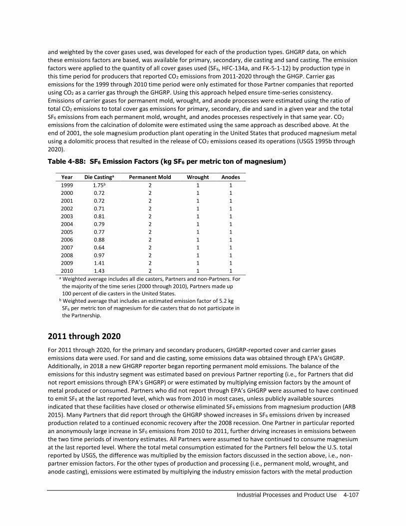
Industrial Processes and Product Use 4-107
and weighted by the cover gases used, was developed for each of the production types. GHGRP data, on which these emissions factors are based, was available for primary, secondary, die casting and sand casting. The emission factors were applied to the quantity of all cover gases used (SF6, HFC-134a, and FK-5-1-12) by production type in this time period for producers that reported CO2 emissions from 2011-2020 through the GHGP. Carrier gas emissions for the 1999 through 2010 time period were only estimated for those Partner companies that reported using CO2 as a carrier gas through the GHGRP. Using this approach helped ensure time-series consistency. Emissions of carrier gases for permanent mold, wrought, and anode processes were estimated using the ratio of total CO2 emissions to total cover gas emissions for primary, secondary, die and sand in a given year and the total SF6 emissions from each permanent mold, wrought, and anodes processes respectively in that same year. CO2 emissions from the calcination of dolomite were estimated using the same approach as described above. At the end of 2001, the sole magnesium production plant operating in the United States that produced magnesium metal using a dolomitic process that resulted in the release of CO2 emissions ceased its operations (USGS 1995b through 2020).
Table 4-88: SF6 Emission Factors (kg SF6 per metric ton of magnesium)
Year Die Castinga Permanent Mold Wrought Anodes
1999 1.75b 2 1 1
2000 0.72 2 1 1
2001 0.72 2 1 1
2002 0.71 2 1 1
2003 0.81 2 1 1
2004 0.79 2 1 1
2005 0.77 2 1 1
2006 0.88 2 1 1
2007 0.64 2 1 1
2008 0.97 2 1 1
2009 1.41 2 1 1
2010 1.43 2 1 1
a Weighted average includes all die casters, Partners and non-Partners. For the majority of the time series (2000 through 2010), Partners made up 100 percent of die casters in the United States.
b Weighted average that includes an estimated emission factor of 5.2 kg SF6 per metric ton of magnesium for die casters that do not participate in the Partnership.
2011 through 2020
For 2011 through 2020, for the primary and secondary producers, GHGRP-reported cover and carrier gases emissions data were used. For sand and die casting, some emissions data was obtained through EPA’s GHGRP. Additionally, in 2018 a new GHGRP reporter began reporting permanent mold emissions. The balance of the emissions for this industry segment was estimated based on previous Partner reporting (i.e., for Partners that did not report emissions through EPA’s GHGRP) or were estimated by multiplying emission factors by the amount of metal produced or consumed. Partners who did not report through EPA’s GHGRP were assumed to have continued to emit SF6 at the last reported level, which was from 2010 in most cases, unless publicly available sources indicated that these facilities have closed or otherwise eliminated SF6 emissions from magnesium production (ARB 2015). Many Partners that did report through the GHGRP showed increases in SF6 emissions driven by increased production related to a continued economic recovery after the 2008 recession. One Partner in particular reported an anonymously large increase in SF6 emissions from 2010 to 2011, further driving increases in emissions between the two time periods of inventory estimates. All Partners were assumed to have continued to consume magnesium at the last reported level. Where the total metal consumption estimated for the Partners fell below the U.S. total reported by USGS, the difference was multiplied by the emission factors discussed in the section above, i.e., non-partner emission factors. For the other types of production and processing (i.e., permanent mold, wrought, and anode casting), emissions were estimated by multiplying the industry emission factors with the metal production

4-108 Inventory of U.S. Greenhouse Gas Emissions and Sinks: 1990–2020
or consumption statistics obtained from USGS (USGS 2020). USGS data for 2020 were not yet available at the time of the analysis, so the 2019 values were held constant through 2020 as an estimate.
Emissions of carrier gases for permanent mold, wrought, and anode processes were estimated using an approach consistent with the 1999 through 2010 time series.
Methodological approaches were applied to the entire time series to ensure time-series consistency from 1990 through 2020. 2006 IPCC Guidance methodologies were used throughout the timeseries, mainly either a Tier 2 or Tier 3 approach depending on available data. Additionally, in this Inventory, steps were taken to ensure time-series consistency for CO2 emissions. These steps are further highlights in the recalculations discussion below.
Uncertainty Uncertainty surrounding the total estimated emissions in 2020 is attributed to the uncertainties around SF6, HFC-134a, and CO2 emission estimates. To estimate the uncertainty surrounding the estimated 2020 SF6 emissions from magnesium production and processing, the uncertainties associated with three variables were estimated: (1) emissions reported by magnesium producers and processors for 2020 through EPA’s GHGRP, (2) emissions estimated for magnesium producers and processors that reported via the Partnership in prior years but did not report 2020 emissions through EPA’s GHGRP, and (3) emissions estimated for magnesium producers and processors that did not participate in the Partnership or report through EPA’s GHGRP. An uncertainty of 5 percent was assigned to the emissions (usage) data reported by each GHGRP reporter for all the cover and carrier gases (per the 2006 IPCC Guidelines). If facilities did not report emissions data during the current reporting year through EPA’s GHGRP, SF6 emissions data were held constant at the most recent available value reported through the Partnership. The uncertainty associated with these values was estimated to be 30 percent for each year of extrapolation (per the 2006 IPCC Guidelines). The uncertainty of the total inventory estimate remained relatively constant between 2019 and 2020.
Alternate cover gas and carrier gases data was set equal to zero if the facilities did not report via the GHGRP. For those industry processes that are not represented in the Partnership, such as permanent mold and wrought casting, SF6 emissions were estimated using production and consumption statistics reported by USGS and estimated process-specific emission factors (see Table 4-89). The uncertainties associated with the emission factors and USGS-reported statistics were assumed to be 75 percent and 25 percent, respectively. Emissions associated with die casting and sand casting activities utilized emission factors based on Partner reported data with an uncertainty of 75 percent. In general, where precise quantitative information was not available on the uncertainty of a parameter, a conservative (upper-bound) value was used.
Additional uncertainties exist in these estimates that are not addressed in this methodology, such as the basic assumption that SF6 neither reacts nor decomposes during use. The melt surface reactions and high temperatures associated with molten magnesium could potentially cause some gas degradation. Previous measurement studies have identified SF6 cover gas degradation in die casting applications on the order of 20 percent (Bartos et al. 2007). Sulfur hexafluoride may also be used as a cover gas for the casting of molten aluminum with high magnesium content; however, the extent to which this technique is used in the United States is unknown.
The results of this Approach 2 quantitative uncertainty analysis are summarized in Table 4-89. Total emissions associated with magnesium production and processing were estimated to be between 0.84 and 1.00 MMT CO2 Eq. at the 95 percent confidence level. This indicates a range of approximately 9 percent below to 9 percent above the 2020 emission estimate of 0.92 MMT CO2 Eq. The uncertainty estimates for 2020 are slightly higher to the uncertainty reported for 2019 in the previous Inventory. This increase in uncertainty is attributed to the increased uncertainty around the emissions data that was estimated for reporters that did not report in 2020 or, in some cases, dating back to 2010. The longer the time period for which EPA needs to estimate emissions the larger the associated uncertainty with those emission estimates will be.

Industrial Processes and Product Use 4-109
Table 4-89: Approach 2 Quantitative Uncertainty Estimates for SF6, HFC-134a and CO2 Emissions from Magnesium Production and Processing (MMT CO2 Eq. and Percent)
Source Gas
2020 Emission Estimate Uncertainty Range Relative to Emission Estimatea
(MMT CO2 Eq.) (MMT CO2 Eq.) (%)
Lower
Bound
Upper
Bound
Lower
Bound
Upper
Bound
Magnesium
Production
SF6, HFC-
134a, CO2 0.92 0.84 1.00 -9% 9%
a Range of emission estimates predicted by Monte Carlo Stochastic Simulation for a 95 percent confidence interval.
QA/QC and Verification General quality assurance/quality control (QA/QC) procedures were applied consistent with the U.S. Inventory QA/QC plan, which is in accordance with Volume 1, Chapter 6 of 2006 IPCC Guidelines as described in the introduction of the IPPU chapter (see Annex 8 for more details). For the GHGRP data, EPA verifies annual facility-level reports through a multi-step process (e.g., including a combination of pre-and post-submittal electronic checks and manual reviews by staff) to identify potential errors and ensure that data submitted to EPA are
accurate, complete, and consistent (EPA 2015).70 Based on the results of the verification process, EPA follows up with facilities to resolve mistakes that may have occurred. The post-submittals checks are consistent with a number of general and category-specific QC procedures, including: range checks, statistical checks, algorithm checks, and year-to-year checks of reported data and emissions.
Recalculations Discussion Sand casting and permanent mold casting volumes were updated based on the release of an updated USGS Minerals Yearbook (USGS 2020). Primary production SF6 emissions were set equal to zero from 2016 through 2020 because of a confirmation that the facility transitioned completed to HFC-134a in 2016. Additionally, one facility’s reported GHGRP emissions were revised in 2017 due to additional information provided on emissions from HFC-134a and CO2. Lastly, a correction was made for a die casting facility for 2016. This facility did not report in 2016 and previously 2016 SF6 emissions were held constant at 2015 levels. This approach was updated to estimate 2016 SF6 emissions through interpolation between 2015 and 2017.
Three changes were made in this Inventory in relation to CO2 emissions. First, CO2 emissions were added for permanent mold, wrought, and anode production throughout the time series. Second, it was discovered that CO2 emissions from sand casting were not included from 1990 through 2010. These emissions were added in this Inventory. Lastly, CO2 emissions from the use of dolomite in primary production from 1990 to 2001 are now reported under Magnesium Production and Processing instead of elsewhere in the inventory, which is consistent with the 2006 IPCC Guidelines. The methods used to implement these changes are described above.
Planned Improvements Cover gas research conducted over the last decade has found that SF6 used for magnesium melt protection can have degradation rates on the order of 20 percent in die casting applications (Bartos et al. 2007). Current emission estimates assume (per the 2006 IPCC Guidelines) that all SF6 utilized is emitted to the atmosphere. Additional
70 GHGRP Report Verification Factsheet. See https://www.epa.gov/sites/production/files/2015-07/documents/ghgrp_verification_factsheet.pdf.

4-110 Inventory of U.S. Greenhouse Gas Emissions and Sinks: 1990–2020
research may lead to a revision of the 2006 IPCC Guidelines to reflect this phenomenon and until such time, developments in this sector will be monitored for possible application to the Inventory methodology.
Additional emissions are generated as byproducts from the use of alternate cover gases, which are not currently accounted for. Research on this topic is developing, and as reliable emission factors become available, these emissions will be incorporated into the Inventory.
4.21 Lead Production (CRF Source Category 2C5)
In 2020, lead was produced in the United States only using secondary production processes. Until 2014, lead production in the United States involved both primary and secondary processes—both of which emit carbon dioxide (CO2) (Sjardin 2003). Emissions from fuels consumed for energy purposes during the production of lead are accounted for in the Energy chapter.
Primary production of lead through the direct smelting of lead concentrate produces CO2 emissions as the lead concentrates are reduced in a furnace using metallurgical coke (Sjardin 2003). Primary lead production, in the form of direct smelting, previously occurred at a single smelter in Missouri. This primary lead smelter was closed at the end of 2013. In 2014, the smelter processed a small amount of residual lead during demolition of the site (USGS 2015).
Similar to primary lead production, CO2 emissions from secondary lead production result when a reducing agent, usually metallurgical coke, is added to the smelter to aid in the reduction process. Carbon dioxide emissions from secondary production also occur through the treatment of secondary raw materials (Sjardin 2003). Secondary production primarily involves the recycling of lead acid batteries and post-consumer scrap at secondary smelters. Secondary lead production has increased in the United States over the past decade, while primary lead production has decreased to production levels of zero. In 2020, secondary lead production accounted for 100 percent of total lead production. The lead-acid battery industry accounted for about 92 percent of the reported U.S. lead consumption in 2020 (USGS 2021).
In 2020, U.S. primary lead production remained at production levels of zero, and secondary lead production in the United States decreased by approximately 6 percent compared to 2019, due to the COVID-19 pandemic, the resulting quarantine-related restrictions, and a decrease in demand for lead (USGS 2021). Secondary lead production in 2020 is 19 percent higher than in 1990 (USGS 1994 and 2021). The United States has become more reliant on imported refined lead, owing to the closure of the last primary lead smelter in 2013. Exports of spent starting-lighting-ignition (SLI) batteries have been generally decreasing since 2014and were 12 percent lower in the first 9 months of 2020 compared to the same time period in 2014 (USGS 2015 through 2020). In the first 9 months of 2020, 19.7 million spent SLI lead-acid batteries were exported, slightly less than that in the same time period in 2019 (USGS 2021).
In 2020, U.S. lead production totaled 1,100,000 metric tons (USGS 2021). The resulting emissions of CO2 from 2020 lead production were estimated to be 0.5 MMT CO2 Eq. (495 kt) (see Table 4-90).
The United States was the third largest mine producer of lead in the world, behind China and Australia, and accounted for approximately 7 percent of world production in 2020 (USGS 2021).

Industrial Processes and Product Use 4-111
Table 4-90: CO2 Emissions from Lead Production (MMT CO2 Eq. and kt)
Year MMT CO2 Eq. kt
1990 0.5 516
2005 0.6 553
2016 0.5 500
2017 0.5 513
2018 0.5 513
2019 0.5 527
2020 0.5 495
After a steady increase in total emissions from 1995 to 2000, total emissions decreased between 2000 and 2013 (8 percent decline across the time period), exhibited a single year decrease of 16 percent between 2013 and 2014, gradually increased between 2014 and 2019, and are currently 4 percent lower than 1990 levels.
Methodology and Time-Series Consistency The methods used to estimate emissions for lead production71 are based on Sjardin’s work (Sjardin 2003) for lead production emissions and Tier 1 methods from the 2006 IPCC Guidelines. The Tier 1 equation is as follows:
Equation 4-15: 2006 IPCC Guidelines Tier 1: CO2 Emissions From Lead Production (Equation
4.32)
𝐶𝑂2 𝐸𝑚𝑖𝑠𝑠𝑖𝑜𝑛𝑠 = (𝐷𝑆 × 𝐸𝐹𝐷𝑆) + (𝑆 × 𝐸𝐹𝑆)
where,
DS = Lead produced by direct smelting, metric ton S = Lead produced from secondary materials EFDS = Emission factor for direct smelting, metric tons CO2/metric ton lead product EFS = Emission factor for secondary materials, metric tons CO2/metric ton lead product
For primary lead production using direct smelting, Sjardin (2003) and the 2006 IPCC Guidelines provide an emission factor of 0.25 metric tons CO2/metric ton lead. For secondary lead production, Sjardin (2003) and the 2006 IPCC Guidelines provide an emission factor of 0.25 metric tons CO2/metric ton lead for direct smelting, as well as an emission factor of 0.2 metric tons CO2/metric ton lead produced for the treatment of secondary raw materials (i.e., pretreatment of lead acid batteries). Since the secondary production of lead involves both the use of the direct smelting process and the treatment of secondary raw materials, Sjardin recommends an additive emission factor to be used in conjunction with the secondary lead production quantity. The direct smelting factor (0.25) and the sum of the direct smelting and pretreatment emission factors (0.45) are multiplied by total U.S. primary and secondary lead production, respectively, to estimate CO2 emissions.
The production and use of coking coal for lead production is adjusted for within the Energy chapter as this fuel was consumed during non-energy related activities. Additional information on the adjustments made within the Energy sector for Non-Energy Use of Fuels is described in both the Methodology section of CO2 from Fossil Fuel Combustion (3.1 Fossil Fuel Combustion (CRF Source Category 1A)) and Annex 2.1, Methodology for Estimating Emissions of CO2 from Fossil Fuel Combustion.
71 EPA has not integrated aggregated facility-level Greenhouse Gas Reporting Program (GHGRP) information to inform these estimates. The aggregated information (e.g., activity data and emissions) associated with Lead Production did not meet criteria to shield underlying confidential business information (CBI) from public disclosure.
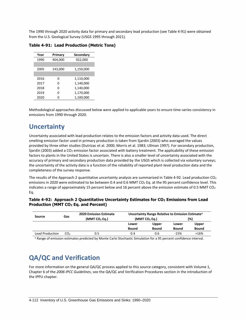
4-112 Inventory of U.S. Greenhouse Gas Emissions and Sinks: 1990–2020
The 1990 through 2020 activity data for primary and secondary lead production (see Table 4-91) were obtained
from the U.S. Geological Survey (USGS 1995 through 2021).
Table 4-91: Lead Production (Metric Tons)
Year Primary Secondary
1990 404,000 922,000
2005 143,000 1,150,000
2016 0 1,110,000
2017 0 1,140,000
2018 0 1,140,000
2019 0 1,170,000
2020 0 1,100,000
Methodological approaches discussed below were applied to applicable years to ensure time-series consistency in emissions from 1990 through 2020.
Uncertainty Uncertainty associated with lead production relates to the emission factors and activity data used. The direct smelting emission factor used in primary production is taken from Sjardin (2003) who averaged the values provided by three other studies (Dutrizac et al. 2000; Morris et al. 1983; Ullman 1997). For secondary production, Sjardin (2003) added a CO2 emission factor associated with battery treatment. The applicability of these emission factors to plants in the United States is uncertain. There is also a smaller level of uncertainty associated with the accuracy of primary and secondary production data provided by the USGS which is collected via voluntary surveys; the uncertainty of the activity data is a function of the reliability of reported plant-level production data and the completeness of the survey response.
The results of the Approach 2 quantitative uncertainty analysis are summarized in Table 4-92. Lead production CO2 emissions in 2020 were estimated to be between 0.4 and 0.6 MMT CO2 Eq. at the 95 percent confidence level. This indicates a range of approximately 15 percent below and 16 percent above the emission estimate of 0.5 MMT CO2 Eq.
Table 4-92: Approach 2 Quantitative Uncertainty Estimates for CO2 Emissions from Lead
Production (MMT CO2 Eq. and Percent)
Source Gas 2020 Emission Estimate Uncertainty Range Relative to Emission Estimatea
(MMT CO2 Eq.) (MMT CO2 Eq.) (%)
Lower
Bound
Upper
Bound
Lower
Bound
Upper
Bound
Lead Production CO2 0.5 0.4 0.6 -15% +16% a Range of emission estimates predicted by Monte Carlo Stochastic Simulation for a 95 percent confidence interval.
QA/QC and Verification For more information on the general QA/QC process applied to this source category, consistent with Volume 1, Chapter 6 of the 2006 IPCC Guidelines, see the QA/QC and Verification Procedures section in the introduction of the IPPU chapter.

Industrial Processes and Product Use 4-113
Initial review of activity data show that EPA’s GHGRP Subpart R lead production data and resulting emissions are fairly consistent with those reported by USGS. EPA is still reviewing available GHGRP data, reviewing QC analysis to understand differences in data reporting (i.e., threshold implications), and assessing the possibility of including this planned improvement in future Inventory reports (see Planned Improvements section below). Currently, GHGRP data are used for QA purposes only.
Recalculations Discussion Emissions for 2019 were revised from 0.5 MMT CO2 Eq. (540 kt) to 0.5 MMT CO2 Eq. (527 kt) based on revised USGS data for secondary lead production.
Planned Improvements Pending resources and prioritization of improvements for more significant sources, EPA will continue to evaluate and analyze data reported under EPA’s GHGRP that would be useful to improve the emission estimates and category-specific QC for the Lead Production source category, in particular considering completeness of reported lead production given the reporting threshold. Particular attention will be made to ensuring time-series consistency of the emissions estimates presented in future Inventory reports, consistent with IPCC and UNFCCC guidelines. This is required as the facility-level reporting data from EPA’s GHGRP, with the program's initial requirements for reporting of emissions in calendar year 2010, are not available for all inventory years (i.e., 1990 through 2009) as required for this Inventory. In implementing improvements and integration of data from EPA’s GHGRP, the latest guidance from the IPCC on the use of facility-level data in national inventories will be relied
upon.72
4.22 Zinc Production (CRF Source Category 2C6)
Zinc production in the United States consists of both primary and secondary processes. Of the primary and secondary processes currently used in the United States, only the electrothermic and Waelz kiln secondary processes result in non-energy carbon dioxide (CO2) emissions (Viklund-White 2000). Emissions from fuels consumed for energy purposes during the production of zinc are accounted for in the Energy chapter.
The majority of zinc produced in the United States is used for galvanizing. Galvanizing is a process where zinc coating is applied to steel in order to prevent corrosion. Zinc is used extensively for galvanizing operations in the automotive and construction industry. Zinc is also used in the production of zinc alloys and brass and bronze alloys (e.g., brass mills, copper foundries, and copper ingot manufacturing). Zinc compounds and dust are also used, to a lesser extent, by the agriculture, chemicals, paint, and rubber industries.
Production of zinc can be conducted with a range of pyrometallurgical (e.g., electrothermic furnace, Waelz kiln, flame reactor, batch retorts, Pinto process, and PIZO process) and hydrometallurgical (e.g., hydrometallurgical recovery, solvent recovery, solvent extraction-electrowinning, and electrolytic) processes. Hydrometallurgical production processes are assumed to be non-emissive since no carbon is used in these processes (Sjardin 2003). Primary production in the United States is conducted through the electrolytic process, while secondary techniques include the electrothermic and Waelz kiln processes, as well as a range of other processes. Worldwide primary zinc production also employs a pyrometallurgical process using an Imperial Smelting Furnace; however, this process is not used in the United States (Sjardin 2003).
72 See http://www.ipcc-nggip.iges.or.jp/public/tb/TFI_Technical_Bulletin_1.pdf.

4-114 Inventory of U.S. Greenhouse Gas Emissions and Sinks: 1990–2020
In the electrothermic process, roasted zinc concentrate and secondary zinc products enter a sinter feed where they are burned to remove impurities before entering an electric retort furnace. Metallurgical coke is added to the electric retort furnace as a carbon-containing reductant. This concentration step, using metallurgical coke and high temperatures, reduces the zinc oxides and produces vaporized zinc, which is then captured in a vacuum condenser. This reduction process also generates non-energy CO2 emissions.
𝑍𝑛𝑂 + 𝐶 → 𝑍𝑛(𝑔𝑎𝑠) + 𝐶𝑂2 (Reaction 1)
𝑍𝑛𝑂 + 𝐶𝑂 → 𝑍𝑛(𝑔𝑎𝑠) + 𝐶𝑂2 (Reaction 2)
In the Waelz kiln process, electric arc furnace (EAF) dust, which is captured during the recycling of galvanized steel, enters a kiln along with a reducing agent (typically carbon-containing metallurgical coke). When kiln temperatures reach approximately 1,100 to 1,200 degrees Celsius, zinc fumes are produced, which are combusted with air entering the kiln. This combustion forms zinc oxide, which is collected in a baghouse or electrostatic precipitator, and is then leached to remove chloride and fluoride. The use of carbon-containing metallurgical coke in a high-temperature fuming process results in non-energy CO2 emissions. Through this process, approximately 0.33 metric tons of zinc is produced for every metric ton of EAF dust treated (Viklund-White 2000).
In the flame reactor process, a waste feed stream, which can include EAF dust, is processed in a high-temperature environment (greater than 2,000 °C) created by the combustion of natural gas or coal and oxygen-enriched air. Volatile metals, including zinc, are forced into the gas phase and drawn into a combustion chamber, where air is introduced and oxidation occurs. The metal oxide product is then collected in a dust collection system (EPA 1992).
In 2020, the only companies in the United States that used emissive technology to produce secondary zinc products were American Zinc Recycling (AZR) (formerly “Horsehead Corporation”) and Steel Dust Recycling (SDR). PIZO Operating Company, LLC (PIZO) operated a secondary zinc production facility that processed EAF dust in Blytheville, AR from 2009 to 2012.
For AZR, EAF dust is recycled in Waelz kilns at their Calumet, IL; Palmerton, PA; Rockwood, TN; and Barnwell, SC facilities. The AZR facility in Beaumont, TX processed EAF dust via flame reactor from 1993 through 2009 (AZR 2021, Horsehead 2014). These Waelz kiln and flame reactor facilities produce intermediate zinc products (crude zinc oxide or calcine), most of which was transported to their Monaca, PA facility where the products were smelted into refined zinc using electrothermic technology. In April 2014, AZR permanently closed their Monaca smelter. This was replaced by their new facility in Mooresboro, NC in 2014.
The Mooresboro facility uses a hydrometallurgical process (i.e., solvent extraction with electrowinning technology) to produce zinc products, which is assumed to be non-emissive as described above. The current capacity of the new facility is 155,000 short tons. Production at the Mooresboro facility was idled in April 2016 and re-started in March 2020, with plans to be at full capacity by 2021 (Recycling Today 2020). Direct consumption of coal, coke, and natural gas were replaced with electricity consumption at the new Mooresboro facility. The new facility is reported to have significantly lower greenhouse gas and other air emissions than the Monaca smelter (Horsehead 2012b).
The Mooresboro facility uses leaching and solvent extraction (SX) technology combined with electrowinning, melting, and casting technology. In this process, Waelz Oxide (WOX) is first washed in water to remove soluble elements such as chlorine, potassium, and sodium, and then is leached in a sulfuric acid solution to dissolve the contained zinc creating a pregnant liquor solution (PLS). The PLS is then processed in a solvent extraction step in which zinc is selectively extracted from the PLS using an organic solvent creating a purified zinc-loaded electrolyte solution. The loaded electrolyte solution is then fed into the electrowinning process in which electrical energy is applied across a series of anodes and cathodes submerged in the electrolyte solution causing the zinc to deposit on the surfaces of the cathodes. As the zinc metal builds up on these surfaces, the cathodes are periodically harvested in order to strip the zinc from their surfaces (Horsehead 2015).
SDR recycles EAF dust into intermediate zinc products using Waelz kilns and sells the intermediate products to companies who smelt it into refined products.
Emissions of CO2 from zinc production in 2020 were estimated to be 1.0 MMT CO2 Eq. (1,008 kt CO2) (see Table 4-93). All 2020 CO2 emissions resulted from secondary zinc production processes. Emissions from zinc production

Industrial Processes and Product Use 4-115
in the United States have increased overall since 1990 due to a gradual shift from non-emissive primary production to emissive secondary production. In 2020, emissions were estimated to be 60 percent higher than they were in 1990. Emissions decreased 2 percent from 2019 levels. Due largely to the COVID-19 pandemic, a decrease in both the demand for zinc and zinc prices led to a decrease in global zinc mine production in most producing countries, including the United States. While total refined zinc production increased in 2020 due to the reopening of an idled secondary zinc refinery, consumption of refined zinc decreased in association with a decline in the U.S. steel industry as a result of the pandemic. (USGS 2021).
Table 4-93: CO2 Emissions from Zinc Production (MMT CO2 Eq. and kt)
Year MMT CO2 Eq. kt
1990 0.6 632
2005 1.0 1,030
2016 0.8 838
2017 0.9 900
2018 1.0 999
2019 1.0 1,026
2020 1.0 1,008
In 2020, United States primary and secondary refined zinc production were estimated to total 150,000 metric tons (USGS 2021) (see Table 4-94). Domestic zinc mine production decreased in 2020, owing partially to a decrease in production at the Red Dog Mine in Alaska and the closure of the Pend Oreille Mine in Washington State in July 2019. Primary zinc production (primary slab zinc) in 2018 is used as an estimate for 2019 and 2020 due to the lack of available data. Secondary zinc production in 2020 increased by 250 percent compared to 2019 and was largely influenced by the reopening of the idled AZR secondary zinc refinery in Mooresboro, NC in March 2020 (USGS 2021; AZP 2021). Secondary zinc production from the reopened facility was estimated by subtracting estimated primary zinc production from the total zinc production value obtained from the USGS Minerals Yearbook: Zinc.
Table 4-94: Zinc Production (Metric Tons) Year Primary Secondary Total
1990 262,704 95,708 358,412
2005 191,120 156,000 347,120
2016 111,000 15,000 126,000
2017 117,000 15,000 132,000
2018 101,000 15,000 116,000
2019 101,000 14,000 115,000 2020 101,000 49,000 150,000

4-116 Inventory of U.S. Greenhouse Gas Emissions and Sinks: 1990–2020
Methodology and Time-Series Consistency The methods used to estimate non-energy CO2 emissions from zinc production73 using the electrothermic primary production and Waelz kiln secondary production processes are based on Tier 1 methods from the 2006 IPCC Guidelines (IPCC 2006). The Tier 1 equation used to estimate emissions from zinc production is as follows:
Equation 4-16: 2006 IPCC Guidelines Tier 1: CO2 Emissions From Zinc Production (Equation
4.33)
𝐸𝐶𝑂2 = 𝑍𝑛 × 𝐸𝐹𝑑𝑒𝑓𝑎𝑢𝑙𝑡
where,
ECO2 = CO2 emissions from zinc production, metric tons Zn = Quantity of zinc produced, metric tons EFdefault = Default emission factor, metric tons CO2/metric ton zinc produced
The Tier 1 emission factors provided by IPCC for Waelz kiln-based secondary production were derived from metallurgical coke consumption factors and other data presented in Vikland-White (2000). These coke consumption factors as well as other inputs used to develop the Waelz kiln emission factors are shown below. IPCC does not provide an emission factor for electrothermic processes due to limited information; therefore, the Waelz kiln-specific emission factors were also applied to zinc produced from electrothermic processes. Starting in 2014, refined zinc produced in the United States used hydrometallurgical processes and is assumed to be non-emissive.
For Waelz kiln-based production, IPCC recommends the use of emission factors based on EAF dust consumption, if possible, rather than the amount of zinc produced since the amount of reduction materials used is more directly dependent on the amount of EAF dust consumed. Since only a portion of emissive zinc production facilities consume EAF dust, the emission factor based on zinc production is applied to the non-EAF dust consuming facilities, while the emission factor based on EAF dust consumption is applied to EAF dust consuming facilities.
The Waelz kiln emission factor based on the amount of zinc produced was developed based on the amount of metallurgical coke consumed for non-energy purposes per ton of zinc produced (i.e., 1.19 metric tons coke/metric ton zinc produced) (Viklund-White 2000), and the following equation:
Equation 4-17: Waelz Kiln CO2 Emission Factor for Zinc Produced
𝐸𝐹𝑊𝑎𝑒𝑙𝑧 𝐾𝑖𝑙𝑛 = 1.19 𝑚𝑒𝑡𝑟𝑖𝑐 𝑡𝑜𝑛𝑠 𝑐𝑜𝑘𝑒
𝑚𝑒𝑡𝑟𝑖𝑐 𝑡𝑜𝑛𝑠 𝑧𝑖𝑛𝑐×
0.85 𝑚𝑒𝑡𝑟𝑖𝑐 𝑡𝑜𝑛𝑠 𝐶
𝑚𝑒𝑡𝑟𝑖𝑐 𝑡𝑜𝑛𝑠 𝑐𝑜𝑘𝑒×
3.67 𝑚𝑒𝑡𝑟𝑖𝑐 𝑡𝑜𝑛𝑠 𝐶𝑂2
𝑚𝑒𝑡𝑟𝑖𝑐 𝑡𝑜𝑛𝑠 𝐶=
3.70 𝑚𝑒𝑡𝑟𝑖𝑐 𝑡𝑜𝑛𝑠 𝐶𝑂2
𝑚𝑒𝑡𝑟𝑖𝑐 𝑡𝑜𝑛𝑠 𝑧𝑖𝑛𝑐
Refined zinc production levels for AZR’s Monaca, PA facility (utilizing electrothermic technology) were available from the company for years 2005 through 2013 (Horsehead 2008, 2011, 2012, 2013, and 2014). The Monaca facility was permanently shut down in April 2014 and replaced by AZR’s new facility in Mooresboro, NC. The new facility uses hydrometallurgical process to produce refined zinc products. Hydrometallurgical production processes are assumed to be non-emissive since no carbon is used in these processes (Sjardin 2003).
Metallurgical coke consumption for non-EAF dust consuming facilities for 1990 through 2004 were extrapolated using the percentage change in annual refined zinc production at secondary smelters in the United States, as provided by the U.S. Geological Survey (USGS) Minerals Yearbook: Zinc (USGS 1995 through 2006). Metallurgical coke consumption for 2005 through 2013 were based on the secondary zinc production values obtained from the Horsehead Corporation Annual Report Form 10-k: 2005 through 2008 from the 2008 10-k (Horsehead Corp 2009); 2009 and 2010 from the 2010 10-k (Horsehead Corp. 2011); 2011 from the 2011 10-k (Horsehead Corp. 2012a);
73 EPA has not integrated aggregated facility-level Greenhouse Gas Reporting Program (GHGRP) information to inform these estimates. The aggregated information (e.g., activity data and emissions) associated with Zinc Production did not meet criteria to shield underlying confidential business information (CBI) from public disclosure.

Industrial Processes and Product Use 4-117
2012 from the 2012 10-k (Horsehead Corp. 2013); and 2013 from the 2013 10-k (Horsehead Corp. 2014). Metallurgical coke consumption levels for 2014 and later were zero due to the closure of the AZR (formerly “Horsehead Corporation”) Monaca, PA electrothermic furnace facility. The secondary zinc produced values for each year were then multiplied by the 3.70 metric tons CO2/metric ton zinc produced emission factor to develop CO2 emission estimates for the AZR electrothermic furnace facility.
The Waelz kiln emission factor based on the amount of EAF dust consumed was developed based on the amount of metallurgical coke consumed per ton of EAF dust consumed (i.e., 0.4 metric tons coke/metric ton EAF dust consumed) (Viklund-White 2000), and the following equation:
Equation 4-18: Waelz Kiln CO2 Emission Factor for EAF Dust Consumed
𝐸𝐹𝐸𝐴𝐹 𝐷𝑢𝑠𝑡 = 0.4 𝑚𝑒𝑡𝑟𝑖𝑐 𝑡𝑜𝑛𝑠 𝑐𝑜𝑘𝑒
𝑚𝑒𝑡𝑟𝑖𝑐 𝑡𝑜𝑛𝑠 𝐸𝐴𝐹 𝐷𝑢𝑠𝑡×
0.85 𝑚𝑒𝑡𝑟𝑖𝑐 𝑡𝑜𝑛𝑠 𝐶
𝑚𝑒𝑡𝑟𝑖𝑐 𝑡𝑜𝑛𝑠 𝑐𝑜𝑘𝑒×
3.67 𝑚𝑒𝑡𝑟𝑖𝑐 𝑡𝑜𝑛𝑠 𝐶𝑂2
𝑚𝑒𝑡𝑟𝑖𝑐 𝑡𝑜𝑛𝑠 𝐶=
1.24 𝑚𝑒𝑡𝑟𝑖𝑐 𝑡𝑜𝑛𝑠 𝐶𝑂2
𝑚𝑒𝑡𝑟𝑖𝑐 𝑡𝑜𝑛𝑠 𝐸𝐴𝐹 𝐷𝑢𝑠𝑡
Metallurgical coke consumption for EAF dust consuming facilities for 1990 through 2020 were calculated based on the values of EAF dust consumed. The values of EAF dust consumed for AZR, SDR, and PIZO are explained below. The total amount of EAF dust consumed by AZR at their Waelz kilns was available from AZR (formerly “Horsehead Corporation”) financial reports for years 2006 through 2015 (Horsehead 2007, 2008, 2010a, 2011, 2012a, 2013, 2014, 2015, and 2016) and from AZR for 2016, 2017, 2018, and 2019 (AZR 2020). EAF dust consumption for 2020 was not available at the time of publication and were estimated using 2019 values. The EAF dust consumption values for each year were then multiplied by the 1.24 metric tons CO2/metric ton EAF dust consumed emission factor to develop CO2 emission estimates for AZR’s Waelz kiln facilities.
The amount of EAF dust consumed by SDR and their total production capacity were obtained from SDR’s facility in Alabama for the years 2011 through 2020 (SDR 2012, 2014, 2015, 2017, 2018, 2021). The SDR facility has been operational since 2008, underwent expansion in 2011 to include a second unit (operational since early- to mid-2012), and expanded its capacity again in 2017 (SDR 2018). Annual consumption data for SDR was not publicly available for the years 2008, 2009, and 2010. These data were estimated using data for AZR’s Waelz kilns for 2008 through 2010 (Horsehead 2007, 2008, 2010a, 2010b, and 2011). Annual capacity utilization ratios were calculated using AZR’s annual consumption and total capacity for the years 2008 through 2010. AZR’s annual capacity utilization ratios were multiplied with SDR’s total capacity to estimate SDR’s consumption for each of the years, 2008 through 2010 (SDR 2013). The 1.24 metric tons CO2/metric ton EAF dust consumed emission factor was then applied to SDR’s estimated EAF dust consumption to develop CO2 emission estimates for those Waelz kiln facilities.
PIZO’s facility in Arkansas was operational from 2009 to 2012 (PIZO 2021). The amount of EAF dust consumed by PIZO’s facility for 2009 through 2012 was not publicly available. EAF dust consumption for PIZO’s facility for 2009 and 2010 were estimated by calculating annual capacity utilization of AZR’s Waelz kilns and multiplying this utilization ratio by PIZO’s total capacity (PIZO 2012). EAF dust consumption for PIZO’s facility for 2011 through 2012 were estimated by applying the average annual capacity utilization rates for AZR and SDR (Grupo PROMAX) to PIZO’s annual capacity (Horsehead 2012; SDR 2012; PIZO 2012). The 1.24 metric tons CO2/metric ton EAF dust consumed emission factor was then applied to PIZO’s estimated EAF dust consumption to develop CO2 emission estimates for those Waelz kiln facilities.
The production and use of coking coal for zinc production is adjusted for within the Energy chapter as this fuel was consumed during non-energy related activities. Additional information on the adjustments made within the Energy sector for Non-Energy Use of Fuels is described in both the Methodology section of CO2 from Fossil Fuel Combustion (3.1 Fossil Fuel Combustion (CRF Source Category 1A)) and Annex 2.1, Methodology for Estimating Emissions of CO2 from Fossil Fuel Combustion.
Beginning with the 2017 USGS Minerals Commodity Summary: Zinc, United States primary and secondary refined zinc production were reported as one value, total refined zinc production. Prior to this publication, primary and secondary refined zinc production statistics were reported separately. For the current Inventory report, EPA sought expert judgment from the USGS mineral commodity expert to assess approaches for splitting total production into primary and secondary values. For years 2016 through 2020, only one facility produced primary
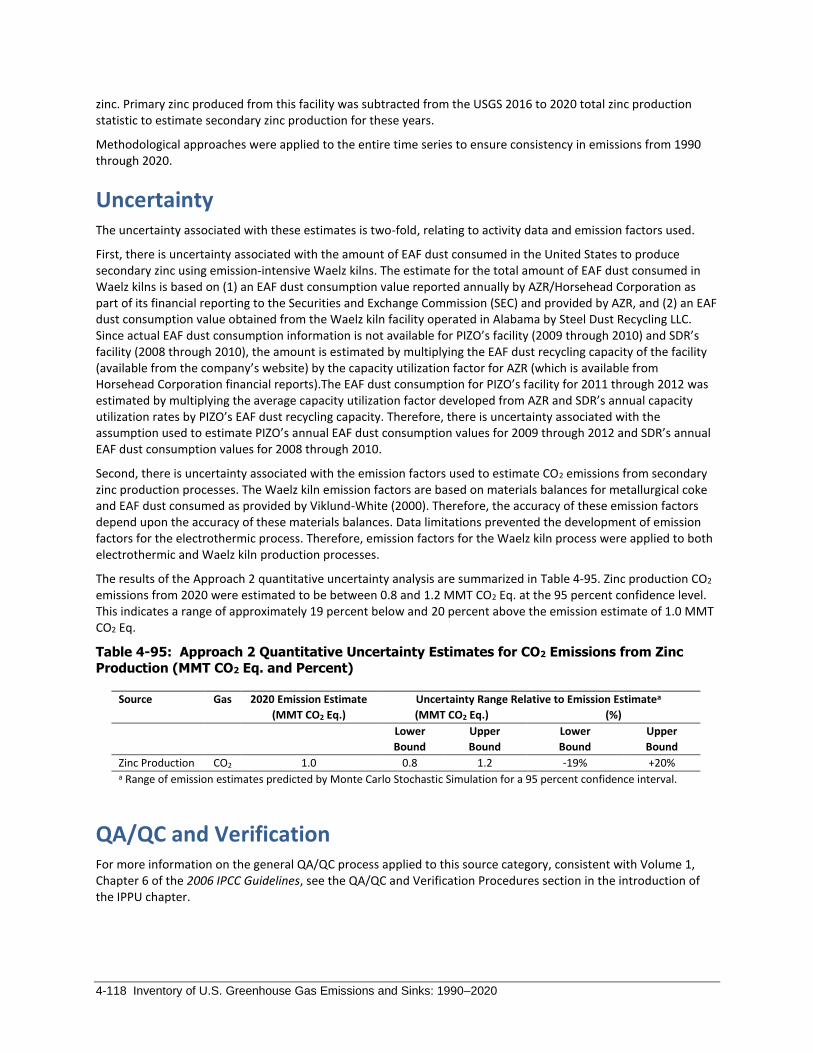
4-118 Inventory of U.S. Greenhouse Gas Emissions and Sinks: 1990–2020
zinc. Primary zinc produced from this facility was subtracted from the USGS 2016 to 2020 total zinc production statistic to estimate secondary zinc production for these years.
Methodological approaches were applied to the entire time series to ensure consistency in emissions from 1990 through 2020.
Uncertainty The uncertainty associated with these estimates is two-fold, relating to activity data and emission factors used.
First, there is uncertainty associated with the amount of EAF dust consumed in the United States to produce secondary zinc using emission-intensive Waelz kilns. The estimate for the total amount of EAF dust consumed in Waelz kilns is based on (1) an EAF dust consumption value reported annually by AZR/Horsehead Corporation as part of its financial reporting to the Securities and Exchange Commission (SEC) and provided by AZR, and (2) an EAF dust consumption value obtained from the Waelz kiln facility operated in Alabama by Steel Dust Recycling LLC. Since actual EAF dust consumption information is not available for PIZO’s facility (2009 through 2010) and SDR’s facility (2008 through 2010), the amount is estimated by multiplying the EAF dust recycling capacity of the facility (available from the company’s website) by the capacity utilization factor for AZR (which is available from Horsehead Corporation financial reports).The EAF dust consumption for PIZO’s facility for 2011 through 2012 was estimated by multiplying the average capacity utilization factor developed from AZR and SDR’s annual capacity utilization rates by PIZO’s EAF dust recycling capacity. Therefore, there is uncertainty associated with the assumption used to estimate PIZO’s annual EAF dust consumption values for 2009 through 2012 and SDR’s annual EAF dust consumption values for 2008 through 2010.
Second, there is uncertainty associated with the emission factors used to estimate CO2 emissions from secondary zinc production processes. The Waelz kiln emission factors are based on materials balances for metallurgical coke and EAF dust consumed as provided by Viklund-White (2000). Therefore, the accuracy of these emission factors depend upon the accuracy of these materials balances. Data limitations prevented the development of emission factors for the electrothermic process. Therefore, emission factors for the Waelz kiln process were applied to both electrothermic and Waelz kiln production processes.
The results of the Approach 2 quantitative uncertainty analysis are summarized in Table 4-95. Zinc production CO2 emissions from 2020 were estimated to be between 0.8 and 1.2 MMT CO2 Eq. at the 95 percent confidence level. This indicates a range of approximately 19 percent below and 20 percent above the emission estimate of 1.0 MMT CO2 Eq.
Table 4-95: Approach 2 Quantitative Uncertainty Estimates for CO2 Emissions from Zinc
Production (MMT CO2 Eq. and Percent)
Source Gas 2020 Emission Estimate Uncertainty Range Relative to Emission Estimatea
(MMT CO2 Eq.) (MMT CO2 Eq.) (%)
Lower
Bound
Upper
Bound
Lower
Bound
Upper
Bound
Zinc Production CO2 1.0 0.8 1.2 -19% +20%
a Range of emission estimates predicted by Monte Carlo Stochastic Simulation for a 95 percent confidence interval.
QA/QC and Verification For more information on the general QA/QC process applied to this source category, consistent with Volume 1, Chapter 6 of the 2006 IPCC Guidelines, see the QA/QC and Verification Procedures section in the introduction of the IPPU chapter.

Industrial Processes and Product Use 4-119
Recalculations Discussion No recalculations were made impacting emissions for the 1990 through 2019 portion of the time series.
Planned Improvements Pending resources and prioritization of improvements for more significant sources, EPA will continue to evaluate and analyze data reported under EPA’s GHGRP that would be useful to improve the emission estimates and category-specific QC for the Zinc Production source category, in particular considering completeness of reported zinc production given the reporting threshold. Given the small number of facilities in the United States, particular attention will be made to risks for disclosing CBI and ensuring time-series consistency of the emissions estimates presented in future Inventory reports, consistent with IPCC and UNFCCC guidelines. This is required as the facility-level reporting data from EPA’s GHGRP, with the program's initial requirements for reporting of emissions in calendar year 2010, are not available for all inventory years (i.e., 1990 through 2009) as required for this Inventory. In implementing improvements and integration of data from EPA’s GHGRP, the latest guidance from the IPCC on
the use of facility-level data in national inventories will be relied upon.74 This is a long-term planned improvement, and EPA is still assessing the possibility of including this improvement in future Inventory reports.
4.23 Electronics Industry (CRF Source Category 2E)
The electronics industry uses multiple greenhouse gases in its manufacturing processes. In semiconductor manufacturing, these include long-lived fluorinated greenhouse gases used for plasma etching and chamber cleaning (CRF Source Category 2E1), fluorinated heat transfer fluids used for temperature control and other applications (CRF Source Category 2E4), and nitrous oxide (N2O) used to produce thin films through chemical vapor deposition and in other applications (reported under CRF Source Category 2H3). Similar to semiconductor manufacturing, the manufacturing of micro-electro-mechanical systems (MEMS) devices (reported under CRF Source Category 2E5 Other) and photovoltaic (PV) cells (CRF Source Category 2E3) requires the use of multiple long-lived fluorinated greenhouse gases for various processes.
The gases most commonly employed in the electronics industry are trifluoromethane (hydrofluorocarbon (HFC)-23 or CHF3), perfluoromethane (CF4), perfluoroethane (C2F6), nitrogen trifluoride (NF3), and sulfur hexafluoride (SF6), although other fluorinated compounds such as perfluoropropane (C3F8) and perfluorocyclobutane (c-C4F8) are also used. The exact combination of compounds is specific to the process employed.
In addition to emission estimates for these seven commonly used fluorinated gases, this Inventory contains emissions estimates for N2O and other HFCs and unsaturated, low-GWP PFCs including C5F8, C4F6, HFC-32, HFC-41, and HFC-134a. These additional HFCs and PFCs are emitted from etching and chamber cleaning processes in much smaller amounts, accounting for 0.02 percent of emissions (in CO2 Eq.) from these processes.
For semiconductors, a single 300 mm silicon wafer that yields between 400 to 600 semiconductor products (devices or chips) may require more than 100 distinct fluorinated-gas-using process steps, principally to deposit and pattern dielectric films. Plasma etching (or patterning) of dielectric films, such as silicon dioxide and silicon nitride, is performed to provide pathways for conducting material to connect individual circuit components in each device. The patterning process uses plasma-generated fluorine atoms, which chemically react with exposed dielectric film to selectively remove the desired portions of the film. The material removed as well as undissociated
74 See http://www.ipcc-nggip.iges.or.jp/public/tb/TFI_Technical_Bulletin_1.pdf.

4-120 Inventory of U.S. Greenhouse Gas Emissions and Sinks: 1990–2020
fluorinated gases flow into waste streams and, unless emission abatement systems are employed, into the atmosphere. Plasma enhanced chemical vapor deposition (PECVD) chambers, used for depositing dielectric films, are cleaned periodically using fluorinated and other gases. During the cleaning cycle the gas is converted to fluorine atoms in plasma, which etches away residual material from chamber walls, electrodes, and chamber hardware. Undissociated fluorinated gases and other products pass from the chamber to waste streams and, unless abatement systems are employed, into the atmosphere.
In addition to emissions of unreacted gases, some fluorinated compounds can also be transformed in the plasma processes into different fluorinated compounds which are then exhausted, unless abated, into the atmosphere. For example, when C2F6 is used in cleaning or etching, CF4 is typically generated and emitted as a process byproduct. In some cases, emissions of the byproduct gas can rival or even exceed emissions of the input gas, as is the case for NF3 used in remote plasma chamber cleaning, which often generates CF4 as a byproduct.
Besides dielectric film etching and PECVD chamber cleaning, much smaller quantities of fluorinated gases are used to etch polysilicon films and refractory metal films like tungsten.
Nitrous oxide is used in manufacturing semiconductor devices to produce thin films by CVD and nitridation processes as well as for N-doping of compound semiconductors and reaction chamber conditioning (Doering 2000).
Liquid perfluorinated compounds are also used as heat transfer fluids (F-HTFs) for temperature control, device testing, cleaning substrate surfaces and other parts, and soldering in certain types of semiconductor manufacturing production processes. Leakage and evaporation of these fluids during use is a source of fluorinated gas emissions (EPA 2006). Unweighted F-HTF emissions consist primarily of perfluorinated amines, hydrofluoroethers, perfluoropolyethers (specifically, PFPMIEs), and perfluoroalkylmorpholines. One percent or less consist of HFCs, PFCs, and SF6 (where PFCs are defined as compounds including only carbon and fluorine). With the exceptions of the hydrofluoroethers and most of the HFCs, all of these compounds are very long-lived in the
atmosphere and have global warming potentials (GWPs) near 10,000.75
MEMS and photovoltaic cell manufacturing require thin film deposition and etching of material with a thickness of one micron or more, so the process is less intricate and complex than semiconductor manufacturing. The manufacturing process is different than semiconductors, but generally employs similar techniques. Like semiconductors, MEMS and photovoltaic cell manufacturers use fluorinated compounds for etching, cleaning reactor chambers, and temperature control. CF4, SF6, and the Bosch process (which consists of alternating steps of SF6 and C4F8) are used to manufacture MEMS (EPA 2010). Photovoltaic cell manufacturing predominately uses CF4, to etch crystalline silicon wafers, and C2F6 or NF3 during chamber cleaning after deposition of SiNx films (IPCC 2006), although other F-GHGs may be used. Similar to semiconductor manufacturing, both MEMS and photovoltaic cell manufacturing use N2O in depositing films and other manufacturing processes. MEMS and photovoltaic manufacturing may also employ HTFs for cooling process equipment (EPA 2010).
Emissions from all fluorinated greenhouse gases (including F-HTFs) and N2O for semiconductors, MEMS and photovoltaic cells manducating are presented in Table 4-96 below for the years 1990, 2005, and the period 2016 to 2020. The rapid growth of the electronics industry and the increasing complexity (growing number of layers and
functions)76 of electronic products led to an increase in emissions of 153 percent between 1990 and 1999, when
75 The GWP of PFPMIE, a perfluoropolyether used as an F-HTF, is included in the IPCC Fourth Assessment Report with a value of 10,300. The GWPs of the perfluorinated amines and perfluoroalkylmorpholines that are used as F-HTFs have not been evaluated in the peer-reviewed literature. However, evaluations by the manufacturer indicate that their GWPs are near 10,000 (78 FR 20632), which is expected given that these compounds are both saturated and fully fluorinated. EPA assigns a default GWP of 10,000 to compounds that are both saturated and fully fluorinated and that do not have chemical-specific GWPs in either the Fourth or the Fifth Assessment Reports. 76 Complexity is a term denoting the circuit required to connect the active circuit elements (transistors) on a chip. Increasing miniaturization, for the same chip size, leads to increasing transistor density, which, in turn, requires more complex interconnections between those transistors. This increasing complexity is manifested by increasing the levels (i.e., layers) of wiring, with each wiring layer requiring fluorinated gas usage for its manufacture.

Industrial Processes and Product Use 4-121
emissions peaked at 9.1 MMT CO2 Eq. Emissions began to decline after 1999, reaching a low point in 2009 before rebounding to 2006 emission levels and more or less plateauing at the current level, which represents a 48 percent decline from 1999 to 2020. Together, industrial growth, adoption of emissions reduction technologies (including but not limited to abatement technologies) and shifts in gas usages resulted in a net increase in emissions of approximately 32 percent between 1990 and 2020. Total emissions from semiconductor manufacture in 2020 were slightly higher than 2019 emissions, increasing by less than 1 percent, largely due to a large increase in N2O emissions.
For 2020, total GWP-weighted emissions of all fluorinated greenhouse gases and N2O from deposition, etching, and chamber cleaning processes in the U.S. semiconductor industry were estimated to be 4.7 MMT CO2 Eq. This is a decrease in emissions from 1999 of 49 percent, and an increase in emissions from 1990 of 30 percent. These trends are driven by the above stated reasons.
Emissions from all fluorinated greenhouse gases from photovoltaic cells and MEMS manufacturing, are in Table 4-96. While EPA has developed a simple methodology to estimate emissions from non-reporters and to back-cast emissions from these sources for the entire time series, there is very high uncertainty associated with these emission estimates.
The emissions reported by facilities manufacturing MEMS included emissions of C2F6, C3F8, c-C4F8, CF4, HFC-23, NF3,
N2O and SF6,77 and were equivalent to only 0.096 percent to 0.233 percent of the total reported emissions from electronics manufacturing in 2011 to 2020. F-GHG emissions, the primary type of emissions for MEMS, ranged from 0.0003 to 0.0107 MMT CO2 Eq. from 1991 to 2020. Based upon information in the World Fab Forecast (WFF), it appears that some GHGRP reporters that manufacture both semiconductors and MEMS are reporting their emissions as only from semiconductor manufacturing (GHGRP reporters must choose a single classification per fab). Emissions from non-reporters have not been estimated.
Total GWP-weighted emissions from manufacturing of photovoltaic cells were estimated to range from 0.0003 MMT CO2 Eq. to 0.0235 MMT CO2 Eq. from 1998 to 2020 and were equivalent to between 0.003 percent to 0.496 percent of the total reported emissions from electronics manufacturing. F-GHG emissions, the primary type of emissions for photovoltaic cells, ranged from 0.0003 to 0.0222 MMT CO2 Eq. from 1998 to 2020. Emissions from manufacturing of photovoltaic cells were estimated using an emission factor developed from reported data from a single manufacturer between 2015 and 2016. This emission factor was then applied to production capacity estimates from non-reporting facilities. Reported emissions from photovoltaic cell manufacturing consisted of CF4,
C2F6, c-C4F8, CHF3, NF3, and N2O.78
Emissions of F-HTFs, grouped by HFCs, PFCs or SF6 are presented in Table 4-96. Table 4-98 shows F-HTF emissions in tons by compound group based on reporting to EPA’s Greenhouse Gas Reporting Program (GHGRP) by semiconductor manufacturers during years 2014 through 2020. Emissions of F-HTFs that are not HFCs, PFCs or SF6 are not included in inventory totals and are included for informational purposes only.
Since reporting of F-HTF emissions began under EPA’s GHGRP in 2011, total F-HTF emissions (reported and estimated non-reported) have fluctuated between 0.6 MMT CO2 Eq. and 0.9 MMT CO2 Eq., with an overall declining trend. An analysis of the data reported to EPA’s GHGRP indicates that F-HTF emissions account for anywhere between 13 percent and 19 percent of total annual emissions (F-GHG, N2O and F-HTFs) from
77 Gases not reported by MEMS manufacturers to the GHGRP are currently listed as “NE” in the CRF. Since no facilities report using these gases, emissions of these gases are not estimated for this sub-sector. However, there is insufficient data to definitively conclude that they are not used by non-reporting facilities. 78 Gases not reported by PV manufacturers to the GHGRP are currently listed as “NE” in the CRF. Since no facilities report using these gases, emissions of these gases are not estimated for this sub-sector. However, there is insufficient data to definitively conclude that they are not used by non-reporting facilities.

4-122 Inventory of U.S. Greenhouse Gas Emissions and Sinks: 1990–2020
semiconductor manufacturing.79 Table 4-98 shows F-HTF emissions in tons by compound group based on reporting
to EPA’s GHGRP during years 2014 through 2020.80
Table 4-96: PFC, HFC, SF6, NF3, and N2O Emissions from Electronics Industry (MMT CO2 Eq.) Year 1990 2005 2016 2017 2018 2019 2020
CF4 0.8 1.1 1.5 1.6 1.7 1.6 1.7
C2F6 2.0 2.0 1.2 1.2 1.1 1.0 0.9
C3F8 + 0.1 0.1 0.1 0.1 0.1 0.1
C4F8 0.0 0.1 0.1 0.1 0.1 0.1 0.1
HFC-23 0.2 0.2 0.3 0.4 0.4 0.4 0.4
SF6 0.5 0.7 0.8 0.7 0.8 0.7 0.7
NF3 + 0.5 0.6 0.6 0.6 0.6 0.6
C4F6 + + + + + + +
C5F8 + + + + + + +
CH2F2 + + + + + + +
CH3F + + + + + + +
CH2FCF3 + + + + + + +
Total Semiconductors 3.6 4.6 4.7 4.6 4.8 4.4 4.4
CF4 0.0 + + + + + +
C2F6 0.0 + + + + + +
C3F8 0.0 + 0.0 0.0 0.0 0.0 0.0
C4F8 0.0 + + + + + +
HFC-23 0.0 + + + + + +
SF6 0.0 + + + + + +
NF3 0.0 + + + + + +
Total MEMS 0.0 + + + + + +
CF4 0.0 + + + + + +
C2F6 0.0 + + + + + +
C4F8 0.0 + + + + + +
HFC-23 0.0 + + + + + +
SF6 0.0 0.0 0.0 0.0 0.0 0.0 0.0
NF3 0.0 0.0 0.0 0.0 0.0 0.0 0.0
Total PV 0.0 + + + + + +
N2O (Semiconductors) + 0.1 0.2 0.3 0.3 0.2 0.3
N2O (MEMS) 0.0 + + + + + +
N2O (PV) 0.0 + + + + + +
Total N2O + 0.1 0.2 0.3 0.3 0.2 0.3
HFC, PFC and SF6 F-HTFs 0.0 + + + + + +
Total Electronics Industry 3.6 4.8 5.0 4.9 5.1 4.7 4.7
+ Does not exceed 0.05 MMT CO2 Eq.
79 Emissions data for HTFs (in tons of gas) from the semiconductor industry from 2011 through 2020 were obtained from the EPA GHGRP annual facility emissions reports. 80 Many fluorinated heat transfer fluids consist of perfluoropolymethylisopropyl ethers (PFPMIEs) of different molecular weights and boiling points that are distilled from a mixture. “BP 200 °C” (and similar terms below) indicate the boiling point of the fluid in degrees Celsius. For more information, see https://www.regulations.gov/document?D=EPA-HQ-OAR-2009-0927-0276.

Industrial Processes and Product Use 4-123
Table 4-97: PFC, HFC, SF6, NF3, and N2O Emissions from Semiconductor Manufacture (Metric Tons)
Year 1990 2005 2016 2017 2018 2019 2020
CF4 114.8 146.2 208.6 219.8 234.7 219.0 224.5
C2F6 160.0 161.7 99.5 97.6 92.9 79.1 70.3
C3F8 0.4 9.0 14.3 11.7 12.1 10.1 9.0
C4F8 0.0 11.4 5.4 5.8 6.0 5.7 5.7
HFC-23 14.6 13.7 23.2 25.7 26.5 25.5 26.5
SF6 21.7 30.7 35.7 30.0 33.4 32.4 31.8
NF3 2.8 28.5 33.2 32.8 34.1 33.2 36.1
C4F6 0.7 0.9 1.0 0.9 0.8 0.9 0.8
C5F8 0.4 0.6 0.5 0.8 0.5 1.2 0.4
CH2F2 0.7 0.9 0.9 1.1 0.9 1.0 1.1
CH3F 1.5 2.0 1.9 2.3 3.0 2.5 2.8
CH2FCF3 + + + + + + +
N2O 120.2 412.0 789.8 911.3 852.0 781.6 993.1
+ Does not exceed 0.05 MT.
Table 4-98: F-HTF Emissions from Electronics Manufacture by Compound Group (kt CO2 Eq.)
Year 2014 2015 2016 2017 2018 2019 2020
HFCs 3.3 3.0 4.1 3.6 2.7 1.1 0.9 PFCs 1.6 2.8 2.6 9.1 10.0 8.4 1.8 SF6 20.7 12.8 11.4 16.6 13.2 6.0 12.8 HFEs 4.8 4.2 7.5 2.9 4.6 1.3 5.3 PFPMIEs 182.2 208.1 173.7 148.5 183.0 171.7 149.9 Perfluoalkylromorpholines 108.3 81.5 75.7 52.3 58.6 56.4 60.9 Perfluorotrialkylamines 490.4 438.9 386.7 383.9 410.7 363.6 379.8
Total F-HTFs 811.4 751.4 661.7 616.9 682.9 608.4 611.3
Note: Emissions of F-HTFs that are not HFCs, PFCs or SF6 are not included in inventory totals and are included for informational purposes only. Emissions presented for informational purposes include HFEs, PFPMIEs, perfluoroalkylmorpholines, and perfluorotrialkylamines.
Methodology and Time-Series Consistency Emissions are based on data reported through Subpart I, Electronics Manufacture, of EPA’s GHGRP, semiconductor
manufacturing Partner-reported emissions data received through EPA’s PFC81 Reduction/Climate Partnership, EPA’s PFC Emissions Vintage Model (PEVM)—a model that estimates industry emissions from etching and chamber
cleaning processes in the absence of emission control strategies (Burton and Beizaie 2001)82—and estimates of industry activity (i.e., total manufactured layer area and manufacturing capacity). The availability and applicability of reported emissions data from the EPA Partnership and EPA’s GHGRP and activity data differ across the 1990 through 2020 time series. Consequently, fluorinated greenhouse gas (F-GHG) emissions from etching and chamber cleaning processes for semiconductors were estimated using seven distinct methods, one each for the periods 1990 through 1994, 1995 through 1999, 2000 through 2006, 2007 through 2010, 2011 and 2012, 2013 and 2014, and 2015 through 2020. Nitrous oxide emissions were estimated using five distinct methods, one each for the period 1990 through 1994, 1995 through 2010, 2011 and 2012, 2013 and 2014, and 2015 through 2020. The
81 In the context of the EPA Partnership and PEVM, PFC refers to perfluorocompounds, not perfluorocarbons. 82 A Partner refers to a participant in the U.S. EPA PFC Reduction/Climate Partnership for the Semiconductor Industry. Through a Memorandum of Understanding (MoU) with the EPA, Partners voluntarily reported their PFC emissions to the EPA by way of a third party, which aggregated the emissions through 2010.
4-124 Inventory of U.S. Greenhouse Gas Emissions and Sinks: 1990–2020
methodology discussion below for these time periods focuses on semiconductor emissions from etching, chamber cleaning, and uses of N2O. Other emissions for MEMS, photovoltaic cells, and HTFs were estimated using the approaches described immediately below.
MEMS
GHGRP-reported emissions (F-GHG and N2O) from the manufacturing of MEMS are available for the years 2011 to 2020. Emissions from manufacturing of MEMS for years prior to 2011 were calculated by linearly interpolating emissions between 1990 (at zero MMT CO2 Eq.) and 2011, the first year where emissions from manufacturing of MEMS was reported to the GHGRP. Based upon information in the World Fab Forecast (WFF), it appears that some GHGRP reporters that manufacture both semiconductors and MEMS are reporting their emissions as only from semiconductor manufacturing; however, emissions from MEMS manufacturing are likely being included in semiconductor totals. Emissions were not estimated for non-reporters.
Photovoltaic Cells
GHGRP-reported emissions (F-GHG and N2O) from the manufacturing of photovoltaic cells are available for 2011, 2012, 2015, and 2016 from two manufacturers. EPA estimates the emissions from manufacturing of PVs from non-reporting facilities by multiplying the estimated capacity of non-reporters by a calculated F-GHG emission factor and N2O emission factor based on GHGRP reported emissions from the manufacturer (in MMT CO2 Eq. per megawatt) that reported emissions in 2015 and 2016. This manufacture’s emissions are expected to be more representative of emissions from the sector, as their emissions were consistent with consuming only CF4 for etching processes and are a large-scale manufacturer, representing 28 percent of the U.S. production capacity in 2016. The second photovoltaic manufacturer only produced a small fraction of U.S. production (<3 percent). They also reported the use of NF3 in remote plasma cleaning processes, which does not have an emission factor in Part 98 for PV manufacturing, requiring them to report emissions equal to consumption. The total F-GHG emissions from non-reporters are then disaggregated into individual gases using the gas distribution from the 2015 to 2016 manufacturer. Manufacturing capacities in megawatts were drawn from DisplaySearch, a 2015 Congressional Research Service Report on U.S. Solar Photovoltaic Manufacturing, and self-reported capacity by GHGRP reporters. EPA estimated that during the 2015 to 2016 period, 28 percent of manufacturing capacity in the United States was represented through reported GHGRP emissions. Capacities are estimated for the full time series by linearly scaling the total U.S. capacity between zero in 1997 to the total capacity reported of crystalline silicon (c-Si) PV manufacturing in 2000 in DisplaySearch and then linearly scaling between the total capacity of c-Si PV manufacturing in DisplaySearch in 2009 to the total capacity of c-Si PV manufacturing reported in the Congressional Research Service report in 2012. Capacities were held constant for non-reporters for 2012 to 2020. Average emissions per MW from the GHGRP reporter in 2015 and 2016 were then applied to the total capacity prior to 2015. Emissions for 2014 from the GHGRP reporter that reported in 2015 and 2016 were scaled to the number of months open in 2014. For 1998 through 2020, emissions per MW (capacity) from the GHGRP reporter were applied to the non-reporters. For 2017 through 2020, there are no reported PV emissions. Therefore, emissions were estimated using the EPA-derived emission factor and estimated manufacturing capacity from non-reporters only.
HTFs
Facility emissions of F-HTFs from semiconductor manufacturing are reported to EPA under its GHGRP and are available for the years 2011 through 2020. EPA estimates the emissions of F-HTFs from non-reporting semiconductor facilities by calculating the ratio of GHGRP-reported fluorinated HTF emissions to GHGRP reported F-GHG emissions from etching and chamber cleaning processes, and then multiplying this ratio by the F-GHG emissions from etching and chamber cleaning processes estimated for non-reporting facilities. Fluorinated HTF use in semiconductor manufacturing is assumed to have begun in the early 2000s and to have gradually displaced other HTFs (e.g., de-ionized water and glycol) in semiconductor manufacturing (EPA 2006). For time-series consistency, EPA interpolated the share of F-HTF emissions to F-GHG emissions between 2000 (at 0 percent) and

Industrial Processes and Product Use 4-125
2011 (at 22 percent) and applied these shares to the unadjusted F-GHG emissions during those years to estimate the fluorinated HTF emissions.
Semiconductors
1990 through 1994
From 1990 through 1994, Partnership data were unavailable, and emissions were modeled using PEVM (Burton
and Beizaie 2001).83 The 1990 to 1994 emissions are assumed to be uncontrolled, since reduction strategies such as chemical substitution and abatement were yet to be developed.
PEVM is based on the recognition that fluorinated greenhouse gas emissions from semiconductor manufacturing vary with: (1) the number of layers that comprise different kinds of semiconductor devices, including both silicon wafer and metal interconnect layers, and (2) silicon consumption (i.e., the area of semiconductors produced) for each kind of device. The product of these two quantities, Total Manufactured Layer Area (TMLA), constitutes the activity data for semiconductor manufacturing. PEVM also incorporates an emission factor that expresses emissions per unit of manufactured layer-area. Emissions are estimated by multiplying TMLA by this emission factor.
PEVM incorporates information on the two attributes of semiconductor devices that affect the number of layers:
(1) linewidth technology (the smallest manufactured feature size),84 and (2) product type (discrete, memory or
logic).85 For each linewidth technology, a weighted average number of layers is estimated using VLSI product-specific worldwide silicon demand data in conjunction with complexity factors (i.e., the number of layers per Integrated Circuit (IC) specific to product type (Burton and Beizaie 2001; ITRS 2007). PEVM derives historical consumption of silicon (i.e., square inches) by linewidth technology from published data on annual wafer starts and average wafer size (VLSI Research, Inc. 2012).
The emission factor in PEVM is the average of four historical emission factors, each derived by dividing the total annual emissions reported by the Partners for each of the four years between 1996 and 1999 by the total TMLA estimated for the Partners in each of those years. Over this period, the emission factors varied relatively little (i.e., the relative standard deviation for the average was 5 percent). Since Partners are believed not to have applied significant emission reduction measures before 2000, the resulting average emission factor reflects uncontrolled emissions and hence may be use here to estimate 1990 through 1994 emissions. The emission factor is used to estimate U.S. uncontrolled emissions using publicly available data on world (including U.S.) silicon consumption.
As it was assumed for this time period that there was no consequential adoption of fluorinated-gas-reducing measures, a fixed distribution of fluorinated-gas use was assumed to apply to the entire U.S. industry to estimate gas-specific emissions. This distribution was based upon the average fluorinated-gas purchases made by semiconductor manufacturers during this period and the application of IPCC default emission factors for each gas (Burton and Beizaie 2001).
83 Various versions of the PEVM exist to reflect changing industrial practices. From 1990 to 1994 emissions estimates are from PEVM v1.0, completed in September 1998. The emission factor used to estimate 1990 to 1994 emissions is an average of the 1995 and 1996 emissions factors, which were derived from Partner reported data for those years. 84 By decreasing features of Integrated Circuit components, more components can be manufactured per device, which increases its functionality. However, as those individual components shrink it requires more layers to interconnect them to achieve the functionality. For example, a microprocessor manufactured with 65 nm feature sizes might contain as many as 1 billion transistors and require as many as 11 layers of component interconnects to achieve functionality, while a device manufactured with 130 nm feature size might contain a few hundred million transistors and require 8 layers of component interconnects (ITRS 2007). 85 Memory devices manufactured with the same feature sizes as microprocessors (a logic device) require approximately one-half the number of interconnect layers, whereas discrete devices require only a silicon base layer and no interconnect layers (ITRS 2007). Since discrete devices did not start using PFCs appreciably until 2004, they are only accounted for in the PEVM emissions estimates from 2004 onwards.

4-126 Inventory of U.S. Greenhouse Gas Emissions and Sinks: 1990–2020
PEVM only addressed the seven main F-GHGs (CF4, C2F6, C3F8, c-C4F8, HFC-23, SF6, and NF3) used in semiconductor manufacturing. Through reporting under Subpart I of EPA’s GHGRP, data on other F-GHGs (C4F6, C5F8, HFC-32, HFC-41, HFC-134a) used in semiconductor manufacturing became available and EPA was therefore able to extrapolate this data across the entire 1990 to 2020 timeseries. To estimate emissions for these “other F-GHGs”, emissions data from Subpart I were used to estimate the average share or percentage contribution of these gases as compared to total F-GHG emissions and then these shares were applied to all years prior to reported data from Subpart I (1990 through 2010) and to the emissions from non-reporters from 2011 to 2020.
To estimate N2O emissions, it was assumed the proportion of N2O emissions estimated for 1995 (discussed below) remained constant for the period of 1990 through 1994.
1995 through 1999
For 1995 through 1999, total U.S. emissions were extrapolated from the total annual emissions reported by the Partners (1995 through 1999). Partner-reported emissions are considered more representative (e.g., in terms of capacity utilization in a given year) than PEVM-estimated emissions and are used to generate total U.S. emissions when applicable. The emissions reported by the Partners were divided by the ratio of the total capacity of the plants operated by the Partners and the total capacity of all of the semiconductor plants in the United States; this ratio represents the share of capacity attributable to the Partnership. This method assumes that Partners and non-Partners have identical capacity utilizations and distributions of manufacturing technologies. Plant capacity data is contained in the World Fab Forecast (WFF) database and its predecessors, which is updated quarterly. Gas-specific emissions were estimated using the same method as for 1990 through 1994.
For this time period emissions of other F-GHGs (C4F6, C5F8, HFC-32, HFC-41, HFC-134a) were estimated using the method described above for 1990 to 1994.
For this time period, the N2O emissions were estimated using an emission factor that was applied to the annual, total U.S. TMLA manufactured. The emission factor was developed using a regression-through-the-origin (RTO) model: GHGRP reported N2O emissions were regressed against the corresponding TMLA of facilities that reported no use of abatement systems. Details on EPA’s GHGRP reported emissions and development of emission factor using the RTO model are presented in the 2011 through 2012 section. The total U.S. TMLA for 1995 through 1999 was estimated using PEVM.
2000 through 2006
Emissions for the years 2000 through 2006—the period during which Partners began the consequential application of fluorinated greenhouse gas-reduction measures—were estimated using a combination of Partner-reported emissions and adjusted PEVM modeled emissions. The emissions reported by Partners for each year were accepted as the quantity emitted from the share of the industry represented by those Partners. Remaining emissions, those from non-Partners, were estimated using PEVM, with one change. To ensure time-series consistency and to reflect the increasing use of remote clean technology (which increases the efficiency of the production process while lowering emissions of fluorinated greenhouse gases), the average non-Partner emission factor (PEVM emission factor) was assumed to begin declining gradually during this period. Specifically, the non-Partner emission factor for each year was determined by linear interpolation, using the end points of 1999 (the original PEVM emission factor) and 2011 (a new emission factor determined for the non-Partner population based on GHGRP-reported data, described below).
The portion of the U.S. total emissions attributed to non-Partners is obtained by multiplying PEVM’s total U.S.
emissions figure by the non-Partner share of U.S. total silicon capacity for each year as described above.86 Gas-specific emissions from non-Partners were estimated using linear interpolation between the gas-specific emissions distributions of 1999 (assumed to be the same as that of the total U.S. Industry in 1994) and 2011 (calculated from
86 This approach assumes that the distribution of linewidth technologies is the same between Partners and non-Partners. As discussed in the description of the method used to estimate 2007 emissions, this is not always the case.

Industrial Processes and Product Use 4-127
a subset of non-Partners that reported through the GHGRP as a result of emitting more than 25,000 MT CO2 Eq. per year). Annual updates to PEVM reflect published figures for actual silicon consumption from VLSI Research, Inc., revisions and additions to the world population of semiconductor manufacturing plants, and changes in IC fabrication practices within the semiconductor industry (see ITRS 2008 and Semiconductor Equipment and
Materials Industry 2011).87, 88, 89
For this time period emissions of other F-GHGs (C4F6, C5F8, HFC-32, HFC-41, HFC-134a) were estimated using the method described above for 1990 to 1994.
Nitrous oxide emissions were estimated using the same methodology as the 1995 through 1999 methodology.
2007 through 2010
For the years 2007 through 2010, emissions were also estimated using a combination of Partner reported emissions and adjusted PEVM modeled emissions to provide estimates for non-Partners; however, two improvements were made to the estimation method employed for the previous years in the time series. First, the 2007 through 2010 emission estimates account for the fact that Partners and non-Partners employ different distributions of manufacturing technologies, with the Partners using manufacturing technologies with greater
transistor densities and therefore greater numbers of layers.90 Second, the scope of the 2007 through 2010 estimates was expanded relative to the estimates for the years 2000 through 2006 to include emissions from research and development (R&D) fabs. This additional enhancement was feasible through the use of more detailed data published in the WFF. PEVM databases were updated annually as described above. The published world average capacity utilization for 2007 through 2010 was used for production fabs, while for R&D fabs a 20 percent figure was assumed (SIA 2009).
In addition, publicly available utilization data was used to account for differences in fab utilization for manufacturers of discrete and IC products for 2010 emissions for non-Partners. The Semiconductor Capacity Utilization (SICAS) Reports from SIA provides the global semiconductor industry capacity and utilization, differentiated by discrete and IC products (SIA 2009 through 2011). PEVM estimates were adjusted using
87 Special attention was given to the manufacturing capacity of plants that use wafers with 300 mm diameters because the actual capacity of these plants is ramped up to design capacity, typically over a 2 to 3 year period. To prevent overstating estimates of partner-capacity shares from plants using 300 mm wafers, design capacities contained in WFF were replaced with estimates of actual installed capacities for 2004 published by Citigroup Smith Barney (2005). Without this correction, the partner share of capacity would be overstated, by approximately 5 percent. For perspective, approximately 95 percent of all new capacity additions in 2004 used 300 mm wafers, and by year-end those plants, on average, could operate at approximately 70 percent of the design capacity. For 2005, actual installed capacities were estimated using an entry in the World Fab Watch database (April 2006 Edition) called “wafers/month, 8-inch equivalent,” which denoted the actual installed capacity instead of the fully-ramped capacity. For 2006, actual installed capacities of new fabs were estimated using an average monthly ramp rate of 1100 wafer starts per month (wspm) derived from various sources such as semiconductor fabtech, industry analysts, and articles in the trade press. The monthly ramp rate was applied from the first-quarter of silicon volume (FQSV) to determine the average design capacity over the 2006 period. 88 In 2006, the industry trend in co-ownership of manufacturing facilities continued. Several manufacturers, who are Partners, now operate fabs with other manufacturers, who in some cases are also Partners and in other cases are not Partners. Special attention was given to this occurrence when estimating the Partner and non-Partner shares of U.S. manufacturing capacity. 89 Two versions of PEVM are used to model non-Partner emissions during this period. For the years 2000 to 2003 PEVM v3.2.0506.0507 was used to estimate non-Partner emissions. During this time, discrete devices did not use PFCs during manufacturing and therefore only memory and logic devices were modeled in the PEVM v3.2.0506.0507. From 2004 onwards, discrete device fabrication started to use PFCs, hence PEVM v4.0.0701.0701, the first version of PEVM to account for PFC emissions from discrete devices, was used to estimate non-Partner emissions for this time period. 90 EPA considered applying this change to years before 2007, but found that it would be difficult due to the large amount of data (i.e., technology-specific global and non-Partner TMLA) that would have to be examined and manipulated for each year. This effort did not appear to be justified given the relatively small impact of the improvement on the total estimate for 2007 and the fact that the impact of the improvement would likely be lower for earlier years because the estimated share of emissions accounted for by non-Partners is growing as Partners continue to implement emission-reduction efforts.

4-128 Inventory of U.S. Greenhouse Gas Emissions and Sinks: 1990–2020
technology-weighted capacity shares that reflect the relative influence of different utilization. Gas-specific emissions for non-Partners were estimated using the same method as for 2000 through 2006.
For this time period emissions of other F-GHGs (C5F8, CH2F2, CH3F, CH2FCF3, C2H2F4) were estimated using the method described above for 1990 to 1994.
Nitrous oxide emissions were estimated using the same methodology as the 1995 through 1999 methodology.
2011 through 2012
The fifth method for estimating emissions from semiconductor manufacturing covers the period 2011 through 2012. This methodology differs from previous years because the EPA’s Partnership with the semiconductor industry ended (in 2010) and reporting under EPA’s GHGRP began. Manufacturers whose estimated uncontrolled emissions equal or exceed 25,000 MT CO2 Eq. per year (based on default F-GHG-specific emission factors and total capacity in terms of substrate area) are required to report their emissions to EPA. This population of reporters to EPA’s GHGRP included both historical Partners of EPA’s PFC Reduction/Climate Partnership as well as non-Partners
some of which use gallium arsenide (GaAs) technology in addition to Si technology.91 Emissions from the population of manufacturers that were below the reporting threshold were also estimated for this time period using EPA-developed emission factors and estimates of facility-specific production obtained from WFF. Inventory totals reflect the emissions from both reporting and non-reporting populations.
Under EPA’s GHGRP, semiconductor manufacturing facilities report emissions of F-GHGs (for all types of F-GHGs) used in etch and clean processes as well as emissions of fluorinated heat transfer fluids. (Fluorinated heat transfer fluids are used to control process temperatures, thermally test devices, and clean substrate surfaces, among other applications.) They also report N2O emissions from CVD and other processes. The F-GHGs and N2O were aggregated, by gas, across all semiconductor manufacturing GHGRP reporters to calculate gas-specific emissions for the GHGRP-reporting segment of the U.S. industry. At this time, emissions that result from heat transfer fluid use that are HFC, PFC and SF6 are included in the total emission estimates from semiconductor manufacturing, and these GHGRP-reported emissions have been compiled and presented in Table 4-96. F-HTF emissions resulting from other types of gases (e.g., HFEs) are not presented in semiconductor manufacturing totals in Table 4-96 and Table 4-97 but are shown in Table 4-98 for informational purposes.
Changes to the default emission factors and default destruction or removal efficiencies (DREs) used for GHGRP reporting affected the emissions trend between 2013 and 2014. These changes did not reflect actual emission rate changes but data improvements. Therefore, for the current Inventory, EPA adjusted the time series of GHGRP-reported data for 2011 through 2013 to ensure time-series consistency using a series of calculations that took into account the characteristics of a facility (e.g., wafer size and abatement use). To adjust emissions for facilities that did not report abatement in 2011 through 2013, EPA simply applied the revised emission factors to each facility’s estimated gas consumption by gas, process type and wafer size. In 2014, EPA also started collecting information on fab-wide DREs and the gases abated by process type, which were used in calculations for adjusting emissions from facilities that abated F-GHGs in 2011 through 2013.
• To adjust emissions for facilities that abated emissions in 2011 through 2013, EPA first calculated the quantity of gas abated in 2014 using reported F-GHG emissions, the revised default DREs (or the
estimated site-specific DRE,92 if a site-specific DRE was indicated), and the fab-wide DREs reported in
2014.93 To adjust emissions for facilities that abated emissions in 2011 through 2013, EPA first estimated
91 GaAs and Si technologies refer to the wafer on which devices are manufactured, which use the same PFCs but in different ways. 92 EPA generally assumed site-specific DREs were as follows: CF4, Etch (90 percent); all other gases, Etch (98 percent); NF3, Clean (95 percent); CF4, Clean (80 percent), and all other gases, Clean (80 percent). There were a few exceptions where a higher DRE was assumed to ensure the calculations operated correctly when there was 100 percent abatement. 93 If abatement information was not available for 2014 or the reported incorrectly in 2014, data from 2015 or 2016 was substituted.

Industrial Processes and Product Use 4-129
the percentage of gas passing through abatement systems for remote plasma clean in 2014 using the ratio of emissions reported for CF4 and NF3.
• EPA then estimated the quantity of NF3 abated for remote plasma clean in 2014 using the ratio of emissions reported for CF4 (which is not abated) and NF3. This abated quantity was then subtracted from the total abated quantity calculated as described in the bullet above.
• To account for the resulting remaining abated quantity, EPA assumed that the percentage of gas passing through abatement systems was the same across all remaining gas and process type combinations where abatement was reported for 2014.
• The percentage of gas abated was then assumed to be the same in 2011 through 2013 (if the facility claimed abatement that year) as in 2014 for each gas abated in 2014.
The revised emission factors and DREs were then applied to the estimated gas consumption for each facility by gas,
process type and wafer size.94
For the segment of the semiconductor industry that is below EPA’s GHGRP reporting threshold, and for R&D facilities, which are not covered by EPA’s GHGRP, emission estimates are based on EPA-developed emission factors for the F-GHGs and N2O and estimates of manufacturing activity. The new emission factors (in units of mass of CO2 Eq./TMLA [million square inches (MSI)]) are based on the emissions reported under EPA’s GHGRP by facilities
without abatement and on the TMLA estimates for these facilities based on the WFF (SEMI 2012, 2013).95 In a refinement of the method used to estimate emissions for the non-Partner population for prior years, different emission factors were developed for different subpopulations of fabs, disaggregated by wafer size (200 mm and 300 mm). For each of these groups, a subpopulation-specific emission factor was obtained using a regression-through-the-origin (RTO) model: facility-reported aggregate emissions of seven F-GHGs (CF4, C2F6, C3F8, c-C4F8,
CHF3, SF6 and NF3)96 were regressed against the corresponding TMLA to estimate an aggregate F-GHG emissions factor (CO2 Eq./MSI TMLA), and facility-reported N2O emissions were regressed against the corresponding TMLA to estimate a N2O emissions factor (CO2 Eq./MSI TMLA). For each subpopulation, the slope of the RTO model is the emission factor for that subpopulation. Information on the use of point-of-use abatement by non-reporting fabs was not available; thus, EPA conservatively assumed that non-reporting facilities did not use point-of-use abatement.
For 2011 and 2012, estimates of TMLA relied on the capacity utilization of the fabs published by the U.S. Census Bureau’s Historical Data Quarterly Survey of Plant Capacity Utilization (USCB 2011, 2012). Similar to the assumption for 2007 through 2010, facilities with only R&D activities were assumed to utilize only 20 percent of their manufacturing capacity. All other facilities in the United States are assumed to utilize the average percent of the manufacturing capacity without distinguishing whether fabs produce discrete products or logic products.
Non-reporting fabs were then broken out into subpopulations by wafer size (200 mm and 300 mm). using information available through the WFF. The appropriate emission factor was applied to the total TMLA of each subpopulation of non-reporting facilities to estimate the GWP-weighted emissions of that subpopulation.
Gas-specific, GWP-weighted emissions for each subpopulation of non-reporting facilities were estimated using the corresponding reported distribution of gas-specific, GWP-weighted emissions from which the aggregate emission factors, based on GHGRP-reported data, were developed. Estimated in this manner, the non-reporting population
94 Since facilities did not report by fab before 2014, fab-wide DREs were averaged if a facility had more than one fab. For facilities that reported more than one wafer size per facility, the percentages of a facility’s emissions per wafer size were estimated in 2014 and applied to earlier years, if possible. If the percentage of emissions per wafer size were unknown, a 50/50 split was used. 95 EPA does not have information on fab-wide DREs for this time period, so it is not possible to estimate uncontrolled emissions from fabs that reported point-of-use abatement. These fabs were therefore excluded from the regression analysis. (They are still included in the national totals.) 96 Only seven gases were aggregated because inclusion of F-GHGs that are not reported in the Inventory results in overestimation of emission factor that is applied to the various non-reporting subpopulations.

4-130 Inventory of U.S. Greenhouse Gas Emissions and Sinks: 1990–2020
accounted for 4.9 and 5.0 percent of U.S. emissions in 2011 and 2012, respectively. The GHGRP-reported emissions and the calculated non-reporting population emissions are summed to estimate the total emissions from semiconductor manufacturing.
2013 and 2014
For 2013 and 2014, as for 2011 and 2012, F-GHG and N2O emissions data received through EPA’s GHGRP were aggregated, by gas, across all semiconductor-manufacturing GHGRP reporters to calculate gas-specific emissions for the GHGRP-reporting segment of the U.S. industry. However, for these years WFF data was not available. Therefore, an updated methodology that does not depend on the WFF derived activity data was used to estimate emissions for the segment of the industry that are not covered by EPA’s GHGRP. For the facilities that did not report to the GHGRP (i.e., which are below EPA’s GHGRP reporting threshold or are R&D facilities), emissions were estimated based on the proportion of total U.S. emissions attributed to non-reporters for 2011 and 2012. EPA used a simple averaging method by first estimating this proportion for both F-GHGs and N2O for 2011, 2012, and 2015 through 2020, resulting in one set of proportions for F-GHGs and one set for N2O, and then applied the average of each set to the 2013 and 2014 GHGRP reported emissions to estimate the non-reporters’ emissions. Fluorinated gas-specific, GWP-weighted emissions for non-reporters were estimated using the corresponding reported distribution of gas-specific, GWP-weighted emissions reported through EPA’s GHGRP for 2013 and 2014.
GHGRP-reported emissions in 2013 were adjusted to capture changes to the default emission factors and default destruction or removal efficiencies used for GHGRP reporting, affecting the emissions trend between 2013 and 2014. EPA used the same method to make these adjustments as described above for 2011 and 2012 GHGRP data.
2015 through 2020
Similar to the methods described above for 2011 and 2012, and 2013 and 2014, EPA relied upon emissions data reported directly through the GHGRP. For 2015 through 2020, EPA took an approach similar to the one used for 2011 and 2012 to estimate emissions for the segment of the semiconductor industry that is below EPA’s GHGRP reporting threshold, and for R&D facilities, which are not covered by EPA’s GHGRP. However, in a change from previous years, EPA was able to develop new annual emission factors for 2015 through 2020 using TMLA from WFF and a more comprehensive set of emissions, i.e., fabs with as well as without abatement control, as new information about the use of abatement in GHGRP fabs and fab-wide were available. Fab-wide DREs represent total fab CO2 Eq.-weighted controlled F-GHG and N2O emissions (emissions after the use of abatement) divided by total fab CO2 Eq.-weighted uncontrolled F-GHG and N2O emissions (emission prior to the use of abatement).
Using information about reported emissions and the use of abatement and fab-wide DREs, EPA was able to calculate uncontrolled emissions (each total F-GHG and N2O) for every GHGRP reporting fab. Using this, coupled with TMLA estimated using methods described above (see 2011 through 2012), EPA derived emission factors by year, gas type (F-GHG or N2O), and wafer size (200 mm and less or 300 mm) by dividing the total annual emissions reported by GHGRP reporters by the total TMLA estimated for those reporters. These emission factors were multiplied by estimates of non-reporter TMLA to arrive at estimates of total F-GHG and N2O emissions for non-reporters for each year. For each wafer size, the total F-GHG emissions were disaggregated into individual gases using the shares of total emissions represented by those gases in the emissions reported to the GHGRP by unabated fabs producing that wafer size.
Data Sources
GHGRP reporters, which consist of former EPA Partners and non-Partners, estimated their emissions using a default emission factor method established by EPA. Like the Tier 2c Method in the 2019 Refinement to the 2006 IPCC Guidelines, this method uses different emission and byproduct generation factors for different F-GHGs and process types and uses factors for different wafer sizes (i.e., 300mm vs. 150 and 200mm) and CVD clean subtypes (in situ thermal, in situ plasma, and remote plasma). Starting with 2014 reported emissions, EPA’s GHGRP required semiconductor manufacturers to apply updated emission factors to estimate their F-GHG emissions. For the years 2011 through 2013 reported emissions, semiconductor manufacturers used older emission factors to estimate their F-GHG emissions (Federal Register / Vol. 75, No. 230 /December 1, 2010, 74829). Subpart I emission factors

Industrial Processes and Product Use 4-131
were updated for 2014 by EPA as a result of a larger set of emission factor data becoming available as part of the Subpart I petition process, which took place from 2011 through 2013. In addition to semiconductor manufacturing, GHGRP also includes reported emissions from MEMS and PV producers.
Historically, semiconductor industry partners estimated and reported their emissions using a range of methods and uneven documentation. It is assumed that most Partners used a method at least as accurate as the IPCC’s Tier 2a Methodology, recommended in the 2006 IPCC Guidelines. Partners are estimated to have accounted for between 56 and 79 percent of F-GHG emissions from U.S. semiconductor manufacturing between 1995 and 2010, with the percentage declining in recent years as Partners increasingly implemented abatement measures.
Estimates of operating plant capacities and characteristics for Partners and non-Partners were derived from the Semiconductor Equipment and Materials Industry (SEMI) WFF (formerly World Fab Watch) database (1996 through 2012, 2013, 2016, 2018, and 2021) (e.g., Semiconductor Materials and Equipment Industry 2021). Actual worldwide capacity utilizations for 2008 through 2010 were obtained from Semiconductor International Capacity Statistics (SICAS) (SIA 2009 through 2011). Estimates of the number of layers for each linewidth was obtained from International Technology Roadmap for Semiconductors: 2013 Edition (Burton and Beizaie 2001; ITRS 2007; ITRS 2008; ITRS 2011; ITRS 2013). PEVM utilized the WFF, SICAS, and ITRS, as well as historical silicon consumption estimates published by VLSI. Actual quarterly U.S. capacity utilizations for 2011, 2012, 2015 and 2016 were obtained from the U.S. Census Bureau’s Historical Data Quarterly Survey of Plant Capacity Utilization (USCB 2011, 2012, 2015, and 2016).
Estimates of PV manufacturing capacity, which are used to calculate emissions from non-reporting facilities, are based on data from two sources. A historical market analysis from DisplaySearch provided estimates of U.S. manufacturing capacity from 2000-2009 (DisplaySearch 2010). Domestic PV cell production for 2012 was obtained from a Congressional Research Service report titled U.S. Solar Photovoltaic Manufacturing: Industry Trends, Global Competition, Federal Support (Platzer 2015).
Uncertainty A quantitative uncertainty analysis of this source category was performed using the IPCC-recommended Approach 2 uncertainty estimation methodology, the Monte Carlo Stochastic Simulation technique. The Monte Carlo Stochastic Simulation was performed on the total emissions estimate from the Electronics Industry, represented in equation form as:
Equation 4-19: Total Emissions from Electronics Industry
Total Emissions (ET) = Semiconductors F-GHG and N2O Emissions (ESemi)+ MEMS F-GHG and N2O Emissions (EMEMS) + PV F-GHG and N2O Emissions (EPV) + HFC, PFC and SF6 F-HTFs Emissions (EHTF)
The uncertainty in the total emissions for the Electronics Industry, presented in Table 4-99 below, results from the convolution of four distributions of emissions, namely from semiconductors manufacturing, MEMS manufacturing, PV Manufacturing and emissions of Heat Transfer Fluids. The approaches for estimating uncertainty in each of the sources are described below:
Semiconductors Manufacture Emission Uncertainty
The Monte Carlo Stochastic Simulation was performed on the emissions estimate from semiconductor manufacturing, represented in equation form as:
Equation 4-20: Total Emissions from Semiconductor Manufacturing
Semiconductors F-GHG and N2O Emissions (ESemi) = GHGRP Reported F-GHG Emissions (ER,F-GHG, Semi) + Non-Reporters’ Estimated F-GHG Emissions (ENR,F-GHG,Semi) + GHGRP Reported N2O Emissions (ER,N2O,Semi) + Non-
Reporters’ Estimated N2O Emissions (ENR,N2O,Semi)

4-132 Inventory of U.S. Greenhouse Gas Emissions and Sinks: 1990–2020
The uncertainty in ESemi results from the convolution of four distributions of emissions, ER,F-GHG,Semi ER,N2O,Semi ENR,F-
GHG,Semi and ENR,N2O,Semi. The approaches for estimating each distribution and combining them to arrive at the reported 95 percent confidence interval (CI) for ESemi are described in the remainder of this section.
The uncertainty estimate of ER, F-GHG,Semi, or GHGRP-reported F-GHG emissions, is developed based on gas-specific uncertainty estimates of emissions for two industry segments, one processing 200 mm or less wafers and one processing 300 mm wafers. Uncertainties in emissions for each gas and industry segment are based on an uncertainty analysis conducted during the assessment of emission estimation methods for the Subpart I rulemaking in 2012 (see Technical Support for Modifications to the Fluorinated Greenhouse Gas Emission Estimation Method Option for Semiconductor Facilities under Subpart I, docket EPA–HQ–OAR–2011–0028).97 This assessment relied on facility-specific gas information by gas and wafer size, and incorporated uncertainty associated with both emission factors and gas consumption quantities. The 2012 analysis did not consider the use of abatement.
For the industry segment that manufactured 200 mm wafers, estimates of uncertainty at a 95 percent CI ranged from ±29 percent for C3F8 to ±10 percent for CF4. For the corresponding 300 mm industry segment, estimates of uncertainty at the 95 percent CI ranged from ±36 percent for C4F8 to ±16 percent for CF4. For gases for which uncertainty was not analyzed in the 2012 assessment (e.g., CH2F2), EPA applied the 95 percent CI range equivalent to the range for the gas and industry segment with the highest uncertainty from the 2012 assessment. These gas and wafer-specific uncertainty estimates were developed to represent uncertainty at a facility-level, but they are applied to the total emissions across all the facilities that did not abate emissions as reported under EPA’s GHGRP at a national-level. Hence, it is noted that the uncertainty estimates used may be overestimating the uncertainties at a national-level.
For those facilities reporting abatement of emissions under EPA’s GHGRP, estimates of uncertainties for the no abatement industry segments are modified to reflect the use of full abatement (abatement of all gases from all cleaning and etching equipment) and partial abatement. These assumptions used to develop uncertainties for the partial and full abatement facilities are identical for 200 mm and 300 mm wafer processing facilities. For all facilities reporting gas abatement, a triangular distribution of destruction or removal efficiency is assumed for each gas. The triangular distributions range from an asymmetric and highly uncertain distribution of zero percent minimum to 90 percent maximum with 70 percent most likely value for CF4 to a symmetric and less uncertain distribution of 85 percent minimum to 95 percent maximum with 90 percent most likely value for C4F8, NF3, and SF6. For facilities reporting partial abatement, the distribution of fraction of the gas fed through the abatement device, for each gas, is assumed to be triangularly distributed as well. It is assumed that no more than 50 percent of the gases are abated (i.e., the maximum value) and that 50 percent is the most likely value, and the minimum is zero percent. Consideration of abatement then resulted in four additional industry segments, two 200-mm wafer-processing segments (one fully and one partially abating each gas) and two 300-mm wafer-processing segment (one fully and the other partially abating each gas). Gas-specific emission uncertainties were estimated by
97 On November 13, 2013, EPA published a final rule revising Subpart I (Electronics Manufacturing) of the GHGRP (78 FR 68162). The revised rule includes updated default emission factors and updated default destruction and removal efficiencies that are slightly different from those that semiconductor manufacturers were required to use to report their 2012 emissions. The uncertainty analyses that were performed during the development of the revised rule focused on these updated defaults but are expected to be reasonably representative of the uncertainties associated with the older defaults, particularly for estimates at the country level. (They may somewhat underestimate the uncertainties associated with the older defaults at the facility level.) For simplicity, the 2012 estimates are assumed to be unbiased although in some cases, the updated (and therefore more representative) defaults are higher or lower than the older defaults. Multiple models and sensitivity scenarios were run for the Subpart I analysis. The uncertainty analysis presented here made use of the Input gas and wafer size model (Model 1) under the following conditions: Year = 2010, f = 20, n = SIA3.

Industrial Processes and Product Use 4-133
convolving the distributions of unabated emissions with the appropriate distribution of abatement efficiency for fully and partially abated facilities using a Monte Carlo simulation.
The uncertainty in ER,F-GHG,Semi is obtained by allocating the estimates of uncertainties to the total GHGRP-reported emissions from each of the six industry segments, and then running a Monte Carlo simulation which results in the 95 percent CI for emissions from GHGRP-reporting facilities (ER,F-GHG,Semi).
The uncertainty in ER,N2O,Semi is obtained by assuming that the uncertainty in the emissions reported by each of the GHGRP reporting facilities results from the uncertainty in quantity of N2O consumed and the N2O emission factor (or utilization). Similar to analyses completed for Subpart I (see Technical Support for Modifications to the Fluorinated Greenhouse Gas Emission Estimation Method Option for Semiconductor Facilities under Subpart I, docket EPA–HQ–OAR–2011–0028), the uncertainty of N2O consumed was assumed to be 20 percent. Consumption of N2O for GHGRP reporting facilities was estimated by back-calculating from emissions reported and assuming no abatement. The quantity of N2O utilized (the complement of the emission factor) was assumed to have a triangular distribution with a minimum value of zero percent, mode of 20 percent and maximum value of 84 percent. The minimum was selected based on physical limitations, the mode was set equivalent to the Subpart I default N2O utilization rate for chemical vapor deposition, and the maximum was set equal to the maximum utilization rate found in ISMI Analysis of Nitrous Oxide Survey Data (ISMI 2009). The inputs were used to simulate emissions for each of the GHGRP reporting, N2O-emitting facilities. The uncertainty for the total reported N2O emissions was then estimated by combining the uncertainties of each facilities’ reported emissions using Monte Carlo simulation.
The estimate of uncertainty in ENR, F-GHG,Semi and ENR, N2O,Semi entailed developing estimates of uncertainties for the emissions factors and the corresponding estimates of TMLA.
The uncertainty in TMLA depends on the uncertainty of two variables—an estimate of the uncertainty in the average annual capacity utilization for each level of production of fabs (e.g., full scale or R&D production) and a corresponding estimate of the uncertainty in the number of layers manufactured. For both variables, the distributions of capacity utilizations and number of manufactured layers are assumed triangular for all categories of non-reporting fabs. The most probable utilization is assumed to be 82 percent, with the highest and lowest utilization assumed to be 89 percent, and 70 percent, respectively. For the triangular distributions that govern the number of possible layers manufactured, it is assumed the most probable value is one layer less than reported in the ITRS; the smallest number varied by technology generation between one and two layers less than given in the ITRS and largest number of layers corresponded to the figure given in the ITRS.
The uncertainty bounds for the average capacity utilization and the number of layers manufactured are used as inputs in a separate Monte Carlo simulation to estimate the uncertainty around the TMLA of both individual facilities as well as the total non-reporting TMLA of each sub-population.
The uncertainty around the emission factors for non-reporting facilities is dependent on the uncertainty of the total emissions (MMT CO2 Eq. units) and the TMLA of each reporting facility in that category. For each wafer size for reporting facilities, total emissions were regressed on TMLA (with an intercept forced to zero) for 10,000 emission and 10,000 TMLA values in a Monte Carlo simulation, which results in 10,000 total regression coefficients (emission factors). The 2.5th and the 97.5th percentile of these emission factors are determined, and the bounds are assigned as the percent difference from the estimated emission factor.
The next step in estimating the uncertainty in emissions of reporting and non-reporting facilities in semiconductor manufacture is convolving the distribution of reported emissions, emission factors, and TMLA using Monte Carlo simulation. For this Monte Carlo simulation, the distributions of the reported F-GHG gas- and wafer size-specific emissions are assumed to be normally distributed, and the uncertainty bounds are assigned at 1.96 standard deviations around the estimated mean. The were some instances, though, where departures from normality were observed for variables, including for the distributions of the gas- and wafer size-specific N2O emissions, TMLA, and non-reporter emission factors, both for F-GHGs and N2O. As a result, the distributions for these parameters were assumed to follow a pert beta distribution.
MEMS Manufacture Emission Uncertainty
The Monte Carlo Stochastic Simulation was performed on the emissions estimate from MEMS manufacturing,

4-134 Inventory of U.S. Greenhouse Gas Emissions and Sinks: 1990–2020
represented in equation form as:
Equation 4-21: Total Emissions from MEMS Manufacturing
MEMS F-GHG and N2O Emissions (EMEMS) = GHGRP Reported F-GHG Emissions (ER,F-GHG,MEMS) + GHGRP Reported N2O Emissions (ER,N2O, MEMS)
Emissions from MEMS manufacturing are only quantified for GHGRP reporters. MEMS manufacturers that report to the GHGRP all report the use of 200 mm wafers. Some MEMS manufacturers report using abatement equipment. Therefore, the estimates of uncertainty at the 95 percent CI for each gas emitted by MEMS manufacturers are set equal to the gas-specific uncertainties for manufacture of 200mm semiconductor wafers with partial abatement. The same assumption is applied for uncertainty levels for GHGRP reported MEMS N2O emissions (ER,N2O,MEMS).
PV Manufacture Emission Uncertainty
The Monte Carlo Stochastic Simulation was performed on the emissions estimate from PV manufacturing, represented in equation form as:
Equation 4-22: Total Emissions from PV Manufacturing
PV F-GHG and N2O Emissions (EPV) = Non-Reporters’ Estimated F-GHG Emissions (ENR,F-GHG,PV) + Non-Reporters’ Estimated N2O Emissions (ENR,N2O,PV)
Emissions from PV manufacturing are only estimated for non-GHGRP reporters. There were no reported emissions from PV manufacturing in GHGRP in 2020. The “Non-Reporters’ Estimated F-GHG Emissions” term was estimated using an emission factor developed using emissions from reported data in 2015 and 2016 and total non-reporters’ capacity. Due to a lack of information and data and because they represent similar physical and chemical processes, the uncertainty at the 95 percent I level for non-reporter PV capacity is assumed to be the same as the uncertainty in non-reporter TMLA for semiconductor manufacturing. Similarly, the uncertainty for the PV manufacture emission factors are assumed to be the same as the uncertainties in emission factors used for non-reporters in semiconductor manufacture.
Heat Transfer Fluids Emission Uncertainty
There is a lack of data related to the uncertainty of emission estimates of heat transfer fluids used for electronics manufacture. Therefore, per the 2006 IPCC Guidelines (IPCC 2006, Volume 3, Chapter 6), uncertainty bounds of 20 percent were applied to the segments of PFCs, HFCs and SF6 at national levels.
The results of the Approach 2 quantitative uncertainty analysis for electronics manufacturing are summarized in Table 4-99. These results were obtained by convolving—using Monte Carlo simulation—the distributions of emissions for each reporting and non-reporting facility that manufactures semiconductors, MEMS, or PVs. The emissions estimate for total U.S. F-GHG, N2O, and HTF emissions from electronics manufacturing were estimated to be between 4.45 and 5.03 MMT CO2 Eq. at a 95 percent confidence level. This range represents 6 percent below to 6 percent above the 2020 emission estimate of 4.74 MMT CO2 Eq. for all emissions from electronics manufacture. This range and the associated percentages apply to the estimate of total emissions rather than those of individual gases. Uncertainties associated with individual gases will be somewhat higher than the aggregate but were not explicitly modeled.
Table 4-99: Approach 2 Quantitative Uncertainty Estimates for HFC, PFC, SF6, NF3 and N2O
Emissions from Electronics Manufacture (MMT CO2 Eq. and Percent)
Source Gas
2020 Emission
Estimate Uncertainty Range Relative to Emission Estimatea
(MMT CO2 Eq.) (MMT CO2 Eq.) (%)
Lower
Boundb
Upper
Boundb
Lower
Bound
Upper
Bound
Electronics
Industry
HFC, PFC, SF6,
NF3, and N2O 4.74 4.45 5.03 -6% 6%

Industrial Processes and Product Use 4-135
a Range of emission estimates predicted by Monte Carlo Stochastic Simulation for a 95 percent confidence interval. b Absolute lower and upper bounds were calculated using the corresponding lower and upper bounds in percentages.
QA/QC and Verification For its GHGRP data, EPA verifies annual facility-level reports through a multi-step process (e.g., including a combination of pre-and post-submittal electronic checks and manual reviews by staff) to identify potential errors
and ensure that data submitted to EPA are accurate, complete, and consistent (EPA 2015).98 Based on the results of the verification process, EPA follows up with facilities to resolve mistakes that may have occurred. The post-submittals checks are consistent with a number of general and category-specific QC procedures including range checks, statistical checks, algorithm checks, and year-to-year checks of reported data and emissions.
For more information on the general QA/QC process applied to this source category, consistent with Volume 1, Chapter 6 of the 2006 IPCC Guidelines, see the QA/QC and Verification Procedures section in the introduction of the IPPU chapter and Annex 8 for more details.
Recalculations Discussion Emissions from 2015 through 2020 were updated to reflect updated emissions reporting in EPA’s GHGRP, relative to the previous Inventory. Additionally, EPA made the following changes:
• To estimate non-reporter F-GHG and N2O emissions, EPA relies on data reported through Subpart I and the World Fab Forecast. This process requires EPA to map facilities that report through Subpart I and which are also represented in the World Fab Forecast. For this inventory update, EPA identified and made corrections to a few instances of this mapping based on new information and additional reviews of the data. This had minimal effects on emission estimates.
• In the dataset used to estimate photovoltaics manufacturing capacity from 2000 to 2009, a correction was made to the formula which sums annual capacity across all producers. This resulted in slight changes to emissions estimates for the years where this dataset is used.
• Previously, all N2O emissions were attributed solely to semiconductor manufacturing. For this inventory update, EPA revised the N2O estimates by assigning emissions to the specific types of electronics manufacturing (i.e., semiconductor, photovoltaic cells, and MEMS). N2O estimates are now reported with subtotals for each product type within the electronics industry.
• EPA revised the individual gases reported for semiconductor manufacturing to remove the “Other F-GHGs” category and replace it with separate totals for each individual gas. Similarly, EPA also updated the MEMS and photovoltaic cells estimates to show disaggregated totals for each individual HFC and PFC compound.
• A GHGRP fab that had previously been identified as a MEMS fab was determined to have produced photovoltaics. Their F-GHG emissions were removed from the MEMS totals and added to the PV totals.
• Previously, F-GHG emissions in 2016 from a PV manufacturer reporting through the GHGRP were held constant for 2017 through the most recent Inventory year. EPA determined that this manufacturer ceased operations in 2016, so their reported emissions were changed to zero for 2017 and beyond.
98 GHGRP Report Verification Factsheet. See https://www.epa.gov/sites/production/files/2015-07/documents/ghgrp_verification_factsheet.pdf.

4-136 Inventory of U.S. Greenhouse Gas Emissions and Sinks: 1990–2020
• To improve the uncertainty analysis for this source category other F-GHGs from semiconductor manufacturing, HFC, PFC, and SF6 emissions from the use of heat transfer fluids and emissions resulting from the manufacturing of PVs and MEMS were included in total uncertainty estimates.
Overall, the impact of these recalculations led to an average decrease of 0.02 MMT CO2 Eq. (0.44 percent) across the time series (1990 through 2019).
Planned Improvements The Inventory methodology uses data reported through the EPA Partnership (for earlier years) and EPA’s GHGRP (for later years) to extrapolate the emissions of the non-reporting population. While these techniques are well developed, the understanding of the relationship between the reporting and non-reporting populations is limited. Further analysis of the reporting and non-reporting populations could aid in the accuracy of the non-reporting population extrapolation in future years. In addition, the accuracy of the emissions estimates for the non-reporting population could be further increased through EPA’s further investigation of and improvement upon the accuracy of estimated activity in the form of TMLA.
The Inventory uses utilization from two different sources for various time periods–SEMI to develop PEVM and to estimate non-Partner emissions for the period 1995 to 2010 and U.S. Census Bureau for 2011 through 2014. SEMI reported global capacity utilization for manufacturers through 2011. U.S. Census Bureau capacity utilization include U.S. semiconductor manufacturers as well as assemblers. Further analysis on the impacts of using a new and different source of utilization data could prove to be useful in better understanding of industry trends and impacts of utilization data sources on historical emission estimates.
Estimates of semiconductor non-reporter and non-Partner emissions are based on EPA-developed emission factors for the time periods pre-2010, 2011 through 2012, and 2015 through 2020. Based on the data available for these time periods, the methods used to develop emission factors for non-reporters and non-Partners are slightly inconsistent for semiconductors (e.g., how data representing emissions and TMLA from the manufacture of various wafer sizes are aggregated or disaggregated for purposes of calculating emission factors). Further analyses to support potentially adjusting the methods for developing these emission factors could be done to better ensure consistency across the time series.
The methodology for estimating semiconductor emissions from non-reporters uses data from the International Technology Roadmap for Semiconductors (ITRS) on the number of layers associated with various technology node sizes. The ITRS has now been replaced by the International Roadmap for Devices and Systems (IRDS), which has published updated data on the number of layers used in each device type and node size (in nanometers). Incorporating this updated dataset will improve the accuracy of emissions estimates from non-reporting semiconductor fabs.
4.24 Substitution of Ozone Depleting Substances (CRF Source Category 2F)
Hydrofluorocarbons (HFCs) and perfluorocarbons (PFCs) are used as alternatives to several classes of ozone-depleting substances (ODSs) that are being phased out under the terms of the Montreal Protocol and the Clean Air
Act Amendments of 1990.99 Ozone-depleting substances—chlorofluorocarbons (CFCs), halons, carbon tetrachloride, methyl chloroform, and hydrochlorofluorocarbons (HCFCs)—are used in a variety of industrial applications including refrigeration and air conditioning equipment, solvent cleaning, foam production, sterilization, fire extinguishing, and aerosols. Although HFCs and PFCs are not harmful to the stratospheric ozone
99 [42 U.S.C § 7671, CAA Title VI].

Industrial Processes and Product Use 4-137
layer, they are potent greenhouse gases. On December 27, 2020, the American Innovation and Manufacturing (AIM) Act was enacted by Congress and directs EPA to address HFCs by phasing down production and consumption (i.e., production plus import minus export), maximizing reclamation and minimizing releases from equipment, and facilitating the transition to next-generation technologies through sector-based restrictions. Emission estimates for
HFCs and PFCs used as substitutes for ODSs are provided in Table 4-100 and Table 4-101.100
Table 4-100: Emissions of HFCs and PFCs from ODS Substitutes (MMT CO2 Eq.)
Gas 1990 2005 2016 2017 2018 2019 2020
HFC-23 0.0 + + + + + +
HFC-32 0.0 0.3 4.6 5.3 6.0 6.8 7.7
HFC-125 + 9.0 46.9 50.1 53.7 58.4 63.5
HFC-134a + 80.1 69.1 64.7 62.1 60.9 59.5
HFC-143a + 9.4 28.2 28.0 27.7 27.8 27.9
HFC-236fa 0.0 1.2 1.3 1.2 1.2 1.1 1.1
CF4 0.0 + + + 0.1 0.1 0.1
Othersa 0.2 7.2 14.9 16.1 16.6 16.8 16.6
Total 0.2 107.2 165.1 165.5 167.3 171.8 176.3
+ Does not exceed 0.05 MMT CO2 Eq. a Others represent an unspecified mix of HFCs and PFCs, which includes HFC-152a, HFC-227ea, HFC-245fa,
HFC-365mfc, HFC-43-10mee, HCFO-1233zd(E), HFO-1234yf, HFO-1234ze(E), HFO-1336mzz(Z), C4F10, and PFC/PFPEs, the latter being a proxy for a diverse collection of PFCs and perfluoropolyethers (PFPEs) employed for solvent applications. For estimating purposes, the GWP value used for PFC/PFPEs was based upon C6F14.
Note: Totals may not sum due to independent rounding.
Table 4-101: Emissions of HFCs and PFCs from ODS Substitution (Metric Tons)
Gas 1990 2005 2016 2017 2018 2019 2020
HFC-23 0 1 2 2 2 2 2
HFC-32 0 397 6,791 7,832 8,937 10,077 11,374
HFC-125 + 2,580 13,399 14,308 15,335 16,682 18,153
HFC-134a + 56,029 48,337 45,264 43,419 42,558 41,590
HFC-143a + 2,093 6,320 6,264 6,188 6,230 6,234
HFC-236fa 0 118 129 124 118 112 108
CF4 0 2 6 6 7 7 7
Othersa M M M M M M M
+ Does not exceed 0.5 MT.
M (Mixture of Gases). a Others represent an unspecified mix of HFCs and PFCs, which includes HFC-152a, HFC-227ea, HFC-245fa,
HFC-365mfc, HFC-43-10mee, HCFO-1233zd(E), HFO-1234yf, HFO-1234ze(E), HFO-1336mzz(Z), C4F10, and PFC/PFPEs, the latter being a proxy for a diverse collection of PFCs and perfluoropolyethers (PFPEs) employed for solvent applications.
In 1990 and 1991, the only significant emissions of HFCs and PFCs as substitutes to ODSs were relatively small amounts of HFC-152a—used as an aerosol propellant and also a component of the refrigerant blend R-500 used in chillers. Beginning in 1992, HFC-134a was used in growing amounts as a refrigerant in motor vehicle air-
conditioners and in refrigerant blends such as R-404A.101 In 1993, the use of HFCs in foam production began, and
100 Emissions of ODSs are not included here consistent with UNFCCC reporting guidelines for national inventories noted in Box 4-1. See Annex 6.2 for more details on emissions of ODSs. 101 R-404A contains HFC-125, HFC-143a, and HFC-134a.

4-138 Inventory of U.S. Greenhouse Gas Emissions and Sinks: 1990–2020
in 1994 ODS substitutes for halons entered widespread use in the United States as halon production was phased out. In 1995, these compounds also found applications as solvents.
The use and subsequent emissions of HFCs and PFCs as ODS substitutes has been increasing from small amounts in 1990 to 176.3 MMT CO2 Eq. emitted in 2020. This increase was in large part the result of efforts to phase out CFCs, HCFCs, and other ODSs in the United States. Use and emissions of HFCs are expected to start decreasing in the next few years and continue downward as production and consumption of HFCs are phased down to 15 percent of their baseline levels by 2036 through an allowance allocation and trading program established by EPA. Improvements in recovery practices and the use of alternative gases and technologies, through voluntary actions and in response to potential future regulations under the AIM Act, will also contribute to a reduction in HFC use and emissions.
Table 4-102 presents emissions of HFCs and PFCs as ODS substitutes by end-use sector for 1990 through 2020. The refrigeration and air-conditioning sector is further broken down by sub-sector. The end-use sectors that contributed the most toward emissions of HFCs and PFCs as ODS substitutes in 2020 include refrigeration and air-conditioning (137.7 MMT CO2 Eq., or approximately 78 percent), aerosols (18.1 MMT CO2 Eq., or approximately 10 percent), and foams (15.5 MMT CO2 Eq., or approximately 9 percent). Within the refrigeration and air-conditioning end-use sector residential unitary AC, part of the Residential Stationary Air-conditioning subsector shown below, was the highest emitting end-use (34.3 MMT CO2 Eq.), followed by large retail food, which is part of the Commercial Refrigeration subsector. Each of the end-use sectors is described in more detail below.
Table 4-102: Emissions of HFCs and PFCs from ODS Substitutes (MMT CO2 Eq.) by Sector
Sector 1990 2005 2016 2017 2018 2019 2020
Refrigeration/Air Conditioning + 89.7 126.4 126.9 129.3 133.3 137.7
Commercial Refrigeration + 15.0 42.8 41.4 40.3 41.1 41.6
Domestic Refrigeration + 0.2 1.3 1.3 1.4 1.3 1.3
Industrial Process
Refrigeration + 1.9 11.6 12.9 14.1 15.3 16.5
Transport Refrigeration + 1.6 5.9 6.4 6.9 7.4 7.9
Mobile Air Conditioning + 67.7 37.4 33.7 31.5 29.3 27.1
Residential Stationary Air
Conditioning + 1.4 21.6 24.8 28.2 31.6 35.7
Commercial Stationary Air
Conditioning + 2.0 5.8 6.3 6.8 7.2 7.6
Aerosols 0.2 10.7 19.6 18.6 17.4 17.8 18.1
Foams + 4.0 14.7 15.6 16.1 16.0 15.5
Solvents + 1.7 1.9 1.9 2.0 2.0 2.0
Fire Protection + 1.1 2.4 2.5 2.6 2.8 2.8
Total 0.2 107.2 165.1 165.5 167.3 171.8 176.3
+ Does not exceed 0.05 MMT CO2 Eq. Note: Totals may not sum due to independent rounding.
Refrigeration/Air Conditioning
The refrigeration and air-conditioning sector includes a wide variety of equipment types that have historically used CFCs or HCFCs. End-uses within this sector include motor vehicle air-conditioning, retail food refrigeration, refrigerated transport (e.g., ship holds, truck trailers, railway freight cars), household refrigeration, residential and small commercial air-conditioning and heat pumps, chillers (large comfort cooling), cold storage facilities, and industrial process refrigeration (e.g., systems used in food processing, chemical, petrochemical, pharmaceutical, oil and gas, and metallurgical industries). As the ODS phaseout has taken effect, most equipment has been retrofitted or replaced to use HFC-based substitutes. Common HFCs in use today in refrigeration/air-conditioning equipment

Industrial Processes and Product Use 4-139
are HFC-134a, R-410A,102 R-404A, and R-507A.103 Lower-GWP options such as hydrofluoroolefin (HFO)-1234yf in motor vehicle air-conditioning, R-717 (ammonia) in cold storage and industrial applications, and R-744 (carbon dioxide) and HFC/HFO blends in retail food refrigeration, are also being used. Manufacturers of residential and
commercial air conditioning have announced their plans to use HFC-32 and R-454B104 in the future. These refrigerants are emitted to the atmosphere during equipment operation (as a result of component failure, leaks, and purges), as well as at manufacturing (if charged at the factory), installation, servicing, and disposal events.
Aerosols
Aerosol propellants are used in metered dose inhalers (MDIs) and a variety of personal care products and technical/specialty products (e.g., duster sprays and safety horns). Pharmaceutical companies that produce MDIs—a type of inhaled therapy used to treat asthma and chronic obstructive pulmonary disease—have replaced the use of CFCs with HFC-propellant alternatives. The earliest ozone-friendly MDIs were produced with HFC-134a, but the industry is using HFC-227ea as well. Conversely, since the use of CFC propellants was banned in 1978, most non-medical consumer aerosol products have not transitioned to HFCs, but to “not-in-kind” technologies, such as solid or roll-on deodorants and finger-pump sprays. The transition away from ODSs in specialty aerosol products has also led to the introduction of non-fluorocarbon alternatives (e.g., hydrocarbon propellants) in certain applications, in addition to HFC-134a or HFC-152a. Other low-GWP options such as HFO-1234ze(E) are being used as well. These propellants are released into the atmosphere as the aerosol products are used.
Foams
Chlorofluorocarbons and HCFCs have traditionally been used as foam blowing agents to produce polyurethane (PU), polystyrene, polyolefin, and phenolic foams, which are used in a wide variety of products and applications. Since the Montreal Protocol, flexible PU foams as well as other types of foam, such as polystyrene sheet, polyolefin, and phenolic foam, have transitioned almost completely away from fluorocompounds into alternatives such as CO2 and hydrocarbons. The majority of rigid PU foams have transitioned to HFCs—primarily HFC-134a and HFC-245fa. Today, these HFCs are used to produce PU appliance, PU commercial refrigeration, PU spray, and PU panel foams—used in refrigerators, vending machines, roofing, wall insulation, garage doors, and cold storage applications. In addition, HFC-152a, HFC-134a, and CO2 are used to produce polystyrene sheet/board foam, which is used in food packaging and building insulation. Low-GWP fluorinated foam blowing agents in use include HFO-1234ze(E) and HCFO-1233zd(E). Emissions of blowing agents occur when the foam is manufactured as well as during the foam lifetime and at foam disposal, depending on the particular foam type.
Solvents
Chlorofluorocarbons, methyl chloroform (1,1,1-trichloroethane or TCA), and to a lesser extent carbon tetrachloride (CCl4) were historically used as solvents in a wide range of cleaning applications, including precision, electronics, and metal cleaning. Since their phaseout, metal cleaning end-use applications have primarily transitioned to non-fluorocarbon solvents and not-in-kind processes. The precision and electronics cleaning end-uses have transitioned in part to high-GWP gases, due to their high reliability, excellent compatibility, good stability, low toxicity, and selective solvency. These applications rely on HFC-43-10mee, HFC-365mfc, HFC-245fa, and to a lesser extent, PFCs. Electronics cleaning involves removing flux residue that remains after a soldering operation for printed circuit boards and other contamination-sensitive electronics applications. Precision cleaning may apply to either electronic components or to metal surfaces, and is characterized by products, such as disk drives, gyroscopes, and optical components, that require a high level of cleanliness and generally have complex shapes, small clearances, and other cleaning challenges. The use of these solvents yields fugitive emissions of these HFCs and PFCs.
102 R-410A contains HFC-32 and HFC-125. 103 R-507A, also called R-507, contains HFC-125 and HFC-143a. 104 R-454B contains HFC-32 and HFO-1234yf.
4-140 Inventory of U.S. Greenhouse Gas Emissions and Sinks: 1990–2020
Fire Protection
Fire protection applications include portable fire extinguishers (“streaming” applications) that originally used halon 1211, and total flooding applications that originally used halon 1301, as well as some halon 2402. Since the production and import of virgin halons were banned in the United States in 1994, the halon replacement agent of choice in the streaming sector has been dry chemical, although HFC-236fa is also used to a limited extent. In the total flooding sector, HFC-227ea has emerged as the primary replacement for halon 1301 in applications that require clean agents. Other HFCs, such as HFC-23 and HFC-125, are used in smaller amounts. The majority of HFC-227ea in total flooding systems is used to protect essential electronics, as well as in civil aviation, military mobile weapons systems, oil/gas/other process industries, and merchant shipping. Fluoroketone FK-5-1-12 is also used as a low-GWP option and 2-BTP is being considered. As fire protection equipment is tested or deployed, emissions of these fire protection agents occur.
Methodology and Time-Series Consistency A detailed Vintaging Model of ODS-containing equipment and products was used to estimate the actual—versus potential—emissions of various ODS substitutes, including HFCs and PFCs. The name of the model refers to the fact that it tracks the use and emissions of various compounds for the annual “vintages” of new equipment that enter service in each end-use. The Vintaging Model predicts ODS and ODS substitute use in the United States based on modeled estimates of the quantity of equipment or products sold each year containing these chemicals and the amount of the chemical required to manufacture and/or maintain equipment and products over time. Emissions for each end-use were estimated by applying annual leak rates and release profiles, which account for the lag in emissions from equipment as they leak over time. By aggregating the data for 78 different end-uses, the model produces estimates of annual use and emissions of each compound. Further information on the Vintaging Model is contained in Annex 3.9.
Methodological approaches were applied to the entire time series to ensure time-series consistency from 1990 through 2020.
Uncertainty Given that emissions of ODS substitutes occur from thousands of different kinds of equipment and from millions of point and mobile sources throughout the United States, emission estimates must be made using analytical tools such as the Vintaging Model or the methods outlined in IPCC (2006). Though the model is more comprehensive than the IPCC default methodology, significant uncertainties still exist with regard to the levels of equipment sales, equipment characteristics, and end-use emissions profiles that were used to estimate annual emissions for the various compounds.
The uncertainty analysis quantifies the level of uncertainty associated with the aggregate emissions across the 78 end-uses in the Vintaging Model. In order to calculate uncertainty, functional forms were developed to simplify some of the complex “vintaging” aspects of some end-use sectors, especially with respect to refrigeration and air-conditioning, and to a lesser degree, fire extinguishing. These sectors calculate emissions based on the entire lifetime of equipment, not just equipment put into commission in the current year, thereby necessitating simplifying equations. The functional forms used variables that included growth rates, emission factors, transition from ODSs, change in charge size as a result of the transition, disposal quantities, disposal emission rates, and either stock (e.g., number of air conditioning units in operation) for the current year or ODS consumption before transition to alternatives began (e.g., in 1985 for most end-uses). Uncertainty was estimated around each variable within the functional forms based on expert judgment, and a Monte Carlo analysis was performed.
The most significant sources of uncertainty for the ODS Substitutes source category include the total stock of refrigerant installed in industrial process refrigeration and cold storage equipment, as well as the charge size for technical aerosols using HFC-134a.
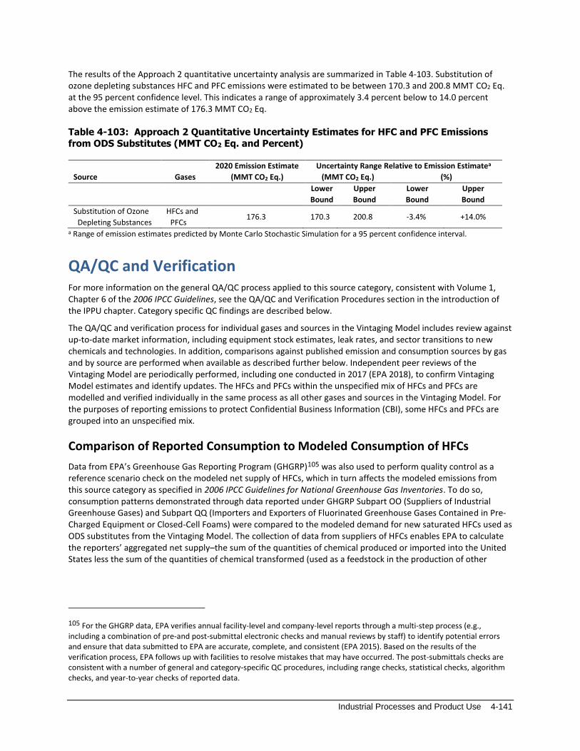
Industrial Processes and Product Use 4-141
The results of the Approach 2 quantitative uncertainty analysis are summarized in Table 4-103. Substitution of ozone depleting substances HFC and PFC emissions were estimated to be between 170.3 and 200.8 MMT CO2 Eq. at the 95 percent confidence level. This indicates a range of approximately 3.4 percent below to 14.0 percent above the emission estimate of 176.3 MMT CO2 Eq.
Table 4-103: Approach 2 Quantitative Uncertainty Estimates for HFC and PFC Emissions
from ODS Substitutes (MMT CO2 Eq. and Percent)
Source Gases
2020 Emission Estimate Uncertainty Range Relative to Emission Estimatea
(MMT CO2 Eq.) (MMT CO2 Eq.) (%)
Lower
Bound
Upper
Bound
Lower
Bound
Upper
Bound
Substitution of Ozone
Depleting Substances
HFCs and
PFCs 176.3 170.3 200.8 -3.4% +14.0%
a Range of emission estimates predicted by Monte Carlo Stochastic Simulation for a 95 percent confidence interval.
QA/QC and Verification
For more information on the general QA/QC process applied to this source category, consistent with Volume 1, Chapter 6 of the 2006 IPCC Guidelines, see the QA/QC and Verification Procedures section in the introduction of the IPPU chapter. Category specific QC findings are described below.
The QA/QC and verification process for individual gases and sources in the Vintaging Model includes review against up-to-date market information, including equipment stock estimates, leak rates, and sector transitions to new chemicals and technologies. In addition, comparisons against published emission and consumption sources by gas and by source are performed when available as described further below. Independent peer reviews of the Vintaging Model are periodically performed, including one conducted in 2017 (EPA 2018), to confirm Vintaging Model estimates and identify updates. The HFCs and PFCs within the unspecified mix of HFCs and PFCs are modelled and verified individually in the same process as all other gases and sources in the Vintaging Model. For the purposes of reporting emissions to protect Confidential Business Information (CBI), some HFCs and PFCs are grouped into an unspecified mix.
Comparison of Reported Consumption to Modeled Consumption of HFCs
Data from EPA’s Greenhouse Gas Reporting Program (GHGRP)105 was also used to perform quality control as a reference scenario check on the modeled net supply of HFCs, which in turn affects the modeled emissions from this source category as specified in 2006 IPCC Guidelines for National Greenhouse Gas Inventories. To do so, consumption patterns demonstrated through data reported under GHGRP Subpart OO (Suppliers of Industrial Greenhouse Gases) and Subpart QQ (Importers and Exporters of Fluorinated Greenhouse Gases Contained in Pre-Charged Equipment or Closed-Cell Foams) were compared to the modeled demand for new saturated HFCs used as ODS substitutes from the Vintaging Model. The collection of data from suppliers of HFCs enables EPA to calculate the reporters’ aggregated net supply–the sum of the quantities of chemical produced or imported into the United States less the sum of the quantities of chemical transformed (used as a feedstock in the production of other
105 For the GHGRP data, EPA verifies annual facility-level and company-level reports through a multi-step process (e.g., including a combination of pre-and post-submittal electronic checks and manual reviews by staff) to identify potential errors and ensure that data submitted to EPA are accurate, complete, and consistent (EPA 2015). Based on the results of the verification process, EPA follows up with facilities to resolve mistakes that may have occurred. The post-submittals checks are consistent with a number of general and category-specific QC procedures, including range checks, statistical checks, algorithm checks, and year-to-year checks of reported data.

4-142 Inventory of U.S. Greenhouse Gas Emissions and Sinks: 1990–2020
chemicals), destroyed, or exported from the United States.106 This allows for an overall quality control check on the modeled demand for new chemical in the Vintaging Model as a proxy for total amount supplied, which is similar to net supply, as an input to the emission calculations in the model.
GHGRP data is not used directly to estimate emissions of ODS Substitutes because it does not include complete, publishable information on the sectors or end-uses in which that chemical will be used, so it does not provide the data that would be needed to calculate the source or time that chemical is emitted. Reports to the GHGRP on production and bulk import (Subpart OO) do not currently include any information on expected end-uses. Reports on fluorinated gases used in equipment and foams (Subpart QQ) do include information on the type of product imported or exported. However, this information is confidential and has not been determined to be publishable at the end-use (i.e., product) level. Irrespective of that, the information would not capture the entire market in the United States, unless it could be determined that for any given product there is no domestic production.
Reported Net Supply (GHGRP Top-Down Estimate)
Under EPA’s GHGRP, suppliers (i.e., producers, importers, and exporters) of HFCs under Subpart OO began annually reporting their production, transformation, destruction, imports, and exports to EPA in 2011 (for supply that occurred in 2010) and suppliers of HFCs under Subpart QQ began annually reporting their imports and exports to EPA in 2012 (for supply that occurred in 2011). Among other provisions, the AIM Act of 2020 directed EPA to develop a U.S. production baseline and a U.S. consumption baseline and to phase down HFC production and consumption relative to those baselines. Data reported to the GHGRP under Subpart OO are relevant to the production and consumption baselines. The data below include aggregated Subpart OO data for AIM-listed HFCs for reporting years 2011 through 2020 from all companies that reported AIM-listed HFCs, though not all species were reported in each reporting year.
Modeled Consumption (Vintaging Model Bottom-Up Estimate)
The Vintaging Model, used to estimate emissions from this source category, calculates chemical demand based on the quantity of equipment and products sold, serviced and retired each year, and the amount of the chemical
required to manufacture and/or maintain the equipment and products.107 It is assumed that the total demand equals the amount supplied by either new production, chemical import, or quantities recovered (often reclaimed) and placed back on the market. In the Vintaging Model, demand for new chemical, as a proxy for consumption, is calculated as any chemical demand (either for new equipment or for servicing existing equipment) that cannot be
met through recycled or recovered material.108 No distinction is made in the Vintaging Model between whether that need is met through domestic production or imports. To calculate emissions, the Vintaging Model estimates the quantity released from equipment over time, which varies by product type as detailed in Annex 3.9. Thus, verifying the Vintaging Model’s calculated consumption against GHGRP reported data, which does not provide details on the end-uses where the chemical is used, is not an exact comparison of the Vintaging Model’s emission estimates, but is believed to provide an overall check of the underlying data.
There are eleven saturated HFC species modeled in the Vintaging Model: HFC-23, HFC-32, HFC-125, HFC-134a, HFC-143a, HFC-152a, HFC-227ea, HFC-236fa, HFC-245fa, HFC-365mfc, and HFC-43-10mee. While some amounts of less-used saturated HFCs, including isomers of those included in the Vintaging Model, are reportable under EPA’s
106 Chemical that is exported, transformed, or destroyed—unless otherwise imported back to the United States—will never be emitted in the United States. 107 The model builds an inventory of the in-use stock of equipment and products and ODSs and HFCs in each of the sub-applications. Emissions are subsequently estimated by applying annual and disposal emission rates to each population of equipment and products. 108 The Vintaging Model does not calculate “consumption” as defined under the Montreal Protocol and the AIM Act, because the model includes chemical supplied to pre-charge equipment made overseas and sent to the domestic market and does not include chemical produced or imported in the United States but placed in products shipped to foreign markets.

Industrial Processes and Product Use 4-143
GHGRP, the data are believed to represent an amount comparable to the modeled estimates as a quality control check.
Comparison Results and Discussion
Comparing the estimates of consumption from these two approaches (i.e., reported and modeled) ultimately supports and improves estimates of emissions, as noted in the 2006 IPCC Guidelines (which refer to fluorinated greenhouse gas consumption based on supplies as “potential emissions”):
[W]hen considered along with estimates of actual emissions, the potential emissions approach can assist in validation of completeness of sources covered and as a QC check by comparing total domestic consumption as calculated in this ‘potential emissions approach’ per compound with the sum of all activity data of the various uses (IPCC 2006).
Table 4-104 and Figure 4-3 compare the published net supply of saturated HFCs in MMT CO2 Eq. as determined from Subpart OO (supply of HFCs in bulk) and Subpart QQ (supply of HFCs in products and foams) of EPA’s GHGRP for the years 2011 through 2020 (EPA 2021a; EPA 2022a) and the chemical demand as calculated by the Vintaging Model for the same time series.
Table 4-104: U.S. HFC Supply (MMT CO2 Eq.)
2011 2012 2013 2014 2015 2016 2017 2018 2019 2020
Reported Net Supply (GHGRP) 257 260 307 294 318 271 322 340 344 344
Industrial GHG Suppliers 250 242 290 269 292 243 290 306 314 309 HFCs in Products and Foams 7 18 17 25 26 28 32 34 30 35
Modeled Supply (Vintaging Model) 270 274 279 283 282 285 276 280 273 270
Percent Difference 5% 6% -9% -4% -11% 5% -14% -18% -21% -22%

4-144 Inventory of U.S. Greenhouse Gas Emissions and Sinks: 1990–2020
Figure 4-3: U.S. HFC Consumption (MMT CO2 Eq.)
As shown, the estimates from the Vintaging Model are lower than the GHGRP estimates by an average of 8.3 percent across the time series (i.e., 2011 through 2020), with the difference growing to an average of 19 percent over the last four years (2017 through 2020). Potential reasons for the differences between the reported and modeled data include:
• The Vintaging Model does not include every saturated HFC that is reported to EPA’s GHGRP. Potential improvements in the modeling could include investigation of what sources use and emit such chemicals—which are not necessarily used as ODS substitutes—and to add them into the Inventory. However, the additional reported HFCs represent a small fraction of total HFC use for this source category, both in GWP-weighted and unweighted terms, and as such, it is not expected that the additional HFCs reported to EPA are a major driver for the difference between the two sets of estimates. To the extent lower-GWP isomers were used in lieu of the modeled chemicals (e.g., HFC-134 instead of HFC-134a), lower CO2 Eq. amounts in the GHGRP data compared to the modeled estimates would be expected.
• Because the top-down data are reported at the time of actual production or import, and the bottom-up data are calculated at the time of actual placement on the market, there could be a temporal discrepancy when comparing data. A potential improvement would be to incorporate a time lag into the model, which would require obtaining data on the movement of supplies through the point of actual use. Because the GHGRP data and the Vintaging Model estimates generally increase over time (although some year-to-year variations exist), EPA would expect the modeled estimates to be slightly lower than the corresponding GHGRP data due to this temporal effect. Regulations under the AIM Act require the reporting of chemical supplies held at the close of the calendar year; such reports may help investigate this possible factor.
• An additional temporal effect can result from the stockpiling of chemicals by suppliers and distributors. Suppliers might decide to produce or import additional quantities of HFCs for various reasons such as expectations that prices may increase, or supplies may decrease, in the future. Based on information collected by the EPA at the time, such stockpiling behavior was seen during ODS phasedowns, but it is unclear if such behavior exists amongst HFC suppliers in anticipation of current and recently promulgated controls on HFCs. Any such activity would increase the GHGRP data as compared to the modeled data.
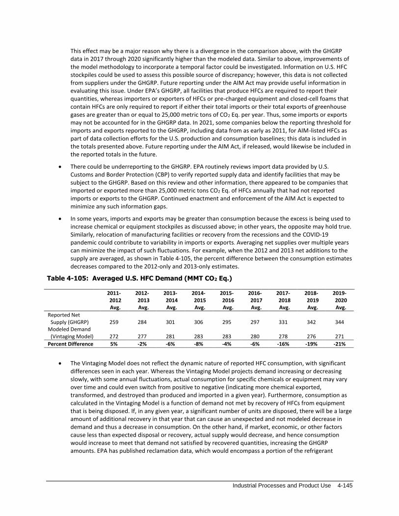
Industrial Processes and Product Use 4-145
This effect may be a major reason why there is a divergence in the comparison above, with the GHGRP data in 2017 through 2020 significantly higher than the modeled data. Similar to above, improvements of the model methodology to incorporate a temporal factor could be investigated. Information on U.S. HFC stockpiles could be used to assess this possible source of discrepancy; however, this data is not collected from suppliers under the GHGRP. Future reporting under the AIM Act may provide useful information in evaluating this issue. Under EPA’s GHGRP, all facilities that produce HFCs are required to report their quantities, whereas importers or exporters of HFCs or pre-charged equipment and closed-cell foams that contain HFCs are only required to report if either their total imports or their total exports of greenhouse gases are greater than or equal to 25,000 metric tons of CO2 Eq. per year. Thus, some imports or exports may not be accounted for in the GHGRP data. In 2021, some companies below the reporting threshold for imports and exports reported to the GHGRP, including data from as early as 2011, for AIM-listed HFCs as part of data collection efforts for the U.S. production and consumption baselines; this data is included in the totals presented above. Future reporting under the AIM Act, if released, would likewise be included in the reported totals in the future.
• There could be underreporting to the GHGRP. EPA routinely reviews import data provided by U.S. Customs and Border Protection (CBP) to verify reported supply data and identify facilities that may be subject to the GHGRP. Based on this review and other information, there appeared to be companies that imported or exported more than 25,000 metric tons CO2 Eq. of HFCs annually that had not reported imports or exports to the GHGRP. Continued enactment and enforcement of the AIM Act is expected to minimize any such information gaps.
• In some years, imports and exports may be greater than consumption because the excess is being used to increase chemical or equipment stockpiles as discussed above; in other years, the opposite may hold true. Similarly, relocation of manufacturing facilities or recovery from the recessions and the COVID-19 pandemic could contribute to variability in imports or exports. Averaging net supplies over multiple years can minimize the impact of such fluctuations. For example, when the 2012 and 2013 net additions to the supply are averaged, as shown in Table 4-105, the percent difference between the consumption estimates decreases compared to the 2012-only and 2013-only estimates.
Table 4-105: Averaged U.S. HFC Demand (MMT CO2 Eq.)
2011-2012 Avg.
2012-2013 Avg.
2013-2014 Avg.
2014-2015 Avg.
2015-2016 Avg.
2016-2017 Avg.
2017-2018 Avg.
2018-2019 Avg.
2019-2020 Avg.
Reported Net Supply (GHGRP) 259 284 301 306 295 297 331 342 344
Modeled Demand (Vintaging Model) 272 277 281 283 283 280 278 276 271
Percent Difference 5% -2% -6% -8% -4% -6% -16% -19% -21%
• The Vintaging Model does not reflect the dynamic nature of reported HFC consumption, with significant differences seen in each year. Whereas the Vintaging Model projects demand increasing or decreasing slowly, with some annual fluctuations, actual consumption for specific chemicals or equipment may vary over time and could even switch from positive to negative (indicating more chemical exported, transformed, and destroyed than produced and imported in a given year). Furthermore, consumption as calculated in the Vintaging Model is a function of demand not met by recovery of HFCs from equipment that is being disposed. If, in any given year, a significant number of units are disposed, there will be a large amount of additional recovery in that year that can cause an unexpected and not modeled decrease in demand and thus a decrease in consumption. On the other hand, if market, economic, or other factors cause less than expected disposal or recovery, actual supply would decrease, and hence consumption would increase to meet that demand not satisfied by recovered quantities, increasing the GHGRP amounts. EPA has published reclamation data, which would encompass a portion of the refrigerant
4-146 Inventory of U.S. Greenhouse Gas Emissions and Sinks: 1990–2020
recovered annually. This data could be reviewed to determine if it can be used to improve the modeling of these factors.
• The Vintaging Model is used to estimate the emissions that occur in the United States. As such, all equipment or products that contain ODSs or alternatives, including saturated HFCs, are assumed to consume and emit chemicals equally as like equipment or products originally produced in the United States. The GHGRP data from Subpart OO (industrial greenhouse gas suppliers) includes HFCs produced or imported and used to fill or manufacture products that are then exported from the United States. The Vintaging Model estimates of demand and supply are not meant to incorporate such chemical. Likewise, chemicals may be used outside the United States to create products or charge equipment that is then imported to and used in the United States. The Vintaging Model estimates of demand and supply are meant to capture this chemical, as it will lead to emissions inside the United States. The GHGRP data from Subpart QQ (supply of HFCs in products) accounts for most of these differences; however, the scope of Subpart QQ does not cover all such equipment or products and the chemical contained therein. Depending on whether the United States is a net importer or net exporter of such chemical, this factor may account for some of the difference shown above or might lead to a further discrepancy.
One factor, however, would only lead to modeled estimates to be even higher than the estimates shown and hence for some years possibly higher than GHGRP data:
• Saturated HFCs are also known to be used and emitted from other sources, such as electronics manufacturing and magnesium production and processing. The Vintaging Model estimates here do not include the amount of HFCs used for these applications, but rather only the amount used for applications that traditionally were served by ODSs. Nonetheless, EPA expects the quantities of HFCs used for electronics and magnesium production to be very small compared to the ODS substitute use for the years analyzed. EPA estimates that electronics and magnesium production respectively consumed 0.8 MMT CO2 Eq. and 0.1 MMT CO2 Eq. of HFCs in 2019, which is much less than the ODS substitute sector in that year (170 MMT CO2 Eq.) (U.S. EPA 2021b).
Comparison of Emissions Derived from Atmospheric Measurements to Modeled Emissions
Emissions of some fluorinated greenhouse gases are estimated for the contiguous United States from the National Oceanic and Atmospheric Administration (NOAA) and were used to perform additional quality control by comparing the emission estimates derived from atmospheric measurements by NOAA to the bottom-up emission estimates from the Vintaging Model. The 2019 Refinement to the 2006 IPCC Guidelines for National Greenhouse Gas Inventories (IPCC 2019) Volume 1: General Guidance and Reporting, Chapter 6: Quality Assurance, Quality Control and Verification notes that atmospheric concentration measurements can provide independent data sets as a basis for comparison with inventory estimates. Further, it identified fluorinated gases as one of most suitable greenhouse gases for such comparisons. The 2019 Refinement makes this conclusion on fluorinated gases based on the lack of natural sources, the potential uncertainties in bottom-up inventory methods for some sources, the long life of many of these gases, and the well-known loss mechanisms. Unlike most other gases in the Inventory, since there are no known natural sources of HFCs, the HFC emission sources included in this Inventory account for the majority of total emissions detectable in the atmosphere, and the estimates derived from atmospheric measurements are driven solely by anthropogenic emissions.
The 2019 Refinement provides guidance on conducting such comparisons (as summarized in Table 6.2 of IPCC 2019 Volume 1, Chapter 6) and provides guidance on using such comparisons to identify areas of improvement in national inventories (as summarized in Box 6.5 of IPCC 2019 Volume 1, Chapter 6).
Emission estimates for four key HFCs from Hu et al. (2017) were used in this comparison. This provides a quality check on the modeled emissions reported above. Hu et al. (2017) provided similar comparisons; here the EPA data used in Hu et al. was updated to reflect the current Inventory estimates. Potential Inventory updates identified due to the comparison with atmospheric data are noted in the Planned Improvements section below.

Industrial Processes and Product Use 4-147
Comparison of Results
Table 4-106 lists the emissions NOAA derived for the contiguous United States from atmospheric measurements as described in Hu et al. (2017) and those from EPA’s Vintaging Model. Figure 4-4 and Figure 4-5 below show this information graphically. Specifically, the data compared are emissions of HFC-32, HFC-125 and HFC-143a (Table 4-106 and Figure 4-4) and emissions of HFC-134a (Table 4-106 and Figure 4-5) for the years covered in Hu et al., i.e., 2008 through 2014. In the Supplemental Information, Hu et al. (2017) provided uncertainty results representing one standard deviation of the spread of several inversion calculations. These are provided in the tables and figures below. There is also uncertainty in the EPA results. Overall, the uncertainty in EPA’s total Substitution of ODS emissions range from -3.4 percent to 14.0 percent (95 percent confidence interval), as shown above. The nature of the model and the uncertainty analysis, however, does not allow EPA to provide specific uncertainties to each species and hence comparisons below are to the EPA estimates without consideration of the uncertainty involved in those estimates.
Table 4-106: U.S. Emissions of HFC-32, HFC-125, HFC-134a and HFC-143a (Gg)
Gas Source 2008 2009 2010 2011 2012 2013 2014
HFC-32 NOAA 1.65±0.34 2.12±0.44 2.87±0.44 3.33±0.66 3.75±0.43 4.26±0.44 5.05±0.86
EPA 1.22 1.56 2.17 2.78 3.44 4.19 5.00
HFC-125 NOAA 7.05±1.68 6.52±1.52 7.91±1.37 7.92±1.29 7.79±0.85 8.79±1.05 9.77±1.40
EPA 5.02 6.05 7.22 8.34 9.37 10.41 11.43
HFC-134a NOAA 49.14±11.05 42.11±9.59 49.81±6.46 40.45±6.90 37.63±3.23 40.80±5.19 42.81±5.97
EPA 60.43 62.27 62.32 59.35 56.34 53.20 52.06
HFC-143a NOAA 4.94±1.22 4.07±1.13 4.95±0.94 3.97±0.59 3.65±0.31 4.18±0.63 5.34±0.84
EPA 3.42 3.99 4.52 4.99 5.40 5.75 6.01
Note: NOAA uncertainty values represent one standard deviation
Figure 4-4: U.S. Emissions of HFC-32, HFC-125, and HFC-143a

4-148 Inventory of U.S. Greenhouse Gas Emissions and Sinks: 1990–2020
Figure 4-5: U.S. Emissions of HFC-134a
As shown, modeled estimates of HFC-32 are comparable with those derived from atmospheric measurements, with only small differences (in Gg y-1). The modeled estimates for 2011 to 2014 lie within the one standard deviation (1 s.d.) uncertainty range of the atmospherically derived estimates after 2010, and both datasets show a similar trend of year-on-year increasing emissions, reaching ~5 Gg y-1 by 2014. On the other hand, modeled emissions of HFC-134a were consistently higher than those seen through atmospheric measurements, well above the one standard deviation uncertainty. While the mean values from NOAA show year-to-year variability, the data may suggest a slight downward trend in HFC-134a emissions through this entire period, like the modeled result; however, confidence in the trend from atmospheric measurements is limited because the magnitude of uncertainties are similar to the overall change and because increasing or decreasing trends of the mean values do not persist for more than two years. The magnitude and time-dependence of the differences for both HFC-125 and HFC-143a were similar, as results from this inventory model were lower in 2008 through 2010 and higher in 2011 through 2014, compared to the means estimated by NOAA. Considering the uncertainty ranges, the modeled results for HFC-125 agree for the years 2009 to 2011, and those for HFC-143a agree for 2009 to 2010 and 2014. The modeled results trend upward year-on-year for both gases, although the increase is smaller for HFC-143a. In the NOAA estimates, no secular trend is discernable from 2008 to 2014 for HFC-143a considering the annual mean uncertainties of approximately 18 percent. NOAA results for HFC-125 have similar uncertainty magnitudes but may suggest a small increase in emissions over time, particularly in the latter years during this time interval.
Table 4-107 shows the differences in the emissions results from EPA’s Vintaging Model and the mean results from NOAA for those years where modeled estimates were not within the given 1 s.d. uncertainty range in the NOAA results. Years when modeled estimates are within the uncertainty range reported by NOAA are not shown as those differences are assumed to be insignificant. Because the uncertainty represents several inversion calculations, a formally estimated 2 s.d. uncertainty range is not available. Instead, EPA considers twice the uncertainty estimated by NOAA, which represents a range that is larger than the actual 2 s.d. from the spread of inversions. Emissions differences found to be outside that range are shown in bold in the table, indicating more attention may be warranted to understand these results. Comparing the results from the individual gases shows changes over time, for example:

Industrial Processes and Product Use 4-149
a. For HFC-32, while the difference was greater than 20 percent prior to 2011 compared to the mean values, the difference from the 1 s.d. amounts averaged only 0.16 Gg during these three years. These differences are insignificant at the twice uncertainty level. Results were within the 1 s.d. uncertainty range of the NOAA estimates starting in 2011.
b. For HFC-125, the difference was within the uncertainty range of the NOAA estimates from 2009 to 2011, but greater than 15 percent of the mean values for 2008 (model results lower) and after 2011 (model results higher). All results were within the twice uncertainty range.
c. For HFC-134a, the differences ranged from 22 percent (in 2014) to 50 percent (in 2012), with all modeled estimates higher than the NOAA estimates even when the 1 s.d. uncertainty ranges were considered. For this gas, only the 2008, 2010, and 2014 estimates were within the NOAA estimates at twice the uncertainty.
d. For HFC-143a, the modeled results were within the uncertainty range in 2009 to 2010 and again in 2014. The 2008 and 2011 model results were within the twice uncertainty range. For 2008, the modeled results were below the uncertainty range by 31 percent compared to the mean value, whereas for 2011 to 2013 the modeled results were above the uncertainty ranges, by an average of 37 percent compared to the mean values.
Table 4-107: Percentage Differences between EPA and NOAA HFC Emission Estimates
Year HFC-32 HFC-125 HFC-134a HFC-143a
2008 -0.43 (-26%) -2.0 (-29%) 11.3 (23%) -1.5 (-31%)
2009 -0.56 (-26%) 20.2 (48%)
2010 -0.70 (-25%) 12.5 (25%)
2011 18.9 (47%) 1.0 (26%)
2012 1.6 (20%) 18.7 (50%) 1.7 (48%)
2013 1.6 (18%) 12.4 (30%) 1.6 (37%)
2014 1.7 (17%) 9.3 (22%)
Average -0.57 (-15%) 0.7 (7%) 14.8 (35%) 0.7 (20%)
Average of Absolute Values 26% 17.3 (21%) 14.8 (35%) 14.6 (36%)
Notes: Differences smaller than the 1 s.d. uncertainty on the annual NOAA-based estimates
are not shown. Differences greater than 2 s.d. shown in bold font. Uncertainties
associated with the Vintaging model have not been estimated by compound and year so
are not included and could imply fewer differences than shown in this table.
Discussion and Areas for Additional Research
The following are potential contributing factors to the variation between the results and possible ways these could inform changes to the model that would reduce the differences seen.
• When examining the NOAA estimates with twice the uncertainties provided, only a few of these larger differences from EPA model results are identified. The uncertainties in the NOAA estimates are primarily driven by the frequency and spatial density of the atmospheric sampling, and the transport model simulations. There is also inherent uncertainty in the consistency of the setup of each gas chromatography measurement taken–e.g., variation in calibration, impurities in the carrier gas used, among others (Barwick 1999); however, that uncertainty is likely less than 1 percent for HFC-125, HFC-134a, and HFC-143a, and less than 5 percent for HFC-32. Given the magnitude of the uncertainties relative to the size of any apparent emission changes, and the limited time period of the analysis, overall trends in most of the gases are hard to discern with confidence except in the case of HFC-32. Although NOAA estimates are derived from thousands of individual sample analyses (approximately 5,000 per year), continued analysis and additional years will enable a better understanding of any secular trends in the NOAA-derived estimates, and hence whether the modeled results are showing similar changes over time.

4-150 Inventory of U.S. Greenhouse Gas Emissions and Sinks: 1990–2020
As discussed above, there is also uncertainty in the EPA estimates. Although these are not available by individual species, these uncertainties may also explain some of the differences seen.
• A thorough discussion of the uncertainties and influencing factors in the NOAA estimates is provided in Hu et al. (2017). That study notes that emissions estimated from inverse modeling of atmospheric data can depend on assumed prior emission distributions and magnitudes, and accordingly the quoted uncertainties on the NOAA results have been augmented to include these influences. In general, in a region where there are fewer atmospheric observations, the NOAA results will inherently tend towards the prior and be impacted by neighboring regions and populations (NOAA/EPA 2020). If the emissions or emissions per person (depending on which prior is used) are significantly different in these areas compared to the nearby areas, derived emissions for these regions can be biased.
• Uncertainty in atmospheric emission estimates is influenced by the number of NOAA’s atmospheric sampling sites, which changed between 2008 and 2014. Uncertainties were greatest in 2008 and 2009—i.e., early on in the North American sampling program (Hu et al. 2017)—due to a fewer number of tower sites and available measurements in those startup years. This may help explain why none of the EPA results for 2008 were within one standard deviation of the NOAA estimates, but all were within twice the uncertainty range. Also, changes in the number and location of measurement sites within the air sampling network containing over 25 sites can lead to biases in the year-to-year emission estimates. During the 2008 to 2014 period addressed by Hu et al. (2017), measurements at four network sites began only after 2008, while observations at two others were terminated. Uncertainties related to network changes were estimated with separate inversion runs in which sites were removed from the analysis and differences ascertained. These influences contribute to the uncertainties quoted on the NOAA estimates, as do the uncertainties related to meteorological models.
• The Vintaging Model estimated emissions for the entire United States, including all 50 states and territories. Conversely, NOAA limits scope to the contiguous 48 states and the District of Columbia (NOAA/EPA 2020). In that regard, EPA would expect the model to estimate slightly higher emissions than those reported by NOAA, by roughly 2 percent based on population data (U.S. Census 2021). Activity data for Hawaii, Alaska and territories could be researched. If available, calculations to reduce the bottom-up results could be made and the results compared again to the NOAA results.
• For HFC-125 and HFC-143a, the EPA model suggests lower emissions in 2008 and higher in 2012 to 2013 relative to the atmosphere-derived estimates. Further research into the refrigeration market might improve the agreement in the estimates for these two gases. As stated in the Introduction above, emissions from the large retail food end-use (e.g., supermarkets), which uses both these gases, were estimated to have the second highest contribution to the overall HFC emissions. Research in this industry on the shift away from blends such as R-404A (which contains both HFC-125 and HFC-143a) or success in lowering emission rates could be used to improve the bottom-up model.
• The modeled emissions of HFC-32 agreed well with the atmospheric inversion results in absolute terms, and both data sets showing the same year-on-year increasing trend. Irrespective of the uncertainties, slightly lower model results might imply that the model assumed a higher than actual use of “dry-charge” residential AC equipment in lieu of R-410A (a 50:50 by mass ratio of HFC-32 and HFC-125). It might also mean the actual emissions from R-410A equipment were slightly higher than modeled.
• The modeled inventory results for HFC-134a are complicated by an assumed decrease in emissions from motor vehicle air conditioning (due to previous shifts towards lower charge sizes and emission rates, as well as the on-going transition to HFO-1234yf) with concurrent increases in other sectors, such as for foam blowing given the HCFC bans in foam blowing and other uses. Even though the NOAA results may also suggest an increase from 2012 to 2014, the magnitudes of uncertainties prevent a robust conclusion of emission increases over this period. While the inter-annual changes in the NOAA mean values for this gas are small compared to the uncertainties, they are not inconsistent with the slow rate of increase followed by a slow rate of decrease seen in the modeled emissions during 2008 through 2014. If the model is overestimating the increased use in foam blowing and/or underestimating the decrease in

Industrial Processes and Product Use 4-151
emissions from the motor vehicle air conditioning end-use, that might account for some of the differences seen.
• In addition to its use as an ODS substitute, HFC-134a is used in a cover gas to prevent oxidation during magnesium metal production and in semiconductor manufacturing. EPA’s Vintaging Model does not include these possible emission sources of HFC-134a, which, if included, would increase the difference between the model-based result and NOAA’s. The use and emissions of HFC-134a from these sources are small (see above and elsewhere in this Inventory), so this would not be a significant contribution to the comparison above.
• There are data limitations inherent in the bottom-up model. As described above, emissions are estimated by applying assumed emission profiles to multiple end-uses, each of which can have thousands or millions of individual uses in the United States. In some cases where equipment stocks or sales are unknown, estimates are made using an average growth rate and by taking the most recent year where the starting stock or sales of equipment is known, then accounting for equipment lifetimes, and subsequently estimating the amount of equipment in future and/or preceding years where a value was not available. Such assumptions are evident in the approximately constant slope of the EPA emission estimates for HFC-32, HFC-125, and HFC-143a, compared to the more varying nature found in NOAA’s mean results. Except for HFC-32, which shows year-on-year increases across both sets of estimates, trends in the NOAA-derived emissions are typically small relative to uncertainty magnitudes in measured data. Future work could look at whether these variations might be consistent with other factors that influence emissions, such as equipment installations, sales, or retirements, which could vary from year to year.
Using a Tier 2 bottom-up modeling methodology to estimate emissions requires assumptions and expert judgment. Comparing the Vintaging Model’s estimates to GHGRP-reported estimates of supply shown above and emissions estimates derived from atmospheric measurements, particularly for more widely used chemicals, can help validate the model but it is expected that the model will have limitations. These comparisons show that Vintaging Model consumption estimates are well within the same order of magnitude as the actual consumption data as reported to EPA’s GHGRP although the differences in reported net supply and modeled demand are still significant. Likewise, these comparisons show reasonable agreement with atmospheric measurement derivations of emissions, though certain chemicals and during certain years differences can be significant. Hence, areas for further research that may improve the modeling are highlighted above. Despite the strengths and weaknesses of three independent approaches for estimating emissions of these HFCs, the reasonable agreement noted here in most instances provides added confidence in EPA’s understanding of total U.S. emissions for these chemicals and how they’ve change over time and, furthermore, has helped identify areas for potential improvement in the future.
Recalculations Discussion For the current Inventory, updates to the Vintaging Model included updating market size, manufacturing loss rate, disposal loss rate, and post-life emission rate assumptions for various PU foam end-uses to align with market research (EPA 2021c). Growth rates for window units were updated to align with sales data for Energy Star- and non-Energy Star-certified units and a transition to HFC-32 was implemented beginning in 2015 to reflect manufacturer transitions (EPA 2022b). In addition, HFC consumption for MDIs was updated to align with an analysis of MDI sales in the United States (EPA 2022c). Together, these updates decreased ODS substitute emissions on average by 0.03 MMT CO2 Eq. (0.004 percent) between 1990 and 2019.
Planned Improvements Future improvements to the Vintaging Model are planned for the Fire Suppression and Aerosols sectors. Specifically, streaming agent fire suppression lifetimes, market size, and growth rates are under review to align more closely with real world activities. In addition, further refinement of HFC consumption in MDIs is expected from review of data collected on HFC use for MDI production, imports, and exports in response to requests for

4-152 Inventory of U.S. Greenhouse Gas Emissions and Sinks: 1990–2020
application-specific allowances for MDIs. EPA expects these revisions to be prepared for the 2023 or 2024 Inventory submission.
EPA has identified several updates to the Vintaging Model based on regularly published or released data that will be implemented in the Vintaging Model on an annual basis, including updating growth rates for residential and commercial unitary air-conditioning to align with annual sales estimates published by AHRI and for window units to align with sales data released by EPA’s Energy Star Program. In addition, as future application-specific allocations for MDIs are granted, EPA will ensure the Vintaging Model is in alignment. Implemented updates are expected to have a lagging effect on Inventory estimates (i.e., 2021 data published in 2022 will appear in the 2023 Inventory submission) and will therefore not be explicitly discussed in the Recalculations Discussion.
As discussed above, future reporting under the AIM Act may provide useful information for verification purposes and possible improvements to the Vintaging Model. EPA expects this reporting by early 2023 and incorporation into the 2024 or 2025 report. Should the data suggest structural changes to the model, such as the handling of stockpiles before use, EPA expects to introduce the revised model for the 2025 or 2026 Inventory submission.
Several potential improvements to the Inventory were identified based on the comparison with atmospheric data. To improve estimates of HFC-125 and HFC-143a, further research into the refrigeration market can be made. Research in this industry on the shift away from blends such as R-404A or success in lowering emission rates could be used to improve the Inventory estimate. This is planned for the 2024 Inventory cycle. Slightly lower model results for HFC-32 might imply that the model assumed a higher than actual use of “dry-charge” residential AC equipment in lieu of R-410A; EPA plans to investigate the amount of “dry-charge” AC imports during the 2023 Inventory cycle. Uncertainty estimates by species would aid in comparisons to atmospheric data. EPA will explore the possibility of revising the Monte Carlo analysis to differentiate between species, staring with the higher-emitted HFCs identified above, in a future (i.e., 2024 or 2025) Inventory submission.
4.25 Electrical Transmission and Distribution (CRF Source Category 2G1)
The largest use of sulfur hexafluoride (SF6), both in the United States and internationally, is as an electrical insulator and interrupter in equipment that transmits and distributes electricity (RAND 2004). The gas has been employed by the electric power industry in the United States since the 1950s because of its dielectric strength and arc-quenching characteristics. It is used in gas-insulated substations, circuit breakers, and other switchgear. SF6 has replaced flammable insulating oils in many applications and allows for more compact substations in dense urban areas. Another greenhouse gas emitted in much smaller amounts by the electric power industry is tetrafluoromethane (CF4), which is mixed with SF6 to avoid liquefaction at low temperatures (Middleton 2000). While mixed gas circuit breakers are more common in extremely cold climates in geographies outside of the United States, some U.S. manufacturers of electrical equipment are emitting CF4 during the manufacturing of equipment designed to hold the SF6/CF4 gas mixture. However, no electrical transmission and distribution facilities in the United States have reported emissions of or equipment using CF4. SF6 emissions exceed PFC emissions from electric power systems on both a GWP-unweighted and GWP-weighted basis.
Fugitive emissions of SF6 and CF4 can escape from gas-insulated substations and switchgear through seals, especially from older equipment. The gas can also be released during equipment manufacturing, installation, servicing, and disposal. Emissions of SF6 and CF4 from equipment manufacturing and from electrical transmission and distribution systems were estimated to be 3.8 MMT CO2 Eq. (0.2 kt) in 2020. This quantity represents an 84 percent decrease from the estimate for 1990 (see Table 4-108 and Table 4-109). There are a few potential causes for this decrease: a sharp increase in the price of SF6 during the 1990s and a growing awareness of the environmental impact of SF6 emissions through programs such as EPA’s voluntary SF6 Emission Reduction Partnership for Electric Power Systems (Partnership) and EPA’s GHGRP, regulatory drivers at the state and local levels, and research and development of alternative gases to SF6 that can be used in gas-insulated substations.

Industrial Processes and Product Use 4-153
Utilities participating in the Partnership have lowered their emission factor from 13 percent in 1999 (kg SF6 emitted per kg of nameplate capacity) to 1 percent in 2020. A recent examination of the SF6 emissions reported by electric power systems to EPA’s GHGRP revealed that SF6 emissions from reporters have decreased by 48 percent from
2011 to 2020,109 with much of the reduction seen from utilities that are not participants in the Partnership. These utilities may be making relatively large reductions in emissions as they take advantage of relatively large and/or inexpensive emission reduction opportunities (i.e., “low hanging fruit,” such as replacing major leaking circuit breakers) that Partners have already taken advantage of under the voluntary program (Ottinger et al. 2014). Total emissions from electrical transmission and distribution in 2020 were lower than 2019 emissions, decreasing by 11.7 percent. The decrease in emissions may be attributed to a decrease in the average emission rate reported to the GHGRP in 2020.
Table 4-108: SF6 and CF4 Emissions from Electric Power Systems and Electrical Equipment
Manufacturers (MMT CO2 Eq.)
Year
Electric Power
Systems
Electrical
Equipment
Manufacturers Total
1990 22.8 0.3 23.2
2005 7.7 0.7 8.4
2016 3.8 0.2 4.1
2017 3.9 0.3 4.2
2018 3.6 0.3 3.8
2019 3.9 0.3 4.2
2020 3.3 0.5 3.8
Note: Totals may not sum due to independent rounding.
Table 4-109: SF6 and CF4 Emissions from Electric Power Systems and Electrical Equipment
Manufacturers (kt)
Year SF6 Emissions CF4 Emissions
1990 1.0 NO
2005 0.4 0.00032
2016 0.2 0.00004
2017 0.2 +
2018 0.2 NO
2019 0.2 0.00006
2020 0.2 0.00002
+ Does not exceed 0.000005 kt. NO (Not Occurring)
109 Analysis of emission trends from facilities reporting to EPA’s GHGRP is imperfect due to an inconsistent group of reporters year to year. A facility that has reported total non-biogenic greenhouse gas emissions below 15,000 metric tons of carbon dioxide equivalent (MT CO2 Eq.) for three consecutive years or below 25,000 MT CO2 Eq. for five consecutive years to EPA’s GHGRP can discontinue reporting for all direct emitter subparts. For this sector, most of the variability in the group of reporters is due to facilities exiting the GHGRP due to being below one of these thresholds; however, facilities must re-enter the program if their emissions at a later date are above 25,000 MT CO2 Eq., which may occur for a variety of reasons, including changes in facility size and changes in emission rates.

4-154 Inventory of U.S. Greenhouse Gas Emissions and Sinks: 1990–2020
Methodology and Time-Series Consistency The estimates of emissions from Electrical Transmission and Distribution are comprised of emissions from electric power systems and emissions from the manufacture of electrical equipment. The methodologies for estimating both sets of emissions are described below.
1990 through 1998 Emissions from Electric Power Systems
Emissions from electric power systems from 1990 through 1998 were estimated based on (1) the emissions estimated for this source category in 1999, which, as discussed in the next section, were based on the emissions reported during the first year of EPA’s SF6 Emission Reduction Partnership for Electric Power Systems (Partnership), and (2) the RAND survey of global SF6 emissions. Because most utilities participating in the Partnership reported emissions only for 1999 through 2011, modeling was used to estimate SF6 emissions from electric power systems for the years 1990 through 1998. To perform this modeling, U.S. emissions were assumed to follow the same trajectory as global emissions from this source during the 1990 through 1999 period. To estimate global emissions, the RAND survey of global SF6 sales was used, together with the following equation for estimating emissions, which is derived from the mass-balance equation for chemical emissions (Volume 3, Equation 7.3) in the 2006 IPCC
Guidelines.110 (Although Equation 7.3 of the 2006 IPCC Guidelines appears in the discussion of substitutes for ozone-depleting substances, it is applicable to emissions from any long-lived pressurized equipment that is periodically serviced during its lifetime.)
Equation 4-23: Estimation for SF6 Emissions from Electric Power Systems
Emissions (kilograms SF6) = SF6 purchased to refill existing equipment (kilograms) + nameplate capacity of retiring equipment (kilograms) 111
Note that the above equation holds whether the gas from retiring equipment is released or recaptured; if the gas is recaptured, it is used to refill existing equipment, thereby lowering the amount of SF6 purchased by utilities for this purpose.
Gas purchases by utilities and equipment manufacturers from 1961 through 2003 are available from the RAND (2004) survey. To estimate the quantity of SF6 released or recovered from retiring equipment, the nameplate capacity of retiring equipment in a given year was assumed to equal 81.2 percent of the amount of gas purchased by electrical equipment manufacturers 40 years previous (e.g., in 2000, the nameplate capacity of retiring equipment was assumed to equal 81.2 percent of the gas purchased in 1960). The remaining 18.8 percent was assumed to have been emitted at the time of manufacture. The 18.8 percent emission factor is an average of IPCC default SF6 emission rates for Europe and Japan for 1995 (IPCC 2006). The 40-year lifetime for electrical equipment is also based on IPCC (2006). The results of the two components of the above equation were then summed to yield estimates of global SF6 emissions from 1990 through 1999.
U.S. emissions between 1990 and 1999 are assumed to follow the same trajectory as global emissions during this period. To estimate U.S. emissions, global emissions for each year from 1990 through 1998 were divided by the estimated global emissions from 1999. The result was a time series of factors that express each year’s global emissions as a multiple of 1999 global emissions. Historical U.S. emissions were estimated by multiplying the factor for each respective year by the estimated U.S. emissions of SF6 from electric power systems in 1999 (estimated to be 13.6 MMT CO2 Eq.).
Two factors may affect the relationship between the RAND sales trends and actual global emission trends. One is utilities’ inventories of SF6 in storage containers. When SF6 prices rise, utilities are likely to deplete internal
110 Ideally, sales to utilities in the United States between 1990 and 1999 would be used as a model. However, this information was not available. There were only two U.S. manufacturers of SF6 during this time period, so it would not have been possible to conceal sensitive sales information by aggregation. 111 Nameplate capacity is defined as the amount of SF6 within fully charged electrical equipment.

Industrial Processes and Product Use 4-155
inventories before purchasing new SF6 at the higher price, in which case SF6 sales will fall more quickly than emissions. On the other hand, when SF6 prices fall, utilities are likely to purchase more SF6 to rebuild inventories, in which case sales will rise more quickly than emissions. This effect was accounted for by applying 3-year smoothing to utility SF6 sales data. The other factor that may affect the relationship between the RAND sales trends and actual global emissions is the level of imports from and exports to Russia and China. SF6 production in these countries is not included in the RAND survey and is not accounted for in any another manner by RAND. However, atmospheric studies confirm that the downward trend in estimated global emissions between 1995 and 1998 was real (see the Uncertainty discussion below).
1999 through 2020 Emissions from Electric Power Systems
Emissions from electric power systems from 1999 to 2020 were estimated based on: (1) reporting from utilities participating in EPA’s SF6 Emission Reduction Partnership for Electric Power Systems (Partners), which began in 1999; (2) reporting from utilities covered by EPA’s GHGRP, which began in 2012 for emissions occurring in 2011 (GHGRP-Only Reporters); and (3) the relationship between utilities’ reported emissions and their transmission miles as reported in the 2001, 2004, 2007, 2010, 2013, and 2016 Utility Data Institute (UDI) Directories of Electric Power Producers and Distributors (UDI 2001, 2004, 2007, 2010, 2013, and 2017), and 2019 and 2020 Homeland Infrastructure Foundation-Level Data (HIFLD) (HIFLD 2019 and 2020), which was applied to the electric power systems that do not report to EPA (Non-Reporters). Total U.S. Transmission mileage was interpolated between 2016 and 2019 to estimate transmission mileage of electric power systems in 2017 and 2018. (Transmission miles are defined as the miles of lines carrying voltages above 34.5 kV).
Partners
Over the period from 1999 to 2020, Partner utilities, which for inventory purposes are defined as utilities that
either currently are or previously have been part of the Partnership,112 represented 49 percent, on average, of total U.S. transmission miles. Partner utilities estimated their emissions using a Tier 3 utility-level mass balance approach (IPCC 2006). If a Partner utility did not provide data for a particular year, emissions were interpolated between years for which data were available or extrapolated based on Partner-specific transmission mile growth rates. In 2012, many Partners began reporting their emissions (for 2011 and later years) through EPA’s GHGRP (discussed further below) rather than through the Partnership. In 2020, approximately 1 percent of the total emissions attributed to Partner utilities were reported through Partnership reports. Approximately 99 percent of the total emissions attributed to Partner utilities were reported and verified through EPA’s GHGRP. Partners without verified 2020 data accounted for less than 1 percent of the total emissions attributed to Partner
utilities.113
The GHGRP program has an “offramp” provision (40 CFR Part 98.2(i)) that exempts facilities from reporting under certain conditions. If reported total greenhouse gas emissions are below 15,000 metric tons of carbon dioxide equivalent (MT CO2 Eq.) for three consecutive years or below 25,000 MT CO2 Eq. for five consecutive years, the facility may elect to discontinue reporting. GHGRP reporters that have off-ramped are extrapolated for three years of non-reporting using a utility-specific transmission mile growth rate. After three consecutive years of non-reporting, they are treated as non-reporters, as described in the section below on non-reporters. Partners that have years of non-reporting between reporting years are gap filled by interpolating between reported values.
112 Starting in the 1990 to 2015 Inventory, partners who had reported three years or less of data prior to 2006 were removed. Most of these Partners had been removed from the list of current Partners but remained in the Inventory due to the extrapolation methodology for non-reporting partners. 113 Only data reported as of August 7, 2021 are used in the emission estimates for the prior year of reporting. Emissions for Partners that did not report to the Partnership or GHGRP are extrapolated for three years using a utility-specific transmission mile growth rate. After four consecutive years of non-reporting they are included in the ‘non-reporting Partners’ category. It should be noted that data reported through EPA’s GHGRP must go through a verification process. For electric power systems, verification involved a series of electronic range, completeness, and algorithm checks for each report submitted.

4-156 Inventory of U.S. Greenhouse Gas Emissions and Sinks: 1990–2020
GHGRP-Only Reporters
EPA’s GHGRP requires users of SF6 in electric power systems to report emissions if the facility has a total SF6 nameplate capacity that exceeds 17,820 pounds. (This quantity is the nameplate capacity that would result in annual SF6 emissions equal to 25,000 metric tons of CO2 equivalent at the historical emission rate reported under the Partnership.) As under the Partnership, electric power systems that report their SF6 emissions under EPA’s GHGRP are required to use the Tier 3 utility-level mass-balance approach. Many Partners began reporting their emissions through EPA’s GHGRP in 2012 (reporting emissions for 2011 and later years) because their nameplate capacity exceeded the reporting threshold. Some Partners who did not report through EPA’s GHGRP continued to report through the Partnership.
In addition, many non-Partners began reporting to EPA for the first time through its GHGRP in 2012. Non-Partner emissions reported and verified under EPA’s GHGRP were compiled to form a new category of reported data (GHGRP-Only Reporters). GHGRP-Only Reporters accounted for 17 percent of U.S. transmission miles and 24
percent of estimated U.S. emissions from electric power system in 2020.114
Emissions for GHGRP-only reporters that off-ramp are extrapolated for three years of non-reporting using a utility-specific annual transmission mile growth rate. After three consecutive years of non-reporting, they are treated as non-reporters, and emissions are subsequently estimated based on the methodology described below.
Non-Reporters
Emissions from Non-Reporters (i.e., utilities other than Partners and GHGRP-Only Reporters) in every year since 1999 were estimated using the results of a regression analysis that correlated emissions from reporting utilities
(using verified data from both Partners and GHGRP-Only Reporters) with their transmission miles.115 As noted above, non-Partner emissions were reported to the EPA for the first time through its GHGRP in 2012 (representing 2011 emissions). This set of reported data was of particular interest because it provided insight into the emission rate of non-Partners, which previously was assumed to be equal to the historical (1999) emission rate of Partners. Specifically, emissions were estimated for Non-Reporters as follows:
• Non-Reporters, 1999 to 2011: First, the 2011 emission rates (per kg nameplate capacity and per transmission mile) reported by Partners and GHGRP-Only Reporters were reviewed to determine whether there was a statistically significant difference between these two groups. Transmission mileage data for 2011 was reported through GHGRP, with the exception of transmission mileage data for Partners that did not report through GHGRP, which was obtained from UDI. It was determined that there is no statistically significant difference between the emission rates of Partners and GHGRP-Only reporters; therefore, Partner and GHGRP-Only reported data for 2011 were combined to develop regression equations to estimate the emissions of Non-Reporters. Historical emissions from Non-Reporters were estimated by linearly interpolating between the 1999 regression coefficient (based on 1999 Partner data) and the 2011 regression coefficient.
• Non-Reporters, 2012 to Present: The emissions data from Partners and by GHGRP-Only Reporters were combined to develop regression equations for 2012. This was repeated for 2013 through 2020 using Partner and GHGRP-Only Reporter data for each year.
o The 2020 regression equation for reporters was developed based on the emissions reported by a subset of Partner utilities and GHGRP-Only utilities who reported non-zero emissions and non-zero
114 GHGRP-reported and Partner transmission miles from a number of facilities were equal to zero with non-zero emissions. These facilities emissions were added to the emissions totals for their respective parent companies when identifiable and not included in the regression equation when not identifiable or applicable. Other facilities reported non-zero transmission miles with zero emissions, or zero transmission miles and zero emissions. These facilities were not included in the development of the regression equations (discussed further below). These emissions are already implicitly accounted for in the relationship between transmission miles and emissions. 115 In the United States, SF6 is contained primarily in transmission equipment rated above 34.5 kV.

Industrial Processes and Product Use 4-157
transmission miles (representing approximately 62 percent of total U.S. transmission miles). The regression equation for 2020 is:
Equation 4-24: Regression Equation for Estimating SF6 Emissions of Non-Reporting Facilities
Emissions (kg) = 0.186 × Transmission Miles
Table 4-110 below shows the percentage of transmission miles covered by reporters (i.e., associated with reported data) and the regression coefficient for 1999 (the first year data was reported), and for 2011 through present (the years with GHGRP reported data). The coefficient decreased between 2016 and 2020.
Table 4-110: Transmission Mile Coverage (Percent) and Regression Coefficients (kg per
mile) 1999 2005 2016 2017 2018 2019 2020
Percentage of Miles Covered by Reporters 50% 50% 72% 73% 72% 66% 62% Regression Coefficienta 0.71 0.35 0.21 0.25 0.21 0.23 0.19 a Regression coefficient for emissions is calculated utilizing transmission miles as the explanatory variable and emissions
as the response variable. The equation utilizes a constant intercept of zero. When calculating the regression coefficient, outliers are also removed from the analysis when the standard residual for that reporter exceeds the value 3.0.
Data on transmission miles for each Non-Reporter for the years 2000, 2003, 2006, and 2009, 2012, and 2016 were obtained from the 2001, 2004, 2007, 2010, 2013, and 2017 UDI Directories of Electric Power Producers and Distributors, respectively (UDI 2001, 2004, 2007, 2010, 2013, and 2017). For 2019 and 2020, non-reporter transmission mileage was derived by subtracting reported transmission mileage data from the total U.S. transmission mileage from 2019 and 2020 HIFLD Data (HIFLD 2019 and 2020). The following trends in transmission miles have been observed over the time series:
• The U.S. transmission system grew by over 22,000 miles between 2000 and 2003 yet declined by almost 4,000 miles between 2003 and 2006. Given these fluctuations, periodic increases are assumed to occur gradually. Therefore, transmission mileage was assumed to increase at an annual rate of 1.2 percent between 2000 and 2003 and decrease by 0.20 percent between 2003 and 2006.
• The U.S. transmission system’s annual growth rate grew to 1.7 percent from 2006 to 2009 as transmission miles increased by more than 33,000 miles.
• The annual growth rate for 2009 through 2012 was calculated to be 1.5 percent as transmission miles grew yet again by over 30,000 miles during this time period.
• The annual transmission mile growth rate for 2012 through 2016 was calculated to be 0.4 percent, as transmission miles increased by approximately 10,250 miles.
• The annual transmission mile growth rate for 2016 through 2019 was calculated to be 0.9 percent, as transmission miles increased by approximately 19,900 miles.
• The annual transmission mile growth rate for 2019 through 2020 was calculated to be 0.06 percent, as transmission miles increased by approximately 420 miles.
Transmission miles for each year for non-reporters were calculated by interpolating between UDI reported values obtained from the 2001, 2004, 2007, 2010, 2013 and 2017 UDI directories and 2019 HIFLD data. In cases where a non-reporter previously reported the GHGRP or the Partnership, transmission miles were interpolated between the most recently reported value and the next available UDI value.
Total Industry Emissions
As a final step, total electric power system emissions from 1999 through 2020 were determined for each year by summing the Partner reported and estimated emissions (reported data was available through the EPA’s SF6 Emission Reduction Partnership for Electric Power Systems), the GHGRP-only reported emissions, and the non-reporting utilities’ emissions (determined using the regression equations).

4-158 Inventory of U.S. Greenhouse Gas Emissions and Sinks: 1990–2020
1990 through 2020 Emissions from Manufacture of Electrical Equipment
Three different methods were used to estimate 1990 to 2020 emissions from original electrical equipment manufacturers (OEMs).
• OEM SF6 emissions from 1990 through 2000 were derived by assuming that manufacturing emissions equaled 10 percent of the quantity of SF6 provided with new equipment. The 10 percent emission rate is the average of the “ideal” and “realistic” manufacturing emission rates (4 percent and 17 percent, respectively) identified in a paper prepared under the auspices of the International Council on Large Electric Systems (CIGRE) in February 2002 (O’Connell et al. 2002). The quantity of SF6 provided with new equipment was estimated based on statistics compiled by the National Electrical Manufacturers Association (NEMA). These statistics were provided for 1990 to 2000.
• OEM SF6 emissions from 2000 through 2010 were estimated by (1) interpolating between the emission rate estimated for 2000 (10 percent) and an emission rate estimated for 2011 based on reporting by OEMs through the GHGRP (5.7 percent), and (2) estimating the quantities of SF6 provided with new equipment for 2001 to 2010. The quantities of SF6 provided with new equipment were estimated using Partner reported data and the total industry SF6 nameplate capacity estimate (156.5 MMT CO2 Eq. in 2010). Specifically, the ratio of new nameplate capacity to total nameplate capacity of a subset of Partners for which new nameplate capacity data was available from 1999 to 2010 was calculated. These ratios were then multiplied by the total industry nameplate capacity estimate for each year to derive the amount of SF6 provided with new equipment for the entire industry. Additionally, to obtain the 2011 emission rate (necessary for estimating 2001 through 2010 emissions), the estimated 2011 emissions (estimated using the third methodology listed below) were divided by the estimated total quantity of SF6 provided with new equipment in 2011. The 2011 quantity of SF6 provided with new equipment was estimated in the same way as the 2001 through 2010 quantities.
• OEM CF4 emissions from 1991 through 2010 were estimated by using an average ratio of reported SF6 and CF4 emissions from 2011 through 2013. This ratio was applied to the estimated SF6 emissions for 1991 through 2010 to arrive at CF4 emissions. CF4 emissions are estimated starting in 1991 and assumed zero prior to 1991 based on the entry of the CF4/SF6 gas mixture into the market (Middleton 2000).
• OEM emissions from 2011 through 2020 were estimated using the SF6 and CF4 emissions from OEMs reporting to the GHGRP, and an assumption that these reported emissions account for a conservatively low estimate of 50 percent of the total emissions from all U.S. OEMs.
Methodological approaches were applied to the entire time series to ensure time-series consistency from 1990 through 2020.
Uncertainty To estimate the uncertainty associated with emissions of SF6 and CF4 from Electrical Transmission and Distribution, uncertainties associated with four quantities were estimated: (1) emissions from Partners, (2) emissions from GHGRP-Only Reporters, (3) emissions from Non-Reporters, and (4) emissions from manufacturers of electrical equipment. A Monte Carlo analysis was then applied to estimate the overall uncertainty of the emissions estimate.
Total emissions from the SF6 Emission Reduction Partnership include emissions from both reporting (through the Partnership or EPA’s GHGRP) and non-reporting Partners. For reporting Partners, individual Partner-reported SF6 data was assumed to have an uncertainty of 10 percent. Based on a Monte Carlo analysis, the cumulative uncertainty of all Partner-reported data was estimated to be 6.0 percent. The uncertainty associated with extrapolated or interpolated emissions from non-reporting Partners was assumed to be 20 percent.

Industrial Processes and Product Use 4-159
For GHGRP-Only Reporters, reported SF6 data was assumed to have an uncertainty of 20 percent.116 Based on a Monte Carlo analysis, the cumulative uncertainty of all GHGRP-Only reported data was estimated to be 8.5 percent.
There are two sources of uncertainty associated with the regression equations used to estimate emissions in 2019 from Non-Reporters: (1) uncertainty in the coefficients (as defined by the regression standard error estimate), and (2) the uncertainty in total transmission miles for Non-Reporters. Uncertainties were also estimated regarding (1) estimates of SF6 and CF4 emissions from OEMs reporting to EPA’s GHGRP, and (2) the assumption on the percent share of OEM emissions from OEMs reporting to EPA’s GHGRP.
The results of the Approach 2 quantitative uncertainty analysis are summarized in Table 4-111. Electrical Transmission and Distribution SF6 and CF4 emissions were estimated to be between 3.2 and 4.5 MMT CO2 Eq. at the 95 percent confidence level. This indicates a range of approximately 16 percent below and 18 percent above the emission estimate of 3.8 MMT CO2 Eq.
Table 4-111: Approach 2 Quantitative Uncertainty Estimates for SF6 and CF4 Emissions from
Electrical Transmission and Distribution (MMT CO2 Eq. and Percent)
Source Gas
2020 Emission
Estimate Uncertainty Range Relative to 2018 Emission Estimatea
(MMT CO2 Eq.) (MMT CO2 Eq.) (%)
Lower
Bound
Upper
Bound
Lower
Bound
Upper
Bound
Electrical Transmission
and Distribution
SF6
and
CF4 3.8 3.2 4.5 -16% +18%
a Range of emission estimates predicted by Monte Carlo Stochastic Simulation for a 95 percent confidence interval.
In addition to the uncertainty quantified above, there is uncertainty associated with using global SF6 sales data to estimate U.S. emission trends from 1990 through 1999. However, the trend in global emissions implied by sales of SF6 appears to reflect the trend in global emissions implied by changing SF6 concentrations in the atmosphere. That is, emissions based on global sales declined by 29 percent between 1995 and 1998 (RAND 2004), and emissions based on atmospheric measurements declined by 17 percent over the same period (Levin et al. 2010).
Several pieces of evidence indicate that U.S. SF6 emissions were reduced as global emissions were reduced. First, the decreases in sales and emissions coincided with a sharp increase in the price of SF6 that occurred in the mid-1990s and that affected the United States as well as the rest of the world. A representative from DILO, a major manufacturer of SF6 recycling equipment, stated that most U.S. utilities began recycling rather than venting SF6 within two years of the price rise. Finally, the emissions reported by the one U.S. utility that reported its emissions for all the years from 1990 through 1999 under the Partnership showed a downward trend beginning in the mid-1990s.
QA/QC and Verification For the GHGRP data, EPA verifies annual facility-level reports through a multi-step process (e.g., including a combination of pre-and post-submittal electronic checks and manual reviews by staff) to identify potential errors
and ensure that data submitted to EPA are accurate, complete, and consistent (EPA 2015).117 Based on the results of the verification process, EPA follows up with facilities to resolve mistakes that may have occurred. The post-
116 Uncertainty is assumed to be higher for the GHGRP-Only category, because 2011 is the first year that those utilities have reported to EPA. 117 GHGRP Report Verification Factsheet. See https://www.epa.gov/sites/production/files/2015-07/documents/ghgrp_verification_factsheet.pdf.
4-160 Inventory of U.S. Greenhouse Gas Emissions and Sinks: 1990–2020
submittals checks are consistent with a number of general and category-specific QC procedures including: range checks, statistical checks, algorithm checks, and year-to-year checks of reported data and emissions.
For more information on the general QA/QC process applied to this source category, consistent with Volume 1, Chapter 6 of the 2006 IPCC Guidelines, see the QA/QC and Verification Procedures section in the introduction of the IPPU chapter and Annex 8 for more details.
Recalculations Discussion The historical emissions estimated for this source category have undergone the following revisions for the period 1990 through 2019.
• GHGRP report resubmissions: Historical estimates for the period 2015 through 2019 were updated relative to the previous report based on revisions to reported historical data in EPA’s GHGRP. In addition, EPA identified two facilities that merged with another reporting facility and another facility who reported under one GHGRP ID in 2011 and switched their ID in subsequent years. Estimation methodologies were revised for these four facilities.
• Transmission mileage update: Historical estimates for total transmission mileage relied on a growth rate of UDI data from 2012 to 2017 to estimate total transmission mileage for 2019 and 2020. EPA used HIFLD data to replace 2019 data and interpolated transmission mileage between 2016 and 2019 to estimate 2017 and 2018 total transmission mileage.
• CF4 emissions from OEMs: Previous inventories did not capture the emissions of CF4 from OEMs. EPA used
GHGRP data to calculate CF4 emissions from 2011 through 2019 and used an average ratio of SF6 emissions to CF4 emissions in 2011 through 2013 to estimate CF4 emissions from 1991 through 2010.
As a result of the recalculations, SF6 emissions from electrical transmission and distribution decreased by 1.20 percent for 2019 relative to the previous report, and SF6 nameplate capacity decreased by 2.5 percent for 2019 relative to the previous report. On average, SF6 emission estimates for the entire time series decreased by approximately 0.2 percent per year.
Planned Improvements EPA plans to more closely examine the methodology used to estimate non-reporter emissions. The current methodology uses a reporter emissions rate to estimate non-reporter emissions. However, the preliminary results of research conducted by the National Oceanic Atmospheric Administration (Hu 2021) indicate that U.S. emissions of SF6 are significantly higher than what is being estimated in the current inventory for emissions of SF6 from all sources. Because emissions from non-reporting electric power systems are a significant source of uncertainty in the current U.S. SF6 inventory, EPA will investigate whether the methodology for determining the emission rate for non-reporters should be revised.
Additionally, as the information on the type of new and retiring equipment is collected through GHGRP reporting, EPA expects this data to provide insight into the relative importance of the two types of equipment as potential emission sources. Historically, hermetically sealed pressure equipment has been considered to be a relatively small source of SF6 in the United States; however, better estimating its potential source of emissions upon end-of-life (i.e., disposal emissions) is an area for further analysis.

Industrial Processes and Product Use 4-161
4.26 Nitrous Oxide from Product Uses (CRF Source Category 2G3)
Nitrous oxide (N2O) is a clear, colorless, oxidizing liquefied gas with a slightly sweet odor which is used in a wide variety of specialized product uses and applications. The amount of N2O that is actually emitted depends upon the specific product use or application.
There are a total of three N2O production facilities currently operating in the United States (Ottinger 2021). Nitrous oxide is primarily used in carrier gases with oxygen to administer more potent inhalation anesthetics for general anesthesia, and as an anesthetic in various dental and veterinary applications. The second main use of N2O is as a propellant in pressure and aerosol products, the largest application being pressure-packaged whipped cream. Small quantities of N2O also are used in the following applications:
• Oxidizing agent and etchant used in semiconductor manufacturing;
• Oxidizing agent used, with acetylene, in atomic absorption spectrometry;
• Production of sodium azide, which is used to inflate airbags;
• Fuel oxidant in auto racing; and
• Oxidizing agent in blowtorches used by jewelers and others (Heydorn 1997).
Production of N2O in 2020 was approximately 15 kt (see Table 4-112).
Table 4-112: N2O Production (kt)
Year kt
1990 16
2005 15
2016 15
2017 15
2018 15
2019 15
2020 15
Nitrous oxide emissions were 4.2 MMT CO2 Eq. (14 kt N2O) in 2020 (see Table 4-113). Production of N2O stabilized during the 1990s because medical markets had found other substitutes for anesthetics, and more medical procedures were being performed on an outpatient basis using local anesthetics that do not require N2O. The use of N2O as a propellant for whipped cream has also stabilized due to the increased popularity of cream products packaged in reusable plastic tubs (Heydorn 1997).
Table 4-113: N2O Emissions from N2O Product Usage (MMT CO2 Eq. and kt)
Year MMT CO2 Eq. kt
1990 4.2 14
2005 4.2 14
2016 4.2 14
2017 4.2 14
2018 4.2 14
2019 4.2 14
2020 4.2 14

4-162 Inventory of U.S. Greenhouse Gas Emissions and Sinks: 1990–2020
Methodology and Time-Series Consistency Emissions from N2O product uses were estimated using the following equation:
Equation 4-25: N2O Emissions from Product Use
𝐸𝑝𝑢 = ∑(𝑃 × 𝑆𝑎 × 𝐸𝑅𝑎)
𝑎
where,
Epu = N2O emissions from product uses, metric tons P = Total U.S. production of N2O, metric tons a = specific application Sa = Share of N2O usage by application a ERa = Emission rate for application a, percent
The share of total quantity of N2O usage by end-use represents the share of national N2O produced that is used by the specific subcategory (e.g., anesthesia, food processing). In 2019, the medical/dental industry used an estimated 89.5 percent of total N2O produced, followed by food processing propellants at 6.5 percent. All other subcategories, including semiconductor manufacturing, atomic absorption spectrometry, sodium azide production, auto racing, and blowtorches, used the remainder of the N2O produced. This subcategory breakdown has changed only slightly over the past decade. For instance, the small share of N2O usage in the production of sodium azide declined significantly during the 1990s. Due to the lack of information on the specific time period of the phase-out in this market subcategory, most of the N2O usage for sodium azide production is assumed to have ceased after 1996, with the majority of its small share of the market assigned to the larger medical/dental consumption subcategory (Heydorn 1997). For 1990 through 1996, N2O usage was allocated across the following subcategories: medical applications, food processing propellant, and sodium azide production. A usage emissions rate was then applied for each subcategory to estimate the amount of N2O emitted.
Only the medical/dental and food propellant subcategories were assumed to release emissions into the atmosphere that are not captured under another source category, and therefore these subcategories were the only usage subcategories with emission rates. Emissions of N2O from semiconductor manufacturing are described in Section 4.23 Electronics Industry (CRF Source Category 2E) and reported under CRF Source Category 2H3. For the medical/dental subcategory, due to the poor solubility of N2O in blood and other tissues, none of the N2O is assumed to be metabolized during anesthesia and quickly leaves the body in exhaled breath. Therefore, an emission factor of 100 percent was used for this subcategory (IPCC 2006). For N2O used as a propellant in pressurized and aerosol food products, none of the N2O is reacted during the process and all of the N2O is emitted to the atmosphere, resulting in an emission factor of 100 percent for this subcategory (IPCC 2006). For the remaining subcategories, all of the N2O is consumed or reacted during the process, and therefore the emission rate was considered to be zero percent (Tupman 2002).
The 1990 through 1992 N2O production data were obtained from SRI Consulting’s Nitrous Oxide, North America (Heydorn 1997). Nitrous oxide production data for 1993 through 1995 were not available. Production data for 1996 was specified as a range in two data sources (Heydorn 1997; Tupman 2002). In particular, for 1996, Heydorn (1997) estimates N2O production to range between 13.6 and 18.1 thousand metric tons. Tupman (2002) provided a narrower range (15.9 to 18.1 thousand metric tons) for 1996 that falls within the production bounds described by Heydorn (1997). Tupman (2002) data are considered more industry-specific and current; therefore, the midpoint of the narrower production range was used to estimate N2O emissions for years 1993 through 2001 (Tupman 2002). The 2002 and 2003 N2O production data were obtained from the Compressed Gas Association Nitrous Oxide Fact Sheet and Nitrous Oxide Abuse Hotline (CGA 2002, 2003). These data were also provided as a range. For example, in 2003, CGA (2003) estimates N2O production to range between 13.6 and 15.9 thousand metric tons. Due to the unavailability of data, production estimates for years 2004 through 2019 were held constant at the 2003 value.

Industrial Processes and Product Use 4-163
The 1996 share of the total quantity of N2O used by each subcategory was obtained from SRI Consulting’s Nitrous Oxide, North America (Heydorn 1997). The 1990 through 1995 share of total quantity of N2O used by each subcategory was kept the same as the 1996 number provided by SRI Consulting. The 1997 through 2001 share of total quantity of N2O usage by sector was obtained from communication with a N2O industry expert (Tupman 2002). The 2002 and 2003 share of total quantity of N2O usage by sector was obtained from CGA (2002, 2003). Due to the unavailability of data, the share of total quantity of N2O usage data for years 2004 through 2019 was assumed to equal the 2003 value. The emissions rate for the food processing propellant industry was obtained from SRI Consulting’s Nitrous Oxide, North America (Heydorn 1997) and confirmed by a N2O industry expert (Tupman 2002). The emissions rate for all other subcategories was obtained from communication with a N2O industry expert (Tupman 2002). The emissions rate for the medical/dental subcategory was obtained from the 2006 IPCC Guidelines.
Methodological approaches were applied to the entire time series to ensure consistency in emissions from 1990 through 2020.
Uncertainty The overall uncertainty associated with the 2020 N2O emission estimate from N2O product usage was calculated using the 2006 IPCC Guidelines (2006) Approach 2 methodology. Uncertainty associated with the parameters used to estimate N2O emissions include production data, total market share of each end use, and the emission factors applied to each end use, respectively.
The results of this Approach 2 quantitative uncertainty analysis are summarized in Table 4-114. Nitrous oxide emissions from N2O product usage were estimated to be between 3.2 and 5.2 MMT CO2 Eq. at the 95 percent confidence level. This indicates a range of approximately 24 percent below to 24 percent above the emission estimate of 4.2 MMT CO2 Eq.
Table 4-114: Approach 2 Quantitative Uncertainty Estimates for N2O Emissions from N2O
Product Usage (MMT CO2 Eq. and Percent)
Source Gas 2020 Emission Estimate Uncertainty Range Relative to Emission Estimatea
(MMT CO2 Eq.) (MMT CO2 Eq.) (%)
Lower
Bound
Upper
Bound
Lower
Bound
Upper
Bound
N2O from Product Uses N2O 4.2 3.2 5.2 -24% +24% a Range of emission estimates predicted by Monte Carlo Stochastic Simulation for a 95 percent confidence interval.
QA/QC and Verification For more information on the general QA/QC process applied to this source category, consistent with Volume 1, Chapter 6 of the 2006 IPCC Guidelines, see the QA/QC and Verification Procedures section in the introduction of the IPPU chapter.
Recalculations Discussion No recalculations were performed for the 1990 through 2019 portion of the time series.
Planned Improvements EPA recently initiated an evaluation of alternative production statistics for cross-verification and updating time-series activity data, emission factors, assumptions, etc., and a reassessment of N2O product use subcategories that accurately represent trends. This evaluation includes conducting a literature review of publications and research

4-164 Inventory of U.S. Greenhouse Gas Emissions and Sinks: 1990–2020
that may provide additional details on the industry. This work remains ongoing, and thus far no additional sources of data have been found to update this category.
Pending additional resources and planned improvement prioritization, EPA may also evaluate production and use cycles, and the potential need to incorporate a time lag between production and ultimate product use and resulting release of N2O. Additionally, planned improvements include considering imports and exports of N2O for product uses.
Finally, for future Inventories, EPA will examine data from EPA’s GHGRP to improve the emission estimates for the N2O product use subcategory. Particular attention will be made to ensure aggregated information can be published without disclosing CBI and time-series consistency, as the facility-level reporting data from EPA’s GHGRP are not available for all inventory years as required in this Inventory. This is a lower priority improvement, and EPA is still assessing the possibility of incorporating aggregated GHGRP CBI data to estimate emissions; therefore, this planned improvement is still in development and not incorporated in the current Inventory report.
4.27 Industrial Processes and Product Use Sources of Precursor Gases
In addition to the main greenhouse gases addressed above, many industrial processes can result in emissions of
various greenhouse gas precursors. The reporting requirements of the UNFCCC118 request that information be provided on precursor emissions, which include carbon monoxide (CO), nitrogen oxides (NOx), non-methane volatile organic compounds (NMVOCs), and sulfur dioxide (SO2). These gases are not direct greenhouse gases, but indirectly impact Earth’s radiative balance by altering the concentrations of greenhouse gases (e.g., ozone) and atmospheric aerosol (e.g., particulate sulfate). Combustion byproducts such as CO and NOx are emitted from industrial applications that employ thermal incineration as a control technology. NMVOCs, commonly referred to as “hydrocarbons,” are the primary gases emitted from most processes employing organic or petroleum-based products, and can also result from the product storage and handling.
Accidental releases of precursors associated with product use and handling can constitute major emissions in this category. In the United States, emissions from product use are primarily the result of solvent evaporation, whereby the lighter hydrocarbon molecules in the solvents escape into the atmosphere. The major categories of product uses include: degreasing, graphic arts, surface coating, other industrial uses of solvents (e.g., electronics), dry cleaning, and non-industrial uses (e.g., uses of paint thinner). Product usage in the United States also results in the emission of small amounts of hydrofluorocarbons (HFCs) and hydrofluoroethers (HFEs), which are included under Substitution of Ozone Depleting Substances in this chapter.
Total emissions of NOx, CO, NMVOCs, and SO2 from non-energy industrial processes and product use from 1990 to 2020 are reported in Table 4-115.
Table 4-115: NOx, CO, NMVOC, and SO2 Emissions from Industrial Processes and Product
Use (kt) Gas/Source 1990 2005 2016 2017 2018 2019 2020
NOx 592 572 402 397 397 397 397 Mineral Industry 246 329 221 220 220 220 220 Other Industrial Processesa 105 125 80 80 80 80 80 Metal Industry 88 60 61 60 60 60 60 Chemical Industry 152 55 39 37 37 37 37 Product Usesb 1 3 1 1 1 1 1
118 See http://unfccc.int/resource/docs/2013/cop19/eng/10a03.pdf.
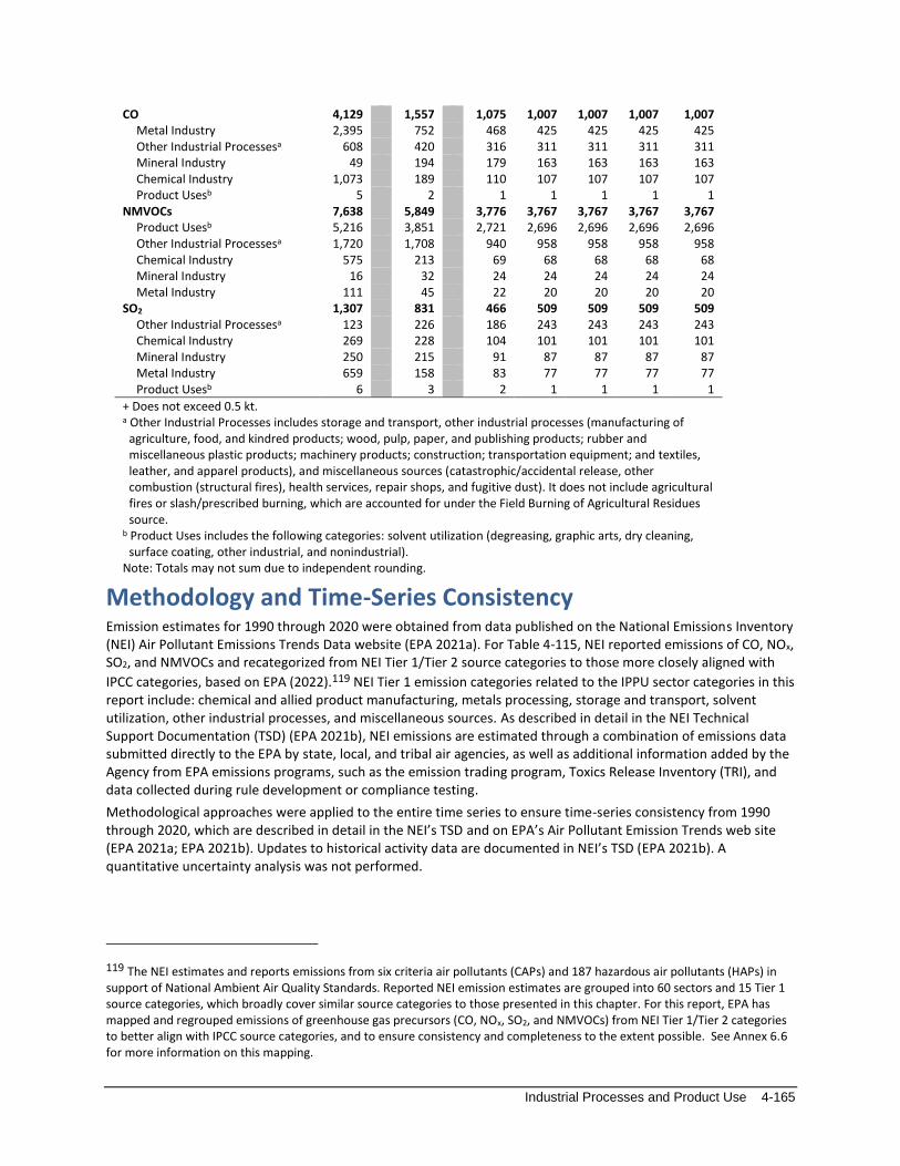
Industrial Processes and Product Use 4-165
CO 4,129 1,557 1,075 1,007 1,007 1,007 1,007 Metal Industry 2,395 752 468 425 425 425 425 Other Industrial Processesa 608 420 316 311 311 311 311 Mineral Industry 49 194 179 163 163 163 163 Chemical Industry 1,073 189 110 107 107 107 107 Product Usesb 5 2 1 1 1 1 1
NMVOCs 7,638 5,849 3,776 3,767 3,767 3,767 3,767 Product Usesb 5,216 3,851 2,721 2,696 2,696 2,696 2,696 Other Industrial Processesa 1,720 1,708 940 958 958 958 958 Chemical Industry 575 213 69 68 68 68 68 Mineral Industry 16 32 24 24 24 24 24 Metal Industry 111 45 22 20 20 20 20
SO2 1,307 831 466 509 509 509 509 Other Industrial Processesa 123 226 186 243 243 243 243 Chemical Industry 269 228 104 101 101 101 101 Mineral Industry 250 215 91 87 87 87 87 Metal Industry 659 158 83 77 77 77 77 Product Usesb 6 3 2 1 1 1 1
+ Does not exceed 0.5 kt. a Other Industrial Processes includes storage and transport, other industrial processes (manufacturing of
agriculture, food, and kindred products; wood, pulp, paper, and publishing products; rubber and miscellaneous plastic products; machinery products; construction; transportation equipment; and textiles, leather, and apparel products), and miscellaneous sources (catastrophic/accidental release, other combustion (structural fires), health services, repair shops, and fugitive dust). It does not include agricultural fires or slash/prescribed burning, which are accounted for under the Field Burning of Agricultural Residues source.
b Product Uses includes the following categories: solvent utilization (degreasing, graphic arts, dry cleaning, surface coating, other industrial, and nonindustrial).
Note: Totals may not sum due to independent rounding.
Methodology and Time-Series Consistency Emission estimates for 1990 through 2020 were obtained from data published on the National Emissions Inventory (NEI) Air Pollutant Emissions Trends Data website (EPA 2021a). For Table 4-115, NEI reported emissions of CO, NOx, SO2, and NMVOCs and recategorized from NEI Tier 1/Tier 2 source categories to those more closely aligned with
IPCC categories, based on EPA (2022).119 NEI Tier 1 emission categories related to the IPPU sector categories in this report include: chemical and allied product manufacturing, metals processing, storage and transport, solvent utilization, other industrial processes, and miscellaneous sources. As described in detail in the NEI Technical Support Documentation (TSD) (EPA 2021b), NEI emissions are estimated through a combination of emissions data submitted directly to the EPA by state, local, and tribal air agencies, as well as additional information added by the Agency from EPA emissions programs, such as the emission trading program, Toxics Release Inventory (TRI), and data collected during rule development or compliance testing.
Methodological approaches were applied to the entire time series to ensure time-series consistency from 1990 through 2020, which are described in detail in the NEI’s TSD and on EPA’s Air Pollutant Emission Trends web site (EPA 2021a; EPA 2021b). Updates to historical activity data are documented in NEI’s TSD (EPA 2021b). A quantitative uncertainty analysis was not performed.
119 The NEI estimates and reports emissions from six criteria air pollutants (CAPs) and 187 hazardous air pollutants (HAPs) in support of National Ambient Air Quality Standards. Reported NEI emission estimates are grouped into 60 sectors and 15 Tier 1 source categories, which broadly cover similar source categories to those presented in this chapter. For this report, EPA has mapped and regrouped emissions of greenhouse gas precursors (CO, NOx, SO2, and NMVOCs) from NEI Tier 1/Tier 2 categories to better align with IPCC source categories, and to ensure consistency and completeness to the extent possible. See Annex 6.6 for more information on this mapping.