
Integration of solar energy with industrial processes - CORE
250
POUR L'OBTENTION DU GRADE DE DOCTEUR ÈS SCIENCES acceptée sur proposition du jury: Dr J. Van Herle, président du jury Prof. F. Maréchal, Prof. S. Haussener, directeurs de thèse Prof. P. Radgen, rapporteur Prof. C. Markides, rapporteur Prof. C. Ludwig, rapporteur Integration of solar energy with industrial processes THÈSE N O 8635 (2018) ÉCOLE POLYTECHNIQUE FÉDÉRALE DE LAUSANNE PRÉSENTÉE LE 27 JUILLET 2018 À LA FACULTÉ DES SCIENCES ET TECHNIQUES DE L'INGÉNIEUR GROUPE SCI STI FM PROGRAMME DOCTORAL EN ENERGIE Suisse 2018 PAR Anna Sophia WALLERAND
-
Upload
khangminh22 -
Category
Documents
-
view
1 -
download
0
Transcript of Integration of solar energy with industrial processes - CORE

POUR L'OBTENTION DU GRADE DE DOCTEUR ÈS SCIENCES
acceptée sur proposition du jury:
Dr J. Van Herle, président du juryProf. F. Maréchal, Prof. S. Haussener, directeurs de thèse
Prof. P. Radgen, rapporteurProf. C. Markides, rapporteurProf. C. Ludwig, rapporteur
Integration of solar energy with industrial processes
THÈSE NO 8635 (2018)
ÉCOLE POLYTECHNIQUE FÉDÉRALE DE LAUSANNE
PRÉSENTÉE LE 27 JUILLET 2018
À LA FACULTÉ DES SCIENCES ET TECHNIQUES DE L'INGÉNIEURGROUPE SCI STI FM
PROGRAMME DOCTORAL EN ENERGIE
Suisse2018
PAR
Anna Sophia WALLERAND


To both my grandmas
“Have no fear of perfection; you’ll never reach it.”
Marie Curie


©Anja Hartig, [email protected]


Acknowledgments
Foremost, I would like to express my gratitude to my Professor, François Maréchal, for the opportu-
nity and the trust given to me. You are not only a great person and musician, but an even greater
scientist and a true inspiration. Thank you.
A great thank also goes to my co-supervisor, Sophia Haussener, for your availability whenever it was
needed and very motivating support. I admire you highly. I am sincerely honored by the participa-
tion of Peter Radgen, Christos Markides, Christian Ludwig in my thesis jury. I would like to express
my deep gratitude for the time, effort and devotion spent on the review of this work. I have greatly
learned from your detailed insight and careful revision.
All this would have never been realised, if it was not for Gianluca Ambrosetti, who introduced
me to the laboratory and created the contact to Airlight Energy SA, who financed the first part of
this PhD. Gianluca, you are a visionary, a great person and an inspiration. I would like to extend
my gratitude to Carina Alles and the BFE for supporting our research and giving us the chance to
participate in the IEA Heat Pump Annex 48. This thank is further extended to Carmen Stadtländer
and Dr. Reiner Jakobs representative for all participants in the Annex and the incredible work they
are doing. Mathias Blaser, du hast mir nicht nur eine wunderbare Zeit auf der Heat Pump Summit
beschert, sondern auch mit grosser Hingabe die wirklich wichtigen Fragen beantwortet, und damit
einen kleinen Einblick in die Industrie bereitet.
Non of this would have been possible without the dedication of talented students. Thank you,
Angelos Selviaridis, for being a great person and teaching me many things including TRNSYS. Régis
Voillat, it was a pleasure working with you. Your grit, wit and talent in this inititally unknown territory
impressed me.
Maziar. You are clearly the most gifted person I know. I do not know how to thank you for be-
ing the most inspiring, fair, and ethical working colleague anyone could ask for. For being an advisor,
a teacher, and most of all being a friend. I hope you will fly.
Ivan, thanks a lot! May I say that once? It fits perfectly. I would like to express my gratitude
i

Acknowledgments
for many fruitful discussions, for a lot of fun while dealing with difficult projects and foremost for
your reading and re-reading of every single document I authored and improving it in any possible
way. You are awesome.
The laboratory has been a great social environment and going to work was a pleasure. Many
colleagues became close friends. Stefano, I cannot really express how much our friendship means to
me, it makes me tearful. Only so much: it is a lot. Victor, your blissful non-caring caring-ness makes
me care about you, you are great. Raman, you are the only poet I know, thank you for being you.
Stéphane, you are the coolest person I know, and you have a great heart.
Ema, you were a great flatmate and friend, thanks. Katie & Guillaume, I would love to make another
attempt at your lives, in the meantime: stay awesome! Thank you, Dilan and Raluca for taking care
of me during ECOS 2016, the great time in Venice, and being generally nice people. Hür, you are
the kindest person I know, and I love watching you suffer (in crossfit). Nils, I want to harvest your
genes; and I admire you. Elfie, while speaking of people I admire... I might also add TiVi, Nicolas,
and Jean-Loup. Samira, thank you for being my first office mate and a mentor. Manu, thank you for
our shared love of Kim, Patrick and Priscilla, who is such a kick-ass woman. Francesco, for offering
yourself voluntarily to a great party joke and for being kind. Francesca, for never giving up. Luise,
for being the future and so lovely German. A great thank you to all the other great colleagues, it was
an amazing time.
Rike and Wiebke, thanks for being such important friends and sharing the path and the pain.
Marion, Birthe, Anna danke für viele schöne Urlaube und die Erinnerung an die wirklich wichtigen
Dinge. Anja, danke für die Zeichnung, du bist super. An alle Konstanzer Mädels: Ihr seid geil.
Danke an meine furchtbar fabelhafte Familie. Misi, André, Enno, Sari, ihr seid grossartig. Opa,
ich bewundere dich, und Jutta, ich bin dankbar, dass es dich gibt. Mama, manchmal hasse ich, wie
sehr ich dich liebe. Papa, danke für alles, immer. Felix, ich hab dich sehr lieb.
Riccardo, I am lacking words and will therefore refer to the words of a friend: If nothing would
have come out of these past years than meeting you, it would have been worth it all.
Lausanne, 31 May 2018
ii

AbstractSolar energy offers a great potential for integration with industrial processes, which conventionally
rely on fossil fuels to provide energy [1]. The seasonal, daily, and regional dependence of solar energy
alongside the scarcity of space or financial resources in many territories constitute great challenges.
These may be overcome by efficient solar energy use through optimal integration methods. Such
methods should address multiple aspects including accurate solar technology models and identifi-
cation of the "true" process requirements. Beyond that, optimal design of the integrated systems
and quantification of the added value of solar integration, particularly with regard to competing
technologies, is crucial. This thesis explores this multi-dimensional problem formulation through
elaboration of methodologies tailored to the low-temperature processing industries.
The intricacies behind this goal are addressed in four main chapters. (a) Chapter 2 examines options
for solar technology modeling in view of industrial integration. A design approach is developed
which allows estimation of solar system performance at sufficient precision and constrained compu-
tational effort. (b) In Chapter 3, a comprehensive method is proposed which addresses simultaneous
optimization of the process heat recovery, the conventional utilities, and the renewable utility system
(including thermal storage) using ε-constrained parametric optimization. (c) The promising results
from the third chapter motivate a more thorough analysis of industrial heat pump systems, which
is addressed in Chapter 4 presenting a novel generic heat pump superstructure-based synthesis
method for industrial applications based on mathematical programming. (d) The subsequent two
chapters address generalization of the derived methods to estimate potentials of relevant technolo-
gies at national and international scale from the perspective of multiple stakeholders. The derived
method generates a database of solutions by applying generalized optimization techniques.
The proposed methods are applied to the dairy industry and results reveal that solar energy should
be considered as part of a series of efficiency measures. It is shown that in many cases heat pumping
or mechanical vapor re-compression lead to more efficient and less costly solutions, which may be
extended with solar thermal energy or complimented with solar electricity.
Keywords
solar thermal collectors; high concentration photovoltaic and thermal system (HCPVT); photovoltaic
panels; industrial refrigeration; mathematical programming; heat pump superstructure; dairy
industry; waste heat recovery and reuse;
iii


ZusammenfassungDie Integration von Solarenergie in industrielle Prozesse, die normalerweise mit fossilen Brennstof-
fen versorgt werden, hat grosses Potential. Doch die saisonale, tägliche und regionale Abhängigkeit
von Sonnenstrahlung zusammen mit einer Knappheit an Platz und finanziellen Mitteln stellen
in vielen Gebieten grosse Herausforderungen dar. Mit effizienter Solarenergienutzung durch opti-
male Integrationsmethoden können diese jedoch überwunden werden. Solche Methoden sollten
verschiedene Blickpunkte berücksichtigen einschliesslich akkurater Modelierung der Solartechnolo-
gien und Identifizierung des wahren Prozesswärmebedarfs. Darüber hinaus muss das integrierte
System optimal geplant und der Mehrwert der Solarenergie gegenüber anderen Technologien genau
bestimmt werden. Diese Doktorarbeit beschäftigt mit dieser mehrdimensionalen Problemstellung
indem Methoden, die besonders auf Niedertemperatur-Prozesse ausgerichtet sind, in vier Kapiteln
entwickelt werden.
(a) Im ersten Kapitel werden verschiedene Möglichkeiten für Modellierung von Solartechnologien
vor dem Hintergrund der Prozessintegration diskutiert. Der entwickelte Ansatz erlaubt es den Ertrag
von Solaranlagen mit minimalem Rechenaufwand und genügender Präzision zu bestimmen. (b) Im
zweiten Kapitel wird eine umfassende Methode vorgestellt, die eine gleichzeitige Optimierung der
Wärmerückgewinnung, Wärmepumpen und des erneuerbaren Energiesystems (mit thermischen
Speichern) unter Verwendung von ε-Bedingungen ermöglicht. (c) Die Ergebnisse des zweiten Ka-
pitels motivieren eine genauere Analyse von industriellen Wärmepumpen, worauf die im dritten
Kapitel vorgestellte neuartige Methode zur generischen Wärmepumpensynthese abzielt. (d) Die
letzten beiden Kapitel dienen der Verallgemeinerung der entwickelten Methoden, um internationale
Potentiale für die relevanten Technologien aus der Perspektive von verschiedenen Akteuren zu
bestimmen. Die Methode entwickelt Lösungen durch verallgemeinerte Optimierungsverfahren.
Die vorgestellten Methoden werden in der Milchindustrie angewendet und die Ergebnisse decken
einen Zusammenhang zwischen solarer Energieintegration und einer Reihe anderer Effizienzmass-
nahmen auf. Die Ergebnisse zeigen, dass in vielen Fällen Wärmepumpen oder Dampfverdichtung
zu effizienteren Systemen mit niedrigeren Kosten führen, was mit solarthermischen Technologien
erweitert oder mit solarelektrischen Systemen komplementiert werden kann.
Schlüsselwörter
solarthermische Kollektoren ; hochkonzentrierte photovoltaisch und thermische Systeme ; photovol-
taische Kollektoren ; industrielle Wärmepumpen ; mathematische Programmierung ; Milchindustrie ;
Restwärmeverwertung und -nutzung;
v


Contents
Acknowledgments i
Abstract (English/Deutsch) iii
Table of content vii
List of figures xiii
List of tables xvii
Acronyms and abbreviations xix
List of Symbols xxiii
Introduction 1
Focus and goal of this thesis . . . . . . . . . . . . . . . . . . . . . . . . . . . . . . . . . . . . . . 2
State-of-the-art: methods for solar energy for industrial processes (SEIP) applications . . . 3
Solar modeling and design . . . . . . . . . . . . . . . . . . . . . . . . . . . . . . . . . . . 3
"Integration" with industrial processes . . . . . . . . . . . . . . . . . . . . . . . . . . . . 5
Extrapolation of solar potential . . . . . . . . . . . . . . . . . . . . . . . . . . . . . . . . . 6
Synthesis and scope . . . . . . . . . . . . . . . . . . . . . . . . . . . . . . . . . . . . . . . 7
Contribution and outline of the thesis . . . . . . . . . . . . . . . . . . . . . . . . . . . . . . . . 8
Terminology, conventions . . . . . . . . . . . . . . . . . . . . . . . . . . . . . . . . . . . . . . . 10
Mathematical conventions . . . . . . . . . . . . . . . . . . . . . . . . . . . . . . . . . . . 10
Cost conversion and currencies . . . . . . . . . . . . . . . . . . . . . . . . . . . . . . . . . 10
1 Context and motivation 11
1.1 Energy requirements in industry . . . . . . . . . . . . . . . . . . . . . . . . . . . . . . . . 11
1.2 Solar energy conversion . . . . . . . . . . . . . . . . . . . . . . . . . . . . . . . . . . . . . 12
1.3 Industrial heat pumping . . . . . . . . . . . . . . . . . . . . . . . . . . . . . . . . . . . . . 14
1.4 Heat recovery potential in a process: pinch analysis . . . . . . . . . . . . . . . . . . . . . 15
1.4.1 Minimum approach temperatureΔTmin . . . . . . . . . . . . . . . . . . . . . . . 15
1.4.2 Graphical representation, pinch point, and pinch rules . . . . . . . . . . . . . . 17
vii

Contents
1.4.3 Implications for solar energy for industrial processes (SEIP) . . . . . . . . . . . . 18
1.4.4 Implications for industrial heat pumps . . . . . . . . . . . . . . . . . . . . . . . . 18
1.4.5 The use of pinch analysis (PA) throughout the thesis . . . . . . . . . . . . . . . . 20
1.5 Integrated solar and heat pump systems . . . . . . . . . . . . . . . . . . . . . . . . . . . 20
2 Solar modeling and design 23
2.1 State-of-the-art . . . . . . . . . . . . . . . . . . . . . . . . . . . . . . . . . . . . . . . . . . 23
2.1.1 Solar collector modeling . . . . . . . . . . . . . . . . . . . . . . . . . . . . . . . . . 24
2.1.2 Design of solar systems . . . . . . . . . . . . . . . . . . . . . . . . . . . . . . . . . 24
2.1.3 Discussion and contribution . . . . . . . . . . . . . . . . . . . . . . . . . . . . . . 26
2.2 Problem statement . . . . . . . . . . . . . . . . . . . . . . . . . . . . . . . . . . . . . . . . 26
2.3 Modeling . . . . . . . . . . . . . . . . . . . . . . . . . . . . . . . . . . . . . . . . . . . . . . 27
2.3.1 Solar technologies . . . . . . . . . . . . . . . . . . . . . . . . . . . . . . . . . . . . 27
2.3.2 Meteorological data clustering . . . . . . . . . . . . . . . . . . . . . . . . . . . . . 32
2.4 System design and integration . . . . . . . . . . . . . . . . . . . . . . . . . . . . . . . . . 33
2.4.1 Objective function . . . . . . . . . . . . . . . . . . . . . . . . . . . . . . . . . . . . 33
2.4.2 Constraints . . . . . . . . . . . . . . . . . . . . . . . . . . . . . . . . . . . . . . . . 34
2.5 Results and discussion . . . . . . . . . . . . . . . . . . . . . . . . . . . . . . . . . . . . . . 37
2.5.1 Solar technologies . . . . . . . . . . . . . . . . . . . . . . . . . . . . . . . . . . . . 37
2.5.2 System design: Sensitivity to data clustering . . . . . . . . . . . . . . . . . . . . . 39
2.6 Conclusions . . . . . . . . . . . . . . . . . . . . . . . . . . . . . . . . . . . . . . . . . . . . 40
3 Comprehensive integration method 41
3.1 State-of-the-art . . . . . . . . . . . . . . . . . . . . . . . . . . . . . . . . . . . . . . . . . . 42
3.1.1 Solar design and system integration . . . . . . . . . . . . . . . . . . . . . . . . . . 42
3.1.2 Industrial heat pumping . . . . . . . . . . . . . . . . . . . . . . . . . . . . . . . . . 44
3.1.3 Discussion and contribution . . . . . . . . . . . . . . . . . . . . . . . . . . . . . . 44
3.2 Methodology . . . . . . . . . . . . . . . . . . . . . . . . . . . . . . . . . . . . . . . . . . . . 45
3.2.1 Problem statement . . . . . . . . . . . . . . . . . . . . . . . . . . . . . . . . . . . . 45
3.2.2 Overview . . . . . . . . . . . . . . . . . . . . . . . . . . . . . . . . . . . . . . . . . . 45
3.2.3 Data collection & clustering (A) . . . . . . . . . . . . . . . . . . . . . . . . . . . . . 46
3.2.4 System resolution (B) . . . . . . . . . . . . . . . . . . . . . . . . . . . . . . . . . . . 51
3.2.5 Performance calculation (C) . . . . . . . . . . . . . . . . . . . . . . . . . . . . . . 53
3.3 Results and discussion . . . . . . . . . . . . . . . . . . . . . . . . . . . . . . . . . . . . . . 55
3.3.1 Scenario definition . . . . . . . . . . . . . . . . . . . . . . . . . . . . . . . . . . . . 55
3.3.2 Daytime operation of the process (Δ) . . . . . . . . . . . . . . . . . . . . . . . . . 55
3.3.3 Continuous process operation (O) . . . . . . . . . . . . . . . . . . . . . . . . . . . 63
3.4 Conclusions . . . . . . . . . . . . . . . . . . . . . . . . . . . . . . . . . . . . . . . . . . . . 66
viii

Contents
4 Generic heat pump superstructure 67
4.1 State-of-the-art . . . . . . . . . . . . . . . . . . . . . . . . . . . . . . . . . . . . . . . . . . 68
4.1.1 Conceptual methods . . . . . . . . . . . . . . . . . . . . . . . . . . . . . . . . . . . 68
4.1.2 Mathematical methods . . . . . . . . . . . . . . . . . . . . . . . . . . . . . . . . . 69
4.1.3 Discussion and contribution . . . . . . . . . . . . . . . . . . . . . . . . . . . . . . 71
4.2 Methodology . . . . . . . . . . . . . . . . . . . . . . . . . . . . . . . . . . . . . . . . . . . . 72
4.2.1 Problem statement . . . . . . . . . . . . . . . . . . . . . . . . . . . . . . . . . . . . 72
4.2.2 Superstructure synthesis . . . . . . . . . . . . . . . . . . . . . . . . . . . . . . . . 73
4.2.3 Mathematical formulation . . . . . . . . . . . . . . . . . . . . . . . . . . . . . . . 73
4.2.4 Fluid selection . . . . . . . . . . . . . . . . . . . . . . . . . . . . . . . . . . . . . . . 79
4.3 Results and discussion . . . . . . . . . . . . . . . . . . . . . . . . . . . . . . . . . . . . . . 79
4.3.1 Benchmarking analysis . . . . . . . . . . . . . . . . . . . . . . . . . . . . . . . . . 80
4.3.2 Optimization . . . . . . . . . . . . . . . . . . . . . . . . . . . . . . . . . . . . . . . 82
4.3.3 Extended analysis . . . . . . . . . . . . . . . . . . . . . . . . . . . . . . . . . . . . . 86
4.4 Conclusions . . . . . . . . . . . . . . . . . . . . . . . . . . . . . . . . . . . . . . . . . . . . 90
5 Generalization (A): heat pumping and co-generation 91
5.1 State-of-the-art . . . . . . . . . . . . . . . . . . . . . . . . . . . . . . . . . . . . . . . . . . 92
5.1.1 Design studies . . . . . . . . . . . . . . . . . . . . . . . . . . . . . . . . . . . . . . . 92
5.1.2 Potential studies . . . . . . . . . . . . . . . . . . . . . . . . . . . . . . . . . . . . . 94
5.1.3 Discussion and contribution . . . . . . . . . . . . . . . . . . . . . . . . . . . . . . 94
5.2 Methodology . . . . . . . . . . . . . . . . . . . . . . . . . . . . . . . . . . . . . . . . . . . . 95
5.2.1 Problem statement . . . . . . . . . . . . . . . . . . . . . . . . . . . . . . . . . . . . 95
5.2.2 Overview . . . . . . . . . . . . . . . . . . . . . . . . . . . . . . . . . . . . . . . . . . 96
5.2.3 Comprehensive solution space generation . . . . . . . . . . . . . . . . . . . . . . 97
5.2.4 Results retrieval . . . . . . . . . . . . . . . . . . . . . . . . . . . . . . . . . . . . . . 102
5.3 Application . . . . . . . . . . . . . . . . . . . . . . . . . . . . . . . . . . . . . . . . . . . . . 102
5.3.1 Modular dairy plant . . . . . . . . . . . . . . . . . . . . . . . . . . . . . . . . . . . 102
5.3.2 Scope definition . . . . . . . . . . . . . . . . . . . . . . . . . . . . . . . . . . . . . . 104
5.3.3 Solution generation . . . . . . . . . . . . . . . . . . . . . . . . . . . . . . . . . . . 106
5.4 Results and discussion . . . . . . . . . . . . . . . . . . . . . . . . . . . . . . . . . . . . . . 109
5.4.1 Comprehensive solution space generation . . . . . . . . . . . . . . . . . . . . . . 109
5.4.2 Results retrieval . . . . . . . . . . . . . . . . . . . . . . . . . . . . . . . . . . . . . . 112
5.5 Conclusions . . . . . . . . . . . . . . . . . . . . . . . . . . . . . . . . . . . . . . . . . . . . 120
6 Generalization (B): addition of solar utilities 123
6.1 State-of-the-art . . . . . . . . . . . . . . . . . . . . . . . . . . . . . . . . . . . . . . . . . . 124
6.1.1 Top-down . . . . . . . . . . . . . . . . . . . . . . . . . . . . . . . . . . . . . . . . . 124
6.1.2 Bottom-up . . . . . . . . . . . . . . . . . . . . . . . . . . . . . . . . . . . . . . . . . 124
ix

Contents
6.1.3 Discussion and contribution . . . . . . . . . . . . . . . . . . . . . . . . . . . . . . 126
6.2 Methodology . . . . . . . . . . . . . . . . . . . . . . . . . . . . . . . . . . . . . . . . . . . . 126
6.2.1 Problem statement . . . . . . . . . . . . . . . . . . . . . . . . . . . . . . . . . . . . 126
6.2.2 Derivation . . . . . . . . . . . . . . . . . . . . . . . . . . . . . . . . . . . . . . . . . 127
6.2.3 Approach . . . . . . . . . . . . . . . . . . . . . . . . . . . . . . . . . . . . . . . . . . 130
6.3 Results and discussion . . . . . . . . . . . . . . . . . . . . . . . . . . . . . . . . . . . . . . 132
6.4 Conclusions . . . . . . . . . . . . . . . . . . . . . . . . . . . . . . . . . . . . . . . . . . . . 136
Conclusions 137
Main results summary . . . . . . . . . . . . . . . . . . . . . . . . . . . . . . . . . . . . . . . . . 137
Significance of the work . . . . . . . . . . . . . . . . . . . . . . . . . . . . . . . . . . . . . . . . 140
Recommendations and guidance . . . . . . . . . . . . . . . . . . . . . . . . . . . . . . . . . . 141
Future perspectives . . . . . . . . . . . . . . . . . . . . . . . . . . . . . . . . . . . . . . . . . . . 142
Appendix 143
A General data 145
A.1 Introduction . . . . . . . . . . . . . . . . . . . . . . . . . . . . . . . . . . . . . . . . . . . . 145
B Comprehensive integration method (Chapter 3) 147
B.1 Additional results . . . . . . . . . . . . . . . . . . . . . . . . . . . . . . . . . . . . . . . . . 147
B.2 Performance parameters and cost functions . . . . . . . . . . . . . . . . . . . . . . . . . 148
B.2.1 Heat exchanger network (HEN) cost estimation . . . . . . . . . . . . . . . . . . . 148
B.2.2 Non-renewable technologies . . . . . . . . . . . . . . . . . . . . . . . . . . . . . . 148
B.2.3 Solar technologies . . . . . . . . . . . . . . . . . . . . . . . . . . . . . . . . . . . . 151
B.3 Weather data & clustering . . . . . . . . . . . . . . . . . . . . . . . . . . . . . . . . . . . . 156
B.4 Dairy process . . . . . . . . . . . . . . . . . . . . . . . . . . . . . . . . . . . . . . . . . . . 157
C Generic heat pump superstructure (Chapter 4) 159
C.1 General . . . . . . . . . . . . . . . . . . . . . . . . . . . . . . . . . . . . . . . . . . . . . . . 159
C.1.1 MOGA input parameters . . . . . . . . . . . . . . . . . . . . . . . . . . . . . . . . . 159
C.1.2 MILP input parameters . . . . . . . . . . . . . . . . . . . . . . . . . . . . . . . . . 160
C.2 Benchmark analysis . . . . . . . . . . . . . . . . . . . . . . . . . . . . . . . . . . . . . . . 160
C.2.1 Benchmark cases . . . . . . . . . . . . . . . . . . . . . . . . . . . . . . . . . . . . . 160
C.2.2 Extended case E2 . . . . . . . . . . . . . . . . . . . . . . . . . . . . . . . . . . . . . 163
C.3 Heat pump superstructure . . . . . . . . . . . . . . . . . . . . . . . . . . . . . . . . . . . 165
C.3.1 Heat pump parameters in targeting problem (MILP) . . . . . . . . . . . . . . . . 165
C.3.2 Heat pump specific constraints . . . . . . . . . . . . . . . . . . . . . . . . . . . . . 167
x

Contents
D Generalization (A) - heat pumping and co-generation (Chapter 5) 171
D.1 General . . . . . . . . . . . . . . . . . . . . . . . . . . . . . . . . . . . . . . . . . . . . . . . 171
D.1.1 MOGA input parameters . . . . . . . . . . . . . . . . . . . . . . . . . . . . . . . . . 171
D.1.2 MILP input parameters . . . . . . . . . . . . . . . . . . . . . . . . . . . . . . . . . 172
D.2 Additional results . . . . . . . . . . . . . . . . . . . . . . . . . . . . . . . . . . . . . . . . . 172
D.2.1 Sampling in detail . . . . . . . . . . . . . . . . . . . . . . . . . . . . . . . . . . . . 172
D.2.2 Solution generation & pruning: remaining plants . . . . . . . . . . . . . . . . . . 173
D.2.3 Results retrieval: remaining plants . . . . . . . . . . . . . . . . . . . . . . . . . . . 176
D.2.4 Database of solutions . . . . . . . . . . . . . . . . . . . . . . . . . . . . . . . . . . 176
D.3 Industrial case study . . . . . . . . . . . . . . . . . . . . . . . . . . . . . . . . . . . . . . . 184
D.3.1 Dairy process . . . . . . . . . . . . . . . . . . . . . . . . . . . . . . . . . . . . . . . 184
D.3.2 Utilities . . . . . . . . . . . . . . . . . . . . . . . . . . . . . . . . . . . . . . . . . . . 186
Curriculum Vitae 213
xi


List of Figures1 Global availability of fossil reserves, and renewable energy supplied to Earth’s surface
within a year. . . . . . . . . . . . . . . . . . . . . . . . . . . . . . . . . . . . . . . . . . . . . 2
2 Focus in literature on "integration" of solar energy with industrial processes. . . . . . 5
3 Bottom-up, top-down approaches for solar potential studies. . . . . . . . . . . . . . . . 6
4 Graphical overview of thesis structure. . . . . . . . . . . . . . . . . . . . . . . . . . . . . 9
1.1 Industrial thermal energy requirements and respective temperature levels. . . . . . . . 12
1.2 Solar energy conversion routes tree diagram. . . . . . . . . . . . . . . . . . . . . . . . . . 13
1.3 Web of science, key words: waste heat recovery, top cited papers of last 10 years. . . . . 16
1.4 Heat pumping technology tree diagram. . . . . . . . . . . . . . . . . . . . . . . . . . . . 16
1.5 Temperature enthalpy profile of a counter current heat exchanger to illustrate theΔTmin. 16
1.6 (a) Individual hot streams, (b) hot composite curve (CC) in temperature enthalpy
diagram. . . . . . . . . . . . . . . . . . . . . . . . . . . . . . . . . . . . . . . . . . . . . . . 17
1.7 (a) Hot and cold CCs, (b) grand composite curve (GCC) in temperature enthalpy diagram. 17
1.8 Heat pump integration to process GCC. . . . . . . . . . . . . . . . . . . . . . . . . . . . . 19
1.9 Comparison of overall sun-to-thermal conversion efficiency. . . . . . . . . . . . . . . . 20
1.10 Solar and heat pump integration to process GCC. . . . . . . . . . . . . . . . . . . . . . . 21
2.1 Angles of the sun towards earth normal and inclined surface. . . . . . . . . . . . . . . . 28
2.2 Transient System Simulation Tool [2] (TRNSYS) flowchart of flat plate collector model. 38
3.1 Methodology proposed in Chapter 3. . . . . . . . . . . . . . . . . . . . . . . . . . . . . . 46
3.2 Dairy process flowsheet including utility system. . . . . . . . . . . . . . . . . . . . . . . 47
3.3 Hot and cold CCs and GCC of dairy process. . . . . . . . . . . . . . . . . . . . . . . . . . 48
3.4 Heat pump superstructure model. (a) Ammonia liquid-vapor saturation curve with
isobars, (b) flowchart of heat pump superstructure. . . . . . . . . . . . . . . . . . . . . . 50
3.5 Load duration curve of DNI in Sion, Switzerland (CH), of original data and 8 typical
plus 2 extreme days. . . . . . . . . . . . . . . . . . . . . . . . . . . . . . . . . . . . . . . . 51
3.6 Integrated composite curves (ICCs) of the dairy process and respective utility system. 57
3.7 Illustration of the conversion cycles involved in the respective scenarios. . . . . . . . . 57
3.8 Process operation scheme and solar radiation during typical periods. . . . . . . . . . . 59
xiii

List of Figures
3.9 Results from ε-constraint optimization of different solar options for daytime only
process operation. . . . . . . . . . . . . . . . . . . . . . . . . . . . . . . . . . . . . . . . . 60
3.10 (a) Optimal active solar area, from ε-constraint optimization (ε between 95 and 60%),
(b) ICC of the dairy process and respective utility system. . . . . . . . . . . . . . . . . . 62
3.11 Solar integration, (a) hot utility streams heat load vs time, (b) multi-period ICCs of the
dairy process and respective utility system. . . . . . . . . . . . . . . . . . . . . . . . . . . 62
3.12 Results of ε-constraint optimization of different solar options for continuous process
operation. . . . . . . . . . . . . . . . . . . . . . . . . . . . . . . . . . . . . . . . . . . . . . 65
3.13 (a) Optimal active solar area, from ε-constraint optimization (ε between 95 and 70%),
(b) ICCs of the dairy process and respective utility system. . . . . . . . . . . . . . . . . . 65
4.1 Flowsheet and temperature-entropy diagram of the heat pump superstructure (HPS)
with sample cycles. . . . . . . . . . . . . . . . . . . . . . . . . . . . . . . . . . . . . . . . . 73
4.2 Method proposed in Chapter 4. . . . . . . . . . . . . . . . . . . . . . . . . . . . . . . . . . 74
4.3 GCCs from process thermal streams of three benchmark cases. . . . . . . . . . . . . . . 81
4.4 E2. (a) Multi-objective results, (b) utility ICCs of Reference and min(HPS). . . . . . . . . 83
4.5 Ethylene. (a) Multi-objective results, (b) utility ICCs. . . . . . . . . . . . . . . . . . . . . 83
4.6 Cold Tray. (a) Multi-objective results, (b) utility ICCs. . . . . . . . . . . . . . . . . . . . . 83
4.7 Flowchart of min(HPS) solutions heat pump designs. . . . . . . . . . . . . . . . . . . . . 85
4.8 (a) Fluid set and (b) multi-objective optimization results. In black: multi-fluid solution. 87
4.9 Performance of compressor between saturation levels T1 (32.5°C) and T2 (-17°C). . . . 88
4.10 Overall non-dominated frontier of MOGA results from master level fluid selection. . . 89
5.1 Standard deterministic multi-objective optimization problem statement. . . . . . . . . 96
5.2 Method proposed in Chapter 5. . . . . . . . . . . . . . . . . . . . . . . . . . . . . . . . . . 97
5.3 Relations between input data and desired output. . . . . . . . . . . . . . . . . . . . . . . 98
5.4 Generalized multi-objective optimization strategy. . . . . . . . . . . . . . . . . . . . . . 99
5.5 Flowsheet of the pruning step. . . . . . . . . . . . . . . . . . . . . . . . . . . . . . . . . . 102
5.6 Flowsheet of the modular dairy plant. . . . . . . . . . . . . . . . . . . . . . . . . . . . . . 105
5.7 Dairy plants’ utility ICCs. . . . . . . . . . . . . . . . . . . . . . . . . . . . . . . . . . . . . 105
5.8 Resource prices, commercial bank lending rates, annualization factor, low voltage
electricity grid emissions of various OECD countries. . . . . . . . . . . . . . . . . . . . . 106
5.9 ε-constraint case: results from multi-objective optimization of plant 2. . . . . . . . . . 109
5.10 Weighted sum of objectives: results from multi-objective optimization of plant 2. . . . 110
5.11 Occurrence of minimum TAC solutions during the sampling of plant 2. . . . . . . . . . 110
5.12 Exergy efficiency and utility selection of selected plants. . . . . . . . . . . . . . . . . . . 111
5.13 Pruned solution characteristics, plant 2. . . . . . . . . . . . . . . . . . . . . . . . . . . . 112
5.14 Cost data, CO2 equivalent emissions, plant 2. . . . . . . . . . . . . . . . . . . . . . . . . 114
5.15 Plant 2, utility maps. . . . . . . . . . . . . . . . . . . . . . . . . . . . . . . . . . . . . . . . 114
xiv

List of Figures
5.16 Plant 2,ΔTmin/2=5K fixed HEN, utility maps. . . . . . . . . . . . . . . . . . . . . . . . . 114
5.17 Most recurring solution of ε-constrained objective of plant 2,ΔTmin/2=5K fixed HEN. 116
5.18 On-line decision making platform. . . . . . . . . . . . . . . . . . . . . . . . . . . . . . . . 117
5.19 Minimum TAC solutions and respective payback time. Influence of political actions
on economically viable solutions. . . . . . . . . . . . . . . . . . . . . . . . . . . . . . . . 118
5.20 Detailed cost data versus CO2 equivalent emissions for min(TAC) points. . . . . . . . . 119
5.21 Boiler, co-generation engine and cooling water loads versus CO2 equivalent emissions
for min(TAC) points. . . . . . . . . . . . . . . . . . . . . . . . . . . . . . . . . . . . . . . . 119
5.22 Electrical power loads (and heat pump data) versus CO2 equivalent emissions for
min(TAC) points. . . . . . . . . . . . . . . . . . . . . . . . . . . . . . . . . . . . . . . . . . 119
6.1 Results from MILP in Chapter 3, flat plate collector area for different process operating
times. . . . . . . . . . . . . . . . . . . . . . . . . . . . . . . . . . . . . . . . . . . . . . . . . 129
6.2 Thermal utility operation for flat plate collector integration, from Chapter 3, non-stop
operation, solar fraction of 0.3. . . . . . . . . . . . . . . . . . . . . . . . . . . . . . . . . . 129
6.3 Thermal utility operation for flat plate collector integration, from Chapter 3, non-stop
operation, solar fraction of 0.5. . . . . . . . . . . . . . . . . . . . . . . . . . . . . . . . . . 129
6.4 Methodology proposed in Chapter 6. . . . . . . . . . . . . . . . . . . . . . . . . . . . . . 131
6.5 Database enhanced with solar data, results of statistical analysis, and break-even
collector cost. . . . . . . . . . . . . . . . . . . . . . . . . . . . . . . . . . . . . . . . . . . . 133
6.6 TAC versus emissions of solar enhanced database. . . . . . . . . . . . . . . . . . . . . . 133
6.7 Cost analysis of min(TAC) points of solar enhanced database, 2500 h. . . . . . . . . . . 133
6.8 Cost analysis of min(TAC) points of solar enhanced database, 2500 h, break-even cost. 135
6.9 Cost analysis of min(TAC) points of solar enhanced database, 8000 h, break-even cost. 135
6.10 Thermal units of min(TAC) points of solar enhanced database, 2500 h, break-even cost.135
A.1 Global availability of DNI and GHI. . . . . . . . . . . . . . . . . . . . . . . . . . . . . . . 145
B.1 Primary energy, fuel, electricity, and CO2 emission savings of non-stop operation
solutions. . . . . . . . . . . . . . . . . . . . . . . . . . . . . . . . . . . . . . . . . . . . . . . 147
B.2 Thermal conversion efficiency of flat plate (FP) solar thermal collectors. . . . . . . . . 151
B.3 Electrical conversion efficiency of photovoltaic modules (PVs). . . . . . . . . . . . . . . 153
B.4 Comparison of TRNSYS results and static model for HCPVT. . . . . . . . . . . . . . . . 154
B.5 Thermal storage volume and temperature distribution. . . . . . . . . . . . . . . . . . . 155
C.1 Analysis of multi-objective genetic algorithm (MOGA) propagation of extended case E2.160
C.2 Set of selected fluids considered during multi-objective optimization. . . . . . . . . . . 163
C.3 Extended case E2 minimum total annualized costs (TAC) solution. . . . . . . . . . . . . 164
C.4 Heat exchanger network design of extended case E2 with Aspen Energy Analyzer. . . . 165
C.5 Temperature-entropy diagram with mass and energy balances of the HPS. . . . . . . . 167
xv

List of Figures
D.1 Analysis of MOGA propagation of plant x = 2. . . . . . . . . . . . . . . . . . . . . . . . . 172
D.2 Selection of solutions with different sampling algorithms. . . . . . . . . . . . . . . . . . 173
D.3 Histogram and cumulative sum of occurrences. . . . . . . . . . . . . . . . . . . . . . . . 173
D.4 Solution generation. . . . . . . . . . . . . . . . . . . . . . . . . . . . . . . . . . . . . . . . 174
D.5 Solution pruning. . . . . . . . . . . . . . . . . . . . . . . . . . . . . . . . . . . . . . . . . . 174
D.6 Pruned solution characteristics. . . . . . . . . . . . . . . . . . . . . . . . . . . . . . . . . 175
D.7 Solution indexes. . . . . . . . . . . . . . . . . . . . . . . . . . . . . . . . . . . . . . . . . . 176
D.8 Cost data. . . . . . . . . . . . . . . . . . . . . . . . . . . . . . . . . . . . . . . . . . . . . . . 177
D.9 ICCs selected during data retrieval of plant 2. . . . . . . . . . . . . . . . . . . . . . . . . 178
D.10 ICCs selected during data retrieval of plant 2,ΔTmin/2=5K. . . . . . . . . . . . . . . . . 181
D.11 Compressor cost functions, installed cost. . . . . . . . . . . . . . . . . . . . . . . . . . . 186
xvi

List of Tables
2.1 State-of-the-art summary of solar modeling and design studies for SEIP applications. 25
2.2 Different numbers of typical days and influence on results of mixed integer linear
programming (MILP) case study. . . . . . . . . . . . . . . . . . . . . . . . . . . . . . . . . 40
3.1 State-of-the-art summary of solar modeling and integration studies for SEIP applications. 43
3.2 Data related to emissions, primary energy consumption and operating cost in Switzer-
land (CH). . . . . . . . . . . . . . . . . . . . . . . . . . . . . . . . . . . . . . . . . . . . . . 53
3.3 Investigated utility technology integration scenarios. . . . . . . . . . . . . . . . . . . . . 55
3.4 Utility integration scenarios as described in Section 3.3.1. . . . . . . . . . . . . . . . . . 57
4.1 Heat pump features considered in this work. . . . . . . . . . . . . . . . . . . . . . . . . . 69
4.2 State-of-the-art summary of synthesis methods for heat pump design and integration
with industrial processes. . . . . . . . . . . . . . . . . . . . . . . . . . . . . . . . . . . . . 70
4.3 Variables and objective function at master level. . . . . . . . . . . . . . . . . . . . . . . . 76
4.4 Variables and objective function at slave level. . . . . . . . . . . . . . . . . . . . . . . . . 80
4.5 Comparison of original data and data reproduced (Reference) in this work with the HPS. 82
4.6 Optimization results. Data shown as Reference was generated with HPS based on the
respective literature input data (Section 4.3.1). . . . . . . . . . . . . . . . . . . . . . . . . 85
5.1 State-of-the-art summary of synthesis methods and potential studies for heat pump
integration with industrial processes. . . . . . . . . . . . . . . . . . . . . . . . . . . . . . 93
5.2 Key performance indicators (KPI) calculated during post-computational analysis. . . 103
5.3 Product mass flow rates and reference resource consumption of examined dairy plants.105
5.4 Free and fixed input parameter set to optimization problem. . . . . . . . . . . . . . . . 107
5.5 Variables and objective function of the problem. . . . . . . . . . . . . . . . . . . . . . . 108
6.1 State-of-the-art summary of potential estimation studies for SEIP applications. . . . . 125
6.2 General solar data assumed. . . . . . . . . . . . . . . . . . . . . . . . . . . . . . . . . . . 134
6.3 Data ranges of free parameters as derived in Chapter 5. . . . . . . . . . . . . . . . . . . 134
B.1 Heat exchanger network (HEN) cost estimation parameters. . . . . . . . . . . . . . . . 148
B.2 Boiler (BOI) parameters. . . . . . . . . . . . . . . . . . . . . . . . . . . . . . . . . . . . . . 149
xvii

List of Tables
B.3 Heat pump parameters. . . . . . . . . . . . . . . . . . . . . . . . . . . . . . . . . . . . . . 150
B.4 Flat plate solar collector (FP) parameters. . . . . . . . . . . . . . . . . . . . . . . . . . . . 152
B.5 Photovoltaic module (PV) parameters. . . . . . . . . . . . . . . . . . . . . . . . . . . . . 154
B.6 High concentration photovoltaic and thermal system (HCPVT) parameters. . . . . . . 155
B.7 Mean data and performance indicators of typical days compared to original. . . . . . 156
B.8 Hot and cold streams of the dairy process. . . . . . . . . . . . . . . . . . . . . . . . . . . 157
C.1 Input parameters for MOGA method. . . . . . . . . . . . . . . . . . . . . . . . . . . . . . 159
C.2 Input parameters for CPLEX. . . . . . . . . . . . . . . . . . . . . . . . . . . . . . . . . . . 160
C.3 Streams data of the three benchmark cases. . . . . . . . . . . . . . . . . . . . . . . . . . 161
C.4 Benchmark case data. . . . . . . . . . . . . . . . . . . . . . . . . . . . . . . . . . . . . . . 162
C.5 Optimization problem description: extended case E2. . . . . . . . . . . . . . . . . . . . 164
C.6 Data of streams of the heat pump superstructure (HPS). . . . . . . . . . . . . . . . . . . 167
D.1 Input parameters for MOGA method. . . . . . . . . . . . . . . . . . . . . . . . . . . . . . 171
D.2 Input parameters for CPLEX. . . . . . . . . . . . . . . . . . . . . . . . . . . . . . . . . . . 172
D.3 Database of solutions for plant 2 (I). . . . . . . . . . . . . . . . . . . . . . . . . . . . . . . 179
D.4 Database of solutions for plant 2 (II). . . . . . . . . . . . . . . . . . . . . . . . . . . . . . 180
D.5 Database of solutions for plant 2,ΔTmin/2=5K (I). . . . . . . . . . . . . . . . . . . . . . . 182
D.6 Database of solutions for plant 2,ΔTmin/2=5K (II). . . . . . . . . . . . . . . . . . . . . . 183
D.7 Hot and cold streams of the generalized dairy process. . . . . . . . . . . . . . . . . . . . 185
D.8 Utility thermal and resource stream data. . . . . . . . . . . . . . . . . . . . . . . . . . . . 185
xviii

Acronyms and abbreviations
SP-A solar system and industrial process analysis
SP-I solar system and industrial process integration and optimization
SP solar systems analysis for industrial process applications
AHP absorption heat pump
AMPL A Mathematical Programming Language [3]
CA Canada
capex annualized capital expenses
CC composite curve
CDC load duration curve of the average
CEPCI Chemical Engineering Plant Cost Index [4]
CH Switzerland
CHP combined heat and power
CO2 carbon dioxide
COGEN co-generation engine
COP coefficient of performance
CPC concentrating parabolic collector
CPLEX IBM ILOG CPLEX Optimization Studio [5]
CPV concentrating photovoltaic system
CSE concentrated solar energy
CST concentrated solar thermal system
DE Germany
DNI direct normal irradiation
environomic environmental and economic
ES Spain
ETC evacuated tube collector
FP flat plate thermal collector
GA genetic algorithm
GCC grand composite curve
GHI global horizontal irradiation
GWP global warming potential
xix

Acronyms and abbreviations
HCPVT high concentration photovoltaic and thermal system
HEN heat exchanger network
HEX heat exchanger
HF heliostat field
HFC Hydrofluorocarbons
HP heat pump
HPS heat pump superstructure
ICC integrated composite curve
ICC Intergovernmental Panel on Climate Change
KPI key performance indicators
LDC load duration curve
LHV lower heating value
LP linear programming
mELDC mean error of the load duration curve
mELDC2 mean squared error of the load duration curve
MER minimum energy requirement
MILP mixed integer linear programming
MINLP mixed integer nonlinear programming
MIP mixed integer programming
MOGA multi-objective genetic algorithm
MSI Marshall and Swift Index [6]
MVR mechanical vapor re-compression
NLP nonlinear programming
NOCT nominal cell operating temperature
OECD Organization for Economic Co-operation and Development
opex yearly operating expenses
ORC organic rankine cycle
PA pinch analysis
PAM partitioning around medoids
PSO particle swarm optimization
PT Portugal
PTC parabolic trough collector
PV photovoltaic module
PVT (non-concentrating) photovoltaic and thermal system
SEIP solar energy for industrial processes
SHIP solar heat for industrial processes
ST solar (non-concentrating) thermal system
STC standard testing conditions
xx

Acronyms and abbreviations
TAC total annualized costs
thermo-
economic
thermodynamic and economic
thermo-
environmental
thermodynamic and environmental
TMY typical meteorological year
TPES total primary energy supply
TRNSYS Transient System Simulation Tool [2]
TSA total site analysis
US United States of America
xxi


List of Symbols
Variables (MILP)
AHE N heat exchanger network (HEN) area [m2]
C capex annualized capital expenses [currency/y]
C HE N investment cost of heat exchanger network (HEN) [currency]
C I NV total (installed) investment cost [currency]
C opex total annual operating expenses [currency/y]
C T AC total annual cost [currency/y]
C w updated investment cost of utility technology w [currency]
CO2,tot system overall resource CO2 equivalent emissions [kgCO2 ]
f g ,COMP i→ jp compressor sizing factor from level i → j of heat pump g in period p [-]
f g ,COND ip condenser sizing factor on level i of heat pump g in period p [-]
f g ,DE-SUP ip de-superheating through mixing unit sizing factor from level i of heat
pump g in period p
[-]
f g ,EVAP ip evaporator sizing factor on level i of heat pump g in period p [-]
f g ,GAS-COOL ip gas-cooling heat exchanger sizing factor from level i of heat pump g
in period p
[-]
f g ,MIX ip mixer sizing factor on level i of heat pump g in period p [-]
f g ,PRESAT j→ip presaturator sizing factor from level j → i of heat pump g in period p [-]
fstloss loss factor of storage unit st [-]
f st ,i np inlet unit sizing factor during period p of storage unit st [-]
f st ,outp outlet unit sizing factor during period p of storage unit st [-]
f stp sizing factor during period p of storage unit st [-]
f wp sizing factor of technology w during period p, [fw,max, fw,min] [-]
f w maximum size of technology w
N HE Nmin minimum number of HEXs [#]
y wp existence of technology w in period p, 0,1 [-]
y w maximum existence of technology w , 0,1
wC T AC weighted total annual cost function [currency/y]
xg , j→iV vapor fraction after expansion from level j to i of heat pump g [-]
xxiii

List of Symbols
y g ,COMP i→ jp compressor existence from level i → j of heat pump g in period p [-]
y st ,i np inlet unit existence during period p of storage unit st , 0,1 [-]
y st ,outp outlet unit existence during period p of storage unit st , 0,1 [-]
E g ,COMP i→ j maximum (electrical) power consumption of compressor i → j in heat
pump g
[kW]
E w maximum (electrical) power consumption of utility technology w [kW]
Er energetic consumption of resource r [kW]
Q st thermal flow during charge and discharge of storage unit st [kJ/period]
Rp,k residual heat in period p transfered from interval k −1 to interval k [kW]
V stp volume of storage material in unit st during p, which is at hot temper-
ature Tsth
[m3]
Variables (nonlinear constraints)
∆Ti ,DSH superheated temperature difference after compression on level i [K]
∆Ti ,PRE preheating temperature difference before compression on level i [K]
∆Ti ,SC subcooling temperature difference before expansion on level i [K]
Ti saturation temperature on level i [K]
εr epsilon constraint on the resource consumption [-]
ξ slave function weighting factor [-]
Greek Letters
α thermal stream heat transfer coefficient [W/m2K]
η0 reference efficiency of solar systems [-]
ηel electrical efficiency [-]
ηisentropic isentropic compressor efficiency of heat pump [kg/s]
ηw sel average solar utility electricity efficiency [-]
ηw sth average solar utility thermal efficiency [-]
ηw s average solar utility efficiency [-]
ηth thermal efficiency [-]
γi surface, i, azimuth angle [°]
γs solar azimuth angle (vector) [°]
λis solar beam incidence angle with respect to an inclined surface, i (vec-
tor)
[°]
Ω storage cycle length (in number of periods) [#]
ρg ground reflectivity [-]
ρst density of fluid in storage unit st [kg/m3]
τα effective transmittance-absorptance product [-]
τ investment cost annualization factor [1/y]
θi surface inclination angle [°]
xxiv

List of Symbols
θs solar zenith angle (vector) [°]
Parameters (heat pump)
Eg ,COMP i→ j
electricity consumption of compressor between temperature level
i → j of heat pump g
[kW]
Qg ,COND i
heat release in condenser on level i of heat pump g [kW]
Qg ,EVAP i
heat consumption on level i in evaporator of heat pump g [kW]
Qg ,GAS-COOL i
heat release during gas-cooling at compressor outlet on level i of heat
pump g
[kW]
Qg ,PRESAT i
heat release during subcooling at outlet of presaturator on level i of
heat pump g
[kW]
Tlog,c logarithmic temperature (cold streams) [K]
Tlog,h logarithmic temperature (hot streams) [K]
Ti ,DSH superheated temperature after compression on level i [K]
Ti ,PRE preheated temperature before compression on level i [K]
Ti ,SC subcooled temperature before expansion on level i [K]
Ti saturation temperature on level i [K]
εr epsilon constraint on the resource consumption [-]
f rp sizing factor of resource r during period p [-]
hg ,COMP k→iout outlet enthalpy of compressor from level k → i of heat pump g [kJ/kg]
hg ,iDSH superheated enthalpy after compression on level i of heat pump g [kJ/kg]
hDSH superheated enthalpy after compression stage of heat pump [kJ/kg]
hisentropic,i isentropic enthalpy after compression from level i of heat pump g [kJ/kg]
hL liquid saturation enthalpy [kJ/kg]
hg ,iPRE preheated enthalpy before compression on level i of heat pump g [kJ/kg]
hPRE preheated enthalpy before compression stage of heat pump [kJ/kg]
hg ,iSC subcooled enthalpy before expansion on level i of heat pump g [kJ/kg]
hSC subcooled enthalpy before expansion [kJ/kg]
hV vapor saturation enthalpy [kJ/kg]
nmaxg maximum number of stages in heat pump g [-]
p pressure level [bar]
Parameters (MILP)
EGRID
reference grid electricity inlet/outlet [kW]
Ew
(electrical) power reference consumption of utility technology w [kW]
E (electrical) power [kW]
FBM bare module factor to account for installation, material, freight, and
taxes
[-]
Qng natural gas consumption [kW]
xxv

List of Symbols
Qsp,k thermal power of process streams s in period p and temperature inter-
val k
[kW]
Qwp,k thermal power of utility w in period p and temperature interval k [kW]
Qw sp,k thermal power of solar utility w s in period p and temperature interval
k
[kW]
Q thermal power [kW]
Tstc cold temperature of storage of storage unit st [°C]
Tsth hot temperature of storage of storage unit st [°C]
Vref,st
reference volume flow rate of storage unit st [m3/period]
Vref,st reference volume of storage unit st , 1 [m3]
CIref cost index in reference year of cost function [-]
CI cost index in current year [-]
CO2,el life cycle emissions related to electricity from the grid [kgCO2 /kWhel]
CO2,ng life cycle emissions related to natural gas from the grid [kgCO2 /kWhng]
COref2,tot reference case resource CO2 equivalent emissions [kgCO2 ]
cstp specific heat capacity of fluid in storage unit st [kJ/kgK]
ΔTmin minimum temperature difference in the heat exchanger [K]
Δtp operating time of period p [h]
ECO2 total emissions [t CO2eq]
ε fractional constraining of a second objective in a single-objective MILP
problem
[-]
IVw1 fixed (installed) investment cost factor of technology w
IVw2 area specific proportional (installed) investment cost factor of tech-
nology wIVw
A proportional (installed) investment cost factor of technology w
mref reference mass flow rate [kg/s]
fw,max maximum size parameter of technology w -
fw,min minimum size parameter of technology w -
m maintenance cost fraction of investment cost [1/y]
n equipment life time [y]
occp occurrence of period p [1/y]
OPw1,p fixed operating cost for using technology w during period p [currency/h]
OPel2,p electricity price during period p [currency/kWhel]
OPng2,p natural gas price during period p [currency/kWhng]
OP2,p proportional operating cost during period p [currency/h]
OPw2,p proportional operating cost using technology w during period p,
scaled with the multiplication factor
[currency/h]
Parameters (Solar)
xxvi
List of Symbols
Aw s solar utility area [m2]
A surface area [m2]
EGRIDel average grid electricity requirement [kW]
EGRIDng average grid natural gas requirement [kW]
EPROC
average process requirements [kW]
Ew sel average solar utility electricity production [kW]
Ew s
average solar energy production over the year [kW]
Qw sth average solar utility thermal energy production [kW]
Qwth average process thermal energy requirements [kW]
Ta,NOCT ambient temperature during NOCT conditions, 20 [°C]
TNOCT nominal cell operating temperature (measured) [°C]
TSTC standard testing conditions temperature, 25 [°C]
Ta,p ambient temperature during period p [°C]
Ta ambient temperature [°C]
Tc,p cell temperature during period p [°C]
Tin inlet temperature [°C]
Tm mean temperature [°C]
Tout outlet temperature [°C]
a1 experimental performance parameter [W/m2K]
a2 experimental performance parameter [W/m2K2]
bi,p direct radiation present on inclined surface i during period p [W/m2]
bn,p direct nominal radiation during period p [W/m2]
bh direct horizontal radiation (vector) [W/m2]
bi direct radiation present on inclined surface i (vector) [W/m2]
bn direct normal radiation (vector) [W/m2]
di,p diffuse radiation present on inclined surface i during period p [W/m2]
dh diffuse horizontal radiation (vector) [W/m2]
di diffuse radiation present on inclined surface i (vector) [W/m2]
∆tPROC process operating time [h/y]
fT temperature reduction factor [-]
ffield field loss factor [-]
fgen generator electrical conversion efficiency factor [-]
fg,p radiation dependent factor [-]
fIAM incidence angle modifier [-]
finst cost installation factor [-]
fw s solar fraction [-]
g200 solar global radiation of 200 [W/m2]
gNOCT radiation during NOCT conditions, 800 [W/m2]
xxvii

List of Symbols
gSTC radiation during STC conditions, 1000 [W/m2]
gh,p global horizontal radiation during period p [W/m2]
gi,p global radiation present on inclined surface i during period p [W/m2]
ggr,i ground reflected radiation present on inclined surface i (vector) [W/m2]
gh global horizontal radiation (vector) [W/m2]
gi global radiation present on inclined surface i (vector) [W/m2]
va,p ambient wind speed during period p [m/s]
z Earth surface normal, zenith [°]
Sets
F set of fluids
P set of time periods p 1,2,3, ...,np
STO set of storage units ⊂ W (a subset of the utility set W)
S set of streams (heating and cooling requirements)
Ws set of solar utility technologies w s ∈ Ws ⊂ W, FP, PV, HCPVT
W set of utility technologies w
K set of temperature intervals 1,2,3, ...,nk
R set of resources electricity, natural gas, etc.
Indexes
BOI boiler
COGEN co-generation engine
COMP compressor unit of heat pump or refrigeration cycle
COND condenser unit of heat pump or refrigeration cycle
CW cooling water
DE-SUP de-superheating through mixing unit of heat pump or refrigeration
cycled fluid index
EVAP evaporator unit of heat pump or refrigeration cycle
field field performance index
GAS-COOL gas-cooling unit of heat pump or refrigeration cycle
GRID electricity grid
g heat pump
ref reference case
k temperature interval
MIX mixer unit between liquid and vapor of refrigeration cycle, this unit is
not physically built in the HP, the function will in reality be covered
by the presaturator, it rather serves as supporting units for closing the
energy balances
xxviii

List of Symbols
obj objective function
PRESAT presaturator of heat pump or refrigeration cycle
PROC process specific property
p period
REF refrigeration cycle
r resource
STO thermal storage tank
s stream (heating or cooling requirement)
w s solar utility technology
FP flat plate thermal collector
HCPVT high concentration photovoltaic and thermal system
PV photovoltaic module
st storage unit∗ new system consumption
w utility technology
xxix


Introduction"Solar energy is the last energy resource that isn’t owned yet - nobody taxes the sun yet."
Bonnie Raitt
Overview
• What are the advantages and challenges of solar energy?
• Motivation and scope of the work.
• Contributions and novelty of this thesis.
• Thesis structure overview.
• Notations and conventions.
Solar energy is free of charge, carbon neutral1, and it is the largest energy resource on the planet
[1, 7, 8]. The solar radiation reaching Earth’s surface within 90 minutes would suffice to fulfill our
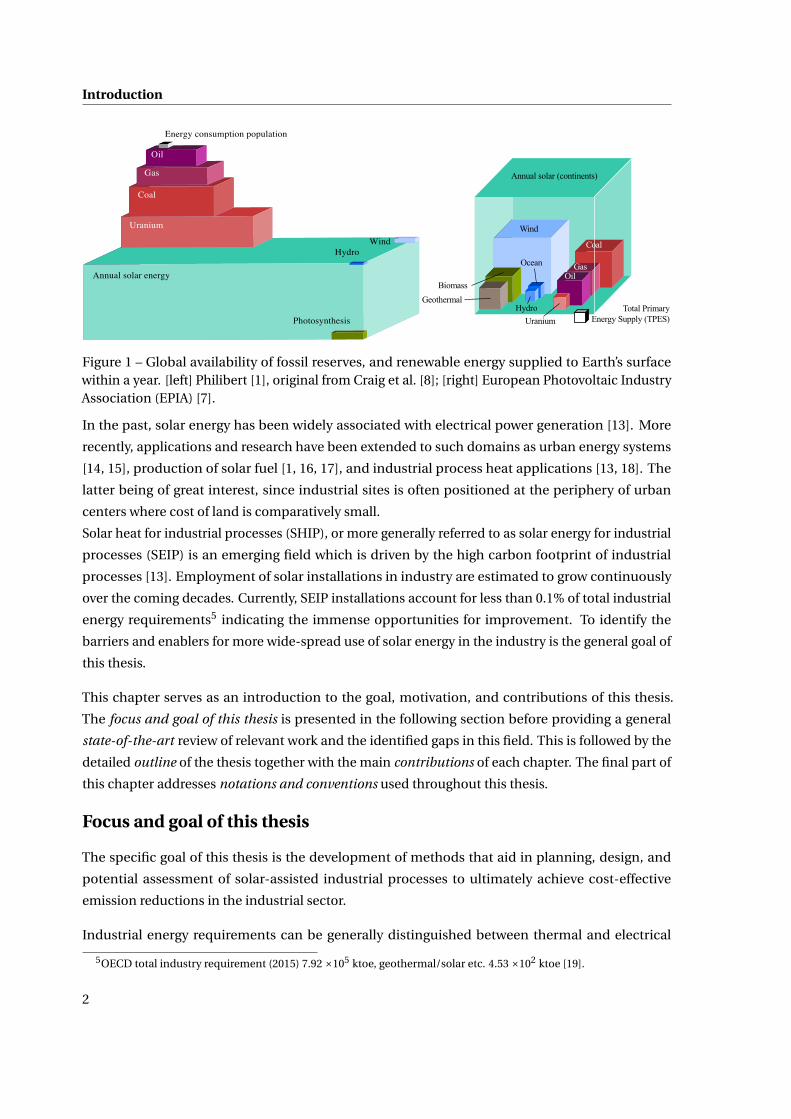
population’s entire yearly energy demand2, if it could be fully converted and stored. Figure 1 shows
the yearly incoming solar radiation on the earth surface in comparison to other (fossil and renewable)
primary energy resources available on the planet based on two different origins [1, 7]. Even though
the estimation of the potential of all resources (especially wind, uranium, and geothermal) is not
consistently estimated, the exhaustive solar potential generally agreed upon [1, 7, 8] is clearly
highlighted.
In tandem with an extensive potential, there are also great challenges to face. The greatest challenge
is the intermittent availability of solar energy which exhibits large temporal (daily and seasonal) and
spatial variations. Furthermore, solar energy is dilute: The maximum horizontal solar irradiance
measurable at the Earth’s surface during solar noon and clear sky conditions approximates 1000
W/m2[10]. In comparison, fueling a car transfers 20 MJ of energy (in the form of fuel) per second of
refueling3. This power requirement is equivalent to the amount of solar radiation which insolates
on a clear day (at noon) a surface area spanning three football fields4.
The aforementioned challenges highlight the need for efficient solar energy conversion routes and
adequate tools to derive these.
1 Life-cycle emissions from conversion equipment are neglected in this statement.2 Incoming yearly radiation 3.19×10⁹ PJ [1], TPES of the population (2015) 5.71×10⁵ PJ [9].3 Car fueling requires 20 MJ/s of diesel with diesel energy density 35.8 MJ/l [11], refueling pump flow rate 35l/min [12].4 Surface of 20×103 m2, with solar energy to fuel conversion efficiency assumed to be 100% for this comparison.
1
Introduction
Figure 1 – Global availability of fossil reserves, and renewable energy supplied to Earth’s surfacewithin a year. [left] Philibert [1], original from Craig et al. [8]; [right] European Photovoltaic IndustryAssociation (EPIA) [7].
In the past, solar energy has been widely associated with electrical power generation [13]. More
recently, applications and research have been extended to such domains as urban energy systems
[14, 15], production of solar fuel [1, 16, 17], and industrial process heat applications [13, 18]. The
latter being of great interest, since industrial sites is often positioned at the periphery of urban
centers where cost of land is comparatively small.
Solar heat for industrial processes (SHIP), or more generally referred to as solar energy for industrial
processes (SEIP) is an emerging field which is driven by the high carbon footprint of industrial
processes [13]. Employment of solar installations in industry are estimated to grow continuously
over the coming decades. Currently, SEIP installations account for less than 0.1% of total industrial
energy requirements5 indicating the immense opportunities for improvement. To identify the
barriers and enablers for more wide-spread use of solar energy in the industry is the general goal of
this thesis.
This chapter serves as an introduction to the goal, motivation, and contributions of this thesis.
The focus and goal of this thesis is presented in the following section before providing a general
state-of-the-art review of relevant work and the identified gaps in this field. This is followed by the
detailed outline of the thesis together with the main contributions of each chapter. The final part of
this chapter addresses notations and conventions used throughout this thesis.
Focus and goal of this thesis
The specific goal of this thesis is the development of methods that aid in planning, design, and
potential assessment of solar-assisted industrial processes to ultimately achieve cost-effective
emission reductions in the industrial sector.
Industrial energy requirements can be generally distinguished between thermal and electrical
5OECD total industry requirement (2015) 7.92 ×10⁵ ktoe, geothermal/solar etc. 4.53 ×10² ktoe [19].
2

State-of-the-art: methods for SEIP applications
demands. Thermal demands usually need to be produced on site6 and adequately fit to the process
temperature levels, while electrical demands can be balanced through the electricity network. Due
to these characteristics, a more detailed analysis of thermal process requirements is conducted in
this thesis. Nevertheless, it is assured that all energy and material balances (including electricity
and natural gas) are closed at all times within each problem formulation presented in this thesis.
For illustration, the methods are applied to an industrial case study from a low-temperature industry.
The choice is motivated in the context and motivation section (Section 1.1). Integration measures
are presented and discussed to investigate the inherent trade-offs between specific technology
options. In particular, the competition and synergy of solar technologies with compression heat
pump options is studied. The environmental benefits of the renewable options in comparison to
conventional measures, such as improved heat recovery and heat pump systems is carefully weighed
and rigorous methods for such analysis are derived.
It has to be noted that the goal of this work is not a complete analysis of all available solar and
heat pump energy conversion routes, but rather a validation of the developed methodologies with
adequate case studies and an in-depth analysis of some specific technologies. The motivation for
the choice of the solar and heat pump equipment is provided in Sections 1.2 and 1.3.
State-of-the-art: methods for SEIP applications
A large body of work has been conducted on various aspects of integration of solar energy with
industrial processes. A detailed state-of-the-art analysis of the specific field addressed in each
chapter of the thesis will be provided at the introduction to the respective chapter. The following
paragraphs provide a general overview of the topics relevant to SEIP and the identified gaps that
motivate the work conducted in this thesis.
Solar modeling and design
Solar collector and field performance modeling in the wider context of SEIP encompasses a wide
range of topics which are introduced in some key points below.
Solar collector modeling Quantification of incoming solar radiation (direct and diffuse) on in-
clined surfaces as well as identification of the angle of incidence and its influence on collector
performance have been subject to numerous studies, especially prior to the 1980s [18, 20–26]. The
steady-state performance estimation of solar (non-concentrating) thermal systems (STs) carried out
by Hottel and Whillier [27] and transient modeling by Klein et al. [28] are still the most applied meth-
ods today [18] and led to the development of the widely-used proprietary software Transient System
Simulation Tool [2] (TRNSYS). Modeling of photovoltaic modules (PVs) has focused on derivation
of the operating cell temperature which is the main factor influencing PV performance [26, 29, 30].
6Industrial symbiosis and district heating can avoid on site production of thermal energy requirements.
3

Introduction
Concentrated solar energy (CSE) performance was originally derived from Monte-Carlo ray-tracing
[16, 31, 32]; however, static (empirical) correlations have been developed based on polynomial
functions [33, 34], typically of Hottel and Whillier-type [18].
Solar field modeling and system design A central research focus in SEIP applications is adequate
performance estimation and design7 of the solar collector field. The methods presented in this
section focus on the solar system while the industrial process is modeled simply as a constant or
intermittent load. Interactions between the solar systems and process were disregarded.
Dynamic modeling provides the most detailed insights to solar (thermal) systems and their transient
behavior and was regularly applied to analyze a fixed design [31, 35, 36]. However, computational
burden is high and evaluating enough design points to identify favorable configurations, let alone
application of more rigorous optimization strategies, often exceeds the computational capacity.
Silva et al. [33] presented a rare example in which a transient collector field and storage model was
optimized with respect to thermodynamic and economic (thermo-economic) objectives using a
memetic genetic algorithm (GA) (though the collector performance is approximated with polynomial
regression).
To overcome computational limitations, a large number of studies presented correlations (mostly
based on regression of results from transient analysis) to estimate annual [37–39] or monthly [40–42]
solar system performance. These were then used to derive optimal designs using analytical [43] and
brute-forcing [44] methods, or mathematical programming (GA) [39]. The most applied brute-force
method is the φ-f-chart method [40, 41], providing the monthly solar fraction of a SHIP system
based on solar collector area, storage fraction, and constant industrial load. It is also available as
a proprietary software [45]8. Another approach is presented by Kulkarni et al. [46, 47], who based
their design strategy on one annual average day. Further contributions include collector tilt angle
optimization [48, 49], and field design optimization (with respect to shading, losses etc.) [31, 50–53],
and optimal temperature control [54], which are not the focus of this thesis.
Synthesis Summarizing, it can be seen that static or dynamic solar system performance estima-
tion at hourly or minutely timescales are well explored, however, are rarely employed for optimal
design purposes due to the computational effort. Monthly or annual regression models provide
good estimates at reduced computational cost; however, the derived correlations are limited in
applicability to the range of operating conditions and control strategies they were designed for.
The f-chart method, for example, was derived from solar water and air heating systems with stor-
age (double-pass) and a constant load profile, assuming a pre-set control strategy and specific
storage sizes [44]. Apart from few exceptions, rigorous design strategies employing mathematical
programming are not commonly applied in the literature discussed here.
7Design refers here to the sizing and layout of the solar collector field.8 The regression functions were derived from various TRNSYS simulations.
4

State-of-the-art: methods for SEIP applications
"Integration" of solar energy with industrial processes
"Integration" is highlighted in the title of this subsection, since it is a fuzzy notion which was
interpreted broadly in scientific literature. Three types of integration studies were identified and are
depicted in Figure 2.
Solar systems analysis for industrial process applications (SP) The first type, "SP", has been
addressed in the previous section and refers to studies which focused on modeling and design
of solar systems considering a constant or intermittent industrial load, with little focus on the
interactions between the solar system, process and potential process improvement measures.
Solar system and industrial process analysis (SP-A) The second type, "SP-A", refers to studies
which analyzed the solar and process system as a whole, addressing not only solar modeling, but
also identification of the relevant process or utility streams suited to solar integration [55–58], heat
exchanger network design [55, 58], and/or technical constraints related to this integration [36].
Alteration in the process design or process improvement measures were not considered.
Solar system and industrial process integration and optimization (SP-I) The third type, "SP-I",
refers to studies which considered the solar and process as a whole and, additionally, addressed
process improvement measures including internal heat recovery through pinch analysis (PA), and
possibly competing technologies. Schnitzer et al. [59] and Atkins et al. [60] analyzed the thermody-
namic and environmental (thermo-environmental) benefits of solar heat integration in the dairy
industry, considering PA to identify the target solar temperatures for a fixed number of collectors. A
complete utility integration, such as by modeling refrigeration of the sub-ambient streams, was not
considered. Integration of a mechanical vapor re-compression (MVR) system was considered in the
study presented by Eiholzer et al. [61], though the refrigeration of the sub-ambient process streams
and the condenser hot stream were not modeled, which were in direct competition to the solar heat
at 60°C. The solar sizing was based on brute-force generation of design points, though the time
horizon and meteorological data were not specified. Perry et al. [62] presented a general approach
of integrating renewable energy to industrial clusters with aid of total site analysis (TSA) but without
elaborating on the specific design and modeling approach. Varbanov and Klemeš [63] extended the
Figure 2 – Focus in literature on "integration" of solar energy with industrial processes.
5

Introduction
approach presented by Perry et al. [62] to account for time-slices and storage, focusing on graphical
derivation of the utility system. Bühler et al. [64] presented a rigorous nonlinear programming (NLP)
approach using particle swarm optimization (PSO) and pattern search to identify the optimal solar
collector and storage sizes considering one year of hourly meteorological data. The sub-ambient
process side and refrigeration was not included. Mian [65] proposed a solar sizing and heat ex-
changer network (HEN) design method for the high-temperature hydrothermal gasification based
on four average seasonal days considering co-generation formulated as a mixed integer nonlinear
programming (MINLP) problem.
Synthesis In summary, analysis of solar energy integration in industrial processes led to derivation
of three types of studies. The most comprehensive type of studies "SP-I" considered the solar
and process system as a whole, addressed process improvement measures including internal heat
recovery through PA, and in rare cases, competing technologies.
A research gap was identified which pertains to comprehensive methods which provide rigorous
sizing of the solar system and consider competing technologies. Particularly relevant technologies
such as heat pumping, refrigeration, and MVR have been disregarded. This is especially relevant
in one of the target industry for these methods: the dairy industry. Recurrently, the concept of
formulating average/typical days was presented, though verification of the selection of typical days
and effect on the sizing has not been addressed.
Extrapolation of solar potential
Solar potential studies form a body of work which aims at identification of the total energetic
potential for solar installations in specific sectors or industries at a regional, national, or global level.
As depicted in Figure 3, these studies are generally distinguished between bottom-up and top-down
approaches.
Classical top-down approaches are presented by Brown et al. [66], Beath [67], and Lauterbach et al.
[68], in which the total energy demands of different industrial sectors at the national level were
estimated, categorized by temperature levels, and matched with solar technologies. Some go as far
Figure 3 – Bottom-up, top-down approaches for solar potential studies.
6

State-of-the-art: methods for SEIP applications
as identifying industrial clusters in specific regions and matching those with the annual irradiation
[66, 67]. Sharma et al. [69–71] presented a more detailed methodology in which the plants associated
with certain sectors were individually identified and classified by their hot utility type (boiler or
co-generation). The solar systems were then sized by plant capacity and the annual CO2 emission
mitigation potentials were derived.
A bottom-up approach was presented by Calderoni et al. [72] presenting three textile plants and
estimating the economic feasibility of solar integration. The solar modeling approach was unfortu-
nately not specified. Meyers et al. [73] compared ST systems for a fixed process load to PV systems
combined with resistance heating, which is an exergetically inefficient way to provide heating. Based
on a regression model, the results were extrapolated to various meteorological conditions to derive
the turn-key cost based on assumed current and future specific project investment costs.
Synthesis Top-down and bottom-up approaches for solar potential estimation were presented.
Top-down approaches provide powerful tools to identify relevant regions, industrial sectors, and
possibly political measures to increase profitability of carbon emission reduction measures. However,
the results are coarse and some options may be completely overlooked. Bottom-up approaches can
also provide estimations for profitability of carbon emission reduction measures, though usually for
specific sectors and regions. The studies presented in the literature either focus on the solar system
or on the industrial process but do not consider them in a combined framework.
A gap was identified for a bottom-up rigorous approach which considers both the process and solar
system, as well as a wider set of utilities and integration options, to identify relationships between
energy prices and utility selection at a national or international level.
Synthesis and scope
The gaps in this state-of-the-art analysis can be summarized in three main points.
1. A lack of rigorous solar design methods is identified which provide precision at reasonable
computational cost.
2. A lack for comprehensive integration methods, especially in the low-temperature sectors
considering competing technologies, process improvements, and rigorous solar design.
3. A gap for bottom-up potential analyses which comprehensively address solar and process
analysis, competing technologies, and allow extrapolation of results to the (inter)national
level in a systematic manner.
Based on the identified gaps, this thesis addresses development of methods for solar energy for
industrial processes (SEIP) (including electrical and thermal technologies) with focus on the low tem-
perature sectors, considering competing technologies specifically heat pumps (HPs), refrigeration,
and mechanical vapor re-compression (MVR).
7

Introduction
Contribution and outline of the thesis
The chapters are presented below with the associated contributions alongside four central research
questions. The main contributions are found in Chapters 3 to 6.
Context of the thesis (Chapter 1): Chapter 1 provides the wider context of the topics discussed in
this thesis. It motivates the case study selection and technologies studied, and introduces concepts
and nomenclature used throughout the work.
How can solar system design be accurately and rigorously addressed?
Solar modeling and design (Chapter 2): A rigorous solar system modeling and design approach is
presented which allows to estimate collector and storage performance at sufficient precision and
constrains the computational effort. The model performance is compared to dynamic results from
TRNSYS. A clustering algorithm [74] is applied to select typical operating periods and results are
compared for different sets of periods. The chapter addresses the gaps identified in point (1) in the
synthesis and scope section. It contributes by adaptation of the multi-period mixed integer linear
programming (MILP) approach from Maréchal and Kalitventzeff [75] to SEIP applications.
What problem formulation is required for a comprehensive design method for solar-assisted
low-temperature processes?
Comprehensive integration method (Chapter 3): A comprehensive method is proposed which
addresses simultaneous optimization of the process heat recovery, the conventional utilities, and the
renewable utility system (including thermal storage) using ε-constrained parametric optimization.
The method, tailored for the low-temperature industry, is based on multi-period utility targeting,
including process heat recovery through pinch analysis (PA) and re-use through heat pumping,
and identifies the optimal design and operation of the utility and storage system. The proposed
methodology is illustrated on the basis of a dairy plant for which the different utility technologies are
compared and evaluated based on economic and environmental criteria. This chapter addresses the
shortcomings mentioned in point (2). The main contribution is the development of a comprehensive
approach for solving the problem.
How can design of an optimal industrial heat pump system be conducted?
Generic heat pump superstructure synthesis and integration method (Chapter 4): Based on the
promising results from Chapter 3, a novel, generic heat pump synthesis method for industrial
applications is presented. The superstructure-based approach is solved with a decomposition
solution strategy based on mathematical programming. Heat pump features are incorporated in a
comprehensive way while considering technical limitations and providing a solution set to allow
8

Contribution and outline of the thesis
expert-based decision-making at the final stage. The main contributions are found in the com-
prehensive superstructure, addressing fluid selection, component sizing, heat exchanger network
(HEN) cost estimations, operating condition selection, and technical constraints.
How can the results be extrapolated to a wider scope?
Extrapolating impact: environomic potential (Chapter 5 and 6): A method for estimating the en-
vironmental and economic (environomic) potential of various emission reduction measures and
technologies in industrial process applications is derived, generalizing the methodologies devel-
oped in the previous chapters. This includes generalized optimization techniques and generation
of a publicly available database9 of solutions based on a wide range of possible economic and
environmental conditions. By fixing the conditions (e.g. considering a particular country), the
optimal solutions for these conditions can be drawn from the database. This allows identification
of environmental and economic (environomic)ally optimal solutions in different countries and
under different political boundary conditions, and hence, brings a twofold advantage: (1) process
engineers can use the results from the generic plants to conduct pre-feasibility assessment, (2)
policy-makers and equipment manufacturers can identify favorable conditions for installation of
the technologies under scrutiny. The method is applied to a modularized dairy plant considering
heat pumping and co-generation utilities, and generalized conclusions are drawn.
In a subsequent step, the methodology is extended to include solar utilities. The results from Chap-
ter 3 are used for deriving a correlation to predict the annual solar collector and storage performance
under optimal control. The chapter addresses the shortcomings mentioned in point (3). The method,
though simple in application, displays a contribution to the field of potential analysis, offering a
novel, detail-oriented, bottom-up approach.
A graphical overview of the presented chapters is depicted in Figure 4.
Figure 4 – Graphical overview of thesis structure.
9 The data can be accessed via an on-line parallel coordinate [76] decision-making platform.
9

Introduction
Terminology, conventions
Mathematical conventions
The conventions in the equations presented throughout the thesis are that scalar decision variables
are represented by italics, scalar parameters by roman text, vectors are always represented in bold
(italic for variables, roman for parameters), and sets are represented in roman bold Uppercase.
Cost conversion and currencies
The equipment cost estimation follows common literature conventions as originally presented by
Guthrie [77], expanded by Ulrich [78], and summarized by Turton et al. [79].
Bare module cost The bare module cost (also here referred to as installed cost) describes the
direct and indirect expenses related to the unit including: material, construction, freight, taxes, and
installation. Thereby the purchase price of the unit is corrected with various factors accounting
for the material (if not carbon steel CS), operating pressures, piping, and the installation. These
factors can be summarized in the bare module factor, FBM [-]. In this work, all cost functions, C w ,
of technology w as well as their linearized cost factors, IVw1 and IVw
2 , refer to their bare module
(installed) costs.
Effect of time: inflation Cost functions which date back to a reference year before the current year
are corrected with cost indexes, CI, to account for inflation. Thereby, the out-dated cost function
is multiplied with the fraction between the current and the reference cost index, as depicted in
Equation 1. Common indexes used in chemical engineering practice and in this thesis are the
Chemical Engineering Plant Cost Index [4] (CEPCI) and the Marshall and Swift Index [6] (MSI).
C w = CI
CIref·C w ,ref (1)
Currencies and conversion The cost functions used throughout the thesis are represented in
different units depending on the context of the study. The studies conducted in Europe are based on
Euros [e] (Chapter 3), while international studies with extra-European references are conducted
in US Dollars [$] (Chapter 4-6). Since most chapters are based on published work, the currencies
were not altered in this thesis so as to retain consistency with the publications. Most cost indexes
are valid for US Dollars only. Therefore, if an original cost functions was provided in Euros (and was
needed in US Dollars), it was converted to Dollars with the currency conversion rate of the reference
year and subsequently updated.
10

1Context and motivationOverview
• Quantification and characterization of process energy requirements
• Classification of solar energy conversion technologies and identification of relevant ones
• Introduction to and identification of relevant heat pumping technologies
• Role of pinch analysis and implications for heat pumping and solar energy
This chapter provides a wider context of the topics discussed in this thesis. It motivates the choice
of the analyzed case study and technologies, and introduces concepts and nomenclature used
throughout the work.
1.1 Energy requirements in industry
Analysis of energy intensity in industry aids in identifying the most impacting industries and,
therewith, candidates for emission reduction measures. As shown in Figure 1.1a, the most energy-
consumptive industrial sectors in Switzerland (CH) are identified as the chemical (22%), mineral
(12%), food (12%), paper (10%), and metal (8%) industry. While the absolute demand is important,
temperature levels of the thermal requirements have a great influence on the feasibility of solar
process heat applications.
Figure 1.1b shows the estimated thermal requirements and related temperature levels of these
sectors from a study in Germany (DE). It reveals that the overall thermal demand of the food, textile,
and paper sector is well below 300 °C, which constitutes a good match with the operating ranges
of most solar thermal systems [13, 18, 68]. The other sectors each display heat requirements above
1000 °C and, hence, are seen to have less potential for solar integration [68].
The dairy industry in CH represents about 15% of the food sector1, and is identified as an ideal
candidate for the application of the methodologies derived in this thesis, due to its favorable
temperature ranges (below 150 °C) and potentially large impact.
11

Chapter 1. Context and motivation
Food, 20.7, 12.10%
Textiles, 2.7, 1.58% Paper, 15.3,
8.94%
Chemicals, 37.9, 22.15%
Minerals, 20.5, 11.98%
Metals, 13.9, 8.12%
Metal products,
4.7, 2.75%
Electronics, 12.2, 7.13%
Machinery, 6.9, 4.03%
Energy, 2, 1.17%Construction
, 5.8, 3.39%
Others, 28.5, 16.66%
(a) CH industrial sector energy consumption (PJ/y)(2010) [82].
0%10%20%30%40%50%60%70%80%90%100%
HW SH <100°C 100-200°C200-300°C 300-500°C 500-1000°C >1000°C
(b) Temperature distribution of thermal requirements in DEindustrial sectors (2009) adapted from Lauterbach et al. [68]a,HW - hot water, SH - space heating.
Figure 1.1 – Industrial thermal energy requirements and respective temperature levels.a Sectors form [68] were consolidated to match sectors depicted in Figure 1.11.1a; food: 12,12 (NACE Rev. 2 Code), textiles: 13-15, paper: 17,18, chemicals: 20,22, minerals: 23,
metal products: 25, electronics: 27, machinery: 28-30.
1.2 Solar energy conversion
Figure 1.2 provides a summary of common solar energy conversion routes excluding natural con-
version pathways such as photosynthesis or wind current generation. Three main products are
identified: electricity, fuel, and heat. The conversion systems are differentiated between active and
passive.
Passive systems describe structural elements or modifications (windows, walls, etc.) in buildings
which are designed with the purpose of specifically harvesting solar energy, for example, as a heat
source during cold seasons and rejecting heat during hot ones [1]. One example is provided by
Congradac et al. [49] who presented an algorithm for automatic control of window blinders based on
the incident solar radiation. Agricultural greenhouses are possibly the oldest passive solar systems.
Active systems can be divided into non-concentrating and concentrating systems, while concen-
trating systems can be further distinguished between self-tracking and active tracking technologies.
Concentrating technologies rely on redirection of the incoming light through reflectors (mirrors)
or refractors (lenses) to increase the energy density in the focus thereby leading to reduced ther-
mal losses due to reduced collector surface area [26]. This leads to increased temperatures in the
receiver, which is advantageous in thermal systems to achieve higher operating temperatures, either
for high-temperature industrial process use, or for thermo-mechanical (solar Rankine cycles) or
thermo-chemical (solar gasification) applications, inducing higher conversion efficiencies. Re-
ducing the active area allows utilization of higher efficiency receivers at similar investment cost,
therefore motivating the use of concentrating photovoltaic systems (CPVs). CPVs require active
cooling, which enables co-generation of heat and electricity.
1 Raw milk treated in CH: 3.49 ×10⁶ t (2015) [80], average energy requirement of raw milk treatment to various products:0.9 GJ/t [81].
12
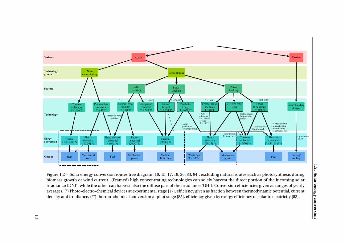
1.2.So
laren
ergyco
nversio
n
Figure 1.2 – Solar energy conversion routes tree diagram [10, 15, 17, 18, 26, 83, 84], excluding natural routes such as photosynthesis duringbiomass growth or wind current. (Framed) high concentrating technologies can solely harvest the direct portion of the incoming solarirradiance (DNI), while the other can harvest also the diffuse part of the irradiance (GHI). Conversion efficiencies given as ranges of yearlyaverages. (*) Photo-electro-chemical devices at experimental stage [17], efficiency given as fraction between thermodynamic potential, currentdensity and irradiance, (**) thermo-chemical conversion at pilot stage [85], efficiency given by exergy efficiency of solar to electricity [83].
13
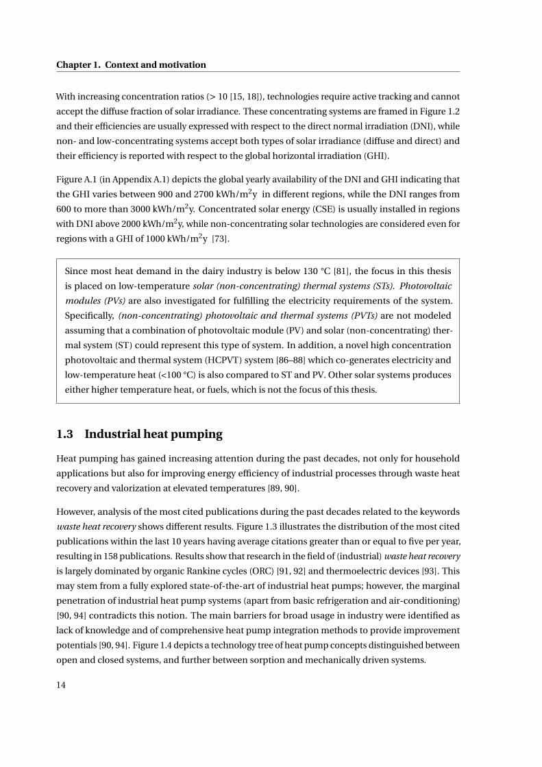
Chapter 1. Context and motivation
With increasing concentration ratios (> 10 [15, 18]), technologies require active tracking and cannot
accept the diffuse fraction of solar irradiance. These concentrating systems are framed in Figure 1.2
and their efficiencies are usually expressed with respect to the direct normal irradiation (DNI), while
non- and low-concentrating systems accept both types of solar irradiance (diffuse and direct) and
their efficiency is reported with respect to the global horizontal irradiation (GHI).
Figure A.1 (in Appendix A.1) depicts the global yearly availability of the DNI and GHI indicating that
the GHI varies between 900 and 2700 kWh/m2y in different regions, while the DNI ranges from
600 to more than 3000 kWh/m2y. Concentrated solar energy (CSE) is usually installed in regions
with DNI above 2000 kWh/m2y, while non-concentrating solar technologies are considered even for
regions with a GHI of 1000 kWh/m2y [73].
Since most heat demand in the dairy industry is below 130 °C [81], the focus in this thesis
is placed on low-temperature solar (non-concentrating) thermal systems (STs). Photovoltaic
modules (PVs) are also investigated for fulfilling the electricity requirements of the system.
Specifically, (non-concentrating) photovoltaic and thermal systems (PVTs) are not modeled
assuming that a combination of photovoltaic module (PV) and solar (non-concentrating) ther-
mal system (ST) could represent this type of system. In addition, a novel high concentration
photovoltaic and thermal system (HCPVT) system [86–88] which co-generates electricity and
low-temperature heat (<100 °C) is also compared to ST and PV. Other solar systems produces
either higher temperature heat, or fuels, which is not the focus of this thesis.
1.3 Industrial heat pumping
Heat pumping has gained increasing attention during the past decades, not only for household
applications but also for improving energy efficiency of industrial processes through waste heat
recovery and valorization at elevated temperatures [89, 90].
However, analysis of the most cited publications during the past decades related to the keywords
waste heat recovery shows different results. Figure 1.3 illustrates the distribution of the most cited
publications within the last 10 years having average citations greater than or equal to five per year,
resulting in 158 publications. Results show that research in the field of (industrial) waste heat recovery
is largely dominated by organic Rankine cycles (ORC) [91, 92] and thermoelectric devices [93]. This
may stem from a fully explored state-of-the-art of industrial heat pumps; however, the marginal
penetration of industrial heat pump systems (apart from basic refrigeration and air-conditioning)
[90, 94] contradicts this notion. The main barriers for broad usage in industry were identified as
lack of knowledge and of comprehensive heat pump integration methods to provide improvement
potentials [90, 94]. Figure 1.4 depicts a technology tree of heat pump concepts distinguished between
open and closed systems, and further between sorption and mechanically driven systems.
14

1.4. Heat recovery potential in a process: pinch analysis
This work addresses open- and closed-cycle, mechanically driven heat pumps with a focus on latent,
single fluid systems, the reasoning for this is introduced in Section 1.4. Improving industrial resource
efficiency through heat pumping is achieved by recovering waste heat at low temperature levels and
returning it at higher temperatures as useful heat to the process. The temperature lift is achieved
through mechanical compression of a working fluid which requires electricity. Before the concept
of heat pumping in industrial processes can be discussed at greater depth, the concept of "waste
heat" must be introduced, and with it, pinch analysis (PA).
1.4 Heat recovery potential in a process: pinch analysis
Pinch analysis is a methodology developed in the 1970s by Linnhoff and Flower [97, 98] and exten-
sively discussed by Kemp [99], which allows estimation of the maximum energy recovery potential
of industrial processes. This requires decomposition of an industrial site into its thermodynamic
requirements. The result is a set of hot (net cooling requirement) and cold (net heating requirement)
thermal streams.
The second principle of thermodynamics states that heat can only flow from a source at higher
temperature to a sink at lower temperature. Ensuring thermodynamic feasibility, the heat cascade2 is
derived which allows estimation of the maximum energy recovery potential of an industrial process
and the temperature ranges in which external heating and cooling are required.
1.4.1 Minimum approach temperatureΔTmin
An ideal heat exchanger is an adiabatic device in which a hot stream transfers heat to a cold stream
at lower temperatures as depicted in Figure 1.5. The second law of thermodynamics dictates that a
temperature gradient between the hot and the cold stream is required to provide a driving force for
heat to flow.
From the principles of pinch analysis (PA), a minimum approach temperature,ΔTmin, defines the
point in a heat exchanger where the hot and the cold streams exhibit the smallest temperature
difference. The position ofΔTmin depends on the inclination of the temperature-enthalpy profiles
of the hot and cold streams, which are proportional to the inverse product of heat capacity and
mass flowrate (mcp). The optimal minimum temperature difference is conventionally found by
optimization which considers the balance between operating and investment cost for heat exchang-
ers. A smaller approach temperature reduces the operating cost due to higher heat recovery while
increasing investment cost related to larger heat exchange area.
In general practice, engineering estimate values of the minimum approach temperature difference
are assumed and to ensure thermodynamic feasibility, the hot (cold) streams are shifted downwards
(upwards) by half of this difference, resulting in what are referred to as corrected temperatures.
2 The heat cascade refers to the theoretical concept of successively transferring thermal energy from high to lowtemperature levels within a process.
15

Chapter 1. Context and motivation
2007 2008 2009 2010 2011 2012 2013 2014 2015 2016 2017
Years
0
500
1000
1500
2000
2500
3000
3500
4000
4500
5000
Cit
ati
on
s
Total (158 publications), 19965 citationsOrganic Rankine cycle applications (81), 8723
Thermoelectric devices (29), 6501
Biomass applications (23), 2494
Process engineering and optimization (21), 1879
Heat pumping and refrigeration (2), 180
Space heating (1), 98
Phase change materials (for storage) (2), 90
Figure 1.3 – Web of science [95], key words: waste heat recovery, top cited papers of last 10 years (≥ 5citations/year), accessed 11.08.2017.
Figure 1.4 – Heat pumping technology tree diagram, adapted and extended based on Nellissen andWolf [96].
Figure 1.5 – Temperature enthalpy profile of a counter current heat exchanger to illustrate theΔTmin.
16

1.4. Heat recovery potential in a process: pinch analysis
1.4.2 Graphical representation, pinch point, and pinch rules
An example of a hot composite curve (CC) generated from the process thermal requirements is
illustrated in Figure 1.6 (b). It is constructed by vectorial addition of all individual hot stream
contributions (shown in Figure 1.6 (a)) in each temperature interval. The cold CC is constructed
likewise. The hot and cold process CCs represent the process total heating and cooling demand. The
vertical overlap between the two curves marks the maximum possible heat recovery potential of the
industrial process.
The grand composite curve (GCC), depicted in Figure 1.7 (b), is derived by subtraction of the thermal
load of the cold from the hot CC in each temperature interval. The GCC monitors the net heating
and cooling loads and their temperature levels under the assumption of maximum heat recovery or
minimum energy requirement (MER). The pinch point is marked by the impingement of the GCC on
the temperature axis. Above, the process exhibits a net heating requirement (heat sink), and below, a
net cooling requirement (heat source).
The distance from the temperature axis at the highest and lowest temperature represents the
Figure 1.6 – (a) Individual hot streams, (b) hot CC in temperature enthalpy diagram [99].
Figure 1.7 – (a) Hot and cold CCs, (b) GCC in temperature enthalpy diagram.
17

Chapter 1. Context and motivation
minimum hot (MERhot) and cold (MERcold) energy requirements, respectively.
The pinch point or pinch temperature induces three thermodynamics-based, so-called, pinch
rules [97, 98]:
1. Hot utilities should only be installed at temperatures above the pinch (point),
2. Cold utilities should only be placed below the pinch (point), and
3. No heat exchange should occur across the pinch (point).
Violating any of these rules results in an increase of the utility requirements and, hence, a reduction
of the process exergy efficiency. In the context of pinch analysis, "waste heat" is referred to as the
heat available below the process pinch point which represents the process’ net cooling demand.
1.4.3 Implications for solar energy for industrial processes (SEIP)
Solar thermal systems constitute classic hot utilities. The pinch rules presented in Section 1.4 clearly
state that a hot utility is only beneficial to the process energy requirements if it is installed above
the pinch temperature. This leaves a simple design guideline for solar heat for industrial processes
(SHIP) applications. The pinch rules do not leave any guidelines for other solar energy systems
which provide electricity or fuel.
1.4.4 Implications for industrial heat pumps
This section addresses mechanically driven heat pumps (HPs) due to their widespread application
[94]; however, it should be noted that sorption systems present different and interesting integration
options but are not within the scope of this work.
Townsend and Linnhoff [100] derived the theoretical foundation for optimal placement of heat
pumps in an industrial process based on pinch analysis: heat pumps should always be placed
across the process pinch point if energy savings are desired. In essence, energy savings are achieved
by recovering waste heat from below the pinch and, after upgrading it through application of
mechanical work, to supply it back to the process above the pinch temperature, which is hence
referred to as waste heat valorization or re-use.
There is one crucial factor which influences the efficiency of heat pump cycles: the required temper-
ature lift and thus the compression ratio. In the context of industrial waste heat valorization, the
temperature lift is directly linked to the "sharpness" of the pinch, meaning the shape of the process
grand composite curve close to the pinch point.
Figure 1.8 shows the temperature enthalpy diagrams of processes (A) and (B). Process (A) has sharp
pinch point with a small temperature lift. While process (B) shows a smooth pinch point with
heating and cooling requirements spanning over a range of temperatures. Integration of different
mechanical heat pump systems are illustrated, starting from a single-stage, single fluid (inverted
18

1.4. Heat recovery potential in a process: pinch analysis
Figure 1.8 – Heat pump integration to process GCC. (A) GCC with "sharp" pinch point & single-stage heat pump (HP), (B) "smooth" pinch point & single-stage HP, (1B) "smooth" pinch point &multi-stage HP, (2B) mixture HP, (3B) inverse Brayton HP.
Rankine cycle) heat pump in Figure 1.8 (A) and (B). If a high temperature lift is required as illustrated
in Figure 1.8 (B), the efficiency of standard (single-stage, single fluid) heat pump cycles is drastically
compromised.
Three options to overcome this issue are discussed in the literature which are depicted in Figure 1.8
(1B-3B).
(1B) Multi-stage or cascaded heat pump cycles based on latent heat release/ consumption in
condenser/ evaporator with multi-stage compression and/or expansion [101–104], potentially
a cascade of cycles
(2B) Zeotropic mixture cycles based on latent heat release of mixtures where the difference in
fluid boiling points is expressed in a temperature glide and liquid/ vapor composition shift
during evaporation and condensation [105, 106]
(3B) Inverse Brayton cycle heat pumps based on sensible heat release and consumption in the
condenser and evaporator, respectively [107]
Single fluid (inverse Rankine) heat pumps can satisfy constant temperature thermal requirements
(single-stage) as well as continuous temperature ranges with help of multi-stage cycles at a rea-
sonable coefficient of performance (COP) (above 2). In generating a temperature glide, zeotropic
mixtures [105, 106] or heat pumps relying on the inverse Brayton cycle [107] may be advantageous
for demands spanning wide temperature ranges, but less flexible relative to constant temperature
requirements.
This thesis focuses on mechanically driven, single fluid, multi stage (inverse Rankine) heat
pumps (depicted in the first three diagrams in Figure 1.8 (A-B-1B)), due to their operational
flexibility, wide-spread application, and the technical realization being mostly dependent on
mature technologies [94].
19

Chapter 1. Context and motivation
1.4.5 The use of PA throughout the thesis
The principles of PA are considered throughout the thesis. Therefore, a heat cascade formulation
from the literature [75] is adopted which is presented in Equations 2.14-2.15 of Chapter 2. The
formulation realizes heat recovery assessment in the process by imposing the second law of thermo-
dynamics to assure that heat is only transferred from higher to lower temperatures. This formulation
is the foundation of all methods developed in the main chapters (3-6) of the thesis, which are solved
with optimization techniques aiming at minimizing the total system cost.
It has to be noted that the pinch rules presented in Section 1.4.2, are thermodynamically driven,
while the objective functions of most optimization problems presented in the thesis are economically
driven, which may lead to solutions that do not comply with the pinch rules. Whenever the utility
temperature levels are, however, manually selected (as presented in Chapter 3) the pinch rules are
respected.
1.5 Integrated solar and heat pump systems
Before discussing the implications of PA on combined solar and heat pump placement in industrial
processes, a conceptual comparison between ST, PV, and HP systems is conducted. The sun-to-
thermal efficiency3 is presented in Figure 1.9 for two types of flat plate ST collectors (high- and low-
efficiency) and heat pumping driven by co-generation and two different PV systems. These are
further compared to PV with resistance heating.
0 20 40 60 80 100 120 140 160
Temperature difference, ∆T, [K]
0
0.2
0.4
0.6
0.8
1
Eff
icie
ncy
, η
, [-
]
FP - 1000 W/m2
FP - 500 W/m2
FP (low η) - 1000 W/m2
FP (low η) - 500 W/m2
HP + Co-gen. (ηel
= 35%, ηex,HP
= 50%)a
HP + PV (ηPV
= 17%, ηex,HP
= 55%)
HP + PV (ηPV
= 10%, ηex,HP
= 50%)
Resistance heating + PV (ηPV
= 17%)
a HP + Co-gen: natural gas-to-thermal efficiency is shown.
b FP [108, 109] ηFP = 0.74−3.5940 · ∆TG −0.00864 · (∆T )2
G , [18](Eq. 76); HP based on COP with exergy efficiency as specified.ΔT =T−Ta, Ta = 20 °C.
Figure 1.9 – Comparison of overall sun-to-heat conversion efficiencya, ST, PV and heat pump orresistance heatingb.
It is observed that increasing temperature increment yields the best performance with high-efficiency
flat plate collectors. However, it should be noted that the applied efficiency correlation of Hottel and
Whillier [27]-type does not include an incidence angle modification (due to the sun inclination),
3 For HP with co-generation: natural gas-to-thermal efficiency.
20

1.5. Integrated solar and heat pump systems
Figure 1.10 – Solar and heat pump integration into process GCC. (A) & single-stage HP, (B) ST, (C)synergetic ST and HP, (D) complementary ST and HP, (E) ST.
which, if applied, would yield lower average efficiencies. Heat pumping with co-generation generates
similar (gas-to-thermal) efficiencies as the flat plate collectors even for a high temperature incre-
ments. High efficiency PV with an exergetically well designed HP (e.g. with liquid subcooling before
expansion) shows better efficiencies than the resistance heating case even for high temperature lifts.
The above presented analysis provides indications for the advantages of the different heating systems
not considering integration with an industrial process. Figure 1.10 depicts different options for
beneficial integration of solar thermal systems and heat pumping in an industrial process. Beneficial
refers to reducing the hot and/or cold conventional utility (boiler and cooling water) consumption.
Figure 1.10 (A) and (B,E) show the classical integration of a heat pump across the process pinch
temperature and a solar thermal system providing heat above the pinch, respectively. Two options
of combined solar and heat pump integration are shown in Figure 1.10 (C) and (D). Figure 1.10 (C)
presents an example of synergistic integration of both solar and heat pump systems. Providing solar
heat below the pinch to the self-sufficient pocket allows for a larger installation of the heat pump
and a drastic reduction in hot and cold utility requirements. Figure 1.10 (D) presents an example of
complementary installation of solar and heat pump system, where the solar energy satisfies the heat
requirement that is not provided by the heat pump.
This analysis exemplifies the need for systematic integration methods, in providing beneficial solu-
tions which do not necessarily comply with the classical pinch rules (section 1.4). Comprehensive
derivation of a range of options for a multitude of different process profiles cannot be manually
achieved which necessitates the use and derivation of systematic, mathematical programming
approaches presented in this thesis.
21


2Solar modeling and design
Overview
• Presentation of solar technologies and respective modeling approaches
• Introduction to typical period clustering and testing
• Introduction of multi-period MILP sizing method
This chapter is a summary of the work presented in Wallerand et al. [110], Wallerand
et al. [111], and Selviaridis et al. [112]
This chapter aims at introducing the solar modeling and sizing approach applied in this thesis.
The goal of this chapter is to derive models for estimation of collector and storage performance
at sufficient precision while constraining the computational effort. The model performance is
compared to transient results (TRNSYS). A clustering algorithm [74] is applied to select typical
operating periods and several sets of typical days are compared. The sensitivity of the optimal sizing
towards the typical days selection is, further, analyzed.
After a state-of-the-art analysis, the different (static, dynamic) modeling approaches are presented,
followed by an introduction to the typical periods selection selection algorithm. In the subsequent
section, the system design and integration method considered in this work is discussed. In the
results and discussion section, the solar modeling approaches are compared to transient results and
the typical period selection criteria are elaborated.
2.1 State-of-the-art
The studies discussed in this section are compared in various aspects in Table 2.1. The solar modeling
and design approaches have already been discussed in the introduction of this thesis. Here, a few
further a points are highlighted, which were not mentioned before in order to increase conciseness.
23

Chapter 2. Solar modeling and design
2.1.1 Solar collector modeling
Early work by Liu and Jordan [20], Perez et al.[21, 22] and others [18, 23–26] dealt with proper
assessment of incident direct and diffuse radiation on (inclined) surfaces.
This development went in parallel with the derivation of models for performance estimation of solar
(non-concentrating) thermal systems (STs) at steady-state by Hottel and Whillier [27] and by Klein
et al. [28] considering transience. The Hottel and Whillier equations augmented by incidence angle
modifiers [18, 26] are still the basis for performance calculation of solar thermal systems (ST and
CST) today.
2.1.2 Design of solar systems
This section addresses solar system design in the context of solar energy for industrial processes
(SEIP). As derived in the introduction section, three levels for solar integration to industrial processes
are treated in the literature ranging from solar systems analysis for industrial process applications
(SP) with focus on the solar system to studies addressing solar system and industrial process inte-
gration and optimization (SP-I). The literature presented in this section is focused on the aspects
of solar modeling and design with weaker focus on the industrial processes. Studies from any of
the three categories (SP, SP-A, SP-I) are hence considered as long as the solar design is treated in a
systematic manner.
As mentioned before, dynamic modeling provides the most detailed insights to solar (thermal)
systems and their transient behavior and was regularly applied to analyze a fixed design [31, 35,
36]. However, computational burden is high and evaluating enough design points to identify
favorable configurations, let alone application of more rigorous optimization strategies, often
exceeds the computational capacity. To overcome computational limitations, a large number of
studies presented correlations (mostly based on regression of results from transient analysis) to
estimate annual [37–39] or monthly [40–42] solar system performance.
Not based on dynamic modeling, however, based on a typical meteorological year (TMY) of hourly
data, Ashouri et al. [113] presented a mixed integer linear programming (MILP) approach for optimal
design and operation in urban districts. The computational effort is low, since integration with
an industrial process and its heat recovery system is not treated. Also Bühler et al. [64] presented
an nonlinear programming (NLP) approach using particle swarm optimization (PSO) and pattern
search to identify the optimal solar collector and storage sizing and operation considering a TMY
of hourly meteorological data. The model is sequentially solved, identifying the relevant heat
exchangers (HEXs) prior to sizing the solar system. The sub-ambient process side and refrigeration
was not included.
Another approach was presented by Kulkarni et al.[46, 47] as well as Quijera et al. [114, 115], who
based their conceptual design strategy on one annual average day.
24

2.1.State-o
f-the-art
Table 2.1 – State-of-the-art summary of solar modeling and design studies for SEIP applications.
Author Year Foc Appr Obj Vars Siz. Ec. Solar modeling Proc. m. SC Process Description.M dT Tool Stor. PA HEN
Hottel and Whillier [27] 1955 S M TP T, IRR F X S hour MEB X X X ST - Commonly used approximation of ST performance.Liu and Jordan [20] 1960 S M TP IRR F X S - MEB X X X various - Determination of diffuse radiation on a horizontal surface.Collares-Pereira and Rabl [23, 24] 1979 S M TP T, IRR B X S hour MEB X X X ST - Long term performance modelling of solar collector output.Suehrcke and McCormick [25] 1988 S M TP air mass F X S inst. MEB X X X ST - Method for instantaneous determination of diffuse fraction.Dudley et al. [34] 1995 S E TP T, IRR PR X D sec R,MEA X X X acrshortptc - Experimental results of PTC and polyn. regression.Weinstock and Appelbaum [50] 2004 S D TP FD M-SQP(NLP) X S hour Matlab X X X FP,PV - NLP model of stationary field shading & optimal configuration.Skoplaki and Palyvos [29] 2009 S R TP IRR F X S hour - X X X PV - Review of correlations for PV cell temperature derivation.Talebizadeh et al. [48] 2011 S D TP FD M-GA (NLP) X S hour MEB X X X ST - Use of genetic algorithm for tilt and azimuth angle optimization for
maximal energy efficiency, considering static equations of [116].Tiwari et al. [30] 2011 S R TP T,IRR F X S hour - X X X PV - Review of PV modeling, efficiencies and cost.Yadav and Chandel [117] 2013 S R TP FD - X - - - X X X ST - Review of tilt angle optimization studies, methods, and correlations.Klein et al. [118], [28] 1975 SP M TP - F X D hour,min.TRNSYS X X X various generic Work presenting the dynamic modeling tool TRNSYS.Beckman et al. [40, 41, 119] 1977 SP D,M TP C,S,L B X D month φf-Chart X X X various generic Modeling approach based on fitting functions from TRNSYS results.Clark [120] 1982 SP A E cost F X S year MEB - X X acrshortptc - Break-even cost analysis of parabolic troughs in US.Gordon and Rabl [37],[38] 1982 SP D,M E C R X S year,
reg(hour)MEB X X X FP textile Optimal collector sizing based on economic analytical optimization,
based on polyn. regression of hourly static calculations [38].Duffie and Mitchell [119] 1983 SP M,E TP C,S,L F X S month f-Chart X X X ST - Testing of f-chart method with performance measurements.Collares-Pereira et al. [43] 1984 SP D E C,S A X S year MEB X X X various generic Analytical storage and collector sizing method (incl. weekend storage).Suehrcke and McCormick [42] 1992 SP D,M,E TP C,L F X S month MEB X X X ST - Yearly fraction estimation method considering a bi-modal control
strategy validated with experiments.Kalogirou [35] 2003 SP A TP - F X D hour TRNSYS X X X ST - Comparison of the performance of various flat plate collectors for SHIP
applications in Cyprus.Kalogirou [39] 2004 SP D,M E C,S M-GA (NLP) X D year ANN,GA X X X various food Train ANN from TRNSYS data, use GA to optimize fitted functions.Kalogirou et al. [121] 2007 SP A TP - F X D hour TRNSYS X X X PV/T - Economic and energetic comparison between various PV/T systems.Kulkarni et al. [46],[47] 2009 SP D,M E C,S B X S hour,
av. d.DSM X X X various milk
past.Design space method for solar collector and storage sizing, however,based on an average day.
Silva et al. [31] 2013 SP M,E TP FD F X D hour TRNSYS,Modelica
X X X acrshortptc generic Dynamic modeling including ray tracing of parabolic troughs for in-dustrial process heat applications.
Silva et al. [33] 2014 SP D TEP FD,S M-GA (NLP) X D VST R,Modelica X X X acrshortptc generic Memetic GA applied to optimize various design variables in CSE plantswith fixed process load. Collector performance polynomially fitted.
Baniassadi et al. [122] 2016 SP D TP SF R X S year MEB X (X) X HF generic R-curve method to add renewables to a co-generation system.Meyers et al. [73] 2018 SP M,Pb E C B X D,S year,
reg(hour)R,TRNSYS X X X various - Method for cost comparison between solar thermal and photovoltaics
via resistance heating based on regression model.Ashouri et al. [113] 2013 SU D,O E C,control M-BC(MILP) X S hour MEB X X X ST,PV urban Optimal design and control of urban district for a TMY.Fazlollahi et al. [123, 124] 2014 SU D,O TEP C,control M-
GA(MINLP)X S hour MEB X X X ST,PV urban Multi-period MINLP design of urban energy systems (based on de-
composition strategy [125]) based on typical days.Quijera et al. [114, 115] 2011 SP-I D TP SF C X S hour MEB X X X ETC various Solar system design based on desired solar fraction and av. annual day.Mian [65] 2016 SP-I D,O TEP C,control,
HEXM-PGSCOM(MINLP)
X S hour,av. d.
MEB X X X CSE,PV fuel Multi-period HEN design and solar sizing based on four av. seasonaldays applied to hydrothermal gasification.
Bühler et al. [64] 2016 SP-I D,O E HEX, C M-PSO(MINLP)
X S hour MEB X X X FP dairy Process integration, HEN synthesis and solar sizing (sequentiallysolved) in a dairy case study (considering process hot side).
Focus: Solar (S), Solar integration to urban system (SU), SP, SP-A, SP-I based on notation presented in the introduction Section, Figure 2Approach: Design (D), operation (O), modeling (M), analysis (A), potential (P), review (R), empirical (E)Objective: Thermodynamic principles (TP), economic (E), thermo-economic (TEP), technical (T)Variables: temperature (T), collector area (C), storage size (S), load (L), irradiation (IRR), field design (FD), solar fraction (SF), location (LOC)Sizing: Fixed (F), brute forcing (variation of parameters, identification of maxima) (B), mathematical programming (M - genetic algorithm (GA) - sequential quadratic programming (SQP) - branch and cut (BC)), conceptual methods (C), R-curve analysis(R), analytical (A), polynomial regression (PR)Economic (Ec.): economics considered in study (X,X)Modeling (M): (Quasi-) static (S), dynamic (D)Time discretization (dT): instantaneous (ins.), variable time step (VST); horizon: unless stated differently: yearly analysis; unless specified differently (the discretization is usually applied to the scope of one year)Tool: Mass and energy balances (MEB), design space method (DSM), regression (R), measurements (MEA)heat exchanger network (HEN): X- full HEN design (analysis), (X) - focus on identification of relevant HEX for solar integration, X - no specific HEN designSolar collector types (SC): Evacuated tube collectors (ETC), flat plate (FP), power tower heliostat field (HF), parabolic trough (PTC), flat plate photovoltaic and thermal systems (PVT), compound parabolic concentrator (CPC)
25

Chapter 2. Solar modeling and design
Mian [65] used four seasonal average days for their design method using a multi-period mixed integer
nonlinear programming (MINLP) approach (with a sequential solution strategy) to design the solar
system and HEN. Typical days (periods) were addressed in a rigorous manner by Domínguez-Muñoz
et al. [126] for combined heat and power (CHP) applications, and Fazlollahi et al. [123] and Rager
[127] for ST integration to urban energy systems. The methods applied rely on k-medoids or k-means
clustering [74] to agglomerate meteorological or energetic data into smaller sets demonstrating that
data clustering reduces the computational effort while maintaining a desired accuracy. Domínguez-
Muñoz et al. [126] did not consider solar technologies, while Fazlollahi et al. [123] did not focus
on the solar system accuracy and neither on the aspect of components sizing, addressing optimal
operation instead.
2.1.3 Discussion and contribution
The state-of-the-art analysis can be summarized in a few main points.
1. Extensive work has been conducted to model (static and dynamic) solar performance accu-
rately at hourly or minutely timescales.
2. Solar design were often applied with aid of monthly or annual regression models, which are
limited in their applicability especially considering the storage system.
3. Rigorous design with mathematical programming has been applied in a yearly scope (TMY) of
hourly time steps, if integration with the process side is not simultaneously addressed.
4. Rigorous, simultaneous solar system and industrial process design requires a reduced time
horizon often resolved with typical or average days.
5. Clustering techniques for typical period selection were applied, but not comparatively studied
at detail.
This chapter addresses points (3) and (4), by proposing a solar system and storage modeling ap-
proach which allows to estimate collector and storage performance at sufficient precision and
constrains the computational effort. The model performance is compared to transient results from
Transient System Simulation Tool [2] (TRNSYS). A clustering algorithm [74] is applied to select typical
operating periods, and selection of the correct number of periods was derived. The contributions in
this chapter are the adaptation of the multi-period MILP approach from Maréchal and Kalitventzeff
[75] for SEIP applications and the comparative analysis of the typical period selection.
2.2 Problem statement
The goal of the research presented in this chapter can be summarized as depicted below.
26

2.3. Modeling
Problem statement
Given
• solar collector technology
• meteorological data
Determine
• governing performance equations as a trade-off between accuracy and computational
effort
• typical days
• rigorous design approach in the context of solar process integration
2.3 Modeling
2.3.1 Solar technologies
As derived in Section 1.2, the focus in this work is placed on non-concentrating, low-temperature
ST and photovoltaic module (PV) systems. A novel high concentration photovoltaic and thermal
system (HCPVT) system [86–88] co-generating electricity and low-temperature heat (<100 °C) is also
compared to traditional technologies. In the subsequent sections the static performance equations
of the three solar systems are presented.
2.3.1.1 Solar irradiation on inclined surfaces
Global horizontal radiation The global solar radiation incident on a horizontal plane is composed
partly of direct and partly of diffuse radiation reflected from the ground, clouds and the atmosphere.
As mentioned in the meteorological data section, a common measurement provided by weather
stations around the globe is the global horizontal irradiation (GHI, gh, [W/m2]) as well as the direct
normal irradiation (DNI, bn, [W/m2]) or beam radiation. The global horizontal irradiation (GHI) is
derived from the diffuse and the direct radiation incident on a plane [128].
gh = dh +bh
= dh +bn ·cos(θs)(2.1)
Where dh [W/m2] is the diffuse horizontal and bh [W/m2] is the direct horizontal radiation, θs [°] is
the solar zenith angle indicated in Figure 2.1 (in grey) as the angle between the earth surface normal
(zenith, z) and the sun.
Global radiation on inclined surface The global radiation present on an inclined surface, i, is
derived from the solar beam on the slope and the present diffuse radiation. The direct beam on an
inclined surface is calculated by the product of the direct horizontal radiation and the cosine of the
27

Chapter 2. Solar modeling and design
Figure 2.1 – Angles of the sun towards earth normal and inclined surface.
incidence angle between beam and slope. Calculation of the diffuse component on a slope is not
trivial since the diffuse sky radiation is anisotropic meaning that it is not uniformly distributed over
the hemisphere. Perez et al. [21, 22] offer correlations for modeling the anisotropic component of the
diffuse radiation. In order to keep the problem at reasonable complexity the isotropic diffuse model
proposed by Lui and Jordan [129], reprinted in Duffie and Beckman [26], is used in this work. It is
divided into three components: the beam, isotropic diffuse, and global radiation diffusely reflected
from the ground (Eq. 2.15.1 Duffie and Beckman [26]).
gi = bn ·cos(λis)︸ ︷︷ ︸bi
+dh ·(
1+cos(θi)
2
)︸ ︷︷ ︸
di
+gh · ρg ·(
1−cos(θi)
2
)︸ ︷︷ ︸
ggr,i
= bi +di +ggr,i
(2.2)
Where bi [W/m2] is the direct beam, di [W/m2] is the sky diffuse and ggr,i [W/m2] is the ground
reflected diffuse radiation present on the surface i, θi [°] is the slope inclination angle. The ground
reflectivity, ρg [-], is fixed at 0.154 as given by Ineichen et al. [130].
Under the assumption that the solar angles are known, the incidence angle of the solar beam with
respect to an inclined surface, λis [°], can be calculated (Eq. 1.6.3 Duffie and Beckman [26]) as
follows.
cos(λis) = cos(θs) ·cos(θi)+ sin(θs) · sin(θi) ·cos(γs −γi
)= sin(αs) ·cos(θi)+cos(αs) · sin(θi) ·cos
(γs −γi
) (2.3)
Where θs [°] is the solar zenith angle (vector), θi [°] surface inclination angle, γs [°] is the solar
azimuth angle (vector), and γi [°] is the surface, i, azimuth angle.
28

2.3. Modeling
2.3.1.2 Solar (non-concentrating) thermal system (ST): flat plate thermal collector (FP)
The efficiency of solar thermal collectors at steady state conditions is commonly described by a
quadratic performance curve that depends on the operating temperature, TmFP = 0.5·(Tin
FP +ToutFP
)[°C],
the incoming radiation intensity during that period, gi,p [W/m2], the ambient temperature during
period p, Ta,p [°C], the conversion factor, η0FP [-], and two experimental parameters accounting for
convection and radiation heat losses, a1FP [W/Km2] and a2
FP [W/K2m2].
The general conversion factor, η0 [-], is defined by the absorber material, thickness, and heat transfer
fluid flow characteristics. The first experimental coefficient is usually related to the collector convec-
tive heat losses, and the latter is influenced by the collector re-radiation losses. The temperature
dependent efficiency Equation 2.4 is then written as follows (Duffie and Beckman [26] Eq. 6.17.7,
[60]).
ηthFP
,p = ηFP0 −aFP
1 · TFPm −Ta,p
gi,p−aFP
2 ·gi,p ·(
TFPm −Ta,p
gi,p
)2
∀p ∈ P (2.4)
The formula accounts for a reduction in efficiency for operating temperatures higher than the
ambient (due to thermal losses) and for reduction in efficiency due to reduced radiation intensities
at normal incidence. However, since panels are installed at a fixed position, an incidence angle
modifier, fIAM [-], is introduced in order to account for optical losses related to the angle of the
incident radiation. By definition, it is set to one at 0 ° incidence and is usually provided at 50 °. In
order to find other data points a cosine law is traditionally suggested (e.g. 6.17.10 [26] also in ASHRAE
93-2003), which however cannot be evaluated for angles close to 90 °. Therefore an Ambrosetti-type
equation [131] is used here which can be evaluated up to 90 °.
fIAMFP (λ) = 1− tana
(λ
2
)(2.5)
Where the coefficient a is usually derived from known data at a certain inclination (e.g. 50 °); For
beam radiation, the incidence angle, λ [°], is equivalent to the solar angle of incidence on the
slope, λis [°]. For the diffuse and ground reflected component, the incidence angle is found from
Equation 2.6 based on the slope inclination angle, θiFP [°], (Duffie and Beckman [26], Figure 5.4.1, Eq.
5.4.1, 5.4.2).
λid = 90−0.5788 ·θiFP +0.002693 · (θi
FP)2
λigr = 59.7−0.1388 ·θiFP +0.001497 · (θi
FP)2 (2.6)
29

Chapter 2. Solar modeling and design
With this, the time-dependent thermal energy production, QFPp [kW], of the solar flat plate collectors
FP can be formulated.
QFPp = ηth
FP,p · fFP
field ·(bi,p · fFP
IAM,ib,p +di,p · fFPIAM,id +ggr,i,p · fFP
IAM,ir
)·AFP ∀p ∈ P (2.7)
Where each type of radiation (direct beam, bp,i [W/m2], sky diffuse, dp,i [W/m2], ground reflected
diffuse, gp,gr,i [W/m2]) is multiplied with the respective incidence angle modifier from Equation 2.5
and Equation 2.6, the collector area, AFP [m2], the thermal field loss factor, ffieldFP [-], and the efficiency
from Equation 2.4.
2.3.1.3 Photovoltaic module (PV)
As mentioned before, the two main parameters influencing the PV performance is the cell tempera-
ture and the irradiation intensity. The cell temperature can be determined by correlations found in
the literature (Eq. 23.3.4 Duffie and Beckman [26]).
Tc,pPV = Ta,p +
gi,p
gNOCT· 9.5
5.7+3.8 ·va,p·[
1− ηPVel
(τα)
]· (TNOCT
PV −Ta,NOCT) ∀p ∈ P (2.8)
where Ta,p [°C] is the (time dependent) ambient temperature during period p, va,p [m/s] is the
ambient wind speed during period p, and gi,p is the global incident radiation on an inclined sur-
face during period p (see 2.3.1.1). The irradiation, gNOCT, of 800 W/m2 and ambient temperature ,
Ta,NOCT, of 20 °C during nominal cell operating temperature (NOCT) conditions are pre-set parame-
ters. The nominal cell operating temperature, TNOCTPV [°C], is a parameter measured and provided
by the module manufacturer. The ambient temperature and wind speed are provided from the
meteorological data described in Section 3.2.3.2.
A factor accounting for the influence of the incident radiation intensity is calculated by linear
interpolation between the standard testing conditions (STC), defined at a radiation, gSTC, of 1000
W/m2 and a cell temperature, TSTC, of 25 °C, and the certified indication at g200 200 W/m2.
fg,pPV = f200 +
(gi,p −g200
)· 1− f200
gSTC −g200∀p ∈ P (2.9)
The time-dependent electricity production EPVp [kW] is then written according to the following (Eq.
30
2.3. Modeling
23.2.16 [26]).
EPVp = ηel
PV · fPVgen · fg,p
PV · [1− fPVT · (Tc,p
PV −TSTC)] ·gi,p ·APV ∀p ∈ P (2.10)
where APV [m2] is the module area, ηelPV [-] is the module reference electrical efficiency, fT
PV [-] is the
temperature reduction factor, fgenPV [-] is the generator electrical conversion efficiency factor.
2.3.1.4 Photovoltaic and thermal (HCPVT)
The high concentration photovoltaic and thermal system (HCPVT) system is novel technology under
development by Airlight Energy Holding SA [86, 87, 132]. It consists of a multi-facet concentrating
dish (reaching concentrations up to 2000).
High concentration devices only convert direct beam radiation. In the focal point, a multi-cell
receiver is placed, which is equipped with PV cells, efficiently cooled by a micro-channel cooling
system. A secondary concentrator is placed around the receiver which also needs to be cooled.
Thermal energy is harvested from the micro-channel (primary cooling), and the secondary con-
centrator (secondary cooling). Due to the high concentration ratio, and based on the results from
dynamic modeling [112], the efficiency is assumed to be independent of the incident radiation
intensity and due to the two axis tracking the angle of incidence is always zero. The time-dependent
electricity, EHCPVTp [kW], and thermal energy production, QHCPVT
p [kW], is formulated according to
the following.
EHCPVTp = fHCPVT
gen ·ηHCPVTel ·bn,p ·AHCPVT ∀p ∈ P
QHCPVTp = QHCPVT
prim,p
∣∣∣THCPVTout,prim
THCPVTin,prim
+ QHCPVTsec,p
∣∣∣THCPVTout,sec
THCPVTout,prim
= fHCPVTfield ·
(η
HCPVTth, prim +ηHCPVT
th, sec
)·bn,p ·AHCPVT ∀p ∈ P
(2.11)
where bp,n is the direct beam normal radiation in period p and ηelHCPVT is the PV electrical conversion
efficiency, and fHCPVTfield is the thermal field loss factor. The primary efficiency, ηHCPVT
th,prim [-], stems
from the PV cell cooling while the secondary efficiency, ηHCPVTth,sec [-], is derived from the cooling of
the secondary concentrators positioned immediately prior to the receiver. The PV cell cooling is
constrained by the cell temperature which should not exceed 100°C; and assuming a minimum
temperature difference in the heat exchanger of ΔTmin of 5K, the cooling stream cannot reach
temperatures higher than 95°C. The secondary cooling, contrary to the restriction imposed for the
primary PV cooling, can reach any temperature. Therefore, two thermal streams are produced which
are between the three temperatures THCPVTin,prim, THCPVT
out,prim, and THCPVTout,sec .
31

Chapter 2. Solar modeling and design
2.3.2 Meteorological data clustering
2.3.2.1 Meteorological data
Due to the non-surprising difficulty of predicting future weather data, a common approach is the
use of weather data from a typical meteorological year (TMY) [133]1. A TMY is derived based on
hourly historical data from a minimum period of ten years, in which each monthly profile is selected
from an individual year selected by statistical indicators.
Weather data of locations which do not possess historical measurements are usually interpolated.
The interpolation of weather data obviously leads to errors which cannot be avoided. In tandem with
planning solar installations, reliable meteorological data should hence be acquired. Meteonorm7.0
[134] and SolarGIS [135] are standard (proprietary) softwares, which provide such (interpolated)
data. Most transient modeling tools provide TMY data [2, 136]. If higher data resolution is desired
(e.g. minute-by-minute) Meteonorm7.0 applies noise on the hourly averages. The meteorological
data usually contained in a TMY are: direct normal irradiation (DNI), global horizontal irradiation
(GHI), dry bulb temperature, humidity ratio, wind velocity, and the solar angles. Throughout this
work, an hourly and minutely TMY [134] for the city of Sion, Switzerland (CH), is considered.
2.3.2.2 Typical periods selection
The MILP presented in the subsequent section relies on typical operating periods. This section
presents a strategy for selecting those periods in a systematic manner.
k-means or k-medoids clustering is usually applied when robustness to outliers is required, or
when the mean or median do not have a clear meaning. Weather data for optimal design of solar
systems naturally falls into both categories. k-medoids clustering was selected since the resulting
set is always a subset of the original data. A Matlab [137] function, which is based on the widely
employed partitioning around medoids (PAM) algorithm [74], was used in order to reduce the
problem size from 8760 points of hourly weather data to below 500 points. In Appendix B.3 the data
and parameters are described in more detail. Following the indications of Domínguez-Muñoz et al.
[126], the typical days were built from n clusters with and without 2 extreme days.
If extreme days are desired, then they are removed from the data set in advance and the clustering is
applied on the remaining data. For clustering, three weather data were chosen which influence the
solar performance the most: direct normal irradiation (DNI), GHI, and the ambient temperature.
Since the DNI fluctuates the most on an hourly, daily, and monthly basis with a high influence on the
solar output, it was chosen as the main reference for determination of the performance indicators.
Also the extreme days were determined based on the DNI.
1 There are various developments related to TMYs, which are distinguished by TMY, TMY-2, TMY-3
32
2.4. System design and integration
The procedure for finding the optimal number of clusters is divided into three steps:
1. Data normalization: The data are scaled such that all values are represented between zero
and one [0,1]. Additionally, they are sub-divided into 365 data knots, each containing 24 hours
of data.
2. k-medoids clustering: Data clustering is performed, increasing the number of clusters after
each iteration until the stopping criterion is met. Since the clustering is a heuristic approach,
for each number of clusters a set of iterations is conducted, and only the best ones are kept for
further analysis.
3. Stopping criterion: The mean squared error of the normalized load duration curve (LDC) of
the DNI is used as stopping criterion, as it is found that the LDC is best representing the data
characteristics.
mELDC2 =
8760∑t=1
(LDCoriginal (t )−LDCtypical days (t )
)2
8760(2.12)
2.4 System design and integration
The solar sizing approach was based on utility targeting constraints [138, 139] which are commonly
used for optimization of industrial process heat recovery and utility systems considering pinch
analysis (PA). The rigorous MILP formulation can be extended to address multi-period problems [75].
This forms an excellent basis for a comprehensive approach which addresses optimal integration of
solar energy in industrial processes. In the following paragraphs, the targeting constraints, which will
be the basis for most of the developments presented in this thesis, are described in detail together
with the modeling of the solar utilities.
2.4.1 Objective function
The objective function can be adapted to the respective needs. It needs to be formulated from linear
dependencies of the decision variables in order to remain in the linear domain. Below, an exemplary
objective function (as used in Chapter 3) is presented. Scalar decision variables are represented by
italic letters and parameters by standard text; vectors and sets are represented in bold. In this case,
the objective is the minimization of the total annualized cost (TAC, depicted in Equation 2.13) which
is composed of the operating cost of each utility technology w during period p and the annualized
investment that is found with aid of the maximum size of each technology.
miny w
p , f wp ,y w , f w
∑p∈P
( ∑w∈W
OPw1,p · y w
p +OPw2,p · f w
p
)· ∆tp ·occp︸ ︷︷ ︸
Operating cost
+ ∑w∈W
(IVw
1 · y w + IVw2 · f w )
︸ ︷︷ ︸Investment cost
(2.13)
33

Chapter 2. Solar modeling and design
WhereP set of periods 1,2,3, ...,np W set of utility technologies wf w
p ∈ R+ continuous variable for sizing technology w during period py w
p ∈ 0,1 binary variable related to existence of technology w during pf w maximum size of technology wy w overall existence of technology wOPw
1,p [e/h] fixed operating cost for using the technology w during period p
OPw2,p [e/h] proportional operating cost for using technology w during period p and is scaled with the multiplication factor
IVw1 [e/y] annualized, actualized fixed cost related to the investment of technology w
IVw2 [e/y] annualized, actualized proportional cost related to the investment of technology wΔtp [h] operating time of period poccp [1/y] the occurrence of period p
2.4.2 Constraints
Heat cascade constraints The second law of thermodynamics states that heat can only flow from
a source at higher temperature to a sink at colder temperature and is expressed in the heat cascade
constraints in Equation 2.14-2.15. These constraints ensure maximum heat recovery in the system,
which refers back to the principles of PA presented in Section 1.4.
∑w∈W
fwp · Q
wp,k +
∑s∈S
Qsp,k + Rp,k+1 − Rp,k = 0 ∀ p ∈ P,k ∈ K (2.14)
WhereP set of time periods 1,2,3, ...,npK set of temperature intervals 1,2,3, ...,nkS set of process streamsQ
wp,k [kW] reference heat release or demand of a utility technology w during period p in the temperature interval k
Qsp,k [kW] heat release or demand of process stream s during period p in the temperature interval k
Rp,k [kW] residual heat of temperature interval k −1 that is cascaded to interval k during period p
Thermodynamic feasibility The thermodynamic feasibility ensures a closed energy balance, as
shown in Equation 2.15.
Rp,k ≥ 0, Rp,1 = 0, Rp,nk+1 = 0 ∀ p ∈ P,k ∈ K (2.15)
Existence of a technology The maximum size of operation and existence of technology w is given
by Equation 2.16.
f w − f wp ≥ 0 ∀w ∈ W, p ∈ P
y w − y wp ≥ 0 ∀w ∈ W, p ∈ P
fw,min · y wp ≤ uw
p ≤ fw,max · y wp ∀w ∈ W, p ∈ P
(2.16)
34

2.4. System design and integration
where fw,min [-] is the minimum size parameter of technology w and fw,max [-] is the maximum size
parameter of technology w .
Electricity balance The electricity balance in Equation 2.17 is closed by considering the electricity
input and output of all utility technologies w .
∑w∈W
fwp · E
w = 0 ∀ p ∈ P (2.17)
Where Ew
is the reference electricity consumption (positive) or production (negative) of a utility
technology w during period p.
Natural gas balance The natural gas balance in Equation 2.18 is closed by considering the natural
gas input and output of all utility technologies w .
∑w∈W
fwp · Qng
w = 0 ∀ p ∈ P (2.18)
Where Qngw is the reference natural gas thermal input (positive) or output (negative) of utility
technology w during period p.
Solar equation An additional equation for the solar utilities is introduced, since their utilization
(multiplication factor), which is equivalent to the installed capacity of collectors or panels, cannot
vary over different time steps. Here the intention is not to waste solar energy and, therefore, always
to operate the solar field at full capacity rather than actively shading parts of the collector field or
defocussing the trackers if less capacity is needed. Hence, the multiplication factor in period p
needs to be equal to the maximum multiplication factor. This implies that if the solar system is
delivering more heat than the amount needed by the process, cooling water will be consumed to
evacuate the surplus heat.
f w s − f w sp = 0 ∀w s ∈ Ws ⊂ W, p ∈ P (2.19)
Where Ws is the set of solar utility technologies which is a subset (⊂) of the set of all utility tech-
nologies W. The solar radiation input and therefore the output does change with time, but that is
accounted for in the constant solar heat release Qw sp,k [kW] of solar technology w s during period p
in temperature interval k. The solar heat release is defined in Equation 2.7 for flat plate thermal
collectors (FPs), in Equation 2.10 for PVs, and in Equation 2.11 for HCPVTs.
35

Chapter 2. Solar modeling and design
Thermal storage constraints The thermal storage model presented by Becker [140] was adapted
to fulfill the imposed requirements of accuracy and reasonable computational effort. The model
of Becker [140] assumes several isothermal tanks which are connected, and between which mass
is transferred when the storage is charged or discharged. A higher number of isothermal storage
tanks may increase the discretization and with that the precision, however preliminary results have
shown that this occurs at high computational costs. Therefore, the mass storage presented by Moret
et al. [141] was further developed to represent a thermal storage tank assuming a fully stratified tank
between two temperature levels and proportional losses. The respective constraints are presented
in Equation 2.20 - 2.24.
The energy balance of the storage is formulated in Equation 2.20.
f stp =
f stp−1 · fst
loss +(
f st ,i np − f st ,out
p
)·Δtp , p ∈ P\1
f st|P| · fst
loss +(
f st ,i np − f st ,out
p
)·Δtp , p = 1
∀st ∈ STO (2.20)
Where f stp [-] is the sizing factor during period p of storage unit st , f st ,i n
p [-] is the inlet unit sizing
factor during period p of storage unit st , f st ,outp [-] is the outlet unit sizing factor during period p of
storage unit st , fstloss [-] is the loss factor of storage unit st , f st
|P| is the sizing factor at the end of the
set of periods |P|, andΔtp [h] is the operating time of period p. The cyclic constraint depicted in
Equation 2.21 ensures that the storage content is the same at the end of each cycle.
f st|P| = f st
ω ∀ω=Ω · l , l ∈ 1,2, ..., |P|/Ω ∀st ∈ STO (2.21)
WhereΩ is the storage cycle length (in number of periods) and is usually 24 periods and l is the cycle
index. The charging constraint depicted in Equation 2.22 ensures that storage charge and discharge
do not happen at the same time.
y st ,i np + y st ,out
p ≤ 1 ∀st ∈ STO (2.22)
Where y st ,i np [-] is the inlet unit existence during period p of storage unit st , 0,1 and y st ,out
p [-] is the
outlet unit existence during period p of storage unit st , 0,1. The heat which is transferred to the
storage tank, Q st [kJ/period], during the charge and discharge mode is depicted in Equation 2.23.
Q st ,i n/out = f st ,i n/outp ·cst
p · Vref,st ·ρst · (Tst
h −Tstc
) ∀st ∈ STO (2.23)
36

2.5. Results and discussion
Where cstp [kJ/kgK] is the specific heat capacity of fluid in storage unit st , V
ref,st[m3/period] is the
reference volume flow rate of storage unit st , ρst [kg/m3] is the density of fluid in storage unit st ,
Tsth [°C] is the hot temperature of storage of storage unit st , and Tst
c [°C] is the cold temperature of
storage of storage unit st . The volume of storage material, V stp [m3], which is at hot temperature of
storage of storage unit st , Tsth , is given by Equation 2.24.
V stp = f st
p ·Vref,st ∀st ∈ STO (2.24)
Where Vref,st is the reference size of the storage, which is equal to 1 m3.
Computational environment The overall thermo-economic model is solved in Lua-based plat-
form OSMOSE developed at École Polytechnique Fédérale de Lausanne in Switzerland [142, 143]. In
the Lua-based platform, the MILP problem is converted to A Mathematical Programming Language
[3] (AMPL) and then solved by IBM ILOG CPLEX Optimization Studio [5] (CPLEX).
2.5 Results and discussion
2.5.1 Solar technologies
2.5.1.1 Flat plate thermal collectors (FPs)
Flat plate thermal collectors (FPs) were modeled based on hourly static equations. The full list of
equations is presented in Section 2.3.1.2. For comparison a TRNSYS model was created to quantify
the difference between the static and transient performance estimation. The TRNSYS model relied
on standard components, the collector was modeled with a Type 539, the pump with a Type 3b,
the temperature was controlled through flow regulation with a Type 22, as depicted in Figure 2.2.
The irradiation on the slope was estimated with a newly made component based on the Lui and
Jordan [129] approach presented in Section 2.3.1.1. Table B.4 in Appendix B.2.3.2 shows the input
data of the FP collector considered in this section and in Section 3.3. The average efficiency found
by the TRNSYS model was 16.8%, while the static, hourly model yielded 17.1%, resulting in a 3 %
error. It has to be noted that this efficiency is very low, which is related to the fact that the collector
is operated at temperatures at the upper limit of its feasible range. The solar collector catalog [109]
presented similar yearly estimations for the city of Sion. This shows on the one hand, that the
modeling equations were correctly chosen, however, the collector type, or technology may in future
work be reconsidered. Other non-concentrating options are evacuated tube collector (ETC) which
yield higher efficiencies, at higher costs. In Chapter 3, the here presented collector is studied, while
in Chapter 6 more efficient collector technologies are assumed.
37

Chapter 2. Solar modeling and design
Figure 2.2 – TRNSYS flowchart of flat plate collector model.
2.5.1.2 Photovoltaic modules (PVs)
The photovoltaic modules (PVs) were modeled based on hourly static equations with the assumption
that the transient behavior is negligible. A full description of the parameters used to model the
photovoltaic modules (PVs) is presented in Table B.5 in Appendix B.2.3.3.
Figure B.3 shows the conversion efficiency from the global horizontal irradiance (GHI) gp,i in each
period p to the electricity produced in the photovoltaic modules ηPVp,tot = EPV
p /(gi,p ·APV), where EPVp is
the electrical production of a PV module in period p. As discussed previously, the GHI only covers the
fraction of the solar radiation that hits the earth at a perpendicular angle. This allows the conversion
efficiency (if it is described in this manner) to exceed the rated efficiency of the PV modules (e.g. on
day 1), since the inclined modules may capture more of the inclined sun rays than the GHI takes
into account. The assessment also changes if shadowing was taken into account, though this was
not considered as a factor in this study. The winter days (1, 4, and 9) show due to this peculiarity and
due to lower ambient temperatures the highest efficiencies. In agreement with the observation from
the plate collectors, it can be seen that higher inclinations are favored in winter days while lower
inclination angles perform better during summer days. The highest overall efficiency was found for
the lowest inclination angle of 30° with an average of 18.5 %. Such efficiencies may only be reached
38

2.5. Results and discussion
for high performance PV modules such as the ones assumed. More detailed modeling, considering
shading and conversion losses, will most likely show lower performance values.
2.5.1.3 High concentration photovoltaic and thermal system (HCPVT)
The high concentration photovoltaic and thermal system (HCPVT) system is novel technology under
development by Airlight Energy Holding SA [86, 87, 132]. It consists of a multi-facet concentrating
dish (reaching concentrations up to 2000), which focuses solar energy on a multi-cell receiver
covered with highly efficient photovoltaic cells. The multi-cell receiver requires constant cooling, so
that the photovoltaic cells do not overheat.
Since the HCPVT is still under development, no standard component in TRNSYS could be found
to adequately model the transient behavior. Therefore, a dynamic model was created in C++ and
linked to TRNSYS. A detailed description of the dynamic model can be found in Refs. [110, 144].
The main challenge was modeling the thermal mass of the multi-cell receiver component, as well
as managing the flow control, such that the cell temperature never exceeds 100 °C. A comparison
between transient and static model was conducted and it was shown that the error between static
and dynamic model was approximately 5%, meaning that the static model slightly overestimated
the solar production. Therefore, the parameters used in this thesis (depicted in Table B.6), were
adapted to show lower efficiencies than in Wallerand et al. [110]. The details of the static model and
the parameters assumed are presented in Appendix B.2.3.4.
2.5.2 System design: Sensitivity to data clustering
The clustering algorithm was applied to the data set of Sion (CH) and different numbers of typical
days (clusters) were selected, as shown in Table 2.2. Several quality indicators are depicted for the
various cluster sizes, including the mean error of the load duration curve (mELDC) presented by
Fazlollahi et al. [123], as well as the deviation from the load duration curve of the average (CDC)
[123], and the profile deviation (profile) [123], and the newly derived mean squared error of the load
duration curve (mELDC2), presented in Equation 2.12.
The typical periods were applied to the case study presented in Chapter 3, and the results are shown
in Table 2.2. What can be observed is that with increasing number of clusters in the typical periods,
the resolution time increases. It can be further seen that the optimal collector size, together with
the storage and objective function converge to similar numbers for increased number of clusters. It
can be concluded that four clusters or less, as used by many studies (in the form of seasonal days),
are absolutely insufficient for optimally sizing the system. Interestingly, eight typical days with two
extreme days show lower resolution time than eight days without extreme days. It turns out that
the CDC is not a good indicator, since the difference in the CDC between six and eight clusters was
comparatively small (0.5%), even though the results are significantly different (6% difference in
collector size). Likewise conclusions can be drawn for the profile deviation. Both the mELDC and
39

Chapter 2. Solar modeling and design
Table 2.2 – Different numbers of typical days and influence on results of MILP case study presentedin Chapter 3. Indicators with respect to DNI.
Number of clusters 4 6 8 8+2a 20
mELDC 0.013025 0.010251 0.0071645 0.0070295 0.005558mELDC2 6.147×10⁻⁴ 3.989×10⁻⁴ 1.65×10⁻⁴ 1.627×10⁻⁴ 9.717×10⁻⁵
CDC 0.71387 0.49138 0.49282 0.46184 0.30262Profile 1.0595 0.78829 0.78368 0.73987 0.57291
Resolution time [s] 56.5036 665.781 1370.73 682.021 3416.75Collector size [-] 73.9372 46.7654 43.8621 43.5626 43.5819Storage size [-] 1182.46 781.398 646.696 654.462 724.065Objective [$/y] 732219 478813 448042 432347 450952
a Eight typical days and two extreme days (selected based on DNI)
the mELDC2 show a higher sensitivity to the higher number of clusters which is in agreement with
the results precision, and are, therefore, both recommended as quality indicators.
For the underlying study, eight typical days with two extreme days were selected, due to the reduced
resolution time and the sufficient accuracy compared to 20 clusters. The collector efficiency was
compared to the previous results and yielded consistent results. The limit was identified based on
the last non-acceptable number of days to be 3.5×10⁻⁴ (below six typical days). In future studies, it
is recommended to always test the results of the clustering on the real model, as not to improperly
identify the numbers of clusters.
2.6 Conclusions
How can solar system design be accurately and rigorously addressed?
This chapter served as an introduction to the approach considered for modeling the solar tech-
nologies evaluated in this thesis. Static hourly performance equations were presented for flat plate
thermal collectors (FPs), photovoltaic modules (PVs), and a high concentration photovoltaic and
thermal system (HCPVT). A rigorous MILP solar system modeling and design approach was pre-
sented which allows estimation of collector and storage performance at sufficient precision and
limited computational effort. The static performance models were compared to dynamic results
from TRNSYS. It was found that hourly static collector performance estimations remain within a 5%
error margin compared to the TRNSYS results.
A clustering algorithm was applied to select typical operating periods, and selection of the correct
number of periods was derived. Comparison of the typical period selection revealed that especially
when addressing storage operation and sizing, adequate period selection is crucial. Application
of a clustering approach reduced the resolution time successfully while guarding the accuracy for
sufficient numbers of clusters. For low cluster numbers a deviation of the results was revealed,
highlighting a need to proper investigation of the clustering results. Eight periods with two extreme
days were selected as the best trade-off between accuracy and computational effort for the Swiss
weather data of the city of Sion treated as a case study in this thesis.
40

3Comprehensive integration method
Overview
• Method to simultaneously optimize the conventional and renewable utility system
• Based on ε-constrained parametric optimization
• Multi-period utility targeting, including process heat recovery through pinch analysis (PA)
• Identification of the optimal design and operation of the solar utility and storage system
• The preliminary version of a heat pump superstructure (HPS) shows great potential thus
motivating more thorough analysis (as conducted in Chapter 4)
This chapter is based on Wallerand et al. [111].
Implementation of solar energy in industrial processes is constrained by several obstacles. Identi-
fication of the best point of integration is not trivial and should comply with the process specific
thermodynamic and technical constraints related to e.g. the heat exchange equipment [145, 146].
One important point which is often neglected is that integration of more efficient or less emitting
heating sources (such as solar thermal) should always be compared to other process optimization
measures. Process integration is a first step in capitalizing the maximum heat recovery potential
together with retrofitting of the heat exchanger network. Beyond this, further measures are possible
such as optimization of the operating points of the available utility equipment (e.g. the temperatures
of the refrigeration system), mechanical vapor re-compression (MVR), or integration of closed cycle
heat pumps (HPs) especially in the low-temperature industry. Therefore, it is advisable to use proper
tools for comparison of various emission and cost reduction measures, including refrigeration cycles,
heat pumping, and various heat sources which is the goal of this chapter.
After a state-of-the-art analysis of current synthesis methods, this chapter presents the applied
methodology, followed by application of the method to the case study of a Swiss dairy, which is
discussed in the results and discussion section.41

Chapter 3. Comprehensive integration method
3.1 State-of-the-art
The studies discussed in this section are compared in various aspects in Table 3.1. As derived in
the introduction section, three levels for solar integration to industrial processes are treated in
the literature (SP, SP-A, SP-I). The literature presented in this section is focused on studies which
address integration between solar energy and industrial processes considering the entire system,
meaning the process as well as the solar side.
3.1.1 Solar design and system integration
"SP-A" refers to studies which analyzed the solar and process system as a whole, addressing not
only solar modeling, but also identification of the relevant process or utility streams suited to solar
integration [55–58], heat exchanger network design [55, 58], and/or technical constraints related to
this integration [36]. Alterations in the process design or process improvement measures were not
considered.
"SP-I" refers to studies which considered the solar and process as a whole and, additionally, ad-
dressed process improvement measures including internal heat recovery through pinch analysis
(PA), and possibly competing technologies. Schnitzer et al. [59] and Atkins et al. [60] analyzed the
thermodynamic and environmental (thermo-environmental) benefits of solar heat integration in
the dairy industry, considering PA to identify the target solar temperatures for a fixed number of
collectors. A complete utility integration, such as by modeling refrigeration of the sub-ambient
streams, was not considered. Quijera et al. [114, 115] analyzed a solar-assisted heat pump integration
to a fish tinning process with aid of the time-average approach disregarding the obvious integration
of mechanical vapor re-compression (MVR), and thereby missing a major process improvement
opportunity.
Integration of a MVR system was considered in the study presented by Eiholzer et al. [61], though the
refrigeration of the sub-ambient process streams and the condenser hot stream were not considered,
which are in direct competition with the solar heat at 60°C. The solar sizing was based on brute-force
generation of design points, though the time horizon and meteorological data were not specified.
Perry et al. [62] presented a general approach of integrating renewable energy to industrial clusters
with aid of total site analysis (TSA) but without elaborating on the specific design and modeling
approach. Varbanov and Klemeš [63] extended the approach presented by [62] to account for
time-slices and storage, focusing on graphical derivation of the utility system.
Bühler et al. [64] presented a rigorous nonlinear programming (NLP) approach using particle swarm
optimization (PSO) and pattern search to identify the optimal solar collector and storage sizes
considering one year of hourly meteorological data. The sub-ambient process side and refrigeration
was not included.
42

3.1.State-o
f-the-art
Table 3.1 – State-of-the-art summary of solar modeling and integration studies for solar energy for industrial processes (SEIP) applications.
Author Year Foc Appr Obj Vars Siz. Econ. Solar modeling Proc. m. SC P Uti. DescriptionM dT Tool Stor. PA HEN
Niemann et al. [55] 1997 SP-A A,D E C C X S hour MEB X X X CPC,ET
AHP AHP Analysis of solar-driven AHP for ice making, sizing based on typicalmonthly days and baseline production volume.
Schweiger et al. [56] 2000 SP-A Pb,D TP C,T B X S year MEB X X X various various - Potential analysis and design of SHIP in ES and PT through steam produc-tion and integration with conventional utility system.
Calderoni et al. [72] 2012 SP-A A,Pb E - F X S - - X X X PT textile - Economic feasibility study of solar-assisted process plants in Tunisia.Lauterbach et al. [68] 2012 SP-A Pt TP L C X S - - X X X various various - Top-down analysis of industrial heat demand, temperature ranges in
Germany.Pietruschka et al. [57] 2012 SP-A D TP C,control C X S year - X X X various various - Preliminary design of multiple SHIP installations based on desired capac-
ity and presentation of online monitoring/control.Schmitt et al. [58, 147] 2012 SP-A D T HEX C X - - - X X X various various - Analysis of integration options for solar process heat at the HEX technical
design level.Lauterbach et al. [36] 2014 SP-A A TP control F X D - TRNSYS X X X FP brewery - Analysis of operational system faults with respect to model.Müller et al. [148] 2014 SP-A Pb TP FD,L C X S year MEB X X X various food - Methodology to estimate the potential for solar heat in the liq. food
industry, based on available area, and temperature levels.Sharma et al. [69, 70] 2016 SP-A Pt,D TP SF C X S year MEB X X X PT paper Co-
gen.Potential analysis of solar heat for paper industry in India, consideringsolar sizing (by capacity), location, and co-generation.
Sharma et al. [71] 2017 SP-A Pt,D TP SF C X S year MEB X X X PT dairy Potential analysis of solar heat for dairy industry in India, consideringsolar sizing (by capacity) and locations of plants.
Schnitzer et al. [59] 2007 SP-I A E - F X S year - - X X FP dairy - Analysis of environmental and economic potential for solar integration toan Austrian dairy (without process sub-ambient side).
Perry et al. [62] 2008 SP-I D TP - C X S year EMINENT[149]X X X PV [150] various TSA with EMINENT tool for urban industrial clusters design.Varbanov and Klemeš [63] 2011 SP-I D TP C,S C X S - - X X X various generic various TSA with time slices to conceptually design renewable utility systems for
urban industrial clusters.Atkins et al. [60] 2010 SP-I A TP T F X S hour MEB X X X ET dairy - Solar collector size is fixed, analysis of outlet temperature on efficiency in
4 scenarios.Quijera et al. [114, 115] 2011 SP-I D TP SF C X S hour MEB X X X ETC dairy - Sizing solar system for desired solar fraction in dairy plant (process hot
side), based on annual av. day.Quijera et al. [151] 2013 SP-I D E SF C X S year MEB X X X ETC fish HP Analysis of solar-assisted heat pump integration to fish tinning process
disregarding the obvious integration of MVR, time av. approach.Quijera and Labidi [152] 2013 SP-I D TP SF C X S year MEB X X X ETC dairy - Exergoeconomic analysis of solar integration to dairy process (process
hot side), time av. approach.Baniassadi et al. [153] 2015 SP-I D TP HEX B,C X D min EnergyPlusX X (X) FP distillation- Solar fraction targeting, main goal: identify appropriate HEX.Bühler et al. [64] 2016 SP-I D E HEX, C M-PSO
(MINLP)X S hour MEB X X X FP dairy - Process integration, HEN synthesis and solar sizing (sequentially solved)
in a dairy case study (considering process hot side).Mian [65] 2016 SP-I D E C,control,
HEXM-PGSCOM(MINLP)
X S hour MEB X X X CSE,PV fuel various Multi-period HEN design and solar sizing based on four av. seasonal daysapplied to hydrothermal gasification.
Eiholzer et al. [61] 2017 SP-I D E C,S B X S month MEB X X X ST brewery MVR Multi-period and time-average analysis of brewery with solar integrationdisregarding heat pump integration/refrigeration.
Baniassadi et al. [154] 2018 SP-I A,D TP HEX B,C X S hour MEB X X X FP generic[99]- Identification of "best" HEX for varying collector number.Becker [140] 2012 P D TEP - M-GA(MINLP) X S hour MEB X X X - dairy HP,MVR Design of industrial heat pump systems with MINLP (bi-level approach).
Focus: Solar (S), Solar integration to urban system (SU), SP, SP-A, SP-I based on notation presented in the introduction Section, Figure 2Approach: Design (D), operation (O), modeling (M), analysis (A), potential (P), review (R), empirical (E)Objective: Thermodynamic principles (TP), economic (E), thermo-economic (TEP), technical (T)Variables: temperature (T), collector area (C), storage size (S), load (L), irradiation (IRR), field design (FD), solar fraction (SF), location (LOC)Sizing: Fixed (F), brute forcing (variation of parameters, identification of maxima) (B), mathematical programming (M - genetic algorithm (GA) - sequential quadratic programming (SQP) - branch and cut (BC)), conceptual methods (C), R-curve analysis(R), analytical (A), polynomial regression (PR)Economic (Ec.): economics considered in study (X,X)Modeling (M): (Quasi-) static (S), dynamic (D)Time discretization (dT): instantaneous (ins.), variable time step (VST); horizon: unless stated differently: yearly analysis; unless specified differently (the discretization is usually applied to the scope of one year)Tool: Mass and energy balances (MEB), design space method (DSM), regression (R), measurements (MEA)heat exchanger network (HEN): X- full HEN design (analysis), (X) - focus on identification of relevant HEX for solar integration, X - no specific HEN designSolar collector types (SC): Evacuated tube collectors (ETC), flat plate (FP), power tower heliostat field (HF), parabolic trough (PTC), flat plate photovoltaic and thermal systems (PVT), compound parabolic concentrator (CPC)
43
Chapter 3. Comprehensive integration method
Mian [65] proposed a solar sizing and heat exchanger network design method for the high-temperature
hydrothermal gasification based on four average seasonal days considering co-generation using a
bi-level solution strategy to solve the mixed integer nonlinear programming (MINLP) problem. Ba-
niassadi et al. [154] most recently presented a conceptual method based on previous work [122, 153]
for identification of good heat exchangers for variable collector area.
In all cases presented in the SP-I category the importance of process integration and pinch analysis
for solar utility integration was considered. However, the time-variance of solar radiation and the
related effect on the solar system performance as well as the influence of storage was often simplified
or even neglected during the design phase. Furthermore, other process optimization techniques
such as heat pumping were completely or partially disregarded. A full utility integration (including
the cold process side and refrigeration, as well as MVR) was seldom conducted.
3.1.2 Industrial heat pumping
Heat pump systems (including refrigeration) allow valorization of low-temperature waste heat
and thereby improve the process energy efficiency. Optimization of industrial heat pumps has
been addressed by various authors. Shelton and Grossmann [101, 102] proposed a mixed integer
linear programming (MILP) model for optimization of flexible heat pump superstructures which
complies with the general process integration methodology presented by Papoulias and Grossmann
[138, 139, 155]. They define all possible connections of refrigeration stages with the drawback of
high complexity for problems with many temperature levels. Other authors based their formulation
in the linear domain [103, 156–158]. More recent work dealt with exergy analysis of heat pumps and
Mixed Integer Nonlinear Programming (MINLP) [159, 160]. None of these works have dealt with
solar utility integration.
Optimization of a refrigeration and heat pump system for a dairy plant has been investigated by
Becker et al. [140, 161] without the presentation of a flexible superstructure containing a variable
number of stages, mixing, and various temperature levels.
3.1.3 Discussion and contribution
The state-of-the-art analysis can be summarized in three main points.
1. Comprehensive utility integration is seldom performed in solar integration studies.
2. The competing role of heat pumping in low temperature applications is neglected.
3. Comprehensive methods which provide rigorous sizing of the solar system and considering
competing technologies are not presented for low temperature processes.
To overcome the identified gaps, a comprehensive method is proposed which addresses simultane-
ous optimization of the process heat recovery, the conventional utilities (including heat pumping),
44

3.2. Methodology
and the renewable utility system (including thermal storage) using ε-constrained parametric opti-
mization. The method is based on multi-period utility targeting, including process heat recovery
through PA and re-use through heat pumping, and identifies the optimal design and operation of
the utility and storage system. The innovative aspects are summarized in the following points:
• A multi-period mixed integer linear programming (MILP) approach is chosen, which has
been applied by other authors [75, 124, 162], but is extended to account for the specific
characteristics of solar utilities and contains ε-constraints.
• A novel heat pump superstructure is applied for optimal design of multiple stage heat pump
cycles.
• The meteorological data is clustered based on common clustering algorithms [74] by propos-
ing a new performance indicator, being the mean squared error of the load duration curve
(mELDC2)
• Solar performance calculations are based on verified state-of-the-art correlations and data
from independent testing facilities and producers.
This chapter bases on the mathematical models introduced in Chapter 2.
3.2 Methodology
3.2.1 Problem statement
The goal of the research presented in this chapter can be summarized as depicted below.
Problem statement
Given
• (low temperature) industrial process thermal and material demands
• meteorological data
• set of utility technologies, including solar utilities and heat pumps
Determine
• optimal utility design and scheduling including
– solar collector area and storage sizes and operating schedules
– heat pump size and operating conditions
3.2.2 Overview
A sketch of the applied methodology is presented in Figure 3.1. The work is employed in a computa-
tional framework which is based on the Lua [163] programming language. It is separated into three
main steps: (A) data collection, (B) system resolution, and (C) performance calculation.
45

Chapter 3. Comprehensive integration method
Figure 3.1 – Methodology proposed in Chapter 3.
(A) Data collection During the data collection phase, utility and process data are gathered, the
energy and mass balances are formulated, and the thermodynamic models are developed. In a
preliminary step the meteorological data are clustered to form a set of typical days such that the
problem size can be reduced from a typical meteorological year (TMY) composed of 8760 hours to a
much smaller set (of a few hundred hours). This part of the procedure is presented in Section 3.2.3.
(B) System resolution The system resolution aims at targeting different utility designs by solving
the multi-period MILP for minimum total annual cost subject to the heat cascade constraints. The
general formulation of the multi-period MILP can be found in Section 3.2.4. During the multi-
period MILP a single-objective optimization is performed with the objective of minimizing the total
annual cost. To compare the different scenarios under equal boundary conditions, an ε-constraint
is introduced to limit the CO2 equivalent emissions for a set of values.
(C) Performance calculation Since the results of step (B) are based on linearized equations, it is
necessary to recalculate some indicators that are more realistically described by non-linear relations
such as the investment cost. Other performance indicators such Carnot efficiency are derived during
this step. The respective equations are presented in Section 3.2.5.
(*) Scenario definition & parameter selection Different utility scenarios are studied by activating
or deactivating the respective integer variables. These scenarios are evaluated based both on cost
and emissions for a continuous process operation and a daytime only scheme. The different cases
are presented in Section 3.3.1.
3.2.3 Data collection & clustering (A)
This step includes utility and process data gathering, meteorological data clustering, energy and
mass balances formulation, and thermodynamic model development.
46

3.2. Methodology
3.2.3.1 Process and utility modeling
A flowsheet of the process case study and proposed utility system is presented in Figure 3.2. The
units marked in black (boiler, and ammonia refrigeration cycle) are the utilities in place. Units
indicated with an asterisk (*) are newly added in this study (mainly the heat pump superstructure
and solar utilities).
Process The analyzed dairy plant is modeled as a retrofit problem, it transforms raw milk into
concentrated milk, pasteurized milk and cream, yogurt, and dessert. Due to various outputs, specific
heat requirements will always be provided with respect to the raw milk inlet of 10 kg/s. The process
requires heating (up to 98 °C) and cooling (down to 4 °C), which in the original plant is provided
by a boiler and an ammonia refrigeration cycle. Heating is conveyed through steam and cooling
through a water glycol mixture (from the refrigeration) or cooling water. The original process energy
requirements are 2.1 MWth of heat and 167 kWel of electricity (from the refrigeration cycle).
Figure 3.3 depicts the process composite curves. The three evaporation stages of the concentrated
milk production create a clear process pinch point at 59 °C. The highest temperature heat require-
ment is slightly below 100 °C. The hot minimum energy requirement (MERhot) is 1.6 MWth and the
Figure 3.2 – Dairy process flowsheet including utility system. Marked in black are the utilities thatare currently in place. Units marked with asterisk (*) are newly added in this thesis.
47
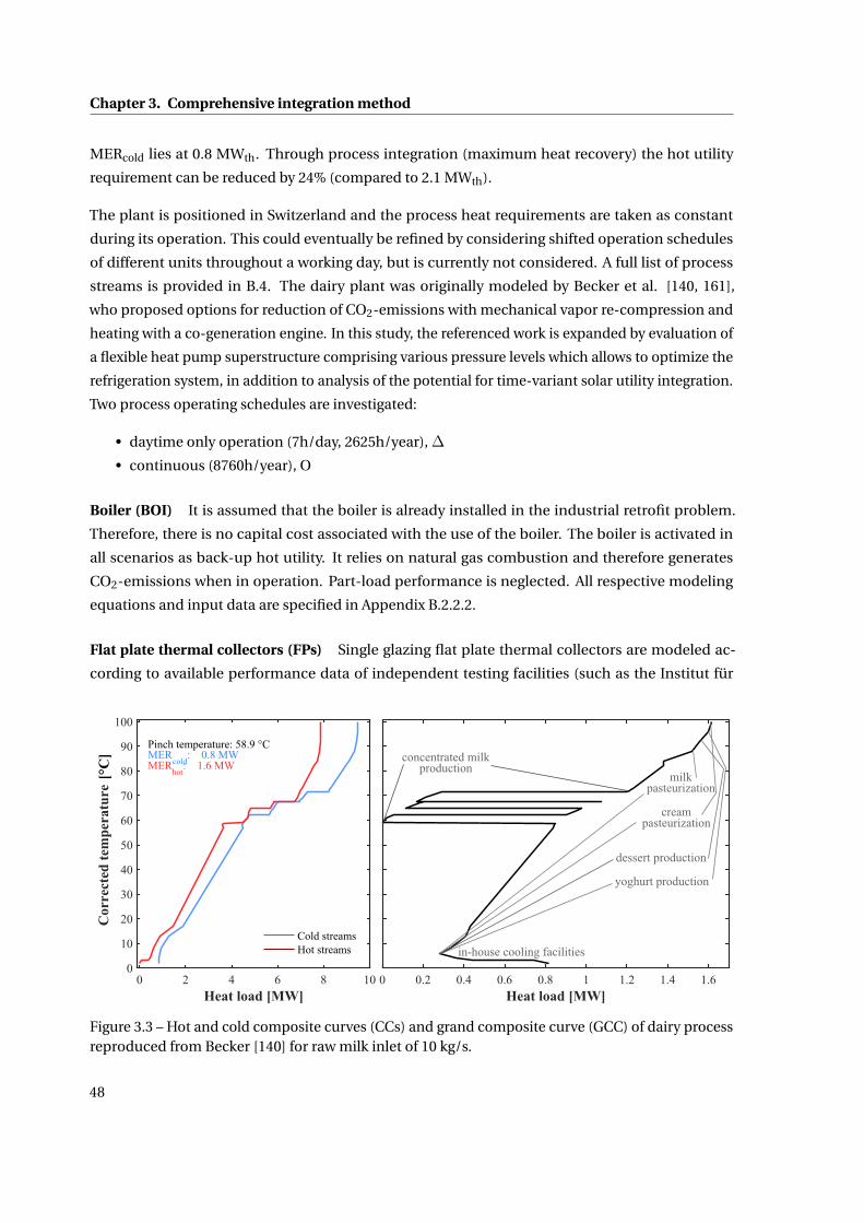
Chapter 3. Comprehensive integration method
MERcold lies at 0.8 MWth. Through process integration (maximum heat recovery) the hot utility
requirement can be reduced by 24% (compared to 2.1 MWth).
The plant is positioned in Switzerland and the process heat requirements are taken as constant
during its operation. This could eventually be refined by considering shifted operation schedules
of different units throughout a working day, but is currently not considered. A full list of process
streams is provided in B.4. The dairy plant was originally modeled by Becker et al. [140, 161],
who proposed options for reduction of CO2-emissions with mechanical vapor re-compression and
heating with a co-generation engine. In this study, the referenced work is expanded by evaluation of
a flexible heat pump superstructure comprising various pressure levels which allows to optimize the
refrigeration system, in addition to analysis of the potential for time-variant solar utility integration.
Two process operating schedules are investigated:
• daytime only operation (7h/day, 2625h/year),Δ
• continuous (8760h/year), O
Boiler (BOI) It is assumed that the boiler is already installed in the industrial retrofit problem.
Therefore, there is no capital cost associated with the use of the boiler. The boiler is activated in
all scenarios as back-up hot utility. It relies on natural gas combustion and therefore generates
CO2-emissions when in operation. Part-load performance is neglected. All respective modeling
equations and input data are specified in Appendix B.2.2.2.
Flat plate thermal collectors (FPs) Single glazing flat plate thermal collectors are modeled ac-
cording to available performance data of independent testing facilities (such as the Institut für
Figure 3.3 – Hot and cold composite curves (CCs) and grand composite curve (GCC) of dairy processreproduced from Becker [140] for raw milk inlet of 10 kg/s.
48

3.2. Methodology
Solartechnik, (SPF) [164]) with solar keymark [165] status. The provided test parameters comply
with the European norm for efficiency measurements of thermal collectors EN-12975. Flat plate
thermal collectors produce heat up to approximately 130°C. However, efficiency decreases with
higher operating temperatures due to heat losses.
Therefore, the operating temperature range is fit to the dairy process demand which is between 80
and 105°C. The collector working fluid is a water glycol mixture. The efficiency is further dependent
on the intensity of the incoming radiation and its direction. All respective performance equations
are presented in Section 2.3.1.2. The input data for the considered collector is shown in Table B.4 in
Appendix B.2.3.2.
Photovoltaic modules (PVs) High efficiency mono-crystalline photovoltaic modules were con-
sidered during the calculation. The modeled energetic output was based on certified producer
data (IEC 61215, IEC 61730,[166] taken from the 10th year of operation. The two main parameters
influencing the PV performance are the cell temperature (dependent on the ambient temperature,
the incident radiation, and the wind speed) and the irradiation intensity. All relevant performance
equations are presented in Section 2.3.1.3. The input data for the considered collector is shown in
Table B.5 in Appendix B.2.3.3.
High concentration photovoltaic and thermal system (HCPVT) The high concentration photo-
voltaic and thermal system is a concentrating dish (with concentrations of up to 2000 at the focal
point) with two axis tracking of the sun which is mounted on a tower. Electricity is generated
with photovoltaic cells in the receiver positioned in the focal point. Highly efficient cooling pre-
vents receiver and photovoltaic cell overheating and provides useful heat around 100°C. Thereby
the exergetic losses of the photovoltaic conversion are recovered. High concentration devices
can only convert direct beam radiation. Performance indicators are retrieved from producer data
[32, 86, 112, 132]. All modeling equations are depicted in Section 2.3.1.4. All respective performance
equations are presented in Section 2.3.1.4. The input data for the considered collector is shown in
Table B.6 in Appendix B.2.3.4.
Thermal storage tank (S) The thermal storage mass and energy balances are formulated based
on the assumption of sensible heat storage at different temperature levels modeled as one tank
operating between two temperatures. An intra-cyclic constraint is introduced, which ensures that
the storage is always at initial conditions at the end of each day. Furthermore, it is defined (in
agreement with a storage tank with two outlets) that the fluid leaving the storage tank is always at the
lowest temperature (bottom) during charge periods or highest temperature (top) during discharge
periods. More information on the considered storage tank can be found in Section 2.4.2 and in
Appendix B.2.3.5.
Limitations The performance of the three respective solar systems is modeled for one piece of
equipment. Industrial applications require large collector fields and, therefore, a constant loss factor
49

Chapter 3. Comprehensive integration method
is introduced in this work to account for thermal and transmission losses in the field. This factor, in
reality, scales with the field size and follows certain power laws. Additionally, the impact of shading
on the overall output is non-negligible especially for the tracking systems considering the space
is usually limited which is not accounted for either. It is planned to explore the validity of these
simplifications by further in-depth analysis in future work.
Heat pump superstructure (REF, MVR, HPS) A superstructure is employed which permits in-
vestigation of possible combinations between different heat pump components: compressors,
evaporators, condensers, and presaturators [167].
For selecting the optimal heat pump structure, a set of pressure levels must be defined. The active
levels are selected during the system resolution with help of integer variables. The choices are
only constrained by the fact that the highest pressure level must be a condenser and the lowest
level needs to be an evaporator. Since the pressures and respective temperature levels are chosen
in advance, the sizing of the components can be formulated by linear constraints as part of the
MILP. Figure 3.4(a) presents a temperature entropy diagram to illustrate the problem definition,
formulating all generic heat pump cycles once the pressure levels are selected. Figure 3.4(b) shows
a flow chart of the superstructure. Connections between all pressure levels are defined as well as
potential presaturation, evaporation, and condensation units on every level.
This permits the generation of all possible single and multi-stage cycles between a predefined set
of pressure levels. The one-stage refrigeration cycle in place, the vapor re-compression system
as well as the improved multi-stage heat pump cycle are modeled with this superstructure. The
performance equations as well as all investigated specifications are presented in Appendix B.2.2.3.
Figure 3.4 – Heat pump superstructure model. (a) Ammonia liquid-vapor saturation curve withisobars (marked in gray in descending order) and potential heat pump cycles (isentropic compressorefficiency ηisentropic = 1), (b) flowchart of heat pump superstructure.
50

3.2. Methodology
Figure 3.5 – Load duration curve of DNI in Sion, Switzerland (CH), of original data and 8 typical plus2 extreme days. In background yearly distribution of DNI of original and typical days.
3.2.3.2 Meteorological data clustering
Meteorological data Weather data including the solar angles (azimuth and elevation), wind speed,
ambient temperature, and global horizontal (GHI) and direct normal (DNI) irradiance of hourly time
resolution is retrieved from a commercial software (Meteonorm 7.0 [134]). The analysis is carried
out for the Swiss city of Sion, having comparably high yearly solar irradiance (global horizontal
irradiation (GHI) 1430, direct normal irradiation (DNI) 1690 kWh/m2) relative to the rest of the
country (1200 kWh/m2) due to a favorable micro-climate.
Data clustering Figure 3.5 presents the results from the clustering algorithm presented in Chapter
2.3.2.2. The load duration curve of the DNI is displayed for the original data and the typical days. In
the background, the hourly data is displayed showing that high values can also be reached during
winter. This is particular for the DNI as it is not reduced by cosine losses in contrast to the GHI. The
mELDC2 is below the limit of 3.5×10⁻⁴ (as derived in Section 2.3.2.2) and is also visibly acceptable.
In the upper right corner the resulting typical days and their occurrence are illustrated. The two
extreme days are represented only once. It can be seen that there are few days with very low DNI.
3.2.4 System resolution (B)
This section presents the optimization problem formulation and the respective constraints. The
sets presented in the following Section 3.2.4.1 are specified in this case study in the following
manner. The set of utility technologies W refers to Section 3.2.3.1. W = boiler (BOI), refrigeration
(REF), mechanical vapor re-compression (MVR),heat pump superstructure (HPS), flat plate thermal
collectors (FPs), photovoltaic modules (PVs), high concentration photovoltaic and thermal system
(HCPVT), thermal storage (STO), cooling water (CW), electricity grid (GRID). The set of periods P
51

Chapter 3. Comprehensive integration method
stems from Section 3.2.3.2.
3.2.4.1 MILP utility targeting formulation
The problem is formulated as a multi-period MILP that solves the heat cascade and finds optimal
utility integration [75, 138, 139, 155].
Objective function The problem objective is the minimization of the total annualized costs (TAC)
is depicted in Equation 3.1. It is composed of the yearly operating expenses (opex) of each utility
technology w during period p and the annualized capital expenses (capex) that is found with aid of
the maximum size of each technology w.
miny w
p , f wp ,y w , f w
∑p∈P
( ∑w∈W
OPw1,p · y w
p +OPw2,p · f w
p
)· ∆tp ·occp︸ ︷︷ ︸
Operating cost
+ ∑w∈W
(IVw
1 · y w + IVw2 · f w )
︸ ︷︷ ︸Investment cost
(3.1)
Where
P set of periods 1,2,3, ...,np W set of utility technologies wf w
p ∈ R+ continuous variable for sizing technology w during period py w
p ∈ 0,1 binary variable related to existence of technology w during pf w maximum size of technology wy w overall existence of technology wOPw
1,p [e/h] fixed operating cost for using the technology w during period p
OPw2,p [e/h] proportional operating cost for using technology w during period p and is scaled with the multiplication factor
IVw1 [e/y] annualized, actualized fixed cost related to the investment of technology w
IVw2 [e/y] annualized, actualized proportional cost related to the investment of technology wΔtp [h] operating time of period poccp [1/y] the occurrence of period p
All respective general constraints related to the solar and conventional utilities are derived in
Section 2.4.
3.2.4.2 ε-constraint
As mentioned, an ε-constraint was added to the MILP which constrains the CO2-equivalent emis-
sions of the system. The total CO2-equivalent emissions depicted in Equation 3.2 are found by taking
into account emissions from natural gas consumption and the electricity grid. Life cycle assessment
of the associated technologies is not considered. The positive impact on the grid created by selling
solar electricity was as well disregarded.
CO2,tot =∑p∈P
(CO2,el · EGRID · f GRID,in
p +CO2,ng · QngBOI · f BOI
p
)·∆tp ·occp (3.2)
Where CO2,el [kgCO2eq/kWhel] are the life cycle emissions related to buying electricity from the
52

3.2. Methodology
Swiss grid and CO2,ng [kgCO2eq/kWhng] are the life cycle emissions from natural gas burning, EGRID
[kW] is the reference electricity supply of the grid utility, f GRID,inp [-] is the multiplication factor of
the incoming grid utility in period p, f BOIp [-] is the multiplication factor of the boiler in period p,
and QngBOI [kW] is the reference natural gas consumption in the boiler.
The ε-constraint ensures that the total emissions do not exceed ε, which is specified as a fraction of
the reference emissions and which is incrementally changed in this work (between 95 and 60% of
the reference emissions).
CO2,tot
COref2,tot
≤ ε (3.3)
3.2.5 Performance calculation (C)
After the optimization step the non-linear functions, such as the investment cost are recalculated as
well as other performance indicators depicted below. The necessary parameters are presented in
Table 3.2.
Operating cost During the MILP optimization step, the buying price of electricity is set to the
market price displayed in Table 3.2, while the selling price is set to a very small negative number.
This serves as a protection against oversizing the photovoltaic systems not to become pure electricity
exporters due to potentially high profits from selling electricity. The solar utilities should be sized
with the ε-constraint on the emissions.
In the performance calculation step, the operating cost are recalculated with adequate numbers. It
is assumed that the solar utilities do not have operating costs. Therefore, the total operating costs
are composed of the electricity bought from or sold to the grid and the natural gas consumption in
the boiler. The selling price of electricity is set to 80% of the buying price to represent the current
market situation more realistically. The yearly operating expenses (opex), C opex [e/y], are a function
Table 3.2 – Data related to emissions, primary energy consumption and operating cost in Switzerland(CH).
Parameter Symbol Unit Value SourceAmbient temperature Ta [K] 298 [-]Interest rate i [-] 0.05 [-]Equipment lifetime n [y] 20 [-]Maintenance cost fraction of total investment m [1/y] 0.05 [-]Cost of buying electricity OPel
2,p [e/kWh] 0.142 [168]
Cost of buying natural gas OPng2,p [e/kWh] 0.081 [168]
Emissions electricity CO2,el [kgCO2eq/kWh] 0.11257 [169]Emissions natural gas CO2,ng [kgCO2eq/kWh] 0.20196 [169]
53

Chapter 3. Comprehensive integration method
of the resource prices and their annual net requirements (natural gas and electricity).
C opex =P∑
p=1
(OPel
2,p · EGRID ·(
f GRID,inp −0.8 · f GRID,out
p
)+OPng
2,p · QngBOI · f BOI
p
)·∆tp ·occp (3.4)
Where OPel2,p [e/kWhel] is the electricity cost, OPng
2,p [e/kWhng] is the natural gas price during period
p, EGRID
[kW] is the reference grid electricity inlet/outlet, QngBOI [kW] is the reference natural gas
consumption of the boiler, f GRID,inp [-] is the multiplication factor of the incoming grid utility in
period p, f GRID,outp [-] is the multiplication factor of the outgoing grid utility in period p, The natural
gas and electricity prices are depicted in Table 3.2.
Investment cost The investment cost of the units in-place (the boiler and standard refrigeration
cycle) are not considered. Other investment cost functions can be found in B.2.2. All cost data are
actualized with the Marshall and Swift index [6]. The total investment cost, C I NV [e], is calculated
as a function of the maximum sizes of each utility technology w over all periods p.
Total annual cost The total annualized costs (TAC), C T AC [e/y], is derived from yearly operating
expenses (opex), C opex [e/y], the annualized capital expenses (capex), where τ= i·(1+i)n
(1+i)n−1 [1/y] is the
investment cost annualization factor, and the maintenance cost, which is a fraction m [1/y] of the
total investment, see Table 3.2.
C T AC =C opex +C I NV · (τ+m) (3.5)
Note Calculating the maintenance cost as a fraction of the investment cost constitutes a neglect of
the running costs of the utilities in place. Their investment cost and with that their maintenance
cost is in this way assumed to be zero. This displays a simplification which, however, generates
conservative utility integration results in underestimating the total cost of the current status quo of
the plant.
Carnot factor The Carnot factor permits re-scaling the temperature levels on the standard com-
posite curve. This has two advantages: firstly, the representation is more compact since the y-axis
will always be between -1 and 1 (equivalent to a temperature range of [-124,∞] °C) which makes
visualization of the process easier; and secondly, the factor is proportional to the exergetic potential
of a temperature level and therefore exergetic losses between sources and sinks can be visualized.
ηCarnot = 1− Ta
T(3.6)
Where Ta [K] is the ambient temperature and T [K] is the temperature of the stream.
54
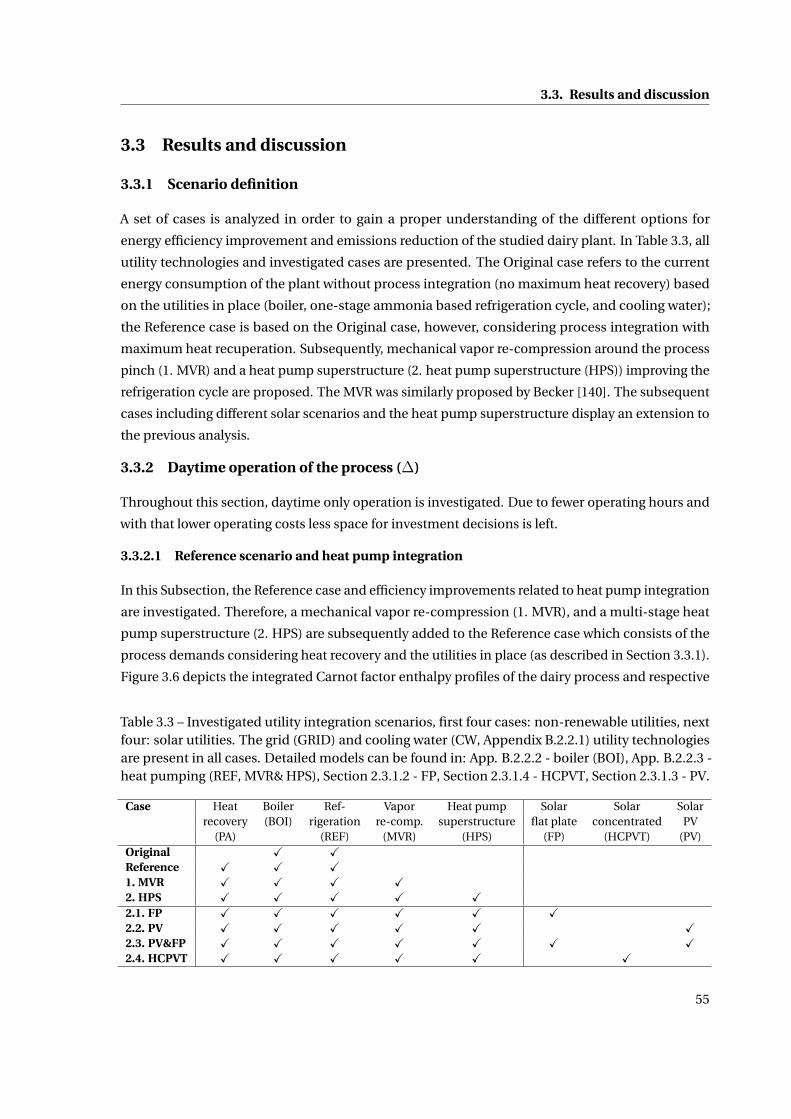
3.3. Results and discussion
3.3 Results and discussion
3.3.1 Scenario definition
A set of cases is analyzed in order to gain a proper understanding of the different options for
energy efficiency improvement and emissions reduction of the studied dairy plant. In Table 3.3, all
utility technologies and investigated cases are presented. The Original case refers to the current
energy consumption of the plant without process integration (no maximum heat recovery) based
on the utilities in place (boiler, one-stage ammonia based refrigeration cycle, and cooling water);
the Reference case is based on the Original case, however, considering process integration with
maximum heat recuperation. Subsequently, mechanical vapor re-compression around the process
pinch (1. MVR) and a heat pump superstructure (2. heat pump superstructure (HPS)) improving the
refrigeration cycle are proposed. The MVR was similarly proposed by Becker [140]. The subsequent
cases including different solar scenarios and the heat pump superstructure display an extension to
the previous analysis.
3.3.2 Daytime operation of the process (Δ)
Throughout this section, daytime only operation is investigated. Due to fewer operating hours and
with that lower operating costs less space for investment decisions is left.
3.3.2.1 Reference scenario and heat pump integration
In this Subsection, the Reference case and efficiency improvements related to heat pump integration
are investigated. Therefore, a mechanical vapor re-compression (1. MVR), and a multi-stage heat
pump superstructure (2. HPS) are subsequently added to the Reference case which consists of the
process demands considering heat recovery and the utilities in place (as described in Section 3.3.1).
Figure 3.6 depicts the integrated Carnot factor enthalpy profiles of the dairy process and respective
Table 3.3 – Investigated utility integration scenarios, first four cases: non-renewable utilities, nextfour: solar utilities. The grid (GRID) and cooling water (CW, Appendix B.2.2.1) utility technologiesare present in all cases. Detailed models can be found in: App. B.2.2.2 - boiler (BOI), App. B.2.2.3 -heat pumping (REF, MVR& HPS), Section 2.3.1.2 - FP, Section 2.3.1.4 - HCPVT, Section 2.3.1.3 - PV.
Case Heat Boiler Ref- Vapor Heat pump Solar Solar Solarrecovery (BOI) rigeration re-comp. superstructure flat plate concentrated PV
(PA) (REF) (MVR) (HPS) (FP) (HCPVT) (PV)Original X XReference X X X1. MVR X X X X2. HPS X X X X X2.1. FP X X X X X X2.2. PV X X X X X X2.3. PV&FP X X X X X X X2.4. HCPVT X X X X X X
55
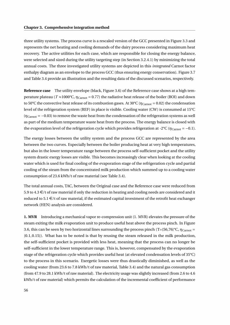
Chapter 3. Comprehensive integration method
three utility systems. The process curve is a rescaled version of the GCC presented in Figure 3.3 and
represents the net heating and cooling demands of the dairy process considering maximum heat
recovery. The active utilities for each case, which are responsible for closing the energy balance,
were selected and sized during the utility targeting step (in Section 3.2.4.1) by minimizing the total
annual costs. The three investigated utility systems are depicted in this integrated Carnot factor
enthalpy diagram as an envelope to the process GCC (thus ensuring energy conservation). Figure 3.7
and Table 3.4 provide an illustration and the resulting data of the discussed scenarios, respectively.
Reference case The utility envelope (black, Figure 3.6) of the Reference case shows at a high tem-
perature plateau (T ≈1000°C, ηCarnot = 0.77) the radiative heat release of the boiler (BOI) and down
to 50°C the convective heat release of its combustion gases. At 30°C (ηCarnot = 0.02) the condensation
level of the refrigeration system (REF) in place is visible. Cooling water (CW) is consumed at 15°C
(ηCarnot =−0.03) to remove the waste heat from the condensation of the refrigeration systems as well
as part of the medium temperature waste heat from the process. The energy balance is closed with
the evaporation level of the refrigeration cycle which provides refrigeration at -2°C (ηCarnot =−0.1).
The exergy losses between the utility system and the process GCC are represented by the area
between the two curves. Especially between the boiler producing heat at very high temperatures,
but also in the lower temperature range between the process self-sufficient pocket and the utility
system drastic exergy losses are visible. This becomes increasingly clear when looking at the cooling
water which is used for final cooling of the evaporation stage of the refrigeration cycle and partial
cooling of the steam from the concentrated milk production which summed up to a cooling water
consumption of 23.6 kWh/t of raw material (see Table 3.4).
The total annual costs, TAC, between the Original case and the Reference case were reduced from
5.9 to 4.3e/t of raw material if only the reduction in heating and cooling needs are considered and it
reduced to 5.1e/t of raw material, if the estimated capital investment of the retrofit heat exchanger
network (HEN) analysis are considered.
1. MVR Introducing a mechanical vapor re-compression unit (1. MVR) elevates the pressure of the
steam exiting the milk evaporation unit to produce useful heat above the process pinch. In Figure
3.6, this can be seen by two horizontal lines surrounding the process pinch (T=56,76°C, ηCarnot =0.1,0.15). What has to be noted is that by reusing the steam released in the milk production,
the self-sufficient pocket is provided with less heat, meaning that the process can no longer be
self-sufficient in the lower temperature range. This is, however, compensated by the evaporation
stage of the refrigeration cycle which provides useful heat (at elevated condensation levels of 35°C)
to the process in this scenario. Exergetic losses were thus drastically diminished, as well as the
cooling water (from 23.6 to 7.8 kWh/t of raw material, Table 3.4) and the natural gas consumption
(from 47.9 to 28.1 kWh/t of raw material). The electricity usage was slightly increased (from 2.6 to 4.6
kWh/t of raw material) which permits the calculation of the incremental coefficient of performance
56

3.3. Results and discussion
Figure 3.6 – Integrated composite curves (ICCs) of the dairy process and respective utility system.[Reference] case with utilities in place, compared to case [1. MVR] with additional mechanical vaporre-compression around 67°C, and [2. HPS] with additional heat pump superstructure between -2,15, 30, and 50°C.
0
10
20
30
40
50
60
70
80
-2°C
30°C
-2°C
35°C
-2°C
56°C
76°C
56°C
76°C
50°C
35°C
15°C
Reference 1. MVR 2. HPS
Cooling water
30°C
Tem
pera
ture
[°C
]
Figure 3.7 – Illustration of the conversion cycles involved in the respective scenarios.
Table 3.4 – Utility integration scenarios as described in Section 3.3.1. Costs and energy specificconsumption data (referred to ton of raw material. (*) total annualized costs (TAC) neglecting HENretrofit cost estimation
Original Reference 1. MVR 2. HPSOperating costs C opex [e/t] 5.9 4.3 2.9 2.6Natural gas cons. Qng [kWh/t] 64.6 47.9 28.1 24.3
Electricity cons. EGRID
[kWh/t] 4.6 2.6 4.6 4.8Compressor size ECOMP [kW] 167.0 94.7 111.8 55.2 87.5 65.1 10.4 9.7Cold coeff. of performance COPc [-] 5.7 4.8 11.6 4.8 11.6 11.0 11.0Cooling water cons. QCW [kWh/t] n.a. 23.6 7.8 4.5Compressor cap. exp. C COMP [e/t] 0 0 0.190 0 0.221 0.042 0.040Heat exchang. area AHE N [m2] 826 1032 1161Number of HEX N HE N
min [-] 48 64 85HEN capital cost est. C HE N [e/t] 0.9 1.2 1.5TAC w/o HEN C T AC ∗ [e/t] 5.9 4.3 3.1 3.0Total annual costs C T AC [e/t] 5.9 5.1 4.3 4.4
57

Chapter 3. Comprehensive integration method
COP=∆Qng/∆EGRID = 9.9 [-]. Where Qng and EGRID are the natural gas and electricity consumption
respectively (as reported in Table 3.4). On top of this improvement in efficiency, the total annual
cost dropped from 5.1 in the Reference case to 4.3e/t of raw material due to drastic reductions in
the operating costs.
The elevation of the condensation level (from 30 to 35 °C) is an engineering choice which was
motivated by the fact that the size of the mechanical vapor re-compression unit is constrained by
how much heat could be delivered to the process from the evaporation stage of the refrigeration
cycle. By elevating this temperature and considering de-superheating of the superheated vapor
exiting the compressor (at slightly elevated temperature) more use of vapor re-compression could
be made and a higher incremental COP was be achieved. However, there is a limit to increasing the
upper pressure of an existing compressor.
2. HPS Therefore, a heat pump superstructure (2. HPS) is introduced to explore further installation
of heat pumps with respect to the total annual costs. Adding the heat pump superstructure provides
various options for single-and multi stage cycles between -2 and 50 °C (in 2 °C intervals) to the system
resolution. With this, a new utility system configuration was found consisting of the refrigeration
cycle in place, the mechanical vapor re-compression unit, and two new heat pump cycles between
-2 and 15 °C and between 30 and 50 °C. In Figure 3.6 it can be seen that this lead to a higher use of the
mechanical vapor re-compression unit, because more heat could be provided to the process by the
heat pumps. And this imposed a further decrease in the boiler consumption and, consequentially,
a reduction of the exergy losses in the system. The total annual costs not considering the HEN
costs (disregarded in the MILP) were reduced as well. However, considering the estimated capital
expenses for the HEN, the TAC slightly increased from 4.3 to 4.4e/t of raw material. The cooling
water consumption was further decreased from 7.8 to 4.5 kWh/t of raw material; and the electricity
consumption was only slightly increased from 4.6 to 4.8 kWh/t. This originated from the use of a
lower temperature refrigeration cycle (-2 to 15 °C) with a higher COPc of 11, which resulted in a
reduction of the consumption of the refrigeration in place (COPc 4.8). Thereby the incremental COP
was further improved to 24.2 [-] with respect to the previous scenario (1. MVR).
Summary What can be concluded from here is that more complex systems (in terms of heat
pumping) offer higher potential from the energetic point of view. And more complex systems require
more complex tools (as illustrated with integration of the heat pump superstructure). However,
there is always a trade-off between efficiency improvements accompanied by potential operating
cost reduction and increase of the complexity of the system and therewith the heat exchanger
network. The presented results indicate the strong potential of such installations and enunciates
the importance of investigating selected case studies in further detail.
In the next section, the relation between efficiency improvements (through heat pumping) on solar
sizing is presented and general guidelines are provided.
58

3.3. Results and discussion
3.3.2.2 Heat pump & solar integration
Process schedule Figure 3.8 depicts the process operating scheme and solar GHI and DNI radi-
ation during the typical periods. The winter days are marked by DNI levels exceeding the GHI,
meaning that the sun elevation is not very high. The starting hours of the process operation was
set to 8:00 o’clock in the morning lasting between 7 and 8 hours per day in order to form 2625
operating hours per year. This is a design choice attempting to overlap process operation with the
sunshine hours. Observing the overlap between solar radiation and process operation, it becomes
clear that there are several instances in which the overlap would be more aligned with the solar
insolation if the process starting time was shifted to later in the morning. However, knowing that
many manufacturing schedules traditionally start at earlier hours, 8:00 o’clock was the accepted
trade-off.
In the daytime operation, the option of storage is not considered. As seen in Figure 3.8, the main
lack of solar energy occurs in the early morning hours. It is difficult to store thermal energy over
night and thus it was unreasonable to consider storage of solar energy for these periods of low solar
productivity.
ε-constraint optimization The results from the ε-constraint optimization can be seen in Figure
3.9. The two heat pump cases (1. MVR 6.2 & 2. HPS 5.5 kg CO2-eq/t) were determined without
ε-constraint as described in Section 3.3.2.1. Among these, the best scenario in terms of emissions
was chosen as reference for the solar integration (2. HPS). For integration of the solar components
the ε-constraint was gradually set to a fraction of these reference emissions (between 95 and 60%)
while minimizing the total system cost. In this way a Pareto type curve was produced (Figure 3.9 (a))
between the annualized investment cost and the specific emissions. As expected, with decreasing
emissions the annualized investment costs increased. The solar cases are presented with error bars
Figure 3.8 – Process operation scheme and solar radiation during typical periods. (GHI: globalhorizontal irradiation, DNI: direct normal irradiation.)
59

Chapter 3. Comprehensive integration method
(the data of which can be found in Sections 2.3.1.3, 2.3.1.2, 2.3.1.4). Especially for the HCPVT system
which is the most novel technology with the most volatile prices, this is a reasonable assumption.
Under the current input data, the solar cases performed very similarly in terms of investment
cost. The total annual cost in Figure 3.9 (b) include besides the investment cost also the operating
expenses. This leads to a different distribution of the data points. In terms of total annual cost, both
heat pumping scenarios and most solar options were profitable with respect to the Reference case
(of the utilities in place). The relative emission reductions amounted to 27% (between Original and
Reference scenario) due to heat recuperation, 38% due to mechanical vapor re-compression (from
Reference to 1. MVR), and 12% due to improved refrigeration (from 1. MVR to 2. HPS). The solar
scenarios further decreased the emissions by 5-40% (ε =95-60%) with respect to the 2. HPS scenario.
It can be observed that some solar technologies potentially resulted in higher emission reductions
than others. With PV modules the least reductions were achieved since they could not replace the
boiler natural gas consumption; however, their advantage is the ability to sell overproduction to
the grid. Still, up to 20% emission reduction was be achieved integrating solar PV. The reduction
is achieved by replacing the incoming electricity from the grid with green electricity. The HCPVT
Figure 3.9 – Results from ε-constraint optimization of different solar options for daytime onlyprocess operation. (a) Annualized capital expenses (capex) versus carbon dioxide (CO2)-equivalentemissions, (b) TAC versus CO2 emissions, (c) detailed cost analysis of various cases.
60

3.3. Results and discussion
system and combined FP and PV can reach the highest emission reductions at reasonable cost. At
specific CO2 reductions of 3.8 kg CO2-equivalent/ton of raw material, which is equivalent to 70% of
the best heat pump only (reference) case, the TAC of all solar systems overlap, which indicates that
this establishes an appropriate balance between operating, investment cost and energy waste.
The uncertainty related to the solar investment cost is indicated on Figure 3.9, but not the uncer-
tainty related to the heat exchanger area cost estimation. This is a rough estimation with errors
varying between 20 and 40%; therefore, grand conclusions should not be drawn when considering a
difference in TAC between 10 and 20%.
Figure 3.9 (c) illustrates the associated total costs of the different scenarios. The operating cost
are predominant in the Reference case, which explains the fact that the total cost of the solar
scenarios did not drastically increase. This is attributed to a shift from operating expenses to specific
investment cost.
A break even CO2 tax was calculated with respect to the case with lowest TAC (1. MVR). If the
respective tax was applied all cases would exhibit the same costs as scenario 1. MVR. The tax lied
between 100 and 300e/ton CO2-equivalent which is slightly higher than the current prices, but in
the same order of magnitude.
Figure 3.10 (a) depicts the optimal active solar area for different CO2-equivalent emissions (ε∈[60%,95%]) of all studied solar collector types. It can be observed that the required solar area
increased with decreasing CO2-equivalent emissions. The relationship between emission reduction
and active solar area does not follow a linear regression, but rather flattens out, especially for HCPVT
and PV (and the lowest three FP data points) systems. This is attributed to the interconnectivity
of the system, where higher solar thermal production has an influence also the utilization of the
heat pumps and mechanical vapor re-compression and therewith on the electricity inflicted CO2-
equivalent emissions. And vice versa, the solar electricity production directly affects the utilization
of the heat pumps which influences the boiler consumption.
The HCPVT system required the smallest active area in comparison to the other solar technologies.
This stems from the high total conversion efficiency. It has to be noted though that due to two axis
tracking and the danger of shading, the actual required land area may be increased by a factor of 2.
Figure 3.10 (b) shows the integrated Carnot factor enthalpy profiles of the dairy process and respec-
tive utility systems. Flat plate collectors (scenario 2.1 FP) at 80% emissions with respect to the 2. HPS
case (at 4.3 kg CO2-equivalent/ton of raw material) are shown at solar noon during different typical
days. The optimization results show that in comparison to the 2. HPS scenario, a different heat
pump configuration was chosen: instead of two heat pumps (30 to 50 °C and -2 to 15 °C) a two stage
heat pump between -2, 15, and 50 with flash gas removal and inter-cooling at 30 °C was selected
during the MILP. In the curve, this can be traced with help of the missing evaporation plateau at 30°C
61
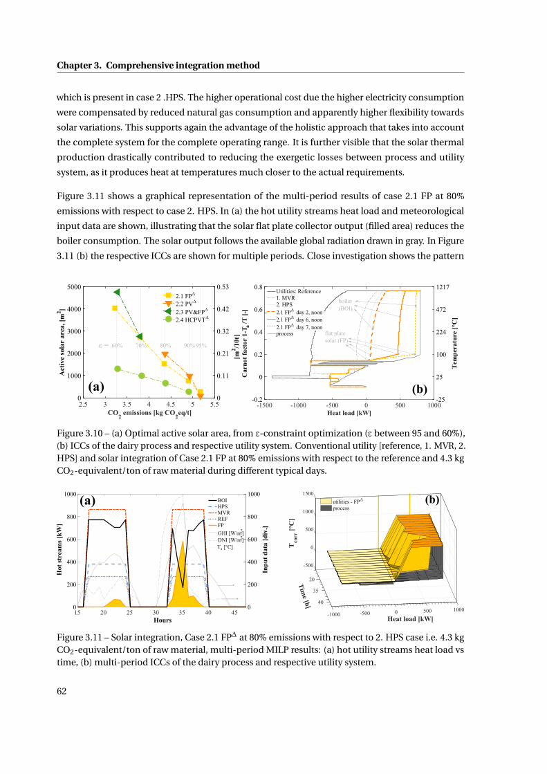
Chapter 3. Comprehensive integration method
which is present in case 2 .HPS. The higher operational cost due the higher electricity consumption
were compensated by reduced natural gas consumption and apparently higher flexibility towards
solar variations. This supports again the advantage of the holistic approach that takes into account
the complete system for the complete operating range. It is further visible that the solar thermal
production drastically contributed to reducing the exergetic losses between process and utility
system, as it produces heat at temperatures much closer to the actual requirements.
Figure 3.11 shows a graphical representation of the multi-period results of case 2.1 FP at 80%
emissions with respect to case 2. HPS. In (a) the hot utility streams heat load and meteorological
input data are shown, illustrating that the solar flat plate collector output (filled area) reduces the
boiler consumption. The solar output follows the available global radiation drawn in gray. In Figure
3.11 (b) the respective ICCs are shown for multiple periods. Close investigation shows the pattern
Figure 3.10 – (a) Optimal active solar area, from ε-constraint optimization (ε between 95 and 60%),(b) ICCs of the dairy process and respective utility system. Conventional utility [reference, 1. MVR, 2.HPS] and solar integration of Case 2.1 FP at 80% emissions with respect to the reference and 4.3 kgCO2-equivalent/ton of raw material during different typical days.
Figure 3.11 – Solar integration, Case 2.1 FP∆ at 80% emissions with respect to 2. HPS case i.e. 4.3 kgCO2-equivalent/ton of raw material, multi-period MILP results: (a) hot utility streams heat load vstime, (b) multi-period ICCs of the dairy process and respective utility system.
62

3.3. Results and discussion
of the solar output from Figure 3.11 (a) in the high temperature plane of the boiler in the curves
in Figure 3.11 (b). This is related to the much lower operating temperatures of the solar system
compared to the boiler and the related drop on the temperature axis.
It should be noted that the required boiler output changes drastically over time when solar heat is
present. This might have an influence on the overall efficiency of the energy conversion if part load
performance of the boiler is modeled in more detail, which was not considered here.
In conclusion, it can be stated that there is high economic and environmental potential for this type
of industrial dairy plants for heat pump and solar integration. Results may be extrapolated to other
low temperature food processing plants especially when operated in the underlying temperature
range. Integration of both types of systems, solar and heat pumping should always be investigated
with a holistic approach. For further steps, it is crucial to investigate the heat exchanger network
design to explore technical feasibility of integrated systems.
3.3.3 Continuous process operation (O)
Throughout this section, continuous process operation is investigated. Due to a higher number of
operating hours (8760 vs 2625h) and with that increased operating costs more space for investment
decisions is potentially available.
Figure 3.12 shows the results from the ε-constraint optimization. It can be observed that the raw
material specific annualized investment cost were lower than the cost for the daytime only operation.
This is explained by the higher operating hours and thus increased yearly raw material consumption.
This increase had no influence on the specific operating cost which scale linearly with the raw
material consumption. But the estimated HEN area and compressor sizes remains unchanged
compared to daytime only operation and, therefore, the specific capital cost estimations decrease
for a higher yearly raw material consumption. This leads to lower TAC of the 2. HPS scenario in
comparison to 1. MVR and daytime operation.
This decrease in relative specific investment costs also showed improvements for the flat plate
thermal collectors (FPs) and photovoltaic modules (PVs) at low emission reductions (ε= 95%), which
in this case are both profitable with respect to the best non-solar case (2. HPS). The PV system
could not reach higher emission reductions than 95%, because batteries are not considered and
the positive impact from a renewable source to the grid is not counted. With increasing emission
reductions the solar size and cost increased and the flat plate scenarios’ TAC reached slightly above
best non-solar case. The HCPVT exhibited the smallest specific TAC of all solar options as the
overproduced electricity could be sold and therefore the operating costs decrease.
The option of storage was only chosen by the optimizer for emission reductions below and including
80% (FP) and 70% (HCPVT), respectively. This is attributed to the additional investment cost imposed
63
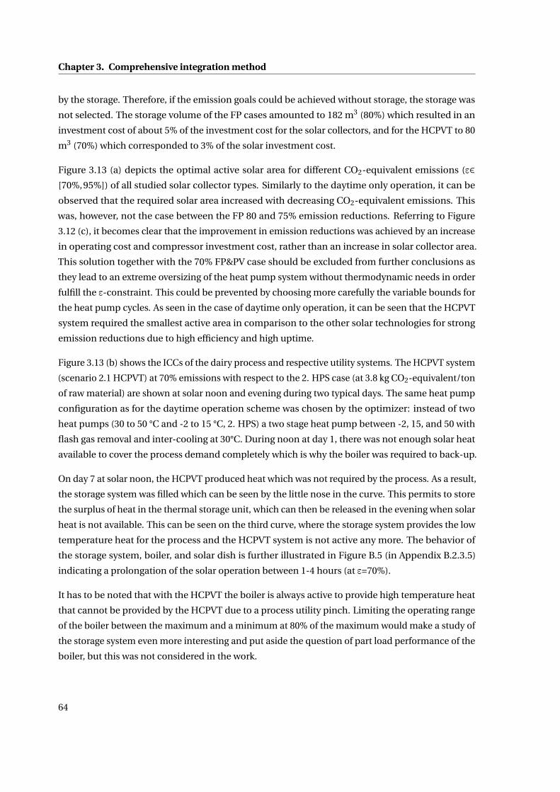
Chapter 3. Comprehensive integration method
by the storage. Therefore, if the emission goals could be achieved without storage, the storage was
not selected. The storage volume of the FP cases amounted to 182 m3 (80%) which resulted in an
investment cost of about 5% of the investment cost for the solar collectors, and for the HCPVT to 80
m3 (70%) which corresponded to 3% of the solar investment cost.
Figure 3.13 (a) depicts the optimal active solar area for different CO2-equivalent emissions (ε∈[70%,95%]) of all studied solar collector types. Similarly to the daytime only operation, it can be
observed that the required solar area increased with decreasing CO2-equivalent emissions. This
was, however, not the case between the FP 80 and 75% emission reductions. Referring to Figure
3.12 (c), it becomes clear that the improvement in emission reductions was achieved by an increase
in operating cost and compressor investment cost, rather than an increase in solar collector area.
This solution together with the 70% FP&PV case should be excluded from further conclusions as
they lead to an extreme oversizing of the heat pump system without thermodynamic needs in order
fulfill the ε-constraint. This could be prevented by choosing more carefully the variable bounds for
the heat pump cycles. As seen in the case of daytime only operation, it can be seen that the HCPVT
system required the smallest active area in comparison to the other solar technologies for strong
emission reductions due to high efficiency and high uptime.
Figure 3.13 (b) shows the ICCs of the dairy process and respective utility systems. The HCPVT system
(scenario 2.1 HCPVT) at 70% emissions with respect to the 2. HPS case (at 3.8 kg CO2-equivalent/ton
of raw material) are shown at solar noon and evening during two typical days. The same heat pump
configuration as for the daytime operation scheme was chosen by the optimizer: instead of two
heat pumps (30 to 50 °C and -2 to 15 °C, 2. HPS) a two stage heat pump between -2, 15, and 50 with
flash gas removal and inter-cooling at 30°C. During noon at day 1, there was not enough solar heat
available to cover the process demand completely which is why the boiler was required to back-up.
On day 7 at solar noon, the HCPVT produced heat which was not required by the process. As a result,
the storage system was filled which can be seen by the little nose in the curve. This permits to store
the surplus of heat in the thermal storage unit, which can then be released in the evening when solar
heat is not available. This can be seen on the third curve, where the storage system provides the low
temperature heat for the process and the HCPVT system is not active any more. The behavior of
the storage system, boiler, and solar dish is further illustrated in Figure B.5 (in Appendix B.2.3.5)
indicating a prolongation of the solar operation between 1-4 hours (at ε=70%).
It has to be noted that with the HCPVT the boiler is always active to provide high temperature heat
that cannot be provided by the HCPVT due to a process utility pinch. Limiting the operating range
of the boiler between the maximum and a minimum at 80% of the maximum would make a study of
the storage system even more interesting and put aside the question of part load performance of the
boiler, but this was not considered in the work.
64
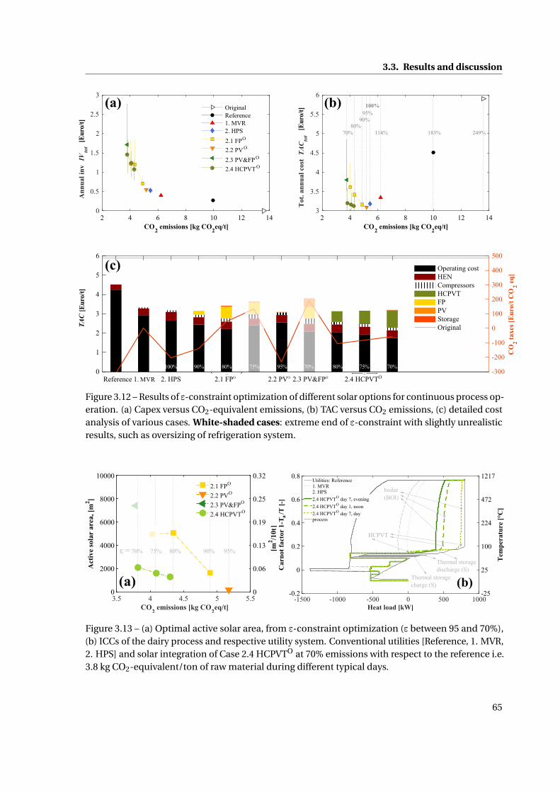
3.3. Results and discussion
Figure 3.12 – Results of ε-constraint optimization of different solar options for continuous process op-eration. (a) Capex versus CO2-equivalent emissions, (b) TAC versus CO2 emissions, (c) detailed costanalysis of various cases. White-shaded cases: extreme end of ε-constraint with slightly unrealisticresults, such as oversizing of refrigeration system.
Figure 3.13 – (a) Optimal active solar area, from ε-constraint optimization (ε between 95 and 70%),(b) ICCs of the dairy process and respective utility system. Conventional utilities [Reference, 1. MVR,2. HPS] and solar integration of Case 2.4 HCPVTO at 70% emissions with respect to the reference i.e.3.8 kg CO2-equivalent/ton of raw material during different typical days.
65

Chapter 3. Comprehensive integration method
3.4 Conclusions
What problem formulation is required for a comprehensive design method for solar-assisted
low-temperature processes?
A comprehensive method was proposed which addressed simultaneous optimization of the process
heat recovery, the conventional utilities, and the renewable utility system (including thermal storage)
using ε-constrained parametric optimization. The method, tailored for the low-temperature industry,
is based on multi-period utility targeting, including process heat recovery through PA and re-use
through heat pumping, and identifies the optimal design and operation of the utility and storage
system. The proposed methodology was demonstrated on the basis of a Swiss dairy plant where
different solar components were compared and evaluated based on economic and environmental
criteria. The methodology permitted to derive cost optimal solar field, heat pump, and thermal
storage tank sizing as well as optimal operation of the system during all operating periods at selected
emission levels.
Optimization of heat recovery, heat pump, and mechanical vapor re-compression placement showed
reduced exergy destruction and total costs at increased energy efficiency in the system. Integration of
a MVR brought emission reductions of ≈38% at 15% reduced TAC, while adding a HPS to study more
complex refrigeration systems decreased CO2 emissions by 12% at comparable TAC. The preliminary
version of a heat pump superstructure (HPS), which was used to model the MVR, refrigeration cycle,
and the HPS proved to be flexible in handling various heat pump types, and indicates great potential
thus motivating more thorough analysis (as conducted in Chapter 4).
Three solar systems were investigated for daytime only and continuous operation of the dairy
process: photovoltaic modules (PVs), flat plate thermal collectors (FPs), and a high concentration
photovoltaic and thermal system (HCPVT). One major conclusion was that integration of solar
energy can contribute to reduce the environmental impact and exergetic losses of the process at
beneficial total costs. Solar energy was, however, only selected by the thermo-economic optimization
algorithm in combination with an optimized system comprising heat recuperation, mechanical
vapor re-compression, and heat pumping. This supports the choice of a comprehensive approach.
For continuous operation of the process, the reduction in specific emissions was not as significant as
for daytime only operation. Due to the capital cost of the thermal storage system, it was only chosen
by the optimization for high emission reductions requirements. Photovoltaic panel integration
offered the least emission reduction potential (up to 20% reduction in daytime only operation
with respect to the best non-solar case). However, installation is simple, independent, and if
overproduced, can be exported to the grid. In comparison, the HCPVT system, had high potential
with very high efficiencies bringing emission reductions easily up to 40% (daytime only) at uncertain
cost and shading losses. The low cost, very low efficiency flat plate collectors offered a simple
solution providing more reliability of the system performance capital cost expenses with emission
reductions of up to 30% (daytime only).
66

4Generic heat pump superstructureOverview
• A comprehensive MINLP superstructure synthesis method for industrial heat pumps
• Optimization of heat pump design, operating conditions, and integration with the process
and utility system
• The superstructure includes sub-cooling, multi-stage phase-changes, presaturators, HEN
cost estimation and fluid selection
• Multi-objective bi-level solution strategy allowing augmentation by expert judgment
• Benchmarking with three literature case studies shows improvements by 5–30%
This chapter is based on Wallerand et al. [170]
Heat pumping has gained increasing attention during the past decades not only for household appli-
cations but also for improving energy efficiency of industrial processes through waste heat recovery
and valorization at elevated temperatures [89, 90]. As demonstrated in Chapter 1.3 (Figure 1.3),
research in the field of industrial waste heat recovery is largely dominated by organic rankine cycle
(ORC) applications and thermoelectric devices. This may stem from a fully explored state-of-the-art
of industrial heat pumps and integration methods; however, the marginal penetration of industrial
heat pump systems (apart from basic refrigeration and air-conditioning) [90, 94] contradicts this
notion. The main barriers for broad usage in industry were identified as lack of knowledge and of
comprehensive heat pump integration methods to provide improvement potentials [90, 94]. This
chapter mainly covers single fluid, mechanically driven systems due to their advanced technological
development and operative flexibility (as discussed in Sections 1.3 and 1.4.4).
After a state-of-the-art analysis of current synthesis methods, this chapter presents a novel heat
pump superstructure with a bi-level solution strategy in the methodology section, followed by
application of the method to various literature cases in the results and discussion section.
67

Chapter 4. Generic heat pump superstructure
4.1 State-of-the-art
The focus of this chapter lies on synthesis methods for mechanically driven heat pump integration
with industrial processes. Since these techniques rely on modeling state-of-the-art heat pump
technologies, a short review of available heat pump features was conducted. Chua et al. [90] and
most recently Arpagaus et al. [104] presented comprehensive literature reviews on advances in
mechanically driven (multi-temperature) heat pump systems. The most recurring features relevant
for large-scale modeling of industrial heat pumps were identified and are presented in Table 4.1.
These include multi-stage compression and expansion, ejectors, cascaded cycles, gas-cooling,
subcooling, economizers, and presaturators. Other developments, which impose different system
architectures (desiccant cooling [90]) or more refined equipment modeling (scroll and oil-free
compressors [90, 104, 171, 172]) are not discussed in this chapter.
Table 4.2 provides an overview of the studies introducing synthesis methods discussed in this
section. In the presented approaches, it is differentiated between conceptual methods which are
based on expert judgment, heuristic rules, or graphical analysis; and mathematical methods, which
rely of mathematical programming to perform systematic optimization. This chapter presents a
contribution to the latter which is thus discussed at greater length.
4.1.1 Conceptual methods
Conceptual, or insight-based, methods are not limited by the problem size and therefore always lead
to a solution though global optimality will seldom be reached. As early as 1974, Barnés and King
[173] and later Cheng and Mah [174] proposed methods based on a set of heuristic rules, dynamic
programming, and expert judgment for synthesis of industrial heat pump systems.
In 1978, a milestone was achieved, when Linnhoff and Flower [97] proposed a method now com-
monly known as pinch analysis (PA) [99] which, for the first time, allowed systematic analysis
of a process net thermodynamic requirements and maximum heat recovery potential. This led
Townsend and Linnhoff [100] to derive the theoretical foundation for ideal placement of heat engines
and heat pumps based on the principles of PA. They concluded that system improvement from a
thermodynamic standpoint can only be achieved if heat pumps are placed across the process pinch
temperature (1.4.2).
Industrial capital budgeting, however, is seldom based upon thermodynamic objectives. Other
drivers play a major role including economic and environmental concerns as well as technical
constraints. Therefore, subsequent researchers added thermo-economic principles and technical
constraints into their decision process as shown e.g. by Ranade [175] with a trade-off formula
between the temperature lift and heat exchanger cost in total site analysis (TSA) (see Table 4.2).
68

4.1. State-of-the-art
Table 4.1 – Heat pump features considered in this work as identified by Chua et al. [90] and Arpagauset al. [104].
Feature Description Feature Description(A)Multi-stagecompres-sion[104, 176–178]
Provide higher coefficient of performance(COP) through intermediate vapor cool-ing while imposing challenges for directvapor injection (multi-stage compressor)or lubrification management (multiplesingle-stage compressors)
(B)Multi-stageexpansion(inter-cooling)[179, 180]
Offers lower technical complexity andhigher performance through cooling atintermediate pressure level (with aid ofseveral expansion valves for a single-stagecompressor)
(C)Cascadedcycles [181]
Enable coverage of wider temperaturesranges due to the possibility of workingfluids switching with applications in nat-ural gas liquefaction or other cryogenicprocesses, or waste heat recovery with astrong temperature lift
(D)Gas-cooling[182]
Allows to recover heat from the super-heated vapor at the compressor outlet(e.g. in a separate heat exchanger), andtherefore generates a multi-temperatureprofile at a single pressure level at highercapital expenses
(E)Economizer[182]
Permits to preheat the saturated vapor be-fore entering a compressor by mixing withsuperheated vapor at the same pressurelevel
(F)Subcooling[178, 180,181]
Subcooling before expansion improvesthe performance of heat pumps, however,possibly at the cost of additional heat ex-changer installation
(G) Presatu-rators(flash-drums) [178,182, 183]
Enable to saturate superheated vapor andto remove flash gas between expansionstages which improves the coefficient ofperformance in multiple ways
(H) Ejectors[104, 180,183–185]
Allow compression of a low pressure fluidthrough the expansion of a high pressurefluid (principle of suction) at low mainte-nance and capital expenses. Ejectors werenot considered in this work, but are men-tioned due to their promising characteris-tics
4.1.2 Mathematical methods
Mathematical methods ensure identification of an ideal point with regard the selected objective(s);
however, convergence of optimization techniques becomes increasingly difficult with growing
problem size. Therefore, many studies considered a reduced solution space, such as discretized
temperature levels, simplified heat pump cycles, disregarding PA principles, or preselecting working
fluids. The studies presenting mathematical methods are analyzed in the following paragraphs
based on selected characteristics.
Temperature level selection In the literature, temperature level (used here interchangeably with
pressure level) selection was handled in two ways. The primary approach relies on predefined or
discretized temperature levels among which compressor units are activated using integer variables.
The first comprehensive methodology for optimal industrial heat pump design based on discrete
temperature levels was presented by Shelton and Grossmann [101, 102] in the form of a mixed
integer linear programming (MILP) superstructure. Many subsequent authors used discretized
temperature levels (as depicted in Table 4.2), resulting in a diminished solution space and therefore
increasing the risk of identifying a sub-optimal solution. Fewer authors presented methods with
continuous temperature levels as part of the decision variables, which renders the problem structure
nonlinear as presented e.g. by Colmenares and Seider [186].
Pinch analysis The principles of PA were considered in most methodologies listed in Table 4.2.
Few authors presented algorithms neglecting PA, which reduced the problem size at the cost of
disregarding the heat recovery system and its dependencies.
69

Ch
apter
4.G
eneric
heatp
um
psu
perstru
cture
Table 4.2 – State-of-the-art summary of synthesis methods for heat pump design and integration with industrial processes.
Authors Year Focus Method PA Property Temp. Detail Objective Cycle features FluidConc. Math. calc. discret. (A) (B) (C) (D) (E) (F) (G) T Selection
Current work HP TC MINLP X CP 0.5 K 3 opex, capex X X X X X X X S X IntegersYang et al. [187, 188] 2017 HP MINLP X - contin. 3 power X X X X X X X SZhang et al. [189] 2016 AHP MINLP - contin. 1 TAC X GOluleye et al. [190] 2016 HP/AHP/HE/AHT TP X HYSYS 10 K 2 fuel X S X TPOluleye et al. [191] 2016 HP/AHP/HE/AHT MILP X HYSYS 10 K 2 TAC X S X BinaryDinh et al. [192] 2015 HP MILP X PR fixed 3 power X X X X S (X) FlowratesKamalinejad et al. [160] 2015 HP MINLP X RP contin. 3 TAC X X X X X X S (X) FlowratesLiu et al. [193] 2014 HP TP X - fixed 3 power X X X S X TPKhan and Lee [194] 2013 HP NLP X PR contin. 3 power 4(∗) M (X) CompositionHackl and Harvey [195] 2013 HP TP X simple fixed 1 - X GBecker [140, 196] 2012 HP MINLP X Belsim contin. 2 opex,capex X X X S X BinaryZhang and Xu [159] 2011 HP TC MINLP X - fixed 3 exergy X X X X X X S (X) FlowratesHasan et al. [197] 2009 HP MINLP simple contin. 3 power X X X S/M (X) FlowratesNogal et al. [106] 2008 HP MINLP X HYSYS contin. 3 capex/power X X X X M (X) CompositionAspelund et al. [198] 2007 HP TP HYSYS, SRK fixed 3 exergy X X X X S X TPBagajewicz and Barbaro [199] 2003 HP NLP X simple contin. 1 opex X GHoliastos and Manousiouthakis [156] 2002 HE/HP LP X simple fixed 1 TAC X GVaidyaraman and Maranas [105] 2002 HP NLP X SRK contin. 3 power X X X M (X) CompositionMaréchal and Kalitventzeff [157] 2001 HP TC MILP X Belsim fixed 3 exergy X X X S X BinaryVaidyaraman and Maranas [103] 1999 HP MILP X [200] 1- 8 K 3 TAC X X X X S X BinaryKauf [201] 1999 HP TP - contin. 2 COP SWallin and Berntsson [202] 1993 HP/AHP/AHT TEP X generic fixed 1 TAC GLinnhoff and Dhole [203] 1992 HP TP X simple fixed 3 power X X X SSwaney [204] 1989 HE/HP LP X simple fixed 3 TAC X X X SColmenares and Seider [186] 1989 HE/HP NLP X PR contin. 2 TAC X S X FlowratesRanade [175] 1988 HP EP X simple contin. 1 TAC GColmenares and Seider [205] 1987 HE/HP NLP X PR fixed 2 TAC X S X FlowratesShelton and Grossmann [101] 1986 HP LP X [206] 1 K 3 TAC X X X SShelton and Grossmann [102] 1986 HP MILP X [206] 10 K 3 TAC X X X STownsend and Linnhoff [100] 1983 HE/HP TP X Tabl. fixed 2 exergy SCheng and Mah [174] 1980 HP HR SRK contin. 3 TAC X X X X X X S X TPBarnés and King [173] 1974 HP HR MIP SRK contin. 3 TAC X X X X X X S
(*) Fixed four stages in optimization studyFocus: HP - compression heat pumps, HE - heat engines, AHP - absorption heat pumps, AHT - absorption heat transformersConceptual methods: TP - Thermodynamic principles, TC - Technical constraints, EP - Economic principles, HR - Heuristic rules, TEP - Thermo-economic principles;PA: pinch analysis [99, 207]Property calculation: CP - CoolProp [208], RP - Refprop [209], SRK - Soave-Redlich-Kwong [210] equation of state, HYSYS - Aspen HYSYS software [211], simple - simplified estimations, PR - Peng-Robinson [212], Belsim - Belsim Vali software [213]Detail: Level of detail in modeling: 1 - general modeling based on thermodynamic estimations for a generic fluid, 2 - modeling of simplified (single-stage) cycles for specific fluids, 3- full detail modeling of (multi-stage) heat pumps with advancedfeatures for different fluidsObjective: TAC (min), fuel - primary fuel consumption (min), exergy - exergy losses (min), opex (min), capex (min), power - compression power (max)Cycle features: (A) Multi-stage compression, (B) multi-stage expansion, (C) cascaded cycles, (D) gas cooling, (E) Economizer (preheating before compression), (F) sub-cooling, (G) presaturatorsFluid: T (types): S - single component fluid, M - fluid mixture, G - generic fluid; Selection: TP: thermodynamic principles
70

4.1. State-of-the-art
Heat pump features In modeling heat pump features, three approaches addressing different levels
of detail were observed in the literature. In the first group (1), heat pump performance was modeled
based on general thermodynamic principles [107, 156, 175, 189, 195, 199]. It aids in estimating
potentials for improvements reachable with heat pump integration but lacks specification of real
fluids or system design. Works contained in the second group (2) modeled basic single-stage heat
pump cycles based on real fluids assuming that superposition of simple cycles could represent
more complex systems [100, 140, 186, 190, 201, 205, 214, 215]. This leads to underestimation of
performance and thus sub-optimal solutions could be generated. The third group (3) contains
work presenting rigorous heat pump models including technical features from Table 4.1. Most of
these included multi-stage compression and pre-saturation [101, 102, 158, 197, 203], while some
additionally considered liquid sub-cooling, preheating before compression, or gas-cooling [105,
159, 173, 174], and very few authors examined multi-stage expansion including Vaidyaraman and
Maranas [105], Nogal et al. [106], Liu et al. [193], Aspelund et al. [198, 198]. No previous work has
comprehensively included all identified heat pump features.
Objective function Apart from the work of Becker et al. [140], the studies discussed here have
presented mathematical approaches for single-objective optimization of industrial heat pump
systems with objectives such as minimizing exergy losses [159, 195] or total cost [101, 102, 160,
186] . In praxis, decision-making is based on many factors and it is thus difficult to obtain the
global solution from single-objective optimization. Therefore, it is advantageous to derive multiple
solutions such that the final decision can be based on several criteria including expert judgment,
which could be facilitated by multi-objective optimization.
Fluid selection Fluid selection has not been considered extensively in heat pumping literature.
Some authors have compared different working fluids based on thermodynamic principles, such
as Oluleye et al. [215], while others mainly derive the optimal mass flow rates or composition from
preselected fluids, including Kamalinejad et al. [160]. Few researchers have integrated fluid selection
into the optimization in the form of integer, binary, or continuous variables such as Vaidyaraman and
Maranas [103], Becker [140], or Colmenares and Seider [205]. The candidate fluids were principally
selected based on fluid critical properties and triple point.
4.1.3 Discussion and contribution
The discussion of studies presenting conceptual and mathematical methods for optimal heat pump
design and integration with industrial processes is summarized as follows.
1. Conceptual methods provide important insight to problems but cannot assess solution opti-
mality. The advantage is, however, that technical infeasibilities and practical constraints can
be considered without facing computational problems.
2. Mathematical methods may experience convergence issues for large scale problems due to
71

Chapter 4. Generic heat pump superstructure
increasing complexity. Therefore, many studies considered a reduced solution space.
3. Few studies provide a combination of conceptual and mathematical approaches, which can
harvest the advantages of both methods, e.g. through introduction of technical constraints, or
multi-solution generation.
4. The potential impact of heat pumping for industrial waste heat recovery is not clearly commu-
nicated.
This chapter addresses the gaps denoted (2) and (3) by presenting a novel comprehensive superstruc-
ture synthesis method which is solved using mathematical programming for optimal integration
of industrial heat pump systems. Preliminary versions of this heat pump superstructure (HPS) as
presented in the previous Chapter, and in [111, 167] were generalized and extended to incorporate
temperature level and fluid selection, heat exchanger network (HEN) cost estimation, technical con-
straints and a comprehensive list of heat pump features. A multi-objective decomposition solution
strategy allows convergence for large problems and provides multiple solutions for expert judgment
adapted to the diverse criteria relevant in industry. This strategy addresses the shortcomings of
previous work and provides a clear design method based on a comprehensive superstructure and
mathematical programming.
4.2 Methodology
4.2.1 Problem statement
This method aims at providing a utility target and preliminary design of the heat pump system as
the basis for detailed design considering dynamic behavior in a subsequent step (not treated here).
The problem statement is depicted below.
Problem statement
Given
• industrial process thermal and material demands
• set of candidate utility technologies, including potential heat pumps with operating
ranges
Determine
• optimal utility system design
• optimal design of the heat pump system including:
– specification of technologies
– features
– working fluid
– operating conditions (temperatures, pressures, etc.)
72

4.2. Methodology
4.2.2 Superstructure synthesis
A flowsheet and a temperature entropy diagram of the novel heat pump superstructure (HPS) are
depicted in Figure 4.1. It illustrates the various potential pathways and features considered in the
superstructure. Some features are represented in sample cycles.
The superstructure is equipped with a condenser and evaporator at the highest and lowest pressure
levels, respectively. The intermediate levels additionally contain a presaturator, a post-compression
gas-cooler, a subcooling heat exchanger, and a superheater. Compressors and valves are made avail-
able between all pressure levels. Superheated vapor exiting the compressor can be de-superheated
in a heat exchanger (gas-cooler) and condensed (represented by one heat exchanger), and/or sent
to a presaturator which saturates the fluid and separates it into its phases. Two-phase flow leaving
the expansion valves can be evaporated (and potentially superheated by mixing or heat exchange)
and then compressed or mixed with condensate with options of inter-cooling and/or subcooling
before expansion.
4.2.3 Mathematical formulation
The statement above corresponds to a non-convex Mixed Integer Nonlinear Programming (MINLP)
problem. The integer variables relate to activation of different technology options while nonlinear-
ities mainly arise from capital cost correlations and the intrinsic nonlinearity of thermodynamic
property correlations. Therefore, a decomposition strategy [125] is applied as presented in Figure 4.2
which incorporates the nonlinearities at the master level solving the linear problem at the slave
Figure 4.1 – Flowsheet and temperature-entropy diagram of the HPS with sample cycles.
73

Chapter 4. Generic heat pump superstructure
i=1
Convergence check
1. Problem statement
Non-linear variables: xLinear variables: yObjective function: obj = f (x,y)
(a) Process data(b) Utility technology data(c) Heat pump superstructurebased on input from master level xi
Process integrationi=i+1
Results evaluationobj, x, y
2. Master level
Post-computational analysis
3. Slave level
3.1. Input data generationAMPL language
3.2 Process integrationsolvers: CPLEX, Gurobi
obji
xi
yi, linear obji
Nonlinear variable selection Dakota: GA
fitnesscheck
infinity ∞
Figure 4.2 – Method proposed in Chapter 4 based on decomposition strategy solving mixed integernonlinear programming (MINLP) superstructure implemented in Lua OSMOSE platform [125, 143].
level. The variables present in the nonlinear constraints are set at the master level and thus act as
parameters for the slave optimization. At the slave level, the linear problem is solved and the deci-
sion variables contained in the linear constraints and the linear objective function are transferred
to a post-computational analysis where the nonlinear capital cost correlations and objectives are
calculated. Based on the objective function values, a convergence check is performed and a new
iteration is initiated at the master level.
The main assumptions considered in the heat pump superstructure are:
• the thermodynamic behavior is at steady-state
• heat losses and pressure drops in piping and the components are negligible
• the outlet of a condenser is either saturated or subcooled
• the outlet of an evaporator is either saturated or superheated
• isenthalpic expansion in the valves
• the minimum approach temperature difference is fixed for every stream (and follows the
indications from the literature cases)
4.2.3.1 Master level
At the master level, a black box optimization is performed where the variables present in the nonlin-
ear constraints are the decision variables. These are mainly the heat pump saturation temperature
levels (Ti ), the fluid (d), the subcooling, gas cooling, and compressor preheating temperature dif-
ferences (∆Ti ,SC , ∆Ti ,DSH , ∆Ti ,PRE ), and all thermodynamic properties derived from these. An
additional variable is introduced in order to vary the weight (ξ) of the two components in the objec-
tive function at the slave level (see Section 4.2.3.2 - objective function). The properties are retrieved
from the open-source database CoolProp [208]. The variables and objective functions at the master
level are found in Table 4.3.
Black-box multi-objective nonlinear optimization is performed by Dakota [216] using a multi-
objective genetic algorithm (MOGA) [217] which allows analysis of a wide solution space. The
specifications used are presented in Appendix C.1.1.
74

4.2. Methodology
Objective function Different objective functions are of interest when optimizing industrial heat
pumps such as the exergy efficiency, coefficient of performance (COP), environmental impact, or
cost. Based on the literature cases considered in the results and discussion section, the objectives of
the multi-objective optimization were based on economic criteria, i.e. annualized capital expenses
(capex) and yearly operating expenses (opex) as shown in Equation 4.1.
minTi ,∆Ti ,DSH,∆Ti ,SC,∆Ti ,PRE,d ,ξ
C opex ,C capex
(4.1)
The capex (depicted in Equation 4.4) consists of the investment costs of all technologies w and the
HEN cost estimation calculated using Equation 4.3. The HEN area is estimated as suggested by
Townsend and Linnhoff [99, 218] based on vertical intervals in the composite curves. HEN design
based on mathematical principles, as well as optimization of the minimum approach temperature
(ΔTmin) was not performed in this work, but could be added to the solution strategy.
Link to slave level The utility and heat pump technology sizing is performed at the slave level.
The results from the slave optimization serve as input to calculate the master level objective func-
tions. These are the maximum size ( f w ) and existence (y w ) of each technology w influencing the
equipment investment and heat exchanger network cost estimation.
4.2.3.2 Slave level
The HPS is embedded in the utility targeting problem of Maréchal and Kalitventzeff [75] where
the optimal utility system for an industrial process is found based on the thermal and material
needs considering maximum heat recovery. This means that all elements of the heat pump, namely
condensers, evaporators, compressors, presaturators (flash-drums) and gas-coolers, are present as
utility technologies in the targeting approach. The main variables at the slave level are the size and
existence of each utility technology, including all heat pump elements. The size of each technology
is decided by optimization based on the objective function while remaining subject to physical and
thermodynamic laws.
To ensure mass and energy conservation within the heat pump, additional constraints are added
at all saturated liquid, vapor, and superheated vapor points. Since the saturation temperature and
respective pressure levels as well as the subcooling and superheated properties are set at the master
level, component sizing is linearly dependent on the state properties. Therefore, the problem can be
described as a multi-period Mixed Integer Linear Programming (MILP) problem which is solved
using commercial software based on AMPL [3] with CPLEX [5]. The specifications are presented in
Appendix C.1.2.
Table 4.4 depicts the objective function and variables at the slave level. The utility targeting con-
straints are described in further detail in Section 2.4. The heat pump parameters for utility targeting
75

Chapter 4. Generic heat pump superstructure
Table 4.3 – Variables and objective function at master level.
Description Symbols Equation
Objectives
Yearly operating expenses(opex) [$/y]
Copex from slave level, see Table 4.4
Total investment cost [$] CINV
∑w∈W
C w (f w,y w )+C HEN (4.2)
W set of utility technologies wf w maximum size of technology wyw existence of technology wC w investment cost function of technology w , see Appendix C.3.1
Heat exchanger networkcost (*) [$]
C HE N maxp
[c1 +c2 ·
(AHE N
tot ,p
N HE Nmi n,p
)c3]·N HE N
mi n,p
(4.3)
AHE Ntot ,p = ∑
k∈K
1
∆Tlog,k·∑
c∈C
Qcp,k
αc + ∑h∈H
Qhp,k
αh
(∗)
K set of temperature intervals 1,2,3, ...,nkH,C set of hot, cold process and utility streams∆Tlog,k [K] logarithmic mean temperature difference
Qh,cp,k fh,c
p · Qh,c
[kW] contribution of hot h, cold stream c to temperature interval k in period p
αh , αc [kW/m2K] hot, cold stream h, c heat transfer coefficient
AHE Ntot ,p [m2] total heat exchanger network area
N HE Nmi n,p [-] minimum number of heat exchanger units
c1 [$] fixed cost parameterc2 [$/m2] scaling cost parameterc3 [-] non-linear parameter
Annualized capitalexpenses (capex) [$/y]
Ccapex C I NV · (τ+m) (4.4)
τ [1/y] i·(1+i)n
(1+i)n−1 investment cost annualization factor
m [1/y] maintenance cost as fraction of total investment
Total annualized costs(TAC) [$/y]
CT AC C capex +C opex (4.5)
Variables
Temperature levels Ti [Tmini ,Tmax
i ], [K] saturation temperature levelsSubcooling ∆Ti ,SC [0,Tmax
i ,SC], [K] temperature difference between condensate and subcooling outletDe-superheating ∆Ti ,DSH [0,Tmax
i ,DSH], [K] temperature difference in gas-cooling heat exchangerPre-heating ∆Ti ,PRE [0,Tmax
i ,PRE], [K] temperature difference for preheating before compression
Fluid index d 1,2, ...,nd from set of fluids FWeighting factor ξ [0,1], [-] for objective function of slave optimization
(*) Area estimation based on Townsend and Linnhoff [218] and Kemp [99]. The minimum number of heat exchangers (units) N HENmi n is estimated following the suggestion of
Linnhoff et al. [98] based on graph theory.
as well as mass and energy balances are found in Appendix C.3.1 and C.3.2.
Objective function The MILP problem is solved with commercial solvers [3, 5] based on branch
and cut methods for a single objective function. Investigation of a wide solution space regarding
both objectives from the master level leaves two options for consideration.
(a) Constraining one objective with a variable controlled from the master level and minimizing
the second objective or
(b) Defining a weighted sum of the two objectives (wC T AC ) where the weighting factor (ξ) is
controlled at the master level.
76
4.2. Methodology
Since alternative (a) generates more infeasible solutions and therefore leads to longer solution times,
option (b) was selected and is expressed in Equation 4.6.
minf w
p , f w ,y wp ,y w
wC T AC
(4.6)
Heat cascade The MILP slave model is subject to heat cascade constraints [75] which ensure heat
transfer feasibility for maximum heat recovery. The set of equations are provided in Chapter 2.4
(Equation 2.14 - Equation 2.15).
Mass and energy balances All material and non-thermal energy requirements are described by a
set of constraints. These equality constraints ensure that material/energy consumption and con-
version are balanced within the system boundaries or compensated with help of the grid (utilities)
which factors into the operating cost, as described in more detail in Section 2.4.
Variables The variables present at the slave level are the existence (y wp ) and sizing ( f w
p ) of each
of the utility technologies w during each period p and the maximum size considering the entire
operating range. Based on the objective function and thermodynamic input parameters selected
at the master level, optimal sizes and operating conditions of all utilities including the heat pump
technologies are derived within the optimization.
Heat pump specific constraints The general heat pump parameters such as the reference heat
load of the evaporator and condenser and the reference electricity consumption of the compressors
are presented in Appendix C.3.1. These enter into the targeting constraints and are sized based on
the process thermal requirements minimizing the objective function. Enforcing energy and mass
conservation within the HPS requires additional constraints to be introduced. These are illustrated
in further detail in Appendix C.3.2.
Mass and energy conservation are introduced at three different points on each pressure level, namely:
the superheated vapor point after compression, the de-superheated or saturated vapor point before
compression or condensation, and the saturated or subcooled liquid point after condensation or
before evaporation. Since these points are fixed at the master level, all equations can be formulated
with purely linear dependencies. Mass balances at all three points ensure that the working fluid
mass flow rate is conserved throughout the heat pump system. Energy balance equations ensure
that mixing (e.g. of two compressor outlets at the same pressure level) do not violate the energy
conservation law. Superheated vapor mass and energy balances are introduced to study the effect of
sensible heat recovery from the vapor (gas-cooling). This can either be achieved by installation of a
separate heat exchanger (gas-cooler) or by accounting for sensible heat release in the condenser
unit. Both options are separately modeled in this superstructure but does not have a major impact
on the heat exchanger network cost estimation (since gas cooling in both cases imposes higher
77

Chapter 4. Generic heat pump superstructure
investment). The de-superheating temperature difference (∆Ti ,DSH ) selected at the master level can
be understood as the temperature from which sensible heat release is considered. This temperature
difference does not influence the energy balance but by manipulating the inlet temperature of
the de-superheating, HEN solutions which require stream splitting can be avoided, which has an
influence on the heat cascade. If it is set to zero, gas-cooling is neglected and the sensible heat
contained in the superheated vapor is considered as if it was available only at saturation temperature
levels.
Apart from energy and mass conservation, technical constraints can be considered as introduced
below.
Number of heat pump stages The maximum number of stages of a heat pump cycle consisting of
one fluid can be restricted as shown in Equation 4.7.
nl∑i=2
i−1∑j=1
y g ,COMP i→ jp ≤ nmax
g ∀g ∈ G (4.7)
Where
G set of heat pumps with one working fluidL set of saturation temperature levels 1,2,3,..nly g ,comp i→ j overall existence of compressor between level i and j of heat pump gnmax
g maximum number of heat pump stages of heat pump g
Compression ratio and minimum pressure Compressors with compression ratios or with pres-
sure levels outside the bounds cannot be activated. This is depicted in Equation 4.8, which forces
the existence of compressor "COMP i → j " to zero, if one of the criteria is met.
y g ,COMP i→ j
p = 0
∣∣∣∣ pg , j
pg ,i> CRmax
g ∨ pg , j
pg ,i< CRmin
g ∨pg ,i < pmin
∀i , j ∈ L | j < i , g ∈ G (4.8)
Where
pg ,k [bar] saturation pressure level of heat pump g at saturation temperature level k
CRmin, maxg [bar/bar] minimum, maximum accepted compression ratio of heat pump g
pmin [bar] minimum accepted saturation pressure level
Heat exchanger size A minimum size for heat exchangers is introduced in the form of a soft
constraint. Thereby, a fixed penalty cost (IVq1 ) is added to the heat pump units containing thermal
78

4.3. Results and discussion
streams as shown in Equation 4.9.
Cfix = a ·(
Qmin
U ·A ·∆T
)b
IVq1 = Cfix
∀h ∈ Hg , g ∈ G (4.9)
Where
Hg set of thermal heat pump units condensers, evaporators, presaturators, gas-coolers in heat pump gU [kW/m2K] overall heat transfer coefficientA [m2] reference heat exchange areaQmin [kW] minimum heat exchanger sizeΔT [K] log mean temperature difference in the heat exchangersa,b [$,-] cost parameters
4.2.4 Fluid selection
Presuming fluid selection from known fluids and sub-critical operation, there are two options for
conducting a fluid selection in the presented method.
(a) the list of candidate fluids is added to the slave level, in which every unit (condenser, evapo-
rator, compressors, etc.) is reproduced as many times as there are fluids; the fluids are then
activated using binary variables connected to the existence of each unit (yw ), or
(b) an integer variable referencing the fluid is added to the master level
The advantage of selection at the slave level, (a), is that cascaded cycles with different fluids can
be designed and convergence of the decomposition strategy is reached after fewer iterations (due
to fewer variables at the master level). The disadvantage is that the slave problem size increases
proportionally with the number of fluids which impacts the MILP resolution time significantly. Both
options were applied in this study depending on the respective problem statement (which will be
indicated).
4.3 Results and discussion
This section is divided into three parts. In the benchmarking analysis, three case studies presenting
optimal heat pump designs for industrial processes from the literature were selected. The literature
results were reproduced with the heat pump superstructure (HPS) to validate its flexibility. During
the optimization study, the multi-objective bi-level approach presented in the methodology is
applied to the three literature cases, and compared to the previous solutions from the literature. In
an extended analysis, one literature case is expanded to consider fluid selection, technical boundary
conditions, and HEN cost estimations better representing the reality of industrial problems.
79

Chapter 4. Generic heat pump superstructure
Table 4.4 – Variables and objective function at slave level.
Description Symbols Equation
Objectives
Weighted totalannualized costs (TAC)[$/y]
wCT AC ξ ·C capex + (1−ξ) ·C opex (4.10)
ξ weighting parameter controlled from master level
Yearly operatingexpenses (opex) [$/y]
Copex
∑p∈P
( ∑w∈W
OPw1,p · y w
p +OPw2,p · f w
p
)·∆tp ·occp (4.11)
Sizing constraint fw,min · y wp ≤ f w
p ≤ fw,max · y wp ∀p ∈ P, w ∈ W
P set of time periods p 1,2,3, ...,npW set of utility technologiesf w
p continuous variable for sizing technology w during period py w
p binary variable related to existence of technology w during pOPw
1,p [$/h] fixed operating cost in period p
OPw2,p [$/h] proportional operating cost in period p
∆tp [h] operating time during period poccp [1/y] occurrence of period p
Annualized capitalexpenses (capex) [$/y]
Ccapex
∑w∈W
IVw1 · y w + IVw
2 · f w (4.12)
f w maximum size of technology wy w overall existence of technology wIVw
1 [$/y] fixed cost related to the annualized, linearized investment of technology wIVw
2 [$/y] proportional cost related to the annualized, linearized investment of technology w
Variables
Multiplication factor f wp [fw,min, fw,max], [-] sizing factor of technology w during period p
Use factor y wp 0,1, [-] existence of technology w in period p
Maximum multiplicationfactor
f w ≥ fwp ∀p ∈ P maximum size of technology w
Overall use factor y w ≥ ywp ∀p ∈ P overall existence of technology w
4.3.1 Benchmarking analysis
The selection of the benchmark cases was based on their recurrence in the literature, even though
not many cases were treated repeatedly, and the diversity in their characteristics. Suitable cases
could not be identified in the most recent literature due to insufficient data provision in terms of
process stream data, cost functions, or detailed heat pump configurations. The selected cases were
each treated in several publications.
(a) Case E2 was selected because it was treated in two consecutive studies by Shelton and Gross-
mann [101, 102] and due to its heating and cooling requirements which span over a continuous
temperature range as shown in Figure 4.3 (a). This case provides exploration potential of a
multi-temperature, multi-stage heat pump system which crosses the pinch located at -8°C.
(b) An ethylene plant separation train [219] discussed by Colmenares and Seider [186] was chosen
due to the refrigeration needs at extremely low temperatures (-115°C) as shown in Figure 4.3
(b). The pinch point is located at approximately 130 °C, which leaves little room for a heat
80

4.3. Results and discussion
pump crossing the pinch. Vaidyaraman and Maranas [103] discussed a slightly modified
version of the same problem (differentΔTmin) with higher total cost, which is not treated here.
(c) A Cold Tray distillation sequence presented by Colmenares and Seider [205] and later studied
by Swaney [204] was selected to revisit the original solution which disregarded an obvious
improvement of heat pumping across the process pinch (≈ 60 °C). Figure 4.3 (c) shows the
process temperature enthalpy profile indicating the process thermal demands and pinch
point. Swaney [204] considered a solution with heat pumping across the process pinch for
this case study, however with modified input data (isentropic compressor efficiency of 0.8)
and is, therefore, not considered here.
The literature optimal cases were reproduced by adding constraints at the slave level of the HPS to
force the resulting heat pump layout to contain the same features and operating conditions as those
presented in the literature. This was achieved by pre-selecting temperature levels and fixing the
active compressor stages and fluids. In this way, the HPS flexibility was tested and reference values for
later comparison were calculated, given that most literature studies used different thermodynamic
property calculations.
An analysis of the original and the reproduced data (referred to as Reference since they serve for
later comparison) is presented in Table 4.5. The results are compared based on the total annualized
costs (TAC) which was the objective function in the literature. It was observed that the results from
literature cases E2 and Cold Tray could be reproduced with a negligible difference (below +/-1%) in
each of the categories including the TAC. The slight difference in results is explained by different
property calculation methods. Reproduction of the Ethylene case generated around 23% higher
electricity consumption which resulted in 22% higher TAC. The thermodynamic conditions are
Figure 4.3 – Grand composite curves (GCCs) (temperature enthalpy profiles) from process thermalstreams of three benchmark cases, reproduced from (a) Shelton and Grossmann [102], (b) Lincoffet al. [219], (c) Colmenares and Seider [205], respectively.
81
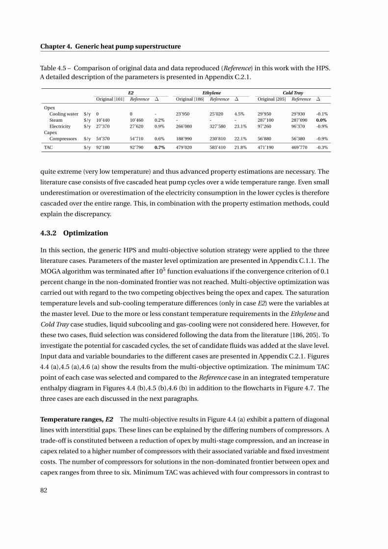
Chapter 4. Generic heat pump superstructure
Table 4.5 – Comparison of original data and data reproduced (Reference) in this work with the HPS.A detailed description of the parameters is presented in Appendix C.2.1.
E2 Ethylene Cold TrayOriginal [101] Reference Δ Original [186] Reference Δ Original [205] Reference Δ
OpexCooling water $/y 0 0 - 23’950 25’020 4.5% 29’950 29’930 -0.1%Steam $/y 10’440 10’460 0.2% - - - 287’100 287’090 0.0%Electricity $/y 27’370 27’620 0.9% 266’080 327’580 23.1% 97’260 96’370 -0.9%
CapexCompressors $/y 54’370 54’710 0.6% 188’990 230’810 22.1% 56’880 56’380 -0.9%
TAC $/y 92’180 92’790 0.7% 479’020 583’410 21.8% 471’190 469’770 -0.3%
quite extreme (very low temperature) and thus advanced property estimations are necessary. The
literature case consists of five cascaded heat pump cycles over a wide temperature range. Even small
underestimation or overestimation of the electricity consumption in the lower cycles is therefore
cascaded over the entire range. This, in combination with the property estimation methods, could
explain the discrepancy.
4.3.2 Optimization
In this section, the generic HPS and multi-objective solution strategy were applied to the three
literature cases. Parameters of the master level optimization are presented in Appendix C.1.1. The
MOGA algorithm was terminated after 105 function evaluations if the convergence criterion of 0.1
percent change in the non-dominated frontier was not reached. Multi-objective optimization was
carried out with regard to the two competing objectives being the opex and capex. The saturation
temperature levels and sub-cooling temperature differences (only in case E2) were the variables at
the master level. Due to the more or less constant temperature requirements in the Ethylene and
Cold Tray case studies, liquid subcooling and gas-cooling were not considered here. However, for
these two cases, fluid selection was considered following the data from the literature [186, 205]. To
investigate the potential for cascaded cycles, the set of candidate fluids was added at the slave level.
Input data and variable boundaries to the different cases are presented in Appendix C.2.1. Figures
4.4 (a),4.5 (a),4.6 (a) show the results from the multi-objective optimization. The minimum TAC
point of each case was selected and compared to the Reference case in an integrated temperature
enthalpy diagram in Figures 4.4 (b),4.5 (b),4.6 (b) in addition to the flowcharts in Figure 4.7. The
three cases are each discussed in the next paragraphs.
Temperature ranges, E2 The multi-objective results in Figure 4.4 (a) exhibit a pattern of diagonal
lines with interstitial gaps. These lines can be explained by the differing numbers of compressors. A
trade-off is constituted between a reduction of opex by multi-stage compression, and an increase in
capex related to a higher number of compressors with their associated variable and fixed investment
costs. The number of compressors for solutions in the non-dominated frontier between opex and
capex ranges from three to six. Minimum TAC was achieved with four compressors in contrast to
82
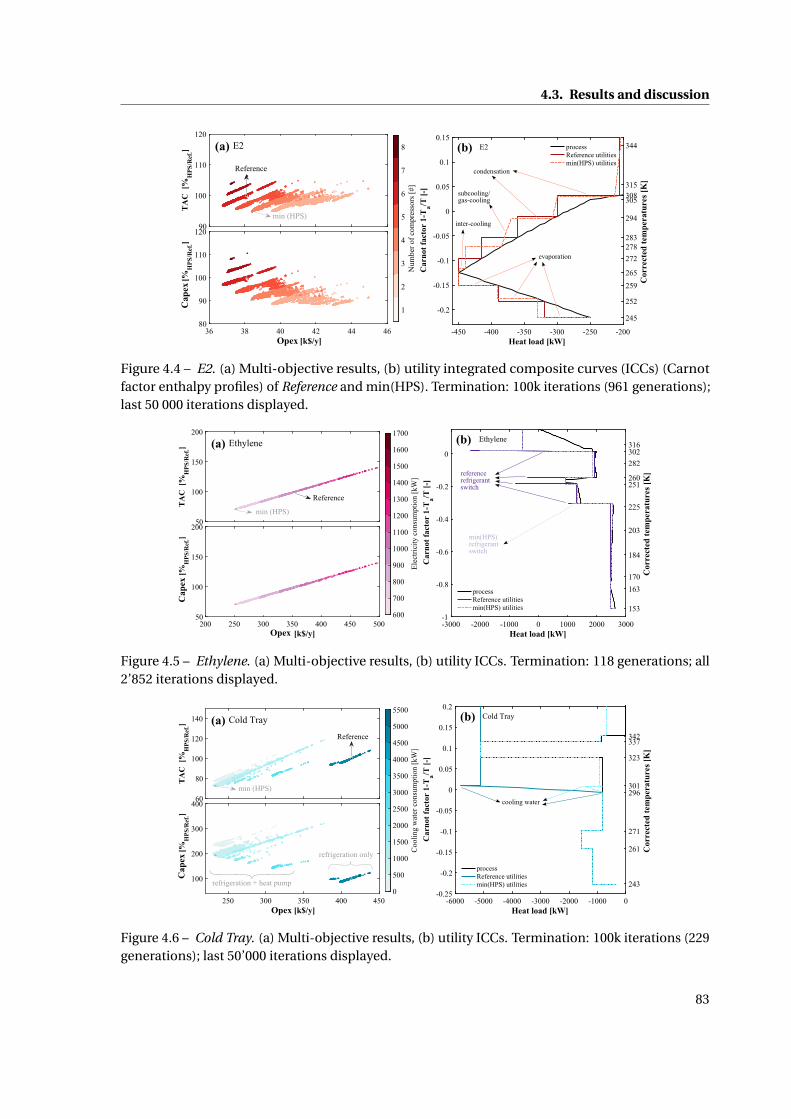
4.3. Results and discussion
Figure 4.4 – E2. (a) Multi-objective results, (b) utility integrated composite curves (ICCs) (Carnotfactor enthalpy profiles) of Reference and min(HPS). Termination: 100k iterations (961 generations);last 50 000 iterations displayed.
Figure 4.5 – Ethylene. (a) Multi-objective results, (b) utility ICCs. Termination: 118 generations; all2’852 iterations displayed.
Figure 4.6 – Cold Tray. (a) Multi-objective results, (b) utility ICCs. Termination: 100k iterations (229generations); last 50’000 iterations displayed.
83

Chapter 4. Generic heat pump superstructure
the six suggested in the Reference. One additional advantage of this multi-objective optimization
approach is also that sub-optimal solutions with lower system complexity can be identified. The
best solution with three compressors e.g. bears similar TAC (<+1%) as the overall minimum cost
solution with four compressors and may therefore be a better solution from the practical perspective.
The HPS allows for a comprehensive analysis of heat pump features and operating conditions.
The proposed minimum TAC solution consists of a heat pump with inter-cooling, subcooling, and
gas-cooling heat exchangers as depicted in Figure 4.4 (b) and Figure 4.7 (a) which contribute to
achieving similar performance (in terms of opex) at reduced compressor fixed costs capex compared
to the Reference. This leads to a potential overall 5% reduction in TAC as displayed in Table 4.6.
Cascaded cycles, Ethylene separation train Results from the multi-objective optimization in
Figure 4.5 (a) show that the two objective functions, opex and capex, are not conflicting. Two main
reasons were identified: (1) Due to the elevated process pinch point at 130°C, a pinch-crossing
heat pump (as presented in case E2) is not feasible, thus there is no trade-off between (higher)
compressor investment (capex) and (lower) hot utility requirements (opex); (2) The fixed investment
costs of the compressors are distinctly smaller than the proportional costs which translates to the
heat pump capex depending primarily on the electricity consumption (opex). Thus all objectives
point in the same direction, which would make a Single Objective Genetic Algorithm (SOGA) [217]
more appropriate. Running SOGA led to an equivalent result. The minimum point reveals an
approximate 30% reduction in the TAC compared to the Reference (shown in Table 4.6) driven by
the drastically diminished electricity consumption. As illustrated in Figure 4.5 (b) and Figure 4.7
(b), the power consumption was reduced due to a decrease in number of refrigerant switches from
four to one, which avoided the minimum temperature difference (ΔTmin = 10 K) in the switching
heat exchangers. Inter-cooling at three levels (174.5 K, 189.5 K, 208.5 K) additionally improved the
refrigerator performance leading to an improvement of the COP from 1.8 to 2.6. Due to the constraint
on the compression ratio (unlike in the original) to be below 10, which may still be extremely high,
the compressor is changed at 180.5 K. This leads to a more complicated, however, beneficial flow
management to saturate the superheated compressor outlet.
Process pinch point, Cold Tray distillation Results from the multi-objective optimization in
Figure 4.6 (a) indicate a pattern of diagonal lines with gaps in between. Unlike case E2 this is
unrelated to the number of compressors in the system, which are mostly at their maximum (five)
due to low compressor fix cost. However, it can be observed that the cooling water consumption
correlates with the formation of lines. At highest opex, the largest amount of cooling water is
consumed. It is used to cool the process and the refrigeration cycle as reported in the Reference
displayed in Figure 4.6 (b) and Figure 4.7 (c). By adding a heat pump around the process pinch, the
cooling water and hot utility consumptions were drastically reduced. The increase in capex is off-set
by a larger decrease in opex leading to a maximum reduction of 27% in TAC in the best point, as
depicted in Table 4.6. The HPS minimum TAC solution consists of two separate (ammonia based)
84

4.3. Results and discussion
246
Figure 4.7 – Flowchart of min(HPS) solutions heat pump designs (a) E2, (b) Ethylene, (c) Cold Trayof benchmark analysis.
Table 4.6 – Optimization results. Data shown as Reference was generated with HPS based on therespective literature input data (Section 4.3.1).
E2 Ethylene Cold TrayReference min(HPS) Reference min(HPS) Reference min(HPS)
OpexCooling water $/y 0 0 25,020 23,150 29,930 4,810Steam $/y 10,460 10,370 0 0 287,090 39,310Electricity $/y 27,620 28,040 327,580 223,340 96,370 189,900
CapexNo. of compressors # 6 4 5 5 3 5Compressors $/y 54,710 49,630 230,810 159,140 56,380 109,220
TAC $/y 92,790 88,050 583,410 405,630 469,770 343,230Improvement % 0 5.1% 0% 30.5% 0% 26.9%COPrefrigeration - 4.4 4.3 1.8 2.6 5.3 5.8
85

Chapter 4. Generic heat pump superstructure
heat pump systems, one satisfying the refrigeration needs (three compressors), and one across
the process pinch (see Figure 4.7 (c) and Figure 4.6 (b), two compressors). With the refrigeration
configuration a lower cost, higher COP solution could be derived compared to the reference case
which consists of two separate heat pump cycles (R-22 (two compressors) and ammonia). The utility
ICCs in Figure 4.6 (b) show that the HPS solution with the pinch heat pump not only reduces cost,
but also exergy losses (proportional to the area between the curves) of the system.
Synthesis In conclusion, the HPS can represent a wide range of heat pump features and cycle
architectures, while at the same time providing improved solutions to different literature optimal
cases. This is attributed to a wider range of heat pump features considered and variable temperature
level selection. As demonstrated, the level of complexity, variety of heat pump features considered,
and technical constraints added depends on the choice of the user, which makes the superstructure
flexible to handle. The solution strategy allows to generate a set of non-dominated solutions which
enable the user to perform further analysis, thereby gaining deeper insight to the problem, and to
apply other selection criteria. The literature cases discussed in this section serve for benchmarking
the underlying approach, however, important criteria are neglected, such as HEN costs, compres-
sor isentropic efficiencies, ”real” utilities, and technical constraints thus generating ”theoretical”
solutions. In the Section 4.3.3, an extended version of the presented case E2 is, therefore, discussed.
4.3.3 Extended analysis
The heat pump system for the extended case E2 was optimized with respect to opex and capex
assuming an isentropic compressor efficiency of 70%, a maximum compression ratio of 8 [bar/bar]
in each compressor, and HEN cost estimation functions from the literature (section 4.2.3.1, Table
4.3). All input data is reported in Appendix C.2.2.
4.3.3.1 Fluid selection
The choice of fluids considered for the extended case E2 was based on the critical temperature
(Tcr i t ≥ 40°C), the boiling point (Tboi l ≤−33°C), and the global warming potential (GWP ≤ 4·103).
The fluid investment cost was not considered in this analysis. An interactive parallel coordinate
visualization tool developed by Kermani et al. [220] was used to facilitate the fluid screening step
which led to ten relevant fluids (see results in Figure 4.8a and Figure C.2). Both fluid selection
methods described in Section 4.2.4 were applied and compared during this analysis. To ensure
reasonable propagation of the MOGA algorithm during fluid selection at the slave level, a time limit
of 600 seconds was imposed for the MILP solver. If the limit is reached, the solver returns the best
integer solution at that point even if it is above the specified optimality gap. Nevertheless, a total of
25,000 MOGA iterations required higher computational time than 100,000 iterations with master
level fluid selection.
Figure 4.8b shows the non-dominated frontiers of the different fluids generated over all MOGA
86
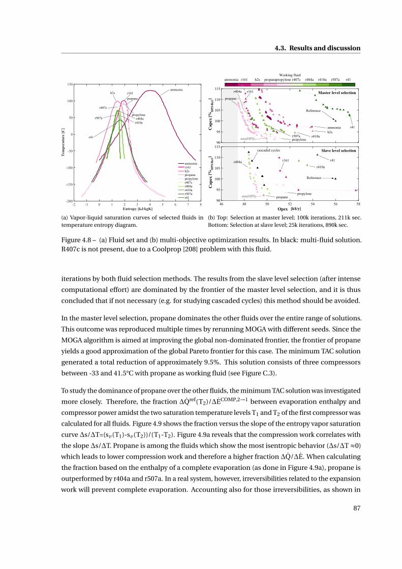
4.3. Results and discussion
(a) Vapor-liquid saturation curves of selected fluids intemperature entropy diagram.
(b) Top: Selection at master level; 100k iterations, 211k sec.Bottom: Selection at slave level; 25k iterations, 890k sec.
Figure 4.8 – (a) Fluid set and (b) multi-objective optimization results. In black: multi-fluid solution.R407c is not present, due to a Coolprop [208] problem with this fluid.
iterations by both fluid selection methods. The results from the slave level selection (after intense
computational effort) are dominated by the frontier of the master level selection, and it is thus
concluded that if not necessary (e.g. for studying cascaded cycles) this method should be avoided.
In the master level selection, propane dominates the other fluids over the entire range of solutions.
This outcome was reproduced multiple times by rerunning MOGA with different seeds. Since the
MOGA algorithm is aimed at improving the global non-dominated frontier, the frontier of propane
yields a good approximation of the global Pareto frontier for this case. The minimum TAC solution
generated a total reduction of approximately 9.5%. This solution consists of three compressors
between -33 and 41.5°C with propane as working fluid (see Figure C.3).
To study the dominance of propane over the other fluids, the minimum TAC solution was investigated
more closely. Therefore, the fraction ∆Qref(T2)/∆ECOMP,2→1 between evaporation enthalpy and
compressor power amidst the two saturation temperature levels T1 and T2 of the first compressor was
calculated for all fluids. Figure 4.9 shows the fraction versus the slope of the entropy vapor saturation
curve ∆s/∆T=(sv (T1)-sv (T2))/(T1-T2). Figure 4.9a reveals that the compression work correlates with
the slope ∆s/∆T. Propane is among the fluids which show the most isentropic behavior (∆s/∆T ≈0)
which leads to lower compression work and therefore a higher fraction ∆Q/∆E. When calculating
the fraction based on the enthalpy of a complete evaporation (as done in Figure 4.9a), propane is
outperformed by r404a and r507a. In a real system, however, irreversibilities related to the expansion
work will prevent complete evaporation. Accounting also for those irreversibilities, as shown in
87

Chapter 4. Generic heat pump superstructure
(a) Complete evaporation. (b) Incomplete evaporation, considering isenthalpic expan-sion from the level above (8°C with 5K subcooling).
Figure 4.9 – Performance of compressor between saturation levels T1 (32.5°C) and T2 (-17°C).
Figure 4.9b, propane yields the highest fraction ∆Q/∆E hence exhibiting ideal thermodynamic
properties in this temperature range.
Comparing the sequence of fluid frontiers (from Figure 4.8b, top) to the thermodynamic perfor-
mance (Figure 4.9b) indicates a close agreement between thermodynamic and economic perfor-
mance, which will be further investigated. The closest competitors to propane were: propylene,
r161, r404a, r410a, and r507a. Ammonia and hydrogen sulfide generated higher cost solutions, still
strongly outperforming r41. All solutions (except r41) outperform the solution presented by the
reference case updated with equivalent input data.
The dominance of propane over the entire solution space agrees with other reports indicating
superior performance in that temperature range [221]. Further fluid selection criteria could include
safety factors (such as flammability or toxicity), fluid cost, ozone layer depletion potential (ODP),
global warming potential (GWP) and heat transfer characteristics. Each of these criteria would favor
different refrigerants and thus the filtering of potential solutions should be completed carefully to
find the best solution for a given case.
4.3.3.2 COP, cycle complexity and HEN costs
Figure 4.10 illustrates the final non-dominated frontier of the results from the master level fluid
selection including several properties of these solutions. The (cold) COP increases with decreasing
opex, thus, reduced electricity consumption at increased number of compressors; the difference
between the lowest (2.9) COP and highest (3.3) is achieved through a higher number of compression
stages, increased subcooling and gas-cooling. The highest reduction in TAC (-9.5%) was achieved
88
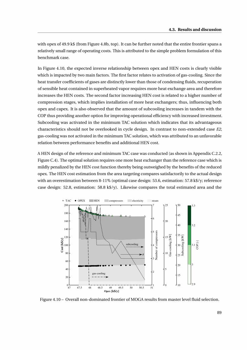
4.3. Results and discussion
with opex of 49.9 k$ (from Figure 4.8b, top). It can be further noted that the entire frontier spans a
relatively small range of operating costs. This is attributed to the simple problem formulation of this
benchmark case.
In Figure 4.10, the expected inverse relationship between opex and HEN costs is clearly visible
which is impacted by two main factors. The first factor relates to activation of gas-cooling. Since the
heat transfer coefficients of gases are distinctly lower than those of condensing fluids, recuperation
of sensible heat contained in superheated vapor requires more heat exchange area and therefore
increases the HEN costs. The second factor increasing HEN cost is related to a higher number of
compression stages, which implies installation of more heat exchangers; thus, influencing both
opex and capex. It is also observed that the amount of subcooling increases in tandem with the
COP thus providing another option for improving operational efficiency with increased investment.
Subcooling was activated in the minimum TAC solution which indicates that its advantageous
characteristics should not be overlooked in cycle design. In contrast to non-extended case E2,
gas-cooling was not activated in the minimum TAC solution, which was attributed to an unfavorable
relation between performance benefits and additional HEN cost.
A HEN design of the reference and minimum TAC case was conducted (as shown in Appendix C.2.2,
Figure C.4). The optimal solution requires one more heat exchanger than the reference case which is
mildly penalized by the HEN cost function thereby being outweighed by the benefits of the reduced
opex. The HEN cost estimation from the area targeting compares satisfactorily to the actual design
with an overestimation between 8-11% (optimal case design: 53.6, estimation: 57.8 k$/y; reference
case design: 52.8, estimation: 58.8 k$/y). Likewise compares the total estimated area and the
47 47.5 48 48.5 49 49.5 50 50.5 51
[k$/y]Opex
0
20
40
60
80
100
120
140
160
180
200
Cos
t [k
$/y]
1
2
3
4
5
6
7
Num
ber
ofco
mpr
esso
rs
TAC OPEX HEN compressors electricity steam
#
gas-cooling
subcooling
0
5
10
15
20
25
Gas
-coo
ling
[kW
]
10
15
20
25
30
35
40
45
50
Sub
cool
ing
[kW
]
2.9
3
3.1
3.2
3.3
CO
P [
-]
Figure 4.10 – Overall non-dominated frontier of MOGA results from master level fluid selection.
89
Chapter 4. Generic heat pump superstructure
minimum number of heat exchangers.
4.4 Conclusions
How can design of an optimal industrial heat pump system be conducted?
This study has presented a mathematical approach for optimal design of industrial heat pumps
spanning a wide variable solution space. The method provides a framework for deriving utility
targets, including optimal heat pump component sizes and operating conditions. This provides
a basis for detailed system design in a subsequent step to account for dynamics and off-design
operation.
The novel superstructure-based synthesis method is embedded in a computational framework and
is solved in a decomposition approach. A comprehensive list of heat pump features are taken into
account while technical limitations are considered and a set of solutions is provided which allows
for expert-based decision making and further in-depth analysis of the solutions.
For benchmarking, the method was compared to a set of literature cases generating between 5 and
30% cost improvements to the optimal solutions reported. An extended version of one case was
presented considering fluid selection, HEN cost estimations, and technical constraints within the
problem formulation.
The extended case highlighted a trade-off between energy efficiency and system complexity ex-
pressed by the increase of heat exchanger network costs with the number of compression stages,
level of gas-cooling and subcooling which all improve the COP. This is especially evident when
comparing the solutions with 3 and 5 compression stages causing an increase of the COP from
2.9 to 3.1 at 3% increase in TAC. Subcooling was activated in the minimum TAC solution which
indicates that its advantageous characteristics should not be overlooked in cycle design. In contrast
to non-extended case E2, gas-cooling was not activated in the minimum TAC solution, which was
attributed to an unfavorable relation between performance benefits and additional HEN cost.
Fluid selection was successfully performed indicating that propane is the most favorable fluid both
in economic and thermodynamic terms in this temperature range. The HPS proves to be flexible for
different requirements serving in a variety of cases. It has to be noted that a comprehensive analysis
of an industrial process should always comprise optimization of the entire utility network, including
the hot utilities. This was neglected in this work to be in accordance with the literature input data.
In subsequent analysis, the trade-off with other utility technologies should be considered. Future
work should also include supercritical cycles, refined fluid and component selection strategies, as
well as consideration of off-design performance in multi-time problems.
90

5Generalization (A): heat pumping and
co-generationOverview
• Derivation of a methodology for environmental and economic (environomic) potential
estimation of technologies in industrial sectors, regions, and countries
• Generalization of methodologies derived in previous chapters
• Applied to heat pumping and co-generation in the overall dairy industry
• Presentation of on-line parallel coordinates decision making tool
• Method addresses multiple stake-holders ranging from policy makers to plant operators
and technology manufacturers
This chapter is based on Wallerand et al. [222]
Having derived methods for optimal solution generation of specific cases, in specific countries,
under specific conditions in the previous chapters, this chapter addresses the question of how these
methods could be generalized and extended to a wider scope. Therefore, method for estimating the
general environmental and economic (environomic) potential of various technologies in industrial
processes with application of optimization techniques is derived, generalizing the methodologies
derived in the previous chapters. This includes derivation of a publicly available database1 of
solutions based on a wide range of possible economic and environmental conditions.
In agreement with the literature [89, 90], Chapters 3 and 4 demonstrate that heat pumping can be
considered as a major contributor for improving energy efficiency and reducing the environmental
impact of industrial processes through waste heat recovery and reuse [89, 90] in low temperature
1 The data can be accessed via an on-line parallel coordinate [76] decision-making platform.
91

Chapter 5. Generalization (A): heat pumping and co-generation
sectors. However, analysis of recent publications in the field of waste heat recovery in Section 1.3
reveals that heat pumping is considered far less frequently than other heat recovery technologies
such as organic Rankine cycles. A general skepticism towards heat pump technologies among
process engineers was reported by several sources [94, 223]. This was assumed to be driven by a lack
of knowledge of the heat pump potential and integration methods and a perceived threat of having
to compromise the process’ operational flexibility [94, 224]. It is further noted that current methods
require extensive on-site analysis, which are often unrealized due to economic or time constraints.
Proper assessment and clear communication of energetic and economic saving potentials are
indispensable for achieving a turning point and, therefore, encouraging more efficient operations
through better use of energy resources. Thorough understanding of process operation and optimal
heat pump placement is the basis for such analysis.
After a state-of-the-art analysis, a novel methodology for heat pump potential estimation in in-
dustrial processes is presented. It considers detailed heat pump modeling and a wide range of
input parameters for a generic plant, thus enabling a pre-feasibility assessment. For illustration, the
method is applied to the dairy industry in the results and discussion section.
5.1 State-of-the-art
Table 5.1 presents a summary of the relevant literature on synthesis methods and potential studies
for heat pump integration in industrial processes. The literature is split between design studies
addressing heat pump design for specific processes, and potential studies which estimate the
technological potential in specific industries.
5.1.1 Design studies
In the past decades, multiple efforts were made to develop methods addressing optimal design
and integration of heat pumps in industrial processes. A general distinction is commonly observed
between conceptual and mathematical methods. Conceptual methods rely on heuristics to generate
good-practice solutions, while mathematical methods are more likely to generate optimal or near-
optimal solutions based on mathematical programming and are hence discussed in more detail.
Mathematical methods are often based on linear and nonlinear problem formulations within
the domain of optimization. Linear problems can be solved by exact methods, which guarantee
optimality in the final result (if terminating in a reasonable time). Nonlinear problems typically
consider different aspects of the problem in more detail and allow investigation of an extended
solution space; however, solving the problem is a more difficult procedure and optimality is not
guaranteed.
In the late 1970s, Linnhoff and Flower [97] developed an important conceptual method aimed at
structurally analyzing a process’ heat recovery potential nowadays known as pinch analysis (PA)
[99, 207].
92

5.1.State-o
f-the-art
Table 5.1 – State-of-the-art summary of synthesis methods and potential studies for heat pump integration with industrial processes.
Citation Year Topic Opt. HR Market Model Integration Par. SynthesisCU HU
Current work D,Pb MINLP X X ME X X X Bottom-up potential analysis based on optimization of detailed heat pump features for the dairyindustry.
Potential studiesWilk et al. [225] 2017 D,Pb X X X COP X X X Analysis of different industrial processes and the benefits related to installation of heat pumps
based on flow sheet software.Brückner et al. [226] 2015 D,Pt X X X COP X X X Economic potential for compression and absorption heat pumps and heat transformers in
different industrial sectors (in Europe) based on estimated heat demands.Wolf et al. [227] 2014 Pt X X X COP X X X Potential estimation in industrial sectors in the German context by analysis based on the tem-
perature ranges.Seck et al. [228] 2013 Pb LP X X COP X X X "Bottom-up" technical (TIMES) model used to estimate the potential for heat pumping in the
French food and beverage sector.Design studiesWallerand et al.[111, 167, 170]
2018 D MINLP X X ME X X X Bi-level superstructure including various features which were not considered by other studiessuch as multi-stage expansion, fluid selection and heat exchanger network (HEN) cost estimationand multi-criteria decision making.
Yang et al. [187, 188] 2017 D MINLP X X ME X X X Comprehensive superstructure considering temperature level selection and component sizing.Oluleye et al. [191, 215] 2016 D,Pb MILP X X COP X X X Method for heat engine, mechanical and absorption heat pump and transformer design based
on coefficient of performance (COP) fitting functions.Kamalinejad et al. [160] 2015 D MINLP X X ME X X X Two-step approach considering various heat pump features.Becker [140, 196] 2012 D MINLP X X ME X X X Bi-level decomposition strategy [125] with simple heat pump cycles solved for continuous
temperature levels.Zhang and Xu [159] 2011 D MINLP X X ME X X X Approach for energy optimal synthesis of cascaded heat pump cycles considering multiple heat
pump features in a retrofit problem with fixed temperature levelsMaréchal andKalitventzeff [157]
2001 D MILP X X ME X X X Method based on technology database and expert system
Vaidyaraman andMaranas [103]
1999 D MILP X X ME X X X Extended superstructure [101] with economizers and working fluid selection.
Swaney [204] 1989 D LP X X COP X X X Heat engine and heat pump integration based on a transportation array.Colmenares and Seider[205]
1987 D NLP X X ME X X X Design of superpositioned simple (one-stage) heat pump cycles (and engines)
Shelton and Grossmann[101, 102]
1986 D MILP X X ME X X X Superstructure-based approach, considering multi-stage heat pumping with flash-gas removal.
Townsend and Linnhoff[100]
1983 D conceptual X X ME X X X Demonstration that exergetically optimal placed heat pumps need to cross the process pinchtemperature.
Topic: D - design methods; P - potential studies (t: top-down, b: bottom-up).Opt. - optimization approach: conceptual; mathematical - mixed integer nonlinear programming (MINLP), mixed integer linear programming (MILP), nonlinear programming (NLP), linear programming (LP).HR: heat recovery in the process is considered, e.g. through PA.Market: economic model considering market competition between technologies.Model - heat pump modeling: ME - based on mass and energy balances; COP: based on Carnot factor efficiencies.Integration: HU - integration of heat pump as hot utility; CU - integration of heat pump as cold utilityPar. - parameter variation: variation of input parameters.93

Chapter 5. Generalization (A): heat pumping and co-generation
Based on these principles, Townsend and Linnhoff [100] demonstrated that optimally-placed heat
pumps need to cross the process pinch temperature to improve the overall energy and exergy
efficiency. In this way, they highlighted the need to investigate the thermodynamic requirements of
the entire system. Most subsequent studies integrated the principles of PA in their methods. Noted
contributions to mathematical methods are presented in Table 5.1.
The methods described in the studies presented in this section allow detailed analysis of a process’
heat recovery potentials and optimal industrial heat pump and refrigeration placement including
the ideal operating conditions. The results are obtained with aid of rigorous mathematical, or
conceptual methods based on economic, energetic, and environmental criteria considering detailed
technical features of the heat pump cycles. Unfortunately, generalization of the obtained results
cannot be conducted due to the dependence on the highly case specific problem input data.
5.1.2 Potential studies
Estimation of the general potential for heat pumping in various industrial sectors was not treated
frequently in the literature. Seck et al. [228] and Wilk et al. [225] presented analyses of different
industrial processes and the benefits related to installation of heat pumps considering the hot and
cold side of the heat pump, modeling them based on the Carnot efficiency. The potential in these
bottom-up approaches is extrapolated assuming that the analyzed processes are representative of
the respective industry. Other studies [226, 227] addressed the problem from a top-down perspective,
estimating the total industrial waste heat potential and the thermal requirements including the
temperature levels, which allowed derivation of the total potential heat pump capacity in certain
industrial sectors in specific countries or regions.
The presented publications are a foundation for further in-depth analysis highlighting the general
potential of heat pumps in certain industrial sectors. Most bottom-up approaches consider the hot
and cold side integration of a heat pump into the industrial process; one addresses the heat recovery
potential within the process. Heat pumps are typically modeled based on the Carnot efficiency.
This circumvents detailed conclusions with recommendations for experimentalists, equipment
developers or process operators while only providing policy-makers with coarse estimations of
potentials.
5.1.3 Discussion and contribution
The state-of-the-art analysis can be summarized in three main points.
1. Design studies provide complex (multi-stage) heat pump models and results for specific case
studies. Generalization of the obtained results has limited impact due to dependence on
case-specific input data.
2. Potential studies provide estimations of heat pump potentials in various industrial sectors.
The heat pump modeling and industrial process analysis is conducted in a coarse manner
94

5.2. Methodology
aiming at deriving overall capacities and temperature levels rather than detailed designs.
3. No studies effectively combine potential estimations with detailed modeling and optimization
techniques thus offering a comprehensive bottom-up approach for technological potential
estimation.
This chapter attempts to close the gaps mentioned in (1-3) by proposing a method for estimating
the general environomic potential of heat pumps in industrial processes with improved fidelity and
application of optimization techniques. The method includes generation of a publicly available
database of optimal solutions (which are based on a reduced input parameter set) via general-
ized multi-objective optimization. Based on user-selected input criteria, case-specific solutions
are drawn from the database and investigated. The data can be accessed via an on-line parallel
coordinates decision-making platform. The publicly-available results may be used to conduct a
pre-feasibility study in a plant, and in general, to identify potentials from the side of policy-makers
or equipment developers. The proposed method may be applied to a variety of technologies and pro-
cesses and is illustrated in this chapter on potential estimation of heat pumping and co-generation in
the general dairy industry based on analysis of various typical plants. Optimal design is achieved with
a heat pump superstructure (HPS) including a wide range of technological features [111, 167, 170]
and a comprehensive integration method.
5.2 Methodology
5.2.1 Problem statement
The methodology derived and the results obtained may be used to address a variety of research
questions, some of which are depicted below.
Problem statement
Given
(A) certain industry/process, a geographical region
(B) specific technology (feature)
Determine
(A) • economically viable emission reduction measures
• key political drivers to enable emission reduction goals
• favorable technologies and system designs which contribute to emission reduc-
tion goals
(B) • target industry/process
• key geographical region
which provide economically/environmentally viable options for integration of the
technology
95

Chapter 5. Generalization (A): heat pumping and co-generation
5.2.2 Overview
A classical deterministic utility design optimization problem, as discussed in Section 5.1.1, is de-
picted in Figure 5.1. The required input parameters can be grouped into two categories. Imposed
parameters (Π) are given by the boundary conditions of the problem, such as the geographical
location of the plant which determines energy prices, interest rates, electricity mix emissions, etc.,
while decision influenced parameters (ΠD) depend on the decisions (D) of the plant manager e.g.
(operating time, production volumes). With aid of these input parameters, a (multi-objective) opti-
mization problem can be formulated and solved. The computational burden of this approach is
quite high, especially considering that the solution is only valid for the specific case considered.
To overcome this limitation, this work presents a methodology in which the computationally expen-
sive optimization problem is solved once, independent from most input parameters. Thereupon,
the solutions are stored in a database from which a quasi-infinite number of scenarios with varying
input conditions can be derived.
The method is depicted in Figure 5.2. During the comprehensive solution space generation, the
problem scope is defined including the fixed and free parameters, followed by solution generation
and pruning to identify the relevant solutions which are added to the database of good solutions.
Once this step has been carried out, the database can be accessed on demand to generate the desired
output which is referred to as results retrieval.
Parallels may be drawn with classic approaches for dealing with uncertainty of input parameters.
Robust optimization addresses uncertainty in mixed integer linear programming (MILP) problems
[229]. The most commonly used approach for mixed integer nonlinear programming (MINLP) prob-
lems is stochastic programming [230] and accounting for parameter variation in post-computational
analysis [231]. The former requires intense computational effort, while the latter approach only
allows recalculation of the objective function, not accounting for the fact that different input param-
eters yield different solutions.
Figure 5.1 – Standard deterministic multi-objective optimization problem statement.
96

5.2. Methodology
Figure 5.2 – Method proposed in Chapter 5.
5.2.3 Comprehensive solution space generation
5.2.3.1 Scope definition
The goal in most optimization approaches for industrial processes is the derivation of more efficient
or less emitting solutions at minimum cost. The scope definition aims at defining the objectives
and input parameters required to formulate the optimization problem. The procedure is illustrated
for the case of minimizing the total annualized costs (TAC) and emissions, though it can be applied
for any problem. Formulating the problem correctly requires understanding of the influence of the
different input parameters on the desired output. The input parameters required to model the TAC
and emissions of a particular process are classified into four categories:
1. Economic inputs
(a) Economic parameters influencing the yearly operating expenses (opex) are the cost of
all incoming material and energy streams, as well as yearly operating time.
(b) The annualized capital expenses (capex) are dependent on the equipment cost func-
tions, the interest rate, and the fraction of maintenance cost (related to the initial invest-
ment).
2. Utility-specific inputs The performances (efficiency, fuel consumption and technical con-
straints) of the utility technologies influence the opex and are determined by input parameters.
3. Process-specific inputs The process configuration and its heat recovery potential have a
major influence on the system cost and emissions, and are therefore treated as an input.
4. Environmental parameters of process conversion steps and the impact of the incoming
material streams allows for a simplified quantification of the process’ environmental impact.
97
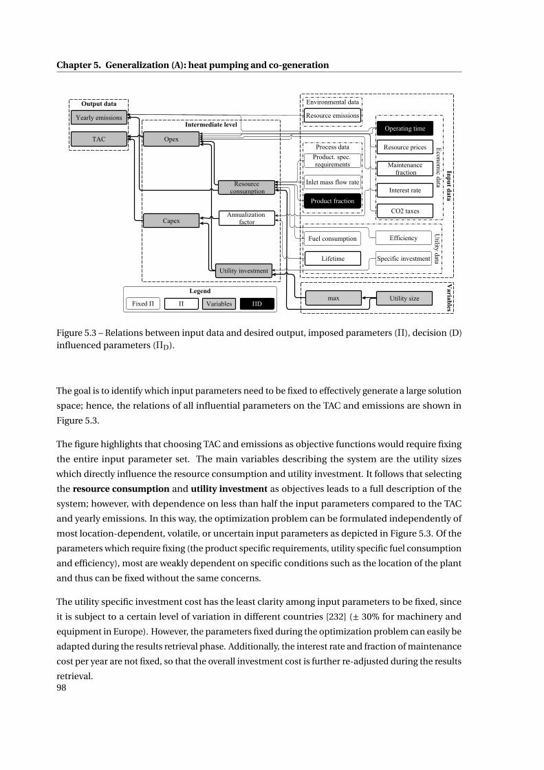
Chapter 5. Generalization (A): heat pumping and co-generation
Figure 5.3 – Relations between input data and desired output, imposed parameters (Π), decision (D)influenced parameters (ΠD).
The goal is to identify which input parameters need to be fixed to effectively generate a large solution
space; hence, the relations of all influential parameters on the TAC and emissions are shown in
Figure 5.3.
The figure highlights that choosing TAC and emissions as objective functions would require fixing
the entire input parameter set. The main variables describing the system are the utility sizes
which directly influence the resource consumption and utility investment. It follows that selecting
the resource consumption and utility investment as objectives leads to a full description of the
system; however, with dependence on less than half the input parameters compared to the TAC
and yearly emissions. In this way, the optimization problem can be formulated independently of
most location-dependent, volatile, or uncertain input parameters as depicted in Figure 5.3. Of the
parameters which require fixing (the product specific requirements, utility specific fuel consumption
and efficiency), most are weakly dependent on specific conditions such as the location of the plant
and thus can be fixed without the same concerns.
The utility specific investment cost has the least clarity among input parameters to be fixed, since
it is subject to a certain level of variation in different countries [232] (± 30% for machinery and
equipment in Europe). However, the parameters fixed during the optimization problem can easily be
adapted during the results retrieval phase. Additionally, the interest rate and fraction of maintenance
cost per year are not fixed, so that the overall investment cost is further re-adjusted during the results
retrieval.98

5.2. Methodology
5.2.3.2 Solution generation
As derived during the scope definition, a multi-objective optimization is carried out with the objec-
tives being the resource consumption and utility investment cost. The problem is formulated as
an MINLP which is solved by decomposing the problem into an nonlinear programming (NLP) at
the master level and MILP at the slave level as shown in Figure 5.4 and discussed by Wallerand et al.
[170] and Weber et al. [125], which is described in more detail below.
Master level The master level optimization is conducted with a multi-objective genetic algorithm
(MOGA) [217] implemented in Dakota [216]. The objectives at the master level, total investment
cost and resource consumption, are depicted in Equation 5.1.
minTi ,∆Ti ,DSH ,∆Ti ,SC ,∆Ti ,PRE ,d i ,ξ,εr
C I NV , Er
∀r ∈ R (5.1)
Where R is the set of resources electricity, natural gas, and Er [kW] is the resource consumption.
The total investment costs are derived from the investment cost, Cw , of each utility equipment w ∈W, and the HEN cost estimation, C HEN as shown in Equation 5.2.
C I NV = ∑w∈W
C w +C HEN (5.2)
The decision variables at the master level, including the minimum heat recovery approach tempera-
ture difference of the process streams, the HPS features, as well as the equipment cost functions of
the specific problem are discussed in the application section.
Slave level At the slave level, the multi-period utility targeting problem from Maréchal and
Kalitventzeff [75] is solved for several utility technologies including the heat pump superstruc-
ture presented by Wallerand et al. [170]. It should be noted that the underlying problem does not
necessarily require a multi-period formulation (and in the applied case study, the number of periods
i=1
Convergence check
1. Problem formulationNon-linear variables: xLinear variables: yObjective function: obj = f1 (x,y),f2 (x,y), ... , fn (x,y)
Scope definition
i=i+1
Solution pruning
2. Master level
Non-linear re-computation
3. Slave level
Input data generationAMPL language
Single-obj. MILP resolutionsolvers: CPLEX, Gurobi
obji
xi
yi, linear obji
Nonlinear variable selection Dakota: GA
fitnesscheck
infinity ∞
f1
f2
f3
(*) ResultsMulti-dimensional, non-dominated surface of solutions
obji, xi, yi
(*)
Figure 5.4 – Generalized multi-objective optimization strategy.
99
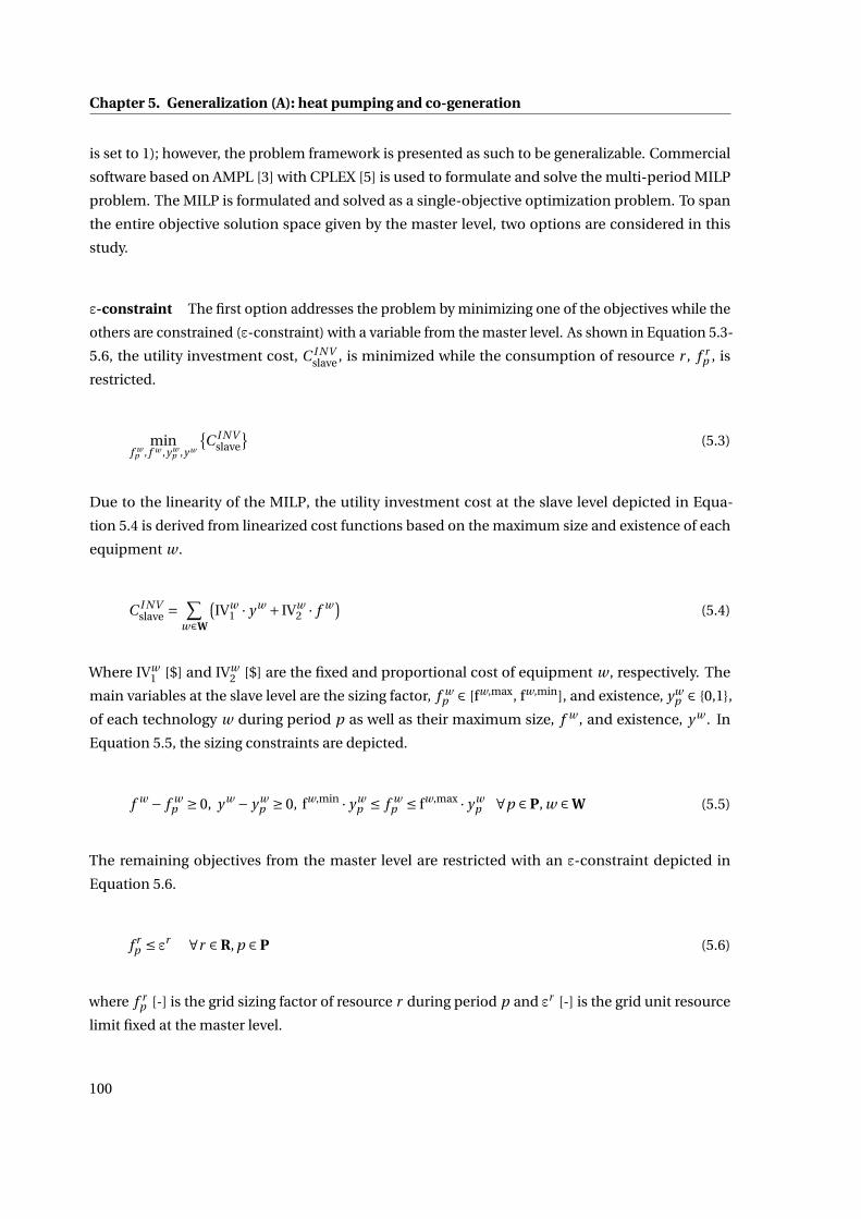
Chapter 5. Generalization (A): heat pumping and co-generation
is set to 1); however, the problem framework is presented as such to be generalizable. Commercial
software based on AMPL [3] with CPLEX [5] is used to formulate and solve the multi-period MILP
problem. The MILP is formulated and solved as a single-objective optimization problem. To span
the entire objective solution space given by the master level, two options are considered in this
study.
ε-constraint The first option addresses the problem by minimizing one of the objectives while the
others are constrained (ε-constraint) with a variable from the master level. As shown in Equation 5.3-
5.6, the utility investment cost, C I NVslave , is minimized while the consumption of resource r , f r
p , is
restricted.
minf w
p , f w ,y wp ,y w
C I NV
slave
(5.3)
Due to the linearity of the MILP, the utility investment cost at the slave level depicted in Equa-
tion 5.4 is derived from linearized cost functions based on the maximum size and existence of each
equipment w .
C I NVslave =
∑w∈W
(IVw
1 · y w + IVw2 · f w )
(5.4)
Where IVw1 [$] and IVw
2 [$] are the fixed and proportional cost of equipment w , respectively. The
main variables at the slave level are the sizing factor, f wp ∈ [fw,max, fw,min], and existence, yw
p ∈ 0,1,
of each technology w during period p as well as their maximum size, f w , and existence, y w . In
Equation 5.5, the sizing constraints are depicted.
f w − f wp ≥ 0, y w − y w
p ≥ 0, fw,min · y wp ≤ f w
p ≤ fw,max · y wp ∀p ∈ P, w ∈ W (5.5)
The remaining objectives from the master level are restricted with an ε-constraint depicted in
Equation 5.6.
f rp ≤ εr ∀r ∈ R, p ∈ P (5.6)
where f rp [-] is the grid sizing factor of resource r during period p and εr [-] is the grid unit resource
limit fixed at the master level.
100
5.2. Methodology
Weighted sum of objectives The second option is to define a weighted sum of all objectives,
wC T AC , where the weighting factors are controlled from the master level. The objective in this case
is shown in Equation 5.7.
minf w
p , f w ,y wp ,y w
wC T AC
(5.7)
The weighted total annual cost (wT AC ) are defined in Equation 5.8 based on the annualized capital
expenses (capex), C capex [$/y]2, the yearly operating expenses (opex), C opex [$/y], the total weighting
factor, ξ [-], and the resource prices (weights), OP2,pr [$/kWh].
wC T AC = ξ ·C capexslave + (1−ξ) ·C opex
= ξ ·τ ·C I NVslave + (1−ξ) ·
∑p∈P
∑r∈R
[OP2,p
r · f rp
]·Δtp ·occp
(5.8)
WhereΔtp [h] is the operating time, and occp [1/y] is the occurrence of period p.
The advantage of the ε-constraint method is full control over exploration of the solution space
while more infeasible scenarios or unnecessary solutions may be generated. The weighted sum of
objectives does not allow direct control over exploration of the solution space; however, it encounters
infeasibility less frequently.
5.2.3.3 Solution pruning
Solution pruning is introduced at this stage to reduce the set of solutions so that only the most
relevant ones are stored in the database. The first step towards solution space reduction happens
during solution generation, where results are slightly rounded so as to reduce the total number
of solutions by combining those which are very similar in several objectives and typically exhibit
marginal differences in the values of continuous decision variables. During the solution pruning,
the relevant solutions are identified by sampling the free input parameters (ΠFree within their
specified ranges) and storing the minimum TAC solutions as shown in Figure 5.53. Several sampling
algorithms were applied to the generated solutions. Each led to similar results (see Appendix D.2.1)
and thus, Matlab [137] intrinsic Latin hypercube sampling [233] was selected as the method for
further use in this work.
2 The slave capex Ccapexslave [$/y] are derived from the slave total total investment C I NV
slave [$], and the annualization factor
τ= i·(1+i)n
(1+i)n−1 [1/y], with i [1/y] being the interest rate and n [y] the equipment lifetime.3 The entire set of minimum TAC solutions, instead of only the non-dominated solutions (with respect to TAC and
emissions) are stored; As demonstrated in the following sections, lower payback times can be achieved in the dominatedregion.
101

Chapter 5. Generalization (A): heat pumping and co-generation
Figure 5.5 – Flowsheet of the pruning step.
If all minimum TAC solutions from each sample are selected, a reduction with respect to the original
population of approximately 25% was observed by applying the pruning technique. Accounting for
the occurrence of each solution during the sampling, and selecting only the 99% most recurring
solutions generates a reduction up to 60% with respect to the original population while keeping the
diversity in the solution space, which is the recommended approach for future studies.
5.2.4 Results retrieval
Results retrieval is the subsequent step once the comprehensive solution space generation has
been finalized. It contains all activities involving analysis, documentation, and investigation of
the solutions stored in the database. Based on selected input parameters and the desired output,
solutions are retrieved from the database and investigated by various key performance indicators
(KPI), which are elaborated in Table 5.2, including the total system cost and emissions, exergy
efficiency, and payback time. As indicated in Figure 5.2, extended analysis of the set of minimum
TAC solutions in various forms, including interactive parallel coordinate plots [76], is presented in
detail in the results section and demonstrates the gain for multiple stakeholders. This provides an
example for assessing and drawing conclusions from the methods to support decisions from various
perspectives.
5.3 Application
This section introduces the industrial case study of with all related data. Since the methodology is
applied to the dairy industry, a modular dairy plant is presented, followed by the scope definition
of the underlying problem. The detailed problem statement of the solution generation is further
elaborated.
5.3.1 Modular dairy plant
The modular dairy plant presented here is based on industrial data from Becker[140, 161, 196],
which was already presented in Chapter 3, and data from the reference document for best available
techniques in the food, drink and milk industry [81]. Figure 5.6 depicts the pathways for conversion
of raw milk into milk-based products as derived by Kantor et al. [234]. Based on European production
102

5.3. Application
Table 5.2 – Key performance indicators (KPI) calculated during post-computational analysis.
Description Symbols Equation
Total annualized costs(TAC) [$/y]
C T AC C capex +C opex =C I NV ·τ+C opex (5.9)
τ [1/y] i·(1+i)n
(1+i)n−1 investment cost annualization factor, i [-/y] interest rate, n lifetime [y]
C I NV [$] total investment cost, see Equation 5.2
Total emissions [t CO2
eq/y]ECO2
∑r∈R
∑p∈P
CO2r · Er · f r
p ·∆tp ·occp (5.10)
P set of time periods 1,2,3, ...,npf r
p [-] grid sizing factor of resource r during period pE
r[kW] reference (thermal, electrical) power of grid resource unit r
CO2r [kgCO2eq/kWh] specific emissions of resource r
∆tp [h] operating time of period poccp [1/y] occurrence of period p
System exergy efficiency[%]
ηexergy
The exergy efficiency of the system is derived by the process exergy requirements andproduction, respectively, as well as the resource exergy import and export.∑
p∈P
( ∑s∈Srequired
Esex +
∑r∈Rexport
Eex,r,p
)·∆tp ·occp
∑p∈P
( ∑s∈Sproduced
Esex +
∑r∈Rimport
Eex,r,p
)·∆tp ·occp
(5.11)
The exergy production within the process stems from the hot streams above and the coldstreams below the ambient temperature (Ta=15 °C), respectively.∑
s∈Sproduced
Esex =
∑c∈C|Tlog,c≤Ta
Qcp ·
(1− Tlog,c
Ta
)+ ∑
h∈H|Tlog,h≥Ta
Qhp ·
(1− Ta
Tlog,h
)
The exergy requirement within the process stems from the cold streams above and thehot streams below the ambient temperature (Ta), respectively.∑
s∈Srequired
Esex =
∑c∈C|Tlog,c≥Ta
Qcp ·
(1− Ta
Tlog,c
)+ ∑
h∈H|Tlog,h≤Ta
Qhp ·
(1− Tlog,h
Ta
)S set of process streamsH,C ⊂ S set of hot, cold process streamsR ⊂ W set of imported/exported resources including electricity, natural gas, etc.∆Tlog,s [K] logarithmic mean temperature difference of stream sQ
sp [kW] process stream s heat consumption/release
Eex,r,p f rp · Eex,r [kW] exergy of each resource r during period p
Payback time [y] t pbC I NV
Copex,ref −C opex(5.12)
C I NV [$] total investment cost, as shown in Equation 5.1
Yearly operating expenses(opex) [$/y]
C opex
∑p∈P
( ∑w∈W
OPw1,p · y w
p +OPw2,p · f w
p
)·∆tp ·occp +m ·C I NV + ECO2 ·cCO2 (5.13)
W set of utility technologiesf w
p [-] continuous variable for sizing technology w during period py w
p [-] binary variable related to existence of technology w during pOPw
1,p [$/h] fixed operating cost in period p
OPw2,p [$/h] proportional operating cost in period p
cCO2 [$/t CO2 eq] CO2 taxesm [1/y] maintenance cost as fraction of total investment
Investment discount [%] b I NV
Percentage of investment reduction (by subsidies or lower utility investment costs) re-quired to achieve the desired payback time.
1− C I NV , desired
C I NV= 1− tpb, desired · (Copex,ref − [
C opex −m ·C I NV])
1+ tpb, desired ·m· 1
C I NV(5.14)
tpb, desired [y] desired payback time, set here to 2 years
Exergy discount [$/Δ%] bexer g y
Investment discount per exergy reduction (by subsidies) required to achieve the desiredpayback time.
C I NV −C I NV , desired
ηexergy −ηrefexergy
(5.15)
COP of heat pumps [-] COP
∑e∈EVAP|Ti n≤0∨≥40°C
Qe + ∑c∈COND|Ti n≥40°C
Qc
∑q∈COMP
E q(5.16)
EVAP set of all evaporator units in heat pumpCOND set of all condensation units in heat pumpCOMP set of all compressor units in heat pumpQe heat consumption by evaporator eQc heat release by condenser cE co electricity consumption by compressor co 103

Chapter 5. Generalization (A): heat pumping and co-generation
volumes [235], the fabrication of fresh dairy products (such as butter, desserts and concentrated
milk) and the production of cheese were identified as the two main routes. The specific energy
requirement of cheese-making is considerably higher than that of fresh dairy products due to the
drying and exporting of whey as a co-product. A combination of cheese-making and fresh products
would, by inspection, lead to a design mainly dominated by the cheese making requirements and
is, hence, not considered. As shown by Kantor et al. [234], the dairy pathways can be decomposed
into functional subprocesses, so-called modules, and their specific thermal requirements (per unit
of product) can be extracted. Scaling these requirements with specified product mass flowrates or
ratios permits generation of a profile for any dairy plant.
In this manner, three different fresh dairy production plants were generated to study the heat pump
potential in this industry. Table 5.3 presents the respective data, which stem (1) from the actual plant
studied by Becker [140], (2) from the average production volumes of dairy goods in the European
Union [235], and (3) a combination of (1) and (2) without the concentrated milk production to
investigate plants with a lower pinch point temperature. Figure 5.7 displays the utility integrated
composite curves (ICCs) of the three plants, revealing the different net thermal requirements and
temperature ranges considering maximum heat recovery. As indicated in Figure 5.6, the process and
utility system are separately modeled so that heat exchange between the utilities and the process
is only allowed through energy carriers such as steam, water, or refrigerant. Figure 5.7 (d) shows
the utility heat cascade of the reference boiler at high temperature heating with high and medium
pressure steam. The curves of the utilities in place and the available energy carriers are shaped
by steam (medium pressure at ≈200°C, low pressure at ≈100°C) generated by a natural gas boiler,
cooling water (15-17 °C), and a two-stage refrigeration cycle (30,-3,-33°C, R161). The reference
resource (natural gas and electricity) consumption of these configurations is shown in Table 5.3.
Having assumed a minimum approach temperature,ΔTmin/2, of 5 K for all process streams (except
the milk evaporation/condensation streams), the energetic requirements of the modelled plant are
in good accordance with the actual plant from Becker [140]. Hence, it is assumed that this approach
temperature represents the actual level of heat recovery in the considered plants, and the derived
resource consumption of each case is treated as its reference.
5.3.2 Scope definition
The scope definition aims at formulating the problem and deriving the data for the solution genera-
tion. Table 5.4 shows the identified free and fixed parameters for the underlying problem. As shown
in Section 5.2.3.1, the fixed parameters are the utility- and HEN-specific (installed) investment cost,
fuel consumption, utility efficiencies, and process data. Data ranges are provided for the free input
parameters. It was assumed that the specific investment of the components already installed in the
plant (boiler and refrigeration cycle) were negligible. The potential utilities to be considered were
selected as a natural gas co-generation engine (COGEN), a mechanical vapor re-compression (MVR),
104

5.3. Application
Figure 5.6 – Flowsheet of the modular dairy plant. Utility and process data depicted in Appendix D.3.
Figure 5.7 – Dairy plants’ utility integrated composite curves (ICCs).
Table 5.3 – Product mass flow rates and reference resource consumption of examined dairy plants.
Name Plant (A) (B) (C1) (C2) (C3) (C4) Flow rate Flow name Mass fraction processing step Electricity Natural gas- - - - - - kg/s outlet/inlet kW kW
Becker [140] 1 1 0 0.157 - 0.225 0.618 10 raw milk 238.8 2208.61.1 past. cream1.40 past. milk0.86 concentrated milk 1 [conc. milk]/2.33 [past. milk]5.50 yogurt & dessert (*) 1 [yog. & dess.]/1 [past. milk]
EU-28 mix 2 1 0.69 0.25 0.25 0.18 0.32 10.00 raw milk 266.4 1852.60.341 past. cream 1/10.759 butter 1 [butter]/1 [past. cream]2.23 past. milk 1/12.23 HT milk 1/10.69 concentrated milk 1/2.332.85 yogurt & dessert (*)
No concentration 3 1 0.3 0.2 0.25 0 0.55 10.00 raw milk 252.5 1424.80.77 past. cream 1/10.33 butter 1/11.78 past. milk 1/12.23 HT milk 1/14.90 yogurt& dessert (*) 1/1
(*) Assumption: 50/50 dessert / yogurt productionOriginal plant [140]: cheese 0%, butter 0%, cream 11 %, drinking milk 14%, milk powder 20%, fresh products 55%European milk consumption [235], 2015: [cheese 36 % not considered], butter 29 %, cream 13 %, drinking milk 11%, milk powder 4%, fresh products 7%; Assumption: 50% ofdrinking milk is UHTNo concentration: removal of the milk concentration unit
105

Chapter 5. Generalization (A): heat pumping and co-generation
and a heat pump superstructure (HPS). The HEN cost is estimated based on a retrofit assumption.
Correspondingly, the minimum number of connections, the minimum heat exchange area, and
the HEN cost were derived for the reference plant and for each new design. The investment cost
difference generates the estimate for the retrofit heat exchanger network (HEN). Thereby, it must
also be noted that if a new solution generates fewer connections (N ), or a smaller area (A), they
are set to the reference values. Applying this concept enforces that the HEN cost is always positive
or zero (and is with respect to the reference plant). Designs with higherΔTmin, meaning less heat
recovery and higher resource consumption will always be inferior to the reference case and, hence,
will be discarded.
Figure 5.8 shows available electricity and natural gas prices in OECD countries, commercial bank
lending rates, and emissions associated with grid electricity, which serve as indications for the free
parameter data ranges, and provide the basis for later analysis.
0.01 0.02 0.03 0.04 0.05 0.06 0.07
Nat. gas [$/kWh]
0.06
0.08
0.1
0.12
0.14
0.16
0.18
0.2
Ele
ctri
city
[$/k
Wh]
Poland i= 6.3%, τ= 0.089
Estonia i= 5.1%, τ= 0.081
Greece i= 6.6%, τ= 0.091
United Kingdom i= 4.4%, τ= 0.076
Japan i= 1.5%, τ= 0.058
Czech Republic i= 4.7%, τ= 0.078
Turkey i= 13.7%, τ= 0.148
United States i= 3.3%, τ= 0.069
Korea i= 4.5%, τ= 0.077
Netherlands i= 2.3%, τ= 0.063
Germany i= 2.6%, τ= 0.065
Ireland i= 3.3%, τ= 0.069
Luxembourg i= 0.0%, τ= NaN
Hungary i= 4.8%, τ= 0.079
Slovak Republic i= 3.2%, τ= 0.068
Slovenia i= 5.2%, τ= 0.082
Italy i= 5.1%, τ= 0.081
Portugal i= 5.5%, τ= 0.084
Spain i= 9.4%, τ= 0.113
Austria i= 2.1%, τ= 0.062
Finland i= 2.0%, τ= 0.061
Belgium i= 3.5%, τ= 0.070
Canada i= 3.0%, τ= 0.067
Switzerland i= 2.7%, τ= 0.065
France i= 2.8%, τ= 0.066
Sweden i= 2.8%, τ= 0.066 0 0.050.1 0.150.2 0.250.3 0.350.4 0.450.5 0.550.6 0.650.7 0.750.8 0.850.9 0.951 1.051.1
Low
volt
age
gri
d [k
gC
O2
/kW
h]
Figure 5.8 – Resource prices (2017) [238][*], commercial bank lending rates (i) [239] (mostly 2015),annualization factor (τ) based on Equation 5.9 (20 y. lifetime), low voltage electricity grid emissions[240] (Reference year 2014, allocation, cut-off by classification, ICC 2013, GWP 100a). [*] Gas priceJapan [241] (2015).
5.3.3 Solution generation
All variables and objectives at both levels of the multi-objective optimization approach described
in Section 5.2.3.2 are depicted in Table 5.5. The general variables at the master level include the
minimum approach temperature difference of the process streams, and the variables controlling
the slave objective function as described by Equation 5.5-5.8. The heat pump superstructure (HPS)
specific variables at the master level are the saturation temperature levels, subcooling tempera-
106
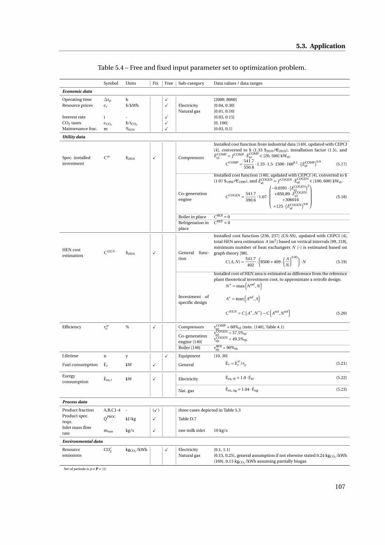
5.3. Application
Table 5.4 – Free and fixed input parameter set to optimization problem.
Symbol Units Fix Free Sub-category Data values / data ranges
Economic data
Operating time Δtp h X [2000, 8000]Resource prices cr $/kWh X Electricity [0.04, 0.30]
Natural gas [0.01, 0.10]Interest rate i - X [0.03, 0.15]CO2 taxes cCO2 $/tCO2 X [0, 100]Maintenance frac. m %INV X [0.03, 0.1]
Utility data
Spec. installedinvestment
C w $2016 X Compressors
Installed cost function from industrial data [140], updated with CEPCI[4], converted to $ (1.33 $2010/e2010), installation factor (1.5), andE COMP
el = f COMP · ECOMPel ∈ [20, 500] kWel.
C COMP = 541.7
550.8·1.33 ·1.5 ·1500 ·1600.1 · (E COMP
el
)0.9(5.17)
Co-generationengine
Installed cost function [140], updated with CEPCI [4], converted to $(1.07 $1999/e1999), and E COGEN
el = f COGEN · ECOGENel ∈ [100, 600] kWel.
C COGEN = 541.7
390.6·1.07 ·
−0.0391 · (E COGEN
el
)2
+850.89 · E COGENel
+306016
+125 · (E COGENel
)0.8
(5.18)
Boiler in place C BOI = 0Refrigeration inplace
C REF = 0
HEN costestimation
C HE N $2016 X General func-tion
Installed cost function [236, 237] (CS-SS), updated with CEPCI [4],total HEN area estimation A [m2] based on vertical intervals [99, 218],minimum number of heat exchangers N [-] is estimated based ongraph theory [98].
C (A, N ) = 541.7
402·(8500+409 ·
(A
N
)0.85)·N (5.19)
Investment ofspecific design
Installed cost of HEN area is estimated as difference from the referenceplant theoretical investment cost, to approximate a retrofit design.
N∗ = max(N ref, N
)A∗ = max
(Aref, A
)C HE N =C
(A∗, N∗)−C
(Aref, N ref
)(5.20)
Efficiency ηwr % X Compressors η
COMPel = 60%el (min. [140], Table 4.1)
Co-generationengine [140]
ηCOGENel = 37.5%el
ηCOGENth = 49.5%th
Boiler [140] ηBOIth = 90%th
Lifetime n y X Equipment [10, 30]
Fuel consumption Er kW X General Er = Ewr /ηr (5.21)
Exergyconsumption
Eex,r kW X Electricity Eex, el = 1.0 · Eel (5.22)
Nat. gas Eex, ng = 1.04 · Eng (5.23)
Process data
Product fraction A,B,C1-4 - (X) three cases depicted in Table 5.3Product spec.requ.
QPROC
kJ/kg X Table D.7
Inlet mass flowrate
mraw kg/s X raw milk inlet 10 kg/s
Environmental data
Resourceemissions
COr2 kgCO2 /kWh X Electricity [0.1, 1.1]
Natural gas [0.15, 0.25], general assumption if not elsewise stated 0.24 kgCO2 /kWh[169], 0.15 kgCO2 /kWh assuming partially biogas
Set of periods is p ∈ P = 1
107

Chapter 5. Generalization (A): heat pumping and co-generation
ture difference, temperature difference below which gas-cooling can be considered, preheating
temperature difference (for dry fluids, which were not considered in this work), and three fluid
indices (to consider cascaded cycles). The slave variables and objective function were introduced
(in Section 5.2.3.2). A set of heat pump specific parameters were also introduced to constrain the
compression ratio, number of compressors per fluid cycle, and compressor size.
Table 5.5 – Variables and objective function of the problem.
Description Symbols Range Unit ε-constraintweightedsum ofobjectives
Master level
Objective function f objmaster
C I NV , Er
,r ∈ R div. X X
General variables
Min. approach temp. diff. ∆Tmi n/2 2,3,5 K X XMax. consumption of resource r (Eq. 5.6) εr,max [0,1] - X XTAC weighting fraction (Eq. 5.8) ξ 0.05,0.1,0.2,0.5,0.6,0.7,0.8,0.95,1 - X XElectricity price (Eq. 5.8) cel 0.01,0.1,0.2,0.5,0.8,1,2,5·cng $/kWh X XNat. gas price (Eq. 5.8) cng 0.06 $/kWh X XPlant index x 1,2,3 - X X
Heat pump superstructure (HPS) specific variables
Saturation temperature Ti = Ti+1 + ∆Ti
∆T1 5,5.5, ...,50 K X X∆T2 5,5.5, ...,50 K X X∆T3 5,5.5, ...,50 K X X∆T4 5,5.5, ...,50 K X XT5 −35,−34.5, ....50 °C X X
Subcooling temperature difference ∆T1,SC 0, 1,..., 30 K X X∆T2,SC 0, 1,..., 30 K X X∆T3,SC 0, 1,..., 30 K X X∆T4,SC 0, 1,..., 30 K X X
Gas-cooling temperature difference ∆Ti ,DSH
Ti−1 −Ti , DSH == 1
0, elseK X X
De-superheating condition DSH 0,1 - X XPreheating temperature difference ∆Ti ,PRE 0 K X XFluid index d1 1,...,9 - X X
d2 1,...,9 - X Xd3 1,...,9 - X X
Fluid set F NH3,H2S,PROPANE, X XPROPYLENE,R161R404A,R410A,R507A,R41
Slave level
Objective function f objslave div. C I NV
slave wC T AC
Constraints (additional) Resource constraint f rp ≤ f r,max ∀r ∈ R X X
Variables
Multiplication factor of techn. w during p f wp [fw,max, fw,min] - X X
Use factor of techn. w , p ywp 0,1 - X X
Maximum multiplication factor f w ≥ fwp ∀p ∈ P - X X
Overall use factor yw ≥ ywp ∀p ∈ P - X X
HPS parameters
Compressor isentropic efficiency ηisentropic 0.6 - X XMinimum temperature difference ∆Tmin/2 2 K X XMin/max compression ratio CPmin,max [1.2,7] bar/bar X XMin/max valve differential pressure [0.5,18] bard X XMin/max compressor power [10,500] kW X XMaximum number of compressors per fluid d 2 - X XMaximum number of compressors per HPS 4 - X X
108

5.4. Results and discussion
5.4 Results and discussion
5.4.1 Comprehensive solution space generation
5.4.1.1 Solution generation
The results from the multi-objective optimization problem introduced in Section 5.3.2 and 5.3.3, are
depicted as surfaces of non-dominated solutions in Figure 5.9 and Figure 5.10. The discontinuities
in the surface are created by the binary variables related to activation and deactivation of units.
It can be observed that the ε-constraint method shows a more uniform distribution of solutions
compared to the weighted sum of objectives method. This was attributed to the brute-force nature
of the constrained optimization. The weighted sum objective function method generated more
feasible points, though the position cannot be controlled to explore specific regions of the solution
space.
The resource plane4 reveals a non-dominated frontier between the natural gas and electricity con-
sumption. It marks the limit of the feasible solution space. Considering conventional technologies,
this line cannot be breached. Several solutions using the weighted objectives method are closer to
the infeasibility frontier, though at higher capital expenses. The original plant with its reference
consumption is marked at highest total resource consumption with zero capital cost. Every other
solution improves either the electricity or natural gas consumption. Determining the preferential
optimization approach requires a more detailed analysis to evaluate the homogeneity and frequency
of solution occurrence in the distribution of solutions as discussed in Section 5.2.3.3. Solution
pruning was thus applied on the solutions generated here.
4 The resource plane refers to the plane formed with the two types of resource consumption as axes, and hence spansthe natural gas and electricity consumption.
(a) Multi-objective optimization solutions plotted with respect to thethree objectives.
-100 0 100 200 300 400 500
Net electricity [kW]
0
200
400
600
800
1000
1200
1400
1600
1800
2000
Net
gas
[kW
]
Infeasible region
0
0.2
0.4
0.6
0.8
1
1.2
1.4
1.6
1.8
2
2.2
Cap
ex [
M$]
Reference
(b) Three objectives projected on the two-dimensional resource plane.
Figure 5.9 – ε-constraint case: results from multi-objective optimization of plant 2.
109
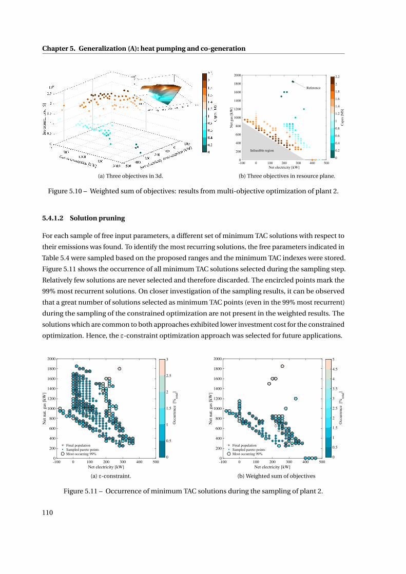
Chapter 5. Generalization (A): heat pumping and co-generation
(a) Three objectives in 3d.
-100 0 100 200 300 400 500
Net electricity [kW]
0
200
400
600
800
1000
1200
1400
1600
1800
2000
Net
gas
[kW
]
Infeasible region
0
0.2
0.4
0.6
0.8
1
1.2
1.4
1.6
1.8
2
2.2
Cap
ex [
M$]
Reference
(b) Three objectives in resource plane.
Figure 5.10 – Weighted sum of objectives: results from multi-objective optimization of plant 2.
5.4.1.2 Solution pruning
For each sample of free input parameters, a different set of minimum TAC solutions with respect to
their emissions was found. To identify the most recurring solutions, the free parameters indicated in
Table 5.4 were sampled based on the proposed ranges and the minimum TAC indexes were stored.
Figure 5.11 shows the occurrence of all minimum TAC solutions selected during the sampling step.
Relatively few solutions are never selected and therefore discarded. The encircled points mark the
99% most recurrent solutions. On closer investigation of the sampling results, it can be observed
that a great number of solutions selected as minimum TAC points (even in the 99% most recurrent)
during the sampling of the constrained optimization are not present in the weighted results. The
solutions which are common to both approaches exhibited lower investment cost for the constrained
optimization. Hence, the ε-constraint optimization approach was selected for future applications.
-100 0 100 200 300 400 500
Net electricity [kW]
0
200
400
600
800
1000
1200
1400
1600
1800
2000
Net
nat
. gas
[kW
]
Final population
Sampled pareto points
Most occurring 99%0
0.5
1
1.5
2
2.5
3
Occ
urr
ence
[%
tota
l]
(a) ε-constraint.
-100 0 100 200 300 400 500
Net electricity [kW]
0
200
400
600
800
1000
1200
1400
1600
1800
2000
Net
nat
. gas
[kW
]
Final population
Sampled pareto points
Most occurring 99%0
0.5
1
1.5
2
2.5
3
3.5
4
4.5
5
Occ
urr
ence
[%
tota
l]
(b) Weighted sum of objectives
Figure 5.11 – Occurrence of minimum TAC solutions during the sampling of plant 2.
110

5.4. Results and discussion
The selected solutions are depicted in Figure 5.12 and Figure 5.13. Figure 5.12a displays the exergy
efficiency of the selected solutions (of plant 2) in the resource plane, highlighting that the exergy
efficiency of the solutions is strongly linked to the net electricity import. This was explained by
the high exergy value attributed to electricity, which neglects the generation process and hence
creating a small bias. This bias could be avoided by considering the electricity generation, though
this is highly dependent on the location of the plant and hence cannot be treated in the generalized
solutions generated in this work.
The utility selection of plants 2 and 3 are shown in Figures 5.12b and 5.12c, respectively. The solutions
without additional utility integration (apart from the utilities in place) are found at the upper right
of the cloud of solutions, at highest resource consumption. From there, heat pump (hp) integration
stretches toward higher net electricity consumption, while co-generation (cogen) towards lower
electricity consumption. It has to be noted that the heat pump designs which are derived from
the HPS, could be integrated at any temperature level (Table 5.5) by the optimizer. However, it can
be observed that for lower capex solutions, the heat pump was placed across the process pinch,
interacting with the milk concentration streams. The mechanical vapor re-compression (MVR) was
never observed in low capex (high resource consumption) solutions due to imposed sizing limits
which are related to the limited availability of process steam for MVR. In the case of plant 2, the
MVR was activated with higher electricity consumption. Since plant 3 does not have a concentrated
milk production unit, MVR was not activated. The lowest combined resource consumption was
achieved with co-generation, mechanical vapor re-compression, and heat pumping.
The characteristics of these selected solutions of plant 2 were further analyzed in Figure 5.13 with
respect to the exergy efficiency. Various trends can be observed. As expected the cooling water,
natural gas, and boiler consumption decreased, while the electricity consumption increased with
increasing exergy efficiency (dropping with the availability of co-generation, since co-generation
generates electricity). The co-generation engine, as stated before, increased initially and then
decreased with increasing exergy efficiency. Heat pumping was utilized with increasing exergy
(a) Exergy efficiency, plant 2. (b) Utilities, plant 2. (c) Utilities, plant 3.
Figure 5.12 – Exergy efficiency and utility selection of selected plants.
111

Chapter 5. Generalization (A): heat pumping and co-generation
30 40 50 60
Exergy efficiency [%]
0
500
1000
1500
2000
Pow
er [
kW
]
Electricity
Nat. gas
Qboiler
Qcogen
Qcw
30 40 50 60
Exergy efficiency [%]
0
100
200
300
400
Pow
er [
kW
]
Ecogen
Eref
Emvr
Ehp
Qsubcool.
Qgas-cool.
30 40 50 60
Exergy efficiency [%]
0
200
400
600
800
1000
Cap
ex [
k$]
HEN
Compress.
Cogen
30 40 50 60 70
Exergy efficiency [%]
0
2
4
6
8
10
[-]
∆Tmin
COP
Stages
Fluid index
Figure 5.13 – Pruned solution characteristics, plant 2.
efficiency, until MVR was activated, at which point it restarted from zero. It is interesting to note that
subcooling was always present when heat pumping was active. This indicates that sub-cooling is a
favorable feature considering the balance between cost and performance. Gas-cooling, in contrast,
was activated mainly in the high efficiency region which indicates that specific technologies need to
be considered for reaching especially efficient operation.
The fluid indexes which were mainly used in the heat pump were 1, 3 and 5, corresponding to
ammonia, propane and R161, respectively. Slight tendency toward higher indexes is observed with
increasing exergy efficiency, which appears to be related to the temperatures and performance of
the heat pumps.
Further, it can be observed that almost all solutions had aΔTmin/2=2K in the process heat exchang-
ers, meaning that the first step in terms of cost and energy efficiency was to increase heat recovery
in the process. These results are consistent with process integration principles. Assessing the eco-
nomic feasibility may not support the same solutions, as the cost estimation functions applied
may underestimate the real cost of a retrofit HEN, or that compressor costs may be overestimated5.
Independent from uncertainty related to the capex, a general discomfort of modifying the HEN was
observed across the industry. Therefore, plant 2 was re-assessed with fixedΔTmin/2=5K, in order to
compare the results. The data of all plants can be found in Appendix D.2.2.
5.4.2 Results retrieval
Once the database of solutions was created, various investigations could be conducted. Additional
interest in this approach stems from the fact that this analysis can be carried out from different
stakeholder perspectives.
5Feedback from the industry suggests that the compressor cost function overestimates especially large heat pumps,due to the high exponential.
112

5.4. Results and discussion
5.4.2.1 Country analysis
As indicated in Figure 5.8, different countries are subject to a large range of resource prices, emissions
associated with grid electricity, and bank lending rates. The goal in this section was to identify
which political and operational boundary conditions were required to generate economically viable
emission reduction measures in the dairy industry in different countries. So-called utility maps were
created, which capture the best economically viable emission reduction measures based on different
boundary conditions (operating time, CO2 tax, electricity generation emissions). Economically
viable was defined here as a payback time below three years. The least emitting solution below this
payback time was selected. If no solution below three years payback time could be identified, the
reference (marked as 0) was assumed.
Heat recovery improvement Figure 5.14 depicts the solutions and respective cost distribution
and emissions of selected OECD countries of plant 2. The number indexes the solution id which can
be found in Table D.3, Figure D.7a, and Figure D.9. One immediate result was that countries with the
lowest resource prices (United States of America (US) and Canada (CA)) exhibited no economically
viable solution for operating times of 2500 hours per year. When adding a CO2 tax, it became
profitable in CA to invest in the first emission reduction measures.
Solution 2 and 142 (143) were similar to the reference utility configurations with different a minimum
approach temperature,ΔTmin/2, of 2K and 3K, respectively (143 - small difference in refrigeration
cycle). Solution 1 represented a single-stage MVR added across the process pinch point to recover
steam from the concentrated milk production (see Figure D.9). This can also be visualized in the
resource price plane in Figure 5.15. The utility map reveals that with introduction of the CO2 tax (20
$/tCO2 ), the line between reference and measures with no additional installed equipment moves
toward lower resource prices. For the context of dairy plants operating in the US, this indicated that
the CO2 tax considered here was insufficient to incentivize owners to invest in reducing emissions
given the imposed economic conditions. Increasing the operating time to 8000h led to a drastic
increase in economically viable measures in all countries. Higher yearly operating expenses (opex)
logically yielded decreased payback times (considering the same investment cost).
Overall, assuming 2500 operating hours, an average viable CO2 emission reduction of 21% across
the considered OECD countries could be achieved, which increased to 25% by adding a CO2 tax.
Higher operating hours logically incentivized investment in emission reductions; this is supported
by looking at the case with 8000 h/y of operation where 55% and 58% emission reductions could
be achieved in an economically viable manner without and with CO2 taxes, respectively. A further
improvement to 65% reduction was observed when assuming a CO2 tax and tax incentives for
the investor which amounted to 20% of the total investment. Co-generation became viable for
countries with high resource prices and high electricity grid emissions, due to its high efficiency
and comparatively low emissions. The background was plotted with an average grid emission
113

Chapter 5. Generalization (A): heat pumping and co-generation
PolandEstonia
United KingdomJapan
United StatesKorea
GermanySpain
Canada
SwitzerlandFrance
0
20
40
60
80
100
%
0
1
2
3
4
Pay
bac
k t
ime
[y]
142 143 2 10 0 18 2 2 0 6 2Average avoid. CO
2 (1) 21 %, 2.38 y
2 2 2 1 0 33 5 2 143 26 18
(2) 25 %, 2.55 y
71 61 61 4 25 17 14 22 10 74 43
(3) 55 %, 2.74 y
61 122 14 4 1 14 78 28 6 74 43
(4) 58 %, 2.71 y
13 47 54 4 6 4 4 64 6 74 43
(5) 65 %, 2.66 y
Opexel
Opexng
OpexCO
2
Opexmaint.
Capexcogen
Capexcompr.
CapexHEN CO
2
elCO
2
ngPayback
Figure 5.14 – Cost data, CO2 equivalent emissions, plant 2. Five bars per country: (1) operatingtime 2500 h, tax 0 $/tCO2 , (2) 2500 h, 20 $/tCO2 ,(3) 8000 h, 0 $/tCO2 ,(4) 8000 h, 20 $/tCO2 , (5) 8000 h, 20$/tCO2 , 20% investment reduction through tax incentives.
0.02 0.04 0.06
Net nat. gas [$/kWh]
0.06
0.08
0.1
0.12
0.14
0.16
0.18
0.2
Net
ele
ctri
city
[$/k
Wh]
PL, 142
EE, 143GR, 2
GB, 2
JP, 10
CZ, 2
TR, 2
US, 0
KR, 18
NL, 142
DE, 2
IE, 2
LU, 143
HU, 142
SK, 2
SI, 2
IT, 33
PT, 2
ES, 2
AT, 15
FI, 2
BE, 2
CA, 0
CH, 6
FR, 2
SE, 2
Reference-MVRHPMVR+HP
(a) 2500 h, 0 $/tCO2
0.02 0.04 0.06
Net nat. gas [$/kWh]
0.06
0.08
0.1
0.12
0.14
0.16
0.18
0.2
Net
ele
ctri
city
[$
/kW
h]
PL, 2
EE, 2GR, 2
GB, 2
JP, 1
CZ, 2
TR, 2
US, 0
KR, 33
NL, 2
DE, 5
IE, 5
LU, 2
HU, 2
SK, 5
SI, 2
IT, 19
PT, 5
ES, 2
AT, 18
FI, 18
BE, 2
CA, 143
CH, 26
FR, 18
SE, 2
Reference-MVRHPMVR+HP
(b) 2500 h, 20 $/tCO2
0.02 0.04 0.06
Net nat. gas [$/kWh]
0.06
0.08
0.1
0.12
0.14
0.16
0.18
0.2
Net
ele
ctri
city
[$
/kW
h]
PL, 71
EE, 61GR, 61
GB, 61
JP, 4
CZ, 28
TR, 61
US, 25
KR, 17
NL, 30
DE, 14
IE, 28
LU, 28
HU, 30
SK, 28
SI, 28
IT, 24
PT, 88
ES, 22
AT, 43
FI, 43
BE, 22
CA, 10
CH, 74
FR, 43
SE, 43
MVRHPCogen+MVRMVR+HPHP+CogenMVR+HP+Cogen
(c) 8000 h, 0 $/tCO2
Figure 5.15 – Plant 2, utility maps with maintenance fraction 0.05, background: τ=0.08, 0.5kgCO2 /kWhel.
0.02 0.04 0.06
Net nat. gas [$/kWh]
0.06
0.08
0.1
0.12
0.14
0.16
0.18
0.2
Net
ele
ctri
city
[$
/kW
h]
PL, 0
EE, 4GR, 12
GB, 0
JP, 18
CZ, 2
TR, 12
US, 0
KR, 53
NL, 2
DE, 4
IE, 2
LU, 56
HU, 2
SK, 2
SI, 56
IT, 6
PT, 2
ES, 0
AT, 56
FI, 87
BE, 4
CA, 0
CH, 25
FR, 56
SE, 18
ReferenceMVRHPCogen+MVRMVR+HPHP+CogenMVR+HP+Cogen
(a) 8000 h, 0 $/tCO2
0.02 0.04 0.06
Net nat. gas [$/kWh]
0.06
0.08
0.1
0.12
0.14
0.16
0.18
0.2
Net
ele
ctri
city
[$
/kW
h]
PL, 12
EE, 12GR, 2
GB, 4
JP, 21
CZ, 2
TR, 34
US, 0
KR, 18
NL, 2
DE, 2
IE, 53
LU, 56
HU, 56
SK, 56
SI, 61
IT, 21
PT, 56
ES, 2
AT, 87
FI, 18
BE, 2
CA, 0
CH, 25
FR, 67
SE, 17
ReferenceMVRHPCogen+MVRMVR+HPMVR+HP+Cogen
(b) 8000 h, 20 $/tCO2
0.02 0.04 0.06
Net nat. gas [$/kWh]
0.06
0.08
0.1
0.12
0.14
0.16
0.18
0.2
Net
ele
ctri
city
[$
/kW
h]
PL, 34
EE, 34GR, 53
GB, 12
JP, 8
CZ, 53
TR, 53
US, 0
KR, 27
NL, 61
DE, 21
IE, 53
LU, 18
HU, 56
SK, 61
SI, 18
IT, 80
PT, 56
ES, 56
AT, 86
FI, 17
BE, 56
CA, 0
CH, 25
FR, 29
SE, 31
ReferenceMVRHPMVR+HPMVR+HP+Cogen
(c) 8000 h, 20 $/tCO2 , 20% investmentreduction through tax breaks.
Figure 5.16 – Plant 2,ΔTmin/2=5K fixed HEN, utility maps with maintenance fraction 0.05, back-ground: τ=0.08, 0.5 kgCO2 /kWhel.
114
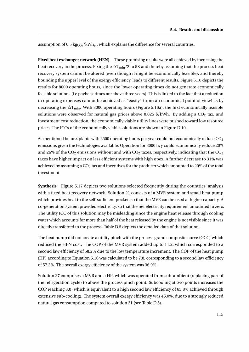
5.4. Results and discussion
assumption of 0.5 kgCO2 /kWhel, which explains the difference for several countries.
Fixed heat exchanger network (HEN) These promising results were all achieved by increasing the
heat recovery in the process. Fixing theΔTmin/2 to 5K and thereby assuming that the process heat
recovery system cannot be altered (even though it might be economically feasible), and thereby
bounding the upper level of the exergy efficiency, leads to different results. Figure 5.16 depicts the
results for 8000 operating hours, since the lower operating times do not generate economically
feasible solutions (i.e payback times are above three years). This is linked to the fact that a reduction
in operating expenses cannot be achieved as "easily" (from an economical point of view) as by
decreasing the ΔTmin. With 8000 operating hours (Figure 5.16a), the first economically feasible
solutions were observed for natural gas prices above 0.025 $/kWh. By adding a CO2 tax, and
investment cost reduction, the economically viable utility lines were pushed toward low resource
prices. The ICCs of the economically viable solutions are shown in Figure D.10.
As mentioned before, plants with 2500 operating hours per year could not economically reduce CO2
emissions given the technologies available. Operation for 8000 h/y could economically reduce 20%
and 26% of the CO2 emissions without and with CO2 taxes, respectively, indicating that the CO2
taxes have higher impact on less efficient systems with high opex. A further decrease to 31% was
achieved by assuming a CO2 tax and incentives for the producer which amounted to 20% of the total
investment.
Synthesis Figure 5.17 depicts two solutions selected frequently during the countries’ analysis
with a fixed heat recovery network. Solution 21 consists of a MVR system and small heat pump
which provides heat to the self-sufficient pocket, so that the MVR can be used at higher capacity. A
co-generation system provided electricity, so that the net electricity requirement amounted to zero.
The utility ICC of this solution may be misleading since the engine heat release through cooling
water which accounts for more than half of the heat released by the engine is not visible since it was
directly transferred to the process. Table D.5 depicts the detailed data of that solution.
The heat pump did not create a utility pinch with the process grand composite curve (GCC) which
reduced the HEN cost. The COP of the MVR system added up to 11.2, which corresponded to a
second law efficiency of 58.2% due to the low temperature increment. The COP of the heat pump
(HP) according to Equation 5.16 was calculated to be 7.8, corresponding to a second law efficiency
of 57.2%. The overall exergy efficiency of the system was 36.9%.
Solution 27 comprises a MVR and a HP, which was operated from sub-ambient (replacing part of
the refrigeration cycle) to above the process pinch point. Subcooling at two points increases the
COP reaching 3.0 (which is equivalent to a high second law efficiency of 63.8% achieved through
extensive sub-cooling). The system overall exergy efficiency was 45.0%, due to a strongly reduced
natural gas consumption compared to solution 21 (see Table D.5).
115

Chapter 5. Generalization (A): heat pumping and co-generation
(a) Utility ICCs of process and utility cluster.
(b) HPS, sol. 21
(c) HPS, sol. 27
Figure 5.17 – Most occurring solution of ε-constrained objective of plant 2,ΔTmin/2=5K fixed HEN;(b,c) T-h diagrams of HPS.
Several intermediate conclusions may be drawn from this analysis. Firstly, it was shown that the
selected solutions provided a wide range of system complexity, from improvement of the heat
recovery system, to single-stage MVR systems (with and without sub-cooling) and multi-stage HPS
systems (illustrated in Table D.5). A decision-making process was suggested which was based on
commonly accepted KPIs such as payback time and emissions.
Political incentives, such as CO2 taxes and tax breaks for investment in emission reduction measures
could increase the economically viable emission reductions from an average of 56% to 67% for an
average plant (including concentrated milk production Figure 5.14, Figure D.8a) in the investigated
OECD countries (assuming 8000 operating hours). In plants, which do not contain a concentrated
milk production unit the numbers were slightly lower (46% to 54%, Figure D.8c). If a fixed process
heat recovery network was considered, these numbers were distinctly lower (20% to 31%, Figure D.8b)
for the analyzed plant (with milk concentration unit), though the relative effect of political incentives
was drastically increased.
The analysis could be used by policy-makers aiming at understanding market drivers which lead to
less-emitting industry, or by equipment manufacturers aiming to identify their potential markets.
The following section addresses both these issues at more depth.
5.4.2.2 Decision-making platform
This section presents the decision-making platform and providing exemplary analysis from different
stakeholder perspectives. The platform is available on-line and contains the solutions of all plants
presented in the previous sections. It can be found in [242] and provides the minimum TAC points for
each range of emissions of each input parameter sample (depicted in the first seven bars) consisting
116

5.4. Results and discussion
80410/80410 Lines at 6.75% opacity. Hide Ticks Dark
What is this?
A multidimensional explorer of optimisation results for different types of dairyplants USDA.
Data inputs (a) nat. gas price ($/kWh)(b) electricity price ($/kWh)(c) CO2 taxes ($/t)(d) annuity factor (-) tau = 0.08, maintenance [0.03,0.07](e) operating time (h)(f) el. grid CO2 eq emissions (kg CO2 / kWh)(g) CO2 nat. gas (kg/kWh)
Data outputs (h) total annualised costs (% reference)(i) total CO2 emissions (% reference)(j) net electricity (% reference)(k) net nat. gas (% reference)(l) capital expenses (% of tac)(m) payback time (y)(n) exergy efficiency (%)(o) cooling water consumption (% ref)(p) electricity refrigeration cycle (% ref)(q) minimum approach temperature difference (K)(r) electricity prod. by co-geneneration engine (kW)(s) electricity cons. by mechanical vapor recompression (kW)(t) electricity cons. by heat pump (kW)(u) heat pump stages (#)(v) fluid [1-NH3, 2-H2S,3-R290,4-R1270,5-R161,6-R407C,7-R404A,8-R410A,9-R507A,10-R41,11-cascade of fluids](w) sucooling heat load (kW)(x) gas-cooling heat load (kW)(y) investment discount (% investment)(z) exergy discount (k$/%)
Data table
Controls
Brush: Drag vertical. along an ax.Remove Brush: Tap axis bkgr.Reorder Axes: Drag label horiz.Invert Axis: Tap axis label.Remove Axis: Drag axis label to leftedge.
Credits & License
Adapted from Maziar Kermani, KaiChang, Mike Bostock and JasonDavies
Copyright © 2017, A.S.WallerandAll rights reserved. Released underthe BSD License.
Legend
20772 EU - 28 mix19158 EU - 28 mix - 5K19493 No concentration
20987 Original plant
Dairy plant - optimal utility systems Export
group (a) gas pr. … (b) el. pr. (… (c) CO2 ta… (d) annuity… (e) op. t. (h) (f) CO2 el. … (g) CO2 g… (h) TAC (%) (i) CO2 em… (j) net el. (%)
EU - 28 mix 0.08 0.3 60 0.13024 8000 1 0.25 35.7739 30.8424 -19.3315
EU - 28 mix 0.08 0.3 60 0.13024 8000 1 0.25 36.9728 29.5249 -9.8504
EU - 28 mix 0.08 0.3 60 0.13024 8000 1 0.25 33.6478 32.5559 -27.9072
EU - 28 mix 0.08 0.3 60 0.13024 8000 1 0.25 39.2097 28.1638 0
EU - 28 mix 0.08 0.3 60 0.13024 8000 1 0.15 35.2281 24.8047 -19.3315
EU - 28 mix 0.08 0.3 60 0.13024 8000 1 0.15 36.5665 23.7451 -9.8504
EU - 28 mix 0.08 0.3 60 0.13024 8000 1 0.15 32.8962 26.1827 -27.9072
EU - 28 mix 0.08 0.3 60 0.13024 8000 1 0.15 38.9901 22.6505 0
EU - 28 mix 0.08 0.3 60 0.13024 8000 0.75 0.25 36.5958 33.9404 -19.3315
EU - 28 mix 0.08 0.3 60 0.13024 8000 0.75 0.25 37.6711 32.4906 -9.8504
EU - 28 mix 0.08 0.3 60 0.13024 8000 0.75 0.25 40.207 30.9195 8.7469
EU - 28 mix 0.08 0.3 60 0.13024 8000 0.75 0.25 34.5658 35.826 -27.9072
EU - 28 mix 0.08 0.3 60 0.13024 8000 0.75 0.25 39.7945 30.9928 0
EU - 28 mix 0.08 0.3 60 0.13024 8000 0.75 0.15 36.077 28.2626 -19.3315
EU - 28 mix 0.08 0.3 60 0.13024 8000 0.75 0.15 37.2887 27.0554 -9.8504
0.0100.0100.0100.0100.010
0.0150.0150.0150.0150.015
0.0200.0200.0200.0200.020
0.0250.0250.0250.0250.025
0.0300.0300.0300.0300.030
0.0350.0350.0350.0350.035
0.0400.0400.0400.0400.040
0.0450.0450.0450.0450.045
0.0500.0500.0500.0500.050
0.0550.0550.0550.0550.055
0.0600.0600.0600.0600.060
0.0650.0650.0650.0650.065
0.0700.0700.0700.0700.070
0.0750.0750.0750.0750.075
0.0800.0800.0800.0800.080(a) gas pr. ($/kWh)(a) gas pr. ($/kWh)(a) gas pr. ($/kWh)(a) gas pr. ($/kWh)(a) gas pr. ($/kWh)
0.060.060.060.060.06
0.080.080.080.080.08
0.100.100.100.100.10
0.120.120.120.120.12
0.140.140.140.140.14
0.160.160.160.160.16
0.180.180.180.180.18
0.200.200.200.200.20
0.220.220.220.220.22
0.240.240.240.240.24
0.260.260.260.260.26
0.280.280.280.280.28
0.300.300.300.300.30
(b) el. pr. ($/kWh)(b) el. pr. ($/kWh)(b) el. pr. ($/kWh)(b) el. pr. ($/kWh)(b) el. pr. ($/kWh)
00000
55555
1010101010
1515151515
2020202020
2525252525
3030303030
3535353535
4040404040
4545454545
5050505050
5555555555
6060606060(c) CO2 tax ($/t)(c) CO2 tax ($/t)(c) CO2 tax ($/t)(c) CO2 tax ($/t)(c) CO2 tax ($/t)
0.1120.1120.1120.1120.112
0.1140.1140.1140.1140.114
0.1160.1160.1160.1160.116
0.1180.1180.1180.1180.118
0.1200.1200.1200.1200.120
0.1220.1220.1220.1220.122
0.1240.1240.1240.1240.124
0.1260.1260.1260.1260.126
0.1280.1280.1280.1280.128
0.1300.1300.1300.1300.130
(d) annuity (-)(d) annuity (-)(d) annuity (-)(d) annuity (-)(d) annuity (-)
2,5002,5002,5002,5002,500
3,0003,0003,0003,0003,000
3,5003,5003,5003,5003,500
4,0004,0004,0004,0004,000
4,5004,5004,5004,5004,500
5,0005,0005,0005,0005,000
5,5005,5005,5005,5005,500
6,0006,0006,0006,0006,000
6,5006,5006,5006,5006,500
7,0007,0007,0007,0007,000
7,5007,5007,5007,5007,500
8,0008,0008,0008,0008,000(e) op. t. (h)(e) op. t. (h)(e) op. t. (h)(e) op. t. (h)(e) op. t. (h)
0.10.10.10.10.1
0.20.20.20.20.2
0.30.30.30.30.3
0.40.40.40.40.4
0.50.50.50.50.5
0.60.60.60.60.6
0.70.70.70.70.7
0.80.80.80.80.8
0.90.90.90.90.9
1.01.01.01.01.0
(f) CO2 el. (kg/kWh)(f) CO2 el. (kg/kWh)(f) CO2 el. (kg/kWh)(f) CO2 el. (kg/kWh)(f) CO2 el. (kg/kWh)
0.150.150.150.150.15
0.160.160.160.160.16
0.170.170.170.170.17
0.180.180.180.180.18
0.190.190.190.190.19
0.200.200.200.200.20
0.210.210.210.210.21
0.220.220.220.220.22
0.230.230.230.230.23
0.240.240.240.240.24
0.250.250.250.250.25(g) CO2 gas (kg/kWh)(g) CO2 gas (kg/kWh)(g) CO2 gas (kg/kWh)(g) CO2 gas (kg/kWh)(g) CO2 gas (kg/kWh)
4040404040
6060606060
8080808080
100100100100100
120120120120120
140140140140140
160160160160160
180180180180180
(h) TAC (%)(h) TAC (%)(h) TAC (%)(h) TAC (%)(h) TAC (%)
1010101010
2020202020
3030303030
4040404040
5050505050
6060606060
7070707070
8080808080
9090909090
100100100100100
(i) CO2 em. (%)(i) CO2 em. (%)(i) CO2 em. (%)(i) CO2 em. (%)(i) CO2 em. (%)
-20-20-20-20-20
00000
2020202020
4040404040
6060606060
8080808080
100100100100100
120120120120120
140140140140140
160160160160160
180180180180180
200200200200200
(j) net el. (%)(j) net el. (%)(j) net el. (%)(j) net el. (%)(j) net el. (%)
00000
1010101010
2020202020
3030303030
4040404040
5050505050
6060606060
7070707070
8080808080
9090909090
(k) net gas (%)(k) net gas (%)(k) net gas (%)(k) net gas (%)(k) net gas (%)
55555
1010101010
1515151515
2020202020
2525252525
3030303030
3535353535
4040404040
4545454545
5050505050
5555555555
6060606060
6565656565
(l) capex (%)(l) capex (%)(l) capex (%)(l) capex (%)(l) capex (%)
1010101010
2020202020
3030303030
4040404040
5050505050
6060606060
7070707070
8080808080
9090909090
(m) payback (y)(m) payback (y)(m) payback (y)(m) payback (y)(m) payback (y)
3535353535
4040404040
4545454545
5050505050
5555555555
6060606060
6565656565
7070707070
(n) ex. efficiency (%)(n) ex. efficiency (%)(n) ex. efficiency (%)(n) ex. efficiency (%)(n) ex. efficiency (%)
1010101010
2020202020
3030303030
4040404040
5050505050
6060606060
7070707070
8080808080
9090909090
(o) cool. w. (%)(o) cool. w. (%)(o) cool. w. (%)(o) cool. w. (%)(o) cool. w. (%)
1010101010
2020202020
3030303030
4040404040
5050505050
6060606060
7070707070
8080808080
9090909090
100100100100100
(p) elec. ref (%)(p) elec. ref (%)(p) elec. ref (%)(p) elec. ref (%)(p) elec. ref (%)
2.02.02.02.02.0
2.22.22.22.22.2
2.42.42.42.42.4
2.62.62.62.62.6
2.82.82.82.82.8
3.03.03.03.03.0
3.23.23.23.23.2
3.43.43.43.43.4
3.63.63.63.63.6
3.83.83.83.83.8
4.04.04.04.04.0
4.24.24.24.24.2
4.44.44.44.44.4
4.64.64.64.64.6
4.84.84.84.84.8
5.05.05.05.05.0(q) DT min (K)(q) DT min (K)(q) DT min (K)(q) DT min (K)(q) DT min (K)
00000
5050505050
100100100100100
150150150150150
200200200200200
250250250250250
300300300300300
350350350350350
400400400400400
450450450450450
(r) elec. cogen (kW)(r) elec. cogen (kW)(r) elec. cogen (kW)(r) elec. cogen (kW)(r) elec. cogen (kW)
00000
55555
1010101010
1515151515
2020202020
2525252525
3030303030
3535353535
4040404040
4545454545
5050505050
5555555555
6060606060
6565656565
7070707070(s) elec. mvr (kW)(s) elec. mvr (kW)(s) elec. mvr (kW)(s) elec. mvr (kW)(s) elec. mvr (kW)
00000
2020202020
4040404040
6060606060
8080808080
100100100100100
120120120120120
140140140140140
160160160160160
180180180180180
200200200200200
220220220220220
240240240240240
260260260260260
280280280280280
300300300300300
320320320320320
340340340340340
(t) elec. hp (kW)(t) elec. hp (kW)(t) elec. hp (kW)(t) elec. hp (kW)(t) elec. hp (kW)
0.00.00.00.00.0
0.20.20.20.20.2
0.40.40.40.40.4
0.60.60.60.60.6
0.80.80.80.80.8
1.01.01.01.01.0
1.21.21.21.21.2
1.41.41.41.41.4
1.61.61.61.61.6
1.81.81.81.81.8
2.02.02.02.02.0
2.22.22.22.22.2
2.42.42.42.42.4
2.62.62.62.62.6
2.82.82.82.82.8
3.03.03.03.03.0(u) hp stages (-)(u) hp stages (-)(u) hp stages (-)(u) hp stages (-)(u) hp stages (-)
00000
11111
22222
33333
44444
55555
66666
77777
88888
99999
1010101010
1111111111
(v) fluid (-)(v) fluid (-)(v) fluid (-)(v) fluid (-)(v) fluid (-)
00000
5050505050
100100100100100
150150150150150
200200200200200
250250250250250
300300300300300
350350350350350
400400400400400
(w) subcool. (kW)(w) subcool. (kW)(w) subcool. (kW)(w) subcool. (kW)(w) subcool. (kW)
00000
2020202020
4040404040
6060606060
8080808080
100100100100100
120120120120120
140140140140140
160160160160160
180180180180180
200200200200200
220220220220220
240240240240240
260260260260260
280280280280280
(x) gas-cool. (kW)(x) gas-cool. (kW)(x) gas-cool. (kW)(x) gas-cool. (kW)(x) gas-cool. (kW)
00000
1010101010
2020202020
3030303030
4040404040
5050505050
6060606060
7070707070
8080808080
9090909090
(y) inv. disc. (%)(y) inv. disc. (%)(y) inv. disc. (%)(y) inv. disc. (%)(y) inv. disc. (%)
00000
500500500500500
1,0001,0001,0001,0001,000
1,5001,5001,5001,5001,500
2,0002,0002,0002,0002,000
2,5002,5002,5002,5002,500
3,0003,0003,0003,0003,000
3,5003,5003,5003,5003,500
4,0004,0004,0004,0004,000
(z) exerg. disc. (k$/d%)(z) exerg. disc. (k$/d%)(z) exerg. disc. (k$/d%)(z) exerg. disc. (k$/d%)(z) exerg. disc. (k$/d%)
1010101010
2020202020
3030303030
4040404040
5050505050
6060606060
7070707070
8080808080
9090909090
100100100100100
110110110110110
(zb) id(zb) id(zb) id(zb) id(zb) id
Optimal dairy utility systems file:///Users/Documents/Google Drive/7_Paper_HPS/4_Results/...
1 von 1 15.03.18, 15:28
Figure 5.18 – On-line decision making platform [242].
of resource prices, CO2 taxes, annuity6, operating time, resource emissions (electricity, natural gas7).
The different plants are marked in different colors and can be (de-)activated in the legend. Different
parameter samples can be selected with help of the sliders and the resulting data can be exported.
The next paragraph provides the motivation for selecting the minimum TAC points for their emis-
sions, and discusses the influence of political actions on the economic viability of the solutions. The
data shown in each of following paragraphs can be found in the decision making platform.
Political actions Figure 5.19 shows the influence of different political actions on the viability of
emission reduction measures. The minimum TAC solution for each emission reduction and the
respective payback time is depicted for plant 2 in three different countries with fixedΔTmin/2 of 5 K.
The lowest payback time was achieved in many cases at higher emissions than the lowest TAC. This
justifies why the entire range of minimum TAC solutions were taken into account, and not only the
non-dominated Pareto frontier between TAC and emissions. It could be observed that the payback
time for solutions close to the reference was quite low (due to low investment costs) and then
increased (with another potential decrease). Five different cases in three different countries were
investigated ranging from 2500 operating hours to 8000 h with CO2 taxes of 0, 20 (with and without
investment cost reduction of 20% through tax incentives), and 60 $/tCO2 . It could be observed that
political measures had less influence in Switzerland, which had the highest resource prices, than in
6The annuity [1/y] is defined as the sum of the annualization factor, τ, and the maintenance fraction, m.7Two options were provided for natural gas: 100%mol fossil gas: 0.25 kgCO2 /kWh [169]; 40%mol biogas: 0.15 kgCO2 /kWh.
117

Chapter 5. Generalization (A): heat pumping and co-generation
20 40 60 80 100
Emissions [%t CO
2eq
]
60
70
80
90
100
110
TA
C [
%$/y
]
0
5
10
15
20
TAC
(a) CH
tbp
20 40 60 80 100
Emissions [%t CO
2eq
]
40
60
80
100
120
140
0
5
10
15
20
TAC
(b) DE
tbp
20 40 60 80 100
Emissions [%t CO
2eq
]
50
100
150
200
250
300
0
5
10
15
20
Pay
bac
k t
ime
[y]
TAC
(c) US
tbp
(1) TAC, 0 $/t CO2, 2.5k h
(2) 20 $/t, 2.5k h
(3) 0 $/t, 8k h
(4) 20 $/t, 8k h
(5) 20 $/t, 8k h, finv
0.8
(6) 60 $/t, 8k h
tpb
1tpb
2tpb
3
tpb
4tpb
5tpb
6
Figure 5.19 – Minimum TAC solutions and respective payback time. Influence of political actions oneconomically viable solutions, plant 2,ΔTmin/2=5K, 8000h.
the other countries. Political measures in Switzerland (CH) reduced the payback time by a maximum
of 1.5 years. This impact, however, may influence the success or failure of a project. For 8000 h, the
tax incentive of 20% of the total investment generated in general the lowest payback times followed
by 60 $/tCO2 especially for high emission reductions.
In the United States of America, where the resource prices are extremely low, the CO2 taxes (especially
60 $/tCO2 ) had a strong impact, meaning that the payback time was reduced by 5 to 10 years. This
could be easily explained by the fact that the CO2 tax can be understood as an absolute increase of
the resource prices8, and hence is equivalent to increasing the natural gas price in the US by 100%,
whereas in CH, the relative increase is only 20%.
In conclusion, CO2 taxes have distinctly higher impact in countries with low resource prices, while
to achieve a change in countries with high resource prices, tax breaks may be a good incentive.
Plant operators and heat pump manufacturers One goal of this work was to allow pre-feasibility
assessment based on the generated results, which is illustrated in this section. The solutions
discussed during the political actions, are further depicted in Figure 5.20 (without incentives for
8000 h). Negative values in the opex arise from the export of electricity. It can be seen that in CH, for
example, in a plant of type 2 one of the first emission and cost reduction measures is installation of a
co-generation engine, since the electricity prices were relatively high. For high emission reductions
in CH, the co-generation engine should be phased out in favor of investing in a more complex heat
pump system and, hence, in compressors due to the fact that the electricity grid emissions were very
low. These solutions also generated the lowest payback times which coincided with the minimum
TAC points. Therefore, from the perspective of plant operators and heat pump manufacturers, heat
pumps are worth considering for dairy plants (of type 2) in Switzerland, should be one conclusion
8For natural gas (0.24 kgCO2 /kWh): 20, 60 $/tCO2 leads to 0.005, 0.014 $/kWh; for electricity (assuming 0.5 kgCO2 /kWh):0.01, 0.03 $/kWh
118

5.4. Results and discussion
20 40 60 80 100
Emissions [%t CO
2eq
]
0
50
100
Co
st [
%k$/y
]
0
5
10
15
20
(a) CHcelec
/cgas
= 1.9
20 40 60 80 100
Emissions [%t CO
2eq
]
0
50
100
0
5
10
15
20
(b) DEcelec
/cgas
= 4.3
20 40 60 80 100
Emissions [%t CO
2eq
]
0
50
100
0
5
10
15
20
Pay
bac
k t
ime
[y]
(c) UScelec
/cgas
= 5.4
TAC OPEX HEN Co-generation Compressors Natural gas Electricity Payback time
Figure 5.20 – Detailed cost data versus CO2 equivalent emissions for min(TAC) points, plant 2, 0$/tCO2 ,ΔTmin/2=5K, 8000h.
20 40 60 80 100
Emissions [%t CO
2eq
]
0
500
1000
1500
2000
Ther
mal
pow
er [
kW
]
(a) CH
20 40 60 80 100
Emissions [%t CO
2eq
]
0
500
1000
1500
2000
(b) DE
20 40 60 80 100
Emissions [%t CO
2eq
]
0
500
1000
1500
2000
(c) US
Boiler Boiler original Co-generation Cooling water C. water original
Figure 5.21 – Boiler, co-generation engine and cooling water loads versus CO2 equivalent emissionsfor min(TAC) points, plant 2, 0 $/tCO2 ,ΔTmin/2=5K, 8000h, solution id in black.
20 40 60 80 100
Emissions [%t CO
2eq
]
0
100
200
300
400
500
Pow
er [
kW
]
(a) CH
20 40 60 80 100
Emissions [%t CO
2eq
]
0
100
200
300
400
500
(b) DE
20 40 60 80 100
Emissions [%t CO
2eq
]
0
100
200
300
400
500
(c) US
E, co-generation E, MVR E, HPS E, refrigeration E, ref. (reference) Q, sub-cooling Q, gas-cooling
Figure 5.22 – Electrical power loads (and heat pump data) versus CO2 equivalent emissions formin(TAC) points, plant 2, 0 $/tCO2 ,ΔTmin/2=5K, 8000h.
119

Chapter 5. Generalization (A): heat pumping and co-generation
drawn from this pre-feasibility assessment.
In Germany (DE) and the US, the highest emission reductions were actually achieved with co-
generation and heat pumping, due to the high electricity grid emissions. Interestingly, in both DE
and US, the minimum payback time did not coincide with the minimum TAC cost. The minimum
payback time was found close to the reference consumption suggesting a small heat pump (10
kWel) installation across the pinch point. It is arguable as to whether such a small installation is
worthwhile achieving a mere emission reduction of less than 5%. At lower emissions (60% compared
to reference) another low payback time can be observed (in both countries). As shown in Figure 5.22,
these solutions required installation of a MVR across the process pinch and of a co-generation engine.
Applying CO2 taxation at the level of 20 $/tCO2 would make these solutions more attractive (payback
time of 4 years in DE and 8 years in the US). The HEN cost of all solutions was comparatively small,
since the processΔTmin/2 was fixed to 5K, and only the utility integration needed to be accounted
for.
Figure 5.21 and Figure 5.22 illustrate the thermal, electrical power and exergy efficiency of various
equipment in these solutions. As noted previously, the exergy efficiency shows an inversely propor-
tional relationship with the cooling water consumption. Figure 5.22 reveals that gas-cooling was
present in various minimum-cost solutions and subcooling even more so. Due to the size limitation
of the MVR unit, heat pumping was the first unit to be activated together with the co-generation unit
(in CH). The refrigeration cycle (in place) was typically operated at its reference size, only high emis-
sion reduction solutions showed heat pumping interfering with the operation of the refrigeration
cycle to create better system efficiencies.
5.5 Conclusions
How can the results be extrapolated to a wider scope?
This chapter presented a methodology for the generation of a database of optimal utility solutions
for industrial processes, independent from the most volatile (cost related) input data. The method
was applied to heat pumping and co-generation in the dairy industry. A modular dairy plant was
presented and three dairy plant types were analyzed with environomic boundary conditions of
various OECD countries. The generated data was discussed at great length from the perspective
of multiple stakeholders. A parallel coordinate on-line decision-making platform was introduced
which grants access to the publicly-available database encompassing a detailed utility design of
each solution and performance data for various contextual parameters, which enabled a cost-free
pre-feasibility assessment of emission reduction measures.
The results indicated that heat pumping contributes to emission reductions and increases exergy
efficiency in the dairy industry, independent from location until a certain threshold. If emissions
120

5.5. Conclusions
must be reduced beyond that point, the CO2 equivalent emissions of the grid electricity in the
specified location have a great influence. The outcome of the optimization further indicated that
internal heat recovery should be the first step for efficiency and emissions reduction at lowest capex.
Restructuring the HEN of a plant may not be a practicable solution and thus plants with fixed HEN
were also investigated. It could be demonstrated that the operating time and energy resource prices
drastically influenced the economic viability of emission reduction measures. Political incentives,
such as CO2 taxes and tax breaks for investment in emission reduction measures could increase
the economically viable emission reductions from an OECD average of 20% to 26% and 31%, in the
least favorable case of a fixed process heat recovery network. These are equivalent to 30% and 55%
increase in viable emission reduction measures achieved through a CO2 tax of 20 $/tCO2 without
and with 20% tax breaks on the investment, respectively. It was found that CO2 taxes had distinctly
higher impact in countries with low resource prices, while to achieve a change in countries with
high resource prices, tax breaks might be a better incentive.
The methodology provides a wide range of applications and valuable insights for multiple stake-
holders. The main limitation of the presented approach is identified as the fixing of the equipment
investment cost, which are uncertain values and may have an influence on the utility selection. In
future work this may be addressed by re-calculating the investment cost with varying cost functions,
or using stochastic programming.
121


6Generalization (B): addition of solar
utilitiesOverview
• Extension of the methodology developed in Chapter 5 to include solar utilities
• Potential analysis of solar utilities, heat pumping, and co-generation in the overall dairy
industry
• Results allow determination of solar break-even costs
This chapter is based on Wallerand et al. [243]
Potential studies aim at identification of the total energetic, economic, and/or environmental
potential of certain technologies in specific sectors or industries, at a regional, national, or global
level. The derived results may be used by multiple stakeholders to generate policy strategies [72],
or to identify sectors and regions most viable for installation of certain technologies [67]. The
methodology derived in the previous chapter adds a further dimension to the available literature:
Through generation of a publicly available database of detailed solutions plant-operators are enabled
to conduct cost-free pre-feasibility assessment, while equipment manufacturers gain insights of the
potential of specific technological features in certain industries and under different environmental
and economic (environomic) conditions.
This chapter presents an extension to the methodology presented in Chapter 5 taking into account
solar utilities. The methodology presented in Chapter 5 is based on generalized multi-objective
optimization stripped of all location-dependent input parameters. Therefore, it is assumed that the
specific investment cost of conventional utilities does not depend on the location. This assumption
cannot be applied to solar utilities, since the required installed capacity needed to satisfy a fixed
constant load depends strongly on the location and its available yearly irradiation.
123
Chapter 6. Generalization (B): addition of solar utilities
After a state-of-the-art analysis of current potential analysis methods for solar energy for industrial
processes (SEIP) applications, this chapter presents an extension to the potential analysis presented
in Chapter 5, in the methodology section. For illustration, the method is applied to the dairy industry
in the results and discussion section.
6.1 State-of-the-art
The studies discussed in this section are compared in various points in Table 6.1. The potential
studies are distinguished between bottom-up and top-down approaches.
6.1.1 Top-down
Classical top-down approaches are presented by Brown et al. [66], Beath [67], and Lauterbach et al.
[68], in which the total energy demands of different industrial sectors at the national level were
estimated, categorized by temperature levels, and matched with solar technologies. Some went
as far as identifying industrial clusters in specific regions and matching those with the annual
irradiation [66, 67]. Sharma et al. [69, 70, 71] presented a more detailed methodology in which the
plants associated with certain sectors were individually identified, classified by their hot utility type
(boiler or co-generation). The solar systems were then sized by plant capacity and the annual CO2
emission mitigation potentials were derived.
6.1.2 Bottom-up
A bottom-up approach was published by Murray [244] who discussed the theoretical potential and
conceptual integration for highly concentrated solar thermal systems in the primary aluminum
industry concluding that integration would be difficult. A more applied study was introduced
by Schweiger et al. [56] who presented a potential analysis and design of solar heat for industrial
processes (SHIP) applications in Spain (ES) and Portugal (PT) through steam production and
integration with conventional utility systems based on selected examples. Calderoni et al. [72]
considered three textile plants and estimated the economic feasibility of solar integration and
the key drivers enabling economic viability. The solar modeling approach was unfortunately not
specified.
Müller et al. [148] derived a methodology to estimate the potential for solar heat integration in the
liq. food industry in general and in specific plants based on the available land area, the process
temperature levels, and an annual average of the specific solar production. Meyers et al. [73]
compared solar (non-concentrating) thermal system (ST) with photovoltaic module (PV) systems
combined with resistance heating for a fixed process load, which is an exergetically inefficient
way to provide heating. Based on a regression model, the results were extrapolated to various
meteorological conditions to derive the break-even cost based on current and future specific project
investment costs.
124

6.1.State-o
f-the-art
Table 6.1 – State-of-the-art summary of potential estimation studies for SEIP applications.
Author Year Foc Appr Obj Vars Siz. Econ. Solar modeling Proc. m. SC Process Uti. Description.M dT Tool Stor. PA HEN
Current work 2018 SP-I D,Pb E C M - GA X S year MEB (X) X X various dairy Co-gen.,HP
Bottom-up optimization-based potential analysis for estimation ofsolar, co-generation and HP in low-temp. industries.
Meyers et al. [73] 2018 SP M,Pb E C B X D,S year,reg(hour)
R,TRN-SYS
X X X various - - Method for cost comparison between solar thermal and photovoltaicsvia resistance heating based on regression model for (kWp/m2).
Brown et al. [66] 1980 SP-A Pt TP LOC,L C X S year MEB X X X PT various - End-use matching analysis of parabolic trough collectors with indus-trial process heat.
Murray [244] 1999 SP-A Pb TP energy C X - - MEB - X X CSE) aluminum- Conceptual analysis of potentials for highly concentrating solar heatin the primary aluminum industry.
Schweiger et al. [56] 2000 SP-A Pb,D TP C, T B X S year MEB X X X various various - Potential analysis and design of SHIP in ES and PT through steamproduction and integration with conventional utility system.
Beath [67] 2012 SP-A Pt TP location,load
C X S year MEB X X X various various - Top-down analysis of industrial heat demand, temperature ranges,and location, matched with solar availability in Australia.
Calderoni et al. [72] 2012 SP-A A,Pb E - F X S - - X X X PT textile - Economic feasibility study of solar-assisted process plants in Tunisia.Lauterbach et al. [68] 2012 SP-A Pt TP load C X S - - X X X various various - Top-down analysis of industrial heat demand, temperature ranges in
DE.Müller et al. [148] 2014 SP-A Pb TP FD,L C X S year MEB X X X various food
(liq.)- Methodology: how to estimate the potential for solar heat in the liq.
food industry, based on available area, and temperature levels.Sharma et al. [69, 70] 2016 SP-A Pt,D TP SF C X S year MEB X X X PT paper Co-gen. Potential analysis of solar heat for paper industry in India, considering
solar sizing (by capacity), location, and co-generation.Sharma et al. [71] 2017 SP-A Pt,D TP SF C X S year MEB X X X PT dairy Potential analysis of solar heat for dairy industry in India, considering
solar sizing (by capacity) and locations of plants.
Focus: Solar (S), Solar integration to urban system (SU), SP, SP-A, SP-I based on notation presented in the introduction Section, Figure 2Approach: Design (D), modeling (M), analysis (A), potential (P), review (R ), empirical (E)Objective: Thermodynamic principles (TP), economic (E), thermoeconomic (TEP), technical (T)Variables: temperature (T), collector area (C), storage size (S), load (L), irradiation (IRR), field design (FD), solar fraction (SF), location (LOC)Sizing: Fixed (F), brute forcing (variation of paramters, identification of maxima) (B), mathematical programming (M - genetic algorithm (GA) - sequential quadratic programming (SQP)), conceptual methods (C), R-curve analysis (R), analytical (A),polynomial regression (PR)Economic (Econ.): economics considered in study (X/X)Modeling (M): (Quasi-) static (S), dynamic (D)Time discretization (dT): instantaneous (ins.), variable time step (VST); horizon: unless stated differently: yearly analysisTool: Mass and energy balances (MEB), design space method (DSM), regression (R), measurements (MEA)heat exchanger network (HEN): X- full HEN design (analysis), (X) - focus on identification of relevant HEX for solar integration, X - no specific HEN designSolar collector types (SC): Evacuated tube collectors (ETC), flat plate (FP), power tower heliostat field (HF), parabolic trough (PTC), flat plate photovoltaic and thermal systems (PVT), compound parabolic concentrator (CPC)
125

Chapter 6. Generalization (B): addition of solar utilities
6.1.3 Discussion and contribution
The state-of-the-art analysis can be summarized in four main points.
1. Top-down approaches provide estimations of the general potential for solar energy in certain
industrial sectors and geographical regions. However, the results are coarse and some options
may be overlooked.
2. Bottom-up approaches aim at derivation of profitability of solar integration measures in
specific sectors. The studies presented in the literature either focus on the solar system or on
the industrial process, but do not consider them in a combined framework.
3. Current literature focuses on conceptual approaches. A lack of systematic potential studies
applying rigorous methods (such as mathematical programming) is found.
4. A gap is identified for a bottom-up approach which considers both the process and solar
system, as well as a wider set of utilities and integration options, to identify relationships
between energy prices and utility selection at a national or international level.
This work attempts to close the gaps mentioned in (3-4) by expanding a bottom-up method for
estimating the general environomic potential of conventional technologies (heat pumps and co-
generation) in industrial processes to consider solar technologies. This requires a complex post-
computational framework including parameter sampling.
The method includes enhancing the databased of solutions generated in Chapter 5 with various
solar technologies, identification of solar system break-even cost, and specific potential estimation.
Based on user-selected input criteria, case-specific solutions are drawn from the database and
investigated. The data would be accessible via an on-line parallel coordinates decision-making
platform (which is in planning). The presented method illustrates, how specific solar performance
models can be generalized to provide indication for industries in various countries.
6.2 Methodology
6.2.1 Problem statement
Since the method presented here is an extension to the method introduced in Chapter 5, the same
research questions can be formulated as depicted in Section 5.2.1. Additionally, the following
questions are derived.
126

6.2. Methodology
Problem statement
Given
(A) certain industry/process, a geographical region
(B) set of solar technologies
Determine
(A) technologies and costs
• solar technologies, which bring the highest emission reductions
• break-even cost of each solar technology
(B) economically viable emission reduction potential and measures
6.2.2 Derivation
As mentioned before, the methodology presented in Chapter 5 is based on generalized multi-
objective optimization stripped of all location-dependent input parameters. Therefore, it was
assumed that the specific investment cost of conventional utilities do not depend on the location.
This assumption cannot be applied to solar utilities for obvious reasons.
Therefore, another approach is suggested to account for solar utility contribution. If a correlation
between collector area and the solar fraction can be identified, multi-objective, multi-period specific
optimization can be avoided and the solar utilities contribution could solely be accounted for in
a post-computational step based on the desired solar fraction and performance solar parameters.
The solar fraction, fw s [-], is defined as the fraction of energy that the solar utilities provide to the
process compared to what the is the actual process (thermal or electrical) requirement, as shown in
Equation 6.1.
fw s = Ew s
EPROC
(6.1)
The solar fraction can be defined instantaneously, or based on a maximum day. In this work, it refers
to the average solar contribution over the whole year, Ew s
[kW], with respect to the average process
requirement, EPROC
[kW].
In order to study the optimal solar collector area for different solar fractions, the ε-contrained mixed
integer linear programming (MILP) model for flat plate collectors with thermal storage, presented
in Chapter 3, was run for various process operating hours and with different solar fractions. The
results are presented in Figure 6.1a. As expected, it can be observed that with increasing process
operating times, more solar collector area is required to satisfy the same fixed average contribution.
And it can further be observed that the required solar area seems to follow a linear relation with the
process operating time.
127
Chapter 6. Generalization (B): addition of solar utilities
From this observation, an intuitive correlation presented in Equation 6.2 was derived and compared
to the results. The correlation links the required solar utility collector area, Aw s [m2], yearly efficiency,
ηw s [-], the yearly available solar radiation (GHI), gh [kWh/m2y], the constant process (thermal or
electrical) requirement, EPROC
[kW], and the process operating time, ∆tPROC [h/y], with the solar
fraction, fw s [-].
fw s =
∑p∈P
gh,p ·ηw s ·Aw s
EPROC ·∆tPROC
(6.2)
The approximation of the collector area based on this correlation are shown in Figure 6.1a. A good
agreement between the approximated collector area and the results from the detailed parametric
optimization from Chapter 3 can be observed for solar fractions ranging from 0.1 to 0.3. The storage
cost of the individual solutions (for solar fraction of 0.3) remains below 10% of the collector costs.
When increasing the solar fraction to 0.4 and 0.5 as shown in Figure 6.1b, the approximation given
by Equation 6.2 drastically underestimates the solar collector area requirement derived by the
MILP model. The discrepancy is linked to the fact that the intuitive correlation relies on a yearly
average, therewith assuming a seasonal storage option. The MILP model, which relies on typical
days, considers only daily storage. This is further illustrated in Figure 6.2 and Figure 6.3. For a solar
fraction of 0.3, the storage in Figure 6.2 is mainly operated on days with high solar radiation, and the
cooling water consumption is only increased on two typical days (one being the extreme day with
occurrence 1). A forced solar fraction of 0.5 (Figure 6.3) results in a drastic increase of cooling water
consumption due to the cyclic constraint of the storage unit (chapter 2.4.2) and the accompanying
overproduction of the solar system.
Since a detailed model of seasonal storage is not available and the cost functions cannot be antici-
pated, it is recommended to use solar fractions below 0.4 for this type of problem.
The agreement between the intuitive correlation and the results from the multi-period MILP is
promising, especially since the correlation does not rely on fitted data. For wider application,
a cross-verification may be recommended, though. In this study, the results from the flat plate
thermal collectors (FPs) are assumed to be applicable also to the high concentration photovoltaic
and thermal system (HCPVT). Since, the photovoltaic modules (PVs) are operated without storage,
the intuitive correlation for PV is assumed without limits on the solar fraction.
128

6.2. Methodology
0
5
10
15
20
25
30
0
1000
2000
3000
4000
5000
6000
7000
8000
9000
10000
2000 4000 6000 8000 10000
Stor
age
cost
[% c
olle
ctor
cos
t]
Col
lect
or a
rea
[m2]
Operating time [h]
0.3, approx.0.2, approx.0.1, approx.0.30.20.1Storage cost (0.3)
(a) Solar fraction 0.1-0.3.
0
5000
10000
15000
20000
25000
30000
35000
40000
2000 4000 6000 8000 10000
Col
lect
or a
rea
[m2]
Operating time [h]
0.3, approx.0.2, approx.0.1, approx.0.30.20.10.5, approx.0.4, approx.0.50.4
(b) Solar fraction 0.1-0.5.
Figure 6.1 – Results from MILP in Chapter 3, flat plate collector area for different process operatingtimes.
0 24 48 72 96 120 144 168 192 216 2400
100
200
300
Vo
lum
e [m
3]
0
500
1000
1500
2000
Th
erm
al p
ow
er [
kW
]
Tc
Th Charge flow Discharge flow Cooling water Solar output Boiler
Operating hours (10 typical days) [h]
Figure 6.2 – Thermal utility operation for flat plate collector integration, from Chapter 3, non-stopoperation, solar fraction of 0.3.
0 24 48 72 96 120 144 168 192 216 2400
200
400
600
800
Vo
lum
e [m
3]
0
500
1000
1500
2000
Th
erm
al p
ow
er [
kW
]
Tc
Th Charge flow Discharge flow Cooling water Solar output Boiler
Operating hours (10 typical days) [h]
Figure 6.3 – Thermal utility operation for flat plate collector integration, from Chapter 3, non-stopoperation, solar fraction of 0.5.
129

Chapter 6. Generalization (B): addition of solar utilities
6.2.3 Approach
The analysis conducted in Section 6.2.2, forms the basis for the suggested approach. Figure 6.4
illustrates the method which aims at incorporating solar utilities into the database of solutions
presented in Chapter 5. Therefore, the solar fraction and utilities under scrutiny need to be selected.
With the selected solar fraction and utilities, the original database created in Chapter 5, is expanded.
Each point in the database is thereby replicated for each solar technology considered and its data is
re-calculated based on the selected solar fraction.
Photovoltaic module (PV) For installation of photovoltaic modules (PVs), the new net electricity
consumption from the grid, EGRIDel
∗ [kWel], is derived by the old consumption and the solar fraction,
as depicted in Equation 6.3.
EGRIDel
∗ = (1− fw s) · E
GRIDel (6.3)
The constant solar contribution is given by Ew sel = fw s · E
GRIDel [kWel].
Flat plate thermal collector (FP) Likewise, the installation of flat plate thermal collectors (FPs) is
treated, though the new natural gas consumption depends on hot utility w of the solution. Therefore,
the new natural gas consumption, EGRIDng , is derived by the old consumption, the solar fraction and
the hot utility thermal efficiency, as depicted in Equation 6.4.
EGRIDng
∗ = (1− fw s) · Q
wth
ηwth
(6.4)
The constant solar contribution is given by Qw sth = fw s · Q
wth [kWth].
High concentration photovoltaic and thermal system (HCPVT) The HCPVT co-generates ther-
mal and electrical power. Since the thermal storage imposes the highest constraints, the sizing is
conducted based on the thermal power, Qw sth = fw s · Q
wth [kWth]. The new natural gas consumption,
E∗ng, is derived by the old consumption, the solar fraction and the hot utility thermal efficiency, as
depicted in Equation 6.5 and Equation 6.6.
EGRIDng
∗ = (1− fw s) · Q
wth
ηwth
(6.5)
EGRIDel
∗ = EGRIDel + Q
w sth ·ηw s
el
ηw sth
(6.6)
130

6.2. Methodology
Figure 6.4 – Methodology proposed in Chapter 6: Combined potential estimation method for solarand conventional utilities.
The constant solar contribution is given by Qw sth = fw s · Q
wth [kWth].
Co-generation If the thermal utilities replace part of the co-generation unit, the solution’s net
electricity demand needs to be adapted, as illustrated in Equation 6.7.
EGRIDel
∗∗ = EGRIDel
∗− fw s · QCOGENth ·ηw s
el
ηw sth
(6.7)
In this way the database of solutions is enlarged considering integration of solar energy by a fixed
solar fraction in each of the additional solutions. When results are retrieved from the database, the
specific solar collector cost [$/m2], the efficiency [-], and the irradiance of the location need to be
submitted, so that the location-dependent solar cost can be accurately estimated.
Break-even cost A second approach is applied, in which the break-even solar cost is determined
based on statistical analysis. Therefore, the data ranges of the free parameters presented in Chapter 5
are sampled (Latin hypercube [233]), and in each run the maximum feasible specific solar energy
cost [$/kWh] of each technology is determined, under the condition that 10% of the best total
annualized costs (TAC) solutions must incorporate the specified solar technology. The details are
presented in the results and discussion section.
131

Chapter 6. Generalization (B): addition of solar utilities
6.3 Results and discussion
The solutions of plant plant 2,ΔTmin/2=5K, were enhanced with solar utilities to study integration of
further emission reductions. The imposed solar fraction of the different technologies under scrutiny
is depicted in Table 6.2.
The enlarged set of solutions is depicted in Figure 6.5a in the resource plane1. The effect of the
respective technology on the set of solutions can be clearly identified. The integration of PV effectu-
ated a fractional reduction of net electricity consumption, therefore, distorting the points towards
the left. Integration of FP resulted in a distortion to the bottom, induced by reduced natural gas
consumption.
Figure 6.6 shows the total annualized costs (TAC) and total emissions of all solutions in the three
different countries, assuming the solar cost and efficiency values depicted in Table 6.2, the radiation
data of the individual countries as written in the caption of Figure 6.6, and electricity and natural
gas prices as depicted in Figure 5.8. As extensively discussed in Chapter 5, the respective minimum
TAC solutions were selected and are depicted in Figure 6.7. Negative values in the yearly operating
expenses (opex) arise from the export of electricity. The conclusions drawn from this analysis
confirm the conclusions derived in Chapter 3, indicating that under current solar system cost
metrics, solar systems should be installed as the last of multiple emission reduction measures. The
first option is heat recovery (not depicted here), followed by mechanical vapor re-compression
(MVR), and heat pump (HP) integration. Solar integration was only selected as additional measure
for emission reduction, after other options had been employed. With solar integration though
additional emission reductions by up to 20% could be achieved, reaching a total reduction of up to
80% compared to the reference in Switzerland (CH). It has to be noted, that integration of HCPVT
in Switzerland (CH), together with mechanical vapor re-compression (MVR) showed reduced TAC,
compared to the reference TAC -10%, which confirms the solutions presented in Chapter 3.
Table 6.3 provides the ranges of free parameters which were sampled. The statistical analysis was
conducted in order to derive the maximum viable solar cost, assuming uniformly distributed param-
eters. Of course, this assumption is more than simplified, but there was not sufficient data available
to derive more precise correlations. Figure 6.5b depicts the results of this analysis, indicating that the
maximum feasible cost ranges from 0.29 to 0.001 $/kWhlifetime prod.2. The 90th percentile was used
to identify the maximum viable cost for each of the technologies, leading to 0.0098 $/kWhth, lifetime
for FP, 0.0392 $/kWhel for PV, 0.0098 $/kWhel+th for HCPVT, and 0.0294 $/kWhel+th for the combined
version of FP and PV. A difference was observed between the two co-generation cases (HCPVT and
FP+PV) due to different imposed solar fractions.
1 The resource plane refers to the plane formed with the two types of resource consumption as axes, and hence spansthe natural gas and electricity consumption.
2 The solar investment costs are derived in dollars per kWh of lifetime energy production, and the lifetime is assumedto be 20y.
132

6.3. Results and discussion
-200 0 200 400 600
Net grid electricity [kW]
0
200
400
600
800
1000
1200
1400
1600
1800
2000
Net
nat
gas
[kW
]
Infeasible region
Original solutions
FP
PV
HCPVT
FP+PV
(a) Resource plane of database en-hanced with solar data.
0.49 0.392 0.294 0.196 0.098 0
Maximum viable solar cost [$/kWh]
0
0.05
0.1
0.15
0.2
0.25
0.3
Occurr
ence [
-]
0
10
20
30
40
50
60
70
80
90
100
Cum
ula
tive s
um
[%
]
FP
PV
HCPVT
FP+PV
(b) Statistical analysis of viable solar costs.
500 1000 1500 2000 2500 3000
Yearly irradiance (DNI, GHI) [kWh/m2/y]
0
100
200
300
400
500
600
Max
imum
via
ble
syst
em c
ost
[$/m
2] FP (GHI) η
th = 30%, η
el = 0%
PV (GHI) ηth
= 0%, ηel
= 15%
HCPVT (DNI) ηth
= 50%, ηel
= 25%
(c) Break-even collector cost, basedon statistical analysis.
Figure 6.5 – Database enhanced with solar data, results of statistical analysis, and break-evencollector cost.
Figure 6.6 – TAC versus emissions of solar enhanced database of plant 2, ΔTmin/2=5K, 2500 h, 0$/tCO2 , solar performance data Table 6.2, global horizontal irradiation (GHI) of three locations1400,1100,2000 kWh/m2/y (a,b,c) DNI 1500,1000,2500 (a,b,c).
20 40 60 80 100
Emissions [%t CO
2eq
]
0
50
100
150
Co
st [
%k$/y
]
0
5
10
15
20
(a) CH
20 40 60 80 100
Emissions [%t CO
2eq
]
-50
0
50
100
150
0
5
10
15
20
(b) DE
20 40 60 80 100
Emissions [%t CO
2eq
]
-100
0
100
200
300
0
5
10
15
20
Pay
bac
k t
ime
[y]
(c) US
TAC OPEX HEN FP+PV HCPVT PV FP Co-generation Compressors Natural gas Electricity Payback time
Figure 6.7 – Cost analysis of min(TAC) points of solar enhanced database of plant 2,ΔTmin/2=5K,2500 h, 0 $/tCO2 .
133

Chapter 6. Generalization (B): addition of solar utilities
Table 6.2 – General solar data assumed, based on Philibert [1], Kalogirou [18], and Kalogirou andTripanagnostopoulos [121].
Solar system ηth [-] ηel [-] Cost [$/m2] fs [-]
Flat plate thermal collector (FP) 0.3 - 400 0.3Photovoltaic module (PV) - 0.15 500 0.5High concentration photovoltaic and thermal system (HCPVT) 0.5 (DNI) 0.25 (DNI) 400 0.3 (thermal)FP + PV 0.3 0.15 400, 500 0.3, 0.5
Table 6.3 – Data ranges of free parameters as derived in Chapter 5.
Parameter Range Unit
Natural gas price [0.01, 0.1] $/kWhElectricity price [0.04, 0.18] $/kWhCO2 tax [0, 60] $/t CO2 eq.Annuity factor (τ+ m) [0.08, 0.25] 1/yOperating time [2000, 8000] hEl. grid CO2 eq. emissions [0.1, 1] t CO2/kWhNat. gas CO2 eq. emissions [0.15, 0.25] t CO2/kWh
Assuming these numbers as break-even costs, the area specific collector costs, could be derived
based on a chosen efficiency and a given annual irradiance, as shown in Figure 6.5c. It can be
observed that FP costs should in many cases not exceed 150 $/m2 (which is quite below current
market prices), while viable PV systems are be in the range of 100 to 300 $/m2 (closer to current
market prices), and cost of the HCPVT system should be between 200 and 500 $/m2 (below current
prices). These number will change, if different efficiencies are assumed.
When applying the break-even cost on the enhanced database of solutions, a change in results was
observed. Figure 6.8 and Figure 6.9 show the minimum TAC points for 2500 and 8000 operating
hours of plant 2, ΔTmin/2=5K, respectively. The results from with 2500h show installation of PV
in Switzerland (CH) and Germany (DE), which was replaced by FP, HCPVT and combined FP and
PV with increasing emission reductions. Interestingly, at 8000h operating hours, PV (in CH and
Germany (DE)) and HCPVT (in United States of America (US)) is replaced by a co-generation unit,
bringing the advantage of co-producing thermal and electrical power, constantly. Due to the high
investment cost of the co-generation unit, this option is only selected for operating hours.
Figure 6.10 depicts the thermal production of the units present in the minimum TAC solutions
(excluding the heat pump units). It can be shown that some of the solar installations generate
increased cooling water consumption, thereby suggesting lower exergy efficiencies, as seen for
United States of America (US) and Germany (DE) at around 50% emission reductions. This con-
firms that economic, and even environmental objectives, cannot verify that solar energy is used
in the exergetically optimal way. This could be avoided by choosing different objectives. However,
considering economic criteria at a certain point cannot be avoided.
134

6.3. Results and discussion
20 40 60 80 100
Emissions [%t CO
2eq
]
0
20
40
60
80
100
120
Co
st [
%k$/y
]
0
5
10
15
20
(a) CH
20 40 60 80 100
Emissions [%t CO
2eq
]
-50
0
50
100
150
0
5
10
15
20
(b) DE
20 40 60 80 100
Emissions [%t CO
2eq
]
-50
0
50
100
150
200
250
0
5
10
15
20
Pay
bac
k t
ime
[y]
(c) US
TAC OPEX HEN FP+PV HCPVT PV FP Co-generation Compressors Natural gas Electricity Payback time
Figure 6.8 – Cost analysis of min(TAC) points of solar enhanced database of plant 2,ΔTmin/2=5K,2500 h, 0 $/tCO2 , with break-even costs: FP: 0.0098 $/kWhth, lifetime, PV: 0.0392 $/kWhel, HCPVT0.0098 $/kWhel+th, FP+PV 0.0294 $/kWhel+th.
20 40 60 80 100
Emissions [%t CO
2eq
]
-50
0
50
100
150
Co
st [
%k$/y
]
0
5
10
15
20
(a) CH
20 40 60 80 100
Emissions [%t CO
2eq
]
-50
0
50
100
150
0
5
10
15
20
(b) DE
20 40 60 80 100
Emissions [%t CO
2eq
]
-50
0
50
100
150
0
5
10
15
20
Pay
bac
k t
ime
[y]
(c) US
TAC OPEX HEN FP+PV HCPVT PV FP Co-generation Compressors Natural gas Electricity Payback time
Figure 6.9 – Cost analysis of min(TAC) points of solar enhanced database of plant 2,ΔTmin/2=5K,8000 h, 0 $/tCO2 , with break-even costs.
20 40 60 80 100
Emissions [%t CO
2eq
]
0
500
1000
1500
2000
Ther
mal
pow
er [
kW
]
(a) CH
20 40 60 80 100
Emissions [%t CO
2eq
]
0
500
1000
1500
2000
(b) DE
20 40 60 80 100
Emissions [%t CO
2eq
]
0
500
1000
1500
2000
(c) US
Boiler Boiler original Co-generation Cooling water C. water original HCPVT
Figure 6.10 – Thermal units of min(TAC) points of solar enhanced database of plant 2,ΔTmin/2=5K,8000 h, 0 $/tCO2 , with break-even costs.
135

Chapter 6. Generalization (B): addition of solar utilities
6.4 Conclusions
How can the results be extrapolated to a wider scope?
This chapter presents an extension to the methodology presented in Chapter 5 taking into account
solar utilities. The presented method illustrates, how specific solar performance models can be
generalized to provide indication for industries in various countries.
The method includes enhancing the databased of solutions generated in Chapter 5 with various
solar technologies, identification of solar system break-even cost, and specific potential estimation.
Based on user-selected input criteria, case-specific solutions were drawn from the database and
investigated. The data could be accessed via an on-line parallel coordinates decision-making
platform (which is in planning).
The method is based on an intuitive correlation derived from the model presented in Chapter 3,
which is employed to assess the annual solar collector and storage performance under optimal
control. Results indicated that ST only achieved economic viability for collector costs ranging from
below 100 $/m2 in areas of low solar radiation to 200 $/m2 in areas with higher incident insolation.
Similarly the cost for PV and HCPVT were derived. Results confirmed the conclusions derived in
Chapter 3 indicating that under current solar system cost metrics, solar systems would be installed
as the last of multiple emission reduction options, favoring heat recovery improvements, mechanical
vapor re-compression, and heat pumping in the first place. When analyzing the results assuming
break-even solar costs, solar systems became more profitable, however, this also promoted solutions
in which the solar energy was used inefficiently, which was manifested in a high cooling water
consumption. This could be avoided using different objectives such as the exergy efficiency.
136

Conclusions
Overview
• Summary of the main results
• Significance of the work
• Recommendations and guidance
• Future perspectives
This thesis explored the multi-dimensional problem formulation of optimal solar integration in
industrial processes through elaboration of methodologies tailored to low-temperature processing
industries. The intricacies behind this goal were addressed in five main chapters. The main findings
and contributions are presented below, followed by recommendations and future perspectives.
Main results summary
Chapter 1 Chapter 1 provides the wider context of the topics discussed in this thesis. It motivates
the case study selection and technologies studied, and introduces concepts and nomenclature used
throughout the work.
Chapter 2 How can solar system design be accurately and rigorously addressed?
The second chapter presented a rigorous solar system modeling and design approach which al-
lows estimation of collector and storage performance at sufficient precision and limited computa-
tional effort. This development addressed shortcomings identified in the literature related to a lack
of rigorous solar design methods at sufficient precision. Comparison of the static collector model
with transient results yielded sufficient precision (<5 % deviation). Application of a clustering ap-
proach reduced the resolution time successfully while guarding the accuracy for sufficient numbers
of clusters. For low cluster numbers a deviation of the results was revealed, highlighting a need to
proper investigation of the clustering results.
Chapter 3 What problem formulation is required for a comprehensive design method for solar-
assisted low-temperature processes?
137

Conclusions
In Chapter 3, a comprehensive method was proposed which addressed simultaneous optimization
of the process heat recovery, the conventional utilities, and the renewable utility system (including
thermal storage) using ε-constrained parametric optimization. The method, tailored for the low-
temperature industry, is based on multi-period utility targeting, including process heat recovery
through pinch analysis (PA) and re-use through heat pumping, and identifies the optimal design
and operation of the utility and storage systems. In the literature, utility integration and solar system
design has not been treated in a comprehensive manner for the low-temperature industries. The
proposed method was demonstrated on the basis of a dairy plant located in Switzerland (CH) where
different solar components were compared and evaluated based on economic and environmental
objectives.
The results demonstrated that the use of a comprehensive method is unavoidable, since the sizing
of all components was shown to be interrelated. Of particular interest was the fact that solar utility
integration was only economically viable in combination with integration of a mechanical vapor
re-compression system, which reduced the hot utility requirements. It could be shown that from an
economic, environmental, and exergetic point of view internal heat recovery was the most effective
measure, followed by mechanical vapor re-compression and improvements in the refrigeration
system. After these measures were in place, solar energy integration yielded economically feasible
solutions (15% reduction in total annualized costs (TAC)) reducing the overall emissions by up to
70%.
For continuous operation of the process, the reduction in specific emissions was not as significant
as for daytime only operation. Due to the capital cost of the thermal storage system, it was only
chosen by the optimization for high emission reductions requirements. Photovoltaic module (PV)
integration offered the least emission reduction potential (up to 20% reduction in daytime only
operation with respect to the best non-solar case). However, installation is simple, independent, and
if overproduced, could be exported to the electricity grid. In comparison, the high concentration
photovoltaic and thermal system (HCPVT) system, had high potential with very high efficiencies
bringing emission reductions easily up to 40% (daytime only) at uncertain cost and shading losses.
The low cost, very low efficiency flat plate thermal collector (FP) collectors offered a simple solution
providing more reliability of the system performance capital cost expenses with emission reductions
of up to 30% (daytime only).
Chapter 4 How can design of an optimal industrial heat pump system be conducted?
Results from Chapter 3 revealed that mechanical vapor re-compression, heat pumping and advanced
refrigeration cycles are key measures for process emission reductions and efficiency improvements
in low-temperature industries, which outperformed solar systems in terms of cost-effectiveness in
emission reductions. Therefore, Chapter 4 focused on the development of a comprehensive and
novel generic heat pump synthesis method for industrial applications.
138

Main results summary
The superstructure-based approach was solved with mathematical programming, and addressed a
comprehensive list of heat pump features, while technical limitations were considered and a set of
solutions was generated which allowed for expert-based decision-making and further deep solution
analysis.
For benchmarking, the method was compared to a set of literature cases, generating between 5%
and 30% cost improvements compared to the optimal solutions reported. An extended version of
one case was presented considering fluid selection, heat exchanger network (HEN) cost estimations,
and technical constraints within the problem formulation. The extended case highlighted a trade-off
between energy efficiency and system complexity expressed by the increase of heat exchanger
network costs with the number of compression stages, level of gas-cooling and subcooling which
all improve the coefficient of performance (COP). This was especially evident when comparing
the solutions with 3 and 5 compression stages causing an increase of the COP from 2.9 to 3.1 at
3% increase in TAC. Subcooling was activated in the minimum TAC solution which indicated that
its advantageous characteristics should not be overlooked in cycle design. In contrast to the non-
extended case, gas-cooling was not activated in the minimum TAC solution, which was attributed to
an unfavorable relation between performance benefits and additional HEN cost. Fluid selection was
successfully performed indicating that propane is the most favorable fluid both in economic and
thermodynamic terms in this temperature range. The heat pump superstructure (HPS) proved to be
flexible for different requirements serving in a variety of cases.
Chapters 5 and 6 How can the results be extrapolated to a wider scope?
Having derived methods for optimal solution generation of specific cases, in specific countries,
under specific conditions in the previous chapters, Chapter 5 and Chapter 6 addressed the question
of how these methods could be generalized and results could be extended to a wider scope. There-
fore, a method for estimating the environomic potential of technologies in industrial process
applications was derived, which was based on generalized optimization techniques. This method
contributes to the state-of-the-art by offering a detailed bottom-up optimization-based approach
based on mathematical programming. Current bottom-up approaches lack rigorous methods, and
often rely on qualitative and (seldom) simple quantitative assessment.
The method was first derived for heat pump and co-generation equipment only, and later extended
to include solar utilities. Applied to the dairy industry, the method revealed a wide applicability
from evaluation of policy measures (CO2 taxes and tax incentives), to pre-feasibility assessment for
project planners. The on-line decision-support tool developed in the context of this work yielded
additional, realistic solutions to guide various stakeholders toward efficient solutions.
It could be demonstrated that the operating time and energy resource prices drastically influenced
the economic viability of emission reduction measures. Political incentives, such as CO2 taxes and
tax breaks for investment in emission reduction measures were found to increase the economically
139

Conclusions
viable emission reductions from an OECD average of 20% to 26% and 31%, in the least favorable
case of a fixed process heat recovery network. These are equivalent to 30% and 55% increase in
viable emission reduction measures achieved through a CO2 tax of 20$/tCO2 without and with 20%
tax breaks on the investment, respectively. It was shown that CO2 taxes had distinctly higher impact
in countries with low resource prices, while to achieve a change in countries with high resource
prices, tax breaks might be a better incentive.
Integration of the solar utilities in Chapter 6 allowed derivation of break-even solar system costs,
which were found to range from below 200 $/m2 for FP, to 250 $/m2 and 450 $/m2 for PV and HCPVT,
respectively.
Results confirmed the conclusions derived in Chapter 3 indicating that under current solar system
and heat pump cost metrics, solar systems would be installed as the last of multiple emission
reduction options, favoring heat recovery improvements, mechanical vapor re-compression, and
heat pumping in the first place. When analyzing the results assuming break-even solar costs, solar
systems became more profitable, however, this also promoted solutions in which the solar energy
was used inefficiently, which was manifested in a high cooling water consumption. This could be
avoided using different objectives such as the exergy efficiency.
In summary Integration of solar energy in industrial processes is a wide field of research with
various applications, foci, and objectives. Dependent on the particular subject of study, different
tools should be applied, as demonstrated within this work. One main conclusion persists throughout
the course of this thesis: In order to quantify the added value of solar integration to industrial
processes, analysis of the entire utility network and process improvement measures (heat recovery)
need to be completed. The developed methods aim at providing guidance to reach optimal solutions
backed by metrics to justify their feasibility to decision makers.
Significance of the work
The benefit of models and explicitly optimization models can be argued. A true representation of
reality by a model is impossible to achieve, and optimization models, in particular, require additional
simplification due to computational limitations. This marks a trade-off between the accuracy of
the model and the computational effort. If the optimization model is drastically simplified, the
computational effort is low but the results may not be meaningful, since the model may not have
captured the actual system behavior and the main bottlenecks. If the model is too complex, the
computational effort can be so high that it does not allow to study a wide solution space and it is,
therefore, unlikely to find optimal points.
Chapter 2 addresses this issue briefly by comparing the modeled performance of solar technologies
with static hourly equations and with transient models, and in a further step the influence of
clustering on the precision. However, this trade-off is not the main focus of this thesis.
140

Recommendations and guidance
Despite these shortcomings, (optimization) models are usually the only mean to derive quantitative
results, if there is a lack of measured data that could elsewise be used for statistical or artificially-
driven analysis. And if this notion is agreed upon, then the role of models is to provide quantitative
results backed up with metrics to aid decision makers. This is (best) achieved in several phases.
General, broader models can identify potentials in a first phase and more detailed, specific models
can aid in planning and execution during the next phases. This thesis has contributed to the first
phase by developing generic synthesis models that support pre-feasibility assessment, pre-design,
and potential estimation of solar energy involving efficiency improvement measures for the low-
temperature industry.
In the first three chapters (2, 3 and 4) this was achieved by the development of easy-to-use generic
methods and models that may be applied by other researchers. These methods aim at enabling
pre-feasibility assessment and pre-design of solar-assisted industry.
The second part of the thesis (Chapters 5 and 6) presented a general method for potential estimation
based on the models developed in the previous chapters. The method itself is a contribution which
can be generally applied, while also the results themselves may be used by process engineers or
decision makers to estimate and weigh up the potential of technologies and efficiency measures in
different global settings.
Recommendations and guidance
• Adapt level of detail to needs. Depending on what goal is pursued, adaption of discretization
and level of detail of the models is imperative. This was illustrated for the generalization
of the solar potential in Chapter 6. If detailed analysis of the optimal control strategy and
sizing is required, it is recommended to use detailed models as presented in Chapters 2 and 3.
However, if general cost estimation is required, a model of reduced complexity as presented in
Chapter 6 is sufficient.
• Comprehensiveness. Instead of focusing on modeling one single technology at high detail, it
is strongly advised to focus on a comprehensive consideration of technologies, which aids in
providing directions on follow-up detailed analysis. It was observed multiple times in literature
[59–61, 151], that the process cold/sub-ambient side together with the refrigeration system or
mechanical vapor re-compression (MVR) was disregarded. This leads to sub-optimal solar
integration and wasted energy.
• Choice of objective function. The choice of the objective function is crucial to the outcome of
the optimization. Economic objectives are uncertain and may not favor renewable resources.
Constraining the objective as performed in Chapter 3, or addressing thermodynamic and
environmental criteria permit assessment from a broader perspective.
141

Conclusions
Future perspectives
The solar modeling and design strategy proposed in this work focused on the collector perfor-
mance. Several aspects were simplified which could be addressed in future work.
• Solar collector field losses were simplified with a constant loss factor. More refined models
should include:
– Pressure drop and pumping power
– Shading
– Thermal losses
• The cost and availability of land were not considered. They would increase the economic
model accuracy if data are known.
The Comprehensive integration method was tailored to the low-temperature processing industries,
adaptation and extension could include:
• Multi-objective, non-linear optimization which would aid in identifying optimal utility tem-
perature levels, though the problem size might drastically increase.
• Identification of additional utility technologies such as: steam network, high temperature/ab-
sorption heat pumps.
• A major issue is unwillingness of operators to change process heat recovery networks. The
method could, therefore, be adapted for total site analysis (TSA), or include fixed HENs in a
different way.
The heat pump superstructure addresses multiple feature, but could be extended to consider
• Equipment selection
• Super-critical fluids
• Mixed refrigerants
• Absorption systems
As mentioned previously, the generalization methodology provides numerous advantages, though
the main limitation of the presented approach is identified as:
• Currently, the equipment investment cost is fixed, which is an uncertain value and may have
an influence on the utility selection. In future work this may be addressed by re-calculating
the investment cost with varying cost functions, or using stochastic programming.
142

Appendix
143

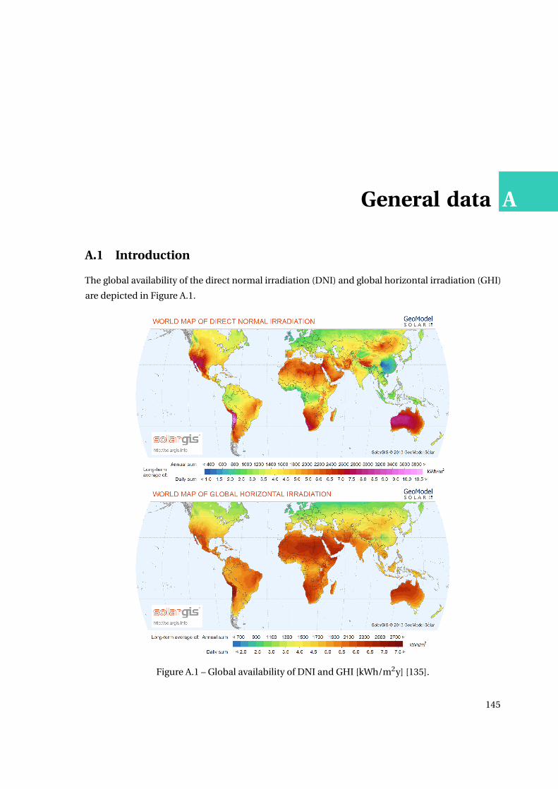
AGeneral data
A.1 Introduction
The global availability of the direct normal irradiation (DNI) and global horizontal irradiation (GHI)
are depicted in Figure A.1.
Figure A.1 – Global availability of DNI and GHI [kWh/m2y] [135].
145


BComprehensive integration method
(Chapter 3)
B.1 Additional results
Figure B.1 shows the primary energy, fuel, electricity, and CO2 emission savings of the non-stop
operation solutions. It can be seen that for all solutions the electricity savings are "negative",
meaning that more electricity is required due to the additional heat pump and MVR units. With
increasing solar installations, the emissions and natural gas consumption are continuously reduced.
The total annual cost and the primary energy savings are decreased with increasing solar system
sizes.
Figure B.1 – Primary energy, fuel, electricity, and CO2 emission savings of non-stop operationsolutions.
147

Appendix B. Comprehensive integration method (Chapter 3)
B.2 Performance parameters and cost functions
B.2.1 Heat exchanger network (HEN) cost estimation
The heat exchanger area is estimated as presented by Kemp [99, 218, 245] (area targeting) based on
vertical intervals placed between the hot and cold composite curves. In each interval the approxi-
mate heat exchanger area is estimated based on the logarithmic mean temperature difference, the
hot and cold average heat transfer coefficients, and the heat transferred within the interval. The
total area AHE Ntot [m2] is found by the summing over all intervals. Estimation of the installed heat
exchanger capital expenses springs from the assumption that all heat exchangers are equal.
C HE Np =
[a+b ·
(AHE N
tot ,p
N HE Nmi n,p
)c]·N HE N
mi n,p (B.1)
The minimum number of heat exchangers (units) N HE Nmi n to be placed in each zone (between pinches)
is estimated following the suggestion of Linnhoff et al. [98] based on graph theory. The cost correla-
tions are taken from Taal et al. [236] reprinted from Hall et al. [237] and can be found in Table B.1 for
retrofit heat exchanger costs. The total cost is calculated for each period p ∈ P and the final installed
cost is then found as the maximum of all periods.
C HE N = maxp
(C HE N
p
)(B.2)
Table B.1 – Heat exchanger network (HEN) cost estimation parameters Hall et al. [237] reprinted byTaal et al. [236](2.33) updated to 2015e, Carbon steel (CS)-CS heat exchangers.
Parameter Symbol Value UnitHeat exchanger cost estimations HENFixed parameter a 9’500 eScaling parameter b 460 e/m2
Non-linear parameter c 0.8 -
B.2.2 Non-renewable technologies
B.2.2.1 Cooling water (CW)
The cooling water is modeled by one cold stream between 15 (Tcwin ) and 17 °C (Tcw
out). The operating
cost are negligible as the cooling water is assumed to origin from a river close by the plant. The
cooling thermal stream is formulated by the following relation, where cCWp [kJ/kgK] is the specific
148

B.2. Performance parameters and cost functions
heat capacity, and mcw, 1 kg/s, is the reference mass flow rate.
QCW = mref,CW ·cCWp · (TCW
out −TCWin
)(B.3)
B.2.2.2 Boiler (BOI)
The boiler heat release is modeled by three streams: air preheating, radiative and convective thermal
power from natural gas combustion. The total heat release is derived by a multiplication of the lower
heating value (LHV) with the reference fuel flow rate including the efficiency. Cooling down the
combustion gases from the adiabatic flame temperature to a pre-defined radiation temperature
defines the radiative component and is displayed as a hot stream at constant temperature (radiation
temperature). The convective component is defined as a hot stream between the radiation tempera-
ture and the exhaust gases outlet temperature. The air preheating is written as a cold stream from
ambient to preheating temperature. This practice has been published by Maréchal and Kalitventzeff
[246] and is applied in the same manner by Becker [140]. The heat release is illustrated below in
Equation B.4.
QBOI =− Qpre
∣∣Tpreh
Ta+ Qrad
∣∣Trad
+ Qconv
∣∣Trad
Tout(B.4)
The parameters are described in Table B.2. The boiler investment cost is set to zero, since it is already
in-place. The natural gas consumption (Equation B.5) is derived from the boiler useful heat release
based on a conversion fraction. The conversion fraction includes the thermal losses as well as the
part of the heat released in the combustion that is dispensed in the exhaust gases and therefore not
delivered to the process as useful heat.
QngBOI = Q
BOI/fBOI (B.5)
Table B.2 – Boiler (BOI) parameters, adapted from Becker [140].
Parameter Symbol Value UnitInvestment (in-place) IVBOI
2 0 e/kWAdiabatic flame temperature Tf
ad 2768 °CRadiation temperature Trad 1027 °CExhaust gases temperature Tout 120 °CAir preheating temperature Tpreh 120 °CRadiative heat load Qrad 28842 kWConvective heat load Qconv 15031 kWAir preheating load Qpreh 1740 kWBoiler conversion fraction fBOI 90 %
149

Appendix B. Comprehensive integration method (Chapter 3)
B.2.2.3 Heat pump superstructure (HPS)
To ensure mass and energy conservation within the heat pump, linear constraints are defined at all
liquid, vapor and superheated vapor points. These constraint are added to the utility targeting con-
straints. These equations are further documented in [167]. The constraints and parameters entering
the mixed integer linear programming (MILP) are derived and depicted in Appendix C.3.1. The
non-linear bare module cost function for compressors COMP [ine, 2010, is not further actualized]
of each heat pump g is formulated after reference [247] reprinted by [140] where the installation
factor was assumed to be 1.5.
C COMP = 1.5 ·1500 ·1600.1 ·(E g ,COMP i→ j
)0.9[e 2010] (B.6)
Where the maximum electricity consumption of compressor from level i → j of heat pump g ,
E g ,COMP i→ j [kW], is provided in Equation B.7 shown for any utility technology w .
E w = Ew · f w (B.7)
Where E w [kW] is the maximum (electrical) power consumption of utility technology w , Ew
[kW] is
the (electrical) power reference consumption of utility technology w , and f w [-] is the maximum
size of technology w . During the MILP problem resolution, the annualized compressor capital costs
as a function of the compressor power rating including the maintenance cost, IVg ,COMP2 , was based
on a linear fitting function of Equation B.6.
Table B.3 – Heat pump parameters.
Parameter Symbol Value UnitHeat pump superstructure (HPS)Investment IVHPS
2 Eq. B.6Temperatures THPS, COND i -2,10,15,20,25,30,35,40,45,50 °CIsentropic compressor efficiency ηisentropic 0.76 -Fluid AmmoniaRefrigeration in-place (REF)Investment IVREF
2 0 e/kWCondenser temperature TREF, CONDi 30 &35 °CEvaporator temperature TREF, EVAP i -2 °CIsentropic compressor efficiency ηisentropic 0.76 -Fluid AmmoniaVapor recompression as proposed by [140] (MVR)Investment IVHP
2 Eq. B.6Condenser temperature TREF, CONDi 76 °CEvaporator temperature TREF, EVAP i 56 °CIsentropic compressor efficiency ηisentropic 0.76 -Fluid Water
150

B.2. Performance parameters and cost functions
B.2.3 Solar technologies
The solar technologies and typical periods clustering are comprehensively discussed in Chapter 2.
B.2.3.1 Solar cost function
The proportional (installed) cost coefficient of a solar technology s is calculated as depicted in
Equation B.8.
IVs2 = finst · IVw
A ·As (B.8)
B.2.3.2 Flat plate thermal collector (FP)
All parameters of the considered flat plate collectors can be found in Table B.4. Figure B.2 shows the
thermal conversion efficiency ηFPp,tot = QFP
p /(gh,p ·AFP) of the thermal energy production of a flat plate
collector QFPp in period p with respect to the global horizontal radiation gh,p in each period p. This
efficiency is comprised of not only the conductive and radiative thermal losses, but also the losses
caused by the non-perpendicular angle of incidence of the sun. Since the collectors are installed
in a fixed position, different angles of inclination need to be tested. The graph indicates clearly
that in some days (e.g. day number four and eight) collectors with 55° inclination outperform the
collectors with smaller inclination angles. This stems from the fact that on these (winter) days the
solar elevation angle is not very high (see Figure 3.5) and collectors installed at higher inclination
can capture more of the incoming radiation. On days in the middle of the summer (e.g. day number
seven and nine), the solar elevation angle is very high and therefore the collectors with the smallest
inclination angles exhibit the best performance. In the end, the total yearly performance is the most
Figure B.2 – Thermal conversion efficiency of flat plate (FP) solar thermal collectors as a functionof time for different inclination angles, input data presented in Table B.4, performance equationsshown in Section 2.3.1.2.
151

Appendix B. Comprehensive integration method (Chapter 3)
important indicator which is displayed in Figure B.2 for all the inclination angles. It is weighted
by the relative occurrence of each typical period in the year. An inclination angle of 35° with an
average efficiency of about 25.3% exhibits the best performance and was therefore chosen for further
analysis. This efficiency is however biased, since it is calculated only when the collector produces
thermal energy. The overall production versus GHI efficiency yields 17.1%.
This average efficiency of the considered flat plate collectors is far below the theoretical maximum
of up to 60%. In this study a balance is struck between performance and capital investment. The
efficiency of single glazed flat plate thermal collectors drops with higher operating temperatures,
lower ambient temperatures, and the inclination of the sun. These insufficiencies are partly over-
come by better insulation or by changing the collector model (e.g. evacuated tube collectors). Both
of these options come at distinctly higher costs (factor 2 and higher [164]) and were, therefore, not
considered.
Table B.4 – Flat plate solar collector (FP) parameters, if no other indication, data taken for singleglazing flat plate collectors from Tehnomont [108] data tested by SPF [164] presented in Table B.4,performance equations presented in Section 2.3.1.2.
Parameter Symbol Value UnitGround reflectivity ρg 0.154 -Heat transfer fluid water glycol mixInvestment cost ([164],2012) IVFP
A 196 e/m2
Installation cost factor fFPinst 1.5 -
Total investment min,max 200,600 e/m2
Collector area AFP 2.059 m2
Standard efficiency/ conversion factor ηFP0 0.74 -
Efficiency coefficient 1 aFP1 3.5940 W/m2K
Efficiency coefficient 2 aFP2 0.00864 W/m2K2
Incidence angle modifier coefficient a 2.40 -Fluid inlet temperature TFP
in 80 °CFluid outlet temperature TFP
out 105 °CSlope Inclination (recommended: similar to latitude) θFP
i 35 °Azimuth, shift towards south γ
FPi 0 °
Thermal field loss factor fFPfield 0.97 -
B.2.3.3 Photovoltaic module (PV)
The photovoltaic modules (PVs) were modeled based on hourly static equations with the assumption
that the transient behavior is negligible. All parameters of the considered for the photovoltaic
modules can be found in Table B.5.
Figure B.3 shows the conversion efficiency from the global horizontal irradiance (GHI) gp,i in each
period p to the electricity produced in the photovoltaic modules ηPVp,tot = EPV
p /(gi,p ·APV), where
EPVp is the electrical production of a PV module in period p. As discussed previously, the GHI only
covers the fraction of the solar radiation that hits the earth at a perpendicular angle. This allows
the conversion efficiency (if it is described in this manner) to exceed the rated efficiency of the PV
152

B.2. Performance parameters and cost functions
modules (e.g. on day 1), since the inclined modules may capture more of the inclined sun rays
than the GHI takes into account. The assessment also changes if shadowing is taken into account,
though this was not considered as a factor in this study. The winter days (1, 4, and 9) show due
to this peculiarity and due to lower ambient temperatures the highest efficiencies. In agreement
with the observation from the plate collectors, it can be seen that higher inclinations are favored in
winter days while lower inclination angles perform better during summer days. The highest overall
efficiency is found for the lowest inclination angle of 30° with an average of 18.5 %. Such efficiencies
may only be reached for high performance PV modules such as the ones assumed. More detailed
modeling, considering shading and conversion losses, will most likely show lower performance
values.
0%
5%
10%
15%
20%
25%
30%
35%
40%
45%
0 24 48 72 96 120 144 168 192 216 240
Eff
icie
ncy
Typical periods
30°
35°
40°
45°
η = 18.5%
18.5%
18.3%
18.1%
Figure B.3 – Electrical conversion efficiency of photovoltaic modules (PVs) as a function of time fordifferent inclination angles, input data presented in Table B.5, performance equations presented inSection 2.3.1.3.
B.2.3.4 High concentration photovoltaic and thermal system (HCPVT)
The high concentration photovoltaic and thermal system (HCPVT) were modeled based on hourly
static equations with the assumption that the transient behavior is negligible. All parameters of the
considered for the HCPVT can be found in Table B.6.
The HCPVT conversion efficiencies are not depicted here as they are assumed to be constant over
time independent from the irradiance and other potentially influencing factors such as the ambient
temperature (active cooling). A comparison between transient and static model was conducted and
the results are depicted in Figure B.4 [110]. The dish thermal efficiency is assumed to approximate
55%, and the electrical efficiency 25%. Constant electrical conversion losses and solar thermal losses
in the field were considered in this study. The average yearly overall efficiency of the HCPVT system
with respect to the DNI was found based on detailed dynamic models, averaging 25%el and 55%th
(total), respectively, which is extremely high and may be overestimated.
153

Appendix B. Comprehensive integration method (Chapter 3)
Table B.5 – Photovoltaic module (PV) parameters, if no other indication, data taken from SunTech[166]. nominal cell operating temperature (NOCT) are a set of conditions which are defined in orderto find the nominal cell operating temperature. Standard testing conditions (STC) are at 1000W/m2,25°C cell temperature and air mass 1.5.
Parameter Symbol Value UnitInvestment cost [248] IVPV
A 260 e/m2
Installation cost factor fPV 1.5 -Total investment min,max 300,800 e/m2
Maximum power EPV,max 290 W
Module area APV 1.63 m2
Module electrical efficiency ηelPV 0.178 -
Temperature reduction factor fPVT 0.004 -/K
Efficiency reduction at g200 = 200W/m2 f200 0.98 -standard testing conditions (STC) temperature TSTC 25 °CSTC radiation gSTC 1000 W/m2
Nominal Operating Cell Temperature TPVNOCT 45 °C
NOCT radiation gNOCT 800 W/m2
NOCT ambient temperature Ta,NOCT 20 °CNOCT wind speed va,NOCT 1 m/sInclination (around latitude) θPV
i 30 °Azimuth, shift towards south γ
PVi 0 °
Effective transmittance-absorptance product τα 0.9 -Electrical conversion factor fPV
gen 0.95 -
Figure B.4 – Comparison of Transient System Simulation Tool [2] (TRNSYS) results and static modelfor HCPVT [110], data shown in Table B.6, static performance equations presented in Section 2.3.1.4.
B.2.3.5 Storage
The storage is detailed in Section 2.4.2, where the thermal storage mass and energy balances are
formulated based on different temperature levels modeled as different interconnected tanks. The
154

B.2. Performance parameters and cost functions
Table B.6 – High concentration photovoltaic and thermal system (HCPVT) parameters, data takenfrom Airlight Energy Holding SA [132].
Parameter Symbol Value UnitHeat transfer fluid water glycol mixInvestment cost IVHCPVT
A 700 e/m2
Dish area AHCPVT 40.05 m2
Installation cost factor fFP 1.5 -Total investment min,max 500,1500 e/m2
Primary efficiency ηHCPVTth,prim 0.5 -
Secondary efficiency ηHCPVTth,sec 0.05 -
Electrical efficiency ηHCPVTel 0.25 -
Fluid temperature primary in THCPVTin,prim 85 °C
Fluid temperature primary out THCPVTout,prim 92 °C
Fluid temperature secondary out THCPVTout,sec 110 °C
Thermal field loss factor fHCPVTfield 0.9 -
Electrical conversion factor fHCPVTgen 0.9 -
implementation relies on the mass storage presented by Moret et al. [141] which is expanded to
represent the thermal behavior.
Performance Figure B.5 illustrates the thermal storage filling in addition to the boiler and solar
dish behavior over a selected range of operating periods. The storage is charged when the availability
of the sun exceeds the process requirements (at around 80% of its total potential) and is consumed
with decreasing solar availability. It can be seen that the solar availability is increased by the storage
or in other words that the boiler utilization is reduced due to the emptying of the tank, which
indicates the advantage of the storage. For higher utilization of the storage, the ε-constraint would
have to be decreased.
0 24 48 72 96 120 144 168 192 216 2400
50
100
150
Vo
lum
e [m
3]
0
500
1000
1500
2000
Th
erm
al p
ow
er [
kW
]
Tc
Th Charge flow Discharge flow Cooling water Solar output Boiler
Operating hours (10 typical days) [h]
Figure B.5 – Thermal storage volume and temperature distribution for the FP collectors non-stopoperation of the industrial process, case 2.1. FPO at ε= 80% of the 2. HPS case.
155

Appendix B. Comprehensive integration method (Chapter 3)
B.3 Weather data & clustering
Follwoing the indications of Domínguez-Muñoz et al. [126] the typical days are built from n clusters
with 2 extreme days. For clustering, 3 indicators are chosen which influence the solar performance
the most: DNI, GHI, and the ambient temperature. Since the DNI fluctuates the most on an hourly,
daily, and monthly basis with a high influence on the solar output, it is chosen as the main reference
for determination of the performance indicator. Also the extreme days are determined based on the
DNI, which means that one extreme day is found for the highest daily radiation and lowest solar
radiation. In Figure 3.5 in the upper corner the typical days and their occurrence are illustrated. The
two last days are extreme days which are represented only once. The operating time of one period is
one hour which leads to 240 operating periods.
Table B.7 displays the yearly average values and mean squared error of the six weather data attributes
of which only three are subject to the clustering. The yearly means of the three attributes that are
used for clustering are very close to the original data and thus the error of the first three indicators is
comparably small. Errors for the outside temperature and the wind speed, however, are distinctly
higher. This may be explained by stronger fluctuations throughout the year even though the ambient
temperature is used as input to the k-medoids clustering.
Table B.7 – Mean data and performance indicators of typical days compared to original.
Attribute Unit Meanoriginal Meantypical mELDC2 10−4
GHI [W/m2] 163.2 163.3 1.685DNI [W/m2] 192.8 190.1 3.242Elevation αs [°] 14.1 13.4 2.603Azimuth γs [°] 44.4 45.2 5.592Ta [°C] 10.7 10.5 51.321va [m/s] 2.1 3.1 100.837
156

B.4. Dairy process
B.4 Dairy process
The process streams as presented by Becker [140] are depicted in Table B.8. A detailed description of
the process model is provided in Appendix D.3.
Table B.8 – Hot and cold streams of the dairy process, reproduced from Becker [140].
Unit Name Tin Tout Q ΔTmin/2 Remarks[°C] [°C] [kW] [°C]
Regrigeration ref 6.0 4.0 76.0 2.0 refrigeration inlet milkPasteurization pasto1a 4.0 66.0 2356.0 2.0 preheating
pasto2a 66.0 86.0 676.4 2.0 pasteurization milkpasto3a 86.0 4.0 2773.2 2.0 refrigeration milkpasto4a 66.0 98.0 119.7 2.0 pasteurization creampasto5a 98.0 4.0 351.6 2.0 refrigeration cream
Concentration eva1 4.0 70.3 504.0 2.0 preheatingeva2 70.3 70.3 904.2 1.2 evaporation 1.effecteva3 66.4 66.4 864.1 1.2 evaporation 2.effecteva4 60.8 60.8 849.8 1.2 evaporation 3.effecteva5 60.8 4.0 151.5 2.0 refrigeration concentrated milkeva6 68.9 68.9 904.2 1.2 condensation 1.effecteva7 65.9 65.9 864.1 1.2 condensation 2.effecteva9 68.9 15.0 87.8 2.0 condensation 3.effecteva10 65.9 15.0 80.8 2.0 cooling condensates 1.effect
Condensates cooling eva8 60.1 60.1 849.8 1.2 cooling condensates 2.effecteva11 60.1 15.0 69.7 2.0 cooling condensates 3.effect
Yoghurt production yog1 4.0 94.0 1026.0 2.0 heatingyog2 94.0 10.0 957.6 2.0 cooling
Desert production des1 4.0 90.0 817.0 2.0 heatingdes2 90.0 70.0 190.0 2.0 cooling
Hot water hw 15.0 55.0 167.2 2.0 hot water prodcutionCleaning in place CIP1a 58.7 70.0 188.6 2.0 maintain temperature CIP1
CIP1b 65.0 15.0 104.5 2.0 recuperation waste heat CIP1CIP2a 67.5 80.0 209.5 2.0 maintain temperature CIP2CIP2b 75.0 15.0 125.4 2.0 recuperation waste heat CIP2
Fridge frig 5.0 5.0 300.0 2.0 maintain storage temperature
157


CGeneric heat pump superstructure
(Chapter 4)
C.1 General
C.1.1 MOGA input parameters
All computations were conducted on a machine with 8-Core Xeon 2.4 GHz processor with 16.0 GB of
RAM. Table C.1 depicts the data used in the multi-objective genetic algorithm (MOGA [217]) from
the Dakota package [216]. Different parameters were used during different runs. Due to danger of
getting trapped in local minima, especially during the extended analysis (in Section 4.3.3) with fluid
selection at the master level, the mutation and crossover parameters were set more aggressively.
These parameters were selected based on a heuristic analysis tracking the propagation of the
non-dominated frontier. Figure C.1 shows the propagation of multi-objective genetic algorithm
(MOGA) and the dominance of each population over the previous indicating that a total of 105
evaluations achieve satisfying convergence for the master level fluid selection, as shown in Figure
C.1a. The dominance change of the slave level fluid selection displayed in Figure C.1b, however,
indicates that after 25,000 iterations, and significant computation time the MOGA has not reached
convergence. These results further support the conclusions derived in Section 4.3.3.1, that the
master level selection if more efficient.
Table C.1 – Input parameters for MOGA method [217].
Parameter Expression Value Comment
Initial population population_size 300, 500 initial set of individuals (section 4.3.2, 4.3.3)Crossover type crossover_type ’shuffle_random’ (section 4.3.2) select one of each design var. of the parents for child
’multi_point_binary 2’ (section 4.3.3) bit switching at 2 pnts. in the binary encoded genome of two parentsCrossover rate crossover_rate 0.9 crossover rate of new generationMutation type mutation_type ’replace_uniform’, (section 4.3.2) randomly choosing variable and reassigning it to a random valid value
’bit_random’ (section 4.3.3) flips a randomly chosen bit in the string of randomly chosen variableMutation rate mutation_rate 0.1, 0.2 (section 4.3.2, 4.3.3)Maximum iteration max_iterations 100, 200×103 maximum number of iteration unless convergence is reached (section 4.3.2, 4.3.3)Convergence type convergence_type ’average_fitness_tracker’Percent change percent_change 0.1 (default) percent change in non-dominated frontier
159
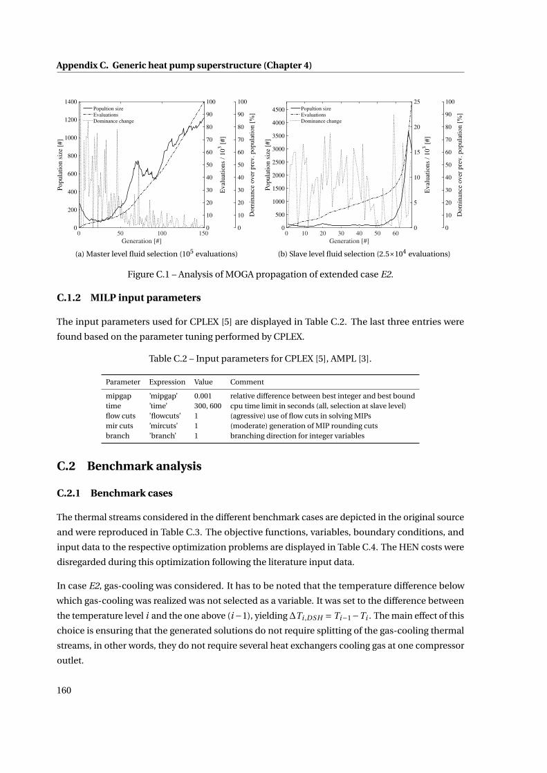
Appendix C. Generic heat pump superstructure (Chapter 4)
0 50 100 150
Generation [#]
0
200
400
600
800
1000
1200
1400
Popula
tion s
ize
[#]
0
10
20
30
40
50
60
70
80
90
100
Eval
uat
ions
/ 10
3 [
#]
Popultion size
Evaluations
Dominance change
0
10
20
30
40
50
60
70
80
90
100
Dom
inan
ce o
ver
pre
v. popula
tion [
%]
(a) Master level fluid selection (105 evaluations)
0 10 20 30 40 50 60
Generation [#]
0
500
1000
1500
2000
2500
3000
3500
4000
4500
Popula
tion s
ize
[#]
0
5
10
15
20
25
Eval
uat
ions
/ 10
3 [
#]
Popultion size
Evaluations
Dominance change
0
10
20
30
40
50
60
70
80
90
100
Dom
inan
ce o
ver
pre
v. popula
tion [
%]
(b) Slave level fluid selection (2.5×10⁴ evaluations)
Figure C.1 – Analysis of MOGA propagation of extended case E2.
C.1.2 MILP input parameters
The input parameters used for CPLEX [5] are displayed in Table C.2. The last three entries were
found based on the parameter tuning performed by CPLEX.
Table C.2 – Input parameters for CPLEX [5], AMPL [3].
Parameter Expression Value Comment
mipgap ’mipgap’ 0.001 relative difference between best integer and best boundtime ’time’ 300, 600 cpu time limit in seconds (all, selection at slave level)flow cuts ’flowcuts’ 1 (agressive) use of flow cuts in solving MIPsmir cuts ’mircuts’ 1 (moderate) generation of MIP rounding cutsbranch ’branch’ 1 branching direction for integer variables
C.2 Benchmark analysis
C.2.1 Benchmark cases
The thermal streams considered in the different benchmark cases are depicted in the original source
and were reproduced in Table C.3. The objective functions, variables, boundary conditions, and
input data to the respective optimization problems are displayed in Table C.4. The HEN costs were
disregarded during this optimization following the literature input data.
In case E2, gas-cooling was considered. It has to be noted that the temperature difference below
which gas-cooling was realized was not selected as a variable. It was set to the difference between
the temperature level i and the one above (i −1), yielding∆Ti ,DSH = Ti−1−Ti . The main effect of this
choice is ensuring that the generated solutions do not require splitting of the gas-cooling thermal
streams, in other words, they do not require several heat exchangers cooling gas at one compressor
outlet.
160

C.2.
Ben
chm
arkan
alysis
Table C.3 – Streams data of the three benchmark cases.
(a) E2 [101] (b) Ethylene [186] (c) Cold Tray [205]
Stream name Tin Tout Q α
K K kW/K kW/m2K
Process
H1 360 320 10 1H2 320 250 10 1C1 260 310 15 1C2 300 360 10 1
Utilities K K
Water for cooling 300 310 0.56Water for heating∗ 300 290 0.56Steam 440 440 0.56
Stream name Tin Tout Q α
K K kW kW/m2K
Process
H1 408 312 -1186 1H2 375 312 -466 1H3 375 312 -387 1H4 375 312 -380 1H5 375 290 -572 1H6 269 260 -20 1H7 168 158 -157 1H8 258 256.8 -381 1H9 313 313 -224 1H10 307 307 -141 1H11 234 234 -1081 1H12 290 230 -451 1C1 393 440 111 1C2 277 302 174 1C3 158 311 208 1C4 346 360 516 1C5 436 498 448 1C6 315 358 133 1C7 252 256 1120 1C8 247 298 96 1
Utilities K K
Cooling water for cooling 297.1 300 0.56Cooling water for heating∗ 297.1 294.2 0.56Steam LP 411 411 1
Stream name Tin Tout Q α
K K kW kW/m2K
Process
H1 -10.7 -10.7 -400.70 1H2 -28.9 -28.9 -823.38 1H3 51.5 51.5 -4285.30 1C1 67.9 67.9 870.83 1C2 -3 -3 758.94 1C3 62.5 62.5 4229.65 1
Utilities K K
Cooling water for cooling 295 300 0.56Cooling water for heating∗ 295 290 0.56Steam 138 13882 1
161
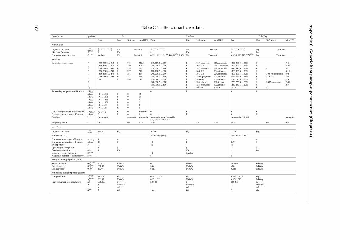
Ap
pen
dix
C.
Gen
erich
eatpu
mp
sup
erstructu
re(C
hap
ter4)
Table C.4 – Benchmark case data.
Description Symbols E2 Ethylene Cold Tray
Data Unit Reference min(HPS) Data Unit Reference min(HPS) Data Unit Reference min(HPS)
Master level
Objective function f objmaster
C opex ,C capex
$/y Table 4.6
C opex ,C capex
$/y Table 4.6
C opex ,C capex
$/y Table 4.6
HEN cost function C HE N 0 $/y 0 $/y 0 $/y
Compressor cost function C COMP as slave $/y Table 4.6 0.15 ·1,925 · (E COMP[kWel])0.963
[186] $/y Table 4.6 0.15 ·1,925 · (E COMP)0.963
$/y Table 4.6
Variables
Saturation temperature T1 300,300.5, ...,313 K 313 312.5 310,310.5, ...,310 K 310, ammonia 310, ammonia 333,333.5, ...,353 K - 344T2 290,290.5, ...,310 K 300 298.5 250,250.5, ...,290 K 307, r22 265.5, ammonia 323,323.5, ...,353 K - 338.5T3 280,280.5, ...,300 K 288 283 230,230.5, ...,280 K 297, ammonia 246, ammonia 313,313.5, ...,343 K - 331T4 265,265.5, ...,285 K 277 272 220,220.5, ...,260 K 266, r22 234, ethane 303,303.5, ...,333 K - 321.5T5 250,250.5, ...,270 K 254 254 200,200.5, ...,240 K 256, r22 224, ammonia 293,293.5, ...,323 K 303, r22,ammonia 302T6 245,245.5, ...,265 K 247 248 190,190.5, ...,230 K 256.8, propylene 205, ethane 283,283.5, ...,313 K 274, r22 298T7 240 K 240 240 170,170.5, ...,210 K 246.8, r22 189, ethane 273,273.5, ...,303 K - 273T8 160,160.5, ...,200 K 234, ethane 180.5, ethane 253,253.5, ...,283 K 259.5, ammonia 259.5T9 150,150.5, ...,190 K 224, propylene 172, ethane 243,243.5, ...,273 K 257T10 148 K ethane ethane 241.3 K r22
Subcooling temperature difference ∆Ti ,SC 0 K 0 K∆T1,SC 0, 1,..., 20 K 0 14∆T2,SC 0, 1,..., 20 K 0 15∆T3,SC 0, 1,..., 15 K 0 0∆T4,SC 0, 1,..., 15 K 0 2∆T5,SC 0, 1,..., 5 K 0 0∆T6,SC 0, 1,..., 5 K 0 0
Gas-cooling temperature difference ∆Ti ,DSH Ti−1 −Ti K 0 as shown 0 K 0 KPreheating temperature difference ∆Ti ,PRE 0 K 0 0 0 K 0 KFluid set F ammonia ammonia ammonia ammonia, propylene, r22, ammonia, r12, r22 ammonia
r13, ethane, ethyleneWeighting factor ξ [0,1] - 0.5 0.47 [0,1] - 0.5 0.87 [0,1] - 0.5 0.74
Slave level
Objective function f objslave wT AC $/y wT AC $/y wT AC $/y
Parameters [101] Parameters [186] Parameters [205]
Compressor isentropic efficiency ηisentropic 1 - 1 - 1 -Minimum temperature difference ∆Tmin 10 K 10 K 2.78 KSet of periods P 1 - 1 - 1 -Operating time of period ∆t1 1 y 1 y 1 yOccurence of period occ1 1 1/y 1 1/y 1 1/yMaximum compression ratio CPmax 10 bar/barMaximum number of compressors nmax 5 - 5 -
Yearly operating expenses (opex)
Steam production OPSTEAM2 50.91 $/kW/y 0 $/kW/y 56.2866 $/kW/y
Electricity grid OPGRID2 608.33 $/kW/y 336 $/kW/y 420 $/kW/y
Cooling water OPCW2 15.97 $/kW/y 6.011 $/kW/y 6.011 $/kW/y
Annualized capital expenses (capex)
Compressor cost IVCOMP1 2824.8 $/y 0.15 · 3,787.4 $/y 0.15 · 3,787.4 $/y
IVCOMP2 831.67 $/kW/y 0.15 · 1,573 $/kW/y 0.15 · 1,573 $/kW/y
Heat exchanger cost parameters a,b 500, 0.8 $, - 500, 0.8 $, - 500, 0.8 $, -U 1 kW/m2K 1 kW/m2K 1 kW/m2KA 1 m2 1 m2 1 m2
Qmin 7 kW 100 kW 7 kW
162

C.2. Benchmark analysis
C.2.2 Extended case E2
The thermal streams considered in this case are depicted in Table C.3(a). Figure C.2a shows the
parallel coordinates information generated with the tool from Kermani et al. [220]. The global
warming potential (GWP) of most selected Hydrofluorocarbonss (HFCs) (r407c, r404a, r410a, r507a)
is above 1500 [249] compared to hydrogen sulfide and natural refrigerants (ammonia (r717), propane
(r290), propylene (r1270)) with GWP of below 10 [249, 250] and lower-impact HFCs such as r161 (12
[251]) and r41 (97 [252]). The objective functions, variables, boundary conditions, and input data
to the extended case E2 are displayed in Table C.5. Figure C.2b depicts the temperature entropy
diagram of the optimized HPS solution. Figure C.3a displays the integrated composite curves of
the extended case. In the reference case, cooling water is required to cool the highest condenser
level which is increased compared to the benchmark case due to the lower compressor isentropic
efficiency. Since the cooling water outlet temperature is above the condenser temperature, part of it
needs to be heated by the hot utility. Figure C.3b presents a flowsheet of the minimum TAC case.
The two HEN design of the reference and optimized case is shown in Figure C.4. It has to be noted
that the HPS solution requires one more heat exchangers which is mildly penalized by the HEN cost
function thereby being outweighed by the benefits of the reduced opex.
(a) Relevant data of selected fluids. Parallel coordinatesselection platform [220] (thermodynamic properties:CoolProp [208] GWP data: [249–252]).
(b) Temperature entropy diagram of the minimumTAC solution.
Figure C.2 – Set of selected fluids considered during multi-objective optimization.
163

Appendix C. Generic heat pump superstructure (Chapter 4)
-450 -400 -350 -300 -250 -200 -150
Heat load [kW]
-0.2
-0.15
-0.1
-0.05
0
0.05
0.1
0.15C
arn
ot
facto
r 1
-Ta/T
[-]
245
252
259
265
272276
283
289
295
301305310315
Co
rrecte
d t
em
peratu
res
[K]
E2 extended
process
Reference utilities
min(HPS) utilities
cooling water
(a) Integrated composite curves of optimized and refer-ence case.
(b) Flowsheet of optimumcase.
Figure C.3 – Extended case E2 minimum TAC solution.
Table C.5 – Optimization problem description: extended case E2.
Description Symbols Data Unit Reference min(HPS)
Master level
Objective function f objmaster
C OPE X ,CC APE X
$/y 56 005 49 944
132 608 121 840Heat exchanger cost function (estimation) C HE N C HE N Table 4.3 $/y 58 800 57 800HEN design $/y 52 800 53 600
c1 fitted [101] 0 $c2 fitted [101] 500 $/yc3 fitted [101] 0.8 -
VariablesSaturation temperature Ti = Ti+1 + ∆Ti
∆T1 5,5.5, ...,40 K 13 9∆T2 5,5.5, ...,40 K 12 11.5∆T3 5,5.5, ...,40 K 11 13∆T4 5,5.5, ...,40 K 23 25∆T5 5,5.5, ...,40 K 7 8.5∆T6 5,5.5, ...,40 K 7 7.5T7 240 K 240 240
Subcooling temperature difference∆T1,SC 0, 1,..., 20 K 0 12∆T2,SC 0, 1,..., 20 K 0 0∆T3,SC 0, 1,..., 15 K 0 0∆T4,SC 0, 1,..., 15 K 0 11∆T5,SC 0, 1,..., 10 K 0 0∆T6,SC 0, 1,..., 10 K 0 0
De-superheating temperature difference ∆Ti ,DSH Ti−1 −Ti K 0 as indicatedPreheating temperature difference ∆Ti ,PRE 0 K 0 0Fluid set F ammonia,r161,h2s,propane,propylene, ammonia propane
r407c,r404a,r410a,r507a,r41Weighting factor ξ [0,1] - 0.5 0.58
Slave level
Objective function f objslave wT AC $/y
Parameters
Compressor isentropic efficiency ηisentropic 0.7 -Minimum temperature difference ∆Tmin 10 KSet of periods P 1 -Operating time of period ∆t1 1 yOccurence of period occ1 1 1/yMaximum compression ratio CPmax 8 bar/bar
Opex
Steam production OPSTEAM2 50.91 $/kW/y
Electricity grid OPGRID2 608.33 $/kW/y
Cooling water OPCW2 15.97 $/kW/y
Capex
Compressor cost IVCOMP1 2824.8 $/y
IVCOMP2 831.67 $/kW/y
164

C.3. Heat pump superstructure
(a) HEN design of extended reference case E2.
(b) HEN design of extended case E2 minimum TAC solution.
Figure C.4 – HEN design of extended case E2 with Aspen Energy Analyzer [253].
C.3 Heat pump superstructure
C.3.1 Heat pump parameters in targeting problem (MILP)
C.3.1.1 HPS parameters entering the utility targeting
In the following formulations, the heat and electricity consumption or production of the heat pump
utilities is described for a reference mass flow rate which is to say, a fixed size. These parameters
enter into the utility targeting constraints Equation 2.14-2.16 where they are multiplied with sizing
factors.
The heat release in a condenser (COND) at saturation temperature Ti of heat pump g for a reference
flow rate mref [kg/s] is composed of three parts: de-superheating from the preheating level Ti ,PRE
[K], condensation at the saturation temperature, and subcooling between saturation and subcooling
165
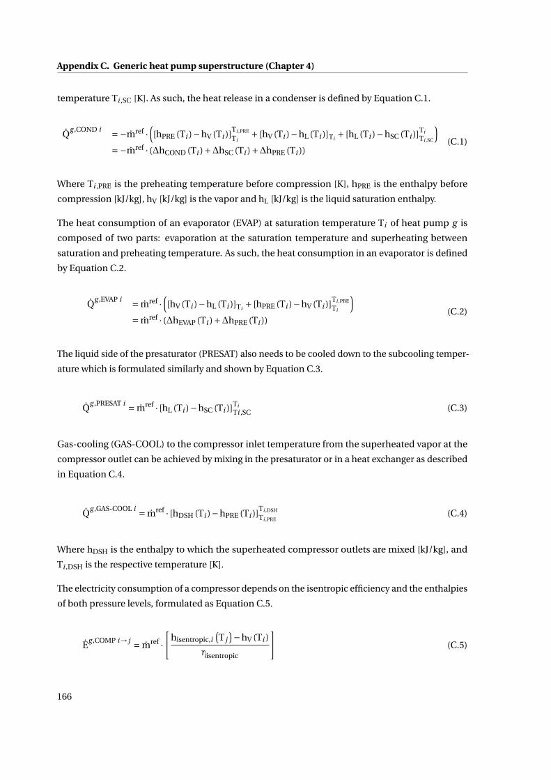
Appendix C. Generic heat pump superstructure (Chapter 4)
temperature Ti ,SC [K]. As such, the heat release in a condenser is defined by Equation C.1.
Qg ,COND i =−mref ·
([hPRE (Ti )−hV (Ti )]
Ti ,PRE
Ti+ [hV (Ti )−hL (Ti )]Ti
+ [hL (Ti )−hSC (Ti )]TiTi ,SC
)=−mref · (∆hCOND (Ti )+∆hSC (Ti )+∆hPRE (Ti ))
(C.1)
Where Ti ,PRE is the preheating temperature before compression [K], hPRE is the enthalpy before
compression [kJ/kg], hV [kJ/kg] is the vapor and hL [kJ/kg] is the liquid saturation enthalpy.
The heat consumption of an evaporator (EVAP) at saturation temperature Ti of heat pump g is
composed of two parts: evaporation at the saturation temperature and superheating between
saturation and preheating temperature. As such, the heat consumption in an evaporator is defined
by Equation C.2.
Qg ,EVAP i = mref ·
([hV (Ti )−hL (Ti )]Ti
+ [hPRE (Ti )−hV (Ti )]Ti ,PRE
Ti
)= mref · (∆hEVAP (Ti )+∆hPRE (Ti ))
(C.2)
The liquid side of the presaturator (PRESAT) also needs to be cooled down to the subcooling temper-
ature which is formulated similarly and shown by Equation C.3.
Qg ,PRESAT i = mref · [hL (Ti )−hSC (Ti )]Ti
Ti ,SC (C.3)
Gas-cooling (GAS-COOL) to the compressor inlet temperature from the superheated vapor at the
compressor outlet can be achieved by mixing in the presaturator or in a heat exchanger as described
in Equation C.4.
Qg ,GAS-COOL i = mref · [hDSH (Ti )−hPRE (Ti )]
Ti ,DSH
Ti ,PRE(C.4)
Where hDSH is the enthalpy to which the superheated compressor outlets are mixed [kJ/kg], and
Ti ,DSH is the respective temperature [K].
The electricity consumption of a compressor depends on the isentropic efficiency and the enthalpies
of both pressure levels, formulated as Equation C.5.
Eg ,COMP i→ j = mref ·
[hisentropic,i
(T j
)−hV (Ti )
ηisentropic
](C.5)
166

C.3. Heat pump superstructure
Where hisentropic,i (T j ) [kJ/kg] is the isentropic enthalpy after compression from saturated vapor at
temperature level Ti to (saturation) temperature level T j , and ηisentropic is the isentropic compressor
efficiency [-]. The HPS stream properties are depicted in Table C.6.
Table C.6 – Data of streams of the heat pump superstructure (HPS).
Unit Name Tin Tout |∆Q| α
K K kJ/kg kW/m2K
Condenser condensation Ti Ti hV (Ti )−hL (Ti ) 1.6sub-cooling Ti Ti ,SC hL (Ti )−hSC (Ti ) 0.56de-superheating Ti ,PRE Ti hPRE (Ti )−hV (Ti ) 0.06
Evaporator evaporation Ti Ti hV (Ti )−hL (Ti ) 3.6preheating Ti Ti ,PRE ∆hPRE (Ti ) 0.06
Gas-cooler gas-cooling Ti ,DSH Ti ,PRE hDSH (Ti )−hPRE (Ti ) 0.06Presaturator sub-cooling Ti Ti ,SC hL (Ti )−hSC (Ti ) 0.56
C.3.2 Heat pump specific constraints
In the following the heat pump specific linear equations at the slave level are introduced. The
respective units, streams and relations are depicted in Figure C.5.
i
i+1
i-1
i+2
1
2
73
5
6
4
evap i+1
mix i+1
presat i-1->i
cond i
de-sup mix i+1
gas-cool i
comp i+2->i
1 presaturator 2 condenser3 mixer4 evaporator5 gas-cooling (heat exchanger)6 compressor7 de-superheating (mixing)
Legend
TiTi,SC
thermal stream
L liquid balance
VS superheated vapor
V saturated vapor
mass stream
pressure level
Ti,DSH
Entropy [kJ/kgK]
T [
°C]
Ti,PRE
Figure C.5 – Temperature-entropy diagram with mass and energy balances of the HPS.
Liquid mass balance The liquid mass balance at temperature level i can be at saturated or sub-
cooled conditions depending whether ∆Ti , SC > 0 (sub-cooled) or ∆Ti , SC = 0 (saturated). It is shown
in Equation C.6 of heat pump g and is composed of:
• the positive contribution from the potential condenser (COND) at level i
• the negative contribution from the potential evaporator (EVAP) at level i
• the positive contribution of the liquid fraction of all valves in combination with presaturators
(PRESAT) that end at level i
• the negative contribution from all valves that exit from level i
167

Appendix C. Generic heat pump superstructure (Chapter 4)
• the negative contribution of the fraction of liquid that may be used to de-superheat the
compressor outlets (mix) at level i (MIX)
f g ,COND ip − f g ,EVAP i
p +i−1∑j=1
(1−xg , j→i
V
)· f g ,PRESAT j→i
p −nl∑
k=i+1f g , PRESAT i→kp − f g ,MIX i
p = 0
∀i ∈ L, g ∈ G, p ∈ P(C.6)
Where
G set of heat pumps g consisting of one fluid dL set of heat pump saturation temperature levels 1,2,3, ...,nl
f g ,COND ip condenser (COND) sizing factor of heat pump g (containing fluid f) during period p
f g ,EVAP ip evaporator (EVAP) sizing factor of heat pump g during period p
f g ,MIX ip mixer (MIX) sizing factor of heat pump g during period p
f g ,PRESAT j→ip presaturator (PRESAT) after expansion from temperature level j → i sizing factor of heat pump g during period p
xg , j→iV vapor fraction after expansion from temperature level j → i of heat pump g
hg ,iSC [kJ/kg] enthalpy at subcooled or saturated temperature level Ti , SC = Ti −∆Ti , SC of heat pump g
Liquid energy balance The liquid energy balance in Equation C.7 is trivial because all streams
enter and exit at the same state of matter and temperature.(f g ,COND i
p − f g ,EVAP ip +
i−1∑j=1
(1−xg , j→i
V
)· f g ,PRESAT j→i
p −nl∑
k=i+1f g ,PRESAT i→kp − f g ,MIX i
p
)·hg ,i
SC = 0
∀i ∈ L, g ∈ G, p ∈ P
(C.7)
Vapor mass balance The vapor mass balance at temperature level i can be at saturated or super-
heated conditions depending whether ∆Ti , PRE > 0 (superheated) or ∆Ti , PRE = 0 (saturated). It is
shown in Equation C.8 of heat pump g and is composed of:
• the positive contribution from the potential evaporator at level i
• the negative contribution from the potential condenser at level i
• the negative contribution from all compressors that exit from level i
• the potential incoming mass flow related to the potential gas-cooling (GAS-COOL) heat ex-
changer unit from the superheated mass balance at level i
• the potential positive contribution from a de-superheating (DE-SUP) through mixing unit at
level i
f g ,EVAP ip − f g ,COND i
p −i−1∑j=1
f g ,COMP i→ jp + f g ,DE-SUP i
p + f g ,GAS-COOL ip = 0
∀i ∈ L, g ∈ G, p ∈ P(C.8)
Where
The energy balance in this case is trivial, since all streams enter and exist at hg ,iPRE [kJ/kg], the enthalpy
168

C.3. Heat pump superstructure
f g ,COMP i→ jp sizing factor of compressor from level i → j sizing factor of heat pump g during period p
f g ,DE-SUP ip sizing factor of the de-superheating(DE-SUP) through mixing unit of heat pump g during period p
f g ,GAS-COOL ip sizing factor of the gas-cooling (GAS-COOL) heat exchanger of heat pump g during period p
at preheated or saturated temperature level Ti ,PRE = Ti +∆Ti ,PRE of heat pump g . This balance is
not displayed here.
Superheated vapor mass balance The superheated vapor mass balance at temperature level i
is conducted at superheated conditions Ti ,DSH = Ti +∆Ti ,DSH. It is shown in Equation C.9 of heat
pump g and is composed of:
• the positive contributions of each compressor entering level i
• the positive contribution of the vapor fraction of all valves in combination with presaturators
that end at level i
• the negative contribution from the gas-cooling and de-superheating through mixing units at
level i
• and the positive contribution from the liquid mixing unit at level i
nl∑k=i+1
f g ,COMP k→ip +
i−1∑j=1
xg , j→iV · f g ,PRESAT j→i
p − f g ,GAS-COOL ip − f g ,DE-SUP i
p + f g ,MIX ip = 0
∀i ∈ L, g ∈ G, p ∈ P(C.9)
Superheated vapor energy balance The energy balance given in Equation C.10 ensures that re-
gardless of which compressor is active, the starting point for de-superheating is always fixed. This
constraint ensures energy conservation and linearity in the problem formulation.
nl∑k=i+1
f g ,COMP k→ip ·hg ,COMP k→i
out − f g ,GAS-COOL ip ·hg ,i
DSH − f g ,DE-SUP ip ·hg ,i
PRE + f g ,MIX ip ·hg ,i
SC = 0
∀i ∈ L, g ∈ G, p ∈ P(C.10)
Where
hg ,iPRE [kJ/kg] enthalpy at preheated or saturated temperature level Ti ,PRE = Ti +∆Ti , PRE of heat pump g
hg ,iDSH [kJ/kg] superheated vapor enthalpy at point Ti ,DSH = Ti +∆Ti ,DSH
hg ,COMP k→iout [kJ/kg] outlet enthalpy of compressor from level k to i
169


DGeneralization (A) - heat pumping and
co-generation (Chapter 5)
D.1 General
D.1.1 MOGA input parameters
All computations were conducted on a machine with 8-Core Xeon 2.4 GHz processor with 16.0
GB of RAM. Table D.1 depicts the data used in the multi-objective genetic algorithm (MOGA [217])
from the Dakota package [216]. Different parameters were used during different runs. Due to
danger of getting trapped in local minima, especially during the extended analysis (in Section
4.3.3) with fluid selection at the master level, the mutation and crossover parameters were set more
aggressively. These parameters were selected based on a heuristic analysis tracking the propagation
of the non-dominated surface. Figure D.1 shows the propagation of MOGA and the dominance of
each population over the previous indicating that after generation 40 the weighted sum of objectives
does not propagate very much any more which could explain the dominance of ε-constraint. ε-
constraint propagates continuously until the stopping criterion (at 1.5×10⁵ evaluations) is reached.
This might indicate that longer runtimes could generate improved solutions, however, reaching
already 40 hours of runtime, this option is currently neglected.
Table D.1 – Input parameters for MOGA method [217].
Parameter Expression Value Comment
Initial population population_size 500 initial set of individualsCrossover type crossover_type ’shuffle_random’ select one of each design var of the parents for child (*)Crossover rate crossover_rate 0.9 crossover rate of new generationMutation type mutation_type ’replace_uniform’, randomly choosing variable and reassigning it to a random valid value (*)Mutation rate mutation_rate 0.1Maximum iteration max_iterations 150e3 maximum number of iteration unless convergence is reachedConvergence type convergence_type ’average_fitness_tracker’Percent change percent_change 0.1 (default) percent change in non-dominated frontier
(*) recommended for MOGA in the reference manual
171

Appendix D. Generalization (A) - heat pumping and co-generation (Chapter 5)
0 20 40 60 80 100
Generation [#]
0
200
400
600
800
1000
1200
1400
1600
1800
2000
Po
pu
lati
on
siz
e [#
]
0
50
100
150
Ev
alu
atio
ns
/ 1
03 [
#]
Popultion size
Evaluations
Dominance change
0
10
20
30
40
50
60
Do
min
ance
ov
er p
rev
. p
op
ula
tio
n [
%]
(a) ε-constraint.
0 20 40 60 80 100
Generation [#]
0
200
400
600
800
1000
1200
1400
1600
1800
2000
Po
pu
lati
on
siz
e [#
]
0
50
100
150
Ev
alu
atio
ns
/ 1
03 [
#]
Popultion size
Evaluations
Dominance change
0
5
10
15
20
25
30
35
40
45
Do
min
ance
ov
er p
rev
. p
op
ula
tio
n [
%]
(b) Weighted sum of objectives
Figure D.1 – Analysis of MOGA propagation of plant x = 2.
D.1.2 MILP input parameters
The input parameters used for CPLEX [5] are displayed in Table D.2. The last three entries were
found based on the parameter tuning performed by CPLEX.
Table D.2 – Input parameters for CPLEX [5], AMPL [3].
Parameter Expression Value Comment
mipgap ’mipgap’ 0.005 relative difference between best integer and best boundtime ’time’ 300 cpu time limit in secondsflow cuts ’flowcuts’ 1 (agressive) use of flow cuts in solving MIPsmir cuts ’mircuts’ 1 (moderate) generation of MIP rounding cutsbranch ’branch’ 1 branching direction for integer variables
D.2 Additional results
D.2.1 Sampling in detail
The results from the sampling are depicted in Figure D.2 and Figure D.3. Figure D.2a compares the
number of evaluations and number of identified solutions (by deriving the non-dominated frontiers)
found with the different sampling algorithms. The sample size is set to 80,000 from which samples
with an electricity to natural gas price ratio of above 8 and below 1 are removed. The factorial
combination of the bounds (of the parameter ranges) is added to the sample size. Brute forcing
indicates manually selected parameter spacing (with different degree fineness) and evaluating
every combination of these. Naturally, the (finest grid) brute forcing requires the largest number of
evaluations as indicated in Figure D.2a. However, investigating the intersection of the Pareto points
identified by the different algorithms yields almost 100% overlap as shown in Figure D.2. Hence,
172

D.2. Additional results
the Matlab [137] intrinsic latin hypercube sampling [233] is suggested and applied within the study.
Figure D.3 shows the histogram and cumulative sum of the occurrences of the different solutions
during the sampling process. If all Pareto solutions are selected, a reduction with respect to the
original of 1-239/239 = 0% is be achieved. If further reduction of the selected solutions is desired,
the histogram can be used as an indicator. It shows that 170, 121, and 95 solutions represent 99%,
95%, and 90% of the occurrences of the Pareto points thereby achieving a reduction of 29%, 49%,
and 60%.
Latin hypercube (L
H)
Orthogonal (O
)
Sobol (S)
Halton (H
AL)
Hammersley (H
AM)
Uniform
(U)
LHround
Or
Sr
HALr
HAMr
Ur
Brute
Bruterough
Bruterougher
0
20
40
60
80
100
[%]
Max. evaluations = 222264Max. sel. solutions: 239 / 239
Evaluations (%max
) Evaluations after price constr. (%max
) Intersection of Pareto pts. (%max
) Difference of Pareto pts. (%max
)
(a) Number of evaluations, and intersection/ difference with max. selected solu-tions.
-50 0 50 100 150
Net electricity [%]
10
20
30
40
50
60
70
80
90
100
Net
nat
. g
as [
%]
Latin hypercube (LH)
Orthogonal (O)
Sobol (S)
Halton (HAL)
Hammersley (HAM)
Uniform (U)
LHround
Or
Sr
HALr
HAMr
Ur
Brute
Bruterough
Bruterougher
(b) All Pareto solutions.
Figure D.2 – Selection of solutions with different sampling algorithms.
0 20 40 60 80 100 120 140 160 180 200 220
Solutions
0
2
4
6
8
10
Occ
urr
ence
of
solu
tio
ns
[%to
tal]
0
10
20
30
40
50
60
70
80
90
100
Cum
ula
tiv
e su
m [
%to
tal]Orig. number of solutions: 239
Latin hypercube (LH)
Orthogonal (O)
Sobol (S)
Halton (HAL)
Hammersley (HAM)
Uniform (U)
LHround
Or
Sr
HALr
HAMr
Ur
Brute
Bruterough
Bruterougher
1 2 3 4
Solutions
0
1
2
Occ
. [%
tota
l]
Figure D.3 – Histogram and cumulative sum of occurrences.
D.2.2 Solution generation & pruning: remaining plants
The results from the multi-objective optimization problem with ε-constraint introduced in Sec-
tion 5.3.2 and 5.3.3, are depicted as surfaces of non-dominated solutions in Figure D.4 for the
remaining plants (plant 1, Figure D.4a; plant 2 with fixed HEN, Figure D.4b; plant 3, Figure D.4c).
The resource plane1 reveals a non-dominated frontier between the natural gas and electricity
consumption. The original plant with its reference consumption is marked at highest total resource
consumption with zero capital cost. Every other solution improves either the electricity or natural
1 The resource plane refers to the plane formed with the two types of resource consumption as axes, and hence spansthe natural gas and electricity consumption.
173

Appendix D. Generalization (A) - heat pumping and co-generation (Chapter 5)
gas consumption. As expected, it can be observed that the solutions of plant 2 with a fixed HEN,
ΔTmin/2=5K, in Figure D.4b are further away from the infeasible region as compared to Figure 5.9b.
Due to the fixed HEN and therewith no further possibility for process heat recovery, the resource
consumption cannot be as strongly reduced as for the case of process heat recovery.
The plants have different resource consumption ranges. While plant 1 in Figure D.4a shows the
highest natural gas consumption, the highest electricity consumption is shown in Figure D.4b. The
lowest resource consumption is displayed by plant 3 in Figure D.4c. These values are linked to the
plant requirements shown in Figure 5.7 and Table 5.3. Plant 1 has the highest hot minimum energy
requirement (MER), while plant 3 does not contain a concentrated milk production unit and has,
therefore, the lowest MER and resource consumption.
-100 0 100 200 300 400 500
Net electricity [kW]
0
500
1000
1500
2000
Net
gas
[kW
]
Infeasible region
0
0.2
0.4
0.6
0.8
1
1.2
1.4
1.6
1.8
2
2.2
2.4
Cap
ex [
M$
]
Reference
(a) Plant 1.
-100 0 100 200 300 400 500
Net electricity [kW]
0
200
400
600
800
1000
1200
1400
1600
1800
2000
Net
gas
[kW
]
Infeasible region
0
0.2
0.4
0.6
0.8
1
1.2
1.4
1.6
1.8
2
2.2
2.4
2.6
Cap
ex [
M$
]
Reference
(b) Plant 2,ΔTmin/2=5K.
-100 0 100 200 300 400
Net electricity [kW]
0
500
1000
1500
Net
gas
[kW
]
Infeasible region
0
0.2
0.4
0.6
0.8
1
1.2
1.4
1.6
1.8
2
2.2
Cap
ex [
M$
]
Reference
(c) Plant 3.
Figure D.4 – Solution generation.
Figure D.5 shows the occurrence of all minimum TAC solutions selected during the sampling step of
the different plants: plant 1 (Figure D.5a), plant 2 with fixed HEN (Figure D.5b), plant 3 (Figure D.5c).
Relatively few solutions are never selected and therefore discarded. The encircled points mark the
99 percentile of the most recurrent solutions. A similarity between the patterns of selected solutions
is observed, indicating, that the solutions at the edges of the surface are the surface of solutions are
the most promising ones.
-100 0 100 200 300 400 500
Net electricity [kW]
0
500
1000
1500
2000
Net
nat
. g
as [
kW
]
Final population
Sampled pareto points
Most occurring 99%0
0.5
1
1.5
2
2.5
3
Occ
urr
ence
[%
tota
l]
(a) Plant 1.
-100 0 100 200 300 400 500
Net electricity [kW]
0
200
400
600
800
1000
1200
1400
1600
1800
2000
Net
nat
. g
as [
kW
]
Final population
Sampled pareto points
Most occurring 99%0
0.5
1
1.5
2
2.5
3
Occ
urr
ence
[%
tota
l]
(b) Plant 2,ΔTmin/2=5K.
-100 0 100 200 300 400
Net electricity [kW]
0
500
1000
1500
Net
nat
. g
as [
kW
]
Final population
Sampled pareto points
Most occurring 99%0
0.5
1
1.5
2
2.5
3
3.5
4
Occ
urr
ence
[%
tota
l]
(c) Plant 3.
Figure D.5 – Solution pruning.
174

D.2. Additional results
The characteristics of the selected solutions of the three plants were analyzed in Figure D.6 with
respect to the exergy efficiency. Similar trends can be observed for the three plants, as for the results
presented in Section 5.4.1.2. The cooling water, natural gas, and boiler consumption decreased,
while the electricity grid consumption increased with increasing exergy efficiency. The co-generation
engine increased initially and then decreased with increasing exergy efficiency. Heat pumping was
utilized with increasing exergy efficiency, until MVR was activated (for all except plant 3), at which
point it restarted from zero. The same observations as stated in Section 5.4.1.2 can be drawn
regarding subcooling, gas-cooling, and the fluid indexes.
30 40 50 60 70
Exergy efficiency [%]
0
500
1000
1500
2000
Pow
er [
kW
]
Electricity
Nat. gas
Qboiler
Qcogen
Qcw
30 40 50 60 70
Exergy efficiency [%]
0
100
200
300
400
500
Pow
er [
kW
]
Ecogen
Eref
Emvr
Ehp
Qsubcool.
Qgas-cool.
30 40 50 60 70
Exergy efficiency [%]
0
200
400
600
800
1000
Cap
ex [
k$]
HEN
Compress.
Cogen
20 40 60 80
Exergy efficiency [%]
0
2
4
6
8
10
[-]
∆Tmin
COP
Stages
Fluid index
(a) Plant 1.
30 35 40 45 50
Exergy efficiency [%]
0
500
1000
1500
2000
Pow
er [
kW
]
Electricity
Nat. gas
Qboiler
Qcogen
Qcw
30 35 40 45 50
Exergy efficiency [%]
0
200
400
600
800
Pow
er [
kW
]
Ecogen
Eref
Emvr
Ehp
Qsubcool.
Qgas-cool.
30 35 40 45 50
Exergy efficiency [%]
0
200
400
600
800
1000
Cap
ex [
k$]
HEN
Compress.
Cogen
20 30 40 50 60
Exergy efficiency [%]
0
2
4
6
8
10
[-]
∆Tmin
COP
Stages
Fluid index
(b) Plant 2,ΔTmin/2=5K.
30 40 50 60
Exergy efficiency [%]
0
500
1000
1500
2000
Pow
er [
kW
]
Electricity
Nat. gas
Qboiler
Qcogen
Qcw
30 40 50 60
Exergy efficiency [%]
0
100
200
300
400
Pow
er [
kW
]
Ecogen
Eref
Emvr
Ehp
Qsubcool.
Qgas-cool.
30 40 50 60
Exergy efficiency [%]
0
200
400
600
800
1000
Cap
ex [
k$]
HEN
Compress.
Cogen
30 40 50 60 70
Exergy efficiency [%]
0
2
4
6
8
10
[-]
∆Tmin
COP
Stages
Fluid index
(c) Plant 3.
Figure D.6 – Pruned solution characteristics.
175

Appendix D. Generalization (A) - heat pumping and co-generation (Chapter 5)
D.2.3 Results retrieval: remaining plants
Figure D.8 depicts the solutions and respective cost distribution and emissions of selected OECD
countries of the three plants (plant 1, Figure D.8a; plant 2 with fixed HEN, Figure D.8b; plant 3,
Figure D.8c).
The number indexes the solution id which can be found in Table D.5, Table D.6, Figure D.7b, and
Figure D.10 for plant 2 with fixed HEN. As found in Section 5.4.2.1, it is visible that countries with
low resource prices (United States of America (US), Canada (CA), and Poland (PL)) exhibited more
seldom economically viable emission reductions measures for operating times of 2500 hours per
year. When adding a CO2 tax and increasing the operating hours, certain measures became more
often profitable.
It has to be noted that especially plant 2 with fixed HEN (Figure D.8b) generated fewer cost-viable
emission reduction solutions, due to the higher constraints on the heat and resource requirements.
And especially plant 1 produced almost exclusively cost-viable emission reduction measures. This
was attributed to the smaller range temperature thermal requirements of the plant, and with that
more options for heat recovery, heat pumping, and co-generation.
D.2.4 Database of solutions
Figure D.7 shows the indexes of the selected solutions of plant 2 (without and with fixed HEN)
on the resource plane. The solutions are represented in more detail in Appendix D.2.4.1 and Ap-
pendix D.2.4.2. The number indexes the solution id which can be found in Tables D.3-D.6.
-100 0 100 200 300 400
Net electricity [kW]
0
500
1000
1500
2000
Net
nat
. g
as [
kW
]
1
2
3
4
5
6
7
8
9
10
11
12
1314
15
16
17
18
1920
21
22
2324
25
26
27
28
29
30
31
32
33
34
35
36
37
38
39
40
41
4243
4445
46
47
48
49 50
51
5253
54
5556
57
58
59
60
61
6263
64
65
66
67
68
69
70
71
72
73
74
75
76
77
78
79
80
81
82
83
8485
86
87
88
89
90
91
92
93
94
95
96
97
98
99
100
101
102
103
104
105
106
107
108
109
110
111
112
113
114
115
116
117 118
119
120
121
122
123
124
125
126
127128
129
130
131
132
133134
135
136
137
138
139140
141
142143
144145146
147148149
150
151152153154155 156
(a) Plant 2.
-100 0 100 200 300 400 500 600
Net electricity [kW]
0
500
1000
1500
2000
Net
nat
. g
as [
kW
]
1
2
3
45
6
7
8
9
10
11
12
13
1415
16
17
18
19
2021
22
23
24
25
26
27
28
2930
31
32
33
34
3536
37
38
39
40
41
42
43
44
45
46
47
48
49
50 51
52
53
54
55
56
57
58
59
60
61
62
63
64
65
66
67
68
69
70
71
7273
74
75
76
77
78
79
8081
82
83
84
85
86
87
88
89
90
91
92
93
94
95
96
97
98
99
100
101
102
103
104
105
106
107
108109
110
111
112
113
114
115
116
117
118
119
120
121
122
123
124125
126
127128129
130
131132
133
134
135
136
137
138
139
140
141
142143
144
145 146
147148149
150
151
152
153
154
155
156157
158
159
160
161
162
163
164
165
166
167
168
169
170
171
172
173
174175
176
177
178
179
180181
182
183
184
185
186
187
188
189
190
191
192
193
194
(b) Plant 2,ΔTmin/2=5K.
Figure D.7 – Solution indexes.
176

D.2. Additional results
PolandEstonia
United KingdomJapan
United StatesKorea
GermanySpain
Canada
SwitzerlandFrance
0
20
40
60
80
100
%
0
1
2
3
4
Pay
bac
k t
ime
[y]
2 17 7 9 2 14 13 7 2 31 13Average avoid. CO
2 (1) 28 %, 2.72 y
7 7 13 31 2 3 13 13 2 72 14
(2) 32 %, 2.76 y
73 68 68 19 14 25 22 49 9 38 74
(3) 57 %, 2.74 y
68 68 22 34 31 58 32 75 31 38 11
(4) 62 %, 2.79 y
22 29 6 34 31 15 19 47 82 38 11
(5) 68 %, 2.68 y
Opexel
Opexng
OpexCO
2
Opexmaint.
Capexcogen
Capexcompr.
CapexHEN CO
2
elCO
2
ngPayback
(a) Plant 1.
PolandEstonia
United KingdomJapan
United StatesKorea
GermanySpain
Canada
SwitzerlandFrance
0
20
40
60
80
100
%
0
1
2
3
4
Pay
bac
k t
ime
[y]
0 0 0 0 0 0 0 0 0 0 0Average avoid. CO
2 (1) 0 %, 0 y
0 0 0 0 0 0 0 0 0 0 0
(2) 0 %, 0 y
0 4 0 18 0 53 4 0 0 25 56
(3) 20 %, 2.22 y
12 12 4 21 0 18 2 2 0 25 67
(4) 26 %, 2.51 y
34 34 12 8 0 27 21 56 0 25 29
(5) 31 %, 2.49 y
Opexel
Opexng
OpexCO
2
Opexmaint.
Capexcogen
Capexcompr.
CapexHEN CO
2
elCO
2
ngPayback
(b) Plant 2,ΔTmin/2=5K.
PolandEstonia
United KingdomJapan
United StatesKorea
GermanySpain
Canada
SwitzerlandFrance
0
20
40
60
80
100
%
0
1
2
3
4
Pay
bac
k t
ime
[y]
0 110 110 2 0 3 1 110 0 31 1Average avoid. CO
2 (1) 21 %, 2.31 y
110 1 1 2 0 4 1 1 0 52 3
(2) 26 %, 2.4 y
29 29 29 38 4 18 10 10 30 12 43
(3) 46 %, 2.71 y
29 29 22 11 2 18 15 28 52 12 12
(4) 49 %, 2.61 y
29 21 38 34 8 14 6 43 7 33 12
(5) 54 %, 2.61 y
Opexel
Opexng
OpexCO
2
Opexmaint.
Capexcogen
Capexcompr.
CapexHEN CO
2
elCO
2
ngPayback
(c) Plant 3.
Figure D.8 – Cost data, CO2 equivalent emissions, plant 1. Five bars per country: (1) operating time2500 h, tax 0 $/tCO2 , (2) 2500 h, 20 $/tCO2 ,(3) 8000 h, 0 $/tCO2 ,(4) 8000 h, 20 $/tCO2 , (5) 8000 h, 20$/tCO2 , 20% investment reduction through tax incentives.
177

Appendix D. Generalization (A) - heat pumping and co-generation (Chapter 5)
D.2.4.1 Plant 2
This section contains a more detailed analysis of the database of solutions generated for plant 2. The
integrated composite curves (ICCs) of selected solutions from the country analysis are displayed
in Figure D.9. In Tables D.3-D.4, economical, energetic, and technical metrics of the solutions are
displayed.
-500 0
500
1000
T [
°C] 1
-1000 0
0
50
100
150
-1000 0
500
10002
-2000 -1000 0
0
50
100
150
-100 -50 0
200
400 4
-1000 0
0
50
100
150
-1000 0
500
10005
-2000 -1000 0
0
50
100
150
-500 0
500
1000
T [
°C] 6
-1000 0
0
50
100
150
-200 -100 0
500
10009
-1000 0
0
50
100
150
-1000 -500 0
500
100010
-1000 0
0
50
100
150
-500 0
500
100013
-1000 0
0
50
100
150
-400 -200 0
500
1000
T [
°C] 14
-1000 0
0
50
100
150
-1000 0
500
100015
-2000 -1000 0
0
50
100
150
-200 0
500
100017
-1000 0
0
50
100
150
-1000 0
500
100018
-2000 -1000 0
0
50
100
150
-1000 -500 0
500
1000
T [
°C] 19
-1000 0
0
50
100
150
-500 0
500
100022
-1000 0
0
50
100
150
-100 0
200
400 24
-1000 0
0
50
100
150
-1000 -500 0
500
100025
-2000 -1000 0
0
50
100
150
-500 0
500
1000
T [
°C] 26
-1000 0
0
50
100
150
-200 0
500
100028
-1000 0
0
50
100
150
-500 0
500
100030
-1000 0
0
50
100
150
-1000 -500 0
500
100033
-2000 -1000 0
0
50
100
150
-100 0
200
400
T [
°C] 34
-1000 0
0
50
100
150
-100 -50 0
200
400 36
-1000 0
0
50
100
150
-200 -100 0
500
100043
-1000 0
0
50
100
150
-400 -200 0
500
100047
-1000 0
0
50
100
150
-100 -50 0
200
400
T [
°C] 49
-1000 0
0
50
100
150
-100 0
200
400 54
-1000 0
0
50
100
150
-500 0
500
100055
-1000 0
0
50
100
150
-500 0
500
100061
-1000 0
0
50
100
150
-200 0
500
1000
T [
°C] 64
-1000 0
0
50
100
150
-500 0
500
100071
-1000 0
0
50
100
150
-40 -20 0
200
400 74
-1000 0
0
50
100
150
-200 0
500
100078
-1000 0
0
50
100
150
-50 0
200
400
T [
°C] 86
-1000 0
0
50
100
150
-200 0
500
100088
-1000 0
0
50
100
150
-100 -50 0
200
400 110
-1000 0
0
50
100
150
-400 0
Q [kW]
500
1000122
-1000 0
Q [kW]
0
50
100
150
-200 0
Q [kW]
500
1000
T [
°C] 131
-1000 0
Q [kW]
0
50
100
150
-1000 0
Q [kW]
500
1000142
-2000 0
Q [kW]
0
50
100
150
-1000 0
Q [kW]
500
1000143
-2000 0
Q [kW]
0
50
100
150
Figure D.9 – ICCs selected during data retrieval of plant 2.
178

D.2. Additional results
Table D.3 – Database of solutions for plant 2 (I).
Id Cap.HEN Cap.Comp Cap.Cogen Nat. gas Net. elec. ΔTmin Qboi Qcogen Ecogen Eref Emvr Ehp stag. fluid subcool. gas-cool. Temp. levels COP Exerg. eff.- k$ k$ k$ kW kW K kW kW kW kW kW kW - kW kW °C - %
1 217 161 0.0 900 228 2 810 0 0 180 48 0 0 - 0 0 - 0.0 46.42 112 0 0.0 1503 184 2 1353 0 0 184 0 0 0 - 0 0 - 0.0 35.83 345 411 940.1 1000 -73 2 0 495 375 174 64 64 1 R161 33 0 25.5,70,Δ12 4.4 53.44 430 564 845.0 800 3 2 0 396 300 121 56 127 1 R161 72 0 75.5,Δ13,1,48.5,Δ12 3.0 55.65 137 39 0.0 1373 190 2 1236 0 0 180 0 10 1 R161 24 0 Δ16,73,56,Δ2 23.4 37.76 233 205 0.0 850 227 2 765 0 0 167 50 10 1 R290 5 0 66.5,Δ1,Δ27,34.5,-7 4.7 47.77 122 39 0.0 1424 190 2 1282 0 0 180 0 10 1 R161 14 0 53.5,82.5,Δ17 13.2 36.98 199 150 0.0 943 229 2 848 0 0 184 45 0 0 - 0 0 - 0.0 45.39 444 531 0.0 300 350 2 270 0 0 180 61 109 1 R290 173 0 50.5,Δ21,26,79.5,Δ17 4.8 62.210 169 104 0.0 1150 210 2 1035 0 0 180 0 30 1 NH3 32 0 75,Δ17,55.5,Δ1 20.6 41.3
11 113 39 0.0 1474 189 2 1327 0 0 179 0 10 1 R161 10 0 77,Δ20,2 3.2 36.212 208 136 0.0 1000 220 2 900 0 0 180 0 40 1 NH3 31 0 Δ2,56.5,74.5,Δ9 21.5 44.213 266 165 748.0 1150 0 2 497 296 224 174 50 0 0 - 0 0 - 0.0 45.614 282 216 748.6 1100 0 2 451 297 224 160 54 10 1 R161 8 0 -7,Δ30,43.5 7.2 46.915 119 39 0.0 1416 194 2 1274 0 0 184 0 10 1 NH3 1 0 Δ2,54.5,79 14.8 37.016 362 399 925.5 969 -55 2 0 480 363 184 70 53 1 R161 65 0 Δ29,66,25.5 5.4 53.417 440 638 0.0 350 309 2 315 0 0 100 57 152 1 R161 137 0 77,Δ16,Δ29,45,0.5 3.3 61.718 134 39 0.0 1374 194 2 1237 0 0 184 0 10 1 NH3 24 0 Δ5,71.5,54.5,Δ20 22.3 37.719 162 86 0.0 1200 204 2 1080 0 0 180 0 24 1 NH3 14 0 56.5,74.5,Δ9 21.5 40.520 235 150 748.8 1212 0 2 551 297 225 180 45 0 0 - 0 0 - 0.0 44.2
21 187 133 0.0 1050 224 2 945 0 0 184 0 39 1 NH3 61 0 75,Δ9,55.5,Δ11 19.7 43.122 286 353 0.0 600 287 2 540 0 0 180 60 48 1 R161 57 0 26,Δ29,70 5.0 53.223 214 161 0.0 900 233 2 810 0 0 184 48 0 0 - 0 0 - 0.0 46.324 450 542 868.9 850 -30 2 0 421 318 114 56 118 1 R161 78 0 74,Δ7,Δ28,42,1 3.4 55.825 152 73 0.0 1250 204 2 1125 0 0 184 0 20 1 NH3 22 0 Δ4,56,74,Δ11 21.7 39.626 236 222 0.0 800 246 2 720 0 0 180 56 10 1 R161 13 0 Δ29,61.5,26 6.1 48.527 461 516 892.7 900 -50 2 0 446 337 122 56 109 1 R161 112 0 75.5,Δ22,Δ28,45,0.5 3.3 55.328 333 444 0.0 450 313 2 405 0 0 174 70 69 1 R290 110 32 25.5,Δ15,69,53,Δ22 5.4 57.529 582 638 589.1 271 282 2 0 134 102 174 62 147 1 R161 172 135 61.5,Δ26,26,82,Δ15 4.4 66.630 322 316 0.0 650 269 2 585 0 0 174 57 39 1 R290 57 0 26,69.5,Δ30 5.1 52.1
31 445 491 916.4 950 -70 2 0 471 356 130 57 98 1 R161 50 0 74,Δ2,Δ27,48,1 3.3 54.832 401 473 0.0 400 329 2 360 0 0 180 57 92 1 R161 83 0 26,75.5,Δ9,Δ17,58.5 4.6 58.833 138 66 0.0 1300 202 2 1170 0 0 184 0 18 1 NH3 26 0 Δ4,56,76.5,Δ19 19.7 38.734 324 429 892.7 900 -24 2 0 446 337 180 70 64 1 R161 53 26 Δ21,67,26 5.1 53.835 376 523 0.0 350 347 2 315 0 0 180 54 114 1 R161 81 0 26,51,Δ17,78.5 4.1 60.136 495 633 773.1 650 69 2 0 322 243 105 70 137 1 R161 75 105 1,70,Δ9,Δ21,46 3.4 58.837 223 110 724.6 1350 0 2 721 272 206 174 0 32 1 NH3 35 0 Δ4,56.5,74.5,Δ11 21.7 41.438 468 746 676.5 450 169 2 0 223 169 87 58 193 1 R290 124 116 75,Δ13,Δ14,48,1 3.1 63.239 318 248 0.0 750 250 2 675 0 0 177 53 21 1 R161 25 0 Δ29,65,24 5.3 49.840 234 128 732.3 1300 0 2 661 280 212 174 0 38 1 NH3 47 0 Δ4,56,75,Δ14 20.8 42.4
41 432 425 876.7 866 -13 2 0 429 325 180 70 62 1 R161 63 52 Δ28,66,26 5.4 54.242 757 792 627.8 350 207 2 0 173 131 70 60 209 1 R290 244 129 78.5,Δ26,Δ28,41,0.5 3.4 66.243 377 560 0.0 300 366 2 270 0 0 184 54 127 1 R161 91 0 80,Δ17,51,26 4.0 61.544 206 105 722.6 1400 0 2 769 270 204 174 0 30 1 NH3 47 0 75.5,Δ9,56,Δ11 19.8 40.445 204 82 713.3 1450 0 2 832 261 197 174 0 23 1 NH3 76 0 56,Δ26,Δ11,74 21.7 39.546 411 482 809.0 725 60 2 0 359 271 180 70 82 1 R161 81 70 Δ29,70,26 5.0 56.347 354 246 784.5 1050 0 2 339 334 252 180 53 20 1 R161 24 0 64.5,Δ28,26 5.6 48.148 194 64 706.0 1500 0 2 890 253 191 174 0 17 1 NH3 37 0 73.5,Δ12,56.5,Δ12 23.2 38.749 485 609 797.1 700 41 2 0 347 262 105 68 130 1 R161 120 100 Δ21,70,1,46,Δ30 3.5 57.950 277 293 0.0 700 267 2 630 0 0 180 52 36 1 R290 27 0 70,Δ14,26 4.4 50.7
51 218 200 0.0 850 243 2 765 0 0 184 49 10 1 NH3 4 0 24,45,Δ15,71 4.6 47.352 156 39 703.7 1622 0 2 1005 251 190 180 0 10 1 NH3 10 0 Δ4,56,77,Δ11 18.5 36.753 177 49 707.5 1550 0 2 932 255 193 180 0 13 1 NH3 18 0 72,Δ5,56.5,Δ9 24.6 37.854 341 447 873.9 861 2 2 0 426 322 184 70 70 1 R161 75 0 70,Δ26,26 4.9 53.655 340 430 0.0 600 269 2 540 0 0 135 61 73 1 R161 33 0 1,39.5,Δ26,68.5 2.6 53.756 295 393 0.0 550 306 2 495 0 0 184 65 57 1 R161 65 0 68.5,Δ29,24 4.9 54.257 144 0 690.8 1719 0 2 1115 238 180 180 0 0 0 - 0 0 - 0.0 35.358 398 701 724.9 550 129 2 0 272 206 103 70 162 1 R1270 125 121 47.5,Δ11,0.5,71.5,Δ22 3.1 60.559 472 591 821.1 750 28 2 0 372 281 118 69 123 1 R161 48 80 68.5,Δ9,Δ11,41.5,0.5 3.3 56.560 295 541 0.0 400 353 2 360 0 0 180 70 103 1 R161 60 86 Δ17,68,24 4.6 57.9
61 278 358 0.0 850 200 2 765 0 0 91 52 57 1 NH3 19 37 24,Δ12,1 0.7 48.362 255 159 719.5 1150 20 2 550 267 202 174 48 0 0 - 0 0 - 0.0 45.263 171 122 0.0 1100 220 2 990 0 0 184 0 36 1 NH3 42 0 Δ4,56.5,77,Δ14 19.3 42.164 438 552 0.0 450 290 2 405 0 0 112 59 119 1 R290 161 0 Δ24,75,Δ29,43.5,1 3.5 58.465 365 532 0.0 350 355 2 315 0 0 184 55 115 1 R161 65 0 80,Δ13,51,26 4.0 59.866 143 0 664.8 1695 20 2 1142 211 160 180 0 0 0 - 0 0 - 0.0 35.367 165 105 0.0 1150 214 2 1035 0 0 184 0 30 1 NH3 26 0 75,Δ13,55.5,Δ1 20.2 41.368 233 222 0.0 800 251 2 720 0 0 184 56 10 1 R161 13 0 Δ29,61.5,26 6.1 48.469 234 150 723.1 1188 20 2 578 271 205 180 45 0 0 - 0 0 - 0.0 44.370 149 39 703.7 1669 0 2 1047 251 190 180 0 10 1 R290 36 0 Δ29,52,84,Δ8 10.1 36.0
179

Appendix D. Generalization (A) - heat pumping and co-generation (Chapter 5)
Table D.4 – Database of solutions for plant 2 (II).
Id Cap.HEN Cap.Comp Cap.Cogen Nat. gas Net. elec. ΔTmin Qboi Qcogen Ecogen Eref Emvr Ehp stag. fluid subcool. gas-cool. Temp. levels COP Exerg. eff.- k$ k$ k$ kW kW K kW kW kW kW kW kW - kW kW °C - %
71 236 310 0.0 900 200 2 810 0 0 107 48 45 1 NH3 15 0 Δ11,23,1 7.1 47.072 276 322 0.0 650 282 2 585 0 0 184 56 41 1 R161 47 0 Δ29,70,24 4.7 51.873 134 88 0.0 1503 160 2 1353 0 0 135 0 25 1 R290 16 0 Δ11,22.5,1 7.4 36.274 491 652 589.1 271 298 2 0 134 102 184 60 155 1 R161 110 149 67,Δ27,84,26 4.1 65.875 265 166 696.7 1100 40 2 548 244 184 174 50 0 0 - 0 0 - 0.0 45.976 283 353 0.0 600 292 2 540 0 0 184 60 48 1 R161 57 0 26,Δ29,70 5.0 53.077 396 475 831.8 772 40 2 0 383 289 180 68 82 1 R161 74 69 Δ28,70,24 4.7 55.378 366 292 796.1 1000 0 2 272 346 261 174 54 34 1 R161 40 0 24,68.5,Δ30 4.9 49.579 234 150 697.2 1164 40 2 604 244 185 180 45 0 0 - 0 0 - 0.0 44.480 484 595 652.2 400 228 2 0 198 150 184 58 135 1 R161 117 106 67,Δ29,26,81.5,Δ2 4.3 62.9
81 268 204 721.8 1100 20 2 501 269 204 164 50 10 1 R290 6 0 Δ11,71,27,Δ13,-7 4.5 46.482 321 655 652.2 400 245 2 0 198 150 180 70 145 1 R290 124 0 64.5,Δ29,26,93.5 4.0 62.283 272 290 0.0 700 271 2 630 0 0 184 52 35 1 R161 20 0 26,Δ13,70 4.5 50.684 288 227 745.2 1050 20 2 412 293 222 174 58 10 1 R161 11 0 Δ21,53.5,26 7.5 47.685 282 216 697.3 1050 40 2 501 244 185 160 54 10 1 R161 5 0 Δ19,41,-7 7.1 47.186 484 631 603.4 300 274 2 0 149 112 180 57 150 1 R161 146 137 26,79,Δ15,Δ17,62 4.3 65.587 265 166 645.0 1050 80 2 598 191 144 174 50 0 0 - 0 0 - 0.0 46.288 376 480 0.0 400 331 2 360 0 0 180 56 96 1 R161 38 0 75.5,Δ9,47.5,26 4.4 58.789 409 453 847.7 806 20 2 0 399 302 180 54 89 1 R161 53 0 26,49,Δ14,75.5 4.3 54.990 355 538 773.1 650 108 2 0 322 243 180 70 102 1 R1270 100 83 24,71,Δ5,Δ20,57 4.7 57.4
91 457 810 652.2 400 201 2 0 198 150 86 70 195 2 R161 207 0 49,Δ29,Δ17,95,1,70,Δ11 3.1 64.192 266 204 669.6 1050 60 2 553 216 163 163 50 10 1 R161 10 0 Δ17,-4.5,Δ23,68,18.5 5.1 46.793 217 102 695.5 1350 20 2 775 242 183 174 0 29 1 NH3 38 0 56.5,Δ4,Δ14,74.5 22.0 41.094 254 159 668.0 1100 60 2 601 214 162 174 48 0 0 - 0 0 - 0.0 45.595 277 208 659.5 1000 80 2 527 206 155 174 51 10 1 R161 12 0 26,66,Δ28 5.4 47.496 409 600 0.0 400 307 2 360 0 0 111 58 138 1 R290 94 0 74,Δ11,Δ14,45,1 3.2 59.797 253 166 589.1 1000 128 2 656 134 102 180 50 0 0 - 0 0 - 0.0 46.398 232 150 645.3 1116 80 2 657 191 145 180 45 0 0 - 0 0 - 0.0 44.799 341 516 797.1 700 86 2 0 347 262 184 70 94 1 R161 68 80 70,Δ22,24 4.5 56.3100 143 0 638.8 1671 40 2 1168 185 140 180 0 0 0 - 0 0 - 0.0 35.4
101 273 217 589.1 950 129 2 611 134 102 166 54 10 1 R290 9 0 Δ27,49.5,-0.5 7.3 47.5102 148 39 677.8 1650 20 2 1078 224 170 180 0 10 1 R290 20 0 87.5,Δ6,54.5,Δ13 9.2 36.0103 389 333 0.0 700 248 2 630 0 0 147 55 46 1 R290 56 0 67.5,Δ18,Δ29,41.5,1 3.7 51.2104 290 228 693.8 1000 60 2 463 241 182 174 58 10 1 R161 8 0 50,Δ13,25.5 8.0 47.9105 435 372 0.0 550 288 2 495 0 0 174 58 56 1 R161 62 48 47,Δ11,26,71,Δ22 5.0 54.8106 244 131 714.7 1250 20 2 649 262 198 180 0 39 1 NH3 90 0 56,Δ14,Δ14,74 22.0 43.0107 170 39 677.8 1569 20 2 1005 224 170 180 0 10 1 R1270 46 0 70.5,Δ6,56,Δ13 23.7 37.2108 202 93 691.7 1400 20 2 827 238 180 174 0 26 1 NH3 33 0 75,Δ9,56.5,Δ7 20.9 40.1109 355 524 0.0 400 345 2 360 0 0 184 70 91 2 R290 161 0 96.5,Δ23,Δ28,68.5,24 4.5 58.2110 444 663 749.0 600 91 2 0 297 225 96 59 160 1 R161 79 80 48,Δ27,1,74,Δ2 3.3 60.0
111 152 39 677.8 1612 20 2 1044 224 170 180 0 10 1 NH3 7 0 Δ5,56,Δ6,79.5 16.0 36.6112 267 204 616.6 1000 100 2 606 162 123 163 50 10 1 R161 7 0 -7,Δ18,63.5,24.5,Δ20 5.3 47.0113 142 0 612.8 1647 60 2 1195 158 120 180 0 0 0 - 0 0 - 0.0 35.5114 192 53 675.8 1500 20 2 946 222 168 174 0 14 1 NH3 30 0 Δ11,56.5,72,Δ11 25.3 38.3115 228 127 709.3 1300 20 2 704 256 194 177 0 37 1 NH3 75 0 54.5,Δ11,Δ17,74 20.5 42.0116 277 262 0.0 750 262 2 675 0 0 184 52 26 1 R161 0 0 67,26 4.3 49.4117 329 305 757.2 950 40 2 300 306 231 180 54 38 1 R161 42 0 24,70,Δ29 4.7 49.8118 291 228 642.2 950 100 2 514 188 142 174 58 10 1 NH3 2 0 24,47,Δ5 8.1 48.2119 193 75 688.2 1450 20 2 878 235 178 177 0 21 1 NH3 83 0 56.5,Δ28,Δ17,74.5 22.4 39.2120 355 272 769.2 1000 20 2 322 318 240 180 54 27 1 R161 34 0 Δ30,67.5,26 5.3 49.0
121 394 773 676.5 450 180 2 0 223 169 94 70 185 2 R161 109 151 Δ14,48,72,Δ13,1 3.6 62.7122 352 462 0.0 750 220 2 675 0 0 81 53 86 2 R161 40 0 23.5,Δ6,Δ24,65.5,0.5 1.3 50.6123 334 324 739.5 900 60 2 288 287 217 180 57 41 1 R161 50 0 Δ30,70,26 5.0 50.7124 227 150 589.1 1064 128 2 714 134 102 184 45 0 0 - 0 0 - 0.0 44.8125 352 483 821.1 750 56 2 0 372 281 184 70 82 1 R161 78 55 70,Δ27,25.5 4.9 55.6126 361 677 773.1 650 73 2 0 322 243 93 70 153 1 R161 134 116 42.5,Δ22,68.5,Δ25,1 3.5 58.7127 233 150 671.3 1140 60 2 631 218 165 180 45 0 0 - 0 0 - 0.0 44.5128 254 160 616.2 1050 100 2 651 162 122 174 48 0 0 - 0 0 - 0.0 45.7129 141 236 0.0 1503 140 2 1353 0 0 66 0 74 1 R161 25 0 23.5,Δ7,0.5 6.7 36.5130 219 294 0.0 943 200 2 848 0 0 112 45 43 1 R161 23 0 24,Δ11,1 6.9 46.0
131 380 553 0.0 450 300 2 405 0 0 122 59 119 1 R161 30 0 48,Δ15,1,74 3.1 58.0132 452 541 760.0 623 120 2 0 309 233 180 57 116 1 R161 179 0 26,64.5,Δ29,Δ19,88.5 4.1 58.0133 334 354 727.0 850 80 2 266 275 208 180 60 48 1 R161 54 0 26,Δ27,70 4.9 51.6134 279 228 589.1 900 146 2 566 134 102 180 58 10 1 R161 4 0 49.5,Δ7,26 8.0 48.4135 383 584 735.2 571 160 2 0 283 214 184 59 131 1 R161 83 0 65,Δ28,24,91 3.8 58.5136 229 128 687.8 1250 40 2 699 234 177 180 0 38 1 NH3 32 0 56,Δ4,Δ7,74 21.2 42.6137 583 644 639.1 373 246 2 0 185 140 174 61 151 1 R290 237 0 24,65,Δ28,Δ11,89.5 3.9 63.3138 219 115 674.9 1300 40 2 768 221 167 174 0 33 1 NH3 41 0 Δ4,56.5,75.5,Δ14 20.8 41.6139 151 39 622.0 1588 60 2 1125 168 127 177 0 10 1 R161 9 0 52,Δ11,84 11.1 36.3140 155 39 651.8 1573 40 2 1056 198 150 180 0 10 1 NH3 6 0 76.5,Δ9,56,Δ1 18.8 36.9
141 333 354 675.0 800 120 2 318 221 167 180 60 48 1 R161 57 0 70,Δ29,26 5.0 51.9142 55 0 0.0 1618 210 3 1456 0 0 210 0 0 0 - 0 0 - 0.0 33.6143 59 0 0.0 1618 204 3 1456 0 0 204 0 0 0 - 0 0 - 0.0 33.7144 90 57 0.0 1450 220 3 1305 0 0 204 0 15 1 NH3 14 0 53.5,74.5,Δ17 19.0 35.8145 67 39 0.0 1513 220 3 1361 0 0 210 0 10 1 R161 4 0 Δ4,72,52.5 17.9 34.9146 58 39 0.0 1570 220 3 1413 0 0 210 0 10 1 R290 0 0 76,38.5 4.3 34.1147 128 150 0.0 1057 249 3 952 0 0 204 45 0 0 - 0 0 - 0.0 42.1148 125 150 0.0 1057 255 3 952 0 0 210 45 0 0 - 0 0 - 0.0 41.9149 137 164 0.0 1000 260 3 900 0 0 210 50 0 0 - 0 0 - 0.0 43.0150 68 77 0.0 1450 231 3 1305 0 0 210 0 21 1 R161 31 0 53.5,82.5,Δ17 13.2 35.6
151 92 0 692.2 1835 20 3 1217 239 181 201 0 0 0 - 0 0 - 0.0 33.2152 92 0 666.3 1811 40 3 1244 213 161 201 0 0 0 - 0 0 - 0.0 33.3153 91 0 640.3 1787 60 3 1270 186 141 201 0 0 0 - 0 0 - 0.0 33.3154 82 0 589.1 1740 109 3 1322 134 101 210 0 0 0 - 0 0 - 0.0 33.3155 91 0 614.2 1763 80 3 1297 160 121 201 0 0 0 - 0 0 - 0.0 33.4156 4 39 0.0 1797 276 5 1618 0 0 266 0 10 1 NH3 0 0 66.5,40.5 13.6 30.3
180

D.2. Additional results
D.2.4.2 Plant 2,ΔTmin/2=5K
This section contains a more detailed analysis of the database of solutions generated for plant 2 with
fixed HEN. The ICCs of selected solutions from the country analysis are displayed in Figure D.10. In
Tables D.5-D.6, economical, energetic, and technical metrics of the solutions are displayed.
Analysis of the ICCs in Figure D.10 reveals that most selected economically viable solutions exhibit a
heat pump or mechanical vapor re-compression system across the process pinch.
-1000 -500 0
200
400
600
800
1000
T [
°C]
2
-2000 -1000 0
0
50
100
150
-1000 -500 0
200
400
600
800
10004
-2000 -1000 0
0
50
100
150
-500 0
200
400
600
800
10006
-2000 -1000 0
0
50
100
150
-200 -100 0
100
200
300
400 8
-2000 -1000 0
0
50
100
150
-1000 -500 0
200
400
600
800
1000
T [
°C]
12
-2000 -1000 0
0
50
100
150
-300-200-100 0
200
400
600
800
100017
-2000 -1000 0
0
50
100
150
-500 0
200
400
600
800
100018
-2000 -1000 0
0
50
100
150
-600 -400 -200 0
200
400
600
800
100021
-2000 -1000 0
0
50
100
150
-300 -200 -100 0
200
400
600
800
1000
T [
°C]
25
-2000 -1000 0
0
50
100
150
-600 -400 -200 0
200
400
600
800
100027
-2000 -1000 0
0
50
100
150
-500 0
200
400
600
800
100029
-2000 -1000 0
0
50
100
150
-300 -200 -100 0
200
400
600
800
100031
-2000 -1000 0
0
50
100
150
-1000 -500 0
200
400
600
800
1000
T [
°C]
34
-2000 -1000 0
0
50
100
150
-1000 -500 0
200
400
600
800
100053
-2000 -1000 0
0
50
100
150
-1000 -500 0
200
400
600
800
100056
-2000 -1000 0
0
50
100
150
-1000 -500 0
200
400
600
800
100061
-2000 -1000 0
0
50
100
150
-500 0
Q [kW]
200
400
600
800
1000
T [
°C]
67
-2000 -1000 0
Q [kW]
0
50
100
150
-200 -100 0
Q [kW]
100
200
300
400 80
-2000 -1000 0
Q [kW]
0
50
100
150
-600 -400 -200 0
Q [kW]
200
400
600
800
100086
-2000 -1000 0
Q [kW]
0
50
100
150
-500 0
Q [kW]
200
400
600
800
100087
-2000 -1000 0
Q [kW]
0
50
100
150
Figure D.10 – ICCs selected during data retrieval of plant 2,ΔTmin/2=5K.
181

Appendix D. Generalization (A) - heat pumping and co-generation (Chapter 5)
Table D.5 – Database of solutions for plant 2,ΔTmin/2=5K (I).
Id Cap.HEN Cap.Comp Cap.Cogen Nat. gas Net. elec. ΔTmin Qboi Qcogen Ecogen Eref Emvr Ehp stag. fluid subcool. gas-cool. Temp. levels COP Exerg. eff.- k$ k$ k$ kW kW K kW kW kW kW kW kW - kW kW °C - %
1 186 684 1081.4 1300 -52 5 0 644 487 207 51 177 1 R161 63 128 81,Δ17,47,3 2.8 43.72 61 207 0.0 1200 323 5 1080 0 0 262 51 10 1 R290 11 0 62.5,Δ30,8.5 4.0 37.53 0 39 0.0 1841 276 5 1657 0 0 266 0 10 1 R161 0 0 62,11 3.5 29.84 16 39 0.0 1712 276 5 1541 0 0 266 0 10 1 NH3 0 0 71.5,56.5 24.7 31.25 6 39 0.0 1775 276 5 1597 0 0 266 0 10 1 NH3 0 0 45.5,67.5 16.4 30.56 92 199 870.7 1600 0 5 671 423 320 262 48 10 1 NH3 0 0 49,8,64.5 3.5 36.17 1 39 0.0 1821 272 5 1639 0 0 262 0 10 1 R161 10 0 Δ16,77,7 3.4 30.18 347 587 1044.5 1221 0 5 0 605 457 266 55 136 1 R161 91 0 91.5,Δ28,70.5,25.5 3.8 42.99 41 84 0.0 1600 290 5 1440 0 0 266 0 24 1 NH3 0 26 54,74 18.3 32.410 236 719 1057.9 1250 -31 5 0 619 468 207 70 161 2 R161 152 0 3,Δ18,90.5,36.5,Δ15,Δ15,64.5 2.8 43.7
11 12 39 0.0 1841 270 5 1657 0 0 260 0 10 1 R161 8 0 62,Δ30,4.5 3.7 29.912 82 160 0.0 1250 315 5 1125 0 0 266 48 0 0 - 0 0 - 0.0 36.813 35 69 0.0 1650 285 5 1485 0 0 266 0 19 1 NH3 0 21 53.5,73.5 18.3 31.814 68 142 0.0 1400 309 5 1260 0 0 266 0 42 1 NH3 0 0 54,74 18.3 34.715 62 128 0.0 1450 304 5 1305 0 0 266 0 38 1 NH3 0 0 54,74 18.3 34.116 77 150 0.0 1292 311 5 1163 0 0 266 45 0 0 - 0 0 - 0.0 36.217 152 769 0.0 450 525 5 405 0 0 266 70 188 1 R290 111 0 88.5,Δ18,66.5,25.5 3.7 49.418 70 564 0.0 850 384 5 765 0 0 207 70 107 2 R161 82 0 68.5,Δ15,94.5,Δ12,3 3.1 42.919 97 140 0.0 1350 308 5 1215 0 0 266 0 42 1 NH3 5 0 Δ2,74.5,56.5 20.7 35.420 56 114 0.0 1500 299 5 1350 0 0 266 0 33 1 NH3 0 0 54,74 18.3 33.5
21 164 223 887.1 1550 0 5 596 440 333 266 56 10 1 NH3 0 0 49,25.5 7.8 36.922 122 150 859.9 1666 0 5 751 412 311 266 45 0 0 - 0 0 - 0.0 35.223 227 490 941.4 1350 0 5 313 497 376 221 67 88 1 R161 70 0 4,Δ30,70.5,35 3.2 40.324 217 650 0.0 700 410 5 630 0 0 195 56 158 1 R161 97 0 78,Δ15,Δ11,46,2 3.1 45.825 316 780 0.0 400 529 5 360 0 0 266 66 198 1 R161 98 0 88.5,Δ20,66.5,25.5 3.8 50.726 52 99 0.0 1550 295 5 1395 0 0 266 0 28 1 NH3 0 0 54.5,74.5 18.3 32.927 255 611 0.0 750 389 5 675 0 0 190 58 141 1 R290 160 0 1.5,35,Δ13,77.5,Δ12,Δ20,59.5 3.0 45.028 387 593 1022.1 1174 20 5 0 582 440 266 56 137 1 R161 126 112 25.5,68,Δ30,Δ5,90.5 3.9 43.529 187 565 0.0 800 389 5 720 0 0 207 58 124 1 R161 34 0 76.5,Δ16,48,3 3.2 43.930 240 509 0.0 850 369 5 765 0 0 207 54 108 1 R161 98 0 74,Δ15,Δ28,45.5,3 3.5 43.2
31 132 892 0.0 400 572 5 360 0 0 266 70 236 1 R290 137 0 66,Δ22,87.5,15 3.3 49.532 121 150 834.4 1642 20 5 777 385 291 266 45 0 0 - 0 0 - 0.0 35.233 340 711 0.0 450 503 5 405 0 0 266 62 174 1 R290 314 0 88.5,Δ15,Δ28,66.5,25.5 4.0 50.034 112 220 0.0 1250 300 5 1125 0 0 236 48 16 1 NH3 0 0 23.5,4.5 8.1 37.135 100 120 847.0 1850 0 5 941 398 301 266 0 35 1 NH3 0 0 53.5,74 17.8 32.736 108 133 852.5 1800 0 5 886 404 305 266 0 39 1 NH3 0 0 54.5,74.5 18.3 33.337 413 786 783.5 672 280 5 0 333 252 266 68 198 1 R290 315 173 25.5,65,Δ28,Δ15,93.5 3.9 49.838 108 537 883.0 1250 60 5 333 436 329 221 51 118 2 R161 115 0 4,Δ22,79,53 3.0 41.139 198 462 912.0 1350 20 5 368 466 352 227 70 75 1 R290 72 0 65,Δ30,4.5 3.5 40.040 96 215 852.4 1550 20 5 661 404 305 262 54 10 1 NH3 5 0 8.5,45.5,Δ22 5.3 36.6
41 116 95 811.5 1850 20 5 1008 362 273 266 0 27 1 NH3 9 0 Δ5,74,56 21.0 32.542 188 325 921.7 1500 0 5 485 476 360 262 59 40 1 R290 40 0 8,Δ29,64.5 3.8 37.743 114 156 862.3 1750 0 5 822 414 313 266 0 47 1 NH3 0 0 55,76 17.4 34.044 250 498 903.5 1300 20 5 339 457 346 207 52 107 1 R161 51 0 3,Δ17,75.5,23,43.5 3.0 40.945 486 698 904.4 925 140 5 0 458 346 266 59 161 2 R161 118 0 25.5,65.5,Δ28,95,Δ1,77 4.1 46.646 95 101 788.2 1850 40 5 1052 338 255 266 0 29 1 NH3 0 0 54.5,74.5 18.3 32.247 128 161 839.2 1600 20 5 731 390 295 266 49 0 0 - 0 0 - 0.0 35.848 185 762 0.0 600 440 5 540 0 0 190 54 196 2 R290 108 122 Δ8,76.5,1.5 3.0 47.549 91 199 820.0 1550 40 5 722 370 280 262 48 10 1 NH3 0 0 65,40.5,7.5 3.6 36.350 364 655 949.9 1021 100 5 0 506 382 266 59 156 1 R290 356 0 25.5,Δ21,94,65.5,Δ28 3.9 45.2
51 195 393 0.0 1000 349 5 900 0 0 227 57 64 1 R161 63 0 71.5,Δ28,Δ13,33.5,4.5 3.2 40.652 91 93 759.2 1850 60 5 1106 308 233 266 0 26 1 NH3 0 0 54.5,74.5 18.3 32.053 131 304 0.0 1200 300 5 1080 0 0 211 52 36 2 NH3 0 0 23.5,3,44 1.2 37.954 278 514 935.6 1300 0 5 279 491 371 207 54 110 1 R161 102 0 3,45.5,Δ30,Δ15,77.5 3.4 41.355 193 394 951.1 1450 0 5 384 507 383 262 65 57 1 R290 58 0 65,Δ30,8 3.8 38.556 117 223 0.0 1150 333 5 1035 0 0 266 56 10 1 NH3 0 0 25.5,48.5 8.0 38.257 533 884 733.1 567 340 5 0 281 212 266 63 223 2 R161 371 0 86,Δ18,101.5,Δ11,Δ20,57.5,24 3.7 51.158 86 89 732.0 1850 80 5 1157 280 212 266 0 25 1 NH3 0 0 74.5,53.5 17.4 31.859 343 833 749.0 600 326 5 0 297 225 266 59 226 1 R290 287 173 64.5,Δ16,24,89,Δ18 3.6 50.660 79 79 702.0 1850 100 5 1213 249 188 266 0 22 1 NH3 0 24 53.5,74 17.8 31.6
61 142 283 0.0 1150 320 5 1035 0 0 237 56 26 2 R161 14 0 46.5,Δ23,24,4 3.5 38.462 145 443 0.0 950 366 5 855 0 0 227 68 70 1 R290 66 0 65,Δ29,4.5 3.5 41.263 240 525 890.2 1250 40 5 320 443 335 207 57 112 1 R161 52 0 3,45.5,Δ28,75.5 3.4 41.564 114 107 816.4 1800 20 5 954 367 277 266 0 31 1 NH3 17 5 Δ9,74,56 21.5 33.165 90 199 768.9 1500 80 5 773 318 240 262 48 10 1 NH3 1 0 64.5,Δ4,39,8 3.4 36.566 217 711 0.0 650 427 5 585 0 0 190 60 178 1 R290 174 35 1.5,82.5,Δ17,Δ20,55 3.0 46.667 73 315 0.0 1100 357 5 990 0 0 262 70 26 1 R161 7 14 48,Δ9,7 4.6 38.668 120 150 808.9 1618 40 5 804 359 271 266 45 0 0 - 0 0 - 0.0 35.369 120 752 0.0 600 518 5 540 0 0 266 70 182 1 R290 103 0 95.5,18.5,65.5,Δ22 3.3 45.770 106 193 0.0 1292 300 5 1163 0 0 244 45 11 1 NH3 0 0 4.5,22.5 9.6 36.4
71 76 68 672.0 1850 120 5 1268 218 165 266 0 19 1 NH3 0 20 53.5,73.5 18.3 31.472 96 216 801.5 1500 60 5 712 351 266 262 54 10 1 NH3 0 0 Δ1,42,8.5 5.4 36.873 87 193 791.7 1550 60 5 775 341 258 262 46 10 1 NH3 0 0 40.5,7.5,65,Δ2 3.6 36.074 423 763 797.9 702 260 5 0 348 263 266 67 190 1 R290 311 174 65,Δ30,92.5,Δ16,25.5 4.0 49.575 122 444 0.0 900 405 5 810 0 0 266 70 69 1 R1270 56 51 22,63.5,Δ19 4.8 41.576 89 200 717.7 1450 120 5 823 265 200 262 49 10 1 NH3 0 0 36,7,64.5 3.3 36.677 237 741 868.9 850 196 5 0 421 318 266 70 178 1 R290 164 140 68,Δ30,25.5,90.5 4.0 47.178 72 60 642.8 1850 140 5 1322 189 143 266 0 16 1 NH3 0 18 54,74 18.3 31.179 86 193 740.5 1500 100 5 826 289 218 262 46 10 1 NH3 0 0 64.5,40,7 3.6 36.280 200 698 1057.9 1250 -29 5 0 619 468 207 58 174 1 R161 47 142 3,79.5,Δ16,52 3.0 43.6
81 459 701 1034.5 1200 -14 5 0 595 449 207 57 172 2 R161 137 107 3,48,Δ29,97.5,Δ1,Δ15,76.5 3.2 44.082 195 726 0.0 600 505 5 540 0 0 262 60 183 1 R161 84 0 87,Δ3,66.5,7,52,Δ20 3.1 46.083 100 117 794.9 1800 40 5 994 345 260 266 0 34 1 NH3 0 0 54,74 18.3 32.984 119 150 757.6 1570 80 5 857 306 231 266 45 0 0 - 0 0 - 0.0 35.485 88 201 666.1 1400 160 5 874 212 161 262 49 10 1 NH3 0 0 7.5,36.5,Δ1,64.5 3.3 36.886 202 603 0.0 750 404 5 675 0 0 207 57 140 1 R161 114 0 3,45.5,Δ28,Δ12,78.5 3.4 44.787 139 343 0.0 1050 366 5 945 0 0 262 60 44 1 R290 45 0 7,64.5,Δ30 3.7 39.488 95 109 766.0 1800 60 5 1048 315 238 266 0 32 1 NH3 0 35 54.5,74.5 18.3 32.689 374 830 0.0 550 447 5 495 0 0 172 50 225 2 R290 253 0 0,Δ3,87.5,79.5,Δ17,47.5,Δ20 5.2 48.790 68 53 614.0 1850 160 5 1376 159 120 266 0 14 1 NH3 0 15 52,72.5 17.8 30.9
182

D.2. Additional results
Table D.6 – Database of solutions for plant 2,ΔTmin/2=5K (II).Id Cap.HEN Cap.Comp Cap.Cogen Nat. gas Net. elec. ΔTmin Qboi Qcogen Ecogen Eref Emvr Ehp stag. fluid subcool. gas-cool. Temp. levels COP Exerg. eff.- k$ k$ k$ kW kW K kW kW kW kW kW kW - kW kW °C - %
91 131 120 821.5 1750 20 5 899 372 281 266 0 35 1 NH3 22 38 74,Δ11,56 21.7 33.792 220 409 863.7 1350 40 5 460 416 314 227 56 71 1 R290 83 0 47,Δ15,Δ25,73,4.5 3.4 39.693 118 150 706.0 1522 120 5 910 253 191 266 45 0 0 - 0 0 - 0.0 35.694 90 104 738.1 1800 80 5 1100 286 216 266 0 30 1 NH3 0 33 53.5,74 17.8 32.495 85 194 689.1 1450 140 5 877 236 178 262 47 10 1 NH3 0 0 7,27,64.5,Δ2,59 3.3 36.496 177 293 0.0 1100 350 5 990 0 0 262 60 28 1 NH3 9 0 53,Δ16,8 4.3 38.897 294 890 916.4 950 128 5 0 471 356 190 70 225 2 R161 87 75 1.5,Δ23,93,46.5,68 2.8 46.398 108 216 750.4 1450 100 5 762 299 226 262 54 10 1 R161 19 0 8.5,Δ20,42,Δ19 5.9 36.999 182 700 0.0 650 494 5 585 0 0 262 63 169 1 R290 143 0 Δ3,88.5,65,Δ29,7.5 3.1 45.0100 333 375 948.9 1400 0 5 343 505 382 266 66 49 1 R290 73 0 68,Δ30,25.5 5.2 39.4
101 399 992 0.0 450 486 5 405 0 0 154 45 287 2 R290 205 190 Δ28,48,79.5,Δ2,-2 5.2 50.5102 251 1104 0.0 350 589 5 315 0 0 207 0 382 2 R161 251 347 Δ16,48,3,76.5 6.1 50.5103 85 96 709.0 1800 100 5 1155 256 194 266 0 27 1 NH3 0 30 53.5,74 17.8 32.2104 187 366 0.0 1050 347 5 945 0 0 235 70 42 1 R404A 46 29 Δ27,53,3 4.1 39.7105 423 851 714.8 529 360 5 0 262 198 266 56 236 1 R161 215 238 89,Δ18,Δ16,64.5,24 3.6 51.7106 395 652 963.8 1050 87 5 0 520 393 266 65 149 1 R290 203 113 25.5,59,Δ21,Δ15,91 4.0 44.8107 87 201 614.4 1350 200 5 925 160 121 262 49 10 1 NH3 3 0 47.5,Δ22,65.5,7.5 3.7 37.0108 127 385 0.0 1000 380 5 900 0 0 262 54 65 1 R161 0 0 7.5,41,73 3.3 40.0109 128 432 0.0 950 397 5 855 0 0 262 58 77 1 R161 0 0 7.5,41,73 3.3 40.7110 120 150 783.2 1594 60 5 830 332 251 266 45 0 0 - 0 0 - 0.0 35.4
111 104 473 760.2 1200 140 5 519 309 233 227 49 97 2 R161 48 0 74.5,Δ16,4.5 3.0 40.6112 83 85 678.8 1800 120 5 1211 225 170 266 0 24 1 NH3 0 26 54.5,74.5 18.3 31.9113 117 150 654.2 1474 160 5 963 200 151 266 45 0 0 - 0 0 - 0.0 35.7114 65 39 589.1 1850 175 5 1421 134 102 266 0 10 1 NH3 0 0 54.5,71 22.3 30.8115 194 611 827.5 1100 120 5 303 378 286 207 66 133 1 R290 97 78 3,35.5,73,Δ29 3.0 43.0116 92 217 589.1 1300 224 5 926 134 102 262 54 10 1 NH3 2 1 7.5,41,Δ9 5.5 37.4117 84 194 637.3 1400 180 5 927 183 138 262 47 10 1 NH3 3 0 49,Δ23,8,64.5 3.8 36.5118 128 113 793.0 1750 40 5 953 343 259 266 0 33 1 NH3 25 0 Δ12,74,56 21.8 33.5119 168 597 0.0 750 456 5 675 0 0 262 57 138 1 R161 0 0 8.5,41.5,80,63.5 3.2 43.6120 79 131 0.0 1749 260 5 1574 0 0 224 0 36 2 NH3 12 0 70,Δ3,3,25,54,Δ9 6.5 31.0
121 132 577 0.0 800 448 5 720 0 0 262 66 121 1 NH3 0 45 7.5,48.5,73 3.2 42.7122 248 802 0.0 550 463 5 495 0 0 195 55 212 2 R290 286 0 83,Δ22,88.5,Δ2,2 3.1 48.3123 119 150 731.8 1546 100 5 883 280 211 266 45 0 0 - 0 0 - 0.0 35.5124 124 107 765.1 1750 60 5 1005 314 237 266 0 31 1 NH3 19 0 Δ10,74,56 21.6 33.2125 78 79 650.4 1800 140 5 1263 196 148 266 0 22 1 NH3 0 24 53.5,74 17.8 31.7126 481 760 868.9 850 189 5 0 421 318 266 65 176 2 R161 154 0 25.5,59,Δ20,97.5,Δ10,79.5 4.0 47.3127 396 627 987.4 1100 60 5 0 545 412 266 60 146 1 R161 51 126 25.5,44.5,87,Δ1,Δ12,65.5 3.9 44.3128 634 855 987.4 1100 39 5 0 545 412 176 58 218 2 R290 281 55 -2,Δ14,93.5,39,Δ22,70,Δ10 4.2 44.7129 239 554 827.0 1150 100 5 349 378 286 207 58 121 1 R161 33 0 49,Δ16,3,75.5 3.2 42.4130 266 681 711.1 900 220 5 341 258 195 190 59 167 1 R290 179 27 54,Δ22,80,Δ19,1.5 3.1 45.3
131 183 631 0.0 700 469 5 630 0 0 262 60 147 1 R161 80 0 81,7.5,63,Δ30 3.3 44.4132 200 684 0.0 650 488 5 585 0 0 262 62 164 1 R290 195 0 Δ12,85.5,62,Δ29,7 3.2 45.1133 116 150 589.1 1414 210 5 1029 134 101 266 45 0 0 - 0 0 - 0.0 35.9134 207 644 0.0 700 419 5 630 0 0 207 58 154 1 R290 155 0 3,48,Δ16,Δ19,80 3.1 45.5135 316 656 589.1 800 305 5 476 134 102 190 57 160 1 R161 92 125 75,Δ12,Δ20,46.5,1.5 3.2 45.8136 389 716 902.2 920 160 5 0 456 345 266 66 172 1 R290 142 150 25.5,70.5,Δ26,91 3.8 46.2137 100 118 743.8 1750 80 5 1045 292 221 266 0 34 1 NH3 0 0 54.5,74.5 18.3 33.0138 241 442 0.0 1150 300 5 1035 0 0 170 57 73 3 various 0 0 2,-6,23.5,45,23.5 2.5 38.7139 253 619 806.8 1050 140 5 297 357 270 207 58 145 1 R161 84 0 3,50,Δ18,77.5,Δ9 3.2 43.7140 98 465 782.0 1250 120 5 523 331 250 227 56 86 2 R161 22 0 4.5,79,61 3.0 40.0
141 74 71 621.0 1800 160 5 1318 166 126 266 0 20 1 NH3 0 21 53.5,74 17.8 31.5142 118 150 680.1 1498 140 5 936 227 171 266 45 0 0 - 0 0 - 0.0 35.6143 164 223 836.4 1500 40 5 646 387 293 266 57 10 1 NH3 0 0 45.5,25.5 9.2 37.1144 97 110 714.8 1750 100 5 1099 262 198 266 0 32 1 NH3 0 0 54.5,74.5 18.3 32.8145 240 573 886.1 1200 60 5 282 439 332 207 66 119 1 R161 59 43 3,46.5,Δ11,Δ12,73 3.2 42.1146 261 486 0.0 1200 280 5 1080 0 0 132 52 95 2 R161 47 57 4.5,-2,Δ12,25.5 4.8 38.2147 100 660 589.1 850 319 5 521 134 102 207 53 161 2 R290 161 0 3,85,Δ14,Δ15,68.5 2.8 44.3148 423 772 852.8 816 220 5 0 404 306 266 0 259 2 R161 600 0 54.5,Δ20,25.5,Δ4,99,Δ18,75 7.9 47.4149 185 597 0.0 750 415 5 675 0 0 221 59 136 1 R161 72 0 4,77,Δ30,62 3.2 44.5150 149 565 0.0 1292 260 5 1163 0 0 76 45 139 1 NH3 11 0 Δ3,23.5,-2 5.8 37.0
151 242 592 589.1 900 286 5 566 134 102 195 58 134 1 R161 61 0 76.5,Δ28,48,2 3.3 43.9152 179 405 0.0 1000 353 5 900 0 0 227 64 61 1 R161 45 0 65.5,Δ15,Δ16,33.5,4.5 3.2 40.5153 140 134 776.2 1650 60 5 894 325 246 266 0 39 1 NH3 27 0 Δ11,74,56 21.7 34.6154 249 516 783.5 1150 120 5 431 333 252 207 57 108 1 R161 41 0 74,Δ1,Δ20,45.5,3 3.4 42.0155 112 86 679.2 1750 120 5 1165 226 171 266 0 24 1 NH3 18 0 74,Δ12,56 21.8 32.5156 235 561 779.2 1100 140 5 394 328 248 207 58 123 1 R161 34 0 3,76.5,Δ16,49 3.2 42.6157 245 553 724.0 1050 180 5 452 272 205 207 56 122 1 R161 38 0 3,48,Δ18,76,63.5 3.2 42.8158 188 358 910.2 1450 20 5 462 464 351 262 52 58 1 R161 37 0 41,Δ22,73,7.5 3.3 38.2159 137 130 800.4 1700 40 5 894 350 265 266 0 38 1 NH3 12 0 Δ5,74.5,56.5 21.0 34.2160 307 623 837.3 1100 100 5 285 388 294 190 57 147 1 R290 197 0 1.5,Δ18,81.5,52,Δ14,Δ22,34 2.9 43.4
161 306 625 0.0 600 471 5 540 0 0 266 62 143 1 R161 92 0 87.5,Δ26,65.5,25.5 4.0 46.8162 307 677 761.3 950 180 5 292 310 234 190 55 169 1 R161 94 120 59.5,Δ15,76,Δ14,35,1.5 2.9 45.1163 71 60 589.1 1800 181 5 1376 134 102 266 0 16 1 NH3 0 18 53.5,73.5 18.3 31.3164 275 518 835.8 1200 80 5 377 387 292 207 55 110 1 R161 88 0 3,45.5,Δ30,76.5,Δ10 3.4 41.7165 281 788 589.1 700 332 5 386 134 102 172 53 208 2 R290 171 131 0,Δ19,79 4.9 47.6166 249 622 705.4 950 220 5 396 252 191 207 56 148 1 R161 104 0 3,48,Δ16,Δ15,78 3.1 44.2167 187 337 0.0 1292 280 5 1163 0 0 182 45 53 2 NH3 0 0 4.5,-2,23.5 3.6 36.7168 103 80 650.6 1750 140 5 1218 197 149 266 0 22 1 NH3 14 25 Δ11,74,56 21.7 32.3169 273 584 748.5 1050 160 5 406 297 224 195 65 124 1 R161 92 98 2,72,Δ11,Δ30,48.5 3.5 43.2170 283 717 674.0 800 280 5 320 220 167 207 58 182 1 R161 105 147 77.5,Δ15,Δ16,49,3 3.1 46.4
171 182 738 0.0 650 446 5 585 0 0 207 52 187 2 R161 39 0 Δ1,92.5,3,76.5 2.8 46.1172 255 667 0.0 1150 280 5 1035 0 0 74 55 151 3 various 19 0 4.5,24.5,Δ2,62,Δ10,-2,Δ2,24.5 4.8 39.1173 293 651 671.0 900 240 5 415 217 164 190 56 159 1 R161 139 109 63.5,Δ22,78.5,Δ8,Δ21,35,1.5 2.9 44.9174 222 483 887.6 1300 40 5 370 441 333 221 62 91 1 R161 50 0 45,Δ11,4,73,Δ12 3.3 40.5175 195 488 839.1 1250 80 5 416 390 295 221 62 92 1 R161 71 0 4,73,Δ29,35 3.1 40.8176 111 142 779.5 1700 60 5 933 329 248 266 0 42 1 NH3 0 0 54,74 18.3 33.9177 117 150 628.1 1450 180 5 989 174 131 266 45 0 0 - 0 0 - 0.0 35.8178 219 576 683.3 1000 220 5 482 230 174 207 57 129 1 R290 104 0 78,Δ4,Δ28,64,3 3.1 43.1179 316 707 0.0 500 502 5 450 0 0 266 57 179 1 R161 193 0 64.5,Δ20,24,89,Δ13 3.7 48.6180 132 122 720.0 1650 100 5 999 267 202 266 0 36 1 NH3 18 0 Δ8,74.5,56.5 21.4 34.0
181 102 126 721.5 1700 100 5 1041 269 203 266 0 37 1 NH3 0 41 54.5,74.5 18.3 33.4182 114 329 0.0 1816 240 5 1635 0 0 137 0 103 2 R161 53 0 69.5,Δ15,-2,24.5,Δ2 6.0 30.5183 107 134 750.6 1700 80 5 987 299 226 266 0 40 1 NH3 0 0 54.5,74.5 18.3 33.6184 348 620 1009.0 1146 40 5 0 568 429 266 60 143 1 R161 96 0 92.5,Δ29,68,25.5 3.8 43.7185 127 114 690.5 1650 120 5 1054 237 179 266 0 33 1 NH3 25 0 74,Δ12,56 21.8 33.8186 186 290 881.8 1500 20 5 561 435 329 262 56 31 1 R290 33 0 8.5,Δ30,65 3.8 37.4187 156 218 705.7 1400 140 5 801 253 191 266 55 10 1 NH3 0 0 54.5,25.5 6.4 37.1188 243 561 624.2 950 260 5 547 170 128 207 55 127 1 R161 96 0 48,Δ16,3,78,Δ17 3.1 43.3189 340 642 0.0 550 478 5 495 0 0 266 59 153 1 R161 156 0 25.5,63,Δ20,84,Δ11 4.0 47.9190 283 590 648.9 950 240 5 501 195 147 195 57 135 1 R161 101 0 78.5,Δ10,Δ28,46,2 3.3 43.8
191 359 703 589.1 600 398 5 296 134 102 266 66 168 1 R161 123 0 25.5,66.5,Δ30,88 4.0 48.6192 39 338 0.0 1837 240 5 1653 0 0 133 0 107 2 R1270 8 0 23.5,62.5,Δ25,-2 5.6 30.2193 303 595 0.0 650 460 5 585 0 0 266 61 133 1 R161 90 0 66.5,Δ28,25.5,88.5 4.0 45.8194 84 197 589.1 1350 218 5 971 134 102 262 48 10 1 R290 5 0 7.5,Δ15,64.5 3.4 36.7
183

Appendix D. Generalization (A) - heat pumping and co-generation (Chapter 5)
D.3 Industrial case study
D.3.1 Dairy process
The process streams as discussed in [140] are depicted in Table D.7. The process was modeled
assuming constant, simultaneous operation of all units with a time average approach. As illustrated
in Figure 5.6, multiple products are (potentially) created from conversion of raw milk, namely yogurt
and dessert, pasteurized milk and cream, high temperature (long lasting) milk, and butter. Upon
arrival in the factory, the raw milk is cooled down to an operating temperature of 4 °C.
The first process step is pasteurization and centrifugation of the raw milk. This requires heating to
60 °C, centrifugation (consuming electricity), which results in a separation of milk and cream. The
milk is then further heated to 86 °C, while the cream is heated to 98 °C, resulting in pasteurized milk
and cream which are cooled again to 4 °C. The heating and cooling requirements of the individual
process steps (referred to as process streams) are estimated based on the specific heat capacity and
temperature levels. The specific heat capacity of (raw) milk was approximated to be 3.8 kJ/kgK, and
that of cream to be 3.4 kJ/kgK.
The pasteurized cream can be further converted to butter, which requires consecutive refrigeration
steps down to -25 °C. The specific heat capacity of butter is assumed to be 2.4 kJ/kgK.
The products are always modeled to reach operating conditions (4 °C) after the conversion steps
before being placed in the storage unit. The storage unit cooling requirements were modeled at
constant temperature and based on data provided by the process operators.
Pasteurized milk can be further converted to various products. Production of high temperature
(HT) milk requires heating to 135 °C and rapid cooling to ambient conditions. Fabrication of
yogurt and dessert requires addition of further ingredients and various heating, storing and cooling
steps. In agreement with process operators, both were modeled by assuming heating and cooling
requirements between 4 and 90 °C. The dessert is packaged at 70 °C, during which the temperature
is assumed to drop to 50 °C. For all conversion processes mentioned above, milk properties are
assumed with a specific heat capacity of 3.8 kJ/kgK.
Concentrated milk is produced in a three stage evaporation process, at sub-atmospheric pressures
between 0.7 and 0.25 bar. Water thermodynamic properties were assumed for partial evaporation.
The vapor is assumed to be captured and subsequently condensed and cooled to ambient conditions
to harvest the latent and sensible heat.
The cleaning in place system requires make-up water at 80 °C.
184

D.3. Industrial case study
Table D.7 – Hot and cold streams of the generalized dairy process, reproduced from Becker [140],Stadler [254], and the EUROPEAN COMMISSION [81].
Unit Operation Stream Tin Tout Q ΔTmin/2 α Remarks[°C] [°C] [kJ/kg] [°C] [kW/K m2]
Centrifugation &pasteurizationReference:[kgraw milk]
Inlet cooling ref 6.0 4.0 -7.60 ∆Tmi n 1.0 refrigeration inlet milkPasteurization pasto1a 4.0 66.0 235.6 ∆Tmi n 1.0 preheating
pasto2a 66.0 86.0 67.64 ∆Tmi n 1.0 pasteurization milkpasto3a 86.0 4.0 -277.32 ∆Tmi n 1.0 refrigeration milkpasto4a 66.0 98.0 11.97 ∆Tmi n 1.0 pasteurization creampasto5a 98.0 4.0 -35.16 ∆Tmi n 1.0 refrigeration cream
HT milkRef: [kgHT]
high temperature milk uht1 86.0 135.0 186.2 ∆Tmi n 1.0 ultra high temperature heatinguht2 135.0 86.0 -186.2 ∆Tmi n 1.0 rapid cooling
ConcentrationRef:[kgconcentrated milk]
Concentration eva1 4.0 70.3 586.1 ∆Tmi n 1.0 preheatingeva2 70.3 70.3 1051.4 1.2 10.0 evaporation 1.effecteva3 66.4 66.4 1004.77 1.2 10.0 evaporation 2.effecteva4 60.8 60.8 988.14 1.2 10.0 evaporation 3.effecteva5 60.8 4.0 -176.2 ∆Tmi n 1.00 refrigeration concentrated milk
Water residuals eva6 68.9 68.9 -1051.4 1.2 10.0 condensation 1.effecteva7 65.9 65.9 -1004.8 1.2 10.0 condensation 2.effecteva8 60.1 60.1 -988.1 1.2 10.0 condensation 3.effect
Condensates cooling eva9 68.9 15.0 -102.1 ∆Tmi n 1.0 cooling condensates 1.effecteva10 65.9 15.0 -94.0 ∆Tmi n 1.0 cooling condensates 2.effecteva11 60.1 15.0 -81.0 ∆Tmi n 1.0 cooling condensates 3.effect
YogurtRef: [kgyogurt]
Yogurt production yog1 4.0 94.0 342 ∆Tmi n 1.0 heatingyog2 94.0 10.0 -319.2 ∆Tmi n 1.0 cooling
DessertRef: [kgyogurt]
Dessert production des1 4.0 90.0 326.8 ∆Tmi n 1.0 heatingdes2 90.0 70.0 -76.0 ∆Tmi n 1.0 cooling to filling temperaturedes3 50 20 -152.0 20.0 1.0 cooling of filled cups
Cleaning in placeRef: [kgraw milk]
Cleaning units CIP1a 58.7 70.0 18.86 ∆Tmi n 1.0 maintain temperature CIP1CIP1b 65.0 15.0 -10.45 ∆Tmi n 1.0 recuperation waste heat CIP1CIP2a 67.5 80.0 20.95 ∆Tmi n 1.0 maintain temperature CIP2CIP2b 75.0 15.0 -12.54 ∆Tmi n 1.0 recuperation waste heat CIP2
Hot water hw 15.0 55.0 16.72 ∆Tmi n 1.0 hot water productionFridge frig 5.0 5.0 -30.0 ∆Tmi n 1.0 maintain storage temperature
ButterRef: [kgbutter]
Butter production but1 4.0 20.0 117.50 ∆Tmi n 1.0 heatingbut2 20.0 10.0 -73.4 ∆Tmi n 1.0 coolingbut3 10.0 7.0 -7.20 ∆Tmi n 1.0 refrigerationbut4 7.0 -21.0 -67.2 ∆Tmi n 1.0 refrigerationbut5 -21.0 -21.0 -60.0 ∆Tmi n 1.0 refrigerationbut6 -21.0 -25.0 -10.6 ∆Tmi n 1.0 refrigeration
Table D.8 – Utility thermal and resource stream data.
Unit Tin Tout Q Er r ΔTmin/2 α fw,min fw,max OPw1,p OPw
2,p Remarks
[°C] [°C] [kW] [kW] [K] [kW/K m2] [-] [-] [$/h] [$/h]
Boiler (BOI) 1027 1027 -288.418 25 0.06 0.6 1000 0 0 Radiative heat release1027 120 -150.305 2 0.06 Convective heat release
487.47 ng Natural gas consumption
Co-generationengine (COGEN)
470.5 120 -86.6 5 0.06 0.7 1000 0 0 Exhaust gases87 79.9 -105.2 3 2 Engine cool. water
387.13 ng Natural gas consumption
Cooling water (CW) 15 17 1000 5 2.0 0 1000 0 0 Cooling water
Electricity (GRID,elin)
-1000 el 0 1000 0 cel· 1000 Electricity grid buy
Electricity (GRID,elout)
1000 el 0 1000 0 0 Electricity grid sell
Nat. gas (GRID,el) -1000 ng 0 1000 0 cng·1000 Nat. gas grid
Refrig., COND 1 30 30 -331.3 2.0 1.6 0 1000 0 0 Refrigeration condenser 1Refrig., EVAP 2 -3 -3 383.358 2.0 1.6 0 1000 0 0 Refrigeration evaporator 2Refrig., EVAP 3 -33 -33 420.076 2.0 3.6 0 1000 0 0 Refrigeration evaporator 3Refrig., COMP 12 73.498 el 0.13606 13.606 0 0 Ref. compressor 2 → 1Refrig., COMP 13 164.1928 el 0.0609 6.0904 0 0 Ref. compressor 3 → 1
Mechanical vaporre-compression(MVR)
74 74 -2516.97805 2 1.6 0 1000 0 0 Condensation MVR56 56 2292.47685 2 3.6 0 1000 0 0 Evaporation MVR
224.5012 el 0.1822 0.31180 0 0 Compressor MVR
185

Appendix D. Generalization (A) - heat pumping and co-generation (Chapter 5)
D.3.2 Utilities
Some of the utilities are discussed in Becker [140]. All utility data is depicted in Table D.8. Each
utility has at least one thermal and/or resource stream. Negative signs represent energy release,
while positive signs represent energy consumption. The utility parameters indicated in the table can
be found in the MILP parameters in the list of symbols.
Several compressor cost functions were compared and the one by Becker [140], which was based on
industrial projects from France, was found to be well aligned with other functions as depicted in
Figure D.11. For this, a bare module factor, FBM, of 2 was assumed based on experience from Becker
[140].
y = 0.3567x + 10.587
y = 9.1035x + 30.921
y = 2.5149x + 18.017
0
500
1000
1500
2000
2500
0 50 100 150 200 250 300
Inst
alle
d co
st [$
201
6]
Compressor size [kW]
Henchoz IsentropicColmenares & Seider 1989Shelton & Grossmann 1986Becker et al.Lin(Becker)Turton (centrifugal)Turton (reciprocary)Linear (Henchoz Isentropic)Linear (Colmenares & Seider 1989)Linear (Shelton & Grossmann 1986)Linear (Becker et al.)
Figure D.11 – Compressor cost functions, installed cost in $ [2016], updated with Chemical Engineer-ing Plant Cost Index [4] (CEPCI); Turton et al. [79] (Bare module factor, FBM, of 2), Henchoz [255](FBM), Colmenares and Seider [205], Shelton and Grossmann [102] (annuity estimated to be 0.151/y), Becker [140] (Lin(Becker) refers to the linearization applied in Chapter 3), Turton et al. [79](FBM=2).
186

Bibliography
[1] Cedric Philibert. Solar Energy Perspectives. Technical report, International Energy Agency
(IEA), 2011. URL https://www.iea.org/publications/freepublications/publication/Solar_
Energy_Perspectives2011.pdf.
[2] S.A. Klein, W.A. Beckman, J.W. Mitchell, J.A. Duffie, N.A. Duffie, and T.L. Freeman. TRNSYS 16.
2006.
[3] Robert Fourer, David M. Gay, and Brian W. Kernighan. AMPL: A Modeling Language for
Mathematical Programming. Duxbury Press / Brooks/Cole Publishing Company, 2003. ISBN
ISBN 0-534-38809-4.
[4] CEPCI. The Chemical Engineering Plant Cost Index - Chemical Engineering. URL http:
//www.chemengonline.com/pci-home.
[5] IBM ILOG CPLEX Optimization Studio V12.7.0 documentation, February 2015. URL
http://www.ibm.com/support/knowledgecenter/SSSA5P_12.7.0/ilog.odms.studio.help/
Optimization_Studio/topics/COS_intro_features.html.
[6] Marshall and Swift. Marshall & Swift Equipment Cost Index, 2017. URL http://
www.equipment-cost-index.com/eci/UserContentStart.aspx. http://www.equipment-cost-
index.com/eci/UserContentStart.aspx, Online; accessed 30-01-2017.
[7] European Photovoltaic Industry Association (EPIA). Solar Generation 6. URL http://www.
greenpeace.org/international/en/publications/reports/Solar-Generation-6/.
[8] Craig, Cunningham, and Saigo. Facing the Hard Truths about Energy – 2007 Report and 2008
Update, 2008. URL http://www.npc.org/NPC909/index.html.
[9] IEA. IEA - Report, 2017. URL http://www.iea.org/statistics/statisticssearch/report/?year=
2015&country=WORLD&product=Balances.
[10] Sophia Haussener. Energy Conversion and Renewable Energy -Solar energy (Lecture slides).
Lecture notes, 2017. URL lrese.epfl.ch.
187

Bibliography
[11] Alternative Fuels Datacenter. Fuel Properties Comparison. URL energy.gov.
[12] Wikipedia. Fuel flow rates. URL https://de.wikipedia.org/wiki/Zapfs%C3%A4ule.
[13] S. Mekhilef, R. Saidur, and A. Safari. A review on solar energy use in industries. Renewable and
Sustainable Energy Reviews, 15(4):1777–1790, May 2011. ISSN 1364-0321. doi: 10.1016/j.rser.
2010.12.018. URL http://www.sciencedirect.com/science/article/pii/S1364032110004533.
[14] María Herrando and Christos N. Markides. Hybrid PV and solar-thermal systems for domestic
heat and power provision in the UK: Techno-economic considerations. Applied Energy,
161:512–532, January 2016. ISSN 0306-2619. doi: 10.1016/j.apenergy.2015.09.025. URL
http://www.sciencedirect.com/science/article/pii/S0306261915010958.
[15] Daniel Chemisana. Building Integrated Concentrating Photovoltaics: A review. Renewable and
Sustainable Energy Reviews, 15(1):603–611, January 2011. ISSN 1364-0321. doi: 10.1016/j.rser.
2010.07.017. URL http://www.sciencedirect.com/science/article/pii/S1364032110001978.
[16] Manuel Romero and Aldo Steinfeld. Concentrating solar thermal power and thermochemical
fuels. Energy & Environmental Science, 5(11):9234–9245, 2012. doi: 10.1039/C2EE21275G.
URL http://pubs.rsc.org/en/Content/ArticleLanding/2012/EE/C2EE21275G.
[17] Ronald R. Gutierrez and Sophia Haussener. Modeling of Concurrent CO2 and Water Splitting
by Practical Photoelectrochemical Devices. Journal of The Electrochemical Society, 163(10):
H1008–H1018, January 2016. ISSN 0013-4651, 1945-7111. doi: 10.1149/2.0661610jes. URL
http://jes.ecsdl.org/content/163/10/H1008.
[18] Soteris A. Kalogirou. Solar thermal collectors and applications. Progress in Energy and
Combustion Science, 30(3):231–295, January 2004. ISSN 0360-1285. doi: 10.1016/j.pecs.2004.
02.001. URL http://www.sciencedirect.com/science/article/pii/S0360128504000103.
[19] International Energy Agency (iea). Statistics (OECD Total), 2015. URL http://www.iea.org/
statistics/statisticssearch/report/?country=OECDTOT&product=balances&year=2015.
[20] Benjamin Y. H. Liu and Richard C. Jordan. The interrelationship and characteristic distribution
of direct, diffuse and total solar radiation. Solar Energy, 4(3):1–19, July 1960. ISSN 0038-092X.
doi: 10.1016/0038-092X(60)90062-1. URL http://www.sciencedirect.com/science/article/pii/
0038092X60900621.
[21] Richard Perez, Robert Seals, Pierre Ineichen, Ronald Stewart, and David Menicucci. A new
simplified version of the perez diffuse irradiance model for tilted surfaces. Solar Energy, 39(3):
221–231, 1987.
[22] R. Perez, R. Stewart, C. Arbogast, R. Seals, and J. Scott. An anisotropic hourly diffuse radiation
model for sloping surfaces: Description, performance validation, site dependency evaluation.
Solar Energy, 36(6):481–497, 1986.
188
Bibliography
[23] Manuel Collares-Pereira and Ari Rabl. Simple procedure for predicting long term average
performance of nonconcentrating and of concentrating solar collectors. Solar Energy, 23
(3):235–253, January 1979. ISSN 0038-092X. doi: 10.1016/0038-092X(79)90163-4. URL http:
//www.sciencedirect.com/science/article/pii/0038092X79901634.
[24] M. Collares-Pereira and A. Rabl. Derivation of method for predicting long term average
energy delivery of solar collectors. Solar Energy, 23(3):223–233, January 1979. ISSN 0038-092X.
doi: 10.1016/0038-092X(79)90162-2. URL http://www.sciencedirect.com/science/article/pii/
0038092X79901622.
[25] H. Suehrcke and P. G. McCormick. The diffuse fraction of instantaneous solar radiation. Solar
Energy, 40(5):423–430, January 1988. ISSN 0038-092X. doi: 10.1016/0038-092X(88)90097-7.
URL http://www.sciencedirect.com/science/article/pii/0038092X88900977.
[26] John A. Duffie and William A. Beckman. Solar Engineering of Thermal Processes. In Solar
Engineering of Thermal Processes, pages i–xxvi. Wiley-Blackwell, 4 edition, 2012. ISBN 978-1-
118-67160-3. doi: 10.1002/9781118671603.fmatter. URL https://onlinelibrary.wiley.com/doi/
abs/10.1002/9781118671603.fmatter.
[27] Hoyt C Hottel and A. Whillier. Evaluation of flat-plate collector performance. In Transactions
of the Conference on the Use of Solar Energy, pages 74–104. University of Arizona Press, 1955.
[28] S. A. Klein, J. A. Duffie, and W. A. Beckman. Transient Considerations of Flat-Plate Solar
Collectors. Journal of Engineering for Power, 96(2):109–113, April 1974. ISSN 0022-0825.
doi: 10.1115/1.3445757. URL http://gasturbinespower.asmedigitalcollection.asme.org/article.
aspx?articleid=1418503.
[29] E. Skoplaki and J. A. Palyvos. Operating temperature of photovoltaic modules: A survey
of pertinent correlations. Renewable Energy, 34(1):23–29, January 2009. ISSN 0960-1481.
doi: 10.1016/j.renene.2008.04.009. URL http://www.sciencedirect.com/science/article/pii/
S0960148108001353.
[30] G. N. Tiwari, R. K. Mishra, and S. C. Solanki. Photovoltaic modules and their applications: A
review on thermal modelling. Applied Energy, 88(7):2287–2304, July 2011. ISSN 0306-2619.
doi: 10.1016/j.apenergy.2011.01.005. URL http://www.sciencedirect.com/science/article/pii/
S0306261911000080.
[31] R. Silva, M. Pérez, and A. Fernández-Garcia. Modeling and co-simulation of a parabolic
trough solar plant for industrial process heat. Applied Energy, 106:287–300, June 2013. ISSN
0306-2619. doi: 10.1016/j.apenergy.2013.01.069. URL http://www.sciencedirect.com/science/
article/pii/S0306261913000809.
189

Bibliography
[32] Max Schmitz, Gianluca Ambrosetti, and Aldo Steinfeld. Optical design of a multi-focus solar
dish CPV system based on ellipsoidal mem-brane facets-Solar flux measurements. In 11 th
SOLLAB Doctoral Colloquium, page 25.
[33] R. Silva, M. Berenguel, M. Pérez, and A. Fernández-Garcia. Thermo-economic design optimiza-
tion of parabolic trough solar plants for industrial process heat applications with memetic al-
gorithms. Applied Energy, 113:603–614, January 2014. ISSN 0306-2619. doi: 10.1016/j.apenergy.
2013.08.017. URL http://www.sciencedirect.com/science/article/pii/S0306261913006521.
[34] V. E. Dudley, L. R. Evans, and C. W. Matthews. Test results, Industrial Solar Technology
parabolic trough solar collector. Technical Report SAND-94-1117, Sandia National Labs.,
Albuquerque, NM (United States), November 1995. URL https://www.osti.gov/biblio/211613.
[35] Soteris Kalogirou. The potential of solar industrial process heat applications. Applied Energy,
76(4):337–361, December 2003. ISSN 0306-2619. doi: 10.1016/S0306-2619(02)00176-9. URL
http://www.sciencedirect.com/science/article/pii/S0306261902001769.
[36] C. Lauterbach, B. Schmitt, and K. Vajen. System analysis of a low-temperature solar process
heat system. Solar Energy, 101:117–130, March 2014. ISSN 0038-092X. doi: 10.1016/j.solener.
2013.12.014. URL http://www.sciencedirect.com/science/article/pii/S0038092X13005318.
[37] J. M. Gordon and A. Rabl. Design, analysis and optimization of solar industrial process
heat plants without storage. Solar Energy, 28(6):519–530, January 1982. ISSN 0038-092X.
doi: 10.1016/0038-092X(82)90323-1. URL http://www.sciencedirect.com/science/article/pii/
0038092X82903231.
[38] Ari Rabl. Yearly average performance of the principal solar collector types. Solar Energy,
27(3):215–233, January 1981. ISSN 0038-092X. doi: 10.1016/0038-092X(81)90123-7. URL
http://www.sciencedirect.com/science/article/pii/0038092X81901237.
[39] Soteris A. Kalogirou. Optimization of solar systems using artificial neural-networks and
genetic algorithms. Applied Energy, 77(4):383–405, 2004.
[40] W. A. Beckman, S. A. Klein, and J. A. Duffie. Solar heating design, by the f-chart method.
NASA STI/Recon Technical Report A, 78, 1977. URL http://adsabs.harvard.edu/abs/1977STIA...
7831071B.
[41] S. A. Klein and W. A. Beckman. A general design method for closed-loop solar energy systems.
Solar Energy, 22(3):269–282, January 1979. ISSN 0038-092X. doi: 10.1016/0038-092X(79)
90142-7. URL http://www.sciencedirect.com/science/article/pii/0038092X79901427.
[42] H. Suehrcke and P. G. McCormick. A performance prediction method for solar energy systems.
Solar Energy, 48(3):169–175, January 1992. ISSN 0038-092X. doi: 10.1016/0038-092X(92)
90135-W. URL http://www.sciencedirect.com/science/article/pii/0038092X9290135W.
190

Bibliography
[43] M. Collares-Pereira, J. M. Gordon, A. Rabl, and Y. Zarmi. Design and optimization of solar
industrial hot water systems with storage. Solar Energy, 32(1):121–133, January 1984. ISSN
0038-092X. doi: 10.1016/0038-092X(84)90055-0. URL http://www.sciencedirect.com/science/
article/pii/0038092X84900550.
[44] I. F. Okafor and G. Akubue. F-Chart Method for Designing Solar Thermal Water Heating Systems.
September 2012. ISBN 2229-5518.
[45] Beckman. Welcome | F-Chart Software : Engineering Software, 2018. URL http://www.fchart.
com/.
[46] Govind N. Kulkarni, Shireesh B. Kedare, and Santanu Bandyopadhyay. Optimization of solar
water heating systems through water replenishment. Energy Conversion and Management, 50
(3):837–846, 2009.
[47] Govind N. Kulkarni, Shireesh B. Kedare, and Santanu Bandyopadhyay. Determination
of design space and optimization of solar water heating systems. Solar Energy, 81(8):
958–968, August 2007. ISSN 0038-092X. doi: 10.1016/j.solener.2006.12.003. URL http:
//www.sciencedirect.com/science/article/pii/S0038092X06003112.
[48] P. Talebizadeh, M. A. Mehrabian, and M. Abdolzadeh. Prediction of the optimum slope
and surface azimuth angles using the Genetic Algorithm. Energy and Buildings, 43(11):
2998–3005, November 2011. ISSN 0378-7788. doi: 10.1016/j.enbuild.2011.07.013. URL
http://www.sciencedirect.com/science/article/pii/S0378778811003185.
[49] Velimir Congradac, Marta Prica, Marija Paspalj, Dubravka Bojanic, and Darko Capko. Al-
gorithm for blinds control based on the optimization of blind tilt angle using a genetic al-
gorithm and fuzzy logic. Solar Energy, 86(9):2762–2770, September 2012. ISSN 0038-092X.
doi: 10.1016/j.solener.2012.06.016. URL http://www.sciencedirect.com/science/article/pii/
S0038092X12002289.
[50] Dan Weinstock and Joseph Appelbaum. Optimal Solar Field Design of Stationary Collectors.
Journal of Solar Energy Engineering, 126(3):898, 2004. ISSN 01996231. doi: 10.1115/1.1756137.
URL http://SolarEnergyEngineering.asmedigitalcollection.asme.org/article.aspx?articleid=
1457085.
[51] J. Bany and J. Appelbaum. The effect of shading on the design of a field of solar collectors.
Solar Cells, 20(3):201–228, April 1987. ISSN 0379-6787. doi: 10.1016/0379-6787(87)90029-9.
URL http://www.sciencedirect.com/science/article/pii/0379678787900299.
[52] Moustafa M. Elsayed and Abdullah M. Al-Turki. Calculation of shading factor for a collector
field. Solar Energy, 47(6):413–424, January 1991. ISSN 0038-092X. doi: 10.1016/0038-092X(91)
90109-A. URL http://www.sciencedirect.com/science/article/pii/0038092X9190109A.
191

Bibliography
[53] Germain Augsburger. Thermo-economic optimisation of large solar tower power plants. 2013.
doi: 10.5075/epfl-thesis-5648. URL https://infoscience.epfl.ch/record/183139.
[54] P. Dorato. Optimal temperature control of solar energy systems. Solar Energy, 30(2):147–
153, January 1983. ISSN 0038-092X. doi: 10.1016/0038-092X(83)90206-2. URL http://www.
sciencedirect.com/science/article/pii/0038092X83902062.
[55] M. Niemann, J. Kreuzburg, K. R. Schreitmüller, and L. Leppers. Solar process heat generation
using an ETC collector field with external parabolic circle concentrator (PCC) to operate an
adsorption refrigeration system. Solar Energy, 59(1):67–73, January 1997. ISSN 0038-092X.
doi: 10.1016/S0038-092X(96)00092-8. URL http://www.sciencedirect.com/science/article/
pii/S0038092X96000928.
[56] Hans Schweiger, João Farinha Mendes, Nikolaus Benz, and Klaus Hennecke. The Potential of
Solar Heat in Industrial Processes. A State of the Art Review for Spain and Portugal. page 11,
2000.
[57] Dirk Pietruschka, Roberto Fedrizzi, Francesco Orioli, Robert Söll, and Reiner Stauss. Demon-
stration of Three Large Scale Solar Process Heat Applications with Different Solar Ther-
mal Collector Technologies. Energy Procedia, 30:755–764, January 2012. ISSN 1876-6102.
doi: 10.1016/j.egypro.2012.11.086. URL http://www.sciencedirect.com/science/article/pii/
S1876610212016025.
[58] Bastian Schmitt, Christoph Lauterbach, and Klaus Vajen. INVESTIGATION OF SELECTED
SOLAR PROCESS HEAT APPLICATIONS REGARDING THEIR TECHNICAL REQUIRMENTS
FOR SYSTEM INTEGRATION. page 9, 2012. URL https://www.uni-kassel.de/maschinenbau/
fileadmin/datas/fb15/SWC_System_Integration_Schmitt.pdf.
[59] Hans Schnitzer, Christoph Brunner, and Gernot Gwehenberger. Minimizing greenhouse gas
emissions through the application of solar thermal energy in industrial processes. Journal of
Cleaner Production, 15(13-14):1271–1286, 2007.
[60] Martin J. Atkins, Michael R. W. Walmsley, and Andrew S. Morrison. Integration of solar thermal
for improved energy efficiency in low-temperature-pinch industrial processes. Energy, 35(5):
1867–1873, 2010.
[61] Tobias Eiholzer, Donald Olsen, Sebastian Hoffmann, Barbara Sturm, and Beat Wellig. Integra-
tion of a solar thermal system in a medium-sized brewery using pinch analysis: Methodology
and case study. Applied Thermal Engineering, 113:1558–1568, February 2017. ISSN 1359-4311.
doi: 10.1016/j.applthermaleng.2016.09.124. URL http://www.sciencedirect.com/science/
article/pii/S1359431116318257.
192

Bibliography
[62] Simon Perry, Jiri Klemes, and Igor Bulatov. Integrating waste and renewable energy to reduce
the carbon footprint of locally integrated energy sectors. Energy, 33(10):1489–1497, 2008.
[63] Petar Sabev Varbanov and Jirí Jaromír Klemeš. Integration and management of renewables
into Total Sites with variable supply and demand. Computers & Chemical Engineering, 35(9):
1815–1826, September 2011. ISSN 0098-1354. doi: 10.1016/j.compchemeng.2011.02.009. URL
http://www.sciencedirect.com/science/article/pii/S0098135411000718.
[64] Fabian Bühler, Tuong-Van Nguyen, Brian Elmegaard, and Anish Modi. Process and Economic
Optimisation of a Milk Processing Plant with Solar Thermal Energy. In Zdravko Kravanja
and Miloš Bogataj, editors, Computer Aided Chemical Engineering, volume 38 of 26 European
Symposium on Computer Aided Process Engineering, pages 1347–1352. Elsevier, January 2016.
doi: 10.1016/B978-0-444-63428-3.50229-0. URL http://www.sciencedirect.com/science/
article/pii/B9780444634283502290.
[65] Alberto Mian. Optimal design methods applied to solar-assisted hydrothermal gasification
plants. 2016. doi: 10.5075/epfl-thesis-6945. URL https://infoscience.epfl.ch/record/216954.
[66] K. Brown, D. Hooker, A. Rabl, S. Stadjuhar, and R. West. End-use matching for solar industrial
process heat. Final report. Technical Report SERI/TR-34-091, 5654045, Solar Energy Research
Inst., Golden, CO (USA), January 1980. URL http://www.osti.gov/servlets/purl/5654045/.
[67] Andrew C. Beath. Industrial energy usage in Australia and the potential for implementa-
tion of solar thermal heat and power. Energy, 43(1):261–272, July 2012. ISSN 0360-5442.
doi: 10.1016/j.energy.2012.04.031. URL http://www.sciencedirect.com/science/article/pii/
S0360544212003118.
[68] C. Lauterbach, B. Schmitt, U. Jordan, and K. Vajen. The potential of solar heat for in-
dustrial processes in Germany. Renewable and Sustainable Energy Reviews, 16(7):5121
– 5130, 2012. ISSN 1364-0321. doi: http://dx.doi.org/10.1016/j.rser.2012.04.032. URL
http://www.sciencedirect.com/science/article/pii/S1364032112003073.
[69] Ashish K. Sharma, Chandan Sharma, Subhash C. Mullick, and Tara C. Kandpal. Potential of
Solar Energy Utilization for Process Heating in Paper Industry in India: A Preliminary Assess-
ment. Energy Procedia, 79:284–289, November 2015. ISSN 1876-6102. doi: 10.1016/j.egypro.
2015.11.486. URL http://www.sciencedirect.com/science/article/pii/S1876610215022183.
[70] Ashish K. Sharma, Chandan Sharma, Subhash C. Mullick, and Tara C. Kandpal. Carbon
mitigation potential of solar industrial process heating: paper industry in India. Journal of
Cleaner Production, 112:1683–1691, January 2016. ISSN 0959-6526. doi: 10.1016/j.jclepro.
2015.04.093. URL http://www.sciencedirect.com/science/article/pii/S0959652615004680.
193
Bibliography
[71] Ashish K. Sharma, Chandan Sharma, Subhash C. Mullick, and Tara C. Kandpal. Poten-
tial of solar industrial process heating in dairy industry in India and consequent carbon
mitigation. Journal of Cleaner Production, 140:714–724, January 2017. ISSN 0959-6526.
doi: 10.1016/j.jclepro.2016.07.157. URL http://www.sciencedirect.com/science/article/pii/
S0959652616310538.
[72] Marco Calderoni, Marcello Aprile, Salvatore Moretta, Aristotelis Aidonis, and Mario Motta.
Solar Thermal Plants for Industrial Process Heat in Tunisia: Economic Feasibility Analysis
and Ideas for a New Policy. Energy Procedia, 30:1390–1400, January 2012. ISSN 1876-6102.
doi: 10.1016/j.egypro.2012.11.153. URL http://www.sciencedirect.com/science/article/pii/
S1876610212016694.
[73] Steven Meyers, Bastian Schmitt, and Klaus Vajen. Renewable process heat from solar thermal
and photovoltaics: The development and application of a universal methodology to determine
the more economical technology. Applied Energy, 212:1537–1552, February 2018. ISSN 0306-
2619. doi: 10.1016/j.apenergy.2017.12.064. URL http://www.sciencedirect.com/science/
article/pii/S0306261917317798.
[74] Leonard Kaufman and Peter J Rousseeuw. Finding groups in data: an introduction to cluster
analysis, volume 344. John Wiley & Sons, 2009.
[75] François Maréchal and Boris Kalitventzeff. Targeting the integration of multi-period utility
systems for site scale process integration. Applied Thermal Engineering, 23(14):1763–1784,
2003. ISSN 1359-4311. doi: 10.1016/S1359-4311(03)00142-X. URL http://www.sciencedirect.
com/science/article/pii/S135943110300142X.
[76] Kai Chang. parallel-coordinates: A d3-based parallel coordinates plot in canvas, February
2018. URL https://github.com/syntagmatic/parallel-coordinates. original-date: 2012-06-
01T11:28:26Z.
[77] K. M. Guthrie. Data and techniques for preliminary capital cost estimating. McGraw-Hill, 1969.
Open Library ID: OL14799127M.
[78] Gael D Ulrich. A guide to chemical engineering process design and economics. Wiley New York,
1984.
[79] Richard Turton, Richard C. Bailie, Wallace B. Whiting, Joseph A. Shaeiwitz, and Debangsu
Bhattacharyya. Analysis, Synthesis, and Design of Chemical Processes. 4th edition, 2012.
[80] Laurstrasse 10 5201 Brugg 056-462 51 11 Schweizerischer Bauernverband. Der Schweizer
Milchmarkt. Number 11.02.2016. 2016. URL https://www.google.ch/url?sa=t&rct=j&q=
&esrc=s&source=web&cd=4&ved=0ahUKEwj2tIyU4P7KAhUFj3IKHfVrAXYQFgg3MAM&
url=http%3A%2F%2Fwww.sbv-usp.ch%2Ffileadmin%2Fsbvuspch%2F07_
194

Bibliography
Preise%2Fmilch%2F131204_Milchmarkt_Schweiz_de.pdf&usg=AFQjCNHms5O_
sMWsSul8vAhkQhExzhZZxA&sig2=XRjlgnshE-pwy7ZixT5x2Q&cad=rja). Online; accessed
11-02-2016.
[81] EUROPEAN COMMISSION. Reference Document on Best Available Techniques in the Food,
Drink and Milk Industries. Technical report, EUROPEAN COMMISSION, August 2006. URL
http://eippcb.jrc.ec.europa.eu/reference/BREF/fdm_bref_0806.pdf.
[82] AG Prognos. Energy perspectives 2050. Technical report, Swiss Federal Office of Energy, Bern,
September 2012. URL http://www.bfe.admin.ch/themen/00526/00527/06431/index.html?
lang=en&dossier_id=06421.
[83] Aldo Steinfeld. Solar thermochemical production of hydrogen––a review. Solar Energy,
78(5):603–615, May 2005. ISSN 0038-092X. doi: 10.1016/j.solener.2003.12.012. URL http:
//www.sciencedirect.com/science/article/pii/S0038092X03004663.
[84] Sung Moon Ha, Daeho Choi, Minsub Han, and Joon Sik Lee. Optical design of a static solar
concentrator using Fresnel lenses. Journal of Mechanical Science and Technology, 31(2):949–
958, February 2017. ISSN 1738-494X, 1976-3824. doi: 10.1007/s12206-017-0147-8. URL
https://link.springer.com/article/10.1007/s12206-017-0147-8.
[85] W. Villasmil, M. Brkic, D. Wuillemin, A. Meier, and A. Steinfeld. Pilot Scale Demonstration
of a 100-kWth Solar Thermochemical Plant for the Thermal Dissociation of ZnO. Journal of
Solar Energy Engineering, 136(1):011016–011016–11, November 2013. ISSN 0199-6231. doi:
10.1115/1.4025512. URL http://dx.doi.org/10.1115/1.4025512.
[86] Giv Zanganeh, Roman Bader, Andrea Pedretti, Marco Pedretti, and Aldo Steinfeld. A solar dish
concentrator based on ellipsoidal polyester membrane facets. Solar Energy, 86(1):40–47, 2012.
[87] Max Schmitz, Gianluca Ambrosetti, Thomas Cooper, and Aldo Steinfeld. On-sun optical
characterization of a solar dish concentrator based on elliptical vacuum membrane facets.
Solar Energy, 153:732–743, September 2017. ISSN 0038-092X. doi: 10.1016/j.solener.2017.06.
009. URL http://www.sciencedirect.com/science/article/pii/S0038092X17305108.
[88] Airlight Energy Holding SA. High concentration photovoltaic thermal, . URL http://www.
airlightenergy.com/high-concentration-photovoltaic-thermal/.
[89] IEA. Application of Industrial Heat Pumps: Executive Sum-
mary, 2014. URL http://heatpumpingtechnologies.org/publications/
application-of-industrial-heat-pumps-executive-summary/.
[90] K. J. Chua, S. K. Chou, and W. M. Yang. Advances in heat pump systems: A review. Applied
Energy, 87(12):3611–3624, 2010. ISSN 0306-2619. doi: 10.1016/j.apenergy.2010.06.014. URL
http://www.sciencedirect.com/science/article/pii/S030626191000228X.
195

Bibliography
[91] Huijuan Chen, D. Yogi Goswami, and Elias K. Stefanakos. A review of thermodynamic cycles
and working fluids for the conversion of low-grade heat. Renewable and sustainable energy
reviews, 14(9):3059–3067, 2010.
[92] T. C. Hung, T. Y. Shai, and S. K. Wang. A review of organic rankine cycles (ORCs) for the
recovery of low-grade waste heat. Energy, 22(7):661–667, July 1997. ISSN 0360-5442. doi:
10.1016/S0360-5442(96)00165-X. URL http://www.sciencedirect.com/science/article/pii/
S036054429600165X.
[93] Lon E. Bell. Cooling, heating, generating power, and recovering waste heat with thermoelectric
systems. Science, 321(5895):1457–1461, 2008.
[94] H.J. Laue. Annex 35 Final Report - Application of Industrial Heat Pumps, Part 1.
Technical report, IEA, 2014. URL http://heatpumpingtechnologies.org/publications/
application-of-industrial-heat-pumps-part-2/.
[95] Web of Science [v.5.25.1] - Web of Science Core Collection Home, August 2017. URL
https://apps.webofknowledge.com/WOS_GeneralSearch_input.do?product=WOS&search_
mode=GeneralSearch&SID=R2JaAJG1qMrpvtvJbFY&preferencesSaved=.
[96] Philippe Nellissen and Stefan Wolf. Heat pumps in non-domestic applications in Europe:
Potential for an energy revolution, May 2015. URL http://www.ehpa.org/fileadmin/red/
_EHPA_Archive_Forum/8th_Heat_Pump_Forum_2015/Presentations/Philippe_Nellissen_
IHP_potential_EU.pdf.
[97] Bodo Linnhoff and John R. Flower. Synthesis of heat exchanger networks: I. Systematic gener-
ation of energy optimal networks. AIChE Journal, 24(4):633–642, July 1978. ISSN 1547-5905.
doi: 10.1002/aic.690240411. URL http://onlinelibrary.wiley.com/doi/10.1002/aic.690240411/
abstract.
[98] Bodo Linnhoff, David R. Mason, and Ian Wardle. Understanding heat exchanger net-
works. Computers & Chemical Engineering, 3(1–4):295–302, 1979. ISSN 0098-1354.
doi: 10.1016/0098-1354(79)80049-6. URL //www.sciencedirect.com/science/article/pii/
0098135479800496.
[99] Ian C. Kemp. Pinch Analysis and Process Integration: A User Guide on Process Integration for
the Efficient Use of Energy. Butterworth-Heinemann, April 2011. ISBN 978-0-08-046826-6.
Google-Books-ID: gQMxilJQmV4C.
[100] D. W. Townsend and Bodo Linnhoff. Heat and power networks in process design. Part II:
Design procedure for equipment selection and process matching. AIChE Journal, 29(5):748–
771, September 1983. ISSN 1547-5905. doi: 10.1002/aic.690290509. URL http://onlinelibrary.
wiley.com/doi/10.1002/aic.690290509/abstract.
196

Bibliography
[101] M. R. Shelton and I. E. Grossmann. Optimal synthesis of integrated refrigeration sys-
tems I. Mixed-integer programming model. Computers & Chemical Engineering, 10(5):
445–459, January 1986. ISSN 0098-1354. doi: 10.1016/0098-1354(86)85014-1. URL http:
//www.sciencedirect.com/science/article/pii/0098135486850141.
[102] M. R. Shelton and I. E. Grossmann. Optimal synthesis of integrated refrigeration systems II.
Implicit enumeration scheme. Computers & Chemical Engineering, 10(5):461–477, January
1986. ISSN 0098-1354. doi: 10.1016/0098-1354(86)85015-3. URL http://www.sciencedirect.
com/science/article/pii/0098135486850153.
[103] Shankar Vaidyaraman and Costas D. Maranas. Optimal synthesis of refrigeration cycles and
selection of refrigerants. AIChE Journal, 45(5):997–1017, 1999. ISSN 1547-5905. doi: 10.1002/
aic.690450510. URL http://onlinelibrary.wiley.com/doi/10.1002/aic.690450510/abstract.
[104] Cordin Arpagaus, Frederic Bless, Jürg Schiffmann, and Stefan S. Bertsch. Multi-temperature
heat pumps: A literature review. International Journal of Refrigeration, 69:437–465, September
2016. ISSN 0140-7007. doi: 10.1016/j.ijrefrig.2016.05.014. URL http://www.sciencedirect.
com/science/article/pii/S0140700716301190.
[105] Shankar Vaidyaraman and Costas D. Maranas. Synthesis of Mixed Refrigerant Cascade Cycles.
Chemical Engineering Communications, 189(8):1057–1078, August 2002. ISSN 0098-6445. doi:
10.1080/00986440213475. URL http://dx.doi.org/10.1080/00986440213475.
[106] Frank Del Nogal, Jin-Kuk Kim, Simon Perry, and Robin Smith. Optimal Design of Mixed
Refrigerant Cycles. Industrial & Engineering Chemistry Research, 47(22):8724–8740, November
2008. ISSN 0888-5885. doi: 10.1021/ie800515u. URL http://dx.doi.org/10.1021/ie800515u.
[107] Chao Fu and Truls Gundersen. A Novel Sensible Heat Pump Scheme for Industrial Heat
Recovery. Industrial & Engineering Chemistry Research, 55(4):967–977, February 2016. ISSN
0888-5885. doi: 10.1021/acs.iecr.5b02417. URL http://dx.doi.org/10.1021/acs.iecr.5b02417.
[108] Tehnomont, Solarna Oprema Pula. SKT 100, Tested 2012. . URL http://www.tehnomont-solari.
hr/. http://www.tehnomont-solari.hr/, Online; accessed: 2016-01-14.
[109] SPF Institut für Solartechnik. Polysun 1.0, 1992. URL http://www.velasolaris.com/english/
company/about-us.html.
[110] Anna S. Wallerand, Angelos Selviaridis, Araz Ashouri, and François Maréchal. Targeting
Optimal Design and Operation of Solar Heated Industrial Processes: A MILP Formulation.
Energy Procedia, 91:668–680, June 2016. ISSN 1876-6102. doi: 10.1016/j.egypro.2016.06.229.
URL http://www.sciencedirect.com/science/article/pii/S1876610216303277.
[111] Anna S. Wallerand, Maziar Kermani, Régis Voillat, Ivan Kantor, and François Maréchal. Opti-
mal design of solar-assisted industrial processes considering heat pumping: Case study of a
197

Bibliography
dairy. Renewable Energy, July 2017. ISSN 0960-1481. doi: 10.1016/j.renene.2017.07.027. URL
http://www.sciencedirect.com/science/article/pii/S0960148117306390.
[112] Angelos Selviaridis, Brian R. Burg, Anna S. Wallerand, François Maréchal, and Bruno Michel.
Thermo-economic analysis of a trigeneration HCPVT power plant. CPV conference Proceedings,
2015.
[113] Araz Ashouri, Samuel S. Fux, Michael J. Benz, and Lino Guzzella. Optimal design and operation
of building services using mixed-integer linear programming techniques. Energy, 59(0):365–
376, 2013.
[114] José Antinio Quijera, María González Alriols, and Jalel Labidi. Usage of Solar Energy in an
Industrial Process. In CHEMICAL ENGINEERING TRANSACTIONS, volume 25, 2011. ISBN 978-
88-95608-16-7. doi: 10.3303/CET1125146. URL https://s3.amazonaws.com/academia.edu.
documents/46436986/Usage_of_Solar_Energy_in_an_Industrial_P20160613-12337-1fsycty.
pdf?AWSAccessKeyId=AKIAIWOWYYGZ2Y53UL3A&Expires=1521381566&Signature=
cwQCA2668U6gzfCRG39YADIMUWE%3D&response-content-disposition=inline%3B%
20filename%3DUsage_of_solar_energy_in_an_industrial_p.pdf.
[115] Jose Antonio Quijera, Maria Gonzalez Alriols, and Jalel Labidi. Integration of a solar thermal
system in a dairy process. Renewable Energy, 36(6):1843–1853, 2011.
[116] S. A. Klein. Calculation of monthly average insolation on tilted surfaces. Solar Energy, 19
(4):325–329, January 1977. ISSN 0038-092X. doi: 10.1016/0038-092X(77)90001-9. URL http:
//www.sciencedirect.com/science/article/pii/0038092X77900019.
[117] Amit Kumar Yadav and S. S. Chandel. Tilt angle optimization to maximize incident solar
radiation: A review. Renewable and Sustainable Energy Reviews, 23:503–513, July 2013. ISSN
1364-0321. doi: 10.1016/j.rser.2013.02.027. URL http://www.sciencedirect.com/science/
article/pii/S1364032113001299.
[118] S. A. Klein, P. I. Cooper, T. L. Freeman, D. M. Beekman, W. A. Beckman, and J. A. Duffie. A
method of simulation of solar processes and its application. Solar Energy, 17(1):29–37, April
1975. ISSN 0038-092X. doi: 10.1016/0038-092X(75)90014-6. URL http://www.sciencedirect.
com/science/article/pii/0038092X75900146.
[119] J. A. Duffie and J. W. Mitchell. f-Chart - Predictions and measurements. ASME Transactions
Journal of Solar Energy and Engineering, 105:3–9, February 1983. URL http://adsabs.harvard.
edu/abs/1983ATJSE.105....3D.
[120] J. A. Clark. An analysis of the technical and economic performance of a parabolic trough
concentrator for solar industrial process heat application. International Journal of Heat and
198

Bibliography
Mass Transfer, 25(9):1427–1438, September 1982. ISSN 0017-9310. doi: 10.1016/0017-9310(82)
90136-3. URL http://www.sciencedirect.com/science/article/pii/0017931082901363.
[121] Sortiris A. Kalogirou and Y. Tripanagnostopoulos. Industrial application of PV/T solar energy
systems. Applied Thermal Engineering, 27(8–9):1259–1270, 2007.
[122] Amir Baniassadi, Mahyar Momen, Mehrdad Shirinbakhsh, and Majid Amidpour. Application
of R-curve analysis in evaluating the effect of integrating renewable energies in cogeneration
systems. Applied Thermal Engineering, 93:297–307, January 2016. ISSN 1359-4311. doi:
10.1016/j.applthermaleng.2015.09.101. URL http://www.sciencedirect.com/science/article/
pii/S1359431115010285.
[123] Samira Fazlollahi, Stephane Laurent Bungener, Pierre Mandel, Gwenaelle Becker, and Francois
Marechal. Multi-objectives, multi-period optimization of district energy systems: I. Selection
of typical operating periods. Computers & Chemical Engineering, 65:54–66, June 2014. ISSN
0098-1354. doi: 10.1016/j.compchemeng.2014.03.005. URL http://www.sciencedirect.com/
science/article/pii/S0098135414000751.
[124] Samira Fazlollahi. Decomposition optimization strategy for the design and operation of
district energy systems. 2014. doi: 10.5075/epfl-thesis-6130. URL https://infoscience.epfl.ch/
record/197534.
[125] Céline Weber, François Maréchal, and Daniel Favrat. Design and optimization of district
energy systems. In Valentin Plesu and Paul Serban Agachi, editor, Computer Aided Chemical
Engineering, volume 24 of 17th European Symposium on Computer Aided Process Engineering,
pages 1127–1132. Elsevier, 2007. URL http://www.sciencedirect.com/science/article/pii/
S1570794607802124.
[126] Fernando Domínguez-Muñoz, José M. Cejudo-López, Antonio Carrillo-Andrés, and Manuel
Gallardo-Salazar. Selection of typical demand days for CHP optimization. Energy and Build-
ings, 43(11):3036–3043, November 2011. ISSN 0378-7788. doi: 10.1016/j.enbuild.2011.07.024.
URL http://www.sciencedirect.com/science/article/pii/S037877881100329X.
[127] Jakob Moritz Fabian Rager. Urban Energy System Design from the Heat Perspective using
mathematical Programming including thermal Storage. 2015. doi: 10.5075/epfl-thesis-6731.
URL https://infoscience.epfl.ch/record/210788.
[128] NREL. National Renewable Energy Laboratory. Renewable Resource Data Cen-
ter. Number 11.02.2016. URL http://rredc.nrel.gov/solar/glossary/gloss_g.html.
http://rredc.nrel.gov/solar/glossary/gloss_g.html, Online; accessed 11-02-2016.
[129] B.Y.H. Lui and R.C. Jordan. Daily insolation on surfaces tilted toward the equator. ASHRAE J.,
3(10):53–59, 1961.
199

Bibliography
[130] Pierre Ineichen, Olivier Guisan, and Richard Perez. Ground-reflected radiation and albedo.
Solar Energy, 44(4):207–214, 1990.
[131] Paolo Ambrosetti, Johannes Keller, and Solar Heating. Das neue Bruttowärmeertragsmodell für
verglaste Sonnenkollektoren: Collaborative Programmes in energy R, D & D, IEA: beeing part of
the IEA Programme to develop and test solar heating and cooling systems; task III: Performance
testing of solar collectors; subtask D: Characterization of the thermal performance of solar
collectors. Eidgenössisches Institut für Reaktorforschung, 1985.
[132] Airlight Energy Holding SA. Company website, . www.airlightenergy.ch, Online; accessed:
2016-01-14.
[133] I. J. Hall, R. R. Prairie, H. E. Anderson, and E. C. Boes. Generation of a typical meteorological
year. Technical Report SAND-78-1096C; CONF-780639-1, Sandia Labs., Albuquerque, NM
(USA), January 1978. URL https://www.osti.gov/biblio/7013202.
[134] Meteonorm7.0. Irradiation data for every place on Earth. 2013.
[135] SolarGIS. Solar resource maps and GIS data for 180+ countries, 2017. URL https://solargis.
com/maps-and-gis-data/download/.
[136] Drury B Crawley, Linda K Lawrie, Frederick C Winkelmann, Walter F Buhl, Y Joe Huang,
Curtis O Pedersen, Richard K Strand, Richard J Liesen, Daniel E Fisher, and Michael J Witte.
EnergyPlus: creating a new-generation building energy simulation program. Energy and
buildings, 33(4):319–331, 2001.
[137] MATLAB. version 8.6.0. (R2015b). The MathWorks Inc., Natick, Massachusetts, 2015.
[138] Soterios A. Papoulias and Ignacio E. Grossmann. A structural optimization approach in
process synthesis—III: Total processing systems. Computers & Chemical Engineering, 7(6):
723–734, January 1983. ISSN 0098-1354. doi: 10.1016/0098-1354(83)85024-8. URL http:
//www.sciencedirect.com/science/article/pii/0098135483850248.
[139] Soterios A. Papoulias and Ignacio E. Grossmann. A structural optimization approach in
process synthesis—II: Heat recovery networks. Computers & Chemical Engineering, 7(6):
707–721, January 1983. ISSN 0098-1354. doi: 10.1016/0098-1354(83)85023-6. URL http:
//www.sciencedirect.com/science/article/pii/0098135483850236.
[140] Helen Carla Becker. Methodology and Thermo-Economic Optimization for Integration of
Industrial Heat Pumps. PhD thesis, 2012.
[141] Stefano Moret, Emanuela Peduzzi, Leda Gerber, and François Maréchal. Integration of deep
geothermal energy and woody biomass conversion pathways in urban systems. Energy
Conversion and Management, 129:305–318, 2016. ISSN 0196-8904. doi: 10.1016/j.enconman.
2016.09.079. URL //www.sciencedirect.com/science/article/pii/S0196890416308780.
200

Bibliography
[142] Raffaele Bolliger. Méthodologie de la synthése des systémes énergétiques industriels. 2010.
[143] Min-Jung Yoo, Lindsay Lessard, Maziar Kermani, and Francois Marechal. OsmoseLua - An
Integrated Approach to Energy Systems Integration with LCIA and GIS. In Kv Gernaey, Jk Hu-
usom, and R Gani, editors, 12Th International Symposium On Process Systems Engineering
(Pse) And 25Th European Symposium On Computer Aided Process Engineering (Escape), Pt
A, volume 37 of Computer Aided Chemical Engineering, pages 587–592, Amsterdam, 2015.
Elsevier Science Bv. ISBN 978-0-444-63578-5.
[144] Angelos Selviaridis. System Modeling and Thermo-Economic Analysis of a High Concentration
Photovoltaic Thermal System. Technical report, Ecole Polytechnique Federale de Lausanne,
Switzerland, 2014.
[145] Bastian Schmitt, Christoph Lauterbach, and Klaus Vajen. Investigation of selected solar
process heat applications regarding their technical requirements for system integration. In
Proceedings ISES Solar World Congress Kassel, 2011.
[146] Christoph Lauterbach, S Javid Rad, Bastian Schmitt, and Klaus Vajen. Feasibility assessment
of solar process heat applications. In Solar World Congress, Kassel, 2011.
[147] Bastian Schmitt. Classification of Industrial Heat Consumers for Integration of Solar Heat.
Energy Procedia, 91:650–660, June 2016. ISSN 1876-6102. doi: 10.1016/j.egypro.2016.06.225.
URL http://www.sciencedirect.com/science/article/pii/S187661021630323X.
[148] Holger Müller, Sebastian Brandmayr, and Wilfried Zörner. Development of an Evaluation
Methodology for the Potential of Solar-thermal Energy Use in the Food Industry. Energy
Procedia, 48:1194–1201, January 2014. ISSN 1876-6102. doi: 10.1016/j.egypro.2014.02.135.
URL http://www.sciencedirect.com/science/article/pii/S187661021400397X.
[149] Jiri Klemeš, Nan Zhang, Igor Bulatov, and Peter Jansen. Novel Energy Saving Technologies
Assessment by EMINENT Evaluation Tool, volume 7. 2005.
[150] Vikas R Dhole and Bodo Linnhoff. Total site targets for fuel, co-generation, emissions, and
cooling. Computers & Chemical Engineering, 17(Supplement 1):S101–S109, January 1993.
ISSN 0098-1354. doi: 10.1016/0098-1354(93)80214-8. URL http://www.sciencedirect.com/
science/article/pii/0098135493802148.
[151] José Antonio Quijera, Araceli García, María González Alriols, and Jalel Labidi. Heat integration
options based on pinch and exergy analyses of a thermosolar and heat pump in a fish tinning
industrial process. Energy, 55:23–37, June 2013. ISSN 0360-5442. doi: 10.1016/j.energy.2013.
02.025. URL http://www.sciencedirect.com/science/article/pii/S0360544213001394.
[152] José Antonio Quijera and Jalel Labidi. Pinch and exergy based thermosolar integration in a
dairy process. Applied Thermal Engineering, 50(1):464–474, January 2013. ISSN 1359-4311.
201

Bibliography
doi: 10.1016/j.applthermaleng.2012.06.044. URL http://www.sciencedirect.com/science/
article/pii/S1359431112004656.
[153] Amir Baniassadi, Mahyar Momen, and Majid Amidpour. A new method for optimization
of Solar Heat Integration and solar fraction targeting in low temperature process industries.
Energy, 90(Part 2):1674–1681, October 2015. ISSN 0360-5442. doi: 10.1016/j.energy.2015.06.
128. URL http://www.sciencedirect.com/science/article/pii/S0360544215008841.
[154] Amir Baniassadi, Mahyar Momen, Majid Amidpour, and Omid Pourali. Modeling and design
of solar heat integration in process industries with heat storage. Journal of Cleaner Production,
170:522–534, January 2018. ISSN 0959-6526. doi: 10.1016/j.jclepro.2017.09.183. URL http:
//www.sciencedirect.com/science/article/pii/S0959652617321844.
[155] Soterios A. Papoulias and Ignacio E. Grossmann. A structural optimization approach in pro-
cess synthesis—I: Utility systems. Computers & Chemical Engineering, 7(6):695–706, January
1983. ISSN 0098-1354. doi: 10.1016/0098-1354(83)85022-4. URL http://www.sciencedirect.
com/science/article/pii/0098135483850224.
[156] Konstantinos Holiastos and Vasilios Manousiouthakis. Minimum hot/cold/electric utility cost
for heat exchange networks. Computers & Chemical Engineering, 26(1):3–16, January 2002.
ISSN 0098-1354. doi: 10.1016/S0098-1354(01)00726-8. URL http://www.sciencedirect.com/
science/article/pii/S0098135401007268.
[157] F. Maréchal and B. Kalitventzeff. A tool for optimal synthesis of industrial refrigeration sys-
tems. In Rafiqul Gani and Sten Bay Jorgensen, editor, Computer Aided Chemical Engineering,
volume 9 of European Symposium on Computer Aided Process Engineering - 1134th European
Symposium of the Working Party on Computer Aided Process Engineering, pages 457–462.
Elsevier, 2001. URL http://www.sciencedirect.com/science/article/pii/S1570794601800717.
[158] François Maréchal, Herve Closon, Boris Kalitventzeff, and Sauro Pierucci. A Tool for Optimal
Synthesis of Industrial Refrigeration Systems: Application to an Olefins Plant. Technical report,
2002.
[159] Jian Zhang and Qiang Xu. Cascade refrigeration system synthesis based on exergy analysis.
Computers & Chemical Engineering, 35(9):1901–1914, September 2011. ISSN 0098-1354. doi:
10.1016/j.compchemeng.2011.02.015. URL http://www.sciencedirect.com/science/article/
pii/S0098135411000779.
[160] Meysam Kamalinejad, Majid Amidpour, and S. M. Mousavi Naeynian. Thermodynamic design
of a cascade refrigeration system of liquefied natural gas by applying mixed integer non-linear
programming. Chinese Journal of Chemical Engineering, 23(6):998–1008, June 2015. ISSN
1004-9541. doi: 10.1016/j.cjche.2014.05.023. URL //www.sciencedirect.com/science/article/
pii/S1004954115000397.
202

Bibliography
[161] Helen Becker, François Maréchal, and Aurelie Vuillermoz. Process integration and opportuni-
ties for heat pumps in industrial processes. International Journal of Thermodynamics, 14(2):
59–70, 2011.
[162] Samira Fazlollahi, Gwenaelle Becker, M. Guichard, and François Maréchal. Multi-objective,
multi-period optimization of district energy systems: Networks design, volume 32. June 2013.
ISBN 1570-7946 (ISSN).
[163] Lua.org. Lua 5.3 Reference Manual, https://www.lua.org/manual/5.3/. URL https://www.lua.
org/manual/5.3/. https://www.lua.org/manual/5.3/, Online; accessed 08-12-2016.
[164] Institut fur Solartechnik. Solar Prufung Forschung (SPF), Hochschule fur
Technik Rapperswil. URL http://www.spf.ch/index.php?id=111&no_cache=1.
http://www.spf.ch/index.php?id=111&no_cache=1, Online; accessed 11-02-2016.
[165] Keymark. THE Quality Label for Solar Thermal Products in Europe. The Solar Keymark. CEN
Keymark Scheme, December 2016. URL http://www.estif.org/solarkeymarknew/index.php.
Online; accessed 11-02-2016.
[166] SunTech. HyPro, STP 290s-20, Monocrystalline silicon. URL http://de.suntech-power.com/
menu/monocrystalline.html. Accessed: 2016-01-14.
[167] Anna Sophia Wallerand, Maziar Kermani, Ivan Daniel Kantor, and François Maréchal. General
Superstructure Synthesis and Bi-level Solution Strategy for Industrial Heat Pumping. 27th
European Symposium on Computer Aided Process Engineering, (40):1159 – 1164, 2017. doi:
10.1016/B978-0-444-63965-3.50195-1. URL https://infoscience.epfl.ch/record/232621.
[168] International Energy Agency (IEA). Key World Energy Statistics 2015. Number 11.02.2016.
February 2016. URL https://www.iea.org/publications/freepublications/publication/
key-world-energy-statistics-2015.html. Online; accessed 11-02-2016.
[169] Rolf Frischknecht, Niels Jungbluth, Hans-Jörg Althaus, Gabor Doka, Roberto Dones, Thomas
Heck, Stefanie Hellweg, Roland Hischier, Thomas Nemecek, Gerald Rebitzer, and others. The
ecoinvent database: Overview and methodological framework (7 pp). The International
Journal of Life Cycle Assessment, 10(1):3–9, 2005.
[170] Anna S. Wallerand, Maziar Kermani, Ivan Kantor, and François Maréchal. Optimal heat pump
integration in industrial processes. Applied Energy, 219:68–92, June 2018. ISSN 0306-2619.
doi: 10.1016/j.apenergy.2018.02.114. URL https://www.sciencedirect.com/science/article/
pii/S0306261918302393.
[171] Xudong Wang, Yunho Hwang, and Reinhard Radermacher. Two-stage heat pump system
with vapor-injected scroll compressor using R410a as a refrigerant. International Journal of
203
Bibliography
Refrigeration, 32(6):1442–1451, September 2009. ISSN 0140-7007. doi: 10.1016/j.ijrefrig.2009.
03.004. URL http://www.sciencedirect.com/science/article/pii/S0140700709000814.
[172] J. Schiffmann. Integrated Design and Multi-objective Optimization of a Single Stage Heat-
Pump Turbocompressor. Journal of Turbomachinery, 137(7):071002–071002–9, July 2015.
ISSN 0889-504X. doi: 10.1115/1.4029123. URL http://dx.doi.org/10.1115/1.4029123.
[173] F.J. Barnés and C.J. King. Synthesis of cascade refrigeration and liquefaction systems. Industrial
and Engineering Chemistry: Process Design and Development, 13(4):421–433, 1974. ISSN 0019-
7882.
[174] W.B. Cheng and R.S.H. Mah. Interactive synthesis of cascade refrigeration systems. Industrial
& Engineering Chemistry Process Design and Development, 19(3):410–420, 1980. ISSN 0196-
4305.
[175] Saidas M. Ranade. New insights on optimal integration of heat pumps in industrial
sites. Heat Recovery Systems and CHP, 8(3):255–263, January 1988. ISSN 0890-4332. doi:
10.1016/0890-4332(88)90061-0. URL http://www.sciencedirect.com/science/article/pii/
0890433288900610.
[176] Michele Zehnder. Efficient air-water heat pumps for high temperature lift residential heat-
ing, including oil migration aspects. 2004. doi: 10.5075/epfl-thesis-2998,urn:nbn:ch:
bel-epfl-thesis2998-6. URL https://infoscience.epfl.ch/record/33470.
[177] H. Sato, Y. Kimata, Y. Hotta, T. Goto, H. Mizuno, and H. Kobayashi. Development of two-stage
compressor for CO2 heat-pump water heaters. Mitsubishi Heavy Ind Tech Rev, 49:92–97, 2012.
[178] Wilbert F. Stoecker. Industrial refrigeration handbook. McGraw-Hill, New York, vol 10 edition,
1998. URL http://library.wur.nl/WebQuery/clc/977739.
[179] Tomoichiro Tamura, Yuuichi Yakumaru, and Fumitoshi Nishiwaki. Experimental study on
automotive cooling and heating air conditioning system using CO2 as a refrigerant. Interna-
tional Journal of Refrigeration, 28(8):1302–1307, 2005. ISSN 0140-7007. doi: 10.1016/j.ijrefrig.
2005.09.010. URL http://www.sciencedirect.com/science/article/pii/S0140700705001829.
[180] Matej Visek, Cesare Maria Joppolo, Luca Molinaroli, and Andrea Olivani. Advanced sequential
dual evaporator domestic refrigerator/freezer: System energy optimization. International
Journal of Refrigeration, 43:71–79, July 2014. ISSN 0140-7007. doi: 10.1016/j.ijrefrig.2014.03.
001. URL http://www.sciencedirect.com/science/article/pii/S0140700714000486.
[181] Chieko Kondou and Shigeru Koyama. Thermodynamic Assessment of High-Temperature
Heat Pumps for Heat Recovery. International Refrigeration and Air Conditioning Conference,
January 2014. URL http://docs.lib.purdue.edu/iracc/1408.
204
Bibliography
[182] Petter Nekså, Håvard Rekstad, G. Reza Zakeri, and Per Arne Schiefloe. CO2-heat pump water
heater: characteristics, system design and experimental results. International Journal of
Refrigeration, 21(3):172–179, 1998. ISSN 0140-7007. doi: 10.1016/S0140-7007(98)00017-6.
URL http://www.sciencedirect.com/science/article/pii/S0140700798000176.
[183] M. Elakdhar, E. Nehdi, and L. Kairouani. Analysis of a Compression/Ejection Cycle for Domes-
tic Refrigeration. Industrial & Engineering Chemistry Research, 46(13):4639–4644, June 2007.
ISSN 0888-5885. doi: 10.1021/ie070377e. URL http://dx.doi.org/10.1021/ie070377e.
[184] Hiroshi Oshitani, Yasushi Yamanaka, Hirotsugu Takeuchi, Katsuya Kusano, Makoto Ikegami,
Yoshiaki Takano, Naohisa Ishizaka, and Takayuki Sugiura. Vapor compression cycle having
ejector. Patent US7254961 B2, August 2007. URL http://www.google.com/patents/US7254961.
[185] Hiroshi Oshitani, Hirotsugu Takeuchi, Etsuhisa Yamada, and Haruyuki Nishijima. Ejector-type
refrigerant cycle device. Patent US8186180 B2, May 2012. URL http://www.google.ch/patents/
US8186180.
[186] T. R. Colmenares and W. D. Seider. Synthesis of cascade refrigeration systems integrated with
chemical processes. Computers & Chemical Engineering, 13(3):247–258, 1989. ISSN 0098-1354.
doi: 10.1016/0098-1354(89)85002-1. URL http://www.sciencedirect.com/science/article/pii/
0098135489850021.
[187] Tao Yang, Yiqing Luo, Yingjie Ma, and Xigang Yuan. Optimal synthesis of compression
refrigeration system using a novel MINLP approach. Chinese Journal of Chemical Engi-
neering, December 2017. ISSN 1004-9541. doi: 10.1016/j.cjche.2017.10.028. URL http:
//www.sciencedirect.com/science/article/pii/S1004954117311011.
[188] Chen Danlei, Ma Xue, Luo Yiqing, Ma Yingjie, and Yuan Xigang. Synthesis of refrigeration
system based on generalized disjunctive programming model. Chinese Journal of Chemical
Engineering, November 2017. ISSN 1004-9541. doi: 10.1016/j.cjche.2017.10.017. URL http:
//www.sciencedirect.com/science/article/pii/S1004954117311023.
[189] B. J. Zhang, Z. L. Zhang, K. Liu, and Q. L. Chen. Network Modeling and Design for Low Grade
Heat Recovery, Refrigeration, and Utilization in Industrial Parks. Industrial & Engineering
Chemistry Research, 55(36):9725–9737, September 2016. ISSN 0888-5885. doi: 10.1021/acs.
iecr.6b02033. URL http://dx.doi.org/10.1021/acs.iecr.6b02033.
[190] Gbemi Oluleye, Robin Smith, and Megan Jobson. Modelling and screening heat pump options
for the exploitation of low grade waste heat in process sites. Applied Energy, 169:267–286,
2016. ISSN 0306-2619. doi: 10.1016/j.apenergy.2016.02.015. URL http://www.sciencedirect.
com/science/article/pii/S0306261916301386.
205

Bibliography
[191] Gbemi Oluleye, Megan Jobson, and Robin Smith. Process integration of waste heat upgrading
technologies. Process Safety and Environmental Protection, 103, Part B:315–333, September
2016. ISSN 0957-5820. doi: 10.1016/j.psep.2016.02.003. URL http://www.sciencedirect.com/
science/article/pii/S0957582016000306.
[192] Ha Dinh, Jian Zhang, and Qiang Xu. Process synthesis for cascade refrigeration system based
on exergy analysis. AIChE Journal, 61(8):2471–2488, August 2015. ISSN 1547-5905. doi:
10.1002/aic.14843. URL http://onlinelibrary.wiley.com/doi/10.1002/aic.14843/abstract.
[193] Guilian Liu, Hua Zhou, Renjie Shen, and Xiao Feng. A graphical method for integrating
work exchange network. Applied Energy, 114:588–599, February 2014. ISSN 0306-2619.
doi: 10.1016/j.apenergy.2013.10.023. URL http://www.sciencedirect.com/science/article/pii/
S030626191300843X.
[194] Mohd Shariq Khan and Moonyong Lee. Design optimization of single mixed refrigerant
natural gas liquefaction process using the particle swarm paradigm with nonlinear constraints.
Energy, 49:146–155, January 2013. ISSN 0360-5442. doi: 10.1016/j.energy.2012.11.028. URL
http://www.sciencedirect.com/science/article/pii/S0360544212008894.
[195] Roman Hackl and Simon Harvey. Applying exergy and total site analysis for targeting re-
frigeration shaft power in industrial clusters. Energy, 55:5–14, June 2013. ISSN 0360-5442.
doi: 10.1016/j.energy.2013.03.029. URL http://www.sciencedirect.com/science/article/pii/
S036054421300217X.
[196] Helen Becker and François Maréchal. Targeting industrial heat pump integration in multi-
period problems. In Iftekhar A. Karimi and Rajagopalan Srinivasan, editor, Computer Aided
Chemical Engineering, volume 31 of 11th International Symposium on Process Systems Engi-
neering, pages 415–419. Elsevier, 2012. URL http://www.sciencedirect.com/science/article/
pii/B9780444595072500755.
[197] M. M. Faruque Hasan, Md. Shamsuzzaman Razib, and I. A. Karimi. Optimization of
Compressor Networks in LNG Operations. In Caludio Augusto Oller do Nascimento and
Evaristo Chalbaud Biscaia Rita Maria de Brito Alves, editor, Computer Aided Chemical
Engineering, volume 27 of 10th International Symposium on Process Systems Engineer-
ing: Part A, pages 1767–1772. Elsevier, 2009. doi: 10.1016/S1570-7946(09)70685-6. URL
http://www.sciencedirect.com/science/article/pii/S1570794609706856.
[198] Audun Aspelund, David Olsson Berstad, and Truls Gundersen. An Extended Pinch Analysis and
Design procedure utilizing pressure based exergy for subambient cooling. Applied Thermal En-
gineering, 27(16):2633–2649, November 2007. ISSN 1359-4311. doi: 10.1016/j.applthermaleng.
2007.04.017. URL http://www.sciencedirect.com/science/article/pii/S1359431107001627.
206

Bibliography
[199] Miguel J. Bagajewicz and Andres F. Barbaro. On the use of heat pumps in total site heat integra-
tion. Computers & Chemical Engineering, 27(11):1707–1719, November 2003. ISSN 0098-1354.
doi: 10.1016/S0098-1354(03)00149-2. URL http://www.sciencedirect.com/science/article/
pii/S0098135403001492.
[200] Thomas E Daubert. Physical and thermodynamic properties of pure chemicals: data compila-
tion. Design Institute for Physacal Property Data (DIPPR), 1989.
[201] Friedrich Kauf. Determination of the optimum high pressure for transcritical CO2-
refrigeration cycles. International Journal of Thermal Sciences, 38(4):325–330, April 1999.
ISSN 1290-0729. doi: 10.1016/S1290-0729(99)80098-2. URL http://www.sciencedirect.com/
science/article/pii/S1290072999800982.
[202] Erik Wallin and Thore Berntsson. Integration of heat pumps in industrial processes.
Heat Recovery Systems and CHP, 14(3):287–296, May 1994. ISSN 0890-4332. doi:
10.1016/0890-4332(94)90024-8. URL http://www.sciencedirect.com/science/article/pii/
0890433294900248.
[203] B. Linnhoff and V. R. Dhole. Shaftwork targets for low-temperature process design. Chemical
Engineering Science, 47(8):2081–2091, June 1992. ISSN 0009-2509. doi: 10.1016/0009-2509(92)
80324-6. URL http://www.sciencedirect.com/science/article/pii/0009250992803246.
[204] Ross E. Swaney. Thermal integration of processes with heat engines and heat pumps. AIChE
Journal, 35(6):1003–1016, June 1989. ISSN 1547-5905. doi: 10.1002/aic.690350614. URL
http://onlinelibrary.wiley.com/doi/10.1002/aic.690350614/abstract.
[205] T. R. Colmenares and W. D. Seider. Heat and power integration of chemical processes. AIChE
Journal, 33(6):898–915, June 1987. ISSN 1547-5905. doi: 10.1002/aic.690330604. URL http:
//onlinelibrary.wiley.com/doi/10.1002/aic.690330604/abstract.
[206] Mark R. Shelton and Ignacio E. Grossmann. A shortcut procedure for refrigeration sys-
tems. Computers & Chemical Engineering, 9(6):615–619, January 1985. ISSN 0098-1354.
doi: 10.1016/0098-1354(85)87017-4. URL http://www.sciencedirect.com/science/article/pii/
0098135485870174.
[207] B. Linnhoff and E. Hindmarsh. The pinch design method for heat exchanger net-
works. Chemical Engineering Science, 38(5):745–763, January 1983. ISSN 0009-2509. doi:
10.1016/0009-2509(83)80185-7. URL http://www.sciencedirect.com/science/article/pii/
0009250983801857.
[208] CoolProp. . www.coolprop.org, Online; accessed 11-02-2016.
207

Bibliography
[209] E.W. Lemmon, M.L. Huber, and M.O. McLinden. NIST Standard Reference Database 23:
Reference Fluid Thermodynamic and Transport Properties-REFPROP. Standard Reference
Data Program Version 9.1, National Institute of Standards and Technology, Gaithersburg, 2013.
[210] Giorgio Soave. Equilibrium constants from a modified Redlich-Kwong equation of
state. Chemical Engineering Science, 27(6):1197–1203, June 1972. ISSN 0009-2509. doi:
10.1016/0009-2509(72)80096-4. URL http://www.sciencedirect.com/science/article/pii/
0009250972800964.
[211] J. Pongo, W. Boras, R. Schacter, K. Hanson, C. Lowe, and J. Forrest. HYSYS-Reference. Technical
Report Vol. 1, 2, Hyprotech Ltd., 1996.
[212] Ding-Yu Peng and Donald B Robinson. A new two-constant equation of state. Industrial &
Engineering Chemistry Fundamentals, 15(1):59–64, 1976.
[213] M.N. Dumont and B. Kalitventzeff. BELSIM Vali H users manual. Technical report, Belsim SA,
1995.
[214] Mehmet Kanoglu. Exergy analysis of multistage cascade refrigeration cycle used for natural gas
liquefaction. International Journal of Energy Research, 26(8):763–774, June 2002. ISSN 1099-
114X. doi: 10.1002/er.814. URL http://onlinelibrary.wiley.com/doi/10.1002/er.814/abstract.
[215] Gbemi Oluleye, Megan Jobson, Robin Smith, and Simon J. Perry. Evaluating the potential
of process sites for waste heat recovery. Applied Energy, 161:627–646, January 2016. ISSN
0306-2619. doi: 10.1016/j.apenergy.2015.07.011. URL http://www.sciencedirect.com/science/
article/pii/S0306261915008405.
[216] B.M. Adams, L.E. Bauman, W.J. Bohnhoff, K.R. Dalbey, M.S. Ebeida, J.P. Eddy, M.S. Eldred,
P.D. Hough, K.T. Hu, J.D. Jakeman, J.A. Stephens, L.P. Swiler, D.M. Vigil, and T.M. Wildey.
Dakota, A Multilevel Parallel Object-Oriented Framework for Design Optimization, Parameter
Estimation, Uncertainty Quantification, and Sensitivity Analysis: Version 6.0 User Manual.
Technical report, July 2014. URL https://dakota.sandia.gov/documentation.html.
[217] J.E. Eddy and K. Lewis. Effective generation of pareto sets using genetic programming. In
Proceedings of ASME Design Engineering Technical Conference, Pittsburgh, Pennsylvania, 2001.
[218] DW Townsend and B Linnhoff. Surface area targets for heat exchanger networks. In IChemE
Annual Research Meeting, Bath, UK, 1984.
[219] AM Lincoff, IE Grossmann, and GE Blau. Separation System for Recovery of Ethylene and
Light Products from Naphtha-Pyrolysis Gas Stream. Process Design Case Study, 1985.
[220] Maziar Kermani, Anna S. Wallerand, Ivan D. Kantor, and François Maréchal. Generic super-
structure synthesis of organic Rankine cycles for waste heat recovery in industrial processes.
208

Bibliography
Applied Energy, 212:1203–1225, February 2018. ISSN 0306-2619. doi: 10.1016/j.apenergy.2017.
12.094. URL http://www.sciencedirect.com/science/article/pii/S0306261917318172.
[221] Y. S Chang, M. S Kim, and S. T Ro. Performance and heat transfer characteristics of hy-
drocarbon refrigerants in a heat pump system. International Journal of Refrigeration,
23(3):232–242, May 2000. ISSN 0140-7007. doi: 10.1016/S0140-7007(99)00042-0. URL
http://www.sciencedirect.com/science/article/pii/S0140700799000420.
[222] Anna S. Wallerand, Ivan Kantor, Maziar Kermani, and François Maréchal. Method for generic
pre-feasibility assessment of industrial energy integration measures: part I. .
[223] Richard Law, Adam Harvey, and David Reay. Opportunities for low-grade heat recovery in
the UK food processing industry. Applied Thermal Engineering, 53(2):188–196, 2013. ISSN
1359-4311. doi: 10.1016/j.applthermaleng.2012.03.024. URL http://www.sciencedirect.com/
science/article/pii/S1359431112002086.
[224] H. T. Chua, H. K. Toh, A. Malek, K. C. Ng, and K. Srinivasan. A general thermodynamic
framework for understanding the behaviour of absorption chillers. International Journal of
Refrigeration, 23(7):491–507, November 2000. ISSN 0140-7007. doi: 10.1016/S0140-7007(99)
00077-8. URL http://www.sciencedirect.com/science/article/pii/S0140700799000778.
[225] Veronika Wilk, Bernd Windholz, Reinhard Jentsch, Thomas Fleckl, Jürgen Fluch, Anna Grub-
bauer, Christoph Brunner, Daniel Lange, Dietrich Wertz, and Karl Ponweiser. Valorization of
industrial waste heat by heat pumps based on case studies of the project EnPro. In Proceedings
of the 12th IEA Heat Pump Conference, Rotterdam, 2017. iea Energy Technology Network.
[226] Sarah Brückner, Selina Liu, Laia Miró, Michael Radspieler, Luisa F. Cabeza, and Eberhard
Lävemann. Industrial waste heat recovery technologies: An economic analysis of heat
transformation technologies. Applied Energy, 151:157–167, August 2015. ISSN 0306-2619.
doi: 10.1016/j.apenergy.2015.01.147. URL http://www.sciencedirect.com/science/article/pii/
S0306261915004584.
[227] S. Wolf, U. Fah, M. Blesl, A. Voß, and R. Jakobs. Analyse des Potenzials von In-
dustrie - Wärmepumpen in Deutschland. Technical report, Universität Stuttgart,
Institut für Energiewirtschaft und Rationelle Energieanwendung (IER), Stuttgart, De-
cember 2014. URL http://www.ier.uni-stuttgart.de/publikationen/veroeffentlichungen/
forschungsberichte/downloads/141216_Abschlussbericht_FKZ_0327514A.pdf.
[228] Gondia Sokhna Seck, Gilles Guerassimoff, and Nadia Maïzi. Heat recovery with heat pumps in
non-energy intensive industry: A detailed bottom-up model analysis in the French food
& drink industry. Applied Energy, 111:489–504, November 2013. ISSN 0306-2619. doi:
10.1016/j.apenergy.2013.05.035. URL http://www.sciencedirect.com/science/article/pii/
S0306261913004364.
209

Bibliography
[229] Stefano Moret. Strategic energy planning under uncertainty. 2017. doi: 10.5075/
epfl-thesis-7961. URL https://infoscience.epfl.ch/record/231814.
[230] John R. Birge and François Louveaux. Introduction to Stochastic Programming. Springer
Science & Business Media, June 2011. ISBN 978-1-4614-0237-4. Google-Books-ID:
Vp0Bp8kjPxUC.
[231] Laurence Tock. Thermo-environomic optimisation of fuel decarbonisation alternative processes
for hydrogen and power production. PhD thesis, STI, Lausanne, 2013.
[232] EUROSTAT. Final Energy Consumption EU-28 (based on tonnes oil equivalent). Number
05.09.2014. EUROSTAT Statistics, 2012.
[233] Ronald L. Iman. Latin Hypercube Sampling. In Wiley StatsRef: Statistics Reference Online. John
Wiley & Sons, Ltd, 2014. ISBN 978-1-118-44511-2. doi: 10.1002/9781118445112.stat03803.
URL http://onlinelibrary.wiley.com/doi/10.1002/9781118445112.stat03803/abstract.
[234] Ivan Kantor, Anna S. Wallerand, Maziar Kermani, Hür Bütün, Allessio Santecchia, Raphaël
Norbert, Sahar Salame, Hélène Cervo, Sebastian Arias, Franz Wolf, Greet van Eetvelde, and
François Maréchal. Thermal profile construction for energy-intensive industrial sectors. In
Proceedings of ECOS 2018, Portugal, June 2018.
[235] EUROSTAT. Milk and milk product statistics - Statistics Explained. URL http://ec.europa.eu/
eurostat/statistics-explained/index.php/Milk_and_milk_product_statistics.
[236] Marcel Taal, Igor Bulatov, Jiri Klemes, and Petr Stehlik. Cost estimation and energy price
forecasts for economic evaluation of retrofit projects. Applied Thermal Engineering, 23(14):
1819–1835, 2003. ISSN 1359-4311. doi: 10.1016/S1359-4311(03)00136-4. URL http://www.
sciencedirect.com/science/article/pii/S1359431103001364.
[237] S.G. Hall, S. Ahmad, and R. Smith. Capital cost targets for heat exchanger networks comprising
mixed materials of construction, pressure ratings and exchanger types. 14(3):319–335, March
1990. URL http://www.sciencedirect.com/science/article/pii/0098135490870692.
[238] International Energy Agency (iea). Key World Energy Statistics 2017. Number 11.02.2017.
2018. URL https://www.iea.org/publications/freepublications/publication/KeyWorld2017.
pdf. Online; accessed 11-02-2016.
[239] Wikipedia. List of countries by commercial bank prime lending rate, August 2017.
URL https://en.wikipedia.org/w/index.php?title=List_of_countries_by_commercial_bank_
prime_lending_rate&oldid=795616870. Page Version ID: 795616870.
[240] Ecoinvent. ecoinvent 3.4 – ecoinvent. URL https://www.ecoinvent.org/database/
ecoinvent-34/ecoinvent-34.html.
210

Bibliography
[241] eia. Japan’s electricity prices rising or stable despite recent fuel cost changes - Today in Energy
- U.S. Energy Information Administration (EIA), September 2016. URL https://www.eia.gov/
todayinenergy/detail.php?id=27872.
[242] Anna Sophia Wallerand, Maziar Kermani, Ivan Daniel Kantor, and François Maréchal. Online
parallel coordinates tool for optimal utility design in the dairy industry. March 2018. URL
https://infoscience.epfl.ch/record/253643.
[243] Anna S. Wallerand, Ivan Kantor, Maziar Kermani, and François Maréchal. Method for generic
pre-feasibility assessment of industrial energy integration measures: part II. .
[244] JEAN P. Murray. ALUMINUM PRODUCTION USING HIGH-TEMPERATURE SOLAR PROCESS
HEAT. Solar Energy, 66(2):133–142, June 1999. ISSN 0038-092X. doi: 10.1016/S0038-092X(99)
00011-0. URL http://www.sciencedirect.com/science/article/pii/S0038092X99000110.
[245] B Linnhoff and S Ahmad. Cost optimum heat exchanger networks-1. Minimum energy and
capital using simple models for capital cost. Computers & Chemical Engineering, 14(7):
729–750, 1990.
[246] François Maréchal and Boris Kalitventzeff. Process integration: Selection of the optimal utility
system. Computers & Chemical Engineering, 22, Supplement 1:S149–S156, 1998. ISSN 0098-
1354. doi: 10.1016/S0098-1354(98)00049-0. URL http://www.sciencedirect.com/science/
article/pii/S0098135498000490.
[247] A Vuillermoz and G Guillotin. Intégration énergétique par analyse du pincement de la fro-
magerie bel à evron: collecte des données, analyse e préconisations. Technical report, EDF
Report H-E26-2010-01532-FR., 2011.
[248] Solarstrom. go Solar GmbH | Solar Solarzellen Photovoltaik so-
larstrom. URL http://www.solarenergy-shop.ch/index.php/de/
20-Stueck-Photovoltaik-Modul-Suntech-Mono-BLACK-290-W-Total/c-KAT17/a-P0635.
http://www.solarenergy-shop.ch/index.php/de/20-Stueck-Photovoltaik-Modul-Suntech-
Mono-BLACK-290-W-Total/c-KAT17/a-P0635, Online; accessed 24-01-2017.
[249] Linde Group. Refrigerants Environmental Data. Ozone Depletion and Global Warm-
ing Potential. URL http://www.linde-gas.com/internet.global.lindegas.global/en/images/
Refrigerants%20environmental%20GWPs17_111483.pdf.
[250] Jo Gwanggon, Amin Kalantarifard, Jang Jihoon, Byeon Eunsong, Jang Yuna, and Yang Gosu.
The effects of malodorous substances from Municipal Solid Waste (MSW) to Climate-Change
as Greenhouse-Gas: Calculating GWP of Hydrogen Sulfide. Japan, 2015. URL https://www.
jstage.jst.go.jp/article/jsmcwm/26/0/26_547/_pdf.
211

Bibliography
[251] Kalpesh N. Kothale, Kundlik V. Mali, and S.D. Nimbalkar. Study of R-161 refrigerant as an
Alternate Refrigerant to various other refrigerants. In PRESSCO IJCET Special Issue - 4, Pune,
India, March 2016. MIT College of Engineering. ISBN E - ISSN 2277 – 4106. URL http:
//inpressco.com/category/ijcet.
[252] Nicholas Cox, Victor Mazur, and Daniel Colbourne. New High Pressure Low-G WP Azeotropic
and Near-Azeotropic Refrige rant Blends. Purdue, 2008. URL http://docs.lib.purdue.edu/
iracc/987.
[253] Aspen Energy Analyzer. Energy Management Software - Energy Optimization |. URL http:
//aspentech.com/products/engineering/aspen-energy-analyzer/.
[254] Paul Stadler. Assessment of energy requirements of commercial and industrial facilities
in Luxembourg. Technical report, École Polytechnique Fédérale de Lausanne, Lausanne,
Switzerland, 2014.
[255] Samuel Henchoz. Potential of refrigerant based district heating and cooling networks. 2016.
doi: 10.5075/epfl-thesis-6935. URL https://infoscience.epfl.ch/record/217013.
212

Anna SophiaWallerandCurriculum Vitae B [email protected]
Education2013–2018 PhD Energy, École Polytechnique Fédérale de Lausanne (EPFL), Switzerland,
Integration of solar energy to industrial processes.Prof. Maréchal, Prof. Haussener
2010-2013 MSc Mechanical Engineering, Eidgenössisch Technische Hochschule Zürich(ETHZ), Switzerland, GPA 5.3/6.0.Focus Energy, Flows and Processes; Thesis "High-Temperature Reactor Combined withThermal Storage for 24/7 Utilization of Concentrated Solar Energy", Professorship ofRenewable Energy Carriers (ETHZ) (6.0/6.0)
2007-2010 BSc Mechanical Engineering, Eidgenössisch Technische Hochschule Zürich(ETHZ), Switzerland.Thesis "Flame synthesis of dye synthesized solar cells", Particle Technology Laboratory(ETHZ) (6.0/6.0)
Professional Experience2013–2018 Research and teaching assistant, IPESE group, EPFL, Switzerland.
Research on solar integration to industrial processes, including heat pumping, organicRankine cycles and heat recovery.Projects: SCCER EIP (Swiss Competence Center for Energy Research - Efficiency in Industrial
Processes). Development of methods for improvement of industrial efficiency and envi-ronmental impact in particular for plantwide integration (WP4) of heat pumping andsolar energy
IEA Annex 48: Contribution to the iea annex by deriving tools and identifying bottlenecksfor wide-scale integration of industrial heat pumps
Teaching: Assistant to master and PhD courses: preparation of exercises, lectures and assistance Supervision of student projects
2012–2013 Intern, Airlight Energy Holding SA, 6710 Biasca, Switzerland, Gianluca Ambrosetti.Development of a stand-alone software with graphic interface for the forecast of yearly solarplant performance.
2010-2011 Scientific assistance, Particle Technology Laboratory (ETHZ), Zürich, Switzerland,Antonio Tricoli.Development, construction, testing, and refinement of dye sensitized photovoltaic cells,involving X-Ray diffraction, UV-visible-near-infrared (UV-vis) spectroscopy, BET surfacearea measurements.
1/2213

2008–2009 Intern, ABB Schweiz AG, Baden, Switzerland, Urs Schneider.Workshop training on mechatronics and electrics, including milling, turning, drilling, welding,planning, and fabrication of equipment.
PublicationsJournals
Jan 2018 Applied Energy, A.S. Wallerand, M. Kermani, I. Kantor, and F. Maréchal,Optimal heat pump integration in industrial processes, ISSN 0306-2619. doi:10.1016/j.apenergy.2018.02.114.
Feb 2018 Applied Energy, M. Kermani, A.S. Wallerand, I. Kantor, and F. Maréchal, Genericsuperstructure synthesis of organic Rankine cycles for waste heat recovery in industrialprocesses, ISSN 0306-2619. doi: 10.1016/j.apenergy.2017.12.094.
July 2017 Renewable Energy, A.S. Wallerand, M. Kermani, R. Voillat, I. Kantor, and F.Maréchal, Optimal design of solar-assisted industrial processes considering heatpumping: Case study of a dairy, ISSN 0960-1481. doi: 10.1016/j.renene.2017.07.
June 2016 Energy Procedia, A.S. Wallerand, A. Selviaridis, A. Ashouri and F. Maréchal, Tar-geting Optimal Design and Operation of Solar Heated Industrial Processes: a MILPformulation, ISSN 1876-6102. doi: https://doi.org/10.1016/j.egypro.2016.06.229.
June 2012 J. Mater. Chem., A. Tricoli, A.S. Wallerand, M. Righettoni, Highly porous TiO 2films for dye sensitized solar cells, doi: 10.1039/C2JM15953H.Conference proceedings
Sept 2017 ESCAPE, A.S. Wallerand, M. Kermani, I. Kantor, R. Voillat, and F. Maréchal,General Superstructure Synthesis and Bi-level Solution Strategy for Industrial HeatPumping, Computer Aided Chemical Engineering, 27th European Symposium onComputer Aided Process Engineering. doi: 10.1016/B978-0-444-63965-3.50195-1.
Sept 2017 ESCAPE, M. Kermani, A.S. Wallerand, I. Kantor and F. Maréchal, A HybridMethodology for Combined Interplant Heat, Water, and Power Integration, ComputerAided Chemical Engineering, 27th European Symposium on Computer Aided ProcessEngineering. doi: 10.1016/B978-0-444-63965-3.50330-5.
June 13-15,2015
CPV-11, A. Selviaridis, B. Burg, A.S. Wallerand, F. Maréchal, B. Michel, Thermo-Economic Analysis of a Trigeneration HCPVT Power Plant, CPV-11 InternationalConference on Concentrator Photovoltaic Systems, Aix-les-Bains, France.
June 15-19,2014
ECOS, A.S. Wallerand, J. Queiroz Albarelli, A. Viana Ensinas, G. Ambrosetti, A.Mian, F. Maréchal, Multi-objective Optimization of a Solar Assisted 1st and 2ndGeneration Sugarcane Ethanol Production Plant, 27th international conference onEfficiency, Cost, Optimisation, Simulation and Environmental Impact of EnergySystems (ECOS).
LanguagesFluent German (mother tongue), English (C1) Fluent in writing and speaking
Intermediate French (B1), Italian (A2/B1)
2/2214