1742-6596 448 1 012010

This content has been downloaded from IOPscience. Please scroll down to see the full text.

Download details:

IP Address: 203.199.213.6

This content was downloaded on 18/10/2013 at 15:31

Please note that terms and conditions apply.

Determination of the response distributions of cantilever beam under sinusoidal base

excitation

View the table of contents for this issue, or go to the journal homepage for more

2013 J. Phys.: Conf. Ser. 448 012010

(http://iopscience.iop.org/1742-6596/448/1/012010)

Home Search Collections Journals About Contact us My IOPscience

iopscience.iop.org/page/terms

http://iopscience.iop.org/1742-6596/448/1

http://iopscience.iop.org/1742-6596

http://iopscience.iop.org/

http://iopscience.iop.org/search

http://iopscience.iop.org/collections

http://iopscience.iop.org/journals

http://iopscience.iop.org/page/aboutioppublishing

http://iopscience.iop.org/contact

http://iopscience.iop.org/myiopscience

Determination of the response distributions of cantilever beam

under sinusoidal base excitation

Wei Sun, Ying Liu, Hui Li and Dejun Pan School of Mechanical Engineering & Automation Northeastern University, Shenyang 110819, China E-mail: [email protected]

Abstract. As a kind of base excitation, shaking table is often used to test the dynamic characteristics of structures. However, the prediction of response to base excitation hasn’t been solved effectively, which limits the further research on the test and analysis method with respect to base movement. This article is based on a cantilever beam and focuses on its response prediction under sinusoidal base excitation. By moment and force equilibrium equations, an analytical model is built for this cantilever beam, and then a method to predict dynamic response at base excitation is proposed. Finally, the method is used to solve the vibration response distributions of the cantilever beam at base excitation. Correctness of this method is also proved by comparing the result with experimental data.

1. Introduction Base excitation is an important way to test vibration parameters of a structure. It is widely used because of stable input energy and being close to real constrained condition [1-4]. Yoshikazu Araki[1] tested the response of an object placed on a vibration isolator by shaker. Francesco Pellicano[2] tested the nonlinear parameters of cylindrical shell by shaker with a sine excitation.

However, the analysis of structure under base excitation progressed slowly compared with the experiment mentioned above. Most scholars generally adopted FEM to analyze the dynamic characteristics. For example, Liu[5] offered a method that simplified base excitation to distributed force by means of equivalent loads and create a FEM model to solve the problem. Allahdadian[6] proposed a topology optimization scheme which was used to reduce the vibration response under the base excitation by FEM.

Some scholars[7-9] also were devoted to doing theory analysis for the structure under base excitation. For example, on the basis of neglecting the mass of the beam, a composite structure at the base exciting was analyzed by Feng[7]. Kocaturk[8] analyzed the response of a viscoelastic support

The 4th Symposium on the Mechanics of Slender Structures (MoSS2013) IOP PublishingJournal of Physics: Conference Series 448 (2013) 012010 doi:10.1088/1742-6596/448/1/012010

Content from this work may be used under the terms of the Creative Commons Attribution 3.0 licence. Any further distributionof this work must maintain attribution to the author(s) and the title of the work, journal citation and DOI.

Published under licence by IOP Publishing Ltd 1

cantilever beam under sinusoidal base excitation by analytical method, but ignored the damping of the beam itself and only considered the damping and stiffness of the support. The analysis results will be inaccurate if the vibration characteristics of the structure at base excitation are not fully introduced.

Therefore, a detailed analytical analysis of the vibration response of a cantilever beam under the base excitation was done in this paper. Firstly, the dynamic differential equation of cantilever beam system was established considered the base excitation and the system damping. Secondly, modal superposition method was used to solve the equation and the response distributions of cantilever beam under sinusoidal base excitation were acquired. Finally, the analysis method was demonstrated using a study case and the validity of the proposed method was verified by the comparison of the analytical solution and the experimental results.

2. Analytical model of cantilever beam under base excitation The cantilever beam system under base excitation is shown in figure 1 and is extremely close to that of a constant section Euler-Bernoulli beam. Set E is the elastic modulus, I is the moment of inertia, m is the mass of per unit length, A is the cross-section area and l is the length of the beam. The total displacement of one point on the cantilever beam under the base excitation is defined as:

( , )= ( ) ( , )x t y t x tλ ϕ+ (1)

where ( , )x tϕ is the deflection curve, ( )y t is the displacement of base. If the base is in sinusoidal movement, it can be defined as ( )= sin( )y t Y tω , where ω is the radian frequency and Y is the displacement amplitude of the base movement.

Figure 1. Cantilever beam under base excitation

A small segment is taken from the beam and the force analysis is done which are shown in figure 2. In the figure, V is the shear force on the vertical section, M is the bending moment and c is velocity damping coefficient.

(a) A small segment beam (b) Force analysis on the cross-section

Figure 2. Force analysis


2

In this study, two types of distributed viscous damping force are taken into consideration [10]: one

is external damping force which is proportional to velocity and represented as ( )=D t ctλ∂

−∂

, the

other is internal damping force which is proportional to deformation velocity and expressed as

=r rctεσ ∂

−∂

, where rc is the damping coefficient of deformation velocity and ε is strain. The

internal damping force can also produce additional bending moment and shown in figure 3.

Figure 3. Bending moment produced from the internal damping force

It is assumed that the strain on the cross-section is linear distribution, and then the additional bending moment produced by the internal damping force can be expressed as:

= d dr r rz z

M z A c z Atεσ ∂

=∂∫ ∫ (2)

Where z is the distance between one point and the neutral surface. From the materials mechanics, the equation between strain and beam deflection can be obtained:

2

2

( , )x tzx

ϕε ∂= −

∂ (3)

Substituting equation (3) into equation (2), the additional bending moment becomes: 2 2 2

22 2 2

( , ) ( , ) ( , )= d dr r r rz z

x t x t x tM c z z A c z A c It x x t x t

ϕ ϕ ϕ⎡ ⎤∂ ∂ ∂ ∂− = − = −⎢ ⎥∂ ∂ ∂ ∂ ∂ ∂⎣ ⎦

∫ ∫ (4)

Then the total bending moment of the small segment is:

2 2

2 2

( , ) ( , )r

x t x tM EI c Ix x t

ϕ ϕ∂ ∂= − −

∂ ∂ ∂ (5)

From the moment balance of the whole small segment, can yield:

22

2

1 ( , ) ( , )d d (d ) 02

M x t x tM x M V x c m xx t t

λ λ⎡ ⎤∂ ∂ ∂+ − − + − − =⎢ ⎥∂ ∂ ∂⎣ ⎦

(6)

Neglecting the high order item and referring to the equation (5), the equation (6) can be simplified as: 2 2

2 2

( , ) ( , )r

M x t x tV EI c Ix x x x t

ϕ ϕ⎡ ⎤∂ ∂ ∂ ∂= = − −⎢ ⎥∂ ∂ ∂ ∂ ∂⎣ ⎦

(7)


3

Further, from the force balance of the whole small segment, can yield: 2

2

( , ) ( , )d d 0V x t x tV x V m c xx t t

λ λ⎡ ⎤∂ ∂ ∂+ − − + =⎢ ⎥∂ ∂ ∂⎣ ⎦

(8)

Substituting the expression of ( , )x tλ shown in equation (1), the equation (8) becomes:

2 2

2 2

( ) ( , ) ( ) ( , )d d 0V y t x t y t x tx m m c c xx t t t t

ϕ ϕ⎡∂ ∂ ∂ ∂ ∂ ⎤− + + + =⎢ ⎥∂ ∂ ∂ ∂ ∂ ⎦⎣ (9)

Further simplification and organization can yield:

2 2

2 2

( , ) ( , ) ( ) ( )V x t x t y t y tm c m cx t t t t

ϕ ϕ∂ ∂ ∂ ∂ ∂− − = +

∂ ∂ ∂ ∂ ∂ (10)

At last, substituting the expression of V shown in equation (7) into the equation (10) can yield the movement equation of the small segment under the base excitation and shown as:

4 5 2 2

4 4 2 2

( , ) ( , ) ( , ) ( , ) ( ) ( )r

x t x t x t x t y t y tEI c I m c m cx x t t t t t

ϕ ϕ ϕ ϕ ⎡ ⎤∂ ∂ ∂ ∂ ∂ ∂+ + + = − +⎢ ⎥∂ ∂ ∂ ∂ ∂ ∂ ∂⎣ ⎦

(11)

3. Solution of response distributions of cantilever beam under base excitation It should be noted from the equation (1), if the deflection curve ,x tϕ( ) is known, the vibration response of any point on the cantilever beam can be determined.

Here, the modal superposition method was adopted to solve the expression of the deflection curve ,x tϕ( ). The every order natural frequency of the beam is set as iω ， 1,2,3,i = , and the relative

regular modal shape function is ( )iY x , which satisfies orthogonally conditions as follows: 2

0( )d 1

l

imY x x =∫ (12)

Then the deflection curve ,x tϕ( ) can be expressed by the regular response ( )i tη and the regular modal shape ( )iY x and shown as:

1

, ( ) ( )i ii

x t Y x tϕ η∞

=∑( )= (13)

For a cantilever beam, the expression of ( )iY x is:

sinh sin( ) cosh cos (sinh sin )cosh cos

i ii i i i i i

i i

k l k lY x D k x k x k x k xk l k l

⎡ ⎤−= − − −⎢ ⎥+⎣ ⎦

(14)

Where iD is a parameter related to the excitation level, ik is a parameter related to nature frequency. Corresponding to the first five order, the values of ik are 1.875 / L , 4.694 / L , 7.855 / L , 10.996 / L ,14.137 / L respectively.

Substituting equation (13) into equation (11) can yield:


4

4 4

4 41 1 1 1

2

2

d d( ) ( ) ( ) ( ) ( ) ( ) ( ) ( )d d

( ) ( )

i i r i i i i i ii i i i

EI Y x t c I Y x t mY x t cY x tx x

y t y tm ct t

η η η η∞ ∞ ∞ ∞

= = = =

+ + +

⎡ ⎤∂ ∂= − +⎢ ⎥∂ ∂⎣ ⎦

∑ ∑ ∑ ∑ (15)

Utilizing the orthogonally conditions, equation (15) is integrated along the longitudinal direction of the beam and can become:

( )4 4

24 40 0 0

1

d ( ) d ( )( ) ( )d ( ) ( ) ( )d ( ) ( )dd d

l l li ii i i r i i i i i

i

Y x Y xt EI Y x x t c I cY x Y x x t mY x x F tx x

η η η∞

=

⎡ ⎤+ + + =⎢ ⎥

⎣ ⎦∑∫ ∫ ∫ (16)

Where ( )2

20

( ) ( ) ( )dl

i iy t y tF t m c Y x xt t

⎡ ⎤∂ ∂= − +⎢ ⎥∂ ∂⎣ ⎦∫

Assume that the two damping coefficient and rc c mentioned above are proportional to andm E , and express as , rc m c Eα β= = . Then equation (16) can be simplified as:

( ) ( ) ( ) ( ) ( )2 2i i i i i it t t F tη α βω η ω η+ + + = (17)

Accordingly, ( )2

20

( ) ( ) ( )dl

i iy t y tF t m m Y x xt t

α⎡ ⎤∂ ∂

= − +⎢ ⎥∂ ∂⎣ ⎦∫ .

Furthermore, the i-order modal damping ratio iζ can be expressed as:

2

2 2 2i i

ii i

α βω βωαζω ω

+= = + (18)

Thus the coefficientα , β can be determined from the modal damping ratio and nature frequency, the solution formulas are:

( )1 2 1 2 2 12 22 1

2ωω ζ ω ζ ωα

ω ω−

=−

(19)

( )2 2 1 12 22 1

2 ζ ω ζ ωβ

ω ω−

=−

(20)

Where 1ζ , 2ζ , 1ω , 2ω can be obtained from the experiment. Combining equation (17) and equation (18) yields the final equation:

( ) ( ) ( ) ( )22i i i i i i it t t F tη ζ ωη ω η+ + = (21)

The solution of equation (21) can be easily obtained by reference to that of a single-degree-of-freedom system and shown as:


5

( ) 0 00 0

1e sin cos ( ) sin ( )di i i itt i i i i

i i i i i ii i

t t t F e tζ ω ζ ωτη ζ ωηη ω η ω τ ω τ τω ω

− ⎡ ⎤+ ′ ′ ′= + + −⎢ ⎥′ ′⎣ ⎦∫ (22)

Where

21i i iω ω ζ′ = − (23)

( )0 0,0 d

l

i im x Y xη ϕ= ∫ (24)

( )0 0,0 d

l

i im x Y xη ϕ= ∫ (25)

Finally, the total displacement of the cantilever beam under sinusoidal base excitation is expressed as:

( ) ( )1

, , ( ) ( )i ii

x t y t x t y t Y x tλ ϕ η∞

=

= + +∑( ) ( )= (26)

From the equation (26), the response distributions of cantilever beam under base excitation can be determined.

4. Study case

4.1. Problem description In this study, a Ti-6Al-4V beam which is in cantilever state is chosen as study object. The shaking table is taken as base excitation device and the acceleration sensor of light mass is taken as the vibration test device. Then the experiment system is constructed and shown in figure 4 and the relative experimental equipments are listed in table 1 detailedly.

Figure 4. Experiment system

cantilever beam

acceleration sensor

shaking table


6

Table 1. The experimental equipments in the base excitation test.

No. Name

1 LMS SCADAS mobile front-end 2 PCB 8206-001 54627 modal hammer 3 KINGDESIGN EM-1000F shaker 4 B&K4517 acceleration sensor of light mass 5 High-performance notebook computers

The material parameters of the beam have already been tested in the related research. The Young’s

modulus is 110.32Gpa, Poisson's ratio is 0.31, and the density is 34420kg / m . The finished dimensions

of the beams are 250mm 20mm 1.5mm× × and a 25mm section to be mounted in the clamping device.

4.2. Solution of the response of Cantilever Beam by analytical method During the analytical analysis, the base excitation is set as displacement harmonic excitation with frequencies 239 Hz and 510 Hz respectively and the level of base excitation need be set as consistency with the experiment. Because the level of base excitation is depicted by acceleration in the real experiment, the acceleration should be converted into the displacement by the formula 2/Y a ω= , where a is the acceleration amplitude. In this study, the acceleration excitation amplitudes are set as 0.3 ,0.8 ,1.6g g g respectively. Corresponding to these acceleration amplitudes, the displacement amplitudes which are used for the analytical analysis are listed in table 2.

Table 2. Displacement excitation amplitude ( )710 m−× .

Exciting level of shaking table Exciting frequency

0.3g 0.8g 1.6g

239 13.037 34.767 69.533 510 2.863 7.635 15.270

The damping parameter can be calculated by the modal damping ratios acquired in the subsequent experiment, and the obtained α is 0.518 and β is 83.168 10−× .

The natural frequencies of the cantilever beam are calculated firstly and are listed in table 3.Then equation (26) is applied to compute the displacement response under base excitation with different exciting levels and frequencies. Here，two location on the beam are chosen as response testing points which exist the distances of 0.1m and 0.15m from the clamp area. In order to compare with the experiment, it is required that the displacement responses obtained by analytical solution be transformed into the acceleration responses. Figure 5 is an example about the response of 0.15x = m location. In this calculation, the excitation amplitude is 1.6g and excitation frequency is 510Hz. From the figure 5, the response amplitude can be obtained and the value is 213.05m/s , Similar with the example, the responses of the beam under different excitation frequency and levels can be computed for the two locations and the relative calculation results are listed in from table 4 to table 7.


7

Table 3. The natural frequencies by analytical calculation and measurement.

No. 1 2 3 4 5

Calculated value A 23.9 149.8 419.6 822.3 1359.2 Measured value B 22.8 145.4 403.5 789.6 1297.4

Difference /A B B− 4.82 3.03 3.99 4.14 4.76

15.1 15.105 15.11 15.115 15.12-15

-10

-5

0

5

10

15

t(s)

a(m

/s2 )

Figure 5. Steady- state response of the cantilever beam

Table 4. Response of the beam when excitation frequency is 239Hz and x=0.1m/ 2m/s . Exciting level 0.3g 0.8g 1.6g

Calculated value A 1.20 3.19 6.21 Measured value B 1.01 2.68 5.37

Difference /A B B− (%) 18.81 19.03 15.64

Table 5. Response of the beam when excitation frequency is 510Hz and x=0.1m/ 2m/s .

Exciting level 0.3g 0.8g 1.6g


Difference /A B B− (%) 12.59 15.88 15.95

Table 6. Response of the beam when excitation frequency is 239Hz and x=0.15m/ 2m/s .

Exciting level 0.3g 0.8g 1.6g


Difference /A B B− (%) 2.24 8.40 6.91

Time (S)

A

ccel

erat

ion(

m/S

2 )


8

Table 7. Response of the beam when excitation frequency is 510Hz and x=0.15m/ 2m/s . Exciting level 0.3g 0.8g 1.6g


Difference /A B B− (%) 0.83 1.70 1.16

4.3. Response test of the Cantilever Beam. Corresponding to the analytical analysis, two measuring points are arranged in the cantilever beam. Firstly, the natural frequencies and modal damping ratios are achieved by the hammer exciting method. The natural frequencies obtained by experiment are also listed in table 3 and the modal damping ratios are listed in table 8. Furthermore, the base excitation is done at the frequencies and levels mentioned in analytical analysis to get the responses of two designated points.

Table 8. The modal damping ratios of the beam obtained by experiment.

1 2 3 4 5

0.393 0.035 0.019 0.013 0.022 Similar with analytical analysis, the response of when the excitation frequency is 510Hz and the

location is 0.15x = m also is taken as an example of the experiment and shown in figure 6.

Figure 6. 3D waterfall chart of the steady-state response of the cantilever beam

From the figure 6, the response amplitude can be obtained and the value is 212.90m/s which is

almost consistent with the analytic calculation results. The other experiment results are also listed in from table 4 to table 7.

4.4. The Comparison between Experiment and Analysis From the comparison in the table 4 to table 7, it can be known that there is only a little difference between the experiment and analysis. In particular, the response at 0.15mx = , the maximum difference between the experiment and analysis is smaller than 7% for the different exciting frequencies, which

Frequency(Hz)

Tim

e(S)

A

ccel

erat

ion

(m/S

2 )


9

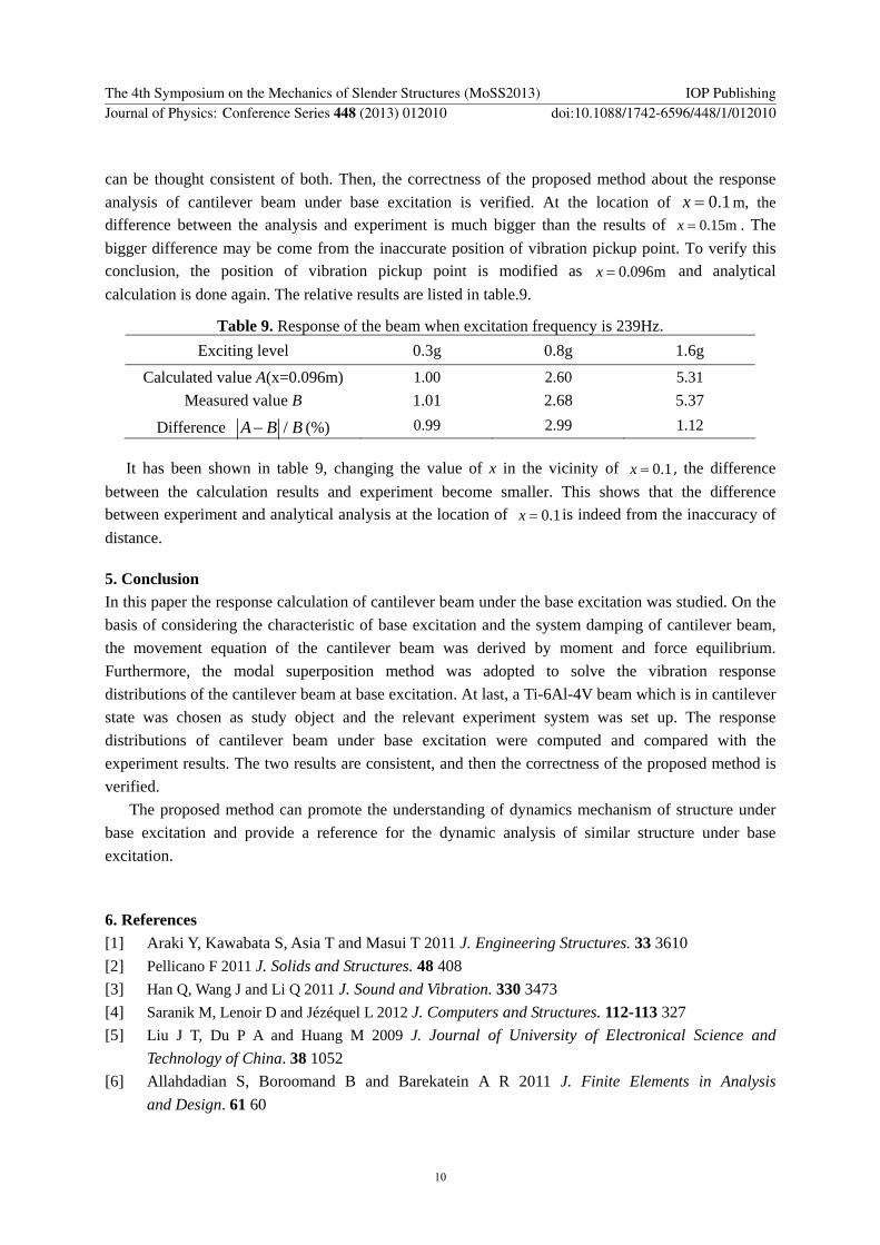
can be thought consistent of both. Then, the correctness of the proposed method about the response analysis of cantilever beam under base excitation is verified. At the location of 0.1x = m, the difference between the analysis and experiment is much bigger than the results of 0.15mx = . The bigger difference may be come from the inaccurate position of vibration pickup point. To verify this conclusion, the position of vibration pickup point is modified as 0.096mx = and analytical calculation is done again. The relative results are listed in table.9.

Table 9. Response of the beam when excitation frequency is 239Hz. Exciting level 0.3g 0.8g 1.6g

Calculated value A(x=0.096m) 1.00 2.60 5.31 Measured value B 1.01 2.68 5.37

Difference /A B B− (%) 0.99 2.99 1.12

It has been shown in table 9, changing the value of x in the vicinity of 0.1x = , the difference between the calculation results and experiment become smaller. This shows that the difference between experiment and analytical analysis at the location of 0.1x = is indeed from the inaccuracy of distance.

5. Conclusion In this paper the response calculation of cantilever beam under the base excitation was studied. On the basis of considering the characteristic of base excitation and the system damping of cantilever beam, the movement equation of the cantilever beam was derived by moment and force equilibrium. Furthermore, the modal superposition method was adopted to solve the vibration response distributions of the cantilever beam at base excitation. At last, a Ti-6Al-4V beam which is in cantilever state was chosen as study object and the relevant experiment system was set up. The response distributions of cantilever beam under base excitation were computed and compared with the experiment results. The two results are consistent, and then the correctness of the proposed method is verified.

The proposed method can promote the understanding of dynamics mechanism of structure under base excitation and provide a reference for the dynamic analysis of similar structure under base excitation.

6. References [1] Araki Y, Kawabata S, Asia T and Masui T 2011 J. Engineering Structures. 33 3610 [2] Pellicano F 2011 J. Solids and Structures. 48 408 [3] Han Q, Wang J and Li Q 2011 J. Sound and Vibration. 330 3473 [4] Saranik M, Lenoir D and Jézéquel L 2012 J. Computers and Structures. 112-113 327 [5] Liu J T, Du P A and Huang M 2009 J. Journal of University of Electronical Science and

Technology of China. 38 1052 [6] Allahdadian S, Boroomand B and Barekatein A R 2011 J. Finite Elements in Analysis

and Design. 61 60


10

[7] Feng A H, Zhu X D and Lan X J 2011 J. International Journal of Non-Linear Mechanics.46 1330 [8] Kocatur kT 2004 J. Sound and Vibration, 281 1145 [9] Kumar V, Miller J K and Rhoads J F 2011 J. Sound and Vibration. 330 5401 [10] Clough R W and Penzien 2011 Dynamics of Structures(Berkeley: Computers & Structures)


11

1742-6596 448 1 012010

Documents

Transcript of 1742-6596 448 1 012010