( ), ( )1 )1 ( )n

1

1.5 Chapter 05.03 Newton’s Divided Difference Interpolation After reading this chapter, you should be able to: 1. derive Newton’s divided difference method of interpolation, 2. apply Newton’s divided difference method of interpolation, and 3. apply Newton’s divided difference method interpolants to find derivatives and integrals.

What is interpolation? Many times, data is given only at discrete points such as ,, 00 yx 11, yx , ......, 11, nn yx ,

nn yx , . So, how then does one find the value of y at any other value of x ? Well, a continuous

function xf may be used to represent the 1n data values with xf passing through the 1n points (Figure 1). Then one can find the value of y at any other value of x . This is called

interpolation. Of course, if x falls outside the range of x for which the data is given, it is no longer interpolation but instead is called extrapolation. So what kind of function xf should one choose? A polynomial is a common choice for an interpolating function because polynomials are easy to

(A) evaluate, (B) differentiate, and (C) integrate,

relative to other choices such as a trigonometric and exponential series. Polynomial interpolation involves finding a polynomial of order n that passes through the 1n points. One of the methods of interpolation is called Newton’s divided difference polynomial method. Other methods include the direct method and the Lagrangian interpolation method. We will discuss Newton’s divided difference polynomial method in this chapter.

Newton’s Divided Difference Polynomial Method To illustrate this method, linear and quadratic interpolation is presented first. Then, the general form of Newton’s divided difference polynomial method is presented. To illustrate the general form, cubic interpolation is shown in Figure 1.

2

Figure 1 Interpolation of discrete data. Linear Interpolation Given ),( 00 yx and ),,( 11 yx fit a linear interpolant through the data. Noting )(xfy and

)( 11 xfy , assume the linear interpolant )(1 xf is given by (Figure 2)

)()( 0101 xxbbxf

Since at 0xx ,

00010001 )()()( bxxbbxfxf

and at 1xx ,

)()()( 0110111 xxbbxfxf

)()( 0110 xxbxf

giving

01

011

)()(

xx

xfxfb

So )( 00 xfb

01

011

)()(

xx

xfxfb

giving the linear interpolant as )()( 0101 xxbbxf

)()()(

)()( 001

0101 xx

xx

xfxfxfxf

00, yx

11, yx

22 , yx

33, yx

xf

x

y

3

Figure 2 Linear interpolation.

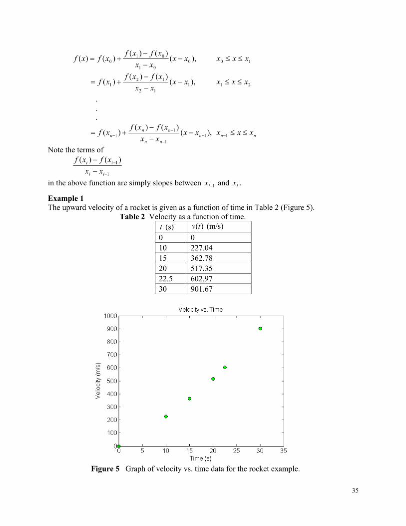
Example 1 The upward velocity of a rocket is given as a function of time in Table 1 (Figure 3).

Table 1 Velocity as a function of time. )s( t )m/s( )(tv

0 0 10 227.04 15 362.78 20 517.35 22.5 602.97 30 901.67

Determine the value of the velocity at 16t seconds using first order polynomial interpolation by Newton’s divided difference polynomial method.

Solution For linear interpolation, the velocity is given by )()( 010 ttbbtv

Since we want to find the velocity at 16t , and we are using a first order polynomial, we need to choose the two data points that are closest to 16t that also bracket 16t to evaluate it. The two points are 15t and 20t . Then ,150 t 78.362)( 0 tv

,201 t 35.517)( 1 tv gives )( 00 tvb

78.362

00, yx

11, yx

xf1

x

y

4

01

011

)()(

tt

tvtvb

1520

78.36235.517

914.30

Figure 3 Graph of velocity vs. time data for the rocket example. Hence )()( 010 ttbbtv

),15(914.3078.362 t 2015 t At ,16t )1516(914.3078.362)16( v m/s 69.393 If we expand ),15(914.3078.362)( ttv 2015 t we get ,914.3093.100)( ttv 2015 t and this is the same expression as obtained in the direct method.

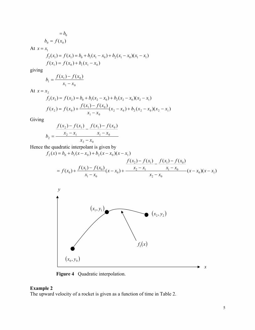
Quadratic Interpolation Given ),,( 00 yx ),,( 11 yx and ),,( 22 yx fit a quadratic interpolant through the data. Noting

),(xfy ),( 00 xfy ),( 11 xfy and ),( 22 xfy assume the quadratic interpolant )(2 xf is

given by ))(()()( 1020102 xxxxbxxbbxf

At 0xx ,

))(()()()( 100020010002 xxxxbxxbbxfxf

5

0b

)( 00 xfb

At 1xx

))(()()()( 110120110112 xxxxbxxbbxfxf

)()()( 01101 xxbxfxf

giving

01

011

)()(

xx

xfxfb

At 2xx

))(()()()( 120220210222 xxxxbxxbbxfxf

))(()()()(

)()( 120220201

0102 xxxxbxx

xx

xfxfxfxf

Giving

02

01

01

12

12

2

)()()()(

xx

xx

xfxf

xx

xfxf

b

Hence the quadratic interpolant is given by ))(()()( 1020102 xxxxbxxbbxf

))((

)()()()(

)()()(

)( 1002

01

01

12

12

001

010 xxxx

xxxx

xfxf

xx

xfxf

xxxx

xfxfxf

Figure 4 Quadratic interpolation.

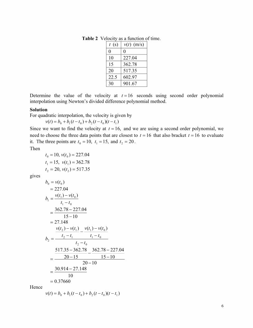
Example 2 The upward velocity of a rocket is given as a function of time in Table 2.

00 , yx

11, yx 22 , yx

xf2

y

x

6

Table 2 Velocity as a function of time.

)s( t (m/s) )(tv

0 0 10 227.04 15 362.78 20 517.35 22.5 602.97 30 901.67

Determine the value of the velocity at 16t seconds using second order polynomial interpolation using Newton’s divided difference polynomial method.

Solution For quadratic interpolation, the velocity is given by ))(()()( 102010 ttttbttbbtv

Since we want to find the velocity at ,16t and we are using a second order polynomial, we need to choose the three data points that are closest to 16t that also bracket 16t to evaluate it. The three points are ,100 t ,151 t and 202 t .

Then ,100 t 04.227)( 0 tv

,151 t 78.362)( 1 tv

,202 t 35.517)( 2 tv gives )( 00 tvb

04.227

01

011

)()(

tt

tvtvb

1015

04.22778.362

148.27

02

01

01

12

12

2

)()()()(

tt

tt

tvtv

tt

tvtv

b

1020

1015

04.22778.362

1520

78.36235.517

10

148.27914.30

37660.0 Hence ))(()()( 102010 ttttbttbbtv

7

),15)(10(37660.0)10(148.2704.227 ttt 2010 t At ,16t )1516)(1016(37660.0)1016(148.2704.227)16( v m/s 19.392 If we expand ),15)(10(37660.0)10(148.2704.227)( ttttv 2010 t we get 237660.0733.1705.12)( tttv , 2010 t This is the same expression obtained by the direct method.

General Form of Newton’s Divided Difference Polynomial In the two previous cases, we found linear and quadratic interpolants for Newton’s divided difference method. Let us revisit the quadratic polynomial interpolant formula ))(()()( 1020102 xxxxbxxbbxf

where )( 00 xfb

01

011

)()(

xx

xfxfb

02

01

01

12

12

2

)()()()(

xx

xx

xfxf

xx

xfxf

b

Note that ,0b ,1b and 2b are finite divided differences. ,0b ,1b and 2b are the first, second, and

third finite divided differences, respectively. We denote the first divided difference by )(][ 00 xfxf

the second divided difference by

01

0101

)()(],[

xx

xfxfxxf

and the third divided difference by

02

0112012

],[],[],,[

xx

xxfxxfxxxf

02

01

01

12

12 )()()()(

xx

xx

xfxf

xx

xfxf

where ],[ 0xf ],,[ 01 xxf and ],,[ 012 xxxf are called bracketed functions of their variables

enclosed in square brackets. Rewriting, ))(](,,[)](,[][)( 1001200102 xxxxxxxfxxxxfxfxf

This leads us to writing the general form of the Newton’s divided difference polynomial for 1n data points, nnnn yxyxyxyx ,,,,......,,,, 111100 , as

8

))...()((....)()( 110010 nnn xxxxxxbxxbbxf

where ][ 00 xfb

],[ 011 xxfb

],,[ 0122 xxxfb

],....,,[ 0211 xxxfb nnn

],....,,[ 01 xxxfb nnn

where the definition of the thm divided difference is ],........,[ 0xxfb mm

0

011 ],........,[],........,[

xx

xxfxxf

m

mm

From the above definition, it can be seen that the divided differences are calculated recursively. For an example of a third order polynomial, given ),,( 00 yx ),,( 11 yx ),,( 22 yx and ),,( 33 yx

))()(](,,,[

))(](,,[)](,[][)(

2100123

1001200103

xxxxxxxxxxf

xxxxxxxfxxxxfxfxf

Figure 5 Table of divided differences for a cubic polynomial.

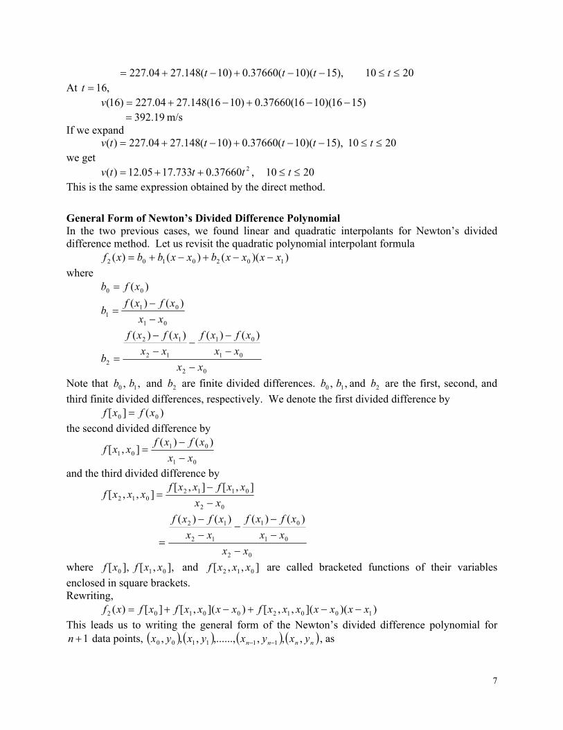
Example 3 The upward velocity of a rocket is given as a function of time in Table 3. Table 3 Velocity as a function of time.

(s) t (m/s) )(tv

0 0 10 227.04 15 362.78

00 xfx

0b

11 xfx

22 xfx

33 xfx

1b

2b

3b 01, xxf

12 , xxf

23 , xxf

012 ,, xxxf

123 ,, xxxf

0123 ,,, xxxxf

9

20 517.35 22.5 602.97 30 901.67

a) Determine the value of the velocity at 16t seconds with third order polynomial interpolation using Newton’s divided difference polynomial method. b) Using the third order polynomial interpolant for velocity, find the distance covered by the rocket from s 11t to s 16t . c) Using the third order polynomial interpolant for velocity, find the acceleration of the rocket at

s 16t .

Solution a) For a third order polynomial, the velocity is given by ))()(())(()()( 2103102010 ttttttbttttbttbbtv

Since we want to find the velocity at ,16t and we are using a third order polynomial, we need to choose the four data points that are closest to 16t that also bracket 16t to evaluate it. The four data points are ,100 t ,151 t ,202 t and 5.223 t .

Then ,100 t 04.227)( 0 tv

,151 t 78.362)( 1 tv

,202 t 35.517)( 2 tv

,5.223 t 97.602)( 3 tv

gives ][ 00 tvb

)( 0tv

04.227 ],[ 011 ttvb

01

01 )()(

tt

tvtv

1015

04.22778.362

148.27 ],,[ 0122 tttvb

02

0112 ],[],[

tt

ttvttv

12

1212

)()(],[

tt

tvtvttv

1520

78.36235.517

914.30 148.27],[ 01 ttv

10

02

01122

],[],[

tt

ttvttvb

1020

148.27914.30

37660.0 ],,,[ 01233 ttttvb

03

012123 ],,[],,[

tt

tttvtttv

13

1223123

],[],[],,[

tt

ttvttvtttv

23

2323

)()(],[

tt

tvtvttv

205.22

35.51797.602

248.34

12

1212

)()(],[

tt

tvtvttv

1520

78.36235.517

914.30

13

1223123

],[],[],,[

tt

ttvttvtttv

155.22

914.30248.34

44453.0 37660.0],,[ 012 tttv

03

0121233

],,[],,[

tt

tttvtttvb

105.22

37660.044453.0

3104347.5 Hence ))()(())(()()( 2103102010 ttttttbttttbttbbtv

)20)(15)(10(105347.5

)15)(10(37660.0)10(148.2704.2273

ttt

ttt

At ,16t

)2016)(1516)(1016(105347.5

)1516)(1016(37660.0)1016(148.2704.227)16(3

v

m/s 06.392

11

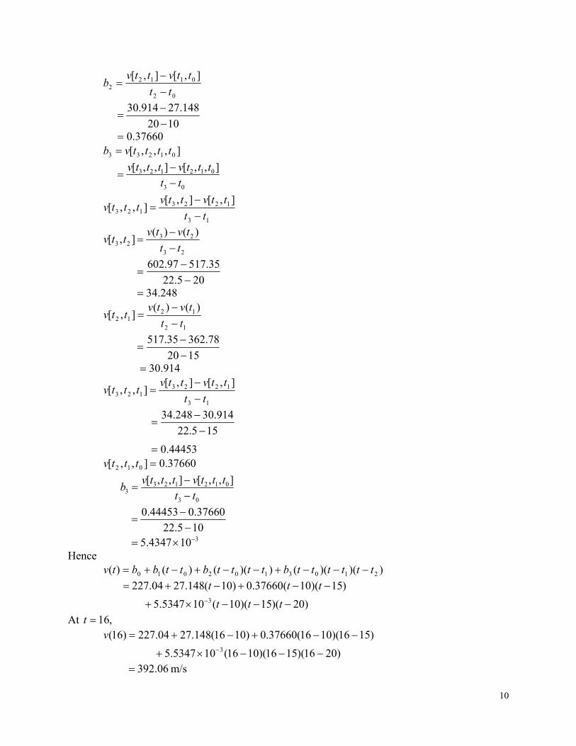
b) The distance covered by the rocket between s 11t and s 16t can be calculated from the interpolating polynomial

)20)(15)(10(105347.5

)15)(10(37660.0)10(148.2704.227)(3

ttt

ttttv

,0054347.013204.0265.212541.4 32 ttt 5.2210 t Note that the polynomial is valid between 10t and 22.5t and hence includes the limits of

11t and 16t . So

16

11

1116 dttvss

dtttt )0054347.013204.0265.212541.4( 3216

11

16

11

432

40054347.0

313204.0

2265.212541.4

tttt

m 1605 c) The acceleration at 16t is given by

16)()16( ttvdt

da

)()( tvdt

dta

32 0054347.013204.0265.212541.4 tttdt

d

2016304.026408.0265.21 tt 2)16(016304.0)16(26408.0265.21)16( a

2m/s 664.29

INTERPOLATION Topic Newton’s Divided Difference Interpolation Summary Textbook notes on Newton’s divided difference interpolation. Major General Engineering Authors Autar Kaw, Michael Keteltas Last Revised Aralık 30, 2016 Web Site http://numericalmethods.eng.usf.edu

Multiple-Choice Test Chapter 05.03 Newton’s Divided Difference Polynomial Method 1. If a polynomial of degree n has 1n zeros, then the polynomial is

(A) oscillatory (B) zero everywhere (C) quadratic

12

(D) not defined 2. The following yx, data is given.

x 15 18 22 y 24 37 25

The Newton’s divided difference second order polynomial for the above data is given by 181515)( 2102 xxbxbbxf

The value of 1b is most nearly (A) –1.0480 (B) 0.14333 (C) 4.3333 (D) 24.000

3. The polynomial that passes through the following yx, data

x 18 22 24 y ? 25 123

is given by ,323775.324125.8 2 xx 2418 x The corresponding polynomial using Newton’s divided difference polynomial is given by 221818)( 2102 xxbxbbxf

The value of 2b is most nearly (E) 0.25000 (F) 8.1250 (G) 24.000 (H) not obtainable with the information given

4. Velocity vs. time data for a body is approximated by a second order Newton’s divided difference polynomial as ,15205540.020622.390 tttbtv 2010 t

The acceleration in 2m/s at 15t is (I) 0.5540 (J) 39.622 (K) 36.852 (L) not obtainable with the given information

5. The path that a robot is following on a yx plane is found by interpolating the following four data points as

x 2 4.5 5.5 7 y 7.5 7.5 6 5

900.3605.9257.21524.0 23 xxxxy

13

The length of the path from 2x to 7x is

(M) 222222 5.57655.45.55.7625.45.75.7

(N) dxxxx 7

2

223 )900.3605.9257.21524.0(1

(O) dxxx 7

2

22 )605.9514.44572.0(1

(P) dxxxx 7

2

23 )900.3605.9257.21524.0(

7. The following data of the velocity of a body is given as a function of time.

Time (s) 0 15 18 22 24 Velocity (m/s) 22 24 37 25 123

If you were going to use quadratic interpolation to find the value of the velocity at 9.14t seconds, the three data points of time you would choose for interpolation are

(Q) 0, 15, 18 (R) 15, 18, 22 (S) 0, 15, 22 (T) 0, 18, 24

For a complete solution, refer to the links at the end of the book.

Newton’s Divided Difference Interpolation – More Examples Chemical Engineering

Example 1 To find how much heat is required to bring a kettle of water to its boiling point, you are asked to calculate the specific heat of water at C61 . The specific heat of water is given as a function of time in Table 1.

Table 1 Specific heat of water as a function of temperature. Temperature, T

C Specific heat, pC

Ckg

J

14

22 42 52 82 100

4181 4179 4186 4199 4217

Figure 1 Specific heat of water vs. temperature. Determine the value of the specific heat at C61T using Newton’s divided difference method of interpolation and a first order polynomial.

Solution For linear interpolation, the specific heat is given by )()( 010 TTbbTC p

Since we want to find the velocity at C61T , and we are using a first order polynomial we need to choose the two data points that are closest to C61T that also bracket C61T to evaluate it. The two points are 52T and 82T . Then ,520 T 4186)( 0 TC p

,821 T 4199)( 1 TC p

gives )( 00 TCb p

4186

15

01

011

)()(

TT

TCTCb pp

5282

41864199

43333.0 Hence

)()( 010 TTbbTC p

),52(43333.04186 T 8252 T At 61T ,

)5261(43333.04186)61( pC

Ckg

J9.4189

If we expand ),52(43333.04186)( TTC p 8252 T

we get ,43333.05.4163)( TTC p 8252 T

and this is the same expression as obtained in the direct method.



C Specific heat, pC

Ckg

J

22 42 52 82 100

4181 4179 4186 4199 4217

Determine the value of the specific heat at C61T using Newton’s divided difference method of interpolation and a second order polynomial. Find the absolute relative approximate error for the second order polynomial approximation.

Solution For quadric interpolation, the specific heat is given by ))(()()( 102010 TTTTbTTbbTC p

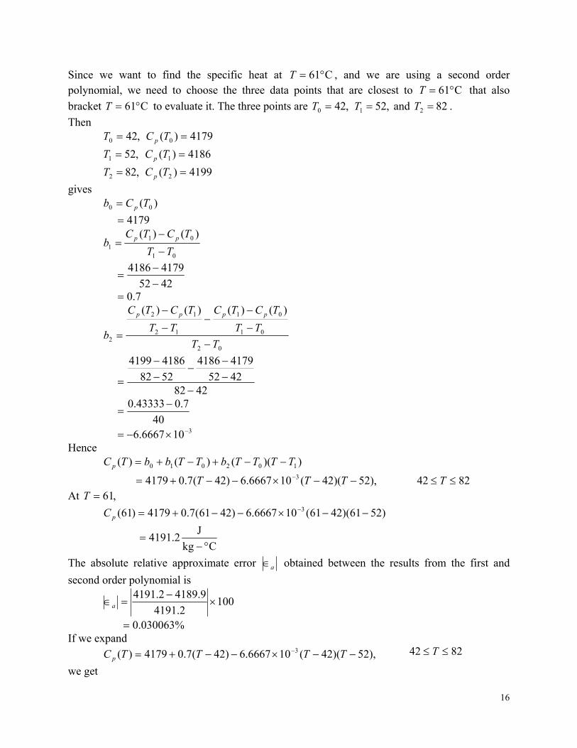
16

Since we want to find the specific heat at C61T , and we are using a second order polynomial, we need to choose the three data points that are closest to C16 T that also

bracket C61T to evaluate it. The three points are ,420 T ,521 T and 822 T .

Then ,420 T 4179)( 0 TC p

,521 T 4186)( 1 TC p

,822 T 4199)( 2 TC p

gives )( 00 TCb p

4179

01

011

)()(

TT

TCTCb pp

4252

41794186

7.0

02

01

01

12

12

2

)()()()(

TT

TT

TCTC

TT

TCTC

b

pppp

4282

4252

41794186

5282

41864199

40

7.043333.0

3106667.6 Hence ))(()()( 102010 TTTTbTTbbTC p

),52)(42(106667.6)42(7.04179 3 TTT 8242 T At ,61T

)5261)(4261(106667.6)4261(7.04179)61( 3 pC

Ckg

J2.4191

The absolute relative approximate error a obtained between the results from the first and

second order polynomial is

1002.4191

9.41892.4191

a

%030063.0 If we expand

),52)(42(106667.6)42(7.04179)( 3 TTTTC p 8242 T

we get

17

,106667.63267.10.4135 23TTTC p 8242 T

This is the same expression obtained by the direct method.



C Specific heat, pC

Ckg

J

22 42 52 82 100

4181 4179 4186 4199 4217

Determine the value of the specific heat at C 61T using Newton’s divided difference method of interpolation and a third order polynomial. Find the absolute relative approximate error for the third order polynomial approximation.

Solution For a third order polynomial, the specific heat profile is given by ))()(())(()()( 2103102010 TTTTTTbTTTTbTTbbTC p

Since we want to find the specific heat at C61T , and we are using a third order polynomial, we need to choose the four data points that are closest to C61T that also bracket C61T .

The four data points are ,420 T ,521 T 822 T and 1003 T .

(Choosing the four points as 220 T , 421 T , 522 T and 823 T is equally valid.)

,420 T 4179)( 0 TC p

,521 T 4186)( 1 TC p

,822 T 4199)( 2 TC p

,1003 T 4217)( 3 TC p

then ][ 00 TCb p

)( 0TC p

4179 ],[ 011 TTCb p

18

01

01 )()(

TT

TCTC pp

4252

41794186

7.0 ],,[ 0122 TTTCb p

02

0112 ],[],[

TT

TTCTTC pp

12

1212

)()(],[

TT

TCTCTTC pp

p

5282

41864199

43333.0

7.0],[ 01 TTC p

02

01122

],[],[

TT

TTCTTCb pp

4282

7.043333.0

3106667.6 01233 ,,, TTTTCb p

03

012123 ],,[],,[

TT

TTTCTTTC pp

13

1223123

],[],[],,[

TT

TTCTTCTTTC pp

p

23

2323

)()(],[

TT

TCTCTTC pp

p

82100

41994217

1

12

1212

)()(],[

TT

TCTCTTC pp

p

5282

41864199

43333.0

13

1223123

],[],[],,[

TT

TTCTTCTTTC pp

p

19

52100

43333.01

011806.0 3

012 106667.6],,[ TTTC p

],,,[ 01233 TTTTCb p

03

012123 ],,[],,[

TT

TTTCTTTC pp

42100

106667.6011806.0 3

4101849.3 Hence

))()(())(()()( 2103102010 TTTTTTbTTTTbTTbbTC p

10042 ),82)(52)(42(101849.3

)52)(42(106667.6)42(7.041794

3

TTTT

TTT

At ,61T

)8261)(5261)(4261(101849.3

)5261)(4261(106667.6)4261(7.04179)61(4

3

pC

Ckg

J0.4190

The absolute relative approximate error a obtained between the results from the second and

third order polynomial is

1000.4190

2.41910.4190

a

%027295.0 If we expand

)52)(42(106667.6)42(7.04179)( 3 TTTTC p

10042 ),82)(52)(42(101849.3 4 TTTT we get 10042,101849.306272.04771.40.4078)( 342 TTTTTC p

This is the same expression as obtained in the direct method.

INTERPOLATION Topic Newton’s Divided Difference Interpolation Summary Examples of Newton’s divided difference interpolation. Major Chemical Engineering Authors Autar Kaw Date Aralık 30, 2016

20

Web Site http://numericalmethods.eng.usf.edu 1.6 Chapter 05.04 Lagrangian Interpolation After reading this chapter, you should be able to:

1. derive Lagrangian method of interpolation, 2. solve problems using Lagrangian method of interpolation, and 3. use Lagrangian interpolants to find derivatives and integrals of discrete functions.




interpolation. Of course, if x falls outside the range of x for which the data is given, it is no longer interpolation but instead is called extrapolation. So what kind of function xf should one choose? A polynomial is a common choice for an interpolating function because polynomials are easy to

(D) evaluate, (E) differentiate, and (F) integrate,

relative to other choices such as a trigonometric and exponential series. Polynomial interpolation involves finding a polynomial of order n that passes through the 1n data points. One of the methods used to find this polynomial is called the Lagrangian method of interpolation. Other methods include Newton’s divided difference polynomial method and the direct method. We discuss the Lagrangian method in this chapter.

21

Figure 1 Interpolation of discrete data. The Lagrangian interpolating polynomial is given by

n

iiin xfxLxf

0

)()()(

where n in )(xfn stands for the thn order polynomial that approximates the function )(xfy

given at 1n data points as nnnn yxyxyxyx ,,,,......,,,, 111100 , and

n

ijj ji

ji xx

xxxL

0

)(

)(xLi is a weighting function that includes a product of 1n terms with terms of ij omitted.

The application of Lagrangian interpolation will be clarified using an example.


Table 1 Velocity as a function of time. t (s) )(tv (m/s)

0 0 10 227.04 15 362.78 20 517.35 22.5 602.97 30 901.67

00, yx

11, yx

22 , yx

33, yx

xf

x

y

22

Determine the value of the velocity at 16t seconds using a first order Lagrange polynomial.

Solution For first order polynomial interpolation (also called linear interpolation), the velocity is given by

1

0

)()()(i

ii tvtLtv

)()()()( 1100 tvtLtvtL

Figure 3 Linear interpolation.

Figure 2 Graph of velocity vs. time data for the rocket example.

00, yx

11, yx

xf1

x

y

23

Since we want to find the velocity at 16t , and we are using a first order polynomial, we need to choose the two data points that are closest to 16t that also bracket 16t to evaluate it. The two points are 150 t and 201 t .

Then 78.362 ,15 00 tvt

35.517 ,20 11 tvt gives

1

00 0

0 )(

jj j

j

tt

tttL

10

1

tt

tt

1

10 1

1 )(

jj j

j

tt

tttL

01

0

tt

tt

Hence

)()()( 101

00

10

1 tvtt

tttv

tt

tttv

2015 ),35.517(1520

15)78.362(

2015

20

ttt

)35.517(1520

1516)78.362(

2015

2016)16(

v

)35.517(2.0)78.362(8.0 m/s 69.393 You can see that 8.0)(0 tL and 2.0)(1 tL are like weightages given to the velocities at 15t

and 20t to calculate the velocity at 16t .

Quadratic Interpolation

24

Figure 4 Quadratic interpolation.



0 0 10 227.04 15 362.78 20 517.35 22.5 602.97 30 901.67

a) Determine the value of the velocity at 16t seconds with second order polynomial interpolation using Lagrangian polynomial interpolation. b) Find the absolute relative approximate error for the second order polynomial approximation.

Solution a) For second order polynomial interpolation (also called quadratic interpolation), the velocity is given by

2

0

)()()(i

ii tvtLtv

)()()()()()( 221100 tvtLtvtLtvtL

Since we want to find the velocity at 16t , and we are using a second order polynomial, we need to choose the three data points that are closest to 16t that also bracket 16t to evaluate it. The three points are 20 and ,15 ,10 210 ttt .

Then 04.227,10 00 tvt

00 , yx

11, yx 22 , yx

xf2

y

x

25

78.362,15 11 tvt

35.517,20 22 tvt gives

2

00 0

0 )(

jj j

j

tt

tttL

20

2

10

1

tt

tt

tt

tt

2

10 1

1 )(

jj j

j

tt

tttL

21

2

01

0

tt

tt

tt

tt

2

20 2

2 )(

jj j

j

tt

tttL

12

1

02

0

tt

tt

tt

tt

Hence

20212

1

02

01

21

2

01

00

20

2

10

1 ),()()()( ttttvtt

tt

tt

tttv

tt

tt

tt

tttv

tt

tt

tt

tttv

)35.517()1520)(1020(

)1516)(1016(

)78.362()2015)(1015(

)2016)(1016()04.227(

)2010)(1510(

)2016)(1516()16(

v

)35.517)(12.0()78.362)(96.0()04.227)(08.0( m/s 19.392 b) The absolute relative approximate error a for the second order polynomial is calculated by

considering the result of the first order polynomial (Example 1) as the previous approximation.

10019.392

69.39319.392

a

%38410.0

Example 3 The upward velocity of a rocket is given as a function of time in Table 3. Table 3 Velocity as a function of time

t (s) )(tv (m/s)

0 0 10 227.04

26

15 362.78 20 517.35 22.5 602.97 30 901.67

a) Determine the value of the velocity at 16t seconds using third order Lagrangian polynomial interpolation. b) Find the absolute relative approximate error for the third order polynomial approximation. c) Using the third order polynomial interpolant for velocity, find the distance covered by the rocket from s 11t to s 16t . d) Using the third order polynomial interpolant for velocity, find the acceleration of the rocket at

s 16t .

Solution a) For third order polynomial interpolation (also called cubic interpolation), the velocity is given by

3

0

)()()(i

ii tvtLtv

)()()()()()()()( 33221100 tvtLtvtLtvtLtvtL

Figure 5 Cubic interpolation. Since we want to find the velocity at 16t , and we are using a third order polynomial, we need to choose the four data points closest to 16t that also bracket 16t to evaluate it. The four points are 20 ,15 ,10 210 ttt and 5.223 t .

Then 04.227,10 00 tvt

00, yx

11, yx

22 , yx

33, yx

xf3

x

y

27

78.362,15 11 tvt

35.517,20 22 tvt

97.602,5.22 33 tvt

gives

3

00 0

0 )(

jj j

j

tt

tttL

30

3

20

2

10

1

tt

tt

tt

tt

tt

tt

3

10 1

1 )(

jj j

j

tt

tttL

31

3

21

2

01

0

tt

tt

tt

tt

tt

tt

3

20 2

2 )(

jj j

j

tt

tttL

32

3

12

1

02

0

tt

tt

tt

tt

tt

tt

3

30 3

3 )(

jj j

j

tt

tttL

23

2

13

1

03

0

tt

tt

tt

tt

tt

tt

Hence

30323

2

13

1

03

02

32

3

12

1

02

0

131

3

21

2

01

00

30

3

20

2

10

1

),()(

)()()(

ttttvtt

tt

tt

tt

tt

tttv

tt

tt

tt

tt

tt

tt

tvtt

tt

tt

tt

tt

tttv

tt

tt

tt

tt

tt

tttv

)97.602()205.22)(155.22)(105.22(

)2016)(1516)(1016(

)35.517()5.2220)(1520)(1020(

)5.2216)(1516)(1016(

)78.362()5.2215)(2015)(1015(

)5.2216)(2016)(1016()04.227(

)5.2210)(2010)(1510(

)5.2216)(2016)(1516()16(

v

)97.602)(1024.0()35.517)(312.0()78.362)(832.0()04.227)(0416.0( m/s 06.392

28

b) The absolute percentage relative approximate error, a for the value obtained for )16(v can

be obtained by comparing the result with that obtained using the second order polynomial (Example 2)

10006.392

19.39206.392

a

%033269.0 c) The distance covered by the rocket between s 11t to s 16t can be calculated from the interpolating polynomial as

5.2210 ),97.602()205.22)(155.22)(105.22(

)20)(15)(10(

)35.517()5.2220)(1520)(1020(

)5.22)(15)(10(

)78.362()5.2215)(2015)(1015(

)5.22)(20)(10()04.227(

)5.2210)(2010)(1510(

)5.22)(20)(15()(

tttt

ttt

tttttttv

)97.602()5.2)(5.7)(5.12(

)20)(15025()35.517(

)5.2)(5)(10(

)5.22)(15025(

)78.362()5.7)(5)(5(

)5.22)(20030()04.227(

)5.12)(10)(5(

)5.22)(30035(

22

22

tttttt

tttttt

)5727.2)(300065045()1388.4)(33755.7125.47(

)9348.1)(45008755.52()36326.0)(67505.10875.57(2323

2323

tttttt

tttttt

,00544.013195.0265.21245.4 32 ttt 5.2210 t Note that the polynomial is valid between 10t and 5.22t and hence includes the limits of

11t and 16t . So

16

11

)()11()16( dttvss

16

11

32 )00544.013195.0265.21245.4( dtttt

16

11

432

400544.0

313195.0

2265.21245.4

tttt

m 1605 d) The acceleration at 16t is given by

16

16

t

tvdt

da

Given that 32 00544.013195.0265.21245.4)( ttttv , 5.2210 t

tvdt

dta

29

32 00544.013195.0265.21245.4 tttdt

d

201632.026390.0265.21 tt , 5.2210 t 2)16(01632.0)16(26390.0265.21)16( a

2m/s 665.29 Note: There is no need to get the simplified third order polynomial expression to conduct the differentiation. An expression of the form

30

3

20

2

10

10 )(

tt

tt

tt

tt

tt

tttL

gives the derivative without expansion as

)(0 tLdt

d

10

1

30

3

30

3

20

2

20

2

10

1

tt

tt

tt

tt

tt

tt

tt

tt

tt

tt

tt

tt

INTERPOLATION Topic Lagrange Interpolation Summary Textbook notes on the Lagrangian method of interpolation Major General Engineering Authors Autar Kaw, Michael Keteltas Last Revised Aralık 30, 2016 Web Site http://numericalmethods.eng.usf.edu

Multiple-Choice Test Chapter 05.04 Lagrange Method of Interpolation 1. A unique polynomial of degree ______________ passes through 1n data points.

(A) 1n (B) n (C) n or less (D) 1n or less 2. Given the two points bfbafa ,,, , the linear Lagrange polynomial xf1 that passes through these two points is given by

(A) bfba

axaf

ba

bxxf

1 (B) bfab

xaf

ab

xxf

1

(C) abab

afbfafxf

1 (D) bfab

axaf

ba

bxxf

1

3. The Lagrange polynomial that passes through the 3 data points is given by

x 15 18 22 y 24 37 25

253724 2102 xLxLxLxf

The value of xL1 at 16x is most nearly

30

(A) –0.071430 (B) 0.50000 (C) 0.57143 (D) 4.3333 4. The following data of the velocity of a body is given as a function of time.

Time ( s ) 10 15 18 22 24 Velocity ( sm ) 22 24 37 25 123

A quadratic Lagrange interpolant is found using three data points, 15t , 18 and 22. From this

information, at what of the times given in seconds is the velocity of the body m/s 26 during the time interval of 15t to 22t seconds.

(A) 20.173 (B) 21.858 (C) 21.667 (D) 22.020 5. The path that a robot is following on a yx, plane is found by interpolating four data points as

x 2 4.5 5.5 7 y 7.5 7.5 6 5

9000.36048.92571.215238.0 23 xxxxy The length of the path from 2x to 7x is

(A) 222222 5.57655.45.55.7625.45.75.7

(B) dxxxx 7

2

223 )9000.36048.92571.215238.0(1

(C) dxxx 7

2

22 )6048.95142.445714.0(1

(D) dxxxx 7

2

23 )9000.36048.92571.215238.0(

6. The following data of the velocity of a body is given as a function of time. Time (s) 0 15 18 22 24 Velocity (m/s) 22 24 37 25 123

If you were going to use quadratic interpolation to find the value of the velocity at 9.14t seconds, what three data points of time would you choose for interpolation?

(A) 0, 15, 18 (B) 15, 18, 22 (C) 0, 15, 22 (D) 0, 18, 24


31

1.7 Chapter 05.05 Spline Method of Interpolation After reading this chapter, you should be able to:

1. interpolate data using spline interpolation, and 2. understand why spline interpolation is important.




interpolation. (çoğu zaman veriler (x0, y0), (x1, y1), …., (xn-1, yn-1), (xn, yn) kesikli noktalar şeklindedir. Bu durumda herhangi bir x değerine karşılık gelecek olan y nasıl elde edilir. F(x) şeklindeki sürekli bir fonksiyonu n+1 noktanın hepsinden geçirilebilir (Şekil 1). Böylelikle herhangi bir x değerine karşılık gelen y değeri bulunabilir. Buna interpolasyo demiştik.) Of course, if x falls outside the range of x for which the data is given, it is no longer interpolation but instead is called extrapolation. x değeri sınırlar dışında kalıyorsa interpolasyon yerine extraolasyon ifadesini kullanabiliriz. So what kind of function xf should one choose? A polynomial is a common choice for an interpolating function because polynomials are easy to (f(x) nasıl olmalıdır? Polinom interpolasyon fonksiyonu f(x) için polinomlar trigonometrik ve üstel serilere göre daha kullanışlıdır: )

(A) evaluate, (geliştirilebilir) (B) differentiate, and (türevlenebilir) (C) integrate (toplanabilir/integre edilebilir)

relative to other choices such as a trigonometric and exponential series. Polynomial interpolation involves finding a polynomial of order n that passes through the 1n points. Several methods to obtain such a polynomial include the direct method, Newton’s divided difference polynomial method and the Lagrangian interpolation method. (polinomiyal interpolasyon n. dereceden ve n+1 veri noktasından geçen polinomdur. Bu tür polinomları elde edebilmek için doğrudan, Newton bölümlü fark veya Lagrangian polinom yöntemleri kullanılabilir.) So is the spline method yet another method of obtaining this thn order polynomial. …… NO! Actually, when n becomes large, in many cases, one may get oscillatory behavior in the resulting polynomial. This was shown by Runge when he interpolated data based on a simple function of (Spline yöntemi n.dereceden polinom elde edebilmek için kullanılabilecek bir yöntemdir. Burada dikkat edilmesi gereken şey n derecesi büyüdükçe polinomdan elde edilen değerlerin osilasyon yapmaktadır. Bu osilasyon Runge tarafından aşağıdaki fonksiyondan elde edilen değerler kullanılarak gösterilmiştir. Bu fonksiyondan [-1, 1] aralığında elde edilmiş 6 değeri kullanılır ve bu değerlere uygun interpolasyon polinomu elde edilmeya çalışılılırsa.)

2251

1

xy

on an interval of [–1, 1]. For example, take six equidistantly spaced points in [–1, 1] and find y at these points as given in Table 1.

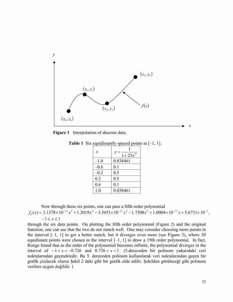
32

Figure 1 Interpolation of discrete data.

Table 1 Six equidistantly spaced points in [–1, 1]. Now through these six points, one can pass a fifth order polynomial

,106731.5100004.17308.1103651.32019.1101378.3)( 111231145115

xxxxxxf

11 x through the six data points. On plotting the fifth order polynomial (Figure 2) and the original function, one can see that the two do not match well. One may consider choosing more points in the interval [–1, 1] to get a better match, but it diverges even more (see Figure 3), where 20 equidistant points were chosen in the interval [–1, 1] to draw a 19th order polynomial. In fact, Runge found that as the order of the polynomial becomes infinite, the polynomial diverges in the interval of 726.01 x and 1726.0 x . (5.dereceden bir polinom yukarıdaki veri noktalarından geçmektedir. Bu 5. dereceden polinom kullanılarak veri noktalarından geçen bir grafik çizilecek olursa Şekil 2 deki gibi bir grafik elde edilir. Şekilden görüleceği gibi polinom verilere uygun değildir. )

x 2251

1

xy

–1.0 0.038461 –0.6 0.1 –0.2 0.5 0.2 0.5 0.6 0.1 1.0 0.038461

00, yx

11, yx

22 , yx

33, yx

xf

x

y

33

So what is the answer to using information from more data points, but at the same time keeping the function true to the data behavior? The answer is in spline interpolation. The most common spline interpolations used are linear, quadratic, and cubic splines.

Figure 2 5th order polynomial interpolation with six equidistant points.

-0.4

0

0.4

0.8

1.2

-1 -0.5 0 0.5 1

x

y

5th Order Polynomial Function 1/(1+25*x^2)

34

-0.4

0

0.4

0.8

1.2

-1 -0.5 0 0.5 1

x

y

5th Order Polynomial Function 1/(1+25*x^2)

19th Order Polynomial 12th Order Polynomial

Figure 3 Higher order polynomial interpolation is a bad idea. Linear Spline Interpolation (çizgisel spline interpolasyonu) Given nnnn yxyxyxyx ,,,......,,,, 111100 , fit linear splines (Figure 4) to the data. This

simply involves forming the consecutive data through straight lines. So if the above data is given in an ascending order, the linear splines are given by )( ii xfy . ((x0,y0), x1,y1), (x2,y2),

...., (xn-1,yn-1), (xn,yn) veriler Şekil 4’deki gibi çizgisel spline’lara fit edilmektedir. Bu ardışık verilerin birbirleri ile çizgisel olarak birleştirilmesi işlemidir. Veriler artan sırada verilirse çizgisel spline yi=f(xi) şeklindedir.)

Figure 4 Linear splines.

(x0, y0)

(x1, y1)

(x2, y2)

(x3, y3)

x

y

35

),()()(

)()( 001

010 xx

xx

xfxfxfxf

10 xxx

),()()(

)( 112

121 xx

xx

xfxfxf

21 xxx

. . .

),()()(

)( 11

11

nnn

nnn xx

xx

xfxfxf nn xxx 1

Note the terms of

1

1 )()(

ii

ii

xx

xfxf

in the above function are simply slopes between 1ix and ix .

Example 1 The upward velocity of a rocket is given as a function of time in Table 2 (Figure 5).


0 0 10 227.04 15 362.78 20 517.35 22.5 602.97 30 901.67

Figure 5 Graph of velocity vs. time data for the rocket example.

36

Determine the value of the velocity at 16t seconds using linear splines.

Solution Since we want to evaluate the velocity at 16t , and we are using linear splines, we need to choose the two data points closest to 16t that also bracket 16t to evaluate it. The two points are 150 t and 201 t .

Then ,150 t 78.362)( 0 tv ,201 t 35.517)( 1 tv

gives

)()()(

)()( 001

010 tt

tt

tvtvtvtv

)15(1520

78.36235.51778.362

t

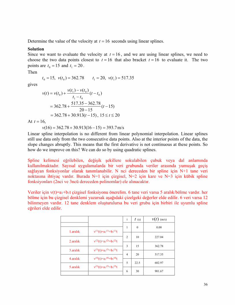
)15(913.3078.362 t , 2015 t At ,16t )1516(913.3078.362)16( v m/s7.393 Linear spline interpolation is no different from linear polynomial interpolation. Linear splines still use data only from the two consecutive data points. Also at the interior points of the data, the slope changes abruptly. This means that the first derivative is not continuous at these points. So how do we improve on this? We can do so by using quadratic splines. Spline kelimesi eğrilebilen, değişik şekillere sokulabilen çubuk veya dal anlamında kullanılmaktadır. Sayısal uygulamalarda bir veri grubunda veriler arasında yumuşak geçiş sağlayan fonksiyonlar olarak tanımlanabilir. N nci dereceden bir spline için N+1 tane veri noktasına ihtiyaç vardır. Burada N=1 için çizgisel, N=2 için kare ve N=3 için kübik spline fonksiyonları (2nci ve 3ncü dereceden polinomlar) ele alınacaktır. Veriler için v(t)=a1+b1t çizgisel fonksiyonu önerelim. 6 tane veri varsa 5 aralık/bölme vardır. her bölme için bu çizgisel denklemi yazarsak aşağıdaki çizelgeki değerler elde edilir. 6 veri varsa 12 bilinmeyen vardır. 12 tane denklem oluşturulursa bu veri grubu için birbiri ile uyumlu spline eğrileri elde edilir.

i t (s) )(tv (m/s)

1 0 0.00

1.aralık v(1)(t)=a1(1)+b1

(1)t

2 10 227.04


(2)t 3 15 362.78


(3)t 4 20 517.35


(4)t 5 22.5 602.97


(5)t 6 30 901.67

37

1.nokta için 0=a1

(0) ilk nokta olduğu için

2.nokta için 227.04=a1

(1)+b1(1)10

227.04=a1(2)+b1

(2)10


(2)+b1(2)15

362.78=a1(3)+b1

(3)15


(3)+b1(3)20

517.35=a1(4)+b1

(4)20


(4)+b1(4)22.5

602.97=a1(5)+b1

(5)22.5


(6)+b1(6)30

b1(6)=0 alınır

Bu şekilde 10 bilinmeyenli 10 eşitliği olan bir denklem elde edilmiş olur.

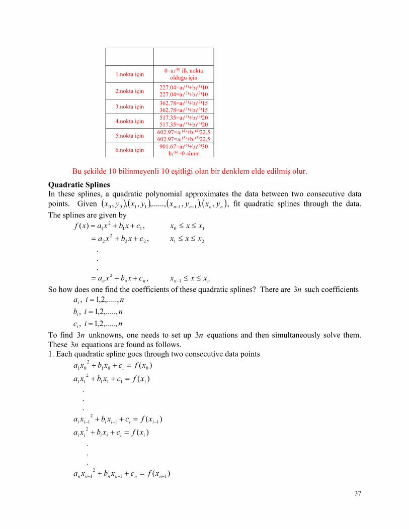
Quadratic Splines In these splines, a quadratic polynomial approximates the data between two consecutive data points. Given nnnn yxyxyxyx ,,,,......,,,, 111100 , fit quadratic splines through the data.

The splines are given by ,)( 11

21 cxbxaxf 10 xxx

,222

2 cxbxa 21 xxx . . . ,2

nnn cxbxa nn xxx 1

So how does one find the coefficients of these quadratic splines? There are n3 such coefficients niai ,.....,2,1 ,

nibi ,.....,2,1 ,

nici ,.....,2,1 ,

To find n3 unknowns, one needs to set up n3 equations and then simultaneously solve them. These n3 equations are found as follows. 1. Each quadratic spline goes through two consecutive data points

)( 01012

01 xfcxbxa

)( 11112

11 xfcxbxa . . .

)( 112

1 iiiiii xfcxbxa

)(2iiiiii xfcxbxa

. . .

)( 112

1 nnnnnn xfcxbxa

38

)(2nnnnnn xfcxbxa

This condition gives n2 equations as there are n quadratic splines going through two consecutive data points. 2. The first derivatives of two quadratic splines are continuous at the interior points. For example, the derivative of the first spline 11

21 cxbxa

is 112 bxa The derivative of the second spline 22

22 cxbxa

is 222 bxa

and the two are equal at 1xx giving

212111 22 bxabxa

022 212111 bxabxa Similarly at the other interior points, 022 323222 bxabxa

. . . 022 11 iiiiii bxabxa

. . . 022 1111 nnnnnn bxabxa

Since there are )1( n interior points, we have )1( n such equations. So far, the total number of equations is )13()1()2( nnn equations. We still then need one more equation. We can assume that the first spline is linear, that is 01 a This gives us n3 equations and n3 unknowns. These can be solved by a number of techniques used to solve simultaneous linear equations.

Example 2 The upward velocity of a rocket is given as a function of time as


0 0 10 227.04 15 362.78 20 517.35 22.5 602.97 30 901.67

39

(a) Determine the value of the velocity at 16t seconds using quadratic splines. (b) Using the quadratic splines as velocity functions, find the distance covered by the rocket from

s11t to s16t . (c) Using the quadratic splines as velocity functions, find the acceleration of the rocket at

s16t .

Solution a) Since there are six data points, five quadratic splines pass through them.

,)( 112

1 ctbtatv 100 t

,222

2 ctbta 1510 t

,332

3 ctbta 2015 t

,442

4 ctbta 5.2220 t

,552

5 ctbta 305.22 t

The equations are found as follows. 1. Each quadratic spline passes through two consecutive data points.

112

1 ctbta passes through 0t and 10t .

0)0()0( 112

1 cba (1)

04.227)10()10( 112

1 cba (2)

222


04.227)10()10( 222

2 cba (3)

78.362)15()15( 222

2 cba (4)

332


78.362)15()15( 332

3 cba (5)

35.517)20()20( 332

3 cba (6)

442

4 ctbta passes through 20t and 5.22t .

35.517)20()20( 442

4 cba (7)

97.602)5.22()5.22( 442

4 cba (8)

552

5 ctbta passes through 5.22t and 30t .

97.602)5.22()5.22( 552

5 cba (9)

67.901)30()30( 552

5 cba (10)

2. Quadratic splines have continuous derivatives at the interior data points. At 10t 0)10(2)10(2 2211 baba (11) At 15t

40

0)15(2)15(2 3322 baba (12)

At 20t 0)20(2)20(2 4433 baba (13)

At 5.22t 0)5.22(2)5.22(2 5544 baba (14)

3. Assuming the first spline 112

1 ctbta is linear,

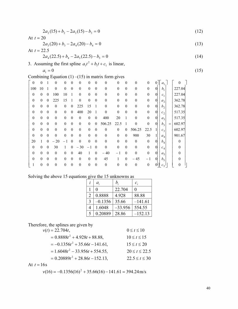
01 a (15) Combining Equation (1) –(15) in matrix form gives

0

0

0

0

0

67.901

97.602

97.602

35.517

35.517

78.362

78.362

04.227

04.227

0

000000000000001

01450145000000000

00001400140000000

00000001300130000

00000000001200120

130900000000000000

15.2225.506000000000000

00015.2225.506000000000

000120400000000000

000000120400000000

000000115225000000

000000000115225000

000000000110100000

000000000000110100

000000000000100

5

5

5

4

4

4

3

3

3

2

2

2

1

1

1

c

b

a

c

b

a

c

b

a

c

b

a

c

b

a

Solving the above 15 equations give the 15 unknowns as

i ia ib ic

1 0 22.704 0 2 0.8888 4.928 88.88 3 –0.1356 35.66 –141.61 4 1.6048 –33.956 554.55 5 0.20889 28.86 –152.13

Therefore, the splines are given by ,704.22)( ttv 100 t

,88.88928.48888.0 2 tt 1510 t

,61.14166.351356.0 2 tt 2015 t

,55.554956.336048.1 2 tt 5.2220 t

,13.15286.2820889.0 2 tt 305.22 t At s16t

61.141)16(66.35)16(1356.0)16( 2 v m/s24.394

41

b) The distance covered by the rocket between 11 and 16 seconds can be calculated as

16

11

)()11()16( dttvss

But since the splines are valid over different ranges, we need to break the integral accordingly as ,88.88928.48888.0)( 2 tttv 1510 t

,61.14166.351356.0 2 tt 2015 t

16

11

15

11

16

15

)()()( dttvdttvdttv

15

11

16

15

22 )61.14166.351356.0()88.88928.48888.0()11()16( dtttdtttss

16

15

23

15

11

23

61.1412

66.353

1356.0

88.882

928.43

8888.0

ttt

ttt

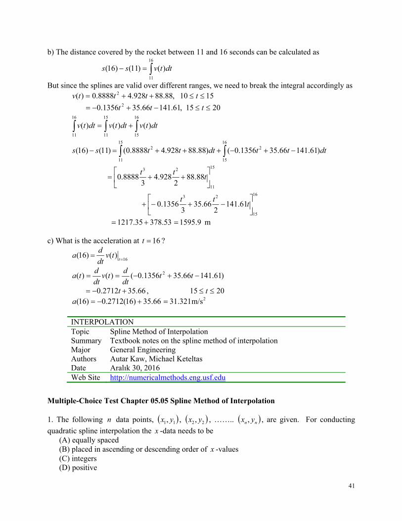
53.37835.1217 9.1595 m c) What is the acceleration at 16t ?

16

)()16(

t

tvdt

da

)61.14166.351356.0()()( 2 ttdt

dtv

dt

dta

66.352712.0 t , 2015 t 66.35)16(2712.0)16( a 2m/s321.31

INTERPOLATION Topic Spline Method of Interpolation Summary Textbook notes on the spline method of interpolation Major General Engineering Authors Autar Kaw, Michael Keteltas Date Aralık 30, 2016 Web Site http://numericalmethods.eng.usf.edu

Multiple-Choice Test Chapter 05.05 Spline Method of Interpolation 1. The following n data points, 11, yx , 22 , yx , …….. nn yx , , are given. For conducting

quadratic spline interpolation the x -data needs to be (A) equally spaced (B) placed in ascending or descending order of x -values (C) integers (D) positive

42

2. In cubic spline interpolation,

(A) the first derivatives of the splines are continuous at the interior data points (B) the second derivatives of the splines are continuous at the interior data points (C) the first and the second derivatives of the splines are continuous at the interior data points (D) the third derivatives of the splines are continuous at the interior data points

3. The following incomplete y vs. x data is given.

x 1 2 4 6 7 y 5 11 ???? ???? 32

The data is fit by quadratic spline interpolants given by 1 axxf , 21 x

42 ,9142 2 xxxxf

64 ,2 xdcxbxxf

76 ,92830325 2 xxxxf where dcba and ,,, are constants. The value of c is most nearly

(A) 00.303 (B) 50.144 (C) 0.0000 (D) 14.000

4. The following incomplete y vs. x data is given. x 1 2 4 6 7 y 5 11 ???? ???? 32

The data is fit by quadratic spline interpolants given by 21 ,1 xaxxf ,

42 ,9142 2 xxxxf

64 ,2 xdcxbxxf

76 ,2 xgfxexxf

where gfedcba and ,,,,,, are constants. The value of dx

df at 6.2x most nearly is

(A) 50.144 (B) 0000.4 (C) 3.6000 (D) 12.200 5. The following incomplete y vs. x data is given.

x 1 2 4 6 7 y 5 11 ???? ???? 32

The data is fit by quadratic spline interpolants given by 21 ,1 xaxxf ,

42 ,9142 2 xxxxf

64 ,2 xdcxbxxf

76 ,92830325 2 xxxxf

where dcba and ,,, are constants. What is the value of 5.3

5.1

dxxf ?

(A) 23.500 (B) 25.667 (C) 25.750 (D) 28.000

43

6. A robot needs to follow a path that passes consecutively through six points as shown in the figure. To find the shortest path that is also smooth you would recommend which of the following? (bir robot ardışık 6 noktadan geçecektir. En kısa yolu bulabilmek için aşağıdakilerden hangisini tavsiye edersiniz?)

(A) Pass a fifth order polynomial through the data (B) Pass linear splines through the data (C) Pass quadratic splines through the data (D) Regress the data to a second order polynomial

Path of a Robot

0

2

4

6

8

0 5 10 15

x

y


44

Chapter 08.02 Euler’s Method for Ordinary Differential Equations After reading this chapter, you should be able to:

1. develop Euler’s Method for solving ordinary differential equations, 2. determine how the step size affects the accuracy of a solution, 3. derive Euler’s formula from Taylor series, and 4. use Euler’s method to find approximate values of integrals.

What is Euler’s method? Euler’s method is a numerical technique to solve ordinary differential equations of the form

00,, yyyxfdx

dy (1)

So only first order ordinary differential equations can be solved by using Euler’s method. In another chapter we will discuss how Euler’s method is used to solve higher order ordinary differential equations or coupled (simultaneous) differential equations. How does one write a first order differential equation in the above form?

Example 1 Rewrite

50,3.12 yeydx

dy x

in

0)0( ),,( yyyxfdx

dy form.

Solution

50,3.12 yeydx

dy x

50,23.1 yyedx

dy x

In this case yeyxf x 23.1,

Example 2 Rewrite

50 ),3sin(222 yxyxdx

dye y

in

0)0( ),,( yyyxfdx

dy form.

45

Solution

50 ),3sin(222 yxyxdx

dye y

50 ,)3sin(2 22

ye

yxx

dx

dyy

In this case

ye

yxxyxf

22)3sin(2,

Derivation of Euler’s method At 0x , we are given the value of .0yy Let us call 0x as 0x . Now since we know the

slope of y with respect to x , that is, yxf , , then at 0xx , the slope is 00 , yxf . Both 0x

and 0y are known from the initial condition 00 yxy .

Figure 1 Graphical interpretation of the first step of Euler’s method.

So the slope at 0xx as shown in Figure 1 is

Slope Run

Rise

01

01

xx

yy

00 , yxf

From here 010001 , xxyxfyy

Calling 01 xx the step size h , we get

y

Φ

Step size, h

x

),( 00 yx

True value

y1, Predicted value

1x

46

hyxfyy 0001 , (2)

One can now use the value of 1y (an approximate value of y at 1xx ) to calculate 2y , and that

would be the predicted value at 2x , given by

hyxfyy 1112 ,

hxx 12

Based on the above equations, if we now know the value of iyy at ix , then

hyxfyy iiii ,1 (3)

This formula is known as Euler’s method and is illustrated graphically in Figure 2. In some books, it is also called the Euler-Cauchy method.

Figure 2 General graphical interpretation of Euler’s method.

Example 3 A ball at K1200 is allowed to cool down in air at an ambient temperature of K300 . Assuming heat is lost only due to radiation, the differential equation for the temperature of the ball is given by

K12000 ,1081102067.2 8412 dt

d

where is in K and t in seconds. Find the temperature at 480t seconds using Euler’s method. Assume a step size of 240h seconds.

Solution

8412 1081102067.2 dt

d

8412 1081102067.2, tf Per Equation (3), Euler’s method reduces to

Φ

Step size

h

True Value

yi+1, Predicted value

yi

x

y

xi xi+1

47

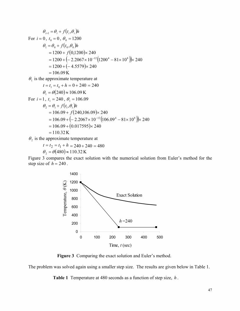
htf iiii ,1

For 0i , 00 t , 12000

htf 0001 ,

2401200,01200 f

24010811200102067.21200 8412

2405579.41200 09.106 K

1 is the approximate temperature at

httt 01 2400 240

09.1062401 K

For 1i , 2401 t , 09.1061

htf 1112 , 24009.106,24009.106 f

240108109.106102067.209.106 8412

240017595.009.106 32.110 K

2 is the approximate temperature at

httt 12 240240 480 32.1104802 K Figure 3 compares the exact solution with the numerical solution from Euler’s method for the step size of 240h .

0

200

400

600

800

1000

1200

1400

0 100 200 300 400 500

Time, t (sec)

Tem

pera

ture

,

h =240

Exact Solution

θ(K

)

Figure 3 Comparing the exact solution and Euler’s method.

The problem was solved again using a smaller step size. The results are given below in Table 1. Table 1 Temperature at 480 seconds as a function of step size, h .

48

Step size, h 480 tE %|| t 480 240 120 60 30

-987.81 110.32 546.77 614.97 632.77

1635.4 537.26 100.80 32.607 14.806

252.54 82.964 15.566 5.0352 2.2864

Figure 4 shows how the temperature varies as a function of time for different step sizes.

-1500

-1000

-500

0

500

1000

1500

0 100 200 300 400 500

Time, t (sec)Tem

pera

ture

,

Exact solution

h =120h =240

h = 480

θ(K

)

Figure 4 Comparison of Euler’s method with the exact solution for different step sizes.

The values of the calculated temperature at 480t s as a function of step size are plotted in Figure 5.

-1200

-800

-400

0

400

800

0 100 200 300 400 500

Step size, h (s) Tem

pera

ture

,θ

(K)

Figure 5 Effect of step size in Euler’s method.

49

The exact solution of the ordinary differential equation is given by the solution of a non-linear equation as

9282.21022067.010333.0tan8519.1300

300ln92593.0 321

t

(4)

The solution to this nonlinear equation is 57.647 K It can be seen that Euler’s method has large errors. This can be illustrated using the Taylor series.

...!3

1

!2

1 31

,3

32

1

,2

2

1,

1 ii

yx

ii

yx

iiyx

ii xxdx

ydxx

dx

ydxx

dx

dyyy

iiiiii

(5)

...),(''!3

1),('

!2

1))(,( 3

12

11 iiiiiiiiiiiii xxyxfxxyxfxxyxfy (6)

As you can see the first two terms of the Taylor series hyxfyy iiii ,1

are Euler’s method. The true error in the approximation is given by

...!3

,

!2

, 32

hyxf

hyxf

E iiiit (7)

The true error hence is approximately proportional to the square of the step size, that is, as the step size is halved, the true error gets approximately quartered. However from Table 1, we see that as the step size gets halved, the true error only gets approximately halved. This is because the true error, being proportioned to the square of the step size, is the local truncation error, that is, error from one point to the next. The global truncation error is however proportional only to the step size as the error keeps propagating from one point to another. Can one solve a definite integral using numerical methods such as Euler’s method of solving ordinary differential equations? Let us suppose you want to find the integral of a function )(xf

b

a

dxxfI .

Both fundamental theorems of calculus would be used to set up the problem so as to solve it as an ordinary differential equation. The first fundamental theorem of calculus states that if f is a continuous function in the interval [a,b], and F is the antiderivative of f , then

aFbFdxxfb

a

The second fundamental theorem of calculus states that if f is a continuous function in the open interval D , and a is a point in the interval D , and if

x

a

dttfxF

then

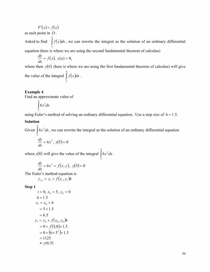
50

xfxF at each point in D .

Asked to find b

a

dxxf , we can rewrite the integral as the solution of an ordinary differential

equation (here is where we are using the second fundamental theorem of calculus)

,0)( , ayxfdx

dy

where then by (here is where we are using the first fundamental theorem of calculus) will give

the value of the integral b

a

dxxf .

Example 4 Find an approximate value of

8

5

36 dxx

using Euler’s method of solving an ordinary differential equation. Use a step size of 5.1h .

Solution

Given 8

5

36 dxx , we can rewrite the integral as the solution of an ordinary differential equation

05,6 3 yxdx

dy

where 8y will give the value of the integral 8

5

36 dxx .

yxfxdx

dy,6 3 , 05 y

The Euler’s method equation is hyxfyy iiii ,1

Step 1 0,5,0 00 yxi

5.1h

5.6

5.15 01

hxx

hyxfyy 0001 ,

5.10,50 f

5.1560 3 1125 )5.6(y

51

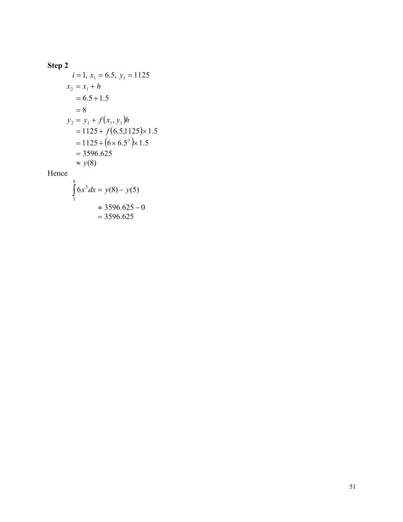
Step 2 1125,5.6,1 11 yxi

8

5.15.6 12

hxx

hyxfyy 1112 ,

5.11125,5.61125 f

5.15.661125 3 625.3596 )8(y Hence

)5()8(68

5

3 yydxx

0625.3596

625.3596

52

ORDINARY DIFFERENTIAL EQUATIONS Topic Euler’s Method for ordinary differential equations Summary Textbook notes on Euler’s method for solving ordinary differential

equations Major General Engineering Authors Autar Kaw Last Revised Aralık 30, 2016 Web Site http://numericalmethods.eng.usf.edu

( ), ( )1 )1 ( )n

Documents

Transcript of ( ), ( )1 )1 ( )n