
15RPT04 TracePQM - IRIS Istituto Nazionale di Ricerca ...
368
15RPT04 TracePQM Page 1 of 36 Report describing the open software tool developed for handling high performance ADCs identified for power and PQ measurements 15RPT04 TracePQM TRACEABILITY ROUTES FOR ELECTRICAL POWER QUALITY MEASUREMENTS DELIVERABLE D2: Report describing of the open software tool developed to control the data acquisition of the modular measurement system, to perform data processing including uncertainty estimation, which implements the most commonly used equipment and algorithms and with a modular design that facilitates easy incorporation of new equipment and algorithms LEAD PARTNER: INRIM CONTRIBUTORS: CMI, SIQ, JV, RISE, LNE, Metroset, FER, TUBITAK, NSAI DUE DATE OF THE DELIVERABLE: August 2018 ACTUAL SUBMISSION DATE OF THE DELIVERABLE: May 2019
-
Upload
khangminh22 -
Category
Documents
-
view
2 -
download
0
Transcript of 15RPT04 TracePQM - IRIS Istituto Nazionale di Ricerca ...

15RPT04 TracePQM Page 1 of 36
Report describing the open software tool developed for handling high performance ADCs identified for power and PQ measurements
15RPT04 TracePQM
TRACEABILITY ROUTES FOR ELECTRICAL POWER QUALITY MEASUREMENTS
DELIVERABLE D2: Report describing of the open software tool developed to control the data acquisition of the modular measurement system, to perform data processing including uncertainty estimation, which implements the most commonly used equipment and algorithms and with a modular design that facilitates easy incorporation of new equipment and algorithms
LEAD PARTNER: INRIM
CONTRIBUTORS: CMI, SIQ, JV, RISE, LNE, Metroset, FER, TUBITAK, NSAI DUE DATE OF THE DELIVERABLE: August 2018
ACTUAL SUBMISSION DATE OF THE DELIVERABLE: May 2019

15RPT04 TracePQM Page 2 of 36
Report describing the open software tool developed for handling high performance ADCs identified for power and PQ measurements
Bruno Trinchera and Danilo Serazio Istituto Nazionale di Ricerca Metrologica (INRIM), Italy
Stanislav Mašláň and Věra Nováková Zachovalová Czech Metrology Institute (CMI), Czech Republic
Marko Berginc Slovenski Institut za Kakovost in Meroslovje (SIQ), Slovenia
Kristian Ellingsberg Justervesenet (JV), Norway
Andrei Pokatilov AS Metroset (Metroset), Estonia
Tobias Bergsten and Stefan Svensson RISE Research Institutes of Sweden, Sweden
Soureche Soccalingame and Aristo Philominraj Laboratoire national de métrologie et d'essais (LNE), France
Damir Ilić Sveuciliste U Zagrebu Fakultet Elektrotehnike I Racunarstva (HMI-FER/PEL), Croatia
Kaan Gulnihar and Hüseyin Çaycı Turkiye Bilimsel ve Teknolojik Arastirma Kurumu (TUBITAK), Turkey
Oliver Power National Standards Authority of Ireland (NSAI), Ireland

15RPT04 TracePQM Page 3 of 36
Report describing the open software tool developed for handling high performance ADCs identified for power and PQ measurements

15RPT04 TracePQM Page 4 of 36
Report describing the open software tool developed for handling high performance ADCs identified for power and PQ measurements
Abstract
This report describes the open software tool developed in the scope of TracePQM project using the outputs coming from A2.1.1-A2.1.4, A2.2.1-A2.2.5, A2.3.1-A2.3.6 and A2.4.1-A2.4.4 activities. The main throughput of the open software tool was to integrate the control, the data acquisition and the data processing modules to optimize the operation and configuration of different hardware platforms and transducers, which will speed up the developing of metrology grade modular setups designed for traceable measurements of power and PQ quantities from industrial frequency up to 1 MHz. The most relevant feature of the open software tool concerns its capability of implementing commonly used equipment and algorithms that combined with the concept of the modular design facilitates the easy incorporation of new equipment and algorithms.
The project 15RPT04 TracePQM has received funding from the EMPIR programme co-financed by the Participating States and from the European Union’s Horizon 2020 research and innovation programme. This collection reflects only the author’s view and EURAMET is not responsible for any use that may be made of the information it contains.

15RPT04 TracePQM Page 5 of 36
Report describing the open software tool developed for handling high performance ADCs identified for power and PQ measurements
Contents
1. OVERVIEW AND PRELIMINARY GUIDELINES ON OPEN SOFTWARE TOOL .................... 7
1.1 INTRODUCTION ....................................................................................................... 7
1.2 SOFTWARE DOWNLOAD ............................................................................................ 8
1.3 SOFTWARE INSTALLATION ......................................................................................... 8
1.4 MACRO-SETUP REQUIREMENTS FOR USE WITH THE OPEN TOOL SOFTWARE ............................ 9
1.4.1 LF MEASUREMENT SETUP ....................................................................................... 9
1.4.2 WIDEBAND MEASUREMENT SETUP ........................................................................... 9
1.4.3 MACRO-SETUPS DESIGN ...................................................................................... 10
1.4.4 POWER AND PQ SOURCES .................................................................................... 11
1.5 SOFTWARE STRUCTURE CONCEPT .............................................................................. 12
1.5.1 INITIAL CONCEPT OF DRIVERS FOR OPEN SW TOOL ..................................................... 12
1.5.2 EXTENDING CONCEPT OF DIGITIZER DRIVERS FOR MULTIPLE CHANNELS ............................ 19
1.5.3 CONCEPT OF COMMUNICATION BETWEEN PROCESSING AND CONTROL MODULE ................ 19
2. DESCRIPTION OF THE OPEN SOFTWARE TOOLS ........................................................ 21
2.1 INTRODUCTION ..................................................................................................... 21
2.2 GENERAL STRUCTURE OF THE SOFTWARE TOOL ............................................................. 21
2.3 TWM OPEN SOFTWARE FOR LABVIEW ENVIRONMENT ................................................. 22
2.4 TPQA OPEN SOFTWARE FOR LABWINDOWS/CVI ENVIRONMENT .................................... 24
2.5 ALGORITHMS TO CAPTURE LONG DURATION SIGNAL PATTERNS ......................................... 25
3. DATA PROCESSING MODULE AND ALGORITHMS ...................................................... 26
3.1 INTRODUCTION ..................................................................................................... 26
3.2 STANDARDIZED MODEL FOR INPUT-OUTPUT DATA EXCHANGE .......................................... 26

15RPT04 TracePQM Page 6 of 36
Report describing the open software tool developed for handling high performance ADCs identified for power and PQ measurements
3.3 PROCESSING MODULE FOR TWM-LABVIEW ................................................................ 26
3.4 PROCESSING MODULE FOR TPQA-LABWINDOWS ......................................................... 26
3.5 ALGORITHMS FOR CALCULATION OF POWER AND PQ PARAMETERS ................................... 27
4. TESTING THE OPEN SOFTWARE TOOL ...................................................................... 28
4.1 INTRODUCTION ..................................................................................................... 28
4.2 TESTING OF TWM TOOL ......................................................................................... 28
4.3 TESTING OF TPQA TOOL ......................................................................................... 29
4.4 EVALUATION, VERIFICATION AND TESTING OF ALGORITHMS WITH REAL DATA ....................... 31
4.4.1 EVALUATION AND VERIFICATION OF ALGORITHMS ...................................................... 31
4.4.2 ASSESSING ALGORITHMS PERFORMANCE USING 5922 DIGITIZER DATA ............................ 32
4.4.3 ASSESSING HARMONICS AND FLICKER ALGORITHMS USING 3458A SETUP ........................ 32
5 REFERENCES............................................................................................................ 33
6 APPENDIX ............................................................................................................... 35

15RPT04 TracePQM Page 7 of 36
Report describing the open software tool developed for handling high performance ADCs identified for power and PQ measurements
Chapter 1
1. OVERVIEW AND PRELIMINARY GUIDELINES ON OPEN SOFTWARE TOOL
1.1 Introduction This chapter gives a general overview of the Open Software Tool (OST) suitable for handling the high performance and precise state-of-the art sampling systems, based on analogue-to-digital converters (ADCs), identified for power and PQ measurements. The sampling systems were opportunely identified during a survey conducted among the project’s partners and to the members of the EURAMET-TC-EM power and energy sub-committee. In particular, the OST will help the end-users to gain further insights into modern and traceable power and power quality (PQ) measurements from power line frequency to 1 MHz. The main features of the OST are:
• the ability to identify the sampling hardware equipment - to interact with the experimental modular measurement setup, and to ensure a direct means for the simultaneous sampling of waveforms from voltage and current transducers employed in the modular measurement setup;
• provide fast and transparent calculation of power and PQ parameters using suitable algorithms.
Furthermore, the OST briges the gap between existing hardware platforms, already in use in many NMIs, based on virtual high speed digitizers and sampling DMMs, which have been proposed for decades for sampled power measurements. The open tool software handles different hardware platforms such as NI 5922 digitizers and sampling DMM 3458As, which, to our knowledge, are already in use in many NMIs. It handles both the macro-setups developed in WP1 and is composed sub-routines for conducting of specific tasks. In particular, one part is dedicated to measurement setups based on two triggered high resolution multimeters, configured as digitizers, e.g. sampling DMMs 3458A, with the possible extension for longer duration measurements. The second part is based on virtual reconfigurable platforms employing high precision ADCs, e.g. NI 5922 digitizers. Furthermore, the data processing module, described in chapter 3, was primarily intended for numerical computations, but has been enriched using dedicated high-level interpreted languages, such as Matlab and GNU Octave. At the end, all parts of the system, the digitizer control and data acquisition module and the data processing module, have been integrated using a special software interface so it appears to the final user as one interactive application. Moreover, the algorithms are made as m-files instead of compiled code with the software environment so they can be used or can be modified for both power and PQ parameter end uncertainty calculation without a need for recompiling the entire application. In particular, the requirements that the open software fulfills are: • Fast identification of the hardware installed (e.g. DMM 3458A or PXI NI-5922);

15RPT04 TracePQM Page 8 of 36
Report describing the open software tool developed for handling high performance ADCs identified for power and PQ measurements
• Initialization of the ADC acquiring parameters with the possibility of changing them ,e.g. sampling frequency, amplitude range, number of points and triggering parameters, during the acquisition process;
• The possibility of interchanging the roles of the triggering process of master-slave ADCs especially in the macro-setup employed for LF power measurements;
• Storage and pre-elaboration of sampled data; • Data processing for estimation of the parameters for power and PQ and uncertainty calculation • Advanced method to communicate and transfer data quickly with the experimental modular
measurement setup. All specific drivers necessary for the reconfigurable platform and the Guide User Interfaces (GUIs) of the open software tool projects, have been developed using development environments such as LabVIEW and LabWindowsTM/CVI. 1.2 Software download The open software tool project can be download from the project website, http://tracepqm.cmi.cz/, or from the GitHub domain:
• https://github.com/smaslan/TWM for the LabVIEW version entitled “TWM-TracePQM Wattmeter”;
• https://github.com/btrinchera/TPQA for the LabVindows/CVI version entitled “TPQA-Traceable Power & Power Quality Analyzer”.
1.3 Software installation Both TWM and TPQA open-source software tools require no installation. Both distributions can be downloaded and copied to any disk location. However, it is recommended to copy the distribution folder to the primary hierarchy root of the system, e.g.:
• C:\TWM\TWM-1.X.0.0\TWM for LabVIEW;
• C:\TPQA\TPQA-1.X.0.0 for LabWindowsTM/CVI.
• Installation of following Runtime Engines:
- LabVIEW 2013 Runtime Engine for TWM;
- LabWindows/CVI Runtime Engine for TPQA.
• Installation of drivers of all integrated instruments, and in particular:
- NI-VISA drivers for handling instruments connected via GPIB NI-488.2 interface;
- niScope drivers for handling NI digitizers
• Installation of GNU Octave and/or MATLAB Runtime Engine (it is mandatory for TPQA) for data
processing.

15RPT04 TracePQM Page 9 of 36
Report describing the open software tool developed for handling high performance ADCs identified for power and PQ measurements
• Registration of Dynamic Link Libraries (DLL) of Matlab, i.e. for 32-bit Matlab version the dlls are
situated in C\Program Files\Matlab\R2013a\bin\win32.
Further information about the prerequisites for TWM and TPQA installation can be found in the folder \TWM\TWM-1.X.0.0\TWM\doc or \TPQA\TPQA-1.X.0.0\doc of the respective distributions.
1.4 Macro-setup requirements for use with the open tool software The new modular setups designed for the measurement of power and PQ quantities are based on the “best-in-class” equipment identified in A1.1.4. The main requirement for the new system is to ensure both the lowest possible uncertainty and the highest possible bandwidth using commercially available devices. Since these contradictory requirements cannot be met by means of a single setup it was decided that the new system will comprise two macro-setups, one for low frequency (LF) measurements with low uncertainties and a frequency range limited by the sampling rate of the digitizer employed, and the second setup will use high sampling frequency digitizers which offer high-bandwidth.
1.4.1 LF measurement setup The hardware requirements for the building of a low frequency metrological grade measurement setup for power and PQ measurements up to few kilohertz are as follows:
• Two sampling DMMs 3458 A;
• One/two IEEE-488.2 interfaces; it is recommended to use GPIB-USB-HS as well as GPIB-USB-HS+ devices;
• Clock generator or Arbitrary Wave Generator, e.g., Agilent 331/332xxA, Agilent 335/336xxA, SRs CG635;
• PC with OS Windows 7 or higher.
1.4.2 Wideband measurement setup The hardware requirements for the building of a wideband metrological grade measurement setup for power and PQ measurements up to 1 MHz are as follows:
a) The first configuration is based on the use of a PC
• PXIe chassis, e.g. model 1082 or equivalent;
• x4/MXI-express for PXIe control, possibility with fiber optic cable;
• Two high-bandwidth digitizers NI PXI-5922, to carry out differential sampled voltage measurement;
• Arbitrary waveform generator or clock generator, e.g., Agilent 331/332xxA, Agilent 335/336xxA, SRs CG635;
• PC with MS Windows 7/8/10 equipped with two or more USB ports.
15RPT04 TracePQM Page 10 of 36
Report describing the open software tool developed for handling high performance ADCs identified for power and PQ measurements
b) The second configuration is based on the use of a mainstream unit as follows:
• PXIe chassis, e.g. model 1082, 1085 or equivalent; • Two high-bandwidth digitizers NI PXI-5922, to carry out differential sampled voltage
measurement; • Arbitrary waveform generator or clock generator, e.g., Agilent 331/332xxA, Agilent 335/336xxA,
SRs CG635; • NI PXI-8840 or equivalent mainstream unit with MS Windows Windows 7 or higher equipped with
two or more USB ports.
1.4.3 Macro-setups design Based on the review of existing measurement setups three candidates were identified for the new LF system based on 3458A multimeter and one candidate for the new WB system based on NI-5922 digitizer.
• The three candidate LF-systems are:
1) Synchronized by external 10 MHz, 3458A ext trig from Arbitrary Waveform Generator(AWG) – both generation of waveforms and measurements are synchronized via a common 10 MHz. When 3458A multimeters are used as samplers, they have no 10 MHz synchronization input so the sampling must be derived from a synchronized pulse generator or arbitrary waveforem generator;
2) Synchronized by software or hardware – the sampling is derived from a trigger synchronization hardware, either built around a phase-locked loop or a synchronized pair of frequency counter and pulse generator;
3) Non/semi-synchronous sampling – synchronization is achieved by post-processing the simultaneous waveforms, e.g. re-sampling based on sinc interpolation method and FFT.
Each design has advantages and drawbacks, the final choice depending on which is deemed most important.
• The WB system is based on single or dual NI-5922 digitizers. The macro setup based on NI-5922 digitizers has the advantage of being easily adaptable from a single phase to three phase measurements system. It is applicable not only to emerging research activities conducted in NMIs but also for direct calibration of the new class of polyphase PQ analyzers, which are designed for power network monitoring and able to reach an accuracy of the order of 0.03%. With respect to the use of precision digitizers for the design of the WB system, the main features are: - flexible vertical resolution depending on the sampling frequency; - several synchronization and clocking strategies depending on the kind of PQ parameters under
investigation; - reconfigurable digital platforms for traditional, real time measurements and continuous acquisition
for long time measurements beyond the capabilities of internal memory; - simple synchronization of all digitizers employed for three-phase power and PQ measurements.

15RPT04 TracePQM Page 11 of 36
Report describing the open software tool developed for handling high performance ADCs identified for power and PQ measurements
Fig. 1 shows a prototype modular system, which comprises both LF and WB macro-setups developed at INRIM. Both LF and WB digitizers are handled by the same PXI chassis, which has a control unit for remote control of both LF and WB digitizers based on a NI mainstream unit.
Fig 1. Fig 1. INRIM prototype of the newly developed modular system developed, which comprises two macro-setups, one for LF measurements based on DMMs 3458A digitizers, and the other based on high-bandwidth digitizers configured for differential sampling measurements. Both macro-setups are equipped with wideband voltage and current coaxial transducers, i.e. compensated resistive voltage dividers and current shunts.
1.4.4 Power and PQ sources As power and power quality source to be used with the two macro-setups it is possible to equip the experimental setup with a power and power quality calibrator or a dedicated system for waveform synthesis having at minimum two frequency-locked outputs, also known as biphase-synthesizer, equipped with suitable voltage and transconductance amplifiers. So the solutions proposed could comprise: • Power and power quality calibrator: Fluke 6105A, 6100B able to generate a wide variety of complex
signals, including:
- Flicker - Harmonics - Dips and swells - Interharmonics - Fluctuating harmonics - Simultaneous application, ecc.
• Dedicated biphase generators or digital-to-analog converters (DACs) which offer more flexibility and higher vertical resolution ranging from 16 to 24 bits suitable for synthesizing of sine-waves with high spectral purity and complex waves having harmonics extending up to 1 MHz or beyond. A DAC’s output capability doesn’t always match the practical capability of power and PQ measurements. In many

15RPT04 TracePQM Page 12 of 36
Report describing the open software tool developed for handling high performance ADCs identified for power and PQ measurements
practical applications, suitable voltage and transconductance amplifiers are employed to extend their output capabilities.
1.5 Software structure concept
The basis for the design of the concept was the results of the study on the choice of the best available components of ADCs as well as voltage and current transducers, which culminated in the design of new modular measurement setups by the NMIs involved in the project.
Based on their experience of existing systems developed by some NMIs, the choice of the software environment(s) was defined with the possibility to integrate as many as possible of the existing acquisition, scaling voltage and current devices and processing algorithms already in widespread use for power and PQ measurements in NMIs. The open software environment strengthens the measurement capacities of NMIs that already perform power measurements and wish to extend their capabilities to PQ measurements, without exchanging their existing platform and scaling devices.
Further details about the concept and flow chart with a partiall description for the software structure for NMIs who use DMMs 3458A or NI 5922 digitizers for primary power metrology are reported in [1] and [2]. Furthermore, the concept and the plan of the software and the modular measurement setup suitable to include multiple sampling DMMs or multiple NI 5922 is given in Appendix #1.
A key component in the realization of the open software tool was the development of the concept for the interface between the data processing module and the data control and data acquisition module. The concept was developed for the interface between LabVIEW to Octave and Matlab and for the interface between LabWindows/CVI to Matlab.
Two variants of SW environments were chosen: LabVIEW and LabWindows/CVI for control and user interface and GNU Octave and/or Matlab for data processing.
Flow charts of the open SW tool projects and drivers are described in the reports [15] and [17] and attached in the Appendix #10 and Appendix #11.
1.5.1 Initial concept of drivers for open SW tool
This section also partially covers A2.1.2 and A2.1.3.
1.5.1.1 Introduction
Following document is a first draft summarizing the possible concept and plan of the modular drivers for the digitizers. It is a general document that suggests preferred methods to be used for the development of drivers, however it is not mandatory plan. It is likely the implementation will differ depending on the inputs from other activities, e.g. A2.2.3 – streaming mode for 3458A.

15RPT04 TracePQM Page 13 of 36
Report describing the open software tool developed for handling high performance ADCs identified for power and PQ measurements
1.5.1.2 Driver concept
The ADC driver will consist of two parts. The first, low level part, will be the device specific functions/VIs. Second layer will be wrapper around these low level functions which will generalize all configuration and accesses to the particular ADCs to a unified format. So we will have only one control module that will be able to work with any ADC via the wrapper.
The discussions made so far the system (let’s call it Digital Sampling Wattmeter (DSW)) will for this moment contain at least following ADCs:
Type Comment
3458A Multiple DMMs synchronized together by some of the many possible techniques. The proper technique for TracePQM must be defined from the concept of new DSW. There may be even multiple synchronization methods but in end the driver of the ADC must appear to the outside world as one multichannel digitizer.
5922 1 to N digitizers 5922 (using 1 or 2 channels per digitizer) will be linked together using ni-TClk drivers so it will appear like one N channel digitizer.
1.5.1.3 Generalized ADC
As mentioned in introduction the goal is to make generalized ADC driver (wrapper) that will allow control any physical ADC using the same function calls so the rest of DSW will remain unchanged when new ADC is implemented. This document cannot describe the low level device drivers since it is not known at this stage how exactly the setup will look like. So this chapter will describe recommendations for the top layer (wrapper) and the drivers will be written accordingly to fulfill the requirements.
The configuration parameters of the particular ADC types must be generalized as much as possible so interchanging them will require minimum device specific configurations. Exception is for instance address and setup of the sync. unit for 3458A which obviously will not be present for 5922. But even these device specific setups will be accessed only via the wrapper. No direct access to the low level drivers will be made in order to keep the SW structure clear.
Control module will identify supported/unsupported features of the generalized ADC by calling specialized functions. Unsupported features will be simply ignored. So for instance there will be function “adc_has_apperture()” that will be used to find out whether the ADC can set sampling aperture. If not the control module (and eventually GUI) will simply disable/ignore this feature. Function “adc_set_apperture()” will simply do nothing for unsupported ADC and GUI will gray the control with this parameter. Such “get_capability_...()” functions will be implemented for every potentially device specific function. However whenever possible the parameters of the device drivers shall be generalized to minimize these exceptions.
Basic wrapper function reference:
[adr_type] = adc_get_address_type(adc_type)

15RPT04 TracePQM Page 14 of 36
Report describing the open software tool developed for handling high performance ADCs identified for power and PQ measurements
Will return device address(es) type required to designate it. Addresses of the particular ADCs can have completely different types.
So for instance to describe channel locations of PXI5922 it will require vector of items device_address, channel_id for every virtual channel of the multichannel ADC.
3458A will require at least vector of VISA addresses (for each DMM) + address for the synchronization unit (also VISA or some proprietary bus).
MIKES adc will probably require only single address.
So it will return one of enumerated values based on which the control module will open the device and GUI will “ungray” the controls.
[error, idn(s)] = adc_open(&adc_session, adc_type, address, reset)
Will open the ADC of type “adc_type” using variable “address”. The address variable will be possibly of “variable” type (LV) or pointer (CVI) to cover different address types by single function call. The function will store working data to “adc_session” structure (opened bus references, etc.). The session will carry everything related to the ADC. No variables/data will be stored in global variables!
This function should return identification strings of the devices. If there are multiple physical devices it should return idn. and serial numbers for each so it can be stored to the measurement report. The function should also enable “reset” function so the ADC will be set to some default and SAFE mode. So for instance force 1MΩ input for PXI5922 just in case someone connects high voltage to input.
Address format example for two channels for 3458A:
addr.channel[] = VISA1; VISA2 addr.sync_unit_address = VISA3
Address format example for 3 channels for 5922:
addr[0].ivi_address = PXI:4 addr[0].channel_id = 0 addr[1].ivi_address = PXI:4 addr[1].channel_id = 1 addr[2].ivi_address = PXI:5 addr[2].channel_id = 0 …
[error] = adc_close(&adc_session, reset)
Will close the ADC session. All physical devices that were opened (opened reference to some bus) shall be closed. Optionally they may be reset to safe default state. For example DMMs to DCV with auto trigger. This function should also force instruments back to the local control mode (set REN state of GPIB) so one does not have to always press “local” to gain control.
[error, idn(s)] = adc_get_idn(&adc_session)

15RPT04 TracePQM Page 15 of 36
Report describing the open software tool developed for handling high performance ADCs identified for power and PQ measurements
Will return clear identification of each component of the virtual ADC. Whenever possible the driver should query serial number, fw revision, etc.
[error, rates] = adc_get_sampling_rates(adc_type, mode)
This function should return available range of sampling rates for the device of type “adc_type” and measurement “mode”. The mode is single shot or continuous. Evidently it will differ and this function should clearly state the ranges. It must return in such format so it can cover various ADCs.
For instance 5922 has discrete steps 150e6/N where N is <4; 1200>. So a list of fs can be returned. 3458A with PLL has theoretically not this option but on the other hand it has maximum rate so it should maybe return it so the GUI can decide if it can be used for particular measurement. Another ADC can be clocked by DDS so the step is very fine so maybe return just range and step.
The function should decide when it is possible to query the parameters from opened session and when it is required to communicate with actual HW to maintain speed. But when it is called with “adc_session” it must be opened before, therefore it cannot be used in GUI to limit control ranges before actually opening the device.
[error, N] = adc_get_max_record_length(adc_type, fs, mode)
Returns maximum samples count per channel for given “mode”. For continuous mode returns 0 (infinite), for single shot it depends on particular setup.
The function should decide when it is possible to query the parameters from opened session and when it is required to communicate with actual HW to maintain speed
[error, actual_fs] = adc_set_sampling_rate(&adc_session, fs, only_exact)
Will setup sampling rate “fs” of the virtual ADC when applicable. In case of DMMs with PLL unit which controls the sampling rate this function have no effect. It will return “actual_fs” which is nearest higher available sampling rate for the device (typical feature for niScope drivers). “only_exact” option will generate error when the desired and set rate does not match (may be useful for coherent setup).
[error] = adc_set_record_length(&adc_session, N, mode)
Setup desired samples count per channel for given mode of sampling single, continuous. It should decide and signalize if it is possible to use such setup for given session. Requires all other sampling parameters already set such as aperture (affects sample width in memory).
[error] = adc_set_dmm_sync(&adc_session, setup)
This is device specific function for 3458A with PLL unit. It should set the PLL ratios, filters, PLL sensitivity, etc. Note it may be omitted if PLL unit will not be used.
[error] = adc_set_trigger_mode(&adc_session, mode, timeout, pretrigger_N)

15RPT04 TracePQM Page 16 of 36
Report describing the open software tool developed for handling high performance ADCs identified for power and PQ measurements
Sets trigger condition for start of capturing. For general periodic signal measurements it is possible to use immediate but for single event measurements it may be useful to synchronize to something. If the trigger will be implemented it should always have timeout! 5922 for instance will freeze forever if there is no trigger event! For 5922, 3458A in continuous sampling it is easy to implement pretrigger so this function can also set it.
To decide in future development: if the pretrigger useful. For 5922 it is solved by niScope driver itself. For 3458A it is doable only in continuous mode which may sample indefinitely and remember the event position when the condition is detected. But this would require trigger detection by additional HW.
[error] = adc_set_input(&adc_session, range[], coupling[], mode, impedance[])
Set voltage range(s) to particular channels of the ADC. If scalar is entered, all channels have the same range, if vector is passed every channel is set accordingly. If vector elements count does not match opened channels error is generated. “coupling” is AC/DC coupling again scalar or vector. “impedance” is input impedance, “mode” is single_ended, unbalanced_differential, differential.
To decide during implementation: 3458A has no mode setup, 5922 support partial floating input “unbalanced differential” so it should be there but actual differential not.
[error, config] = adc_get_configuration(&adc_session)
This function should return very detailed record of basically everything that can be read out of the digitizer. So for all types it should return sampling parameters (rate, aperture, …), vertical parameters (ranges, coupling, input mode, filters, bit resolution, for integer samples from 5922 scale and offsets, …), and specialized information (PLL lock status (5922), temperatures, …).
This will be used to generate as detailed as possible record for every stored waveform so it can be later found what were the conditions of measurement. IT should return this for every component of ADC, so for every DMM/5922/whatever.
[error, u, t, time_stamp] = adc_digitize_single(&adc_session)
This function should initiate digitizing in single shot mode. It will wait for selected trigger, then digitize and then return so it is blocking (synchronous) function.
Returned values are “u” which is 2D array of samples if possible directly in Volts. One column per channel. “t” is time vector with relative times of particular samples. It can be used to determine sample rate and trigger position if pretrigger is enabled (5922). “time_stamp” is relative timestamp of the first captured sample relative to reset of the ADC. This will be implemented only for 5922 which supports it natively and maybe for MIKES digitizer. This is very handy for time multiplexed measurement modes.
To decide during implementation: one of the project tasks is compensation of the 5922 drifts by ADC temperature measurement. So for longer runs this function should probably read temperatures

15RPT04 TracePQM Page 17 of 36
Report describing the open software tool developed for handling high performance ADCs identified for power and PQ measurements
as well every few seconds rather than every sample. Then it would mean to return also temperature(s) 2D array.
[error] = adc_abort(&adc_session)
This function is complementary with “adc_digitize_single()”. It can be called simultaneously with running “adc_digitize_single()” and it should abort digitizing in progress. It is asynchronous function so it will do its business and returns immediately.
To decide during implementation: decide how to abort. It may signalize to “adc_digitize_single()” using some queue/notification. Or will it write something to device so the device will return and “adc_digitize_single()” will recognize it. We have to check if it is possible to write simultaneously to 3458A from two threads/processes. For 5922 it is possible.
[error] = adc_set_clock_sync(&adc_handle, reference_f)
This function should set the ADCs lock to external timebase (usually 10 MHz). It is applicable at least to 5922 which can lock to anything from (1 to 20) MHz with step of 1 MHz. 0 value indicates free running.
Note: this will be needed anytime multiple 5922s are combined because internal sync. is not reliable (occasionally generates pseudorandom jitter).
1.5.1.4 Digitizing modes
The drivers must be made to handle two modes of operation. Single shot mode for “short” records that can fit to the memory of the digitizer (for instance 5922 can have up to 256MB) or it can be realtime transferred to the computer’s RAM buffer via DMA, such as small USB c-DAQ digitizers. But it is still a single shot measurement with predefined length of the record so the driver can tell using some functions whether it is possible or not. If possible the recording may be initiated and the data are returned using memory (not file!) to the calling function/VI (control module).
The second mode that must be supported at least for 3458A and 5922 is continuous sampling. This brings several serious problems. To keep the program structure clear it is not acceptable to let the driver store the captured waveform to data file directly by itself. That will lead to a device specific data format and any change in the format will result in reworking all the drivers. For 3458A the solution is relatively simple because it will digitize at low sampling rate so the data produced even for extreme lengths may still fit into computer’s RAM. So the driver can simply collect the data into referenced buffer and then return. But for 5922 such solution is not possible because the amount of the data will easily exceed maximum supported RAM which is less than 1GB for 32-bit LabVIEW. Therefore such a technique cannot be used. It will be necessary to choose one of the following methods of returning the data from continuous ADC:
1) Let the sampling function store the data in whatever format to temporary file. Then it can be somehow returned to the control module parts by another function from the file.

15RPT04 TracePQM Page 18 of 36
Report describing the open software tool developed for handling high performance ADCs identified for power and PQ measurements
2) To give the driver a pointer (reference) to callback function that will be called by the sampling function every time a certain amount of data is collected. The function will do something with the data – possibly save it. Important is the save format is defined by the function so it is not device specific, it is defined by the control module.
3) To use some kind of pipeline/messages/queues to send chunks of measured data from the sampling function to the control module. So for instance LV implements tool called queue. It is a FIFO/LIFO buffer of given length and data format. The sampling function will store data blocks into it and the control module will simultaneously take the data out and store them in proper format.
Method 1) is simple but very ineffective so is not used. Method 2) is possible but still not necessarily a good solution because the function must be made so it is sufficiently fast to keep the data flow or the driver will have to internally contain secondary FIFO buffer to cover the lag. So it is also not the best idea. Method 3) seems to be simplest for implementation and easiest to read for third party programmer who will eventually want to implement another driver or functionality. It must be tested what is performance of the Queues in LV and to select optimal length of the data packet.
The realtime sampling function must be also made so it can be terminated by asynchronous call of another function or it may be made as an asynchronous function, i.e. one function call will initiate the sampling process, control module will collect the data and when sampling is finished it will just signalize the control module can stop collecting the results.
The whole continuous sampling will inevitably require multithread/multiprocess programming so this functionality should be programmed or at least supervised by someone with enough experiences in this area to overcome under/overflows, race conditions, memory leaks etc. It should be also thoroughly tested on computers with different performance to guarantee some minimum requirements. The functions should also recognize fail conditions such as overflow and terminate capturing and signalize clearly the error.
Possible functions structure for the continuous sampling method may look like this
[error, queue_ref] = adc_cont_initialize(&adc_session, queue_name, samples_per_block, blocks)
This function must be called before digitizing starts. It will create sample data queue (or some FIFO round buffer in CVI). It will set block size “samples_per_block” and “blocks” count in the queue (FIFO). It will return “queue_ref” (reference).
[error] = adc_cont_cleanup(&adc_session, queue_ref)
This function will be called after the digitizing whether it was successful or not to cleanup memory (destroy queue, deallocate buffers, …). It must be immune to input error (LabVIEW) so it will always cleanup.
[error, time_stamp] = adc_cont_digitize(&adc_session, queue_ref, &abort_ref)
This function starts the digitizing process. It is synchronous so it will not return until the digitizing is finished. This is the function that will do the reading from the ADC(s) and stores the data into the queue (or FIFO). “abort_ref” is reference (pointer) to variable (or object) that can abort the
15RPT04 TracePQM Page 19 of 36
Report describing the open software tool developed for handling high performance ADCs identified for power and PQ measurements
sampling. If its value is 1 it will signalize the sampling loop to stop. The function will then signalize “aborted” status to the queue.
When the digitizing is done it will return timestamp of the first sample if supported.
The function must abort the digitizing when the queue overflow occurs and must signalize this condition as an error!
[error, status, data, usage] = adc_cont_fetch_data(&adc_session, queue_ref)
This function will run in PARALLEL with “adc_cont_digitize()” so it must run in another thread or even process. It will be called indefinitely in the loop with a reasonable period. It will always take the data from queue (or FIFO) if there are some unread samples and it will also return “status”. The calling of this function will continue until status is “done” or status is “aborted”. The status flag is transferred with the data via the queue and is issued by the “adc_cont_digitize()”. It should also return usage of the queue so this readout loop has information how much data is in the queue. The function is nonblocking so if no new data is in queue it will return empty (it is easier to terminate the reading if it is nonblocking).
The “data” must contain all information as with the single shot sampling:
data.t[] data.u[]
The actual data format in the queue may look like this:
data.t[] = vector of sample timestamps data.u[] = 2D array of samples (1 column per channel) data.N = samples in the block (may not be full for the last block) data.status = running, done, aborted
1.5.2 Extending concept of digitizer drivers for multiple channels
Single phase power and power quality measurement system requires at least two sampling systems for voltage and current waveforms. Three-phase measurement system requires more than two sampling system, all synchronized to the same timebase. To address the problem the concept of the software developed for single phase system was extended to include multiple sampling DMMs 3458A or multiple digitizers for PQ measurements. The topic is described in Appendix #1 and Appendix #9.
1.5.3 Concept of communication between processing and control module
Concepts of communication between LabVIEW [8], LabWindows/CVI [9] and GNU Octave [6] or Matlab [6] were developed.
The Matlab can be linked to GNU Octave via Matlab Script node [10]. However, to enable equal access to GNU Octave and Matlab which are equivalent in command set, it was decide to extend LabVIEW to Octave

15RPT04 TracePQM Page 20 of 36
Report describing the open software tool developed for handling high performance ADCs identified for power and PQ measurements
interface GOLPI [5] by support of Matlab. Therefore all communication between LabVIEW and Octave/Matlab is done via the same interface GOLPI. The GOLPI itself is described in [5] or Appendix #9.
Several options interfacing the TPQA [2] (LabWindows/CVI [9]) to Matlab were investigated. The most suitable option found was Matlab Engine [11], which is simple ANSI C language compatible library for controlling the Matlab from another application. The details are given in report in Appendix #4.

15RPT04 TracePQM Page 21 of 36
Report describing the open software tool developed for handling high performance ADCs identified for power and PQ measurements
Chapter 2
2. DESCRIPTION OF THE OPEN SOFTWARE TOOLS
2.1 Introduction This chapter gives a general description on the software structure and how the main module are organized within the TWM and TPQA project tools. In general, both tools consist of two main parts, one for handling of different hardware platforms, e.g. NI 5922 digitizers or sampling DMM 3458As, and one for the calculation of the most suitable power and PQ parameters. Both TWM and TPQA open source projects were developed for transparent and traceable measurements of electric power and PQ parameters. They don’t intend to provide a complete solution for all power and PQ measurements but will allow less experienced users to deal with precise and traceable power and PQ measurements following an intuitive guided process that passes through the individuation and configuration of the most suitable digitizers and data processing algorithms. Its development includes all steps related to the identification, initialization of the sampling devices already connected to the host PC, as well as a set of graphical user interface (GUI) to allow the user to select and monitor the many diverse parameters involved in the measurement. Furthermore, there are reported specific acquisition sub-routines which aim to extend the sampling capabilities of 3458 DMMs and algorithms to capture both voltage and current long duration signal patterns, thus extending the sampling capabilities of 3458A DMMs for long duration measurements of parameters such as flicker.
2.2 General structure of the software tool
Detailed description of the software structure based on the information from A2.1.1-A2.1.4, A2.2.1-A2.2.5 and A2.3.1-A2.3.6 can be found on GitHub repository of the TWM open software tool [15] or in Appendix #9.
In general, the main requirements that the open SW tool should cover are as follows:
• Simple expandability of the software by means of modular design. This will lead to flexible addition of new types of digitizers and algorithms for data processing;
• Fast identification of the hardware and initialisation of the ADC acquiring parameters; Storage of data and results in transparent and human readable (where possible) format;
• Separated modules for hardware control, data processing and graphical user interface;
• Estimation of power and power quality quantities;
• Uncertainty calculation (accurate but usually slow) or, where possible, estimation based on previous uncertainty analysis (fast estimate for interactive measurements).
The key methods to reach modular structure relies on virtualization of digitizers and virtualization of calculation algorithms. The virtualization of digitizer provides the translation of device specific hardware commands to a generalized form. Different digitizers are controlled by different commands or communication interfaces however all digitizer have the same types of properties (e.g. sampling frequency,

15RPT04 TracePQM Page 22 of 36
Report describing the open software tool developed for handling high performance ADCs identified for power and PQ measurements
range etc.) and methods (e.g. start sampling, acquire sampled data, etc.). Virtualization will simplify any future addition of new digitizers to the software and ensure simple extensibility and higher usability for users outside the consortium. The virtualization is also used for algorithms used to calculate power and power quality quantities. Typical inputs into all algorithms for power quality are, for example, sampled data and sampling frequency, although every algorithm uses different names for variables. Such virtualization was already achieved in the toolbox QWTB [4]. This toolbox aggregates algorithms required for data processing of sampled measurements. QWTB already contains virtualization interface because it contains data processing algorithms from different sources. QWTB will be directly used in this project. QWTB was developed using high-level interpreted languages Matlab and GNU Octave. The separation of the data acquisition and data calculation will make the data processing transparent. The same set of calculation scripts will be used for calculation of parameters from the acquired data and for the uncertainty or sensitivity analysis or even simulations. Therefore it will be easy to validate calculations independently of the measurement hardware. All parts of the system, the hardware control, data acquisition, data processing etc., are integrated together, so it will appear to the user as one interactive application.
2.3 TWM open software for LabVIEW Environment
The SW tool version made in LabVIEW was named TWM [1]. Figure 2-1 shows the general guide user interface (GUI) developed for TWM open software tool. The description of its internal operation can be found in [15] or directly in Appendix #9.

15RPT04 TracePQM Page 23 of 36
Report describing the open software tool developed for handling high performance ADCs identified for power and PQ measurements
Figure 2-1:Main GUI interface of the TWM open tool software developed in LabVIEW environment.

15RPT04 TracePQM Page 24 of 36
Report describing the open software tool developed for handling high performance ADCs identified for power and PQ measurements
2.4 TPQA open software for LabWindows/CVI Environment The SW tool version made in LabWindows/CVI was named TPQA [2]. Figure 2-1 shows the general guide user interface (GUI) developed for TWM open software tool. The description of its internal operation can be found in [17] or directly in Appendix #10.
Figure 2-2: Main GUI interface of the TPQA open tool software developed in LabWindows/CVI environment.

15RPT04 TracePQM Page 25 of 36
Report describing the open software tool developed for handling high performance ADCs identified for power and PQ measurements
2.5 Algorithms to capture long duration signal patterns
For estimation of specific power and PQ parameters as well as the capturing of electrical disturbances and continuous monitoring of the quality of the power requires suitable acquisition algorithms capable of interfacing with the hardware platform for long data acquisition beyond the capabilities of the internal memory of the sampling system in use. Suitable algorithms have been developed with the aim of capturing both voltage and current long-duration signal patterns.
In particular the algorithms extend the sampling capabilities of DMMs 3458A for loung duration measurements such as flicker. Two methods were tested: (i) with and (ii) without the need for external HW. The reports on the methods are attached in Appendix #2 and Appendix #3. The method (i) without the need for external HW was selected for practical implementation and integration to SW tool.

15RPT04 TracePQM Page 26 of 36
Report describing the open software tool developed for handling high performance ADCs identified for power and PQ measurements
Chapter 3
3. DATA PROCESSING MODULE AND ALGORITHMS 3.1 Introduction This chapter gives a general overview of the development of all the necessary processing algorithms for the calculation of power and PQ parameters from the raw data available at the output of the control and data acquisition module. Fast and robust computational algorithms for quasi real-time and post-processing of the data have been chosen. Furthermore, integration of high level processing algorithms for power and PQ measurements as well as algorithms for uncertainty calculation have been checked and tested.
Much emphasis has been laid on defining a suitable format of the data from the calibration datasets of the digitizers as well as scaling voltage and current transducers, taking into account the need for greater standardization, dissemination and speed among the partners and external users. For this purpose, the computational environment based on existing algorithms previously developed by the partners or other projects for power and PQ measurements has been enriched with suitable interfaces to render the system more user-friendly.
3.2 Standardized model for input-output data exchange
The first step prior to thedevelopment of the processing module and algorithms was preparation of the data exchange concept between the control module and the processing module. An up-to-date version of the concept is available at [14] attached in Appendix #5.
In coherence with the standardized data exchange model, the file format for correction files of digitizers and transducers was developed. The up to date version of the correction reference manual is available online at [13]. Local copy is attached in Appendix #6.
The basic concept was extended by a document describing naming convention of variables passed in and out of the QWTB [4] algorithms. An up-to-date version of the document is available at [12] and in Appendix #7.
3.3 Processing module for TWM-LabView The processing module is described in [15] and in local copy in Appendix #10.
3.4 Processing module for TPQA-LabWindows TPQA processing consists of two modules and is described in [17] and in local copy in Appendix #10. The first one has been upgraded for quasi real-time processing based on LabWindows/CVI algorithms; the second one was developed for post-processing and has a similar structure and algorithms like to the TWM open software tool.

15RPT04 TracePQM Page 27 of 36
Report describing the open software tool developed for handling high performance ADCs identified for power and PQ measurements
3.5 Algorithms for calculation of power and PQ parameters
The goal of the project was to develop at least 10 different algorithms for the most commonly required power and PQ parameters. The goal was met with following algorithms:
Name Uncertainty Verification Description
TWM-PSFE GUF Yes Single-harmonic estimation (amplitude, frequency and phase)
TWM-FPNLSF GUF Yes Single-harmonic estimation (offset, amplitude, frequency and phase)
TWM-MFSF GUF, MCM Yes Multi-harmonic estimation (offset, amplitudes, phases, frequency)
TWM-WRMS GUF, MCM Yes RMS level calculation in time-domain
TWM-WFFT GUF Yes Multi-harmonic estimation (offset, amplitudes, phases)
TWM-PWRTDI GUF, MCM Yes Power parameters estimation in time-domain
TWM-PWRFFT GUF Yes Power parameters estimation in frequency domain
TWM-Flicker GUF Yes Flicker measurement following IEC 61000-4-15
TWM-MODTDPS GUF Yes Amplitude modulation estimator
TWM-HCRMS GUF Yes Half-cycle RMS detector following IEC 62586
TWM-InDiSwell GUF Yes Events detector IEC 61000-4-30
TWM-THDWFFT GUF Yes Harmonics and THD estimator
TWM-InpZ None No Estimation of digitizer input impedance.
Detailed description of the algorithms (A2.3.2), uncertainty calculation/estimation methods (A2.3.5) and numeric verification (A2.3.3) are available in up to date online document [16] or in local copy in Appendix #9.

15RPT04 TracePQM Page 28 of 36
Report describing the open software tool developed for handling high performance ADCs identified for power and PQ measurements
Chapter 4
4. TESTING THE OPEN SOFTWARE TOOL 4.1 Introduction The complete open software tool has been built by integrating the control and data acquisition module and the data processing module for both LabVIEW and LabWindows/CVI development environments. All parts of the system, the digitizer control and data acquisition module and the data processing module, have been integrated together using special software interface so it appears the end user as one interactive application. In particular, the separation of the data processing module into the independent Matlab/GNU Octave environment from the compiled control and data acquisitions modules makes the data processing transparent. So, since the QWTB algorithms are made as m-file instead of compiled within the LabVIEW or LabWindows/CVI as control and data acquisition modules, they can be used for both parameter calculation as well as uncertainty calculation and they can be modified whenever without a need for recompiling the entire project. 4.2 Testing of TWM tool
The data acquisition module, user interface and processing modules were built in to executable. For convenience the control module was modified so it can be built only with drivers for the desired digitizer. This allows the select of a version with limited support that will not need installation of several gigabytes of drivers which is very time consuming. Two options are available at project GitHub:
1) Full package (DMM 3458A, PXI 5922 and soundcard) 2) DMM support only (DMM 3458A and soundcard)
The versions do not differ in anything else but the lack of support of a particular digitizer.
The tool was tested in several stages. First, a test of the processing module was performed. A special m-function “twm_selftest()” was designed. The function is located in the “qwtb” subfolder of the project and also in the built application. It uses virtual algorithm “TWM-VALID”. The function is designed to verify the entire chain of operations to be performed to obtain a power parameter:
1) Generates correction files for digitizer and transducers with all known corrections and their uncertainties.
2) Generates measurement session with random data and assigned corrections. 3) Generates “qwtb.info” processing control file. 4) Executes processing of the simulated session using “qwtb_exec_algorithm()”. The algorithm “TWM-
VALID” returns all the input parameters as outputs. 5) Retrieves the results from the measurement session using “qwtb_get_results”. 6) Compares the retrieved results from 5) to the generated from 1) and 2). 7) Repeats for all transducer combinations:

15RPT04 TracePQM Page 29 of 36
Report describing the open software tool developed for handling high performance ADCs identified for power and PQ measurements
a. Single input algorithm, single-ended b. Single input algorithm, differential c. Dual input algorithm, single-ended + single-ended d. Dual input algorithm, single-ended + differential e. Dual input algorithm, differential + single-ended f. Dual input algorithm, differential + differential
Thus the function verifies the entire processing chain. Since the processing module is common to both the for TWM and TPQA, this verification is valid for both SW tools.
The econd step of testing was recording of the waveforms in multiple configurations. The DMM 3458A mode was tested in memory mode and streaming mode for sync. modes involving internal TIMER or external AWG as a clock source. The recorded waveforms were inspected to confirm that they contained the sample data in the correct order. Note that in early development stage the data were in reversed order due to the complicated behavior of the 3458A memory handling. This issue was fixed. The correctness of the acquired data was tested using several algorithms on the known signals (e.g. in A2.3.4). The measurement session produced by the TWM was also inspected to check for the presence of the required parameters of the digitizer.
A similar test was performed for 5922 digitizer. The test in the memory mode showed no problems for one or more cards.
The third step of the testing was focused on the correct selection and usage of correction files. Various combinations of transducer and digitizer correction combinations were tested. It was then manually observed if the selected configuration from GUI is stored correctly to the measurement session. No issues were found. TWM correctly identified faulty corrections combinations or corrections not matching to the selected HW as expected.
4.3 Testing of TPQA tool
The TPQA tool was tested starting by its executable file. Into the executable file there were implemented the control and data acquisition module as well as the data processing modules. The tool was tested using several strategies.
First the control, data acquisition and processing modules have been tested using both LF DMMs digitizers and WB digitizers without the need of current and voltage transducers. These test have been conducted connecting both the digitizer channels in parallel through a T-voltage node. The aim was to establish a first traceability chain in terms of voltage ratio and phase angle measurements using the sampling strategy. The measurement strategy foresaw the use of a commercial calibrated inductive voltage for power line frequencies and of a wideband inductive voltage divider for higher frequencies [19] .
The second test concerned the study of hardware corrections. For this purpose the hardware corrections have been modified within the *.info file [13] for both voltage and current transducers without changing the level of the signals applied to the transducers.

15RPT04 TracePQM Page 30 of 36
Report describing the open software tool developed for handling high performance ADCs identified for power and PQ measurements
The third and final tests concerned the validation of both setup and software tool together with the transducer correction. These tests were conducted using a power calibrator and a direct comparison principle between power meters. The measurement setup and software tool were fist compared using a commercial primary standard of accuracy 0.005 %. Then the same comparison was performed using INRIM’s primary power standard [20]. The measurement results at power line frequencies using both LF and WB macrosetups were consistent with the measurement uncertainty.
Figure 3 shows the unified block diagram of LF (low frequency) and WB (wide-band) macro-setups developed at INRIM and used for testing of both TPQA and TWM open tool software.
Figure 3: Block diagram of unified LF and WB macro-setups developed at INRIM.
Figure 4 shows the results of the comparison in terms of active power at cosϕ = 1 between the LF and WB setup at power line frequency using different calibrated voltage and current transducers.

15RPT04 TracePQM Page 31 of 36
Report describing the open software tool developed for handling high performance ADCs identified for power and PQ measurements
Figure 4: Comparison in terms of active power between the primary wattmeter and the WB macrosetup using proper voltage and
current transducers.
For testing of TPQA with WB macrosetup, especially in the audio frequency range a validation strategy based on the use of a calibrated dual transformer is being characterized [21].
4.4 Evaluation, verification and testing of algorithms with real data
In the framework of the project a set of algorithms were developed for fast and robust calculation of power and PQ parameters. The algorithms aim to compute the most commonly measured power and PQ parameters and there were selected following the results of a questionnaire distributed to the partners and members of the EURAMET TC-EM power and energy sub-committee prior to the start of the project.
The algorithms are based on the concept of discrete Fourier transform (DFT), multi-harmonic sine fitting and data compression and the output is able to provide information about: power in the presence of pure waveforms, waveform distortion, transient swell, sag, flicker, overvoltage, under-voltage, interruption, etc.
4.4.1 Evaluation and verification of algorithms
Evaluation of the performance of all the algorithms developed in the framework of TracePQM was performed using simulations. A set of the most appropriate power quality events (dips/swells, flicker, harmonics, etc.) with different values (variations of RMS value, duration of the events, period, transient, harmonics, etc.) was selected to provide a comprehensive test of the various algorithms. Reference samples for these for these selected events are generated either by sampling the real signal produced by the power quality standard or theoretically using Matlab. These samples serve as common reference input data for all the algorithms developed, in order to define which algorithms most accurately estimates a certain PQ parameters.
The outcomes of this activity are in local copy in Appendix #8.

15RPT04 TracePQM Page 32 of 36
Report describing the open software tool developed for handling high performance ADCs identified for power and PQ measurements
4.4.2 Assessing algorithms performance using 5922 digitizer data
The testing of power and PQ algorithms developed in A2.3.2 and evaluated in A2.3.3 on real data acquired from existing setups has been performed in order to assess their performance, in particular their speed and ability to work with existing setup and already developed algorithms in use in many well experienced NMIs.
The method and the results obtained using single tone signals at various frequencies and wideband digitizers PXI5922 are attached in Appendix #11.
4.4.3 Assessing harmonics and flicker algorithms using 3458A setup
The method and the results obtained using high precision DMMs as HP3458A and complex waveforms are attached in Appendix #11

15RPT04 TracePQM Page 33 of 36
Report describing the open software tool developed for handling high performance ADCs identified for power and PQ measurements
5 REFERENCES
[1] TWM tool, url: https://github.com/smaslan/TWM
[2] TPQA tool, url: https://github.com/btrinchera/TPQA
[3] INFO-STRINGS, url: https://github.com/KaeroDot/info-strings
[4] QWTB toolbox, url: https://qwtb.github.io/qwtb/
[5] GOLPI interface, url: https://github.com/KaeroDot/GOLPI
[6] GNU Octave, url: https://www.gnu.org/software/octave/
[7] MATLAB - MathWorks - MATLAB & Simulink, url: https://www.mathworks.com/products/matlab.html
[8] LabVIEW environment, url: http://www.ni.com/download/labview-run-time-engine-2013/4061/en/
[9] LabWindows/CVI environment, url: http://www.ni.com/download/labwindowscvi-full-development-system-2013/4073/en/
[10] MATLAB Script Node, url: http://zone.ni.com/reference/en-XX/help/371361P-01/gmath/matlab_script_node/
[11] MATLAB Engine, url: https://www.mathworks.com/help/matlab/Cpp-api.html
[12] A232 Algorithms exchange format, url: https://github.com/smaslan/TWM/tree/master/doc/A232 Algorithm Exchange Format.docx
[13] A231 Correction Files Reference Manual, url: https://github.com/smaslan/TWM/tree/master/doc/A231 Correction Files Reference Manual.docx
[14] A231 Data Exchange Format, url: https://github.com/smaslan/TWM/tree/master/doc/A231 Data exchange format and file formats.docx
[15] A245 TWM Structure, url: https://github.com/smaslan/TWM/blob/master/doc/A245%20TWM%20structure.docx
[16] A244 Algorithms description, url: https://github.com/smaslan/TWM/blob/master/doc/A244%20Algorithms%20description.pdf
[17] A245 TPQA Structure, url: https://github.com/btrinchera/TPQA/blob/master/doc/A245_TPQA%20Structure_extended.docx
[18] A214 concept of the interface between LabWindows/CVI and Matlab, url: https://github.com/btrinchera/TPQA/blob/master/doc/A214-%20LabWidowsCVI_to_Matlab_Interface.docx
[19] U. Pogliano, B. Trinchera, and D. Serazio, “Wideband guarded inductive divider for linearity test in synchronized generators” in CPEM Dig. Washington, DC, USA. Pp. 504-505, Jul. 2012.
[20] U. Pogliano “Use of integrative ADCs for high-precision measurement of electrical power,” IEEE. Trans. Instrum. Meas., vol. 50, no. 5, pp. 1315-1318, Oct. 2001.

15RPT04 TracePQM Page 34 of 36
Report describing the open software tool developed for handling high performance ADCs identified for power and PQ measurements
[21] U. Pogliano, B. Trinchera, G. Bosco and D. Serazio, “Dual transformer for power measurements in the audio-frequancy band,” IEEE. Trans. Instrum. Meas., vol. 60, no. 7, pp. 2223-2228 Jul. 2011.

15RPT04 TracePQM Page 35 of 36
Report describing the open software tool developed for handling high performance ADCs identified for power and PQ measurements
6 APPENDIX
Appendix #1 A2.1.2 Extension the concept of the SW and modular measurement system to
include multiple sampling DMMs
Appendix #2 A2.2.3 Extending the data record length of sampling with DMM 3458A for long
duration measurements
Appendix #3 A2.2.3 Extending the data record length of sampling with DMM 3458A for long
duration measurements (variant with additional HW)
Appendix #4 A2.1.4 Concept of interfacing LabWindows/CVI to Matlab
Appendix #5 A2.3.1 Data Exchange Format
Appendix #6 A2.3.1 Correction Files Reference Manual
Appendix #7 A2.3.2 Algorithms exchange formats
Appendix #8 A2.3.3 & A2.4.4: Evaluation of performance and description of algorithms
Appendix #9 A2.4.5 Description of the TWM software structure
Appendix #10 A2.4.5 Description of the TPQA software structure
Appendix #11 A2.3.4 Assessing the performance of algorithms using 5922 and 3458 digitizer data

15RPT04 TracePQM Page 36 of 36
Report describing the open software tool developed for handling high performance ADCs identified for power and PQ measurements

15RPT04 TracePQM
Report describing the open software tool developed for handling high performance ADCs identified for power and PQ measurements
Appendix #1
A2.1.2 - Extension the concept of the SW and modular measurement system to include multiple sampling DMMs

1
Report A2.1.2: Concept of the software to include multiple sampling DMMs 3458A for PQ measurements
Contents: 1 Objective ............................................................................................................................. 2
2 Sampling with multiple DMMs .......................................................................................... 2
2.1 Connection ............................................................................................................... 2
2.2 Software structure .................................................................................................... 2
2.3 Running the instruments ........................................................................................... 4
2.4 Results ...................................................................................................................... 4
3 Conclusions ......................................................................................................................... 5
Appendix A: Matlab code for long time sampling (master computer) ...................................... 6
Appendix B: Matlab code for long time sampling (slave computer) ......................................... 9

2
1 Objective PQ measurements usually need simultaneous sampling of several waveforms (e.g. voltage and current, voltage in all three phases, etc.), therefore the aim of the activity A2.1.2 was the development of the concept which could include multiple sampling DMMs 3458A (both voltage and/or current signals) for long duration PQ measurements (i.e. from minutes to several hours). A few solutions are possible:
• Development of specially designed external hardware (memory) which allows simultaneous writing of the data received from the GPIB and simultaneous reading from the PC (this solution is under investigation, JV).
• Two (or more) 3458A DMMs connected through two (or more) NI GPIB-USB controllers connected to one PC (the solution is less appropriate when high sampling frequencies are needed).
• Two (or more) 3458A DMMs, connected through two (or more) NI GPIB-PCI cards inserted in one PC (this solution is under investigation, JV).
• Two (or more) 3458A DMMs, connected through two (or more) NI GPIB-USB controllers connected to a master and slave(s) PC.
The last solution has been examined and successfully implemented. The connection scheme, software and the results are given below.
2 Sampling with multiple DMMs
2.1 Connection The connection scheme is presented in Fig. 1. The master PC is connected to master 3458 DMM through USB-GPIB controller. Similar connection is also used for the slave PC and slave DMM. Instead of the USB-GPIB controllers it is also possible to use PCI-GPIB cards, but this solution has not been tested yet. The “Ext Out” output of the master 3458 DMM should be connected to “Ext Trig” input of the slave 3458 DMM. In principle it is possible to add several slaves 3458 DMMs and slave computers to sample additional waveforms. In this case the “Ext Out” output of the master 3458 DMM should be connected to “Ext Trig” inputs of all slaves 3458 DMMs.
2.2 Software structure In addition to specific connection scheme (Fig. 1) the sampling software optimized for one 3458 DMM (see report A1.2.4 and A2.2.3) needs to be modified for the master and the slave PC/DMM. Modified codes are given in Appendix A and B for the master and the slave(s), respectively. All changes compared to the software optimized for one 3458 DMM (see A1.2.4 and A2.2.3) are highlighted yellow and also listed below:

3
Fig. 1: Connection of two 3458 DMMs in master-slave configuration. The connection allows simultaneous sampling of two signals. In principle it is possible to use several slave 3458 DMMs
• Master: The external output should be enabled as in this configuration the
master 3458 DMM triggers the slave DMM(s). The following command is added:
gpibWrite(DMM1,'EXTOUT APER, NEG');
The external output of the master DMM adds additional triggering pulse after initialization and this pulse might trigger the slave DMM too quickly (the first loop of the slave DMM will be started before the first loop of the master). To solve this the following block of commands needs to be inserted and is used to read just one “dummy” sample:
gpibWrite(DMM1,'NRDGS 1,TIMER'); gpibWrite(DMM1,Strt); gpibWrite(DMM1,'TRIG AUTO'); gpibWrite(DMM1,'TARM SGL'); dummy = fread(DMM1,1,'int32');
After the master DMM is initialized (all) slave DMM(s) need to be started and initialized too. The following commands are added:
disp('Run SLAVE!'); pause(10); %longer time might be required if more slaves
• Slave(s): The triggering of the slave DMM(s) needs to be set to external trigger
and not to auto triggering: gpibWrite(DMM1,'TRIG EXT'); %before it was TRIG AUTO
The sampling settings for the master and slave(s) should match otherwise the sampling with several DMMs will not work and/or will not be synchronised. These matching settings are listed below and are also highlighted green in Appendixes A and B, respectively:
• number of loops (M) • output format (Res=’SINT’; or Res=’SINT’;)

4
• number of samples per loop NRDGS (N) • sampling frequency (fs) • aperture time (Ta)
The following commands need to be individually modified for the master and slave(s) according to the measurement parameter and range (the commands are highlighted pink in Appendixes A and B):
• gpibWrite(DMM1,'DCV 10'); • AddrM = 22;
2.3 Running the instruments To sample two (several) waveforms the “RealTimeRead_Master.m” script needs to be started on the master computer. The address of the master 3458 DMM (AddrM = 22;) needs to be corrected if necessary. Additionally the required subfunctions should be also available (see A1.2.4 and A2.2.3). After master initialization (a few seconds) a message “Run SLAVE” appears on the master PC. The master computer waits 10 seconds and let the slave(s) to be run and initialized too. When this message appears the “RealTimeRead_Slave.m” script needs to be started on slave computer(s). In this case (i) all required common subfunctions needs to be included too and (ii) the slave address(es) corrected if necessary. After running the “RealTimeRead_Slave.m” script the 3458 DMM initializes first and afterwards a massage “i=1” will appear on the slave’s PC. Afterwards the slave 3458 DMM waits for the external trigger from the master. When the trigger appears both (all) 3458 DMMs simultaneously sample the input waveforms according to predefined measurement parameters, their ranges, number of samples NRDGS and number of loops M. The “RealTimeRead_Master.m” script could be also used for sampling with one DMM instead of the “RealTimeRead.m” script that was optimized for sampling with one 3458 DMM (see A1.2.4 and A2.2.3). However additional unnecessary delays will be introduced during the initialization due to (i) enabling of the external output, (ii) due to reading of the “dummy” sample and (iii) due to the 10 seconds delay when the slave is to be started.
2.4 Results The scripts have been tested. The settings that were used were:
• number of loops M=8 • output format Res=’DINT’ • number of samples per loop N=100 kS • sampling frequency fs=50 kHz • aperture time Ta=10 µs
The same voltage input signal was applied to both inputs (amplitude 5 V, frequency 1 Hz, 10 Hz, 100 Hz, 1 kHz and 10 kHz, respectively). Both DMMs simultaneously sampled the input signal. At the end of the sampling we used the PSFE estimator to define the initial phase of the waveform for each loop for the master and the slave. Ideally the phase difference between the corresponding phases between the master and slave should be 0 degrees, since the same signal was applied to both inputs. However, the measured delay between the master and slave due to triggering and non-synchronized internal clock is around 1 µs.

5
3 Conclusions Herein we present the concept of the software which include two (or multiple) sampling DMMs 3458A for long duration measurements (from minutes to several hours). In this concept two PCs, two USB-GPIB controllers and two 3458 DMMs are used (i.e. the master and the slave PCs are connected to master and slave DMMs using USB-GPIB controllers). Additionally the “Ext Out” of the master 3458 DMM is connected to “Ext Trig” of the slave 3458 DMM. For sampling we used similar software as optimized for one 3458 DMM (developed in A1.2.4 and A2.2.3). However, slight modifications have been made for master (external output has been enabled, a “dummy” sample needs to be read, a 10 second pause needs to be introduced to run and initialize the slave) as well as for the slave (external trigger instead of the auto trigger needs to be used). Some sampling setting needs to be the same for the master and slave(s) (i.e. number of loops, number of samples per loop, output format, sampling frequency and aperture time) while the others needs to be changed according to requirements (GPIB addresses, measuring parameter and its range). In order to run the synchronous sampling we need to run the software on the master PC first. After initialization a massage “Run SLAVE” appears and let the slave to initialized too (i.e. 10 second pause). Afterwards both (all) DMMs synchronously sample the input signals according to predefined sampling setting. We would like to stress out that both 3458 DMMs rely on their own internal time bases therefore the sampling is not entirely synchronized. A negligible time delay could be found between the master and the slave since (i) both internal time bases are not synchronised and even more (ii) the DMMs might have slightly different time base frequencies. Further on, a non-negligible ~1 µs time delay between the master and slave was always found due to the triggering. However, herein we present just one possible workaround while other settings are also possible.

6
Appendix A: Matlab code for long time sampling (master computer) RealTimeRead_Master.m clc; clear; format long Sim = false; AddrM = 22; M = 8; %number of repetitions Res = 'DINT'; switch Res case 'SINT' N = 2000000; Nbuffer = 2*N; fs = 100000; Ta = 1.4e-6; Strf = 'OFORMAT SINT;MFORMAT SINT'; case 'DINT' N = 100000; Nbuffer = 4*N; fs = 50000; Ta = 10e-6; Strf = 'OFORMAT DINT;MFORMAT DINT'; end Ns = N; BurstLength_s = N/fs if Ns>2048 Ns = 2048; end Ts = 1/fs; % Hz Stra = ['APER ' num2str(Ta)]; Strn = ['NRDGS ' num2str(N) ',TIMER']; Strt = ['TIMER ' num2str(Ts)]; fsignal = 2000; % Hz U = 6 * sqrt(2); % V Mode = 'DCV'; Periods = fsignal*Ts*N Resolution = HP3458A_Res(10, Ta); noise = Resolution.std; if Sim Iden.CalStr = 'Sim'; tjump = floor((rand*0.9)*N); for j = 1:M t = (0:N-1)*Ts; t(tjump:N-1) = t(tjump:N-1) + 100e-9; % first step %t(0.8*N:N-1) = t(0.8*N:N-1) + 100e-9; % second step Result(:,j) = U*sin(2*pi*fsignal*t+0) + noise*randn(1,N); end else %% Listing code

7
DMM1 = gpibOpen3458A(AddrM,20,Nbuffer); %% Initialize GPIB and DMM gpibWrite(DMM1,'END ALWAYS'); gpibWrite(DMM1,'CALSTR?'); Iden.CalStr = gpibRead(DMM1); Iden.CalStr = strrep(Iden.CalStr,' ','_'); % replace spaces with '_' Iden.CalStr = strrep(Iden.CalStr,'"',''); % remove quotation marks Iden.CalStr = strrep(Iden.CalStr,char(13),''); % remove Carriage Return Iden.CalStr = strrep(Iden.CalStr,char(10),''); % remove Line Feed gpibWrite(DMM1,'MSIZE?'); Iden.Msize = gpibRead(DMM1); gpibWrite(DMM1,'REV?'); Iden.Rev = gpibRead(DMM1); gpibWrite(DMM1,'LINE?'); Iden.Line = gpibRead(DMM1); gpibWrite(DMM1,'ERR?'); Iden.Err = gpibReadNumber(DMM1); gpibWrite(DMM1,'CAL? 1'); Iden.CALres = gpibRead(DMM1); gpibWrite(DMM1,'CAL? 2'); Iden.CALvolt = gpibRead(DMM1); gpibWrite(DMM1,'CAL? 245'); Iden.CALfreq = gpibRead(DMM1); gpibWrite(DMM1,'PRESET DIG'); gpibWrite(DMM1,Strf); % MFORMAT & OFORMAT gpibWrite(DMM1,'DCV 10'); gpibWrite(DMM1,Stra); % APER gpibWrite(DMM1,'NRDGS 1,TIMER'); gpibWrite(DMM1,Strt); % TIMER gpibWrite(DMM1,'TRIG AUTO'); gpibWrite(DMM1,'TARM SGL'); dummy = fread(DMM1,1,'int32'); disp('Run SLAVE!'); pause(10) gpibWrite(DMM1,Strn); % NRDGS gpibWrite(DMM1,Strt); % TIMER gpibWrite(DMM1, 'ISCALE?'); Iscale = gpibReadNumber(DMM1); gpibWrite(DMM1,'TRIG AUTO'); gpibWrite(DMM1,'EXTOUT APER, NEG'); %enabling external output gpibWrite(DMM1,'TARM SYN'); for j = 1:M switch Res case 'SINT' databin(:,j) = fread(DMM1,N,'int16'); case 'DINT'

8
databin(:,j) = fread(DMM1,N,'int32'); end end Result = databin * Iscale; gpibClose(DMM1); %% cleanup end

9
Appendix B: Matlab code for long time sampling (slave computer) RealTimeRead_Slave.m clc; clear; format long Sim = false; AddrM = 22; M = 8; % number of repetitions Res = 'DINT'; switch Res case 'SINT' N = 200000; Nbuffer = 2*N; fs = 100000; Ta = 1.4e-6; Strf = 'OFORMAT SINT;MFORMAT SINT'; case 'DINT' N = 100000; Nbuffer = 4*N; fs = 50000; Ta = 10e-6; Strf = 'OFORMAT DINT;MFORMAT DINT'; end Ns = N; BurstLength_s = N/fs if Ns>2048 Ns = 2048; end Ts = 1/fs; % Hz Stra = ['APER ' num2str(Ta)]; Strn = ['NRDGS ' num2str(N) ',TIMER'];% prej je bil timer Strt = ['TIMER ' num2str(Ts)]; fsignal = 2000; % Hz U = 6 * sqrt(2); % V Mode = 'DCV'; Periods = fsignal*Ts*N Resolution = HP3458A_Res(10, Ta); noise = Resolution.std; if Sim Iden.CalStr = 'Sim'; tjump = floor((rand*0.9)*N); for j = 1:M t = (0:N-1)*Ts; t(tjump:N-1) = t(tjump:N-1) + 100e-9; % first step %t(0.8*N:N-1) = t(0.8*N:N-1) + 100e-9; % second step Result(:,j) = U*sin(2*pi*fsignal*t+0) + noise*randn(1,N); end else %% Listing code

10
DMM1 = gpibOpen3458A(AddrM,10,Nbuffer); %% Initialize GPIB and DMM gpibWrite(DMM1,'END ALWAYS'); gpibWrite(DMM1,'CALSTR?'); Iden.CalStr = gpibRead(DMM1); Iden.CalStr = strrep(Iden.CalStr,' ','_'); % replace spaces with '_' Iden.CalStr = strrep(Iden.CalStr,'"',''); % remove quotation marks Iden.CalStr = strrep(Iden.CalStr,char(13),''); % remove Carriage Return Iden.CalStr = strrep(Iden.CalStr,char(10),''); % remove Line Feed gpibWrite(DMM1,'MSIZE?'); Iden.Msize = gpibRead(DMM1); gpibWrite(DMM1,'REV?'); Iden.Rev = gpibRead(DMM1); gpibWrite(DMM1,'LINE?'); Iden.Line = gpibRead(DMM1); gpibWrite(DMM1,'ERR?'); Iden.Err = gpibReadNumber(DMM1); gpibWrite(DMM1,'CAL? 1'); Iden.CALres = gpibRead(DMM1); gpibWrite(DMM1,'CAL? 2'); Iden.CALvolt = gpibRead(DMM1); gpibWrite(DMM1,'CAL? 245'); Iden.CALfreq = gpibRead(DMM1); gpibWrite(DMM1,'PRESET DIG'); gpibWrite(DMM1,Strf); % MFORMAT & OFORMAT gpibWrite(DMM1,'DCV 10'); gpibWrite(DMM1,Stra); % APER gpibWrite(DMM1,Strn); % NRDGS gpibWrite(DMM1,Strt); % TIMER gpibWrite(DMM1, 'ISCALE?'); Iscale = gpibReadNumber(DMM1); gpibWrite(DMM1,'TRIG EXT'); %before gpibWrite(DMM1,'TRIG AUTO'); gpibWrite(DMM1,'TARM SYN'); for j = 1:M switch Res case 'SINT' databin(:,j) = fread(DMM1,N,'int16'); case 'DINT' databin(:,j) = fread(DMM1,N,'int32'); end end Result = databin * Iscale; gpibClose(DMM1); %% cleanup end

15RPT04 TracePQM - Appendix
Report describing the open software tool developed for handling high performance ADCs identified for power and PQ measurements
BLANK PAGE

15RPT04 TracePQM
Report describing the open software tool developed for handling high performance ADCs identified for power and PQ measurements
Appendix #2
A2.2.3 - Extending the data record length of sampling with DMM 3458A for long duration measurements

1
Report A1.2.4 and A2.1.2: Extending the data record length of sampling with DMM 3458A for long duration measurements
Contents: 1 Objective ............................................................................................................................. 2
2 Software structure ............................................................................................................... 2
3 Results ................................................................................................................................. 4
3.1 Maximal number of readings NRDGS ............................................................................ 4
3.2 Time delay between loops ............................................................................................... 4
4 Sampling with two (several) DMMs 3458 .......................................................................... 5
5 Conclusions ......................................................................................................................... 5
References .................................................................................................................................. 6
Appendix A: Matlab code for long time sampling ..................................................................... 7
Appendix B: Other subfunctions ................................................................................................ 9
Appendix C: Increasing a Heap Memory Size ......................................................................... 10

2
1 Objective Herein we investigate the possibility, how to extend the data record length when sampling with one DMMs 3458A which is needed for long duration measurements (i.e. minutes to hours). The solution should not require excessive hardware modifications and it should be also compatible with various generations of sampling DMMs 3458A as design and production changes have resulted in several incompatible variants of this instrument.
2 Software structure The 3458A DMMs are equipped with internal memory where the samples are stored in real time even at the highest sampling frequencies. When the sampling is stopped, the stored values can be read from the memory. However, the size of the internal memory is always limited and at the highest sampling frequency only a few seconds of the sampled waveform can be captured. This relatively short time interval is insufficient for specific power and power quality measurements so a different approach is required. In our approach, we directly connected the DMM 3458A to a PC via NI USB-GPIB controller and run a script written in Matlab environment (see Appendix A). In the script we (i) define the sampling parameters first and then (ii) initialize the GPIB bus and DMM 3458. The (iii) sampling is started immediately after the USB controller becomes ready to receive the data since the arming is set to SYN and the triggering is set to AUTO. After the predefined number of samples/readings (NRDGS) is received the loop is repeated according to predefined number of loops (M). This is usually required since the maximal number of readings NRDGS (16.555.215 samples) might not be satisfactory for long duration measurements especially at high sampling frequencies. Each additional loop is stared when the USB controller becomes ready again to receive the data. After all samples in all loops are gathered the measurement is closed.
I. Defining the sampling parameters (parameters are highlighted yellow in Appendix A):
• address of the DMM 3458: AddrM = 23;
• number of loops M: M = 5;
• output and memory format (SINT for higher speed and lower resolution or DINT for higher resolution and lower speed):
Res = 'DINT'; • number of readings NRDGS (maximal NRDGS is limited to 16.777.215 [1]):
N = 1000000; • sampling frequency fs:
fs = 50000; • aperture time Ta:
Ta = 10e-6;
II. Initializing the GPIB bus and DMM 3458 • Define the strings for setting up:

3
Strf = 'OFORMAT DINT;MFORMAT DINT'; Stra = ['APER ' num2str(Ta)]; Strn = ['NRDGS ' num2str(N) ',TIMER']; Strt = ['TIMER ' num2str(Ts)];
• Initialization of the GPIB bus (The GPIB timeout needs to be increased for long duration measurements according to the number of samples and sampling frequency. It can be also disabled by setting the timeout to 0.):
DMM1 = gpibOpen3458A(AddrM,200,Nbuffer);%GPIB timeout is set to 200 s or DMM1 = gpibOpen3458A(AddrM,0,Nbuffer);% GPIB timeout is disabled
• EOI (End Or Identify) line is set true when the last byte of each reading is sent: gpibWrite(DMM1,'END ALWAYS');
• The block of commands highlighted grey (Appendix A) is not required but it can be used to (i) read the DMM’s name or its serial number (that is pre-stored in the memory) which can be used for data saving, (ii) number of readings that can be stored using a particular format (iii) revision query i.e. the first returned number is the DMM's master processor firmware revision and the second number is the slave processor firmware revision, (iv) exact measured line frequency (v) error query, (vi) calibration query, (vii) etc.
• Configuration of the DMM for DCV digitizing using PRESET DIG command (the following commands are executed simultaneously: DCV 10, AZERO OFF, DELAY 0, DISP OFF, TARM HOLD, TRIG LEVEL, LEVEL 0, AC, NRDGS 256, TIMER, TIMER 20E-6, APER 3E-6, MFORMAT SINT):
gpibWrite(DMM1,'PRESET DIG'); • defining the memory and output format, setting the measurement mode and range,
setting aperture time, number of readings and the timer: gpibWrite(DMM1,Strf); % define mem. format & out. format gpibWrite(DMM1,'DCV 10'); % DC voltage measurement, 10 V range gpibWrite(DMM1,Stra); % define aperture time gpibWrite(DMM1,Strn); % define NRDGS gpibWrite(DMM1,Strt); % define sampling frequency
• reading the ISCALE factor: gpibWrite(DMM1, 'ISCALE?'); Iscale = gpibReadNumber(DMM1);
• setting the trigger to auto: gpibWrite(DMM1,'TRIG AUTO');
• setting the arming to SYN (The synchronous event occurs whenever the DMM's output buffer is empty, reading memory is off or empty, and the controller requests data. This means that measurements are made whenever the controller wants them.).
gpibWrite(DMM1,'TARM SYN');
III. Sampling • The reading of one block of samples (i.e. one loop) is performed by fread command.
This command is repeated M-times (i.e. total number of loops), Fig. 1: for j = 1:M

4
switch Res case 'SINT' databin(:,j) = fread(DMM1,N,'int16'); case 'DINT' databin(:,j) = fread(DMM1,N,'int32'); end end
Fig. 1: Multiple trigger arming. The figure is taken from [1].
IV. Closing the measurements
• Scaling the results: Result = databin * Iscale;
• Closing the GPIB bus: gpibClose(DMM1);
3 Results The script described above starts sampling immediately after the USB port is ready to receive the first sample. The samples are then transferred from DMM to internal PC’s memory one by one until the predefined total number of samples (NRDGS) is read. However, the maximal NRDGS supported by DMMs 3458 is limited to maximum 16.777.215 [1]. If a higher number of samples is required the reading loop needs to be repeated.
3.1 Maximal number of readings NRDGS In the first test we verified if the maximum number of samples NRDGS=16.777.215 [1] could be read in one loop. We applied a sinewave signal having 6 V RMS and 10 Hz (function generator: Agilent 33522A with external 10 MHz reference time base) to several DMMs 3458 that belong to different generations (i.e. Hewlett-Packard, Agilent and Keysight). We observed that the script is fully compatible with all tested generations of DMMs 3458. The continuous sampling was always obtained even at the highest supported sampling frequency (i.e. 50 kHz and 100 kHz) since the USB bus allows smooth data transfer in real time. However, the heap memory size needs to be increased (see Appendix C).
3.2 Time delay between loops As described above we require additional reading loop(s) if more samples than 16.777.215 are needed. However, in this case a small delay related to arming is introduced between the loops. In order to define the delay we used a sinewave signal having 6 V RMS and 10 Hz (function

5
generator: Agilent 33522A with external reference 10 MHz time base) and performed two reading loops. Afterwards we used PSFE estimation algorithm to define the frequency of the signal and the initial phase of each reading loop and these parameters along with the sampling frequency fs were then used to calculate the time delay between both loops. Ideally, the time difference between the last sample of the first loop and the first sample of the second loops should equal 1/fs. However, we observed additional delay ranging between 37 ms and 47 ms, depending on the DMM 3458 generation (Table 1). The time delays have been additionally verified using the input signals having different frequencies.
Table 1: Time delay between the loops for DMMs that belong to different generations (HP, Agilent and Keysight) DMMs 3458 s.n. delay between loops (ms)
RealTimeRead / RealTimeReadDS* HP 2823A-20702 38.5 / 38.7 Agilent US28032184 39.0 / 39.1 Agilent US28028518 37.2 / 37.6 Keysight MZ45052833 43.3 / 46.7 * sampling in sample-and-hold regime
4 Sampling with two (several) DMMs 3458 PQ measurements usually need sampling of more waveforms (e.g. voltage and current, voltage in all three phases, etc.) therefore the solution described above should be expendable to allow synchronous sampling with at least two (or several) DMM(s) without any significant modification of the sampling script. In our experiment we used two DMM 3458A connected through two NI GPIB-USB controllers connected to a master and slave PC. Additionally we connected the “external output” of the master 3458A to the “trigger input” of the slave DMM 3458A. The scripts were also slightly modified for the master and the slave:
• master: external output should be enabled (EXTOUT APER, NEG), • slave: triggering should be set to external (TRIG EXT).
The other settings (aperture time, sampling frequency and especially the NRDGS and number of loops) should be the same for both DMMs. The master should be started first. After initialization a message “Run SLAVE” appears. The master PC is stopped for 10 seconds so the slave could be stared and initialized too. After initialization the slave waits for the trigger from the master. After the trigger appears, both DMMS simultaneously sample the input signals. The concept and the code have been already tested are fully operational. More details could be found in A2.1.2.
5 Conclusions Herein we presented the concept and the script for long duration sampling with one DMM 3458. In this concept the DMM starts sampling immediately after the USB port is ready to receive the data. The sampling is performed until the predefined number of samples is gathered. The maximal number of samples is limited to 16.777.215. If more samples are needed for long duration measurement and/or at higher sampling frequencies, additional

6
reading loop(s) are required. However, a time delay (≈40 ms) related to additional arming is introduced between the loops and during this delay the samples are missing. The presented concept allows continuous sampling with one DMM even at the highest supported sampling frequency (in practice 50 kHz for DINT and 100 kHz for SINT output and memory format). The total number of samples is virtually limited only by the PC’s memory. The script can be also easily modified for the master and slave configuration which allows simultaneous sampling with two (several) DMMs.
References [1] Keysight 3458A Multimeter, User’s guide, Edition 7, August 2014 [2] https://www.mathworks.com/matlabcentral/answers/92813-how-do-i-increase-the-heap-space-for-the-java-vm-in-matlab-6-0-r12-and-later-versions

7
Appendix A: Matlab code for long time sampling RealTimeRead.m %DEFINING THE SAMPLING PARAMETERS AddrM = 23; % address of the DMM 3458 M = 5; % number of repetitions (loops) Res = 'DINT'; % resolution of the DMM: SINT or DINT switch Res case 'SINT' N = 2000000; % number of samples, max. 16.777.215 Nbuffer = 2*N; % buffer initialisation fs = 100000; % sampling frequency Ta = 1.4e-6; % aperture time Strf = 'OFORMAT SINT;MFORMAT SINT'; case 'DINT' N = 1000000; % number of samples, max. 16.777.215 Nbuffer = 4*N; % buffer initialisation fs = 50000; % sampling frequency Ta = 10e-6; % aperture time Strf = 'OFORMAT DINT;MFORMAT DINT'; end % INITIALIZATION Ts = 1/fs; % Hz Stra = ['APER ' num2str(Ta)]; % defining strings for setup Strn = ['NRDGS ' num2str(N) ',TIMER']; Strt = ['TIMER ' num2str(Ts)]; Mode = 'DCV'; DMM1 = gpibOpen3458A(AddrM,200,Nbuffer); % Initialize GPIB and DMM
% 200 is GPIB timeout; it should be % increased for longer sampling
gpibWrite(DMM1,'END ALWAYS'); % EOI (End Or Identify) line set true %when the last byte of each reading sent.
gpibWrite(DMM1,'CALSTR?'); %the commands highlighted grey are Iden.CalStr = gpibRead(DMM1); %not required Iden.CalStr = strrep(Iden.CalStr,' ','_'); % replace spaces with '_' Iden.CalStr = strrep(Iden.CalStr,'"',''); % remove quotation marks Iden.CalStr = strrep(Iden.CalStr,char(13),''); % remove Carriage Return Iden.CalStr = strrep(Iden.CalStr,char(10),''); % remove Line Feed gpibWrite(DMM1,'MSIZE?'); Iden.Msize = gpibRead(DMM1); gpibWrite(DMM1,'REV?'); Iden.Rev = gpibRead(DMM1); gpibWrite(DMM1,'LINE?'); Iden.Line = gpibRead(DMM1); gpibWrite(DMM1,'ERR?'); Iden.Err = gpibReadNumber(DMM1);

8
gpibWrite(DMM1,'CAL? 1'); Iden.CALres = gpibRead(DMM1); gpibWrite(DMM1,'CAL? 2'); Iden.CALvolt = gpibRead(DMM1); gpibWrite(DMM1,'CAL? 245'); Iden.CALfreq = gpibRead(DMM1); gpibWrite(DMM1,'PRESET DIG'); gpibWrite(DMM1,Strf); % MFORMAT & OFORMAT gpibWrite(DMM1,'DCV 10'); % RANGE SETING gpibWrite(DMM1,Stra); % APER gpibWrite(DMM1,Strn); % NRDGS gpibWrite(DMM1,Strt); % TIMER gpibWrite(DMM1, 'ISCALE?'); Iscale = gpibReadNumber(DMM1); gpibWrite(DMM1,'TRIG AUTO'); gpibWrite(DMM1,'TARM SYN'); % SAMPLING for j = 1:M switch Res case 'SINT' databin(:,j) = fread(DMM1,N,'int16'); case 'DINT' databin(:,j) = fread(DMM1,N,'int32'); end end % CLOSING Result = databin * Iscale; gpibClose(DMM1); % closing GPIB

9
Appendix B: Other subfunctions
gpibOpen3458A function [InstrumentName] = gpibOpen3458A(GPIBaddress,TimeOut,BufferSize) % Initializes GPIB at GPIBaddress and returns GPIB object InstrumentName if (nargin < 2) TimeOut = 100; BufferSize = 5000000; end if (nargin < 3) BufferSize = 5000000; end InstrumentName = instrfind('Type', 'gpib', 'BoardIndex', 0, 'PrimaryAddress', GPIBaddress, 'Tag', ''); % Find a GPIB object if isempty(InstrumentName) InstrumentName = gpib('ni', 0, GPIBaddress); % Create the GPIB object if it does not exist else fclose(InstrumentName); % otherwise use the object that was found. InstrumentName = InstrumentName(1); end InstrumentName.Timeout = TimeOut; InstrumentName.InputBufferSize = BufferSize; InstrumentName.EOSMode = 'none'; InstrumentName.ByteOrder = 'bigEndian'; fopen(InstrumentName); end
gpibRead function [ Message ] = gpibRead( InstrumentName ) Message = fscanf(InstrumentName); End
gpibWrite function [ ] = gpibWrite( InstrumentName, Message ) fprintf(InstrumentName, [Message char(13) char(10)]); end
gpibReadNumber function [ Value ] = gpibReadNumber( InstrumentName ) str = fscanf(InstrumentName); Value = str2double(str); End
gpibClose function [ ] = gpibClose( InstrumentName ) fclose(InstrumentName); delete(InstrumentName); clear InstrumentName; end

10
Appendix C: Increasing a Heap Memory Size When the number of samples is significantly increased it might exceed the memory that is reserved for the Matlab. In this case an error “java.lang.OutOfMemoryError: Java heap space” or similar might appear. In this case a heap space should be increased accordingly following the procedure defined below [2] (the settings might be slightly different for different versions of Matlab, Windows and Java Runtime Environment):
• Create a text file named java.opts in the MATLAB_root/bin/ARCH directory. MATLAB_root is the MATLAB root directory and ARCH is the system architecture, which can be defined by typing the following commands at the MATLAB Command Prompt:
Matlabroot; %(the command returns something like: “C:\Program Files\MATLAB\R2013a”) computer('arch'); %(the command returns “win32” or “win 64”)
• Define the version of the Java Virtual Machine (JVM) that is running by typing the following command at the MATLAB Command Prompt:
version –java %the command returns something like “ Java 1.6.0_17-b04 with Sun Microsystems Inc. Java HotSpot(TM) 64-Bit Server VM mixed mode”
• Define the value to put in the java.opts file according to the JVM version (see default values in Table C1). Users can override these values by setting them manually in a java.opts file. For example, including the following line in a java.opts file sets the Max Heap Size value to 256 MB for JVM of 1.2.2 version and later:
-Xmx256m
Table C1: The default settings that MATLAB uses for versions of the JVM JVM Internal heap Size Max. heap size 1.6.0 -Xms64m -Xmx128m (32-bit) -Xmx196m (64-bit) 1.5.0 -Xms64m -Xmx96m (32-bit) -Xmx128m (64-bit) 1.4.2 -Xms16m -Xmx96m 1.3.1 -Xms16000000 -Xmx64000000 1.2.2 -Xms16000000 -Xmx64000000 1.1.8 -ms16000000 -mx64000000
* JVM stands for Java Virtual Machine
• Save the java.opts file to your Matlab root directory. • The information about the current Java heap space usage might be obtained by typing
the following commands in the MATLAB Command Prompt: java.lang.Runtime.getRuntime.maxMemory; %define max. memory java.lang.Runtime.getRuntime.totalMemory; %define total memory java.lang.Runtime.getRuntime.freeMemory; %define free memory

15RPT04 TracePQM - Appendix
Report describing the open software tool developed for handling high performance ADCs identified for power and PQ measurements
BLANK PAGE

15RPT04 TracePQM
Report describing the open software tool developed for handling high performance ADCs identified for power and PQ measurements
Appendix #3
A2.2.3 - Extending the data record length of sampling with DMM 3458A for long duration measurements (variant with additional
HW)

A2.2.3 – Extending the sampling capabilities of 3458A (variant with additional HW)
1.1 Control and data aquisition module
The LabView driver for the 3458A is packed in a LLB-liberary, which contain all sub-VI’s and 4 top VI’s. Off these four, one VI is a striped-down bear bone demo, showing how the tree driver-VI’s work together, and how initialization and how data is acquired.
The tree vi’s are:
1. SyncronSampling Init.vi : • for initializing the 3458A-devices
2. SyncronSampling Trig&Read.vi : • (re)triging the system for next sample serier and read the data that was streamed
during the sampling 3. SynchronSampling Close.vi :
• Clean up and close the session, driver and setting the 3458A in idle state
Maximum sampling length(limits):
• Sampling time: Max. timeout-value that can be specified ( in labview) is 1000 sec. Which is ca. 16,7 min. at 10kHz sampling rate, time out is at ~10 M samples. It’s possible to set “no timeout” (timeout –1 ), However this is undesirable because in the event of an error, the software will not be able to detect it, and the software basically will hang indefinitely.
Limits:
• Hp-multimeteret : The 3458A has a 24-bits counter that gives a max, series of 16 777 216 samples, which would be 28 min. at 10 kHz sampling rate.
• Windows: Without problems we can do 11 M -samples, when going to 12-13 M –samples, Windows get problems allocating the required memory buffer ( using to long time ? ), which make the sampling crash! --- Sometimes the sampling starts, and sometime it fails in the startup. When it fails, it reports the message: ”Data over run” in the DMM.

1.1.1 Initialization module (VI)
VI-name: SyncronSampling Init.vi
This VI set up the instruments to enable continuous sampling for long sampling series by two multimeters. The internal memory is not used, and an external sampling clock are trigging every sample.
Although the sampling is done using an external trigger source, the Sampling Interval and Number of Samples is used to calculate a Timeout value for the transfer of the data samples from the instrument(s) to the computer. An incorrect Sampling Interval value can therefore cause a timeout error when reading big samples.
Input parameters (common for both channels):
• APER (sec.) : Aperture time in seconds. Be aware that the 3458A needs a steeling time between each sample of 10us.
• Sampling Interval: This is time between samples, or 1/sf. This is not controlling the sampling rate, but is needed internally in the driver to work correctly. The input value should match the actual sampling rate.
• Number of Samples: This input tell the driver how many samples the acquisition module should read for each repetition.
• Sample Event : fixed to “External” Should be set to External for this application. • Memory Buffer Type: fixed to “OFF”. The sampling technique is based on not using the
internal memory buffer. • Output Format: fixed to “Double Integer”. The data is transferred binary, for efficient use of
band width.
Input parameters (specific for each channel):
• Maximum Input Range:

• Instr. Descriptor : Specifies the GPIB address for the instrument of the cannel. Since the instruments are located on separate GPIB-busses, the address can be the same.
Outputs:
• Dbg : (string) Debug output, only useful while the VI was programmed. • Param-log : (string) Debug output, only useful while the VI was programmed. • DMM-data : (Cluster output), for use by the other VI’s. internal settings data. This output
should be wired to the input of the next VI • Time-serial : Timestamp of the start, Output time(sek). PC-time.
1.1.2 Acquisition module (vi)
VI-name: SyncronSampling Init.vi
For each repetition this VI is called. Because it’s impossible to read out the memory of the GPIB-card while it is filled with data from the GPIB-bus, the data acquisition will have to have a little interruption because the instruments has to be re-armed to start next repetition.
Input parameter:
• DMM data : (Cluster input), internal settings data, passed on from the initialization VI.
Outputs:
• Waveform 1 : (Double array), This is the actual sampled values for channel 1. The size should match the number set in the initialization
• Waveform 2 : (Double array), This is the actual sampled values for channel 2. The size should match the number set in the initialization
• Trigtime : Timestamp, Output time(sek). PC-time. • Visa_Read_Error • DMM-data : (Cluster output) internal settings data. This output should be wired to the input
of the next VI
1.1.3 Close session module (vi)
VI-name: SynchronSampling Close.vi

This VI close the session. Set the 3458A in idle state.
Input parameter:
• DMM data : (Cluster input), internal settings data, passed on from the initialization VI.
Outputs:
• Error out (1) : Error-cluster from the Visa-drive for channel 1 • Error out (1) : Error-cluster from the Visa-drive for channel 1 • Instrument status: Cluster, contains div. status. • Trigtime : Timestamp, Output time(sek). PC-time.

Report A1.2.4: Performing tests on developed methods for long duration measurements with 3458A DMM
15RPT04 TracePQM
Kaan GULNIHAR TUBITAK UME
Power & Energy Laboratory

1
Contents: 1 Objective ......................................................................................................................................... 2
2 Measurement setup for the method developed by SIQ.................................................................... 2
3 Measurement results of the SIQ method ......................................................................................... 3
4 Measurement setup for the method developed by JV...................................................................... 9
5 Measurement results of the JV method ......................................................................................... 10
6 Conclusions ................................................................................................................................... 14
References ............................................................................................................................................. 14

2
1 Objective In the scope of the work package A1.2.4 in the TracePQM project [1], SIQ has developed a software based method and JV has developed hardware & software based method for long duration measurements with 3458A DMM. Performances of these methods have been tested in TUBITAK UME. Completed tests and relevant results have been given in this report.
2 Measurement setup for the method developed by SIQ Measurement setup, software and preliminary results of the method developed by SIQ were stated in the related report [2]. Measurement setup established in TUBITAK UME is shown in Figure 1. Agilent 33120A signal generator was locked to the 10 MHz output of the SRS FS725 rubidium frequency standard to achieve more signal stability in measurements. Signal output of the 33120A was directly connected to the input of the 3458A DMM. Connection between Laptop PC and 3458A DMM was established by using National Instruments GPIB-USB-HS+ type GPIB to USB controller & analyzer. SIQ has developed two Matlab script files for measurements; “RealTimeRead.m” (DCV mode) and “RealTimeReadDS.m” (DSDC mode). Performance analysis has been completed for both of the Matlab scripts.
Figure 1: Measurement setup for method developed by SIQ.
According to the structure of the software, user can define the parameters stated below:
• GPIB address of the 3458A DMM (AddrM) • Number of data packages (M) • Output and memory format (Res) • Number of readings in each data package (N) • Sampling frequency (fs) • Aperture time (Ta)

3
3 Measurement results of the SIQ method As a first step, maximum available number for N was tested. According to the SIQ report [2], 16.777.215 samples could be read in one package but 15.020.000 samples were able to read in the tests made in TUBITAK UME. If N value was increased more than that value, error messages were taken. Main purpose of this work is making long duration samplings with 3458A DMM. As stated above, maximum number of N is a limited value. Matlab software developed by SIQ can perform sampling with multiple data packages. Important point is, there are time delays between each data packages and these time gaps will be problem when this method will be applied to the PQ parameter measurements like flicker. So these time delays must be measured and characterised. 3458A DMM used in the measurements was manufactured by Agilent. A sine wave signal having 6 VRMS was applied from 33120A. Signal frequency was changed from 10 Hz to 100 Hz with 10 Hz steps. Matlab code parameters used in the measurements are;
• Number of data packages M = 2. So two data packages were taken in each measurement step. Matlab functions for time delay calculation between data packages (developed by SIQ, based on the PSFE estimation algorithm) were used.
• Output and memory format Res = ‘DINT’. • Number of readings in each data package. N was selected 105 and 106 to see the effect
of this value to the time delay between data packages. • Sampling frequency fs = 50 kSps. • Aperture time Ta = 10 µs.
Matlab code developed by SIQ was changed to repeat the measurements 100 times in a loop. So, two consecutive data packages were taken 100 times and time delays were calculated. Three seconds time gap was set between each measurement loop. Mean value and standard deviation of the time delays were calculated for each frequency (10 Hz – 100 Hz) and N value (105 and 106). All measurements were repeated for both of “RealTimeRead.m” and “RealTimeReadDS.m” Matlab scripts. Results are shown in Table 1, Table 2, Table 3 and Table 4. Histograms of the 100 time delays for each measurement point are also shown in Figure 2, Figure 3, Figure 4 and Figure 5.
Table 1: Time delay between loops: RealTimeRead.m, N = 105, Fsignal = 10 Hz – 100 Hz.
Fsignal (Hz) Time delay between loops (ms) Standard deviation (ms)
10 6.373 1.809 20 6.888 3.598 30 6.396 2.399 40 6.229 1.959 50 6.450 1.871 60 6.379 2.057 70 6.201 1.733 80 6.353 1.821 90 6.050 1.700
100 5.525 1.287
Table 2: Time delay between loops: RealTimeRead.m, N = 106, Fsignal = 10 Hz – 100 Hz.

4
Fsignal (Hz) Time delay between loops (ms) Standard deviation (ms)
10 38.992 6.027 20 33.532 12.276 30 14.183 10.341 40 11.742 7.854 50 8.888 6.807 60 7.817 4.967 70 9.048 2.942 80 4.338 3.723 90 5.872 2.750
100 5.249 3.548
Table 3: Time delay between loops: RealTimeReadDS.m, N = 105, Fsignal = 10 Hz – 100 Hz.
Fsignal (Hz) Time delay between loops (ms) Standard deviation (ms)
10 6.628 2.650 20 6.043 1.768 30 6.190 1.822 40 5.657 1.304 50 5.983 1.780 60 6.093 1.813 70 6.358 1.894 80 6.396 2.032 90 5.874 2.379
100 4.810 1.902
Table 4: Time delay between loops: RealTimeReadDS.m, N = 106, Fsignal = 10 Hz – 100 Hz.
Fsignal (Hz) Time delay between loops (ms) Standard deviation (ms)
10 36.584 5.353 20 30.315 13.105 30 13.874 11.367 40 11.478 5.811 50 11.880 5.590 60 7.588 4.880 70 7.236 3.855 80 4.931 3.472 90 4.949 2.888
100 6.320 2.647 It can be clearly seen from the tables above that frequency of the applied input signal is very affecting to the time delay between loops when N = 106. In this case, mean of the time delays are getting very different values according to the frequency of the applied input signal and deviations are also high. But in the case of N = 105, time delay between loops are approximately 6 ms and deviations are getting smaller values. It could not seen any effect of using “RealTimeReadDS.m” rather than “RealTimeRead.m” to the results.

5
Figure 2: Time delay between loops: RealTimeRead.m, N = 105, Fsignal = 10 Hz – 100 Hz.

6
Figure 3: Time delay between loops: RealTimeRead.m, N = 106, Fsignal = 10 Hz – 100 Hz.

7
Figure 4: Time delay between loops: RealTimeReadDS.m, N = 105, Fsignal = 10 Hz – 100 Hz.

8
Figure 5: Time delay between loops: RealTimeReadDS.m, N = 106, Fsignal = 10 Hz – 100 Hz.
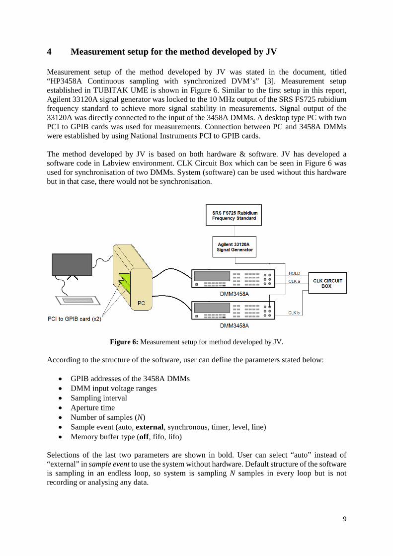
9
4 Measurement setup for the method developed by JV Measurement setup of the method developed by JV was stated in the document, titled “HP3458A Continuous sampling with synchronized DVM’s” [3]. Measurement setup established in TUBITAK UME is shown in Figure 6. Similar to the first setup in this report, Agilent 33120A signal generator was locked to the 10 MHz output of the SRS FS725 rubidium frequency standard to achieve more signal stability in measurements. Signal output of the 33120A was directly connected to the input of the 3458A DMMs. A desktop type PC with two PCI to GPIB cards was used for measurements. Connection between PC and 3458A DMMs were established by using National Instruments PCI to GPIB cards. The method developed by JV is based on both hardware & software. JV has developed a software code in Labview environment. CLK Circuit Box which can be seen in Figure 6 was used for synchronisation of two DMMs. System (software) can be used without this hardware but in that case, there would not be synchronisation.
Figure 6: Measurement setup for method developed by JV.
According to the structure of the software, user can define the parameters stated below:
• GPIB addresses of the 3458A DMMs • DMM input voltage ranges • Sampling interval • Aperture time • Number of samples (N) • Sample event (auto, external, synchronous, timer, level, line) • Memory buffer type (off, fifo, lifo)
Selections of the last two parameters are shown in bold. User can select “auto” instead of “external” in sample event to use the system without hardware. Default structure of the software is sampling in an endless loop, so system is sampling N samples in every loop but is not recording or analysing any data.

10
5 Measurement results of the JV method A few modifications were made in software developed by JV in Labview environment. With this modification, Labview code takes two consecutive data packages then transfers data to the Matlab and stops. Time delay between data packages were calculated with using same Matlab code which is used for evaluation of SIQ method. This matlab code was developed by SIQ, based on the PSFE estimation algorithm. 3458A DMM (Agilent) which was used in the measurements of SIQ method was also used to test JV method. A second 3458A DMM was also connected to the test setup but gathered data is not evaluated. A sine wave signal having 6 VRMS was applied from 33120A. Signal frequency was changed from 10 Hz to 100 Hz with 10 Hz steps. Labview code parameters used in the measurements are;
• DMM input voltage ranges: 10 V • Number of samples: N was selected 2x10⁴ and 2x10⁵ to see the effect of this value to
the time delay between data packages. • Sampling interval: 100 µs • Aperture time: 90 µs
Sampling frequency was fixed at 10 kSps due to the structure of the JV’s hardware. CLK Circuit Box has own internal clock oscillator. Therefore, N values were selected to achieve same GPIB data transfer time of the SIQ tests. Labview code was run 100 times and two consecutive data packages (each contains N samples) were taken 100 times then time delays were calculated. Mean value and standard deviation of the time delays were calculated for each frequency (10 Hz – 100 Hz) and N value (2x10⁴ and 2x10⁵). Results are shown in Table 5 and Table 6. Histograms of the 100 time delays for each measurement point are also shown in Figure 7 and Figure 8.
Table 5: Time delay between loops: N = 2x10⁴, Fsignal = 10 Hz – 100 Hz.
Fsignal (Hz) Time delay between loops (ms) Standard deviation (ms)
10 51.827 1.211 20 2.152 1.331 30 18.734 1.358 40 2.090 1.395 50 12.134 1.412 60 1.909 1.234 70 8.845 1.445 80 1.739 0.961 90 7.051 1.154
100 1.846 1.000

11
Table 6: Time delay between loops: N = 2x10⁵, Fsignal = 10 Hz – 100 Hz.
Fsignal (Hz) Time delay between loops (ms) Standard deviation (ms)
10 85.347 1.075 20 34.666 0.991 30 17.826 0.932 40 9.704 1.029 50 4.683 1.155 60 1.684 1.021 70 12.903 0.683 80 9.805 0.801 90 6.721 0.910
100 4.478 0.959

12
Figure 7: Time delay between loops: N = 2x10⁴, Fsignal = 10 Hz – 100 Hz.

13
Figure 8: Time delay between loops: N = 2x10⁵, Fsignal = 10 Hz – 100 Hz.

14
6 Conclusions Long duration sampling with one DMM 3458A is needed in some applications especially in PQ measurements. SIQ and JV have developed their solutions for this purpose and both solutions have been tested and evaluated. Results showed that it is possible to transfer more data with using these methods than standard data transfer method could achieve. However, time delays between sampled data packages could be a problem source. Results showed that JV’s method is more stable than SIQ’s method according to the standard deviations of the time delays. An important point must be stated here; calculation method of the time delays between sampled data packages has a problem. If the time delay value is bigger than full period of the input signal, method gives the remaining time according to the period. For example, if we apply 50 Hz sine wave (20 ms period) and actual time delay is 22 ms then calculation method gives 2 ms as a result. In this case, we can’t know if the actual time delay is only 2 ms or it includes a full period.
References [1] JRP Protocol, Version date: 19 April 2016, 15RPT04 TracePQM – Traceability routes for electrical power quality measurements [2] Report A1.2.4 and A2.1.2: Extending the data record length of sampling with DMM 3458A for long duration measurements – Report written by SIQ [3] HP3458A Continuous sampling with synchronised DVM’s – Document written by JV

15RPT04 TracePQM - Appendix
Report describing the open software tool developed for handling high performance ADCs identified for power and PQ measurements
BLANK PAGE

15RPT04 TracePQM
Report describing the open software tool developed for handling high performance ADCs identified for power and PQ measurements
Appendix #4
A2.1.4 - Concept of interfacing LabWindows/CVI to Matlab

1
Report A2.1.4: Concept of Interfacing LabWindows/CVI to Matlab.

2
Objective
This report is related with activity A2.1.4: “The concept for the interface between the data processing module and the control and data acquisition module”, of TracePQM-15RPT04, and only describes the concept for interfacing LabWindows/CVI to MATLAB tool.
The Labview to MATLAB /Octave interface was already developed with GOLPI library [1] and lv_process, the low level library to access hardware via pipes. The required interface for LabWindows/CVI to MATLAB has been developed using MATLAB Engine API. [2] This API requires also MATLAB installed, not only Runtime Engine, to use properly, related to documentation given form MATLAB internet site.
Structure
In order to use MATLAB functions/scripts from C or LabWindows/CVI environment, MATLAB tool must be installed in the system. The operating system, hardware and all related software should use the same bit number, 32-Bit or 64-Bit.
The last version of TWM tool should be downloaded from source site.[3] The TWM tool uses MATLAB and QWTB tool, the Quantum Wave ToolBox. [4]The other related libraries, niscope, niTClk, should be exist and accessible from user space in order to run virtual digitizers used in TWM software.
Figure 1 GUI window of the module
The CVI tool, the second version is shown can be downloaded from TracePQM web site, both source codes and compiled as a standalone application. [5] The CVI tool uses QWTB tool and its scripts like

3
TWM application and performs the desired calculations. When it runs, it looks like the picture shown in Figure 1, similar to QWTB calculation section of TWM software.
The results obtained from digitizers are stored as result files with required format and many calculations can be performed with CVI tool being used MATLAB scripts background.
LabWindows/CVI to MATLAB interfacing is done with using dedicated header files, library and MATLAB Engine. The CVI project/program must include these header files and use the functions of libraries. The libeng.lib and libmx.lib files must be included in project tree and the system-wide path of these files must be added the operating system paths in order to run MATLAB engine calls.
Implementation
The name of CVI module is “Matlab Module” and name of related c file is Matlab Module.c. The name of GUI (Graphic User Interface) of the module is Matlab Module.uir. The screenshot of the window is shown in Figure 1.
When the application runs, it first initiates GUI and calls the main procedure, named main, located in Matlab Module.c.
Figure 2 MATLAB engine initialization and starting in main procedure.
This procedure also initiates the MATLAB session calling the mlink_init, declared in mlink.c source file and starts the MATLAB engine at the background calling mlink_start, declared in the same source file, Figure 2, Figure 3, respectively.

4
Figure 3 Declaring MATLAB engine start procedure in mlink.c source file.
The TMLink parameter is a C struct and declared in mlink.h header files. ML_MATLAB and ML_OCTAVE constants are also declared in the same header file, shown in Figure 4.
Figure 4 TMLink struct.
The MATLAB engine opens with engOpen command and returns a pointer for handle of MATLAB engine. The init parameter passed to function must be NULL for Windows operating systems, declared in [1].
The first interaction of MATLAB environment is completed with the command sequence. Now, we have an engine handle to be used in LabWindows/CVI environment.

5
The main procedure runs the twm_init command, declared in twm_matlab.c, with the parameter which returned from the mlink_start procedure, shown in Figure 5, if there are no errors from previous operations.
Figure 5 Declaration of twm_init procedure.
When the twm_init runs, the MATLAB is ready to run with the desired working paths. This command calls the mlink_cmd command, declared in mlink.c source file, shown in Figure 6. This command calls the engine API procedures, engEvalString and engOutputBuffer including correct paths and command string to be evaluated by MATLAB. The engEvalString command evaluates the expression contained in command string for the MATLAB engine session, lnk, previously started by engOpen. The engOutputBuffer command defines a character buffer for engEvalString to return any output that ordinarily appears on the screen. This buffer will be filled with output values of MATLAB and used by main program.

6
Figure 6 mlink_cmd command structure.
After the main program initiates, the user must select the proper info file by pressing LOAD button on the top-right side of main window. The open-file dialog of operation system appears and waits an info file to select when this button is pressed, shown in Figure 7.

7
Figure 7 Loading the info file.
The session.info file can be selected as an example. The format of info file, including all required digitizer, transducer corrections, offsets, data formats, raw data etc, was described detailed in activity A2.3.1.
When the selected file loaded, it should be clicked the REFRESH button at the left-bottom of window. With activating the REFRESH button, the dedicated CALLBACK procedure of main GUI evaluated. The CALLBACK function performs a list of command sequence and determines the required evaluation/calculation parameters such as algorithm type, the paths for info, results, corrections, assigns the related variables and calls the twm_get_result_info, twm_get_results_data,
twm_get_alg_list, twm_get_alg_info commands, declared in twm_matlab.c source file with passing the required parameter, the pointer to handle that represents MATLAB engine, to perform various operations on the measurement dates.

8
Figure 8 The actual window.
Conclusions
The basic interaction of LabWindows/CVI to MATLAB tool is briefly explained. The only MATLAB like calculation tool is MATLAB, so the OCTAVE part is not implemented by code developer at the moment. With this successful communication scheme of these two environments, the well known algorithms written in MATLAB have been used efficiently without re-written completely for the other languages.
References
[1] https://github.com/KaeroDot/GOLPI
[2] https://uk.mathworks.com/help/matlab/calling-matlab-engine-from-c-programs-1.html
[3] https://github.com/smaslan/TWM/blob/master/builds/TWM.zip
[4] https://qwtb.github.io/qwtb/
[5] http://tracepqm.cmi.cz/database/files/wp2/task%202.3/20Matlab%20Module%20v2.zip

9
Appendix
• The Matlab Module.c source file: //============================================================================== // // Title: Matlab Module // Purpose: A short description of the application. // // Created on: 2.3.2014 at 16:16:57 by . // Copyright: . All Rights Reserved. // //============================================================================== //============================================================================== // Include files #include <ansi_c.h> #include <windows.h> #include <Shlwapi.h> #include <cvirte.h> #include <userint.h> #include "Matlab Module.h" #include "toolbox.h" #include "qwtb_alg_select.h" #include "mlink.h" #include "twm_matlab.h" #include "utils.h" #include "matlab_globals.h" //============================================================================== // Constants #define INIFILE "config.ini" //============================================================================== // Types //============================================================================== // Static global variables static int panelHandle = 0; //============================================================================== // Static functions //============================================================================== // Global variables // Matlab link handle TMLink mlink; // config.ini full path char ini[MAX_PATHNAME_LEN]; // last result path char resfld[MAX_PATH]; //============================================================================== // Global functions /// HIFN The main entry-point function. int main (int argc, char *argv[])

10
int error = 0; int ret; // get app directory char appdir[MAX_PATHNAME_LEN]; GetProjectDir(appdir); // build ini path strcpy(ini,appdir); strcat(ini,"\\config.ini"); // load TWM function path from INI file char twm_path[MAX_PATH]; ret = GetPrivateProfileString("PATH","twm_octave_folder","",twm_path,MAX_PATH,ini); if(!ret) MessageBoxA(NULL,"Missing INI file or the [PATH],twm_octave_folder value!","Error",0); goto Error; // load last result folder path from INI file ret = GetPrivateProfileString("PATH","last_result_path","",resfld,MAX_PATH,ini); // --- MATLAB INIT --- // init mlink_init(&mlink,ML_MATLAB); // try to start Matlab ret = mlink_start(&mlink); if(ret) MessageBoxA(NULL,"Cannot start Matlab!","Error",0); else // initialize TWM link char *errstr; ret = twm_init(&mlink,&errstr,twm_path); // failed? if(ret) MessageBoxA(NULL,errstr,"Matlab error",0); free((void*)errstr); else /* initialize and load resources */ nullChk (InitCVIRTE (0, argv, 0)); errChk (panelHandle = LoadPanel (0, "Matlab Module.uir", PANEL)); /* display the panel and run the user interface */ errChk (DisplayPanel (panelHandle)); errChk (RunUserInterface ()); Error: /* clean up */ if (panelHandle > 0) DiscardPanel (panelHandle); return 0; //==============================================================================

11
// UI callback function prototypes /// HIFN Exit when the user dismisses the panel. int CVICALLBACK panelCB (int panel, int event, void *callbackData, int eventData1, int eventData2) if (event == EVENT_CLOSE) QuitUserInterface (0); // try to close Matlab mlink_close(&mlink,1); // store last path WritePrivateProfileString("PATH","last_result_path",resfld,ini); return 0; //------------------------------------------------------------------------------ // Refresh result view // int CVICALLBACK btn_cmd (int panel, int control, int event, void *callbackData, int eventData1, int eventData2) switch (event) case EVENT_COMMIT: char path[MAX_PATH]; // default alg/res selection: int alg_id = -1; int res_id = -1; int ref_id = -1; // results found? int res_exist = 0; // get result path GetCtrlVal(panel,PANEL_PATH_RES,(void*)path); // -- two pass assignement // 1) fill result/alg selectors // 2) load selected alg and result for(int pass = 0;pass < 2;pass++) // get last algorithm selection // 0 - last used // 1,2,... - alg. selection ID GetCtrlIndex(panel,PANEL_RING_ALG,&alg_id); if(alg_id < 0) alg_id = 0; // get last result selection // 0 - last measured // 1 - average of all // 2,3,... - result selection ID GetCtrlIndex(panel,PANEL_RING_RES,&res_id); if(res_id < 0) res_id = 0; // get ref channel mode selection // 0 - no ref // 1,2,... - channel selection ID

12
GetCtrlIndex(panel,PANEL_REFMODE,&ref_id); if(ref_id < 0) ref_id = 0; // alg. selection string char alg_id_str[256]; strcpy(alg_id_str,""); if(pass && alg_id) GetLabelFromIndex(panel,PANEL_RING_ALG,alg_id,(void*)alg_id_str); // read results char *res_files; char *alg_list; char *chn_list; char *errstr; int ret = twm_get_result_info(&mlink,&errstr,path,alg_id_str,&res_exist,&res_files,&alg_list,&chn_list); if(ret) // failed MessageBoxA(NULL,errstr,"Matlab error",0); free((void*)errstr); return(1); // clear result selectors ClearListCtrl(panel,PANEL_RING_RES); ClearListCtrl(panel,PANEL_RING_ALG); ClearListCtrl(panel,PANEL_REFMODE); if(res_exist) // --- something found - fill the dialog int rows,cols,cc; char **cells,*csv; // fill algorithms list csv = (char*)malloc((strlen(alg_list)+100)*sizeof(char)); strcpy(csv,"Current: "); strcat(csv,alg_list); free((void*)alg_list); cc = csv_parse(csv,';','\t',&rows,&cols,NULL); cells = (char**)malloc(cc*sizeof(char*)); csv_parse(csv,';','\t',&rows,&cols,cells); InsertListItem(panel,PANEL_RING_ALG,0,cells[0],0); for(int k=2;k<cc;k++) InsertListItem(panel,PANEL_RING_ALG,k-1,cells[k],k-1); free((void*)cells); free((void*)csv); if(alg_id >= cc-1) SetCtrlIndex(panel,PANEL_RING_ALG,0); SetCtrlIndex(panel,PANEL_RING_RES,0); else SetCtrlIndex(panel,PANEL_RING_ALG,alg_id); // fill results list csv = (char*)malloc((strlen(res_files)+100)*sizeof(char)); strcpy(csv,"Current result\tAverage\t"); strcat(csv,res_files); free((void*)res_files); cc = csv_parse(csv,';','\t',&rows,&cols,NULL); cells = (char**)malloc(cc*sizeof(char*)); csv_parse(csv,';','\t',&rows,&cols,cells);

13
for(int k=0;k<cc;k++) InsertListItem(panel,PANEL_RING_RES,k,cells[k],k); free((void*)cells); free((void*)csv); if(res_id >= cc) SetCtrlIndex(panel,PANEL_RING_RES,0); res_id = 0; else SetCtrlIndex(panel,PANEL_RING_RES,res_id); // fill results list csv = (char*)malloc((strlen(chn_list)+100)*sizeof(char)); strcpy(csv,"None;"); strcat(csv,chn_list); free((void*)chn_list); cc = csv_parse(csv,'\t',';',&rows,&cols,NULL); cells = (char**)malloc(cc*sizeof(char*)); csv_parse(csv,'\t',';',&rows,&cols,cells); for(int k=0;k<cc;k++) InsertListItem(panel,PANEL_REFMODE,k,cells[k],k); free((void*)cells); free((void*)csv); if(ref_id >= cc) SetCtrlIndex(panel,PANEL_REFMODE,0); ref_id = 0; else SetCtrlIndex(panel,PANEL_REFMODE,ref_id); else // failed MessageBoxA(NULL,"Selected result is invalid or contains no calculated results.","Matlab error",0); break; if(res_exist) // -- load result data // display config TResCfg cfg; GetCtrlVal(panel,PANEL_MAXDIM,(void*)&cfg.max_dim); GetCtrlVal(panel,PANEL_MAXDIMSZ,(void*)&cfg.max_array); GetCtrlVal(panel,PANEL_GRPMODE,(void*)&cfg.group_mode); GetCtrlVal(panel,PANEL_UNCMODE,(void*)&cfg.unc_mode); GetCtrlVal(panel,PANEL_PHIMODE,(void*)&cfg.phi_mode); GetCtrlVal(panel,PANEL_REFMODE,(void*)&cfg.phi_ref_chn); // alg. selection string char alg_id_str[256]; strcpy(alg_id_str,""); if(alg_id) GetLabelFromIndex(panel,PANEL_RING_ALG,alg_id,(void*)alg_id_str); // obtain result data from matlab char *csv = NULL; char *errstr; int ret = twm_get_result_data(&mlink,&errstr,path,res_id-1,alg_id_str,&cfg,&csv); if(ret) // failed MessageBoxA(NULL,errstr,"Matlab error",0); free((void*)errstr);

14
return(1); int rows,cols; int cc = csv_parse(csv,'\t','\n',&rows,&cols,NULL); char **cells = (char**)malloc(cc*sizeof(char*)); csv_parse(csv,'\t','\n',&rows,&cols,cells); // disable table refresh SetCtrlAttribute(panel, PANEL_TABLE, ATTR_VISIBLE, 0); // refresh table data size DeleteTableColumns(panel,PANEL_TABLE,1,-1); DeleteTableRows(panel,PANEL_TABLE,1,-1); InsertTableRows(panel,PANEL_TABLE,1,rows-1,VAL_CELL_STRING); InsertTableColumns(panel,PANEL_TABLE,1,cols-1,VAL_CELL_STRING); // refresh headers SetTableRowAttribute (panel, PANEL_TABLE, -1, ATTR_USE_LABEL_TEXT, 1); for(int r = 1;r<rows;r++) SetTableRowAttribute(panel,PANEL_TABLE,r,ATTR_LABEL_TEXT,cells[r*cols]); SetTableColumnAttribute (panel, PANEL_TABLE, -1, ATTR_USE_LABEL_TEXT, 1); for(int c = 1;c<cols;c++) SetTableColumnAttribute(panel,PANEL_TABLE,c,ATTR_LABEL_TEXT,cells[c]); // refresh data for(int r = 1;r<rows;r++) SetTableCellRangeVals(panel,PANEL_TABLE,MakeRect(r,1,1,cols-1),&cells[r*cols+1],VAL_ROW_MAJOR); // autoscale for(int c = 1;c<cols;c++) SetColumnWidthToWidestCellContents(panel,PANEL_TABLE,c); // enable table refresh SetCtrlAttribute(panel, PANEL_TABLE, ATTR_VISIBLE, 1); free((void*)cells); free((void*)csv); break; return 0; //------------------------------------------------------------------------------ // Select result file // int CVICALLBACK btn_load (int panel, int control, int event, void *callbackData, int eventData1, int eventData2) switch (event)

15
case EVENT_COMMIT: // open result file char path[MAX_PATH]; if(FileSelectPopup(resfld,"*.info","*.info","Select result file",VAL_LOAD_BUTTON,0,0,1,1,path) == VAL_EXISTING_FILE_SELECTED); // extract folder path char *p = strrchr(path, '\\'); if(p) *p = '\0'; // remember last result folder strcpy(resfld,path); // write file path to the box SetCtrlVal(panel,PANEL_PATH_RES,path); break; return 0; //------------------------------------------------------------------------------ // processing configuration panel // int CVICALLBACK btn_proc_cfg (int panel, int control, int event, void *callbackData, int eventData1, int eventData2) switch (event) case EVENT_COMMIT: int cfg_panel = LoadPanel(0,"qwtb_alg_select.uir",PROCPANEL); DisplayPanel(cfg_panel); break; return 0; //------------------------------------------------------------------------------ // fake generation of some measurement data int CVICALLBACK btn_fake_proc (int panel, int control, int event, void *callbackData, int eventData1, int eventData2) switch (event) case EVENT_COMMIT: // open folder char path[MAX_PATH]; if(DirSelectPopup(resfld,"Select destination for fake measurement",1,1,path) == VAL_DIRECTORY_SELECTED); // crate some fake sample data float smpl_c1[1000]; float smpl_c2[1000]; float smpl_c3[1000]; for(int i = 0;i < 1000;i++) smpl_c1[i] = (float)(i%100);

16
smpl_c2[i] = (float)(i%150); smpl_c3[i] = (float)(i%75); // create record info structure TTWMssnInf info; memset((void*)&info, 0, sizeof(info)); // always clear it before filling new stuff!!! // now fill in the basic sampling informations info.N = 1000; // samples count info.fs = 100000; // sampling rate info.chn_count = 3; // digitizer channels count (not transducers!) info.chn_data_type = TWMMATFMT_SGL; // sample data in real32 format // -- now build list of digitizre channel setups for up to TWMMAXTR = 6 channels strncpy(info.chn_idns[0],"channel 1",TWMMAXSTR); // create name of dig. channel 1 info.chn_gains[0] = 1.0001; // gain factor of channel 1 info.chn_offs[0] = 0.0003; // offset of channel 1 info.chn_rng[0] = 10.0; // nominal range of channel 1 info.time_stamps[0] = 1.2345; // relative timestamp of channel 1 (may be zero) info.chn_data[0] = smpl_c1; // sample data pointer for channel 1 strncpy(info.chn_idns[1],"channel 2",TWMMAXSTR); // create name of dig. channel 2 info.chn_gains[1] = 1.0002; // gain factor of channel 2 info.chn_offs[1] = 0.0004; // offset of channel 2 info.chn_rng[1] = 10.0; // nominal range of channel 2 info.time_stamps[1] = 1.2346; // relative timestamp of channel 2 (may be zero) info.chn_data[1] = smpl_c2; // sample data pointer for channel 2 strncpy(info.chn_idns[2],"channel 3",TWMMAXSTR); // create name of dig. channel 3 info.chn_gains[2] = 1.0003; // gain factor of channel 3 info.chn_offs[2] = 0.0005; // offset of channel 3 info.chn_rng[2] = 10.0; // nominal range of channel 3 info.time_stamps[2] = 1.2347; // relative timestamp of channel 3 (may be zero) info.chn_data[2] = smpl_c3; // sample data pointer for channel 3 // next channels ... // path to selected digitizer correction file strcpy(info.dig_corr,"c:\\TPQA\\corrections\\digitizer\\HP3458A\\HP3458_v1.info"); // -- now define transducer and how their are connected to the digitizer channels: // transducers count info.tr_count = 2; // first transducer definition strcpy(info.tr_corr[0],"c:\\TPQA\\corrections\\transducers\\shunt_1A1\\shunt_1A1.info"); // path to correction file info.tr_phase[0] = 1; // phase index of transducer (use the same index for U-I pair for power, but different indices if measuring multi phse U or multiphase I) info.tr_map[0][0] = 2; // mapping to digitizer for differential connection [][2]-[][3], i.e. dig channels 2-3 info.tr_map[0][1] = 3; // second transducer definition strcpy(info.tr_corr[1],"c:\\TPQA\\corrections\\transducers\\rvd_230V1\\shunt_230V1.info"); info.tr_phase[1] = 1; info.tr_map[0][0] = 1; // mapping to digitizer: example of single-ended connection to dig. channel 1

17
// next transducer definitions... // copy QWTB setup from config panel (not nice solution! may be uninitalized!) info.qwtb = cfg_qwtb; // generate measurement session twm_write_session(path, &info); break; return 0;
• m_link.c source file: //============================================================================== // // Title: matlab_module.c // Purpose: A short description of the implementation. // // Created on: 2.3.2014 at 17:46:31 by . // Copyright: . All Rights Reserved. // //============================================================================== //============================================================================== // Include files #include <ansi_c.h> #include "mlink.h" #include "engine.h" #include "matrix.h" //============================================================================== // Constants //============================================================================== // Types //============================================================================== // Static global variables //============================================================================== // Static functions //============================================================================== // Global variables //============================================================================== // Global functions // --- initialize Matlab link lib --- int mlink_init(TMLink *lnk,int mode) lnk->eng = NULL; lnk->mode = mode; // Octave not done yet return(mode != ML_MATLAB/* && mode != ML_OCTAVE*/); // --- start Matlab --- int mlink_start(TMLink *lnk)

18
if(lnk->mode == ML_MATLAB) // MATLAB mode: // close link before if(lnk->eng) engClose(lnk->eng); // try to open lnk->eng = engOpen(NULL); return(lnk->eng == NULL); else // OCTAVE mode: return(1); // --- close Matlab --- int mlink_close(TMLink *lnk,int close) if(lnk->mode == ML_MATLAB) // MATLAB mode: if(lnk->eng) // evaluate "exit" command? if(close) engEvalString(lnk->eng,"exit"); // close engine engClose(lnk->eng); lnk->eng = NULL; return(0); else // OCTAVE mode: return(1); // --- exec command Matlab --- int mlink_cmd(TMLink *lnk,char *cmd,char *ret,int retmax) if(lnk->mode == ML_MATLAB) // MATLAB mode: // register answer buffer? if(ret) engOutputBuffer(lnk->eng,ret,retmax-1); else engOutputBuffer(lnk->eng,NULL,0); // eval command engEvalString(lnk->eng,cmd); // unregister buffer engOutputBuffer(lnk->eng,NULL,0);

19
// detect error if(ret) char *err = strstr(ret,"??? "); if(err) strcpy(ret,err); return(1); return(0); else // OCTAVE mode: return(1); // --- Get string variable from engine --- int mlink_get_var_str(TMLink *lnk,char *var_name,char **data) // no data yet *data = NULL; if(lnk->mode == ML_MATLAB) // MATLAB mode: // try to obtain variable mxArray *arr = engGetVariable(lnk->eng,var_name); if(!arr) // not exist! return(1); if(!mxIsChar(arr)) // not char array! mxDestroyArray(arr); return(1); // get var dimensions size_t cols = mxGetN(arr); size_t rows = mxGetM(arr); // allocate string buffer *data = (char*)malloc((rows*cols + 1)*sizeof(char)); **data = '\0'; // try to read string data mxGetString(arr,*data,cols*rows + 1); // get rid of the array mxDestroyArray(arr); return(0); else // OCTAVE mode: return(1);

20
// --- Get real vector variable from engine --- int mlink_get_var_dbl_vec(TMLink *lnk,char *var_name,double **data,int *size) // no data yet *data = NULL; if(lnk->mode == ML_MATLAB) // MATLAB mode: // try to obtain variable mxArray *arr = engGetVariable(lnk->eng,var_name); if(!arr) // not exist! return(1); if(!mxIsNumeric(arr) || mxIsComplex(arr)) // not numeric array! mxDestroyArray(arr); return(1); // get dimensions size_t dimn = mxGetNumberOfDimensions(arr); mwSize *sz = mxGetDimensions(arr); // total elements size_t num = mxGetNumberOfElements(arr); if(dimn>2 || (dimn == 2 && sz[0]>1 && sz[1]>1)) // not 1D mxDestroyArray(arr); return(1); // array data pointer void *dptr = mxGetData(arr); // allocate string buffer *data = (double*)malloc(num*sizeof(double)); if(mxIsDouble(arr)) // --- double array // copy array memcpy((void*)*data,dptr,num*sizeof(double)); // total elements *size = (int)num; else if(mxIsInt32(arr)) // --- int32 array - cast to double and no bitching... int *iptr = (int*)dptr; for(int k = 0;k < num;k++) (*data)[k] = (double)*iptr++; // total elements *size = (int)num;

21
else // --- not supported free((void*)*data); *data = NULL; *size = 0; mxDestroyArray(arr); return(1); // get rid of the array mxDestroyArray(arr); return(0); else // OCTAVE mode: return(1); // --- Get int32 vector variable from engine --- int mlink_get_var_int_vec(TMLink *lnk,char *var_name,int **data,int *size) // no data yet *data = NULL; if(lnk->mode == ML_MATLAB) // MATLAB mode: // try to obtain variable mxArray *arr = engGetVariable(lnk->eng,var_name); if(!arr) // not exist! return(1); if(!mxIsNumeric(arr) || mxIsComplex(arr)) // not numeric array! mxDestroyArray(arr); return(1); // get dimensions size_t dimn = mxGetNumberOfDimensions(arr); mwSize *sz = mxGetDimensions(arr); // total elements size_t num = mxGetNumberOfElements(arr); if(dimn>2 || (dimn == 2 && sz[0]>1 && sz[1]>1)) // not 1D mxDestroyArray(arr); return(1); // array data pointer

22
void *dptr = mxGetData(arr); // allocate string buffer *data = (int*)malloc(num*sizeof(int)); if(mxIsDouble(arr)) // --- double array - cast to int32 double *ptr = (double*)dptr; for(int k = 0;k < num;k++) (*data)[k] = (int)*ptr++; // total elements *size = (int)num; else if(mxIsInt32(arr)) // --- int32 array // copy array memcpy((void*)*data,dptr,num*sizeof(int)); // total elements *size = (int)num; else // --- not supported free((void*)*data); *data = NULL; *size = 0; mxDestroyArray(arr); return(1); // get rid of the array mxDestroyArray(arr); return(0); else // OCTAVE mode: return(1);
• m_link.h header file: //============================================================================== // // Title: matlab_module.h // Purpose: A short description of the interface. // // Created on: 2.3.2014 at 17:46:31 by . // Copyright: . All Rights Reserved. // //============================================================================== #ifndef __mlink_H__ #define __mlink_H__ #ifdef __cplusplus

23
extern "C" #endif //============================================================================== // Include files #include "cvidef.h" #include "engine.h" //============================================================================== // Constants #define ML_MATLAB 0 #define ML_OCTAVE 1 //============================================================================== // Types typedef struct int mode; Engine *eng; TMLink; //============================================================================== // External variables //============================================================================== // Global functions int mlink_init(TMLink *lnk,int mode); int mlink_start(TMLink *lnk); int mlink_close(TMLink *lnk,int close); int mlink_cmd(TMLink *lnk,char *cmd,char *ret,int retmax); int mlink_get_var_str(TMLink *lnk,char *var_name,char **data); int mlink_get_var_dbl_vec(TMLink *lnk,char *var_name,double **data,int *size); int mlink_get_var_int_vec(TMLink *lnk,char *var_name,int **data,int *size); #ifdef __cplusplus #endif #endif /* ndef __matlab_module_H__ */ Twm_matlab.c source file: //============================================================================== // // Title: twm_matlab.c // Purpose: A short description of the implementation. // // Created on: 2.3.2014 at 20:14:31 by . // Copyright: . All Rights Reserved. // //============================================================================== //============================================================================== // Include files #include <ansi_c.h> #include <windows.h> #include <utility.h> #include "twm_matlab.h" #include "mlink.h" //============================================================================== // Constants #define MAXERR 4096

24
//============================================================================== // Types //============================================================================== // Static global variables //============================================================================== // Static functions //============================================================================== // Global variables //============================================================================== // Global functions //------------------------------------------------------------------------------ // Initialize TWM link - set TWM functions path // // lnk - Matlab link session // path - TWM functions root folder // errstr - allocates and returns error string, if no error, returns NULL // // NOTE: Do not forget to free the allocated buffers! // int twm_init(TMLink *lnk,char **errstr,char *path) char cmd[MAX_PATH+100]; int err; // allocate error string char *errbuf = (char*)malloc(MAXERR*sizeof(char)); if(errstr) *errstr = errbuf; // add TWM root path sprintf(cmd,"addpath('%s');",path); err = mlink_cmd(lnk,cmd,errbuf,MAXERR); if(err) return(1); // add TWM info path sprintf(cmd,"addpath('%s\\info');",path); err = mlink_cmd(lnk,cmd,errbuf,MAXERR); if(err) return(1); // add TWM info path sprintf(cmd,"addpath('%s\\qwtb');",path); err = mlink_cmd(lnk,cmd,errbuf,MAXERR); if(err) return(1); // no errors, loose error buffer free((void*)errbuf); if(errstr) *errstr = NULL; return(0); //------------------------------------------------------------------------------ // TWM: load result(s) info(s) // // lnk - Matlab link session // errstr - allocates and returns error string, if no error, returns NULL // path - measurement root folder // alg_id - string id of QWTB algorithms ("": last calculated) // res_exist - returns non-zero if selection is valid // res_files - allocates and returns pointer to list of result files, // csv string separated by tabs

25
// alg_list - allocates and returns pointer to list of calc. algorithms // csv string separated by tabs // chn_list - allocates and returns pointer to list of possible ref. channels // csv string separated by tabs // // NOTE: Do not forget to free the allocated buffers! // int twm_get_result_info(TMLink *lnk,char **errstr,char *path,char *alg_id, int *res_exist,char **res_files, char **alg_list, char **chn_list) char cmd[MAX_PATH+200]; // build command sprintf(cmd,"[res_files, res_exist, alg_list, chn_list] = qwtb_get_results_info('%s','%s');",path,alg_id); // allocate error string char *errbuf = (char*)malloc(MAXERR*sizeof(char)); if(errstr) *errstr = errbuf; // exec command int err = mlink_cmd(lnk,cmd,errbuf,MAXERR); if(err) return(1); // read result exist flag if(res_exist) *res_exist = 0; int *buf = NULL; int size; mlink_get_var_int_vec(lnk,"res_exist",&buf,&size); if(buf && size) *res_exist = buf[0]; free((void*)buf); // read result files list if(res_files) *res_files = NULL; mlink_get_var_str(lnk,"res_files",res_files); // read calculated algorithms files list if(alg_list) *alg_list = NULL; mlink_get_var_str(lnk,"alg_list",alg_list); // read channels list if(chn_list) *chn_list = NULL; mlink_get_var_str(lnk,"chn_list",chn_list); // no errors, loose error buffer free((void*)errbuf); if(errstr) *errstr = NULL; return(0);

26
//------------------------------------------------------------------------------ // TWM: load result data // // lnk - Matlab link session // path - measurement root folder // res_id - ID of the result file to select (-1: last, 0: average, >0: IDs of files) // alg_id - string id of QWTB algorithms ("": last calculated) // cfg - display setup structure // cfg.max_dim - max shown dim (0: scalar, 1: vectors, 2: matrices) // cfg.max_array - max vector size to be shown // cfg.group_mode - grouping mode (0: quantities, 1: channels) // cfg.unc_mode - uncertainty display mode (0: none, 1: val±unc, 2: val;unc) // cfg.phi_mode - phase display mode (0: ±pi [rad], 1: 0-2pi [rad], 2: ±180 [deg], 3: 0-360 [deg]) // cfg.phi_ref_chn - reference channel is (0: none, >0: channel ids) // csv - allocates and returns pointer to list 2D CSV table of results, // tabs separator // // NOTE: Do not forget to free the allocated buffers! // int twm_get_result_data(TMLink *lnk,char **errstr,char *path,int res_id,char *alg_id,TResCfg *cfg, char **csv) char cmd[MAX_PATH+1024]; // build command sprintf(cmd,"cfg = struct();\n" "cfg.max_dim = %d;\n" "cfg.max_array = %d;\n" "cfg.group_mode = %d;\n" "cfg.unc_mode = %d;\n" "cfg.phi_mode = %d;\n" "cfg.phi_ref_chn = %d;\n" "[csv, desc, var_names, chn_index] = qwtb_get_results('%s', %d, '%s', cfg);", cfg->max_dim,cfg->max_array,cfg->group_mode,cfg->unc_mode,cfg->phi_mode,cfg->phi_ref_chn, path,res_id,alg_id); // allocate error string char *errbuf = (char*)malloc(MAXERR*sizeof(char)); if(errstr) *errstr = errbuf; // exec command int err = mlink_cmd(lnk,cmd,errbuf,MAXERR); if(err) return(1); // read result files list if(csv) *csv = NULL; mlink_get_var_str(lnk,"csv",csv); // no errors, loose error buffer free((void*)errbuf); if(errstr) *errstr = NULL; return(0);

27
//------------------------------------------------------------------------------ // TWM: call algorithms passing through qwtb.exec.algorithm.m of matlab // // TWM: Executes QWTB algorithm based on the setup from meas. session // inputs: // **errstr - error string, autoallocates data if error // *path - path to measurement file session.info // *calc_unc - override uncertainty calculation mode (default "") // is_last_avg - is last record from repeated group? // avg_id - record id // group_id - group id // // NOTE: Do not forget to free the allocated buffers! // int twm_exec_algorithm(TMLink *lnk,char **errstr,char *path, char *calc_unc, int is_last_avg, int avg_id, int group_id) char cmd[MAX_PATH+1024]; // build command sprintf(cmd, "qwtb_exec_algorithm('%s', '%s', %d, %d, %d);", path, calc_unc, is_last_avg, avg_id, group_id); // allocate error string char *errbuf = (char*)malloc(MAXERR*sizeof(char)); if(errstr) *errstr = errbuf; // exec command int err = mlink_cmd(lnk,cmd,errbuf,MAXERR); if(err) return(1); // no errors, loose error buffer free((void*)errbuf); if(errstr) *errstr = NULL; return(0); //------------------------------------------------------------------------------ // TWM: get list of algorithms // // inputs: // **errstr - error string, autoallocates data if error // **alg_ids - list of algorithms IDs (NULL if not needed) // **alg_names - list of algorithm names (NULL if not needed) // // NOTE: Do not forget to free the allocated buffers! // int twm_get_alg_list(TMLink *lnk,char **errstr,char **alg_ids,char **alg_names) char cmd[1024]; // build command sprintf(cmd,"[ids, names] = qwtb_load_algorithms('qwtb_list.info');"); // allocate error string char *errbuf = (char*)malloc(MAXERR*sizeof(char)); if(errstr) *errstr = errbuf; // exec command int err = mlink_cmd(lnk,cmd,errbuf,MAXERR); if(err) return(1);

28
// load algorithm ids: if(alg_ids) *alg_ids = NULL; mlink_get_var_str(lnk,"ids",alg_ids); // load algorithm names: if(alg_names) *alg_ids = NULL; mlink_get_var_str(lnk,"names",alg_names); // no errors, loose error buffer free((void*)errbuf); if(errstr) *errstr = NULL; return(0); //------------------------------------------------------------------------------ // TWM: get algorithm info // // inputs: // *alg_id - algorithm ID string // **errstr - error string, autoallocates data if error // **par_tab - 2D table of parameters to be displayed in Table (auto alloc, NULL if not needed) // **par_list - list of names of parameters (auto alloc, NULL if not needed) // *has_ui - algorithm has U and I inputs (auto alloc, NULL if not needed) // *is_diff - algorithm suports differential mode (auto alloc, NULL if not needed) // *is_multi - algorithm can process more records at once (auto alloc, NULL if not needed) // *unc_guf - algorithm can estimate uncertainty (auto alloc, NULL if not needed) // *unc_mcm - algorithm can calculate uncertainty by Monte Carlo (auto alloc, NULL if not needed) // // // NOTE: Do not forget to free the allocated buffers! // int twm_get_alg_info(TMLink *lnk,char *alg_id,char **errstr,char **par_tab,char **par_list, int *has_ui,int *is_diff,int *is_multi,int *unc_guf,int *unc_mcm) char cmd[1024]; // build command //[alginfo,ptab,input_params,is_multi_inp,is_diff,has_ui,unc_guf,unc_mcm] = qwtb_load_algorithm(alg_id) sprintf(cmd,"[alginfo,ptab,par,is_multi_inp,is_diff,has_ui,unc_guf,unc_mcm] = qwtb_load_algorithm('%s');\n" "flag = int32([has_ui,is_diff,is_multi_inp,unc_guf,unc_mcm]);",alg_id); // allocate error string char *errbuf = (char*)malloc(MAXERR*sizeof(char)); if(errstr) *errstr = errbuf; // exec command int err = mlink_cmd(lnk,cmd,errbuf,MAXERR); if(err) return(1); // get flags int *flag; int size; mlink_get_var_int_vec(lnk,"flag",&flag,&size); if(has_ui) *has_ui = flag[0]; if(is_diff)

29
*is_diff = flag[1]; if(is_multi) *is_multi = flag[2]; if(unc_guf) *unc_guf = flag[3]; if(unc_mcm) *unc_mcm = flag[4]; free((void*)flag); // load parameters table: if(par_tab) *par_tab = NULL; mlink_get_var_str(lnk,"ptab",par_tab); // load parameter names if(par_list) *par_list = NULL; mlink_get_var_str(lnk,"par",par_list); // no errors, loose error buffer free((void*)errbuf); if(errstr) *errstr = NULL; return(0); //------------------------------------------------------------------------------ // TWM: write record session in TWM format // // inputs: // *meas_path - root folder of measurement session // *inf - session structure // int twm_write_session(char *meas_path, TTWMssnInf *inf) // build sessio.info path char tsi[TWMMAXSTR]; merge_path(tsi, meas_path, TWMSSNINFO); // create folder chain create_fld_chain(tsi,0); // create measurement file FILE *fw = fopen(tsi, "wt"); fprintf(fw,"====== COMMON SETUP ======\n\n"); info_write_text_column(fw, "channel descriptors", inf->chn_idns, inf->chn_count); info_write_text_column(fw, "auxiliary HW descriptors", NULL, 0); info_write_int(fw, "channels count", inf->chn_count); info_write_string(fw, "sample data format", "mat-v4"); info_write_string(fw, "sample data variable name", "y"); info_write_int(fw, "groups count", 1); info_write_int(fw, "temperature available", 0); info_write_int(fw, "temperature log available", 0); fprintf(fw,"\n====== SETUP(S) FOR AVERAGE GROUPS ======\n\n"); fprintf(fw,"#startsection:: measurement group 1\n\n"); info_write_int(fw, "repetitions count", 1);

30
info_write_int(fw, "samples count", inf->N); info_write_int(fw, "bit resolution", 24); // to take from setup info_write_dbl(fw, "sampling rate [Sa/s]", inf->fs); info_write_dbl_row(fw, "voltage ranges [V]", inf->chn_rng, inf->chn_count); if(inf->aperture) info_write_dbl_row(fw, "aperture [s]", &inf->aperture, 1); // build record path char rec_name[TWMMAXTR][TWMMAXSTR]; strcpy((char*)rec_name, "RAW\\G0001-A0001.mat"); info_write_text_column(fw, "record sample data files", rec_name, 1); // MAT file full path char rec_pth[TWMMAXSTR]; merge_path(rec_pth, meas_path, (char*)rec_name); info_write_int_column(fw, "record samples counts", &inf->N, 1); double Ts = 1/inf->fs; info_write_dbl_column(fw, "record time increments [s]", &Ts, 1); info_write_dbl_row(fw, "record sample data gains [V]", inf->chn_gains, inf->chn_count); info_write_dbl_row(fw, "record sample data offsets [V]", inf->chn_offs, inf->chn_count); info_write_dbl_row(fw, "record relative timestamps [s]", inf->time_stamps, inf->chn_count); fprintf(fw,"\n#endsection:: measurement group 1\n\n"); fprintf(fw, "====== MEASUREMENT SETUP CONFIGURATION ======\n\n"); fprintf(fw, "#startsection:: measurement setup configuration\n\n"); info_write_string(fw, "digitizer corrections path", inf->dig_corr); info_write_text_column(fw, "transducer paths", inf->tr_corr, inf->tr_count); info_write_int_column(fw, "channel phase indexes", inf->tr_phase, inf->tr_count); char str[TWMMAXTR][TWMMAXSTR]; for(int i = 0;i < inf->tr_count;i++) if(inf->tr_map[i][1]) sprintf(str[i],"%d;%d",inf->tr_map[i][0],inf->tr_map[i][1]); /* differential channel */ else sprintf(str[i],"%d",inf->tr_map[i][0]); /* single-ended channel */ info_write_text_column(fw, "transducer to digitizer channels mapping", str, inf->tr_count); fprintf(fw, "\n#endsection:: measurement setup configuration\n\n"); fclose(fw); // write MAT file with sample data twm_write_mat(rec_pth,"y",inf->chn_data_type,inf->chn_count,inf->N,(void**)inf->chn_data); // write processing info twm_write_proc_info(meas_path, &inf->qwtb); return(0); //------------------------------------------------------------------------------ // TWM: write processing info // Note: NOT CALLED DIRECTLY - CALLED FROM twm_write_session()

31
// // inputs: // *meas_path - root folder of measurement session // *qwtb - QWTB processing setup structure // int twm_write_proc_info(char *meas_path, TTWMqwtbCfg *qwtb) // build sessio.info path char qwin[MAX_PATH]; merge_path(qwin, meas_path, TWMQWTBINFO); // create folder chain create_fld_chain(qwin,0); // create qwtb.info file FILE *fw = fopen(qwin, "wt"); fprintf(fw,"====== QWTB processing setup ======\n\n"); fprintf(fw,"#startsection:: QWTB processing setup\n\n"); info_write_string(fw, "algorithm id", qwtb->alg_id); info_write_int(fw, "calculate whole average at once", qwtb->all_rec); info_write_string(fw, "uncertainty mode", qwtb->unc_mode); info_write_dbl(fw, "coverage interval [%]", qwtb->loc); info_write_int(fw, "monte carlo cycles", qwtb->mcm_cyc); info_write_text_column(fw, "list of parameter names", qwtb->par_names, qwtb->par_count); for(int k = 0;k < qwtb->par_count;k++) info_write_text_column(fw, qwtb->par_names[k], &qwtb->par_data[k], 1); fprintf(fw,"\n#endsection:: QWTB processing setup\n"); fclose(fw); return(0); //------------------------------------------------------------------------------ // TWM: write sample data to MAT file // // inputs: // *path - MAT file path // *name - variable name to be stored // fmt - data element format code (TWMMATFMT_???: SGL, DBL, I32, I16) // chn_count - number of channels to be stored // smpl_count - number of samples to be stored // **data - 2D array of samples data (array of pointers to arrays belonging each channel) // int twm_write_mat(char *path,char *name,int fmt,int chn_count,int smpl_count,void **data) // create folder chain create_fld_chain(path,0); // create binary file for writting FILE *fw = fopen(path,"wb"); // store data type flag fwrite((void*)&fmt,4,1,fw); // write channels count (rows) fwrite((void*)&chn_count,4,1,fw); // write samples count (columns) fwrite((void*)&smpl_count,4,1,fw);

32
// imaginary flag (always 0) int imag = 0; fwrite((void*)&imag,4,1,fw); // write variable name length (including '\0' terminator) int len = (int)strlen(name) + 1; fwrite((void*)&len,4,1,fw); // write the variable name + '\0' terminator fwrite((void*)name,len,1,fw); // now we can write data, per rows, so the sample data are written horizontally! switch(fmt) case TWMMATFMT_DBL: double **dbl = (double**)data; for(int s = 0;s < smpl_count;s++) for(int c = 0;c < chn_count;c++) fwrite((void*)&dbl[c][s],sizeof(double),1,fw); break; case TWMMATFMT_SGL: float **sgl = (float**)data; for(int s = 0;s < smpl_count;s++) for(int c = 0;c < chn_count;c++) fwrite((void*)&sgl[c][s],sizeof(float),1,fw); break; case TWMMATFMT_I32: int **i32 = (int**)data; for(int s = 0;s < smpl_count;s++) for(int c = 0;c < chn_count;c++) fwrite((void*)&i32[c][s],4,1,fw); break; case TWMMATFMT_I16: short **i16 = (short**)data; for(int s = 0;s < smpl_count;s++) for(int c = 0;c < chn_count;c++) fwrite((void*)&i16[c][s],2,1,fw); break; default: return(1); // close file fclose(fw); return(0);
• Sample sessions.info file: ====== COMMON SETUP ====== #startmatrix:: channel descriptors

33
HP3458A, channel 1 HP3458A, channel 2 #endmatrix:: channel descriptors #startmatrix:: auxiliary HW descriptors #endmatrix:: auxiliary HW descriptors channels count:: 2 sample data format:: mat-v4 sample data variable name:: y groups count:: 1 temperature available:: 0 temperature log available:: 0 ====== SETUP(S) FOR AVERAGE GROUPS ====== #startsection:: measurement group 1 repetitions count:: 5 samples count:: 100000 bit resolution:: 28 sampling rate [Sa/s]:: 100000.000000000 #startmatrix:: voltage ranges [V] 1.00; 1.00 #endmatrix:: voltage ranges [V] trigger mode:: Immediate #startmatrix:: aperture [s] 1.4000E-6 1.4000E-6 1.4000E-6 1.4000E-6 1.4000E-6 #endmatrix:: aperture [s] #startmatrix:: sampling mode DCV #endmatrix:: sampling mode #startmatrix:: synchronization mode MASTER-SLAVE, MASTER clocked by TIMER #endmatrix:: synchronization mode #startmatrix:: record sample data files RAW\G0001-A0001.mat RAW\G0001-A0002.mat RAW\G0001-A0003.mat RAW\G0001-A0004.mat RAW\G0001-A0005.mat #endmatrix:: record sample data files #startmatrix:: record samples counts 100000 100000 100000 100000 100000 #endmatrix:: record samples counts #startmatrix:: record time increments [s] 1.00000000000000E-5 1.00000000000000E-5 1.00000000000000E-5 1.00000000000000E-5 1.00000000000000E-5 #endmatrix:: record time increments [s] #startmatrix:: record sample data gains [V] 4.2404940E-5; 4.2844103E-5 4.2404940E-5; 4.2844103E-5 4.2404940E-5; 4.2844103E-5 4.2404940E-5; 4.2844103E-5 4.2404940E-5; 4.2844103E-5

34
#endmatrix:: record sample data gains [V] #startmatrix:: record sample data offsets [V] 0.0000000; 0.0000000 0.0000000; 0.0000000 0.0000000; 0.0000000 0.0000000; 0.0000000 0.0000000; 0.0000000 #endmatrix:: record sample data offsets [V] #startmatrix:: record relative timestamps [s] 0.00000000000000000; 0.00000000000000000 0.00000000000000000; 0.00000000000000000 0.00000000000000000; 0.00000000000000000 0.00000000000000000; 0.00000000000000000 0.00000000000000000; 0.00000000000000000 #endmatrix:: record relative timestamps [s] #startmatrix:: record absolute timestamps 2018-05-02T17:34:12.13001632690429687497 2018-05-02T16:34:13.66410398483276367185 2018-05-02T15:34:15.16519021987915039060 2018-05-02T14:34:16.67727661132812499997 2018-05-02T13:34:18.18936300277709960935 #endmatrix:: record absolute timestamps #endsection:: measurement group 1 ====== MEASUREMENT SETUP CONFIGURATION ====== #startsection:: measurement setup configuration // Path to the digitizer correction file digitizer corrections path:: DIGITIZER\HP3458A_2x.info // Paths to the transducer correction files, one row per channel #startmatrix:: transducer paths TRANSDUCERS\T01\dummy.info TRANSDUCERS\T02\dummy.info #endmatrix:: transducer paths // Phase index to which each channel/transducer belongs (1, 2, 3, ...), one row per channel #startmatrix:: channel phase indexes 1 1 #endmatrix:: channel phase indexes // Mapping of the digitizer channels to the transducers: // one row per transducer, each row contain index(es) of the attached channels (1 or 1;2, etc.) // for single-ended connection: one index per row // for differential connection: two indexes, first high-side, then low-side #startmatrix:: transducer to digitizer channels mapping 1 2 #endmatrix:: transducer to digitizer channels mapping #endsection:: measurement setup configuration

15RPT04 TracePQM - Appendix
Report describing the open software tool developed for handling high performance ADCs identified for power and PQ measurements
BLANK PAGE

15RPT04 TracePQM
Report describing the open software tool developed for handling high performance ADCs identified for power and PQ measurements
Appendix #5
A2.3.1 – Standardized model for the exchange of the input and output data between the control and data acquisition module
and the data processing module

A2.3.1 – Standardized model of data exchange V1.0, 7.8.2018, Stanislav Mašláň, CMI
Following text describe formats and structure of the files used for (i) data exchange between LabVIEW and Octave/Matlab and (ii) data formats of corrections (iii) data formats of the transfer of data between GUI and processing module (Matlab/Octave).
Table of contents TODO
Abbreviations:
LV – LabVEIW CVI – LabWindows CVI EOS – End of string DWORD – unsigned 32bit variable INT16 – signed 16bit integer INT32 – signed 32bit integer Float32 – 32-bit real number BYTE – unsigned 8bit variable HDD – Hard drive TWM – The LV program developed in scope of TracePQM project GUI – Graphical User Interface HW – HardWare QWTB – Q-Wave toolbox INFO – Brain-dead structured, human readable text file Matlab – Matlab SW (Mathworks)? GNU Octave – Open source equivalent of Matlab that happens to be almost 100% comatible m-script – Matlab/Octave’s function file
1.1 References [1] TWM tool, url: https://github.com/smaslan/TWM [2] INFO-STRINGS, url: https://github.com/KaeroDot/info-strings [3] QWTB toolbox, url: https://qwtb.github.io/qwtb/ [4] A232 Algorithms exchange format, url:
https://github.com/smaslan/TWM/tree/master/doc/A232 Algorithm Exchange Format.docx [5] A231 Correction Files Reference Manual, url:
https://github.com/smaslan/TWM/tree/master/doc/A231 Correction Files Reference Manual.docx
1.2 Date Flow and Data Interchange Structure The TWM is organized according to the diagram below. The whole TWM application is split into several separate processes that run in parallel. Main process is ‘GUI Process’. It contains configuration panels of the HW, configuration panels of the measurement, configurations of the result display and selector of the correction files (not loading, just selection).

When the user wants to initiate a new measurement the ‘GUI process’ will create ‘Measurement Process’ which will do following:
(i) Loads correction files (ii) Loads selected QWTB algorithm’s configuration from QWTB alg. database file (iii) Builds measurement sequence (iv) Initiates acquisition (v) Stores acquired data and full copy of the Corrections and QWTB alg. setup (vi) When requested by user, initiates calculation of the stored waveforms (vii) Signalizes ‘new result available’ to the GUI process and (viii) Repeats from (iv) until all acquisitions are done.
When ‘GUI Process’ receives notification of the new result or user requires refresh of the results view, it will look into the current measurement folder and will read, format and display the results.
Key feature of the proposed system is the LV workload is minimized to acquisition of the data, storage of the measurement data and displaying of the results. However the actual work related to the processing the data, loading corrections, reading and formatting the results for displaying are done in Octave/Matlab! This way both LV and CVI implementation can share ALL processing and file handling m-scripts. Sharing of the data between the LV/CVI and Matlab/Octave is made via files that remains archived in the measurement folder (unique folder for each new measurement). Details on the selected file formats and files/folder hierarchy are shown in the following chapters.
1.3 Storage of the measured data Main requirements for storage of the captured records are following:
1) Must be easy to handle in LV, CVI, Octave and Matlab or plain C/C++. 2) Must have human readable and editable header (text file). 3) Must be memory-saving because of streaming modes from fast digitizers.

After analyzing possibilities it was decided to use combination of two files. First, the raw binary data are stored in the Matlab MAT version 4 format. Second, the header will be stored as text file in INFO format.
Organization of the files in the measurement folder is following:
1.3.1.1 Raw Binary Data Format MAT-v4 file format is very primitive and easy to handle format having following file structure:
Offset Item type Description 0 DWORD ID if the variable data type. 4 DWORD Rows count M. 8 DWORD Columns count N. 12 DWORD Is complex flag. 16 DWORD Length Q of the name. 20 [BYTE*Q] Name of the variable including ‘\0’ EOS. 20+Q [M*N*item_size] Array of the items organized per columns
[column_1, column_2, …, column_M]. … … next variable …
The limitation of the format is the data cannot have more than 4 GSamples as the matrix dimensions are store in 32-bit variables (Matlab actually states only 100 MItems are allowed). However, the format may be in future replaced by plain binary if the limitation became important. Only difference will be save routine in LV/CVI and a few lines of a loader function in Matlab/GNU Octave. The concept of the measurement data is prepared on possibility of multiple formats.
The sample data from all channels are merged and stored into the 2D matrix variable called ‘y’, one row per channel. Traditional order one column per channel is not possible due to internal structure of MAT format – during streaming of data to the file it is easy to add columns, however whole file have to be reordered to add rows. In order to minimize HDD usage and maximize the data throughput, the sample data are stored directly in the integer format generated by the digitizers. So far, only two formats are considered (i) INT32 and when possible in terms of resolution (ii) INT16. If the selected HW supports logging of the temperature, the MAT file will also contain two variables with temperatures. Two variables are related to the temperature:
temp_sample – 1D array of the sample indices when the temperature was measured (float32)
temp_data – 2D array of measured temperatures in float32 (rows: channels, columns: readings)
Measurement folder: session.info - measurement header qwtb.info - processing setup header RAW/*.mat - raw waveform records results.info - calculated results header RESULTS/*.info - results data headers RESULTS/*.mat - results data (large objects) DIGITIZER/*.* - digitizer correction files TRANSDUCERS/*.* - transducer’s correction files

Note the ‘temp_sample’ values are indices of the sample where the temperature was measured, i.e. value 100 means hundredth sample, 1000 means thousandth sample, etc… The sampling rate for the temperature is set to 10 seconds so there is not unnecessarily lot of values.
The file naming rules for the record data are show in the following table:
1.3.1.2 Data header format Second file related to the raw records is human readable header. Many formats can be used here. However, as the file structure must support subsections in order to make it versatile enough. It was decided to use INFO format developed at CMI [2]. This is very simple ‘braindead’ text format which can be generated by any program or can be written manually and it is also very easy to read. Libraries are available for LV, Octave and Matlab and can be implemented even for C/C++. Each header of the measurement (= one measurement session) is structured into following levels: (i) Session, (ii) Repetition group, (iii) Record. The groups are intended for statistical processing. E.g.: the N records made within the group will be averaged and type A uncertainty will be calculated. Each group has different sampling setup which is intended for the future sequenced measurements, such as frequency dependence, level dependence, etc.
Each session (i) contains one or more repetition groups (ii) defined by item ‘groups count’. The session (i) always contains setup of the HW, which is common for all groups (ii), such as HW identifiers, capabilities of HW, etc. Next, it contains ‘measurement group G’ sections (ii), where G is index of the group. Each group (ii) contains setup that is unique for each group, such as number of samples, sampling rate, etc. Finally, each group also contains information about particular records (iii) within the group.
The example of the header of the record that contains one measurement group is shown in the following text:
// ====== COMMON SETUP ====== // Unique identifiers of each channel: #startmatrix:: channel descriptors HP3458A, sn. MY45053095 HP3458A, sn. MY45053104 #endmatrix:: channel descriptors // unique identifiers of auxiliary HW (AWG, Counter, …): #startmatrix:: auxiliary HW descriptors #endmatrix:: auxiliary HW descriptors // number of virtual channel of the digitizer: channels count:: 2 // file format of the sample data: sample data format:: mat-v4 // name of the variable with the sample data: sample data variable name:: y // number of measurement groups: groups count:: 1 // digitizer has temperature measurement capability?: temperature available:: 0 // digitizer has temperature logging during sampling?:
RAW records data (./RAW/): G0001-A0001.mat - record for 1. average of 1. group G0001-A0002.mat - record for 2. average of 1. group G0002-A0001.mat - record for 1. average of 2. group G0002-A0002.mat - record for 2. average of 2. group …

temperature log available:: 0 // DMM sampling mode (HW specific attribute): sampling mode:: DCV // DMM synchronization mode (HW specific attribute): synchronization mode:: MASTER-SLAVE, MASTER clocked by TIMER #startsection:: measurement group 1 // ====== GROUP #1 ====== // number of repetition cycles (repeated records): repetitions count:: 3 // number of desired samples per record: samples count:: 10000 // set sampling rate: sampling rate [Sa/s]:: 48000.0000000000 // voltage ranges for each channel: #startmatrix:: voltage ranges [V] 1.00; 1.00 #endmatrix:: voltage ranges [V] // DMM aperture time (HW specific attribute): aperture [s]:: 1e-6 // trigger setup: trigger mode:: Immediate // ====== RECORDS ====== // relative file paths to the files with sample data: #startmatrix:: record sample data files RAW\G0001-A0001.mat RAW\G0001-A0002.mat RAW\G0001-A0003.mat #endmatrix:: record sample data files // actual samples counts for each record file: #startmatrix:: record samples counts 10000 10000 10000 #endmatrix:: record samples counts // time increment (sampling period) for each record: #startmatrix:: record time increments [s] 2.08333333333333E-5 2.08333333333333E-5 2.08333333333333E-5 #endmatrix:: record time increments [s] // gain factors for scaling of the sample data for each channel and record: #startmatrix:: record sample data gains [V] 9.9999997E-10; 9.9999997E-10 9.9999997E-10; 9.9999997E-10 9.9999997E-10; 9.9999997E-10 #endmatrix:: record sample data gains [V] // offset for scaling of the sample data for each channel and record: #startmatrix:: record sample data offsets [V] 0.0000000; 0.0000000 0.0000000; 0.0000000 0.0000000; 0.0000000 #endmatrix:: record sample data offsets [V] // relative timestamp for each channel and record (initial time of first sample): #startmatrix:: record relative timestamps [s] 0.0312291666666667; 0.0312291666666667 0.406229166666667; 0.406229166666667 0.687479166666667; 0.687479166666667 #endmatrix:: record relative timestamps [s] // absolute timestamps of each record start (using low. res system time): #startmatrix:: record absolute timestamps 2014-03-03T22:18:53.77343750000000000001 2014-03-03T22:18:54.16308593749999999997 2014-03-03T22:18:54.47265625000000000002 #endmatrix:: record absolute timestamps #endsection:: averaging group 1 // ====== MEASUREMENT SETUP CONFIGURATION ====== #startsection:: measurement setup configuration // relative paths for correction file of each channel:
#startmatrix:: transducer paths T01\dummy.info T02\dummy.info #endmatrix:: transducer paths // Phase index to which each channel/transducer belongs (1, 2, 3, ...), // one row per channel #startmatrix:: channel phase indexes 1 1 #endmatrix:: channel phase indexes
// Mapping of the digitizer channels to the transducers: // one row per transducer, each row contain index(es) // of the attached channels (1 or 1;2, etc.) // for single-ended connection: one index per row // for differential connection: two indexes, first high-side, then low-side #startmatrix:: transducer to digitizer channels mapping 1 2;3 #endmatrix:: transducer to digitizer channels mapping // relative path for correction file of the digitizer: digitizer corrections path:: DIGITIZER\HP3458A_awg.info #endsection:: measurement setup configuration
Meaning of the particular items of the header file should be obvious from the attached comments. Note the comments introduced by ‘//’ are not required. It is just for documentation. Note the INFO format can handle any text aside of the keys and keywords. However the keys and key words starting with ‘#’ must be the first non-white symbol in the line.
1.4 Correction files One of the key concerns are the correction files. The corrections loaded in the TWM at the time of the measurement must be somehow stored together with the measurement sample data and header (in the same folder). The requirement is the measured data can be easily copied, therefore some link from measured data to data with corrections somewhere else at the disk drive is not possible, because these corrections would be missing in the copy. When the raw data are later (re)processed, all necessary information must be available together with the measured data. After considering possibilities it was found the only reasonable way is to not modify the correction data before the storage. I.e. the correction data loaded into the TWM are identical to the correction data attached to the each measurement. Therefore, if the corrections in the measurement folder are somehow modified during the manual processing of the data, e.g. if some mistake is found in the correction files, the corrections from the measurement folder can be easily copied back to the location of TWM and loaded into the TWM and used for next measurements. This, of course, leads to the problem of format choice because the corrections are relatively complex in content.
The correction data format must be versatile enough in order to enable storage of any calibrated dependency (frequency, voltage, aperture, temperature, …) and must enable filtering the correction file based on the setup of the HW which is also very complex. Furthermore the dependencies of the correction parameters on the attributes of the digitizers themselves are not known in advance as the TWM may be extended by another digitizer with another attributes. Several choices were considered:
(i) XLS file with one sheet per correction parameter. This solution was discarded because XLS files are not directly readable in all required systems. Only reliable way to access them is via ActiveX. First of all, that requires installed MS Office and secondly, it would not be possible to handle such files when batch-processing the data or performing

uncertainty analysis on the supercomputers which are typically using Linux OS. Furthermore the sheet organization of the data is not sufficient for the purpose.
(ii) Storing all the data in the something like INFO file or XML file. Such solution is possible because these formats allow to store anything in structured form however editing of large number of dependencies in such formats is not easy for non-programmers.
(iii) Combination of minimalistic human readable header such as INFO file and CSV tables with correction data (frequency/voltage/… dependence). This solution has advantage it requires minimum (or none) editing of the headers and all correction data can be stored as simple CSV tables which are editable in many tools and also readable in Excel, LV, CVI, Octave and Matlab.
The third (iii) option was chosen for the TWM. Three types of corrections are supported by the TWM: Transducer correction, Digitizer correction and Channel correction. Detailed description of the corrections can be found in [5].
1.4.1.1 Transducer corrections The transducer corrections are relatively simple as they do not contain any links between two transducers or between transducer and another HW. Each transducer is defined by INFO file header and several correction tables in *.csv format (see [5] for details). Example of the correction file:
// type of the correction: type:: shunt // name of the transducer: name:: Current shunt 1A // serial number of the transducer: serial number:: CMI/1A/1/13 // identifier of the channel of the digitizer if the transducer was calibrated together with the digitizer: // note: leave empty or remove if not needed linked to digitizer channel:: HP3458A, sn. MY45053095 // nominal/DC ratio: V/A for shunt, Vin/Vout for divider: nominal ratio:: 0.600005 nominal ratio uncertainty:: 0.000009 // frequency transfer of the transducer - amplitude (input/output): // 2D CSV table: // y-axis: frequency // x-axis: input rms value // quantity 1: in/out transfer values // quantity 2: absolute uncertainties amplitude transfer path:: csv\tfer_amp.csv // frequency transfer of the transducer - phase (input - output): // 2D CSV table identical format to amp. transfer. phase transfer path:: csv\tfer_phi.csv // frequency dependence of impedance of the low-side resistor of RVD: // 2D CSV table, // y-axis: fundamental frequency // x-axis: fundamental amplitude // quantities order: sfdr [dB], u(sfdr) sfdr path:: csv\sfdr.csv // --- loading correction components --- // frequency dependence of series impedance of transducer’s high-side terminal: // 1D CSV table, y-axis: frequency, quantities order: Rs, Ls, u(Rs), u(Ls) output terminals series impedance path:: csv\Zca.csv // frequency dependence of series impedance of transducer’s low-side terminal: // 1D CSV table, y-axis: frequency, quantities order: Rs, Ls, u(Rs), u(Ls) output terminals series impedance path (low-side):: csv\Zcal.csv // frequency dependence of mutual inductance between transducer’s terminals: // 1D CSV table, y-axis: frequency, quantities order: M, u(M) output terminals mutual inductance path:: csv\Zcam.csv // frequency dependence of loss admittance between the transducer’s terminals: // 1D CSV table, y-axis: frequency, quantities order: Cp, D, u(Cp), u(D) output terminals shunting admittance path:: csv\Yca.csv // frequency dependence of series impedance of the cable to digitizer input:

// 1D CSV table, y-axis: frequency, quantities order: Rs, Ls, u(Rs), u(Ls) output cable series impedance path:: csv\Zcb.csv // frequency dependence of shunting admittance of the cable to digitizer input: // 1D CSV table, y-axis: frequency, quantities order: Cp, D, u(Cp), u(D) output cable shunting admittance path:: csv\Ycb.csv // frequency dependence of impedance of the low-side resistor of RVD: // 1D CSV table, y-axis: frequency, quantities order: Rp, Cp, u(Rp), u(Cp) rvd low side impedance path:: csv\Z_low.csv
The files structure of the transducer corrections in the measurement folder is following:
The transducer correction folders will be always renamed to the ‘Txx’ format, when copied from the calibration data folder because multiple channels can share the same correction file so there may be a folder name collision.
1.4.1.2 Digitizer corrections The correction of the digitizer and its channels is more complicated. Special care has been taken in order to make it both versatile and also simple enough to enable editing for less skilled users. It consists of the two parts: (i) Definition of the whole digitizer (interchannel corrections), (ii) definition of the particular channels (corrections that are independent to another channel or HW). See [5] for details. Example of the digitizer correction header file is show in the following text:
// correction type: type:: digitizer // description of the digitizer corrections: name:: Demonstration corrections for setup with two 3458A digitizers // names of the channels as they appear in the digitizer identification: // these are exact unique names of the channels in the order that will be loaded to the SW #startmatrix:: channel identifiers HP3458A, sn. MY45053095 HP3458A, sn. MY45053104 #endmatrix:: channel identifiers // relative links to the files with channel corrections for each channel: #startmatrix:: channel correction paths ..\channel_MY45053095\HP3458_MY45053095.info ..\channel_MY45053104\HP3458_MY45053104.info #endmatrix:: channel correction paths // definition of ANY correction, in this case interchannel timeshift: #startsection:: interchannel timeshift // 2D array with the list of values of the correction: // rows: vectors of correction values, eg. relative timeshifts to the first channel // columns: primary parameter (synchronization mode) #startmatrix:: value 0.0; 0.1; 0.2 0.0; 0.1; 0.2 0.0; 0.01; 0.02 #endmatrix:: value // uncertainty (same rules as 'value'): #startmatrix:: uncertainty 0.0; 0.001; 0.001 0.0; 0.001; 0.001 0.0; 0.001; 0.001 #endmatrix:: uncertainty // --- Filtering of the correction by HW attributes: --- // this is the list of channel specific attributes for which the correction is valid // anything put here will be checked with the digitizer setup stored in the header file
Transducer corrections (./TRANSDUCER/): T01/transducer_1.info - transducer 1 header T01/tables/*.csv - transducer 1 CSV files with dependencies T02/transducer_2.info - transducer 2 header T02/tables/*.csv - transducer 2 CSV files with dependencies … …

// of the measurement and if it does not match, the loader will return an error #startmatrix:: valid for attributes sampling mode; #endmatrix:: valid for attributes // list of allowed values of attribute 1 (eg.: sampling mode): #startmatrix:: sampling mode DCV; #endmatrix:: sampling mode // --- List of parameters on which the correction values depends: --- // primary parameter (remove if not used): #startsection:: primary parameter // name of the HW parameter: // note: it must be exact name of the parameter that appears in measurement header name:: synchronization mode // is this parameter interpolable? // note: set to 0 or remove if not interpolable interpolable:: 0 // list of supported values of a primary parameter on which the correction depends: // eg.: synchronization modes of the 3458A multimeters #startmatrix:: value MASTER-SLAVE, MASTER clocked by TIMER MASTER-SLAVE, MASTER clocked by AWG ALL clocked by AWG; #endmatrix:: value #endsection:: primary parameter #endsection:: interchannel timeshift
Note it may look complex, but most of the entries are not necessary and are made only once. Calibration data are only the values highlighted in red color. The rest will stay unchanged and will come from a prepared template so the user doesn’t need to write the whole structure.
Files structure of the digitizer correction is following:
The green elements only are related to the digitizer correction itself. The rest of elements are the channel corrections.
1.4.1.3 Channel corrections Channel corrections define corrections that apply only to a single channel (see [5] for details). Example of the channel correction file:
// type of the correction type:: channel // correction name string name:: Channel correction HP3458A, sn. MY45053095 // device/channel identification as it appears in the digitizer identification // note: leave empty or remove if this correction should be independent of the instrument/channel channel identifier:: HP3458A, sn. MY45053095 #startsection:: nominal gain // 2D array with the list of values of the correction: // rows: primary parameter (range) // columns: secondary parameter (unused) #startmatrix:: value 1.000005
Digitizer corrections (./DIGITIZER/): correction_name/correction_name.info - digitizer correction header correction_name/tables/*.csv - CSV tables with correction dependencies channel_1/channel_1.info - channel 1 correction channel_1/tables/*.csv - channel 1 CSV tables with correction dependencies channel_2/channel_2.info - channel 1 correction channel_2/tables/*.csv - channel 1 CSV tables with correction dependencies …

1.000003 1.000006 #endmatrix:: value // uncertainty (same rules as 'value'): #startmatrix:: uncertainty 0.000003 0.000003 0.000003 #endmatrix:: uncertainty // --- List of parameters on which the correction values depends: --- // primary parameter (remove if not used): #startsection:: primary parameter // name of the HW parameter: // note: it must be exact name of the parameter that appears in measurement header name:: voltage ranges [V] // list of supported values of a primary parameter on which the correction depends // eg.: voltage range of the DMM #startmatrix:: value 1 10 100 #endmatrix:: value #endsection:: primary parameter #endsection:: nominal gain #startsection:: frequency dependence // 2D array with the list of values of the correction // rows: primary parameter (aperture) // columns: secondary parameter (range) // note: in this case the values of the correction are stored in the CSV files #startmatrix:: value tables/fdep_rng1V_aper1u.csv; tables/fdep_rng10V_aper1u.csv tables/fdep_rng1V_aper10u.csv; tables/fdep_rng10V_aper10u.csv tables/fdep_rng1V_aper100u.csv; tables/fdep_rng10V_aper100u.csv #endmatrix:: value // --- List of parameters on which the correction values depends: --- // primary parameter (remove if not used): #startsection:: primary parameter // name of the HW parameter: // note: it must be exact name of the parameter that appears in measurement header name:: aperture [s] // is this parameter interpolable? // note: set to 0 or remove if not interpolable interpolable:: 1 // list of supported values of a primary parameter on which the correction depends // eg.: voltage range of the DMM #startmatrix:: value 1e-6 1e-5 1e-4 #endmatrix:: value #endsection:: primary parameter // secondary parameter (remove if not used): #startsection:: secondary parameter // name of the HW parameter: // note: it must be exact name of the parameter that appears in measurement header name:: voltage ranges [V] // list of supported values of a primary parameter on which the correction depends // eg.: voltage range of the DMM #startmatrix:: value 1 10 #endmatrix:: value #endsection:: secondary parameter #endsection:: frequency dependence #startsection:: input admittance // 2D array with the list of values of the correction:

// rows: primary parameter (unused) // columns: secondary parameter (unused) // note: in this case the correction is independent of any parameters but the on in the CSV #startmatrix:: value tables_input_Y.csv #endmatrix:: value #endsection:: input admittance
The file structure of the channel corrections:
Note only the green items are related to the channel correction, rest is the digitizer correction.
1.5 Data interchange format between GUI and Processing module Data exchange between the GUI of TWM and Processing Module is realized via the INFO files. All calculations will be performed via the QWTB toolbox [3]. The QWTB toolbox contains a lot of algorithms. Most of them are not suitable for the TWM so the TWM will contain a database of supported algorithms and their configurations. The database is stored in the INFO format. Format of the database file is following:
// filter of the algorithms type:: qwtb list // === list of the supported algorithms === // note: enter algorithm ID's, e.g.: PSFE, SFDR, ... #startmatrix:: list of supported algorithms PSFE SFDR SP-FFT #endmatrix:: list of supported algorithms // === setup for the particular algorithms === // These are optional sections, one for each algorithm. Name of the section must // be equal to the value in the 'list of supported algorithms'. These are used // to configurate the algorithm behaviour. // // parameters: // exclude outputs: matrix of output quantities that will be excluded // from display (usually time vector or frequency) // graphs: 2D matrix of graph-like outputs (frequency dependence, ...), one row per graph, // column: x; y // example: f; A; // spectrum: output quantity that will be displayed as default frequency spectrum // number formats: 2D matrix of configurations for particular variables, // one row per variable, columns: // variable name; format specifier; minimum abs. uncertainty; minimum rel. uncertainty; // // variable name - name of the output variable // format specifier - number format: // 'f': float (no exponent) // 'si': SI prefix // minimum abs. uncertainty - minimum absolute uncertainty of the quantity // - this will have effect in case no uncertainty is available // minimum rel. uncertainty - minimum relative uncertainty of the quantity (unit-less) // - this will have effect in case no uncertainty is available // // example: f; si; 1e-6; 0.0001; // #startsection:: SP-FFT #startmatrix:: exclude outputs f #endmatrix:: exclude outputs
Digitizer corrections (./DIGITIZER/): correction_name/correction_name.info - digitizer correction header correction_name/tables/*.csv - CSV tables with correction dependencies channel_1/channel_1.info - channel 1 correction channel_1/tables/*.csv - channel 1 CSV tables with correction dependencies channel_2/channel_2.info - channel 1 correction channel_2/tables/*.csv - channel 1 CSV tables with correction dependencies …

#startmatrix:: graphs f; A f; ph #endmatrix:: graphs spectrum:: A #startmatrix:: number formats f; si; 1e-6; 1e-6 A; si; 1e-6; 1e-6 ph; f; 1e-6; 1e-6 #endmatrix:: number formats #endsection:: SP-FFT
The ‘list of supported algorithms’ contains IDs of the algorithms from the QWTB toolbox. Only these will be visible in the TWM GUI. Optionally, each algorithm can contain configuration placed in the section named according the algorithm’s ID. The configuration is used only for the displaying of the results in GUI, not for the calculation itself. Its format is preliminary and will be most likely modified along with development of the TWM GUI.
The TWM will define the algorithm to be used for the calculation and its parameters by an additional INFO file in the measurement folder root named ‘qwtb.info’. Content is following:
// --- copy of the QWTB algorithm setup: #startsection:: QWTB processing setup // ID of the QWTB algorithm: algorithm id:: SP-FFT // calculate result for each averaging cycle (0) or calculate all averaging cycles at once (1): calculate whole average at once:: 0 // uncertainty calculation mode: uncertainty mode:: none // level of confidence for uncertainty: level of confidence [-]:: 0.9500 // list of algorithm parameters: #startmatrix:: list of parameter names window #endmatrix:: list of parameter names // parameter(s) data: #startmatrix:: window hann #endmatrix:: window // algorithm configuration (copy from algorithms formats and filter): #startsection:: algorithm configuration #startmatrix:: exclude outputs f #endmatrix:: exclude outputs #startmatrix:: graphs f; A f; ph #endmatrix:: graphs spectrum:: A #startmatrix:: number formats f; si; 1e-6; 1e-6 A; si; 1e-6; 1e-6 ph; f; 1e-6; 1e-6 #endmatrix:: number formats #endsection:: algorithm configuration #endsection:: QWTB processing setup
QWTP processing file location:
Measurement folder: session.info - measurement header qwtb.info - processing setup header RAW/*.mat - raw waveform records results.info - calculated results header RESULTS/*.info - results data headers RESULTS/*.mat - results data (large objects) DIGITIZER/*.* - digitizer correction files TRANSDUCERS/*.* - transducer’s correction files

The calculation execution function of the TWM will load the measurement header and data, the corrections (see above) and the ‘QWTB processing setup’ section and will execute the calculation accordingly. After the execution of the QWTB algorithm, it will store the results of the calculation into the folder ‘RESULTS’ in the measurement folder:
The caller of the QWTB toolbox will store the calculated variables into the INFO file and complementary MAT file of the same name. Naming rules are derived from the names of the records:
Note the MAT file is optional and will be created automatically if the results are too large for INFO text format. That may happen if the algorithm returns e.g. spectrum which may contain several millions of values. In such case the INFO file will contain just a link to the MAT file and a name of the variable inside MAT file which holds the data. Example of the result data (*.info):
// --- copy of the QWTB algorithm setup: #startsection:: QWTB processing setup // ID of the QWTB algorithm: algorithm id:: SP-FFT // calculate result for each averaging cycle (0) or calculate all averaging cycles at once (1): calculate whole average at once:: 0 // list of algorithm parameters: #startmatrix:: list of parameter names window #endmatrix:: list of parameter names // parameter(s) data: #startmatrix:: window hann #endmatrix:: window #endsection:: QWTB processing setup // --- list of phases/channels for which the QWTB algorithm was executed: #startmatrix:: list u1 u2 #endmatrix:: list // --- calculated data of the phase/channel 'u1': #startsection:: u1 // index of the digitizer's phase/channel: phase index:: 1 // tag(s) of the channels related to the phase/channel (e.g.: u1; i1 for phase L1): #startmatrix:: channel tag u1 #endmatrix:: channel tag // names of the output varibles of the QWTB algorithm: #startmatrix:: variable names f A rms #endmatrix:: variable names // data for the variable 'f': #startsection:: f // name: name:: f // description: description:: Frequency series // dimensions of the variable (Matlab's size() command): #startmatrix:: dimensions 1; 5000 #endmatrix:: dimensions // name of the MAT file's variable with the data: MAT file variable - value:: f_v #endsection:: f // data for variable 'A': #startsection:: A
QWTB toolbox result: ALGID-G0001-A0001.info - algorithm calculated results ALGID-G0001-A0001.mat - algorithm calculated results
Results (./RESULTS/): *.info - algorithm calculated results *.mat - algorithm calculated results

// name: name:: A // description: description:: Amplitude spectrum // dimensions of the variable (Matlab's size() command): #startmatrix:: dimensions 1; 5000 #endmatrix:: dimensions // name of the MAT file's variable with the data: MAT file variable - value:: A_v // name of the MAT file's variable with the uncertainty: MAT file variable - uncertainty:: A_u #endsection:: A // data for variable 'rms': #startsection:: rms // name: name:: rms // description: description:: RMS value // dimensions of the variable (Matlab's size() command): #startmatrix:: dimensions 1; 1 #endmatrix:: dimensions // matrix with values of the variable: #startmatrix:: value 1.00053 #endmatrix:: value // matrix with uncertainties of the variable (optional): #startmatrix:: uncertainty 0.00028 #endmatrix:: uncertainty #endsection:: rms #endsection:: u1 // --- calculated data of the phase/channel 'u2': #startsection:: u2 // identical format to 'u1' ... #endsection:: u2
This file starts with a copy of the setup of the QWTB algorithm. It contains ID of the QWTB algorithm and a list and values of the algorithm’s parameters. Next the file contains a list of channels/phases. When the QWTB algorithm has just one input, it will be called for each channel of the digitizer and the ‘list’ will contain values such as: u1; i1; u2; i2; … If it has multiple inputs, such as for power calculation, the algorithm will be called for each group of the digitizer channels (one phase), such as u1+i1 for phase one, u2+i2 for phase two, etc. So the ‘list’ will contain values: L1; L2; … Assigning of the virtual digitizer’s channels to the phases is defined in the measurement header, section ‘corrections’, subsection ‘channel phase indexes’. Next the file contains section with calculated data for each phase/channel. For details, see the comments in the example.
Note the executer of the QWTB processing will also always create (or update) file ‘results.info’ in the measurement folder. Location of the file in measurement folder:
Example of the results header file:
// ID of the last calculated QWTB algorithm: last algorithm:: SP-FFT // ID of the last result for selected QWTB algorithm: last result id:: 3
Measurement folder: session.info - measurement header qwtb.info - processing setup header RAW/*.mat - raw waveform records results.info - calculated results header RESULTS/*.info - results data headers RESULTS/*.mat - results data (large objects) DIGITIZER/*.* - digitizer correction files TRANSDUCERS/*.* - transducer’s correction files

// List of calculated algorithms: #startmatrix:: algorithms SP-FFT #endmatrix:: algorithms // List(s) of relative paths to the result files for each QWTB algorithm: #startmatrix:: SP-FFT RESULTS\SP-FFT-G0001-A0001 RESULTS\SP-FFT-G0001-A0002 RESULTS\SP-FFT-G0001-A0003 #endmatrix:: SP-FFT
The file contain list of ‘algorithms’ with all the calculated QWTB algorithms for the measurement. Next it contains a list(s) of calculated results for each algorithm. The file also contains information about last calculated algorithm and the last calculated result. This file will be used by the GUI of the TWM to identify available results and their locations in the measurement folder. When GUI needs to display the result, it will just call the loader of the result(s). The loader function will look into this list, select the results(s) for displaying and load the data. Next, it will format the result data and will return table of the formatted strings which will be displayed in the GUI. This way the workload of the GUI will be significantly reduced, as the GUI will just display table. Furthermore it can be shared for both LV and CVI implementation.

15RPT04 TracePQM - Appendix
Report describing the open software tool developed for handling high performance ADCs identified for power and PQ measurements
BLANK PAGE

15RPT04 TracePQM
Report describing the open software tool developed for handling high performance ADCs identified for power and PQ measurements
Appendix #6
A2.3.1 – Calibration datasets reference manual of the digitizers and voltage and current transducers

TWM correction datasets reference manual V0.4, 2018-12-04
Following text describes how to create the correction datasets for digitizer and transducers for TWM tool [1].
TABLE OF CONTENTSTABLE OF CONTENTS ..................................................................................................... 1
1.1 RESOURCES ....................................................................................................................................... 1
1.2 ABBREVIATIONS ................................................................................................................................ 2
1.3 INTRODUCTION ................................................................................................................................. 2
1.3.1 CSV TABLES ............................................................................................................................................... 2 1.3.1.1 1D CSV table format ...................................................................................................................... 2 1.3.1.2 2D CSV table format ...................................................................................................................... 3
1.3.2 CORRECTION MODEL ................................................................................................................................... 3
1.4 TRANSDUCER CORRECTIONS ............................................................................................................. 5
1.4.1 TRANSDUCER CORRECTION ITEMS .................................................................................................................. 6 1.4.1.1 Nominal ratio ................................................................................................................................ 6 1.4.1.2 Amplitude and phase transfer (optional) ...................................................................................... 6 1.4.1.3 Transducer SFDR value (optional) ................................................................................................. 7 1.4.1.4 Transducer low-side RVD impedance (optional) ........................................................................... 8 1.4.1.5 Transducer high-side output terminal series impedance (optional) ............................................. 8 1.4.1.6 Transducer low-side output terminal series impedance (optional) ............................................... 9 1.4.1.7 Transducer output terminals mutual inductance (optional) ......................................................... 9 1.4.1.8 Transducer output terminals shunting admittance (optional) .................................................... 10 1.4.1.9 Optional buffer output series impedance (optional) ................................................................... 10 1.4.1.10 Cable(s) series impedance (optional) .......................................................................................... 11 1.4.1.11 Cable(s) shunting admittance (optional) .................................................................................... 11
1.5 DIGITIZER CORRECTIONS ................................................................................................................. 11
1.5.1 DIGITIZER CORRECTION TABLE FORMAT ......................................................................................................... 12 1.5.2 DIGITIZER CORRECTIONS ............................................................................................................................. 14
1.5.2.1 Inter-channel time-shift correction (optional) ............................................................................ 14 1.5.2.2 Timebase correction (optional) ................................................................................................... 15 1.5.2.3 Inter-channel crosstalk ................................................................................................................ 15
1.5.3 CHANNEL CORRECTIONS ............................................................................................................................. 15 1.5.3.1 Nominal gain (optional) .............................................................................................................. 15 1.5.3.2 Gain frequency transfer (optional) .............................................................................................. 16 1.5.3.3 Phase frequency transfer (optional) ........................................................................................... 16 1.5.3.4 DC offset (optional) ..................................................................................................................... 17 1.5.3.5 Aperture correction (optional) .................................................................................................... 17 1.5.3.6 SFDR value (optional) .................................................................................................................. 18 1.5.3.7 RMS jitter (optional) .................................................................................................................... 18 1.5.3.8 Input admittance (optional) ........................................................................................................ 18
1.1 Resources [1] TWM tool, url: https://github.com/smaslan/TWM [2] INFO-STRINGS, url: https://github.com/KaeroDot/info-strings [3] QWTB toolbox, url: https://qwtb.github.io/qwtb/

[4] A232 Algorithms exchange format, url: https://github.com/smaslan/TWM/tree/master/doc/A232 Algorithm Exchange Format.docx
1.2 Abbreviations TWM – Traceable power quality WattMeter
SFDR – Spurious Free Dynamic Range
1.3 Introduction All correction files are based on the combination of INFO-STRINGS library [2] and ordinary CSV files. The corrections are loaded automatically by the TWM tool and passed to the PQ algorithm wrapped in the QWTB toolbox [3]. The following text shows the formats of the correction datasets, behavior of the TWM correction loader and naming of the correction values and tables that will be passed to the QWTB algorithm.
1.3.1 CSV tables Many of the correction tables in the TWM tool are stored as a CSV tables separated by semicolon “;”. This is e.g. the case of dependencies, such frequency transfers. This solution was chosen to ensure flexibility and easy editing for the users. All the tables must have unified format.
1.3.1.1 1D CSV table format 1D dependence CSV table with three quantities A, B and C dependent on axis Y:
Comment Y A B C
y1 a1 b1 c1 y2 a2 b2 c2 y3 a3 b3 c3
The “Comment” is any text string that describes content of the table. The row is mandatory even if the comment is not required!
Any table can contain empty values:
Comment Y A B C
y1 a1 c1 y2 b2 c2 y3 a3 b3
The missing value a2 will be interpolated from a1 and a3 by the loader. However, missing value b1 and c3 will be loaded as NaN because they are at the boundary of the table and extrapolation is disabled since the uncertainty of extrapolation cannot be properly evaluated.
The 1D table can be also independent on the axis Y if the table has just one data row and empty Y axis, i.e. missing value y1:
Comment Y A B C a1 b1 c1
All TWM functions will ignore the axis Y and will assume the values a1, b1, c3 for any value of Y.

1.3.1.2 2D CSV table format TWM also supports 2D tables dependent on two axes X and Y:
Comment A A B B C C
Y \ X x1 x2 x1 x2 x1 x2 y1 a11 a12 b11 b12 c11 c12 y2 a21 a22 b21 b22 c21 c22 y3 a31 a32 b31 b32 c31 c32
The table can contain any number of quantities (A, B, C, …). Y axis is identical as in 1D tables. X axis is horizontal and its values x1, x2, … are repeated for each quantity. All quantities must have identical number of X values. The 2D table can be independent on Y axis:
Comment A A B B C C
Y \ X x1 x2 x1 x2 x1 x2 a11 a12 b11 b12 c11 c12
The 2D table can be also independent on X axis if all X values are empty:
Comment A B C
Y \ X y1 a11 b11 c11 y2 a21 b21 c21 y3 a31 b31 c31
Eventually, the 2D table can be independent on both axes X, Y:
Comment A B C
Y \ X a11 b11 c11
1.3.2 Correction model The TWM tool and the implemented algorithms perform corrections to the errors introduced by the digitizer and transducer. However, when the transducer is connected to the digitizer via cable, the transducer’s transfer will be affected by the loading effects due to finite input impedance of the digitizer and capacitance of the cable. This effect can be corrected if the lumped impedance model of the transducer terminals, cables and digitizer is known. Thus a special function dealing with this problem for single-ended and differential connection of the transducer to digitizer channels was developed and each algorithm should employ it. The function is able to calculate corrections in four different configurations shown in Figure 0-1, Figure 0-2, Figure 0-3 and Figure 0-4.
TWM will choose single-ended or differential based on the configuration of the transducer corrections. The buffered mode is enabled by including the buffer output impedance “Zbuf” to the transducer corrections (see details below).

Figure 0-1: Single-ended direct connection (no buffer).
Figure 0-2: Single-ended buffered connection.
Figure 0-3: Direct differential connection (no buffer).
Figure 0-4: Buffered differential connection.

The impedance components “Yin” (and “lo_Yin”) comes from the digitizer channel corrections, whereas the rest of the model components are loaded from the transducer correction file.
1.4 Transducer corrections TWM recognizes two types of transducer corrections: “divider” and “shunt”. Format of the correction file is identical for both. File starts with the identifier “type” which defines the transducer type. “name” and “serial number” is description of the transducer. Optional item “linked to digitizer channel” can restrict the use of the transducer correction file to particular digitizer channel which may be needed when the transducer and digitizer channel were calibrated together. Next, the main correction data follows (description below). Example of the file for a shunt:
// type of the correction: type:: shunt // name of the transducer: name:: Current shunt 1A // serial number of the transducer: serial number:: CMI/1A/1/13 // identifier of the channel of the digitizer if the transducer was calibrated together with the digitizer: // note: leave empty or remove if not needed linked to digitizer channel:: HP3458A, sn. MY45053095 // nominal/DC ratio: V/A for shunt, Vin/Vout for divider: nominal ratio:: 0.600005 nominal ratio uncertainty:: 0.000009 // frequency transfer of the transducer - amplitude (input/output): // 2D CSV table: // y-axis: frequency // x-axis: input rms value // quantity 1: in/out transfer values // quantity 2: absolute uncertainties amplitude transfer path:: csv\tfer_amp.csv // frequency transfer of the transducer - phase (input - output): // 2D CSV table identical format to amp. transfer. phase transfer path:: csv\tfer_phi.csv // frequency dependence of impedance of the low-side resistor of RVD: // 2D CSV table, // y-axis: fundamental frequency // x-axis: fundamental amplitude // quantities order: sfdr [dB], u(sfdr) sfdr path:: csv\sfdr.csv // --- loading correction components --- // frequency dependence of series impedance of transducer’s high-side terminal: // 1D CSV table, y-axis: frequency, quantities order: Rs, Ls, u(Rs), u(Ls) output terminals series impedance path:: csv\Zca.csv // frequency dependence of series impedance of transducer’s low-side terminal: // 1D CSV table, y-axis: frequency, quantities order: Rs, Ls, u(Rs), u(Ls) output terminals series impedance path (low-side):: csv\Zcal.csv // frequency dependence of mutual inductance between transducer’s terminals: // 1D CSV table, y-axis: frequency, quantities order: M, u(M) output terminals mutual inductance path:: csv\Zcam.csv // frequency dependence of loss admittance between the transducer’s terminals: // 1D CSV table, y-axis: frequency, quantities order: Cp, D, u(Cp), u(D) output terminals shunting admittance path:: csv\Yca.csv // frequency dependence of series impedance of the cable to digitizer input: // 1D CSV table, y-axis: frequency, quantities order: Rs, Ls, u(Rs), u(Ls) output cable series impedance path:: csv\Zcb.csv // frequency dependence of shunting admittance of the cable to digitizer input: // 1D CSV table, y-axis: frequency, quantities order: Cp, D, u(Cp), u(D) output cable shunting admittance path:: csv\Ycb.csv // frequency dependence of impedance of the low-side resistor of RVD: // 1D CSV table, y-axis: frequency, quantities order: Rp, Cp, u(Rp), u(Cp) rvd low side impedance path:: csv\Z_low.csv // frequency dependence of impedance of the buffer output series impedance (leave out to disable buffer!):

// 1D CSV table, y-axis: frequency, quantities order: Rs, Ls, u(Rs), u(Ls) buffer output series impedance path:: csv\Z_buf.csv
1.4.1 Transducer correction items Following paragraphs describe particular correction components. It will always show formats of the correction data and naming of the correction data quantities that will be passed to the QWTB.
1.4.1.1 Nominal ratio Nominal ratio item “nominal ratio” is scalar real value that defines nominal (typically DC) ratio of the transducer. For shunt it is value in Ohms. For divider it is input/output ratio. The value has also absolute uncertainty “nominal ratio uncertainty”. Both values are mandatory.
Note it is possible to use these items to store nominal gain for any frequency, e.g. 50 Hz. It is not restricted to DC. The relative Amplitude transfer will be always relative to this value. So the choice is up to the user.
1.4.1.2 Amplitude and phase transfer (optional) “amplitude transfer path” and “phase transfer path” are paths to the CSV files with 2D frequency-amplitude transfers relative to the nominal ratio. Both amplitude and phase transfers can have different frequency and amplitude dependency axes. If these corrections(s) are not defined, TWM will use value of 1 for “amplitude transfer path” and value 0 for “phase transfer path”. User should always define the correction down to zero frequency in order to make algorithms requiring DC value work! It may be also needed to define frequency dependence up to Nyquist frequency for the FFT based algorithms.
Format of the CSV table for amplitude transfer:
x-axis: input rms value [V] or [A] y-axis: frequency [Hz] Quantities: gain – relative gain
u(gain) – absolute std. uncertainty of gain Format of the CSV table for phase transfer:
x-axis: input rms value [V] or [A] y-axis: frequency [Hz] Quantities: phi – absolute phase shift
u(phi) – absolute std. uncertainty of phi
Note the x-axis is dependent on input voltage (or current), not the output one! The correction loader will always combine “nominal ratio” and “amplitude transfer path” into a single absolute correction table:
abs gain = nominal ratio * gain
abs gain uncertainty = sqrt((nominal ratio uncertainty)^2 + u(gain)^2)
Note the “abs gain” and its uncertainty will be automatically inverted by TWM for a shunt so the “abs gain” is always a ratio of measured input quantity (voltage or current) and transducer output voltage. Which means the “gain” for divider is relative dependence of input-to-output division ratio, whereas “gain” for shunt is relative dependence of impedance of the shunt!

The “abs gain” is always passed to the QWTB as quantities:
QWTB name Default value Meaning *tr_gain_f.v [] Frequency axis [Hz] *tr_gain_a.v [] Input RMS value axis [V] or [A] *tr_gain.v *tr_gain.u
1 0
Gain Abs. std. uncertainty of gain
* - transducer prefix [4] (i.e. “u_” or “i_” or nothing)
The transducer’s phase shift is always passed to the QWTB as quantities:
QWTB name Default value Meaning *tr_phi_f.v [] Frequency axis [Hz] *tr_phi_a.v [] Input RMS value axis [V] or [A] *tr_phi.v *tr_phi.u
0 0
Phase correction [rad] Abs. std. uncertainty of phase correction [rad]
* - transducer prefix [4] (i.e. “u_” or “i_” or nothing)
Follows example of shunt correction data. Lets assume a shunt has following impedance characteristic:
f Z [Ω] u(Z) [Ω] DC 0.600 000 0.000 001 1 kHz 0.600 006 0.000 003 10 kHz 0.600 060 0.000 030 100 kHz 0.600 600 0.000 060
Then the shunt can be described by nominal ratio (DC value of resistance): nominal ratio = 0.600000 nominal ratio uncertainty = 0.000001 and by the relative amplitude transfer “amplitude transfer path” CSV table:
My shunt description gain u(gain) f \ rms DC 1.000000 0.000000 1 kHz 1.000010 0.000005 10 kHz 1.000100 0.000050 100 kHz 1.001000 0.000100
1.4.1.3 Transducer SFDR value (optional) Defines effects of distortion of the transducer. The “sfdr path” is path to the 2D CSV file with measured SFDR values dependent on amplitude and frequency if fundamental frequency of the signal. The values are in [dB]. Note the values are positive, i.e.: 120 dB means max spur amplitude is A0*10^-(120/20).
Format of the CSV table:
x-axis: input amplitude of fundamental frequency value [V] or [A] y-axis: fundamental frequency [Hz]

Quantities: sfdr – SFDR value [dB] The QWTB quantity naming:
QWTB name Default value Meaning *tr_sfdr_f.v [] Frequency axis [Hz] *tr_sfdr_a.v [] Input amplitude axis [V] or [A] *tr_sfdr.v 180 SFDR value [dB] * - transducer prefix [4] (i.e. “u_” or “i_” or nothing)
1.4.1.4 Transducer low-side RVD impedance (optional) 1D CSV table “rvd low side impedance path” defines rough impedance of the low-side resistor for RVDs. This value is needed only for RVD and it is used to calculate loading effect of the cable and digitizer input to the transfer. It is a “Zlo” component in the connection diagram. Typically it is not necessary to calibrate the value to uncertainty below 0.1 % if the resistance of the RVD is up to few hundred ohms and total impedance is above 1 MΩ. For a shunt the value is ignored as the impedance of shunt can be calculated from the absolute complex transfer.
Format of the CSV table:
y-axis: frequency [Hz] Quantities: Rp – parallel resistance [Ω]
Cp – parallel capacitance [F] u(Rp) – absolute std. uncertainty Rp u(Cp) – absolute std. uncertainty Cp
The QWTB quantity naming:
QWTB name Default value Meaning *tr_Zlo_f.v [] Frequency axis [Hz] *tr_Zlo_Rp.v *tr_Zlo_Rp.u *tr_Zlo_Cp.v *tr_Zlo_Cp.u
1e3 0 0 0
Rp value [Ω] Abs. std. uncertainty of Rp [Ω] Cp value [F] Abs. std. uncertainty of Cp [F]
* - transducer prefix [4] (i.e. “u_” or “i_” or nothing)
1.4.1.5 Transducer high-side output terminal series impedance (optional) 1D CSV table “output terminals series impedance path” is estimate of the series impedance of the transducer’s high-side output terminal (component “Zca” in the correction diagram). It is part of the transducer loading corrections. The value is usually not measurable, but at least its uncertainty should be estimated in order take the loading effect into the uncertainty budget.
Format of the CSV table:
y-axis: frequency [Hz] Quantities: Rs – series resistance [Ω]
Ls – series inductance [H] u(Rs) – absolute std. uncertainty Rs u(Ls) – absolute std. uncertainty Ls
The QWTB quantity naming:
QWTB name Default value Meaning *tr_Zca_f.v [] Frequency axis [Hz] *tr_Zca_Rs.v 1e-9 Rs value [Ω]

*tr_Zca_Rs.u *tr_Zca_Ls.v *tr_Zca_Ls.u
0 1e-12
0
Abs. std. uncertainty of Rs [Ω] Ls value [H] Abs. std. uncertainty of Ls [H]
* - transducer prefix [4] (i.e. “u_” or “i_” or nothing)
1.4.1.6 Transducer low-side output terminal series impedance (optional) 1D CSV table “output terminals series impedance path (low-side)” is estimate of the series impedance of the transducer’s low-side output terminal (component “Zcal” in the correction diagram). It is part of the transducer loading corrections. The value is usually not measurable, but at least its uncertainty should be estimated in order take the loading effect into the uncertainty budget. Note for the single-ended connection this component can be part of the high-side impedance “Zca” and this correction can be left unassigned.
Format of the CSV table:
y-axis: frequency [Hz] Quantities: Rs – series resistance [Ω]
Ls – series inductance [H] u(Rs) – absolute std. uncertainty Rs u(Ls) – absolute std. uncertainty Ls
The QWTB quantity naming:
QWTB name Default value Meaning *tr_Zcal_f.v [] Frequency axis [Hz] *tr_Zcal_Rs.v *tr_Zcal_Rs.u *tr_Zcal_Ls.v *tr_Zcal_Ls.u
1e-9 0
1e-12 0
Rs value [Ω] Abs. std. uncertainty of Rs [Ω] Ls value [H] Abs. std. uncertainty of Ls [H]
* - transducer prefix [4] (i.e. “u_” or “i_” or nothing)
1.4.1.7 Transducer output terminals mutual inductance (optional) 1D CSV table “output terminals mutual inductance” is estimate of the mutual inductance between the transducer’s output terminals (component “M” in the correction diagram). It is part of the transducer loading corrections. The value is usually not measurable, but at least its uncertainty should be estimated in order take the loading effect into the uncertainty budget. Note for the single-ended connection the value of impedance “M”, “Zcal” and “Zca” can be combined to correction “Zca”:
Zca = Zca + Zcal – j*4*pi*M
In that case this correction and low-terminal series impedance correction “Zca” can be left empty. However for differential mode the values of “Zca”, “Zcal” and “M” should be at least estimated especially for high frequency measurements.
Format of the CSV table:
y-axis: frequency [Hz] Quantities: M – mutual inductance [H]
u(M) – absolute std. uncertainty M The QWTB quantity naming:
QWTB name Default value Meaning

*tr_Zcam_f.v [] Frequency axis [Hz] *tr_Zcam.v *tr_Zcam.u
1e-12 0
M value [H] Abs. std. uncertainty of M [H]
* - transducer prefix [4] (i.e. “u_” or “i_” or nothing)
1.4.1.8 Transducer output terminals shunting admittance (optional) 1D CSV table “output terminals shunting admittance path” is estimate of the shunting admittance between the transducer’s output terminals (component “Yca” in the correction diagram). It is part of the transducer loading corrections. The value is usually not measurable, but at least its uncertainty should be estimated in order take the loading effect into the uncertainty budget.
Format of the CSV table:
y-axis: frequency [Hz] Quantities: Cp – parallel capacitance [F]
D – loss tangent [-] u(Cp) – absolute std. uncertainty Cp u(D) – absolute std. uncertainty D
The QWTB quantity naming:
QWTB name Default value Meaning *tr_Yca_f.v [] Frequency axis [Hz] *tr_Yca_Cp.v *tr_Yca_Cp.u *tr_Yca_D.v *tr_Yca_D.u
1e-15 0 0 0
Cp value [F] Abs. std. uncertainty of Cp [F] D value [-] Abs. std. uncertainty of D [-]
* - transducer prefix [4] (i.e. “u_” or “i_” or nothing)
1.4.1.9 Optional buffer output series impedance (optional) 1D CSV table “buffer output series impedance path” is effective series output impedance of the buffer placed between transducer and output terminals “Zca”/”Zcal”. The buffer presence is identified by this correction, so do not assign it to tell TWM that no buffer is used.
Format of the CSV table:
y-axis: frequency [Hz] Quantities: Rs – series resistance [Ω]
Ls – series inductance [H] u(Rs) – absolute std. uncertainty Rs u(Ls) – absolute std. uncertainty Ls
The QWTB quantity naming:
QWTB name Default value Meaning *tr_Zbuf_f.v [] Frequency axis [Hz] *tr_Zbuf_Rs.v *tr_Zbuf_Rs.u *tr_Zbuf_Ls.v *tr_Zbuf_Ls.u
0 0 0 0
Rs value [Ω] Abs. std. uncertainty of Rs [Ω] Ls value [H] Abs. std. uncertainty of Ls [H]
* - transducer prefix [4] (i.e. “u_” or “i_” or nothing)

1.4.1.10 Cable(s) series impedance (optional) 1D CSV table “output cable series impedance path” is effective series impedance of the cable between transducer and digitizer (component “Zcb” in the correction diagram). It is part of the transducer loading corrections. In differential mode both high- and low-side cables are expected to be identical! Note the cable correction can be omitted if the transducer was calibrated together with the cable.
Format of the CSV table:
y-axis: frequency [Hz] Quantities: Rs – series resistance [Ω]
Ls – series inductance [H] u(Rs) – absolute std. uncertainty Rs u(Ls) – absolute std. uncertainty Ls
The QWTB quantity naming:
QWTB name Default value Meaning *Zcb_f.v [] Frequency axis [Hz] *Zcb_Rs.v *Zcb_Rs.u *Zcb_Ls.v *Zcb_Ls.u
1e-9 0
1e-12 0
Rs value [Ω] Abs. std. uncertainty of Rs [Ω] Ls value [H] Abs. std. uncertainty of Ls [H]
* - transducer prefix [4] (i.e. “u_” or “i_” or nothing)
1.4.1.11 Cable(s) shunting admittance (optional) 1D CSV table “output cable shunting admittance path” is estimate of the shunting admittance between the transducer’s output terminals (component “Ycb” in the correction diagram). It is part of the transducer loading corrections. In differential mode both high- and low-side cables are expected to be identical! Note the cable correction can be omitted if the transducer was calibrated together with the cable.
Format of the CSV table:
y-axis: frequency [Hz] Quantities: Cp – parallel capacitance [F]
D – loss tangent [-] u(Cp) – absolute std. uncertainty Cp u(D) – absolute std. uncertainty D
The QWTB quantity naming:
QWTB name Default value Meaning *Ycb_f.v [] Frequency axis [Hz] *Ycb_Cp.v *Ycb_Cp.u *Ycb_D.v *Ycb_D.u
1e-15 0 0 0
Cp value [F] Abs. std. uncertainty of Cp [F] D value [-] Abs. std. uncertainty of D [-]
* - transducer prefix [4] (i.e. “u_” or “i_” or nothing)
1.5 Digitizer corrections Digitizer correction dataset consists of the two parts:
(i) Definition of the whole digitizer (interchannel corrections),

(ii) Definition of the particular channels (corrections that are independent to another channel or HW).
1.5.1 Digitizer correction table format The format of every correction table for the digitizer and its channels is identical. The format was designed so the so it allows following:
(i) Filtering the correction file by attributes of the digitizer (ii) Automatic selection or interpolation of the correction data by the configuration
(parameters) of the digitizer. (iii) Loading either embedded numeric tables or CSV tables.
The correction data are always enclosed in the INFO file section, where the “my correction name” is the name of the correction:
#startsection:: my correction name // correction content #endsection:: my correction name
The correction must contain at least one item – the matrix with the correction data named “value”:
#startsection:: my correction name // up to 2D matrix with the list of values of the correction: #startmatrix:: value 0.0; 0.10000; 0.20000 0.0; 0.10000; 0.20000 0.0; 0.01000; 0.02000 #endmatrix:: value #endsection:: my correction name
The value may be scalar, vector or 2D matrix of real numbers. If nothing else is present in the correction section, the correction loader will load the table of values as it is and will pass it to the QWTB algorithm under quantity name defined by the particular correction (see particular correction descriptions). The value may also contain relative path(s) to the CSV tables (single, vector of CSV files or 2D matrix of CSV files) that contains CSV table with 1D or 2D dependence (see introduction). If the “value” contains real numbers, the TWM can also load associated absolute std. uncertainty from complementary matrix “uncertainty” (for CSV file mode the uncertainty is part of the CSV table):
#startsection:: my correction name
// ........ #startmatrix:: uncertainty
0.00; 0.00010; 0.00020 0.00; 0.00010; 0.00020 0.00; 0.00011; 0.00022 #endmatrix:: uncertainty #endsection:: my correction name
Any correction can be disabled without removing the correction section by inserting line:
#startsection:: my correction name
// ........ disabled:: 1
#endsection:: my correction name

The correction loader can automatically select or interpolate between the values in the matrices “value” (and “uncertainty”) based on the value of any attribute (parameter) of the digitizer that is present in the measurement header. This is useful whenever the correction value depends on some setting of the digitizer. For example the measurement header always contains parameter “voltage ranges [V]” with range of the digitizer so it is possible to insert following section to the correction:
#startsection:: my correction name // ........
// --- List of parameters on which the correction values depends: --- // primary parameter (remove if not used): #startsection:: primary parameter
// name of the HW parameter: // note: it must be exact name of the parameter that appears in measurement header name:: voltage ranges [V]
// is this parameter interpolable? // note: set to 0 or remove if not interpolable interpolable:: 0
// list of supported values of a primary parameter on which the correction depends: // eg.: range of the digitizer #startmatrix:: value
1 10 100
#endmatrix:: value #endsection:: primary parameter #endsection:: my correction name
The section “primary parameter” defines vertical axis of interpolation (selection) of the “value” matrix. I.e. for range value “10”, it will select second row of table “value”. The “value” of the interpolation parameter may be string as well as numeric. If it is numeric and the “interpolable” is non-zero, the loader will interpolate the “value” vertically per columns. If section “secondary parameter” is added to the correction section, it will do the same as “primary parameter” except in horizontal direction. Note each parameter reduces size of the “value” matrix by one dimension by the interpolation/selection, so when it is 2D matrix and one parameter is used, it will be interpolated to 1D vector (horizontal or vertical). If two parameters are defined, it will be interpolated to scalar value.
Note if the “value” matrix of the correction data is table of paths to CSV files, the loader will select/interpolate between the CSV tables as well. It will first interpolate content of all involved CSV tables to identical x- and y-axes, then it will interpolate between the tables by the “primary parameter” and “secondary parameter”, so the result is one CSV table. This is useful for example for the frequency dependence of the digitizer channel gain which may be dependent on the aperture and range of the digitizer.
Last supported feature of the correction section is filtering the corrections by attribute of the digitizer. Let’s assume the measurement header contains parameter “sampling mode”. The filter may look like this:
#startsection:: my correction name // ........
// --- Filtering of the correction by HW attributes: --- // this is the list of channel specific attributes for which the correction is valid // anything put here will be checked with the digitizer setup stored in the header file // of the measurement and if it does not match, the loader will return an error #startmatrix:: valid for attributes
sampling mode #endmatrix:: valid for attributes

// list of allowed values of attribute 1 (eg.: sampling mode): #startmatrix:: sampling mode
DSDC DSAC
#endmatrix:: sampling mode #endsection:: my correction name
The “valid for attributes” list defines list of measurement header attributes which are used for filtering. Each attribute has its own list of allowed string values. In this case matrix “sampling mode” contains values “DSDC” and “DSAC”. If any other value is found in the measurement header or the “sampling mode” attribute is not found at all, the loader will return an error, which signalizes the correction is not compatible with selected HW and its configuration.
1.5.2 Digitizer corrections The digitizer correction defines the digitizer as a whole system. It contains list of all channels (e.g. sampling multimeters used in the setup). It also contains correction data which are somehow defines relation between multiple channels, such as interchannel timeshift. Example of the digitizer correction header INFO file is show in the following text:
// correction type: type:: digitizer // description of the digitizer corrections: name:: Demonstration corrections for setup with two 3458A digitizers // names of the channels as they appear in the digitizer identification: // these are exact unique names of the channels in the order that will be loaded to the SW #startmatrix:: channel identifiers HP3458A, sn. MY45053095 HP3458A, sn. MY45053104 #endmatrix:: channel identifiers // relative links to the files with channel corrections for each channel: #startmatrix:: channel correction paths ..\channel_MY45053095\HP3458_MY45053095.info ..\channel_MY45053104\HP3458_MY45053104.info #endmatrix:: channel correction paths // here follows definitions of ANY correction tables // ..........
The identifier of the correction type “type” must be set to value “digitizer”. The “name” is any string describing the correction data file. Next, there is a list of a digitizer channel identifiers “channel identifiers”. This is the list of digitizer channel identification strings exactly as they are returned during the instrument identification in the TWM tool. These are used to filter the correction file only for particular instruments. Otherwise the TWM tool will return an error if the processing of data is initiated. Next item is “channel correction paths” which are relative paths to the files with the channel corrections, one for each channel of the digitizer. Next, the correction data tables follows.
1.5.2.1 Inter-channel time-shift correction (optional) The table “interchannel timeshift” defines correction values for time shifts between the channels of the digitizer. It must be a row vector of values, one for each channel, that defines correction of time shift of each channel relative to the first channel in the “channel indentifiers” list, e.g. for three channels:
#startsection:: interchannel timeshift #startmatrix:: value 0.0; 0.010000; 0.020000 #endmatrix:: value #startmatrix:: uncertainty 0.0; 0.000012; 0.000011 #endmatrix:: uncertainty
#endsection:: interchannel timeshift
Note the first value is always zero. Shown example means second channel correction is (0.010000 ± 0.000012) s, and third correction is (0.020000 ± 0.000011) s. Note it is a correction factor, not a time shift, so the sign of the values is opposite to the measured time shifts. The correction is optional. By default the time shifts and uncertainty is zero.
The values of the time shift are combined with the timestamps coming from the digitizer and are passed to the QWTB algorithm according to the rules defined in [4].
1.5.2.2 Timebase correction (optional) The correction “timebase correction” defines relative correction to the error of timebase of the digitizer. It is optional parameter. E.g.: value +1e-7 means the actual timebase of the digitizer f_ref is: f_ref = f_nom*(1 + 1e-7). Note the value is common for all channels thus it was placed in the digitizer correction instead of channel correction.
The value will be passed to the QWTB under quantity names:
QWTB name Default value Meaning adc_freq.v adc_freq.u
0 0
Value of correction Abs. std. uncertainty
1.5.2.3 Inter-channel crosstalk To be defined.
1.5.3 Channel corrections Channel corrections define corrections that apply only to a single channel of the digitizer. Example of the channel correction file header:
// type of the correction type:: channel // correction name string name:: Channel correction HP3458A, sn. MY45053095 // device/channel identification as it appears in the digitizer identification // note: leave empty or remove if this correction should be independent of the instrument/channel channel identifier:: HP3458A, sn. MY45053095 // here follows definitions of ANY correction tables // ..........
The “type” must be “channel” for the channel correction file. “name” is any string describing the correction file. “channel identifier” is optional item that will cause the TWM correction loader will throw and error if this channel correction is applied digitizer channel with different identification. It must be the exact string as returned by the TWM tool during digitizer identification. It may be removed if it is not required.
1.5.3.1 Nominal gain (optional) Optional correction “nominal gain” defines DC gain of the digitizer and its std. uncertainty. The value is combined with relative channel frequency transfer to absolute transfer (see below). Example:
#startsection:: nominal gain
#startmatrix:: value 1.000005
#endmatrix:: value #startmatrix:: uncertainty
0.000003 #endmatrix:: uncertainty
#endsection:: nominal gain

1.5.3.2 Gain frequency transfer (optional) Optional correction “gain transfer” defines relative frequency dependence of the gain of the digitizer channel. It is combined with the nominal gain to absolute gain transfer:
abs gain = nominal gain * gain
abs gain uncertainty = sqrt((nominal gain uncertainty)^2 + u(gain)^2)
The calculated absolute correction value is multiplied by the measured amplitude to get actual amplitude of the input signal.
The correction data is 2D CSV table dependent on the frequency and amplitude. Example of the correction section:
#startsection:: gain transfer
#startmatrix:: value csv\tfer_gain.csv
#endmatrix:: value #endsection:: gain transfer
2D CSV table format:
x-axis: harmonic component amplitude [V] y-axis: harmonic component frequency [Hz] Quantities: gain – relative gain
u(gain) – absolute std. uncertainty of gain The value of absolute gain will be passed to the QWTB under quantity names:
QWTB name Default value Meaning *adc_gain_f.v [] Frequency axis *adc_gain_a.v [] Amplitude axis *adc_gain.v *adc_gain.u
1 0
Value of correction Abs. std. uncertainty
* - channel prefix [4] (e.g. “u_”, “i_”, “u_lo_”, …)
1.5.3.3 Phase frequency transfer (optional) Optional correction “phase transfer” defines frequency dependence of the correction to the phase error of the digitizer channel. It is the value which must be added to the measured phase of the harmonic component to get actual phase angle of the input signal.
The correction data is 2D CSV table dependent on the frequency and amplitude. Example of the correction section:
#startsection:: phase transfer
#startmatrix:: value csv\tfer_phi.csv
#endmatrix:: value #endsection:: phase transfer
2D CSV table format:
x-axis: harmonic component amplitude [V] y-axis: harmonic component frequency [Hz] Quantities: phi – phase correction [rad]
u(phi) – absolute std. uncertainty of gain [rad] The value will be passed to the QWTB under quantity names:
QWTB name Default value Meaning *adc_phi_f.v [] Frequency axis *adc_phi_a.v [] Amplitude axis *adc_phi.v *adc_phi.u
0 0
Value of correction Abs. std. uncertainty
* - channel prefix [4] (e.g. “u_”, “i_”, “u_lo_”, …)
1.5.3.4 DC offset (optional) Correction “dc offset” defines DC offset of the digitizer and its uncertainty. Note it is DC offset, not the correction! Example of the correction section:
#startsection:: dc offset
#startmatrix:: value 1.234e-6
#endmatrix:: value #startmatrix:: uncertainty
2.5e-6 #endmatrix:: uncertainty
#endsection:: dc offset
Non-zero value enables the correction. This correction has no uncertainty value.
The value will be passed to the QWTB under quantity names:
QWTB name Default value Meaning *adc_offset.v 0 DC offset *adc_offset.u 0 Absolute uncertainty of DC offset * - channel prefix [4] (e.g. “u_”, “i_”, “u_lo_”, …)
1.5.3.5 Aperture correction (optional) Correction “aperture correction” defines whether the TWM algorithms should perform gain and phase correction to the effect of the aperture time of the ADC. The correction has effect only for digitizers that have aperture parameter such as 3458A. It will perform corrections:
k_gain = Ta*pi*f/sin(Ta*pi*f) [-],
k_phi = Ta*pi*f [rad],
where the Ta is aperture time from measurement header. Example of the correction section:
#startsection:: aperture correction
#startmatrix:: value 1
#endmatrix:: value #endsection:: aperture correction
Non-zero value enables the correction. This correction has no uncertainty value.
The value will be passed to the QWTB under quantity names:
QWTB name Default value Meaning *adc_aper_corr.v 1 0/1 to disable/enable correction * - channel prefix [4] (e.g. “u_”, “i_”, “u_lo_”, …)
1.5.3.6 SFDR value (optional) Correction “sfdr” defines effects of the distortion of the digitizer. It is defined as 2D CSV table of SFDR values dependent on fundamental component amplitude and frequency. It is a value in [dB]. Note the values are positive, i.e.: 120 dB means max spur amplitude is A0*10^-(120/20). The SFDR value is not correction as such as SFDR cannot be used to correct anything. It is just used by the TWM algorithms to estimate uncertainty caused by the SFDR.
Example of the correction section:
#startsection:: sfdr
#startmatrix:: value csv\sfdr.csv
#endmatrix:: value #endsection:: sfdr
2D CSV table format:
x-axis: Fundamental harmonic component amplitude [V] y-axis: Fundamental harmonic component frequency [Hz] Quantities: sfdr – positive SFDR value [dB] The value will be passed to the QWTB under quantity names:
QWTB name Default value Meaning *adc_sfdr_f.v [] Frequency axis *adc_sfdr_a.v [] Amplitude axis *adc_sfdr.v 180 SFDR values * - channel prefix [4] (e.g. “u_”, “i_”, “u_lo_”, …)
1.5.3.7 RMS jitter (optional) Correction “rms jitter” defines rms value of the channel time jitter in [s]. Example of the jitter correction section:
#startsection:: rms jitter
#startmatrix:: value 1e-8
#endmatrix:: value #endsection:: rms jitter
The value will be passed to the QWTB under quantity names:
QWTB name Default value Meaning *adc_jitter.v 0 RMS jitter value [s] * - channel prefix [4] (e.g. “u_”, “i_”, “u_lo_”, …)
1.5.3.8 Input admittance (optional) Correction “input admittance” defines input admittance of the digitizer channel. It is used as a part of the transducer loading corrections where it is component “Yin” (and “lo_Yin” for differential connection). The correction data are in form of 1D CSV table. Example of the correction section:
#startsection:: input admittance
#startmatrix:: value csv\Y_inp.csv
#endmatrix:: value #endsection:: input admittance

1D CSV table format:
y-axis: Frequency [Hz] Quantities: Cp – parallel capacitance [F]
Gp – parallel loss conductance [S] u(Cp) – absolute std. uncertainty of Cp [F] u(Gp) – absolute std. uncertainty of Gp [S]
The value will be passed to the QWTB under quantity names:
QWTB name Default value Meaning *adc_Yin_f.v [] Frequency axis *adc_Yin_Cp.v *adc_Yin_Cp.u *adc_Yin_Gp.v *adc_Yin_Gp.u
0 0
1e-12 0
Cp value [F] u(Cp) [F] Gp value [S] u(Gp) [S]
* - channel prefix [4] (e.g. “u_”, “i_”, “u_lo_”, …)

15RPT04 TracePQM - Appendix
Report describing the open software tool developed for handling high performance ADCs identified for power and PQ measurements
BLANK PAGE

15RPT04 TracePQM
Report describing the open software tool developed for handling high performance ADCs identified for power and PQ measurements
Appendix #7
A2.3.2 – Algorithms for fast and robust calculation of power and PQ parameters and exchange formats

A2.3.2 Development of algorithms Following document summarizes interface between the algorithm and the QWTB toolbox [3] to which it will be integrated. Updated versions of the document will be present at the in the TWM GitHub repository [1]. Author strongly suggests to check the updates as the parameters may change once the design of the wideband setup is determined.
Version V0.6.9, 7.8.2018, Stanislav Mašláň.
1.1 Input quantities The format of the input quantities is given by the QWTB design. QWTB toolbox passes parameters to the algorithm’s wrapper function as a structure containing substructures, one for each quantity. Each quantity structure may contain several items. First, the values ‘v’, associated uncertainty ‘u’ if exists, etc. For more details see documentation of the QWTB [3]. Example of the input to the algorithms wrapper:
DI.Ts.v – value of sampling period DI.Ts.u – uncertainty of sampling period DI.y.v – input waveform data DI.y.u – uncertainty of the input waveform data … Note the uncertainty ‘u’ may not be present if the quantity does not need it (e.g. window type for FFT)! Rules for naming the input quantities:
1) Each algorithm will receive the predefined mandatory parameters listed in the table below. 2) Each algorithm may receive custom correction quantities from the TWM corrections loader
under names defined by the user. 3) Each algorithm may have any number of custom parameter-quantities that are entered by
the user on runtime, such as window type, etc.
Note the names of the custom quantities and parameters must not collide with the predefined names of the mandatory parameters!
Each algorithm will automatically receive following quantities from the TWM system:
Name Note type Description support_diff 3 Integer
scalar This is special parameter that has no importance for the algorithm, but its presence in ‘alg_info.m’ tells TWM tool that this algorithm can accept differential input data from the transducers.
support_multi_inputs 4 Integer scalar
This is special parameter that has no importance for the algorithm, but its presence in ‘alg_info.m’ tells TWM tool that the algorithm is capable of processing more than one waveform per input channel, which is intended for processing of several

repeated measurements at once. Ts 3 Real scalar Sampling period in [Seconds]. y or u and i
2, 3, 4 Real column vector(s)
Sample data. For single input channel algorithm, such as THD, only one vector ‘y’ will be passed. For multichannel algorithms, such as power, two vectors are passed, the voltage and current. Both ‘u’ and ‘i’ vectors have the same size. The samples are in [Volts] as returned by the digitizer (no transducer scaling). Note the ‘y’, ‘u’, ‘i’ may have multiple columns, one per record if the algorithm supports ‘support_multi_inputs’!
time_stamp 6 Real scalar Relative time-stamp of the first sample of ‘y’ or ‘u’. The time-stamp is relative time to some reference event of the TWM system. In case of 5922 digitizer it is a reset of the cards. This has relevance for instance for time multiplexed measurements. To get time-shift of other channels of the system, use ‘time_shift*’ values. Note this has also relevance for single input algorithms. E.g. phase measurement algorithm may use this to cancel each channel timeshift so the estimated phase of each channel can be compared.
time_shift Real scalar Timeshift between ‘u’ and ‘i’ channel in [Seconds] (t_i – t_u). Applies only for multichannel algorithms.
time_shift_lo 2 Real scalar Timeshift between high-side and low-side channel of the differential channels in [Seconds] (t_hi – t_lo).
adc_jitter 1, 2 Real scalar Sampling jitter value [Seconds]. adc_offset 1, 2 Real scalar Offset voltage of ADC. adc_aper 3 Real scalar Aperture value [s] of the ADC at current settings.
Note this value may not be available for some ADCs. adc_aper_corr 1, 2,
3, 5 Real scalar Non-zero value in this parameter indicates the
algorithm should automatically apply gain/phase correction to compensate aperture effect. Note it will work only if ‘adc_aper’ aperture time is present.
adc_gain 1, 2 2D real matrix
2D matrix of the absolute gain coefficients of the digitizer in [Vout/Vin]. I.e. value 1.001 means the sample data will be multiplied by 1.001 to get corrected value. Dependent on the frequency ‘adc_gain_f’ and amplitude ‘adc_gain_a’.
adc_gain_f 1, 2, 3 Real column vector
Independent variable of the ‘adc_gain’ containing nominal frequency in [Hertz], one item per row of ‘adc_gain’.
adc_gain_a 1, 2, 3 Real row vector
Independent variable of the ‘adc_gain’ containing nominal amplitude in [Volts], one item per column of ‘adc_gain’.
adc_phi 1, 2 2D real matrix
2D matrix of the absolute phase correction coefficients of the digitizer channel in [rad]. Value +12e-6 rad means the phase of harmonic component must be increased by 12e-6 rad. Note this is not interchannel phase correction! Dependent

on the frequency ‘adc_phi_f’ and amplitude ‘adc_phi_a’.
adc_phi_f 1, 2, 3 Real column vector
Independent variable of the ‘adc_phi’ containing nominal frequency in [Hertz], one item per row of ‘adc_phi’.
adc_phi_a 1, 2, 3 Real row vector
Independent variable of the ‘adc_phi’ containing nominal amplitude in [Volts], one item per column of ‘adc_phi’.
adc_freq Real scalar Frequency correction of the digitizer timebase. Note it is expected to have identical correction for all channels.
tr_gain 1 2D real matrix
2D matrix of the absolute gain coefficients of the transducer in [Vin/Vout] for dividers or [Ain/Vout] for shunt. Dependent on the frequency ‘tr_gain_f’ and amplitude ‘tr_gain_a’.
tr_gain_f 1, 3 Real column vector
Independent variable of the ‘tr_gain’ containing nominal frequency in [Hertz], one item per row of ‘tr_gain’.
tr_gain_a 1, 3 Real row vector
Independent variable of the ‘tr_gain’ containing nominal rms value in [Volts] or [Ampers], one item per column of ‘tr_gain’.
tr_phi 1 2D real matrix
2D matrix of the absolute phase correction coefficients of the transducer in [rad]. Dependent on the frequency ‘tr_phi_f’ and amplitude ‘tr_phi_a’.
tr_phi_f 1, 3 Real column vector
Independent variable of the ‘tr_phi’ containing nominal frequency in [Hertz], one item per row of ‘tr_phi’.
tr_phi_a 1, 3 Real row vector
Independent variable of the ‘tr_phi’ containing nominal rms value in [Volts] or [Ampers], one item per column of ‘tr_phi’.
crosstalk_re
crosstalk_im
??? Real column vectors
Complex crosstalk coefficients expressing complex transfer from ‘u’ channel to ‘i’ channel defined as: crosstalk = i/u. Crosstalk in the opposite direction is assumed to be identical. The value is dependent on the frequency ‘crosstalk_f’.
TODO: how to pass corrections for the differential mode??? Up to 4x3xN matrix? Or up to four 3xN matrices?
crosstalk_f ???, 3 Real column vector
Independent variable of the ‘crosstalk*’ containing nominal frequency in [Hertz], one item per row of ‘crosstalk*’.
adc_sfdr 1, 2 2D real matrix
Spurious Free Dynamic Range coefficients of the digitizer channel [dBc]. The values are ratios of the fundamental amplitude to the highest spurious component, i.e. 100 dBc means highest spur is fundamental_amplitude*1e-5. The value is dependent on the fundamental frequency

‘adc_sfdr_f’ and amplitude ‘adc_sfdr_a’. adc_sfdr_f 1, 2, 3 Real column
vector Independent variable of the ‘adc_sfdr’ containing frequency of the fundamental harmonic in [Hertz], one item per row of ‘adc_sfdr’.
adc_sfdr_a 1, 2, 3 Real row vector
Independent variable of the ‘adc_sfdr’ containing amplitude of the fundamental harmonic in [Volts], one item per column of ‘adc_sfdr’.
tr_sfdr tr_sfdr_f tr_sfdr_a
1, 3 Spurious Free Dynamic Range coefficients of the transducer. Meaning is the same as for digitizer.
adc_Yin_Cp adc_Yin_Gp adc_Yin_f
1, 2 Real column vectors
Measured input capacitance ‘adc_Yin_Cp’ and conductance ‘adc_Yin_Gp’ of the digitizer channel. One row per frequency in ‘adc_Yin_f’. Note the ‘adc_Yin_f’ may be empty matrix. In such case the capacitance and resistance are not dependent on frequency.
tr_type 3 Char string String identifier of the connected transducer: empty – no tran. correction will be applied ‘shunt’ – resistive current shunt ‘rvd’ – resistive voltage divider
tr_Zlo_Rp tr_Zlo_Cp tr_Zlo_f
1 Real column vectors
RVD low-side impedance value in Cp-Rp format, one column per frequency in ‘tr_Zlo_f’. Note the ‘tr_Zlo_f’ may be empty matrix. In such case the impedance is not dependent on frequency. Note this parameter have importance only for RVD and is part of the loading correction.
tr_Zca_Rs tr_Zca_Ls tr_Zca_f
1 Real column vectors
Effective series impedance of the transducer’s output terminals in Ls-Rs format, one row per frequency in ‘tr_Zca_f’. Note the ‘tr_Zca_f’ may be empty matrix. In such case the impedance is not dependent on frequency.
tr_Yca_Cp tr_Yca_D tr_Yca_f
1 Real column vectors
Effective shunting admittance of the transducer’s output terminals in Cp-D format, one row per frequency in ‘tr_Yca_f’. Note the ‘tr_Yca_f’ may be empty matrix. In such case the impedance is not dependent on frequency.
tr_Zcal_Rs tr_Zcal_Ls tr_Zcal_f
1 Real column vectors
Effective series impedance of the transducer’s low-side terminal in Ls-Rs format, one row per frequency in ‘tr_Zcal_f’. Note the ‘tr_Zcal_f’ may be empty matrix. In such case the impedance is not dependent on frequency.
tr_Zcam tr_Zcam_f
1 Real column vectors
Effective mutual inductance of the transducer’s output terminals, one row per frequency in ‘tr_Zcam_f’. Note the ‘tr_Zcam_f’ may be empty matrix. In such case the impedance is not dependent on frequency.
Zcb_Rs Zcb_Ls Zcb_f
1 Real column vectors
Effective series impedance of the cable(s) between transducer and digitizer in Ls-Rs format, one row per frequency in ‘Zcb_f’. Note the ‘Zcb_f’ may be empty matrix. In such case the impedance is not dependent on frequency.

Ycb_Cp Ycb_D Ycb_f
1 Real column vectors
Effective shunting admittance of the transducer’s output terminals in Cp-D format, one row per frequency in ‘Ycb_f’. Note the ‘Ycb_f’ may be empty matrix. In such case the impedance is not dependent on frequency.
adc_bits 1, 2, 3 Integer scalar
Bit resolution of the ADC of the digitizer.
adc_nrng 1, 2, 3 Real scalar Range of the digitizer channel in [Volts]. lsb 1, 2, 3 Real scalar Value of the least significant bit of the ADC [Volts].
Note 1): The parameters are defined for each channel of the measurement system. For algorithms with single input ‘y’ the names of the parameters are as defined in the table above. For multichannel algorithms which have two inputs ‘u’ and ‘i’ the parameters will be combined with prefixes defining the channel ‘u_’ and ‘i_’. See following example for parameter naming rules:
Parameter name U channel parameter name I channel parameter name adc_gain u_adc_gain i_adc_gain adc_gain_f u_adc_gain_f i_adc_gain_f adc_nrng u_adc_nrng i_adc_nrng … … …
Note 2): The TWM supports differential connection of the transducers, i.e. each transducer have two digitizer channels assigned: (i) high-side, (ii) low-side as shown in [5]. If the algorithm has input quantity ‘support_diff’ and user sets the TWM to the differential mode, the TWM will pass additional quantities for the low-side of the transducer (ADC channel data and its corrections). If user of TWM sets it to single-ended mode, the TWM will pass only the single ended quantities. The naming convention:
Single ended parameter name High-side name Low-side name y y y_lo adc_gain adc_gain lo_adc_gain U u u_lo I i i_lo u_adc_gain u_adc_gain u_lo_adc_gain u_adc_gain_f u_adc_gain_f u_lo_adc_gain_f u_adc_nrng u_adc_nrng u_lo_adc_nrng … … … Note the transducers have no additional low-side quantities! The impedance model of the transducer is made in the single ended mode and the connection cable ‘Zcb’ and ‘Ycb’ is expected to be identical for both low and high side (for simplification).
Note 3): These parameters have no assigned uncertainty, just value ‘v’.
Note 4): The main waveform data quantities ‘y’, ‘u’ and ‘i’ can be either single waveforms (single record) or can be multi-record if the ‘support_multi_inputs’ is present. In case the TWM will pass the multiple records at once, it will set ‘support_multi_inputs = N’ and the ‘y’, ‘u’ and ‘i’ will contain N columns, one for each record.

Note 5): Integrating ADCs have large gain/phase errors as the aperture time approaches period of the sampled signal. One way to compensate it is to create ADC gain/phase calibration tables that includes this effect. However, it is more convenient to correct it by formula as it can be easily calculated and correct the residual errors using ADC gain/phase tables. The formulas algorithm should apply are: gain_correction = (pi*f*ta)/sin(pi*f*ta), where f is analyzed frequency component and ta is aperture time. Phase correction is calculated as: phase_correction = +pi*f*ta.
Note 6): The ‘time_stamp’ parameter is relevant for both single and dual input algorithms. The TWM algorithms executed function ‘qwtb_exec_algorithm()’ does following. It takes interchannel timeshift correction for each of the digitizer channels: tc = [0, t2-t1, t3-t1 , …] and timestamps returned by the digitizer (these are in 99.999% identic for all channels but not necessarily): ts = [ts1, ts2, ts3, …] and it will sum the two vectors: tt = ts + tc. Now assume we calculate mutual phase angles of three line phases e.g. by PSFE algorithm. The phases are connected to the channels in order: [L1, L2, L3]. So the TWM will repeat the PSFE algorithm for each of the channels (phases) but for L1 it will pass in ‘time_stamp = tt(1)’, for L2 ‘time_stamp = tt(2)’ and for L3 ‘time_stamp = tt(3)’. Therefore the three results should be synchronized (time shifts corrected). The same applies for dual input algorithms or differential algorithms, except apart from ‘time_stamp’ the TWM also calculates the ‘time_shift‘ and ‘*time_shift_lo’ values from the vector ‘tt’. Therefore each algorithm that calculates phase or some time event should perform correction to the ‘time_stamp’ (optionally). For phase the correction is defined by: phi_corr = -2*pi*f_of_component*time_shift.
Note if any of the default corrections is not available (not loaded to the TWM system), it will be still passed into the algorithm but with nominal value, such as 1.0 for gains, 0.0 for phase, etc. However for convenience of the user who may want to call the algorithm manually it is better to make the algorithm in such a way it does not require any correction data at the input and it will therefore use nominal values.
Note that independent variables (amplitude and frequency) of the 1D or 2D dependencies in the input quantities table may differ for each channel and even for gain and phase of the same correction! The ranges and steps of the independent variables depend on the user correction data files. Each algorithm must check the range of each of the correction individually and somehow respond if the correction range does not cover the required range (throw and error, warning, etc.).
Note the 1D and 2D corrections which are dependent on the frequency or amplitude quantity may have one or both of the dependencies undefined! I.e. the corresponding dimension of the correction data ‘v’ and uncertainty ‘u’ matrices will have size of 1. In such case the algorithm shall assume the correction is not dependent on that quantity and apply the correction and its uncertainty in the whole range of frequency, amplitude or both. E.g.:
adc_sfdr.v = [93]; means algorithm shall assume 93 dBc SFDR for all frequencies and amplitudes. adc_sfdr.v = [93; 90]; adc_sfdr_f.v = [1e3; 1e4]; means to assume 93 dBc for frequency 1e3 Hz and 90 dBc for frequency 1e4.
Note the SFDR data are not meant as corrections. These are only for estimation of the uncertainty.

Note the ‘lsb’ parameter may not be present depending on the selected digitizer. If it is not available, the algorithm should use combination of the ‘adc_bits’ and ‘adc_nrng’ for estimation of the ‘lsb’.
1.2 Input quantities preparation/conversion The inherent feature of the QWTB toolbox is it automatically converts vectors to horizontal (row vectors). Under normal conditions it is useful function because algorithm will receive the vector data always in the same orientation. However, in case of the 2D correction data it will cause a trouble as the correction data may have one dimension undefined (unity size). Therefore, the data become 1D vector and it may be incorrectly oriented. In order to fix it, a function ‘qwtb_restore_twm_input_dims()’ was made (available in ‘TWM\octprog\utils’). The function shall be called as a first thing in the algorithm’s wrapper ‘alg_wrapper.m’. It will restore original orientations of all predefined correction to the ones defined in the list above. It can be also called to fix orientation of individual corrections, see its help. After the orientation fix it will check availability of the default quantities (see table above) and it will generate default values for each of them. Therefore the algorithm wrapper won’t fail even if none of the correction is passed in. On top of that is will also analyze the input quantities and sets a flags that are useful for further processing of the algorithm.
Another function ‘qwtb_restore_correction_tables()’ was prepared. This will take the QWTB quantities and it will create TWM style correction tables for the 1D and 2D dependencies. Its use it not necessary, but it makes the algorithm must simpler to use as some comfortable functions for interpolation can be used.
Example of the alg. startup:
function dataout = alg_wrapper(datain, calcset) % Part of QWTB. Wrapper script for algorithm TWM-FPNLSF. % Restore orientations of the input vectors to originals (before passing via QWTB) % This is critical for the correction data! [datain,cfg] = qwtb_restore_twm_input_dims(datain,1); if cfg.y_is_diff % Input data 'y' is differential: if it is not allowed, put error message here %error('Differential input data ''y'' not allowed!'); end if cfg.is_multi % Input data 'y' contains more than one record: if it is not allowed, put error message here error('Multiple input records in ''y'' not allowed!'); end % Rebuild TWM style correction tables: % This is not necessary but the TWM style tables are % more comfortable to use then raw correction matrices tab = qwtb_restore_correction_tables(datain,cfg); % -------------------------------------------------------------------- % Start of the algorithm % -------------------------------------------------------------------- % Processing stuff … % --- returning results --- dataout.f.v = dataout.f.u = …

% -------------------------------------------------------------------- % End of the algorithm. % -------------------------------------------------------------------- end
1.3 Output quantities Algorithm may return any quantities: scalars, vectors or matrices. Naming of the output quantities is irrelevant. It will be translated by the QWTB toolbox wrapper function and stored into the file.
If the algorithm calculates frequency spectrum in some intermediate step of the calculation, it is preferred to return it as an output quantity together with its frequency scale so it can be displayed in the TWM software.
1.4 Resources [1] TWM tool, url: https://github.com/smaslan/TWM [2] INFO-STRINGS, url: https://github.com/KaeroDot/info-strings [3] QWTB toolbox, url: https://qwtb.github.io/qwtb/ [4] GOLPI interface, url: https://github.com/KaeroDot/GOLPI [5] A231 Correction Files Reference Manual, url:
https://github.com/smaslan/TWM/tree/master/doc/A231 Correction Files Reference Manual.docx

15RPT04 TracePQM - Appendix
Report describing the open software tool developed for handling high performance ADCs identified for power and PQ measurements
BLANK PAGE

15RPT04 TracePQM - Appendix
Report describing the open software tool developed for handling high performance ADCs identified for power and PQ measurements
BLANK PAGE

15RPT04 TracePQM
Report describing the open software tool developed for handling high performance ADCs identified for power and PQ measurements
Appendix #8
Here appear the outcomes of the activity A2.3.3 and A2.4.4, and in particular:
- The report describing:
- The algorithms implemented including the description of their internal structure and an uncertainty calculation or estimation method;
- The verification of algorithms.
- Sampling watt meter, power calculation algorithms.

A2.4.4 Description of algorithms
Version: 2019-04-24, V0.9, Stanislav Maslan, Marko Berginc
Note: Consider this document as a permanent draft! Further changes are very likely asthe algorithms are being further developed. However, the validation reports should reflectcurrent state of the algorithms in the TWM tool unless noted otherwise.
This document describes detailed internal function of algorithms developed in TracePQM activityA2.3.2 and their uncertainty calculation developed in A2.3.5. The algorithm files are located in theTWM project [2] in folder “octprog/QWTB” They are all integrated in the copy of QWTB toolbox [1].This document won’t describe principle of the QWTB toolbox as it is documented on the project webpage [1]. The method how the algorithms are called by the TWM toolbox, i.e. what input quantitiesthey receive and what may be returned as a result is defined in the document [4].
In general, the goal of QWTB is to make a wrapper function (next it will be called just “wrapper”) thattranslates the algorithm specific inputs and outputs to a unified format of input and output quantities.This is job of the so called algorithm wrappers: PSFE, SP-WFFT, etc., which are already present in theQWTB toolbox. These wrappers also may or may not contain some uncertainty calculation method ormethods. However, non of these wrappers apply any HW component corrections defined by the TWMdocuments [4], [3]. Therefore, there is a second layer of wrappers (these will be called “TWM wrappers”in the text), which starts with “TWM-” prefix, e.g.: TWM-PSFE, TWM-PWRTDI, etc. The TWMwrappers contain all signal corrections defined by TWM. TWM wrappers perform the necessary TWMcorrection, they call either a QWTB wrapper (e.g. PSFE) or calculate the result by themselves andcombines and returns the corrected results. Note some of the wrappers may call several other wrappersto achieve the desired result. This approach reduces duplication of code in the QWTB toolbox. One ofthese repeatedly called wrappers is “SP-WFFT” algorithm which is used for spectrum analysis.
References
[1] QWTB toolbox. https://qwtb.github.io/qwtb/.
[2] TWM tool. https://github.com/smaslan/TWM.
[3] Stanislav Maslan. Activity A2.3.1 - Correction Files Reference Manual. https://github.com/
smaslan/TWM/tree/master/doc/A231CorrectionFilesReferenceManual.docx.
[4] Stanislav Maslan. Activity A2.3.2 - Algorithms Exchange Format. https://github.com/smaslan/
TWM/tree/master/doc/A232AlgorithmExchangeFormat.docx.
1

Contents
1 TWM-PSFE - Phase Sensitive Frequency Estimator 41.1 TWM wrapper parameters . . . . . . . . . . . . . . . . . . . . . . . . . . . . . . . . . . . 41.2 PSFE algorithm description . . . . . . . . . . . . . . . . . . . . . . . . . . . . . . . . . . . 61.3 TWM wrapper description . . . . . . . . . . . . . . . . . . . . . . . . . . . . . . . . . . . . 61.4 PSFE description . . . . . . . . . . . . . . . . . . . . . . . . . . . . . . . . . . . . . . . . . 61.5 Uncertainty estimator . . . . . . . . . . . . . . . . . . . . . . . . . . . . . . . . . . . . . . 71.6 Validation . . . . . . . . . . . . . . . . . . . . . . . . . . . . . . . . . . . . . . . . . . . . . 10
2 TWM-MODTDPS - Modulation analyzer in Time Domain, by quadrature PhaseShifting 122.1 TWM wrapper parameters . . . . . . . . . . . . . . . . . . . . . . . . . . . . . . . . . . . 122.2 MODTDPS algorithm description . . . . . . . . . . . . . . . . . . . . . . . . . . . . . . . . 142.3 Uncertainty estimator . . . . . . . . . . . . . . . . . . . . . . . . . . . . . . . . . . . . . . 172.4 Validation . . . . . . . . . . . . . . . . . . . . . . . . . . . . . . . . . . . . . . . . . . . . . 19
3 TWM-FPNLSF - Four Parameter Non Linear Sine Fit 223.1 TWM wrapper parameters . . . . . . . . . . . . . . . . . . . . . . . . . . . . . . . . . . . 223.2 Algorithm description . . . . . . . . . . . . . . . . . . . . . . . . . . . . . . . . . . . . . . 243.3 Uncertainty estimator . . . . . . . . . . . . . . . . . . . . . . . . . . . . . . . . . . . . . . 263.4 Validation . . . . . . . . . . . . . . . . . . . . . . . . . . . . . . . . . . . . . . . . . . . . . 27
4 TWM-HCRMS - Half Cycle RMS algorithm 304.1 TWM wrapper parameters . . . . . . . . . . . . . . . . . . . . . . . . . . . . . . . . . . . 304.2 Algorithm description . . . . . . . . . . . . . . . . . . . . . . . . . . . . . . . . . . . . . . 324.3 Uncertainty calculation . . . . . . . . . . . . . . . . . . . . . . . . . . . . . . . . . . . . . 344.4 Validation . . . . . . . . . . . . . . . . . . . . . . . . . . . . . . . . . . . . . . . . . . . . . 35
5 TWM-InDiSwell - Interruption, Dip, Swell event detector 375.1 TWM wrapper parameters . . . . . . . . . . . . . . . . . . . . . . . . . . . . . . . . . . . 375.2 Algorithm description . . . . . . . . . . . . . . . . . . . . . . . . . . . . . . . . . . . . . . 395.3 Uncertainty calculation . . . . . . . . . . . . . . . . . . . . . . . . . . . . . . . . . . . . . 405.4 Validation . . . . . . . . . . . . . . . . . . . . . . . . . . . . . . . . . . . . . . . . . . . . . 40
6 TWM-THDWFFT - THD from Windowed FFT 426.1 TWM wrapper parameters . . . . . . . . . . . . . . . . . . . . . . . . . . . . . . . . . . . 426.2 Algorithm description and uncertainty evaluation . . . . . . . . . . . . . . . . . . . . . . . 446.3 Validation . . . . . . . . . . . . . . . . . . . . . . . . . . . . . . . . . . . . . . . . . . . . . 49
7 TWM-PWRTDI - Power by Time Domain Integration 537.1 TWM wrapper parameters . . . . . . . . . . . . . . . . . . . . . . . . . . . . . . . . . . . 537.2 Algorithm description . . . . . . . . . . . . . . . . . . . . . . . . . . . . . . . . . . . . . . 57
7.2.1 Windowed RMS function “proc wrms()” . . . . . . . . . . . . . . . . . . . . . . . . 587.3 Uncertainty calculator and estimator . . . . . . . . . . . . . . . . . . . . . . . . . . . . . . 60
7.3.1 Monte Carlo uncertainty calculator . . . . . . . . . . . . . . . . . . . . . . . . . . . 617.3.2 Fast uncertainty estimator . . . . . . . . . . . . . . . . . . . . . . . . . . . . . . . . 62
7.4 Validation . . . . . . . . . . . . . . . . . . . . . . . . . . . . . . . . . . . . . . . . . . . . . 65
8 TWM-WRMS - RMS value by Windowed Time Domain Integration 708.1 TWM wrapper parameters . . . . . . . . . . . . . . . . . . . . . . . . . . . . . . . . . . . 708.2 Algorithm description . . . . . . . . . . . . . . . . . . . . . . . . . . . . . . . . . . . . . . 728.3 Uncertainty calculator and estimator . . . . . . . . . . . . . . . . . . . . . . . . . . . . . . 738.4 Validation . . . . . . . . . . . . . . . . . . . . . . . . . . . . . . . . . . . . . . . . . . . . . 73
2

9 TWM-WFFT - Windowed FFT spectrum analysis 759.1 TWM wrapper parameters . . . . . . . . . . . . . . . . . . . . . . . . . . . . . . . . . . . 759.2 Algorithm description . . . . . . . . . . . . . . . . . . . . . . . . . . . . . . . . . . . . . . 779.3 Uncertainty calculator and estimator . . . . . . . . . . . . . . . . . . . . . . . . . . . . . . 789.4 Validation . . . . . . . . . . . . . . . . . . . . . . . . . . . . . . . . . . . . . . . . . . . . . 78
10 TWM-Flicker - Flicker algorithm 8110.1 TWM wrapper parameters . . . . . . . . . . . . . . . . . . . . . . . . . . . . . . . . . . . 8110.2 Algorithm description . . . . . . . . . . . . . . . . . . . . . . . . . . . . . . . . . . . . . . 82
10.2.1 QWTB algorithm wrapper “flicker sim” . . . . . . . . . . . . . . . . . . . . . . . . 8310.3 Uncertainty estimator . . . . . . . . . . . . . . . . . . . . . . . . . . . . . . . . . . . . . . 8410.4 Validation . . . . . . . . . . . . . . . . . . . . . . . . . . . . . . . . . . . . . . . . . . . . . 84
11 TWM-MFSF - Multi-Frequency Sine Fit 8611.1 TWM wrapper parameters . . . . . . . . . . . . . . . . . . . . . . . . . . . . . . . . . . . 8611.2 Algorithm description . . . . . . . . . . . . . . . . . . . . . . . . . . . . . . . . . . . . . . 88
11.2.1 QWTB algorithm MFSF . . . . . . . . . . . . . . . . . . . . . . . . . . . . . . . . 8911.2.2 Uncertainty calculation . . . . . . . . . . . . . . . . . . . . . . . . . . . . . . . . . 90
11.3 Validation . . . . . . . . . . . . . . . . . . . . . . . . . . . . . . . . . . . . . . . . . . . . . 93
12 TWM-PWRFFT - Power by FFT 9612.1 TWM wrapper parameters . . . . . . . . . . . . . . . . . . . . . . . . . . . . . . . . . . . 9612.2 Algorithm description . . . . . . . . . . . . . . . . . . . . . . . . . . . . . . . . . . . . . . 100
12.2.1 Uncertainty calculation . . . . . . . . . . . . . . . . . . . . . . . . . . . . . . . . . 10112.2.2 Validation . . . . . . . . . . . . . . . . . . . . . . . . . . . . . . . . . . . . . . . . . 101
3

1 TWM-PSFE - Phase Sensitive Frequency Estimator
TWM-PSFE is a TWM wrapper for the Phase Sensitive Frequency Estimator algorithm (PSFE) [1].PSFE is an algorithm for estimating the frequency, amplitude, and phase of the fundamental componentin harmonically distorted waveforms. The algorithm minimizes the phase difference between the sinemodel and the sampled waveform by effectively minimizing the influence of the harmonic components.It uses a three-parameter sine-fitting algorithm for all phase calculations. The resulting estimates showup to two orders of magnitude smaller sensitivity to harmonic distortions than the results of the four-parameter sine fitting algorithm.
The TWM wrapper TWM-PSFE is designed for single-ended transducers. It will estimate onlyfrequency in the differential input transducer mode. The algorithm is equipped by a fast uncertaintyestimator for the frequency quantity only.
1.1 TWM wrapper parameters
The TWM wrapper accepts inputs and corrections (see [4] for details) specified in the table 1. List ofoutput quantities is shown in the table 2. The TWM wrapper also accepts “calcset” options shown inthe table 3.
Table 1: List of input quantities to the TWM-PSFE wrapper.
Name Default Unc. Descriptioncomp timestamp 0 N/A Enable compensation of phase shift by timestamp value:
φ′ = φ− 2 · π · f est · time stamp.yy lo
N/AN/A
NoNo
Input sample data vector and complementary low-side in-put data vector y lo for differential mode only.
Tsfst
N/AN/AN/A
NoNoNo
Sampling period or sampling rate or sample time vector.Note the wrapper always calculates in equidistant mode, sot is used just to calculate Ts.
lsbadc nrngadc bitslo lsblo adc nrnglo adc bits
N/A100040N/A100040
NoNoNoNoNoNo
Either absolute ADC resolution lsb or nominal range valueadc nrng (e.g.: 5 V for 10 Vpp range) and adc bits bit res-olution of ADC.
adc offsetlo adc offset
00
YesYes
Digitizer input offset voltage.
adc gainadc gain fadc gain alo adc gainlo adc gain flo adc gain a
1[][]1[][]
YesNoNoYesNoNo
Digitizer gain correction 2D table (multiplier).
adc phiadc phi fadc phi alo adc philo adc phi flo adc phi a
0[][]0[][]
YesNoNoYesNoNo
Digitizer phase correction 2D table (additive).
adc freq 0 Yes Digitizer timebase error correction:f tb′ = f tb · (1 + adc freq.v)The effect on the estimated frequency is opposite:f est′ = f est/(1 + adc freq.v)
adc jitter 0 No Digitizer sampling period jitter [s].adc aper 0 No ADC aperture value [s].
4

Table 1: List of input quantities to the TWM-PSFE wrapper.
Name Default Unc. Descriptionadc aper corrlo adc aper
00
No ADC aperture error correction enable:A′ = A · pi · adc aper · f est/ sin(pi · adc aper · f est)phi′ = phi+ pi · adc aper · f est
time stamp 0 Yes Relative timestamp of the first sample y.adc sfdradc sfdr fadc sfdr alo adc sfdrlo adc sfdr flo adc sfdr a
180[][]180[][]
NoNoNoNoNoNo
Digitizer SFDR 2D table.
adc Yin Cpadc Yin Gpadc Yin flo adc Yin Cplo adc Yin Gplo adc Yin f
1e-151e-15[]1e-151e-15[]
YesYesNoYesYesNo
Digitizer input admittance 1D table.
tr type “” No Transducer type string (“rvd” or “shunt”).tr gaintr gain ftr gain a
1[][]
YesNoNo
Transducer gain correction 2D table (multiplicative).
tr phitr phi ftr phi a
0[][]
YesNoNo
Transducer phase correction 2D table (additive).
tr sfdrtr sfdr ftr sfdr a
180[][]
NoNoNo
Transducer SFDR 2D table.
tr Zlo Rptr Zlo Cptr Zlo f
1e31e-15[]
YesYesNo
RVD transducer low-side impedance 1D table. Note this isrelated to loading correction and it has effect only for RVDtransducer and will work only if adc Y in is defined as well.
tr Zbuf Rstr Zbuf Lstr Zbuf f
00[]
YesYesNo
Loading corrections: Transducer output buffer output se-ries impedance 1D table. Leave unassigned to disable bufferfrom the correction topology.
tr Zca Rstr Zca Lstr Zca f
1e-91e-12[]
YesYesNo
Loading corrections: Transducer high side terminal seriesimpedance 1D table.
tr Zcal Rstr Zcal Lstr Zcal f
1e-91e-12[]
YesYesNo
Loading corrections: Transducer low side terminal seriesimpedance 1D table.
tr Yca Cptr Yca Dtr Yca f
1e-151e-12[]
YesYesNo
Loading corrections: Transducer output terminals shuntingimpedance.
tr Zcamtr Zcam f
1e-12[]
YesNo
Loading corrections: Transducer output terminals mutualinductance 1D table.
Zcb RsZcb LsZcb f
1e-91e-12[]
YesYesNo
Loading corrections: Cable series impedance 1D table.
Ycb RsYcb LsYcb f
1e-151e-12[]
YesYesNo
Loading corrections: Cable series impedance 1D table.
5
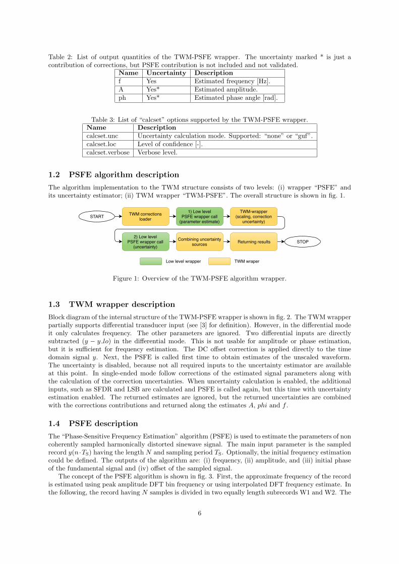
Table 2: List of output quantities of the TWM-PSFE wrapper. The uncertainty marked * is just acontribution of corrections, but PSFE contribution is not included and not validated.
Name Uncertainty Descriptionf Yes Estimated frequency [Hz].A Yes* Estimated amplitude.ph Yes* Estimated phase angle [rad].
Table 3: List of “calcset” options supported by the TWM-PSFE wrapper.Name Descriptioncalcset.unc Uncertainty calculation mode. Supported: “none” or “guf”.calcset.loc Level of confidence [-].calcset.verbose Verbose level.
1.2 PSFE algorithm description
The algorithm implementation to the TWM structure consists of two levels: (i) wrapper “PSFE” andits uncertainty estimator; (ii) TWM wrapper “TWM-PSFE”. The overall structure is shown in fig. 1.
START TWM correctionsloader
1) Low level PSFE wrapper call
(parameter estimate)
TWM-wrapper (scaling, correction
uncertainty)
2) Low level PSFE wrapper call
(uncertainty) Combining uncertainty
sources Returning results STOP
Low level wrapper TWM wraper
Figure 1: Overview of the TWM-PSFE algorithm wrapper.
1.3 TWM wrapper description
Block diagram of the internal structure of the TWM-PSFE wrapper is shown in fig. 2. The TWM wrapperpartially supports differential transducer input (see [3] for definition). However, in the differential modeit only calculates frequency. The other parameters are ignored. Two differential inputs are directlysubtracted (y − y lo) in the differential mode. This is not usable for amplitude or phase estimation,but it is sufficient for frequency estimation. The DC offset correction is applied directly to the timedomain signal y. Next, the PSFE is called first time to obtain estimates of the unscaled waveform.The uncertainty is disabled, because not all required inputs to the uncertainty estimator are availableat this point. In single-ended mode follow corrections of the estimated signal parameters along withthe calculation of the correction uncertainties. When uncertainty calculation is enabled, the additionalinputs, such as SFDR and LSB are calculated and PSFE is called again, but this time with uncertaintyestimation enabled. The returned estimates are ignored, but the returned uncertainties are combinedwith the corrections contributions and returned along the estimates A, phi and f .
1.4 PSFE description
The “Phase-Sensitive Frequency Estimation” algorithm (PSFE) is used to estimate the parameters of noncoherently sampled harmonically distorted sinewave signal. The main input parameter is the sampledrecord y(n ·TS) having the length N and sampling period TS. Optionally, the initial frequency estimationcould be defined. The outputs of the algorithm are: (i) frequency, (ii) amplitude, and (iii) initial phaseof the fundamental signal and (iv) offset of the sampled signal.
The concept of the PSFE algorithm is shown in fig. 3. First, the approximate frequency of the recordis estimated using peak amplitude DFT bin frequency or using interpolated DFT frequency estimate. Inthe following, the record having N samples is divided in two equally length subrecords W1 and W2. The
6

DC offset correction
Dig. time basecorrection
START
Diff. input? y = y - y_lo
1st PSFE wrapper call with disabled forparameter: A, phi, f
Phase correction by time stamp
Diff. input?
ADC aperture correction (A, phi)
Dig. gain, phasecorrection (A, phi)
Transducer gain,phase and loadingcorrection (A, phi)
Transducer gain,phase and loadingcorrection (A, phi)
2nd PSFE wrapper call with enabled
uncertainty
Preparation ofparameters for
uncerainty calc.:SFDR, LSB, jitter
Combining PSFEunc. with correctioncontrib. (A, phi ,f)
Unc. calc?
Returning results: A, phi, f
calcset
STOP data, parametersuncertainty
Figure 2: Detailed internal structure of the TWM-PSFE algorithm wrapper.
W1 starts at the beginning of the record while the W2 starts after d number of samples within the recordwhere N/4 ≤ d ≤ N/2. The phases of W1 and W2 subrecords are estimated using three-parameterssine fitting algorithm (3PSF) and the estimated phases are then subtracted to obtain estimated sampledsignal phase difference. When the subrecord distance d is selected to position two subrecords as closeas possible to the integer number of signal periods, the 3PSF phase estimation error due to harmonicswill almost completely cancel out in (the difference between the estimated phase and the fundamentalsignal phase φ1 is a periodic function with frequency f , independent of the harmonic components in thesampled signal). Using equation 1 will thus provide a more accurate frequency estimate of the sampledsignal and by repeating the procedure described above, the phase difference between the sine model andthe sampled waveform will be minimised and the estimated frequency will converge toward the actualfrequency of the sampled signal.
f =∆φε
2 · π · Ts · d. (1)
The iterations j are completed when error according equation 2 is ε < 2.4 · 10−12 or when the number ofiterations exceeds 20. However, the PSFE algorithm typically needs only a few iterations to converge tothe final value. After obtaining the frequency, the amplitude and initial phase of the record are estimatedusing the 3PSF algorithm and complete sampled record y. The PSFE algorithm shows up to two ordersof magnitude smaller sensitivity to harmonic distortions than the results of the four parameter sinefitting algorithm with only a slight increase in noise standard deviation and only a slight increase incomputational requirements and estimation time, independent of the number of harmonic components.
ε =
∣∣∣∆φε,j−1 −∆φε,j
∣∣∣2 · π ·N · Ts · d · fj−1
. (2)
1.5 Uncertainty estimator
Uncertainty estimator consists of two components: (i) Uncertainty of corrections, (ii) uncertainty of thePSFE algorithm itself. The algorithm uncertainty is evaluated in the PSFE wrapper, the correctionsuncertainty and combining with the algorithm uncertainty is implemented in TWM-PSFE wrapper.
7

Figure 3: The principle of frequency estimation by measuring the phase difference between sampled datawindows W1 and W2 [2].
Four uncertainty contributions for the PSFE algorithm were considered for the estimator (see Table 4):jitter, resolution, interharmonics and harmonics. Additionally, several other parameters related to thesampled signal or sampling (i.e. condition) are expected to affect the uncertainty, therefore enormousnumber of Monte Carlo simulations would be needed for accurate uncertainty analysis.
Table 4: A list of parameters that were varied during the Monte-Carlo simulations.Uncertainty contribution Variation range Reference value
RMS jitter 1 ns - 10 ns 1 ns (0 ns)resolution 10 pV - 100 mV 10 µV (0 V)interharmonic’s amplitude, Ai 0.1 mV - 0.2 V 10 mV (0 V)harmonic’s amplitude, Ah 1 mV - 0.5 mV 50 mV (0 V)Condition parameters
amplitude of the fundamental signal, A1 0.1 V – 1000 V 1 Vfrequency of the fundamental signal, f1 10 Hz – 2 kHz 100 Hztime stamp 0 s – 10 s 0.1 ssampling frequency, fs 500 Hz – 1 MHz 10 kHznumber of samples, N 500 Sa – 1 MSa 100 kSaADC gain at 1 MHz∗1 1 – 1.5 1.5ADC phase at 1 MHz∗2 –0.5 rad – 0.5 rad 0.5 radADC frequency 1 · 10−6 – 5 · 10−3 1 · 10−3
transducer gain at 1 MHz∗3 0.5 – 1.0 0.6transducer phase at 1 MHz∗4 –0.5 rad – 0.5 rad –0.5 radADC aperture correction 0 or 1 1ADC aperture 10 µs – 40 µs 20 µs
∗1 1 at DC.∗2 0 rad at DC.∗3 1 at DC.∗4 0 rad at DC.
Herein we used different and slightly simplified approach. We run 52 different Monte Carlo simulationsets. For each set only one uncertainty contribution was considered using the bold reference value given
8

in Table 4. The other three uncertainty contributions were neglected by using the reference valuesgiven in the brackets. Additionally, only one condition parameter has been varied at the time usingthe variation range as defined in Table 4 while we used the reference values for the other conditionsparameters. We also verified the linearity of the uncertainty contribution by varying its value over acertain variation range while neglecting other uncertainty contributions (using the reference values inbrackets) and keeping all condition parameters at reference values.
Effect of jitter: For each condition 5000 Monte-Carlo simulations were performed. We introduced arandom jitter to each sample while keeping overall RMS jitter value at specified value. Additionally, theinitial phase of the fundamental signal φ1 was randomly varied between +π and –π. For each simulationa Gaussian distribution has been obtained. The uncertainty contribution of the frequency estimationuf,jitter due to the jitter (Gaussian distribution, k = 1) is defined by equation:
uf,jitter =
(1.341 Hz/s
2.981 + (0.622 ·N/Sample)0.521
)· f1
1Hz· jitter, (3)
where jitter is the value of sampling jitter.Effect of resolution: For each condition 10000 Monte-Carlo simulations were performed. The value
of each sample has been rounded according to the resolution setting. Additionally, the initial phase of thefundamental signal φ1 was randomly varied between +π and –π. In this case a non-Gaussian distributionwas obtained therefore the maximal error has been noted instead. The uncertainty contribution of thefrequency estimation uf,res due to the resolution (rectangular distribution) is defined by equation:
uf,res = 0.23mHz ·(
N
100 kSa
)−1.5·(
fS10 kHz
)0.9
· resA1
, (4)
where res is the absolute ADC resolution.Effect of interharmonics: For each condition 5000 Monte-Carlo simulations were performed. In
this case, one interharmonic with fixed amplitude Ai and with random frequency (between 1 Hz and f1)and with random initial phase (between +π and –π) has been added to the fundamental signal. Addi-tionally, the initial phase of the fundamental signal φ1 was randomly varied between +π and –π. In thiscase a non Gaussian distribution was also obtained therefore the maximal error has been noted instead.The uncertainty contribution of the frequency estimation uf,inter due to the presence of interharmonic(rectangular distribution) is defined by equation:
uf,inter = 0.046Hz · AiA1
(N
100 kSa
)−1· fS
10 kHz, (5)
where Ai/A1 is the interharmonic to fundamental amplitude ratio.Effect of harmonics: For each condition 5000 Monte-Carlo simulations were performed. In this
case, one random harmonic component with fixed amplitude Ah and with random frequency (between2 · f1 and n · f1 < 1MHz) and random initial phase (between +π and –π) has been added to thefundamental signal. Additionally, the initial phase of the fundamental signal φ1 was randomly variedbetween +π and –π too. In this case a non Gaussian distribution was also obtained therefore the maximalerror has been noted instead. The uncertainty contribution of the frequency estimation uf,harm due tothe presence of harmonic component (rectangular distribution) is defined by following equation (equationis valid only for N ≥ 3000):
uf,harm = 40mHz · AhA1
, (6)
where Ah/A1 is the harmonic to fundamental amplitude ratio.All uncertainty contributions are combined and recalculated for Gaussian distribution, k = 2:
uf = 2 ·√u2f,jitter +
uf,res3
2+uf,inter
3
2+uf,harm
3
2, (7)
.
9

1.6 Validation
The algorithm TWM-PSFE has many input quantities and some of them are matrices. That is toomany possible degrees of freedom. Thus, varying the quantities in some systematic way would be verycomplicated if the validation should cover full range of used signals and corrections. Therefore, analternative approach was used.
QWTB test function “alg test.m” was created, which performs the validation using randomly gen-erated test setups. It randomizes the signal parameters, correction quantities and uncertainties andalgorithm configurations in ranges expected to occur during the real measurements. The test is runmany times to cover full operating range of the algorithm. Following operations are performed for eachrandom test setup:
1. Generate reference signal with known frequency f .
2. Distort the signal by inverse corrections, i.e. simulate the transducers, and digitizer (e.g. gainerrors, phase errors, DC offsets, quantisation errors, ...).
3. Run the algorithm TWM-PSFE on the signals with enabled uncertainty evaluation to obtain fre-quency estimates and their uncertainties.
4. Compare reference and estimated frequency and decide if the errors of the algorithm for particularfrequency is smaller than the assigned uncertainties.
5. Repeat the test N times from step 1 with different setup parameters, with randomised correctionsby their uncertainties, and with randomised noise, SFDR and jitter.
6. Check that at least 95 % of results passed (for default 95 % level of confidence). The evaluation ismade for each calculated frequency separately.
Total number of Monte-Carlo simulations was 100000. The parameters of the input signal and thedigitizer and transducer settings were randomly varied. The sampling frequency was between 500 Hzand 500 kHz and the number of samples between 500 Sa and 200 kSa. The frequency of fundamentalsignal was between 10 Hz and one tenth of the Nyquist frequency, but never above 5 kHz. The frequencyof the harmonics and interharmonics were always above the frequency of the fundamental signal butbelow the Nyquist frequency. The number of harmonics that were added to the fundamental signal wasgenerally 10, but the number was sometimes reduced if the Nyquist limit is to be exceeded. The numberof interharmonics was 1. The amplitude of the fundamental signal was between 0.1 V and 1000 V andthe amplitude of the harmonics and interharmonics between 0.00001 and 0.05 of the amplitude of thefundamental signal. The DC was between -10 V and +10 V. The phases of the fundamental signal aswell as of the harmonics and interharmonics were individually and randomly varied between +3.14 radand -3.14 rad. The ADC noise was between 1e-11 and 1e-2 of the amplitude of the fundamental signalwhile the jitter was between 1e-9 s and 100e-9 s. ADC aperture was between 1e-5 s and 4e-5 s, ADC gainbetween 1 and 1.5, ADC phase between +1.57 rad and -1.57 rad, frequency correction of the digitizertimebase between 5e-8 and 5e-3, ADC offset between 0.00001 V and 0.005 V (random value for low-andhigh-side channel) and number of bits between 22 and 24. Relative time-stamp of the first sample wasvaried between 0 s and 10 s. The transducer gain was between 0.5 and 20 and the transducer phase wasbetween +1.57 rad and -1.57 rad. The resistive voltage divider low-side impedance value (i.e. resistanceand capacitance) were between 100 Ω and 500 Ω and 0.1 pF and 10 pF, respectively (only resistive voltagedivider was used in the simulations). The randomisation of corrections was also enabled which means thatnot only the uncertainty of the algorithm but also the contributions of the correction uncertainties wereincluded in the Monte-Carlo simulations. The success rate of the TWM-PSFE algorithm uncertaintyestimator for the frequency estimation was 99.38 %.
References
[1] Rado Lapuh. Estimating the fundamental component of harmonically distorted signals from nonco-herently sampled data. IEEE Transactions on Instrumentation and Measurement, 64(6):1419–1424,June 2015.
10

[2] Rado Lapuh. Sampling with 3458A. Left Right d.o.o., Sep 2018.
[3] Stanislav Maslan. Activity A2.3.1 - Correction Files Reference Manual. https://github.com/
smaslan/TWM/tree/master/doc/A231CorrectionFilesReferenceManual.docx.
[4] Stanislav Maslan. Activity A2.3.2 - Algorithms Exchange Format. https://github.com/smaslan/
TWM/tree/master/doc/A232AlgorithmExchangeFormat.docx.
11

2 TWM-MODTDPS - Modulation analyzer in Time Domain,by quadrature Phase Shifting
TWM-MODTDPS is algorithm for calculation of the amplitude modulation parameters of non-coherentlysampled signal in time domain. It was designed for basic estimation of the modulation parameters of asinusoidal carrier modulated by sine wave or rectangular wave with duty cycle 50 %.
The algorithm operates in time domain and it is based on the so called “analytical signal”. It iscapable to estimate the parameters up to modulating-to-carrier frequency ratio 33 %. The record mustcontain at least 3 periods of the modulating signal and it also requires at least 10 samples per period ofcarrier.
It is capable to use the differential transducer connection, however the uncertainty is not calculatedfor the differential mode. The algorithm is equipped by an uncertainty estimator, which covers most ofthe operating range. The estimator parameter space contains a few gaps where the algorithm may fail,which will be always indicated as an error message. These gaps problems may be prevented by changingthe sampling parameters, e.g. by changing the samples count or a sampling rate.
2.1 TWM wrapper parameters
The input quantities supported by the algorithm are shown in table 5. Algorithm returns output quan-tities shown in table 6. Calculation setup supported by the algorithm is shown in table 7.
Table 5: List of input quantities to the TWM-MODTDPS wrapper.Details on the correction quantities can be found in [3].
Name Default Unc. Descriptionwave shape “sine” N/A User string parameter that defines if the algorithm calcu-
lates “sine”: sinusoidal modulation or “rect”: rectangularmodulation wave shape.
comp err 0 N/A Enable self-compensation of the algorithm error (non-zerovalue or “on” string).
yy lo
N/AN/A
NoNo
Input sample data vector and complementary low-side in-put data vector y lo for differential mode only.
Tsfst
N/AN/AN/A
NoNoNo
Sampling period or sampling rate or sample time vector.Note the wrapper always calculates in equidistant mode, sot is used just to calculate Ts.
lsbadc nrngadc bitslo lsblo adc nrnglo adc bits
N/A100040N/A100040
NoNoNoNoNoNo
Either absolute ADC resolution lsb or nominal range valueadc nrng (e.g.: 5 V for 10 Vpp range) and adc bits bit res-olution of ADC.
adc gainadc gain fadc gain alo adc gainlo adc gain flo adc gain a
1[][]1[][]
YesNoNoYesNoNo
Digitizer gain correction 2D table (multiplier).
adc phiadc phi fadc phi alo adc philo adc phi flo adc phi a
0[][]0[][]
YesNoNoYesNoNo
Digitizer phase correction 2D table (additive).
12

Table 5: List of input quantities to the TWM-MODTDPS wrapper.Details on the correction quantities can be found in [3].
Name Default Unc. Descriptionadc freq 0 Yes Digitizer timebase error correction:
f tb′ = f tb · (1 + adc freq.v)The effect on the estimated frequency is opposite:f est′ = f est/(1 + adc freq.v)
adc jitter 0 No Digitizer sampling period jitter [s].adc aper 0 No ADC aperture value [s].adc aper corrlo adc aper
00
No ADC aperture error correction enable:A′ = A · pi · adc aper · f est/ sin(pi · adc aper · f est)phi′ = phi+ pi · adc aper · f est
time stamp 0 Yes Relative timestamp of the first sample y.time shift lo 0 Yes Low-side channel time shift [s].adc sfdradc sfdr fadc sfdr alo adc sfdrlo adc sfdr flo adc sfdr a
180[][]180[][]
NoNoNoNoNoNo
Digitizer SFDR 2D table.
adc Yin Cpadc Yin Gpadc Yin flo adc Yin Cplo adc Yin Gplo adc Yin f
1e-151e-15[]1e-151e-15[]
YesYesNoYesYesNo
Digitizer input admittance 1D table.
tr type “” No Transducer type string (“rvd” or “shunt”).tr gaintr gain ftr gain a
1[][]
YesNoNo
Transducer gain correction 2D table (multiplicative).
tr phitr phi ftr phi a
0[][]
YesNoNo
Transducer phase correction 2D table (additive).
tr sfdrtr sfdr ftr sfdr a
180[][]
NoNoNo
Transducer SFDR 2D table.
tr Zlo Rptr Zlo Cptr Zlo f
1e31e-15[]
YesYesNo
RVD transducer low-side impedance 1D table. Note this isrelated to loading correction and it has effect only for RVDtransducer and will work only if adc Y in is defined as well.
tr Zbuf Rstr Zbuf Lstr Zbuf f
00[]
YesYesNo
Loading corrections: Transducer output buffer output se-ries impedance 1D table. Leave unassigned to disable bufferfrom the correction topology.
tr Zca Rstr Zca Lstr Zca f
1e-91e-12[]
YesYesNo
Loading corrections: Transducer high side terminal seriesimpedance 1D table.
tr Zcal Rstr Zcal Lstr Zcal f
1e-91e-12[]
YesYesNo
Loading corrections: Transducer low side terminal seriesimpedance 1D table.
tr Yca Cptr Yca Dtr Yca f
1e-151e-12[]
YesYesNo
Loading corrections: Transducer output terminals shuntingimpedance.
tr Zcamtr Zcam f
1e-12[]
YesNo
Loading corrections: Transducer output terminals mutualinductance 1D table.
13

Table 5: List of input quantities to the TWM-MODTDPS wrapper.Details on the correction quantities can be found in [3].
Name Default Unc. DescriptionZcb RsZcb LsZcb f
1e-91e-12[]
YesYesNo
Loading corrections: Cable series impedance 1D table.
Ycb RsYcb LsYcb f
1e-151e-12[]
YesYesNo
Loading corrections: Cable series impedance 1D table.
Table 6: List of output quantities of the TWM-MODTDPS wrapper.Name Uncertainty Descriptionf0 Yes Frequency of the carrier [Hz].A0 Yes Amplitude of the carrier.f mod Yes Modulating frequency [Hz].A mod Yes Modulating amplitude.mod Yes Modulating depth [%].dVV Yes ∆V/V depth [%]. Alternative expression of mod, i.e.: dV V = 2 ·mod.cpm Yes Changes per minute. Alternative expression of f mod, i.e.: cpm = 120 · f mod.env No Modulation envelope.env t No Modulation envelope env time vector.
Table 7: List of “calcset” options supported by the TWM-MODTDPS wrapper.Name Descriptioncalcset.unc Uncertainty calculation mode. Supported: “none”
or “guf” for uncertainty estimator.calcset.loc Level of confidence [-].calcset.verbose Verbose level.
2.2 MODTDPS algorithm description
The overview of the TWM wrapper structure is shown in the fig. 4. The algorithm supports differentialtransducer inputs. The TWM wrapper first estimates the carrier frequency f0 and mean amplitude ofthe modulated signal A0 by a PSFE algorithm. It uses these two values to obtain and apply gain andaperture error corrections for the high-side channel y (and for low-side channel y lo in the differentialmode).
In the differential transducer mode, the wrapper also applies high-to-low side time shift correctionand phase correction to the low-side input y lo by time shifting it according to the estimate f0. Thistrivial phase synchronization of the high-low side phase obviously works only to one frequency f0 andit is dependent on its correct estimation, however it turned out to be sufficient for the purposes of thisalgorithm. Next, the wrapper calculates voltage difference y = y − y lo, so the differential is reducedto single ended input y. The transducer gain correction in the differential mode uses additional voltagevectors Y (f0), phi(f0) and Y lo(f0), phi lo(f0) obtained from the two spectra calculated by anotherQWTB algorithm “SP-WFFT”. Although the vectors have absolute values distorted by the spectralleakage, their ratio stays fixed, so it is enough to make the transducer transfer and loading correctionfunction work. At this point the signal is single ended and scaled.
The next step is the main algorithm for the estimation of modulation parameters “mod tdps()” whichis shown in fig. 5. The algorithm internally calls the function “mod fit sin()” (see fig. 6), which does theparameter estimation itself.
The algorithm itself is based on the estimation of the carrier frequency f0 by means of PSFE algorithm[2]. Once the carrier f0 is known, the algorithm applies 90deg phase shift to the input signal y and builds
14

START
PSFE call to get initial est. of carrier:
f0, A0
SP-WFFT call tohgih-side spectrum:
f, Y(f), ph(f)
SP-WFFT call to low-side spectrum:
f, Y(f), ph(f) Diff. input?
Apply gain andaperture corr. to high-side in time domain
Diff. input? Apply transducergain correction
Gain and aperturecorr. to low-side in
time domain
Phase corr. to low-side in time domain,
assuming f0component only
Calculate differential: high-low side
Modulation estimatormod_tdps() call: f0, A0, fm, Am
Prepare systemparameters:
LSB, SFDR, jitter
Prepare low-sideparameters and
combine with high-side parameters
Diff. input?
SP-WFFT call to getdifferential spectrum:
f, Y(f), ph(f)
Identify harmonicsand inter-harmonicsto get ratios signalSFDR, merge with
system SFDR
Estimate residualnoise, combine withjitter to effective jitter
Estimate LSB topeak-peak ratio
Get modulation tocarrier ratio fm/f0
Get sampling rate toto carrier ratio fs/f0
Get periods count ofcarrier N/fs*fm
Get modulation depthAm/a0
Interpolateuncertainty from LUT:
u(f0), u(A0), u(fm),u(mod)
Est. correctionsuncertainty and
combine with alg.: u(f0), u(A0), u(fm),
u(mod)
Format and returnquantities:
f0, A0, f_mod, cpm,A_mod. mod
mod. envelope
STOP
yes
no
yes
no
yesno
Figure 4: Overview of the TWM-MODTDPS algorithm wrapper. Green cells are calls to other QWTBwrappers. Gold blocks are calls of the local functions which are described in the text.
sine
rectangular
START
Call to "mod_fit_sin()" toget initial mod. parameter
estimate E
Call to "mod_fit_sin()" toget modulation estimates Ex(k)
Shape?
Synthesize 'ux'waveform for E1
parameters.
Estimate uncertainty 'ub(Ea)' of algorithm from (E1-E) difference
Call to "mod_fit_sin()"of 'ux' to get mod.
estimates E2
Calculate est. error: dE = E1 - E2
Fix E1 error: E1 = E1 - dE
Create temp estimateE1 = E
next iteration?
Return estimates anduncertainty
Self-correct?
Override E by E1 (no uncertainty contribution
here) next iteration?
Synthesize 'ux' waveformfor E with random phase
of mod. wave.
Calc. uncertainty estim. of 'Ex' set ub(Ex)
Combine uncertainties: ub(Ex), ub(Ea), ua(E)
STOP
yes
no
yes
no
estimates
uncertainties
Figure 5: Overview of the “mod tdps()” function of the TWM-MODTDPS algorithm wrapper. Goldblocks are calls of local functions of the algorithm.
two virtual quadrature signals (analytical signals):
ya(t) = y(t) + j · y(t+
pi
2 · f0
), (8)
yb(t) = y(t)− j · y(t− pi
2 · f0
), (9)
(10)15

START
Estimate DC fromwindowed signal 'u',
remove DC in from 'u'
PSFE call to getcarrier 'f0' from 'u'
Time shift waveform'u' by ±90deg to
create twoquadrature signals
Obtain modulationenvelope from thequad. signals: me
PSFE call on the 'me'to get mod.parameters:
'fm', 'Am', 'phm'
Estimate 'A0' fromwindowed envelope
'me' (= DC ofenvelope)
Shape?
Filter envelope byButterworth low-pass1st order, fcut = fs/3
Modulation waveformphase detection
Measuring averageamplitude of the filteredmodulation envelope:
Am = (mean(ev_tops) -mean(ev_lows))/2
Measuring averagecarrier amplitude of thefiltered mod. envelope: A0 = (mean(ev_tops) +
mean(ev_lows))/2
STOP
Return modulationestimates:
dc, f0, A0, fm, Am,phm, ua(A0), ua(Am),
me un
certa
inty
type
A: u
a(A0
), ua
(Am
)sine
rectangular
Figure 6: Overview of the “mod fit sin()” function of the TWM-MODTDPS algorithm wrapper. Goldblocks are calls of local functions of the algorithm.
The average of amplitudes of the signals ya(t) and yb(t) is roughly equal to the modulation envelope:
ev(t) = 0.5 · (|ya(t)|+ |yb(t)|) (11)
The envelope ev(t) is used as an input to the next call of the PSFE algorithm which returns modulationamplitude Am, modulation frequency fm and modulation phase phm. The algorithm differs for thesinusoidal and rectangular wave shape from this point.
In the sinusoidal mode, the carrier amplitude A0 is obtained as a DC value of the envelope ev(t)using a windowed average method with Blackman window:
A0 =
∑Nt=1 w(t) · e(t)∑N
t=1 w(t), (12)
where the w(t) are coefficients of the Blackman window and N is samples count of the envelope. Thistrivial method obtains acceptable suppression of errors caused by the non-coherent window size if atleast three modulating periods were recorded.
In the rectangular mode, the A0 from PSFE cannot be used. Only the modulation frequency esti-mate fm and phase estimate phm are relevant. The envelope ev(t) is filtered by a low-pass 1st orderButterworth filter with cutoff frequency fs/6. This reduces the noise caused by the harmonic and inter-harmonic spurs present in the envelope ev(t) but does not distort the shape too much at high modulationfrequencies. Next, the phase phm of the modulation wave is used to detect the tops and lows of thefiltered envelope rectangular wave. It was experimentally decided to use 15 % to 30 % of the periods fordetection of the tops and 75 % to 85 % for the lows. The modulation parameters are calculated accordingto formulas:
A0 =1
2M
M∑m=1
[tops ev(t),m − lows ev(t),m], (13)
Am =1
2M
M∑m=1
[tops ev(t),m+ lows ev(t),m], (14)
16

where m is the period index and M is total count of modulation periods in the signal. The type Auncertainty estimate is calculated from the differences between the periods m.
In the sine wave mode, the algorithm also contains a self-correcting routine that is capable to reducethe inherent error of the algorithm itself (see diagram in fig. 5). The idea is following: First, the algorithmcore function “mod fit sin()” is called on the real waveform data y to obtain the initial estimate E of themodulation parameters. Next, a new simulated waveform ysim is synthesized so it has the modulationparameters E. The core function “mod fit sin()” is called again on the waveform ysim to obtain estimatesE2. Finally, an algorithm error dE = E2−E is calculated. The whole operation is repeated three timesin a loop which was sufficient to get stable error dE. The dE is either used as a correction to the initial E(when self-correction is enabled) or it is used to estimate algorithm error uncertainty contribution, whenself-correction is disabled. This method significantly reduced the error of the algorithm even for highmodulation frequencies. The performance was evaluated so the uncertainty calculation reflects sensitivityof this method to the imperfect input signal.
The “mod tdps()” function automatically calculates estimate of maximum error caused by the un-certain phase shift of the modulating waveform. It is calculated by repeating the estimator 10 times fordifferent phase shifts and calculating maximum error. This is part of the total uncertainty budget.
2.3 Uncertainty estimator
The algorithm is too complex for evaluation of the uncertainty following the GUM guide. It is also rela-tively slow, so the Monte-Carlo uncertainty calculation for an interactive application would be too slowespecially for waveforms longer than few thousand of samples. Therefore, a fast uncertainty estimatorwas developed. The estimator is based on the massive lookup tables (LUT) that contains precalculateduncertainties for various combinations of the parameters of the input signal.
First step for creation of the estimator was selection of the relevant signal parameters. The set waschosen so it is minimalist, because each parameter means one more dimension of the simulation and thusadditional data in the LUT. Selection is follows:
1. Modulating periods count: The count of modulating signal periods in the recored waveform.
2. Samples per period of carrier: The ratio of sampling rate and carrier frequency fs/f0.
3. Relative modulation frequency: The ratio of the modulating frequency to carrier fm/f0.
4. Total SFDR: Combination of system SFDR (corrections) and signal SFDR (harmonics and in-terharmonics).
5. Effective jitter: Total effective sampling jitter in seconds. This also includes equivalent value ofthe residual RMS noise found in the signal. The jitter value is normalized to the carrier frequency.
6. Bit resolution: The bits count per used peak-to-peak ADC range. This is theoretically replaceableby rms noise, but it may easily lead to nonlinear behaviour for low resolutions. Therefore, thisparameter was simulated separately.
7. Modulation depth: The ratio of the modulating amplitude to the carrier amplitude Am/A0.
The simulation ranges of the parameters were chosen according to table 8. The ranges were chosento cover the typical operating range, however most of the dependencies are extrapolable in one direction.
Fro simplicity it was assumed all the parameters may be correlated, so all combinations of the sevenparameters were generated (6x5x8x4x5x6x8 = 230400 combinations). At least 1000 Monte-Carlo (MC)iteration cycles of following sequence of operations was performed for each combination:
1. Get one combination of simulation parameters Eref .
2. Randomize Eref parameters in a small range (few percent), so each MC iteration generates abit different signal. This is to prevent unfortunate selection of a combination Eref where theuncertainty is exceptionally low, e.g. due to the coherent sampling.
3. Generate other random parameters, such as DC offset, phase shift of the modulation signal, randomspurs up to SFDR parameter value, etc.
17

Table 8: Simulation ranges and steps of the parameters for uncertainty estimator of MODTDPS algo-rithm.
Name DescriptionModulating periods count Log. space: 3 to 30, 6 stepsSamples per period of carrier Log. space: 10 to 100, 5 stepsRelative modulation frequency Log. space: 0.01 to 0.33, 8 stepsTotal SFDR List: [120; 80; 60; 30] dB, 4 stepsEffective jitter Log. space: 10−9 to 10−2, 5 stepsBit resolution Log. space: 6 to 24 bits, 6 stepsModulation depth Log. space: 0.01 to 0.99, 8 steps
4. Synthesize modulated waveform of known parameters.
5. Distort the waveform by: spurs, jitter, quantisation, etc.
6. Perform estimation of the modulation parameters Ex by “mod tdps()” algorithm. Note the un-certainties returned by the “mod tdps()” itself are ignored, as they will be calculated on runtimeduring actual measurements.
7. Compare estimates Ex to generated parameters Eref : ∆Ex(k) = Ex − Eref .
The set of algorithm errors ∆Ex(k) from the MC iterations k for each combination of parametersis processed according to the GUM guide, supplement 1 [1]. The whole batch of combinations wasprocessed on the supercomputer, so it took only three days per configuration (“sine”, “rect”, with orwithout self-corrections). The 1000 MC cycles was enough to obtain stable estimates. Output of thecalculation is 7-dimensional matrix of uncertainties of modulation parameters: f0, fm, A0 and Am.The 7D array was manually inspected along various axes (= along simulation parameters), however itwas not possible to find a simple empiric formulas that would cover full range of any axis. There werealways some non-linearity dependencies on the other axes. All tries resulted either in significant over orunderestimation of uncertainty in some part of the parameter space.
Therefore, the whole 7D matrix was simply compressed to the log. space and 16bit integers (resolutionbetter 0.005) and saved to a compressed MAT file as lookup table (LUT). The size of LUT is roughly1.7 MBytes per configuration which is still acceptable and thus it was decided to not continue withfurther optimalisations. The LUT contains definitions of the axes (parameters), their permissible ranges,interpolation modes (linear or logarithmic) and definition of the estimator action, when the parameteris out of range (error or limit at max/min known value). A multidimensional interpolator was developedwhich is capable to read the LUT and return interpolated values of the quantities stored in the LUT.The usable range of parameters is shown in the table 9. Note the interpolator permits to extrapolateoutside the stated limits, which should prevent problems around the limits. The additional permissiblerange is set to up to ±5 % of given range.
Table 9: Permissible range of signal parameters for the uncertainty estimator. The values in parenthesisare permissible, but outside simulation range. The actions when the min or max value of axis is reachedare: “error” - generate error; “const” - return value of uncertainty at min. or max. of simulated range.
Name Range On min On maxModulating periods count 3 to 30 (3 to ∞) error constSamples per period of carrier 10 to 100 (10 to ∞) error constRelative modulation frequency 0.01 to 0.33 (0 to 0.33) const errorTotal SFDR 120 to 30 dB (∞ to 30 dB) error constEffective jitter 10−9 to 10−2 (10−∞ to 10−2) const errorBit resolution 6 to 24 bits (6 to ∞bits) error constModulation depth 0.01 to 0.99 error error
The estimator itself in the TWM-MODTDPS wrapper is based on the estimated modulation param-eters and spectrum analysis of the input signal y. It obtains the parameters of the LUT axes by followingprocedure:
18

1. Calculate the basic parameters from corrections and estimated modulation parameters: (i) Mod-ulating periods count; (ii) Samples per period of carrier; (iii) Relative modulation frequency; (iv)Modulation depth; (v) Bit resolution.
2. Perform spectrum analysis to obtain: (i) Harmonics (except the ones belonging to modulationsidebands); (ii) Interharmonics; (iii) RMS noise estimate. These value are used to calculate signalSFDR estimate and noise, which is converted to equivalent jitter at the carrier frequency f0.
3. Interpolate the LUT table for given configuration to get the algorithm uncertainty.
4. Calculate estimate of uncertainty of the corrections. This covers estimate of the error caused bythe fact the signal scaling is made at a single frequency spot f0 instead of complicated frequencydependent correction.
5. Combine uncertainties: (i) Runtime calculated uncertainty from “mod tdps()” itself; (ii) Uncer-tainty from the LUT table; (iii) Uncertainty of the corrections.
2.4 Validation
The algorithm TWM-MODTDPS has many input quantities (71 in differential transducer input mode)and some of them are matrices. That is too many possible degrees of freedom. Thus, varying thequantities in some systematic way would be very complicated if the validation should cover full range ofused signals and corrections. Therefore, an alternative approach was used.
QWTB test function “alg test.m” was created, which performs the validation using randomly gen-erated test setups. It randomizes the signal parameters, correction quantities and uncertainties andalgorithm configurations in ranges expected to occur during the real measurements. The test is runmany times to cover full operating range of the algorithm. Following operations are performed for eachrandom test setup:
1. Generate signal y with known modulation parameters Mref.
2. Distort the signal y by inverse corrections, i.e. simulate the transducers, and digitizer (e.g. gainerrors, quantisation, SFDR ...).
3. Run the algorithm TWM-MODTDPS with enabled uncertainty evaluation to obtain the harmoniclevels Mx and their uncertainties u(Mx).
4. Compare the reference and calculated harmonics and distortion and check if the deviations arelower than assigned uncertainties:
pass(i) = |(Mref −Mx| < u(Mx), (15)
where i is test run index.
5. Repeat N times from step 1, with the same test setup parameters, but with randomised correctionsby their uncertainties, and with randomised noise, SFDR and jitter.
6. Check that at least 95 % of pass(i) results passed (for 95 % level of confidence). The evaluationis made for each estimated modulation parameter separately. So it is possible to inspect whichparameter fails.
The test runs count per test setup was set to N = 500, which is far from optimal infinite set, but dueto the computational requirements it could not have been much higher.
The algorithm in the uncertainty estimation mode was tested in 6 different configurations with atleast 5000 test setups per each. I.e. the algorithm was ran 15 million times in total (6x5000x500). Theprocessing itself was performed on a supercomputer [4] and it took about 15 days at 300 parallel octaveinstances.
The randomization ranges of the signal are shown in table 10. The randomization ranges of thecorrections are shown in table 11.
The test results were split into several groups given by the randomiser setup: (i) Wave shape; (ii)Randomisation of corrections by uncertainty enabled/disabled. When the randomisation of corrections is
19

disabled, the test runs cover only the algorithm itself and the contributions of the correction uncertaintiesare ignored.
The summary of the validation test results is shown in table 12. The success rate without correctionsrandomisation was close to 100 %. The success rate with corrections randomisation was a bit worse,because the success rate of the individual test runs within the test setup was just around 95 %. Therefore,the decision pass/fail is problematic. The obtained set of test results was manually investigated and nocases with far outliers were detected, e.g. the failed test setups contained occasional estimates offsetsjust around the uncertainty boundaries. Also no cases where all test runs failed were found.
Table 10: Validation range of the signal for TWM-MODTDPS algorithm.Parameter RangeSampling rate 9 to 11 kHz (no need to randomize in wider range, as all
other parameters are generated relative to this rate).Samples count 3 to 100 kSamples.Carrier frequency Random, so it is higher than 50 Hz and there are at least
10 samples per period.Carrier amplitude Random from 10 to 100% of nominal input range.Modulating frequency Random, so there are always at least 3 modulating pe-
riods in the record and so the ratio to carrier frequencyis up to 32% (24% for rectangular wave shape).
Modulating depth Random, 2 to 98%.DC offset Random up to ±2% of carrier amplitude.Phase angle Random for carrier, modulating frequency and spur har-
monics.SFDR -100 to -60 dBc, 10 harmonic spurs of carrier, each spur
has random level up to SFDR, frequencies are ran-domised by ±10% of carrier frequency.
Digitizer RMS noise 1 to 50 µV.Sampling jitter 1 to 100 ns.
20

Table 11: Validation range of the correction for the TWM-MODTDPS algorithm.Parameter RangeTransducer type Random ’shunt’ or ’rvd’.Nominal input range 5 to 70 V (5 to 70 A)Aperture 1 ns to 100 µsDigitizer gain Randomly generated frequency transfer simulating
NI 5922 FIR-like gain ripple (possibly the worst imag-inable shape) and some ac-dc dependence. The trans-fer matrix has up to 50 frequency spots. Nominal gainvalue is random from 0.95 to 1.05 with uncertainty 5 to50 µV/V. Maximum ac-dc value at fs/2 is up to ±1 %with uncertainty up to 250 µV/V. Gain ripple amplitudeis random from 0.005 to 0.03 dB with up to 5 periodsbetween 0 and fs/2.
Digitizer SFDR Value based on table 10.Transducer SFDR Value based on table 10. Note the “SFDR” from ta-
ble 10 is randomly split between digitizer and transducerSFDR correction.
Digitizer DC offset ±2 mV with uncertainty 0.1 mV.Digitizer bit resolution 16 to 28 bits.Digitizer nominal range 1 VTransducer gain Randomly generated frequency transfer. The transfer
matrix has 30 to 50 frequency spots. Nominal gainvalue is random (see above) with relative uncertainty50 µV/V. Maximum ac-dc value at fs/2 is up to ±2 %with uncertainty up to 250 µV/V. Gain ripple amplitudeis 0.005 dB with 4 to 10 periods between 0 and fs/2.
Table 12: Validation results of the algorithm TWM-MODTDPS. The “passed test” shows percentage ofpassed tests under conditions defined in tables 10 and 11.
Wave shape Self-corr. Rand. corr.Passed test [%]
A0 Am f0 fm
sine onno 100.00 100.00 100.00 100.00yes 100.00 100.00 100.00 100.00
sine offno 100.00 100.00 100.00 99.98yes 100.00 100.00 100.00 100.00
rect offno 100.00 100.00 100.00 100.00yes 100.00 100.00 100.00 100.00
References
[1] JCGM. Evaluation of measurement data - Supplement 1 to the “Guide to the expression of uncertaintyin measurement” - Propagation of distributions using a Monte Carlo method. Bureau Internationaldes Poids et Measures.
[2] Rado Lapuh. Estimating the fundamental component of harmonically distorted signals from nonco-herently sampled data. IEEE Transactions on Instrumentation and Measurement, 64(6):1419–1424,June 2015.
[3] Stanislav Maslan. Activity A2.3.2 - Algorithms Exchange Format. https://github.com/smaslan/
TWM/tree/master/doc/A232AlgorithmExchangeFormat.docx.
[4] Miroslav Valtr. CMI HPC System Online. https://translate.google.cz/translate?sl=cs&tl=
en&js=y&prev=_t&hl=cs&ie=UTF-8&u=http%3A%2F%2Fprutok.cmi.cz%2Fsc%2Fdoku.php%3Fid%
3Dsystem&edit-text=, 2014.
21
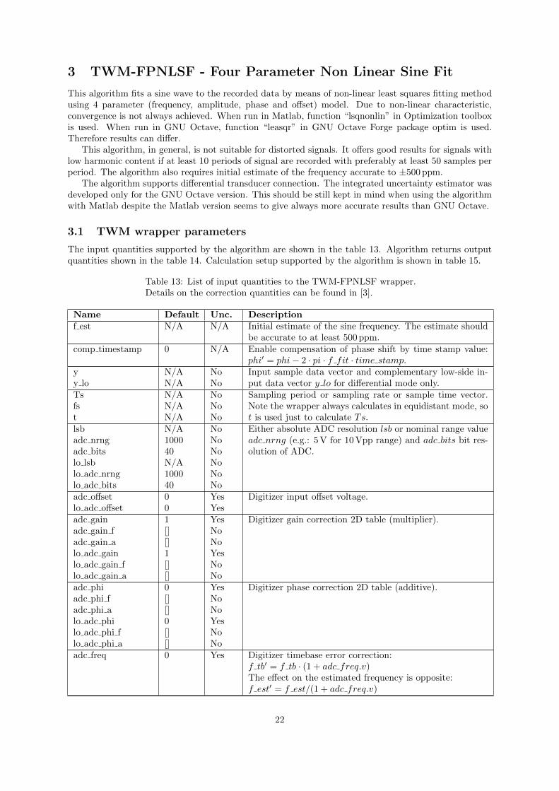
3 TWM-FPNLSF - Four Parameter Non Linear Sine Fit
This algorithm fits a sine wave to the recorded data by means of non-linear least squares fitting methodusing 4 parameter (frequency, amplitude, phase and offset) model. Due to non-linear characteristic,convergence is not always achieved. When run in Matlab, function “lsqnonlin” in Optimization toolboxis used. When run in GNU Octave, function “leasqr” in GNU Octave Forge package optim is used.Therefore results can differ.
This algorithm, in general, is not suitable for distorted signals. It offers good results for signals withlow harmonic content if at least 10 periods of signal are recorded with preferably at least 50 samples perperiod. The algorithm also requires initial estimate of the frequency accurate to ±500 ppm.
The algorithm supports differential transducer connection. The integrated uncertainty estimator wasdeveloped only for the GNU Octave version. This should be still kept in mind when using the algorithmwith Matlab despite the Matlab version seems to give always more accurate results than GNU Octave.
3.1 TWM wrapper parameters
The input quantities supported by the algorithm are shown in the table 13. Algorithm returns outputquantities shown in the table 14. Calculation setup supported by the algorithm is shown in table 15.
Table 13: List of input quantities to the TWM-FPNLSF wrapper.Details on the correction quantities can be found in [3].
Name Default Unc. Descriptionf est N/A N/A Initial estimate of the sine frequency. The estimate should
be accurate to at least 500 ppm.comp timestamp 0 N/A Enable compensation of phase shift by time stamp value:
phi′ = phi− 2 · pi · f fit · time stamp.yy lo
N/AN/A
NoNo
Input sample data vector and complementary low-side in-put data vector y lo for differential mode only.
Tsfst
N/AN/AN/A
NoNoNo
Sampling period or sampling rate or sample time vector.Note the wrapper always calculates in equidistant mode, sot is used just to calculate Ts.
lsbadc nrngadc bitslo lsblo adc nrnglo adc bits
N/A100040N/A100040
NoNoNoNoNoNo
Either absolute ADC resolution lsb or nominal range valueadc nrng (e.g.: 5 V for 10 Vpp range) and adc bits bit res-olution of ADC.
adc offsetlo adc offset
00
YesYes
Digitizer input offset voltage.
adc gainadc gain fadc gain alo adc gainlo adc gain flo adc gain a
1[][]1[][]
YesNoNoYesNoNo
Digitizer gain correction 2D table (multiplier).
adc phiadc phi fadc phi alo adc philo adc phi flo adc phi a
0[][]0[][]
YesNoNoYesNoNo
Digitizer phase correction 2D table (additive).
adc freq 0 Yes Digitizer timebase error correction:f tb′ = f tb · (1 + adc freq.v)The effect on the estimated frequency is opposite:f est′ = f est/(1 + adc freq.v)
22

Table 13: List of input quantities to the TWM-FPNLSF wrapper.Details on the correction quantities can be found in [3].
Name Default Unc. Descriptionadc jitter 0 No Digitizer sampling period jitter [s].adc aper 0 No ADC aperture value [s].adc aper corrlo adc aper
00
No ADC aperture error correction enable:A′ = A · pi · adc aper · f est/ sin(pi · adc aper · f est)phi′ = phi+ pi · adc aper · f est
time stamp 0 Yes Relative timestamp of the first sample y.time shift lo 0 Yes Low-side channel time shift [s].adc sfdradc sfdr fadc sfdr alo adc sfdrlo adc sfdr flo adc sfdr a
180[][]180[][]
NoNoNoNoNoNo
Digitizer SFDR 2D table.
adc Yin Cpadc Yin Gpadc Yin flo adc Yin Cplo adc Yin Gplo adc Yin f
1e-151e-15[]1e-151e-15[]
YesYesNoYesYesNo
Digitizer input admittance 1D table.
tr type “” No Transducer type string (“rvd” or “shunt”).tr gaintr gain ftr gain a
1[][]
YesNoNo
Transducer gain correction 2D table (multiplicative).
tr phitr phi ftr phi a
0[][]
YesNoNo
Transducer phase correction 2D table (additive).
tr sfdrtr sfdr ftr sfdr a
180[][]
NoNoNo
Transducer SFDR 2D table.
tr Zlo Rptr Zlo Cptr Zlo f
1e31e-15[]
YesYesNo
RVD transducer low-side impedance 1D table. Note this isrelated to loading correction and it has effect only for RVDtransducer and will work only if adc Y in is defined as well.
tr Zbuf Rstr Zbuf Lstr Zbuf f
00[]
YesYesNo
Loading corrections: Transducer output buffer output se-ries impedance 1D table. Leave unassigned to disable bufferfrom the correction topology.
tr Zca Rstr Zca Lstr Zca f
1e-91e-12[]
YesYesNo
Loading corrections: Transducer high side terminal seriesimpedance 1D table.
tr Zcal Rstr Zcal Lstr Zcal f
1e-91e-12[]
YesYesNo
Loading corrections: Transducer low side terminal seriesimpedance 1D table.
tr Yca Cptr Yca Dtr Yca f
1e-151e-12[]
YesYesNo
Loading corrections: Transducer output terminals shuntingimpedance.
tr Zcamtr Zcam f
1e-12[]
YesNo
Loading corrections: Transducer output terminals mutualinductance 1D table.
Zcb RsZcb LsZcb f
1e-91e-12[]
YesYesNo
Loading corrections: Cable series impedance 1D table.
23

Table 13: List of input quantities to the TWM-FPNLSF wrapper.Details on the correction quantities can be found in [3].
Name Default Unc. DescriptionYcb RsYcb LsYcb f
1e-151e-12[]
YesYesNo
Loading corrections: Cable series impedance 1D table.
Table 14: List of output quantities of the TWM-FPNLSF wrapper.Name Uncertainty Descriptionf Yes Frequency of the carrier [Hz].A Yes Amplitude of the carrier.phi Yes Phase of main signal component [rad].ofs Yes DC offset of signal.
Table 15: List of “calcset” options supported by the TWM-FPNLSF wrapper.Name Descriptioncalcset.unc Uncertainty calculation mode. Supported: “none”
or “guf” for uncertainty estimator.calcset.loc Level of confidence [-].calcset.verbose Verbose level.
3.2 Algorithm description
The wrapper TWM-FPNSLF overview is shown in fig. 7. It first calls the core function “FPNLSF loop()”on the unscaled high-side input signal y to get initial estimate of the signal frequency fx. This isnecessary to get gain and phase correcting coefficients. Follows the signal scaling in the time domain,i.e. application of the digitizer DC offset, gain, phase and aperture corrections.
The wrapper also allows differential input sensor connection. In this case it compensates the high-lowside phase error by time shifting the low-side signal y lo according to the estimated frequency compo-nent fx. Such a phase correction of course works only for the single frequency component fx, butthe results were acceptable as it is the main signal component. Next, it calculates differential signalyd = y− y lo. Only additional difference is the TWM defines relatively complex transducer loading cor-rections scheme (see [2]). This is ensured by the function “correction transducer loading()”. However,the function operates in frequency domain, whereas FPNLSF operates in time domain and the algo-rithm expects non-coherent sampling. Therefore, an additional step is done to obtain scaling transducercorrection factor. The windowed FFT of the high and low-side signals y and ylo is calculated by “SP-WFFT” algorithm. The voltage vectors are obtained from the FFTs are used as an inputs to the “correc-tion transducer loading()”. Although the voltage vectors are distorted by the spectral leakage, their ratiostays unaffected, so the transducer scaling factor obtained from the “correction transducer loading()” issufficiently accurate. At this point, the differential signals y and y lo are reduced to single ended signalyd which is correctly scaled. The “FPNLSF loop()” is called again on the differential signal yd. Nextcalculation steps are identical for single ended and differential modes.
The FPNLSF algorithm itself and its uncertainty analysis was described in [4]. The basic principleis use of the non-linear least square minimising algorithm to fit the input signal y by a four parametersine wave model:
ym = o+A · sin (2πft+ φ) , (16)
where o is DC offset, A is amplitude, t is time vector, f is sine frequency and φ is phase angle. This methodis quite sensitive to harmonics and especially interharmonics and also requires good initial estimates forthe minimising algorithm, however for clean signals it offers acceptable estimates of the fundamentalcomponent.
24

signal, parameterscorrections
uncertainty
STARTFPNLSF_loop() call to
get initial estimates fromsignal y:
fx, Ax, phx, ox
Time base frequencycorrection of fx
Diff. input?
Digitizer gain andaperture error correctionsin time domain for fx freq:
y and y_lo
Digitizer offset in timedomain: y and y_lo
Digitizer interchannelphase and time shiftcorrections in time
domain for fx freq by timeshifting y_lo
Algorithm uncertaintyestimator:
u(fx), u(Ax), u(phx), u(ox)
Calculate differentialsignal: y = y - y_lo
SP-WFFT call on y andy_lo to get fx frequency
voltage vectors: Y0(fx), Y0_lo(fx)
Apply all digitizercorrections in freq.domain as in time
domainto: Y0(fx),Y0_lo(fx)
Calculate transducercorrection factors for fx
and dc: trg, trp, dcg
Combine uncertainties: corrections, algorithm
FPNLSF_loop() call toget diff. estimates from
differential signal y: fx, Ax, phx, ox
Apply transducercorrections to estimates
and uncertainties
Digitizer gain andaperture corrections:
Ax, phx, ox
Digitizer DC offsetcorrection: ox
Apply transducercorrections: Ax, phx, ox
Algorithm uncertaintyestimator:
u(fx), u(Ax), u(phx), u(ox)
Combine uncertainties: corrections, algorithm
Combine and expressresults
SP-WFFT call on y to getspectrum for uncertainty
estimator.
STOP
differential spectrum
yes
no
low-side high-side
high-sidelow-side
transducer scaling factors
corrections
QWTB calls
Local function calls
Figure 7: Overview of the TWM-FPNLSF algorithm wrapper.
The core function of the TWM-FPNLSF wrapper is function “FPNLSF loop()”. Structure is shownin fig. 8. The function accompanies the FPNLSF algorithm itself by several supporting functions. Firstmajor problem to solve was its sensitivity to the precision of initial estimate of the parameters, especiallyfrequency f est. It was merely impossible to perform the Monte Carlo (MC) uncertainty calculation ofthe FPNLSF itself as the FPNLSF minimising process often ended in a local minima, which is notalways detectable. So the histogram of the MC iterations contained many far outliers, which made theuncertainty unusable. Therefore, the permissible range of initial estimate fest was set to ±500 ppmfrom the actual signal frequency. The FPNLSF was placed in a retry loop that tries repeatedly run theFPNLSF with slightly randomised initial estimates until the fitted frequency f is within the ±500 ppmrange. The retry loop also contains limit for the total retries count and total timeout, so it won’t getlocked up. The loop was also accompanied by initial zero cross estimation, which tries to obtain at leastapproximate initial phase estimate.
STARTZero cross phasedetection: phi_zc
Randomize initialestimates: phi_zc, ofs, f First try?
Call FPNSLF to getsignal parameters
estimates: Ax, fx, phx, ox
PASS?
PASS = (fx - f_est) < limit && eval time < limit && retries count < limit
STOP
no
yesno
yes
Figure 8: The structure of the “FPNLSF loop()” function of the TWM-FPNLSF algorithm wrapper.
25

3.3 Uncertainty estimator
The algorithm is too complex for GUF uncertainty calculation. It is also relatively slow, so the Monte-Carlo uncertainty calculation for an interactive application would be too slow especially for waveformslonger than few thousand samples. Therefore, a fast uncertainty estimator was developed. The estimatoris based on the lookup tables (LUT) that contains precalculated uncertainties for various combinationsof the input signal parameters.
First step for creation of the estimator was selection of the relevant signal parameters. The set waschosen so it is minimalist, because each parameter means one more dimension of the simulation and thusadditional data in the LUT. Selection is follows:
1. Periods count: The count of signal periods in the recored waveform.
2. Samples per period: The ratio of sampling rate and fundamental frequency fs/f0.
3. Total SFDR: Combination of system SFDR (corrections) and signal SFDR (harmonics and in-terhamonics).
4. Effective jitter: Total effective sampling jitter in seconds. This also includes equivalent value ofthe residual RMS noise found in the signal. The jitter value is normalized to the carrier frequency.
5. Bit resolution: The bits count per used peak-to-peak ADC range. This is theoretically replaceableby the jitter (resp. noise), but it may easily lead to nonlinear behaviour for low resolutions.Therefore, this parameter was simulated separately.
The simulation ranges of the parameters were chosen according to table 16. The ranges were chosento cover the typical operating range, however most of the dependencies is extrapolable in one direction.
Table 16: Simulation ranges and steps of the parameters for uncertainty estimator of “FPNLSF loop()”function.
Name DescriptionPeriods count List: [10; 20; 50; 100], 4 stepsSamples per period Log. space: 10 to 1000, 10 stepsTotal SFDR List: [180; 120; 80; 40; 30] dB, 4 stepsEffective jitter Log. space: 10−9 to 10−2, 9 stepsBit resolution Log. space: 4 to 24 bits, 8 steps
Fro simplicity it was assumed all the parameters may be correlated, so all combinations of the fiveparameters were generated (4x10x4x9x8 = 11520 combinations). 1000 Monte-Carlo (MC) iteration cyclesof following sequence of operations was performed for each combination:
1. Get one combination of simulation parameters Eref .
2. Randomize Eref parameters in a small range (few percent), so each MC iteration generates abit different signal. This is to prevent unfortunate selection of a combination Eref where theuncertainty is exceptionally low, e.g. due to the coherent sampling.
3. Generate other random parameters, such as DC offset, phase shift of the signal, random spurs upto SFDR parameter value, etc.
4. Synthesize modulated waveform of known parameters.
5. Distort the waveform by: spurs, jitter, quantisation, etc.
6. Perform estimation of the signal parameters Ex by “FPNLSF loop()” algorithm.
7. Compare estimates Ex to generated parameters Eref : ∆Ex(k) = Ex − Eref .
26

The set of algorithm errors ∆Ex(k) from the MC iterations k for each combination of parameters wasprocessed according to the GUM guide, supplement 1 [1]. The whole batch of combinations was processedon the supercomputer, so it took only two days. The 1000 MC cycles was enough to obtain stableestimates. Output of the calculation was a 5-dimensional matrix of uncertainties of signal parametersestimates: frequency, amplitude, phase and DC offset. The 5D array was manually inspected alongvarious axes (= along simulation parameters) to verify there are no extrema. As the array is relativelysmall it was decided to not look for empirical formulas to reduce the axes. Therefore, the whole 5Dmatrix was simply compressed to the log. space and 16bit integers (resolution better 0.005) and savedto a compressed MAT file as lookup table (LUT). The size of LUT is roughly 120 kBytes, which is stillacceptable. The LUT contains definitions of the axes (parameters), their permissible ranges, interpolationmodes (linear or logarithmic) and definition of the estimator action, when the parameter is out of range(error or limit at max/min value). A multidimensional interpolator was developed which is capable toread the LUT and return interpolated values (or errors) of the quantities stored in the LUT. The usablerange of parameters is shown in the table 17. Note the interpolator permits to extrapolate outside thestated limits, which should prevent problems around limits. The additional permissible range is set toup to ±5 % of given axis range.
Table 17: Permissible range of signal parameters for the uncertainty estimator of “FPNLSF loop()”function. The values in parenthesis are permissible, but outside simulation range. The actions when themin or max value is reached are: “error” - generate error; “const” - return value of uncertainty at min.or max. of simulated range.
Name Range On min On maxPeriods count 10 to 100 (10 to ∞) error constSamples per period 10 to 1000 (10 to ∞) error constTotal SFDR 180 to 30 dB (∞ to 30 dB) error constEffective jitter 10−9 to 10−2 (10−∞ to 10−2) const errorBit resolution 4 to 24 bits (4 to ∞ bits) error const
The estimator itself in the TWM-FPNLSF wrapper is based on the estimated parameters of thesignal returned by the “FPNLSF loop()” and spectrum analysis of the input signal y. It obtains theparameters of the LUT axes by following procedure:
1. Calculate the basic parameters from corrections and estimated parameters: (i) Periods count; (ii)Samples per period; (iii) Bit resolution.
2. Perform spectrum analysis of y (or yd for differential mode) to obtain: (i) Harmonics; (ii) Inter-harmonics; (iii) RMS noise estimate. These value are used to calculate signal SFDR estimate andnoise, which is converted to the equivalent jitter at the fitted frequency fx.
3. Interpolate the LUT table for given parameters to get the algorithm uncertainty.
4. Calculate estimate of uncertainty of the corrections.
5. Combine uncertainties: (i) Uncertainty from the LUT table; (ii) Uncertainty of the corrections.
Note the precalculated LUT was calculated on the GNU Octave system, which is using differentminimising algorithm than Matlab. However, the long validation test was performed with generatingmany random signal parameters and no case where the calculated estimates were outside the uncertaintywere found for Matlab. In fact, the Matlab version seems to give much better results than GNU Octave.However, this fact should be still kept in mind, as there may be some case, where Matlab performs worse.
3.4 Validation
The algorithm TWM-FPNLSF has many input quantities and some of them are matrices. That istoo many possible degrees of freedom. Thus, varying the quantities in some systematic way would bevery complicated if the validation should cover full range of used signals and corrections. Therefore, analternative approach was used.
27

QWTB test function “alg test.m” was created, which performs the validation using randomly gen-erated test setups. It randomizes the signal parameters, correction quantities and uncertainties andalgorithm configurations in ranges expected to occur during the real measurements. The test is runmany times to cover full operating range of the algorithm. Following operations are performed for eachrandom test setup:
1. Generate signal with known frequency, amplitude, phase and DC of the fundamental signal.
2. Distort the signal by inverse corrections, i.e. simulate the transducers, and digitizer (e.g. gainerrors, quantisation, SFDR ...).
3. Run the algorithm TWM-FPNLSF with enabled uncertainty evaluation to obtain the estimatedvalues and corresponding uncertainties of frequency, amplitude, phase and DC of the fundamentalsignal.
4. Compare the reference and calculated values and check if the deviations are lower than assigneduncertainties.
5. Repeat N times from step 1, with different test setup parameters, different corrections randomisedby their uncertainties, and with randomised noise, SFDR and jitter.
6. Check that at least 95 % of results passed (for 95 % level of confidence).
The total number of Monte-Carlo simulations was 100000. The parameters of the input signal, thedigitizer and transducer settings were randomly varied. The sampling frequency was between 5 kHzand 500 kHz and the number of samples between 1 kSa and 200 kSa. The frequency of fundamentalsignal was between 0.5 Hz and 45 kHz. The frequency of the harmonics and interharmonics were alwaysabove frequency of the fundamental signal but below the Nyquist frequency. The number of harmonicsthat were added to the fundamental signal was generally 10, but the number was sometimes reducedif the Nyquist limit is to be exceeded. The number of interharmonics was 1. The amplitude of thefundamental signal was between 0.1 V and 10 V and the amplitude of the harmonics and interharmonicsbetween 0.000001 and 0.01 of the amplitude of the fundamental signal. The DC was between -0.1 and+0.1 of the amplitude of the fundamental signal. The phases of the fundamental signal as well as of theharmonics and interharmonics were individually and randomly varied between +3.14 rad and -3.14 rad.The ADC noise was between 1e-11 and 1e-3 of the amplitude of the fundamental signal while the jitterwas between 1e-9 s and 1e-6 s. ADC aperture was between 1e-6 s and 4e-5 s, ADC gain between 1 and1.5, ADC phase between +1.57 rad and -1.57 rad, frequency correction of the digitizer timebase between-5e-3 and 5e-3, ADC offset between 0.005 V and 0.005 V (random value for low-and high-side channel)and number of bits between 22 and 24. Relative time-stamp of the first sample was varied between -10 sand 10 s. The transducer gain was between 0.5 and 20 and the transducer phase was between +1.57 radand -1.57 rad. The resistive voltage divider low-side impedance value (i.e. resistance and capacitance)were between 100 Ω and 500 Ω and 0.1 pF and 10 pF, respectively (only resistive voltage divider was usedin the simulations). The randomisation of corrections was also enabled which means that not only theuncertainty of the algorithm but also the contributions of the correction uncertainties were included in theMonte-Carlo simulations. The success rate of the TWM-FPNLSF algorithm for the frequency estimationwas 99.70 %, amplitude estimation 98.36 %, phase estimation 99.36 % and DC offset estimation 99.07 %.
References
[1] JCGM. Evaluation of measurement data - Supplement 1 to the “Guide to the expression of uncertaintyin measurement” - Propagation of distributions using a Monte Carlo method. Bureau Internationaldes Poids et Measures.
[2] Stanislav Maslan. Activity A2.3.1 - Correction Files Reference Manual. https://github.com/
smaslan/TWM/tree/master/doc/A231CorrectionFilesReferenceManual.docx.
[3] Stanislav Maslan. Activity A2.3.2 - Algorithms Exchange Format. https://github.com/smaslan/
TWM/tree/master/doc/A232AlgorithmExchangeFormat.docx.
28

[4] M. Sıra and S. Maslan. Uncertainty analysis of non-coherent sampling phase meter with four pa-rameter sine wave fitting by means of monte carlo. In 29th Conference on Precision ElectromagneticMeasurements (CPEM 2014), pages 334–335, Aug 2014.
29

4 TWM-HCRMS - Half Cycle RMS algorithm
Algorithm for calculation of the so called half cycle RMS values or sliding window RMS values of a singlephase waveform. It calculates RMS value of signal in length of one period with window step definedby the method of calculation. That is, according to the IEC 61000-3-40: (i) Class A - half-cycle step;(ii) Class S - “sliding window” step (20 windows per period for this implementation). Examples of thecalculated values for the modes A and S are shown in fig. 9.
The algorithm is designed so it can handle non-coherent sampling and also it is capable to compensateslow frequency drifts. It uses PSFE and resampling technique to ensure coherent sampling internally.The user can enter signal frequency manually if coherent sampling was ensured by the digitizer.
In general, the algorithm will work better with higher sampling rates. At least 100 samples shouldbe recorded per period of the fundamental component (= sampling rate 5 kSa/s for 50 Hz networks).The higher is better, because the RMS algorithm will better suppress the harmonic and interharmoniccontent.
The algorithm is for single-ended input only and it is equipped with fast uncertainty estimator.
Figure 9: Example of Half Cycle RMS calculation for a “dip” event. The circles in RMS plot show valuescalculated according IEC 61000-3-40 “class A”, the dashed line shows result of sliding window mode for“class S”.
4.1 TWM wrapper parameters
The input quantities supported by the algorithm are shown in the table 18. Algorithm returns outputquantities shown in the table 19. Calculation setup supported by the algorithm is shown in table 20.
Table 18: List of input quantities to the TWM-HCRMS wrapper.Details on the correction quantities can be found in [1].
Name Default Unc. Descriptionmode “A” N/A Mode of calculation: “A” for class A or “S” for class S.nom f N/A N/A Optional user defined frequency of the fundamental fre-
quency. The algorithm will identify the fundamental fre-quency by itself when it is not assigned.
y N/A No Input sample data vector.Tsfst
N/AN/AN/A
NoNoNo
Sampling period or sampling rate or sample time vector.Note the wrapper always calculates in equidistant mode, sot is used just to calculate Ts.
adc lsbadc nrngadc bits
N/A100040
NoNoNo
Either absolute ADC resolution lsb or nominal range valueadc nrng (e.g.: 5 V for 10 Vpp range) and adc bits bit res-olution of ADC.
30

Table 18: List of input quantities to the TWM-HCRMS wrapper.Details on the correction quantities can be found in [1].
Name Default Unc. Descriptionadc offset 0 Yes Digitizer input offset voltage.adc gainadc gain fadc gain a
1[][]
YesNoNo
Digitizer gain correction 2D table (multiplier).
adc phiadc phi fadc phi a
0[][]
YesNoNo
Digitizer phase correction 2D table (additive).
adc freq 0 Yes Digitizer timebase error correction:f tb′ = f tb · (1 + adc freq.v)The effect on the estimated frequency is opposite:f est′ = f est/(1 + adc freq.v)
adc jitter 0 No Digitizer sampling period jitter [s].adc aper 0 No ADC aperture value [s].adc aper corr 0 No ADC aperture error correction enable:
A′ = A · pi · adc aper · f est/ sin(pi · adc aper · f est)phi′ = phi+ pi · adc aper · f est
time stamp 0 Yes Relative timestamp of the first sample y.adc sfdradc sfdr fadc sfdr a
180[][]
NoNoNo
Digitizer SFDR 2D table.
adc Yin Cpadc Yin Gpadc Yin f
1e-151e-15[]
YesYesNo
Digitizer input admittance 1D table.
tr type “” No Transducer type string (“rvd” or “shunt”).tr gaintr gain ftr gain a
1[][]
YesNoNo
Transducer gain correction 2D table (multiplicative).
tr phitr phi ftr phi a
0[][]
YesNoNo
Transducer phase correction 2D table (additive).
tr sfdrtr sfdr ftr sfdr a
180[][]
NoNoNo
Transducer SFDR 2D table.
tr Zlo Rptr Zlo Cptr Zlo f
1e31e-15[]
YesYesNo
RVD transducer low-side impedance 1D table. Note this isrelated to loading correction and it has effect only for RVDtransducer and will work only if adc Y in is defined as well.
tr Zbuf Rstr Zbuf Lstr Zbuf f
00[]
YesYesNo
Loading corrections: Transducer output buffer output se-ries impedance 1D table. Leave unassigned to disable bufferfrom the correction topology.
tr Zca Rstr Zca Lstr Zca f
1e-91e-12[]
YesYesNo
Loading corrections: Transducer high side terminal seriesimpedance 1D table.
tr Zcal Rstr Zcal Lstr Zcal f
1e-91e-12[]
YesYesNo
Loading corrections: Transducer low side terminal seriesimpedance 1D table.
tr Yca Cptr Yca Dtr Yca f
1e-151e-12[]
YesYesNo
Loading corrections: Transducer output terminals shuntingimpedance.
tr Zcamtr Zcam f
1e-12[]
YesNo
Loading corrections: Transducer output terminals mutualinductance 1D table.
31

Table 18: List of input quantities to the TWM-HCRMS wrapper.Details on the correction quantities can be found in [1].
Name Default Unc. DescriptionZcb RsZcb LsZcb f
1e-91e-12[]
YesYesNo
Loading corrections: Cable series impedance 1D table.
Ycb RsYcb LsYcb f
1e-151e-12[]
YesYesNo
Loading corrections: Cable series impedance 1D table.
Table 19: List of output quantities of the TWM-HCRMS wrapper.Name Uncertainty Descriptiont Yes Time vector of the calculated samples [s].env Yes Calculated half-cycle RMS values env(t).f0 Yes Average detected fundamental frequency.
Table 20: List of “calcset” options supported by the TWM-HCRMS wrapper.Name Descriptioncalcset.unc Uncertainty calculation mode. Supported: “none”
or “guf” for uncertainty estimator.calcset.loc Level of confidence [-].calcset.verbose Verbose level.calcset.dbg plots Non-zero value to enable plotting of debugging/sig-
nal analysis plots.
4.2 Algorithm description
The overview of the wrapper TWM-HCRMS structure is shown in the diagram in fig. 10. It startswith signal scaling and corrections. First step is digitizer timebase correction. Follows removal of thedigitizer DC offset. Next, the signal y is split into DC and AC components. Next, the wrapper callsPSFE to estimate fundamental frequency f0 est of the signal y unless user defined f nom in algorithmparameters. The frequency f0 est is used to obtain and apply the gain, phase, aperture error correctionsand transducer corrections to DC and AC components separately. Note the AC corrections are appliedin time domain and applies only for the f0 est frequency. No frequency dependent corrections wereimplemented as the required accuracy of the algorithm is not critical for the PQ events detection. Thescaled DC and AC components are merged back to the single time domain signal y, which is ready forthe processing.
The processing itself is performed by function “hcrms calc pq()” which is shown in the fig. 11. Thefirst step of the algorithm is detection of the fundamental frequency and resampling to coherent samplingif user did not defined f nom parameter. The algorithm uses PSFE algorithm called 200 times usinga sliding window of size N/200 with step N/200. So the development of the fundamental frequencyf0(t) in time is found (see example in fig. 12, top-left). The time development f0(t) is filtered and theoutliers caused by the PQ events are removed based on the simple heuristic algorithm. The removedportions usually happens on the edges of the “dip”-like events. The missing parts are replaced by theinterpolation, so the frequency f0(t) is known in full range of the processing time t. The f0(t) is used tocalculate resampling coefficients to achieve pseudo-coherent sampling in the full duration of the signal.The resampling by the dynamic frequency ratio is performed using ordinary spline interpolation, whichseems to produce the least harmonic distortion of the resampled signal yx. The samples count per periodof the resampled signal is chosen to be divisible by factor 2 for class A (so each period can be split tohalf) or by 20 for class to S (the algorithm calculates only 20 sliding windows per period).
32

signal, parameterscorrections
uncertainty
QWTB calls
Local function calls
START
f_est = f_nom
PSFE call on signal y toget initial fundamentalfreq. estimate: f0_est
User f_nom?
Fix digitizer DC error, split AC and DC part of y
Obtain digitizergain/phase corrections,
aperture error corrections and transducer
corrections for AC+DC
Apply AC and DC gaincorrections in time
domain, merge the ACand DC back to single
signal y
Convert phase correctionto time shift, combined
with time stamp toeffective time stamp: ts
Obtain system SFDR foruncertainty analysis
hcrms_calc_pq() call toget rms envelope, time
stamps anduncertainties:
t, rms, u_t, u_rms
Scale time stamps bytimebase correction
Return quantities: t, rms, f0
STOP
yes
no
ac
acdc
time stamp
scaled signal y
Figure 10: Overview of the TWM-HCRMS wrapper for evaluation of the RMS envelope in time.
START
Coherent?
Generate local timevector (non-coherent): t0
Call PSFE repeatedly toget frequency andamplitude in time
Detect and discard eventtransitions, interruptions,replace by interpolation:
f_env(t0)
Resampling y tocoherent signal: tx, yx
Filtering, smoothing andperiod-by-period phase
detection of yx Fine resampling
(frequency and phasesynchronization) of
original signal y: tx, yx
Build fine resamplingcoefficients
Half Cycle RMSdetection according toclass A or S (half-cyclestep or sliding window):
env_time, env_rms
Call of SP-WFFT to getaverage signal spectrum
Detect harmonics andinterhamonics
Perform Monte Carlo onone period with
simulated harmonics andinterharmonics to get
averaged uncertainty forwhole record.
Scale the averageuncertainty by actualRMS envelope to getuncertainty for each
env_rms value.
Combine algorithmuncertainty with input
correction contribution: u_env_time, u_env_rms
Return quantities: env_time, env_rms
u_env_time, u_env_rms average f0
STOP
yes
no
inpu
t sig
nal y
nom
inal
freq
uenc
y1s
t res
ampl
ing
coef
s.
correction unc.
syst
em S
FDR
RM
S en
velo
pe
Figure 11: Detailed structure of the main half-cycle RMS calculator and uncertainty evaluator.
The next step is period-by-period phase detection and synchronization of yx. This is almost uselesswhen there are at least 100 samples per period, however the first resampling is not absolutely precise,so this additional step improves the coherent sampling of each period. The wrapper first filters theresampled yx by a very narrow passband filter to yxf , which removes the harmonics. Next, the yxf issplit per periods and send to FFT, which calculates phase error of each period phi p(p) (see example infig. 12, top-right). Heuristic algorithm discards the parts of phi p(p) affected by the PQ events same as forthe first resampling step and the missing parts are replaced by the interpolation and it also upsamples the
33

phase value for each time sample to phi p(t). The phi p(t) is finally used to fine tune the first resamplingcoefficients and the resampling is performed again on the original data y to get synchronised signal yx.Example of the phase detection after the resampling is shown in fig. 12, bottom-left.
Follows the main RMS calculation algorithm which calculates RMS value with step 1/2-period (classA) or 1/20-period (class S) by ordinary non-windowed discrete RMS method:
rms(p) =
√√√√ 1
N1T·N∑k=1
yx(k + p ·N1T )2, (17)
where k is sample index, p is window offset in periods and N1T is length of the period in samples.
Figure 12: Debug plots showing the intermediated stages of TWM-HCRMS signal processing.
4.3 Uncertainty calculation
The algorithm is relatively straightforward and not excessively slow, so the calculation of uncertaintyis performed on runtime when the “guf” option in “calcset” is selected. The core of the calculation isbased on the spectrum analysis of the resampled signal yx. The spectrum is used to identify dominantharmonic and interharmonic components (example is shown in fig. 12, bottom-right). Follows a smallMonte Carlo loop which simulates the effect of harmonics and interharmonics on the RMS value of oneperiod of the signal. It also simulates uncertain quality of the resampling, i.e. non-perfect coherency.The loop uses just 200 cycles and it is fast as it is performed on one period only.
The previous steps were performed on the conditions identified from the averaged spectrum of thewhole record. Therefore, if the record contained PQ events, such as “dip” or “swell”, the estimateduncertainty will be inaccurate. So the calculated uncertainty is scaled proportionally for each period bythe actual RMS level. This simple method based on average spectrum analysis showed good agreementwith repeated calculation for each single period, so it was decided to use it as a solution of choice. Theonly disadvantage is the uncertainty around event edges is larger than it may be, however RMS methoddoes not allow exact localisation of the events, so tries to fix this often lead to the underestimation.
34

The final step is combining the uncertainty coming from the corrections with the uncertainty of thealgorithm and assigning it to the particular RMS samples. Note the uncertainty estimator also assigns theuncertainty to the timestamps of each RMS value, however these are almost irrelevant as the techniquefor detecting the PQ events introduces uncertainty orders of magnitude higher.
4.4 Validation
The algorithm TWM-HCRMS has many input quantities and some of them are matrices. That is toomany possible degrees of freedom. Thus, varying the quantities in some systematic way would be verycomplicated if the validation should cover full range of used signals and corrections. Therefore, analternative approach was used.
QWTB test function “alg test.m” was created, which performs the validation using randomly gen-erated test setups. It randomizes the signal parameters, correction quantities and uncertainties andalgorithm configurations in ranges expected to occur during the real measurements. The test is runmany times to cover full operating range of the algorithm. The Following operations were performed:
1. Generate signal with known reference values.
2. Distort the reference signal by inverse corrections, i.e. simulate the transducers, and digitizer (e.g.gain errors, quantisation, SFDR ...).
3. Run the algorithm TWM-HCRMS with enabled uncertainty evaluation to obtain the estimatedvalues and corresponding uncertainties of the meanRMS, maxRMS and minRMS (i.e. the outputparameters of the algorithm).
4. Compare the reference and calculated values and check if the deviations are lower than assigneduncertainties.
5. Repeat N times from step 1, with different setup parameters, with different corrections randomisedby their uncertainties, and with randomised noise, SFDR and jitter.
6. Check that at least 95 % of results passed (for 95 % level of confidence).
The total number of Monte-Carlo simulations was 50000. The parameters of the input signal, thedigitizer and transducer settings were randomly varied. The sampling frequency was 10 kHz and thenumber of samples between 40 kSa and 100 kSa (i.e. simulation time was between 4 s and 10 s). Thefrequency of fundamental signal was between 20 Hz and 240 Hz and the drift of the frequency between-0.00005 Hz and 0.00005 Hz. The frequency of the harmonics and interharmonics were always abovefrequency of the fundamental signal but below the Nyquist frequency. The number of harmonics thatwere added to the fundamental signal was 10 and the number of interharmonics was 1. The nominalRMS of the signal was between 10 V and 1000 V, the spurious free dynamic range was between 1e-3and 1e-1. The DC value was between -5 V and +5 V. The phases of the fundamental signal as wellas of the harmonics and interharmonics were individually and randomly varied between +3.14 rad and-3.14 rad. The ADC noise was between 1e-11 V and 1e-4 V, ADC aperture was between 1e-6 s and 4e-5 s,ADC gain between 1 and 1.5, ADC phase between +1.57 rad and -1.57 rad, frequency correction of thedigitizer timebase between -5e-3 and 5e-3, ADC offset between -0.00001 V and 0.005 V (random valuefor low-and high-side channel). Relative time-stamp of the first sample was varied between -10 s and10 s. The transducer gain was between 10 and 500 and the transducer phase was between +1.57 rad and-1.57 rad. The resistive voltage divider low-side impedance value (i.e. resistance and capacitance) werebetween 100 Ω and 500 Ω and 0.1 pF and 10 pF, respectively (only resistive voltage divider was used in thesimulations). The randomisation of corrections was disabled which means that only the uncertainty ofthe algorithm without the contributions of the correction uncertainties were included in the Monte-Carlosimulations.
The success rate of the TWM-HCRMS algorithm was 100 % for the mean RMS estimation, 97.49 %for the max RMS estimation and 97.41 % for the min RMS estimation. The time of event was estimatedby another algorithm.
35

References
[1] Stanislav Maslan. Activity A2.3.2 - Algorithms Exchange Format. https://github.com/smaslan/
TWM/tree/master/doc/A232AlgorithmExchangeFormat.docx.
36

5 TWM-InDiSwell - Interruption, Dip, Swell event detector
This algorithm detects power quality events “dip”, “swell” and “interruption” for a single phase systemsaccording to the IEC 61000-3-40, “class A” (half-cycle step) or “class S” (sliding window). It returnsrelative event time, duration and its residual RMS value in percents relative to the entered nominal levelnom rms. Note the result provided for the classes A and S should be identical as long as the event issynchronised with the nominal frequency. However that is rarely the case of real life situations, so theselection must be made depending on the prescription for the given PQ meter test or PQ event calibrator.
The algorithm internally uses RMS envelope detector TWM-HCRMS, so the accuracy of the detectiondepends on its properties. In general, the algorithm will work better with higher sampling rates. Atleast 100 samples should be recorded per period of the fundamental component (= sampling rate 5 kSa/sfor 50 Hz networks). The higher is better, because the RMS algorithm will better suppress the harmonicand interharmonic content.
The algorithm is for single-ended input only and it is equipped with fast uncertainty estimator.Example of the detected event as plotted by the algorithm is shown in the fig. 13.
Figure 13: Example of the “dip” event evaluated according to the class S of IEC 61000-3-40.
5.1 TWM wrapper parameters
The input quantities supported by the algorithm are shown in the table 21. Algorithm returns outputquantities shown in the table 22. Calculation setup supported by the algorithm is shown in table 23.
Table 21: List of input quantities to the TWM-InDiSwell wrapper.Details on the correction quantities can be found in [1].
Name Default Unc. Descriptionmode “A” N/A Mode of calculation: “A” for class A or “S” for class S.nom f N/A N/A Optional user defined frequency of the fundamental fre-
quency. The algorithm will identify the fundamental fre-quency by itself when it is not assigned.
nom rms 230 N/A Optional user defined nominal RMS value of the network.The event thresholds will be related to this value.
sag thresh 90 N/A Optional threshold value for “sag” (resp. “dip”) event eval-uation. It is percent of nominal level nom rms.
swell thresh 110 N/A Optional threshold value for “swell” event evaluation. It ispercent of nominal level nom rms.
int thresh 10 N/A Optional threshold value for “interruption” event evalua-tion. It is percent of nominal level nom rms.
hyst 2 N/A Detection hysteresis in percent of nominal level nom rms.plot 0 N/A Enables plotting of the detected events. One plot per event
type will be generated with detection levels, RSM envelopeand markers of the event.
y N/A No Input sample data vector.
37
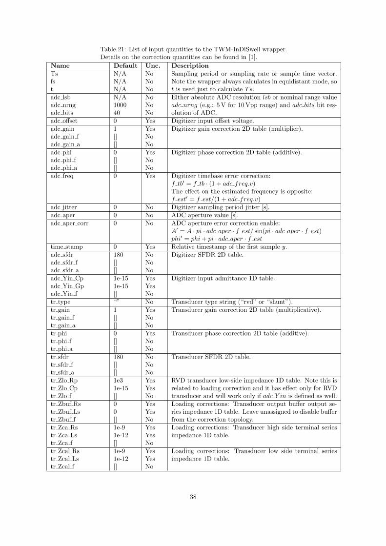
Table 21: List of input quantities to the TWM-InDiSwell wrapper.Details on the correction quantities can be found in [1].
Name Default Unc. DescriptionTsfst
N/AN/AN/A
NoNoNo
Sampling period or sampling rate or sample time vector.Note the wrapper always calculates in equidistant mode, sot is used just to calculate Ts.
adc lsbadc nrngadc bits
N/A100040
NoNoNo
Either absolute ADC resolution lsb or nominal range valueadc nrng (e.g.: 5 V for 10 Vpp range) and adc bits bit res-olution of ADC.
adc offset 0 Yes Digitizer input offset voltage.adc gainadc gain fadc gain a
1[][]
YesNoNo
Digitizer gain correction 2D table (multiplier).
adc phiadc phi fadc phi a
0[][]
YesNoNo
Digitizer phase correction 2D table (additive).
adc freq 0 Yes Digitizer timebase error correction:f tb′ = f tb · (1 + adc freq.v)The effect on the estimated frequency is opposite:f est′ = f est/(1 + adc freq.v)
adc jitter 0 No Digitizer sampling period jitter [s].adc aper 0 No ADC aperture value [s].adc aper corr 0 No ADC aperture error correction enable:
A′ = A · pi · adc aper · f est/ sin(pi · adc aper · f est)phi′ = phi+ pi · adc aper · f est
time stamp 0 Yes Relative timestamp of the first sample y.adc sfdradc sfdr fadc sfdr a
180[][]
NoNoNo
Digitizer SFDR 2D table.
adc Yin Cpadc Yin Gpadc Yin f
1e-151e-15[]
YesYesNo
Digitizer input admittance 1D table.
tr type “” No Transducer type string (“rvd” or “shunt”).tr gaintr gain ftr gain a
1[][]
YesNoNo
Transducer gain correction 2D table (multiplicative).
tr phitr phi ftr phi a
0[][]
YesNoNo
Transducer phase correction 2D table (additive).
tr sfdrtr sfdr ftr sfdr a
180[][]
NoNoNo
Transducer SFDR 2D table.
tr Zlo Rptr Zlo Cptr Zlo f
1e31e-15[]
YesYesNo
RVD transducer low-side impedance 1D table. Note this isrelated to loading correction and it has effect only for RVDtransducer and will work only if adc Y in is defined as well.
tr Zbuf Rstr Zbuf Lstr Zbuf f
00[]
YesYesNo
Loading corrections: Transducer output buffer output se-ries impedance 1D table. Leave unassigned to disable bufferfrom the correction topology.
tr Zca Rstr Zca Lstr Zca f
1e-91e-12[]
YesYesNo
Loading corrections: Transducer high side terminal seriesimpedance 1D table.
tr Zcal Rstr Zcal Lstr Zcal f
1e-91e-12[]
YesYesNo
Loading corrections: Transducer low side terminal seriesimpedance 1D table.
38

Table 21: List of input quantities to the TWM-InDiSwell wrapper.Details on the correction quantities can be found in [1].
Name Default Unc. Descriptiontr Yca Cptr Yca Dtr Yca f
1e-151e-12[]
YesYesNo
Loading corrections: Transducer output terminals shuntingimpedance.
tr Zcamtr Zcam f
1e-12[]
YesNo
Loading corrections: Transducer output terminals mutualinductance 1D table.
Zcb RsZcb LsZcb f
1e-91e-12[]
YesYesNo
Loading corrections: Cable series impedance 1D table.
Ycb RsYcb LsYcb f
1e-151e-12[]
YesYesNo
Loading corrections: Cable series impedance 1D table.
Table 22: List of output quantities of the TWM-InDiSwell wrapper.Name Uncertainty Descriptiont Yes Time vector of the calculated samples [s].env Yes Calculated half-cycle RMS values env(t).f0 No Average detected fundamental frequency.sag start Yes Sag (dip) event start relative time stamp [s].sag dur Yes Sag (dip) event duration [s].sag res Yes Sag (dip) event residual RMS level [%].swell start Yes Swell event start relative time stamp [s].swell dur Yes Swell event duration [s].swell res Yes Swell event residual RMS level [%].int start Yes Interruption event start relative time stamp [s].int dur Yes Interruption event duration [s].int res Yes Interruption event residual RMS level [%].
Table 23: List of “calcset” options supported by the TWM-InDiSwell wrapper.Name Descriptioncalcset.unc Uncertainty calculation mode. Supported: “none”
or “guf” for uncertainty estimator.calcset.loc Level of confidence [-].calcset.verbose Verbose level.calcset.dbg plots Non-zero value to enable plotting of debugging/sig-
nal analysis plots of the TWM-HCRMS, which isused internally by the TWM-InDiSwell.
5.2 Algorithm description
The algorithm TWM-InDiSWell internally uses algorithm TWM-HCRMS to calculate RMS envelope ofthe signal. Therefore, all input signal conditioning of y is performed in the TWM-HCRMS. The TWM-HCRMS output RMS values and corresponding time stamps are used to detect events according to thepreset thresholds. The detection method follows the IEC 61000-3-40 standard. The start of event isassigned to the first RMS sample whose value exceeds the threshold. End of event is assigned to the firstsample whose RMS value returned below the (threshold − hysteresis), which prevents multiple eventsdetection around the threshold. Flowchart of the algorithm is shown in fig. 14.
39

START
TWM-HCRMS call onsignal y to get rms
envelope: env_time, env_rms
u_env_time, u_env_rms
Detect "dip" event from envelope.
Detect "swell" event from envelope.
Detect "interruption"event from envelope.
Return event quantitiesand rms envelope
STOP
unce
rtain
ty
rms
enve
lope
Figure 14: Flowchart of the algorithm wrapper TWM-InDiSwell. Note the green cells are calls to anotherQWTB/TWM wrappers.
5.3 Uncertainty calculation
The main component of uncertainty is the output of TWM-HCRMS. However, due to the principle ofdetection, especially for class A, the uncertainty of the event start can never be lower than half of theperiod, as that is the resolution of the RMS detector. The duration uncertainty cannot be lower thanone full period, as the same resolution applies to the end of the event. The resolution in the class S modeis higher, however the uncertainty remains the same as that is the requirement of the IEC standard.
5.4 Validation
The validation of the TWM-InDiSwell algorithm has not been performed by the Monte-Carlo simulationssince the algorithm is usually used with the TWM-HCRMS algorithm. It was instead tested on numeroustypical cases such as shown in Fig. 15. The uncertainty is always one half-cycle as suggested by thestandard, so the detected events were always within or exactly on the uncertainty limit as the timeresolution is also one half-cycle.
Figure 15: Validation test examples for the TWM-InDiSwell algorithm.
40

References
[1] Stanislav Maslan. Activity A2.3.2 - Algorithms Exchange Format. https://github.com/smaslan/
TWM/tree/master/doc/A232AlgorithmExchangeFormat.docx.
41

6 TWM-THDWFFT - THD from Windowed FFT
This algorithm is designed for calculation of the harmonics and Total Harmonic Distortion (THD) of thenon-coherently sampled signal. It uses windowed FFT to detect the harmonic amplitudes, which limitsthe achievable accuracy of the harmonics detection due to the window scalloping effect. However, thealgorithm was initially designed for THD calculation of the low-distortion signals, where the accuracywas not critical. The relative expanded uncertainty of the harmonics is at least 0.015 % (or 0.005 % afterhighly experimental correction method). On the other hand, the algorithm was designed to compensatethe spectral leakage of the noise to the harmonics near noise level, so it offers decent accuracy for thevery low distortions near self-THD of the digitizer itself.
The algorithm supports direct processing of a multiple records which are used to produce averagedspectrum before the main calculation. This possibility should be preferred instead of repeated call of thealgorithm for each record as it reduces the noise. The algorithm supports only single-ended transducerconnection.
The algorithm returns: (i) Full spectrum; (ii) Identified harmonics; (iii) THD coefficients accordingvarious definitions; (iv) RMS noise estimate; (v) THD+Noise estimate.
Example of the algorithm output is shown in fig. 16.
Figure 16: Example of the TWM-THDWFFT algorithm output.
6.1 TWM wrapper parameters
The input quantities supported by the algorithm are shown in table 24. Algorithm returns outputquantities shown in table 25. Calculation setup supported by the algorithm is shown in table 26.
Table 24: List of input quantities to the TWM-THDWFFT wrap-per. Details on the correction quantities can be found in [4].
Name Default Unc. Descriptionf0 N/A N/A Optional user defined frequency of fundamental component.
Do not assign to enable auto detection.f0 mode “PSFE” N/A Optional selection of the fundamental frequency auto de-
tection mode.scallop fix 0 N/A Non-zero value to enable experimental window scalloping
error correction. It will try to use known scalloping error ofthe window at given frequency to correct the error, howeverit will work only for stable signals when the fundamentalfrequency detection is accurate.
H 10 N/A Optional limit of maximum harmonics count to analyse (in-cluding fundamental). Note the high values will signifi-cantly increase calculation time!
42

Table 24: List of input quantities to the TWM-THDWFFT wrap-per. Details on the correction quantities can be found in [4].
Name Default Unc. Descriptionband inf N/A Optional bandwidth limit which can reduce the harmonics
count to analyse. This also affects the bandwidth of thenoise calculation.
plot 0 N/A Non-zero value, “on”, “true” or “enabled” string enablesplotting of the detected harmonics.
y N/A No Input matrix of the samples. One column per record (the al-gorithm can directly calculate average of multiple records).
Tsfst
N/AN/AN/A
NoNoNo
Sampling period or sampling rate or sample time vector.Note the wrapper always calculates in equidistant mode, sot is used just to calculate Ts.
adc lsbadc nrngadc bits
N/A100040
NoNoNo
Either absolute ADC resolution lsb or nominal range valueadc nrng (e.g.: 5 V for 10 Vpp range) and adc bits bit res-olution of ADC.
adc jitter 0 No Digitizer sampling period jitter [s].adc aper corr 0 No ADC aperture error correction enable:
A′ = A · pi · adc aper · f est/ sin(pi · adc aper · f est)phi′ = phi+ pi · adc aper · f est
adc aper 0 No ADC aperture value [s].adc gainadc gain fadc gain a
1[][]
YesNoNo
Digitizer gain correction 2D table (multiplier).
adc freq 0 Yes Digitizer timebase error correction:f tb′ = f tb · (1 + adc freq.v)The effect on the estimated frequency is opposite:f est′ = f est/(1 + adc freq.v)
adc sfdradc sfdr fadc sfdr a
180[][]
NoNoNo
Digitizer SFDR 2D table.
adc Yin Cpadc Yin Gpadc Yin f
1e-151e-15[]
YesYesNo
Digitizer input admittance 1D table.
tr type “” No Transducer type string (“rvd” or “shunt”).tr gaintr gain ftr gain a
1[][]
YesNoNo
Transducer gain correction 2D table (multiplicative).
tr sfdrtr sfdr ftr sfdr a
180[][]
NoNoNo
Transducer SFDR 2D table.
tr Zlo Rptr Zlo Cptr Zlo f
1e31e-15[]
YesYesNo
RVD transducer low-side impedance 1D table. Note this isrelated to loading correction and it has effect only for RVDtransducer and will work only if adc Y in is defined as well.
tr Zbuf Rstr Zbuf Lstr Zbuf f
00[]
YesYesNo
Loading corrections: Transducer output buffer output se-ries impedance 1D table. Leave unassigned to disable bufferfrom the correction topology.
tr Zca Rstr Zca Lstr Zca f
1e-91e-12[]
YesYesNo
Loading corrections: Transducer high side terminal seriesimpedance 1D table.
tr Zcal Rstr Zcal Lstr Zcal f
1e-91e-12[]
YesYesNo
Loading corrections: Transducer low side terminal seriesimpedance 1D table.
43

Table 24: List of input quantities to the TWM-THDWFFT wrap-per. Details on the correction quantities can be found in [4].
Name Default Unc. Descriptiontr Yca Cptr Yca Dtr Yca f
1e-151e-12[]
YesYesNo
Loading corrections: Transducer output terminals shuntingimpedance.
tr Zcamtr Zcam f
1e-12[]
YesNo
Loading corrections: Transducer output terminals mutualinductance 1D table.
Zcb RsZcb LsZcb f
1e-91e-12[]
YesYesNo
Loading corrections: Cable series impedance 1D table.
Ycb RsYcb LsYcb f
1e-151e-12[]
YesYesNo
Loading corrections: Cable series impedance 1D table.
Table 25: List of output quantities of the TWM-THDWFFT wrapper. Note the uncertainty “No” meansthe algorithm may return some uncertainty but it should be ignored because it is either incomplete ornot validated.
Name Uncertainty DescriptionH No Harmonics count analysed.noise bw No Bandwidth used for the noise estimation [Hz].thd Yes Total Harmonic Distortion referenced to the fundamental.thd2 Yes Total Harmonic Distortion referenced to the RMS value.thdn No Total Harmonic Distortion + Noise referenced to the fundamental.thdn2 No Total Harmonic Distortion + Noise referenced to the RMS value.noise No RMS noise estimate.h Yes Amplitudes of the harmonics.f No Frequencies of the harmonics h.spec a No Full spectrum from the windowed FFT.spec f No Frequencies of the spectrum components spec a.thd raw No thd without noise spectrum leakage correction.thd2 raw No thd2 without noise spectrum leakage correction.
Table 26: List of “calcset” options supported by the TWM-THDWFFT wrapper.Name Descriptioncalcset.unc Uncertainty calculation mode. Supported: “none” or
“guf” for uncertainty estimator. Note the algorithmis internally made in such a way it always calculatesthe uncertainty, so this option should have no effectin current version.
calcset.loc Level of confidence [-].calcset.verbose Verbose level.
6.2 Algorithm description and uncertainty evaluation
The whole algorithm is extended and improved version of the THD analyser presented in [5]. Theoverview of the algorithm wrapper structure and internal functions is shown in fig. 17. The wrapperstart by a call to the top level function “thd wfft()”, which performs entire calculation and uncertaintyestimation. Next, the wrapper may optionally plot graph showing the identified harmonics and nearspectrum. Note the wrapper reduces the asymmetric uncertainty limits to symmetric as the TWM was
44

not designed for such a case. This has no effect when the level of harmonics is at least twice the noiselevel. It will expand the uncertainty only for very small harmonic levels near noise level.
The “thd wfft()” itself internally does just two steps: (i) Calculating spectra of input records and esti-mates their fundamental frequency (function “thd proc waves()”); (ii) Initiates main evaluation function“thd eval thd()”.
Call thd_proc_waves()to get fundamental
frequency andspectra sig
for each record in y
Prepare calculationparameters
Call thd_wfft() tocalculate THD
TWM-THDWFFT
Optional spectrumplotting by function
thd_plot_spectrum()
Formatting results toreturn in QWTB style: thd, thd2, thdn, thdn2,
noise, harmonics,spectrum
STOP
thd_wfft()
Call thd_eval_thd() tocalculate the THD and
uncertainties: thd, thd2, thdn, thdn2,
noise, harmonics,spectrum
RETURN
thd_proc_waves()
Next record?
Call thd_find_freq() todetect fundamental
frequency f_sig by givenmethod: PSFE,
zerocross, FPNLSF ormanual
Call ampphspectrum() to get windowed
amplitude spectrum ampand frequency vector f.
RETURN
Average frequencies andfrequency vectors
yes
all done
Figure 17: Flow chart of the algorithm wrapper TWM-THDWFFT. Note the rounded gold blocks arecalls to other local functions which are shown in another diagram or mentioned in the text.
The function “thd proc waves()” first detects fundamental frequency of each record in y. It containsseveral modes of detection. The simplest is zero crossing, however it is very unreliable. Another optionsif FPNLSF [7], which may fail when initial estimate from zero cross detector is poor. Last and bestoption (default) is PSFE [3], which is capable to identify the fundamental frequency with good accuracyeven with strong harmonic content. User may also override the auto detection by manual entry of thefundamental frequency. The next step is calculation of amplitude spectrum for each record y using awindowed FFT. The widest, flattest window with highest suppression of side lobes was chosen for thegoal - Flattop HFT248D from [1]. This window offer side lobes suppression by 248 dB and scallopingerror only 0.0104 % for range ±0.5 DFT bin.
all done
Obtain windowscalloping: flat
Generate LUT for noiseleakage correction
Decide range of analysis: harmonics count and
bandwidth
thd_eval_thd()
Obtain and apply digitizergain, transducer gain and
aperture corrections tosignal sig
Average spectra sig tosig_m and calculate type
A uncertainty sig_ua.
Get harmonic's:frequency, peak
amplitude, near noiselevel, type A uncertainty
Optionally call thd_window_gain_corr()to correct scalloping error
Next harmonic?yes
Estimate RMS noise
Prepare system SFDRand LSB parameters
Call thd_eval_harmonic() toevaluate amplitude and
uncertainty of eachharmonic. Returns meanvalues and Monte Carlo
randomized sets.
Evaluate THD from meanharmonic amplitudes.
High THD mode: THD uncertainty usingMonte Carlo from therandomized harmonic
sets
High THD?
Combine and formatTHD values anduncertainties and
harmonic values anduncertainties
Low THD mode: THD uncertainty usingworst case harmonics
uncertainty combination
RETURN
yesno
signal, parameterscorrections
uncertainty
Figure 18: Flow chart of the main algorithm function “thd eval thd()” for the TWM-THDWFFT algo-rithm.
45

The internal structure of the evaluation function “thd eval thd()” is shown in fig. 18. The functiondoes following steps:
1. Obtaining parameters of the window function Flattop HFT248D used for the processing.
2. Generation of lookup table (LUT), which will be used for the numeric solver that compensatesspectrum leakage of the noise to the harmonic DFT bin (details below).
3. Decision of how many harmonics to analyse based on the user limits (H and bandwidth).
4. Application of all gain corrections to scale the spectra from “thd proc waves()” to actual levels.
5. Averaging of the spectra and type A uncertainty calculation.
6. Detection of harmonics. The algorithm picks the harmonics from the average spectrum one byone. It searches the highest DFT bin in preset frequency range for each estimated harmonicsfrequency. It also extracts the nearby noise level which is needed for compensation of the noisespectral leakage.
7. The parameters required for the uncertainty evaluation of each harmonics are obtained (systemSFDR and LSB).
8. Evaluation of the harmonic values and uncertainties using function “thd eval harmonic()” (seebelow). This returns mean harmonic levels and calculated uncertainties and also randomizedharmonic levels, because it internally uses Monte Carlo.
9. Calculation of the THD coefficients from the mean harmonic amplitudes according to variousdefinition and calculation of their uncertainties using one of the methods (see below).
The evaluation of the THD coefficients in the step 9) is performed according to the several definitions.The most common is so called “fundamental referenced” THD:
thd =
√U22 + U2
3 + · · ·+ UMU1
, (18)
where Ux is mean harmonic voltage and x is harmonic index and M is harmonics count. The next isRMS value referenced mode, which uses total RMS of the signal in the denominator:
thd2 =
√U22 + U2
3 + · · ·+ U2M√
U21 + U2
2 + U23 + · · ·+ U2
M
. (19)
The results should be very close for low distortion signals. Next result is combined fundamental referencedTHD and noise THD+N:
thdn =
√U22 + U2
3 + · · ·+ UM + U2noise
U1, (20)
where the Unoise is RMS noise in specified bandwidth (parameter band). Last definition is RMS referencedTHD+N:
thdn2 =
√U22 + U2
3 + · · ·+ U2M + U2
noise√U21 + U2
2 + U23 + · · ·+ U2
M + U2noise
. (21)
The algorithm also returns the same four coefficient without the noise leakage correction, howeverthose are just informative.
The uncertainty evaluation for the THD coefficients uses heuristic approach. The THD coefficientsare calculated from the mean values from step 8 ignoring the uncertainty and its distribution. Theuncertainty calculation method depends on the “is high” obtained in step 8, which is set when theweighted average of the harmonic amplitudes is significantly above noise. So two cases occur:
1. is high = true: The distribution of the uncertainty of the harmonics is near Gaussian so therandomized amplitudes from step 8) are passed to the THD formulas above and the THD isevaluated using Monte Carlo and function “scovint()” (follows GUM guide [2]).
46
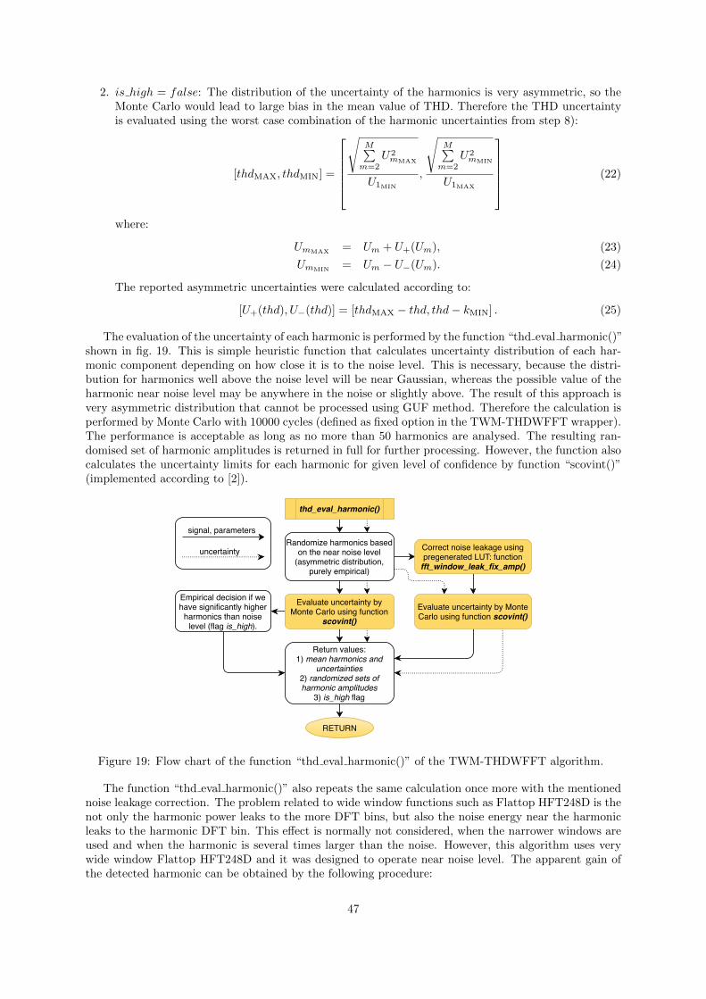
2. is high = false: The distribution of the uncertainty of the harmonics is very asymmetric, so theMonte Carlo would lead to large bias in the mean value of THD. Therefore the THD uncertaintyis evaluated using the worst case combination of the harmonic uncertainties from step 8):
[thdMAX, thdMIN] =
√
M∑m=2
U2mMAX
U1MIN
,
√M∑m=2
U2mMIN
U1MAX
(22)
where:
UmMAX= Um + U+(Um), (23)
UmMIN= Um − U−(Um). (24)
The reported asymmetric uncertainties were calculated according to:
[U+(thd), U−(thd)] = [thdMAX − thd, thd− kMIN] . (25)
The evaluation of the uncertainty of each harmonic is performed by the function “thd eval harmonic()”shown in fig. 19. This is simple heuristic function that calculates uncertainty distribution of each har-monic component depending on how close it is to the noise level. This is necessary, because the distri-bution for harmonics well above the noise level will be near Gaussian, whereas the possible value of theharmonic near noise level may be anywhere in the noise or slightly above. The result of this approach isvery asymmetric distribution that cannot be processed using GUF method. Therefore the calculation isperformed by Monte Carlo with 10000 cycles (defined as fixed option in the TWM-THDWFFT wrapper).The performance is acceptable as long as no more than 50 harmonics are analysed. The resulting ran-domised set of harmonic amplitudes is returned in full for further processing. However, the function alsocalculates the uncertainty limits for each harmonic for given level of confidence by function “scovint()”(implemented according to [2]).
thd_eval_harmonic()
Randomize harmonics basedon the near noise level
(asymmetric distribution,purely empirical)
Evaluate uncertainty byMonte Carlo using function
scovint()
Correct noise leakage usingpregenerated LUT: functionfft_window_leak_fix_amp()
Evaluate uncertainty by MonteCarlo using function scovint()
Empirical decision if wehave significantly higher
harmonics than noiselevel (flag is_high).
Return values: 1) mean harmonics and
uncertainties 2) randomized sets ofharmonic amplitudes
3) is_high flag
RETURN
signal, parameters
uncertainty
Figure 19: Flow chart of the function “thd eval harmonic()” of the TWM-THDWFFT algorithm.
The function “thd eval harmonic()” also repeats the same calculation once more with the mentionednoise leakage correction. The problem related to wide window functions such as Flattop HFT248D is thenot only the harmonic power leaks to the more DFT bins, but also the noise energy near the harmonicleaks to the harmonic DFT bin. This effect is normally not considered, when the narrower windows areused and when the harmonic is several times larger than the noise. However, this algorithm uses verywide window Flattop HFT248D and it was designed to operate near noise level. The apparent gain ofthe detected harmonic can be obtained by the following procedure:
47

1. generation of sine wave x(t) with amplitude Um,
2. addition of gaussian noise with level Unoise to the x(t),
3. windowing of the x(t) by selected window function (Flattop HFT248D),
4. reading the amplitude Ux from amplitude spectrum of X(f) of signal x(t).
Alternatively the same result can be obtained by means of Monte Carlo method from equation:
Ux =1
I
I∑i=1
∣∣∣∣∣Um + Unoise
K∑k=1
Wk · e−j2πR(i,k)
∣∣∣∣∣ (26)
where K is number of coefficients of window function amplitude spectrum Wk and I is number of MCiterations (at least 104). The R(i, k) is uniformly distributed random number generator from 0 to 1. Theright sum term represents a vector sum of a noise vectors with random angle and amplitude weightedby window spectrum coefficients Wk. The resulting gain vs. noise to signal ratio is shown in fig. 20.
1
1.2
1.4
1.6
1.8
2
2.2
2.4
2.6
0 0.2 0.4 0.6 0.8 1
ha
rmo
nic
re
ad
ing
ga
in [
-]
noise to signal ratio [-]
Figure 20: Error of the harmonics amplitude measurement using FFT with window Flattop HFT248D.Note the “noise” means amplitude of the noise in surrounding DFT bins, not RMS noise.
.
The direct inverse evaluation from the detected to actual harmonic level is nto possible, so thealgorithm uses iterative function based on the precalculated LUT with the gain error (the dependence infig. 20). The correction itself is performed by the function “fft window leak fix amp()”, which takes theharmonic level, noise level detected around (assuming the noise is the same for all related DFT bins).Effect of this correction is shown in fig. 21.
Figure 21: Deviation of THDWFFT algorithm from simulated THD level 10 ppm for various noiseto higher harmonic ratios. The simulated waveform has 10 harmonic components with amplitudesUm = 0.9, 3 · 10−6, 3 · 10−6, . . . V. Left graph shows results without noise spectral leakage correction,right graph shows the same dependence with corrected values. The error bars show the standard deviationof a repeated simulations.
48

6.3 Validation
The algorithm TWM-THDWFFT has many input quantities (45) and some of them are matrices. Thatis too many possible degrees of freedom. Thus, varying the quantities in some systematic way would bevery complicated if the validation should cover full range of used signals and corrections. Therefore, analternative approach was used.
QWTB test function “alg test.m” was created, which performs the validation using randomly gen-erated test setups. It randomizes the signal parameters, correction quantities and uncertainties andalgorithm configurations in ranges expected to occur during the real measurements. The test is runmany times to cover full operating range of the algorithm. Following operations are performed for eachrandom test setup:
1. Generate signal y with known harmonic content Aref(h) and thus known THD thdref.
2. Distort the signal y by inverse corrections, i.e. simulate the transducers, and digitizer (e.g. gainerrors, quantisation, SFDR ...).
3. Run the algorithm TWM-THDWFFT with enabled uncertainty evaluation to obtain the harmoniclevels Ax(h), distortion thdx and their uncertainties u(Ax(h)) and u(thdx).
4. Compare the reference and calculated harmonics and distortion and check if the deviations arelower than assigned uncertainties:
pass A(i, h) = |Aref(h)−Ax(h)| < u(Ax(h)), (27)
pass thd(i) = |thdref − thdx| < u(thdx), (28)
where i is test run index.
5. Repeat N times from step 1, with the same test setup parameters, but with corrections randomisedby their uncertainties, and with randomised noise, SFDR and jitter.
6. Check that at least 95 % of pass A(i, h) and pass thd(i) results passed (for 95 % level of confidence).
The test runs count per test setup was set to N = 300, which is far from optimal infinite set, butdue to the computational requirements it could not have been much higher. Note the low count of testinduces uncertainty to the obtained pass rates.
The algorithm in the uncertainty estimation mode was tested in 4 different configurations with 10000test setups per each. I.e. the algorithm was ran 12 million times in total (4x10000x300). The processingitself was performed on a supercomputer [6] so it took about 3 days at 400 parallel octave instances.
The randomization ranges of the signal are shown in table 27. The randomization ranges of thecorrections are shown in table 28.
The test results were split into several groups given by the randomiser setup: (i) Scalloping correctionenabled/disabled; (ii) Randomisation of corrections by uncertainty enabled/disabled. When the randomi-sation of corrections is disabled, the test runs cover only the algorithm itself and the contributions of thecorrection uncertainties are ignored.
The summary of the validation test results is shown in table 29. The success rate was 100 % for allcases.
49

Table 27: Validation range of the signal for TWM-THDWFFT algorithm.Parameter RangeSampling rate 30 to 70 kHz (no need to randomize in wider range, as
all other parameters are generated relative to this rate).Sampling time 0.3 to 5 seconds.Fundamental frequency Random, so there are at least 30 DFT bins between
harmonics and the highest harmonic is no higher then0.4 · fs.
Analysed harmonics count 5 to 10.Fundamental amplitude 0.1 to 0.9 of fullscale digitizer input.Harmonic amplitudes Each harmonic is randomised from 1 µV to A max of
fundamental, where the A max is randomised from0.0001 to 0.1 of fundamental.
Phase angles Random for all harmonics.Averaging cycles 10.SFDR -140 to -80 dBc, all spurs have the same level.Digitizer RMS noise 1 to 50 µV.Sampling jitter 1 to 100 ns.
Table 28: Validation range of the correction for the TWM-THDWFFT algorithm.Parameter RangeTransducer type Random ’shunt’ or ’rvd’.Nominal input range 0.1 to 100 V (0.1 to 100 A)Aperture 1 ns to 100 µsDigitizer gain Randomly generated frequency transfer simulating
NI 5922 FIR-like gain ripple (possibly the worst imag-inable shape) and some ac-dc dependence. The transfermatrix has up to 50 frequency spots. Nominal gain valueis random from 0.95 to 1.05 with uncertainty 2 µV/V.Maximum ac-dc value at fs/2 is up to ±1 % with uncer-tainty 50 µV/V. Gain ripple amplitude is random from0.005 to 0.03 dB with up to 5 periods between 0 andfs/2.
Digitizer SFDR Value based on table 27.Transducer SFDR Value based on table 27. Note the “SFDR” from ta-
ble 27 is randomly split between digitizer and transducerSFDR correction.
Digitizer bit resolution 16 to 28 bits.Digitizer nominal range 1 VTransducer gain Randomly generated frequency transfer. The transfer
matrix has up to 50 frequency spots. Nominal gain valueis random (see above) with relative uncertainty 2 µV/V.Maximum ac-dc value at fs/2 is up to ±2 % with uncer-tainty 50 µV/V. Gain ripple amplitude is 0.005 dB with4 to 10 periods between 0 and fs/2.
50

Table 29: Validation results of the algorithm TWM-THDWFFT. The “passed test” shows percentage ofpassed tests under conditions defined in tables 27 and 28.
Scallop. fix. Rand. corr.Passed test [%]
thd h(1) h(2..n)
nono 100.00 100.00 100.00yes 100.00 100.00 100.00
yesno 100.00 100.00 100.00yes 100.00 100.00 100.00
51

References
[1] Gerhard Heinzel, A. Rudiger, and R. Schilling. Spectrum and spectral density estimation by thediscrete fourier transform (dft), including a comprehensive list of window functions and some newflat-top windows. Technical report, Max-Planck-Institut fur Gravitationsphysik (Albert-Einstein-Institut) Teilinstitut Hannover, Feb 2005.
[2] JCGM. Evaluation of measurement data - Supplement 1 to the “Guide to the expression of uncertaintyin measurement” - Propagation of distributions using a Monte Carlo method. Bureau Internationaldes Poids et Measures.
[3] Rado Lapuh. Estimating the fundamental component of harmonically distorted signals from nonco-herently sampled data. IEEE Transactions on Instrumentation and Measurement, 64(6):1419–1424,June 2015.
[4] Stanislav Maslan. Activity A2.3.2 - Algorithms Exchange Format. https://github.com/smaslan/
TWM/tree/master/doc/A232AlgorithmExchangeFormat.docx.
[5] Stanislav Maslan and Martin Sıra. Automated non-coherent sampling thd meter with spectrumanalyser. In Proceedings CPEM, 2014.
[6] Miroslav Valtr. CMI HPC System Online. https://translate.google.cz/translate?sl=cs&tl=
en&js=y&prev=_t&hl=cs&ie=UTF-8&u=http%3A%2F%2Fprutok.cmi.cz%2Fsc%2Fdoku.php%3Fid%
3Dsystem&edit-text=, 2014.
[7] M. Sıra and S. Maslan. Uncertainty analysis of non-coherent sampling phase meter with four pa-rameter sine wave fitting by means of monte carlo. In 29th Conference on Precision ElectromagneticMeasurements (CPEM 2014), pages 334–335, Aug 2014.
52

7 TWM-PWRTDI - Power by Time Domain Integration
TWM-PWRTDI is an algorithm for calculation of power parameters using a time domain integration ofu(t) · i(t) product. It is based on the use of window function to eliminate effects of non-coherent samplingas was demonstrated in [1] and [4]. Therefore, it does work even for non-coherently sampled waveforms.The algorithm itself without contribution of corrections can easily reach errors below 1 µW/VA withproper selection of a sampling rate and windows size.
The algorithm can calculate all basic parameters: active power P , reactive power Q, apparent powerS, RMS voltage U , RMS current I and power factor PF . It also returns DC components separately:Udc, Idc and Pdc. User may choose optional AC coupling mode by setting parameter “accoupling = 1”in which case the U , I, P , Q, S and PF will be calculated without the AC component.
Note the windowed RMS method itself can calculate power in any quadrant, however it is not able todistinguish all four quadrants. The quadrant identification (proper signs for P and Q) is obtained froma complementary windowed FFT algorithm which is running along the main RMS calculation. Note thequadrant selection may fail around PF = 0 (the absolute values will be correct).
The algorithm uses following definitions for the power components: (i) The AC power componentsP , Q and S are related by equation:
S2 = P 2 +Q2. (29)
(ii) Power factor PF is calculated including DC components according to equation:
PF =P
S. (30)
(iii) The sign of Q is calculated using harmonic components method according Budenau definition:
sing(Q) = sign
H∑h=1
(U(h) · I(h) · sinφ(h))
, (31)
where h is harmonic index, H is harmonics count, U(h), I(h) and φ(h) are harmonic voltage, currentand phase shift. Note the absolute value of Q is still calculated from AC components following equation29. Only the sign of Q is decided from the Budenau definition 31.
The TWM-PWRTDI algorithm wrapper is able to use single-ended or differential input sensors forvoltage channel, current channel or both. The algorithm is also equipped by a fast uncertainty estimatorand the Monte Carlo uncertainty calculation method for more accurate but slower uncertainty evaluation.
7.1 TWM wrapper parameters
The input quantities supported by the algorithm are shown in the table 30. Algorithm returns outputquantities shown in the table 31. Calculation setup supported by the algorithm is shown in table 32.
Table 30: List of input quantities to the TWM-PWRTDI wrapper.Details on the correction quantities can be found in [5].
Name Default Unc. Descriptionac coupling 0 N/A Enables virtual AC coupling of the wattmeter. This option
will cause the DC value will be ignored.uu lo
N/AN/A
NoNo
Input voltage sample data vector and complementary low-side input data vector i lo (for differential mode only).
ii lo
N/AN/A
NoNo
Input current sample data vector and complementary low-side input data vector i lo (for differential mode only).
Tsfst
N/AN/AN/A
NoNoNo
Sampling period or sampling rate or sample time vector.Note the wrapper always calculates in equidistant mode, sot is used just to calculate Ts.
time shift 0 Yes Timeshift between voltage channel u and current channeli.
u time shift loi time shift lo
00
YesYes
Time shift between high-side channel u low-side channelu lo (or i and i lo for current).
53

Table 30: List of input quantities to the TWM-PWRTDI wrapper.Details on the correction quantities can be found in [5].
Name Default Unc. Descriptionu lsbu adc nrngu adc bitsu lo lsbu lo adc nrngu lo adc bitsi lsbi adc nrngi adc bitsi lo lsbi lo adc nrngi lo adc bits
N/A100040N/A100040N/A100040N/A100040
NoNoNoNoNoNoNoNoNoNoNoNo
Either absolute ADC resolution lsb or nominal range valueadc nrng (e.g.: 5 V for 10 Vpp range) and adc bits bit res-olution of ADC.
u adc offsetu lo adc offseti adc offseti lo adc offset
0000
YesYesYesYes
Digitizer input offset voltage.
u adc gainu adc gain fu adc gain au lo adc gainu lo adc gain fu lo adc gain ai adc gaini adc gain fi adc gain ai lo adc gaini lo adc gain fi lo adc gain a
1[][]1[][]1[][]1[][]
YesNoNoYesNoNoYesNoNoYesNoNo
Digitizer gain correction 2D table (multiplier).
u adc phiu adc phi fu adc phi au lo adc phiu lo adc phi fu lo adc phi ai adc phii adc phi fi adc phi ai lo adc phii lo adc phi fi lo adc phi a
0[][]0[][]0[][]0[][]
YesNoNoYesNoNoYesNoNoYesNoNo
Digitizer phase correction 2D table (additive).
adc freq 0 Yes Digitizer timebase error correction:f tb′ = f tb · (1 + adc freq.v)The effect on the estimated frequency is opposite:f est′ = f est/(1 + adc freq.v)
u adc jitteru lo adc jitteri adc jitteri lo adc jitter
0000
NoNoNoNo
Digitizer sampling period jitter [s].
u adc aperu lo adc aperi adc aperi lo adc aper
0000
NoNoNoNo
ADC aperture value [s].
54

Table 30: List of input quantities to the TWM-PWRTDI wrapper.Details on the correction quantities can be found in [5].
Name Default Unc. Descriptionu adc aper corru lo adc aperi adc aper corri lo adc aper
0000
NoNoNoNo
ADC aperture error correction enable:A′ = A · pi · adc aper · f est/ sin(pi · adc aper · f est)phi′ = phi+ pi · adc aper · f est
u adc sfdru adc sfdr fu adc sfdr au lo adc sfdru lo adc sfdr fu lo adc sfdr ai adc sfdri adc sfdr fi adc sfdr ai lo adc sfdri lo adc sfdr fi lo adc sfdr a
180[][]180[][]180[][]180[][]
NoNoNoNoNoNoNoNoNoNoNoNo
Digitizer SFDR 2D table.
u adc Yin Cpu adc Yin Gpu adc Yin fu lo adc Yin Cpu lo adc Yin Gpu lo adc Yin fi adc Yin Cpi adc Yin Gpi adc Yin fi lo adc Yin Cpi lo adc Yin Gpi lo adc Yin f
1e-151e-15[]1e-151e-15[]1e-151e-15[]1e-151e-15[]
YesYesNoYesYesNoYesYesNoYesYesNo
Digitizer input admittance 1D table.
u tr typei tr type
“” No Transducer type string (“rvd” or “shunt”).
u tr gainu tr gain fu tr gain ai tr gaini tr gain fi tr gain a
1[][]1[][]
YesNoNoYesNoNo
Transducer gain correction 2D table (multiplicative).
u tr phiu tr phi fu tr phi ai tr phii tr phi fi tr phi a
0[][]0[][]
YesNoNoYesNoNo
Transducer phase correction 2D table (additive).
u tr sfdru tr sfdr fu tr sfdr ai tr sfdri tr sfdr fi tr sfdr a
180[][]180[][]
NoNoNoNoNoNo
Transducer SFDR 2D table.
55

Table 30: List of input quantities to the TWM-PWRTDI wrapper.Details on the correction quantities can be found in [5].
Name Default Unc. Descriptionu tr Zlo Rpu tr Zlo Cpu tr Zlo fi tr Zlo Rpi tr Zlo Cpi tr Zlo f
1e31e-15[]1e31e-15[]
YesYesNoYesYesNo
RVD transducer low-side impedance 1D table. Note this isrelated to loading correction and it has effect only for RVDtransducer and will work only if adc Y in is defined as well.
u tr Zbuf Rsu tr Zbuf Lsu tr Zbuf fi tr Zbuf Rsi tr Zbuf Lsi tr Zbuf f
00[]00[]
YesYesNoYesYesNo
Loading corrections: Transducer output buffer output se-ries impedance 1D table. Leave unassigned to disable bufferfrom the correction topology.
u tr Zca Rsu tr Zca Lsu tr Zca fi tr Zca Rsi tr Zca Lsi tr Zca f
1e-91e-12[]1e-91e-12[]
YesYesNoYesYesNo
Loading corrections: Transducer high side terminal seriesimpedance 1D table.
u tr Zcal Rsu tr Zcal Lsu tr Zcal fi tr Zcal Rsi tr Zcal Lsi tr Zcal f
1e-91e-12[]1e-91e-12[]
YesYesNoYesYesNo
Loading corrections: Transducer low side terminal seriesimpedance 1D table.
u tr Yca Cpu tr Yca Du tr Yca fi tr Yca Cpi tr Yca Di tr Yca f
1e-151e-12[]1e-151e-12[]
YesYesNoYesYesNo
Loading corrections: Transducer output terminals shuntingimpedance.
u tr Zcamu tr Zcam fi tr Zcami tr Zcam f
1e-12[]1e-12[]
YesNoYesNo
Loading corrections: Transducer output terminals mutualinductance 1D table.
u Zcb Rsu Zcb Lsu Zcb fi Zcb Rsi Zcb Lsi Zcb f
1e-91e-12[]1e-91e-12[]
YesYesNoYesYesNo
Loading corrections: Cable series impedance 1D table.
u Ycb Rsu Ycb Lsu Ycb fi Ycb Rsi Ycb Lsi Ycb f
1e-151e-12[]1e-151e-12[]
YesYesNoYesYesNo
Loading corrections: Cable series impedance 1D table.
56

Table 31: List of output quantities of the TWM-PWRTDI wrapper.Name Uncertainty DescriptionU Yes RMS voltage [V].I Yes RMS current [A].P Yes Active power [W].S Yes Apparent power [VA].Q Yes Reactive power [VAr].phi ef Yes Effective phase angle: arccos (PF ) [rad].Udc Yes DC voltage component [V].Idc Yes DC current component [A].Pdc Yes DC power component [W].spec U No Voltage channel spectrum [V].spec I No Current channel spectrum [A].spec S No Apparanet power spectrum [VA].spec f No Frequency vector of spec U , spec I and spec S.
Table 32: List of “calcset” options supported by the TWM-PWRTDI wrapper.Name Descriptioncalcset.unc Uncertainty calculation mode. Supported: “none”,
“guf” for uncertainty estimator, “mcm” for MonteCarlo.
calcset.mcm.method Monte Carlo evaluation mode: “singlecore” - sin-gle core evaluation, “multicore” - Parallel evaluationusing “parcellfun” for GNU Octave or “parfor” forMatlab “multistation” - Multicore evaluation using“multicore” package (GNU Octave only yet).
calcset.mcm.repeats Monte Carlo iterations count. Use at least 100 to getany usable estimate.
calcset.mcm.proc no Number of parallel instances to use for the paral-leled modes. Use zero value to not start any serverprocesses for the “multistation” mode. This optionexpects user started the server processes manually inthe shared folder. This option causes less overheadfor the batch processing or runtime calculations.
calcset.mcm.tmpdir Jobs sharing folder for the “multistation” mode.This should be an absolute path to the sharing folder.Keep in mind the package “multicore” will erase thecontent of this folder before each new calculation!
calcset.mcm.user fun User function to call in the “multistation” mode af-ter startup of the serve processes. Example: “calc-set.mcm.user fun = @coklbind2”. Leave empty tonot execute any function.
calcset.loc Level of confidence [-].calcset.verbose Verbose level.
7.2 Algorithm description
The TWM-PWRTDI wrapper starts with automatic cropping of the input data to a size of multiple oftwo, which is required by the algorithm core. Next, the wrapper creates two virtual channels, one forvoltage and one for current, because the applied corrections are identical for both so the code duplicationis minimised. It also creates virtual sub-channels for the low-side signals u lo and i lo (differential mode).Next, the wrapper calculates windowed spectra of each input signal u and i (and u lo, i lo) and also splitsthe time domain signals u and i (and u lo, i lo) to AC and DC components which are treated separately.
57

The next step are the frequency dependent corrections of the input signals. Note the windowed RMS(WRMS) algorithm itself operates in time domain, so the frequency dependent corrections of the gainand phase must be applied in time domain to u and i (and u lo, i lo). However, the uncertaintycalculator/estimator needs a spectrum, i.e. frequency domain representation of the time domain signals.Therefore, the correcting code does two things at once: (i) It calculates total combined gain and phasecorrections for each virtual channel but does not apply it to time domain data u and i (and u lo, i lo)yet; (ii) It applies the same corrections to the frequency domain representation only. At the same timethe spectra of the eventual differential pair u and ulo (and i and i lo) are merged to a single single-endedspectrum of u and i.
In the next step, the wrapper calls the main WRMS function “proc wrms()”, which applies thecalculated corrections in time domain to u, i (and u lo, i lo), calculates the differential time domainsignal (for differential mode only) and calculates the AC RMS parameters U , I, AC power P (see below)and the DC components U dc and I dc. Follows the uncertainty calculation (see below) of the RMSand active power quantities and expression of the other desired quantities and their uncertainties. Forsimplicity the uncertainty calculator calculates only uncertainty of the RMS voltage, RMS current aactive power. The remaining uncertainties are calculated from these three. The definitions of particularparameters is shown in the table 33. Note the Q bud quantity in the table is reactive power estimatedfrom the FFT spectra of voltage and current according the Budenau definition:
Q bud =
H∑h=1
(0.5 · U(h) · I(h) · sinφ(h)), (32)
where h is harmonic component index, H is total harmonics count, U(h) and I(h) are harmonic voltageand current amplitudes and φ(h) is voltage to current phase shift. The purpose of the (sign)(Q bud)term is to distinguish correct polarity of Q, because the WRMS algorithm itself cannot distinguish allfour quadrants of power. One solution would be to use Hilbert transformation on either voltage or currentwaveform and repeat the WRMS calculation. This would allow to calculate the Q directly, however suchsolution seemed to complex. Therefore, instead of the Hilbert transform, the sign of Q was obtainedfrom the Budenau’s definition. Such solution should work reliably if power factor is |PF | > 0.05 andthere are no excessive harmonics.
Table 33: Definitions of the TWM-PWRTDI output quantities based on the basic quantities U , I, P ,U dc and I dc. Note the input quantities marked * are obtained from the other output quantity.
Returned quantity AC coupled definition DC coupled definitionDC voltage Udc U dc U dcDC current Idc I dc I dcDC power component Pdc U dc · I dc U dc · I dcRMS voltage U U
√U2 + U dc2
RMS current I I√I2 + I dc2
Active power P P P + U dc · I dcReactive power Q
√(UI)2 − P 2 · sign(Q bud)
√(UI)2 − P 2 · sign(Q bud)
Apparent power S (UI)2√U2 + U dc2 ·
√I2 + I dc2
Power factor PF P/S∗ P/S∗Effective phase angle phi ef atan2(Q∗, P ) atan2(Q∗, P )
7.2.1 Windowed RMS function “proc wrms()”
The core of the algorithm is function “proc wrms()”. Before the algorithm itself is described, it must benoted the “proc wrms()” function was made in such a way it can be used for a Monte Carlo uncertaintyevaluation in a parallel manner. I.e. the function is called once for each Monte Carlo iteration (seebelow). This affected its structure.
The function can be executed either on the input time domain signals u, i (and u lo, i lo) whichis used for evaluation of the power parameters and it can be also called repeatedly in the simulatormode, where it calculates the power of synthesized signals with prescribed parameters randomized by
58

input uncertainties (Monte Carlo calculation mode). The synthesizer of the waveforms is included inthis function, so the following section will show its function as well.
The function starts with selection of the mode of operation. For the simulated mode, it overridesinput signals u, i (and u lo, i lo) by a synthesized ones with known spectral components and knowntotal power, power factor, etc. It also applies various distortions, e.g. noise, quantisation errors, ...
Follows the calculation part which is common for both modes of operation. First, it applies the timedomain frequency dependent correction of each virtual channel (u, i, u lo and i lo)). This is done by the“td fft filter()”. Note the function “td fft filter()” itself also estimates the phase errors it causes, whichis used only in the calculation mode (they are ignored in the simulating mode). The DC corrections tothe previously split DC components are also applied in this step.
Figure 22: Example of FFT filter profile. From left right: Gain correction, Phase correction, Detail ofphase correction. Blue - desired correction, red - applied correction.
The function “td fft filter()” is critical for correct functionality of the whole algorithm. The functionis a frequency domain filter executed per smaller windows. The function does following steps:
1. Building a filter spectral profile from the gain/phase correction data for the positive frequencies.
2. Empirical post-processing of the filter profile to suppress the errors caused by high phase anglecorrection. This step applies weighting mask to the phase of the filter at its ends (at DC andNyquist frequency). So both “ends” of the filter have zero phase. This drastically reduces inherenterrors of this filtering method. See fig. 22 for an example.
3. Estimation of the filter post-processing errors on the phase.
4. Extending the filter profile to negative frequencies.
5. Performing the spectral filtering per small overlapping windows by a function“sFreqDep PG Comp(y, fft size, filter)”:
(a) Obtaining Hann window function coefficients w of size fft size/2.
(b) Extend Hann by zero padding: w = [zeros(1, fft size/4), w, zeros(1, fft size/4)] to a totalsize of fft size.
(c) Window fft size input samples y(offset : offset+ fft size− 1) by the window w.
(d) Performing FFT of the windowed portion of y to get spectrum Y .
(e) Applying filter profile to the spectrum Y .
(f) Performing inverse-FFT of the Y to get time domain representation y frame.
(g) Extracting < fft size/4; fft size · 3/4 > samples of y frame.
(h) Merging y frame samples with overlapping samples of output signal yf and storing result toyf(offset+ fft size/2).
59

(i) Move offset to next frame by fft size/4 samples and repeat from step 5c for all possibleframes.
6. Removing invalid portions of the filtered signal (fft size/2 samples from beginning and end ofsignal).
In the next step the “proc wrms()” evaluates the RMS parameters U , I and P according the followingdefinitions:
U =1
W·
√√√√ N∑k=1
w(k)2 · u(k)2, (33)
I =1
W·
√√√√ N∑k=1
w(k)2 · i(k)2, (34)
P =1
W 2·
√√√√ N∑k=1
w(k)2 · u(k) · i(k), (35)
W =
√√√√ N∑k=1
w(k)2, (36)
where k is a sample index, N is total samples count and w(k) is k-th sample of the window functionBlackman-Harris. For clarity, the Blackman-Harris window used in the WRMS algorithm is defined by[2]:
w(k) = 0.35875− 0.48829 · cos2πk
N+ 0.14128 · cos
4πk
N− 0.01168 · cos
6πk
N. (37)
Note the coefficients are exact (not rounded). This window was selected because the calculation errorsof the RMS parameters due to the non-coherency decays fastest with growing number of signal periods(see [1]).
Last step of the function “proc wrms()” is performed only for the simulation mode. The functioncalculates the deviation of calculated power from the theoretical synthesized power (used for Monte Carloevaluation).
7.3 Uncertainty calculator and estimator
The TWM-PWRTDI algorithm wrapper is equipped by two modes of uncertainty evaluation: (i) Theordinary Monte Carlo (MC) calculator; (ii) Fast estimator based on several precalculated lookup tables(LUT). The MC mode is more accurate, however it may take up to several minutes to perform even justa few hundreds of iterations. The calculation time drastically rises with the length of the record. Thusthe fast estimator was created as well.
The WRMS algorithm itself can calculate a power of any voltage and current waveforms. However,calculation of uncertainty for general non-periodic waveforms would be extremely complex and slow.Therefore, the uncertainty calculation is based on the analysis of spectral components obtained from theaverage spectrum of the whole digitized waveform. This simplification should not have any effect, as thealgorithm is primarily intended for a calibration of stationary signals.
The first step of the uncertainty evaluation for both modes is spectral analysis of the voltage andcurrent spectra Uh(fh), Ih(fh) and phase shifts between the voltage and current harmonic componentsph(fh). These spectra along with their uncertainties were obtained in the corrections section (see sec-tion 7.2). The algorithm identifies the fundamental component of power by searching the dominantvoltage harmonic assuming the fundamental voltage harmonic should be always present. The algorithmthen searches up to 100 spectral components Ux(fh), Ix(fh) and phx(fh), whose current or voltageamplitude exceeds certain threshold relative to the fundamental harmonic. These spectral componentsare successively removed from the spectra Uh(fh) and Ih(fh). Whatever is left after the removal isconsidered and later used as a residual RMS noise estimate. The identified spectral components will bemarked Ux(h), Ix(h) (amplitudes) and phx(h) in the following text. Their uncertainties coming from
60

the correction uncertainties will be marked u Ux(h), u Ix(h), u phx(h). The h is index of harmonicfrom one to H.
The identified spectral components Ux(h), Ix(h) and phx(h) are used to calculate estimate of theRMS and power parameters following the Budenau definition:
U rms =
√√√√ H∑h=1
0.5 · Ux(h)2, (38)
I rms =
√√√√ H∑h=1
0.5 · Ix(h)2, (39)
P = 0.5 ·H∑h=1
Ix(h) · Ix(h) · cos(phx(h)), (40)
Q = 0.5 ·H∑h=1
Ix(h) · Ix(h) · sin(phx(h)), (41)
S = 0.5 ·H∑h=1
Ix(h) · Ix(h), (42)
(43)
Following algorithm structure differ for Monte Carlo and Estimator.
7.3.1 Monte Carlo uncertainty calculator
The MC uncertainty calculator is very straightforward. It starts with preparation of the two virtualchannels. One for voltage and one for current. Each channel contains a list of the identified spectralcomponents Ux(h), Ix(h) and phx(h) to synthesize with assigned uncertainties coming from the correc-tions u Ux(h), u Ix(h), u phx(h). Each channel have also assigned RMS noise, system SFDR and LSBof the ADC. Then the WRMS processing function “proc wrms()” is called in the simulator mode repeat-edly for each iteration of MC. The returned randomised lists of RMS voltage, RMS current and activepower are evaluated according GUM annex 1 [3] using a function “scovint()” to obtain absolute finaluncertainties of quantities U , I and P . The uncertainties of the other returned quantities are evaluatedin the wrapper (see above) from these three uncertainties.
Note the MC evaluator itself uses function “qwtb mcm exec()”. This function is internally designedto enable parallel calculation of the MC iteration cycles. It is offers three modes of parallelisation:
1. calcset.mcm.method = ‘singlecore’: Single core calculation.
2. calcset.mcm.method = ‘multicore’: Multicore operation using “parcellfun()” from “parallel”package for GNU Octave or “parfor” for Matlab. Note the use of Matlab’s “parfor” for paral-lelisation is just a user wish. Actual parallelisation mode is decided by Matlab. The package“parcellfun()” implementation does work only for Linux. Windows implementation was not func-tional at least up to GNU Octave version 4.2.2.
3. calcset.mcm.method = ‘multistation’: Multiprocess/multistation calculation using “multi-core” package for GNU Octave (Matlab is not supported yet). Note the The “multistation” methodrequires to define shared folder path for the job files. Otherwise it will create the shared folder intemp folder, which may not be appreciated by the SSD disks owners. The mode “multistation”also have one specific feature. It can initiate the user function after startup of the server processes.The function is defined in the “calcset.mcm.user fun” variable. The example of the use for thisoptional input is CMI’s supercomputer “Cokl” [6] which requires to call a special script to assignserver processes to particular CPU cores.
See table 32 for list of the additional parameters. Note at least 100 iterations is the absolute minimumfor which the MC mode provides any usable uncertainty estimates. The processing time for an evaluationat 4 cores with 1000 cycles and N = 10000 input samples is typically below one minute. However, thesituation may change drastically when high count of harmonic components is presents in the signal.
61

7.3.2 Fast uncertainty estimator
The uncertainty estimator is significantly more complex than the Monte Carlo calculator. It consistsof four separate estimation routines which contributes to the final uncertainty: (i) Uncertainty of time-domain frequency dependent filter “td fft filter()”; (ii) Uncertainty of a system SFDR; (iii) UncertaintyWRMS algorithm for a single tone signal; (iv) Uncertainty of WRMS mutual harmonic effects. Theseare executed in order. The estimation routine (i) is affecting steps (ii), (iii) and (iv). The obtaineduncertainty components from the particular steps are combined to the total uncertainty of U , I and P .The uncertainties of the other returned quantities are evaluated in the wrapper (see above) from thesethree uncertainties.
7.3.2.1 Uncertainty of time-domain frequency dependent filter “td fft filter()”
The first estimator quantifies the errors introduced by the frequency dependent gain and phase filter“td fft filter()”. The uncertainty estimate is calculated using a complementary function “td fft filter unc()”,which is called for voltage and current channel separately. This estimator is far most problematic. The“td fft filter()” is using the time-¿frequency-¿time conversion (filtering in frequency domain per smallsized windows). The filtering in the frequency domain can cause hardly predictable errors when highphase shift corrections are applied. This is especially problematic if there are significant spectral compo-nents near the Nyquist frequency or near DC. The function have too many degrees of freedom to create asimple but reliable estimator. Therefore, the only usable solution found to this problem was to performa small scale Monte Carlo (MC). In particular, 10 cycles of following steps are performed:
1. Synthesize waveform with spectral components Ux(h) (resp. Ix(h)) with random phase anglesφ(h) and with uncertain frequency ±1 DFT bin, because accuracy of the frequency estimationfrom FFT spectral analysis is limited.
2. Perform the frequency dependent filtering by “td fft filter()” with calculated channel gain andphase correction data and calculate spectrum.
3. Perform the frequency dependent correction with the same correction data in frequency domain tothe spectral components Ux(h) (resp. Ix(h)) and the generated phase angles φ(h).
4. Compare the difference of the spectral components from 3) and 2) to estimate the filter error.
The set of error estimates is processed to find a maximum probable amplitude and phase error of eachspectral component. Surprisingly this simple solution provides reliable estimates.
This gain uncertainties u fa U(h), u fa I(h) and phase uncertainties u fp U(h), u fp I(h) obtainedby this estimator are used to expand the correction uncertainties u Ux(h), u Ix(h) and u phx(h) beforefollowing estimator steps:
u Ux(h) =√u Ux(h)2 + u fa U(h)2, (44)
u Ix(h) =√u Ix(h)2 + u fa I(h)2, (45)
u phx(h) =√u phx(h)2 + u fp U(h)2 + u fp I(h)2. (46)
7.3.2.2 Uncertainty of a system SFDR
The next step is estimation of the uncertainty introduced by the system SFDR (digitizer and transducer).The effect on the U , I and P is estimated as a wost case combination of the spurs according:
u U sfdr =1√3·
√√√√U2 + 0.5
S∑s=1
U spur(s)2 − U
, (47)
u I sfdr =1√3·
√√√√I2 + 0.5
S∑s=1
I spur(s)2 − I
, (48)
u P sfdr =1√3·
√√√√0.5
S∑s=1
U spur(s) · I spur(s), (49)
62

where U spur and I spur are vectors of voltage and current spur amplitudes (2nd, 3rd, 4th harmonic,etc.), s is spur index and S is spurs count.
7.3.2.3 Uncertainty WRMS algorithm for a single tone signal
This step is estimation of the WRMS algorithm error for each identified spectral component Ux(h),Ix(h). Note this estimator does not cover mutual effects between spectral components. It is just a singletone estimator for each component. The estimation is performed by the function “wrms unc st()”. Thisfunction uses precalculated LUT (see below) and empiric formulas to form an uncertainty interpolatordependent on following parameters: (i) Voltage amplitude, (ii) Current amplitude, (iii) Voltage noise,(iv) Current noise, (v) Voltage bit resolution, (vi) Current bit resolution, (vii) Periods count in thewaveform, (viii) Samples per period. The usable range of each parameter for the “wrms unc st()” isshown in table 35. This interpolator returns a relative uncertainty estimate of frequency componentvoltage u U st′(f), current u I st′(f) and active power u P st′(f). The component uncertainties areconverted to absolute and combined to obtain RMS uncertainties:
u U st =
√√√√∑Ff=1 u U st′(f)2 · Ux(f)2∑F
f=1 Ux(f)2, (50)
u I st =
√√√√∑Ff=1 u I st
′(f)2 · Ix(f)2∑Ff=1 Ix(f)2
, (51)
u P st =
√√√√ F∑f=1
u P st′(f)2. (52)
The LUT table itself for the interpolator of “wrms unc st()” was calculated as a worst case errorof the WRMS algorithm from 50000 Monte Carlo iterations. The simulation was performed for eachcombination of parameters shown in table 34. I.e. 11x12x15x9x5 = 89100 combinations were calculatedusing a supercomputer (processing time roughly two days on 300 cores). Note the phase shift betweenvoltage and current was randomised for each iteration as it had no effect on the relative active poweruncertainty (when expressed in units W/VA). The bit resolution of one channel was held fixed at 32 bitas the error is defined by the worse of the voltage and current channel. Noise was also simulated forthe worse of the channels only. Manual inspection of the obtained 5-dimensional space of uncertaintiesshowed only the parameters “Periods count” and “Samples per period” are necessary in the LUT asthey have hardly expressible shape given by the window function. The other parameters effects wereapproximated by empirical formulas. Therefore, the LUT size after compression is only 2.5 kBytes, whichis perfectly acceptable.
Table 34: Simulation ranges and steps of the parameters for uncertainty estimator of “wrms unc st()”function.
Name DescriptionPeriods count List: [3; 4; 5; 6; 7; 9; 11; 15; 20; 50; 100], 11 stepsSamples per period Log. space: 7 to 100, 12 stepsU to I phase shift random*U to I amplitude ratio Log. space: 0.01 to 1, 15 stepsU bit resolution 32 bitsI bit resolution Log. space: 4 to 32 bits, 9 stepsmax(U noise,I noise) Log. space: 10−7 to 10−3, 5 steps
63

Table 35: The usable range of input parameters of the single tone error estimator “wrms unc st()”. Theactions on min or max value is reached are: “error” - generate error; “const” - return value of uncertaintyat min. or max. of simulated range.
Name Range On min On maxVoltage amplitude 0 to ∞ const constCurrent amplitude 0 to ∞ const constVoltage noise 0 to ∞ const constCurrent noise 0 to ∞ const constVoltage bit resolution 4 to ∞ error constCurrent bit resolution 4 to ∞ error constPeriods count 3 to ∞ error constSamples per period 7 to ∞ const const
7.3.2.4 Uncertainty of WRMS mutual harmonic effects
This estimator calculates mutual effect of spur harmonic to analysed harmonic. The paper [1] showsexample of these errors, however this effect had to be quantified extensively for means of the uncertaintyestimator. Theoretically the calculation of mutual effect should be performed for each pair of componentsUx(h), Ix(h), phx(h), however that would be very slow. So and assumption was made the fundamentalharmonic carries dominant portion of the active power, RMS voltage and current, so the mutual effectscalculation is performed only between the fundamental component Ux(1), Ix(1), phx(1) and the restof components Ux(h), Ix(h), phx(h), where h ≥ 2. The estimation of the mutual effect itself is doneby estimator function “wrms unc spur()”. This function is an interpolator dependent on: (i) Referenceharmonic voltage, (ii) Reference harmonic current, (iii) Relative spur frequency, (iv) Spur harmonicvoltage, (v) Spur harmonic current, (vi) Periods of reference harmonic, (vii) Samples per period ofreference harmonic. The estimator function is called once for each spur component to obtain uncertaintycomponents u U sp′(h− 1), u I sp′(h− 1) and u P sp′(h− 1). These (H − 1) components are combinedto a combined uncertainty due to the spur components:
u U sp(h) =
√√√√∑H−1h=1 u U sp′(h)2 · Ux(h+ 1)2∑H
h=1 Ux(h)2, (53)
u I sp(h) =
√√√√∑H−1h=1 u I sp
′(h)2 · Ix(h+ 1)2∑Hh=1 Ix(h)2
, (54)
u P sp(h) =
√√√√H−1∑h=1
u P sp′(h)2. (55)
The interpolator “wrms unc spurr()” itself is a combination of two precalculated LUT tables andempiric formulas. First LUT is used to estimate the uncertainty of active power. It was obtained as aworst case error of 1000 Monte Carlo iterations performed each parameter combination (10x10x7x9x15= 94500 combinations) shown in table 36. The simulation was performed without noise or quantisationerrors, because these are already covered by the single tone WRMS estimator (section 7.3.2.3). Thesimulator performed following steps for each combination:
1. Synthesize waveforms with known apparent power S ref with no spurs.
2. Calculate active power using the WRMS algorithm P dut 0.
3. Synthesize waveforms with known active power with spur at voltage channel.
4. Calculate active power using the WRMS algorithm P dut tot.
5. Calculate relative error of the WRMS power: δP (i) = |P dut tot− P dut 0|/S ref .
6. Repeat 1000 times from step 1.
64

7. Estimate worst case uncertainty: δP = max δP (i) for i = 1..1000.
The simulator for the first LUT generates spur only for voltage channel, because the voltage and currentchannels are interchangeable. Thus the same LUT is used twice for the estimation (once for voltage spureffect and once for current spur effect with swapped voltage and current parameters).
The second LUT is used to estimate the spur effect to the RMS voltage (or RMS current). It wassimulated together with the first LUT. Only exception is the resulting LUT does not contain axis “U toI amplitude ratio”, as it obviously has no effect to RMS level of single channel. So the table containsonly 11x10x9x15 = 14850 combinations. The procedure performed for each combination is following:
1. Synthesize waveform with known RMS level A ref with no spurs.
2. Calculate RMS level using the WRMS algorithm: A dut.
3. Synthesize waveform with known RMS level with spur of RMS level S ref .
4. Calculate RMS level using the WRMS algorithm: A dut tot.
5. Calculate relative error of the WRMS RMS amplitude: δA(i) = (√|A dut tot2 − S ref2|−A ref)/A ref .
6. Repeat 1000 times from step 1.
7. Estimate worst case uncertainty: δA = max δA(i) for i = 1..1000.
This LUT called twice to obtain spur effects for RMS voltage and RMS current.Total size of both LUTs after compression is 265 kBytes which is still acceptable, so no further
optimalisations were performed. Total range of input parameters to the estimator “wrms unc spur()” isshown in table 37.
Table 36: Simulation ranges and steps of the parameters for uncertainty LUT of “wrms unc spur()”function.
Name DescriptionPeriods count List: [3; 4; 5; 6; 7; 9; 12; 20; 50; 100], 10 stepsSamples per period Log. space: 7 to 100, 10 stepsU to I phase shift random*U to I amplitude ratio Log. space: 0.01 to 1, 7 stepsU or I spur amplitude Log. space: 0.001 to 1, 9 stepsRelative spur frequency Log. space: 0.01 to 50 DFT bins, 15 steps
Table 37: The usable range of input parameters of the single tone error estimator “wrms unc spur()”.The actions on min or max value is reached are: “error” - generate error; “const” - return value ofuncertainty at min. or max. of simulated range.
Name Range On min On maxRef. component voltage 0 to ∞ const constRef. component current 0 to ∞ const constRelative spur frequency 0.01 to ∞ const constSpur component voltage 0 to ∞ const constSpur component current 0 to ∞ const constPeriods count 3 to 100 error constSamples per period 7 to 100 const const
7.4 Validation
The algorithm TWM-PWRTDI has many input quantities (for the differential transducer connectionabout 120 quantities) and some of them are matrices. That is too many possible degrees of freedom.
65

Thus, varying the quantities in some systematic way would be very complicated if the validation shouldcover full range of used signals and corrections. Therefore, an alternative approach was used.
QWTB test function “alg test.m” was created, which performs the validation using randomly gen-erated test setups. It randomizes the signal parameters, correction quantities and uncertainties andalgorithm configurations in ranges expected to occur during the real measurements. The test is runmany times to cover full operating range of the algorithm. Following operations are performed for eachrandom test setup:
1. Generate voltage and current signals u and i with known power parameters Pref .
2. Distort the signals u and i by inverse corrections, i.e. simulate the transducers, and digitizer (e.g.gain errors, phase errors, DC offsets, quantisation errors, ...).
3. Run the algorithm TWM-PWRTDI on the signals u and i with enabled uncertainty evaluation toobtain power parameters estimates Px and their uncertainties u(Pref).
4. Compare Pref and Px and decide if the errors of the algorithm for particular power parameters issmaller than the assigned uncertainties u(Pref):
pass(i) = abs(Pref − Px) < u(Pref), (56)
where i is test run index.
5. Repeat the test N times from step 1 with the same test setup parameters, but with randomisedcorrections by their uncertainties, and with randomised noise, SFDR and jitter.
6. Check that at least 95 % of pass(i) results passed (for default 95 % level of confidence). Theevaluation is made for each calculated power parameter separately. So it is possible to inspectwhich parameter fails.
The test runs count per test setup was set to N = 200, which is far from optimal “infinite” set, butdue to the computational requirements it could not have been much higher. Note the low count of testinduces uncertainty to the obtained pass rates.
The algorithm in the uncertainty estimation mode was tested in 4 different configurations with 10000test setups per each. I.e. the algorithm was ran 8 million times in total (4x10000x200). The processingitself was performed on a supercomputer [6] so it took only about 2 days at 400 parallel octave instances.
The test was also repeated in a smaller scale with Monte Carlo uncertainty calculation mode. 1000test setups with 290 repetitions and 1000 Monte Carlo cycles per each repetition were performed tovalidate the algorithm with the Monte-Carlo uncertainty calculator. Processing time was roughly 2 daysat 400 parallel octave instances.
The randomization ranges of the signal are shown in table 38. The randomization ranges of thecorrections are shown in table 39.
The test results were split into several groups given by the randomiser setup: (i) Single ended/d-ifferential mode; (ii) Randomisation of corrections by uncertainty enabled/disabled; (iii) Uncertaintyestimator or Monte Carlo method. When the randomisation of corrections is disabled, the test runscover only the algorithm itself and the contributions of the correction uncertainties are ignored.
The summary of the validation test results is shown in table 40. The success rate without correctionsrandomisation was close to 100 %. The success rate with corrections ransomisation was a bit worse,because the success rate of the test runs within the test setup is just around 95 %. Therefore the decisionpass/fail is problematic. The obtained set of test results was manually investigated and no cases withfar outliers were detected, e.g. the failed test setups contained occasional estimates offsets just aroundthe uncertainty boundaries. Also no case where all test runs fails were found.
The Monte Carlo uncertainty calculation mode was a bit less successful than estimator, because itsuncertainties are more accurate, so the success rate is just around 95 % even with randomisation ofcorrections disabled, so the detection of pass/fail is problematic.
66

Table 38: Validation range of the signal for TWM-PWRTDI algorithm.Parameter RangeSampling rate random 9 to 11 kHz (all other parameters are varied rel-
ative to this sampling rate, so it is not needed to ran-domise in wider range).
Samples count 5000 to 20000 (0.5 to 2 seconds integration time).Fundamental frequency random, so there are at least 10 samples per period and
at least 20 full periods recorded.Harmonics count 1 to 5 in order (no gaps).Fundamental amplitudes 0.1 to 1 of full scale digitizer input.Harmonic amplitudes 0.01 to 0.1 of fundamental.Inter-harmonic frequency anywhere between harmonics, not overlapping (at least
9 DFT bins from nearest other component). If not pos-sible to place between harmonics, the inter-harmonic isput anywhere up to Nyquist limit.
Inter-harmonic amplitude 0.001 to 0.01 of fundamental.Phase angles Random for all harmonics and inter-hamonics.DC offset ±0.05 of fundamental.SFDR -120 to -80 dBc, max. 10 harmonic components, ampli-
tude randomized for each spur in the SFDR range.Digitizer RMS noise 1 to 10 µV.Sampling jitter 1 to 100 ns.
67

Table 39: Validation range of the correction for the TWM-PWRTDI algorithm. Note the low-side channelcorrections in the differential mode are generated in the same way.
Parameter RangeNominal input U range 10 to 70 VNominal input I range 0.5 to 5 AAperture time 1 ns to 10 sDigitizer gain Randomly generated frequency transfer simulating
NI 5922 FIR-like gain ripple (possibly the worst imag-inable shape) and some ac-dc dependence. The transfermatrix has up to 50 frequency spots. Nominal gain valueis random from 0.95 to 1.05 with uncertainty 2 µV/V.Maximum ac-dc value at fs/2 is up to ±1 % with uncer-tainty 50 µV/V. Gain ripple amplitude is random from0.005 to 0.03 dB with up to 5 periods between 0 andfs/2.
Digitizer phase Randomly generated phase frequency transfer up to±1 mrad with uncertainty 2 to 50 µrad.
Digitizer SFDR Value based on table 38.Digitizer bit resolution 16 to 28 bits.Digitizer nominal range 1 VDigitizer DC offset Up to ±10 mV with uncertainty 0.1 mV.Low-side channel time shift Random value so the phase shift at Nyquist frequency
won’t exceed 0.1 rad with uncertainty 20 ns.I-to-U channel time shift Random value so the phase shift at Nyquist frequency
won’t exceed 0.1 rad with uncertainty 20 ns.Transducer gain Randomly generated frequency transfer. The transfer
matrix has up to 50 frequency spots. Nominal gain valueis random (see above) with relative uncertainty 2 µV/V.Maximum ac-dc value at fs/2 is up to ±2 % with uncer-tainty 50 µV/V. Gain ripple amplitude is 0.005 dB with4 to 10 periods between 0 and fs/2.
Transducer phase Randomly generated phase frequency transfer up to±1 mrad with uncertainty 2 to 50 µrad.
Table 40: Validation results of the algorithm TWM-PWRTDI. The “passed test” shows percentage ofpassed tests under conditions defined in tables 38 and 39. Note the pass condition is when all testedquantities (U , I, P , Q, S, PF ) passes. The “mode” signifies uncertainty evaluation mode (calculationoption “calcset.unc”), where “mcm” is Monte Carlo and “guf” is estimator.
Mode Connection Rand. corr. Passed test [%]
gufsingle-ended
off 100.00on 100.00
differentialoff 100.00on 100.00
mcmsingle-ended
off 100.00on 100.00
differentialoff 100.00on 100.00
68

References
[1] K. B. Ellingsberg. Predictable maximum rms-error for windowed rms (rmws). In 2012 Conferenceon Precision electromagnetic Measurements, pages 308–309, July 2012.
[2] Gerhard Heinzel, A. Rudiger, and R. Schilling. Spectrum and spectral density estimation by thediscrete fourier transform (dft), including a comprehensive list of window functions and some newflat-top windows. Technical report, Max-Planck-Institut fur Gravitationsphysik (Albert-Einstein-Institut) Teilinstitut Hannover, Feb 2005.
[3] JCGM. Evaluation of measurement data - Supplement 1 to the “Guide to the expression of uncertaintyin measurement” - Propagation of distributions using a Monte Carlo method. Bureau Internationaldes Poids et Measures.
[4] R. Lapuh, B. Voljc, and M. Lindic. Measurement and estimation of arbitrary signal power using awindow technique. In 2016 Conference on Precision Electromagnetic Measurements (CPEM 2016),pages 1–2, July 2016.
[5] Stanislav Maslan. Activity A2.3.2 - Algorithms Exchange Format. https://github.com/smaslan/
TWM/tree/master/doc/A232AlgorithmExchangeFormat.docx.
[6] Miroslav Valtr. CMI HPC System Online. https://translate.google.cz/translate?sl=cs&tl=
en&js=y&prev=_t&hl=cs&ie=UTF-8&u=http%3A%2F%2Fprutok.cmi.cz%2Fsc%2Fdoku.php%3Fid%
3Dsystem&edit-text=, 2014.
69

8 TWM-WRMS - RMS value by Windowed Time Domain In-tegration
TWM-WRMS is an algorithm for calculation RMS value and DC component of signal a time domainintegration of windowed signal y(t). The windowing function eliminates effects of non-coherent samplingas was demonstrated in [1] and [2]. Therefore, it does work even for non-coherently sampled waveforms.The algorithm itself without contribution of corrections can easily reach errors below 1 µV/V with properselection of a sampling rate and windows size.
The TWM-WRMS algorithm wrapper is able to use single-ended or differential input sensors. Thealgorithm is also equipped by a fast uncertainty estimator and the Monte Carlo uncertainty calculationmethod for more accurate but slower uncertainty evaluation.
8.1 TWM wrapper parameters
The input quantities supported by the algorithm are shown in the table 41. Algorithm returns outputquantities shown in the table 42. Calculation setup supported by the algorithm is shown in table 43.
Table 41: List of input quantities to the TWM-WRMS wrapper.Details on the correction quantities can be found in [3].
Name Default Unc. Descriptionac coupling 0 N/A Enables virtual AC coupling for the RMS calculation. This
option will cause the DC value will be ignored in the RMScalculation.
yy lo
N/AN/A
NoNo
Input sample data vector and complementary low-side in-put data vector y lo (for differential mode only).
Tsfst
N/AN/AN/A
NoNoNo
Sampling period or sampling rate or sample time vector.Note the wrapper always calculates in equidistant mode, sot is used just to calculate Ts.
time shift lo 0 Yes Time shift between high-side channel y low-side channely lo.
lsbadc nrngadc bitslo lsblo adc nrnglo adc bits
N/A100040N/A100040
NoNoNoNoNoNo
Either absolute ADC resolution lsb or nominal range valueadc nrng (e.g.: 5 V for 10 Vpp range) and adc bits bit res-olution of ADC.
adc offsetlo adc offset
00
YesYes
Digitizer input offset voltage.
adc gainadc gain fadc gain alo adc gainlo adc gain flo adc gain a
1[][]1[][]
YesNoNoYesNoNo
Digitizer gain correction 2D table (multiplier).
adc phiadc phi fadc phi alo adc philo adc phi flo adc phi a
0[][]0[][]
YesNoNoYesNoNo
Digitizer phase correction 2D table (additive).
adc freq 0 Yes Digitizer timebase error correction:f tb′ = f tb · (1 + adc freq.v)The effect on the estimated frequency is opposite:f est′ = f est/(1 + adc freq.v)
70

Table 41: List of input quantities to the TWM-WRMS wrapper.Details on the correction quantities can be found in [3].
Name Default Unc. Descriptionadc jitterlo adc jitter
00
NoNo
Digitizer sampling period jitter [s].
adc aperlo adc aper
00
NoNo
ADC aperture value [s].
adc aper corrlo adc aper
00
NoNo
ADC aperture error correction enable:A′ = A · pi · adc aper · f est/ sin(pi · adc aper · f est)phi′ = phi+ pi · adc aper · f est
adc sfdradc sfdr fadc sfdr alo adc sfdrlo adc sfdr flo adc sfdr a
180[][]180[][]
NoNoNoNoNoNo
Digitizer SFDR 2D table.
adc Yin Cpadc Yin Gpadc Yin flo adc Yin Cplo adc Yin Gplo adc Yin f
1e-151e-15[]1e-151e-15[]
YesYesNoYesYesNo
Digitizer input admittance 1D table.
tr type “” No Transducer type string (“rvd” or “shunt”).tr gaintr gain ftr gain a
1[][]
YesNoNo
Transducer gain correction 2D table (multiplicative).
tr phitr phi ftr phi a
0[][]
YesNoNo
Transducer phase correction 2D table (additive).
tr sfdrtr sfdr ftr sfdr a
180[][]
NoNoNo
Transducer SFDR 2D table.
tr Zlo Rptr Zlo Cptr Zlo f
1e31e-15[]
YesYesNo
RVD transducer low-side impedance 1D table. Note this isrelated to loading correction and it has effect only for RVDtransducer and will work only if adc Y in is defined as well.
tr Zbuf Rstr Zbuf Lstr Zbuf f
00[]
YesYesNo
Loading corrections: Transducer output buffer output se-ries impedance 1D table. Leave unassigned to disable bufferfrom the correction topology.
tr Zca Rstr Zca Lstr Zca f
1e-91e-12[]
YesYesNo
Loading corrections: Transducer high side terminal seriesimpedance 1D table.
tr Zcal Rstr Zcal Lstr Zcal f
1e-91e-12[]
YesYesNo
Loading corrections: Transducer low side terminal seriesimpedance 1D table.
tr Yca Cptr Yca Dtr Yca f
1e-151e-12[]
YesYesNo
Loading corrections: Transducer output terminals shuntingimpedance.
tr Zcamtr Zcam f
1e-12[]
YesNo
Loading corrections: Transducer output terminals mutualinductance 1D table.
Zcb RsZcb LsZcb f
1e-91e-12[]
YesYesNo
Loading corrections: Cable series impedance 1D table.
Ycb RsYcb LsYcb f
1e-151e-12[]
YesYesNo
Loading corrections: Cable series impedance 1D table.
71

Table 42: List of output quantities of the TWM-WRMS wrapper.Name Uncertainty Descriptionrms Yes RMS level [V] or [A].dc Yes DC component [V] or [A].spec A No Amplitude spectrum [V] or [A].spec f No Frequency vector of spec A.
Table 43: List of “calcset” options supported by the TWM-WRMS wrapper.Name Descriptioncalcset.unc Uncertainty calculation mode. Supported: “none”,
“guf” for uncertainty estimator, “mcm” for MonteCarlo.
calcset.mcm.method Monte Carlo evaluation mode: “singlecore” - single coreevaluation, “multicore” - Parallel evaluation using “par-cellfun” for GNU Octave or “parfor” for Matlab “multi-station” - Multicore evaluation using “multicore” pack-age (GNU Octave only yet).
calcset.mcm.repeats Monte Carlo iterations count. Use at least 100 to getany usable estimate.
calcset.mcm.proc no Number of parallel instances to use for the paralleledmodes. Use zero value to not start any server pro-cesses for the “multistation” mode. This option expectsuser started the server processes manually in the sharedfolder. This option causes less overhead for the batchprocessing or runtime calculations.
calcset.mcm.tmpdir Jobs sharing folder for the “multistation” mode. Thisshould be an absolute path to the sharing folder. Keepin mind the package “multicore” will erase the contentof this folder before each new calculation!
calcset.mcm.user fun User function to call in the “multistation” mode af-ter startup of the serve processes. Example: “calc-set.mcm.user fun = @coklbind2”. Leave empty to notexecute any function.
calcset.loc Level of confidence [-].calcset.verbose Verbose level.calcset.fetch luts Optional, non-zero will prefetch uncertainty LUT tables
to global variables to make the execution faster. Notethis was intended ONLY for validation process wherereduction of disk access is beneficial.
calcset.dbg plots Optional, non-zero will plot some debugging graphs.
8.2 Algorithm description
The TWM-WRMS algorithm is a wrapper of TWM-PWRTDI algoritm. It copies the input data andcorrection to both voltage and current channels of TWM-PWRTDI (see sectition 7), executes it andcopies either voltage or current results to the TWM-WRMS results depending on the used transducertype. Internal principle of operation is thus identical as for TWM-PWRTDI. This “backwards” solutionwas used because it was not possible to effectively build the TWM-PWRTDI power algorithm from singlechannel processing using TWM-WRMS. As a result it is a bit slower, because most of the TWM-PWRTDIis not used in TWM-WRMS. Block diagram is shown in fig. 23.
72

START
Duplicate signal y andcorrections to virtualvoltage and current
channels
Call TWM-PWRTDI toobtain rms voltage andcurrent: U_rms, I_rms
Select voltage or currentoutput depending on the
transducer type
STOP
trans
duce
r typ
e
Figure 23: Internal structure of TWM-WRMS algorithm..
8.3 Uncertainty calculator and estimator
The TWM-WRMS algorithm wrapper is equipped by two modes of uncertainty evaluation: (i) Theordinary Monte Carlo (MC) calculator; (ii) Fast estimator based on several precalculated lookup tables(LUT). The MC mode is more accurate, however it may take up to several minutes to perform even justa few hundreds of iterations. The calculation time drastically rises with the length of the record. Thusthe fast estimator was created as well.
The WRMS algorithm itself can calculate a RMS of any voltage and current waveforms. However,calculation of uncertainty for general non-periodic waveforms would be extremely complex and slow.Therefore, the uncertainty calculation is based on the analysis of spectral components obtained from theaverage spectrum of the whole digitized waveform. This simplification should not have any effect, as thealgorithm is primarily intended for a calibration of stationary signals.
Detailed description of the uncertainty evaluation can be found in the TWM-PWRTDI algorithm.
8.4 Validation
Only limited validation of TWM-WRMS was performed as it internally uses TWM-PWRTDI (see sec-tition 7).
Table 44: Validation results of the algorithm TWM-WRMS. The “passed test” shows percentage ofpassed tests under conditions defined in tables 38 and 39. The “mode” signifies uncertainty evaluationmode (calculation option “calcset.unc”), where “mcm” is Monte Carlo and “guf” is estimator.
Mode Connection Rand. corr. Passed test [%]
gufsingle-ended
off 100.00on 100.00
differentialoff 100.00on 100.00
mcmsingle-ended
off 100.00on 100.00
differentialoff 100.00on 100.00
73

References
[1] K. B. Ellingsberg. Predictable maximum rms-error for windowed rms (rmws). In 2012 Conferenceon Precision electromagnetic Measurements, pages 308–309, July 2012.
[2] R. Lapuh, B. Voljc, and M. Lindic. Measurement and estimation of arbitrary signal power using awindow technique. In 2016 Conference on Precision Electromagnetic Measurements (CPEM 2016),pages 1–2, July 2016.
[3] Stanislav Maslan. Activity A2.3.2 - Algorithms Exchange Format. https://github.com/smaslan/
TWM/tree/master/doc/A232AlgorithmExchangeFormat.docx.
74

9 TWM-WFFT - Windowed FFT spectrum analysis
Algorithm for single or multi-tone harmonic analysis using windowed FFT. The algorithm performswindowed FFT of the signal, applies TWM corrections and extracts FFT bin(s) with selected frequencies.It also calculates rms value estimate, however rms will be usable only for coherent sampling. The mainpurpose of the algorithm is interchannel phase shift and voltage ratio analysis. That will work even fornon-coherent sampling, when non-rectangular window is used.
Note the harmonics spacing in the spectrum must be higher, then width of the selected window! E.g.the wide ”flattop 248D” needs at least some 25 FFT bins spacing. Also note the wider windows havehigher equivalent noise bandwidth, so the noise in the analysed harmonic is amplified. See section 9.3for more details on the effects of windows.
The TWM-WFFT algorithm wrapper is able to use single-ended or differential input sensors. Thealgorithm is also equipped with a fast uncertainty estimator for the harmonic components.
9.1 TWM wrapper parameters
The input quantities supported by the algorithm are shown in the table 45. Algorithm returns outputquantities shown in the table 46. Calculation setup supported by the algorithm is shown in table 47.
Table 45: List of input quantities to the TWM-WFFT wrapper.Details on the correction quantities can be found in [3].
Name Default Unc. Descriptionf nom N/A N/A Optional nominal frequency (or vector of frequencies) to
extract from the spectrum. The algorithm will choose thenearest FFT bin(s). If the f nom is not assigned, the al-gorithm will search the fundamental component by callingPSFE algorithm [1].
h num N/A N/A Optional list of relative harmonic frequencies related to thef nom. E.g.: when f nom = 50 Hz and h num = [123],the extracted frequencies will be [50, 100, 150] Hz.
window ”rect” N/A Window type used before FFT. ”rect” window can be usedfor coherent sampling without significant interharmoniccomponents only. Another windows may be used for non-coherent sampling, however the harmonic analysis will beusable only for interchannel amplitude ratios and phase dif-ferences for the non-coherent case!
yy lo
N/AN/A
NoNo
Input sample data vector and complementary low-side in-put data vector y lo (for differential mode only).
Tsfst
N/AN/AN/A
NoNoNo
Sampling period or sampling rate or sample time vector.Note the wrapper always calculates in equidistant mode, sot is used just to calculate Ts.
time stamp 0 Yes Relative timestamp of the first sample y.time shift lo 0 Yes Time shift between high-side channel y low-side channel
y lo.lsbadc nrngadc bitslo lsblo adc nrnglo adc bits
N/A100040N/A100040
NoNoNoNoNoNo
Either absolute ADC resolution lsb or nominal range valueadc nrng (e.g.: 5 V for 10 Vpp range) and adc bits bit res-olution of ADC.
adc offsetlo adc offset
00
YesYes
Digitizer input offset voltage.
75

Table 45: List of input quantities to the TWM-WFFT wrapper.Details on the correction quantities can be found in [3].
Name Default Unc. Descriptionadc gainadc gain fadc gain alo adc gainlo adc gain flo adc gain a
1[][]1[][]
YesNoNoYesNoNo
Digitizer gain correction 2D table (multiplier).
adc phiadc phi fadc phi alo adc philo adc phi flo adc phi a
0[][]0[][]
YesNoNoYesNoNo
Digitizer phase correction 2D table (additive).
adc freq 0 Yes Digitizer timebase error correction:f tb′ = f tb · (1 + adc freq.v)The effect on the estimated frequency is opposite:f est′ = f est/(1 + adc freq.v)
adc jitterlo adc jitter
00
NoNo
Digitizer sampling period jitter [s].
adc aperlo adc aper
00
NoNo
ADC aperture value [s].
adc aper corrlo adc aper
00
NoNo
ADC aperture error correction enable:A′ = A · pi · adc aper · f est/ sin(pi · adc aper · f est)phi′ = phi+ pi · adc aper · f est
adc sfdradc sfdr fadc sfdr alo adc sfdrlo adc sfdr flo adc sfdr a
180[][]180[][]
NoNoNoNoNoNo
Digitizer SFDR 2D table.
adc Yin Cpadc Yin Gpadc Yin flo adc Yin Cplo adc Yin Gplo adc Yin f
1e-151e-15[]1e-151e-15[]
YesYesNoYesYesNo
Digitizer input admittance 1D table.
tr type “” No Transducer type string (“rvd” or “shunt”).tr gaintr gain ftr gain a
1[][]
YesNoNo
Transducer gain correction 2D table (multiplicative).
tr phitr phi ftr phi a
0[][]
YesNoNo
Transducer phase correction 2D table (additive).
tr sfdrtr sfdr ftr sfdr a
180[][]
NoNoNo
Transducer SFDR 2D table.
tr Zlo Rptr Zlo Cptr Zlo f
1e31e-15[]
YesYesNo
RVD transducer low-side impedance 1D table. Note this isrelated to loading correction and it has effect only for RVDtransducer and will work only if adc Y in is defined as well.
tr Zbuf Rstr Zbuf Lstr Zbuf f
00[]
YesYesNo
Loading corrections: Transducer output buffer output se-ries impedance 1D table. Leave unassigned to disable bufferfrom the correction topology.
76
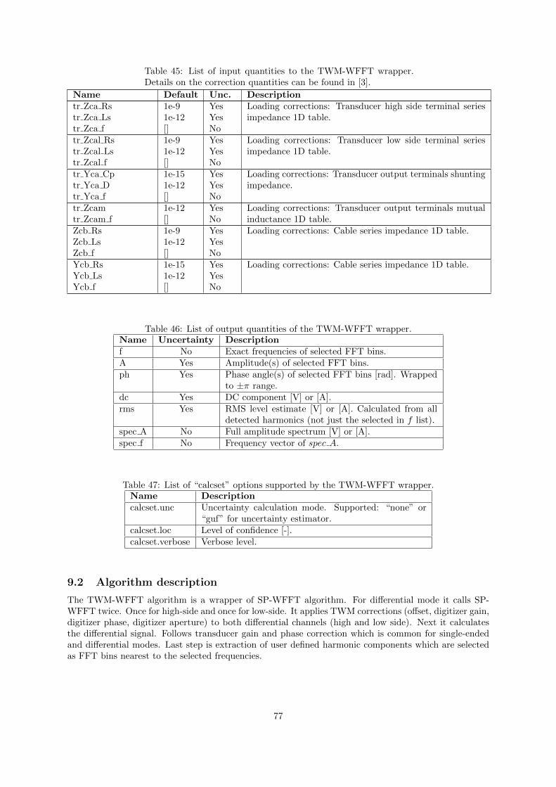
Table 45: List of input quantities to the TWM-WFFT wrapper.Details on the correction quantities can be found in [3].
Name Default Unc. Descriptiontr Zca Rstr Zca Lstr Zca f
1e-91e-12[]
YesYesNo
Loading corrections: Transducer high side terminal seriesimpedance 1D table.
tr Zcal Rstr Zcal Lstr Zcal f
1e-91e-12[]
YesYesNo
Loading corrections: Transducer low side terminal seriesimpedance 1D table.
tr Yca Cptr Yca Dtr Yca f
1e-151e-12[]
YesYesNo
Loading corrections: Transducer output terminals shuntingimpedance.
tr Zcamtr Zcam f
1e-12[]
YesNo
Loading corrections: Transducer output terminals mutualinductance 1D table.
Zcb RsZcb LsZcb f
1e-91e-12[]
YesYesNo
Loading corrections: Cable series impedance 1D table.
Ycb RsYcb LsYcb f
1e-151e-12[]
YesYesNo
Loading corrections: Cable series impedance 1D table.
Table 46: List of output quantities of the TWM-WFFT wrapper.Name Uncertainty Descriptionf No Exact frequencies of selected FFT bins.A Yes Amplitude(s) of selected FFT bins.ph Yes Phase angle(s) of selected FFT bins [rad]. Wrapped
to ±π range.dc Yes DC component [V] or [A].rms Yes RMS level estimate [V] or [A]. Calculated from all
detected harmonics (not just the selected in f list).spec A No Full amplitude spectrum [V] or [A].spec f No Frequency vector of spec A.
Table 47: List of “calcset” options supported by the TWM-WFFT wrapper.Name Descriptioncalcset.unc Uncertainty calculation mode. Supported: “none” or
“guf” for uncertainty estimator.calcset.loc Level of confidence [-].calcset.verbose Verbose level.
9.2 Algorithm description
The TWM-WFFT algorithm is a wrapper of SP-WFFT algorithm. For differential mode it calls SP-WFFT twice. Once for high-side and once for low-side. It applies TWM corrections (offset, digitizer gain,digitizer phase, digitizer aperture) to both differential channels (high and low side). Next it calculatesthe differential signal. Follows transducer gain and phase correction which is common for single-endedand differential modes. Last step is extraction of user defined harmonic components which are selectedas FFT bins nearest to the selected frequencies.
77

9.3 Uncertainty calculator and estimator
The TWM-WFFT algorithm wrapper is equipped by fast uncertainty estimator. The estimator calculatesuncertainty correctly only for the coherent sampling case! It uses two main components: (i) TWMcorrections contribution and (ii) Noise, bit resolution, jitter and SFDR effects.
TWM corrections component (i) comprises of gain, phase corrections of the digitizer and transducerand offset correction of the digitizer. These components are calculated along with application of thecorrections and will apply even for non-coherent sampling case correctly.
The other components (ii) requires further processing. The rms noise is estimated from the fullspectrum with removed harmonic components. Sampling Jitter may be defined by user correction dataas well as bit resolution. SFDR of the digitizer and transducer are also definable by user and theireffect to extracted harmonics can be easily calculated. The uncertainty contribution coming from thenoise, jitter and bit resolution were calculated following the formulas in [2], section 4.10 Noise. Thecomponents are automatically calculated for any window type. The validity of the implementation waschecked by Monte Carlo simulation. However, it is not known weather these approximations are validfor non-coherent case.
The uncertainty estimator does not take into account any effects caused by the interleaving of sidelobes of the particular harmonics and also effects of non-coherent sampling. I.e. harmonic spacing inthe spectrum must be wide enough, so the side lobe of one harmonic does not interfere with another.All windows containing only harmonic components (Hann, Hamming, Flattops, Blackman, etc.) havefinal width, so for the coherent sampling they can affect the other harmonics only up to finite distance.However, in non-coherent case they have side lobes with finite amplitude in full bandwidth of the FFT.E.g. Blackman–Nuttall window have almost constant side lobes at -100 dBc, so when we have funda-mental with level of 1 V and second harmonic with level of 10 mV, the second harmonic will be affectedby up to 10−5 · 1 V. That is 0.1 %. This must be taken into account by user when using the algorithmfor non-coherent sampling and proper window function should be selected.
Another problem related to the non-coherent sampling not covered by the estimator is scallopingloss. Whenever the actual frequency of the harmonic component does not match FFT bin frequencyexactly, there will be error given by flatness of the window in range ±0.5 FFT bin. E.g. even flattestwindow ”flattop 248D” has this flatness only roughly 0.01 %, which may not be acceptable for somemeasurements. As it is not possible to tell algorithmically if all the frequency components are coherent,the uncertainty contribution of this effect was intendedly omitted from the calculation and user mustadd the effect to the uncertainty budget manually.
In general, wider window functions with more harmonic components have lower side lobes and betterflatness, so they are more suitable for non-coherent measurements. However the cost for this is highernoise bandwidth, which increases type A uncertainty up to several times.
9.4 Validation
The algorithm TWM-WFFT has many input quantities and some of them are matrices. That is toomany possible degrees of freedom. Thus, varying the quantities in some systematic way would be verycomplicated if the validation should cover full range of used signals and corrections. Therefore, analternative approach was used.
QWTB test function “alg test.m” was created, which performs the validation using randomly gen-erated test setups. It randomizes the signal parameters, correction quantities and uncertainties andalgorithm configurations in ranges expected to occur during the real measurements. The test is runmany times to cover full operating range of the algorithm. Following operations are performed for eachrandom test setup:
1. Generate signals y with random and known harmonic content Href .
2. Distort the signal y by inverse corrections, i.e. simulate the transducers, and digitizer (e.g. gainerrors, phase errors, DC offsets, quantisation errors, ...).
3. Run the algorithm TWM-WFFT on the signal y with enabled uncertainty evaluation to obtainharmonic parameter estimates Hx and their uncertainties u(Hx).
78

4. Compare Href and Hx and decide if the errors of the algorithm for particular parameters is smallerthan the assigned uncertainties u(Hx):
pass(i) = abs(Href −Hx) < u(Hx), (57)
where i is test run index.
5. Repeat the test N times from step 1 with the same test setup parameters, but with randomisedcorrections by their uncertainties, and with randomised noise, SFDR and jitter.
6. Check that at least 95 % of pass(i) results passed (for default 95 % level of confidence). Theevaluation is made for each parameter separately (DC component, fundamental amplitude andphase and other harmonics’ amplitudes and phases). So it is possible to inspect which parameterfails.
The test runs count per test setup was set to N = 500, which is far from optimal “infinite” set, butdue to the computational requirements it could not have been much higher. Note the low count of testinduces uncertainty to the obtained pass rates.
The algorithm in the uncertainty estimation mode was tested in 4 different configurations with 10000test setups per each. I.e. the algorithm was ran 20 million times in total (4x10000x500). The processingitself was performed on a supercomputer [4] so it took only about 2 days at 400 parallel octave instances.
The randomization ranges of the signal are shown in table 48. The randomization ranges of thecorrections are shown in table 49.
The test results were split into several groups given by the randomiser setup: (i) Single ended/differ-ential mode; (ii) Randomisation of corrections by uncertainty enabled/disabled. When the randomisationof corrections is disabled, the test runs cover only the algorithm itself and the contributions of the cor-rection uncertainties are ignored. This option was chosen because corrections uncertainties may maskthe algorithm uncertainty.
The summary of the validation test results is shown in table 50. In both cases the pass rates werevery close to expected 95 % boundary and no cases where all test runs fails were found.
Table 48: Validation range of the signal for TWM-WFFT algorithm.Parameter RangeSampling rate random 9 to 11 kHz (all other parameters are varied rel-
ative to this sampling rate, so it is not needed to ran-domise in wider range).
Samples count 5000 to 20000 (0.5 to 2 seconds integration time).Fundamental frequency random, so there are at least 10 samples per period and
at least 20 full periods recorded. It is rounded so thesampling is always coherent.
Harmonics count 1 to 5 in order (no gaps, e.g.: [1, 2, 3, 4] or [1, 2]).Fundamental amplitudes 0.1 to 1 of full scale digitizer input.Harmonic amplitudes 0.01 to 0.1 of fundamental.Phase angles Random for all harmonics.DC offset ±0.05 of fundamental.SFDR -120 to -80 dBc, max. 10 harmonic components, ampli-
tude randomized for each spur in the SFDR range.Digitizer RMS noise 1 to 10 µV.Sampling jitter 1 to 100 ns.
79

Table 49: Validation range of the correction for the TWM-WFFT algorithm. Note the low-side channelcorrections in the differential mode are generated in the same way.
Parameter RangeNominal input range 0.1 to 10Aperture time 1 ns to 10 µsDigitizer gain Randomly generated frequency transfer simulating
NI 5922 FIR-like gain ripple (possibly the worst imag-inable shape) and some ac-dc dependence. The transfermatrix has up to 50 frequency spots. Nominal gain valueis random from 0.95 to 1.05 with uncertainty 2 µV/V.Maximum ac-dc value at fs/2 is up to ±1 % with uncer-tainty 50 µV/V. Gain ripple amplitude is random from0.005 to 0.03 dB with up to 5 periods between 0 andfs/2.
Digitizer phase Randomly generated phase frequency transfer up to±1 mrad with uncertainty 2 to 50 µrad.
Digitizer SFDR Value based on table 48.Digitizer bit resolution 16 to 28 bits.Digitizer nominal range 1 VDigitizer DC offset Up to ±10 mV with uncertainty 0.1 mV.Low-side channel time shift Random value so the phase shift at Nyquist frequency
won’t exceed 0.1 rad with uncertainty 20 ns.Transducer gain Randomly generated frequency transfer. The transfer
matrix has up to 50 frequency spots. Nominal gain valueis random (see above) with relative uncertainty 2 µV/V.Maximum ac-dc value at fs/2 is up to ±2 % with uncer-tainty 50 µV/V. Gain ripple amplitude is 0.005 dB with4 to 10 periods between 0 and fs/2.
Transducer phase Randomly generated phase frequency transfer up to±1 mrad with uncertainty 2 to 50 µrad.
Table 50: Validation results of the algorithm TWM-WFFT. The “passed test” shows percentage ofpassed tests under conditions defined in tables 48 and 49.
Connection Rand. corr.Passed test [%]
dc A(1) ph(1) A(2..n) ph(2..n)
Single endedno 100.00 100.00 100.00 100.00 100.00yes 99.99 100.00 99.99 100.00 100.00
Differentialno 100.00 100.00 100.00 100.00 100.00yes 99.97 99.98 99.97 99.98 99.98
References
[1] Rado Lapuh. Estimating the fundamental component of harmonically distorted signals from nonco-herently sampled data. IEEE Transactions on Instrumentation and Measurement, 64(6):1419–1424,June 2015.
[2] Rado Lapuh. Sampling with 3458A. Left Right d.o.o., Sep 2018.
[3] Stanislav Maslan. Activity A2.3.2 - Algorithms Exchange Format. https://github.com/smaslan/
TWM/tree/master/doc/A232AlgorithmExchangeFormat.docx.
[4] Miroslav Valtr. CMI HPC System Online. https://translate.google.cz/translate?sl=cs&tl=
en&js=y&prev=_t&hl=cs&ie=UTF-8&u=http%3A%2F%2Fprutok.cmi.cz%2Fsc%2Fdoku.php%3Fid%
3Dsystem&edit-text=, 2014.
80

10 TWM-Flicker - Flicker algorithm
The TWM wrapper TWM-Flicker is an algorithm for evaluation of the short term flicker parameters. Itcalculates instantaneous flicker sensation Pinst and short-term flicker severity Pst Sampling rate has tobe higher than 7 kHz. If sampling rate is higher than 23 kHz, signal will be down sampled by algorithm.More than 600 s of signal is required as the algorithm needs at least a minute to settle the filters. Typicalsampling time value is above 660 s. The algorithm requires either Signal Processing Toolbox when runin MATLAB or a signal package when run in GNU Octave. Frequency of line (carrier frequency) f linecan be only 50 or 60 Hz.
The algorithm was implemented according IEC 61000-4-15 [3], [4], [2] and [5].The algorithm wrapper is equipped by a simple uncertainty estimator based on the worst observed
error of the algorithm on the tabulated Pst values for various sampling rates.Note the algorithm output slightly differ for Matlab and GNU Octave implementation. The cause
of this difference was not yet identified. Also the observed performance in the Matlab 2017b was aboutfive times higher then in GNU Octave 4.2.2 on the same computer.
10.1 TWM wrapper parameters
The input quantities supported by the algorithm are shown in the table 51. Algorithm returns outputquantities shown in the table 52. Calculation setup supported by the algorithm is shown in table 53.
Table 51: List of input quantities to the TWM-Flicker wrapper.
Name Default Unc. Descriptionf line N/A N/A Nominal frequency of the network (50 HZ or 60 Hz).y N/A No Input sample data vector.Tsfst
N/AN/AN/A
NoNoNo
Sampling period or sampling rate or sample time vector.Note the wrapper always calculates in equidistant mode, sot is used just to calculate Ts.
lsbadc nrngadc bits
N/A100040
NoNoNo
Either absolute ADC resolution lsb or nominal range valueadc nrng (e.g.: 5 V for 10 Vpp range) and adc bits bit res-olution of ADC.
adc offset 0 Yes Digitizer input offset voltage.adc gainadc gain fadc gain a
1[][]
YesNoNo
Digitizer gain correction 2D table (multiplier).
adc phiadc phi fadc phi a
0[][]0
YesNoNo
Digitizer phase correction 2D table (additive).
adc freq 0 Yes Digitizer timebase error correction:f tb′ = f tb · (1 + adc freq.v)The effect on the estimated frequency is opposite:f est′ = f est/(1 + adc freq.v)
adc jitter 0 No Digitizer sampling period jitter [s].adc aper 0 No ADC aperture value [s].adc aper corr 0 No ADC aperture error correction enable:
A′ = A · pi · adc aper · f est/ sin(pi · adc aper · f est)phi′ = phi+ pi · adc aper · f est
adc Yin Cpadc Yin Gpadc Yin f
1e-151e-15[]
YesYesNo
Digitizer input admittance 1D table.
adc sfdradc sfdr fadc sfdr a
180[][]
NoNoNo
Digitizer SFDR 2D table.
81

Table 51: List of input quantities to the TWM-Flicker wrapper.
Name Default Unc. Descriptiontr type “” No Transducer type string (“rvd” or “shunt”).tr gaintr gain ftr gain a
1[][]
YesNoNo
Transducer gain correction 2D table (multiplicative).
tr phitr phi ftr phi a
0[][]
YesNoNo
Transducer phase correction 2D table (additive).
tr sfdrtr sfdr ftr sfdr a
180[][]
NoNoNo
Transducer SFDR 2D table.
tr Zlo Rptr Zlo Cptr Zlo f
1e31e-15[]
YesYesNo
RVD transducer low-side impedance 1D table. Note this isrelated to loading correction and it has effect only for RVDtransducer and will work only if adc Y in is defined as well.
tr Zbuf Rstr Zbuf Lstr Zbuf f
00[]
YesYesNo
Loading corrections: Transducer output buffer output se-ries impedance 1D table. Leave unassigned to disable bufferfrom the correction topology.
tr Zca Rstr Zca Lstr Zca f
1e-91e-12[]
YesYesNo
Loading corrections: Transducer high side terminal seriesimpedance 1D table.
tr Zcal Rstr Zcal Lstr Zcal f
1e-91e-12[]
YesYesNo
Loading corrections: Transducer low side terminal seriesimpedance 1D table.
tr Yca Cptr Yca Dtr Yca f
1e-151e-12[]
YesYesNo
Loading corrections: Transducer output terminals shuntingimpedance.
tr Zcamtr Zcam f
1e-12[]
YesNo
Loading corrections: Transducer output terminals mutualinductance 1D table.
Zcb RsZcb LsZcb f
1e-91e-12[]
YesYesNo
Loading corrections: Cable series impedance 1D table.
Ycb RsYcb LsYcb f
1e-151e-12[]
YesYesNo
Loading corrections: Cable series impedance 1D table.
Table 52: List of output quantities of the TWM-Flicker wrapper.Name Uncertainty DescriptionPst Yes Short-term flicker severity.Pinst No Instantaneous flicker sensation.
Table 53: List of “calcset” options supported by the TWM-Flicker wrapper.Name Descriptioncalcset.unc Uncertainty calculation mode. Supported: “none” or “guf”.calcset.loc Level of confidence [-].calcset.verbose Verbose level.
10.2 Algorithm description
The structure of the TWM-Flicker algorithm wrapper is shown in fig. 24. The wrapper first appliescorrection to scaled the input signal y to actual measured level. The scaling is simplistic. The user
82

defined frequency f line with tolerance 2 Hz is assumed to be dominant component of the input signal y.Thus, the gain correction of digitizer, aperture error gain correction and transducer gain correction areobtained for the f line only. Resulting combined gain correction is applied to the time domain signal y.The wrapper also applies DC gain correction despite the main QWTB wrapper “flicker sim” which doesthe flicker calculation is not using it.
After the signal is scaled, the wrapper calls the main QWTB algorithm “flicker sim” to evaluate theflicker parameters.
TWM-Flicker
Split AC and DC part of signal y.
Obtain combined digitizergain correction,transducer gain
correction, aperture gainerror correction
Apply gain correction toAC and DC part of y.
Merge AC and DC backto single signal y.
Call flicker_sim QWTBalgorithm to get Pst and
Pinst.
STOP
Estimate uncertainty ofPst. Return results.
Fix digitizer DC offset.
signal corrections
corrections
ac
dc
dc g
ain
ac g
ain
ac g
ain
unce
rtain
ty
signal
Figure 24: TWM-flicker algorithm wrapper diagram. The green blocks are calls to another QWTBwrappers.
10.2.1 QWTB algorithm wrapper “flicker sim”
The core of the flicker algorithm is QWTB wrapper “flicker sim”. It calculates the flicker using a function“flicker sim(u, fs, f line, ...)”. In general the algorithm calculates according to the block diagram shownin fig. 25.
The algorithm starts by checking of the input sampling rate. It will throw an error if the samplingrate is below 7 kHz. If the sampling rate is higher than 23 kHz, the algorithm will perform downsamplingto a sampling rate near 17 kHz, which was empirically identified as optimal for the rest of the algorithm.Follows removal of the DC component and calculation of the RMS level of the whole signal u, which isused just for determination of the 120 V or 230 V systems.
Next step half-cycle RMS envelope calculation. The signal u is first passed via narrow passband filter(1st order Butterworth with passband 50 to 60 Hz). The filtered, theoretically noise-free signal is usedfor the zero-crossing detection. Next, RMS value of each half-cycle is calculated, so the u half rmsenvelope is calculated. This is input for the main flicker calculation as shown in fig. 25.
Following description of the flicker algorithm blocks is direct citation of report [1]:Block 1 is the voltage adapter that scales the input mains frequency voltage to an internal reference
level. Flicker measurements can be made independently of the actual input voltage level by this way.Block 2 is the squaring multiplier that recovers the voltage fluctuation by squaring the input voltage
signal. This block is simulating the behaviour of a lamp. Block 3 contains two sections. First sectionis composed of a cascade of two filters, a low-pass type and a high-pass type. Low-pass filter eliminates
83

Figure 25: Flicker calculation block diagram according IEC 61000-4-15 [3].
the double mains frequency ripple components in the signal. High-pass filter eliminates any DC voltagecomponents in the signal. Second section is a weighting filter that simulates the frequency response of thehuman visual system to sinusoidal voltage fluctuations of a coiled filament gas-filled lamp (60 W/230 Vor 60 W/120 V). Block 4 contains a squaring multiplier and a low-pass filter.
Combination of Block 2, Block 3 and Block 4 composes a non-linear system that simulates flickersignal applied to a lamp and human eye-brain response to this light. Output of the Block 4 is theinstantaneous flicker severity P inst.
Block 5 is the statistical analysis block that contains two sections. First section forms a cumulativeprobability function and second section forms a flicker level classifier. After the proper statistical evalu-ation of the P inst values for 10 minutes observation, short-term flicker value P st is generated by thisblock.
10.3 Uncertainty estimator
The uncertainty estimation is performed when the calcset.unc =‘guf’. The estimation is performed atthe TWM-Flicker algorithm wrapper level as the uncertainty comes partially from the gain uncertaintyand timebase error uncertainty. However, it was found the effect of the typical gain and frequencyuncertainties is so low, it is not even necessary to include their effect, because the error of the algorithmitself is orders of magnitude higher. So the uncertainty of this algorithm was estimated from maximumobserved deviations of the calculated P st for various sampling rates at tabulated values from IEC 61000-4-15 [3]. In particular the uncertainty was set to fixed 2% of the P st value for level of confidence 95%.It is quite highs value, however the limits of the IEC 61000-4-15 [3] are at least three times higher, whichis sufficient for a calibration purposes.
10.4 Validation
Validation of the algorithm was performed using a simulator function “verify flicker sim()” present on the“flicker sim” QWTB wrapper folder. This function automatically performs series of the tests accordingdifferent versions of IEC 61000-4-15 [3]. The test was run for various sampling rates to verify thealgorithm works in full range of sampling rates. Example of the results is shown in the fig. 26.
84

Figure 26: Example of flicker algorithm “flicker sim” validation against IEC 61000-4-15 [3], edition 2,for sampling rate fs = 50 kHz.
References
[1] Report A2.3.2: Developing a Matlab script file for Flicker calculation algorithm. Empir activitycompletion report, TUBITAK Ulusal Metroloji Enstitusu, January 2018.
[2] Solcept AG. Solcept Open Source Flicker Measurement-Simulator. https://www.solcept.ch/en/
tools/flickersim/.
[3] Electromagnetic compatibility (EMC), Testing and measurement techniques, Flickermeter. Standard,August 2010.
[4] Wilhelm Mombauer. Messung von Spannungsschwankungen und Flickern mit dem IEC-Flickermeter.VDE-Verlag.
[5] NPL. NPL Reference Flickermeter Design. http://www.npl.co.uk/electromagnetics/
electrical-measurement/products-and-services/npl-reference-flickermeter-design,2007.
85

11 TWM-MFSF - Multi-Frequency Sine Fit
TWM-MFSF is an algorithm for estimating the frequency, amplitude, and phase of the fundamental andharmonic components in a waveform. Amplitudes and phases of harmonic components are adjusted tofind minimal sum of squared differences between sampled signal and multi-harmonic model. When allsampled signal harmonics are included in the model, the algorithm is efficient and produces no bias. It caneven handle aliased harmonics, if they are not aliased back exactly at frequencies where other harmonicsare already present. Further, it can also handle non harmonic components, when their frequency ratioto the fundamental frequency is exactly known a-priori. It is based on the [5] and [3].
The TWM wrapper TWM-MFSF is equipped with a Monte Carlo uncertainty calculator and also afast uncertainty estimator limited for certain types of signal and algorithm setup.
11.1 TWM wrapper parameters
The input quantities supported by the algorithm are shown in table 54. Algorithm returns outputquantities shown in table 55. Calculation setup supported by the algorithm is shown in table 56.
Table 54: List of input quantities to the TWM-MFSF wrapper.
Name Default Unc. Descriptionfest 0 N/A Initial estimate of fundamental frequency [Hz]. Options:
ExpComp N/A N/A List of relative frequencies of the harmonic components tofit (e.g. [1, 2, 4, 3.3] means to fit fundamental, 2nd and 4thharmonic and interharmonic 3.3 · f0).
H 3 N/A Alternative to ExpComp. Defines number of harmonics tofit, i.e. 3 means to fit fundamental, 2nd and 3rd harmonic.
CFT 3.5e-11 N/A Cost Function Threshold for the MFSF minimising algo-rithm. Note the uncertainty estimator was calculated forthe default value only!.
comp timestamp 0 N/A Enable compensation of phase shift by time stamp value:phi′ = phi− 2 · pi · f fit · time stamp.
y N/A No Input sample data vector.Tsfst
N/AN/AN/A
NoNoNo
Sampling period or sampling rate or sample time vector.Note the wrapper always calculates in equidistant mode, sot is used just to calculate Ts.
lsbadc nrngadc bits
N/A100040
NoNoNo
Either absolute ADC resolution lsb or nominal range valueadc nrng (e.g.: 5 V for 10 Vpp range) and adc bits bit res-olution of ADC.
adc offset 0 Yes Digitizer input offset voltage.adc gainadc gain fadc gain a
1[][]
YesNoNo
Digitizer gain correction 2D table (multiplier).
adc phiadc phi fadc phi a
0[][]0
YesNoNo
Digitizer phase correction 2D table (additive).
adc freq 0 Yes Digitizer timebase error correction:f tb′ = f tb · (1 + adc freq.v)The effect on the estimated frequency is opposite:f est′ = f est/(1 + adc freq.v)
adc jitter 0 No Digitizer sampling period jitter [s].adc aper 0 No ADC aperture value [s].
86

Table 54: List of input quantities to the TWM-MFSF wrapper.
Name Default Unc. Descriptionadc aper corr 0 No ADC aperture error correction enable:
A′ = A · pi · adc aper · f est/ sin(pi · adc aper · f est)phi′ = phi+ pi · adc aper · f est
adc Yin Cpadc Yin Gpadc Yin f
1e-151e-15[]
YesYesNo
Digitizer input admittance 1D table.
adc sfdradc sfdr fadc sfdr a
180[][]
NoNoNo
Digitizer SFDR 2D table.
tr type “” No Transducer type string (“rvd” or “shunt”).tr gaintr gain ftr gain a
1[][]
YesNoNo
Transducer gain correction 2D table (multiplicative).
tr phitr phi ftr phi a
0[][]
YesNoNo
Transducer phase correction 2D table (additive).
tr sfdrtr sfdr ftr sfdr a
180[][]
NoNoNo
Transducer SFDR 2D table.
tr Zlo Rptr Zlo Cptr Zlo f
1e31e-15[]
YesYesNo
RVD transducer low-side impedance 1D table. Note this isrelated to loading correction and it has effect only for RVDtransducer and will work only if adc Y in is defined as well.
tr Zbuf Rstr Zbuf Lstr Zbuf f
00[]
YesYesNo
Loading corrections: Transducer output buffer output se-ries impedance 1D table. Leave unassigned to disable bufferfrom the correction topology.
tr Zca Rstr Zca Lstr Zca f
1e-91e-12[]
YesYesNo
Loading corrections: Transducer high side terminal seriesimpedance 1D table.
tr Zcal Rstr Zcal Lstr Zcal f
1e-91e-12[]
YesYesNo
Loading corrections: Transducer low side terminal seriesimpedance 1D table.
tr Yca Cptr Yca Dtr Yca f
1e-151e-12[]
YesYesNo
Loading corrections: Transducer output terminals shuntingimpedance.
tr Zcamtr Zcam f
1e-12[]
YesNo
Loading corrections: Transducer output terminals mutualinductance 1D table.
Zcb RsZcb LsZcb f
1e-91e-12[]
YesYesNo
Loading corrections: Cable series impedance 1D table.
Ycb RsYcb LsYcb f
1e-151e-12[]
YesYesNo
Loading corrections: Cable series impedance 1D table.
87

Table 55: List of output quantities of the TWM-MFSF wrapper. The quantities marked * may havepartial or none assigned uncertainty depending on the selected uncertainty calculation mode. They willbe available only for Monte Carlo uncertainty method.
Name Uncertainty Descriptionf Yes Vector of frequencies of all fitted components [Hz].A Yes Vector of amplitudes of all fitted components.ph Yes* Vector of phases of all fitted components [rad].thd Yes Total harmonic distortion of the fitted components [%].
Note it is a fundamental referenced value.
Table 56: List of “calcset” options supported by the TWM-MFSF wrapper.Name Descriptioncalcset.unc Uncertainty calculation mode. Supported: “none”,
“guf” for uncertainty estimator, “mcm” for MonteCarlo.
calcset.mcm.method Monte Carlo evaluation mode: “singlecore” - sin-gle core evaluation, “multicore” - Parallel evaluationusing “parcellfun” for GNU Octave or “parfor” forMatlab “multistation” - Multicore evaluation using“multicore” package (GNU Octave only yet).
calcset.mcm.repeats Monte Carlo iterations count. Use at least 100 to getany usable estimate.
calcset.mcm.proc no Number of parallel instances to use for the paral-leled modes. Use zero value to not start any serverprocesses for the “multistation” mode. This optionexpects user started the server processes manuallyin the job sharing folder. This option causes lessoverhead for the batch processing or runtime calcu-lations.
calcset.mcm.tmpdir Jobs sharing folder for the “multistation” mode.This should be an absolute path to the sharing folder.Keep in mind the package “multicore” will erase thecontent of this folder before each new calculation!
calcset.mcm.user fun User function to call in the “multistation” mode af-ter startup of the server processes. Example: “calc-set.mcm.user fun = @coklbind2”. Leave empty tonot execute any function.
calcset.loc Level of confidence [-].calcset.verbose Verbose level.calcset.dbg plots Non-zero value shows debugging plots of the MFSF
uncertainty calculator.
11.2 Algorithm description
Internal structure of the TWM-MFSF wrapper is shown in the fig. 27. The wrapper supports onlysingle-ended input, so the signal conditioning is simple. The wrapper starts by a call of the QWTBalgorithm “MFSF” to calculate the estimates of the harmonics. This call is performed with uncertaintyoption disabled, because at this point the required parameters for its calculation are not know.
Follows correction of the timebase frequency error. Next, the DC offset of the digitizer is corrected. Inthe next step, the wrapper compensates the aperture error, digitizer gain and phase errors and transducergain and phase errors. At the same time the uncertainties of the corrections are calculated.
Next, the uncertainty calculator/estimator takes place. First, the required parameters for the calcu-lation are prepared: jitter, system SFDR and digitizer resolution. Then, the wrapper calls the QWTB
88

“MFSF” algorithm for the second time, but this time with enabled uncertainty calculation. Returneduncertainties are scaled by the correction factors so they match the scaled estimates. Next, the algorithmuncertainties are combined with the correction uncertainties and the required quantities are expressedand returned.
TWM-MFSF
Call MFSF QWTBalgorithm with disabled
uncertainty to getestimates: f, A, ph, dc
Fix timebase error of f.
Fix digtitizer DC offset ofdc.
Fix aperture error for: A, ph
Apply digitizer gain andphase corrections to:
A, ph, dc
Apply transducer gainand phase corrections to:
A, ph, dc
Get system parameters: SFDR, LSB, jitter, etc.
Call MFSF QWTBalgorithm with enableduncertainty to get its
uncertainty estimates:u_f, u_A, u_ph, u_dc
Scale uncertainties u_f,u_A, u_ph, u_dc by gain
correction factors tomatch f, A, ph, dc.
Combine algorithm andcorrection uncertainties
of: f, A, ph, dc
Express quantities: f0, f, A, phi, dc, thd
STOP
signal
estim
ates
unce
rtain
ty
Optional uncertaintycalculation
Figure 27: Structure of TWM-MFSF algorithm wrapper. Note the green blocks are calls to anotherQWTB wrappers.
11.2.1 QWTB algorithm MFSF
The structure of the QWTB wrapper “MFSF”, which contains the fitting function “MFSF()” itself isshown in fig. 28. The wrapper starts with optional override of the internal initial estimator of fundamentalcomponent frequency by function “ipdft spect()”. Follows the call of the “MFSF()” function itself. Thefunction returns fitted harmonic coefficients f , A, ph and offset O. It also calculated Total HarmonicDistortion (THD) following the “fundamental referenced” definition:
THD =
√∑Hh=2A(h)2
A(1), (58)
where h is harmonic index and H is harmonics count.The Multi-Frequency Sine-Fit algorithm itself (function “MFSF()”) is used to estimate the harmonic
components that are present in non-coherently sampled periodic signal. The main input parameter isthe sampled record y(n ·TS) having the length N , the sampling period TS and the index signal harmonicsto be estimated k = [1, h]. Optionally, the method for initial guess estimation and the cost functionthreshold can be defined (the default value for the threshold is 3.5 ·10−11). The outputs of the algorithmare: (i) frequency of the fundamental signal f1, (ii) amplitudes A1 to Ah and (iii) the phases φ1 to φh ofthe analysed fundamental signal and harmonics, (iv) offset of the sampled signal A0, (v) total harmonicdistortion THD, (vi) total number of iterations and (vii) variance amplitude estimate.
The frequency of the fundamental signal f1, and complex amplitudes Acomp,k are estimated firstby nonlinear-least-square algorithm which iteratively minimize the KNLS function (equation 59) using
89

signal
MFSF
Call MFSF() to getestimates: f, A, ph
Remove near-DC bins
Call SP-WFFT QWTBalgorithm to get
spectrum: fh, amp
Remove fittedcomponents f.
Remove harmonics off(1).
Remove up to 100remaining componentswith highest amplitudes.
Calculate RMS estimateof the residual spectrum:
rms_noise.
Unc. mode?
Prepare list of harmonicsto simulate (all fitted + upto 10 harmonics + up to
10 other dominantcomponents)
Perform Monte Carlousing the harmonics, rms
noise, system SFDR,jitter, adc resolution, etc.:
u_f, u_A, u_ph
Add remaining freq.components to
rms_noise.
Calculate SNR, checklimits of the estimator
input parameters.
Estimate uncertainties: u_A(1), u_A(2..?), u_f0
Combine estimates anduncertainties.
Express quantities: f, A, ph, THD
STOP
guf - estimator
mcm - Monte Carlo
estimates
spec
trum
com
pone
nts
uncertainties
Optional call toipdft_spec() to get better
initial estimate of f0.fest signal
Figure 28: Structure of MFSF algorithm wrapper. Note the green blocks are calls to another QWTBwrappers, the gold cells are calls to another functions described in the text.
Gauss-Newton procedure [4]. The first approximate frequency of the record y is estimated using eitherpeak amplitude DFT bin frequency or interpolated DFT frequency estimate.
KNLS(Acomp,0, Acomp,1, ..., Acomp,h, f1) =
N∑n=1
(y(n · TS)−
h∑k=−h
Ak · expj·k·n·2·π·f1·TS
)2
, (59)
A−k = A∗k. (60)
After the complex harmonic amplitudes Acomp,k are defined the amplitudes Ak and the phases φk ofthe fundamental signal and harmonic components as well as the offset A0 and the THD of the recordare calculated using following equations:
Ak =√A2
comp,real,k +A2comp,imag,k, k ∈ [1, h], (61)
φk = arctanAcomp,imag,k
Acomp,real,k, k ∈ [1, h], (62)
A0 = Acomp,0, (63)
THD =
∑hk=2A
2k
A21
. (64)
11.2.2 Uncertainty calculation
The TWM-MFSF supports two modes of uncertainty calculation. First option is the Monte Carlo mode,which is slower, but more accurate and it can handle any number of fitted components. Second optionis fast estimator, which is less accurate, but considerably faster.
Note the uncertainty calculation is split between the “TWM-MFSF” wrapper and “MFSF” wrapperas shown in fig. 27. The uncertainty of the algorithm is calculated in the “MFSF” wrapper, whereas theuncertainty of the corrections is included in the TWM wrapper “TWM-MFSF”.
First part of the uncertainty calculation is in the “MFSF” wrapper and it is common for both modes ofcalculation . The spectrum analysis of the input signal is performed by the “SP-WFFT” algorithm withthe windowing function “Flatttop HFT116D” [1], which has low scalloping and good spectral resolution.The spectrum is heuristically analysed:
1. The fitted components are removed from the spectrum. These are not relevant for the uncertainty
90

evaluation, as they are already known from the “MFSF()” function itself, but they must be removedfrom the spectrum before searching the additional frequency components.
2. All harmonics of the fundamental frequency “f0” exceeding the threshold relative to the fundamen-tal component are identified and removed in a full bandwidth.
3. Up to 100 residual components (harmonic or inter-harmonic) exceeding the threshold relative tothe fundamental component are identified and removed in a full bandwidth.
4. The residual signal is taken as RMS noise.
Following steps differ for the Monte Carlo mode and estimator.
11.2.2.1 Monte Carlo
The Monte Carlo would be extremely slow if all harmonics and inter-harmonics are taken into account,because in fact it takes longer to synthesize the waveform with all the frequency components thanto apply MFSF algorithm. So, before Monte Carlo itself, a selection of the dominant components isperformed. All fitted components are simulated, up to 10 harmonics of “f0” are simulated and 10 ofthe remaining harmonic and inter-harmonics with highest amplitudes are simulated. The rest of thecomponents identified from the spectrum is added to the RMS noise and simulated together as a noise.
The Monte Carlo (MC) simulation itself is performed by the function “proc MFSF()”, which is calledonce for each MC iteration cycle. The function does following steps:
1. Randomize fundamental frequency f0 in a small range ±0.001 Hz/Hz to prevent accidental lock insome local minimum of uncertainty.
2. Generate time vector with the jitter effect.
3. Generate list of fitted harmonics and randomise their amplitudes by ±1 % to reflect fitted amplitudeuncertainty. Generate random phase angles of the harmonics, because it is not easy to state whatwas accuracy of the fit. This should produce the worst case errors.
4. Randomise the fitted harmonics by system SFDR.
5. Generate additional harmonics of the f0, based on the identified list from the spectrum. Randomizetheir amplitudes by ±1 % and generate random phase.
6. Generate inter-harmonics based on the spectral analysis. Randomise frequency by ±1 DFT bin toreflect resolution of FFT spectrum, amplitude by 1 % and generate random phase.
7. Synthesize waveform with all the harmonics and inter-harmonics.
8. Add RMS noise.
9. Add random offset with very pessimistic uncertainty, because MFSF may not estimate the DCcorrectly, when not all harmonics are in the fitted list.
10. Perform quantisation of the waveform.
11. Call “MFSF()” to get estimates of f , A, ph and O.
12. Compare the estimates to the actually generated parameters.
The results from the iterations are processed according to the GUM Annex 1 [2] using function “scovint()”to get uncertainties of the estimated components.
Note the MC evaluator itself uses function “qwtb mcm exec()”. This function is internally designedto enable parallel calculation of the MC iteration cycles. It offers three modes of parallelisation:
1. calcset.mcm.method = ‘singlecore’: Single core calculation.
91

2. calcset.mcm.method = ‘multicore’: Multicore operation using “parcellfun()” from “parallel”package for GNU Octave or “parfor” for Matlab. Note the use of Matlab’s “parfor” for paral-lelisation is just a user wish. Actual parallelisation mode is decided by Matlab. The package“parcellfun()” implementation does work only for Linux. Windows implementation was not func-tional at least up to GNU Octave version 4.2.2.
3. calcset.mcm.method = ‘multistation’: Multiprocess/multistation calculation using “multi-core” package for GNU Octave (Matlab is not supported yet). Note the The “multistation” methodrequires to define shared folder path for the job files. Otherwise it will create the shared folder intemp folder, which may not be appreciated by the SSD disks owners. The mode “multistation”also have one specific feature. It can initiate the user function after startup of the server processes.The function is defined in the “calcset.mcm.user fun” variable. The example of the use for thisoptional input is CMI’s supercomputer “Cokl” [6] which requires to call a special script to assignserver processes to particular CPU cores.
See table 56 for list of the additional parameters. Note at least 100 iterations is the absolute minimumfor which the MC mode provides any usable uncertainty estimates. The processing time for an evaluationat 4 cores with 1000 cycles and N = 10000 input samples, 3 fitted harmonics and 10 additional spurharmonics is typically below 20 seconds. However, the situation may change drastically when moreharmonics is fitted or high count of spur harmonic components is presents in the signal.
11.2.2.2 Fast estimator
The MFSF algorithm estimates several output parameters therefore the uncertainty was analysed for thefrequency and the amplitude of the fundamental signal f1 and A1, and for the amplitudes of the otherharmonic components A2 to Ah. The phases, the offset A0 and the THD are additional informativeparameters calculated by the MFSF algorithm, therefore the uncertainty analysis for those parameterswas not performed.
Three uncertainty contributions were considered in this study (see Table 57): resolution, jitter andnoise. Additionally, several other parameters related to the sampled signal or sampling (i.e. condition)are expected to affect the uncertainty therefore enormous number of Monte Carlo simulation would beneeded for accurate uncertainty analysis.
Table 57: A list of parameters that were varied during the Monte-Carlo simulations.Uncertainty contribution Variation range Reference value
RMS jitter 1 ns - 10 ns 1 ns (0 ns)resolution 10 pV - 100 mV 10 µV (0 V)noise, SNR∗1 102 - 106 1000 (infinite)Condition parameters
amplitude of the fundamental signal, A1 0.1 V – 1000 V 1 Vfrequency of the fundamental signal, f1 10 Hz – 200 Hz 100 HzSFDR∗2 0 – 0.5 0.1sampling frequency, fs 5 kHz – 200 kHz 10 kHznumber of samples, N 500 Sa – 100 kSa 10 kSa
∗1 SNR in this study is defined as an amplitude of the fundamental signal vs.the RMS noise ratio.∗2 SFDR is spurious-free dynamic range which is defined as the harmonic am-plitude to fundamental signal amplitude ratio.
Herein, different and slightly simplified approach was used. We run 18 different Monte Carlo simula-tion sets. For each set only one uncertainty contribution was considered using the bold reference valuegiven in Table 57. The other two uncertainty contributions were neglected by using the reference valuesgiven in the brackets. Additionally, only one condition parameter has been varied at the time usingthe variation range as defined in Table 57 while we used the reference values for the other conditionparameters. We also verified the linearity of uncertainty contribution by varying its value over a certainvariation range while neglecting the other uncertainty contributions (by using the reference values given
92

in brackets) and keeping all condition parameters at reference values. For each combination of uncer-tainty contribution, condition and variation range we performed 25000 simulation where one additionalharmonic component has been randomly chosen between 2nd and 10th components. Additionally, theinitial phases of the fundamental signal and harmonic component have been randomly varied between +πand −π. For each simulation a Gaussian distribution has been obtained. The uncertainty contribution(Gaussian distribution, k = 1) for each estimated parameter (i.e. f1, A1, Ak) due to the resolution, noiseand jitter are defined by equations 68 to 76. The uncertainty contributions for each estimated parameterare finally combined, and recalculated for Gaussian distribution, k = 2:
uf1 = 2 ·√u2f1,res + u2f1,noise + u2f1,jitter, (65)
uA1= 2 ·
√u2A1,res
+ u2A1,noise+ u2A1,jitter
, (66)
uAh= 2 ·
√u2Ah,res
+ u2Ah,noise+ u2Ah,jitter
. (67)
uf,res = 0.52 mHz ·(
fS10 kHz
)1.6
·(
N
10 kSa
)−2·(res
A1
), (68)
uA1,res = 0.5 ·(f1fS
)0.5
· res, (69)
uAh,res = 1.3 ·(f1fS
)0.5
· res, (70)
uf,noise = 5.5 µHz ·(
fS10 kHz
)·(
N
10 kSa
)−1.5·(SNR
1000
)−1, (71)
uA1,noise = 10 µHz ·(
N
10 kSa
)−0.5·(A1
1 V
)1
·(SNR
1000
)−1, (72)
uAh,noise = 25 µHz ·(
N
10 kSa
)−0.5·(A1
1 V
)1
·(SNR
1000
)−1, (73)
uf,jitter = 1 µHz ·(
fS10 kHz
)1.2
·(
N
10 kSa
)−1.7·(
f1100 Hz
)0.55
·(jitter
1 ns
)1.2
, (74)
uA1,jitter = 2.1 µV ·(A1
1 V
)1
·(
f1100 Hz
)1
·(jitter
1 ns
)1
, (75)
uAh,jitter = 5 µHz ·(
N
10 kHz
)−0.5·(A1
1 V
)1
·(
f1100 Hz
)1
·(jitter
1 ns
)1
. (76)
11.3 Validation
The algorithm TWM-MFSF has many input quantities and some of them are matrices. That is toomany possible degrees of freedom. Thus, varying the quantities in some systematic way would be verycomplicated if the validation should cover full range of used signals and corrections. Therefore, analternative approach was used.
QWTB test function “alg test.m” was created, which performs the validation using randomly gen-erated test setups. It randomizes the signal parameters, correction quantities and uncertainties andalgorithm configurations in ranges expected to occur during the real measurements. The test is runmany times to cover full operating range of the algorithm. Following operations are performed:
1. Generate signal with known frequency, amplitude, phase of the fundamental fundamental andharmonics component and with a know DC offset.
2. Distort the signal by inverse corrections, i.e. simulate the transducers, and digitizer (e.g. gainerrors, quantisation, SFDR ...).
93

3. Run the algorithm TWM-MFSF with enabled uncertainty evaluation to obtain the estimated valuesand corresponding uncertainties of the frequency (fundamental signal), amplitude (fundamentalsignal and harmonics), phase (fundamental signal and harmonics), DC and THD estimation.
4. Compare the reference and calculated values and check if the deviations are lower than assigneduncertainties.
5. Repeat N times from step 1, with different setup parameters, different corrections randomised bytheir uncertainties, and with randomised noise, SFDR and jitter.
6. Check that at least 95 % of results passed (for 95 % level of confidence).
Following validation applies only to the fast uncertainty estimator. The Monte-Carlo uncertaintycalculator was not validated.
The total number of Monte-Carlo simulations was 200000. The parameters of the input signal, thedigitizer and transducer settings were randomly varied. The sampling frequency was between 5 kHz and200 kHz and the number of samples between 500 Sa and 100 kSa. The frequency of fundamental signalwas between 10 Hz and 200 Hz. The frequency of the harmonics and interharmonics were always abovefrequency of the fundamental signal but below the Nyquist frequency. The number of harmonics thatwere added to the fundamental signal and that needs to be estimated by the algorithm was 3. The numberof interharmonics was 1. The amplitude of the fundamental signal was between 0.1 V and 1000 V and theamplitude of the harmonics and interharmonic between 0.00001 and 0.05 and between 0.00001 and 0.02of the amplitude of the fundamental signal, respectively (the amplitudes have been varied individuallyfor each harmonics and interharmonic). The DC offset was between -10 and +10 of the amplitude of thefundamental signal. The phases of the fundamental signal as well as of the harmonics and interharmonicwere individually and randomly varied between +3.14 rad and -3.14 rad. The ADC noise was between1e-11 and 1e-3 of the amplitude of the fundamental signal while the jitter was between 1e-9 s and 1e-7 s.Additionally, the spur has been added to the signal (spurious free dynamic range was 100e-6, numberof spurs 10). ADC aperture was between 1e-5 s and 4e-5 s, ADC gain between 1 and 1.5, ADC phasebetween +1.57 rad and -1.57 rad, frequency correction of the digitizer timebase between -5e-3 and 5e-3,ADC offset between 0.005 V and 0.005 V and number of bits between 22 and 24. Relative time-stamp ofthe first sample was varied between -10 s and 10 s. The transducer gain was between 0.5 and 20 and thetransducer phase was between +1.57 rad and -1.57 rad. The resistive voltage divider low-side impedancevalue (i.e. resistance and capacitance) were between 100 Ω and 500 Ω and 0.1 pF and 10 pF, respectively(only resistive voltage divider was used in the simulations). The randomisation of corrections was alsoenabled which means that not only the uncertainty of the algorithm but also the contributions of thecorrection uncertainties were included in the Monte-Carlo simulations.
The success rate of the TWM-MFSF algorithm for the fundamental frequency estimation was 99.91 %,99.63 % for the amplitude of the fundamental signal, 99.40 % for the amplitude of the harmonics, 99.77 %for the phase of the fundamental signal, 77.62 % for the phase of the harmonics, 68.24 % for the DC and59.59 % for the THD.
Note the preliminary tests for the Monte Carlo method show much higher success rates at least forthe harmonics, however the processing time is much higher.
References
[1] Gerhard Heinzel, A. Rudiger, and R. Schilling. Spectrum and spectral density estimation by thediscrete fourier transform (dft), including a comprehensive list of window functions and some newflat-top windows. Technical report, Max-Planck-Institut fur Gravitationsphysik (Albert-Einstein-Institut) Teilinstitut Hannover, Feb 2005.
[2] JCGM. Evaluation of measurement data - Supplement 1 to the “Guide to the expression of uncertaintyin measurement” - Propagation of distributions using a Monte Carlo method. Bureau Internationaldes Poids et Measures.
[3] Rado Lapuh. Sampling with 3458A. Left Right d.o.o., Sep 2018.
94

[4] R. Pintelon and J. Schoukens. An improved sine-wave fitting procedure for characterizing dataacquisition channels. IEEE Transactions on Instrumentation and Measurement, 45(2):588–593, April1996.
[5] J. Schoukens, R. Pintelon, and G. Vandersteen. A sinewave fitting procedure for characterizing dataacquisition channels in the presence of time base distortion and time jitter. IEEE Transactions onInstrumentation and Measurement, 46(4):1005–1010, Aug 1997.
[6] Miroslav Valtr. CMI HPC System Online. https://translate.google.cz/translate?sl=cs&tl=
en&js=y&prev=_t&hl=cs&ie=UTF-8&u=http%3A%2F%2Fprutok.cmi.cz%2Fsc%2Fdoku.php%3Fid%
3Dsystem&edit-text=, 2014.
95

12 TWM-PWRFFT - Power by FFT
Algorithm for calculation of power parameters from FFT spectra of voltage and current channels. Itcalculates the power in full bandwidth. It designed for coherent sampling.
The algorithm can calculate all basic parameters: active power P , reactive power Q, apparent powerS, RMS voltage U , RMS current I and power factor PF . It also returns DC components separately:Udc, Idc and Pdc. User may choose optional AC coupling mode by setting parameter “accoupling = 1”in which case the U , I, P , Q, S and PF will be calculated without the AC component.
The algorithm uses following definitions for the power components: (i) The AC power componentsP , Q and S are related by equation:
S2 = P 2 +Q2. (77)
(ii) Power factor PF is calculated including DC components according to equation:
PF =P
S. (78)
(iii) The sign of Q is calculated using harmonic components method according Budenau definition:
sing(Q) = sign
H∑h=1
(U(h) · I(h) · sinφ(h))
, (79)
where h is harmonic index, H is harmonics count, U(h), I(h) and φ(h) are harmonic voltage, currentand phase shift. Note the absolute value of Q is still calculated from AC components following equation77. Only the sign of Q is decided from the Budenau definition 79.
The TWM-PWRFFT algorithm wrapper is able to use single-ended or differential input sensors forvoltage channel, current channel or both. The algorithm is also equipped by a fast uncertainty estimator.
12.1 TWM wrapper parameters
The input quantities supported by the algorithm are shown in the table 58. Algorithm returns outputquantities shown in the table 59. Calculation setup supported by the algorithm is shown in table 60.
Table 58: List of input quantities to the TWM-PWRFFT wrapper.Details on the correction quantities can be found in [1].
Name Default Unc. Descriptionac coupling 0 N/A Enables virtual AC coupling of the wattmeter. This option
will cause the DC value will be ignored.uu lo
N/AN/A
NoNo
Input voltage sample data vector and complementary low-side input data vector i lo (for differential mode only).
ii lo
N/AN/A
NoNo
Input current sample data vector and complementary low-side input data vector i lo (for differential mode only).
Tsfst
N/AN/AN/A
NoNoNo
Sampling period or sampling rate or sample time vector.Note the wrapper always calculates in equidistant mode, sot is used just to calculate Ts.
time shift 0 Yes Timeshift between voltage channel u and current channeli.
u time shift loi time shift lo
00
YesYes
Time shift between high-side channel u low-side channelu lo (or i and i lo for current).
96

Table 58: List of input quantities to the TWM-PWRFFT wrapper.Details on the correction quantities can be found in [1].
Name Default Unc. Descriptionu lsbu adc nrngu adc bitsu lo lsbu lo adc nrngu lo adc bitsi lsbi adc nrngi adc bitsi lo lsbi lo adc nrngi lo adc bits
N/A100040N/A100040N/A100040N/A100040
NoNoNoNoNoNoNoNoNoNoNoNo
Either absolute ADC resolution lsb or nominal range valueadc nrng (e.g.: 5 V for 10 Vpp range) and adc bits bit res-olution of ADC.
u adc offsetu lo adc offseti adc offseti lo adc offset
0000
YesYesYesYes
Digitizer input offset voltage.
u adc gainu adc gain fu adc gain au lo adc gainu lo adc gain fu lo adc gain ai adc gaini adc gain fi adc gain ai lo adc gaini lo adc gain fi lo adc gain a
1[][]1[][]1[][]1[][]
YesNoNoYesNoNoYesNoNoYesNoNo
Digitizer gain correction 2D table (multiplier).
u adc phiu adc phi fu adc phi au lo adc phiu lo adc phi fu lo adc phi ai adc phii adc phi fi adc phi ai lo adc phii lo adc phi fi lo adc phi a
0[][]0[][]0[][]0[][]
YesNoNoYesNoNoYesNoNoYesNoNo
Digitizer phase correction 2D table (additive).
adc freq 0 Yes Digitizer timebase error correction:f tb′ = f tb · (1 + adc freq.v)The effect on the estimated frequency is opposite:f est′ = f est/(1 + adc freq.v)
u adc jitteru lo adc jitteri adc jitteri lo adc jitter
0000
NoNoNoNo
Digitizer sampling period jitter [s].
u adc aperu lo adc aperi adc aperi lo adc aper
0000
NoNoNoNo
ADC aperture value [s].
97

Table 58: List of input quantities to the TWM-PWRFFT wrapper.Details on the correction quantities can be found in [1].
Name Default Unc. Descriptionu adc aper corru lo adc aperi adc aper corri lo adc aper
0000
NoNoNoNo
ADC aperture error correction enable:A′ = A · pi · adc aper · f est/ sin(pi · adc aper · f est)phi′ = phi+ pi · adc aper · f est
u adc sfdru adc sfdr fu adc sfdr au lo adc sfdru lo adc sfdr fu lo adc sfdr ai adc sfdri adc sfdr fi adc sfdr ai lo adc sfdri lo adc sfdr fi lo adc sfdr a
180[][]180[][]180[][]180[][]
NoNoNoNoNoNoNoNoNoNoNoNo
Digitizer SFDR 2D table.
u adc Yin Cpu adc Yin Gpu adc Yin fu lo adc Yin Cpu lo adc Yin Gpu lo adc Yin fi adc Yin Cpi adc Yin Gpi adc Yin fi lo adc Yin Cpi lo adc Yin Gpi lo adc Yin f
1e-151e-15[]1e-151e-15[]1e-151e-15[]1e-151e-15[]
YesYesNoYesYesNoYesYesNoYesYesNo
Digitizer input admittance 1D table.
u tr typei tr type
“” No Transducer type string (“rvd” or “shunt”).
u tr gainu tr gain fu tr gain ai tr gaini tr gain fi tr gain a
1[][]1[][]
YesNoNoYesNoNo
Transducer gain correction 2D table (multiplicative).
u tr phiu tr phi fu tr phi ai tr phii tr phi fi tr phi a
0[][]0[][]
YesNoNoYesNoNo
Transducer phase correction 2D table (additive).
u tr sfdru tr sfdr fu tr sfdr ai tr sfdri tr sfdr fi tr sfdr a
180[][]180[][]
NoNoNoNoNoNo
Transducer SFDR 2D table.
98

Table 58: List of input quantities to the TWM-PWRFFT wrapper.Details on the correction quantities can be found in [1].
Name Default Unc. Descriptionu tr Zlo Rpu tr Zlo Cpu tr Zlo fi tr Zlo Rpi tr Zlo Cpi tr Zlo f
1e31e-15[]1e31e-15[]
YesYesNoYesYesNo
RVD transducer low-side impedance 1D table. Note this isrelated to loading correction and it has effect only for RVDtransducer and will work only if adc Y in is defined as well.
u tr Zca Rsu tr Zca Lsu tr Zca fi tr Zca Rsi tr Zca Lsi tr Zca f
1e-91e-12[]1e-91e-12[]
YesYesNoYesYesNo
Loading corrections: Transducer high side terminal seriesimpedance 1D table.
u tr Zcal Rsu tr Zcal Lsu tr Zcal fi tr Zcal Rsi tr Zcal Lsi tr Zcal f
1e-91e-12[]1e-91e-12[]
YesYesNoYesYesNo
Loading corrections: Transducer low side terminal seriesimpedance 1D table.
u tr Yca Cpu tr Yca Du tr Yca fi tr Yca Cpi tr Yca Di tr Yca f
1e-151e-12[]1e-151e-12[]
YesYesNoYesYesNo
Loading corrections: Transducer output terminals shuntingimpedance.
u tr Zcamu tr Zcam fi tr Zcami tr Zcam f
1e-12[]1e-12[]
YesNoYesNo
Loading corrections: Transducer output terminals mutualinductance 1D table.
u Zcb Rsu Zcb Lsu Zcb fi Zcb Rsi Zcb Lsi Zcb f
1e-91e-12[]1e-91e-12[]
YesYesNoYesYesNo
Loading corrections: Cable series impedance 1D table.
u Ycb Rsu Ycb Lsu Ycb fi Ycb Rsi Ycb Lsi Ycb f
1e-151e-12[]1e-151e-12[]
YesYesNoYesYesNo
Loading corrections: Cable series impedance 1D table.
99

Table 59: List of output quantities of the TWM-PWRFFT wrapper.Name Uncertainty DescriptionU Yes RMS voltage [V].I Yes RMS current [A].P Yes Active power [W].S Yes Apparent power [VA].Q Yes Reactive power [VAr].phi ef Yes Effective phase angle: arccos (PF ) [rad].Udc Yes DC voltage component [V].Idc Yes DC current component [A].Pdc Yes DC power component [W].spec U No Voltage channel spectrum [V].spec I No Current channel spectrum [A].spec S No Apparanet power spectrum [VA].spec f No Frequency vector of spec U , spec I and spec S.
Table 60: List of “calcset” options supported by the TWM-PWRFFT wrapper.Name Descriptioncalcset.unc Uncertainty calculation mode. Supported: “none”,
“guf” for uncertainty estimatorcalcset.loc Level of confidence [-].calcset.verbose Verbose level.
12.2 Algorithm description
The TWM-PWRFFT algorithm internally uses TWM-WFFT (section 9) algorithm to calculate spectraof voltage and current channels. The amplitude spectra UH(f) and IH(f) and the phase difference φH(f)between them are processed to obtain the power parameters:
U =
√√√√ F∑f=1
0.5 · UH(f)2, (80)
I =
√√√√ F∑f=1
0.5 · IH(f)2, (81)
P =
F∑f=1
0.5 · UH(f) · IH(f) · cos(φH(f)), (82)
Qbud =
F∑f=1
0.5 · UH(f) · IH(f) · sin(φH(f)), (83)
Q =√S2 − P 2 · sign(Qbud), (84)
where f is frequency component and F is total spectrum components count. For DC coupling mode, theDC components are included:
U =√UH(0)2 + U2, (85)
I =√IH(0)2 + I2, (86)
P = UH(0) · IH(0) + P. (87)
The S and PF are then calculated using following formulas:
S = U · I, (88)
PF =P
S. (89)
100

12.2.1 Uncertainty calculation
Uncertainty is calculated from the spectrum component uncertainties returned by the TWM-WFFTalgorithm.
u(U) =
√√√√ 1
(2 · U)2
F∑f=1
u(UH(f))2 · UH(f)2, (90)
u(I) =
√√√√ 1
(2 · I)2
F∑f=1
u(IH(f))2 · IH(f)2, (91)
u(P ) =
√√√√√0.5
F∑f=1
IH(f)2 · cos(φH(f))2 · u(UH(f))2
+UH(f)2 · cos(φH(f))2 · u(UH(f))2
+UH(f)2 · IH(f)2 · sin(φH(f))2 · u(φH(f))2
, (92)
u(S) =√I2 · u(U)2 + U2 · u(I)2, (93)
u(Q) =
√S2 · u(S)2 + P 2 · u(P )2
S2 − P 2. (94)
For DC coupling mode, the uncertainties are expanded (empiric formulas):
u(PDC) =√
1.5 · I2DC · u(UDC)2 + 1.5 · U2DC · u(IDC)2 + u(P )2, (95)
u(UDC) =√u(UDC)2 + 1.5 · u(U)2, (96)
u(IDC) =√u(IDC)2 + 1.5 · u(I)2, (97)
u(U) =
√U2DC · u(UDC)2 + U2 · u(U)2
U2DC + U2
, (98)
u(I) =
√I2DC · u(IDC)2 + I2 · u(I)2
I2DC + I2, (99)
u(S) =√I2 · u(U)2 + U2 · u(I)2. (100)
Power factor PF uncertainty is calculated empirically using Monte Carlo:
f o r k = 1:2000Px = P + (1 − 2∗ rand )∗u(P) ∗ 3 ˆ 0 . 5 ;Sx = S + (1 − 2∗ rand )∗u(S ) ∗ 3 ˆ 0 . 5 ;v PF [ k ] = Px/Sx ;
endu(PF) = max( abs ( v PF − PF) ) / 3 ˆ 0 . 5 ;
12.2.2 Validation
The algorithm TWM-PWRFFT has many input quantities (for the differential transducer connectionabout 120 quantities) and some of them are matrices. That is too many possible degrees of freedom.Thus, varying the quantities in some systematic way would be very complicated if the validation shouldcover full range of used signals and corrections. Therefore, an alternative approach was used.
QWTB test function “alg test.m” was created, which performs the validation using randomly gen-erated test setups. It randomizes the signal parameters, correction quantities and uncertainties andalgorithm configurations in ranges expected to occur during the real measurements. The test is runmany times to cover full operating range of the algorithm. Following operations are performed for eachrandom test setup:
1. Generate voltage and current signals u and i with known power parameters Pref .
101

2. Distort the signals u and i by inverse corrections, i.e. simulate the transducers, and digitizer (e.g.gain errors, phase errors, DC offsets, quantisation errors, ...).
3. Run the algorithm TWM-PWRFFT on the signals u and i with enabled uncertainty evaluation toobtain power parameters estimates Px and their uncertainties u(Pref).
4. Compare Pref and Px and decide if the errors of the algorithm for particular power parameters issmaller than the assigned uncertainties u(Pref):
pass(i) = abs(Pref − Px) < u(Pref), (101)
where i is test run index.
5. Repeat the test N times from step 1 with the same test setup parameters, but with randomisedcorrections by their uncertainties, and with randomised noise, SFDR and jitter.
6. Check that at least 95 % of pass(i) results passed (for default 95 % level of confidence). Theevaluation is made for each calculated power parameter separately. So it is possible to inspectwhich parameter fails.
The test runs count per test setup was set to N = 500, which is far from optimal “infinite” set, butdue to the computational requirements it could not have been much higher. Note the low count of testinduces uncertainty to the obtained pass rates.
The algorithm in the uncertainty estimation mode was tested in 4 different configurations with 10000test setups per each. I.e. the algorithm was ran 20 million times in total (4x10000x500). The processingitself was performed on a supercomputer [2] so it took only about 5 days at 200 parallel octave instances.
The randomization ranges of the signal are shown in table 61. The randomization ranges of thecorrections are shown in table 62.
The test results were split into several groups given by the randomiser setup: (i) Single ended/differen-tial mode; (ii) Randomisation of corrections by uncertainty enabled/disabled. When the randomisationof corrections is disabled, the test runs cover only the algorithm itself and the contributions of thecorrection uncertainties are ignored.
The summary of the validation test results is shown in table 63. The success rate without correctionsrandomisation was close to 100 %. The success rate with corrections ransomisation was a bit worse,because the success rate of the test runs within the test setup is just around 95 %. Therefore the decisionpass/fail is problematic. The obtained set of test results was manually investigated and no cases withfar outliers were detected, e.g. the failed test setups contained occasional estimates offsets just aroundthe uncertainty boundaries. Also no case where all test runs fails were found.
Table 61: Validation range of the signal for TWM-PWRFFT algorithm.Parameter RangeSampling rate random 9 to 11 kHz (all other parameters are varied rel-
ative to this sampling rate, so it is not needed to ran-domise in wider range).
Samples count 5000 to 20000 (0.5 to 2 seconds integration time).Fundamental frequency random, so there are at least 10 samples per period and
at least 20 full periods recorded but always coeherent.Harmonics count 1 to 5 in order (no gaps).Fundamental amplitudes 0.1 to 1 of full scale digitizer input.Harmonic amplitudes 0.01 to 0.1 of fundamental.Phase angles Random for all harmonics and inter-hamonics.DC offset ±0.05 of fundamental.SFDR -120 to -80 dBc, max. 10 harmonic components, ampli-
tude randomized for each spur in the SFDR range.Digitizer RMS noise 1 to 10 µV.Sampling jitter 1 to 100 ns.
102

Table 62: Validation range of the correction for the TWM-PWRFFT algorithm. Note the low-sidechannel corrections in the differential mode are generated in the same way.
Parameter RangeNominal input U range 10 to 70 VNominal input I range 0.5 to 5 AAperture time 1 ns to 10 sDigitizer gain Randomly generated frequency transfer simulating
NI 5922 FIR-like gain ripple (possibly the worst imag-inable shape) and some ac-dc dependence. The transfermatrix has up to 50 frequency spots. Nominal gain valueis random from 0.95 to 1.05 with uncertainty 2 µV/V.Maximum ac-dc value at fs/2 is up to ±1 % with uncer-tainty 50 µV/V. Gain ripple amplitude is random from0.005 to 0.03 dB with up to 5 periods between 0 andfs/2.
Digitizer phase Randomly generated phase frequency transfer up to±1 mrad with uncertainty 2 to 50 µrad.
Digitizer SFDR Value based on table 61.Digitizer bit resolution 16 to 28 bits.Digitizer nominal range 1 VDigitizer DC offset Up to ±10 mV with uncertainty 0.1 mV.Low-side channel time shift Random value so the phase shift at Nyquist frequency
won’t exceed 0.1 rad with uncertainty 20 ns.I-to-U channel time shift Random value so the phase shift at Nyquist frequency
won’t exceed 0.1 rad with uncertainty 20 ns.Transducer gain Randomly generated frequency transfer. The transfer
matrix has up to 50 frequency spots. Nominal gain valueis random (see above) with relative uncertainty 2 µV/V.Maximum ac-dc value at fs/2 is up to ±2 % with uncer-tainty 50 µV/V. Gain ripple amplitude is 0.005 dB with4 to 10 periods between 0 and fs/2.
Transducer phase Randomly generated phase frequency transfer up to±1 mrad with uncertainty 2 to 50 µrad.
Table 63: Validation results of the algorithm TWM-PWRFFT. The “passed test” shows percentage ofpassed tests under conditions defined in tables 61 and 62. Note the pass condition is when all testedquantities (U , I, P , Q, S, PF ) passes.
Connection Rand. corr. Passed test [%]
single-endedoff 100.00on 100.00
differentialoff 100.00on 99.95
References
[1] Stanislav Maslan. Activity A2.3.2 - Algorithms Exchange Format. https://github.com/smaslan/
TWM/tree/master/doc/A232AlgorithmExchangeFormat.docx.
[2] Miroslav Valtr. CMI HPC System Online. https://translate.google.cz/translate?sl=cs&tl=
en&js=y&prev=_t&hl=cs&ie=UTF-8&u=http%3A%2F%2Fprutok.cmi.cz%2Fsc%2Fdoku.php%3Fid%
3Dsystem&edit-text=, 2014.
103

Sampling watt meter, power calculation algorithms
Matlab implementations of JV sampling watt meter (a sub. set)
Containing:
1. Simulated signal generation (Amplitude, phase, sampling rate, etc.)
2. Compensation for Frequency-dependent Gain and Phase errors. o Generation of a few pre-defined compensations:
Null-compensation Cable-delay compensation 3458A’s Frequency dependent response from Aperture size
o Compensation algorithm (time-to-Frequenzy-to-time)
3. Calculation of base Power and PQ-parameters: o RMS-Voltage RMS-Current, AC and DC o Active Power o Reactive Power o Apparent Power o Power factor
4. Simple testing of result
o Calculation of theoretical correct value o Calculate the deviation between algorithm output and theoretical values.

1: Simulated signal generation (Amplitude, phase, sampling rate, etc.)
Generate Test signal (func.) testsignal.m Inputs: N Numbers of samples fs Sampling frequency bf Base signal frequency (ex:50Hz) amp Base signal Amplitude (rms) phi Base signal phase in degrees dc Base signal DC-offset noiseamp random noise amplitude Output: s 1-dim. Data array with the generated simulated data
2: Compensation for Frequency-dependant Gain and Phase errors.
Functions:
Main compensation function Inputs: sFreqDep_PG_Comp.m U1, U2 Sampling buffer data arrays (uncompensated) fft_size FFT size CmpVector1
CmpVector2 Complex vector holding Gain and Phase compensation
Outputs: Uc1, Uc2 Compensated Data arrays for Channel 1 & 2 first, last Index of beginning and end-part of the input
buffer that the output represents (*) (* When compensating for phase, a certain numbers of samples at the ends will be unusable)
When compensating for phase, a certain numbers of samples at the ends will be unusable. The function only returns the useful data array in the middle, which is shorter than the Input array. The function returns two compensated arrays and indicate the index of first and last relative to where in the Input data array it originates.
As a thumb-of-rule, the function returns the array between index:
< fft_size/2 : SIZE - ~fft_size/2 > ,
and the cut-off at the end depends on the matches between the Input-length and the FFT-length-multiple. If an fft-buffer is incomplete, the surplus data will be discarded. The length of the output is (last - first).

Functions that generate a Compensation vector.
Pre.made Compensation func. Inputs: Func. Description: NullCompVector.m FFT_size Default Null compensation ConstantDelayCompVector.m fs, FFT_size, delay_s Generate compensation for cable-delay
(constant delay) H3458ACompVector.m fs, FFT_size, intgration_time Generate compensation for the HP3458A
frequency-dependant gain, as a function of the Aperture time.
Outputs: CompVector Complex array used as argument for
sFreqDep_PG_Comp.
I addition to these examples, the user should characterize their own setup, to identify the phase and gain corrections needed in the spectra.
The CompVector has this form:
Complex array of length FFT_size, the absolute value of the complex value is the gain, and the angel[rad] give the phase correction.
For element i,
freq[hz]=fs/FFT_size*i; for i <0,FFT_size/2-1> , and
freq[hz]=fs/FFT_size*(FFT_size-i); for i <FFT_size/2, FFT_size-1 >
The Phi is complex-conjugated, and thus the phi-values are symmetric for the first and second half of the array, so the sign of the values and the order are flipped round FFT_size/2.
Gain: Gain values are mirrored round the center of the array.

Other functions:
Help-functions: Description: HannFcompMask.m Generate window masking edge-effects of the inv. FFT PackMan.m Generate indexing for position of FFT-window sincm.m The sinc-function: [sin(x)/x] hanningw.m Even-number Hanning-window function, with asymmetric peek-
point FDcomp.m The core “time-frequency-time”-domain comp.function (FFT)
4: Calculation of base Power and PQ-parameters:
Functions:
Main Calculation function Inputs: swm1.m U1 Compensated sampled data array for U1
(Voltage-channel) U2
Compensated sampled data array for U2 (Current-channel)
rootedWW Windowing-function1(*) WW Windowing-function2(*) Main Parameters calculated are: Outputs: U1rmws RMS-value of U1(Voltage-channel) U2rmws RMS-value of U1(Voltage-channel) U1dc DC-offset of U1 (Voltage-channel) U2dc DC-offset of U2 (Current-channel) Pact RMS-value of Active Power Prea RMS-value of Reactive Power Papp RMS-value of Apparent Power PF Power factor
(* For efficiency, calculating the window once, and give the arrays as argument for repeated calls)
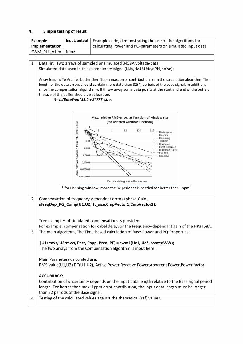
4: Simple testing of result
Example-implementation
Input/output Example code, demonstrating the use of the algorithms for calculating Power and PQ-parameters on simulated input data
SWM_PUI_v1.m None 1 Data_in: Two arrays of sampled or simulated 3458A voltage-data.
Simulated data used in this example: testsignal(N,fs,Hz,U,Udc,dPhi,noise); Array-length: To Archive better then 1ppm max. error contribution from the calculation algorithm, The length of the data arrays should contain more data than 32(*) periods of the base signal. In addition, since the compensation algorithm will throw away some data points at the start and end of the buffer, the size of the buffer should be at least be:
N= fs/BaseFreq*32.0 + 2*FFT_size;
(* for Hanning-window, more the 32 periodes is needed for better then 1ppm)
2 Compensation of frequency-dependent errors (phase-Gain),
sFreqDep_PG_Comp(U1,U2,fft_size,CmpVector1,CmpVector2); Tree examples of simulated compensations is provided. For example: compensation for cabel delay, or the Frequency-dependant gain of the HP3458A.
3 The main algorithm, The Time-based calculation of Base Power and PQ-Properties: [U1rmws, U2rmws, Pact, Papp, Prea, PF] = swm1(Uc1, Uc2, rootedWW); The two arrays from the Compensation algorithm is input here. Main Paraneters calculated are: RMS-value(U1,U2),DC(U1,U2), Active Power,Reactive Power,Apparent Power,Power factor ACCURRACY: Contribution of uncertainty depends on the Input data length relative to the Base signal period length. For better then max. 1ppm error contribution, the input data length must be longer than 32 periods of the Base signal.
4 Testing of the calculated values against the theoretical (ref) values.

15RPT04 TracePQM - Appendix
Report describing the open software tool developed for handling high performance ADCs identified for power and PQ measurements
BLANK PAGE

15RPT04 TracePQM
Report describing the open software tool developed for handling high performance ADCs identified for power and PQ measurements
Appendix #9
A2.4.5 – Description and building of TWM software structure

A2.4.5 - TWM structure This report also covers at least partially following activities:
A2.1.1 – Flow chart of TWM tool
A2.1.2 – Extension for a multiple digitizers
A2.1.4 – Concept of the LV to Octave/Matlab interface
A2.2.2 – Integration of the drivers to the virtual driver
A2.4.2 – TWM tool structure
A2.4.3 – Acquisition and control module description
A2.4.4 – Processing module description
A3.3.3 – Guidance on integration of new HW
Following text describes internal structure of the TWM (LabVIEW version).
1.1 References [1] TWM tool, url: https://github.com/smaslan/TWM [2] INFO-STRINGS, url: https://github.com/KaeroDot/info-strings [3] QWTB toolbox, url: https://qwtb.github.io/qwtb/ [4] GOLPI interface, url: https://github.com/KaeroDot/GOLPI [5] A232 Algorithms exchange format, url:
https://github.com/smaslan/TWM/tree/master/doc/A232 Algorithm Exchange Format.docx [6] A231 Correction Files Reference Manual, url:
https://github.com/smaslan/TWM/tree/master/doc/A231 Correction Files Reference Manual.docx
[7] A231 Data Exchange Format, url: https://github.com/smaslan/TWM/tree/master/doc/A231 Data exchange format and file formats.docx
1.2 Abbreviations LV – LabVIEW CVI – LabWindows CVI EOS – End of string DWORD – unsigned 32bit variable INT16 – signed 16bit integer INT32 – signed 32bit integer INT64 – signed 32bit integer Double – 64bit real number Cluster – LabVIEW structure of elements

Bool – Logic variable HDD – Hard drive TWM – The LV program developed in scope of TracePQM project GUI – Graphical User Interface HW – HardWare QWTB – Q-Wave toolbox [3] INFO – Brain-dead structured, human readable text file Matlab – Matlab SW (Mathworks) GNU Octave – Open source equivalent of Matlab that happens to be almost 100% comatible m-script – Matlab/Octave’s function file
1.3 Overview The TWM is organized according to the diagram shown in Figure 0-1. The whole TWM application consists of two parts:
(i) LabVIEW modules (Control and Processing) that controls the instruments, initiates processing and serves as a user interface
(ii) Calculation or Processing module based on the Matlab/GNU Octave which performs the processing of the acquired data, post-processing and formatting the data for displaying and generation of the measurement report (summary of the results formatted in compact form).
Figure 0-1: TWM tool structure. The coloured frames are used to distinguish the process in which the tasks run.
The modules communicate on runtime via the GOLPI interface [4] and via files in the measurement folder [7]. So TWM appears as one interactive application. This apparent complication has several benefits. The separation of the acquisition and processing enables several features:

(i) The acquired data may be processed at any time. It is possible to just record batch of measurements without processing which may be helpful for time consuming calculations. The processing of the whole batch of measurements can be initiated later either via TWM or on a supercomputer.
(ii) The same acquired data can be used for calculation of multiple parameters using multiple algorithms.
(iii) The measurement data is (can be) archived so the data may be reprocessed later if new parameters or correction are needed.
(iv) The Processing module can run independently on the Control module so TWM can run even without installed Matlab/GNU Octave and the processing can run on any system without drivers required for the TWM (e.g. supercomputer).
(v) The Processing module is identical for LabVIEW and CVI version of the tool and the data are interchangeable.
(vi) The processing module is FULLY transparent. The m-functions of the module do everything: loading the acquired data, loading correction, processing, saving results, loading and formatting results for display, generating report.
The control module is split into four separate processes that run in parallel. Main process is “GUI Process”. It contains configuration panels of the HW, configuration panels of the measurement, configurations of the result display and selector of the correction files for the HW components.
When the user wants to initiate a new measurement the “GUI process” will create “Measurement Process” which does following:
(i) Loads correction files. (ii) Loads selected QWTB algorithm’s configuration from QWTB alg. database file. (iii) Builds measurement sequence. (iv) Initiates acquisition. (v) Stores acquired data and full copy of the Corrections and QWTB alg. setup to the
measurement folder. (vi) When requested by user, initiates processing of the acquired waveforms. (vii) Signalizes “new result available” to the GUI process. (viii) Repeats from (iv) until all acquisitions are done or user terminates the process by “STOP”
button.
When “GUI Process” receives notification of the new result or user requires refresh of the results view, it will initiate refresh of the results view according to the current view setup by initiating another process “Results Viewer Process”. This process will search the measurement folder and will update the results view or initiates export of the measurement report. Note this process requires Matlab/GNU Octave, because the actual post-processing and formatting is done in Matlab/GNU Octave. The split into the processes means they can partially run in parallel, so when the digitizers are acquiring new waveforms, the “Results Viewer Process” can simultaneously perform the post-processing and displaying. The user can even plot graphs of the so far measured results during the measurements.
Finally, TWM contains “Server control process”, which allows to control some of the TWM functions and query status and data. The communication happens via Windows named pipe, so it can be controlled from any environment. The key point of this feature is the TWM can be controlled by another application that e.g. performs sequence of measurements. However, note the interface is in

development stage and it is not part of the TracePQM project. Thus, it may not be fully developed before end of the project so it will be documented separately when it is ready to use.
1.4 GOLPI The communication between LabVIEW and Matlab/GNU Octave is ensured by the GOLPI interface [4]. The interface was designed for bidirectional runtime communication between LV and GNU Octave. The communication happens via the pipes which transfers commands and data between the two environments. User can also inspect the communication in console window. The pipes are based on the DLL library “lv_process.dll” which is part of the project [4]. The “lv_process.dll” can be used in any language such as CVI. However, it ensures just a low level text data exchange. Variables transfer between the LV and GNU Octave is done at LV level.
The project TracePQM also calls for a communication with Matlab which is far more popular among the potential users. Therefore, the GOLPI library for LV was modified so it also enables almost identic communication with Matlab via the Matlab Script nodes. The nodes are hidden in the GOLPI so from outside there is no difference between use of GOLPI for Matlab and GNU Octave and there should be no difference apart from the performance, which may differ significantly. The only functional difference may be in some algorithms, where Matlab and GNU Octave implementation differs (see algorithms documentation).
1.4.1 Multi-process GOLPI access The TWM is a multi-process application. It was not principally possible to ensure the GOLPI is accessed from only one process at the time, so obvious problem arises – the resource sharing between the processes. Obviously only one process can work with Matlab at the time. This is ensured by additional LV library “GOLPI Multi Process.lvlib”. This lib contains several functions. First, before the lib can be used, user must call the VI “golpi_mpc_init_session.vi”, which will initiate the GOLPI instance session.
Figure 0-2: Initializing VI of the multiprocess library. This must be called somewhere at the beginning of the TWM application before any other access to the GOLPI is made.
This VI initializes the GOLPI instance session, i.e. local variable “GOLPI”, which is part of the “main.vi”. This is only VI that can access this variable directly! All other VIs accesses the “GOLPI” variable via reference. The initialization itself is part of the VI “GOLPI Initialize.vi” whose location in the “main.vi” is shown in Figure 0-3.

Figure 0-3: The location of the multiprocess initialization VI.
Before exiting the TWM, the multi-process GOLPI session should be closed by calling VI “golpi_mpc_close_session.vi”. This will also optionally force the GNU Octave process to close, so there is no zombie process left on exit.
Figure 0-4: VI for closing the multi-process GOLPI session. The "exit octave" option will force the Octave or Matlab to close (terminate the process).
Whenever any part of TWM needs accessing the GOLPI instance, it must first obtain the GOLPI session by calling VI “golpi_mpc_get_access.vi”. The VI will wait indefinitely for the access to the GOLPI session. That is internally solved by semaphores. It won’t return until all other processes released the GOLPI by “golpi_mpc_release.vi” or until the semaphore is destroyed by “golpi_mpc_close_session.vi”. It retunes the local copy of the GOLPI session, which must be store back by the “golpi_mpc_release.vi” (see below).
Figure 0-5: VI for gaining exclusive access to the GOLPI. The "golpi session" is reference to the TWM local variable “GOLPI”. The “allow octave start” option will allow autoamtic startup of GNU Octave/Matlab, when it is not running yet.
“don’t querry version” will disable query of the version, which is quite time consuming. The main output is “GOLPI ref out”, which is the GOLPI reference to be used with the GOLPI library VIs. The VI also returns “golpi session out”, which is
the multi-process GOLPI session that contains some more elements that may be useful.
When the work with GOLPI is finished, the user must call VI “golpi_mpc_release.vi” to store the local copy of “GOLPI ref” (or “golpi session”) back to the TWM variable “GOLPI” and to release the exclusive access to the GOLPI. This will clear the semaphore and thus allow other processes to gain access by “golpi_mpc_get_access.vi”.

Figure 0-6: VI for releasing the exclusive access to the GOLPI. It accepts
Example of usage of the multi-process GOLPI is shown in Figure 0-7. The “GOLPI” variable reference is obtained from somewhere (typically from the TWM measurement session “session”). The exclusive access is gained, the GOLPI commands are executed and the exclusive access is released again.
Figure 0-7: Accessing GOLPI in TWM tool. Before any operation with GOLPI instance, user must obtain the exclusive access. Follow the operations with GOLPI. When done, the GOLPI instance must be released.
1.5 Control and data acquisition module The Control and acquisition module consists of two sub-modules: (i) Control (user interface GUI), (ii) Acquisition.
This module controls and run the data acquisition by managing initial settings of the sampling process, call to specific instrument drivers through an abstraction layer and handles the acquisition of data from the ADCs, while ensuring storage of the acquired data into the file system.
The controlled of the acquisition process is based on parameters set by the user. Parameters are set prior to data acquisition. Important parameters are filenames, sampling frequency, length of sampling sequence and repetitions. When first called, the module will evaluate the settings, and for certain parameters, the will be prompted with a GUI for confirmation.
During the acquisition, the module updates the values that is visible for the user in the Main window, such as status, the sampling progress, and update of the trace-view and FFT-view if applicable. Finally the data is collected from the instruments and stored to the file system as defined by the parameters.

Figure 0-8: The top-level of this module: Call to the user panel for parameter setting, before Data Acquisition. The acquisition stars by call to the Meas Asyncronious start, which start the main acquisition in a separate process.
1.5.1 Control module The Control submodule is a set of subroutines that let user set up the sampling environment and controls the acquisition proses. It also performs validity-check of the parameters before the data acquisition starts, and updates
Part of the control is the user interface. It can be called separately or as part of the start of acquisition. When the acquisition has been selected, a validity-check is done by the control module, and if it finds any issue, the user will be prompted with the GUI for user confirmation.
The acquisition will be performed based on the settings set in the “Meas Config Panel”.
The submodules for the control are:
• “ADC Config Panel”, where specification of digitizer type and related parameters are set, and • “Meas Panel” for the acquisition the, which are the interface where device none-specific
parameters are set. Here things like filename and algorithm selection can be done as well.

Certain parameters are relevant for each specific sample run, and in the main data acquisition these parameters are is set in the “Meas Panel”
Meas Panel:
Parameters for sampling and storage is set here, as well as selection of post processing algorithm. The inputs ensure the instrument drivers can be initiated correctly and data is stored at appropriate locations.
The Acquisition is set up by the “Set Measurement” or “Start” option on the front panel.
lvprog\measure\Meas Config Panel.vi
Figure 0-9: Invoking of the user panel for setting the data acquisition parameters. This is called before the Meas Asynchronous start, which start the main acquisition
Throughout the data acquisition-loop, the front display, data for the View Record and the View FFT is updated with current data. This is done through the “GUI Update Wave” and the “GUI Update FFT”. These two vi’s are called in the acquisition subroutines. (Yellow colour VI-icons)

1.5.2 Acquisition module The acquisition module runs in a separate process (see Figure 0-1).
The “main measurement loop” is where the system is set up for data acquisition, and where the system is cleaned up and closed after the sampling is finished.
Figure 0-10: MeasMain (details removed for clarity) The overall sequence of the acquisition process. The steps are in short; Initiate, Measure, Close/Reset.
For this module, the following four functions are involved:
• Initialize status fields in the mail GUI • Initialize digitizer (instrument) • Call to the main measurement loop (where sampling is done) • Close digitizer v. channels • Reset digitizer
Data acquisition:
The active data acquisition is done as a subsequence of the “main measurement loop”.
The VI “Meas Loop Sequence” is the outer loop, to accommodate for repetitions.
The steps are in short:
• Set the sampling parameters to the devises • Open the file system for data storage to File • Take One record of data from the ADC (data acquisition • Store data to file system

• Update views on the Main GUI • (pipe data to the DSP-algorithm)
Figure 0-11: Meas Loop Sequence. Outer loop of the data acquisition sequence
Inner loop: Data acquisition. “measure\Meas Single Record.vi”
The core of the data acquisition module is found in this VI. The main task of this VI is to get data from instrument and pipe it into the data stream to the next level, the storage and processing. In addition it do the time critical initiation of the hardware.
Overview of main steps taken by this VI:
Get the ADC- cofig. (from the control module) Opens the MatLab data stream Initiate ADC Open data stream for the result. (Fast-loop for repeated sampling series
o Fatch data from instrument o and write the data to Data stream
Clean-up ADC after sampling Close the Data stream
Figure 0-12: Meas Single Record: The inner loop of the Data Acquisition sequence.

1.5.2.1 Modular driver design The project objectives call for a modular driver concept. The key idea is the Acquisition module does not access the drivers of the particular instruments directly, because each digitizer requires completely different approach. Therefore the TWM tool would have to use different structure to work with different digitizers. So it was decided to insert a command translation layer in between the acquisition module and the drivers of physical instruments. This layer was called virtual digitizer. All HW specific function calls of each digitizer are translated to a universal format and merged into a few basic VI functions which are, for the acquisition module, identic for any digitizer no matter how different is the HW control implementation inside. The basic block diagram of the TWM in current version is shown in Figure 0-13.
Figure 0-13: Block diagram of TWM Virtual drivers.

Figure 0-14: Virtual digitizer driver structure and data flow. Green: virtual driver functions; Red: TWM acquisition module; White: Instrument specific part.
Detailed view on the driver structure and its usage in the TWM acquisition module is shown in Figure 0-14. The virtual driver functions are shown in green colour. It was decided the driver should not directly write the sample data file, because whenever format of the data changes, each driver would have a different implementation. That is not effective and clean solution. The amount of data in the streaming mode can easily exceeds memory limit, which is just around 1 GB for the 32bit LabVIEW, so the driver cannot simply collect the sample data and then send them to TWM acquisition module at once for saving. Therefore, a rather complex solution capable of runtime storage of sample data based on the background digitizing process(es) was developed. Thanks to the acquisition in the separate process(es) the main fetch loop is non-blocking. Fetching and storing of the sample data runs continuously, so just a limited memory buffers are needed. The acquisition module can easily refresh sampling status and terminate it at any point even if the HW drivers do not allow that directly (e.g. by killing the process(es)). Furthermore, the execution priority of the digitizing process(es) was increased. This way the digitizing runs unaffected by the workload of rest of the application. That may be crucial for the time critical 3458A streaming mode and for high speed streaming from the NI 5922 cards. The throughput was tested and the limiting factor was HDD, which limited the write

speed to some 120 Mbytes/s. However, as will be shown in the following chapters, the drivers for other, simpler digitizers do not need to use such a complex structure.
1.5.2.2 Virtual driver functions structure Following chapters describes particular functions of the virtual digitizer, describes their inputs and outputs, behaviour and also explains where and when are they called by the TWM acquisition module.
To implement a new driver one must adapt and merge the low level instrument driver functions so they principally fit into the functions below (resp. the green coloured blocks in Figure 0-14). Note there are also a few more functions that need to be implemented apart from the functions shown in the Figure 0-14.
The virtual driver is a just a wrapper layer that translates the standardized inputs and outputs to the particular instrument drivers. See example for “Setup channels” for DMM 3458A driver:
Each of the following functions contains the case selectors with one item per digitizer “type”. Each function extracts the session related to the particular digitizer (“3458A” in the example) from the virtual digitizer “adc session”, it executes the function(s) of the instrument driver(s) and it stores the modified session “3458A” back to the virtual digitizer “adc session”. Other functions are made the same way. The only exception is the configuration panel for the digitizers which will be described separately.
There are just a few steps to be done to integrate new drivers. First, change the type definition of “type” in the “adc session”, i.e. add a new item to “type” Enum. The item names should be chosen clearly, such as “NI 9234”. Next, a session cluster (or class) of the new driver must added to the “adc session”. This object can contain absolutely anything. It depends on the driver. Finally, each of the case selectors in each of the virtual driver functions must be extended by the new page, e.g.

“NI 9234” and the driver functions must be inserted. TWM will then automatically allow to use the new digitizer without any changes in the rest of the application.
1.5.2.2.1 ADC session “ADC session” is a virtual digitizer cluster that has to contain all sub-sessions of the particular digitizers. It also contains several common items. Details on content of this cluster at the time of writing this document (may extend in future):
Name Type Meaning niScope cluster 5922 (niScope) driver session. 3458A cluster Virtual DMM 3458A driver session. Dsdll cluster DirectSound driver session. simadc cluster Simulated ADC session. * * New driver sessions…
Type enum Selected digitizer type ‘niScope’,’3548A’,’DirectSound’,’dummy’.
modified? bool Flag set by TWM to “True” when HW setup was modified.
channel idn str 1D array of string Array of last queried identifier strings of particular channels of selected digitizer. One item per channel.
aux instr idn str 1D array of string Array of last queried identifiers of auxiliary HW related to the selected digitizer (e.g.: AWG, Counter, etc.).
Adding a new digitizer means the session of the digitizer driver will be added and “type” enum will be redefined to contain unique identification name of a new digitizer. The rest must not be changed.
1.5.2.3 Virtual driver function reference manual
1.5.2.3.1 Initialize driver (optional) Some digitizer drivers may need to perform some step to make them usable. This optional function is called once automatically on the TWM startup.
Function inputs and outputs:
Name Direction Type Meaning adc session in in cluster Virtual digitizer session. adc session out out cluster “adc session in” copy with eventual changes. error in in cluster Error signal. error out out cluster Error signal.
1.5.2.3.2 Enumerate devices (optional) This optional function is called manually in the digitizer selection panel. It was added, because some of the drivers may require additional manual refresh of the installed HW configuration. It was used for the DirectSound drivers where it enumerates available input capture devices.

Input and outputs:
Name Direction Type Meaning adc session in in cluster Virtual digitizer session. adc session out out cluster “adc session in” copy with eventual changes. error in in cluster Error signal. error out out cluster Error signal. capture devices ring ref in reference
to ring Reference to a ring control to be filled with enumerated devices.
1.5.2.3.3 Initialize digitizer (required) It is first function called by TWM before new measurement. Its purpose is to initialize and identify all HW components related to the digitizer. E.g.: for virtual digitizer based on the 3458A multimeters it is one or more 3548A units and optionally a pulse generator AWG or a counter. The function also sets the parameters which are not expected to change during the whole measurement session, such as mode of sampling (“DC V”, “DSDC”, …), coupling, etc. It always returns unique and clear identifiers of the channels and auxiliary HW.
Inputs and outputs:
Name Direction Type Meaning adc session in in cluster Virtual digitizer session. adc session out out cluster “adc session in” copy with eventual changes. error in in cluster Error signal. error out out cluster Error signal.
reset? in bool Force reset of the instruments? Similar to standard instrument driver template.
channel idn strings out 1D array
of strings Queried identifiers for each virtual channel.
aux intr. idn strings out 1D array
of strings Queried identifiers of additional HW related to the selected digitizer.
all instruments idn strings out 1D array
of strings All identifiers merged to one array.
1.5.2.3.4 Setup channels (required) This function is called once per group of measurements. I.e. it is not recalled before each repetition cycle so the driver must be prepared to perform several acquisition without recalling this. It will configure the virtual channels of and the virtual digitizer to the desired setup prior the acquisition.

This function sets sampling rate, sample count, aperture, triggers, ranges, etc. The digitizer shall be ready to start acquisition after this function call.
Input and outputs:
Name Direction Type Meaning adc session in in cluster Virtual digitizer session. adc session out out cluster “adc session in” copy with eventual changes. error in in cluster Error signal. error out out cluster Error signal. fs [Hz] in double Desired sampling rate in [Hz]. samples count in double Desired samples count per channel. trigger in cluster Trigger setup cluster.
aperture [s] in double Desired aperture of the ADC. Note this parameter will be ignored if digitizer does not support it.
Cluster “trigger” contains following items:
Name Type Meaning
source Enum
Trigger type ‘Immediate’ – start immediately; ‘External’ – from external trigger input; ‘Level’ – input channel level trigger. Note the ‘Level’ is always related to the first channel. This may be eventually configured in driver specific configuration panel.
slope Enum Trigger slope sensitivity for “Level” and “External” triggers “POS” or “NEG”.
coupling Enum Coupling of the “Level” trigger “DC” or “AC”. Eventual other configurations must be handled by the driver itself and set from configuration panel.
level [V] Double Trigger level for “Level” mode in Volts.
1.5.2.3.5 Initiate sampling (required) This is when TWM is ready to digitize. This function should immediately initiate the sampling (arm the virtual digitizer) and return. The actual operation depends on the implementation of the “Fetch samples” function (see below).
Input and outputs:
Name Direction Type Meaning

adc session in In cluster Virtual digitizer session. adc session out out cluster “adc session in” copy with eventual changes. error in In cluster Error signal. error out out cluster Error signal.
1.5.2.3.6 Fetch samples (required) The function is called in the loop to fetch the sample data and status. Purpose of this function is to obtain the acquired data from the virtual digitizer channels. There are three basic options for its implementation depending on the particular digitizer:
(i) Blocking function that won’t return until all samples were acquired. This is suitable for smaller counts of samples, however the cost for this solution is TWM cannot query state of the sampling and the termination by STOP command is harder to implement (or impossible) as well as timeout. This is typical way the most of the instrument drivers are made.
(ii) Asynchronous function that just checks weather the sampling is done and eventually returns available samples block. When not done, it will just return status if possible. This way the sampling loop is not blocked and the TWM can update sampling status and easily terminate sampling by STOP command. This mode is however not possible for all digitizers as some of them do not allow asynchronous operation.
(iii) Complex implementation shown in the Figure 0-14 where the “Initiate sampling” just starts the “digitizer process(es)” and the “Fetch samples” periodically checks, weather there are a new sample data available. If so, it returns block of samples that is stored to the file by “Store samples”. It is hard to implement, but it seems to be very useful for the 3458A streaming driver and for high speed PXI 5922 driver because the process(es) may be run with increased priority. This should prevent overflows for high speed digitizing or time critical digitizing (3548A).
Note this function always receives LV reference to a global Boolean variable “STOP”. This reference can be used as an alternative way to terminate the sampling (default is “Abort Digitizing Process”). Note the driver function must not change the values of “STOP”. It is just for reading.
Input and outputs:
Name Direction Type Meaning adc session in in Cluster Virtual digitizer session. adc session out out Cluster “adc session in” copy with eventual changes. error in in Cluster Error signal. error out out Cluster Error signal.
stop ref in Reference to bool
Reference to the global Boolean variable STOP. The variable becomes “True” when stop is requested. The function cannot modify the flag.
data packet Out Cluster Cluster with block of sample data. aux data Out Cluster Cluster of additional data returned by the driver.

fetching done? Out Bool This flag must be “True” when sampling is finished or it was terminated.
The “data packet” is a cluster containing following:
Name Type Meaning int32 2D array of int32 2D array of samples. One column per channel. int16 2D array of int16 2D array of samples. One column per channel.
is int16? Bool Defines which of the “int16” or “int32” is valid. The other must be empty.
all done? Bool “True” when all samples were fetched. sampling? Bool “True” when digitizing is in progress.
valid? Bool “True” means the other items are valid. Otherwise they are ignored by acquisition module. This may indicate the iteration of fetching was returned no data.
instr buffer [%] Double Indicates utilisation of the digitizer buffer. This is e.g. used for the 5922. May be “NaN” is not supported.
queue buffer [%] Double Utilisation of the data queue between digitizing process(es) and fetch function. May be “NaN” if not supported.
offset [smpl] Int64 Offset of the first sample in the block from start of the acquisition. Counting from zero.
count [smpl] Int64 Samples count in the sample array per channel. May be zero if no data fetched.
The “aux data” content:
Name Type Meaning
T smpl 1D array int64 Indices of the samples to which the temperature readings are aligned.
T [deg C] 2D array of doubles
2D array of temperature readings during the acquisition. One column per channel, one row per item of “T smpl”. Note this is optional and the arrays may be empty.
Time stamp [s] Double Relative timestamps returned by the channels. These are relative time intervals in Seconds of the first sample of each channel related to some common event, e.g. reset of 5922.
Gain [V] 1D array of doubles
Gain factors to get voltage from the integers in data packets. One per channel.
Offset [V] 1D array of doubles
DC offset to add to real samples to get actual voltage. One per channel. u(k) = gain*y(k) + offset; u – voltage, y – integer sample
Increment [s] Double Sampling period [s].
Valid? Bool
“True” means the other items are valid. Otherwise they are ignored by acquisition module. Note the driver may return this cluster valid any time during the sampling. Whenever the flag is set, acquisition module remembers the data. So it does not matter if it returns at the start or the end of sampling.

1.5.2.3.7 Cleanup session (required) This function should terminate everything that may have left in the memory/system after the “Initiate sampling” function, e.g.: the processes, queues, shared memory, etc. This is called by TWM every time to cleanup after acquisition (even terminated or failed).
Input and outputs:
Name Direction Type Meaning adc session in in cluster Virtual digitizer session. adc session out out cluster “adc session in” copy with eventual changes. error in in cluster Error signal. error out out cluster Error signal.
1.5.2.3.8 Close digitizer (required) This function is called after acquisitions are done even in case of error or termination. This function should put all affected instruments to some default safe state and close opened sessions to them. It is strongly recommended to put the instruments to such a state so they cannot be damaged. E.g.: not 50 Ω input, higher range, etc. Also it is good practice to turn all instruments programmatically to the local control as some of them may not even have “Local” button.
Input and outputs:
Name Direction Type Meaning adc session in in cluster Virtual digitizer session. adc session out out cluster “adc session in” copy with eventual changes. error in in cluster Error signal. error out out cluster Error signal.
Reset to preset mode (True) In Bool
“True” means the function should reset the digitizer instruments to some safe default state before closing the handles.
1.5.2.3.9 Abort Digitizing Process (recommended) This function is called in the fetch loop when GUI signalizes STOP command. Implementation depends on the “Fetch samples” variant. For variant (i) it cannot be used as the function is blocking. For the other two variants, it may either send the signal to the digitizer if it supports such a function, or it can kill the digitizing process(es) (variant iii). Naturally “Fetch samples” must be able to recognize the digitizing process(es) were terminated and also signalize sampling done so acquisition module will leave the fetching loop.

Inputs and outputs:
Name Direction Type Meaning adc session in in cluster Virtual digitizer session. adc session out out cluster “adc session in” copy with eventual changes. error in in cluster Error signal. error out out cluster Error signal. Send abort signal? In Bool Sends abort only when “True”. Nothing happens when
“False”.
1.5.2.3.10 Get Digitizer Capabilities (required) This function returns capabilities of the selected digitizer. It is called at various places of the TWM. It should NOT touch the HW by itself! All HW related information shall be obtained in the “Initialize digitizer” function and kept in the digitizer session even after “Close digitizer” is called! TWM decides by itself when to call “Initialize Digitizer”+”Close digitizer” to refresh the parameters so the time consuming querying is not performed when it is not needed. The capabilities are used to limit the GUI entries and disable the unsupported features. The driver should just query the information from the session and return the desired capabilities.
Inputs and outputs:
Name Direction Type Meaning adc session in in cluster Virtual digitizer session. adc session out out cluster “adc session in” copy with eventual changes. error in in cluster Error signal. error out out cluster Error signal.
Initialize HW? In Bool Forces new query of the instruments capabilities. Otherwise uses last queried capabilities from digitizer session (fast mode).
Parameters In Cluster Cluster of some parameters that may be needed to obtain the capabilities.
Capabilities Out Cluster Cluster of obtained capabilities.
Cluster “parameters” contains following:
Name Type Meaning fs [Hz] Double Current sampling rate in [Hz aperture [s] Double Aperture time [s].

Cluster “capabilities” contains following:
Name Type Meaning Max samples count Int64 Maximum number of samples to be acquired in one record.
Max fs [Hz] Min fs [Hz] Double Maximum and minimum sampling rate [Hz].
Ts step [s] Double Available sampling period step in which the rates can be set.
fs step [Hz] Double Available sampling rate step that can be set by digitizer. Note either “Ts” of “fs” step can be used. The other must be “NaN”.
Smpl rate step mode Enum Mode of sampling rate selection ‘const period’,’const frequency’.
Selects which of the “Ts” of “fs” is valid. Max Ts [s] Min Ts [s] Double Maximum and minimum sampling period [s].
Aper min [s] Aper max [s] Double Minimum and maximum apertures [s]. Or “NaN” if not supported.
Channels count Double Number of virtual channels available configured. Allows streaming? Bool Set when the driver supports two modes: memory buffer and direct
streaming. If it supports just one, it is ignored. Streaming on? Bool Streaming mode configured. Has level trig? Bool Driver/digitizer supports level triggering. Has ext trig? Bool Driver/digitizer supports external input triggering. Has aperture? Bool Driver/digitizer supports setting the appertures. Has ranges? Bool Driver/digitizer can set multiple ranges. Has temperature? Bool Driver/digitizer supports temperature measurement.
Has temperature log? Bool Driver/digitizer supports temperature logging during acquisition.
Has selfcal? Bool Driver/digitizer supports self-calibration routine.
1.5.2.3.11 Get Current Setup (required) Similar to the “Get Digitizer Capabilities”. It should not touch the HW. It should return last used configuration from the digitizer session. This function returns two groups of parameters. First, the standard ones, e.g.: sampling rate, samples count, trigger, etc. Next, the specific for given digitizer.
Function inputs and outputs:
Name Direction Type Meaning adc session in In cluster Virtual digitizer session. adc session out Out cluster “adc session in” copy with eventual changes. error in In cluster Error signal. error out Out cluster Error signal. Common attributes Out Cluster Standard attributes/parameters of the digitizer.
Device specific Out 1D array 1D array of clusters containing:

attributes of clusters “name” – attribute name string “value” – 1D array of test string with formatted value “is constant per group” – when trues, the attribute is stored just once for measurement group. Otherwise it is stored for each record. Note the value may be numeric. In that case format the number to decimal, floating or exponential format with decimal dot “.”. These attributes are not used by TWM anywhere, they are just store as additional items to the measurement session header. They will appear there as “name:: value” or as: #startmatrix:: name value(1); value(2);… #endmatrix:: name Note the “aperture” value is one of these attributes.
Cluster “common attributes” contains following items:
Name Type Meaning Count [smpl] Int64 Configured number of samples to acquire per channel. Channels count Int32 Number of configured channels in the virtual digitizer. fs [Hz] Double Configured sampling rate in [Hz].
Ranges [V] 1D array of doubles
Array of set range values as defined by the particular drivers. One value per virtual channel of the digitizer.
Trigger Cluster Trigger setup, see above. Ext freq. locked? Bool Status of PLL lock if supported. Streaming on? Bool Set when streaming is enabled.
Is int16? Bool Set when data is/will be in int16 format for the configured sampling setup.
Bitres Int32 Actual bit resolution (how many bits are utilised in the integer).
1.5.2.3.12 GUI Get Info (recommended) This function takes digitizer session and returns a brief description of the digitizer which is displayed in the digitizer panel. It must not touch the HW. It may contain e.g. trigger connection notes (3458A mode). It is called in the digitizer configuration panel.
Inputs and outputs:
Name Direction Type Meaning adc session in In cluster Virtual digitizer session. Configuration description Out String String with brief description of the current
configuration of the digitizer.

1.5.2.3.13 Selfcal Virtual Channels (optional) This function should initiate self-calibration of the digitizer HW components if such function is supported. It is synchronous operation. TWM is blocked during its execution.
Inputs and outputs:
Name Direction Type Meaning adc session in In cluster Virtual digitizer session. adc session out Out cluster “adc session in” copy with eventual changes. error in In cluster Error signal. error out Out cluster Error signal.
1.5.2.3.14 Digitizer configuration panel (required) The digitizers in the TWM must be configured before they can be used. The configuration is done in a panel “Digitizer configuration”. The panel contains page control with one page per digitizer:
A new page must be added to implement a new digitizer. The order of the pages must match the order in the “type” Enum in the “adc session”. The new page can contain any configuration needed for the new digitizer. On initialization the current settings from the digitizer sessions must be set to the panel items related to the particular digitizers:

Accordingly before exiting the panel, the new settings must be stored back to the “adc session”:

The panel itself is based on the Event structure. Most of the events are common for all digitizers and thus doesn’t need to be modified. However, each digitizer may have some special requirements which must be placed in the new event. Example for DirectSound driver:
1.6 Processing module Processing module consists of two components: (i) LabVIEW VI’s and (ii) Matlab/Octave functions. The Matlab functions are common for the LabWindows/CVI version of the tool and they can be used standalone without TWM.
1.6.1 Processing module – LabVIEW component The LV component of the processing module consists of several parts: (i) Processing configuration GUI; (ii) Algorithm execution routines; (iii) Results viewer/interpreter; (iv) Batch processing GUI. The TWM allows two modes of processing. The first and simplistic is an execution of user entered m-code as it is and simple display of eventual calculated results. This is intended just for debugging purposes and simple tests and it won’t be described to details. The relevant mode is execution of a QWTB algorithm [3]. In this mode, the TWM interacts on runtime with the QWTB m-functions via the GOLPI interface [4] to obtain the information about available algorithms or execute them or to retrieve the calculated results. Logical flow of the processing module in runtime processing during measurements is shown in Figure 0-15. Note the Matlab does not return any data back to the LV (apart from error messages). The results are stored back to the measurement folder and queried asynchronously by the TWM tool whenever requested.
Figure 0-15: Processing module logic flow. Note the grey blocks are not part of the processing module.
1.6.1.1 Processing configuration GUI The processing GUI is a panel dedicated to configuration of the new calculation. It is shared for the runtime processing of the sampled data and also for the batch processing of previously sampled data. It has several sub-functions.

Figure 0-16: GUI panel of the QWTB processing setup.
First, it queries the list of available algorithms by calling an m-function “qwtb_load_algorithms.m” via the VI “Meas Proc QWTB Load List of Algorithm.vi”. The obtained algorithms are displayed in the selector. The function also applies the filtering of the algorithms based on the content of file “qwtb_list.info”. This is needed to prevent user of TWM from selecting QWTB algorithms that are not compatible with TWM.
Figure 0-17: Loader VI of the QWTB algorithms. “session” is the measurement session of TWM and the “menu ring” is a reference to the control that receives the list of available algorithms.
Next, the GUI allows to select the algorithm from the list and query its options and description. This is done by calling the m-function “qwtb_load_algorithm.m” via the VI “Meas Proc QWTB Load Algorithm.vi”. The GUI will obtain the standard QWTB info entries, such as the full name, brief description and notes. It will also query the TWM specific flags which tell TWM if the algorithm can accept differential input sensors, if it is algorithm with multiple inputs (e.g. power) and if it can process multiple records at once. It also queries available modes of uncertainty calculation so user can select only the valid ones. The function also queries the list of algorithm’s user parameters and displays them in the parameter matrix.

Figure 0-18: Loader VI of the QWTB algorithm. The “session” is the measurement session of TWM, “qwtb alg selector” is the ref. to the ring with loaded and selected algorithm IDs. The “qwtb unc mode” and “param table” are references to
the uncertainty mode selector ring and to the user parameters table.
Finally, when user confirms the calculation, the GUI will parse the eventual user parameters and stores them together with the selections made to a processing session. It does not store anything to the processing related file “qwtb.info” [7]! The processing setup is stored at the time of digitizing or before batch processing starts.
1.6.1.2 Algorithm execution routines There are several processing related routines. First, the processing setup generated by the processing GUI must be stored to the processing info file “qwtb.info” in the measurement folder [7]. This is done by VI function “Meas Proc QWTB Write Algorithm Processing Header.vi”. The VI is called just once before the sequence of measurements as the processing setup is the same for all acquisitions.
Figure 0-19: Writer of QWTB processing setup. The "sequence item" contains the measurement root path. The "processing setup" is the setup obtained from processing setup GUI.
Next routine is the VI “Meas Process Record.vi”. This VI will initiate the QWTB algorithm execution by calling m-function “qwtb_exec_algorithm.m”. The VI does not transfer anything but measurement folder and record index to the Matlab. The rest of the configuration is obtained by the m-function from “qwtb.info”. Note the VI also does not query anything back from the Matlab (apart from eventual error). The results are stored to the measurement folder and this VI just notifies the other process of TWM that new result is available. The VI is equipped by the timeout capability, which allows to limit the processing time, but it will work only for GNU Octave. No way of terminating the Matlab Script Node was found yet. When the timeout ran out for GNU Octave, the calculation actually still runs. Just the VI returns and error. So the user may need to manually restart the GOLPI before next operations.
Figure 0-20: Data processing executer. The “session” is measurement session of TWM, the “sequence item” contains measurement root path and index of current record. The “result string label” is not part of QWTB processing (it is used
only for the raw m-code processing).

The “new result” notification VI “Meas Proc QWTB Notify Result Queue.vi” can be (is) called from anywhere from the TWM. It internally uses queue to which it stores the configuration flags that defines what the results viewer will do. Note it cannot be used before initiating the queue by VI “Meas Proc QWTB Initialize Result Queue.vi”!
Figure 0-21: New result notifier VI. The "session" is optional. The "plot setup" takes place only when the “show graph” is set. The “new session” must be set when new meas. folder is selected, the “new result” must be set when new record
was processed or reprocessed, the “show graph” will display result as graph instead as a matrix. When no flag is set, the TWM will just refresh current result view.
1.6.1.3 Results viewer/interpreter The calculated results are displayed by the results viewer process. It is a standalone process VI that is initiated from the main process of TWM whenever the “new result” queue contains the refresh notification. The asynchronous execution in another process was chosen because the process of retrieving the results and formatting the data take considerable time, so the synchronous execution in the GUI process would lockup the main panel GUI. However, the asynchronous execution just unloads the main panel, but the results viewer still uses the GOLPI to communicate with the Matlab. Therefore, when the refresh is initiated during the measurement, the algorithm execution routines (see above) and the results viewer shares the same Matlab instance, so only one of those two can operate at the time. This will result in delays in the processing or results viewing when the operations take longer time. However, the solution is in fact mostly effective, because the results viewing happens when the digitizers are acquiring new record, so there are no collisions.
Figure 0-22: Results viewer panel.

The periodic checking of the “new result” and eventual execution of the main viewer process is done in the timeout event of TWM main panel GUI by VI “Meas Proc QWTB Update Result View.vi”. The VI checks execution state of the previous call of the results viewer process (ref. to the process is entered from the local variable “qwtb view VI ref”). If the process is finished, it will check the state of the “new result” notifier and eventually initiate the results viewer process. The reference to the new process is returned and stored back to the “qwtb view VI ref”. The VI may or may not return the “qwtb view” depending on the execution state of the process itself. When it just returned, the TWM stores the viewer session “qwtb view” back to the local variable. Note the “qwtb view VI ref” must not be lost, otherwise there will be memory leakage of unclosed references!
Figure 0-23: TWM results viewer process executer (located in main panel GUI event structure in the timeout event). Note the “qwtb view VI ref” must be preserved in the local variable otherwise there would be memory leakage! This VI may or
may not return the “qwtb view” depending on the state of execution of the results viewer process.
The results viewer process itself is VI “Meas Proc QWTB Update Result View Process.vi”. The VI accepts references to all the results viewing GUI controls, e.g. the selectors of the algorithm, quantities, etc. Is starts by obtaining the information about the selected measurement, i.e. it queries list of available results for current (or selected) correction folder. This is done by call of m-function “qwtb_get_results_info.m”. It fills in the GUI controls: list of processed algorithms; list of quantities for selected algorithm; list of channels/phases. Next, the VI takes the result view selector value and uses them as parameters for m-function call “qwtb_get_results.m” for matrix display or “qwtb_plot_results.m” for graph display. When successful, the VI will update the results matrix in the main panel.
Figure 0-24: Results viewer VI. Note the "session in" and "QWTB result session out" were intededly converted to "variable" data type, which is much easier to handle when using assycnhronou function calls.
Eventual export of the results table to the Excel sheet is performed in the main panel of TWM in the event structure. The exporting and other functions are available in right click popup menu of the results matrix.
TODO: condensed report export.
1.6.1.4 Batch processing GUI TWM enables either runtime processing of the records or a batch processing. The batch processing is performed in the panel “Meas Batch Proc QWTB panel.vi”, which is shown in Figure 0-26. The logic flow of the batch processor is shown in Figure 0-25. The panel allows user to select measurement session and select the particular records to be processed. User must also set the configuration of the processing. This configuration will invoke the “Processing configuration GUI” as was described above.

When the configuration is confirmed, the new calculation setup is store to the “qwtb.info” by VI call “Meas Proc QWTB Write Algorithm Processing Header.vi”. Next use may initiate the processing, which will call the “Meas Process Record.vi” for each record. The panel has no other relevant sub-VIs.
Figure 0-25: Logical flow of the TWM’s batch processing of the previously recorder measurements.
Figure 0-26: Batch processing panel.
1.6.2 Processing module – Matlab component The Matlab component of the processing module is standalone set of m-functions. They are executed from TWM via the GOLPI interface [4]. From typical user point of view the only four functions are to be called directly:
1) “qwtb_exec_algorithm.m” for execution of the processing on the measurement session. 2) “qwtb_get_results_info.m” to get information about available results in the session. 3) “qwtb_get_results.m” to load and format results for displaying in matrix form. 4) “qwtb_plot_result.m” to load and display results as a graph.
The rest of the m-functions are either sub-functions of abovementioned or special functions that are rarely used directly. Only the top level functions will be described in following sections.

1.6.2.1 qwtb_exec_algorithm.m Function “qwtb_exec_algorithm.m” is top level function for execution of the algorithm on the TWM data. This is the function to be called when new processing is to be initiated. It performs all steps needed for the processing:
(i) Load record(s) and correction files from the measurement folder using function “tpq_load_record.m”.
(ii) Loads processing setup from “qwtb.info” [7] from measurement session. (iii) Executes the selected algorithm on each channel or phase of the measurement session. (iv) Stores the results to the measurement folder using function “qwtb_store_results.m”. (v) Updates content of the “results.info” [7] so it contains information about the newly
processed algorithm.
The details on the function call are shown in Table 0-1.
Table 0-1: Processing module m-function “qwtb_exec_algorithm.m” – execution of the TWM algorithm on the TWM data.
Function prototype: qwtb_exec_algorithm(meas_file, calc_unc, is_last_avg, avg_id, group_id) Parameters: Name Data type Description meas_file Char string Full path to the measurement session header INFO file
“…/session.info”. calc_unc Char string
Override uncertainty calculation mode from “qwtb.info”. Allowable values: ‘’ (default), ‘none’, ‘guf’ or ‘mcm’ (see QWTB documentation [3]).
is_last_avg Bool Flag that should be set to confirm all records for the calculation are in available. If not set and algorithm requires multiple records at once, the function will do nothing (no error).
avg_id Integer Optional index (1, 2, 3, …) of the repetition cycle of the measurement session to process. The function processes the last available record if value is zero.
group_id Integer Optional index (1, 2, 3, …) of the group index of the measurement session. Zero value selects the last available group.
Returns values: None. Function can only generate errors.
1.6.2.2 qwtb_get_results_info.m This m-function will retrieve selected information on the available results in the selected measurement folder. This function is mainly intended for the interface to the TWM, so the return values are formatted in a way that is easily readable by GOLPI [4]. The vectors of strings and matrices are returned as a CSV style strings. E.g. the Matlab table “A = [‘code’,’55’;’msg’,’Hallo’]” will be returned as a string: “code\t55\nmsg\tHallo”. Note the column and row separators may vary. The function prototype and return values are listed in the Table 0-2.

Table 0-2: Processing module m-function “qwtb_get_results_info.m” – query of the TWM results information.
Function prototype: [res_files, res_exist, alg_list, chn_list, var_names] = qwtb_get_results_info(meas_root, alg_id) Parameters: Name Data type Description meas_root Char string Path to the measurement session folder (no session file name!). alg_id Char string QWTB algorithm ID string, e.g. “TWM-PWRTDI”. Leave empty to
load the last available results from the “results.info” [7]. Returns values: Name Data type Description res_files Char string CSV string with the list of available results files for the given
measurement folder and algorithm. The list is separated by ‘\t’. res_exist Bool Non-zero of the result(s) exists. alg_list Char string CSV string with the list of algorithm IDs that were processed in the
measurement folder. The list is separated by ‘\t’. chn_list Char string CSV string with the list of available channel/phase names for the
selected algorithm. The list is 2D matrix with ‘,’ as column separator and ‘;’ as a row separator. Each row contains one channel name (e.g. “u1,i1” for single input algorithms) or single phase name (e.g. “L1” for dual input algs.).
var_names Char string CSV string with the list of available result quantities for given algorithm. The list is separated by ‘\t’.
Errors: The function won’t return error when “meas_root” contains no results (yet). It will return error only if the desired “alg_id” is not found or the data in the measurement folder are inconsistent.
1.6.2.3 qwtb_get_results.m This m-function will retrieve and format the selected results data in to a text matrix. The function performs following operations:
(i) Selects the result from the measurement folder and loads its data using function “qwtb_load_results.m”. The function also enables selection of the quantities to be loaded and optional averaging of multiple results.
(ii) Formats the quantities to a matrix form in one of the supported view modes (scalars, vectors, matrices).
The function plots the data in two ways. When all quantities are scalar and “cfg.max_dim” is set to scalar, it will show the quantities development in time, i.e. their values for each repetition cycle of the measurement. If the “cfg.max_dim” is set to vector mode, the vector(s) of the quantities will be shown horizontally. Note the function limits maximum allowable number of element to be displayed by option “cfg.max_array”, because displaying 1000 values would be extremely slow. If the amount of data exceeds the “cfg.max_array”, the quantity in the table “txt” will contain “only graph” string instead of the data to indicate user may display the long vector as plot by function “qwtb_plot_result.m”.

Note this function is primarily intended for linking to the TWM tool, so it returns the text matrices in a CSV string format which is easier to handle by LV and GOLPI interface [4]. E.g. the Matlab 2D cell-array “A = ‘code’,’55’;’msg’,’Hallo’” will be returned as a string: “code\t55\nmsg\tHallo”. Note the column and row separators may vary for various returned variables. The function prototype and return values are listed in the Table 0-3.
Table 0-3: Processing module m-function “qwtb_get_results.m” – query of the TWM results as a text matrix.
Function prototype: [txt, desc, var_names, chn_index] = qwtb_get_results(meas_root, res_id, alg_id, cfg, var_list) Parameters: Name Data type Description meas_root Char string Path to the measurement session folder (no session file name!). res_id Integer Index of result(s) to load. Use -1 to load last available result, >1 to
select particular result or 0 to average all results. alg_id Char string QWTB algorithm ID string, e.g. “TWM-PWRTDI”. Leave empty to
load the last available results from the “results.info” [7]. cfg Structure Configuration structure for the results formatting. All elements are
optional. cfg.max_dim = maximum shown dimension of quantity
0: scalars, 1: vectors, 2: matrices cfg.max_array = Maximum size of vector to be shown in
the matrix cfg.unc_mode = Uncertainty display mode 0: none, 1:
val±unc, 2: alternating rows val,unc,val,unc,…
cfg.group_mode = Grouping of the multichannel results 0: sort by channels, 1: sort by quantities
cfg.phi_mode = phase display mode 0: ±pi, 1: 0-2pi, 2: ±180°, 3: 0-360°
cfg.phi_ref_chn = non-zero index of reference channel to use as a phase reference, use zero to disable interchannel phase display
var_list Cell array of char string
List of quantity names to load and display. Empty list will load all quantities. The list may contains only the names obtained by the “qwtb_get_results_info.m” function.
Returns values: Name Data type Description txt Char string CSV string with 2D matrix of the formatted result values with ‘\t’ as
column separator and ‘\n’ as row separator. First row contain table headers, first column contains quantity names with channel/phase indices. The rest of table are formatted quantity values.
desc Char string CSV string with 1D matrix of text descriptions of each data row of the “txt” matrix. The list is separated by ‘\t’.
var_names Char string CSV string with 1D matrix of short quantity name for each data row of the “txt” matrix. The list is separated by ‘\t’.
chn_index 1D array of integers
Vector of channel/phase index for each row of “txt”.

Errors: The function should throw an error only if the results data is inconsistent, which should not happen.
1.6.2.4 qwtb_plot_result.m This function is equivalent of the “qwtb_get_results.m”, except it will display the one selected quantity as a plot, instead of in the matrix. The plot can be made from a single record or average of records. If the scalar quantities are selected, the function will plot quantity value for each repetition cycle of the measurement. If the vector quantities are selected, the function plots the vector. Matrix quantities are not supported. The detail on the function are shown in Table 0-4.
Table 0-4: Processing module m-function “qwtb_plot_result.m” – plotting selected quantity of the TWM results.
Function prototype: [] = qwtb_plot_result(meas_root, res_id, alg_id, chn_id, cfg, var_name, plot_cfg) Parameters: Name Data type Description meas_root Char string Path to the measurement session folder (no session file name!). res_id Integer Index of result(s) to load. Use -1 to load last available result, >0 to
select particular result or 0 to average all results. Alg_id Char string QWTB algorithm ID string, e.g. “TWM-PWRTDI”. Leave empty to
load the last available results from the “results.info” [7]. chn_id Integer Index of channel/phase to plot. Use zero to plot all channels/phases
in one plot. Cfg Structure Configuration structure for the results formatting. All elements are
optional. cfg.max_dim = maximum shown dimension of quantity
0: scalars, 1: vectors, 2: matrices cfg.phi_mode = phase display mode 0: ±pi, 1: 0-2pi, 2:
±180°, 3: 0-360° cfg.phi_ref_chn = non-zero index of reference channel to
use as a phase reference, use zero to disable interchannel phase display
var_name Char string Name of the quantity to plot. The name must exist in the results file. plot_cfg Structure plot_cfg.xlog = Non-zero to enable x-axis log scale.
Plot_cfg.ylog = Non-zero to enable y-axis log scale. Plot_cfg.box = Show plot box (see Matlab “plot” doc). Plot_cfg.grid = Show plot grid (see Matlab “plot” doc). Plot_cfg.legend = Legend display position. (see Matlab
“plot” doc for position names). Leave empty to disable plot.
Returns values: None. Errors: The function should throw an error only if the results data is inconsistent, which should not happen.

1.6.2.5 qwtb_load_algorithms.m This function is used by the TWM to get list of available QWTB algorithms compatible with TWM. The list is created from the “qwtb_list.info” file. The function is intended for the linking to the TWM via the GOLPI, so the returned arrays of strings were converted to the CSV strings, which are easier to handle. E.g. the Matlab 2D cell-array “A = ‘code’,’55’;’msg’,’Hallo’” will be returned as a string: “code\t55\nmsg\tHallo”. Details on the function are shown in Table 0-5.
Table 0-5: Processing module m-function “qwtb_load_algorithms.m” – obtains list of the available TWM algorithms.
Function prototype: [ids, names] = qwtb_load_algorithms(list_file) Parameters: Name Data type Description list_file Char string Path to the INFO-strings [2] file “qwtb_list.info” with the list of
supported TWM algorithms and their configuration. Returns values: Name Data type Description ids Char string CSV string of the QWTB algorithm ID strings. The list is separated by
the ‘\t’. names Char string CSV string of the QWTB algorithm names. The list is separated by
the ‘\t’. Errors: The function may throw an error if inconsistent data are in the “qwtb_list.info” or in the QWTB algorithm wrappers.
1.6.2.6 qwtb_load_algorithm.m This function is used by TWM to obtain information about the selected algorithm. It is intended for the linking to the TWM via the GOLPI, so the returned arrays of strings were converted to the CSV strings, which are easier to handle. E.g. the Matlab 2D cell-array “A = ‘code’,’55’;’msg’,’Hallo’” will be returned as a string: “code\t55\nmsg\tHallo”. Details are shown in Table 0-6.
Table 0-6: Processing module m-function “qwtb_load_algorithm.m” – obtains algorithm parameters.
Function prototype: [alginfo, ptab, input_params, is_multi_inp, is_diff, has_ui, unc_guf, unc_mcm] = qwtb_load_algorithm(alg_id) Parameters: Name Data type Description alg_id Char string QWTB algorithm ID [3] of the algorithm to select. Returns values: Name Data type Description alginfo Char string QWTB algorithm info as returned by QWTB [3]. Ptab Char string CSV string with the 1D matrix of algorithm parameters. Rows are
separated by the ‘\n’. input_params Char string CSV string with the 1D matrix of algorithm’s parameter names.

Rows are separated by the ‘\n’. is_multi_inp Bool Flag that indicates the algorithm accepts multiple records at once. Is_diff Bool Flag indicates the algorithm supports differential inputs. has_ui Bool Flag that indicates the algorithm requires two inputs (voltage and
current). unc_guf Bool Flag that indicates the algorithm supports GUF uncertainty
calculation. unc_mcm Bool Flag that indicates the algorithm supports Monte Carlo
uncertainty. Errors: The function may throw an error if inconsistent data in the QWTB algorithm wrappers.
1.6.2.7 tpq_load_record.m This function is main loader function for the TWM measurement. It performs following steps:
(i) Loads common information from the measurement session INFO file [7]. (ii) Loads the selected records of from the measurement folder. (iii) Loads transducer corrections by function “correction_load_transducer.m”. (iv) Loads digitizer corrections by function “correction_load_digitizer.m”.
The function is capable to load one or more records from given measurement group. It returns one data structure with all data and parsed corrections. The details on the function call are shown in Table 0-7.
Table 0-7: Processing module m-function “tpq_load_record.m” – load TWM measurement.
Function prototype: function [data] = tpq_load_record(header, group_id, repetition_id, data_ofs, data_lim) Parameters: Name Data type Description header Char string Path to the measurement session file “./session.info” [7]. group_id Integer Default value -1 will select last available group. Value >0 will
select particular measurement group. repetition_id Integer Index of the repetition cycle (record) to load. Value -1 will load
the last record, value 0 will load all records, value >0 will load particular record.
data_ofs Integer Optional sample-offset of the loader. Non-zero value means the loader will skip “data_ofs” samples of the record(s). Note it will adapt the timestamp value(s) accordingly, so the timestamp(s) still applies to the first sample.
data_lim Integer Non-zero value limits the amount of loaded samples per channel to “data_lim” samples.
Returns values: Name Data type Description data Structure Structure containing the loaded sample data and corrections, see
Table 0-8 for details.

Errors: The function will throw an error if the record selection is invalid, or if there are inconsistent data anywhere in the measurement session or the correction data.
Table 0-8: Processing module m-function “tpq_load_record.m” – output structure data.
Name Data type Description group_count Integer Total measurement groups count in the measurement
session. repetitions_count Integer Total repetition cycles (records) in the selected group. channels_count Integer Digitizer channels in the measurement session. is_temperature Bool Temperature measurement available. sample_count Integer Samples count per channel in the loaded record(s). y Double Sample data, one row per channel. If multiple records are
loaded, the records are merged horizontally: chn1,chn2, chn1,chn2, …
timestamp Double Relative timestamp(s) in seconds for the first sample(s) of each record in the “y”.
Ts Double Sampling period in seconds. corr Structure Data structure containing the loaded corrections:
corr.phase_idx = phase index for each digitizer channel which is used to define which channels belongs together for multi-input algorithms
corr.dig = digitizer corrections structure corr.tran = cell array of the transducer
corrections, one for each transducer

15RPT04 TracePQM - Appendix
Report describing the open software tool developed for handling high performance ADCs identified for power and PQ measurements
BLANK PAGE

15RPT04 TracePQM
Report describing the open software tool developed for handling high performance ADCs identified for power and PQ measurements
Appendix #10
A2.4.5 – Description and building of TPQA software structure

15RPT04 TracePQM Page 1 of 34
Report describing the open software tool TPQA developed in LabWindows/CVI environment
A2.4.5 - TPQA structure
This report also covers the following activities:
A2.1.1 – Flow chart of TPQA tool
A2.1.2 – Extension for a multiple digitizers
A2.1.4 – Concept of the LV to Octave/Matlab interface
A2.2.2 – Integration of the drivers to the virtual driver
A2.4.2 – TPQA tool structure
A2.4.3 – Acquisition and control module description
A2.4.4 – Processing module description
A3.3.3 – Guidance on integration of new HW

15RPT04 TracePQM Page 2 of 34
CONTENTS A2.4.5 - TPQA structure ........................................................................................................... 1
1.1 References ................................................................................................................. 3
1.2 Overview .................................................................................................................... 4
1.3 TPQA Flow Chart ....................................................................................................... 5
1.4 TPQA structure in LabWindows/CVI Environment ..................................................... 5
1.5 Control and data acquisition module .......................................................................... 7
1.5.1 Control module ................................................................................................... 8
1.5.2 Acquisition module .............................................................................................. 9
1.5.2.1 Function prototype for LF DMMs ............................................................... 10
1.5.2.2 Acquisition module for wideband digitizers ............................................... 15
1.5.2.3 Modular driver design ................................................................................ 15
1.5.2.4 Virtual driver functions structure ................................................................ 16
1.5.2.4.1 ADC configuration and selection ............................................................ 17
1.5.2.5 Virtual driver function reference manual .................................................... 18
1.5.2.5.1 Sessions Configuration .......................................................................... 19
1.5.2.5.2 Sessions Initialization ............................................................................. 20
1.5.2.5.3 Trigger Configuration .............................................................................. 21
1.5.2.5.4 Synchronization session ......................................................................... 22
1.5.2.5.5 Initiate sampling ..................................................................................... 22
1.5.2.5.6 Fetch and store matrix sampled data ..................................................... 23
1.5.2.5.7 Function’s list .......................................................................................... 24
1.5.2.5.8 Abort Digitizing Process ......................................................................... 26
1.5.2.5.9 Clean-up sessions .................................................................................. 27
1.6 Processing module .................................................................................................. 27
1.6.1 Processing module – LabWindows/CVI environment ....................................... 27
1.6.2 Post - processing module – Matlab environment .............................................. 32
1.6.2.1 Post - processing module in TPQA ........................................................... 32

15RPT04 TracePQM Page 3 of 34
1.1 References [1] TPQA tool, url: https://github.com/btrinchera/TPQA
[2] TracePQM, url: https://www.euramet.org/research-innovation/search-research-projects/details/?page%5BeurametCtcp_project_listResearch%5D=2&eurametCtcp_project_show%5Bproject%5D=1407&eurametCtcp_project%5Bback%5D=450&cHash=69ff67e07cffde667e34af3a7ef39df3
[3] TWM tool, url: https://github.com/smaslan/TWM
[4] INFO-STRINGS, url: https://github.com/KaeroDot/info-strings
[5] QWTB toolbox, url: https://qwtb.github.io/qwtb/
[6] GOLPI interface, url: https://github.com/KaeroDot/GOLPI
[7] A232 Algorithms exchange format, url:
https://github.com/smaslan/TWM/tree/master/doc/A232 Algorithm Exchange Format.docx
[8] A231 Correction Files Reference Manual, url:
https://github.com/smaslan/TWM/tree/master/doc/A231 Correction Files Reference Manual.docx
[9] A231 Data Exchange Format, url:
https://github.com/smaslan/TWM/tree/master/doc/A231 Data exchange format and file formats.docx
[10] A331 Installation and Guide_TPQA, url:
https://github.com/btrinchera/TPQA/blob/master/doc/A331%20Installation%20and%20Guide_TPQA.docx
[11] A245 TWM structure, url: https://github.com/smaslan/TWM/blob/master/doc/A245%20TWM%20structure.docx
[12] A214 Interfacing LabWindows/CVI to Matlab, url: https://github.com/btrinchera/TPQA/blob/master/doc/A214-%20LabWidowsCVI_to_Matlab_Interface.docx

15RPT04 TracePQM Page 4 of 34
1.2 Overview
TPQA [1] is an open source project that is being developed in scope of EMPIR project
TracePQM [2] using the Labwindows/CVI environment. Together with TWM [3] open source
project, developed in LabVIEW environment, furnish an open platform to help unexperienced
NMIs to speed up in the developing of state-of-the-art standards suitable to perform traceable
measurements of electric power and power quality parameters using the concept of waveform
digitizing. It is not restricted to power and PQ area but it allows recording and processing of
pure and complex voltage and current waveforms.
The TPQA is organized according to the flow chart diagram shown in Figure 0-1. The whole
TPQA application consists of two parts:
(i) LabWindows modules (Control and Processing) that controls the instruments, initiates
processing and serves as a user interface implemented into a suitable User Interface
Guide (GUI).
(ii) Calculation or Processing module based on the Matlab which performs the processing of
post-processing and formatting the data for displaying and generation of the measurement
report (summary of the results formatted in compact form), as well as a second processing
module based on CVI algorithms for quasi real-time data processing. Note that CVI
algorithms are not validated yet and serve only to establish a first processing approach on
sampled data.
Further characteristic of the post-processing module can be found in [4] and [7].
The control module consists in several separated processes. Main functions are inserted in
TPQA.C source file and declared in TPQA.h file.

15RPT04 TracePQM Page 5 of 34
1.3 TPQA Flow Chart
The flow chart of TPQA is shown in Figure 0-1. The meaning of main blocks is reported below.
Figure 0.1: TPQA flow chart structure. The coloured frames are used to distinguish the process in which the tasks run.
- Configuration and ADCs setup: main process for the configuration of digitizers using specific drivers: - NI PXI 5922 digitizers using niScope and niTLCK drivers provided by National
Instruments. All drivers must be installed on the PC. - DMMs HP 3458 configured as sampling multimeters (NI-GPIB driver must be
installed). - New GUI Parameters: allows to set new digitizing parameters during the sampling
process. - Acquisition and storage: enables the possibility of storing sampled and/or
processed data through a mechanism based on multiple flags. - CVI quasi real time-processing: CVI algorithms for data processing during the
acquisition process. - Writing QWTB proc.: creates measurement process, based on TWM concept of post-
processing data [1], and does following: loads correction files; builds measurement sequence; stores acquired data and generates suitable files for further processing.
- TPQA (QWTB batch processing): enables GUI panel for post-processing of data and does following: loads selected algorithm’s configuration from QWTB alg. database file.
- QWTB execution: when requested by user, initiates processing of all acquired data stored in the folder.
- Results available and Results viewer process: initiates refresh of the results view according to the current setup and algorithm selection.
1.4 TPQA structure in LabWindows/CVI Environment
There are two possibilities to test the functionality of TPQA open source project:

15RPT04 TracePQM Page 6 of 34
i) Developer mode: first the user launches the LabWindows/CVI environment and then opens the file TPQA.CWS. The user can run the project and interact with it through the user interface guide that appears. This mode is useful for expert users, which intend to modify or add new functionality or routines into the project.
ii) User mode: After compiling the entire project the executable file TPQA_32bit.exe will be generated. The user could compile the project also for 64-bit distribution. In this case the environment must be switched to 64 bit distribution and libgen.lib (64-bit ) and libmx64.lib (64-bit) matlab *.dll files must be inserted into the Libraries folder of the project.
Note that, since the project includes a communication with the Matlab engine the necessary *.dlls cannot be freely distributed. However the user must install Matlab distribution on local PC and must check careful the path of octprog folder within the config.ini file. By default the path is: twm_octave_folder = C:\TPQA\TPQA_1.1.0\octprog. The internal hierarchy structure of the TPQA in NI-LabWindows\CVI environment is shown in Figure 0.2.
Figure 0.2: Internal TPQA structure shown in Labwindows/CVI.
The project files are arranged as follows: a) Source Files, containing:

15RPT04 TracePQM Page 7 of 34
- TPQA.c contains the main and auxiliary functions which allow the various parts of the software to communicate together. Within the same function it was inserted also the communication routine for DMMs LF digitizing multimeters.
- GenericMultiDevice……. .c contains specific sub-routines to communicate with single or multiple NI-5922 digitizers based on the use of NI-Digitizers and NI-TCLK synchronization driver. That is a single file that implement everything we need to communicate with wideband digitizers.
- Matlab Module folder, (developed by CMI) composed by several additional files suitable to establish a communication protocol with the Matlab engine for data processing using QWTB toolbox: Matlab Module.c, Mlink.c, qwtb_alg_select.c, Processing_panel.c, Twm_matlab.c and Utils.c
b) User Interface Files: containing all the GUI developed to communicate with the macro setups.
- TPQA.uir which contains the main panel and additional GUIs for control and data acquisition modules.
- Matlab Module Folder, (developed by CMI) composed by several GUI, as: Matlab Module.uir, processing_panel.uir and qwtb_alg_select.uir.
c) Instrument Files, containing: - niScope.fp to communicate with wideband NI 5922 digitizers. For further information about
the installation instructions and features please NI-SCOPE Readme guide provided by NI. - niModInstCustCtrl.fp to search for already connected instruments.
d) Include Files: (*.h files contains the prototype of *.c functions and variables definition as
well as CVI callback function used by GUIs) - TPQA.h - GenericMultiDeviceConfiguredAcquisitionTClk.h - Tpqa_globals.h - Matlab Mudule directory, which containd the following files: engine.h, Matlab Module.h,
matlab_globals.h, matrix.h, mlink.h, processing_panel.h, qwtb_alg_select.h, tmwtypes.h, twm_matlab.h and utils.h.
1.5 Control and data acquisition module
This module consists of two sub-modules: (i) Control (user interface GUI), (ii) Acquisition. It is invoked starting from the main routine, where the basic prototype is shown in Figure 0.3. Consequently an unified control and data acquisition GUI appears.

15RPT04 TracePQM Page 8 of 34
Figure 0.3: Main routine on TPQA
1.5.1 Control module
The control module is inserted within the main GUI and handles the macro setups developed for traceable power and PQ parameter measurements. It handles four main functions. Figure 0.3 shows the control module on TPQA developed in LabWindows/CVI.
Each button is linked to specific callback functions, generated automatically by the software environment, as follows:
- Main four control button for specific routines entitled LF-Setup DMMs, QWTB Processing, CVI Data Processing and HW Corrections . The callback function for each button are shown in Figure 0.5.
Figure 0.4: Control module of TPQA open source project.

15RPT04 TracePQM Page 9 of 34
Figure 0.5: Callback functions for each command button.
1.5.2 Acquisition module
Acquisition module runs in a separate process (see Figure 0-1). It is composed of two separated GUIs developed for handling of wideband digitizers as PXI-5922 and low speed but high precision DMMs such as HP3458A. Each GUI controls the acquisition parameters of the digitizers. The instrument driver is integrated into the upper level software to create a virtual generic digitizer by means of two control modules. Figure 0.6 shows the control modules for wideband and LF digitizers. A detailed description of all TPQA control buttons and parameters are given in A331 [8].
Figure 0.6: Control module for wideband and DMMs digitizers.

15RPT04 TracePQM Page 10 of 34
1.5.2.1 Function prototype for LF DMMs
The Figure 0.7 shows the function prototype for handling DMMs connected via GPIB IEEE4882 using VISA drivers. To allow the acquisition of sampled data with DMMs digitizers, in the *.c file of TPQA there are several functions, some of these are CVICALLBACK functions. These are functions that start to run when their correspondent button is pressed (see [8]). In Figure 0.8 is possible to see a prototype of the functions set to acquire with DMMs digitizers.
Figure 0.8: Set of Callback functions developed for handling DMMs HP3458A.
To understand better the task that each function does, below will be given a detailed description of them:
Figure 0.7: Function prototype for handling HP3458A configured as high-precision digitizers.

15RPT04 TracePQM Page 11 of 34
- CfgChannelDMM: is a function that is callback when the user presses the button to configure the channels for the acquisition, in fact this function allows to configure the digitizer channels;
Figure 0.9: Function used to configure the acquisition channels
- CVICALLBACK Sampling_DMMs: is a function that is callback when the user presses the button to start the sampling of data. Within it is employed the function that processes the sampling data ( SamplingDMM function).

15RPT04 TracePQM Page 12 of 34
Figure 0.10: CVICALLBACK Sampling_DMMs function.
- Sampling function: is the function that deals with to implement the sampling routine, it is shown in the Figure 0.11.
Figure 0.11: SamplingDMM function.
- CVICALLBACK CLOSE_DP: is a function that is callback when the user presses the button to close the sampled data processing session. Using this function, how is possible to see in Figure 0.12, the panel where are processed the sampled data and any of its child panels are removed from memory and them off to the screen.

15RPT04 TracePQM Page 13 of 34
Figure 0.12: CVICALLBACK CLOSE_DP function.
- CVICALLBACK TEST_DMMs: is a function that is callback when the user presses the button to Test DMMs digitizers. This function is mainly constituted to three steps: • Open Visa session: used to establish a communication session with a device and
creates an Instrument Handle that is used by all other VISA operations to perform operations on that session.
• Call device clear: used to send a command to clear the device. For GPIB devices, this operation sends a GPIB clear.
• Set Visa: used to set a specified attribute for the given object.
The function is shown in Figure 0.13.
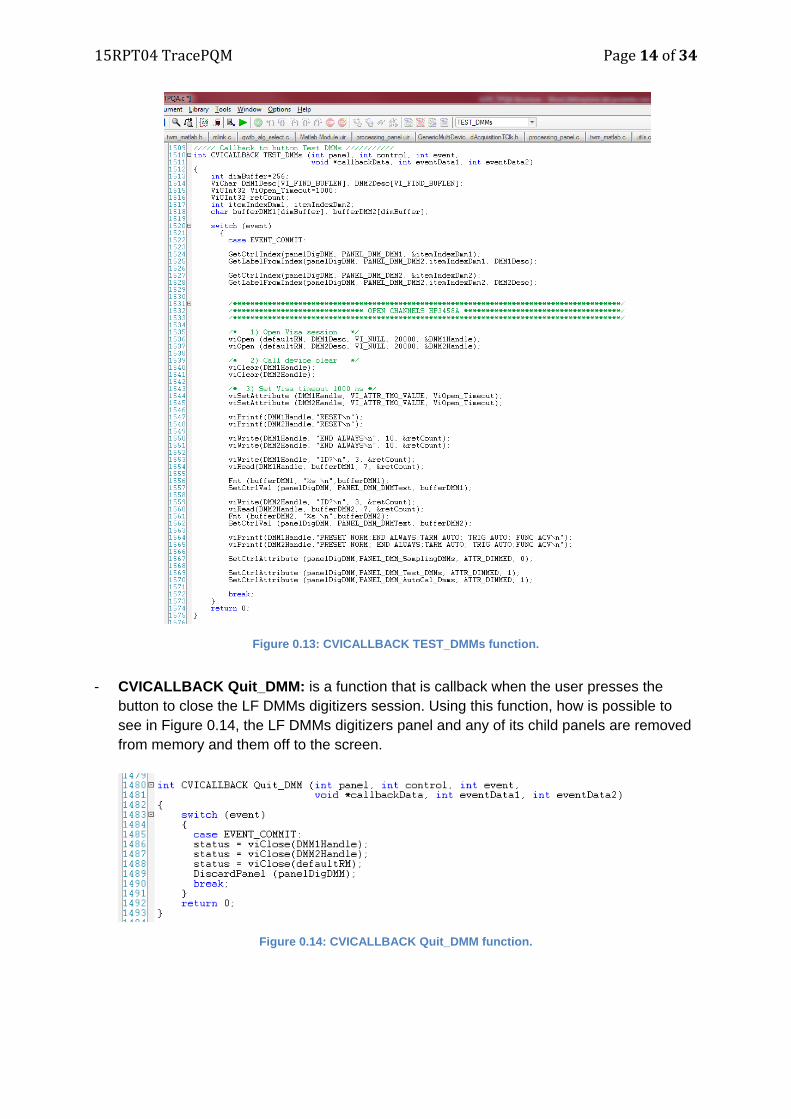
15RPT04 TracePQM Page 14 of 34
Figure 0.13: CVICALLBACK TEST_DMMs function.
- CVICALLBACK Quit_DMM: is a function that is callback when the user presses the button to close the LF DMMs digitizers session. Using this function, how is possible to see in Figure 0.14, the LF DMMs digitizers panel and any of its child panels are removed from memory and them off to the screen.
Figure 0.14: CVICALLBACK Quit_DMM function.

15RPT04 TracePQM Page 15 of 34
1.5.2.2 Acquisition module for wideband digitizers The acquisition module for WB digitizers starts with the following callback ,which implements the Continuous Acquisition button, as shown in Figure 0.15
int CVICALLBACK Acquisition (int panel, int control, int event, void *callbackData, int eventData1, int eventData2)
Within this callbak a generic function suitable to perform an acquisition is called: niScope_GenericMultiDeviceConfiguredAcquisitionTClk(meas_fld);
Its description is done as part of the virtual driver functions structure given in 1.5.2.4 and in the following sections.
1.5.2.3 Modular driver design
The concept of the modular driver design has been extensively described in TWM. The key idea is the Acquisition module that does not access the drivers of the particular instruments directly, because each digitizer requires completely different approach. So it was decided to insert a command translation layer between the acquisition module and the drivers of physical instruments. This layer was called Virtual digitizer. All HW specific function calls of each digitizer are translated to a universal format and merged into a few basic VI functions which are, for the acquisition module, identic for any digitizer no matter how different is the HW control implementation inside. The basic block diagram of the TPQA in current version is shown in Figure 0.16.
Figure 0.15: GUI for acquisition module for WB digitizers.

15RPT04 TracePQM Page 16 of 34
Figure 0.16: Virtual digitizer driver structure and data flow for TPQA open software tool project.
1.5.2.4 Virtual driver functions structure
The concept of the virtual driver has been developed in order to avoid the direct access directly the drivers of particular instruments.

15RPT04 TracePQM Page 17 of 34
It was verified that accessing directly of instrument drivers requires a different approach for each particular ADC board. It was substituted such an approach with a different mechanism which uses a *.c function translator able to interact as an interface layer between the data acquisition module and the physical instrument drivers. These *.c functions represent the virtual driver.
In TPQA open software project such an interface is composed for a specific board, e.g. PXI- NI-5922 digitizer, by two files a (*.c file and a header (*.h)) file: - GenericMultiDeviceConfiguredAcquisitionTClk.c;
- GenericMultiDeviceConfiguredAcquisitionTClk.h.
Only some remarks to take into account regard to the data storing of sampled data when the digitizer runs continually. The solution adopted aims to collect the sampled data and then stored them directly on hard drive while the ADCs runs continually. Furthermore, the TPQA program allows to the user to change the parameters in real time. For this reason the developed TPQA code has some difference with the TWM structure.
In Figure 0.17 is shown the *.h file (header file) employed as translator for the virtual driver used with ni.Scope driver.
1.5.2.4.1 ADC configuration and selection
ADC configuration and selection is handled by two separated process: i) for wideband and
future digitizers; ii) for LF DMMs digitizers. This option i) is governed by a switch/case
statement, which is inserted into the following function:
int CVICALLBACK Acquisition (int panel, int control, int event, void *callbackData,
int eventData1, int eventData2)
Figure 0.17 Header structure of the translator used with ni.scope driver.

15RPT04 TracePQM Page 18 of 34
Figure 0.17 shows an implementation of the ADC selection by the switch/case process for WB
digitizers.
Figure 0.18: Routine for WB digitizers selection
Instead, the process for LF DMMs digitizer selection is the same of that described in 1.5.2.1.
1.5.2.5 Virtual driver function reference manual
Within a virtual driver are employed several functions. An example of virtual driver developed for use with ni.Scope driver is shown in Figure 0.17.

15RPT04 TracePQM Page 19 of 34
Figure 0.19 Prototype of *.c translator developed for LabWindows/CVI to be used with niscope driver.
The virtual driver namely Vi_Status _Vi_FUNC ni Scope_GenericMultiDeviceConfiguredAcquisitionTClk (char*meas_folder) is mainly composed by functions that deal with of:
• Session configuration;
• Sessions initialization;
• Synchronization of session;
• Trigger configuration;
• Initiate sampling;
• Fetch and store matrix sampled data;
• Abort digitizing process;
• Clean-up sessions.
In the following sessions will be explain the tasks of these several functions.
1.5.2.5.1 Sessions Configuration
The session configuration is mainly composed by these functions:
• GetParametersFromGUI (): a prototype is shown in Figure 0.18 and the function has as input variables all parameters shown in TPQA panel. Through this function the algorithm read all parameters insert by user;

15RPT04 TracePQM Page 20 of 34
Figure 0.20: GetParametersFromGUI function.
• GetCorrectionsFromGUI(), this function is shown in Figure 0.19 and through it away the algorithm read the hardware corrections uploaded by user;
Figure 0.21: GetCorrectionsFromGUI function.
• twm_write_session (), for the generation of measurement session for use with QWTB post-processing tool.
1.5.2.5.2 Sessions Initialization
It is first function called by TPQA before new measurement when NI-PXI5922 digitizers are
used. Its purpose is to initialize and identify all HW components related to WB digitizer. The
functions performs the following steps:
- gets comma-separated list of resource names from GUI,
- parses the list
- initializes resources and
- reports initialized sessions and the number of sessions.
Figure 0.22 shows the implementation of the function ViStatus _initSessions(ViUInt32* numberOfSessions, ViSession sessions[])

15RPT04 TracePQM Page 21 of 34
Figure 0.22: Implementation of the_initSessions in TPQA.
1.5.2.5.3 Trigger Configuration
To configure common properties of trigger are employed the following functions, where all
the properties are set by means of control parameters inserted by the user.
- handleNIScopeErr(niScope_ConfigureTriggerEdge(vi, triggerSource, triggerLevel,
triggerSlope, triggerCoupling, triggerHoldoff, triggerDelay)));
- handleNIScopeErr(niScope_ConfigureTriggerHysteresis(vi, triggerSource,
triggerLevel, hysteresis, triggerSlope, triggerCoupling, triggerHoldoff,triggerDelay));
- handleNIScopeErr(niScope_ConfigureTriggerDigital (vi, triggerSource, triggerSlope,
triggerHoldoff, triggerDelay));
- handleNIScopeErr(niScope_ConfigureTriggerWindow (vi, triggerSource,
lowWindowLevel, highWindowLevel, windowMode,triggerCoupling,
triggerHoldoff,triggerDelay));
- handleNIScopeErr(niScope_ConfigureTriggerImmediate (vi)).
The first four functions listed above are used to configure common properties for analog
triggering, while the last one is used when the user insert an immediate trigger. In Figure 0.20
is shown the mode to configure the trigger type using a switch/case statement.

15RPT04 TracePQM Page 22 of 34
Figure 0.23: Trigger configuration code.
1.5.2.5.4 Synchronization session
The functions used to synchronize the devices are (see Figure 0.21):
(i) handleNITClkErr(niTClk_ConfigureForHomogeneousTriggers(numberOfSessions, sessions)), this function is used to configure the attributes for the reference clocks, start triggers, reference triggers, script triggers, and pause triggers.
(ii) handleNITClkErr(niTClk_Synchronize(numberOfSessions, sessions, 0.0)), this function synchronizes the TClk signals on the given sessions.
Figure 0.24: Synchronization session code.
1.5.2.5.5 Initiate sampling
The function used to initiate sampling is called
handleNITClkErr(niTClk_Initiate(numberOfSessions, sessions)) and it is the function that
initiates the acquisition or generation session. An implementation of this function is shown in
Figure 0.25.

15RPT04 TracePQM Page 23 of 34
Figure 0.25: Initiate sampling function.
1.5.2.5.6 Fetch and store matrix sampled data
HandleNIScopeErr(_fetchAndPlotData(sessions[i], channelName, timeout)) is function used to fetch the acquisition data and then plot them. In the code this function has been used as shown in the figure below.
Figure 0.26: Fetch and store sampled data.
The final aim of this function is to plot the sampled data (waveforms acquired). To reach this goal there is a function recalled in the fetchAndPlotData() function, that allows to have an interface between the virtual digitizers (GenericMultiDeviceConfiguredAcquisitionTClk() function) and main callback function (CVICALLBACK Acquisition(int panel, int control, int event, void *callbackData, int eventData1, int eventData2)). This function just described is PlotWfms (ViInt32 numWaveforms,ViReal64 *waveformPtr,struct niScope_wfmInfo *wfmInfoPtr,ViReal64 actualSampleRate,ViInt32 actualRecordLength,ViReal64 **SaveWavPtr, ViInt32 Size, ViInt32 Sessions)) function and it is employed within the primary TPQA software open tool, that is TPQA.c file.
In this file the virtual drive goes in action when the CVICALLBACK Acquisition() function is recalled. This happens when the user through the TPQA main panel presses the CONTINOUS ACQUISITION button.
After that the acquisition session is concluded, all the sampled data and main ADC acquisition parameters are passed as arguments to PlotWfms () function, where its implementation is shown in Figure 0.26.

15RPT04 TracePQM Page 24 of 34
Figure 0.27 PlotWfms function.
The PlotWfms function is constituted from different input variables that will be described in the following:
- ViInt32 numWaveforms: is the number of waveforms recorded by acquisition units. In particular the number is two if there is just one single board, instead the number becomes four when there are two boards and so on;
- ViReal64 *waveformPtr:: variable used to allocated the information of the waveforms, for example the number of waveforms;
- struct niScope_wfmInfo *wfmInfoPtr:: matrix (struct) that contains all values of waveforms recorded;
- ViReal64 actualSampleRate: sample rate returned from the digitizer, i.e. the digitizer returns a value of sample rate that is closer to that to which it can work;
- ViInt32 actualRecordLength: array returned from the digitizers that contains the length of recorded data;
- ViReal64 **SaveWavPtr: mxn matrix containing the sampled data coming from all ADCs;
- ViInt32 Size: number of ADC channels;
- ViInt32 Sessions: number of ADC boards.
With all information on virtual drive given in the Flow chart LabWindowsTM/CVI environment section, the users can to start to acquaint themselves with TPQA software open tool and, if they want, start to integrate new digitizers.
1.5.2.5.7 Function’s list In the following section will be given a list of prototype functions explain in the chapters above. This list could be useful to user to better understand the LabWindows/CVI algorithms.
GetParametersFromGUI:
Class="Function" Prototype="int GetParametersFromGUI(char *channel, long *acquisitionType, double *verticalRange, double *verticalOffset, long *verticalCoupling, double *probeAttenuation, double *inputImpedance, double *maxInputFrequency, double *minSampleRate, long *minRecordLength, double *timeout, long *numRecords, double *refPos, long *triggerType, char *triggerSource, long *triggerCoupling, long *triggerSlope, double

15RPT04 TracePQM Page 25 of 34
*triggerLevel, double *triggerHoldoff, double *triggerDelay, long *windowMode, double *lowWindowLevel, double *highWindowLevel, double *hysteresis, long *fileFlag);"
Acquisition: Class="Function" Prototype="int Acquisition(int panel, int control, int event, void *callbackData, int eventData1, int eventData2);" Quit_DMM: Class="Function" Prototype="int Quit_DMM(int panel, int control, int event, void *callbackData, int eventData1, int eventData2);"
AUTOCAL_DMMs: Class="Function" Prototype="int AUTOCAL_DMMs(int panel, int control, int event, void *callbackData, int eventData1, int eventData2);" [TEST_DMMs] Class="Function" Prototype="int TEST_DMMs(int panel, int control, int event, void *callbackData, int eventData1, int eventData2);" [Sampling_DMMs] Class="Function" Prototype="int Sampling_DMMs(int panel, int control, int event, void *callbackData, int eventData1, int eventData2);" [CfgChannelDMM] Class="Function" Prototype="int CfgChannelDMM(unsigned long Inst_Handle, char *Master_Slave);" [SamplingDMM] Class="Function" Prototype="int SamplingDMM(unsigned long Inst_Handle, char *Master_Slave);" [CLOSE_DP] Class="Function" Prototype="int CLOSE_DP(int panel, int control, int event, void *callbackData, int eventData1, int eventData2);"
[PlotWfms] Class="Function" Prototype="int PlotWfms(long numWaveforms, double *waveformPtr, struct niScope_wfmInfo *wfmInfoPtr, double actualSampleRate, long actualRecordLength, double **SaveWavPtr, long Size, long Sessions);" [_fetchAndPlotData] Class="Function" Prototype="long _fetchAndPlotData(unsigned long vi, char *channelName, double timeout);" [GetCorrectionsFromGUI]

15RPT04 TracePQM Page 26 of 34
Class="Function" Prototype="int GetCorrectionsFromGUI(int panel, TTWMssnInf *info);" [niScope_GenericMultiDeviceConfiguredAcquisitionTClk] Class="Function" Prototype="long niScope_GenericMultiDeviceConfiguredAcquisitionTClk(char *meas_folder);"
1.5.2.5.8 Abort Digitizing Process
The digitizing process is aborted by pressing the STOP button, which is linked to the following
callback function, shown in Figure 0.27.
This function changes the state of the variable stop from NISCOPE_VAL_FALSE to
NISCOPE_VAL_TRUE. The state is processed by a second function, which process the
events of the system or when the user presses the buttons. The state of the stop variable is
passed to the while loop control flow, which executes repeatability the acquisition process,
until its state doesn’t change.
// Find out wether to stop or not int ProcessEvent (int *stopPtr) *stopPtr = stop; // Take care of any pending operations, like pressing the stop button return ProcessSystemEvents();
After pressing the STOP button the user can perform a new acquisition by pressing the
Acquisition button.
Figure 0.28: Stop function to abort the acquisition process.

15RPT04 TracePQM Page 27 of 34
1.5.2.5.9 Clean-up sessions
The clean-up of all acquisition sessions is performed at the end of the entire acquisition
process. This function terminates everything that may have left in the memory/system after the
“Initiate sampling” function. This is called by TPQA every time to cleanup sessions when all
data are fetched and memorized. An implementation prototype is shown in Figure 0.29.
Figure 0.29: Clean-up of acquired sessions performed within the error handling routine.
1.6 Processing module
The processing module implemented within the TPQA open software project consists of two modules: (i) LabWindowsTM/CVI for quasi real-time elaboration of sampled data; (ii) QWTB and Matlab engine for post-processing of the sampled data. In [10] it is reported the description of the GUI interface that users can used to exploit both mechanisms employed for quasi real-time approach or post processing and formatting of sampled data. The following paragraphs contain a description of the routines employed within the TPQA’s data processing modules.
1.6.1 Processing module – LabWindows/CVI environment
This processing module uses LabWindows/CVI native functions for on-line and fast data
processing of sampled date. The GUI linked with this module is called by pressing CVI Data Processing from the main Acquisition and data Processing control panel. Figure 0.30 reports
the prototype of the callback function “Data_Processing()” and Figure 0.31 shows its relative
user interface (GUI).

15RPT04 TracePQM Page 28 of 34
Figure 0.30: Callback function for CVI Data processing.
Figure 0.31: GUI related ti CVI DataProcessing Callback
The function related to the data elaboration is called every time by flagging on the check box
“flag_DataProcess” positioned in the main control panel. An implementation of the callback
process using DMMs or NI PXI5922 is shown in Figure 0.31.
Figure 0.32: Example of DataElaboration callback for DMMs digitizers.

15RPT04 TracePQM Page 29 of 34
The declaration of the function DataElaboration() is as follows:
int DataElaboration(double *diff_ADC1, double *diff_ADC2, ViReal64 actualSampleRate,
ViInt32 actualRecordLength);
where: *diff_ADC1, double *diff_ADC2 are pointer to arrays containing the sampled data;
ViReal64 actualSampleRate reports the sampled rate of the digitizers and ViInt32
actualRecordLength contains the length of the array returned by the digitizer.
The implementation or its interface is reported in Figure 0.32.

15RPT04 TracePQM Page 30 of 34
Figure 0.33: Example of DataElaboration function

15RPT04 TracePQM Page 31 of 34
The native LabWindows/CVI functions implemented, belong to the class Measurements, which
contains functions that perform the spectral measurements for a given signal. The functions
prototype are:
- AnalysisLibErrType SingleToneInfo (double Waveform[], ssize_t Waveform_Size, double Sample_Period_in_Seconds, SearchType *Search_Type, double *Frequency, double *Amplitude, double *Phase); which takes a real signal, finds the single tone with
the highest amplitude or searches a specified frequency range, and returns the single tone
frequency, amplitude, and phase. This function performs an analysis of a single tone signals
expressed as shown in the following equation , where A, f, and φ are the
amplitude, frequency, and phase of the tone signal, respectively, and Fs is the sample rate
in samples per second of the input waveform signal.
- AnalysisLibErrType RMS (double Input_Array[], ssize_t Number_of_Elements,
double *Root_Mean_Squared); which computes the root-mean-square (rms) value of the
input array, using the formula .
The prototype of the functions employed for direct analysing of harmonics presented in the
voltage and current inputs are as follows:
- AnalysisLibErrType AutoPowerSpectrum (double Input_Array[],
ssize_t Number_of_Elements, double dt, double Auto_Spectrum[], double *df);, which
calculates the single-sided, scaled auto power spectrum of a time-domain signal. The auto
power spectrum is defined as shown in the following equation, , where
Number_of_Elements is the number of points in the signal array X, * denotes a complex
coniugate. This function converts the auto power spectrum to a single-side form.
- AnalysisLibErrType HarmonicAnalyzer (double Auto_Power_Spectrum[], ssize_t Auto_Power_Spectrum_Size, ssize_t Frame_Size, int Number_of_Harmonics, int Window_Type, double Sampling_Rate, double Fundamental_Frequency, double Harmonic_Amplitude[], double Harmonic_Frequency[], double *Percent_THD, double *Percent_THDNoise);, finds the amplitude and frequency of the fundamental and
harmonic components present in autoPowerSpectrum. Furthermore, this function also
calculates the percent of total harmonic distortion and the total harmonic distortion plus
noise. If the sampling rate is 1,000 Hz and the fundamental frequency is 250 Hz, the number

15RPT04 TracePQM Page 32 of 34
of harmonics is limited by samplingRate/(2 × fundamentalFrequency) = 2. If you set
numberOfHarmonics equal to 4, HarmonicAnalyzer sets the third and the fourth element
of the harmonicAmplitude and harmonicFrequency array equal to 0.0.
1.6.2 Post - processing module – Matlab environment
The Matlab component of the processing module is standalone set of m-functions. They are
executed from TWM via the GOLPI interface [6]. From typical user point of view the only four
functions are to be called directly:
1) “qwtb_exec_algorithm.m” for execution of the processing on the measurement session.
2) “qwtb_get_results_info.m” to get information about available results in the session.
3) “qwtb_get_results.m” to load and format results for displaying in matrix form.
4) “qwtb_plot_result.m” to load and display results as a graph.
The rest of the m-functions are either sub-functions of abovementioned or special functions
that are rarely used directly. The top level functions and the interaction mechanism are
described in the Batch processing GUI paragraph of the TWM open tool project [11]. The
implementation of the generic concept of interfacing LabWindows/CVI to Matlab is decribed
in [12].
1.6.2.1 Post - processing module in TPQA
Here is reported the implementation of QWTB processing approach into TPQA open software
tool. The user can interact with the post-processing GUIs, once all the measurement
parameters have been set, and in particular those related to the measurement setup using HW
Corrections GUI.
The source and header ( *.c and *.h) files included in the project are shown in Figure 0.34.
Figure 0.34: Source and Include files of TPQA environment developed for Matlab engine interfacing.
By pressing QWTB Processing button from the main GUI a second GUI is invoked. The
callback function for matlab engine launching is reported in Figure 0.34.

15RPT04 TracePQM Page 33 of 34
Figure 0.35: Function callback for Matlab engine launching.
The processing_panel.uir shown Figure 0.35 is called form the *.c source
processing_panel.c, where its implementation and function’s prototype developed are shown
in Figure 0.37. Each function performs specific callback.
Figure 0.36: GUI of the post-processing module.

15RPT04 TracePQM Page 34 of 34
Figure 0.37: Implementation of the processing_panel.c function.

15RPT04 TracePQM - Appendix
Report describing the open software tool developed for handling high performance ADCs identified for power and PQ measurements
BLANK PAGE

15RPT04 TracePQM
Report describing the open software tool developed for handling high performance ADCs identified for power and PQ measurements
Appendix #11
Here appear the outcomes of the activity A2.3.4, and in particular:
• Assessing the performance of algorithms using real data
acquired from existing setups based on 5922 digitizer.
• Assessing the performance of harmonics and flicker
algorithms using 3458A setup.
• Algorithm test of power quality related algorithms

TracePQM activity A2.3.4 Algorithm testing with 5922 digitizer data We tested a number of algorithms using single tone signals. The main signal (A) was generated by a Fluke 5700 calibrator with very stable amplitude. The second signal (B) was generated by an Agilent 33500 dual waveform generator. The waveform generator was locked to an external 10 MHz clock, and the two channels were phase locked to each other. The second channel provided phase lock to the calibrator. The 10 MHz clock also provided the reference clock signal for the digitizer.
The calibrator amplitude (signal A) was 1 V peak and the signal B amplitude was 1 V rms (1.414 V peak). The phase shift between A and B was 1 rad. The harmonics from the calibrator (or digitizer?) were -80 dB or lower, and there were also some 50 Hz harmonics below -100 dB. Noise level was around -120 dB.
In addition to the TWM algorithms we also measured with the existing power reference system at RISE for comparison. This system uses two different algorithms for calculating signal amplitude. One is the “Extract Single Tone Information.vi” (ESTI) provided with the LabVIEW programming environment. It is based on an interpolated Fourier transform algorithm. The second algorithm is a lock-in algorithm where the signal is multiplied with a sine and cosine calculated waveform. Frequency is calculated using ESTI and the phase is calculated by normalising the two signals to 1, subtracting the two signals and calculating the amplitude of the difference signal using the lock-in algorithm.
Sampling time was 2 s for all tests, except for the FPNLSF algorithm which was 0.2 s (because it would fail for longer signals).
Test 1 – 1 kHz signal with 100 kHz sampling rate Synchronized sampling with 100 times oversampling and integer number of periods.
Algorithm Frequency Hz
Amp. A V peak
Phase A-B rad
Ratio A/B
TWM-FPNLSF 1 000.0000 1.000 005 1.000 008 TWM-MFSF 1 000.000 000 0.999 985 1.000 019 TWM-PSFE 1 000.0000 0.999 987 0.999 998 TWM-WFFT (no window) 1 000.000 000 1.000 030 0.708 132
TWM-WFFT (hanning) 1 000.000 000 1.000 030 0.708 107
RISE ESTI 1 000.000 001 1.000 006 1.000 031 RISE lock-in 1.000 006 0.708 144

Test 2 – 1000.3 Hz signal with 100 kHz sampling rate Asynchronous sampling with 100 times oversampling.
Algorithm Frequency Hz
Amp. A V peak
Phase A-B rad
Ratio A/B
TWM-FPNLSF 1 000.3001 0.999 988 0.999 933 TWM-MFSF 1 000.300 002 0.999 991 0.999 986 TWM-PSFE 1 000.3000 0.999 986 1.000 001 TWM-WFFT (hanning) 1 000.500 000 1.000 016 0.708 116
RISE ESTI 1 000.299 998 1.000 004 1.000 011 RISE lock-in 1.000 006 0.708 157
Test 3 – 20 kHz signal with 100 kHz sampling rate Synchronized sampling with 5 times oversampling and integer number of periods.
Algorithm Frequency Hz
Amp. A V peak
Phase A-B rad
Ratio A/B
TWM-FPNLSF 20 000.000 0.999 989 1.000 055 TWM-MFSF 20 000.000 00 0.999 995 1.000 002 TWM-PSFE 20 000.000 0.999 983 1.000 013 TWM-WFFT (no window) 20 000.000 00 1.000 001 0.708 128
TWM-WFFT (hanning) 20 000.000 00 1.000 008 0.708 127
RISE ESTI 20 000.000 01 1.000 008 1.000 004 RISE lock-in 1.000 009 0.708 164
Test 4 – 20.0003 kHz signal with 100 kHz sampling rate Asynchronous sampling with 5 times oversampling.
Algorithm Frequency Hz
Amp. A V peak
Phase A-B rad
Ratio A/B
TWM-FPNLSF 20 000.301 0.999 801 0.999 818 TWM-MFSF 20 000.300 00 0.999 984 1.000 007 TWM-PSFE 20 000.300 0.999 988 1.000 015 TWM-WFFT (hanning) 20 000.500 00 1.000 022 0.708 140
RISE ESTI 20 000.300 00 1.000 013 1.000 012 RISE lock-in 1.000 005 0.708 151
Specifying frequency estimate as 20.0000 kHz (15 ppm error) TWM-FPNLSF 20 000.000 0.988 592 1.003 519 TWM-MFSF 20 000.000 00 0.51 0.999 994 TWM-WFFT (hanning) 20 000.000 00 0.57 0.708 134

Summary 5922 data tests All the tested algorithms performed well in this test with a clean single tone signal, with a few exceptions. The WFFT frequency resolution is limited to the Fourier spectrum resolution, but all the other algorithms perform well for frequency.
The amplitude and phase calculations worked well for all algorithms, but the FPNLSF was 200 ppm off at 20.0003 kHz with asynchronous sampling. This is not surprising since the fitting algorithm should have a much higher oversampling ratio than 5 for optimum performance.
A special test was also performed for FPNLSF, MFSF and WFFT algorithms, where a frequency estimate which was 15 ppm wrong was specified as input to the algorithms. In these cases, all three algorithms fail to various degrees. This demonstrates that the frequency estimate needs to be accurate for good results.
Test with 3458A system Three test signals were used, a sinusoidal 50 Hz signal a 50 Hz square wave, and a 2,72 % square wave modulated sinusoidal signal equal to flicker severity PST=1.00.
Two triggering set-ups were tested. Most test were made with both metres triggered by a common AWG, a few with the master/slave set-up. . The results were compared with the RISE DSWM reference wattmeter system.
Result for sinusoidal signals
Algorithm Coherent Fs=50*1024/7
Vpeak
Coherent Stdev Vpeak
Noncoherent Fs=10 050
Vpeak
Noncoherent Stddev Vpeak
TWM-WFFT 1,131590 0,000010 1,0167 0,003000 TWM-MFSF 1,131601 0,000010 1,131596 0,000005 TWM-PWRTDI 1,131606* 0,000500* 1,131600* 0,000500* RISE DSWM 1,131605* 0,000010*
* Result multiplied by √2 to get from RMS V to Vpeak
As can be seen in the table above, the results were very similar for coherent sampling, even though the standard deviation were somewhat higher for PWRTDI. As expected, only PWRTDI gave good results also for non-coherent sampling.
Additionally a functional test were done for TWM-PWRTDI measurements with a master/slave setup (Fs=10kS/s, N= 3000 samples). This set-up worked as expected.
Result for square-wave signals Only WFFT were tested for square-wave. The results were compared with the RISE DSWM reference wattmeter system.
Algorithm WFFT, Coherent
50*1024/7 (mVpeak)
WFFT Coherent
Stdev (mVpeak)
RISE DSWM
(mVpeak)
Coherent 10.000 kS/s
(mVpeak)
Coherent 10.000 kS/s
Stddev mVpeak
1 509.8283 0,0025 509.8230 509.7991 0.0500 3 169,9381 0,0025 169,9326 169.8516 0.0500 5 101,9577 0,0025 101.9549 101.8182 0,0500 11 46,3420 0,0025 43.3356 46.0327 0,0500

Compared to RISE DSWM, the result agree quite well when the same sampling rate is used while it does not agree well when another, more straightforward, cohering sampling rate is used. This is as expected because there is aliasing and both settings are affected by aliasing but the second to a much higher degree. It shows that it is not only the algorithms that is of importance but also the choice of sampling rate.
TWM Flicker The flicker algorithm, with one 3458A and using TWM bitstream mode facilitating long measurement times, was tested with a 230 V ac signal with 2.72 %, one change per minute, square wave modulation from an equipment normally used for flicker calibration at RISE. The algorithm needs at least one-minute pre-test time to establish the correct rms value, and three ten minute PST values were taken. This results in 670 seconds of measurement times three. With the minimum sampling rate 7 kS/s for this algorithm, this means close to 15 Msamples, which is the limit for un-interrupted bitstream mode.
The flicker result is shown in the table below.
Nbr of PST values
Flicker Nominal PST value
TWM Flicker Mean PST value
TWM Flicker Stdev
3 1.0000 0,99957 0,00095
This might seem not so very precise, but it means that the underlaying modulation (mean measurement) was within about 0,0013 % of the nominal value, which is quite good.
Summary 3458A test data Three test signals were used, a sinusoidal 50 Hz signal a 50 Hz square wave, and a 2,72 % square wave modulated sinusoidal signal equal to flicker severity PST=1.00. Both actual values and standard deviations were recorded. Two triggering set-ups were tested. Most test were made with both metres triggered by a common AWG, a few with the master/slave set-up. The results were compared with the RISE DSWM reference wattmeter system.
All three tested algorithms TWM-WFFT, TWM-MFSF TWM-PWRTDI worked well for sinusoidal signals and coherent sampling. As expected only TWM-PWRTDI gave acceptable results for non-coherent samples.
TWM-WFFT worked for square-wave signals but were affected by alias, different for different setting, as expected
TWM-flicker results agreed well with expected values.

15RPT04 TracePQM - Appendix
Report describing the open software tool developed for handling high performance ADCs identified for power and PQ measurements
BLANK PAGE

Algorithm test of power quality related algorithms
The following algorithms was tested in this section of algorithm tests:
• TWM-MODTDPS • TWM-THDWFFT • TWM-HCRMS • TWM-InDiSwell
TWM-MODTDPS
This algorithm perform an amplitude modulation analysis. During the test, a base frequency of 50 Hz is applied, modulated with a combination of low/high frequency and with Sine/Square modulation signal.
[Hz] Sine-wave modulation Square-wave modulation 5
Modulation:20%, 5Hz, Sine-wave Modulation:20%, 5Hz, Square-wave 0.5
Modulation:5%, 0.5Hz, Sine-wave Modulation:5%, 0.5Hz, Square-wave
Error calculation: The output parameters evaluated are the f_mod (modulation-frequency) and the mod (modulation-depth). We compare these with the signal generator parameters (modulation-frequency and depth), to calculate the error. Any discrepancy between source-settings and the actual signal produced by the source will be an additional contributor to the error found. We had no way of compensate for this at the time of test.
Average estimation error for F_MOD :

Hz , depth
Sine-wave modulation Square-wave modulation
5, 20% -0,0576%, 0,0000% (-576ppm, 0,1ppm) -0,0484%, 0,0011% (-484ppm, 11ppm) Modulation:20%, 5Hz, Sine-wave Modulation:20%, 5Hz, Square-wave 0.5, 5% -0,4503%, 0,0001% (-4503ppm, 1ppm) -0,7802%, 0,0028% (-7802ppm, 28ppm) Modulation:5%, 0.5Hz, Sine-wave Modulation:5%, 0.5Hz, Square-wave
Average estimation error for MOD :
[Hz] Sine-wave modulation Square-wave modulation
5, 20% -0,4931%, 0,0003% (-4931ppm, 3ppm) 0,1329%, 0,0003% 1329ppm, 3ppm) Modulation:20%, 10Hz, Sine-wave Modulation:20%, 10Hz, Square-wave 0.5, 5% 0,3498%, 0,0687% (-3498ppm, 687ppm) -0,0328%, 0,0006% (-328ppm, 6ppm) Modulation:5%, 0.5Hz, Sine-wave Modulation:5%, 0.5Hz, Square-wave
Observation: The algorithm do not auto-detect which modulation type it is exposed to (sinusoidal or rectangular). The algorithm require the user to set modulation type (Default is sinusoidal). If it is a mismatching modulation type, the output of the algorithm can have large errors.
Example of result when modulation-type is not matching:
Actual modulation Correct mod. setting None-matching mod. setting Sinusoidal, 20% -0,4931%, ±0,0003% -6,4298%, ±0,0002% Rectangular, 20% 0,1329%, ±0,0003% 34,3069%, ±0,0531% Sinusoidal, 5% 0,3498%, ±0,0687% -6,9100%, ±0,0011% Rectangular, 5% -0,0328%, ±0,0006% 26,7344%, ±0,0095%
Conclusion: The MODTDPS algorithm performs well. The algorithm is better at finding the modulation frequency with higher modulation depth. Higher modulation depth give a better signal to noise ratio, which can explain the observation. The algorithm show slightly better ability to find the modulation depth for square-wave modulation then sinusoidal modulation.

TWM-THDWFFT The algorithm perform Harmonic distortion analysis, and calculate the THD.
The reported THD-values returned from the algorithm where compared with the calculated values. The Reference values are calculated based on the settings of the generated signal:
Error calculation: The test signal is defined by the parameters controlling the signal generator, which are the relative amplitudes of each harmonics and their phase. Calculation of the corresponding THD-value are based these source settings. The returned output parameters value from the TWM-algorithms are compare to the calculated values to calculate the error. Any discrepancy between source-settings and the actual signal produced by the source will be an additional contributor to the error found. We had no way of compensate for this at the time of test.
Testsignals: The following tree signals where used for testing.
Source setting:1 Harm.[#] 3 5 7 41
Rel.amp.[%] 50 0 0 10 Phi[deg] 34 0 0 0
THD: Rel.amp. THD:
(calculated) 0,51 50,99 [%]
Source setting:2 Harm.[#] 3 5 7 41
Rel.amp.[%] 3 3 3 1 Phi[deg] 34 0 0 0
THD: Rel.amp. THD:
(calculated) 0,05 5,29 [%]
Source setting:3 Pure sinusoidal signal for reference Harm.[#] 3 5 7 41
Rel.amp.[%] 0 0 0 0 Phi[deg] 0 0 0 0
THD: Rel.amp. THD:
(calculated) 0,00 0,00 [%]
Measurements:
Source setting: Setting:
Harm.[#] 1
Rel.amp.[%] 2
Rel.amp.[%] 3
Rel.amp.[%]
3 50 3 0 5 0 3 0 7 0 3 0
41 10 1 0 THD[%] 50,99 5,29 0,00

Results: (Algorithm calc.) Reps: Error[%] Error[%] Error[%] Std.dev[%]
thd[] -0,89 1,28 0,2016 0,0001 thd2[] -6,17 1,27 0,2016 0,0001
thd_raw[] -0,89 1,28 0,2016 0,0001 thd2_raw[] -6,17 1,27 0,2016 0,0001
noise[] 0,08 1,67 0,0002 0,00001
Conclusion: The algorithm performed as expected. The THD-values found by the algorithm matched the signal parameters. Source of uncertainty and error here can be noise and the sources ability to accurately produce a signal that is fateful to the settings.
TWM-HCRMS
This algorithm perform an RMS-estimation for half-waves. This test where performed by applying a sinusoidal AC-voltage with constant amplitude and constant frequency during the sampling. Fluke 5790 where used as reference. The input voltage where connected in parallel into both channels of the TWM and the Fluke in parallel.
The algorithm where tested at 3 different voltages and for each, with 3 repetitions.
Results:
Fluke 5790 TWM-HCRMS error[ppm] std.dev[ppm] Ref. [V] mean[V] [ppm] [ppm]
0,5990382 0,5990441 9,9 7,8 0,5990398 0,5990579 30,1 6,8 0,5990402 0,5990499 16,2 10,7
Fluke5790 mean[V] error[ppm] std.dev[ppm] 1,0982062 1,0982328 24,2 29,1 1,0982058 1,0982162 9,5 8,4 1,0982048 1,0982295 22,5 19,7
Fluke5790 mean[V] error[ppm] std.dev[ppm] 2,2908860 2,2909354 21,6 7,4 2,2908760 2,2909029 11,8 6,7 2,2908720 2,2909064 15,0 7,5
Input: sin. wave at 52.43Hz
Comment: The algorithm performs very well. The source used during the test was not as stable as we would like, and this probably contributed to some uncertainty and accuracy loss. It should be possible to improve performance by better setup.

TWM-InDiSwell
This algorithm perform Sag, Swell and Interruption analysis. The algorithm quantize the following attributes of the event:
• Time of event(time-stamp[sek]) • Duration(time[sek]) • Depth/height of sag/swell/interruption in [%]
The type of event it recognize is
• Sag • Swell • Interruption(int)
Generation of testsignals: This algorithm where tested by applying a known test signal that was controlled by four parameters:
1. Fade-in time 2. Hold time 3. Fade out-time, and 4. Depth/Height of Sag/Swell (nominal=100%, Swell >100%, Dip <100%)
Duration-analysis:
The algorithm will identify a Sag, Swell and Interruption-event based on the limit set by the sag_thresh, swell_threash and the int_threash. The algorithm estimates the duration where the amplitude is above or below the set limit.
Error calculation: For reference, we calculate the ideal duration for sag and int. based on the “Fade-in”, “Hold-time” and the “fade-out” time parameters used by the generator, and the sag_thresh and int_threash threasholds. Measurement error where found by comparing the result from the TWM-algorithm with the calculated ideal value.
Depth-analysis:

For an InDiSwell-event, the algorithm will determine the relative residual signal level, as the sag_res, swell_res or int_res. The value is expressed in persent[%] of the moninal signal level, and corresponds to the signal level at the plateau of max. or min. during the event.
Since it is the same algorithm and the same input, we expect the value to be the same for Int and Sag for the same event. The only difference between Sag-event and an interruption-event is the trigger-value set for the two.
Test 1: Short Sag
Source setting: Unit nom.
100%Vrms [volt] 1,00 Base Frequency [Hz] 53 Dip/Swell-depth % of nom. 50
Fade-in time [sek] 0,02 Hold-time [sek] 0,03
Fade-out-time [sek] 0,02 Dip-Threashold 90% [sek] 0,062
sag_dur[u1] 0,06603373 0,06603374 0,06603375 0,06603374 Mean[%] sag_dur[u2] 0,06603373 0,06603374 0,06603375 9,261E-09 Stddev[%]
For the Sag duration, the average estimation error is 6,996%, with std.dev 0% (0,14ppm).
sag_res[u1] 49,873991 49,873427 49,872223 49,8733485 Mean[%] sag_res[u2] 49,874187 49,87345 49,872813 0,00073292 Stddev[%]
For the Dip-depth, the average estimation error is -0,1266%, or 1266[ppm], with std.dev 7,3ppm.
Test 2: Short Swell
Source setting: Unit nom.
100%Vrms [volt] 1,00 Base Frequency [Hz] 53 Dip/Swell-depth % of nom. 149,5
Fade-in time [sek] 0,02 Hold-time [sek] 0,03
Fade-out-time [sek] 0,02 Swell-Threash. 110% [sek] 0,062
swell_dur[u1] 0,05660054 0,05660053 0,06603395 0,05974501 mean swell_dur[u2] 0,05660055 0,05660053 0,06603396 0,0048714 stddev
For the Swell duration, the average estimation error is -3,637%, with std.dev 7,8%.
swell_res[u1] 149,04951 149,05214 149,04986 149,050348 mean swell_res[u2] 149,04913 149,05226 149,04919 0,00145821 stddev

For the swell-height, the average estimation error is -0,4497%, or 4497[ppm], with std.dev 14,5ppm.
Comment: For these short sag and swells, it is expected that quantization errors occurs, due to how few periods of the fundamental that is involved, and this is what we observe for the swell_dur.
Test 3: Medium length Sag
Source setting: Unit nom.
100%Vrms [volt] 1,00 Base Frequency [Hz] 53 Dip/Swell-depth % of nom. 50
Fade-in time [sek] 0,20 Hold-time [sek] 0,50
Fade-out-time [sek] 0,70 Dip-Threash. 85% [sek] 1,066
sag_dur[u1] 1,0754 1,0754 1,0848 1,07853418 mean sag_dur[u2] 1,0754 1,0754 1,0848 0,004873 stddev
For the Sag duration, the average estimation error is 1,1718%, with std.dev 0,45%.
sag_res[u1] 49,872392 49,872647 49,872282 49,8724665 mean sag_res[u2] 49,872288 49,872776 49,872414 0,00020129 stddev
For the Sag-depth, the average estimation error is -0,1275%, or -1275[ppm], with std.dev 2ppm.
Test 4: Short interruption with increasing length
For the interruption-detection, the algorithm will identify a Sag-event as well, since an interruption is in fact a very deep sag, per definition. Both interruption and sag-results are presented here.
Interruption depth is down to 5%:
Settings [sek] [sek] [sek] Fade-in 0,02 0,02 0,02 Hold 0,03 0,05 0,10 Fade-out 0,02 0,02 0,02 Sag-dur 90% 0,0558 0,0858 0,1358 Intr-dur 10% 0,0221 0,0521 0,1021
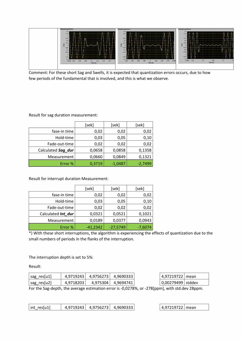
Comment: For these short Sag and Swells, it is expected that quantization errors occurs, due to how few periods of the fundamental that is involved, and this is what we observe.
Result for sag duration measurement:
[sek] [sek] [sek] fase-in time 0,02 0,02 0,02
Hold-time 0,03 0,05 0,10 Fade-out-time 0,02 0,02 0,02
Calculated Sag_dur 0,0658 0,0858 0,1358 Measurement 0,0660 0,0849 0,1321
Error % 0,3719 -1,0487 -2,7499
Result for interrupt duration Measurement:
[sek] [sek] [sek] fase-in time 0,02 0,02 0,02
Hold-time 0,03 0,05 0,10 Fade-out-time 0,02 0,02 0,02
Calculated Int_dur 0,0321 0,0521 0,1021 Measurement 0,0189 0,0377 0,0943
Error % -41,2342 -27,5749 -7,6074 *) With these short interruptions, the algorithm is experiencing the effects of quantization due to the small numbers of periods in the flanks of the interruption.
The interruption depth is set to 5%:
Result:
sag_res[u1] 4,9719243 4,9756273 4,9690333 4,97219722 mean sag_res[u2] 4,9718203 4,975304 4,9694741 0,00279499 stddev
For the Sag-depth, the average estimation error is -0,0278%, or -278[ppm], with std.dev 28ppm.
int_res[u1] 4,9719243 4,9756273 4,9690333 4,97219722 mean

int_res[u2] 4,9718203 4,975304 4,9694741 0,00279499 stddev For the Int-depth, the average estimation error is -0,0278%, or -278[ppm], with std.dev 28ppm.
Note: Since it is the same algorithm and the same input, not unexpectedly it has identical result. The only difference between Sag-event and an interruption-event is the trigger-value set for the two.
Test 4: Long interruption with increasing length
The duration of the Sag and Interruption
Duration-estimation: [settings] [sek] [sek] [sek] Sag-depth[%] 0 0 0 Fade-in 0,20 0,20 0,20 Hold 0,10 0,20 0,50 Fade-out 0,40 0,40 0,40 sag_dur* 0,64 0,74 1,04 int_dur* 0,16 0,26 0,56 Interrupt. depth: 0%
*) Values calculated based on settings
Result for sag duration measurement:
[sek] [sek] [sek] fase-in time 0,20 0,20 0,20
Hold-time 0,10 0,20 0,50 Fade-out-time 0,40 0,40 0,40
Calculated Sag_dur 0,6400 0,7400 1,0400 Measurement 0,6414 0,7451 1,0470
Error % 0,2174 0,6933 0,6729
Result for interrupt duration Measurement:
[sek] [sek] [sek]

fase-in time 0,2 0,2 0,2 Hold-time 0,1 0,2 0,5
Fade-out-time 0,4 0,4 0,4 Calculated Int_dur 0,1600 0,2600 0,5600
Measurement 0,1603 0,2641 0,5660 Error % 0,2157 1,5820 1,0683
The depth of the interruption is set to 0%:
Result:
int_res[u1] 0,024055 0,0143529 0,0047963 0,01441405 mean int_res[u2] 0,023249 0,0152541 0,0047771 0,00845084 stddev
For the Sag-depth, the average estimation error is 0,0144%, or 144[ppm], with std.dev 84ppm.
sag_res[u1] 0,024055 0,0143529 0,0047963 0,01441405 mean sag_res[u2] 0,023249 0,0152541 0,0047771 0,00845084 stddev
For the Int-depth, the average estimation error is 0,0144%, or 144[ppm], with std.dev 84ppm.
Conclusion: The InDiSwell performs well. The algorithm face challenges when the slopes of the event are short in time and maybe includes or happen over very few periods of the base signal. This make it difficult to determine within one period the exact start or end-time of the event. From the results presented above, we see that for the short events, the error is higher than for long duration events. The residual analysis performed overall quite comparable for all tests. Duration length did not influence noticeably. However, any noise in the signal will make the signal amplitude to be slightly overestimated, and thus the estimate of the depth of the event is slightly underestimated.

15RPT04 TracePQM - Appendix
Report describing the open software tool developed for handling high performance ADCs identified for power and PQ measurements
BLANK PAGE