14 Kaste Nord RID

REPORT SNO 6617-2014

Review and application of Russian and Norwegian methods for measuring and

estimating riverine inputs of heavymetals to the Barents Sea

Gaustadalléen 21 • NO-0349 Oslo, NorwayTelephone: +47 22 18 51 00 • Fax: 22 18 52 00www.niva.no • [email protected]

NIVA: Norway’s leading centre of competence in aquatic environments

NIVA provides government, business and the public with a basis forpreferred water management through its contracted research, reports and development work. A characteristic of NIVA is its broad scope ofprofessional disciplines and extensive contact network in Norway andabroad. Our solid professionalism, interdisciplinary working methods and holistic approach are key elements that make us an excellent advisor for government and society.

Riv

er M

ezen

(pho

to: A

. Yak

ovle

v)

Norwegian Institute for Water Research – an institute in the Environmental Research Alliance of Norway REPORTMain Office Regional Office, Sørlandet Regional Office, Østlandet Regional Office, Vestlandet Regional Office Central

Gaustadalléen 21 Jon Lilletuns vei 3 Sandvikaveien 59 Thormøhlens gate 53 D Høgskoleringen 9 NO-0349 Oslo, Norway NO-4879 Grimstad, Norway NO-2312 Ottestad, Norway NO-5006 Bergen Norway NO-7034 Trondheim Phone (47) 22 18 51 00 Phone (47) 22 18 51 00 Phone (47) 22 18 51 00 Phone (47) 22 18 51 00 Phone (47) 22 18 51 00 Telefax (47) 22 18 52 00 Telefax (47) 37 04 45 13 Telefax (47) 62 57 66 53 Telefax (47) 55 31 22 14 Telefax (47) 73 54 63 87 Internet: www.niva.no

Title

Review and application of Russian and Norwegian methods for measuring and estimating riverine inputs of heavy metals to the Barents Sea

Report No..

6617-2014

Project No.

11490

Date

January 2014

Pages Price

41

Author(s)

Ø. Kaste, I.J. Allan, K. Austnes, Guttorm Christensen (Akvaplan-NIVA), A.B. Christiansen, Anna Chultsova (IO-RAS), T. Høgåsen, Nikolay Kashulin (INEP), Tatyana Kashulina (INEP), Grigory Khomenko (IO-RAS), L.B. Skancke, J.R. Selvik, E. Yakushev.

Topic group

Monitoring

Geographical area

Barents region

Distribution

Free

Printed

NIVA

Client(s)

Norwegian Ministry of Environment

Client ref.

Ingrid Lillehagen

Abstract

This report presents the results from the Norwegian-Russian collaboration project NordRID project, which was carried out from December 2011 to December 2013. Four institutions have been involved; INEP and IO RAS from the Russian side and Akvaplan-NIVA and NIVA from the Norwegian side. The main purpose of the project has been to review Russian and Norwegian methods for measuring and estimating riverine inputs of heavy metals to the Barents Sea. The report gives an overview of the most common methods applied for monitoring and calculating riverine inputs of heavy metals. INEP and IO-RAS have provided both meta-data and to some extent also real data for a number of rivers draining from the Kola and Arkhangelsk area, respectively. Two pilot studies with passive sampling techniques were performed as part of the project; one with DGTs (Diffusion Gradient in Thin-films) for detection of metals, and one with passive samplers for detection of hydrophobic contaminants. Two bilateral project meetings/workshops have been carried out during the project (at Svanhovd and in Oslo). The report contains recommendations for future work based on the studies and experiences made from the project.

4 keywords, Norwegian 4 keywords, English

1. Tungmetaller 1. Heavy metals 2. Elver 2. Rivers 3. Analysemetoder 3. Analytical methods 4. Passive prøvetakere 4. Passive samplers

Øyvind Kaste Atle Hindar Claus Beier

Project Manager Manager Region South Research Director

ISBN 978-82-577-6352-7

Review and application of Russian and Norwegian methods for measuring and estimating riverine

inputs of heavy metals to the Barents Sea

NIVA 6617-2014

Preface

The NordRID project “Review and application of Russian and Norwegian methods for measuring and estimating riverine inputs of heavy metals to the Barents Sea” has been carried out during a two-year period between December 2011 and December 2013. It has been funded under the Norwegian-Russian environmental cooperation programme, by the Norwegian Ministry of Foreign Affairs and administered by the Norwegian Ministry of the Environment (contact person: Ingrid Lillehagen). NIVA has coordinated the project, with Institute of the North Industrial Ecology Problems (INEP) - Laboratory of Aquatic Ecosystems, P.P.Shirshov Institute of Oceanology of the Russian Academy of Sciences (IO RAS) and Akvaplan-NIVA (APN) as main partners. The project team has included: INEP: Nikolay Kashulin and Tatyana Kashulina IO-RAS: Anna Chultsova and Grigory Khomenko APN: Guttorm Christensen NIVA: Kari Austnes, Evgeniy Yakushev, John Rune Selvik, Tore

Høgåsen, Ian Allan, Øyvind Garmo, Anne B. Christiansen, Liv Bente Skancke, and Øyvind Kaste

Thanks to the funding institutions and all project participants for their valuable contributions to the project! Thanks also to Dr. Atle Hindar for carrying out quality assurance of the report

Oslo, January 2014

Øyvind Kaste

NIVA 6617-2014

Contents

Summary 5

1. Introduction 7

1.1 Background 7 1.2 Objectives 7 1.3 Links to bilateral collaboration programmes 7

2. Methods for monitoring and calculating riverine inputs to the sea 8

2.1 Heavy metals 8 2.2 Other components 8 2.3 Automatic sampling and continuous measurements 9

3. Review of existing data 11

3.1 Some characteristic features of the Barents Sea. 11 3.2 Norwegian rivers draining to the Barents Sea 12 3.3 Russian rivers draining to the Barents Sea. 14 3.4 Relevant projects 17

4. Results from pilot studies with passive samplers 18

4.1 DGTs for detection of metals 18 4.2 Passive samplers for detection of hydrophobic contaminants 21

5. Source-apportionment models as tools to estimate riverine inputs 24

5.1 The TEOTIL model 24 5.2 Application of the TEOTIL model within the RID programme 25

6. Meetings/workshops and further work 26

7. References 27

Appendix A. Analytical methods 31

Appendix B. River data 34

Appendix C. DGT data 38

Appendix D. Svanvik workshop programme 40

Appendix E. Final meeting, Oslo 42

NIVA 6617-2014

5

Summary

The management plan for the marine environment in the Barents Sea and the Lofoten area, and the Norwegian Marine Pollution Monitoring Programme (alternating between Norway’s three main ocean areas) have revealed a number of gaps in our knowledge related to discharges of environmental hazardous substances to the Barents Sea. One gap is the lack of available data on riverine inputs from the Russian side of the Barents Sea, which represents a major uncertainty in the modelling of concentrations and fluxes of contaminants to the marine environment. This represents the starting point for the Norwegian-Russian collaboration project NordRID project, which aims at:

- Reviewing and discussing Russian and Norwegian methods for measuring and calculating riverine inputs of heavy metals to the Barents Sea

- Getting an overview of the most important datasets on riverine inputs from Norway and Russia to the Barents Sea

- Demonstrating passive sampling as a possible technique for estimating fluxes of heavy metals and persistent organic compounds in rivers

- Demonstrating how source-apportion models can provide estimates of riverine inputs from un-monitored catchments

- Improving the Norwegian-Russian cooperation in the Barents Region by bringing together key research institutes from both sides of the border

The report provides an overview of the most common methods applied for monitoring and calculating riverine inputs of heavy metals. In Norway this is based on the RID principles of the OSPAR (OSlo-PARis) Convention for the Protection of the Marine Environment of the North-East Atlantic (www.ospar.org). The Norwegian RID programme uses three methods to record loads from land to the sea: monitoring of concentrations in river water; monitoring of direct discharges from point sources; and modelling/estimating loads from unmonitored areas. In Russia, element concentrations in rivers are analysed by standardised methods, and with respect to the heavy metals Hg, Pb, Cd, Cu, Zn, Cr, Ni and As, both IO-RAS (Arkhangelsk) and INEP (Murmansk) apply atomic absorption spectrometry or ICP-MS as the main analytical instruments. The Barents Sea receives riverine inputs from a land area of approximately 56000 km2 on the Norwegian side and approximately 931000 km2 on the Russian side. The main currents travel from west to east, and the Russian river inputs therefore enter the Barents Sea “downstream” of the Norwegian coastal area. The currents, however, follow a circular pathway west of Novaja Semlja and return to the south before approaching Svalbard. INEP and IO-RAS have provided both meta-data (catchment characteristics, availability of hydrological and chemical data, references to reports, etc.) and to some extent also real data for a number of rivers draining from the Kola and Arkhangelsk area, respectively. Two pilot studies with passive sampling techniques were performed as part of the project; one with DGTs (Diffusion Gradient in Thin-films) for detection of metals, and one with passive samplers for detection of hydrophobic contaminants. The first pilot study was performed in three rivers located in Pasvik, around Nikel, and in the Arkhangelsk area. The main purpose of the pilot study was to demonstrate the methods and the possibilities they offer in terms of integrating metal concentrations in rivers over longer or shorter periods. Another purpose was that each institute should get experience with deploying DGTs in the field, analyse them in the lab, and calculate the integrated metal concentrations in their rivers. Passive sampling for detection of hydrophobic contaminants in the Pasvik river showed that most compounds of interest were detected and quantified in the freely dissolved phase. As expected, highest

NIVA 6617-2014

6

PAH concentrations were found for the least hydrophobic substances while hydrophobic contaminants were well below 1 ng L-1. Concentrations of low molecular weight PAHs were significantly lower in the River Pasvik than in the Alna or Glomma rivers in south-eastern Norway (part of the RID programme). Less difference could be observed for the higher molecular weight PAHs. PCB concentrations were in the low pg L-1 range or below. PCB concentrations were found to be lower than those measured with silicone samplers in the Alna River a relatively polluted stream that runs through Oslo. Good communication and good knowledge of each institute’s infrastructure and working practices is essential for achieving an effective trans-national cooperation in the Barents Region, which in turn is needed for an integrated and knowledge-based management of the Barents Sea. In bilateral collaboration projects like NordRID, project meetings and workshops are an important arena for exchanging knowledge, experiences and data. An example is exchange of experiences with modelling tools as the TEOTIL model (which is briefly described in chapter 5 of this report). Two bilateral project meetings/workshops have been carried out during the project:

- 18-20 June 2012: Scientific workshop, Pasvik - 21-22 October 2013: Final meeting, Oslo

Recommendations for future work: The review of Russian and Norwegian methods for measuring heavy metals and other water quality determinants show that the approaches are quite similar and the detection limits are generally low and comparable for most variables. Hence, there is a very good basis for exchanging data and for development of more integrated monitoring activities in main rivers draining to the Barents Sea. Access to existing data from Russian rivers can be a challenge, however, due to restrictions set by different data-owners. An improved access to historical data would be extremely valuable as basis for future monitoring and assessments. Implementation of novel monitoring techniques, including real-time measurements and use of time-integrative passive sampling techniques (cf. pilot studies performed in this project) is highly recommended. The latter can be especially relevant in remote areas, due to relatively low cost and the abilities to detect and quantify heavy metals as well as organic contaminants, which is a major environmental concern in arctic regions.

NIVA 6617-2014

7

1. Introduction

1.1 Background

In March 2006 the Norwegian Government presented a comprehensive management plan for the marine environment in the Barents Sea and the marine areas outside Lofoten (Report to the Norwegian Parliament; Stortingsmelding 8, 2005-2006). The management plan emphasised that all activities in the area should be managed within a framework that ensures that the overall environmental impact does not exceed the carrying capacity of ecosystems. Distinct environmental quality targets were defined and a more coordinated and systematic marine monitoring programme was initiated; e.g. Green et al. (2010, 2013). This particular programme calculated and modelled annual fluxes of environmental hazardous substances, oil and radioactive substances from all known sources on land and offshore. The monitoring programme alternates between three ocean areas, and started with the Barents Sea in 2009. The report for the Barents Sea 2009 pointed out a number of knowledge gaps (Green et al. 2010). Lack of data on riverine inputs from the Russian side of the Barents Sea represents an uncertainty in the modelling of concentrations and fluxes of environmental hazardous substances in the marine area. Inputs from the Norwegian mainland are currently monitored by the RID-OSPAR programme (Riverine inputs and direct discharges to Norwegian coastal waters) and the TEOTIL programme (Theoretical calculation of phosphorus and nitrogen inputs in Norway), both led by NIVA on commission from the Norwegian Environment Agency (Skarbøvik et al. 2012; Tjomsland et al. 2010).

1.2 Objectives

The starting point for the NordRID project is the need for a close Norwegian-Russian collaboration to get a better overview of the total inputs of environmental hazardous substances to the Barents Sea. The main objectives of the project are:

- Review and discuss Russian and Norwegian methods for measuring and calculating riverine inputs of heavy metals to the Barents Sea (other contaminants are considered if applicable)

- Get an overview of the most important datasets on riverine inputs from Norway and Russia to the Barents Sea

- Demonstrate passive sampling techniques (for heavy metals and persistent organic compounds) at selected Norwegian and Russian case study sites

- Demonstrate how source-apportion, coefficient-based models (like TEOTIL) can provide estimates of riverine inputs from un-monitored catchments

- Improve Norwegian-Russian cooperation in the Barents Region by bringing together key research institutes from both sides of the border and thereby contribute to more knowledge-based management of the Barents Sea.

1.3 Links to bilateral collaboration programmes

The NordRID project has contributed to the working programmes for Norwegian-Russian environmental cooperation (2011-2012, and 2013-2015) and is directly linked to “Protection of the marine environment” and the activity HAV-4 “Inputs of pollution to the Barents Sea”. The project addresses both sub-tasks of HAV4: “Review of Russian and Norwegian methods for calculating inputs from various sources to the Barents Sea” and “Pilot project in a Norwegian and a Russian river for testing identified methods for calculating inputs of pollutants”. The activities are supportive of the main objective of “Protection of the marine environment” as regards assembling the necessary knowledge base for preserving the clean, rich ecosystem of the Barents Sea. The project will also contribute with data and knowledge to the “Pasvik programme” (DGS-1).

NIVA 6617-2014

8

2. Methods for monitoring and calculating riverine inputs to the sea

The analytical methods applied at the laboratories at NIVA, INEP and IO-RAS are presented in more detail in Appendix A1, A2 and A3, respectively. Appendix A4 contains a more extensive description of analytical methods applied at IO RAS

2.1 Heavy metals

The methods for analysing heavy metals are quite similar at the three institutes. NIVA applies ICP-MS, IO-RAS uses Atomic Absorption Spectrometry (AAS), whereas INEP applies three different instruments depending on the detection limits required (AAS, ICP-EOS, ICP-MS). A comparison of detection limits are given in Table 1. The table shows that INEP and NIVA have low and relatively similar detection limits when using ICP-MS. INEP has the lowest detection limits for copper, zinc and arsenic. Table 1. Detection limits for analyses of heavy metals at NIVA, IO-RAS, and INEP.

2.2 Other components

Also when it comes to other standard water quality parameters, the analytic methods and detection limits are quite similar (Table 2). Altogether, the simple review of analytical methods and detection limits for heavy metals and other chemical determinants shows an excellent basis for integrated monitoring activities and data exchange and comparison across the border. Table 2. Detection limits for analyses of other standard parameters at NIVA, IO-RAS, and INEP.

Unit NIVA_ICP‐MS IO‐RAS_AAS INEP_AAS INEP_ICP‐EOS INEP_ICP‐MS

Lead (Pb) µg/L 0.005 2 0.5 1 0.005

Cadmium (Cd) µg/L 0.005 0.2‐0.3 0.05 0.1 0.005

Copper (Cu) µg/L 0.01 0.4‐0.6 0.2 0.5 0.005

Zinc (Zn) µg/L 0.05 0.2‐0.3 0.1 0.2 0.03

Arsenic (As) µg/L 0.05 0.05 0.5 0.3 0.01

Chromium (Cr) µg/L 0.1 1.5‐2 0.2 0.2 0.1

Nickel (Ni) µg/L 0.05 3 0.5 0.4 0.05

Mercury (Hg) ng/L 1 6 ‐ ‐ ‐

Unit NIVA IO‐RAS INEP

pH 0.01 0.01 0.01

Conductivity mS/m 0.05 0.01 0.05

Suspended particulate matter (SPM) mg/L 0.1 3 0.1

Total Organic Carbon (TOC) mg C/L 0.1 ‐ ‐

Total phosphorus µg P/L 1 0.01* 2

Orthophosphate (PO4‐P) µg P/L 1 0.01* 2

Total nitrogen µg N/L 10 ‐ 10

Nitrate (NO3‐N) µgN/L 1 0.01* 5

Ammonium (NH4‐N) µg N/L 2 ‐ 2

Silicate (SiO2) mg SiO2/L 0.02 0.1 5

* mg/L

NIVA 6617-2014

9

2.3 Automatic sampling and continuous measurements

Some experiences at NIVA NIVA has long experience with automated sampling techniques and continuous monitoring of water quality. Automated sampling (time-integrated or flow-proportional) is most commonly used within research projects or for short-term campaigns (episode studies). An example is the CLUE project (Stuanes et al. 2008), where a number of small headwater streams were instrumented with a tipping-bucket system for flow measurements, data loggers and ISCO automated water samplers (Figure 1a).

Figure 1. a) ISCO water sampler, b) TinyTag temperature logger In 2013, new sampling techniques were implemented in the RID-OSPAR programme (cf. presentation by Kari Austnes at the NordRID final meeting; Appendix D): - Basic parameters:

- Continuous measurements of pH, conductivity, turbidity and temperature in three rivers - TinyTag loggers for continuous temperature measurements installed in all remaining min

rivers (Figure 1b) - Organic contaminants (three rivers):

- Passive samplers (dissolved): PBDE, HBCDD, PCB, PAH - Centrifuge (particles): PBDE, HBCDD, PCB, PFC, TBBPA, BPA, SCCP, MCCP, PAH - Bottle samples: Siloxanes

Heavy metals:

- Ag (all rivers) - DGT: Pb, Cd, Cu, Ni, Zn, Ag (six rivers)

Pilot studies with passive samplers for heavy metals and organic contaminants from this project are described in Chapter 4. Continuous monitoring performed by IO-RAS IO-RAS has experience with e.g., SeaGuard RCM SW (AANDERAA), a multi-parameter instrument that can be deployed both in the sea and in freshwater. Sensors applied by IO-RAS: Temperature, conductivity, pressure, turbidity, oxygen, speed and direction of water.

NIVA 6617-2014

10

Figure 2. Continuous monitoring of pH, conductivity, turbidity and temperature in a RID river (photo: NIVA).

NIVA 6617-2014

11

3. Review of existing data

3.1 Some characteristic features of the Barents Sea.

Barents Sea has a mean depth of 230 m. There are three main bodies of water: warm Atlantic water with high salinity, cold Arctic water from the north and warm coastal water with less salinity. Main circulation patterns in surface waters Figure 3 are dominated by a northbound flow of warm water along the coast and on the west side of Bear Island and Svalbard. A branch of this stream follows the coast past the North Cape and along the west coast of Novaya Zemlya in the Russian part of the Barents Sea. It is a cold southbound flow on the eastern side of Svalbard. The ice front in February is normally located on the western side of Svalbard, south of Bear Island and west of Novaya Zemlya.

Figure 3. Circulation patterns of surface waters in the Barents Sea (from IMR). The temperature of the Barents Sea has increased in recent years, and in several years since 2000 it has been ice-free in summer (Sunnanå et al. 2010). Changes in climate can theoretically affect the distribution and dispersion of pollutants and also lead to bioaccumulation of potential harmful substances. Changes in temperature can affect the distribution of pollutants between different media or phases as air, particles, and water (Smith and McLachlan 2006, Macdonald et al. 2005). This will affect the bioavailability of these chemicals. Climate change may also affect the transport of contaminants between geographical regions, by changes in transport routes and volumes in water and air with different pollution levels (Macdonald et al. 2005).

NIVA 6617-2014

12

Elevated precipitation amounts in the future may also lead to increased leaching of contaminants from land to sea (Ruus et al. 2010). Increased levels of CO2 in the atmosphere also promote ocean acidification, with potentially huge negative environmental impacts (Orr et al. 2005). Although the overall pollution load is low in the Barents Sea, human activities can still put seafood safety under pressure (Sunnanå et al. 2010).

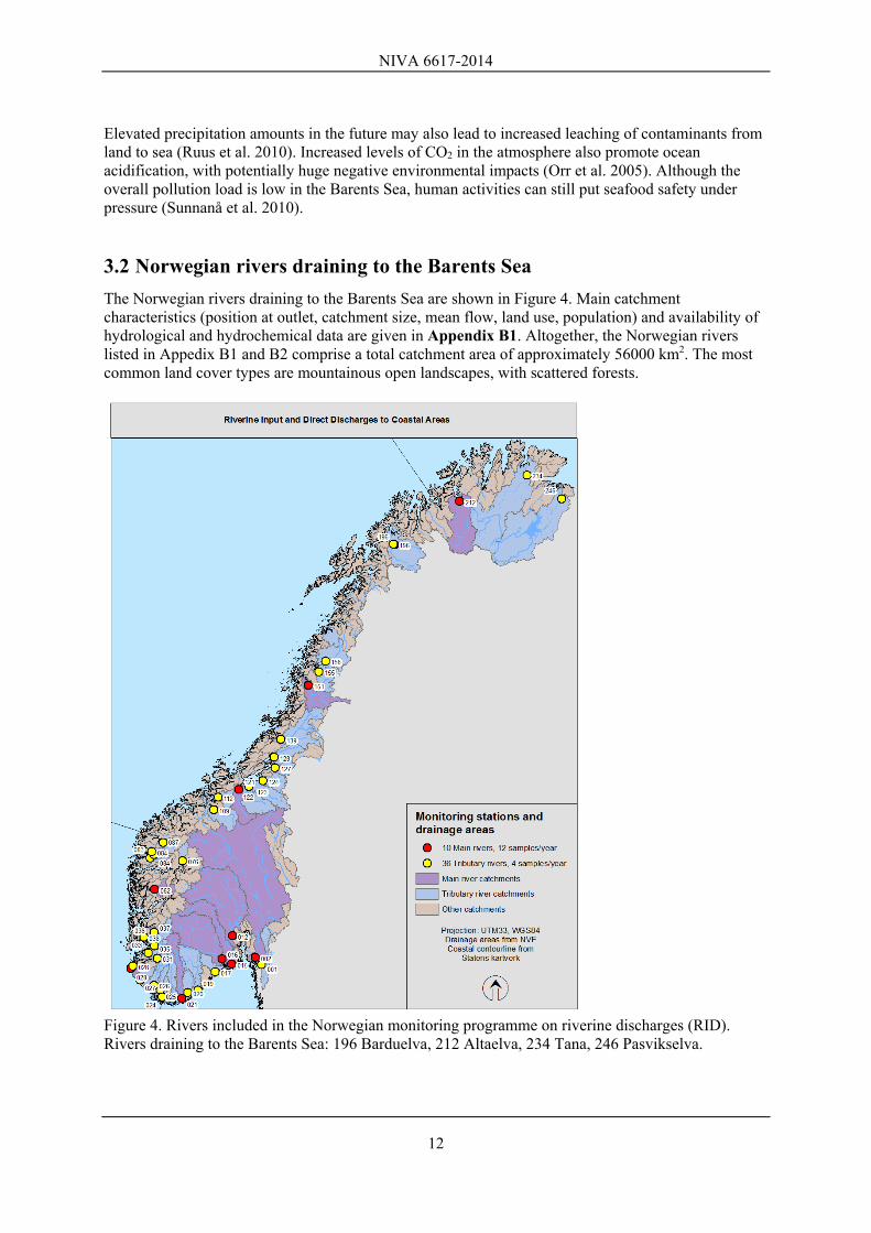
3.2 Norwegian rivers draining to the Barents Sea

The Norwegian rivers draining to the Barents Sea are shown in Figure 4. Main catchment characteristics (position at outlet, catchment size, mean flow, land use, population) and availability of hydrological and hydrochemical data are given in Appendix B1. Altogether, the Norwegian rivers listed in Appedix B1 and B2 comprise a total catchment area of approximately 56000 km2. The most common land cover types are mountainous open landscapes, with scattered forests.

Figure 4. Rivers included in the Norwegian monitoring programme on riverine discharges (RID). Rivers draining to the Barents Sea: 196 Barduelva, 212 Altaelva, 234 Tana, 246 Pasvikselva.

NIVA 6617-2014

13

Figure 5 displays mean concentrations (1990-2011) of heavy metals (Cu, Cd, Cr, Ni, Zn, Hg, Pb) and general water quality parameters as total organic carbon (TOC) and suspended particulate matter (SPM). All data (Appendix B2) are collected as part of the RID programme (Skarbøvik et al. 2012). In the Barents Sea region the RID programme includes one main river (Alta; monthly sampling) and three rivers with less extensive sampling (Barduelva/Målselv, Tana and Pasvik; sampled quarterly). The remaining rivers included in Appendix B2 have less frequent data, mostly obtained before 2003. The concentrations of heavy metals are generally low (Figure 5), but there is a clear increase in Cu and Ni concentrations close to the Russian border (especially in the Pasvik river and Grense Jakobselv). The concentrations of TOC and SPM are moderate, indicating relatively low loads of organic matter and particles to the Barents Sea. Barduelva and Målselv had the highest SPM-concentrations (6-7 mg/L).

Figure 5. Mean concentrations (1990-2011) of heavy metals (Cu, Cd, Cr, Ni, Zn, Pb), total organic carbon (TOC) and suspended particulate matter (SPM). Data from the RID programme (Skarbøvik et al. 2012).

0.00

0.50

1.00

1.50

2.00

2.50

3.00

3.50

Barduelva

Målselv

Nordkjoselva

Signaldalselva

Skibotnelva

Kåfjordelva

Reisa

Mattiselva

Tverrelva

Repparfjordelva

Stab

burselva

Lakselv

Børselva

Mattusjåkka

Storelva

Soussjåkka

Adam

selva

Tanavassdraget

Vesterelva

V. Jakobselv

Pasvikelva

Neiden

Grense Jakobselv

Cu, u

g/L

0.0

0.5

1.0

1.5

2.0

2.5

Cr, ug/L

0.00

0.50

1.00

1.50

2.00

2.50

3.00

3.50

Barduelva

Målselv

Nordkjoselva

Signaldalselva

Skibotnelva

Kåfjordelva

Reisa

Mattiselva

Tverrelva

Repparfjordelva

Stabburselva

Lakselv

Børselva

Mattusjåkka

Storelva

Soussjåkka

Adam

selva

Tanavassdraget

Vesterelva

V. Jakobselv

Pasvikelva

Neiden

Grense Jakobselv

Zn, u

g/L

0.0

0.5

1.0

1.5

2.0

2.5

3.0

3.5

4.0

TOC,m

g/L

0.000

0.005

0.010

0.015

0.020

0.025

0.030

Barduelva

Målselv

Nordkjoselva

Signaldalselva

Skibotnelva

Kåfjordelva

Reisa

Mattiselva

Tverrelva

Repparfjordelva

Stab

burselva

Lakselv

Børselva

Mattusjåkka

Storelva

Soussjåkka

Adam

selva

Tanavassdraget

Vesterelva

V. Jakobselv

Pasvikelva

Neiden

Grense Jakobselv

Cd, u

g/L

0.00

1.00

2.00

3.00

4.00

5.00

6.00

7.00

8.00

9.00

Barduelva

Målselv

Nordkjoselva

Signaldalselva

Skibotnelva

Kåfjordelva

Reisa

Mattiselva

Tverrelva

Repparfjordelva

Stabburselva

Lakselv

Børselva

Mattusjåkka

Storelva

Soussjåkka

Adam

selva

Tanavassdraget

Vesterelva

V. Jakobselv

Pasvikelva

Neiden

Grense Jakobselv

Ni, ug/L

0.00

0.05

0.10

0.15

0.20

0.25

0.30

0.35

0.40

Barduelva

Målselv

Nordkjoselva

Signaldalselva

Skibotnelva

Kåfjordelva

Reisa

Mattiselva

Tverrelva

Repparfjordelva

Stabburselva

Lakselv

Børselva

Mattusjåkka

Storelva

Soussjåkka

Adam

selva

Tanavassdraget

Vesterelva

V. Jakobselv

Pasvikelva

Neiden

Grense Jakobselv

Pb, u

g/L

0.00

1.00

2.00

3.00

4.00

5.00

6.00

7.00

8.00

Barduelva

Målselv

Nordkjoselva

Signaldalselva

Skibotnelva

Kåfjordelva

Reisa

Mattiselva

Tverrelva

Repparfjordelva

Stab

burselva

Lakselv

Børselva

Mattusjåkka

Storelva

Soussjåkka

Adam

selva

Tanavassdraget

Vesterelva

V. Jakobselv

Pasvikelva

Neiden

Grense Jakobselv

SPM m

g/L

NIVA 6617-2014

14

Figure 6. Pasvik river, looking downstream from the RID monitoring station (photo: E. Pettersen)

3.3 Russian rivers draining to the Barents Sea.

The Russian rivers draining to the Barents Sea are shown in Figure 7. Main catchment characteristics (position at outlet, catchment size, mean flow, land use, population) and availability of hydrological and hydrochemical data are given in Appendix B2. Altogether, the Russian rivers comprise a total catchment area of approximately 931000 km2 (~16 times larger than the contributing area on the Norwegian side) (Figure 7). Land cover distribution varies among the catchments (cf Appendix B3), the main types being tundra, grassland, bogs, taiga, forests and agricultural land.

Figure 7. Large Russian rivers draining to the Barents Sea (from Brittain et al. 2008) Hydrology Typical for rivers in the Barents region is that water flow is strongly affected by snow accumulation and melting. Snow melt often contributes more than 50% of the total annual runoff. The rest comes from rainfall during summer and autumn, of which the autumn period contributes the most. Runoff through the soils is extremely poor because of the permafrost. The presence of permafrost creates

NIVA 6617-2014

15

special conditions for the hydrological regime of rivers. Frozen ground promotes increased surface runoff during snowmelt and rainfall, and it also prevents soil runoff during the cold period. The hydrological regime of rivers is characterized by low flow during winter, high spring floods and generally low flow during the summer-autumn period, interrupted by rain floods. The main part of the runoff occurs in the spring, on average 70-80% of the annual volume. In comparison, the summer and autumn period on average contributes with 15-25%, and the winter period 1.5-1.6% of the annual runoff. The spring flood in rivers of the region normally begins around 5 to 10 May, with the maximum usually occurring in the end of May. The average duration of the spring flood in small and medium rivers is 1.5-2 months. The total volume of the spring flood is 160 mm on average, and it often increases the river water level by 1.5 to 3.7 m. Average dates for termination of the spring flood are 20-25 June. The summer-autumn low-water period generally occurs during the second half of June and normally lasts for 60-70 days. The total runoff volume during this period often is 10-30 mm. In some years, rain peaks during summer or autumn can promote floods larger than the spring flood in small and medium-sized rivers. The greatest rain floods are usually observed in August and October. Rises in river water level by rainfall can be in the range from 0.3 to 1.5 m. Rivers in this area is heavily affected by ice formation. In late autumn the ice regime is characterized by formation of cake ice and sludge. The first river ice formations usually appear in the end of October. Several rivers are affected by ice drift during spring. During dry and cold winters some streams might dry up and freeze completely. A B

C

Figure 8. A) Northern Dvina river near the city of Arkhangelsk (photo: G. Khomenko), B) River Mezen (photo: A. Yakovlev), C) River Pinega (photo: A. Yakovlev).

NIVA 6617-2014

16

Water quality Chemical composition of surface waters in the Arkhangelsk region is affected by a severe climate, low solar radiation (especially in winter), waterlogging, and the presence of permafrost. The water quality is usually controlled by the hydrocarbonate system, although low weathering and mineralization rates give moderate concentrations of base cations as calcium. Most rivers have a large influence of humic compounds and particles. The average annual water turbidity (measured as suspended particulate matter) is often in the range of 25-50 mg/l. Oxygen saturation of water in the ice-free period ranges between 75-95%, with typical concentrations 7-12 mg/l. During summer, the concentration of oxygen is often reduced to 7-8 mg/l. In winter, the oxygen content of surface waters decrease, some places to values around 2-3 mg/L. The low oxygen content of the water is caused by decomposition of a high content of organic matter during the long ice-period. The biological oxygen demand (as BOD5-values) is often in the range of 1.0-3.5 mg О2/l). The highest BOD5 values are observed in spring and summer, due to melt water with high content of organic compounds and generally high activity of biological processes. The total concentration of oxidable organic and mineral substances is measured as COD (chemical oxygen demand, with typical values around 20-40 mg О2/l). Maximum COD-values are observed in spring when the soils are washed with water from melted snow. The water acidity is controlled by dissolved humic acids. But in summer (24 hours with daylight) primary production during mass development of Cyanobacteria can raise pH up to 9.0. The main anions are hydro-carbonates, with concentrations in the range 5.9 - 135 mg/L, followed by chloride ions (0,9-30.0 mg/L) and sulphate ions (0,08-4,1 mg/L). The cation composition is dominated by calcium, and only in rare cases sodium ions. The highest nutrient concentrations occur during the winter, whereas a minimum occurs in the vegetation period. The concentration of silica varies in the range of 0.5-0.6 mg/l, phosphate-phosphorus 0-0.1 mg/l, ammonium nitrogen 0.05-0.04 mg/l, nitrite nitrogen 0-0.01 mg/l, and nitrate nitrogen 0-0.3 mg/l. For mineral nutrients the general tendency is an increase during low flow, when the groundwater influence is highest. Enrichment with iron is common in areas which drain wetlands. A significant amount of organic substances, including humic and fulvic acids form organometallic complexes with iron. Water quality of small lakes and streams in the Norwegian, Finnish and Russian border area Results from the trilateral Pasvik monitoring programme for water bodies in the border area of Norway, Finland and Russia are reported by Puro-Tahvanainen et al. (2011). The data obtained confirms the ongoing pollution of river and water systems: “Copper (Cu), nickel (Ni) and sulphates are the main pollution components. The highest levels were observed close to the smelters. The most polluted water source of the basin is the River Kolosjoki, as it directly receives the sewage discharge from the smelters. The concentrations of metals and sulphates in the River Pasvik are higher downstream from the Kuetsjarvi Lake. There has been no decrease in the concentrations of pollutants in Pasvik watercourse over the last 10 years. Ongoing recovery from acidification has been evident in the small lakes of the Jarfjord and Vätsäri areas during the 2000s. The buffering capacity of these lakes has improved and the pH has increased. The reason for this recovery is reduced sulphate deposition, which is also reflected in reduced water concentrations. However, concentrations of some metals, especially Ni and Cu, have increased during the 2000s. Ni concentrations have increased in all three areas, and Cu concentrations in the Pechenganickel and Jarfjord areas, closer to the smelters. Emission levels of Ni and Cu did not fall during the 2000s. In fact, the emission levels of Ni compounds even increased compared to the 1990s”.

NIVA 6617-2014

17

3.4 Relevant projects

The following tables include some examples of projects related to rivers and lakes draining to the Barents Sea. NIVA Name of project Sites Duration References Riverine inputs and direct discharges to Norwegian coastal waters

Bardu river, Alta river, Tana river, Pasvik river

1990- Skarbøvik et al. (2012)

Monitoring long-range transboundary air pollution. Effects

Dalelva (Jarfjord), small lakes on the Jarfjord plateau

1989- Schartau et al. (2012)

National lake survey, part 2: Sediments. Pollution of metals, PAH and PCB

25 lakes in Eastern Finnmark

2004 – 2006 Rognerud et al. (2008)

IO RAS Name of project Sites Duration References Grant RFBR 08-05-98814- r_north_а «The study of accumulation of nutrients in the ice and snow of the delta Northern Dvina River».

Northern Dvina River 2008-2009 1-4

Assessment of the role of different-scale physical and chemical processes in the formation of the characteristic features of ecosystems estuarine areas of the rivers of the White sea basin.

Northern Dvina River. Small rivers Onega peninsula: Nizhma, Känd, Tamtsa, Lopshenga.

2010-2012 5-8

References: 1. Chultsova and Skibinski (2008) 2. Chultsova (2009) 3. Chultsova and Skibinski (2009) 4. Chultsova (2009) 5. Kotova et al. (2012) 6. Chultsova (2010) 7. Khomenko and Leshchyov (2010) 8. Khomenko (2010) INEP Name of project Sites Duration References КО370- Trilateral cooperation on environmental challenges in the joint border area (TEC 2012-2014)

Pasvik river 2012-2014

State of the Environment in the Norwegian, Finnish and Russian Border Area.

Pasvik river 2003-2006 *)

Heavy metals from the Nikel area. Investigations in Kolosjoki river 1995, Kola peninsula, Russia.

Kolosjoki river 1995 Traaen et al. (1996)

Pasvik River Watercourse, Barents Region:Pollution Impacts and Ecological Responses. Investigations in 1993

Pasvik river 1993 Moiseenko et al. (1994)

Pasvik Water Quality Report. Environmental Monitoring Programme in the Norwegian, Finnish and Russian Border Area

Pasvik river 2007- Puro-Tahvanainen et al. (2011)

Pollution impact on freshwater communities in the border region between Russia and Norway

border region between Russia and Norway

1990-1996 Nøst et al. (1997)

*) http://www.pasvikmonitoring.org/eng/index.html

NIVA 6617-2014

18

4. Results from pilot studies with passive samplers

4.1 DGTs for detection of metals

Principles The Diffusion Gradient in Thin-films (DGT) technique (Davison and Zhang 1994; Zhang and Davison 1995) is based on a simple device that accumulates metals in situ, over time in a Na resin gel. These samplers bind metals in an ion exchange sorbent packed behind a filter and a diffusion gel and have been successfully applied to a wide range of environmental monitoring scenarios (Warnken et al. 2007). More information on the technique can be found in Røyset et al. (2012) and references therein. Methodology (field and lab) At the Svanvik workshop (Appendix D1) it was agreed to carry out a simple pilot study with DGTs deployed in three rivers located in the Pasvik, Nikel and Arkhangelsk area. The suggested design of the pilot study is given below. DGT pilot study – suggested procedure: Study sites (one site per river)

1) Pasvik river (responsible: NIVA/Akvaplan-NIVA) 2) Stream near Nikel (responsible: INEP) 3) River/stream near Arkhangelsk (responsible: IO RAS)

DGT deployment Two (parallel) DGTs deployed at each sampling event (please store DGTs cold before as well as after deployment)

Field procedure See attached document from NIVAs lab. (Note: Remember to fill out the registration form with water temperature, flow velocity, etc.)

Exposure period One week (3-5 days at heavily polluted sites)

Sampling rounds Four consecutive rounds á one week (i.e., 8 DGTs per round)

Manual samples Water samples (0.5 L) should be taken at each sampling site – before and after each DGT deployment.

Storage DGTs and water samples should be stored cold (4oC) until analysis

Analysis One set of DGTs (4 pieces) and the water samples are analysed at the local laboratory. The parallel set of DGTs (4 pieces) is shipped to NIVA for analysis (remember to attach the field registration form). Both DGTs and water samples are analyzed by ICP-MS for the following constituents: Cu, Ni, Cr, Cd, Pb, and Zn.

Correction of DGT concentrations

Average concentrations of DGT-labile metal species through exposure period can be calculated by a simple formula. NIVA can help with this calculation if the following data are provided: metal concentration in the DGT-gel, water temperature and flow velocity before and after exposure of the DGT.

NIVA 6617-2014

19

Calculation If diffusion through the diffusion gel is known, the concentration of labile metal compounds in water (Cv) is calculated on the basis of the concentration in the ion exchanger (M), the sampling period (t) and the diffusion coefficient (D).

Δg: thickness of the diffusion membrane A: area of the sampling window The diffusion coefficient varies with temperature and therefore must be measured for different temperatures. An overview of diffusion coefficients for different temperatures is given for various metals on http://www.dgresearch.com/. Results Figure 9 and

NIVA 6617-2014

20

Table 3 displays heavy metal concentrations at the sites that were selected for the pilot studies. The data show high Ni and Cu concentrations in the Kolosjoki river (near Nikel), and relatively high levels of Cr, Pb and Zn in River Pinega in the Arkhangelsk area. The results from the pilot study with metal DGTs are displayed in Appendix C (on the Norwegian side the smaller Karpelva river was studied instead of the larger Pasvik river). The main purpose of the pilot study was to demonstrate the methods and the possibilities it offers in terms of integrating metal concentrations in rivers over longer or shorter periods. Another purpose was that each institute should get an experience with both deploying DGTs in the field, analyse them in the lab, and calculate the integrated metal concentrations (Cv) based on the equation above. Hence, the main focus in this round with metal DGTs was more on the methodology than on the actual results.

Figure 9. Concentrations of heavy metals in the Pasvik river (Norwegian side, sampled 3 May 2012), River Pinega (Arkhangelsk area, sampled 31 August 2012) and the Kolosjoki river (near Nikel, 22 August 2012. Samples are analysed at NIVA (Pasvik), IO-RAS (Pinega) and INEP (Kolosjoki)

0

5

10

15

20

25

30

35

40

Cd Cr Cu Ni Pb Zn

µg/L

Pasvik river

River Pinega

Kolosjoki river

407 µg/L

NIVA 6617-2014

21

Table 3. Same data as in Figure 9 showed in table format.

4.2 Passive samplers for detection of hydrophobic contaminants

Principle of passive sampling for hydrophobic contaminants Passive sampling is based on the diffusive movement of substances from the environmental matrix being sampled into a polymeric device (initially free of the compounds of interest) in which contaminants absorb. For the passive sampling of hydrophobic compounds the best known sampler is the SemiPermeable Membrane Device (SPMD) comprising a low density polyethylene membrane containing a triolein lipid phase (Huckins et al., 2006). Nowadays, single phase polymeric samplers constructed from material such as low density polyethylene or silicone rubber as a result of their robustness (Allan et al., 2009, Allan et al., 2010, Allan et al., 2011). At equilibrium, the mass of a chemical absorbed in the sampling device can be translated into a freely dissolved contaminant concentration in the water the device was exposed to through Ksw, the sampler-water partition coefficient. Passive sampling techniques that allow to derive freely dissolved contaminant concentrations have been the subject of much development over the last two decades (Vrana et al., 2005). For hydrophobic contaminants with logKow (Octanol-Water Partition Coefficient) > 5-6, polymeric samplers have a large capacity. For typical deployment periods of a few weeks, equilibrium between the sampler and water will not be attained for these chemicals. Uptake in the linear mode (i.e. far from equilibrium) is therefore time-integrative for the deployment period in water. The resulting time-integrated freely dissolved concentration can be estimated if in situ sampling rates, Rs, equivalent amount of water sampled per unit of time (L d-1) are known. Sampling rates can be estimated from the dissipation of performance reference compounds (PRC), analogues of compounds of interest (but not present in the environment) spiked into the samplers prior to exposure (Booij et al., 1998, Huckins et al., 2002). Methodology (field and lab) Samplers, similar to those used for the RID programme 2013 and made of AlteSil silicone rubber (1000 cm2 and 30 g, strips 100 cm long and 2.5 cm wide) were prepared in the NIVA laboratory following standard procedures. In short, the silicone rubber samplers were placed in a Soxhlet extractor for 24 hour cleaning using ethyl acetate. Samplers were then left to dry before further cleaning with methanol. PRCs (deuterated PAHs) were spiked into the samplers using a methanol-water solution (Booij et al., 2002). Onced spiked with PRCs, samplers were kept in the freezer at -20 C until deployment. Replicate samplers were deployed in the Pasvik River using SPMD canisters and samplers mounted on spider holders. A control sampler was used to assess potential contamination of the samplers during preparation and deployment procedures and to assess initial PRC concentrations. The deployment duration was 70 days. Once back in the laboratory, the surface of samplers was thoroughly cleaned to remove any fouling before extraction with pentane (twice 200 mL over 48 hours). Extract were combined and reduced. The solvent was changed to dichloromethane before clean-up by gel permeation chromatography. The extract was then reduced and analysed by gas chromatography-mass spectrometry for polycyclic aromatic hydrocarbons (PAHs), polychlorinated biphenyls (PCBs) and other chlorinated organics.

Site Date Cd Cr Cu Ni Pb Znµg/L µg/L µg/L µg/L µg/L µg/L

Pasvik river 03/05/2012 0.02 0.20 4.03 3.58 0.27 6.72River Pinega 31/08/2012 5.19 21.35 1.29 3.92 27.88 22.66Kolosjoki river 22/08/2012 0.47 1.35 15.18 407 1.79 17.50

NIVA 6617-2014

22

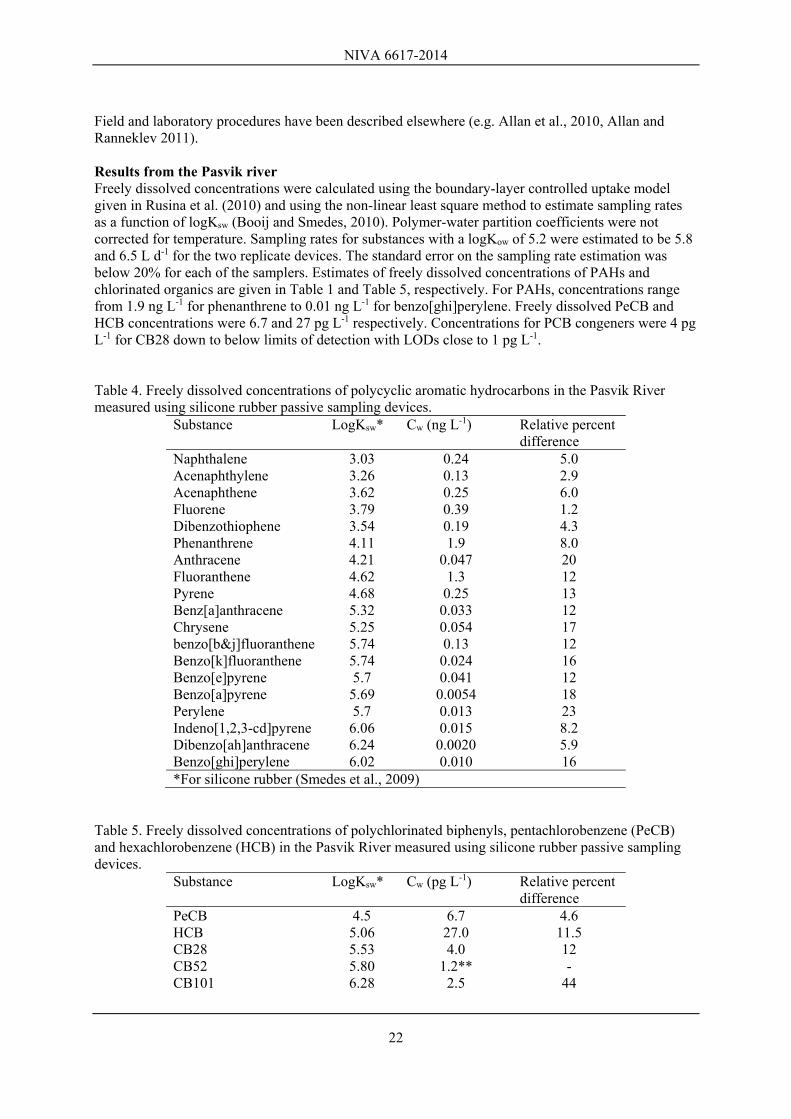
Field and laboratory procedures have been described elsewhere (e.g. Allan et al., 2010, Allan and Ranneklev 2011). Results from the Pasvik river Freely dissolved concentrations were calculated using the boundary-layer controlled uptake model given in Rusina et al. (2010) and using the non-linear least square method to estimate sampling rates as a function of logKsw (Booij and Smedes, 2010). Polymer-water partition coefficients were not corrected for temperature. Sampling rates for substances with a logKow of 5.2 were estimated to be 5.8 and 6.5 L d-1 for the two replicate devices. The standard error on the sampling rate estimation was below 20% for each of the samplers. Estimates of freely dissolved concentrations of PAHs and chlorinated organics are given in Table 1 and Table 5, respectively. For PAHs, concentrations range from 1.9 ng L-1 for phenanthrene to 0.01 ng L-1 for benzo[ghi]perylene. Freely dissolved PeCB and HCB concentrations were 6.7 and 27 pg L-1 respectively. Concentrations for PCB congeners were 4 pg L-1 for CB28 down to below limits of detection with LODs close to 1 pg L-1. Table 4. Freely dissolved concentrations of polycyclic aromatic hydrocarbons in the Pasvik River measured using silicone rubber passive sampling devices.

Substance LogKsw* Cw (ng L-1) Relative percent difference

Naphthalene 3.03 0.24 5.0 Acenaphthylene 3.26 0.13 2.9 Acenaphthene 3.62 0.25 6.0 Fluorene 3.79 0.39 1.2 Dibenzothiophene 3.54 0.19 4.3 Phenanthrene 4.11 1.9 8.0 Anthracene 4.21 0.047 20 Fluoranthene 4.62 1.3 12 Pyrene 4.68 0.25 13 Benz[a]anthracene 5.32 0.033 12 Chrysene 5.25 0.054 17 benzo[b&j]fluoranthene 5.74 0.13 12 Benzo[k]fluoranthene 5.74 0.024 16 Benzo[e]pyrene 5.7 0.041 12 Benzo[a]pyrene 5.69 0.0054 18 Perylene 5.7 0.013 23 Indeno[1,2,3-cd]pyrene 6.06 0.015 8.2 Dibenzo[ah]anthracene 6.24 0.0020 5.9 Benzo[ghi]perylene 6.02 0.010 16 *For silicone rubber (Smedes et al., 2009)

Table 5. Freely dissolved concentrations of polychlorinated biphenyls, pentachlorobenzene (PeCB) and hexachlorobenzene (HCB) in the Pasvik River measured using silicone rubber passive sampling devices.

Substance LogKsw* Cw (pg L-1) Relative percent difference

PeCB 4.5 6.7 4.6 HCB 5.06 27.0 11.5 CB28 5.53 4.0 12 CB52 5.80 1.2** - CB101 6.28 2.5 44

NIVA 6617-2014

23

CB118 6.42 1.1 27 CB105 6.42 1.2 29 CB153 6.72 < 1.0 - CB138 6.77 1.1 12 CB156 6.72 < 1.0 - CB180 6.99 < 1.1 - CB209 8.51 < 1.5 - *For silicone rubber (Smedes et al., 2009) **One measurement above limits of detection

Discussion Most compounds of interest were detected and quantified in the freely dissolved phase in the Pasvik River. As expected, highest PAH concentrations were found for the least hydrophobic substances while those with logKow over 5-6 were well below 1 ng L-1. Concentrations of low molecular weight PAHs were significantly lower in the River Pasvik than in the Aln or Glomma (Table 6). Less difference could be observed for the higher molecular weight PAHs. PCB concentrations were in the low pg L-1 range or below. PCB concentrations were found to be lower than those measured with silicone samplers in the Alna River a relatively polluted stream that runs through Oslo (Allan et al. 2011; Allan et al., 2013). Table 6. Comparison of freely dissolved concentrations of PAHs measured with silicone samplers in the Rivers Alna, Glomma and Pasvik.

Substance Cfree (ng L-1

)

Pasvik Glomma Alna

Acenaphthylene 0.13 0.26 0.78

Acenaphthene 0.25 1.6 2.1

Fluorene 0.39 1.2 3.6

Dibenzothiophene 0.19 0.17 4.1

Phenanthrene 1.9 3.2 13.7

Anthracene 0.047 0.13 3.3

Fluoranthene 1.3 0.59 5.4

Pyrene 0.25 0.33 7.3

Benz[a]anthracene 0.033 0.024 0.31

Chrysene 0.054 0.033 0.36

benzo[b&j]fluoranthene 0.13 0.034 0.13

Benzo[k]fluoranthene 0.024 <0.01 0.042

Benzo[e]pyrene 0.041 0.018 0.12

Benzo[a]pyrene 0.0054 <0.01 0.042

Perylene 0.013 0.037 0.017

Indeno[1,2,3-cd]pyrene 0.015 <0.01 0.012

Dibenzo[ah]anthracene 0.002 <0.01 <0.005

Benzo[ghi]perylene 0.01 <0.01 0.022

NIVA 6617-2014

24

5. Source-apportionment models as tools to estimate riverine inputs

5.1 The TEOTIL model

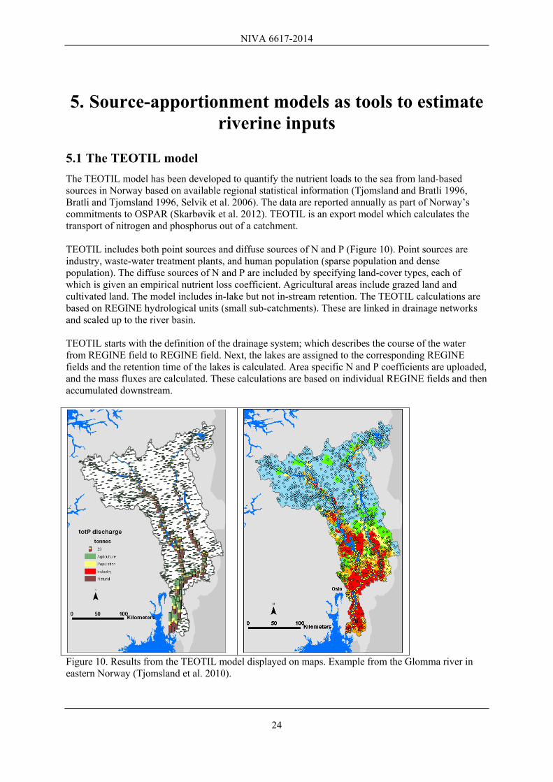
The TEOTIL model has been developed to quantify the nutrient loads to the sea from land-based sources in Norway based on available regional statistical information (Tjomsland and Bratli 1996, Bratli and Tjomsland 1996, Selvik et al. 2006). The data are reported annually as part of Norway’s commitments to OSPAR (Skarbøvik et al. 2012). TEOTIL is an export model which calculates the transport of nitrogen and phosphorus out of a catchment. TEOTIL includes both point sources and diffuse sources of N and P (Figure 10). Point sources are industry, waste-water treatment plants, and human population (sparse population and dense population). The diffuse sources of N and P are included by specifying land-cover types, each of which is given an empirical nutrient loss coefficient. Agricultural areas include grazed land and cultivated land. The model includes in-lake but not in-stream retention. The TEOTIL calculations are based on REGINE hydrological units (small sub-catchments). These are linked in drainage networks and scaled up to the river basin. TEOTIL starts with the definition of the drainage system; which describes the course of the water from REGINE field to REGINE field. Next, the lakes are assigned to the corresponding REGINE fields and the retention time of the lakes is calculated. Area specific N and P coefficients are uploaded, and the mass fluxes are calculated. These calculations are based on individual REGINE fields and then accumulated downstream.

Figure 10. Results from the TEOTIL model displayed on maps. Example from the Glomma river in eastern Norway (Tjomsland et al. 2010).

NIVA 6617-2014

25

5.2 Application of the TEOTIL model within the RID programme

Within the Norwegian RID programme (Skarbøvik et al. 2012) the TEOTIL model has been utilised for pollution load compilations of nitrogen and phosphorus in unmonitored catchments or groups of unmonitored catchments (in order to estimate the total N and P load from the entire Norwegian mainland). The point source estimates are based on national statistical information on sewage, industrial effluents, and aquaculture (fish farming). Nutrient loads from diffuse sources (agricultural land and natural runoff from forest and mountain areas) are modelled by a coefficient approach (Selvik et al., 2006). Area specific export coefficients for nutrients have been estimated for agricultural land in different geographical regions. The coefficients are based on empirical data from agricultural monitoring fields in Norway and are adjusted annually by Bioforsk based on reported changes in agricultural practice (national statistics). For forest and mountain areas, concentration coefficients for different area types and geographical regions have been estimated based on monitoring data from reference sites. The annual loads of natural runoff vary from year to year depending on the annual discharge. So far, the TEOTIL model has been applied on N and P export only. Other elements might be included in future versions of the model (e.g. heavy metals), but this will require further developments of the model and extensive testing against measured data.

NIVA 6617-2014

26

6. Meetings/workshops and further work

Project meetings / workshops An important element in the project has been to maintain and further develop the Norwegian-Russian cooperation in the Barents Region by bringing together key research institutes from both sides of the border. The best way to achieve this is through project meetings/workshops, where the researchers involved can share competences, experiences and data that can improve our common understanding and thereby contribute to a better and more knowledge-based management of the rivers discharging into the Barents Sea. Two bilateral project meetings/workshops have been carried out during the project:

- 18-20 June 2012: Scientific workshop, Pasvik - 21-22 October : Final meeting, Oslo

The workshop programmes are displayed in Appendix D and E, respectively. Presentations held at the workshops are stored electronically at NIVA, and pdf-files can be made available on request. Recommendations for future work The review of Russian and Norwegian methods for measuring heavy metals and other water quality determinants show that the approaches are quite similar and the detection limits are generally low and comparable for most variables. Hence, there is a very good basis for exchanging data and development of more integrated monitoring activities in main rivers draining to the Barents Sea. Access to existing data from Russian rivers can be a challenge, however, due to restrictions set by different data-owners. An improved access to historical data would be extremely valuable as basis for future monitoring and assessments. Implementation of novel monitoring techniques, including real-time measurements and use of time-integrative passive sampling techniques (cf. pilot studies performed in this project) is highly recommended. The latter can be especially relevant in remote areas, due to relatively low cost and the abilities to detect and quantify heavy metals as well as organic contaminants, which is a major environmental concern in arctic regions.

NIVA 6617-2014

27

7. References

Allan, I.J., Booij, K., Paschke, A., Vrana, B., Mills, G.A., Greenwood, R. 2009. Field Performance of Seven Passive Sampling Devices for Monitoring of Hydrophobic Substances. Environmental Science & Technology 43: 5383-5390.

Allan, I.J., Harman, C., Kringstad, A., Bratsberg, E. 2010. Effect of sampler material on the uptake of PAHs into passive sampling devices. Chemosphere 79: 470-475.

Allan, I.J., Harman, C., Ranneklev, S.B., Thomas, K.V., Grung, M. 2013. Passive sampling for target and nontarget analyses of moderately polar and nonpolar substances in water. Environmental Toxicology and Chemistry 32: 1718-1726.

Allan, I.J., Ranneklev, S.B. 2011. Occurrence of PAHs and PCBs in the Alna River, Oslo (Norway). Journal of Environmental Monitoring 13: 2420-2426.

Booij, K., Sleiderink, H.M., Smedes, F. 1998. Calibrating the uptake kinetics of semipermeable membrane devices using exposure standards. Environmental Toxicology and Chemistry 17: 1236-1245.

Booij, K., Smedes, F., 2010. An Improved Method for Estimating in Situ Sampling Rates of Nonpolar Passive Samplers. Environmental Science & Technology 44: 6789-6794.

Booij, K., Smedes, F., van Weerlee, E.M. 2002. Spiking of performance reference compounds in low density polyethylene and silicone passive water samplers. Chemosphere 46: 1157-1161.

Bratli, J.L., Tjomsland, T. 1996. TEOTIL Presentasjon av tilførselsdata på kart ved et geografisk informasjonssystem. [TEOTIL. Presentation of input data on maps with a geographical information system]. NIVA report 3556, 103 pp.

Brittain, J.E., Bogen. J., Khokhlova, L.G., Melvold, K., Stenina, A.S., Gislason, G.M., Brørs, S., Kochanov, S.K., Olafsson, J.S., Ponomarev, V.I., Jensen, A.J., Kokovkin, A.V., Petterson, L-E. 2008. Arctic Rivers. In: Tockner, K., Uehlinger, U., Robinson, C.T. Rivers of Europe. Academic Press, 728 pp.

Chultsova, A.L. 2009. Assessment of the state of biogenic elements in the winter low-water period 2007-2008 in the Delta of the Northern Dvina. Mater. XVIII International conference (school) on marine Geology «Geology of seas and oceans». Moscow. Publishing house GEOS. So 3. p. 268-271.

Chultsova, A.L. 2009. The distribution of biogenic elements in the Delta of the Northern Dvina in the winter low water period 2007-2008. Materials of the scientific conference (with international participation). «Modern fundamental problems of hydrochemistry and monitoring the quality of surface waters of Russia». Rostov-on-Don. LLC «Virazh». part 1. p. 255-257.

Chultsova, A.L. 2010. The distribution biogenic elements in the marginal filter Zolotica river - The White Sea in July 2009. Proceedings of XI All-Russian conference with international participation «Problems of studying, rational use and protection of natural resources of the White Sea». St. Petersburg. Zoological Institute of the Russian Academy of Sciences. P. 207-208.

Chultsova, A.L., Skibinski, L.E. 2008. Distribution of biogenic substances in snow and ice cover estuary of the Northern Dvina river. Materials of all-Russian scientific conference dedicated to the International Polar Year (2007-2008), «Studies of the Russian Arctic: past, present, future». Arkhangelsk. p. 205-211.

Chultsova, A.L., Skibinski, L.E. 2009. Ecological and hydrochemical condition of the ice and snow cover mouths of the rivers of the Arctic (on the example of the Northern Dvina river). Materials of the XXI Symposium «Modern chemical physics».

NIVA 6617-2014

28

Davison W, Zhang H.1994. In situ speciation measurements of trace components in natural waters using thin-film gels. Nature 367: 546–548

Green, N., Molvær, J., Kaste, Ø., Schrum, C., Yakushev, E., Sørensen, K., Allan, I., Høgåsen, T., Christiansen, A., Heldal, H.E., Klungsøyr, J., Boitsov, S., Børsheim, K.Y., Måge, A., Jalshamn, K., Aas, W., Braathen, O-A. , Breivik, K., Eckhardt, S., Rudjord, A.L., Iosjpe, M., Brungot, A.L. 2010. Tilførselsprogrammet 2009. Overvåking av tilførsler og miljøtilstand i Barentshavet og Lofotenområdet. [The Marine Pollution Monitoring Programme 2009. Monitoring of discharges and environmental status in the Barents Sea and the Lofoten area] NIVA report 5980, 243 pp.

Green, N., Skogen, M., Aas, W., Iosjpe. M, Måge, A., Breivik, K., Yakushev, E., Høgåsen, T., Eckhardt, S., Ledang, A., Jaccard, P., Staalstrøm, A., Isachsen, P.E., Frantzen, S. 2013. Tilførselsprogrammet 2012. Overvåking av tilførsler og miljøtilstand i Barentshavet og Lofotenområdet [The Marine Pollution Monitoring Programme 2012. Monitoring of discharges and environmental status in the Barents Sea and the Lofoten area]. NIVA report 6544, 149 pp.

Huckins, J.N., Petty, J.D., Booij, K. 2006. Monitors of organic chemicals in the environment: Semipermeable membrane devices. Springer, New York.

Huckins, J.N., Petty, J.D., Lebo, J.A., Almeida, F.V., Booij, K., Alvarez, D.A., Clark, R.C., Mogensen, B.B. 2002. Development of the permeability/performance reference compound approach for in situ calibration of semipermeable membrane devices. Environmental Science & Technology 36: 85-91.

Khomenko, G.D, Leshchyov, A.V. 2010. Runoff coastal front in the Pechora Sea. Bulletin of the Pomeranian University. Series "Natural Sciences" no. 4.

Khomenko, G.D. 2010. At the turn of oceanography and hydrology – the moth of rivers. Proceedings of International conference «50 Years of Education and Awareness Raising for Shaping the Future of the Ocean and Coasts». St.Petersburg.

Kotova, E.I., Korobov, V.B., Shevchenko V.P. 2012. Features of formation of the ionic composition of the snow cover in the coastal zone of the western sector of the Arctic. - Modern Problems of Education, No 6.

Kuznetsov, V. Miskevich, I., Zaytsev, G. 1991. Hydrochemical characteristics of the large rivers of the basin of Northern Dvina, L. Gidrometeoizdat

Lukin A., Dauvalter V., Novoselov A. 2000. Ecosystem of the Pechora river in modern conditions. Apatity. Kola Sci Centre Russ Acad Sci Publ, 192 pp.

MacDonald, R. W., T. Harner and J. Fyfe, 2005. "Recent climate change in the Arctic and its impact on contaminant pathways and interpretation of temporal trend data." Science Of The Total Environment 342(1-3): 5-86.

Moiseenko, T. (INEP) Mjelde, M. Brandrud, T.E. Brettum, P. Dauvaltar, V. (INEP) Kagan, L. (INEP) Kashulin, N. (INEP) Kudriavtseva, L. (INEP) Lukin, A. (INEP) Sandimirov, S. (INEP) Traaen, T.S. Vandysh, O. (INEP) Yakovlev, V. (INEP), 1994. Pasvik River Watercourse, Barents region: Pollution Impacts and Ecological Responses Investigation in 1993. Norsk institutt for vannforskning (NIVA). Rapport 1. nr OR-3118. 87 s.

Nøst, T., Lukin, A., Schartau, A.K.L., Kashulin, N., Berger, H.M., Yakolev, V., Sharov, A. & Danvalter, V. 1997. Impacts of pollution on freshwater communities in the border region between Russia and Norway. III. Results of the 1990-96 monitoring programme. - NINA Fagrapport 29. 37 s. (With Russian abstract).

Orr, J. C., V. J. Fabry, O. Aumont et al., 2005. Anthropogenic ocean acidification over the twenty-first century and its impact on calcifying organisms. Nature 437, 681-686, 2005.

NIVA 6617-2014

29

Ovsepyan A., Fedorov, Y. 2011. Mercury in the Northern Dvina River Estuarine Area. Rostov-on-Don. 109.

Puro-Tahvanainen, A., Zueva, M., Kashulin, N., Sandimirov, S., Christensen, G.N., Grekelä, I. 2011. Pasvik Water Quality Report. Environmental Monitoring Programme in the Norwegian, Finnish and Russian Border Area. Centre for Economic Development, Transport and the Environment for Lapland, Publications 7/2011, 52 pp.

Rognerud, S., Fjeld, E., Skjelkvåle, B.L., Christensen, G., Røyset, O. 2008. Nasjonal innsjø-undersøkelse 2004 - 2006, del 2: Sedimenter. Forurensning av metaller, PAH og PCB. [National lake survey 2004 - 2006, part 2: Sediments. Pollution of metals, PAH and PCB]. NIVA report 5549, 77 s.

Røyset, O., Garmo, Aaberg Ø., Steinnes, E., Flaten, T.P. 2002. Performance study of diffusive gradients in thin films (DGT) for 55 elements. NIVA report 4604.

Rusina, T.P., Smedes, F., Koblizkova, M., Klanova, J. 2010. Calibration of Silicone Rubber Passive Samplers: Experimental and Modeled Relations between Sampling Rate and Compound Properties. Environmental Science & Technology 44: 362-367.

Ruus, A; Green, NW; Maage, A; Amundsen, CE; Schoyen, M; Skei, J. 2010. Post World War II orcharding creates present day DDT-problems in The Sorfjord (Western Norway) - A case study. Marine Pollution Bulletin, 60: 1856-1861.

Schartau A.K. , Fjellheim A., Walseng B., Skjelkvåle B.L., Halvorsen G.A., Skancke L.B., Saksgård R., Manø S., Solberg S., Jensen T.C., Høgåsen T., Hesthagen T., Aas W., Garmo Ø., 2012. Overvåking av langtransportert forurenset luft og nedbør. Årsrapport - Effekter 2011. [Monitoring of long-range transboundary air pollution in Norway. Effects in 2011] The Climate and Pollution Directorate (Klif). Report TA 2934/2012, 160 pp.

Selvik, J.R., Tjomsland, T., Borgvang, S.A., Eggestad, H.O.. 2006. Tilførsler av næringssalter til Norges kystområder i 2005, beregnet med tilførselsmodellen TEOTIL2. Norwegian State Pollution Control Authority, Report 973/2006.

Skarbøvik, E., Stålnacke, P., Austnes, K., Selvik, J.R., Aakerøy, P.A., Tjomsland, T., Høgåsen, T., Beldring, S. 2012. Riverine inputs and direct discharges to Norwegian coastal waters – 2011. The Climate and Pollution Directorate (Klif). Report TA-2986/2012, 66 pp + Appendices and Addendum.

Smedes, F., Geertsma, R.W., van der Zande, T., Booij, K. 2009. Polymer-Water Partition Coefficients of Hydrophobic Compounds for Passive Sampling: Application of Cosolvent Models for Validation. Environmental Science & Technology 43: 7047-7054.

Smith, K. E. C. and M. S. McLachlan (2006). "Concentrations and partitioning of polychlorinated biphenyls in the surface waters of the southern Baltic Sea - Seasonal effects." Environmental Toxicology And Chemistry 25(10): 2569-2575.

Stuanes, A.O., de Wit, H.A., Hole, L.R., Kaste, Ø., Mulder, J., Riise, G., Wright, R.F. 2008. Effect of Climate Change on Flux of N and C: Air-Land-Freshwater-Marine Links: Synthesis. Ambio 37: 2-8.

Sunnanå, K., Fossheim, M., Olseng, C.D. (Eds), 2010. Forvaltningsplan Barentshavet. Rapport fra Overvåkningsgruppen [Management plan for the Barents Sea. Report from the monitoring group]. Fisken og Havet, Særnummer 1b-2010, 110 sider.

Tjomsland, T., Bratli, J.L. 1996. Brukerveiledning for TEOTIL. Modell for teoretisk beregning av fosfor- og nitrogentilførsler i Norge. [User guideline for TEOTIL. Model for calculation of phosphorus and nitrogen inputs in Norway]. NIVA report 3426, 84 pp.

NIVA 6617-2014

30

Tjomsland, T., Selvik, J., Brænden, R. 2010. Teotil - Model for calculation of source dependent loads in river basins. NIVA report 5914, 58 pp.

Traaen, T., Arnesen, R.T., Moiseenko, Tatjana, INEP Mokrotovarova, Olga, MUGMS Kudryavtseva, Ljuba, INEP, 1996. Heavy metals from the Nikel area Investigation in Kolosjoki river 1995, Kola Peninsula, Russia. Norsk institutt for vannforskning (NIVA). Rapport 1. nr OR-3543. 37 s.

Vrana, B., Mills, G.A., Allan, I.J., Dominiak, E., Svensson, K., Knutsson, J., Morrison, G., Greenwood, R. 2005. Passive sampling techniques for monitoring pollutants in water. Trac-Trends in Analytical Chemistry 24: 845-868.

Warnken, K., Zhang, H., Davison, W. 2007. In situ monitoring and dynamic speciation measurements in solution using DGT. In; R. Greenwood, G. Mills and B. Vrana (eds) passive sampling techniques in environmental monitoring. Compr Anal Chem 48: 251–278

Zhang, H., Davison, W. 1995. Performance-characteristics of diffusion gradients in thin-films for the in-situ measurement of trace-metals in aqueous-solution. Anal Chem 67: 3391–3400

NIV

A 6

617-

2014

31

Ap

pen

dix

A.

An

alyt

ical

met

hod

s

A1

– M

eth

ods

and

eq

uip

men

t ap

pli

ed a

t N

IVA

Variable:

Unit

Nam

e of method

Analytic instrument

Detection limit

Reference

Lead

(Pb)

µg/L

Perkin‐Elm

er Sciex ELAN 6000 ICP‐M

S,

with P‐E autosampler AS‐90, A

S‐90b

sample board and P‐E Rinsing Port Kit.

0.005

NIVA’s accredited method E8‐3

Cadmium (Cd)

µg/L

Same equipment (ICP‐M

S)0.005


Copper (Cu)

µg/L


S)0.01


Zinc (Zn)

µg/L


S)0.05


Arsenic (As)

µg/L


S)0.05


Chromium (Cr)

µg/L


S)0.1


Nickel (Ni)

µg/L


S)0.05


Mercury (Hg)

ng/L

Perkin‐Elm

er FIMS‐400 with P‐E AS‐90

autosampler and P‐E Amalgam System

AA Accessory

1NS‐EN

1483 and NIVA’s accredited method E4‐3

Optional:

pH

Metrohm titrator (Titrino 799 GPT)

0.01

NS 4720

Conductivity

mS/m

Metrohm Conductivity Meter 712

0.05

NS‐ISO 7888

Suspended particulate matter (SPM)

mg/L

Sartorius 4503 Micro with Static

Elim

inator Bar Pu 210, Item LC 9793

0.1

NS 4733 modified, nuclepore filter with mesh size

0.4 μm and diameter 47 mm.

Total O

rganic Carbon (TO

C)

mg C/L

Phoenix 8000 TO

C‐TC analysator

0.1

EPA number 415.1 and 9060A

STD

.

Total phosphorus

µg P/L

Peroxidisulphate oxidation method

Skalar San

Plus Autoanalysator

1NS 4725 –

Orthophosphate (PO4‐P)

µg P/L

Automated molybdate method

Skalar San

Plus Autoanalysator

1NS 4724 –

Total nitrogen

µg N/L


Skalar San

Plus Autoanalysator

10NS 4743 –

Nitrate (NO3‐N)

µgN

/LLiquid chromatography

Dionex model D

X 320

1NS‐EN

ISO 10304‐1

Ammonium (NH4‐N)

µg N/L

Liquid chromatography

Dionex model D

X 320

2NS‐EN

ISO 14911

Silicate (SiO2)

mg SiO2/L

ICP‐AES

0.02

ISO 11885 + NIVA’s accredited method E9‐5

NIV

A 6

617-

2014

32

A2

– M

eth

ods

and

eq

uip

men

t ap

pli

ed a

t IO

-RA

S

Param

eter

Unit

Nam

e of method

Analytic instrument

Detection limit

Reference

Lead

(Pb)

µg/L

Atomic absorption spectrometry (AAS)

Atomic Absorption Spectrometry "Kvant‐2A

"2

Accredited method PND F 14.1:2.214‐2006

Cadmium (Cd)

µg/L



"0.2‐0.3


Copper (Cu)

µg/L



"0.4‐0.6


Zinc (Zn)

µg/L



"0.2‐0.3


Arsenic (As)

µg/L

Hydride generation technique


"

Generator mercury ‐ hydride "GRG‐107"

0.05


Chromium (Cr)

µg/L



"1.5‐2


Nickel (Ni)

µg/L



"3


Mercury (Hg)

ng/L

Cold vapor technique


"

Generator mercury ‐ hydride "GRG‐107"

6Accredited method PND F 14.1:2.20‐95

Optional

pH

pH‐m

eter HI 991001 by «HANNA instrument»

0.01

RD 52.10.243‐92

Conductivity

mS/cm

(mkS/cm)

Cond 197i from W

TW (Germ

any)

0.01

EhmV

ORP HI 988202 by «HANNA instrument»

0.1

RD 52.10.243‐92


membrane ultrafiltration method

under vacuum through

nuclear filters

with a diameter of 0.45 mm

3PND F 14.1:2.110‐97

Total O

rganic Carbon (TO

C)

Total phosphorus

µg/L

Colorimetric method

Single‐beam

spectrophotometer UNICO

(model 1201), the company «United Products

& Instruments, Inc», U

SA0.01

RD 52.10.243‐92


µg/L

Colorimetric method

‐//‐

0.01

RD 52.10.243‐92

Total nitrogen

‐‐

‐‐

Nitrate (NO3‐N)

µg/L

Colorimetric method

‐//‐

0.01

RD 52.10.243‐92

Nitrite (NO2‐N)

µg/L

Colorimetric method

‐//‐

0.01

RD 52.10.243‐92

Ammonium (NH4‐N)

‐‐

‐‐

Silicate (SiO2)

µg/L

Colorimetric method

‐//‐

0.1

RD 52.10.243‐92

Oxygen (O2)

µg/L

Winkler method

0.02

RD 52.10.243‐92

NIV

A 6

617-

2014

33

A3

– M

eth

ods

and

eq

uip

men

t ap

pli

ed a

t IN

EP

Param

eter

Unit

Nam

e of method

Analytic instrument

Detection limit

Reference

Lead

(Pb)

µg/L

AAS‐GF

Perkin‐Elm

er Aanalyst‐800, with P‐E

autosampler AS‐800.

0.5

Russia’s accredited method

Cadmium (Cd)

µg/L

AAS‐GF

Perkin‐Elm


autosampler AS‐800.

0.05


Copper (Cu)

µg/L

AAS‐GF

Perkin‐Elm

er ‐5000, HGA‐400

0.2


Zinc (Zn)

µg/L

AAS‐GF

Perkin‐Elm

er ‐5000, HGA‐400

0.1


Cobalt (Co)

µg/L

AAS‐GF

Perkin‐Elm


0.5


Chromium (Cr)

µg/L

AAS‐GF

Perkin‐Elm

er ‐5000, HGA‐400

0.2


Nickel (Ni)

µg/L

AAS‐GF

Perkin‐Elm

er ‐5000, HGA‐400

0.5


Lead

(Pb)

µg/L

ICP‐EOS

Perkin‐Elm

er ICP‐EOS O

PTIMA 2100D

V1


Cadmium (Cd)

µg/L

ICP‐EOS

Perkin‐Elm

er ICP‐EOS O

PTIMA 2100D

V0.1


Copper (Cu)

µg/L

ICP‐EOS

Perkin‐Elm

er ICP‐EOS O

PTIMA 2100D

V0.5


Zinc (Zn)

µg/L

ICP‐EOS

Perkin‐Elm

er ICP‐EOS O

PTIMA 2100D

V0.2


Cobalt (Co)

µg/L

ICP‐EOS

Perkin‐Elm

er ICP‐EOS O

PTIMA 2100D

V0.3


Chromium (Cr)

µg/L

ICP‐EOS

Perkin‐Elm

er ICP‐EOS O

PTIMA 2100D

V0.2


Nickel (Ni)

µg/L

ICP‐EOS

Perkin‐Elm

er ICP‐EOS O

PTIMA 2100D

V0.4


Lead

(Pb)

µg/L

ICP‐M

SPerkin‐Elm

er ICP‐M

S ELAN 9000

0.005


Cadmium (Cd)

µg/L

ICP‐M

SPerkin‐Elm

er ICP‐M

S ELAN 9000

0.005


Copper (Cu)

µg/L

ICP‐M

SPerkin‐Elm

er ICP‐M

S ELAN 9000

0.005


Zinc (Zn)

µg/L

ICP‐M

SPerkin‐Elm

er ICP‐M

S ELAN 9000

0.03


Cobalt (Co)

µg/L

ICP‐M

SPerkin‐Elm

er ICP‐M

S ELAN 9000

0.01


Chromium (Cr)

µg/L

ICP‐M

SPerkin‐Elm

er ICP‐M

S ELAN 9000

0.1


Nickel (Ni)

µg/L

ICP‐M

SPerkin‐Elm

er ICP‐M

S ELAN 9000

0.05


Optional

pH

Metrohm pHM‐82

0.01


Conductivity

mS/m

Metrohm Conductivity Meter 660

0.05



mg/L

Sartorius 2472

0.1


Total O

rganic Carbon (TO

C)

Total phosphorus

µg P/L


Spectrophotometry

2Russia’s accredited method


µg P/L

Molybdate method

Spectrophotometry


Total nitrogen

µg N/L


Spectrophotometry

1 0Russia’s accredited method

Nitrate (NO3‐N)

µgN

/LCd reduction method

Spectrophotometry


Ammonium (NH4‐N)

µg N/L

Phenol‐hypochlorite method

Spectrophotometry


Silicate (SiO2)

mg SiO2/L

Molybdate method

Spectrophotometry


NIV

A 6

617-

2014

34

A

pp

end

ix B

. R

iver

dat

a

B1.

Nor

weg

ian

riv

ers

(sor

ted

fro

m w

est

to e

ast)

– c

atch

men

t ch

arac

teri

stic

s (S

kar

bøv

ik e

t al

. 201

2)

Nam

e of river

Catchment

Mean

flow

Position at outlet

Dominating landuse

Population

Hydrol data

Water quality data (m

etals)

Water quality data (other param

eters)

km2

m3/s

Latitude/longitude

Barduelva

2906

82.2398

69.04299/18.596474

88% Mountains, 10%

forest

5046

yes

As, Cd, Cr, Cu, H

g, Ni,Pb, Zn *

pH, Kond, TOC, SPM, Tot‐N, NH4, NO3, Tot‐P, PO

4, SiO

2, PCB, Lindan***

Målselv

3200

92.9

69.035985/18.667482

84% Mountains, 12%

forest

2480

yes

As, Cd, Cr, Cu, H

g, Ni,Pb, Zn*


4, SiO

2, PCB, Lindan***

Nordkjoselva

191

5.2907

69.217998/19.55799

72% Forest, 15%

mountains

1194

yes

As, Cd, Cr, Cu, H

g, Ni,Pb, Zn**


4, SiO

2, PCB, Lindan***

Signaldalselva

473

13.1021

69.265994/19.898977

87% Mountains, 9% forest

3649

yes

As, Cd, Cr, Cu, H

g, Ni,Pb, Zn**


4, SiO

2, PCB, Lindan***

Skibotnelva

770

13.86

69.363996/20.274979

Mountains

583

yes

As, Cd, Cr, Cu, H

g, Ni,Pb, Zn**


4, SiO

2, PCB, Lindan***

Kåfjordelva

358

7.16

69.491993/20.815979

Mountains

1501

yes

As, Cd, Cr, Cu, H

g, Ni,Pb, Zn**


4, SiO

2, PCB, Lindan***

Reisa

2702

43.232

69.764991/21.017979

60% Mountains, 33%

forest

1089

yes

As, Cd, Cr, Cu, H

g, Ni,Pb, Zn**


4, SiO

2, PCB, Lindan***

Mattiselva

325

8.6125

69.913991/23.032989

Mountains

336

yes

As, Cd, Cr, Cu, H

g, Ni,Pb, Zn**


4, SiO

2, PCB, Lindan***

Tverrelva

234

3.5334

69.956994/23.412996

Mountains

1325

yes

As, Cd, Cr, Cu, H

g, Ni,Pb, Zn**


4, SiO

2, PCB, Lindan***

Repparfjordvasdraget

1090

27.25

70.443998/24.333

Mountains

381

yes

As, Cd, Cr, Cu, H

g, Ni,Pb, Zn**


4, SiO

2, PCB, Lindan***

Stabburselva

1108

20.2764

70.181993/24.908978

Mountains

331

yes

As, Cd, Cr, Cu, H

g, Ni,Pb, Zn**


4, SiO

2, PCB, Lindan***

Lakselv

1533

24.3747

70.065995/24.930985

Mountains

890

yes

As, Cd, Cr, Cu, H

g, Ni,Pb, Zn**


4, SiO

2, PCB, Lindan***

Børselva

883

26.3134

70.315993/25.568997

Mountains

323

yes

As, Cd, Cr, Cu, H

g, Ni,Pb, Zn**


4, SiO

2, PCB, Lindan***

Mattusjåkka

101

2.3028

70.389991/26.489998

Mountains

71yes

As, Cd, Cr, Cu, H

g, Ni,Pb, Zn**


4, SiO

2, PCB, Lindan***

Storelva (Stuorrajåkka)

690

15.111

70.313992/26.387991

Mountains

71yes

As, Cd, Cr, Cu, H

g, Ni,Pb, Zn**


4, SiO

2, PCB, Lindan***

Soussjåkka

922.3276

70.343995/26.520978

Mountains

71yes

As, Cd, Cr, Cu, H

g, Ni,Pb, Zn**


4, SiO

2, PCB, Lindan***

Adam

selva

705

14.0295

70.381991/26.633989

Mountains

279

yes

As, Cd, Cr, Cu, H

g, Ni,Pb, Zn**


4, SiO

2, PCB, Lindan***

Tanavassdraget

16389

188.4735

70.229993/28.173988

Mountains

5700

yes

As, Cd, Cr, Cu, H

g, Ni,Pb, Zn*


4, SiO

2, PCB, Lindan***

Vesterelva

469

16.2274

70.525998/29.997978

Mountains

51yes

As, Cd, Cr, Cu, H

g, Ni,Pb, Zn**


4, SiO

2, PCB, Lindan***

V. Jakobselv

627

11.3487

70.112/29.328976

Mountains

785

yes

As, Cd, Cr, Cu, H

g, Ni,Pb, Zn**


4, SiO

2, PCB, Lindan***

Pasvikelva

18404

171.1572

69.500996/30.115996

Mountains

1129

yes

As, Cd, Cr, Cu, H

g, Ni,Pb, Zn*


4, SiO

2, PCB, Lindan***

Neiden

2960

29.008

69.691992/29.369979

Mountains

390

yes

As, Cd, Cr, Cu, H

g, Ni,Pb, Zn**


4, SiO

2, PCB, Lindan***

Grense Jakobselv

234

4.212

69.730995/30.886987

Mountains

266

yes

As, Cd, Cr, Cu, H

g, Ni,Pb, Zn**


4, SiO

2, PCB, Lindan***

* 0‐1 times/yr, 1990‐2003, 4 tim

es/yr from 2004

** 0‐1 tim

es/yr, 1990‐2003

*** frequency as for metals

NIV

A 6

617-

2014

35

B2.

Nor

weg

ian

riv

ers

(sor

ted

fro

m w

est

to e

ast)

– c

hem

ical

dat

a (S

kar

bøv

ik e

t al

. 201

2)

Arithmetic m

ean 1990‐2011

Nam

e of river

TOC

SPM

Cu

Cd

Cr

Ni

ZnHg

Pb

mg C/L

mg/L

µg/L

µg/L

µg/L

µg/L

µg/L

µg/L

µg/L

Barduelva

1.3

6.68

0.80

0.010

1.5

0.86

2.45

0.001

0.11

Målselv

1.3

6.99

0.75

0.010

1.6

0.94

1.85

0.001

0.11

Nordkjoselva

1.0

1.34

0.60

0.018

0.4

0.32

0.70

0.002

0.11

Signaldalselva

3.7

3.10

0.86

0.018

1.0

0.67

1.38

0.002

0.17

Skibotnelva

1.4

0.81

0.66

0.019

0.4

0.87

0.74

0.002

0.12

Kåfjordelva

0.78

0.79

1.26

0.024

0.4

0.57

0.94

0.001

0.10

Reisa

1.6

1.27

0.87

0.020

0.4

0.47

0.96

0.002

0.13

Mattiselva

2.1

0.61

0.72

0.019

0.5

0.43

1.00

0.002

0.18

Tverrelva

3.6

0.89

0.87

0.018

0.6

0.49

0.98

0.002

0.11

Repparfjordvasdraget

2.8

0.61

1.07

0.017

0.8

0.47

0.64

0.002

0.10

Stabburselva

2.2

0.61

0.72

0.022

0.5

0.34

0.83

0.001

0.34

Lakselv

2.5

4.19

0.82

0.016

0.8

0.64

0.90

0.002

0.18

Børselva

0.90

0.74

0.29

0.017

0.5

0.29

1.42

0.002

0.15

Mattusjåkka

1.2

0.71

0.46

0.028

2.2

0.54

2.02

0.002

0.24

Storelva (Stuorrajåkka)

0.72

0.45

0.33

0.022

1.7

0.71

1.76

0.002

0.15

Soussjåkka

1.1

0.55

0.29

0.019

0.7

0.35

1.22

0.002

0.11

Adam

selva

1.7

0.58

0.40

0.021

1.2

0.39

1.46

0.002

0.29

Tanavassdraget

3.1

1.32

0.90

0.019

0.4

0.39

2.57

0.001

0.19

Vesterelva

0.78

0.50

0.26

0.017

0.9

0.28

0.54

0.002

0.11

V. Jakobselv

2.0

0.65

0.3 8

0.018

0.8

0.40

0.89

0.002

0.11

Pasvikelva

3.3

1.38

3.26

0.021

0.4

6.71

2.08

0.001

0.14

Neiden

3.7

1.59

0.77

0.024

0.5

1.04

3.23

0.002

0.13

Grense Jakobselv

2.5

0.95

2.26

0.024

1.8

7.77

2.04

0.002

0.28

TOC = total organic carbon, SPM=suspended organic matter

NIV

A 6

617-

2014

36

B3.

Ru

ssia

n r

iver

s (s

orte

d f

rom

eas

t to

wes

t) –

cat

chm

ent

char

acte

rist

ics

Referen

ces: Brittain et al. 2008, G

rigory Khomen

ko (pers. comm.), A

nna Chultsova (pers. comm.), N

ikolay Kashulin

(pers. comm.)

Main river

Tributary river

Sub‐tributary

Catchment

Mean

flow Coordinates

Distance with

Landuse

Population

Pollution sources

Hydrological data

Data series

Data series

km2

m3/s

Degree N

Degree E

tidal fluct, km

in catchment

available

‐ metals

‐ other elements

Pechora

322000

4100

68.3045

54.4167

141

53.1% forest, 42.5%

natural grassland

no data

Industry, agriculture,

population

yes

Fe, Cu, A

l, Cd, Cr, Ni,

Zn, H

g, Pb

О2, NH4, NO3, NO2, PO4, totP,

Si, BOD5, phenols,

form

aldehyde, m

ethanol, DDT,

DDE, α‐HCH, β

‐HCH

Usa

93600

1310

65.9668

56.9335

Forest, tundra

"

Oil production

Kolva

18100

65.9213

57.3168

"

"

"

Northern Dvina

357000

3490

64.7000

40.4833

137

90.6% forest, 7.2%

arable

"


population

yes

"

Pinega

42600

430

64.1338

41.9007no

Forest, bogs,

agriculture, lakes

"

Population

yes

"

Yomtsa

14100

7063.5385

41.8853no

"

"

Agriculture, population

yes

"

Vaga

44800

384

62.8067

42.8700no

Mainly forest

"

"

yes

"

Uftyuga

6300

37.5

61.5520

46.2230no

Forest, bogs,

agriculture, lakes

"

"

yes

"

Vychegda

121000

1160

61.2833

46.6183no

"

"


population

yes

"

Vishera

8780

"

Yug

35600

292

60.7248

46.3249no

"

"

"

yes

"

Sukhona

50300

456

60.7263

46.3235no

"

"

"

yes

"

Vologda

3030

59.2850

40.2173no

"

"

"

yes

"

Northern Dvina estuary

(17 sampling points)

"

"

>40 yrs

"

"

Mezen

78000

866

66.1915

43.9712

56.5% forest, 24.8%

pasture, 11.9%

wetland

"

"

yes

"

Onega

56900

505

63.9343

37.9862

25

51.9%forest, 19.1%

arable, 11.3%

pasture,

14.7%wetland

"

"

yes

"

Kem

27700

275

64.9532

34.6713

9.8

Bogs, taiga,

agriculture, lakes

20000Agriculture, population

yes

"

Niva

12800

164

67.1541

32.3735

0.5

Forest, bogs,

agriculture, lakes

210000


population

yes

yes

Varzuga

9840

7766.2581

36.9398

8.3

49.9%forest, 20.2%

pasture, 26.2%

wetland,

400Agriculture, population

no

Ponoy

15500

140

66.9720

41.2882

12.36

Forest, bogs,

agriculture, lakes

1000

Population

no

Iokanga

6020

6068.0232

39.6237

6.2

"

2200

"

no

Voronya

9800

110

69.1751

35.7926

10.3

"

3000


population

yes

Kola

3850

4068.8834

33.0338

1 "

45000 "

yes

"

Monthly sam

pling

Tuloma

21500

241

68.8867

33.0085

10.4

"

34700 "

yes

"

Pechenga

1829

22.5

69.5500

31.2500

5.6

Bogs, taiga,

agriculture, lakes

19500 "

yes

"

Teriberka

2227

69.1681

35.1241

5.2

"

1000

No data

yes

"

Umba

6250

78.2

66.6566

34.3005

4.3

"

5532

Agriculture, population

yes

"

NIV

A 6

617-

2014

37

B4.

Ru

ssia

n r

iver

s (s

orte

d f

rom

eas

t to

wes

t) –

ch

emic

al d

ata

R

efer

ence

s:

1) L

ukin

set

al.

(200

0)

2) K

uzne

tsov

et a

l. (1

991)

. 3)

Ovs

epya

n an

d F

edor

ov (

2011

).

Main river

Tributary river

Sub‐tributary

Calcium

Colour

Cu

Ni

ZnHg

Reference

mg/L

mg Pt/L

µcg/L

µcg/L

µcg/L

µcg/L

Pechora

14.5‐14.8

0.5‐5.2

0‐5.2

0.2‐14.9

1

Usa

18.1

310.6‐2

0.4‐4.9

0.4‐12.2

1

Kolva

14.8

147

0.8‐12.5

0.7‐6.2

1.4‐16.9

1

Northern Dvina

13‐66

0.005‐0.18

2 (Ca), 3 (Hg)

Pinega

Yomtsa

Vaga

Uftyuga

Vychegda

7‐53.9

2

Vishera

Yug

Sukhona

Vologda

Onega

18.8

160

?

Kem

2.56

42?

NIV

A 6

617-

2014

38

Ap

pen

dix

C.

DG

T d

ata

Sit

eS

tati

on n

ame

Pos

itio

nS

ampl

eS

tart

exp

osur

eEn

d ex

posu

reL

abC

dC

rC

uN

iP

bZ

nC

oLa

titud

eLo

ngitu

deD

ate

Tim

eT

emp

CD

ate

Tim

eT

emp

Cµg

/lµg

/lµg

/lµg

/lµg

/lµg

/lµg

/lR

iver

Pin

ega

Mai

n st

atio

n64

.696

9443

.399

83D

GT

31/0

8/20

1210

:00

10.6

07/0

9/20

1209

:00

12.1

NIV

A0.

013

0.15

0.18

0.21

0.00

590.

67R

iver

Pin

ega

Mai

n st

atio

n64

.696

9443

.399

83D

GT

07/0

9/20

1209

:00

12.1

14/0

9/20

1209

:30

10.2

NIV

A0.

0017

0.15

0.08

10.

100.

0088

0.70

Riv

er P

ineg

aM

ain

stat

ion

64.6

9694

43.3

9983

DG

T14

/09/

2012

09:3

010

.221

/09/

2012

09:3

010

.2N

IVA

0.00

550.

170.

260.

170.

0230

1.9

Riv

er P

ineg

aM

ain

stat

ion

64.6

9694

43.3

9983

DG

T21

/09/

2012

09:3

010

.228

/09/

2012

09:3

010

.1N

IVA

0.00

250.

110.

110.

071

0.00

640.

37

Riv

er A

sham

baIn

flow

Bla

ck S

eaD

GT

24/0

6/20

1210

:00

24.0

29/0

6/20

1213

:00

24.0

NIV

A0.

0003

40.

008

0.01

30.

0088

0.00

150.

056

Riv

er P

ineg

aM

ain

stat

ion

64.6

9694

43.3

9983

DG

T31

/08/

2012

10:0

010

.607

/09/

2012

09:0

012

.1IO

-RA

S0.

381

2.30

05.

026

0.24

4R

iver

Pin

ega

Mai

n st

atio

n64

.696

9443

.399

83D

GT

07/0

9/20

1209

:00

12.1

14/0

9/20

1209

:30

10.2

IO-R

AS

0.07

70.

126

1.64

40.

085

Riv

er P

ineg

aM

ain

stat

ion

64.6

9694

43.3

9983

DG

T14

/09/

2012

09:3

010

.221

/09/

2012

09:3

010

.2IO

-RA

S0.

345

1.58

96.

300

0.83

0R

iver

Pin

ega

Mai

n st

atio

n64

.696

9443

.399

83D

GT

21/0

9/20

1209

:30

10.2

28/0

9/20

1209

:30

10.1

IO-R

AS

0.17

20.

925

1.09

10.

032

Riv

er P

ineg

aM

ain

stat

ion

64.6

9694

43.3

9983

Wat

er31

/08/

2012

IO-R

AS

5.84

13.9

4<

0,4

< 3

33.9

527

.4R

iver

Pin

ega

Mai

n st

atio

n64

.696

9443

.399

83W

ater

31/0

8/20

12IO

-RA

S4.

3526

.33

< 0,

4<

318

.66

11.6

Riv

er P

ineg

aM

ain

stat

ion

64.6

9694

43.3

9983

Wat

er31

/08/

2012

IO-R

AS

6.33

32.2

1.29

< 3

31.0

340

.98

Riv

er P

ineg

a M

ain

stat

ion

64.6

9694

43.3

9983

Wat

er31

/08/

2012

IO-R

AS

4.22

12.9

2<

0,4

3.92

<210

.65

Riv

er A

sham

baIn

flow

Bla

ck S

eaW

ater

28/0

6/20

12IO

-RA

S4.

9018

.28

< 0,

420

.94

18.9

621

.5

Kar

pelv

aK

arpe

lva

69.6

5230

.423

DG

T19

/06/

2012

12:0

012

(est

)14

/09/

2012

12:0

012

(est

)N

IVA

0.00

490.

010.

74.

50.

001

0.61

Kol

osjo

ki ri

ver

Stat

ion

1Fr

om N

ikel

to P

asvi

kD

GT

22/0

8/20

1212

:00

12 (e

st)

25/0

8/20

1212

:00

12 (e

st)

NIV

A0.

350.

292.

931

00.

024

17K

olos

joki

rive

rSt

atio

n 2

""

DG

T22

/08/

2012

12:0

012

(est

)25

/08/

2012

12:0

012

(est

)N

IVA

0.36

0.31

6.2

320

0.04

518

Kol

osjo

ki ri

ver

Stat

ion

3"

"D

GT

22/0

8/20

1212

:00

12 (e

st)

25/0

8/20

1212

:00

12 (e

st)

NIV

A0.

320.

285.

1428

60.

027

16K

olos

joki

rive

rSt

atio

n 4

""

DG

T22

/08/

2012

12:0

012

(est

)25

/08/

2012

12:0

012

(est

)N

IVA

0.33

0.25

4.8

300

0.03

115

Kol

osjo

ki ri

ver

Stat

ion

1"

"W

ater

22/0

8/20

12N

IVA

0.40

70.

6911

.638

41.

3015

.2K

olos

joki

rive

rSt

atio

n 2

""

Wat

er22

/08/

2012

NIV

A0.

420

0.77

11.6

394

1.31

15.7

Kol

osjo

ki ri

ver

Stat

ion

3"

"W

ater

22/0

8/20

12N

IVA

0.38

70.

5810

.738

71.

0614

.8K

olos

joki

rive

rSt

atio

n 4

""

Wat

er22

/08/

2012

NIV

A0.

418

0.69

11.2

383

1.21

15.4

Kol

osjo

ki ri

ver

Stat

ion

1"

"W

ater

25/0

8/20

12N

IVA

0.38

20.

9611

.138

80.

492

14.3

Kol

osjo

ki ri

ver

Stat

ion

2"

"W

ater

25/0

8/20

12N

IVA

0.37

20.

9711

.038

60.

521

14.2

Kol

osjo

ki ri

ver

Stat

ion

3"

"W

ater

25/0

8/20

12N

IVA

0.35

60.

9911

.339

20.

546

13.9

Kol

osjo

ki ri

ver

Stat

ion

4"

"W

ater

25/0

8/20

12N

IVA

0.38

31.

111

.839

20.

604

14.5

Kol

osjo

ki ri

ver

Stat

ion

1"

"D

GT

22/0

8/20

1212

:00

12 (e

st)

25/0

8/20

1212

:00

12 (e

st)

INEP

Ave

rage

1.08

2.10

20.3

1115

1.08

22.7

Kol

osjo

ki ri

ver

Stat

ion

1"

"D

GT

22/0

8/20

1212

:00

12 (e

st)

25/0

8/20

1212

:00

12 (e

st)

INEP

St.d

ev.

0.04

0.1

0.3

360.

020.

5K

olos

joki

rive

rSt

atio

n 2

""

DG

T22

/08/

2012

12:0

012

(est

)25

/08/

2012

12:0

012

(est

)IN

EPA

vera

ge1.

141.

9319

.311

601.

5423

.1K

olos

joki

rive

rSt

atio

n 2

""

DG

T22

/08/

2012

12:0

012

(est

)25

/08/

2012

12:0

012

(est

)IN

EPSt

.dev

.0.

010.

10.

512

0.04

0.4

Kol

osjo

ki ri

ver

Stat

ion

3"

"D

GT

22/0

8/20

1212

:00

12 (e

st)

25/0

8/20

1212

:00

12 (e

st)

INEP

Ave

rage

1.08

1.68

14.0

1169

0.84

23.6

Kol

osjo

ki ri

ver

Stat

ion

3"

"D

GT

22/0

8/20

1212

:00

12 (e

st)

25/0

8/20

1212

:00

12 (e

st)

INEP

St.d

ev.

0.03

0.05

0.2

260.

060.

2K

olos

joki

rive

rSt

atio

n 4

""

DG

T22

/08/

2012

12:0

012

(est

)25

/08/

2012

12:0

012

(est

)IN

EPA

vera

ge1.

141.

9214

.912

141.

0824

.7K

olos

joki

rive

rSt

atio

n 4

""

DG

T22

/08/

2012

12:0

012

(est

)25

/08/

2012

12:0

012

(est

)IN

EPSt

.dev

.0.

010.

150.

173

0.06

0.1

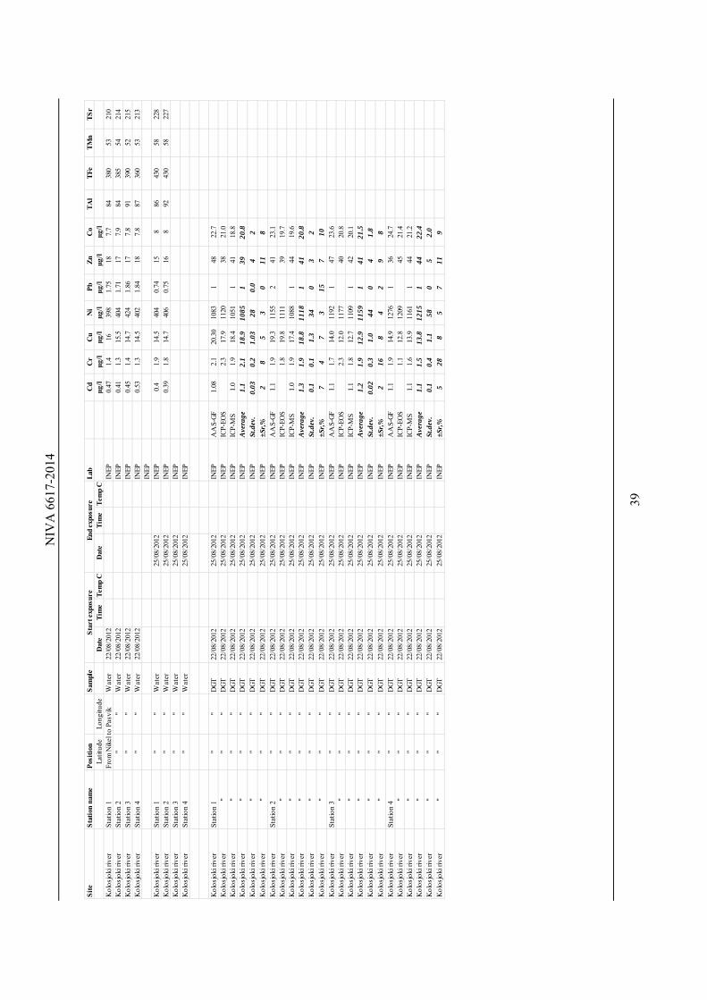
NIV

A 6

617-

2014

39

S

ite

Sta

tion

nam

eP

osit

ion

Sam

ple

Sta

rt e

xpos

ure

End

expo

sure

Lab

Cd

Cr

Cu

Ni

Pb

Zn

Co

TA

lT

FeT

Mn

TS

rLa

titud

eLo

ngitu

deD

ate

Tim

eT

emp

CD

ate

Tim

eT

emp

Cµg

/lµg

/lµg

/lµg

/lµg

/lµg

/lµg

/lK

olos

joki

rive

rSt

atio

n 1

From

Nik

el to

Pas

vik

Wat

er22

/08/

2012

INEP

0.47

1.4

1639

81.

7518

7.7

8438

053

210

Kol

osjo

ki ri

ver

Stat

ion

2"

"W

ater

22/0

8/20

12IN

EP0.

411.

315

.540

41.

7117

7.9

8438

554

214

Kol

osjo

ki ri

ver

Stat

ion

3"

"W

ater

22/0

8/20

12IN

EP0.

451.

414

.742

41.

8617

7.8

9139

052

215

Kol

osjo

ki ri

ver

Stat

ion

4"

"W

ater

22/0

8/20

12IN

EP0.

531.

314

.540

21.

8418

7.8

8736

053

213

INEP

Kol

osjo

ki ri

ver

Stat

ion

1"

"W

ater

25/0

8/20

12IN

EP0.

41.

914

.540

40.

7415

886

430

5822

8K

olos

joki

rive

rSt

atio

n 2

""

Wat

er25

/08/

2012

INEP

0.39

1.8

14.7

406

0.75

168

9243

058

227

Kol

osjo

ki ri

ver

Stat

ion

3"

"W

ater

25/0

8/20

12IN

EPK

olos

joki

rive

rSt

atio

n 4

""

Wat

er25

/08/

2012

INEP

Kol

osjo

ki ri

ver

Stat

ion

1"

"D

GT

22/0

8/20

1225

/08/

2012

INEP

AA

S-G

F1.

082.

120

.30

1083

148

22.7

Kol

osjo

ki ri

ver

""

"D

GT

22/0

8/20

1225

/08/

2012

INEP

ICP-

EOS

2.3

17.9

1120

3821

.0K

olos

joki

rive

r"

""

DG

T22

/08/

2012

25/0

8/20

12IN

EPIC

P-M

S1.

01.

918

.410

511

4118

.8K

olos

joki

rive

r"

""

DG

T22

/08/

2012

25/0

8/20

12IN

EPA

vera

ge1.

12.

118

.910

851

3920

.8K

olos

joki

rive

r"

""

DG

T22

/08/

2012

25/0

8/20

12IN

EPSt

.dev

.0.

030.

21.

0328

0.0

42

Kol

osjo

ki ri

ver

""

"D

GT

22/0

8/20

1225

/08/

2012

INEP

±Sr,%

28

53

011

8K

olos

joki

rive

rSt

atio

n 2

""

DG

T22

/08/

2012

25/0

8/20

12IN

EPA

AS-

GF

1.1

1.9

19.3

1155

241

23.1

Kol

osjo

ki ri

ver

""

"D

GT

22/0

8/20

1225

/08/

2012

INEP

ICP-

EOS

1.8

19.8

1111

3919

.7K

olos

joki

rive

r"

""

DG

T22

/08/

2012

25/0

8/20

12IN

EPIC

P-M

S1.

01.

917

.410

881

4419

.6K

olos

joki

rive

r"

""

DG

T22

/08/

2012

25/0

8/20

12IN

EPA

vera

ge1.

31.

918

.811

181

4120

.8K

olos

joki

rive

r"

""

DG

T22

/08/

2012

25/0

8/20

12IN

EPSt

.dev

.0.

10.

11.

334

03

2K

olos

joki

rive

r"

""

DG

T22

/08/

2012

25/0

8/20

12IN

EP±S

r,%7

47

315

710

Kol

osjo

ki ri

ver

Stat

ion

3"

"D

GT

22/0

8/20

1225

/08/

2012

INEP

AA

S-G

F1.

11.

714

.011

921

4723

.6K

olos

joki

rive

r"

""

DG

T22

/08/

2012

25/0

8/20

12IN

EPIC

P-EO

S2.

312

.011

7740

20.8

Kol

osjo

ki ri

ver

""

"D

GT

22/0

8/20

1225

/08/

2012

INEP

ICP-

MS

1.1

1.8

12.7

1109

142

20.1

Kol

osjo

ki ri

ver

""

"D

GT

22/0

8/20

1225

/08/

2012

INEP

Ave

rage

1.2

1.9

12.9

1159

141

21.5

Kol

osjo

ki ri

ver

""

"D

GT

22/0

8/20

1225

/08/

2012

INEP

St.d

ev.

0.02

0.3

1.0

440

41.

8K

olos

joki

rive

r"

""

DG

T22

/08/

2012

25/0

8/20

12IN

EP±S

r,%2

168

42

98

Kol

osjo

ki ri

ver

Stat

ion

4"

"D

GT

22/0

8/20

1225

/08/

2012

INEP

AA

S-G

F1.

11.

914

.912

761

3624

.7K

olos

joki

rive

r"

""

DG

T22

/08/

2012

25/0

8/20

12IN

EPIC

P-EO

S1.

112

.812

0945

21.4

Kol

osjo

ki ri

ver

""

"D

GT

22/0

8/20

1225

/08/

2012

INEP

ICP-

MS

1.1

1.6

13.9

1161

144

21.2

Kol

osjo

ki ri

ver

""

"D

GT

22/0

8/20

1225

/08/

2012

INEP

Ave

rage

1.1

1.5

13.8

1215

144

22.4

Kol

osjo

ki ri

ver

""

"D

GT

22/0

8/20

1225

/08/

2012

INEP

St.d

ev.

0.1

0.4

1.1

580

52.

0K

olos

joki

rive

r"

""

DG

T22

/08/

2012

25/0

8/20

12IN

EP±S

r,%5

288

57

119

NIVA 6617-2014

40

Appendix D. Svanvik workshop programme

Venue: Svanvik conference centre Date: 18-20 June 2012 Participants: IO RAS: Anna Chultsova, Grigory Khomenko INEP: Nikolay Kashulin, Tatyana Kashulina Akvaplan-NIVA Guttorm Christensen NIVA: Øyvind Kaste, Evgeniy Yakushev, Kari Austnes, John Rune Selvik, Tore Høgåsen Workshop programme: Monday 18 June: 1230-1330 Lunch 1330-1400 Welcome and short introduction of participants 1400-1530 Presentations (20-30 min) followed by discussion:

About the Norwegian-Russian bilateral project on riverine inputs (Øyvind Kaste) The Norwegian monitoring programme on Riverine inputs and direct discharges to

Norwegian Coastal Waters – RID (Kari Austnes) 1530-1600 Coffee break 1600-1800 Presentations (30-40 min) followed by discussion:

An overview of INEP’s monitoring activities in lakes and rivers draining to the Barents Sea (Nikolay Kashulin)

An overview of relevant monitoring activities at IO RAS (Grigory Khomenko/Anna Chultsova)

1900 Dinner Tuesday 19 June: 0900-1030 Presentations (20-30 min) followed by discussion:

An overview of relevant monitoring activities at Akvaplan-NIVA (Guttorm Christensen) The Norwegian Marine Pollution Monitoring programme – some results from the Barents Sea monitoring and modelling in 2009 (Evgeniy Yakushev)

1030-1100 Coffee break 1100-1230 Presentations (20-30 min) followed by discussion:

Modelling direct discharges and diffuse inputs in river basins – an introduction to the TEOTIL model (John Rune Selvik) Methods for calculating riverine export based on measurements and model results – examples from the Norwegian RID programme (Tore Høgåsen) Methodological approaches in river monitoring conducted by INEP and IO RAS –manual sampling vs. automatic sampling, passive samplers, sensors, models, etc. (informal discussion with inputs from Grigory Khomenko, Anna Chultsova, Nikolay Kashulin)

1230-1330 Lunch 1330-1430 Preparation for field trip:

Potential case study sites for method testing and calculation riverine inputs and direct discharges to the Barents Sea (discussion)

NIVA 6617-2014

41

An introduction to the Pasvik River – a potential case study site on the Norwegian side (Øyvind Kaste, Kari Austnes, Guttorm Christiansen)

1500-1800 Field trip to the Pasvik River and other long-term monitoring sites in the Pasvik valley 1900 Dinner Wednesday 20 June: 0900-1030 Discussion / work session:

Use of passive samplers (DGTs) to detect heavy metals and contaminants (Øyvind Kaste) Common protocol for case studies/ pilot studies (sampling, analysis, reporting).

1030-1100 Coffee break 1100-1230 Discussion / work session:

Workplan and deliverables (notes, reports, etc.), next 12 months Project finance Next meeting, any other business

1230-1330 Lunch 1400- Workshop ends / departure from Svanvik.

NIVA 6617-2014

42

Appendix E. Final meeting, Oslo

Venue: CIENS, Oslo Date: 21-22 October 2013 Participants: IO RAS: Anna Chultsova, Grigory Khomenko INEP: Nikolay Kashulin, Tatyana Kashulina Akvaplan-NIVA Guttorm Christensen NIVA: Øyvind Kaste, Evgeniy Yakushev, Kari Austnes, Ian Allan Programme: Tuesday 22 October: 1030-1100 Welcome and introduction to the meeting (Øyvind Kaste) 1130-1200 New developments in the RID monitoring programme (Riverine inputs and direct

discharges to Norwegian coastal waters) – continuous monitoring and inclusion of more organic contaminants (Kari Austnes)

1200-1230 Passive sampling techniques for organic contaminants: General overview, experiences from the RID programme, and preliminary results from the Pasvik river (Ian Allan)

1230-1330 Lunch 1330-1400 Review of the draft project report – current status and supplementary information

needs (Øyvind Kaste) 1400-1430 On-going research at INEP with relevance to the NordRID project – inputs or

comments to the final report (Nikolay Kashulin) 1430-1500 Coffee brake 1500-1530 On-going research at IO-RAS with relevance to the NordRID project – inputs or

comments to the final report (Anna Chultsova/Grigory Khomenko) 1530-1600 The Pasvik project – overview and results so far (Guttorm Christensen) 1600-1610 End of first day: Practical information and a brief introduction to tomorrow’s

programme 1800 Dinner Wednesday 23 October 0900-0930 Examples from monitoring and modelling activities with relevance to the Barents Sea

(Evgeniy Yakushev) 0930-1030 Working session on the final report 1030-1100 Coffee brake 1100-1145 Working session on the final report (cont.) 1145-1200 Follow-up and conclusions - end of meeting 1145-1200 Lunch

Gaustadalléen 21 • NO-0349 Oslo, NorwayTelephone: +47 22 18 51 00 • Fax: 22 18 52 00www.niva.no • [email protected]

NIVA: Norway’s leading centre of competence in aquatic environments

NIVA provides government, business and the public with a basis forpreferred water management through its contracted research, reports and development work. A characteristic of NIVA is its broad scope ofprofessional disciplines and extensive contact network in Norway andabroad. Our solid professionalism, interdisciplinary working methods and holistic approach are key elements that make us an excellent advisor for government and society.

14 Kaste Nord RID

Documents

Transcript of 14 Kaste Nord RID