10991717.pdf - Enlighten: Theses

https://theses.gla.ac.uk/

Theses Digitisation:

https://www.gla.ac.uk/myglasgow/research/enlighten/theses/digitisation/

This is a digitised version of the original print thesis.

Copyright and moral rights for this work are retained by the author

A copy can be downloaded for personal non-commercial research or study,

without prior permission or charge

This work cannot be reproduced or quoted extensively from without first

obtaining permission in writing from the author

The content must not be changed in any way or sold commercially in any

format or medium without the formal permission of the author

When referring to this work, full bibliographic details including the author,

title, awarding institution and date of the thesis must be given

Enlighten: Theses


[email protected]

http://www.gla.ac.uk/myglasgow/research/enlighten/theses/digitisation/




mailto:[email protected]

STRUCTURAL PERFORMANCE OF

POLYESTER RESIN CONCRETE

by

TAHA NASR EL DIN MEGAHED, B.Sc., M.Sc

A Thesis submitted for the degree of

Doctor of Philosophy

Department of Civil Engineering

University of Glasgow

September, 1985

ProQuest Number: 10991717

All rights reserved

INFORMATION TO ALL USERS The quality of this reproduction is dependent upon the quality of the copy submitted.

In the unlikely event that the author did not send a com p le te manuscript and there are missing pages, these will be noted. Also, if material had to be removed,

a note will indicate the deletion.

uestProQuest 10991717

Published by ProQuest LLO (2018). Copyright of the Dissertation is held by the Author.

All rights reserved.This work is protected against unauthorized copying under Title 17, United States C ode

Microform Edition © ProQuest LLO.

ProQuest LLO.789 East Eisenhower Parkway

P.Q. Box 1346 Ann Arbor, Ml 48106- 1346

ACKNOWLEDGEMENTS

The work reported in this thesis was carried out in the

Department of Civil Engineering at the University of Glasgow

under the general direction of Professor A.Coull, whose

encouragement is deeply acknowledged.

1 would like to express my sense of obligation to my

supervisor Dr. l.A. Smith to whom 1 give full credit for his

appreciated involvement in this work and for his matchless

supervision as manifested in useful criticisms, sincere

efforts, valuable guidance and admirable interests.

I feel an obligation to Professor H.B. Sutherland for his

irreplaceable supports throughout this work.

Gratitude is also due to:

Dr. P.V. Arthur for his interest and useful discussions

particularly those pertaining to the experimental work.

Dr. D.R. Green for his constructive proposals and positive

response in permitting special testing requirements to be

carried out.

Mr. T.W. Finlay for useful information.

Members of the teaching staff of Civil Engineering Department,

University of Glasgow for their cooperation.

All my post-graduate collègues in the same department for

their useful discussions and comments.

The staff of the Structural Laboratory and the Concrete

Laboratory, in particular the late Mr. J. Love, Mr. J.

Thompson and Mr. J. Colman for their valuable assistance in PC

processing and testing.

Mr. I. Todd for the help he gave in recording various electric

and electronic experimental readings.

Mrs. L. Williamson for her efficient typing ot the tables.

Thanks are also reserved for the managements of the following

companies for their responsible response in supplying the raw

materials needed and the relevant information ;

Scott Bader Polyester Division and Strand Glassfibre, Glasgow

Regional Centre.

Cairneyhill Quarry, near Airdrie.

Alexander Russel Pic, Glasgow.

TILCON - Scotland.

1 would like to express my indebtedness to the Government of

the Arab Republic of Egypt for the full financial support that

enabled me to carry out this work.

Finally 1 pay my heartfelt feelings of acknowledgement to my

parents, wife and son for their priceless forbearance and

peerless endurance that kept my spirit up all through this

research period.

11

SUMMARY

This work was carried out in an attempt to widen the potential

use of polymer concrete in the construction industry. The

concept of ultimate strength limit state in design of PC is

furnished on the bases of the mechanical properties found

experimentally.

Five distinct PC grades of polyester resin concrete that might

fairly represent average properties of PC were proportioned

after studying the potential optimization techniques of resin

mortar mix design for which a mix design chart is developed.

Most of the mechanical properties of the five PC grades were

investigated under short term conditions. The stress block

shape and parameters of the compression zone in flexure are

explored. Empirical and theoretical values for the stress

block parameters are developed. These values were used in full

scale structural applications, a beam and a column for each PC

grade, and were found to be satisfactorily accurate. The

concept of specific reinforcement ratio to be used with high

tensile steel reinforcement which has no definite yield point

is established.

The effects of rate of loading and sustained load were

studied. Expressions for long-term ultimate compressive

strength, long-term modulus of elasticity, sustained strength,

macrocracking strain and creep strains are given for various

PC grades.

Ill

Ultimate strength design procedures and their design charts

for various loading conditions and relevant values of capacity

reduction factors are suggested on the basis of the structural

performance of PC under short-term and long-term conditions.

IV

CONTENTS

Acknowledgements

Summary

Contents

Notations

Pages.

i - ii

iii - iv

V - X

Abbreviations xi

Xll - XV

Chapter One: Introduction 1 - 60

1.1 Recent attitudes in the construction industry 1

1.2 C o n c r e t e - p o l y m e r m a t e r i a l s and their

definitions 2

1.3 Historical development of concrete-polymer

materials 3

1.3.A Polymer-portland cement concrete (PPCC) 3

1.3.B Polymer-impregnated concrete (PIC) 7

1.3.C Polymer-concrete (PC) 10

1.4 Manufacturing techniques and the nature of

strength 13

1.4.A Polymer-portland cement concrete (PPCC) 13

1.4.B Polymer-impregnated concrete (PIC) 16


1.5 Advantages and disadvantages of polymers in

concrete 22

1.6 State of the art of concrete-polymer materials 26

1.6.A Polymer-impregnated concrete (PIC) 26

1.6.B Polymer-portland cement concrete (PPCC) 27


1.7 Objectives of the present work 31

Chapter Two : Mix Proportioning and Optimization

of Polyester Resin Mortars 61 - 107

2.1 Introduction 61

2.2 Chemistry of polyester resin 63

2.2.A Polyester resin manufacture 64

2.2.B Polymerization of polyester resin 65

2.2.C Properties of polyester resin 66

2.3 Resins used in the present work 68

2.4 Materials used in the present work 69

2.4.A Chemicals 69

2.4.B Aggregates and fillers 70

2.5 Resin mortar (RM) investigation 70

2.5.A Specimens 71

2.5.B Mixing; casting and curing 71

2.6 Tests and their results 72

2.6.A First group of RM 72

2.6.B Second group of RM 74

2.6.C Third group of RM 76

2.6.C.i Effect of grading 77

2.6.C.Ü Effect of moisture 81

2.6.C.iii Effect of styrene content 83

2.6.C.iv. Statistical interpretations of RM

results 84

Chapter Three : Short Term Mechanical Properties

of Polyester Resin Concrete 108 - 144

3.1 Introduction3.2 Review of PC mix proportioning 110

3.3 Considerations for PC mix-design in the

present work ^

VI

3.3.A Economy 116

3.3 .B Performance 116

3 .3.C Reproduction of mixes 118

3.4 Description of the experimental work 119

3.4.A Materials used 119

3.4 .B Mixing ratios 119

3.4 .C Specimens for different tests 122

3.4 .D Casting and curing 122

3.4 .E Testing 123

3 .4.F Measurements of strains and deflections 124

3.5 Test results of short-term mechanical

properties 125

3.5 .A Results of compression test 125

3 .5 .B Results of splitting test 125

3.5.C Results of flexure test 126

3.5 .D Results of shear test 126

3 .5 .E Results of bond test 127

Chapter Four : Stress Distribution in Flexure at

Ultimate Strength of PC 145 - 181

4.1 Introduction 145

4.2 Review of methods for measuring flexural

stress distribution 147

4.2.A Axial compression test 148

4.2.B Bending simulation test 149

4.2.C Photoelastic method 149

4.2.D Stress meters method 150

4.2.E Tests of reinforced concrete members 150

4.3 Stress block shape and parameters for resin

concrete 154

vii

4.3.A Test specimen dimensions

4.3.B Measurements of loads, strains and

deflections

4.3.C Test results and their interpretation

4.4 General stress-strain curve for different PC

grades

Chapter Five : Reinforced PC Beams and Their Test

Analyses

5.1 Introduction

5.2 Fundamental equation for pure flexure

5.3 Description of PC Reinforced beams5 .3.A Dimensioning5.3.B Reinforcement arrangements5.3.C Measurements and testing

5.4 Test results

5.5 Analysis of results

5.6 Theoretical calculation of the ultimate moment

and the specific reinforcement ratio

5.7 Mode of failure for the five beams tested

Chapter Six : Reinforced PC Columns and Their Test

Analyses

6.1 Introduction

6.2 Fundamental equation for uniaxial eccentric

loads

6.3 Tests of reinforced PC columns

6.3 .A Dimensioning6 .3.B Arrangement of the reinforcement

6.3.C Testing and measurements

154

155

157

163

182 - 233 182

183 186

186

187188

189

192

194200

234 - 307 234

236237

237239240

Vlll

6.4 Test results 242

6.5 Analyses of results 244

6.6 Theoretical calculation of the ultimate

carrying capacity 252

6.6.A Theoretical calculations of T 253

6.6.B Small and large eccentricity-columns 260

6.7 Mode of failure 263

Chapter Seven : Long-Term Mechanical Performance

of PC 308 - 370


7.2 Deformations of PC 311

7.3 Shrinkage strains and resulting stresses of PC 316

7.4 Creep behaviour of PC 319

7.5 E x p e r i m e n t a l study of t i m e - d e p e n d e n t

properties of PC 322

7.5.A The effect of rate of strain on the

properties of PC 323

7.5.A.i Some structural implications 323

7.5.A.Ü Description of the experimental work 325

7.5.A.iii T e s t r e s u l t s a n d t h e i r

interpretation 327

7.5.B Experimental work on creep behaviour of PC 333

7.5.B.i Description of the experimental work 333

7.5.B.Ü Results and their intrpretation 336

Chapter Eight: Ultimate Strength Design of

Reinforced PC Structures in Flexure 371 - 412


8.2 Factors of safety and their significance 372

8.3 Assumptions considered in the design 376

ix

8.4 Design of reinforced PC memebers in pure

flexure 377

8.5 Design of reinforced PC members with flexure

and axial compression load 387

Chapter Nine : G e n e r a l C o n c l u s i o n s and

Recommendations for Future Work 413 - 426

9 .1 General 413

9.2 Conclusions regarding mix proportioning 414

9.3 C o n c l u s i o n s r e g a r d i n g the stru c t u r a l

performance of PC 417

9.4 C o n c l u s i o n s r e g a r d i n g the e c o n o m i c a l

feasability of reinforced PC structures 422

9.5 Recommendations for future work 427

References 427 - 443

LIST OF ABBEREVIATIONS

PC Polymer-concrete

PCC Portland-cement concrete

PPCC Polymer-portland cement concrete

PIC Polymer-impregnated concrete

REC Resin concrete.

RM Resin mortar.

XI

LIST OF NOTATIONS

A, B Constants of the steel tension stress-strain curve at

any of the three idealized zones.

A',B' Constants of the steel compression stress-strain

curve at any of the three idealized zones.

Ag Area of tension steel.

A'g Area of compression steel,

b Width of rectangular cross-section.

Cq Concrete compression force.

Cg Steel compression force.

Cj. Coefficient of relative retained carrying capacity,

c Compression zone depth.

Cy Compression zone depth at ultimate strength,

d Effective depth of the cross-section.

d-| Distance measured from the extreme compression fibre

to the centroid of the outermost tension steel layer.

d2 Distance measured from the extreme compression fibre

to the centroid of the innermost tension steel layer,

d ' Distance measured from the centoid of the compression

steel layer to the extreme compression fibre,

d ’* Distance between the two centroids of the innermost

and outermost tension steel layers,

dg^ Maximum specific depth,

dgjj Minimum specific depth.

E q Compression modulus of elasticity.

Flexure modulus of elasticity,

e^ Basic creep strain,

e j Ultimate creep strain.

Xll

e I n s t a n t a n e o u s strain.

Limiting failure strain.

®su Total sustained strain.

Total creep strain,

e Eccentricity of normal force from the centroid of the

tension steel,

er Ratio of eccentricity level.

e*r Balanced eccentricity ratio.

Fc Ratio of filler content by weight.

F^^ Capacity reduction factor.

Fg Steel tension force,f^g Anchorage bond strength.

f| 2 Local bond strength,f^ Compressive strength.

f f» Compressive stress of the stress block in flexure.

f^2 Long-term axial compressive strength.

f^^ Ultimate compressive strength.

f-„ Axial cylinder compressive strength,c yf£* Modulus of rupture,

f^ Induced tensile stress.

fp Ratio of ultimate strength at any strain rate to

ultimate strength at rate [11.

fg Stress in tension steel.

f»g Stress in compression steel,

fg^ Sustained strength,

fgy Yield strength of steel,

f^ Splitting strength.

G Global coefficient of average uniform stress,

h Overall depth of cross-section.

K1 Parameter of average uniform stress distribution.

Xlll

K2 Parameter of stress block-resultant location.K2u Value of K2 at ultimate strength.

K3 Parameter of maximum compressive stress in flexure

Ko3 Peak value of the parameter K3.

k Index of mix richness.

Coefficient of creep.

^cu Ultimate coefficient of creep.

Coefficient of instantaneous creep recovery.

k^ Coefficient of creep recovery.

L Coefficient of reduced load.

Lu Coefficient of reduced load at ultimate strength.

Me Moisture content of aggregates.

MF Modulus of fineness.

P Normal force acting on a cross-section.

R Ratio of tension reinforcement.

R* Ratio of compression reinforcement.

Rs Specific tension reinforcement ratio.

R's Specific compression reinforcement ratio.

r Rate of loading.

Creep recovery.

Instantaneous recovery.

Total strain recovery.

SA Nominal surface area.

SI Normal distribution significance level.

SSA Nominal specific surface area.

ST/UP Ratio of styrene/ unsaturated polyester by weight.

Stc Styrene content.

T Coefficient of reduced compression zone depth.

Tg Gel time.

XIV

Ti Polymerization induction interval.

Tp Polymerization propagation interval.

Tg Index of tension reinforcement.

T*g Index of compression reinforcement.

Tu Coefficient of reduced compression depth at ultimate

strength.

t^ Time required for PC to develop its macrocracking,

ty Time corresponding to the ultimate creep strain.

W/C Water/ cement ratio by weight .

Wlb Binder working life.

Wlc Polymer concrete working life.

Ws Ratio of sand content in the mix by weight.

Y Overall stress block coefficient.

Z Coefficient of reduced moment.

Zu Coefficient of reduced moment at ultimate strength.

Maximum concrete strain (compressive extreme fibre).

Eel Lateral concrete strain.

^cm Axial concrete macrocracking strain.

Gcu Ultimate concrete strain.

Ecv Volumetric concrete strain.

^ml Long-term concrete axial macrocracking strain.

Emr Ratio of ^cm at any strain rate to that at rate [1].

Gqc Concrete strain at maximum stress.

Strain in tension steel.

€s' Strain in compression steel.

Egy Yield strain of steel.

XV

CHAPTER ONE

INTRODUCTION

1.1, Recent attitudes in the construction industry

Progress in the construction industry depends on the greater

understanding of and improvement in basic properties of

materials. Improved methods of construction and better

economics can be achieved by improving existing materials and

by the development of new ones. Portland-cement concrete (PCC)

will be as indispensible in the future as it is now. Its use

is a technology which is well understood.

PCC has been available for more than 150 years and has a good

range of mechanical properties. Despite possessing high

qualities of short and long-term stability, however,PCC still

has poor flexural tensile strength and low tensile cracking

and ultimate compressive strains. These limitations must be

considered at the design stage. In this respect, probably the

most critical inherent weakness of PCC lies in its low

limiting strains which may lead to progressive crushing and

spalling. These in turn make the material more permeable, less

durable and increasingly sensitive to external effects.

Consequently restrictions may be imposed in exploring new

fields where PCC could be used. Permeability influences

concrete vulnerability to frost and corrosion of reinforcement

where heads of water and humidity differences exist along and

across concrete structures. Permeability can have a decisive

effect on performance, particularly when considering chemical

resistance, abrasion and erosion-resistance.

New construction materials must have better performance and

economics than existing ones. New materials also require

careful and reliable interpretation of laboratory-research

results before they can be used efficiently in actual design.

This is due to the lack of available accumulated data based on

previous experience with these materials. The prevailing

attitude in the construction industry is by nature a

traditional one, and any new material must challenge it to

gain acceptance. This can only be done by providing and

proving a better cost-performance efficiency. The cost

effectiveness of these materials is one major element in

justifying their use, and pilot applications often have to be

investigated first if new markets are to be explored.

1.2. Concrete-Dolvmer materials and their definitions

Concrete-polymer materials like other composite materials may

generally be defined as a three-dimensional combination of at

least two chemically and mechanically distinct phases; namely

a polymer matrix or phase and dispersed aggregates. In some

cases Portland cement may form a third phase. Electron-

microscope photographs of the microstructure of these

materials are shown in Fig.(1.1) (1). There is a definite

interface between the different components.

Although there are many different versions of concrete-polymer

materials, they can be specifically categorized into three

main types as follows;

(a) Polymer-portland cement concrete or polymer-modified

cement concrete, abbreviated as PPCC. This is prepared by

using both polymer and portland cement to form the binding

paste or the system matrix. Mixing is carried out in the same

way as when mixing conventional concrete.

(b) Polymer-concrete or resin-concrete, abbreviated as PC or

REC, which is prepared by mixing resin as the only binder,

with selected aggregates without any other cementing agent or

water.

(c) Polymer-impregnated concrete, abbreviated as PIC which is

prepared by monomer impregnation into hardened precast cement

concrete elements with -subsequent polymerization.

1 .3. Historical development of concrete polymer materials

In the late fifties following the growth of the petrochemical

industry, synthetic rubber latexes, resin emulsions and

monomers were produced and developed . Their production

activated fundamental and practical research on concrete-

polymer materials in general. Trials using polymers with

concrete were undertaken in different places , and some

British patents on the concept of a natural latex-hydraulic

cement systems were issued about sixty years ago (2).

1. 3.A. Polvmer-portland cement cone refe (PPCC) The first

concrete polymer material was PPCC, for which neither

synthetic resins nor advanced techniques were required.

Monomers usable with concrete were available. Work was

initiated primarily in enhancing cement concrete properties by

adding to the mixture, while still in fresh state, water-

soluble latexes and emulsions. The first report on this type

of material was produced in Japan by M.Itakura in 1953 (3),

and concerned polyvinyl acetate-modified concrete. In the

following years extensive work on the development of PPCC and

its mortar was undertaken by different institutes and research

laboratories. Since that time polymer modified concretes and

mortars have often been used in building and construction

works such as those needed for the Tokyo Olympics in Japan,

1964. Table (1.1) shows some of the properties of typical

polymer-cement mortars used in Japan, where work to

standardize quality and testing methods of PPCC was commenced

in 1974. A specific standard was established recently (1978) and included in the Japanese Industrial Standards (J.I.S.)

(4). Some results of the early research (2) on PPCC made with

different polymers are shown in Fig.(1.2). They represent the

effect of polymer/cement ratio and polymer type on the

compressive, tensile, flexural and shear strength of PPCC.

In Germany since around 1948 PPCC had been under research

using various aqueous polymer dispersions, as well as some

powder-f orm dispersions. The work in Germany aimed at

improving specific properties of concrete, mortar and slurry

for particular applications. The polymers initially used were

acrylic-ester based c o p o l y m e r s and v i n y l p r o p r i o n a t e

copolymers. The results obtained using these polymers are

shown in Fig.(1.3) and Fig.(1.4). In these figures the effects

of polymer addition to cement mortars on the mechanical

properties are demonstrated. The only gain was the improvement

in the adhesive properties of the different formulated mortars

or slurries. These mixes are covered by DIN standards (5).

Synchronized work was being carried out in Germany for

improving flow properties and workability of conventional PCC.

Using plasticizers the W/C ratio could be reduced without

reducing workability and higher strengths could be attained.

In this work (6) dispersions based on vinylacetate aroused

interest initially, but because of some shortcomings regarding

water curing, work turned eventually to other polymer types.

The influence of water on the performance of the polymers used

can be seen by comparing Fig.(1.5) with Fig.(1.6). Generally,

satisfactory improvements in flow properties could be obtained

by using acrylates, ethylene and many others.

In the U.K. different institutions have been involved in

modifying conventional concrete by introducing polymer

dispersions. At the beginning of the 1 970’s a programme was

conducted by The Building Research Establishment (7) to

investigate all missing data required for reliable evaluation

of PPCC properties and its performance in different

environments. Many of the polymers originally introduced had

been found to perform badly in wet conditions, see

Figs.(1.7; 1.8& 1.9). Acrylic-based polymers gave the best

results as shown in Figs.(1.10, 1.11 & 1.12) .Numerous polymer

dispersions were investigated such as polyvinyl acetate,

polyvinylidene dichloride, acrylic methacrylate, vinyl

propionate and many others. In this programme various curing

and testing methods were used over very long testing periods.

Another study was undertaken in the University of Southampton

(8) in an attempt to overcome some of the drawbacks of cement

mortars and concretes such as poor tensile impact stregth,

limited resistance to corrosion and poor adhesion to old

concrete. This work formed a part of a study of the

interrelationships between mechanical properties and the

microstructure of cement paste modified by the addition of a

styrene-butadiene p o l y m e r latex to the m i x i n g water.

Additional research work was aimed at producing competitively

low-cost flooring compounds using special epoxy-water

slurries. The concept of a fibre-reinforced polymer cement

composite, was introduced tentatively and on a small scale

through various universities and companies in the U.K. (9).

More recently there has been an upsurge in interest in fibre-

reinforced polymer cement composites. It has been recognised

that polymer dispersions may have a valuable role to play if

used with fibres. By the begining of the 1 980's a great deal

of information about most properties of PPCC was available.

However very little was known about their long-term

deformation c h a r a c t e r i s t i c s under d i f f e r e n t l o a d i n g

conditions. Since a knowledge of these properties is of great

importance in assessing the advantages and applications of

PPCC products, some experimental work has been initiated

recently cocerning the study of creep properties for different

PPCC’s (10).

In the U.S.A. 1 atex-modi f ied concrete dates back to the

1950’s, but the real impetus for using polymers in concrete

developed in the late 1960’s with the publication of research

performed by the Brookhaven National Laboratory and the Bureau

of Reclamation (now the U.S. Water and Power Resources

Services) (11) & (12). This research was primarily oriented

towards polymer-impregnated concrete. The dramatic increase in

strength, stiffness and durability created considerable

interest in potential applications of different concrete

polymer composites. The American Concrete Institute A Cl

recognised the importance of these new materials, and in 1971

"Committee 548-Polymers in Concrete" was formed with the

intention of gathering, correlating and evaluating information

on the effects and properties of polymers in concrete, and

different symposia were sponsored by this committee (13) &

(14).

Polymer latexes have been used very successfully to make

latex-modified concretes, these latexes are mainly copolymers

which include acrylic and vinyl acetate, styrene, vinyl

chloride, butadieneand other latexes which are commercially

available in different formulations. However, PPCC has not

received as much attention in the U.S. as PIC or PC, since

most of the successful polymers that have been identified for

PPCC have been proprietary. In the late 1970*s, investigations

at Washington State University, made a preliminary evaluation

of the feasibility of preparing PPCC with furfuryl alchol. A

study was also carried out for the determination of the

effects of various proportions of aniline hydrochloride

catalyst and calcium chloride on the development of concrete

strength. These effects have been reported on in the Soviet

Union as increasing strength and durability of concrete. The

resultsfor a two mix series are shown inFigs.(1.13 & 1.14)

(15). Many other studies concerning PPCC have been carried out

in different countries , such as the Soviet Union, France,

Australia, Spain, Italy and Canada. Some of the results of

these studies will be dealt with later in this chapter.

1.3.B. Polymer-impregnated cocrete (PIC) As mentioned earlier,

PPCC and PC materials have been studied since the 1 950’s.

However PIC came to the fore in the development of polymer use

in concrete in 1 966. At that time research sponsored by the

U.S. Government, was initiated to develop methods for

impregnating hardened portland cement concrete (PCC). Various

liquid monomers were employed in the impregnation process,

based on the known fact that this impregnation treatment

provided a material with significant improvements in strength

and durability. Initial tests of PIC showed that the

structural and durability properties of this new composite

could be quite remarkable. The U.S.Government spent several

millions of dollars over the next few years to identify

suitable monomers for impregnation, to enhance impregnation

processes and to study and develop applications for PIC. It

should be noted that a patent for PIC had been issued in the

Soviet Union in 1954, although work on PIC was not started in

that country until after the U.S. work had become available in

the literature (16).

The improvements in properties which were being achieved

through p o l y m e r i m p r e g n a t i o n of c o n c r e t e generated

considerable interest among investigators in many countries

around the world and resulted in numerous other researches. By

the early 1970’s several applications had been produced. The

American Concrete Institute, recognizing the importance of

this rapidly developing new family of construction materials,

formed the previously mentioned "Committee 548", whose

membership includes representatives from countries around the

world, and which sponsored two symposia on "Polymers In

Concrete" in 1972 and 1973 ( 16). Two more sessions were held

in 1976 on the same subject. Most of these symposia

proceedings were published by the ACI in 1978. The committee

also prepared a state-of-the-art report on polymers in

8

concrete which was published in 1977.

As a part of other international activities in this field, a

number of symposia and conferences have been held since 1967

by different organizations. Since then, research on PIC was

spread in different directions; one of which, concerned with

relating pore-structure with degree of pore-filling in terms

of polymer molecular weight, was carried out in Canada (17).

Another investigation was carried out in Japan to clarify the

relationship between the molecular weight of polymer formed in

PIC and the condition of its manufacturing process. In this

the monomer used was methyl methacrylate (MMA). Two main

relationships were determined; molecular weight as a function

of polymerization temperature, and molecular weight as a

function of impregnation depth (18). These two relationships

are represented in Figs. (1.15 & 1.16).

Further studies showed that, not only does the performance of

concrete impregnation depend upon decrease of porosity or

increase in degree of pore-filling (which is a function of

matrix capillary pore diameter and distribution, viscosity and

surface tension of the monomer used), but also it depends upon

molecular dimensions and the interaction between cement

capillary walls and and organic molecules of monomer. In Italy

through research conducted by A.Rio (19), it was found that

one must first have very well compacted concreete for it to be

structurally fit for impregnation. High quality concrete,

fully impregnated with low polymer content, will show higher

mechanical strengths than a lower quality concrete, even if

the latter was fully impregnated with a larger quantity of

monomer. So the main improvement in PIC performance, can be

attributed to the cement matrix prior to impregnation. This

matrix should have diffused micro-porosity allowing easy

permeation of monomer and also low total porosity to limit the

quantity of monomer needed for partial or full impregnation.

Similar studies were made in W.Germany by H.Schorn (20), in

Canadaby B.B. Hope (21) and in other countries in the early

seventies. By the begining of the 1980’s, the concept of PIC

was well established internationally. Since then, different

aspects were dealt with in more detail, such as the effect of

polymerization techniques, impregnation depth, monomer types

available and high temperatures on the performance of PIC.

Other applications were developed ranging from ceramics to

containers for the disposal of low and intermediate level

radio-active wastes.

l.l.C. Polvm er-concrete (PC) Polymer-concrete was used

commercially as early as 1 958 in the U.S. (22) to produce

precast building panels; and "cultured marble" has been in use

for many years to produce many items ranging from bath tubes

and drain tops to submarine periscopes. Initially most of PC

was made with polyester and epoxy resins. In the late 1 970’s

MMA monomer received high attention especially for repairing

deteriorated PCC structures. More recently the aim has been to

develop m u l t i - f u n c t i o n a l res i n s that will e n s u r e

polymerization at ambient conditions and within prescribed

times of hardening. As far as resin or binder type is

concerned, there are in general five types of thermosetting

resins which are used with PC. Epoxy, polyester, polyurethane,

poly-MMA and furane. Limitations applicable to one alone can

10

not be applied to another binder or another mix. The low

shrinkage and versatility of epoxy resin and its ability to

set and to develop excellent adhesion to aggregates of various

types in wet air conditions, make it suitable for use in

difficult environments; while polyester for example, is

preferred for precasting.

One of the earliest studies on PC was conducted by Holifield

National Laboratory in the U.S., to determine the effect of

different constituent materials on PC properties and to obtain

data for evaluating the feasibility of "tailor-made" resin-

aggregate mixtures with a wide range of predictable strength,

density and stiffness properties (23). The resins used were

polyester and epoxy with different chemical and physical

properties. Widely varying groups of coarse and fine

aggregates were carefully selected for better understanding of

the contribution of each constituent in the composite. Some of

the relevant findings of this work are quoted as shown in

Figs.(1.17; 1.18& 1.19).In the U.S., the deterioration of

concrete bridge decks imposed an increasing problem for all

state high-way departments ; it has been estimated that

approximately 105000 bridges in the U.S. are in need of repair

(24). Ideally, the repair should be made quickly, allow the

bridge to be opened to traffic in a few hours and be

permanent. Those requirements accelerated the development and

use of PC in the U.S., made with polyester and MMA-based

polymers. Recently the use of PC for major restoration of

hydraulic structures and their protection, has increased very

rapidly, and both user-formulated and proprietary PC's are now

in use.

1 1

Most PC formulations will cure in thirty to sixty minutes at 5

C and higher. Curing time is adjustable as desired at ambient

temperatures. Very special resin formulations might be

required for particular constructions and restorations whereotemperature is as low as -5 C and when time available is very

limited. The U.S. Air Force sponsored research for developing

certain PC formulations for repairs to airfields that would

cure in a very short time at very low temperatures and as

D.W.Fowler states, this work has been achieved successfully

(25) .

In Japan, the first research and development of PC was

conducted in the Electrical Communication Laboratory of Nippon

Telegraph and Telephone Public Corp. (NTTP) in the late

1950's, and the results were reported in 1 961 ( 26). The

practical development of PC was initiated in the Meihan Resin

Concrete Industries Corp. and several other boards in Japan.

K.Okada et al. carried out exclusive basic studies on PC and

its structural applications (27) & (28). Responding to the

active practical development of PC, work on standardization of

quality and testing methods for polyester PC has been in

progress since 1974 (29). In 1978, and with the supervision of

K.Okada, six JIS's have been issued describing different

methods for manufacturing and testing polyester PC. As far as

the practical applications used in Japan are concerned,

developed manholes made of PC were designed and installed by

NTTP, and the estimated figures of production amounted to

20000 tons of PC annually. Pipes were also produced at the

rate of about 30000 tons/year (29). Many other structural

applications of PC are now in progress in Japan.

1 2

In the U.K. research seems to be involved in PPCC development

and its practical applications. Very few studies have been

made regarding PC applications, out of which the work of B.W. Staynes and Brighton Polytechnic (30) will be quoted

hereafter. However resin mortars have been used for repair

work and jointing in the civil and structural engineering

fields. In most cases, these applications have been supported

by acceptance-testing of the materials e m p l o y e d , without attempting to evaluate their ultimate capabilities, or their behaviour under long-term loadings in particular. A notable exception is the extensive study carried out by Johnson (31) on long-term loading and other effects on epoxy resin-mortar

joints. As a logical extension to this work, B.W.Staynes carried out a full investigation for the production of epoxy resin-concrete and the optimization of mix propotions. He also

recommended some precautions to be taken in the manufacture of PC dating back to the early 1970’s (32).

1.4. Manufacturing techniques and the nature of strength

1.4.A Polvmer-portland cement concrete (PPCC) Polymer- portland cement concretes and mortars are made by partial

substitution of the portland cement by a polymer. Polymers

used should be either aqueous polymer-dispersions (latexes and emulsions) or water-soluable polymers (monomers). As shown in Fig.(1.20), these polymers can be added to the mixing water or to the f r e s h concrete (or mortar). Curing can be carried out in the same ways as with PCC. Accelerated curing techniques are applicable whether performed under high temperature, high

1 3

presuure or both. The amounts of polymers added (the solid

content of the disperion) are normally within 5 to 20% of

cement weight (solid polymer/ cement by weight). Proper anti-

foaming agents are often used to control excessive air

entrainment. On curing a polymer film is formed and enhances

the cement-aggregate bond, which is reflected in higher

mechanical strengths, increased ductility and improved water

proofness.

The nature of PPCC strength is mainly attributed to the binder

interface influence, and its capability of transferring stress

between different components without excessive deformation.

The Portland cement matrix, which provides the binder for

ordinary concrete, is responsible for the final strength of

the composite through the precipitation of cement hydrates

into interlaced and elongated crystals, with high cohesive or

adhesive properties. Another theory (33) accounts for the

cement matrix strength through the colloidal effects of the

hydrated calcium silicates, which being almost insoluble, form

a rigid gel mass. Whatever the exact nature of cement-concrete

strength , the randomly-formed crystallates represented by

cement hydrates are intrinsically weaker than high molecular

weight amorphous polymers. They also are inherently less

suited as an interface, particularly for the transfer of

tensile stresses. In this respect the salient feature of PPCC

technology , as repeatedly confirmed by chemists, is that

ionic bonding can be an additional factor contributing to the

performance of concrete. It has been shown (34) that all the

components of high performance composites are linked by ionic

bonds, a feature which is not present in PCC, and it is from

14

this stand point that the idea of PPCC has initially emerged.

Although not all ionic bonds are chemical ones, there is a

contribution to performance in actual use provided by ionic

associations, i.e., between cement hydrates and the pendant

groups on a polymer chain. Comatrix structures of the

crystalline skeleton inside an amorphous polymer particularly

present a high potential for ionic association (34). The

formation of the polymer-cement comatrix can be achieved

through different chemical and biochemical reactions. For

instance with a polyvinylidiene comatrix, hydration of both

cement and polymer is dominant. The condensation process may

take place if the polymers used have reactive terminal groups,

such as epoxide resins and furfuraldéhyde. In the case of

acrylic and methacrylic esters reaction is initiated by free

radicals using conventional oil-soluble catalysts. In either

of the previous cases, it is reported that fairly satisfying

achievements in PPCC technology are within reach.

Regarding its processing, PPCC batching is a quite different

process from that of PCC, primarily because polymer formation

starts when its different components are distributed by mixing

with the aggregate. A balance is necessary between the rate of

increase in polymer-viscosity (polymerization) and the

completion of the whole system reaction (initial cement

hydration). For that reason and others, it is recommended (35)

that polymer-dispersion should be added up to one hour after

the addition of the mixing water to the cement and aggregate.

In some studies and practical applications (36), special Super

High Early Strength cement was used to overcome this

difficulty. The use of this cement resulted in a far better

15

performance as shown in Figs. (1.21 to 1.24), obtained by

Y.Ohama. It is also reported (35) that excessive vibration and

steam-heat curing techniques have deleterious effects on PPCC

performance.

1.4.B Polvm er-im pregnated concrete (PIC) PIC is made by

impregnating a hardened and dried cement-concrete base with

one of a wide variety of polymerizable polymers or monomers.

Polymerization is usually c a r r i e d out by t h e r m a l or

radioactive techniques. The production of PIC depends chiefly

upon the degree of monomer absorption and the consequent

degree of pore-filling in the finished product. Processing

technology for the production of PIC can be listed as follows:

[a] Concrete fabrication : It was noticed that concrete mix

variables (VI/C, entrained air, aggregate size and type, etc.)

do not greatly affect the properties of PIC. Low or high

strength concrete gave almost the same improved strength after

impregnation. The main effect of concrete quality is reflected

in the polymer loading and the consequent cost of unit

production. However the question of whether the base concrete

should be of high quality with low required polymer loadings,

or of lower quality with higher polymer loadings is still a

controversial one (20). As shown in Fig.(1.25), the. matrix

porosity and the degree of polymer-filling strongly affect the

strength of PIC.

[b] Dehydration : After conventional curing of the concrete

units, they are oven-dried to get rid of the free moisture at

temperatures ranging from 100 to 250 C, according to

production requirements. Particular attention should be paid

to the dehydration degree which must be sufficient to remove

16

only free-pore water (evaporable water) and not the combined

water (nonevaporable); otherwise concrete destruction will

take place. The effect of the degree of dehydration on

strength is shown in Figs.(1.26 & 1.27).

[c] Impregnation : Impregnation is performed in two main

stages as follows;

(1) Evacuation of fully dried elements by using vacuum pumps

to the desired value of pressure, to get rid of the entrained

air, partially or totally, and to aid in the polymer

absorption process.

(2) Soaking the cured, dried and evacuated base concrete

element in pressurized polymer liquid in sealed containers.

Soak-pressure may vary from 0.1 to 1.0 N/mm2. depending on

different processing parameters. These parameters are the

degree of drying performed, the evacuation vacuum applied and,

the time of soaking and the required impregnation depth, etc.

[d] Polymerization : This can be achieved by a wide range of

techniques, depending in the first place on the type of

polymer used. Most commonly, polymerization is carried out

thermally, c a t a 1 y t i c a 11 y or by radiation. D i f f e r e n t

combinations of these three techniques can be used.

If polymerization is to be made without the use of

encapsulating techniques, certain precautions should be taken

to prevent or help reduce monomer evaporation and drainage

losses from concrete units. A specific processing technique

for p r o d u c i n g PIC is s h o w n in Fig.(1.28), in w h i c h

polymerization is carried out under water (37).

1 7

The high performance of PIC with regard to the mechanical

properties or durability can be simply attributed to the

decrease of the composite porosity. However this decreased

porosity can not account for the differences in performance

recorded with different polymers. Additional factors are

involved, one of which is the interpha se bonding in its

broadest sense. As shown in Fig.(1.29), the only fillable

pores in the system matrix (cement paste or mortar) are those

which are connected to the capillary pore system (free-water

pores). Evidently, reducing matrix porosity means reducing

microcracks and flaws as well as matrix capillary pores. This

implies a reduced probability of microfracture initiation at

crack tips, and an enhanced mechanical performance of the

system matrix as a whole.

Many studies suggest that the increased linearity of the

stress-strain curve for PIC is attributed to the improved

paste-aggregate i n t e r f a c i a l bond. But m o r e recently

investigations show that it is the smaller difference between

the improved elastic modulus of the cement-paste phase and

that of aggregate phase, which causes this increase in

linearity and strength. This reduction in the moduli

difference , as shown in Fig.(1.30), produces less cracking at

the paste-aggregate interface (21).

Depending on the nature of the polymer itself, there is

evidence that chemical interaction between the paste capillary

walls and the monomer, introduced during polymerization,

interferes with and improves the microstructure of the paste

(1 8).

1 8

Recently, p r o g r e s s in PIC processing has been directed towards

partial impregnation techniques, since full impregnation

proved to be almost impossible, especially for large

structural elements. Partial impregnation may be carried out

to a specified impregnation depth without resorting to the

soaking of concrete units under pressure in huge sealed

vessels. It can also be used for restoring deteriorated

structures such as platforms, bridge decks and in many other

applications for which full impregnation techniques are not

practically possible (38).

1 .4. C Polvmer-concrete (PC) PC consists of aggregates bound

with a polymeric material and contains no hydraulic cement or

water. This type of material has many of the advantages of

PIC, as will be seen later, though its processing techniques

are much easier and simpler than those of PIC. PC processing

is very similar to that of conventional concrete, provided

precautions are taken. Processing techniques depend on the

finished product desired and the required performance. One

process is shown in Fig.(1.31) and is suggested for some

prercast applications (4).

To summarise, PC processing can be classified into four main

stages as follows :

[a] Proportioning : In which different constituents are

selected according to the desired performance in the fresh and

hardened stages. Polymer, catalyst and accelerator, if needed,

are selected and mixed uniformly just prior to mixing with

aggregate and filler. In certain processing techniques.

19

formulated polymer is mixed first with filler, then the

aggregate is added gradually until the desired consistency is

reached. This is done to help provide complete uniformity in

the binding polymeric paste (resin and filler). A saving in

the mixing time after the addition of the aggregate is also

gained.

[b] Mixing : Any type of concrete mixer can be used provided

that an effective ’washing-up’ solvent is available. There is

a wide variety of resin-diluting agents that can be used

depending primarily upon the resin type itself and its

formulation. Resin should be carefully formulated so that

hardening or setting will not be initiated while the materials

are still in the mixer. Careful production-supervision should

allow complete and uniform mixing while the PC is fresh. For

precasting, the mixer should be cleaned periodically, if there

is a continuous line of production. Dry-mixing of filler and

aggregate before the addition of resin usually produces a

better mix uniformity.

[c] Casting : Before placing PC releasing agents should be

used to provide easy and sound demoulding. Vibration may be

needed with some harsh PC mixes, but generally excessive

vibrating times are not recommended.

[d] Curing : This can be carried out in several ways but in

principle there are only two; catalytic or thermal. The wide

range of catalysts (hardeners) and accelerators (initiators)

available are capable of initiating and completing the

polymerization of liquid resins in different ways. Curing

rates can be enhanced by applying some high temperature during

2 0

the hardening time, or even after the initial hardening. The

finished product can also be subjected to heated dry-air for a

prescribed period and temperature compatible with the resin

used.

PC as a composite material can be closely investigated at the

macrostructure or m i c r o s t r u c t u r e level, as s h o w n in

Fig.(1.32). On the macrostructure level, PC can simply be

regarded as a continuous phase of polymer containing dispersed

inert aggregate with irregular pores. On the microstructure

level, the polymeric paste can be described as a combination

of filler particles each covered with a film or thin envelope

consisting of different polymer-chain layers, as shown in

Fig.(1.32). Those layers can be categorised into fully-

oriented, semi-oriented and unoriented layers. The continuous

polymer matrix is formed mainly through covalent bond

reactivities, which result in long chains with high molecular

weight compounds. These long chains are crosslinked through

their active sites and provide a high-performance matrix, on

which the overall PC performance depends. Naturally the

strength of PC is strongly dependent on the properties of the

resulting polymer matrix, the degree of its crosslinking, the

length of the formed chains and consequently their molecular

weight.

The chemistry of polyester resin-concrete is briefly described

in the following chapter. However it must be emphasized here

that at the microstructure level, the polymer matrix is

primarily responsible for all rheological properties of PC,

including shrinkage strains on hardening, creep and stress

relaxation (39). The system matrix also provides the necessary

2 1

cohesion and adhesion for the dispersed aggregate phase. On

the macrostructure level, PC performance depends on the type

of aggregate and filler used, on their gradings and on the way

they are compacted. As far as the filler-hinder or aggregate-

hinder interface is concerned, studies carried out in the

U.S.S.R. (39) have revealed a clear relationship between the

change in the nature of long-chain molecule formation and the

associated polymer/filler ratio. A clear dependence of the

internal shrinkage stresses on the nature of the polymer and

the filler was also found.

Many investigations aimed at reaching a theoretical estimation

of PC strength or optimum mix-design, were carried out

recently in the U.S.S.R. Theoretical models were developed and

helped produce several equations. These equations were

derived to predict PC compressive strengths and strength

development rates (39) & (40) and were experimentally

verified.

1.5. Advantages and disadvantages of polymers in concrete

Different concrete-polymer materials have proved themselves

reliable as construction materials over the last decade. As

with all new materials, future applications and developments

are generally different from those initially anticipated. For

example, in the early 1 970's PIC appeared to be the most

promising of the concrete-polymer materials. At present, PC is

attracting much more attention than PIC (22). The initial

interest in PC was for the restoration of structures like

bridges and airfield runways. But the largest future use now

appears to be in the industrial applications such as machine

2 2

parts , machine foundations and particularly for precast parts

and components made using continuous processing.

Apart from the high cost and other economic aspects of PC,

which will be dealt with later, the main disadvantages found

with concrete-polymer materials in general are as follows ;

(1) Certain physical and mechanical shortcomings : In the

initial stages of research, a large range of applications was

envisaged. However, as more data became available for the

different concrete-polymer types, a number of unacceptable

properties were found which restricted the wide potential use

of these materials. The main shortcoming being their poor

rheological jperformance. High shrinkage strains with

consequent high internal tensile stresses usually cause some

setting cracks. The development of shrinkage strains and their

relation to strength development, for PC made of polyester

(41), are shown in Fig.(1.33 & 1.34). This effect is

encountered much more clearly when steel reinforcement is

used. Fig.(1.34) represents the effect of reinforcement ratio

on the setting-shrinkage strains. Creep behaviour and stress

relaxation constitute more restrictions for most structural

applications.

Due to the nature of polymers, these materials suffer some

deterioration in performance in moist and wet environments

when not completely cured. They are sensitive to high

temperatures and fire attack. Their performance under dynamic

loads is still unsatisfactory especially under repetitive

loads which induce internal heat evolution. In one research

series conducted in Japan (42), the internal temperature

g 3

recorded in fatigue tests with PC specimens, reached well

over 80 C as shown in Fig.(1.35), and caused excessive strength reduction.

(2) Lack of suitable polymers for use with concrete : Due to

the lack of cooperation between biochemical and civil

engineering on one hand, and to the lack of exchange of

experience between polymer manufacturers and concrete-polymer

dealers on the other hand, the expected rate of development

has not been attained. For example, the absence of structural

knowledge in biochemical engineering resulted in a very wide

variety of monomers and polymers which unfortunately have no

structural value at all. The lack of meaningful performance-

data for most polymers and monomers, makes it impossible for a

structural engineer or consultant to evaluate them. The

manufacturers of polymers usually describe their product in

terms of acid-value, non-volatile content and stability in

darkness or viscosity gel-time, etc.

No polymers , so far, have been specially developed and

produced for use with concrete. The structural engineer will

often find it difficult to decide on the best polymer that

would result in the most desirable end-use properties. In this

context, it seems that changes in attitudes are required

generally. As chemical companies turn more attention towards

the expanding market of concrete-polymer materials, it is

likely that significant development will occur.

When considering the advantages of concrete-polymer materials,

it is essential to make a clear distinction between the

çjpf*0 0 t types of these materials. As shown in table (1.2),

24

most concrete mechanical properties are improved with polymer

inclusion. PC and PPCC generally have lower moduli of

elasticity than conventional cement concrete. The most

significant improvements are those related to durability. In

certain tests of freeze-thaw resistance, PC had a weight loss

of almost zero after 1500 cycles, while the corresponding PCC

specimens lost 2 5 % of their weight after only 700 similar

cycles. Improvement in erosion and abrasion resistance is

remarkable. Chemical resistance for concrete-polymer materials

is much better than that of cement concrete.

Several advantages can be mentioned for the PC-type in

particular, apart from its high mechanical and durability

properties. These are as follows :

[a] Simple production techniques are involved : Processing is

adaptable to existing PCC technology. It can be used either

for cast in place or precast applications.

[b] Versatility : PC can be tailor-made in an almost unlimited

number of different mixes with various properties. Setting

time can be very finely controlled, as shown in Fig.(1.36), at

all temperatures even those well below zero C (43). PC can be

made with different toughnesses and stiffnesses depending on

the incorporated constituents.

[c] Esthetic and decorative uses : Using special colour dyes

dissolved in the polymer before or during mixing, can result

in a ’terrazzo’ effect with a lustrous finished product. This

can in some applications be of considerable benefit.

25

-3.t..gte q £ Ihe af concrete polymer materials

I'&'A ^ppcrete (PIC) in the last five

years, the rate of PIC development has decreased dramatically.

The excellent structural performnace and the enhanced

durability could not in themselves justify commercial use on a

large scale. At the outset it was thought that this type of

construction material would revolutionise the construction

industry. But the complicated techniques and industrial

hazards involved halted the anticipated progress. Perhaps the

most serious factor was and still is, the insistence on having

full impregnation. Another factor that has limited the growth

of PIC is the progress and the competitiveness of other

concrete polymer materials such as PC.

Full impregnation techniques can only be used for precast

products, which are relatively small (44), Usually they have

an adverse balance between cost and performance. Recently PIC

has gained a sudden wider use in outdoor applications, all of

which are based on surface impregnation techniques. Several

methods have been suggested and carried out, in which applying

monomer at a t m o s p h e r i c pressure could result in an

impregnation depth varying from 20 to 50 mm (44). Primarily,

these methods can be used with horizontal and flat surfaces

such as bridge decks and panels, platforms and heavy-duty

flooring. Impounding the imprégnant over the cured and dried

cement concrete base, is the latest technique for partial

impregnation. Several bridge deck constructions and repairs

have been carried out in the U.S., Japan and other countries

using such simple ponding techniques. Specially— formulated

monomers are used for better results and deeper penetration.

26

In certain applications, the time elapsed from the start of

imprégnant ponding till the completion of polymerization was

30-40 minutes; and the resulting impregnation depths varied from 20-25 mm.(45).

Now it is universally established that PIC can be classified

into three different groups. Depending on the techniques used

and the consequent impregnation depth, PIC can have full,

partial or surface impregnation. The last is being extensively

used at the present time, where most of the advantages of full

impregnation are retained while most of its processing

disadvantages are avoided.

Surface impregnation is used for the protection of many

hydraulic structures like outlet walls of dams, spillway and

stilling basins. It is also used to improve runway and roadway

construction and maintenance. One major field of application

is the repair of bridge decks. This technique, despite being a

simple one, could be used in very particular ways. For

instance, it could be used for consolidating and stiffening

soft materials in a zone of loose soil for certain

pétrographie excavations (44). Ferro-cement products have been

enhanced by polymer impregnation. Containers for radio-active

wastes, made of PIC, are now under investigation in many

countries.

1.6.B Pniympr-cernent concrete (PPCC) Polymer-cement concretes

and mortars have been in use since the early fifties. However,

polymer—modified cement mortars and slurries have been used

more often than polymer—modified concretes. Those polymer-

modified cementitious materials are mainly used for protective

2 7

linings and finishing works. Concretes modified by polymers

have not obtained a worldwide practical acceptance because their cost can not be justified.

Many new latexes, emulsions and water-dispersable polymers

have been developed and have helped widen the potential fields

of application for polymer modified mortars. These

applications are numerous, but can be simply classified into

flooring, waterproofing, decorating and adhesive works. Table

(1.3) shows some of these applications (45). Many additives

have been developed for the enhancement of polymer modified

mortars, such as anti-foaming agents, fire-retardants, anti

corrosive agents and many others which have enlarged the

possible fields of application.

Now there are commercially available certain prepacked PPCC’s,

mortars and slurries which can be used satisfactorily (45).

Apart from prepacking, the process of PPCC mixing is similar

to that of conventional concrete. It is noteworthy that in

Japan, eight Japanese Industrial Standards have been

established for the quality control and testing methods of

PPCC; where their annual consumption of polymers in PPCC

manufacturing amounted to 100000 tons.

1 . 6 . C poT ymmr-cnncrete (PC) Polymer-concretes and mortars

have recently attracted much more interest than any other type

of concrete-polymer material. New resins, techniques and

research on PC have brought it into the front line of new

construction materials. Generally its use is distributed

equally amongst load—carrying elements, aggressive media—

pPQ^0Q j j g alements and decorative or esthetic elements.

28

Tables (1.4 &1.5) show these possible fields of application

(45). These applications are still to be explored and

exploited. Load-carrying elements are mostly precast products

such as underground components, sea-water structures,

supporting systems, housing elements,machine tools and even

street furniture.

As a protective coating against aggressive media, PC and

mortars are extensively used for industrial flooring and

paving. In the U.K., flooring is by far the widest field of

application. In one construction project, newly-setting cement

concrete (green) was covered by a resin-mortar layer resulting

in 15 years of maintenance-free heavy-duty flooring (46). The

range of industrial and commercial flooring applications is

being progressively extended to include areas not subjected to

aggressive media. For instance, the increasing demand for very

level, easily maintained and dust-free floors is being met by

fine PC finishes which offer direct cost competition with

ordinary cement concrete. Coatings to marine pipelines, dam

spillways, channel linings and aircraft pavements are now

popular in the U.K. Cast-iron for the bed and frame segments

in machines is being replaced by PC.

Another interesting field for using PC and its mortar is in

grouting. British Telecom used some 8000 tons of polyester

mortar for installing or raising manholes in roads. They

proved cost-effective and it is reported that no more

regrouting is likely to be required. Another example of mass

grouting is that made for the heavy-duty crane rails of the

giant Goliath Krupp Crane in Belfast, in which 280 tons of

2 9

epoxy-mortars were grouted between the rail-soleplates and the

supporting beams (47). Many similar applications for

structural joints , bedding of bridge-bearings, fixing of

street furniture and the like are in wide use in the U.K.

Recently, interests have developed on a wide scale in the U.S.

and other countries for producing thermal insulator panels and

electrical insulators made of PC. Some major work comprising

the installation of thermal insulating panels was carried out

in the U.S. These panels protected dykes that contain liquid

gas tanks, against explosive spilling by the impounded liquid

gas reaching a high temperature. Light-weight polyester mortar

and concrete was specially formulated for this project, using

certain c e 11 u 1 a r - s t r u c t u r e a g g r e g a t e s (48). T h e r m a l

conductivity was reported to be very much lower than that of

conventional concrete insulators , that is in addition to the

better structural performance and durability that was given by

the new PC insulating panels.

A major field of PC use is the rehabilitation and repairing of

deteriorated structures, and the restoration of historical

structures. Special types of quick-setting resin mortars are

now available. They can be used for protecting and replacing

spalled concretes caused by steel corrosion. They can be

simply trowelled vertically or overhead without any supporting

or slipping forms. An example of the size of a similar repair

work can be quoted from the latest bridge-repair project

carried out in the U.S. In this project, in 1 983, two bridges

alone have utilized 1 800 tons of PC for the repair of their

decks (49).

30

Several continuous-mixing machines are now available on the

market for PC processing. Due to the nature of PC, most

mixing and casting techniques should be subject to high

quality control. For that reason and others, many of the

continuous and ordinary mixing machines for PC, are

automatically controlled. Different types of these machines

are capable of PC-shotcreting up to 20 m and in some cases up

to 45 m. (50). One of those PC-shotcreting machines is shown

in Fig.(1.37) along with its basic system ’flow-chart’. This

and similar machines are now in wide use in Japan, W.Germany

and other countries.

New methods in PC processing have evolved such as ’ready-to-

cast’ PC sacks, and polymer injection to the already compacted

and placed aggregates. In Japan, a new construction method for

making sma 11-diameter tunnels ( up to 1.20 m ) has been

operated successfully (51). In this method , as shown in

Fig.(1.38), automated tunnelling and lining with a 100 mm -

thick PC layer was achieved. The fast curing and high early

strength of PC segments cast in place, replaced what would

have been conventional ’cut-and-cover’ techniques using other

materials.

1.7. Obiectives of the present work

From the previous review of different concrete polymer

materials, one is left with no doubt that these materials

could form a useful tool for the construction industry. The

number of the practical applications and their relevant

research programmes are increasingly expanding. Both PIC and

PPCC, with some exceptional applications, could not compete in

31

cost with PC. With the current progress in the petro-chemical

industry, new resins are being developed and produced

regularly all over the world. Thus the future should show a

greater spread in use of PC.

Most of the research on PC , as reviewed earlier, has been

dedicated to its physical and mechanical properties . Mix

proportioning and the effect of different constituents on the

performance of PC is by far the widest field of ongoing

research. In addition, studying the physiochemical parameters

of the micro and macrostrcture of PC and their effect on its

performance is another active field of research.

So far the majority of PC structural elements are made of

mortars or plain PC. Relatively few applicationshave used

reinforcement in any form . The number of PC structural

members reinforced with steel bars is surprisingly limited.

Most of those structures are designed with margins of safety

so large as to lose all the structural advantages of PC. The

lack of research in the field of structural performance of

reinforced PC is mainly responsible for this situation.

Very little is known about the flexural behaviour Of PC when

reinforced. Not enough knowledge about how to utilize

efficiently the high performance of PC together with steel

bars, is available. Structural limits related to different

modes of failure do not exist. Some researchers have used high

tensile steel with PC members, but no general flexural theory

is established yet. The long term structural performance has

been completely ignored, and almost no one seems to have been

interested in applying the different creep test results or the

32

vital rheological behaviour findings of PC to real structural

elements using reinforced PC. In addition the economic aspects

and the feasibility of producing structural elements of PC

have been paid very little attention.

Based on these above mentioned conclusions of PC utiliy in the

present construction industry, the objectives of this work

were chosen to be as follows :

(A) Optimizing mix-proportioning of the available materials to

produce five different grades of PC. These grades would serve

as the base materials for the coming objectives.

(B) Studying different physical and mechanical properties of

those grades, either in short-term or long-term performance.

(C) Studying flexural stress-strain distribution , flexural

stress-bloek parameters and their dependence on mechanical

properties and time.

(D) Deriving an ’ultimate-flexure theory* that would help

calculate the actual ultimate capacity in both short and long-

terms for any reinforced PC member. This would also help

establish a * design code* based on chosen factors of safety

within the ultimate structural limits and serviceability

limits to be set later.

(E) Applying the findings to full-scale structural members

made of reinforced PC using a beam and a column for each

grade.

33

(UM-4O O6 4J iCO c O O o O O o OA: -wXU CO 00 c O O o O d d dO *H •H t-H m O o o O m o oÆ CO (U r4 CM r-4 o CM r-4 cn r-v mc/i cuX CO CM T—1 rH 1-4 CM---

>C CUo•H >-lXO CM CM X CO CM 1-4 vOCO <yCUO I—1 m (T\ 00 o CM 00 ovcd Xt T3i—1 m mj- cn on Mt VO CM vOV4 CO 03XJ H M 60 1—)E

P•H o•Hw C CjOCOu O C CO CM cn r4 CJN r4 CM 1-4 Mf cnCti •H »H CU g m ro 00 «—4 Ml- m 1-4 cn4-1 CO U U E}-l (U CO PL- C r-4 t—< 1—! 1—1 1-4 o 1-4o X: cu E 5aS 73 X: o< c/i CJ4-10 j-Q) 1 1 o 0\ CO r- MÎ- Ml-E c -l M cO o 00 00 Mf CO C3V Ml- OVQ X X X 1-4 t—1 CMu c/i1o M 1ÇU 0) P, p4J O O CM 0\ vO Ml- VO m or—1 CO CO•H fe'SCO 13 X 4-J r-l rn vO CM cn m cnÜ CO p- r-i•HcuHmo CU CM u

> g f—1 I—f 1-4 Mf 1-4 cr.CO 4J U(U CO ^ p p O 00 VO O 00 Ml- o cn-H C g: & o CM «—4 r-4 CM 1-4 1-4 CM4-J 0)X X(U , pPL, O M p p o o\ 00 r-l O MÎ- Mf MfU 4J o u t—i r-H CM 1—1 CM 1-4 CMC/ir—1T—41 X4-1(U 00r-1 C pXI (U (U P vD r-4 CM CM 00 O r-. 1-4CÜ V4 4-J U O 00 CM CO o o Ml- SfH 4J p pCO u <r m MT m CM CM Ml-CMI—1 ECO E}-4

X ^ p CM o CM X o CM OVCO U P o vD Ml- 00 m o Ml- r4rH O Pk u cn m OV VO CM vO 00

0) 4J

5nPP pP p 1-4 CM•H u 1 1X p pd Pp o PQ PQo Ë CO CO ou CJ

Pd c oPQ Pi > >5a Iz Pu Pu

35

mvDLO vO \0

00OJ

CN incn

COinCO

CNm

VOmmo

inmcnin

cn00CN

■um

mCNmcn mCNVD•H O 4J ■U (U

mCNCN

CN

•MO r-l

(U 4-1U XCO *1-1 T3 U (J U

H O0) 4-1

3 6

COCO p- 1 1 1 1 P p 1 1 1 1P r— CO CNl en en CN Cl Cl C7\ O" mU O •l-l > >o ce Q O o O O o o o O o oCu

Cl en p cn en en en enCe P •X) en ! 1 1 1 t

X c en en 1 O o O CN CNX W) cO CN

•H •H COs O)

DTJClCO PQ p

T3 cC 0)CO e r—1 rP rP |H iP fp P P fp pP (UCO o

eu CO fn co Pp p P Cl CO p p

CO CJ (U o Cl co Cl •p O co 30) P p o p Cl 3 P O O OCO o> ü P Cl fp •p o p ü UD ci 00 OO p p •p X p Ci 1 »O • CO CO o c CO Ci ü tn p ü co X i X i Ce

Æ CO p OJ o •p I—l •H Cl ci P 2 P co 3 •p O0) P Fi bû CO p p o o cp B O fX 3 ) S HP O cO CO T3 •H CO Cl o p O OcO O re p c •p P fp p u O p CO u Cl3 *-e ce CO CO 3 eu D o X i P eO P o P p X)

cp bO CO p CO ci p cO cp ce ip ClX 1—1 p CO CO Ci o O p 1 P ceCl CO P CO O B •H o p fp x i co cO •HO 0) o ü CO p CO P o o CO •p Ci O Cl X

S CO r-e •H X) p •p OO p o ■p B U O O •P cn cop *p B « o Ci CO ci CO p •p CO •P B g

cp o o (U o B cO •p CI Cl x i B P Cl O PQ X P rC p p p X X) p p Cl P cO X X co

o CO o Cl Cl o X O X i ü Cl 3c3 I—1 •> p rX o X i p o ip g h Po cO CO A CO o eu c p en ci CJ o 3 P cO Cl co

P ce CO B (U p CO p P o Ci CO 00 O o [5 P rXp 0) o p p XJ CO P cO X o CO c cp cp X UcO c js •H o 1 c • p u p U ci •P P Cl CD ClCJ 0) CO cO ip p O CI P Cl CO CO •p P co cO X X io ÙO p p o •P X Cl P 15 P P CO 3 CO p O '2 ü. j 'X) CO cO o CO P P cO Cl p O p O fX o •P g Cl Cl

p c 1p p rP ce cO Ci o X i P g o p co X i ûOo CO »> ce Ip (U CO B CO CO B cp 00 cO fp 3 X I

p CO (U cO CO CJ P p W) _ O p P Cp Cl P Cl •pCO Q) ïn p > OO CO p C > Ci Ü cO OO P

CO <1) 00 CO (U •H Ci •P g •p Cl P Cl co O g 3 X i JQp u cO D p M CO CO •p P p Ci •P 3 P •P p B P •po «p CO tP ü U P Cl iH O ci (0 fp O P g P Cl P Po cp CO -H Ci o O X p x i •p X3 ce cp O ce cO co P JQ O

I—1 ip cO cO o Ip 0 X) CO cO ci O Ci (U cp fp Cl fp X 3 OPe O ce p u X ce < 5 B cO •n co pel W cp co ce ce P «a- cp

cio•rH■PCOü•HI—Ia5*

cO•HspcO tflS w)ùO-rl

| s(0 fP P4 Pw

003•PcpO CO coO P 3p 3 >3i *P •PP P U01 3 3P P X3 3 '2:3 s <

3 co> 00• P 3CO • Po Pp 3p >o co OU 00 O1 3•p «pp 3 Ü3 "P 3< X Q

37

Table 1.4: Applications of Polymer Mortars

Application Location of WorkFloorings (including Decorative Finishings)

Floors for general houses, warehouses, offices, schools, hospitals, factories and shops, toilet floors, passages, stairs, garages, railway platforms, train floors, etc.

Pavings Roads (footways and travelled ways), bridge decks foot-bridge decks, parking lots, runways, etc.

Anti-corrosiveLinings

Effluent drains, chemical and machinery floors, grouts for acid-proof tiles, floors for chemical laboratories and pharmaceutical warehouses, septic tanks, electrolytic baths, hot spring baths, offshore structures, e.g., piers and sea berths, etc.

Adhesives

Adhesives for floorings, walling materials and heat- insulating materials, tile adhesives, adhesives for jointing new cement concrete or mortar to old cement concrete or mortar, embedment of anchor bolts, etc.

RepairingMaterials

Grouts for repairing cracks and delaminations of concrete structures, patching materials for damaged concrete structures, protective coatings for corroded reinforcing bars, etc.

Integral waterproof ings

Concrete roof-decks, mortar walls, concrete blocks, water tanks, swimming pools, septic tanks, silos, etc.

Small-diameter Automatic Tunnelling System

Telecommunication cable lines, etc.

Precast ProductsFRP-reinforced mortar pipes for sewerage and irrigation systems, FRP-reinforced mortar panels, vibration isolators, etc.

38

Table 1.5: Applications of Polyester Concretes

Application Location of Work

Structural Precast Products

Manholes and handholes for telecommunication cable lines, electric power cable lines and gas pipelines, tunnel liner segments for telephone cables and sewerage systems, piles for port or hot spring construction, machine tool structures, e.g., beds and saddles, FRP-reinforced frame or panels for buildings, etc.

Non-Structural Precast Products

Gutter covers, U-shaped gutters, footpath panels, terrazzo tiles and panels and large-sized or curved decorative panels for buildings, partition wall panels, sinks, prefabricated cellars, counters, washstands, speakes for stereo phonographs, etc.

Cast-In-PlaceApplications

Spillway coverings in dams, protective linings of stilling basin in hydro-electric power stations, coverings of checkdams, foundations of buildings in hot spring areas, etc.

3 9

i

(a) Resin Modified Concrete

iüüS'(b) Resin Concrete

iPil&y iliiii

(c) Resin Impregnated Concrete

□ Cement Reactive Resin

Aggregates - Predominantly

Fig. (1.1) MicrostructurG of Concrete Polymer materials.

40

IISO

40

9

9

IP0 s is

II

' PVAC

0 s ISPolyfflQr/comont ratio Polymor/camant ratio

I&

0 I V IS 2dtPoIymor/cernant ratio

1I?Ia

0

0 S t> is

Polymar/camant ratio

PAEi Polyacrylic aatar.PVACi Polyvinyl acetate SBRi etyrene butadiene rubber

Fig. 1.2 Strength proper tie® of vorloue PCC.

41

ui:

X

? i!s is -

1 1n

2UIUI/NX X^îof^aoj» j.o sn^npon

151

S ’4.^ ° . mD. D07 -D ^ 0

ÜL E

(4.0a1g♦»o'aL

gUIUI/N SSB U a S Bt(BUe-)

R

<=>.

01 u;ou%# sSoHUfJMS gwtti/N H^Bu b j ^b [OjnxBij

a070XcLr0c0ap0c0 L0û. *)0 LL 0Q. EX y-c 0> r*)070 Cap Lü •Pa 0«4-4-ÜJ 0

L3m X04-

OïTDCUl 0

42

O)

lo

(DS'O

ï m

I1 1ObXa

^u.

(D

gluui/N q%Bueu%# %ounxei j

o

X XX

s

(_ guiiu/N q%Gue_i%# BATaseudiuo5 à S =

IIO o

C° xî

:.|

2Uiui/|s| l|-5.Bubj^8 %ounxB% j g u iu i /N h ^ B u b j ^ b B A T B S B u d u io g

X EO+) +)ac >O' 0L♦i U)(D cO L> 00 C<0 i*.0La 0EO LÜ 4>0T3 DC T)O , Co CL ODXa c 0

ou. Ecin aE U

OO *oG E

O) ta Ou. T) c

4 3

r* m

guiw/Nyï •n jn p o u i # ,Gunox gmw/NM •nxnpow #,6unox

X

MS

\ \\#

o

• ^ S « ^guiw/NX «ninpoiM •,Bunox 2UIW/NX #n [npow # ,b u n o x

Om (D

H3 :î i s :3 2■g iE 13<. g

ü>■ -• 0

^ 5O•2- b

IL >

9enoL01 L O

!9 U

î|.• ili= 12^bU. >

44

!î#\n

« 1.8 ffi

30

20

10

2,2

2.0

Water cijred

Air cured

- A13 _ AS12

Polymer eolide ratioD 5 10 IS 20

Fig 1.9 Density and Young's modulus versus P/C ofter 1 year storoge

(V

I

iL#

PVA20 PVA3

16

12Control

Air curing month®

16 2U0 8

?Zt!

20

16

12

Wotor curing months

0 16a

Fig. 1. 10 Flexural strength versus storoge time for vorious polymer modified cement mortars • W/C*0. 35.

45

iou.

20

16

AMI 412

Control

t Air curing month#* A ' *0 4 • 12 16 20 24

II#

20

16

12

ft

4 Wotor curlnq month#0 4 0 12 16 20 24

Fig. 1.11 Floxural strength versus storage time for various polym moolf led cement mortars, W/C-0. 3.i

or

(V

I#Iu.CU

i

20

%

X

s

20

s

10

s

0

365 day# of ago

N

X\ 180 day# of age

90 day# of age28 dcye of age

(o) Acrylic polymer A13

(b) Styrene acrylic polymer AS12

Polymer/cement ratio (P/C) 1--- 1— * n i10 15 20 25

Fig. 1.12 Flexural strength versus P/C at various ages.

46

orsi3

RrJ<

<

o

glUUI/ji L| 6uBJ 8 0A|890jdui03 gUIUI/ L|%6uBJ%S BAÎSSB-lduiOQ

?0

1LOX UoIIg

«4-o£ a?S bQ)a>a in?l. u

6U-O

u5%

U*DD

sXE■D8ü

uu.

CaXop vie

•Xop 2. ui

13...... U.

X<htin

i

il2““/N yq^GuBUl^B BA|B8Bjdui03

o .*D (D

ilHa uc Q-^ oé £ï g•p +3ü 10

ï ?g

R g

^ o. üs c o

■*» •* •*» ♦* b k k«L M a o.

< BU o

u.

IM IV

n

« %

liiI IIi nUJ u. . l i

I>u.<u.

47

5-

1Zfe-3*I - l î

IIti ?0 *4IIi l1 i

10

Mw

Mn

Polymer loading

Polymer-extroct

5-

Ui;II4>üDLtLOEXOQ.

10

5

70 80 90Polymerization temperature Ct

Flg. 1.15 Polymorizatlon t-omperoture VOP6U6 molocular weight or nonunlformlty of polymer formed In PMMA-IC.

Po1ymer1zot1on temperature Ci70 80 80

Mw

10distance

20(mm)

30 40from eurfoce

Fig. 1. IB. Croec «ectionol location versus molecular weight or nonun1form1ty polymer formed in PMMA-IC.

-10-1010-— k1010-t10-Unlt mm

Sampling section In PMMA-IC specimen for molecular weight determination.

PMMAi Polymethyl methacrylate

48

(V

u

t

CLIU

20 0

15 D

10 0

0Unit weight gm/mm3

00.5 1,0 1,5 2.0 2.5

Uru«ILtnimi

2,5

2.0

1,5

UP1.0V

0.5

100,0 150,00.0 50,0

ig. 1.17 unit

Compressive strength versus weight for different PC's.

Fig. 1. IB Effect of temperot on comprosive strength

ru

z4i*♦-

&£L*>#mc

cS-

0

S

0

5CompreeslvQ strength (fc) N/mm2

0100 150 20050

Fig. 1.19 Compressive strength versus splitting strength for various PC's.

UPi Polyester PC El Epoxy PC.

49

CQ 0>• Z O

• uo e V• JO c

to jD a>'-'3 "I ta "o . w n>^ 9> V pi J3 c. 3

, , 0 0 (0 ^U 3 OS""ac "D 0 mm ij*• m m® C 3 M UJQ 0 IQ 0u XI 3 10 0 U O IK « .Ht 0 3

4JI .H £ 05 0t 3 M Xi c a 0 0 # -H Z C Ik. 0 c 0aa, c o .H -HO # HI ^.-o *. lu ><x: 00 >ntt -Lt JJ■HI j»Jl tu 0 3u> n < z ta1 ,1 ,-L J — I

0)

Û c w > >< 0. I

•DU 0 H0 u UJ 0 0 m *j H M 0 j=. ü < "H H c >.>10 u C -OO -H 0 0 > H > 1 > 1 > 1 H H C

i ^ >

> > > Xo a. u8.

os 0. Uz

0

So•H

H « 0^5xi C5^

4JM0

t0

0aV>i

>.JZ

0 > u. > 0 .XJH XI •0 0 H XI •x: > 0 H Ha c H £ 0 0n 0 u u (o x:< 0 H u

X in Q < Ü H•D 0 H -H <;0 • XI 3 0 H H

« m e 0 E in > ,H H4J H H U W 0 c u >,H U vu H -u U UJ0 0 VU •O "O 3 > 0 3J= 0 0 0 0 H >, >»vua o U X X H H H Um 3 0 0 0 0 3< OS CU z z 0 0 . CU b.!_ L J 1___1 1 1 1 _l

Izr,a, 0

o, in m 3 H O "O • 0 C 3 wi O tr 0 -H < E W I--------

I£

O'b.

M •>.H U9 oou «U

50

Norme] Port1end cornantSpocSo] ouper high oorly otrongthicomont

ruzI 10

P/C-D.0

5

0 1 .1 7 20

P/C-1OXPAtSBRPVAC

1 * 7 * * 1 I 7 21Wotor curing period doym

Fig. 1.21 Water curing period versus flexural strength of polymer modified mortar

ru

zX*>cn

SO

30

20

10

0S 7 211

PAE

SBRPVAC

1—1 . 1 7 2ft I 7 211

Wotor curing poriod doyoFlq. I. 22 Water curing period versus compress1ve strength of polymer modified mortar

PAE* Polyacrylic esterSBR* Styrene butadiene rubberPVAC* Polyvinyl ocetoto

51

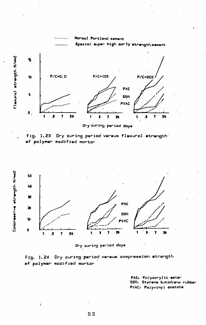
N o r m o ï P o r t 3 e n d c e m e n t

BpectaJ euper high eor3y etrengthcement

ou.

15

P/C-D.D10

0 1

P/C-20%

PAESBR

PVAC

1 .1 T It1 I 7 I t

Dry curing period doye

Fig. 1.23 Dry curing period voreue flexurol etrength of polymer modified mortar

ru

i?

iu

SO

to

SO

20

10

0 1

PAE

SBRPVAC

I 7 I t 1 S 7 I t1

Dry curing period days

Fig. 1,24 Dry curing period versus compression etrength of polymer modified mortar

PAE* Pol y aery H e ester 'SBRi Styrene butadiene rubber PVAC* Polyvinyl oeetote

52

\Fig. 1.25 Example of etrength ^

d e v e lo p m e n t b y traneformatlon of , cement concrete Into PIC. I

\

Iz"r•p?0LPtta>1ou

u

150

1007DX i*pr«gnotlon

OX impragnatJon

400

3,00100

200100 '

0 0,010 2 0 30 4 0 5 0 6 0 7 0 100

IFor# volume of the matrix X

120 nonovoporobla wotorEvoporablo wotor

100

outociovodogroo of dohydrotion —H2D X

604 61 2 3 50

Fig. 1.26 Vorlotion in compresive strength of o thermally treated concrete versus degree of hydration.

s:rlLPOa>

801l_)

140

120

100

80

24 h-200 Cdohydrotion

rohumidlflection± H2CT1& ovoporoblo

1 3

140 24 h-200 C

120 rohumidiflootion

100

RolotiVC humi dity %0 10 30 50 TO %

Fig. 1. 27 Variation in compressive strength of a mortar versus degree of dehydration and rehumidif ication.

i

III I

1=

II

bO1 ua•o#"4

t âVc •oo cu fd

$ îë

«Il

s u

54

Polymor Imprognotod

SurfaceGel pores

Compaction pores without connect 1 on to the copiilory

pore systemCompaction pores with

connection to the capiJiorypore system \

Capillary pore

non-1mpreqnaced

Fig. 1.29 Typos of pores In o hardened cement paste.

CM

I,coL

o>:ofe.E5

120

90

VA

60

MA30

Strain0

0,060

CMINZ5iÏ?:aLg-0u

MMA160

120 VA

SO

MA

Stroln0

0,060a- Cement paste b- Cement mortar

MMA, Methyl methacrylate VAt Vinyl acetate A: Acrylonitrlle MA, Methyl acrylate S, Styrene U, Untreated

Fig. 1.30 Effect of various polymers on stress-strain rejationship.

55

{weighing Weighing {weighing^

Mixing

{Assembling {.

Mixing

DryingDrying

Weighing

LiquidResins Aggregates

Molding by Vibrator

Resin Concrete Mixing

Molds Reinforcements______

Mold-Releasing Agent Coating

Mold-Releasing Agent (Silicone)

Fillers (Calcium Carbonate, etc)

Heated Dry Cure

Demolding

(Finishing

Resin Concrete Product

Fig 1.31 Typical Process for REG Procast Product (Casting Method)

56

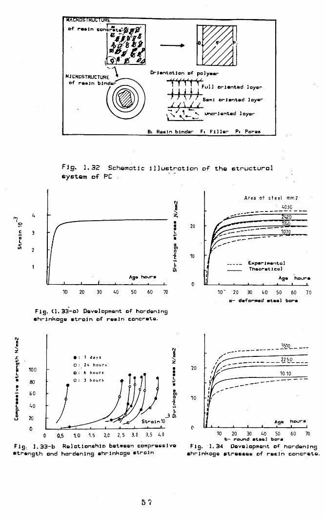
TRCkOG IWUüTUWkDf raaln conerat#%

M t v ' f e

"AMJCRD5TRUCTURE * of ramjn binder

Orlantotlon of polymar

't'rviv,4fWFull oriented loyer

Semi oriented layer

unoriented loyer

Bi Reain binder Fi Filler Pi Pores

P lg. 1.32 Schematic Illustration of the structural system of PC

3

Age houra

10 3020 40 6050 70

Fig. (1. 33-o) Development of hordening ehrlnkoge strain of reein concrete.

a201070

10Exparimantel Thaoraticel

Age houra0

10" 20 30 40 50 60 70o - daformed atoel bora

X♦»orÏba>a:1

100

30

0

40

200

a5 1.0 1.5 2.0 2.5 3.0 3,5 4.00Fig. 1.33-b RelatlonshiD between compreeelve strength and hardening shrinkage strain

3510

225020

10 10

10

Age houraC

10 20 30 40 50 60 70b- round steel bori

Fig. 1.34 Development of hardening shrinkage stresses of resin concrete.

5 7

u0D1

eo70

60

50

AO

30

20

Hoxlmum levs] 52%Fr#qu*ncy-4DD cpir

Room tamporatuTB

Mcxlmum level 55%Frequency-200 cpm.

Maximum etreee level 52% Frequency-200cpml

Numbe- of cyclee — » «10' 10 10“ 10'

Fig. 1.35 Voriotion in internal temperature with number of cyclee of Joaaing for resin concrete.

LO■UDLOauuDbbD•PC

U-o

10

a- 20 to GO mln. setting times

BzPDMPT

costing temperature

3020-30 -20 -10 100

bpoLaaoVoLLopDPC

PDq;

10

Accolorotor DMPTi Dlmothyl-paro-toluldlno Initiator ' BzPi Benzoyl peroxide

b- 20 to 120 mln. setting times

DMPT costing temperature

302010-10 0-20-30

Fiq. 1.36 Variation in optimal formulation ot the binder with casting temperature to yield PC. with o desired setting times ( 70% MMA, 30% TTEGDA)

58

Cl=>-

(U X O)3 ■*-> O -t->1— C cn O)C3 cnc c oic 'acX i. X •^srce <c »-s:

w

(x£

a>cvjori/>

5 9

[>Q><a>Q>a><a>a

g

□

60

CHAPTER TWO

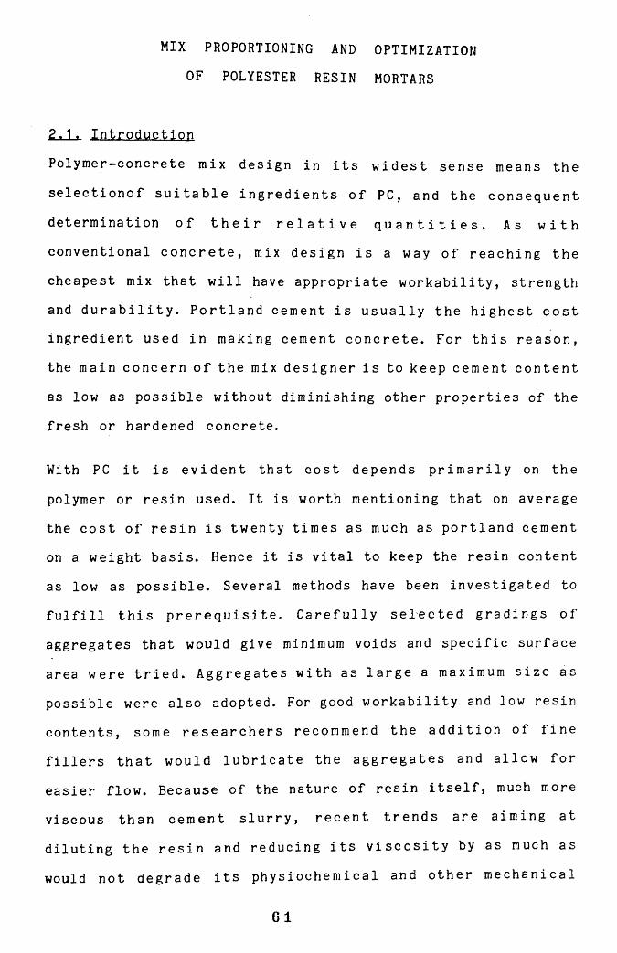
MIX PROPORTIONING AND OPTIMIZATION

OF POLYESTER RESIN MORTARS

1.«- Introduction

Polymer-concrete mix design in its widest sense means the

selectionof suitable ingredients of PC, and the consequent

determination of their relative quantities. As with

conventional concrete, mix design is a way of reaching the

cheapest mix that will have appropriate workability, strength

and durability. Portland cement is usually the highest cost ingredient used in making cement concrete. For this reason,

the main concern of the mix designer is to keep cement content

as low as possible without diminishing other properties of the

fresh or hardened concrete.

With PC it is evident that cost depends primarily on the

polymer or resin used. It is worth mentioning that on average

the cost of resin is twenty times as much as portland cement

on a weight basis. Hence it is vital to keep the resin content

as low as possible. Several methods have been investigated to

fulfill this prerequisite. Carefully selected gradings of

aggregates that would give minimum voids and specific surface

area were tried. Aggregates with as large a maximum size as

possible were also adopted. For good workability and low resin

contents, some researchers recommend the addition of fine

fillers that would lubricate the aggregates and allow for

easier flow. Because of the nature of resin itself, much more

viscous than cement slurry, recent trends are aiming at

diluting the resin and reducing its viscosity by as much as

would not degrade its physiochemical and other mechanical

61

properties. Interest is now gaining ground in using resins that are initially much lighter and less viscous.

As far as PC workability is concerned, the same definitions as with conventional concrete still apply. One of these is that

workability can be defined as the amount of useful internal

work necessary to produce full compaction (52). Itis well

known that a sufficiently workable PC would not only allow

good placement with minimum vibration in its fresh state, but

would also produce a high-performance concrete when hardened.

With PC made of polyester-styrene resin, the ratio of styrene

/polyester is very similar to the W/C ratio in cement concrete

(53). So styrene content or more specifically resin viscosity, has a dominating influence on workability. Resin content in PC

determines the mix richness just like cement content with PCC.

Aggregate shape and texture has an effect on PC workability,

especially with the lean mixes which are usually the case with

PC. Maximum aggregate size has also an effect on PC

workability as well as the grading and entrapped or entrained

air. Very little has been done regarding the development of

different methods of measuring PC workability. A clear

distinction between workability and consistency has yet to be

defined. Some of the conventional tests for measuring

workability might provide a rough idea about the flowability

of PC mixes. However, most of these tests would fail in

measuring various parameters controlling PC stiffening.

Stiffening of PC fresh mixes is made apparent by the loss in

solvent content by evaporation and the onset of the

polymerization process. All resins have their individual gel

62

times and final setting times, which change greatly when mixed

with other PC ingredients. The traditional troubles with poorly designed cement concrete mixes like segregation,

bleeding and nonuniformity are just as likely to happen with PC mixes if not given due attention.

Abram’s law relates concrete strength to W/C ratio for given

materials in cement concretes. This law should remain

applicable for PC strength by substituting W/C ratio with

styrene/polyester ratio. Resin viscosity may be used as a

measure of this ratio (53).

Very little information is available about proper mixing

times, proper mixer types, best vibration techniques and the

consequent strength variations for PC. The relationships

between the required minimum strength and the mean or the

characteristic strength are not established yet. Furthermore,

methods of testing and specimen dimensions are still awaiting

standardization in most countries. Little is known about

strength ’frequency-distribution’ for PC. The need for

reliable mix-design methods and quality control still calls

for greater research efforts.

2.2. Chemistry q L polvester-resinAlthough the chemistry of Polyester resin is primarily the

field of organic chemists, the basics of polyester

manufacturing and polymerizing processes will be briefly dealt

with.

Regardless of having a neutral charge, an atom will only be

stable when its outer electron-shell is filled to its capacity

63

by electrons (54). This can be done either by ionic bonds in

which atoms are held together by opposite electrostatic

attractions, or by covalent bonds in which atoms share

electrons. Elements in the central groups of the Periodic

Table (P.T.), or on the same side of the table tend to share

electrons rather than to transfer them. Carbon is an element

near the P.T. centre, so it is always covalently bonded.

Organic chemistry is the chemistry of carbon compounds and

might for this reason be named as the chemistry of covalent-

bond reactivities. These covalent bonds have a wide variety

and a rather specialized terminology. However, it may be

useful to stress some of them here. The simplest covalent bond

is ’sigma-bonding’, in which the resulting molecular orbitals

contain two electrons as is the case with methane, see

Fig.(2.1). In the same figure, examples of double and triple

bonds are given. The important thing to notice is that with

all double and triple covalantly bonded molecules, there is a

reactive or unstable site known in organic chemistry as a ’pi’

bond. These sites are principally responsible for crosslinking

long-chain molecules. As will be seen later, any resin type

containing these sites is called ’unsaturated resin’.

2.2.A Pq Iyester-resin m anufacture Polyesters are formed by

the reaction of an organic dibasic acid with a dihydric

alcohol (glycol). As shown in Fig.(2.2-a) an ester is formed

by condensation. In this case the acid has just one carboxylic.

group ( CO.OH), and the alcohol has just one hydroxyl group

(OH). The more general case is represented in Fig.(2.2-b)

where each alcohol and acid molecule has two end functional

groups. The resulting ester in this case has hydroxyl and

64

carboxyl end groups which allow for more reaction and much

longer polyester chains as shown in Fig.(2.2-c). This type of

polyester is termed as a ’thermoplastic saturated’ resin. Terylene is an example of this type of resin.

If the acid used in processing is of the reactive

’unsaturated’ type, the resulting polyester will still be

thermoplastic, Fig.(2.2-d); if catalysed the reactive sites

are caused to link together and a polymer network is formed,

Fig.(2.2-e), with thermosetting properties (does not flow on

heating while under pressure). This type of polyester is very

viscous and when hardened is very brittle due to the high

degree of crosslinking in the final product. That is why most

manufacturers use a ratio of saturated/unsaturated acids to

reduce the frequency of crosslinking.

Usually another component is added in the manufacture of

thermosetting polyesters. This is often a reactive monomer

such as styrene, methyl methacrylate or diallyl phthalate. As

shown in Fig.(2.3), the reactive monomer (styrene) has two

reactive sites which are capable of crosslinking polyester

chains at the sites of the reactive acid. Styrene serves in

two ways; one is to make the resin more liquid in the

prehardened state, the other is to allow less brittle products

in the hardened state.

2.2.B Pûixffierizaliûn Q.f While the

manufacturing process is essentially a condensation reaction

in which water results as a by-product, polyesters are said to

be polymerized when they have transferred from the liquid to

the solid state. To start polymerization liquid resin should

65

first be given a small amount of energy or otherwise

activated. Thereafter it proceedss spontaneouslyto full

polymerization. Energy can be provided either by heat or

radiation. Activation is provided by the addition of catalysts (initiators) and accelerators (promotors).

When the catalyst is added to the liquid resin, it can be decomposed either by an energy supply or by the addition of accelerators. When the catalyst is decomposed ,*free radicals’ are formed and they initiate the ohain-reaction polymerization and crosslinking at the reactive sites of polyester chains through a process called 'addition-réaction*. Under accidental energy application to the liquid resin, this reaction can take place without the addition of catalysts. For this reason most manufacturers add inhibitors to the resin. These inhibitors must be neutralized first if full curing is to be reached.

2.2.C Properites of polyester resins During the manufacture of polyester, cooling will stop the condensation reaction at any desired acid number, molecular weight or viscosity. The higher the molecular weight of the polyester resin and the more points of unsaturation in it, the more rapidly will the

polyester-monomer combination gain strength during the curing process. Higher mechanical properites of cured resins are

attained with increased molecular weight.

The ratio of saturated /unsaturated acids affects the final product properties. Increasing this ratio gives a more loosely

polymeric structure, a slower curing rate, more flexibility,

lower heat — distortion temperature and less resistance to

chemical attack.

6 6

The type of acid used in manufacture has a dramatic influence

on the finished product properties. Phthalic saturated acid can be used in the i sophtha lie or terephthalie form. Use of

the former would result in substantially higher molecular

weight with superior strength, toughness and increased heat

and chemical resistance over standard phthalic-acid resins. If

the acids used were all of the saturated type, the result

would be a resilient-polyester type (plasticizer) with

improved toughness and flexibility suitable for coatings and

plastic products. Fumaric-based unsaturated acids give better

mechanical and chemical properties than maleic-based ones.

Water and heat resistance are properties which are

particularly affected by the choice of the alcohol. Monomers

used have also certain effects. While styrene is preferred for

its low price, good reactivity and compatibility, others might

be used for special applications. Even the type of inhibitor

incorporated has some effect on the performance of the

hardened product.

Specially-formulated polyester resins are now available for

particular applications that require superior weatherability,

high flame-resistance, high heat-resistance and low shrinkage

strains, etc.

The dominant constituent in the resin polymerization process

is by far the catalyst, which is usually an organic peroxide.

Its selection depends on temperature of curing and its desired

rate, incorp o r a t e d inhibitors, desired degree of

polymerization and the activating means (heat, accelerator,

67

ultraviolet light, etc.). For any given resin-catalyst system

there is an optimum temperature at which the resin can utilize

all the free radicals formed by the peroxide decomposition at

that temperature. Above this temperature peroxide is wasted

and below it too much time is required for completing curing.

As catalysts are very expensive, the temperature ranges within

which catalysts are effective must be fully investigated.

used in the present work

The polymeric binder chosen for the PC of this work was of the

Polyester resin type. This was mainly because of its high

physical and mechanical properties, its low viscosity, its

simple curing techniques at ambient temperature and its

comparatively low cost compared to other resins.

Initially two different types were investigated and the best

one adopted throughout the whole work. The first polyester

resin chosen was "Crystic 196" which is a versatile, rapid-

curing and general purpose one. It is said to have excellent

mechanical properties. It also conforms to B.S. 3532 Type B.

Another preaccelerated, low-viscosity version of this resin,

"Crystic 196 PLAV", was also chosen. Typical properties of

these two versions of "Crystic-resin" are shown in tables

(2. 1 & 2 .2 ).

The second polyester-resin type chosen was "Cellobond A2661",

which is a heat-stable and chemical resistant resin. It has a

medium viscosity suitable for both cold and hot applications

where heat stability is essential. Typical test results on

liquid "Cellobond" resin are shown in table (2.3), while

properties of the cured resin are shown in table (2.4).

68

Z J L . Mtgrials ügfd In I M Present Work

2.4.A Chemicals

111 MniJls As mentioned above "Crystic 196", "Crystic 196 PLAV" and "Cellobond A2661" resins were used.

12 ) ^n^nlynjis Out of the large variety of organic peroxides

that are suitable for use, the chosen one was that recommended

by the manufacturer. It is a 60% solution of methyl ethyl

keton peroxide (MEKPO). This catalyst was used with the chosen resins at room temperature.

(3) Accelerators As cobalt derivatives are the most effective

promotors for use with the already chosen catalyst type, a

0.6% cobalt solution was selected as an accelerator. As will

be seen later, the preaccelerated version of "Crystic" resin

was much more convenient for use as it did not require the

addition of accelerator.

2.4.B Aggregates and fillers(1) Fillers Very fine fillers like calcium carbonate powder,

fly ash, Portland cement and aluminium silicates may be used

with PC. Those fillers have a vital role to play in PC

manufacture and performance. They permit the use of high

curing temperatures, where they tend to reduce the exothermic-

reaction temperature by reducing the concentration of reactive

materials. In addition to being a filling material at a very

low cost, they also improve workability and act as lubricants

when mixed with the resin by reducing the required internal

work to overcome internal friction in the mix. Fillers also

69

provide smoother finished products, with reduced setting and

volumetric shrinkage cracking. They also provide along with

the resin the system matrix giving it a lower coefficient of

thermal expansion, a higher modulus of elasticity and much

lower internal strains on setting and final hardening. Resin

absorption by aggregates and mix bleeding are greatly reduced by using fillers.

Two main filler-types were chosen for this work; calcium

carbonate powder and fly ash. Their properties are shown in

tables (2.5 & 2.6) respectively.

L Z) All the aggregates used in the present work,

with few exceptions, were supplied by Hyndford Quarry, near

larnak, Scotland. As will be shown later, different

classifications and particle shapes of natural sands and

irregular gravels were used. Wide ranges of gradings were

investigated. Crushed basalt stone supplied by Cairneyhill

Quarry, near Airdrie was also used.

Physical, chemical and mechanical properties of the different

fine and coarse aggregates used are shown in tables (2.7 to

2.9). For the whole work aggregates and fillers have been

oven-dried overnight unless otherwise mentioned.

2.5. Resin-mortar (RM) investigation

For the highest performance concrete, one should first find

the highest performance mortar. Different parameters were investigated to discover their influence on RM properties in

regard to workability and strength. As will be seen, the

experimental work on resin mortars (RM's) was divided into

70

three groups. These groups were designed to study the following :

(a) The effect of sand grading and its content.

(b) The effect of filler type and its content.

(c) The effect of resin type and its content.

(d) The effect of moisture content.

(e) The effect of resin formulation in terms of styrene/ polyester ratio.

(f) The effect of elevated temperatures.

2 f51A Specimens For the investigation of RM, small specimens

were manufactured to allow small batches and to provide more

quality control on the reproduceability of them. Small

specimens reduced the required number of batches and allowed

for collective mixing, casting, vibrating and curing.

For the evaluation of compressive strength and its 'frequency

distribution ', the two sizes of cubes chosen were 70 and 50

mm. respectively. For tensile strength (splitting strength),

cylinders of 50 mm. diameter and 100 mm. length were used. All

moulds were made of PVC which allowed good demoulding when

silicone grease and other releasing oils were applied.

2.5.B Mixing, casting and curing As the specimens were small,

the size of batch was small enough to allow mixing to be

carried out manually using an impermeable hardboard base. To

ensure consistent batching the resin viscosity was measured

before mixing using a viscometer of the type shown in

Fig.(2.4). Catalysts and accelerators were first added to the

resin at the ratio recommended by the resin-suppliers. Dried

fillers and sand were dry-mixed and the formulated resin added

71

to them.

Manual mixing continued until a uniform mix was reached.

Moulds painted with releasing agents were then filled and

vibrated for 3 min. on a vibrating table. Specimens were

allowed to cure at ambient temperature until the day of testing.

2.6. Tests and their results

Different groups of tests were made to investigate the effects

of the previously mentioned parameters on resin mortar performance as follows.

2.6. A first group of JRM In this group seven different mixes

were studied collectively and general comparisons were made on

the basis of their results. Four of these mixes used calcium

carbonate powder as a filler, while the other three mixes used

fly ash. The various mixing ratios are shown in table (2.11).

The sand grading was as shown in Fig.(2.5-a) and lies within

the second zone of sand gradings’ standards (B.S.882).

For this group "Crystic 196 PLAV" resin was used. The effects

of different mix-proportioning parameters were studied as well

as the effect of elevated temperature on strength. Elevated

temperatures were applied by keeping specimens for 30 min. at

80 C° followed by 90 min. at 100 C°in an electric-fan oven.

Table (2.12) shows the results obtained through this group,

which are represented as shown in Fig.(2.6)

From mixs (1) and (2) it is clear that increasing resin

content will for a given temperature result in an increase in

7 2

strength, but the deleterious effect of increased temperature

becomes more apparent as resin content increases. For low

resin contents, the filler had a very clear effect. By

referring to mixes (2) and (4) it can be seen that as filler

content was decreased from 16% to 5% by weight, compressive

and tensile strengths decreased by 20% and 30% respectively.

This effect is once again pronounced with mixes (5) and (7) in

which another type of filler (fly ash) was used. This confirms

the importance of the filler regardless of its type. It is

noteworthy that increasing resin content by 5% resulted only

in a 10% and 15% increase in compressive and tensile strengths

respectively,see mixes (1) and (2). This increase could well

be exceeded by adjusting the filler content to its optimum

fractional volume in the mix.

As no standard testing equipment was available for assessing

mortar workability, it was judged visually by the ease of

mixing, casting, vibrating and the surface finish of cured

specimens. Improved workability was noticed in both low and

high resin content mortar mixes by the increase of filler

content. Mixes (1), (2) and (7) produced almost void-free

specimens. This suggests that filler has similar effects in PC

proportioning where resin contents used are much less than in

RM.

By comparing identical mixes which differ only in filler type,

it is apparant that calcium carbonate powder is better than

fly ash; for example see mixes (2) and (7) or (4) and (5). It

is probable that fineness may be responsible for that, but

also d i f f e rences in chemical properties and their

compatibility with the resin used are the main reasons for the

73

better performance of calcium carbonate as a filler.

Z fZ 5..£c„giLd SJ2-Q1LD Q.Î. This group was designed to help find

out the best resin type to be used with PC. In this work, the

sand available in the laboratory with the grading shown in

Fig.(2.5-b) was used. Another grading was used in which sand

finer than 150 umm. is removed as shown in Fig.(2.5-c). Mixing

ratios and different resin types used are shown in table

(2.13). The results of the six different mixes are given in

table (2.14), in terms of compressive and tensile strengths.

It was found that "Crystic 196 PLAV" resin type had the

highest potential and viability for manufacture of RM, see

mixes (1), (2) and (3). It gave the best mechanical properties

, the best workability and the most well finished specimens.

Also this type of resin has the advantage of being

preaccelerated which necessarily simplifies mixing and reduces

the risk inherent in dealing with pure catalysts and

accelerators in the mixing area.

Although "Cellobond " resin is a specially formulated one

capable of coping with elevated temperatures, it was found

that specimens made out of it, mixes (3) and (5), still suffered heat deterioration. Despite the fact that this

deterioration was less than that given by "Crystic" general

purpose resin, the difference was not large enough to justify

the use of "Cellobond" whose performance at ambient

temperature is inferior to "Crystic" resin, see Fig.(2.7).

It was also found that continuous-grading sand with fine

particles included, gives better results than uniform size or

74

gap-graded sands, even with the use of fillers, see mixes (2)

and (4), A parallel study on the strength development rates

within this second group, confirmed that RM’s gain strength at

a rate which decreases with time. As shown in table (2.15),

compressive strength for mix (1) was 100 N/mm2 at 3-days of

age, increasing to 104 and 108 N/mm2 at 14 and 21-days

respectively. However, this rate depends principally on the

resin formulation and the ambient temperature during curing, as it can be made very fast or very slow.

To clarify the process of polymerization for the two different

types of the resins used, the following test series was

carried out within this second group. Three cylinders of 150

mm. diameter and 300 mm. in length, were cast of mixes (1) and

(3) which are made of ’’Crystic" and "Cellobond" resins

respectively. During casting a well protected thermocouple was

inserted in the centre of each cylinder. Immediately after

vibration, the internal temperature of the mix was recorded at

5 min. intervals up to the maximum temperature, and at 10 min.

intervals thereafter up till two hours from the start of

mixing. From that time, readings were taken every 30 min.

until the temperature became once again equal to the ambient

one.

As shown in Fig.(2.8), the ’induction interval (Ti)’ ,(57), is

bigger for "Cellobond" resin than that of "Crystic" resin;

this indicates a higher amount of inhibitor in the former. The

rate of polymerization is indicated by the higher rate of heat

evolution than heat dissipation , and is shown as an increase

in the recorded mix temperature, through the ’propagation

interval (Tp)’. It is evident from the same figure that

75

"Crystic" resin has a higer rate of polymerization. The 'gel

time (T g )' which is the time elapsed to reach the peak

exothermic temperature was about 70 min. for "Crystic" resin

and 90 min. for "Cellobond" resin. If the temperature gain in the mix is a function of the polymerization rate, it is clear

that "Crystic" resin is more reactive.

Based on the same figure, it can be said that curing of the

mix usually continues after the peak temperature is reached.

However, it is impossible to tell precisely when the

polymerization might stop, as it is completely dependent on

the existence of reactive free radicals and the polymer chain

end-functional groups. When the rate of heat dissipation

becomes greater than the rate of heat supply from the exotherm

reaction the mix temperature falls as shown in Fig.(2.8),

until it reaches the ambient temperature. If that temperature

is high enough (15 C°for most resins), polymerization would

continue for a much longer period than indicated in the

figure. This is proved by the experimentally observed strength

development rate. The time when this rate reaches zero should

be the real termination of the polymerization or curing

process.

From these exothermic tests, it was also found that gel time

and curing rates given for pure resins by the manufacturers,

are not particularly reliable or applicable to the same resin

type when it is mixed with aggregates. This is obviously

because of the transfer of heat evolved in the process from

the resin paste to the dispersed aggregates.

2.6.C Third group of IM This group was designed to study in

76

detail the effect of sand grading, moisture and styrene

content on compressive strength and its 'frequency

distribution'. Because of the large number of specimens used, 50 mm. cubes were prepared for this group.

2-t-j011 £.XXe.c.jt o£ trading Five different gradings of sand

were prepared with nominal specific surface areas ( SSA's)

varying from 2800 to 6700 m m 2/gm. These five gradings are

shown in Fig.(2.9) and table (2.16) as well. The SSA was

calculated from sieve test analyses. Assuming that the natural

sands used had spherical-shaped particles, the surface area

(SA) could be found for each weight of sand retained on

different successive sieves. The overall SSA was calculated as

the sum of SA's of different sizes divided by the overall

weight of the sand sample.

As shown in table (2.17), the first three mixes made in this

group were proportioned identically. To clarify the effect of

grading in terms of SSA's and moduli of fineness (MF) on the

performance of RM's, these three identically proportionated

mixes used different sand gradings. On testing the compressive

strength varied widely. Mix (1) gave a higher strength than

mix (2) which is made using a finer sand, and a higher

strength than mix (3) which is made with a coarser sand. Based

on the findings of the first three mixes, more work on the

effect of sand-SSA was undertaken as will be shown with the

following four mixes in this group.

Using the coefficient 'k' to express the mix richness as the

ratio of the mix resin weight in gm., to the SA in mm2 of the

sand used, four different mixing ratios were calculated on the

77

basis of equal k-value and variable SSA's as shown in table

(2.17). To make the comparison on SSA-basis valid, the type of

the four different gradings used with these four mixes was of

the continuous-type grading. Uniform or gap-graded gradings

were not used, see Fig.(2.9). The coefficient k was found to

have three values with the first three mixes (1), (2) and (3).

The value chosen for the last four mixes was that of mix (1);

as it gave the highest strength. This value of k which is

5x10"5gm/mm2 produced four different mixing ratios for mixes

(4), (5), (6) and (7), which differed in the SSA's values of

the sand used with them, as shown in table (2.17).

Fig.(2.10) shows the relationships between 24-hour compressive

strength and SSA for the first three mixes , curve (A), as

well as the last four mixes, curve (B). In the same figure,

using another ordinate, the relationship between RM unit-

weight and SSA is shown. Curve (E) represents mixes (1) to

(3), while curve (F) represents mixes (4) to (7). It is clear

from this figure that whether k is a variable as in curve (A)

or constant as in curve (B), there is a certain range for SSA

within which a maximum strength can be obtained. The

intersection of these two curves should satisfy the

requirements of both of them. Using this condition and the

other available points ( each is the average of twenty-five

results), these two curves (A & B) were plotted as shown in

Fig.(2.10). Despite the fact that these two curves represent

one value of k and a particular mixing ratio, numerous

different values of k can be deduced from curve (A), and a

wide range of mixing ratios can be found from curve (B). For

instance any point on curve (A) can be translated into a

78

corresponding k-value depending on the SSA given. Any point on

curve (B) can also be translated into a distinct mixing ratio.

The only provision to be considered is that the filler content

is 15% by weight, i.e., the same filler content as that

employed in the mixes on which these test results are based.

Bearing in mind this provision, curves (C) and (D) were

calculated and plotted as shown in Fig.(2.10), with two

different ordinates drawn in a downward direction. From curve

(C), the value of k is shown to vary from around 3.5x10” to

7 • 5x 10”5gm/mm2. These two values of k were experimentally

found to represent the upper and the lower limits within which

RM would be workable. Higher values than the upper limits

imply very sloppy mixes with high bleeding tendencies. Lower

values than the lower limit imply very harsh RM with poor

finishing properties. The range of SSA's in this chart, as

investigated, is from 2500 to 6500 mm2/gm.

The chart can be used for mix-proportioning of RM's made of

"Crystic 1,96 PLAV" resin type, with 15% by weight calcium

carbonate powder as a filler and continuously-graded sands. It

can also be used for mix-optimizing and prediction of the 24-

hour compressive strength and density as will be shown in the

following example.

Example Find the optimum mixing ratio and the expected 24-

hour compressive strength and density for resin mortar made of

the same materials given above and sands with SSA's of the

value (1) 2900 mm2/gm. (2) 3800 mm2/gm.

Solution(1) Using the given chart in Fig.(2.10), draw a vertical line

79

at SSA z 2900. Find its intersections with the six given

curves. Intersections i, i* and i" for a constant mixing

ratio of 15:15:70, give a strength of 102 N/mm2 at a k-value

of 7.4x10“^gm/mm2. with a corresponding density of 2.11

gm/cm3. Intersections ii, ii’ and ii" for a constant k-value

of 5x10-5, give a strength of 90 N/mm2 at a mixing ratio of

12:15:73; with density of 2.07 g m / c m 3. For the highest

strength, intersection (i) should be considered which means a

mixing ratio of 15:15:70. As the corresponding k-value is

almost equal to its upper limit, no higher resin content can

be used and the given mixing ratio is the optimum one.

(2) Following the same procedure with sand SSA z 3800 mm2/gm ,

one will have two sets of values representing intersections

(i) and (ii) which are as shown in table (2.18). From this

table it is clear that neither of the mixing ratios is the

optimum one. The shown value of k still can be increased up to

the upper limit , at which a new mixing ratio can be found and

would give a higher strength . This mixing ratio can be

calculated as follows.

The ratio of the sand in the mix by weight Ws can be

calculated from the equation;

Ws z (1 _ Fc)/(1 + k.SSA)

in which Fc is the filler content (15% as assumed), then

substituting for k z 7.5x10-5, SSA z 3 800, then Ws z 0.66.

Hence the optimum mixing ratio is 19:15:65 (resin : filler :

sand by weight.). Extrapolating the values of intersections (i

& ii) to the new mixing ratio , the corresponding strength was

found to be 120 N/mm2 with 2.25 gm/cm3 -density. It is

80

important to stress that the previously made extrapolation was

found to be valid through various experimental results as long

as the limiting k-values are not exceeded. That is to say that

for any RM the strength is directly proportional to the resin

content within the suggested limits of k-value.

The applicability of this chart could be extended . If six

families of curves like curves (A, B, C, D, E & F) were

constructed RM’s could be proportionated to give a desired

strength and density at a given sand SSA. Due to limitations

in time and the existance of other objectives to be fulfilled

in this present work, experimental investigation of resin

mortars was stopped at this stage. However, the basic

principle of mix proportioning of RM's on an SSA basis is

believed to be clear enough for any one wishing to undertake

any further work in this field.

2.6.C.ii Effect of moisture To clarify the influence of water on the degree of polymerization and the consequent performance

of RM, the following set of specimens were made. Four

identical mixes made with mixing ratios 15:15:70 were used in

making sixteen 50-mm. cubes for each mix. The sand used was of

the continuous-grading type as shown in Fig.(2.9-1). Four

different moisture contents (Me) were used namely 0.0, 0.5,

1.0 and 1.5% of the sand weight. The mixing ratios and the

results are shown in table (2.1 9) as well as in Fig.(2.11).

The deterimental effect of moisture on the strength of RM is

evident as is the fact that loss of strength is not

proportional to the water content. Increasing Me from 0.0 to

0.5% of sand weight resulted in a decrease in the compressive

81

strength of about 22.5%. While a moisture content of 1.5% caused a strength reduction of 41.5%.

As shown in Fig.(2.11), it can be seen that there is a certain

Mc-value above which no further significant loss in strength

will be caused. Generally speaking, this set of tests showed

that wet aggregates can be used in batching RM and PC, and

still can give high mechanical performance.

The question of whether to use dry, surface-dry or wetted

aggregates depends primarily on the drying-energy costs and

the available types of aggregate. It is not possible to set a

particular limit for the allowable Me of aggregates used; but

a compromise between required performance and allowable Me in

the mix would be required.

Recent attitudes call for improved performance of resin itself

in a wet environment. Many chemicals are now being used for

this purpose such as silane coupling agents and different

water absorbents. In Japan, it is reported that up to 3% Mc-

aggregates have been successfully used in making RM's without

loss in strength (56). Due to the nature of this controversial

and chemical specific point, no further work was made in this

present work.

The main conclusion drawn from this set of tests was that

moisture content can have a damaging effect on the mechanical

performance of resin mortars and consequently on resin

concretes. This is mainly because the water existing in the

aggregate lessens the effect of the incorporated initiators.

In that case polymerization speed is reduced and curing may

82

interfere with curing in one way or another (55). Water has

two effects, the first is prolonging or preventing complete

polymerization and the second is reducing strength. Prolonging

the polymerization process leads to further disruption as

other chemical factors may exercise a more marked influence

which is not apparent in the course of normal-speed

polymerization. One of these is the oxidation of reactive

styrene monomers into styrene peroxide instead of acting as a

crosslinker. Eventually this peroxide degrades into organic

components which act as inhibitors (55).

2.6.C.iii Effect styrene content It is well known that by

increasing the content of styrene, which acts as a diluent for

a polyester, the setting time or gel time becomes shorter due

to the increased reactivity. Styrene decreases the liquid

resin viscosity with a consequent increase in the mix

workability. At the same time, increased styrene content (Stc)

reduces the strength, as the micromolecular distance (54)

between polymer chains increases and the binding matrix

becomes much more flexible and looser. To clarify this effect

on the performance of polyester resin, the following tests

were carried out using "Crystic 196 PLAV”.

Four identical mixes were prepared using a mixing ratio

15:15:70. The sand grading used was that shown in Fig.(2.9-1).

The only difference between mixes was in resin formulation.

Four styrene/polyester ratios (ST/UP) by weight were tried as

follows; 0.0, 5.0, 10.0 and 15.0%. The same amount of catalyst

(2% of resin weight) was used for the four mixes. Out of each

mix sixteen 50 mm.-cubes were cast, cured at ambient

83

temperature and tested at 24-hours of age. As shown in table

(2.20) and Fig.(2.12), strength decreased almost linearily at

the rate of 1.2 N/mm2 for each ^% increase in ST/UP ratio.

Obviously the rate will depend on the resin used and its

properties, but the general trend of strength degradation by

increasing Stc is still applicable to any RM or PC.

"Crystic" resin has reasonable workability and gel time as

delivered by the manufacturer so that there was no need to

alter or interfere with its properties. In the tests which

follow no styrene or any other diluting agent was

incorporated.

2,&,C,iv Slallslic^l i n t e r s of K h results At this

stage it may be useful to examine some of the experimentally

observed variables and their uncertainities, which usually

arise from the complex of variations termed as errors. No

matter how precise the experimentation and measurements are,

different-source errors usually creep into all observations.

Full statistical analysis that would help in reaching reliable

and safe confidence limits through statistical interpretation

of the laboratory findings, is not within the scope of this

work. However, interpretation of some of the laboratory data

regarding RM’s will be discussed.

Out of the previous RM mixes, six were chosen for statistical

analysis. For each mix, twenty-five cubes (50 mm.) were cast

and tested in compression. To minimise errors, one mix was

prepared and all twenty-five cube moulds were filled, vibrated

and cured together. For each mix, the compression tests were

carried out on the same testing machine and with the same

84

instrumentation. The specimens of each mix were tested at the same age, temperature and rate of loading.

Table (2.21) shows the arithmetic mean, the standard deviation

and the coefficient of variation for the six different mixes.

The full results are reproduced graphically for each mix as

shown in Fig.(2.13). In this figure the strength frequency

distribution is presented by a histogram, in which the

horizontal axis represents group interval in N/mm2, The

heights of the rectangles shown represent the number of

specimens within the interval. Because of the limited number

of observations, this graphical presentation may not

accurately represent the distribution of the whole population.

Before any further statistical interpretation of data, it was

necessary to check the ’normality’ of the strength frequency

distribution. The Shapiro test for normality (58) was applied

and its results are represented in table (2.22). It was found

that four mixes are normally distributed with a significance

level (31) less than 0.01 ( more than 99% confidence level ).

It was also found that five mixes out of six were normally

distributed with 51 less than 0.05. Only two mixes did not

qualify for normal distribution for SI = 0.01. However, the

general frequency distribution for these resin mortars could

be regarded as a ’normal ’ distribution.

Values derived from any one set of observations will be

subjected to some uncertainity, and can be considered only as

estimates of the unknown true values. Such estimates should

always be accompanied by measures of their uncertainity (59),

by giving two limits and asserting with a certain probability

85

that they include the true values (confidence limits). Table

(2.23) shows the mean and the standard deviation for each mix

with their confidence limits for 95% and 99% probability. Also

it is usually useful to have a simple procedure with which one

may test the homogenity of observations. The British Standards

(B.S. 2846 Part 1: 1975) provide 'controlling charts' for such

a procdure. These charts have inner and outer limits as shown

in Figs.(2.14 & 2.15). The inner and outer limits correspond

to probabilities of 1:40 and 1:1000 respectively. The

occurance of points outside the outer limit or of more than

one or two points outside the inner limits is considered to be

evidence that data are not homogeneous. As shown in Figs.(2.14

& 2.15); the observations for each mix were divided rationally

into five subgroups. The mean and the range of each subgroup

was found and the general means and the mean ranges were

calculated and used in constructing the charts. For each mix

the group mean and range were plotted and compared to the set

limits.

Some conclusions can be drawn from the previous statistical

analysis. The variance in compressive strength for resin

mortars tested ranges from 2 - 3.4%, a range which is well

below the accepted value for conventional concretes and

mortars in different standards (60). The true compressive

strength values are found to have maximum confidence limits

ranging from +0.99 to +1.85 with 99% probability. This

suggests the reliability of the derived means for the

different mix strengths. The homogenity test for the given

observations confirmed once again the consistency and validity

of those observations. In addition, it is shown that RM can be

86

fairly regarded as a material with a 'normal frequency

distribution' strength. So all the rules applied in deriving

the characteristic strength statistically for conventional

concretes and mortars, should remain applicable to resin

mortars and resin concretes. This is an important conclusion

that will be used later in chosing different PC grades.

87

Table 2.1: Typical properties of liquid CRYSTIC 196

Viscosity at 25°C 9 poise3.5 poise PALV

Specific gravity at 25°C 1.121.11 PALV

Acid value 21 mg KOH/g 19 mg KOH/g PALV

Volatile content 33%38% PALV

Appearance light straw pinkish PALV

Stability in the dark at 20°C 6 months

Gel time at 25°C (determined under laboratory conditions using:CRYSTIC 196 100 pbw.Catalyst Paste H 3 pbw. Accelerator E 4 pbw)

8 minutes

Gel time at 25°C (determined under laboratory conditions using;CRYSTIC 196 PALV 100 pbw. Catalyst M 2 pbw)

14 minutes PALV

Test methods as in BS 2782: 1976

88

Table 2.2: Typical properties of cured CRYSTIC 196(unfilled casting)

Barcol hardness (Model GYZJ-934-1) 45

Water absorption 16.5 mg

Deflection temperature under load (1.80 MPa) 72°C

Elongation at break* 2.3%

Tensile strength 69 MPa"*"

Tensile modulus 3.8 GPa

Specific gravity at 25°C 1.22

20Refractive index n — 1.560

Dielectric loss (tan 6 at 1000 Hz) 0.006

Dielectric constant (at 1000 Hz) 3.0

Residual styrene content (Measured by BPF-approved method for freight containers)

0:01%

Test methods as in BS 2782: 1976

* Filtered resin, void-free casting

89

Table 2.3; Typical Test Results

Specific gravity at 25°C Viscosity at 25 C

Volatile content Gelation time at 25°C (using 2 mis of liquid catalyst 60% MEK peroxide LA+3 mis of

0.6% Cobalt solution on lOOg resin)

10 ^m^/s cS

%minutes

1.1174754753735

Table 2.4; Cellobond A2661 typical properties of cured cast resin.Test methods as in BS 2782 and BS 3532.

Test Cured cast resin

Tensile strength MN/m^ 49.3Young's modulus in tension MN/m^ 3450Flexural strength, dry After immersion for 2 hours in

MN/m^ 96.5

boiling water MN/m^ 79.3Young's modulus in flexure MN/m^ 3725Izod impact strength J/m 12.3

Heat Distortion Temperature atft.lbf/in notch 0.23

1.81 MN/mZ (264 Ib/in^) "C 130Water absorption 1 day mg 32Power factor at 23°C at 1 MHz 0.004Permittivity at 23°C at 1 MHz pF/m 30Volume resistivity ohm m > 1.2 X 10^3Surface resistivity ohm > 3.74x1014Electric strength MV/m 15.0Electric strength Volt/mil 380

90

Table 2.5: Properties of calcium carbonate powder used.

Chemical analysis of the raw material

Fineness

Technical data

CaCOg 99.75%MgO tracesFezOg 0.02%so^z- 0.06%Colloidal aluminium silicate 0.1%Loss on ignition (DIN 55918) 43.34%Moisture (DIN 53198) below 0.2%

Residue on a 40 micron sieve (DIN 53195)

0.1%

Top cut 25 micronsMean particle size 5 micronsFiner than 2 microns (Sedigraph)

10%

Density (DIN 53193) 2.7Refractive index 1.65Hardness (Mohs) 3Particle shape crystalline

rhombohedralPacked bulk density (DIN 53194) 1.4 g/mlDry brightness:Elrepho green filter (FMY/C) 91pH value (DIN 53200) 9Oil absorption (rub-out, ASTM D 281-31)

16 gper lOOg powder

DOP absorption (rub-out, ASTM D 281-31)

25 gper lOOg powder

91

Table 2.6: Typical p r o p e r t i e s o f fly ash* used

Chemical analysis of the raw material Si O2

ALoOq FezOg Ti O2 MngOiCa 0 Mg 0 NazO KzO SOgP205

Combustible + moisture Loss of ignition

Specific gravity Fineness:

Effective size D^Q mm Uniformity coefficient

Dio% finer than 0.02 Specific surface area cm^/gm

52.030.47.230.870.062.550.790.490.970.640.28

2.25

3.3621%

0.00532.5

79%4960

* Barony fly ash, Ayrshire, Scotland.(1) Research report No.01038, CEGB, the Univ. of Glasgow, by

Prof. H.B. Sutherland and P.N. Gaskin.

Table 2.7: Properties of the natural sand* used

Relative density:Saturated surface dried basis Apparent basis

Bulk density:Loose density Rodded "

Water absorption(l) (% of dry mass)Alkaline reactivity ( i n n o c u o u s ) (2) Reduction in alkalinity Rc Dissolved SiOz in (mmol/1) Sc

2.592.75

1545 kgs/m3 1680 l/gs/m3 1.6

90 (mmol/1) 16.4

(1) B.S. 812: Part 2: 1975(2) ASTM C289-81* Hyndford Quarry, Near Lanark.

92

Table 2.8; Properties of the natural gravel* used

Flakiness index 8.0%Elongation 1.0%Crushing value 24 %Impact value (2) 22 %Content of clay, silt and dust 0.2%Relative density:

Saturated surface dried basis 2.6Apparent basis 2.77

Bulk density:Loose density 1495 kgs/m3Rodded density 1565 Kgs/m3

Water absorption (2) (% of dry mass) 2.7

(1) B.S. 812: Part 2: 1975(2) B.S. 882; 1983* Hyndford Quarry, near Lanark

Table 2.9: Properties of crushed basalt stone*

Impact value 10Crushing value 1510% Fines value* 260 kNAbrasion value 4.8Polished stone value 61Relative density:

Oven dried basis 2.74Apparent basis 2.90

Bulk density (surface dry):Uncompacted 1285 kg/m3Compacted 1420 kg/m3

Water absorption (% of dried mass) 2.0

(1) B.S. 812: Part 3: 1975* Cairneyhill Quarry, near Airdrie, Scotland

93

Table 2.10; Gradings for the natural sand, natural gravel and crushed basalt used.

A: Sand gradingSieve size (mm)

4.752.361.180.6000.3000.150

% passing95.583.562.5 40.08.01.5

B: Gravel grading

Sieve Size (mm)

16.010.06.75.02.361.18

% passing

10089.537.5 9.5 0.5 0.0

C; Crushed basalt

Size (mm)

61014

% by wt.

255520

84

Table 2.11: 1st group mixing ratios of resin-mortars

Mix No. Percentage by WeightResin* Filler Sand

1 20 15 652 15 16 693 20 10 704 15 5 805 15 5** 806 15 10** 757 15

.

16** 69

* Used resin: Crystic PLAV 196 unsaturated polyester resin, ** Filler: fly ash, otherwise calcium carbonate powder.

Table 2.12: 1st Group results*.

Mix No. Compressive(a) strength in N/mmZ

Tensile (b) strength in N/mmZ

at room temp.

at elevated(c) temperature

strength loss %

at room temp.

at elevated temperature

strength loss %

1 126 83 34 15.5 10.5 322 114 80 30 13.5 9.5 303 126 91 28 14.5 10 314 97 80 17.5 10.5 8.2 225 87 58 33 10.5 7.5 286 101 72 29 12.0 8.2 347 109 77 34 12.5 8.5 32

(a) Average of 6 cubes (40 mm - size)(b) Average of 6 cylinders (d = 50 L = 100 mm)(c) Specimens kept for 30 min in 80°C, 90 min in 100°C, then immediately

tested.* Tests were made at 14 days of age.

95

Table 2.13: 2nd group mixing ratios of resin mortars

Mix No. Resin type used ('a''Resin formulation Mix ratio by weightResin Filler Sand

1 Crystic PLAV 196 2: -: 98 16 16 682 Crystic 196 2: 2: 96 16 16 683 Cellobond A2661 2: 2: 96 16 16 684 Crystic 196 2: 2: 96 16 16 68^^)5 Cellobond A2661 2: 2: 96 20 15 656 Crystic PLAV 196 2: -: 98 15 15 70

(a) Formulation in weight% of catalyst; accelerator: resin(b) Calcium carbonate powder.(c) Available sand in the laboratory of the shown grading in Fig.(2.5-b),

All other sand used are of the grading shown in Fig. (2,5-c).

Table 2.14: 2nd group results*.

Mix No.Strength in N/mm2

(1) (2) (3) (4) (5) (6)

o • (a)Compressivestrength 105 92 100 98 102 106

Tensilestrength 12.0 12.0 9.5 12.5 12.0 11.0

* At 14-days age.(a) Average of 6 cubes (70 mm size)(b) Average of 6 cylinders (d = 50 mm, L = 100 mm).

96

Table 2.15: Strength development of resin-mortars

Age Compressive strengths (N/mm^) for Mix no.^^^

(1) (2) (3)3 days 100 92 8214 days 104 97 9221 days 108 102 94

(a) Average of 6 cubes (70 mm size)(b) Mixes used in 2nd group.

Table 2,16: Different sand gradings used with 2nd group

Sieve No. (S.I.)

Percentage retained for different grades

I II III IV V

10 0.0 0.0 0.0 0.0 0.05 16.6 34 5 25 10

2.36 16.6 19 5 15 51.18 16.6 20 5 20 50.6 16.6 3 15 15 200.3 16.6 7 45 10 450.15 16.6 12 25 15 15

S.S.A.(*) 4200 2800 6700 3600 5600M.F. 3.5 4.3 2.35 2.95 2.7

(a) Specific surface area in mm^/gm.

97

Table 2.17; Mixing ratios and compressive strengths forresin-mortars (3rd group).

Mix No. SandGrading

Mix ratio (by wt) Resin** ;filler*; sand

K gm/mm^X 10-6

CompressivestrengthN/mm^

standarddeviationN/mm^

1 I 15 ; 15 ; 70 50.0 1103.8 2.52 III 15 ; 15 ; 70 32.0 92.5 1.83 II 15 ; 15 ; 70 75.0 101.7 3.34 II 10.4 ; 15 ; 74.6 50.0 88.1 2.85 IV 13 ; 15 ; 72 50.0 95.3 3.26 V 18.5 ; 15 : 66.5 50.0 104.7 3.07 III 21 ; 15 ; 64 50.0 97.8 2.6

* Calcium carbonate powder.** Cystic PLAV - 196.(1) 24 hours - age, 50 mm cubes, average of 25 specimens.

Table 2.18; Mixing ratios and results for different M -resin mortars.

Mix No. Mix ratio (by w t l ___*** Moisture 24-hourResin ; filler : Sand content

%comp.strength

N/mm^ *1 15 ; 15 ; 70 0.0 104.02 15 ; 15 ; 70 0.5 81.03 15 ; 15 ; 70 1.0 59.04 15 ; 15 ; 70 1.5 61.0

* Average of 4 specimens, 50 mm cubes, 24-hour age.** Percentage of sand weight.

*** Used grading curve I Fig,2.9,

98

Table 2.19: Mixing ratios and results for different Stc-resinmortars.

Mix No, MixResin

ratio (by wt) Filler Sand

Styrenecontent

%

24 hours compressive strength N/ram^

(1) 15 15 70 0.0 104.0(2) 15 15 70 5 97.0(3) 15 15 70 10 91.0(4) 15 15 70 15 87.0

Table 2.20: Statistical interpretation of 6 resin-mortar mixes

Mix No. X ^n-1 0n V

(1) 92.524 ±1.77 1.73 1.9(2) 101.684 ±3.31 3.24 3.25(3) 88.1 ±2.87 2.81 3.25(4) 95.28 ±3.24 3.18 3.4(5) 104.70 ±3.024 2.96 2.88(6) 97.80 ±2.57 2.53 2.6

n-1

Compressive strength arithmetic mean in N/mm^ , average of 25 observations.

: estimate standard deviation in N/mm^.: population ": variance percent.

Table 2.21: Results of Shapiro Test for Normality.

Mix No.* Correlation factor** Conclusion***

a = 1% a = 5%

(1) 0.986 N N

(2) 0.940 NN NN

(3) 0.961 NN N

(4) 0.987 N N

(5) 0.988 N N

(6) 0.991 N N

NNN*

significance level (confidence level = 1-a) normal distribution not normally distributed a complete sample of 25 observationsfactor that relates original observation values to those of normal order statistics.

HH— H

Hmethane

? ? H— G— C— H

ethane

I H— Ck -N

formaldehyde hydrogen cyanide

Xethylene acetylene

Flg. 2.1 Examples of different carbon covolent bonds.

( a ; C CO-OM . M0-(22) C ">coo-<r "j-> Wf Acid - Alcohol Ester -» Wale»

I B ) ! > C0 0h ♦ »0-G , *!)-0" HOO:^ ~ > COO-C > Olt. Hfi

"® czi>“Xiz3>oo czr>x7'r2><>ocGr>“'°czz>‘'--Acid C'lycoi Mc;c Glycol Acc G-,coI t ) 01 mc.-f s moly:

( D )

I El

CrciSlir.Ktd ro'yestc" wi’h&ot styier.e ptesc

Fig. 2.2 Schematic representation for the mcnufocture of polyester resi

100

&«wW#d polyittti with ilytvfw pfM»nlNon MmclivT ÜMCIIvt

K W onii #cW unti #cid im ii

CD— d>I unii #cW wWiHpCD Cp CD--

ftoKtivtmonomrt unit

fo*Y#iie iCtMini

Cp CD— d>>—CD CDfP— cp— CD CD— CD— CD— CD

monom*' yn.l

CureCD CD— CD

CD— CD— CD

CD CD— CDFig. 2.3 Effeet of styrene monomer on

the physiochemi co] properties of polyester.

TORSION W*CGRADUATED SCALE.

.CYUNOER AQJUSniNG SOnEW

STOP RELEASE PIN CYUNOER SUPPORT STEMCYLtOER

Fig. 2.4 Universal Torsion Viscometer C Assembly Diagram),

i O l

100“/o

c£ 60 108a%

?5uka

GO

40

20

0.0

J 1----- 1-----71--a- Continuous grodlng with MF-Ë. B6 b- Continuous qroding with Mf*3. 05 c- Cop grodod with MF*»3. 0 /

Sieve clze mm (umm)

75 150 300 600 1.18 2.36 5.0 10 .0

Fig. 2.5 Various sand gradings used with the first and second groups of resin mortars.

Filler: Calcium carbonate

I

'’20

60

ftÏ .U)

11] 12] :i][3]

33 33

121

Compressive s t r e n g t h

3 3Splitting s t r e n g t h

Resin content Filler cont e n t Filler content

(\)I

120

80

r.m01 40+»in

Filler: Fly ash

141 BÏ163 [6lI7l

Comp'-essive s t r e n g t h

S p litting s t r e n g t h

Resin content Filler cont e n t F l 11er content

Strength ct ele v c t c d t e m p e r o t u r e

' FiQ. 2.6 Test results of the first group.

102

120

fvI 60

XO' 40ÎLin

Compressive strength

111 131121 131

Splitting strength

bü tti

[51

II] 131 [21

h t 7 days of cge Bi J 4 ocys of ogc Ct ocys of oge

Reoln type Resin content Strength development

Fig. 2.7 Test results of the second group.

uoL3OL0Q-E0

T3abIBDO%

(1) "Crystic PLAV 196" resin

Tenipa'rcti/ir» recordo—

(2) "Cellobond"resin'40 Thermo coup J o

Tpi Propcgotlon time

Tgj Gg I tlmo

Til Induction time4

ji J f i ic J r> xniin#

36030024018012060

Fig. 2. 8 Reactivity of the two resin types used.

103

?Ioy+>couV

CL

100III

80

6Ô

n /20

SlGvc size mm0

150 30C75 600 1.18 23 6 5.0 10,0

Fie. 2.9 Differtcnt sand gradings used with 3rd group of resin mprtars

%'FzX5L+>ID

01>u(A0LaEOu

NEE%

+>C01uItO r-u —

100

Constont mixing ratio

70

- 2,1'

Specific surfocc crcc mm2/gm(i00)60

0

AO

0

70

mEE\I,4JXm01»

Fig. 2.10 Chart for mix-design of resin mortars made of "Crystic" resin vyith J5% calcium carbonate as o filler.

1 0 4

(\izI 120VLw01>inin01h.EOu Moleture content

0.5 1.51.0

FIG. 2. 11 Effect of moisture content of sond on fnc compressive strengtn ot resin mortar.

IXzXu56 (ta>uIB0)h Eu

100

90

80 Styrene content ( X of resin weight)

15.010.05.0

Fig. 2. 12 Effect of styrene content on the compressi strength of resin mortar

105

p»oPSSB C£ X

z

8

8

F9LP10a>10(011

;8cR S„ X

n

E

8 mLO4JL0'EC0«L*30

_ LO>g L0'

în 4-e aX 0p 3

O8 >

HP 4JDl» C0L+Jm

h-omEOl.m0+jm%

8 m

g •»r wX mz ::j.oOV

%DAja%u; uj a u p u jja a d s *ofg

1 0 6

Mix n> O o

Mix (2)

Mix (3)

o ° o o Mix (1)

0 oc o o Mix (2)

T5 5"o Mix (3)

Mix (5) O o

o c Mix <4)

o o o Mix (5)------ o--------

Mix (6)O O

o o ° o Mix (6)

Outer limit (1: 1000 probobility) Inner limit ( ii 4D probability)

Fig. 2. 14 Controlling charts constructed for the subgroups' range.

Fig. 2.15 Controlling charts constructed for the subgroups' mean.

1 0 7

CHAPTER THREE

SHORT TERM MECHANICAL PROPERTIES

OF POLYESTER RESIN CONCRETE

3.1, Introduction

One of the basic prerequisites of this present work was to

obtain different structural grades of PC's. These grades were

intended to be used in the structural analysis of PC. when

reinforced. They varied in strengths, moduli of elasticity,

cracking strains and ultimate compressive strains. As will be

shown various mix proportions were tried to obtain five

distinct PC grades.

The properties of PC as a composite material can be regarded

as the superposition of the additive and synergetic

interactions between different components (61). These

components affect the performance of PC on micro and

macrostructural levels. On the micro level, the component

surface properties are responsible for all possible

interfacial interactions whether they are physical or chemical

ones. On the macro level, the fractional volume and the bulk properties of the component do have a dominating influence on

PC properties. Numerous bulk models have been developed for PC

and most of its mechanical properties could be calculated

accordingly using the additive-mechanism concept. These bulk

models which depend on the law of mixture were used after

introducing some modifications and new concepts (61). They

could be used successfully in predicting strength and other

mechanical properties from knowledge of the technical

characteristics of PC and the boundary conditions relevant to

108

them.

As shown in Fig.(3.1), PC can be generally divided into a

continuous matrix phase and a dispersed-inclusion phase. The

variables in structure that would affect the performance of

PC, as shown in Fig.(3.1), are numerous and can result in a

wide range of PC performance. For example it was found (61)

that pores represent an important macrostructure factor. The

formulation and type of resin used has another important

influence. Different aggregates may result in a variation of

PC compressive strength of almost 50% while keeping all other

mix variables constant. A quantitative representation of the

effect of the main PC-structure c o m p o n e n t s on the

macrostructural level is shown in Fig.(3.2) after Gamski and

Bares et al (62) & (63).

On the microstructural level , many polymer-morphology studies

have been undertaken to clarify the effect of synergetic

interfacial combinations. The most important outcome is the

fact that the creation of polymer-aligned layers or envelopes

around filler particles produces PC performance (64)

essentially different from those in which alignment has not

taken place. Chemists are involved in modifying the

interfacial layer between matrix and filler. Their main task is to help keep the polymer envelope around the particles as

thin as possible with as large an aligned-polymer volume

fraction as possible. The effect of the thickness of the

aligned polymer envelope on the mechanical performance is

shown in Fig.(3.3), along with the effect of PC porosity.

A study made in the U.S.S.R. on the physiochemical structural

109

formation of PC reached several interesting conclusions (64).

One of these was that there is an optimum filler-surface area

in the binding matrix ranging from 3000 to 5000 cm2/gm, at

which the binder can be used efficiently. In addition there is

an optimum ratio of binder which can only be reached with the

highest possible degree of aggregate-compaction. Different

morphology studies of the micros truetre of globular or

fibrillar polymer macromolecules showed that its formation

depends upon: (a) polymer and filler ratio, (b) monomer

chemical composition and (c) the properties of filler itself.

These studies revealed the possibility of modifying and/or

controlling polymer macromolecule structures along with the

asssociated shrinkage strains and stresses. Some newly

developed PC’s were produced using active-surface fillers

(65). These PC’s are termed as expansive resin concretes and

may expand rather than suffer shrinkage on setting. Several

phsiochemical studies undertaken in the U.S.S.R. (66) & (67)

suggested different material models with different component-

structure-properties to suit different applications. The

importance of such models is that they primarily help provide

technical information for the development and production of

PC. The high cost and the sophisticated applications of PC

necessitate such models to serve as a tool in PC design. One

of the suggested procedures for establishing design

characteristics of PC is shown in Fig.(3.4).

3.2. Review q L PC proportioningBefore proceeding towards mix-proportioning of PC, different

mix variables and their influences on PC performance as found

in various researches were revised along with their

1 1 0

experimental findings. Optimizing PC mix-design could be

achieved by improving either the continuous-matrix phase or

the dispersed-inclusion phase. Improving the continuous phase

(the binder) is usually achieved by modifying its formulation

and chemical composition. This is done by the addition of special high-cost additives. They are mainly coupling agents,

shrinkage reducing agents and flame retardants. On the other

hand, improving the dispersed phase is made by much simpler

and cheaper techniques. It is simply achieved by proper

choice of sound, strong, dry and well-compacted aggregates.

Fine fillers or powders of inert or active-surface nature have

been tried. Methods of mixing and casting may also have an

effect on the final perfomance of PC. In the U.S.A., use of

a vibratory mixer equipped with evacuation techniques to

remove entrained air improved remarkably PC performance (68).

One of the relevant works on polyester resin concrete mix-

design is that undertaken by Y.Ohama in Japan (69). In this

work the development of PC mix-design was based on the properties of both binder and aggregate. From his previous

work (53), Ohama found that most of the mechanical properties

of PC are related to the styrene/polyester ratio (ST/IIP)

regardless of the resin type and its formulation. In a trial

to find a rational PC mix-design method that work was extended

(70) and variables other than ST/UP ratio were investigated as

will be shown in the following paragraphs.

Mix variables studied were the amount of catalyst and

accelerator, binder content, required workability and strength

for given resin and aggregate types. Properties of aggregates

1 1 1

and resin used are shown in tables (3.1) and (3.2). The range

of mixing ratio investigated is shown in table (3.3) with the following binder formulation;

ST/UP ratio was 2/3, 1.0, and 3/2.

Accelerator content (Co.Oct): 0.3, 0.5, 0.75 and 1.0 % of resin weight.

Catalyst content (MEKPO): 2/3 to 2 times the acceleratorcontent.

Experimental findings showed that the binder working life as a

fluid (Wlb) is inversely proportional to the accelerator and

catalyst contents. As shown in Fig.(3.5), a linear relation

could be found and expressed as follows;

Wlb = a + b /(cc.cm)

where cc and cm are the percentages of accelerator and

catalyst contents. The constants a and b could be found and

expressed for each ST/UP ratio as follows;

a = 2.211 + 19.87 log (ST/UP)

b = 1/C0.097S + 0.0613 (ST/UP)]

This binder working life in minutes measured according to JIS-

A1101, could be related (71) to PC working life Wlc in another

linear relation as follows;

Wlc = 2.59 + 1.01 Wlb.

The workability of PC itself was measured by the conventional

slump test. As shown in Fig.(3.6), the binder content has a

great influence on the slump particularly at low resin

contents. However the accuracy and reliability of this test is

1 1 2

not satisfactory, where as shown in Fig.(3.7) resin viscosity

had no effect on slump. In addition Ohama made slump tests for

neither accelerated nor catalysed PC which makes the findings

lose their practical importance as a real measure of PC workability.

The relations between the compressive strength fc in N/mm2 and

ST/UP ratio for differing accelerator content are shown in

Fig.(3.8). They are mathematically expressed as follows;

fc = A + b (ST/UP)

where A = 165.4 - 3.605 (cc), B = 1/L-0.0147 - 0.0466 (cc)]

Based on the previous findings, Ohama suggested the mix-design

chart (70) shown in Fig.(3.9). The main resin formulation can

be selected from Fig.(3.10) according to the desired working

life as a fluid. Mix proportions can then be found from

Fig.(3.11); which is experimentally derived and can only be applied to the given types of the materials shown in table

(3.1).

From the previous discussion of Ohama method of mix-design, it

is clear that it does not consider the effect of aggregate

grading on the strength or workability, which can be

considered as a major drawback.

Another detailed experimental study made in Egypt (72), on PC

mix proportioning showed that the aggregate grading with all

its parameters (max. aggregate size, fineness, shape and

texture, etc.) does have an important role in mix-design. In

this study different aggregate types gave different strengths

while keeping all other mix variables constant, as shown in

113

Fig.(3.12). This dependency was emphasized repeatedly in many

other studies, as shown in Fig.(3.13) after Ohama. The main objective of this study was to choose the best aggregate

grading and to relate it with the mechanical properties and

workability of PC. The resin used was a polyester-resin type

formulated by using MEKPO and Co.Oct as a catalyst and

accelerator respectively. The coarse aggregate used was

crushed basalt with a maximum aggregate size of 20.0 mm, while the fine aggregate used was natural sand, along with calcium

carbonate powder as a filler. Three main gradings were

prepared which had low, moderate and high specific surface areas depending on coarse:fine aggregate ratios of 0.4, 0.6

and 0.8 respectively. These gradings are shown in Fig.(3.14),

while table (3.4) represents the mixing ratios for the

different mixes investigated.

Using three different mixing ratios for three gradings, nine

distinct PC mixes could be individually studied and

collectively compared. Two different parameters that could

measure workability were considered. Penetration depth and

penetration resistance were chosen. Using a pocket concrete-

penetrometer with the proper needle size, the pressure needed

to obtain 20.0 mm depth in the fresh cylindrical specimens

(150 mm diameter and 300 mm length) was recorded. Fig.(3.15)

shows the relation between penetration resistance and elapsed

time estimated from the moment when catalyst and accelerator

were first added to the resin. The second workability

parameter, the penetration depth, was measured for the nine

mixes by allowing a steel bar to penetrate the fresh PC

cylinders under its own weight. Measurements of the

114

penetration depth versus the elapsed time are shown in Fig.(3.16).

Compression tests were made and their relative values ( values

as percentages of the highest recorded strength ) are shown in

table (3.5). From the two quoted figures, Figs.(3.15 & 3.16),

it is clear that irrespective of the resin formulation or its

content, mixes which used finer aggregates offered lower penetration resistance and depth. This implied that finer

aggregate-mixes would have required an increased amount of

resin due to the high specific surface area. The poor

consistency and consequent poor compaction were reflected as a

decrease in the strength as shown in table(3.5) and Fig(3.17).

The compressive strength was found to decrease with an increase in the fineness of aggregate for any given mix ratio.

This decrease amounted to 30% for either high or low resin

content mixes. Out of this work the recommended coarse:fine

aggregate ratio for the investigated aggregates was found to

be 4:5 by weight. This ratio is suggested to be 3:5 by Ohama,

see Fig.(3.1 1 ).

Out of this work (72), it can be said that both strength and workability of PC depend strongly upon the type and grading of

the aggregate used. The quoted values of coarse:fine aggregate

ratios do not, however, preclude the use of much higher or

smaller ratios depending on the available aggregate and the

purpose for which PC is intended to be used. Yet they imply

the importance of this ratio in mix-design.

3.3. Considerations for £C piiX-design jji th? present work

115

Some considerations had to be taken into account in the

proportioning of the various PC constituents to obtain five

distinct and consistently reproducible PC grades, as follows;

3,13. A JE.c.QIlDiny To keep the production cost as low as possible,

local aggregates were used after proper selection. Available

aggregates were given first priority in proportioning. No

special chemicals were used as additives, as the enhancement

given by most of them can be obtained by proper mix-design

and their costs are usually unjustifiable. Only the catalyst

recommended by the manufacturer of the resin was used. No

accelerator was required where the resin used was already

preaccelerated. General-purpose unsaturated polyester resin

was used as the binder. The resin content was kept as low as

possible. For that purpose and others, coarse:fine aggregate

ratios considered were as high as consistency and other

workability requirements would allow. Curing of all PC

specimens was at ambient temperature and no oven curing or any

other technique of accelerated curing was applied.

3.3.B Performance The required performance of those five PC

grades was such as to represent sufficiently the average range

of performance dealt with by other researchers. This would

make any likely comparison between the findings of this

present work and the others more useful. It would also allow

for a more realistic representation of PC performance. The

absence of this approach precluded the beneficial use of many

results obtained in several studies, each of which was

concerned with improving one specific mechanical or physical

property. Being very keen to obtain high compressive

strengths, many researchers have neglected other structural

116

requirements for the successful use of PC in construction. For

example, little concern was given to the stiffness of PC, the

internal strains and stresses on setting and the rheological

behaviour, etc. High compressive strength in itself can not be

regarded as an advantage, where it might create problems of

deflections, flexural rigidity and elastic instability. From

an economic point of view, effective and efficient utilization

of a high portion of the available strength is more importrant

than the use of a smaller portion of a much higher strength.

Most of the available work on PC mix-design often quotes the

compressive strength as the only quality-indicator parameter.

To show how far compressive strength is misleading. Fig.(3.18)

shows different stress-strain curves for pure resin, resin

paste, resin mortar and resin concrete. These curves were

found experimentally at the outset of PC proportioning.

Compressive strength values from 100.0 to 120.0 N/mm2 are\

suggested (73) to be the ceiling that can be economically

employed in construction. Above these values deflection is likely to control or cross-sections be too small to

accommodate reinforcement. As will be shown later, setting

shrinkage with consequent internal stresses and cracking have

limited the structural use of many reinforced applications of

PC. The excessive creep strains and other inferior rheological

properties dictated a very high margin of safety in most of

those applications. It is believed that these inferior

rheological properties are mainly attributed to the very

nature of the binder-matrix phase of PC. Hence reducing its

fractional volume in the mix should enhance these properties

at the expense of the compressive strength. That is to say

117

that by increasing the fractional volume of the dispersed

phase ( aggregates), the viscoelastic flow of PC under load

will be reduced and strength will inevitably be reduced. This

can be done by increasing the coarseifine aggregate ratio and

the microfiller content as well. There is another advantage

given by increasing dispersed phase content in the mix which is reflected as less setting shrinkage, less internal tensile

stresses and shrinkage cracks especially when the mix is used

for reinforced applications.

It was decided to find the highest possible strength and

stiffness by optimizing the available PC constituents.

Thereafter it was possible to obtain the five different grades

which were made to represent a wide range of PC performance.

These grades as will be seen later, were obtained by

controlling the resin content, the filler content, the

coarse:fine ratio and by changing the type of aggrgate itself.

3.3.C Rf.^f.0 duct ion q _£. jsiies To keep those five grades

consistent over all the the work to come, several precautions

were taken. All fillers and aggregates were ovendried. The

required amounts of aggregates and fillers for the whole work

were estimated, ordered and stored. The maximum amount of

resin which could be used within its permissible storage-life

time was ordered and received with the same batch number. The

mixing procedure was kept as consistent as possible. The

releasing agents and the vibrating techniques were the same

for the whole work. The ambient temperature was around 18 - 22

C with the only exception of the few summer weeks when

temperature rose to 28 C. The viscosity of the resin was

118

checked and verified before mixing by the previously shown

viscometer. The same testing machines were used for the

different grades and throughout the whole work.

3LiiL> Description the experimental work

The descriptions of the five grades of PC’s, which were made

to serve as base materials for the structural analysis of

reinforced PC, are given below.

3.4.A Materials used

[1] Filler : Calcium carbonate powder whose properties are

given in table (2.5).

[2] Resin : Crystic 196-PLAV unsaturated polyester resin with

the properties shown in tables (2.1) and (2.2).

[3] Sand : Available sand in the laboratory supplied by

Hyndford Quarry, near Larnak, with the properties and grading

shown in table (2.7) and table (2.10-a) respectively.

[4] Coarse aggregate : Two main types were used; an

irregularly shaped gravel with the properties given in table

(2.8) and the grading shown in table (2.10-b). The second type

was crushed basalt stone with the grading shown in table

(2.10-c), and whose properties are given in table (2.9).

3.4.B Mixing ratiosFive different mixing ratios were chosen, as shown in table

(3.6), in a way that is believed to represent fairly average

PC properties. As said earlier, the mix variables on the micro

and macro-levels were adjusted in proportioning these five

grades. Their microstructure was controlled by incorporating

119

three different resin contents and three resinifiller ratios.

The macrostructure was modified by using three different

coarse:fine aggregate ratios as well as different types and textures of the coarse aggregate itself.

Based on the previous reviews of PC mix-design, and its

incorporated constituents and their influence on performance,

it was possible to predict performance before testing. As

shown in table (3.6) and on a quantitative basis, grade "E"

should give the highest compressive strength because of its

high resin content and its high filler:resin ratio. As the

coarse:fine aggregate ratio is lower than other mixes, grade

”E” is predicted to be more workable ( more paste and less

aggregate internal friction). The hardened elasticity of "E"

is also low because the fractional volume of the continuous

matrix-phase is high. Hence the expected ultimate and failure

strains should be higher than those with other grades. At the

other extreme, grade "C" was predicted to give the lowest

strength since it had the lowest resin content and the lowest

filler :resin ratio. Reduced strength was also due to the use

of the gravel in mix "C". This gravel was much weaker than the

basalt stone used with other mixes. The workability of this

grade and that of grade "D", was expected to be poor due to

the limited amount of paste available for eliminating the

internal friction of the much bigger volume of the coarse

aggregate used. Grade "C" was also found to be much stiffen

than grade "E" for the same previous reasons. The type and

texture of the coarse aggregate should be reflected in the

mechanical performance as well. For instance, grade "A” and

”B" have the same mixing ratios but the former is made with

1 2 0

gravel having much smoother texture and much lower mechanical

strength than basalt crushed stone used with the latter. So

grade "A" should be more workable than "B" while "B" should

have higher structural stiffness and ultimate compressive strength than "A".

From a statistical point of view, as PC workabilitydiminishes, reproducibility of tests becomes more difficult

and results less consistent. That is to say that "the

variance" in any estimated property increases with the

decrease of workability and the decrease of strength. Many

codes and standard specifications allow for higher

"dispersion" for poor quality concretes than for high quality

ones because of the same reason (60). As poor-workability PC

essentially produces poor quality PC, it was known from the

beginning that such concretes, grade "C" and "D" for example,

would have a higher degree of variance and that this would

affect the interpretation of their test results. Where these

grades are supposedly new materials and there is no sufficient

statistical history Available for their performance , it was

imperative to adopt a few assumptions that might keep

interpretation of results simple enough yet avoid the usual

risk involved in simplification. These assumptions are derived

from the previous resin mortar investigation (Chapter Two),

and the available provisions for cement concrete quality

control(60) & (74), as follows:

(1) The mechanical properties of these grades have a "normal

frequency distribution" charcteristics.(2) The coefficient of variation in the compressive strength

is 5% for grade "E" and is increased by ^% for the other

1 2 1

grades "B", "A", "D" and "C" respectively.

(3) The nominal value of any property is the value exceeded by

84% of test specimens, i.e., one standard deviation below the mean value, hence;

f% = f - s/ n0.5

where f^ and f’ : nominal and mean value of number (n) ofspecimens, s rstandard deviation.

3.4.C Specimens for different tests Table (3.7) shows the

dimensions of the specimens used for different tests. The

properties tested for each grade were compressive strength,

splitting strength, flexural strength, moduli of elasticity in

compression and flexure, shear strength and bond strength.

Fig.(3.19) shows the specimen chosen for shear testing, while

Fig.(3.20) shows the pull-out test arrangements for estimating

bond strength.

3.4.D Casting and curing For each mix all-in aggregates were

dry-mixed with the filler in a rotary mixer for five minutes.

The catalyst was added to the resin, stirred by a steel bar

for two minutes and then poured over the mixed aggregates in a

rotary mixer. This mixer ( 5 ft^) has a pan that rotates

around two axes, vertically and horizontally. Using this

facility of the mixer, PC ingredients could be uniformly mixed

within five minutes. Moulds painted with the releasing agent were immediately filled and then vibrated for a time just

sufficient to allow good finish by trowelling the top surface

of the specimen. All specimens throughout this work were left

to cure at the ambient temperature for 24-hours then demoulded

1 2 2

and stored until tested without any special curing techniques.

3,„t.4jE All tests for each grade were carried out at

three days of age. A universal testing machine was used for

all these tests. The recommended rates for testing

conventional cement concrete were used. The chosen rate for

compression tests was 15 MN/m^/min. For each grade three

specimens were prepared for measurement of different moduli of

elasticity. To eliminate creep effects on the measurements

cyclic loading was first applied at the same given rate of

loading (three cycles from zero to 4 0% of the ultimate

strength ). Then the load was increased from zero up to failure load. The planeness of the test surface was attained

by grinding, where no structurally compatible material could

be employed for capping or packing. The testing machine was

equipped with a rigid non-rotating platen for the compression

test. The dimensions of the compression specimens were defined

to suit the maximum-aggregate size. Cylinders were preferred

to cubes or prisms as they have been reported (75) to

represent compressive strength more satisfactorily. Depending

on the low variance in the strength of resin-mortars

investigated in the previous chapter, and assuming that this

would more or less be the same with PC, the smallest possible

dimensions of the cylinders were considered. The

height : diameter ratio was taken to be 2:1 based on other

findings (76), which showed that this is the maximum ratio

above which no decrease in strength is noticeable, see

Fig.(3.21). The same considerations were applied for thq

dimensioning of all other test specimens, bearing in mind that

a high number of small specimens is more representative than a

123

smaller number of bigger specimens.

For flexure tests, the arrangements shown in Fig.(3*22) were

made. Third point-flexure tests were carried out rather than

centre-point tests; in the former almost one third of the span

is subjected to maximum stresses with more probability of

failure initiated by the weakest element. The rate of loading

was 1.6 N/mm2/min. Moduli of elasticity and rupture were

calculated assuming a linear stress distribution. Their values

were calculated only for the comparison of different grades.

Another measure of the tensile strength is the splitting test

which was carried out with a similar rate of loading to that

of flexure test. Strips of hardboard of 5.0 mm-width and 2.0

mm-thickness were used between the machine platens and the

specimen along diametrically opposite generators. For shear

tests, as shown in Fig.(3.19), rotating platens were used as

in both flexure and splitting tests. The load rate for shear

test was similar to that of flexure test. Pull-out tests were

operated using the same universal testing machine after

replacing the machine platens with suitable grips, as shown in

Fig.(3.20). The rate of loading was around 2,3 KN/min.

3.4.F Measurements strains ani ieil&çil^ns For the

measurements of different moduli of elasticity in compression,

three electric strain gauges of 20.0 mm-length were attached

to each cylinder at the middle of its height, making an angle

of 120° in horizontal plan to each other. Using an electronic

recorder "Data_Logger", continuous recording of strains could

be traced until failure. For flexure tests, two transducers

with 50.0 mm-travel were attached to the upper surface of the

1 2 4

beam and continuous recording of the deflection was obtained

by the Data Logger. The same type of transducers were used for

measuring shear slip as shown in Fig.(3.19). For pull-out

tests, four 5.0 electric strain gauges were attached to the

embedded part of the steel bar; a pair at 50.0 mm distance and

the second pair at 150.0 mm distance from the end of the

cylinder. By recording the tensile strains at the two levels

and knowing the stress-strain curve for the steel used, the

corresponding tensile forces could be calculated and as will

be shown later, the bond strength could be derived.

3.5. Test results of short-term mechanical properties

3.5.A Results of com pression test As the rate of loading was

more or less constant, the failure of the specimens was often

sudden and sometimes explosive, particularly with grade "C"

and "D". The ultimate compressive strength was calculated for

each specimen, then the average and the nominal values were

found. For the calculations of the different elastic moduli,

the stress-strain curves ( average of three specimens ) were

plotted as shown in Fig.(3.23). No falling branch could be

traced in these curves.

3.5.B Results of splitting test The nominal values of the

splitting strength for the five grades are shown in table

(3.8); the splitting strength (f^) is calculated as follows:

f^ = 2 P/( 71 d.l) where,

P : the ultimate compression load.

d, 1 : diameter and length of the cylinder.

The nominal value of the splitting strength varied from 8.5 up

1 2 5

to 11.0 N./mm2, which is 11 to 12 % of the nominal compressive

strength respectively.

3 15 f C £.g.,goXts flexure test In all flexure tests beams had

the fracture plane within the middle third of the span. The

following equation was used to calculate the modulus of

rupture (ff) :

ff = P L / (b.d^) where,P : total machine load at failure,

b, d : width and depth of test beam.

The flexural modulus of elasticity E^was calculated using the deflection y at midspan under one fifth of failure load,

using the equation :

Ef=(23/1296).(PL^)/(yI) where I=moment of inertia and L=span.

As shown in Fig.(3.24), the maximum recorded deflection at

midspan varied from 0.4 to 0.7 mm. The calculated nominal

values of f^ and Ef are shown in table (3.8).

3.5.D Results of shear test The measurements of shear slip

versus shear load were not satisfactorily consistent. Within

each grade the values varied considerably from a specimen to

another. Fig.(3.25) shows different curves obtained for grades

"E", "B" and "A" resectively. This wide dispersion in

observations may be due to the nature of the shear strength

itself, which depends on the interfacial bond and the

aggregate interlock at the shear plane. In addition the high

dependency of shear strength and rigidity on shrinkage

cracking and its width and depth, however small, along the

1 2 6

shear plane might be another reason for this inconsistency.

Yet the nominal shear strength derived from the average shear

strength of the test results showed the expected trends. For

instance for grade "E" it reached 11.0 N/mm2, while for grade

”D" it amounted to 8.5 N/mm2. Different moduli of rigidity or

shear stiffness could not be reliably derived from these shear

tests and the significant value of these tests was only in the

evaluation of the shear strength that would serve in the

flexure analysis yet to come.

3.5.E Results bond tests The ultimate anchorage and local

bond strengths could be calculated for different grades as

represented schematically in Fig.(3.26). The average axial tensile strains were first recorded at positions (2) and (1)

at distances of 50.0 and 150.0 mm from the top of the cylinder

respectively. Knowing the load-strain curve for the steel

used; the axial tensile forces corresponding to different

strain values at the two locations were calculated (T 1 and

T2). The average local bond strength was calculated as a

uniform shear stress acting along the embedded surface area of

the steel bar between the two positions (1) and (2). The

average anchorage bond strength was calculated as the uniform

shear stress resisting the whole tensile force along the total

embedded surface area of the bar. These values are given in

table (3.8); and the curves they are derived from are shown in

Fig.(3.27) for grade "A", "B" and "E" respectively. Regarding

grades "C" and "D", the measurements of the axial strains in

the steel bars varied widely and in some specimens obviously

faulty readings were recorded. That might be attributed to the

high fractional volume of the coarse aggregate and the

1 2 ?

harshness of these two grades which made it very difficult to

maintain strain gauges undamaged after casting and vibrating.

The anchorage bond strength could be calculated as it depends

only upon the total pull-out load resisted by this strength.

1 2 8

Table 3,1: Properties of Filler and Aggregates

Type of Filler and Aggregate

Grading(ram)

SpecificGravity(20°C)

WaterContent(%)

OrganicImpurities

Calcium Carbonate, 2.5 X lo"^ 2.70 0.1 NilHeavyHatsukari 10-20 2.53 0.1 NilCrushedAndésite 5-10 2.50 0.1 Nil

Abukumagawa 1.2 - 5 2.51 0.1 NilRiverSand < 1.2 2.61 0.1 Nil

Table 3.2: Properties of unsaturated polyester resin.

Specific gravity (20°C) Viscosity (20°C,cp) Styrene content %

Acid Value

1.127 695 28.0 21.3

Table 3.3: Mix Proportions of Polyester Resin Concrete

Material1

Binder Content (wt I) j

Binder: Unsaturated Polyester Resin + Styrene 9.00 11.25 13.00

Filler: Ground Calcium Carbonate 9.00 11.25 13.00

Aggregate

CoarseAggregate

Size10-20mm5-lOmm

15.3915.39

14.5514.55

13.8913.89

FineAggreaget

Size 1.2-5 mm 1. 2mm

10.3641.06

9.6038.80

9.1737.05

129

Table 3.4: Different mixes investigated

Grading Coarse: Fine by wt. Binder ratio by wt % 7 9 11

Fine (A) 2:5 1 2 3

Intermediate (B) 3:5 4 5 6

Coarse (C) 4:5 7 8 9

* Coarse aggregate 3/4", retained on 3/16".* Fine aggregate passing 3/16", retained on no. 30.

Table 3.5: Relative compressive strengths for differentmixes.

Specimen No. 1 2 3 4 5 6 7 8 9

Relativecompressivestrength

58 67 71 73 80 84 89 94 100

1 3 0

Table 3.6; Mixing ratios by weight % for the fivedifferent P.C. grades

Mix Filler Resin Fine agg. Coarse agg.

A 11.0 10.0 31.5 47.5B 11.0 10.0 31.5 47.5*

C 10.0 8.0 32.0 50.0

D 10.0 8.0 32.0 50.0*

E 12.0 12.0 38.0 38.0*

* Crushes Basalt stone.

Table 3.7: Dimensions of specimens used.

Property Dimensions of specimen

Compressive strength Cylinders, # 75 x 150.0 mmCompressive mod. of

elasticity ff

Splitting strength II

Flexure strength Prism 70 x 150 x 650 mm (600 mm test span).

Bond strength Cylinders, # 100 x 200.0 mmShear strength Shear plane 100 x 100 nm.

131

M o oes

0) 00 o m 41'S o O m r-4 m 00 00 a\cd o 00 ON o pN.u m m vO dO o> o rH r-4 f—• d o r-4

es <t<r o

md

Q o O. m'2 o o r-4 vO 1-4 m vntd o m o m st mu o O es en

o 00 o es r-4 es d d 00 1 1 rC

o o Or--tu m o mTd o O pN. 1-4 1-4 vO ocd O oo vO O sr o oV4 m 00 es Oo 1— o 1—) 1-4 es o o 00 1 1 r»

000)•sM00Otu

>44%

44O00(U

•HUVl(U§ -Mtu

td0 •H100m(Ur4

■3H

PO 00 O O(U vO d Ul'td o O in px» O r>. \0 en estd O S5 O O sf m Ou d p en o o r4o (d\ O 1-4 1-4 es O O 1-4 t-4 m m

< O Oentu P-» vO m otd o o vO tj> 1-4td o vO tTku m vO es 00o 00 o 1-4 1-4 1-4

O mo o

3 es >»44•r»

44 Ü•i4 2! •i4O 44

1 •H Jfi ta44 44 (U fi

es ta 00 M 1-4td fi fi tu

1-4 (U 44<u M tu (44

25 44 fi O(44 ta M

43 O ta44 fi tu (44 fi00 •H ta 44 O rHfi td fi fi fitu V4 r-4 8 ta tdP4 44 fi •r4 fi g44 ta td 44 1-4 8t/1 g r—4 fi

(U 8 fi td 1-4(U 44 g td

.5 g44f i

a wfi

ta .3 td 1-4 Xta 44 o 44 fi (Ud> r4 tu fi y 1-4u 3 t/î 3

Pc«

ï 3o (—4

0 # o u•r4 o w X u <0m r4 1-4 44 440» cQ -r*

Om

' m oes • •«-4 m oo

ts

CJ Pm

.. a*25 es aI

JC 1 r-4 tJ44 fi 2Sw ’Z ►4 ofi 43# td JfiM ;fi fi # «444 44 o *ca

3 43 dfU g

60 @ <—« o Ufi IM <0 Jfi 4L»-r4 44 CJ fi #44 00 o fi414 < S4I-f# td «r-« fiO. o Jfim m w

132

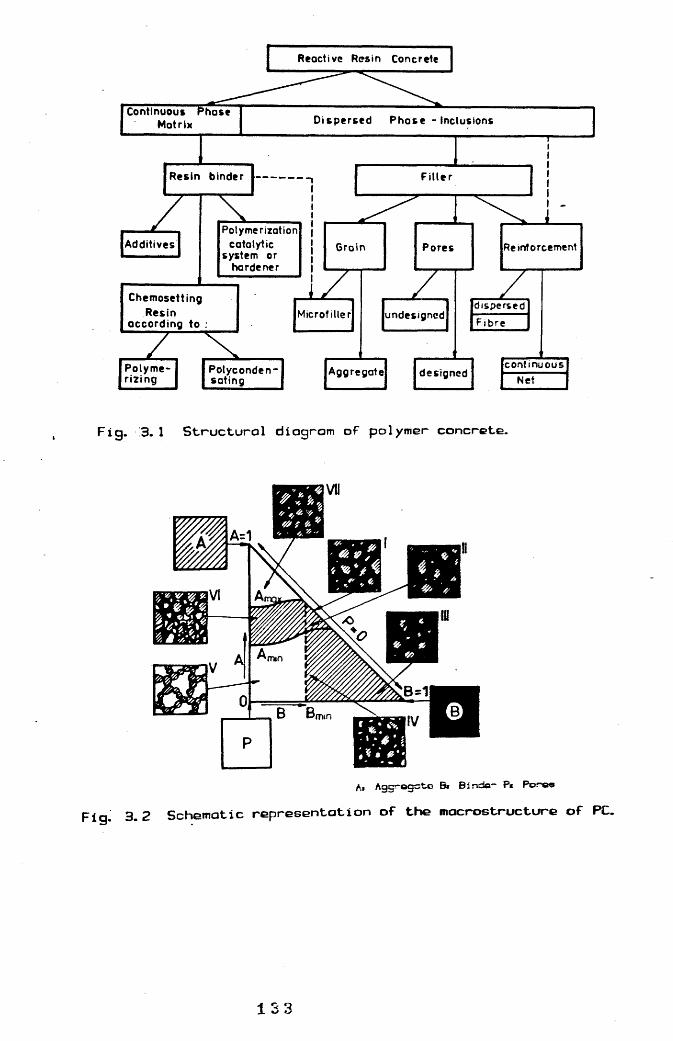
Continuous i^hose M atrix D ispersed P hase - Inclusions

Additives

Polymerizing designed

dispersedFibre

Aggregate

Microfiller

continuousNet

undesigned

Polyconden- soting______

Pores

Resin binder

Groin ReinforcementPolymerization

catalytic system or

hardener

Reactive Resin Concrete

F ille r

ChemosettingResin

according to :

Fig. 3. 1 Structural diagram of polymer concrete.

VII

f it Agçnagato Bi Bfndo- Pi Poiroo

Fig. 3.2 Schematic representation of the macrostructure of PC.

1 3 3

Mac.roKtructurc Microfttructure

E.GPa; 1 10 100 150 45

U.V. 32

Fig. 3.3 Schematic Illustration of compressive strength Cfc> and modulus of elasticity CE) versus thickness of resin binder Ct) os the superposition of the Interaction on the micro and mocro structural levels.

1 3 4

Determination of components' properties

Determination of properties of the binder'■ c o m p o n e n t s __________

Determination of Interrelation between the binder eind dispersed subsystems

HezostructureMlcrostructure

Determination of propertlei of polymineral subsystems

Macrostructure

Determination of design characteristics of polymer concretes

The system model and Its matheme- tlcal description

Obtaining of polymer concretes with predicted properties

Establishing of functional dependence between the properties and structure of the system

Fig. 3.4 Optimal PC compositions and their design characteristics determination.

1 3 5

£E

I&

I

120 ST/UP0,61

60

. Cm. Cc0

5 10 15 20

ST/UP (phr)300

II 200

100

Binder content #b%

9 10 11 12 13

Fig. 3.5 Effect of accelerator ond cotolyst content© (Cc ono Cm) on working life of binder.

Fig. 3.6 Binder content versus slump of fresh polyester PC.

(/)

Binder content Wb (wt.%)300

200

100

9.00

0 100 200 .300 400 500

IBinder viocoeity cP

100

50

Cc (phr)

0.5 1.0

ST/UP

15 ZC

Fig. 3.7 Binder viscosity versus Slump of fresh polyester PC.

Fig- 3.8 Relationship botwoer ST/UP ratio and compressive strength of polyester.

1 3 6

application ofPolytBter RpBln Concreten^equircd Workability I jpeBlgri Strength (dfç )|

Required Consistency of Fresh Polyester Resin Con^ete_____[petermination of Slump]Determination of Binder Content (Wb)■ _ ------

Required Working Life of Polyester Resin Concrete

IDetermination of Working Life of Binder (WLb)

\Determination of ST/UP for Respective CoOc Contents

3 :Determination of Weights of Materials per Unit Weight of Polyester Resin Concrete

Selection of Suitable Combination of ST/UP and CoOc Content

Estimation of HEKFÜ Content from Eqs.

I Trial Mixing!,_ _ _ — Z3EZZZZ- ,{Determination of Mix Proportions]

Fig. 3.9 Chart showing mlx-dosign procedure for polyester resin concrete.

u.o

fe

120

100

80

60

40

20

0

AccoIorator contort Cc (phr)

0.5 1.0 1,5 0.5 1.C 13

60 Wf0=52. 47 - i. 25 Wb

50

40Wco=37. 53 - D. 749 Wb

30

20

10 Bindo'* content Wb%

12C8.0

6T/UPFig. 3. ID N o m o g r a p h for selection of Fig. 3.11 Nomogroph for determiningvarious occeieratoh content~ST/UP quantities of filler, fine and coore©

aggregate per unit weight of polyesterPC.

1 3 7

1I 80

60

20

B Basolt cruehod •tone L Crushed lime stone C Granite crushed stone F Irrequlor #rsv#L

■ 2

f\JIT.

t*SL»07C4JCLtn

■f'ig. 3. 12 Influence of aggregate type on itiecbonlcal ctrongthe of PC.

Fig. 3. 13 Volume fraction of cooree aggregate versus compressive strengthof PC. !

I

u

.Crushed ondeelte

Crushed basaltic ondes1te A -Crushed bosoltic ondes1te B

rushed bosolt

Volume froctlon Vca

M

IU-o

f?s.

10Ç

A B C Used sand80

60

40

C Crus! led bosclt stone^ C All-In oggroggtss.

20

Sieve size nr.0 26020.013010.05.02.3 60.60,15 0,3

Fig. 3. 14 Grading used In making different PC mixes.

1 3.8

V

gI 8 S 9 8 o(udj) 03UDqs;s3u OAjrioiay

\ 29

a

8

(jdj) oouo' sjsaj BAj ioxay

m

g# 8 8 9 8 o

(udj) 03uo%aioau oA; o;ay

y8u-01E

*0S8-

L . CL (*- \y

g5(D0(PLC00LOfC60>o

inm

d)Ü.

^ ^ • çi «uiiu qtidap uo;:>DU:^au8j

E-

a ? îï 'Outui qtjdap uofSQuqauey

V»

9

a

8

iî KH

filccc>«

III

9

a8

k!L0 U.

1

If

1 ?îs/X

tgt)2

I10m

AiT

uiui qidap uot^ougauay

139

1

t(D?

!

M

,X

f%

?

i?

Si

100

Mix CMix B

7 9 1 1 % 7 9 11% 7 9 1 1 %

Fig. 3. 17 relative compressive strength versus binder content for different aggregate-grading PC mixes.140

120

• Raeln poetoj Ep**7. 0 KN/iimZ

100

Rosin mortor Em=l'7.0 KN/iw"2

Roe in concrotet Ec*»16. D KN/mn2

Puno rosin* Er*2. 0 KN/rtrmZ

Cyllndor 75 om-dlo., 150 «ir. hlght.S p e d

Stroin0

0 070,060.050,040.01 0,02

Fig. 3. 18 Compressive stress-stroin relationships for various resin-based materials.

140

^ v l n g platan

Pivottad hood

Staal bor 12 mrn-dlo.Tranaducar g lOD mm

Shaor «pactmon.

t504- 504-50-^50 200 m m----d

Fig. 3. 19 Arrangements for ©hear test.

Moving pldtan

4.2 mm-dlo. doformod H. T. S. bar

Stoel ploto with o slot

Cyllndor 100 mm-dlo., 200 mm hlÿit-

Fig. 3.20 Arrangements for pull-out test.

Is

I!I t

r

1.101,000.93

Ratio of hlght to dlomctcr4.03.0200. 61.0

Fig. 3.21 Effect of hight/diameter ratio of cylindrical specimens on the compressive strength of PC.

1 4 1

Moving plotonPivottod haod

Stool rectangular -ooctlon beamwo traneducere

Teetepee1men

Fixed ploten ïjp7■200 - 200 —

- 6 50 mm200

Fig. (3.22) Arrangements for flexure test.

.100

8Q

60

5

40

20

Grade A Grade B Grade Ç Grade D Grade E

Strain

0.0 6 0,07 0,0 80,0 3 0,04 0.050,01 0,02

Fig. 3.23 Compressive stress—strain curves for the five PC grades.

1 4 2

«oo'

oo'

o

CO V) ^N% ut oouoj JDsqs

«DO

O< tnu a uj

o

o

mo

CMo

o

a0L0an0(0DCDLa>01 CDü aL TD0 pU. Lü)L0 UG)Q.H(/) 01>in Q-ru (Vm X+J-? L0ü. u-

L0U.CDa>LD 0)ü L3C X0 a4J M-U0 Cl4-a CDTD a1 TDTD 00 L0 en_J

uCLCM 01>m -r4

U.0) 01XLL 4i

o-J- unmNX PD°T au;qoDm %D oi

4 3

1I

Loood-«troln ot point (2) Lood-otroln for th* #t#el grodo u#*d.Lcod-otroln ot point (J)T3

T3

12

Anchorage bond oroo Local bond ormo

T1Avorrogo onchorogo bond Average local bond etrength fba-T3/At. etrength fbl«T2-Tl/Al-2

Axlol tensile strain

Fig. ,3. 26 Schematic representation of the derivation of the average anchorage bond strengths.

BO

8

X<

,60

40

20

Grade A Grade BGrode E

Axial tensile strain0,01 0,012 0,0140,0060,0040,002

Fig. 3.27 Lood-strain curves for estimating bond strer^ths for PC grades.

1 4 4

CHAPTER FOUR

STRESS DISTRIBUTION IN FLEXURE AT

ULTIMATE STRENGTH OF PC

.4 *.1 .f Introduction

In recent decades progress has been made towards replacing

classical elastic structural design methods by new ones which

represent actual conditions to a greater degree. Numerous

investigations of conventional concrete structures have been

carried out leading to several new design theories, these

generally show good agreement with test results particularly

in the case of pure flexure. However these theories start from

different, sometimes even contradictory, assumptions about the

physical behaviour of the material employed. An engineer seeks

to evaluate the true behaviour of a structure. Approximate

results obtained on the basis of widely different assumptions

are not satisfactory. The agreement of various theories in

design ,however, is understandable when only under reinforced

beams have been considered . In such cases the tensile force

in the steel at failure is determined irrespective of the

concrete quality and the lever arm is not strongly dependent

of concrete strength. Only tests of over reinforced members

can, therefore, furnish a true measure of the validity of a

flexural theory.

For polymer-concrete there is a need for a theory which is not

restricted to approximate results in a limited range. Such a

theory must be based on the actual limiting properties of the

materials and must be valid for all cases of loading. With

resin-concrete very little work has been done to clarify its

structural behaviour in flexure. Most of that work relies

1 4 5

entirely on beam tests (77), (78) & (79). Three conditins

are available for such tests; the equilibrium condition, the

deformation condition and the assumption that plane sections

remain plane. As the number of unknowns is generally greater

than the available number of equations some plausible

assumptions had often to be made in the evaluation of certain

quantities. As the unknown quantities are closely interrelated

it is quite understandable that one may thus arrive at widely

different solutions.

The rheological behaviour of hardened PC poses some

restrictions on their structural use. Many researchers have

studied creep behaviour, stress relaxation and shrinkage

strains and stresses of PC. However there is very little

interest in applying these findings to the structural

behaviour of reinforced PC members and the consequent effects

of sustained loading on the ultimate strength of these

members. Despite the fact that PC has an inferior long-term

performance under load, most of the structural applications

were derived disregarding this fact. In consequence, PC

designers considered exaggerated factors of safety that would

compensate for any hidden influences and the lack of a

reliable flexure-theory. As will be seen later, the effect of

load application rate can result in a strength variation in PC

of up to 20%.

The distribution of concrete stress in the compression zone of

reinforced concrete members subject to flexure is of a

fundamental importance in theories regarding the ultimate

strength and behaviour of such structural members. This stress

1 4G

distribution often called the "Stress Block" is a powerful

tool in furnishing structural relationships in a direct manner for any flexural theory.

For conventional concrete many ultimate strength theories

involving a variety of hypothetical stress block shapes have

been developed. Generally theories based on stress-strain

relations obtained in axial prism tests carried beyond the

maximum load have also been presented (80). Some

investigators have attempted directly or indirectly to measure

the distribution of flexural stresses in tests of reinforced

beams, the stress block generally has three main parameters

K1, K2 and K3 as shown in Fig.(4.1), which can be used in

ultimate strength design. These parameters together with the

ultimate strain can be used for different cases ranging from

pure flexure to pure compression for reinforced structures or

prestressed ones. If the whole shape of the stress block is

known and expressed in a certain function it can be used for

the design of structures having cross-sections of various

shapes or subjected to biaxial moment or any other case of

loading. For this reason early researchers paid most

attention to finding the stress-strain relationship for

conventional cement concrete in flexure.

To find these relationships for PC previous techniques used

with cement concrete were revised. Although strains can be

directly and easily measured, stresses in the compression zone

are difficult to measure and as will be shown direct methods

for their measurements are not practical.

4.2. lexi^w of m^a^urin^

1 4 7

distribution

iL_2_tl ÂXlsl çninpr.eggiQP ±^st In this method it is assumed that the extreme fibre in bending at ultimate moment is subjected

to a maximum stress and a corresponding maximum strain,

similar to those found in simple axial compression tests. In

most of these the stress-strain curve is traced only up to the

maximum load. These relations have been applied to bending of

reinforced concrete structures by assuming a linear strain

distribution in the compression zone. However some recognized

that ultimate strain can have a greater value in flexure than

that corresponding to the maximum stress in compression test.

So it was believed that the full stress-strain curve in axial

compression , i.e., with the falling branch, can fairly

represent stress distribution in flexure. Consequently stiff

testing machines that would be less affected by the sudden

release of energy at maximum load, were used (81) & (82) and

even steel springs around the test specimen were used to

enhance the machine stiffness. These special techniques made

it possible to trace the stress-strain relation beyond the

maximum load.

Neverthless this method of obtaining stress blocks in flexure

from compression tests has been vigorously challenged (83) &

(84); a plain concrete specimen which has been sustained

beyond the maximum load in axial compression is generally

cracked and the strain response to load is highly sensitive to

time. It has been asserted therefore that concrete strained

beyond the maximum point of its stress-strain curve is useless

for load carrying purposes in beams and columns.

1 4 8

An opposite view has been expressed by some who pointed out

that special testing techniques are required to determine the

true stress-strain relationship in axial compression but that

the general characteristics of the axial compression stress-

strain curve are applicable to flexure of reinforced concrete.

Other experimental work (85) showed an increase in the values

of the initial modulus of elasticity and in ultimate strains

in flexure tests over corresponding values in axial

compression tests. The applicability of this method is

approximate and can by no means repesent the actual stress

distribution in flexure.

4.2.B Bending simulation test One of the earliest trials to

find the stress distribution along the beam cross-section was

that made at Imperial College, London 1941 (86); they

constructed a special testing machine which had six pairs of

horizontal jacks producing axial loads in the test beam at six

vertical levels. By assuming a linear strain profile along the

beam cross-section, jack loads were adjusted to give that

predetermined strain profile. Hence stresses could be

calculated from the loads at different stages and up till

failure. The low accuracy and the complicated experimentation

made this technique impractical.

4 .2.C Photoelastic method In this method the stresses have

been measured by embedding a piece of special glass in the

compression zone of a reinforced beam (87). Photoelastic

patterns obtained by passing polarized light through the glass

plate at various beam loads gave information from which the

stress distribution in the compression zone in flexure was

14 9

determined. Major drawbacks such as susceptibility to

moisture, humidity , volumetric changes in concrete and others

affected the measurements greatly in addition to the difficulties involved.

4 t£fP Sfregg meters method In this method the concrete beam

is cast with a stack of eight steel plates embedded at the

test zone (88). These steel plates have the same beam width

but reduced at the middle to the equivalent area of concrete

on a modular ratio basis. By measuring strains in the plates,

stresses in them could be calculated and were considered to be

the same as the stresses in the concrete at the compression

zone. However the results gave a linear stress-strain

relationship. A major drawback was the effect of the steel

stack on the compression zone which could not be well defined.

Also the stress transfer from concrete to steel plates is a

function of the bond strength which loses its effect near

ultimate loads on crushing or cracking. To eliminate these

effects some used pressure cells embedded in the beam instead

of the steel plates and satisfactory results were obtained

(89). However the complex and expensive instrumentation was

probably the reason why the use of this approach has been

limited.

4.2.E Tests of reinforced concret^ members As said earlier

the main parameters of the stress block, and not the whole

shape, could be calculated from reinforced members. Strains

can be directly measured by using strain gauges. The

parameters of the stress block can be generally derived

indirectly by computations from the equilibrium conditions.

150

The main assumption often made was that the strain profile in

the cross-section is linear even near failure. This assmption

is accepted by most of the investigators. The controversial

value was that of the ultimate strain. Some considered it in a

direct proportionality with concrete strength while others

found it inversely proportional to the strength. Many others

took it as a function of load rate only.

This discrepancy led to widely different values of the stress

block parameters. Thus interest in the whole block shape was

great and a pioneer work regarding the whole shape of the

stress-strain curve in flexure was done by Prentis (90),

Hamann (91) and Lee (92). They have derived full information

about the stress distribution from reinforced beam test data

by numerical differentiation. They made four main assumptions

as follows :

(1) For the steel used the stress was equal to the strain

times EgUp to the yield stress, after which stress is constant

(2) Concrete does not resist tension.(3) Linear distribution of strain over the beam cross-section.

(4) Concrete compressive stress is a function of strain only.

With the notations of Fig.(4.2) the compressive stress as a

function of the extreme fibre strain could be found as

follows:

C = b cC beF(e )dx = —o

Ec

o ( a )

Ewhere £ = ___£— (P)d E + Ec s

Then substituting Eq.(b) into Eq.(a), differentiating with

1 5 1

respect to c and rearranging, two expressions for the stress

component in flexure could be obtained as follows;

% = 6 ^ ) " ( d )r y e These equations are valid only for singly reinforced members

which are completely cracked in the tension zone. Hence

calculated values at low stresses before complete cracking are

not correct. Also the equations can only be applied for under

reinforced members. In this method measurements of steel

strain depend strongly on the locations of the cracks relative

to the position of the strain gauges which might give

misleading readings. If this is the case experimental errors

will be amplified in the differentiation.

In a trial to avoid the influence of the relative crack

position to the strain gauge Prentis (90) applied his

differentiation to prestressed beams using unbonded cables and

obtained better results. A major enhancement of this procedure

was developed by Hognestad (85) in which tensile stresses were

avoided in a plain concrete specimen. No need then existed for

measurements of steel strains with the problematic effect of

concrete crack location relative to the gauges. As shown in

Fig.(4.3) a major load was applied by the testing machine (PI)

and by further applying a minor eccentric load (P2), the

neutral axis could be maintained at the outer face of the

plain test region throughout the test. Thereby complications

resulting from tensile stresses in concrete were completely

eliminated. Steel strain measurements were not required. Using

two reasonable assumptions stresses could be calculated; (a)

15 2

linear strain profile, (b) concrete steress is a function of

concrete strain only. From equilibrium of forces and moments Eq. (a)can be rewritten as

F( x)d x “ 1 2 “ )C_ = b [ F(e _ ) dx = —c

Jo ^ < o

Equating the internal and the external applied moments, then

.2X F(e )dx “ o * 1

ECF(e )e dx = P-a + P a« = M bc^ .....(f) X X Z 2. oo

M =

in which = (P + ?^)/2 = (P a + P2a2)/bc

By differentiating with respect to c and rearranging then,

d Ff = E -— - + F .... (g)Cf C d O

d Mf = E 3— - + 2M .... ( h )Cf c d E oI c

Eqs.( g ) & ( h ) calculate the concrete stress f^^ ^^ sfunction of the continuously measured concrete strain (C and

the measured quantities Fo and Mo. Thus by calculating in

small increments the differentials can be closely approximated

by the finite difference dFo/d^c and dMo/d % . It is worth

mentioning that the block parameters can be calculated at any

load level from equilibrium requirements as follows;

P, + P,Where c = be f K, K_ = P + P. I en K.K, = — r-^c c 1 3 1 2 13 be f

y C yP\a P.aWhere m = cCl-K ) then = 1 - c(P, +

Where k, ■= f- It then k, = K.K, f /f3 Cf Cy 1 1 3 Cy Cf

It is clear that this method (85) is very powerful and all the

stress block parameters as well as the whole stress strain

curve in flexure at any stage of loading can be found. This

1 5 3

method is also a very simple one and does not require any

special technique. Only a high degree of precision is required

for arriving at a reliable interpretation. The interesting

thing is that stress can be found either from Eq.(g) or Eq. (h)

which provides a double-check process on the validity of the

results. For these reasons this method of defining the stress

distribution in flexure was adopted for the present work on PC.

4.3. Stress block shape and parameters for resin-concrete

4.3.A. Test specimen dimensions Different considerations were

taken into account in dimensioning the specimen. Two main

shapes and sizes were chosen. The first was that shown in

Fig.(4.4). The cross-sectional area was 100.0x200.0 mm. The

required axial load for this area to reach its ultimate

capacity was too great. This load produced very high bearing

stresses particularly after the bearing plates began to bend

and the bearing area reduced sharply near failure. It was far

from practical to design a supporting system that would

support 1000.0 KN load needed for this size of specimen,

without bending of the bearing plates. However the first two

specimens were cast using this size. On testing failure of the

intended test zone was never reached. Crushing of the specimen

under the bearing plates took place first and longitudinal

cracks propagated along the specimen length. Eventually

failure occured near the end-bracket reinforcement.

The second size and shape was then designed to avoid these

troubles. The cross-section of the test zone was chosen to be

100.0x120.0 mm which required the major load to be around

15 4

500.0 KN. The cross-sectional area was intended to represent

the compression zone in actual full-scale PC structural

members. For this reason smaller dimensions were not

considered, to avoid any likely troubles in scaling up the

results or in applying them to real structures. As shown in

Fig.(4.5) the test zone was pre-defined using haunches between

the brackets and the longitudinal prism. All specimens made

with the shown shape and size failed in the intended test

zone.

Sufficient tension, compression and shear reinforcement was

provided for the end-bracke ts, as shown in Fig.(4.6), to

obtain failure in the central plain test zone. All such

reinforcement ended 100.0 mm from the middle of the specimen,

allowing a plain test zone of 200.0 mm length. The end-

brackets were designed to be as stiff as possible so that full

fixity at the bracket-prism joint could be satisfied. To avoid

excessive elastic and plastic deflections at the free edge of

the bracket the least possible cantilever span that would

provide enough room for the hydraulic jack and other loading

instrumentation was considered.

4.3.B Measurem ents of 1 oads^ strains and deflectil^D^ Where

the interpretation of these test results involved numerical

differentiation, it was very important to achieve the highest

possible degree of accuracy. The net dimensions of each

specimen were measured after being demoulded. The strain

gauges used were 20.0 mm-length. The choice of these 20.0 mm -

electric strain gauges was based on some other tests made with

the first specimen size and shape ; in those initial tests

1 5 5

100.0 mm -length strain gauges were used with the 20.0 mm

ones. Both types gave more or less identical readings. Where

the 100.0 mm -gauges are very expensive and did not give any

increase in accuracy, the much cheaper 20.0 mm -gauges were

used throughout the whole work to come.

As shown in Fig.(4.7) five pairs of strain gauges were used.

Pairs 1 & 2 were attached to measure the strain at the extreme

fibre and at the experimentally maintained zero strain fibre

(neutral axis N.A.) respectively. Pairs 2 & 3, one on each

side, were for recording strains at 2/3 and 1/3 the cross-

section depth respectively. Pair 4 is used for adjusting the

load ratio P2/P1 to maintain the N.A. at the outer face of the

test zone throughout the test. Strains recorded were not more

than 50.0 microstrain at that face in the worst case. Pair 5

was attached horizontally to the inner face which represents

the extreme fibre to measure the lateral strain.

Lateral deflection at the middle of the test zone as well as

the vertical displacement of the bracket free end were

measured using electric transducers.

The major axial load was applied by a universal testing

machine and the minor eccentric load was applied by a

hydraulic jack. This load was measured by a calibrated load

cell and its value could be recorded continuously as well as

all other deflection and strain values by using an electronic

Data Logger. The test procedure was to apply an increment of

PI load and hold it. Then watching the displayed strain at the

N.A. face, minor load P2 was increased until the negative

compressive strain is reduced to zero; at this moment a

1 5 6

reading for the different values is taken. Then another

increment of PI is applied and again strain, gauge 4, was

brought down to zero by further increase of P2 and so on. At

later stages P2 required to be reduced by controlling the pump pressure.

Bearing in mind that the greater number of load increments

means greater accuracy, the increment of P 1 was 2000.0 lbs

(this is the available scale units of the testing machine).

This resulted in around 60-80 readings for the whole test

depending on the PC grade. The rate of load application was

kept as constant as possible. Each increment of load took on

average a time of one minute to apply. Then the load P 1 was

held constant until the N.A. starins were brought to zero

which took another 30.0 seconds on average. Near failure the

rate of load application was increased significantly to keep

the load increasing while excessive strains were taking place.

4.30 Test results and their interpretation For each grade

two specimens were cast using a single batch, cured at

atmospheric temperature until testing at seven days of age.

The readings of loads, strains and deflections were recorded

for each specimen. Then the average values of the two

specimens were considered in the analysis of each PC grade.

The stress distribution in the test region was found using the

previously mentioned two equations [ Eqs.(g and h)3;AF . AM .

^cfi = "ci * ' oi cfi = "ci IT - * “ oicl Cl

in which = F . -

»oi “ — ' A"ci ' "oi - "o(i-D

1 5

A=ci " 'ci - 'c(i-l) a«ji = eccentricity of major load from N.A.+lateral deflection.

321 = eccentricity of minor load from N.A.+lateral deflection.

At each load increment the stress block parameters are calculated as follows;

% fcy(Kj) = 1.0 - ( 11*11 *

(K3). . - f icy

(Ki). - (K1K3). /fy f 1Hence at each load level, corresponding to certain extreme

fibre strain ®c, the stress strain curve of the compression

zone (all the test zone) in flexure was found with its

parameters as shown in Fig.(4.8).

The value K1 is the average uniform stress distribution

parameter, it should be equal to 0.5 for a triangular stress

distribution; while for 2nd. degree p a r b o l a - s t r e s s

distribution it is 2/3. Therefore the value of KI was expected

to increase with increasing load level and approaching failure

where the stress distribution loses its linearity.

The value K2 is the parameter that defines the position of the

resultant internal compressive force. If the depth of the

compression zone is *c', then the internal force is at K2.c

distance from the extreme fibre. So for very low levels of

load when the stress distribution is linear this value of K2

is almost 1/3. As the stress strain curve develops

nonlinearity the value of K2 will increase.

1 5 8

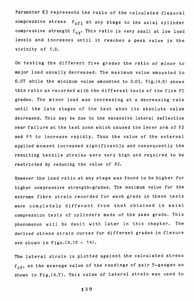
Parameter K3 represents the ratio of the calculated flexural

compressive stress f^fi at any stage to the axial cylinder compressive strength f^y. This ratio is very small at low load

levels and increases until it reaches a peak value in the

vicinity of 1.0.

On testing the different five grades the ratio of minor to

major load usually decreased. The maximum value amounted to

0.07 while the minimum value amounted to 0.03. Fig.(4.9) shows

this ratio as recorded with the different tests of the five PC

grades. The minor load was increasing at a decreasing rate

until the late stages of the test when its absolute value

decreased. This may be due to the excessive lateral deflection

near failure at the test zone which caused the lever arm of P2

and PI to increase rapidly. Thus the value of the external

applied moment increased significantly and consequently the

resulting tensile strains were very high and required to be

restricted by reducing the value of P2.

However the load ratio at any stage was found to be higher for

higher compressive strength-grades. The maximum value for the

extreme fibre strain recorded for each grade in these tests

were completely different from that obtained in axial

compression tests of cylinders made of the same grade. This

phenomenon will be dealt with later in this chapter. The

derived stress strain curves for different grades in flexure

are shown in Figs.(4.10 - 14).

The lateral strain is plotted against the calculated stress

as the average value of the readings of pair 5-gauges as

shown in Fig.(4.7). This value of lateral strain was used to

159

calculate the apparent Poisson’s ratio as shown in Fig.(4.15)

for the different grades. Where the longitudinal and the

lateral strains [^c and ^cl] are measured at two different

positions on the extreme fibre face and not at the same point,

Poisson's ratio plotted is just an approximate one. However it

was useful in calculating the volumetric strain ^cv approximately as follows;

E . = e . - 2e ,. cvi Cl ell

The stress values derived were calculated using the two

equations given previously. The values derived by using either

of the two equations were almost identical which indicated a

high degree of reliablity of the experimental measurements.

Poisson's ratio had a starting value in the vicinity of 0.27

and as shown in Fig.(4.15) it increased at a decreasing rate

until it reached a stabilized value of around 0.4. These

values may seem very excessive if compared to conventional

concrete. However this is mainly due to the nature of the PC

itself and its rheological properties which will be discussed

in another chapter.

The parameter K2 is plotted against the extreme fibre strain

in Fig.(4.16). The initial K2-values for various grades were

within the range of 0.33 to 0.34. This asserts the linear

stress distribution at the early stages of strain levels.

Parameter K2 increases at a decreasing rate and all grades

seem to have a maximum stablized value within the range of

0.42 to 0.44. It is evident that the greater the compressive

strength , the greater is the value of K2, particularly at low

strain levels. However by extrapolating the five curves shown

1 6 0

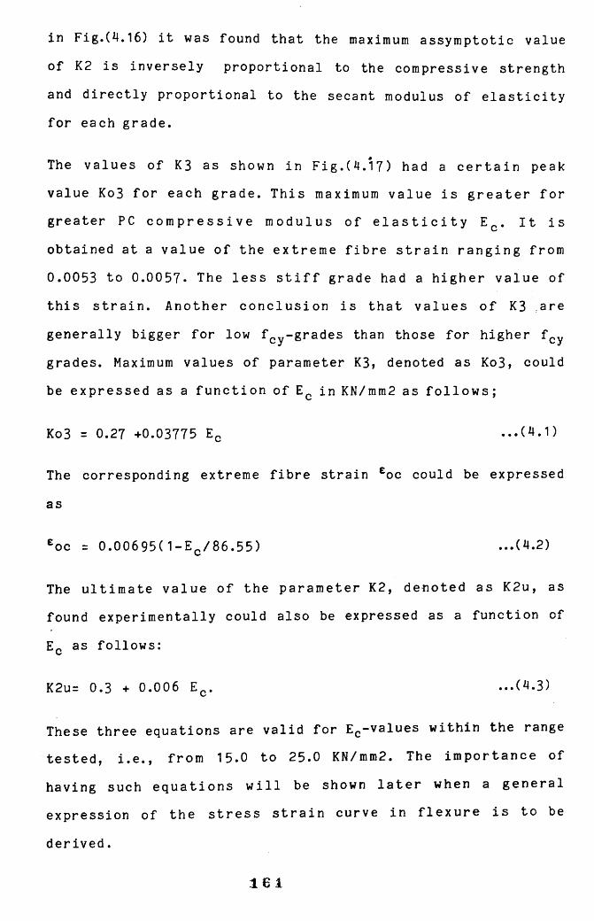
in Fig.(4,16) it was found that the maximum assymptotic value

of K2 is inversely proportional to the compressive strength

and directly proportional to the secant modulus of elasticity

for each grade.

The values of K3 as shown in Fig.(4.17) had a certain peak

value Ko3 for each grade. This maximum value is greater for

greater PC compressive modulus of elasticity E ^ . It is

obtained at a value of the extreme fibre strain ranging from

0.0053 to 0.0057. The less stiff grade had a higher value of

this strain. Another conclusion is that values of K3 are

generally bigger for low f^y-grades than those for higher f^y

grades. Maximum values of parameter K3, denoted as Ko3, could

be expressed as a function of E^ in KN/mm2 as follows;

Ko3 = 0.27 +0.03775 ...(4.1)

The corresponding extreme fibre strain ^oc could be expressed

as

^00 = 0.00695C 1-E^/86.55) ...(4.2)

The ultimate value of the parameter K2, denoted as K2u, as

found experimentally could also be expressed as a function of

Eg as follows:

K2u= 0.3 + 0.006 Eg. ...(4.3)

These three equations are valid for Eg-values within the range

tested, i.e., from 15.0 to 25.0 KN/mm2. The importance of

having such equations will be shown later when a general

expression of the stress strain curve in flexure is to be

derived.

1 6 1

The experimental values of parameter KI were found to be a

function only of the extreme fibre strain, irrespective of the

PC grade itself as shown in Fig.(4.18). This function could be expressed as

KI = 0.9 - 0.38 [ 1.0 — (Ec/0.009)2] ...(4.4)

The derived stress-strain curves in flexure differed

remarkably from their respective ones in the axial compression

tests. As shown in the previous figures (4.10-14), the

flexural modulus of elasticity is much higher than Eg. The

maximum compressive stress in flexure occurred at a strain

lower than that in compression where maximum stress occurred

at maximum strain.

The mode of failure differed widely in both methods. For

example in axial compression tests the whole specimen cross-

section will usually crack considerably if strained beyond the

maximum load. These cracks could take the form of either

tension diagonal cracks, longitudinal axial-splitting cracks,

or combinations of both. The chance for strain or stress

redistribution is very limited where the whole cross-section

is stressed uniformly.

The mode of failure observed with the eccentrically loaded

prisms was quite different. Primarily it is a failure caused

by excessive compressive stresses producing principal tensile

strains greater than the material can stand. The specimen had

one face at virtually zero strain (the outer face) while the

inner face was subjected to maximum compressive strains.

1 6 2

The concept of "critical stress" can be of some use in describing the failure mode. As shown in Figs.(4.10-14) the

critical stress is defined as the stress at which volumetric

strain is equal to zero, i.e., the stress after which the

specimen begins to expand volumetrically. The ratio of the

extreme fibre strain at the critical stress to that at failure

ranged from 0.45 to 0.61, while the ratio of the critical

stress to the maximum stress ranged from 0.77 to 0.91

respectively. The strain profile was found, as assumed, to be

linearly distributed over the specimen cross-section. So for grade E for example, the critical stress ratio was 82% at a

strain ratio of 50%. As shown in Fig.(4.19) it can be said

that 50% of the cross-section is subjected to stress up to 18%

more than the critical stress. Hence the crushing of the

cross-section at failure is expected to extend to 50% of its

depth after which the test zone acts as a plastic hinge with

excessive rotations around it. Finally failure occurs by

tensile cracks propagating from the zero strain-face to the

crushing maximum strain area. For grade C the critical stress

ratio was found to be 77% while the strain ratio was 46%. That

is to say that 54% of the cross-section is subjected to stress

higher than the critical stress by 23%. This high margin of

stresses over the critical stress produces a rapid crushing

and a brittle failure. Experimental observations showed that

most of the specimens tested failed in this mode, i.e.,

lateral tension cracking extending from the outer face until

it reaches the crushing zone. This zone had a depth ranging

from 0.5 to 0.65 of the whole depth of the test zone.

4.4. General flexural stress-strain çyrïë for difffr&nl g r . M & ^

o o

All the previous findings of the stress block shape and

parameters of various PC grades are based on certain

assumptions. Some of these were proved experimentally to be

valid while others were found not to be. The linear strain

profile was found to be a valid assumption. However the

assumption that stress is a function of strain alone can by no

means be a realistic one. The stress in PC is extremely time-

dependent. As will be shown later, creep and strength

reduction under sustained load are quite significant and

should be considered if a general approach for flexural design

is to be obtained. Consequently the effect of time in terms

of rate of load application and stress history must be paid

due attention. Hence these findings so far can be termed as

"short-term" flexural behaviour.

Another fact is that simulating the compression zone in real

reinforced beams by a plain eccentrically loaded prism might

allow for some misleading results. For example, in a

reinforced beam, steel stresses between cracks are reduced or

even converted into compressive ones near supports and can

contribute to the ultimate capacity of the section, i.e.,

tension stiffening. Thus calculating the ultimate capacity in

flexure based only on the compression zone stresses would

usually give a slightly lower value than that found if the

tension stiffening was considered. In this case neglecting the

reinforcement contribution is conservative.

The type of test itself preassumes that the ultimate capacity

is controlled by the concrete and not by the reinforcement, a

case which is often encountered with over-reinforced sections.

1 6 4

Applying these test findings to under reinforced sections may

thereby be misleading. However as PC is a relatively expensive

construction material it may be out of the question to use it

in under-reinforced sections. Over-reinforced sections are not

desirable either due to the unfavourable mode of failure. So

PC structural members are probably best designed for crushing

of concrete to occur simultaneously with yielding of the

reinforcement.

On the other hand if high tensile steel without a well defined

yield point is used, the ultimate capacity will be controlled

eventually by the concrete reaching its ultimate strain.

Bearing this in mind the findings still apply to balanced ,or

over-reinforced sections made of mild steel, or to sections

reinforced with cold-drawn steel at any reinforcement ratio.

In addition they can be applied to under-reinforced sections

if the PC strain level is known in these sections.

The test zone also was not laterally confined, while in real

structures stirrups are often used. The effect of lateral

confinement is such that it would increase the ultimate

capacity of the section particularly for high loads with small

eccentricities. So once again, neglecting this effect means

additional safety over the present findings and does not

preclude their validity.

The only apparent reservation may be faced in the mode of

failure itself. For instance in a real reinforced beam the

strain can not strictly be plane for there is a discontinuity

at every crack in the tension zone; a case which is not

simulated in the present test. Regarding the statistical

1 6 5

effects, the specimen would fail at the weakest section in

compression selected from only those sections which have

developed tension cracks. Despite this reservation it was

found that the present findings are applicable to reinforced

structures and the effect of tension crack propagation on the

compression zone depth is felt only at the very late stages of

the test and even beyond the ultimate capacity. Hence this

reservation is practically outside useful structural limits.

From the previous paragraphs the validity of the present

findings are evidently acceptable. The assumptions appear to

allow the derivation of reasonably accurate and reliable

stress strain curves in flexure. The only remaining, yet

controversial, point is that regarding the ultimate capacity

of the section and how it is defined. The controlling

parameter is the ultimate concrete strain if the section is

balanced, under or over-reinforced. This value of ultimate

strain for cement concrete was expressed in many different

ways. Some related it directly, or even indirectly, to

concrete strength while others considered it as completely

independent of concrete strength (93). In addition other

researchers found it to be a function of the loading rate and

the associated rate of strain. Higher rates of strain would

produce ultimate conditions at lower values of strain .

At the present stage and regarding the "short-term” stress-

block in flexure the ultimate strain was defined purely on a

mathematical basis. The different derived stress-strain curves

could be expressed as a 'sine-funetion’ with the notations

given in Fig.(4.20) as follows;

1 6 6

fcf " f sin ( -5— -- ) ...(4.5)oc

In which Ko3 can be calculated from Eq.(a). The ultimate

strain cu is that strain that would give maximum internalmoment Mu; Where m

fCX dx

Substituting for x = c. x/ c and rearranging, the ultimate

moment can be obtained using the simple differentiation dM/dSc=0.0.

This expression of the the ultimate moment can thus be used to

calculate the ultimate -strain value as a ratio of 'oc. This

ratio ^oc / ^cu was found to be 0.75. So for each grade , oc

can be calculated from Eq.(4.2) and then ^cu can be found.

Knowing the value of Ko3, ^oc and 'cu the full stress-strain

curve in flexure at ultimate strength can be traced for each

grade with a given f^y by using Eq.(4.5). These theoretical curves for the different grades are plotted against the

experimentally derived ones. They appear to be in good

agreement and should be useful in calculating the ultimate

capacity of any section under any case of loading. It is

important to stress the fact that the mathematically derived

value of the ultimate strain preassumes that the ultimate

carrying capacity of the cross-section is controlled by the

concrete and not by the reinforcement, a case which is often

encountered when cold-drawn steel is used for reinforcement.

Other effects were overlooked for simplification, such as the

effect of the cross-section shape, and the position of the

neutral axis (N.A.). With conventional concrete, ultimate

strain was found to increase by reducing the compression zone

area; either by decreasing the N.A. depth or by reducing the

1 6 7

concentration of the area above the N.A. as shown in

Fig.(4,21). For a constant compression zone area and depth it

was also found that irrespective of the steel type or the

reinforcement ratio, the ultimate strain is a function of time

or rate of strain by which the load is applied as shown in Fig.(4.22).

In one of the early researches (92) the ultimate strain value

of cement concrete members varied from 0.0022 to 0.0048 for

the same concrete strength,rate of strain and load duration

,by changing only the cross-section shape and N.A. position.

This suggested that with other concrete qualities , other

rates of deformation and load duration, even more pronounced

differences might be expected. This qualitatively explains the

wide divergence in the ultimate strain values arrived at by

different researchers on cement concrete as shown in

Fig.(4.23). It could even be argued that all these reported

values, though apparently contradictory, can actually occur.

They were probably recorded under widely different conditions

and the fundamental error consisted in generalization.

Concrete ultimate strain has not and can not have one

permanently fixed value.

For PC the ultimate strain value can be even more

controversial. All the previously mentioned effects can result

in the same, if not more, divergence in ^cu values. Bearing in

mind the lack of accumulated data of PC structural performance

and its high time-dependency, it is necessary to accept an

approximate average value even if a certain amount of error

would exist in it. These errors should be taken into account

in setting the safety factors in the actual design and

1 6 8

practice of PC. The extent to which the chosen values of 'oc

and feu give acceptable results or not will be demonstrated in

more detail later in the analysis of results for reinforced

members.

1 6 9

KIK3. fey

NüQtral axle

e,s

K2.CK3. fey I

. StressStress bl ock

Strain distribution stress distribution

Fig. v4. I Definition of the three main porometers of the stress block in flexure

Nauttrol oxIs

Tension stool As

C o n c ro te conp '-osa 1 on f o r e sCcF fe»

Stool tonsion forco

Strain Stressdistribution distribution

Fig. 4.2 Notations for o singly reinforced rectongulor section in flexure-

1 7 0

Fig. 4.3 Test specimen of Hognestad.

100 I 100 25Û.

Sg

I

IM410 m m

Fig. 4.4 The first specimen chosen for the derivation of the stress block

Fig. 4-5 The second specimen chosen for the derivation of the stress block

171

oinml

I90.0

13 30

Fig. 4.6 Details of reinforcement of the end brocket.

Moving plotanGrip---Load cell

— Pivottod hoodHydroulie Jock—

.Bearing platesTransducer

Stroin gaugesStraingauges

Test zone

16 mm—dig. H. T. S. rod

Outer faceInner face Fixed platen

Fig. 4.7 Testing instrumentation and arrangements.

1 72

r P2

Cc'R

a0P1I.If

Strain dletrlbutlon Stro#s distributionUÎ4, -1 Innor face

Outer foco 1

Croee section of test zone

Strain In extreme fibre

Fig. 4.8 Development of stress-strain relationship in the test zone.

1 7 3

o‘ oo04

0.06

0.05o£

3O.M

0.03

0.001000 0.002 0.003 0.00* 0.005 0.007 0.006 0.009

Max I mum HioroatrainLOAD RATIO (ECCENTRIC/AXIAL) VS. MAX. MICROSTRAIN FOR DÎFFFERENT RE.C.

40Theoretical ©treee-etraln curve

[ Slne-functlon ]

0.006 0.006 0.0070.0040.0030.0020.001>0.005 -0.004 -0.003 -0.002 -0.001 0.000L # t# r# l,V o lu m # tr io t A x ia l N io ro a tra in

F ig . 4.10 STRESS-STRAIN CURVES FOR GRADE "A "

1 7 4

Jî1

fO«•0

TO

M

SO

40 •TheorjBtlcal etroee-etratn curve L Slne-functlon ]

80

20

10 Lmi

0 ............... ... . ------------- ------------ L_4».005 -0.004 -0.003 -0.002 -0.001 0.002 0.0030.000 0.001 0.004 0.005 0.006 O.OOT

LataralfVoluMtrio t Axial Hioreatrain Fig. 4.11 STRESS-STRAIN CURVES FOR GRADE “ B"

-

y♦ ♦ ^ **

: -A O/ o' Ô

0 ^ \ o

♦

«

A i

* / ) O

•* * / O0

4~ ■■■' ♦♦ i

orotict:ol Btr Slne-

'086-0Functl

:raln on ]

curve": A

A / 1 hs

4

AA

A t/

4

4

i "JT

4--- »k i# l

Lataral

>0 lu a tr to♦ *--- «

fO

80

TO

1

{«! 00

40

80

20

10

L a te ra l ,V o lu a a tr Io t A x ia l M io ro a tra inFig . 4.12 STRESS-STRAIN CURVE FOR GRADE T '

175

ItI

«0♦♦♦

•0 OOOo

«0

90

40Thooretlcal etroeo-»traln curve

[ Slne-functlon ]80

»

L#ti10VelUBMrio

0 ---------------------- 1—-0.005 -O.OM -0.003 -0.002 -0.001 0.0060.001 0.002 0.003 0.004 0.005 0.0070.000

L»t«r«l,VoluB*trio t Axi«l Mioro#tr«in Fig. 4.13 STRESS-STRAIN CURVE FOR GRADE T"

«0

00

70

00

JO

Theoretical etreee-etroln curve ------- [ Slne-functlon ]_______40

30

00

10* VolUMtMO

0 — -0.005 0.004 0.0050.001 0.0060.000 0.007-0.004 -0.003 -0.002 -0.001

3

L * ts r« l,V o lu B * tr io t A x ia l N io ro a tra inF ig .4.14 STRESS-STRAIN CURVE FOR GRADE

176

0.7

0.6

J O-

£ 0.4

0.3

0.2

0.1

o oo 6

9*4

o o

Grad* A

Crada B

Grada C

Grada D

Grada t

D.ODO 0.001 0.002 0.003 0.004 0.005 0.006 0.007

Hex I nun HicroatrainF i^ . 4 .1 5 APPARENT POISSON'S RATIO VS. HICROSTRAIN FOR FIFFERENT RE.C. CRAOES.

0.45

DÏ5S 0.40

-

a

A■ A

* a •a ♦

* a

•a aO ♦) ♦ 1

Da ”

0

6 * * O---- € ^ada Aa----- ft-ada 0a----a ( M a Ca— — a »ada D a a frmda E

0.35

0.300.Maximum Mioroatrain

F ig . 1*^6 BLOCK-RESULTANT LKATION FACTOR (K2) VS. HICROSTRAIN FOR DIFFERENT RE.C

1 7 7

1.0

0.9

0.8

0.7

C 0.6

0.5

■ • .• / .

i• • • A

•*. a' O " t aA♦♦ ' ♦

fi fifi

•D g

9

-■ v » -

O— © Or#d# A

4-------- 4 Or#d# B

^ — A 8r*to Cf

/

«--- » CM» DE

è#

0.4

0.3

0.2

0.1

D.000 0.001 0.002 0.003 0.004 0.005 0.006 0.007

NaxiM» MiorovtrainF i g . L M MAXIMUM STRESS FACTOR (KJ) VS. MICROSTRAIN FOR DIFFERENT RE.C. CRADES.

-*

/*

y

o

' 0 ,

y / 1^ a

y

* ^

0 o. * ♦ »

* * ‘i-ko

) o---e Orad. A

---- » &«ad. 8

a- —— a Grada C

a— a ^ada D

a . - a fr<ada E

fM» ■ ^

D 0 0 "

-

0.8

0.7

J0.6

0.5

0.4

Maximum MioroatramF,g.4.1 B AVERAGE UNIFORM STRESS COEFFICIENT (KJ) V5. MICROSTRAIN.

1 7 8

IInner foce

Critical •trees Cfcr>Stress distribution

Stroin ot for;50% depth of epee1men

Strain distributionCritical stress (for)

Stress distributionGrade C

54% depth of specimen Strain distribution

Test zone

Fig. 4.19 Mode of failure os related to the compression zone depth subjected to stresses higher than the critical stress.

1 ? 9

IExtromc fibre «train

.«train at ulfimate «trongth^ ------------- Ultimate «train—K

Fig. 4.20 Theoretical stress-strain relationships for the five PC grades in flexure.

Ib

I05I

1.0

0.5

B

mr n

f " 2 DOO psi (20.7 N, • f “ at max

mm*)

moment" / \

C=J 0 c “ Oat max no ment

0.001 0.002Extreme fibre «train at ultimate strength of concrete

Fig. .4,21 Ultimate strain as o function of cross section and position of neutral axis.

I S O

028R e c to n g u lo r te c f io n

l c «3000 ps i

a t 56 do y s

&'0400.27 ►

0.25 j-

024 0.001 . ___C o n c re te S trom ,n e x tre m e f ib e r s , £ c

0.003 0.005flIb e rs ,m

Fl,g. 4. 22 Variation In reduced moment with concrete strain and time

Ù.OIO

008

f 006

/Gronholm5004

RÛsch, Stûss.002

/ Limiting Volues Torrojo '

0 30P20D10.0

Fig. 4.23 Relationships between ultimate strain and concrete strength.

1 8 1

CHAPTER F IV E

REINFORCED PC BEAMS AND THEIR

TEST ANALYSES

5-t.l.t. Introduction

Knowledge of the structural performance of PC’s when

reinforced; is the major prerequisite for the design of

reinforced PC structures. Yet the work done to clarify it is

surprisingly limited. Little research has been reported on the

structural behaviour of PC reinforced beams (77), (78) & (79).

As stated earlier most of that research has been directed

towards mechanical and durability properties. The effects of

different steel types, reinforcement ratio, PC ultimate

strength and strain were not studied. In addition most of the

reported work on reinforced PC was for reduced-scale members

which did not help in the derivation of general design

equations or produce reliable conclusions (94).

Recognizing the importance of the stress-strain relationship

in flexure, little research has been carried out on PC to

obtain different stress-block parameters. Generally the stress

distribution in the compression zone at ultimate capacity was

often expressed as a rectangular uniform distribution. This

simplification led to some m i s i n t e r p r e t a t i o n of the

experimental results obtained by the researchers. The full

behaviour of a reinforced PC beam from small load-levels up to

failure, including flexural deformations, can not be obtained

without a general expression of the stress value at any strain

level in the concrete. The ultimate carrying capacity of a

member made of a given PC grade depends on the reinforcement

1 8 2

ratio R and the type of steel used. Consequently the type of

failure is governed by these two factors. If steel with a

well-defined yield point is used, the concepts of over, under

and balancd reinforcement can be dealt with theoretically and

experimentally. On the other hand, when using high tensile

steel without a well-defined yield point, these concepts can

not exist. In this case there is a specific reinforcement

ratio Rg at which steel strain would not exceed a prescribed value, if the whole section is to develop its ultimate

strength. Increasing R normally implies an increase in the

ultimate carrying capacity and a reduction in the resulting

strains in steel. However, there is obviously a certain

maximum R that will result in a desirable mode of failure and

would allow the efficient use of steel.

The present work was carried out primarily in an attempt to

specify this specific reinforcement ratio Rg and to check the

validity of the previously found stress-block shapes and

parameters for different PC grades.

5 .2. Fundamental equation for pure flexureFor any rectangular cross-section with the notations shown in

Fig.(5.1), There are three conditions. Two of these are

concerned with equilibrium of forces and moments, while the

third is that of strain compatibility. Using these conditions,

the ultimate moment or rather the moment at any chosen

concrete strain can be expressed as follows:

(1) Equating internal and external forces then,

P z Cc + Cs - Fg , which can be rewritten as

P = K 1 . K 3 . f c y . c . b + A ’ g . f ’ s - A g . f g

183

Substituting for K1.K3 = G, then

P/(b.d.fgy) = G.c/d + A'g/(b.d).f'g/fcy _ A g / ( b . d ) . f g / f c y

Let A ’g / ( b . d ) =R', A g / ( b . d ) = R, and P/(b.d.foy) = L, then L = G.c/d + R'.f'g/f^y - R.fg/fcy

L z T + T ' g - T g ...(5.1)

(2) Equating externaland internal moments:

P.e = M = Cg (d -K2.c) + Cs (d-d'), then

M = G.f^y.c.b (d-K2.c) + A'g.f’g (d-d')

M/(b.d2.f^y) = G.c/d (1-K2.T/G) + R'.f'g/fcy (1-d'/d)

Substituting for Y = K2/G and M = b.d^.f^^.z, then

Z = T (1-Y.T) + T'g (l-d'/d) ...(5.2)

(3) Assuming a linear strain profile over the cross-section:

c/d = ^c/(^c + s) = T/G

Then c = T.d/G ...(5.3)

^s = ^c (G/T - 1) . ..(5.4)

^s' = Cc (1 - d'/c) = Ec (1 -d'/d.G/T) ...(5.5)

Equations (5.1 to 5.5) apply to any section subjected to

combined moment and axial load. For the case of purs flexure

Eq.(5.1) can be rewritten as

T + T'g -Tg = 0.0 from which T = Tg - T'g ...(5.1-a)

It is evident that the problem is now reduced to finding only

the value T. From T the strains in the steel can be calculated

and the reduced moment value Z can also be found. The value Z

is dependent on Y and G which are the two characteristic

parameters of the stress block and vary from one grade to

another. They are also dependent on concrete strain. Thus

depending on the chosen values of Y and G one can estimate the

184

internal moment developed in any section at any load or

concrete strain level. The values of G and Y as derived

experimentally are shown in Figs.(5.2 and 5.3) for the five grades investigated.

Where the steel used has no definite yield point, its stress-

strain curve had to be idealized. The chosen idealisation was

a trilinear stress-strain curve as shown in Fig.(5.4). This

idealization was based on the experimental findings of various

tension tests carried out using the same type of steel as that

used throughout this present work. As shown in Fig.(5.4), the

steel stress in each of the three linearly idalized zones can

generally be expressed as

fg = A + B. s. or f'g = A' + B'.Es'where A, B, A ’ and B’ are constants and change from zone to

zone in the steel stress-strain curve. Now by using Eq.(5.1-a)

and Eqs.(5.3; 4 and 5), then

T = R. f g / f c y - f r . f ' g / f c y

T = R / f c y (A + B.^s) - R ' / f c y (A* + B ’. %*)T = R / f c y [A + B (G/T -1)] - R*/fcy[A* + B'( 1-dVd.G/T)] ...(5.6)

Equation (5.6) can be rewritten in the following general form,

t 2 + 2.S.T = Q ...(5.6-a)

Solving for T, the reduced moment factor (Z) and compression

zone depth can be calculated for any assumed maximum concrete

strain level. The only remaining provision is that steel

stress constants have to be assumed first and the derived

steel stresses should lie within the assumed zone. If this is

not the case, another zone should be assumed and the

1 8 5

calculations repeated. The process should be continued until

constants and stresses are compatible. Examples of the use of

these equations will be given later during the evaluation of

the experimental data for different reinforced beams.

5-«.Bf PegcriptlGn ol. fc reinforced beams

5.3.A M m ^H-Slonlng Five reinforced beams were cast and tested, one for each PC grade. The beam dimensions were chosen

such as to represent full scale structural members and to be

suitable for the available facilities in the laboratory.

Bearing in mind the maximum volume of a single batch that

could be mixed, the number of batches,the required time for

placing each batch and the time of setting, the beam volume

was calculated to suit these conditions.

Because of the heavy reinforcement, vibration had to be

carried out using a vibrating table rather than other

techniques. The size of the table and the limited space around

it set a limit to overall dimensions. The overall length of

the beam was thus chosen to be 2600 mm. The minimum width was

chosen such that it could accommodate four steel bars of up to

20 mm-diameter. In addition by consideration of the maximum

aggregate size used with different grades, the beam width was

eventually chosen to be 150 mm.

The beam depth was defined such that no more than two layers

of tension reinforcement would be required for failure to take

place in concrete at and not before 0,2% proof stress was

reached in the tension reinforcement. This last condition was

taken into a c count to ensure e f f i c i e n t use of the

1 S B

reinforcement. The initial calculations of the beam depth gave

a value of 250 mm to satisfy the previous prrequisites.

These dimensions proved to be convenient in mix batching,

placing, vibrating and testing. Each beam was cast using two

batches, each of which took around 20 min. to mix, place and

vibrate. The beam was supported across the vibrating table

diagonally with its two overhanging ends supported by two

struts each the same height as the table.

5.3.B Reinforcement arrangements The reinforcement ratio for

each beam was calculated on the basis of the previous findings

on PC stress-block parameters. As said earlier, no balanced

reinforcement ratio R c a n be found with steel not having a well-defined yield point. A wider range of possible R's was

thus available. As the main purpose of this series of tests

was to check the validity and reliability of the previously

given findings, specific reinforcement ratios Rg were chosen.

These values of Rg were estimated on the basis that concrete

strain and not steel strain is the limiting factor for the

beam to attain its ultimate carrying capacity. That is to say

that failure should be forced to be by the concrete reaching

its ultimate compressive strain before excessive steel strains

have reduced the compression zone depth in so called tension

failure. This makes the best use of PC. Thus Rg was chosen toensure at least a compression zone depth at failure of 45% of

the effective depth. On calculation, different Rg values

ranged from around 6% to 8%.

No compression reinforcement was used in the five beams made

from the five PC grades. The internal compression force was

1 8 ?

supplied by the concrete only as there was no steel in the

compression zone. Shear reinforcement was provided in the

shear span. No such reinforcement was used in the middle

third of the beam to avoid any effect of lateral confinement.

Details of the r e i n f o r c e m e n t of the five b e a m s are

demonstrated in Figs. (5.5-a,b,c,d&e). Although the nominal

shear stresses at failure were very high the total capacity of

the bent up bars and links together with the PC itself was

more than sufficient to prevent any shear cracking. Failure

always occurred as intended in the middle third test zone.No

single shear crack was observed in the shear span for the five

beams up to failure at which nominal shear stresses reached

levels in the vicinity of 10.0 N/mm2.

5.3.C M easurements and testing Each beam was tested using a

third point flexure test as shown in Fig.(5.6). The two-point

load was applied using a suitable steel beam with two

bearings. To measure strains in the tension reinforcement,

eight pairs of 5.0 mm strain gauges were attached to the four

middle bars (two bars for each layer). Each bar had two pairs

of gauges located 400.0 mm apart (one gauge on top of the bar,

the other on the bottom). The average reading of each pair was

calculated. In this way each of the two steel layers gave

eight readings, whose average was taken to represent strain

level in that layer. As shown in Fig.(5.7-a), the strain

gauges were distributed in such a way that any single crack

which might occur accidentally at the location of one strain

gauge would not affect more than a single pair of strain

gauges. In this way reliable strain readings were maintained

throughout the whole test.

1 8 8

For measuring concrete strains, electric strain gauges of 20

mm. length were used as shown in Fig.(5.7-b). Twenty strain

gauges , ten for each side , were attached to the concrete

surface at five levels. The highest level was as near to the

compressive extreme fibre as possible (5 mm. from the top),

while the lowest coincided with the centroid of the lowest

steel layer. The distance between these two extreme levels was

divided into four equal divisions and five pairs of gauges

attached on each side of the beam. Deflections at the

centreline of the beam were measured using two electric

transducers as shown in Fig.(5.7-a). For each beam there were

sixteen gauges for measuring steel strains, twenty gauges for

concrete strains and two transducers for deflections. All

these gauges and transducers were connected to a Data-Logger.

Flexure tests were carried out at a rate of loading initially

equal to 1.0 KN/min. In the later stages near failure the rate

of machine platen movement had to be increased to compensate

for the excessive deflections. Readings were taken at 2000.0

lbs.-incremental load.

5.4. Test results

Concrete strain at each load level was calculated as the

average of the four readings at the same level. The steel

strain value for each layer was taken as the average of the

eight readings of the strain gauges at the same layer. Strain

profiles for each beam as found experimentally are shown in

Figs . ( 5 . 8-a , b , c , d&e) for grades "A" to ”E” respectively.

Curvature of each beam is shown in Figs.(5.9) for the five

189

grades. The strain profiles are more or less linear even near

failure for all beams. The change in the compression zone

depth c was insignificant in the early test stages as was the

curvature of the beam. At final stages near failure, the

neutral axis moved rapidly upwards and the curvature increased

in proportion with consequent high deflections at failure.

Steel strains in the two layers plotted against concrete

maximum strain, at the extreme fibre, for the different beams

tested are shown in Figs.(5.10-a,b,c,d&e). To help analyse the

results, the maximum compressive concrete strains at which

steel tensile strain in either of the two layers, reached its

proprortional limit, its 0.1 % proof stress or its 0.2 % proof

stress, were defined using the actual stress-strain curve of

the steel used. These stages are denoted respectively as 1,

111, V and 11, IV, VI for the first and second steel layers.

The steel strain was found to be linearily relatedto the

concrete strain at the early stages and up to stage 1 and 11

for the first and second layers. After exceeding its

proportional limit the steel strain increased rapidly and at a

higher rate than the increase in the concrete strain. Near

failure, the first steel layer often reached a strain beyond

that corresponding to 0.2 % proof stress. The second steel

layer always reached a stress greater than its 0.1 % proof

strength. This shows that steel was used efficiently despite

the very high reinforcement ratios chosen.

The effect of the chosen R on the behaviour of the steel can

be seen by comparing, for instance, beam with beam ”B”.

With beam "B" which had R equal to 0.07, concrete strain at

190

the compressive extreme fibre amounted to 0.0029 and 0.004 for

the first and the second layer to reach their proportional

limits (1, 11). In Beam ”E", with R = 0.078, concrete strains

for the same two stages amounted to 0.0035 and 0.0047.

The change in the compression zone depths as calculated from

the steel and concrete strains are shown in Figs.(5.11-

a,b,c,d&e) for the respective beams. As shown in these

figures, the depth c was almost constant up to the

proportional limit of the first steel layer (1). A decrease in

c was initiated when stages 1 and 11 were reached. This

decrease was very apparent after the steel reached stages V

and VI, when the two layers reached 0.2 % proof strength.

However, the final value of c was never less than 50% of the

effective beam depth.

The tension force in the steel was calculated using the

idealized stress-strain curve of the steel, from which the

stress at any corresponding recorded strain could be obtained.

Figs . ( 5 .12-a, b , c , d&e) show the development of the steel

tensile forces for the two layers plotted against the concrete

strain. The large difference in the tension forces between the

two layers for beam "A" is mainly due to the large difference

in the steel areas used for each layer.

Maximum deflections varied from 37.0 mm. for beam "A", to 50.0

mm. for beam ”E”. The full load-deflection curves as recorded

experimentally are shown in Fig.(5.13). The ultimate moment

calculated from the maximum recorded machine load also changed

significantly from one beam to another. The lowest machine

load and moment at failure was recorded with beam "D" where

191

they amounted to 418.0 KN and 167.2 KN.m respectively. The

highest values were recorded with beam "E" with a maximum

machine load and moment of 533.0 KN and 213.5 KN.m

respectively. Table (5.1) shows the recorded values of the

maximum machine load and the associated applied moment for the

different beams tested.

5 ,5 , Analyslg j:æ .s.u2.LsFor each beam the internal forces, the internal moments, the

ratios of the applied to the calculated moments and the ratios

of internal tension forces to compression forces were

calculated. The curvature of each beam was also calculated.

These relationships could be found fully from the beginning of

load application up to failure. The concrete stress

distribution in the compression zone for each beam was already

known. So the values of the compression force and its location

at any concrete strain level could be readily calculated.

In an attempt to check the applicability and accuracy of the

previously derived stress distribution in flexure, the block

parameters were used directly in the different calculations

without any idealization.

For any value of compressive extreme fibre strain ^c, the

internal compressive force Cq , see Fig.(5.14), can be found

as follows:

= b.c.K1k3.fcy where c = * ’c/(^s1+^c).d'| = ^c/(^s2 +^c).d2

The tension forces in the two steel layers and the total

internal tension force in each beam could be calculated

1 9 2

g gknowing the average strain in each layer si and s2 as follows :

Fgi r Asi (A1 + Bl.^sl) and Fg2 = Agg (A2 + B2. ^s2) in which A 1 , A2, B1 and B2 are the constants of the idealized

steel stress-strain curve as given in Fig.(5.14). The total

internal tension force F g was calculated then as follows :

^s - ^s 1 ^s2

The calculated internal forces are plotted against each other

in Figs.(5.15-a,b;C;d&e). In these figures it is evident that

the equilibrium condition of internal forces is satisfied

especially at early stages of testing. Up to the proportional

limit of the reinforcement, the tension force is almost

identical with the compression force as calculated. Slight

divergence between the two calculated forces existed after the

steel had exceeded its 0.2% proof stress. This can be

attributed to the approximation involved in the idealization

of the steel stress-strain curve and to the hardening of the

steel causing differences from that curve.

Internal moments could also be found using the derived block

parameters. As shown in Fig.(5.14), the moment M at any stage

concrete strain level could be expressed as :

M = Cg. (d1 -K2.C) - Fg2 (d'')

Using this equation a comparison between the calculated

internal moment and the actual applied one could be found as

shown in Fig s.(5.1 6 - a , b ,c ,d & e ). Generally the calculated

internal moments were found to be slightly less than the

193

corresponding applied ones at the early test stages. This is

due to the assumption previously made that the whole concrete

cross-section below the neutral axis resists no tensile

stresses. The two moment values are almost equal for all beams

with the exception of beam "A". The analysis of moments in

beam "A" gave a noticeable divergence between the calculated

and the actual moments, despite the fact that force

equilibrium condition was satisfied for the same beam, see

Fig.(5.15-a).

As a clearer demonstration, the ratios of the total tension

forces to the compression ones as calculated, and the ratios

of the internal moments to the actual moments are plotted in

Figs.(5 .17-a,b ,c ,d&e). These ratios fluctuated in the vicinity

of 1.0 +/- 10%. This is mainly due to the various sources of

probable errors involved in the strain readings, the

idealization of the steel stress-strain curve and other

flexural parameters neglected in simplifying the calculations.

The curvature of the different beams tested could also be

calculated from zero to failure load. Knowing the compression

zone depth c and ^c, the curvature 4) could be found from the

equation; 4> = ^/c, see Fi gs. ( 5.9-a, b, c, d,&e ).

As (j) i s strongly dependent upon c, the value of 4) increased

disproportionately after the reinforcement steel exceeded its

proportional limit. Beams with low F offered higher 4) at any stage of loading than those with higher R, despite the latter

having much lower PC moduli of elasticity than the former.

S.6. Theoretical calculation Q.1 iaJLLilDS.l£ IDilJDÊJli Ihe

194

specifl.ç reinforcement ratio

All the previous calculations of the internal forces and

moments were based on the experimental readings of the strains

in concrete and steel. However, it is possible to calculate

these different forces and moments theoretically. Using the

fundamental equation given before, Eq.(5.6) , the parameter T

and the reduced moment factor Z can be estimated for any given

concrete strain. As will be seen, this equation could be used

for the calculation of the specific reinforcement ratio Rg* This ratio by definition would provide an ultimate moment at a

specific, predetermined steel strain and mode of failure.

For the beams tested, some simplifications could be introduced

to Eq.(5.6); where no compression reinforcement is used,

Eq.(5.6) can be rewritten as :

T = R/fcy (A + B.CG/T - 1.0)) ...(5.6-b)Knowing T, the reduced moment factor Z could be expressed as:

Z = T (1.0 - YT) ...(5.2-a)

From Eq.(5.2-a), it is clear that there is a single value for

the coefficient T that would give maximum Z. This value is at

T = 0.5/Y and is equal to 0.25/Y. The parameter Y is dependent

on the concrete grade and strain value reached at ultimate

carrying capacity for different grades as given in table

(5.2). The variation in Y as derived experimentally for any

point on the whole stress-strain curve of concrete in flexure

has been demonstrated before in Fig.(5.13). As this work is

concerned with the ultimate moment, only a single value

corresponding to this limiting state was quoted in table

(5.2). The maximum value of Z however, can not be practically

1 9 5

attained as it would require an extremely high value of R.

This would imply a heavily reinforced section, in which even

if enough room could be provided to accommodate the steel,

most of this steel reinforcement would not be used

efficiently. In addition, the mode of failure would be

extremely sudden and explosive.

On the other hand, using a much lower R than that which would

give the maximum Z is not an economic approach in design. With

a low R the strain in the reinforcement steel would be very

high and the compression zone depth would be so small as to

give an inefficient use of the PC itself. There would also be

severe curvatures and flexural deformations. This situation

dictated the search for such a specific reinforcement ratio

that would allow the economic use of both concrete and steel,

and would provide an acceptable structural behaviour and mode

of failure.

To, find Rg for each grade, several relationships had to be first clarified. The value of T was calculated as a function

only of R, by using Eq.(5.6-b), as follows;

- Given PC grade and fey, find G and Y at the theoretical

value of ultimate strain ^cu, or by using the empirical

equations previously given, [ Eqs.(4.1-4.4) ].

- Assume R and the steel stress constants A, B (each can take

any of the three values in the idealized steel curve).

- Using Eq.(5.6-b), calculate T.

- Using Eq.(5.4), find steel strain S.

- Check the value of which must be within the assumed

constants zone, otherwise chose another set of constants and

1 9 6

repeat the calculations until the assumed constants apply to the same zone in which lies.

- Fix the last value obtained for T.

- Using Eq.(5.2-a), calculate Z.

- Using Eq.(5.3), find the compression zone depth c.

Following this simple procedure, the coefficient T for various

grades could be found and plotted against F as shown in

Fig.(5.18). The investigated range of R-values was from 0.0 to

10%. The highest value of T corresponding to that range

chosen, amounted to 0.55 which is well below 0.5/Y that would

give a maximum Z. By extrapolation, it was found that to

reach this maximum value at T = 0.50/Y, the required R would

be 16.0% which, as said earlier, is a very high value. With

this high value of R , neither would there be enough room for

accommodating steel, nor would the steel be used efficiently.

The resulting steel strain and its dependency on R to reach

the ultimate concrete carrying capacity is shown in

Fig.(5.19). While the values of Z versus R are plotted in

Fig.(5.20). The change in the compression zone depth expressed

as a percentage of the whole beam depth, is shown in

Fig.(5.21) for different R-values.

All these curves. Figs.(5.18-21), for the five PC grades tend

to have a horizontal assymptote which obviously corresponds to

T z 0.5/Y at an R z 16%. Hence, within the investigated range

of R-values, the factor Z, the ratio c/d and the coefficient T

are directly proportional to R. Whereas steel strain is,

inversely proportional to R.

The two decisive factors for an efficient and an economic

197

design that would also give a desirable mode of failure, can

be concluded from the paragraphs above. They are the steel

strain. F i g . (5.19), and the c o m p r e s s i o n zone depth. Fig.(5.21).

The value Rg can be calculated by setting certain limits according to the design requirements. In this work, when

calculating Rg for d i fferent grade-beams, two main prerequisites had to be satisfied, as follows :

[1] The steel strain shall not be less than 0.004 and not more

than 0.01.

[2] The compression zone depth shall not be more than 65% of

the beam depth and not less than 50% .

The first requirement implies an efficient use of the

reinforcement without allowing for excessive tensile strains

that might initiate a tension failure mode. While the second

requirement primarily implies an economic use of the PC itself

with full use of the high compressive strength of the

material. To illustrate how these Rg's were calculated, beam

”E” is taken as an example, as follows.

Referring to Fig.(5.19), an R-value that can satisfy the first

requirement, may take any value from 0.05 to 0.082. From

Fig.(5.21), the same R-value can be in the range from 0.085 to

0.006. As the ultimate moment is a direct function of Z which

is directly proportional to R, the highest possible value of R

= 0.082 was initially considered. This value required slightly

more space for steel than that already available with the beam

cross-section chosen. The highest value of R that could be

accommodated was 0.078, and this was taken as the R^ fon beam

198

"E".

Beam "D" is taken as another example. Following the same

procedure R was found to be within the range from 0.05 to

0.081, and from 0.062 to 0.088 by using Figs.(5.18) and (5.21)

respectively. As grade "D" is a very brittle one, it was

decided to take an Rg-value lying in the middle of these

ranges, to avoid excessive sudden and explosive failure. The

Rg-value chosen was 0.0637 which allowed for around 52% of the beam depth above the neutral axis and steel strain of about

0.0072 at the ultimate capacity.

In this way, different Rg's were calculated and employed in

the design of the different beams. Needless to say the value

taken for Rg is optional and depending on the limits set and

these might vary from one structure to another or from one

design code to another.

To see how precise the experimentally-derived stress-block

parameters are, the ultimate moment for each beam as well as

the steel strain and the compression zone depth were

calculated theoretically using the previously found values of

the parameter T. Their values are compared with the direct

experimental ones as shown in table(5.3). Using Fig.(5.20),

the reduced moment Z for each beam was calculated according to

the value of Rg employed. One interesting fact about

Figs.(5.18-21), is that the ultimate capacities of the

members are assumed to be attained at a certain maximum

compressive concrete strains (^cu). These limiting strain-

values have been established earlier mathematically using the

idealized si ne - c u r v e for the flexural stres s - s t r a i n

1 9 9

relationships for different PC grades. The ratio of the

theoretical to the experimental ultimate moment for all beams,

ranged from 0.925 to 1.035, as given in table (5.3). The

compression zone depths and the steel strains for different

grades as calculated theoretically by using Figs.(5.18 and

5.21), were verified experimentally and almost identical

values were obtained.

5.7, Mode q £ failure for the five beams tested

The specific reinforcement ratios chosen, varied from one beam

to another depending on the parameters G and Y for each beam

grade. They were mainly determined such that steel and

concrete would be efficiently utilized. This efficient

utilization of both steel and c o n c r e t e should allow

for concrete crushing after and not before the steel has

attained its 0.2% proof strength. As there was no definite

yield point for the steel used, the failure of these beams

could not be described in terms of initial tension or

compression failure.

In all beams the load-deflection relationships. Fig.(5.13),

were almost linear up to 60-75% of the failure load, with

corresponding small values of midspan deflection. Clear

dependency of flexural stiffness on PC modulus of elasticity

Ec can be seen in Fig.(5.13). Where, irrespective of R, beams

made from higher Ec-grade had higher stiffnesses and lower

deflection values at failure, than beams made from lower Ec -

grades.

Failure in all beams was reached after the two tension steel

2 0 0

layers had developed stresses more than the 0.2% proof

strength. As shown in Fig.(5.22), flexural stiffnesses at the

six previously defined stages of steel (I to VI), can predict

the failure mode. Deflections at stage I (first steel layer

reaching its proportional limit), amounted to 14.5 and 18.4

mm. for beam "A" and "E" at associated maximum concrete

strains of 0.003 and 0.0035 respectively. The machine load

values at this stage for these two beams were 258 and 320 KN.

Up to stage I, concrete and steel could be considered to be in

an elastic state. By the time that the second steel layer had

reached its proportional limit (stage II), stress in the first

layer had exceeded its proportional limit and began to develop

nonlinearity which affected the load-deflection linearity

itself. After stage II, deflection began to increase and

stiffness began to decrease but the applied load was still far

below its ultimate value. Excessive increases in steel and

concrete strains were recorded after the two steel layers had

reached their 0.1% proof strength, stages III and IV. At the

beginning of stage IV,concrete had a maximum strain, for

example, of 0.005 and 0.0067 for beam " C " and ”E"

respectively. The recorded deflections at this stage for beam

”D” and ”E” were 25.7 and 37.2 mm. respectively at load values

of 95% of the ultimate load of each beam.

Tension cracks began to develop immediately after stage I was

reached and a sharp drop in the compression zone depth took

place. However these cracks could not be seen or traced before

stage IV when failure was imminent. For safety reasons, the

propagation of these cracks was not traced while the beam was

under test. After the test had stopped these cracks were

2 0 1

investigated and copied for further analysis. When steel had

reached stages IV and V, at strain values of not less than

0.004, maximum concrete strain became very great and a rapid

increase in deflections took place. This resulted in a

significant decrease in c, which led to excessive increases in

steel strains. At these two stages, flexural stiffness dropped

,for example, to 0.6 and 0.8 of their initial values at stage

I for beam ”E" and respectively.

In the last few load increments tension cracks widened and

severe crushing of concrete became apparent. Eventually

deflections reached such values that the machine load began to

decrease. Rate of movement of the machine platens had to be

increased to compensate for these high delection values. By

doing this, load could be slightly increased until the

ultimate value was obtained, at which tension cracking and

concrete crushing propagated rapidly and machine load could

not be increased or maintained. However, the machine platens

were kept moving to allow for all the existing cracks to be

clearly traced at the end of the test. This movement of the

machine platens induced concrete and steel strains much higher

than those expected at the ultimate load. Figs.(5.23 a , b , c , d ,

and e).

As shown in these figures, a plastic hinge developed in each

beam at the location of the deepest, longest and widest crack

or group of cracks. The centres of these hinges coincided with

the recorded compression zone depth at failure. After the

development and failure of these hinges the machine load

dissipated and the flexure test came to its end.

On close inspection of the crack pattern on both sides of each

2 0 2

beam, almost no cracks could be found outside the test zone,

i.e., the beam middle third. Cracks on both sides were almost

identical. Cracks on each side, and opposite to each other,

were connected by a horizontal crack running through the beam

width. The test zone of each beam was subjected to pure

flexure with no associated shear stresses. Thus tension cracks

in this zone propagated, as expected, more or less vertically

from the onset of the cracking process. A few of these cracks

were inclined, and most of them eventually propagated through

the weakest and shortest path heading towards a common point

near the neutral axis .

The interesting thing about crack formation was that when

crack spacing and width were calculated using a classical

approach (95), they gave good agreement with the experimental

observations. To illustrate this , take beam "B" as an

example. The calculated minimum crack spacing was 66.5 mm.

with a corresponding minimum crack width of 0.15 mm. The

maximum spacing of cracks accordingly is twice the min.

spacing, with an average value for crack spacing and width of

3/2 the minimum spacing and minimum width. These two average

values , i.e., 100 and 0.22 mm., agreed well with the crack

spacing and depth observed with b e a m "B". By referring to

Fig. (5.23“b), the minimum and maximum crack spacings are

around 40.0 and 90.0 mm. respectively.

As shown with all other beams the cracks were distributed

almost uniformly at spacings within the minimum and maximum

values of spacing for each beam. The important thing to be

stressed here is that the possible prediction of crack

2 0 3

spacings and widths can be of outstanding significance in

controlling the crack f o r m a t i o n s often required for

srviceability limit state design.

204

Table 5,1: Ultimate machine loads and moments recordedfor the five PC beams

Beam A B C D EMachine ultimate load KN Ultimate moment KN.m.

427.0170.8

507.0203.0

422.5169.0

418.0167.2

533.0213.5

Table 5.2: Theoretical values of ultimate concrete strainand coefficients Y,G at ultimate conditions.

Grade A B C D E

Ultimate strain 0.0075 0.0073 0.0072 0.0071 0.0076

Coefficient Y (experimental)

0.57(0.614)

0.56(0.582)

0.55(0.568)

0.536(0.54)

0.57(0.627)

Coefficient G (experimental)

0.70(0.66)

0.72(0.706)

0.75(0.751)

0.789(0.783)

0.686(0.643)

Table 5.3: Comparison between theoretical and experimentalultimate capacity for the five PC beams

Grade A B C D E

Ultimate moment KN.mM .theoretical uMy-Experimental

Ratio of M th./M exp. u u

177.2171.01.035

194.3203.00.96

160.0169.00.95

176.8167.21.06

197.6213.50.93

Compression zone depth (mm)

C - theoretical uC^ - experimental

Ratio of C th/C exp. u u

124.0130.0 0.95

120.0120.01.0

110.0113.00.97

110.0114.00.96

133.0128.0 1.04

2 0 5

rM*lon A»' E-

Tmnmlon «taal As E

C«; Stso 1 comprsfcrcoConcrets comprees fores

Neutral axis

Steal tension force

Strain distribution Stress distribution

Fig. 5. 1 Notations of doubly-reinforced eoctlon at ultimate strength.

0,7

0.6

0.5

0.4

0.3

0.2

0.1

« A» A

‘

A * ♦

*

-

A) D

*« sCP

%

O - -O Cr#d* 4

B

A--------A Cr«d» C

s-------- D Cr#dm E

#

1.000 0.001 0.003 0.004 0.005 0.006 0.007

MiorostreinF ig .5 2 EQUIVALENT STRESS FACTOR (K1K3) VS. MICROSTRAIN FOR DIFFERENT RE. C. GRAD

206

ïüs

—D

Or#d# C

I >M 4P* « *' >

0.006 0.0070.00? 0.003 0.004 0.005 0.006 0.0090.000 0.001

M ioroatrainFig.5.3 5TRE55-BL0CK RATIO (K 2 /K !K 5 ) VS. HICR05TRAIN FOR DIFFERENT RE.C . CRADES.

I

Itn

600

500 (3) 476 4778 e(2) f=4D0 + 20000 C

400

300

200 (1) f“22000 e100

Strain

0,008 0.010,002 0,0 0 4 0,00 6

Fig. 5.4 IdealIzcd tri linear stress-straln curve for the eteel used.

20 7

2 Y 20.

Beam A

2Y20^2Y‘I6^ Y 202 Y 20

2Y1 62Y2n,2Y162Y2Q.2Y162 Y 16

Beam B

Beam C

ZY16 1 2Y16 . 4 Y M2 Y 20 _ 4 Y 20 . 4 Y 20

Beam D

-12R_Æ

2 Y 2 04Y20kXM)

9.0.0 m m

I3 0 0 0 m m

Beam E

Fi g. 5.5 Det.ails of re i nf orcement of the five PC beams.

2 0 8

II IT— Moving plobon — Pi vottod head '

Booring pIotQs 15x100x150 mtn — Stool boom (B.F.I)

Fixed platen800800 600

Fig- 5.6 Arrangements for third-point flexure tests of the five PC beams.

10 strain gouges for each side

200

cross section

(c) Measurements of PC strains and max. defiocttion

gouges

(b) Measurements of steel strains.

Fiq. 5.7 Measurements of str oins and deflections.

209

0,0 0.M2 0404 0406 0,006 Strain

400 KN

At follurs lood 4 2 7 KN.

Boom A

0,0 O.qo? o.qoc o.pot o.ope strain

At folluTB lood 507 KN.

Boom B

o.poso.qtc< Each profile for on increment In mochine -lood of 66.6 KN except otnerwlee give*4>

At follurc load

Boom C

.urc load 422.5 KN

Fig. 5.8 Strain profiles at various testing stages for the five PC beams tested ( A, B & C ).

2 1 0

0 .002 0.00# Strain0.0 0 4 0 4 . 0 4 0 6

At folluro load 418 KN

Boom 0

0.0 0.002 0.004 0.006 0.00# Strain

< Each profila for on incromont In machina lood of 88.8 KN axcopt otharwioo givan>'

At failure load 533 KN

Fig. '5.8' Strain profilas at various testing stages for the five PC baams tested ( D & E ).

2 1 i

0.»

o.t

o.r

0.6

0.5

0.4

0.3

0.2

0.1

'

1 1 1 4

1

-_|---

11

1 ,

11

' 1 1 ' 1 1

il jll ♦ | m1liv Iv 1 1

I ♦11

t" '■ 1 1

1 11 1

4---- — » 6red« 4

4

♦ 111

111

1 'j 1

♦♦

111

111

1 1 1 1 1 1

.000 0.001 0.002 0.003 0.004 0.005 0.006 0.007 0.006 0.009 O.OlO 0.011

Concret# •icro#tr#tn.F ,p . 5 .9 -A CURVATURE K5. CONCRETE STRAIN FOR REINFORCED RE.C. BEAM

-

«

111

11

1 11

1

111 |iv . . . 1

1IV1

VI

111 .

1 1

. * 1 1 1

1

1

111

4----------- » Cred# ' r

«

♦ 1i1 1 i i

111

11

1

«♦

« 111 1 !(

11

111

0.0

0.0

0.7

0.6

0.5

0.4

0.3

0.2

0.1

5.000 0.001 0.002 0.003 0.004 0.005 0.006 0.007 0.006 0.009 0.010 0.011

Concret# m io ro e tre in .Fig . 5.9-B CURVATURE VS. CONCRETE STRAIN FOR REINFORCED RE.C. BEAM “B".

2 1 2

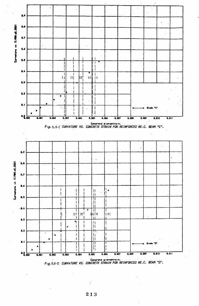
1.9

1 ..

'

1 1 ! 1111

111

111

1 •11

'

1II

....... 1

1"1

1 .

1 *inj VI

1|V1

11

19 1

111

111

4---_ 4 Greda T♦

♦ 1)1

1

1

111

111

♦♦

> 111

11\

1 . 1

11

Ù.*

0.3

0.2

0.1

1.000 0.001 0.002 0.003 0.004 0.005 0.006 0.007 0.000 0.009 0.010 0.011

Cenoret* mioroetrein.Fig. 5.9-C curvature VS. CONCRETE STRAIN FOR REINFORCED RE.C. BEAM " C .

- ■

-

1

111

111

I I . II

I -1

1I

■ " T " 1

1

1

1

IJIII I

111

------— 1-----

f

- 1

III1

I 4

n i l I 1

I I/ | l v

I I

11 VI

1

11

♦1

11

1

11

IIit

1

1

♦

--------- e ■ "

11

1

1

11

1 11

1

1Cred# *0*

«♦

11

111

11

I I

i;

111

0.0

0 0

0.7

0.6

0.5

0.4

0.3

0.2

0.1

Concrete m io ro e tre in .F ig .B .9 -0 CURVATm VS. CONCRSTC STRAIN FOR RFINFORCED RE.C. BEAN 'fl*

2 1 3

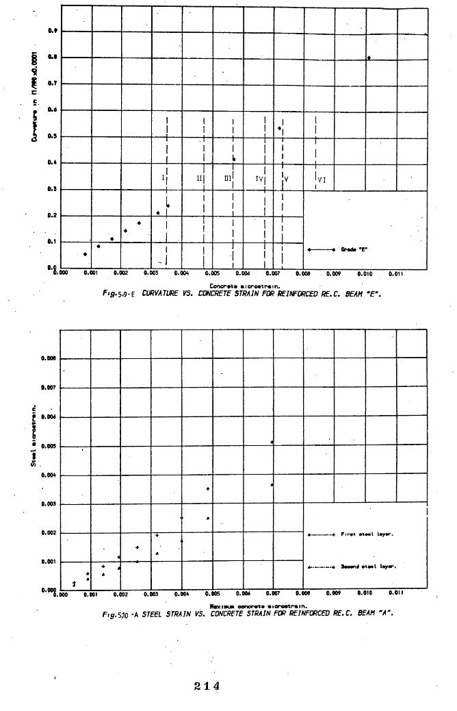
0.9

0.0

111

11 1

1111

1"1

111

11

. 1 1 1

■ ■ ■ 1 1 1»

111

■—r 1 1

t"-1

■111

"11 “'11

IV|1 h.

r”"l..ivi11

I ♦ 1

11

111

11

11

e--- e kede "E♦

♦♦ 1

1 .1I1

111 1

“I"'"11

. ee 1

-111

t11

■■ "1 1 1

111

0.4

0.3

0.2

0.1

.000 0.001 0.002 0.003 0.004 0.005 0.006 0.007 0.008 0.009 0.010 0.011

Concrete mioroetrein.Fig.s.9-E CURVATURE VS. CONCRETE STRAIN FOR REINFORCED RE.C. BEAM - E \

- -

4

+

4-------------4- F ir#% e te a l l# y # r .

4

+

+

*

t '♦ à

0.008

0.007

cI 0.006

0.005

0.004

0.003

0.002

0.001

'^ .0 0 0 0.001 0.002 0.003 0.004 0.005 0.006 0.007 0.008 0.009 0.010 0.011

Neximimi oonorete e ie ro e tre in .F»g.5.10 *A STEEL STRAIN VS. CONCRETE STRAIN FOR REINFORCED RE.C. BEAM 'A '

2 1 4

0.006

0.007

0.006

" 0.005I0.004

0.005

0.002

0.001

+

+

'

+

+ .

+ ^

+ ------------ -+ F i r e t e t w l la y e r .

+

+

»• ,A

+

* ‘+ e

0.00g.000 0.001 0.002 0.003 0.004 0.005 0.006 0.007 0.006 0.009 0.010 0.011

Mmximum oonorete m ioroetrein.F ig , 5.10-B STEEL STRAIN VS. CONCRETE STRAIN FOR REINFORCED RE.C. BEAM ‘'B \

+

+-

a a l la y e r .

4-

+

+

»• 4 ..... — -» F i r a t a t

+i *

i a

0.006

0.007

cf 0.006

* 0.005J0.004

0.003

0.002

0.001

®*®®&000 0.001 0.008 0.003 0.004 0.005 0.006 0.007 0.006 0.009 0.010 0.011

Mmximum oonorete m io ro e tre in .Fig.S.IO'C STEEL STRAIN VS. CONCRETE STRAIN FOR REINFORCED RE.C. BEAM 'C '.

2 1 5

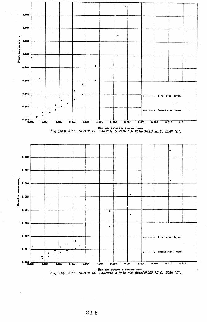
- O.OM

0.007

Cf 0.006

■ 0.005

I0.004

0.003

0.002

0.001

♦

+

à

+

♦♦

*4— —+ Firet eteel layer,

e---- - e Saoond ataal layer.♦

t 't «

1.000 0.001 0.002 0.003 0.004 0.005 0.006 0.007 O.OM 0.009 0.010 0.011

HeximuB oonorete mioroetrein.F<g.5.10-D STEEL STRAIN VS. CONCRETE STRAIN FOR REINFORCED RE.C. BEAM "D " .

- 4

+

+

aal layer.

- A

+

+% a

0.000

0.007

cg 0.006

1■ 0.005

1A0.004

0.003

0.002

0.001

0.000

Heximue oonorete mioroetrein.F ig . S.^O-Z STEEL STRAIN VS. CONCRETE STRAIN FDR REINFORCED RE.C. BEAM '’E".

216

180

t

s iw

140

120

X * > X X

>

X------------- X a -e d . 4

too0.000 0.001 0.002 0.003 0.004 0.005 0.006 0.007 0.008 0.009 0.010 0.011

Concret# e io ro e tre in .F»g.5.11-A COMP. ZONE DEPTH V5. CONCRETE STRAIN FOR RE.C. BEAM * A " .

180

140

120

1.000 0.001 0.002 0.003 0.004 0.005 0.006 0.007 0.008 0.009 0.010 0.011

Concrete m ioroetrein.F»g. 5.11-B COMP. ZONE DEPTH VS. CONCRETE STRAIN FOR RE.C. BEAM 'B ' .

2 1 ?

INI{

140

120

K feed. *r.1.000 0.N1 0.002 0.003 0.004 0.005 0.M 6 ^ 0.M 7 0.008 0.009 0.010

. Concrete m ioroetrein.Fig.5.11-C COHP. ZONE DEPTH VS. CONCRETE STRAIN FOR RE.C. BEAM "C ".

0.011

■

'

* XX

X

* X* X

X

X

X ----------- X IW d . 'D *.

c

X 175

II8I 150

125

INO.ON 0.N1 0.002 0.003 0.004 0.005 0.006 0 .N 7 O.ON 0.009 0.010

Concrete m io ro e tre in .F/g.5.11-D COPP. ZONE DEPTH VS. CONCRETE STRAIN FOR RE.C. BEAM * D \

0.011

2 1 8

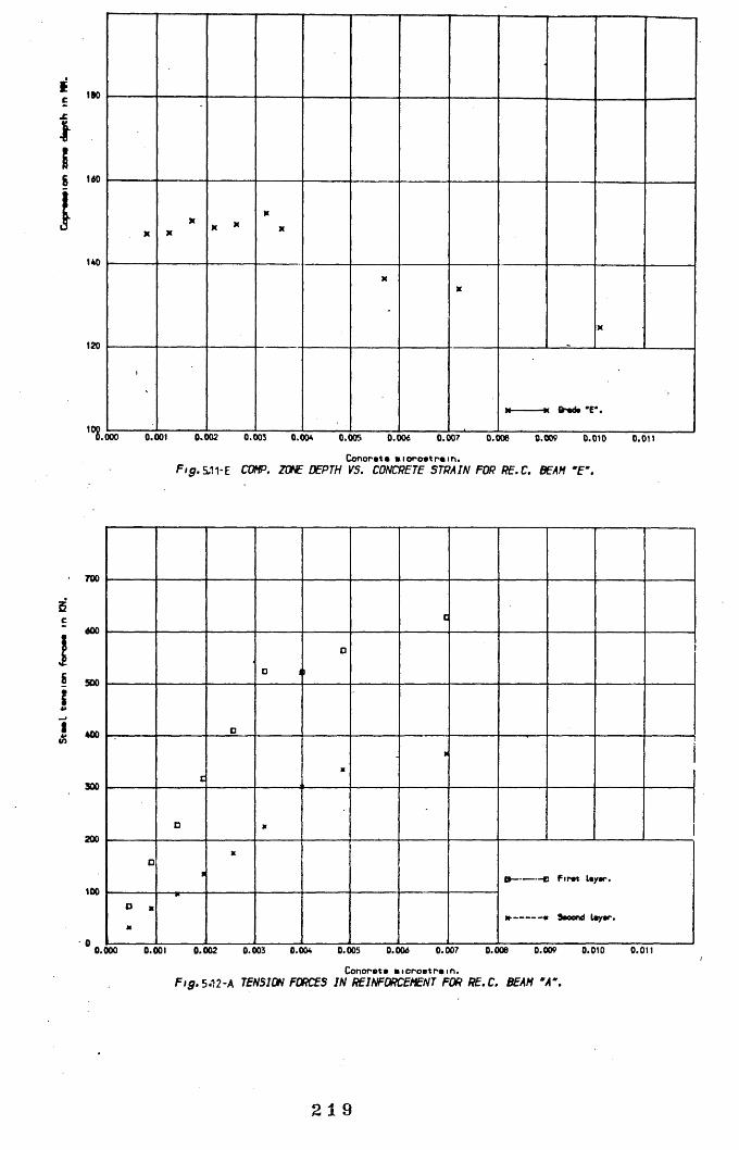
100

II5 160

140

120

K fted* "E".

.000 0.001 0.002 0.003 0.004 0.005 0.006 0.007 0.006 0.009 0.010 0.011

Concrete m io ro e tre in .F/g.ill-E CCWP. ZONE DEPTH VS. CONCRETE STRAIN FOR RE.C. BEAM "f'.

c

O 1

0

1

D

c

-

o

o69— —•■C Firet leyer.

*■----- — a Second leyer.D a

700

600

§ 500

iI 400

300

200

100

0.000 0.001 0.002 0.003 0.004 0.005 0.006 0.007 0.006 0.009 0.010 0.011

Concrete m io ro e tre in .Fig.5.12-A TENSION FORCES IN REINFORCEMENT FOR R E.C . BEAM •’A \

2 1 9

no

«00

900

400

900

800

too

o 0

1' o

D

OR

oR R

3

0

0B------------B F ire t layer.

o

0.000 0.001 0.002 0.003 0.004 0.005 0.006 0.007 0.006 0.009 0.010 0.011

Concrete mioroetrein.F/g.5.12-B TENSION FORCES IN REINFORCEMENT FOR RE.C. BEAM

D

O3

b

,

D

O

□

]-

B------------B F ire t layer.

»•---------- e Second layer.D m

TOO

«00

500

400

300

200

100

0.000 0.001 0.002 0.003 0.004 0.005 0.006 0.007 0.006 0.009 0.010 0.011

Concrete mioroetrein.F i g . 5.12-C TENSION FORCES IN REINFORCEMENT FOR RE.C. BEAM T ' .

220

TOO

«00

I SCO

II *“

300

200

100

0

V

DD

D

D

D

□

D B— -HD Firet leyer.

D «

0.000 0.001 0.002 0.003 0.004 0.005 0.006 0.007 0.006 0.009 0.010 0.011

Concrete m icrcetrein .F ig . 5 :2 -0 TENSION FORCES IN REINFORCEMENT FOR RE.C. BEAM " 0 " .

D□

o

o

□

O

O-

D

o

□

B------------ B F irs t leyer.

————— a Seoflfid leyer •

TOO

«00

900

400

300

200

100

0 000 0.001 0.002 0.003 0.004 0.005 0.006 0.007 0.006 0.009 0.010 0.011

Concrete aicrcetrein.F i g . 5.12-E TENSION FORCES IN REINFORCEMENT FOR RE.C. BEAM "E".

2 2 1

500

5c *00

1

gï 300

200

100

, 1 '

♦> o' é ‘

4

. O• o *

* 4♦ to 1

♦ «4>

* a f o# o

1 o >

« to * mt

* ** m

aoto

•m

D

G--------G B«#a A

tr-------« • C$-------■* Bmb D

a-------- e Bm b E

to

mto

m

20 30 *0 50

Mid-«p«n d#fl#ctlom in MM. F,g. 5.13 LOAD-DEFLECT ION RELATIONS FOR REINFORCED RE.C. BEAMS.

TanaIon ataal Aa

K2.C

Concrata compraoalon força

Nautrol oxla

Staol tonalon força

Croos oQctlon Strain distribution Strass distribution

Fi g. 5. 14 Notations of rectcngular cross section at ultimate strength. ' in pure flexure.

222

1000

000

400

400

200

•

m

..... "1

m

-

i

m

m

m

V

,— --- — . Conor**# coop. fero*.m<

0.000 0.001 0.002 0.003 0.00* 0.005 0.006 0.007 0.000 0.009 0.010 0.011

Conorat* aicroatrain.F'g. 5.15-A COMPARISON BETVEEN CALCULATED INTERNAL FORCES FOR RE.C. BEAM

■

■■

1■

1

■

■

■

1

*

■# - ■ -m 5 t * * l «anaion fo re*.

---------------- Conor*»* ooap. fo r ** .É

1000

000

400

400

200

Conorat* a io ro a tra in .Fig. COMPARISON BETVEEN CALCULATED INTERNAL FORCES FOR RE.C. BEAM •’B".

2 23

1000

BOO

M O

M O

200

aa

a

■

aa

a

1 a ——' a St«*l «arwien foro*.

------------ - Carter*»* eoop. fore*.

aa

0.000 0.001 0.002 ^ 0.003 0.00* 0.005 0.006 0.007 0.000 0.009 0.010 0.011

Conor#t# ■loroatroin.F/ .5.1S-C c o m par is o n BETVEEN CALCULATED INTERNAL FORCES FOR RE.C. BEAM "C".

1000

000

M O

M O

200

'

----- ---

a

a -

a

■

f

a

a

■ ~a

a

0.000 0.001 0.002 0.003 0.00* 0 .005 0.006 0.007 0.000 0.009 0.010 0.011

Conorat» a ie r o a t r a in .Fiÿ.5.15-D COMPARISON BETVEEN CALCULATED INTERNAL FORCES FOR RE.C. BEAM "D".

2 2 4

1000

•00

400

400

200

a-a----

a

a

a

a

a

■

a

------------ - Conorata ooap. foroa.

0.000 0.001 0.002 0.003 0.004 0.005 0.004 0.007 0.006 0.009 0.010 0.011

Conorat« aioroatrain.Fig. 5.15 E COMPARISON BETVEEN CALCULATED INTERNAL FORCES FOR R E .C . BEAM "E " .

c -

O-

I10

0 a

-

0

Calculât ad aoaant.9 e---------- c

..4 —a Actual aoaant.

200

180

140

140

120

100

80

40

40

20

0.000 0.001 0.002 0.003 0.004 0.005 0.004 0.007 0.008 0.009 0.010 0.011

Concrata aioroatrainF;^.5.16-A COMPARISON BET. CALCULATED i ACTUAL MOMENT FOR RE.C. BEAM *A\

2 2b

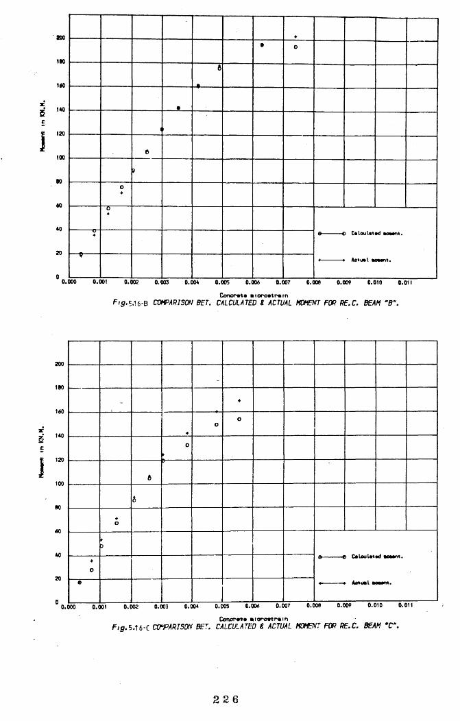
200

ISO

140

140

120

ICO

00

40

40

20

• 0

6

e

6»

0

0

0 0 Caloulatad aoaant.

*- - ■ < Aotual aoaant.9

0.000 0.001 0.002 0.003 0.004 0.005 0.006 0.007 0.006 0.009 0.010 0.011

Conorata aioroatrainF/5.5.I6-B COMPARISON BET. CALCULATED i ACTUAL MOMENT FOR RE.C. BEAM "B " .

-

-

00

0

t

6

0

3Calculât ad aoaant.

0

a---- f

4 4----------- » Actual aoaant.

200

100

140

140

120

100

00

40

40

20

Conorata aioroatrainF j p.5 .1 6-C CO ARISON BET. CALCULATED & ACTUAL MOMENT FOR RE.C. BEAM “C\

2 2 6

200

tac

140

1*0

120

100

K

40

*0

20

0

0

0

♦

6

0

9

ad aoaant.8

* - --------- - * Caloulat

"■■■"f ' » ■ I Aotual aoaant.

0.000 0.001 0.002 0.003 0.004 0.005 0.004 0.007 0.006 0.009 0.010 0.011

Conorata aioroatrainFig.SAù-DCO M PARISON BET. CALCULATED i ACTUAL MOMENT FOR RE.C. BEAM

♦

00 0

0ft ♦

0

0

b

9

Calculât ad aoaant.• 0 <

200

too

140

140

120

100

N

40

40

20

0.000 0.001 0.002 0.003 0.004 0.005 0.004 0.007 0.006 0.009 0.010 O.OM

Conorata a io r o a t r a inF 15. 5.16-E COMPARISON BET. CALCULATED i ACTUAL MOMENT FDR RE.C. BEAM

2 s 7

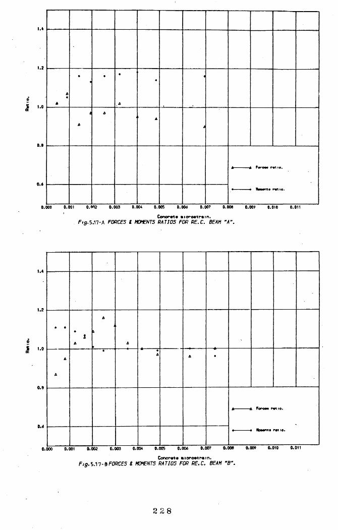
1.4

1.2

1.0

0.0

0.6

0.000 0.001 0.002 0.003 0.004 0.005 0.004 0.007 O.OM 0.009 0.010 0.011

Conorata aioroatrain.F/ .5.17-A FORCES t MOMENTS RATIOS FOR RE.C . BEAM "A " .

t4

4

4

4

4

* •4 4

4---- 4 Fcroaa ratio.

• « Moaont# ratio.

1.4

1.2

Î 1.0

0.0

0.4

0.000 0.001 0.002 0 .003 0.00* 0.005 0.004 0.007 0.000 0.009 0.010 0.011

Conorata a io r o a t r a in .Fig.S.M-BFORCES i MOMENTS RATIOS FOR RE.C. BEAM B\

2 2 8

1.4

1.2

O.B

4

4

4

4t . *

4

4

4

*

4 4 Faroa# r a t i o .

0 .4

0.000 0.001 0.002 0.003 0.004 0.005 0.004 0.007 0.000 0.009 0.010 0.011

Conorata aioroatrain.F,g.5.17-C FOffCES i MOMENTS RATIOS FOR RE.C . BEAM "C.

, 4* 4

4

4

4

♦

4 * 4♦

À

*4

4

4 ------ a Foroaa r a t i o .

« « Moaont# r a t i o .

1.4

1.2

1.0

0.0

0.4

0.000 0.001 0.002 0.003 0.004 0.005 0.004 0.007 0.000 0.009 0.010 0 .0 1 I

Conorata aioroatrain.F ig .S .M -U FORCES i MOMENTS RATIOS FOR RE.C . BEAM "D " .

2 2 9

1.4

1.2

6J•

*

A

A

i6

A

AA

A

A

A

•

A---------------A feroea retie .

♦ .............■* Neeente re tio .

0.8

0.6

0.000 O.'OOl 0.002 0.003 0.004 0.005 0.006 0.007 0.008 0.009 0.010 0.011

Conor#** #ioro#tr#in.F i g . s M - l FORCES t MOMENTS RATIOS FOR RE.C. BEAM "f.

0.5

0.4

hÎ

— tro ♦

0.2

0.1

-e Cr#6# A.

— . Cr#d« B.

Ç o Cr#d# C.Ç o

» Grad* D.

------ * Cr#d# C.

0.00.00 0.01 0.02 0.03 0.04 0.05 0.06 0.07 0.08 0.09 0.10Reinforcement retlo.

F ig .S .^ S EFFECT OF REINFORCEMENT RATIO ON THE FACTOR T .

0.11

2 3 0

a.of

e.oB

C 0.07

f0.06

0.05

0.04

0.03

0.02

0.01

< Crmd# A,

..... ♦ Grad* 0.

Grade C,

...... -* Grade D.

-------m Grade £.

9 0 e •

‘ h

0.00

T ÏT M l0.00 0.01 0.02 0.03 0.04 0.05 0.06 0.07 0.06 0.09 0.10

R#Inforcement re tlO .F i g . S A 9 EFFECT OF REINFORCEMENT RATIO ON STEEL STRAIN,

0.11

* * *1 : '

- a ♦ a ♦

' n

a » *

, 0 » “

, 6 0 °

, 0 = =

A *

à « A ♦ , " 1

* OO * ,

I

. ‘ Ç

t n O ■ O Grade A.

a--------- - Grade B.

a--------—♦ Grade D.

e *' *e Grade £.

9

—B ---

I

0.35

0.30

0.25

0.20

0.15

0.10

0.05

0.00

Reinforcement r e t lo .F , g . 5.20 EFFECT OF REINFORCEMENT RA TIO ON THE REDUCED MOMENT.

2 3 1

0.7

0.6

0.5

S010.3

0.2

0.1

0.0

-----jj-l

9

99 0) D t0 t , 1

-n ■ ' S

( 9/Xp •, *

9^ D »> D *

, •e— — O Cr#d* A.

Cr#6# D.

# . .— a Cr#6# E,

e

, 9

1/'

ff

0.00 0.01 0.02 0.03 0.04 0.05 0.06 0.07 0.08 0.09 0.10

I&

F i g . 5.21R#inforc#m#nt ratio.

EFFECT OF REINFORCEMENT RATIO ON COMPRESSION ZONE DEPTH.

0.11

15.0Beam B

Beam C

Beam A

10.0 Beam E ' ■

5.0

Machine load KN0.0

500,04 0 0 .0300,0200,0

Fig. 5.22 Variation in flexural stiffnnss versus machine load at the six steel stages far the five PC beams tested.

2 3 2

Boom A

Beam C

Boom 0

Fi g. 5. 23 Crack pattern within the constan moment span for the five P C Deams test-ed (Dotted lines represent the back side crack pattern).

2 3 3

CHAPTER S IX

REINFORCED PC COLUMNS AND THEIR

TEST ANALYSES

6.1, Introduction

Any ultimate flexure theory should cover loadings other than

pure flexure. The most common case of loading is probably that

of combined moment and axial load. Members subjected to this

type of loading are encountered in almost any structure.

Hence, the methods for structural analysis and design of

reinforced PC members under this loading should first be

reliably established. Thereafter any case of biaxial moment,

with or without normal force, can be dealt with. In this

present work, short columns with small eccentricities were

investigated. Proper interpretation and extrapolation of the

findings should allow a general approach for dealing with

short or slender columns with any degree of eccentricity.

As columns generally have compression reinforcement, its

influence on the ultimate capacity must be thoroughly

investigated. The reinforcement steel used in the present work

had no definite yield point and its strength continued to

increase up to very high strain values. This type of steel has

dictated, as said before, the concept of the specific

reinforcement ratio 'Rg\ at which a prescribed value of steel strain can take place at the ultimate capacity. These values

of Rg were determined in the analysis of pure flexure in beams on the basis of the efficient use of steel and the desired

mode of failure. However, and as will be shown later, with

columns Rg can not be determined in this way. This is mainly

2 3 4

because of the fact that efficient use of steel is not a

matter of only adjusting tension and compression reinforcement

ratios.

For a given section under the action of combined moment and

direct axial load the ultimate moment capacity depends on the

magnitude of the axial load; this capacity depends on the

eccentricity of loading defined as the ratio of moment to

axial load. This mutual dependency between the normal force

and its eccentricity for the ultimate moment capacity,

prevents the possibility of setting a general Rg for any

section without consideration of the eccentricity level. For

any given section, an infinite number of values of Eg can

exist depending on the eccentricity of the normal force. In

other words, for a section having tension and compression

reinforcement ratios R and R', there is only one value of

eccentricity that would allow the development of certain

prescribed value of steel strain at ultimate condition.

As said earlier in Chapter Five, The so called tension or

compression failure had little significance in describing the

failure mode. All columns made of this type of steel would

fail when the ultimate compressive concrete strain ^cu has

been reached. Hence, columns that might have very small R will

still fail eventually when the concrete develops its cu in

the compression zone , no matter how high the tension steel

strains might be.

As will be shown in this chapter, the different parameters of

the stress block for various PC grades were employed along

with the concept of specific reinforcement ratio for specific

235

eccentricities in the design of the five columns tested. To

simplify derivations and calculations the effect of lateral

confinement and its contribution to the stress block

parameters was neglected.

6^2. fuDdaiDgntei g.aP9tion f&c eccentric JLg.ad,sFor any rectangular cross-section, and with the notations

given in Fig.(6.1), the previously derived Eqs.(5.1 ^ 5.5)

still can be applied. Dividing Eq.(5.2) by Eq.(5.1 ) then,

Z/L = [T( 1-YT) + T'g( i_d Vd)]/(T + T's-Tg) , from which

(e /d)(T+T's-Tg) = T( 1-YT) + T's( 1-d Vd) ...(6.1)

in which Tg, T*g and T are as follows,

Ts = R.fs/fcy . T's = R’.f's/fcy > ^ = G.c/dand e is the eccentricity measured from the centroid of the

tension steel to the applied load.

Using the idealized steel stress-strain curve and Eq.(5:4) &

Eq.(5.5), the stresses in the tension and compression steel fg

and f’g can be expressed as follows;

fg = A + B. s = A + B(G/T -1)

f’g = A» + B'.^s’ = A ’ + B ’(1- d ’.G/(d.T))

By substituting in Eq.(6.1) and rearranging then

At 3+ BT^ + CT + D = 0.0 . ...(6.2)

in which : A = Y , B = e /d -1.0

C =(R'/dfgy)[ (A' + B'. c)(e -d + d') - (R.e /R')(A-B )] andD = (R'.B'.^c.G/dfcy)(d'-d'2/d-R.eB/R'B'-e d'/d)

Eq. (6.2) can now be used to calculate the value of the factor

T for any cross-section having a certain R, R' and e . It is

2 3 6

clear that this equation is similar to Eq.(5.6-a) which was

derived for pure flexure. While the factor T in the case of

pure flexure is defined by a second degree function, this is

increased to a third degree in the case of combined direct

force and moment. This increase in the function order is due

to the additional effect of the normal force which does not

exist in the case of pure moment.

The factor T can be used for calculating T^ and T'g. Knowing

these three factors , the normal force and the moment at any

value of ^c can be calculalted (Eqs.(5.1 &5.2 ) ) ; the ultimate

values can be found if c is substituted by ^u.

As with Eq.(5.6-a), the constants of the steel stress-strain

curve should first be assumed and then checked. Several cycles

might be required until the assumed constants are verified.

The PC stress block parameters affect Eq.(6.2) in terms of

G,y,^c and f^y, which express each PC grade explicitly. One major difficulty is the solution of the third degree equation

which can be solved graphically or mathematically. Computer

programmes can easily provide such solutions.

On being solved, this fundamental equation (Eq.(6.2) ) can

provide the calculation of not only the ultimate moment but

almost any other value in the section. The compression zone

depth c, the strains in tension and compression steel s &^s',

the internal forces in PC and steel, and the curvature can be

calculated at any maximum compressive strain in PC.

6.3. Tests of reinforced £C cplumng

6.3.A Dimensioning Five reinforced PC columns were tested,

2 3 7

one for each grade. The same considerations taken into account

in dimensioning the beams were applied to columns. In addition

the test-zone cross-sectional area was chosen in such a way

that not more than 2000 KN would be required as an eccentric

load. This was to allow the design of the supporting system to

be practically possible.

The width of the cross-section was taken to be 150 mm. as was

that of the beams. Cosidering the maximum load value set

before, the total depth was taken to be 200 mm. For this area

of cross-section, the expected ultimate load necessitated a

minimum bearing area of 1 5 0x250 m m 2. To allow for this

increased area at the two ends of the column, haunches of 1:1

slope had to be made as shown in Fig.(6.2). The column-end

dimensions and the bearing plates dimensions gave a possible

maximum eccentricity of 75 mm measured from the geometrical

centroid of the test zone cross-section.

The shear force in the vertical haunch-column plane for the

chosen loadings and the given dimensions was found to be 800

KN. This high shear force required a minimum shear plane of

150x500 m m 2. As was experimentally verified, this shear area

in addition to the shear reinforcement was sufficient and no

shear failure took place in any of the five columns.

The columns were cast horizontally with the tension side being

the top level. Before casting the.column mould was painted

with silicone grease which helped provide sound demoulding and

well finished surfaces when hardened. Because of the heavy

reinforcement used, a vibrating table and steel tamping rods

had to be used during PC placement and for prolonged periods.

2 3 8

Each column required one batch which took around 30 min. to

mix, place and vibrate.

6f 3 1P O.L reinforcement The stress block

parameters found previously are based on a plain prism in

which no compression reinforcement nor lateral ties were used.

Therefore it was essential to check the applicability of these

parameters to columns whose compression zone is reinforced and

laterally confined. Generally compression reinforcement R’ has

a little role to play in beams where its contribution can only

be of significance near failure and only with associated high

tension reinforcement R. Conversely, in columns with small

eccentricities, R’ has more effect on the ultimate capacity

and behaviour. Unlike beams, compression failure can not be

avoided by limiting the tensile steel area. A major factor

controlling the failure mode and the contribution of R or R’

is the eccentricity level.

For any given section reinforced with the type of steel

adopted in this work, the ultimate axial load and the ultimate

moment are inversely proportional to eccentricity e . This

effect of e can be more clearly seen when R is small, R’ is

high or both. Consequently steel strains are strongly related

to the chosen value of e for any given section.

In the five columns tested, a range of R’ values was employed,

varying from 2.4% to 4.6%. Although these varying ratios were

determined to suit the P.C. grades they also helped in the

analysis and investigation of the effect of compression

reinforcement on the ultimate structural performance of these

columns. As will be shown later, for the cross-section chosen

239

increasing R theoretically from 0.5% to 10% can result in an

increase in the ultimate load or moment of only about 15%.

With the available range of e , around 120 to 150 mm. from the

tension reinforcement centroid, the influence of R was

limited. The value of R has a significant effect on the

resulting stresses and strains in the tensile steel only at

high e values. This implies that only for such cases will R

have a dominant effect on the associated deformations and the

lateral buckling of the column. The chosen values of R were

based on the concept of the specific reinforcement ratio

which would allow prescribed strains in steel to develop at

failure. These ratios varied from 2.9% to 7.7% and it will be

shown later how they were reached.

To limit the buckling of the longitudinal steel and to allow

for full use of PC up to its ^cu, ties were provided. As shown

in Figs.(6.3-a,b,c,d&e), these ties were closely spaced. The

lateral confinement given by the ties and its contribution to

the ultimate carrying capacity will be dealt with later.

Sufficient shear reinforcement was provided as shown in the

same figures for each column and no shear failure took place.

6.3.C Testing and m easurem ents The eccentric load for each

column was applied using a 1000-Tonne Los System Testing

Machine. The required loads were high and no single-roller

supporting system could be provided for them. As shown in

Fig.(6.4), three rollers made of high tensile steel were used ;

each is 50 mm diameter and 150 mm long. The rollers only

allowed lateral movement where no rotation could have been

tolerated as the three rollers were assumed to support the

2 4 0

load equally; see details in Fig.(6.5). The chosen thickness

of the bearing plates was proved sufficient to prevent any

local bending in them that could have initiated local crushing

failure.

Steel strains were measured using 5 mm. electric strain

gauges. For each column, strains in two tension and two

compression steel bars were recorded within the test zone. Two

pairs of strain gauges were attached to each of these four

bars at two positions, 100 mm. apart. The two gauges at each

position were attached opposite to each other (right and left

sides of the bar, not inner and outer faces). In this way each

column had eight strain gauges for either tension or

compression reinforcement, which were kept away from direct

contact or friction with the lateral ties by attaching the

gauges to faces remote from them. The average values of

strains were calculated (out of eight individual readings) and

used in the analysis.

PC strains were measured using 20 mm. electric strain gauges.

Eight strain gauges were attached to each column, two on each

side or face at the midheight of the column. Strains recorded

•at the inner and outer faces measured the maximum compressive

and tensile strains in PC respectively. As shown in Fig.(6.6),

the concrete strain profile along the cross-section could be

traced by recording these strains and those at one third and

two thirds of the total depth of the test zone. The average

value of each of two opposite gauges was calculated and used

in the analysis. The tensile strains in PC at the outer face

were small enough to enable the gauges at this face to

241

continue operating into the late test stages. In some columns

no tension cracks developed before concrete crushing had taken

place in the inner side (the compression zone).

The strain gauges and the machine load readings could be

recorded incrementally by the use of a Data-Logger. Load

increment was 50.0 KN every 2 min. At the end of each

increment, instantaneous reading of all values of strain and

the machine load were taken. Tests continued at this rate

until failure. There was no need to increase the rate of the

platen movement where no excessive deflections occurred near

failure.

6.4. Test results

Using the average strain values in concrete and steel at

different positions, the strain profiles for various load

levels could be plotted for each column. These incremental

strain profiles are shown in Figs. (6.7-a, b, c , d &e). In all

these figures increase in curvature was almost at a constant

rate, until at late stages when failure was imminent and this

rate increased rapidly. The neutral axis always lay between

the two ’tension ’steel layers (column B, C & E). Columns A

and D which had only one tension steel layer, had their

neutral axes lying below and above this layer respectively

throughout the test. Columns E, B and C had generally tensile

strains in the outermost layer and compressive strains in the

innermost layer. The ’tension’steel was subjected to tensile

and compressive strains in columns D and A respectively.

Figs. (6.8-a,b,c,d & e ) s h o w the s t e e l s t r a i n s as

experimentally recorded and plotted against the maximum

2 4 2

compressive concrete strain (^c).

The compression zone depth (c) as calculated from the strain

profiles at different stages are plotted against c in

Figs. ( 6. 9-a I b , c , d & e ). Column A which had the smallest

eccentricity (e ), had a c-value in the vicinity of 190

mm.,which is greater than the effective depth (d). The change

in c for column A was almost zero which is mainly due to the

small value of e applied rather than the values of tension

and compression reinforcement ratios (R & R') employed.

As the tension steel strains were generally much smaller than

the compressive strains in the compression steel, three stages

of that steel's stress-strain curve were defined to help

analyze the results. These stages are ;[i ] compression steel

reaching its proportional limit,[ii] compression steel

reaching its 1.0% proof strength and [iii] compression steel

reaching its 2.0% proof strength.

For column A, c is almost constant at any stage. The strain in

compression reinforcement after reaching stage [i], increased

slightly and when this steel reached stage [ii], ^c amounted

to around 0.004. At stage [iii], ^c was 0.0055 after which it

increased rapidly until failure.

Column B had a constant compression zone depth of around 170

mm. up to stage [i], which kept the innermost layer of tension

steel continuously under compression strains, while the other

outer layer developed tensile strains. Despite grade B having

90 N/mm.2 compressive strength, the ultimate load recorded

with column B was much lower than that of column A whose

compressive strength was 85 N/mm2. This can well be attributed

2 4 3

to the higher e used with column B. This relatively high

value of e produced a value of c much smaller than that with

column A, with a consequent smaller ultimate load. Full

analysis and interpretation of results for the five columns

will be given later. However, what should be stressed here is

that the value of c decreased for all columns (except column

A) as the test load was increased.

Knowing the steel strains and using the idealized stress-

strain curve for the steel , the axial tensile and compressive

forces could be calculated at various load levels. Figs.(6.10-

а,b,c,d &e) represent these steel forces plotted against ^c.

These figures show how beneficial compression steel might be

in short columns with small eccentricities. On average, the

compression force provided by this steel amounted to 25% of

the total internal compression force at any load level. This

indicated that R’ contributes to the section carrying capacity

even at the elastic stages and long before the initiation of

concrete crushing (compression failure).

The ultimate failure load recorded varied from a one column to

another. The highest value was recorded with column A (2250

KN), while the smallest was recorded with column C (1750 KN).

The recorded ultimate compressive concrete strain cu well

exceeded the theoretically derived value for each grade.

Values of up to 0.01 were recorded near failure. This implies

that the theoretical values are conservative although they are

within the range from 0.007 2 to 0.0076.

б.5. Analyses q 1 regulfcg

244

By using the results of the five columns tested, the

previously given strain profiles were produced. These strain

profiles are almost linear at any load level and even near

failure. From these profiles steel and concrete strains could

be obtained and used in the analysis of each column. As shown

previously, by knowing the steel and concrete strains and

having the stress-strain curve for each of them, the internal

forces could be calculated on these bases. The internal

concrete compressive force, the total internal force and the

external eccentric machine load are plotted against c for

each column as shown in Figs. ( 6.11-a, b , c , d,&e). The internal

moments calculated on the above bases are plotted along

with the actual applied moment at various test stages for each

column as shown in Figs. ( 6.1 2-a, b , c, d,&e ). The ratios of the

calculated to the actual applied loads and moments are also

derived and shown in Figs. ( 6.1 3-a, b , c , d,&e ).

As tension steel strains were small and within the elastic

stage, compression steel strain was used in describing

the behaviour of the different columns tested as this steel

generally developed much higher strains. In addition to the

three previously defined stages [i, ii & iii], a fourth stage

[iv] will be used in the analysis of results. This stage

represents the stage at which a column will develop a maximum

concrete compressive strain equal to the theoretical ultimate

value cu) set for its PC grade.

Table (6.1) shows the various reinforcement ratios and the

eccentricity values employed in the five columns tested. The

high tension reinforcement ratios (R) were those chosen

primarily to ensure as large a compression zone depth as

2 4 5

possible, and to control the mode of failure. The high

compression reinforcement ratios employed were mainly to help

increase the ultimate carrying capacity of the columns. These

prerequisites had to be taken into consideration due to the

small range of eccentricity available.

With small eccentric!ty-columns, a compromise has to be made

between the efficient use of tension steel and the economic

use of PC itself. In such a case, using tension steel

efficiently so as to develop a high proportion of its ultimate

strength by reducing R, would imply a great reduction in c and

a consequent waste of the merit of PC in compression. This

would also allow for uncontrolled propagation of tension

cracking and in general would cause a reduction in the

ultimate carrying capacity. Hence to keep this capacity as

high as possible, and to control tension cracking development

high values of R had to be icorporated even if tension steel

would develop only a small proportion of its ultimate

strength.

As shown in the given profiles, the outermost tension steel

layer developed strains amounting to 0.0003 and 0.001 at stage

[iv], for column A and D respectively. Despite column A having

R=2.94% and column D having R=4.65%, tension steel strains

recorded with the latter were much higher than with the former

(almost three times as much). This is mainly because column A

had e =127 mm., while column D had e =155 mm. So it is evident

that the tension steel strains are not only dependent on R,

but probably to a greater extent, on the eccentricity level

itself. This mutual relationship between R and e will be

246

dealt with later in more detail. But the conclusion here is

that the definition of small or large eccentricity- columns

must be considered and introduced on the bases of the mutual

effects of R, R' and e on the ultimate behaviour of the column.

The values of R' employed, as shown in table (6.1), are high .

This was to provide the maximum possible internal compressive

force resisted by the cross-section. This would necessarily

give a maximum ultimate moment. As shown in the given strain

profiles, recorded strains in compression steel at stage fiv]

ranged from 0.00645 with column E to 0.0069 with column A.

These high strains confirmed the importance of this

compression steel, where they p r o vided forces w h ich

contributed considerably to the total internal compressive

force of the cross-section , particularly at early stages. For

example, with column A the ratio of the compression force

resisted by this compression steel to that resisted by

concrete amounted to around 70%, 50%, 45% and 40% at stages

i,ii,iii and iv respectively.

At early stages of loading, the associated strains in both

concrete and compression steel are small. For instance, at

stage i column A developed an c = 0.0022 while steel strain was

0.002. At these small strain values, compression steel

develops almost 75% of its ultimate strength, while PC

develops only 30% of its ultimate strength. On further

increase in test load, PC develops its ultimate strength at a

much higher rate than that of steel and the proportion of

compression steel force in the total internal force is

reduced. This trend of compression steel contribution in terms

2 47

of the internal forces provided obviously applies to all other columns tested.

The applicability of the different stress-block parameters

found previously with various PC grades, can now be closely

examined. Referring to Figs.(6.11 and 6.12),the calculated

total internal direct forces at any test-load level were

generally less than the actually applied external forces, in

columns A, B and E. Conversely , columns C and D had generally

higher calculated direct forces than the actual ones. These

calculated total internal forces are the sum of the

compression force in PC and the forces in the tension and

compression steel. On the other hand, the calculated moments

were less than the actually applied ones for all columns. The

difference between the actual and the calculated values of

either forces or moments was almost negligible at early test

stages (stage i). Thereafter a significant divergence began to

take place. This situation can be partially attributed to the

steel used and the PC itself, where assumptions for

simplifying the analyses are made. The idealized stress-strain

curve of the steel used , no matter how precise it is, should

reflect some errors in the derivations of the steel stresses

on the basis of the experimentally recorded strain values.

PC stress-block parameters which were used with the previous

calculations are so far based on the plain prism findings

where no compression steel existed. As these findings applied

well to the beam analyses where no compression steel was

involved and did not apply well to present column analyses,

some modifications have to be carried out on these parameters

2 4 8

when considering PC columns.

The stress-block has two main parameters namely K1.K3 (G) and

K2. The reliability of the first of these is reflected only in

the calculations of the internal forces, while both factors

affect the calculated values of the internal moments. The

parameter K1K3 is dependent on the ultimate cylinder

compressive strength f^y nominated for each grade, and on the

concrete strain c reached at any stage. The special vibrating

techniques used when casting the five columns might be a

reason for a variation in the values of f^y. As said before,

because of the heavy reinforcement employed, prolonged periods

of vibration using steel rods and a vibrating table were

required and must have had effects on the actual value of f^y in these columns. Resin bleeding occurred in columns A,B and

E which were made of high resin content-PC grade. This

bleeding was probably responsible for decreasing f ^ y in the

respective columns. This effect was persistently reflected by

the actual loads being less than the calculated ones which are

based on the higher nominal fç,y-valoes.

On the contrary, columns C and D seem te have gained an

increase in their f^y-values by the elongated vibrating times.

With these two columns, the actual loads were generally higher

than the calculated ones. These two grades in particular, have

the stiffest consistency as they had the largest fractional

volume of coarse aggregate and the lowest resin content. The

results for columns C and D in terms of the internal forces

confirmed this gain in strength due to better compaction and

the consequent limited voids resulting in the composite as a

whole resulting from the prolonged vibrating periods.

2 4 9

The same reasons can be held responsible for the greater

divergence in the actual and the calculated values of moments

, where not only the value of K1K3 but also that of K2 are

used in the calculations. In addition the calculations of the

moments included that part provided with compression steel

which being idealized could cause a magnification in the

errors when multiplied by the lever arm. The actual and

calculated moments up to stage [i] were slightly different and

changed almost linearily with c as shown in Figs.(6.12).

After the compression steel has reached stage [ii], the rate

in moment increase decreased (actual or calculated value);

when this steel exceeded its 0.2% proof strength, no

remarkable increases in these moment values took place.

The tension steel did not develop strains in any column tested

more than those within its proportional limit. This was mainly

due to the small applied eccentricity. In addition the

innermost layer of tension steel was under compressive

strains. As will be shown later these columns had a

compression failure-mode. Considering Figs.(6.8), it is clear

that tension steel in itself was not used economically. But as

said before high values of R helped maintain a high value of

c, which provided high ultimate carrying capacity.

For the columns tested and with the given small range of

eccentricity, it was theoretically found that the ratio of c/d

can be caused to vary from around 0.6 to 0.9 by mutual

changing of R and R». Generally the greater R the greater the

compression zone depth is, irrespective of e . Column A for

example, can have its tension steel strained up to 0.0033 at

2 5 0

R=R'=0.5% with ultimate eccentric force of 1090 KN. at e =140

mm. The same column could support an ultimate load of 1515 KN.

at the same e if R and R ’ are increased to 10% and 3%

respectively; in this case tension steel strains would be only

0.00038. The 50% increase in the normal force and moment can

well justify the use of high values of R even if tension steel

has low strains. This was the main consideration when choosing

the specific values of R with different columns tested.

Stresses and strains in compression reinforcement were fully

developed and this reinforcement contributed greatly to the

internal force provided by each column section. This steel has

little effect on the value of c particularly in columns with

small eccentricity level ratios er ( er =e /d), as had the

columns tested. This effect almost vanishes completely with

cross-sections having high er-values. The compressive strains

recorded in the compression steel with the five columns

reached well beyond those strains corresponding to its 0.2%

proof strength. For example,at stage [iv], these strains as

experimentally observed, amounted to 0.00644 and 0.0069 for

columns B and E respectively. At this stage, the machine loads

were generally smaller than the recorded failure loads except

for column D. This increase in the failure load over the

theoretically defined ultimate load (stage [iv]), could be

partially attributed to the additional effect of the heavy

lateral confinement.

The compression zone depth was generally constant until stage

[i], afterwhich a decrease in c took place in all columns,

except column A. This decrease took place at a decreasing rate

2 5 1

and after stage [iii], c became once again more or less

constant. With column A, which had er = 0.69, compression steel

could not exercise any significant effect on c-value. This

value was experimentally found to be constant at all stages,

see Figs.C 6.9).

è.jù.t Theoretical calculation nf the ultimate carrying capacity

In the previous analyses of results, values of internal forces

and moments, steel strains and values of c were calculated

using the experimental readings of the strains in the concrete

and steel at various test stages. Having the idealized steel

stress-strain curve and the concrete stress-block parameters,

the recorded strain values could be used in the analysis of

the different columns from the first load increment up to

failure. As it is the main objective of this work to clarify

the ultimate behaviour of PC, the theoretical deriviation of

the ultimate capacity of short PC-columns with small

eccentricity will be given.

The previously given Eq.(6.2) can be used for calculating the

coefficient T for any given section made from any PC grade

with a certain e at any desirable value of c. This equation

can thus estimate the single ultimate value of T at the

theoretically defined ultimate compressive concrete strain ^cu

for any given section. This coefficient T can be used in the

calculations of the reduced nor m a l force and m o m e n t

coefficients L and Z, by using Eqs.(5.1 & 5.2).

The following paragraphs demonstrate how T can be derived and

used in the calculations of all the other relevant quantities

to the ultimate carrying capacity of a given cross-section.

2 5 2

6 ^6 A ûT 1 The previously derivedequation ( Eq.(6.2)) is of the third degree in T and its

constants A, B, C and D have been defined above. Constant A is

equal to the stress-block parameter Y= K2/ K1K3, which is

dependent on PC grade. Constant B is a function of the applied

eccentricity e , and the effective depth d ( e/d= er). While

each of the constants C and D is a function of R and R’, fg

and f's> d and d’, assumed maximum concrete strain and e. Hence constants A and B can be given fixed values for each PC

grade and each value of er. While the other two constants,

depending primarily on the state of stresses in the steel

used, will vary even for a given cross-section.

In addition these stresses which are derived from the

idealized steel stress-strain curve can result from any one

of three different functions of the steel strain. Each of

these three functions has different stress constants depending

on the zone in which the steel strain lies. Generally if the

constants of Eq.(6.2) are known, its solution should be

mathematically possible. On solving this third degree-

equation, T can have any of three different values, out of

which one is relevant.

For any section made of a certain PC grade, having a known

er ratio, the following steps can be followed to obtain the

ultimate value of T (Tu), if c was substituted by ^cu. After

obtaining Tu the whole analysis for the section can be carried

out.

(1) Depending on the PC grade fix the constant A.

2 5 3

(2) Depending on the value er fix the constant B.

(3) Depending on R, R’, er, d, d' and ^cu, and assuming the

stress constants for tension and compression steel, calculate

the values of constants C and D.

( 4) Using Eq.(6.2) solve for Tu, and by elimination find the relevant value of Tu.

(5) Using Eqs.(5.4 and 5.5) calculate strains in tension and

compression steel ^s and s* respectively.

(6) Check the assumed values of the steel constants to ensure

that they are compatible with the derived values of S and

®s'. If not, assume another set of steel constants and repeat

steps (3) to (6) until the check is positive.

(7) Fix the last value of Tu, ^s and S ’.

(8) using Eqs.( 5.3, 5.4 & 5.5) calculate c.

(9) Using the idealized stress-strain curve calculate the

steel stresses fg and f’g.(10) Using Eq.(5.1) calculate the coefficient Lu.

(11) Using Eq.(5.2) calculate the coefficient Zu.

This procedure could be carried out using computing facilities

to solve for Tu for a wide range of R and R’ ratios. The range

of R chosen varied from 0.5% to 10%, while that of R’ was from

0.5% to 3%. The calculations were carried out for the five PC

grades. In addition these calculations were repeated with

various er ranging from 0.6 to 2.4. The theoretically derived

values of Tu are applicable to any rectangular cross-section

made of these five grades, provided it has the same er, R and

R ’ .

The output of this computing work helped greatly in clarifing

the effect of each individual parameter on the ultimate

2 5 4

behaviour of short columns in general. However, to make direct

use of these calculations in examining the ultimate structural

performance of the five columns tested, another set of

calculations based on the er values actually used with each

column was carried out. In this set the reinforcement ratios R

and R’ varied from 2.5% and 0.5% to 12% and 5% respectively.

The variation in Tu for different R values with R' as a

parameter is shown in Figs.(6.14-a, b , c , d &e) for the five

columns respectively. The value of Tu increased at a

decreasing rate with the increase in R. The effect of R’ bn Tu

was almost negligible for columns having high values of er.

In column A which had er as small as 0.69, R' had a much

more evident effect on Tu. In such a case, a greater increase

in Tu can be obtained by increasing R’ rather than increasing

R.

Irrespective of er, the decreasing rate in the increase of Tu

by either increasing R or R’, makes it approach a maximum

value for each cross-section. Unlike beams, this maximum value

depends on the stress-block parameters, er and to a lesser

extent on R and R’. This dependency can be closely examined by

referring , for instance, to Fig.(6.14-d) and Fig.(6.1 4-e).

Columns made from grade D and E had exactly the same er,

however, the value of Tu is much higher with grade D than with

grade E for any given R and R’. As grade D is much stiffer

than grade E, it is quite evident that Tu depends on the

stiffness of PC which is reflected in the values of stress-

block parameters. For example, at R=6% and R'=3% the values of

Tu were 0.568 and 0.68 for columns made of grade E and D

2 5 5

respectively. Grade D, as discussed before in Chapter 3,

relative to all grades and in contrast to grade E has the

highest stiffness, highest modulus of elasticity and the

smallest concrete compressive ultimate strain 'cu.

As said above, a maximum value of Tu does exist theoretically,

but would require very high values of R and R’which are far

from being practical. That is in addition to the fact that the

increase in the ultimate carrying capacity near this maximum

value of Tu by increasing R or R’, is insignificant and can

not justify the use of the extremely high values of R and R'

required for it.

Figs. ( 6.15-a, b, c, d & e ) show the variation in the reduced

load coefficient Lu as plotted against R, and R ’ as a

parameter. From these figures the effect of R and R’ on the

ultimate structural behaviour can be partially understood. It

was found that increasing R’ has a greater effect on the

ultimate load than that of increasing R, particularly at small

values of er. Columns made from grade A with er = 0.69 had an

increase in Lu of around 5% for each 0.5% increase in R’,

while the same increase amounted to 0.1% for a similar

increase in R. When the value er increases, the effect of R'

on Lu decreases and that of R becomes more dominant as shown

in the same figures. If er is infinity ( case of pure moment

), the situation is completely reversed and the effect of R

becomes far greater than that of R’. So for the available

small values of er adopted in this work, it is clear that

ultimate capacity in terms of the normal force is more

practically and economically enhanced by increasing R’ and not

R. In such cases the compression reinforcement ratio is the

2 5 6

decisive one.

The definition of small or large eccentricity has therefore to

be established or reconsidered on these bases, where it can

provide an initial evaluation of tension or compression steel

contribution to the cross-section. This definition is that for

any given section the eccentricity ratio er at which changing

R results in a higher effect on Lu than when changing R ’, is

considered to be a large eccentricity and vice versa. In

between these two limits a balanced eccentricity ratio e*r

will exist. The derivation of this ratio will be given later

on in this chapter.

Having calculated Tu, the reduced moment Zu could be found

using Eq.(5.2). The variations in Zu with different R and R'

values are shown in Fi g s. ( 6.1 6 - a , b, c, d & e). This

coefficient Zu showed the same dependency on R, R’ and er as

that of Lu. That is, the factor Zu is more dependent on R at

high values of er and R*. Once again a certain value of er

that would make the effect of either R or R’ more dominant for

a given section should be mathematically definable.

Another conclusion regarding the mutual relationship between

Lu and Zu at any value of er can be drawn. This is that a

maximum value of Zu can only exist when a maximum value of Lu

is reached and not before. In other words, for a given e ,

there is only one value of Zu corresponding to each value of

Lu. With ordinary cement concretes reinforced with steel

having a well-defined yield point, there can exist a maximum

value of Zu at a certain eccentricity irrespective of Lu-

value. If this eccentricity was decreased the value of the

2 5 7

column load would increase and the lever arm would decrease in

such a way that Zu will eventually decrease (compression

failure). Conversely, if this eccentricity is increased the

column load will decrease and the lever arm will increase in

such a way that Zu will eventually decrease ( tension failure

).

This situation can not take place in columns made of PC and

reinforced with steel having no yield point. The block-

parameters of PC and the stress-strain curve of the steel are

such that if the compression zone depth is increased by

decreasing e, the partial reduction in Zu by the reduction of

the lever arm will still be smaller than the partial increase

in Zu by the increase in the internal compressive forces.

To check the applicability of these theoretical findings to

the five columns tested, the ratios of the ultimate

theoretical load to that actually recorded were calculated for

each column. These ratios varied from 75% with column C to 95%

with column A. These big differences showed that the adopted

values of Y, G and ^cu in this theoretical approach are very

conservative. It should be noticed that ^cu for each grade was

first fixed mathematically and then used in the derivation of

y and G from their idealized and experimentally found curves.

The actual ultimate loads were reached at concrete strain

values much greater than ^cu.

The steel strain either in the tension or in the compression

sides for the investigated range of cross-sections could be

calculated using the coefficient Tu. Figs.(6.17-a, b, c, d &

e) show the tension steel strains as plotted against R with R’

2 5 8

as a parameter. Similar curves for compression steel are shown

in Fig s. ( 6.18-a , b, c, d & e). From these figures it is

evident that for a given PC grade and er, steel strains are

strongly related to R and R’. Increasing R while keeping all

other variables constant, would obviously reduce the resulting

strains in tension steel; this is mainly because c will

increase. In addition this increase in c would necessarily

increase the associated strains in the compression steel, but

to a lesser extent. This effect of R on steel strains becomes

more dominant at high values of er and at small values of R'.

The effect of R* on the steel strains can be significant in

sections where R and/or er are very small, if R is high, c

will usually be big enough to make any small variation in it

by changing R’ have virtually no effect on steel strains.

The value of c at ultimate (cy) could be found for various R

and R» by using the equation; c^ = d.Tu/G. Figs.(6.19-a, b, c, d

& e) show the dependency of c^ on R and R’. Generally c^ willincrease at a decreasing rate by increasing R. It will also

increase by increasing R’ only at small er ; while it will

decrease at a very low rate at high er by increasing R’. In

the case of pure flexure R* has almost no effect on cy

On comparing these c^-figures to the five columns tested, it was found that they agree well with the experimental

observations. The maximum value was 178 mm. for column A, and

the smallest value was 149 mm. with column C. The other three

values for columns B, D and E were 1 52, 153 and 154 mm.

respectively. Unlike the values of Lu, c^ seems to be less affected by the idealization, assumptions and ^cu-values

2 5 9

involved in the analyses.

^ ,61P S m M l and large accentricitv-columns Before proceeding

towards how the specific reinforcement ratio can be defined,

the definition of small or large eccentricity has to be first

clarified. As said before, it was found that irrespective of

PC grade, there is a certain ratio of eccentricity e*r at

which the influence of R or R’ on the ultimate column load is

equal. Ratios smaller than e*r cause a higher rate of change

in L with respect to R ’, dL/dR’ , than that with respect to R,

dL/dR , and vice versa. This ratio e*r can therefore represent

a clear distinction between large and small eccentricity-

sections on the previous bases. It should be noticed that the

corresponding rate of change in Z ( or the ultimate moment ),

with respect to R or R’ can be used as an alternative method

for the definition of e*r.

So to specify any reinforcement ratio, the eccentricity level

has first to be defined on the bases of the suggested

definition. Knowing e*r for any given cross-section and the

eccentricity level to which it is subjected, the question of

whether tension or compression steel will be the controlling

steel on the ultimate capacity, can be answered. Using this

controlling, or rather decisive, steel and other provisions

similar to those regarded in calculating ^ for beams, the

specific tension and compression steel can be conveniently

obtained.

For the determination of e*r a comprehensive partial

differentiations of the values dL/dR and dL/dR' were carried

out using computing facilities. For any given cross-section R

2 6 0

was kept constant and R» was changed. The value dL/dR' was

then calculated for a wide range of er. The same was done by

keeping R' constant and changing R. In this way the ratio er

at which dL/dR = dL/dR' could be derived. This ratio e*r was

found to be equal to unity irrespective of PC grade,

dimensions of the cross-section and the reinforcement ratios

themselves. This implies that the ultimate capacity of any

given cross-section having an eccentricity measured from the

centroid of the tension steel to the applied force less than

the effective depth will depend more powerfully on R'. In such

a case the section can be termed as having a small

eccentricity. On the other hand if e is bigger than d the

same cross-section will be more dependent on R and is

therefore classified as having a large eccentricity.

The variation in c as discussed earlier can now be easily

accounted for. Where er is less than e*r, increasing R' would

increase c significantly. While in sections where er is

bigger than e*r, increasing R' would decrease c rather than

increase it. On the other hand increasing R usually increases

c whether er is less or more than e*r.

Now the specific reinforcement ratios can be dealt with on a

firm basis. For short columns two cases are likely to exist;

small or large eccentricity. For large eccentricity- columns

the case is very much like that of pure moment and similar

provisions can be considered depending on the structural

performance required. In this case the tension steel

reinforcement is the one to be specified first to satisfy

those requirements. Having done that, R' can be calculated

2 6 1

accordingly.

In the other case of the small eccentricity, R' will be

specified first. Provisions to be satisfied in calculating R'

and then R, can vary in their limits and significance as

required. For example regarding the failure mode, a clear

distinction between initial tension and compression failures

has to be made. This distinction can be related to the yield

strength of the steel if it has such a definable strength.

With other steel types having no yield point, a limiting

tensile steel strain has to be set at which c/d will not be

less than certain ratio. In this present work this limiting

steel strain and c/d at ultimate capacity are considered to be

0.01 and 0.5. Accordingly, sections having lower values of

steel strain and/or higher values of c/d at ultimate capacity

will have an initial compression failure.

Using the above definitions of the eccentricity level and

failure mode , the reinforcement ratios were chosen to allow

for only initial compression failure. This failure mode was

aimed at as it represents the more general mode of failure

with short columns having small eccentricity.

Column A can be taken as an example of how these specific

reinforcement ratios were calculated. In this column, er was

less than e*r, therefore R’ is the ratio to be specified

first. As increasing R ' would necessarily increase the

ultimate carrying capacity, R' must be as high as possible.

For the available cross-section the maximum R'-value that

could be accomodated was, the chosen one of 4.6%. As the

initial failure mode was chosen to be a compression one, the

2 6 2

value of c/d had to be not less than 0.5. This provision would

primarily dictate the chosen value of R. However, as er

employed with column A was a very small one, R had virtually

no effect on c and could have been chosen to be zero. The

actual value of R was 2.94%. This value was mainly employed to

control tension crack-propagation after the ultimate load had

been reached and to help eliminate any sudden rotation at

failure.

This procedure of choosing Rg and R'g was followed with all

the other columns. Their values varied depending on PC grade

and the applied er for each column. It should be emphasized

that with the beams tested previously, the specific

reinforcement ratios were determined on the bases of

prescribed steel strain values and c/d ratios only while with

columns a third factor related to the eccentricity level had

to be considered.

6.7. Mode of failure

Due to the small applied eccentricity and the relatively high

Rg-values employed, the five columns failed by concrete

crushing in the compression zone. The five columns were short

ones and the resulting strains in the tension steel were small

so that Cy was always very large. These large values of Cy

allowed only very small values of curvature. The small

curvature and the short lengths of these columns did not

produce any significant deflections at the test zone. The

small deflection values kept the eccentricity level close to

its initially set value for the whole test up to stage [iv].

In the five columns tested, the machine load was applied at a

2 6 3

constant rate by providing a constant rate of platen movement.

No increase in this rate was required even near failure. After

the ultimate capacity was reached, the test load began to

decrease as the rate of the platen movement was not changed.

For safety reasons, no crack tracing was conducted while the

test was in progress. These crack patterns were traced and

copied only after the test had come to an end.

Figs. (6.20-a, b, c, d & e ) show the crack pattern for the five

columns after failure. In these columns crushing of the

concrete started immediately before the maximum recorded load

was reached. On further application of load, the maximum

compressive concrete strains increased rapidly and the test

zone acted as a plastic hinge allowing high rotation and

curvature values about it. This rotation induced high tensile

strains in the tension steel and in the concrete below the

neutral axis which until that stage had been very small. Thus

horizontal tension cracks began to develop in the tension side

and these propagated towards the compression zone. This

resulted in a decrease in Cy and consequently further increase in concrete compressive strains. Had the columns had little or

zero tension steel, a sudden and possibly an explosive failure

would have occurred in the form of quick rupture by cracks

propagating in the tension zone and travelling towards the

compression one. However, as there was a considerable amount

of tension steel in each column, this steel could exercise its

intended role by controlling the failure process. This steel

could take the tensile forces lost by the concrete and

redistribute the strains in the form of many horizontal

tension cracks almost uniformly distributed along the middle

2 6 4

third of the total column length. As shown in Figs.(6.20),

these cracks reduced c and allowed for large curvatures only at the final stages of the test.

On further maintaining the load, the concrete in the

compression zone began to spall. All the five columns had

their inner faces (at maximum compressive strain) spalled off

completely at the end of the test. Parts of the compression

zone along the two sides of each column also spalled.

It should be noticed that the column load began to decrease

immediately after the concrete began to crush. After this

stage , and by the time when tension cracks began to develop

and propagate, the column load had sharply decreased.

Thereafter, the columns began to behave more or less like a

beam. The horizontal tension cracks tilted and became diagonal

cracks heading eventually towards a specific point at the

centre of the plastic hinge at the failure zone.

This mode of failure was observed with all columns except

column A. In this column the tensile strains in the concrete

and the steel were not large enough to produce any significant

curvature or reduction in c at the final test stages. The load

began to decrease with concrete crushing in the test zone and

beneath the supporting plates under high local bearing

stresses. This local bearing failure did not allow for

increase in the test load to the extent required to produce a

significant reduction in c at failure. The tension cracks in

this column were distributed along a relatively small length

of the column ( the middle sixth); their propagation was also

very limited in depth.

2 6 5

As seen from the crack patterns of the five columns, tension

cracks on each side of any column were almost identical and

pairs of cracks in opposite sides were joined with a

horizontal crack across the outer tension-face.

As said earlier, the links must have contributed to the

carrying capacity of each column by their lateral confinement

effects. This contribution, however, was found to be very

limited. To clarify this effect, associated measurements of

tensile strains in the lateral ties of column A in particular

were carried out. Column A was a prime candidate for

examining the lateral confinement effect, as it had the

smallest er. Strains in four lateral ties were experimentally

recorded for the whole test range of column A. These four ties

were distributed as the third one from the top, the third one

from the bottom and two at the middle of the test zone.

Recorded strains in these ties and their locations are shown

in Fig.(6.21). At any load level, the middle pair of ties

developed lower tensile strains than the other top and bottom

pair. The recorded strains in the middle ties were as small as

0.0007 up to around 90% of the ultimate load. At this ultimate

load, they developed strains of about 0.001. The significant

increase in the strains recorded took place only after the

ultimate load has been reached and the concrete has begun to

crush. By maintaining the load after this stage, the machine

load decreased and the strains in the ties began to increase

excessively. At the time when the load was down to 90% of the

ultimate value, the strains reached 0.0022. However, by

further reduction in the machine load strains in the ties

2 6 6

began to decrease and at complete failure the strains recorded

were almost zero.

Based on these experimental findings, it can be said that the

real contribution of the lateral confinement to the

compressive strength and consequently the column load is of

little significance with these rectangular ties before the

ultimate capacity is reached. It can only exercise some

influence at early failure stages. In other words rectangular

lateral ties can only enhance the carrying capacity of columns

after these columns begin to fail and not before. So in terms

of ultimate carrying capacity, lateral ties can not be

effective and their effect can be completely ignored. They can

only help produce additional lateral stability to the

longitudinal steel, by supporting it.

2 6 7

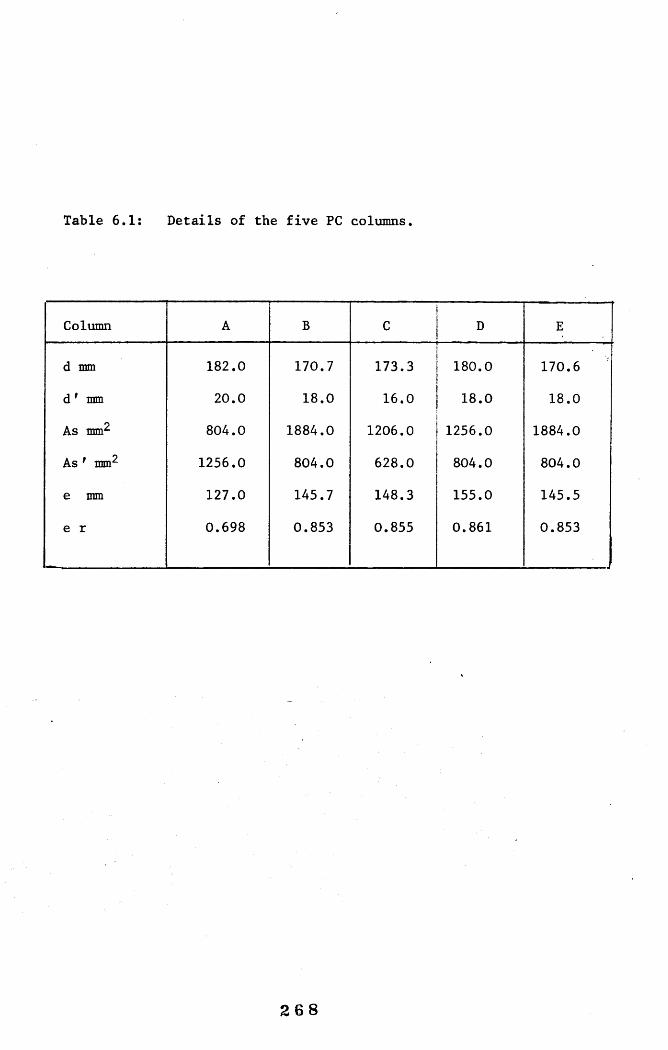
Table 6.1: Details of the five PC columns.

Column A B C D E

d mm 182.0 170.7 173.3 180.0 170.6

d ' mm 20.0 18.0 16.0 18.0 18.0

As mm^ 804.0 1884.0 1206.0 1256.0 1884.0

As ' mm^ 1256.0 804.0 628.0 804.0 804.0

e mm 127.0 145.7 148.3 155.0 145.5

e r 0.698 0.853 0.855 0.861 0.853

2 6 8

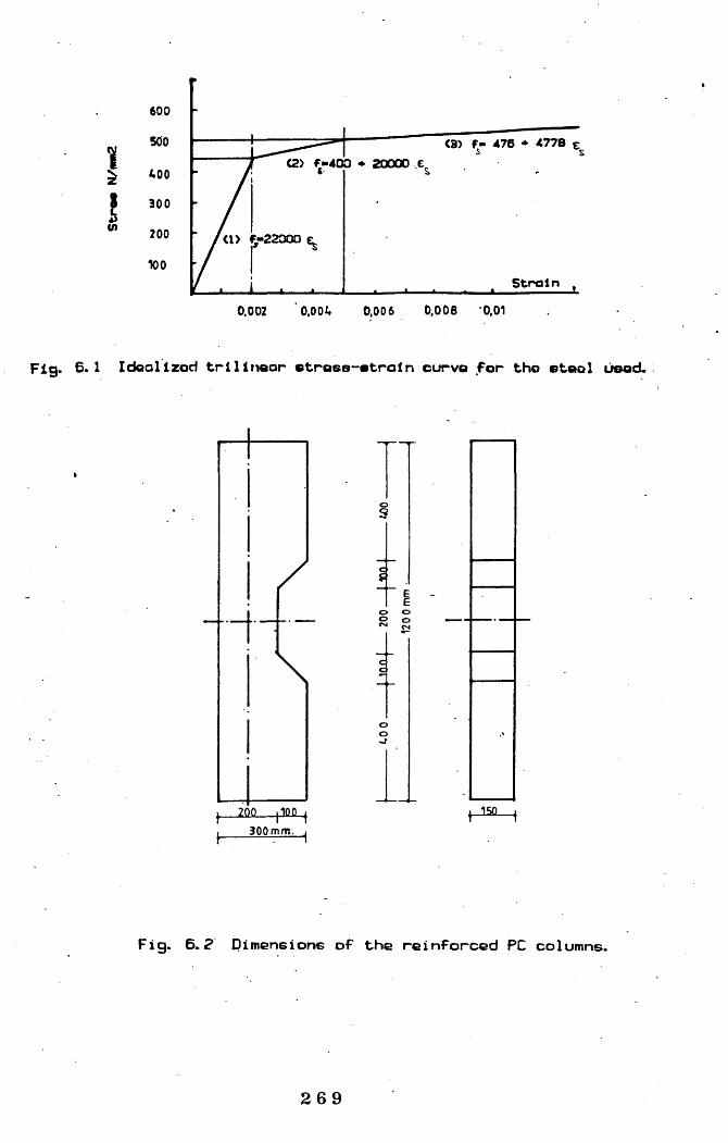
II600

500 (3) f - 476 ♦ 4778 e(2) f -400 * 20000 e

400

300

200100

Strain0,008 0,010.002 0.006

Fig. 6.1 Idoallzod trllinoar otrose-otroin curvo for tho otool wood.

/i

I 200 1100 jI 300 mm. ^

I"IO O8 S

Fig. 6.2 Plmeneione of the reinforced PC columns.

2 6 9

ÜJc5

9 L A *7

L_91A*7

œi53

__ÜA* l osf g ïïi— '--- os^âg •

(0cED0uuû.u01 ü L0 U-c5L01 >

-01r+jL0 U-c01 E (V Ü L 0 U.caLU.0

0VaQ

(dmIL

2 7 0

Moving platen

-Bearing plates

Eccentricity of. machine load

— Bearing plates

Fixed platen

Fig. 6. 4 Testing of reinforced PC col umns.

Three rollers dia. —50 mm

,20» 42 42 , 4225ûmm

1 5 0 m m

Side view

Fig. 6.5 Details of the bearing plates.

2 7 1

, &Two polr# of otroln pougow

on oocS otoal bar '

ill

a) 50 50 jnm

Oütor foco Tost zone

5Pi5Qi5QI

Inner foca

Fig- 6.6 Locations of ©train gauges for measuring strains in PC and ©x^el.

0.0 O.qtc o.qot o.poi o.ope strain

At failure load 2100 KN

1 < Each profile for on Increment in oocnine load of 200 KN except other»lee given)

Column A

Fig. 6.7 Strain profile ot various testing stages for the five reinforced PC column#. (Grade A)

2 7 2

P.O 0404 0406 0,000 s t r a in

At folluTfi lood 1B50 KN

Column B

O.pOf 0,0p0 Strain0.0

At foilunc lood 1750 KN

Column X

O.pOS O.OpO Strain0.q04o.qm04

•At foiluro load 1B50 KN

Column 0

Fig. 6.7 Strain profile ot vorloue testing etoges for the five reinforced PC columns. I Grade B,C R-D 1

27 3

o.qpl O.pOi o.opi strain

At fo i lu re lood 1000 KN

Column E

Fig. 6.7 Strain profile ot vorioue testing stages for the five reinforced PC columns. (Grade E )

- -

111

11 11

111

•*

V I »111

♦ 1 ' 11 "1

] . n1

■f 11liv1

♦ ♦

111

1

' .

JJ11

]1JI1

11

111

1JJ1

• 4 "* T#n#i#n l#y#r.»--— Cnfrini#n Imymr.

♦11

111

11J1

O.AM

a.«K

0.002

0 000

•0.002

-0.004

-O.OOd

-O.OM0.000 0.001 0.002 . 0.003 0.004 0.005 .0.006 0.007 0.006 0.009 •

Conor#!# a ic r o « t r# in .F is .b .8 -A STEEL STRAIN VS. CONCRETE STRAIN FOR RE.C. COLUMN "A ".

27 4

0.006

0.004

0.002

0.000

1 11.1

1 11

.

4 1 â

|I' «

In1

III I 1

|IV *

1 *1

1r

1i1

1

1....11

111

11

+ ...........“ + F ir e t ta n e io n l e y ^ .

4------------• Second te n e io n l ^ é r .

♦ .......... - e Coapreeaion la y e r .

111

-0.002

-0.004

-0.006

-«•“g.000 0.001 0.002 0.003 0.004 0.005 0.006 0.007 0.008 0.009

Concrete nicroetrein.Fig .6 .e -B STEEL STRAIN KS. CONCRETE STRAIN FOR RE.C, COLUMN " B \

♦ +I1

11r

1+ 1 •f 1

1*

' * - - i- - 1 - - - 1

'

L11 "1

f i l l1

1| i v1

1 •11

1

1 -11

1111 ■ 1

11 1

• I " 4 Firet teneion layer.

o.--- -e Second teneion layer.

« .... - Caop-eeeion layer.1

I111

0.006

0.004

0.002

0.000

-0.002

-0.004

-0.006

-0.0080.000 0.001 0.002 0.003 0.004 0.005 0.006 0.007 0.008 0.009

Concrete eicroetrein.F ,g .6 .8 -[ STEEL STRAIN VS. CONCRETE STRAIN FOR RE.C. COLUMN "C".

2 7 5

O.OM

0.004

é

I

i

* 0.000

-0.002

•0.004

-O.OM

— ^ - A

1J1 -

11

1 ^

r1 +1

♦ +11I

1 1 1

1III1

1l i i i1 ! ■ >

"■"T ■ - - - -

11

!

, 1 11 '

1

1

1 . . . . .1

11I

11

f.......1 •1 4------- 1- Tana ion layer,

oapraeeien layer.11.1..........

1111-0.008

0.000 0.001 0.002 0.003 0.004 0.005 0.006 0.007 0.006 0.009

Concret# eicroetrein.F ig . 6.B-D STEEL STRAIN VS. CONCRETE STRAIN FOR RE.C. COLUMN ‘’D " .

_

1

11

111

1. 1

1

' 1i Ï i " 1 * ‘ 1 ' 1Î

1| i i

1

*

‘ r

I

1

11I

11

♦ 1

i111

11

1

11

i •11

•4-----------4 Firet teneion layer.

e------a Second teneion layer.

*— ----. Compreeeicn layer,

*

1..... 111

J

It

0.0M

0.004

0.002

0.000

•0.002

-0.004

-O.OM

) 000 0.001 0.002 r 003 0.004 0.005 O.OM 0.007 0.008 0.009

Concrete eiorostrein.F,g.b.Q-l STEEL STRAIN VS. CONCRETE STRAIN FOR RE.C. COLUMN "E".

2 7 6

240

icIsÈ

210

180

ISO

+ + + + 4 -f- + 4-

4---- k Grede *4*.

120

Concret» micro#tr#in.F , g . 6.9-A COtÿ^RESSION ZONE DEPTH VS. CONCRETE STRAIN FOR ~RE.C. COLUMN "4".

+ ■ - *

4-♦

^ — 4. Grade "8".

240

EcXiI1

210

IN

ISO

120

Concret» eicroetrein.F,g. S.9-B COMPRESSION ZONE DEPTH KS. CONCRETE STRAIN FOR RE.C. COLUMN "d".

2 7 7

MO

SeIii

210

100

ISO

♦ ■( ♦ ♦+ ♦

♦ + ♦ ♦

4-------► Grade 'C '.

130

0.000 0.001 0.002 0.003 0.004 O.OOS 0.006 o.oor o.ooe 0.009

Concret* eicroetrein.F i g . 6.9-C COMPRESSION ZONE DEPTH VS. CONCRETE STRAIN FOR RE.C . COLUMN "C " .

♦+

+4 +

+ + +

4-,---- k Crade *0*.

MO

210cIIi too

ISO

120

0.000 0.001 0.0Q2 0.003 0.004 0.005 0.006 o.oor o.ooe 0.009

Concrete eioroctrein.F i g . 6 . 9 - D COMPRESSION ZONE DEPTH VS. CONCRETE STRAIN FOR RE.C . COLUMN •'D"

2 7 8

M

E

I8i

aio

lao

ISO

♦ ♦ ♦y

♦6- + 4 4

4---y Crad. 'f.

120

0.000 0.001 0.002 0.003 0.004 0.005 0.006 0.007 0.000 0.009

Conorat* a io ro a tra in .f,g.6.9-E COMPRESSION ZONE DEPTH VS. CONCRETE STRAIN FOR R E.C . COLUMN "f".

'

•

a

■

Ll D b c o o o

•

• aa

ana ion iayar.

eapraaaian a ta a l. ■ a

000

400

200

J-200

-400

0.000 0.001 0.002 0.003 0.004 0.005 0.006 0.007 0.000 0.009Conorat* aioroatrain.

Fig. 6.W-A axial STEEL FORCES VS. CONCRETE STRAIN FOR RE.C. COLUMN "X".

279

éOO

400

300

n

0

ï 11 00

0

0

■> ■

“

■ a

0--------« ira t a taa l layar.

laoond a ta a l layar.

.aapraaaion a taa l.a--------- a

-200

-400

-«00

-*000.000 0.001 0.002 0.003 0.004 0.005 0.006 0.007 o.ooe 0.009

Concret# a ic ro e tra in .F/5.6.IO-B AXIAL STEEL FORCES K5. CONCRETE STRAIN FOR RE.C. COLUMN "B".

-

---------g_____ Ç D ° D 0 0a 0

------D —

.• • a

Q-----------e F ira t a taa l layar.

«*■-------- -» Second a taa l layar.

a a Coapraaaion a taa l.

«00

400

200

-200

-400

-«00

-•00

Concret# eioroetram.F/ÿ. 6.10-C AXIAL STEEL FORCES VS. CONCRETE STRAIN FOR RE.C. COLUMN "C".

2 8 0

«00

«00

200

■

D0

0 D D °D

3 D0

#«

BB

■ B •

•naion l#y#r.

o#pre*#ion eteal.

-200

-400

•400

000 0.001 0.002 0.003 0.004 0.005 0.006 0.007 0.006 0.009

Concrete e icroet ra in .F ig .S .W -D A X lA L STEEL FORCES VS. CONCRETE STRAIN FOR RE.C. COLUMN

-

. -

00

0.

0

■ U B S

■

1 ®

-

■> ■

■ ' 1 -. ... -Q--- « F ira t e ta#I layar.

«■---- Second a taa l layar,

B a Coapraaaion a ta a l.

«00

400

200

i-200

•400

000 0.001 0.002 0.003 0.004 0.005 0.006 0.007 0.006 0.009

Concrete mioroetrain.F 15.6 .IO-E AXIAL STEEL FORCES VS. CONCRETE STRAIN FOR RE.C. COLUMN "f".

2 8 1

22002000

ttoo

1400

Sc 1400i 1200

1000

000

400

400

200

. a

• •

•

•

•

•

••

• '

c•

1— .... 1 Concret* ooop. foroo.

# --------- -» Total eoofi. foroa.

♦ ' « Applied eooantrio load.

o •

•

0.000 0.001 0.002 0.003 0.004 0.005 0.006 0.007 0.008 0.009

Conor#:# •icro#tr«in. 'F ig .é ^yA IN T E R N A L t APPLIED FORCES VS. / CONCRETE STRAIN FCOR RE.C . COLUMN"A '

g 1 g

g •

o

• '

• r — -------« Conor#»» eoap. fo re * .

o ------ —» Total eoap. foroa.

« ' ' Applied aooantric load.

2200

2000

1000

1400

5c 1400

I '200 1000

000

400

400

200

0.000 0.001 0.002 0.003 0.004 0.005 0.006 0.007 0.008 0.009

Concret# Bicroetrein.F»5.6.11-B internal i APPLIED FORCES VS. / CONCRETE STRAIN FCOR RE.C. COLUMN"B".

2 8 2

2200

1000

1000

1400

ç 1400

I »w>1000

000

400

400

200

4 *'

••

•

g •

9

'

.

,------------1 Concrete ooap. force.

e----------- e Totel ooep. force.

4------------ f Applied eooentric loed.

•

0.000 0.001 0.002 0.003 0.004 0.005 0.006 0.007 o.ooe 0.009

Concret» e ic ro e tra in .F/5.6.II-C INTERNAL i APPLIED FORCES VS. / CONCRETE STRAIN FGOR RE.C . COLUHN"C

*

0 ®

*

* •

0•

r - ------ » Concrete ooep. force.

e ---------- # Total eoap. force.

♦ 1 Applied eooentric lead.

2200

2000

1000

1400

Sc 1400

J 1200

1000

000

400

400

200

0.000 0.001 0.002 0.003 0.004 0.005 0.006 0.007 o.ooe 0.009

Concrete eicroetrain.FI INTERNAL t APPLIED FORCES VS./ CONCRETE STRAIN FCOR RE.C. COLUMN"D

2 8 3

BOO

MOO

IMO

1400

Sc 1400

I 1200

1000

MO

400

400

200

0

0 •

0 ®

•

.

>

•

Y

t—---------, Conor**# ooap. foroa.

a - a Total ooap. foroa.

•*------------1 Applied eooantrio load.

0.000 0.001 0.002 0.003 0.004 0.005 0.006 0.007 o.ooe 0.009

Concrete e ic r c e t r e in .F ig . INTERNAL i APPLIED FORCES VS. / CONCRETE STRAIN FCOR RE.C. COLUMN"E'‘

•

•

ÙA A

« 6

o

A

O

e

t.

A

A-----------£ Caculatad aoaant.

» - ■« Actual aoaant.A

300

250

200

150

100

50

0.000 0.001 0.002 0.003 0.004 0.005 0.006 0.007 o.ooe 0.009

Ccncrete e ic r c e t r e in .Ftg .b .n -A C A LC U LA T E D g ACTUAL MOMENTS VS. CONCRETE STRAIN FOR RE.C. COLUMN "A ‘

284

J

MO

250

200

ISO

100

so

•

A

AA

A

A

A

A ------------A C a cu la ta d a oa an t.

• ' « A c tu a l aoa an t.A

0.000 0.001 0.002 0.003 0.004 0.005 0.006 0.007 0.009

C o n c re te e i c r o e t r a in .F/5.6.I2-B CALCULATED g ACTUAL MOMENTS VS, CONCRETE STRAIN FOR RE.C. COLUMN " B ’'

a

•

A

A A

aA

A

A

i

A

300

250

200

ISO

100

50

0.000 0.001 0.002 0.003 0.004 0.005 0.006 0.007 o.ooe 0.009

Concrete eicrcetrein.F ig . f> y i< CALCULATED t ACTUAL MOMENTS VS. CONCRETE STRAIN FOR RE.C. COLUMN "C

2 8 5

MO

BO

S- MO

150

A ^

•A

, A

i •

A

I

i

A------------ A CeouUtad eoM nt.

♦ — -* Actual eoaant.A

100

50

0.000 o.oot 0.002 0.003 0.004 0.005 0.006 0.007 o.ooe 0.009

Concrete eicrcetrein.F/5.6.I2-D CALCULATED & ACTUAL MOMENTS VS. CONCRETE STRAIN FOR RE.C . COLUMN "D "

«

* AA

AA

A

A

•

1

A

A-----------A Caculatad aoaant.

»" " « Actual aoaant.

BOO

250

sc 200

150

too

50

0.000 0.001 0.002 0.003 0.004 0.005 0.006 0.007 o.ooe 0.009

Ccncrete eicrcetrein.Fig.tn-l CALCULATED i ACTUAL MOMENTS VS. CONCRETE STRAIN FOR RE.C. COLUMN

286

1.4

1.2»

K

K "K

H

e >

XX

X

•

•

• ••

M------------ K Fo rce» r e t i c ,

a ----------- a Hoeente r e t lo .

o.e

0.4

0.000 0.001 0.002 . 0.003 0.004 0.005 0.006 0.007 o.ooe 0.009

Concret# eicrcetrein.F ,g .6 ^3 -A FORCES S MOMENTS RATIOS VS. CONCRETE STRAIN FÛff RE.C. C O L im "A ‘

X

•

X ■

X

XX X

-

-X

X------------X fo r c e # r e t i o .

----------- a Moeante r a t i o .

1.4

1.2

iJ

0.0

0,6

0.000 0.001 0.002 0.003 0.004 0.005 0.006 0.007 0.008 0.009Concrete eiarœtrein.

F i ^ . 6.13-B FORCES i MOMENTS RATIOS KS. CONCRETE STRAIN FOR RE.C. Cm.UMN

2 87

t.4

1.2

1. K

K Mn

*•

i *X 1jK

m

• • 1 ♦

m--- m hntmm mm »*.

--- —# MHMnM 'Vm II#.J.fi.i

0.6

0.000 0.001 0.002 0.1X0 0.004 0.006 0.00#' 0.007

Conorete eioroetrenn.F,g.6.13-[ FORCES t HOfENTS RATIOS ¥S. C IM X T E S m jM ' FOR flf.C. COLUm

%

M

*

« »

-

■

M

' ♦

M * * ■

M-------------* mmrwêm irmeam.

wmmtom mmiiau

1

1.4

1.2

1.0

0 0

0.6

OuOOO 0.001 0.0C2 0 .0 0 0.004 0 .0 0 0.00 O.OW* iiiarwiMtineiiiia.

Fig. 6/3-BFORŒS Ê HW9M5 mriœ ifS. mmmEm m m m fm a & c a u m v .

2 8 8

t.4

1.2

i

i * X

( X

K

X XX

X

I • * ♦

X X fo rce* re t 10.

« .----------a Hoeente re t lo .

0.0

0.4

0.000 0.001 0.002 0.003 0.004 0.005 0.006 0.007 0.000 0.009

Concrete e ic rc e tre in .Fig.6.13-E FORCES & MOMENTS RATIOS VS. CONCRETE STRAIN FOR R E .C . COLUMN

■

. » •* * *

. e "

, c = " '

» » •

I 0 B » . • •

1 -» X ■I 0 O c 1

a « ® '

0c

' 0

♦

c " " ® " ■ a

. ® '

• : Ô ■

e ® *a ® ,

, o “ °

, o o ° ‘1

. • c 'o

o1

o1

o

o

-

0----------C R' 0.025R Oe 030

R* Oe035

♦----------a R' 0.040 (C r-0 ,e--------- e R' 0.045

R* OeOSO

1

0.46

0.45

0.44

0.43

0.42

0.41

0.400.02 0.04 0.06 o.oe 0.10 0.12 0.14Tenaion-reinfcrceeent retic.

Fig.e. U-A VARIATION IN T COEFFICIENT FOR COLUMN "A\

289

o.«?

0.60

: ...

0.56

0.54

0.52

. • •

1

• •1

1

1

Î

I r 0.025

«----------» r 0.030

#.--------# r 0.035

«----------- r 0.040 Ce^=o,853 )

# ' — # y 0*045

>► ——— # y 0*050

1

0.02 0.04 0.06 o.oe 0.10 0.12 0.14Tenaïon-reinforowent ratio.

F/^.6,U-B VARIATION IN T COEFFICIENT FOR COLUMN "B " .

. * ' ’

-

...ii

1

i82

!

0--- c tt 0.02------ r 0.03#.---# r 0.03

5Q5g (e,= 0.B55)5D

e---e y 0.04—— — # y 0.05

0.40

0.44

s

i •-**

0.42

0.40

0 se0.02 0.04 0.06 o.oe 0.10 0.12 0.14Ten#Ion-rainforcaeant ratio.

F / 5 .6. H - C VARIATION IN T COEFFICIENT FOR COLUMN ‘C".

290

o.ro

0.40

##

#

. • '•

e

e

#

#

e

e

•

» . ......... * r 0.025

I------------- r 0.030

•“■'■ll Br 0*035

_______ . r o . w

e----------« O' 0.045

»■—— —« O' 0.050#

0.44

0.42

0.40.0.02 0.04 0.04 o.oe 0.10 0.12 0.14

T e n # Io n -r# m fo rc m e en t r e t to .Fi^.6.U-D VARIATION IN T COEFFICIENT FOR COLUMN " 0 “ .

••

•

1

#

■•

•

■

•

■

#

e --------- e O' 0.02

-------------» O' 0.03

R' 0.03

5

0

5

5

D

#e----------e O' 0 .04

e — — # O' 0 .C

0.40

0.50

0.54

0.52

0.500.02 0.04 0.04 o.oe 0.10 0.12 0.14

T e n # lo n -r e in fe r e e e e n t r a t i o .fiÿ.6.U-E VAKIATJON i n T C 0£FFIC ICN T FOR C O L ttn

291

O.fS

0.90JI5j »•«

1 D D B 11 D p O 1 D D B 1

* * .

0----------© f t 0.025

0

5

0

5

0

a*""*....—a 0 0.02

R' 0.02

0 o O <1 0 0 o (1 o o b 1f t 0.04

O' 0.05

0.80

0.75

0.700.02 0.04 0. 0.08 0.10 0.12 0.14

Teneion-neinforoeeent ra t io . F lg .6 .^ S -A VARIATION IN COEFFICIENT FDR COLUMN "A " .

0.75

0.70

o o

♦ ♦ ♦

« A * * A

0.60

O O o o o o o o o

0.55

«---------- C f f 0.025

4~-—' ♦ R* 0.030

* . --------- a R- 0.035

a------ -a R- 0.040

a—.-— a O' 0.045

» --------- « f t 0.050

0.500.02 0.04 0.04 o.oe 0.10 0.12 0.14Tansion-rainforcaaent ratio.

F,g.6.15-B VARIATION IN "L" COEFFICIENT FOR COLUMN "B".

292

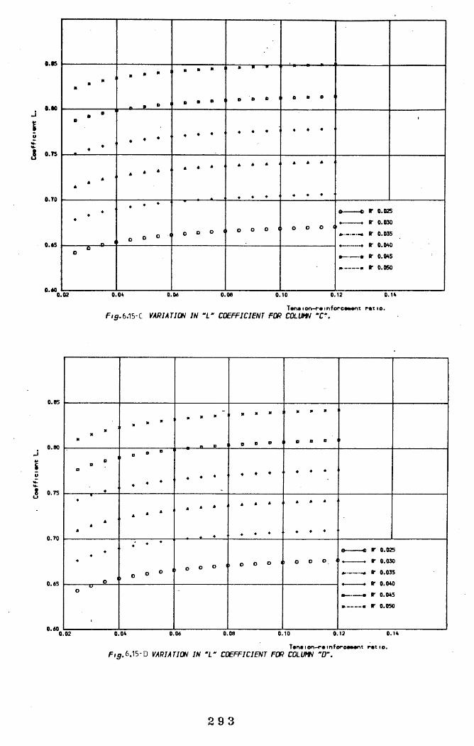
O .K

O.M

a " *

. " "

- a «•

1 ■ • • ' r ~ ■ ' ■ ■

a •a ♦ •

a a *

* * •# a a

a a a ' a a a '

r <

a ♦ *

, 0 0 0 4, 0 0 0 4 1 O 0 0 41 0 0 0 4

O ■■ c r 0.025

a---------- a r 0.030

m— — O' 0.035

a— a O' 0.040

a---------a O' 0.045

ja— — ai O' 0.050

o ^

o.ro

0.65

O.M0.02 0.04 0.06 o.oe 0.10 0.12 0.14

TanaIon-raInforcaeant ra t io .F , p .6,15-C VARIATION IN " L " COEFFICIENT FOR COLUMN *C * .

-

« " "1 ■ ■ "

. = 0

, • ' '

♦

, 0 4» "

a * •a a a

a a a a a a

* ® ‘

a aa a a a a a

O ° '

a' * *

1 O O C . 1 O O ° ', 0 0 0 4 1 O O 0 4

e--------- e O' 0.02

>a------------ r 0.03

a--------- a O' 0.03

5

0

5

0

5

D

oa— — a O' 0.04

la------- # O' 0.05

0.85

0.80-1i

8 0.75

0.70

0.65

0.600.02 0.04 0.06 0.08 0.10 0.12 0.14T an»Ion-rain foroaaant ratio.

F,g.6.15-0 VARIATION IN "L" COEFFICIENT FOR COLUMN "D".

e.T5

o.roJ

I

0.60

0.55

0.50

o o o 0 O ,, o O o II o o o—© R" 0.025

—a r 0.030

•-# r 0.035

- •a ft 0.040

—a tr 0.045

ft 0.050

0.02 0.04 0,06 0.08 0.10 0.12 0.14

T an# I o n - r # i n f o r r a t i o .F 15. 6. I5-E VARIATION IN COEFFICIENT FOR COLUMN "E " .

0 6 0 1 0 0 0 11 0 D 0 11 0 0 0 11 0 0 0 1

* V ‘ '

* a a

0 0 0 4

a a a

0 0 0 4

a a a

1 0 0 0 11 0 0 0 <1 0 0 0 (

0 0 R* 0.025a------------a R- 0.030#“•—— *—# R* 0.035a----------- a R* 0.040a— ------ a R" 0.045#■— — « R* 0.050

0.65

KlkI 0.60

0.55

0.500.02 0.04 0.06 o.oe 0.10 0.12 0.14Tana I on-ra inf oroa*iant ratio.

Fig.tAt-A VARIATION IN THE REDUCED HOfENT FACTOR 1 FOR COLUMN ‘A*.

294

•.00

J0.94

0.»

•.*

o o O O

O O O

D o o

o o O

o----e R- 0.025

R- 0.030

) * . ---------* R' 0.035

♦----------a R" 0.040

a--------- a R' 0.045

»._____, R' 0.050

O.OB 0.04 0.06 0.00 0.10 0.12 0.14

Tanaion-r#infor o— nt r a t io .F ig .e ^ b - B VARIATION IN THE REDUCED MOMENT FACTOR Z FOR COLUMN '

0.75

0.70

0.05

0.00

0.55

0 I' o o I D o o 0 0 0 1

O O o <1 O O o <> O O O <1

0.50.

O V 0.025

» R- 0.030

- — ^ R* 0.035

R 0.040

e R- 0.045

* R" 0.050

0.02 0.04 0.06 0.00 0.10 0.12 0.14Tenaien-remforoaaent r#t lo.

F,g. 6,16 C VARIATION IN THE REDUCED MOMENT FACTOR Z FOR COLUMN "C".

2 9 5

0.T9

0.T0

I -

0.00

0.95

0.90.

O o

D B o

O O O

O B B

a ♦ ♦

o o o

a a a

Il O O O <1o---- — e 17 0.02b

— R' 0.030

m - r 0.035

♦— — # R- 0.040

a-----— a R- 0.045

» — — • R' 0.050

0.02 0.04 0.06 0.00 0.10 0.12 0.14

T#n#ion-r#inforoaaamt r a t io . F ig . 6 ,16-D VARIATIC»^ IN THE REDUCED MOMENT FACTOR Z FOR COLUHt< "D " .

0.05

0.00

0.90 -

0.45 - -

0.40

o B C B B

4 *

O O C O O

a a a a a a

O O O <» O O O O----e R" 0.025

a----------- a R- 0.030

a-----------a R' 0.035

a-----------a fr 0.040

a----------a R- 0.045

«--------- « R- 0.050

0.02 0.04 0.06 o.oe 0.10 0.12 0.14Tanaïon-rainforoaaant ratio.

F,g.6.16-E VARIATION IN THE REDUCED MOMENT FACTOR Z FOR COLUMN "F".

2 9 6

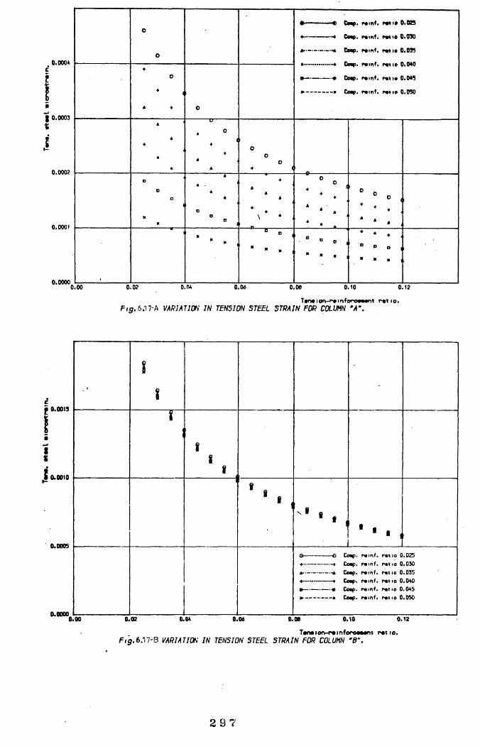
0.0004

I 0.0003

«

0.0002

o

o

a-—- ........... -4 Caap. ra in f . r a t io 0.030

---------- Camp, raim f. r a t io 0.040

a— ------------a Coop, raim f. r a t io 0.0450

* a O

*0

A

>0

60

a 11

00

a : ; '

‘ ‘ o '

’ • . • a ,* * â ,

1

" - - ,-_0 ^

" " X ," ■ » 1

‘ ♦ a .

' " B D 1

■ ■ « 1

0.0001

0.00000.00 0.02 O.M 0.06 o.oe 0.10 0.12

Taneion-reinforoeeant ratio.F,5.6.17-A v a r ia t io n IN TENSION STEEL STRAIN FOR COLUMN 'A " .

-•Î

i-

i

tt

»

V f a■ f 1

• • . I

O------© Coop, ro in f. rot 10 0.025Coop, ro in f. ro t 10 0.030Coop, ro in f. ro tlo 0.035Coop, ro in f. ra t io 0.040Coop, ro in f. ra t io 0.045

» a Coop, ro in f. ra t io 0.050

cI 0.0015

I.{ 0.0010

0.0005

0.00000.00 0.02 0.04 0.06 0.00 0.10 0.12

Tanaion-rainforoaaant ratio.F,g.6M-B VARIATION IN TENSION STEEL STRAIN FOR COLUMN

2 9 ?

0.0015

0010

0.0005

0 0000

- © Coop, - a Coop, —a Coop, —a Coop. " 4 Coop.

r a m f. ra t lo 0.025 ro in f. ro t lo 0.030 ro in f, ro t lo 0.035 ro in f. ro t 10 0.040 ro in f. ra t to 0.045

Coop, ro in f. r a t io 0.050

0.00 0.02 0.04 0.06 0.00 0.10 0 .12

Tana I ort-ra I nforoaaant r a t io .F /p . 6.17-C VARIATION IN TENSION STEEL STRAIN FOR COLUMN 'C * .

cg 0.0015

I%S 0.0010

0.0005

> C Coop, ro in f. r a t io 0.025 ....... a Coop, ro in f. r a t io 0.030•— — — -A Coop, ra in f. r a t io 0.035—---------- a Coop, ro in f. r a t io 0.040I— -------------a Coop. ra m f. r a t io 0.045I-— — — -N Coop. ra m f. r a t io 0.050

0.00000.00 0.02 0.04 0.06 o.oe 0.10 0.12Tan*Ion-raInforoaaant ratio.

Fig. 6.17-0 VARIATION IN TENSION STEEL STRAIN FOR COLUMN •’D".

2 9 8

dg O .W 1 5

IS 0.0010

0.0005

0.0000

Coap. ra in f. r a t io 0.025 Coap. r a in f . r a t io 0.030

Coap. ra in f . r a t io 0.035

Coap. r a in f . r a t io 0.040 Coap. r a in f . r a t io 0.045 Coap. r a in f . r a t io 0.050

0.00 0.02 0.04 0.06 0.00 0.10 0 .12

TanaIon-raInforo— nt r a t io .F/5.6.17-E Va r ia t io n i n t e n s io n s t e e l s t r a in f o r co lum n

c^ .0 0 6 6 5

I%

& . 00660

0.00655■ O Coap. r a in f . r a t io 0.025

Coap. r a in f . r a t io 0.030---------------« Coap. r a m f . ra t 10 0.035--------------- * Coap. r a m f . r a t io 0.040 — a Coap. r a m f . r a t io 0.045---------------■ Coap. r a m f . r a t io 0.050

0.00650.0.00 0.02 0.04 0.06 o.oe 0.10 0.12Tana Ion-raInforoaaant ratio.

F/5 .6.I8 -A VARIATION IN COMPRESSION STEEL STRAIN FOR COLUMN "A".

299

•.OOiB

.00450

JB. 00445

.00440

0.004S

0.00430

0.00425

0.00420.

#

—O Caap. ra in f . r a t io 0.025

♦ Coap. ra m f. ra t io 0.030

- a Coop. ra m f. ra t io 0.035

—* Coap. ra m f. ra t io 0.040

- a ' Coap. ra m f. ra t io 0.045

- a Coap. ra m f. ra t io 0.050

0.00 0.02 0.04 0.06 o.oe 0.10 0.12

Ta n # Io n -ra in fo ro a a a n t r a t io .F»5.6.16-13 VARIATION IN COMPRESSION STEEL STRAIN FOR COLUMN "6".

0.00655

c.0065 0

Ij o . 00645

%

.00640

0.00635

0.00630

0.00625

0.00620

— © Coap. r a m f. ra t io 0.025

— * Coap. ra m f. ra t io 0.030

—A Coap. ra m f. ra t io 0.035

— a Coap. ra m f. ra t io 0.040

—a Coop. ra m f. ra t io 0.045

--B Coap. r a m f. ra t io 0.050

0.00 0.02 0.04 0.06 0.08 0.10 0.12Tarta I on-ra I nforoaaant ratio.

£ i S.6 .1 8-C VARIATION IN COMPReSSION STEEL STRAIN FOR COLUMN * C * .

30 0

0.00495

).00«30

_J0.00425

\&.00620

0.00615

0.00610

0.00605

, 1 . • • '. • • '1

1 ■■

1

1

9

0— ■ --------© Coap. ra m f. ra t io 0.025

....— Coap. ra m f. ra t io 0.030

a— — — a Coap. ra m f. ra t io 0.040

a----------------a Coap. ra m f. ra t io 0.045

a---------------- ■ Coap. ra m f. ra t io 0.050

......0.00600.0.00 0.02 0.04 0.06 0.00 0.10 0.12

Taoaion-rainforo— nt ra t io .F»5.6.18-D v a r ia t io n IN COMPRESSION STEEL STRAIN FOR COLUMN "D ".

0.00675

cÿO. 00670

..0 .00665S

9.00660

0.00655

0.00650

0.00645

0.00640

C -P

C -p

—* Coap

- 4 Coap

ra m f. ra t le 0.025


ra m f. ra t lo 0.035


ra m f. ra t io 0.045

Coap. ra m f. ra t io 0.050

0.00 0.02 0.04 0.06 o.oe 0.10 0.12

Tanalon-raInforoaaant ratlo.F 15.6-.ie-E VARIATION IN COMPRESSION STEEL STRAIN FOR COLUMN "E".

301

1 « a ■ ' II M » <: K « « 1 1 D 0 0 t. !■ "0 “ ;• * a

a

g O B '1 O B D 1 . • • 4 ♦ ♦ ' ♦ 4 •

, ; Î j '

* * o00

o

O-------- O Coap. ra in f. ra t io 0.025

*■---------Coap. ra in f. ra t io 0.030

a-----------a Coap. ra in f. ra t io 0.035

4--------- -* Coap. ra m f. r a t io 0.040

a----------a Coap. ra m f. r a t io 0.045

a-— — a Coap. ra m f. ra t io 0.050

0.00 0.02 0.04 0.06 0.08 0.10 0.12

Tan a io n -ra in fo ro aaan t r a t io .F ig .t. '1 9 -A VARIATION IN COMPRESSION ZONE DEPTH FOR COLUMN "A " .

-

m # • ■ • 1

. • •1 1 ^

88

88 O C Coap. r a m f. r a t i# 0.025

a in f. r a t i# 0.030

• in f. ra t io 0 .0 5

• in t. ra t to 0.040

• in f. ra t io 0.045

a-----------a Coap. r

a— ------ a Caap. r

0.02 0.04 0.06 0.08 0.10 0.12

Tana Ion-raInforoaaant ratio.Fig. 6 . 1 9 - 3 VARIATION IN COMPRESSION ZONE DEPTH FOR COLUMN "B".

3 0 2

us

f UD C

155

150

145

140

135

^ 4 •

g * _. • '

1 *

. « ‘

1 8 i

■

1

1»-■ « Caap. ra m f . ra t 1* 0.025

a m f . ra t le 0.030

a m f . ra t 1* 0.035

D1B

Caap. f

ia— ------ a Caap. r a in f . ra t 1* 0.045

a - - ------ a Caap. ra m f . ra t 10'0 .0 5 0

'

1300.00 0.02 0.04 0.06 0.08 0 .1 0 0.12

T a n * Io n -ra In fo ro a a a n t r a t i o .F,g.6.19-[ VARIATION IN COMPRESSION ZONE DEPTH FOR COLUMN "C.

. 1 '

1 '. . '

1 • •

18

8

8

f

8

» C Coap. r a m f . r a t 10 0.025

• i n f . r a t 10 0.030

o m f . r a t 10 0.035

o in f . r a t 10 0.040

o m f . r a t i o 0.045

m*—— 0 Ctap. r

a —— -a Coap. r

.

165

160

150

145

140

135

130

125

1200.00 0.02 0.04 0.06 0.08 0.10 0.12Tan*Ion-raInforoaaant ratio.

F/5 .6.I9 -D VARIATION IN COMPRESSION ZONE DEPTH FOR COLUMN "D". .

3 0 3

c

I

1

165

160

155

150

145

140

135

130

125

. • •

1 • • • '

. :• • ‘

1I1

%

Î » ------ ♦ Camp, r a in t . r # t i# 0.025

♦ ------ Caap. r a in f . r a t la 0.030

♦ Caap. r a in f . r a t la 0.040

• — — ■a clap, r a in f . r a t la 0.045

a----------a Caap. r a in f . r a t la O.OSO

•

1200.00 0.02 0.04 0.06 O.Ofl 0.10 0.12

T #n# Io n -r#tn forcement r a t io .F,g.6.19-E VARIATION IN COMPRESSION ZONE DEPTH FOR COLUMN

Column A Inner face

Fiq. 6.20 Crock pattern for the five PC columns.(Grade A)

304

Outer face Inner faceColumn B

Outer foce Column C Inner face

Fig. 6.20 Crock pattern for the five PC columns.(Grade B & C)

305

- e

Outer face Inner faceColumn D

Outer face Column E Inner face

Fig. 6.20 Crock pattern for the five PC columns.(Grade D & E)

308

< —

(0c0Lu>01

TJc 00

c c01 E0 D> 0a uj] 01a X

*>rCD ~0c c0 0

CD0 JC

c01q :

0(\i L

01(Ô 4J

0£77 ca *<-•

N X p D o % u w n j o g

307

CHAPTER SEVEN

LONG-TERM MECHANICAL PERFORMANCE

OF POLYMER CONCRETE

7.1.IntroductionTime-dependent d e f o r m a t i o n s play a vital role in the

mechanical performance of any structural material and can lead

to failure if the associated stresses are high enough to

initiate microcracking. These deformations can be either

recoverable viscous or irrecoverable plastic ones. The

nonlinearity observed with most concrete stress-strain curves

is mainly due to microcracking in the interface between paste

and aggregate (96). The initiation of microcracking depends on

the stress level; if this level is high the rate of

deformation will be high and creep may cause time-dependent

failure. On the other hand, linear proportionality between

time-dependent deformations and stress level in terms of the

short-term strength usually ends at the onset of microcracking

(97) & (98). This implies that failure will take place with

time if the applied stresses can produce microcracking.

Concrete under sustained stresses fails at à lower stress than

the short term strength measured by conventional tests. This

led to the early conclusion (99) that failure occurs at a

limiting strain rather than a limiting strength and regardless

of whether this strain is reached by a rapidly applied high

stress or a lower sustained stress. The limiting strain takes

place at a 'limiting' stress/strength ratio, often termed the

"plastic limit" (100), which can have a value of 0.25 up to

0.85 or more depending on the material itself. Time-dependent

308

failure can not take place below the "plastic limit". Time-

dependent deformations will take place in any case of loading.

The relative values of these deformations are high for cases

of sustained load, smaller for cases of load increasing at a

small rate and even smaller for loads applied at high rates.

A different cause of time-dependent deformations in concrete

is the process of hardening on setting. Differential shrinkage

strains can sometimes be big enough to induce significant

internal stresses. These induced stresses can cause setting

and shrinkage cracking with the result of seriously limiting

the structural use of PC.

Conventional cement concretes undergo creep and shrinkage

deformations essentially due to the relative moisture movement

required for hygral equilibrium of the cement paste. Many

hypotheses on a phenomenological basis were suggested for

describing the mechanism of creep and shrinkage of PCC (101).

A theory of visco-elastic flow (102) & (103) was produced on

the basic assumption that the hydrated cement paste is a

highly viscous liquid. The viscosity of this liquid increases

with time as a result of chemical changes within the paste

structure. In this theory, cem e n t i t i o u s m a t e r i a l s are

considered to behave in a viscous manner when loaded. The

inert aggregates do not flow and in resisting the paste

movement they are increasingly stressed with time. If this

were the case, creep would progressively reduce with time. In

addition, a viscous flow by definition requires a constant

volume and a Poisson's ratio of 0.5, a case which can not

exist in concretes. For these reasons and others, the theory

of visco-elastic flow was not widely accepted.

309

The solid solution theory (103) was based on the assumption

that vapour pressure of water in a gel is affected by the

applied stress, with the result that the water content of the

gel and its volume are altered. However, other studies (102)

showed that cement gel in particular shows a remarkable

structural stability against external loads to the extent that

the solid solution approach can not be reliable.

Probably the most generally accepted theory in this respect is

the seepage theory, first postulated bu Lynam in 1934 (104).

In this, creep of concrete is taken to be due to seepage of

the gel water ( dispersion media ) under pressure through the

elastic skelton of the paste ( dispersed phase ). This

expulsion or viscous flow causes stress redistribution from

the viscous component to the elastic skelton. On removing the

load such a system will undergo a partial immediate elastic

recovery followed by a slow time-dependent recovery often

termed as elastic after-effect. In this way creep can be

considered to be analogous with shrinkage, but the motive

force is an externally applied pressure instead of a direct

internal vapour pressure.

Polymer concretes suffer shrinkage and creep to a greater

extent than cement concretes. The explanation for these time-

dependent deformations in PC is completely different from that

of PCC. The cement paste with its combined and free water ,

cement gel, hydrates and capillary pores are just a few

features that do not exist in PC. On the microstructural

level, cement hydrates are gels with particles attracted

electrostatically at van der Waals* distances, whereas PChas

3 10

amorphous molecules distributed at covalent distances. The exact nature of creep and other deformation sources in polymers are not within the scope of this work. However, deformations resulting in PC either due to external or internal stresses are give below.

7.2. Deformations of PC

Deformations of PC can be classified into two general types; load induced deformations and self induced deformations. Both of these are dependent on time. The self induced deformations are mainly related to the physio-chemical properties of PC. They can be either shrinkage or expansion deformations. Shrinkage occurs during the polymerization process. In this two main phenomena can induce shrinkage deformations as

follows :

(1) Temperature gradient : The polymerization processunsaturated polyester ( IIP ) is a highly exothermic process ( some 60 Cal/g in 2 hours ). In the early reaction stages, heat evolution is usually greater than heat dissipation with the result that a peak mix temperature usually exists. This peak temperature can be as high as 20 above the ambient

temperature depending on resin formulation and degree of filling, etc. After the peak temperature is reached, PC cools and the lowered temperature causes thermal v o l u m e t r i c shrinkage of as much as 5-8% for the pure resin. The process of thermal shrinkage increases rapidly after the peak temperature is reached and then attenuates slowly for as long time as completion of polymerization might take. This type of

shrinkage will decrease as the filler or the dispersed phase

3 i 1

content in the mix increases. Obviously the shrinkage will be

very small after these filler particles come into contact.

Internal tensile stresses will begin to be induced at the

moment when shrinkage starts and can only take place after

gelation which occurs at the peak exotherm. As the modulus of

elasticity at this stage is very small, the induced tensile

stresses will also be very small. On further hardening, the

modulus of elasticity increases and the shrinkage strains

become measurable. In some cases, the induced stresses can

exceed the tensile strength and cause setting cracking in PC.

However, all studies in this context show that the rate of

tensile strength development increases rapidly after gelation

and the induced stresses at any time are too small to initiate

shrinkage cracks. The only possible case of cracking resulting

from thermal shrinkage can exist if PC is heavily restrained

and can be controlled by casting and curing in a temperature-

controlled environment.

The thermal volumetric changes of neat UP resin can be very

high as it has a coefficient of thermal expansion of 6-11x10”

/C.° With PC this coefficient is around 1 x 10"^/C° This large

decrease is caused by the presence of fillers and aggregates

used when making PC and the thermal capacity of the system is

said to be enhanced or increased. The enhanced thermal

capacity will reduce the magnitudes of the resulting tensile

stresses in the binder, the compressive stresses in the

aggregates and the interfacial shear stresses. It follows that

a well-graded and compacted aggregates bound together with the

thinnest possible resin layer ( smallest resin content

3 1 2

possible ) will virtually suffer no more thermal volumetric

changes than those encountered with PCC.

(2) Chemical shrinkage : The p o l y m e r i z a t i o n process is

essentially a process in which individual molecules are caused

to be covalently bonded into macromolecules and contraction is

induced in the system as a whole. Growth in viscosity is

mainly caused by the formation of these macromolecules in the

form of long chains. The process of crosslinking these linear

chains results in a further chemical contraction.

While thermal volumetric changes can be controlled by resin

formulation, mix ratio of PC or controlling the ambient

temperature, the chemical reaction can not be controlled by

using similar external effects. To avoid chemical contraction

several physio-chemical methods have been tried (105). The

' Pore-method’ is the most traditional one and has been in use

in plastic technology for a long time. A few research trials

making use of this method with PC have been carried out (106)

& (107). In this method, special foaming agents are used to

produce gas which provides a cellular structure in the

material and compensates for the chemical contraction. The

main disadvantage is the resulting high porosity of the

material and the consequent inferior mechanical performance.

More recently it became possible to control the free volume of

monomers and polymers by special macromolecule alignment

techniques (108) through forming controlled microstructures in

the resin binder. Expansion in the resin volume during curing

can be obtained by using polyring monomers which help produce

ring opening polymerization (109). The main disadvantage of

3 13

this method is that it requires the synthesis of highly

complicated c h e m i c a l s which can provide such special

potential. Other methods have been developed and used such as

'low-profile method' by Ohama (110) or 'geometrical active-

microfiller method' by Czarnecki (105). These methods in

general should counteract the chemical contraction and even

the thermal shrinkage. There is the possibility that some of

these methods could produce an overall expansion in resin

concretes made with UP resin and 'expansive P C could be

manufactured (105).

Load-induced deformations can exist after PC has reached its

initial set at gelation. When hardened, PC can be regarded as

a dispersed phase of inert aggregate in a continuous phase of

polymer matrix. This implies that PC can not readily be

treated as a homogeneous material for which traditional

methods of caculating deformations can be used. Polymer

concrete with its amorphous polymerized monomers and unreacted

monomers, microfillers, sand and aggregates, composite voids

and base-matrix pores is heterogeneous at virtually any

observation l e v e l ; w h e n steel is pre,sent it b e c o m e s

anisotropic as well.

While the theoretical study of molecular or atomic behaviour

can provide explanations for deformation, it only applies to

materials which are homomgeneous and isotropic. Hence the most

practical way of assessing the deformations of PC can only be

on a empirical basis. In this, the rheological properties can

be approximated to certain physical models whose constants can

be derived from associated e x p e r i m e n t a l stress-strain

314

relationships. This approach has attracted the majority of the

very few studies carried out in this field.

In the rheological sense, PC can exhibit elasticity or visco

elasticity. This will primarily depend on the rate of load

application and its duration. PC behaves elastically at very

high rates of load application or at very small durations of

load. Deviation from this linear stress-strain relationship is

incurred by interfacial bond microcracking at high levels of

stress, which is related to PC heterogeneity rather than

energy dissipation. However, Davydov (111) reported that PC

has hysteresis which causes this deviation particularly at

prolonged load durations. That is to say that the rate of

energy dissipation increases with increase in load duration

whereas the restored strain energy decreases. It follows that

nonlinearity of the stress-strain curve is not fully dependent

on the initiation of bond microcracking but probably to a

greater extent on rate of loading or its duration ( the

relative relation between the external potential load energy

and the internal thermal energy ). Experimental observations

(111) suport the view that PC possesses viscoelasticity. All

stress-strain curves show recoverable time-dependent strains.

The proportionality between stress and rate of strain is

satisfied at any stress level before microcracking. On being

stressed, PC develops a certain amount of irrecoverable time-

dependent deformation. The ratio of this irrecoverable

deformation to the instantaneous recoverable and time-

dependent deformation is not constant. It varies considerably

depending on the applied stress level and the rate at which it

is applied. Temperature can have another major effect on the

315

response of PC to stresses. These combined effects make it

difficult to represent PC rheologically on a clear basis.

7.3. Shrinkage strains and resulting stresses of PC

Polymer concretes usually undergo shrinkage strains at early

ages. This proceeds at a high rate in the first phase after

gelation sets in; thereafter the rate decreases considerably

and almost reaches zero after polymerization and thermal

balance is attained. Shrinkage induces tensile stresses in the

polymer phase and compressive stresses in the aggregate and in

the steel if the PC is reinforced. The resulting tensile

stresses can in some cases be high enough to initiate tension

cracking especially in heavily reinforced members. The

shrinkage stresses are i n t r i n s i c a l l y dependent on the

polymerization rate, that is the slower the polymerization the

more favourable the state of the induced stresses due to

shrinkage. In addition other factors can interfere in

shrinkage such as the binder ratio, the degree of aggregate

compaction, the resin type and its viscosity .

A.Watanabe (112) carried out a study on the stresses in plain

PC resulting from setting shrinkage. In that study most

shrinkage strains of polyester resin concrete took place in

the first ten hours and no increase in this shrinkage could be

traced after PC had reached 24-hrs of age. The shrinkage

strains (e^ ) at any time (t) could be expressed as a

hyperbolic function of time as follows :

c^=(t-A)/[B+C(t-A)] in which A, B and C are constants.

Theoretical estimation of the tensile stresses in PC could be

3 16

derived on the b a s i s that Hook's law is v a l i d for

infinitesimally small periods of time. By integrating the

stress components corresponding to very small time values ,

Watanabe could express theoretically the total value of the

induced tensile stress f w i t h i n any given time period t = t2~ t^•as follows :

- i2 - ilt-t

^ . E A E \in w h i c h „ _ s s ctt ” E A +A^E^

Eg , Eg : steel ancf fc moduli of elasticity and,

Ag , Ag: steel and PC cross-sectional areas.

Based on experimental measurements E^ at any time t could be

expressed as a single function of time for a given PC type ; in

this way the coefficient could be expressed for any given

reinforced PC section. As creep would have some effect on the

resulting tensile stresses, corrections due to creep recession

were introduced and rather lengthy equations were obtained.

Both theoretical and experimental measurements showed that

tensile stresses resulting from shrinkage increase very

rapidly at the early stages. This increase then attenuates and

eventually reaches a more or less constant value. The

noteworthy observation of that study is that the tensile

stresses in PC members having 4% reinforcement amounted to

2.0-2.5 N/mm 2 at associated tensile strengths of 7.0-8.0

N/mm 2. This implies that although tensile stresses can

develop rapidly they will be smaller than the corresponding

values of the tensile strength attained. As with PCC, the

induced tensile stresses in PC are inversely proportional to

the reinforcement ratio. However, Watanabe (112) observed

3 17

experimentally that the resulting stresses in PC decreased

when the reinforcement ratio had exceeded a certain value;

this value is reported to be 5%. It is also reported that half

of the final shrinkage strain takes place while PC is still in

a liquid state and when no shrinkage stresses can be induced.

In another relevant study carried out by W.koyanagi (113), the

experimentally measured strains in PC and reinforcement steel

increased rapidly, after the peak exothermic temperature was

reached, for about ten hours after which time the increase

became very small. Strains in either steel or PC decreased by

increasing the reinforcement ratio as shown in Fig.(7.1). In

Koyanagi's work it was found that there is a definite time lag

between the occurence of strain in PC and in the steel. This

is because strains occurring in PC while still in a liquid

state can not produce strains in the steel. It followed that

induced stresses can not be explained merely by the total

recorded strains in PC based on an elastic analysis; thus

inelastic deformations were taken into account.

In this work Koyanagi adopted a rheoIogicaL model similar to

that of Burgers (Kelvin and Maxwill elements in series), see

Fig.(7.2). As the deformation equation of this model is a

second order differential, some assumptions were made for

simplifying the solution. By equating the theoretical

deformations of the m o d e l 6a, 6b and 6c to s i m i l a r

experimentally-recorded deformations, see Fig. (7.3), the

constants of the dashpots and springs could be calculated.

Their values as plotted against time for PC are shown in

Fig.(7.4). In this figure relaxation time Tp%( time required

3 18

for the internal stress to relax ) increases rapidly with

time, whereas retardation time time required for the

strains to be recovered ) is almost constant.

Based on these observations, Koyanagi suggested that PC

transforms from a viscous liquid to a viscoelastic solid in

the course of time. On calculating the induced tensile

stresses using the suggested rheological model, it was found

that the stress increases with increased reinforcement ratio

as shown in Fig. (7.5).

7.4. Creep behaviour of fC

Despite the importance of long term deformations in the

structural behaviour of PC, very little work has been carried

out on the creep properties and the consequent effects of

sustained load. Furthermore, even less i n f o r m a t i o n is

available regarding the effects of different rates of stress

and/or strains on the short term properties of PC.

One of the earliest studies concerned with the creep behaviour

of PC was that of T.Broniewski (114), who found deviation from

the linear s t r e s s - s t r a i n relationship as recorded in

conventional tests began at almost one third of the ultimate

strength of PC. That deviation in addition to the high

ultimate strains was reported to be mainly due to the highly

viscoelastic nature of the polymer matrix. On conducting a few

direct tensile creep tests Broniewski found that creep-time

relationships can be expressed using the following equation of

Macleod (115);

Oj. = ei(t/B)M in which and e^ are creep and initial

3 19

strain, while B and m are constants. This equation is

presented in Fig.(7.6). It is suggested that with viscoelastic

materials it is quite sufficient to use a few experimental

measurements at the first 100 hours for the derivation of the

constants. This is mainly because the material response tends

to stabilize in the course of time. In this simple equation,

the effect of age at loading is pronounced in the value of e^,

while the effect of the stress level is pronounced in the

constants B and m.

This equation can be rewritten as t = B. (e^/ej^)^ For a

given PC grade, a limiting failure strain e^ exists and this

equation can be used to predict the time required for PC to

reach this limiting strain under a particular stress level.

Partial factors of safety can be introduced to the value of e^

to give the life time of a member under given load conditions

so that no more than, for instance, 50% of e^ should develop.

Other studies of PC creep carried out by K.Okada (28) , showed

that creep is proportional to stress level and that it is

greatly influenced by temperature. As shown in Fig.(7.7),

elevated temperature can induce excessively high creep strains

due to the strong thermo-dependency of all the mechanical

properties of PC.

Obviously, this dependency is a function of the resin type and

the mix proportions. High values of the resin and/or small

values of aggregate contents in the mix would allow for higher

values of creep; fig.(7.8) shows the effect of these two

factors on creep. In this figure, mix M made with high resin

content ( 15% by wt.), high filler and high sand contents gave

3 2 0

much higher creep values than mix R which is made of low resin

content and high coarse aggregate contents (10% and 40%

respectively).

In another study made by T.Yamasaki (112), the creep

coefficient in terms of the true creep relative to the

instantaneous strain increased with increase in load duration.

The creep coefficient approached a horizontal assymptote after

72 hours of loading. The magnitude of the assymptote of the

creep coefficient was found to increase with increased age at

loading. However this increase was at a decreasing rate and at

ages more than 24 hours a decrease in the creep coefficient

was observed.

Yamasaki (112) studied the proportionality between creep and

the associated stress level. It was found that the maximum

stress/strength ratio that would not produce time related

failure was below 57%. At this ratio time induced failure

occurred after 43 hours. For stress levels of 60% and 70%

failure took place after only 1.5 and 3.0 hours respectively.

The relationship between creep and stress/ strength ratio

based on the experimental observations was not linear at any

stage as shown in Fig.(7.9). This behaviour has been confirmed

by other relevant studies in the United States (116). This is

unlike the case with cement concretes and mortars, which can

exhibit linear creep-stress ratio relationships of up to 0.5

and 0.8 stress/ strength ratios respectively.

In a study made by M.Helal (116), further disimilarity

between PC and PCC responses to sustained load was found. It

is usually assumed that a final creep strain (ultimate creep)

321

will be reached in any member under loads. Ultimate creep can

be reached in PCC after almost 20 years. With PC Helal found

that this ultimate value can be reached within only one year.

While with PCC 50% and 75% of ultimate creep can take place

approximately after three months and after one year, they are

reached w i t h PC after o n l y one w e e k and six w e e k s

respectively. In his experimental work, Helal found that the

stress level that can cause time-related failure is 50%; this

value is very comparable to the value obtained by Yamasaki

(112). It is worth mentioning that the sustained strength for

PCC as reported by Neville may vary from 0.7 to 0.9 of the

short term strength (117). This implies that PC strength is

usually more affected by sustained load than that of PCC.

7.5. Experimental study of time-dependent properties Mi fC

In the present work, time-dependent properties of PC were

investigated using two main approaches. The first of which was

to investigate the effect of different rates of strain on the

ultimate compressive strength, modulus of elasticity and

values of strain at failure. The second approach was to study

the effect of the duration of a constant load (creep response)

on the resulting strains and the associated sustained

strengths.

The fundamental aim is to arrive at a clear interpretation of

the time-dependency of PC on which basis reliable partial

factors of safety can be drawn up. It should be clear that a

general assessment of such dependency would require greater

study of the phenomenological and theoretical levels than that

undertaken in the present work. However what is aimed at here

is an experimental evaluation of those t i m e - d e p e n d e n t

3 22

properties of PC which might provide, along with the results

of other relevant studies, a starting step towards the

production of a practical code of PC structural design.

7.5.A I M effect of rale o£ strain on the properties M fC

7.5.A .i ^^me structural i m plications The effect of rate of

strain is essentially related to the load duration and creep

effects which will tend to increase with decrease in the rate

of strain or with increased load duration. A chosen rate of

strain is usually more accurately attainable in compression

tests than rate of stress. A d j u s t m e n t of the testing

instrumentation to maintain a constant rate of stress over

the whole testing period is difficult. Near its ultimate

strength PC, like PCC, would develop extremely high rates of

deformation. This would necessarily give misleading results

even if the testing machine could still provide such a

constant rate of stress. In addition the stress-strain curve

recorded under constant rate of stress can only be traced up

to the ultimate strength, after which no load increase can

exist. Any falling branch of the curve would be lost. This

falling part can be of fundamental importance for certain

applications in assessing the load-carrying capacity of PC

near and after its ultimate strength is reached. For these

reasons it was decided to carry out the series of axial

compression tests using different but constant rates of strain

rather than stress.

For a given PCC, increasing the load duration leads to a

reduction in the strength and to an increase in deformations.

This phenomenon as said earlier is due to the effects of creep

323

and shrinkage of PCC. The same should apply to PC with the

reservation that in PC the effects of creep are more evident

and those of shrinkage are less dominant than in PCC. In fact

shrinkage of PC becomes of very little significance after one

to three days of age, depending on the type of PC. This fact

has dictated the study of PC creep rather than its shrinkage

as will be shown later.

As different rates of loading affect d e f o r m a t i o n s and

strengths, these rates would also affect all the stress-block

parameters in flexure which already have been derived. The

short-term findings of stress-block shape and parameters at

ultimate capacity might therefor require some modifications.

These modifications will primarily depend on the nature of the

load, whether it is increasing or constant, and on the values

of the applied rates of loading or load duration. Consequently

the stress-strain curve for a given PC grade can never be

given one fixed shape and should differ from one case of

loading to another.

In the compression zone of any PC flexural member, strains can

be fairly asssumed to be linear. It follows that each fibre

will be strained at a different rate from the others and this

rate will be proportional to distance from the neutral axis.

Based on this assumption, Rusch (93) could derive a stress-

strain curve for PCC in flexure from axially tested prisms at

different rates of loading. He also suggested a procedure from

which various s t r e s s-strain relationships, attained at

different loading durations, can be derived.

Out of this procedure it can be said that s t r ess-block

324

parameters whet h e r for PCC or PC, will vary for a given

concrete depending on the strain chosen to be reached within a

prescribed period of time. Fig.(7.11) shows schematically how

Rusch could derive the flexural stress-strain curve from the

axial compression stress-strain curve carried out at different

rates of loading. This derivation was based on reasonably

accurate assumptions the most important of which is that for

each rate of strain in various fibres across the compression

zone, there will appear the same stresses as in the

corresponding fibres of axially loaded prisms at similar rates

of strain. In this the effect of a nisotropy and strain

gradient were not considered.

7.5.A.ii Description of the experimental work

The experimental study of the effect of the different loading

rates on the stress-block shape and parameters was carried out

for each of the five PC grades. The axially loaded specimens

in compression were tested at various constant rates of

strain. These rates were made to cover as wide a range as the

available testing machine would practically allow. The fastest

and the slowest rates that the machine could provide and which

are of significance were chosen to be 2.9x10"? and 415x10“?^ second. These chosen rates required loading times in the range

from 2 minutes to around 20 hours. Between the fastest and the

slowest rates six additional rates were determined as given in

table (7.1).

The specimens were cylinders of 100 mm-diameter and 200 mm-

length. For each grade and each rate of strain, two cylinders

were tested. The sixteen cylinders tested for each grade were

325

cast altogether using one batch and vibrated on a vibrating

table. Curing was the same as that carried out with all

previous specimens.

The testing machine is "LOS-SYSTEM UPS.2000". This machine

can be adjusted to the required rate of platen movement with

the result of producing a constant rate of deformation in the

test specimen throughout the whole test.

To overcome any ill effects of uneven end surfaces, all

specimens were finely ground at both ends before testing. No

capping or packing could be made where it could have affected

the readings of the deformations. Having done so, the relative

displacement of the two stiff and non-rotating platens of the

machine could be taken as the d e f o r m a t i o n in the test

specimen. This indirect method of measuring the deformations

should remain correct as long as the specimen is in complete

contact with the top moving platen; a condition which was

persistently satisfied throughout the test. Fig.(7.12) shows

how the displacements of the cylinders were measured and

recorded. The displacement was recorded using a transducer.

The machine load and the displacement were continuously

recorded using a plotter connected to the machine control

console. In addition these values of load and displacement

were printed out at intervals using a Data Logger connected to

the machine as a second output of the test results. The

machine has a safety-1imit operational system which made it

possible that continuous testing of up to about 20 hours be

carried out unattended. This safety system can stop the load

increase after a predetermined displacement value is reached

3 2 3

or can stop the displacement increase if a given load is

reached.

7,5,A , H i Test results and their interpretation

The curves of load-displacement as given by the plotter were

checked against the output of the Data Logger, then reproduced

as stress-strain relationships. For each rate, the average

curve of two specimens was found and considered in further

analysis. Fi gs. (7.1 3-a, b , c , d&e ) show these curves for the

eight chosen testing rates for the five prospective grades. A

major reservation on these curves is that the two specimens

tested for each rate of strain did not always prove sufficient

for drawing up a general stress-strain curve for that rate.

While consistency of the results and their invariability was

acceptable for good-workability grades (grade E for instance),

poor workability grades like D and C suffered divergence in

the results for each of two cylinders tested at the same rate.

As shown in Figs(7.13), all PC grades seem to follow a similar

trend in their response to various rates of strains as that of

PCC. Irrespective of PC grade, faster rates of strain gave

higher ultimate strengths, smaller strains at failure and

quicker failure immediately after the ultimate load was

reached. Slower rates were associated with smaller ultimate

loads, higher strains and greater retained carrying capacities

after macrocracking.

The relative retained carrying capacity C^ at any time after

the ultimate load is reached, is defined here as the ratio of

the retained machine load at that time to the ultimate load.

With high rates of strain the drop in C^ was very large and

3 2 7

took place within a few minutes after the ultimate load was

reached. For example, with grade D at rates [1] and [2] the

reduction in Cp was 100% and 95% respectively after only two

minutes. On the other hand, with small rates of strains like

rate [8] for instance, Cp calculated for grade E and B had

values 60% and 40% respectively, 8 hours after the ultimate

load was reached. Quite a few of the specimens tested at rate

[8] retained considerable Cp-values and the machine load could

be maintained for as long as 16 hours beyond the ultimate load

with strain values of as much as 0.015, especially with lower

stiffness grades.

The linearity of the stress-strain curves obtained are more

evident with fast rates. For each grade, the features of the

stress-strain curves obtained at rate [1] are comparable to

those of the short term tests carried out previously at a

constant rate of stress (see chapter 3). This applied only up

to the ultimate load after which the falling branch of the

curve in short term tests could not usually be traced.

The stress-strain curves corresponding to rates [1] and [8]

for each grade are shown in Fig.(7.13). These two curves

represent the boundaries for all possible stress-strain curves

carried out at a rate of strain ranging from 2.9x10"7/sec to

415x1o"?/sec. Within these two boundary curves, the ultimate

strength decreased by almost 16% to 22% depending on PC grade.

On the other hand, the axial strains occurring at ultimate

load increased by almost 6% to 14%.

The stiffness of the various grades increased with increased

rate of strain. For the five PC grades tested , grade E had

328

the lowest modulus of elasticity while grade C had the highest

one. The initiation of microcracking is indicated by the

beginning of nonlinearity of the stress-strain curve, whereas

macrocracking is made manifest by the test load starting to

decrease. Both micro and m a c r o c r a c k i n g as defined here,

required more loading time at small rates of strain. In

addition the small rates produced cracking at smaller stress

levels than with high rates of loading.

To clarify these effects, F i g s . ( 7 .1 4 - a , b , c , d&e ) were

constructed. In these figures, the time required for each PC

grade to develop its macrocracking (t^) is plotted against the

stress level ( relative to strength at rate [1]). It is clear

from these figures that the strength of PC is strongly

dependent on rate of loading or load duration. In the same

figures. Figs.(7.14), the axial macrocracking strain ^cm is

plotted against tm. The two relationships of stress level and

strains with macrocracking time as given in Figs.(7.14), tend

to reach stabilized values. Time-dependency is shown mostly

in the first two hours of loading, after which neither a

significant increase in the axial strain nor a decrease in the

strength would occur.

As said earlier, time-dependent deformations are present in

all cases of loadings and their magnitude for a given stress

level are increased by prolonging the loading times. If the

strength recorded with rate [1] is to be taken as the short

term strength, point 1 on curve a, then all other points on

this stress level-time curve would represent cases of long

term or time-dependent failure. The smallest stress level

which caused such time-related failure according to a- curves

3 2 9

varied from 77% to 84% for different grades, and on average

was about 80%.

On the other hand the largest macrocracking strain relative to

macrocracking strain for short-term loading was on average

110%. This increase in the strain energy of a given PC grade

by increasing the loading time can be useful in the structural

applications of PC. Higher strains at failure would allow the

initiation and formation of wider warning cracks and can

provide more use of the reinforcement steel at failure. The

retained carrying capacity as defined before is higher for

longer periods and can therefor offer a greater safety margin

in structures at failure.

At this stage it should be noticed that if a cylinder is

subjected to a gradually increasing load at a constant rate of

strain, t h e r e w i l l e x i s t a d e f i n i t e s t r e s s l e vel

corresponding to a particular rate of strain or certain

loading time below which no failure would take place. This

stress is termed here as the long-term strength f^i* All the

given curves of Figs.(7.14) show that for each PC grade there

can exist two horizontal a s s y m p t o t e s for the axial

macrocracking strain ratio ^cmr and for the stress level fp.

By extrapolating each of these curves the ultimate values of

%mr and fp could be obtained and used in deriving the long

term strength and macrocracking strain ml for each grade.

For example, with grade E the extrapolated assymptote values

^cmr and fp, at 10 hours loading, were 105.5% and 83%

respectively. As the short term values of the strength and the

macrocracking strain (rate [1]) are 0.0078 and 95 N/mm2, it

3 3 0

follows that the respective long-term values are 0.00823 and

79 N/mm2. To attain a strain value of 0.00823 within 10 hours

the required rate of strain would be 1.4x10~^/min. This

implies that for rates of strains smaller than 1.4x1o“^/min.,

or for constantly increasing loads with duration not less than

10 hours only a stress equal to or more than 79 N/mm2 will

cause failure. This value is the long-term strength for grade

E. By similar derivations, the long-term strengths for grades

A, B, C and D were found to be 78, 73, 70 and 75 N/mm2.

The variation in the ultimate strength versus different rates

of strain are shown in Figs. (7.1 5-a , b, c , d &e). This variation

could be expressed using the following equation :

p.rV (7.1)

in which . is the ultimate strength in N/mm2 at a given rate

of strain r in ( 1/min. )x 10^. To obtain the constants p and v

for each grade, Eq.(7.1) was plotted logarithmically as shown

in Figs. (7.16-a, b, c , d &e). The intersection of the line with

the ordinate (log f) gives the value of log p, while the slope

of the line gives the value of the constant v. The values of

these constants for each grade are shown in Figs.(7.16). In

these figures the highest rate of strain was fixed for the

five grades at a value of 0.0025/min., whereas the lowest rate

was that corresponding to the long-term strength of each grade

previously derived. Using Eq.(7.1) the ultimate strength at

any rate of strain can be calculated. It should be noticed

that this equation is valid only within the boundaries set,

i.e., within the highest and the lowest rates of strains given

for each grade.

3 3 1

As given before in Figs.(7.13), the stiffness of PC dropped

considerably with decreased rates of strain or increased load

durations. This decrease in stiffness and linearity of PC

stress-strain curves might be attributed to the effect of

hysteresis of the material itself. Prolonging load duration

allows for an increase in the rate of energy dissipation

through losses in internal thermal energy, a case which does

not exist in fast loading rates. These losses are reflected

through a decrease in the strain energy restored ( the

instantaneous and time-dependent recoverable strain), and this

would lead to an increase in the plastic flow and result in

reducing the modulus of elasticity and the microcracking

stress level (the onset of nonlinearity). The reduction in the

elastic moduli was significant within the rates of strain

chosen. For example with grade C this reduction amounted to

20%. The variation in the elasticity moduli with different

rates of strains could be expressed using a similar equation

to Eq.(7.1) as follows :

E = q r*. (7.2)

in w h i c h E is the m o d u l u s of e l a s t i c i t y in N / m m 2

corresponding to a rate of strain r in (1/min)x10^. The

constants q and w could be obtained from the logarithmic

plotting of Eq.(7.2) as done before with constants p and v.

Once again Eq.(7.2) is applicable only within the previously

given range of rates of strain. Table (7.2) gives the values

of the constants p, v, q and w of Eqs.(7.1 and 7.2) for the

five PC grades.

3 32

7 f 5 «B Experimental work ou creep behaviour £C

The effect of sustained load on the ultimate strength and the

stiffness of PC is of vital importance for its structural

applications. Time-dependent deformations can take place under

any loading. Here the experimentally found effects on stress-

strain relationships with time will be given for constant load

levels. In these, the effects of the applied stress level and

load duration on various creep parameters were investigated.

Needless to say that many other effects still require to be

examined such as the effect of temperature and the effect of

different mix ingredients of PC. Nevertheless, several effects

which exercise strong influences on the creep behaviour of PCC

have little significance with PC and therefore may be

disregarded. For instance, as there is no water, the effect of

relative humidity movement and associated drying shrinkage

does not exist in PC. In other words, apart from the chemical

and physical shrinkages that occur in early ages, PC is almost

in stable hygral equilibrium and the total changes in

deformation under loads can be fairly assumed to consist of

only elastic deformations and basic (true) creep. Fig.(7.17)

shows schematically the different components of deformations

under constant loading versus loading time and their

definitions for PC and PCC.

7.5.B.i Description of the experimental work

Creep tests were carried out using 'THE TYLER' portable creep

rig as shown in Fig. (7.18). This rig is designed to accept a

prismatic specimen measuring not more than 508x108x108 mm. The

specimen is sandwiched between two circular platens each 32 mm

thick and 203 mm diameter. A hydraulic jack is inserted

3 3 3

between one of these platens and a third outer end platen.o

Three High Tensile steel rods pitched at 120 running through

the three platens provide the loading frame. A nut on each rod

above the intermediate platen helps transfer and maintain the

jack load. After the jack load is applied the nuts are

tightened and the jack pressure is released. The losses in the

jack load on transfer to the nuts can be estimated from charts

as a function of the applied load. To compensate for creep

strains in the specimen, the load is adjusted periodically.

The stress levels in the creep tests were dictated by the

loading capacity of the rigs. The maximum allowable load as

given by the rig suppliers are 217.5 and 156 KN for rigs with

supporting rods 14 and 16 mm respectively. The specimens

chosen were prisms and had two sizes measuring 500x100x100 mm

and 350x70x70 mm; which will be termed as ’large’and ’s m a l l ’

specimens. For each PC grade, two specimens ( one of each size

) were cast horizontally, vibrated and cured in the same way

as before.

For testing the large size, a rig with 16 mm-diameter rods

were used, while 14 mm-diameter rods were used for testing the

small specimens. The actual applied jack loads as obtained

from a calibrated pressure gauge-jack load curve for the

hydraulic system used, were 202 and 172 KN for the large and

small specimens respectively. After calculating the losses on

load transfer, the effective axial loads were found to be 182

and 155 KN which produced constant stress values of 18.5 and

31.5 N/mm2 respectively. Within the limits of the maximum

allowed load set by the rig capacity, and the minimum specimen

334

cross-sectional area (70x70 mm) set by the maximum aggregate

size , a wide range of stress levels was not possible. These

rigs are originally designed for testing PCC and in such a

case stresses such as those mentioned above would give very

high stress levels. Because of the high value of PC strength,

these stresses gave maximum stress levels of only 42%.

The strains were measured using mechanical extensometers. Each

specimen had three pairs of studs located at the center line

of each of the specimen's clean faces. The gauge length was

200 mm for the large specimens and 100 mm for the small ones.

As said before the applied constant load had to be adjusted to

allow for creep strains and to maintain a constant stress.

Each load was adjusted before every reading and the given

strain values are the averages of the three strain readings.

Based on the available knowledge of the creep behaviour of PC,

these creep tests were made to last for short loading times

relative to tests of PCC. For instance, studies made by Ohama

(118) showed that rate of creep in resin mortars becomes

insignificant after 90 days of loading (ultimate creep e^^),

and that about 80% of it occurs during the first 20-30 days.

Helal (116), using resin concrete, reported that 50% of e^^ (

after one year ) takes place within the first 7 days and that

75% of it occurs within the first 5-7 weeks of loading. Other

researchers carried out creep tests on PC for only 20-30 days

and useful results were obtained (119). This is m ainly

because, as said earlier, the properties of PC develop almost

fully in very short times compared to PCC, and because of the

lower stiffness of PC which makes its response to time very

rapid.

3 3 5

In accordance with these implications, the creep measurements

were observed for 64 days. After measuring the instantaneous

strain, readings were taken at 1, 2, 4 and 8 hours. Then a

reading was taken each day for the first 8 days, thereafter

each 2 days for another 12 days. After 20 days, a reading was

taken every four days until the load was removed. A similar

time table was followed in measuring strain recovery and

continued until two successive readings of the residual

strains became equal. The test was then stopped.

To help draw some general conclusions regarding the effect of

the different mix ingredients of PC and their proportions on

creep, four grades were investigated; namely grade A, C, D and

E. All the creep tests were carried out at normal ambient

temperatures.

7.5.B.ii Results and their interpretations

The total strains ( instantaneous + creep ) recorded at

various constant stress levels for the four PC grades are

plotted versus loading times in Figs.C 7.19-a,c,d &e). The

effect of age at loading is not considered as it was

previously found that the rate of strength development becomes

very small after the first few days of age. It was found that

at ages more than 14 days the strength of PC can be fairly

assumed to be fully developed, and no practical gain in

elastic moduli or in strength will take place. All the creep

tests were carried out at ages not less than 20 days.

On loading, the values of the instantaneous strains e^ were

found to be directly proportional to the stress level applied.

336

The modulus of elasticity calculated as the ratio of the

applied stress to the associated value of e , at either of

the two stress levels provided, were almost identical for each

grade. However, the calculated values of the elastic moduli

were smaller than the corresponding values previously found

for each grade in short-term tests ( see Chapter 3).

All the strain-time curves of Figs.(7.19) had the strain

increasing at a decreasing rate over a period of time varying

from one PC to another. Creep strain taking place within this

period of time is often termed as ’primary c r e e p ’. The

elapsed loading time for primary creep varied from about 5

days with grade D to almost 30 days with grade A. Thereafter

creep rate became constant with time and very approximate

linear r e l a t i o n s h i p s b e t w e e n s t r a i n and t i m e w e r e

experimentally observed with all curves. This stage of

stationary rate of creep is usually termed ’secondary creep’.

In all creep tests carried out, only primary and secondary

creep stages were observed. No tertiary creep could be reached

as stress levels were too small to initiate strains big enough

to cause the rate of creep to increase.

The basic creep strain e^ at any loading time is calculated as

the difference between the total strain et t that time and

the instantaneous strain e . Similarly, creep recovery r^ is

calculated as the difference between the total strain recovery

r^ and the instantaneous recovery r^. The creep coefficient kg

is calculated as the ratio of e^/e^, while the creep recovery

coefficient k is calculated as the ratio r g / r . The

coefficient of instantaneous creep recovery kj is defined as

the ratio of the instantaneous recovery to the instantaneous

3 3?

strain on loading (kj = ej[/r ). Tables (7.3-6) shows some creep

results and the calculated values of e ^ , k^ , k , and k^ at various loading times.

The effect of resin content in the mix on creep behaviour can

be demonstrated by comparing the results of grade A to those

of grade C, or grade D to E as each pair of these grades are

made of the same aggregate type. The values of e^ for grade A

at any time were 2-3 times as much as those of grade C, that

is despite the nominal stress level in the former being 21%

and in the latter 2 4% ( large spec i m e n s ). With small

specimens observed values of e g with grade C at a stress level

of 42% were almost 0.5-.75 times those recorded with grade A

at a stress level of 37%.

The same trend was found with grade D and E with the latter

consistently giving higher e^-values. Grade C and A were made with the same aggregate type ( river gravel) and the same

mixing ratios except that grade A had a resin content of 10%,

while in grade C it was 8%. Also grade D and E were made of the same aggregate ( crushed basalt stone ) with 8% and 12%

resin contents respectively, but grade E had only 38%

aggregate content by weight whereas grade D bad 50%.

From the above it is clear that increasing resin content while keeping all other mix variables constant, leads to an Increase in creep strains as would be expected. Referring to grade A and C, it can be seen that an increase in resin content of

only 25% gave increase in e^-values of about 1410%

after 64 days of loading at stress levels of IS and 31-5

respectively.

3 3 8

The effect of aggregate type on creep can be seen by comparing

the Cg-values of grade C and D which were made with exactly

the same mixing ratio but in which grade C contained river

gravel while grade D was made of crushed basalt stone. Grade D

always developed higher eg-values than grade C at almost the

same stress levels. After 64 days of loading, grade C had e^-

values of 0.00045 and 0.001 at stress levels 24% and 42%,

while the corresponding two e^-values for grade D were 0.00034

and 0.000687 at stress levels of 22.5% and 39.5% respectively.

These findings support the fact that while creep values of PC

at a given stress level are essentially a function of the

creep strains of the polymer matrix; the higher the modulus of

elasticity of the aggregate or the higher its fractional

volume, the higher the restraint effect.

The values of the creep coefficient at 64 days of loading

for grades C, D, A and E were 0.47, 0.336, 1.08 and 0.76

respectively at a stress value of 18 N/mm2. These values

increased at a stress value of 31.5 N/mm2 to 0.625, 0.466,

1.147 and 0.79 respectively. It is clear that kg-value is as

dependent on resin content and on aggregate type and its

content as eg-value is. The relationship between the stress

level and e^ or k^ could not be established reliably from the

limited data obtained from the small range of stress levels

investigated with each PC grade.

The total strain-time curves obtained could be expressed using

a power expression similar to that of Mcleod (115), as follows

339

et = et [(b+t)/b]m. ...(7.3)

in which b and m are constants depending on PC grade and et is

the total strain after loading time t in hours, under the

stress level causing an instantaneous strain of value e^. The

theoretical strain-time curves according to Eq.(7.3) are shown

in Fig.(7.19). The constants b and m were calculated for each

grade by using its experimental creep data.

As shown in Figs.(7.19), the theoretical and the experimental

strain-time curves agreed well throughout the loading period.

Using Eq.(7.3); the creep strain e^ at any loading time t can

be found as follows;

c = et - z ei[(1 + t/b)m -1] ...(7.4)

Equation (7.4) can be used for predicting creep strains after

any time, and it is clear from this equation that e^-values

would always increase if the load duration is increased.

However this increase in e^ occurs at a decreasing rate which

can be calculated by differentiating Eq.(7.4) with respect to

time as follows;

de^/dt = (e^.m/b) [1+t/b]^"^ .... (7.5)

The value of the constant m was found to be less than 1 for

all PC grades. It follows that the magnitude of the power in

Eq.(7.5) is always negative with the result that increasing t

would lead to decrerasing de^/dt. Using Eq.(7.4), the values

of creep strain at 50 days of loading e^^Q could be expressed

theoretically in terms of the corresponding e^-values for each

grade. Assuming that the time tu at which the rate of increase

in e^ will be equal to 0.01 e^^g/day is the time corresponding

3 4 0

to the ultimate creep e^^ the values of e^^ and tu could be

calculated from Eq.(7.5). Table (7.8) gives the values of e^y,

tu and the associated ultimate creep values for each grade

tested as calculated t h e o r e t i c a l l y on the above bases.

Eq.(7.4) can be rearranged to predict theoretical k^-values at

any loading time as follows;

eg/ei = kc = (1 +t/b)“ -1 ....(7.6)

From Eq.(7.6) it is clear that is assumed to be a function

of time only for a given PC grade , where the constants b and

m depend only on the material and not on the stress level.

This implies that if the stress level is increased, e^ and e^-

values would have equal relative increases in such a way that

kg will remain unchanged. This can be demonstrated by Eq.(7.5)

where for instance 25% increase in e^ would cause an increase

in creep rate of the same value.

Expressing creep in a function that is related to e^-value,

Eq.(7.4), makes the calculations much easier by avoiding the

tedious calculations of different constants corresponding to

each stress/strength ratio. The instantaneous strain e^

embodies indirectly this effect of various stress levels. As

was experimentally verified, the pair of constants b and m

derived for each grade applied well to the creep results at

the two stress levels used in testing each grade. Eq.(7.4)

does not apply at stress levels high enough to initiate

failure or to produce 'tertiary creep', and Eqs.(7.3-7.6), are

intended to predict creep only when no time-dependent failure

can take place.

The working life-time of a PC member subjected to a constant

341

compressive stress at which a certain value of total strain

will occur can be e s timated using Eq.(7.3) after being

rearranged into the following form;

t =(b/24) (7 .7 )

in which t is the loading time in days under the stress value

that caused an instantaneous strain value e^ on loading. After

time t the total strain will be e^. Partial factors of safety

can be introduced into the e^-value such that its value after

time t might not exceed a prescribed ratio of the ultimate

strain of the material.

For example, with grade A (b=33, m=0.1944), and for stress

level of 37% 0.0017), the time required for a strain

value of 0.004 to take place is 110 days. At stress level of

21% ( e =0.00102), the required time for the same strain value

is 4 years and 90 days. Table (7.9) gives the working life

times for the different PC grades at various constant stress

levels as calculated by Eq.(7.7).

On unloading, instantaneous recovery r w a s found to be less

than the corresponding e f o r each PC grade. The value of k^

(ki=ri/ei) for low stress levels was always greater than with

higher stress levels. The coefficient of creep recovery k^

(rc/Gc after 64 days of laoding) varied from 0.16 with grade A

(large specimen) to 0.625 with grade C (small specimen). The

coefficient kj was always smaller for higher stress levels and

kj, was higher for higher stress levels.

This suggests that with small stress levels, most of the

strains are elastic and only limited amounts of viscous and

3 42

plastic strains exist. When these small stresses are removed,

a higher ratio of the elastic strain is recovered ( high Re

values) and the remaining time-dependent recoverable strains

will be smaller (small k^-values) than the case with high

stress levels.

While creep was found to increase at a decreasing rate, creep

recovery was found to approach a s s y m p t o t i c values and

horizontal assymptotes for the various PC grades were reached

within as little as 30-50 days after unloading. After that

time no m e a s u r a b l e creep recovery took place. It was

experimentally found that creep recovery is dependent on resin

content in addition to the stress level. High resin contents

in PC produced considerably lower values of k^ than low resin

contents. This can be seen by comparing k^-values of grades A

and C or D and E.

On these bases, it can be said that PC made of high resin

contents will undergo high creep strains most of which is

irrecoverable and in such a case r e v e rsible loads or

variations in live loads over a long period would have serious

consequnces in terms of excessive irrecoverable time-dependent

deformations and the resulting internal stresses. Conversely,

k^-value is higher the higher the resin content, which implies

that despite the decreased stiffness and consequently

increased value of e , the relative increase in e^ is usually

higher than that of e .

On comparative bases, it can be said that creep strains of PC

on average are higher that those of PCC. For instance, at

stress levels of about 20% and 40%, PCC would develop creep

343

strain of the order 0.0004 and 0.0008 respectively after one

year under load. At the same stress levels, PC would develop

creep strains on average of 0.0007 and 0.0013. While the

absolute values of creep strains of PC are twice as much as

those of PCC, the s p e c i f i c c r e e p s t r a i n s and c r e e p

coefficients of both concretes are very comparable.

In these creep tests the two stress levels applied were not

enough to extrapolate or derive the sustained strength f^^ for

each grade reliably. However, making reasonable assumptions

for the definition of sustained strength could help derive

such a strength. For this, the sustained strength was assumed

to be reached when the total sustained strain e^^ after one

year of loading becomes equal to the axial macrocracking

strain ^cm corresponding to the long-term strength fg^ found

previously in this chapter.

Using this predetermined strain value and using Eq.(7.3), the

corresponding value of e^ can be calculated. For a given PC

grade with a given modulus of elasticity E, the stress that

would produce this instantaneous strain can be estimated and

considered as the sustained strength of the material. For

example, with grade E we have;

e^^ = ^cm = 0.00823, m = 0.0916, b = 3.0, Eg = 15850 N/mm2.

Using Eq.(7.3) the value of e^zO.00396, then the sustained

strength is e^xEg = 62.7N/mm2. If the value eg^ were to be

reached after a shorter loading time the value of the

sustained strength would be increased accordingly. For

instance, if the sustained strength were assumed to be reached

after 100 loading days, its value for grade E would be 70.7

3 4 4

N/mm2.

The question of whether the assumed loading time for the Gg^-

value to develop should be more or less than one year should

be related to the partial factors of safety of the material

that might be specified in relevant design codes as will be

shown later. Nevertheless, it is evident that using such a

definition for s u s t a i n e d s t r e n g t h s can r e s u l t in a

considerable sim pl if ic at io n in their derivation without

resorting to other much more complex functions, and from the

practical point of view any small errors resulting from such a

simplification are insignificant.

345

Table 7.1: Chosen strain rates for compression test

Rate Strain/sec. Strain/min. Strain/hr. Strain/day

[1] 415 xio”^ 250X loT^ 150 x lo“^ 360 xlo"2

[2] 85 " 50 " 30 " 72 "

[3] 40 " 25 " 15 " 36 "

[4] 15 " 10 " 6 14.5 "

[5] 8 " 5 " 3 " 7.2 "

[6] 5.5 " 3.25 " 1.95 " 4.7 "

[7] 4.0 " 2.5 " 1.5 " 3.6 "

[8] 2.9 " 1.75 " 1.05 " 2.5 "

Table 7.2: Values of constants of the expressions of long-termstrength and modulus of elasticity

Constant Grade A Grade B Grade C Grade D Grade E

P 78 75 70 76 79

u 0.045 0.05 0.052 0.038 0.043

q 12160 12996 11773 ' 13066 13841

V 0.0497 0.0348 0.0527 0.025 0.0205

34 6

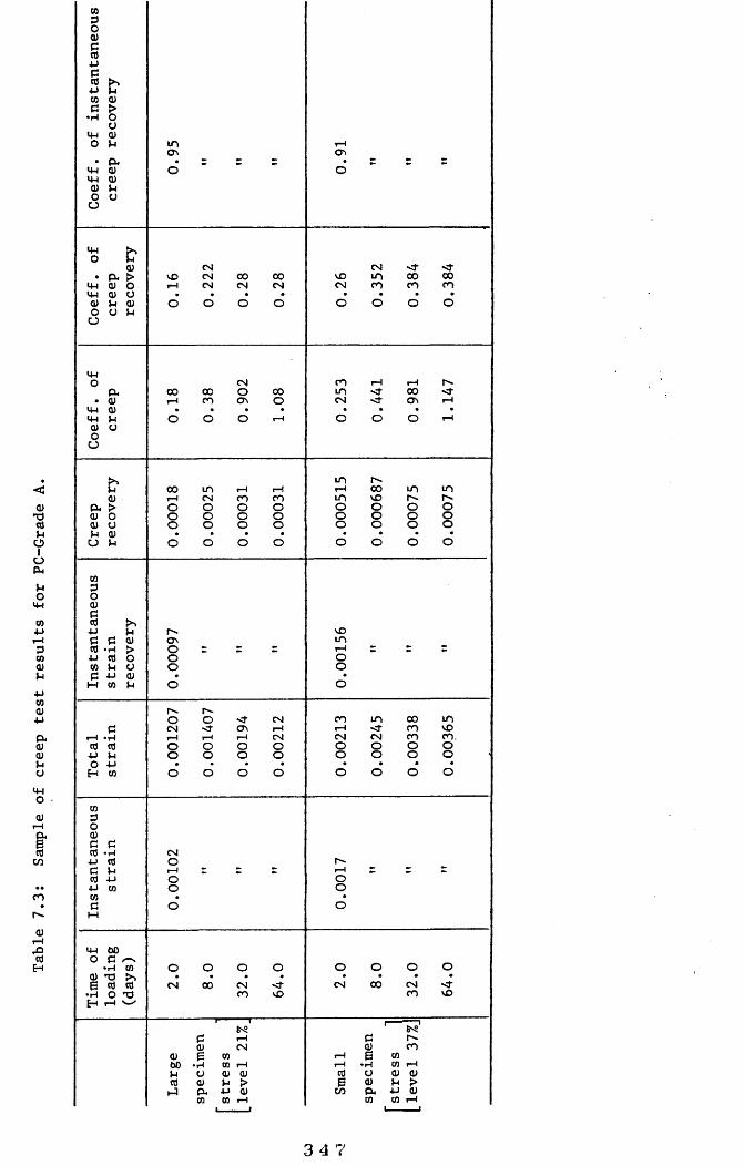
(0g0)g4JgGO (UG >•H O OGM (U O >-i• aGM (U Gw 0) (U M<5 "

O UW• eu >G4-I Cü oG44 Q) u (U o 

VDiM

00

00 T— I

I

c:\o8

OCMrM8

CMCMCM 00CM 00CM

COCOCMO 00O

inCM8O

co8O

co

I

Ot—t

8<J\

8CM8

CMOoO

OCM

0)00uco

oCMCO -d"vo

GIOQ)euco

6SI—ICMCOCD 1-4 CI CI

U > ■M OCO T—I

CT\d

UDCMCMGOCO

O-00CO 00co

coGOCM 00cr\ <r

GO1—4GOOoo

Os00vO8O

GOr>.o8

GO

8

\DGOOO

co1-4CM8

GO-MFCM8

00coco8

GOVOco,8

8

OCM

O00 CMCO vO

I (U (U

3 4 7

goCO pG 0)O >0) o

44 G CJO cd

44(Up

G VOcp cd eu 00 0044 •p 0)(U co 0) o oO G p

O •H CJ

44O gop0) 0\ VD vD vD UO UO UO

44 eu > 00 m m UO CM 00 r -44 0) o H t m m m vD r- 00 000) os CJO p Q) o O o O O O o OO ü P

44O eu m(U o CM VD CM CM ip 00 UO0) o VD m r- rP co vD CM

44 p 1-4 CM co o- CM co -d- vD44 CJQ) o O o o O o o OOU

ugo UO UO UO0) P CM m m UO CM 00 p-D eu 0) CM CM CM CM vD r~- 00 00

cd o > o o o O O O o OU 0) o O o o O O O o O00 p ü O o o o O o O O1 C_) oCJ p O o o o O o O OP4PO co

mg

(0 d)•p esr—1 cd go0 ■p P CM 00CO es es (U 00 CM(U cd •|4 > O iPM ■p

coCdp

oCJ

OO g■P c 44 0)CO M CO p o O(U■p m co coeu -d- o Ov o -d" co UO(U r4 C O CM CM -d" cri tp co(U Cd •P I—H rP 1-4 1-4 T—4 CM CM VDu ■P Cd o O o O O O O CMo O P o o o o o O O O

H pCH co o o o o o O O Oo<u«—4 coe)o

0)co gp es

mmC3V VDG H O 1—4

«d- cd Cd O o44 P O oCOG pco d d

(U M1-4,jdCdH 44 60

o es O O•P co o o o o o OP QJ P > çd dJ P dJcd eu P d) e eu p iPP) co CO 1-4 w co CD

3 4 8

goœ uG 01O >44 0) o

O c o« 01p p VD44 G cr»44 « eu0) p 0) o

O co 0)U G p

•H u

44 r-o g>1 VD m 1-4 1-4 vD un en enp r- o 1-4 1-4 ov 1-40) m r-. vD 00 00 0044 eu >44 0) o o O O O O O O o

0) Ci oo p 0)o o p

44o -d" 00 vD CM vD en VDen O VD vD vD VD -d-• eu 1-4 CM en en 1-4 CN en -d"44 0)44 0) O o o o O O O O0) po oo

VD CM CM 00cr» -d" 4t r~- VDeu p r4 CM CM CM -d" un vD VD0) 0) O O O O O O O O(U > o o O o O O o Op o o o o O O O o Oo o0) o O O O O o o OpcoGo0)g g in 1-4p p as oG c 0) 00 encd -H > O rHp Cd o O oco p a O oc p eu1-4 co p o o

vD 00 r-00 <f 1-4 P~ cri un CMG O 1-4 CM CM as r4 CMr-f «H 1-4 1-4 1-4 1-4 r4 1-4 N CMcd Cd o O O o o o o op p o o o o o o o Oo pE4 CD o o o o o o o O

coGoQ)cd c en -d-p ‘H Ov unG Cd o 1-4cd p o op p o oco œG o oM

44 60o G•H co o o o o o o o O0) T3 g>Ve Cd cd CM 00 CM «d- CM 00 CM -d"•H o 'O en vD en vDH 1-4

-d"00

0)60g

C6•r4o(U(Xw

r-4 oen 1-4 B CDco 1-4 S'S Cd •H CO 1-4(U (U un 6 O 01 (Up > co 0) P >p 0) CM eu P 0) OVco r4 CM co CO 1-4 en

3 4 9

CO UG dJo >44 d> oO C ocd <up M 0044 G 0044 cd eud)p d) oO co d)U G U•H o

44O gnP VD 00 un un 00 vD CM CM

d) m CM Ht O •Ht 00 0044 eu g> m Ht Ht ■Ht H t Ht -d" < t44 d) Od) d) O o o O o O O O oO p d)(_) CJ p

44O eu vD

d) o\ 00 vD t-4 VO O vD CMd) VD o CM VD as en CM Ctv

44 p CM <t VD r - en un r- r -.44 CJd> o O O O o o O OO

. C_)

Md)ta CM uncd P t-4 as as 00 un 1-4 1-4p eu d) en en en en VD r- 00 00

o d) > O O O o O o o O1 d) O O O o o O o o O

u p CJ O o O o O o o oP4 o d)

p o o o o O o o OPO44 — .

GCO oP d)r4 GG cd gnco p P un VDd) G G d) 1-4 unp cd •H > o 1-4p Cd O 1-4 r4p co p U o oco G p d) o od) M co pp o o

eud) un un(U G VD CM r - CM VD Ht VDp 1-4 •H Ht VD 00 O Ov CM vD 00o Cd cd 1-4 r4 1—1 CM CM en en enp P o o O O O o O o44 o p o o o o O o O oO H co o o o o O o O od)

t-4eu ..xrre Gcd oco d)G G

cd •Hp Cd un CMVD G p 1-4 r4cd p 1-4 CMp co o Oco o o

d) G1-4 M o o43cdH

44 60O G

•H co o o o o o o O od) T3 gnG Cd cd CM 00 CM -d" CM 00 CM «d-•i4 O T) en vD en vDH 1-4

00

G Gd) gjd) B co B co60 •H co 1-4 1-4 •H co r-4P Ü d) dJ 1-4 CJ d) 0)cd dJ p > Çd dJ p > 6P) eu p d) as B eu p d) enco co 1-4 1-4 co co co 1-4 en

3 o 0

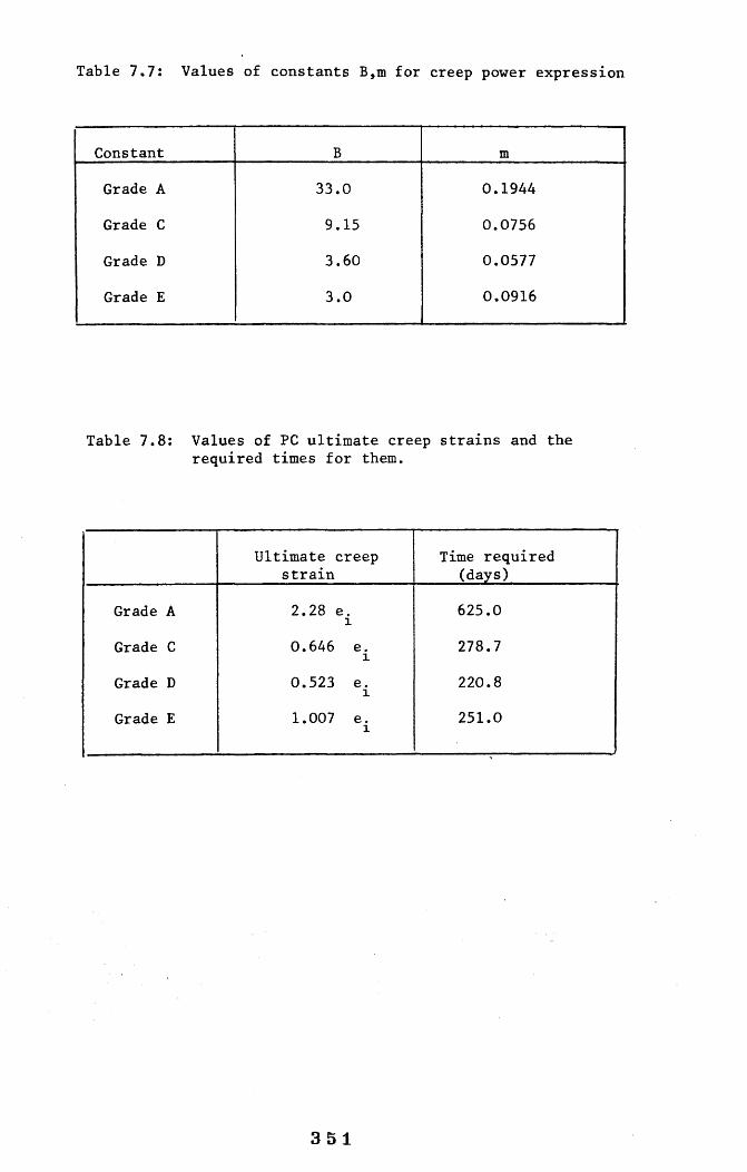
Table 7.7: Values of constants B,ni for creep power expression

Constant B m

Grade A 33.0 0.1944

Grade C 9.15 0.0756

Grade D 3.60 0.0577

Grade E 3.0 0.0916

Table 7.8: Values of PC ultimate creep strains and therequired times for them.

Ultimate creep strain

Time required (days)

Grade A 2.28 e. 625.01Grade C 0.646 e. 278.71Grade D 0.523 e. 220.81Grade E 1.007 e. 251.01

351

COT)C•H•na)4-)0•HTd0)Mp4|

1eu

CW•F - l

a•H

f-lS

VOO CM m VOO 8 8 8 8 8 8 8 r4 COCM CMo CO mco Mf 00 MfCO

UO8 00

8CM

8co UOO T—1 co r-l T—1r—1 ---- '

O - mo r—1o UO CMUO 'd-o 1—1

CMOO

8 8 8 8 m<r

00o 8 8UO<r co CM

8 8 8CM Oco CO

coO CM vO

vOCM CJV

8co o CM 00

O 1 8UO 00 vO M t T—1 00 UOd CO CO r—1

UO * CJv O CO1 1 8 1 8 1

CM VD r-4 'O-1—1 co

03ë(U

8

S-C4-10)f-lg

co0o(U(d CM vD 00 VO Mf

vDcd C O o O 00 vD r» UO co CM o -4-1 •H t—1 CM co o r—1 CM O rH CM r-l CM coC Cd o O o o o O O o O O O oCd f-l O O O o o o o o O O O O4-1 4JCO

aCO o o o o o O o o O O o o

coco r—I(U (U>-i >4J QJ wC/3 r-l

(DT)COO

O O O CM vD

o o oCM "O’ vD oCM O oM t v£)

o o oCM < f vD

W

3 52

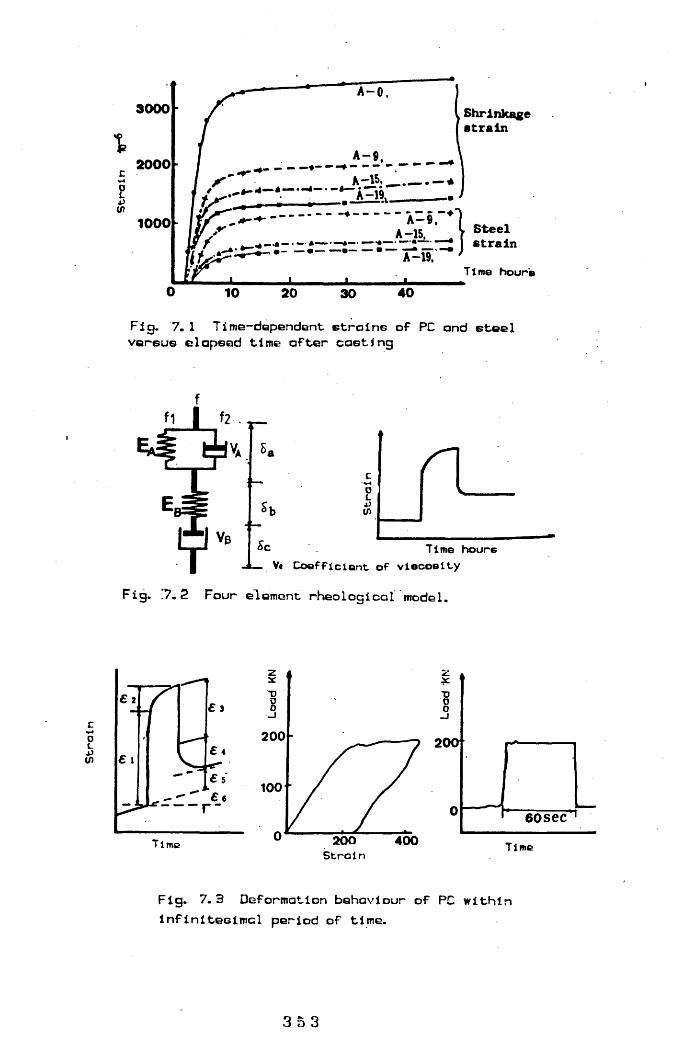
3000 ShrinkagestrainI

c2000

EA-9A-15,1000 steel

strainA-19.Time hour'e

4010 20 30Fig. 7.1 Time-dependent etroine of PC and steel versus elapsed time after casting

f1 I >2 T-

Sb

Sc

n

Time heure-À— Vt Coefficient of viscosity

Fig. .7.2 Four element rheological model.

coLtn

— r -

Timc

200

100

200Strain

400

200

Time

Fig. 7.3 Deformation behaviour of PC within i n f I n l t e G l m c l period of time.

3 5 3

2000

Trx

,7rd

Time hours

H2 4 106 8

Fig. 7.4 Variation in relaxation time (Trx) and retardation time (Trd) versus elapsed time after casting for PC.

I I

Experimental data e a -19 • A-15 O A-11

« , • A-9Calculated stress3

2

1

Time hours

U12106 &2 4

Fig. 7.5 Comparison of the calculated and experimental induced stresses.

354

I

b: 0,0005 me 0.01

b.m dapend on materiel

m% 0.03

Time^ ^ 9 " 7.0 RepPGSQntat i on of M a d cod GxpPGss i o for cPGGp.

30

I 20

P

ITime da/e

20 30

Fig. '7.7 Dependency of creep of polymer paste Cpolymer+fine Filler) on temperature and stress level.

355

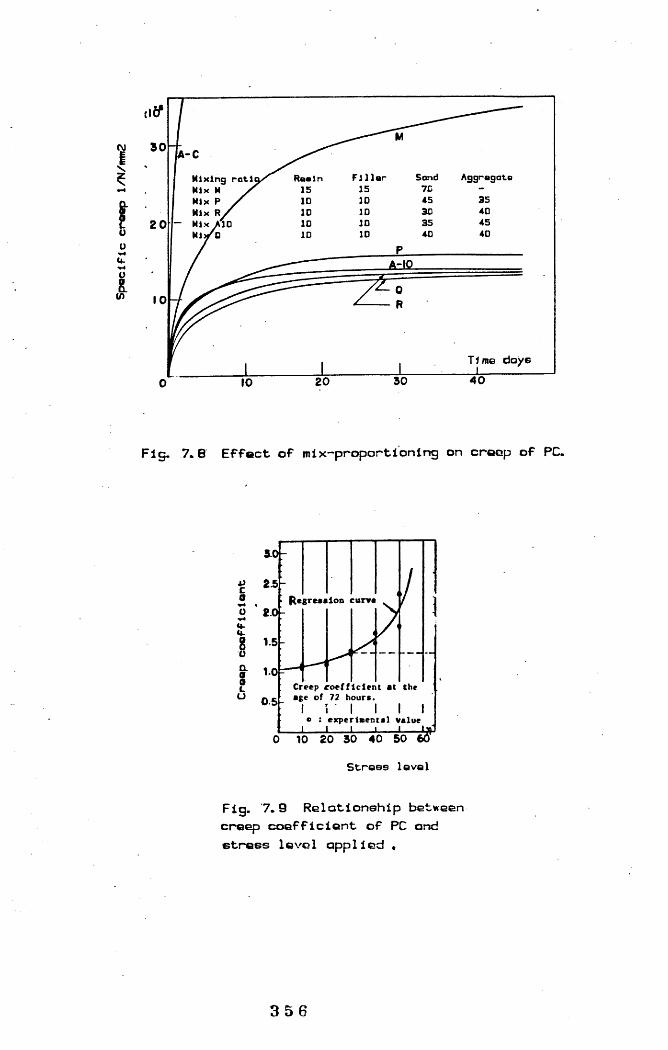
IIruu.

I

3 0 A-CM

Mixing rotio/^ Roain Filler Sand AggragatsMix M y' 15 15 70 -Mix P / 10 ID 45 35Mix r/ 10 ID 30 40Mix AID 10 10 35 45Mij/o 10 10 40 40

Time days

Fig. 7.6 Effect of mix-proportioning on creep of PC.

K cg rcss loD curve

Creep c o e ff ic ie n t at the age of 72 hours.I r I I I I

o : experim ental value_ J I______I___I-----1----0 10 20 30 40 50 60

Strees level

Fig. 7.9 Relationship between creep coefficient of PC and stress level applied «

3 5 6

10

8

S 6c3IIII4

Time under load:U

87 days 20 days, 10 days 5 days

2

0.2 0.80.4 0.6Stress—strength ratio

Fig. (7.10) Relationship between creep and stress/strength ratio for some PCC's.

1.0

I .0

Ïi1.

"Uo

050.005 per hr I 0003 per hr I.:-r0001 per hr. ' j

&u.0o

0.00400020.002 0004Conci~ato « t r c l nConcret.c etrcin

Cleft] Stress-etro1n curves for axial compr-esslon at various rates, [right] Stress-etroln relationship for eccentric compression after 1 hour of loodlng at constant rate of strain.

Fig. 7.11 Derivation of stress-strain relationship in flexure Cschematically)

3 5 7

^ Moving hood

Tronedijcor for meoei/rlng deflection ^ of •peclmen.

Cyllndorlcol epee1men IDO mm-die. 200 mm hlaht

Fixed heod

Fig. 7. 12 Axial compression testing of PC at constant rate of stroin.

358

rai sso^'^» -xoM

S

I'■•w*

1

gwM/'X HiSueui# aAioaajduioQ

359

«.ro'

oo'

oo'

oo'

oo'sooosooo*

oo*tn

S

8

ooo*

c0frü

0c0E1g-0*D10 U

1eo0o>DU

Of ï0 0) 0 -o

B

m(Sd)

IL

8 O O«o «

gmui/N i|i)Gu0uqs BA^esa-idiuog

360

[ 8 ] o : ; o j q o S I

r-[] W50J ssBj^s *xow

o'

oo'p*oo'

oo'

oo'8oos§

so'oooomI

SSaLI

SI•MI•D%8aL

(ÙOs>8U

2x>(I)i

ooo'

CO o

(O

d)•r*u.

s s u«0 « 3

guHM/X y)Guou^# OAj##*u(Ama3

3 6 1

[G] »30J HD *xow

5

:

oo

oo*

oo*s

sg

ioocTinSoo

iooo*

s

IIëlïDisf s

S 2mNd)u.

8 o«o

3 6 2

o

o

o

g[8] 1:0 S0OJ:;* -xow[ I ] o ^ o j • • o -j:v* *x o W

inI

o

CM

II IZ S 8>§

|b8 ^0 (CAsmw

d>

gmu/N y:)Guouqe BAissauduiOQ

363

< 1 \ O^^DJ u ? D u q s

: y 30U0CU30W/ UtDUSS bu?y30U30U0DWè o o

< œ u aTJ -O TJ X c

o

8

<1) W50J eseu a •xoui/aaej'a *xdw

c0r lJj0L"O*D§Co(0c

•l-lE??Ob0LÜOE"Oc0r4JF(0

010E

U-0Xuc■sIvr*-4

mU.

364

X

« œ u a ui

u o u ta

g

8

t*.0SDLC0X*)10>s g•H

f—4Dq-0

Q)1inMmÜ_

365

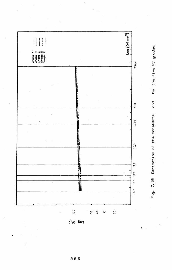
iim< m u o wÜ 33IIU U o u à

I8!01>

ÏLOu~

g

0)*)csI8Ïl4 -Oco

-t-l

o>La(ONmu_

(")) So-i

366

0

X)8

II

■O

II0

86Io

H8)<

j.

f\J

Uk!

U-0

8L . ÜL0

.U -

(DC0A)cU-

T)c0CDEL01 H

Kd)u_

3 6?

Hydraulic Jock ^AdJuBtoblo nute

Load tranofarrlng frame

Fig. 7. 18 The Tyler portable creep rig.

368

I

Unlbodtng

InvtatorMouB «trcii r»oovory0,003

înatcnfcortBOii* mloetlc •troln

Crodo A

TIirq days0.00

10 20 40 50 60 70 to 90

0.004

0.003Loading Unloodlrg

Inototoneoue «train racovQpyCE

U " P' Craap recovery

Inetcntoneous cloetic •troln0.001

Grade C

0.00 7050 6040 9030 60

____________ Theoretical expreeslon of creepo o o 0 O o Large ^Madmen • • • • • • Small «peclmen

Fig. 7. 19 Creep results for PC. (Grade A & C)

369

,003

UnloadingLoading

OJ002

Inatatoneouo «train rocovory'C Inotcntcnocu» ola#tic

•train:U)Croda 0

Creep recovery

0.00

UnloadingLoading

0,003 Instatoneoue «train rocovory

Inetcntcnooue oloetic. «trainom

Creep recovery

Tima days0.00

10 20 30 to

______________ Thoorotical oxproeeion of croopo o o 6 : o o Lor go «pocimon • • • • * * * Small «pocimon

Fig. 7. 19 Creep results for PC.(Grade D & E)

3 70

CHAPTER EIGHT

ULTIMATE STRENGTH DESIGN OF REINFORCED

PC STRUCTURES IN FLEXURE

8.1 Introduction

The design of reinforced concrete structures based on their

ultimate strength has been accepted in many countries and is a

viable alternative to the classical design approach of the

elastic theory. The reasons for an ultimate strength design

method for PCC structures being more favourable than elastic

design apply even more to PC structures.

As has been shown, The stress-strain curve for PC is not

linear; most of its strains are inelastic and highly time-

dependent. Ultimate strength design is not bound to crudely

approximated modular ratios. It takes inelastic strains into

account and therefore can predict a reasonably accurate load

factor. The limit state design method as introduced by the

European Concrete Committee in 1964 (120) aimed at combining

the best features of ultimate strength and working stress

design theories. In this, the ultimate strength approach is

used for proportioning the sections and the elasticity theory

is used to ensure that deflections or crack widths will not

exceed certain values under service load. Crack widths and

deflections are c o n s i d e r e d as the limit state of

serviceability.

For reinforced PC structures, the serviceability limit state

as a design approach is likely to be of vital importance and

therefore has to be carefully examined. The high ultimate

strength of PC usually leads to relatively small sections

371

under high loads resulting in large deflections and the probability of lateral instability. Bearing these in mind in

addition to the inherent low stiffnesses and the high ultimate

strains of PC, it is evident that the conditions of

serviceability might be most critical for design.

In this work ultimate strength design will be discussed in

detail for pure flexure and combined flexure and compressive

axial loads. The serviceability limiting states are not

included. Before establishing such limiting states a thorough

revision and assessment of the practical structural

performance of PC under service loads and the consequent

deformations has to be carried out. With the traditional

limits for deformations, crack width and ductility the use of PC structures will be limited to fields of application where

there is no need for such stringent s e r v i c e a b i l i t y

requirements.

8.2. Factors of safetv and their significance

One of the most important features of the ultimate strength

design is that it allows for the selection of more realistic

factors of safety than those considered in the elastic theory.

The progressive reduction in these factors of safety as a

result of refinement of the structural analyses and better

knowledge of the properties of the material, can be considered

as an outstanding outcome from the economic point of view. The

mutual relationship between performance and cost is

essentially related to the chosen magnitudes of the factors of

safety.

It should be borne in mind that no matter how far the

372

structural analysis is refined or how much our material

knowledge is increased , factors of safety will have to be

applied in the design of reinforced concrete structures. This

is mainly because of the inevitable variations in the strength

of concrete and steel and the assumpotions usually involved in

the analysis. The uncertainity in the magnitude of the loads

applied requires the use of load factors.

Variation in strength is primarily due to the heterogeneity of

concrete and the way it is mixed, cured and cast. With the

highest possible quality control and site supervision,

strength of a given concrete grade will still vary from a slab

to a beam, from a beam to a column and even within the same

member, strength of concrete will change in horizontal and

vertical directions depending on the size of the member. The

dispersion in strength may further increase with increased

number of batches and by casting at different times with

slightly different environments. Consistency of the mix

constituents over several mixes of the same concrete does not

actually exist.

Variation in the live loads is in the nature of these loads,

and no one can claim fixed values for them. It is therefore

imperative that the range within which these loads can vary

should be covered by appropriate load factors based on

accumulated experience.

Additional factors of safety should be considered to

compensate for any likely approximation or inaccuracy of the

assumptions made in the analyses. The stress occurring in

concrete is not merely a function of the associated strain. To

3 7 3

assume that concrete and steel have compatible strains at all

times and that no bond slip or bond failure is occurring, is

another plausible but inaccurate assumption for which as for

many others, factors of safety have to be introduced.

For ultimate strength design the American Concrete Institute

AGI has issued its provisions for the factors of safety to be

considered. These provisions and the corresponding factors of

safety can be used for the design of PC reinforced structures

after few necessary modifications have been carried out.

The ACI code divides these factors into load factors and

capacity reduction factors (121). There was no need to modify

the load factors specified by the ACI.

The capacity reduction factors as specified by the ACI require

modification to suit the particular structural performance of

PC. In this respect the only difference between PCC and PC

lies in time dependency and in reduced fire and elevated

temperature resistances. The performance of PC at elevated

temperature is still a c o n t r o v e r s i a l point, and is

fundamentally related to the type of resin used and its

formulation. For instance in Japan and in the U.S.A., certain

special resin formulations resulted in PC with stable

performances at temperatures up to 240 C.

For the time being, however, and until new versions of high

thermal-resistant resins become economically feasible, all

structural applications should be restricted to fields where

no elevated temperatures or fire attack can take place.

As for the time-dependency of the stress-strain curve, it has

374

been shown previously that PC suffers severe deterioration in

strength resulting from creep and that the short-term

performance is appreciably different from the long term one.

Despite the fact that creep strains and the associated

strength reduction can be significant, the relative decrease

in the ultimate carrying capacity of a reinforced PC member

would usually be much less than the relative decrease in the

PC strength. This is partly because of the stress

redistribution effect and partly because of the restraint

effect of the steel on the creep of PC itself. It can be shown

that in flexure for instance, any increase in concrete strain

by creep would result in such an increase in the compression

zone depth (creep of steel is virtually nil) that the overall

percentage reduction in the compression force provided by the

concrete would be much smaller than the percentage reduction

in the ultimate compressive strength f ^ of the stress block.

For PCC Hognestad (122) demonstrated that the influence of

sustained load on beams has no significance, and that with

columns it can reduce the ultimate carrying capacity by up to

only 10%. This reduction is well covered by the specified

capacity reduction factors. The same trend should apply to PC

but based on its higher time-dependency than PCC, the capacity

reduction factors for PC are chosen here to be 0.1 less than

the corresponding values in the ACI provisions. This value,

0.1, was found from detailed comparative calculations of the

ultimate capacity of PC cross-sections under short-term and

long-term conditions.

So for pure flexure the capacity reduction factor is chosen to

375

be 0.8 instead of 0.9 for PCC, while for flexure and axial

compression it is 0.6 instead of 0.7. For design purposes, the

ultimate load should at least equal the sum of each service

load multiplied by its respective load factor, as specified by

the ACI Building Requirements (121).

8.3. Assumptions considered in the design

The design approach as will be given later in this chapter, is

primarily valid for PC grades having similar properties to the

five PC grades investigated in this work. The main two

parameters that can describe any PC grade are considered to be

the ultimate axial compressive strength and the secant modulus

of elasticity measured at one third of it. Any PC grade having

its modulus of elasticity and/or ultimate compressive strength

within the range investigated, as given in Chapter Three, can

be designed using the following design approach after

extrapolating the block stress parameters.

The steel used here was a cold-drawn type whose idealized

stress-strain curve is shown in Fig.(8.1). No mild steel is

considered in this work. Had it been attempted it would have

led to extremely high reinforcement ratios which could not

have been accommodated in the section; with mild steel the

maximum possible reinforcement ratios will not be great enough

to allow PC to be utilised efficiently or economically.

For the calculations of the ultimate strength of members or

for proportioning their sections, the following assumptions

are made:

[1] Plane sections before bending remain plane after bending.

3 7 6

[2] The stress-strain curve for the cold-worked steel is a

trilinear function as shown in Fig.(8.1).

[3] The distribution of concrete stress in the compression

zone is defined by the three block parameters k1, k2 and kS

and the ultimate compressive strength fey* The block parameters can be obtained using the following empirical

formulae :

K1 = 0.9 - 0.38 [1 - (Scu/O.009)2] ...(8.1-a)

K2 = 0.3 + 0.006 Ec ...(8.1-b)

K3 = 0.27 + 0.03775 ...(8.1-c)

in which E^ the secant modulus of elasticity in KN/mm2 and the

concrete ultimate strain c u can be obtained from the

following empirical formula :

®cu = 0.00926 ( 1 - Ec/86.55 ) ...(8.1-d)

An alternative set of theoretical calculation formulae can be

derived using the previously given sine-function of the stress

distribution with the value of ^cu=1.333 ^oc (see Chapter

four).

[4] Tensile strength of concrete and tension stiffening are

neglected.

[5] the effect of lateral confinement is neglected.

8.4. Design reinforced fC members in p.ur^ flexvrë

The previously derived equations [ Eqs.(5.1, 5.2) ] can be

used in the design of rectangular sections whether they are

singly or doubly reinforced. Substituting in Eq.(5.1) for

L=0.0, then

377

T g = T + T ' s ...(8.2-a)where T'g/Tg= R'.f'g/(R.fg) then

T's = Tg [(R'f'g)/(R fg)] ...(8.2-b)

By eliminating T'g from Eqs.(8.2-a and 8.2-b) then

Tg = T/[1-(R'/R)(f'g/fg)] ...(8.2-c)

T'g = T/[(R/R')(fg/f'g)-1] ...(8.2-d)

From Eq.(5.2) and by substituting for T'g in terms of T, then

M/(bd2fcy)= Z

Z = T(1-YT)+T(1-d'/d)/[(R/R')(fg/f.g) _i] ...(8.3-a)

From Eq.(8.2-c) the tensile reinforcement ratio R in terms of

T is as follows :

R = Tfcy/fg[1/(1 - {R'/R} {fg/fg})] . ..(8.3-b)

Using Eqs.(8.3-a,b) the values of R and Z can be obtained for

a given value of T and R'/R ratio at given values of G, Y and

f^y. If these values are those corresponding to the ultimate

strength ( ultimate concrete strain ^cu), the values of R and

Z at ultimate strength can be calculated and the section can

be proportioned. The only provision so far required for

calculating R and Z, as can be seen from Eqs.(8.3-a,b), is

that the ratio d'/d has to be known. In this work d'/d is

taken to be 0.1.

It should be borne in mind that for a given T-value, the

compression zone depth will be also known as c/d=T/G, and

therefore the strains in the tension and compression steel and

consequently the stresses in them can be calculated as

378

follows:

fgS %u (C/T - D A + B ...(8.4-a)f*g= %u [1 -(d'/d)(C/T)3A ♦ B ...(®.«i-bî

From Eq.(8.3-b) It Is clear that increasing R for a given E"/Kratio will lead to an increase In T-valoe. By referring t©

Eq.(8.3-#) this increase in T-value will increase the

coefficient Z which implies that for a given moment an0

section width, the required effective depth will fee reduced* Conversely by increasing the effective depth ( decreasing 2- value) for a given RVR ratio would lead to a reduction in the required R-value for a given moment.

Thus Eq.(8.3-a) and Eq.(8.3-b) can provide a basis on which an economic choice of the mutual areas required of tension steel and of PC can be decided. Similarly it can be shown fey using these two equations that, for a given R the effective depth required for a given -moment can be reduced by increasing the R'/R -ratio and from this standpoint the two equations can

tell when the use of compression reinforcement is necessary*

For example if the effective depth is to be reduced and no

further increase in tension steel can be accommodated in the

section, or if the tension steel ratio is fixed at a desired

value then the required R'/R ratio can be estimated.

To facilitate the use of these two equations, the values of R and Z were calculated for a wide range of different T and RVR

values. The relationships between Z and T on one hand and R

and T on the other were plotted as shown in Figs.(8.2-a, b, c , d it) for the five PC grades with R'/R as a parameter. In

these figures I and R values are plotted using two opposite

3 7 9

ordinates against T-values as an abscissa. These figures are

charts that can be used in different ways to satisfy almost

all design requirements.

For a section of given dimensions, made of a given PC grade,

the value of Z corresponding to a certain ultimate moment can

be calculated from Eq.(8.3-a). A horizontal line at this value

of Z would intersect with infinite number of T-Z curves. Each

of these can be used to find the required R at the desired

R ’/R ( by projecting the intersections down to the T-R curves

respectively ).

Conversely, for a given R and R’ the required effective depth

can be obtained by drawing a horizontal line at the given R-

value and using its intersection with the T-R curve of the

corresponding R’/R value to determine the relevant values of T

and Z. These charts give an infinite number of mutual

solutions for the cross-section parameters and they

consequently have evident potential when translated into

practical design charts for reinforced PC structures in pure

flexure.

Despite the versatility of Figs.(8.2), it should be noticed

that they have theoretical values of T, Z and R that must be

limited to lie within practical boundaries. For example, these

figures were derived on the bases of Eq.(5.1) and Eq.(5.2)

which assume that the neutral axis lies within the section, or

from c/d=0.0 to c/d = 1.0. This implies that according to these

equations values of T can not be less than zero or more than

the value of the parameter G of the PC grade. In addition and

from the structural performance point of view, c/d must have a

Q SO

minimum value high enough to control the magnitudes of

curvature and the resulting strains in the tension steel , and

to make efficient use of the high strength of PC in the

compression zone. At the other extreme, c/d should not be

higher than a maximum value small enough to reduce the amount

of the tension steel required and to produce a reasonably

ductile failure.

In this work the maximum and minimum values of c/d are taken

to be 0.6 and 0.25 respectively. This means that the

corresponding maximum and minimum values of T will be 0.6G and

0.25G respectively. Values of T outside these two limits,

which are represented by vertical lines (2) and (1) on the

figures, will not therefore be permitted in design.

In addition another limiting boundary is that for any section

subjected to pure flexure, the tension reinforcement ratio can

not be allowed to exceed the maximum value that can be

practically accommodated. For rectangular sections this value

of maximum R is taken here to be 5%. A horizontal line drawn

at R=5%, will intersect the various R-T curves at the maximum

practical t-values corresponding to each R’/R ratio. This

horizontal line, line (3), represents a third boundary for the

curves to be used in actual design. The intersection of this

line with R-T curve whose R’/R = 0.0 would give another maximum

practical value of T less than that set above at c/d = 0.6 for

each PC grade. This value can be calculated exactly by using

Eq.(8.3-b) and Eq.(8.4-a) and substituting for R'/R = 0.0. By

drawing a vertical line at this value of maximum practical T,

line (4), the range of T-values within which sections can be

381

practically proportioned is thus defined by line (1) and line

(4) rather than line (1) and line (2).

The intersections of line (3) with different T-R curves having

different R’/R can be projected up to the corresponding Z-T

curves which on being connected together form another boundary

of the maximum practical values of Z , curve (5). These values

of maximum possible Z can be calculated by using Eq.(8.3-a)

and the associating values of T previously derived. In

addition the maximum possible value of R’/R can be found by

substituting in Eq.(8.3-b) for T = 0.25 G and R = 5%.

In this way the design chart is completely defined by the

figure ABCD shown in Figs.(8.2) and reproduced in Figs.(8.3-a,

b, c, d &e) after eliminating the parts of curves outside the

previously mentioned limits; these figures represent the

design charts for the five PC grades respectively.

In these charts two limiting values of Z , minimum and

maximum, exist at the extreme intersections of Z-T curves with

line (1) ( c/d = 0.25). The maximum value lies at the Z-T curve

with the maximum possible R’/R within the limits set, whereas

the minimum value is at R’/R=0.0. The corresponding values of

the effective depth will be termed respectively as the minimum

specific depth dg^ and the maximum specific depth dg^. In actual design based on these design charts the required

effective depth will lie within these two extreme values of

dgn and dg^*

In this respect it might appear unreasonable that unlike PCC,

a limiting maximum value of the effective depth should be

3 8 2

specified. Nevertheless, by referring to Figs.(8.2) it can be

shown that if the effective depth is increased beyond dg^, the

value of c/d will be reduced to a value less than 0.25 with

the result that strains in tension steel will be more than

three times the ultimate concrete strain ^cu. Bearing in mind

that ^cu-values are as much as 0.0071-0.0076, it is quite

reasonable to limit the tension steel strains to the value

3 cu by not allowing T-value less than 0.25 G . The maximum

effective depth is a consequence of the assumption that T

should not be less than a given value.

These design charts will not allow values of effective depth

smaller than d^^ as the required reinforcement ratios would

then exceed the prescribed maximum values of R and RVR. It is

useful to identify the four corners of each of these design

charts before proceeding any further. Corners A and B together

represent one single point on the R-T and Z-T curves

respectively which have the maximum R'/R ratio at c/d = 0.25,

and they further represent the case of the minimum specific

effective depth with doubly reinforced sections. On the other

hand corners C and D correspond to one singly reinforced

section proportioned to the minimum effective depth with the

maximum possible value of R.

For a given moment and a given PC grade, the value of the

effective depth can be made to vary from dgn to dg^ ( from Z=EB' to Z=EB ). The tensile reinforcement ratio can also vary

from RzEA' to R=EA, while the values of R'/R can be chosen to

have any of the values from zero to the maximum ratio of P'/R.

The design charts can be used in many different ways to find

3 F 3

the missing data for the section to be designed. In using

these charts the relevant factors of safety previously given

must be introduced as will be demonstrated in the following

examples.

E xemple 1.8, IJA 250 mm wide rectangular cross-section is to carry a service

load bending moment of 200.0 KN.m for dead load and 250.0 KN.m

for live load. Using the given cold-drawn steel and the five

PC grades, design the section to have the maximum effective

depth.

Solution

Using load factors 1.4 and 1.7 for dead and live load

respectively, then the ultimate moment Mu will be ;

Mu=1.4(200) + 1.7(250) = 705.0 KN.m.

For the maximum effective depth T=0.25 G and R'/R=0.0, then

from the design charts minimum Z-values can be found, hence

the value of the maximum effective depth can be calculated

from the following equation in which the capacity reduction

factor Fcr=0'B is introduced;

d=[Mu/(Zbd2fcyFcr)]°'5 ...(8.5)

The tensile reinforcement ratio R at T = 0.25 G and R'/R = 0.0,

corresponds to point A'in the design charts and can be found

directly from them. The derived and calculated values of

minimum Z, maximum effective depth , R and Ag are given below

for the five PC grades.

Grade A B O D E

384

Zmin. 0.158 0.160 0.168 0.172 0.152

^max 512.0 495.0 529.0 506.0 494.0R % 2.54 2.76 2.54 2.64 2.78

Ag (mm2) 3250.0 3415.0 3360.0 3340.0 3433.0

Example I8.,.£J.

The same as given in Example [8.1], except that the sections

are to be designed to have minimum effective depth.

Solution

The required sections will be those corresponding to points A

and B on the design charts at which RVR is maximum and R = 5%.

Substituting for the value of Zmax. corresponding to point B

in Eq.(8.5), the minimum depth can be calculated . Knowing

maximum values for R'/R and R = 5%, the areas of the steel

required can be calculated, the results for the five sections

are as follows;

Grade A B C D E

Zmax. 0.315 0.300 0.350 0.330 0.280

dmin (mm) 363.0 361.0 366.0 365.0 364.0

R'/R 0.574 0.515 0.600 0.528 0.520

R'max % 2.870 2.570 3.000 2.640 2.600

Ag (mm2) 4538 4512 4575 4818 4550

A'g(mm2) 2605 2323 2745 2544 2366

Examole[8

The same,3]example [8.1] except that the sections are to

designed for an effective depth d=400.0 mm.

Solution

385

Using Eq.(8.5) the value of Z required for the given value of

effective depth, can be calculated. Using the design charts

and by drawing a horizontal line at that calculated value of

Z, a range of possible R and R'/R values can be obtained that

would provide such a predetermined effective depth. It is

clear from the charts that as R increases the associated ratio

of R'/R required will also increase and vice versa. Therefore,

for the calculated Z-value for each PC grade an infinite

number of solutions are available ranging from R'/R max. and

Rmin. to R'/R min. and Rmax. These limits of the

reinforcement ratios can be directly derived from the design

charts or found by extrapolation. The results are as given

below.

Grade A B C D E

Calculated Z 0.259 0.244 0.294 0.275 0.232

Rmax. % 5.0 5.0 5.0 5.0 5.0

R'/R min. 0.02 0.0 0.15 0.0 0.0

Ag max.(mm2) 5000 5000 5000 5000 5000

A* gmin.(mm2) 100 0.0 750 0.0 0.0

Rmin. % 4.0 4.2 4.4 4.2 4.3

R'/R max. 0.45 0.40 0.52 0.41 0.41

Ag min.(mm2) 4000 4200 4400 4300 4300

A 'gmax.(mm2) 1800 1680 2290 1722 1763

Examole[8.4]

The same as given in example [8.1] except that the sect]

are to be designed for a given R=4% and R'/R = 0.2.

Solution

386

Using the R-T curves of the design charts , find the value of

T corresponding to R=4% and R’/R=0.2, that is the intersection

of 4% R-horizontal line with R-T curve whose R’/R=0.2. In such

a case, one specific value of T will exist for each PC grade.

Using this value of T, the corresponding value of Z can be

obtained from the intersection of a vertical line drawn at T

with the Z-T curve of RVR=0.2. The value of Z can then be

used for calculating the required depth from Eq.(8.5). The

results for the five PC grades are given below.

Grade A B C D E

Z 0.228 0.222 0.256 0.246 0.213d (mm) 426.0 420.0 428.0 392.0 417.0

Ag (mm2) 4260 4200 4280 3920 4170

A ' g(mm2) 852.0 840.0 856.0 784.0 834.0

In all the above examples, the value of T corresponding to any

section chosen is known, hence the position of the neutral

axis can be calculated where T=Gc/d. Knowing the position of

the neutral axis and the ultimate concrete strain ^cu, the

strains and the stresses in the steel can be checked using

Eqs.(8.4-a &b). These given examples indicate the versatility

of the design charts and numerous further examples could have

been cited to emphasize this feature. The use of these charts

is almost unlimited and therefore it is left to the designer

to satisfy his design requirements as desired. Obviously

another alternative for design is direct use of the equations

used in the construction of these charts.

8,5. Design reinforced fC wilh flexure ami

38

compressive load

The equations used previously in the analyses of reinforced PC

columns can be used in the design after various factors of

safety are considered. As stated, the additional axial load

leads to a function in the third order of T the manual

solution of which is not easy. It was also emphasized that

unlike beams, columns must have compression steel at least in

one side of the column if not both. The use of compression

steel in columns is absolutely necessary from the economic and

performance points of view.

In Chapter Six, it was shown that the relative contribution of

either compression or tension steel to the ultimate carrying

capacity will vary depending on the eccentricity ratio er=e/d.

It was further found that for er-values less than unity, the

compression steel ratio R' should be as high as possible and

the tension steel ratio R should be calculated accordingly. At

the other extreme, for er-values greater than unity, the R-

value should be as high as possible with R’being calculated

accordingly.

For rectangular sections with flexure and axial compression ,

Eq.(5.1) can be rewritten in the following form;

Tg = T + T'g - L ...(8.2-a» )

Using Eq.(8.2-a') and the previously derived Eq.(8.2-b), T'g can be eliminated and by similar operations as those carried

out with pure flexure, the values of R, R' and Z could be

expressed in terms of T as given in the following three

equations ;

3 S 3

R = f c y C T - D / f g / E l - ( R ' / R ) ( f ' s / f g ) ] ...(8.6-a)

R ’ = fcy(T -L)/f's/[(R/R')(fg/f'g) -1] ...(8.6-b)

Z = T ( 1 - Y T ) + C T - L ) ( 1 - d ' / d ) / [ ( R / R ' ) ( f g / f ' g ) - 1 ] ...(8.6-c) in which L = Z.d/e = Z/er. ...(8.6-d)

Substituting in Eq.(8.6-c) for L in terms of Z, the value of Z

at a given er-value can be obtained for various T-values and

R ’/R ratios ( d'/d = 0.1). Then using the value of Z in either

of Eqs.(8.6-a or b), the corresponding values of R and R' can

be calculated. It is important to note that while Z or R

values in pure flexure were dependent only on T and RVR, they

are further dependent on er-value when moment and axial load

are combined.

Equations (8.6-a to 8.6-d) are now sufficient to be used in

design after the factors of safety are introduced. For a given

load at a given eccentricity and for a known depth and width

of the section, a wide range of possible R and R'-values

exists, depending on the desired compression zone depth or

alternatively on the value of T. This wide range of R and R’

is reduced to one single value for each if and only if either

of R and R’ are known on one hand, or R ’/R ratio is fixed on

the other. As the use of these equations will lead to

undesirably lengthy calculations, design charts for columns

similar to those developed for beams can be of great use.

Equations (8.6-a and 8.6-c) represented graphically are shown

in Figs. ( 8.4-a, b, c , d &e) for the five PC grades. In these

figures, the values of Z and R are plotted using two opposite

ordinates against the values of T as a common abscissa. These

389

figures correspond to one single value of eccentricity level er=2.0. They can be similarly constructed for any other value

of er; as an example, Fig.(8.4-a’) is constructed with er = 1.0

for grade A.

For deriving the column design charts on the bases of these

figures, similar provisions to those considered with pure

flexure were taken into account. The first of which is that T-

value should be within 0.25 G and 0.6 G, whether the column

has small or large eccentricity. Accordingly the range of T is

defined by the two vertical lines (1) and (2) as shown in

Figs.(8.5). The second provision is that R’/R ratio must not

be less than 0.2 and neither of R nor R’ should exceed 5% for

large or small eccentricity columns respectively. This second

provision provides a third limiting vertical line, line (5) in

Figs.(8.5), drawn at the T-value corresponding to the

intersection of the T-R curve whose R’/R = 0.2 and line (3).

Accordingly the right-sided boundary of the design charts will

be either line (2) or line (5) whichever has the smaller T-

value.

It should be stressed that for c o l u m n s with small

eccentricities, the design charts are much more easily

derived from Z-T-R’ curves than Z-T-R curves allowing a

limiting value of R’=5% to be introduced. The figures shown.

Figs.(8.5), are for large eccentricity and therefore the

provision of R=5% is relevant. By drawing a horizontal line at

R=5%, line (3), and projecting the limiting T-values on the

corresponding Z-T curves, the upper boundary of the design

chart, curve (4), is defined. While maximum value of R’/R in

beams reached almost 0.6, this ratio can have much higher

3 9 0

values with columns and in this respect an additional

provision had to be considered. That is, for large

eccentricity columns where er > unity, R’/R must not be more

than 1.0 and consequently R’will be always less than or equal

to 5%. Conversly, for small eccentricity columns where er <

unity, R’/R should not be less than 1.0 with the result that R

can have any value up to a maximum of 5%.

Referring to Figs(8.4), in which er = 2.0, the maximum value of

R ’/R is 1.0 and all the Z-T or R-T family curves are

constructed accordingly with R’/R ranging from 0.2 to 1.0.

Thus the design charts are confined to the boundaries denoted

ABCDEF. The design charts are reproduced in Figs.(8.6-a, b, c,

d &e) for the five PC grades with eccentricity level er = 2.0.

In addition, to demonstrate the effect of the eccentricity

level Fig s. ( 8 .6-a 1 , a 2 & a 3) are constructed for three

different values of er.

In these charts it can be shown that a maximum specific

effective depth dgm occurs at T = 0.25 G corresponding to the

minimum value of Z at B’, while a minimum specific effective

depth dgn exists with R = 5% and R’ = 5% at point C which has a

maximum value of Z. In between the two extreme values of dg^

and dgn corresponding to a certain er-value, an unlimited

number of effective depths are available with various mutual

values of R and R’ as will be shown in later examples.

It should be borne in mind that while the interaction diagram

solves for a given section at various er-values, the developed

design charts solve for various sections at given er-value. In

particular design cases, one approach may be preferred to the

3 9 1

other. However, these design charts can be translated to

similar ones, as shown in Fig. (8.5), that can work as

interaction diagrams not only for a given section but also for

as many sections as desired provided that they have a known

R'/R.

This can be done by using Eq.(8.6-a) and Eq.(8.6-c) for

finding R and Z values for different T values at a constant

optional R'/R ratio with er-value as a parameter. An example

of these interaction design charts is given in Fig.(8.7) for

grade A, with R’/R=1.0 and er-values changing from 1.0 to 2.5.

Obviously a much wider range of er-values can be considered.

The interaction design chart shown in Fig.(8.7) is limited

with the vertical lines (1) and (2) as defined before, while

the lower boundary, line (3), is drawn at R=5% as the R'/R

considered is 1.0. Had the ratio R'/R been more than 1.0, line

(3) would have been drawn at R=0.05 R/R'. The intersections of

line (3) with various R-T curves can be used to plot the upper

boundary, curve (4), as shown in Figs. (8.5 & 8.7). It is

noteworthy that the intersection of line (3) with line (1)

will concide with an R-T curve having the maximum possible er-

value at Rz5%, while the intersection with line (2) identifies

another R-T curve at the minimum er-value for the same R so

that T will not exceed the prescribed limits (points A and D

respectively). The intersection of curve (4) with lines (1)

and (2) would give the corresponding minimum and maximum

values of Z respectively. Similar curves to curve (4) can be

constructed for any other value of R < 5%. Knowing the maximum

er-value and the associated minimum Z-value, the value of the

minimum axial load Pmin can thus be obtained for a column of

392

any dimensions with a given RVR.

Conversely, using the minimum er-value and the corresponding

maximum value of Z, the maximum axial load that can be

supported by a given column can be calculated. It is important

to note that for a given section there exist two specific

ultimate loads occurring at two specific eccentricities that

would satisfy the practical limits given.

In the following, some representative examples are cited to

demonstrate how the above mentioned design charts and

interaction design charts can be used.

Example 18.,5_1A 200 mm wide rectangular cross-section is to carry a service

axial load of 180 KN from dead load and 270 KN from live load

at an eccentricity level er=2.0. For an effective depth d=400

mm, find the required areas of compression and tension steel

(cold-drawn type) for columns made of each of the five PC

grades given with [a] R V R = 0.2, [b] R'/R = 0.6 and [c] R'/R = 1.0.

SolutionConsidering load factors of the value 1.4 and 1.7 for dead and

live load respectively, then the ultimate load Pu is as

follows;

Pu= 1.4(180) +1.7(270) =711 KN.

Taking a capacity reduction factor F j, = o.6, then the required value of Z can be calculated from the following equation;

Z =Pu.e/[bd2fj,yFcr) ...(8.7)

393

Using the design charts a horizontal line drawn at Z equal to

the calculted value will intersect with Z-T curves of R’/R

equal 0.2, 0.6 and 1.0 at three distinct points, each of which

can be used to find the required value of R corresponding to

each R’/R ( curves R-T ). Having done that, the compression

and the tension steel areas can be calculated. The results

according to the three R’/R ratios are given below.

Grade A B C D E

Z 0.35 0.33 0.39 0.37 0.31

[a] R ’/R=0.2

R % 4.56 4.20 4.82 4.38 4.08

Ag (mm2) 3648 3360 3856 3504 3264

A'g(mm2) 730 672 771 700 653

[b] R ’/R=0.6

R % 3.60 3.60 3.84 3.64 3.56

Ag (mm2) 2880 2880 3072 2912 2848

A *g(mm2) 1728 1728 1843 1747 1709

[c] R ’/R=1.0

R % 3.20 3.16 3.36 3.30 3.12

Ag (mm2) 2560 2528 2688 2640 2496

A 'g(mm2) 2560 2528 2688 2640 2496

Example [8.6]

As given in the above example, but it is required to design

the section for the maximum possible effective depth at which

tensile steel strains will not exceed three times the ultimate

concrete strain, with [a] R'/R=0.4 and [b] R ’/R=0.8.

3 94

Solution

From the design charts, the minimum Z-value at the given R’/R

ratio is that corresponding to the intersection of Z-T curve

of the same R’/R value with line (1). Having obtained Zmin.,

the maximum possible effective depth can be calculated from

Eq.(8.5) after substituting for e=er.d. The required values of

R and R’ can then be found from the respective R-T curves. The

results are as follows.

Grade A B C D E

[a] R ’/R=0.4

Zmin. 0.192 0.200 0.204 0.218 0.189

dmax 726 658 775 680 660

R % 1.80 1.84 1.64 1.80 1.86

Ag (mm2) 2613 2420 2542 2448 2455

A's 1045 968 1016 980 982

[b] R ’/R=0.8 :

Zmin. 0.252 0.254 0.268 0.280 0.242

dmax 553 518 589 530 515

R % 2.24 2.40 2.16 2.36 2.42

Ag (mm2) 2477 2486 2544 2501 2492

A ’g(mm2) 1980 1990 2035 2001 1994

Example 1.8 ,.7J

As in the above example but the sections are to be designed

for the minimum possible effective depth.

Solution

From the design charts the minimum depth occurs at the

maximum value of Z, i.e., lies on curve (4). For each R’/R

395

given, the corresponding maximum value of Z can be found. The value of R occurring at the same T-value and R’/R can thus be

obtained from the relevant R-T curve. The solution can then be

carried out as given in Example [8.6]. The results are as

follows ;

Grade A B O D E

[a] R ’/R=0.4 :

Zmax. 0.405 0.390 0.445 0.430 0.375

dmin (mm) 344 337 355 344 323

R % 5 5 5 5 5

Ag (mm2) 3440 3370 3550 3440 3230

A'g(mm2) 1376 1348 1420 1376 1292

[b] R ’/R=0.8 :

Zmax. 0.490 0.450 0.520 0.495 - 0.420

dmin (mm) 284 293 304 299 296

R % 5 5 5 5 5Ag (mm2) 2840 2926 3040 2992 2960

A ’g(mm2) 2272 2340 2432 2394 2368

Example [8.81

A 200 mm wide rectangular cross-section is reinforced with

R=3% and has R’/R = 1.0. Find the range of eccentricity and the

ultimate load that can be supported by such a section if it is

made of PC grade A with 450 mm effective depth.

Solution

The interaction diagram for sections made of grade A with

R’/R = 1.0 is shown in Fig.(8.7). A horizontal line drawn at

Rz3% will intersect with lines (1) and (2) at R-T curves

396

having e r - v a l u e s of 2.2 and 1,1 respectively. The

corresponding values of Z are 0.32 and 0.5 and are found

respectively from the intersections of lines (1) and (2) with

curve (4) constructed for R = 3%. As Z and er values are known,

then the corresponding ultimate load Pu can be found from the

following equation;

PuzZbdf^yFgr/er ...(8.8)

If er is substituted for by er = 1.1, the resulting value of Pu

will be the maximum axial load that can be taken at this

minimum eccentricity. Conversely, if er were substituted for

with er = 2.2, the calculated load Pu will be the minimum and Pu

min.=667.6 KN and Pu max. = 2086 KN.

For the given column cross-section, the magnitude of the load

can increase from 667 KN acting at 990 mm eccentricity up to

2086 KN with 495 mm eccentricity. These are the ranges within

which mutual alteration in Pu and e can be carried out.

Example [8.9]

For a 250x500 mm rectangular section made of PC grade A and

cold-drawn steel of the given type, find the ultimate load

that can be supported at an er-value of [a] 1.5, [b ] 2.0 and

[c] 2.5 if the section has R = 4% and R V R = 1.0. Find also the

maximum load capacity.

Solution

From Fig.(8.7) a horizontal line drawn at R = 4% will intersect

the three desired T-R curves ( with the given er-values) at

three points which can be used for finding the corresponding

Z-values. Knowing Z,the ultimate load Pu can be calculated by

3 9 7

using Eq.(8.8). For the maximum load this column can support,

the intersection of the horizontal line with the vertical

line, line (2), pinpoints an R-T curve with the minimum er-

value. Using this value of minimum er and the associated value

of Z, the maximum load Pu max. can also be calculated. The

results are as given below.

er 1.5 2.0 2.5

Z 0.48 0.41 0.375

Pu (KN) 2040 1306 956

For Pu max., er=1.3 then Z = 0.54 and Pu max=2648 KN,

3 8 8

w

ootoooo'

ooo

O o o o oO O O O o<o in ^ m <x

gwiu/N

I•II.?824>1ab9

b8I0>d)

3 9 9

o

o

o

«o

Y -0 e o+>II

gDTDO

i l

hCDSL CL E O U

CDCD CDl Ba8 ? C Lcv od (4.

iS 0

CD L £■*>H80-r-l

O

CaE 0Ufe

<4.CD c oq: ^ L

" 5CM 0 • C —'

CD O «4-

onioA-z ®nxoA-y

40 0

o

ou

o«o

o

o u

o

cu8 «OC 4J0

L

*3

Ii

'-‘È£ 2t s

îE

îUD

*DO

S8

(P 0 0

ilC L 0 O a u.il0 L

e §c E

2 gO O

^ U-

~ c

u. *3

<e •*

«n|DA-z

3 8oen%OA-y

S

4 01

o

o -

o8en%OA_z an%oA_y

'0 Cc0 3

0c01 0E L0E t)

C•0 33 E0 33 ü■O L3 0L U.Cr 3LCL3 C"0 03 3C 30 3N LCLC E0 0033 33 3L 0CLE L0 0U >C L3 03 U.»

03ii03 Lû.

-r>»H C3 3C E0 8LG 0<4.3 C 3o: L

3 3L X

Oü 3 KCœ 0 ti. W•Cd) 2 g

coklU. 3 3CL

O

4 0 2

e

d

d

onOO51

dd

doTd

d

ddI

u

•»«>o•H

fC

U

ind

dddrJ'd

m <

*»«>o

X*)

gIE

UL0C4-c01LLD

U .

5LOXü

ai c,s 'o c

mCD

LL

BniOA-2 a n ]D A _ y

4 0 3

ind

dpTdord

dcT

1

m

W

6

dd

ddd

•A

d

dcT

io:

oo

I

aLDaX

0L1 0EU Q_TD 0Ü L O u- c9LL0 u.1Li -O Om-a-w CC

anxoA-z onxoA-y

m00Ü)LL

4 04

o •

o

or>*

m

o

o

o

(P.

o

o

TJg

C *3gg■üI‘■'È5 ?

| ga ec <eoN L

2 §0)CD O

8 5C L (V Oo u.* .*3 OTJ 0 - ^ 0 ^ O O^ o n c (D o X

r-^ U .

8 3 -c Z <

GO O <«■ c -. D O C

-Ü_ -P Q_^

*3O

e n iO A - Z en%OA-y

4 05

o* oo

o

o

uI

!1I E

il‘■'i

i l

I ê

IIS gHc L 01 0 01 u.* 0 T) 01 -r- O J3 0

X c 2g I go (P ü^ fe—• u.

. cCD 0m g-w 01 Ü. *3

Y0

*m%DA_z en%DA-y

4 0 6

o

CJ

CD

«ô

C*0 V#c0 0)0"Wci E0E *)CX) Qf01 Eü 013 UT) L0 0L (4-Cr aLaa C■ü 00 0)c 00 0N LCLC E0 0U0)(D 0a DL 0Q.E L0 0U >C L0 0a (t.% 0 TDa 04J 0

0(D LCL 0j: C(D 0 XC E 00 g T) gL C k0 0 0 L

(4-o c 0q : L <

o 3L X •e

aCD C0 u.

0 aCT) C L

0 3U_ V a

en%DA_z «niDA-y

4 0 7

0.6 ar*l. Of 1. 5, 2. Dy 2. 5

0.6

0.2

0.6T-valuo

0.04

Crada A

0.16(RVR=i.o,dVd-a n

0.20

Fig. 8.5 Relationships Between compression zone depth, reduced moment and tension reinforcement ratio for various eccentricity levels.

4 0 8

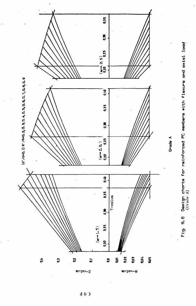
O)d

o

oTd

d«rduTd

doTdoTIoc

o

; o*

mO O

I

g

1io

IË!T)gfeU.c •g

o(4-0LC (L ÜD’5vW tC8'“= OC

(DODd)U.

en%DA-z ©niDA-y

4 03

doT

o

u

o

i

tn

m

o

oïm

"000

0•HX0T3C0(SL3Xau.

JZ*3•-4*(DLdEaEUQ.-OdÜL0U.cdLL0U-(0t)L u0i: oBu CCc QjCD T3cecod CQ

(O00

*u.

en%OA-z en%OA-y

4 1 0

in

«r pdifd

dciTd(f

§ ë S

0 (\I1

g S P O O PinS

■Dg

XO■DCO

gXo

f

IaEUQ.T»0üL0U.caLL0U.h2 - ü c

ê,é"W ^P(OCD

mü.

en%DA-z en%OA_y

4 1 1

ar>l. 0, 1. s, 2. 0, s.

I op“l. 0, i. 5» 2. 0»

R V R -1 .0 -------

R '/R -O . 5 —

Grodo A0.20 0.25 0,35

T-volue

0.02oc

0.03

0.0 i.

Fiq. 6.7 Interaction diagrame for columns mode of grade A-PC.

" 2

CHAPTER N INE

GENERAL CONCLUSIONS AND RECOMMENDATIONS

FOR FUTURE WORK

9.1. General

In this experimental study of PC structural performance, the

work was made to cover as wide a range of properties and

structural applications as possible. Mix design and its

optimization for resin mortars and PC were investigated with

the object of producing fairly representative properties

reproduceable at the lowest cost. Recognizing the importance

of the stress distribution of PC in flexure at ultimate

strength, the stress block shape and parameters were derived

experimentally and were expressed theoretically. Assessment of

short-term mechanical properties was carried out using full-

scale structural members made of reinforced PC. On comparing

the actual applied loads with the calculated ones the derived

properties and parameters of the different PC grades were

found to be reasonably accurate.

It was also found that time-dependency can reduce some of the

material merits as recorded on a short-term basis. Although

the long-term strength and the sustained strength,as defined

were up to 20% to 30% less than the short-term strength, it

was not found necessary to modify the short-term findings and

the deterioration in strength by creep was accounted for by

chosen magnitudes of factors of safety. A general ultimate

strength flexure theory was proposed and representative design

charts are provided.

The following represents the general conclusions that can be

4 1 3

drawn from this work.

9,2^ I:4DCluaions regarding mix-proportioning[1] PC mix-proportioning can be controlled at two levels,

either by controlling the individual bulk properties of the

various igredients or by controlling the synergetic properties

existing at the interfacial planes of these ingredients. PC/■ 'prope rites are related to the additive and synergetic

interactions of the different constituents on the macro and

micro-structure levels.

[2] The enhancement of PC properties by controlling the

individual bulk properties is the most economic and practical

approach. This can be achieved in several ways as follows :

(a) Aggregates and fillers must be carefully selected. It

does not make sense to use poor quality aggregates and fillers

with highly expensive resins used with the intention of

producing high quality concretes. The aggregates must have

gradings that provide minimum void ratios, the highest

possible degree of compaction, minimum surface areas and as high a maximum aggregate-size as possible. High quality

aggregates with good mineralogical properties should be used

to be compatible with the high strength that the polymeric

base-matrix usually offers.

(b) The fractional volumes of aggregates and fillers in the

mix should be as high as workability considerations will

allow. These materials in addition to being low cost filling

materials , play an essential role in the rheological

performance of PC. Fine powders when used with resin provide a

4 14

better-performance matrix with a lower coefficient of thermal

expansion, less setting microcracking and higher stiffness.

Aggregates provide the necessary restraining effect for

controlling creep in the sytem matrix.

(c) Moisture content in the aggregates must be limited to

prevent the presence of water leading to serious limitations

to the high performance of PC; an economic compromise must be

made between losses in performance and the costs of having

dried aggregates.

(d) The filler type must be the most compatible and its

content must be optimized for each specific resin and

aggregate; it is necessary to establish these clearly if a

proper mix-design is to be reached.

[3] For PC made with fine aggregates or for resin mortars ,

there exists an optimum surface area of the aggregates used

compatible with a given mixing ratio. A mix-design method

based on the fineness of the aggregates can be of great help

in mix-proportioning and in predicting strength.

[4] Elevated temperatures have a deleterious influence on the

performance of PC and only by enhancement of the properties of

the polymer matrix can these effects be avoided.

[5] The resin is the dominating constituent in the design of PC mixes. Strength of PC is directly proportional to the resin

content yet the structural performance of PC is reduced by

increased resin contents. For the structural use of PC, a

compromise has to be made between strength and stiffness by

controlling the resin content.

4 15

[6] Polyester resin type should be chosen to suit particular

applications, as cheap general-purpose resins may prove in the

long run to be more expensive than high cost specially-

formulated resins. Special resins that can provide desired

high chemical resistance, high weatherability and toughness

are available and are being continually developed by modifying

the types and ratios of acids used in the manufacture of

polyesters.

[7] Additives to the resin can greatly modify its reactivity and viscosity, and consequently can modify PC workability and

consistency. Unless it is absolutely necessary, no additives

other than the required catalysts and accelerators should be

employed. Before using these two, the optimum curing

temperature relevant to them has to be investigated if

efficient and economic use is to be made of them.

[8] The gel time, rate of polymerization and optimum amounts

of accelerators and catalysts should be found for PC

proportioning irrespective of the manufacturer's data on these

materials and the recommended amounts of the additives. This

is because all the data provided for the resin is altered by

the presence of aggregates and becomes very misleading.

[9] Workability of PC is as dependent on the mixing ratio asi

on the resin viscosity itself. However, Reducing the resin

viscosity by using compatible monomers like styrene, will have

unfavourable consequences in the form of increased reactivity

and rapid mix stiffening. Workability is more efficiently

improved by using well graded aggregates and fillers in

correct proportions. A ratio of coarse:fine aggregates of 4:5

4 13

with 10% filler content by weight appear to be reasonable

proportions from which the best performance/workability mix

can be reached through trial mixes.

[10] Casting troubles such as segregation and resin bleeding

are likely to happen if due attention is not given to mix

proportioning. Bleeding can be controlled by adjusting the

amount of the fine materials in the mix (fillers and fine

sand) and by special casting and vibrating techniques.

[11] Dry mixing of the mix ingredients is useful in producing

a uniform mix and in saving time and energy needed for mixing.

In addition the use of preaccelerated resins can have

considerable potential in mix handling where the possibility

of dangerous direct contact between accelerators and catalysts

can be avoided.

Q.3. Conclusions regarding the structural performance of PC

[1] For given materials the stiffness of PC is inversely

related to its compressive strength. Hence for proper

presentation of PC at least the compressive strength and the

modulus of elasticity have to be quoted.

[2] All strengths pertaining to a given PC grade ( shear,

tension, bond, etc.) are directly proportional to the

compressive strength while properties such as shrinkage, time-

dependent strains, micro and macrostrains and ultimate strains

are inversely proportional to the stiffness or modulus of

elasticity.

[3] Shear and bond strengths in PC are approximately the same

4 1 ?

ratios of compressive strength as in PCC. On average, shear

and bond strength are 10% and 12% of compressive strength

respectively.

[4] The stress-strain curve at all points in the compression

zone with a strain gradient , is different from the stress-

strain curve recorded under axial compression for the same PC

grade. In flexure, ultimate conditions occur at higher values

of strain than in axial compression.

[5] The method adopted in deriving the stress block shape and

parameters in flexure by using eccentrically loaded plane

prisms was effective. The stress block parameters as found

experimentally gave good a g reement with the actual

measurements of strains and loads for reinforced members at

all stages of loading up to failure. Those block parameters at

ultimate strength could be expressed empirically as functions

of the modulus of elasticity of each PC grade.

[6] A general sine function can express the stress-strain

curves for different PC grades in flexure. The constants of

that function Ko3 and are dependent only on the secant

modulus of elasticicty and can be calculated using the

equations given in Chapter Four. Knowing these constants and

the ultimate compressive strength f^y, the stress-strain curve

can be obtained up to any strain level, and can be of

considerable use in checking the serviceability limiting

states before ultimate strength is reached.

[7] The assumption of a linear strain profile in flexure was experimentally verified and was observed with all test

specimens which had a strain gradient, regardless of the type

4 18

of loading, ratio of reinforcement or specimen shape and size.

[8] Neglecting lateral confinement effects, and tension

stiffening effects not only simplifies the analysis and

design, but also does not lead to any significant inaccuracy

in the calculations.

[9] A theoretical value for the ultimate strain of PC can be taken as 4/3 times the macrocracking strain which can be

calculated using the empirical equation derived for it. This

expression of ultimate strain was proved to be conservative.

It should be noted that ultimate strains in PC are very much

higher than those of PCC and can range up to 0.01.

[10] Although PC can be made to set within a few minutes or

within a few days, its mechanical properties , unlike PCC,

stabilize relatively quickly and rate of strength development

becomes zero at relatively short ages. In addition, apart from

the thermal, chemical and physical shrinkages that occur

during polymerization, PC can be said to be a shrinkage-free

material at late ages. This can lead to considerable

simplification in the cal c u l a t i o n of t i m e - d e p e n d e n t

deformations under loading.

[11] Deviation of the stress-strain curve from linearity is

dependent on the stress level as much as on the rate of

loading itself. Faster rates of loading produce lower

microcracking strains at higher stress levels, and higher

ultimate strengths at lower macrocracking strains with lower

reserve carrying capacity. Slower rates of loading can reduce

the modulus of elasticity by as much as 20%.

4 1 9

[12] Long-term strength of PC can be of the order of 0.75 to

0.85 of the short-term strength. The long-term strength of PC

can be expressed in a power expression whose constants are

only dependent on PC grade itself.

[13] The creep response of PC can be estimated from creep

tests lasting for periods as relatively short as 60 days. The

effects of age at loading and shrinkage can be neglected for

PC tested in creep after complete curing.

[14] Although absolute values of creep strains for PC are much

higher than those of PCC at the same stress-level, specific

creep for both is comparable. The value of the creep

coefficient for PC is almost equal to that of PCC, and it

depends primarily on the stress level and on the mix

proportions ( resin content and aggregate fractional volume

and its properties).

[15] Creep of PC can be expressed as a general power function

of time irrespective of the stress level as effect of the

stress is embodied indirectly in the value of instantaneous

strain. The constants of these creep expressions depend only

on the grade of PC. The suggested creep expressions are valid

for any stress level that is low enough not to initiate time-

dependent failure.

[16] Unlike creep, creep recovery of PC tends to stop after

30-50 days of unloading depending on the stiffness of the PC

grade and the original stress level. The coefficient of creep

recovery k^ or instantaneous creep recovery as defined previously, is significantly smaller than unity. This

indicates the serious consequences which creep might have in

4 20

PC structures subjected to reversible or frequently recurrent

loads.

[17] The sustained strength of PC is smaller than the longterm strength and it is in the range of 60-70% of the short

term strength. Despite the high time-dependency of PC, there

was no need to modify the stress block shape and parameters

derived from short-term tests. This is mainly because of the

fact that stress redistribution due to creep in a reinforced

PC member will be such that no significant reduction in the

total ultimate capacity can take place. Based on previous

experience with PCC it was decided to take the less

advantageous creep and shrinkage properties of PC into account

only in the choice of the magnitudes of capacity reduction

factors. These factors range from 0.6 for flexure with axial

compression loads to 0.8 for pure flexure.

[18] The creep coefficient of PC could be expressed as a power function of time and can be satisfactorily used in calculating

the effective modulus of elasticity for each PC grade. The

importance of having such an effective value is that it can help derive the modular ratio often required in checking the serviceability of PC structures using any of the elastic or transformed section approaches.

[193 Mild steel with low yield strength of the order 250-350 N/mra2 should not be used with PC if efficient and economic use

of PC is to be obtained. For cold-drawn steel without a

definite yield point, the concept of under, over or balanced

reinforcement ratio does not apply and it was necessary to introduce an alternative a p p r o a c h based on s p e cific

4 2 1

reinforcement ratios which would allow prescribed strains at

ultimate conditions. Consequently, the mode of failure for

reinforced PC structures can be chosen, depending on the

reinforcement ratios, to be either ductile, with sufficient

warning deflections and cracking, or brittle with small

deflections and cracking.

[20] Rectangular PC cross-sections reinforced with high

tensile steel and subjected to normal forces, can be

categorised into sections with small or large eccentricity.

Small eccentricity sections are those having normal force

acting at a distance from the centroid of the tension steel

less than the effective depth and vice versa.

[21] The suggested design charts for reinforced PC members are

versatile, convenient to use and easy to construct. Using the

versatility of these charts, economical optimization of the

section can be achieved on the bases of the mutual areas of PC

and steel required for a given ultimate load.

Q .4. Conclusions regarding tiie economical feasabilitv of

reinforced PC structures

The construction cost items of PC can be briefly categorised

into the following; (a) material costs., (b) workmanship cost

and (c) maintenance cost. PC is a very expensive construction

material if the price is expressed on a volume basis. However,

the true assessment of costs for construction materials has to

be carried out on wider basis which includes the strength

produced per unit volume. For example, for an ultimate moment

of 600 KN.m, it can be shown that average quality PCC would

4 22

require a cross-sectional area twice that required by PC if

both sections were made with the same grade of steel and equal

reinforcement areas. This ratio can be shown to be more than

two, if the member considered is subjected to combined moment

and axial load. For columns with small eccentricity that ratio

of cross-sectional areas would increase more than for columns

with large eccentricity. The reduced area of PC cross-sections

would reduce the volume required for supporting given loads.

In pure flexure, for example, with cross-sectional area

reduction of 50%, the price of PC on volume/strength basis is

reduced by 50%. This is only one aspect that can justify the

cost of PC in construction. Another important feature is that

with reduced volumes of PC members, a considerable saving in

dead load can be gained and the load for which they are to be

designed is reduced accordingly. For example, if the above

mentioned value of ultimate moment results from 40% dead load,

the overall ultimate moment when using PC can be reduced by

20%. This saving in dead load would lead to further reduction

in the required cross-sectional area with a ratio less than

50%. Hence the evaluation of costs on a volume/strength basis

can partially justify the apparent high costs of the material

judged on a volume basis.

The labour costs required in making PC are comparable to those

of PCC. No special mixing, casting or vibrating techniques are

required for the processing although a few precautions are

required on site to ensure industrial safety. All the

experience accumulated in the processing of PCC is adaptable

to PC production. However as structural members made of PC are

4 2 3

usually lighter and stronger, costs of transportation and

errection involved in PC construction may be considerably

lower than those of PCC, and can therefore help reduce the

overall construction costs especially in precast applications.

The major justification for the use of the relatively

expensive PC in construction is by far maintenance costs. In

certain applications, the use of PC can have significant

potential. For example, PC can replace PCC in those parts of

structures where it is necessary to provide better freeze-thaw

resistance and better corrosion and abrasion resistances. This

can save the whole structure the disasterous situation in

which maintenace costs can be more than the construction

costs. Similarly PC when used in heavy duty industrial

floorings, bridge decks, irrigation structures and the like

can prove in the long run that they are not as expensive as

first thought.

The above are some of the features which should be considered

when assessing the economic potential of PC as a construction

material. Other features might arise such as the aesthetic and

decorative uses of PC in construction which can save some of

the finishing costs. Curing times of ordinary PCC can in some

cases be very expensive. PC can be made to cure within a few

hours and to support loads in remarkably short times. This can

be of great use in precasting operations or in other urgent

construction works.

9.5.Recommendations for future work

Despite the great amount of research devoted to the study of

PC, quite a few aspects pertaining to the efficient use of PC

424

in the construction industry remain to be explored. Based on

the previous work and on this work, the following aspects may

be recommended for future work :

[1] The response of PC to dynamic and/or loads likely to cause

fatigue is a feature which is most required for practical use

of PC.

[2] The thermo-dependent properties of PC and their possible

enhancement by the use of new versions of resins which are

being continuously improved. This could dramatically broaden

the structural use of PC.

[3] Standardization of different PC processing stages from the preliminary choice of mix ingredients up to casting is a field

of research which should be given due attention. No standard

techniques are accepted for mixing, vibrating, curing and

testing. The measurement of workability is so far a matter of

personal opinion.

In addition, shape and size of test specimens are at present

optional with the result that experimental observations vary

from one country to another, from one researcher to another

and the actual physical property of the material is lost in

between. For these reasons much of the work that has been done

on PC can not easily be related between different researchers.

[4] Study is required of the serviceability limiting states

and the possible compromise between them and the high ultimate

strength that PC can offer. In this respect, lateral

instability and buckling which are likely to occur with

limited cross-sectional areas of PC must be studied.

[5] Detailed study should be made of the economical

feasibility of PC in construction based on the various

features previously mentioned and through which PC may or may

not justify its use.

4 26

REFERENCES.

(1) Schorn, H., ” Theoretical comparison between resin

concrete, resin modified concrete and resin impregnated

concrete,” Proc. of the 4th International Congress on Polymers

in Concrete, ITW, Darmstadt W.G., Sep. 1984, pp. 3-11.

(2) Cresson, L., British patent No. 191, 474, Jan. 1923,

Ditmar, R., British patent No.214, 224, Mar. 1924; etc.

(3) Itakura, M ., ” Concrete pipes modified with vinyl

emulsion,” (in Japanese), Journal of the Japan Society for

Testing Materials, Vol. 2, No. 10, pp. 488-489.

(4) Ohama, Y., ”Development of concrete-polymer materials in

Japan,” Proc. of the 2nd International Congress on Polymers in

Concrete, College of Engineering, The University of Texas at

Austin, U.S.A., Oct. 1978, pp., 121-134.

(5) Teichmann, H ., ”Polymer dispersions for cement and

concrete,” Proc. of the 1st International Congress on Polymers

in Concrete, The Concrete Society, London, May 1 975, pp.112-

124.

(6) Harreus, ’’Synthetic resin dispersions as a mortar and

concrete admixture,” Proc. of the 1st International Congress

on Polymers in Concrete, The Concrete Society, London, May

1975, pp.125-130.

(7) De Vekey, R.C., ’’The properties of polymer modified cement

pastes,” Proc. of the 1st International Congress on Polymers

in Concrete, The Concrete Society, London, May 1975, pp. 97-

4 27

104.

(8) Bell, R.L. and Dingley, R.G., "The mechanical properties

of hydrated portland cement pastes modified with an SBR

polymer latex,” Proc. of the 1st International Congress, The

Concrete Society, London, May 1975, pp. 162-167.

(9) Hughes, B.P. and Guest, J.E., "Polymer modified fibre

reinforced cement composites,” Proc. of the 1st International

Congress on Polymers in Concrete, The concrete Society,

London, May 1975, pp. 85-92.

(10) Mangat, P.S., Baggot, R. and Evans, D.A., "Creep

characteristics of polymer modified concrete under uniaxial

compression,” Proc. of the 3rd International Congress on

Polymers in Concrete, Nihon University, Koriyama, Japan, May

1981, pp.193-208.

(11) Steinberg, M. and Dikeou, J.T., et. al., "Concrete

polymer materials - First Topycal Report,” Brookhaven National

Laboratory and U.S. Bureau of Reclamation, BNL No. 50134 (T-

509) and USBR Gen. Report 41, Dec. 1968.

(12) Dikeou, J.T. and Kukacka, L.E., et. al., "Polymerization

makes tougher concrete,” Journal of the American Concrete

Institute, No. 10, Proc. Vol. 66, Oct. 1969, 829 pp.

(13) "Polymers in concrete,” Report by the American Concrete

Institute, SP-40, Detroit, U.S.A., MI, 1973.

(14) "Polymers in concrete,” Report by the American Concrete

Institute, SP-58, Detroit, U.S.A., MI, 1978.

42 8

(15) "Concrete polymer materials- Fifth Topycal Report,"

Brookhaven National Laboratory and the U.S. bureau of

Reclamation.

(16) Dikeou, J.T., "Polymers in concrete: New construction

achievements on the horizon," Proc. of the 2nd International

Congress on Polymers in Concrete, College of Engineering, the

University of Texas at Austin, Oct. 1978, pp. 1-8.

(17) Bach, L., Hastrup, K. and Radjy, F., "Pore structure,

mechanical properties and polymer characteristics of porous

materials i m p r e g n a t e d with MMA," Proc. of the 1st

International Congress on Polymers In Concrete, The Concrete

Society, London, May 1975, pp. 43-53.

(18) Ohama, Y ., "Molecular weight of polymer formed in

polymer-impregnated concrete," Proc. of the 1st International

Congress on Polymers In Concrete, The Concrete Society,

London, May 1975, pp. 60-63.

(19) Rio, A. and Biagini, S., "Recent progress in the field of

P.I.e.," Proc. of the 1st International Congress on Polymers

In Concrete, The Concrete Society, London, May 1975, pp.14-21.

(20) S c h o r n , H ., "Limits in the m o d i f i c a t i o n of

characteristics by the trnsformation of cement concrete into

P.I.e.," Proc. of the 1st International Congress on Polymers

In Concrete, The Concrete Society, London, May 1975, pp. 31-

36.

(21) Manning, P.G. and Hope, B.B., "The role of polymers in

polymer impregnated paste and mortar," Proc. of the 1st

429



(22) Fowler, D.W. and Paul, D.R., "Status of conerete-polymer

materials in the U.S.A.," Proc. of the 3rd International

Congress on Polymers In Concrete, Nihon University, Koriyama,

Japan, May 1981, pp. 20-31.

(23) Valore, R.C. and Naus, D.J., "Resin bound aggregate

material systems," Proc. of the 1st International Congress on

Polymers In Concrete, The Concrete Society, London, May 1975,

pp. 216-222.

(24) Anonymous, "U.S. bridge dangers cited," ASCE News, June

1977, Vol. 2, No. 6.

(25) Fowler, D.W. and Paul, D.R., "Polymer concrete for repair

of bridge decks," Proc. of the 2nd International Congress,

College of Engineering, The University of Texas at Austin,

U.S.A., Oct. 1978, pp.338-350.

(26) Murai, N. and Mizuno, S., "Thermosetting plastics swelled

with grainy fillers," Review of the Electrical Communication

Laboratory, Vol. 9, No. 9-10, Sep.-Oct. 1961,pp. 581-588.

(27) Okada, K., Sakamura, A., Murai, N. and Sato, Y., "Resin

concrete," (in Japanese), Journal of the Society of Materials

Science, Japan, Vol.16, No. 167, Aug. 1967, pp.667-675.

(28) Okada, K . , K o y a n a g i , W. and Y o n e z a w a , T.,

"Thermo-dependent properties of polyester resin concrete,"

Proc. of the 1st International Congress on Polymers In

Concrete, The Concrete Society, London, May 1975, pp. 210-215.

4 30

(29) Okada, k. and Ohama, Y., "Status of concrete-polymer

composites in Japan," Proc. of the 3rd International Congress

on Polymers In Concrete, Nihon University, Koriyama, Japan,

May 1981, pp. 3-16.

(30) Staynes, B.W., "Epoxide resin concrete as a structural

material," Proc. of the 1st International Congress on Polymers

in Concrete, The Concrete Society, London, May 1975, pp. 340-

345.

(31) Johnson, P.P., "Glued joints for structural concrete,"

The Structural Engineer-Oct. 1963, "Creep tests on glued

joints," Conference of the Institution of Structural

Engineers, 1966.

(32) Staynes, B.W., "Epoxide resin concrete as a structural

material with special reference to the limit state design

philosophy," Ph.D. thesis. National Council of Academic

Awards, U.K., May 1972.

(33) Neville, A.M., Properties of concrete , Pitman

publishing ltd, 3rd edition 1981, pp. 33-35.

(34) Nutt, W.O., "The advancing concrete," Proc. of the 3rd

International Congress on Polymers In Concrete, Nihon

University, Koriyama, Japan, May 1981, pp.35-44.

(35) Fowler, D.W. and Paul, D.R., "Status of concrete-polymer

materials in the U.S.," Proc. of the 3rd International


Japan, May 1981, 30 pp.

(36) Ohama, Y., "Strength of polymer modified mortars using

431

Super High Early Strength cement," Proc. of the 1st



(37) Fukuchi, T. and Ohama, Y ., "Process technology and

properties of 2500 kg/cm2- strength P.I.C.," Proc. of the 2nd

International Congress on Polymers In Concrete, College of

Engineering, The university of Texas at Austin, Oct.1978,

pp.45-56.

(38) Katawaki, K. and Paul, D.R., "Effect of depth of polymer

impregnation and cracking on corrosion of reinforced steel,"

Proc. of the 3rd International Congress on Polymers In

Concrete, Nihon University, Koriyama, Japan, May 1981, pp.904-

917.

(39) Paturoev, V.V. and Fantalov, A.M., "Fundamentals of

polymer concrete structure formation and factory production

technology," Proc. of the 3rd International Congress on

Polymers In Concrete, Nihon University, Koriyama, Japan, May

1981, pp. 642-643.

(40) Czarnecki, H.L., "Introduction to material model of

polymer concrete," Proc. of the 4th International Congress on

Polymers In Concrete, ITW, Darmstadt, W.G., Sep. 1 984, p. 63.

(41) Watanabe, A. and Yamasaki, T., "Studies on hardening

shrinkage stress of resin concrete," Proc. of the 3rd

International Congress on Polymers In Concrete, Nihon

University, Koriyama, Japan, May 1981, pp. 437-439.

(42) Kobayashi, K. and Ito, T., "Several physical properties

4 32

of resin concrete," Proc. of the 1st International Congress on

Polymers In Concrete, The Concrete Society, London, May 1975, pp. 236-240.

(43) Fowler, D.W., Meyer, A.H. and Paul, D.R., "Law

temperature curing of polymer concrete," Proc. of the 4th

International Congress on Polymers In Concret, ITW, Darmstadt,

W.G., Sep. 1984, pp. 421-434.

(44) Depuy, G.W., "Applications of polymers in concrete in

the U.S.A.," Proc. of the 4th International Congress on

Polymers In Concrete, ITW, Dramstadt, W.G., Sep. 1 984, pp. 79-

82.

(45) Ohama, Y., "Recent research and development of concrete -

polymer composites in Japan," Proc. of the 4th International

Congress on Polymers In Concrete, ITW, Darmstadt, W.G., Sep.

1984, pp.21-26.

(46) Nutt, W.C., "Polymer concrete comes of age," Proc. of the

4th International Congress on Polymers In Concrete, ITW,

Darmstadt, W.G., Sep. 1984, pp. 37-43.

(47) Shaw, D.N., "Polymer concretes - U.K experience," Proc.

of the 4th International Congress on Polymers In Concrete,

ITW, Darmstadt, W.G., Sep. 1984, pp.85-87.

(48) Fontana, J.T., "Formulations and properties of PIC with

thermal conductivities of 0.08 to 0.12 Btu/hr-ft-F," Proc. of

the 4th International Congress on Polymers In Concrete, ITW,

Darmstadt, W.G., Sep. 1984, pp. 99-102.

(49) John, B.S. and Kane, F., "New applications of polymer

4 33

concrete in bridge and tunnel rehabilitation," Proc. of the

4th International Congress on Polymers In Concrete, ITW,

Darmstadt, W.G., Sep.1984, pp.447-450.

(50) Sakamoto, 0., "A new continuous spraying system for resin

mortar," Proc. of the 4th International Congress on Polymers

In Concrete, ITW, Darmstadt, W.G., Sep. 1984, pp.293-298.

(51) Tsuka, T. and Okada, T.,"Quick setting resin mortar for

small diameter tunnel lining," Proc. of the 4th International

congress on Polymers In Concrete, ITW, Darmstadt, W.G.,

Sep.1984, pp.195-200.

(52) Neville, A.M., Properties of concrete. Pitman

publishing ltd., 3rd edition 1981, pp.203-205.

(53) Ohama, Y., "Properties of polyester resin concrete with

various styrene contents," Proc. of the 20th Japan Congress on

Material Research, The Society of Materials Science , Koyoto,

Japan, 1977, pp.360-363.

(54) Fessenden, R. j. and Fessenden , J. S., The basis of

organic chemistry, Allyn and Bacon Inc., 1971, Chapter One.

(55) Bares, R.A., "Causes of polyester resin filler surfacing

system failures," Proc. of the 2nd International Congress on

Polymers in Concrete, College of Engineering, The University

of Texas at Austin, U.S.A, Oct. 1978, pp. 322-328.

(56) Ohama, Y. and Hamatsu, M., "Techniques for strength

improvement of polymer concrete made with wet aggregates,"

Proc. of the JCI 6th Conference, 1984, Japan Concrete

Institute , Tokyo(57) Lubin, G., Handbook of fibre glass and advanced Plastic

434

composites Polymer technology series, van Nostrand reinhold

company, 1969, Chapter Two.

(58) Shapiro, S.S. and Wilk, M.B., "An analysis of Variance

Test for normality," Biometrika, Vol. 52.

(59) B.S. 2846 Part 1; 1975.


publishing ltd., 3rd edition 1981, pp.653-665.

(61) Czarnecki, H.L., "Introduction to material model of

polymer concrete," Proc. of the 4th International Congress on

Polymers In Concrete, ITW, Darmstadt, W.G., Sep. 1 984, pp.59-

64.

(62) Bares, P., "Some basic features in mechanics of

inhomogeneous materials," Proc. of the 1971 International

Conference on Mechanical Behaviour of Materials, The Society

of Material Science, Japan, 1972, Vol. 5, pp.42-53.

(63) Gamski, K., "Resinous binder concrete," Proc. of the 1st


Society, London, May 1975, pp.223-229.

(64) Paturoev, V.V. and Fantalov, A.M., "Fundamentals of

polymer concrete structure formation and factory production

technology," Proc. of the 3rd International Congress on


1981, pp.638-648.

(65) Czranecki, H.L., "Expansive resin concrete : Some

fundemental questions," Proc. of the third International

4 35


Japan, May 1981, pp.744-754.

(66) Manson, J.A., Overview of current research on polymer

concrete materials and future needs. Application of PC, ACJ

SP-69, 1981, pp. 1-17.

(67) Solomatov, W.J., Approach of general building composite

material theory (in Russian), No. 8, 1980, pp.61-70.

(68) Gunasekaran, M. and Perry, E.R., "Polymer concrete for

high voltage electrical insulation," Proc. of the 2nd

International Congress on Polymers In Concrete, College of

Engineering, The University of Texas at Austin, U.S.A., Oct.

1978, pp.187-191.

(69) Ohama, Y., "Effect of coarse aggregate on compressive

strength of polyester resin concrete," , The International

Journal of Cement Composites, Vol.1, No. 3, 1979, pp.111-115.

(70) Demura, K., Ohama, Y. and Shinizu, A., "Proposed mix

proportioning of polyester resin concrete," Proc. of the 4th

International Congress on Polymers In Concrete, ITW,

Darmstadt, W.G., Sep. 1984, pp.265-269.

(71) Ohama, Y., "Determination methods for working life of

polyester resin concrete," Proc. of the 20th Japan Congress on

Material Research, Kyoto, Japan, 1977, pp. 173-175.

(72) Megahed, T.N., Polymers in concrete, M.Sc. thesis,

Alexandria University, Egypt, 1981, pp.178-186.

(73) Swamy, R.N., "Some engineering implications of design in

polymer concrete," Proc. of the 1st International Congress on

4 1 6

Polymers In Concrete, The Concrete Society, London, May 1975,

pp. 349-356.

(74) Mindess, S. and Young, J. F., Concrete, Civil

Engineering and Mechanics Series, 1981, pp. 453-468.


publishing ltd., 3rd edition 1981, p.545.

(76) Aguado de Cea, A., Martinez, A. and Salla, J.M., "Effects

of different factors in mixing and placing of polymer

concrete," Proc. of the 4th International Congress on Polymers

In Concrete, ITW, Darmstadt, W.G., Sep.1984, pp.299-303.

(77) Okada, K., Kobayashi, K. and Tukunaga, H., " Fundamental

studies on structural use of resin concrete ," Proc. of the

3rd International Congress on Polymers In Concrete, Nihon

University, Koriyama, Japan, May 1981, pp.538-552.

(78) Helal, M.S., Experimental study of mechanical properties

and structural applications of polymer concrete, Ph.D thesis

, Rice University 1981.

(79) Fowler, D., "Static and cyclic behaviour of polymer

concrete beams," Proc. of the 4th International Congress on

Polymers in Concrete, ITW, Darmstadt, W.G., Sep. 1984, pp.

159-164.

(80) Hognestad, E., "A study of combined bending and axial

load in reinforced concrete members," Bulletin No. 399,

University of Illinois Engineering Experiment Station, Urbana,

Nov. 1951, 128 pp.

(81) Ramaley, D. and Me Henry, D., "Stress-strain curves for

437

concrete strained beyond the ultimate load”, Laboratory Report

No. SP-12 , U.S. Bureau of Reclamation, Denver, Mar. 1947,

pp.23.

(82) Blanks, R.F. and Me Henry, D., "Plastic flow of concrete

relieves high-load stress concentrations," Civil Engineering,

Vol. 19, No. 5, May 1949, pp. 320-322.

(83) Gilkey, H.J., Discussion of a paper by V.P.Jensen, "The

plasticity ratio of concrete and its effects on the ultimate

strength of beams," ACI journal, Nov. 1943, Supplement, Proc.

Vol. 39, pp. 584-6 to 584-15.

(84) Hadley, H.M., "When concrete becomes discrete," Civil

Engineering, vol. 20, No. 4, April 1950, pp. 249-251.

(85) Hognestad, E., Hanson, N.W. and Me Henry, D., "Concrete

stress distribution in ultimate strength," Journal of the ACI,

Dec. 1955, Title No. 52-28.

(86) Baker, A.L.L., "Recent research in reinforced concrete

and its application to design," Journal of the Institute of

Civil Engineers, London, Vol.35, No.4, Feb. 1941, pp. 262-298.

(87) Herr, L.A. and Vandegrift, L.E., "Studies of compressive

stress distribution in simply reinforced concrete near the

point of failure," Proc. Highway Research Board, Vol.30, 1950,

pp.114-125.

(88) Brice, L.P., "Essaie de mesure des contraintes dans une

section flechie d’une poutre en béton arme," Publications,

International A s s o c i a t i o n for Bridge and S t r uctural

Engineering, Zurich, Vol. 10, Nov. 1950, pp. 19.

4 38

(89) Parme, A.L., Discussion of a paper by C.P. Siess,

"Review of research on ultimate strength of reinforced

concrete members," ACI Journal, June 1 952, Proc. Vol. 48, pp.

862-864.

(90) Prentis, J.M., "The distribution of concrete stress in

reinforced and prestressed concrete beams when tested to

destruction by a pure bending moment," Magazine of Concrete

Research, London, No. 5, Jan. 1951, pp. 73-77.

(91) Hamann, H., "Berechnung der Druckspannungs-kurve in

stahlbeton - Biegequer Schnitt," Schweizerische Bauzeitung,

Zurich, Vol.70, No. 44, Nov. 1, 1952,pp.629-630.

(92) Lee, L.H.N, "Inelastic behaviour of reinforced concrete

members subjected to short-time static loads," Proc. ASCE,

Vol. 79, separate No. 286, Sep. 1953, 26 pp.

(93) Rusch, H., "Research towards a general flexural theory

for structural concrete," Journal of the ACI, July I960, Title

No. 57-1, pp. 9-22.

(94) Imamura, K., Nakano, M. and Tsuji, K., "Reinforced resin concrete research in NTT," Proc. of the 3rd International


Japan, May 1981, pp. 572-583.

(95) Park, R. and Pauly, T., Reinforced concrete structures, A

Wiley-interscience publication, John Wiley and Sons, Inc.,

pp.479-482.

(96) Neville, A.M., Creep of concrete: Plain, reinforced and

4 3 9

prestressed, North-Holand publishing Company, Amsterdam, 1970,

25 pp.

(97) Neville, A.M.,"Role of cement in the creep of mortar,"

Journal of the ACI, Proc.55, 1959, pp.963-984.

(98) Freudenthal, A.M. and Roll, F., "Creep and creep recovery

of concrete under high com press ive stress," Journal of the

ACI, Proc.54, 1958, pp.1111-1142.

(99) Neville, A.M., Properties of concrete. Pitman publishing

ltd, 3rd edition 1981, pp. 281-284.



23 pp.



pp.258-271.

(102) Hansen, T.C., "Creep and stress relaxation of concrete,"

Swedish Cement and Concrete Research Institute, Stockholm,

Proc.31, I960, 112 pp.

(103) Lee, F.M. and Lee, C.R., "Shrinkage and creep in

concrete," The Society of Cemical Industry, London, Symp. on

The Shrinkage and Cracking of Cementive Materials, May 1946,

pp. 7-17.

(104) Lynam, C.G., Growth and movement in portland cement

concrete, London, Oxford University Press, 1934, 139 pp.

(105) Czarnecki, L., "Expansive resin concrete : Some

4 40

Fundamental questios," Proc. of the 3rd International congress

on Polymers In Concrete, Nihon University, Koriyama, Japan,

May 1981, pp.746-747.

(106) Putlajew, I. and Mychibowa, I., "Reducing shrinkage,

shrinkless and expansive Polymer concrete with FA monomer,"

Beton i Zhelezobeton, No. 9, 1973, pp. 29.

(107) Irtuganowa, S.M., "Polymer concrete mixture," USSR

patent 420, 591, 1972.

(108) Czarnecki, L. and Broniewski, T., "Resin concrete and

polymer impregnated concrete; A comparative study," Proc. of

the 3rd International congress on Polymers In Concrete, Nihon


(109) Bailey, W.J, "Synthesis of monomers that expand on

polymerizatio," Journal of Elastoplastics, Vol.5, No. 3, July

1973, pp. 142-151.

(110) Ohama, Y. and Komiyama, M., "Early strength and length

change of polyester resin concrete with shrinkage reducing

agent," Proc. of the 22nd Japan Congress on Materials

Research, The Society of Materials Science, Kyoto, 1979, pp.

356-359.

(111) Davydov, S.S., Chebanenko, A.I., Fantalov, A.M. and

Kluckin, V.I., "Armoured polymeric concrete bearing structures

for industrial construction," Proc. of the 3rd International

congress on Polymers In Concrete, Nihon University, Koriyama,

Japan, May 1981, pp 836-839.

(112) Watanabe, A. and Yamasaki, T., "Studies on hardening

4 41

shrinkage stress of resin concrete," Proc. of the 3rd

International congress on Polymers In Concrete, Nihon


(113) Koyanagi, W ., Murai, N., Hayashi, F. and Ohno, S.,

"Stresses in reinforcement and in polyester resin concrete

generated by setting shrinkage," Proc. of the 3rd

International congress on Polymers In Concrete, Nihon


(114) Broniewski, T., Jamrozy, Z. and Kapko, J., "Long life

strength polymer concrete," Proc. of the 1st International

congress on Polymers In Concrete, The Concrete Society,

London, May 1975, pp.179-184.

(115) Macleod, A.A., Ind. Eng. Chem., Vol.47, 1319, 1955.

(116) Helal, M.S., Experimental study of mechanical

properties and structural applications of polymer concrete,

Ph.D thesis. Rice University 1978, pp.45-49.



pp. 92.

(118) Ohama, Y ., "Creep of resin concrete and polymer

impregnated concrete," Proc. 17th Japan Congress on Material

Research, 1974, pp.140-143.

(119) Ayyar, R.S. and Deshpande, S.N., "Creep studies on

polymer mortars," Proc. of the 3rd International congress on


1981, pp.504-522.

4 X2

(120) CEE; "Recommendations for an International Code of

Practice for reinfoerced concrete," Comité Européen du Beton (

CEB ), Paris, 1964 [ English translation available from Cement

and Concrete Ass., London, 156 pp.]

(121) ACI Committee 318, "Building Code Requirements for

reinforced concrete (ACI 318-32,33) .

(122) Rusch, H., Research towards a general flexural theory

for structural concrete," ACI Journal, Vol.57, No. 1, July

I960, pp.1-28, Discussion in Journal ACI, Vol. 57, No. 9,

March 1961, pp. 1147-1164.

4 4 3

10991717.pdf - Enlighten: Theses

Documents

Transcript of 10991717.pdf - Enlighten: Theses