Geosciences 2022, 12, 135. https://doi.org/10.3390/geosciences12030135 www.mdpi.com/journal/geosciences

Article

Extreme Sea Surges, Tsunamis and Pluvial Flooding Events

during the Last ~1000 Years in the Semi-Arid Wetland,

Coquimbo Chile

Karen Araya 1,2,*, Práxedes Muñoz 3,4, Laurent Dezileau 2, Antonio Maldonado 4,5, Rodrigo Campos-Caba 6,

Lorena Rebolledo 7,8, Paola Cardenas 9 and Marcos Salamanca 9

1 Laboratoire Geosciences, CNRS, UMR 5243, Université Montpellier, 34000 Montpellier, France 2 Laboratoire de Morphodynamique Continentale et Côtière, UMR CNRS 6143 M2C, Université de

Caen-Normandie, 14200 Caen, France; laurent.dezileau@unicaen.fr 3 Departamento Biología Marina, Facultad de Ciencias del Mar, Universidad Católica del Norte,

Coquimbo 1780000, Chile; praxedes@ucn.cl

4 Centro de Estudios Avanzados en Zonas Áridas—CEAZA, Universidad de la Serena,

La Serena 1700000, Chile; antonio.maldonado@ceaza.cl 5 Instituto de Investigación Multidisciplinario en Ciencia y Tecnología, Universidad de La Serena,

La Serena 1700000, Chile 6 Escuela de Ingeniería Civil Oceánica, Universidad de Valparaíso, Valparaíso 2340000, Chile;

rodrigo.campos@uv.cl 7 Instituto Antártico Chileno (INACH), Plaza Muñoz Gamero 1055, Punta Arenas 6210445, Chile;

lrebolled@inach.cl 8 Centro IDEAL (Centro de Investigación Dinámica de Ecosistemas Marinos de Atlas Latitudes), Universidad

Austral de Chile, Punta Arenas 6210445, Chile 9 Departamento de Oceanografía, Facultad de Ciencias Naturales y Oceanográficas, Universidad de

Concepción, Concepción 4030000, Chile; p.cardenas888@gmail.com (P.C.); msalaman@udec.cl (M.S.)

* Correspondence: karen.araya-flores@unicaen.fr

Abstract: The coast of Chile has been exposed to marine submersion events from storm surges,

tsunamis and flooding due to heavy rains. We present evidence of these events using sedimentary

records that cover the last 1000 years in the Pachingo wetland. Two sediment cores were analyzed

for granulometry, XRF, pollen, diatoms and TOC. Three extreme events produced by marine sub-

mersion and three by pluvial flooding during El Niño episodes were identified. Geochronology was

determined using a conventional dating method using 14C, 210Pbxs and 137Cs). The older marine

event (E1) was heavier, identified by a coarser grain size, high content of seashells, greater amount

of gravel and the presence of two rip-up clasts, which seems to fit with the tsunami of 1420 Cal AD.

The other two events (E3 and E5) may correspond to the 1922 (E3) tsunami and the 1984 (E5) storm

waves, corroborated with a nearshore wave simulation model for this period (SWAM). On the other

hand, the three flood events (E2, E4, E6) all occurred during episodes of El Niño in 1997 (E6), 1957

(E4) and 1600 (E6), represented by layers of fine-grain sands and wood charcoal remains.

Keywords: extreme events; tsunami deposit; flood events; storm deposits; wetland areas;

Coquimbo; Chile

1. Introduction

Chile has been frequently affected by extreme telluric events such as large-scale

earthquakes and tsunamis or extreme meteorological events such as storms and heavy

rains. The latest significant extreme telluric events are (i) three more significant earth-

quakes: in Valdivia in 1960, with a magnitude of 9.5° Mw; (ii) in El Maule in 2010, with a

magnitude of 8.8° Mw; and (iii) in Illapel in 2015, with a magnitude of 8.3° Mw. In all

cases, a tsunami occurred a few minutes later [1–6]. The one that has caused the most

Citation: Araya, K.; Muñoz, P.;

Dezileau, L.; Maldonado, A.;

Campos-Caba, R.; Rebolledo, L.;

Salamanca, M. Extreme Sea Surges,

Tsunamis and Pluvial Flooding

Events during the Last ~1000 Years

in the Semi-Arid Wetland,

Coquimbo Chile. Geosciences 2022,

12, 135. https://doi.org/10.3390/

geosciences12030135

Academic Editors: Markes E.

Johnson, Efim Pelinovsky and Jesus

Martinez-Frias

Received: 26 November 2021

Accepted: 9 March 2022

Published: 14 March 2022

Publisher’s Note: MDPI stays neu-

tral with regard to jurisdictional

claims in published maps and institu-

tional affiliations.

Copyright: © 2022 by the authors. Li-

censee MDPI, Basel, Switzerland.

This article is an open access article

distributed under the terms and con-

ditions of the Creative Commons At-

tribution (CC BY) license (https://cre-

ativecommons.org/licenses/by/4.0/).

Geosciences 2022, 12, 135 2 of 30

human and economic losses is the 1960 tsunami, in Chile alone, it caused the death of 1700

people, 3000 wounded, 2,000,000 homeless victims. reflecting in an economic loss of 550

million dollars (CIGIDEN: Centro de Investigación para la Gestión Integrada del Riesgo

de Desastres/Chile). In the 2015 tsunami, in Coquimbo, deposits with a thickness that var-

ies between 10 and 50 cm were observed [7]. The latest extreme meteorological events

were (i) 21–22 May 1957, with rainfall of 77.4 mm per month affecting La Serena city. There

were overflows of the Elqui river, and more than 200 people were affected by the flood;

the main routes were cuts, and two people died. (ii) 11 June 1997, rainfall of 104.9 mm per

month. This time the rain was accompanied by hail, thunderstorms and winds of 90–100

km per hour. It caused the activation of two streams that devastated eight houses and

caused the death of two people (/https://explorador.cr2.cl/ (access date: 20 October 2021)).

(iii) 22 January 2015, which produced mudslides affecting the three most extensive areas of

northern Chile in the pre-mountain range sectors, leaving half of Copiapo city (Atacama

region) buried under ~2 m of mud, with a high human and economic cost of $1500 million

dollars (MINVU-Chile [7–9].

The latest tsunami events to have affected the Coquimbo region occurred in 1730,

1880, 1922, 1943 and 2015, after large ruptures of the fault line [2,10–20]. Of these, the most

destructive according to historical records occurred in 1922, which affected 400 km of

coastline from the Atacama to the Coquimbo regions (27–30° S) [16,20–22] and caused

extensive damage in an area stretching approximately from Caldera to Coquimbo (27–30°

S). More than 1000 deaths resulted from the earthquake, and the tsunami killed hundreds

of people in coastal areas, mostly in Coquimbo. The range of total damage was estimated

to be 5–25 million USD [23]. Other marine events affecting the coastal area have been the

great wave storms. The main events occurred on 10 August 1965, 10 July 1984, and 8 Au-

gust 2015, causing damaged coastal infrastructure and eroding beaches and dunes [24–

26]. They were categorized as M4 to M5, according to the official wave intensity scale

(https://marejadas.uv.cl/index.php/categorias/folleto-categorias (access date: 23 July

2021)), or 6 to 7 on the scale proposed by Campos-Caba (2016) (/https://oleaje.uv.cl/mare-

jadas.html (access date: 5 October 2021)). These categories indicate “the evacuation of the

coast is imminent, the structures are severely damaged or destroyed, the persistent over-

pass generates flows in walks and streets, causing significant damage or destruction of

properties”.

Therefore, Coquimbo has experienced numerous extreme coastal events, caused by

meteorological conditions as well as tsunami events. These have caused casualties and

economic damages [27,28], and thus it is necessary to study the frequency and intensity

of past events to predict future trends, determine their frequency and prevent risks. How-

ever, historical records and meteorological data limit the analysis to only a few centuries

[29,30]. Rainfall is recorded by the General Directorate of Water (DGA; https://explora-

dor.cr2.cl/, access date: 20 October 2021), and for the Pachingo wetland, the data have been

collected since 1930. In the case of storms, wave record data have been collected since 1823

(Campos-Caba et al., 2016/https://oleaje.uv.cl/marejadas.html, access date: 20 October

2021; https://marejadas.uv.cl/, access date: 20 October 2021) and tsunami records for some

centuries, since 1562, although the oldest records are based only on historical records in

habited areas (https://www.proteccioncivil.es/catalogo/naturales/jornada-maremo-

tos/documentacion/docu2.pdf/, access date: 20 October 2021; CERESIS: Regional Seismol-

ogy Center for South America. Catalogue of Earthquakes for South America. 1985;

NOAA/ https://www.ngdc.noaa.gov/hazel/view/hazards/tsunami/event-data?max-

Year=2015&minYear=1200&country=CHILE, access date: 20 October 2021). Tsunami rec-

ords begin after the Spanish invasion in 1535 [20]. Meanwhile, geological records contrib-

ute to the reconstitution of climatic weather events, intense storms and tsunami activity

at a longer scale [30]. In this sense, there are other environments with similar suitability

for such studies in coastal areas are wetlands with sandy barriers. These natural environ-

ments have been highly affected by changes in water inputs controlled by the amount of

precipitation and by the geo-morphological alterations of the basin and coast, caused by

Geosciences 2022, 12, 135 3 of 30

the sea-level changes, tidal waves, tectonic movements, tsunamis and flooding events [31–

35]. These changes can be observed in the sediment stratification because there is scarce

post-depositional remobilization due to the roots’ mechanical action, which retains the

organic and clayey particulate material [36,37]. The interpretation of proxies in these sed-

imentary environments is relevant to establishing meteorological events and extreme sea

events of the past [31,38,39]. The identification of different depositional environments

formed by the recurrence of overwash layers and associated contents allows the recon-

struction of marine paleo-events [31,32,35,39–52]. In this study, we reconstruct past ex-

treme sea events (storm waves or tsunamis) and pluvial flooding events (extreme rains)

using a multiproxy analysis based on sedimentological, biological and geochemical data

in the Pachingo wetlands. In these sediments, we analyzed wood charcoal and carbonates

for the age estimations. In addition, a swam model was used to understand how storms

waves affect the coastal area of the Pachingo wetlands. Results were then compared with

the historical extreme sea event records available at Pachingo to identify the events that

may have reached or submerged the sites.

2. Study Area

Pachingo’s wetland (30°18′36.00″ S; 71°34′17.21″ W) is near to Tongoy Bay in the Co-

quimbo region, Chile. It is a glacio-eustatic bay formed by the abrasive action of the suc-

cessive interglacial transgressions that occurred during the Quaternary [53,54]. These

movements formed the stepped littoral marine terraces, caused by coastal elevation,

where three wetlands were formed—Salinas Chicas, Salinas Grande and Pachingo—with

a progradation rate of ca. 0.14 m [14,32,55]. The Coquimbo region is a semi-arid zone,

strongly affected by the warm phase of El Niño Southern Oscillation (ENSO) when rainfall

increases strongly compared to neutral periods or during the cold phase of La Niña. It

causes streams to grow that generally are dry or have low flows [56–58]. The intense flood

events recorded by the Meteorological Directorate of Chile are from 1957, 1965, 1972, 1987,

1991, 1992, 2015 and 2017, all of which were related to the El niño phenomenon [56]. The

wetland has a permanent shallow stream and is separated from the sea by a dune barrier

[55,59,60], which disappears in cases of heavy rains that generate large floods, being tem-

porarily connected to the sea [61,62]. The creeks are fed by the runoff from small river

inputs (Elqui and Limari), groundwater flow and precipitation in the basin [61–63]. Stud-

ies in different terrace levels of the Pachingo’s ravine [55] showed evidence of the occur-

rence of torrential rivers in several periods during the mid-to-late Holocene, and repeated

tectonic elevation of the coastal segment occurred during the Holocene [32].

The wetland’s total area is ~0.3 km2, and it is at a height of 0.5 to 1.0 MSL (mean sea

level). The climate is characterized by high humidity (85%), the temperature varies be-

tween 11–22 °C, and the annual temperature average is 14.7 °C. Precipitation is concen-

trated in the winter months (May to August), and it does not exceed 75 mm per year (an-

nual average last 10 years: 90 a 100 mm) except during El Niño (200 to 400 mm) [56–59,64].

3. Methodology

Sediment cores PT1 (50 cm long) and PT4 (47 cm long), were obtained in 2014 in the

Pachingo wetland at ~850 m and 920 m from the coastline, respectively—an area currently

flooded by tsunamis [1] (Figure 1). The core was obtained with a manual core under 20

and 50 cm of water depth, respectively. X-rays were taken for the PT1 core in the San Juan

de Dios Hospital of La Serena, Chile, performed with the methodology used for femur

and spinal column inspection. Then, the cores were sectioned every 1 cm, and the samples

were stored in sterilized Whirlpak® bags, frozen and subsequently freeze-dried.

Geosciences 2022, 12, 135 4 of 30

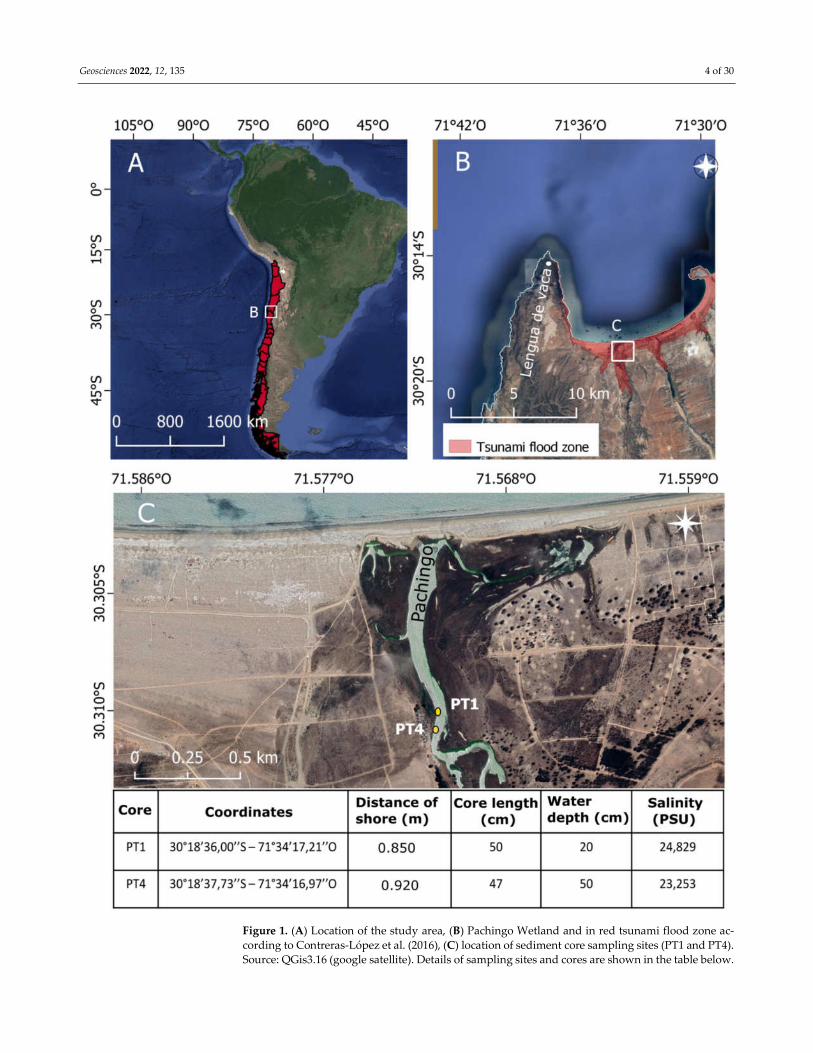
Figure 1. (A) Location of the study area, (B) Pachingo Wetland and in red tsunami flood zone ac-

cording to Contreras-López et al. (2016), (C) location of sediment core sampling sites (PT1 and PT4).

Source: QGis3.16 (google satellite). Details of sampling sites and cores are shown in the table below.

Geosciences 2022, 12, 135 5 of 30

Visual stratigraphic examination was conducted for both cores. The PT1 core was

analyzed for sedimentology (grain size, Kurtosis and Skewness, magnetic susceptibility),

geochemistry (elemental composition, TOC, biogenic opal, 15C,13N) and biological proxies

(Diatoms and pollen). Diatoms and pollen were identified, and their abundance was esti-

mated. The Geochronology analyses 137Cs, 210Pb and 14C were used. The core PT4 was only

analyzed for granulometry and geochemistry to compare the events identified at both

cores.

3.1. Lithology and Stratigraphy

The lithological units were visually characterized according to the Munsell chart

scale, X-rays, granulometry and the types of contact between units. These units were rep-

resented with a schematic log. Magnetic susceptibility (SI × 10−8) was measured with a

Bartington Susceptibility Meter MS2E in the Sedimentology Laboratory at Centro Eula,

Universidad de Concepción. Samples were measured three times, and the values were

expressed as mean values.

The grain size was determined using a Beckman–Coulter LS13320 laser diffraction

particle size analyzer (Géosciences Montpellier Laboratory, Montpellier, France). The

analysis was carried out in each centimeter, considering particles <2 mm in diameter using

a sieve. The particle sizes were classified according to the scale of Folk and Ward (1957).

Sorting, skewness and kurtosis were evaluated using the GRADISTAT statistical soft-

ware using the method moments logarithmic according to Blott and Pye, (2001); which

includes all particle size spectra.

In addition to laser particle size analysis (<2 mm), we performed sieve analyses (0.63,

0.08, 0.1, 0.125, 0.16, 0.2, 0.25, 0.315, 0.4, 0.5, 0.63, 0.8, 1, 1.25, 1.6, 2, 2.5, 3.15, 4, 5 and 6.3

mm) to specify more specifically the distribution of particles greater than 2 mm on two

key samples (E1 and E5). However, no statistical analysis was performed on this coarser

fraction.

3.2. Geochemical Characterization

Elemental analyses were performed by X-ray fluorescence (XRF) spectrometry for

each centimeter on the surface of the PT1 core using a hand-held Niton XL3t spectrometer

(pXRF; CRAHAM laboratory, Université de Caen-Normandie, Caen, France). The analy-

sis considered Ba, K, Rb, Sr, Ca, P, Mg, Mn, Zr, Fe, Zn, Ti, Ni and V. Principal Components

Analysis (PCA) was used to identify correlated variables between geochemical poles us-

ing the XLStat Program and to identify the most representative element of each geochem-

ical family.

3.3. Geochronology

Radiochronological data for the last century were obtained using 210Pbxs (activity “in

excess” or unsupported) on 22 selected samples along the PT1 core. This method consists

of evaluating 210Po, in secular equilibrium with 210Pb. The 210Po activities were quantified

by alpha spectroscopy using a CANBERRA QUAD alpha spectrometer (model 7404) until

obtaining an adequate statistical count (~4–10%, error). The chemical procedure consid-

ered the digestion of ~0.5 g of sediment with concentrated acids in the presence of a chem-

ical tracer (209Po, 2.22 dpm g−1) and the plating on silver discs 99.9% pure for 3 h at ~75 °C

according to Flynn (1968). The alpha counting was performed at the Oceanography De-

partment of Universidad de Concepción, Chile.

Geochronology was then established based on excess activities following the CRS

method described by McCaffrey and Thomson (1980); details are described in Muñoz and

Salamanca (2003). Additionally, 137Cs measurements were quantified with a BEGe 3825

gamma spectrometer at Géosciences Montpellier Laboratory (Montpellier, France).

Radiocarbon measurements were performed to obtain older ages (>200 years) on five

estuarine snail shells (Heleobia sp.) and one sample of wood charcoal obtained from PT1

Geosciences 2022, 12, 135 6 of 30

core. The samples were dated using conventional 14C-AMS measurements submitted to

the DirectAMS (Radiocarbon Dating Services; directams.com, access date: 20 October

2021). The dates obtained were calibrated using the marine 20.14C calibration curve for

shell samples and Shcal20.14C curve for southern hemisphere 14C dates for wood char-

coal [65,66]. The dates obtained from shells were adjusted with the three reservoir ages

calculated for the area (Table 1).

Table 1. Radiocarbon details and resulted ages on shells (Heleobia sp.) and wood charcoal from the

PT1 core. The dates obtained for the snail shells were calibrated using Calib 8.20, and the marine

20.14C curve, testing three reservoir ages (a, b and c); for wood charcoal age, it was calibrated using

the Shcal20.14C curve [65,66].

Fraction Modern 14C Age Age Calib

ID Material Section Lab Code pMC 1σ Error BP 1σ Error BC/AD BC/AD BC/AD BC/AD

Core cm DirectAMS 210Pb ΔR 625 ± 46 a ΔR 165 ± 107 b ΔR 442 c

PT1 Shell 1 D-AMS

009072 94.27 0.29 474 25 2010 invalid age invalid age

invalid

age

PT1 Shell 8 D-AMS

009060 87.62 0.26 1062 * 24 1986 invalid age 1468–1700 1832–1950

PT1 Shell 23 D-AMS

009061 76.14 0.22 2190 * 23 - 901–1072 403–658 729–871

PT1 Wood

charcoal 24

D-AMS

013087 96.68 0.34 271 28 - 1640–1671 1640–1671 1640–1671

PT1 Shell 36 D-AMS

009063 74.59 0.27 2355 * 30 - 726–902 199–491 580–700

PT1 Shell 49 D-AMS

009064 80.56 0.28 1736 * 28 - 1336–1468 858–1129 1205–1324

* reverse ages: observed in extreme event deposits; a Ortega et al., 2019; b Carré et al., 2016; c

Muñoz et al., 2020.

3.4. Biogenic Components in the Sedimentary Records

Diatoms and pollen are relevant tools to reconstruct the environmental and meteor-

ological variability of the past [67–75]. For the determination of diatoms, 500 mg of freeze-

dried sediments were used. The samples were oxidized and mounted following the meth-

odology of Rebolledo et al. (2005). The clean samples were observed under a Carl Zeiss

microscope at 400 and 1000× using a contrast phase. Fragments containing more than half

a valve were included in the count. Diatoms were identified to the lowest taxonomic level

and were grouped by fresh water, brackish and marine species following [76–78]. The

counts were expressed as diatom valves g−1. Biogenic opal was determined as SiOPAL (%)

according to Mortlock and Froelich (1989), and the values were estimated with a precision

of ±0.5%. All laboratory and microscopy work was performed in the Paleoceanography

Laboratory at the University of Concepción.

The samples for palynological determination were carried out according to the stand-

ard protocols for terrestrial sedimentary samples, including a treatment with 10% KOH

solution and the dissolution of the carbonates with 5% HC. The silica-clastic fraction was

dissolved with a concentrated HF solution, and the cellulose was removed with an Ace-

tolysis reaction [79]. The samples were mounted with glycerol and permanently sealed

with paraffin wax. These were analyzed using a light microscope at 40× magnification.

The identification of the palynological samples was performed with the assistance of the

reference samples housed in the Paleoecology laboratory of the Center for Advanced

Studies in Arid Zones (CEAZA) and based on the Catalog published by Heusser (1971).

The pollen count considered between 10 and 300 terrestrial grains, depending on the

abundance of pollen in each sample. The counts were expressed as grains g-1. Abundant

changes of each taxon were expressed in percentage values. The pollen percentage from

Geosciences 2022, 12, 135 7 of 30

aquatic species and ferns was calculated for the total of the terrestrial taxa. The percentage

diagrams were developed with the Tilia version 2.04 software (E. Grimm, Illinois State

Museum, Springfield, IL, USA).

3.5. SWAN Model

The open-source numerical model SWAN (Simulating Waves Nearshore), developed

by the Delft University of Technology, was used to propagate the waves from deep waters

and understand the impact of waves on the coastline. SWAN is a third-generation phase-

averaged numerical wave model that simulates the effects of refraction, diffraction, break

due to slenderness and bottom influence, wind effects, wave–wave interaction and white

capping in coastal regions and inland waters [80]. The model solves the spectral action

balance equation, allowing the calculation of the wave spectrum evolution in a time/space

domain from which statistical parameters of a sea state can be determined [81].

The wave conditions of propagation were evaluated considering the peak values of

the significant wave height (Hs) in deep waters, with the associated peak period (Tp) and

peak direction (Dp). These variables were considered for the evaluation of events identi-

fied on 5 and 10 July 1984 (Figure 2). The parameters in deep waters are specified in Table

2. The statistics of waves in deep waters were obtained from the database of the project

“Un Atlas de Oleaje para Chile” [82]. The deep-water wave statistics used were generated

with the Wavewatch III v.4.18 model in the high-performance cluster of the Center for

Mathematical Modeling of the University of Valparaíso (CIMFAV).

Table 2. Wave parameters in deep water for SWAN model propagation. Hs: wave height, Tp: peak

period, Dp: peak direction.

Date Hs [m] Tp [s] Dp [°]

5 July 1984 5.67 14.8 232.5

10 July 1984 4.87 9.2 322.5

Geosciences 2022, 12, 135 8 of 30

Figure 2. (A) Wave conditions at deep water (5.67 m) from 28 June to 11 July 1984 and (B) wave

conditions at deep water (4.87 m) from 9 July to 20 July 1984. Hs: wave height, Tp: peak period, Dp:

peak direction. The point is −31, −73 (https://oleaje.uv.cl/descargas.html,access date: 20 October

2021). The data come from the Universidad Valdivia wave atlas database, which is a hindcasting

(reconstruction) of wave conditions.

Regarding the configuration of the SWAN model, three structured calculation

meshes were used with resolution elements of 300 × 300 (m), 100 × 100 (m) and 20 × 20

(m), reducing in size toward the coast to obtain greater precision in the area of interest.

Bottom friction and dissipation due to breakage were not considered in the modeling to

maintain a conservative criterion for estimating wave heights at the site of interest.

Geosciences 2022, 12, 135 9 of 30

4. Results

4.1. Lithostratigraphic Description

The core PT1 has six units presented with a schematic log named from E1 to E6 (Fig-

ure 3). The deposits exhibited significant differences in texture, color and composition; the

presence of shell remains and very coarse sand in the base of the core (identified as E1)

was evident compared to the other units. In general, the thicker sand deposits were iden-

tified in units E1, E3 and E5 from medium sand to very coarse sand. According to the

Munsell color scale, these layers varied from very dark gray (2.5Y 3/1) to dark gray (2.5Y

4/1). These three deposits (E1, E3 and E5), are generally nominated by a high density (>1.5

g/cm3), a decreasing trend of skewness (Coarse skewed <0.3), kurtosis (Platykurtic <2) and

magnetic susceptibility. The three deposits present an erosive contact surface with the de-

posits that delimit them (Figure 4A, Table 3).

Table 3. Sedimentological characteristics of meteorological event deposits along the PT1 and PT4

cores.

ID ID Section Sorting

Contact Munsell

Color Scale Other Characteristics

Core Unit cm Upper Basal

PT1 E1 30–50 Moderately sorted

Very poorly sorted * Sharp - 2.5Y 4/1

High content of gravel, angu-

lar fragments of seashell, sea-

shell and two rip-up clasts (30

and 40 cm)

PT1 E2 20–22 Poorly sorted Relatively sharp Sharp 2.5Y 2.5/1 High content of roots, wood

charcoal and estuarine shell

PT1 E3 16–19 Well sorted Relatively sharp Relatively sharp 2.5Y 4/1 High content of gravel and

fragments of angular seashell

PT1 E4 10–12 Poorly sorted Sharp Slightly sharp 2.5Y 2.5/1

High content of roots, round

gravel, wood charcoal and es-

tuarine shell

PT1 E5 4–8 Moderately well

sorted Relatively sharp Sharp 2.5Y 4/1

High content of gravel and

seashell fragments

PT1 E6 2–3 Moderately sorted gradational Relatively sharp 2.5Y 3/1 High content of roots and es-

tuarine shell

PT4 E1 22–47 Poorly sorted Sharp - 2.5Y 4/1

High content of gravel, angu-

lar fragments of seashell and

seashell

PT4 E2 17–20 Very poorly sorted Relatively sharp Sharp 2.5Y 2.5/1 High content of roots, wood

charcoal and estuarine shell

PT4 E4 6–8 Poorly sorted Slightly sharp Slightly sharp 2.5Y 2.5/1 High content of roots and es-

tuarine shell

PT4 E5 3–5 Poorly sorted Relatively sharp Sharp 2.5Y 4/1

High content of gravel, angu-

lar fragments of seashell and

seashell

PT4 E6 1–2 Poorly sorted Gradational Relatively sharp 2.5Y 2.5/1

Presence of gravel, angular

fragments of seashell, seashell

and fish bones

* 40 cm Rip-up clast.

Geosciences 2022, 12, 135 10 of 30

Figure 3. Lithologic diagram of PT1 core units (C: clay, S: silt, FS: fine sand, MS: medium sand, CS:

coarse and very coarse sand), X-ray, photographic records of each lithologic unit and details of sed-

iment composition in each deposit considered as events. Rip-up clasts are highlighted in unit 1 and

wood charcoal fragments in units 2 and 4. Seashells are present in units 1, 3 and 5.

Geosciences 2022, 12, 135 11 of 30

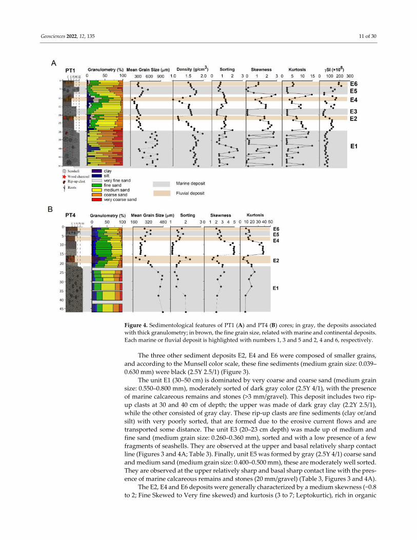
Figure 4. Sedimentological features of PT1 (A) and PT4 (B) cores; in gray, the deposits associated

with thick granulometry; in brown, the fine grain size, related with marine and continental deposits.

Each marine or fluvial deposit is highlighted with numbers 1, 3 and 5 and 2, 4 and 6, respectively.

The three other sediment deposits E2, E4 and E6 were composed of smaller grains,

and according to the Munsell color scale, these fine sediments (medium grain size: 0.039–

0.630 mm) were black (2.5Y 2.5/1) (Figure 3).

The unit E1 (30–50 cm) is dominated by very coarse and coarse sand (medium grain

size: 0.550–0.800 mm), moderately sorted of dark gray color (2.5Y 4/1), with the presence

of marine calcareous remains and stones (>3 mm/gravel). This deposit includes two rip-

up clasts at 30 and 40 cm of depth; the upper was made of dark gray clay (2.2Y 2.5/1),

while the other consisted of gray clay. These rip-up clasts are fine sediments (clay or/and

silt) with very poorly sorted, that are formed due to the erosive current flows and are

transported some distance. The unit E3 (20–23 cm depth) was made up of medium and

fine sand (medium grain size: 0.260–0.360 mm), sorted and with a low presence of a few

fragments of seashells. They are observed at the upper and basal relatively sharp contact

line (Figures 3 and 4A; Table 3). Finally, unit E5 was formed by gray (2.5Y 4/1) coarse sand

and medium sand (medium grain size: 0.400–0.500 mm), these are moderately well sorted.

They are observed at the upper relatively sharp and basal sharp contact line with the pres-

ence of marine calcareous remains and stones (20 mm/gravel) (Table 3, Figures 3 and 4A).

The E2, E4 and E6 deposits were generally characterized by a medium skewness (−0.8

to 2; Fine Skewed to Very fine skewed) and kurtosis (3 to 7; Leptokurtic), rich in organic

Geosciences 2022, 12, 135 12 of 30

matter, plant remains, roots and wood charcoal (Figures 3 and 4A). The deposit E2 (21–23

cm depth) was characterized by finer sediments (0.250–0.330 mm), poorly sorted and a

low bulk density (~1.17 g/cm3). They are observed at the upper relatively sharp and basal

sharp contact line. The layer E4 (10–11 cm) was characterized by finer sediments (0.140–

0.200 mm) and the lowest bulk density (<1.3 g/cm3), with a poorly sorted and upper sharp

and basal sharp contact line. This deposit had the highest content of wood charcoal parti-

cles. Finally, the E6 (2–3 cm depth) had fine sands (~0.300 mm), moderately well sorted

and higher bulk density (1.5–1.6 g/cm3). They are observed at the upper gradational and

basal relatively sharp contact line (Figures 3 and 4A; Table 3).

Biogenic lagoonal deposits are not always present. These deposits are characterized

by a mean grain of 0.300 mm, a decrease in density, kurtosis from the base upwards (~8;

Very leptokurtic) and skewness (>2; Very fine skewed). In addition, they are observed at

an erosive contact line between deposits (Figures 3 and 4).

The core PT4 presented the same deposits succession as core PT1, but the deposits

were composed of finer grains size than the PT1 core; the range size was 0.180–0.500 mm

compared to 0.140–0.800 mm in PT1. The deposits E1 and E5 in PT4 core were character-

ized by medium and coarse sands (>0.280 mm), poorly sorted (1–2), medium skewness

(2–3; Very fine skewed3) and high kurtosis (8 to 22; Very leptokurtic), except in the range

of 13–15 cm, in which the values increased skewness (>4; Very fine skewed) and the kur-

tosis (>28; Very leptokurtic). E2 and E4 deposits were characterized by finer sediments

(<0.200 mm), poorly sorted (1.5 to 2.5), high skewness (1.3 to 2.8; Very fine skewed) and

kurtosis (4 to 7; Leptokurtic) (Figures 3 and 4B; Table 3).

4.2. Geochemistry

The sediments of Pachingo wetland, are formed by the particles of the surrounding

landmasses; namely, the old Cenozoic basin sediment and/or that of the coastal sandy

dune. These potential source areas are characterized by the different geochemical compo-

sitions used to identify the source of lithogenic particles in the sediment cores. We used

Principal Component Analysis (PCA) to trace the origin of sediments. The PCA varimax

rotation permitted us to identify two components that explained 80% of the total variance

(Figure 5).

Geosciences 2022, 12, 135 13 of 30

Figure 5. Principal Component Analysis (PCA) showing the relationship between the geochemical

elements in response to the environmental gradient. The main two factors of the PCA explain 64.48%

and 15.51% of the variance, respectively. In blue, it is the negative loading marine representative

marine and in brown, positive loading associated continental deposit.

Factor 1 accounts for 64.48% of the total variance. It is characterized by high positive

loadings for Fe, Ti, Zn and Ni, whereas Ca and Sr have negative loadings. Fe and Ti indi-

cate the dominance of alumino-silicate minerals, and the granulometric distribution re-

lated to these elements was in the clay and silt range (Figures 4 and 6). These elements

were linked to the fluvial source. The high percentages of Ca and Sr were related to the

significant presence of biogenic material and shell debris. The granulometric distribution

of sediment samples associated with these elements was the sand fraction (Figures 4 and

6) linked to the marine source. Thus, we use the Fe/Sr ratio to discriminate between the

two potential source areas; that is, a high Fe/Sr ratio value indicates a high concentration

of fluvial terrigenous particles, and a lower Fe/Sr ratio indicates a higher relative contri-

bution from the coastal sandy dunes. Except in E3, where the geochemical values did not

show significant variation.

Geosciences 2022, 12, 135 14 of 30

Figure 6. Biological l features of the PT1 (A) and PT4 (B) core; in gray, the deposits associated with

thick granulometry; in brown, deposits associated with a fine grain size, related with marine (1, 3

and 5) and continental deposits (2, 4 and 6).

In the PT1 core, E1, E3 and E5 deposits were characterized by a high content of Sr

with values above 600 ppm in E1 and E5. These deposits showed low Fe concentrations

(<25,000 ppm), resulting in a low Fe/Sr ratio. An anomaly was found in the E1 unit (40 cm)

with a low Sr and high Fe content and, therefore a high Fe/Sr ratio, related to the presence

of a rip-up clast (Figure 6A).

Similarly, in core PT4, the deposit E1 presented similar Sr values (~600 ppm), increas-

ing from E5 to E6. Contrarily, the Fe in deposit E2 has higher concentrations than those

observed in the fine sediments of the core PT1. The Fe/Sr ratio was highest in E2, with its

minimum in E1 (Figure 6B).

The δ13C and C/N distributions were used to track the sources of organic matter. The

continental plants have a relatively narrow δ13C range from −18 to −35‰ [67,68]. In PT1,

the highest values of δ13C were in the first 4 cm, with values around −20 to −22‰ and C/N

values of >70, tending to have a slight increase in units E2 and E4. These values decreased

to lower than −26‰ and C/N values of <20 towards the core base. Still, they were lower

also in units E1, E3 and E5 (Figure 6).

4.3. Biogenic Components

We identified 32 species taxa of diatoms for PT1 (Appendices A and B). In PT1, the

total contents of diatoms varied between 0 and 1.2 × 106 valves g−1, and the total pollen

Geosciences 2022, 12, 135 15 of 30

count was between 0 and 304. We noted that the contents of diatoms and pollen in depos-

its E2 and E4 were maximum (1.2 × 106, 612; respectively) and well preserved in the finer

grain sediments. On the contrary, in deposits E1, E3 and E5, the diatoms and pollen abun-

dances were very low and poorly preserved (<200), with a high content of fragments of dia-

toms coincident with the coarser-grained deposits (Figure 6; Appendices B and C).

4.4. Marine and Flood Layer Identification

The combined approach of sedimentology and biogeochemistry analyses helped us to

identify six events: the E1, E3 and E5 deposits were clearly associated with marine events ac-

cording to the Sr and Fe content and the low Fe/Sr ratio. In addition, these deposits had many

seashells and stones with a size above 0.200 mm (gravel) and were characterized by low con-

tents of diatoms with high amounts of fragments and low pollen counts. (Figures 3, 4 and 6).

In contrast, three fine deposits (E2, E4 and E6) had a high content of Fe, low content of Sr and

thus a high Fe/Sr ratio and more freshwater diatoms (Appendix B). These deposits also pre-

sented high content of organic matter and high content of plant remains, roots and wood char-

coals. These deposits were associated with fluvial events (Figures 3, 4 and 6).

4.5. Geochronology

210Pbxs and 137Cs activity profiles of the core PT1 are shown in Figure 7. The maximum 210Pbxs activity was observed at 6 cm depth in the core (1.5 dpm/g) and decreased to reach

constant activities below ~20 cm depth (~0.46 dpm/g). The 210Pb activity was variable with

depth, which was caused by differences in the grain size and bulk density; therefore, ra-

dioactive decay cannot explain the profile by itself. Thus, the activity within E4, E5 and

E6 units is linked to the grain-size variations and sediment reworking [83]. In agreement

with this, we assumed that coarse sediments with very low 210Pb activities at depths of 3,

5–8, 10–11 and 16–20 cm represented anomalies in these reworked deposits (E4, E5, E6)

and therefore were not considered in the age calculations.

Geosciences 2022, 12, 135 16 of 30

Figure 7. Lithology description, and 210Pb (black) and 137Cs (Red) graphic with gray bars indicating

the flood and marine events identified, in correspondence with the estimated Cal BC/AD ages from

radionuclide activities (210Pb, 137Cs and 14C). The calibrated ages were obtained using the calib 8.2

program. For unit 1, an age range was obtained using three reservoir ages according to the values

reported for this area (see Table 1).

For better age estimation, we used 137Cs activity. This profile presented a sharp peak

(0,08 mBq/g) at 11–12 cm and near to zero above and below this depth (Figure 7). The most

common dating method based on 137Cs data [84] assumes that depths with 137Cs activities

in the sediment correspond to the period of atmospheric production due to nuclear bomb

testing in 1950–1965; therefore, we considered that the sharp peak at 11–12 cm in the core

PT1 was associated with the 1950–1965 period. This result is in good agreement with 210Pbxs (1976 ± 7) and confirms our assumptions and the estimated age–depth relationship.

For estuarine shells, the ages were calibrated considering the three known reservoir

ages reported for the area, 165 ± 107 years [85], 625 ± 46 years [86] and 442 ± 2 years [87].

We obtained an age range because we could not constrain these different reservoir ages.

Geosciences 2022, 12, 135 17 of 30

Thus, we obtained a maximum and minimum age for our 14C dates (Table 1). The ages

obtained at other depths (8, 23 and 36 cm) presented inversions in reworked deposits,

complicating the age–depth modeling; therefore, we only consider the ages from wood

charcoal data at 23 cm and the shell data at 49 cm to date the E1 and E2 units, which

resulted in an age between AD 1468 and 858 (minimal age) at 49 cm and 1664 ± 28 at 23

cm (Figure 7 and Table 1).

4.6. SWAN Model

The results of the ocean wave propagation are shown in Figure 8, with the significant

height and direction fields for the 100 × 100 (m) (mid-resolution) and 20 × 20 (m) (high-

resolution) domains, respectively. For the 5 July 1984 storm, waves coming from the third

quadrant (SW) were caused by the presence of Lengua de Vaca Point, which generated a

diffraction pole to the incident wave (Figure 8A). This induced attenuation of the wave

height within Tongoy Bay, in which the Hs values were between 1.0 and 2.0 m (Figure 8B).

Figure 8. SWAN model propagation for mid-resolution mesh 100 × 100 (A,C) and SWAN model

propagation for high-resolution mesh 20 × 20 (B,D). Hs: indicates the wave height in m. Black square

indicates the zoom area for images on the left side (B,C).

Geosciences 2022, 12, 135 18 of 30

On the contrary, the event of 10 July affected the fourth quadrant (NW), the sector

towards which the Bay of Tongoy is exposed (Figure 8C). This means that the waves did

not undergo major transformation processes in their propagation, presenting Hs values

above 4.0 m within the bay (Figure 8D).

5. Discussion

5.1. Extreme Events Identification

Core PT1 is located in the Pachingo wetland at ~850 m and 920 m from the coastline—

an area sometimes flooded by storms, tsunamis or heavy rain events (Figure 8). The whole

core comprises alternating biogenic lagoonal sediment, fine-grained pluvial flood facies

or coarse-grained tsunami or storm facies (Figures 3 and 4). The pluvial flood facies are

characterized by a high content of organic carbon with a low lithic fragment content

(<20%). In core PT1, this facies is usually represented by a grain size that is typically ~3mm

(Figure 4). Extreme sea events are characterized by the presence of gravel, fragments of

seashells, high density, low skewness and kurtosis (Figure 4), in addition to the high con-

centration of Sr and almost no presence of diatoms and pollen (Figure 6A). The extreme

pluvial flood events are characterized by high concentration Fe, TOC and better conser-

vation and presence of pollen and diatoms (Figure 6B), in addition to a low concentration

of Sr and absence of seashells. Biogenic lagoonal facies are not always present (Figure 6).

This may be explained by the impact of high-energy events that erode this deposit. In that

case, we observe an erosive contact line between deposits. It is also possible that this in-

situ biological contribution occurs at a very low sedimentation rate and that it is not visi-

ble. In this case, we observe a succession of intense events deposits.

5.2. Reconstitution of Marine Submersion Deposits

The sedimentological, biological and geochemical results described above allow us

to identify three submersion events (storms and tsunamis). The three layers identified as

marine events E1, E3 and E5 are characterized by an increase in Sr content, by the presence

of numerous seashell remains and an increase in grain size (>0.300 mm) except at E3. These

three deposits are also characterized by a low content and poor preservation of diatoms

and pollen. In E1, the grain size is particularly larger and poorly selected (>0.400 mm). The

coarse sand and very coarse sand comprise an important percentage of the sediment com-

position (0.800 mm, >70%). In this deposit, the highest percentage of diatoms were fresh-

water or estuarine, these are better preserved marine diatoms (Appendix B). This type of

distribution may be due to the fact that the tsunami wave enters with great energy, pro-

ducing poor preservation of marine diatoms, on the contrary, the return wave has less

energy and drags freshwater diatoms with it towards the coast. These high-energy events

produce a dilution effect, causing the removal of previous deposits (Figures 4 and 6).

Site sensitivity to overwash deposits may result from different factors such as a

change in sea level [39,47,48]. An increase in sea level induces a shift of the barrier or sandy

beach landward. Therefore, an increase in sand layers in a sediment core may be due to a

sea level change. In our area, the sea level has remained more or less constant during the

last 500 years (<0.5 m) [88,89]. Moreover, according to Ota and Paskoff (1993), the position

of the sandy beach has not shifted significantly during the last 500 years. They suggest a

constant progradation rate of ca. 0.14 m/year, representing 70 m seaward in 500 years.

This distance is negligible compared to the core site position of our cores, extracted at 850

m and 920 m from the coastline. Therefore, the minor relative sea-level fluctuations and

shoreline changes during the last 500 years did not drastically alter the lagoon’s deposi-

tional environment; hence the sensitivity of the site in recording intense paleostorms and

paleotsunamis. These three deposits (E5, E3 and E1) are thicker in PT1 and thinner to-

wards PT4; if it is more, E3 disappears. The thickness of these two deposits (E5 and E1),

decreases from the coastal area toward the watershed; they are overwash layers—that is,

coming from marine incursions during intense sea events (Figure 9). In addition, it has

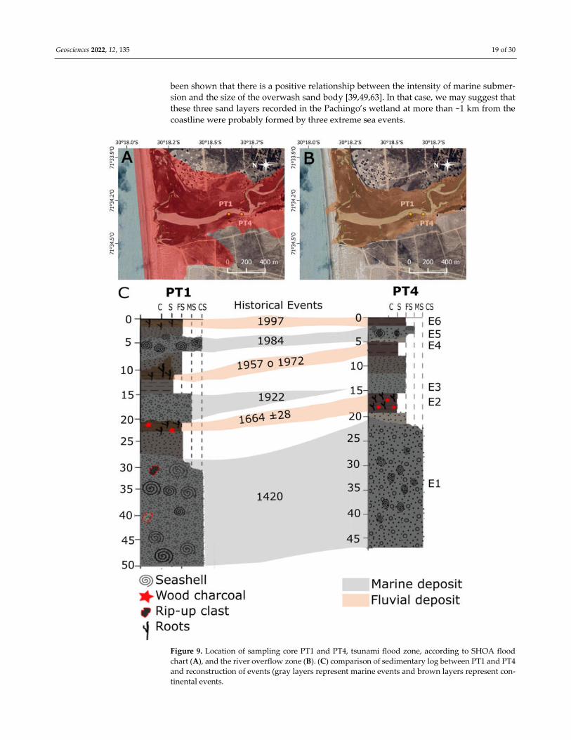
Geosciences 2022, 12, 135 19 of 30

been shown that there is a positive relationship between the intensity of marine submer-

sion and the size of the overwash sand body [39,49,63]. In that case, we may suggest that

these three sand layers recorded in the Pachingo’s wetland at more than ~1 km from the

coastline were probably formed by three extreme sea events.

Figure 9. Location of sampling core PT1 and PT4, tsunami flood zone, according to SHOA flood

chart (A), and the river overflow zone (B). (C) comparison of sedimentary log between PT1 and PT4

and reconstruction of events (gray layers represent marine events and brown layers represent con-

tinental events.

Geosciences 2022, 12, 135 20 of 30

The E1 unit has the highest Sr concentrations, which is related to the coarsest grain

sizes in the whole core and the significant content of seashells. This deposit also presents

stones larger than 3 cm (gravel) and two rip-up clasts at depths of 30 and 40 cm (Figures

4 and 6), suggesting a high-intensity event such as a tsunami [89–92]. According to the

ages estimated in unit E1, this could have occurred between 858 and 1468 AD; in this pe-

riod, two tsunamis were recorded based on textual and geological archives [93–98] Trans-

oceanic events occurred in 1361 and 1420. The event of 1361 was generated by an earth-

quake greater than 8.5 Mw in Japan that affected the Prefectures of Tokushima, Osaka,

Wakayama and Nara, and the Awaji Island. Large amounts of damage in the Kii Peninsula

of Japan, the destruction of ~1700 homes and more than 60 deaths were caused by the

tsunami that occurred in Awa [93–95] (NCEI/WDS). According to Satake et al., (2020), this

event could have had the required characteristics to affect Chile at that time; however, it

has not left strong evidence in sedimentary records in Chile [96]. The second event, which

occurred in 1420, was generated by an earthquake of 8.8–9.4 Mw in Atacama (Chile), 354

km further north than our study area. As described by Abad et al. (2020), this may have

been one of the most significant events in a supercycle of earthquakes in the Atacama

region that caused a rupture of greater than 600 km and probably produced a trans-oce-

anic tsunami that affected the area of Japan (the 1420 Oei orphan tsunami). Abad et al.

(2020) described a large boulder produced by a flood that may have had a height of >18.5

m above high tide level and an inland penetration greater than 284 m from the cliff edge

of Cisne Bay in the southern Atacama.

According to this presented background, our E1 deposit should correspond to the

Atacama Tsunami (1420), due to its proximity to the place of the epicenter and the mag-

nitude described by Abad et al., (2020).

The following marine deposit, E3, is characterized by a decrease in biological param-

eters such as TOC, total pollen and Fe concentrations. This deposit is not well constrained

by a change in granulometry, which suggests that event E3 was probably of lower energy

than event E1 (Figure 4). This deposit is dated 1918 ± 26 AD and could be related to the

1922 tsunami, produced by the earthquake which occurred in Vallenar (central Chile),

with a magnitude of 8.5 Mw [20,99]. This event produced a destructive tsunami that af-

fected a large part of the area from Chañaral to Coquimbo. The maximum variation in sea

level was recorded at 9 m in Chañaral, 5 and 7 m above high tide in Caldera and in Co-

quimbo Bay, and the run-up exceeded 7 m in the southern part of the Coquimbo Bay

[20,32,100–102]. Interestingly, this deposit has similar sedimentological characteristics to

the sandy layer associated with the tsunami of 1922 described by DePaolis et al., (2021),

which also supports its association with this tsunami event.

The last marine deposit, E5, is characterized by a clear increase in grain size and the

presence of seashells, in contrast to the E3 deposit. These characteristics were preserved

in both cores PT1 and PT4 cores, indicating a more significant event. This deposit is dated

1986 ± 5 AD and could be associated with the tsunami that impacted Valparaiso in 1985,

312 km further south of our study area. It caused a high tide in Valparaiso with a maxi-

mum wave height of 1.15 m. However, this event has been characterized as a low-energy

event [103] (SHOA, 15 October 2021 http://www.shoa.cl/s3/servicios/tsunami/data/tsuna-

mis_historico.pdf). Alternatively, the E5 deposit could correspond to the tsunami that im-

pacted Valdivia in 1960, 1085 km further south than our study area. This event hit Co-

quimbo with a wave height of 2.2 m (SHOA, 15 October 2021 http://www.shoa.cl/s3/ser-

vicios/tsunami/data/tsunamis_historico.pdf). Apparently, no significant damages were

recorded in our study area due to the orientation of Tongoy Bay. Due to their low energy

and direction, we suggest that these two events did not significantly impact our study

area. During this period, three high-intensity wave storm surge events affected the Co-

quimbo region in 1965 and two during 1984; both occurred during an El Niño event. This

phenomenon induces a rise in the sea level and produces an intensification of sea events

[26,103–105]. The first occurred on 10 August 1965 (category V) and had extraordinary

features that caused great destruction to coastal infrastructure and the flooding of the

Geosciences 2022, 12, 135 21 of 30

coast [24–26]. Several regions of Chile were affected, between 21°28′–37°00′ S [24], but

Tongoy Bay did not report damages due to the orientation of the bay. The second occurred

on 5 July 1984 (category II). This event affected the north and center of Chile. It produced

damages to fishing vessels, and the ports were closed as a preventative measure. Both

events originated from the SW direction (third quadrant), and Tongoy Bay did not report

damages due to Lengua de Vaca Point. This induced the attenuation of the wave height

within the bay and the study area (Figure 8A,B). Finally, the third event occurred on July

10, 1984; in contrast to earlier events, it occurred in the NW direction (fourth quadrant).

Therefore, the bay was exposed to the waves hitting the coast with Hs values above 4.0

[m] (Figure 8C,D). This event, of category IV, produced boat strandings, port closures and

the flooding of the coastal area. This storm caused enormous damages and destruction to

the coastal infrastructure of the central coast of Chile, similar to the 2015 event [26]. These

storm waves were more intense than the 2015 tsunami [26], and in Coquimbo, the run-up

of the storm waves exceeded 3 m. This event was probably strong enough to produce sand

deposits more than 1 km from the coastline (unit 5).

5.3. Reconstitution of Flooding Associated Extreme Rain

It should be noted that Pachingo only records extreme flood events. The creek is fed

by underwater flow, and only an important superficial flow is seen during heavy rains

[62], allowing the transport of sediments from the basin to the lagoon. This occurs in pe-

riods of the warm phase of ENSO (El Niño phenomenon) [56], Appendix D.

The three events corresponding with the deposits in units E2, E4 and E6 are charac-

terized by a high content of Fe and TOC concomitantly with a decrease in the grain size,

density and Sr content (Figures 4 and 6). These deposits are thicker at PT4 and become

thinner at the PT1 core (Figure 9). The E2 deposit has a high Fe content, high Fe/Sr ratio

and TOC with a large amount of wood charcoal and roots (Figure 6). These characteristics

are also observed in PT4. This deposit is dated 1664 ± 562 AD and could correspond to a

humid phase developed between 1550 and 1650 AD, related to the Little Ice Age. This

period was characterized by a southern displacement of ITCZ from the mean position,

increasing the precipitation southward [106], it is reported in a study based on tree rings

reconstruction [107] and the public database SADA (South American Drought Atlas,

https://sada.cr2.cl/?fbclid=IwAR0fiTvBJWH76A-

pQjQKS3WLyEti68GOZpROKvIb2EnesSGfotp63NzEiHQ, 15 October 2021) [108]. The in-

crease of intense heavy rain and floods during this period strongly affected the rainfall

distribution in Peru and Argentina [109–111].

The deposit E4 is characterized by a decrease in grain size and an increase in the Fe

and the Fe/Sr ratio (Figure 4); it presents a high diatom and pollen content, roots and better

preservation of these biological components (Figure 6A). These characteristics are also ob-

served in the two cores. This unit corresponds to 1976 ± 7 AD and is consistent with the

flood of 1957 or 1972 related with the El Niño event [56]

(https://origin.cpc.ncep.noaa.gov/products/analysis_monitoring/en-

sostuff/ONI_v5.php10; 20 October 2021). (i) According to DGA (General Direction of Wa-

ters, Chile) data (ID 04552002) from the Chile Tower station (30.6164° S, 71.3742° W),

heavy rains occurred in May 1957 with a value of 229 mm per month (https://explora-

dor.cr2.cl/; 5 October 2021). These intensive rains began on 18–19 May and affected the

north and the center of Chile, leaving economic losses that exceeded 8000 million pesos,

20 people dead and more than 4 thousand victims. The Elqui River overflowed, washing

away houses and neighboring buildings and breaking electricity and drinking water ser-

vices [27,28]. This event was classified as the most catastrophic mud flow in the region’s

history, and La Serena and Coquimbo were isolated for many days [56]. (ii) According to

Ortega et al., (2012), the rains that occurred on 24 August 1972 (occurred during an El

Niño event) produced flooding and landslides. There were trees that fell down, power

lines were cut, traffic interrupted and the streets of La Serena city seemed like rivers. In

addition, the was intense snowfall at Elqui Valley, registered at more than 4 m. According

Geosciences 2022, 12, 135 22 of 30

to the official journal, this event was the most intense and persistent since the mud flow

of 1957.

Finally, the age of event E6 is characterized by high Fe content, Fe/Sr ratio, C/N ratio

and the presence of roots (Figure 4). These characteristics were observed in both cores PT1

and PT4. This unit is dated at 1999 ± 4 AD, and fits reasonably with the 1997 extreme

pluvial flooding, concomitant with the strongest El Niño in the last decades. This event

caused damages from Puerto Montt (42° S) to Coquimbo (30° S), and the latter was the

most affected region, with monthly rainfall that exceeded 150 mm (June and August, with

164.5 and 143 mm, respectively). This event caused significant economic losses due to

bridge cuts, electrical lighting cuts and the destruction of houses and buildings near the

riverbed and streams, leaving thousands of people affected and isolated [27,28].

Our sediment cores have recorded three flood events between 1500 and 2000 AD,

related to El Niño events. Other El Niño and intense flood events occurred between 1500

and 2000 AD, including 1641, 1700, 1840, 1965, 1972, 1983, 1987 and 1991–1992, but these

events were not recorded in our sediment cores; most probably, they were eroded by ma-

rine events. Otherwise, for the wetland, a flood deposit should not always be associated

with a single event, but rather with several heavy precipitation events occurring in a short

time. It is a small basin covering 487 km2, with a temporary runoff strongly affected during

abundant rain forming small lagoons that do not reach the sea. Thus, the Pachingo wet-

land is not an ideal area to reconstruct the recurrence of flood events

[27,28,56,104,106,112]; however, we could recover evidence of the most extreme events

that have impacted the region.

6. Conclusions

The cores retrieved from Pachingo wetland provided sedimentological and age in-

formation of the last 1000 years. We identify six extreme events related to marine and

continental deposits; the deposits named units E1, E3 and E5 were identified as marine

events, and E6, E4 and E2 as continental. The E1 and E5 units correspond to tsunamis that

occurred before 1500 AD and in 1922, respectively. The E1 unit would be related to the

Atacama tsunami recorded in 1420. The E3 unit does not seem to be associated with a

tsunami event but with an extreme storm event on 10 July 1984.

Regarding the continental events, the most recent (E6) seems to correspond to the

heavy rain event of 1997, intensified by the warm phase of ENSO. The event E4 could

correspond to the 1957 heavy rain event, which produced large overflows of rivers. The unit

E2, dated at 1664 ± 28 AD, was of greater intensity, producing a significant carry-over of

organic material, and could correspond to a humid phase between 1550 AD and 1650 AD.

The six events identified in the sedimentary records agree very well with the main

extreme events reported for the zone; unfortunately, the lack of old records (>1930) makes

it difficult to establish the events of unit 1 with confidence, but it certainly is a marine

extreme event. This information highlights the relevance of these studies that record the

sensitivity of these coastal areas to the impact of these extreme events related to the mete-

orological variability in the SE Pacific. Additionally, it will enrich the Chilean database of

past marine and continental extreme events and assist coastal managers in improving

coastal zone management and developing adaptation strategies to protect the population

from future damage caused by them.

Author Contributions: K.A., performed the granulometry and geochemical analysis, analyzed the

data, prepared figures and tables, authored the drafts of the paper and approved the final draft.

P.M. and L.D. worked on the data analysis, prepared figures and tables, authored and/or reviewed

drafts of the paper and approved the final draft. R.C.-C. performed the wave models and their in-

terpretations, and prepared tables, authored the drafts of the paper and approved the final draft.

A.M. performed and analyzed the pollen data, helped with the geochemical interpretations and

dating methods and reviewed and approved the final drafts. L.R. and P.C. classified and analyzed

Geosciences 2022, 12, 135 23 of 30

the Diatoms data, reviewed and prepared the appendix and approved the final drafts. M.S. per-

formed the determination of 210Pb by alpha spectroscopy. All authors have read and agreed to the

published version of the manuscript.

Funding: This work was funded by the Projects: Fondecyt#1140851/Fondecyt #1180413, CLAP pro-

gram (Concurso de Fortalecimiento al Desarrollo Científico de Centros Regionales 2020-R20F0008-

CEAZA), ANID scholarship program (CONICYT), ANID—Millennium Science Initiative Program-

Nucleo Milenio UPWELL (NCN19_153).

Institutional Review Board Statement: Not applicable.

Informed Consent Statement: Not applicable.

Data Availability Statement: The data set is available free of charge at the CENDHOC (National

Hydrographic and Oceanographic Data Center) of Chile through the portal

http://www.shoa.cl/n_cendhoc/, access date: 20 October 2021 (Araya, 2021)

Acknowledgments: The authors of this document are grateful for the financial support of the Project

Fondec-yt#1140851/Fondecyt #1180413 and the international cooperation project Conicyt related to

the ANID scholarship program within the framework of the DOCTORATE SCHOLAR-SHIP CON-

TEST ABROAD, SCHOLARSHIPS CHILE, CALL 2017/Folio 72180323. We extend our gratitude to

the CLAP program (Concurso de Fortalecimiento al Desarrollo Científico de Centros Regionales

2020-R20F0008-CEAZA), that contributed to the completion of this study. We also thank the staff of

the oceanography laboratory of Universidad Católica del Norte and Gabriel Easton, Sedimentology

Laboratory of the Universidad de Chile. We are also grateful to Anne Bocquet-Liénard, Marie-Pierre

Bouet and Juliette Dupre of the Archeology Laboratory at the Center Michel-de-Boüard/CRAHAM

(UMR 6273) of Normandie University, Unicaen, CNRS, for allowing us to conduct the chemical

analyses, and to Magalie Legrain from the Laboratoire de Morphodynamique Continentale et

Côtière, UMR CNRS 6143 M2C, Université de Caen-Normandie, for allowing us to perform the

granulometric analyses.

Conflicts of Interest: The authors declare no conflict of interest. The funders had no role in the

design of the study; in the collection, analyses, or interpretation of data; in the writing of the manu-

script, or in the decision to publish the results.

Appendix A

Table A1. List of diatom taxas present on the sediments of the Pachingo core PT1. The diatoms were

classified into ecological groups: Freshwater (FW), Marine benthic (MB) and Brackish.

Freshwater (FW) Marine (M)

Amphora copulata (Kützing) Schoeman & Archibald Achnanthes brevipes C.Agardh

Cocconeis placentula var. lineata (Ehrenberg) Grammatophora sp.1

Ctenophora pulchella (Ralfs ex Kützing) Williams & Round Lyrella sp. 1

Cyclotella meneghiniana (Kützing) Lyrella sp. 2

Diatoma vulgaris (Bory) Surirella minuta Brebisson

Encyonema sp1. Surirella striatula Turpin

Ephitemia sp2. Rhaphoneis amphiceros (Ehrenberg)

Epithemia adnata (Kützing) Brébisson

Gomphoneis sp.

Gyrosigma acuminatum (Kützing) Rabenhorst 1853

Hantzschia amphioxys (Ehrenberg) Grunow Brackish (BR)

Martyana schulzii (Brockmann) Snoeijs Achnanthes submarina Hustedt

Navicula gregaria Donkin Halamphora sp.

Navicula amphiceropsis Lange-Bertalot & Rumrich Pleurosira laevis (Ehrenberg) Compère

Nitzschia palea (Kützing) W. Smith Tabularia sp.

Pinnularia sp1. Tryblionella sp.

Planothidium delicatulum (Kützing) Round & Bukhtiyarova

Rhopalodia musculus (Kützing) Otto Müller

Staurosirella martyi (Héribaud) Morales & Manoylov

Geosciences 2022, 12, 135 24 of 30

Appendix B

Figure A1. Abundance of diatom species Freshwater (light blue), Marine benthic (marine blue), and

Brackish (green) in the different marine (grey) and continental (brown) deposits.

Geosciences 2022, 12, 135 25 of 30

Appendix C

Figure A2. Abundance of pollen species in the different marine (grey) and continental (brown) de-

posits.

Geosciences 2022, 12, 135 26 of 30

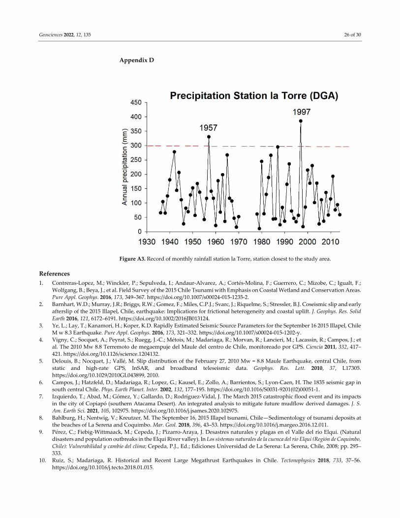
Appendix D

Figure A3. Record of monthly rainfall station la Torre, station closest to the study area.

References

1. Contreras-Lopez, M.; Winckler, P.; Sepulveda, I.; Andaur-Alvarez, A.; Cortés-Molina, F.; Guerrero, C.; Mizobe, C.; Igualt, F.;

Wolfgang, B.; Beya, J.; et al. Field Survey of the 2015 Chile Tsunami with Emphasis on Coastal Wetland and Conservation Areas.

Pure Appl. Geophys. 2016, 173, 349–367. https://doi.org/10.1007/s00024-015-1235-2.

2. Barnhart, W.D.; Murray, J.R.; Briggs, R.W.; Gomez, F.; Miles, C.P.J.; Svarc, J.; Riquelme, S.; Stressler, B.J. Coseismic slip and early

afterslip of the 2015 Illapel, Chile, earthquake: Implications for frictional heterogeneity and coastal uplift. J. Geophys. Res. Solid

Earth 2016, 121, 6172–6191. https://doi.org/10.1002/2016JB013124.

3. Ye, L.; Lay, T.; Kanamori, H.; Koper, K.D. Rapidly Estimated Seismic Source Parameters for the September 16 2015 Illapel, Chile

M w 8.3 Earthquake. Pure Appl. Geophys. 2016, 173, 321–332. https://doi.org/10.1007/s00024-015-1202-y.

4. Vigny, C.; Socquet, A.; Peyrat, S.; Ruegg, J.-C.; Métois, M.; Madariaga, R.; Morvan, R.; Lancieri, M.; Lacassin, R.; Campos, J.; et

al. The 2010 Mw 8.8 Terremoto de megaempuje del Maule del centro de Chile, monitoreado por GPS. Ciencia 2011, 332, 417–

421. https://doi.org/10.1126/science.1204132.

5. Delouis, B.; Nocquet, J.; Vallé, M. Slip distribution of the February 27, 2010 Mw = 8.8 Maule Earthquake, central Chile, from

static and high-rate GPS, InSAR, and broadband teleseismic data. Geophys. Res. Lett. 2010, 37, L17305.

https://doi.org/10.1029/2010GL043899, 2010.

6. Campos, J.; Hatzfeld, D.; Madariaga, R.; Lopez, G.; Kausel, E.; Zollo, A.; Barrientos, S.; Lyon-Caen, H. The 1835 seismic gap in

south central Chile. Phys. Earth Planet. Inter. 2002, 132, 177–195. https://doi.org/10.1016/S0031-9201(02)00051-1.

7. Izquierdo, T.; Abad, M.; Gómez, Y.; Gallardo, D.; Rodríguez-Vidal, J. The March 2015 catastrophic flood event and its impacts

in the city of Copiapó (southern Atacama Desert). An integrated analysis to mitigate future mudflow derived damages. J. S.

Am. Earth Sci. 2021, 105, 102975. https://doi.org/10.1016/j.jsames.2020.102975.

8. Bahlburg, H.; Nentwig, V.; Kreutzer, M. The September 16, 2015 Illapel tsunami, Chile—Sedimentology of tsunami deposits at

the beaches of La Serena and Coquimbo. Mar. Geol. 2018, 396, 43–53. https://doi.org/10.1016/j.margeo.2016.12.011.

9. Pérez, C.; Fiebig-Wittmaack, M.; Cepeda, J.; Pizarro-Araya, J. Desastres naturales y plagas en el Valle del rio Elqui. (Natural

disasters and population outbreaks in the Elqui River valley). In Los sistemas naturales de la cuenca del rio Elqui (Región de Coquimbo,

Chile): Vulnerabilidad y cambio del clima; Cepeda, P.J., Ed.; Ediciones Universidad de La Serena: La Serena, Chile, 2008; pp. 295–

333.

10. Ruiz, S.; Madariaga, R. Historical and Recent Large Megathrust Earthquakes in Chile. Tectonophysics 2018, 733, 37–56.

https://doi.org/10.1016/j.tecto.2018.01.015.

Geosciences 2022, 12, 135 27 of 30

11. Soto, M.-V.; Märker, M.; Rodolfi, G.; Sepúlveda, S.A.; Cabello, M. Assessment of geomorphic processes affecting the paleo-

landscape of Tongoy Bay, Coquimbo region, central Chile. Geogr. Fis. Din. Quat. 2014, 37, 51–66.

https://doi.org/10.4461/GFDQ.2014.37.6.

12. Métois, M.; Vigny, C.; Socquet, A.; Delorme, A.; Morvan, S.; Ortega, I.; Valderas- Bermejo, C.M. GPS-derived interseismic

coupling on the subduction and seismic hazards in the Atacama region, Chile. Geophys. J. Int. 2013, 196, 644–655.

https://doi.org/10.1093/gji/ggt418.

13. Udías, A.; Madariaga, R.; Buforn, E.; Muñoz, D.; Ros, M. The large Chilean historical earthquakes of 1647, 1657, 1730, and 1751

from contemporary documents. Bull. Seismol. Soc. Am. 2012, 102, 1639–1653. https://doi.org/10.1785/0120110289.

14. Saillard, M.; Hall, S.R.; Audin, L.; Farber, D.L.; Herail, G.; Martinod, J.; Regard, V.; Finkel, R.C.; Bondoux, F. Non-steady

longterm uplift rates and Pleistocene marine terrace development along the Andean margin of Chile (31 °S) inferred from 10Be

dating. Earth Planet. Sci. Lett. 2009, 277, 50–63.

15. Lomnitz, C. Major earthquakes of Chile: A historical survey, 1535–1960. Seismol. Res. Lett. 2004, 75, 368–378.

http//doi.org/10.1785/gssrl.75.3.368.

16. Beck, S.; Barrientos, S.; Kausel, E.; Reyes, M. Source characteristics of historic earthquakes along the central Chile subduction

zone. J. S. Am. Earth Sci. 1998, 11, 115–129. https://doi.org/10.1016/S0895-9811(98)00005-4.

17. DeMets, C.; Gordon, R.G.; Argus, D.F.; Stein, S. Effect of recent revisions to the geomagnetic reversal time scale on estimates of

current plate motions. Geophys. Res. Lett. 1994, 21, 2191–2194. https://doi.org/10.1029/94GL02118.

18. Nishenko, S.P. Seismic potential for large and great interplate earthquakes along the Chilean and Southern Peruvian margins

of South America: A quantitative reappraisal. J. Geophys. 1985, 90, 3589–3615.

19. Kellehier, J.A. Rupture zones of large South American earthquakes and some predictions. J. Geophys. Res. 1972, 11, 2087–2103.

https://doi.org/10.1029/JB077i011p02087.

20. Lomnitz, C. Major earthquakes and tsunamis in Chile during the period 1535 to 1955. Geol. Rundsch. 1970, 59, 938–960.

https://doi.org/10.1007/BF02042278.

21. Kanamori, H.; Rivera, L.; Ye, L.; Lay, T.; Murotani, S.; Tsumura, K. New constraints on the 1922 Atacama, Chile, earthquake

from Historical seismograms. Geophys. J. Int. 2019, 219, 645–661. https://doi.org/10.1093/gji/ggz302.

22. Carvajal, M.; Cisternas, M.; Gubler, A.; Catalán, P.A.; Winckler, P.; Wesson, R.L. Reexamination of the magnitudes for the 1906

and 1922 Chilean earthquakes using Japanese tsunami amplitudes: Implications for source depth constraints. J. Geophys. Res.

Solid Earth 2017, 122, 4–17. https://doi.org/10.1002/2016JB013269.

23. Dunbar, P.-K.; Lockridge, P.-A.; Whiteside, L.-S. Catalogue of Significant Earthquakes 2150 B.C.-1991 A.D.; World Data Center A for

Solid Earth Geophysics Reports; U. S. Dept. of Commerce, NOAA, National Geophysical Data Center: Boulder, CO, USA, 1992;

Volume SE-49, p. 320.

24. Campos-Caba, R.V. Análisis de marejadas históricas y recientes en las costas de Chile. In Memoria de Título de Ingeniero Civil

Oceánico; Facultad de Ingeniería, Universidad de Valparaíso: Valparaíso, Chile, 2016; p. 136.

25. Campos-Caba, R.; Beyá, J.; Mena, M. Cuantificación de los Daños Históricos a Infraestructura Costera por Marejadas en las

Costas de Chile. In Proceedings of the XXII Congreso Chileno de Ingeniería Hidráulica, SOCHID, Santiago, Chile, 21–23 October

2015; p. 14.

26. Winckler, P.W.; Contreras, M.; Campos, R.C.; Beya, J.; Molina, M.M. El temporal del 8 de agosto de 2015 en las regiones de

Valparaiso y Coquimbo, Chile Central. Latin Am. J. Aquat. Res. 2017, 45, 622–648. https://doi.org/10.3856/vol45-issue4- fulltext-1.

27. Urrutia, H.; Lazcano, C.L. Catástrofes en Chile 1541–1992; Editorial La Noria: Santiago, Chile, 1993.

28. Pérez, C. Cambio Climático: Vulnerabilidad, Adaptación y Rol Institucional. Estudio de Casos en el Valle de Elqui. Memoria para Optar al

Título de Ingeniero Civil Ambiental; Facultad de Ingeniería, Universidad de La Serena: La Serena, Chile, 2005.

29. Paris, R.; Fournier, J.; Poizot, E.; Etienne, S.; Morin, J.; Lavigne, F.; Wassmer, P. Boulder and fine sediment transport and

deposition by the 2004 tsunami in Lhok Nga (western Banda Aceh, Sumatra, Indonesia): A coupled offshore–onshore model.

Mar. Geol. 2010, 268, 43–54.

30. Paris, R.; Wassmer, P.; Sartohadi, J.; Lavigne, F.; Barthomeuf, B.; Desgages, E.; Grancher, D.; Baumert, P.; Vautier, F.; Brunstein,

D. Tsunamis as geomorphic crises: Lessons from the 26 December 2004 tsunami in Lhok Nga, west Banda Aceh (Sumatra,

Indonesia). Geomorphology 2009, 104, 59–72.

31. Liu, K.; Fearn, M.L. Lake-sediment record of Late Holocene hurricane activities from coastal Alabama. Geology 1993, 21, 793–796.

32. May, S.; Pint, A.; Rixhon, G.; Kelletat, D.; Wennrich, V.; Brückner, H. Holocene coastal stratigraphy, coastal changes and

potential palaeoseismological implications inferred from geo-archives in Central Chile (29–32 °S). Z. Für Geomorphol. Suppl.

Issues 2013, 57, 201–228. https://doi.org/10.1127/0372-8854/2013/S-00154.

33. Day, J.W.; Christian, R.R.; Boesch, D.M.; Yáñez-Arancibia, A.; Morris, J.; Twilley, R.; Naylor, L.; Schaffner, L.; Stevenson, C.

Consecuencias del Cambio Climático en la Ecogeomorfología de los Humedales Costeros. Estuarios Costas 2008, 31, 477–491.

https://doi.org/10.1007/s12237-008-9047-6Lom.

34. Long, A.J.; Waller, M.P.; Stupples, P. Driving mechanisms of coastal change: Peat compaction and the destruction of late

Holocene coastal wetlands. Mar. Geol. 2006, 25, 63–84. https://doi.org/10.1016/j.margeo.2005.09.004.

35. Cundy, A.B.; Kortekaas, S.; Dewez, T.; Stewart, I.S.; Collins, P.E.F.; Croudace, I.W.; Maroukian, H.; Papanastassiou, D.; Gaki-

Papanastassiou, P.; Pavlopoulos, K.; et al. Coastal wetlands as recorders of earthquake subsidence in the Aegean: A case study

of the 1894 Gulf of Atalantiearthquakes, central Greece. Mar. Geol. 2000, 170, 3–26. https://doi.org/10.1016/S0025-3227(00)000621.

Geosciences 2022, 12, 135 28 of 30

36. Parish, F.; Sirin, A.; Charman, D.; Joosten, H.; Minaeva, T.; Silvius, M. Assessment on Pleatlands, Biodiversity and Climate Change;

Global Environment Center, Kulala Lumpur: Kuala Lumpur, Malaysia; Wentlands International: Wageningen, The

Netherlands, 2008.

37. McCaffrey, R.; Thomson, J. A Record of the Accumulation of Sediment and Trace Metals in a Connecticut Salr Marsh; Elsevier:

Amsterdam, The Netherlands, 1980; Volume 22, pp. 165–236.

38. Woodruff, J.D.; Donnelly, J.P.; Emanuel, K.; Lane, P. Assessing sedimentary records of paleohurricane activity using modeled

hurricane climatology. Geochem. Geophys. Geosyst. 2008, 9, 9. https://doi.org/10.1029/2008GC002043.

39. Dezileau, L.; Sabatier, P.; Blanchemanche, P.; Joly, B.; Swingedouw, D.; Cassou, C.; Castaings, J.; Martinez, P.; Von Grafenstein,

U. Intense storm activity during the Little Ice Age on the French Mediterranean coast. Palaeogeogr. Palaeoclimatol. Palaeoecol. 2011,

299, 289–297. ISSN 0031-0182. https://doi.org/10.1016/j.palaeo.2010.11.009.

40. DePaolis, J.M.; Dura, T.; MacInnes, B.; Lisa, L.E.; Cisternas, M.; Carvajal, M.; Tang, H.; Fritz, H.M.; Mizobe, C.; Wesson, R.L.; et

al. Stratigraphic evidence of two historical tsunamis on the semi-arid coast of north-central Chile. Quat. Sci. Rev. 2021, 226,

1070252. ISSN 0277-3791. https://doi.org/10.1016/j.quascirev.2021.107052.

41. Khalfaoui, O.; Dezileau, L.; Degeai, J.; Snoussi, M. Reconstruction of past marine submersion events (storms and tsunamis) on

the North Atlantic coast of Morocco. Nat. Hazards Earth Syst. Sci. Discuss. 2019, 130, 11–14. https://doi.org/10.5194/nhess-2019-130.

42. Degeai, J.-P.; Devillers, B.; Dezileau, L.; Oueslati, H.; Bony, G. Major storm periods and climate forcing in the Western

Mediterranean during the Late Holocene. Quat. Sci. Rev. 2015, 129, 37–56.

43. Raji, O.; Dezileau, L.; Von Grafenstein, U.; Niazi, S.; Snoussi, M.; Martinez, P. Extreme sea events during the last millennium in

the northeast of Morocco. Nat. Hazards Earth Syst. Sci. 2015, 15, 1533–1543. https://doi.org/10.5194/nhess-15-1-2015.

44. Shennan, S.; Downey, S.; Timpson, A.; Edinborough, K.; Colledge, S.; Kerig, T.; Manning, K.; Thomas, M.G. Regional population

collapse followed initial agriculture booms in mid-Holocene Europe. Nat. Commun. 2013, 4, 2486.

https://doi.org/10.1038/ncomms3486.

45. Sabatier, P.; Dezileau, L.; Condomines, M.; Briqueu, L.; Colin, C.; Bouchette, F.; Le Duff, M.; Blanchemanche, P. Reconstruction

of paleostorm events in a coastal lagoon (Hérault, south of France). Mar. Geol. 2008, 251, 224–232.

46. Nanayama, A.C.; Tatavarti, R.; Shinu, N.; Subeer, A. Tsunami of 26 December 2004 on the southwest coast of India: Post-tsunami

geomorphic and sediment characteristics. Mar. Geol. 2007, 242, 155–168.

47. Scileppi, E.; Donnelly, J.P. Sedimentary evidence of hurricane strikes in western Long Island, NY. Geochem. Geophys. Geosyst.

2007, 8, Q06011. https://doi.org/10.1029/2006GC001463.

48. Donnelly, J.P.; Cleary, P.; Newby, P.; Ettinger, R. Coupling Instrumental and Geological Records of Sea-Level Change: Evidence

from southern New England of an increase in the rate of sea-level rise in the late 19th century. Geophys. Res. Lett. 2004, 31,

L05203. https://doi.org/10.1029/2003gl018933.

49. Dezileau, L.; Lehu, R.; Lallemand, S.; Hsu, S.-K.; Babonneau, N.; Ratzov, G.; Lin, A.; Dominguez, S. Historical Reconstruction

of Submarine Earthquakes Using Pb-210, Cs-137, and Am-241 Turbidite Chronology and Radiocarbon Reservoir Age Estimation

off East Taiwan. Radiocarbon 2016, 58, 25–36.

50. Dezileau, L.; Bordelais, S.; Condomines, M.; Bouchette, F.; Briqueu, L. Evolution des Lagunes du Golfe d’Aigues-Mortes à Partir de

l’Étude de Carottes Sédimentaires Courtes (Étude Géochronologique, Sédimentologique et Géochimique des Sédiments Récents);

Publications ASF: Paris, France, 2015; Volume 51, p. 91.

51. Webster, P.J.; Holland, G.J.; Curry, J.A.; Chang, H.R. Change in tropicalcyclone number, duration, and intensity in a warming

environment. Science 2000, 309, 1844–1846.

52. Collins, E.S.; Scott, D.B.; Gayes, P.T. Hurricane records on the South Carolina coast: Can they be detected in the sediment record?

Quat. Int. 1999, 56, 15–26.

53. Paskoff, R. Contribuciones recientes al conocimiento del cuaternario marino del centro y norte de Chile. Revista de Geografía

Norte Grande 1999, 26, 43–575.

54. Herm, D.; Paskoff, R. Vorschlag zur Gliederung des marinen Quart&s en Nord- und Mittel-Chile. Neues Jahrb. Geol. Palontología

Montashefte 1967, 10, 577–588.

55. Ota, Y.; Paskoff, R. Holocene deposits on the coast of north-central Chile: Radiocarbon ages and implications for coastal changes.

Rev. Geol. Chile 1993, 20, 25–32. https://doi.org/10.5027/andgeoV20n1-a03.

56. Ortega, C.; Vargas, G.; Rutllant, J.; Jackson, D.; Méndez, C. Major hydrological regime change along the semiaridwestern coast

of South America during the Early Holocene. Quat. Res. 2012, 78, 513–527.

57. Rutllant, J.; Montecino, V. Multiscale upwelling forcing cycles and biological response off northcentral Chile. Ciclos multiescala

en el forzamiento de la surgencia y respuesta biológica en el centro-norte de Chile. Rev. Chil. Hist. Nat. 2002, 75, 217–231.

58. Rutllant, J.; Fuenzalida, H. Synoptic aspects of the central Chile rainfall variability associated with the Southern Oscillation. Int.

J. Clim. 1991, 11, 63–76.

59. Soto, M.-V.; Arriagada-Gonzalez, J.; Cabello-Espinola, M. The Accretional Beach Ridge System of Tongoy Bay: An Example of

a Regressive Barrier Developed in the Semiarid Region of Chile. Recent Adv. Petrochem. Sci. (RAPSCI) 2018, 4, 1–8.

https://doi.org/10.19080/RAPSCI.2018.04.555641.

60. Lagos, S.G. Caracterización Geomorfológica y Dinámica Costera de Bahías del Semiárido de Chile; Universidad de Chile, Santiago,

Chile, 2013; p. 87.

61. Figueroa, R.; Suárez, M.L.; Asunción, A.; Ruiz, V.; Vidal-Abarca, M. Wetlands ecological characterization of Central Chile semi-

dry area. Gayana 2009, 73, 76–94.

Geosciences 2022, 12, 135 29 of 30

62. Niemeyer, H. Hoyas Hidrográficas de Chile Cuarta Región. Obtenido de DGA (General Directorate of Waters). 1980. Available

online: https://snia.mop.gob.cl/sad/CUH2886v4.pdf (accessed on 20 October 2021).

63. Downing, S.M.; Baranowski, R.A.; Grosso, L.J.; Norcini, J.J. Item type and cognitive ability measured: The validity evidence for

multiple true–false items in medical specialty certification. Appl. Meas. Educ. 1995, 8, 89–199.

64. Montecinos, A.; Aceituno, P. Seasonality of the ENSO-Related Rainfall Variability in Central Chile and Associated Circulation

Anomalies. J. Clim. 2002, 16, 281–296.

65. Hogg, A.G.; Heaton, T.J.; Hua, Q.; Palmer, J.G.; Turney, C.S.M.; Southon, J.; Bayliss, A.; Blackwe, P.G.; Boswijk, G.; Bronk-

Ramsey, C.; et al. SHCal20 Southern Hemisphere calibration, 0-55,000 years cal BP. Radiocarbon 2020, 62, 759–778.

https://doi.org/10.1017/RDC.2020.59.

66. Heaton, T.; Köhler, P.; Butzin, M.; Bard, E.; Reimer, R.; Austin, W.; Skinner, L. Marine20—The Marine Radiocarbon Age

Calibration Curve (0–55,000 cal BP). Radiocarbon 2020, 62, 779–820. https://doi.org/10.1017/RDC.2020.68.

67. Marshall, J.D.; Brooks, J.R.; Lajtha, K. Sources of Variation in the Stable Isotopic Composition of Plants. In Stable Isotopes in

Ecology and Environmental Science; Michener, R., Lajtha, K., Eds.; John Wiley & Sons: Hoboken, NJ, USA, 2007;

https://doi.org/10.1002/9780470691854.ch2.

68. Khan, N.S.; Vane, C.H.; Horton, B.P. Stable carbon isotope and C/N geochemstry of coastal wetland sediments as a sea-level

indicator. Handb. Sea-Level Res. 2015, 1, 295–311.

69. Carrasco-Puga, G.; Díaz, F.P.; Soto, D.C.; Hernández-Castro, C.; Contreras-López, O.; Maldonado, A.; Latorre, C.; Gutiérrez,

R.A. Revealing hidden plant diversity in arid environments. Ecography 2021, 44, 98–111. https://doi.org/10.1111/ecog.05100.

70. Jara, I.; Maldonado, A.; Porras, M.E. Late Holocene dynamics of the south American summer monsoon: New insights from the

Andes of northern Chile (21° S). Quat. Sci. Rev. 2020, 246, 106533. https://doi.org/10.1016/j.quascirev.2020.106533.

71. Hong, I.; Dura, T.; Ely, L.L.; Horton, B.P.; Nelson, A.R.; Cisternas, M.; Nikitina, D.; Wesson, R.L. A 600-year-year-long

stratigraphic record of tsunamis in south-central Chile. Holocene 2016, 27, 1–13. https://doi.org/10.1177/0959683616646191.

72. De Porras, M.E.; Maldonado, A.; Zamora-Allendes, A.; Latorre, C. Calibrating the pollen signal in modern rodent middens from

northern Chile to improve the interpretation of the late Quaternary midden record. Quat. Res. 2015, 84, 301–311.

https://doi.org/10.1016/J.YQRES.2015.10.004.

73. Sawai, Y.; Fujii, Y.; Fujiwara, O.; Kamataki, T.; Komatsubara, J.; Okamura, Y.; Satake, K.; Shishikura, M. Marine incursión of the

past 1500 years and evidence of tsunamis at suijin-numa, a coastal lake facing the Japan Trench. Holocene 2008, 18, 517–528.

74. Maldonado, A.; Betancourt, J.L.; Latorre, C.; Villagran, C. Pollen analyses from a 50 000-yr rodent midden series in the southern

Atacama Desert (25°30′ S). J. Quat. Sci. 2005, 20, 493–507. https://doi.org/10.1002/jqs.936.

75. Dura, T.; Cisternas, M.; Horton, B.; Ely, L.; Nelson, A.; Wesson, R.; Pilarczyk, J. Coastal evidence for Holocene subduction-zone

earthquakes and tsunamis in central Chile. Quat. Sci. Rev. 2015, 113, 93–111. http://doi.org/10.1016/j.quascirev.2014.10.01502.

76. Rivera, R. Guide for References and Distribution for the Class Bacillariophyceae in Chile between 18°28′ S and 58 °S; J. Cramer: Summit,

NJ, USA, 1983.

77. Rebolledo, L.; Lange, C.B.; Figueroa, D.; Pantoja, S.; Muñoz, P.; Castro, R. 20th century fluctuations in the abundance of siliceous

microorganisms preserved in the sediments of the Puyuhuapi Channel (44 °S), Chile. Rev. Chil. Hist. Nat. 2005, 78, 469–488.

78. Vos, P.C.; de Wolf, H. Methodological aspects of paleo-ecological diatom research in coastal areas of the Netherlands. Geol.

Mijnb. 1988, 67, 31–40.

79. Faegri, K.; Iversen, J. Textbook of Pollen Analysis. Blackwell Scientific Publication, 4th ed.; John Wiley and Sons: Chichester, UK, 1989.

80. Holthuijsen, L. Olas en Aguas Oceánicas y Costeras; Cambridge University Press: Cambridge, UK, 2007;

https://doi.org/10.1017/CBO9780511618536.

81. Winckler, P. Introducción al Modelado de Procesos Costeros, 1st ed.; Universidad de Valparaíso: Valparaíso, Chile, 2018.

82. Beyá, J.; Alvarez, M.; Gallardo, A.; Hidalgo, H.; Aguirre, C.; Valdivia, J.; Parra, C.; Méndez, F.; Contreras, F.; Winckler, P.; et al.

Atlas de Oleaje de Chile; Escuela de Ingeniería Civil Oceánica, Universidad de Valparaíso: Valparaíso, Chile, 2016; p. 169.

83. Arnaud, F.; Lignier, V.; Revel, M.; Desmet, M.; Beck, C.; Pourchet, M.; Charlet, F.; Trentesaux, A.; Tribovillard, N. Flood and

earthquake disturbance of 210Pb geochronology Lake Anterne, NW Alps. Terra Nova 2002, 14, 225–232.

84. Robbins, J.A.; Edgington, D.N. Determination of recent sedimentation rates in Lake Michigan using Pb-210 and Cs-137. Geochim.

Cosmochim. Acta 1979, 39, 285–304. https://doi.org/10.1016/0016-7037(75)90198-2.

85. Carré, M.; Jacksonb, D.; Maldonado, A.; Chase, B.M.; Sachs, J.P. Variability of 14C reservoir age and air—Sea flux of CO2 in the

Peru–Chile upwelling region during the past 12,000 years. Quat. Res. 2016, 85, 87–93.

86. Ortega, C.; Vargas, G.; Rojas, M.; Rutllant, J.; Muñoz, P.; Lange, C.B.; Pantoja, S.; Dezileau, L.; Ortlieb, L. Extreme ENSO-driver

torrential rainfalls at the southern Edge of the Atacama Desert during the Late Holocene and their projection into the 21th

century. Glob. Planet. Change 2019, 175, 226–237. https://doi.org/10.1016/j.gloplacha.2019.02.011.

87. Muñoz, P.; Rebolledo, L.; Dezileau, L.; Maldonado, A.; Mayr, C.; Cárdenas, P.; Lange, C.B.; Lalangui, K.; Sánchez, G.; Salamanca,

M.; et al. Reconstructing past variations in environmental conditions and paleoproductivity over the last ~8000 years off north-

central Chile (30° S). Biogeociencias 2020, 22, 5763–5785. https://doi.org/10.5194/bg-17-5763-2020.

88. Lambeck, K.; Bard, E. Sea-level change along the French Mediterranean coast for the past 30,000 years—Earth Planet. Sci. Lett.

2000, 175, 203–222.

89. Takashi, I.; Kazuhisa, G.; Yusuke, Y.; Yosuke, M.; Chikako, S.; Keita, T. Reducing the age range of tsunami deposits by 14C

dating of rip-up clasts. Sediment. Geol. 2018, 364, 334–341. https://doi.org/10.1016/j.sedgeo.2017.09.008.

Geosciences 2022, 12, 135 30 of 30

90. Sakuna-Schwartz, D.; Feldens, P.; Schwarzer, K.; Khokiattiwong, S.; Stattegger, K. Internal structure of event layers preserved

on the Andaman Sea continental shelf, Thailand: Tsunami vs. storm and flash-flood deposits. Nat. Hazards Earth Syst. Sci. 2015,

15, 1181–1199.

91. Switzer, A.D.; Jones, B.G. Large-scale washover sedimentation in a freshwater lagoon from the southeast Australian coast: Sea-

level change, tsunami or exceptionally large storm? Holocene 2008, 5, 787–803.

92. Morton, R.A.; Gelfenbaum, G.; Jaffe, B.E. Physical criteria for distinguishing sandy tsunami and storm deposits using modern

examples. Sediment. Geol. 2007, 200, 184–207. https://doi.org/10.1016/j.sedgeo.2007.01.003.

93. Lomnitz, C. Development in Geotectonics #5, Global Tectonics and Earthquake Risk; Elsevier Scientific Publishing Co.: Amsterdam,

The Netherlands, 1974.

94. Soloviev, S.L.; Go, C.N. A Catalogue of Tsunamis on the Western Shore of the Pacific Ocean [Dates Include 173–1968]; Academy of

Sciences of the USSR, Nauka Publishing House: Moscow, Russia, 1974; p. 439.

95. Imamura, A. Topographical Changes Accompanying Earthquake or Volcanic Eruptions; Publications of the Earthquake Investigation

Committee in Foreign Languages: Tokyo, Japan, 1930; 35, pp. 16–38.

96. Abad, M.; Izquierdo, T.; Cáceres, M.; Bernárdez, E.; Vidal, J. Coastal boulder deposit as evidence of an ocean-wide prehistoric

tsunami originated on the Atacama Desert coast (Northern Chile). Sedimentology 2020, 67, 1505–1528.

https://doi.org/10.1111/sed.12570.

97. Nentwig, V.; Bahlburg, H.; Górecka, E.; Huber, B.; Bellanova, P.; Witkowski, A.; Encinas, A. Multiproxy analysis of tsunami

deposits—The Tirúa example, central Chile. Geosphere 2018, 14, 1067–1086. https://doi.org/10.1130/GES01528.1.

98. Sakate, K.; Heidarzadeh, M.; Quiroz, M.; Cienfuegos, R. History and features of trans-oceanic tsunamis and implications for

paleo-tsunami studies. Earth-Sci. Rev. 2020, 202, 103–112.

99. Lockridge, P.A. Tsunamis in Peru-Chile. In World Data Center a for Solid Earth Geophysics; National Geophysical Data Center:

Boulder, CO, USA, 1985; Report SE-39, 97p.

100. Ceresis: Centro Regional de Sismología para América del Sur. Catálogo de Terremotos para América del Sur; 1985, 12 Lima,

Perú. Available online: http://www.ceresis.org/ (accessed on 20 October 2021).

101. Urbina, X.; Gorigoitía, N.; Cisternas, M. Aportes a la historia sísmica de Chile: El caso del gran terremoto de 1730. Anu. Estud.

Am. 2016, 73, 657–687. (In Spanish)

102. NCEI/WDS: National Geophysical Data Center/World Data Service: Global Historical Tsunami Database; NOAA National Centers for

Environmental Information: Stennis Space Center, MI, USA, 2020. https://doi.org/10.7289/V5PN93H7.

103. Nakamura, S. An Analysis of the 1985 Chilean Tsunami. Mar. Geod. 1992, 15, 277–281.

104. Maturana, J.; Bello, M.; Manley, M. Antecedentes Históricos y Descripción del Fenómeno El Niño, Oscilación del Sur. History and

Description of “El Niño, Southern Oscillation” Phenomenon; SHOA—Servicio Hidrográfico y Oceanográfico de la Armada de Chile,

Departamento de Oceanografía: Valparaíso, Chile, 2004.

105. Quinn, W.; Neal, V.T.; Mayolo, S.E.A. El Niño ocurrences over the past four and half centuries. J. Geophys. Res. 1987, 92, 14449–14461.

106. Koutavas, A.; deMenocal, P.B.; Olive, G.C.; Lynch-Stieglitz, J. Mid-Holocene El Niño–Southern Oscillation (ENSO) attenuation re-

vealed by individual foraminifera in eastern tropical Pacific sediments. Geology 2006, 34, 993–996. https://doi.org/10.1130/G22810A.1.

107. Morales, M.S.; Cook, E.R.; Barichivich, J.; Christie, D.A.; Villalba, R.; LeQuesne, C.; Srur, A.M.; Ferrero, M.E.; González-Reyes,

A.; Couvreux, F.; et al. Six hundred years of South American tree rings reveal an increase in severe hydroclimatic events since

mid-20th century. Proc. Natl. Acad. Sci. USA 2020, 117, 16816–16823. https://doi.org/10.1073/pnas.2002411117.

108. Ferrada, A.; Christie, D.A.; Muñoz, F.; González, A.; Garreaud, R.D.; Bustos, S. Explorador del Atlas de Sequías de Sudamérica;

Centro de Cienciencia del Clima y la Resiliencia (CR)2: Santiago, Chile, 2021; htpps://doi.org/10.13140/RG.2.2.14020.35209.

109. Rein, B.; Lückge, A.; Reinhardt, L.; Sirocko, F.; Wolf, A.; Dullo, W.C. Variabilidad de El Niño frente a Perú durante los últimos

20.000 años. Paleoceanografía 2005, 20, PA4003. https://doi.org/10.1029/2004PA001099.

110. Morales, M.; Duncan, A.C.; Neukom, R.; Rojas, F.; Villalba, R. Variabilidad Hidroclimática en el Sur del Altiplano: Pasado, Presente y

Futuro. La Puna Argentina Naturaleza y Cultura, Serie Conservación de la Naturaleza 24: La Puna Argentina: Naturaleza y Cultura,

Fundación Miguel Lillo; Fundación Miguel Lillo: Tucumán, Argentina, 2018; ISBN 978-950-668-032-9.

111. Prieto, M.D. ENSO signals in South America: Rains and floods in the Paraná River region during colonial times. Clim. Change

2007, 83, 39–54. https://doi.org/10.1007/s10584-006-9188-1.

112. Cepeda, P.J. (Ed.) Los Sistemas Naturales de la Cuenca del Rio Elqui (Región de Coquimbo, Chile): Vulnerabilidad y Cambio del Clima;

Ediciones Universidad de La Serena: La Serena, Chile, 2008.