1-s2 0-S0167473005000597-main

Structural Safety 29 (2007) 2–15

www.elsevier.com/locate/strusafe

STRUCTURAL

SAFETY

Filtered importance sampling with support vector margin:A powerful method for structural reliability analysis

Jorge E. Hurtado *

Universidad Nacional de Colombia, Apartado 127, Manizales, Colombia

Received 6 December 2005; received in revised form 8 December 2005; accepted 8 December 2005Available online 24 January 2006

Abstract

In structural reliability, simulation methods are oriented to the estimation of the probability integral over the failuredomain, while solver-surrogate methods are intended to approximate such a domain before carrying out the simulation.A method combining these two purposes at a time and intended to obtain a drastic reduction of the computational laborimplied by simulation techniques is proposed. The method is based on the concept that linear or nonlinear transformationsof the performance function that do not affect the boundary between safe and failure classes lead to the same failure prob-ability than the original function. Useful transformations that imply reducing the number of performance function callscan be built with several kinds of squashing functions. A most practical of them is provided by the pattern recognitiontechnique known as support vector machines. An algorithm for estimating the failure probability combining this methodwith importance sampling is developed. The method takes advantage of the guidance offered by the main principles of eachof these techniques to assist the other. The illustrative examples show that the method is very powerful. For instance, aclassical series problem solved with O(1000) importance sampling solver calls by several authors is solved in this paper withless than 40 calls with similar accuracy.� 2005 Elsevier Ltd. All rights reserved.

Keywords: Importance sampling; Support vector machines; Structural reliability; Markov chains; Neural networks; Monte Carlosimulation

1. Introduction

As is well known, the assessment of the reliability of structural or mechanical systems and their reliability-based optimization starts from the determination of the probability of failure under the presence of randomparameters, such as elasticity or plasticity moduli, loads, dimensions, etc. Normally it is to the probability ofexceeding a specified threshold. To be specific, let x = (x1, x2, . . . , xn) be the vector of random parameters,known as basic variables, px(x) its multivariate probability density function and g(x) a function definingthe critical threshold, known as the performance or limit-state function, such that S ¼ fx : gðxÞ > 0g and

0167-4730/$ - see front matter � 2005 Elsevier Ltd. All rights reserved.

doi:10.1016/j.strusafe.2005.12.002

* Corresponding author. Tel.: +57 68863990; fax: +57 68863220.E-mail address: [email protected].

mailto:[email protected]

J.E. Hurtado / Structural Safety 29 (2007) 2–15 3

F ¼ fx : gðxÞ 6 0g represent the safe and failure sets, respectively. The probability of failure Pf of a structuralsystem is therefore defined as [1]

P f ¼ZF

pxðxÞdx ð1Þ

which can be formulated equivalently in the form

P f ¼Z

RdI ½gðxÞ 6 0�pxðxÞdx ð2Þ

where d is the number of dimensions of the problem and I[Æ] is an indicator function which equals 1 if the im-plied condition is true and 0 if it is false.

Several methods have been devised to solve this problem. They can be classified as analytic and synthetictechniques. The first (among which are the classical FORM and SORM) are aimed at the estimation of thefailure probability using as much analytical information on function g(x) as possible, especially its gradientand curvatures. The second, collectively known as Monte Carlo methods, are based on a collection of samplesof the random variables, with the aid of which the structural response is calculated, in such a way that Pf isestimated as the fraction of samples leading to failure. The basic Monte Carlo method yields the followingestimate of the probability of failure:

bP f ¼1

N

XN

i¼1

I ½gðxiÞ 6 0� ð3Þ

where N is the number of samples generated with the given joint density function. It is known that the methodrequires Oð100 � P�1

f Þ samples [2]. Several techniques have been proposed to reduce this large figure, such asimportance sampling (IS) [1], directional simulation [3], conditional simulation [4], antithetic variates [5]and others. The importance sampling method, which is used in this paper, is based on the simpletransformation

P f ¼ZF

pxðxÞhðxÞ hðxÞdx ð4Þ

where h(x) is an auxiliary density function intended to produce samples in the region that contributes most tothe integral (1). This transformation implies that the estimate of the failure probability becomes

bP f ¼1

N

XN

i¼1

I ½gðxiÞ 6 0�pxðxiÞhðxiÞ

ð5Þ

where the samples xi, i = 1, . . . , n are now drawn from h(Æ). It is well known that the optimal IS density is givenby

hðxÞ ¼I ½gðxÞ 6 0�pxðxÞ

P f

ð6Þ

which is not directly applicable as it depends on the goal of the calculation, i.e. the failure probability. Thenumerator, however, can be used for estimating the IS density using a Markov Chain Monte Carlo approach[6]. A variant of this method is used to estimate the design point in an algorithm proposed in a latter section ofpresent paper.

Despite variance reduction methods require much less samples than basic Monte Carlo, in some cases theirquantity can still be considered as large, especially when the computation of each sample is very costly as itmay involve nonlinear finite element solutions. A method for reducing this cost is by means of solver substi-tution devices, which are purported to act as a surrogate of the code used for the deterministic evaluations formost of the Monte Carlo samples in the special but most common case where the function is given only implic-itly through a numerical solver. In this group we have the classical response surface method [7] together withthe statistical (or computational) learning tools such as neural networks [8–10] and support vector machines(SVM) [11] which are gaining increasing application in reliability analysis and probabilistic mechanics in

4 J.E. Hurtado / Structural Safety 29 (2007) 2–15

general [12–14]. A thorough examination of the applicability of these techniques in this context can be foundin a recent monograph by the author [15]. In all these cases there is a need of having a set of input/output datafor calculating the parameters of the solver surrogate. After training, the solver surrogate can be used hence-forth to estimate the failure probability using conventional Monte Carlo techniques. Moreover, the derivedhypersurface can also be analyzed under a geometric viewpoint, like in FORM and SORM techniques, dueto the simplicity of the approximating function.

From this discussion, it becomes apparent that while variance reduction Monte Carlo methods are pur-ported to estimate the integral (1), solver-surrogate methods are only aimed at an approximation of the con-tours of the failure domain for facilitating the posterior numerical integration. A question that naturally arisesis how these approaches could be combined with the aim of further reducing the number of samples needed ina reliability estimation, especially when function g(x) is given in implicit form. This would report the advan-tage that no computational efforts are applied in refining the limit state approximation in regions that are notrelevant from the probabilistic point of view.

In this paper, a combination of such a kind is proposed. Among the methods mentioned above the impor-tance sampling has been chosen from the simulation group, because it is perhaps the most widely studied andapplied. On the other hand, the solver surrogate method selected for the combination is the support vectormachine for reasons that will become clear in the sequel. Less than 40 solver calls are required for the estima-tion of the probability of failure in the numerical examples, which correspond to cases in which the directapplication of importance sampling requires more than 500 samples. Before explaining the algorithm andits application it is important to discuss briefly the relevance of pattern recognition and squashing functiontransformation for structural reliability analysis.

2. The pattern recognition paradigm

As shown by the author in recent research [9,16,11,15,17] the interpretation of the fundamental reliabilityproblem as a pattern recognition task opens new possibilities for the development of structural safety meth-ods. To illustrate this interpretation, consider the second of the two formulations of the failure probability(Eq. (2)). It defines a two-class pattern recognition problem, in which we can assign the number �1 for thecondition g(xi) 6 0 and +1 for the opposite. If a criterion were available to separate these two classes thenthe failure probability could be estimated as

bP f ¼N�1

Nð7Þ

where N�1 is the number of samples, generated with a standard Monte Carlo procedure, that fall into the fail-ure class.

There is a large list of statistical techniques developed for pattern recognition. For a detailed discussion ontheir applicability in structural safety analysis the reader is referred to [15,17]. In these references it is shownthat among the many methods a kind of neural networks known as multi-layer perceptron and the kernelmethod known as support vector machines [18] are the most useful to the purpose at hand. Also, it is dem-onstrated the superiority of these techniques over the classical response surface method, which is due to theirgreater model flexibility and adaptivity to samples, confirming the observations of [19].

A comparison of Eqs. (1) and (2) indicates that the latter admits the following interpretation: the integra-tion of the joint density function over the failure domain is shifted to the integration over the entire real spaceunder the condition that the performance function defining the failure domain is substituted by the indicatorfunction as a factor in the integrand. This suggests that actually it is not necessary to approximate the entireperformance function but only its sign over the entire real space, because the indicator and sign functions arerelated by I(z) = (sgn(z) + 1)/2. Thus, a valid approach is to approximate the indicator function and perform-ing the integration in the entire real space. For instance, nonlinear transformations of the g(Æ) function thatrender the same distribution of signs, such as the sigmoid or other squashing functions, are allowable. (Asquashing function is a nondecreasing, rapidly increasing map s : R7!½0; 1� with limz!1s(z) = 1 andlimz!�1sðzÞ ¼ 0; z 2 R [20]). In fact, this is nothing else than the so-called formulation invariance criterionthat should be met by reliability indices [21], according to which the reliability for e.g., g3(x) should be the


same than that of the original g(x), as they cross the space x by the same contour and therefore lead to thesame probability of failure.

3. Proposed approach

Upon the basis of these considerations, let us consider the following Two-layer perceptron approximationto the sign of the performance function c(x) = sgn[g(x)] [22]:

cðxÞ ¼ sXm

k¼0

wk � sXd

j¼0

wkjxj

! !ð8Þ

where m the number of hidden layer neurons, the w are weights and s(Æ) is a squashing function such as thelogistic sigmoid (Fig. 1)

sðgÞ ¼ 1

1þ expð�cgÞ ð9Þ

The coefficient c defines the slope of the function. Notice that the function has an active support of width 2kthat embraces the unknown contour g(x) = 0, if the network has been correctly fitted to the training data.Therefore, this suggests an iterative method for training neural classifiers and estimating alongside the failureprobability with simulation techniques: calculate the actual value of the performance function only for sam-ples for which its estimate given by the outer parentheses in Eq. (8) is in the interval 2k; otherwise use the cor-responding right or left limit value of the function. Then update the neural classifier with the samples forwhich the performance function have been calculated with the numerical solver of the structural model.

However, this combination of neural networks and Monte Carlo simulation is not as attractive as thatwhich can be made with support vector machines. This is because the 2k zone, which has no explicit equationsin the x-space, is substituted by a margin that is obtained after an optimization process that renders explicitequations for the margin limits which facilitate the selection of the samples to be processed by the numericalsolver.

Briefly, a support vector machine [18] yields the following approximation of the classification function:

cðxÞ ¼ sgn½gðxÞ� ¼ sgnXS

i¼1

aiciKðxi; xÞ � b

!ð10Þ

where K(x, xi) is a linear or nonlinear kernel function, b is a threshold, ci 2 {�1, + 1} is the class sign of the ithsample, ai is a value obtained from a Lagrange optimization and S is the number of so-called support vectors,which for a perfectly separable problem are the samples closest to the boundary (Fig. 2). The structural

Fig. 1. Ridge function employed by neural classifiers and its active support.

Fig. 2. The basic elements of a support vector machine as applied to the reliability problem.


reliability problem involves separable classes, because the limit state function defines two classes with no sam-ples of one class inside the domain of the other. The squashing function is provided in this case by the fact thata normalization technique applied by the method associates the values ±1 to the margin functions, as shownin Fig. 2. Accordingly, as more training samples are added the margin becomes narrower and the ridge be-tween the borders becomes more steep. A summary of the support vector method for pattern recognition isgiven in the Appendix.

The key to the reported success of support vector method when applied to very high-dimensional problems[23] lies in the use of kernels that satisfy the Mercer conditions for positive-definite functions that allow aninfinite eigenfunction series, similarly to the Karhunen-Loeve expansion used in stochastic finite element anal-ysis [24]. This is because the implicit expansion implies a large increase of the dimensionality of the problemthat facilitates the calculation of a separating hyperplane in the new space, according to Cover theorem [25].

Therefore, the support vector margin can be used as a filter for the samples that should be used in calls ofthe numerical solver of the g(Æ) function (Fig. 3). On the contrary, samples lying beyond the margin need notbe given to the solver, as their sign can be assessed with the current classification function. Accordingly, thealgorithm of the proposed approach is the following:

Algorithm SVM · IS:

1. Generate a set of N random variates of the basic variables using the importance sampling density h(x). Thevalue of N is selected according to the importance sampling method that the analyst intends to apply. Thevariates are not classified, i.e. they are not processed by the numerical solver of the structural model.

Fig. 3. Proposed method: the margin of the support vector machine is used for selecting the worth-testing samples.


2. Set the estimate of the probability of failure equal to one.3. Select a few (eight, say) failure and a safe vectors, using some information on the problem in hand. For

instance, importance sampling densities are normally placed on the design point or over the most likely fail-ure point [2]. Its coordinates can be used for the selection of the initial training points. Also, if the designpoint is not known beforehand, use can be made of the algorithm reported in Section 5 of this paper. Thesamples generated with it can be used as the initial training samples on the failure side.

4. Fit the support vector machine.5. Calculate the estimate of the failure probability using the fitted classifier and the importance sampling for-

mula (Eq. (5)). If the estimate stabilizes, i.e. if its difference with respect to the previous estimate lies withina small tolerance, stop. Otherwise select a new sample lying inside the current margin and go to step 4.

6. After finishing the calculation of the learning machine, use the rest of the set of the N random variates tocalculate the failure probability using it as a surrogate of the actual structural model function.

The last step of the algorithm expresses that the estimate of the failure probability can be separated as

bP f ¼1

N

XT

i2T;i¼1

I ½gðxiÞ 6 0�pxðxiÞhðxiÞ

þXN�T

j2T;j¼1

I ½gðxjÞ 6 0�pxðxjÞhðxjÞ

0@ 1A ð11Þ

where T is the set of samples actually used in the training process and T is its cardinality. This indicates thatthe first summation requires calls of the structural model function whereas the second summation does not.This is indicated by the symbol bI ½��, suggesting that the indicator function is estimated with the support vectormachine.

The algorithm is inspired in that reported in [11], which was purported to a close approximation of thelimit state function in stochastic finite element analysis that could be used as a solver surrogate. Therefore,the stopping criterion is given there by the accuracy of the approximation of the contour. In the present case,it is given by a more meaningful criterion: the target of the entire calculation, i.e. the failure probability. Thisis made possible by the implication of importance sampling in an on-line training process. In fact, it must betaken into account that all solver surrogates are fitted with a non-probabilistic method, such as least squaresin the response surface method, gradient descent in multi-layer perceptrons and Lagrange optimization insupport vector machines. While this feature makes their learning pretty independent of the failure probabil-ity, the calculation of the function apart from the estimation of this very probability may imply a waste ofcomputational efforts in refining the solver surrogate in regions that are unimportant from a probabilisticviewpoint.

Summarizing, it can be said that the proposed method makes use of the guiding principles of the impor-tance sampling and the support vector machines to assist each other technique. First, the method avoids train-ing the support vector machine in regions of little probabilistic interest by the guidance of importancesampling. Conversely, a reduction of the number of solver calls implied by importance sampling is achievedwith the guidance of the critical sampling region revealed by the ancillary margin functions of the learningmachine. The following examples illustrate the advantages of the proposed method.

4. Examples

In the present section, three examples that have been used in other papers are calculated. In all cases thecomparison is made with respect to the results given by the importance sampling calculation, not with respectthe ‘‘exact’’ failure probability because the goal of the paper is to propose a method for a drastic reduction ofthe computational effort of the importance sampling technique as such. The accuracy of the estimation withrespect to the exact results highly depends on the importance sampling approach selected in each case, forwhich there are several proposals [1,26,27,5,6,28] (see also the valuable benchmark study reported in [29]and the theoretical study of the method exposed in [30]). In the same vein it is assumed that the (normallylittle) previous work conducting to the calculation of the parameters of the importance samplingdensity has been done. Accordingly, the comparison concerns only the computational job performed after thatstep.


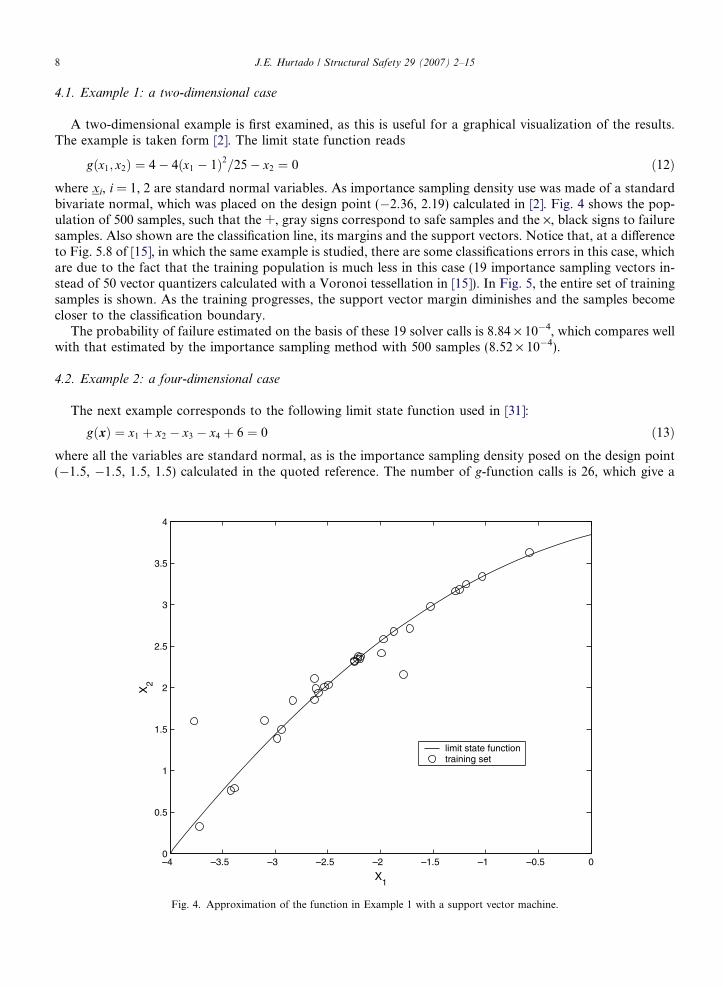
4.1. Example 1: a two-dimensional case

A two-dimensional example is first examined, as this is useful for a graphical visualization of the results.The example is taken form [2]. The limit state function reads

gðx1; x2Þ ¼ 4� 4ðx1 � 1Þ2=25� x2 ¼ 0 ð12Þ
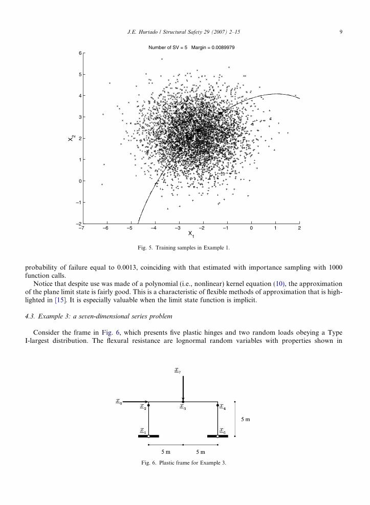
where xi, i = 1, 2 are standard normal variables. As importance sampling density use was made of a standardbivariate normal, which was placed on the design point (�2.36, 2.19) calculated in [2]. Fig. 4 shows the pop-ulation of 500 samples, such that the +, gray signs correspond to safe samples and the ·, black signs to failuresamples. Also shown are the classification line, its margins and the support vectors. Notice that, at a differenceto Fig. 5.8 of [15], in which the same example is studied, there are some classifications errors in this case, whichare due to the fact that the training population is much less in this case (19 importance sampling vectors in-stead of 50 vector quantizers calculated with a Voronoi tessellation in [15]). In Fig. 5, the entire set of trainingsamples is shown. As the training progresses, the support vector margin diminishes and the samples becomecloser to the classification boundary.
The probability of failure estimated on the basis of these 19 solver calls is 8.84 · 10�4, which compares wellwith that estimated by the importance sampling method with 500 samples (8.52 · 10�4).

4.2. Example 2: a four-dimensional case

The next example corresponds to the following limit state function used in [31]:

gðxÞ ¼ x1 þ x2 � x3 � x4 þ 6 ¼ 0 ð13Þ
where all the variables are standard normal, as is the importance sampling density posed on the design point(�1.5, �1.5, 1.5, 1.5) calculated in the quoted reference. The number of g-function calls is 26, which give a
–4 –3.5 –3 –2.5 –2 –1.5 –1 –0.5 00

0.5

1

1.5

2

2.5

3

3.5

4

X1

X2

limit state functiontraining set

Fig. 4. Approximation of the function in Example 1 with a support vector machine.

–7 –6 –5 –4 –3 –2 –1 0 1 2–2

–1

0

1

2

3

4

5

6

X1

X2

Number of SV = 5 Margin = 0.0089979

Fig. 5. Training samples in Example 1.


probability of failure equal to 0.0013, coinciding with that estimated with importance sampling with 1000function calls.

Notice that despite use was made of a polynomial (i.e., nonlinear) kernel equation (10), the approximationof the plane limit state is fairly good. This is a characteristic of flexible methods of approximation that is high-lighted in [15]. It is especially valuable when the limit state function is implicit.

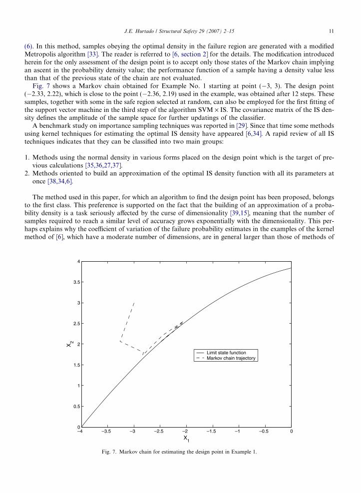
4.3. Example 3: a seven-dimensional series problem

Consider the frame in Fig. 6, which presents five plastic hinges and two random loads obeying a TypeI-largest distribution. The flexural resistance are lognormal random variables with properties shown in

Fig. 6. Plastic frame for Example 3.

Table 1Example 3 – probability distributions of the basic variables

Variable Distribution Mean Coefficient of variation

x1, x2, x3, x4, x5 Lognormal 60 kN m 0.1x6 Type I-largest 20 kN 0.3x7 Type I-largest 25 kN 0.3

Table 2Main results of the examples

Example Dimensions bP f (IS) Function calls (IS) bP f (SVM · IS) Function calls (SVM · IS)

1 2 8.52 · 10�4 500 8.84 · 10�4 192 4 0.0013 1000 0.0013 263 7 0.0180 1000 0.0184 37


Table 1, together with those of the loads. This is a classical example that has been studied in [27,5] amongothers. The limit state functions of the collapse mechanisms are as follows:

g1ðXÞ ¼ x1 þ x2 þ x4 þ x5 � hx6

g2ðXÞ ¼ x1 þ 2x2 þ 2x4 þ x5 � hx6 � hx7

g3ðXÞ ¼ x1 þ 2x3 þ x4 � hx7

ð14Þ

where h = 5 m. The importance sampling analysis was carried out with a normal density placed on the point ofcoordinates (59.39, 59.30, 58.15, 58.31, 59.29, 26.85, 46.33), taken from [5]. The covariance matrix was com-posed with the standard deviations of the basic variables with no cross-moments. As in the previous examples,use was made of a polynomial kernel of degree 2.

The probability of failure calculated with 1000 importance samples is 0.0180 while that obtained with thesupport vector classifier trained with 37 solver calls selected with the proposed algorithm is 0.0184, represent-ing a fairly good agreement.

For comparison with other techniques, it is important to quote the number of function calls used in thisvery problem with the same or similar data sets: 1200 in [27]; 1000 in [5]; 1000 in [32]. Also, a similar problemwith a single limit state and four random variables reported in [4] required 500 function calls.

Table 2 summarizes the main results of the three examples. Seemingly, there is no evident increase of thenumber of function calls on the failure probability. This is indeed a desirable result, which can be explained bythe fact that the computational effort employed by solver surrogate methods in general is not related to such aprobability, as they do not have a probabilistic formulation. Despite the number of solver calls required byimportance sampling is somewhat dependent on the probability (because of the need of reducing the varianceof the estimate of Pf, which depends on it), the number of solver calls in the proposed approach is controlledonly by the support vector margin and therefore it is independent of Pf.

5. The design point and the importance sampling density

In the above examples use was made of a multivariate normal density function, with variances equal tothose of the given basic variables, for generating the importance samples. The function was placed on a designpoint. This is a conventional method widely applied. In the examples, use was made of design points indicatedin different papers where the same cases have been calculated with other methods. For the sake of complete-ness a method for calculating this point is now proposed. Then follows a discussion on the selection of theimportance sampling density as such that justifies the use of the conventional IS technique.

Since the importance region is that having the highest probability mass in the failure region, the designpoint should ideally be that showing the highest density value in that set [2]. It can be found by modifyingthe Markov chain Monte Carlo method proposed in [6] for approximating the optimal IS density function


(6). In this method, samples obeying the optimal density in the failure region are generated with a modifiedMetropolis algorithm [33]. The reader is referred to [6, section 2] for the details. The modification introducedherein for the only assessment of the design point is to accept only those states of the Markov chain implyingan ascent in the probability density value; the performance function of a sample having a density value lessthan that of the previous state of the chain are not evaluated.

Fig. 7 shows a Markov chain obtained for Example No. 1 starting at point (�3, 3). The design point(�2.33, 2.22), which is close to the point (�2.36, 2.19) used in the example, was obtained after 12 steps. Thesesamples, together with some in the safe region selected at random, can also be employed for the first fitting ofthe support vector machine in the third step of the algorithm SVM · IS. The covariance matrix of the IS den-sity defines the amplitude of the sample space for further updatings of the classifier.

A benchmark study on importance sampling techniques was reported in [29]. Since that time some methodsusing kernel techniques for estimating the optimal IS density have appeared [6,34]. A rapid review of all IStechniques indicates that they can be classified into two main groups:

1. Methods using the normal density in various forms placed on the design point which is the target of pre-vious calculations [35,36,27,37].

2. Methods oriented to build an approximation of the optimal IS density function with all its parameters atonce [38,34,6].

The method used in this paper, for which an algorithm to find the design point has been proposed, belongsto the first class. This preference is supported on the fact that the building of an approximation of a proba-bility density is a task seriously affected by the curse of dimensionality [39,15], meaning that the number ofsamples required to reach a similar level of accuracy grows exponentially with the dimensionality. This per-haps explains why the coefficient of variation of the failure probability estimates in the examples of the kernelmethod of [6], which have a moderate number of dimensions, are in general larger than those of methods of

–4 –3.5 –3 –2.5 –2 –1.5 –1 –0.5 00

0.5

1

1.5

2

2.5

3

3.5

4

X1

X2

Limit state functionMarkov chain trajectory

Fig. 7. Markov chain for estimating the design point in Example 1.


the first group for a similar number of samples, as reported by Engelund and Rackwitz [29]. Thus, a practicalapproach is to avoid non-parametric IS density estimation with the initial exploring samples and to use theminstead to determine the design point in order to place a parametric density on top of it. In the method pro-posed herein, these samples are also used for the first assessment of the SVM classifier, which allows a drasticincrease of the efficiency of importance sampling techniques.

6. Conclusions

The following are the main conclusions emerging from the research exposed herein:

1. Pattern recognition methods providing a squashing discrimination function, such as perceptron classifiersand support vector machines, are highly useful for selecting the samples of Monte Carlo simulation tech-niques that are worth processing with a numerical solver in probabilistic structural analysis.

2. The parsimonious on-line training of support vector machines with samples generated with the importancesampling simulation technique allows both the estimation of the failure probability and the approximationof the limit state function strictly in those regions where there is a higher concentration of failure proba-bility mass. Conversely, the importance sampling is guided by the support vector margin such that the sam-ples lying beyond it are not processed by the numerical solver of the structural model. Thus, it is avoidedthe computational effort implied by an unnecessary adjustment of the solver surrogate in unimportantregions as well as that employed in computing the response to random input vectors for which the learningmachine clearly indicates that are in the safe or in the failure domains.

3. A Markov chain method for determining the design point, defined as that having the maximum likelihoodof failure, has been proposed. It helps to define the importance sampling density.

4. The examples presented in this paper demonstrate that the proposed combination permits a drastic reduc-tion of the number of samples needed by the conventional importance sampling method. Moreover, thenumber of solver calls required by the method does not depend on the value of the failure probability.

Acknowledgments

Financial support for the realization of the present research has been received from the Universidad Nac-ional de Colombia. The support is gratefully acknowledged.

Appendix. Support vector machines

This section is devoted to a summary of the support vector machine method of classification.For classes that can be separated through a hyperplane, this is such that it maximizes the margin with

respect to both classes. This means that the optimal hyperplane

gðxÞ ¼ hw; xi � b; ð15Þ
where w is a vector of weights, must be as far as possible from the points closest to it (see Fig. 8). This isreached by defining the following optimization problem:
maxw;b minifkx� xik : hw; xi þ b ¼ 0; i ¼ 1; 2; . . . ; ng ð16Þ
because we are searching the maximum separation among the minimal distances to the hyperplane. Let us re-scale the threshold b and the weight vector w such that the samples closest to the hyperplane satisfyhw, xi � b = ±1 and select two such samples x1 and x2 on different sides of the plane (see Fig. 8). Substractingthe two margin equations for them yields hw, (x1 � x2)i = 2. Dividing by the norm of vector w, it is found thatthe margin width becomes
D ¼ 2

kwk ð17Þ

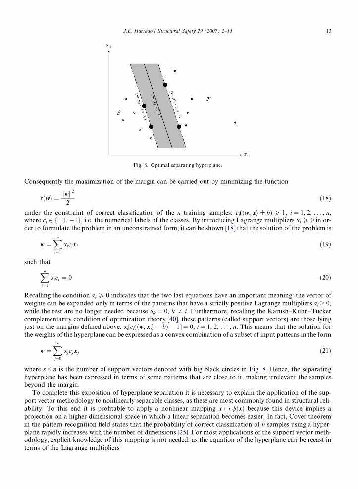
Fig. 8. Optimal separating hyperplane.


Consequently the maximization of the margin can be carried out by minimizing the function

sðwÞ ¼ kwk2

2ð18Þ

under the constraint of correct classification of the n training samples: ci(hw, xi + b) P 1, i = 1, 2, . . . , n,where ci 2 {+1, �1}, i.e. the numerical labels of the classes. By introducing Lagrange multipliers ai P 0 in or-der to formulate the problem in an unconstrained form, it can be shown [18] that the solution of the problem is

w ¼Xn

i¼1

aicixi ð19Þ

such that
Xn
i¼1

aici ¼ 0 ð20Þ

Recalling the condition ai P 0 indicates that the two last equations have an important meaning: the vector ofweights can be expanded only in terms of the patterns that have a strictly positive Lagrange multipliers ai > 0,while the rest are no longer needed because ak = 0, k 5 i. Furthermore, recalling the Karush–Kuhn–Tuckercomplementarity condition of optimization theory [40], these patterns (called support vectors) are those lyingjust on the margins defined above: ai[ci(hw, xii � b) � 1] = 0, i = 1, 2, . . . , n. This means that the solution forthe weights of the hyperplane can be expressed as a convex combination of a subset of input patterns in the form

w ¼Xs

j¼0

ajcjxj ð21Þ

where s < n is the number of support vectors denoted with big black circles in Fig. 8. Hence, the separatinghyperplane has been expressed in terms of some patterns that are close to it, making irrelevant the samplesbeyond the margin.

To complete this exposition of hyperplane separation it is necessary to explain the application of the sup-port vector methodology to nonlinearly separable classes, as these are most commonly found in structural reli-ability. To this end it is profitable to apply a nonlinear mapping x # w(x) because this device implies aprojection on a higher dimensional space in which a linear separation becomes easier. In fact, Cover theoremin the pattern recognition field states that the probability of correct classification of n samples using a hyper-plane rapidly increases with the number of dimensions [25]. For most applications of the support vector meth-odology, explicit knowledge of this mapping is not needed, as the equation of the hyperplane can be recast interms of the Lagrange multipliers


gðxÞ ¼Xs

i¼1

aiciðhxi; xi � bÞ ð22Þ

so that the transformation is made on the factors of the inner product

gðxÞ ¼Xs

i¼1

aiciðhwðxiÞ;wðxÞi � bÞ ð23Þ

This suggests the substitution of the inner product by a kernel function K(xi, x) in a Hilbert space, as this isdefined just by a generalization of the inner product operation. As a consequence, the approximating supportvector expansion for linearly or nonlinearly separable classes has the general expression

gðxÞ ¼Xs

i¼1

aiciðKðxi;xÞ � bÞ ð24Þ

If the kernel function satisfies the Mercer conditions of functional analysis to be positive definite [41], then itcan be expanded in an infinite series of eigenfunctions w(Æ)

Kðx; yÞ ¼XJ

j¼1

kjwjðxÞwjðyÞ ð25Þ

corresponding to the J positive eigenvalues kj

kjwjðyÞ ¼Z

Kðx; yÞwjðxÞdx ð26Þ

Normalizing with fjð�Þ ¼ wjð�Þ=ffiffiffiffikj

pyields

Kðx; yÞ ¼XJ

j¼1fjðxÞfjðyÞ ¼ hfðxÞ; fðyÞi ð27Þ

This means that a kernel satisfying the conditions for application of Mercer’s theorem is the Euclidean innerproduct of vectors f(x), f(y), which remain implicit. Mercer’s theorem then assures that the implicit dimen-sionality of the f-space is virtually infinite, thus enormously facilitating hyperplane classification accordingto Cover theorem. Eq. (24) is then the expression of a hyperplane in the f-space.

Frequently employed kernels are the radial basis function defined as� �
Kðx; zÞ ¼ exp �kx� zk
212; 1 2 R ð28Þ

and the polynomial kernel given by

Kðx; zÞ ¼ ðhx; zi þ hÞp; h 2 R; p 2 N ð29Þ

References

[1] Shinozuka M. Basic analysis of structural safety. J Struct Eng 1983;109:721–40.[2] Melchers RE. Structural reliability: analysis and prediction. Chichester: Wiley; 1999.[3] Bjerager P. Probability integration by directional simulation. J Eng Mech 1988;114:1285–302.[4] Ayyub BM, Chia CY. Generalized conditional expectation for structural reliability assessment. Struct Saf 1992;11:131–46.[5] Schueller GI, Bucher CG, Bourgund U, Ouypornprasert W. On efficient computational schemes to calculate failure probabilities.

Probabilist Eng Mech 1989;4:10–8.[6] Au SK, Beck JL. A new adaptive importance sampling scheme for reliability calculations. Struct Saf 1999;21:135–58.[7] Bucher C. A fast and efficient response surface approach for structural reliability problems. Struct Saf 1990;7:57–66.[8] Papadrakakis M, Papadopoulos V, Lagaros ND. Structural reliability analysis of elastic–plastic structures using neural networks and

Monte Carlo simulation. Comput Method Appl Mech Eng 1996;136:145–63.[9] Hurtado JE, Alvarez DA. Neural network-based reliability analysis: a comparative study. Comput Method Appl Mech Eng

2001;191:113–32.[10] Hurtado JE. Analysis of one-dimensional stochastic finite elements using neural networks. Probabilist Eng Mech 2002;17:35–44.[11] Hurtado JE, Alvarez DA. A classification approach for reliability analysis with stochastic finite element modeling. J Struct Eng

2003;129:1141–9.


[12] Rocco CM, Moreno JA. Fast Monte Carlo reliability evaluation using support vector machine. Reliabil Eng Syst Saf 2002;76:237–43.[13] Gomes HM, Awruch AM. Comparison of response surface and neural network with other methods for structural reliability analysis.

Struct Saf 2004;26:49–67.[14] Zhang J, Foschi RO. Performance-based design and seismic reliability analysis using designed experiments and neural networks.

Probabilist Eng Mech 2004;19:259–67.[15] Hurtado JE. Structural reliability. Statistical learning perspectives. Heidelberg: Springer; 2004.[16] Hurtado JE. Neural networks in stochastic mechanics. Arch Comput Method Eng 2001;8:303–42.[17] Hurtado JE. An examination of methods for approximating implicit limit state functions from the viewpoint of statistical learning

theory. Struct Saf 2004;26:271–93.[18] Vapnik VN. Statistical learning theory. New York: Wiley; 1998.[19] Guan XL, Melchers RE. Effect of response surface parameter variation on structural reliability estimates. Struct Saf 2001;23:429–44.[20] Hornik KM, Stinchcommbe M, White H. Multilayer feedforward networks are universal approximators. Neural Networks

1989;2:359–66.[21] Ditlevsen O, Madsen HO. Structural reliability methods. Chichester: Wiley; 1996.[22] Cichocki A, Unbehauen R. Neural networks for optimization and signal processing. Chichester: Wiley; 1993.[23] Scholkopf B, Smola A. Learning with kernels. Cambridge: The M.I.T. Press; 2002.[24] Ghanem RG, Spanos PD. Stochastic finite elements: a spectral approach. New York: Springer; 1991.[25] Cover TM. Geometrical and statistical properties of systems of linear inequalities with applications in pattern recognition. IEEE

Trans Electron Comput 1965;14:326–34.[26] Bucher CG. Adaptive sampling: an iterative fast Monte-Carlo procedure. Struct Saf 1988;5:119–26.[27] Melchers RE. Importance sampling in structural systems. Struct Saf 1989;6:3–10.[28] Au SK, Beck JL. Estimation of small failure probabilites in high dimensions by subset simulation. Probabilist Eng Mech

2001;16:263–77.[29] Engelund S, Rackwitz R. A benchmark study on importance sampling techniques in structural reliability. Struct Saf 1993;12:255–76.[30] Au SK, Beck JL. Importance sampling in high dimensions. Struct Saf 2003;25:139–63.[31] Melchers RE. Search-based importance sampling. Struct Saf 1990;9:117–28.[32] Hong HP, Lind NC. Approximate reliability analysis using normal polynomial and simulation results. Struct Saf 1996;18:329–39.[33] Metropolis N, Rosenbluth AW, Rosenbluth MN, Teller AH, Teller E. A new algorithm for adaptive multidimensional integration. J

Chem Phys 1953;21:1087–92.[34] Ang GL, Ang AH-S, Tang WH. Optimal importance sampling density estimator. J Eng Mech 1991;118:1146–63.[35] Ibrahim Y. Observations of applications of importance sampling in structural reliability analysis. Struct Saf 1991;9:269–81.[36] Schueller GI, Stix R. A critical appraisal of methods to determine failure probabilities. Struct Saf 1987;4:293–309.[37] Harbitz A. An efficient sampling method for probability of failure calculation. Struct Saf 1986;3:109–15.[38] Maes MA, Breitung K, Dupois DJ. Asymptotic importance sampling. Struct Saf 1993;12:167–86.[39] Scott DW. Multivariate density estimation. New York: Wiley; 1992.[40] Kall P, Wallace SW. Stochastic programming. Chichester: Wiley; 1995.[41] Riesz F, Nagy S. Functional analysis. New York: Dover Publications; 1990.

1-s2 0-S0167473005000597-main

Documents

Transcript of 1-s2 0-S0167473005000597-main