1 Hierarchical Indexing for Out-of-Core Access to Multi-Resolution Data

1 Hierarchical Indexing forOut-of-Core Access to Multi-Resolution Data

Valerio Pascucci and Randall J. Frank

Center for Applied Scientific Computing, Lawrence Livermore National Laboratory.

Summary. Increases in the number and size of volumetric meshes have popularized the useof hierarchical multi-resolution representations for visualization. A key component of theseschemes has become the adaptive traversal of hierarchical data-structures to build, in realtime, approximate representations of the input geometry for rendering. For very large datasetsthis process must be performed out-of-core. This paper introduces a new global indexingscheme that accelerates adaptive traversal of geometric data represented with binary trees byimproving the locality of hierarchical/spatial data access. Such improvements play a criticalrole in the enabling of effective out-of-core processing.

Three features make the scheme particularly attractive: (i) the data layout is independentof the external memory device blocking factor, (ii) the computation of the index for rectilineargrids is implemented with simple bit address manipulations and (iii) the data is not replicated,avoiding performance penalties for dynamically modified data.

The effectiveness of the approach was tested with the fundamental visualization tech-nique of rendering arbitrary planar slices. Performance comparisons with alternative indexingapproaches confirm the advantages predicted by the analysis of the scheme.

1.1 Introduction

The real time processing of very large volumetric meshes introduces unique algorithmic chal-lenges due to the impossibility of fitting the data in the main memory of a computer. The basicassumption (RAM computational model) of uniform-constant-time access to each memorylocation is not valid because part of the data is stored out-of-core or in external memory. Theperformance of many algorithms does not scale well in the transition from the in-core to theout-of-core processing conditions. This performance degradation is due to the high frequencyof I/O operations that start dominating the overall running time (trashing).

Out-of-core computing [22] addresses specifically the issues of algorithm redesign anddata layout restructuring, necessary to enable data access patterns with minimal out-of-coreprocessing performance degradation. Research in this area is also valuable in parallel anddistributed computing, where one has to deal with the similar issue of balancing processingtime with data migration time.

The solution of the out-of-core processing problem is typically divided into two parts:(i) algorithm analysis to understand its data access patterns and, when possible, redesign

to maximize their locality;(ii) storage of the data in secondary memory with a layout consistent with the access

patterns of the algorithm, amortizing the cost individual I/O operations over several memoryaccess operations.

In the case of hierarchical visualization algorithms for volumetric data, the 3D input hi-erarchy is traversed to build derived geometric models with adaptive levels of detail. The

2 Valerio Pascucci and Randall J. Frank

shape of the output models are then modified dynamically with incremental updates of theirlevel of detail. The parameters that govern this continuous modification of the output geom-etry are dependent on runtime user interaction, making it impossible to determine, a priori,what levels of detail will be constructed. For example, parameters can be external, such asthe viewpoint of the current display window or internal, such as the isovalue of an isocontouror the position of an orthogonal slice. The general structure of the access pattern can be sum-marized into two main points: (i) the input hierarchy is traversed coarse to fine, level by levelso that the data in the same level of resolution is accessed at the same time and (ii) withineach level of resolution the data is mainly traversed coherently in regions that are in closegeometric proximity.

In this paper we introduce a new static indexing scheme that induces a data layout satisfy-ing both requirements (i) and (ii) for the hierarchical traversal of �-dimensional regular grids.The scheme has three key features that make it particularly attractive. First, the order of thedata is independent of the out-of-core blocking factor so that its use in different settings (e.g.local disk access or transmission through a network) does not require any large data reorga-nization. Second, conversion from the standard Z-order indexing to the new indexing schemecan be implemented with a simple sequence of bit-string manipulations making it appealingfor a possible hardware implementation. Third, there is no data replication, avoiding any per-formance penalty for dynamic updates or any inflated storage typical of most hierarchical andout-of-core schemes.

Beyond the theoretical interest in developing hierarchical indexing schemes for �-dimen-sional space filling curves, our approach targets practical applications in out-of-core visual-ization algorithms. In this paper, we report algorithmic analysis and experimental results forthe case of slicing large volumetric datasets.

The remainder of this paper is organized as follows. Section 1.2 discusses briefly previ-ous work in related areas. Section 1.3 introduces the general framework for the computationof the new indexing scheme. Section 1.4 discusses the implementation of the approach forbinary tree hierarchies. Section 1.5 analyzes the application of the scheme for progressivecomputation of orthogonal slices reporting experimental timings for memory mapped files.Section 1.6 presents the structure of the I/O system and practical results obtained with com-pressed data. Concluding remarks and future directions are discussed in section 1.7.

1.2 Related Previous Work

External memory algorithms [22], also known as out-of-core algorithms, have been rising tothe attention of the computer science community in recent years as they address, systemat-ically, the problem of the non-uniform memory structure of modern computers (e.g. L1/L2cache, main memory, hard disk, etc). This issue is particularly important when dealing withlarge data-structures that do not fit in the main memory of a single computer since the ac-cess time to each memory unit is dependent on its location. New algorithmic techniquesand analysis tools have been developed to address this problem in the case of geometric al-gorithms [1,2,9,15] and scientific visualization [4,8]. Closely related issues emerge in thearea of parallel and distributed computing where remote data transfer can become a primarybottleneck in the computation. In this context space filling curves are often used as a toolto determine, very quickly, data distribution layouts that guarantee good geometric local-ity [10,18,20]. Space filling curves [21] have been also used in the past in a wide varietyof applications [3] because of their hierarchical fractal structure as well as for their well

1 Hierarchical Indexing for Out-of-Core Access to Multi-Resolution Data 3

(a) (b) (c) (d) (e)

(f) (g) (h) (i) (j)

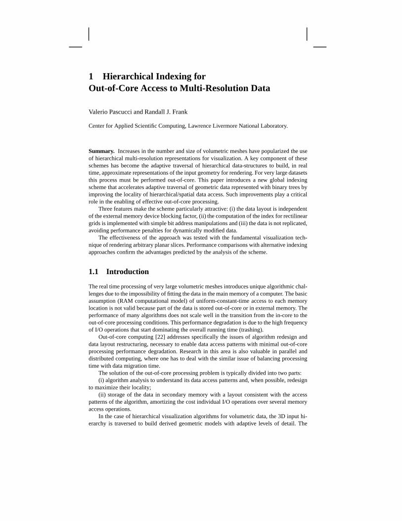
Fig. 1.1. (a-e) The first five levels of resolution of the 2D Lebesgue’s space fillingcurve. (f-j) The first five levels of resolution of the 3D Lebesgue’s space fillingcurve.

known spatial locality properties. The most popular is the Hilbert curve [11] which guaran-tees the best geometric locality properties [19]. The pseudo-Hilbert scanning order [7,6,12]generalizes the scheme to rectilinear grids that have different number of samples along eachcoordinate axis.

Recently Lawder [13,14] explored the use of different kinds of space filling curves todevelop indexing schemes for data storage layout and fast retrieval in multi-dimensionaldatabases.

Balmelli at al. [5] use the Z-order (Lebesque) space filling curve to navigate efficiently aquad-tree data-structure without using pointers.

In the approach proposed here a new data layout is used to allow efficient progressiveaccess to volumetric information stored in external memory. This is achieved by combininginterleaved storage of the levels in the data hierarchy while maintaining geometric proximitywithin each level of resolution (multidimensional breadth first traversal). One main advan-tage is that the resulting data layout is independent of the particular adaptive traversal of thedata. Moreover the same data layout can be used with different blocking factors making itbeneficial throughout the entire memory hierarchy.

1.3 Hierarchical Subsampling Framework

This section discusses the general framework for the efficient definition of a hierarchy overthe samples of a dataset.

Consider a set � of � elements decomposed into a hierarchy � of � levels of resolution� � �� such that:

��


where �� is said to be coarser than �� if � � �. The order of the elements in � is defined bya cardinality function � � � �� . This means that the following identity alwaysholds:

��

where square brackets are used to index an element in a set.One can define a derived sequence �� of sets �� as follow:

��

where formally �� . The sequence �� is a partitioning of ��A derived cardinality function � � � � �� can be defined on the basis of thefollowing two properties:

� ��

� � ��

If the original function has strong locality properties when restricted to any level of res-olution �� then the cardinality function � generates the desired global index for hierarchicaland out-of-core traversal. The scheme has strong locality if elements with with close indexare also close in geometric position. This locality properties are well studied in [17].

The construction of the function can be achieved in the following way: (i) determine thenumber of elements in each derived set �� and (ii) determine a cardinality function ��

�

restriction of � to each set ��. In particular if �� is the number of elements of �� onecan predetermine the starting index of the elements in a given level of resolution by buildingthe sequence of constants �� with

� �

��

�� (1.1)

Next, one must determine a set of local cardinality functions �� sothat:

� �� (1.2)

The computation of the constants � can be performed in a preprocessing stage so that thecomputation of � is reduced to the following two steps:

� given determine its level of resolution � (that is the � such that �� compute �� and add it to ��

These two steps must be performed very efficiently as they will be executed repeatedly at runtime. The following section reports a practical realization of this scheme for rectilinear cubegrids in any dimension.


(a)

(e)

(i)

(b) (c)

(f)(d)

(g) (h)

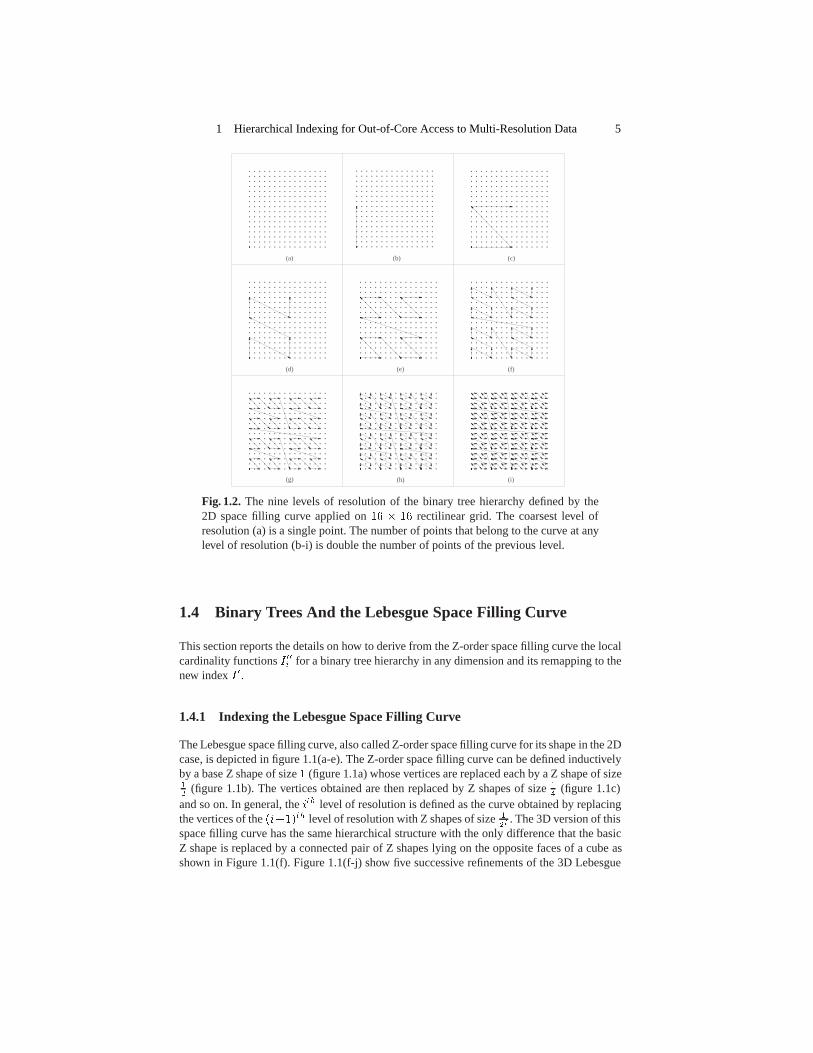
Fig. 1.2. The nine levels of resolution of the binary tree hierarchy defined by the2D space filling curve applied on �� rectilinear grid. The coarsest level ofresolution (a) is a single point. The number of points that belong to the curve at anylevel of resolution (b-i) is double the number of points of the previous level.

1.4 Binary Trees And the Lebesgue Space Filling Curve

This section reports the details on how to derive from the Z-order space filling curve the localcardinality functions �� for a binary tree hierarchy in any dimension and its remapping to thenew index �.

1.4.1 Indexing the Lebesgue Space Filling Curve

The Lebesgue space filling curve, also called Z-order space filling curve for its shape in the 2Dcase, is depicted in figure 1.1(a-e). The Z-order space filling curve can be defined inductivelyby a base Z shape of size � (figure 1.1a) whose vertices are replaced each by a Z shape of size�

�(figure 1.1b). The vertices obtained are then replaced by Z shapes of size �

�(figure 1.1c)

and so on. In general, the �� level of resolution is defined as the curve obtained by replacingthe vertices of the �� level of resolution with Z shapes of size �

��. The 3D version of this

space filling curve has the same hierarchical structure with the only difference that the basicZ shape is replaced by a connected pair of Z shapes lying on the opposite faces of a cube asshown in Figure 1.1(f). Figure 1.1(f-j) show five successive refinements of the 3D Lebesgue


space filling curve. The �-dimensional version of the space filling curve has also the samehierarchical structure, where the basic shape (the Z of the 2D case) is defined as a connectedpair of ��-dimensional basic shapes lying on the opposite faces of a �-dimensional cube.

The property that makes the Lebesgue’s space filling curve particularly attractive is theeasy conversion from the � indices of a �-dimensional matrix to the 1D index along thecurve. If one element � has �-dimensional reference �� its 1D reference is built byinterleaving the bits of the binary representations of the indices �� . In particular if ��is represented by the string of � bits ��

�

� � � � �� (with � � �� ) then the 1D reference of � is represented the string of �� bits � ��

�

� � � � �� .

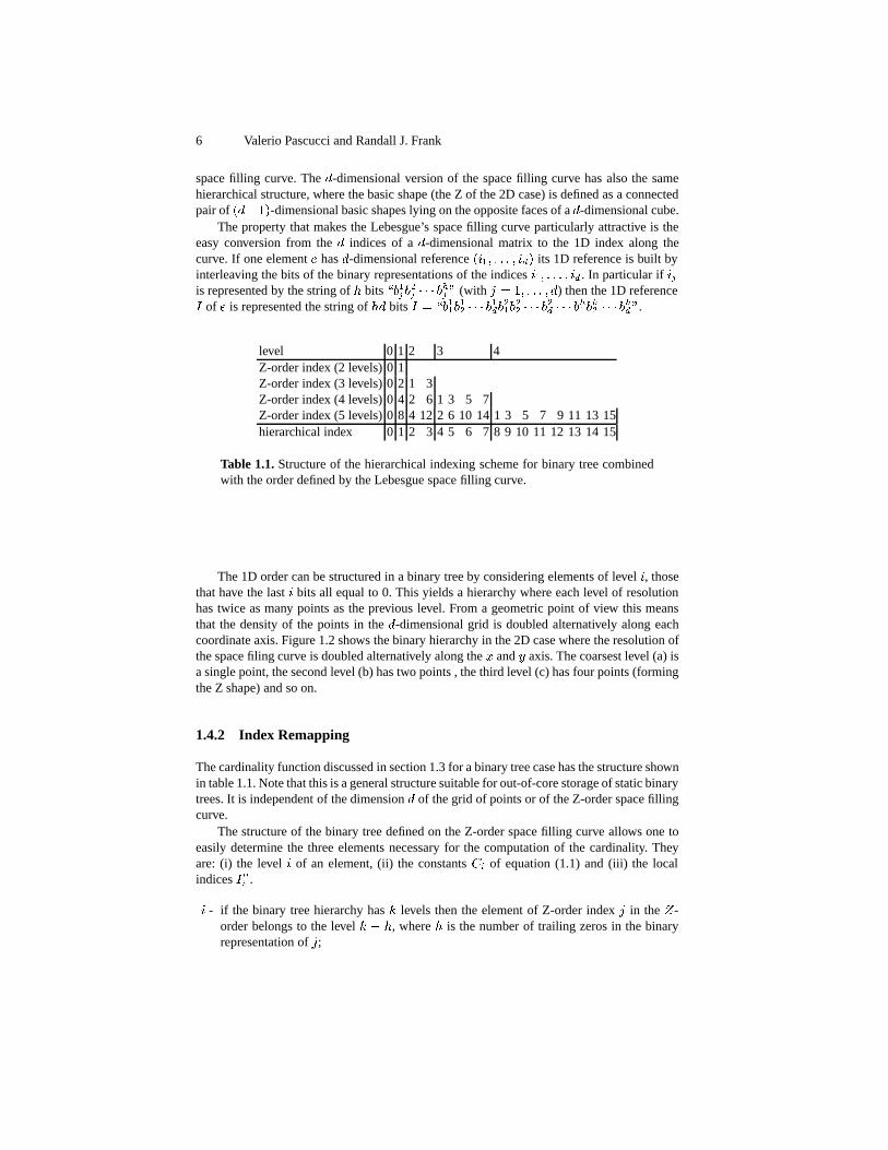
level 0 1 2 3 4Z-order index (2 levels) 0 1Z-order index (3 levels) 0 2 1 3Z-order index (4 levels) 0 4 2 6 1 3 5 7Z-order index (5 levels) 0 8 4 12 2 6 10 14 1 3 5 7 9 11 13 15hierarchical index 0 1 2 3 4 5 6 7 8 9 10 11 12 13 14 15

Table 1.1. Structure of the hierarchical indexing scheme for binary tree combinedwith the order defined by the Lebesgue space filling curve.

The 1D order can be structured in a binary tree by considering elements of level �, thosethat have the last � bits all equal to 0. This yields a hierarchy where each level of resolutionhas twice as many points as the previous level. From a geometric point of view this meansthat the density of the points in the �-dimensional grid is doubled alternatively along eachcoordinate axis. Figure 1.2 shows the binary hierarchy in the 2D case where the resolution ofthe space filing curve is doubled alternatively along the � and � axis. The coarsest level (a) isa single point, the second level (b) has two points , the third level (c) has four points (formingthe Z shape) and so on.

1.4.2 Index Remapping

The cardinality function discussed in section 1.3 for a binary tree case has the structure shownin table 1.1. Note that this is a general structure suitable for out-of-core storage of static binarytrees. It is independent of the dimension � of the grid of points or of the Z-order space fillingcurve.

The structure of the binary tree defined on the Z-order space filling curve allows one toeasily determine the three elements necessary for the computation of the cardinality. Theyare: (i) the level � of an element, (ii) the constants � of equation (1.1) and (iii) the localindices �� .

� - if the binary tree hierarchy has � levels then the element of Z-order index � in the �-order belongs to the level � � �, where � is the number of trailing zeros in the binaryrepresentation of �;


1

Shift

0

Shift

Loop: While the outgoing bit is zero

Incoming bit Outgoing bit

0 0 1 0 1 1 0 1 0 0

1 0 0 1 0 1 1 0 1 0� 0

0 1 0 0 1 0 1 1 0 1� 0

0 0 1 0 0 1 0 1 1 0� 1

0 0 1 0 0 1 0 1 1 0

(a) (b)

Step 1: shift right with incoming bit set to 1

shift right with incoming bit set to 0

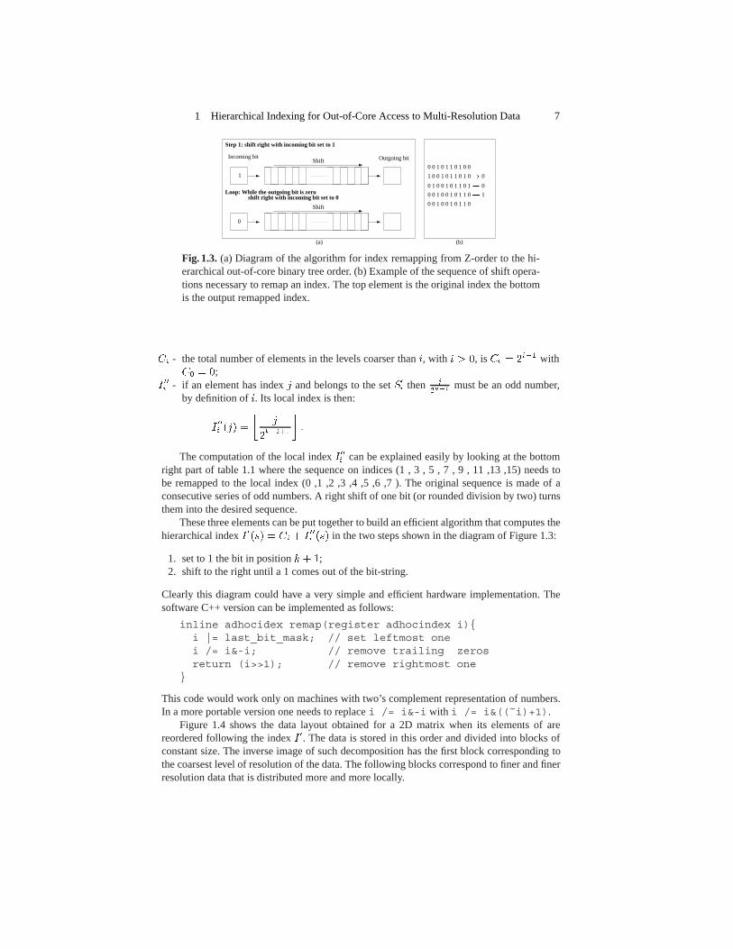
Fig. 1.3. (a) Diagram of the algorithm for index remapping from Z-order to the hi-erarchical out-of-core binary tree order. (b) Example of the sequence of shift opera-tions necessary to remap an index. The top element is the original index the bottomis the output remapped index.

� - the total number of elements in the levels coarser than �, with � � �, is � � �� with � � �;

�� - if an element has index � and belongs to the set �� then �

��must be an odd number,

by definition of �. Its local index is then:

��

��

��

��

The computation of the local index �� can be explained easily by looking at the bottomright part of table 1.1 where the sequence on indices (1 , 3 , 5 , 7 , 9 , 11 ,13 ,15) needs tobe remapped to the local index (0 ,1 ,2 ,3 ,4 ,5 ,6 ,7 ). The original sequence is made of aconsecutive series of odd numbers. A right shift of one bit (or rounded division by two) turnsthem into the desired sequence.

These three elements can be put together to build an efficient algorithm that computes thehierarchical index �� in the two steps shown in the diagram of Figure 1.3:

1. set to 1 the bit in position � �;2. shift to the right until a 1 comes out of the bit-string.

Clearly this diagram could have a very simple and efficient hardware implementation. Thesoftware C++ version can be implemented as follows:

inline adhocidex remap(register adhocindex i){i |= last_bit_mask; // set leftmost onei /= i&-i; // remove trailing zerosreturn (i>>1); // remove rightmost one

}

This code would work only on machines with two’s complement representation of numbers.In a more portable version one needs to replace i /= i&-i with i /= i&((˜i)+1).

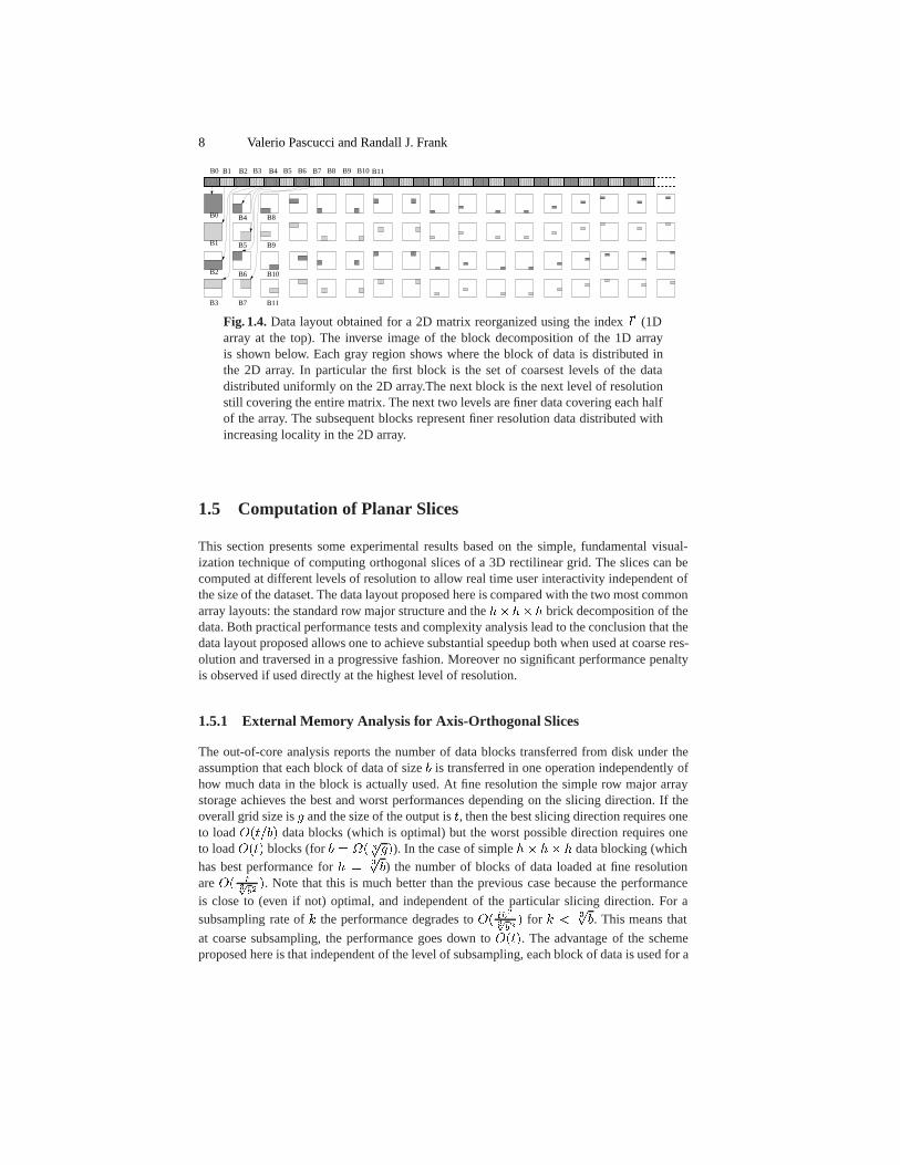
Figure 1.4 shows the data layout obtained for a 2D matrix when its elements of arereordered following the index �. The data is stored in this order and divided into blocks ofconstant size. The inverse image of such decomposition has the first block corresponding tothe coarsest level of resolution of the data. The following blocks correspond to finer and finerresolution data that is distributed more and more locally.


B0 B1 B2 B3 B4 B5 B6 B7 B8 B9 B10

B0

B1

B2

B3

B4

B5

B6

B7

B8

B9

B10

B11

B11

Fig. 1.4. Data layout obtained for a 2D matrix reorganized using the index � (1Darray at the top). The inverse image of the block decomposition of the 1D arrayis shown below. Each gray region shows where the block of data is distributed inthe 2D array. In particular the first block is the set of coarsest levels of the datadistributed uniformly on the 2D array.The next block is the next level of resolutionstill covering the entire matrix. The next two levels are finer data covering each halfof the array. The subsequent blocks represent finer resolution data distributed withincreasing locality in the 2D array.

1.5 Computation of Planar Slices

This section presents some experimental results based on the simple, fundamental visual-ization technique of computing orthogonal slices of a 3D rectilinear grid. The slices can becomputed at different levels of resolution to allow real time user interactivity independent ofthe size of the dataset. The data layout proposed here is compared with the two most commonarray layouts: the standard row major structure and the �� brick decomposition of thedata. Both practical performance tests and complexity analysis lead to the conclusion that thedata layout proposed allows one to achieve substantial speedup both when used at coarse res-olution and traversed in a progressive fashion. Moreover no significant performance penaltyis observed if used directly at the highest level of resolution.

1.5.1 External Memory Analysis for Axis-Orthogonal Slices

The out-of-core analysis reports the number of data blocks transferred from disk under theassumption that each block of data of size � is transferred in one operation independently ofhow much data in the block is actually used. At fine resolution the simple row major arraystorage achieves the best and worst performances depending on the slicing direction. If theoverall grid size is � and the size of the output is �, then the best slicing direction requires oneto load �� data blocks (which is optimal) but the worst possible direction requires oneto load �� blocks (for � � ��

��). In the case of simple �� data blocking (which

has best performance for � � ��) the number of blocks of data loaded at fine resolution

are �� . Note that this is much better than the previous case because the performance

is close to (even if not) optimal, and independent of the particular slicing direction. For asubsampling rate of � the performance degrades to ��

�� for � � �

��. This means that

at coarse subsampling, the performance goes down to ��. The advantage of the schemeproposed here is that independent of the level of subsampling, each block of data is used for a


1

10

100

1000

10000

100000

1e+06

1e+07

1e+08

1e+09

1 10 100 1000 10000

dat

a lo

aded

Sub-sampling frequency (1=full resolution, 2=every other element, ....).

binary tree with Z-order remapping32*32*32 blocks

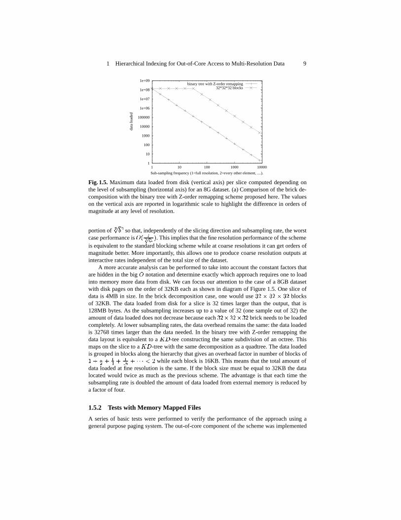
Fig. 1.5. Maximum data loaded from disk (vertical axis) per slice computed depending onthe level of subsampling (horizontal axis) for an 8G dataset. (a) Comparison of the brick de-composition with the binary tree with Z-order remapping scheme proposed here. The valueson the vertical axis are reported in logarithmic scale to highlight the difference in orders ofmagnitude at any level of resolution.

portion of �� so that, independently of the slicing direction and subsampling rate, the worst

case performance is �� . This implies that the fine resolution performance of the scheme

is equivalent to the standard blocking scheme while at coarse resolutions it can get orders ofmagnitude better. More importantly, this allows one to produce coarse resolution outputs atinteractive rates independent of the total size of the dataset.

A more accurate analysis can be performed to take into account the constant factors thatare hidden in the big � notation and determine exactly which approach requires one to loadinto memory more data from disk. We can focus our attention to the case of a 8GB datasetwith disk pages on the order of 32KB each as shown in diagram of Figure 1.5. One slice ofdata is 4MB in size. In the brick decomposition case, one would use �� blocksof 32KB. The data loaded from disk for a slice is 32 times larger than the output, that is128MB bytes. As the subsampling increases up to a value of 32 (one sample out of 32) theamount of data loaded does not decrease because each �� brick needs to be loadedcompletely. At lower subsampling rates, the data overhead remains the same: the data loadedis 32768 times larger than the data needed. In the binary tree with Z-order remapping thedata layout is equivalent to a ��-tee constructing the same subdivision of an octree. Thismaps on the slice to a ��-tree with the same decomposition as a quadtree. The data loadedis grouped in blocks along the hierarchy that gives an overhead factor in number of blocks of� �

� �

� �

�� while each block is 16KB. This means that the total amount of

data loaded at fine resolution is the same. If the block size must be equal to 32KB the datalocated would twice as much as the previous scheme. The advantage is that each time thesubsampling rate is doubled the amount of data loaded from external memory is reduced bya factor of four.

1.5.2 Tests with Memory Mapped Files

A series of basic tests were performed to verify the performance of the approach using ageneral purpose paging system. The out-of-core component of the scheme was implemented


�� Grid �� Grid500Mhz Intel PIII, 128MB RAM 300Mhz MIPS R12000, 600MB RAM

1e-05

0.0001

0.001

0.01

0.1

1

10

1 10 100

aver

age

slic

e co

mpu

tatio

n tim

e in

sec

onds

subsampling rate (1=full resolution, 2=every other element, ....).

binary tree with Z-order remapping16x16x16 bricks

array order - (j,k) plane slicesarray order - (j,i) plane slices

1e-05

0.0001

0.001

0.01

0.1

1

10

1 10 100 1000

slic

e co

mpu

tatio

n tim

e in

sec

onds

subsampling rate (1=full resolution, 2=every other element, ....).

binary tree with Z-order remapping16x16x16 bricks

array order - (j,k) plane slicearray order - (j,i) plane slice

(a) (b)

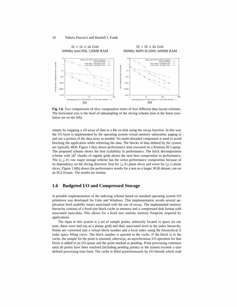
Fig. 1.6. Two comparisons of slice computation times of four different data layout schemes.The horizontal axis is the level of subsampling of the slicing scheme (test at the finest reso-lution are on the left).

simply by mapping a 1D array of data to a file on disk using the mmap function. In this waythe I/O layer is implemented by the operating system virtual memory subsystem, paging inand out a portion of the data array as needed. No multi-threaded component is used to avoidblocking the application while retrieving the data. The blocks of data defined by the systemare typically 4KB. Figure 1.6(a) shows performance tests executed on a Pentium III Laptop.The proposed scheme shows the best scalability in performance. The brick decompositionscheme with �� chunks of regular grids shows the next best compromise in performance.The �� row major storage scheme has the worst performance compromise because ofits dependency on the slicing direction: best for �� plane slices and worst for �� planeslices. Figure 1.6(b) shows the performance results for a test on a larger, 8GB dataset, run onan SGI Octane. The results are similar.

1.6 Budgeted I/O and Compressed Storage

A portable implementation of the indexing scheme based on standard operating system I/Oprimitives was developed for Unix and Windows. This implementation avoids several ap-plication level usability issues associated with the use of mmap. The implemented memoryhierarchy consists of a fixed size block cache in memory and a compressed disk format withassociated meta-data. This allows for a fixed size runtime memory footprint, required byapplications.

The input to this system is a set of sample points, arbitrarily located in space (in ourtests, these were laid out as a planar grid) and their associated level in the index hierarchy.Points are converted into a virtual block number and a local index using the hierarchical Zorder space filling curve. The block number is queried in the cache. If the block is in thecache, the sample for the point is returned, otherwise, an asynchronous I/O operation for thatblock is added to an I/O queue and the point marked as pending. Point processing continuesuntil all points have been resolved (including pending points) or the system exceeds a userdefined processing time limit. The cache is filled asynchronously by I/O threads which read


0.001

0.01

0.1

1

10

100

1 2 4 8 16 32 64

Ave

rage

Slic

e C

ompu

tatio

n T

ime

(s)

Subsampling Rate

R1-BITR1-BLKR1-ARR

T1-BITT1-BLKT1-ARR

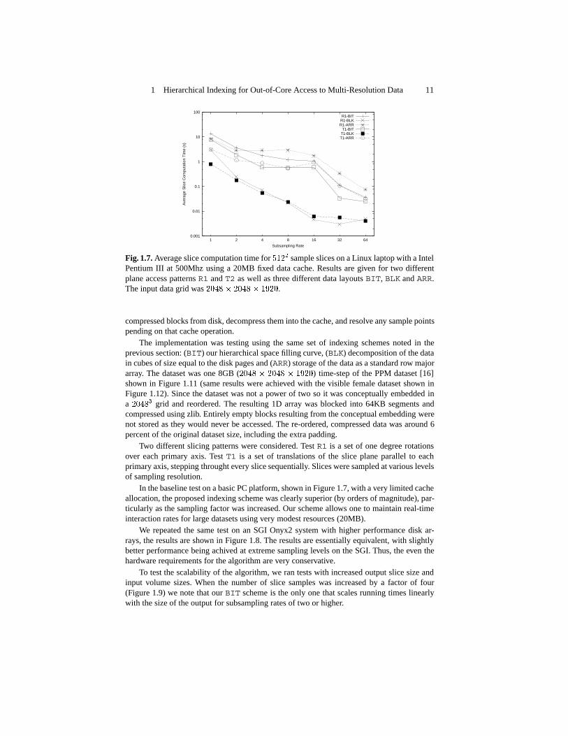
Fig. 1.7. Average slice computation time for �� sample slices on a Linux laptop with a IntelPentium III at 500Mhz using a 20MB fixed data cache. Results are given for two differentplane access patterns R1 and T2 as well as three different data layouts BIT, BLK and ARR.The input data grid was �� .

compressed blocks from disk, decompress them into the cache, and resolve any sample pointspending on that cache operation.

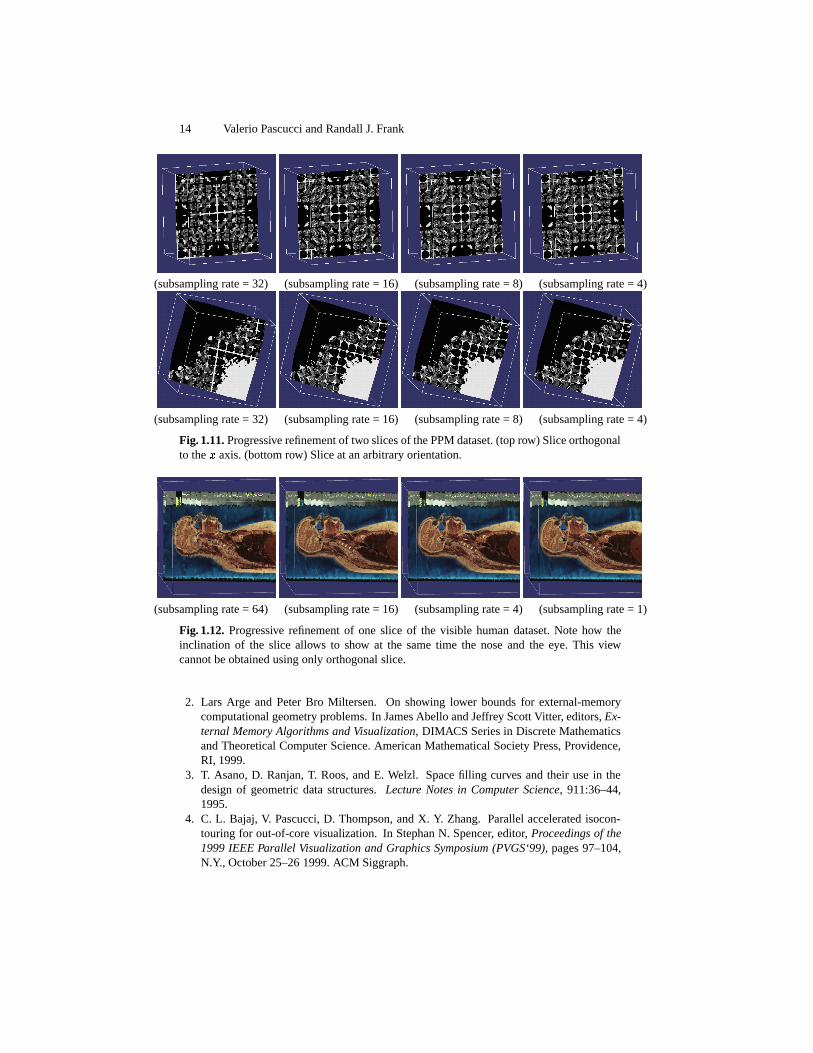
The implementation was testing using the same set of indexing schemes noted in theprevious section: (BIT) our hierarchical space filling curve, (BLK) decomposition of the datain cubes of size equal to the disk pages and (ARR) storage of the data as a standard row majorarray. The dataset was one 8GB (�� ) time-step of the PPM dataset [16]shown in Figure 1.11 (same results were achieved with the visible female dataset shown inFigure 1.12). Since the dataset was not a power of two so it was conceptually embedded ina �� grid and reordered. The resulting 1D array was blocked into 64KB segments andcompressed using zlib. Entirely empty blocks resulting from the conceptual embedding werenot stored as they would never be accessed. The re-ordered, compressed data was around 6percent of the original dataset size, including the extra padding.

Two different slicing patterns were considered. Test R1 is a set of one degree rotationsover each primary axis. Test T1 is a set of translations of the slice plane parallel to eachprimary axis, stepping throught every slice sequentially. Slices were sampled at various levelsof sampling resolution.

In the baseline test on a basic PC platform, shown in Figure 1.7, with a very limited cacheallocation, the proposed indexing scheme was clearly superior (by orders of magnitude), par-ticularly as the sampling factor was increased. Our scheme allows one to maintain real-timeinteraction rates for large datasets using very modest resources (20MB).

We repeated the same test on an SGI Onyx2 system with higher performance disk ar-rays, the results are shown in Figure 1.8. The results are essentially equivalent, with slightlybetter performance being achived at extreme sampling levels on the SGI. Thus, the even thehardware requirements for the algorithm are very conservative.

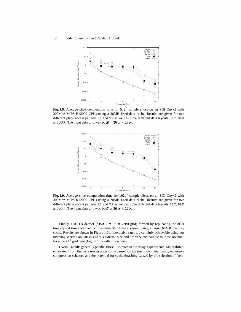
To test the scalability of the algorithm, we ran tests with increased output slice size andinput volume sizes. When the number of slice samples was increased by a factor of four(Figure 1.9) we note that our BIT scheme is the only one that scales running times linearlywith the size of the output for subsampling rates of two or higher.


0.0001

0.001

0.01

0.1

1

10

100

1 2 4 8 16 32 64

Ave

rage

Slic

e C

ompu

tatio

n T

ime

(s)

Subsampling Rate

R1-BITR1-BLKR1-ARR

T1-BITT1-BLKT1-ARR

Fig. 1.8. Average slice computation time for �� sample slices on an SGI Onyx2 with300Mhz MIPS R12000 CPUs using a 20MB fixed data cache. Results are given for twodifferent plane access patterns R1 and T2 as well as three different data layouts BIT, BLKand ARR. The input data grid was �� .

0.0001

0.001

0.01

0.1

1

10

100

1000

1 2 4 8 16 32 64

Ave

rage

Slic

e C

ompu

tatio

n T

ime

(s)

Subsampling Rate

R1-BITR1-BLKR1-ARR

T1-BITT1-BLKT1-ARR


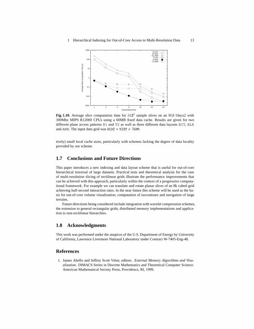
Finally, a 0.5TB dataset (�� grid) formed by replicating the 8GBtimestep 64 times was run on the same SGI Onyx2 system using a larger 60MB memorycache. Results are shown in Figure 1.10. Interactive rates are certainly achievable using ourindexing scheme on datasets of this extreme size and are very comparable to those obtainedfor a the �� grid case (Figure 1.8) with this scheme.

Overall, results generally parallel those illustrated in the mmap experiments. Major differ-ences stem from the increases in access time caused by the use of computationally expensivecompression schemes and the potential for cache thrashing caused by the selection of (rela-


0.001

0.01

0.1

1

10

100

1000

1 2 4 8 16 32 64

Ave

rage

Slic

e C

ompu

tatio

n T

ime

(s)

Subsampling Rate

R1-BITR1-BLKR1-ARR

T1-BITT1-BLKT1-ARR


tively) small local cache sizes, particularly with schemes lacking the degree of data localityprovided by our scheme.

1.7 Conclusions and Future Directions

This paper introduces a new indexing and data layout scheme that is useful for out-of-corehierarchical traversal of large datasets. Practical tests and theoretical analysis for the caseof multi-resolution slicing of rectilinear grids illustrate the performance improvements thatcan be achieved with this approach, particularly within the context of a progressive computa-tional framework. For example we can translate and rotate planar slices of an 8k cubed gridachieving half-second interaction rates. In the near future this scheme will be used as the ba-sis for out-of-core volume visualization, computation of isocontours and navigation of largeterrains.

Future directions being considered include integration with wavelet compression schemes,the extension to general rectangular grids, distributed memory implementations and applica-tion to non-rectilinear hierarchies.

1.8 Acknowledgments

This work was performed under the auspices of the U.S. Department of Energy by Universityof California, Lawrence Livermore National Laboratory under Contract W-7405-Eng-48.

References

1. James Abello and Jeffrey Scott Vitter, editors. External Memory Algorithms and Visu-alization. DIMACS Series in Discrete Mathematics and Theoretical Computer Science.American Mathematical Society Press, Providence, RI, 1999.


(subsampling rate = 32) (subsampling rate = 16) (subsampling rate = 8) (subsampling rate = 4)


Fig. 1.11. Progressive refinement of two slices of the PPM dataset. (top row) Slice orthogonalto the � axis. (bottom row) Slice at an arbitrary orientation.


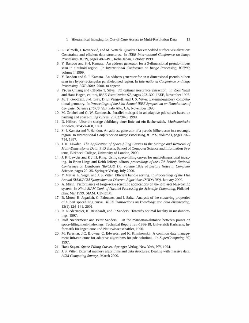
Fig. 1.12. Progressive refinement of one slice of the visible human dataset. Note how theinclination of the slice allows to show at the same time the nose and the eye. This viewcannot be obtained using only orthogonal slice.

2. Lars Arge and Peter Bro Miltersen. On showing lower bounds for external-memorycomputational geometry problems. In James Abello and Jeffrey Scott Vitter, editors, Ex-ternal Memory Algorithms and Visualization, DIMACS Series in Discrete Mathematicsand Theoretical Computer Science. American Mathematical Society Press, Providence,RI, 1999.

3. T. Asano, D. Ranjan, T. Roos, and E. Welzl. Space filling curves and their use in thedesign of geometric data structures. Lecture Notes in Computer Science, 911:36–44,1995.

4. C. L. Bajaj, V. Pascucci, D. Thompson, and X. Y. Zhang. Parallel accelerated isocon-touring for out-of-core visualization. In Stephan N. Spencer, editor, Proceedings of the1999 IEEE Parallel Visualization and Graphics Symposium (PVGS‘99), pages 97–104,N.Y., October 25–26 1999. ACM Siggraph.


5. L. Balmelli, J. Kovacevic, and M. Vetterli. Quadtree for embedded surface visualization:Constraints and efficient data structures. In IEEE International Conference on ImageProcessing (ICIP), pages 487–491, Kobe Japan, October 1999.

6. Y. Bandou and S.-I. Kamata. An address generator for a 3-dimensional pseudo-hilbertscan in a cuboid region. In International Conference on Image Processing, ICIP99,volume I, 1999.

7. Y. Bandou and S.-I. Kamata. An address generator for an n-dimensional pseudo-hilbertscan in a hyper-rectangular parallelepiped region. In International Conference on ImageProcessing, ICIP 2000, 2000. to appear.

8. Yi-Jen Chiang and Claudio T. Silva. I/O optimal isosurface extraction. In Roni Yageland Hans Hagen, editors, IEEE Visualization 97, pages 293–300. IEEE, November 1997.

9. M. T. Goodrich, J.-J. Tsay, D. E. Vengroff, and J. S. Vitter. External-memory computa-tional geometry. In Proceedings of the 34th Annual IEEE Symposium on Foundations ofComputer Science (FOCS ’93), Palo Alto, CA, November 1993.

10. M. Griebel and G. W. Zumbusch. Parallel multigrid in an adaptive pde solver based onhashing and space-filling curves. 25:827:843, 1999.

11. D. Hilbert. Uber die stetige abbildung einer linie auf ein flachenstuck. MathematischeAnnalen, 38:459–460, 1891.

12. S.-I. Kamata and Y. Bandou. An address generator of a pseudo-hilbert scan in a rectangleregion. In International Conference on Image Processing, ICIP97, volume I, pages 707–714, 1997.

13. J. K. Lawder. The Application of Space-filling Curves to the Storage and Retrieval ofMulti-Dimensional Data. PhD thesis, School of Computer Science and Information Sys-tems, Birkbeck College, University of London, 2000.

14. J. K. Lawder and P. J. H. King. Using space-filling curves for multi-dimensional index-ing. In Brian Lings and Keith Jeffery, editors, proceedings of the 17th British NationalConference on Databases (BNCOD 17), volume 1832 of Lecture Notes in ComputerScience, pages 20–35. Springer Verlag, July 2000.

15. Y. Matias, E. Segal, and J. S. Vitter. Efficient bundle sorting. In Proceedings of the 11thAnnual SIAM/ACM Symposium on Discrete Algorithms (SODA ’00), January 2000.

16. A. Mirin. Performance of large-scale scientific applications on the ibm asci blue-pacificsystem. In Ninth SIAM Conf. of Parallel Processing for Scientific Computing, Philadel-phia, Mar 1999. SIAM. CD-ROM.

17. B. Moon, H. Jagadish, C. Faloutsos, and J. Saltz. Analysis of the clustering propertiesof hilbert spacefilling curve. IEEE Transactions on knowledge and data engeneering,13(1):124–141, 2001.

18. R. Niedermeier, K. Reinhardt, and P. Sanders. Towards optimal locality in meshindex-ings, 1997.

19. Rolf Niedermeier and Peter Sanders. On the manhattan-distance between points onspace-filling mesh-indexings. Technical Report iratr-1996-18, Universitat Karlsruhe, In-formatik fur Ingenieure und Naturwissenschaftler, 1996.

20. M. Parashar, J.C. Browne, C. Edwards, and K. Klimkowski. A common data manage-ment infrastructure for adaptive algorithms for pde solutions. In SuperComputing 97,1997.

21. Hans Sagan. Space-Filling Curves. Springer-Verlag, New York, NY, 1994.22. J. S. Vitter. External memory algorithms and data structures: Dealing with massive data.

ACM Computing Surveys, March 2000.

Global Static Indexing for Real-time Exploration of Very Large Regular Grids

Valerio Pascucci Center for Applied Scientific Computing

Lawrence Livermore National Laboratory

[email protected]

Randall J. Frank Livermore Computing

Lawrence Livermore National Laboratory

[email protected]

ABSTRACT In this paper we introduce a new indexing scheme for progressive traversal and visualization of large regular grids. We demonstrate the potential of our approach by providing a tool that displays at interactive rates planar slices of scalar field data with very modest computing resources. We obtain unprecedented results both in terms of absolute performance and, more importantly, in terms of scalability. On a laptop computer we provide real time interaction with a 20483 grid (8 Giga-nodes) using only 20MB of memory. On an SGI Onyx we slice interactively an 81923 grid (½ tera-nodes) using only 60MB of memory. The scheme relies simply on the determination of an appropriate reordering of the rectilinear grid data and a progressive construction of the output slice. The reordering minimizes the amount of I/O performed during the out-of-core computation. The progressive and asynchronous computation of the output provides flexible quality/speed tradeoffs and a time-critical and interruptible user interface.

1. INTRODUCTION The real time processing of very large volumetric meshes introduces specific algorithmic challenges due to the impossibility of fitting the input data in the main memory of a computer. The basic assumption (RAM computational model) of uniform-constant-time access to each memory location is not valid because part of the data is stored out-of-core or in external memory. The performance of most algorithms does not scale well in the transition from the in-core to the out-of-core processing conditions. The performance degradation is due to the high frequency of I/O operations that may start dominating the overall running time. Out-of-core computing [29] addresses specifically the issues of algorithm redesign and data layout restructuring to enable data access patterns with minimal performance degradation in out-of-core processing. Results in this area are also valuable in parallel and distributed computing where one has to deal with the similar issue of balancing processing time with data migration time. In this paper we introduce a new storage layout for rectilinear

grids of data that minimizes the amount of disk access necessary during a progressive traversal. The layout is coupled with a simple mapping of the 3D index (i, j, k) of an element in the grid to its 1D index I on disk. This new mapping improves on the approach introduced in [25] by using a conceptual 2n tree decomposition instead of a binary tree. The scheme has three key features that make it particularly attractive. First the order of the data is independent of the out-of-core blocking factor so that its use in different settings (e.g. local disk access or network transmission) does not require large data reorganization. Secondly the conversion from the standard Z-order indexing to the new index can be implemented with a simple sequence of bit-string manipulations making it appealing for possible hardware implementations. Third, there is no data replication. This is especially desirable when the data is accessed through slow connections and avoids performance degradation when the data is dynamically modified. We use this approach to optimize progressive visualization algorithms where the input grid is traversed like a hierarchical structure (from the coarse level to the fine level) while displaying a continuously improved image of the output. In this paper we focus our attention to the case of progressive computation of planar slices with general orientation. The scheme achieves interactive performance for progressive slicing of extremely large datasets using moderate resources. On a laptop computer we provide real time interaction with a grid of 20483 using only 20MB of cache memory. Until recently real time navigation with this dataset [21] was only possible on a large multiprocessor systems, limiting interaction to the computation of orthogonal slices and requiring the duplication of the data for each slicing direction. With the new approach, data replication is not necessary and on the same multiprocessor system we can slice interactively at any orientation a dataset of 81923 resolution (½ tera-nodes grid) using only 60MB of cache memory and four threads.

2. PREVIOUS WORK Interest in external memory algorithms [29], also known as out-of-core algorithms, has been increasing in recent years in the computer science community since they address systematically the problem of non-uniform memory structure of modern computers (fast cache, main memory, hard disk, etc). This issue is particularly important when dealing with large data-structures that do not fit in the main memory of a single computer since the access time to each memory unit is dependent on its location. New algorithmic techniques and analysis tools have been developed to address this problem for example in the case of

© 2001 Association for Computing Machinery. ACM acknowledges that this contribution was authored or co-authored by a contractor or affiliate of the U.S. Government. As such, the Government retains a nonexclusive, royalty-free right to publish or reproduce this article, or to allow others to do so, for Government purposes only. SC2001 November 2001, Denver © 2001 ACM 1-58113-293-X/01/0011 $5.00

mailto:[email protected]

2

geometric algorithms [1][2][13][20] or scientific visualization [4][10]. Closely related issues emerge in the area of parallel and distributed computing where remote data transfer can become the primary bottleneck in the computation. In this context space filling curves are often used as a tool to determine very quickly data distribution layouts that guarantee good geometric locality [14][22][24]. Space filling curves [27] have been also used in a wide variety of applications [3] both because of their hierarchical fractal structure as well as for their spatial locality properties. The most popular is the Hilbert curve [15], which guarantees the best geometric locality properties [23]. The pseudo-Hilbert scanning order [7][8][16] generalizes the scheme to rectilinear grids that have different number of samples along each coordinate axis. Recently Lawder [17][18] explored the use of different kinds of space filling curves to develop indexing schemes for data storage layout and fast retrieval in multi-dimensional databases. Balmelli at al. [5][6] use the Z-order space filling curve to navigate efficiently a quad-tree data-structure without using pointers. They use simple, closed formulas for computing neighboring relations and nearest common ancestors between nodes to allow fast generation of adaptive edge-bisection triangulations. They improve on the basic data-structure already used for terrain visualization [11][19] or adaptive mesh refinement [26]. The use of the Z-order space filling curve for traversal of quadtrees [28] (also called Morton-order) and has been also proven useful in the speedup of matrix operations allowing them to make better use of the memory cache hierarchies [9][12][29]. In the approach proposed here a new data layout is used to allow efficient progressive access to volumetric information stored in external memory. This is achieved by combining interleaved storage of the levels in the data hierarchy while maintaining geometric proximity within each level of resolution. One main advantage is that the resulting data layout is independent of the particular adaptive traversal of the data. Moreover the same data layout can be used with different blocking factors making it beneficial throughout the entire memory hierarchy.

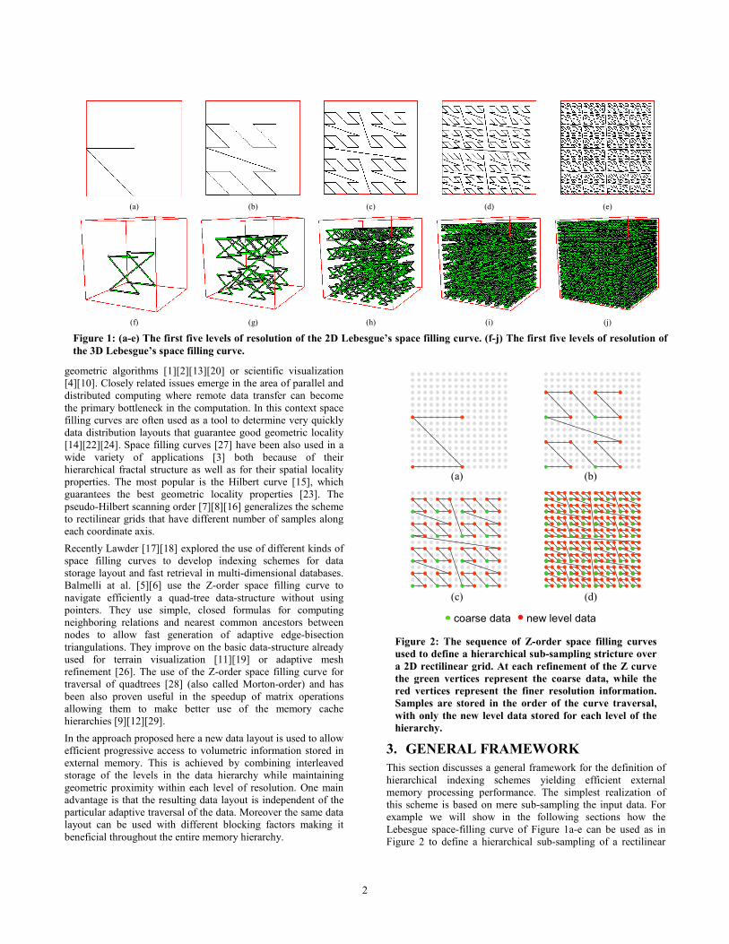
3. GENERAL FRAMEWORK This section discusses a general framework for the definition of hierarchical indexing schemes yielding efficient external memory processing performance. The simplest realization of this scheme is based on mere sub-sampling the input data. For example we will show in the following sections how the Lebesgue space-filling curve of Figure 1a-e can be used as in Figure 2 to define a hierarchical sub-sampling of a rectilinear

(a) (b) (c) (d) (e)

(f) (g) (h) (i) (j)

Figure 1: (a-e) The first five levels of resolution of the 2D Lebesgue’s space filling curve. (f-j) The first five levels of resolution of the 3D Lebesgue’s space filling curve.

(a) (b)

(c) (d)

coarse data new level data

Figure 2: The sequence of Z-order space filling curvesused to define a hierarchical sub-sampling stricture overa 2D rectilinear grid. At each refinement of the Z curvethe green vertices represent the coarse data, while thered vertices represent the finer resolution information.Samples are stored in the order of the curve traversal,with only the new level data stored for each level of thehierarchy.

3

grid. More sophisticated schemes can be realized within this framework but will not discussed further here. Consider a set S of n elements decomposed into a hierarchy H of k levels of resolution H = {S0, S1, …, Sk-1} such that:

S0 ⊂ S1 ⊂ … ⊂ Sk-1 = S

where Si is said to be coarser than Sj iff i < j. The order of the elements in S is defined by the cardinality function I : S → {0 … n-1}. This means that the following identity always holds:

S[I(s)] ≡ s

where the square brackets are used to index an element in a set.

We can define a derived sequence H′ of sets S′i as follows:

S′i = Si \ Si -1 i = 0, … , k-1

Where formally S-1 = ∅. The sequence H′ = { S′0, S′1, …, S′k-1} is a partitioning of S. A derived cardinality function I′ : S → {0 … n-1} can be defined on the basis of the following properties:

∀s, t ∈ S′i : I′(s) < I′(t) ⇔ I(s) < I(t);

∀s ∈ S′i, ∀t ∈ S′j : i < j ⇒ I′(s) < I′(t).

If the original function I has strong locality properties when restricted to any level of resolution Si then the cardinality function I′ generates the desired global index for hierarchical and out-of-core traversal. The construction of the function can be achieved in the following manner: (i) determine the number of elements in each derived set S′i and (ii) determine a cardinality function I″i = I′ | S′j restriction of I′ to each set S′j. In particular if ci is the number of elements of S′i one can predetermine the starting index of the elements in a given level of resolution by building the sequence of constants C0, … , Ck-1 with

∑−

=

=1

0

i

jji cC (1)

Secondly one needs to determine a set of local cardinality functions I″i : S′j → {0 … ci -1} so that

∀s ∈ S′i : I′(s) = Ci + I″i (s) (2)

The computation of the constants Ci can be performed in a pre-processing stage so that the computation of I′ is reduced to the following two steps:

(1) Given s, determine its level of resolution i (that is the i such that S ∈ S′i);

(2) Compute I″i (s) and add it to Ci

These two steps need to be performed very efficiently because they are going to be executed repeatedly at run time. The following section reports a practical realization of this scheme for rectilinear cube grids in any dimension.

4. 2n TREE AND THE LEBESQUE CURVE Here we detail the derivation from the Z-order space filling curve the local cardinality functions I″i for a binary tree hierarchy in any dimension.

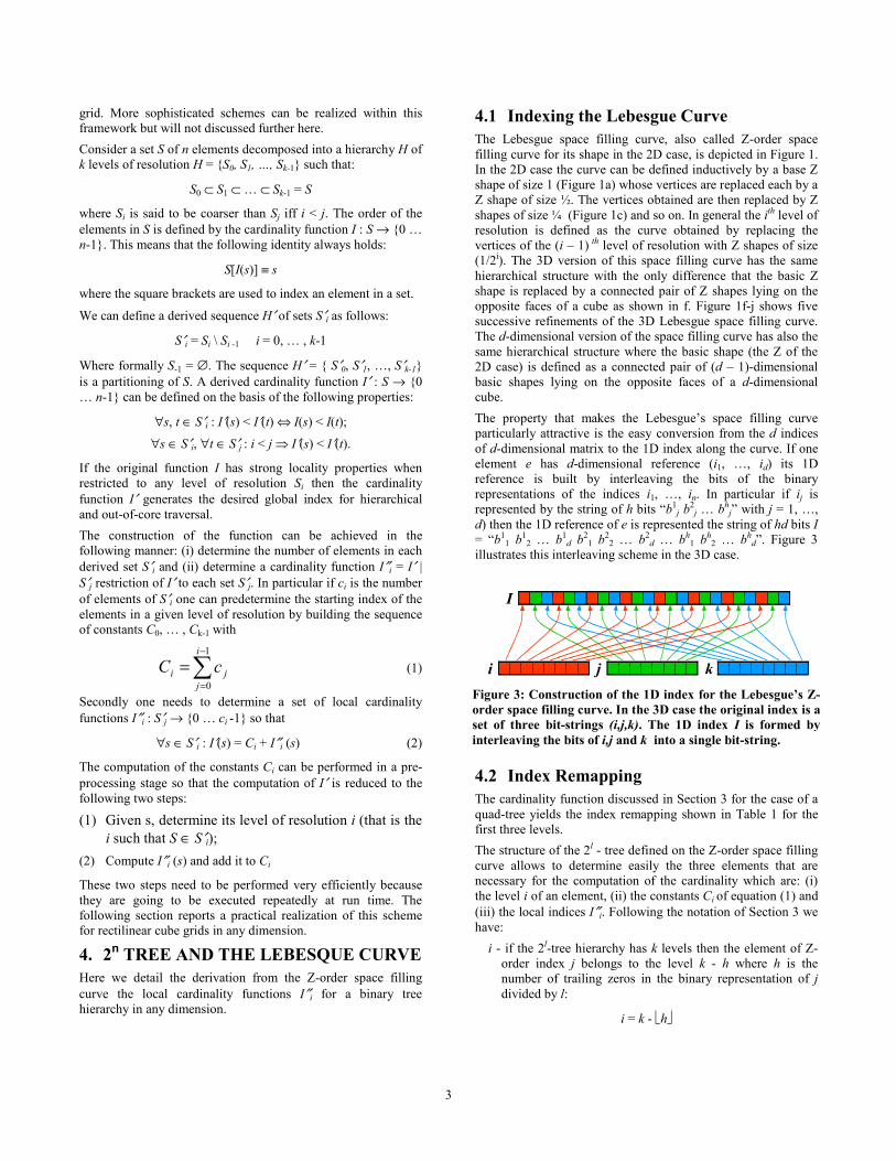
4.1 Indexing the Lebesgue Curve The Lebesgue space filling curve, also called Z-order space filling curve for its shape in the 2D case, is depicted in Figure 1. In the 2D case the curve can be defined inductively by a base Z shape of size 1 (Figure 1a) whose vertices are replaced each by a Z shape of size ½. The vertices obtained are then replaced by Z shapes of size ¼ (Figure 1c) and so on. In general the ith level of resolution is defined as the curve obtained by replacing the vertices of the (i – 1) th level of resolution with Z shapes of size (1/2i). The 3D version of this space filling curve has the same hierarchical structure with the only difference that the basic Z shape is replaced by a connected pair of Z shapes lying on the opposite faces of a cube as shown in f. Figure 1f-j shows five successive refinements of the 3D Lebesgue space filling curve. The d-dimensional version of the space filling curve has also the same hierarchical structure where the basic shape (the Z of the 2D case) is defined as a connected pair of (d – 1)-dimensional basic shapes lying on the opposite faces of a d-dimensional cube. The property that makes the Lebesgue’s space filling curve particularly attractive is the easy conversion from the d indices of d-dimensional matrix to the 1D index along the curve. If one element e has d-dimensional reference (i1, …, id) its 1D reference is built by interleaving the bits of the binary representations of the indices i1, …, in. In particular if ij is represented by the string of h bits “b1

j b2j … bh

j” with j = 1, …, d) then the 1D reference of e is represented the string of hd bits I = “b1

1 b12 … b1

d b21 b2

2 … b2d … bh

1 bh2 … bh

d”. Figure 3 illustrates this interleaving scheme in the 3D case.

4.2 Index Remapping The cardinality function discussed in Section 3 for the case of a quad-tree yields the index remapping shown in Table 1 for the first three levels. The structure of the 2l - tree defined on the Z-order space filling curve allows to determine easily the three elements that are necessary for the computation of the cardinality which are: (i) the level i of an element, (ii) the constants Ci of equation (1) and (iii) the local indices I″i. Following the notation of Section 3 we have:

i - if the 2l-tree hierarchy has k levels then the element of Z-order index j belongs to the level k - h where h is the number of trailing zeros in the binary representation of j divided by l:

i = k - h

k

I

i j Figure 3: Construction of the 1D index for the Lebesgue’s Z-order space filling curve. In the 3D case the original index is aset of three bit-strings (i,j,k). The 1D index I is formed byinterleaving the bits of i,j and k into a single bit-string.

4

1

IAdd a high bit set to 1

0 0 0x xxLoop: while

0 0 0 x x x 0 0 0

0 0 00 0 1

zeros inserted ~

~

~

~

+

Perform the following arithmetic operationSTEP3

STEP2

STEP1

= shift right 3 bits with incoming bits set to 0

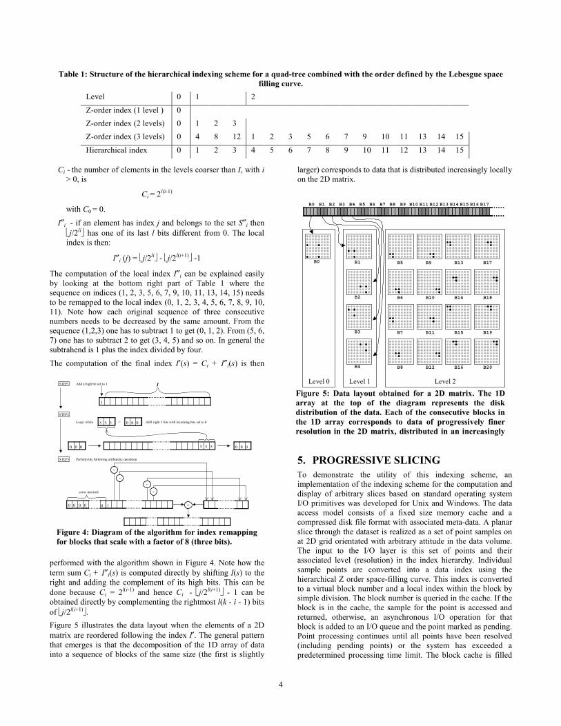
Figure 4: Diagram of the algorithm for index remappingfor blocks that scale with a factor of 8 (three bits).

Ci - the number of elements in the levels coarser than I, with i > 0, is

Ci = 2l(i-1)

with C0 = 0.

I″i - if an element has index j and belongs to the set S″i then j/2li has one of its last l bits different from 0. The local index is then:

I″i (j) = j/2li - j/2l(i+1) -1

The computation of the local index I″i can be explained easily by looking at the bottom right part of Table 1 where the sequence on indices (1, 2, 3, 5, 6, 7, 9, 10, 11, 13, 14, 15) needs to be remapped to the local index (0, 1, 2, 3, 4, 5, 6, 7, 8, 9, 10, 11). Note how each original sequence of three consecutive numbers needs to be decreased by the same amount. From the sequence (1,2,3) one has to subtract 1 to get (0, 1, 2). From (5, 6, 7) one has to subtract 2 to get (3, 4, 5) and so on. In general the subtrahend is 1 plus the index divided by four.

The computation of the final index I′(s) = Ci + I″i(s) is then

performed with the algorithm shown in Figure 4. Note how the term sum Ci + I″i(s) is computed directly by shifting I(s) to the right and adding the complement of its high bits. This can be done because Ci = 2l(i-1) and hence Ci - j/2l(i+1) - 1 can be obtained directly by complementing the rightmost l(k - i - 1) bits of j/2l(i+1). Figure 5 illustrates the data layout when the elements of a 2D matrix are reordered following the index I′. The general pattern that emerges is that the decomposition of the 1D array of data into a sequence of blocks of the same size (the first is slightly

larger) corresponds to data that is distributed increasingly locally on the 2D matrix.

5. PROGRESSIVE SLICING To demonstrate the utility of this indexing scheme, an implementation of the indexing scheme for the computation and display of arbitrary slices based on standard operating system I/O primitives was developed for Unix and Windows. The data access model consists of a fixed size memory cache and a compressed disk file format with associated meta-data. A planar slice through the dataset is realized as a set of point samples on at 2D grid orientated with arbitrary attitude in the data volume. The input to the I/O layer is this set of points and their associated level (resolution) in the index hierarchy. Individual sample points are converted into a data index using the hierarchical Z order space-filling curve. This index is converted to a virtual block number and a local index within the block by simple division. The block number is queried in the cache. If the block is in the cache, the sample for the point is accessed and returned, otherwise, an asynchronous I/O operation for that block is added to an I/O queue and the point marked as pending. Point processing continues until all points have been resolved (including pending points) or the system has exceeded a predetermined processing time limit. The block cache is filled

Level 0 Level 1 Level 2

B0 B1 B5 B9 B13 B17

B2 B6 B10 B14 B18

B3 B7 B11 B15 B19

B4 B8 B12 B16 B20

B0 B1 B2 B3 B4 B5 B6 B7 B8 B9 B10 B11 B12 B13 B14 B15 B16 B17

Figure 5: Data layout obtained for a 2D matrix. The 1Darray at the top of the diagram represents the diskdistribution of the data. Each of the consecutive blocks inthe 1D array corresponds to data of progressively finerresolution in the 2D matrix, distributed in an increasingly

Table 1: Structure of the hierarchical indexing scheme for a quad-tree combined with the order defined by the Lebesgue space filling curve.

Level 0 1 2 Z-order index (1 level ) 0 Z-order index (2 levels) 0 1 2 3 Z-order index (3 levels) 0 4 8 12 1 2 3 5 6 7 9 10 11 13 14 15 Hierarchical index 0 1 2 3 4 5 6 7 8 9 10 11 12 13 14 15

5

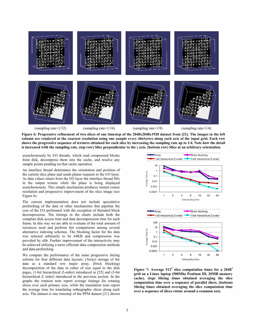
asynchronously by I/O threads, which read compressed blocks from disk, decompress them into the cache, and resolve any sample points pending on that cache operation. An interface thread determines the orientation and position of the current slice plane and sends planar requests to the I/O layer. As data values return from the I/O layer the interface thread fills in the output texture while the plane is being displayed asynchronously. This simple mechanism produces instant coarse resolution and progressive improvement of the slice image (see Figure 6). The current implementation does not include speculative prefetching of the data or other mechanisms that pipeline the cost of the I/O performed with the exception of threaded block decompression. The timings in the charts include both the complete disk access time and data decompression time for each frame. In this way we are able to evaluate of the total amount of resources used and perform fair comparisons among several alternative indexing schemes. The blocking factor for the data was selected arbitrarily to be 64KB and compression was provided by zlib. Further improvement of the interactivity may be achieved utilizing a more efficient data compression methods and data-prefetching. We compare the performance of the same progressive slicing scheme for four different data layouts: (Array) storage of the data as a standard row major array, (brick blocking) decomposition of the data in cubes of size equal to the disk pages, (1-bit hierarchical Z-order) introduced in [25] and (3-bit hierarchical Z order) introduced in the previous section. In the graphs the rotation tests report average timings for rotating slices over each primary axis, while the translation tests report the average time for translating orthographic slices along each axis. The dataset is one timestep of the PPM dataset [21] shown

(sampling rate=1/32) (sampling rate=1/16) (sampling rate=1/8) (sampling rate=1/4)

Figure 6: Progressive refinement of two slices of one timestep of the 2048x2048x1920 dataset from [21]. The images in the left column are rendered at the coarsest resolution using one sample every thirtytwo along each axis of the input grid. Each row shows the progressive sequence of textures obtained for each slice by increasing the sampling rate up to 1/4. Note how the detail is increased with the sampling rate. (top row) Slice perpendicular to the z axis. (bottom row) Slice at an arbitrary orientation.

0.0001

0.001

0.01

0.1

1

10

1 2 4 8 16 32 64Subsampling Rate

Ave

rage

Tim

e (s

)

Array Brick blocking1-bit hierachical Z-order 3-bit hierachical Z-order

0.0001

0.001

0.01

0.1

1

10

100


Ave

rage

Tim

e (s

)


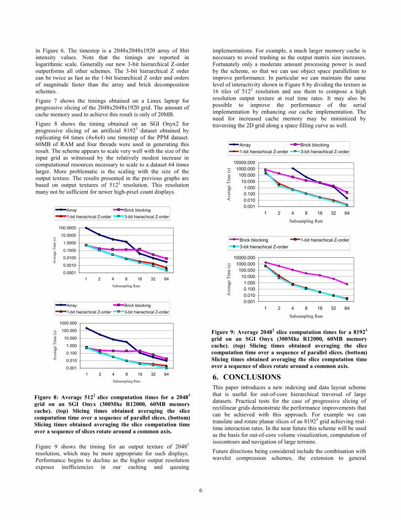
Figure 7: Average 5122 slice computation times for a 20483

grid on a Linux laptop (500Mhz Pentium III, 20MB memorycache). (top) Slicing times obtained averaging the slicecomputation time over a sequence of parallel slices. (bottom)Slicing times obtained averaging the slice computation timeover a sequence of slices rotate around a common axis.

6

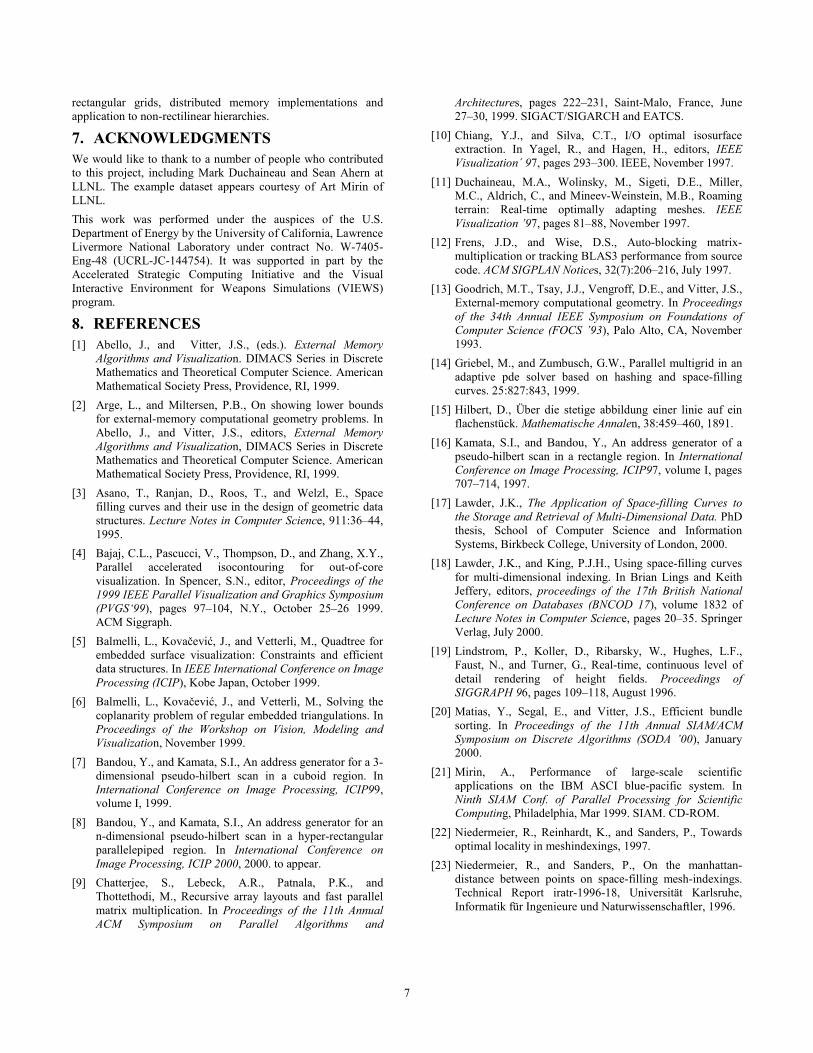
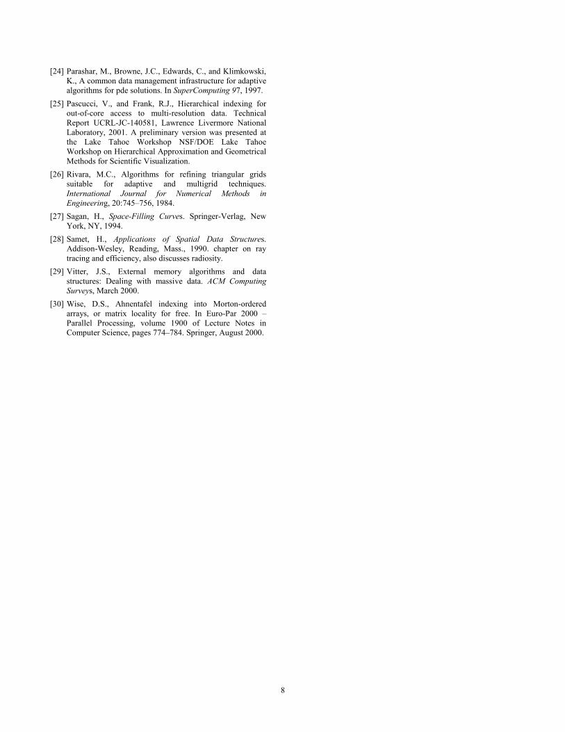
in Figure 6. The timestep is a 2048x2048x1920 array of 8bit intensity values. Note that the timings are reported in logarithmic scale. Generally our new 3-bit hierarchical Z-order outperforms all other schemes. The 3-bit hierarchical Z order can be twice as fast as the 1-bit hierarchical Z order and orders of magnitude faster than the array and brick decomposition schemes. Figure 7 shows the timings obtained on a Linux laptop for progressive slicing of the 2048x2048x1920 grid. The amount of cache memory used to achieve this result is only of 20MB. Figure 8 shows the timing obtained on an SGI Onyx2 for progressive slicing of an artificial 81923 dataset obtained by replicating 64 times (4x4x4) one timestep of the PPM dataset. 60MB of RAM and four threads were used in generating this result. The scheme appears to scale very well with the size of the input grid as witnessed by the relatively modest increase in computational resources necessary to scale to a dataset 64 times larger. More problematic is the scaling with the size of the output texture. The results presented in the previous graphs are based on output textures of 5122 resolution. This resolution many not be sufficient for newer high-pixel count displays.

Figure 9 shows the timing for an output texture of 20482 resolution, which may be more appropriate for such displays. Performance begins to decline as the higher output resolution exposes inefficiencies in our caching and queuing

implementations. For example, a much larger memory cache is necessary to avoid trashing as the output matrix size increases. Fortunately only a moderate amount processing power is used by the scheme, so that we can use object space parallelism to improve performance. In particular we can maintain the same level of interactivity shown in Figure 8 by dividing the texture in 16 tiles of 5122 resolution and use them to compose a high resolution output texture at real time rates. It may also be possible to improve the performance of the serial implementation by enhancing our cache implementation. The need for increased cache memory may be minimized by traversing the 2D grid along a space filling curve as well.

6. CONCLUSIONS This paper introduces a new indexing and data layout scheme that is useful for out-of-core hierarchical traversal of large datasets. Practical tests for the case of progressive slicing of rectilinear grids demonstrate the performance improvements that can be achieved with this approach. For example we can translate and rotate planar slices of an 81923 grid achieving real-time interaction rates. In the near future this scheme will be used as the basis for out-of-core volume visualization, computation of isocontours and navigation of large terrains. Future directions being considered include the combination with wavelet compression schemes, the extension to general

0.0010.0100.1001.000

10.000100.000

1000.00010000.000

1 2 4 8 16 32 64

Subsampling Rate

Ave

rage

Tim

e (s

)


0.0010.0100.1001.000

10.000100.000

1000.00010000.000

1 2 4 8 16 32 64

Subsampling Rate

Ave

rage

Tim

e (s

)

Brick blocking 1-bit hierachical Z-order3-bit hierachical Z-order


grid on an SGI Onyx (300Mhz R12000, 60MB memorycache). (top) Slicing times obtained averaging the slicecomputation time over a sequence of parallel slices. (bottom)Slicing times obtained averaging the slice computation timeover a sequence of slices rotate around a common axis.

0.0001

0.0010

0.0100

0.1000

1.0000

10.0000

100.0000


Ave

rage

Tim

e (s

)


0.001

0.010

0.100

1.000

10.000

100.000

1000.000


Ave

rage

Tim

e (s

)



grid on an SGI Onyx (300Mhz R12000, 60MB memorycache). (top) Slicing times obtained averaging the slicecomputation time over a sequence of parallel slices. (bottom)Slicing times obtained averaging the slice computation timeover a sequence of slices rotate around a common axis.

7

rectangular grids, distributed memory implementations and application to non-rectilinear hierarchies.

7. ACKNOWLEDGMENTS We would like to thank to a number of people who contributed to this project, including Mark Duchaineau and Sean Ahern at LLNL. The example dataset appears courtesy of Art Mirin of LLNL. This work was performed under the auspices of the U.S. Department of Energy by the University of California, Lawrence Livermore National Laboratory under contract No. W-7405-Eng-48 (UCRL-JC-144754). It was supported in part by the Accelerated Strategic Computing Initiative and the Visual Interactive Environment for Weapons Simulations (VIEWS) program.

8. REFERENCES [1] Abello, J., and Vitter, J.S., (eds.). External Memory

Algorithms and Visualization. DIMACS Series in Discrete Mathematics and Theoretical Computer Science. American Mathematical Society Press, Providence, RI, 1999.

[2] Arge, L., and Miltersen, P.B., On showing lower bounds for external-memory computational geometry problems. In Abello, J., and Vitter, J.S., editors, External Memory Algorithms and Visualization, DIMACS Series in Discrete Mathematics and Theoretical Computer Science. American Mathematical Society Press, Providence, RI, 1999.

[3] Asano, T., Ranjan, D., Roos, T., and Welzl, E., Space filling curves and their use in the design of geometric data structures. Lecture Notes in Computer Science, 911:36–44, 1995.

[4] Bajaj, C.L., Pascucci, V., Thompson, D., and Zhang, X.Y., Parallel accelerated isocontouring for out-of-core visualization. In Spencer, S.N., editor, Proceedings of the 1999 IEEE Parallel Visualization and Graphics Symposium (PVGS‘99), pages 97–104, N.Y., October 25–26 1999. ACM Siggraph.

[5] Balmelli, L., Kovačević, J., and Vetterli, M., Quadtree for embedded surface visualization: Constraints and efficient data structures. In IEEE International Conference on Image Processing (ICIP), Kobe Japan, October 1999.

[6] Balmelli, L., Kovačević, J., and Vetterli, M., Solving the coplanarity problem of regular embedded triangulations. In Proceedings of the Workshop on Vision, Modeling and Visualization, November 1999.

[7] Bandou, Y., and Kamata, S.I., An address generator for a 3-dimensional pseudo-hilbert scan in a cuboid region. In International Conference on Image Processing, ICIP99, volume I, 1999.

[8] Bandou, Y., and Kamata, S.I., An address generator for an n-dimensional pseudo-hilbert scan in a hyper-rectangular parallelepiped region. In International Conference on Image Processing, ICIP 2000, 2000. to appear.

[9] Chatterjee, S., Lebeck, A.R., Patnala, P.K., and Thottethodi, M., Recursive array layouts and fast parallel matrix multiplication. In Proceedings of the 11th Annual ACM Symposium on Parallel Algorithms and

Architectures, pages 222–231, Saint-Malo, France, June 27–30, 1999. SIGACT/SIGARCH and EATCS.

[10] Chiang, Y.J., and Silva, C.T., I/O optimal isosurface extraction. In Yagel, R., and Hagen, H., editors, IEEE Visualization´ 97, pages 293–300. IEEE, November 1997.

[11] Duchaineau, M.A., Wolinsky, M., Sigeti, D.E., Miller, M.C., Aldrich, C., and Mineev-Weinstein, M.B., Roaming terrain: Real-time optimally adapting meshes. IEEE Visualization ’97, pages 81–88, November 1997.

[12] Frens, J.D., and Wise, D.S., Auto-blocking matrix-multiplication or tracking BLAS3 performance from source code. ACM SIGPLAN Notices, 32(7):206–216, July 1997.

[13] Goodrich, M.T., Tsay, J.J., Vengroff, D.E., and Vitter, J.S., External-memory computational geometry. In Proceedings of the 34th Annual IEEE Symposium on Foundations of Computer Science (FOCS ’93), Palo Alto, CA, November 1993.

[14] Griebel, M., and Zumbusch, G.W., Parallel multigrid in an adaptive pde solver based on hashing and space-filling curves. 25:827:843, 1999.

[15] Hilbert, D., Über die stetige abbildung einer linie auf ein flachenstück. Mathematische Annalen, 38:459–460, 1891.

[16] Kamata, S.I., and Bandou, Y., An address generator of a pseudo-hilbert scan in a rectangle region. In International Conference on Image Processing, ICIP97, volume I, pages 707–714, 1997.

[17] Lawder, J.K., The Application of Space-filling Curves to the Storage and Retrieval of Multi-Dimensional Data. PhD thesis, School of Computer Science and Information Systems, Birkbeck College, University of London, 2000.

[18] Lawder, J.K., and King, P.J.H., Using space-filling curves for multi-dimensional indexing. In Brian Lings and Keith Jeffery, editors, proceedings of the 17th British National Conference on Databases (BNCOD 17), volume 1832 of Lecture Notes in Computer Science, pages 20–35. Springer Verlag, July 2000.

[19] Lindstrom, P., Koller, D., Ribarsky, W., Hughes, L.F., Faust, N., and Turner, G., Real-time, continuous level of detail rendering of height fields. Proceedings of SIGGRAPH 96, pages 109–118, August 1996.

[20] Matias, Y., Segal, E., and Vitter, J.S., Efficient bundle sorting. In Proceedings of the 11th Annual SIAM/ACM Symposium on Discrete Algorithms (SODA ’00), January 2000.

[21] Mirin, A., Performance of large-scale scientific applications on the IBM ASCI blue-pacific system. In Ninth SIAM Conf. of Parallel Processing for Scientific Computing, Philadelphia, Mar 1999. SIAM. CD-ROM.

[22] Niedermeier, R., Reinhardt, K., and Sanders, P., Towards optimal locality in meshindexings, 1997.

[23] Niedermeier, R., and Sanders, P., On the manhattan-distance between points on space-filling mesh-indexings. Technical Report iratr-1996-18, Universität Karlsruhe, Informatik für Ingenieure und Naturwissenschaftler, 1996.

8

[24] Parashar, M., Browne, J.C., Edwards, C., and Klimkowski, K., A common data management infrastructure for adaptive algorithms for pde solutions. In SuperComputing 97, 1997.

[25] Pascucci, V., and Frank, R.J., Hierarchical indexing for out-of-core access to multi-resolution data. Technical Report UCRL-JC-140581, Lawrence Livermore National Laboratory, 2001. A preliminary version was presented at the Lake Tahoe Workshop NSF/DOE Lake Tahoe Workshop on Hierarchical Approximation and Geometrical Methods for Scientific Visualization.

[26] Rivara, M.C., Algorithms for refining triangular grids suitable for adaptive and multigrid techniques. International Journal for Numerical Methods in Engineering, 20:745–756, 1984.

[27] Sagan, H., Space-Filling Curves. Springer-Verlag, New York, NY, 1994.

[28] Samet, H., Applications of Spatial Data Structures. Addison-Wesley, Reading, Mass., 1990. chapter on ray tracing and efficiency, also discusses radiosity.

[29] Vitter, J.S., External memory algorithms and data structures: Dealing with massive data. ACM Computing Surveys, March 2000.

[30] Wise, D.S., Ahnentafel indexing into Morton-ordered arrays, or matrix locality for free. In Euro-Par 2000 – Parallel Processing, volume 1900 of Lecture Notes in Computer Science, pages 774–784. Springer, August 2000.

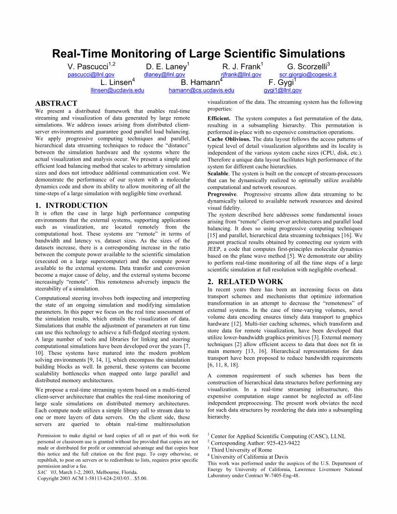
Real-Time Monitoring of Large Scientific Simulations V. Pascucci1,2 D. E. Laney1 R. J. Frank1 G. Scorzelli3

[email protected] [email protected] [email protected] [email protected] L. Linsen4 B. Hamann4 F. Gygi1

[email protected] [email protected] [email protected]

ABSTRACT We present a distributed framework that enables real-time streaming and visualization of data generated by large remote simulations. We address issues arising from distributed client-server environments and guarantee good parallel load balancing. We apply progressive computing techniques and parallel, hierarchical data streaming techniques to reduce the “distance” between the simulation hardware and the systems where the actual visualization and analysis occur. We present a simple and efficient load balancing method that scales to arbitrary simulation sizes and does not introduce additional communication cost. We demonstrate the performance of our system with a molecular dynamics code and show its ability to allow monitoring of all the time-steps of a large simulation with negligible time overhead.

1. INTRODUCTION It is often the case in large high performance computing environments that the external systems, supporting applications such as visualization, are located remotely from the computational host. These systems are “remote” in terms of bandwidth and latency vs. dataset sizes. As the sizes of the datasets increase, there is a corresponding increase in the ratio between the compute power available to the scientific simulation (executed on a large supercomputer) and the compute power available to the external systems. Data transfer and conversion become a major cause of delay, and the external systems become increasingly “remote”. This remoteness adversely impacts the steerability of a simulation. Computational steering involves both inspecting and interpreting the state of an ongoing simulation and modifying simulation parameters. In this paper we focus on the real time assessment of the simulation results, which entails the visualization of data. Simulations that enable the adjustment of parameters at run time can use this technology to achieve a full-fledged steering system. A large number of tools and libraries for linking and steering computational simulations have been developed over the years [7, 10]. These systems have matured into the modern problem solving environments [9, 14, 1], which encompass the simulation building blocks as well. In general, these systems can become scalability bottlenecks when mapped onto large parallel and distributed memory architectures. We propose a real-time streaming system based on a multi-tiered client-server architecture that enables the real-time monitoring of large scale simulations on distributed memory architectures. Each compute node utilizes a simple library call to stream data to one or more layers of data servers. On the client side, these servers are queried to obtain real-time multiresolution

visualization of the data. The streaming system has the following properties:

Efficient. The system computes a fast permutation of the data, resulting in a subsampling hierarchy. This permutation is performed in-place with no expensive construction operations. Cache Oblivious. The data layout follows the access patterns of typical level of detail visualization algorithms and its locality is independent of the various system cache sizes (CPU, disk, etc.). Therefore a unique data layout facilitates high performance of the system for different cache hierarchies. Scalable. The system is built on the concept of stream-processors that can be dynamically realized to optimally utilize available computational and network resources. Progressive. Progressive streams allow data streaming to be dynamically tailored to available network resources and desired visual fidelity. The system described here addresses some fundamental issues arising from “remote” client-server architectures and parallel load balancing. It does so using progressive computing techniques [15] and parallel, hierarchical data streaming techniques [16]. We present practical results obtained by connecting our system with JEEP, a code that computes first-principles molecular dynamics based on the plane wave method [5]. We demonstrate our ability to perform real-time monitoring of all the time steps of a large scientific simulation at full resolution with negligible overhead.

2. RELATED WORK In recent years there has been an increasing focus on data transport schemes and mechanisms that optimize information transformation in an attempt to decrease the “remoteness” of external systems. In the case of time-varying volumes, novel volume data encoding ensures timely data transport to graphics hardware [12]. Multi-tier caching schemes, which transform and store data for remote visualization, have been developed that utilize lower-bandwidth graphics primitives [3]. External memory techniques [2] allow efficient access to data that does not fit in main memory [13, 16]. Hierarchical representations for data transport have been proposed to reduce bandwidth requirements [6, 11, 8, 18].

A common requirement of such schemes has been the construction of hierarchical data structures before performing any visualization. In a real-time streaming infrastructure, this expensive computation stage cannot be neglected as off-line independent preprocessing. The present work obviates the need for such data structures by reordering the data into a subsampling hierarchy.

1 Center for Applied Scientific Computing (CASC), LLNL 2 Corresponding Author: 925-423-9422 3 Third University of Rome 4 University of California at Davis This work was performed under the auspices of the U.S. Department of Energy by University of California, Lawrence Livermore National Laboratory under Contract W-7405-Eng-48.

Permission to make digital or hard copies of all or part of this work for personal or classroom use is granted without fee provided that copies are not made or distributed for profit or commercial advantage and that copies bear this notice and the full citation on the first page. To copy otherwise, or republish, to post on servers or to redistribute to lists, requires prior specific permission and/or a fee. SAC ’03, March 1-2, 2003, Melbourne, Florida. Copyright 2003 ACM 1-58113-624-2/03/03…$5.00.








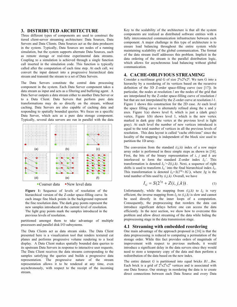
3. DISTRIBUTED ARCHITECTURE Three different types of components are used to construct the tiered client-server streaming architecture: Data Sources, Data Servers and Data Clients. Data Sources act as the data producers in the system. Typically, Data Sources are nodes of a running simulation, but the system supports alternate Data Sources, such as remote storage or real-time experimental data streams. Coupling to a simulation is achieved through a single function call inserted in the simulation code. This function is typically called after the computation of each time step. At each call, we convert the input dataset into a progressive hierarchical data stream and transmit the stream to a set of Data Servers.

The Data Servers constitute the central data processing component in the system. Each Data Server component takes a data stream as input and acts as a filtering and buffering agent. A Data Server outputs a data stream either to another Data Server or to a Data Client. Data Servers that perform pure data transformations may do so directly on the stream, without caching. Data Servers are also capable of caching data and responding to spatially bounded queries. We focus on a specific Data Server, which acts as a pure data storage component. Typically, several data servers are run in parallel with the data

partitioned amongst them to take advantage of multiple processors and parallel disk I/O subsystems.

The Data Clients act as data stream sinks. The Data Client presented here is a visualization tool that renders textured cut planes and performs progressive volume rendering to a local display. A Data Client makes spatially bounded data queries to its upstream Data Servers in response to interactive user requests. The Data Client receives the data streams corresponding to the samples satisfying the queries and builds a progressive data representation. The progressive nature of the stream representation allows it to be rendered at any time, even asynchronously, with respect to the receipt of the incoming stream.

Key to the scalability of the architecture is that all the system components are realized as distributed software entities with a fully interconnected communication infrastructure between each component. A major challenge in this type of architecture is to ensure load balancing throughout the entire system while maintaining scalability of the global communication. The format of the data stream itself addresses this problem. Implicit in the data ordering of the stream is the parallel distribution logic, which allows for asynchronous load balancing without global communication.

4. CACHE-OBLIVIOUS STREAMING Consider a rectilinear grid G of size 2gx2gx2g. We turn G into a hierarchy by a reordering of its vertices based on the recursive definition of the 3D Z-order space-filling curve (see [17]). In particular, the nodes at resolution l are the nodes of the grid that are interpolated by the Z-order space-filling curve of resolution l but that are not interpolated by the Z-order curve at resolution l-1. Figure 1 shows this construction for the 2D case. At each level the space filling curve is alternately refined along the x and y axes. Figure 1(a) shows level 0, which is just a (dark gray) vertex. Figure 1(b) shows level 1, which is the new vertex marked in dark gray (the vertex at the previous level is light gray). At each level the number of new vertices introduced is equal to the total number of vertices in all the previous levels of resolution. This data layout is called “cache oblivious” since the locality of the mapping is independent of the block size used to partition the 1D array.

Coarser data New level data

(a) (b) (c)

(d) (e) (f)

The conversion from the standard (i,j,k) index of a row major array order is performed in three simple steps as shown in [16]. First, the bits of the binary representation of i, j and k are interleaved to form the standard Z-order index IG’. This transformation is denoted IG’=Z(i,j,k). Next, a sequence of right shifts is used to transform IG’ into the final hierarchical index IG. This transformation is denoted IG=S(23g+IG’), where 3g is the total number of bits used by (i,j,k). Overall, we have

)),,(2( 3 kjiZSI gG += . (1)

Unfortunately, while the mapping from (i,j,k) to IG is very efficient, the inverse mapping from IG to (i,j,k) is slow and cannot be used directly in the inner loops of a computation. Consequently, the preprocessing that reorders the data can introduce significant delays before one can access the data efficiently. In the next section, we show how to overcome this problem and allow direct streaming of the data while hiding the preprocessing stage in the data transmission stage.

Figure 1: Sequence of levels of resolution of thehierarchical version of the Z-order space-filling curve. Ineach image fine black points in the background representthe fine resolution data. The dark gray points represent thenew samples introduced at the current level of resolution.The light gray points mark the samples introduced in theprevious levels of resolution.

4.1 Streaming with embedded reordering One main advantage of the approach proposed in [16] is that the data preprocessing is reduced to computing a permutation of the storage order. While this fact provides orders of magnitude of improvement with respect to previous methods, it would introduce a significant delay in the data servers since they would need to store a temporary copy of the data and then perform a redistribution of the data based on the new index. The entire dataset G is partitioned into equal bricks B1…Bm. Each brick is a grid of 2bx2bx2b vertices and is associated with one Data Source. Our strategy in reordering the data is to create direct connections between each Data Source and every Data

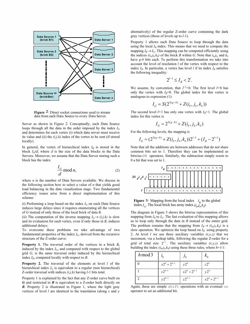
Server as shown in Figure 2. Conceptually, each Data Source loops through all the data in the order imposed by the index IG and determines for each vertex (i) which data server must receive its value and (ii) the (i,j,k) index of the vertex to be sent (if stored locally). In general, the vertex of hierarchical index IG is stored in the block IG/d, where d is the size of the data blocks in the Data Servers. Moreover, we assume that the Data Server storing such a block has the index

mod ,GI nd

(2)

where n is the number of Data Servers available. We discuss in the following section how to select a value of n that yields good load balancing in the data visualization stage. Two fundamental efficiency issues arise from a direct implementation of this scheme: (i) Performing a loop based on the index IG on each Data Source induces large delays since it requires enumerating all the vertices of G instead of only those of the local brick of data B. (ii) The computation of the inverse mapping IG→ (i,j,k) is slow and its evaluation for each vertex, even if only those in B, induces additional delays. To overcome these problems we take advantage of two fundamental properties of the index IG, derived from the recursive structure of the Z-order curve:

Property 1. The traversal order of the vertices in a brick B, induced by the index IG, and computed with respect to the global grid G, is the same traversal order induced by the hierarchical index IB, computed locally with respect to B. Property 2. The traversal of the elements at level l of the hierarchical index IG is equivalent to a regular (non hierarchical) Z-order traversal with indices (i,j,k) having l-1 bits total. Property 1 is explained by the fact that any Z-order curve built on G and restricted to B is equivalent to a Z-order built directly on B. Property 2 is illustrated in Figure 1, where the light gray vertices of level l are identical to the translation (along x and y

alternatively) of the regular Z-order curve containing the dark gray vertices (those of levels up to l-1).

FS2

FS3

Data Source 1 (brick B1)

Data Source 2 (brick B2)

Data Source m (brick B m )

Data Server 1

Data Server 2

Data Server 3

Data Server n

Figure 2 : Direct socket connections used to stream data from each Data Source to every Data Server.

Property 1 allows each Data Source to loop through the data using the local IB index. This means that we need to compute the mapping IB→ IG. This mapping can be computed efficiently using the indices (ib,jb,kb) of the brick B within G. Note that ib,jb, and kb have g-b bits each. To perform this transformation we take into account the level of resolution l of the vertex with respect to the index IB. In particular, a vertex has level l if its index IB satisfies the following inequality:

12 2l lBI− .≤ <

We assume, by convention, that 2-1=0. The first level l=0 has only the vertex with IB=0. The global index for this vertex is analogous to expression (1):

3( )(2 ( , , ))g bG b b bI S Z i j−= + k

)b b

The second level l=1 has only one vertex with IB=1. The global index for this vertex is

3( )2 ( , ,g bG bI Z i j k−= +

For the following levels, the mapping is 3( ) 1 1(2 ( , , ))2 ( 2 )g b l l

G b b b BI Z i j k I− − −= + + −

Note that all the additions are between addresses that do not share common bits set to 1. Therefore they can be implemented as bitwise-OR operators. Similarly, the subtraction simply resets to 0 a bit that was set to 1.

I B

I 1

1

Z(ib,j

b,k

b)

x x x x x x x x x x x x xx

x x x x x x x x x x x x xx

y y y y y y

y y y y y y

Figure 3: Mapping from the local index I B to the global index IG . The local brick has array index (i b ,j b ,k b).

The diagram in Figure 3 shows the bitwise representation of this mapping from IB to IG. The fast evaluation of this mapping allows us to loop only through the data in B instead of the entire grid. The problem remains that the mapping from IB→ (ib,jb,kb) is a slow operation. We optimize the loop based on IB using property 2. At level l we use three auxiliary variables (x,y,z) that we increment, via a lookup table, following the regular Z-order for a grid of total size 2 1l− . The auxiliary variables (x,y,z) allow building the index (ib,jb,kb) using these three rules, where h=l-1:

mod 3h bi bj bk

0 12 2h hx −+ 2hy 2hz

1 12hz − 12 2h hx −+ 2hy

2 12hy − 12hz − 12 2h hx −+

Again, these are simple shift operations with an eventual or operator to set an additional bit.

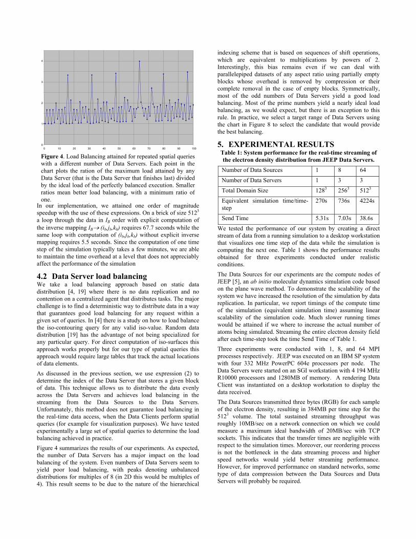
In our implementation, we attained one order of magnitude speedup with the use of these expressions. On a brick of size 5123 a loop through the data in IB order with explicit computation of the inverse mapping IB→ (ib,jb,kb) requires 67.7 seconds while the same loop with computation of (ib,jb,kb) without explicit inverse mapping requires 5.5 seconds. Since the computation of one time step of the simulation typically takes a few minutes, we are able to maintain the time overhead at a level that does not appreciably affect the performance of the simulation

4.2 Data Server load balancing We take a load balancing approach based on static data distribution [4, 19] where there is no data replication and no contention on a centralized agent that distributes tasks. The major challenge is to find a deterministic way to distribute data in a way that guarantees good load balancing for any request within a given set of queries. In [4] there is a study on how to load balance the iso-contouring query for any valid iso-value. Random data distribution [19] has the advantage of not being specialized for any particular query. For direct computation of iso-surfaces this approach works properly but for our type of spatial queries this approach would require large tables that track the actual locations of data elements. As discussed in the previous section, we use expression (2) to determine the index of the Data Server that stores a given block of data. This technique allows us to distribute the data evenly across the Data Servers and achieves load balancing in the streaming from the Data Sources to the Data Servers. Unfortunately, this method does not guarantee load balancing in the real-time data access, when the Data Clients perform spatial queries (for example for visualization purposes). We have tested experimentally a large set of spatial queries to determine the load balancing achieved in practice. Figure 4 summarizes the results of our experiments. As expected, the number of Data Servers has a major impact on the load balancing of the system. Even numbers of Data Servers seem to yield poor load balancing, with peaks denoting unbalanced distributions for multiples of 8 (in 2D this would be multiples of 4). This result seems to be due to the nature of the hierarchical

indexing scheme that is based on sequences of shift operations, which are equivalent to multiplications by powers of 2. Interestingly, this bias remains even if we can deal with parallelepiped datasets of any aspect ratio using partially empty blocks whose overhead is removed by compression or their complete removal in the case of empty blocks. Symmetrically, most of the odd numbers of Data Servers yield a good load balancing. Most of the prime numbers yield a nearly ideal load balancing, as we would expect, but there is an exception to this rule. In practice, we select a target range of Data Servers using the chart in Figure 8 to select the candidate that would provide the best balancing.

4

3

2

1

5. EXPERIMENTAL RESULTS 0 0 10 20 30 40 50 60 70 80 90 100

Table 1: System performance for the real-time streaming of the electron density distribution from JEEP Data Servers. Figure 4. Load Balancing attained for repeated spatial queries

with a different number of Data Servers. Each point in the chart plots the ration of the maximum load attained by any Data Server (that is the Data Server that finishes last) divided by the ideal load of the perfectly balanced execution. Smaller ratios mean better load balancing, with a minimum ratio of one.

Number of Data Sources 1 8 64

Number of Data Servers 1 3 3

Total Domain Size 1283 2563 5123

Equivalent simulation time/time-step

270s 736s 4224s

Send Time 5.31s 7.03s 38.6s

We tested the performance of our system by creating a direct stream of data from a running simulation to a desktop workstation that visualizes one time step of the data while the simulation is computing the next one. Table 1 shows the performance results obtained for three experiments conducted under realistic conditions. The Data Sources for our experiments are the compute nodes of JEEP [5], an ab initio molecular dynamics simulation code based on the plane wave method. To demonstrate the scalability of the system we have increased the resolution of the simulation by data replication. In particular, we report timings of the compute time of the simulation (equivalent simulation time) assuming linear scalability of the simulation code. Much slower running times would be attained if we where to increase the actual number of atoms being simulated. Streaming the entire electron density field after each time-step took the time Send Time of Table 1. Three experiments were conducted with 1, 8, and 64 MPI processes respectively. JEEP was executed on an IBM SP system with four 332 MHz PowerPC 604e processors per node. The Data Servers were started on an SGI workstation with 4 194 MHz R10000 processors and 1280MB of memory. A rendering Data Client was instantiated on a desktop workstation to display the data received. The Data Sources transmitted three bytes (RGB) for each sample of the electron density, resulting in 384MB per time step for the 5123 volume. The total sustained streaming throughput was roughly 10MB/sec on a network connection on which we could measure a maximum ideal bandwidth of 20MB/sec with TCP sockets. This indicates that the transfer times are negligible with respect to the simulation times. Moreover, our reordering process is not the bottleneck in the data streaming process and higher speed networks would yield better streaming performance. However, for improved performance on standard networks, some type of data compression between the Data Sources and Data Servers will probably be required.

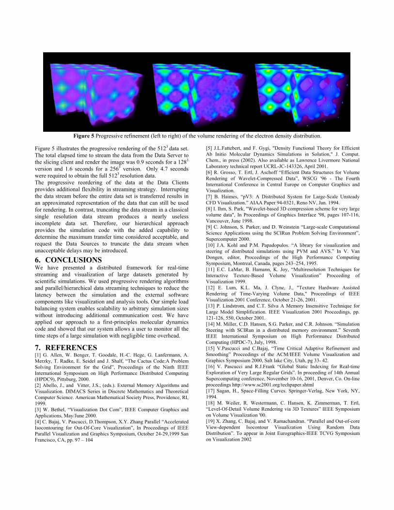
Figure 5 Progressive refinement (left to right) of the volume rendering of the electron density distribution.

Figure 5 illustrates the progressive rendering of the 5123 data set. The total elapsed time to stream the data from the Data Server to the slicing client and render the image was 0.9 seconds for a 1283 version and 1.6 seconds for a 2563 version. Only 4.7 seconds were required to obtain the full 5123 resolution data. The progressive reordering of the data at the Data Clients provides additional flexibility in streaming strategy. Interrupting the data stream before the entire data set is transferred results in an approximated representation of the data that can still be used for rendering. In contrast, truncating the data stream in a classical single resolution data stream produces a nearly useless incomplete data set. Therefore, our hierarchical approach provides the simulation code with the added capability to determine the maximum transfer time considered acceptable, and request the Data Sources to truncate the data stream when unacceptable delays may be introduced.

6. CONCLUSIONS We have presented a distributed framework for real-time streaming and visualization of large datasets generated by scientific simulations. We used progressive rendering algorithms and parallel/hierarchical data streaming techniques to reduce the latency between the simulation and the external software components like visualization and analysis tools. Our simple load balancing system enables scalability to arbitrary simulation sizes without introducing additional communication cost. We have applied our approach to a first-principles molecular dynamics code and showed that our system allows a user to monitor all the time steps of a large simulation with negligible time overhead.

7. REFERENCES [1] G. Allen, W. Benger, T. Goodale, H.-C. Hege, G. Lanfermann, A. Merzky, T. Radke, E. Seidel and J. Shalf, “The Cactus Code:A Problem Solving Environment for the Grid”, Proceedings of the Ninth IEEE International Symposium on High Performance Distributed Computing (HPDC9), Pittsburg, 2000. [2] Abello, J., and Vitter, J.S., (eds.). External Memory Algorithms and Visualization. DIMACS Series in Discrete Mathematics and Theoretical Computer Science. American Mathematical Society Press, Providence, RI, 1999. [3] W. Bethel, “Visualization Dot Com”, IEEE Computer Graphics and Applications, May/June 2000. [4] C. Bajaj, V. Pascucci, D.Thompson, X.Y. Zhang Parallel “Accelerated Isocontouring for Out-Of-Core Visualization”, In Proceedings of IEEE Parallel Visualization and Graphics Symposium, October 24-29,1999 San Francisco, CA, pp. 97 – 104

[5] J.L.Fattebert, and F. Gygi, "Density Functional Theory for Efficient Ab Initio Molecular Dynamics Simulations in Solution," J. Comput. Chem., in press (2002). Also available as Lawrence Livermore National Laboratory technical report UCRL-JC-143326, April 2001. [6] R. Grosso, T. Ertl, J. Aschoff “Efficient Data Structures for Volume Rendering of Wavelet-Compressed Data”, WSCG '96 - The Fourth International Conference in Central Europe on Computer Graphics and Visualization. [7] B. Haimes, “pV3: A Distributed System for Large-Scale Unsteady CFD Visualization.” AIAA Paper 94-0321, Reno NV, Jan. 1994. [8] I. Ihm, S. Park, "Wavelet-based 3D compression scheme for very large volume data", In Proceedings of Graphics Interface '98, pages 107-116, Vancouver, June 1998. [9] C. Johnson, S. Parker, and D. Weinstein “Large-scale Computational Science Applications using the SCIRun Problem Solving Environment”, Supercomputer 2000. [10] J.A. Kohl and P.M. Papadopulos. “A library for visualization and steering of distributed simulations using PVM and AVS.” In V. Van Dongen, editor, Proceedings of the High Performance Computing Symposium, Montreal, Canada, pages 243–254, 1995. [11] E.C. LaMar, B. Hamann, K. Joy, “Multiresolution Techniques for Interactive Texture-Based Volume Visualization” Proceeding of Visualization 1999. [12] E. Lum, K.L. Ma, J. Clyne, J., "Texture Hardware Assisted Rendering of Time-Varying Volume Data," Proceedings of IEEE Visualization 2001 Conference, October 21-26, 2001. [13] P. Lindstrom, and C.T. Silva A Memory Insensitive Technique for Large Model Simplification. IEEE Visualization 2001 Proceedings, pp. 121-126, 550, October 2001. [14] M. Miller, C.D. Hansen, S.G. Parker, and C.R. Johnson. “Simulation Steering with SCIRun in a distributed memory environment.” Seventh IEEE International Symposium on High Performance Distributed Computing (HPDC-7), July, 1998. [15] V.Pascucci and C.Bajaj, “Time Critical Adaptive Refinement and Smoothing” Proceedings of the ACM/IEEE Volume Visualization and Graphics Symposium 2000, Salt lake City, Utah, pg 33- 42. [16] V. Pascucci and R.J.Frank “Global Static Indexing for Real-time Exploration of Very Large Regular Grids”. In proceeding of 14th Annual Supercomputing conference, November 10-16, 2001, Denver, Co. On-line proceedings http://www.sc2001.org/techpaper.shtml [17] Sagan, H., Space-Filling Curves. Springer-Verlag, New York, NY, 1994. [18] M. Weiler, R. Westermann, C. Hansen, K. Zimmerman, T. Ertl, “Level-Of-Detail Volume Rendering via 3D Textures” IEEE Symposium on Volume Visualization '00. [19] X. Zhang, C. Bajaj, and V. Ramachandran. “Parallel and Out-of-core View-dependent Isocontour Visualization Using Random Data Distribution”. To appear in Joint Eurographics-IEEE TCVG Symposium on Visualization 2002

http://raphael.mit.edu/pv3/reno94.ps

http://raphael.mit.edu/pv3/reno94.ps

http://www.supercomp.de/

http://vis.computer.org/vis01

http://www.mcs.anl.gov/hpdc7/



http://www.sc2001.org/techpaper.shtml

http://www.vis.rwth-aachen.de/Research/VOLVIS00.pdf

1 Hierarchical Indexing for Out-of-Core Access to Multi-Resolution Data

Documents

Transcript of 1 Hierarchical Indexing for Out-of-Core Access to Multi-Resolution Data