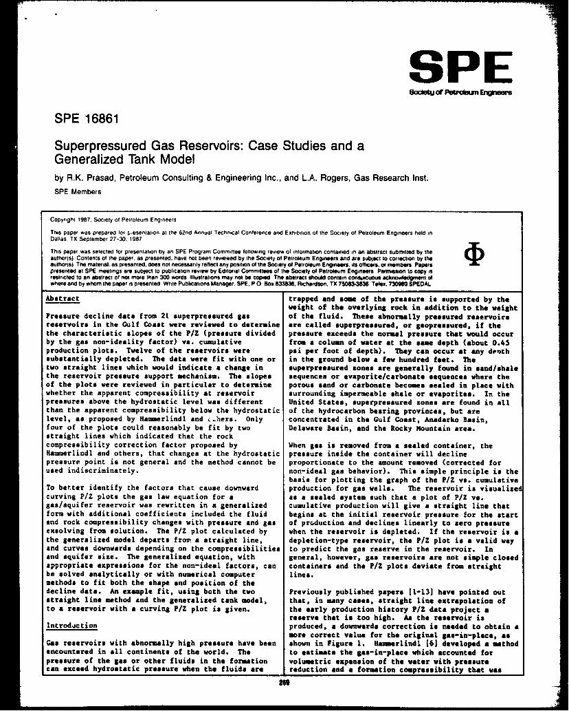
.

SPESPE 16861

Superpressured Gas Reservoirs: Case Studies and aGeneralized Tank Modelby R.K. Prasad, Petroleum Consulting & Engineering Inc., and LA. Rogers, Gas Research Inst.

SPE Members

Copyr!ghl 1987. Sm,ely 01 Petroleum E ngmeers

This paper was grepareo lot f,, esenlahon al the 62nd Annual Techmcal Conference an~ E xhiJatvOfl of the %c,ety cd Petroleum Engmaara held mDallas. TX Seplember 27-30, 1987

Thvi paper was selected for ptes.entalson by an SPE Program CommNtea Iollovsmg review 01 mlormahon conlamed m an Sbatfact submtttesi by theaulhof(s) COnIen:a of the Paper. as fYeSSnWO. have no: been lewewad by Ihe SOOely of Petroleum Engme$r$ and are sub~l 10 corrachon by Ihaauthor(a) The matefial. aa presented. 00ss not naceaaanly reflect any pea!fton of the society of Petroleum Ehemeem. es offcefs,ocmembers Papera @

Bfeaenled al SPE maatmgs are subfec! 10 publication rawew by Editorial Commmwa of ma SwISty of Petroleum Engmeare Pammwmn fo copy ISremnctacl to an aoetrac! of not more Ihan 300 words Illustrahoh$ may not be copd The ebaIract should ccesfam cona#cucssa ackmwWgment ofwhere and @ whom the paper IS preaenfec Write Pubhcattons Manager. SPE. P O Box S33&M. R&mdaon, TX 750S33836 Telex. TWWf) SPEDAL

Abstract trapped ●nd some of the pressure ie ●upported by theweight of the overlying rock in ●ddition to the wei~ht

Pressure decline data from 21 superpreseured gas of the fluid. These abnormally pressured reeervoirare~ervoiro in the Gulf Coast were reviewed to determine ●re called superpreeeured, or geopressured, if thethe charecterietic slope. of the P/Z (preeaasre divided preseure exceeds the nornal preesure that would occurby the ges non-ideality fector) ve. cumulative from ● column of wster ●t the s- depth (about 0.45production plote. Twelve of the reservoirs were psi per foot of depth). They cen occur ●t ●ny dmthsubetentially depleted. The data were fit with one or in the ground below ● few hundred feet. Thetwo straight lines which would indicate ● change in auperpreeaured xonea are generally found in ●and/shalethe reservoir pressure support mechsraism. The elopee aequencee or evaporite/carbostate ●equessce. where theof the plots were reviewed in particular to determine porous sand or cerbonate bec~a sealed in place withwhether the apparent coaapreaaibility ●t reeervoir surrounding impermeable shale or evaporitaa. In thepressures above the hydrostatic level was differentthan the apparent compreaeibility below the hydrostatic

United Statea, euperpreaaured zones are found in allof the hydrocarbon bearing provinces, but are

level, as proposed by Heuauerlindl and i.hers. Only concentrated in the Gulf Coast, Anadarko Baein,four of the plote could reasonably be fit by two Delaware Basin, and the Rocky Mountain ●rea.

straight linee which indicated that the rockcompreeoibility correction factor propooed by When gae ia removed from a ssealed container, theHamerlindl and otherz, that changea at the hydrostatic preeaure inside the container will declinepresaeure point ia not general and the method cannot be proportionate to the amount removed (corrected forused indiscriminately. non-ideal gaa behavior). This simple principle is the

basic for plotting the graph of the P/Z vs. cumulativeTo better identify the factore that cause downward production for gas wells. The reservoir is visualizedcurving P/Z plots the gao law equation for a ae a eealed ayatem such that a plot of P/Z va.gaS/aqUife? reservoir was rewritten in a generalized cumulative production will give a straight line thatform with additional coefficient included the fluid begins at the initial reservoir preamsre for the @tartand rock compressibility changes with preamsre and gas of production and declines linearly to zero pressureexaolving from ●olution. The P/Z plot calculated by when the reeervoir ia depleted. If the reeervoir is ●

the generalized model departz from ● straight line, depletion-type reservoir, the P/Z plot ia ● valid way●nd curves downwards depending on the compressibilities to predict the gas reserve in the reservoir. In●nd aquifer size. l%e generalized equation, with general, however, gaa reeervoira ●re not simple closed●ppropriate expresaiona for the non-ideal factora, can containers ●nd the P/Z plots deviate from straightbe solved analytically or with ntsmarical computer lines.methods to fit both the shape ●nd position of thedecline data. An example fit, usiat~ both the two Previously publiehed papers [1-13] have pointad outetraight line method and the generalized tank model, that, in many caaea, straight line extrapolation ofto ● reservoir with ● curving P/Z plot ia given. the early production history P/Z data project ●

reaerva that ia too high. AC the reservoir isIntroduction produced, ● dowatwarda correction ia needed to obtain ●

more correct value for the original gaa-ia-place, ●aGaa reservoirs with ●bnormally high preaeura have been ohown in Figure 1. ~rlindL [6] developed ● method●ncountered in ●ll continents of the world. The to ●atimata the Saa-ist-place which ●ccounted forpreamtre of the gaa or other fluids in the formation volumetric ●xpanaion of the water with preasssrecm ●xceed hydrostatic preamtre when the fluide ●re reduction ●nd ● formation compressibility that waa

___

. . . .- --.”--” “-. -s., . . . ..”* m.. .-.. . . ““. .0 -.” m “.,. elwu,a. w ,mI. fi ““”&b ar~ . ..w

ii fferent above or below the hydrostatic pressure. Subcategory C2 is the data that could be fit with oneMmsgost [8] introduced a ~thod to include the rock straight line. This data indicated that there is nomatrix and pore volume compressibilities. Bernard [11] need to postulete a suddenly changing rockintroduced a method where the ton-ideal factora ●re compressibility at hydrostatic pressure.lumped together into a term that is linear in pressure,>ut with an empirical constant. In this study a Diacuaaion on Curve Fitting~eneralized P/Z equation is introduced. Wang [13]~resented a microcomputer program to calculate original The early and late time straight line fits to the P/Z;as in place with or without a water influence data plot can be matched by Ne=rlindl’a method;function. His computer program can fit production data however, the curving portion of the plot is notFor three different P/Z methode. adequately explained. 8y having rock compressibility

a function of preaeure and including the effect of gas)ata For This Study exsolving from solution in the associated aquifer, the

data can be better fit.the data used in this study were acquired by the‘etroleum Engineering Department at Louisiana State Generalized P/Z EquationJniveraity (LSU) from the data bank of the Mineralmanagement Services of Louisiana. The 21 reservoira As mentioned above, a first approximation to eetimstiq~ere selected from a group of about 300 reservoir.s in the gas-in-place of a gas reservoir is to visualize th(:he data bank that were euperpreseured and reservoir as an underground tank that can be describedsignificantly depleted. The nemea of the reaervoira by the fundamental gas law ●nd material balancetere then repiaced with code numbers to diaguiae the consideration from thermodynamics. For an ideal gas,identity of the reservoirs. The data waa coded by the the equation that relates the pressure to the amount.SU personnel such that the authore of this paper did of gas-in-place ia:lot know the actual identity of the reservoirs. Ten~f the twenty-one reservoir used in this etudy were PV=nRT (1)tlso used by Bernard in hia 1985 SPE paper [11].rable 1 lists the available information about the With V, R, and T constant, the pressure “P’O is directljIelected reaervoire. proportional to the amount of gaa “n” remaining in the

reservoir. Natural gas ic not ●n ideal gaa, however,:urve Fit Results so the firat correction made to the ideal gaa equation

ia to include the non-ideality of the gas ●a the factoj?iguree 2 through 22 are the P/Z plots for the 21 “Z” on the right-hand-side of the equation. The?eaervoira in the study where the data was fit with equation ia then written in the following general formme or two straight lines. The results were thenlivided into three categories, as shown in Figure 23. PV-GZRT (2)rable 2 aumeserizes the analyais reeulta, both with andiithout correction for apparent rock compressibility. For the initial reservoir conditions, Equation (1) is

written with the subscripts “i” as follows:‘or Category A, where the pressures were all abovehydrostatic, the original gas-in-place aa reported by PiVi_GiZiRTi (3):he operator ia generally lower than the amount:alculated from the P/Z data corrected for rock The amount of gas produced can be expressed aa the:ompreasibility. amount of gaa initially in place less the amount still

remaining in the reservoir:?or Category B, where the pressures are all below~ydrostatic, the original gas-in-place aa reported by GP_Gi-G (4):he operators is generally within 25% of the amounts>btained from extrapolation of the P/Z data. Equations (2), (3), and (4) are combined with the

aeaumption that the reservoir volume and temperature~or Category C, where the data spanned the hydrostatic remain constant (Vi D V, Ti = 7) and the pressure>resaure, some of the data could be fit with one is uniform throughout the reservoir to obtain thedtraight line and some of the data could be fit with equation:two lines. Category C was thus divided into twosubcategories. (P/Z) = (Pi/Zi) ‘Gp (RT/Vi) (5)

Subcategory Cl is the data that can be fit with two This is a linear equation such that for a plot oflines. The crossover points of the two linee is (P/Z) VS. Gp, the intercept on the (P/Z) axis forusually at ● point substantially different than the Cp = O is (Pi/Zi). The intercept on the cumulativehydrostatic preaeure. Only four of the 21 reservoir production (Gp) ●xis for (P/Z) = O ia the initialfit into this category. The method of Hmmaerlindl [5] ●mount of gaa-in-place, The slope of the line iscould possibly be used for these cases. Note, hewever, (R T/Vi).that the data shows more of ● continuous curve, ratherthan two strsight line segments, ●nd the two-line In ●ctual practice of applying thie equation there i.method is essentially an ●pproximation procedure to frequently the problem of getting good reservoir orfit the early portion of the production data with one bottom-hole pressure measuramenta. Meet of the time,straight line ●nd tha late time portion of the dats only well-head preseurea ●re ●vailable ●nd ●omswith ●nether straight line. This procedure will correction procedure must be used to calculate or●dequately represent the ●nd points, without ● good estimate the bottom-hole ●nd reservoir preoeure. Evenmatch in the middle. when good data ia obtained, it ie found thst plote of

P/Z vs. c-lative production frequently do not yieldstraight lines. Strsight-line fits to the data ●nd

---

SPE 16861 R. K. PRASADAND L. A. ROGERS

straight-line extrapolation. are comaonly used, extrapolation of the P/Z plot came closer to the ●ctuahowever. These straight-line extrapolations will gas-in-place in his sampling of reservoirs. Once ●

mnetimea overeatlmate the initial gaa-in-place. The reservoir is in the advanced stage of depletion thennctual production will fall off more rapidly than an empirical value for the constant “C” can be aelecteprojected by the extrapolation. to best fit the data.

Corrections to P/Z for Water and Rock Compressibility Wang [13] modifies the P/Z equation into the followingform:

Varioua ~aya have been used to make corrections toEquation (5) in order to get the actual data to plot P/Z = (Pi/Zi)(G-GP)/[G(l-Ceff(pi-P))-y] (10me a straight line on the P/Z VS. production plot.fie primary problem with using Equation (5) for wherewater-drive reservoirs is that the assumption ofconstant volume ia not valid. The volume of the pore y = [Pi TBC (We-WP Bw)] / (Zi P~c T) (11rnpace in the reservoir rock will change depending onthe compre.saibility of the rock matrix as well as the Wang reports that this equation can be used in anrock itself. As the gas is removed, the reservoir rock iteration method to obtain an accurate pr.+ssure matchoettles down to help maintain the pressure. Also, the to all kinds of reservoir. This technique calculateswater and oil in the reservoir will expand in volume aa the required water influx to get the beat match of thethe pressure is reduced. model to the data.

Itamnerlindl [5] developed a method of obtaining an Generalized Tank Modeleffective compressibility to make corrections to theextrapolation of the P/Z plot for early reservoir The basic assumption for the generalized tank model iaproduction in abnormally preaaured reservoirs. This that the gas reservoir snd the ●amciated aquifera ●ramethod ia to determine the effective compressibility considered together in a eesled tank. Thie should befrom the equation: generaily true for geopreaaured reservoir. since they

●re initially ●t preaauraa ●bove hydrostatic ●nd theCeff - (Cg Sg + q# s“ + Cf) / Sg (6) reservoir must be effectively sealed to maintain the

preaaure. For the generalized model the extendedand then get the ●ctual gaa-in-place from the equation: reservoir cyatem which hae precaure cmnication ia

viewed ●a a single system. This is distinctlyActual Ci = (Apparent Gi) / (Ceff/Cg) (7) different than the cmn reservoir engineering

practice of considering only the hydrocarbon-bearingWhile this method can be used to match the actual zone aa the reservoir, separate from the connectedproduction data, the values that need to be used for aquifera. The distinction between “depletion drive”the saturations or formation rock compreaaibility may and “water drive” categories ia not made. All of thenot be realistic. reaervoir$ are ●esumed to contain some amount of wate:

lhe question i. how much water there ia and how theRamagost [8] developed an adjustment factor for the water effects the production history; not whether wattwater and formation compressibilities that aucceaafully is simply present or ●baent.fit the data from some abnormally pressured gasreservoirs. He wrote the P/Z equation in the following The generalized model proposed here adda two correcticform: terms to the basic P/Z model. One correction term ia

to collect the non-ideal factors related to the(P/Z) [(l-(Pi -P)(CU Sw + Cf) / (l-SW))] reservoir volume, and the other term is to collect the- (Pi/Zi) - (Pi/ZiG) Gp (8) non-ideal factors related to the mess balance. The

revised equation can be written as follows:Bernard [11] proposed that the P/Z equation be modifiedby including a term that is linear in pressure PAT (1:difference. His proposed equation is:

where(P/Z)[l-C(Pi-P)]=(Pi/Zi)-(Pi/ZiGi)GP (9)

X ● correction to reservoir pore apace volume (V)In this equation, the constant “C” lumps together the Y = correction to amount of gas in reservoir (G)compresaibilitiea of the rock, water, and other factors Z = gas non-ideality (aupercompressibility) factolthat ●re linear functions of pressure. The value of“C” ia empirically adjusted until the plot made by the The “X” correction to the reservoir pore apace includ{equation fits the data. In this model, the volume of the rock or pore voluum compressibility ●nd thewater in ●ssociated aquifera or exaolution of gas from compressibility of the liquids in the reservoir. Thilthe reservoir brine ●nd oil ●re not specifically term describes the ●ctual volume in tha reservoir theidescribed. These other ●ffects are implicitly buried the gas can occupy. If water is produced from thein the constant “C” and are ●saumed to be linear reservoir then the volume available to the free gaa

functions of pressure difference. increases. If shalea dewater or if water moves intothe reservoir, the water influx will decrease the

Bernard also ●rgues that in the early stagea of volume available to the free gas.production you cannot tell what the correct correctionfactora ●re, bated on the data. On the ●verage, The “Y” term corrects for gas added or removed from tlhowever, the straight-line extrapolation of the early syetem other than the measured production. Geetime data will overeetimete the gaa-in-place. Hia exsolved from the oil ●nd water in the reservoir duril●tatiatical ●tudy ●hewed that s correction of 0.7 production will be the main contributor to this term,spplied to the initial gaa-in-place baeed on

m

SUPERPRESSUR~ GAS RESERVOIRS: MS]

me “Z” term i. the ueusl supercompreseibility:orrection to the ges conetant, or proportionelityFactor “R” that ●llowe the ideal gas equetion to betoed for reel 8ases.

fiese three correction term. are defined inlquation (12) a. dimansionlesa termm that aremultipliers to the parameters they correct.

hmbining Equations (12) ●nd (4) using subscript “i”For initial conditions gives the equation:

‘[(X V)/(y Z)]=[(Pi Vi)/(yi Zi)]-[R T]GP ( 13)

~quation (13) is a generalized form of the gas law!quation for conetant temperature. It should beApplicable to the extent that sufficiently ●ccurate!xpresoiona can be developed for X, Y, and Z. Its~rimary limitation ie that it treats the entirereservoir aa being at equilibrium preesure. This>mita traneient or non-steady state effects, which can>e highly significant in real reservoirs.

ro get a straight line plot for Equation (13) the?ertical ●xis ●hould be (P X V)/(Y Z), rather than thetaual P/Z, with the horizontal ●xie being the ueual:umuletive gas production, .

?This initiel preseure

intercept point is (Pi Xi Vi /(Yi Zi)s and ● ●lope)f the straight line preesure decline it (R T). Note:hat for Equation (8) by Ramagoat the corresponding:orrection factor ie [(l-(Pi-P)(Cw ~ + ~f)/(1-Q)]/Z,tnd for Equetion (9) by Sernard the correction factorL6 [l-C (Pi-P)l/Z. Both of theee ●uthors hed successin describing the correction factore as eimple linearFunctions of preseure.

?or the currently propoeed generalized model the X, Y,tnd Z correction terme can be calculated separately.l%ey do not need to be eimple linear functions ofmeasure that can be written as an analytical termsuch as Ramagoat or Bernard have done. They do,mwever, need to be state function. that don’t dependm time or the process used in getting from the initial:onditiono to the final conditions. The ‘*X” term:orrects for the rock mechanica and fluid mechanics!ffecta of the reservoir ●nd can generally>e expreaeed as a function of preaeure only (withtemperature constent), such as Bernard has done. Forthe computer program developed here, the pore volume:ompreeaibility was assumed to be a linear function of>reeaure according to the equation:

Cpor =a+bP (14)

me “Y” term corrects for the gas material balance inthe ayatem and is largely related to the gas thattxsolves or disaolvea in the liquid phases. This termis largely ● function of pressure but may also beinfluenced by the change in composition of the liquidresulting from the gas entering or leaving the liquid.I’he following gas volubility equation reported byPrice and Blount [14] was used.

Ln(CN4) = -3.3544 - 0.002277t+ 6.278C-6t2 - 0.004042s + 0.9904 LM(P)- 0.0311(Ln P)2 + 3.204E-4 t Ln(P) ( 15)

fie “Z” tene corrects for the gas non-ideality and ieB strong function of pressure, Sas composition andtemperature. A variety of mathematical methods ●retvaileble to calculate Z.

3TUDIES AND A GENERALIZED TANXMODSL SPE ~Production from the reservoir “tenk” ia then●ccomplished by wells located somewhere ●l- thereservoir. If ● wall is ●t the uppermost point of thegas cap, only ges will be produced until the welleither depletes or watere out. If the wall ie partwey down the reservoir structure, towerds ●n ●quifer,the well will produce only Ses until the encroachi~water reaches the well. Then the well will producegas from the up-dip “attic” portion of the reeervoirand water from the down-dip ●ncroechiog ●quifer. Ifthe producing well is below the initial gas-watercontact, the production will be only weter (anddiaaolved ges) until the ●ttic gas conee down to thewall. Then both gaa and.,water will be produced.Reservoir ●ngineere ehou~~ test wet zone. in newwells, if poesible (befo,te they are declared dry ●ndabandoned), to determin$ whether ● new well might beexpected to cleen-up and produce gae from up-dip byconing down the water with co-production of gas andwater.

This generalized model will predict the onset of waterproduction et some preesure above zero for reservoirwith eufficieatly large ●quifers. If the preoeure ●

which weter production will ●tart ie below the●bandonment pressure, water will probably not beproduced during the uteful lifetime of the reeervoir.If, on the other bend, the preseure for onset of waterim ●bove the ●bandonment preeaure, the opetetor may beourprised to find the wells watering out prematurely,●e predicted by the conventional practice ofextrapolating the P/Z curves.

Example Resulte

An example calculation wee done to show the ●ffect of● weter drive ●quifer where gas exsolution from theweter was included ●long with linear compreseibilitieefor the rock, porosity, ●nd fluide in the reeervoir.Since the gas aupercompreoeibility and volubility ofgas in water ia beat described by complicatednon-linear equations, ● numerical method, using ● deektop personal computer, wes used to model the reservoirdrawdown. The numerical method and computer progremare described in the ●ppendix.

Figure 24 shows ● hypothetical example of the P/Z v..cumulative production where there ia only gas and brinin the reeervoir “tank”. For this example, the initi~amount of free geo in the tank is held constant ●nd thtank i. increased in size so that the ●ssociatedaquifer becomes larger. The parametric curves ●re interms of the fraction (percentage) of the tank porevolume that was initially free gaa. Note thet thecurvature of the P/Z plot increases ●e the size of thaaquifer increases. The model therefore predicts thatwhere ● significant curvature to the P/Z plot is foundthere may be chenging rock compressibility or a rathetlarge ●quifer ●saocieted with the gas reservoir.

In theory, one should be ●ble to ●eeume various gaeand brine volumae for the model to match the detataken from a produci~ reeervoir. The valuee selectedfor the verioue input paramatere, however, should beconeietent with the geology ●nd phyeicai parameter ofthe reeervoir. If good fite to the data cannot beobtained, the conclusion may be that the eyetem ie moteealed or there ●re other factore that negate the ueeof thie generalized ●quilibrium tank model. Thereported bottom-hole preaeuree ueed for the reeervoirpreeeure may be ●uepect or the data do not repreeentthe etatic conditions.

m

‘. c, *VW* m. m . . —- . ...” -. . . . ..-.. -...?*

~i~re 25 ie the resulting match in applying thie Wxmclatureoathod to Reservoir 33 in the current dsta. Areaeoncbly good match to the data using the water-drive ● = Constant term for C r (l/psi) [l/kPa]:ank model was found. Since the reeervoir identities b =~~depandant !%mforCWr(l/pei2)tere not known to the authors, no ●ssessment can beBade here ●s to whether this conclusion ie consistent c = Lumped constanttith the ●ctual geolosy ●nd reservoir engineering Ceff = Effective compressibility (psi-l) [kPa-l]>armetere. Cpor

{{= Pore volume cazpressibility (1 psi) [1 kPa]

Cv = Compressibility of water (pol- ) [kPa- ]:onclusion c~ = Methane dissolved in weter/brine (SCF/Bbl)

[m3/~J

hntrary to a co-n industry belief, ●ll G - Amount of gaa in free ges volume (SCF) [m31tupercompreesibility sas reservoirs do not show Gi = Original gae in placeiownwards curving P/Z plots. A case study of 21 > = Produced gae (SCF) [m3]rnuperpressured reservoirs in the Gulf Coaet has shown - Hase of gas (moles) [mol]that the commonly used P/Z plots produce both straight p = Pressure (psia) [kPa]line and curved line.. Fitting the curved line data Pi = Initial PL soure (paia) [kPa]tiith two ●traight lines may be an adequate engineering P~c = Pressure at Standard Conditions (psia) [kPa]Bpproximetion, but it may misinterpret the actual R = Gae equation of state constantreservoir parameters. A generalized tank model was s = Salinity of water/brine (g/L) [g/L]developed which includes factors not included in s“ = Watet saturation (fraction)previous model., such aa variable compre.sibilitiea T = Temperature (“It) [oK]tnd the effects of gao coming out of solution in the Ti = Initial Temperature (%) [°K]aquifer. In this generalized tank model, correction Tac = Temperature ●t Standard Condition (~) [°C]teme ●re ●dded to the real gae ●quation to account tfor changes in gas content ●e wall ●t chancing v

:&WaPetJreJF)&;m31

reeervoir vol~. A material balance cap.ter program Vi = Initial Volu9a of $as (ft3) [m31waa written for the de$k-top personal computar to ‘e = Cumulative water influx (MRB) [rea m3]calculate tha P/Z curves. Am example match was ‘P - cumulative water producad (MBTB)calculated for one of the reeervoira that had ● [ $tock-taak m3]non-linear P/Z vs. cumulative production curve. x = Pore volm correction factor (diaanaionleee)

Y = Gee in reeervoir correction factorThe practical implication from this model ia that (dimensionless)current estimates of gaa-in-place and ●stimated Y = Correction factor defined by Equation 12producible reaervea for auperpremaured reaarvoira z = Gee non-ideality factor (dimenaionleas)baaed solely on the conventional P/Z v.. cumulative Zi = Initial Gea non-ideality factorproduction curves with empirical constanta may need to (dimanaionlesa)be ravioed. It may be prudent to reevaluate the P/Zdata for auperpreswred gaa wells with this generalized Referencesmodel to provide insight into which fsctors predominatein controlling production. 1. Basa, D. M.; Analysis of Abnormally Pressured Gas

Reaervoira with Partial Water Influx”, SPE 3850,Becauae of gas ●ccounting needs, it is neceaaary to 3rd Symposium on Abnormal Subsurface Porepredict the producible gas, or reserves, early in the Preaaure, Louisiana State University, May 1972.life of the reservoir. To make the best estimateuoing a P/Z plot, ●n analyaia needs to be made early 2. Burgoyne, A. T. et.al.; “Shale Water ●s ● Preaourin the reservoir’s lifa to determine whether the P/Z Support Mechanimm ie Superpresaured Raservoira”,plot will be a straisht line, or a curved line. Care SPE 3851, 3rd Symposium on Abnormal Subsurfaceshould be therefore taken to get accurate preaaure Pore Preaaure, Louisiana State University,data for the early production of a reservoir such that Hay 1972.● downward curvature can be detected as soon espossible , if it existo. Known geological ●nd reservoi r 3. Burns, J. R., Fetkovitch, M. J., ●nd Meitzan,properti~a should to be used in conjunction with the V, C.; “The Effect of Water Influx on P/Z -genaralizt~d tank modal to obtain realistic parameters Cumulative Gas Production Curves”, Journal offor the model of the reservoir. Petroleum Technology, vol. 17, pp. 287-291, 1965.

Much is still unknown about predicting the behavior of 4. Dump, J. o.; “me Mobil-David (Anderson “L”)superpre.aured reservoirs and further recearch is Fiald - An Abnormally Preasurad Gaa Raoervoir inneeded to understand the parameters that determine South Texas”, SPK 2938, 45th AIME Fall Heating,whether the original gas in place can be determined by 1970, Houston Texas.ctraight line extrapolation of the ●arly time P/Z data,or whether corrections are needed. 5* Ha~rlindl, D. J.; “Predicting Gae Raeerves in

Abnormally Preoaured ‘reservoirs”, SPE 3479,Annual Pleating Octob?r 3-6, 1971, New Orleans,Loui9iana.

60 Harville, D. W. ●nd Navkins, IL F.; “RockCompracsibility ●nd Failure ●. ReservoirMechanisms in Geopressured Gas Reservoirs”,Journal of Petroleum Technology, vol. 21,pp. 1528-1530, 1969.

.-.

.’

6 SUPERPRESSUREDGAS RESER$OSRS: CASE STUDIESAND A GENEMLIZSD TANKMODPS. SPS 16861

7. Hurst, w.; “On the Subject of Abnormally Preseured 4. Calculate the amount of water and trapped gasGas Reservoirs”, Journal of Petroleum Technology, that ●tsy in the ●quifer zone and the amount thatvol. 21, pp. 1509-1510, 1969. move into the imbibed zone. The exoolved pe ie

reteined in the ●quifer until the critical gas8. Ramagost, B. P.; Wp/Z Abno~lly pressured ’86 eaturstion for drainage ia reached. Cae in

Reservoirs”, SPE 10125, Annual Meeting exceaa of the critical gaa saturation ia ●laoOctober 5-7, 1981. transferred to the imbibed zone.

9. Wickenhauaer, T. L.; “Shale Water a. a Pressure 5. Calculate the volume of the imbibed, or floodedSupport Mechaniam in Superpresaure Reaervoira”, zone. The imbibed zone trapa gaa from the freeM.S. Theaia, Louisiana State University, gae zone and the ●quifer to develope an imbibed

Baton Rouge, 1966. zone that containa gaa at the critical saturationpoint for imbibition.

LO. Fertl, W. H.; “Abnormal Formation Presaurea”,Elsevier Scientific Fubliehing Co., 1976. 6. Calculate the amount of gaa required in the free

gae zone for the given pressure. The differenceil. Eernard, W. J.; “Gulf Coaet Geopreaaured Gaa between what wae in the zone before the preaaure

Reaervoira: Drive Mechanism and Performance reduction and after the pressure reduction ia thePrediction”, SFE 14362, Annual Meeting amount of gaa produced.September 22-25, 1985.

7. If the imbibed zone hsa moved up in the reservoir12. Begland, T. F. and Whitehead, W. R.; “Depletion to intersect the production point in the well

Performance of Volumetric High-Preaaured Gaa then the program ●leo calculate the amount ofReaervoir8”, SPE 15523, Annual Meeting water that must be produced to keep theOctober 5-8, 1986, New Orleana, Louisiana. imbibition zone top ●t the specified production

point.13. Wang, B and Teasdale, T.S.; “GASWAT-PC: A

Microcomputer Program for Gaa Material Balance 8. The program than printa out the preaeure, P/Z,With Water Influx”, SPE 16484, SPE Petroleum ●nd the quantities of gaa ●nd water produced. ItIndustry Applications of !4icrocomputera, then recycles to Step 1 until all the specifiedJune 23-26, 1987, Montgomery, Texaa. preaaure atepa ●re calculated. The output can

then be used to generate ● P/Z plot to compare to14. Price, L. C., ●nd Blount, C. W.; “Methane the ●ctual data.

Solubilities In Brine With Application To TheGeopreaaured Resource”, Fifth Gecpreaaured- The computer program (called PZTANX) waa written inGeothemal Energy Conference, October 13-15, Turbo Paacal for IBM-PC compatible computers. Tha1981, Baton Rouge, Louisiana. executable program and the source code have been

provided to the SPE microcomputer disk library onkPPENDIX 5-1/4” floppy disk.

Computational Method:

rhe computational model aasumea that the reservoir isa tank, initially at equilibrium, with water in thelower portion, and gaa in the upper portion. Thepreaaure in the tank ia aasumed to be constanteverywhere, and the water is aesumed to be saturatedwith diaaolved gaa. A well is placed in the tankwhich drawa gaa, and possibly water, from some pointnear the top of the tank. The volume in the tankbetween the gas withdrawal point and the top of thetank ia the “attic” volume.

The computer program firat calculates the initial gas,water and diaaolved gas volumes given the inputparameter. The parameter are entered manuallythrough ●n input screen provided by the program. Thenthe program goes into ● loop which cslculatea thevolumes and material balancea for atepwiae decreasingpreaaurea. The steps in the loop are as follows:

10 For the next reduced reservoir preaaure,calculate the new total re.ervoir volume from therock pore volume compreaaibility. Also calculateZ and P/Z for the new preaaure.

2. Calculate the revised volumes f~r the aquifer andgas zones due to reservoir compaction.

3. Calculata the watar expanaion ●nd the ●mount ofgaa exaolved from the water due to decompreaaion.

.- .

$?E 16861

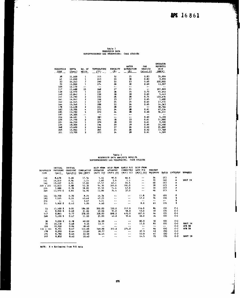
Table 1REsERVOIR OA7A

SUPERPRZSSURED GAS RKXRVOIBS: CASE STUDIES

OPSRATORIAATER GAS REPORTtD

RCSERVOIR OCPTII No. OF TE74PF,RATURE POROSITY SATURATION CRAV1TY OCIPCOOE w v- (*F) _LaL (a) ~Air.l .0) (~F)

3sIll

11.60011,650i19,21k215,00012,17011,473812,97012,8b212,790lb,957l&,5b515. MO

1171

215213290216

. .

268

3229

2530

0.030.830.600.69

-.--

0.720.62o.7fl0.6S0.650.65

--

0.610.60

--

0.620.610.610.650.620.620.61

35, ?999.999

3370

2228

2330

200;00013,207

109117

. .272828

--212s2828573526252028--.-

332919262628

..327,909

k5, bk23,bL2

123,6761,600

17,57116,3632L6,76667,23h36,h51

1513914011.I161162ib&17818319519721422022123526S269311

11

231230

22

232330

2.s23

11

317288216273273

.-

28327427919b242265273

25222s26

12,k2813,700

2II5

--

1212

13,700118,300

2fl-- .-

5,10951,000

9,>0033*WZ25,000i3,7bSk,599

lb, kOllk,75011!, ?5010,30013,60015,96b13,700

--18lB2927252k

212

Table 2RESERVOIR OATA ANALVSIS RESULTS

SUPERPPIESSU6!P.OGAS RESERVOIRS: CASE S’7C01ES

INITIAL INITIAL OCIP PROM OCIP PRCAII EARLY ?/2 oCIP FNIWRFSFRUO!R PRESSURt GRADIENT C12MVLATIVE OPF.RATCM APPAUPX7 f’ORRECT&O LATE P/z PERCENT

CODL (p8}.L (~~i/f~} f~-(nc?) (BCF) (Aj (RCF)--(B) (BC~). (C) (.BCF)-(o) WI?VFRY RSJU-B-SS

SHUT IN

SHUT INVTRONVTA OR

SHUT IN

EATEQOR~

AAAAAA

PsBB

\&olb::b2

220 ● 2212352bQ

lbb1s321431i

33

l;;2b8

0.678 0.b80.9b0.910.8B0.780.85

0.700.55

.-

o.b3

0..s10.b90.770.67

0.780.680.8b0.b70,66O.bb0.62

17.561.15

17.0053.3018.00lb.90

n,21463.69

2.b7$.00

186.0021.00

278.0011.00

llo. oo9.35

18. LIO111.00

12.0032.5010. LO

5.441.60

17.5794.3033.3013. Flo

11..3b&7.23

5.11&,bO

200,00Io. oo

326.0025.00

36.00,3,~1

90.02.b

63.13L’J.O

7L. b7b.5

bb. b1.5

35.5191.0

57.037.0

2672LA2832116

7076--

b3

.S640Lb34

5085-.bbL361?2

(c)(A)(c)(c)(c)(c)

16,319

13,22712,913

7,988

-.

--

13, !00 E -.

11.857.2

--

8.0

(D)(0).-

(D)

10,7007,525

----.---

----

--5,900 E

----

11,500 E8,oOO ES,6659,100 E

332.091.0

898.062,8

217.058.0

670.030.(!

216.053.0

507,032.0

(o)(D)(o)(o)

c-lc- Ic-ic-1

C-2c-2c-2c-2c-2c-2c-2

9,000 E10,13010,500

S,701n, 0008,7828,850

80.011.0

.-

.-

27.953.014. s

(0)(0)-.

(A)(0)(D)(0)

3870

109131 ● 141

178I .?>197

------

271.. O--.---

-.-.

-- --312.0

---.

169.0028,773b.45

-- -.

NoTE : t . E81iMted fr~ ?/2 12at.

m 4-+

Actual App8r.ntOGIP OGIP

Cuntulativo Gas ProductIon, MMCF

. . l.l*Ptz—*~——

8.000

7*000 Ii

u IAGiP = 2.4 6CFGW trom tt~ Mdhod = 1.606CF I

6,000Y -?CC~om~t@kGrti

~ s,-

:

; 4,m0

2 3#00

2.Otm k

1,000

00 5 10 1s 20

Cuntulattvo Gas production (6CFI

~ 4,0G0

g3,0GG

2a

2,0G0

1.OGo

o I I 1 I I 1 1 1 1 io 102030405060 70~90100

Cumulotlvo Gcs Production (6CF]

w 241zpubrn9v.wh 140

9,000

8,000 AGIP = 62.05 wGIPfrom HanrrrrortirwMethod = 33.50 BCF

?,000

. ●IZmud on lf~a~ w

~

u 4.000\

a 3,000

o! I I I I 1’-’0 10 20 30 40 60;

Cumut@ivo Gas Production {BCFI mw

+umpmllu~wz.

9.OW

8,000

7,000

6*U)O

z~ 5,000k; 4.000\- 3,000

2.000

1,000

0 1 I I I

o so 100 150 200 250

Cunwt@ivo Gas Production (BCF]

w %-mzcW—— ?m..wnv

S.000

GtPlfom~Nottmd=37.06CF

7.000

6,000_.. —— W2Wan Hvtimwtatk Ord

z S*OOOg~ 4.000

~ 3,000

2,000

1*000

oi I I I i I I I I

O 5 10 15 20 25 30 35 40 45 60

Cunwdativo Gos Production (6CF]

7,000

6,000

5*W

z 4,000z&; 3.000:

2,000

1,000

0

0

I I 1 I I I I 1

Moo

7,000

6,000

0 10 10 20 30 40 so 60 70 60

2.000

4.000

0

GIP trom id, P/Z = 11.75 BCF.

I l\ I 10 s 10 15 20 a.

CutnuldivO Gas Production (6CF) w

II

7,000

S,GOO

2,0G0

**WO

o

F

GIP from lat. PIZ = 57.232CF

k.●PRnanlt@,aukcnd

1 I I I I

o 10 20 30 40 50 so 70 60 w 100

CumdotiuO Gu production [3CF)

6*OGGFfzm89d- ~M

s@w

4*OWz

g 3@00 GR trom late PIZ = 0.07 SCFN

2 2,000

l@OO

o 5 10 1s 20

~tivo Gas Production (eq

2.OGO

1.000

o~o s 10 15 20 2s

Cumutativo G- Production (BCF)

6@oo

7*000

Spoo

4.000

3,000

2@00

l,OGO

o 1 10 so too 1s0 200 250

Cunlulatiuo Gas Producuom (BCF)

~m-wzmtw~n

!s

Oam9-

s#oo

2@oo

1.000

0o 20 40 so so 100

74)00

SSOO

z A(3P s 42.6 2CF~ 4@oo GWfma~-Umd==.62CP~ wtrambtOP/z=33suF

w-

z

2.oa)

*@w

o 10 to 20 30 40 so

CumddvOGa8Production(BCF)

6,090

S.000

1.000

o~o so lm 1s0 200 2s0 2W 330 ~

CumutattwG@s Producttom(2CFI

7*000

6@W

S.000

~ 3,000a

2.000

1,000

0

0.

0 20 40 so 30 100

CuIIUISttve Gos Production[6CF)

m-@18tlu-n.

2@oo

*.000

o0 5 10 15 20 2s

~tivo GA8 Froductiom (BCF}

I

o~o so 100 1s0 2s0

7.000

6,000

5*000

2*000

1.0001- 1

Cundoth Gas Production [3CFI

6@oo

S$loo

4#oo

3,0m

2Som

l@OO

o

ap tmm lab P/z= 27.s 2CF

?lz9mOdm~w

O*

1

0 s 10 15 20 2s 30

Callu18ttvo G48 PrOdwction(ecF]

0 10 20 30 40 50 60 70

~tiw Gss Pm&wt@a [GCF]

s@w

7*000

6.000

5.000

q 3,0D0&

2,0DD

1.000

00 5 10 15 20 2s

-..● “?!

I Gw from l.sts P/z = 14.s 6CFI

!5*ii los

lss+m141

19s

9,000

8,000

7,000

6,000

q 4,000&

3,000

2,000

1,000

0

10,000

9,000

8,000

7,000

~ 4,000

3,000

2,000

1,000

0

o 100 200 300

Cumulatlvo Ga$ Production (BCF)

1=1-

●

I I I 1 .

E I I 1 I I F

0 40 80 120 160 200 240

Cumulative Gas ProductIon fBCF)