¥ffrey R. Alwang 7 George W. Norton Jan Flora Paul Driscbll

THE EFFECTS OF AGRICULTURAL PRICE POLICIES ON THE

FUNDING OF AGRICULTURAL RESEARCH: CHILE 1960 - 1988

by

Jaime Ortiz

Dissertation submitted to the Faculty of the

Virginia Polytechnic Institute and State University

in partial fulfillment of the requirements for the degree of

DOCTOR OF PHILOSOPHY

in

Agricultural Economics

APPROVED:

/ / ¥ffrey R. Alwang 7 George W. Norton Co-chairman Co-chairman

Jan Flora Paul Driscbll

Irma Silva-Barbeau

December, 1993

Blacksburg, Virginia

THE EFFECTS OF AGRICULTURAL PRICE POLICIES ON THE

FUNDING OF AGRICULTURAL RESEARCH: CHILE 1960 - 1988

by

Jaime Ortiz

Committee Chairmen: Jeffrey R. Alwang and George W. Norton

(ABSTRACT)

Chilean governments have simultaneously used a combination of price policies and expenditures

on agricultural research in their efforts to enhance the performance of the agricultural sector. These

two policy instruments, under changing political environments, have had important distributional

implications for agricultural producers and consumers. Neglecting the interactions between these

instruments may have distorted the measurement of research benefits. This dissertation examines

the implications of agricultural price policies on the funding of public agricultural research. A

political-economy framework allows for the interactions between producers and

consumers/taxpayers in affecting policy formation. The welfare effects on each interest group are

identified.

Agricultural price policies and research expenditures on beef, wheat, milk, apples, and grapes are

considered within a simultaneous system of supply, demand, price and research policy equations.

Economic and political considerations determine the choice between direct price policies and public

research expenditures.

Results conform to theoretical expectations that the level and distribution of public research

investments are affected by agricultural price policies. The implications derived from these results

are that policies can be made more effective if decision-makers consider the complementarity or

substitutability of these policy instruments. Agricultural production was influenced by direct price

policies and by domestic agricultural research and foreign technology transfers. Publicly-sponsored

agricultural research in Chile has had positive economic returns. The benefits to research,

however, would have been larger if distorting price policies had not been present.

ACKNOWLEDGMENTS

A very special recognition goes to my major professors Drs. George Norton and Jeff Alwang for

their advice, friendship, and support during my doctoral program at Virginia Tech. In Holland,

George introduced me to the area of sources of technical change and offered me the financial

support to enhance my education through a research project financed by the International Service

for National Agricultural Research (ISNAR). Later, halfway in my Ph.D. program, Jeff came to

play a crucial role in directing this dissertation. Much of the consistency of this study is due to his

guidance and rigorous criticisms in and out of the classroom. I am thankful to both of them. I wish

to thank Drs. Paul Driscoll, Jan Flora and Irma Silva-Barbeau for serving on my committee and

their insightful comments. As faculty members, Paul Driscoll and Anya McGuirk were important

in teaching me methods of economic analysis.

Acknowledgments Iv

I would like to extend my appreciation to those colleagues who either shared some information

used in this study or commented on it at particular stages during its preparation. Particularly,

Sergio Bonilla from the Instituto Nacional de Investigaciones Agropecuarias, Hernan Caballero,

specialist emeritus of the Inter-American Institute of Cooperation on Agriculture, Ramon Lépez

from the University of Maryland, Alberto Valdés from the World Bank, and Eduardo Venezian

from the Universidad Catélica de Chile. John Beghin from North Carolina State University, Matt

McMahon from the World Bank, and James Nelson from Virginia Tech all made some information

available to me that also contributed to this study. The advise and assistance of Carlos Valverde

of ISNAR is also greatly appreciated.

A few wonderful people made our residence in Blacksburg a pleasant experience. Jeff and Amada

Alwang and their family shared with us uncountable moments of laughter and good time. Roy and

Catherine Blaser gave us the caring support that only grandparents could provide. Luis and Silvia

Meléndez adopted us in a warm environment and wisely advised me on many aspects of this life.

It was natural then, to find in their children, particularly José and Karen Meléndez the same

empathy. Even though we overlapped with Luciano and Darci Novaes for nearly two years we still

keep memories of being such good friends. We will truly miss them all.

Special thanks to our families in Chile, Uruguay, and Sweden for their love and continual

encouragement. Especially, to my mother Pilar for her confidence in my capabilities and her

blessings, and my parents-in-law, Hernén and Monica for their cheer and support. I also deeply

thank my late father, Sergio and my aunt Tencha, for instilling in me the value of education from

a very early age.

Acknowledgments Vv

I truly thank my beloved wife Pamela for her courage, patience, and constant support during the

course of my studies. She, along with our daughters Marfa Pamela and Marfa Alejandra, was

always a source of inspiration and I dedicate to them this dissertation. From now on, I just ask the

Lord to let me continue building up my beautiful family. This time, however, I will share much

more of my time than I have in the past four years.

A word of gratitude goes to my former bosses, Dr. Fausto Jordan and Mrs. Erika Hanekamp from

ECLOF-Ecuador. Without their encouragement I may have not had the opportunity to expand and

diversify my professional career. It is gratifying to know that I always counted on their stalwart

support as both supervisors and human beings.

To avoid omissions, I thank those sincere and truthful individuals I met here in Blacksburg as well

as those fellows from soccer for the opportunity they offered me to teach them the essence and the

way this sport should be played.

Finally, I thank my neighbor Ms. Patricia Gonzdles from Santiago - Chile for her impressive

ability to anticipate events and warn me accordingly.

Acknowledgments Vi

TABLE OF CONTENTS

Acknowledgments iv

List of Illustrations xii

List of Tables xiii

CHAPTER ONE: INTRODUCTION 1

Introduction 1

Problem Statement 4

Justification of the Study 5

Objectives 8

Hypotheses 9

Methods 10

Organization of the Study 12

CHAPTER TWO: CHILEAN AGRICULTURE 13

Introduction 13

A Historical Context 14

The Agricultural Situation 16

Production 16

Foreign Trade 18

Labor 20

Land 20

Table of Contents Vii

Land Reform 22

Machinery and Other Inputs 24

Evolution of Agricultural Price and Other Policies 26

The Import Substitution Strategy 26

The Socialist Administration 30

The Free Market Model 32

Management of Agricultural Price Policies 35

Intervention by Products 35

Beef 35

Wheat and its derivatives 37

Milk 38

Apples and Grapes 39

Intervention in Input Prices 39

Transfer Effects of Agricultural Price Policies 42

Revenues from Price Interventions 43

Expenditures from Price Interventions 43

Direct and Indirect Price Interventions 45

The National Agricultural Research System 48

Historical Evolution 48

Organizational Structure 49

Human Resources 52

Financial Resources 54

Private Sector 56

International Technology Availability 57

Summary 59

CHAPTER THREE: THEORETICAL MODEL 61

Introduction 61

Collective Action and Public Policies 62

Table of Contents Vili

An Agricultural Policy Model

Characterization of a Political Optimum

Modeling a Political Optimum

The Technology

The Production Function

The Profit Function

The Utility Function

Graphical Depiction of the Market and Policy Scenarios

Beef Market

Wheat and Milk Market

Apples and Grapes Market

Comparative Statics Results

A Dynamic Perspective

Summary

CHAPTER FOUR: EMPIRICAL MODEL

Introduction

Presentation of the Model

Commodity Modeling

Supply Equations

Demand Equations

Price and Research Equations

Measurement of the Variables

Output Quantity Variables

Price Variables

Price Policy Variables

Research Policy Variables

Technical Change Variables

Political Variables

Table of Contents

67

71

78

78

79

80

82

87

88

90

92

94

105

107

108

108

109

111

111

114

117

118

119

120

121

123

125

126

ix

Other Variables

Dummy Variables

Estimation Procedures

Supply Block

Demand Block

Price and Research Policy Blocks

Estimation Issues

Research Gains under Price-Distorting Policies

Summary

CHAPTER FIVE: RESULTS AND POLICY IMPLICATIONS

Introduction

Treatment of the Model

Misspecification Tests

Identification Issues

Miscellaneous Procedures

Assessment of the Estimation Technique

Test for Exogeneity

Supply Equations

Policy Equations

Econometric Estimates

Supply Equations

Demand Equations

Price Policy Equations

Research Policy Equations

Supply Elasticities

Demand Elasticities

Income Elasticities

Table of Contents

129

130

131

131

132

133

135

137

141

142

142

143

143

145

146

148

152

153

154

156

156

161

164

170

175

178

179

Welfare Estimates

Policy Implications

CHAPTER SIX: SUMMARY AND CONCLUSIONS

Summary of the Dissertation

Conclusions of the Study

Limitations of the Study

BIBLIOGRAPHY

Appendix A. Comparative Statics Derivatives

Appendix B. Solution of the Equation System Using Cramer’s Rule

Appendix C. Data Used in the Model

Appendix D. Misspecification Tests

Appendix E. Ordinary and Two-Stage Least Square Estimates

Appendix F. Exogeniety Tests

Appendix G. Derivation of Economic Surplus Formulas

VITA

Table of Contents

180

187

190

190

193

195

197

209

222

227

240

244

253

260

273

XI

List of Illustrations

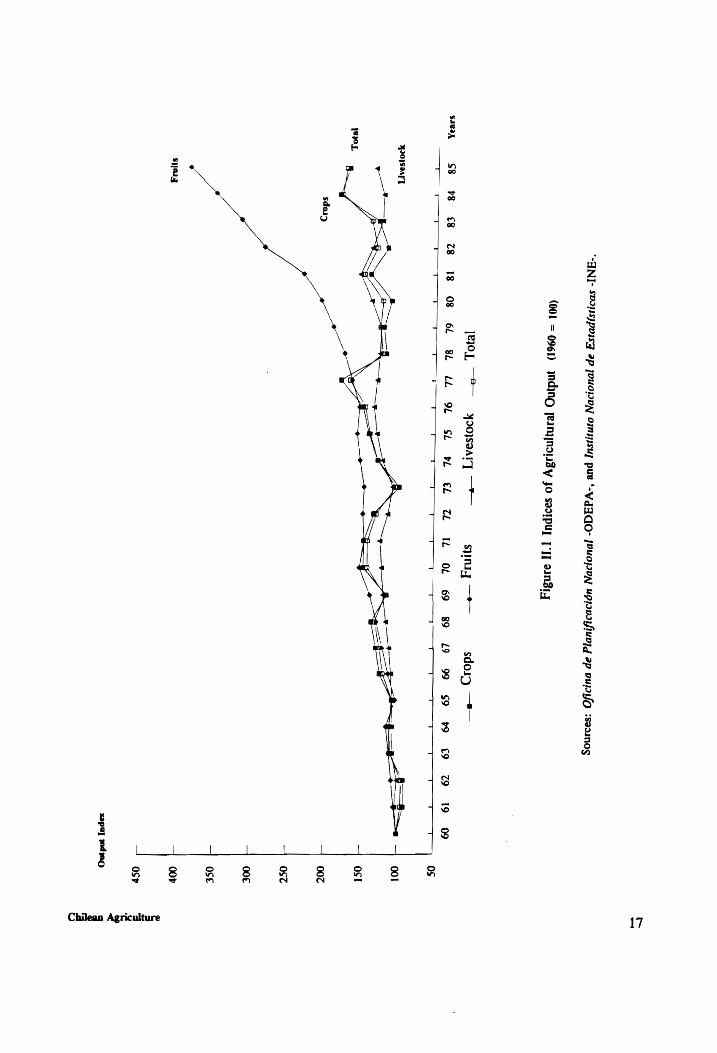
Figure II.1. Indices of Agricultural Output (1960 = 100)

Figure II.2. Evolution of Agricultural Research Expenditures

Figure III.1 Direct Price Intervention (Tax) to Beef-cattle

Figure IlI.2 Direct Price Intervention (Subsidy) to Wheat and Milk

Figure III.3 Direct Price Intervention (Subsidy) to Apples and Grapes

Table of Contents

17

55

89

91

93

xii

List of Tables

Table II.1. Land Use in Thousands of Hectares

Table II.2. Consumption of Fertilizers in Metric Tons

Table II.3. Direct Price Interventions at the Official Exchange Rate

Table II.4. Researchers involved in Publicly-funded Agricultural Research

Table III.1. Effects of AB, aw, Es, and Ep on Price and Research Policies

Table IV.1. Variables of the Model

Table V.1. Estimated Parameters for the Block of Supply Equations

Table V.2. Estimated Parameters for the Block of Demand Equations

Table V.3. Estimated Parameters for the Block of Price Policy Equations

Table V.4. Estimated Parameters for the Probit Model

Table V.5. Estimated Parameters for the Block of Research Policy Equations

Table V.6. Supply, ES, Demand, ED, and Expenditure, IE, Elasticity Estimates

Table V.7. Benefits from Agricultural Research under Minimum - Maximum

Price Policies

Table V.8. Benefits from Agricultural Research under Different Supply

Elasticity Scenarios

Table V.9. Benefits from Agricultural Research by Interest Groups under

Minimum - Maximum Price Policies, assuming a 10 percent discount rate.

Table V.10. Benefits from Agricultural Research using Border Prices

fable of Contents

21

25

53

102

112

158

163

165

168

171

179

182

183

185

186

xiii

CHAPTER ONE

INTRODUCTION

Introduction

Chile has faced unprecedented political changes since the late 1950s. Until 1964, Chile was

exposed to a fairly traditional conservative regime. Then, from 1965 to 1970, a more populist

government initiated reforms. In 1970, a radical socialist administration gained power. From the

end of 1973 to 1990, a military government led the country to an ambitious free market economy.

The result of changing ideologies translated into macroeconomic and sectoral policies that have

continuously affected the allocation of resources within agriculture and between agriculture and

other sectors (Valdés, 1988).

Introduction 1

Since the early 1940s manufacturing has been the sector of major interest in Chilean development

policies (Corbo and de Melo, 1985; CIEPLAN, 1988). A fall in the external terms of trade for

agricultural and other primary products, as well as increased instability in international markets

triggered the adoption of policies that encouraged industrialization. This industrialization was

accomplished behind high levels of protection for industrial goods and by depressing agricultural

prices that, in turn, shifted the profitability of investment from agriculture to industry. Several

policies that discriminated against agriculture were pursued to provide cheap agricultural goods

to urban consumers. Ceiling prices, exchange rate misalignments, credit subsidies, and quantitative

trade restrictions were the most commonly used policy instruments. After the late 1950s, these

policies were gradually intensified by successive governments to influence the performance of

Chilean agriculture.

By 1974, there was a recognition that the process of import substitution by itself could not generate

the fast and broad effects that were desired from industrial protection policies. As a result, the

military government replaced import-substitution with liberalization and stabilization policies in

most markets. These policy reforms included deregulation of financial markets, the dismantling

of non-tariff trade restrictions, eradication of a chronic fiscal deficit, and an overall reduction of

government intervention in economic activity. For the agricultural sector in particular, the reforms

sought to eliminate price controls, reduce protection for competing commodities, and lower the

taxation of export activities.

The positive relationship between growth in the agricultural sector and the contribution of

agriculture to the development process has been well documented (Schultz, 1964; Timmer, 1988).

Introduction 2

In the Chilean case, the rate of growth of its agricultural gross domestic product has been lower

than in several more-developed countries and below that found in other sectors of the economy.

From 1960 to 1988 the economy grew at an average annual rate of 3.0 percent, while the value

of agricultural production increased at an annual rate of 2.3 percent in the same period. The need

for fostering the role of Chilean agriculture to enhance overall national economic growth is widely

recognized. However, fiscal constraints force politicians and international funding agencies to

carefully assess the rationale of policy intervention in Chilean agriculture. When maximizing

expected social benefits for their constituency, decision-makers are aware that welfare gains arise

in conjunction with making appropriate expenditure decisions on a variety of sectoral policies.

In the efforts of governments to promote agricultural growth the allocation of public funds

becomes critical. Government policies such as price intervention and publicly sponsored

agricultural research compete with each other for budgetary resources. Failure to appropriate

optimal levels of expenditures on each policy instrument may entail substantial opportunity costs

for society. Within that context, policy-makers may fail to equalize the marginal rates of return

across policy instruments in order to maximize the social return from total funds available. For

example, rates of return on improved varieties of wheat and maize in Chile averaged 28 percent

per year (Yrarrazaval et al, 1982) '. While returns to other public investments are not known,

these significant payoffs to research imply a possible underinvestment in agricultural research and

' That study, however, did not consider the effects of price policies when calculating the benefits of

research and therefore, may have mismeasured the true rates of return. Such an omission may also have biased the distributional effects of research benefits.

Introduction 3

have resulted in recommendations for higher levels of public investment in agricultural research

and development.

Problem Statement

Chilean policies have failed to help stimulate rapid and significant increases in aggregate

agricultural growth. Among the possible reasons for this failure are the interactions between price

interventions and the development of improved technologies. Distortionary agricultural price

policies may have sent signals to the national agricultural research system that have distorted the

allocation of research resources and hence the generation of technologies. Policies that distort

relative prices may have affected the level and distribution of income of both producers and

consumers as their incentives to press for new technologies have been altered. Also, efforts to

encourage the adoption of technologies and to strengthen agricultural institutions appear to have

fallen victim to a decreasing government involvement in research and extension.

Introduction 4

Justification for the Study

Chile has been in the midst of a transition from a traditional agricultural sector to a modern export-

oriented one (CEPAL, 1982). Throughout this transition, Chile has faced inconsistencies among

the development role assigned by the public sector to agriculture, the level of public financial

resources allocated to agriculture, and the policies designed to enhance the role of agriculture

(FAO, 1988). National agricultural objectives related to public resource allocation to agriculture

are defined at the highest levels of government. Policies developed at this level have distorted

product and factor markets, thus impeding the growth of Chilean agriculture, except for a few

commodities (Sanfuentes, 1987).

A negative direct nominal protection rate of -1.2 percent for all Chilean agricultural commodities

between 1960 and 1983 was found by Valdés (1991). That figure indicates the degree of direct

taxation, on a percentage basis, imposed on agriculture as a result of direct price interventions.

Indirect economy-wide price intervention was also negative and greater than the direct taxation

with an indirect nominal taxation rate on agriculture of -20.4 percent. In addition, recent estimates

show modest increases or even declining amounts of real public investment in agricultural research

for Chile (McMahon, 1992; Pardey and Roseboom, 1989).

Introduction 5

The strength of different interest groups in influencing government policies was discussed by

Hurtado et al in their study of agricultural price policies in Chile. Based on the concept of pressure

groups, that study argued that price policies have been implemented when powerful coalitions

support policy reform because the rents perceived from those reforms are greater than the costs

associated with lobbying. There is also general agreement that price policies have often been

designed to enhance the welfare of the more numerous urban consumers over the welfare of

agricultural producers. Rent-seeking efforts of non-producer groups seem to have succeeded in

directing government price interventions to benefit those groups 7. However, political pressures

exercised by farm lobbies to achieve price stabilization, increases in minimum prices, and subsidies

for input purchases have also been repeatedly observed over the years (Muchnik and Allue, 1991).

The national agricultural research system has tended to focus its research efforts on a broad range

of commodities. Market considerations and the opportunistic behavior of fruit producers have

guided the development of technological innovations by private sector research (Jarvis and

CIEPLAN, 1989). In comparison, political pressures exerted by farm groups on public research

institutions appear to have directed the technological pattern toward commodities characterized by

some degree of price intervention such as crops and livestock. By targeting technological advances

and price policies to the production scheme of a selected number of producers, the allocation of

public resources to agriculture has been distorted. The productivity of food crops traditionally

produced in Chile has not increased substantially over the last 30 years (ODEPA, 1987).

*The most obvious example of rent-seeking efforts by urban consumers has been their drive to keep

food prices low.

Introduction 6

In recent years, pressures on Chilean governments to revitalize the agricultural sector have

increased substantially. Foreign exchange constraints have been exacerbated by one of the highest

per-capita external debts. In 1989 Chile’s total debt mounted to $ 19.0 billion, or 2.7 times the

level of annual merchandise exports (Inter-American Development Bank, 1990). In addition, Chile

has exhausted its ability to promote production through expanding is agricultural frontier. Raising

the productivity of the agricultural sector will help foster increases in agricultural output.

However, Chile’s limited agricultural base and changing political and economic environments have

created challenges to raising this productivity.

A comprehensive political-economy framework within which to assess the simultaneous impacts

of price policies and research-generated technologies is needed to make more explicit the

distributional consequences of the various policies affecting producers, consumers, and taxpayers.

Attempts to identify the sources of growth in Chilean agriculture are relatively recent. Past studies

have not considered the effects of agricultural price policies on the supply of and demand for

agricultural research. Rather, these studies have measured the levels and the effects of both direct

and indirect price interventions on specific agricultural commodities while seeking to understand

the incentives provided by trade and macroeconomics policies (Hurtado et al, 1990). Alternatively,

they have concentrated on the supply side of the economy by modelling sectoral growth with

aggregate demand only tacitly introduced (Coeymans and Mundlak, 1993). No attempts have been

made to explicitly evaluate the joint determination of agricultural research investments and price

policies while allowing technology to be endogenous to the economic policies themselves.

Introduction 7

Objectives

The overall objective of this study is to analyze the determinants of the level and distribution of

research investments in Chilean agriculture between 1960 and 1988. To fulfill this objective, a

political-economy framework is built to examine the interactions between agricultural research and

price policies, institutional and economic linkages with the rest of the economy, and international

technology availability. The specific sub-objectives are:

i) to identify the impact of both domestic and foreign agricultural research on Chilean

agricultural production growth in the presence of specific price policies;

ii) to examine the determinants of the level and distribution of public spending on agricultural

research; and

iti) to quantify the distribution of research benefits under the distorted agricultural price policy

setting in Chile.

Introduction 8

Hypotheses

The central hypothesis tested in this study is that agricultural price policies in Chile between 1960

and 1988 affected the level of performance of the agricultural sector, not only directly but through

their effects on the supply of and demand for agricultural research. Thus, this study contains the

following specific hypotheses:

i) that government price policies in agriculture have Jowered the benefits to Chile from

indigenous and international agricultural research; and

ii) that the level and distribution of public financial support for agricultural research have

been influenced by the pressures imposed by various interest groups on government.

Introduction 9

Methods

A framework consisting of a system of equations representing Chilean agriculture that distinguishes

among the effects of political and economic factors and of resource availability in determining the

choice of price policies and technological innovations is used to address the above hypotheses.

Agricultural growth within that framework is explained inter alia by the interactions between the

government and a diverse set of interest groups. The allocation of public resources to finance

agricultural research and price policies is endogenously considered. The level and distribution of

price policies and public-sector research investments are assumed to be determined by a

government that responds to the differential political power of producers and consumers/taxpayers

in order to maximize a given policy preference function.

Livestock, grain crops, and fruit production are represented by five commodities: beef, milk,

wheat, apples, and grapes. These commodities have been subject to extensive direct and indirect

price intervention and, at the same time, represent a significant share of Chilean agricultural GDP.

To analyze the distributional aspects in this framework, the interest groups included are broadly

defined as producers and consumers/taxpayers. Further categorization of these two economic

groups by farm size or types of consumers is hindered by a lack of disaggregated data and by the

high degree of output diversity of most Chilean farms. The aggregative approach regarding interest

groups taken in this study is appropriate to capture the interactions between price policies and

research spending and to identify the distributive effects on each group.

Introduction 10

At the empirical level, the model has a simultaneous structure that determines within the system

the effects of price-support (price-tax) policies on research spending. The agricultural budget,

political variables, and market conditions account for exogenous changes in a model characterized

by policy interdependence. Government interventions not only alter the relative prices within

agriculture, but also between agriculture and non-agriculture. Therefore, the interactions between

the agricultural sector and the rest of the economy that are reflected in trade and macroeconomic

variables are implicitly considered in the model.

The benefits of technical change in Chilean agriculture are evaluated by estimating changes in

economic surplus. The forces driving supply and demand are identified from the system of

equations described above. In turn, this system allows for the assessment of the impacts of price

policies and research investments on producers, consumers, and taxpayers. If a trade-off in welfare

is a response to political influences by profit-maximizing farmers and _ utility-maximizing

consumers/taxpayers, the relative political power of the interest groups can explain such a trade-

off. The economic surplus approach is used to identify the long-run benefits of research-induced

supply shifts.

Introduction ll

Organization of the Study

This dissertation is organized as follows. Chapter IT describes Chile’s economic development since

1960. An overview is presented of the Chilean economy. Past and current agricultural price

policies, and the role that agricultural research has played over the past three decades are

highlighted. Chapter III discusses the political-economy perspective of agricultural price policies

and expenditures in agricultural research. Among the issues raised are the endogeneity of price

policies and research investments in the presence of collective action as well as the effects of

relevant exogenous variables on both policy instruments. The empirical model is presented in

Chapter IV along with variable specifications and data sources used for measuring the level and

distributional impacts of price and technology policies. The results and policy implications of the

empirical analyses are presented and discussed in Chapter V. Finally, Chapter VI summarizes the

dissertation drawing some conclusions from the study that may be translated into effective policy

actions.

Introduction 12

CHAPTER TWO

CHILEAN AGRICULTURE

Introduction

This chapter describes the performance of Chilean agriculture since 1960. In the first section, a

brief historical perspective of the Chilean economy is presented. Then, the main issues that have

shaped the agricultural sector including the agricultural price policies implemented are identified.

In the third section, the general evolution of the agricultural policies applied since 1960 are

presented in more detail. The management and budgetary costs of the price policies for specific

commodities are described in the fourth section. Finally, the role of the national agricultural

research system in promoting technical change is examined.

Chilean Agriculture 13

A Historical Context

In the mid point of the nineteenth century, Chile was mainly an agricultural country with

landowners enjoying a prosperous export market. After almost 30 years of booming exports of

grain and other agricultural products, conditions changed in 1875 when other countries brought

new areas under cultivation at lower cost. In 1879, as a result of the victory in the War of the

Pacific against Peru and Bolivia, Chile held a virtual monopoly in the production of natural nitrate.

Between 1880 and 1925, Chile was a classic example of an enclave economy with nitrate being the

engine of a dynamic domestic market (Roddick, 1976). When nitrate exports declined, Chile

adopted protective measures to encourage industrial expansion. Still facing the impacts of the Great

Depression of the thirties, Chile subordinated agriculture to an industrial development strategy.

With minor differences in tone, successive governments reinforced the process of import

substitution that tended to close the economy for the next forty years (Edwards, 1985).

Inward-oriented economic policies were implemented to reduce the vulnerability of the economy

to external economic shocks and to achieve distributional objectives. Interventions in agriculture

included price fixing, subsidies, and quantitative restrictions on trade. With a trade policy

characterized by overvalued real exchange rates and high tariffs, large and continuous devaluations

were constantly required to respond to balance of payment disequilibria. The instability of the

exchange rate along with other inconsistent trade policies discouraged agricultural exports more

than the adverse conditions in the international markets (Valdés, 1973).


Price interventions in Chilean agriculture began in 1931. That year the Agricultural Export Board

was established to fix the prices of wheat, flour, and bread and to prohibit or limit the export of

wheat. A year later, the government created a Prices Secretariat with enough authority to set the

prices of essential goods, prohibit or limit their exports, import such items in the event of domestic

shortages, control the marketing of food, and fight price speculation. Although both institutions

functioned on a permanent basis, the intended programs were never fully implemented. In 1953,

the authority to fix the prices of wheat, flours, and bread according to their production and

processing costs and general norms of profit margins was given to the Ministry of Economics and

Commerce (Hurtado et al, 1990).

Prices for agricultural commodities were kept low to boost real income in the non-agricultural

sector, without increasing the wages of industrial labor. Market interventions made agriculture

unattractive to potential investors compared to non-farm activities. Between 1930 and 1960,

industrial production grew almost five times more than agricultural production. In fact, per capita

agricultural production decreased at an average rate of 0.4 percent during the same period (Crispi,

1980). Thus, Chile entered the 1960s as a net importer of agricultural products with aggregate

agricultural production growing well below the rates of growth in population and per-capita

incomes.


The Agricultural Situation

Production

For the last three decades the share of Chilean agriculture in the total gross domestic product

averaged 8.5 percent per year. The evolution of production of the main groups of agricultural

products produced between 1960 and 1988 is shown in Figure II. 1. Total agricultural production

in Chile increased by 74 percent during that period, an average rate of 1.9 percent per year. With

the exception of fruits, modest annual fluctuations in output can be observed across the twenty-six

year period. In the early 1970s, political unrest, insecurity in land tenure, and severe droughts

were the main causes of an absolute decline in agricultural production. Although during the 1980s,

crop and livestock production began to increase, production barely kept pace with a population

growth of 2.0 percent. Fruit exports have exhibited, since 1975, an impressive upward trend.

According to statistics of the Oficina de Planificaci6n Nacional, ODEPA, traditional crops

represented by cereals, pulses, and tubers, which in 1965 accounted for about 43 percent of the

value of production, fell to 37 percent in 1988 as a result of the decline in area sown. The share

of the fruit sector in agricultural output constantly increased. Representing less than 5 percent of

the total sectoral value in the early 1960s, the fruit sector accounted for about 21 percent of the

total in 1988. This large increase in fruit production occurred at the expense of traditional crops.


““ANI- SDONS)pyisg

ap jouoinn

omjyjsuy pus

‘-WdAdO- [2uo}pvN

upiovolfiuvjg ap

puja

:se21n0g

(001 =

0961) anding

jeanynoq3y Jo

sao1puy |]

aIN3Ly

J30L ~F—

yoojsaary —*—

sini —*—

sdory —*—

SiBaX $8

#8 €8

78 I8

O8 62

8 LL

OL SL

bL €L

ch If

OL 69

89 #249

99 $9

#9 €9

%@ 19

09 oye

T

40)Saayr]

oo

N=

—=

eg

1890],

sdoiy

symg

T TF

T T

1 1

T T

T T

T T

oT Os

OOl

ost

J wee +

osz

— ose

J OSY

xapuy wdmo

17 Chilean Agriculture

The share of the livestock sector remained constant at around 52 percent of the total value of

agricultural output in the 1960s and 1970s, but decreased steadily to 42 percent by 1988. On

average, beef and milk accounted together for almost 70 percent of the value of livestock

production. The production of poultry, hogs, and eggs accounted in roughly equal amounts for an

additional 22 percent (ODEPA, 1990).

Moderate increases in the volume of total production may be constrasted with improvements in

farming technology for some individual crops. Since 1965, leading crops in terms of area sown

such as maize, wheat, and potatoes have shown annual yield increases of 4.0, 3.0, and 2.9 percent,

respectively. The livestock sub-sector also incorporated advanced imported technologies

(Venezian, 1992). Concentrated in a few large commercial firms, the value of swine and poultry

production have increased annually by more than 5.9 percent since 1965. Moreover, substantial

gains have been made in dairy production where modern processing technologies and

diversification in the end products marketed have also occurred.

Foreign Trade

Before the trade liberalization process which began in 1975, copper represented about 80 percent

of total exports. Trade liberalization decreased the importance of an already small amount of

traditional manufactures. They were replaced by a spectacular growth in exports of non-traditional

products, especially agricultural perishables. The export volume of the main agricultural products


has doubled in the last decades. Prior to the liberalization reforms, pulses were the most important

agricultural exports, accounting for nearly 35 percent of the sector’s export value (ODEPA, 1990).

After the reforms, the fruit sector gained in importance reaching in 1988 more than 75 percent of

total agricultural exports. This agricultural growth boosted agricultural exports to over 20 percent

of the agricultural GDP and over 14 percent of the total value of exports. The annual share of

agricultural imports in total value of imports decreased from around 22 percent in 1965 to 6.4

percent in 1988. Agricultural imports reached their peak in 1973 and 1975 when domestic

production fell greatly and the average degree of self-sufficiency in those two years fell to 63

percent (ODEPA, 1990).

After decades of substantial trade deficits, Chile’s agricultural trade balance did not turn positive

until 1979 and then only if forest products are included. According to the Banco Central de Chile,

it was not until 1985 that Chile became a net exporter of agricultural products with a $ 268 million

surplus. In 1988, nearly 50 percent of agricultural production was exported, with North America

and Europe being the most important markets. South Africa, Argentina, and Greece were Chile’s

most important competitors. However, these competitors have been constrained in recent years by

climatic limitations, phytosanitary conditions and/or unfavorable economic policies.


Labor

Chilean agriculture reduced its share of total employment from about 30 percent in 1960 to about

20 percent in 1985. Between those years, the economically active population in agriculture

decreased from about 741,000 to 614,500 people. Moreover, there is evidence that the number of

workers hired on a permanent basis dropped while the number of workers hired on a temporary

basis increased by 50 percent (CEPAL, 1982).

Land

Approximately 26.8 million hectares -36 percent- of the nation’s total are currently considered

adequate for agricultural purposes out of a total of 74.9 million hectares in the country (Table

II.1). Of that area, land for cultivation, livestock, and forestry roughly represent 17, 50, and 33

percent, respectively. In 1988, cereals were planted on about 77 percent of the area devoted to

crops whereas pulses and tubers were planted on about 13 and 10 percent of the cropland,

respectively (ODEPA, 1990).

The quality of the agricultural land constantly declined from an index value of 100 in 1960 to 91

in 1985 (Peterson, 1987) '. The main reasons for this decline are soil erosion and ground and

' This international index of land quality was calculated by using an hedonic approach to valuing the

cross-sectional differences in land used for agricultural purposes.


Table IT.1

Land Use in Thousands of Hectares

1960 1975 1990

Land Area 73,300 74,880 74,880

-Agricultural Use 3,572 5,792 4,525

-Arable Land 3,415 5,600 4,276

-Permanent Crops 157 192 249

-Permanent Pastures 10,207 11,700 13,450

-Forest and Wood Use 20,565 20,686 8,800

-Non - Agricultural Use 38,956 36,702 48,105

Source: FAO Production Yearbooks.

Chilean Agriculture

surface water contamination. Consequently, in the past twenty years marginal lands have been

abandoned and regional land use has shifted to increasing specialization in production (Venezian,

1992). Due to urban expansion, more than ten thousand hectares of agricultural and forest land

have been converted to non-agricultural purposes.

Aproximately 1.8 million hectares or around 10 percent of the land used for agricultural or

livestock purposes are irrigated. Chile’s agricultural production takes place in a belt approximately

1,700 kilometers long from Region III in the North to Region XI in the South *. Production from

areas outside these administrative regions are only important in ovine meat and wool which

represented in 1988 less than 4 percent of the total production value (ODEPA, 1990).

Land Reform

The first agrarian reform law was passed in 1962. However, only in 1965 did the government of

Eduardo Frei implement a program to improve the land holding distribution. Approved by

Congress, the government authorized the Corporacién de la Reforma Agraria, CORA, to

expropriate uncultivated lands and holdings above 80 HRBs *. Expropriated farms were handed

Over tO permanent agricultural workers organized on a semi-cooperative basis called

asentamientos. This was a transitional arrangement, pending a final settlement that could be either

private ownership or collective cooperative farming (Nove, 1976). Between 1965 and 1970, more

2 Chile is divided into thirteen administrative regions starting from the north of the country.

3 One hectdrea de riego basico, HRB, was defined as a standard irrigated hectare of the best quality land

in the Central Valley of Chile.


than 900 asentamientos containing 20,970 families were formed (de Vylder, 1976). By 1970, these

asentamientos represented some 2.6 million hectares and 16 percent of the arable land (Kaufman,

1972; Roddick, 1976).

Inheriting the legal instruments from the past administration, the expropriation process was

reinforced between 1970 and 1973. The minimum size of landholdings to be redistributed

continued to be farms above 80 HRBs. However, after almost all large farms or /atifundios had

been expropriated, the government began a selective expropriation of 4,394 farms between 40 and

80 HRBs (Kay, 1976). Based on ideological grounds, the government devised a strategy to form

collective production units on the expropriated farms. This strategy included rural workers other

than permanent farmers, such as seasonal laborers, sharecroppers, and minifundistas in general.

In March 1973 when the first phase of the land reform process was completed, a total of 5,512

farms had been expropriated since 1965 (de Vylder, 1976).

The military government that took over in September 1973 initiated a process of "counter agrarian

reform" that assigned a large portion of expropriated land to rural families in the form of Unidades

Agrtcolas Familiares (Hurtado et al, 1990). These small family holdings averaged about 10 HRBs

and benefitted some 37,000 farm families. Another 10,000 families had land assigned on a

cooperative basis. By May 1974 about two thirds of expropriated land were either handed over to

its former Owners or auctioned to highly capitalized agricultural producers.

The land reform process that started in 1965 and lasted until 1974 contributed, in spite of

transitional problems, to help modernize the agricultural sector from the /atifundios structure


(Serven and Solimano, 1991). Its general principle was to provide unrestricted access to

landholding with guaranteed private property. By 1965 this was a popular move in a country where

about one-third of the population worked in agriculture and 63 percent of all agricultural land was

in the hands of 1.3 percent of landowning families (Hurtado et al, 1990). As a result, the land

reform process distributed around 48 percent of the agricultural land to over 50,000 small farmers.

Machinery and Other Inputs

Statistics on the number of tractors in Chile can not be considered reliable. Discrepancies of more

than 14,000 units can be found for some years in data series compiled by Zegers (1981) and the

Trade Yearbooks of FAO, with the stock of agricultural tractors listed by the former consistently

lower than FAO figures. In 1960, one of the years in which the fewest discrepancies arise, there

were some 13,000 units or about one for every 57 persons working in agriculture. It is also

estimated by de Vilder that in 1972 some 22,000 tractors were in use. That represented about one

tractor for every 31 agricultural workers. By that time, more than 60 percent of these tractors were

in hands of the reformed sector and the rest in private medium-sized farms and public tractor

Stations (O’Brien, 1976). For other years the magnitude of the differences between each data series

is SO immense that no further conclusions can be drawn.

The application of fertilizers almost doubled between 1960 and 1986 due to increased usage

following the introduction of modern varieties. As shown in Table II.2, nitrogen fertilizer

represented between 30 and 52 percent of total fertilizer consumption during the 27 year period.


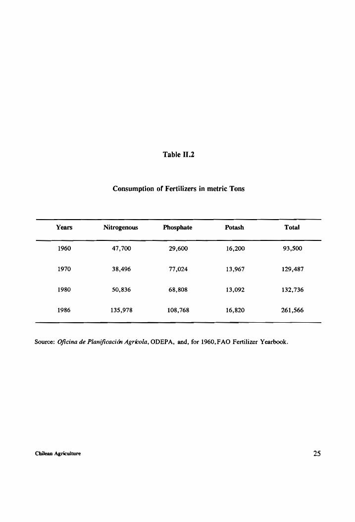
Table II.2

Consumption of Fertilizers in metric Tons

Years Nitrogenous Phosphate Potash Total

1960 47,700 29,600 16,200 93,500

1970 38,496 77,024 13,967 129,487

1980 50,836 68,808 13,092 132,736

1986 135,978 108,768 16,820 261,566

Source: Oficina de Planificacién Agricola, ODEPA, and, for 1960,FAO Fertilizer Yearbook.


Phosphate fertilizer, which in 1960 represented no more than 32 percent of overall fertilizer use,

represented around 47 percent of the total in 1986. Consumption of potash fertilizer decreased over

time and in 1986 accounted for less than 10 percent of the total.

Evolution of Agricultural Price and Other Policies ‘

The Import Substitution Strategy

In 1958 the government of Jorge Alessandri maintained hopes of an intensified industrialization

Strategy as a source of economic growth. Protectionist measures were revived by establishing

temporary prior deposits on all imports (Berhman, 1977). Import quotas and licensing were

implemented and the nominal protection rate on manufactured goods averaged 111 percent

(Balassa, 1985). The government authorities devised some policies to aid farmers and exporters

of agricultural commodities and others to tax them. These policies included inter alia, fixing the

prices of commodities considered "essentials", setting up marketing boards to stabilize prices at

the farm level, providing public information services for prices and markets at the retail levels, and

expanding commodity storage and processing capacity.

4 The following two sections draw on "Trade, Exchange Rate and Agricultural Pricing Policies in Chile"

by H. Hurtado, A. Valdés, and E. Muchnik. This probably is the most comprehensive study on Chilean agricultural price policies.


In 1960, the Empresa de Comercio Agrtcola, ECA, a state-owned marketing agency was created

for the purpose of buying and selling cereals. Over time, ECA extended its authority to a greater

number of agricultural products including the monopoly of imports. The same year, the

Corporacién de Fomento de la Produccién, CORFO, a production development corporation,

created an agricultural office to design policies for certain regions or sub-sectors within

agriculture.

Measures to stimulate agricultural productivity included lowering production costs through

research to develop new technologies and encouraging more intensive use of modern inputs. To

improve the sectoral terms of trade, the economic authorities simplified their export rules,

promoted exports of fruits such as grapes and apples, and agreed to participate in a Latin American

free trade area to gain access to foreign markets (Hurtado et al, 1987). Farmers were compensated

with reduced tariffs for imported agricultural inputs and subsidies for purchases of fertilizers and

certified seeds and for transportation costs. In addition, credit was made available at subsidized

interest rates along with technical assistance to small producers. Public financing was provided to

the livestock sector for importing breeding animals and constructing slaughterhouses and milk

plants. Programs to create additional pasture land were initiated and meat imports were controlled

to reduce competition from foreign suppliers.

The government of Eduardo Frei took over in 1964 on a platform that called for changing the

existing income distribution and the structure of demand in the economy. The development of the

agricultural sector was viewed as a necessary condition for the overall development of the country.

Low capital accumulation, an increasing trade deficit, and an uneven land distribution were


identified as the main obstacles to growth in Chilean agriculture. However, the government faced

the trade-off between improving relative agricultural prices and the need to restrain real wages in

the non-agricultural sector. To modernize the sector, systematic measures were introduced to

mechanize agricultural activities and expand and rationalize the use of irrigation infrastructure.

Production was stimulated by readjusting agricultural prices faster than non-agricultural prices.

Policy-makers devised an export promotion scheme at the time that import restrictions were

progressively reduced.

Agricultural price policies were emphasized under this government. They were part of a general

policy aimed at increasing agricultural production by 44 percent between the period 1965 and

1971. The price policy had three main objectives: i) to increase farm incomes for generating

surpluses needed to finance investments within the agricultural sector, ii) to achieve a price

structure that would encourage certain products and discourage others, and iii) to orient

consumption towards products more in line with the production possibilities of the country. Prices

would be fixed according to international levels and announced at planting time. In addition, price

fluctuations would be diminished to achieve these objectives established by the Farm Development

Plan.

The credit policy was designed to promote production and marketing of certain commodities.

Credit was allocated in order to reduce its concentration and target it to small and medium size

farms. The roles of public and private credit institutions were redefined and maximum levels were

established for credit allocation to producers. Helped by extremely favorable terms of trade and


increased foreign debt, public sector credit was usually provided at negative real interest rates

(Hurtado et al, 1990).

Marketing policy was expected to improve trade channels, diminishing marketing margins and

increasing the degree of participation of producers, consumers, and cooperatives in marketing

activities. Measures used included increasing storage and processing facilities in producing areas,

improving transportation systems, accumulating commodities for food security reasons, and

Operating marketing boards to support prices of certain products and of certain groups of

producers.The Direccién Nacional de Industria y Comercio, DIRINCO, was in charge of the

whole price control system with the power to set prices to consumers. The purpose of these

measures was to achieve stable food supply at the lowest possible prices to consumers while

providing income stability to producers.

The tax policy was designed to obtain financial resources for the government and to promote

investment within farms. A single agricultural tax based on potential land productivity was

adopted. Motivated by an insufficient use of technological inputs, the government sought to lower

the production costs of farmers by fixing input prices and by subsidizing the prices of fertilizers

and pesticides. In addition, public sector institutions increasingly monopolized the import of

machinery and parts as well as fertilizers.


The Socialist Administration

Supported by a left-wing coalition, the government of Salvador Allende began in 1970 to

nationalize key economic activities and to reactivate the industrial sector by adopting an active

monetary policy and heavy protectionism. Import deposit requirements of 10,000 percent for 90

days were established over 60 percent of imports, with subsequent extension of the list and most

products being subjected to import licensing (Berhman, 1977).

The National Agricultural Plan for the period 1971 - 1976 included the expropriation of all farms

over 80 HRBs to create 100,000 new peasant proprietors and strengthen peasant organizations. It

was expected that changing the land tenure system and subsidizing agricultural credit would

increase production by 46 percent between 1971 and 1976 (Zammit, 1973). These transformations

could not be accomplished within the existing institutional framework, and therefore, disrupted the

productive structure of the country. The process of agrarian reform demanded such a large amount

of fiscal expenditures that by 1973, it contributed to create a fiscal deficit of almost 25 percent of

the gross domestic product (Balassa, 1976).

In theory, the agricultural price policy was set to meet three fundamental requirements: i) to serve

as a means for a change in the income distribution, ii) to stimulate agricultural producers to raise

production, and iii) to guide producers in their choice towards exportable and high value-added

products (de Vylder, 1976). The instruments used were basically the same as in the previous

period, but the degree of intervention was intensified. Official nominal prices increased


substantially during 1972 - 1973. Prices for agricultural commodities were based on production

costs and consumption needs. These prices were modified automatically twice a year on the basis

of seasonal variations in production.

The marketing policy sought to expand the coverage of marketing boards to a greater number of

agricultural commodities in order to regulate supply and demand. Products were bought by ECA

at official prices and a state-owned company, the Sociedad de Cooperativas Agropecuarias,

SOCOAGRO, contracted livestock production with small farmers and other cooperatives of small

producers. The government intervened in the cattle market and placed poultry slaughterhouses and

marketing firms in the public sector. As an additional means of stimulating production, the state

provided subsidized credit to purchase capital goods and fertilizers and supply technical assistance

to peasant organizations.

Facing an annual inflation of 400 percent, the government instituted price controls on more than

3,000 products by the Juntas de Abastecimientos y Precios, JAP. Unsuccessfully, the government

tried in early 1973 to curb inflation by controlling the purchase, sale, and distribution of the most

important agricultural products, as well as fertilizers. The excess demand resulting from price

intervention was channeled to black markets and queuing proliferated. An attempt was made by

the government to control the agricultural black market through vertical integration of state

enterprises. However, organizational problems were overwhelming and any efforts taken by the

state could not counteract the devastating effects of food shortages.


The Free Market Model

Within a relatively simplified power structure, the military government that came to power in 1973

following a violent coup reinvigorated an economic system where market forces establish prices,

the state assumes a subsidiary role, trade is liberalized, and private ownership is strengthened. To

achieve economic stabilization, the authorities gradually eliminated subsidies and price and

exchange-rate controls (Corbo and de Melo, 1985). Trade liberalization was fully exercised in all

sectors of the economy.

Poor results of most agricultural policies in the past were attributed by the new authorities to

inadequate market signals. Therefore, all non-tariff barriers on trade were eliminated in 1974 to

encourage agricultural imports. These measures included eliminating prior deposits and a decrease

to an average of 20 percent in all ad-valorem tariffs on most imported goods. A series of norms

were considered to overcome inefficiencies and distortions in other markets. Initial differences in

tariffs for certain import categories were reduced in 1978 so that the tariff rate on all agricultural

output and inputs was 10 percent, except for pesticides which remained at 16 percent and nitrogen

fertilizer which was set at 11 percent (Hurtado et al, 1990).

Initially negative real interest rates sharply increased to positive levels when a deep liberalization

of the financial system was effected in 1979 (Edwards, 1985). Preferential credits were abolished

and farmers had to rely on private banks as their only source of funds after relying on government

loans at subsidized interest rates for years (Hurtado et al, 1990). These two combined effects


inhibited medium- and long-run investment and may have contributed to decapitalization of the

agricultural sector.

Taxation of the agricultural sector did not differ from that applied to any other economic activity.

In 1981, despite extremely light taxation, farmer associations pressured authorities to be taxed on

the basis of renta presunta which is based at 10 percent of the fiscal assessment of the land or on

the basis of effective accounting of the farm enterprise. Given that less than | percent of farmers

preferred the second alternative, it seems clear that the existing tax system provided an implicit

subsidy to highly profitable agricultural activities (de Vylder, 1976; Hurtado et al, 1987).

In 1982, the Chilean economy experienced a dramatic reduction in its level of activity (Serven and

Solimano, 1991). In the words of Edwards, the crisis was basically, but not exclusively, triggered

by policy inconsistencies. Various policy adjustments were introduced in these years in response

to the world recession. As part of its countercyclical policy, the government abandoned the wage

indexation and the fixed exchange rate system to adjust to the worldwide recession. However,

shortages of foreign exchange in 1983 forced the government to raise the uniform tariff rate on all

kind of imports from 10 to 20 percent. In 1984 it was raised again to 35 percent (Corbo and de

Melo, 1985).

To protect both farmers and consumers’ income, a price band mechanism for a limited number of

products was implemented. The price band was announced by the government before planting and

adjusted over time according to the relevant free trade CIF and FOB international prices. Under

the band mechanism producer prices were annually kept within pre-determined limits to avoid


excessive short-run fluctuations. Producers were offered prices slightly below import prices in

order to increase competitiveness in the marketing process. The minimum price was supported by

procurement at harvest by the Confederacién de Productores Agricolas, COPAGRO, a private

cooperative with public financing.

The set of economic policies towards agriculture was carried out on the basis of non-discrimination

among productive sectors. However, some adjustments or regulations were still applied to

agricultural products such as wheat, maize, milk, rice, oilseeds, and wool (Muchnik, 1991).

Marketing policies based on the principle of free trade would allow domestic prices to adjust in

the medium-run to their international levels. With the exception of ECA, all public enterprises in

the marketing of inputs and products were eliminated. Production incentives were expected to

improve as private property became more secure and prices were based on market competition.

Agricultural research was stimulated with a more active participation of the private sector.

However, the partial withdrawal of the state from its role in development assistance affected small

producers. Until the late 1970s, technology transfer programs were reduced to the point where the

Instituto Nacional de Desarrollo Agropecuario, INDAP, was the only entity to deliver extension

services to small farmers. In fact, the research and technology transfer policy was designed to

secure financing for basic research and pass the cost of applied research on to medium-large farm

owners through technology transfer groups (Sanfuentes, 1987; Jarvis and CIEPLAN, 1991).


Management of Agricultural Price Policies

This section highlights the degree of government intervention over time in the production and

marketing of the products under study. Price policies applied to production inputs are also

described. Overall, it is clear that the rationale of the agricultural price policies applied was mainly

to achieve nominal price stability at the consumer level when those products represented a high

proportion of the consumer budget. In few cases, pure agricultural development considerations

prevailed. The main policy instruments used at the product and input level were price fixing,

ceiling prices, confiscation, tariffs, as well as import policy quotas.

Intervention by Products

Beef

Starting in 1960, the most commonly-used instruments to control the prices of beef and related

products were ceiling prices. These prices were initially restricted to carcass meat and then to meat

cuts and other related processed products. Complementary instruments were established in 1962

to prohibit meat sales during certain days of the month in order to regulate the supply of beef.

Meatless days became more frequent thereafter, increasing from one per week at the beginning to

ten days per month later in the year. Slaughtering prohibitions were first used in April 1963 and

covered slaughter of young cattle and pregnant female cattle. Their purpose was to prevent pricing


policy from compromising the growth of the cattle stock in the country. These measures

encouraged the government to exert direct control on slaughterhouses and cattle marketplaces and,

therefore, meat confiscations became more frequent. During 1965, the government emphasized

price-fixing at the retail level. From 1970 to 1973, tariffs and import controls for live cattle were

implemented. In addition, export restrictions and quotas on beef as well as subsidies for railway

transport costs of live cattle and frozen meat were also put in place.

The control and eradication of foot-and-mouth disease was accompanied by sanitary barriers to

imports. During 1970 - 1973 this disease control campaign was unintentionally aided by

restrictions on the free transit of cattle between regions. Imports of live animals and chilled or

frozen bone meat from countries such as Argentina and Uruguay where the disease is endemic

were also prohibited after 1975. Therefore, beef changed from being a large import during the

1960s to a relatively non-traded commodity after that. In this regard, Muchnik and Aldunate hold

the view that this non-tariff barrier on beef trade had a definite positive impact on domestic beef

production and prices.

The nature of the above policies indicates that authorities faced problems in trying to sustain beef

prices at the target levels. Hurtado et al pointed out that beef retailers were able to obtain as

compensation legal barriers to entry into the business. The military government initiated a slow

price liberalization process for meats and cattle in October 1974. It also lifted all restrictions on

the slaughter of cattle and it decreed internal price liberalization for all meats in November 1976.


Wheat and its derivatives

Between 1960 and 1973, the government established the price of wheat for the harvest season a

year in advance as well as the wholesale price of wheat flour. The government subsidized rail

transport costs by a higher percentage in regions more distant from Santiago in order to equalize

the price received by farmers in all regions. Legal prices were determined every year by the

Ministerio de Economita y Comercio and were sustained with the aid of import controls, export

prohibitions for wheat and flour, and the power to confiscate products being secretly stored.

Confiscation was uncommon during the 1960s, but was intensely applied during 1972 - 1973 when

black markets were operating. During these two years, eleven legal resolutions on confiscation of

wheat and flour were passed (Hurtado et al, 1990). Government intervention also reached

consumers. Specific legislation was instituted to fix the prices of flour, bread, and pasta. Besides

the extensive intervention, scarcity was also a problem and producers, millers, and retailers

developed strong associations to fight for their interests.

The objectives of intervention in the market for wheat and its derivatives were not the same in all

cases. During 1960 - 1965 price stabilization received priority, whereas during 1966 - 1970

increasing farm income became more important. Although the military government freed the prices

of non-agricultural goods by the end of 1973, only in October 1977 were the retail prices of flour,

bread, and pastas liberated. Facing stagnant wheat production, a band mechanism implemented

during the 1977 - 1979 seasons was specifically demanded by farmers. However, the next season


they asked for its abolishment when they realized that the maximum prices established by the band

would be lower than international prices. In the 1983 and 1984 seasons, the band price was

reintroduced due to pressures exerted by farm lobbies in order to decrease price variability, and

in turn, raise the nominal level of protection (Muchnik and Allue, 1991).

Milk

Milk was subject to frequent price controls at all levels of the marketing chain during 1960 - 1973.

Ceiling prices were set for fluid, powdered, and condensed milk and for butter and other related

products. The price control scheme was supported by import controls such as tariffs, quotas, prior

deposits, and by export prohibitions. Milk prices were fixed throughout the nation based on quality

specifications given by milk fat content. This policy changed in 1972 when a four-zone regional

pricing system was introduced. Price controls for condensed milk and its related products were

easier to administer because there was only one firm in the market.

The government liberalized the price of fluid milk when production seemed to be adversely

affected by pricing policy. In October 1973, the government freed the prices of milk products,

except for pasteurized fluid milk which was freed in November 1975. However, in 1977,

alledgedly unfair competition due to dumping by foreign countries induced the government to

apply additional variable tariffs on imports of both powdered and condensed milk. In 1985,

compensatory antidumping measures of protection were imposed. A tariff was imposed, based on


the FOB price of exported milk products from the European Economic Community, EEC, along

with estimated transport costs rather than the CIF price containing the EEC subsidy.

Apples and Grapes

The cases of grapes and apples differ from the products mentioned above since these fruits have

a low impact on the cost of living of the urban population. Only in 1959, after an earthquake in

1960, and in 1966, were the prices of grapes and apples fixed by law, as these prices were

expected to be determined by market forces. The main intervention in these commodities has been

through export incentives. Policies related to fruit products have been sensitive to the behavior of

the real exchange rate. During 1963 - 1965 and 1972 - 1973, these products were awarded

preferential exchange rates, whereas during 1965 - 1974 they received subsidies on FOB prices

as well as credit facilities on "preshipments". After 1974 there has been no intervention in the

prices of these products.

Interventions in Input Prices

Intervention in agricultural input prices during 1960 - 1973 had the objective of increasing

agricultural production. The intervention also helped compensate agricultural producers for the

discriminatory effects of other policies. However, in some cases, these objectives clashed with the

objective of protecting domestic input producers (Valdés, 1973). For instance, to protect domestic

production of natural nitrate, various Chilean governments imposed a fairly high import duty on


urea, the competing nitrogen fertilizer. This tariff was gradually reduced between 1967 and 1970

and replaced by a prior deposit requirement in 1970. The import deposit on domestic nitrogen

fertilizer was briefly suspended in 1971 and reestablished a year later in the hands of a government

agency.

Every year the authorities provided bonuses with a retroactive effect for fertilizer purchases, either

as a percentage of the input price or in absolute nominal terms. Usually, when the bonus was set

in percentage terms, a lower subsidy was set for the Northern region as compared with the

Southern region of Chile. Such differentiation was designed to equalize the price of fertilizer across

regions. A subsidy on railway transportation for fertilizer was extended and, in general, transport

tariffs for natural nitrate were lowered by some 20 percent in relation to regular transport costs.

After 1973, prior deposit requirements were eliminated as were the bonuses and the subsidy for

railway transport costs. Since March 1978, the import duty on urea has been lowered to 10 percent

and it has evolved together with the general uniform tariff rate applied on all other imports.

Import duties on phosphate fertilizers were lower than those on nitrogen as there was no domestic

production of phosphate inputs. Between 1960 and 1967, the duty on triple superphosphate was

zero percent, together with a prior deposit for thirty days of 100 percent. In 1967, this situation

changed when a firm producing phosphate fertilizer was established and a ninety-day prior deposit

of 10 percent was imposed. This deposit requirement was suspended in 1968 but reestablished in

1971. Between 1967 and 1977, the price was fixed and a subsidy representing up to 50 percent of

the fixed price was provided to offset an initial protection given to the infant phosphate fertilizer

industry. Besides this special bonus for purchases of domestic phosphate, there were other similar


subsidies to those for nitrogen, such as subsidies on railway transport costs and subsidies to

buyers. In 1977, all bonuses and subsidies were eliminated and duties on phosphates evolved in

the same way as those applied to urea.

Import duties were the only price intervention applied to tractors and milking machinery. In

contrast to their practice for fertilizer, government agencies were not involved in the marketing

of agricultural machinery except during 1970 - 1973. It seems, however, that at least in the case

of tractors, the government fixed the marketing margins of importers (Hurtado et al, 1990). From

1960 to 1964, import duties on tractors and machinery for dairy farms were between 0 and 10

percent reflecting government desires to promote farm mechanization. Later, during 1965 - 1970

these duties increased substantially and fluctuated between 50 and 130 percent as part of the

import-substitution strategy. During 1971 - 1973, duties were prohibited and government agencies

became directly involved in imports and distribution of agricultural machinery. Since 1974, import

duties of 10 percent have remained as the only instrument used.

Interventions affecting the prices of herbicides, pesticides and fungicides from 1960 to 1970 were

minimal. These interventions consisted of import duties of 20 percent or less. Prior deposits for

thirty days at 50 percent were used from 1960 to 1967. In April 1971, the prior deposit of 10,000

percent made the government the sole importer, able to fix its own protection levels. After 1973,

as with other inputs, import tariffs were reduced until a 10 percent level was reached in December

1981. Since then, duties have remained equal to the uniform tariff.


In conclusion, fertilizers were the inputs with the most intervention in terms of diversity of

instruments used and agencies involved. This diversity of instruments can be attributed to the dual

purposes of stimulating agricultural production and protecting domestic fertilizer production.

Hurtado et al stress, however, that the effectiveness of fertilizer subsidies were unpredictable, for

two reasons. First, the subsidy was established and paid with a one-year delay and hence its real

value depended on the inflation rate, and second, the laws that established the size of the subsidies

were only approved after the purchases had taken place.

Transfer Effects of Agricultural Price Policies

The resource impacts on agriculture of direct. price interventions on grain crops, fruits, and

livestock production and a set of aggregate inputs are discussed in this section. Chilean price

policies involved the subsidization and taxation of agricultural activities at both producer and

consumer levels. Price interventions were instruments to generate the necessary surplus for

financing the development of the non-agricultural sector. They were justified at various times as

mechanisms to transfer income towards producers or to provide low-cost food for urban

consumers. Therefore, there were combinations of both maximum and minimum price policies

applied to Chilean agriculture between 1960 and 1988. The results of this mix of apparently

contradictory policy instruments were increased allocative inefficiency and more complex

distributional consequences than would be expected from the implementation of only one type of

policy.


Revenues from Price Interventions

Revenues from agriculture resulting from explicit tax policies were an important source of income

for all Chilean governments °. The largest sources of these types of revenues included import

tariffs for wheat, beef, milk, nitrogen and phosporus fertilizers, tractors, and other agricultural

machinery °. However, these revenues coming from ad-valorem import tariffs varied during the

period analyzed. In real terms, they reached a peak value in 1974 of over 20 billion of 1985

Chilean pesos and have remained steady at around 5 billion of 1985 Chilean pesos afterward

(Hurtado et al, 1990). Up to 1970, border tax revenues on the four input categories were the main

source of revenues from agriculture. During the 1970s and 1980s, tariffs on wheat took the lead

as a source of government earnings. On average, they were more than ten times the revenues

obtained from import duties on other commodities and inputs.

Expenditures from Price Interventions

Direct price-supports for outputs and inputs were used to partially offset losses due to other

policies and to provide incentives to farmers for a more intensive use of technologies. At the

producer level, governments subsidized domestic sales of fertilizers, pesticides, and some transport

services. Subsidies on fertilizers that prevailed until 1976 created a significant cash drain. Less

important in terms of cash outlays were the implicit subsidies on domestic consumption of wheat

5 Taxes on wine, beer and pisco production have also been a major source of revenues since 1902.

® Import duties on beef left producers unprotected as CIF prices plus ad-valorem tariff rates on beef remained above its producer price.


and other products. Until 1973, this implicit subsidy was the result of the operations of ECA. This

marketing board sold wheat to the private sector at prices below those it had purchased it from

domestic producers or foreign suppliers.

From 1963 to 1975, exports of grapes and apples were subsidized. Subsidies for railway

transportation of wheat, frozen beef and fertilizers lasted from 1964 to 1973. With the exception

of the subsidy on milk consumption which is still in existence, most other subsidies were removed

in the mid-1970s as part of the objective of reducing government intervention. At the consumer

level, a subsidy on milk was targeted to children under six and pregnant women from low-income

families. Overall, the highest government cost associated with price policies was incurred in the

milk distribution program.

Based on figures reported in Hurtado et al, until 1974 pricing policies had a negative impact on

the government budget ’. That is, the government incurred operational financial losses that

averaged around 1.8 billion of 1985 Chilean pesos as a result of its price intervention in the

aforementioned outputs and inputs. Subsequently, the effects of price interventions translated into

net revenues for the government with the exception of years 1971 and 1972 in which expenditures

on related agricultural price interventions were higher than the revenues obtained from those

interventions. After 1973, collected tariffs on imports provided a consistent flow of revenues to

the government averaging around 4.5 billion of 1985 Chilean pesos.

7 Subsidies on forestation have been excluded for purposes of this analysis. Subsidies on short-term credit

from CORA, INDAP, and the Central Bank are not included either even though by 1985 they remained active.


Direct and Indirect Price Interventions

Agricultural price interventions on specific products and factors included minimum and maximum

prices for producers and consumers as well as trade controls. These direct-price interventions

represent the level of nominal protection at the official exchange rate computed as the difference

between producer and border prices. Direct-price interventions in percent values for slaughtered

cattle, wheat, milk, apples, and grapes are presented in Table II.3 °. Within the livestock sector,

beef was taxed consistently until the year that its imports were restricted because of foot-and-mouth

disease regulations. During the period 1960 - 1988 wheat was taxed in seven years and milk was

only taxed in 1973. Apples and grapes were continously subsidized from 1963 through 1975.

The "true" opportunity costs incurred by different governments as a result of direct price

interventions are shown in Table C.8. These calculations indicate that livestock production

contributed the most to the extraction of resources from agriculture. Milk received a continous

positive transfer for practically the whole period. Wheat and fruits production and the set of

aggregate inputs shared roughly equal amounts of resource transfers. Since 1977 and with the

exception of years 1979 and 1988, wheat producers enjoyed a net transfer gain that might be

attributed to the implementation of the price bands scheme. Grapes and apples benefitted from

modest transfers over the whole period that exports were subsidized. On the input side, Hurtado

et al assert that the combined domestic price of nitrogen, phosphorus, pesticides, tractors, and

8 A graphical depiction of these direct price interventions on all five commodities is provided in the following Chapter.


Direct Price Interventions at the Official Exchange Rate in percent 1/

Table II.3

Year Beef 2/ Wheat Milk Apples Grapes

1960 -36.0 15.3 148.9 0.0 0.0

1961 -30.9 5.0 144.4 0.0 0.0

1962 -20.7 1.4 130.1 0.0 0.0

1963 -23.4 -3.4 132.1 25.7 26.7

1964 -22.2 -6.5 133.6 13.5 16.2

1965 -43.3 26.0 55.8 11.6 11.3

1966 -46.9 62.1 31.0 1.5 1.5

1967 -46.6 12.4 21.6 31.2 32.8

1968 -35.8 10.3 21.3 30.8 29.3

1969 -27.8 8.6 20.4 32.2 33.8

1970 -30.1 16.1 39.9 28.2 29.8

1971 -32.6 19.7 11.8 40.6 32.2

1972 -42.6 8.2 2.8 52.2 42.5

1973 -52.5 -23.1 ~0.6 19.3 30.1

1974 -43.0 -5.3 10.8 9.8 22.8

1975 0.0 13.2 27.0 0.7 3.0

1976 0.0 -12.6 25.8 0.0 0.0

1977 0.0 66.6 2.7 0.0 0.0

1978 0.0 9.8 10.9 0.0 0.0

1979 0.0 -10.5 56.0 0.0 0.0

1980 0.0 0.9 19.9 0.0 0.0

1981 0.0 9.5 7.5 0.0 0.0

1982 0.0 12.2 6.7 0.0 0.0

1983 0.0 8.9 10.0 0.0 0.0

1984 3/ 0.0 20.0 72.5 0.0 0.0

1985 3/ 0.0 13.2 15.3 0.0 0.0

1986 3/ 0.0 54.1 48.1 0.0 0.0

1987 3/ 0.0 19.4 52.2 0.0 0.0

1988 3/ 0.0 -10.2 26.6 0.0 0.0

Sources: 1/ Schiff, M. and A. Valdés. The Political Economy of Agricultural Pricing Policies. Volume 4. The World

Bank, Washington D.C. 1992. 2/ Refers to slaughtered cattle in Table 3-1 in Hurtado, H., A. Valdés, and E. Muchnik.

"Trade, Exchange Rate, and Agricultural Pricing Policies in Chile." Volume I. The Country Study. The World Bank,

Washington D.C. 1990. 3/ Valdés A. "Domestic Survelliance for Transparency in Agricultural Price and Trade

Policies." LATED Project. The World Bank, Washington D.C. 1993.

Note: Direct Price Interventions are defined as the difference between the producer price, PP, and the border price, BP,

divided by the border price.


other machinery was above its border price index after 1966. Therefore, these inputs transfered

revenues from agriculture to the rest of the economy throughout the time span analized.

Indirect price distortions resulting from trade and macroeconomic policies disrupted the relative

price structure of agricultural commodities. Export taxation schemes, overvalued exchange rates,

and protection to manufactures were common devices to transfer resources from agriculture into

non-agricultural activities. For instance, the overvaluation of the exchange rate after 1964

reinforced the effects of direct price interventions in transferring resources out of agriculture. The

initial undervaluation in real terms in the first years of the military administration induced a period

of positive transfers to agriculture that lasted from 1974 until 1980. From then on, resource

transfers to agriculture due to indirect price intervention policies turned negative as a result of a

fixed nominal exchange rate policy in the presence of inflation. Even though the overvaluation of

the exchange rate taxed agricultural producers on commodity prices it subsidized them on tradable

input prices. However, the net effect was a resource transfer from agriculture.

Overall pricing policies imposed important burdens on the Chilean agricultural sector by

transfering to the non-agricultural sector substantial amounts of resources. The magnitude of the

extracted resources via direct and indirect price policies was sizable. From 1960 to 1974, Chile

consistently taxed its agriculture. After that, the agricultural sector enjoyed a six year period of

positive protection to producers. In the following years, Chile again imposed indirect policies that

led to net taxation of agriculture but with less intensity than before. Resource transfers from

agriculture due to total price interventions relative to the agricultural GDP averaged 4.2 percent

and lasted for 17 years.


The National Agricultural Research System

Historical Evolution

Agricultural research began in Chile in 1881 when the Sociedad Nacional de Agricultura, SNA,

created an Agronomic Station. With a strong discipline-orientation, numerous cereal varieties and

forage species were tested and the results published annually. Almost fifty years later, the Ministry

of Agriculture established the Department of Genetic and Plant Improvement providing it with

several experiment stations to produce improved varieties of wheat. However, to reinforce the

research functions this department was reorganized and renamed in 1948 as the Department of

Agricultural Research, DAR. In the meantime, international donors such as the Rockefeller

Foundation and the Guggenheim Foundation along with the Soil Conservation Department of the

USDA had initiated in 1940 an active fellowship program that lasted several decades (Elgueta,

1982).

An important breakthrough in the evolution of agricultural research in Chile was the creation in

1957 of the Office of Special Studies, OSS. The OSS was created by a cooperative agreement

between the Minister of Agriculture and the Rockefeller Foundation. The OSS functioned as an

adjunct entity to the DAR to increase technical cooperation. The OSS developed an active graduate

training program for its own staff as well as for the DAR and other Faculties of Agronomy and

Veterinary Medicine. The training program was crucial to augmenting the efforts of universities


to develop their research and teaching activities. The OSS also helped to organize and adequately

fund most research programs (Elgueta, 1982). Nonetheless, the current administrative system was

bureaucratic and constrained DAR and OSS efforts to execute their research tasks. This

bureaucracy limited their capacity to implement their research objectives with regard to wheat,

forages, and animal production.

The DAR and the OSS felt the need to create a decentralized entity free from fiscal restraints and

jointly formulated a project that gave life to a semi-autonomous national agricultural research

institute. In April 1964, a Decree Law authorized the Instituto Nacional de Desarrollo

Agropecuario, INDAP, the Corporacién de Fomento de la Produccién, CORFO, the University

of Chile, the Catholic University of Chile and the University of Concepcidn to establish the

Instituto Nacional de Investigaciones Agropecuarias, INIA. These entities gave INIA the judicial

Status of a corporation with private rights, autonomous government funding, and enough

administrative flexibility to carry out research. Nevertheless, after a few years of functioning and

supporting national agriculture, INIA became steadily absorbed by the fiscal bureaucracy. Finally,

in 1980 a Decree law gave INIA back its autonomy from the central government.

Organizational structure

Generally speaking, the organizational structure of INIA has remained unchanged since 1964.

INIA’s Board of Directors is composed of the Minister of Agriculture who acts as chairman,


INIA’s Executive President, the Director of ODEPA, two representatives of Producers’

Associations, one member of the founding Universities, and one professional staff of INIA.

Today, the Chilean national agricultural research system is composed of three subsystems. Each

of them competes for agricultural research funds. One subsystem embraces two state bodies: INIA

the largest agricultural research institution, and the Fondo de Investigacién Agropecuaria, FIA,

with the task of setting priorities and coordinating mechanisms for funding research among the

subsystems. A second subsystem is the university subsystem that involves more than nine

universities and thirteen agricultural and non-agricultural faculties all over Chile. Although their

main responsability is teaching, some limited research activities are undertaken as the

undergraduate curriculum has always required a thesis for students to graduate (Elgueta, 1982).

Finally, a third entity called the private and semi-private subsystem represents a small component

of the NARS. It includes three private companies mainly associated with the SNA and the seed

industry, three semi-private organizations, and other private enterprises that finance some research

programs (Bonilla, 1989b). With modest efforts, other Non-Governmental Organizations have

emerged in the past fifteen years conducting simple, applied research experiments (Venezian,

1992).

The objectives of INIA have changed little since the institute was founded. Its central objective is

to generate, adapt, and transfer technologies in order to increase national agricultural production.

To fulfill this objective, INIA addresses its efforts to solve production problems in a

multidisciplinary environment. As a complementary objective, INIA encourages the development

of transformation processes that incorporate value added to agricultural products and supports any


action that can raise the nutritional status of the population through better use of the agricultural

resources. To accomplish their tasks, INIA is composed of its headquarters in Santiago and a

network of five major experiment stations, eight sub-experiment stations, and one regional office.

These stations cover the most significant agro-climatic areas in the country.

National-level technical goals are considered by the Director of Research, charged with

coordinating the Research and Services Programs, and a Director of Technology Transfer, with

responsibilities to the Technology Transfer Program. Approximately 17 percent of INIA’s staff

has been exclusively engaged in farm extension activitities since the late 1970s. Administrative

duties are in the hands of a development manager, a finance manager, and two directors, one for

technical services and the other for human resources. Each research, technology transfer, and

production program is organized by specific projects in accordance with their commercial

importance for Chilean agriculture. In turn, these projects are classified by commodities and/or

scientific disciplines by the directors of experiment stations. By 1989, the active areas organized

by products and disciplines were agricultural and livestock production, agro-ecology, technology

transfer, technical services, agricultural economics, and producer services.

Initially, the NARS was supposed to promote close collaboration among the actors involved in

research endeavors. Today, according to Venezian, the NARS lacks a coordinated central structure

responsible for providing national guidelines for agricultural research. Advocating the strong free-

market policy orientation adopted over the past nineteen years, Venezian points out that nation-

wide competition for research funds has tended to isolate each subsystem and sometimes has put

them in antagonistic positions with respect to each other. Thus, cooperation and research linkages


between INIA and other NARS’s components are minimal despite the signing of a few

collaborative research agreements. For example, the only formal linkage among INIA, the

university subsystem, and the private and semi-private subsystem is restricted to a national seed

testing and evaluation program. Informal and professional linkages with the agricultural research

community, although abundant, do not imply that the NARS is strongly linked together.

Human Resources

Between 1960 and 1990 the public research system increased its research personnel 1.9 times from

121 to 230 researchers (Table II.4). Austerity measures, political distress, and strategic

management errors resulted in some staff losses in particular years (Elgueta, 1982). By 1990,

about 15 percent of INIA’s researchers held doctorate degrees whereas about 30 percent held

master degrees. This represents a 20 percent increase in the proportion of INJA’s personnel with

graduate training over the last two decades. For a long time, the United States has been the

primary source of graduate training followed by the United Kingdom, France, and New Zealand.

In 1989, the supporting personnel was comprised of 184 technicians and 177 administrative

officers, laboratory technicians, and maintenance workers. In addition, more than 670 agricultural

workers contributed to form a total labor force of 1,270 employees (Bonilla, 1989b).


Table II.4

Researchers involved in Publicly-funded Agricultural Research

-Various Years-

Years PhD MSc BSc « Total

1960 --- --- --- 121

1970 t 11 28 114 153

1980. 17 36 115 168

1990 . 35 70 125 230

Note: a) Includes agricultural engineers, doctors in medicine veterinary, and other professionals.

b) Source: P. Pardey and H. Roseboom. Agricultural Research Indicators Series. Great Britain: Cambridge

University Press, 1989.

c) Source: E. Venezian. Agricultural Research in a Growing Economy: The Case of Chile, 1970 - 1990.

Agricultural Division. The World Bank. Washington D.C., 1992.


Financial Resources

From the time INIA was created, most of its financial resources for research and technology

transfer have come from the Ministry of Agriculture. In 1980, INIA went into an organizational

restructuring that added more financing sources. Since then, its activities have been financed less

by the central government and other state dependencies. To overcome diminished state funds as

a source of financing, INIA resorted to the self-generation of resources by selling certified seeds

as well as products and sub-products coming from experimental herds or other research

experiments. There have been some years in which selling fixed assets has been important. Finally,

a third source of funds comes from research contracts with public and private institutions. This

financing scheme has been significant despite the large number of projects involved (Bonilla,

1989a).

The evolution of real public research expenditures on agricultural research is presented in Figure

II.2. An important increase in government outlays is observed after the creation of INIA in 1964.

In 1988, INIA’s budget was almost sixteen times that in 1950. That is, an increase from about 136

million of 1985 Chilean pesos to about 2,189 million of 1985 Chilean pesos. Such an increase in

expenditures in the latter years was largely influenced by a loan provided in 1986 by the Inter-

American Development Bank, IDB, for $ 32.5 million to essentially finance both capital and

Operating expenses as well as to expand the advanced training of INIA’s staff (Venezian, 1992).

Despite reflecting an upward trend, INIA’s budget has fluctuated over time mainly due to

economic and political events. Altogether INIA and FIA accounted in the 1980s for about 78


‘soday UNUDY

8, VINI ‘O66

‘Ie 39 OPELME

“H S786]

‘Te 9

fBawzpusTEsA “Y

:saduNOg

soinjipuedxg yoseasoy

yesnginsisy jo

uoNnjoag Z"][

2N314

sawaA 88

L8 98

SB 8

C8 78

18 O8

GL BL

LL OL

SL HL

EL ZL I

L

OL 69

89 LO

99 SD

9 £9

7D 19 09

6S BS

LS 9S

SS HS

ES TS

IS OS

T

T T

T TT

T T

T T

re

| rT 4s

ty ttt

eo

T T

T c_,

|

T T

T 0

eae ae

J

oe

8

—s—o_s—-a®

“« -

- |

00s S94) Ss0Agu/)

no

a 1

0001 \ oe

| OOS!

VINI |

0002

a

— 00S

Sosa TBI.)

S86I Jo

SONTW

55 Chilean Agriculture

percent of the current NARS research expenditures. Expenditures made on agricultural research

by the pool of universities and faculties have gained in importance even though at a lower rate than

INIA’s expenditures. In the last decade, the share of research expenditures of these learning

institutions has represented on average around 21 percent of all NARS’s budget.

Private Sector

Although agricultural research in Chile was initially financed by the private sector, today the

private sector plays a limited role and, with the exception of fruits, most of the sectoral research

is concentrated in the public sector. Research expenditures by private companies barely represents

1.0 percent of total NARS expenditures by means of specific contracts and project agreements

(Venezian, 1992). In terms of human resources, the role of the private sector has also gradually

diminished since the 1950s. Also private companies have specialized in genetic selection and the

production and distribution of seeds. Therefore, Pray (1989) concludes that there is no evidence

that the private breeding sector in Chile has stimulated more private research. In fact, any impact

of private breeding research has been overwhelmed by the decline in demand for wheat seed and

importation of technology from the United States and Argentina.

The fruit boom experienced by Chile was undoubtedly boosted by the great amounts of agricultural

technology generated by public research institutions in 1960s and beginning 1970s. However, the

private fruit sector has also been responsible for varied and broadly diffused technological

advances during a period of rapid technological change because exporters attracted and hired


outstanding technical staffs out of INIA, the Universities, and the Ministry of Agriculture. This

situation increased in the late 1970s when the fruit boom was gaining speed and the government

reduced salaries and research budgets (Jarvis and CIEPLAN, 1991).

By that time, public research staff were allowed to increase their outside consulting, thus reducing

the standard institutional work week on fruit research. Although it has seemed profitable in the

short-run to shift some research expertise to private exporters and to allow them to help solve

problems of a pressing nature, in the long-run, the public sector is the only agent to undertake the

kinds of research viewed as non-profitable yet socially worthwhile by the private sector. And,

INIA’s research capacity has been weakened by this shift Jarvis and CIEPLAN, 1991; Elgueta,

1982). In extension, INIA also redirected its efforts to assisting predominantly large producers and

to identifying and transferring non-fruit technologies to them.

International Technology Availability

The NARS participates in several international networks for agriculture. The main international

network in which INIA is involved is the Programa Cooperativo en Investigacién para el Cono

Sur, PROCISUR, sponsored by the Inter-American Institute of Cooperation on Agriculture, IICA,

and the IDB. PROCISUR involves the six southern countries of South-America ’. This network

has been instrumental in enhancing national research programs and facilitating the exchange of

agricultural research results among the member countries. In a recent study conducted by Evenson

” These countries are Argentina, Bolivia, Brazil, Chile, Paraguay, and Uruguay.


and da Cruz (1992), internal rates of return to PROCISUR research averaged 160 percent. These

extremely high payoffs to the PROCISUR program almost double the rates of return obtained from

research investments sponsored by the International Agricultural Research Centers in Latin

America. Although FAO maintains some regional technical cooperation networks in which INIA

participates, FAO’s activities are not always related to agricultural research, and therefore, their

impacts have been less important (Elgueta, 1982)

The universities and to a degree, INIA, participate in academic and professional networks at the

national and Latin American levels such as Asociacién Latino-Americana de Produccién Animal,

ALPA, and Red de Investigacién Agropecuaria, REDINA. These networks meet periodically and

provide useful forums for exchange and research communication. One exclusively university-based

research network, the Red de Pasturas Andinas with headquarters in Chile was funded by the

IDRC and involves the six Andean countries. This network has an active multi-country research

program and holds periodic regional meetings (Venezian, 1992).

For many years, Chile has been linked with several international agricultural research centers of

the Consultative Group on International Agricultural Research, CGIAR. Stressing the relevance

of these international research networks in improving national food-crop research, Venezian

concludes that these centers have been an important source of institutional innovation by

transfering scientific and technical knowledge. For example, the International Potato Center, CIP,

the International Center for Maize and Wheat Improvement, CIMMYT, and the International

Center for Tropical Agriculture, CIAT, have given valuable support to Chilean agriculture with

regard to varietal improvements and genetic material (Venezian, 1992). In addition, Chilean


researchers have benefitted from training and demonstration courses. Other forms of collaboration

exist also with the International Center for Agricultural Research in the Dry Areas, ICARDA, the

International Board for Plant and Genetic Resources, IBPGR, and the International Service for

National Agricultural Research, ISNAR. These centers collaborate more closely with INIA, but

faculties of agriculture and the private sector also mantain active contacts around issues of mutual

interest.

Summary

A brief description of several aspects that have characterized Chilean agriculture was presented in

this chapter. Chilean agriculture has been exposed to various degrees of policy intervention under

governments with different political ideologies. Price interventions in the form of implicit subsidies

and taxes on both outputs and inputs have resulted in substantial impacts on production and the

public budget for agriculture. The effects of these price interventions on the the amount of

revenues transferred into and out of agriculture have been compounded by trade and

macroeconomic policies. The efforts of policy-makers to alter both agricultural and non-

agricultural price policies have been influenced by drastic political changes. The important increase

in real terms in public research funding by the NARS indicates that resources are available to

generate dynamic technological change. International technology transfers have also helped to

foster the growth of agricultural production over time. The most plausible explanation for the


observed variations in the degree of support to producers and consumers is that political-economy

considerations have played a role in determining the level of funding of alternative price policies

and agricultural research.


CHAPTER THREE

THEORETICAL MODEL

Introduction

This chapter is divided into seven sections. The first section reviews the influence of collective

action on government intervention in agriculture and the non-separability of political and economic

markets is stressed. The second section introduces a political-economy model in which the roles

of producers and consumers in choosing price policies and agricultural research expenditures are

identified. The third section characterizes a social optimum assuming that the government

maximizes a political preference function. The welfare effects on producers and

consumers/taxpayers of an optimal mix of two endogenous policy instruments are discussed.

Section four accomodates the elements described above in a political-economy framework.

Theoretical Model 61

Comparative statics results of the political-economy model are obtained and discussed in the fifth

section. Then, a discussion of dynamic issues associated with the theoretical model is presented

to illustrate the long-run adjustments in output due to both price policies and research spending.

Finally, the seventh section briefly summarizes the main issues presented in the chapter.

Collective Action and Public Policies

Agriculture is subject to government intervention with differing intensities throughout the world.

Across countries, the pattern of government involvement in the agricultural sector ranges from

strong subsidization to heavy taxation (Krueger et al, 1988). Government intervention results in

various allocative and distributive effects that have stimulated discussion about the determinants

of policy decisions. Becker (1983) for instance, formally developed a non-cooperative model in

which the government responds to more politically-powerful constituent groups in order to

determine the equilibrium structure of public policies. Competition among these pressure groups

for political influence and access to political resources would lead to an optimal level of taxes and

subsidies.

Several studies have attempted to analyze the political and institutional factors that influence

agricultural policy formation. Among these studies, Huffman and Miranowski (1981) show that

resource allocation to U.S. agricultural experiment stations is positively affected by the support


of public interest groups. In a related study, Rose-Ackerman and Evenson (1985) find evidence

that political effectiveness of farmers influences the level of public financial support to U.S.

agricultural research and extension. A more theoretical generalization of the policy-making process

in agriculture is provided by Rausser (1982a) who develops an analytical framework to explain and

forecast government behavior. His framework is mainly based on the view that economic markets

can not be viewed as separable from the political markets and that pure transfers among interest

groups do not exist. Given these premises, collective action exerted by politically ascendant interest

groups seeking to enhance their own welfare influences the government’s choice of agricultural

policy instruments. As a result, the endogenizing of government policies and the integration of

political and economic markets are required for analyzing public policy reforms.

Numerous authors have highlighted the effects of the opportunistic behavior of various interest

groups and the functioning of markets when addressing the productivity of public agricultural

investments (Guttman, 1978; de Janvry et al, 1987; de Gorter and Zilberman, 1990). Despite the

economic inefficiencies that opportunistic behavior may create, special interests often prevail

because of their political power. Political coalitions are formed to create or countervail potentially

redistributive effects embedded in agricultural policies. By placing pressure on governments to

provide levels of support that reinforce their own advantages, groups may redirect the allocation

of resources to activities away from socially-optimal levels (Bhagwati, 1982).

It is often claimed that governments underinvest in the provision of public goods such as

agricultural research. Evidence of this underinvestment is the fact that estimated returns to

agricultural research are, in general, higher than returns on alternative public and even private


investment opportunities ' (Ruttan, 1982). However, other forms of government interventions in

commodity markets need to be considered when assessing the economic impacts of investments

in agricultural research (Oehmke, 1988; de Gorter and Norton, 1988). Inadequate identification

of the interactions between agricultural price-distorting policies and public research investments

can severely bias the measurement of both the size and distribution of research benefits (Gardner,

1988; de Gorter et al, 1992).

When there are significant interactions between price policies and public research investments, the

estimated benefits to research are likely to be biased upwards. This upwards bias will occur

because the level of price policies is jointly determined with the level of public funds in agricultural

research. Neglecting such interactions in the policy formulation process, the policy being analyzed

captures the influence of the policy mistakenly considered as exogenous. Such an omission would

induce to a substantial positive return to public research investments that in turn would suggest the

the existence of underinvestment in agricultural research. Interestingly, Chambers and L6épez

(1992) have shown that negative social rates of return to investments in public agricultural research

can be found when proper consideration is given to a government price intervention such as a fixed

real-price support.

To represent the strategic behavior of the government and two interest groups, Rausser and Foster

(1990) develop a model in which equilibrium outcomes are obtained in political and economic

' Fox (1985), however, argues that at least for the US and after full adjustment of the social benefits of

private investments as well as the social opportunity costs of public expenditures have been made, private and public rates of return would roughly be comparable. Thus, the apparently "high" rates of return on

agricultural research would not indicate such underinvestment.


markets. The support received by the government from each interest group is reflected by their

level of economic welfare obtained and the efforts spent by each political organization in serving

its clients’ collective interest. In Rausser and Foster’s view, each political organization behaves

as a Stackelberg leader with respect to the optimal combination of wealth transfer chosen by the

government. In other words, each political organization anticipates the effects of its own actions

on maximizing the likelihood that the government will make decisions that allocate benefits to its

own client group taking its rival reaction function as given.

Alternatively, Balisacan and Roumasset (1987) explain investment in political influence by two

competing and non-cooperative interest groups in terms of the Cournot-Nash behavioral

assumption. They stress that a social equilibrium between producers and consumers/taxpayers

results from their political activities, which in most cases are aimed at conflicting objectives. For

instance, lobbyists representing the welfare of consumers/taxpayers would prevent mobilizing

public funds in price support policies that only benefit producers. Conversely, coalitions of

producers would not allow the government to appropriate research funds if optimal levels of

research spending would result in substantial increases in output that would in turn lower

agricultural prices, potentially making producers worse off. Under such a scenario, the marginal

investment in political pressure by any interest group is likely to be offset by the marginal spending

of the other. A Nash equilibrium of investment in political activity will be obtained at the

intersection point of each group’s reaction function.

An explanation of the public financial support for agricultural research may need to be nested

within a public choice context in which price policies and agricultural research expenditures are


jointly endogenous and therefore, analyzed simultaneously. This joint analysis seems reasonable

as long as the main source of research funds is the public sector and the decisions about price

policies are made by the same governmental agencies that fund research. Only in cases when the

people in charge of making research policy decisions operate completely independently from the

people who make price policies, would both policy instruments be better modeled as exogenous

(Alston and Pardey, 1991).

According to Rausser, two distinctions should be made when examining the process of joint

determination of public policies. On the one hand, governments design a set of rules to reduce

transaction costs of the private sector in order to correct for market failures. An example of these

political economic-resource transaction (PERT ) policies is when political authorities provide

public goods such as agricultural research in their efforts to pursue greater allocative efficiency as

a result of collective action. On the other hand, political economic-seeking transfer ( PEST )

policies are aimed at redistributing wealth and income among groups within society. In Rausser’s

view, since these policies are not introduced to improve allocative efficiency they lead to

government failures. For instance, government policies aimed at subsidizing commodity programs

or agricultural production processes are essentially redistributive in nature and as such lead only

to political efficiency as a result of competition and rent-seeking among the various interest groups.

In a similar fashion, Gardner (1983) casts the analysis of governmental behavior in two related but

distinct analytical perspectives, one normative and one positivist. The positivist approach is

concerned with how policy variations over time and across commodities can be explained in terms


of efficiency levels. Conversely, the normative application of policy analysis would be to rank

prospective programs according to purely redistributive standards.

Nevertheless, for purposes of this study labeling PERT and PEST policies under such definitions

is restrictive and prevents capturing how their combined effects lead to increased total welfare and

changes in income distribution. To pursue a positivist analysis of the public policy process, PERTs

and PESTs are viewed as substitute policy instruments since governments employ a portfolio of

policy interventions to achieve a mixture of efficiency and equity of competing interest groups. The

mix of these two types of policy interventions are ultimately determined by the government’s own

capacity to engage in price policies and in research and development.

An Agricultural Policy Model

The following discussion draws on the concepts developed by Gardner (1988) and by de Gorter

et al (1992) to maximize a single criterion in the presence of collective action. A set of structural

equations for the agricultural sector captures the main implications of price and technology policies

within a political preference function. The resulting political-economy model is capable of

including collective action to analyze changes in policy decisions. It allows one to identify the

effects of economic and political incentives that may influence the process of technological change.


The level of each policy instrument is simultaneously chosen by decision-makers who take into

account the efforts of citizen groups to influence policy.

The proposed framework assumes that producers and consumers/taxpayers are homogeneous, and

that minimum or maximum prices to producers ( Pp ) and the level of public expenditures in

agricultural research ( RP ) are the only policy instruments available. These policy instruments are

assumed to be simultaneously formulated by policy-makers given the existing political structure

of each interest group. Policy-makers decide about the optimal level of expenditures on each policy

instrument by taking into account political pressures of constituency groups and alternative levels

of deadweight losses that may occur through intervention in agricultural markets.

The model that follows assumes the same type of bargaining behavior between interest groups and

the government assumed by Gardner and de Gorter et al, but several important refinements are

added. First, no a priori assumptions are made about the effects of price policies at the producer

level and research expenditures on the well-being of producers and consumers/taxpayers. Thus,

there is no explicit need to compensate any social group for welfare-transferring or welfare-

increasing policies affecting some other interest group. Price policies and research funding are

analyzed purely on efficiency grounds where subsidies (taxes) implicit in minimum (maximum)

prices and investment in agricultural research are exclusively motivated by a welfare-maximizing

state. Viewing these two policy instruments as substitutes rather than complements seems

appropriate for countries where agriculture is generally taxed and there is underinvestment in

agricultural-enhancing technology.


Second, and contrary to previous studies that assume a large open economy, the conceptual

framework presented in this chapter refers to a small open economy. This condition is suitable for

for Chile which is characterized by an inability to influence prices in agricultural world markets.

Therefore, alternative price elasticity specifications are explicitly included to account for a variety

of market commodity conditions and changes in the degree of openness of the economy to

international trade. Elasticities of supply and demand affect the welfare implications of the policies

and thus influence the optimal combination of government pricing policies and publicly-sponsored

agricultural research. The distribution of benefits from any policy instrument among producers and

consumers/taxpayers is particularly sensitive to both supply and demand elasticity parameters

(Rose, 1980; Alston et al, 1988) 2.

Third, the management of the budget and especially the overall budget balance play a major role

in the economic policy of any government. In this simplified representation, the budget spent on

agriculture ( AB ) is assumed to be exogenously set by government authorities. Within agriculture,

however, the allocation of public funds is endogenously determined for each policy instrument by

a combination of economic and political variables. The budgets associated with Pp and RP are

guided by the demands of commodity-specific constituency groups for price policies and technical

change.

Budget allocations by commodities associated with each policy instrument depend heavily on the

cohesiveness of the interest groups and their ability to exercise successful collective action on

? The nature of the research-induced supply shift also plays an important role in these results.


sectoral authorities. Politically influential groups of producers and consumers/taxpayers have

vested interests in obtaining public funds for only those commodities that increase their economic

welfare. Furthermore, well-organized interest groups would likely obtain higher shares of the

budget allocated to each commodity compared to less homogenous interest groups who may

develop less intensive relationships with policy decision-makers.

Governments intervene in agricultural markets in a variety of ways. Among the wide array of

pricing policies available, minimum or maximum prices are applied in virtually every country to

achieve income transfers (Stiglitz, 1987; Gardner, 1987a). In Chile for example, these minimum

(maximum) prices were enforced by imposing tariffs, quotas, or import licensing requirements to

maintain producer prices above (below) their equilibrium level. Prices legislated below the market-

clearing price level implied a direct taxation on the products of farmers. In such a case, the

government policy is extracting resources from agriculture. The following model accommodates

the most commonly-used price-policy instrument in Chile between 1960 and 1988. Other forms

of price intervention in agricultural markets such as an ad-valorem per-unit subsidy or a per-unit

tax do not alter the basic results if they are used as a generalized price-policy mechanism.

Finally, the model explicitly recognizes agricultural research as a variable within the underlying

technology available to Chilean producers. The technology set not only includes technologies

produced by indigenous research but also international technologies as well as some other

economic and political variables referred to here as state variables.


Characterization of a Political Optimum

The framework used here to estimate the welfare effects of price policies and research investments

evolves around the concept of economic surplus. Accepting the appropriateness of economic

surplus as a measure of social benefits, the distribution of gains and losses among interest groups

can be modelled formally (Curie et al, 1971; Just et al, 1982; Alston et al, 1994).

The government is assumed to maximize a strictly-concave, political welfare function ( W ) of the

aggregate economic surpluses of producers ( PS ) and consumers/taxpayers ( CTS ), subject to a

limited agricultural budget ( AB ). The function W and the budget constraint are both assumed to

be well-behaved, in that the political welfare function is continous with positive and negative first

and second derivatives, respectively, and the budget constraint is linear since the budget set is

assumed to be closed and bounded. The properties of W indicate first, that an increase in the

welfare of any interest group holding the welfare of the others constant increases social welfare;

and second, that if one interest group is made worse off, then another interest group must be made

better off to retain the same level of social welfare. The underlying welfare function describing

policy preferences under a given institutional and political structure is defined as:

(3.1) W=f(PS, CTS)


Direct price intervention ( DPI ) affecting each unit of agricultural production is the difference

between the minimum (maximum) producer price, Pp, and the border price, Bp. Such a price

differential does not necessarily translate into resources flowing through the agricultural budget

( AB ), because import or supply restrictions applied to implement minimum (maximum) prices

would not create or require revenues. In the case of taxation, however, the revenues received

directly affect the agricultural budget. Thus, depending on the means of implementing the

minimum or maximum prices, the agricultural budget might or might not directly be affected by

the policies.

We assume, for the moment, that the pricing policies are implemented via taxation/subsidization

and this flows directly through the budget. Hence, the government expenditure constraint takes the

following form:

(3.2) AB = ( P, - B,) Q, + Rp

Thus, the government considers the following constrained maximization problem in its efforts to

maximize the welfare function (3.1 ) subject to the budget expenditure constraint (3.2 ):


(3.3 ) Max W = PS * CTS *-*

such that : AB 2 Pp, Q,; - Bp Q, + Rp

The welfare function is assumed to take a multiplicative form that is homogeneous of degree one

in PS and CTS. While it is recognized that this asumption imposes several strong restrictions on

its functional form, it simplifies the interpretation of the economic relationships embedded in the

model *. The parameter a represents the result of political pressures of the interest groups which

in turn are determined by their relative costs to organize. Factors that might affect the parameter

a include inter alia the size of the group, the structural constraints of the economy, the distribution

of benefits within the group, and the ability of the interest groups to recognize conflicts (Oehmke

and Yao, 1990).

The political welfare w2ights a and ( 1 - a ) correspond to producers and consumers/taxpayers,

respectively. These weights can be modified to allow for a variety of policy scenarios in the

bargaining process among interest groups that form coalitions to lobby government. The

government is willing to redistribute welfare between both pressure groups by taxing or

subsidizing them depending on the magnitude of these political weights. For example, if

4 Later, it will become apparent that the plausibility of the results remains unaltered if homogeneity of

any degree is assumed for this political welfare function.


consumers/taxpayers have a relatively lower political weight than producers, the less the former

group will have redistributed to them.

Substituting the aggregate economic welfare definitions for producers and consumers/taxpayers

into (3.3 ), yields the following Lagrangian function:

(3.4) L = W(PS* CTS'*) +4 (AB - P, Q, + Bp Q, - Rp)

The economic interpretation of the Lagrangian multiplier is a change in welfare for an infinitesimal

change in the total budget. The minimum political cost of producing a desired amount of welfare

W is proportional to the ratio of marginal costs over the marginal productivities of both policy

instruments. First-order conditions for maximizing W are obtained by setting the partial derivatives

of equation (3.4 ) with respect to Pp, Rp, and X equal to zero. These first-order conditions are

presented in equations ( 3.5a ) to (3.Sc ).


OL _ oW aPS . aW ocTS 1 9. - 4 (P, - B,) “8 0

(354) Sp” aps ap, OCIS aP, Pp

(3.5b ) OL _ OW OPS , OW CTS _, _4 ~p _ py Ws _ 4 ORp OPS OR, OCTS AR, PP" AR,

a ( 3.5¢ ) <= = AB - Py Qs + Bp Qs - Rp = 0

Equations ( 3.5a ) to (3.5c ) highlight the interactions between price policies and research-funding

decisions. The joint optimization over both policy instruments in a general equilibrium setting leads

to a trade off of welfare between producers and consumers/taxpayers. Recognizing the interaction

between policy instruments, the government responds to political pressures from producers and

consumers/taxpayers by balancing the marginal welfare benefits from price policies PP and

investments in agricultural research RP.

The optimal policy mix is found at the tangency point between the marginal rates of social welfare

obtained from price policies and agricultural research expenditures. These marginal rates of

welfare substitution measure the rates at which both producers and consumers/taxpayers are willing

to trade one policy instrument for another. Tangency conditions where producers and

consumers/taxpayers maximize their surplus can be represented are:


aps aps

( 3.6 ) = oCTS OCTS

The marginal social welfare effect of changes in price policies and in research expenditures must

be equated across interest groups for each policy instrument *. Under any given political weight

on the welfare of producers and consumers/taxpayers, the combined effect of price policies and

research spending ensures a socially optimal outcome. For producers and consumers/taxpayers,

such an optimal outcome is reflected in the net social welfare effect it provides to both interest

groups. Nonetheless, if any one group is more heavily weighted than the other, there will be more

incentives for the government to invest in policies that increase the well-being of that group.

Differential political weights given to interest groups can be considered a natural response of the

government to the pressures exerted by those groups in order to maximize political support. The

coexistence of price policies and research-induced technical change indicates that the social benefits

from funding research endeavors may be increased, decreased, or left unchanged by changes in

price policies. Both types of policies thus change the incentives of any interest group to lobby for

investments in research.

4 The model presented treats commodities as if they were aggregated. In practice, however, these

marginal equalities would have to hold over all commodities.


Failure to account for changes in welfare of one interest group when measuring the cost of any of

these two government policies may bias the estimates of the welfare effects of that particular policy

instrument. For example, as argued above, returns to research tend to be overestimated when the

endogeneity of price policies is ignored. Failure to treat both policies as endogenous might lead

to sub-optimal resource allocation decisions with respect to price policies and investments in

agricultural research. A sub-optimal policy mix will be reflected by a point below a surplus

transformation possibilities frontier that describes all the efficient combinations of PS and CTS that

can be achieved by the government for a given institutional and political structure.

The larger the degree of political power ( a ) achieved by the producer group the greater its

obtained gains from Pp and RpP at the expense of the consumer group. The fact that both interest

groups can benefit from both policy instruments is a perfectly possible outcome of this political-

economy model. The aggregate well-being of each interest group is constrained by both the total

agricultural budget and the scheme devised by the government to transfer that welfare towards

those groups. For example, increasing the level of funding for any policy instrument by one dollar

is equivalent to giving up the economic welfare that could be obtained from one dollar invested

in the other policy instrument. Indeed, the optimal mixture of Pp and Rp will be found at the point

where the marginal welfare gains equal the marginal welfare losses for a given political

equilibrium between interest groups.


Modeling a Political Optimum

In this section, convenient representations of the technology and of profit and utility functions

including the two policy instruments are presented in a partial equilibrium supply and demand

framework. Following this presentation, a discussion of changes in producer and consumer

surpluses is provided as these measures will be introduced later in the political preference function

presented in equation (3.4 ).

The Technology

Any attempt to identify the factors influencing the pace of technical change must address the

concept of a technology. A technology ( T ) represents the way something is produced. It

encompasses the collection of all possible techniques. Techniques are chosen by producers from

a broader set of available technologies based on output and input prices as well as on resource

constraints. The co-existence of different techniques employed by producers within a single time

period is recognized as the implemented technology (Mundlak, 1986; McGuirk and Mundlak,

1991). The arguments associated with each technique are described by a production function that

reflects the economic and political environment at each point in time. These arguments are public

agricultural research expenditures ( RP ), an index for internationally available technology ( F ),

and a set of exogenous economic and political variables referred to here as state variables (1 ).

In symbols, the implemented technology is represented by:


(3.7) T = g(R,;F,Q)

With respect to all its arguments, g is assumed to be twice-continuously-differentiable with positive

and negative first and second derivatives, respectively. The input research requirement set for T

is assumed to be non-empty and closed.

The Production Function

The production function can be specified in terms of the technologically efficient production

activities available. The production function assumed in this study is a strictly-concave function

that indicates the maximum physical output ( Qs ) that producers can obtain from a given vector

of inputs ( X ) and the available technology ( T ). The production function presented in ( 3.8 ) is

assumed to be twice-continuous differentiable.

h(X;T) ( 3.8 ) Q,

The relationship between the chosen technology and the farmer’s production function can be seen

by substituting (3.7) into (3.8), shown in (3.9). The endogeneity of the implemented


technology and the intensity of its implementation is explicitly taken into account as the technology

depends on state variables.

(3.9) Q, = ACX;eCRpsF,Q))

The Profit Function

Producers can obtain profits through two mechanisms directly associated with price intervention.

First, they can receive an input subsidy during the production process thereby lowering direct

production costs; and second, the government can guarantee at harvest time a minimum

(maximum) price ( PP ) per-unit of output. For purposes of the analysis there is no loss of

generality whether the government subsidizes (taxes) ad-valorem output or input factors. The profit

function that gives maximum profits as a function of output and factor prices. Using standard

notation for the production function of a single output Qs and variable factor-price relationships,

the profit function for any individual farmer can be written as:

( 3.10 ) Il( P,, Py; F,2) = Max(P, h(X,g(Rp3F,Q))-PyX)

The vector of inputs valued at their market prices is noted by Px. It should be stressed that the

producer price PP may be endogenously determined by producers as a group. However, once this


lobbying has taken place, each individual producer chooses the factor combination that maximizes

profits taking Pp, Px, and RP as given. Such a factor mix is obtained by solving the first-order

conditions from the maximization of the right-hand side of (3.10 ) with respect to each input.

The producer’s output supply is obtained by taking the partial derivative of the profit function with

respect to the producer’s price Pp. This supply function gives the profit-maximizing level of output

that will be produced as a function of both product and factor prices and the technology function.

Horizontal summation over all individual supply schedules in a single competitive market yields

the following aggregate supply function ( Qs ):

N

(3.11 ) Qs (Pp, Py, 8(Rp; F , Q)) = D> Qs; (Pp. Py» 8(Rp; F , Q)) i=l

Under perfect competition ( 3.11 ) expresses a schedule of quantities offered at all possible prices

and coincides with the marginal cost curve for all producers. In turn, welfare effects can be

measured by producer surplus ( PS ) if the price of a commodity reflects its value to the suppliers.

The PS is defined as the geometric area below the price line and above the supply curve. In other

words, PS is the excess of total revenues received for the production of a good over the cost of

producing it. It is also the return to the owners of fixed or quasi-fixed factors of production. Thus,

the inverse or price-dependent output supply curve for (3.11 ), PS is defined as:


Pp

(3.12 ) PS = P,Q, - { Q,( Pp) dP,

In general, the change in producer surplus following a change in price ( dPS ) depends on the

elasticity of supply. As the price changes, the change in producer surplus Qs (PP) dPp depends on

this elasticity. For more elastic supplies, a given increases in price will create a higher change in

producer surplus than for less elastic supplies.

The Utility Function

Neoclassical consumer preference theory suggests that rational consumers maximize a utility

function subject to a budget constraint. Consumer preferences are assumed to be complete,

reflexive, transitive, and continuous in order that they may be represented by a continous utility

function. When consumer preferences satisfy monotonicity or local non-satiation the utility-

maximizing bundle of goods must meet the budget constraint as an equality. Facing an initial

amount of available income, M, the consumers’ problem is to maximize a strictly quasi-concave,

twice-continuously differentiable direct utility function (U ) to obtain the maximum level of

satisfaction at a price Pc. Consistent with the representations offered by Gardner and by de Gorter

et al, the government forces consumers/taxpayers to bear the full budgetary costs of both policy

instruments. However, on an individual basis these costs are negligible when the number of

consumers/taxpayers is large.


Consider a closed-economy where consumers/taxpayers subsidize the production of Qs units of

output and finance agricultural research undertaken by public research institutions. Assuming that

the costs of administering the price policy program are zero, the consumer utility maximization

problem can be written as:

( 3.13a ) Max U (Q) )

such that : M = P, Q, + Rp

and Q, = Q;

A different budget constraint is needed to characterize the problem faced by consumers/taxpayers

who subsidize via price and research policies the domestic production of an imported good. In this

case, the amount of money spent is composed of three elements. The first element is the subsidy

on total domestic production given by the producer price PP times the amount supplied by domestic

producers Qs. A second element is given by the output differential between the domestic

consumption and domestic production. Being a net agricultural importer, this gap is filled with

imports valued at the border price which is assumed to be equivalent to the consumer price, Pc.

Finally, there is the cost of funding agricultural research efforts. Algebraically this scenario can

be represented as:


( 3.135 ) Max U(Q,)

such that: M > P, Q, + (Q, - Q,) Po + Rp

Alternatively, the budget constraint for consumers/taxpayers who subsidize the domestic

production of an exported good includes in addition to the cost of their own consumption of QD

units valued at a producer price Pp, the cost of subsidizing the net amount of output being

exported, plus the research expenditures, RP. This scenario can be represented by:

( 3.13¢ ) Max U(Q, )

such that: M = P, Qn + (Q, - Q,) (Pp - Bp) + Rp

Assuming that the income constraint holds with equality, solving the consumer/taxpayer’s

constrained maximization problem indicated in ( 3.13a ) to (3.13c ) is begun by setting up the

following Lagrangian functions:


( 3.14a@ ) L=U(Q,)+p(M - Pp Q, - Rp)

( 3.145 ) L=U(Q,)+p(M - Pp Qs - (Qp - Qs) Po - Rp)

( 3.14¢ ) L=U(Q,)+e(M - Pp Qy - (Qs - Qn) (Pp - Bp) Rp.

First-order conditions are obtained by differentiating in each case L with respect to consumption

Qp and the Lagrangian multiplier, o. Setting first-order conditions equal to zero the solution of

this system of equations gives optimal values of Qp and p. The generalized demand function for

QD as a function of the consumer price, describes consumers/taxpayers’ optimal behavior in the

market as determined by the price Pc, the income M, and the policy instruments Pp and Rp. The

aggregate demand function ( QD ) that retains the properties of each individual demand function

for the agricultural good can be stated as:

N

( 3.15 ) Qn (Po.M,P,p,R,) = Qn, ( Po» MM; Pp, Rp) i=l

The welfare measure for consumers/taxpayers associated with a price change is refered to as

consumer surplus. Assuming that the demand price for a good measures its value to consumers,

the area above the price line and under the demand curve indicates such a measure of welfare.


Consumer surplus is assumed to be an approximation of consumers’ compensating and equivalent

variations. These two alternative willingness to pay measures allow a consumer to maintain a

particular level of welfare in response to changes in prices and/or income (Just et al, 1982).

Inverting the above aggregate demand assuming a closed-economy scenario and then integrating

it along the overall level of production Qp being subsidized, changes in the level of welfare of

consumers/taxpayers ( CTS ) are presented as °:

( 3.16 ) CTS = [ Qy)( Pc) aPc - Pc Q Pe

The size of the integral and thus consumer surplus depend critically on the own price elasticity of

demand. As the price changes ( dPc ), the change in demand depends on the elasticity. A more

elastic demand schedule in which consumers respond more to changes in prices will result in larger

consumer surplus changes as compared to more inelastic ones in which consumption remains

relatively stable.

5 Notice that changes in consumers/taxpayers surplus for importable (exportable) commodities need to

be represented by two integrals. While the limit of integration for the first integral are zero and the level of domestic consumption, those of second integral are the level of domestic consumption and the level of

imports (exports) of the commodity. See Figure III.2 (III.3).


Graphical Depiction of the Market and Policy Scenarios

Three different depictions are used to illustrate the welfare effects in Chile where governments

intervened in agriculture at the same time that technical change was promoted. These welfare

effects depend on whether Chile imported, exported, or did not trade any particular agricultural

product. The representation offered here for slaughtered cattle refers to direct price interventions

via maximum prices to producers. Direct price interventions via minimum prices are used to

represent policies for wheat, milk, apples, and grapes. Minimum price policies for slaughtered

cattle and maximum price policies for the rest of the commodities can be seen as the mirror image

of the above examples, and thus, are not illustrated. That is, these alternative price policies have

an equal but opposite effect on welfare.

Assuming that the level of price intervention remains the same, changes in economic surplus before

and after technological advances are highly related to the nature of the supply shift (Lindner and

Jarrett, 1978; Rose, 1980). A parallel supply shift is employed to represent the market and policy

Scenarios. In contrast, a pivotal supply shift would provide low and very conservative estimates

of the total annual flow of economic benefits compared to a parallel supply curve shift.


Beef Market

In Chapter II it was stated that since 1975 beef has reduced its importance as a traded commodity

and that direct price interventions in the slaughtered cattle market have been virtually non-existent.

However, between 1960 to 1974, the most commonly-used policy instruments designed to tax

cattle producers and redistribute income to both consumers/taxpayers and the government were

price ceilings and legal maximum prices. Figure III.1 depicts Chilean beef production before 1975

as receiving a maximum price, say at PP which is below the no-trade equilibrium price Po* and the

border price BP. In that context, producers (consumers) chose to produce (consume) output QPO

( Qc ) which was lower (higher) than under a pure competitive closed or open-economy scenario.

The government sought to satisfy this excess demand by importing meat at the border price Bp and

sold it to consumers at the same border price. The budgetary cost of this type of policy instrument

was indicated by the price differential ( Pp - BP ) per unit times the quantity imported ( Qpo - Qc ).

After research investments produced new technologies that were adopted by producers, producers

lowered their marginal costs and the entire supply curve shifted downward to the right ( Sai ).

This shift increased the level of output supplied to QPi and decreased the level of meat imports by

the difference QP1 - Qpo. Domestic consumption was not affected. Net social gains from

agricultural research equals the increase in producer surplus of area IOABIi plus the reduction in

the subsidy expenditure for the government of ( Pp - Cp )( QP! -Qpo ) minus the costs of the

research.


Price

DQ SQe SQ:

Qp. Qp. Qp: Qt Q Qc Quantity

Figure III.1 Direct Price Intervention (Tax) to Beef-cattle production


In 1975 the government stopped its price interventions in the beef market. The magnitude of the

supply shift as well as sanitary regulations imposed on the imports of live cattle affected beef

market clearing conditions (Hurtado et al, 1990). Altogether, these two factors pulled both the

price and the quantity of slaughtered cattle up to their new equilibrium level Bp and Qpz,

respectively. Under autarky conditions and without maximum price policies total annual benefits

from the research-induced supply shift would have been IODEI1 and shared by both producers and

consumers based on the price elasticities of supply and demand. However, since Chile is a small

importer of beef, only producers gained from research innovations by the area indicated by

IoGHIi. The absence of price interventions in the market left taxpayers paying the cost of

undertaking agricultural research.

Wheat and Milk Market

Figure III.2 presents the nature of the market of wheat and milk that prevailed for many years. As

a small-importer, Chile faced an infinitely elastic output supply at the border price BP. In this case,

the government provided a per-unit output subsidy. The level of such a price intervention is

measured by the difference between the price received by producers Pp and the border price BP.

As a result of imposing a minimum price, domestic supply increased from QPo to QPi and imports

were reduced from Qc - Qpo to Qc - QpPi. Consumers were not affected by this price policy

instrument as import transactions still took place at a price very close to BP, leaving their

consumption level of Qc unaffected. However, taxpayers paid (Pp - BP) times QPi!, or

equivalently, the area PPADBP. The efficiency loss for the society as a result of this resource


Price

DQ SQo SQ:

Pp

Bp Qpe Qpr Qpe Qe Quantity

Figure III.2 Direct Price Intervention (Subsidy) to Wheat and Milk production

Theoretical Model 9]

transfer relative to free trade was equal to the ACD triangle. This efficiency loss arose because

resources were allocated by the government at a price Pp which is different than the competitive

equilibrium price BP.

Publicly sponsored research would shift the initial supply curve out to Sqi. No effects on either

the price received by producers or the price paid by consumers would result. Since imports were

reduced further to Qc - Qp2, the government reduced its import costs. However, at the same time,

price subsidies increased to the area PPBFBP plus the cost of the research program that made the

technical change possible.

Apples and Grapes Market

The welfare effects of a price intervention on the production of exportable products such as apples

and grapes are presented in Figure JII.3. Facing an infinitely elastic output demand at the border

price Bp, Chilean producers received export incentives from 1963 to 1975 of a magnitude PP - Bp.

The level of protection given to fruit producers allowed them to increase production from QP0 to

Qpi whereas domestic consumption was reduced from Qco to Qc1. Exports were raised from QPo -

Qco to QPi - Qc1. Thus, producer surplus increased by the value PPBFBP. Total transfers from

taxpayers to producers were equal to ( Pp - Bp )(Qp1 - 0 )or, equivalently, PPAEBP. Nevertheless,

there were efficiency losses in production and consumption. On the consumption side, the decrease

in output consumed implied a loss to consumers represented by ADE. On the production side, the


Price

Qe. Qce Qps Qp: Qp: Quantity

Figure III.3 Direct Price Intervention (Subsidy) to Apples and Grapes production


efficiency loss resulting from the government’s desire to set the producer price above the border

price was the triangular area BFG.

Successful agricultural research shifted the supply curve as in SQi increasing producer surplus by

the area IoBCI1. This right-downward shift had no effect on the welfare of domestic consumers as

their prices were not altered. However, taxpayers ended up financing a larger amount of output

due to the price policy which was given by BCIG. Exports were increased from QP1 - Qc1 to Qp2 -

Qc1. The overall efficiency loss to society was analogous to the pre-research case. That is, the

CHI triangle.

Comparative Statics Results

To illustrate the role of technology and pricing policies within a political-economy framework,

comparative statics exercises are carried-out. In particular, predictions about the expected signs

of the impact of a change in the exogenous variables on price policies ( PP ), research spending

( RP ), and the marginal utility of the agricultural budget ( » ), are obtained. As shown earlier, the

government is assumed to maximize the welfare of producers and consumers/taxpayers through

price policies and expenditures on agricultural research subject to a sectoral budget constraint. The

maximization problem faced by a government that subsidizes the production of non-tradable good

involves the following Lagrangian function:


( 3.174 ) L = W(PS,CTS) + 4 ( AB - P, Q, + Bp Q, - Rp)

The maximization problem of a government that subsidizes the production and research on an

importable (exportable) commodity is slightly different than the above representation *. As seen

in equation (3.17b ) below, the price Bp faced by consumers needs to be included to reflect

taxpayers costs in an international trading regime when imports (exports) are allowed to satisfy

internal (external) demand.

(3.176) L=W(PS,CTS) +A (AB -— P,Q, - (Qp - Q,) Bp - Rp)

Assuming an interior solution, first-order conditions for a maximum require that the derivative of

the Lagrangean ( 3.17a ) with respect to each of its arguments are zero.

® However, the government budget constraint for an import-oriented and an export-oriented economy are

algebraically equivalent since in both cases all domestic production is affected by the price policy.


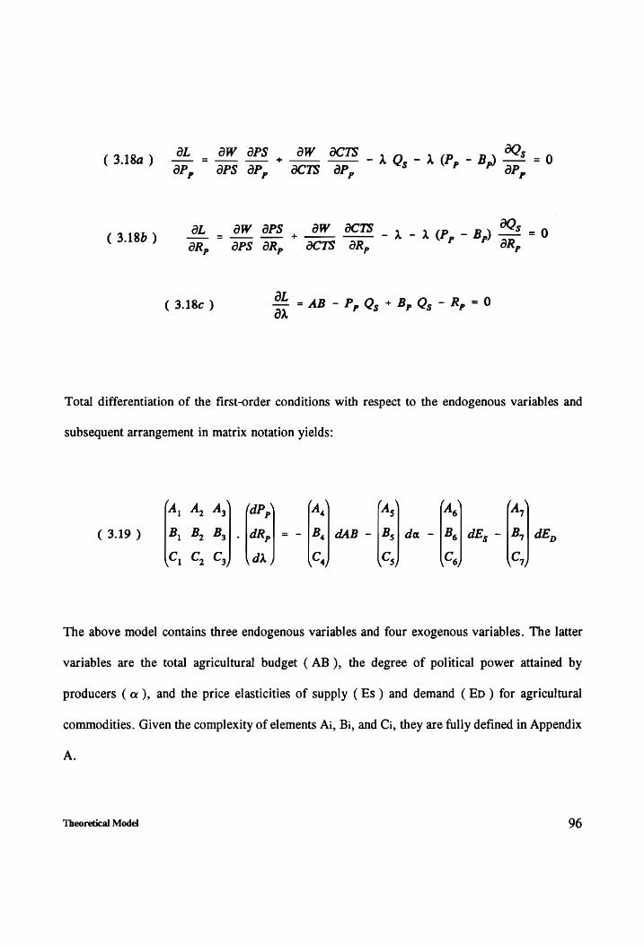
OL _ oW aPS | aw acTS _1 9 -a(P,-B,) “2 0

( 3.184 ) = = OP, OPS oP, CTS 4P, OP,

aL _ OW aPS , OW SCTS _, _y(p _B Qs _ (3.180) oR,” aPS OR, OCTS AR, PT Rp

OL _ - Pp + B - R, = 0 ( 3.18¢ ) a AB - Pp Qs + Bp Qs — Rp

Total differentiation of the first-order conditions with respect to the endogenous variables and

subsequent arrangement in matrix notation yields:

A, A, A,) (dP, A, Ag A. A,

( 3.19 ) B, B, B, . dR, = - B, dAB _” B, da 7” B, dE, ” B, dE,

C, C, C, di C, Cs Cs C,

The above model contains three endogenous variables and four exogenous variables. The latter

variables are the total agricultural budget ( AB ), the degree of political power attained by

producers (a ), and the price elasticities of supply ( Es ) and demand (ED ) for agricultural

commodities. Given the complexity of elements Ai, Bi, and Ci, they are fully defined in Appendix

A.


The presence in the model of the political variable a reflecting the level of political pressure

exerted by an interest group needs further explanation. One of these explanations is provided by

Cukierman et al (1992) who suggest that political factors such as political instability and political

polarization induce governments to exacerbate socio-economic inequalities among their

constituency groups compared to less asymmetric societies. Performing under unstable and

polarized political systems, policy-makers and legislators tend to support policies that favor

politically-stronger interest groups. However, those policies would be the reflection of a political

system that does not allow for full participation of less prominent interest groups. Linked to the

availability of the budget, fiscal pressures may constrain the ability of governments to finance the

specific needs of traditionally disadvantaged pressure groups, and sooner or later social conflicts

will become visible.

Conversely, consolidated and more democratic systems of government are likely to lead to a

different optimal solution by using an alternative combination of policy instruments. Within an

environment based on consensus and mutual agreement, comparable political weights among all

interest groups can indeed influence policy formation on a more egalitarian basis. For instance,

policy decision-makers would be less inclined to tax agriculture and spend those revenues outside

the agricultural sector the stronger the political participation of producers. Alternatively, political

pressures from the consumers may encourage the government to rely more on price policies and

less on agricultural research if that group perceives greater gains from price interventions than

from research investments.


There have been relatively few empirical studies directed at trying to understand the determinants

of government policies using a political-economy approach. The studies that do exist have mainly

emphasized macroeconomic issues. In dealing with the role of political factors affecting inflation

and fiscal policies in a group of developing countries, Edwards and Tabellini (1991) reported a

positive correlation between political variables and specific government policy actions. They

suggest that political weakness of the government and political instability in a country have a role

to play in explaining overall economic performance. In a related study dealing with the importance

of various sources of government revenues for a larger set of countries, Cukierman et al found that

less democratic countries present more inefficient tax structures to finance their government

expenditures than more stable and homogeneous regimes.

In the agricultural arena, Beghin and Kherallah (1991) analyzed the influence of four political

systems as well as indices of civil liberties and political rights in patterns of agricultural protection

across commodities and countries °. Concentrating their analysis in the 1982 - 1988 period, they

found that pluralistic systems are associated with higher levels of agricultural protection and that

further levels of democratization may stimulate more support to agriculture. Even though

Statistically less robust, their results indicate that worsening political rights and civil liberties

decreases agricultural assistance because interest groups would be more restrained in exerting

influence on policy formation.

°, The dummy variables for political systems were the existence of multiparty, dominant party, one party,

and no-party system. The index of civil liberties reflected freedom of opinion and organization, whereas the

index of political nghts involved the voting rights and rights of political opposition to organize.


The inclusion of price elasticities of both supply and demand as exogenous variables is appealing

as well because they influence the distribution of economic surplus associated with domestic

pricing policies and research investments. In fact, the relative distribution of benefits among

producers and consumers/taxpayers is particularly sensitive to alternative price elasticity

formulations when the trade status and the international trade policies affecting a country are

considered. Therefore, the nature of government pricing policies and the allocation of research

resources can significantly influence producer and consumer surplus and thus, economic efficiency.

Marginal changes in the steady state values of Pp, RP, and A given a change in AB, a, Es, and ED

can be determined by applying Cramer’s rule to ( 3.19 ). By solving each differential in the

exogenous variables with respect to dPp, dRP, and da at their initial equilibrium values and

interpreting each partial derivative, important qualitative information emerges. These results,

presented in Appendix B, are required to assess the impacts of an exogenous increase in AB, a,

Es, or ED on the endogenous variables Pp, Rp, and X.

At this point two simplifying assumptions are necessary in order to keep the structure of the model

more manageable, and at the same time, consistent with the problem at hand.

1. The impact of agricultural research on a small-open economy does not affect

the world price and all the change in economic surplus is captured by producers.

AS a result, the marginal effect of RP on consumers/taxpayers is zero. In this case,

it is assumed that price policies PP emerge as the only viable alternative to transfer

income from producers to consumers/taxpayers, and


2. A marginal change in one direction in PP is assumed to induce a marginal

change in the same direction on producers’ welfare regardless of the cost-reducing

or output-increasing effects of RP on producer’s welfare. In other words,

producers will always benefit (lose) when minimum (maximum) price policies are

in place.

Given the above assumptions, the signs of A1, A2, B1, B2, B3, and C2 in equation 3.19 depend on

whether a minimum or a maximum price policy is used. If a minimum price policy is in effect, A2

and B2 have a positive sign and B3 and C2 are negative. The signs of Ai and Bi are inconclusive,

although intituively they should be positive. The inconclusiveness of Ai and Bi arises mainly

because some second-order, cross-partial derivatives of the involved terms have simultaneous

impacts on producers as well as on consumers/taxpayers in opposite directions. Thus, the effect

On one interest group is countervailed by the effect on the other group. Alternatively, if a

maximum price is being used A2, B2, B3 and C2 are unequivocally positive whereas the signs of

Ai and Bi are negative. The other individual terms present no ambiguity regarding their signs

when minimum or maximum policies are the price policies being implemented.

The signs for the determinant of the three element matrix on the left-hand side of ( 3.19 ) are

unambiguously negative for a minimum price policy and positive for a maximum price policy.

Noting that a minimum or a maximum price policy brings opposite signs to each determinant

formed to solve any of the three endogenous variables, the final signs remain the same regardless

the type of price policy being implemented. An implication of these results for comparative statics


suggests that welfare effects flowing to producers and consumers/taxpayers from any price policy

are monotonic. These comparative statics effects are presented in Table III.1.

These partial effects are suggestive of several intuitively reasonable results. The first column in

Table III.1 indicates that an increase in the government budget ( AB ) would lead to an increase

in funding for both price interventions as well as research programs. On the other hand, tax

revenue increases reduce the government is need to further extract resources from agriculture.

Therefore, the level of taxation would decrease since a budget expansion would translate into

larger government spending on agriculture. For the same reason, if price-tax policies are being

implemented, an increase in the sectoral budget would increase the amount of resources spent on

research endeavors. The effects of AB under both policy instruments on the marginal utility of the

agricultural budget are, in equilibrium, positive.

The second column shows the effect of a change in the political power a of producers. As

expected, succesful coalitions of producer groups would put pressure on the government for higher

levels of price-support. Rational profit-maximizing individuals would pressure policy-makers for

prices above the legislated maximum level. Signing the effect of a change in the level of research

expenditures resulting from a change in the political pressures of producers is not straightforward

because a decrease in the marginal total welfare resulting from allocating an extra unit of

expenditure on research may imply positive or negative impacts on producers welfare, depending

on the type of price policy being implemented.


Effects of AB, a , ES and ED on Price and Research Policies

Table III.1

aP,

OR, aAB

OA

oAB

oP p

Oa

OR,

oa

On

0a

aP, OE,

aR, OE,

da OE,

ap aE,

OR

OE

OA

oE


For example, assuming that producers are already beneficiaries of minimum price policies they

may give up their willingness to press for higher research funding. Conversely, producers would

have stronger incentives to demand additional public support for research to partially compensate

the losses of being taxed under maximum price policies. The implication is that, in either case,

agricultural research investments respond positively to the political influence of producers. The

sign in the steady state marginal utility of the agricultural budget \ for an exogenous change in a

iS poSitive.

The third column represents the impact of the absolute price elasticity value of output supply on

the endogenous variables assuming a well-behaved demand function and holding everything else

constant. As expected, the effects of the supply elasticity on price policies and research

expenditures work in the same direction. Whereas the effects of a higher price-elasticity of supply

Es unambiguously decrease the desirability of price interventions in agriculture, the impact of a

more elastic output supply schedule on the research outlay levels is negative.

Assuming a well-behaved supply curve and everything else constant, the fourth column highlights

the impacts of Eb in absolute value. The effects of the size of the price elasticity of output demand

on the endogenous variable PP will be positive under any price distorting policy. On the research

side, a more elastic price elasticity of demand will encourage the appropriation of additional

research funds. In contrast, decreased use of research funding or diminished needs for additional

research expenditures will be expected for agricultural products facing more inelastic price

elasticities of demand.


The above results support Rausser and Foster’s and de Gorter et al’s findings that resource

transfers to (from) agriculture due to price policies tend to be associated with products with highly

inelastic demand schedules. In contrast, resource transfers to (from) agriculture from price policies

are generally non-existent for commodities with more elastic demands, especially when those

commodities show low supply responses to price and research policies.

The impacts of price elasticities of supply and demand for agricultural goods on the marginal utility

of the government budget turned out to be positive for price policies and negative for public

research expenditures.

The comparative statics exercises performed for the tradable commodity case yielded the same

basic results as in the non-tradable case. Some degree of generality is still present in the model.

However, the nature of the assumptions used to simplify it do not jeopardize these comparative

Statics results and the theoretical underpinnings of the model still allow its empirical

parameterization.

Summarizing, the results obtained above allow for a more detailed specification of the forces at

work when assessing both price policies and public expenditures on more advanced agricultural

technologies. In that sense, the conceptual framework originally put forward by Gardner and by

de Gorter et al and used as a point of departure for this study is extended to incorporate the role

of the agricultural budget, the behavior of interest groups, and the elasticity parameters in deciding

the best combination of price policies and research expenditures to maximize a government welfare

function. The directions of the effects of these exogenous variables on the two policy instruments


are unambiguous. In some cases, however, their magnitudes will depend on each type of market

intervention, the tradability of the good, and the set of technologies made available by public

research institutions. As suggested by numerous authors, failure to account for the effects of the

endogeneity of price and research policies can strongly bias their estimated returns, thereby

distorting the direction of public spending on agriculture.

A Dynamic Perspective

The induced innovation theory of agricultural development hypothesizes that the rate and bias of

technological change are determined in a dynamic process in which producers and research

institutions respond to changes in the relative prices of products and factors (Hayami and Ruttan,

1985). Therefore, dynamic adjustments should not be ignored since policy-makers continuously

change price policies or modify research budgets given their inclination to respond to pressures

from interest groups. Policies that artificially raise output prices or lower input prices, bias the

future allocation of research resources and hence the development of technologies that truly reflect

resource scarcities (Miller and Tolley, 1989). These effects may be compounded as lags between

research investments and the generation of new technologies can be as long as 30 years (Pardey

and Craig, 1989).


Expectations of producers, researchers, and policy-makers also play a role of systematically

changing over time the demand for and supply of technologies. In effect, the ability of farmers to

respond to changing economic and political conditions is conditioned by current and past price

policies as well as those past research investments that are determining the current level of

technology. By the same token, new technology developments are influenced by price policies

formulated today, as long as those policies alter producers’ long-run price expectations. On the

supply side of technologies, public sector research expenditures realized long time ago can still

persist and influence current agricultural output. Public research institutions adjust slowly to

changes in today’s relative prices of output and inputs. Even though their activities tend to be, in

the long-run, more effective for inducing stronger effects on output growth than price policies

alone (Binswanger, 1990) °°.

The implications of omitting the dynamic effects between agricultural production, price policies

and research investments may be significant. One means of finding the time-path of price and

research policy decisions is to use a dynamic, control-theory optimization framework. However,

the complexity of the problem will likely not provide a tractable solution for an optimal level of

policy funding. Modeling both the mix and the timing of price interventions and technology

advances using such a dynamic control approach was considered beyond the scope of this study.

Instead, an econometric dynamic formulation sheds more light in determining the relative

'© Individual and/or export-oriented crops respond strongly and faster to both price policy changes and

public research spending compared to an aggregate group of non-tradable or imported crops. Such a

response, takes place generally, by taking resources away from non-tradable crops. For a recent treatment

of the response of agriculture to changes in policies, see Binswanger, 1990.


importance of research lags, output adjustments, and expectations. This is the approach pursued

in the following Chapter.

Summary

This chapter has recognized the importance of price policies and publicly funded research in

shaping the path of agriculture during the development process. However, political-economy

considerations determine, ultimately, the effectiveness of these two policy instruments in

translating their impacts into significant welfare gains. Misleading conclusions can be obtained

when price and research policies are assumed exogenous to the policy-making process and are

treated independently from the political factors that affect them. Consequently, a theoretical

framework is articulated for a better understanding of the interactions of price policies and

agricultural research investments as a result of collective action exerted by two interest groups.

Relative costs and benefits associated with these two types of public policies on producers and

consumers/taxpayers are explicitly identified. The interactions that govern agricultural pricing

policies and public research spending indicate also that a static framework does not suffice to

understand entirely the complexities of the agricultural policy process.


CHAPTER FOUR

EMPIRICAL MODEL

Introduction

This chapter includes five sections. The first section presents an econometric model consistent with

the hypothesized process underlying public policy formation for five commodities. Emphasis is

placed on the linkage between the theoretical and the empirical models and captures the influence

of interest groups in the policy-decision process. Section two discusses the variables included in

the econometric model along with their data sources. The third section describes the empirical

model and the econometric technique by which a system of simultaneous equations is estimated.

Section four reviews the formulas to measure the gains from research when direct price

intervention policies are considered. A summary of the chapter is presented in section six.

Empirical Model 108

Presentation of the Model

The implications of agricultural price policies on the funding of public Chilean agricultural

research are captured by a Set of structural equations for each agricultural commodity. The analysis

covers a 29-year period from 1960 to 1988 and the observation units are years. The data used in

the estimation of the empirical model are given in Appendix C. The level of price policies and

public research expenditures result from collective action exerted on the government by pressure

groups. Producers, consumers/taxpayers, and the government are involved in the production,

consumption, and financing of beef, wheat, milk, apples, and grapes.

The generic model presented below in equations ( 4.1 ) to (4.4 ) assumes commodity producers

are profit-maximizers whose main motivation comes from the prices they receive. Economywide

policies that may, for instance, have induced realignments in the real exchange rate are embedded

in the price received by agricultural producers. The simultaneous system presented in the equations

is general for both non-traded and traded goods. Subscripts i denote any of the five agricultural

commodities considered in this study. Variable definitions are presented in Table IV.1. Specific

features for each commodity are described in the section that follows.

Empirical Model 109

(4.1) Ln Qe, = Gy + &y Ln Pp, + ay (Ln Pp, )? + Oy Ln Rp,

+ Cig RPT, + Cis F, + ig KAP + aj, Ln Pp, + Gig ININ

+ Og INOC + G19 W, + % 4), DAR + Bys t

P ci Pei Biot DO Ye Lt Po, (4.2) SHARE, EXP

i=]

TEXP + By In ( =~ ) + by SPI

(43) PPT, = (Pp, - Bp, ) Qs; = My + Ny RPT, + ny Lt Qs,

+ 1,, DRP + n,, DSA + y,, DDR + n,, NRT + 1, IPS

+ Ng SV + Ny ES; + Ny ED, + by

(4.4) RPT, = 0,, + 0, RPT,., + 9,> PPT, + 0,; Ln Q;, + 6,, F,

+ 0,, NRT + 0, IPS + 6, SV + 6, ES, + 8, ED; + B,,

Empirical Model 110

Commodity Modeling

Supply Equations

The first equation (4.1) is a domestic supply of the ith commodity, Qsi. Livestock has a

production cycle different than that for other agricultural products. Differences in ages, sex, and

breeding potential of the herd are all factors that may mask the relationship between slaughtered

cattle production and price changes. For example, a short-run increase in the price of cattle might

reduce current slaughter decisions and thereby beef supply since producers withhold their stocks

for further fattening. Therefore, the current producer price of beef, PPB, was used in the supply

of slaughtered cattle.

A significant role in Chile’s agricultural trade is played by importables such as wheat and milk and

exportables such as apples and grapes. During most of the 1960 - 1988 period a minimum output

price for wheat and milk was determined by the government one year ahead on the basis of their

expected levels of supply and demand. Consequently, a one year lag in the producer prices of

wheat, Ppw-1, and milk, PPM-1, was used as a proxy for expected prices in their corresponding

supply equations. Modeling supply response relationships for apples and grapes is difficult, but

it was decided to use current producer prices for apples, PPA, and grapes, PPG. More is discussed

about the particular price variables used in the following chapter when the model specification is

presented.

Empirical Model 111

Table IV.1

Variables of the Model

1. Output Quantity Variables

Qsi = Quantity supplied of commodity i (tons/liters)

QDi = Total domestic consumption of commodity i (tons/liters) Qci = Disappearance quantities of commodity i (kilos/liters per capita)

Xi = Exports of commodity i (tons)

Mi = Imports of commodity i (tons)

2. Price Variables

Pri = Producer price of commodity i (pesos 1985) Bpi = Border price of commodity i (pesos 1985)

Pci = Consumer price of commodity i (pesos 1985)

ININ = Price index of non-livestock agricultural inputs INOC = Price index of other annual crops

TRAC = Stock of agricultural tractors (units)

KAP = Capital stock of the value of agricultural machinery other than tractors (U.S. dollars 1978)

3. Price and Research Policy Variables

PPTi = Current resource transfers to (from) producers of commodity i due to direct price intervention (pesos 1985) RPTi = Current research expenditures on commodity i (pesos 1985)

4. Technical Change Variables

RFi = Distributed lag of public research expenditures on commodity i Fi = Index of internationally available technology for commodity i

5. Political Variables

IPS = Index of political stability SV = Structural variable 1 for democratic regimes, 1960 - 1973; 0 otherwise

6. Other Variables

NRT = Net resource transfers as a result of direct price intervention and agricultural research for all commodities (pesos 1985)

N = Total population

Wi = Index of weather specified by the main regions where each commodity i is produced

ESi = Price-elasticity of supply of commodity i EDi = Price-elasticity of demand of commodity i

8. Dummy Variables

DAR = 1 if agrarian reform period, 1965 - 1974; 0 otherwise

DDR = 1 if drought of 1968 - 1969; 0 otherwise DRP = 1 if recession period in 1975 and 1982; 0 otherwise

DSA = 1 if socialist administration period, 1971 - 1973; 0 otherwise

Empirical Model 112

Current and past public expenditures on commodity-specific agricultural research are represented

by a polynomial lag, RPi. Annual public research expenditures are noted by RPTi. A proxy for

internationally available technology is represented by Fi. All these three explanatory variables are

expected to be positively related to each commodity supply, QsSi.

In addition to the shift factors given by the indigenous and foreign technologies, each supply

equation includes the price of a relevant substitute commodity in production to account for those

commodities that compete for similar production factors. Thus, the current price of fluid milk,

PPM, was included in the beef supply equation whereas the current price of beef, PPB, was entered

in the milk supply equation. In this short run model, it is expected that a change in the price of

fluid milk will be negatively related to the domestic supply of beef. In the long run, however, these

two products may be complements because of the dual purpose of most of the Chilean cattle. In

that case, their prices would be expected to move in the same direction.

Although the degree of production substitutability between apples and grapes seems less evident

in the short run, both products may compete with one another for resources in the medium to long

run. Thus, the supply function of apples, QSA, contains the price of grapes, PPG. Similarly, the

supply function of grapes, QSG, includes the price of apples, PPA. The price index of other annual

crops, INOC, is used in the wheat supply equation. Each of these variables representing the prices

of substitutes is expected to be negatively related to domestic supply.

An input price index represented by ININ is included in the wheat, apples, and grapes supply

equations. The level of capital stock in agricultural machinery is represented by KAP. Feed prices

Empirical Model 113

were not available, and therefore, could not be included in the beef supply equation. An index of

weather conditions, Wi, of the main Chilean geographical regions where each commodity is

produced captures a main environmental factor affecting their supply. Lastly, a dummy variable,

DAR, is used to reflect the influence of the land reform process.

Demand Equations

Although theoretically and practically important, private and government changes in stocks held

from one year to the next were not considered due to lack of information. Therefore, the

assumption that stocks are constant across years is maintained. This assumption seems reasonable

since import (export) orders can be placed quickly for all commodities of interest. In a free-trade

scenario, the difference between domestic quantity supplied and domestic quantity demanded for

all five commodities was relatively large. A definitional relationship is needed to obtain total

domestic consumption, QDi, for each commodity of interest. The market-clearing identity below

indicates that total domestic quantities consumed are the sum of (difference between) domestic

supply and imports (exports). Algebraically,

Qpi = Qsi + (- ) Mi ( Xi)

Per capita consumption, QCi, is obtained from the above identity by dividing total domestic

consumption, QDi, by total population, N. Thus, in per capita terms the demand equation for the

ith commodity is represented in the second equation ( 4.2 ) as a budget share in total expenditures,

Empirical Model 114

TEXP, on all five goods. The budget share on each commodity would be positively related to total

expenditures as these commodities are considered necessity goods. This budget share is defined

as: SHAREi = Qci- Pci / TEXP. If each commodity is a normal good, its share in the budget

will move in the opposite direction of its own price. It is assumed that the input-output relationship

between commodities at the farm level and their processed counterpart at the retail level have

remained relatively constant over time.

Depending on the price poicy being implemented, either border prices or producer prices were

used to represent the price consumers faced. In particular, the consumer price of beef, PCB, was

assumed to be represented by its border price, BPB, between 1960 and 1974. After the government

withdrew its direct pricing intervention on beef production in 1975, the prevailing free-market

price was determined by the interaction between domestic supply and domestic demand. Hence,

following 1975 the consumer price of beef was assumed to coincide with its producer price.

Domestic supply for importable commodities such as wheat and milk clears at the minimum or

maximum price set for producers, PPi. However, the demand for those commodities is realized

at their border price, BPi, since domestic consumption is not affected by the price policy. In the

case of exportable goods such as apples and grapes, domestic demands and excess supplies are

determined by the domestic minimum producer price in years of direct price intervention.

Empirical Model 115

Price and Research Policy Equations

Price and research policy functions of the political-economy model are specified in equations 4.3

and 4.4, respectively. These two equations describe the demands for each policy instrument as

related to supply of and demand for each commodity, the levels of production and consumption,

and the incentives provided by the government. The dependent variable is the level of resource

transfers, PPTi, to (from) commodity producers or the difference between. The dependent variable

for the research policy equation is current agricultural research expenditures on each commodity

production, RPTi. Including each policy variable as the dependent variable in its own policy

equation as well as an explanatory variable in the other policy equation endogenizes the policy

variables.

The national significance of the commodity being studied is taken into account by including its

supply as an explanatory variable in both policy equations. Political influences and collective action

are expected to increase the larger the production value of the commodity.

Three dummy variables are used to account for upheavals resulting from changes in weather and

other economic and political variables. Years with extremely abnormal weather, DDR-1, or strong

recession years, DRP-1, may have detrimental impacts on production. Therefore, producers may

have been compelled to press for additional levels of price support, or conversely, decreased levels

of taxation for the next planting season. A priori, these two variables lagged one period are

expected to be positively related to increased levels of price policy transfers.

Empirical Model 116

The socialist administration period, DSA, is also dummied out to account for a period of high

intervention in the Chilean agriculture. Given the relatively high degree of urban bias exercised

by the government in each commodity, the sign for this variable is expected to move in the

opposite direction to the demand for price policies. Thus, it will be negative (positive) for a

commodity whose consumer price is subsidized (taxed).

On the research policy side, the level of technology abroad, Fi, is included. The sign of this

technology variable will be negative if governments have substituted indigenous research for

foreign technologies, or positive if they conducted complementary research.

Net resource transfers, NRT, to (from) agriculture are an explanatory variable in both sets of

policy equations. These resource transfers due to direct price policies and research expenditures

on all five commodities are assumed to be positively related to policies that establish minimum or

maximum producer prices. Regardless of the price policy scenario, NRT will also be positively

associated with investments in agricultural research. It should be stressed that the variable NRT

is not equivalent to the AB variable introduced in Chapter III to reflect real changes in the

agricultural budget. Information on the effective subsidies (taxes) made out of the government

budget at the time the government introduced minimum (maximum) producer prices was not

obtainable.

As noted in Chapter III, non-constant price elasticities of supply and demand are relevant

independent variables in the political-economy model. These price elasticities are represented by

ESi and EDi, respectively.

Empirical Model 117

An index of political stability, IPS, explains the impact of political pressure brought by interest

groups represented by producers and consumers/taxpayers for policy decision-making. Consistent

with theoretical expectations developed earlier, any increase in IPS would trigger a further demand

for price policies and research expenditures. An exception would be given when democratic

mechanisms and political institutionalization are absent. In these cases, the degree of political

stability would exert no influence on agriculture if it is discriminated against.

Measurement of the Variables

The variables used to capture the interactions between price policies and agricultural research along

with their abbreviations were listed in Table IV.1. In 1988 these commodities represented

approximately 55 percent of the total value of agricultural production (ODEPA, 1990). Each of

these commodities has been affected by substantial direct price intervention on the part of different

governments.

Wheat, W, represents the grain crops sub-sector; beef-cattle, B, and milk, M, together describe

the livestock sub-sector; and apples, A, and grapes, G, represent the fruit sub-sector. In terms of

acreage planted, wheat is the most important Chilean crop. Beef-cattle and milk are considered

import-substituting goods, specifically produced for domestic consumption. Grapes and apples by

Empirical Model 118

themselves account for over 50 percent of the total value of all agricultural exports. In fact, these

fruits are grown almost exclusively for the external market.

All monetary variables are deflated to 1985 Chilean pesos. In the absence of reliable producer and

consumer price indices the adjusted Consumer Price Index, CPI, presented by Banco Central de

Chile was used as the price deflator '.

Output Quantity Variables

Aggregate quantities are depicted by QsB for beef-cattle slaughtered assuming that 1 cattle unit is

equivalent to 450 kilograms, QSW for wheat production, QSM for fluid milk received in plants,

QSA for apple production, and QsG for table-grape production. As presented in the Appendix C,

all unit variables are tons, except fluid milk which is expressed in millions of liters. This

information was obtained from /ndicadores Agro-econémicos of ODEPA, Ministry of Agriculture.

Exports and imports of each agricultural product are indicated by Xi and Mi, respectively.

Consistent with the FAO-Trade Yearbook, it was assumed that 1 kilo of imported powdered milk

corresponds to 10 liters of fluid milk. Data sources for these trade variables were several annual

issues from Direccién de Comercio Exterior - Banco Central de Chile, the United Nations

Commodity Trade Statistics, and the Agricultural Outlook and Situation Report USDA.

' In the mid-1970s the official CPI computed by Instituto Nacional de Estadisticas, INE, underestimated the actual price increases. The impact of this error on the level of indexation of wages and salaries as well

as on the exchange rate behavior was substantial over the years (Banco Central de Chile, 1990)

Empirical Model 119

Price Variables

Prices received by domestic producers are denoted by PPi. As shown in Table C.4 these producer

prices are computed by the Instituto Nacional de Estadtsticas, INE, and included in several

publications from Indicadores Agro-Econémicos of ODEPA. In the case of apples and grapes,

producer prices were calculated by developing an index that reflected the exported and non-

exported fractions of apples and grapes produced in order to account for the higher quality of the

exportable fraction. Border prices, BPi, for each individual commodity are presented in Table C.5.

These border prices for the years 1960 - 1984 were taken from Hurtado et al (1990) and for the

years after 1984 they were provided by Alberto Valdés (personal communication). Both price

Series were constructed using the same methodology. These border prices were adjusted (by both

Hurtado et al and Valdés) for quality factors, seasonality, storage, custom expenses, marketing

margins, and transportation costs to the consumer centers. Consumer prices, PCi, are shown in

Table C.6. These prices were assumed to be equivalent to the producer or border prices depending

on government price intervention exerted on each commodity.

Prices of inputs used on wheat, apple, and grape production obtained from Hurtado et al were used

to construct a price index, ININ, for fertilizers, insecticides, fungicides, and herbicides. This index

was constructed by giving a 55 percent weight to fertilizers and 15 percent weight to each of the

other inputs.

Empirical Model 120

Capital stock in non-tractor agricultural machinery, KAP, is included in each supply equation

while the number of tractors, TRAC, is included only in the wheat equation. Both data series were

extrapolated for years 1985 - 1988 from original data provided by Zegers and reported in Hurtado

et al.

Price Policy Variables

Two alternatives for measuring the extent of price intervention in Chilean agriculture were

considered. One of these alternatives was to use producer and consumer subsidy equivalents,

PSEs/CSEs. However, PSEs/CSEs are relatively rough measures of government policy

interventions. For a given commodity, PSEs/CSEs are estimates of the amount required to

compensate producers (consumers) if existing government policies and programs in agriculture

were removed (USDA, 1987). Computation of PSEs/CSEs is relatively simple. They are calculated

as ratios between the total value of policy transfers to producers (consumers) and total producers’

income (total consumers’ income).

Hence these indicators combine in one single measure price specific interventions, financing of

research activities, or economy-wide policies, inter alia *. Thus, the individual effects of each

policy instrument can not be identified because these highly aggregate measures of several

distortions will likely mask the ultimate effects on producers’ and consumers’ decisions of

* The USDA (1987) includes six broad policy categories in the PSE/CSE framework. These categories

are: market price support, direct income support, programs affecting variable costs of production, programs affecting marketing of commodities, programs affecting long-term agricultural production, and controlled exchange rates.

Empirical Model 121

removing specific distortionary government policies. Seasonal variations in international prices,

shocks in the world supply, and exchange rate changes could also modify PSEs/CSEs levels

without actual changes in the policy intervention levels.

A second option to capture the net effects of distortionary agricultural price policies is to measure

them as nominal protection coefficients. Assuming the existence of unique international markets,

homogeneous commodities, and the absence of market-distorting practices by major trading

countries, border prices, are a theoretically simple standard against which to measure direct price

distortions. Prevailing border prices would represent the true opportunity cost for Chile of

obtaining an agricultural good under a purely competitive free trade regime given the official

exchange rate and degree of industrial protection. The direct nominal protection rate, NPR, is

calculated as follows:

In Chapter II it was stated that as a result of direct price interventions resources have been

transferred both to and from Chilean agriculture. Minimum and maximum prices to producers

were the main policies used to either support or discriminate against agriculture within a given

development strategy. The annual resource transfers from (to ) agriculture, PPTi, as a result of

direct price intervention in Chilean agriculture were calculated by using the following relationship:

PPT, = (Pp, - Bp, ) Qs;

Empirical Model 122

The above formula specifies direct price interventions as the difference between the producer price,

Ppi, and the border price, BPi. Resource transfers due to price policy intervention in any given

year are determined by this price differential times the total domestic quantities produced, QSsi.

These price policy transfers are presented in Table C.7. A negative value for PPTi indicates that

for a particular year the border price of commodity i was higher than the price received by

domestic producers implying, thus, a net taxation of the commodity. Naturally, a positive value

for PPTi occurs when the commodity i is subsidized and domestic producers protected as a result

of a producer price higher than the border price.

Research Policy Variables

Data on annual resource transfers for public agricultural research were gathered back to 1950.

Public research outlays before INIA began its activities in 1964, were obtained from Yrarrdzaval

et al. Their data included the budget statistics of the Ministry of Agriculture, the operational

expenses of the Department of Genetic and Plant Improvement, and the allowances provided by

the Rockefeller Foundation. Because these figures were reported in constant 1978 US dollars, they

were inflated to 1985 US dollars by using the US Wholesale Price Index. This new expenditure

series was then converted to 1985 Chilean pesos based on the prevailing exchange rate reported

by the Banco Central de Chile for that year. Until 1964, these values match very closely those

reported by Hurtado et al when citing a study of Venezian in 1985. However, from 1965 to 1970,

discrepancies arise between the data series, and therefore, expenditures on public agricultural

research were directly taken from INIA’s Annual Reports.

Empirical Model 123

These research transfers already broken down for vegetable and animal programs were

disaggregated by individual commodities to create the RPTi variable. This disaggregation was

accomplished by multiplying the monetary transfers by the proportion of researchers in each

commodity area. The number of scientists by commodity from 1965 to 1988 were obtained from

unpublished sources provided by INIA’s External Relations Director. The average number of

researchers between 1964 and 1966 only was used to extrapolate the expenditure series back to

1950.

Across the years, INIA has tried to maintain a similar number of researchers in beef, wheat, and

milk. On average, 14 percent of all researchers in vegetable production was devoted to wheat

research, while more than 75 percent of all scientific personnel in animal production was involved

in beef-cattle and milk production. Substantial personnel losses have occurred in apples and grapes,

as research on these commodities has been taken over by universities and the private sector.

Expenditures on apples and grapes jointly did not represent more than 8 percent of all scientific

personnel in the vegetable production area. Some biases should be expected when estimating the

impact of public research on fruit production because after 1974 fruit research was supported less

by the main public agricultural research institution, but no variable was included to capture the

effects of university and private research.

Empirical Model 124

Technical Change Variables

Public research expenditures by commodity are used to capture the impact of technical change on

each commodity’s supply in equation 4.1. However, the impact of research expenditures on

agricultural output occurs over several years. The technological knowledge obtained through

agricultural research takes time to be adopted and eventually deteriorates and becomes obsolete.

Therefore, these expenditures on research are introduced in each supply equation, Qsi, with a lag

structure. A quadratic distributed lag for the impacts of research expenditures was imposed to

reduce the number of parameters to be estimated, conserve degrees of freedom, and reduce

potential problems with multicollinearity.

A second variable used to capture technical change is the internationally available technologies

adopted by Chile. Aggregate technological spill-in effects from abroad are difficult to measure.

On a commodity basis, this measurement is difficult because very few countries report research

expenditures by product. Therefore, proxy variables were developed for research spillovers from

other countries as well as the affiliated centers of the CGIAR for each of the commodities being

studied. The research spill-in variable, Fi, contains a total factor productivity-index for the United

States, Argentina, and Brazil for each commodity. Lags involved in conducting, transferring, and

adopting those technologies are taken into account by using a weighted five-year moving-average

productivity index.

Empirical Model 125

For construction of the Fi index, the weights given to the total productivity of each country were

based on its aggregate research expenditures as reported by Pardey and Roseboom (1989). Thus,

the weight for Argentina was 6 percent and for Brazil 9 percent. The remaining 85 percent was

assigned to the United States given its leading role in developing new technologies for problems

faced by Chile under similar geographic conditions. The relevant productivity series used to build

the Fi variables were taken from FAO Production Yearbooks.

Political Variables

In previous chapters it was stated that both price and research policies are based in part on the

economic structure and the political system of a country. Resource transfers to interest groups are

likely to be explained by the way the political system influences the design of those policies. Legal

or illegal forms of political pressure include inter alia electoral activity, lobbying efforts,

organizational activity, and violence. These actions may be taken by interest groups in isolation

or combined in order to persuade existing authorities to change aspects or even the structure of the

political system that would favor their status >.

The first political variable used in this study refers to the degree of institutionalization of the

Chilean political system. An index of political stability, IPS, constructed from a probit model on

time series data is first constructed. The dependent variable, GCH, takes two possible outcomes

based on the frequency of regular and irregular government changes through time. The value zero

3 See Huntington and Nelson (1976) for a review of the role of political participation in the context of

economic development in developing countries.

Empirical Mode 126

is for the years in which there were no changes in the government and the value one is otherwise.

The behavior of the dependent variable is described by the probability of a government change that

depends on a set of variables on political participation. The estimated probability obtained is used

to determine the role of political stability in governing the design of policy instruments towards

agriculture over the twenty-nine year period. Even though no distinction is made between the type

of regime ruling the country (i.e. regular or irregular), the political stability after a change in

government taking the form of a coup will likely be lower than one occurring through regular

democratic procedures.

A set of eight indicators of political participation in Chile were aggregated to form three

explanatory variables. These political indicators, assembled since 1948 by Taylor and Jodice, were

measured as deviations from their annual averages. Missing years from the political data set were

updated from Banks and Gastil. The first explanatory variable, VA, is built upon violent actions

and includes the number of protest demonstrations, riots, and armed attacks. Repressions, R,

indicated by the number of deaths from domestic political violence, governmental sanctions,

assassinations and political executions constitute the second explanatory variable. Finally,

executive adjustments, EA, understood as changes in the composition of the cabinet members give

rise to the third explanatory variable.

Representing for convenience the above set of these explanatory variables as X, then IPS is

linearly related to X with an additive random component as follows,

Empirical Model 127

IPS = B/X-u

Thus, the outcome of expected probability of government change is determined by :

P(IPS=1|X)=P(Bp/X-p>0)

and estimated using a probit equation.

The second political characteristic chosen is a structural variable, SV, that discriminates between

regular governments and those originated by the coup d’etat of 1973. This variable takes the value

one for the democratic periods that occurred between 1960 and 1973 and the value zero

afterwards. As stated by Cukierman et al, democracies are more likely to be viable in societies

with higher degree of internal cohesiveness, and therefore, they tend to have lower levels of

political polarization than totalitarian regimes. Hence, the existence of a more efficient set of

policy instruments should be positively related to constitutional changes in governments ruled by

pluralistic political parties.

Empirical Model 128

Other Variables

Governments allocate their agricultural budgets for funding both price policies and agricultural

research endeavors to specific commodities based on economic and political grounds. For purposes

of this study, net resource transfers, NRT, were considered as the sum of net resource transfers

from direct price interventions on all five commodities plus the sum of individual expenditures in

agricultural research. In symbols,

NRT = > PPT, + ). RPT,

Total population in million of inhabitants is denoted by N and this information is obtained from

the Instituto Nacional de Estadtsticas, INE.

A commodity-specific weather variable, Wi, is incorporated as an index of average deviations from

normal average rainfall. Ten meteorological stations were chosen to cover Chile’s main

agricultural regions. In the case of beef and milk production Linares, Chillén, Los Angeles,

Concepcién, Valdivia, Osorno, and Puerto Montt were the meteorological stations considered.

Wheat production is mainly concentrated in regions covered by the following meteorological

stations: Santiago, Linares, Chillan, Los Angeles, Concepcion, and Valdivia. The meteorological

stations used to characterize climatic conditions in fruit production were Santiago and Linares for

apples; and La Serena, Coquimbo, Santiago, and Linares for table-grape production. Yearly

amounts of precipitation in millimeters by meteorological station since 1950 were obtained from

Empirical Model 129

the World Weather Disc Software and several issues of the World Weather Records covering the

1961 - 1980 years. Missing values for some meteorological stations after 1985 were extrapolated.

AS mentioned before, domestic price elasticities of supply and demand are also hypothesized to

play a major role in the design of pricing policies and the funding of agricultural research. These

two main supply and demand characteristics describing both producers’ and consumers’ behavior

are related to levels of government intervention on each policy instrument because they affect the

welfare results of each policy. Price elasticities of supply and demand by commodity are calculated

for each year from their individual supply and demand equations, respectively.

Dummy Variables

One dummy variable, DAR, represents the period under agrarian reform that took place between

1965 and 1973. The severe drought in years 1968 and 1969 is captured by another dummy

variable, DDR. A third dummy variable, DRP, is included to pick up the strong recession

experienced by Chile in 1975 and again in 1982. The binary variable, DSA, is introduced to

capture the socialist administration period from 1971 to 1973.

Empirical Model 130

Estimation Procedures

The empirical model is comprised of four blocks of equations. All four blocks of equations are

estimated simultaneously as an interdependent system. The coefficients to be estimated are

represented by greek letters and the y,’s are the random disturbance terms. All variables considered

endogenous in the model are denoted with a dot on top.

Supply Block

The first block of equations presented below consists of five supply functions, one for each

commodity. These output supply equations are derived by applying duality theory to five highly

flexible cost functions. Double logarithmic specifications with additive disturbances are used to

characterize the supply function for each commodity. Some flexibility in specification of price

elasticities is gained by allowing a quadratic interaction between own-commodity prices. Output

quantity variables, QSi, and producer prices, PPi, are endogenous as they are jointly determined

through their interaction with the sets of price and research policy equations.

Empirical Model 131

® e @

Ln Qsa = GO 50, + Oy, Lin Pry + & 52, (Lin Ppg )? + @ yy, Lan Rog + & 54, RPT, + 55, Fy + Ojo, Ln Py +

Qin We + ju D73 + A 5m DAR + #j101

@ e e

Ln Qsw = & jon + G2 Ln Qgw + Ox Ln Poy, + Oj 9 (Ln Pry)? + & 5 Ln Rey + @ 59 RPTy + je Fy +

@ jm ININ + aj. INOC + aj, Ww + & 51 DAR + Bin

e oe e

Ln Qu = 503 + O13 Ln Qe + O2, Ln Pay, + O 553 (Lin Pry)? + jas La Rey + & 553 RPT + 563 Fu +

e @ e

51 ININ + @& 54, Ln Pog + & 504 Wa + & j 104 DAR + Wiis

e e e

Ln Qgg = @ jos + O15 Ln Qegs + O25 Lin Pog + O j55 (Lin Ppg )? + o 545 La Rog + @ j 55 RPT + & j 65 Fe +

375 ININ + @ j¢5 La Ppa, + & 95 Wo + @y 105 DAR + Bais

Demand Block

On the demand side, an almost ideal demand system ( AIDS ) and the Stone’s price index ( SPI )is

used aS an approximation of the true AIDS price index. The AIDS is derived by applying

Shepard’s lemma to an expenditure function of all five commodities. Besides its ease of

computation the AIDS model has the advantage of implying a more flexible relationship between

quantity demanded and prices than other more rigid functional forms. This demand system satisfies

the axioms of consumer theory at the same time that it aggregates over commodities. Adding-up,

homogeneity, and symmetry restrictions are imposed from the start to keep consistency with the

neoclassical theory of utility maximization. Each budget share equation includes in a logarithmic

form prices of each commodity and total expenditures on the group of five commodities. The

AIDS model in a budget share form is expressed as follows:

Empirical Model 132

e

SHARE, = 86 yo + Yun Ln Po + Yan Ln Pew + Yugs Lm Pen + Ying Lo Pea + Vins La Poo + 542, LTEXP - 642

((SHARE, Ln P., + SHARE, Ln Pq, + SHARE,, Ln Pq, + SHARE, Ln P,, + SHAREg Ln Pog) + Hea

e

SHAREw = B uo t Yun La Pos + Yum Ln Pow + Yus Ln Peg + Yun Ln Pex + Vues Ln Pog + S429 LTEXP - 5.22

((SHARE, Ln Py, + SHARE,, Ln Pa, + SHARE, Ln P,, + SHARE, Ln P,, + SHARE, Ln Py) + he

e

((SHARE, Ln Py, + SHARE, Ln Poy + SHARE,, Ln Pa, + SHARE, Ln P,, + SHARE, Ln P.g)) + pxes

e

SHARE, = 8 wo + Yuu Ln Pog + Yigg Lo Paw + Vins Lm Poy + Ying Ln Poa + Ving Ln Pog + 542, LTEXP - 64%

((SHARE, Ln Pg + SHARE, Ln Poy + SHARE, Ln Pq, + SHARE, Ln P,, + SHAREg Ln Py) + xa

e

((SHARE, Ln P,, + SHARE, Ln Pay + SHARE,, Ln P,, + SHARE, Ln P,, + SHARE, Ln Py) + Hxas

Consumer prices, PCi, are endogenized along with per capita disappearance quantities, QCi, since

prices are in part determined by the block determining the demand for price policies. Estimated

price elasticity parameters obtained from the supply and demand subsystems feed the blocks of

policy equations ( 4.3 ) and ( 4.4 ).

Price and Research Policy Blocks

Linear functional forms are used for the policy equations. One equation for each commodity and

for each of the two policy instrument are required. Thus, two blocks of equations are estimated.

The demands for both government policy interventions were formulated in a structural form in

order to analyze changes in policy decisions in response to exogenous shocks. The third block

describing the price policy equations is summarized as follows:

Empirical Model 133

PPT,

PPT y

PPT x

PPT ,

PPT,

e e

= myo: + M1n RPT 5 + 2112 Ln Qop + 113 DRP-1+ 951, DSA + 94,5 DDR-1 + 9445 NRT +

Mir IPS + Tye SV + 1119 ES 8 + Nim EDs + iso

e e

Nice + Nin RPT w+ Min Ln Qsw + 9123 DRP-1 + 912, DSA + 9425 DDR-1 + 9 126 NRT +

Nin IPS + Mia SV + Nin ESwt Nin EDw + Hin

e e

= myos + Misi RPT ag + 9152 Ln Qsu + 9133 DRP-1 + 915 DSA + 913s DDR-1 + 9 155 NRT +

Nis7 IPS + Miss SV + tis ES ut Nia ES au + His

® e

Nios + N14: RPT, + 9 p42 Ln Qgy + M143 DRP-1 + 14 DSA + 9 145 DDR-1 + 9 14, NRT + tt

1147 IPS + nigg SV + Nim ES, + Nis0 ED, + Bia

@ e

M150 + Nis: RPT g + M19 Ln Qgg + 9453 DRP-1 + 9,5 DSA + 915; DDR-1 + 945, NRT +

Nis IPS + nissSV + Nip ESg + Mim EDG + bis

The fourth block describing the research policy equations is described as follows:

RPT, = 8 201 + 641, RPT,, + 62, PPT, + 0,,,;1nQn + 604F 3 + 641; NRT + 0.4. IPS +

Our SV + Oni ESn +O ED, + Kar

RPT, = 6. + 622, RPT wo. + 62> PPT. + 6 22,InQn +O 04Fw + 62.2, NRT + 6... IPS +

RPT y = 6 nos + 6 as; RPT gs + 8 a PPT, + Oa IN Qa, + Oey Fue + Oa5; NRT + 0, IPS +

RPT, = 6 wos + 8 oa, RPT a: + 8 age PPT, + Oa lnQn + Oau Fa + 0 245s NRT + 0 24, IPS +

6 SV + Oe ES, +904 ED, thaw

RPT, = 6 20s + 8 a5: RPT 6: + Ouse PPT Gg + Ons, bnQ tOuu Fo +925; NRT + 0_,, IPS +

Empirical Model

605S5V + 62%ES, +0_., ED, + Law

134

It can be seen from the above blocks of policy equations that supply levels, Qsi, producer prices,

Ppi, and research expenditures, RPi, enter into each policy equation along with other

predetermined variables. Within the policy blocks, producer prices, form part of the dependent

variable in the equation explaining resource transfers due to price policy equations, PPTi. These

resource transfers are, in turn, related to the research policy block. Similarly, current research

expenditures, RPTi, are endogenized in the blocks forming both supply and price policy equations.

The interdependency between the SHAREi variable and the blocks of price and research policy

equations is established through inclusion of price elasticities of demand, EDi, in the policy

equations.

Estimation Issues

The simultaneous equation model contains five sets of endogenous variables, namely, Qsi, QCi,

Pri, Rpi, and Pci. However, non-linearities arise because some endogenous variables enter

different equations in different forms. For example, in the block of supply equations the

endogenous variable PPi appears log-squared while in the block of price policy equations it

emerges as forming part of another variable. Similarly, the endogenous variable, PCi, in the block

of demand equations is logged while in the price-policy block is introduced through the elasticities

of demand, EDi, whose form depends on the particular functional form employed in the demand

block.

Empirical Model 135

The simultaneous nature of the non-linear system violates the ordinary least squares ( OLS )

assumption of independence. The presense of endogenous variables on the right-hand side of each

equation leads to a contemporaneous correlation between the error term and the set of explanatory

variables. Thus, applying conventional OLS to all four blocks of equations would yield biased and

inconsistent estimates. Alternative estimation procedures must be sought. Among these alternative

procedures, non-linear three-stage least squares (NL3SLS) or non-linear full-information

maximum likelihood ( NLFIML ) allow us to jointly obtain parameter estimates for all structural

equations in the system. In practice, these two methods are equivalent when each structural

equation is just identified, and they converge to the same limiting distribution Judge et al, 1985).

The NL3SLS procedure applies the method of least squares in three succesive steps by taking into

account the overall structure of the model. In the first step, each equation is estimated in its

reduced-form by using ordinary least squares on all predetermined variables to obtain estimates

for the reduced form parameters. These parameters are then used to obtain the fitted values of all

endogenous variables. In a second stage, the estimated covariance matrix is formed to obtain

estimates of the structural parameters. Finally, in a third stage, generalized least squares is applied

to the set of transformed equations from the reduced-form residuals of the previous stage.

Despite the fact that all restrictions imposed on the values of the parameters in other equations are

considered, the NL3SLS estimates obtained are still consistent and asymptotically normal, provided

the error term has mean zero. Therefore, NL3SLS estimators are more robust against non-

normality than NLFIML because the former are consistent regardless of whether or not the system

of non-linear simultaneous equations yields a unique solution for the endogenous variables

Empirical Model 136

(Amemiya, 1985; Godfrey, 1988). However, difficulties in obtaining the covariance of each

estimator make NL3SLS less efficient than NLFIML estimators. Weighing the advantages and

disadvantages of both methods, it was decided to estimate the block system of equations ( 4.1 )

through ( 4.4 ) by using the non-linear 3SLS procedure.

Research Gains under Price-Distorting Policies

The formulas used to measure the size and distribution of economic benefits between domestic

producers and consumers under price-distorting policies and publicly supported research are

presented in this section. Specific derivations of these formulas are presented in Appendix G. The

coexistence of these two policy instruments leads to several welfare implications for both interest

groups. Failure to include minimum (maximum) price policies under a variety of market conditions

can significantly bias the estimates of research benefits accruing to producers and consumers. Both

policy mechanisms are modeled in a partial equilibrium analysis and welfare effects in related

markets are not considered. Subsequently, net present values or internal rates of return to research

can be determined from the net surplus changes. Minimum (maximum) price policies and parallel

shifts in the supply schedule are considered in all three cases to illustrate the research benefits

accruing to domestic consumers ( ACS ), domestic producers ( APS ), as well as changes in

taxpayer transfers ( ATS ) and total domestic benefits ( ABT ).

Empirical Model 137

Changes in welfare due to direct price interventions and research expenditures can be determined

from the supply and demand equations described in the first two blocks of equations. The estimated

coefficients of the research variable along with the price elasticities of supply and demand were

measured from these relatively flexible functional forms. However, linear approximations of

market supply and demand functions were used to estimate economic surplus changes in order to

simplify the calculations of welfare impacts. The use of linear approximations should not create

significant bias when calculating the welfare impacts. In fact, greater approximation errors can be

encountered with the type of supply shift and the size of elasticities than with errors associated with

the use of particular functional forms (Alston et al, 1994). Formulas to measure economic surplus

areas, assuming linear supply and demand approximations, are presented for a small

importer/exporter country case.

The model presented in Figure III.1, Chapter II] characterized the market of beef-cattle before and

after 1975. When governments instituted a maximum price PP for producers, the result was a

reduction in domestic production to Qpo. The excess demand Qc - QPo was met by governments

through imports bought at a price BP. Maximum price policies only affected producers when the

supply curve due to research-induced technical change shifted out no further than point C in Figure

TIl.1 *.

The distribution of benefits from research-induced supply shifts was affected when maximum

prices to beef-cattle producers were set below the border price Bp. Assuming that the government

“ A maximum price policy becomes ineffective when the supply curve shifts further than point C.

Empirical Model 138

is able to prevent clandestine exports and imports, domestic production and trade decreased due

to maximum prices. Considering a domestic market functioning at the regulated maximum price,

producer benefits were lowered by the amount of reduction in import subsidy expenditures. Thus,

as shown by Alston et al, the changes in economic surplus for a proportional vertical shift in the

domestic supply equation are

ACS =0

APS = K P; Qp, (1 + 4% K ES, )

ATS = (Bp - Pp) Qp, K ES, - RPTi

ABT = APS + ATS = KB, On (1 + % KES, ) - RPT:

where K is the percentage cost reduction due to research, PP is the producer price, BP is the border

price, ESi is the price elasticity of supply, and QP! and Qpo are the quantities of beef before the

supply shift under the producer and the border price, respectively.

After 1975, distortionary price government policies were absent from the Chilean beef market.

Ever since then producer price of beef-cattle has fluctuated according to its border price. Referring

to Figure III.1, the research benefits resulting from a parallel supply curve shift accrue all to

domestic producers. Taxpayers reduce their surplus because tax revenues are no longer generated

and taxpayers need to fund agricultural research endeavors. These results are given by:

Empirical Model 139

ACS = 0

APS = K Bp Quy (1 + 4% KES, )

ATS = RPTi

ABT = APS - ATS = K Bp Ow (1 + 4 KES,) - RPT:

The welfare implications of both minimum price policies and agricultural research in a small-open

importer or exporter economy were illustrated in Figures III.2 and III.3 in Chapter III,

respectively. As the country cannot affect the world price, total net agricultural research benefits

are in both cases unaffected by minimum price policies but their distribution does indeed change

because domestic production and trade increase. Specifically, producers capture the economic

surplus obtained by a domestic producer price, PP, above the border price, BP, plus the economic

surplus generated by a parallel supply shift due to research.

As shown previously, producers increase their surplus by a magnitude given by the increase in

government subsidy costs ( Pp - Bp ) times ( QPi - Qpo ). However, these government outlays plus

the costs of undertaking research, RPTi, represent a reduction in taxpayer surplus. With the sole

exception of the sign describing changes in government transfers, economic benefits are analogous

for the maximum price policy case. With all variables retaining the same meaning as before,

changes in economic surplus shown are calculated as

Empirical Model 140

ACS = 0

APS = K P, Qp, (1 + 4% K ES, )

ATS = -(( Pp- Bp) Qp, K ES; + RPT: )

ABT = K Bp On (1 + 4 KES, ) - RPT:

Summary

In this chapter the empirical model used in this study has been introduced. Its main objective is to

analyze the role that public resource expenditures had on the performance of the Chilean

agricultural sector. The model was specified as a system of four blocks of simultaneous equations

for the period 1960 to 1988. These blocks included supply and demand functions by commodities

as well as two sets of policy equations used to capture price and research policies, respectively.

The variables included in each equation were justified according to the theoretical framework and

the empirical facts observed in Chilean agriculture. A non-linear three-stage least squares

procedure is chosen to simultaneously estimate a system of four block of equations, non-linear in

the variables. In turn, formulas are presented to measure the welfare implications of direct price

interventions and publicly sponsored agricultural research.

Empirical Model 141

CHAPTER FIVE

RESULTS AND POLICY IMPLICATIONS

Introduction

This chapter presents the estimation results for the simultaneous equations model developed in the

preceding chapter. In the first section, the steps used during the estimation of the non-linear system

are reported. The second section focuses on the results obtained from the system of four blocks

of equations. It includes a discussion of the coefficients obtained as well as the calculated supply

and demand elasticities. The welfare impacts of price and research policies on beef, wheat, milk,

apples, and grapes are presented in the third section. The last section discusses the policy

implications derived from the results.

Results and Policy Implications 142

Treatment of the Model

Misspecification Tests

The most general description of the statistical information contained in a data set is provided by

the Haavelmo distribution framework (Spanos, 1986). A statistically adequate model consistent

with economic theory can be derivable from the Haavelmo distribution. It is useful to consider

Statistical adequacy in the context of a reduction from the Haavelmo distribution because it

provides the link between the information contained in a data set and the assumptions of the

regression model. Statistically misspecified models may yield biased and inconsistent parameters

with the result that hypothesis testing is invalidated. Therefore, pursuing statistical adequacy in the

simultaneous equation context is viewed as a necessary condition for both identification and

estimation of the structural model (Spanos, 1990).

Diagnostic tests to identify potential misspecifications of linear systems of simultaneous equations

have not systematically been considered. Misspecification tests for non-linear multi-equation

models have not been developed and implemented in a comprehensive way (Godfrey, 1988). To

deal with this problem, the statistical adequacy of each individual equation was checked

sequentially. Misspecification tests performed on an equation-by-equation basis do not account for

all cross-interactions with other equations of the system. Nonetheless, those tests are still useful

to identify individual equations that may potentially be misspecified. In turn, misspecification of

a single equation would lead to the rejection of the whole system of equations.


Misspecification tests were conducted to assess normality, homoskedasticity, and temporal

independence by using the methodology proposed by Spanos for linear equations '. A description

of these tests is presented in Appendix D. Appropriate respecifications were undertaken whenever

an equation failed to accept the validity of any of these assumptions. For example, tests for

normality performed on the supply equations of beef and milk indicated departures from the

normality assumption. Residual plots highlighted two outliers, one in the beef supply equation for

the year 1973 and another one in the milk supply equation for the year 1972. Consequently, two

dummy variables D73 and D72 were included in these equations.

In the case of wheat, milk, apple, and grape supply, the assumption of parameter time

independence was rejected. Hence, a dynamic reformulation was utilized. The dependent variable

lagged one period, LSQi-1, was included in each of these supply equations to ensure that the

independence assumption held. Rejection of the independence assumption in the research policy

equations suggested the need for their respecification. Temporal dependence in these block of

equations was tackled by including their dependent variable lagged one period, RPTi-1, as an

explanatory variable.

Final results from the equation by equation misspecification tests are shown in Appendix D. There

were few cases where misspecification problems could not be corrected by alternative

respecification efforts. For example, violations of the normality assumption persisted in the block

' For more details about the different misspecification tests used to investigate departures from the assumptions underlying the probability model, see Chapter 21 in Spanos 1986.


of price policy equations. However, as Godfrey has suggested, NL3SLS estimators are consistent

and asymptotically normally distributed even when the errors are non-normal.

Identification Issues

Following testing of the assumptions and specifying each individual equation, we turn to issues of

identification. Unique and consistent estimation of all structural coefficients would have been

impossible for under-identified equations. Identification rules for linear systems of equations do

not apply to simultaneous equation models that are non-linear in the variables. An alternative

approach for determining appropriate identification conditions in models that are non-linear in the

variables depends on the likelihood function and thus, it requires the specification of a particular

distribution for the errors (Judge et al, 1985, p 582). Necessary and sufficient conditions for

identification of non-linear systems have been developed under weaker assumptions about the

errors. However, the assumptions needed to attain these conditions make the above approach

cumbersome and therefore, difficult to implement (Judge et al, 1985, p 583).

To overcome these difficulties, the system of equations was initially treated as if it were linear.

Traditional order and rank conditions for identification of linear models were examined for each

equation. All equations were found to be over-identified according to these conditions. This check

provided some evidence that the system was identified. Identification of the non-linear system was

subsequently assessed by simply running the model under the non-linear procedure SYSNLIN


available in SAS / ETS modelling system. Had the system been underidentified, it would have been

impossible to obtain a solution.

Miscellaneous Procedures

Other econometric procedures were undertaken before estimating the entire system of equations.

In the supply block, for example, lag structures on the research variable, RPi, that make no

assumptions regarding the shape of the research lag and are estimated in a form-free manner would

require several degrees of freedom. Lag structures such as a third-order polynomial or a rational

lag might create severe multicollinearity problems (Judge et al, 1985). These two alternative lag

structures were disregarded a priori in the analysis. A second-order distributed lag was chosen and

both end-points were constrained to further reduce the problems mentioned above. Since the

research expenditure series was extended back to 1950, lengths of the research lag of up to 10

years were tested before choosing the appropriate one. The choice of the optimal length was based

on the dynamics of each commodity supply, the statistical significance of RPi, and the goodness

of fit of each supply equation. These lag lengths varied from 5 to 8 years depending on the

commodities.


There were only four equations included in the demand block. The omission of one equation from

the demand system was necessary since the budget share equations add up to one, and the sum of

errors across the five equations is thus zero at each observation. These zeros imply that the

variance-covariance matrix would be singular. The share equation for grapes was dropped from

the system. The coefficients for this deleted equation could have been recovered by making use

of symmetry, homogeneity, and adding-up restrictions implied by consumer theory in conjunction

with the rest of the estimated parameters. However, in order to obtain the standard errors for the

coefficients of the grape share equation, a separate estimation that included the grape share

equation but excluded the apple share equation was performed. This procedure should not have

affected the rest of parameter coefficients or their t-ratios both of which would be identical because

of the invariance of the maximum likelihood estimates to the choice of the omitted equation. In

practice, however, the estimated values differed slightly due to rounding errors.

Convergence problems are not uncommon in non-linear estimation routines (SAS / ETS, 1992,

p 348). A clear consequence of convergence problems is that the minimization method may be

unable to find a step that improves the objective function. These convergence problems are more

prevalent when some parameters are associated with several dependent variables or the data values

are unreasonably scaled. Therefore, the variables NRT, PPTi, and RPTi were scaled to facilitate

convergence.

According to Amemiya (1985), the best non-linear three-stage least square estimates are produced

when the expected values of all exogenous variables are projected through the instruments’ space.

Hence, all exogenous variables were chosen as instruments. The number of linearly independent


variables in each equation was at least equal to the number of parameters to be estimated. Since

the number of observations was always more than the number of instruments, no efficiency losses

in the estimated parameters would be observed.

The Gauss-Newton method was used to minimize the objective function. In the Gauss-Newton

method the objective function is changed by computing parameter change values at each iteration

(SAS / ETS, 1992, p 346). The convergence criteria used to control the minimization process was

set at 0.001.

Following the statistical tests and procedures outlined earlier, the parameters of the non-linear

system were estimated by using SAS / ETS non-linear modeling system, SYSNLIN.

Assessment of the Estimation Technique

The estimation method has an important effect on the quality of the parameter coefficients. Biased

and inconsistent parameter estimates will be obtained if an endogenous variable is not considered

as such when choosing the regression technique. In the OLS context, every right-hand side variable

of the equation to be estimated is treated as exogenous. Differences between parameter coefficients

obtained from a method that treats appropriate right-hand-side variables as endogenous and OLS

estimates would provide evidence of simultaneity bias.


However, direct comparison of OLS estimates with the NL3SLS estimates of the non-linear system

would be unfair because there are a large number of non-linear restrictions in the full system.

Thus, there are two potential sources of differences between the linear OLS parameter coefficients

estimated equation by equation and the non-linear simultaneous system: i) simultaneity, and ii) the

non-linear restrictions. An intermediate estimation method is needed to separate the effects of

simultaneity and of the non-linear restrictions. Instrumental variable estimates obtained by 2SLS

are used for each block of supply, demand, price, and research policy equations in order to

contrast them with OLS outcomes. The results for each of these two estimation methods are given

in Appendix E.

Several findings emerge from comparing the parameter estimates obtained from each econometric

routine. Differences in magnitude for the regression coefficients are present as we move from one

estimation technique to another. About 47 percent of all parameters estimated by OLS are

approximately halved as compared with parameter estimated by 2SLS in the block of supply

equations. About 22 percent of all parameter coefficients estimated by 2SLS are smaller than those

obtained when the OLS method is used. A case in point are the supply and demand elasticity

variables, ESi and EDi, in the block of price policy equations of beef and grapes.

Comparison of the standard errors is also revealing. This time, however, the results are reversed

in favor of the OLS method. Many of the standard errors in the 2SLS case are almost twice the

size of the standard errors from the OLS estimates. This loss of efficiency in the use of 2SLS is

to be expected (Judge et al, 1985). The combined effect of similar parameter estimates and larger

standard errors leads to the lack of statistical significance of at least ten 2SLS estimates as


compared with OLS estimates. For example, the parameters for the distributed research lag

variables, RPi, in the apples and grapes supply equations, the variable portraying foreign

technology availability, Fi, in the grapes supply equation, and the production lag variable in the

milk and grapes supply equation are all non-significant under 2SLS.

The results from comparing the OLS method with the 2SLS method are mixed. Gains in

unbiasedness for regression coefficients obtained by 2SLS are offset by losses in efficiency.

Significant differences in signs and magnitude for both set of coefficients suggest the presence of

simultaneity. Formal testing of simultaneity is provided below. A logical next step is to contrast

2SLS estimates with NL3SLS estimates in order to see how these parameters change after the

equations are linked to each other within a non-linear system of simultaneous equations.

Differences in the magnitude of some estimated parameters are observed between the 2SLS

estimates presented in Appendix E and the NL3SLS estimates shown in Tables V.1 - V.5. For

instance, the own-price coefficients in the supply equations of beef and wheat are almost three

times larger in the 2SLS case than in the NL3SLS case. Differences of similar magnitude are

observed in the variable that represents foreign technology, Fi, in these two commodities. The

coefficient for the ESA variable estimated by NL3SLS in the apple price policy equation is less

than half its corresponding estimate by 2SLS. Alternatively, the parameters for the ESG and the

EDG variables in the grape price policy equation are much lower in the 2SLS method than in the

NL3SLS method.


The lack of significance of some estimates when 2SLS are used as compared with NL3SLS is

noticeable as well. The influence of RPTB on the beef price policy equation is positive and non-

significant using 2SLS, but negative and significant using NL3SLS. This switch in sign is

unexpected. In the same policy equation, the influence of price elasticities of supply and demand

ESi and EDi are non-significant using 2SLS but significant using NL3SLS. Major switches occur

in the block of research policy equations as well. The standard errors in almost every equation

estimated by 2SLS are large contrasted to the blocks of equations estimated by NL3SLS.

The blocks of share equations are compared with one another by imposing the same set of

restrictions derived from consumer theory. However, consumer prices, PCi, are assumed to be

exogenous in the block of share equations estimated by 2SLS while these consumer prices are

assumed to be endogenous when estimated by NL3SLS. Estimates using the 2SLS method switch

signs only in the parameters representing LPCA and LTEXP in the beef and wheat share equations,

respectively. However, at least, seven parameter estimates are no-longer significant as their

standard errors are substantially reduced when the share equations estimated by 2SLS consider PCi

as exogenous.

From all of the above, it becomes evident that the results differ widely among estimation methods

when simultaneity and non-linear restrictions are present. Individual structural equations estimated

by OLS provide biased and inconsistent parameter estimates when the explanatory variables are

dependent on the error term. Although single equations estimated by 2SLS render unbiased

estimates, these parameter estimates are asymptotically inefficient since the 2SLS method takes into

account only information on the equation to be estimated. Parameter estimates obtained by


NL3SLS in the simultaneous equation system may still be biased but are more efficient than 2SLS

estimates because the NL3SLS method uses all information in the system. This bias in the NL3SLS

may result because of the non-linear restrictions imposed on the parameters. For practical

purposes, it was decided to use the NL3SLS method despite the potential added bias because of

the need to adequately tackle the endogeneity of some of the variables, at the time that consistent

parameter estimates are provided.

Test for Exogeneity

Budget allocations for price-setting policies and agricultural research expenditures are treated as

simultaneously determined. Neglecting the potential endogeneity of the policy variables, PPi and

RPi, in the supply equations leads to a simultaneous equation bias. The joint dependence between

both policy variables will affect the estimated returns to agricultural research. The direction of this

bias has been examined among others by Wonnacott and Wonnacott (1979).

In effect, as shown above, applying OLS to each supply equation assumes a one-way direction of

influence between the dependent variable and the explanatory variables. Therefore, OLS estimator

of RPi absorbs part of the the error term and thus overestimate the true coefficient. On the other

hand, if RPi is negatively correlated with the error term, p, then the direction of the simultaneous

equation bias is expected to be negative as some of the effect of the error term is wrongly

attributed to RPi.

Results and Policy Implicatiens 152

The difference between the OLS and the 2SLS estimates implied that supply, prices, and the two

policies are simultaneously determined. Simultaneity is thus formally tested. Details regarding the

exogeneity test used in this study as well as its results are presented in Appendix F. Five sets of

variables on the right-hand side were tested for simultaneity with the dependent variables. These

five sets were producer prices, LPPi; supply levels, LQSi; resource transfers due to price policies,

PPTi; public research investments, RPTi; and, net resource transfers as a result of price and

research policies, NRT. Exogeneity results are presented by their probability values in order to

avoid subjectivity in choosing "too" conservative or “too” extreme significance levels. Smaller p-

values provide stronger evidence for rejection of the null hypothesis, that any of the above

variables or group of variables is exogenous.

Supply Equations

Based on the exogeneity results shown in Table F.1 there is weak evidence that producer prices

for wheat, LPpw, are endogenously determined with the wheat supply. However, the evidence of

exogeneity is relatively stronger for producer prices of beef and milk in their respective supply

equations since they have p-values of 0.1947 and 0.2212, respectively. Producer prices of apples

and grapes seem to be also exogenously related to the level of output of these fruits. Truly

exogenous producer prices would indicate in these cases that supply should be treated as

predetermined within the system.


Results from the exogeneity tests are stronger when testing the role of current research

expenditures RPTi, on the supply of each commodity, LQsi. These results suggest a feedback

relation between current research expenditures and the supplies of beef, wheat and milk. As judged

by their relatively high p-values, public research investment decisions, RPTi, for apples and grapes

are made independently of the levels of supply.

Policy Equations

The p-values obtained from testing the exogeneity of the supply variable, LQSi, in the price policy

equations are displayed in Table F.2. These results tend to show that commodity supply is

exogenous in all price policy equations. In constrast, p-values associated with the level of net

resource transfers, NRT, in the beef, wheat, and milk price policy equations provide convincing

evidence that resource transfers are jointly determined with price policies. Similarly, a

simultaneous interaction between public research expenditures, RPTi, and price policies was found

for beef, wheat, and milk.

Table F.3 presents the findings for the endogeneity test applied to the variables LQsi, NRT, and

PPTi in each research policy equation. Except for the LQSw variable in the wheat research policy

equation, the remaining relatively high p-values fail to reject the hypothesis of exogeneity of the

LQSi variable. However, some evidence is provided regarding the endogeneity of NRT and PPTi

in the beef, wheat, and milk research policy equations. The p-values for both variables on these

three commodities fall in the 0.0101 - 0.0903 range. These results indicate that such an


endogeneity would seem to be more important in commodities that enjoyed some level of

protection either positive or negative.

Theoretical expectations that price and research policies are jointly determined are not supported

by the exogeneity analyses in the case of apples and grapes. Direct price intervention policies for

these commodities appear exogenous to research funding decisions. Analogously, public research

investments seem to be made in isolation of government incentives that either tax or subsidize these

commodities. Direct price intervention was largely ignored in these two exportable fruits during

most of the 1960 - 1988 period, thus there is very little variation in the level of intervention.

Table F.4 in the Appendix summarizes the findings of the exogeneity tests applied to each variable

on each equation of the system. Sixteen out of forty variables can be labeled as endogenously

determined within the simultaneous equation model. Most of these endogenous variables were the

levels of total net resource transfers to (from) agriculture, NRT, price policies, PPTi, and public

research expenses, RPTi, affecting both price and research policy equations of beef, wheat, and

milk. Regarding the supply equations, only for wheat did its supply level, LQSw, and its producer

price, LPpw, exhibit a definitive pattern of endogeneity.


Econometric Estimates

This section presents with the results obtained from estimating the non-linear system of 20

structural equations. These estimated results can be used to explain the political-economy process

involved in the formulation of price and research policies. Four sets of equations are discussed for

each of the five commodities. The model contains 180 parameters with 19 endogenous and 26

exogenous variables.

When testing multiple hypotheses it becomes important to adjust nominal levels of significance

(McGuirk et al, 1993). The Bonferroni or Sheffé approximations are two means of making such

an adjustment. Instead, however, of adjusting the overall nominal test size directly, the discussion

of parameters will focus on those estimates with asymptotic ¢-values above two. Approximately

50 percent of the coefficients had asymptotic f-ratios above two.

Supply Equations

The NL3SLS results corresponding to the block of supply equations are shown in Table V.1. As

expected, producer price variables, LPPi, had a positive influence in all supply equations. The

variables representing current price of beef, LPPB, and prices of wheat, LPpw and milk, LPpM,

lagged one year had relatively high t-statistics.


The lagged dependent variable, LQsi-1, in the supply equations of wheat, milk, apples, and grapes

had strong effects. The signs of these variable coefficients were positive as expected suggesting

that current supply response is largely explained by one year lag in output. This lagged variable

helps capture the dynamic adjustment of production.

Public research expenditures, RPi, included as a quadratic distributed lag structure show a positive

impact in every output supply equation. These results confirm the beneficial influence of Chilean

public research expenditures on the commodities analyzed. The research coefficient for beef was,

however, not significant. Each individual lag coefficient on the research variable initially increase

and subsequently decline over several years. The elasticities of production with respect to public

research investments are in the 0.23 to 0.45 range. This means that at their average values, a 10

percent increase in public research expenditures in one year induces a 2.3 - 4.5 percent increase

in output. The total response of production with respect to RPi is realized after 5 years for apples

to 8 years for beef.

Current research expenditures on each commodity, RPTi, were included in each supply equation

in order to capture their effects on production. As indicated by the exogeneity tests the RPTi

variable was endogenous in the beef, wheat, and milk equations. However, the current expenditure

variables did not show statistically significant impacts on the supply of any commodity except

grapes. These results indicate that current research expenditures do not influence current

production and that the time lag required for research to show any impact on production is

generally longer than a year.


Estimated Parameters for the Block of Supply Equations a/

Table V.1

Dependent Variables

LQS Beef LQS Wheat LQS Milk LQS Apples LQS Grapes

-6.31 CONST -16.96 CONST 18.05 CONST 0.291 CONST -3.74 CONST

(9.38) (5.70) (3.28) (1.99) (2.64)

0.751 LPPB 0.419 LQsw.1 0.419 LQsm-1 0.788 LQSa-1 -0.921 LQsc-1

(0.37) (0.10) (0.09) (0.08) (0.05)

-0.750 (LPps)? 0.409 LPPw-1 0.603 LPPM-1 0.060 LPPA 1.26 LPPG

(0.32) (0.23) (0.07) (0.68) (0.74)

0.225 RPB b -0.463 (LPPw.-1)? -0.049 (LPpm-1)? -0.004 (LPpa)* -0.177 (LPPG)?

(0.12) (0.04) (0.01) (0.01) (0.10)

-0.247 RPTB 0.272 RPW b 0.381 RPM b 0.451 RPA b 0.247 RPG b

(0.24) (0.12) (0.10) (0.17) (0.21)

0.502 FB 0.270 RPTW 0.149 RPTM -0.461 RPTA -1.34 RPTG

(0.85) (0.34) (0.06) (0.64) (0.42)

0.486 KAP -2.09 Fw 0.614 Fm 1.18 FA 0.107 FG

(0.23) (0.34) (0.30) (0.35) (0.39)

-0.597 LPPM 1.41 KAP 0.784 KAP -0.036 ININ -0.016 ININ (0.16) (0.34) (0.22) (0.02) (0.04)

0.013 Wc -0.094 ININ -0.098 LPPB -0.064 LPPG -0.235 LPPA

(0.01) (0.12) (0.07) (0.05) (0.05)

-0.666 D73 -0.313 INOC -0.014 Wc -0.005 WA 0.010 We

(0.09) (0.10) (0.008) (0.03) (0.01)

-0.188 DAR -0.056 Ww -0.424 D72 0.073 DAR 0.005 DAR

(0.04) (0.02) (0.07) (0.03) (0.04)

-0.374 DAR -0.087 DAR

(0.12) (0.04)

Adj R? 0.790 Adj R? 0.746 Adj R? 0.868 Adj R? 0.982 Adj R? 0.989

SSE 0.163 SSE 0.325 SSE 0.058 SSE 0.098 SSE 0.083

N 29 N 28 N 28 N 28 N 28

a/ Figures in parentheses are standard errors.

b/ Calculated based on the a coefficient for a quadratic distributed research lag variable with both end-points constrained. The research lengths were 8 years for beef, 6 years for wheat, 7 years for milk, 5 years for apples, and 6 years for grapes.


Consistent with expectations, the variables representing available technologies from abroad, Fi,

were positively associated in all but the wheat supply equation. The negative and highly significant

sign found in the wheat supply equation is counter-intuitive given the fact that international

research on wheat is one of the oldest and more well structured programs. The presence of lagged

dependent variables in some supply equations suggests that adjustments in current production to

current changes in the level of foreign technologies are not instantaneous. In fact, the full response

of output to a change in Fi only asymptotically approaches its equilibrium level. Therefore, the

elasticities for the Fi variable in these partial adjustment models should be interpreted as a long-run

estimate. These elasticity estimates indicate that a one percent change in the productivity levels of

the United States, Argentina, and Brazil has an impact in domestic production that fluctuates

between 0.047 for apples and 0.005 for grapes.

The stock value of capital, KAP, consisting of non-tractor agricultural machinery was positive and

had reasonably high asymptotic t-values in the beef, wheat, and milk supply equations ”. Its impact

on apples and grapes production was statistically non-significant and also negative. Given its lack

of significance this variable was omitted from these two equations. By dropping this variable no

Specification error was added to the apple and grape equations since KAP was almost uncorrelated

with the variables left in the model.

* The variable representing the stock of tractors, TRAC, was only included in the wheat supply equation.

Somewhat surprinsingly, this variable was non-significant in this equation. A similar result found by Hurtado

et al (1990), suggests either quality problems in constructing this variable or simply the fact that a great deal of wheat is produced on small farms in which labor can be easily substituted for tractors. This variable was

subsequently excluded from the model.


The coefficient associated with the aggregate input price index, ININ, in the wheat, apples, and

grapes supply equations was found to be negative as expected. Nevertheless, it was not

significantly different from zero in any of these supply equations.

Producer prices of competing commodities were included in each supply equation to reflect the

commodities’ competition for productive resources. The signs of the coefficients representing

competing commodities were negative as expected in all supply equations. All of these coefficients

were significantly different from zero except the estimates representing the effect of LPPB and

LPpG in the milk and apples supply equations, respectively. These results illustrate production

substitutability between beef and milk, wheat and other annual crops, and apples and grapes.

The weather variable, Wi, performed poorly in all supply equations. Mixed signs and non-

significant coefficients were encountered everywhere. Such results are not uncommon when indices

of yearly rainfall are used. Behrman also did not find a statistically significant coefficient for this

variable when analyzing the aggregate response of Chilean agriculture to weather fluctuations after

World War II. Explaining the lack of success in obtaining a significant coefficient on weather, he

argued that the runoff from melting snow in the Andes may be more important to crop production

than rainfall. To reinforce his point, he cited a study by Garcfa who also estimated the Chilean

aggregate agricultural supply function over the 1929 - 1961 period. In that study, Garcfa reported

a significantly negative coefficient for the lagged value of rainfall.

As stressed in Chapter II, years 1973 and 1972 were highly unstable both politically and

economically. For the livestock subsector, the presence of a highly regulated economic


environment inhibited livestock slaughtering and encouraged illegal slaughters to be sold in the

black market. As a result, the f-statistics corresponding to D73 and D72 were large and positive

in the beef and milk supply equations.

The impact of the agrarian reform between 1965 and 1974 on agricultural production was modeled

as a dummy variable, DAR. The results obtained by capturing land tenure reform are mixed. The

DAR variable appears to have had a negative impact on the production of beef, wheat, and milk.

This result is consistent with the fact that already large productive farms were targeted by the

agrarian reform process. In comparison, the positive effect on the output supply of apples and

grapes may be disguised by the rapid process of land concentration that took place in the beginning

of the 1970s as a result of the fruit boom and the stimulation of the land market. In these years,

current and new land-owners purchased most of the high quality land made available by collective

beneficiaries of the land reform.

Demand Equations

The AIDS demand block accounts for interdependence in consumption among all five commodities

considered in this study. The budget share SHAREi for the ith commodity is expressed as a

function of its own price, prices of the other commodities, and total expenditures on the group of

five commodities. The price coefficient for the LPCij variable represents the effects on the budget

share for a commodity i with respect to a change in the log price of commodity j holding real total


expenditures constant. The LTEXP variable represents changes in the budget share of the ith

commodity with respect to a change in log of total expenditure when prices are held constant.

AIDS results appear in Table V.2. Symmetry, homogeneity, and adding-up were all imposed. No

severe symptoms of model misspecifications were found in this static version of the AIDS model

during the misspecification testing described earlier.

Own-price parameters for all five commodities were positive and had relatively high ¢-values.

Because of symmetry there are ten cross-price coefficients in the AIDS system. Since very few of

these ten cross-price coefficients are statistically significant, no strong statements can be made

about the degree of substitutability or complementarity in consumption among these commodities.

The expenditure coefficients LTEXP were expected to be positive for luxuries and negative for

necessities. With the exception of beef, all expenditure parameters are negative. Changes in the

budget share of milk with respect to total expenditures are statistically different from zero.

Coefficients for the total expenditure variable of beef, wheat, milk, and apples are not statistically

Significant.


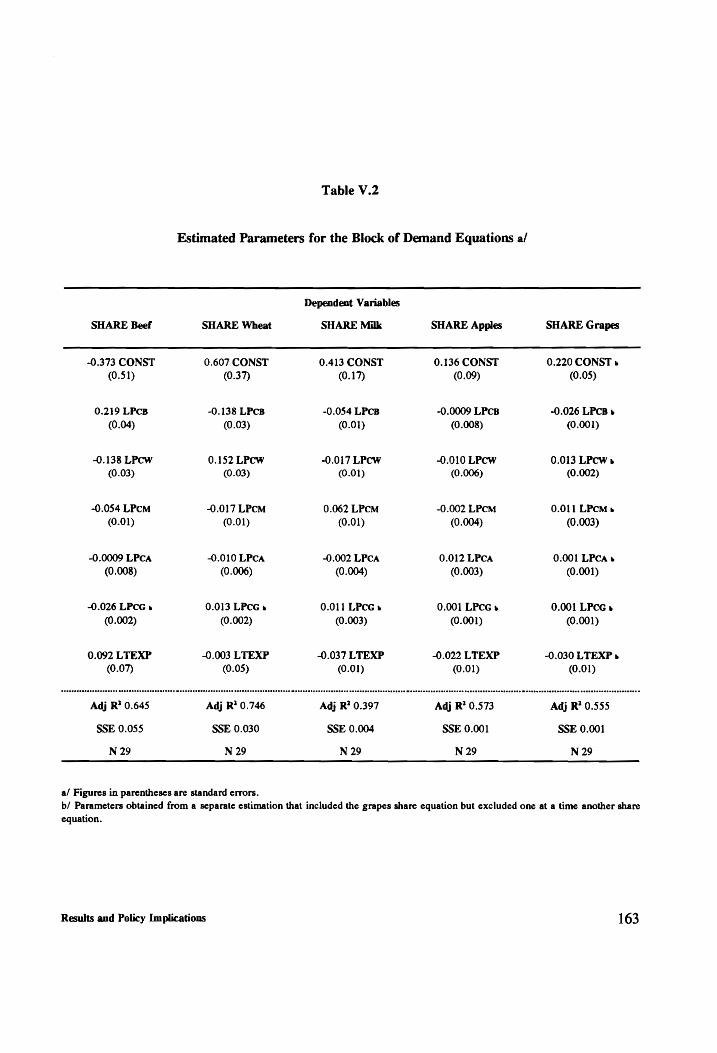
Table V.2

Estimated Parameters for the Block of Demand Equations a/

Dependent Variables

SHARE Beef SHARE Wheat SHARE Milk SHARE Apples SHARE Grapes

-0.373 CONST 0.607 CONST 0.413 CONST 0.136 CONST 0.220 CONST b (0.51) (0.37) (0.17) (0.09) (0.05)

0.219 LPcB -0.138 LPcs -0.054 LPcB -0.0009 LPcB -0.026 LPCB »

(0.04) (0.03) (0.01) (0.008) (0.001)

-0.138 LPcw 0.152 LPcw -0.017 LPcw -0.010 LPcw 0.013 LPCW » (0.03) (0.03) (0.01) (0.006) (0.002)

-0.054 LPcM -0.017 LPCM 0.062 LPcM -0.002 LPcM 0.011 LPcM +

(0.01) (0.01) (0.01) (0.004) (0.003)

-0.0009 LPca -0.010 LPCA -0.002 LPca 0.012 LPCA 0.001 LPCA »

(0.008) (0.006) (0.004) (0.003) (0.001)

-0.026 LPCG » 0.013 LPcc » 0.011 LPcG » 0.001 LPcG s 0.001 LPcG

(0.002) (0.002) (0.003) (0.001) (0.001)

0.092 LTEXP -0.003 LTEXP -0.037 LTEXP -0.022 LTEXP -0.030 LTEXP » (0.07) (0.05) (0.01) (0.01) (0.01)



N 29 N 29 N 29 N 29 N 29

a/ Figures in parentheses are standard errors. b/ Parameters obtained from a separate estimation that included the grapes share equation but excluded one at a time another share

equation.


Price Policy Equations

In the block of policy equations, the dependent variable, PPTi, presented in Table C.8, was

defined as the difference between producer and border prices times total output. Based on an

efficiency concept, this variable can be interpreted as the opportunity cost of domestically

producing a commodity instead of importing it. All price policy equations have the same linear

functional form. Results are presented in Table V.3. The generally good fit of these equations

suggests a close relationship between the demand for government price policies and the explanatory

variables. A positive sign for a right-hand side variable means that price support increases along

with the variable; negative signs indicate taxation.

As reflected by its lack of statistical significance, current research expenditures by commodity,

RPTi, seem not to play a role in determining the level of price intervention for wheat, milk,

apples, and grapes. However, the negative and significant parameter estimate for RPTB in the beef

price policy equation indicates that current investments in beef-cattle research move in opposite

direction to the resource transfers caused by price policies. These two means of supporting beef

producers are substitutes.

Domestic production, LQsi, was found to be positively related to the level of price intervention

in all cases and with large f-values only in all but the grape policy equation. These results are

expected as long as political weights increase with the importance of the commodity in total

Results and Policy Implication; 164

Table V.3

Estimated Parameters for the Block of Price Policy Equations a/

Dependent Variables

PPT Beef PPT Wheat PPT Milk PPT Apples PPT Grapes

8.56 CONST 39.95 CONST 9.87 CONST -12.12 CONST -9.73 CONST (6.89) (5.57) (46.41) (4.49) (4.78)

-6.46 RPTB 14.32 RPTW -3.28 RPTM 4.07 RPTA 0.970 RPTG (6.04) (4.11) (1.34) (1.61) (0.46)

5.15 LQsB 2.50 LQsw 0.618 LQsM 0.615 LQSA 0.024 LQsc (1.65) (1.08) (2.33) (0.23) (0.04)

5.73 DRP-1 4.39 DRP-1 1.02 DRP.1 -0.122 DRP-1 -0.044 DRP-1 (1.96) (1.65) (0.14) (0.23) (0.06)

-4.90 DSA -3.90 DSA -0.735 DSA 0.960 DSA 0.132 DSA (2.78) (1.08) (0.94) (0.28) (0.08)

4.85 DDR-1 5.26 DDR-1 0.860 DDR-1 0.606 DDR-1 0.173 DDR-1 (2.54) (1.90) (0.89) (0.28) (0.07)

0.844 NRT 0.195 NRT 0.066 NRT -0.004 NRT -0.006 NRT (0.06) (0.05) (0.01) (0.005) (0.001)

-0.377 IPS 0.434 IPS -0.047 IPS -0.045 IPS 0.004 IPS (1.33) (1.08) (0.37) @.11) (0.03)

-10.31 SV 5.33 SV 0.618 SV 0.812 SV 0.111 SV (1.33) (2.52) (1.02) (0.28) (0.08)

6.43 ESB -5.19 ESw -8.61 ESM -5.68 ESA -3.80 ESG (3.25) (1.36) (1.79) (2.09) (1.54)

2.37 EDB 6.31 EDW 7.24 EDM 1.84 EDA 4.93 EDc (1.94) (2.24) (2.37) (0.68) (2.29)



N29 N 29 N 29 N29 N 29



output. Unfortunately, these outcomes can not be directly related to the size of each producer

group Since there was no information on the number of producers by commodity, on a yearly

basis.

The government intervened heavily in all sectors of the economy during the socialist period. The

results for the DSA variable representing years 1971 to 1973 were negative in all importable

commodities but only had large f-statistics in the wheat, apple, and grape price policy equations.

Negative signs are associated with increased taxation. An explanation for this negative sign is

provided in Chapter II. Despite a highly protected economy, agricultural price policies during the

socialist government were biased towards urban consumers, almost neglecting the role of prices

in providing incentives to producers. In fact, Table II.3 clearly shows beef, wheat, and milk

producers as receiving, on average, lower nominal protection rates than they received during

previous administrations. The effect of DSA on apples and grapes price policies was positive but

non-significant.

Since price policies were, in general, formulated prior to the planting season, unfavorable weather,

DDR.-1, or depressed market conditions, DRP-1, would influence the demand for price policies at

least one year ahead. Lagged one period, the effect of DDR-1 had a positive impact on the level

of resource transfers toward all commodities, except milk. However, the DRP-1 variable had large

t-values only in the beef and wheat price policy equations. In all other cases these two dummy

variables were statistically insignificant.


Net resource transfers, NRT, between agriculture and the rest of the economy reflect transfers to

agriculture either directly through the price policies or indirectly through some of the government

expenditures. In the beef, wheat, and milk price policy equations this variable had a t-statistic

greater than two and with the predicted positive sign. This implies a positive relationship between

NRT and transfers to producers. As seen in Table II.3, there were no price supports for apples and

grapes for most of the 1960 - 1988 period. Hence, it should not come as a surprise that the NRT

variable was not significantly different from zero in the equations for these commodities.

An index of political stability, IPS, was constructed based on a probit model. The meaning of both

dependent and independent variables was given in Chapter IV. Estimated coefficients, standard

errors, and f-ratios of the probit regression are presented in Table V.4. The variable representing

violent actions was significant at the 5 percent level. The variables used to depict changes in

executive officers and the number of deaths because of political reasons were both non-significant.

Overall, the probit model specification yielded a 90.3 percent of correct predictions in government

changes. Yearly values of the IPS are reported in Table C.7 in Appendix C.

The IPS variable was statistically non-significant in all price policy equations. Conceived as an

indicator of the degree of pressure on the political process to enhance welfare in agriculture, the

IPS index was unrelated to changes in the level of subsidies or taxes attained by producers during

1960 - 1988. Perhaps, decision-making regarding agricultural price policies was not affected by

political stability, or alternatively, politicians may have not adequately represented their farm

constituency. It could also be possible that the rest of dummy variables may have absorbed the

influence of the IPS variable.


Table V.4

Estimated Parameters for the Probit Model

Asymptotic Variable Estimated Coefficient Standard Error

t - ratios

Constant -1.807 0.543 -3.328

Violent Actions 0.502 0.218 2.302

Repressions 0.0014 0.010 0.135

Executive Adjustments -0.346 0.274 -1.264

Log - Likelihood function = -9.8721

x? = 7.603

N = 29

SSE = 0.021


The SV variable reflects the structural transformations that occurred in the political and economic

system following the military coup of 1973. Hence, SV takes the value one from 1960 to 1973 and

the value zero afterwards. The coefficient on this dummy variable was positive in all five

commodities and associated with ¢-values higher than two in the beef, milk, and apple policy

equations. The positive sign for this variable coefficient reflects the success of market liberalization

policies in removing the disparity between producer prices and border prices. As shown in Table

II.3, non-beef producers were subsidized while beef-producers were taxed prior to 1973.

Afterwards, the commitment for stimulating competitiveness in agriculture and eliminating direct

price controls was so strong that it drastically changed the framework reflected in past price

policies.

Price elasticities of supply, ESi, were expected to explain some of the demand for price policies

because elasticities affect the welfare impacts of these policies and thus alter the desirability of

direct price interventions for interest groups. The negative signs of the estimates for all five

commodities were in line with comparative statics results developed in Chapter III and the variable

ESi had consistently large ¢-statistics. That is, more elastic supply schedules in a small open-

economy make producers more susceptible to distortionary price policies. As a result, producers

tend to lobby for lower price interventions.

Consistent with the theory presented in Chapter III, the role of price elasticities of demand, EDi,

in determining price policies is also important. The signs for the demand elasticity variable were

all positive as predicted. Variable coefficients with low t-values only appeared in the apples and

grapes policy equations. Redistributive price policies resulted in low deadweight losses when


demand was sufficiently price inelastic. As a consequence, commodities facing more inelastic

demand functions like wheat and milk were recipients of higher resource transfers than more price

elastic commodities such as beef and fruits. In fact, wheat and milk production received higher

producer subsidies for a longer period of time than apples and grapes.

Research Policy Equations

Real public investments in agricultural research, RPTi, are the dependent variable in the block of

linear research policy equations. The results from this block are given in Table V.5. These

equations explain on average about two thirds of the total variation in public research spending

over the 1960 - 1988 period.

The significance of previous year’s budget research expenditures, RPTi-1, on current research

resource allocation decisions is shown by the relatively high t-values for their coefficients in all

research policy equations except beef. The positive response in the current research budget of

wheat and apples with respect to their research budget lagged one year suggests that a 10 percent

increase in the previous years’ research budget translates into a 6.4 and 6.3 percent increase in

today’s research budget for wheat and apples, respectively.


Table V.5

Estimated Parameters for the Block of Research Policy Equations a/

Dependent Variables

RPT Beef

RPT Wheat RPT Milk RPT Apples RPT Grapes

-3.01 CONST -1.57 CONST -10.92 CONST 0.392 CONST 0.636 CONST (1.20) (1.04) (2.55) (0.26) (0.17)

0.130 RPTB-1 0.629 RPTW-1 0.542 RPTM-1 0.621 RPTA-1 0.306 RPTG-1 (0.11) (0.09) (0.09) (0.07) (0.10)

-0.005 PPTB -0.007 PPTW -0.010 PPTM 0.017 PPTA 0.059 PPTG

(0.001) (0.001) (0.01) (0.006) (0.02)

0.094 LQsB 0.079 LQsw 0.529 LQsM -0.022 LQsA -0.022 LQsG (0.05) (0.04) (0.12) (0.01) (0.01)

1.02 FB 0.148 Fw 0.783 FM 0.112 Fa -0.040 Fe

(0.24) (0.12) (0.38) (0.05) (0.06)

0.0001 NRT 0.002 NRT 0.003 NRT 0.0007 NRT ~0.0002 NRT

(0.001) (0.001) (0.001) (0.0002) (0.0004)

-0.041 IPS -0.053 IPS -0.063 IPS -~0.010 IPS -0.013 IPS (0.02) (0.02) (0.04) (0.004) (0.008)

0.167 SV 0.081 SV 0.147 SV 0.002 SV 0.013 SV

(0.05) (0.06) (0.08) (0.01) (0.02)

-0.105 ESB -0.618 ESw -1.10 ESM -0.509 ESA -2.19 ESc (0.05) (0.22) (0.52) (0.15) (0.76)

0.598 EDB 0.011 EDw 0.138 EDM 0.063 EDA 0.212 EDG

(0.28) (0.07) (0.16) (0.01) (0.06)



N 28 N 28 N 28 N 28 N 28



Resource transfers from price policies, PPTi, had high t-statistics in the beef and wheat research

expenditure equations. The negative sign for PPTB in the beef research implies that increased

funding for beef-cattle research is a compensating mechanism for the negative protection to beef

production. Thus, price and research policies for beef are substitute instruments.

Similarly, the negative sign for the coefficient on the PPTi variable in the wheat and milk research

policy equations indicates substitutability between policy instruments. Government pricing policies

for wheat and milk production were negatively correlated with public expenditures on research

technologies. Wheat and milk producers lowered their demands for government-sponsored research

funds when they enjoyed positive levels of nominal protection.

The evidence obtained here suggests that domestic output, LQSi, is positively associated with the

level of research expenditures in the beef, wheat, and milk research policy equations. The negative

sign attached on the LSQi variable in the apple and grape research expenditure equations suggests

that increased outputs of these commodities actually induce fewer public research investments. The

parameter estimates for apples and grapes were not, however, significantly different from zero.

For the most part, the variable representing internationally available technologies, Fi, was positive

and only had a relatively large t-value in the beef research policy equation. This sign indicates a

positive role of foreign technologies in inducing public expenditures on research in beef, wheat,

milk, and apples. Public agricultural research is thus complementary to research conducted in

international centers or in other countries. Long-run elasticity estimates can be obtained when

lagged values of the dependent variables are included as explanatory variables. Calculated at the


mean of the sample values these long-run elasticities indicate that an additional 10 percent increase

in the level of foreign beef technology induces a 0.21 percent increase in domestic beef supply.

Elasticity estimates for the other commodities fluctuated between 0.002 for wheat and 0.011 for

milk.

The coefficients for the variable representing net resource transfers, NRT, had high t-values only

in the wheat and milk research policy equations. The sign associated with this variable was

positive, as expected, in all but the grapes research policy equation. This positive sign indicates

that net resource transfers to agriculture are positively related to public research expenditures. The

relatively small estimated coefficients in the apples and grapes equations could be explained by the

increasing role undertaken by the private sector in the fruit industry. In the last nineteen years

technical knowledge developed in the private sector overwhelmed the demand for public research

resources.

Large t-statistics are encountered for the index of political stability, IPS, in the wheat and apples

research policy equations. For all five equations, however, IPS does not conform to a priori

expectations that public agricultural research investments in Chile are positively influenced by the

activities of interest groups.

The second political variable represents a unique economic and political period in the history of

Chile. This variable was considered relevant in this block of equations as a previous run of the

model indicated that the IPS variable was an inadequate proxy for political reforms. Except for

the coefficient on SV in the beef research equation, the variables was significant in all the other


research policy equations. The sign for the SV variable is positive in all cases, yet changes in the

institutional framework were obviously not as important in affecting research resource allocation

as it was in influencing resource transfers due to price policies.

Price elasticities of supply and demand appear to play a significant role in determining the level

of investment on Chilean public agricultural research. In seven out of ten cases, the variables

representing price elasticities of supply, ESi, and demand, EDi, had relatively large t-values. For

all commodities, the signs for these two elasticity variables conform to prior expectations regarding

the structure of agricultural production and consumption. That is, a negative sign for the price

elasticity of supply and a positive sign for the price elasticity of demand were expected.

From the producers viewpoint, higher price elasticities of supply tend to induce lower demands

for research expenditures. On the demand side, more elastic price elasticities lead to increased

demand for research funds. The signs of the parameters imply that producers are given more

weight in the policy formulation process than are consumers.

The magnitude of the estimated coefficients attached to each ESi and EDi variable in the block of

research policy equations were, in general, smaller than their corresponding coefficients in the

block of price policy equations *. This difference in magnitude can be explained by the way that

both price and research policy transfers are defined. While resource transfers due to distortionary

3 The coefficients for ESi and EDi in the research policy equations are approximately one tenth the ones

found in the price policy equations.


price policies do not necessarily represent actual government expenses or revenues, public

agricultural research expenditures are, in contrast, budgeted and directly invested.

Supply Elasticities

Short-run own-price elasticities of supply of beef were calculated as follows:

ES, = 4, + 2 a5, ( LnPp, )

where a; ;, and a; ., are the estimated parameters corresponding to the linear and quadratic terms

of the beef price variable, respectively.

One year own-price elasticities of supply in the equations that included a lagged dependent variable

were computed within the framework provided by the Nerlovian partial adjustment model *. These

price elasticities were obtained from their respective supply equations as follows

ES; = a5; (1 —% 4) +244, C1 ~ 04; ) CLnP, ; )

‘ Despite the existence of lagged dependent variables, the relationship between short and long-run price elasticities can easily be disentangled because of the relative fixity of production factors in a particular year. Formal derivations can be seen in Nerlove and Addison (1958) and Mundlak (1986).


where ay; >, and a; 3 are the parameter coefficients associated with the linear and quadratic terms

of the price variable, respectively; and q; ,; is the adjustment coefficient associated with the lagged

dependent variable, LSQi-1. This adjustment coefficient indicates the length of the adjustment

period, since the desired level of output, LSQi, in any one period depends partly on the level of

output in that period and partly on the existing level of output at the beginning of the period.

Short-run own-price elasticities of supply by commodities are presented in Table V.6. Computed

at their sample means these price elasticity estimates were found to be in the 0.006 - 0.42 range.

These results are similar to those reported in other studies. The relatively high elasticity values

found for beef and wheat indicate larger short-run supply responses than the ones observed for

apples and grapes. Wheat, the only crop analyzed in this study that is produced on small farms

exhibits the lowest price elasticity variation over the period of study. The estimated price elasticity

of milk supply was below the 0.35 - 0.45 short-run supply elasticity range reported by Hurtado

et al (1990) and Zegers.

Production of apples and grapes involves a different time dimension than the one encountered in

wheat or livestock products. Relatively long lags between initial production decisions and the

period in which output materializes distinguish the supply of perennials from the supply of annual

crops. Thus, it is not surprising to find inelastic apple and grape supply since most factors of

production are fixed in the short-run.

These short-run price elasticities of supply are in some cases smaller than the aggregate supply

responses reported by Coeymans and Mundlak for Chilean agriculture during 1962 to 1982. They


Table V.6

Supply, ES, Demand, ED, and Expenditure, IE, Elasticity Estimates a/

Elasticity Commodities

Levels Beef Wheat Milk Apples Grapes

ES 0.424 0.238 0.186 0.006 0.008

ED -0.712 -0.347 -0.213 -0.356 -0.736

IE 1.188 0.955 0.360 0.443 0.958

a/ Average elasticity estimates computed at the means of the sample data


reported cumulative aggregate price elasticities of supply between the 0.32 - 1.02 range after three

and ten years period, respectively. Their estimates are, however, consistent with the relatively low

supply elasticity estimates presented in Table V.6 as short-run elasticities tend to be lower than

their long-run counterparts.

Demand Elasticities

As suggested by Blanciforti et el (1986), own-price uncompensated elasticities of demand, EDi,

were estimated from the AIDS model as follows °:

eye tit B; Y; ‘ SHARE i SHARE i

where SHARE: is the share of total expenditure allocated to commodity i, y;,; is the own-price

parameter, @i is the expenditure parameter for the ith commodity, and y, is the elasticity of the

group price index with respect to the jth price.

The values reported in Table V.6 confirm a priori expectations of negative and relatively inelastic

own-price elasticities of demand for all five commodities. The largest price elasticity is for beef

with -0.71 and the lowest for essentials such as wheat and milk with -0.35 and -0.21, respectively.

5 This formula for the AIDS model differs somewhat with the uncompensated price elasticity formula suggested by Green and Alston (1990) for the linear approximate AIDS system. However, both

uncompensated price elasticity estimates turn out to be very similar across each alternative approach.


Intermediate values were found for apples and grapes with -0.36 and -0.74, respectively. The

average price elasticity of demand for wheat is much higher than the one presented by Pacheco de

Carvalho (1989). He found a direct price elasticity of demand for the Chilean wheat to be -0.06.

Income Elasticities

Following Blanciforti et al (1986), average own-expenditure elasticities IEi were calculated as

follows:

IE, = 1 + _ Pi SHARE i

where fi and SHARE: keep the same definitions than above.

All expenditure coefficients presented in Table V.6 except for beef were negative. The implications

of these negative coefficients are that total expenditure elasticities are less than one which in turn

implies that these non-meat commodities are all necessary goods. Beef is relatively a luxury item

among the basket of five goods since its expenditure coefficient is positive. The expenditure

elasticities vary between 0.36 and 1.19. The interpretation of the 1.19 value is that as expenditure

on these five commodities increases by 1 percent the consumption of beef would rise by 1.19

percent. Conversely, expenditure elasticities are less inelastic for wheat, milk, apples, and grapes.


Welfare Estimates

Welfare impacts of the research resources invested by the Instituto Nacional de Investigaciones

Agropecuarias and the Fondo de Investigacién Agropecuaria in the presence of market-distorting

price policies were measured within a partial equilibrium framework. The basic procedure of the

economic surplus approach is to calculate annual welfare changes from rightward shifts in the

supply curve that occurred from the adoption of more efficient production techniques.

Expenditures on public agricultural research in Chile and technology transfers from environments

similar to Chile shifted the supply schedule. International transmission of knowledge has allowed

Chile to internalize some of the benefits of research conducted elsewhere resulting in reductions

in per-unit domestic costs of production.

A parallel shift for the supply curve was used in this study. Estimates of the proportionate shift in

the supply curve resulting from research-induced technical change were measured as marginal cost-

reducing shifts. Relative magnitudes of supply elasticities in a small-open economy are important

when measuring the benefits derived from the combined effects of direct price policies and

agricultural research investments. Nevertheless, price elasticities of demand do not enter in the

economic surplus calculations given the trading status of Chile ©. The average price elasticities

of supply illustrated in Table V.6 for the 1960 - 1988 period were used as a yardstick in the

6 Explicit derivations of the formulas used to calculate these welfare changes are shown in Appendix G.


economic surplus calculations. Real discount rates of five and ten percent were used to reflect the

value of alternative public investments.

Changes in total economic surplus minus research costs using average price elasticities of supply

are presented in Table V.7. Typically, economic surplus gains are almost doubled when the

discount rate is lowered to five percent. The greater value of beef and wheat production as

compared with the other commodities is reflected in the net economic payoffs to beef-cattle and

wheat research. The exclusion of private research on fruits may have translated into relatively high

returns for apples and grapes if both private and public research expenditures were positively

correlated. Therefore, caution should be exercized when interpreting the returns to public research

investments on these commodities because a possible overestimation may be present.

The sensitivity of the benefits to research under distortionary price policies to different supply

elasticity estimates is observable in Table V.8. Economic surplus figures differed across alternative

elasticity scenarios. As expected, aggregate social welfare gains tended to be largest for elastic

supply elasticities and least where supply elasticities were more inelastic. Net social benefits for

beef appear substantially lower for the more inelastic price elasticity. Such a small surplus figure

is unlikely because this lower-bound price elasticity for beef supply was obtained for one particular

year between the 1960 - 1988 period. Therefore, the results reported in Table V.7 for average

supply elasticities should be considered appropriate for providing conservative economic surplus

estimates.


Table V.7

Benefits from Agricultural Research under Minimum - Maximum Price Policies

-Millions of 1985 Chilean Pesos-

Discount Commodities

Rate Beef Wheat Milk Apples Grapes

5% 18,705 17,687 4,813 2,199 2,316

10 % 8,891 9,161 1,950 1,221 852


Table V.8

Benefits from Agricultural Research Under Different Supply Elasticity Scenarios


Using the Most Elastic Supply Elasticity Estimate



5% 18,544 20,208 7,671 2,350 3,014

10 % 10,028 10,448 3,139 1,309 1,117

Using the Most Inelastic Supply Elasticity Estimate



5% 1,158 18,094 6,209 2,044 1,977

10 % 501 9,377 2,563 1,135 747


Economic surplus changes dissagregated by consumers, producers, taxpayers, and net social

benefits are shown in Table V.9 for a 10 percent discount rate. Gains from cost reductions on beef,

wheat, milk, apples, and grapes due to indigenous and foreign research were all captured by

domestic producers. Productivity increases did not change international prices since Chile had a

marginal importance in the world commodity market for each commodity. Therefore, there was

no price decrease to benefit domestic consumers. As a result of of the net taxation on beef

production taxpayers enjoyed welfare gains from this activity despite their commitments for

financing beef-cattle research. Welfare losses for taxpayers were given by the relative importance

of the commodity and the degree of price intervention.

Estimates of the research benefits without price intervention policies under average supply

elasticities are required in order to compare the net effects of distortionary prices on welfare. Table

V.10 summarizes the results when producer prices are replaced by border prices in the surplus

calculations. Compared to the results shown in Table V.7, returns for all commodities were eroded

as a result of government price interventions. Depending on the market of interest, net economic

surplus gains for society as a whole would have been 0.6 to 36 percent larger if discriminatory

prices had been ignored. The magnitude of the welfare increases caused by the removal of direct

price policies appeared to be less important in apples and grapes but more significant in milk and

beef. Had technical change not prevailed in Chilean agriculture the effects of these direct price

policies would have made just a marginal contribution to overall economic growth.


Table V.9

Benefits from Agricultural Research by Interest Groups under Minimum - Maximum

Price Policies, Assuming a 10 percent Discount Rate


Consumer Producer Taxpayers Net

Commodity Surplus Surplus Transfers Benefits

Beef 0 8,007 884 8,891

Wheat 0 9,617 (456) 9,161

Milk 0 2,324 (374) 1,950

Apples 0 1,399 (178) 1,221

Grapes 0 1,116 (122) 994

a/ Rounded figures.


Table V.10

Benefits from Agricultural Research using Border Prices




5% 21,616 19,071 6,456 2,208 2,371

10 % 11,735 9,872 2,652 1,228 888


Policy Implications

The above results suggest several policy implications in terms of the degree of government

intervention in Chilean agriculture over the period of study. First, price and research policies were

alternative ways to distribute welfare among interest groups. Pressures on governments to

subsidize (tax) agriculture and promote public research investments resulted in resource transfers

that varied among commodities. Public support for agricultural research tended to be associated

with commodities that enjoyed some degree of price protection either positive or negative. The

level of public investments in agricultural research was increased when price policies discriminated

against producers of a commodity and decreased when those price policies subsidized it.

For example, the effects of price policies that taxed beef producers induced lobbying efforts of

those producers for additional expenditures on public research on beef. However, the lobbying

activity of wheat and milk producers led to favorable price policies that directly hurt the group of

consumers/taxpayers. Public research investments on exportables like apples and grapes appeared

to be exogenously related to price policies and independent of the incentives of producers and

consumers/taxpayers groups.

Results and Policy Implicatious 187

A second major finding is that the interactions between technology and pricing policies and the

response of governments for policy reforms were mainly determined by the relative political

weights of producers and consumers/taxpayers. Research-induced production in a small open-

economy like Chile left producers and input owners as being the only beneficiaries. However,

consumers/taxpayers have also been strong advocates in the formulation of both policy

instruments. Price elasticities of demand for almost all commodities studied here affected

significantly producers’ demands for price and research policies. Thus, the differential political

power of both interest groups may have helped to spread over the costs and benefits of government

intervention as the incentives of these interest groups were modified.

A third policy implication is that the long-run effects of direct price intervention were undesirable.

The presence of taxes and subsidies distorted the social value of research on every single

commodity. Despite the existence of market distortions caused by commodity price policies,

Chilean net domestic benefits from public agricultural research were positive. However, these net

economic surplus changes would have been even higher if output price interventions had been

aimed at reducing distortions and putting producer prices more in line with international prices.

Finally, technologies made available by the Chilean agricultural research system have played an

important role in explaining agricultural production increases. In order for Chile to reap the largest

aggregate welfare gains, public research funds should be channeled into commodities that are the

least price distorted. At the same time, Chile should continue the adoption of new cost-reducing

technologies from abroad. Some of these technologies have been adopted from other countries

without any additional research while other required adaptive research before they were applicable.


The existence of spillovers of research benefits suggests that technology adaption from Argentina,

Brazil, and United States would strengthen Chile’s competitive advantage.

In general, the stability of the overall political system did not affect the direction of price policies

and expenditures in agricultural research. Activities of specific producer groups to support

legislation that would modify price structures and research endeavors favorable to their own

interests seem not to be triggered by the existing political climate. Therefore, a better measure of

political influences is needed to capture within agriculture the dynamics of an economic

environment characterized by policy changes.


CHAPTER SIX

SUMMARY AND CONCLUSIONS

This chapter summarizes the main elements of the dissertation and provides conclusions in light

of the results obtained in the previous chapter. Limitations and suggestions for further research are

offered as well.

Summary of the Dissertation

The need for a rational allocation of budgetary resources to enhance agricultural growth has been

widely recognized. Among the variety of policy instruments available, direct price intervention and

publicly-sponsored research compete with each other for scarce funds. Failure to account for the

interactions between these two policy instruments may have seriously distorted public expenditure

decisions. Neglecting the joint determination of direct price policies and agricultural research

investments in the policy formulation process will likely lead to an overestimation of the returns

Conclusions 190

to agricultural research. Regardless of the size or the degree of openness of an economy, this issue

has simply been ignored in past studies. In addition, relatively large estimated research suggest a

possible underinvestment in public agricultural research.

A political-economy framework was used to assess, from 1960 to 1988, the simultaneous impacts

of Chilean price and research policies in order to make the welfare consequences of these policies

on different interest groups explicit. The main objective of this dissertation was to analyze the

determinants of the level and distribution of public research investments by assuming that

agricultural price policies affected the level of performance of the agricultural sector not only

directly but through their effects on the supply and demand for agricultural research.

The past performance of Chilean agriculture is summarized in Chapter II. The main political,

economic, and institutional characteristics of previous policy interventions and governments are

highlighted. For example, minimum and maximum price interventions on beef, wheat, milk,

apples, and grapes were enforced by quantitative trade restrictions and resulted in substantial

impacts on production. The effects of these price interventions on the amount of resources

transferred within and between agriculture have been altered by indirect economy-wide

interventions. The Chilean agricultural research system has also played an important role in

promoting technical change. Human and capital resources along with international technologies

were available to foster agricultural growth over time.

The influence of collective action on agricultural policy formation is discussed in Chapter III. A

theoretical framework is articulated to provide a better understanding of the interactions between

Conclusions 191

price policies and agricultural research investments as a result of collective action exerted by

producers and consumers/taxpayers. The impact of price policies and publicly-funded research on

welfare gains is determined in a political-economy model. Stressing the non-separability of political

and economic markets, a political optimum is established for a government that maximizes a

political preference function. Welfare effects associated with an optimal mix of these two types of

public policies are derived.

An econometric approach consistent with the hypothesized process underlying public policy

formation is presented in Chapter IV. The empirical model is specified as a system of four blocks

of simultaneous equations. These blocks include supply and demand systems and two sets of policy

equations used to capture price and research policies, respectively. A non-linear three-stage least

Squares procedure is chosen to simultaneously estimate the system. In turn, formulas are presented

to measure changes in welfare from publicly sponsored agricultural research when direct price

interventions are considered.

The results obtained are presented in Chapter V. More than 50 percent of the parameter estimates

had asymptotic f-ratios above two. Policy implications derived from those results are summarized

in the following section.

Conclusions 192

Conclusions of the Study

Resource transfers between agriculture and the rest of the economy seem to have been dominated

by the vested interests of pressure groups representing importable commodities. Beef, wheat, and

milk producers have directed their demands for price and research policies in order to increase or

at least maintain their welfare gains. Concentration of production in specific agricultural zones and

farm homogeneity may have been important in facilitating their ability to press for policy changes.

As a result, the government engaged in compensatory mechanisms to transfer resources to these

groups of producers. Public investments in beef-cattle research were used to off-set detrimental

effects of price-tax intervention on beef production. Conversely, positive rates of protection were

used to compensate wheat and milk producers for the effects of price-reducing technologies in

wheat and milk production.

Producers of apples and grapes seem to have been less active in the formulation of commodity

price and research policies. Since the middle 1970s, apple and grape producers have used political

pressure very little to influence the development of fruit technologies in public research

institutions. Instead, they shifted their demands for technological advances to research efforts by

the private agricultural research system in order to seek more practical solutions than the ones

provided by the public sector. Thus, pressing for additional public research resources to adapt and

transfer fruit technologies was no longer part of the agenda of fruit-growers.

Conclusions 193

The interactions between price and research policies were formally addressed in this study in order

to avoid biased estimates of the benefits to Chile from indigenous and international agricultural

research. Endogeneity results indicate, in general, that distortionary price policies and public

research investments on importables like beef, wheat, and milk have been jointly determined. In

constrast, research funding decisions on apples and grapes commodities were exogenously

determined.

Government pricing policies influenced the innovative behavior of the main Chilean public

research institution and reduced the benefits from cost-reducing research benefits relative to those

obtained under free trade conditions. Despite the existence of market distortions caused by

commodity price policies, Chilean net domestic benefits from public agricultural research were

positive. However, these net economic surplus changes would have been higher if output price

interventions would have been aimed at reducing distortions and putting producer prices more in

line with international prices.

For example, beef producers increased their benefits from research on beef when output taxes were

lifted after 1974. Conversely, the existence of minimum price policies for wheat and milk reduced

welfare gains from research in these commodities by a magnitude equivalent to the taxpayer costs

of direct price intervention. Social returns to apple and grape research, in constrast, remained

almost unaltered as government pricing policies on these commodities were temporary and low in

magnitude.

Conclusions 194

Limitations of the Study

The economic surplus analysis used to estimate the benefits and costs of price policies and publicly

sponsored agricultural research was constructed under a partial equilibrium framework. This

implies that the welfare effects on various interest groups included impacts in only the market of

interest. The magnitude of the error introduced by ignoring the effects of in inputs or other output

markets is likely to be small the smaller the income effects associated with a price change and/or

the proportion of the product cost on the average budget. However, horizontal market relationships

were explicitly taken into account by simultaneously estimating supply and demand elasticities for

all five commodities.

The degree of direct price intervention in Chilean agriculture was measured as the nominal rate

of protection. This indicator compares the domestic price of a commodity to its border price

leaving aside the effects of price interventions on the inputs purchased for producing that

commodity. Thus, the incidence of input subsidies (taxes) for taxed (subsidized) commodities can

offset their levels of direct output price interventions. In these cases, it could be argued that a more

comprehensive indicator for price interventions would have been the rate of effective protection,

EPR, which expresses the effects of protection on both output and inputs in value-added terms.

However, the bulk of assumptions required to obtain the amount of intermediate inputs needed to

produce each commodity during the whole period of study precludes the use of EPR as a reliable

measure of price intervention. Furthermore, there is evidence across products that input price

interventions including credit subsidies represented in Chile a relatively small resource transfer mechanism.

Conclusions 195

Indirect price interventions such as exchange rate manipulations have in many cases overwhelmed

the positive or negative incentives created by direct price intervention. On average, the impact of

indirect intervention implied a net taxation on Chilean agriculture of about 20 percent as compared

to a net taxation rate below 2 percent as a result of direct price interventions. Therefore, some bias

in the results could be expected since these economy-wide policies were not modeled. Capturing

the effects of these macroeconomic interventions on the agricultural sector was beyond the scope

of this study.

Political factors are always relevant to the policy debate. In this study, however, the variable

representing the stability of the Chilean political system may have not adequately represented the

dynamics of the political process. It is left for further research to design a better political variable

for capturing the activities of specific producer groups to support legislation that would modify

price structures and research endeavors favorable to their own interests.

Data limitations were a pressing issue in the results obtained in this study. The lack of consistent

and reliable statistical information is common to most developing countries. In that regard, Chile

is not an exception. An obvious improvement thus would be the availability of a complete set of

consumer prices, better information on resource allocation, or even a headcount of commodity

producers.

Finally, a more formal dynamic optimization model may be needed to assess the driving forces

underlying price and research policies in a political-economy process. Control-theory could be an

additional tool for defining optimal levels of policy funding over time.

Conclusions 196

BIBLIOGRAPHY

ALSTON, J., G. EDWARDS and J. FREEBAIRN. “Market Distortions and Benefits from

Research." American Journal of Agricultural Economics, Vol. 70 (2): 281 - 288, 1988.

. and P. PARDEY. "Technical Change, Constraints and Incentives: The Damaging Consequences of Getting Policies Wrong." Paper presented at the Conference on Agricultural Technology: Current Policy Issues for the International Community and The World Bank, Airlie

House, Virginia - USA. October, 1991.

, G. NORTON and P. PARDEY. Science under Scarcity: Principles and Practice for

Research Evaluation and Priority Setting, New York: Cornell University Press, 1994.

AMEMIYA, T. Advanced Econometrics, Boston: Harvard University Press, 1985.

ANTLE, J. "Dynamics, Causality, and Agricultural Productivity." in S. Capalbo and J. Antle.

Eds. Agricultural Productivity: Measurement and Explanation, Washington D.C.: Resources for

the Future, 1988.

ARNDT, T., D. DALRYMPLE and V. RUTTAN. Eds. Resource Allocation and Productivity in

National and International Agricultural Research, Minneapolis: University of Minnesota Press, 1977.

BALISACAN, A. and J. ROUMASSET. "Public Choice of Economic Policy: The Growth of

Agricultural Protection." Weltwirtschafliches Archiv 123 (2): 232 - 247, 1987.

BALASSA, B. “Policy Experiments in Chile, 1973 - 1983." in G. Walton. Ed. Zhe National

Economic Policies in Chile. Jai Press Inc., 1985.

BANCO CENTRAL DE CHILE. Indicadores de Comercio Exterior, Various issues.

. Indicadores Econémicos y Sociales, Various issues.

BANKS, A. Political Handbook of the World, New York: Binghampton: Multiple Years.

BHAGWATI, N. “Directly Unproductive Profit Seeking Activities." Journal of Political Economy,

Vol.90 (4): 982 - 1002, 1982.

BECKER, G. "A Theory of Competition among Pressure Groups for Political Influence."

Quarterly Journal of Economics, Vo\.93 (3): 372 - 400, 1983.

Bibliography 197

BEGHIN, J. "A Game-Theoretic Model of Endogenous Public Policies." American Journal of Agricultural Economics, Vol. 72 (1): 138 - 148, 1990.

. and M. Kherallah. “Political Institutions and International Patterns of Agricultural

Protection.” Faculty Working Paper 91 - 02. Department of Agricultural and Resource Economics.

North Carolina State University. April 1991.

BIERI, J., A. de JANVRY and A. SCHMITZ. “Agricultural Technology and the Distribution of Welfare Gains." American Journal of Agricultural Economics, Vol. 54 (3): 801 - 808, 1972.

BEHRMAN, J. "Aggregative Market Responses in Developing Agriculture: The Postwar Chilean

Experience.” in R. Eckaus and P. Rosenstein-Rodan. Eds. Analysis of Development Problems, The Netherlands: North Holland Publishing Company, 1973.

. Macroeconomic Policy in a Developing Country. The Chilean Experience, North

Holland Publishing Company, 1977.

BINSWANGER, H. and V. RUTTAN. Eds. Induced Innovation: Technology, Institutions and

Development, Baltimore: Johns Hopkins University Press, 1978.

. "The Policy Response of Agriculture." in Proceedings of The World Bank Annual Conference on Development Economics. Washington D.C., 1990.

BLANCIFORTI, L., R. GREEN, and G. KING. "U.S. Consumer Behavior Over the Postwar

Period: An Almost Ideal Demand System Analysis." Giannini Foundation Monograph N 40, University of California, Davis. August 1986.

BONILLA, S. "El Rol del Instituto Nacional de Investigaciones Agropecuarias -INIA- como

Generador y Proveedor de Tecnologfa para el Desarrollo de la Investigacié6n Agropecuaria

Chilena." Paper presented at the Workshop on Management on Agricultural Research and

Technology Transfer. Santiago - Chile. August, 1989a.

. "El Sistema Chileno y Modelo Institucional del Instituto Nacional de Investigaciones

Agropecuarias." Paper presented at the Annual Conference on Agricultural Research. Lima - Pert.

October, 1989b.

CAPALBO, S. and J. ANTLE. Eds. Agricultural Productivity: Measurement and Explanation, Washington D.C.: Resources for the Future, 1988.

CAUAS, J. "Report on the State of Public Finance." in J.C. Méndez. Ed. Chilean Economic Policy. Santiago: Imprenta Calderén, 1979.

CAVALLO, D. and Y. MUNDLAK. Agriculture and Economic Growth in an Open Economy: The Case of Argentina, /nternational Food Policy Research Institute, Research Report N 36,

Washington D.C., 1982.

Bibliography 198

CEPAL Review. Economic Commission for Latin America. Santiago - Chile. April 1982.

CHAMBERS, R. Applied Production Analysis. A Dual Approach, United States: Cambridge


. and R. LOPEZ. "Public Investments and Real-Price Supports." Working Paper N 91 - 12. Department of Agricultural and Resource Economics. University of Maryland. January 1992.

CHENERY, H. and T. SRINIVASAN. Eds. Handbook of Economic Development, The

Netherlands: Elsevier Science Publishers, 1988.

CIEPLAN. Neo-estructuralismo, Neo-monetarismo y Procesos de Ajuste en América Latina,

Coleccién No. 23. Santiago - Chile. March 1988.

COEYMANS, J.E. and Y. MUNDLAK. “Sectoral Growth in Chile, 1962-82." International Food

Policy Research Institute, Research Report Manuscript, Washington D.C., 1993.

CORBO, V and J. de MELO. Scrambling for Survival, The World Bank. Staff Working Paper N 764. Washington D.C., 1985.

CRISPI, J. "El Agro Chileno después de 1973: Expansidn Capitalista y Campenizacién

Pauperizante." Academia de Humanismo Cristiano, Santiago - Chile. 1980.

CUKIERMAN, A., S. EDWARDS and G. TABELLINI. "Seignorage and Political Instability."

American Economic Review, Vol. 82 (3): 537 - 555, 1992.

CURIE, J., J. MURPHY, and A. SCHMITZ. "The Concept of Economic Surplus and Its Use in

Economic Analysis." Economic Journal, Vol.81 (324): 741 - 798, 1971.

DAVIS, J., P. ORAM and J. RYAN. Assessment of Agricultural Research Priorities: An International Perspective. Australia: ACIAR Monograph No 4, 1987.

de GORTER, H. and D. ZILBERMAN. "On the Political Economy of Public Good Inputs in Agriculture." American Journal of Agricultural Economics, Vol. 72 (1): 131 - 147, 1990.

and G. NORTON. "A Critical Appraisal of Analyzing the Gains from Research with Market Distortions." Mimeo. Department of Agricultural Economics. Cornell University, 1990.

and Y. TSUR. "Explaining Price Policy Bias in Agriculture: The Calculus of

Support-Maximizing Politicians." American Journal of Agricultural Economics, Vol. 73 (4): 1244

- 1254, 1991.

Bibliography 199

, D. NIELSON and G. RAUSSER. "Productive and Predatory Public Policies: Research Expenditures and Producer Subsidies in Agriculture." American Journal of Agricultural

Economics, Vol. 74 (1): 27 - 37, 1992.

de JANVRY, A., E. SADOULET and M. FAFCHAMPS. “Agrarian Structure, Technological Innovations, and the State." Working Paper N 442. Department of Agriculture and Resource

Economics. University of California, Berkeley. May 1987.

de VYLDER, S. Allende’s Chile: The Political Economy of the Rise and Fall of the Unidad Popular, Great Britain: Cambridge University Press, 1976.

ECKAUS, R. and P. ROSENSTEIN-RODAN. Eds. Analysis of Development Problems. Studies of the Chilean Economy, The Netherlands: North Holland Publishing Company, 1973.

EDWARDS, G. and J. FREEBAIRN. "The Gains from Research into Tradeable Commodities."

American Journal of Agricultural Economics, Vol. 66 (1): 41 - 49, 1984.

EDWARDS, S. "Economic Policy and the Record of Economic Growth in Chile, 1973 - 1982."

in G. Walton. Ed. The National Economic Policies of Chile, Jai Press Inc., 1985.

, and G. TABELLINI. "Explaining Fiscal Policies and Inflation in Developing Countries. An Empirical Analysis." Journal of International Money and Finance, Vol. 10 (4): 516 -548, 1991.

ELGUETA, M. and E. VENEZIAN. Eds. Economta y Organizacién de la Investigacién Agropecuaria, INIA, Santiago - Chile, 1982.

. "La Investigacién Agrfcola en Chile. Evolucién Histérica.” in M. Elgueta and E.

Venezian. Eds. Economta y Organizacion de la Investigaci6n Agropecuaria, INIA, Santiago -

Chile, 1982.

EVENSON, R. and E. da CRUZ. "Economic Impacts of the PROCISUR Programmes: An

International Study." in Issues in Agricultural Development: Sustainability and Cooperation.

I.A.A.E. Occasional Paper N 6: 22 - 28, 1992.

FAO. Documento de Debate sobre las Tendencias, Estrategias y Opciones de Polftica para el

Desarrollo Alimentario Agrfcola y Rural en América Latina y el Caribe, Rome - Italy, 1988.

___. FAO Production Yearbook, Rome - Italy: Multiple Years.

___. FAO Fertilizer Yearbook, Rome - Italy: Multiple Years.

FOX, G. "Is the United States Really Underinvesting in Agricultural Research." American Journal

of Agricultural Economics, Vol. 63 (4): 807 - 812, 1985.

Bibliography 200

FRISVOLD, G. "Emerging Issues in the Allocation of Public Agricultural Research Funds." American Journal of Agricultural Economics, Vol. 73 (3): 876 - 881, 1991.

FULGINITI, L. and R. PERRIN. "Prices and Productivity in Agriculture." Working Paper

Department of Economics. Iowa State University. 1991.

GARDNER, B. "Efficient Redistribution through Commodity Markets." American Journal of

Agricultural Economics, Vol. 65 (1): 225 - 234, 1983.

. The Economics of Agricultural Policies, New York: Macmillan Publishing Company,

1987a.

. "Causes of U.S. Commodity Program." Journal of Political Economy, Vol. 95 (2):

290 - 310, 1987b.

. "Price Supports and Optimal Spending on Agricultural Research." Working Paper

N 88-1. Department of Agricultural and Resource Economics. University of Maryland. June 1988.

GASTIL, R. Freedom in the World: Political and Civil Liberties, New York: Freedom House

Publisher. Multiple Years.

GODFREY, L. Misspecification Tests in Econometrics, Great Britain: Cambridge University

Press, 1988.

GREEN, R. and J. ALSTON. “Elasticities in AIDS Models." American Journal of Agricultural Economics, Vol. 72 (2): 442 - 445, 1990.

GUTTMAN, J. "Interest Groups and the Demand for Agricultural Research." Journal of Political

Economy, Vol. 86 (3): 467 - 484, 1978.

HAYAMI, Y. and V. RUTTAN. Agricultural Development: An International Perspective. Revised

and Expanded Edition, Baltimore: The Johns Hopkins University Press, 1985.

HENDERSON J. and R. QUANDT. Microeconomic Theory: A Mathematical Approach, New

York: McGraw-Hill, 1980.

HERTFORD, R. and A. SCHMITZ. "Measuring Economic Returns to Agricultural Research."

in T. Arndt, D. Dalrymple and V. Ruttan. Eds. Resource Allocation and Productivity in National and International Agricultural Research, Minneapolis: University of Minnesota Press, 1977.

HUFFMAM, W. andJ. MIRANOWSKI. "An Economic Analysis of Expenditures on Agricultural Experiment Station Research." American Journal of Agricultural Economics, Vol. 63 (1): 104 - 118, 1981.

Bibliography 201

and M. McNULTY. "Endogenous Local Public Extension Policy." American Journal of Agricultural Economics, Vol. 67 (3): 761 - 768, 1985.

HUNTINGTON, S. and J. NELSON. No Easy Choice. Political Participation in Developing

Countries, Cambridge: Harvard University Press, 1976.

HURTADO, H., A. VALDES, and E. MUCHNIK. The Political Economy of Agricultural Pricing

Policies:The Case of Chile, Unpublished Report, Santiago - Chile, December, 1987.

. Trade, Exchange Rate and Agricultural Pricing Policies in Chile. Volumes I and II, The World Bank. Washington D.C., 1990.

INTER-AMERICAN DEVELOPMENT BANK, Economic and Social Progress in Latin America,

Multiple years.

INSTITUTO NACIONAL DE ESTADISTICAS, INE, Encuesta Nacional Agropecuaria, Multiple

years.

INSTITUTO NACIONAL DE INVESTIGACIONES AGROPECUARIAS, INIA, Informe Anual, Multiple years.

JARVIS, L. and CIEPLAN. "The Role of Markets and Public Intervention in Chilean Fruit

Development since the 1960s: Lessons for Technology Policy." Paper presented at the Conference

on Agricultural Technology: Current Policy Issues for the International Community and The World Bank. Airlie Huose, Virginia - USA. October, 1991.

JUDD, M., J. BOYCE and R. EVENSON. "Investing in Agricultural Supply: The Determinants

of Agricultural Research and Extension Investment." Economic Development and Cultural Change,

Vol. 35 (1): 77 - 113, 1986.

JUDGE, G., W. GRIFFITHS, R. CARTER HILL, H. LUTKEPOHL, and T. LEE. The Theory and Practice of Econometrics. Second Edition, United States: John Wiley & Sons, Inc., 1985.

JUST, R., D. HUETH and A. SCHMITZ. Applied Welfare Economics and Public Policy, New

York: Prentice Hall, 1982.

KAMIEN, M. and N. SCHWARTZ. "Market Structure and Innovation." Journal of Economic

Literature, Vol. 13 (1): 1 - 37, 1975.

KAY, C. "Agrarian Reform and the Transition to Socialism." in P. O’Brien. Ed. Allende’s Chile, New York: Praeger Publishers, 1976.

KAUFMAN, R. The Politics of Land Reform in Chile, 1950 - 1970, Cambridge: Harvard


Bibliography 202

KRUEGER, A., M. SCHIFF and A. VALDES. "Agricultural Incentives in Developing Countries: Measuring the Effect of Sectoral and Economywide Policies." Zhe World Bank Economic Review,

Vol. 2 (3): 255 - 271, 1988.

. "Government Failures in Development." Journal of Economics Perspectives. Vol. 4 (1): 9 - 23, 1990.

, M. SCHIFF and A. VALDES. The Political Economy of Agricultural Pricing Policy.

Volume I. Latin America, Baltimore: The John Hopkins University Press, 1991.

LINDNER, R. and F. JARRETT. “Supply Shifts and the Size of Research Benefits." American Journal of Agricultural Economics, Vol. 60 (1): 48 - 58, 1978.

LEE, D. and G. RAUSSER. "The Structure of Research and Transfer Policies in International

Agriculture: Evidence and Implications." Proceedings of the Twenty-first International Conference

of Agricultural Economists, IAAE, Tokyo - Japan. August, 1991.

LUCAS, R. "On the Mechanics of Economic Development." Journal of Monetary Economics,

Vol. 22 (1): 3 - 42, 1988.

MADDALA, G. Introductionto Econometrics. New York: Macmillan Publishing Company, 1988.

MAUNDER, A. and A. VALDES. Agriculture and Governments in an Interdependent World,

Eds. Proceedings of the Twentieth International Conference of Agricultural Economists, University

of Oxford, 1989.

McGUIRK, A. and Y. MUNDLAK. Incentives and Constraints in the Transformation of Punjab

Agriculture. International Food Policy Research Institute. Research Report No 87, Washington

D.C., 1991.

., P. DRISCOLL, and J. ALWANG. "Misspecification Testing: A Comprehensive Approach.” American Journal of Agricultural Economics, Vol. 75 (4): 1044 - 1055, 1993.

McMAHON, M. Getting Beyond the "National Institute Model" for Agricultural Research in Latin

America, Agriculture Division. The World Bank. Washington D.C., 1992.

MENDEZ, J.C. Ed. Chilean Economic Policy, Santiago: Imprenta Calder6én, 1979.

MILLER, T and G. TOLLEY. "Technology Adoption and Agricultural Price Policy." American

Journal of Agricultural Economics, Vol. 71 (4): 847 - 857, 1989.

MONKE, E. and S. PEARSON. The Policy Analysis for Agricultural Development, New York:

Cornell University Press, 1989.

Bibliography 203

MUNDLAK, Y. Intersectoral Factor Mobility and Agricultural Growth. International Food Policy

Research Institute. Research Report No 6, Washington D.C., 1978.

. Agriculture and Economic Growth: Theory and Measurement. Lecture Notes, Department of Economics. The University of Chicago, September 1986.

. "Endogenous Technology and the Measurement of Productivity", in S. Capalbo and

J. Antle. Eds. Agricultural Productivity: Measurement and Explanation, Washington D.C.:

Resources for the Future, 1988.

, D. CAVALLO and R. DOMENECH. Agriculture and Economic Growth in

Argentina, 1913 - 84, International Food Policy Research Institute. Research Report No 76,

Washington D.C., 1989.

MUCHNIK, E. and M. ALLUE. "The Chilean Experience with Agricultural Bands." Food Policy, Vol. 16 (2): 67 - 73, 1991.

. "Impact of Policy Reforms on the Agricultural Sector in Chile." Proceedings of the Twenty-first International Conference of Agricultural Economists. IAAE, Tokyo - Japan. August, 1991.

NERLOVE, M. and W. ADDISON. "Statistical Estimation of Long-Run Elasticities of Supply and

Demand." Journal of Farm Economics, Vol 40 (4): 861 - 880, 1958.

NORTON, G. and J. DAVIS. "Evaluating Returns to Agricultural Research: A Review." American Journal of Agricultural Economics, Vol 16 (1): 121 - 128, 1981.

, V. GANOZA and C. POMAREDA. "Potential Benefits of Agricultural Research and

Extension in Peru." American Journal of Agricultural Economics, Vol 69 (1): 247 - 257, 1987.

NOVE, A. "The Political Economy of the Allende Regime." in P. O’Brien. Ed. Allende’ Chile, New York: Praeger Publishers, 1976.

O’BRIEN, P. Ed. Allende’ Chile, New York: Praeger Publishers, 1976.

OEHMKE, J. "The Calculations of Returns to Research in Distorted Markets." Agricultural

Economics. Vol 2 (4): 291 - 302, 1988.

.and X. YAO. "A Policy Preference Function for Government Intervention in the U.S. Wheat Market." American Journal of Agricultural Economics, Vol. 72 (3): 631 - 640, 1990.

ODEPA, "El Sector Agricola Chileno: Polfticas y Resultados." Oficina de Planificacién Nacional. Ministerio de Agricultura. Multiple years.

Bibliography 204

PACHECO DE CARVALHO, B. Demand Constraints and Technical Change, Ph.D. Dissertation.

Minneapolis: University of Minnesota, 1989.

PARDEY, P., S. KANG, and H. ELLIOTT. "The Structure of Public Support for National Agricultural Research Systems: A Political Economy Perspective." Agricultural Economics. Vol. 3 (4): 261 - 278, 1989.

and J. ROSEBOOM. Agricultural Research Indicators Series, Great Britain: Cambridge University Press, 1989.

and B. CRAIG. "Causal Relationships between Public Sector Agricultural Research

Expenditures and Output." American Journal of Agricultural Economics, Vol. 71 (1): 9- 19, 1989.

, J. ROSEBOOM and J. ANDERSON. Eds. Agricultural Research Policy:

International Quantitative Perspectives, Great Britain: Cambrige University Press, 1991.

PETERSON, W. International Land Quality Indexes, Staff Paper Series P87-19. Department of Agricultural and Applied Economics, Minneapolis: University of Minnesota, 1987.

PINSTRUP-ANDERSEN, P., N. RUIZ de LONDONO and E. HOOVER. "The Impact of

Increasing Food Supply on Human Nutrition: Implications for Commodity Priorities in

Agricultural Research." American Journal of Agricultural Economics, Vol. 58 (1): 131 - 142,

1976.

PRAY, C. "Plant Breeders’ Right Legislation, Enforcement and R&D: Lessons for Developing

Countries." Proceedings of the Twenty-first International Conference of Agricultural Economists,

IAAE, Tokyo - Japan. August, 1991.

RAUSSER, G. “Political Economy Markets: PERTs and PESTs in Food and Agriculture." American Journal of Agricultural Economics, Vol. 64 (3): 821 - 833, 1982a.

. Ed. New Directions in Econometric Modeling and Forecasting in U.S. Agriculture,

The Netherlands: North Holland Publishing Co., 1982b.

and W. FOSTER. "Political Preference Functions and Public Policy Reforms." American Journal of Agricultural Economics, Vol. 72 (3): 641 - 652, 1990.

, E. LICHTENBERG and R. LATTIMORE. "Developments in Theory and Empirical Applications of Endogenous Governmental Behavior." in G. Rausser Ed. New Directions in Econometrics Modeling and Forecasting in U.S. Agriculture, The Netherlands: North Holland

Publishing Co., 1982.

RAMALHO de CASTRO, J. and G. SCHUH. "An Empirical Test of an Economic Model for

Establishing Research Priorities: A Brazil Case Study." in T. Arndt, D. Dalrymple and V. Ruttan

Bibliography 205

Eds. Resource Allocation and Productivity in National and International Agricultural Research,

Minneapolis: University of Minnesota Press, 1977.

RODDICK, J. "Class Structure and Class Politics in Chile", in P. O’Brien. Ed. Allende’ Chile,

New York: Praeger Publishers, 1976.

ROE, T. and P. PARDEY. “Economic Policy and Investment for Rural Public Goods: A Political

Economy Perspective." in P. Pardey, J. Roseboom and J. Anderson. Eds. Agricultural Research Policy: International Quantitative Perspectives, Great Britain: Cambrige University Press, 1991.

ROSE, R. "Supply Shifts and Research Benefits: Comment." American Journal of Agricultural

Economics, Vol. 62 (4): 834 - 837, 1985.

ROSE-ACKERMAN, S. and R. EVENSON. "The Political Economy of Agricultural Research and Extension: Grants, Votes and Reapportionment.” American Journal of Agricultural Economics,

Vol. 67 (1): 1 - 14, 1985.

RUTTAN, V. Agricultural Research Policy, Minneapolis: University of Minnesota Press, 1982.

SANFUENTES, A. "Chile: Effects of the Adjustment Policies on the Agriculture and Forestry Sector.” CEPAL REVIEW N 33. Santiago - Chile, December 1987.

SAS INSTITUTE INC. SAS/ETS User’s Guide, Version 6.04, Cary, North Carolina, 1992.

SCHIFF M. and A. VALDES. The Political Economy of Agricultural Pricing Policy. Volume 4.

A Synthesis of the Economics of Developing Countries, Baltimore: The John Hopkins University

Press, 1992. D.C., 1992.

SCHUH, E. and G. NORTON. "Agricultural Research in an International Policy Context." in P. Pardey, J. Roseboom and J. Anderson. Eds. Agricultural Research Policy: International Quantitative Perspectives, Great Britain: Cambrige University Press, 1991.

SCHULTZ, T.W. Transforming Traditional Agriculture, Chicago: University of Chicago Press,

1964.

. "Uneven Prospects for Gains and Agricultural Resear Related to Economic

Policy." in T. Arndt, D. Dalrymple and V. Ruttan. Eds. Resource Allocation and Productivity in National and International Agricultural Research, Minneapolis: University of Minnesota Press,

1977.

SERVEN, L. and A. SOLIMANO. An Empirical Model for Policy Design. The Case of Chile,

WPS 709. The World Bank. Washington D.C., June 1991.

SILBERGER, E. The Structure of Economics: A Mathematical Analysis, New York: McGraw-Hill,

1978.

Bibliography 206

SPANOS, A. Statistical Foundations of Econometric Modelling, Great Britain: Cambridge University Press, 1986.

STIGLITZ, J. "Some Theoretical Aspects Agricultural Policies." Research Observer, Vol 2 (1):

43 - 60, 1987.

. "Markets, Market Failures and Development." American Economic Review, Vol.

79: 107 - 139, 1989.

TAYLOR, CH. and JODICE, D. World Handbook of Social and Political Indicators, New

Heaven: Yale University Press, 1983.

THIRTLE, C. "The Microeconomic Approach to Induced Innovation: A Reformulation of the

Hayami-Ruttan Model.” The Manchester School of Economic and Social Studies, Vol. 53: 263 - 279, 1985.

and V. RUTTAN. The Role of Demand and Supply in the Generation and Diffusion

of Technical Change, England: Harwood Academic Publishers, 1987.

TIMMER, P. "The Agricultural Transformation." in H. Chenery and T. Srinivasan. Eds. Handbook of Economic Development, The Netherlands: Elsevier Science Publishers, 1988.

TOLLEY, G., V. THOMAS and Ch. MING WONG. Agricultural Price Policies and the

Developing Countries, Baltimore: The Johns Hopkins University Press, 1982.

UNITED NATIONS. Commodity Trade Statistics. New York, Multiple Years.

USDA. Government Intervention in Agriculture. Measurement, Evaluation and Implications for

Trade Negotiations, Washington D.C., 1977.

. Agricultural Outlook and Statistics Report, Washington D.C., Multiple Years.

USDC. World Weather Records. Volume 3, West Indies, South and Central America. Washington

D.C., Several Volumes.

VALDES, A. "Trade Policy and Its Effect on the External Agricultural Trade of Chile 1945 - 1965." American Journal of Agricultural Economics, Vol. 55 (1): 154 - 164, 1973.

. "Polftica Macroeconémica: jImportante para la Agricultura?." Panorama Econémico de la Agricultura, Departamento de Economfa Agraria. Pontificia Universidad Catélica de Chile. No. 60: 3 - 5, 1988.

. "Agricultural Trade and Pricing Policies in Developing Countries: Inplications for

Policy Reforms." Proceedings of the Twenty-first International Conference of Agricultural

Economists, IAAE, Tokyo - Japan. August, 1991.

Bibliography 207

. Domestic Survelliance for Transparency in Agricultural Price and Trade Policies, LATED. The World Bank, Washington D.C., 1993.

VARIAN, H. Microeconomics Analysis, Third Edition, United States: Norton & Company Inc.,

1992.

VENEZIAN, E. Agricultural Research in a Growing Economy: The Case of Chile, 1970 - 1990,

Agriculture Division. The World Bank. Washington D.C., 1992.

WALTON, G. Ed. The National Economic Policies of Chile, Jai Press Inc., 1985.

WHITE, C. and J. HAVLICEK. "Optimal Expenditures for Agricultural Research and Extension: Implications of Underfunding." American Journal of Agricultural Economics, Vol 64 (1): 47 - 55,

1982.

WONNACOTT, R. and T. WONNACOTT. Econometrics, Canada: John Wiley & Sons, Inc.,

1979.

WORLD WEATHER DISC SOFTWARE. World Monthly Surface Station Climatology. Version 2.1. Weather Disc Associates, Inc. Seattle, 1990.

YRARRAZAVAL, R., R. NAVARRETE and V. VALDIVIA. "Costos y Beneficios Sociales de

los Programas de Mejoramiento Varietal de Trigo y Mafz en Chile." in M. Elgueta y E. Venezian.

Eds. Economta y Organizacion de la Investigacién Agropecuaria, INIA. Santiago - Chile, 1982.

ZAMMIT, A. The Chilean Road to Socialism, England: University of Sussex, 1973.

ZEGERS, C. "Evolucién del Producto, Ocupacion y Capital en el Sector Agricola Chileno entre

1974 y 1980." Departamento de Economfa Agraria, Pontificia Universidad Catdlica de Chile, 1981.

ZEGERS, C. "Potencial Pecuario: Estudio Econémico de la Produccién Bovina." Departamento

de Economfa Agraria, Pontificia Universidad Cat6lica de Chile, 1985.

Bibliography 208

APPENDIX A

COMPARATIVE STATICS DERIVATIVES

209

Non-Tradable Commodity Case

The Lagrange function to be maximized when the government establishes minimum (maximum)

prices to the production of a non-tradable commodity and at the same time, finance their

agricultural research (i.e. see Equation 3.4 in the text) is:

L = W(PS,CTS) +2(AB - P, Q, + Bp Q, - Rp)

Total differentiation of the above function and subsequent arrangement yields:

A, dP, + A, dR, + A, da + A, dAB + A, da + A, dE, + A, dE, = 0

B, dP, + B, dR, + B, da + B, dAB + B, da + B, dE, + B, dE, = 0

C, dP, + C, dR, + C, di + C, dAB + C, da + C, dE, + C, dE, = 0

Expressed in matrix notation:

A, A, 4;| (dP, A, As Ag A, B, B, B, ° dR, =- B, dAB - B, da - B, dE, - B, dE,

C, ©, Gy) \da C, Cs Cs C;

where:

Appendix A 210

A. = OPS _FW , OW FPS | OCTS FW | OW CTS OP, OPS Pp, APS ap? Pp OCTS OPp CTS ap?

6Q, @Q, OB &Q -4(2 5 - —* + (Pp - Bp) >) oP, OP, OP, ap?

p - OPS _ FW, OW FPS, OCIS OW, OW _&CTS , OP, OPS OP, OPS @P,0R, OP, OCTS aP, OCTS GP, OR,

d 8Q, oB - -a(1+ Bs. Rs Me cp gy Qs )

aP, aP, OP, 2

0Q C= - Qs- (Pp - Be) op

Appendix A 211

A. = OPS _ FW, OW PS) | OCIS OW O, OW_ CCT > OR, OPS OR, OPS OP, OR, OR, OCTS OR, ACTS OP, OR,

02; ag(. dQ, OP, 9Q, OB eQ ~a( s. Og(.) , s Op | s P+ (P, - Bp) —~)

Og(.) ORp OP, OR, OP, OR, ap?

p = OPS _ PW | OW PPS , OCTS PW OW CTS , ORp OPS ORp OPS ap? Rp OCTS Rp ACTS ap?

OP, GQ, OB e ~aci+ Bs p 9, -+(P,- B,) Qs

OP, OR, OP, OR, AR?

C, = -1 - (P, - By) 2S eC) dg(.) OR,

Appendix A 212

~ Be) op Q (Pp P ) — 7 Us A, =

dQ,

Fe) aR 1-( Pp, P aR, B, =

= 0 C, =

= 0 A, =

= 0 B, =

= |] Cy =

213 dix A Appen

ops Wats = &w > @P, OPS da = AP,-«OCTS 0a

OPS OW , 9CTS Cw

OR, OPS da OR, OCTS da

C, = 0

, 20s @Bp aP, dE,

8Q, OB,

Appendix A 214

Appendix A

oB, aE,

aB OE,

215

Tradable Commodity Case

The Lagrange function to be maximized when the government establishes minimum (maximum)

prices to the production of an importable or exportable commodity, in addition to finance its

agricultural research is:

L = WC PS, CTS) + 4 (AB - P, Q, - (Qp - Qs ) Bp - Rp)

Total differentiation of the above function and subsequent arrangement yields:

A, dP, + A, dR, + A, di + A, dAB + A, da + A, dE, + A, dE, = 0

B, dP, + B, dR, + B, di + B, dAB + B, da + B, dE, + B, dE, = 0

C, dP, + C, dR, + C, dA + C, dAB + C, da + C,; dE, + C, dE, = 0

Expressed in matrix notation:

A, A, A; dP, A, A, Ag A,

B, B, B, . dR, = B, GAB - B, da - B, dE, - B, dE,

C, ©, C3) (da C, Cs Ce C;

where:

Appendix A 216

A. = OPS _ FW, OW PPS , OCIS = FW , OW &CTS ' OP, OPS aPp APS ap? aPp ACTS AP,» ACTS ap?

0 OB 0 a (2 Bs , Wr p _ Qs Br op py Qs

oP, @P, aP, OP, @P, ap? )

p - PS PW, WwW FPS, OCIS OW, OW «PCTS : OP, OPS OP, OPS OP, OR, OP, OCTS OP, OCTS OP, OR,

a OB eB - ac + 22s _ p As -+(P, - Bp) Qs ,

OR, OR, OP > OR, OP > OR;

0Q 0Q 0Q C, = -Q,-P,—*+B,(—* -—)

aP, ap, aP,

Appendix A 217

OPS OW _ OW &PS , 9CTS ow _ Ww &CTS A. = OR, OPS OR, OPS OP, OR, OR, ACTS OR, ACTS AP, OR,

OQ, ag.) + OQ OBp 0Q, OP,

( Og(.) OR, OP, OR, OP, OR,

dQ, oB e _ Rs Be. p, - B,) Qs ,

OP, OR, 2 P

p = OPS _@W_, OW PPS | IS FW, OW SCTS * @Rp OPS AR, APS gR2_ = ORyp_« OCTS ORp = ACTS. ap?

@Q, OB, OQ, OP, -A(1+

aR, OR, oR, OR,

+ Rs oP y PRs — +(P,-B OR, OR, (Pp - Bp) oR?

C, = -1-p, Cs BC) , p , 0Qs Og(.) _ 0Qp og(.) )

Qg(.) ORp =" ag(.) OR, ag.) OR,

Appendix A 218

Appendix A

8Q, OQp ~ Pp ~ Be) ae

- B. — 7 > Os Be ap A, =

aQ; See (Pe Be) ae

B = 1 Be aR 3

C, = 0

A, = 0

B, = 0

C, = 1

219

A. = PS _@W_ , CTs FW OP, OPS da AP, ACTS da

3p = OPS _@W_ , OCs FW * @R, OPS da = AR,_-«OCTS Ba

C, = 0

20, 2B, 20, aB, OP, dE, OP, OE, nN

a

tl >»

-~

6Q, 3B, 8Q, aB, OR, OE, OR, Ey

Appendhx A 220

0Q, OB, 9Q, OB OP» OE, OP, Ey

6Q, OB, 3Q, aB,

€R, GE, OR, 2, a") " >»

-o~ !

Now

Appendix A 221

APPENDIX B

SOLUTION OF THE EQUATION SYSTEM USING CRAMER’S RULE

Cramer’s rule is a convenient way of solving the linear-equation system presented in Equation

(3.19 ). This rule provides solution values for each endogenous variable at a time, provided that

the determinant of the matrix in non-singular. These results are as follows:

Appendix B 222

ty tg

ty _

te Ig

ty yy by

Og ty

Ny tg

Hy _

;

ae ta

y+

'g W -

ve

Ofa'vy-‘D'av+'o'av+'o

‘a 'v- ae

‘aq‘v -‘a‘y

“ue

‘Ofa'v-‘o'a*v+'o'a

v+'

a'v- ge

‘a “v

+ “a

‘y- “de

YX pus

‘ 4y ‘ 4g

uo ( gy

) SpnNg

JeanjNdsy ay)

Jo s)90]I7q

Appendix B 223

224

‘av -*%'gty+'o

‘a vs

‘og W-

. gy -%'¢

v:+'o gg W

e'd

“gq Vv -

ne Sq

ty ly

- §g''5

Sy t>

Nes Sy

ly Uy

~ ¥e

‘O‘a v-‘SD'a'y+

ota +

av- DO'a'v-D'av+'o

‘a v+ ‘oa 'v-

7¢ ‘a‘o'v

‘Vv 'o ‘a

“ue

0 fd v-Dtaty+

ota'v+ oa v-

Sofa 'y-o'a

y+ 'o

‘avs ‘a

W- me

‘ao 'v

*y “oD ‘a-

“de

\ pus

‘4a § 4g

uo (0 )

Jamog [89191]0g

JO 3a199q]

BY) Jo

S)903)7q

Appendix B

*y fg

y -

“9 'g Vs

'o 'g

Ws

'o “gy -

, 2 ‘

ay

-‘o'a ‘y+

' ‘a

‘V+ '9 ‘a

Vv - 97

ty by

- 9g

5

ty 9y

ty Ie

4 Op

ly te

-

O'a'v-‘O'a'v+'o'a'v+ ‘o‘a'v-

DO'a'y-%o'a

y+ ‘0 ‘a ‘V+ ‘0 “ay -

‘a '>

y

*v 'o ‘a

“ue

9 ‘a tv -

‘ola ‘y+

lota y+

Do atv-

‘fay

- ‘ola tvs tote

y+ to ‘atv-

“ae "a

‘ov °y "o

“a -

“de

\ pus

‘ 4y * 4q

uo ( 8 )

Ayddng Jo

Ajrjsepy adp1g

ay) Jo

s790])7q

225

Appendix B

Stay -%'gtv+

‘n'a w+

'o “Gg

W-

. “9

‘ag vy -

%

'g vila

gg Ws

'd g

Wy -

_ 72 ‘aD

'v -‘a'oV

yg

+ yy

gq -

ve

‘Oa v-‘O'a'v+'ofa

y+ ‘oa v-

DSfa'v-D'av+'o'av+

"a v-

qe ‘a'o

‘v vy

'> ‘a

“ye

oS f'a'v-oO'

velo

v+'o a v- O'a'v-D'a'v+'

‘av: ‘oa 'v-

“Ge +

=

‘a ov

‘v ‘D

a -

“de

X pus

‘ 4y * 4q

uo ( 9G

) pusuag jo

A4yoysery a41g

ay) Jo

S)90jIq

226 Appendix B

APPENDIX C

DATA USED IN THE MODEL

Appendix C 227

Table C.1

Domestic Production

Years Beef Wheat Milk Apples Grapes -Tons- -Tons- -1000 Liters- -Tons- -Tons-

1960 264,428 1,043,600 360,647 106,900 46,700

1961 284,747 1,030,500 381,836 109,500 49,100

1962 306,404 969,700 375,195 112,100 51,400

1963 297 ,964 1,135,600 432,101 115,500 $3,200

1964 239,326 1,158,800 441,631 118,200 55,800

1965 243,180 1,115,834 415,821 101,700 57,800

1966 268,139 1,346,410 415,102 110,520 57,388

1967 275,509 1,203,450 439,216 125,000 57,000

1968 299,805 1,219,733 476,384 137,000 56,500

1969 288,923 1,214,206 $19,409 150,000 56,000

1970 301,787 1,306,910 §25,949 160,800 §5,737

1971 253,806 1,367,974 §71,203 145,000 55,200

1972 183,047 1,195,135 506,365 130,000 54,912

1973 146,165 746,864 441,702 120,000 $4,500

1974 301,963 733,824 §22,821 120,800 $8,200

1975 401,817 1,003,070 579,960 125,000 59,100

1976 364,379 866,468 593,942 130,000 63,000

1977 303,462 1,219,320 607,753 150,000 68,900

1978 286,524 892,601 §57,025 175,000 75,400

1979 296,679 995,119 $19,147 210,000 78,880

1980 274,701 965,983 592,240 245,000 85,000

1981 310,500 685,953 663,137 298,000 121,670

1982 351,402 650,452 567,061 345,000 162,400

1983 395,730 585,946 502,016 365,000 196,400

1984 389,829 988,283 491,517 410,000 226,000

1985 323,100 1,164,691 $88,453 425,000 276,200

1986 318,150 1,625,809 666,325 $15,000 317,500

1987 313,200 1,874,117 643,671 580,000 397,000

1988 359,550 1,734,199 655,654 630,000 400,000

Source: ODEPA, Indicadores Agro-econémicos, Ministry of Agriculture.

Appendix C 228

Table C.2

Imports (-) and Exports (+) by Commodities -Tons-

Years Beef Wheat Milk Apples Grapes

1960 -80,500 -57,500 -3,900 11,798 §,972

1961 -110,000 -118,300 ~7,600 6,287 6,623

1962 -105,000 -250,800 -13,300 7,497 7,537

1963 -80,600 -397,300 -12,200 12,463 7,495

1964 -92,900 -230,400 -11,200 12,533 9,612

1965 -54,700 -290,700 -17,300 20,275 8,924

1966 -54,800 -565,200 -22,100 21,839 9,735

1967 -72,700 -183,300 -11,300 18,232 8,779

1968 -80,200 -203,700 -8,300 20,852 13,383

1969 -65,700 -237,900 -6,900 15,402 14,869

1970 -59,000 -137,700 -6,000 18,898 15,861

1971 -56,200 -354,600 -5,200 27,960 17,442

1972 -84,000 -327,400 -28,800 23,906 15,425

1973 -32,600 -457,400 -14,000 24,545 13,573

1974 -44,100 -696,200 -14,800 29,203 17,149

1975 -1,500 -361,200 -13,600 45,329 25,363

1976 -4,900 -915,300 -12,000 73,574 30,770

1977 -11,200 -474,300 -14,400 76,516 37,309

1978 -27,300 -925,500 -13,600 116,121 $1,055

1979 -8,900 -739,000 -17,900 124,307 50,649

1980 -9,500 -918,400 -16,400 163,013 49,848

1981 -13,400 -1,049,300 -14,200 187,171 79,802

1982 -9,400 -1,005,600 -11,400 181,626 109,231

1983 -3,400 -1,177,000 -15,100 179,296 149,930

1984 -8,600 -963,800 -16,700 208,370 178,516

1985 -6,133 ~-475 242 -4,004 202,898 231,557

1986 -2,877 -156,365 -724 312,816 251,294

1987 -1,234 -27,462 -18,062 331,200 271,600

1988 -2,716 -67,927 -19,126 347,300 349,900

Sources: Banco Central de Chile, Direccién de Comercio Exterior, UN Commodity Trade Statistics, and

Agricultural Outlook and Situation Report USDA. Multiple years.

Appendix C 229

Table C.3

Domestic Consumption

Years Beef Wheat Milk Apples Grapes -Tons- -Tons- -1000 Liters- -Tons- -Tons-

1960 344,928 1,101,100 399,647 95,102 40,728

1961 394,747 1,148,800 457,836 103,213 42,477

1962 411,404 1,220,500 508,195 104,603 43,863

1963 378,564 1,532,900 §54,101 103 ,037 45,705

1964 332,226 1,389,200 553,631 105,667 46,188

1965 297,880 1,406,534 588,821 81,425 48,876

1966 322,939 1,911,610 636,102 88,681 47,653

1967 348,209 1,386,750 §52,216 106,768 48,221

1968 380,005 1,423,433 §59,384 116,148 43,117

1969 354,623 1,452,106 588,409 134,598 41,131

1970 360,787 1,444,610 585,949 141,902 39,876

1971 310,006 1,722,574 623,203 117,040 37,758

1972 267 ,047 1,522,535 794,365 106,094 39,487

1973 178,765 1,204,264 §81,702 95,455 40,927

1974 346,063 1,430,024 670,821 91,597 41,051

1975 403,317 1,364,270 715,960 79,671 33,737

1976 369,279 1,781,768 713,942 56,426 32,230

1977 314,662 1,693,620 751,753 73,484 31,591

1978 313,824 1,818,101 693,025 58,879 24,345 1979 305,579 1,734,119 698,147 85,693 28,231 1980 284,201 1,884,383 756,240 81,987 35,152

1981 323,900 1,735,253 805,137 110,829 41,868

1982 360,802 1,656,052 681,061 163,374 53,169

1983 399,130 1,762,946 653,016 185,704 46,470

1984 398,429 1,952,083 658,517 201,630 47,484

1985 329,233 1,639,933 628,493 222,102 44,643

1986 321,027 1,782,174 673,565 202,184 66,206

1987 314,434 1,901,579 824,291 248,800 125,400

1988 362,266 1,802,126 846,914 282,700 50,100

Source: Tables C.1 and C.2.

Appendix C 230

Table C.4

Producer Prices by Commodities in Pesos 1985


Kilos Liters Kilos

1960 128.6 16.5 12.8 18.8 15.8

1961 125.3 15.5 12.9 20.7 17.8

1962 120.8 15.8 13.9 26.6 19.0

1963 128.5 14.8 12.8 24.2 17.9

1964 145.0 14.9 11.1 26.9 21.4

1965 146.2 16.7 13.5 21.1 19.6

1966 140.5 17.8 17.4 32.4 24.5

1967 146.5 17.3 18.1 35.2 26.6

1968 161.0 17.2 17.4 36.6 27.4

1969 198.4 18.0 17.9 45.2 31.5

1970 206.8 17.5 17.4 52.5 32.3

1971 199.2 16.9 17.9 43.8 26.5

1972 175.7 10.1 11.1 60.1 29.9

1973 170.3 16.7 18.7 50.7 19.3

1974 241.4 28.0 22.1 38.4 43.5

1975 129.6 36.8 19.9 44.1 $4.2

1976 181.9 31.7 19.0 27.8 39.8

1977 216.4 24.9 17.3 25.8 37.5

1978 203.8 21.9 18.0 30.5 52.9

1979 227.8 21.8 19.8 21.7 57.9

1980 225.7 20.1 18.3 22.7 39.5

1981 195.7 18.7 14.3 16.5 34.4

1982 172.8 17.9 15.7 18.3 41.3

1983 241.4 24.3 23.8 18.4 45.4

1984 272.0 25.6 24.6 17.2 47.2

1985 312.0 28.8 24.5 16.7 51.5

1986 304.0 27.8 26.6 16.8 44.4

1987 312.9 25.3 27.6 18.0 42.1

1988 304.8 27.5 28.4 20.5 39.1

Sources: H. Hurtado, A. Valdés, and E. Muchnik. "Trade, Exchange Rate, and Agricultural Pricing Policies in Chile." Volume II. Appendixes: Data and Methodology, The World Bank, 1990; and A. Valdés, LATED,

The World Bank, 1993. Survelliance Project.

Appendix C 231

Table C.5

Border Prices by Commodities in Pesos 1985

Beef Wheat Milk Apples Grapes

Years

Liters

1960 200.9 14.3 5.1 18.8 15.8

1961 181.3 14.7 5.3 20.7 17.8

1962 152.3 15.6 6.0 26.6 19.0

1963 167.8 15.4 5.5 19.3 14.1

1964 186.4 16.0 4.8 23.7 18.4

1965 257.8 13.3 8.7 18.9 17.6

1966 264.7 11.0 13.3 31.9 24.2

1967 274.3 15.4 14.9 26.8 20.0

1968 250.8 15.6 14.3 28.0 21.3

1969 274.8 16.5 14.8 34.2 23.5

1970 295.8 15.1 12.4 41.0 24.8

1971 295.5 14.1 16.1 31.2 20.0

1972 306.1 9.4 10.8 39.5 21.0

1973 358.6 21.7 18.8 42.5 14.8

1974 423.5 29.6 19.9 35.0 35.4

1975 129.6 32.3 15.7 43.8 52.6

1976 181.9 36.3 15.1 27.8 39.8

1977 216.4 15.0 16.8 25.8 37.5

1978 203.8 20.0 16.2 30.5 52.8

1979 227.8 24.4 12.7 21.7 57.9 1980 225.7 19.9 15.3 22.7 39.5

1981 195.7 17.0 13.3 16.5 34.4

1982 172.8 16.0 14.7 18.3 41.3

1983 241.4 22.3 21.7 18.4 45.4

1984 280.3 21.4 14.3 17.1 47.2

1985 272.0 25.4 21.2 16.6 51.5

1986 304.1 18.1 18.0 16.8 44.4

1987 312.9 21.2 18.1 18.0 42.1

1988 304.8 30.6 22.4 20.5 39.1

Sources: H. Hurtado, A. Valdés, and E. Muchnik. "Trade, Exchange Rate, and Agricultural Pricing Policies

in Chile." Volume II. Appendixes: Data and Methodology, The World Bank, 1990; and A. Valdés, LATED, The World Bank, 1993. Survelliance Project.

Appendix C 232

Table C.6

Consumer Prices by Commodities in Pesos 1985


Kilos Liters Kilos

1960 200.9 16.5 12.8 18.8 15.8

1961 181.3 15.5 12.9 20.7 17.8

1962 152.3 15.8 13.9 26.6 19.0

1963 167.8 15.4 12.8 24.2 17.9

1964 186.4 16.0 11.1 26.9 21.4

1965 257.8 16.7 13.5 21.1 19.6

1966 264.7 17.8 17.4 32.4 24.5

1967 274.3 17.3 18.1 35.2 26.6

1968 250.8 17.2 17.4 36.6 27.4

1969 274.8 18.0 17.9 45.2 31.5

1970 295.8 17.5 17.4 52.5 32.3

1971 295.5 16.9 17.9 43.8 26.5

1972 306.1 10.1 11.1 60.1 29.9

1973 358.6 21.7 18.8 50.7 19.3

1974 423.5 29.6 22.1 38.4 43.5

1975 129.6 36.8 19.9 44.1 54.2

1976 181.9 36.3 19.0 27.8 39.8

1977 216.4 24.9 17.3 25.8 37.5

1978 203.8 21.9 18.0 30.5 52.9

1979 227.8 24.4 19.8 21.7 57.9

1980 225.7 20.1 18.3 22.7 39.5

1981 195.7 18.7 14.3 16.5 34.4

1982 172.8 17.9 15.7 18.3 41.3

1983 241.4 24.3 23.8 18.4 45.4

1984 272.0 25.6 24.6 17.2 47.2

1985 312.0 28.8 24.5 16.7 51.5

1986 304.0 27.8 26.6 16.8 44.4

1987 312.9 25.3 27.6 18.0 42.1

1988 304.8 30.6 28.4 20.5 39.1

Source: Constructed based on the specific price policies being implemented as described in Chapters ITI and

IV.

Appendix C 233

Table C.7

Indices for Prices of Inputs, Other Crops, and Political Stability

Years Price Indices 1/ Government Predicted Political

Inputs Other Change Value Stability 2/

Crops

1960 0.660 1.117 0 0.066 -1.507

1961 0.494 1.044 0 0.251 -0.671

1962 0.507 0.941 0 0.046 -1.684

1963 0.595 1.013 0 0.022 -2.012

1964 0.596 1.014 1 0.201 -0.840

1965 0.559 1.108 0 0.437 0.158

1966 0.690 1.233 0 0.015 -2.176

1967 0.707 1.110 0 0.156 -1.009

1968 0.881 0.960 0 0.154 -1.018

1969 0.930 1.254 0 0.047 -1.676

1970 0.870 1.384 1 0.505 0.014

1971 0.830 1.335 0 0.202 -0.834

1972 0.796 1.497 0 0.349 -0.387

1973 1.755 1.612 1 0.907 1.321

1974 2.369 1.198 0 0.037 -1.789

1975 2.448 2.192 0 0.006 -2.498

1976 1.193 2.078 0 0.004 -2.624

1977 0.927 1.294 0 0.016 -2.144

1978 0.915 1.375 0 0.010 -2.341

1979 1.046 1.415 0 0.010 -2.344

1980 1.017 1.421 0 0.010 -2.344

1981 1.058 1.228 0 0.010 -2.344

1982 1.086 0.947 0 0.015 -2.176

1983 1.282 1.215 0 0.015 -2.176

1984 1.399 1.341 0 0.015 -2.177

1985 1.126 ,, 1.158 ,, 0 0.022 -2.011

1986 1.088 ,, 1.107 ;, 0 0.047 -1.676 1987 1.046 ,, 1.054 ,, 0 0.047 -1.677

1988 1.000 5, 1.000 5, 0 0.047 -1.677

Sources: 1/ Hurtado, H., A. Valdés, and E. Muchnik. "Trade, Exchange Rate, and Agricultural Pricing

Policies in Chile.” Volume II. Appendixes: Data and Methodology, The World Bank, 1990;

2/ Calculations based on the results of the probit model presented in Chapter V. 3/ Extrapolated values obtained from appropriate regressions of each 1960 - 1984 series that included a constant, time trends, and dummy variables.

Appendix C 234

Table C.8

Price Policy Transfers by Commodities

-Thousands of Pesos 1985


1960 -19,122,137 2,285,661 2,762,603 0 0

1961 -15,950,849 758,928 2,909 ,086 0 0

1962 -9,659,758 211,143 2,940,819 0 0

1963 -11,698,149 -592,671 3,158,878 371,298 200,363

1964 -9,901,326 1,203,368 2,812,451 378,673 166,539

1965 -27,144,698 3,854,803 2,009,017 222,654 114,765

1966 -33,281,963 9,196,027 1,710,089 52,864 20,803

1967 -35,214,432 2,298, 126 1,412,812 1,045,445 373,938

1968 -26,921,540 1,953,790 1,452,490 1,181,282 350,304

1969 -22,072,697 1,727,308 1,571,525 1,650,939 445,521

1970 -26,873,636 3,171,216 2,603,855 1,857,585 412,647

1971 -24,448,854 3,802,288 1,081,579 1,834,477 355,745

1972 -23,865,224 917,162 153,520 2,680,223 489,976

1973 -27,514,525 -3,743,963 -49 766 984,571 243,499

1974 -54,983,471 -1,150,578 1,125,359 414,210 470,151

1975 0 4,506,118 2,458,527 38,283 93,301

1976 0 -3,962,747 2,318,565 0 0

1977 0 12,137,806 276,362 0 0

1978 0 1,745,192 985,165 0 0 1979 0 -2,549,678 3,685,729 0 0

1980 0 173,310 1,797,319 0 0

1981 0 1,109,681 662,982 0 0

1982 0 1,265,957 558,923 0 0

1983 0 1,163,063 1,088,126 0 0

1984 0 4,221,424 7,144,794 0 0

1985 0 4,311,461 2,691,209 0 0

1986 0 17,587,641 7,054,539 0 0

1987 0 7,707,581 8,075,531 0 0

1988 0 ~4,227,148 5,422,473 0 0

Source: Calculations based on Tables III.4 in Chapter III and C.4, and C.5 in this Appendix.

Appendix C 235

Table C.9

-Thousands of Pesos 1985

Research Expenditures by Commodities


1960 23,948 31,845 31,075 6,728 12,673

1961 25,748 34,238 33,410 7,234 13,625

1962 25,445 33,835 33,017 7,149 13,465

1963 25,961 34,521 33,687 7,294 13,738

1964 25,950 34,506 33,672 7,291 13,732

1965 23,895 34,635 29,868 7,603 15,417

1966 42,451 56,056 54,490 11,901 22,077

1967 58,724 72,500 79,402 14,635 25,668

1968 64,634 71,741 89,507 14,438 21,658

1969 61,902 72,780 84,645 14,154 24,111

1970 47,966 60,985 65,918 11,362 21,054

1971 $1,161 72,203 70,839 13,013 26,446

1972 48,040 62,117 61,344 12,587 24,520

1973 36,743 41,039 42,396 9,514 18,032

1974 51,042 47,273 54,968 12,789 23,214

1975 30,601 41,524 30,601 11,864 20,564

1976 57,408 56,655 65,878 16,693 26,203

1977 55,563 61,412 73,110 17,912 26,254

1978 47,846 61,624 72,221 18,439 24,747

1979 48,016 63,521 83,749 19,507 24,008

1980 40,739 56,173 81,478 18,046 19,462

1981 47,320 66,773 110,412 22,082 22,082

1982 45,071 53,227 83,703 15,453 17,599

1983 41,397 44,717 62,096 10,996 14,661

1984 51,470 50,612 62,907 11,152 16,728

1985 49,127 44,743 63,542 9,449 14,081

1986 55,740 58,837 76,493 11,910 17,627

1987 56,677 55,266 82,758 10,725 15,759

1988 57,139 50,834 89,058 9,457 13,792

Source: Instituto Nacional de Investigaciones Agropecuarias, Annual Reports.

236 Appendix C

Table C.10

Fiscal and Monetary Indicators

Years Total GDP Ag GDP % Population TPCI -Pesos 1985-

-Million Pesos of 1985-

1960 1,239,438 127,662 10.3 7,585,300 163,400

1961 1,298,713 124,676 9.6 7,773,300 167,074

1962 1,360,255 118,342 8.7 7,961,300 170,858

1963 1,446,307 125,829 8.7 8,147,300 177,520

1964 1,478,488 125,672 8.5 8,330,400 177,481

1965 1,490,439 127,865 8.6 8,579,066 173,730

1966 1,656,640 154,920 9.4 8,767,916 188,943

1967 1,710,424 159,590 9.3 8,955,831 190,984

1968 1,771,661 167,089 9.4 9,141,853 193,797

1969 1,837,581 147,812 8.0 9,325,023 197,059

1970 1,881,196 153,111 8.1 9,504,382 197,929

1971 2,043,310 150,329 7.4 9,679,489 211,097

1972 2,018,521 139,226 6.9 9,850,982 204,906

1973 1,906,190 124,911 6.6 10,019,525 190,248

1974 1,924,765 158,278 8.2 10,185,781 188,966

1975 1,676,275 165,943 9.9 10,350,411 161,953

1976 1,735,246 161,067 9.3 10,509,669 165,109

1977 1,906,323 177,781 9.3 10,663,112 178,777

1978 2,062,972 169,116 8.2 10,816,362 190,727

1979 2,233,817 178,635 8.0 10,975,041 203,536

1980 2,407 ,636 185,001 7.7 11,144,769 216,033

1981 2,540,821 190,010 7.5 11,327,271 224,310

1982 2,182,914 186,042 8.5 11,518,800 189,509

1983 2,167,393 179,271 8.3 11,716,769 184,982

1984 2,304,824 192,030 8.3 11,918,590 193,381

1985 2,361,271 202,788 8.6 12,121,677 194,797

1986 2,494,953 220,429 8.8 12,327,030 202,397

1987 2,638,061 230,406 8.7 12,536,374 210,433

1988 2,816,770 241,164 8.6 12,748,207 220,954

Source: Banco Central de Chile and Instituto Nacional de Estadisticas.

Appendix C 237

Table C.11

Indices of Foreign Technologies


1960 0.617 0.576 0.839 0.608 0.543

1961 0.673 0.548 0.842 0.629 0.586

1962 0.713 0.563 0.849 0.664 0.598

1963 0.745 0.560 0.852 0.698 0.644

1964 0.779 0.568 0.845 0.735 0.668

1965 0.817 0.605 0.833 0.747 0.672

1966 0.851 0.643 0.822 0.746 0.664

1967 0.878 0.657 0.809 0.750 0.678

1968 0.900 0.660 0.801 0.719 0.644

1969 0.915 0.689 0.802 0.700 0.654

1970 0.930 0.693 0.800 0.683 0.653

1971 0.934 0.707 0.799 0.675 0.689

1972 0.942 0.740 0.798 0.645 0.755

1973 0.964 0.810 0.801 0.672 0.832

1974 0.998 0.859 0.805 0.681 0.848

1975 1.027 0.905 0.816 0.699 0.850

1976 1.052 0.913 0.826 0.727 0.845

1977 1.040 0.944 0.837 0.761 0.820

1978 1.018 0.967 0.849 0.788 0.822

1979 0.988 1.026 0.862 0.814 0.820

1980 0.963 1.092 0.880 0.844 0.930

1981 0.952 1.150 0.904 0.862 0.969

1982 0.968 1.193 0.920 0.864 0.971

1983 0.986 1.198 0.941 0.846 0.971

1984 1.002 1.136 0.956 0.852 0.998

1985 1.010 1.077 0.969 0.908 0.954

1986 1.013 1.022 0.974 0.926 0.969

1987 1.009 0.972 0.993 0.963 0.997

1988 1.000 1.000 1.000 1.000 1.000

Source: FAO Production Yearbook. Multiple Years.

238 Appendix C

Table C.12

Indices of Weather by Commodities


1960 0.283 0.478 0.283 0.084 -2.039

1961 -1.093 -0.777 -1.093 0.613 -1.173

1962 1.334 0.846 1.334 -0.450 -2.191

1963 -1.277 -1.035 -1.277 -0.053 0.098

1964 0.947 1.195 0.947 -0.110 -2.581

1965 -2.131 -2.008 -2.131 0.271 0.204

1966 0.214 -0.650 0.214 -0.177 -0.913

1967 -0.612 -0.107 -~0.612 0.203 -0.610

1968 1.946 2.234 1.946 0.120 -1.584

1969 -1.779 -1.092 -1.779 -0.200 -2.907

1970 1.629 1.401 1.629 -0.373 0.741

1971 0.037 0.803 0.037 -0.239 0.053

1972 -0.671 -1.168 -0.671 0.073 2.493

1973 1.787 2.022 1.787 -0.032 0.211

1974 2.608 2.080 2.608 0.475 0.792

1975 0.305 1.160 0.805 -0.063 -0.836

1976 1.406 1.141 1.406 0.209 -0.731

1977 -0.410 0.210 -0.410 -0.240 0.471

1978 0.529 0.371 0.529 -0.173 0.575

1979 0.789 1.032 0.789 0.068 -1.149

1980 0.246 0.452 0.246 0.162 0.363

1981 0.939 0.959 0.939 0.211 -0.261

1982 0.263 0.089 0.263 -0.001 1.843

1983 2.019 1.280 2.019 -0.091 1.085

1984 1.025 0.499 1.025 0.317 1.285

1985 0.823 0.845 0.823 0.076 0.802

1986 0.930 0.381 0.930 0.229 0.673

1987 0.950 0.250 0.950 0.200 0.849

1988 1.000 1.000 1.000 1.000 1.000

Source: World Weather Disc Software and World Weather Records. Multiple Years. These indices were calculated as deviations from average rainfall by regions.

239

Appendix C

APPENDIX D

MISSPECIFICATION TESTS

Appendix D 240

Normality

Distributed chi-squared with two degrees of freedom, the following parametric skewness-kurtosis

test was used to test for normality

Hy T T (D1) sk =(— a3 + = (a, - 3%) — xa,

where T is the number of observations, a, is the sample skeweness coefficient or third central

moment, and a, is the sample kurtosis coefficient or fourth central moment. Algebraically,

a, = E(p/o) =Oanda, = E(p*/ 0) = 3.

Homoskedasticity

Formal examination of the homoskedasticity assumption was made by using a F-test. This F test

is based on the hypothesis: H, . y = 0, against H, - y # O based in the context of the following

auxiliary regression.

(D2) Be =¥o +1, ¥,+ 72 Y,7 + v,

241 Appendix D

where p,’ , Y, , and Y, are squared residuals, predicted, and squared predicted values from the

equation being tested, respectively.

Temporal Independence

The misspecification test for temporal independence was based on the hypothesis: H, - y = 0,

against H, : y # 0. The auxiliary regression used to assess the significance of y using a f-type test

was

(D3) H, = Bo + B; X, + ¥,; Bey + Y,

where yp, and y,., are current and lagged one period residuals obtained from the equation being

tested, and X, are all the original independent variables.

242

Appendix D

Table D.1

Tests for Normality, Homoskedasticity, and Temporal Independence

- p-values -

Equation Normality Homoskedasticity Independence

LQsB 0.2375 0.2647 0.2940

LQsw 0.4187 0.1018 0.0870

LQsM 0.0610 0.2295 0.1619

LQSA 0.2780 0.1570 0.1192

LQsG 0.3595 0.0161 0.0752

PPTB 0.3327 0.2368 0.1434

PPT w 0.4012 0.1846 0.2662

PPTM 0.4544 0.0702 0.3368

PPTA 0.2804 0.0001 0.2462

PPTG 0.4262 0.0943 0.3730

RPTB 0.3530 0.2942 0.0259

RPTw 0.1834 0.1241 0.0065

RPTM 0.3049 0.4199 0.0020

RPTA 0.1366 0.2846 0.0205

RPTG 0.3101 0.3428 0.1000

. 243 Appendix D

APPENDIX E

ORDINARY LEAST-SQUARES AND TWO-STAGE LEAST SQUARES ESTIMATES

244 Appendix E

Table E.1 OLS Estimates for Individual Supply Equations a/

Dependent Variables

LSQ Beef LSQ Wheat LSQ Milk LSQ Apples LSQ Grapes

-2.30 CONST * -17.65 CONST * 13.82 CONST * -0.195 CONST -2.35 CONST (1.13) (7.15) (4.01) (3.23) (3.79)

0.534 LPPB 0.399 LSqw.1 * 0.433 LSQm-1 * 1.01 LSQa-1 * 0.930 LSQc-1 * (0.39) (0.14) (0.13) (0.12) (0.08)

-0.552 (LPPB)? 0.504 LPPw.1 0.531 LPPM-1 * 0.473 LPPA 1.53 LPPG

(0.38) (0.33) (0.10) (1.09) (1.13)

-0.057 RPB b -0.028 (LPpw-1)? -0.051 (LPPM-1)? * -0.069 (LPpa)? 0.220 (LPP)?

(0.03) (0.06) (0.02) (0.16) (0.16)

0.010 RPTB 0.048 RPw b 0.312 RPM b * 0.220 RPA b * 0.061 RPG b * (0.26) (0.03) (0.12) (0.09) (0.03)

-0.430 Fs 0.045 RPTW 0.029 RPTM 1.39 RPTA -0.521 RPTG

(1.04) (0.41) (0.08) (0.91) (0.57)

0.408 KAP -1.83 Fw * 0.199 Fm 0.361 FA 0.375 Fc *

(0.28) (0.46) (0.39) (0.53) (0.18)

0.703 LPPM * 1.59 KAP * -0.496 KAP -—0.008 ININ -0.004 ININ (0.21) (0.48) (0.27) (0.03) (0.06)

0.020 Wc 0.090 ININ -0.006 LPPB 0.027 LPPG -0.195 LPPA * (0.02) (0.16) (0.09) (0.08) (0.08)

-0.728 D73 * -0.247 INOC -0.013 Wc -0.038 WA 0.004 We

(0.11) (0.14) (0.01) (0.05) (0.01)

-~0.205 DAR * -0.047 Ww -0.382 D72 * -0.042 DAR -0.006 DAR (0.06) (0.04) (0.10) (0.04) (0.05)

-0.281 DAR 0.052 DAR (0.17) (0.05)

0.823 Adj R? 0.773 Adj R? 0.901 Adj R? 0.987 Adj R? 0.992 Adj R?

0.142 SSE 0.290 SSE 0.044 SSE 0.074 SSE 0.065 SSE

N 29 N 28 N 28 N 28 N 28


b/ Calculated based on the a coefficient for a quadratic distributed research lag variable with both end-points constrained. The research lenghts were 8 years for beef, 6 years for wheat, 7 years for milk, 5 years for apples, and 6 years for grapes. */ Denotes significance at least at the 0.05 level.

Appendix E 245

Table E.2 OLS Estimates for Individual Share Equations a b/

Dependent Variables

SHARE Beef SHARE Wheat SHARE Milk SHARE Apples SHARE Grapes

-1.27 CONST * 1.48 CONST * 0.657 CONST *® 0.088 CONST 0.045 CONST (0.37) (0.32) (0.11) (0.09) (0.04)

0.073 LPcB * -0.078 LPCB * -0.0001 LPcB 0.004 LPcB 0.002 LPcB

(0.03) (0.03) (0.01) (0.008) (0.004)

-0.184 LPcw * 0.213 LPcw * 0.006 LPcw -0.027 LPcw * -0.008 LPcw (0.04) (0.03) (0.01) (0.009) (0.004)

-0.074 LPcm -0.031 LPcm 0.064 LPcm * -0.031 LPcm * 0.011 LPcm

(0.06) (0.05) (0.02) (0.01) (0.006)

-0.035 LPCA * 0.014 LPCA 0.007 LPCA 0.019 LPCaA * -0.004 LPCA *

(0.02) (0.02) (0.005) (0.004) (0.002)

-0.046 LPcG 0.041 LPcc * 0.008 LPcG -0.006 LPcG 0.003 LPcG (0.03) (0.02) (0.007) (0.005) (0.003)

0.267 LTEXP * -0.162 LTEXP * -0.086 LTEXP * -0.013 LTEXP -0.005 LTEXP (0.05) (0.04) (0.01) (0.01) (0.005)



N 29 N 29 N 29 N 29 N 29


b/ Homogeneity has been imposed by deflating all prices and income by the Consumer Price Index. */ Denotes significance at least at the 0.05 level.

Appendix E 246

Table E.3 OLS Estimates for Individual Price Policy Equations a/

Dependent Variables

PPT Beef PPT Wheat PPT Milk PPT Apples PPT Grapes

-7.92 CONST -1.71 CONST -4.38 CONST -1.40 CONST -0.531 CONST (16.17) (5.77) (5.43) (5.54) (0.98)

-1.14 RPTB 4.18 RPTW -0.121 RPTM 2.07 RPTA 0.332 RPTG

(1.08) (6.44) (1.35) (2.40) (0.66)

-2.61 LSQs -4.47 LSqw 2.50 LSQmM 0.719 LSQa * 0.031 LSQc

(8.45) (3.42) (2.71) (0.29) (0.04)

3.51 DRP-1 -5.67 DRP-1 -0.910 DRP-1 -0.021 DRP-1 -0.055 DRP-1

(3.96) (2.83) (0.77) (0.28) (0.07)

-0.120 DSA -0.214 DSA -0.390 DSA 0.774 DSA 0.085 DSA

(4.60) (2.84) (1.02) (0.37) (0.09)

0.176 DDR-1 -4.66 DDR-1 -0.529 DDR-1 0.564 DDR-1 0.131 DDR-1

(4.42) (2.93) (0.93) (0.38) (0.10)

0.785 NRT * 0.254 NRT 0.040 NRT * -0.002 NRT -0.005 NRT *

(0.07) (0.06) (0.01) (0.006) (0.002)

-0.376 IPS -0.643 IPS -0.006 IPS -0.081 IPS -0.002 IPS

(1.91) (1.20) (0.35) (0.12) (0.03)

0.003 SV 5.52 SV 0.982 SV 0.975 SV * 0.184 SV (6.06) (3.14) (0.99) (0.31) (0.10)

0.636 ESB 6.67 ESw * -4.87 ESM * -4.02 ESa * -0.847 ESG * (5.73) (2.01) (1.01) (1.63) (0.49)

4.62 EDB 2.79 EDw * 2.50 EDM * 0.641 EDA 0.239 EDG

(2.96) (1.30) (0.70) (0.74) (0.27)



N 29 N 29 N 29 N 29 N 29

a/ Figures in parentheses are standard errors. */ Denotes significance at least at the 0.05 level.

247 Appendix E

Table E.4 OLS Estimates for Individual Research Policy Equations a/

Dependent Variables

RPT Beef RPT Wheat RPT Milk RPT Apples RPT Grapes

-2.42 CONST -2.57 CONST -1.28 CONST * 0.089 CONST 0.354 CONST (2.31) (1.79) (0.64) (0.59) (0.40)

0.228 RPTB-1 0.734 RPTW-1 * 0.534 RPTM-1 * 0.671 RPTA-1 * 0.499 RPTc-1 * (0.19) (0.15) (0.17) (0.12) (0.22)

0.0008 PPTB 0.007 PPT w 0.020 PPTM 0.007 PPTA 0.028 PPTG

(0.004) (0.005) (0.03) (0.02) (0.07)

0.072 LSop 0.114 LSqw 0.606 LSom * -0.005 LSQA -0.014 LSoc (0.11) (0.08) (0.32) (0.04) (0.02)

0.912 Fs * 0.161 Fw 0.653 FM 0.101 FA 0.010 Fe (0.45) (0.25) (0.75) (0.14) (0.16)

-0.002 NRT -0.003 NRT * -0.005 NRT 0.0006 NRT * -0.0001 NRT

(0.003) (0.001) (0.002) (0.0003) (0.0007)

-0.062 IPS * 0.075 IPS * -0.094 IPS * 0.011 IPS * -0.018 IPS

(0.03) (0.02) (0.04) (0.006) (0.01)

0.185 SV * 0.091 SV 0.168 SV 0.011 SV 0.009 SV (0.09) (0.12) (0.12) (0.03) (0.05)

-0.126 ESB -0.520 ESw * 0.967 ESM -0.094 ESA 0.327 ESc * (0.08) (0.19) (0.21) (0.11) (0.14)

-0.424 EDB -0.490 EDw -0.089 EDM 0.101 EDA * 0.079 EDG

(0.26) (0.30) (0.12) (0.04) (0.08)



N 28 N 28 N 28 N 28 N 28


*/ Denotes significance at least at the 0.05 level.

248 Appendix E

Table E.5 2SLS Estimates for Individual Supply Equations a/

Dependent Variables

LSQ Beef LSQ Wheat LSQ Milk LSQ Apples LSQ Grapes

4.84 CONST -3.94 CONST * 2.16 CONST * -4.86 CONST -29.81 CONST (20.51) (1.34) (0.84) (7.72) (39.26)

0.381 LPPB 0.346 LSQw-1 0.291 LSQM-1 1.10 LSQa-i * 1.43 LSQG-1 (0.73) (0.25) (0.23) (0.20) (0.85)

-0.448 (LPps)’ 0.903 LPPw-1 0.625 LPPM-1 * 1.80 LPPA 6.81 LPPG (0.69) (0.66) (0.17) (2.71) (11.39)

0.193 RPB b 0.199 (LPpw-1)? -0.058 (LPPM-1)? * -0.284 (LPpa)? -1.11 (LPPpG? (0.12) (0.14) (0.04) (0.39) (1.68)

0.254 RPTB -0.436 RPW b 0.496 RPM b * 0.315 RPA b 0.381 RPG b (0.43) (0.27) (0.22) (0.75) (0.89)

-1.54 FB 0.180 RPTw 0.264 RPTM 0.745 RPTA 2.09 RPTG (1.45) (0.63) (0.20) (1.53) (8.49)

0.701 KAP -2.31 Fw * 0.610 FM -0.315 FA -3.28 FG (0.47) (0.86) (0.58) (1.00) (5.06)

0.865 LPPM * 3.29 KAP * (0.946 KAP -0.009 ININ 0.528 ININ (0.28) (1.06) (0.60) (0.05) (0.78)

0.016 Wc 0.380 ININ -0.122 LPPB 0.061 LPPG -0.630 LPPA * (0.02) (0.31) (0.15) (0.11) (0.26)

-0.764 D73 * -0.096 INOC -0.014 Wc -0.063 WA 0.049 We (0.14) (0.20) (0.02) (0.07) (0.07)

-0.265 DAR * -~0.016 Ww 0.458 D72 * 0.018 DAR -0.420 DAR

(0.08) (0.06) (0.15) (0.10) (0.62)

-0.422 DAR 0.088 DAR (0.28) (0.07)



N 29 N 28 N 28 N 28 N28


b/ Calculated based on the a coefficient for a quadratic distributed research lag variable with both end-points constrained. The research

lenghts were 8 years for beef, 6 years for wheat, 7 years for milk, 5 years for apples, and 6 years for grapes.


Appendix E 249

Table E.6 2SLS Estimates for Individual Share Equations a/

Dependent Variables

SHARE Beef SHARE Wheat SHARE Milk SHARE Apples SHARE Grapes b

-0.693 CONST 0.582 CONST 0.264 CONST 0.049 CONST 0.798 CONST *

(0.52) (0.39) (0.22) (0.09) (0.05)

0.256 LPcs * 0.143 LPcB -0.041 LPcB 0.009 LPcB -0.081 LPcs (0.05) (0.08) (0.03) (0.01) (0.006)

-0.143 LPcw 0.137 LPcw * -0.036 LPCW -0.016 LPcw 0.058 LPcw

(0.08) (0.04) (0.02) (0.006) (0.004)

-~0.041 LPcmM -0.036 LPCM 0.061 LPCM * -0.007 LPCM 0.022 LPcmM *

(0.03) (0.02) (0.03) (0.007) (0.004)

0.009 LPCA -0.016 LPCA -0.007 LPCA 0.012 LPca * 0.003 LPCA

(0.01) (0.009) (0.007) (0.006) (0.003)

-0.081 LPcc 0.058 LPcc 0.022 LPcG 0.003 LPcG -0.002 LPce (0.06) (0.04) (0.03) (0.003) (0.002)

0.145 LTEXP 0.002 LTEXP 0.015 LTEXP -0.010 LTEXP -0.022 LTEXP

(0.08) (0.06) (0.03) (0.02) (0.006)



N 29 N 29 N 29 N 29 N 29


b/ Parameters obtained from a separate estimation that included the grapes share equation but excluded one at a time another share equation.


Appendix E

250

Table E.7 2SLS Estimates for Individual Price Policy Equations a/

PPT Beef

Dependent Variables

PPT Wheat PPT Milk PPT Apples PPT Grapes

7.41 CONST 2.33 CONST 4.39 CONST -3.65 CONST * -0.871 CONST (20.23) (15.07) (6.13) (1.00) (1.65)

1.40 RPTB 3.95 RPTW 0.184 RPTM -2.84 RPTA 0.976 RPTG (2.20) (4.02) (2.01) (6.41) (1.69)

-2.92 LSQB -1.04 LSQw 2.52 LSQM 0.206 LSQa * 0.039 LSoc (1.06) (1.11) (3.05) (0.53) (0.08)

4.00 DRP-1 -5.26 DRP-1 -1.26 DRP-1 0.451 DRP-1 -0.075 DRP-1 (5.98) (1.04) (1.38) (1.04) (0.12)

-0.975 DSA -1.07 DSA -0.437 DSA 1.99 DSA 0.110 DSA (5.59) (1.27) (1.25) (0.86) (0.25)

-0.946 DDR-1 -2.98 DDR-1 -0.714 DDR-1 2.37 DDR-1 * 0.237 DDR-1 (7.91) (2.71) (2.04) (1.05) (0.35)

0.842 NRT * 0.357 NRT * 0.040 NRT * -0.007 NRT 0.005 NRT (0.10) 0.18) (0.01) (0.01) (0.003)

1.21 IPS 2.89 IPS 0.022 IPS -0.263 IPS -0.002 IPS (2.53) (4.66) (0.40) (0.23) (0.06)

-3.53SV* 1.41 SV 1.02 SV 0.423 SV * 0.105 SV (7.83) (1.20) (1.27) (0.55) (0.18)

6.95 ESB 6.45 ESw -4.93 ESM * -2.94 ESA * -0.314 ESG (8.06) (7.00) (1.03) (1.24) (0.71)

3.43 EDB 3.15 EDw * 2.46 EDM * 1.05 EDA 0.069 ED¢ (3.68) (1.69) (0.73) (1.67) (0.39)



N29 N29 N29 N 29 N 29


Appendix E 251

Table E.8 2SLS Estimates for Individual Research Policy Equations a/

Dependent Variables

RPT Beef RPT Wheat RPT Milk RPT Apples RPT Grapes

-1.42 CONST -2.47 CONST -1.29 CONST * -0.530 CONST ~0.044 CONST (2.47) (1.86) (0.65) (0.68) (0.47)

0.431 RPTB-1 0.799 RPTw-1 * 0.590 RPTM-1 * 0.837 RPTa-1 * 0.819 RPTG-1 *

(0.25) (0.21) (0.19) (0.15) (0.29)

0.002 PPTB 0.007 PPTW 0.021 PPTM -0.007 PPTA 0.012 PPTG (0.005) (0.006) (0.03) (0.02) (0.08)

0.028 LSos 0.105 LSQw 0.613 LSQm * 0.031 LSQA 0.007 LSQc (0.11) (0.09) (0.32) (0.04) (0.03)

0.670 FB 0.105 Fw 0.589 Fm -0.021 Fa -0.063 Fe

(0.54) (0.27) (0.76) (0.16) (0.17)

0.003 NRT 0.003 NRT 0.005 NRT 0.00001 NRT -0.0004 NRT

(0.004) (0.002) (0.003) (0.0003) (0.0008)

0.070 IPS * -0.077 IPS * 0.096 IPS * -0.012 IPS -0.022 IPS (0.03) (0.03) (0.04) (0.007) (0.01)

0.151 SV 0.082 SV 0.167 SV 0.039 SV -0.004 SV

(0.09) (0.12) (0.12) (0.03) (0.06)

-0.194 ESB * 0.131 ESw * 0.899 ESM ~0.161 ESA 0.200 ESc (0.07) (0.22) (1.13) (0.12) (0.20)

-0.417 EDs 0.033 EDw 0.073 EDM 0.130 EDa * -0.114 EDe *

(0.67) (0.21) (0.12) (0.05) (0.03)



N 28 N 28 N 28 N 28 N 28


252 Appendix E

APPENDIX F

EXOGENEITY TESTS

253

Appendix F

The presence of simultaneity bias was examined by applying the test for exogeneity outlined by

Spanos (1986, p 653). This exogeneity test is a variant of similar procedures developed by Wu

(1973) and Hausman (1978) and was considered suitable because of its simplicity and ease of

implementation. To illustrate how this test is implemented let us consider the following example

for testing one supposedly "endogenous" variable. In the context of the following single identified

structural equation:

(F1) Y,, = Bo + Bi Xy + ¥: Var + Vie

the "endogenous" variable is specified by Y,, and all exogenous or predetermined variables are X,,.

A convenient formulation for testing the appropriateness of the "endogeneity" of Y,, is suggested

by the following equation:

(F2) Yi, = Bo + By X, + 1 Yue + 8) Bae + Wie

where Y,, is the variable being tested for exogeneity and yu, are the residuals obtained by previously

regressing the "endogenous" variable Y,, against all exogenous variables.

Treating Y,, in the same way as X, requires to test the null hypothesis that there is no difference

when a chosen policy variable or a set of policy variables are treated as exogenous.

Appendix F 254

Hence,

Hy: (¥1-¥,) = 0, against H, - (y,~-7,) # 0

Thus, the Spanos’ F-type test statistic takes the form:

(F3) F Test = RRSS_- URSS (T-2(m-1)~-k

URSS m-1 )

The above F-type test indicates if the stochastic component of the supposedly "endogenous"

variable Y,, contributes significantly to the identified single equation. The terms RRSS and URSS

refer to the sum of squared residuals from equations ( F1 ) and ( F2 ) estimated both by using

ordinary least-squares. The total number of observations is T while the number of endogenous and

exogenous variables are, in turn, represented by m and k. Degrees of freedom of the F distribution

are (m- 1 ) for the denominator and (7-2 (m- 1) -k ) for the numerator.

Appendix F 255

P-values from Exogeneity Tests for each Supply Equation

Table F.1

Commodity LPPi RPTi

Beef 0.1947 0.1284

Wheat 0.0846 0.0077

Milk 0.2212 0.0467

Apples 0.7818 0.2330

Grapes 0.5237 0.2513

Appendix F

256

P-values from Exogeneity Tests on each Price Policy Equation

Commodity LQsi NRT RPTi

Beef 0.1785 0.0019 0.0027

Wheat 0.1303 0.0109 0.0683

Milk 0.2707 0.0488 0.0784

Apples 0.8235 0.4272 0.3455

Grapes 0.4169 0.9726 0.3019

Appendix F

257

P-values from Exogeneity Tests on each Research Policy Equation

Table F.3

Commodity LQsi NRT PPTi

Beef 0.1938 0.0903 0.0823

Wheat 0.0686 0.0389 0.0101

Milk 0.1428 0.0740 0.0850

Apples 0.2438 0.4879 0.3845

Grapes 0.5906 0.5307 0.4422

Appendix F 258

Table F.4

Endogenous Variables as indicated by the Exogeneity Tests

Commodity LQsi LPri NRT PPT: RPTi

Beef v7 / / /

Wheat v 7 f / av

Milk vf Jv Jf 7

Apples

Grapes

A / indicates the variable is endogenous in the corresponding commodity.

Appendix F 259

APPENDIX G

DERIVATION OF ECONOMIC SURPLUS FORMULAS

Appendix G 260

This appendix shows the specific derivations of the formulas used by Alston et al to measure the

net changes in economic surplus presented in Chapter IV. The discussion concentrates on a small

Open-economy where minimum prices are imposed on importable and exportable commodities '.

Implicit in the derivation of these formulas are the assumptions that both supply and demand are

linear and that the supply schedule shifts rightward in a parallel fashion. Consider the following

relationships before entering into the formal derivations.

The cost-reduction change or vertical shift in the supply function expressed as a proportion of the

initial price that could be either Pp or Bp is defined as:

(G1) kK-—- 1

Multiplying both sides of G.1 by the quantity produced before the supply shift, Qpo, and Pp, we

get

( G2) K P, Qe = ( Pp - Pi) Qbo

' It was shown before that surplus measures in the minimum price policy case are analogous for the maximum price policy situation. Therefore, the latter is not repeated here.

Appendix G 261

Let the price elasticity of supply, ESi, be:

(G3) gs, = ~2 6 Gri = Cro} ‘ — Qpo (Pp - Py)

where QP! is the quantity produced after technical change has taken place.

Multiplying both sides of G.3 by (Pp - P1) / Pp, the proportional production change related to the

supply shift can be expressed as:

Qp; - Qpo

PO

(G4) K ES, =

Another important relationship to the derivation for the change in total economic surplus, is

obtained by forming the following identity:

(G5) (P, - P,) =(P,- P,)

Appendix G 262

Multiplying both sides of G.5 by ( QP1 - Qpo ) and then by Qpo / QPo, we obtain:

( Q,, - Qpy ) (G6) Qro

(Pp - P, ) Qpg = ( Pp - P, ) ( Qp; - Qn)

Appendix G 263

Price

DQ SQ. SQ:

Ppz Bp ‘ " .

:

Qpe Qp: Qe Quantity

Figure G.1 Research Benefits in a Small Open Economy

264 Appendix G

Table G.1

Research Benefits in a Small Open Economy

After Price Policy After Price Policy Net Surplus

before Research and Research Change

Consumers DQ C Bp DQ C Bp 0

Producers Bp A Io Be BI I ABI

Total Benefits Bp A Io Be Bit JoA Blt

265

Appendix G

From Table G.1 above is becomes clear that a change in consumer surplus due to research, ACS,

is 0.

However, measuring producer surplus, APS, is equivalent to:

APS = IO ABI

APS = BPADP1 + ABD

APS = (Bp - P1) Qpo + 0.5 (BP - P1) (QP! - QPO)

APS = Bp Qpo K + 0.5 ( QP! - QPo / Qpo ) (BP - P1) Qpo

APS = Bp Qpo K + 0.5 ( QP! - Qpo) / Qpo ) BP Qpo K

APS = Bp Qpo K (1 + 0.5 ( QP! - Qpo / QPo )

APS = Bp Qpo K (1 + 0.5 K ESi )

Taxpayers cost of funding direct price policies are:

ATS = 0

Total benefits for society are:

ABT = Bp Qpo K (1 + 0.5 K ESi )

Appendix G 266

Price

DQ SQe SQ:

Qp. Qp: Qps Qc Quantity

Figure G.2 Research Benefits with Minimum Prices for an Importable Commodity

267 Appendix G

Table G.2

Research Benefits with Minimum Prices for an Importable Commodity



Consumers DQ G Bp DQ G BP 0

Producers Pp A Io PepBIi IoABIt

Taxpayers (PP - BP) QP1 (PP - BP) QP2 (PP-BP) (QP2-QP!1)

Total Benefits DQ GC Io DQOGEI ICEh

Appendix G 268

From Table G.2 above is becomes clear that the change in consumer surplus due to research, ACS,

is 0.

However, measuring a change in producer surplus, APS, is equivalent to:

APS = I0ABII

APS = PPAF Pi + ABF

APS = (Pp - P1) Qp1 + 0.5 (Pp - Pit) (Qp2 - QP!)

APS = Pp QP! K + 0.5 ( Qp2 - QP! / QP! ) (PP - P1) QP!

APS = Pp Qpi K + 0.5 ( Qp2 - QP1) / QP1 ) Pp Qpi K

APS = Pp Qp1 K (1 + 0.5 ( Qp2 - QP / QP! )

APS = Pp Qpi K (1 + 0.5 K ES )

Changes in taxpayers transfers, ATS, are equivalent in Figure G.2 to the area given by -ABEC.

Then,

ATS = -(PP-P1)QP1 (PP(QP2 - QpP1)/QPi(PP - P1)) + (BP-P1)QP1 (PP(QP2 - QP1)/QP1(PP - P1))

ATS = -Pp Qp1 K (Pp(Qr2 - Qp1)/Qpi(PP - P1)) + Bp Qpi K (Pp(Qr2 - Qp1)/QPi(PP - P1))

ATS = -Pp Qp1 K ESi + Bp Qpi K ESi

ATS = -( Pp - Bp ) Qp1 K ESi

Finally, it can be shown that geometrically the change in total benefits, ABT, is equivalent to Io

CEN.

ABT = IOABIi

ABT = BPCHIi + CEH

ABT = (Bp - P2) Qpo + 0.5 (Bp - P2) (QP! - QPo)

ABT = Bp Qpo K + 0.5 (QP! - QPo) / QPO (BP - P2) Qpo

ABT = Bp Qpo K + 0.5 (K ESi) (BP Qpo K)


Appendix G 269

Price.

elie >

Qc, Qc, Qpe Qp: Qp: Quantity

Figure G.3 Research Benefits with Minimum Prices for an Exportable Commodity

270 Appendix G

Table G.3

Research Benefits with Minimum Prices for an Exportable Commodity



Consumers DQ A Pp DQ A Pp 0

Producers Pp B Io PepCii IoBCHhi

Taxpayers (PP - BP) QP! (PP - BP) Qp2 (PP-BP) (QP2-QP1)

Total Benefits DQ ABIo DQACI loDFI

271 Appendix G

From Table G.3 above it is clear that consumer surplus changes due to research, ACS, are 0.

However, a measure of the change in producer, APS, is equivalent to:

APS = IO BCH

APS = PPBEI!+EBC

APS = (Pp - Pi) Qpi + 0.5 (PP - P1) (Qp2 - QP!)

APS = Pp Qpi K + 0.5 ( Qp2 - QP! / QP! ) (PP - P1) QP1

APS = Pp Qpi K + 0.5 ( Qp2 - Opt) / QP1 ) Pp QP1 K

APS = Pp Qe: K (1 + 0.5 ( Qp2 - QPi / QP! )

APS = Pp Qpi K (1 + 0.5 K ESi )

Alternatively, ATS is equivalent to the area given by -BCFD in addition to research expenditures.

Therefore, by using the law of parallelograms, we get:

ATS = -(PP-P1)QpPi (PP(QP2 - QP1)/QP1(PP - P1)) + (BP-P1)QP1 (PP(Qr2 - QP1)/QPi(PP - P1))

ATS = -Pp Qp! K (Pp(QP2 - Qp1)/Qpi(Pp - P1)) + Bp Qpi K (Pp(Qr2 - Qpi)/QP1(PP - P1))

ATS = -Pp Qpi K ESi + Bp Qpi K ESi

ATS = -( Pp - Bp ) QP1 K ESi

The change in total benefits, ABT, is equivalent to Io D F I.

ABT = -IoDF I!

ABT = BPDGIli+DFG

ABT = (Bp - P2) Qpo + 0.5 (Bp - P2) (QP1 - QPo)

ABT = Bp Qpo K + 0.5 (QP1 - QP0) / QPO (BP - P2) QPo

ABT = Bp Qpo K + 0.5 (K ESi) (BP Qpo K)


Appendix G 272

VITA

Jaime Ortiz was born in Santiago - Chile in January 22, 1958 as the son of Sergio Ortiz and Pilar

Arizabalo. He studied at Colegio San Agustin from 1963 - 1974. In 1975, he attended the Faculty

of Agronomy of the Universidad de Chile graduating in 1980 as Ingeniero Agrénomo. In 1981,

he earned a Post-Graduate Diploma in Formulation and Evaluation of Projects from the

Department of Industrial Engeneering of the Faculty of Engeneering at the Universidad de Chile.

In 1988, he obtained a M.A. degree in Economic Development from the Institute of Social Studies

at The Hague - The Netherlands. In 1993, he received a Ph.D. degree in Agricultural Economics

from Virginia Tech - United States.

His work experience includes being teaching assistant in econometrics and agricultural marketing

at the Rural Development Department of the Faculty of Agronomy at the Universidad de Chile,

Specialist in project analysis and agricultural planning for the Inter-American Institute of

Cooperation on Agriculture - IICA, in Quito - Ecuador; technical advisor for the Ecuadorian

Chapter of the Ecumenical Church Loan Fund - ECLOF, a non-governmental organization

depending of the World Council of Churches in Geneva - Switzerland; visiting staff for the

International Service for National Agricultural Research - ISNAR, in The Hague - The

Netherlands; and research assistant in the Department of Agricultural and Applied Economics of

Age Vita 273

Virginia Tech while pursuing his doctoral degree.

¥ffrey R. Alwang 7 George W. Norton Jan Flora Paul Driscbll

Documents

Transcript of ¥ffrey R. Alwang 7 George W. Norton Jan Flora Paul Driscbll