軌道最適化による旅客定期便の運航効率評価に関す る研究 - 九州大学
168
九州大学学術情報リポジトリ Kyushu University Institutional Repository 軌道最適化による旅客定期便の運航効率評価に関す る研究 ビクラマシンハ, ナヴィンダ, キトマル https://doi.org/10.15017/1543985 出版情報:Kyushu University, 2015, 博士(工学), 課程博士 バージョン: 権利関係:Fulltext available.
-
Upload
khangminh22 -
Category
Documents
-
view
0 -
download
0
Transcript of 軌道最適化による旅客定期便の運航効率評価に関す る研究 - 九州大学

九州大学学術情報リポジトリKyushu University Institutional Repository
軌道最適化による旅客定期便の運航効率評価に関する研究
ビクラマシンハ, ナヴィンダ, キトマル
https://doi.org/10.15017/1543985
出版情報:Kyushu University, 2015, 博士(工学), 課程博士バージョン:権利関係:Fulltext available.

OPERATIONAL PERFORMANCE ANALYSIS ON JET PASSENGER AIRCRAFT VIA TRAJECTORY OPTIMIZATION
by
Navinda Kithmal Wickramasinghe
B.Eng., Kyushu University (2011) M.Eng., Kyushu University (2012)
This dissertation is submitted to the Department of Aeronautics and Astronautics in partial fulfilment of the requirements for the degree of
Doctor of Engineering
at the
KYUSHU UNIVERSITY
July 2015
Author…………………………………………………………………………………………………………………………….. Flight Dynamics Laboratory, Department of Aeronautics and Astronautics
Certified by……………………………………………………………………………………………………………………... Professor Yoshikazu Miyazawa
Thesis Supervisor
Accepted by…………………………………………………………………………………………………………………….. Professor Shinji Hokamoto
Department of Aeronautics and Astronautics, Kyushu University
Associate Professor Shin-Ichiro Higashino Department of Aeronautics and Astronautics, Kyushu University
Associate Professor Noboru Takeichi Department of Aerospace Engineering, Tokyo Metropolitan University

ii

iii
“Aeronautics confers beauty and grandeur, combining art and science
for those who devote themselves to it.”
Georges Besançon (1866-1934)

iv
ABSTRACT The ever increasing demand for air transportation despite of global economic instability
propels the air traffic management (ATM) to a paradigm shift towards trajectory based
operations (TBO) where flight trajectory evolves towards a 4-D flight path optimized for space
and time which could exert the individual maximum performance of each aircraft. On the
contrary to fleet replacements by airline operators with highly advanced aircraft, conventional
air traffic control (ATC) with its aging procedures is on the verge of handling the rapidly
increasing air traffic which often causes flight delays and excessive fuel costs. Over the past 30-
40 years the airline industry has generated one of the lowest returns on invested capital
among all industries. To achieve an ATM system that can overcome these challenges in the
future, an appropriate approach is demanded to understand the conventional operational
performance and demonstrate potential benefits of a TBO system. Research projects based on
this motive are abundant in NextGen and SESAR projects, but studies with similar motive to
emphasize the significance of benefits obtained by implementing trajectory based operations
in Japan, proposed in the CARATS program of Japan Civil Aviation Bureau are scarce.
This research study is a unique contribution towards the development of CARATS program
by focusing on the operational performance analysis of jet passenger aircraft from the
viewpoint of trajectory optimization based on Dynamic Programming (DP) method. It
proposes a 4-D trajectory optimization model to perform a quantitative evaluation to
understand the potential benefits of a future ATM system by exerting the maximum
performance of the aircraft, based on a series of GPS track data and radar surveillance data
covering a day’s air traffic in the entire Japanese airspace. The required weather data are
obtained from the Japan Meteorological Agency (JMA) and the aircraft performance data from
the BADA model of EUROCONTROL. Trajectory optimization was applied for problems of fuel
optimal, fuel optimal with route constraint and fuel optimal with arrival time constraint, and
results were compared for a comprehensive analysis on operational performance. Cost index
settings in reference data are estimated through trajectory optimization.
Analytical results show that estimation of air data and performance parameters were highly
accurate and this was achieved only by referring to the time histories of the airplane’s 3-D
position from the flight data. Optimization results reveal that conventional operational
procedures are time oriented and result in excessive fuel consumption due to the application
of conventional ATC procedures. Fuel-optimal Results indicate that dynamic planning of flight
path and flight speed according to weather conditions would significantly reduce fuel
consumption with the trade-off of extending flight time. Route and time constraints provided
more realistic optimal trajectories trading-off with fuel consumption and flight time.
Quantitative evaluation on radar data confirmed the fact that current ATC procedures are
time-oriented and plausible benefits could achieve by evolving the current ATC system to a
more relaxed operator-oriented ATM system.

v
LIST OF PUBLICATIONS List of publications by the candidate resulting from this PhD are listed in chronological order.
Journal Papers
• Wickramasinghe, N.K., Harada, A., Totoki, H., Miyamoto, Y. and Miyazawa, Y.,
“Flight Trajectory Optimization for Modern Jet Passenger Aircraft with Dynamic
Programming,” Air Traffic Management and Systems, Lecture Notes in Electrical
Engineering 290, edited by Electronic Navigation Research Institute, DOI
10.1007/978-4-431-54475-3_6, Springer, pp. 87-104, 2014.
• Wickramasinghe, N. K., Miyamoto, Y., Harada, A., Kozuka, T., Shigetomi, S.,
Miyazawa, Y., Brown, M., and Fukuda, Y., “Flight Trajectory Optimization for
Operational Performance Analysis of Jet Passenger Aircraft,” Asia-Pacific
International Symposium on Aerospace Technology (APISAT) 2013 Special Issue,
Transactions of JSASS Aerospace Technology Japan [online journal], Vol.2, No.
APISAT-2013, pp. a17-a25, 2014.
Conference Proceedings (First author contributions)
• Wickramasinghe, N.K., Totoki, H., Harada, A., Miyamoto, Y., Kozuka, T., and
Miyazawa, Y., “Flight Trajectory Optimization for Jet Passenger Aircraft using
Dynamic Programming,” APISAT2012, Jeju, November 2012.
• Wickramasinghe, N.K., Totoki, H., Harada, A., and Miyamoto, Y., “A Study on
Benefits Gained by Flight Trajectory Optimization for Modern Jet Passenger
Aircraft,” The 3rd ENRI International Workshop on ATM/CNS, Tokyo, February
2013.
• Wickramasinghe, N.K., Miyamoto, Y., Harada, A., Kozuka, T., Shigetomi, S.,
Miyazawa, Y., Brown, M., and Fukuda, Y., “Flight Trajectory Optimization for
Operational Performance Analysis of Jet Passenger Aircraft,” APISAT2013,
Takamatsu, November 2013.
• Wickramasinghe, N.K., Brown, M., Fukushima, S., Fukuda, Y., Harada, A., and
Miyazawa, Y., “Correlation between Flight Time and Fuel Consumption in Airliner
Flight Plan with Trajectory Optimization – Part II,” (in Japanese), 52nd Aircraft
Symposium, Nagasaki, 2014.

vi
• Wickramasinghe, N.K., Brown, M., Fukushima, S., Fukuda, Y., Harada, A., and
Miyazawa, Y., “Correlation between Flight Time and Fuel Consumption in Airliner
Flight Plan with Trajectory Optimization,” AIAA Guidance, Navigation and Control
Conference, SCITECH2015, Florida, January 2015.
• Wickramasinghe, N.K., Brown, M., Fukushima, S., and Fukuda, Y., “Optimization-
Based Performance Assessment on 4D- Trajectory Based Operations with Track
Data,” The 4th ENRI International Workshop on ATM/CNS, Tokyo, November 2015
(accepted).
Conference Proceedings (Co-author contributions)
• Miyazawa, Y., Wickramasinghe, N.K., Harada, A., and Miyamoto, Y., “Dynamic
Programming Application to Airliner Four Dimensional Optimal Flight Trajectory,”
AIAA Guidance, Navigation and Control Conference, Boston, August 2013.
• Harada, A., Kozuka, T., Miyazawa, Y., Wickramasinghe, N.K., Brown, M. and Fukuda,
Y., “Analysis of Air Traffic Efficiency using Dynamic Programming Trajectory
Optimization,” 29th Congress of the International Council of the Aeronautical
Sciences (ICAS2014), St. Petersburg, September 2014.

vii
ACKNOWLEDGEMENTS This thesis had a five years and a half long journey since I started my research on mid-air collision risk assessment as an undergraduate student at the Flight Dynamics Laboratory of the Department of Aeronautics and Astronautics at Kyushu University. I learned much during this time period, got to know interesting personalities around the world and made new friends. My goal of accomplishing a doctoral degree came to light thanks to a great number of people whose contribution in assorted ways to the research and the making of this thesis deserves special mention. It is a pleasure to convey my sincere gratitude to them all in my humble acknowledgement.
First of all I would like to thank my advisor Prof. Yoshikazu Miyazawa. His impeccable wisdom and invaluable guidance provided me with immense knowledge and courage to pursue my doctoral degree, even after I started to perform a new full-time job in Tokyo and was facing with logistical challenges to discuss the progress of my research. He always taught me the ability on how to approach a problem which was so helpful in deciding the right path towards this thesis.
I also convey my sincere gratitude to Associate Prof. Shin-Ichiro Higashino for his precious advice and guidance during the seminars at our laboratory and for providing feedback on the research I was carrying out. Special thanks also go to Assistant Prof. Shuji Nagasaki for his great help and advice throughout the research period and the time I spent at the laboratory.
Within Electronic Navigation Research Institute (ENRI), special thanks go to my research team leaders Mrs. Sachiko Fukushima and Mr. Mark Brown for providing me with valuable feedback on my thesis contents and immense support on providing me with a work-friendly environment so I could prioritize and concentrate on my thesis research. Many thanks go to my colleagues at ENRI, Shigeo Kaizu, Kota Kageyama, Hiroko Hirabayashi, Atsushi Senoguchi, Eri Itoh and Yoichi Nakamura for their technical and moral support in succeeding this research.
I convey my sincere thanks to all my colleagues at Kyushu University, especially my colleagues at the laboratory who helped me to pursue, not only a fruitful academic life, but also a happy foreign student life in Fukuoka for almost a decade.
Also my gratitude goes to all the staff members and students of the Department of Aeronautics and Astronautics whom I think are the best people to work with.
Finally I would like to thanks my beloved mother, Mrs. M.S.P. Wickramasinghe, father Mr. D.P. Wickramasinghe, brother Mr. Tarinda Wickramasinghe and sister Mrs. K.G. Ratnayake for their incredible and lovable support and encouragement towards me to pursue this degree.
Navinda Kithmal Wickramasinghe, M.Eng.
Tokyo, July 2015.

viii
CONTENTS 1 INTRODUCTION................................................................................................................... 1
1.1 HISTORICAL PERSPECTIVE ........................................................................................................................... 2
1.2 CURRENT STATUS OF ATS IN JAPAN ........................................................................................................... 4
1.2.1 Airlines ........................................................................................................................................................... 4
1.2.2 Airports ......................................................................................................................................................... 6
1.2.3 Air traffic control ...................................................................................................................................... 7
1.3 FUTURE VISION ON ATM .............................................................................................................................. 8
1.3.1 Global prospect .......................................................................................................................................... 9
1.3.2 National prospect .................................................................................................................................. 10
1.4 PROBLEM STATEMENT ............................................................................................................................... 11
1.5 THESIS OUTLINE.......................................................................................................................................... 12
1.6 LITERATURE REVIEW................................................................................................................................. 13
1.6.1 Operational performance .................................................................................................................. 13
1.6.2 Flight trajectory optimization ......................................................................................................... 15
1.6.3 The optimal control problem ........................................................................................................... 15
1.6.4 Direct methods ........................................................................................................................................ 16
1.6.5 Indirect methods .................................................................................................................................... 18
1.6.6 Dynamic Programming (DP) method .......................................................................................... 19
2 RESEARCH OVERVIEW .................................................................................................... 22
2.1 RESEARCH OBJECTIVE ................................................................................................................................ 22
2.2 ANALYTICAL PROCESS ................................................................................................................................ 22
2.3 DATA SOURCES............................................................................................................................................ 24
2.3.1 GPS data logger track data ............................................................................................................... 24
2.3.2 Accuracy evaluation on lateral navigation ............................................................................... 27
2.4 AIR ROUTE SURVEILLANCE RADAR TRACK DATA ................................................................................... 35
2.4.1 Traffic congestion at major airports ............................................................................................ 37
2.5 WEATHER DATA MODEL ............................................................................................................................ 44
2.6 AIRCRAFT PERFORMANCE MODEL (APM) ............................................................................................. 45

ix
2.6.1 Base of Aircraft Data (BADA) Model - Family 3 ...................................................................... 46
3 ESTIMATION OF FLIGHT PARAMETERS ................................................................... 53
3.1 AIR DATA COMPUTATIONS ......................................................................................................................... 54
3.1.1 Altitude ....................................................................................................................................................... 55
3.1.2 Airspeed ..................................................................................................................................................... 57
3.1.3 Atmospheric data from GPS track data ...................................................................................... 59
3.1.4 Atmospheric data from radar surveillance data .................................................................... 65
4 FLIGHT TRAJECTORY OPTIMIZATION ...................................................................... 67
4.1 EQUATIONS OF MOTION ............................................................................................................................. 67
4.2 MATHEMATICAL FORMULATION .............................................................................................................. 73
4.3 APPLICATION OF DYNAMIC PROGRAMMING (DP) METHOD ............................................................... 76
4.3.1 DP Algorithm ........................................................................................................................................... 76
4.3.2 Performance Index ............................................................................................................................... 78
4.3.3 Computational time reduction ........................................................................................................ 79
4.4 COST INDEX (CI) ......................................................................................................................................... 80
4.4.1 Definition of the cost index concept .............................................................................................. 80
4.4.2 Impact of cost index on aircraft performance ......................................................................... 82
4.4.3 Cost index application in trajectory optimization ................................................................. 86
5 OPERATIONAL PERFORMANCE ................................................................................... 88
5.1 STATIC PERFORMANCE OF AIRCRAFT ...................................................................................................... 88
5.2 DYNAMIC PERFORMANCE OF AIRCRAFT .................................................................................................. 94
5.3 SYSTEM PERFORMANCE OF OPERATIONAL PROCEDURES ..................................................................... 98
5.3.1 Analysis on data accuracy ............................................................................................................... 100
5.3.2 Quantitative evaluation on performance parameters ....................................................... 110
6 POTENTIAL BENEFITS ESTIMATION ....................................................................... 113
6.1 PROBLEM SETTING ...................................................................................................................................113
6.2 TRAJECTORY OPTIMIZATION RESULTS BASED ON GPS TRACK DATA ...............................................115
6.2.1 Fuel-minimum trajectory results ( 0=µ ) ............................................................................... 115
6.2.2 Fuel-minimum trajectory with arrival time constraint ( 0≠µ ). ................................ 121

x
6.3 OPERATIONAL PERFORMANCE BASED ON RADAR TRACK DATA ........................................................ 124
7 CONCLUSION ................................................................................................................... 132
7.1 SUMMARY ................................................................................................................................................... 133
7.2 FUTURE WORK .......................................................................................................................................... 135
8 REFERENCES .................................................................................................................... 137

xi
LIST OF TABLES TABLE 2.1: GPS TRACK DATA PARAMETERS. .................................................................................................... 25
TABLE 2.2: SYSTEM SPECIFICATIONS OF THE GLOBALSAT GPS DATA LOGGER. ......................................... 25
TABLE 2.3: SYSTEM SPECIFICATIONS OF THE TABIRECO GPS DATA LOGGER. ............................................ 25
TABLE 2.4: AIRPORT CODE DESIGNATORS. ........................................................................................................ 27
TABLE 2.5: AIRWAY DESCRIPTION AND ADJUSTMENTS (MAY 2011- JUNE 2014). .................................. 31
TABLE 2.6: ANNUAL NUMBER OF LANDINGS AT FUKUOKA AIRPORT (2007-2012). ............................... 32
TABLE 2.7: VALUES OF AIRCRAFT FUSELAGE RADIUS. ..................................................................................... 35
TABLE 2.8: RDP DATA PARAMETERS. ................................................................................................................ 37
TABLE 2.9: NUMERICAL WEATHER PREDICTION MODEL SPECIFICATIONS. ................................................. 44
TABLE 2.10: PERFORMANCE PARAMETERS OF TYPE A AIRCRAFT. ............................................................... 50
TABLE 2.11: PERFORMANCE PARAMETERS OF TYPE B AIRCRAFT. ............................................................... 51
TABLE 2.12: PERFORMANCE PARAMETERS OF TYPE C AIRCRAFT. ............................................................... 51
TABLE 3.1: CRUISING ALTITUDE. ........................................................................................................................ 61
TABLE 4.1: COST INDEX RANGES FOR GIVEN BOEING AIRPLANES. ................................................................ 81
TABLE 4.2: EFFECT OF CLIMB SPEED ON FUEL CONSUMPTION. ..................................................................... 83
TABLE 4.3: EFFECT OF CLIMB SPEED ON FLIGHT TIME. ................................................................................... 83
TABLE 5.1: SPECIFIC RANGE COMPARISON. ....................................................................................................... 91
TABLE 5.2: NUMBER OF AIRPLANES ACQUIRED FROM RADAR TRACK DATA. .............................................. 99
TABLE 5.3: REFERENCE FLIGHTS FOR RDP DATA ACCURACY ANALYSIS. ...................................................102
TABLE 5.4: CORRELATION COEFFICIENTS FOR PERFORMANCE PARAMETERS BASED ON RADAR TRACK
DATA. ............................................................................................................................................................111
TABLE 6.1: CALCULATION GRID DEFINITION FOR ESTIMATED FLIGHT PROFILE. ......................................113
TABLE 6.2: CHARACTERISTICS OF THE SUBJECTED AIRPLANE TYPES. ........................................................115
TABLE 6.3: NUMERICAL RESULTS ON FUEL-MINIMUM OPTIMAL TRAJECTORY RESULTS. .........................116
TABLE 6.4: NUMERICAL RESULTS ON FUEL OPTIMAL TRAJECTORY WITH ARRIVAL TIME CONSTRAINT.
.......................................................................................................................................................................122
TABLE 6.5: QUANTITATIVE ANALYSIS ON SYSTEM PERFORMANCE. ............................................................125

xii
LIST OF FIGURES FIGURE 1.1: WORLD AIRLINE NET PROFITS VS. CRUDE OIL PRICE (1978-2015) [9], [10]. ...................... 6
FIGURE 1.2: AIRPORTS IN JAPAN.. .......................................................................................................................... 7
FIGURE 1.3 THE STRUCTURE OF FIR AND ACC SECTORS IN JAPAN [12]. ...................................................... 8
FIGURE 1.4: WORLDWIDE REGISTERED CARRIER DEPARTURES (1994-2013) [20]. .............................. 10
FIGURE 1.5: WORLDWIDE PASSENGER ENPLANEMENTS (1994-2013) [20]. ......................................... 10
FIGURE 1.6 DOMESTIC PASSENGER ENPLANEMENTS IN JAPAN [21]. ........................................................... 11
FIGURE 1.7: NUMBER OF AIRPLANES HANDLED BY AREA CONTROL CENTRE (1994-2012) [22]. ........ 11
FIGURE 2.1: ANALYTICAL PROCESS OF THE RESEARCH. .................................................................................. 23
FIGURE 2.2: (A) DATA MEASURING INSIDE AIRLINER CABIN. (B) DATA VALIDITY CHECK AT GROUND
(10TH OCT. 2011). ....................................................................................................................................... 24
FIGURE 2.3: GPS TRACK DATA (DOMESTIC AND VERY-SHORT HAUL INTERNATIONAL FLIGHTS). ........... 26
FIGURE 2.4: GPS TRACK DATA (OTHER INTERNATIONAL FLIGHTS). ............................................................ 26
FIGURE 2.5: DEFINITION OF GEOCENTRIC UNIT VECTORS AND DEVIATION ANGLE. ................................... 28
FIGURE 2.6: DEFINITION OF PROJECTION VECTOR. .......................................................................................... 29
FIGURE 2.7: DECISION CONDITION FOR REQUIRED INTERVAL ALLOCATION. .............................................. 29
FIGURE 2.8: FLIGHT ROUTE (RJTT -> RJFF) AND AIRWAY RNAV Y20 (16TH MAY 2011). .................. 30
FIGURE 2.9: FLIGHT ROUTE (RJFF -> RJTT) AND AIRWAY YOKAT SID + RNAV Y23 (25TH JUNE
2011). ............................................................................................................................................................ 30
FIGURE 2.10: FLIGHT ROUTE (RJFF -> RJTT) AND AIRWAY YOKAT SID + RNAV Y23 (08TH MARCH
2014). ............................................................................................................................................................ 30
FIGURE 2.11: DEVIATION FROM RNAV Y20 AIRWAY (RJTT->RJFF). ...................................................... 33
FIGURE 2.12: DEVIATION FROM YOKAT SID + RNAV Y23 AIRWAY (RJFF->RJTT). ........................... 33
FIGURE 2.13: MEAN AND STANDARD DEVIATION VALUES OF ROUTE DEVIATION (RJTT->RJFF). ........ 34
FIGURE 2.14: MEAN AND STANDARD DEVIATION VALUES OF ROUTE DEVIATION (RJFF->RJTT). ........ 34
FIGURE 2.15: ROUTE DEVIATION COMPARISON FOR TOTAL GPS TRACK DATA. ......................................... 34
FIGURE 2.16: EN-ROUTE RADAR FACILITIES IN JAPAN. .................................................................................. 36
FIGURE 2.17: COMMERCIAL FLIGHTS OVER JAPANESE AIRSPACE (9TH MAY 2012). ................................. 36

xiii
FIGURE 2.18: TIME HISTORIES OF DEPARTURES/ARRIVALS AT TOKYO (HANEDA) AIRPORT (9TH MAY
2012). ............................................................................................................................................................ 38
FIGURE 2.19: FREQUENCY OF DEPARTURES/ARRIVALS AT TOKYO (HANEDA) AIRPORT (9TH MAY 2012).
......................................................................................................................................................................... 39
FIGURE 2.20: DEPARTURE ROUTES AT TOKYO (HANEDA) AIRPORT (9TH MAY 2012). ........................... 40
FIGURE 2.21: ARRIVAL ROUTES AT TOKYO (HANEDA) AIRPORT (9TH MAY 2012)................................... 40
FIGURE 2.22: TIME HISTORIES OF DEPARTURES/ARRIVALS AT FUKUOKA AIRPORT (9TH MAY 2012). . 41
FIGURE 2.23: FREQUENCY OF DEPARTURES/ARRIVALS AT FUKUOKA AIRPORT (9TH MAY 2012). ........ 42
FIGURE 2.24: DEPARTURE ROUTES AT FUKUOKA AIRPORT (9TH MAY 2012). ........................................... 43
FIGURE 2.25: ARRIVAL ROUTES AT FUKUOKA AIRPORT (9TH MAY 2012). ................................................. 43
FIGURE 3.1: AIRCRAFT ANTENNAS AND SENSORS LOCATIONS. ...................................................................... 53
FIGURE 3.2: DEFINITIONS OF ALTITUDE. ........................................................................................................... 55
FIGURE 3.3: HORIZONTAL 2D- INTERPOLATION AND VERTICAL LINEAR INTERPOLATION. ..................... 59
FIGURE 3.4: EXAMPLE FOR PRESSURE ALTITUDE ESTIMATION (28TH AUG. 2011, RJTT->RJFF). ........ 62
FIGURE 3.5: ZOOMED VIEW OF CRUISE ALTITUDE (28TH AUG. 2011, RJTT->RJFF). .............................. 62
FIGURE 3.6: ALTITUDE DEVIATION FROM DETERMINED CRUISE ALTITUDE. ............................................... 62
FIGURE 3.7: MEAN AND STANDARD DEVIATION VALUES OF ALTITUDE DEVIATION. .................................. 63
FIGURE 3.8: EXAMPLE FOR AIRSPEED ESTIMATION (17TH OCT. 2011, RJTT->RJFF). ............................ 63
FIGURE 3.9: EXAMPLE FOR MACH NUMBER ESTIMATION (17TH OCT. 2011, RJTT->RJFF). .................. 64
FIGURE 3.10: MACH SPEED DEVIATION FROM OPERATIONAL MACH NUMBER. .......................................... 64
FIGURE 3.11: MEAN AND STANDARD DEVIATION VALUES OF MACH SPEED DEVIATION. .......................... 65
FIGURE 4.1: DEFINITION OF EARTH-CENTRED EARTH-FIXED AXIS AND ROTATION AXIS. ........................ 68
FIGURE 4.2: COORDINATE SYSTEMS, TRANSFORMATION AND AERODYNAMIC FORCES. ............................ 69
FIGURE 4.3: DEFINITION ON FLIGHT ROUTE SETTINGS OVER SPHERICAL EARTH. ..................................... 71
FIGURE 4.4: 3-D TRANSLATIONAL MOTION OF THE AIRPLANE. .................................................................... 74
FIGURE 4.5: DYNAMIC PROGRAMMING LOGIC ON TRAJECTORY TRANSITION. ............................................. 77
FIGURE 4.6: OPTIMIZATION PROCESS WITH DYNAMIC PROGRAMMING METHOD. ..................................... 78
FIGURE 4.7: THE PARTIAL SEARCH SPACE IN MOVING SEARCH SPACE DYNAMIC PROGRAMMING
METHOD. ........................................................................................................................................................ 80

xiv
FIGURE 4.8: COST INDEX SETTING IN THE FLIGHT MANAGEMENT COMPUTER. ......................................... 82
FIGURE 4.9: EFFECT OF COST INDEX IN CLIMB PHASE. .................................................................................... 84
FIGURE 4.10: CORRELATION BETWEEN SPEED PROFILE AND OPERATING COSTS. ..................................... 84
FIGURE 4.11: EFFECT OF COST INDEX IN DESCENT PHASE. ............................................................................ 85
FIGURE 4.12: TRAJECTORY OPTIMIZATION WITH ARGUMENTS ON PERFORMANCE INDEX ADJUSTMENT.
......................................................................................................................................................................... 87
FIGURE 5.1: BALANCE OF FORCES FOR STEADY LEVEL FLIGHT. ..................................................................... 89
FIGURE 5.2: AIRCRAFT PERFORMANCE DIAGRAM – AIRCRAFT DRAG (THRUST) VERSUS AIRSPEED........ 90
FIGURE 5.3: FLIGHT ENVELOPE WITH OPERATIONAL LIMITATIONS. ............................................................ 90
FIGURE 5.4: FLIGHT ENVELOPE AND SPECIFIC RANGE ESTIMATION (TYPE A, BADA FAMILY 3). .......... 91
FIGURE 5.5: FLIGHT ENVELOPE AND SPECIFIC RANGE ESTIMATION (TYPE A, BADA FAMILY 4). .......... 92
FIGURE 5.6: FLIGHT ENVELOPE AND SPECIFIC RANGE ESTIMATION (TYPE B, BADA FAMILY 3). .......... 92
FIGURE 5.7: FLIGHT ENVELOPE AND SPECIFIC RANGE ESTIMATION (TYPE B, BADA FAMILY 4). .......... 92
FIGURE 5.8: FLIGHT ENVELOPE AND SPECIFIC RANGE ESTIMATION (TYPE B, UOM). .............................. 93
FIGURE 5.9: FLIGHT ENVELOPE AND SPECIFIC RANGE ESTIMATION (TYPE C, BADA FAMILY 3). ........... 93
FIGURE 5.10: FLIGHT ENVELOPE AND SPECIFIC RANGE ESTIMATION (TYPE C, BADA FAMILY 4). ........ 93
FIGURE 5.11: CALIBRATED AIRSPEED WITH RESPECT TO FLIGHT TIME. (MAY 2011 ~ JUNE 2014). .. 94
FIGURE 5.12: FUEL FLOW WITH RESPECT TO FLIGHT TIME. (MAY 2011 ~ JUNE 2014). ....................... 94
FIGURE 5.13: ENGINE THRUST WITH RESPECT TO FLIGHT TIME (MAY 2011 ~ JUNE 2014). ............... 95
FIGURE 5.14: LIFT-TO-DRAG RATIO WITH RESPECT TO FLIGHT TIME. (MAY 2011 ~ JUNE 2014). ..... 95
FIGURE 5.15: LIFT-TO-DRAG RATIO WITH RESPECT TO CALIBRATED AIRSPEED. (MAY 2011 ~ JUNE
2014). ............................................................................................................................................................ 95
FIGURE 5.16: FLIGHT ALTITUDE, CALIBRATED AIRSPEED AND TRUE AIRSPEED (YSSY→RJAA). ......... 96
FIGURE 5.17: FUEL CONSUMPTION, FUEL FLOW AND LIFT-TO-DRAG RATIO (YSSY→RJAA). ................ 97
FIGURE 5.18: FLIGHT PATH ANGLE AND FLIGHT HEADING ANGLE (YSSY→RJAA). ................................. 97
FIGURE 5.19: DOWNRANGE AND CROSS RANGE WIND COMPONENTS (YSSY→RJAA). ............................ 97
FIGURE 5.20: FLIGHT ROUTE WITH WIND CONTOURS AT 200HPA (YSSY→RJAA). ............................... 98
FIGURE 5.21: FLIGHT TRAJECTORIES PERFORMED BY TYPE A AIRPLANE (9TH MAY 2012). ................... 99
FIGURE 5.22: FLIGHT TRAJECTORIES PERFORMED BY TYPE B AIRPLANE (9TH MAY 2012). ................. 100

xv
FIGURE 5.23: FLIGHT TRAJECTORIES PERFORMED BY TYPE C AIRPLANE (9TH MAY 2012). .................100
FIGURE 5.24: DEFINITION OF RDP DATA TRACKING DEVIATION................................................................101
FIGURE 5.25: CROSS-TRACK DISPOSITION (F01). .........................................................................................103
FIGURE 5.26: CROSS-TRACK DISPOSITION (F05). .........................................................................................103
FIGURE 5.27: CROSS-TRACK DISPOSITION (F03). .........................................................................................103
FIGURE 5.28: CROSS-TRACK DISPOSITION WITH RESPECT TO LONGITUDE. ..............................................104
FIGURE 5.29: ALONG-TRACK DISPOSITION WITH RESPECT TO LONGITUDE. .............................................104
FIGURE 5.30: CROSS-TRACK DISPOSITION WITH RESPECT TO ALONG-TRACK DISPOSITION. ..................104
FIGURE 5.31: SUBJECTED FLIGHT ROUTES WITH ARSR RADAR SITES. ......................................................105
FIGURE 5.32: WILD POINT REMOVAL AND DATA INTERPOLATION FOR VERTICAL FLIGHT PROFILE. ....107
FIGURE 5.33: WILD POINT REMOVAL AND DATA INTERPOLATION FOR LATERAL FLIGHT PROFILE. .....107
FIGURE 5.34: COMPARISON OF PERFORMANCE PARAMETERS ESTIMATION WITH DATA SMOOTHING FOR
GPS TRACK DATA, RADAR TRACK WITHOUT AND WITH FILTERS (F04). ..........................................108
FIGURE 5.35: COMPARISON OF PERFORMANCE PARAMETERS ESTIMATION WITH DATA SMOOTHING FOR
GPS TRACK DATA AND RADAR TRACK WITH FILTERS (F04). .............................................................109
FIGURE 5.36: NORMALIZED FUEL CONSUMPTION WITH RESPECT TO FLIGHT TIME. ................................110
FIGURE 5.37: NORMALIZED FUEL CONSUMPTION WITH RESPECT TO FLIGHT RANGE..............................111
FIGURE 6.1: FUEL CONSUMPTION DIFFERENCE WITH RESPECT TO FLIGHT TIME DIFFERENCE. .............115
FIGURE 6.2: FLIGHT RANGE DIFFERENCE WITH RESPECT TO FLIGHT TIME DIFFERENCE. .......................116
FIGURE 6.3: PERFORMANCE PARAMETER COMPARISON WITH FUEL-MINIMUM OPTIMAL (8TH AUG.
2012). ..........................................................................................................................................................117
FIGURE 6.4: PERFORMANCE PARAMETER COMPARISON WITH FUEL-MINIMUM OPTIMAL (7TH OCT.
2013). ..........................................................................................................................................................119
FIGURE 6.5: PERFORMANCE PARAMETER COMPARISON WITH FUEL-MINIMUM OPTIMAL (21ST DEC.
2012). ..........................................................................................................................................................120
FIGURE 6.6: PERFORMANCE PARAMETER COMPARISON WITH FUEL-MINIMUM OPTIMAL (12TH DEC.
2013). ..........................................................................................................................................................121
FIGURE 6.7: RESULTS FOR FUEL-MINIMUM OPTIMAL WITH ARRIVAL TIME CONSTRAINT (4TH AUG.
2012). ..........................................................................................................................................................122
FIGURE 6.8: CORRELATION BETWEEN FUEL CONSUMPTION AND FLIGHT TIME. .......................................123
xvi
FIGURE 6.9: FUEL CONSUMPTION DIFFERENCE WITH FLIGHT TIME DIFFERENCE (TOTAL EVALUATION).
................................................................................................................................................................ ....... 126
FIGURE 6.10: FLIGHT RANGE DIFFERENCE WITH FLIGHT TIME DIFFERENCE (TOTAL EVALUATION). .. 126
FIGURE 6.11: FUEL CONSUMPTION DIFFERENCE WITH FLIGHT RANGE DIFFERENCE (TOTAL
EVALUATION). ............................................................................................................................................. 126
FIGURE 6.12: FUEL CONSUMPTION DIFFERENCE WITH FLIGHT TIME DIFFERENCE (TYPE A AIRCRAFT).
....................................................................................................................................................................... 127
FIGURE 6.13: FLIGHT RANGE DIFFERENCE WITH FLIGHT TIME DIFFERENCE (TYPE A AIRCRAFT). ....... 127
FIGURE 6.14: FUEL CONSUMPTION DIFFERENCE WITH FLIGHT RANGE DIFFERENCE (TYPE A AIRCRAFT).
................................................................................................................................................................ ....... 127
FIGURE 6.15: FUEL CONSUMPTION DIFFERENCE WITH FLIGHT TIME DIFFERENCE (TYPE B AIRCRAFT).
................................................................................................................................................................ ....... 128
FIGURE 6.16: FLIGHT RANGE DIFFERENCE WITH FLIGHT TIME DIFFERENCE (TYPE B AIRCRAFT). ...... 128
FIGURE 6.17: FUEL CONSUMPTION DIFFERENCE WITH FLIGHT RANGE DIFFERENCE (TYPE B AIRCRAFT).
....................................................................................................................................................................... 128
FIGURE 6.18: FUEL CONSUMPTION DIFFERENCE WITH FLIGHT TIME DIFFERENCE (TYPE C AIRCRAFT).
....................................................................................................................................................................... 129
FIGURE 6.19: FLIGHT RANGE DIFFERENCE WITH FLIGHT TIME DIFFERENCE (TYPE C AIRCRAFT). ...... 129
FIGURE 6.20: FUEL CONSUMPTION DIFFERENCE WITH FLIGHT RANGE DIFFERENCE (TYPE C AIRCRAFT).
................................................................................................................................................................ ....... 129
FIGURE 6.21: POTENTIAL SAVINGS OF FUEL WITH RESPECT TO ARRIVAL TIME (COLOUR DISTINCTION
FOR FLIGHT RANGE DIFFERENCE). ........................................................................................................... 130
FIGURE 6.22: POTENTIAL SAVINGS OF FUEL WITH RESPECT TO ARRIVAL TIME (COLOUR DISTINCTION
FOR FLIGHT TIME DIFFERENCE). .............................................................................................................. 130
FIGURE 6.23: EXAMPLE ON PERFORMANCE PARAMETERS COMPARISON FOR EXTREME CASES. ............ 131

xvii
LIST OF ABBREVIATIONS AND ACRONYMS ACC air control centre ADC air data computer ADS-B automatic dependent surveillance – broadcast AIM aeronautical information manual AIP aeronautical information publication ANA All Nippon Airways APF airline performance file ARSR air route surveillance radar ASM air space management ATC air traffic control ATCS air traffic control services ATFM air traffic flow management ATM air traffic management ATMC air traffic management center ATS air transportation system BADA Base of Aircraft Data BR&TE Boeing Research & Technology Europe CARATS Collaborative Actions for the Renovation of Air Traffic Systems CAS calibrated airspeed CEO Chief Executive Officer CI Cost Index CIAJ Communications Industry Association of Japan DARP dynamic air route procedures DAPs downlink aircraft parameters DOC direct operating cost DOF degree of freedom DP Dynamic Programming EAS equivalent airspeed ECCAIRS European Coordination Centre for Accident and Incident Reporting
System ECON economy EEC EUROCONTROL Experiment Centre EIAJ Electronic Industries Association of Japan EUROCONTROL European Organization for the Safety of Air Navigation FAA Federal Aviation Administration FDR flight data recorder FIR finite impulse response FIR flight information region FL flight level FMC flight management computer FMS flight management system GAME General Aircraft Modelling Environment GATMOC global air traffic management operational concept GCR great circle route GNSS global navigation satellite system GPS global positioning system

xviii
GPV grid point value GSM global spectral model HJB Hamilton-Jacobi-Bellman IAS indicated airspeed IATA International Air Transport Association ICAO International Civil Aviation Organization IECS Integrated En-route Control System IFR instrument flight rules ISA international standard atmosphere JAL Japan Airlines JCAB Japan Civil Aviation Bureau JEIDA Japan Electronic Industry Development Association JMA Japan Meteorological Agency LBS location-based services LCC low cost carrier LFM local forecast model LR long range LRC long range cruise MLS microwave landing system MO maximum operating MR maximum range MRC maximum range cruise MRJ Mitsubishi Regional Jet MS-DP Moving Search space Dynamic Programming MSL Mean Sea Level MSM meso scale model MTOW maximum take-off weight NAMC Nihon Aircraft Manufacturing Corporation NASA National Aeronautics and Space Administration NCA Nippon Air Cargo NWP numerical weather prediction NextGen Next Generation Air Transportation System OPF operational performance file ORSR oceanic route surveillance radar PDC performance data computer PEP performance engineering program PSR primary surveillance radar PTD performance table data file PTF performance table file QAR quick access recorder RDPS radar data processing system RNAV area navigation RNP required navigation performance RoHS restriction of hazardous substances SESAR Single European Sky Air Traffic Management Research SID standard instrument departure SQP sequential quadratic programming SR specific range

xix
SSR secondary surveillance radar TAAM Total Airspace and Airport Modeller TAS true airspeed TBO trajectory based operations TEM total energy model TOC top of climb TOD top of descent TSAFE Tactical Separation-Assured Flight Environment VNAV vertical navigation WAAS wide area augmentation system WGS84 world geodetic system 1984

xx
This page is intentionally left blank.

1 Introduction 1
Operational Performance Analysis on Jet Passenger Aircraft via Trajectory Optimization – N. K. Wickramasinghe, M.Eng.
1 INTRODUCTION
Conventional air traffic control (ATC) coordinates the safe separation of airborne aircraft
and manages the air traffic flow in a congested and complex environment. Traditional
procedures used in the current system often result in inefficient operations and limited
controller workload. Sky rocketing fuel prices and CO2 emissions have also raised
concerns towards greener and efficient flight operations. These significant issues are
further compounded by ever increasing demand in the civil aviation industry. The Global
Air Traffic Management (ATM) Operational Concept (GATMOC) proposed by the
International Civil Aviation Organization (ICAO) envisions an integrated, harmonized and
globally interoperable ATM system by shifting from an airspace-based ATC system to a
trajectory-based ATM system [1].
The name itself realizes that the trajectory plays a critical role in achieving a futuristic air
transportation system (ATS). Currently, air traffic flow is controlled through traditional
sector based procedures complied with various constraints and regulations on altitude,
speed and airspace. Though these procedures allow controllers to safely manage highly
dense air traffic, they do not concentrate on advanced avionics on-board modern aircraft.
A concept is envisioned allowing the aircraft to exert its maximum capabilities to optimize
the entire flight path through uplink real time weather data and relaxed ground based
handling restrictions, referred to by ICAO as 4D- trajectory planning or, commonly known
as trajectory based operations (TBO) [1], [2]. The global air navigation policy of ICAO Doc
9750 states the efficient flight paths as one of the targets aimed for performance benefits
in its block upgrade modules with full TBO as a realized operational concept. This is also
taken into consideration at a global scale in long-term projects such as NextGen (Next
Generation Air Transportation System, United States) [3], SESAR (Single European Sky for
ATM Research, Europe) [4] and CARATS (Collaborative Actions for the Renovation of Air

1 Introduction 2
Operational Performance Analysis on Jet Passenger Aircraft via Trajectory Optimization – N. K. Wickramasinghe, M.Eng.
Traffic Systems, Japan) [5]. The key is to understand the critical bottlenecks in current
operations and investigate plausible solutions to overcome these issues and facilitate the
development of above mentioned programs in means of trajectory optimization.
This thesis contributes to the current state of trajectory planning and trajectory
management, and proposes a framework for the generation of flight trajectories optimized
in means of fuel consumption and flight time that consider constraints in the conventional
ATC system to review a quantitative evaluation on the current operational performance
and discuss potential benefits in a futuristic ATM system.
1.1 Historical perspective The airplane has become one of the most common and arguably the most reliable mode of
transport since Wilbur and Orville Wright (the Wright Brothers) pioneered the first ever
flight in aviation history on the 17th of December 1903 at Kitty Hawk, North Carolina of the
United States. The air transportation highly gained its reputation during the period of 1st
and 2nd World War, when countries greatly depended on airplanes to provide military
personnel and logistics to the warfront. In the post-war era, civil aviation was increasing
positively where large ex-military transport airplanes were converted to transport
passengers and cargo. Formation of the ICAO was a significant step towards the air
transport modernization. ICAO eventually accepted the United States navigation and
communications system as the worldwide standard for air traffic control [6]. The first jet
commercial airliner was the British Havilland Comet which entered the service in 1952.
Companies such as McDonnell Douglas and Boeing also emerged to contribute to the
commercial aviation industry while Comet was trying to overcome many technical and
structural difficulties which caused several catastrophic accidents. The civil aviation
continued to expand during the ‘60s and ‘70s and the so called jet age widened up the
boundaries of speed, comfort and technology in the latest built passenger airplanes
followed by the digital age in the latter half of the 20th century which changed the
emphasis of the then conventional air transportation system.
Although the early types of aircraft were noisy and inefficient to operate, it was not a
compelling problem as only the high-class and rich people were managed to use air travel.
As the demand for air travel increased, airlines were searching for efficient and reliable
aircraft. It led the aircraft to undergo comprehensive changes; propulsion systems have
become far more efficient than its predecessors and especially the cockpits with its
integrated systems include digital displays replacing analogue gauges and computerized
control systems such as fly-by-wire replacing mechanical controls helping the pilots to
perform efficient operations in means of safety and cost.

1 Introduction 3
Operational Performance Analysis on Jet Passenger Aircraft via Trajectory Optimization – N. K. Wickramasinghe, M.Eng.
In the early days of flight, pilots did not have navigation aids to guide their planes. They
had to follow automobile roadmaps or specific visual landmarks to identify their positions.
The improvement of night flying capabilities of aircraft revealed the necessity for a ground
based navigation aid system and the first of its kind was developed in late 1930s. The
earliest types were based on radio beacons. Doppler navigation systems were introduced
in mid-1940s which help the pilots to use dead-reckoning systems without any external
inputs or ground references. With the improvement of aircraft systems, navigation system
also underwent a series of modifications from inertial navigation systems (INS) in 1950s,
through the introduction of microwave landing system (MLS) in 1978 to the modern area
navigation system (RNAV) and required navigation performance (RNP) procedures.
The increase in air traffic congestion also made ground based facilities to go through
significant modifications which enable air traffic controllers to control high-density
airspace with higher accuracy and safety. The implementation of primary surveillance
radar (PSR) provided controllers with a clear picture on what they are manning in the
airspace and to keep the airplanes in a safe distance with each other. The development of
secondary surveillance radar (SSR) enhanced this capability by enabling the controller to
individually identify and instruct the aircraft to guide them through necessary procedures.
Furthermore, the definition of ATC changed its course with the introduction of Global
Positioning System (GPS) which immensely increased the accuracy of position monitoring
from both ground based and airborne equipment.
The ATC system is another area which experienced a significant evolution since when
earliest air traffic controllers used coloured flags to communicate with pilots. The policy of
mandatory usage of radio communications in 1930s was the birth of modern ATC.
Furthermore, the capability of instrument flying procedures (IFR) with the improvement
of avionics further influenced the necessity of a sophisticated ATC system. The current
ATC system is manned by an air traffic controller who monitors the air traffic flow within a
designated sector and hand over the flow to the controller who is in charge of the
adjoining sector.
Despite decades of painstaking trial and errors and numerous ground and airborne fatal
accidents, the air transportation system gradually transformed into a highly reliable and
well-established platform to serve the global community. Present day commercial aviation
operations are supported by what is probably the most complex man-built transportation
system in the world.

1 Introduction 4
Operational Performance Analysis on Jet Passenger Aircraft via Trajectory Optimization – N. K. Wickramasinghe, M.Eng.
1.2 Current status of ATS in Japan In Japan, the civil aviation industry had a boost after the 7 years ban on operating any
private aircraft was lifted in 1952. The authority of air traffic control was transferred by
US forces in the late 50’s and since then Japan’s air transportation system went through
various changes and modifications to accomplish its present state. This section
investigates the current status of Japan’s ATS from the viewpoints of operations, ATC and
consumer demand.
1.2.1 Airlines The two main national carriers, Japan Airlines (JAL) and All Nippon Airways (ANA) were
formed in the early 50’s and have dominated the country’s both domestic and
international air services. Besides, subsidiaries of JAL (J-Air, JAL Express, Japan
Transocean Air and Japan Air Commuter) and subsidiaries of ANA (ANA Wings, Air Japan
and Vanilla Air) are among the other airline companies which provide domestic air
services. Skymark Airlines is the main low-cost airline in Japan while Air Do, Jetstar, Peach
Aviation, Solaseed Air, StarFlyer and Vanilla Air are also among the low cost carriers (LCC)
providing domestic and regional air services.
At present, airline fleets in Japan mainly consist of Boeing 737, Airbus A320, Boeing 767,
Boeing 777 and Boeing 787 and its variants. Domestic flights are mainly operated by
variants of Boeing 737 and Airbus A320 while heavy aircraft are also operated depending
on the demand of the route. Long haul flights to Europe and North Pacific are operated
with variants of Boeing 777 and Boeing 787. Airlines’ keenness to modernize its fleets in
means of increasing efficiency and remaining profitable in a highly competent market have
led to several major changes in recent Japan’s aviation industry such as,
The development of Mitsubishi Regional Jet (MRJ): One of the most noteworthy steps
towards the future of Japan’s aviation industry is the development of MRJ next generation
regional jet aircraft. The first completed aircraft was rolled out in October 2014 after
several years of delay in the development process. The aircraft with its noise reduction
capabilities, state-of-the–art aerodynamic design and next generation geared-turbofan
engines, is capable of reducing fuel consumption and CO2 emissions significantly
compared to other regional aircraft in the market. The aircraft is hoping to enter the
passenger service by year 2017 with the predicting demand of more than 5000 jets over
the next twenty years according to its manufacturer [7]. The previous state built aircraft
was the Nihon Aircraft Manufacturing Corporation (NAMC) YS-11 turboprop airliner,
which made its first flight more than five decades ago.

1 Introduction 5
Operational Performance Analysis on Jet Passenger Aircraft via Trajectory Optimization – N. K. Wickramasinghe, M.Eng.
The retirement of Boeing 747 aircraft: A 40 yearlong passenger service with the Boeing
747 was drawn to an end in 2014. Despite the impressive service record for safety and
reliability, the aircraft had become expensive to operate in means of fuel costs and
maintenance. The Japanese Air Force One referred to as the Japanese government exclusive
aircraft (日本国政府専用機, Nihon-koku seifu senyouki) operates two Boeing 747-400
aircraft (eventually to be replaced by Boeing 777-300ER) and the Nippon Air Cargo (NCA)
fleet’s Boeing 747-400F and Boeing 747-8 variants still remain in service.
The inclusion of Boeing 787 Dreamliner aircraft: As a result of concentrating on point-
to-point market theory rather than aiming at a hub-to-hub market strategy, airline
companies in Japan have chosen the Boeing 787 aircraft over the Airbus A380 aircraft to
replace its aging aircraft. ANA became the launch customer for Boeing 787-8 and the two
major airlines in Japan, ANA and JAL have become two of the few major operators of the
type. The revolutionary lightweight design with Carbon composites and greener engines
with chevron nozzles are able to reduce fuel emissions up to 20% according to the
manufacturer.
The procurement plan for Airbus A350 aircraft: In 2013, JAL confirmed an order for 31
Airbus A350 XWB aircraft with further options for 25 aircraft [8] which would enter the
service by 2019. Regardless the dominance of Boeing built aircraft in Japan’s civil aviation
industry, operations with airbus built aircraft has increased rapidly in recent years with
seven airlines operating narrow to wide body variants.
Furthermore, a tendency in air fare reduction by introducing various campaigns and
promotional tour packages could be seen in major airlines as a strategy to compete with
LCC companies. Also, new types of seat configurations are introduced to the market,
designed to meet the specific needs of customers by providing comfort, reliability and
value for money.
Despite these strategies and increasing demand for air travel, airline companies are
struggling to sustain its profitable business due to economic uncertainties and
unprecedented fuel cost volatility. Many airlines have implemented route cutbacks and job
cuts due to low profits. Several airline companies experienced heavy losses in profits in
the recent years which brought them close to bankruptcy. Fuel cost is one of the main
challenges to overcome for large fuel consuming companies such as airlines to remain
profitable. Since crude oil is the source for jet fuel, the price variations of crude oil and jet
fuel are considerably correlated. Figure 1 shows the average price of a crude oil barrel and
the total net profits of world airlines over a period of four decades.

1 Introduction 6
Operational Performance Analysis on Jet Passenger Aircraft via Trajectory Optimization – N. K. Wickramasinghe, M.Eng.
Figure 1.1: World airline net profits vs. crude oil price (1978-2015) [9], [10].
Though the net profits are extremely variable and cyclical throughout the period, it is
visible that during the periods when crude oil price was considerably high, the airlines
were recording negative profits. Strategies such as fuel hedging have somehow reduced
the jet fuel prices in a short term basis, but airlines are curious on more stable and long
term solutions which would help them to design its future marketing policies. Hence,
airline companies are optimistic in improving the current system of operations to increase
efficiency and to suffice the future demands. Therefore, the understanding of potential
benefits through realizing TBO is significantly important from airlines perspective to
improve its operational performance. The section 1.3 discusses the role and commitment
of airlines in shaping Japan’s future system of operations.
1.2.2 Airports The Tokyo International (Haneda) Airport is designated as the hub for domestic flights
although it handles a part of international flights as well, while the Narita International
Airport works as the international hub in Tokyo. In total, there are about 127 airports all
over Japan, including regional and military airports. Figure 1.2 depicts the airport
locations in Japan, categorized according to the administration level and mode of service.
The ground handling services at Japanese airports have been impressive throughout the
years. According to FlightStats, Haneda Airport held the top spot among the world’s
busiest airports for on-time performance with a rate of 91.28%, while Narita Airport ranks
3rd place with an on-time performance of 84.90% [11]. Haneda airport further increased
its capacity with the introduction of its newly added international terminal.

1 Introduction 7
Operational Performance Analysis on Jet Passenger Aircraft via Trajectory Optimization – N. K. Wickramasinghe, M.Eng.
Figure 1.2: Airports in Japan. Class 1 and Class 2(A) airports are established and
administered by MLIT. Other airports are under the responsibility of local governments.
Class 1 airports are mainly for international air transport and Class 2(A) airports are major
airports which handle domestic air transport [12], [13].
Osaka and Kansai airports dominate the air travel handling in the Kansai area while
Fukuoka airport plays a crucial role in performing as the hub in Kyushu area. Fukuoka
airport is also considering in increasing its aircraft handling capabilities by adding a
second runway to its assets. Naha airport is the workhorse for Okinawa islands air travel
handling.
Studies are conducted with the motive of improving airport operations, paving the way
to meet future predicted demands [14] [15] & [16]. Core areas subjected in these studies
include improving push-back time, optimizing taxiing-time, increasing handling capacities
with existing facilities etc…
1.2.3 Air traffic control Generally, air traffic control services (ATCS) are divided as en-route ATCS, aerodrome
control service, approach control service, terminal radar control service and ground
controlled approach service. Air traffic control services are provided within the Fukuoka
flight information region (FIR) illustrated in Fig. 1.3.

1 Introduction 8
Operational Performance Analysis on Jet Passenger Aircraft via Trajectory Optimization – N. K. Wickramasinghe, M.Eng.
Figure 1.3 The Structure of FIR and ACC sectors in Japan [12].
The Fukuoka FIR is divided into four main area control centres (ACC) which are Sapporo,
Tokyo, Fukuoka and Naha. These area control centres are further divided into small blocks
which are called sectors. The traffic flow of each sector is controlled by air traffic
controllers.
Along with the increase of demand for air travel, restructuring of airspace and airways
are taken into consideration by the JCAB. Setting of RNAV air routes instead of
conventional routes with radio beacons and restructuring airspace in metropolitan area to
handle more aircraft are among those actions. Further increase of air travel has challenged
these upgrades and is seeking more efficient ways to include the added air traffic into the
system.
1.3 Future vision on ATM ATM is nowadays a very complex and highly regulated system that encompasses air traffic
flow management (ATFM), ATC and air space management (ASM). The frequency of flights
has dramatically increased creating the airspace much more reserved for air travel.
According to the Chief Executive Officer (CEO) of International Air Transport Association
(IATA), the major goals to be achieved to realize a futuristic system would be [17],

1 Introduction 9
Operational Performance Analysis on Jet Passenger Aircraft via Trajectory Optimization – N. K. Wickramasinghe, M.Eng.
Safety: Safety is the utmost priority of the industry and so will be in the future. Arguably,
air travel is the safest mode of transportation and the industry’s stakeholders will
continue contributing to make flying ever safer. Despite only 16 recorded fatal accidents
among some 36.4 million flights in 2013 [17], recent calamities involving Malaysia Airlines
MH370 [18], Malaysia Airlines MH17 [19] and AirAsia QZ8501 (any official reports are yet
to be published) which claimed hundreds of lives, have raised doubts over safe operations.
Advanced cockpit instruments (so called glass cockpits), powerful propulsion systems and
composite structures have proved that modern aircraft could perform highly efficient
flights and provide safe air traveling at most extreme operating conditions. There is a
saying that with the high reliability of modern technology in airplanes, an airplane would
never let its controller down unless he/she makes sure he/she won’t let it. Likewise, the
human factor plays a crucial role and inevitably would be the ultimate challenge to
overcome in means of safety in a futuristic ATM system.
Sustainability: Sustainability is one of the key points for the success of any industry. The
environmental and financial sustainability are vital for the aviation industry to meet
customer and regulatory demands in the future. The world is dedicated in achieving a
carbon-free society and the aviation industry has an immense responsibility in
contributing to succeed this goal. The long term challenge is by 2050, cut down the net
emissions to half the levels which were emitted in 2005.
1.3.1 Global prospect Surveys to forecast the global traffic growth are implemented by various domestic and
international affiliations and the results are quite alarming. The global air traffic growth is
expected to increase at a rate of 10 percent per year over the next decade [6]. Statistics
illustrated on Figs. 1.4 and 1.5 clearly indicates the rapid increase of airplane passengers
as well as number of airplanes in service to meet the demands. ICAO is hoping to initiate
its Global Air Navigation Plan to meet these future demands and is seeking for plausible
methods to succeed the challenges exposed in its future modernization plan. The main
contributors in this effort are the United States and collaborated effort of European
countries. A global effort is taking place to broaden research and development projects to
enhance the capabilities of the conventional air transportation system in a global scale.

1 Introduction 10
Operational Performance Analysis on Jet Passenger Aircraft via Trajectory Optimization – N. K. Wickramasinghe, M.Eng.
Figure 1.4: Worldwide registered carrier departures (1994-2013) [20].
Figure 1.5: Worldwide Passenger Enplanements (1994-2013) [20].
1.3.2 National prospect The Japan Civil Aviation Bureau is taking various measures to meet the demands of future
air travel in Japan. Figures 1.6 and 1.7 respectively demonstrate the increment of air travel
within the past few decades despite of natural and artificial phenomena which had severe
impact in Japan’s economy over the years. The target is to improve the current air
transportation system by 2030 including the 2020 Olympics which is planned to be held in
Tokyo. Efforts in improving the tourism industry has also lead to rapid increase in air
travel demand in the country. Operations by low cost carriers, tour packaging promotions
and have further increased the competition in the aviation industry with more demand is
anticipated in the foreseeable future.

1 Introduction 11
Operational Performance Analysis on Jet Passenger Aircraft via Trajectory Optimization – N. K. Wickramasinghe, M.Eng.
Figure 1.6 Domestic passenger enplanements in Japan [21].
Figure 1.7: Number of airplanes handled by area control centre (1994-2012) [22].
1.4 Problem statement The trajectory based operations concept requires that airborne and ground-based systems
operate with synchronized and consistent views of an aircraft’s optimal trajectory,
forming one of the biggest challenges. The modern aircraft is well capable of performing
highly efficient missions contrary to conventional sector-based procedures which apply
various constraints and regulations on the pilot to maintain safe and smooth operations.
In a future system, this technology gap has to be narrowed down in order to achieve the
highest benefits while meeting the demands. According to statistical resources, over the
past several decades the airline industry has generated one of the lowest returns on
invested capital among all industries [23]. To overcome these challenges, many studies

1 Introduction 12
Operational Performance Analysis on Jet Passenger Aircraft via Trajectory Optimization – N. K. Wickramasinghe, M.Eng.
discuss the importance of estimating benefits associated with new avionics and
operational concepts [24]. Without tangible benefits realised, the airline industry may find
it difficult to attract the required investment capital and delay on acquiring equipment
needed to realise the concept of trajectory based operations.
In response to these challenges facing the modernization of ATM, this thesis aims to
contribute answers to the following problem;
How to understand the operational performance of jet passenger aircraft in the conventional
ATC system and propose a method to discuss the achievable potential benefits from a free-
flight based future ATM system compared to conventional ATC procedures with limited data
resources.
This research contributes to the above problem by proposing simple, yet reliable
methods to estimate air data and aircraft performance parameters with considerable
accuracy by utilizing publicly available data resources. Then the research is scoped on
proposing a trajectory optimization method by assuming a free-flight based ATM system
where the aircraft can exert its maximum performance capabilities to understand the
achievable potential benefits through such a system if the ICAO proposed operational
concept is realised in the future. Contributions also concentrate on generating trajectories
with time constraints through the proposed method that will simulate conventional
procedures to understand the trade-off between current and future objectives in a
quantitative approach.
1.5 Thesis outline The contents of the thesis are outlined as following.
(1) An insight into the history, current status and future demands of the air
transportation system with a literature review to emphasize the originality and
significance of this research (Chapter 1).
(2) A general description of the analytical approach to the quantitative evaluation to
attest the accomplishment of the objectives targeted with an introduction on data sources
and their characteristics (Chapter 2).
(3) Explanation on analytical approach in estimating flight parameters from the data
sources introduced in chapter 2 (Chapter 3).
(4) Introduction of the proposed trajectory optimization model, application and
calculation technique for DP method and the acquisition of the Cost Index (CI) concept to
define the required performance index in the model (Chapter 4).
(5) Analytical results on the operational performance of the current system with
explanation on examples (Chapter 5).

1 Introduction 13
Operational Performance Analysis on Jet Passenger Aircraft via Trajectory Optimization – N. K. Wickramasinghe, M.Eng.
(6) Analytical results on potential benefits estimation through trajectory
optimization (Chapter 6).
(7) Concluding remarks of this research study and an overview of its extension to
future applications (Chapter 7).
1.6 Literature Review Operational performance analysis of jet passenger aircraft has been studied in a broad
scope in the past few decades. Also, with the continuous advancement of computer
technology and computational resources, numerous methods of flight trajectory
optimization have been introduced. Flight trajectory optimization is an immensely diverse
field that providing a comprehensive review is a daunting challenge. Hence, this review
focuses on two main prospects; operational performance of aircraft and flight trajectory
optimization. The discussion will concentrate on related studies corresponding to above
mentioned areas and compare with the proposed study to emphasize its originality and to
present the significance of its contribution towards the field of ATM.
1.6.1 Operational performance The keyword operational performance represents the backbone of the aviation industry.
Operational performance can be mainly viewed from the perspectives of users and service
providers. The operational aspect (description of operational methods, applications and
logics of cockpit avionics, operational procedures etc…) of aircraft performance can be
categorized as one of the three main aspects to represent the performance of aircraft.
Regulatory aspect and physical aspect represent the other two aspects considered. Since
this study concentrates on improving the operational performance of aircraft from the
viewpoint of trajectory optimization, this section is dedicated to review on relative studies
conducted on aircraft operational performance.
Most airlines and other carriers manage their flight operations under a system of
prioritized goals including, safety, Economics and customer service [9]. Therefore, the
operational performance is highly important to provide the customer with a reliable and
an efficient service while generating revenue for the airline company. The total operating
cost of an airline company is typically constituted by passenger services, administration
costs, sales and promotion, depreciation, maintenance, and the subjected component,
flight operations [25]. According to ICAO definitions, direct operating cost (DOC) mainly
includes passenger service costs, fuel cost, maintenance, flight crew, ground handling costs
and other utility costs and indirect operating cost includes costs related to administration,
marketing and depreciation.

1 Introduction 14
Operational Performance Analysis on Jet Passenger Aircraft via Trajectory Optimization – N. K. Wickramasinghe, M.Eng.
Studies on minimizing the operating cost from the viewpoint of trajectory optimization
were conducted since 1970’s. Sorensen et al. [26] summarized various applications of
trajectory optimization principles proposed during that time period with the objective of
minimizing the operational costs. Chakravarty [27] applied the Hamiltonian principle to
derive the relationship between fuel-related cost and time-related cost which is commonly
known as the Cost Index (CI). Cost Index is a parameter set in the cockpit prior to a flight
and the value set by each airline is different according to their company policies. The CI
reflects the relative effects of fuel cost on overall trip cost compared to time-related DOC
as mentioned by Boeing [28]. As Boeing implies, not many operators obtain the full
advantage of this capability. Airbus has provided its own explanation on CI as to
understand the importance of balancing both fuel-related and time-related costs in a
future system [29]. Cook et al. [30] developed a tool to encompass the ability to manage
flight delay costs by introducing dynamic cost indexing functionality. Valenzuela et al. [31]
discussed the effect of wind shear on aircraft’s optimal cruise with review on flight profile
according to different settings of CI.
Studies are abundant on aircraft performance analyses based on fuel consumption rather
than time-related cost. As Chakravarty implies, this is because fuel cost is a direct cost so
its influence is easier to evaluate rather than the indirect time-related cost on aircraft
performance. The highly competitive industry and ever-increasing demand for air travel
have led to various studies on aircraft performance from the fuel consumption perspective
in recent years. Babikian et al. [32] studied on the impact of regional aircraft on the US
aviation industry based on a fuel consumption analysis. Senzig et al. [33] proposed a
method using data from a major airplane manufacturer. Accurate predictions could
achieve for fuel consumption in the terminal area compared to airline
performance/operational data. Palopo et al. [34] applied a quantitative evaluation to study
different performance metrics to understand the aircraft's operational performance.
Optimal trajectories are generated according to an algorithm used in neighbouring
optimal aircraft guidance in winds and compared with real filed flights from the Airspace
Concept Evaluation System (ACES) simulations. Oaks et al. [35] introduced a 4D trajectory
fuel burn model based on BADA performance data. This model retrieve aircraft specific
data, estimate take-off weight, collect weather data, calculate air data and processes the
altitude data to estimate the fuel consumption. Estimated values are compared with data
from flight data recorder (FDR). Ryerson et al. [36] conducted fuel consumption analysis
based on a major US-airliner and checked for fuel consumption variations due to
departure/arrival delays and air traffic congestions. Examples for other related studies
include Torres et al. [37] introducing a method to integrate user preferences in ATM
operations by considering the cost coefficients in trajectory management, Lovegren et al.

1 Introduction 15
Operational Performance Analysis on Jet Passenger Aircraft via Trajectory Optimization – N. K. Wickramasinghe, M.Eng.
[38] implementing a quantitative evaluation to understand the fuel savings during cruise
by adjusting the conventional speed and altitude profiles, Turgut’s study [39] on fuel flow
estimation to understand the effect of altitude on fuel consumption of commercial aircraft
for a specific flight-path angle and Chatterji’s study [40] on a procedure to estimate the
fuel burn based on actual fight track data using BADA performance data.
This study uses a series of flight data measured by a commercial GPS receiver and radar
track data from air route surveillance radar data to estimate aircraft performance
parameters and conduct a quantitative evaluation on aircraft performance. The literature
review shows that research based on this type of data are scarce and is considered original
among related research conducted in Japan. Hence this study is considered to be a vital
contribution towards the understanding of conventional procedures in the national ATC
system.
1.6.2 Flight trajectory optimization Trajectory optimization methods are introduced in a vastly wide area depending on the
optimization objective, optimization method, subjected flight phase etc… Rising fuel costs
and other economic factors in the 70’s and 80’s lead to considerable research effort
towards the development of on-board algorithms for the computation of fuel efficient
flight trajectories. Erzberger et al. used optimal control theory in several studies on
minimizing the DOC through an efficient real-time algorithm for computing vertical
profiles over a fixed range and free arrival time [41], [42], [43], [44] and [45]. Later on, the
studies broaden in a wide scale and several surveys on existing trajectory optimization
techniques have been introduced in [46], [47], [48] and [49]. These surveys have
categorized the subjected references according to the used optimization technique. This
review also takes a similar approach by looking into different optimization techniques
introduced to solve the trajectory optimization problem as an optimal control problem
while providing examples.
1.6.3 The optimal control problem Trajectory optimization can be typically considered as an optimal control problem. The
general formulation of a dynamic system is given in the explicit form of ordinary
differential equations (ODEs) as shown in Eq. (1.1).
( ) ( ) ( )( ) mntttt ∈∈= uxuxfx ,,,, (1.1)
where, x represents the state vector (state variables) and u represents the decision
vector (control variables) as derived in Eqs. (1.2) and (1.3). Time t is used here as the

1 Introduction 16
Operational Performance Analysis on Jet Passenger Aircraft via Trajectory Optimization – N. K. Wickramasinghe, M.Eng.
monotonic independent variable to derive the general formulation in the range of
fttt ≤≤0 .
[ ] 1T
1 , ≥∈⋅⋅⋅= nxx nx (1.2)
[ ] 1T
1 , ≥∈⋅⋅⋅= muu mu (1.3)
The objective function could be derived according to following general functional forms
which are used for quantitative evaluation of a system’s performance.
Lagrange form: ( ) ( ) ( )( ) ttttft
td,,
0
uxu ∫= (1.4)
Mayer form : ( ) ( ) ( )( )ff tttt xxu ,,, 00ϕ= (1.5)
Bolza form : ( ) ( ) ( )( ) ( ) ( )( ) tttttttt ft
tff d,,,,,0
00 uxxxu ∫+= ϕ (1.6)
with →+1: nϕ and ( ) 00 =tx is the initial value of the state variable.
Constraints are generally added either on state or control variables for more realistic
problems as given in Eqs. (1.7) and (1.8) [46].
Constraints on control variables: ( )( ) ftttttuC ≤≤≤ 0,0, (1.7)
Constraints on state variables : ( )( ) ftttttxS ≤≤≤ 0,0, (1.8)
1.6.4 Direct methods In direct methods, the optimal control problem is generally transformed into a nonlinear
programming problem. To implement this transformation, various techniques are used to
parameterize state and control variables. Typical formulation techniques include direct
collocation algorithms and direct multiple shooting algorithms mentioned and compared
in [50]. Direct methods are often popular regardless of its expensive computations due to
the robustness with respect to the required starting solution for the optimization process.
Compared to indirect methods, direct methods are known to its feasibility in convergence
and flexibility in applying to different constraint problems but are weaker to provide the
true optimal solution compared to indirect methods. Mostly known methods include
direct shooting, direct multiple shooting and direct collocation.
The most basic direct method to solve optimal control problem is the direct shooting
method. This is a control parameterization where the control is parameterized using a
specified functional. Kang et al. [51] applied this method to a hypersonic vehicle and
compared the results with numerical solutions obtained through genetic algorithm.

1 Introduction 17
Operational Performance Analysis on Jet Passenger Aircraft via Trajectory Optimization – N. K. Wickramasinghe, M.Eng.
Studies from Rosen et al. [52], Lasdon et al. [53] and Gill et al. [54] can be given as other
examples which have applied the direct shooting method.
On the other hand, direct multiple shooting methods are considered to be significantly
improved in distribution of nonlinearity and numerical stability over single shooting
methods because the time interval is divided into multiple points and a single shooting
method is then used over each subinterval with the values of the state at the beginning of
each subinterval. Rushen et al. [55] used a 3-DOF nonlinear model and a direct multiple
shooting method to generate finite horizon avoidance trajectories with a gradient based
optimization algorithm. Results show that computation time is feasible for real-time
applications in different classes of constraints.
Hargraves and Paris [56] used an algorithm for direct numerical solution with cubic
polynomials representing state variables and linearly interpolated control variables
through direct collocation to satisfy the differential equations. Bulirsch et al. [57] treated a
constrained optimal control problem through an appropriate discretization of state and
control variables solved by sequential quadratic programming (SQP). Also, Suzuki et al.
[58] used a multistage direct collocation method to obtain off-time numerical solutions for
optimal trajectories in emergency landing and multiple descents and study the trade-off
between fuel consumption and flight time. Verhoeven et al. [59] implemented a study on
real-time aircraft trajectory optimization algorithm for descent and approach optimized
for minimum use of thrust and speed brake. Airbus A320 aircraft is subjected by
complying with ATC time constraints for maintaining runway throughput and considering
realistic wind conditions.
Other direct methods include Hessian calculation method, direct transcription, Hermite-
Simpson collocation, pseudospectral method, trapezoidal collocation method etc… Visser
[60] used a direct numerical optimization technique to develop real-time algorithms to
optimize 4-D arrival flights with the objective of accommodating the increasing capacity of
the air traffic system. Different wind conditions are also applied to see the variations of
fuel and flight time reductions. Betts et al. [61] and Tsuchiya et al. [62] consider Hessian
information in their optimal trajectory problems. Maximum-downrange and maximum-
crossrange, and minimum-flight time are respectively added as constraints in their studies.
Betts et al. [63] also discussed an approach which combines a nonlinear programming
algorithm with a discretization of trajectory dynamics which demonstrates considerable
robustness when applied for atmospheric and orbital trajectories. Results have shown that
smooth approximations significantly improve the convergence of the optimal solution.
Benson et al. [64], Bousson et al. [65] and Fahroo et al. [66] are example studies for direct
trajectory optimizations with pseudospectral collocation applications. Ringertz [67]

1 Introduction 18
Operational Performance Analysis on Jet Passenger Aircraft via Trajectory Optimization – N. K. Wickramasinghe, M.Eng.
applied a Hermite-Simpson collocation and direct solution using nonlinear programming
method to obtain optimal trajectories by defining an objective function for minimum time
or fuel for a given mission. Valenzuela and Rivas [68] used a parametric optimization to
understand the difference between unrestricted and restricted optimal trajectories under
ATC rules in cruise phase. Here the optimization problem is formulated as a mixed-integer
nonlinear programming problem on the vertical plane. Yokoyama et al. [69] introduced a
unique method to obtain valid initial solutions to achieve global optimums from gradient-
based trajectory optimization to reduce the sensitivity of the result to initial solutions
provided in direct collocation methods.
To enhance the knowledge in direct method applications, the reader is also encouraged
to refer [70], [71], [72], [73], [74], & [75].
1.6.5 Indirect methods Contrary to the direct method, indirect methods are based on calculus of variations or the
Pontryagin’s maximum (or minimum) that transforms the optimal control problem into
Euler-Lagrange equations. The optimal solution is obtained by satisfying the given
optimality conditions instead of minimizing a cost function directly as in direct methods.
Depending on the problem, the optimality conditions lead to a two-point or multi-point
boundary value problem.
Early studies by Schultz et al. [76] & [77] treated the minimum-fuel fixed range problem
with the calculus of variations to generate various fixed end optimal trajectories. The
model is simplified by eliminating the requirement of integrating the Euler Lagrange
adjoint differential equations. Also Burrows’ work [78] on suboptimal trajectories
generated by using the maximum principle theory and singular perturbation theory with
the consideration of total energy of the aircraft & the extended study [79] on DOC optimal
trajectories generated as a maximum principle application for several aircraft types
provided results showing that time cost is minimum for maximum endurance cruise.
Results were also discussed for free arrival time and fixed arrival time. Pontryagin’s
maximum principle was applied by Chakravarty [80] and Menon [81] in their works to
solve Euler Lagrange equations to obtain optimal cruise trajectories. Chakravarty
extended the study to the descent phase for a Boeing 767 aircraft considering the wind
effect.
Recent studies include Seywald [82] which is a study on Pontryagin's minimum principle
obtained for maximum downrange optimal control problem for a high-performance
atmospheric flight vehicle operating in a vertical plane. Control variables are given as load
factor and throttle settings and dynamic pressure limit is given as a first-order state-

1 Introduction 19
Operational Performance Analysis on Jet Passenger Aircraft via Trajectory Optimization – N. K. Wickramasinghe, M.Eng.
inequality constraint. Yakimenko [83] solved the optimal control problem as a nonlinear
programming problem to obtain results on real-time near-optimal spatial trajectories and
are compared with real flight data and solutions obtained by Pontryagin's maximum
principle. Malaek et al. [84] used the Pontryagin's minimum principle to generate 3D
optimal trajectories in climb with the objective of fuel savings. Results are computed with
a multiple shooting method and consist of bang-bang control actions for throttle settings.
A case study on a Boeing 727 revealed 18% of fuel savings compared to the conventional
climb procedures. Works from Sridhar et al. [85] & [86] concentrated on optimal
trajectories in contrail avoidance and the optimal solutions were obtained by solving a
nonlinear programming problem with a shooting method with the cost function defined
according to time, fuel, fuel rate and penalty areas with free terminal time conditions.
Sagalakov et al. [87] discussed the aircraft's maximum range problem with Pontryagin's
maximum principle with various constraints on altitude, speed, fuel consumption and
aerodynamic loads.
In order to overcome the disadvantages of direct and indirect methods, studies are
conducted to propose hybrid optimal control methods [88], [89], [90], [91] & [92].
1.6.6 Dynamic Programming (DP) method The Dynamic Programming (DP) method was pioneered by Richard Bellman in early
1950s as a solution for multistage decision problems [93]. The method is based on the
Hamilton-Jacobi-Bellman (HJB) partial differential equation and can be categorized as a
direct method since its expression with finite discretized grid and combinatorial
optimization application in obtaining the optimal solution [94]. DP method is widely
known for its following advantages in solving an optimal control problem.
• Capability of global optimization: The DP method finds a global optimum in the
given state space grid with the provided constraints for a correctly formulated
problem based on the HJB optimality conditions.
• Feasibility in handling inequality constraints: In the context of Dynamic
Programming, handling inequality constraints is pretty much straight forward,
since any inequality constraint cannot be violated because the state space is
trivially delimited.
• Predictability of computational time and quantity: The basic algorithm of DP
method does not include any iterative calculations, letting the user to predict the
required amount of calculations from the number of state variables and the
resolution of the state space grid.

1 Introduction 20
Operational Performance Analysis on Jet Passenger Aircraft via Trajectory Optimization – N. K. Wickramasinghe, M.Eng.
• Simplicity of computer programming environment: The discrete form of the HJB
optimality conditions provides a feasible platform for coding.
As any other approach to optimal control problems, DP also possesses disadvantages due
to its unique characteristics. The most famous drawback is the Curse of Dimensionality. As
the amount of computations (computational time) and required memory capacity of
computational hardware impetuously increase with the increase of state variables.
Despite the applications of the DP method by Abbott et al. [95] and Schultz et al. [96] ,
early studies were reluctant to apply the DP method [47] & [60] because computing and
storing the solution to an even moderately complicated problem was already plagued by
the huge quantity of numbers to be dealt with. Quantization error is another challenge in
using the DP method. The resolution of the grid could be made finer but this is not always
a plausible solution because the rapid increase of computational time with the finement of
the state space grid also has to be considered. The dimensional difference between state
and control variables is another major issue in solving optimal control problems. Efforts
are taken to propose unique solutions in solving optimal control problems with the
existence of dimensional difference between state and control variables [97] & [98].
Studies involving the DP method in trajectory optimization include Hagelauer et al. [99]
who has applied a similar type of approach to this research to generate 4D- optimal
trajectories for an Airbus A340 aircraft flight profile. Computation time is reduced by
reducing the search space and the number of transitions by introducing elimination tests
both a priori and during the algorithm execution providing feasible computational time for
real-time trajectory generations. Jardin et al. [100] uses a dynamic programing method
and neighbouring optimal control solution method are used to compute minimum-time
flight paths in an extended study of the classical Zermelo problem. Study conducted by
Dobrovinsky et al. [101] discussed the range maximization for aircraft in cruise flight by
the throttle control system by finding the optimal cruise speed and the transition to the
optimal control solution from non-optimal conditions. The cost function is given by fuel
per unit flight distance and results are compared with direct pseudospectral numerical
solutions.
Many techniques are proposed to overcome the drawbacks of the DP method. Bellman
himself had proposed a basic idea on reducing the grid size in his publication [102].
Iterative techniques to reduce the grid calculations were studied by Luus [103], [104] &
[105], Wang et al. [106] and Wahl et al. [107]. These studies have proved that significant
reduction of computational time could be achieved by considering a required local space
for trajectory transition within the universal state space grid.

1 Introduction 21
Operational Performance Analysis on Jet Passenger Aircraft via Trajectory Optimization – N. K. Wickramasinghe, M.Eng.
The review conducted in this study is a simple glance at the extensive literature existing
in the field of aircraft operational performance and flight trajectory optimization. Periodic
optimization techniques proposed by Ueno [108], sequential quadratic programming
techniques proposed by Pierson et al. [109] and Jain et al. [110], Franco et al. [111] &
[112] and Nguyen [113] works on singular arc problems, Jardin et al. [114] on piecewise
linear varying wind and horizontal wind shear consideration on classical Zermelo problem
and other recent studies on optimal trajectories with various applied constraints [115]
[116], [117], [118], [119], [120] and [121] show the significance of continuing research
and development in this field in order to contribute towards a better ATM system in the
future.

2 Research Overview 22
Operational Performance Analysis on Jet Passenger Aircraft via Trajectory Optimization – N. K. Wickramasinghe, M.Eng.
2 RESEARCH OVERVIEW
This chapter provides an overview to the research conducted highlighting its objective,
analytical process and introducing the used data sources with its characteristics.
2.1 Research objective This research is a unique contribution towards the development of CARATS program by
focusing on the operational performance of jet passenger aircraft from the viewpoint of
trajectory optimization. The main objective of this research is to promote the potential
benefits of a future ATM system based on TBO operations. Analytical results are to be
obtained in consolidating this idea by comparing the operational performance between
conventional and future systems. The future system is assumed to be ideal where the
operator has prime ability to choose the optimal flight profile with real time weather data.
The primary objective of the operator would be fuel consumption reduction by letting the
airplane to perform at its maximum capability. Performance comparison with an ideal
system is considered here as the basis to provide key points on performance variations of
the current system and paving way to critical suggestions on enhancing the system’s
efficiency to succeed in future challenges.
2.2 Analytical process The total flow of the conducted analysis is illustrated in Fig. 2.1. The process is categorized
into four sub components and numbered according to the process sequence. These are
based on the two main components of the research which are the operational performance
analysis of the conventional system and the potential benefits estimation through
trajectory optimization.

2 Research Overview 23
Operational Performance Analysis on Jet Passenger Aircraft via Trajectory Optimization – N. K. Wickramasinghe, M.Eng.
Figure 2.1: Analytical process of the research.
The four main analyses are introduced as following.
①. Air data estimation: A series of flight data measured by a commercial GPS
receiver between May 2011 and June 2014 and a day’s air route surveillance radar data
covering the entire Japanese airspace are acquired as reference data. Weather data
distributed by the Japan Meteorological Agency is interpolated in a 4-dimensional manner
over space and time upon requirement and air data parameters are evaluated.
②. Performance parameters estimation: The Base of Aircraft Data (BADA) model,
developed and maintained by EUROCONTROL aircraft performance data are utilized to the
obtained air data to evaluate the individual performance of the airplane by estimating
performance parameters such as fuel flow, engine thrust and lift-to-drag ratio.
③. Flight trajectory optimization: Initial and terminal points of reference flights
are extracted to implement trajectory optimization with identical weather data and
aircraft performance data to minimize the fuel consumption. Dynamic Programming
method is used to implement a combinatorial optimization within a state space grid
defined by airplane’s 3-D position and speed.
④. Potential benefits estimation: Performance parameters estimated through
process ② and process ④ are compared to understand the potential benefits obtained by
the proposed trajectory optimization. The results are used to show the trade-off between
fuel consumption and flight time and tendencies of the conventional air transportation
system. Possible suggestions towards the increase of efficiency targeting a future ATM
system are anticipated as conclusions from the obtained results.

2 Research Overview 24
Operational Performance Analysis on Jet Passenger Aircraft via Trajectory Optimization – N. K. Wickramasinghe, M.Eng.
2.3 Data Sources Firstly, this section introduces two different types of data sources of flight data acquired in
this research. A commercial GPS receiver based data and air route surveillance radar
based data are used to implement micro-scale and macro-scale analyses. GPS track data
are considered to be highly accurate and are applied to check the precision of data tracked
by the air route surveillance radar. Also, meteorological data applied in air data estimation
are introduced with its characteristics. Furthermore, acquired aircraft performance
models and its characteristics are also investigated to understand the rationality of
applying these models in the study.
2.3.1 GPS data logger track data Two commercial GPS data receivers (Globalsat DG-100 GPS Logger and Tabireco GPS
Logger) are used inside an airborne airliner cabin to track a series of flights from May
2011 to June 2014. The data tracking was implemented during the flight time period,
commencing from the announcement for electronic devices usage is given after departure
until the announcement of landing precautions is given. Flights were tracked mainly along
the Tokyo (Haneda) ⇔ Fukuoka flight route, known to be ranked among the top two
busiest domestic flight routes in Japan. Other tracked flights include Narita ⇔ Fukuoka
route, Tokyo (Haneda) ⇔ Naha route, several domestic regional routes and international
routes. Tracked data parameters for each flight are given on table 2.1. Figures 2.2 (a) and
2.2 (b) respectively represent the aspect of data measuring inside airliner cabin and data
validity check at ground.
(a) (b)
Figure 2.2: (a) Data measuring inside airliner cabin. (b) Data validity check at ground (10th
Oct. 2011).
The system specifications of the two data loggers are given on Tables 2.2 and 2.3 [122],
[123] and the tracked GPS data are illustrated on Figs. 2.3 and 2.4.

2 Research Overview 25
Operational Performance Analysis on Jet Passenger Aircraft via Trajectory Optimization – N. K. Wickramasinghe, M.Eng.
Table 2.1: GPS track data parameters.
Flight time (sec)
Latitude (deg)
Longitude (deg)
Altitude (m)
Ground speed (km/h)
Table 2.2: System specifications of the Globalsat GPS data logger.
Electrical Specifications
GPS Standard SiRF Star III
Frequency L1, 1572.42[MHz]
C/A Code 1.023[MHz] chip rate
Channels 20 channel all-in-view tracking
Accuracy
Position Horizontal 10[m], 2D RMS 1~5[m]2D RMS, WAAS corrected
Velocity 0.1[m/s]
Time 1 micro-second synchronized to GPS time
DATUM
Datum Default: WGS-84
Temperature
Operating -20◦C ~ 50◦C
Dynamic Conditions
Acceleration limit Less than 4g
Altitude limit 18000[m] (60000[ft]) max.
Velocity limit 515[m/s] (1000[kt]) max.
Jerk limit 20[m/s3]
Table 2.3: System specifications of the Tabireco GPS data logger.
Device interface USB mini B
External dimensions ( ) ( ) ( )mmH75D30W32 ××
Approx. mass g39 (without the battery)
Temperature range c35~5
Humidity range %80~20
Regulatory standard VCCI Class B, RoHS directive

2 Research Overview 26
Operational Performance Analysis on Jet Passenger Aircraft via Trajectory Optimization – N. K. Wickramasinghe, M.Eng.
Figure 2.3: GPS track data (domestic and very-short haul international flights).
Figure 2.4: GPS track data (other international flights).
The SiRF StarIII standard used in the Globalsat data logger is a range of high sensitivity
GPS microcontroller chips manufactured by SiRF Technology, Inc. to be used in wireless
handheld location-based services (LBS) applications [124]. The position tracking is
corrected according to wide area augmentation system (WAAS) which is system
introduced by the Federal Aviation Administration (FAA) to improve the accuracy,
integrity and availability of GPS signals [125]. The VCCI Class B regulatory standard used
in the Tabireco data logger stands for Voluntary Control Council for Interference by
Information Technology, a joint establishment by the Japan Electronic Industry
Development Association (JEIDA), the Japan Business Machine Makers Association (JBMA),
the Electronic Industries Association of Japan (EIAJ) and the Communications Industry
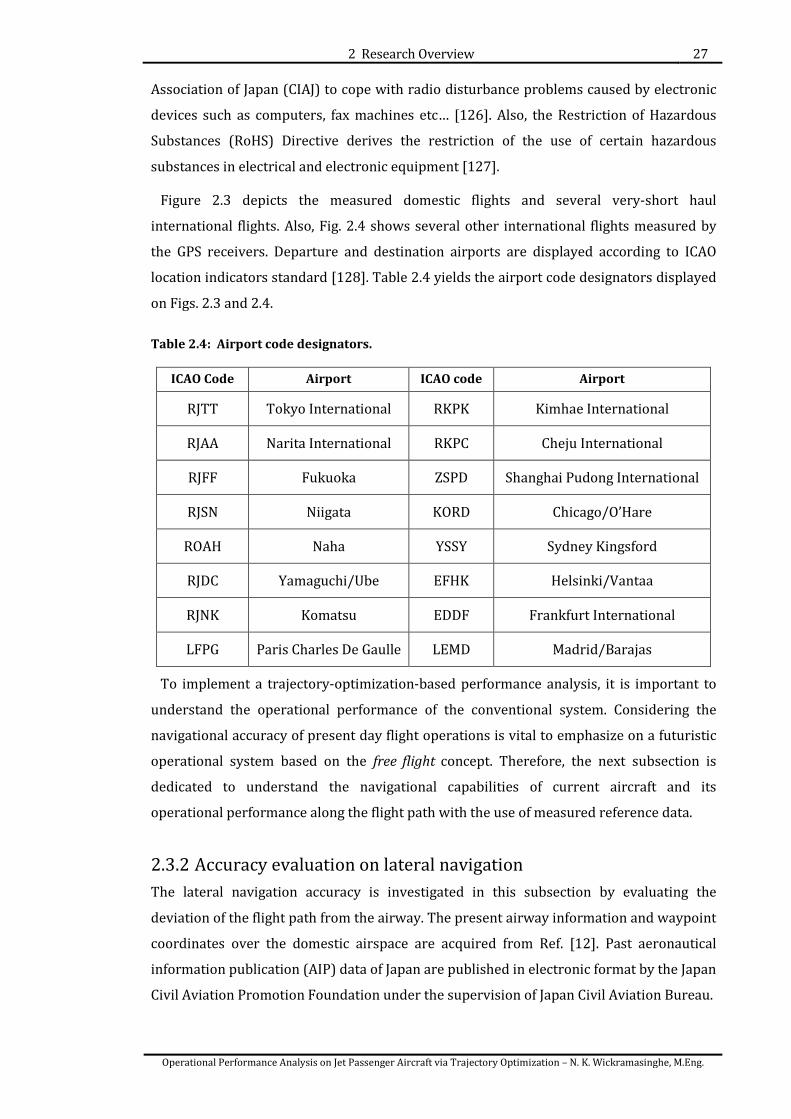
2 Research Overview 27
Operational Performance Analysis on Jet Passenger Aircraft via Trajectory Optimization – N. K. Wickramasinghe, M.Eng.
Association of Japan (CIAJ) to cope with radio disturbance problems caused by electronic
devices such as computers, fax machines etc… [126]. Also, the Restriction of Hazardous
Substances (RoHS) Directive derives the restriction of the use of certain hazardous
substances in electrical and electronic equipment [127].
Figure 2.3 depicts the measured domestic flights and several very-short haul
international flights. Also, Fig. 2.4 shows several other international flights measured by
the GPS receivers. Departure and destination airports are displayed according to ICAO
location indicators standard [128]. Table 2.4 yields the airport code designators displayed
on Figs. 2.3 and 2.4.
Table 2.4: Airport code designators.
ICAO Code Airport ICAO code Airport
RJTT Tokyo International RKPK Kimhae International
RJAA Narita International RKPC Cheju International
RJFF Fukuoka ZSPD Shanghai Pudong International
RJSN Niigata KORD Chicago/O’Hare
ROAH Naha YSSY Sydney Kingsford
RJDC Yamaguchi/Ube EFHK Helsinki/Vantaa
RJNK Komatsu EDDF Frankfurt International
LFPG Paris Charles De Gaulle LEMD Madrid/Barajas
To implement a trajectory-optimization-based performance analysis, it is important to
understand the operational performance of the conventional system. Considering the
navigational accuracy of present day flight operations is vital to emphasize on a futuristic
operational system based on the free flight concept. Therefore, the next subsection is
dedicated to understand the navigational capabilities of current aircraft and its
operational performance along the flight path with the use of measured reference data.
2.3.2 Accuracy evaluation on lateral navigation The lateral navigation accuracy is investigated in this subsection by evaluating the
deviation of the flight path from the airway. The present airway information and waypoint
coordinates over the domestic airspace are acquired from Ref. [12]. Past aeronautical
information publication (AIP) data of Japan are published in electronic format by the Japan
Civil Aviation Promotion Foundation under the supervision of Japan Civil Aviation Bureau.

2 Research Overview 28
Operational Performance Analysis on Jet Passenger Aircraft via Trajectory Optimization – N. K. Wickramasinghe, M.Eng.
In this analysis, the 3D- position data of the aircraft are processed on the assumption
that the Earth is a sphere although the position data from the GPS data loggers are based
on the WGS84 system. The disposition occurs due to this assumption is considered to be
negligible. The following process is applied to estimate the lateral deviation from the
predetermined airway [129].
Two arbitrary consecutive waypoints are considered as 1P and 2P along the airway. As
illustrated on Fig. 2.5, the two geocentric unit vectors to 1P and 2P are given as 1r and 2r .
Also, the geocentric unit vector xr represents an arbitrary position of the aircraft xP .
Figure 2.5: Definition of geocentric unit vectors and deviation angle.
The unit vector normal to the plane created by 1r and 2r is nr and is calculated by Eq.
(2.1).
21
21
rrrr
r××
=n (2.1)
The inclination between xr vector and the plane created by 1r and 2r is defined as angle
ϕ and is evaluated as shown in Eq. (2.2).
( )nx rr ⋅= arcsinϕ (2.2)
The deviation E between the aircraft’ position and the airway is calculated from Eq. (2.3)
by using the Earth radius ER , where km6371=ER according to the WGS84 datum. The
angle ϕ is given in radians.
ϕERE = (2.3)

2 Research Overview 29
Operational Performance Analysis on Jet Passenger Aircraft via Trajectory Optimization – N. K. Wickramasinghe, M.Eng.
The calculated deviation is the distance between aircraft’s position at an arbitrary time
and an exclusive interval configured by the airway over the Earth’s surface. In order to
distinguish the required interval, a decision condition is acquired as following;
In Fig. 2.6, xpr vector is considered which is the projection of xr vector on the 21rr plane.
Figure 2.6: Definition of projection vector.
If the definition of vector xr is considered as,
nx rrrr 12111 xxx ++= (2.4)
then the following relationship is used to define the vector xpr from 1r and 2r vectors.
[ ] [ ] xnT rrrr 1
21321 ,,,, −=xxx (2.5)
2111 rrr xx +=xp (2.6)
The decision condition for vector xpr to exist within the interval configured by 1r and 2r
is,
0,0 21 >> xx (2.7)
The decision condition is illustrated in Fig. 2.7.
Figure 2.7: Decision condition for required interval allocation.

2 Research Overview 30
Operational Performance Analysis on Jet Passenger Aircraft via Trajectory Optimization – N. K. Wickramasinghe, M.Eng.
Three graphical examples are given in Figs. 2.8 ~ 2.10, along the RJTT ⇔ RJFF flight route.
Figure 2.8: Flight route (RJTT -> RJFF) and airway RNAV Y20 (16th May 2011).
Figure 2.9: Flight route (RJFF -> RJTT) and airway YOKAT SID + RNAV Y23 (25th June 2011).
Figure 2.10: Flight route (RJFF -> RJTT) and airway YOKAT SID + RNAV Y23 (08th March
2014).

2 Research Overview 31
Operational Performance Analysis on Jet Passenger Aircraft via Trajectory Optimization – N. K. Wickramasinghe, M.Eng.
Table 2.5: Airway description and adjustments (May 2011- June 2014).
Airway Description and adjustments
RNAV Y20 Waypoints:
TETRA 354626N 1401556E ARASI 351055N 1354754E SEKID 353925N 1392830E GINGI 350540N 1351651E TAKAO 353725N 1390838E WAKIT 350158N 1345532E KOSYU 353344N 1383328E KAMMY 345928N 1344119E MAGOH 352634N 1373856E CLOVE 344927N 1335113E SWING 352322N 1371529E BASIL 343056N 1322541E OWARI 352106N 1365858E PASLI 342019N 1313858E OSAKI 351807N 1363737E STOUT 341127N 1310058E HIKNE 351415N 1361037E KIRIN 340718N 1304919E KRAMA 351308N 1360257E EBISU 340220N 1303528E
Adjustments: -Waypoint establishment: ‘WAKIT’ effective from 15 Dec 2012. -Waypoint abolishment: ‘TOYOTA’ effective from 18 Oct 2012. -Waypoint establishment: ‘STOUT’ effective from 18 Oct 2012. -Waypoint establishment: ‘GINGI’ effective from 6 Feb 2012.
YOKAT SID + RNAV Y23 Waypoints:
YOKAT 331824.0N 1304954.8E HALKA 341306N 1345902E KOHZA 332110.5N 1310116.1E FLUTE 343219N 1365749E BRAID 332305.6N 1310911.1E ENSYU 343236N 1380203E LUFFY 333312.0N 1321837.3E BOKJO 343232N 1382306E SANJI 335458.4N 1333940.0E BRIGE 343223N 1384817E YANKS 340749.0N 1342925.3E BATIS 343205N 1394214E
Adjustments: -YOKAT TWO SID->YOKAT THREE SID effective from 03 May 2012. - IGOSO Transition abolishment: effective from 26 Jul 2012. -YANKS Transition establishment: effective from 26 Jul 2012.
In Figs. 2.8~2.10, green solid line depicts the flight route measured by the GPS data logger
and the red dotted line represents the airway which is believed to be the pilot input in the
FMC. Standard instrument departure routes (SID) are assigned according to airport’s
geographical location while area navigation (RNAV) routes allow aircraft to choose any
course within a network of navigation beacons. The purple lines denote the deviation of
the flight route from the airway and are magnified by 500 times for feasibility. Also, airway
data used in this analysis and adjustments applied during the time period of data
allocation are given in Table 2.5.
In case of flights from Tokyo (Haneda) to Fukuoka, RNAV route Y20 is generally referred
to be the predetermined airway. The Y20 route is designed close to the great circle route
where the heading of the aircraft varies slightly along the en-route flight. Therefore, the
lateral deviation of the aircraft is quite small. According to departure procedures at Tokyo
(Haneda) airport, aircraft performs a rapid climb with a steep turn in order to maintain
safe separation with arrival flights. Also, departures from Haneda airport are usually
handled in the Northern part of airport’s airspace. Furthermore, latter part of the
measured flights shows deviated en-route flight procedures between waypoints CLOVE
and BASIL. It can be considered that these flights have experienced vectoring under air

2 Research Overview 32
Operational Performance Analysis on Jet Passenger Aircraft via Trajectory Optimization – N. K. Wickramasinghe, M.Eng.
traffic flow control procedures due to the increased air traffic handling at the Fukuoka
airport. Numerical data on annual number of landings at Fukuoka airport provided in
Table 2.6 [21] confirms that the amount of air traffic handling has rapidly increased
between year 2011 and 2012.
Table 2.6: Annual number of landings at Fukuoka airport (2007-2012).
Year 2007 2008 2009 2010 2011 2012
Domestic 63,242 59,251 59,848 60,438 60,632 67,119
International 8,214 8,443 7,832 8,237 8,921 10,865
Total 71,456 67,694 67,680 68,675 69,553 77,984
Furthermore, according to data from [21], the passenger increase percentage in 2012
compared to 2011 along the Tokyo->Fukuoka flight route is 103% while the passenger
increase percentage in2012 compared to 2011 along the Narita->Fukuoka flight route is
288%. During the 3 years period of data allocation, the airway RNAV Y20 remains almost
unchanged except for the removal of waypoint TOYOTA and the addition of waypoints
WAKIT, STOUT and GINGI.
Two examples are illustrated in Figs. 2.9 and 2.10 for flight cases from Fukuoka to Tokyo
(Haneda) due to airway adjustments occurred during the time period of data allocation.
Typically, YOKAT standard instrument departure (SID) route is used prior to the
connection with the RNAV route Y23 in case of flights from Fukuoka to Tokyo. Also,
contrary to Y20 airway, RNAV Y23 airway includes a significant heading change at
waypoint FLUTE. This is due to the air traffic flow management procedures implemented
at Haneda airport. Haneda airport handles departures in the Northern part of the airport
while accommodating arrivals from the Southern side of the airport. As the figure shows,
large route deviations are visible at LUFFY, IGOSO, YANKS and FLUTE waypoints. These
results denote that aircraft perform in-bound or out-bound turns at a certain waypoint in
order to proceed to the next waypoint according to the FMS. Also, large deviations appear
on both sides of the airway after passing over FLUTE. This is due to vectoring procedures
implemented by the ATC to manage a smooth air traffic flow towards the airport.
Figures 2.11 and 2.12 represent the total route deviations from the predetermined air
route for RJTT -> RJFF and RJFF -> RJTT flights respectively. The deviations are plotted in
respect to longitude and each coloured solid line represents a specific flight.
Corresponding waypoints are also given on the bottom of each figure for reference
feasibility. Results show that deviations along the Y20 RNAV route are relatively smaller
than deviation values along the Y23 RNAV route.

2 Research Overview 33
Operational Performance Analysis on Jet Passenger Aircraft via Trajectory Optimization – N. K. Wickramasinghe, M.Eng.
Figure 2.11: Deviation from RNAV Y20 airway (RJTT->RJFF).
Figure 2.12: Deviation from YOKAT SID + RNAV Y23 airway (RJFF->RJTT).
These results signify that aircraft performance characteristics considerably vary according
to the assigned flight route as a result of conventional ATC procedures. The purpose of this
study is to provide a platform that strengthens the concept of TBO operations which is to
reduce these characteristic variations and increase the aircraft performance by providing
the pilot with sufficient freedom to select an optimal route considering weather and traffic
conditions through a centralized ATM system.
Furthermore, a statistical expression is provided as shown in Figs. 2.13 ~ 2.15. All
figures hold the standard deviation values in respect to mean value of deviation. In Figs.
2.13 and 2.14, plots are categorized according to the aircraft type while the total deviation
plotting in Fig. 2.15 are categorized according to the flight route. The subjected track data
are usually measured at window seat for better GPS signal reception. Therefore, the above
results include the bias error of the location of GPS receiver, in other means the radius of
the aircraft’s fuselage. Hence, the aircrafts’ fuselage values, defined in table 2.7 [130],
[131] [132] & [133], are deducted from the analysed route deviations for clarity.

2 Research Overview 34
Operational Performance Analysis on Jet Passenger Aircraft via Trajectory Optimization – N. K. Wickramasinghe, M.Eng.
Figure 2.13: Mean and standard deviation values of route deviation (RJTT->RJFF).
Figure 2.14: Mean and standard deviation values of route deviation (RJFF->RJTT).
Figure 2.15: Route deviation comparison for total GPS track data.

2 Research Overview 35
Operational Performance Analysis on Jet Passenger Aircraft via Trajectory Optimization – N. K. Wickramasinghe, M.Eng.
Table 2.7: Values of aircraft fuselage radius.
Aircraft type Fuselage radius [m]
Boeing 737-800 1.77
Boeing 747-400 3.05
Boeing 767-300 2.36
Boeing 777-200 2.93
Mean values on route deviation in case of both flight routes are distributed in a similar
range while the standard deviation show different characteristics between the two flight
routes. The small values of mean deviation show that modern aircraft are capable of
performing highly precise flight missions along the assigned flight routes. Also the varied
standard deviation values represent the distributed characteristics of flight routes due to
the conventional ATC procedures.
This subsection concentrates on the performance of airplane in an individual basis. To
understand the operational performance of a system in a broader scale, flight data
covering the entire national airspace are required. The next subsection is dedicated to
introduce the radar data used in the study and its validity and applicability in research to
improve the conventional ATC system. The characteristics of the radar data including an
analysis on data accuracy are also explained.
2.4 Air route surveillance radar track data The air route surveillance radar track data (referred to as RDP data here on) utilized in
this thesis consists of time-series data based on the radar data processing (RDP) system.
The RDPS system automatically tracks and processes information data provided by air
route surveillance radar (ARSR) and oceanic route surveillance radar (ORSR) and flight
plan data provided by the flight data processing section (FDPS) of the Fukuoka Air Traffic
Management Center (ATMC) [134]. Finally, the smoothed position data of the aircraft are
displayed on the so called Integrated En-route Control System (IECS). In Japan, the four
area control centres (Sapporo, Tokyo, Fukuoka and Naha) allocate data from ARSR and
ORSR which the geographical locations are shown in Fig. 2.16 [135].
Since 2014, JCAB has started to distribute a series of RDP data to enable wider
participation in research to promote the CARATS project. These aircraft track data include
all scheduled commercial IFR flights in Japan’s en-route airspace. The data parameters
included in the distributed data are given in table 2.8. Also, an example of full day radar

2 Research Overview 36
Operational Performance Analysis on Jet Passenger Aircraft via Trajectory Optimization – N. K. Wickramasinghe, M.Eng.
coverage is illustrated in Fig. 2.17. The colour distinction represents the flight altitude of
each flight profile.
Figure 2.16: En-route radar facilities in Japan.
Figure 2.17: Commercial flights over Japanese airspace (9th May 2012).

2 Research Overview 37
Operational Performance Analysis on Jet Passenger Aircraft via Trajectory Optimization – N. K. Wickramasinghe, M.Eng.
Table 2.8: RDP data parameters.
Flight time (sec) Virtual call sign Latitude
(deg) Longitude
(deg) Altitude
(m)
2.4.1 Traffic congestion at major airports Time histories of departures/arrivals at seven major airports are verified to understand
the propensity of traffic congestion in an airport-wise basis.
An area of NM10 radius around each airport is considered. If the distance from an
airport to an aircraft’s location is less than NM10 , it is considered to be either a
departure or an arrival from or to that specific airport. Initial and terminal time histories
and direct distances from the airport of each flight are considered to categorize between
departures and arrivals.
Results on departures/arrivals are illustrated in Figs. 2.18 ~ 2.21 and Figs. 2.22 ~ 2.25 for
Tokyo (Haneda) and Fukuoka airports respectively. In Figs. 2.18 and 2.22, red coloured
triangles represent departures while cyan coloured triangles represent the arrivals.
Figures 2.19 and 2.23 depict the histograms of number of handled aircraft in an hourly
basis. Finally, Figs. 2.20, 2.21, 2.24 and 2.25 are given for a visual understanding on how
departure/arrival routes are set according to airport’s geographical locations and
assigned ATC procedures to that specific airport. Similar to Fig. 2.17, the colour distinction
denotes the flight altitude of each flight profile. Obtained information from this analysis is
referred in the flight trajectory optimization chapter in comparing with the optimal results.
Tokyo (Haneda) airport operates both domestic and international flights with four
runways. From the results it is clear that full-scale operations at the airport begin from
0600 Hrs mainly with departures. Results from Fig. 2.18 express that simultaneous
parallel approaches and segregated approaches/departures are also implemented during
peak hours. In case of Haneda airport, operations are quite frantic throughout the day.
Haneda airport is Japan’s main hub for domestic operations. As shown in Figs. 2.20 and
2.21, flights from/to all over Japan are operated to/from the Haneda airport. From the
results, it is understood that the highest number of departures was recorded at 38 during
0700 Hrs. ~ 0800 Hrs. time period and the most number of landings handled were 38
during 1300 Hrs. ~ 1400 Hrs. and 2000 Hrs. ~ 2100 Hrs. time periods. Furthermore, the
most number of aircraft were handled during 2000 Hrs. ~ 2100 Hrs. time period with 38
arrivals and 34 departures averaging 83.0 minutes between two operations.

2 Research Overview 38
Operational Performance Analysis on Jet Passenger Aircraft via Trajectory Optimization – N. K. Wickramasinghe, M.Eng.
Figure 2.18: Time histories of departures/arrivals at Tokyo (Haneda) airport (9th May 2012).

2 Research Overview 39
Operational Performance Analysis on Jet Passenger Aircraft via Trajectory Optimization – N. K. Wickramasinghe, M.Eng.
Figure 2.19: Frequency of departures/arrivals at Tokyo (Haneda) airport (9th May 2012).

2 Research Overview 40
Operational Performance Analysis on Jet Passenger Aircraft via Trajectory Optimization – N. K. Wickramasinghe, M.Eng.
Figure 2.20: Departure routes at Tokyo (Haneda) airport (9th May 2012).
Figure 2.21: Arrival routes at Tokyo (Haneda) airport (9th May 2012).

2 Research Overview 41
Operational Performance Analysis on Jet Passenger Aircraft via Trajectory Optimization – N. K. Wickramasinghe, M.Eng.
Figure 2.22: Time histories of departures/arrivals at Fukuoka airport (9th May 2012).

2 Research Overview 42
Operational Performance Analysis on Jet Passenger Aircraft via Trajectory Optimization – N. K. Wickramasinghe, M.Eng.
Figure 2.23: Frequency of departures/arrivals at Fukuoka airport (9th May 2012).
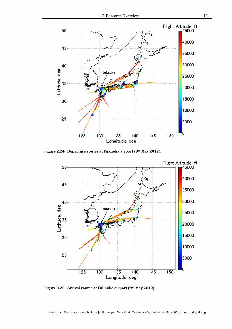
2 Research Overview 43
Operational Performance Analysis on Jet Passenger Aircraft via Trajectory Optimization – N. K. Wickramasinghe, M.Eng.
Figure 2.24: Departure routes at Fukuoka airport (9th May 2012).
Figure 2.25: Arrival routes at Fukuoka airport (9th May 2012).

2 Research Overview 44
Operational Performance Analysis on Jet Passenger Aircraft via Trajectory Optimization – N. K. Wickramasinghe, M.Eng.
On the other hand, Fukuoka airport is usually opened for operations between 0700 Hrs.
and 2200 Hrs. Operators at Fukuoka airport face a daunting task, especially during rush
hours to handle the airport operations efficiently with a single air strip. Figure 2.23 shows
that air traffic tends to peak between 0900 Hrs. ~ 1300 Hrs and 1600 Hrs. ~ 2000 Hrs. The
highest number of landings was recorded at 21 during 1700 Hrs. ~ 1800 Hrs. time period
and the highest number of departures was recorded at 18 during 1000 Hrs. ~ 1100 Hrs.
time period. The highest number of aircraft was handled during the time period of 1700
Hrs. ~ 1800 Hrs. with a total number of 35 aircraft averaging 1.71 minutes between two
operations.
This preliminary evaluation reveals the great potency of RDP data being applied in
performance evaluations. In-depth analysis on aircraft operations (airport-wise aircraft
handling efficiency, departure/arrival sequence procedures according to aircraft type,
conflict detection and resolution techniques etc…) using RDP data will be conducted in
future research studies. Related studies based on SSR surveillance data are conducted
[136] & [137] and the scope will be extended to a broader scale by utilizing RDP data as
the reference data. In this thesis, RDP data are solely used as reference data to perform a
quantitative evaluation on aircraft performance in means of fuel consumption and flight
time.
2.5 Weather data model The Japan Meteorological Agency provides a variety of numerical weather prediction
(NWP) data in a grid point value (GPV) format depending on the forecasting requirements.
There are three main NWP models available and its specifications are given on table 2.9
[138]. These data are periodically updated and are available for non-commercial use.
Table 2.9: Numerical weather prediction model specifications.
Global Spectral Model (GSM)
Meso Scale Model (MSM)
Local Forecast Model (LFM)
Forecast range (Initial time)
84 hours (00, 06, 18 UTC) 264 hours (12 UTC)
15 hours (00,06,12,18 UTC) 33 hours (03,09,15,21 UTC)
9 hours (00,03,06,09,12,15,18,21 UTC)
Forecast domain Global Japan East Asia Eastern part of Japan globe East Asia
Grid spacing 20 km 5 km 2 km
Horizontal grids (1920-60)×960 721×577 551×801
Pressure layers (Data acquired) 1000, 925, 850, 700, 600, 500, 400, 300, 250, 200, 150, 100 hPa (GSM)
Physical elements Geopotential altitude, temperature, vertical flow, relative humidity, wind velocity

2 Research Overview 45
Operational Performance Analysis on Jet Passenger Aircraft via Trajectory Optimization – N. K. Wickramasinghe, M.Eng.
Furthermore, the GSM model as mentioned above possesses two different models; one
model covering the weather conditions of the entire globe and the other covering a more
specified area around Japan which is provided by the JMA. Evaluated results on the
forecast accuracy of above data have shown that these NWP data are sufficiently accurate
to be applied in performance parameter estimation as well as in flight trajectory
optimization [139]. The application and evaluation process of these data are provided in
the latter part of the study.
2.6 Aircraft performance model (APM) The accurate estimation of aircraft performance is vital to implement an efficient ATM
system. An aircraft performance model is the core in computing aircraft trajectories and
has a key role to play in developing future ATM systems. Many aircraft performance
models exist but very few of them are accessible to public due to the sensitivity of data and
developer’s policies. These models are generally based on reference performance data and
aircraft performance manuals of aircraft manufacturers. Boeing performance software
INFLT/REPORT and Airbus Performance Engineering Program (PEP) are examples for
high quality aircraft performance reference data by aircraft manufacturers. These data are
highly confidential and most are not allowed access. Other models include,
• Total Airspace and Airport Modeller (TAAM): This is a fast-time gate-to-gate
software developed by Jeppesen to simulate airport and airspace operations. It has
the capability to compute 4D full airspace and flight profiles [140].
• General Aircraft Modelling Environment (GAME): GAME is developed and
maintained by EUROCONTROL that includes a database consists of parameters for
different models and constitutes a set of aircraft modeling tools that allow the
generation and optimization of aircraft models and compare the characteristics of
different models [141].
• Base of Aircraft Data (BADA) family 3 and family 4: These models are developed
and maintained by EUROCONTROL Experiment Centre (EEC) which includes
performance data for a large amount of aircraft types. BADA family 3 mdoel is
based on total energy model (TEM) under ISA conditions. BADA family 4 is a joint
development by EEC and Boeing Research & Technology Europe (BR&TE). It is
consdiered to be highly accurate for all types of power plants (jets, turboprops and
piston engines) and valid for the entire flight envelope including non-clean
configurations of the aircraft [142]. The access to BADA family 3 is provided
through license agreement but the access to family 4 is highly regulated.

2 Research Overview 46
Operational Performance Analysis on Jet Passenger Aircraft via Trajectory Optimization – N. K. Wickramasinghe, M.Eng.
• Other local models: There are also other APMs developed for local objectives such
as the APM of Boeing 767-300ER (referred to as UOM APM hereon) applied for
analysis of optimal aircraft cruise considering wind effects [143].
The aircraft performance estimation highly relies on accurate computations of fuel
consumption in different flight conditions. Feasibility in accessing data, applicability of
performance data into analytical programs and existence of data for a large variety of
aircraft types are important in reviewing the operational performance of aircraft and the
operating system. Therefore, in this study BADA family 3 aircraft performance data are
acquired to investigate the individual performance of aircraft and implement a
quantitative evaluation on operational performance of the current ATM system.
2.6.1 Base of Aircraft Data (BADA) Model - Family 3 BADA is an aircraft database based on the kinetic approach to aircraft performance
modelling that has been developed and maintained by EEC. The kinematic approach
defines the direct modelling of path characteristics of the aircraft without attempting to
model the underlying physics [144]. The model definitions and performance estimation
equations explained in this subsection are extracted from Refs. [145] and [146].
The BADA modelling process is generally divided into three parts as following;
• Data Preparation: This section includes all the required performance reference
data over a large variety of aircraft. Following reference aircraft performance data
categories are considered to be necessary in BADA modelling process.
General characteristics
Operating characteristics
Aircraft performance characteristics
Aircraft configurations and speed characteristics
• Identification Process: In this section, the non-linear parameter estimation
problem is treated by splitting the problem into several linear sub-problems to
obtain the global optimal solution through an iterative scheme. Instead of dealing
with engine type, aerodynamic configuration and thrust level setting as separate
models, generalized models are used which are valid for all flight phases. The
parameters are achieved by so called BADA Enhanced Approach to Modelling
(BEAM) related to both operational and airline performance.
• Validation Process: The validation process includes checking the behaviour of
developed models in respect to input performance data, cross validation of the

2 Research Overview 47
Operational Performance Analysis on Jet Passenger Aircraft via Trajectory Optimization – N. K. Wickramasinghe, M.Eng.
BEAM implementation and validation of developed models in respect to real data.
The advantage of using this model is that it is intensively checked for calculation
errors to gain highly accurate data.
BADA model provides four performance data files unique to each aircraft. They are
operational performance file (OPF), airline performance file (APF), performance table file
(PTF) and performance table data file (PTD). OPF and APF files are generated as results of
the BEAM identification process while the PTF and PTD files are results of the BEAM
implementation.
The main models utilized in this study are aerodynamics model, engine thrust model and
fuel consumption model. Each model has its own characteristics and operational
constraints depending on the aircraft. The following symbols are used to define the
equations used to estimate aircraft’s performance parameters.
a : speed of sound [ ]sm L : lift [ ]N
0g :gravitational acceleration [ ]2sm M : Mach number
FF : fuel flow [ ]minkg S : wing reference area [ ]2m
p : ambient pressure [ ]Pa T : ambient temperature [ ]K
R : real gas constant [ ]KdegkgJ Thr : engine thrust [ ]N
pH : pressure altitude [ ]ft TASV : true airspeed [ ]sm
m : aircraft mass [ ]kg ρ : air density [ ]3mkg
D : aerodynamic drag [ ]N σ : fuel flow coefficient [ ]kNminkg
tG : temperature gradient [ ]Kft wG : mass gradient [ ]Kkg
2.6.1.1 Aerodynamic model
When the flight path angle γ is given, the lift coefficient LC is defined as Eq. (2.8).
SVgmC
TASL
⋅⋅⋅
⋅⋅=
20
21
cosρ
γ (2.8)
Under the nominal conditions, the drag coefficient DC is defined as a function of lift
coefficient as shown in Eq. (2.9).
2,2,0 LCRDCRDD CCCC ×+= (2.9)
The subscript CR represents the coefficients related to cruise phase of the aircraft.
Therefore, the aerodynamic drag is derived as follows;
SVCD TASD ⋅⋅⋅⋅= 22
1 ρ (2.10)

2 Research Overview 48
Operational Performance Analysis on Jet Passenger Aircraft via Trajectory Optimization – N. K. Wickramasinghe, M.Eng.
2.6.1.2 Engine thrust model The BADA model provides data to calculate the following thrust levels.
• Maximum climb and take-off
• Maximum cruise
• Descent
The engine thrust available for climb phase is calculated as a function of geopotential
pressure altitude pH and the thrust available for cruise and descent phases are calculated
as a ratio of the thrust available at the climb phase. This ratio factor TCRC is a global
aircraft parameter which is defined as the maximum cruise thrust coefficient.
For climb phase the maximum thrust is derived as Eq. (2.11).
⋅⋅+−⋅= 2
312
1climbmax_ 1 pTcTcTc
pTc HCC
CH
CThr (2.11)
Coefficients 1TcC , 2TcC and 3TcC are aircraft-based thrust coefficients provided in the
BADA model. The dimensions for pressure altitude are given as feet in the above equation.
Thrust available for cruise phase is shown in Eq. (2.12).
max_climbTcrcruise ThrCThr ⋅= (2.12)
The thrust available for decent phase is given as a ratio of the maximum climb thrust as
depicted in Eqs. (2.13) and (2.14) depending on the transition altitude des,pH .
( )des,max_climbhighdes,_highdes, ppT HHThrCThr >⋅= (2.13)
( )des,max_climblowdes,_lowdes, ppT HHThrCThr <⋅= (2.14)
As the reference data does not include des,pH , this study only considers the Eq. (2.13) to
estimate the engine thrust.
2.6.1.3 Fuel consumption model The thrust specific fuel consumption (fuel flow coefficient) σ is specified as a function of
the true airspeed.
+×=
21 1
f
TASf C
VCσ (2.15)
For all flight phases except idle descent and cruise, fuel flow nomFF is computed as a
nominal value while for idle thrust descent conditions, fuel flow minFF is computed as

2 Research Overview 49
Operational Performance Analysis on Jet Passenger Aircraft via Trajectory Optimization – N. K. Wickramasinghe, M.Eng.
minimum value. Fuel flow in cruise phase cruiseFF is calculated as a ratio of nomFF in
which the ratio coefficient is given as fcrC . This coefficient is also based on the aircraft
type and is provided in the BADA model.
ThrFF ×=σnom (2.16)
( )ThrCFF ×⋅= σfcrcruise (2.17)
The descent fuel flow minFF is derived as a function of pH .
−×=
43min 1
f
pf C
HCFF (2.18)
The larger value is finally considered as the fuel flow of the aircraft at a certain position.
( )minnom ,max FFFFFF = (2.19)
2.6.1.4 Operational constraints BADA model consists of operational limits for each aircraft depending on aircraft mass,
airspeed and operating altitude.
The aircraft’s operating speed varies with the aircraft mass. Hence, the lowest possible
operating speed or the safety margin at a certain altitude is defined as a function of stall
speed.
stall3.1 VVCAS ×= (2.20)
The stall speed in Eq. (2.20) is calculated as a function of reference stall speed provided in
the BADA model and the ratio of mass at a certain flight position and reference mass which
is also provided in the BADA model.
refstall_refstall mmVV ×= (2.21)
The maximum flight altitude actmax,H for a given mass m is defined as following. The value
is decided as the minimum between the maximum operating altitude MOH and the
altitude calculated by referring to the maximum altitude maxH above standard mean sea
level (MSL) at maximum take-off weight under International Standard Atmospheric (ISA)
conditions.
( ) ( )[ ]mmGCTGHHH wTtMO −×+−∆×+= maxmaxactmax, ,min (2.22)

2 Research Overview 50
Operational Performance Analysis on Jet Passenger Aircraft via Trajectory Optimization – N. K. Wickramasinghe, M.Eng.
Variables mentioned as C with subscripts denote various types of coefficients related to
the performance of aircraft. These data are unique to the aircraft type which include in
each OPF.
Three mainly deployed aircraft types (referred to as Type A, Type B and Type C) in the
Japan domestic air transportation system are reviewed in this study. Type A is a short-to-
medium rage narrow body twin-engine jet airliner, Type B is a mid-to-large size, long-
range wide body twin-engine jet airliner. Type C is long-range, wide body, twin-engine jet
airliner. Type D aircraft is considered only in the performance parameter estimation to
review the performance characteristics of international long-haul flights. This aircraft is
also categorized under long-range, wide body, twin-engine aircraft class. The Following
tables represent the performance parameters used in the operational analysis for above
aircraft. These data are defined in respective BADA performance files and are presented
here for better understanding of the reader.
Table 2.10: Performance parameters of Type A aircraft.
minm : 41150 [ ]kg Tc1C : 7104659.1 × [ ]N
refm : 65300 [ ]kg Tc2C : 6103872.5 × [ ]ft
maxm : 78300 [ ]kg Tc3C : 11100453.3 −× [ ]2ft1
S : 65.124 [ ]2m Tc4C : 6177.9 [ ]K
MOM 82.0 Tc5C : 3105132.8 −× [ ]K1
MOM (oper.)
: 78.0 TcrC : 95.0
MOV (CAS) : 280 [ ]kt f1C : 70057.0 [ ]kNminkg
refstall,V(CAS)
: 149 [ ]kt f2C : 3100681.1 × [ ]kt
maxH : 43100 [ ]ft f3C : 1104190.1 × [ ]minkg
CRD0,C : 2105452.2 −× f4C : 4105932.6 × [ ]ft
CRD2,C : 2105815.3 −× fcrC : 92958.0
tG : 110410.5 ×− [ ]Kft wG : 26974.0 [ ]kgft

2 Research Overview 51
Operational Performance Analysis on Jet Passenger Aircraft via Trajectory Optimization – N. K. Wickramasinghe, M.Eng.
Table 2.11: Performance parameters of Type B aircraft.
minm : 90011 [ ]kg Tc1C : 7102241.3 × [ ]N
refm : 154590 [ ]kg Tc2C : 6106718.5 × [ ]ft
maxm : 186880 [ ]kg Tc3C : 11103638.1 −× [ ]2ft1
S : 35.283 [ ]2m Tc4C : 5535.9 [ ]K
MOM 86.0 Tc5C : 3107598.3 −× [ ]K1
MOM (oper.)
: 80.0 TcrC : 95.0
MOV (CAS) : 310 [ ]kt f1C : 74220.0 [ ]kNminkg
refstall,V(CAS)
: 167 [ ]kt f2C : 3100605.2 × [ ]kt
maxH : 43100 [ ]ft f3C : 1105902.1 × [ ]minkg
CRD0,C : 2101112.2 −× f4C : 5104538.1 × [ ]ft
CRD2,C : 2102118.4 −× fcrC : 90048.0
tG : 110112.4 ×− [ ]Kft wG : 11823.0 [ ]kgft
Table 2.12: Performance parameters of Type C aircraft.
minm : 138100 [ ]kg Tc1C : 7101741.4 × [ ]N
refm : 208700 [ ]kg Tc2C : 6107757.5 × [ ]ft
maxm : 287000 [ ]kg Tc3C : 11105629.3 −× [ ]2ft1
S : 82.427 [ ]2m Tc4C : 4466.9 [ ]K
MOM : 87.0 Tc5C : 3108099.9 −× [ ]K1
MOM (oper.)
: 84.0 TcrC : 95.0
MOV (CAS) : 310 [ ]kt f1C : 54864.0 [ ]kNminkg
refstall,V(CAS)
: 149 [ ]kt f2C : 4101750.8 × [ ]kt
maxH : 43100 [ ]ft f3C : 3103262.3 × [ ]minkg
CRD0,C : 2108452.1 −× f4C : 6104211.6 × [ ]ft
CRD2,C : 2104604.4 −× fcrC : 93687.0
tG : 110125.6 ×− [ ]Kft wG : 3102253.7 −× [ ]kgft

2 Research Overview 52
Operational Performance Analysis on Jet Passenger Aircraft via Trajectory Optimization – N. K. Wickramasinghe, M.Eng.
In the next chapter, the estimation methods of air data and performance parameters are
discussed with the application of above data sources. Weather data interpolation and two
different approaches on performance parameter estimation according to obtained data
parameters from flight data sources are explained.

3 Estimation of Flight Parameters 53
Operational Performance Analysis on Jet Passenger Aircraft via Trajectory Optimization – N. K. Wickramasinghe, M.Eng.
3 ESTIMATION OF FLIGHT PARAMETERS
Chapter 3 confines attention to the process of estimating flight parameters from the two
types of data sources introduced in chapter 2 to investigate the operational performance
of the current system. This chapter garners data to construct the platform in promoting
the flight trajectory optimization proposed in this study.
An analysis on aircraft operational performance requires parameters which define the
aircraft’s motion and aircraft’s energy consumption. Aircraft are equipped with air data
computers (ADC) which estimate the airspeed from the computed dynamic pressure along
its motion. Also, aircraft performance predictions are evaluated in a high frequency by
using stored engine performance data and real-time inputs from the on-board systems.
Figure 3.1 shows a schematic overview of different types of antennas and sensors located
on the aircraft fuselage. They are used in gathering information, computing air data and
communicating with ground stations to maintain efficient and safe flight operations.
Figure 3.1: Aircraft antennas and sensors locations (http://malaysiaflipflop.blogspot.jp).
On the other hand, ground-based tracking systems such as ARSR and ORSR gather range
and azimuth measurements of multiple aircraft within its sectors and the radar data

3 Estimation of Flight Parameters 54
Operational Performance Analysis on Jet Passenger Aircraft via Trajectory Optimization – N. K. Wickramasinghe, M.Eng.
processing system (RDPS) processes the incoming data from multiple radar sources to be
finally viewed at ATC radar displays [147]. Following data are among the radar
surveillance data requirements.
• time history and aircraft horizontal position
• aircraft identification
• aircraft vertical position
• ground speed
SSR uses a different approach by transmitting a low energy signal assigned to a specific
aircraft and receive a response signal (not a reflective signal) which is analysed by the
aircraft’s transponder. The latest SSR mode S (select) includes a data linking capability
which provides a cooperative surveillance and communications system in addition to the
basic identification and altitude information [148]. This enables to acquire a wide variety
of air data processed by the ADC, which are commonly called as Downlink Aircraft
Parameters (DAPs). Furthermore, equipment such as Automatic Dependent Surveillance -
Broadcast (ADS-B) or data loggers which utilize conventional global navigation satellite
system (GNSS) provides time histories of geometric position and ground speed. Flight data
from an aircraft is usually acquired through a Quick Access Recorder (QAR). Though QAR
data provides a large variety of flight parameters over a total flight, access is highly
regulated due to company policy. Also, to study the operational performance of aircraft in
micro- and macro-scale, precise individual aircraft data and flight data over a vast area of
airspace are required.
This chapter concentrates on estimating air data and atmospheric data based on the two
types of flight data acquired. These estimations are then applied to estimate various
aircraft operational parameters to understand the current policies of airline companies
and to investigate critical areas in the current system in means of trajectory management
and operational cost optimization.
3.1 Air data computations Air data computation is related with the estimations of altitude and velocity in different
atmospheric conditions. The worldwide standard on computing air data is the ISA model
which is an idealized, steady state representation of the Earth’s atmosphere [149].
Generally, defining constants and equations in ISA are used to estimate atmospheric
conditions in non-disturbed air. However, this is not always practically true as various
phenomenon result continuous change in behaviour of the atmosphere. Therefore, a
validated process is highly essential to estimate these atmospheric conditions precisely in

3 Estimation of Flight Parameters 55
Operational Performance Analysis on Jet Passenger Aircraft via Trajectory Optimization – N. K. Wickramasinghe, M.Eng.
order to understand the aircraft’s performance accurately. The following subsections
review and estimate significant components of atmosphere and discuss the validation of
the estimating process by investigating application examples.
3.1.1 Altitude One of the key data parameters in an operational performance analysis is the flight
altitude of the aircraft and depending on the data source, output altitude could differ.
According to aviation altimetry, following could be distinguished as definitions of altitude
and Fig. 3.2 illustrates the overview of altitude definitions.
Figure 3.2: Definitions of altitude.
• Geometric altitude (True altitude): The exact or true distance between the
pressure level at which the aircraft is flying and the MSL.
• Geopotential altitude: This is the altitude at which the amount of work done to lift
a certain amount of mass through a hypothetical atmosphere with constant gravity,
equals to the amount of work done to lift the same mass through the true
atmosphere with gravity decreases with altitude.
• Indicated altitude: The altitude above MSL read by the flight crew from the
aircraft’s altimeter when calibrated to the regional MSL pressure, also known as
QNH altitude. In Japan, the transition altitude for local QNH is ft000,14 .
• Pressure altitude: The altitude above MSL read by the flight crew from the
aircraft’s altimeter when calibrated to the International Standard Atmosphere
(ISA) conditions ( inHg92.29 or hPa1013.25 ). This altitude is commonly referred
as flight level (FL) where 1FL = 100ft.

3 Estimation of Flight Parameters 56
Operational Performance Analysis on Jet Passenger Aircraft via Trajectory Optimization – N. K. Wickramasinghe, M.Eng.
Altitude settings in an aircraft have to be adjusted according to the variations in
atmospheric pressure. During operations, the barometric subdial of the cockpit altimeter
is set at one of the following three settings [150].
• QNE: barometric subdial is set to inHg92.29 .
• QNH: barometric subdial setting for altimeter to indicate elevation of airport.
• QFE: barometric subdial setting for altimeter when approach for a landing.
The Newton’s gravitational law implicates that,
2
0
00
2
00
+=
=
ga Hrrg
Hrgg (3.1)
where 0r is the effective radius of the Earth at a specific latitude according to Lambert’s
equations and the standard value is km766.6356 which is consistent with the adopted
gravitational acceleration value. Also, aH is the height above the center of the Earth and
gH is the geometric altitude. Then, there are two governing equations which define the
Earth’s atmosphere. The first equation is the state equation of the atmosphere relating its
pressure p , density ρ and temperature T with the assumption that air behaves as a dry,
perfect gas that obeys the laws of Charles and Boyle,
RTp ρ= (3.2)
where R is the universal gas constant, equal to KdegJ/kg053.287 . The second equation is
that the hydrostatic balance equates the compression of the atmosphere due to gravity to
the pressure gradient force working in the opposite direction,
( ) ( ) 0=+∂∂ zzg
zp ρ (3.3)
where g is the gravitational acceleration corresponds to the given z geometrical height.
Geometrical height is the vertical distance above the World Geodetic System 1984
(WGS84) reference ellipsoid. The height of MSL above the WGS84 reference ellipsoid
usually depends on the geographic position but is ignored here for simplicity. Therefore,
zH g ≈ (3.4)
Hence, the geometric altitude is used to define the hydrostatic balance as,

3 Estimation of Flight Parameters 57
Operational Performance Analysis on Jet Passenger Aircraft via Trajectory Optimization – N. K. Wickramasinghe, M.Eng.
( ) ( ) 0=+∂∂
ggg
HHgHp ρ (3.5)
Substituting Eq. (3.2) to Eq. (3.5) yields,
( ) ( )
( ) 0=+∂∂
g
gg
g HRTHpHg
Hp (3.6)
3.1.2 Airspeed The pressure developed by the forward moving motion of a body in incompressible flow is
called the dynamic pressure q , which is related to the airspeed of the body relative to air
or commonly known as true airspeed TASV by the equation
2
21
TASVq ρ= (3.7)
Usually on an aircraft, the dynamic pressure can be directly converted using the
Bernoulli’s law and the air density at sea level 0ρ , to the indicated airspeed IASV .
202
1IASVq ρ= (3.8)
The pressure at sea level 0p and total pressure tp at the position of aircraft are used to
derive the IASV . The pressure difference of tp and ambient pressure ap at the flight
altitude equates the dynamic pressure q .
−
+−
= 1175.3
1
00
0
ppppV at
IAS ρ (3.9)
The indicated airspeed corrected for position and instrument error is called the calibrated
airspeed CASV . Calibrated airspeed is equal to the true airspeed in standard atmosphere at
sea level [151]. Due to the negligible influence of position and instrument error, the
assumption in Eq. (3.10) is considered.
IASCAS VV ≅ (3.10)
The equivalent airspeed EASV is the corrected calibrated airspeed for adiabatic
compressible flow for a particular altitude. Equivalent airspeed is equal to calibrated
airspeed in standard atmosphere at sea level [151]. Therefore, we could define EASV as
follows;

3 Estimation of Flight Parameters 58
Operational Performance Analysis on Jet Passenger Aircraft via Trajectory Optimization – N. K. Wickramasinghe, M.Eng.
−
+−
= 1175.3
1
0 a
ataEAS p
pppVρ
(3.11)
The true airspeed is the airspeed of an aircraft relative to undisturbed air. TASV can be
derived by the relative density correlation with EASV as given in Eq. (3.12).
ρρ0
EASTAS VV = (3.12)
The aircraft also measures its true heading (by compass considering magnetic variation)
and position (by GPS), enabling to estimate the ground speed GV and determine the wind
speed wV from the following vector relationship.
wGTAS VVV −= (3.13)
When the pressure and density of air is known for a certain flight altitude, then TASV can
be derived by CASV as,
21
1
12
0
00 112
1111
2
−
−
−++
−=
−
−κκ
κκ
ρκ
κρκ
κCASTAS V
ppppV (3.14)
where 4.1=κ is the specific heat for air. Similarly, CASV can be derived from TASV when
indicated airspeed is not available.
21
1
12
00
0 112
1111
2
−
−
−++
−=
−
−κκ
κκ
ρκ
κρκ
κTASCAS V
ppppV (3.15)
In such case, true airspeed is estimated by the difference between ground speed and wind
speed as mentioned in Eq. (3.13). The required wind data are acquired from the JMA NWP
model data explained in the previous chapter.
The process of atmospheric data estimation varies according to the data source and the
parameters obtained from them. A similar application with two different approaches is
discussed in this section, defining essential equations to obtain necessary atmospheric
data from the two data sources. In order to obtain weather data at each 3D- position of the
aircraft, the study uses a 2D- horizontal interpolation method and a 1D- linear

3 Estimation of Flight Parameters 59
Operational Performance Analysis on Jet Passenger Aircraft via Trajectory Optimization – N. K. Wickramasinghe, M.Eng.
interpolation method for vertical interpolation. These methods are depicted in Eq. (3.16)
and Eq. (3.17) respectively for an arbitrary physical quantity X .
( ) ( )( )
( )( )( ) ( )( )
( )( )( )
( )( )( )( )
( ) ( )( )( )( )
( )221212
1112
1212
21
211212
1211
1212
22
,,
,,,
θφθθφφθθφφθφ
θθφφθθφφ
θφθθφφθθφφθφ
θθφφθθφφθφ
XX
XXX
−−−−
+−−−−
+
−−−−
+−−−−
=
(3.16)
( ) ( ) ( ) ( )( ) ( )
( )( )ngpgpngpngp
nnn pHH
pHpHpXpXpXHX −
−−
+=+
+
1
1,,θφ (3.17)
Figure 3.3: Horizontal 2D- interpolation and vertical linear interpolation.
Thus, the subscripts n and 1+n respectively denote the lower and upper pressure
surfaces in between which the subjected altitude of the aircraft exists. Also, the subscripts
1 and 2 represent the latitude φ and longitude θ which form the NWP data grid, and
satisfies the range 21 φφφ << and 21 θθθ << .
3.1.3 Atmospheric data from GPS track data GPS data logger data includes the geometrical altitude. Hence, the geopotential altitude
gH is calculated as,
gg
gp HHr
rH
+
=0
0 (3.18)
Two pressure layers 1p and 2p are considered from the weather data with corresponding
geopotential altitudes as 1_gpH and 2_gpH , and corresponding temperatures as 1T and 2T .

3 Estimation of Flight Parameters 60
Operational Performance Analysis on Jet Passenger Aircraft via Trajectory Optimization – N. K. Wickramasinghe, M.Eng.
The following assumption is considered which derives that temperature linearly decreases
along the altitude where b is the temperature lapse rate.
1_2_
12
gpgp HHTTb
−−
= (3.19)
An arbitrary position of the aircraft is subjected with its geopotential altitude as gpH
( 2_1_ gpgpgp HHH << ) at which the temperature can be calculated from Eq. (3.20).
( ) ( )gpgpgpgp HHbTHHbTT −−=−+= 2_21_1 (3.20)
Also, the relationship between atmospheric pressure and geopotential altitude can be
derived as Eq. (3.21) and Eq. (3.22).
( ) bRg
gpgpa
THHbT
pp −
−+=
1
1_1
1 (3.21)
( ) bRg
gpgpb
THHbT
pp −
−−=
2
2_2
2 (3.22)
Pressure ap is calculated from the weather data ( 1p , 1T , 1_gpH ) from the lower pressure
layer and pressure bp is calculated from the weather data ( 2p , 2T , 2_gpH ) from the upper
pressure layer. These two values are usually not identical. Therefore, the exact pressure at
the aircraft’s position when it is in the troposphere is estimated as a weighted mean value.
1_2_
1_
1_2_
2_
gpgp
gpgpb
gpgp
gpgpa HH
HHp
HHHH
pp−−
+−−
= (3.23)
In case of 710−<b , the aircraft’s altitude is considered to be above the tropopause
( km11 ), also known as the isothermal atmosphere, where the pressure is calculated
according to Eq. (3.24).
( )
−−= 1_
11 exp gpgp HH
RTgpp (3.24)
3.1.3.1 Pressure altitude The cockpit altimeter is an aneroid barometer that measures air pressure. The altimetry
equation shown in Eq. (3.25) which forms the basis for the calibration of cockpit altimeter
is used to calculate the pressure altitude pH .

3 Estimation of Flight Parameters 61
Operational Performance Analysis on Jet Passenger Aircraft via Trajectory Optimization – N. K. Wickramasinghe, M.Eng.
−
=−
10
0 gR
p ppTH
λ
λ (3.25)
The subscript 0 denotes the ISA atmospheric values on MSL with hPa25.10130 =p and
K15.2880 =T . The standard adiabatic lapse rate K/m0065.0−=λ . Pressure Altitude above
tropopause is calculated according to Eq. (3.26).
11000ln +−=t
tp p
pg
RTH (3.26)
The subscript t denotes the ISA atmospheric values at the tropopause with
hPa32.226=tp and K65.216=tT .
According to the aeronautical information manual of Japan, aircraft should perform
instrument flight rules (IFR) procedures at cruise altitudes between ft29000 and
ft41000 [152]. These operational altitude levels are in ft1000 intervals depending on the
heading direction of the aircraft as shown in table 3.1.
An example on pressure altitude estimation is given in Figs. 3.4 and 3.5. In Fig. 3.4, the
red solid line represents the measured altitude or the geometrical altitude from the GPS
data logger. The green line is the pressure altitude calculated from ISA conditions without
using weather data. The blue line depicts the estimated pressure altitude from the
weather data. It is apparent that in this flight the aircraft was performing its cruise at an
altitude of ft40000 . Also, Fig. 3.5 shows that aircraft’s altitude fluctuates around the
determined cruise altitude. Results from a quantitative evaluation for deviation from
cruise altitude are illustrated in Figs. 3.6 and 3.7. Each coloured line and each coloured dot
in the figures represent a different flight scenario from the reference data.
Table 3.1: Cruising altitude.
Flight direction in magnetic bearing
000 ~ 179 180 ~ 359
FL410 FL400
FL390 FL380
: :
FL310 FL320
FL290 FL300

3 Estimation of Flight Parameters 62
Operational Performance Analysis on Jet Passenger Aircraft via Trajectory Optimization – N. K. Wickramasinghe, M.Eng.
Figure 3.4: Example for pressure altitude estimation (28th Aug. 2011, RJTT->RJFF).
Figure 3.5: Zoomed view of cruise altitude (28th Aug. 2011, RJTT->RJFF).
Figure 3.6: Altitude deviation from determined cruise altitude.

3 Estimation of Flight Parameters 63
Operational Performance Analysis on Jet Passenger Aircraft via Trajectory Optimization – N. K. Wickramasinghe, M.Eng.
Figure 3.7: Mean and standard deviation values of altitude deviation.
Results show that the maximum deviation is less than m100 from the assigned cruise
altitude. Furthermore, the small values for mean and standard deviation prove that the
aircraft are capable of performing along an assigned altitude with high accuracy. Generally,
the vertical measurement error from GPS is considered to be around 1.5 times greater
than the lateral measurement error [153]. Yet, by comparing the results in Figs. 2.15 and
3.7, it is clear that the lateral deviation is larger than the altitude deviation. The predicted
reason is that the cruise altitude remains constant throughout a long period of time while
the flight route is based on an airway constructed from a series of waypoints. Hence, the
aircraft has to perform heading changes in order to maintain its course over the
predetermined flight route.
Figures 3.8 and 3.9 yield an example for airspeed and Mach number estimation. The blue
line represents the estimated airspeed and Mach number by utilizing weather data. The
red line shows the airspeed and Mach number estimated according to ISA conditions. In
other means, the red lines represent the ground speed and Mach number without winds
respectively. Usually, aircraft performs the cruise phase at a constant Mach number [154].
Figure 3.8: Example for airspeed estimation (17th Oct. 2011, RJTT->RJFF).

3 Estimation of Flight Parameters 64
Operational Performance Analysis on Jet Passenger Aircraft via Trajectory Optimization – N. K. Wickramasinghe, M.Eng.
Figure 3.9: Example for Mach number estimation (17th Oct. 2011, RJTT->RJFF).
Figure 3.10: Mach speed deviation from operational Mach number.
The example on speed estimation is performed by a Type C aircraft (introduced in chapter
2) which usually operates at a cruising Mach number of 0.84 according to BADA model.
Therefore, by assuming this value is given at the cruise flight, a quantitative evaluation is
done on airplane speed performance as given in Fig. 3.10. Obtained results yield a
dispersion of about 0.02 ~ 0.03 from the assigned Mach number denoting the high
performance capabilities of modern airplanes. Figure 3.11 shows statistical characteristics
of this quantitative evaluation. The mean value shows a very small deviation for all cases
while the standard deviation also possesses a very small value. These numerical results
also confirm the high performance capabilities of modern aircraft and concrete the fact
that safety margins on aircraft separations and route selections can be relaxed due to the
reliability of aircraft’s performance.

3 Estimation of Flight Parameters 65
Operational Performance Analysis on Jet Passenger Aircraft via Trajectory Optimization – N. K. Wickramasinghe, M.Eng.
Figure 3.11: Mean and standard deviation values of Mach speed deviation.
3.1.4 Atmospheric data from radar surveillance data Radar surveillance data consists of similar flight parameters as of the GPS data logger
except for the altitude. Radar data includes the pressure altitude pH which is transmitted
by the aircraft fitted transponder. As this transmitted altitude is always set to QNE setting,
ISA model is applied to estimate the static pressure p of the aircraft’s position. Equation
(3.27) and Eq. (3.28) are respectively used to estimate the static pressure at troposphere
(temperature gradient layer) and stratosphere (temperature constant layer).
Rg
p
THT
ppλλ −
+=
0
00 (3.27)
( )
−−= 11000exp p
tt H
RTgpp (3.28)
As the weather data are in an isobar structure, upper and lower pressure surfaces can be
distinguished in between which the aircraft’s position is located. Then, the temperature
lapse rate can be calculated by using Eq. (3.29) leading to the calculation of temperature at
the aircraft’s altitude as derived in Eq. (3.30).
1_2_
12
gpgp HHTTb
−−
= (3.29)
( ) ( )gpgpgpgp HHbTHHbTT −−=−+= 2_21_1 (3.30)
Equations (3.29) and (3.30) are identical to the Eqs. (3.19) and (3.20) but the physical
quantities denoted by subscripts 1 and 2 in this section satisfy 12 ppp ≤≤ condition.
The geopotential altitude gpH can be calculated in two ways by using the upper and lower

3 Estimation of Flight Parameters 66
Operational Performance Analysis on Jet Passenger Aircraft via Trajectory Optimization – N. K. Wickramasinghe, M.Eng.
pressure surface values as 1_ pgpH and
2_ pgpH . Equations (3.31) and (3.32) respectively
correspond to the troposphere and stratosphere.
( ) bRg
gppgp
THHbT
pp
−
−+=
1
1__1
1
1 (3.31a)
( ) bRg
pgpgp
THHbT
pp
−
−−=
2
_2_2
2
2 (3.31b)
( )
−−= 1__1
1exp gppgp
tHH
RTg
pp (3.32a)
( )
−−= 2__2
2exp gppgp
tHH
RTg
pp (3.32b)
Theoretically, 1_ pgpH is equal to
2_ pgpH but in practical environment these two values are
not identical. Therefore, as shown in Eq. (3.33) the exact geopotential altitude is calculated
as a weighted mean value.
12
1_
12
2_ 21 pp
ppH
pppp
HH pgppgpgp −−
+−−
= (3.33)
This calculated geopotential altitude is used to estimate other physical quantities related
to weather by using Eq. (3.17).

4 Flight Trajectory Optimization 67
Operational Performance Analysis on Jet Passenger Aircraft via Trajectory Optimization – N. K. Wickramasinghe, M.Eng.
4 FLIGHT TRAJECTORY OPTIMIZATION
The proposed flight trajectory optimization model is thoroughly explained in this chapter,
from airplane’s basic dynamics of motion to application of Dynamic Programming method
and performance index allocation for problem setting. Also, an insight into the cost index
concept and its influence on the aircraft performance is reviewed to express the
significance of considering the cost index in the optimization model and its impact on the
potential benefits.
4.1 Equations of motion In this subsection, point mass approximated 3-D motion of an aircraft is considered to
generate kinematic equations to be applied in the mathematical model of this study.
Though the formulation process is known to be a classical problem as explained in [155],
only the final formulations are used in modelling definitions in recent studies. The process
is solved and summarized according to [155] in order to refresh the reader’s
understanding on general formulation of aircraft’s 3-D motion.
The airplane is assumed to be a point mass and its instant motion at an arbitrary time t
can be given by,
( )tr = position vector, ( )tV = velocity vector, ( )tm = mass
Based on an inertial system, the kinematic vector equation can be derived as,
Vr=
tdd (4.1)
An airplane's motion is generally expressed by six degree of freedom (DOF) equations of
motion by selecting a set of coordinates to represent the position and velocity vectors with
six scalar equations. If an instant position of the point mass, given by position vector r , is

4 Flight Trajectory Optimization 68
Operational Performance Analysis on Jet Passenger Aircraft via Trajectory Optimization – N. K. Wickramasinghe, M.Eng.
fixed in a system and rotates with angular velocity ω , the linear velocity of the point mass
is given as,
rωV ×= (4.2)
If r is taken as the vector i , j and k respectively, then it can be given as,
iωi×=
tdd , jωj
×=td
d , kωk×=
tdd (4.3)
An Earth-centred Earth-fixed system OXYZ is considered with a rotating coordinate
system Oxyz of which the x -axis is along the position vector, y -axis along the
equatorial plane orthogonal to x -axis and z -axis on the vertical plane. The definitions
are illustrated on Fig. 4.1 according to [155].
Figure 4.1: Definition of Earth-centred Earth-fixed axis and rotation axis.
The position vector is defined with by its magnitude r , its longitude θ and latitude φ .
The flight path angle γ of the aircraft is the angle between the local horizontal plane and
the velocity vector V . The heading angle ψ of the aircraft is measured positively about
the x -axis. Unit vectors i , j and k are considered along the axes of the rotating system.
The coordinate systems are illustrated in Fig. 4.2 for better understanding on the

4 Flight Trajectory Optimization 69
Operational Performance Analysis on Jet Passenger Aircraft via Trajectory Optimization – N. K. Wickramasinghe, M.Eng.
coordinate transformation. The vertical considered here is the ( )Vr, plane. Let x′ , y′
and z′ axes be parallel to the rotating axes x , y and z respectively. Also a 111 zyPx
system is considered such that 1y axis is parallel to the velocity vector. This 111 zyPx
system is deduced from the zyxP ′′′ system by a rotation ψ in the horizontal plane,
followed by a rotation γ by the vertical plane.
Figure 4.2: Coordinate systems, transformation and aerodynamic forces.
This transformation can be derived as a matrix equation according to Eq. (4.4).
−
−=
′′′
1
1
1
1000cossin0sincos
cossin0sincos0001
zyx
zyx
γγγγ
ψψψψ (4.4)
The matrix multiplication results,
−−−=
′′′
1
1
1
cossincossinsinsincoscoscossin0sincos
zyx
zyx
ψψγψγψψγψγ
γγ (4.5)
For any rotation matrix R acting on n , property of an orthogonal matrix is applied as,

4 Flight Trajectory Optimization 70
Operational Performance Analysis on Jet Passenger Aircraft via Trajectory Optimization – N. K. Wickramasinghe, M.Eng.
1−= RRT (4.6)
Hence, the Eq. (4.5) can be also written as,
′′′
−
−−=
zyx
zyx
ψψψγψγγψγψγγ
cossin0sincoscoscossinsinsincossincos
1
1
1
(4.7)
Therefore, the unit vector 1j along the 1y axis and parallel to V can be derived as,
kjij ψγψγγ sincoscoscossin1 ++= (4.8)
Hence, the velocity vector can be given as,
kjiV ψγψγγ sincoscoscossin VVV ++= (4.9)
Also, from Fig. 4.1, the angular velocity ω is derived on the Oxz plane as,
kiω φωφω cossin += (4.10)
In order to obtain the time derivative of r to solve the Eq. (4.1) with respect to the OXYZ
system using their components along the rotating system Oxyz , the evaluation of angular
velocity Ω of the rotating axes is required. The rotating system Oxyz is obtained by a
rotation θ about the positive Z -axis, followed by a rotation φ about the negative y -
axis. Therefore, the angular velocity can be derived as,
kjiΩttt d
dcosdd
ddsin θφφθφ +−= (4.11)
By using the Eq. (4.3) we deduce the time derivatives of i , j and k with respect to the
Earth-centred Earth-fixed system OXYZ as,
kjiΩittt d
dddcos
dd φθφ +=×= (4.12)
kijΩjttt d
dsinddcos
dd θφθφ +−=×= (4.13)
jikΩkttt d
dsindd
dd θφφ
−−=×= (4.14)
As the velocity vector can be expanded as Eq. (4.15), it can be re-written as Eq. (4.16).
t
rtr
t dd
dd
dd iirV +== (4.15)
kjirVt
rt
rtr
t dd
ddcos
dd
dd φθφ ++== (4.16)

4 Flight Trajectory Optimization 71
Operational Performance Analysis on Jet Passenger Aircraft via Trajectory Optimization – N. K. Wickramasinghe, M.Eng.
Identifying the vector components of this equation with Eq. (4.9), three scalar equations
can be derived as given in Eqs. (4.17) ~ (4.19) which are called the kinematic equations.
γsindd V
tr= (4.17)
φψγθ
coscoscos
dd
rV
t= (4.18)
r
Vt
ψγφ sincosdd
= (4.19)
These kinematic equations are used to derive the flight route settings and distance
calculations over a spherical Earth. Figure 4.3 reflects the general definition followed by
mathematical derivatives of the required parameters.
Figure 4.3: Definition on flight route settings over spherical Earth.
Generally, the design concept of flight route assumes a spherical Earth with radius 0R and
aircraft’s position is given by longitude θ , latitude φ and altitude H in a polar coordinate
system XYZ . The great circle route 21PP (GCR), defined as the shortest distance between
two waypoints, is reviewed here as the standard flight route. Let 0r and fr be the
geocentric unit vectors to initial point 1P and terminal point 2P respectively as given in
Eq. (4.20). The downrange angle x between these two points are obtained by considering
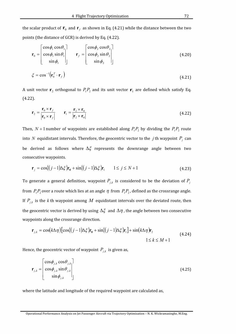
4 Flight Trajectory Optimization 72
Operational Performance Analysis on Jet Passenger Aircraft via Trajectory Optimization – N. K. Wickramasinghe, M.Eng.
the scalar product of 0r and fr as shown in Eq. (4.21) while the distance between the two
points (the distance of GCR) is derived by Eq. (4.22).
=
=
2
22
22
1
11
11
0
sinsincoscoscos
sinsincoscoscos
φθφθφ
φθφθφ
frr (4.20)
( )fT rr ⋅= −0
1cosx (4.21)
A unit vector 2r orthogonal to 21PP and its unit vector 1r are defined which satisfy Eq.
(4.22).
02
021
0
02 rr
rrr
rrrr
r××
=×
×=
f
f (4.22)
Then, 1+N number of waypoints are established along 21PP by dividing the 21PP route
into N equidistant intervals. Therefore, the geocentric vector to the j th waypoint jP can
be derived as follows where x∆ represents the downrange angle between two
consecutive waypoints.
( ){ } ( ){ } 111sin1cos 1 +≤≤∆−+∆−= Njjjj rrr 0 xx (4.23)
To generate a general definition, waypoint kjP , is considered to be the deviation of jP
from 21PP over a route which lies at an angle η from 21PP , defined as the crossrange angle.
If kjP , is the k th waypoint among M equidistant intervals over the deviated route, then
the geocentric vector is derived by using x∆ and η∆ , the angle between two consecutive
waypoints along the crossrange direction.
( ) ( ){ } ( ){ }[ ] ( ) 21, sin1sin1coscos rrrr 0 ηxxη ∆+∆−+∆−∆= kjjkkj
11 +≤≤ Mk (4.24)
Hence, the geocentric vector of waypoint kjP , is given as,
=
kj
kjkj
kjkj
kj
,
,,
,,
,
sinsincoscoscos
φθφθφ
r (4.25)
where the latitude and longitude of the required waypoint are calculated as,
4 Flight Trajectory Optimization 73
Operational Performance Analysis on Jet Passenger Aircraft via Trajectory Optimization – N. K. Wickramasinghe, M.Eng.
( ) ( )( )
== −−
kj
kjkjkjkj
XZ
,
,1,,
1, cos
cossinφ
θφr
r (4.26)
These definitions are used in the next sections to introduce the mathematical formulation
for the proposed trajectory optimization method.
4.2 Mathematical formulation An airplane’s motion is generally expressed by six degree of freedom (6-DOF) equations of
motion. The number of state variables is reduced from six to four by treating the airplane’s
dynamics with point mass approximations and omitting the state variables which
represent airplane’s attitude. Furthermore, the dynamics of velocity direction is neglected
while the dynamics of the velocity change which directly corresponds to energy is
considered. These assumptions are made with the motive of relaxing the mathematical
model and increase the feasibility of DP application.
An airplane’s three-dimensional translational motion is defined in Eqs. (4.27) ~ (4.30).
The graphical definition is illustrated on Fig. 4.4.
( )( )xaaTAS WV
HRt+
+= ψγ
φθ sincos
cos1
dd
0 (4.27)
( )( )yaaTAS WV
HRt+
+= ψγφ coscos1
dd
0 (4.28)
aTASVt
H γsind
d= (4.29)
( ) ( ) aaaES mgDTt
Vm γψψγγ sincoscosd
d−−=−− (4.30)
Equations (4.27) and (4.28) respectively represent the time derivatives or the angular
velocities of the airplane along longitude and latitude directions defined by airplane’s 3-D
position, true airspeed TASV , flight path angle aγ , azimuth angle aψ , zonal wind
component xW and meridional wind component yW . The subscript a denotes that
corresponding angles are defined with respect to air flow. Regarding wind components,
Westerly winds and Southerly winds are considered positive and the vertical wind
components are assumed to be negligible. Equation (4.29) derives the equilibrium of
forces acting on the airplane. The left hand side of Eq. (4.29) includes airplane’s Earth
speed (kinematic speed defined on the Earth-centered Earth-fixed coordinate system) ESV ,
and cosine components of flight path angle and azimuth angle differences. Flight path
angle γ and azimuth angle ψ are derived with respect to ground.

4 Flight Trajectory Optimization 74
Operational Performance Analysis on Jet Passenger Aircraft via Trajectory Optimization – N. K. Wickramasinghe, M.Eng.
Figure 4.4: 3-D Translational motion of the airplane.
Equations (4.27) ~ (4.29) are deformed according to the following format to create a
feasible calculation platform.
( ) xaaTAS WVHRtdt
dx+=+
∆∆
= ψγφθ sincoscos0 (4.31)
( ) yaaTAS WVHRtdt
dy+=+
∆∆
= ψγφ coscos0 (4.32)
aTASVt
Hdt
dH γsin=∆∆
= (4.33)
Equations (4.34) ~ (4.36) are obtained from above mathematical terms.
( ) ( )22yx WdtdyWdtdxl ⋅−+⋅−= (4.34)
TAS
a VdtdH⋅
=γsin (4.35)
TAS
a Vdtl⋅
=γcos (4.36)
Since 1cossin 22 =+ aa γγ , we get the following mathematical term as,
22
2 1cos
⋅
−=
⋅
=TASTAS
a VdtdH
Vdtlγ (4.37)
Hence, a mathematical expression for l is derived as,

4 Flight Trajectory Optimization 75
Operational Performance Analysis on Jet Passenger Aircraft via Trajectory Optimization – N. K. Wickramasinghe, M.Eng.
( ) 222 dHVdtl TAS −⋅= (4.38)
Equating the Eqs. (4.34) and (4.38) the following quadratic equation is achieved for dt .
( ) ( ) ( ) 222
22 dHVdtWdtdyWdtdx TASyx −⋅=
⋅−+⋅− (4.39)
is equal to,
( ) ( ) 22222 dHVdtWdtdyWdtdx TASyx −⋅=⋅−+⋅− (4.40)
The expansion of Eq. (4.40) gives,
222222222 22 dHVdtWdydtWdtdyWdxdtWdtdx TASyyxx −⋅=⋅−⋅++⋅−⋅+ (4.41)
Therefore,
( ) ( ) ( ) 02 2222222 =+++⋅+⋅−−+ dHdydxdtWdyWdxdtVWW yxTASyx (4.42)
Considering the roots of Eq. (4.42), dt is evaluated by,
( ) ( )( ) ( )( )( )222
2222222
2
422
TASyx
TASyxyxyx
VWW
dHdydxVWWWdyWdxWdyWdxdt
−+
++−+−⋅+⋅±⋅+⋅=
(4.43)
The Earth speed ESV is derived in Eqs. (4.44) ~ (4.46) from the relationship between
airplane’s true airspeed and wind.
aaTASxES VWV ψγψγ sincossincos += (4.44)
aaTASyES VWV ψγψγ coscoscoscos += (4.45)
aTASES VV γγ sinsin = (4.46)
Equations (4.44) ~ (4.46) are squared and added to derive a quadratic equation in Eq.
(4.47) to solve for ESV .
( ) ( )( ) ( ) ( )222
2222
sincoscossincos
sincoscossincos
aTASaaTASaaTAS
ESyESxES
VVV
VWVWV
γψγψγ
γψγψγ
++
=+−+− (4.47)
Hence, Eq. (4.48) is obtained.
( ) ( ) 0cossincos2 2222 =−+++− TASyxESyxES VWWVWWV ψψγ (4.48)

4 Flight Trajectory Optimization 76
Operational Performance Analysis on Jet Passenger Aircraft via Trajectory Optimization – N. K. Wickramasinghe, M.Eng.
4.3 Application of Dynamic Programming (DP) method This section discusses the algorithm of DP method and its application in the proposed
trajectory optimization model.
4.3.1 DP Algorithm Consider the general control formulation of the objective function given in Eq. (1.6).
Therefore, the optimal cost function opt can be defined as Eq. (4.49) when an optimal
control problem is solved from an arbitrary state x at time t to the terminal point.
( ) [ ] ( ) ( )( ) ( ) ( )( )
+= ∫ ttttttttt f
f
t
tffttuopt d,,,,,min,0
00,uxxxx ϕ (4.49)
A recursive definition could be given to the above optimal cost function by considering an
infinitesimal value of td as shown in Eq. (4.50).
( )[ ]
( ) ( )( ) ( )
+++= ∫
+
+tttttttt opt
tt
ttttuopt d,dd,,min,d
d,fxuxx
( ) ( )( ) ( )( )ttttttt optud,dd,,min +++= fxux
(4.50)
This recursive definition provides a feasible combinatorial optimization platform for the
optimal control problem. Therefore, the state variables are quantized into an orthogonal
iso-grid at each interval of the independent variable which is commonly referred to as a
stage. The ‘cost’ of all the allowable transitions is then computed as each different
transition emanating of the same point in the state space corresponds to a different
control, which are considered to be analogous to the decision at that point.
The independent variable t is divided into tN increments and the k th increment is
yielded as follows.
( )( ) [ ]fttfk tttNkNktttt ,1,2,11 000 ∈+⋅⋅⋅=−−+= (4.51)
Accordingly, state variable x is divided into iN increments and the j th increment is
defined. This general formulation enables the setting of quantized n state variables at
each grid point of the 1+n dimensional state space grid.
( ) ( ) ( )( )( ) 1,,2,1,,2,11minmaxmin, +⋅⋅⋅=⋅⋅⋅=−−+= iiiiiji NjniNjxxxx (4.52)
Hence, the discrete objective function could be derived by the time step kk ttt −=∆ +1 as
given in Eq. (4.53) where the optimality condition provides ( )kkopt t,x as a functional of
the state variables at time kt .

4 Flight Trajectory Optimization 77
Operational Performance Analysis on Jet Passenger Aircraft via Trajectory Optimization – N. K. Wickramasinghe, M.Eng.
( ) ( )[ ]kkoptuuukkopt ttn
,min,21 ,11 xx +∆=⋅⋅⋅++ (4.53)
where, ∆ is the increment of Lagrangian at each transition. Also, kx and 1+kx
respectively depict the state vectors at time kt and 1+kt .
( ) ( )( ) ( ) ( )( ) ttttttttk
k
t
t∆==∆ ∫
+ uxux ,,d,,1 (4.54)
The terminal condition is given in Eq. (4.55).
( ) [ ]1111 ,, ++++ =tttt NNNNopt txt ϕx (4.55)
Figure 4.5: Dynamic Programming logic on trajectory transition.
The illustrative definition of the transition between two stages is denoted in Fig. 4.5. The
number of combinations searched between two stages in order to obtain the right hand
side of Eq. (4.53) is ( )2
1
1
+∏
=
n
iiN [97].
In this study, the Dynamic Programming method is applied in the trajectory optimization
model, by concentrating on four state variables and three control variables. The airplane’s
3-D position of latitude, longitude and altitude, and the speed are considered. The control
variables are given as airplane’s flight path angle, heading angle and engine thrust. A state
space grid is defined by discretized state variables which are applied in Eqs. (4.27) ~
(4.30) to evaluate the control variables. For the feasibility, the distribution of wind over
the reviewed airspace is assumed constant within the flight time. This assumption was
made because the change of wind conditions during the average flight time subjected in
this study is negligible [139]. Hence, the equations of motion are independent functions of

4 Flight Trajectory Optimization 78
Operational Performance Analysis on Jet Passenger Aircraft via Trajectory Optimization – N. K. Wickramasinghe, M.Eng.
time which enable the utilization of monotonically varied state variable, downrange as the
independent variable and reduce the dimension of state space by 1. Trajectory transition
between each two grid points within a stage is considered to perform the algorithm. It is
assumed that the rate of change between two grid points is constant. This is achieved by
treating the utilized control variables as constants during a stage transition.
Figure 4.6: Optimization process with Dynamic Programming method.
The definition given in Fig. 4.5 is illustrated here with the subjected state and control
variables. In this application, the downrange angle along with other three state variables
constitutes an equidistant orthogonal grid. System parameters based on the Earth-centred
Earth-fixed coordinate system are transformed into the Polar coordinate system to create
a feasible calculation platform. As discussed in section 4.1, airplane’s translational motion
defined by ( )dydx, along longitude and latitude directions are defined by downrange
angle x and crossrange angle η as ( )ηx , . The optimization problem is to steer the system
by considering the equations of motion mentioned in Eqs. (4.27) ~ (4.30), from an initial
state ( )0000 ,,, xηVH at 0t to a final state ( )ffff VH xη ,,, at ft so that the fuel consumed
is minimized.
4.3.2 Performance Index The core objective of this optimization method is to reduce the fuel consumption.
Therefore the basic definition of the performance index can be given as to minimize the
time integral of fuel flow FF during the flight time ( )0tt f − .
( )∫=
ft
tttFF
0
d (4.56)

4 Flight Trajectory Optimization 79
Operational Performance Analysis on Jet Passenger Aircraft via Trajectory Optimization – N. K. Wickramasinghe, M.Eng.
A modified version of Eq. (4.56) is given in Eq. (4.57) in order to consider the trade-off
with flight time (explained in detail in the next section) with µ as the weighting
parameter or penalty for the flight time which has similar dimensions as the fuel flow.
( ) ( )∫ −+= ft
t f ttttFF0
0d µ (4.57)
To express a general definition for performance index evaluation, an arbitrary state
( )kjih kkkVH xη ,,, at stage k is reviewed on the grid where an optimal trajectory with a
given initial state is already obtained. Subscripts h , i and j are respectively
correspondent to arbitrary discretized values of altitude, speed and crossrange angle. The
minimized performance index or the optimal performance index at stage k is given as
( )kjihopt kkkVH xη ,,, . Hence, the optimal solution or the optimal transition (in this study,
the optimal trajectory) from stage k to stage 1+k can be derived as,
( ) ( ){ } ∆+=
+++
+++
→→→+ kjihopt
jjiihhkjihopt kkk
kkkk
kkkkk
VHVH xηxη ,,,min,,,
11
1111 1
(4.58)
The increment of performance index for each transition is derived by ∆ where the fuel
flow is assumed to be constant during each transition.
tFF k
k∆=∆ +1x
x (4.59)
4.3.3 Computational time reduction Computational time is a trade-off between calculation accuracy and grid resolution in the
DP method. With the available computational hardware, one has to determine a proper
grid resolution in order to obtain optimal solutions with sufficient accuracy within a
reasonable amount of computational time based on the problem. In particular, future
systems in which operations would highly rely on real-time-based simulations, similar to a
system reviewed in this study, prefer trajectory optimizers that could generate optimal
trajectories according to airplane and weather conditions in a real-time basis. Increasing
the performance of hardware is one of the solutions to overcome this challenge which is
not always a plausible selection. Therefore, a mathematical technique is required to relax
the calculation platform while achieving a valid solution to the problem.
An iterative computational technique called the Moving Search space Dynamic
Programming or MS-DP method was introduced in this optimization model [156] & [157].
This method requires a reference (initial) trajectory since it is based on a combination of
gradient method and DP method. The advantage of applying this method is that it does not
search for the global optimum by considering the whole state space since the beginning of

4 Flight Trajectory Optimization 80
Operational Performance Analysis on Jet Passenger Aircraft via Trajectory Optimization – N. K. Wickramasinghe, M.Eng.
calculations. This method commences with a partial state space with the provided initial
trajectory as shown in Fig. 4.7. The initial trajectory is defined as a steady level flight at the
initial altitude provided in the model.
Figure 4.7: The partial search space in Moving Search space Dynamic Programming method.
This partial grid is set by considering the physical motion of the airplane. If the obtained
partial optimal trajectory is different from the initial trajectory, the newly obtained
trajectory becomes the initial trajectory for the next iteration of calculations. This method
repeats until the newly obtained trajectory identically converges to the previous optimal
trajectory at a certain number of iterations. This method significantly reduces the number
of calculations required though it does not guarantee the global optimum, which is one of
the advantages in the original DP logic. Yet, this method is considered to be effective in
airliner trajectory applications in which the global optimality is not a problem in general.
Furthermore, the global optimum could be confirmed through the original DP method
with some penalty of computational time upon requirement.
4.4 Cost Index (CI) The fundamental understanding of the Cost Index (CI) concept is to minimize the overall
trip cost by means of a trade-off between operating costs per hour and incremental fuel
burn. This idea was introduced with the Performance Data Computer (PDC) which is the
predecessor of the Flight Management System. This section discusses the concept of the
cost index, its influence in aircraft performance and its application in the proposed study.
4.4.1 Definition of the cost index concept The cost index is a parameter set in the airplane cockpit, which determines how the
airplane will perform its flight. It provides the capability of adjusting the flight profile by
flying faster to recover delays or flying slower to conserve fuel consumption [158]. The
cost index is fundamentally given as the relationship between fuel- and time-related costs
[28] [29]. The total cost C of a specific trip is the sum of fixed and variable costs.

4 Flight Trajectory Optimization 81
Operational Performance Analysis on Jet Passenger Aircraft via Trajectory Optimization – N. K. Wickramasinghe, M.Eng.
fixedTF CCCC TF +⋅+⋅= (4.60)
where, FC is the unit cost of fuel, F is the total fuel consumption of the operation, TC is
the unit cost of time, T is the total flight time of the operation and fixedC is the fixed costs
which are independent of time such as landing charges, rentals, depreciation etc… . To
minimize the overall cost of the operation, only the first two terms in Eq. (4.60) need to be
considered. Hence, a mathematical expression can be defined for the cost index CI as,
TF ⋅+=
F
TI C
CC (4.61)
Cost Index (CI) = lbcents
hrCCCI
F
T
//$
costFuelcostTime
== (4.62)
For any airplane, 0=CI provides the minimum trip for fuel and does not consider the
cost of time. Conversely, the maximum CI provides the minimum time trip which does not
consider the cost of fuel. Yet, neither of the extreme values of cost index is used in real
operations. Instead, operators select an optimal value based on their company cost
structure modified if necessary for individual flight requirements. As a result, CI typically
varies among models, may also vary for individual routes and also according to the FMS
manufacturer. A series of allowable cost indices for different classes of airplanes are given
in table 4.1 for Ref. [28].
Table 4.1: Cost index ranges for given Boeing airplanes.
Prior to a flight, the pilot inserts the company cost index in the performance initialization
page of the flight management computer (FMC) along with other basic flight data to
implement vertical navigation (VNAV) calculations as shown in Fig. 4.8. The input of CI
enables the calculation of economy (ECON) climb, cruise and descent speeds. ECON
defines the speed schedule calculated to minimize the operating cost.

4 Flight Trajectory Optimization 82
Operational Performance Analysis on Jet Passenger Aircraft via Trajectory Optimization – N. K. Wickramasinghe, M.Eng.
Figure 4.8: Cost index setting in the Flight Management Computer.
Main factors affecting the CI are time-related direct operating cost and fuel costs. Fuel
costs are usually easier to understand than the more complicated time-related costs. Ref.
[28] cites that many operators do not take full advantage of this tool, although a recent
airline case study denotes potential annual savings of US$ 4-5 million were achievable
‘with a negligible effect on schedule’.
Performing either minimum fuel or minimum time operations are not practicable. An
optimal cost index has to be carefully selected considering the fuel costs of which the
prices can be highly varied due to operating locations, fuel tankering and fuel hedging, and
time-related costs which include not only the flight operational time, but also flight crew
wages, maintenance costs (correlates with operational usage time) etc… .
4.4.2 Impact of cost index on aircraft performance In this part, the effect of cost index on aircraft performance is reviewed according to the
flight phase.
4.4.2.1 CLIMB The normal economy climb speed schedule of the FMC minimizes the trip cost. This is
usually varied according to the gross weight of the airplane and the cost index. Therefore,
the fixed speed profile provided by the FMC is a function of cost index and weight. The
climb phase is generally performed in three phases [159] which are,
• Assigned indicated airspeed until flight level 100: 250 kt indicated airspeed is
maintained until flight level 100 unless permitted due to ATC terminal procedures.
• Constant indicated airspeed until crossover altitude
• Constant Mach number until top of climb (TOC) .
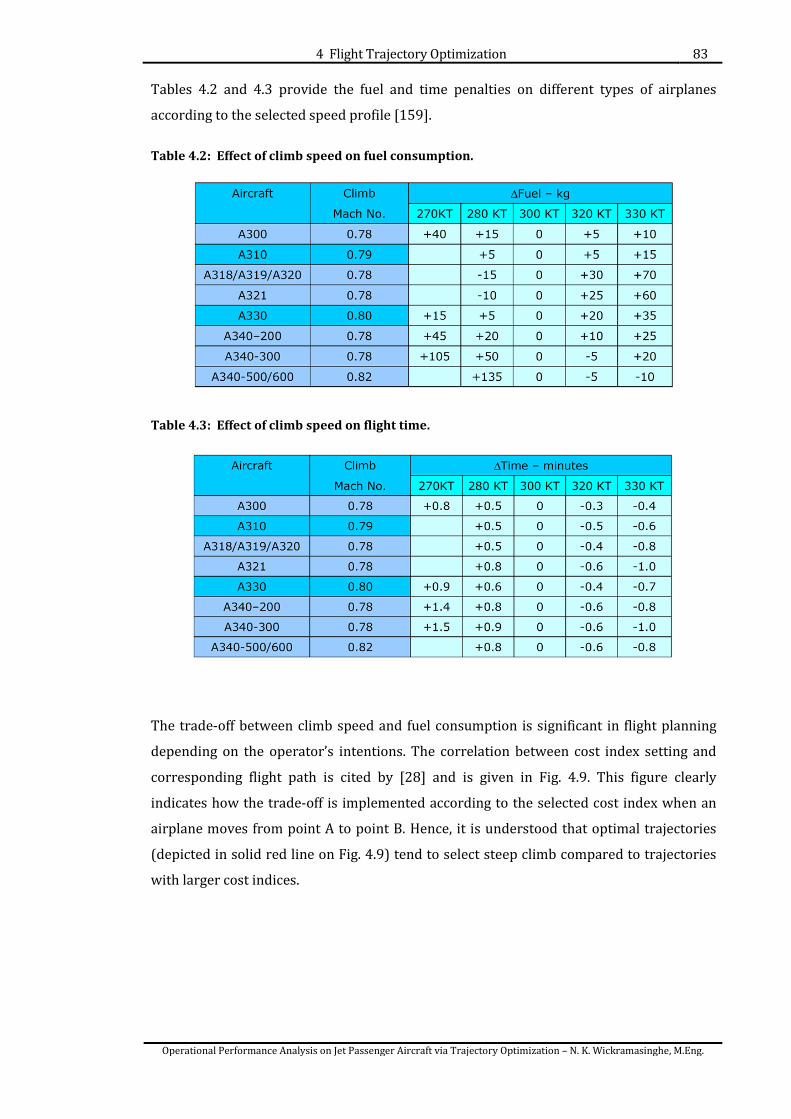
4 Flight Trajectory Optimization 83
Operational Performance Analysis on Jet Passenger Aircraft via Trajectory Optimization – N. K. Wickramasinghe, M.Eng.
Tables 4.2 and 4.3 provide the fuel and time penalties on different types of airplanes
according to the selected speed profile [159].
Table 4.2: Effect of climb speed on fuel consumption.
Table 4.3: Effect of climb speed on flight time.
The trade-off between climb speed and fuel consumption is significant in flight planning
depending on the operator’s intentions. The correlation between cost index setting and
corresponding flight path is cited by [28] and is given in Fig. 4.9. This figure clearly
indicates how the trade-off is implemented according to the selected cost index when an
airplane moves from point A to point B. Hence, it is understood that optimal trajectories
(depicted in solid red line on Fig. 4.9) tend to select steep climb compared to trajectories
with larger cost indices.

4 Flight Trajectory Optimization 84
Operational Performance Analysis on Jet Passenger Aircraft via Trajectory Optimization – N. K. Wickramasinghe, M.Eng.
Figure 4.9: Effect of cost index in climb phase.
4.4.2.2 CRUISE The largest percentage of time and fuel of a flight is consumed in the cruise phase. A
careful selection of an optimal cost index for this phase can radically reduce fuel
consumption without asserting any negative impact on the time schedule.
The two theoretical speed profiles in a cruise flight are long range cruise (LRC) and
maximum range cruise (MRC). The LRC is derived as to achieve 1 percent of range by
trading off 3~5 percent of cruise velocity, which result about 1 percent decrease in fuel
mileage [28]. MRC is the fuel minimum speed for a given range.
The ECON speed selection considering the DOC can be given as Fig. 4.10 where MMR is
Mach for maximum range, MLR is Mach for long range and MMO is the maximum operating
Mach of the airplane.
Figure 4.10: Correlation between speed profile and operating costs.

4 Flight Trajectory Optimization 85
Operational Performance Analysis on Jet Passenger Aircraft via Trajectory Optimization – N. K. Wickramasinghe, M.Eng.
4.4.2.3 DESCENT The descent phase has similar characteristics to the climb phase in means of cost index
setting for an efficient flight. Figure 4.11 is provided for reference on how the cost index
setting would affect the descent profile of an airplane.
Figure 4.11: Effect of cost index in descent phase.
It is understood that the fuel minimum cost index (zero cost index) tends to set its top of
descent (TOD) point at an early stage to perform a descent with a low descent rate. The
graph yields that the increase in cost index setting for descent phase would provide a
steeper flight path with a later TOD, leading to a trade-off of shorter descent distance with
additional fuel burn. Procedures such as delayed-flaps approach (also known as low-drag
approach or noise abatement approach) and continuous descent approach are reviewed
for new operational procedures as fuel saving strategies. Aircraft manufacturers provide
following tips as efficient descent procedures to minimize the fuel consumption.
• Carefully planned descent profile.
• Selection of approporiate starting point for the descent.
• Selection of appropriate speed.
• Setting of idle thrust.
• Avoiding extended periods of low altitude flight.
• Configuration of optimal time for flap and landing gear engagement.
The overview reveals the significance of optimal cost index setting for fuel saving
strategies. Hence, as a part of the study, the proposed trajectory optimization model

4 Flight Trajectory Optimization 86
Operational Performance Analysis on Jet Passenger Aircraft via Trajectory Optimization – N. K. Wickramasinghe, M.Eng.
focuses on the conventional operational performance and potential benefits estimation
from the viewpoint of cost index setting.
4.4.3 Cost index application in trajectory optimization The performance index defined in Eq. (4.57) is considered here. It is built by considering
the minimum cost with the trade-off between fuel consumption and flight time. In other
terms, CI is considered as the key factor in setting the performance index to minimize the
operational cost. Equations (4.57) and (4.62) are integrated to obtain the following
definition for the optimal performance index.
( ) ∫∫ +⋅=
ff t
t T
t
t F tCttFFCJ00
ddmin (4.63)
The fuel consumption is proportional to the time integral of fuel flow FF [kg/s] in the first
term and the time integral of second term is proportional to flight time. The Eq. (4.63) is
converted into SI units and a simplified version is obtained. The process is described in
Eqs. (4.64) ~ (4.68).
[ ] ( ) [ ]∫ ∫+=
f ft
t
t
tTF tCttFFCJ0 0
dhr$dlbcentsmin (4.64)
[ ] ( ) [ ]∫ ∫+=f ft
t
t
tTF tCttFFCJ0 0
d3600
1s$d10020462.2kg$min (4.65)
( )∫ ∫⋅+⋅⋅=f ft
t
t
tTF tCttFFCJ0 0
d13600
1d10020462.2min (4.66)
( )
⋅
+⋅⋅
= ∫ ∫f ft
t
t
tF
TF tC
CttFFCJ0 0
d137.79
d100
20462.2min (4.67)
aCC
F
T 37.79CI == → ( ) ( )∫ −+=ft
t f ttttFFJ0
0dmin µ (4.68)
This enables us to gain a clear definition on CI defined in Eq. (4.66), and understand how
to provide the model with valid performance evaluation logic. To calculate the suggested
CI in the proposed model and the presumed CI selected in actual flight, we use the penalty
parameter µ [kg/s].
Hence, flight trajectories for optimal fuel consumption could be generated with or
without considering the flight time constraint from the proposed trajectory model by
using Eq. (4.68). According to the logic we could presume the following arguments. Figure
4.12 illustrates these arguments with based on the cost index curve.
(1) Zero penalty on flight time or 0=µ generates trajectories optimized only for fuel

4 Flight Trajectory Optimization 87
Operational Performance Analysis on Jet Passenger Aircraft via Trajectory Optimization – N. K. Wickramasinghe, M.Eng.
consumption or in other words, fuel minimum trajectories (refers to as (1) in the following
arguments).
(2) A positive penalty on flight time or 0>µ would consume additional fuel than (1) as
the airplane has to accomplish the mission at a shorter period of time than the trajectory
generated at (1). This method constitutes the fundamental framework of conventional
operations.
(3) A negative penalty on flight time or 0<µ would consume additional fuel than (1) as
the airplane has to accomplish the mission at a longer period of time than the trajectory
generated at (1).
Figure 4.12: Trajectory optimization with arguments on performance index adjustment.
The proposed trajectory optimization model with key factors obtained in this chapter is
applied in the following chapter to provide a comprehensive review on the analytical
results.

5 Operational Performance 88
Operational Performance Analysis on Jet Passenger Aircraft via Trajectory Optimization – N. K. Wickramasinghe, M.Eng.
5 OPERATIONAL PERFORMANCE
This chapter provides a comprehensive insight into analytical results based on the
performance parameter estimation of the conventional ATM system. Results concerning
aircrafts’ static and dynamic performance and quantitative evaluation on system
performance are mainly reviewed here.
5.1 Static performance of aircraft This section discusses the aircraft’s static performance by referring to the performance
parameter specific range (SR) in a static flight envelope in order to understand aircraft’s
behaviour and to review the characteristics of acquired aircraft performance models
introduced in the chapter 2.
The range performance of an aircraft is obtained from estimates of drag, thrust and fuel
consumption characteristics [160]. Specific range SR is defined here as the instantaneous
value of distance achieved by an aircraft per unit quantity of fuel consumed at a specific
weight, altitude and speed. This parameter is a representation of aircraft’s performance
during cruise and considered to be significantly important from manufacturer’s point of
view (in checking the performance of newly designed aircraft) and from airframe and
engine designer’s point of view (in checking the performance of original design estimates
for drag and fuel consumption). The simplest definition for the estimation of specific range
can be performed according to following steps. Eq. (5.1) denotes the rate of change of
aircraft weight where c is the specific fuel consumption (SFC), Thr is the engine thrust
and W is the aircraft weight.
Thrct
W⋅−=
dd
(5.1)

5 Operational Performance 89
Operational Performance Analysis on Jet Passenger Aircraft via Trajectory Optimization – N. K. Wickramasinghe, M.Eng.
The instantaneous range Rd can be estimated as,
WThrcVtVR ddd⋅
−=⋅= (5.2)
where V defines the aircraft’s cruise speed. As a steady level cruising flight is considered
here, the incidence and attitude variations of the aircraft are too small and can be
neglected. Therefore, it is assumed that lift L is equal to aircraft’s weight and thrust is
equal to drag. Hence, the specific range expression can be rewritten as following and the
equilibrium of forces is depicted in Fig. 5.1.
DL
cV
WThrcV
WRSR 1
dd
=⋅
=−= (5.3)
Figure 5.1: Balance of forces for steady level flight.
As the objective of this analysis is to understand the aircraft’s static performance, the
assumption is made that the aircraft weight remains unchanged during the cruise. Figure
5.2 schematically visualizes the airspeed – thrust force correlation in given configuration
and atmospheric conditions. This relationship elaborates the region of airspeed in which
level steady flight can be achieved [24]. The maximum endurance is obtained from
minimum drag speed and the maximum range is obtained when the airspeed is selected
for minimum fuel for given range.
Flight envelope is defined as the region of velocity-altitude plane where the airplane can
safely perform during its flight [161]. Figure 5.3 illustrates the flight feasible region or the
generic flight envelope with operational limitations (aerodynamic and structural) applied
on the aircraft.

5 Operational Performance 90
Operational Performance Analysis on Jet Passenger Aircraft via Trajectory Optimization – N. K. Wickramasinghe, M.Eng.
Figure 5.2: Aircraft performance diagram – aircraft drag (thrust) versus airspeed.
Figure 5.3: Flight envelope with operational limitations.
The maximum altitude is derived according to the structural limitation of the aircraft
which is bounded by the maximum pressure difference the pressurized cabin can
withstand. The maximum operational speed is derived from compressibility effects of the
air and the left side of the envelope is bounded by stall conditions.
Three types of aircraft acquired in radar data analysis are considered here to evaluate its
maximum specific range. BADA family 3, family 4 and aircraft performance model
described in Ref. [143] are applied to compare the variation of performance output from
the models. Table 5.1 provides the compared aircraft types, APM and output values of
maximum specific range.

5 Operational Performance 91
Operational Performance Analysis on Jet Passenger Aircraft via Trajectory Optimization – N. K. Wickramasinghe, M.Eng.
Table 5.1: Specific range comparison.
Type A Type B Type C
BADA 3 BADA 4 BADA 3 BADA 4 UOM BADA 3 BADA 4
Max SR (m/kg) 12.382 4.376 202 183 186 150 142
Altitude (m) 12479 11568 13118 10715 9232 13118 11653
Airspeed (m/s) 6.241 0.225 4.253 226 231 3.256 3.243
BADA family 3 APM possesses a trend that aircraft achieves the highest performance
flying close to the maximum altitude and maximum Mach number. On the contrary, BADA
family 4 APM and UOM models provide with information that a peak exists among the
contours meaning that the highest performance of an aircraft appears at a certain altitude
and airspeed. This analysis proved the variation of APM behaviour on aircraft
performance. Considering the availability and versatility, BADA family 3 APM is acquired
to conduct the operational performance review in this thesis. Related analysis confirms
the accuracy of BADA family 3 APM in fuel flow estimation for flights in clean
configuration to be ± 5% compared to on-board measurement [162]. This numerical error
is assumed not to affect the study directly because an identical process is used to estimate
the fuel consumption for both reference and optimal flights. Figures 5.4 ~ 5.10 illustrate
the SR numerical results obtained for the three aircraft types with respective APMs.
Figure 5.4: Flight envelope and specific range estimation (Type A, BADA family 3).

5 Operational Performance 92
Operational Performance Analysis on Jet Passenger Aircraft via Trajectory Optimization – N. K. Wickramasinghe, M.Eng.
Figure 5.5: Flight envelope and specific range estimation (Type A, BADA family 4).
Figure 5.6: Flight envelope and specific range estimation (Type B, BADA family 3).
Figure 5.7: Flight envelope and specific range estimation (Type B, BADA family 4).

5 Operational Performance 93
Operational Performance Analysis on Jet Passenger Aircraft via Trajectory Optimization – N. K. Wickramasinghe, M.Eng.
Figure 5.8: Flight envelope and specific range estimation (Type B, UOM).
Figure 5.9: Flight envelope and specific range estimation (Type C, BADA family 3).
Figure 5.10: Flight envelope and specific range estimation (Type C, BADA family 4).

5 Operational Performance 94
Operational Performance Analysis on Jet Passenger Aircraft via Trajectory Optimization – N. K. Wickramasinghe, M.Eng.
5.2 Dynamic performance of aircraft The previous subsection discussed the static performance of airplane with neglecting the
mass variation along its flight path. Yet, to identify airplane’s performance from the
beginning to the end of its mission, an analysis of its dynamic performance is required.
This subsection discusses on this topic by referring to several analytical examples.
A representative example on the dynamic performance of a twin-engine wide-body type
airplane over Tokyo → Fukuoka flight route between May 2011 and June 2014 are given in
Figs. 5.11 ~ 5.15. The figures respectively denote calibrated airspeed, fuel flow, engine
thrust, lift-to-drag ratio with respect to flight time while Fig. 5.15 is the lift-to-drag ratio
achieved by the airplane through the selected flight profile. Each coloured line represents
a different flight within the above mentioned time period. In this analysis, only the clean
configuration of the airplane is considered.
Figure 5.11: Calibrated airspeed with respect to flight time. (May 2011 ~ June 2014).
Figure 5.12: Fuel flow with respect to flight time. (May 2011 ~ June 2014).

5 Operational Performance 95
Operational Performance Analysis on Jet Passenger Aircraft via Trajectory Optimization – N. K. Wickramasinghe, M.Eng.
Figure 5.13: Engine thrust with respect to flight time (May 2011 ~ June 2014).
Figure 5.14: Lift-to-drag ratio with respect to flight time. (May 2011 ~ June 2014).
Figure 5.15: Lift-to-drag ratio with respect to calibrated airspeed. (May 2011 ~ June 2014).
The calibrated airspeed is dispersed along a broad range, even at the cruise phase. Also,
large speed values are recorded at the descent phase in many cases. It is understood that

5 Operational Performance 96
Operational Performance Analysis on Jet Passenger Aircraft via Trajectory Optimization – N. K. Wickramasinghe, M.Eng.
the corresponding values of fuel flow show similar characteristics to the values at cruise
phase. These variations result in larger dispersion of lift-to-drag ratio which represents
the airplane performance. Figure 5.13 depicts negative thrust values at descent stage for
numerous flight cases. This is considered as to applying speed brakes to reduce the
aircraft speed. These results indicate that speed profiles are not optimized for descent
phase due to time-oriented flight missions. Also, Fig. 5.15 yields the correlation between
lift-to-drag ratio and calibrated airspeed. Results show that due to the large variations of
executed speed profiles, airplane performance also varies at a broad scale. These points
reveal that the performance of current operations largely varies even for a single type of
airplane performing over an identical flight route. This dispersion resembles the
involvement of ATC procedures in the operations, restricting the airplane of performing
efficient flight missions regardless its capability. Settings of high speeds in descent phase
declare the tendency for time-prioritized operations conducted in the conventional air
transportation system. These results evoke the significance of a future ATM system that
targets the maximum performance of exertion airplane by providing it sufficient ability to
select optimal altitude and speed profiles depending on the operating environment.
The above analysis subjected a series of domestic flight routes. The following results
show the performance evaluation of an international long-haul flight from Sydney
International Airport (YSSY) to Narita International Airport (RJAA). The flight was
performed on 29th September 2012. Results show a step up cruise due to the initial weight
of the airplane with a relatively high CAS speed profile throughout the flight. An altitude
change is also performed besides the step up cruise procedure.
Figure 5.16: Flight altitude, calibrated airspeed and true airspeed (YSSY→RJAA).

5 Operational Performance 97
Operational Performance Analysis on Jet Passenger Aircraft via Trajectory Optimization – N. K. Wickramasinghe, M.Eng.
Figure 5.17: Fuel consumption, fuel flow and lift-to-drag ratio (YSSY→RJAA).
Figure 5.18: Flight path angle and flight heading angle (YSSY→RJAA).
Figure 5.19: Downrange and cross range wind components (YSSY→RJAA).

5 Operational Performance 98
Operational Performance Analysis on Jet Passenger Aircraft via Trajectory Optimization – N. K. Wickramasinghe, M.Eng.
Figure 5.20: Flight route with wind contours at 200hPa (YSSY→RJAA).
The airplane had maintained a relatively high lift-to-drag ratio during its cruise but as the
other domestic flights subjected in previous analyses, the airplane loses its high
performance at the descent due to high CAS setting and steep descent rate applied.
Although the majority part of cruise was performed at a level flight, several heading
adjustments are performed during the cruise. As the wind effect is not that influential,
these changes can be understood as to the predetermined flight route input in the FMS.
Besides weather conditions, international flight routes are set by considering various
policies including tax rates charged by foreign countries for using its airspace etc… In
conventional operations, dynamic air route procedures (DARP) are implemented in some
regions to create weather optimal trajectories. Yet regulations such as above mentioned
policies can hold a negative impact on airline companies in maintaining efficient
operations. These issues are considered in a future ATM system by allowing airline
operators to perform at optimal flight profiles through a single harmonized airspace.
5.3 System performance of operational procedures The approach discussed in the above sections is applied to RDP track data for a
comprehensive analysis of operational performance of the system. Domestic flights
performed by Type A, Type B and Type C aircraft are subjected here to evaluate the fuel
consumption. These values are eventually used in the next chapter to compare with

5 Operational Performance 99
Operational Performance Analysis on Jet Passenger Aircraft via Trajectory Optimization – N. K. Wickramasinghe, M.Eng.
optimal results to investigate possible potential benefits by the proposed model. The
number of airplanes for each type subjected in the study is given in table 5.2.
Table 5.2: Number of airplanes acquired from radar track data.
Type A Type B Type C TOTAL
Number of aircraft 447 290 169 906
Flight trajectories performed by each airplane type are respectively shown in Figs. 5.21 ~
5.23. The colour distinction denotes the flight altitude distribution over the Japanese
airspace The flight pressure altitude data are included in the radar data. These flights
represent a total of one thirds of total flights operated within Japan airspace during a day.
It yields that Type A aircraft performs half of these flights including very short regional
flights in the Southern part of Japan. Figure 5.21 shows that these flights are performed at
very low altitudes as the flight time is quite short that the airplane does not have sufficient
time to climb to a high cruising altitude which provides higher performance. Also from
these figures it is understood that flights connecting main islands and Okinawa perform
along four major air routes. This occurs due the conventional ATC procedures where
designated sectors and duly set flight routes are used to relax the workload of human air
traffic controllers in managing high density air traffic flow.
Figure 5.21: Flight trajectories performed by Type A airplane (9th May 2012).

5 Operational Performance 100
Operational Performance Analysis on Jet Passenger Aircraft via Trajectory Optimization – N. K. Wickramasinghe, M.Eng.
Figure 5.22: Flight trajectories performed by Type B airplane (9th May 2012).
Figure 5.23: Flight trajectories performed by Type C airplane (9th May 2012).
5.3.1 Analysis on data accuracy The RDP data are integrated to provide constant tracking capability for the ground
controllers. Due to the resolution limitations of composed systems inside the radar sites

5 Operational Performance 101
Operational Performance Analysis on Jet Passenger Aircraft via Trajectory Optimization – N. K. Wickramasinghe, M.Eng.
and integration and smoothing processes of data allocated from different radar sites,
occurrence of tracking error is inevitable. Even though this type of error, or rather can be
referred to as an anomaly or deviation, is unavoidable in the conventional system, it does
not make significant influence on sector-based ATC because the error occurs uniformly on
each tracking, therefore cancelling the effect on final integrated output. Yet, the
understanding of such anomaly is important because future ATM systems are considered
to be transformed from the conventional sector-based procedures to more relaxed time-
based procedures included with trajectory prediction technologies and any deviation or
error in tracking would be critical for safe and precise operations.
In this analysis, seven GPS track data are assumed to be the true value to compare the
along-track and cross-track dispositions of RDP data. Table 5.3 shows the details of
subjected flight cases. Considering the radar coverage area given in Fig. 2.16, track data
above 15000 ft. are subjected in this analysis. Although the airplane performs a 3-D
motion of flight, radar usually use a 2-D Cartesian coordinate system to visualize the
tracking on the ATC console. Therefore, an accuracy analysis on a 2-D platform is
considered to be sufficient for this review. Figure 5.24 graphically explains the calculation
method for tracking deviation. The analysis is based on the flight route deviation analysis
introduced in Fig. 2.5.
Figure 5.24: Definition of RDP data tracking deviation.
The cross-track disposition is defined as the normal distance from an arbitrary RDP data
point 1J to the surface created by two consecutive GPS track data points 1G and 2G , and
the center of Earth. Decision condition discussed for Fig. 2.6 is applied in this analysis to
clarify the correct measured distance. The cross-track disposition is represented by ''11JJ

5 Operational Performance 102
Operational Performance Analysis on Jet Passenger Aircraft via Trajectory Optimization – N. K. Wickramasinghe, M.Eng.
or distance y where ''1J is the projection of 1J on the GPS track. The along-track
disposition is represented by ''11JG or distance r by assuming that 1G is the
corresponding GPS track point measured at the identical track time of 1J . Therefore, the
along-track disposition is considered positive or negative depending on the direction of
flight. Dispositions over the Earth are calculated by using Eqs. 2.1 ~ 2.3.
Table 5.3: Reference flights for RDP data accuracy analysis.
Flight Date of flight Departure / Destination Aircraft type
F01 11th May 2012 Fukuoka / Tokyo B777-200
F02 14th July 2012 Fukuoka / Tokyo B777-200
F03 07th November 2012 Niigata / Fukuoka B767-300
F04 11th January 2013 Fukuoka / Tokyo B777-200
F05 13th January 2013 Tokyo / Fukuoka B777-200
F06 09th March 2013 Fukuoka / Tokyo B777-200
F07 10th March 2013 Tokyo / Fukuoka B737-500
5.3.1.1 Along-track disposition and cross-track disposition The following map plots illustrate the cross-track disposition along the flight path and the
colour distinction of each line shows the evaluated along-track disposition at that specific
data point in nautical miles (1NM = 1.852km). Figures 5.25, 5.26 respectively represent
eastbound and westbound flights between Tokyo and Fukuoka while Fig. 5.27 represents
a flight from Niigata to Fukuoka. The red solid line depicts the reference GPS track while
the blue solid line represents the subjected radar track data. The cross-track disposition is
magnified by 50 times for easier visibility. Cross-track dispositions evaluated in the
Northern hemisphere are considered positive while cross-track dispositions appear in the
Southern hemisphere is considered negative. Results show that radar track data in fact
generate along-track and cross-track dispositions from the GPS track data. Positive cross-
track dispositions appear far to the Tokyo area while the negative appear in areas
relatively close to Tokyo. Also, turn manoeuvres (heading changes) result in disposition
variations which can be seen in Fig. 5.25. Furthermore, it is understood that eastbound
flights result in negative along-track dispositions while westbound flights result in
positive along-track dispositions. Hence, as an overall conclusion, it yields that ARSR radar
tracking positions tend to deviate towards the South-western direction. Results from the
quantitative evaluation for all seven flights are given in Figs. 5.28 ~ 5.30.

5 Operational Performance 103
Operational Performance Analysis on Jet Passenger Aircraft via Trajectory Optimization – N. K. Wickramasinghe, M.Eng.
Figure 5.25: Cross-track disposition (F01).
Figure 5.26: Cross-track disposition (F05).
Figure 5.27: Cross-track disposition (F03).

5 Operational Performance 104
Operational Performance Analysis on Jet Passenger Aircraft via Trajectory Optimization – N. K. Wickramasinghe, M.Eng.
Figure 5.28: Cross-track disposition with respect to longitude.
Figure 5.29: Along-track disposition with respect to longitude.
Figure 5.30: Cross-track disposition with respect to along-track disposition.

5 Operational Performance 105
Operational Performance Analysis on Jet Passenger Aircraft via Trajectory Optimization – N. K. Wickramasinghe, M.Eng.
Blue plots represent flights from Fukuoka to Tokyo, red plots represent flights from Tokyo
to Fukuoka and green plots represent the only flight from Niigata to Fukuoka. Cross track
dispositions are recorded between ± 1.5NM (2.78km) while the along-track dispositions
record between -2.5NM (4.63km) and 2.0NM (3.7km). Overall results show that cross-
track disposition vary from negative to positive along the increment of distance from
Tokyo. Along-track dispositions show some kind of a symmetrical tendency long zero-
disposition depending on the direction of flight. Negative values for along-track
disposition mean that the radar track shows a position lag while positive values show that
radar data processing system over estimates the airplane’s location. Also, along-track
disposition values show discontinuities at certain locations. This can be considered due to
the alternation of radar site during the tracking sequence. Furthermore, relatively larger
deviations are recorded in areas where airplanes have performed turns. Position
predictions involved in the radar processing system can be considered as the reason for
this phenomenon.
ARSR radar sites that are considered to be involved in data tracking for these flights are
plotted in Figs. 5.28 and 5.29. This type of radar provides coverage for an area with a
radius of approximately 200 NM (≈ 370km) [163] as shown in Fig. 5.31. The coverage area
is calculated over an ellipsoidal Earth based on the Tokyo Area Control Center using
following values [164].
Longitude ( )km90.673NM96.481 = Latitude ( )km110.971NM92.591 = (5.4)
Figure 5.31: Subjected flight routes with ARSR radar sites.
This analysis reveals that acquired radar track data include position deviation up to
some extent. This is not a significant issue in the current ATC system because this
deviation occurs for each airplane cancelling the effect in means of safety when

5 Operational Performance 106
Operational Performance Analysis on Jet Passenger Aircraft via Trajectory Optimization – N. K. Wickramasinghe, M.Eng.
considering the total system. Also, it is considered that position deviation of this scale does
not have any large effect on performance parameter estimation.
The next subsection overviews the data smoothing techniques used prior to performance
parameter estimations.
5.3.1.2 Data smoothing Tracking and processing radar data is a daunting task. Due to the geographical locations of
radar sites, weather conditions and other phenomena data can include noise. In order to
estimate performance parameters with a considerable accuracy, a technique in data
smoothing is required. Many data smoothing techniques are available depending on the
objective. In this study, a data smoothing technique is experimentally introduced by
checking its validity with an analytical example. It is understood that various challenges
are to overcome in implementing performance parameter estimation in a broad scale by
using radar track data. These include discontinuity of data tracking, inclusion of irregular
data etc… Therefore, a technique is required which treats the smoothing process in a
general manner rather than a process which needs manual adjusting according to the
characteristics of each flight, which is quite unrealistic.
A data smoothing technique was developed by Bach et. al [165] to support the testing of
Tactical Separation-Assured Flight Environment (TSAFE) by NASA which is a tool that
calculate trajectories by using flight intent information and dead reckoning with the
objective of reducing airborne conflicts in the United States en-route airspace [166]. This
method provides smoothing, wild-point removal and interpolation to a common time base
and smoothing of the interpolated records. The smoothing is done by sliding a cubic
polynomial, fit to an odd number of consecutive data points, taking each “interior” center
point as the smoothed estimate. This is iterated from the starting point 2 to ending point
npts-1 for a data record with npts data points by taking the center point of each fit to
complete the smoothed record. The smoothed and original records are used to calculate
the mean and standard deviation for the error sequence (difference between the
smoothed and original data records at each time point) and any point which is outside of
three standard deviations is considered to be a wild point and is removed from the
original record. This creates non-periodic position and altitude data in the smoothed
record. Hence, these parameters are again smoothed and interpolated according to the
desired time interval of the user.
In this research, this technique is experimentally applied in radar track data smoothing
by adjusting the matlab source code provided by the authors of Ref. [165]. The required
inputs (number of allocated points for cubic polynomial fitting) are adjusted by referring
to the original radar track data record and GPS data record in order to avoid any over

5 Operational Performance 107
Operational Performance Analysis on Jet Passenger Aircraft via Trajectory Optimization – N. K. Wickramasinghe, M.Eng.
smoothing. Figures 5.32 and 5.33 show how the proposed smoothing technique enabled
the removal of wild points and interpolation of the original data record with given time
interval. It is understood that the smoothing process has no negative effect on the flight
profile, especially at critical areas where heading changes are occurred.
Figure 5.32: Wild point removal and data interpolation for vertical flight profile.
Figure 5.33: Wild point removal and data interpolation for lateral flight profile.
The second step is the application of a zero phase finite impulse response (FIR) low pass
filter to eliminate the remaining noise in the data record. The cut-off frequency is set to
0.025 Hz and the Nyquist frequency is 0.05 Hz with the normalized cut-off frequency at 0.5.
This application is based on an analysis conducted in Ref. [162]. An analytical example is
given in Figs. 5.34and 5.35 to investigate the clarity of the proposed method. Parameters
are compared here only at a degree of reference while the process in analysing these
parameters is thoroughly discussed in later chapters of this thesis.

5 Operational Performance 108
Operational Performance Analysis on Jet Passenger Aircraft via Trajectory Optimization – N. K. Wickramasinghe, M.Eng.
Figure 5.34: Comparison of performance parameters estimation with data smoothing for
GPS track data, radar track without and with filters (F04).

5 Operational Performance 109
Operational Performance Analysis on Jet Passenger Aircraft via Trajectory Optimization – N. K. Wickramasinghe, M.Eng.
Figure 5.35: Comparison of performance parameters estimation with data smoothing for
GPS track data and radar track with filters (F04).

5 Operational Performance 110
Operational Performance Analysis on Jet Passenger Aircraft via Trajectory Optimization – N. K. Wickramasinghe, M.Eng.
Results show that noise was significantly reduced from the applied technique and the
performance parameters were evaluated with considerable accuracy compared to the GPS
track data. The accuracy of these results provides a valid platform to proceed with the
performance parameters estimation based on radar track data through the proposed data
smoothing technique application. A comprehensive evaluation is required to understand
the exact effect of the introduced data smoothing technique on performance parameter
estimation but the accuracy obtained is considered to be sufficient to apply in this
research study.
5.3.2 Quantitative evaluation on performance parameters A generalized version of the model for performance parameters estimation with the data
smoothing technique introduced in the previous section is used to obtain following results
for all 906 flights. As the fuel consumption considerably changes according to aircraft type,
the following figures represent normalized fuel consumption by the initial mass of each
airplane (the reference mass of BADA model). Figures 5.36 and 5.37 depict normalized
fuel consumptions with respect to flight time and flight range. Blue, red and yellow plots
respectively represent the results for Type A, Type B and Type C airplanes. Solid lines are
the least squared fittings for each data series followed by estimation of correlation
coefficient corrr . The value 2corrr represents the quality of a least square fitting to a data
series. Hence the correlation coefficient for each case is given in table 5.4.
Figure 5.36: Normalized fuel consumption with respect to flight time.

5 Operational Performance 111
Operational Performance Analysis on Jet Passenger Aircraft via Trajectory Optimization – N. K. Wickramasinghe, M.Eng.
Figure 5.37: Normalized fuel consumption with respect to flight range.
Table 5.4: Correlation coefficients for performance parameters based on radar track data.
Correlation coefficient 2corrr Type A Type B Type C
Normalized fuel vs. flight time 0.9806 0.9886 0.9926
Normalized fuel vs. flight range 0.9335 0.9504 0.9551
Correlation coefficients for normalized fuel versus flight time are larger and closer to 1
than the correlation coefficients for normalized fuel versus flight range. The correlation
between fuel consumption and flight time denote a stronger relationship than the
correlation between fuel consumption and flight range. This shows the strong relationship
between fuel consumption and flight time in means of aircraft performance which is
addressed by the cost index.
Results discussed in this chapter reveal the characteristics of the operational performance
of the conventional air transportation system. Aircraft’s static performance could largely
vary according to the subjected aircraft performance model and it has a significant impact
on the performance parameter estimation. Large variations in operational performance
were revealed over a single air route performed by a single aircraft type. Furthermore, a
data smoothing method was proposed as an initial stage for the quantitative operational
performance analysis and preliminary results show considerable accuracy in data process.
Yet, the degree of efficiency of the conventional operational performance is not tangible
without an appropriate reference. This reveals the importance of understanding the
operational performance of an ideal system which could be used as a reference to measure
the efficiency of the current operational performance. Hence, flight trajectories which are

5 Operational Performance 112
Operational Performance Analysis on Jet Passenger Aircraft via Trajectory Optimization – N. K. Wickramasinghe, M.Eng.
capable of exerting the maximum performance of the aircraft are generated from the
proposed trajectory optimization model as reference to discuss the operational
performance of the current system.
The next chapter concentrates on the potential benefits which can be gained by
increasing the performance of the airplane by relaxing these restrictions applied in the
current system.

6 Potential Benefits Estimation 113
Operational Performance Analysis on Jet Passenger Aircraft via Trajectory Optimization – N. K. Wickramasinghe, M.Eng.
6 POTENTIAL BENEFITS ESTIMATION
This chapter provides a comprehensive review on potential benefits estimation through
the viewpoint of flight trajectory optimization. In this chapter, operational performance
discussed in the previous chapter is compared with generated optimal trajectory results to
find plausible benefits of a future ATM system. Section 6.1 discusses the problem setting
for the trajectory optimizer. Section 6.2 discusses results based on GPS track data while
the section 6.3 depicts a quantitative evaluation on potential benefits estimation based on
air route surveillance radar data.
6.1 Problem setting The general settings for the calculation grid are given in table 6.1. All operational
constraints are acquired from the BADA model for clarity. MS-DP values represent the
number of reference grid points used in the MS-DP optimization technique.
Table 6.1: Calculation grid definition for estimated flight profile.
Variable Discretization of the calculation grid Downrange angle 31 grid points x∆ = 0.26 deg (28.2 km)
Altitude
minimum: 3000 m maximum: MIN[max. operating altitude, max. altitude at MTOW] 101 grid points MS-DP: △H = 100 m, ±5 points around the reference trajectory.
Calibrated airspeed
minimum: 1.3×stall speed maximum: Maximum operating Mach number 61 grid points MS-DP: △V = 1 m/s, ±5 points around the reference trajectory.
Crossrange angle
±2.5 deg normal to the great circle route connecting initial and terminal points 101 grid points MS-DP: η∆ = 0.05 deg, ±2 points around the reference trajectory.

6 Potential Benefits Estimation 114
Operational Performance Analysis on Jet Passenger Aircraft via Trajectory Optimization – N. K. Wickramasinghe, M.Eng.
The maximum altitude constraint is the minimum value between the maximum operating
altitude and the maximum altitude at maximum take-off weight (MTOW). The minimum
speed constraint is defined according to the stall speed of the specific airplane. The
discretization is selected by considering the airplane’s physical motion and conforming the
conservation of its total energy. Also, the optimization is implemented only for the
airplane’s clean configuration. The clean configuration is considered to be the flight time
duration where flaps and landing gear are retracted. This configuration is subjected in the
study to neglect any additional drag forces implying on the aircraft due to arming of flaps
or the landing gear. This enables to understand the performance of the aircraft solely
based on the flight profile initiated by the pilot according to guidelines provided by the
ATC ground control. Initial and terminal values of altitude and calibrated airspeed are set
to be identical to those of reference trajectory at each flight case to perform a fair
evaluation. The problem of optimal trajectory generation is treated in two different
approaches to understand the correlation between fuel consumption, flight time and flight
range.
1) Fuel minimum 4-D trajectory generation: The flight trajectory is optimized for
airplane’s vertical and lateral flight profiles based on the great circle route (initial
trajectory provided in the optimization model) between initial and terminal points of each
corresponding reference trajectory without considering any constraint on the arrival time.
In other words, the weighting parameter µ on flight time is set to zero to obtain
trajectories optimized only for fuel consumption
2) Fuel minimum trajectory generation with constraints: In this case, trajectories are
optimized for minimum fuel consumption with constraints applied in the model. Arrival
time constraint is considered in this study to investigate the characteristics of the optimal
trajectories and model the current flight operation scenarios.
• Arrival time constraint: The weighting parameter µ is set to model the current
flight operations and review the outcome of the results. The flight time of the
corresponding fuel-minimum optimal trajectory is considered in setting the value
for µ as positive or negative as mentioned in the previous chapter. Value setting
for µ is used in determining the CI setting of the subjected flight case.
Table 6.2 provides the general characteristics of three airplane types subjected in this
research of which the performance coefficients are introduced in chapter 2.

6 Potential Benefits Estimation 115
Operational Performance Analysis on Jet Passenger Aircraft via Trajectory Optimization – N. K. Wickramasinghe, M.Eng.
Table 6.2: Characteristics of the subjected airplane types.
Property Type A Type B Type C
Category • Twin engine • wide body • Long range
• Twin engine • wide body • Medium to long range
• Twin engine • wide body • Short to medium range
Airplane mass (reference), ton 65.3 154.5 208.7
Wing area, m2 124.65 283.35 427.82 Max.operating Mach No. 0.84 0.80 0.84 Max. operating speed, kt 290 310 310 Max. operating altitude, ft 41,000 43,100 43,100 Stall speed, kt 149 167 149
6.2 Trajectory optimization results based on GPS track data
6.2.1 Fuel-minimum trajectory results ( 0=µ ) In this section, representative results are shown for a series of flights along the Tokyo
Haneda (RJTT) ⇔ Fukuoka (RJFF) flight route operated by type C aircraft between May
2011 and June 2014. Results from a quantitative evaluation are discussed in the first half
of the section to denote general characteristics followed by flight-wise examples to
provide much more specified properties of the evaluation.
Figures 6.1 and 6.2 respectively represent percentages of fuel consumption difference
and flight range difference with respect to flight time difference obtained for each flight
case. Numerical results of the comparison are given in table 6.3. A total of 90 flights are
subjected in the comparison. The blue plots represent the performance parameter
comparisons for Tokyo Haneda→Fukuoka route while red plots resemble results for
Fukuoka→Tokyo Haneda route.
Figure 6.1: Fuel consumption difference with respect to flight time difference.

6 Potential Benefits Estimation 116
Operational Performance Analysis on Jet Passenger Aircraft via Trajectory Optimization – N. K. Wickramasinghe, M.Eng.
Figure 6.2: Flight range difference with respect to flight time difference.
Table 6.3: Numerical results on fuel-minimum optimal trajectory results.
RJTT→RJFF RJFF→RJTT TOTAL
Fuel consumption, kg -822 -836 -829
Flight time, s +199 +151 175
Flight range, km -6.1 -39.9 -23
Results show that fuel consumption reduction was achieved for all the subjected flights.
For both flight routes, the fuel reduction levels are quite similar compared to an average of
7169 kg of fuel consumption over RJTT→RJFF route and 6758 kg of fuel over RJFF→RJTT
route. On the other hand, optimal trajectory results in longer flight time in most cases. The
most significant difference appears in flight range difference comparison. Optimal
trajectories based on RJFF→RJTT flight route result a significant reduction of flight range
compared to results based on the RJTT→RJFF flight route. Furthermore, optimal flights
corresponding to flight cases with largest differences on flight range result reductions in
both fuel consumption and flight time. These results yield that operational performance
largely varies even for a single airplane type over an identical flight route. For a better
understanding of these characteristics, examples in various flight conditions are provided
here. Results illustrated in Fig. 6.3 show comparisons on operational performance for a
standard flight over the RJTT→RJFF flight route at very weak wind conditions (referred to
as example 1). The reference flight (referred to as GPS track) performs relatively close to
the great circle route, enabling the assumption that this flight has not been bound by route
deviations from ATC procedures at en-route. Comparing results for this flight case would
emphasize the strategies in zero CI setting achieved by the proposed model.

6 Potential Benefits Estimation 117
Operational Performance Analysis on Jet Passenger Aircraft via Trajectory Optimization – N. K. Wickramasinghe, M.Eng.
(a) Altitude, calibrated airspeed, true airspeed
and Mach number. (b) Fuel flow, lift-to-drag ratio, fuel
consumption and flight range.
(c) Flight path angle, heading angle, thrust for
optimal route and thrust for GPS track. (d) Flight route, downrange wind component
and crossrange wind component.
Figure 6.3: Performance parameter comparison with fuel-minimum optimal (8th Aug. 2012).
The red solid line indicates performance parameters for the GPS track while the blue solid
line represents the corresponding parameters of the optimal trajectory. Characteristics on
fuel consumption reduction and flight time extension can be pointed out as following.
(1) The climb phase results similar fuel consumption results but the GPS track climbs
with a constant calibrated airspeed. As maximum throttle settings are applied in both
flights, the airplane tends to perform at high speeds to gain large flight range which
eventually results in low lift to drag ratio. Hence, no significant difference is visible for the
climb phase.
(2) The optimal flight selects a relatively higher cruise altitude with similar cruise
speed in respect to the GPS track. This is because according to the BADA model, airplane
achieves higher specific range [m/kg] at high altitudes and high speeds. This helps the
aircraft to reduce the time spent for cruise flight up to some extent while achieving a long
flight range of the flight.
(3) The speed selection shows a significant difference at the descent phase where the
optimal flight chooses a slower speed while the GPS track selects a higher speed. This

6 Potential Benefits Estimation 118
Operational Performance Analysis on Jet Passenger Aircraft via Trajectory Optimization – N. K. Wickramasinghe, M.Eng.
results a higher lift to drag ratio in the descent phase for the optimal flight which results
less fuel consumption with respect to the GPS track.
(4) The difference in flight range is not significant as the optimal flight proceeds
along the great circle route and the GPS track follows the predetermined Y20 RNAV route
(explained in chapter 2). The optimal flight performs over the great circle route to
minimize the flight range due to the less effect of wind conditions. The green colour
arrows denote the wind distribution at 200 hPa barometric pressure altitude.
(5) The aircraft on the optimal flight sets its top of descent (TOD) point early in its
cruise phase and descends with a lower descent rate compared to the reference flight. As
the optimal flight is not bound by arrival time constraints, it chooses a slower descent rate
which results less fuel consumption but longer flight time. On the contrary, the airplane on
the GPS track follows ATC procedures when entering a terminal airspace and it can be
assumed that this airplane had to descend rapidly after performing a long cruise flight
according to the air traffic flow management implemented by the ground control.
(6) The proposed trajectory model does not include heading angle constraints but is
evaluated as a control variable. Therefore the heading of the optimal flight changes
monotonously with time. In case of the GPS track, airplane initiates heading adjustments
at departure/arrival phases after/prior to climb/approach procedures.
The next example is given on a flight case over RJFF→RJTT flight route with weak wind
conditions (referred to as example 2). From the analytical review in chapter 2, it is
understood that flights bound to Tokyo Haneda international airport often follow
vectoring procedures in order to make a smooth air traffic flow to the airport. Therefore, a
flight relatively less bounded by ATC vectoring was selected to initiate standard
suggestions on fuel saving strategies over the RJFF→RJTT flight route. Figure 6.4 denotes
the results on performance parameter comparison for this flight.
(1) Climb phase shows similar characteristics of the previous example with the
optimal trajectory climbs to a higher altitude and selects a low CAS to gain a high lift-to-
drag ratio.
(2) Cruise phase is short for the optimal trajectory where it begins the descent at an
earlier stage than the GPS track, therefore gaining a descent profile close to the maximum
lift-to-drag. The GPS track performs at a similar cruise speed profile with a short and rapid
descent at a constant CAS mode.
(3) Other performance parameters also show similar characteristics to example 1
due to the weak impact of weather conditions and less influence of ground control. Hence,
the optimal trajectory results in fuel consumption reduction with a trade-off of extended
flight time.

6 Potential Benefits Estimation 119
Operational Performance Analysis on Jet Passenger Aircraft via Trajectory Optimization – N. K. Wickramasinghe, M.Eng.
(a) Altitude, calibrated airspeed, true airspeed
and Mach number. (b) Fuel flow, lift-to-drag ratio, fuel
consumption and flight range.
(c) Flight path angle, heading angle, thrust for
optimal route and thrust for GPS track. (d) Flight route, downrange wind component
and crossrange wind component.
Figure 6.4: Performance parameter comparison with fuel-minimum optimal (7th Oct. 2013).
In the next two examples, strategies of the trajectory optimizer are discussed for strong
headwind and tailwind conditions. Figures 6.5 and 6.6 respectively represent results for
performance parameter comparisons at strong headwind and tailwind conditions. Strong
westerly winds called Jet stream winds are unique to the Japanese airspace during the
winter season. Due to this phenomenon, westbound flights experience severe headwinds
while eastbound flights experience large tailwinds. These examples are given to
understand the performance of current flight operations on such conditions and possible
strategies in a future system to increase the operational efficiency in such conditions.
Following facts are unveiled from the results in Fig. 6.5.
(1) GPS track performs a similar flight profile as of example 1 along the
predetermined airway.
(2) The optimal trajectory manages to result in fuel reduction mainly by selecting a
higher cruising altitude which has increased the performance (lift-to-drag ratio in cruise
phase) and extending the descent phase compared to the GPS track. It also laterally
deviates from the great circle route to reduce the impact of headwinds up to some extent.

6 Potential Benefits Estimation 120
Operational Performance Analysis on Jet Passenger Aircraft via Trajectory Optimization – N. K. Wickramasinghe, M.Eng.
(a) Altitude, calibrated airspeed, true airspeed
and Mach number. (b) Fuel flow, lift-to-drag ratio, fuel
consumption and flight range.
(c) Flight path angle, heading angle, thrust for
optimal route and thrust for GPS track. (d) Flight route, downrange wind component
and crossrange wind component.
Figure 6.5: Performance parameter comparison with fuel-minimum optimal (21st Dec.
2012).
Following facts are revealed from the results obtained for the flight case illustrated in Fig.
6.6.
(1) This flight case experiences strong and uniform tailwinds throughout its mission.
The optimal trajectory utilizes this advantage in order to reduce its speed profiles and
hence reducing the fuel consumption.
(2) Though the GPS track performs on a flight route similar to example 2, it
resembles that the operators are obliged to input identical flight routes prior to flight in
current flight operations regardless any advantages that can be extracted from dynamic
routing from the existing weather conditions.

6 Potential Benefits Estimation 121
Operational Performance Analysis on Jet Passenger Aircraft via Trajectory Optimization – N. K. Wickramasinghe, M.Eng.
(a) Altitude, calibrated airspeed, true airspeed
and Mach number. (b) Fuel flow, lift-to-drag ratio, fuel
consumption and flight range.
(c) Flight path angle, heading angle, thrust for
optimal route and thrust for GPS track. (d) Flight route, downrange wind component
and crossrange wind component.
Figure 6.6: Performance parameter comparison with fuel-minimum optimal (12th Dec.
2013).
Fuel minimum optimal trajectory with a zero cost index provides a flight profile with ideal
performance. Yet, this is unrealistic in the real world because airline operators have to
maintain tight time schedules in delivering punctual services to its customers. Therefore,
assigning a required time of arrival constraint in the proposed model has to be addressed
as an approach towards a more realistic review. The next subsection discusses the
behaviour of generated optimal trajectories with arrival time constraints and compare the
aircraft performance based on reference flights and fuel minimum flights with CI = 0.
6.2.2 Fuel-minimum trajectory with arrival time constraint ( 0≠µ ). The results denoted in Fig. 6.7 represents the performance parameters for example 1
which includes a positive penalty parameter for flight time. The penalty parameter was
selected by manually adjusting the time of arrival of optimal trajectory until it converges
within ±5[s] of the corresponding reference flight. This means the optimal flight is bound
to reduce the flight time it performed in example 1 and arrive at the destination within the
assigned time.

6 Potential Benefits Estimation 122
Operational Performance Analysis on Jet Passenger Aircraft via Trajectory Optimization – N. K. Wickramasinghe, M.Eng.
(a) Altitude, calibrated airspeed, true airspeed
and Mach number. (b) Fuel flow, lift-to-drag ratio, fuel
consumption and flight range.
(c) Flight path angle, heading angle, thrust for
optimal route and thrust for GPS track. (d) Flight route, downrange wind component
and crossrange wind component.
Figure 6.7: Results for fuel-minimum optimal with arrival time constraint (4th Aug. 2012).
The corresponding numerical results are given in table 6.3. The set penalty parameter was
38.1=µ which corresponds to a cost index value of 109.
Table 6.4: Numerical results on fuel optimal trajectory with arrival time constraint.
Reference flight
Optimal flight
CI = 0 CI = 109 (%, %)
Fuel consumption [kg] 6792 6146 6359 (-6.37, 3.46)
Flight time [s] 3541 3870 3537 (-0.11, -8.6)
Flight range [km] 858.25 846.28 846.28 (-1.39, 0.0)
Based on the performance results obtained from the example 1, following characteristics
can be given for the optimal trajectory with arrival time constraint.
(1) The airplane performance parameters show similar results for both optimal and
reference flights.

6 Potential Benefits Estimation 123
Operational Performance Analysis on Jet Passenger Aircraft via Trajectory Optimization – N. K. Wickramasinghe, M.Eng.
(2) The climb phase does not show any significant changes from the fuel-optimal-
only analysis.
(3) The airplane on optimal flights performs a longer cruise flight with higher cruise
speed compared to the previous case. This results a lower lift to drag ratio, but covering a
large portion of the flight distance.
(4) The descent speed and descent rate of both reference and optimal flights are
similar resulting similar performance characteristics such as approximately equal lift to
drag ratio. This is due to the airplane on optimal flight has to increase the speed
accordingly to reduce the flight time which resembles the aspects of time-prioritized
operations conducted in the current ATC system.
(5) The fuel consumption gradient of optimal flight is smaller than that of the
reference flight because the aircraft on optimal flight increases its speed gradually along
its descent while the aircraft on reference flight descends at a constant high speed.
These points confirm the fuel consumption reduction while satisfying the arrival time
constraints for this representative example. Figure 6.8 denotes the so called CI curve, the
classical trade-off curve between fuel consumption and flight time. All the corresponding
results are plotted according to the fuel consumption difference versus the flight time
difference evaluated against the fuel minimum optimal results. The blue solid line denotes
the results for the optimal flight corresponding to example 1.
Figure 6.8: Correlation between fuel consumption and flight time.
CI curve in Fig. 6.8 is generated by only considering results over the RJTT→RJFF route
because the optimal results for flights over RJFF→RJTT route include significant impact
from flight range differences. The square symbols represent the subjected reference flights.

6 Potential Benefits Estimation 124
Operational Performance Analysis on Jet Passenger Aircraft via Trajectory Optimization – N. K. Wickramasinghe, M.Eng.
The illustrated colours are distinguished according to the respective headwinds during
each flight. Also, several CI curves for different flight conditions are also plotted for
reference.
Figure 6.8 also indicates that flight cases in stronger headwinds depart from the optimal
trade-off line, although every symbol shows relative performance, or difference from
optimal flight which considers each respective wind conditions. This tendency indicates
that procedures to overcome the wind effect in current operations are not sufficient. In
other words, it is understood that further improvements for efficient flight procedures are
possible in strong wind conditions. In the proposed model, it is understood that in order to
shorten the flight time, the performance index should be provided with a positive penalty
and to extend the flight time, accordingly a negative penalty. Therefore, respective values
should appear either on the left side or on the right side of the graph in Fig. 6.8. Except for
two particular flight cases, all results from reference flights appear on the left side of the
graph, which confirms that present flight procedures persuade airline operators to select
cost indexes by prioritizing the time cost. Also, it yields that by applying constraints which
are practically used in the present system, results from the proposed model incrementally
show similar characteristics of the reference flights. With a positive penalty on flight time,
the performance index impairs along with the increment of flight time. Hence, the optimal
flight tends to reduce the flight time, thus resulting higher speeds and lower altitudes
selection which eventually leads to further consumption of fuel. On the other hand, when
the model is provided with a negative penalty on flight time, the performance index
impairs along with the decrement of flight time. Hence, the optimal flight tends to increase
the flight time, thus leading to slower airspeeds with high lift-to-drag ratio which
eventually leads to further consumption of fuel. Results denote that a subtle adjustment of
CI enables achieving optimal trajectories with considerable difference of flight time by
trading off a slight increase in fuel consumption. This denotes that in case of an
early/delay arrival assignment; the required time can be generated by
increasing/decreasing the velocity in the total flight with less fuel increase.
6.3 Operational performance based on radar track data The previous section discussed the operational performance of the current system, mainly
on an individual scale. The access to air route surveillance radar data provides the
possibility to promote a comprehensive analysis on the performance of flight operations in
a national scale. In this section, the previously mentioned analytical approach is
generalized as an application to evaluate performance parameters and optimize flight
trajectories obtained from air route surveillance radar data to achieve a system-wide
review on operational performance. Three major aircraft types operating on domestic

6 Potential Benefits Estimation 125
Operational Performance Analysis on Jet Passenger Aircraft via Trajectory Optimization – N. K. Wickramasinghe, M.Eng.
routes (906 flights, May 9th, 2012) are considered in this analysis which cover about one
third of the total air traffic during a day in Japan. Type A, B and C respectively represent
the airplane types introduced in table 6.2.
Figures 6.9 and 6.10 respectively denote the fuel consumption difference and flight range
difference with respect to the flight time difference while Fig. 6.11 illustrates the
correlation between fuel consumption difference and flight range difference. Yellow
asterisk on each plot represents the average value of corresponding performance
parameters. Table 6.6 shows the average values of subjected performance parameters
based on aircraft type and total evaluation.
Table 6.5: Quantitative analysis on system performance.
Type A Type B Type C TOTAL
Fuel consumption , kg -296 -554 -679 -450
Flight time, s 299 55 152 194
Flight range, km -21.5 -25.3 -19.8 -22.4
Results resemble that fuel savings were achieved for the entire system with the trade-off
of flight time. The largely dispersed results show that the operational performance is
largely varied due to current ATC operations regardless the type of aircraft. Comparison of
fuel consumption shows that fuel reduction is proportional to the aircraft mass. This is
apparent as to the physical characteristics of aircraft. The non-dimensional fuel-reduction
percentages based on aircraft initial mass for Type A, Type B and Type C are 0.45%, 0.35%
and 0.32% respectively. These numerical results denote that fuel-saving percentages are
inversely proportional to aircraft mass. These results are obtained according to assumed
initial mass from BADA model. The impact caused by this assumption is considered to be
small as the identical initial mass values are used to estimate performance parameters for
both reference and optimal flights.
Figures 6.12~6.20 respectively represent the potential benefits obtained according to
aircraft type. These illustrated figures are provided for reader’s feasibility in
understanding the tendency of potential benefits outcome according to different aircraft
types. Fuel consumption difference has a tendency to possess a linear proportionality to
flight time difference regardless the aircraft type. Flight range difference for each aircraft
type shows a large dispersion. This can be considered due to the varied applications of
route restrictions and operational procedures according to flight route. These dispersions
also resemble the variability of operational performance in the conventional system.

6 Potential Benefits Estimation 126
Operational Performance Analysis on Jet Passenger Aircraft via Trajectory Optimization – N. K. Wickramasinghe, M.Eng.
Figure 6.9: Fuel consumption difference with flight time difference (total evaluation).
Figure 6.10: Flight range difference with flight time difference (total evaluation).
Figure 6.11: Fuel consumption difference with flight range difference (total evaluation).

6 Potential Benefits Estimation 127
Operational Performance Analysis on Jet Passenger Aircraft via Trajectory Optimization – N. K. Wickramasinghe, M.Eng.
Figure 6.12: Fuel consumption difference with flight time difference (Type A aircraft).
Figure 6.13: Flight range difference with flight time difference (Type A aircraft).
Figure 6.14: Fuel consumption difference with flight range difference (Type A aircraft).

6 Potential Benefits Estimation 128
Operational Performance Analysis on Jet Passenger Aircraft via Trajectory Optimization – N. K. Wickramasinghe, M.Eng.
Figure 6.15: Fuel consumption difference with flight time difference (Type B aircraft).
Figure 6.16: Flight range difference with flight time difference (Type B aircraft).
Figure 6.17: Fuel consumption difference with flight range difference (Type B aircraft).

6 Potential Benefits Estimation 129
Operational Performance Analysis on Jet Passenger Aircraft via Trajectory Optimization – N. K. Wickramasinghe, M.Eng.
Figure 6.18: Fuel consumption difference with flight time difference (Type C aircraft).
Figure 6.19: Flight range difference with flight time difference (Type C aircraft).
Figure 6.20: Fuel consumption difference with flight range difference (Type C aircraft).

6 Potential Benefits Estimation 130
Operational Performance Analysis on Jet Passenger Aircraft via Trajectory Optimization – N. K. Wickramasinghe, M.Eng.
The stochastic analysis conducted show potential benefits that are possible to be achieved
by maximizing the airplane’s performance in a user-prioritized operational system. The
proposed optimization model provides fuel savings at an average of 450 kilograms per
flight which corresponds to 407.7 tons of fuel savings for one third of flights operated in
the Japanese airspace for a day and an annual savings of approximately 148810 tons of
fuel. These statistics are usually very important in forecasting future trends of the aviation
industry and planning future concepts with the objective of reducing excessive fuel
consumption procedures and environmental impact. Another significance of generalizing
the trajectory optimization model is that it paves the way to various other stochastic
reviews on operational performance of the air transportation system in an overall
perspective.
Figure 6.21: Potential savings of fuel with respect to arrival time (colour distinction for flight range difference).
Figure 6.22: Potential savings of fuel with respect to arrival time (colour distinction for flight time difference).
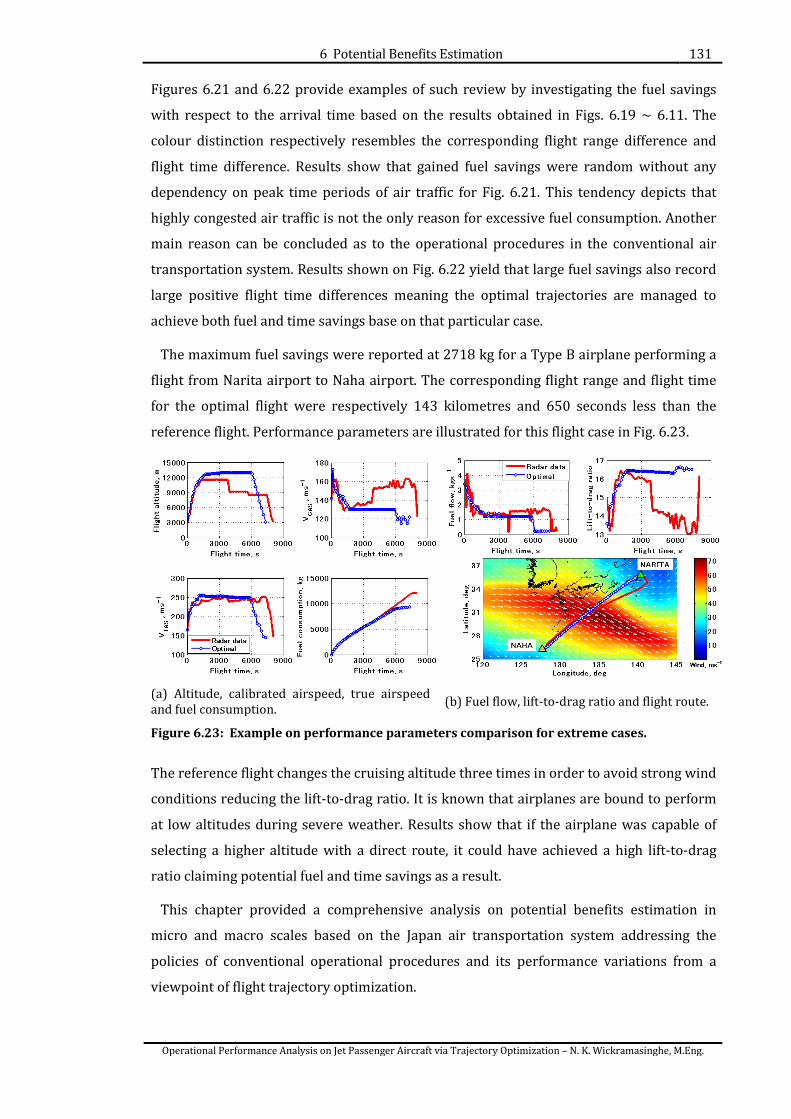
6 Potential Benefits Estimation 131
Operational Performance Analysis on Jet Passenger Aircraft via Trajectory Optimization – N. K. Wickramasinghe, M.Eng.
Figures 6.21 and 6.22 provide examples of such review by investigating the fuel savings
with respect to the arrival time based on the results obtained in Figs. 6.19 ~ 6.11. The
colour distinction respectively resembles the corresponding flight range difference and
flight time difference. Results show that gained fuel savings were random without any
dependency on peak time periods of air traffic for Fig. 6.21. This tendency depicts that
highly congested air traffic is not the only reason for excessive fuel consumption. Another
main reason can be concluded as to the operational procedures in the conventional air
transportation system. Results shown on Fig. 6.22 yield that large fuel savings also record
large positive flight time differences meaning the optimal trajectories are managed to
achieve both fuel and time savings base on that particular case.
The maximum fuel savings were reported at 2718 kg for a Type B airplane performing a
flight from Narita airport to Naha airport. The corresponding flight range and flight time
for the optimal flight were respectively 143 kilometres and 650 seconds less than the
reference flight. Performance parameters are illustrated for this flight case in Fig. 6.23.
(a) Altitude, calibrated airspeed, true airspeed and fuel consumption. (b) Fuel flow, lift-to-drag ratio and flight route.
Figure 6.23: Example on performance parameters comparison for extreme cases.
The reference flight changes the cruising altitude three times in order to avoid strong wind
conditions reducing the lift-to-drag ratio. It is known that airplanes are bound to perform
at low altitudes during severe weather. Results show that if the airplane was capable of
selecting a higher altitude with a direct route, it could have achieved a high lift-to-drag
ratio claiming potential fuel and time savings as a result.
This chapter provided a comprehensive analysis on potential benefits estimation in
micro and macro scales based on the Japan air transportation system addressing the
policies of conventional operational procedures and its performance variations from a
viewpoint of flight trajectory optimization.

7 Conclusion 132
Operational Performance Analysis on Jet Passenger Aircraft via Trajectory Optimization – N. K. Wickramasinghe, M.Eng.
7 CONCLUSION
This research proposed an analytical approach to evaluate the operational performance of
the current air transportation system from the viewpoint of trajectory optimization with a
limited number of data sources. Focus is on the extent of the performance distortion of
current operations based on a concept which is expected to exert the maximum
performance of the airplane.
The main objective of this research is to contribute towards the development of CARATS
program by declaring the operational performance of the current air transportation
system and propose a valid review method to quantitatively evaluate the performance to
reveal critical areas to be improved in a future ATM system. Therefore, an analytical
method is proposed to quantitatively evaluate the operational performance of the current
air transportation system with flight track data of jet passenger aircraft operated in
Japanese airspace. The process is based on a physical model and has the capability to
address the full flight profile. Estimated results were sufficiently accurate to review the
system performance considering the limited availability of data sources. The degree of
efficiency of the current system is discussed in an individual and quantitative basis based
on an ideal ATM system. In order to accomplish this task, the research study proposed a
trajectory optimization model which provides fuel optimal trajectories via a combinatorial
optimization process implemented through Dynamic Programming method. The research
process discussed in this study can be summarized as follows;
Firstly, estimation of air data was implemented from the position data of acquired flight
data. Position data measured by a commercial GPS receiver and air route surveillance
radar track data were used as data sources to conduct a comprehensive analysis on air
data estimation and highly accurate results were achieved through the application of 4-D
interpolated weather data.

7 Conclusion 133
Operational Performance Analysis on Jet Passenger Aircraft via Trajectory Optimization – N. K. Wickramasinghe, M.Eng.
Secondly, aircraft performance parameters were estimated by applying the BADA
aircraft performance data. Combining with the estimation of air data, a unique analytical
approach was proposed to identify the operational performance of any jet airplane type in
clean configuration, only by referring to time histories of the airplane’s position data.
Thirdly, a 4-D trajectory optimization method was introduced by considering a point
mass model which exerts the maximum performance of the airplane, as a standard to
review the performance of current operations. Dynamic Programming method was
applied to search for fuel-optimal solutions in a defined computational grid. Cost Index
concept was applied in the performance index to consider the flight time constraint in the
model and its impact on the fuel consumption. A mathematical technique developed to
reduce the computational time in the process while assuring the validity of the output is
applied in the optimization model. Arrival time constraints are applied in the model to
simulate current flight operations and review the operational procedures, obligations and
regulations in the current system.
7.1 Summary • The two-stage process on performance parameter estimation with its application
of publicly accessible data sources, enables the understanding of air data such as
true airspeed, calibrated airspeed Mach number etc…, and performance
parameters such as fuel flow, lift-to-drag ratio and fuel consumption which are
highly meticulous data in means of airplane’s performance. Due to the sensitivity,
the access to such data is genreally restricted only to airline operators and airplane
manufacturers. Also, the discussion on the system’s operational performance
enables the understanding the relevance of air navigation procedures and air
traffic congestion according to the ground control procedures.
• The Dynamic Programming method based trajectory optimization model provided
a plausible rference platform to review the performance of the current system. The
application of Dynamic Programming method was proved to be an efficient
approach in trajectory optimization by allocating its advantages in the analytical
process and an appropriate mathematical technique, the MS-DP method was
applied to avoid one of the major drawbacks in Dynamic Programming method, the
curse of dimensionality. The proposed optimization method was capable of
demonstrating an ideal ATM system and the current air transportation system in
an individual and quantitative basis only by referring to weather model data and
aircraft performance model data. Valid optimization results were obtained and
critical areas to be improved in the current system were clearly declared by

7 Conclusion 134
Operational Performance Analysis on Jet Passenger Aircraft via Trajectory Optimization – N. K. Wickramasinghe, M.Eng.
referring to aircraft’s performance. Furthermore, a comprehensive analysis on
potential benefits could be initiated through the proposed optimization processs.
• Characteristics of data sources were unveiled through a quantitative evaluation
where intriguing results on data tracking accuracy were obtained. These results
resembled unique characteristics of the national radar tracking system which were
obscured facts prior to this analysis.
• A plausible method for trajectory optimization was proposed to demonstrate the
performance distortion of current flight operations and potential benefits possible
to achieve by modeling the aspects of an operator-prioritized future air
transportation system. The introduced model considers airplane dynamics and
wind effect which is capable of demonstrating airplane behaviour when its
maximum performance are exerted.
Analytical results reveal that current flight operations are mainly time-oriented
and exceesive fuel is consumed in order to achieve these priorities. High speed
profiles are selected, especially during descent phase reducing the aircraft’s
performance. Also, tendency in operating at low altitudes with high speed profiles
was visible during strong weather conditions causing excessive fuel consumption
with longer flight time durations. Fuel-minimum optimization analysis based on
one of the busiest domestic flights routes in Japan performed by a twin-engine
wide body aircraft revealed an average of 829 kilograms of fuel reduction by
enabling the aircraft to,
perform cruise flight with high altitude profiles
set the Top pf Descent point at an early stage.
Select lower speed profiles with a long descent phase for a maximum lift-
to-drag ratio capability.
The scope of the fuel-minimum trajectory optimization analysis was extended to
generate optimal trajectories with the assigned arrival time that could
demonstrate the current operational scenario. A performance comparison showed
that a cost index of 109 was applied in a standard conventional flight which could
be considered as not optimal in means of fuel saving strategies. These results
further confirmed that current descent operations could be significantly improved
as a strategy for fuel reduction. The operational peroformance analysis was further
extended to address the system performance by applying the trajectory
optimization method to one third of daily operational flights in Japanese airspace.
Three aircraft types were subjected and an average of 450 kilograms of fuel could

7 Conclusion 135
Operational Performance Analysis on Jet Passenger Aircraft via Trajectory Optimization – N. K. Wickramasinghe, M.Eng.
be reduced by the proposed optimization method. This value was relevant to an
annual amount of 148810 tons of fuel savings in the national airspace.
• The obtained results on operational performance and potential benefits estimation
could promote public awareness regarding the inefficiency of the present air traffic
control system and the necessity of efficient flight operations in a future air traffic
management system.
7.2 Future work • The air data are estimated for the whole flight profile while the performance
parameters are evaluated considering only the clean configuration of the airplane.
This is due to the lack of data related to position data of flaps and landing gear.
BADA model provides formulae and coefificients for non-clean configuration but
the numerical error is considered to be relatively large. An aircraft performance
model which reflects complex aircraft dynamics has to be speculated for accurate
estimation of non-clean configuration flight performance.
• Parameters for smooting air route surveillance radar data is implemented in a trial
and error basis. The large amount of data acquired in the study show immensely
varied characteristics due to the geographical positions of tracking radar sites and
techniques used at preliminary stages of data processing. Hence, a robust
smoothing technique is required to identify paricular variations and implement a
rational data smoothing process.
• The trajectory optimization method proposed in this study considers the control
variables to be constant during a transition in the computational grid to increase
the calculation feasibility. Though any influence due to this assumption is reduced
by further discretization of each transition, more complex dynamics of the airplane
has to be considered to increase the clarity of the output trajectories.
• Approaches besides Dynamic Programming method should also be considered to
understand the advantages and disadvantages of solving the trajectory
optimization problem as an optimal control problem.
• The optimization method implies that higher the aircraft flies, better the output
performance is. These characteristics directly depend on the applied aircraft
performance model. Hence, buffet margins on vertical acceleration should also be
complied and comparisons of optimal trajectory characteristics generated from
different aircraft performance models are significant in understanding the validity
of the results.

7 Conclusion 136
Operational Performance Analysis on Jet Passenger Aircraft via Trajectory Optimization – N. K. Wickramasinghe, M.Eng.
Furthermore, aircraft mass data is assumed according to BADA performance
model data. Also BADA family 3 provides aircraft performance data for a specific
aircraft type based on a single engine type. The impact of these variations in
achieved potential benefits have to be declared for better review.
• Heading and flight path angles of the generated optimal trajectories are evaluated
as control variables, restricting them to be identical at initial and final states of the
corresponding reference trajectories. This paves the way to model the subjected
trajectory optimization problem from a different approach by providing these
variables as state variables so it can be adjusted upon requirement.
• This research considered arrival time constraints to model the conventional
operations scenario. Restrictions such as route limitations, military airspace and
altitude and speed limitations at approach configurations are considered to be
inevitable even in a future ATM system. Review on these applications in the
trajectory optimizer would reveal further characteristics on the achieved potential
benefits.
• Quantitative evaluations can be extended at the availability of flight data to review
the impact of seasonal changes, air traffic capacity variations etc… on the achieved
potential benefits.

8 References 137
Operational Performance Analysis on Jet Passenger Aircraft via Trajectory Optimization – N. K. Wickramasinghe, M.Eng.
8 REFERENCES
[1] International Civil Aviation Organization, "Global Air Traffic Management Operational Concept," 2005.
[2] International Civil Aviation Organization, "2013-2028 Global Air Navigation Plan - Capacity and Efficiency 4th ed. (Doc 9750)," 2013.
[3] Federal Aviation Administration (FAA), “NextGen Implementation Plan,” Aug. 2014.
[4] European Navigation for the Safety of Air Navigation (Eurocontrol), “European ATM Master Plan 2nd ed. - The Roadmap for Sustainable Air Traffic Management”.
[5] CARATS Study Group for the Future Air Traffic Systems, "Long-term Vision for the Future Air Traffic Systems (Changes to Intelligent Air Traffic Systems)," Japan Civil Aviation Bureau, 2010.
[6] M. S. Nolan, Fundamentals of Air Traffic Control, 5 ed., NewYork: Cengage Learning, 2011.
[7] "Mitsubishi Regional Jet," Mitsubishi Aircraft Corporation, Mitsubishi Heavy Industries, Ltd., [Online]. Available: http://www.mrj-japan.com/.
[8] "Airbus and Japan Airlines sign their first ever order," 7 10 2013. [Online]. Available: http://www.airbus.com/newsevents/news-events-single/detail/airbus-and-japan-airlines-sign-their-first-ever-order/.
[9] P. Belobaba, O. Amedeo and C. Barnhart, The Global Airline Industry, N. Allen, Ed., Wiley and Sons Ltd. (copublished by American Institute of Aeronautics and Astronautics), 2009.
[10] “BP Statistical Review of World Energy,” London, 2014.
[11] "Airline and Airport On-time Performance Report - Summary of Airline Arrivals and Airport Departures for the period July 1, 2013 through July 31, 2013," FlightStats On-time Performance Report, August 2013.
[12] "Japan Aeronautical Information Service Center (AIS JAPAN)," Ministry of Land,

8 References 138
Operational Performance Analysis on Jet Passenger Aircraft via Trajectory Optimization – N. K. Wickramasinghe, M.Eng.
Infrastructure, Transport and Tourism, [Online]. Available: https://aisjapan.mlit.go.jp/.
[13] "Airports in Japan," Ministry of Land, Infrastructure and Transport, Japan, [Online]. Available: http://www.mlit.go.jp/koku/15_hf_000124.html.
[14] I. Yamada, M. Sumiya, M. Brown and H. Aoyama, "Numerical Analysis of Surface Congestion Factors for Modeling Taxi-Out Times," 33rd Digital Avionics Systems Conference, 2014.
[15] R. Mori, "Development of Fast-Time Stochastic Airport Ground and Runway Simulation Model and Its Traffic Analysis," Mathematical Problems in Engineering, pp. 1-11, Article ID 919736, 2014.
[16] R. Mori, "Optimal Pushback Time with Existing Uncertainities at Busy Airport," 29th International Congress of the Aeronautical Sciences (ICAS 2014), St. Petersburg, 2014.
[17] "Remarks of Tony Tyler at the World Knowledge Forum, Seoul," International Air Transport Association (IATA), 14 10 2014. [Online]. Available: http://www.iata.org/pressroom/speeches/Pages/2014-10-14-01.aspx.
[18] "MH370 Search and rescue Response," The Second Meeting of the APANPIRG ATM Sub-Group, HongKong, China, 2014.
[19] “Preliminary Report: Crash involving Malaysia Airlines Boeing 777-200 flight MH17,” Hague, Netherlands, July 2014.
[20] "World Development Indicators Database," Source: International Civil Aviation Organization, Civil Aviation Statistics of the World, [Online]. Available: http://search.worldbank.org/data?qterm=air+traffic&language=&format=.
[21] Numerical Statistics in Aviation (2005-2014) (In Japanese 「数字でみる航空」), Japan Civil Aviation Promotion Foundation (supervised by Japan Civil Aviation Bureau), 2005-2014.
[22] "Number of planes handled by area control center (in Japanese, 航空路管制取扱機
数)," Ministry of Land, Infrastructure and Transport, Japan, [Online]. Available: http://www.mlit.go.jp/koku/15_bf_000387.html.
[23] International AIr Transport Association, "Profitability and the Air Transport Value Chain - IATA Economics Briefing 10," Montreal, Canada, 2013.
[24] J. Bronsvoort, "Contributions to Trajectory Prediction Theory and its Application to Arrival Management for Air Traffic Control," 2014.
[25] P. Horder, "Airline Operating Costs," Managing Aircraft Maintenance Costs Conference, Brussels, 2003.
[26] J. A. Sorensen, S. A. Morello and H. Erzberger, "Application of Trajectory Optimization Principles to Minimize Aircraft Operating Costs," 18th IEEE Conference on Decision and Control including the Symposium on Adaptive Processes, 1979.
[27] A. Chakravarty, "Selection of an Optimal Cost Index for Airline Hub Operation," AIAA Journal of Guidance, Control and Dynamics, vol. 8, no. 6, pp. 777-781, 1985.
[28] Boeing, "Fuel Conservation Strategies: Cost Index Explained," Aero Quarterly, no. QTR_02, 2007.

8 References 139
Operational Performance Analysis on Jet Passenger Aircraft via Trajectory Optimization – N. K. Wickramasinghe, M.Eng.
[29] Airbus, "getting to grips with the Cost Index," Flight Operations Support & Line Assistance, Issue 2, 1998.
[30] A. Cook, G. Tanner, V. Williams and G. Meise, "Dynamic Cost Indexing," EUROCONTROL Innovative Research Workshops & Exhibition, Bretigny sur Orge, France, 2007.
[31] A. Valenzuela and D. Rivas, "Analysis of Wind-Shear Effects on Optimal Aircraft Cruise," 6th International Conference on Research in Air Transportation (ICRAT 2014), Istanbul. Turkey, 2014.
[32] R. Babikian, S. P. Lukachko and I. A. Waitz, "The Historical Fuel Efficiency Characteristics of Regional Aircraft from Technological, Operational, and Cost Perspectives," Journal of Air Transport Management, vol. 8, no. 6, pp. 389-400, 2002.
[33] D. A. Senzig and G. G. Fleming, "Modeling of Terminal-Area Airplane fuel consumption," AIAA Journal of Aircraft, vol. 46, no. 4, pp. 1089-1093, 2009.
[34] K. Palopo, R. D. Windhorst, S. Suharwardy and H.-T. Lee, "Wind-Optimal Routing in the National Airspace System," AIAA Journal of Aircraft, vol. 47, no. 5, pp. 1584-1592, 2010.
[35] R. D. Oaks, H. F. Ryan and M. Paglione, "Prototype Implementation and Concept Validation of a 4-D Trajectory Fuel Burn Model Application," AIAA Guidance, Navigation, and Control Conference, 2010.
[36] M. S. Ryerson, M. Hansen and J. Bonn, "Fuel Consumption and Operational Performance," The 9th USA/Europe Air Traffic Management Research and Development Seminar (ATM 2011), 2011.
[37] S. Torres, J. Klooster, J. Hochwarth, R. Subbu, M. C. Effen and L. Ren, "Trajectory Management Driven by User Preferences," 30th Digital Avionics Systems Conference, Seattle, 2011.
[38] J. A. Lovegren and R. J. Hansman, "Estimation of Potential Aircraft Fuel Reduction in Cruise Via Speed and Altitude Optimization Strategies," MIT International Center for Air Transportation, 2011.
[39] E. T. Turgut, "Estimating Aircraft Fuel Flow for a Three-Degree Flight-Path-Angle Descent," AIAA Journal of Aircraft, vol. 48, no. 3, pp. 1099-1106, 2011.
[40] G. B. Chatterji, "Fuel Burn Esimation Using Real Track Data," AIAA Aviation Technology, Integration and Operations Conference, Virginia, 2011.
[41] H. Erzberger and H. Q. Lee, "Optimum Horizontal Guidance Techniques for Aircraft," AIAA Journal of Aircraft, vol. 8, no. 2, pp. 95-101, 1971.
[42] H. Erzberger and H. Q. Lee, "Terminal-Area Guidance Algorithms for Automated Air Traffic Control," NASA Technical Note TN D-6773, 1972.
[43] H. Erzberger and H. Q. Lee, "Constrained Optimum Trajectories with Specified range," AIAA Journal of Guidance and Control, vol. 3, no. 1, pp. 78-85, 1980.
[44] H. Erzberger and L. Tobias, "A Time Based Concept for Terminal Air Traffic Management," NASA Technical Memorandum 88243, 1986.
[45] H. Erzberger and W. Nedell, "Design of Automated System for Management of Arrival Traffic," NASA Technical Memorandum 102201, 1989.
[46] O. von Stryk and R. Bulirsch, "Direct and Indirect Methods for Trajectory

8 References 140
Operational Performance Analysis on Jet Passenger Aircraft via Trajectory Optimization – N. K. Wickramasinghe, M.Eng.
Optimization," Annals of Operations Research, vol. 37, pp. 357-373, 1992.
[47] J. T. Betts, "Survey of Numerical Methods for Trajectory Optimization," AIAA Journal of Guidance, Control and Dynamics, vol. 21, no. 2, pp. 193-207, 1998.
[48] V. Di Vito, F. Corraro, U. Ciniglio and L. Verde, "An Overview on Systems and Algorithms for On-Board 3D/4D Trajectory Management," Recent Patents on Engineering, vol. 3, pp. 149-169, 2009.
[49] G. Moldoveanu and O. T. Pleter, "Multidisciplinary Optimization in Services Management," Theoretical and Applied Economics, pp. 7-15, 2007.
[50] B. Passenberg, "Theory and Algorithms for Indirect Methods in Optimal Control of Hybrid Systems," Technische Unversitat Munchen, 2012.
[51] B.-n. Kang, D. B. Spencer, S. Tang and D. Jordan, "Optimal Periodic Cruise Trajectories via a Two-Level Optimization Method," AIAA Journal of Spacecraft and Rockets, vol. 47, no. 4, pp. 597-613, 2010.
[52] J. B. Rosen and J. Kreuser, "A Gradient Projection Algorithm for Nonlinear Constraints," Numerical Methods forNon-Linear Optimization, pp. 297-300, 1972.
[53] L. S. Lasdon and A. D. Waren, "Generalized Reduced Gradient Software for Linearly and Nonlinearly Constrained Optimization," Design and Implementation of Optimization Software, pp. 335-362, 1978.
[54] P. E. Gill, W. Murray, M. A. Saunders and M. H. Wright, "User's Guide for NPSOL (version 4.0): A Fortran Package for Nonlinear Programming," Department of Operations Research, Stanford University, 2001.
[55] R. B. Patel and P. J. Goulart, "Trajectory Generation for Aircraft Avoidance Maneuvers Using Online Optimization," AIAA Journal of Guidance, Control and Dynamics, vol. 34, no. 1, pp. 218-230, 2011.
[56] C. R. Hargraves and S. W. Paris, "Direct Trajectory Optimization using Nonlinear Programming and Collocation," AIAA Journal of Guidance, Control and Dynamics, vol. 10, no. 4, pp. 338-342, 1987.
[57] R. Bulirsch, A. Miele, J. Stoer and K. H. Well, "Optimal Control - Calculus of Variations, Optimal Control Theory and Numerical Methods," International Series of Numerical Mathematics, vol. 111, pp. 129-143, 1993.
[58] S. Suzuki, T. Tsuchiya and A. Andreeva, "Trajectory Optimization for Safe, Clean and Quiet Flight," Proceedings of the 2nd ENRI International Workshop on ATM/CNS, 2009.
[59] R. Verhoeven, R. Dalmau, X. Prats and N. de Gelder, "Real-Time Aircraft Continuous Descent Trajectory Optimization with ATC Time Constraints Using Direct Collocation Methods," Proceedings of the 29th International Council of the Aeronautical Sciences (ICAS 2014), 2014.
[60] H. G. Visser, "A 4-D Trajectory Optimization and Guidance Technique for Terminal Area Traffic Management," Delft University of Technology, 1994.
[61] J. T. Betts and W. P. Huffman, "Application of Sparse Nonlinear Programming to Trajectory Optimization," AIAA Journal of Guidance, Control and Dynamics, vol. 15, no. 1, pp. 198-206, 1992.
[62] T. Tsuchiya, M. Miwa, S. Suzuki, K. Masui and H. Tomita, "Real-Time Flight Trajectory Optimization and Its Verification in Flight," Engineering Notes, AIAA Journal of

8 References 141
Operational Performance Analysis on Jet Passenger Aircraft via Trajectory Optimization – N. K. Wickramasinghe, M.Eng.
Aircraft, vol. 46, no. 4, pp. 1468-1470, 2009.
[63] J. T. Betts and E. J. Cramer, "Application of Direct Transcription to Commercial Aircraft Trajectory Optimization," AIAA Journal of Guidance, Control and Dynamics, vol. 18, no. 1, pp. 151-159, 1995.
[64] D. A. Benson, G. T. Huntington, T. P. Thorvaldsen and A. V. Rao, "Direct Trajectory Optimization and Costate Estimation via an Orthogonal Collocation Method," Engineering Notes, AIAA Journal of Guidance, Control and Dynamics, vol. 29, no. 6, pp. 1435-1440, 2006.
[65] K. Bousson and P. Machado, "4-D Flight Trajectory Optimization Based on Pseudospectral Methods," World Academy of Science, Engineering Technology, vol. 4, no. 9, pp. 471-477, 2010.
[66] F. Fahroo and I. M. Ross, "Direct Trajectory Optimization by a Chebyshev Pseudospectral Method," AIAA Journal of Guidance, Control, and Dynamics, vol. 25, no. 1, pp. 160-166, 2002.
[67] U. Ringertz, "Optimal Trajectory for a Minimum Fuel Turn," Engineering Notes, Journal of Aircraft, vol. 37, no. 5, pp. 932-934, 2000.
[68] A. Valenzuela and D. Rivas, "Optimization of Aircraft Cruise Procedures Using Discrete Trajectory Patterns," AIAA Journal of Aircraft, vol. 51, no. 5, pp. 1632-1640, 2014.
[69] N. Yokoyama and S. Suzuki, "Modified Genetic Algorithm for Contrained Trajectory Optimization," AIAA Journal of Guidance, Control and Dynamics, vol. 28, no. 1, pp. 139-144, 2005.
[70] J. T. Betts, "Practical Methods for Optimal Control Using Nonlinear Programming," SIAM: Advances in Design and Control, 2001.
[71] J. T. Betts and W. Huffman, "Path-Constrained Trajectory Optimization Using Sparse Sequential Quadratic Programming," AIAA Journal of Guidance, Control, and Dynamics, vol. 16, no. 1, pp. 59-68, 1993.
[72] J. T. Betts and W. Huffman, "Mesh Refinement in Direct Transcription Methods for Optimal Control," Optimal Control Applications & Methods, vol. 19, pp. 1-21, 1998.
[73] B. A. Conway and K. M. Larson, "Collocation Versus Differential Inclusion in Direct Optimization," AIAA Journal of Guidance, Control and Dynamics, vol. 21, no. 5, pp. 780-785, 1998.
[74] D. G. Hull, "Conversion of Optimal Control Problems into Parameter Optimization Problems," AIAA Journal of Guidance, Control, and Dynamics, vol. 20, no. 1, pp. 57-60, 1997.
[75] H. Seywald, "Trajectory Optimization Based on Differential Inclusion," AIAA Journal of Guidance, Control and Dynamics, vol. 17, no. 3, pp. 480-487, 1994.
[76] R. L. Schultz and R. Zagalsky, "Aircraft Performance Optimization," AIAA Journal of Aircraft, vol. 9, no. 2, pp. 108-114, 1972.
[77] R. L. Schultz, "Fuel Optimality of Cruise," AIAA Journal of Aircraft, vol. 11, no. 9, pp. 586-587, 1974.
[78] J. W. Burrows, "Fuel Optimal Trajectory Optimization," AIAA Journal of Aircraft, vol. 19, no. 4, pp. 324-329, 1982.

8 References 142
Operational Performance Analysis on Jet Passenger Aircraft via Trajectory Optimization – N. K. Wickramasinghe, M.Eng.
[79] J. W. Burrows, "Fuel Optimal Aircraft trajectories with fixed arrival times," AIAA Journal of Aircraft, vol. 6, no. 1, pp. 14-19, 1983.
[80] A. Chakravarty, "Four Dimensional Fuel-Optimal Guidance in the Presence of Winds," AIAA Journal of Guidance, Control and Dynamics, vol. 8, no. 1, pp. 16-22, 1985.
[81] P. K. Menon, "Study of Aicraft Cruise," AIAA Journal of Guidance, Control and Dynamics, vol. 12, no. 5, pp. 631-639, 1989.
[82] H. Seywald, "Long Flight-Time Range-Optimal Aircraft Trajectories," Engineering Notes, AIAA Journal of Guidance, Control and Dynamics, vol. 19, no. 1, pp. 242-244, 1996.
[83] O. A. Yakimenko, "DirectMethod for Rapid Prototyping of Near-Optimal Aircraft trajectories," AIAA Journal of Guidance, Control and Dynamics, vol. 23, no. 5, pp. 865-875, 2000.
[84] S. M. Malaek, M. A. Marzaabaadi and S. H. Sadati, "Minimum Fuel Trajectory in a 3D Time Scheduled Climb," Journal of Aerospace Science and Technology, Iranian Aerospace Society, vol. 2, no. 2, pp. 11-18, 2005.
[85] B. Sridhar, N. Chen and H. K. Ng, "Simulation and Optimization Methods for Assessing the Impact of Aviation Operations on the Environment," Proceedings of the 27th International Congress of the Aeronautical Sciences (ICAS 2010), 2010.
[86] B. Sridhar, H. K. Ng and N. Y. Chen, "Aircraft Trajectory Optimization and Contrails Avoidance in the Presence of Winds," Engineering Notes, AIAA Journal of Guidance, Control and Dynamics, vol. 34, no. 5, pp. 1577-1583, 2011.
[87] A. E. Sagalakov and A. S. Filatyev, "New Periodic Solutions in the Aircraft Maximum Range Problem," Proceedings of the 29th International Congress of the Aeronautical Sciences (ICAS 2014), 2014.
[88] X.-M. Tang and Y.-X. Han, "4D Trajectory Estimation for Air Traffic Control Automation System Based on Hybrid System Theory," Science in Traffic and Transport, vol. 24, no. 2, pp. 91-98, 2012.
[89] M. Soler, A. Olivares and E. Staffetti, "Hybrid Optimal Control Approach to Commercial Aircraft Trajectory Planning," AIAA Journal of Guidance, Control and Dynamics, vol. 33, no. 3, pp. 985-991, 2010.
[90] M. Jacobsen and U. T. Ringertz, "Airspace Constraints in Aircraft Emission Trajectory Optimization," AIAA Journal of Aircraft, vol. 47, no. 4, pp. 1256-1265, 2010.
[91] A. Franco and D. Rivas, "Optimization of Multiphase Aircraft Trajectories Using Hybrid Optimal Control," AIAA Journal of Guidance, Control and Dynamics, vol. 38, no. 3, pp. 452-467, 2015.
[92] M. Soler, D. Zapata, A. Olivares, E. Stafetti and J. u. Cegarra, "Comparative Analysis of Commerical Aicraft Trajectory Optimzation," 2nd International Conference on Engineering Optimization, 2010.
[93] S. Dreyfus, "Richard Bellman on the Birth of Dynamic Programming," Operations Research, vol. 50, no. 1, pp. 48-51, 2002.
[94] A. E. Bryson and Y.-C. Ho, Applied Optimal Control - Optimization, Estimation and Control, Taylor & Francis, 1975.
[95] A. S. Abbott and J. E. McIntyre, "Guidance, Flight Mechanics and Trajectory

8 References 143
Operational Performance Analysis on Jet Passenger Aircraft via Trajectory Optimization – N. K. Wickramasinghe, M.Eng.
Optimization - Volume X: Dynamic Programming," NASA Contractor Report, 1968.
[96] W. Schultz and H. -K. Schulze, "A Method of Dynamic Programming and its Application to Optimization Problems of Flight Mechanics," NASA Technical Translation NASA TT F-483, Washington D.C., 1967.
[97] A. Harada, H. Matsuda and Y. Miyazawa, "Dynamic Programming Trajectory Optimization by Piecewise Linear Approximation," AIAA Guidance, Navigation and Control Conference (SCITECH 2015), 2015.
[98] H. Matsuda, A. Harada and Y. Miyazawa, "Dynamic Programming Trajectory Optimization using Linear Approximation by Grid Point Value," Aerospace Technology Japan, vol. 14, pp. 33-41, 2015.
[99] P. Hagelauer, "A Soft Dynamic Programming Approach for On-Line Aircraft 4D- Trajectory Optimization," European Journal of Operational Research, vol. 107, no. 1, pp. 87-95, 1998.
[100] M. R. Jardin and A. E. Bryson, "Methods for Computing Minimum-Time Paths in Strong Winds," AIAA Journal of Guidance, Control and Dynamics, vol. 35, no. 1, pp. 165-171, 2012.
[101] M. Dobrovinsky and J. Z. Ben-Asher, "Cruise Flight Throttle Optimization by Approximate Dynamic Programming," Proceedings of the 29th International Congress of the Aeronautical Sciences (ICAS 2014), 2014.
[102] R. E. Bellman and S. E. Dreyfus, Applied Dynamic Programming, Princeton University, 1962.
[103] R. Luus, "Optimal Control by Dynamic Programming using Systematic Reduction in Grid Size," International Journal of Control, vol. 51, no. 5, pp. 995-1013, 1990.
[104] R. Luus, "Numerical Convergence Properties of Iterative Dynamic Programming when applied to High Dimensional Systems," Chemical Engineering Research and Design, vol. 74, pp. 55-62, 1996.
[105] R. Luus, Iterative Dynamic Programming, Chapman and Hall CRC, 2000.
[106] Y. Wang, B. O'Donoghue and S. Boyd, "Approximate Dynamic Programming via Iterated Bellman Inequalities," International Journal of Robust and Nonlinear Control, pp. 1-25, 2014.
[107] H.-G. Wahl and F. Gauterin, "An Iterative Dynamic Programming Approach for the Global Optimal Control of Hybrid Electric Vehicles under Real-time Constraints," Proceedings of the 2013 IEEE Intelligent Vehicles Symposium (IV), 2013.
[108] S. Ueno, "Minimum Fuel Cruise by Periodic Optimization," JSASS Aerospace Technology Japan, vol. 37, no. 429, pp. 44-48, 1989.
[109] B. L. Pierson and S. Y. Ong, "Minimum-Fuel Aircraft Transition Trajectories," Mathematical and Computer Modelling, vol. 12, no. 8, pp. 925-934, 1989.
[110] S. Jain and P. Tsiotras, "Trajectory Optimization Using Multiresolution Techniques," AIAA Journal of Guidance, Control and Dynamics, vol. 31, no. 5, pp. 1424-1436, 2008.
[111] A. Franco, A. Valenzuela and D. Rivas, "Optimal Control of CruiseFlight at Constant Altitude," Proceedings of the 27th International Congress of the Aeronautical Sciences (ICAS 2010), 2010.
[112] A. Franco, D. Rivas and A. Valenzuela, "Minimum-Fuel Cruise at Constant Altitude

8 References 144
Operational Performance Analysis on Jet Passenger Aircraft via Trajectory Optimization – N. K. Wickramasinghe, M.Eng.
with fixed Arrival time," Engineering Notes, AIAA Journal of Guidance, Control and Dynamics, vol. 33, no. 1, pp. 280-285, 2010.
[113] N. Nguyen, "Singular Arc Time-Optimal Climb Trajectory of Aircraft in a Two-Dimensional Wind Field," AIAA Guidance, Navigationa and Control Conference, 2006.
[114] M. R. Jardin and A. E. Bryson, "Neighboring Optimal Aircraft Guidance in Winds," AIAA Journal of Guidance, Control and Dynamics, vol. 24, no. 4, pp. 710-715, 2001.
[115] J. A. Sorensen and M. H. Waters, "Airborne Method to Minimize Fuel with Fixed Time-of-Arrival Constraints," AIAA Journal of Guidance, Control, and Dynamics, vol. 4, no. 3, pp. 348-349, 1981.
[116] S. J. Bijlsma, "Optimal Aircraft Routing in General Wind Fields," AIAA Journal of Guidance, Control and Dynamics, vol. 32, no. 3, pp. 1025-1028, 2009.
[117] T. R. Jorris and R. G. Cobb, "Three-Dimensional Trajectory Optimization Satisfying Waypoint and No-Fly Zone Constraints," AIAA Journal of Guidance, Control and Dynamics, vol. 32, no. 2, pp. 551-571, 2009.
[118] D. Wu and Y. J. Zhao, "Performances and Sensitivities of Optimal Trajectory Generation for Air Traffic Control Automation," AIAA Guidance, Navigation and Control Conference, 2009.
[119] O. T. Pleter and C. E. Constantinescu, "Objective Function for 4D Trajectory Optimization in Trajectory Based Operations," AIAA Guidance, Navigation and Control Conference, 2009.
[120] M. Kamgarpour, V. Dadok and C. Tomlin, "Trajectory Generation for Aircraft Subject to Dynamic Weather Uncertainty," 49th IEEE Conference on Decision and Control, 2010.
[121] N. E. Dougui, D. Delahaye, S. Puechmorel and M. Mongeau, "A New Method for Generating Optimal Conflict Free 4D Trajectory," Proceedings of the 4th International Conference on Research in Air Transportation (ICRAT 2010), 2010.
[122] DG-100 Data Logger User Manual Ver. 12.1.
[123] "Tabireco GPS Data Logger User Manual (in Japanese)," I-O DATA Device, Inc., [Online]. Available: http://www.iodata.jp/lib/manual/pdf2/gpslog-m-manu200887.pdf.
[124] "SiRF StarIII," [Online]. Available: http://en.wikipedia.org/wiki/SiRFstarIII.
[125] United States Department of Transportation, 2011 Federal Aviation Regulations Aeronautical Information Manual, Aviation Supplies and Academics, Inc., 2011.
[126] Voluntary Control Council for Interference by Information Technology Equipment (VCCI) Council, "Objective in Establishing the Council," [Online]. Available: https://www.vcci.jp/vcci_e/general/objective.html.
[127] "Restriction of Hazardous Substances Directive," [Online]. Available: http://en.wikipedia.org/wiki/Restriction_of_Hazardous_Substances_Directive.
[128] International Civil Aviation Organization, "European Coordination Centre for Accident and Incident Reporting Systems (ECCAIRS) 4.2.8 Data Definition Standard - Location Indicators by State," 2010.
[129] H. Totoki, N. K. Wickramasinghe, T. Hamada and Y. Miyazawa, "Estimation of Flight

8 References 145
Operational Performance Analysis on Jet Passenger Aircraft via Trajectory Optimization – N. K. Wickramasinghe, M.Eng.
Trajectories by Using GPS Data Measured in Airliner Cabin," Aerospace Technology Japan (In Japanese), vol. 11, no. 0, pp. 43-50, 2012.
[130] Boeing Commercial Airplanes, "737 Airplane Characteristics for Airport Planning," Boeing, D6-58325-6, 2013.
[131] Boeing Commerical Airplanes, "747-400 Airplane Characteristics for Airport Planning," D6-58326-1, 2002.
[132] Boeing Commerical Airplanes, "767 Airplane Characteristics for Airport Planning," D6-58328, 2005.
[133] Boeing Commerical Airplanes, “777-200/300 Airplane Characteristics for Airport Planning,” D6-58329, 1998.
[134] M. Oka, Y. Fukuda and K. Uejima, "Outline of Air Traffic Open Data and Application," Proceedings of the 52nd Aircraft Symposium, Nagasaki, Japan, 2014.
[135] Civil Aviation Bureau, MLIT, Japan, "Radar Facilities En-route," [Online]. Available: http://www.mlit.go.jp/koku/15_hf_000079.html.
[136] S. Shigetomi, T. Kozuka, Y. Miyazawa, N. K. Wickramasinghe, M. Brown and Y. Fukuda, "Analysis of Air Traffic in and around Terminal Airspace with SSR Surveillance Data (in Japanese)," Proceedings of the 52nd Aircraft Symposium, Nagasaki, Japan, 2014.
[137] T. Kozuka, Y. Miyazawa, N. K. Wickramasinghe and M. Brown, "A Study on Estimation of Aircraft Interference Resolution Procedure (in Japanese)," Proceedings of the 52nd Aircraft Symposium, Nagasaki, Japan, 2014.
[138] Japan Meteorological Agency, "Numerical Weather Prediciton Models (Chapter 3), Outline of the Operational Numerical Weather Prediction at the Japan Meteorological Agency," 2013. [Online]. Available: http://www.jma.go.jp/jma/jma-eng/jma-center/nwp/outline2013-nwp/index.htm.
[139] H. Totoki, T. Kozuka, Y. Miyazawa and K. Funabiki, "Comparison of JMA Numerical Prediction GPV Meteorological Data and Airliner Flight Data (in Japanese)," Aerospace Technology Japan, vol. 12, pp. 57-63, 2013.
[140] Jeppesen, "Total Airspace and Airport Modeller (TAAM) Product Profile," 2011.
[141] P. Calders, "G.A.M.E. Aircraft Performance Model Description," European Organization for the Safety of Air Navigation (EUROCONTROL), 2002.
[142] E. Gallo, F. A. Navarro, A. Nuic , M. Iagaru, “Advanced Aircraft Performance Modeling for ATM: BADA 4.0 Results,” 25th Digital Avionics Systems Conference, 2006.
[143] A. Franco and D. Rivas, "Analysis of Optimal Aircraft Cruise with Fixed Arrival Time Including Wind Effects," Aerospace Science and Technology, ELSEVIER, vol. 32, no. 1, pp. 212-222, 2014.
[144] A. Nuic, C. Poinsot, M. G. Iagaru, E. Gallo, F. A. Navarro , C. Querejeta, “Advanced Aircraft Performance Modelling for ATM: Enhancements to the BADA Model,” 24th Digital Avionics Systems Conference, 2005.
[145] EUROCONTROL Experimental Centre, "User Manual for the Base of Aircraft Data (BADA) Revision 3.11," European Organization for the Safety of Air Navigation (EUROCONTROL) , 2013.
8 References 146
Operational Performance Analysis on Jet Passenger Aircraft via Trajectory Optimization – N. K. Wickramasinghe, M.Eng.
[146] EUROCONTROL Experimental Centre, "Base of Aircraft Data (BADA) Aircraft Performance Modelling Report," European Organization for the Safety of Air Navigation (EUROCONTROL), 2009.
[147] European Air Traffic Control Harmonisation and Integration Programme (EUROCONTROL), "Radar Surveillance in En-Route Airspace and Major Terminal Areas," 1997.
[148] M. Tooley and D. Wyatt, Aircraft Navigation and Communications Systems - Principles, Maintenance and Operation, 1 ed., ELSEVIER, 2007.
[149] National Oceanic and Atmospheric Administration (NOAA), National Aeronautics and Space Administration (NASA) and United States Air Force, "U.S. STANDARD ATMOSPHERE," 1976.
[150] W. Gracey, Measurement of Aircraft Speed and Altitude, John Wiley & Sons, Inc., 1981.
[151] Joint Aviation Authorities (JAA), "JAR-1 Definitions and Abbreviations," July 1996. [Online]. Available: http://www.fzt.haw-hamburg.de/pers/Scholz/vorschriften/JAR-1.html.
[152] Japan Civil Aviation Bureau and Japan Meteorological Agency, "Aeronautical Information Manual Japan," pp. 3-3, 2013.
[153] T. Sakai, K. Koremura and K. Niimi, "Height Measurement Error of Barometric Altimeter and Its Correction," Electronic Navigation Research Institute Papers, no. 114, pp. 1-13, 2005.
[154] Y. Fukuda, M. Shirakawa , A. Senoguchi, “Development and Evaluation of Trajectory Prediction Model,” Proceedings of the 27th International Congress of the Aeronautical Sciences (ICAS 2010), 2010.
[155] N. X. Vinh, Flight Mechanics of High-Performance Aircraft, Cambridge Aerospace Series 4, Cambridge University Press, 1993.
[156] Y. Miyamoto, N. K. Wickramasinghe, A. Harada and Y. Miyazawa , "Computational Time Reduction for Dynamic Programming Trajectory Optimization Applied to Passenger Aircraft," Proceedings of the JSASS Western Branch Conference, Fukuoka, 2012.
[157] Y. Miyazawa, N. K. Wickramasinghe, A. Harada and Y. Miyamoto, "Dynamic Programming Application to Airliner Four Dimensional Optimal Flight Trajectory," AIAA Guidance, Navigation and Control Conference, 2013.
[158] A. Cook, G. Tanner and G. Meise, "Dynamic Cost Indexing," 6th EUROCONTROL Innovative Research Workshops and Exhibition, Orge, France, 2007.
[159] Airbus, "Flight Operations Support & Line Assistance - Getting to Grips with Fuel Economy," Airbus, Issue 3, 2004.
[160] D. H. Peckham, "Range Performance in Cruising Flight," Royal Aircraft Establishment, Farnborough, England, 1974.
[161] D. G. Hull, Fundamentals of Airplane Flight Mechanics, 1 ed., Springer-Verlag Berlin Heidelberg, 2007.
[162] A. Harada, Y. Miyamoto, Y. Miyazawa and K. Funabiki, "Accuracy Evaluation of an Aircraft Performance Model with Airliner Flight Data," Transactions of the Japan Society of Aeronautical and Space Sciences, Aerospace Technology Japan , vol. 11, no.

8 References 147
Operational Performance Analysis on Jet Passenger Aircraft via Trajectory Optimization – N. K. Wickramasinghe, M.Eng.
0, pp. 79-85, 2013.
[163] "Overview of Air Route Surveillance Radar (in Japanese, 航空監視レーダー(ARSR)等の概要)," Ministry of Land, Infrastructure and Tourism, Japan, [Online]. Available: http://www.mlit.go.jp/koku/15_bf_000404.html.
[164] "Vincenty Solutions of Geodesics on the Ellipsoid - Distances and bearings between points on an ellipsoidal earth model," [Online]. Available: http://www.movable-type.co.uk/scripts/latlong-vincenty.html.
[165] R. E. Bach and R. A. Paielli, "A User Guide for Smoothing Air Traffic Radar Data," NASA/TM-2014-216520, California, 2014.
[166] National Aeronautics and Space Administration, "Terminal TSAFE," [Online]. Available: http://www.aviationsystemsdivision.arc.nasa.gov/research/tactical/ttsafe.shtml.
[167] D. Bertsekas, Dynamic Programming and Stochastic Control, Academic Press, 1976.
[168] D. E. Kirk, Optimal Control Theory, Prentice Hall, 1970.