CHAPTER

3

Forecasting

Manajemen Transportasi & LogistikManajemen Transportasi & LogistikManajemen Transportasi & LogistikManajemen Transportasi & Logistik

Forecasting

Rahmi Yuniarti,ST.,MTAnni Rahimah, SAB,MAB

FIA - Prodi Bisnis Internasional Universitas Brawijaya

Manajemen PermintaanManajemen Permintaan2

Order Pesanan

Ramalan Permintaan

Manajemen Permintaan

Pengelolaan Order PesananPengelolaan Order Pesanan3

Permintaan

Penawaran

Negosiasi

KesepakatanPerjanjian

FORECAST:• A statement about the future value of a variable of

interest such as demand.• Forecasts affect decisions and activities throughout

an organization

What is Forecasting?What is Forecasting?

• Accounting, finance• Human resources• Marketing• MIS• Operations• Product / service design

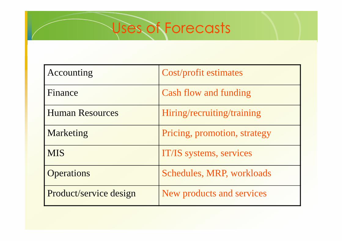
Accounting Cost/profit estimates

Finance Cash flow and funding

Human Resources Hiring/recruiting/training

Uses of ForecastsUses of Forecasts

Marketing Pricing, promotion, strategy

MIS IT/IS systems, services

Operations Schedules, MRP, workloads

Product/service design New products and services

Peramalan PermintaanPeramalan Permintaan6

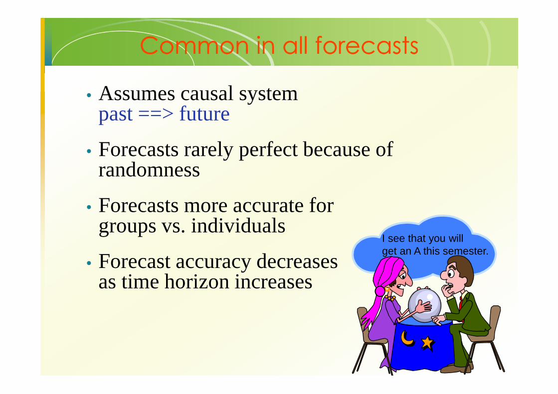
• Assumes causal systempast ==> future

• Forecasts rarely perfect because of randomness

Forecasts more accurate for

Common in all forecastsCommon in all forecasts

• Forecasts more accurate forgroups vs. individuals

• Forecast accuracy decreases as time horizon increases

I see that you willget an A this semester.

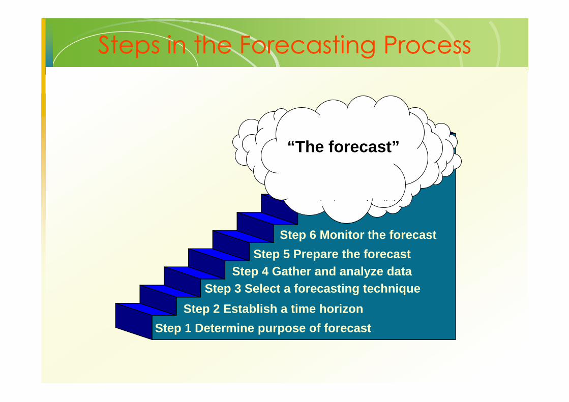
Steps in the Forecasting ProcessSteps in the Forecasting Process

“The forecast”

Step 1 Determine purpose of forecast

Step 2 Establish a time horizon

Step 3 Select a forecasting techniqueStep 4 Gather and analyze data

Step 5 Prepare the forecast

Step 6 Monitor the forecast

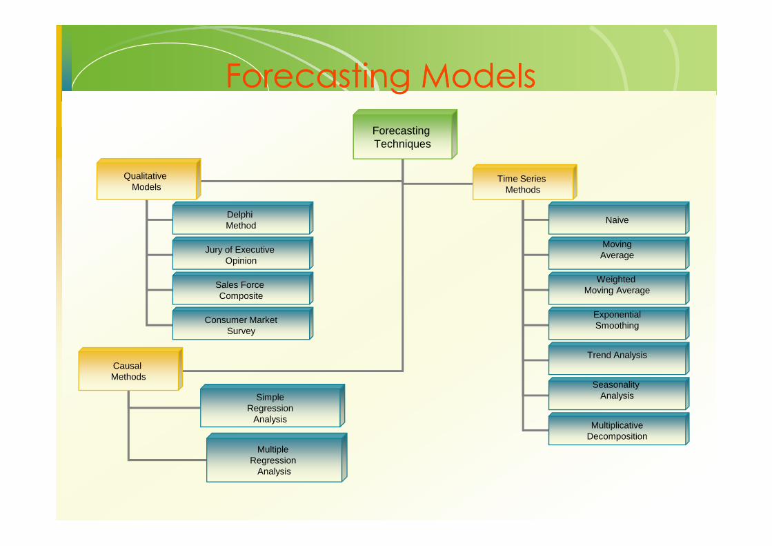
Forecasting ModelsForecasting Models

Forecasting Techniques

Qualitative Models

Time Series Methods

Delphi Method

Jury of Executive Opinion

Naive

MovingAverage

Causal Methods

Sales Force Composite

Consumer MarketSurvey

Weighted Moving Average

ExponentialSmoothing

Trend Analysis

Seasonality AnalysisSimple

RegressionAnalysis

Multiple Regression

Analysis

MultiplicativeDecomposition

Model DifferencesModel Differences

• Qualitative – incorporates judgmental & subjective factors into forecast.

• Time-Series – attempts to predict the future by using historical data.

• Causal – incorporates factors that may influence • Causal – incorporates factors that may influence the quantity being forecasted into the model

Qualitative Forecasting ModelsQualitative Forecasting Models

• Delphi method• Iterative group process allows experts to make forecasts

• Participants: • decision makers: 5 -10 experts who make the forecast

• staff personnel: assist by preparing, distributing, collecting, and summarizing a series of questionnaires and survey resultssummarizing a series of questionnaires and survey results

• respondents: group with valued judgments who provide input to decision makers

Qualitative Forecasting Models Qualitative Forecasting Models

(cont)(cont)

• Jury of executive opinion• Opinions of a small group of high level managers, often in combination

with statistical models.• Result is a group estimate.

• Sales force composite• Each salesperson estimates sales in his region.• Each salesperson estimates sales in his region.• Forecasts are reviewed to ensure realistic.• Combined at higher levels to reach an overall forecast.

• Consumer market survey.• Solicits input from customers and potential customers regarding future

purchases.• Used for forecasts and product design & planning

Metode Peramalan Deret Waktu Metode Peramalan Deret Waktu

(Time Series Methods)(Time Series Methods)• Teknik peramalan yang menggunakan data-data historis

penjualan beberapa waktu terakhir dan mengekstrapolasinya untuk meramalkan penjualan di masa depan

• Peramalan deret waktu mengasumsikan pola kecenderungan pemasaran akan berlanjut di masa depan.

13

kecenderungan pemasaran akan berlanjut di masa depan.

• Sebenarnya pendekatan ini cukup naif, karena mengabaikan gejolak kondisi pasar dan persaingan

LangkahLangkah--langkah Peramalan Deret Waktulangkah Peramalan Deret Waktu

• Kumpulkan data historis penjualan

• Petakan dalam diagram pencar (scatter diagram)

• Periksa pola perubahan permintaan

• Identifikasi faktor pola perubahan permintaan

• Pilih metode peramalan yang sesuai

14

• Pilih metode peramalan yang sesuai

• Hitung ukuran kesalahan peramalan

• Lakukan peramalan untuk satu atau beberapa periode mendatang

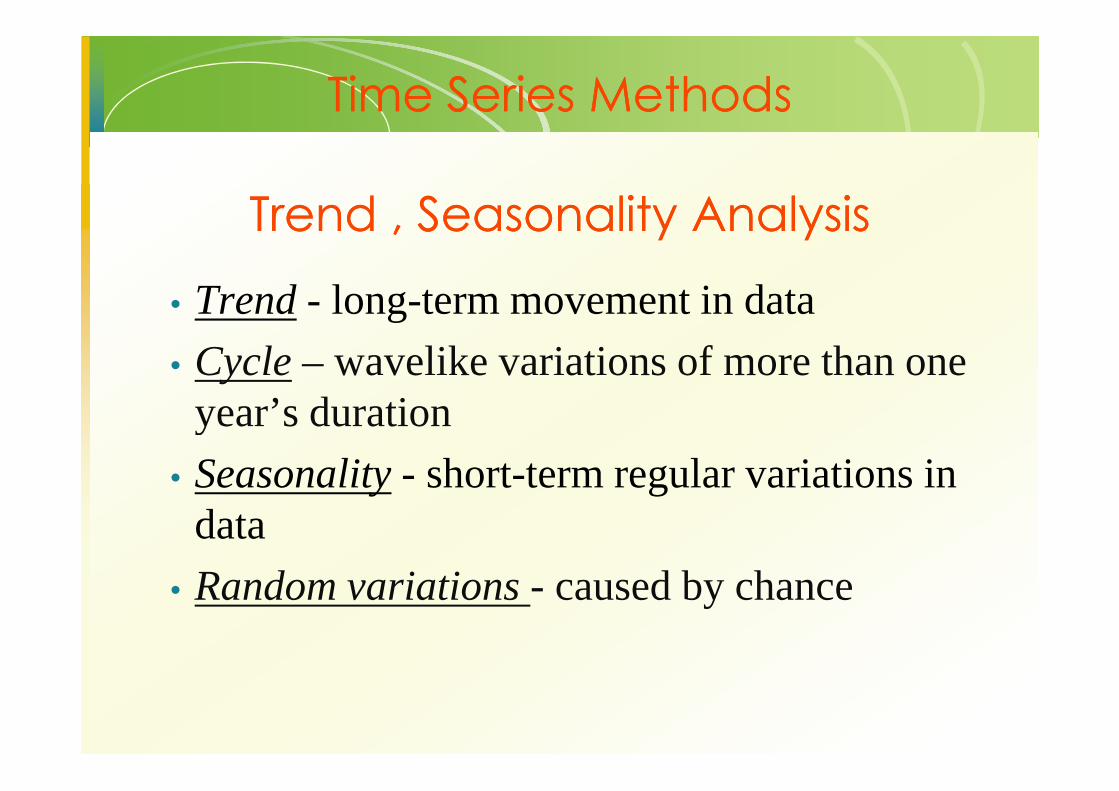
TTrend , Seasonalityrend , Seasonality Analysis Analysis

• Trend - long-term movement in data

• Cycle – wavelike variations of more than one year’s duration

Time Series Time Series Methods Methods

year’s duration

• Seasonality - short-term regular variations in data

• Random variations - caused by chance

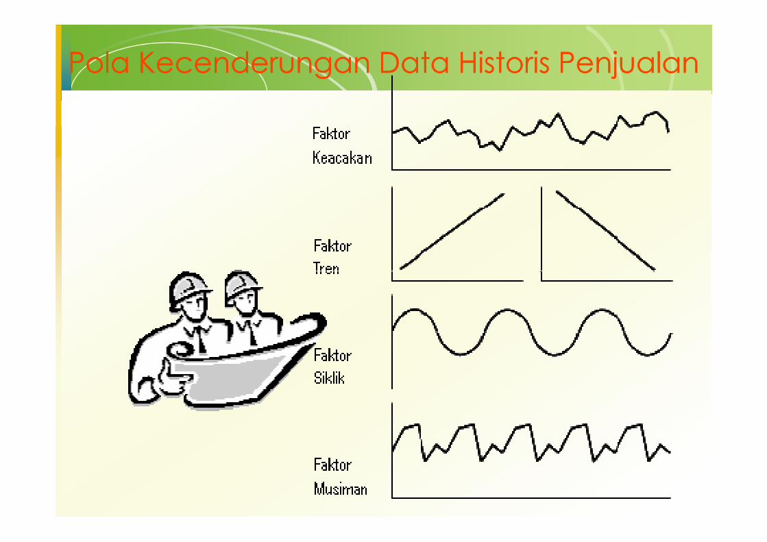
Pola Kecenderungan Data Historis PenjualanPola Kecenderungan Data Historis Penjualan

Forecast ErrorForecast Error

• Bias - The arithmetic sum of the errors

• Mean Square Error - Similar to simple sample variance

tt FAErrorForecast −=

TFA

MSE

tt

T

/)(

/T|errorforecast |

2

T

1t

2

−=

=

∑

∑=

• MAD - Mean Absolute Deviation

• MAPE – Mean Absolute Percentage Error

TFAMAD tt

T

t

/|| /T|errorforecast |1

T

1t

−==∑ ∑= =

TAFAMAPE ttt

T

t

/]/|[|1001

−= ∑=

TFA ttt

/)( 1

−=∑=

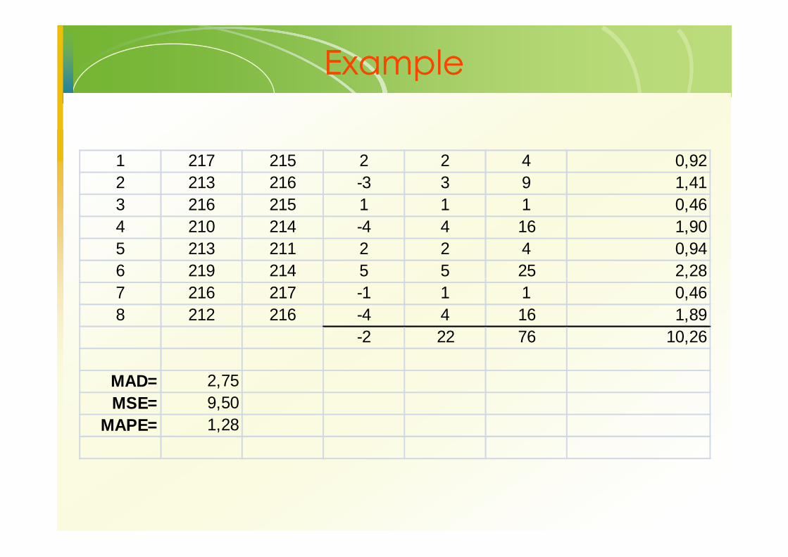
ExampleExample

1 217 215 2 2 4 0,922 213 216 -3 3 9 1,413 216 215 1 1 1 0,464 210 214 -4 4 16 1,905 213 211 2 2 4 0,946 219 214 5 5 25 2,286 219 214 5 5 25 2,287 216 217 -1 1 1 0,468 212 216 -4 4 16 1,89

-2 22 76 10,26

MAD= 2,75MSE= 9,50

MAPE= 1,28

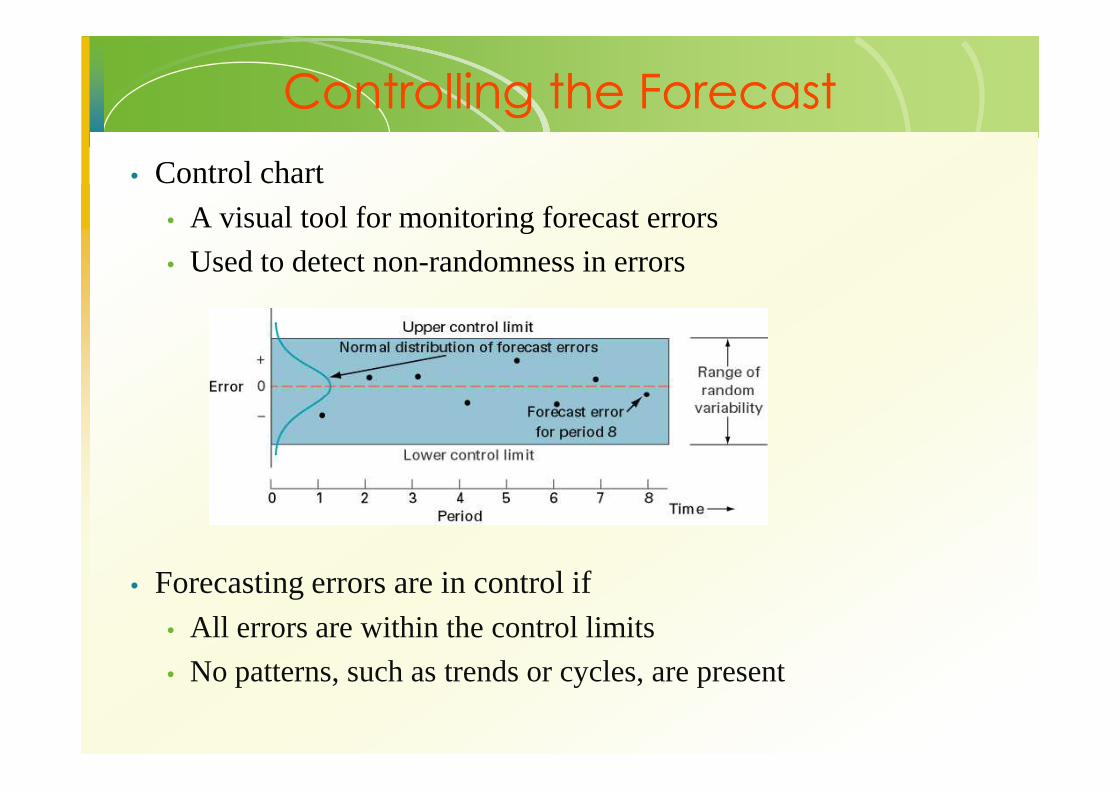
Controlling the ForecastControlling the Forecast

• Control chart• A visual tool for monitoring forecast errors

• Used to detect non-randomness in errors

• Forecasting errors are in control if• All errors are within the control limits

• No patterns, such as trends or cycles, are present

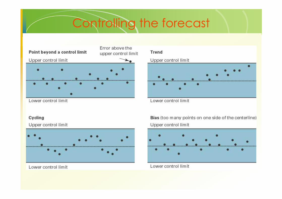
Controlling the forecastControlling the forecast

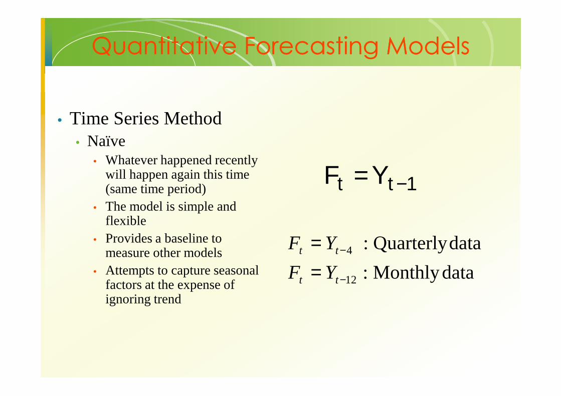
Quantitative Forecasting Models Quantitative Forecasting Models

• Time Series Method • Naïve

• Whatever happened recently will happen again this time (same time period) 1−= tt YF

• The model is simple and flexible

• Provides a baseline to measure other models

• Attempts to capture seasonal factors at the expense of ignoring trend

dataMonthly:

dataQuarterly:

12

4

−

−

==

tt

tt

YF

YF

Naive ForecastsNaive Forecasts

Uh, give me a minute.... We sold 250 wheels lastweek.... Now, next week we should sell....we should sell....

The forecast for any period equals the previous period’s actual value.

Naïve ForecastNaïve ForecastWallace Garden SupplyForecasting

PeriodActual Value

Naïve Forecast Error

Absolute Error

Percent Error

Squared Error

January 10 N/AFebruary 12 10 2 2 16,67% 4,0March 16 12 4 4 25,00% 16,0

Storage Shed Sales

April 13 16 -3 3 23,08% 9,0May 17 13 4 4 23,53% 16,0June 19 17 2 2 10,53% 4,0July 15 19 -4 4 26,67% 16,0August 20 15 5 5 25,00% 25,0September 22 20 2 2 9,09% 4,0October 19 22 -3 3 15,79% 9,0November 21 19 2 2 9,52% 4,0December 19 21 -2 2 10,53% 4,0

0,818 3 17,76% 10,091BIAS MAD MAPE MSE

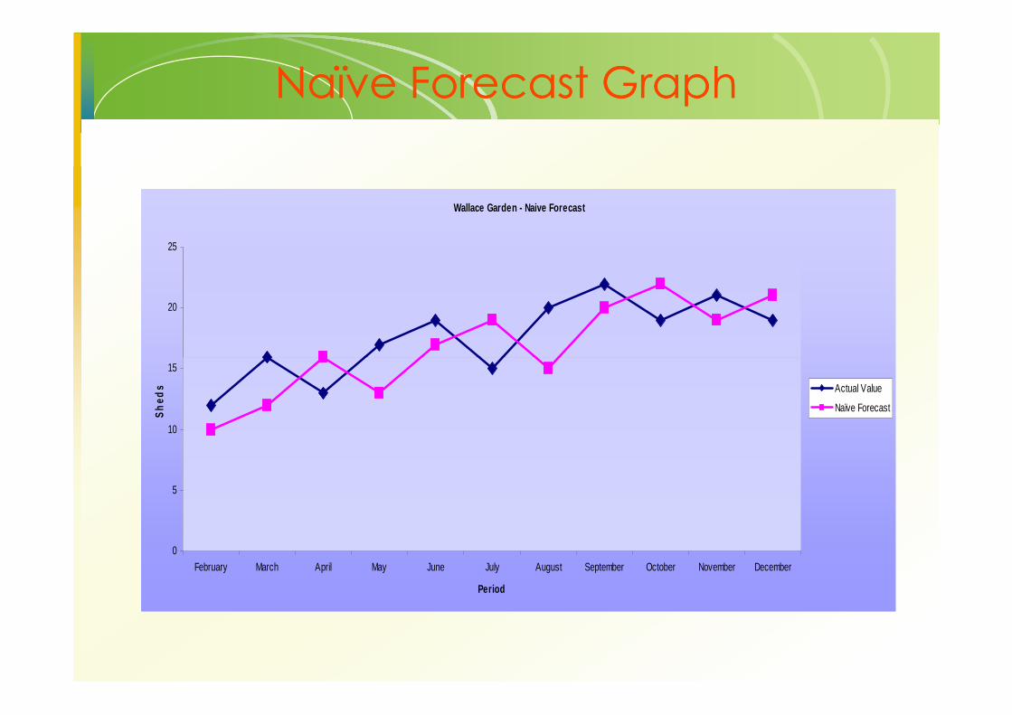
Naïve Forecast GraphNaïve Forecast Graph

Wallace Garden - Naive Forecast

20

25

0

5

10

15

February March April May June July August September October November December

Period

Sh

eds Actual Value

Naïve Forecast

• Simple to use

• Virtually no cost

• Quick and easy to prepare

• Easily understandable

Naive ForecastsNaive Forecasts

• Easily understandable

• Can be a standard for accuracy

• Cannot provide high accuracy

Techniques for AveragingTechniques for Averaging

• Moving average

• Weighted moving average

• Exponential smoothingExponential smoothing

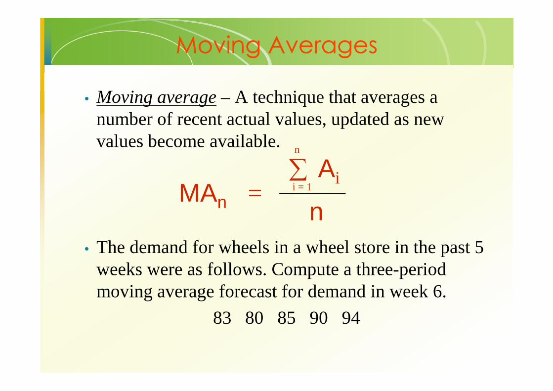
Moving AveragesMoving Averages

• Moving average – A technique that averages a number of recent actual values, updated as new values become available.

MAn =Ai

i = 1∑n

• The demand for wheels in a wheel store in the past 5 weeks were as follows. Compute a three-period moving average forecast for demand in week 6.

83 80 85 90 94

MAn =n

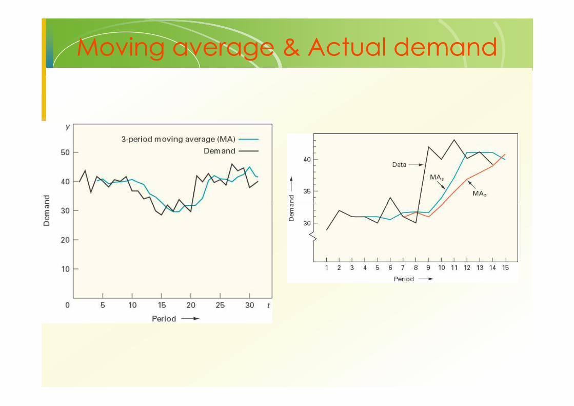
Moving average & Actual demandMoving average & Actual demand

Moving AveragesMoving Averages

Wallace Garden SupplyForecasting

PeriodActual Value Three-Month Moving Averages

January 10

Storage Shed Sales

January 10February 12March 16April 13 10 + 12 + 16 / 3 = 12.67May 17 12 + 16 + 13 / 3 = 13.67June 19 16 + 13 + 17 / 3 = 15.33July 15 13 + 17 + 19 / 3 = 16.33August 20 17 + 19 + 15 / 3 = 17.00September 22 19 + 15 + 20 / 3 = 18.00October 19 15 + 20 + 22 / 3 = 19.00November 21 20 + 22 + 19 / 3 = 20.33December 19 22 + 19 + 21 / 3 = 20.67

Moving Averages ForecastMoving Averages Forecast

Wallace Garden SupplyForecasting 3 period moving average

Input Data Forecast Error Analysis

Period Actual Value Forecast ErrorAbsolute

errorSquared

errorAbsolute % error

Month 1 10

Actual Value - Forecast

Month 1 10Month 2 12Month 3 16Month 4 13 12,667 0,333 0,333 0,111 2,56%Month 5 17 13,667 3,333 3,333 11,111 19,61%Month 6 19 15,333 3,667 3,667 13,444 19,30%Month 7 15 16,333 -1,333 1,333 1,778 8,89%Month 8 20 17,000 3,000 3,000 9,000 15,00%Month 9 22 18,000 4,000 4,000 16,000 18,18%Month 10 19 19,000 0,000 0,000 0,000 0,00%Month 11 21 20,333 0,667 0,667 0,444 3,17%Month 12 19 20,667 -1,667 1,667 2,778 8,77%

Average 12,000 2,000 6,074 10,61%Next period 19,667 BIAS MAD MSE MAPE

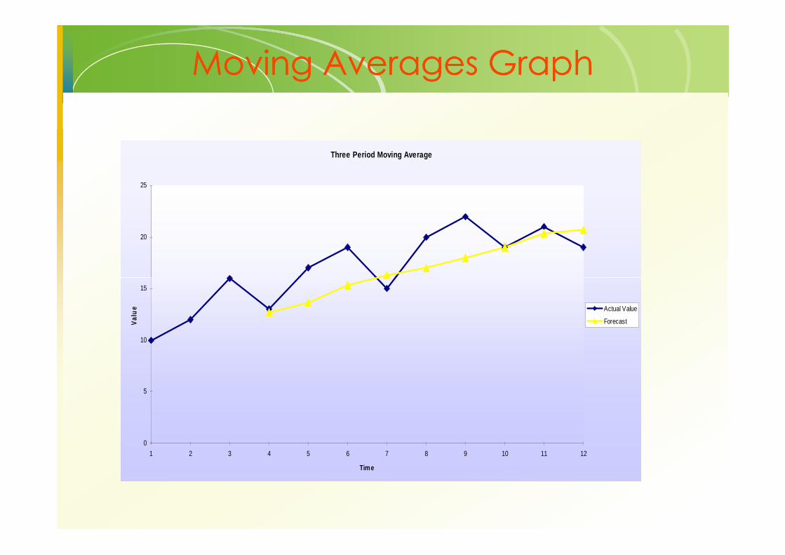
Moving Averages GraphMoving Averages Graph

Three Period Moving Average

20

25

0

5

10

15

1 2 3 4 5 6 7 8 9 10 11 12

Time

Val

ue Actual Value

Forecast

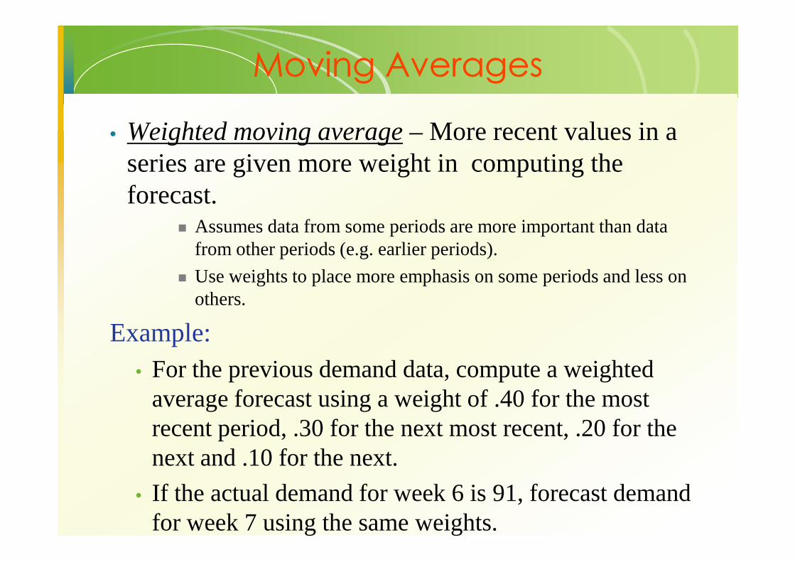
Moving AveragesMoving Averages

• Weighted moving average – More recent values in a series are given more weight in computing the forecast.

� Assumes data from some periods are more important than data from other periods (e.g. earlier periods).

� Use weights to place more emphasis on some periods and less on � Use weights to place more emphasis on some periods and less on others.

Example:• For the previous demand data, compute a weighted

average forecast using a weight of .40 for the most recent period, .30 for the next most recent, .20 for the next and .10 for the next.

• If the actual demand for week 6 is 91, forecast demand for week 7 using the same weights.

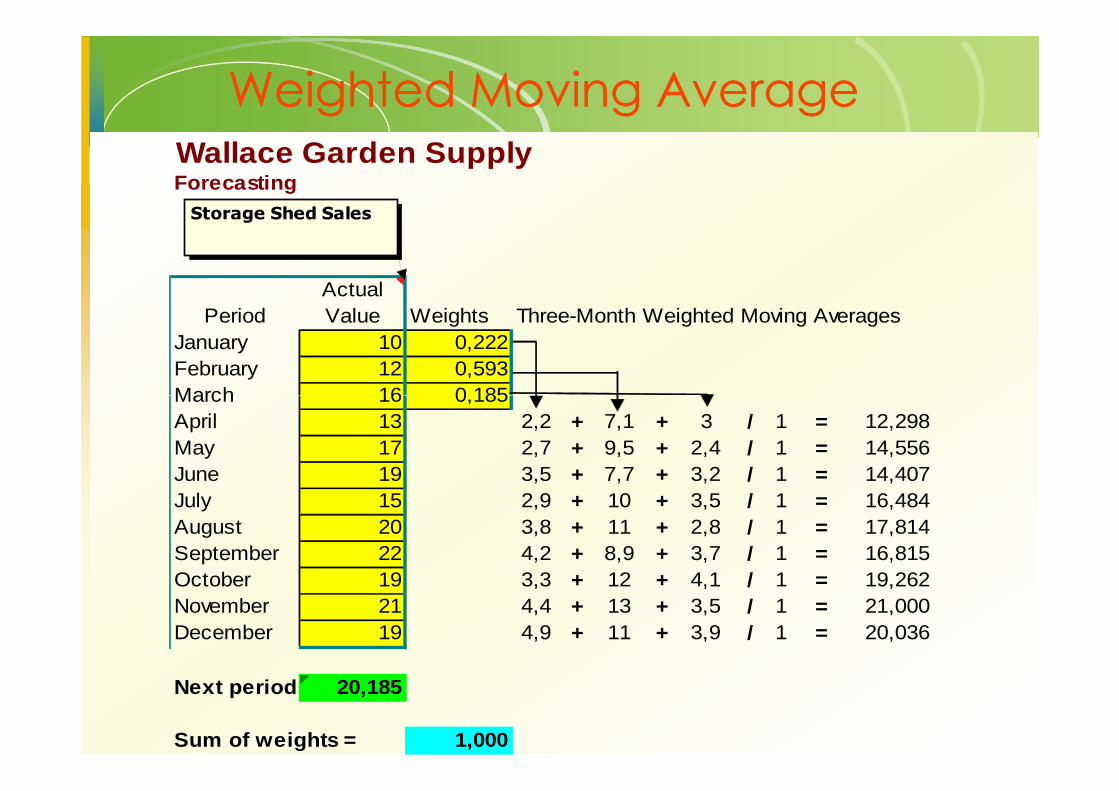
Weighted Moving AverageWeighted Moving AverageWallace Garden SupplyForecasting

PeriodActual Value Weights Three-Month Weighted Moving Averages

January 10 0,222February 12 0,593March 16 0,185

Storage Shed Sales

March 16 0,185April 13 2,2 + 7,1 + 3 / 1 = 12,298May 17 2,7 + 9,5 + 2,4 / 1 = 14,556June 19 3,5 + 7,7 + 3,2 / 1 = 14,407July 15 2,9 + 10 + 3,5 / 1 = 16,484August 20 3,8 + 11 + 2,8 / 1 = 17,814September 22 4,2 + 8,9 + 3,7 / 1 = 16,815October 19 3,3 + 12 + 4,1 / 1 = 19,262November 21 4,4 + 13 + 3,5 / 1 = 21,000December 19 4,9 + 11 + 3,9 / 1 = 20,036

Next period 20,185

Sum of weights = 1,000

Weighted Moving AverageWeighted Moving Average

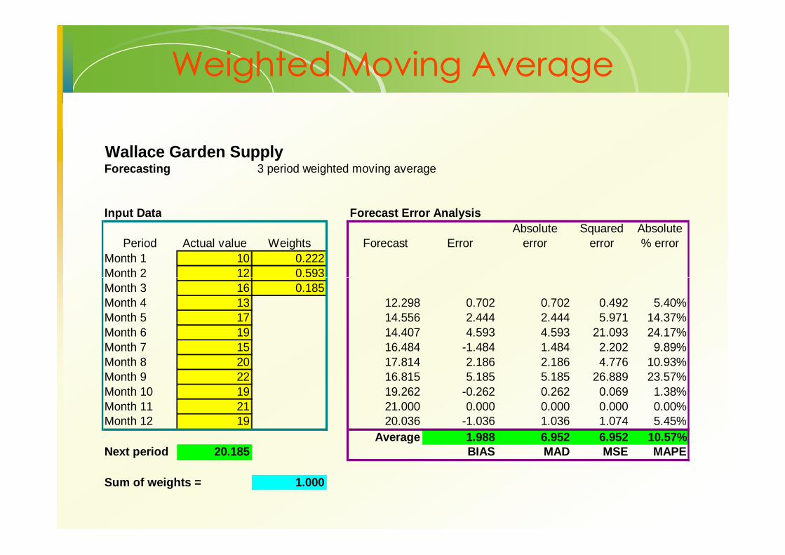
Wallace Garden Supply Forecasting 3 period weighted moving average

Input Data Forecast Error Analysis

Period Actual value Weights Forecast ErrorAbsolute

errorSquared

errorAbsolute % error

Month 1 10 0.222Month 2 12 0.593Month 2 12 0.593Month 3 16 0.185Month 4 13 12.298 0.702 0.702 0.492 5.40%Month 5 17 14.556 2.444 2.444 5.971 14.37%Month 6 19 14.407 4.593 4.593 21.093 24.17%Month 7 15 16.484 -1.484 1.484 2.202 9.89%Month 8 20 17.814 2.186 2.186 4.776 10.93%Month 9 22 16.815 5.185 5.185 26.889 23.57%Month 10 19 19.262 -0.262 0.262 0.069 1.38%Month 11 21 21.000 0.000 0.000 0.000 0.00%Month 12 19 20.036 -1.036 1.036 1.074 5.45%

Average 1.988 6.952 6.952 10.57%Next period 20.185 BIAS MAD MSE MAPE

Sum of weights = 1.000

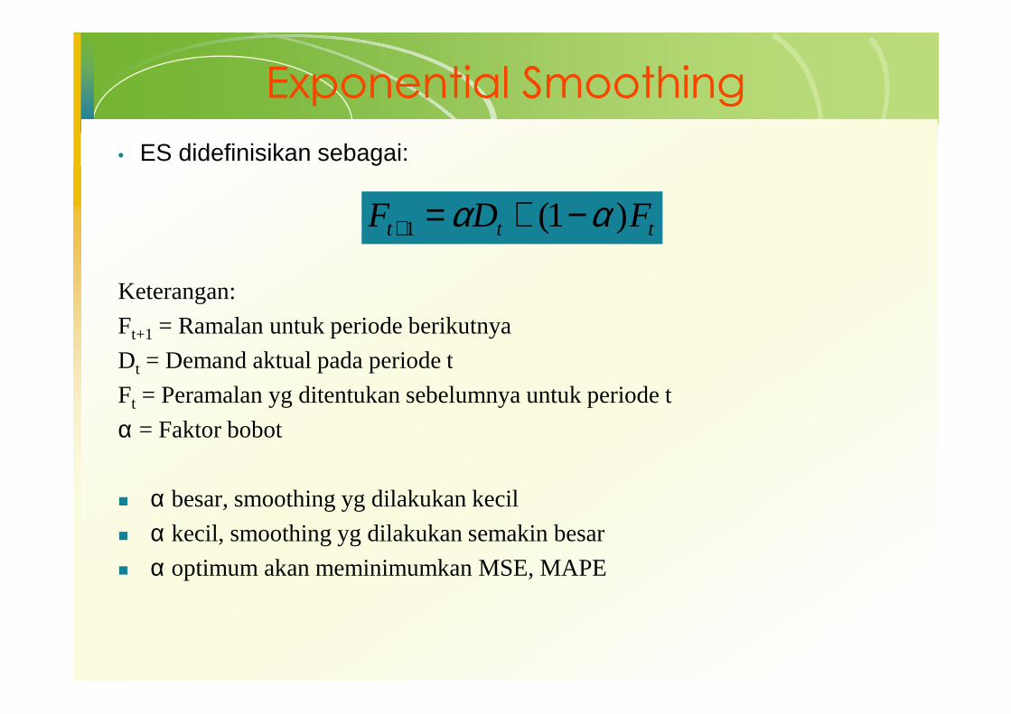
Exponential SmoothingExponential Smoothing

• ES didefinisikan sebagai:

Keterangan:

Ft+1 = Ramalan untuk periode berikutnya

D = Demand aktual pada periode t

ttt FDF )1(1 αα −+=+

Dt = Demand aktual pada periode t

Ft = Peramalan yg ditentukan sebelumnya untuk periode t

α = Faktor bobot

� α besar, smoothing yg dilakukan kecil

� α kecil, smoothing yg dilakukan semakin besar

� α optimum akan meminimumkan MSE, MAPE

Exponential SmoothingExponential Smoothing

• Weighted averaging method based on previous forecast plus a percentage of the forecast error

Ft = Ft-1 + α(At-1 - Ft-1)

forecast plus a percentage of the forecast error

• A-F is the error term, α is the % feedback

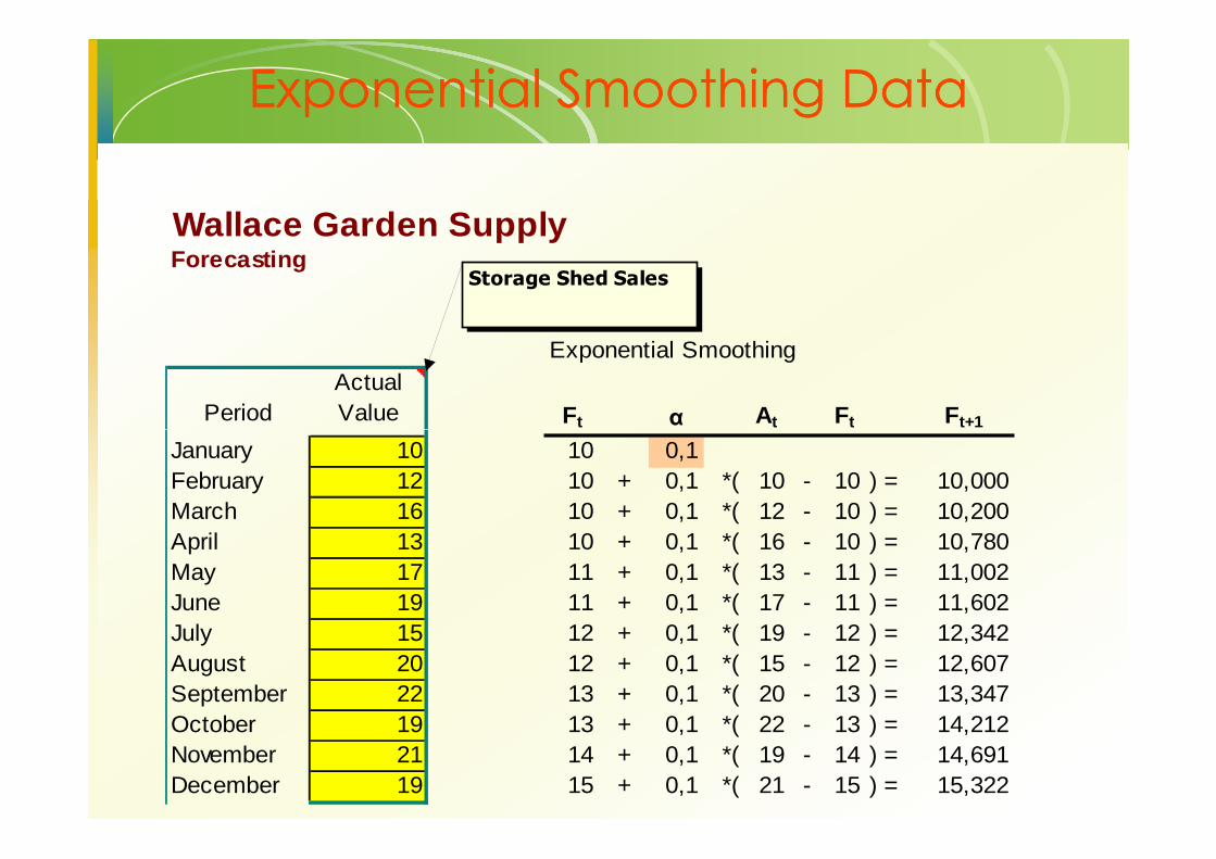
Exponential Smoothing DataExponential Smoothing Data

Wallace Garden SupplyForecasting

Exponential Smoothing

PeriodActual Value Ft α At Ft Ft+1

Storage Shed Sales

t α t t t+1

January 10 10 0,1February 12 10 + 0,1 *( 10 - 10 ) = 10,000March 16 10 + 0,1 *( 12 - 10 ) = 10,200April 13 10 + 0,1 *( 16 - 10 ) = 10,780May 17 11 + 0,1 *( 13 - 11 ) = 11,002June 19 11 + 0,1 *( 17 - 11 ) = 11,602July 15 12 + 0,1 *( 19 - 12 ) = 12,342August 20 12 + 0,1 *( 15 - 12 ) = 12,607September 22 13 + 0,1 *( 20 - 13 ) = 13,347October 19 13 + 0,1 *( 22 - 13 ) = 14,212November 21 14 + 0,1 *( 19 - 14 ) = 14,691December 19 15 + 0,1 *( 21 - 15 ) = 15,322

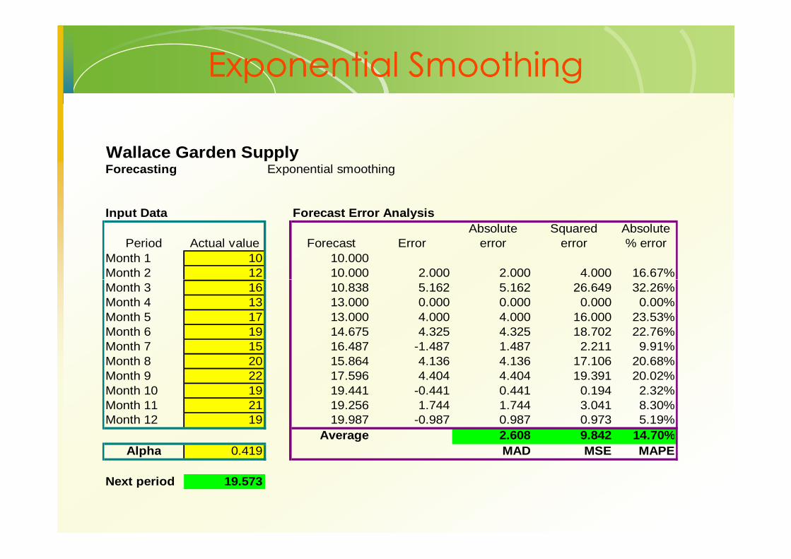
Exponential SmoothingExponential Smoothing

Wallace Garden SupplyForecasting Exponential smoothing

Input Data Forecast Error Analysis

Period Actual value Forecast ErrorAbsolute

errorSquared

errorAbsolute % error

Month 1 10 10.000Month 2 12 10.000 2.000 2.000 4.000 16.67%Month 3 16 10.838 5.162 5.162 26.649 32.26%Month 4 13 13.000 0.000 0.000 0.000 0.00%Month 5 17 13.000 4.000 4.000 16.000 23.53%Month 6 19 14.675 4.325 4.325 18.702 22.76%Month 7 15 16.487 -1.487 1.487 2.211 9.91%Month 8 20 15.864 4.136 4.136 17.106 20.68%Month 9 22 17.596 4.404 4.404 19.391 20.02%Month 10 19 19.441 -0.441 0.441 0.194 2.32%Month 11 21 19.256 1.744 1.744 3.041 8.30%Month 12 19 19.987 -0.987 0.987 0.973 5.19%

Average 2.608 9.842 14.70%Alpha 0.419 MAD MSE MAPE

Next period 19.573

Exponential SmoothingExponential Smoothing

Exponential Smoothing

15

20

25

She

ds Actual value

Forecast

0

5

10

Janu

ary

Febr

uary

Mar

ch

April

May

June July

Augu

st

Sept

embe

r

Octo

ber

Novem

ber

Decem

ber

She

ds

Forecast

Techniques for TrendTechniques for Trend

• Develop an equation that will suitably describe trend, when trend is present.

• The trend component may be linear or nonlinear• The trend component may be linear or nonlinear

• We focus on linear trends

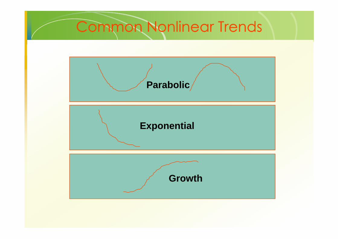
Common Nonlinear TrendsCommon Nonlinear Trends

Parabolic

Exponential

Growth

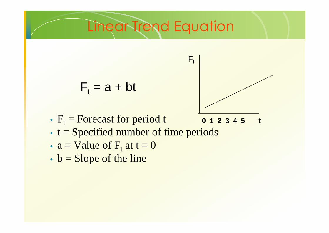
Linear Trend EquationLinear Trend Equation

• F = Forecast for period t

Ft = a + bt

0 1 2 3 4 5 t

Ft

• Ft = Forecast for period t• t = Specified number of time periods• a = Value of Ft at t = 0• b = Slope of the line

0 1 2 3 4 5 t

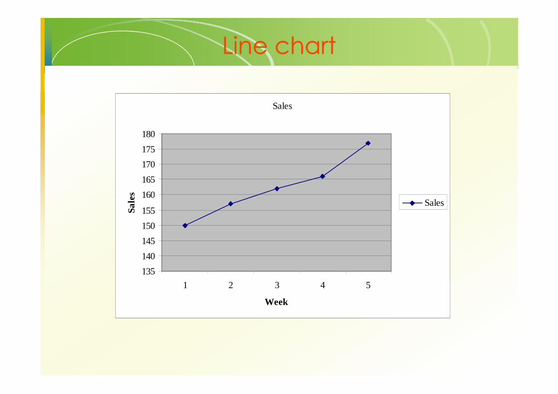
ExampleExample

• Sales for over the last 5 weeks are shown below:

Week: 1 2 3 4 5Sales: 150 157 162 166 177

• Plot the data and visually check to see if a linear trend line is appropriate.

• Determine the equation of the trend line• Predict sales for weeks 6 and 7.

Line chartLine chart

Sales

160

165

170

175

180S

ale

s

135

140

145

150

155

160

1 2 3 4 5

Week

Sa

les

Sales

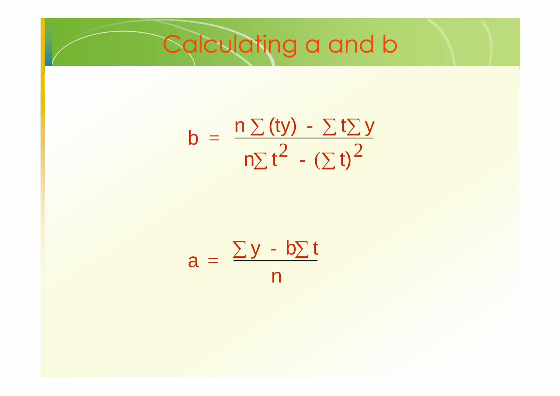
Calculating a and bCalculating a and b

b =n (ty) - t y

n t2 - ( t)2∑∑∑

∑∑

a =y - b t

n∑∑

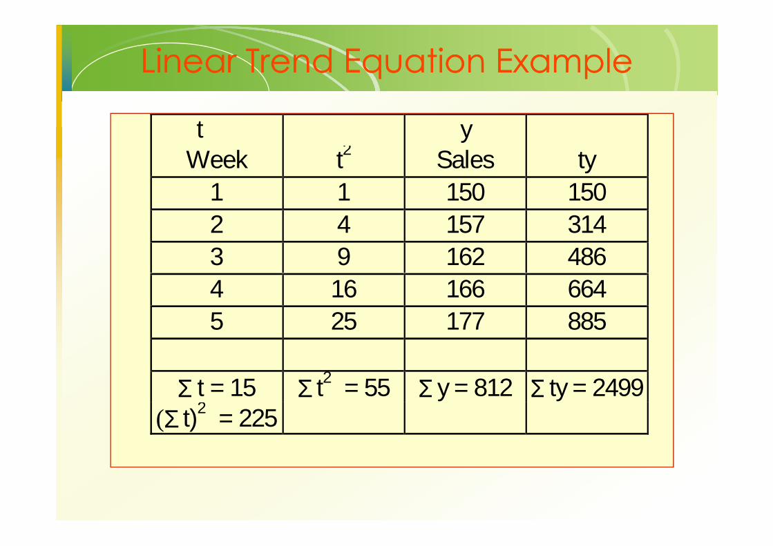
Linear Trend Equation ExampleLinear Trend Equation Example

t yWeek t2 Sales ty

1 1 150 1502 4 157 3143 9 162 4864 16 166 6645 25 177 885

Σ t = 15 Σ t2 = 55 Σ y = 812 Σ ty = 2499(Σ t)2 = 225

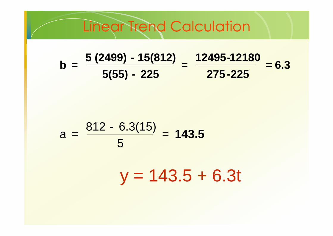
Linear Trend CalculationLinear Trend Calculation

b =5 (2499) - 15(812)

5(55) - 225=

12495-12180

275 -225= 6.3

y = 143.5 + 6.3t

a =812 - 6.3(15)

5= 143.5

Linear Trend plotLinear Trend plot

165

170

175

180

Actual data Linear equation

135

140

145

150

155

160

165

1 2 3 4 5