


Bahasa
Halaman
Hukum

arX
iv:h
ep-p
h/03
1028
5v1
24
Oct
200
3
CERN-TH/2003-259
UAB-FT-554
Weakly coupled Higgsless theories
and
precision electroweak tests
Riccardo Barbieri a, Alex Pomarol b and Riccardo Rattazzi c
aScuola Normale Superiore and INFN, Pisa, ItalybIFAE, Universitat Autonoma de Barcelona, 08193 Bellaterra (Barcelona), Spain
cTheory Division, CERN, CH-1211 Geneva 23, Switzerland
Abstract
In 5 dimensions the electroweak symmetry can be broken by boundary conditions, leading to a
new type of Higgsless theories. These could in principle improve on the 4D case by extending the
perturbative domain to energies higher than 4πv and by allowing a better fit to the electroweak
precision tests. Nevertheless, it is unlikely that both these improvements can be achieved, as we
show by discussing these problems in an explicit model.
1

1 Introduction
Higgsless theories of the electroweak interactions do not appear to allow an acceptable de-
scription of the ElectroWeak Precision Tests (EWPT) [1]. At least, since they become
strongly interacting at an energy of about 4πv, where v is the Higgs vacuum expectation
value, the calculability of the precision observables is limited. Furthermore, when an esti-
mate can be made under suitable assumptions [2], the ultraviolet (UV) contribution to the
parameter ǫ3 [3] (or to the parameter S [4]) is positive, which, added to the infrared (IR)
piece cut off at some high scale ∼ 4πv, makes it essentially impossible to fit the EWPT,
independently of the value of ǫ1 (or of the T parameter).
Breaking the electroweak symmetry by boundary conditions on an extra dimension may
however be a new twist of the problem (see for example refs. [5, 6]). The specific reason
for this statement is the following. It is well known that a gauge group G can be broken
by boundary conditions at compactification down to a subgroup H . In this situation the
vectors in H have a Kaluza-Klein (KK) tower starting with a massless 4D mode, while the
lightest state in G/H has mass 1/R, where R is the radius of compactification. A feature
of gauge symmetry breaking by boundary conditions, for example on orbifolds, is that in
general it does not introduce new physical scales associated to a strongly interacting regime
in the theory. For instance, using naive dimensional analysis (NDA)[7, 8], a five dimensional
gauge theory will become strongly coupled at a scale Λ ∼ 24π3/g25, whether it is broken by
boundary conditions or not. Now the potentially interesting fact is that, if we interpret the
lightest KK modes in G/H as the W and Z, the 5D cut-off Λ is written in terms of 4D
quantities as Λ ∼ 12π2mW/g24 (we have used 1/g2
4 = 2πR/g25 and mW ∼ 1/R). Compared
to the cut-off 4πmW/g4 ∼ 1 TeV of a 4D Higgsless theory, the cut-off of the 5D Higgsless
theory is a factor 3π/g4 bigger: Λ ∼ 10 TeV. To summarize, what happens physically is
the following: an appropriate tower of KK states may play the role of the normal 4D Higgs
boson in preventing the relevant amplitudes from exceeding the unitarity bounds up to an
energy scale Λ which is not arbitrarily large but can be well above the cut-off 4πv of a 4D
Higgsless theory. This is why we call them weakly interacting Higgsless theories.
One may do the same power counting exercise for a D-dimensional gauge theory com-
pactified down to 4-dimensions. In that case the cut-off is ΛD−4 ∼ (4π)D/2Γ(D/2)/g2D, while
2

the 4D gauge coupling is 1/g24 = (2πR)D−4/g2
D. If we identify mW ∼ 1/R we can then write
Λ = mW [16Γ(D/2)π(4−D/2)/g24]
1/(D−4), from which we conclude that by going to D > 5 we
do not actually increase the cut-off. For D = 6 the cut-off is again roughly 4πv, while for
D → ∞ it becomes ∼ mW . This result is intuitively clear: with a large number of extra
dimensions, in order to keep g4 finite, the radius of compactification should be right at the
cut-off. We therefore stick to D = 5.
The next obvious problem is to see how these 5D Higgsless theories can do in describing
the EWPT, which is the purpose of this paper ∗. We do this by analysing a specific model
designed to keep under control the effects of the breaking of custodial isospin, so that we
can focus on the effects of ǫ3 only. We shall also comment on the likely general validity of
our conclusions.
2 The model
Motivated by the simple argument given in the introduction we consider a 5D gauge theory
compactified on S1/Z2. Since we want calculable (and small) custodial symmetry breaking
effects, we must separate in 5D the sectors that break the electroweak symmetry from those
that break the custodial symmetry. A necessary requirement to achieve this property is the
promotion of custodial symmetry to a gauge symmetry. Then the minimal model with a
chance of giving a realistic phenomenology has gauge groupG = SU(2)L×SU(2)R×U(1)B−L.
Following refs. [10, 11] we break G → SU(2) × U(1)Y at one boundary, y = 0, and G →SU(2)L+R × U(1)B−L at the other boundary, y = πR. Then the only surviving gauge
symmetry below the compactification scale is U(1)Q. We achieve the breaking by explicitly
adding mass terms for the broken generator vector at the boundary and by sending this mass
to infinity †. The most general lagrangian up to two derivatives is then
L = L5 + δ(y)L0 + δ(y − πR)Lπ , (1)
∗For a related discussion, see ref. [9].†Even if the boundary mass is kept to its natural value, M ∼ Λ, this will only modify our calculations
by O(ML/(Λ2R)) effects.
3
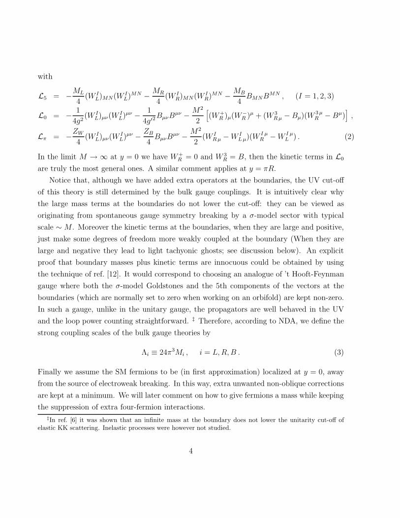
with
L5 = −ML
4(W I
L)MN(W IL)MN − MR
4(W I
R)MN(W IR)MN − MB
4BMNB
MN , (I = 1, 2, 3)
L0 = − 1
4g2(W I
L)µν(WIL)µν − 1
4g′2BµνB
µν − M2
2
[
(W+R )µ(W−
R )µ + (W 3R µ − Bµ)(W
3 µR −Bµ)
]
,
Lπ = −ZW
4(W I
L)µν(WIL)µν − ZB
4BµνB
µν − M2
2(W I
R µ −W IL µ)(W
I µR −W I µ
L ) . (2)
In the limit M → ∞ at y = 0 we have W+R = 0 and W 3
R = B, then the kinetic terms in L0
are truly the most general ones. A similar comment applies at y = πR.
Notice that, although we have added extra operators at the boundaries, the UV cut-off
of this theory is still determined by the bulk gauge couplings. It is intuitively clear why
the large mass terms at the boundaries do not lower the cut-off: they can be viewed as
originating from spontaneous gauge symmetry breaking by a σ-model sector with typical
scale ∼M . Moreover the kinetic terms at the boundaries, when they are large and positive,
just make some degrees of freedom more weakly coupled at the boundary (When they are
large and negative they lead to light tachyonic ghosts; see discussion below). An explicit
proof that boundary masses plus kinetic terms are innocuous could be obtained by using
the technique of ref. [12]. It would correspond to choosing an analogue of ’t Hooft-Feynman
gauge where both the σ-model Goldstones and the 5th components of the vectors at the
boundaries (which are normally set to zero when working on an orbifold) are kept non-zero.
In such a gauge, unlike in the unitary gauge, the propagators are well behaved in the UV
and the loop power counting straightforward. ‡ Therefore, according to NDA, we define the
strong coupling scales of the bulk gauge theories by
Λi ≡ 24π3Mi , i = L,R,B . (3)
Finally we assume the SM fermions to be (in first approximation) localized at y = 0, away
from the source of electroweak breaking. In this way, extra unwanted non-oblique corrections
are kept at a minimum. We will later comment on how to give fermions a mass while keeping
the suppression of extra four-fermion interactions.
‡In ref. [6] it was shown that an infinite mass at the boundary does not lower the unitarity cut-off ofelastic KK scattering. Inelastic processes were however not studied.
4

3 The low energy effective theory
To study the low energy phenomenology one way to proceed is to find the KK masses and
wave functions. However, since the SM fermions couple to W IL(x, y = 0) ≡ W I(x) and
W 3R(x, y = 0) = B(x, y = 0) ≡ B(x), it is convenient to treat the exchange of vectors in a
two step procedure. First we integrate out the bulk to obtain an effective lagrangian for W I
and B. Then we consider the exchange of the interpolating fields W I and B between light
fermions. Indeed we will not need to perform this second step: to compare with the data we
just need to extract the ǫ’s [3], or S, T, U observables [4], from the effective lagrangian for
the interpolating fields. This way of proceeding is clearly inspired by holography, though we
do not want to emphasize this aspect for the time being.
To integrate out the bulk, we first must solve the 5D equations of motions, imposing at
y = πR the boundary conditions that follow from the variation of the action, while at y = 0
the fields are fixed at W IL(x, y = 0) = W I(x) and W 3
R(x, y = 0) = B(x, y = 0) = B(x). By
substituting the result back into the action, we obtain the 4D effective lagrangian
Leff =∫ 2πR
0dy (L5 + Lπ) . (4)
We will work in the unitary gauge gauge where the 5th components of the gauge fields are
set to zero. At the quadratic level in the 4D fields W IL(x), B(x), integration by parts and
use of the equations of motion allows to write Leff as a boundary integral
Leff =[
MLWIµ∂yW
I µL + Bµ
(
MR∂yW3µR +MB∂yB
µ)]
y=0. (5)
In order to solve the equations of motion it is useful to work in the momentum representation
along the four non-compact dimensions: xµ → pµ. Moreover it is useful to separate the
fields in the longitudinal and transverse components Vµ(y) = V tµ + V l
µ satisfying separate 5D
equations
(∂2y − p2)V t
µ = 0 ,
∂2yV
lµ = 0 . (6)
Nevertheless, since we are interested in the coupling to light fermions, we will just focus
on the transverse part and eliminate the superscript alltogether. The general bulk solution
5
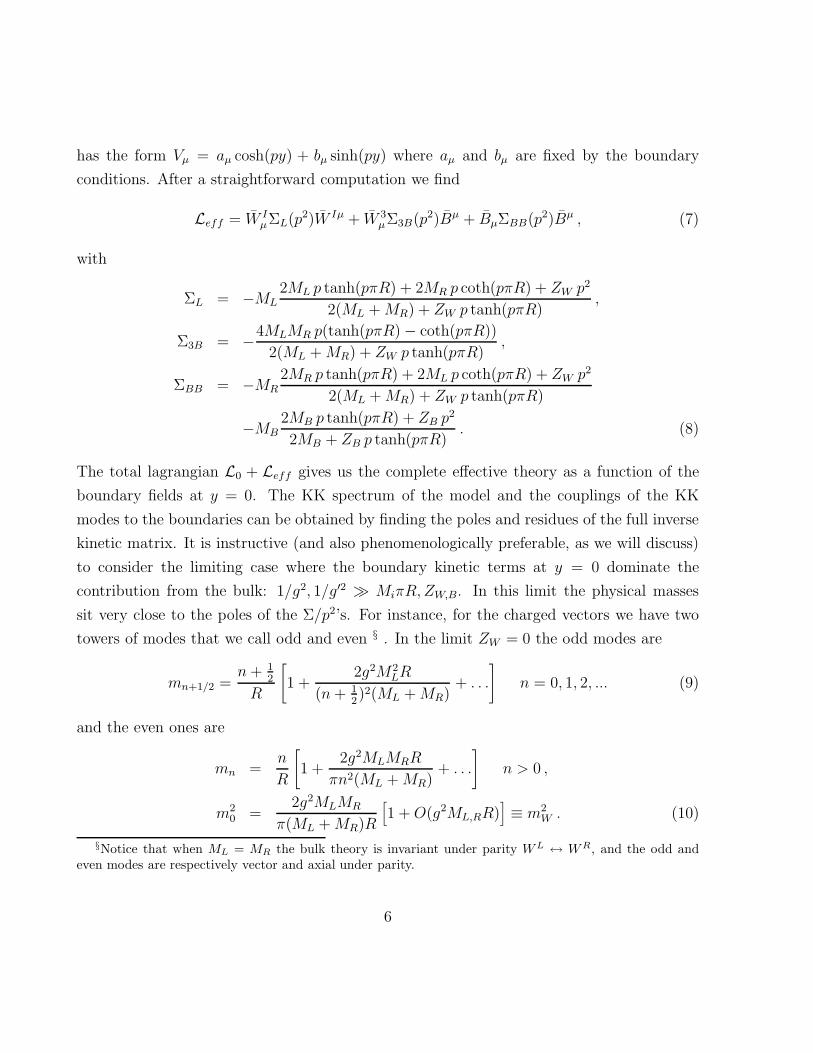
has the form Vµ = aµ cosh(py) + bµ sinh(py) where aµ and bµ are fixed by the boundary
conditions. After a straightforward computation we find
Leff = W IµΣL(p2)W Iµ + W 3
µΣ3B(p2)Bµ + BµΣBB(p2)Bµ , (7)
with
ΣL = −ML2ML p tanh(pπR) + 2MR p coth(pπR) + ZW p2
2(ML +MR) + ZW p tanh(pπR),
Σ3B = −4MLMR p(tanh(pπR) − coth(pπR))
2(ML +MR) + ZW p tanh(pπR),
ΣBB = −MR2MR p tanh(pπR) + 2ML p coth(pπR) + ZW p2
2(ML +MR) + ZW p tanh(pπR)
−MB2MB p tanh(pπR) + ZB p
2
2MB + ZB p tanh(pπR). (8)
The total lagrangian L0 + Leff gives us the complete effective theory as a function of the
boundary fields at y = 0. The KK spectrum of the model and the couplings of the KK
modes to the boundaries can be obtained by finding the poles and residues of the full inverse
kinetic matrix. It is instructive (and also phenomenologically preferable, as we will discuss)
to consider the limiting case where the boundary kinetic terms at y = 0 dominate the
contribution from the bulk: 1/g2, 1/g′2 ≫ MiπR, ZW,B. In this limit the physical masses
sit very close to the poles of the Σ/p2’s. For instance, for the charged vectors we have two
towers of modes that we call odd and even § . In the limit ZW = 0 the odd modes are
mn+1/2 =n+ 1
2
R
[
1 +2g2M2
LR
(n+ 12)2(ML +MR)
+ . . .
]
n = 0, 1, 2, ... (9)
and the even ones are
mn =n
R
[
1 +2g2MLMRR
πn2(ML +MR)+ . . .
]
n > 0 ,
m20 =
2g2MLMR
π(ML +MR)R
[
1 +O(g2ML,RR)]
≡ m2W . (10)
§Notice that when ML = MR the bulk theory is invariant under parity WL ↔ WR, and the odd andeven modes are respectively vector and axial under parity.
6

In the limit we are considering, the lightest mode is much lighter than the others m0 ≪ 1/R:
it sits close to the Goldstone pole of ΣL/p2. This mode should be interpreted as the usual
W -boson of the standard model. Similarly in the neutral sector we find a lightest massive
boson, the Z, with mass
m2Z =
2(g2 + g′2)MLMR
π(ML +MR)R
[
1 +O(g2ML,RR)]
. (11)
One can compute the couplings of Z, W and photon to elementary fermions from the first
∂p2 derivative of the full 2-point function at the zeroes. For small g2ML,RR, one finds that
the leading contribution arises from the boundary lagrangian L0. We then conclude that, up
to corrections of O(g2ML,RR), the SM relations between masses and couplings are satisfied.
This can also be seen from the wave-function of the lowest KK modes that, for large kinetic
terms on the y = 0 boundary, is peaked at y = 0, and then the SM gauge fields correspond
approximately to the boundary fields W I and B.
All the deviation from the SM at the tree level are due to oblique corrections and can be
studied by expanding eq. (8) at second order in p2 around p2 = 0: Σ(p2) ≃ Σ(0)+p2Σ′(0). As
custodial isospin is manifestly preserved by eq. (7), we find that the only non-zero observable
is ǫ3 (S parameter):
ǫ3 = −g2Σ′3B(0) = g24πR
3
MLMR
ML +MR
[
1 +3ZW
4π(ML +MR)R
]
. (12)
It is convenient to define 1/Λ = 1/ΛR + 1/ΛL, so that Λ is essentially the cut-off of the
theory. It is also convenient to define ZW ≡ δ/16π2, as δ = O(1) corresponds to the natural
NDA minimal size of boundary terms. This way ǫ3 is rewritten as
ǫ3 =g2
18π2(ΛR)
[
1 +9δ
8(ΛR + ΛL)R
]
. (13)
Now, the loop expansion parameter of our theory is ∼ 1/(ΛR). In order for all our approach
to be any better that just a random strongly coupled electroweak breaking sector we need
ΛR ≫ 1. This can be reconciled with the experimental bound ǫ3 <∼ 3 · 10−3 ¶ only if δ
¶ǫ3 <∼ 3 · 10−3 is the limit on the extra contribution to ǫ3 relative to the SM one with mH = 115 GeV.The limit is at 99% C.L. for a fit with ǫ1 and ǫ3 free, but ǫ2 and ǫb fixed at their SM values. Letting ǫ2 andǫb be also free would weaken the limit, but only in a totally marginal way.
7

is large and negative, δ ∼ −ΛR, and partially cancels the leading term in eq. (13). This
requirement, however, leads to the presence of a tachyonic ghost with m2 ∼ −1/R2 in the
vector spectrum, again a situation that would make our effective theory useless.
4 Fermion masses
The discussion so far assumed the SM fermions to be exactly localized at y = 0, in which
case they would be exactly massless, having no access to the electroweak breaking source
at y = πR. As we have argued, in this limiting case there are only oblique corrections to
fermion interactions: all the information that there exists an extra dimension (and some
strong dynamics) is encoded in the vector self-energies in eq. (7). For example, there are no
additional 4-fermion contact interactions.
A more realistic realization of fermions is the following. Consider bulk fermions with the
usual quantum numbers under SU(2)L ×SU(2)R ×U(1)B−L. For instance, the right handed
fermions will sit in (1, 2, B−L) doublets. Each such 5D fermion upon orbifold projection will
give rise to one chiral multiplet with the proper quantum numbers under SU(2)L × U(1)Y .
Fermion mass operators mixing left and right multiplet can then be written at y = πR, very
much like the WR−WL vectors. However in the case of fermions, since their mass dimension
in 5D is 2, the mass coefficient at the boundary is dimension-less. Then, in the limit in
which the scale of electroweak breaking at y = πR is sent to infinity, the fermion mass at the
boundary should stay finite. Indeed if we indicate by F the scale of electroweak breaking
at the boundary and put back the Goldstone field matrix U which non linearly realizes the
symmetry, the fermion mass operator has the form ψUψ while the vector mass arises from
the Goldstone kinetic term F 2(DµU)†(DµU).
Finally, to make the masses small, to break isospin symmetry, and to cause effective
approximate localization on the y = 0 boundary it is enough to add large kinetic terms for
the fermions at y = 0. Since isospin is broken at y = 0 the kinetic terms will distinguish
fermions with different isospin, for instance sR from cR, and a realistic theory can be easily
obtained. Fermion masses mf will go roughly like 1/√ZLZR, where ZL and ZR are the
boundary kinetic coefficients of the left and right handed components respectively. Notice
that the Z’s for fermions have dimension of length. Non oblique effects due to the fermion
8

tail into the bulk will then scale like ∼ R/Z ∼ mf/mKK , which is negligible for the 2 light
generations, but probably not for the bottom quark. One could also spread the fermions
more into the bulk by decreasing the Z ′s while decreasing at the same time the fermion mass
coefficients at the electroweak breaking boundary. This way one would get more sizeable
non-oblique corrections to EWPT, in the form of corrections to the W and Z vertices and
four-fermion interactions from the direct coupling to vector KK modes. In principle these
extra parameters could be used to improve the fit, tuning the effective ǫ3 small. We do not
pursue this here, since we do not think of this possibility as being very compelling.
5 ǫ3 for a general metric
One can wonder whether different 5D geometries can change the result above by giving, for
example, a negative contribution to ǫ3. Here we will show that this is not the case and
ǫ3 stays positive whatever the metric. As we want to preserve 4D Poincare symmetry the
curvature will just reduce to a warping. It is convenient to choose the 5th coordinate y in
such a way that the metric is
ds2 = e2σ(y)dxµdxµ + e4σ(y)dy2 , (14)
and take, to simplify the notation, 0 ≤ y ≤ 1 (πR = 1). With this choice the bulk equation
of motion of a transverse vector field becomes
(∂2y − p2e2σ)Vµ = 0 . (15)
To simplify the discussion we limit ourselves to the case MR = ML = M , in which parity is
conserved in the bulk and we set ZW = 0. Moreover, as U(1)B−L does not play any role in
ǫ3, we neglect it alltogether. The extension to the general case is straightforward.
To calculate ǫ3 it is convenient to work in the basis of vector V = (WL + WR)/√
2 and
axial A = (WL −WR)/√
2 fields, for which
ǫ3 = −g2
4[Σ′
V (0) − Σ′A(0)] , (16)
9

where ΣV = 4MV (−1)∂yV |y=0 and similarly for ΣA. Since we are only interested in the Σ’s
at O(p2), we can write the solutions of the bulk equations of motion as
Vµ = Vµ(p2)(
v(0)(y) + p2v(1)(y) +O(p4))
,
Aµ = Aµ(p2)(
a(0)(y) + p2a(1)(y) +O(p4))
, (17)
where, as before, Aµ and Vµ are the fields at y = 0. The functions v(0) and a(0) solve eq. (15)
at p2 = 0, with boundary conditions v(0)(0) = a(0)(0) = 1 and ∂yv(0)|y=1 = a(0)(1) = 0. We
obtain
v(0) = 1 , a(0) = 1 − y . (18)
The function v(1) solves ∂2yv
(1) = e2σ(y)v(0) with boundary conditions v(1)(0) = ∂yv(1)|y=1 = 0.
For a(1) the boundary conditions are a(1)(0) = a(1)(1) = 0. Then we find
ǫ3 = g2M{∫ 1
0e2σ(y)dy −
∫ 1
0dy∫ y
0(1 − y′)e2σ(y′)dy′
}
, (19)
which is manifestly positive. The first term can in fact be written as an integral in two
variables by multiplying by 1 =∫ 10 dy
′. Then, since e2σ > (1 − y)e2σ > 0 and the domain of
integration of the second term is a subset of the domain of the first, ǫ3 > 0 follows.
While ǫ3 is always positive, it could become very small if e2σ decreases rapidly away from
y = 0. However this is the situation in which the bulk curvature becomes large. Indeed
the Ricci scalar is given by R = [8σ′′ + 4(σ′)2]e−4σ and tends to grow when the warp factor
decreases. In fact the curvature length scales roughly like e2σ, so that the general expression
in eq. (19) roughly corresponds to the flat case result, eq. (13), with the radius R replaced
by the curvature length at y = 1.
As an explicit example consider the family of metrics (in the conformal frame)
ds2 = (1 + y/L)2d{
dxµdxµ + dy2
}
, (20)
with 0 ≤ y ≤ πR as originally. With this parametrization the massive KK modes are still
quantized in units of 1/R. On the other hand the curvature goes like
R ∼ 1
L2(1 + y/L)2+2d, (21)
10

so that for d < −1 it grows at the electroweak breaking boundary (d = −1 corresponds to
AdS). Indicating ∆ = (1 + πR/L) we have
ǫ3 = g2ML
d+ 1
{
−1 + ∆1+d +4 + (d− 1)2(∆2 − 1) + (d− 3)∆1−d − (1 + d)∆d−1
(3 − d)(2 − ∆1−d − ∆d−1)
}
, (22)
which for d < −1, L ≪ R (big warping) gives roughly ǫ3 ≃ g2ΛRC/(18π2) where the
curvature length at y = 1, RC ∼ L∆d+1, has replaced the radius R. Of course when ΛRC < 1
we loose control of the derivative expansion for our gauge theory. We then conclude that the
model in the regime of calculability, ΛR,ΛRC ≫ 1 , gives always large contributions to ǫ3.
6 Similarities with strongly coupled 4D theories
In this Section we comment on the relation between the model presented here and technicolor-
like theories in 4D. We will consider the case M = ML = MR and ZW = 0.
As done for the case of AdS/CFT one can establish a qualitative correspondence between
the bulk theory (in fact the bulk plus the y = πR boundary) and a purely four dimensional
field theory with a large number of particles, indeed a large N theory. The loop expansion
parameter 1/(ΛR) of the 5D theory corresponds to the topological expansion parameter
1/N , so that our tree level calculation corresponds to the planar limit. Consistent with this
interpretation, the couplings among the individual KK bosons go like 1/√N , as expected
in a large N theory. The result of eq. (13), written as ǫ3 ∼ g2N/18π2, also respects the
correspondence: it looks precisely like what one would expect in a large N technicolor.
Similarly the 1-loop gauge contribution to ǫ1 and ǫ2 is proportional to g′2/16π2, with no
N enhancement. This result is easy to understand in the ”dual” 4D theory. Custodial
isospin is only broken by a weak gauging of hypercharge by an external gauge boson (≡living at the y = 0 boundary). Isospin breaking loop effects involve the exchange of this
single gauge boson and are thus not enhanced by N . Similar considerations can be made for
the top contribution. Of course, though useful, this correspondence is only qualitative, in
that we do not know the microscopic theory on the 4D side. We stress that this qualitative
correspondence is valid whatever the metric of the 5D theory. The case of AdS geometry only
adds conformal symmetry into the game allowing for an (easy) extrapolation (for a subset
of observables) to arbitrarily high energy. On the other hand, when looking for solutions to
11
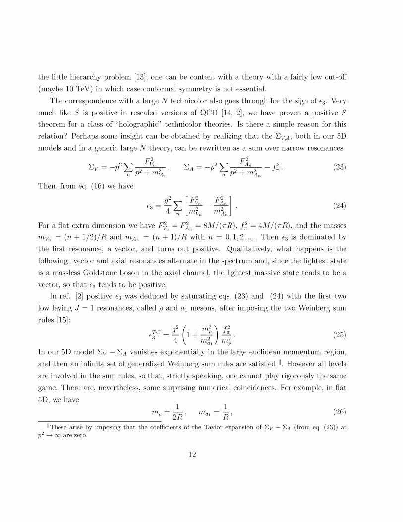
the little hierarchy problem [13], one can be content with a theory with a fairly low cut-off
(maybe 10 TeV) in which case conformal symmetry is not essential.
The correspondence with a large N technicolor also goes through for the sign of ǫ3. Very
much like S is positive in rescaled versions of QCD [14, 2], we have proven a positive S
theorem for a class of “holographic” technicolor theories. Is there a simple reason for this
relation? Perhaps some insight can be obtained by realizing that the ΣV,A, both in our 5D
models and in a generic large N theory, can be rewritten as a sum over narrow resonances
ΣV = −p2∑
n
F 2Vn
p2 +m2Vn
, ΣA = −p2∑
n
F 2An
p2 +m2An
− f 2π . (23)
Then, from eq. (16) we have
ǫ3 =g2
4
∑
n
[
F 2Vn
m2Vn
− F 2An
m2An
]
. (24)
For a flat extra dimension we have F 2Vn
= F 2An
= 8M/(πR), f 2π = 4M/(πR), and the masses
mVn= (n + 1/2)/R and mAn
= (n + 1)/R with n = 0, 1, 2, .... Then ǫ3 is dominated by
the first resonance, a vector, and turns out positive. Qualitatively, what happens is the
following: vector and axial resonances alternate in the spectrum and, since the lightest state
is a massless Goldstone boson in the axial channel, the lightest massive state tends to be a
vector, so that ǫ3 tends to be positive.
In ref. [2] positive ǫ3 was deduced by saturating eqs. (23) and (24) with the first two
low laying J = 1 resonances, called ρ and a1 mesons, after imposing the two Weinberg sum
rules [15]:
ǫTC3 =
g2
4
(
1 +m2
ρ
m2a1
)
f 2π
m2ρ
. (25)
In our 5D model ΣV − ΣA vanishes exponentially in the large euclidean momentum region,
and then an infinite set of generalized Weinberg sum rules are satisfied ‖. However all levels
are involved in the sum rules, so that, strictly speaking, one cannot play rigorously the same
game. There are, nevertheless, some surprising numerical coincidences. For example, in flat
5D, we have
mρ =1
2R, ma1
=1
R, (26)
‖These arise by imposing that the coefficients of the Taylor expansion of ΣV − ΣA (from eq. (23)) atp2 → ∞ are zero.
12

and eq. (12) can be rewritten as
ǫ3 =g2π2
30
(
1 +m2
ρ
m2a1
)
f 2π
m2ρ
. (27)
This result deviates by less than a 30% from the expression of eq. (25).
Based on these considerations, one is therefore driven to establish a connection, inspired
by holography, between the 5D model presented here and technicolor-like theories in the
large N limit. If this is the case, the impossibility to fit the EWPT, while keeping the
perturbative expansion, goes in the same direction as the claimed difficulty encountered in
4D technicolor-like theories to account for the EWPT.
Acknowledgements
We would like to thank Kaustubh Agashe, Nima Arkani-Hamed, Roberto Contino, Csaba
Csaki, Antonio Delgado, Paolo Gambino, Tony Gherghetta, Gian Giudice, Christophe Gro-
jean, Markus Luty, Santi Peris, Luigi Pilo, Raman Sundrum and John Terning for very
useful discussions. AP and RR thank the Physics Department at Johns Hopkins Univer-
sity for hospitality. RR thanks the Aspen Center for Physics and the participants to the
workshop “Theory and Phenomenology at the Weak Scale”. This work has been partially
supported by MIUR and by the EU under TMR contract HPRN-CT-2000-00148. The work
of AP was supported in part by the MCyT and FEDER Research Project FPA2002-00748
and DURSI Research Project 2001-SGR-00188.
References
[1] The ElectroWeak Working Group, http:// lepewwg.web.cern.ch/LEPEWWG/
[2] M. E. Peskin and T. Takeuchi, Phys. Rev. D 46 (1992) 381.
[3] G. Altarelli and R. Barbieri, Phys. Lett. B 253 (1991) 161; G. Altarelli, R. Barbieri
and S. Jadach, Nucl. Phys. B369 (1992) 3. Erratum-ibid.B376 (1992) 444.
[4] M. E. Peskin and T. Takeuchi, Phys. Rev. Lett. 65 (1990) 964.
13

[5] R. Sekhar Chivukula, D. A. Dicus and H. J. He, Phys. Lett. B 525 (2002) 175.
[6] C. Csaki, C. Grojean, H. Murayama, L. Pilo and J. Terning, arXiv:hep-ph/0305237.
[7] A. Manhoar and H. Georgi, Nucl. Phys. B234 (1984) 189; H. Georgi and L. Randall,
Nucl. Phys. B276 (1986) 241.
[8] Z. Chacko, M. A. Luty and E. Ponton, JHEP 0007, 036 (2000)
[9] Y. Nomura, arXiv:hep-ph/0309189.
[10] K. Agashe, A. Delgado, M. J. May and R. Sundrum, JHEP 0308 (2003) 050.
[11] C. Csaki, C. Grojean, L. Pilo and J. Terning, arXiv:hep-ph/0308038.
[12] M. A. Luty, M. Porrati and R. Rattazzi, JHEP 0309 (2003) 029.
[13] R. Barbieri, talk given at ”Frontiers Beyond the Standard Model”, Minneapolis, October
10-12, 2002
[14] M. Golden and L. Randall, Nucl. Phys. B361 (1990) 3; B. Holdom and J. Terning,
Phys. Lett. 247 (1990) 88; A. Dobado, D. Espriu and M. J. Herrero, Phys. Lett. 255
(1990) 405; R. Cahn and M. Suzuki, Phys. Rev. D 44 (1991) 3641.
[15] S. Weinberg, Phys. Rev. Lett. 18 (1967) 507.
14
Top Related
Copyright © 2022 FDOKUMEN

