京都大学防災研究所年報 第 46号 B 平成 15年４月

Annuals of Disas. Prev. Res. Inst., Kyoto Univ., No.46 B, 2003

Values of b and p: their Variations and Relation to Physical Processes for Earthquakes in Japan

Bogdan ENESCU and Kiyoshi ITO

Synopsis

This work reviews some results obtained already for the variations of the seismicity pa-rameters b and p in different seismogenic and tectonic regions in Japan. We bring as well new evidence that the time and space changes in seismicity parameters are correlating well with the crustal structure and/or some parameters of the earthquake process. In the first part of the paper we show that several seismicity precursors (clear b-value changes, quiescence and clustering) occurred about two years before the 1995 Kobe earthquake and they correlate well with other geophysical premonitory phenomena of the major event. The precursory phenomena occurred in a relatively large area, which corresponds probably with the preparation zone of the future event. In the second part, we analyze the b and p value spatial and temporal distribution for the aftershocks of the 2000 Tottori earthquake. The results indicate significant correlations be-tween the spatio-temporal pattern of b and p and the stress distribution after the main shock, as well as the crustal structure. The swarm-like seismic sequences occurred in 1989, 1990 and 1997 showed significant precursory b and p values. In the third part of the paper we analyze the seismicity during the 1998 Hida Mountain earthquake swarm. The double-difference-relocated events are analyzed for their frequency-magnitude distribution and stress changes. While again the b-value is significantly different in south comparing with the north part of the epicentral area, the physical interpretation is difficult and complex. The changes in the Cou-lomb failure stress (∆CFF) can explain the b-value distribution features, but the crustal struc-ture may be also important. The seismicity distribution and migration, in relation with ∆CFF is also discussed. We refer as well to other world-wide studies.

Keywords: magnitude-frequency distribution, Omori law, seismicity, earthquake statistics, Coulomb stress changes, double-difference earthquake relocation

1. Introduction

The characteristics of the seismic activity in a cer-tain region can give important and reliable information about the structure of the crust and the stress distribu-tion associated with the earthquake occurrence. Besides, if the state of the stress or other physical parameters undergoes premonitory variations before a large event, the seismicity is, arguably, the “first candidate” which should show precursory changes, as it is the most obvi-

ous “product” of the stress distribution in a crustal vol-ume. Closely monitoring the micro-earthquake activity, in particular, might be an effective tool to detect pre-monitory changes.

The frequency-magnitude distribution, which mainly expresses the relative amount of smaller to lar-ger earthquakes through its “slope-parameter” b, has been extensively studied in laboratory experiments, as well as for synthetic and real seismicity. There are three main natural factors, as inferred from laboratory studies,

that can cause significant changes of the frequency-magnitude distribution from an average, “normal” value of 1.0: a) an increased material heterogeneity increases the b-value (Mogi, 1962); b) a shear stress or effective stress increase decreases the b-value (Scholz, 1968; Wyss, 1973); c) an increase in the thermal gradient may cause an increase in the b-value (Warren and Latham, 1970).

In volcanic areas, high b-values are observed near magma chambers and highly cracked volumes; in creeping sections of faults high b-values are found, whereas asperities exhibit a low b-value (see a review, Wiemer and Wyss, 2002). The b-value is also found to decrease with depth in strike-slip fault zones (Mori and Abercrombie, 1997), probably as a result of the in-creased applied stress. There are as well many reports of b-value increase and/or decrease prior to large earth-quakes (for example, Smith, 1981).

The occurrence rate of aftershock sequences in time is empirically well described by the Modified Omori law (Utsu, 1961): n(t) = K/(t+c)p, where n(t) is the fre-quency of earthquakes per unit time, at time t after the main shock, and K, c, p are constants. The characteristic

parameter p, which is a measure of the decay rate of aftershocks, changes from 0.9 to 1.5 and its variability may be related to the structural heterogeneity, stress and temperature in the crust (Utsu et al., 1995).

The spatial distribution of well-located events can give important and reliable information about the fault structure, cracks distribution, earthquake migration and the state of stress in the crust. In sub-chapter 3.3 of this study we used the double-difference relocation algo-rithm in order to improve the accuracy of hypocentral parameters for the 1998 Hida Mt. earthquake swarm. The stress changes associated with the largest events in the sequence are determined and compared with the earthquake epicentral distribution. 2. Method

We first give a brief description of the methods and algorithms used in the paper and refer the reader to sev-eral references where one can find more detailed infor-mation.

For the computation of the relevant parameters in the frequency-magnitude distribution and Omori law,

Fig. 1 Clustered (a) and undeclustered (b) seismicity (1976-1998, M ≥ 1.5) in a large region surrounding the epicenter of the 1995 Kobe earthquake. A – epicentral region, B – Tanba region. Star – Kobe earthquake.

we used a maximum likelihood procedure (Utsu, 1965, 1992; Ogata, 1983). The probability that two different frequency-magnitude distributions come from the same population was determined by using Utsu’s test (Utsu, 1992). The spatial (2D) distribution of b- and p- values was determined by superposing a dense grid of points on the seismicity map and computing b and p for each node of the grid by using the closest 100-200 earth-quakes. The magnitude of completeness (MC), i.e. the magnitude above which the earthquake catalog is com-plete, was checked for each node of the grid (Wiemer and Katsumata, 1999; Enescu and Ito, 2002a). For the determination of the temporal change of parameters a simple moving-window technique was applied.

As we mentioned already a double-difference relo-cation technique (Waldhauser and Ellsworth, 2000) was applied to the events of the 1998 Hida Mt. earthquake swarm. The method minimizes the residuals between observed and theoretical travel-time differences (or double-differences) for pairs of earthquakes at each station while linking together all observed event-station pairs. A least-squares solution is found by iteratively adjusting the vector difference between hypocentral pairs. We have used only absolute P-and S-wave travel-time differences, even the location method can incorpo-rate also cross-correlation differential travel-time meas-urements.

In sub-chapter 3.3 we investigate as well the Cou-lomb stress change associated with the largest earth-quakes during the 1998 Hida Mountain earthquake swarm. Our aim is to correlate the stress changes with the seismic activity and, finally, the b-value changes. In the Coulomb criterion, failure occurs on a plane when the Coulomb stress σf exceeds a specific value: σf = τβ - µ’σβ (1) where τβ is the shear stress on the failure plan, σβ is the normal stress and µ’ is the effective coefficient of fric-tion, which incorporates as well the effects of pore fluid pressure (e.g. King et al., 1994, Beeler et al., 2000). The change in the Coulomb stress is defined by the differ-ence between the Coulomb failure stresses after and before an earthquake.

For computations we used the computer programs: Zmap (Wiemer, 2001), the Coulomb failure stress mod-eling tools GNStress 1_5 (author: R. Robinson), CFF (author M. Hashimoto) and DLC (author B. Simpson). Some of the routines we wrote or adapted for aftershock analysis (Enescu and Ito, 2002a) are available in the

new release (version 6) of the seismicity analysis soft-ware Zmap. A new toolbox for stress analysis, written in Matlab and integrated with the Zmap software, will be available in early August from B.E. web page. 3. Characteristics of b and/or p-values for three re-

cent earthquakes in Japan 3.1. 1995 Kobe earthquake: seismic quiescence, b-

value and fractal dimension premonitory changes. Correlation with other geophysical pre-cursors. Enescu and Ito (1998, 2001) and Ito and Enescu

(2001a) present in detail the DPRI catalog analyzed for significant seismicity changes before the 1995 Kobe earthquake. The catalog consists of 19604 events with M ≥ 1.5, occurring in the area delimited by 340-360N and 1340-1360E, from 1976 to 1998 (fig. 1). The catalog is firstly declustered (aftershocks are removed), by us-ing a method by Resenberg (1985). Then, the com-pleteness of the catalog is checked by using a method of Rydelek and Sacks (1989) based on a day-to-night modulation scheme.

By analyzing the declustered catalog, Enescu and Ito (1998, 2001) found a significant quiescence anom-

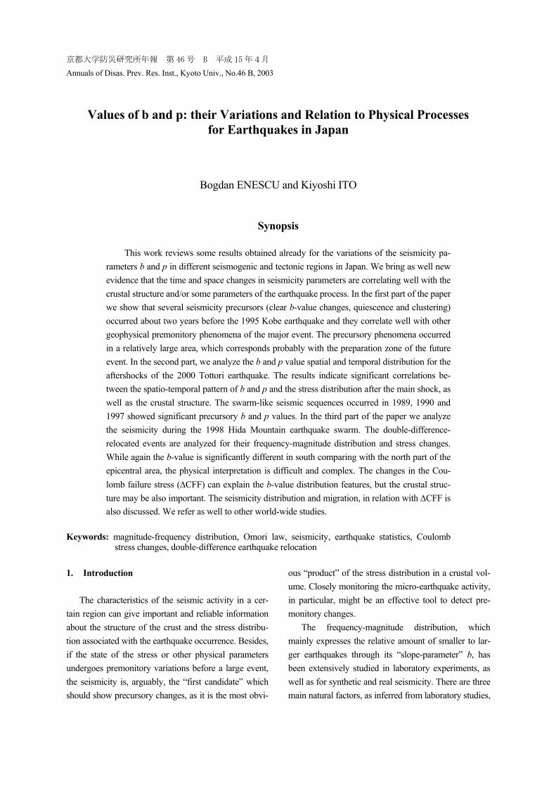
Fig. 2 From up do down: seismicity rate changes, with aclear seismic quiescence pattern (SQ) followed by anincrease in seismic activity (ISA), several months be-fore the Kobe earthquake; b) strain variation and pre-cipitation (DPRI); c) b-value changes: increase anddecrease before Kobe earthquake; d) changes in thefractal dimension (D2) of the epicentral distribution ofearthquakes: large decrease associated probably withISA, correlates well with the decrease in b-value.

aly, which started about 2 years before the main shock, followed by a significant increase of the seismicity rate, several months before the 1995 large event. The z-value

statistical test, which can quantify a relative decrease or increase of the seismicity rate (Habermann, 1983), was applied to infer the spatial pattern of the quiescence anomaly, by using a gridding technique. It was found that the quiescence anomaly occurs in a relatively large region surrounding the epicenter of the main shock as well as in the source area. The quiescence anomaly is clearly seen, in particular in the Tanba region (fig. 1). The analysis of the declustered catalog revealed as well that the background seismicity rate in the Tanba region, situated NE from the aftershock region of the 1995 Kobe earthquake, increased about 6 times after the large event, probably due to static stress triggering (Hashi-moto, 1996; Toda et al., 1998; Nakamura, 1999).

Because by applying the declustering procedure (re-quired for the application of the z-value statistical test) we may have eliminated as well some useful premoni-tory information, the original catalog (undeclustered) was also analyzed. The b-value and fractal dimension, D2, variation with time showed clear premonitory pat-terns, while the quiescence anomaly is seen as well. Figure 2 shows the time evolution of the seismicity rate, b-value and fractal dimension, five years before the main shock. One can easily recognize the discussed precursors. The variation of strain and precipitation with time (DPRI, Kyoto University) are also presented in Fig. 2. One can see that the precursory variation of seismic-ity parameters corresponds well to an increase in stress at the crustal deformation observation stations Yama-zaki, Abuyama and Amagase. Ito and Enescu (2001a) discuss other reports of long-, intermediate- and short-term geophysical precursors occurred before the 1995 Kobe earthquake.

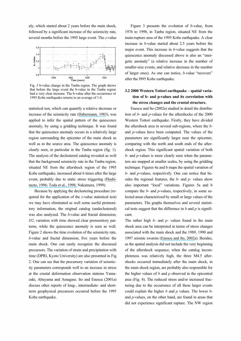
Figure 3 presents the evolution of b-value, from 1976 to 1998, in Tanba region, situated NE from the main-rupture area of the 1995 Kobe earthquake. A clear increase in b-value started about 2.5 years before the major event. This increase in b-value suggests that the quiescence anomaly discussed above is also an “ener-getic anomaly” (a relative increase in the number of smaller-size events, and relative decrease in the number of larger ones). As one can notice, b-value “recovers” after the l995 Kobe earthquake. 3.2 2000 Western Tottori earthquake – spatial varia-

tion of b- and p-values and its correlation with the stress changes and the crustal structure.

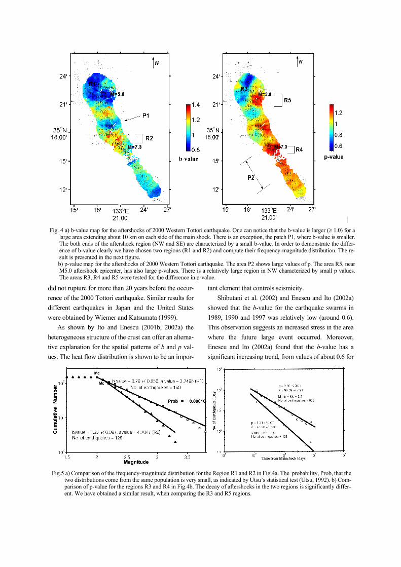
Enescu and Ito (2002a) studied in detail the distribu-tion of b- and p-values for the aftershocks of the 2000 Western Tottori earthquake. Firstly, they have divided the aftershock area in several sub-regions, where the b- and p-values have been computed. The values of the parameters are significantly larger near the epicenter, comparing with the north and south ends of the after-shock region. This significant spatial variation of both b- and p-values is more clearly seen when the parame-ters are mapped at smaller scales, by using the gridding technique. Figures 4a and b maps the spatial variation of b- and p-values, respectively. One can notice that be-sides the regional features, the b- and p- values show also important “local” variations. Figures 5a and b compare the b- and p-values, respectively, in some se-lected areas characterized by small or large values of the parameters. The graphs themselves and several statisti-cal tests suggest that the difference in b and p is signifi-cant. The rather high b- and p- values found in the main shock area can be interpreted in terms of stress changes associated with the main shock and the 1989, 1990 and 1997 seismic swarms (Enescu and Ito, 2002a). Besides, as the spatial analysis did not include the very beginning of the aftershock sequence, when the catalog incom-pleteness was relatively high, the three M4.5 after-shocks occurred immediately after the main shock, in the main shock region, are probably also responsible for the higher values of b and p observed in the epicentral area (Fig. 4). The reduced stress and/or increased frac-turing due to the occurrence of all these larger events could explain the higher b and p values. The lower b- and p-values, on the other hand, are found in areas that did not experience significant rupture. The NW region

Fig. 3 b-value change in the Tanba region. The graph showsthat before the large event the b-value in the Tanba regionhad a very clear increase. The b-value after the occurrence of1995 Kobe earthquake returns to an average of 1.0.

did not rupture for more than 20 years before the occur-rence of the 2000 Tottori earthquake. Similar results for different earthquakes in Japan and the United States were obtained by Wiemer and Katsumata (1999).

As shown by Ito and Enescu (2001b, 2002a) the heterogeneous structure of the crust can offer an alterna-tive explanation for the spatial patterns of b and p val-ues. The heat flow distribution is shown to be an impor-

tant element that controls seismicity. Shibutani et al. (2002) and Enescu and Ito (2002a)

showed that the b-value for the earthquake swarms in 1989, 1990 and 1997 was relatively low (around 0.6). This observation suggests an increased stress in the area where the future large event occurred. Moreover, Enescu and Ito (2002a) found that the b-value has a significant increasing trend, from values of about 0.6 for

Fig.5 a) Comparison of the frequency-magnitude distribution for the Region R1 and R2 in Fig.4a. The probability, Prob, that thetwo distributions come from the same population is very small, as indicated by Utsu’s statistical test (Utsu, 1992). b) Com-parison of p-value for the regions R3 and R4 in Fig.4b. The decay of aftershocks in the two regions is significantly differ-ent. We have obtained a similar result, when comparing the R3 and R5 regions.

Fig. 4 a) b-value map for the aftershocks of 2000 Western Tottori earthquake. One can notice that the b-value is larger (≥ 1.0) for a

large area extending about 10 km on each side of the main shock. There is an exception, the patch P1, where b-value is smaller.The both ends of the aftershock region (NW and SE) are characterized by a small b-value. In order to demonstrate the differ-ence of b-value clearly we have chosen two regions (R1 and R2) and compute their frequency-magnitude distribution. The re-sult is presented in the next figure.

b) p-value map for the aftershocks of 2000 Western Tottori earthquake. The area P2 shows large values of p. The area R5, nearM5.0 aftershock epicenter, has also large p-values. There is a relatively large region in NW characterized by small p values.The areas R3, R4 and R5 were tested for the difference in p-value.

the first swarms to 1.3-1.4 after the Tottori main shock, in the main-rupture area. 3.3. The 1998 Hida Mountain earthquake swarm:

double-difference event relocation, frequency-magnitude distribution and Coulomb stress changes.

The discrimination between different physical mechanisms responsible for the occurrence of earth-quakes in a certain region is certainly a difficult task. Anyway, a reliable answer depends heavily on the qual-ity and accuracy of the data to be analyzed.

The 1998 Hida Mountain earthquake swarm started on August 7 and its most active period lasted for about two months. In this period, 18 shocks with M ≥ 4.0 oc-curred, the largest one (M = 5.0) being recorded on Au-gust 16. The swarm started in the south and migrated toward the north, reaching the northern most point in about one month. Most of the largest events in the se-quence (fifteen) occurred during this south to north- migration period. For the following month, an opposite, north to south-migration of seismicity was observed. The average speed of migration was of about 1-2 km/day (Wada et al., 2000).

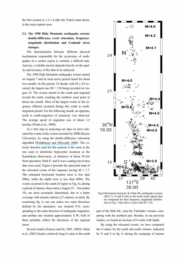
As a first step in analyzing our data we have relo-cated the events of the swarm recorded by DPRI (Kyoto University), by using the double-difference relocation algorithm (Waldhauser and Ellsworth, 2000). The ve-locity structure used for this analysis is the same as the one used to determine hypocenter locations at the Kamitakara observatory, at distances of about 30 km from epicenters. Both P- and S-wave catalog travel time data were used. Figure 6 presents the epicentral map of the relocated events of the sequence having M ≥ 1.7. The estimated horizontal location error is less than 200m, while the depth error is less than 600m. The events occurred in the south (S region in Fig. 6), during a period of intense observation (August 25 – November 10), are most accurately determined, due to a better coverage with seismic stations (27 stations, in total). By examining fig. 6, one can notice two main directions defined by the epicenters: one oriented N-S, corre-sponding to the main direction of earthquake migration, and another one oriented approximately E-W; both of them probably reflect the directions of the regional stress.

Several studies (Enescu and Ito, 2001, 2002b; Sakai et al., 2002) found a relatively large b-value in the south

part of the Hida Mt., near the Yakedake volcano, com-paring with the northern part. Besides, in our previous studies, we found an increase of b-value with depth.

By using the relocated events, we have computed the b-values for the north and south clusters, indicated by N and S in fig. 6, during the campaign of intense

Fig.6 Relocated seismicity for Hida Mt. earthquake swarms (M≥1.7). N and S refer to the north south regions that are compared for their frequency magnitude distribu-tion in Fig.7. Star show events with M>=4.0.

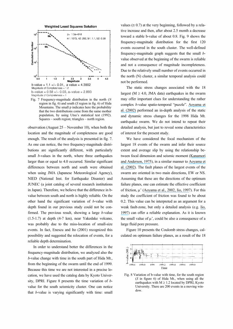
observation (August 25 – November 10), when both the location and the magnitude of completeness are good enough. The result of the analysis is presented in fig. 7. As one can notice, the two frequency-magnitude distri-butions are significantly different, with particularly small b-values in the north, where three earthquakes larger than or equal to 4.0 occurred. Similar significant differences between north and south were obtained when using JMA (Japanese Meteorological Agency), NIED (National Inst. for Earthquake Disaster) and JUNEC (a joint catalog of several research institutions in Japan). Therefore, we believe that the difference in b-value between south and north is highly reliable. On the other hand the significant variation of b-value with depth found in our previous study could not be con-firmed. The previous result, showing a large b-value (1.5-1.7) at depth (4-7 km), near Yakedake volcano, was probably due to the miss-location of small-size events. In fact, Enescu and Ito (2001) recognized this possibility and suggested the relocation of events, for a reliable depth determination.

In order to understand better the differences in the frequency-magnitude distribution, we analyzed also the b-value change with time in the south part of Hida Mt., from the beginning of the swarm until the end of 1999. Because this time we are not interested in a precise lo-cation, we have used the catalog data by Kyoto Univer-sity, DPRI. Figure 8 presents the time variation of b-value for the south seismicity cluster. One can notice that b-value is varying significantly with time: small

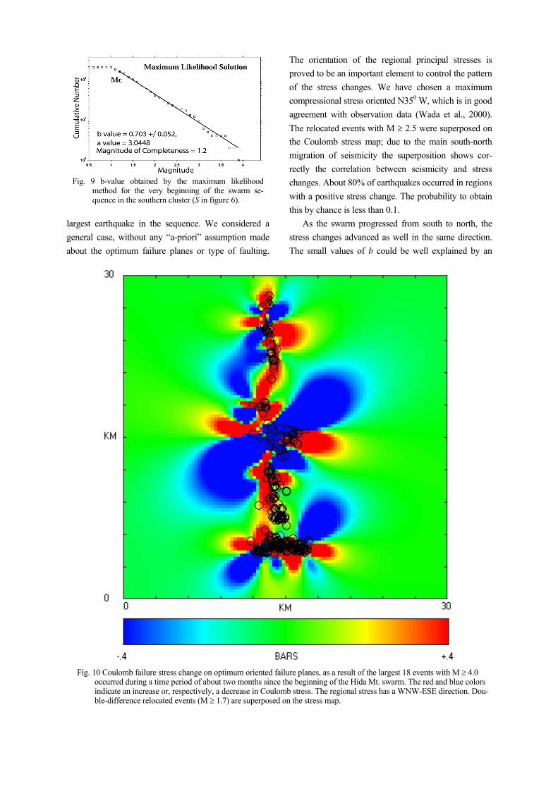
values (≅ 0.7) at the very beginning, followed by a rela-tive increase and then, after about 2.5 month a decrease toward a stable b-value of about 0.8. Fig. 9 shows the frequency-magnitude distribution for the first 120 events occurred in the south cluster. The well-defined frequency-magnitude graph suggests that the small b-value observed at the beginning of the swarm is reliable and not a consequence of magnitude incompleteness. Due to the relatively small number of events occurred in the north (N) cluster, a similar temporal analysis could not be performed.

The static stress changes associated with the 18 largest (M ≥ 4.0, JMA data) earthquakes in the swarm may offer important clues for understanding the rather complex b-value spatio-temporal “puzzle”. Aoyama et al. (2002) performed an in-depth analysis of the static and dynamic stress changes for the 1998 Hida Mt. earthquake swarm. We do not intend to repeat their detailed analysis, but just to reveal some characteristics of interest for the present study.

We have considered the focal mechanism of the largest 18 events of the swarm and infer their source extent and average slip by using the relationship be-tween focal dimension and seismic moment (Kanamori and Anderson, 1975), in a similar manner to Aoyama et al. (2002). The fault planes of the largest events of the swarm are oriented in two main directions, EW or NS. Assuming that these are the directions of the optimum failure planes, one can estimate the effective coefficient of friction, µ’ (Aoyama et al., 2002, Iio, 1997). For this study the coefficient of friction was found to be about 0.2. This value can be interpreted as an argument for a weak fault-zone, but only a detailed analysis (e.g. Iio, 1997) can offer a reliable explanation. As it is known the small value of µ’, could be also a consequence of a large fluid pore pressure.

Figure 10 presents the Coulomb stress changes, cal-culated on optimum failure planes, as a result of the 18

Fig. 7 Frequency-magnitude distribution in the north (Nregion in fig. 6) and south (S region in fig. 6) of HidaMountains. The small p indicates here the probability that the two distributions come from the same motherpopulation, by using Utsu’s statistical test (1992).Squares – south region; triangles – north region.

Fig. 8 Variation of b-value with time, for the south region(S in figure 6) of Hida Mt., when using all theearthquakes with M ≥ 1.2 located by DPRI, KyotoUniversity. There are 200 events in a moving win-dow.

largest earthquake in the sequence. We considered a general case, without any “a-priori” assumption made about the optimum failure planes or type of faulting.

The orientation of the regional principal stresses is proved to be an important element to control the pattern of the stress changes. We have chosen a maximum compressional stress oriented N350 W, which is in good agreement with observation data (Wada et al., 2000). The relocated events with M ≥ 2.5 were superposed on the Coulomb stress map; due to the main south-north migration of seismicity the superposition shows cor-rectly the correlation between seismicity and stress changes. About 80% of earthquakes occurred in regions with a positive stress change. The probability to obtain this by chance is less than 0.1.

As the swarm progressed from south to north, the stress changes advanced as well in the same direction. The small values of b could be well explained by an

Fig. 9 b-value obtained by the maximum likelihoodmethod for the very beginning of the swarm se-quence in the southern cluster (S in figure 6).

Fig. 10 Coulomb failure stress change on optimum oriented failure planes, as a result of the largest 18 events with M ≥ 4.0

occurred during a time period of about two months since the beginning of the Hida Mt. swarm. The red and blue colors indicate an increase or, respectively, a decrease in Coulomb stress. The regional stress has a WNW-ESE direction. Dou-ble-difference relocated events (M ≥ 1.7) are superposed on the stress map.

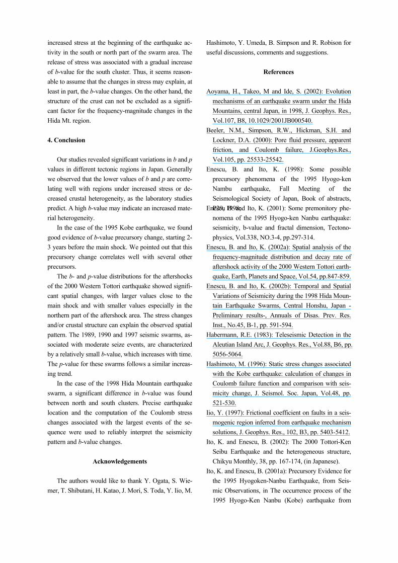
increased stress at the beginning of the earthquake ac-tivity in the south or north part of the swarm area. The release of stress was associated with a gradual increase of b-value for the south cluster. Thus, it seems reason-able to assume that the changes in stress may explain, at least in part, the b-value changes. On the other hand, the structure of the crust can not be excluded as a signifi-cant factor for the frequency-magnitude changes in the Hida Mt. region.

4. Conclusion

Our studies revealed significant variations in b and p values in different tectonic regions in Japan. Generally we observed that the lower values of b and p are corre-lating well with regions under increased stress or de-creased crustal heterogeneity, as the laboratory studies predict. A high b-value may indicate an increased mate-rial heterogeneity.

In the case of the 1995 Kobe earthquake, we found good evidence of b-value precursory change, starting 2-3 years before the main shock. We pointed out that this precursory change correlates well with several other precursors.

The b- and p-value distributions for the aftershocks of the 2000 Western Tottori earthquake showed signifi-cant spatial changes, with larger values close to the main shock and with smaller values especially in the northern part of the aftershock area. The stress changes and/or crustal structure can explain the observed spatial pattern. The 1989, 1990 and 1997 seismic swarms, as-sociated with moderate seize events, are characterized by a relatively small b-value, which increases with time. The p-value for these swarms follows a similar increas-ing trend.

In the case of the 1998 Hida Mountain earthquake swarm, a significant difference in b-value was found between north and south clusters. Precise earthquake location and the computation of the Coulomb stress changes associated with the largest events of the se-quence were used to reliably interpret the seismicity pattern and b-value changes.

Acknowledgements

The authors would like to thank Y. Ogata, S. Wie-mer, T. Shibutani, H. Katao, J. Mori, S. Toda, Y. Iio, M.

Hashimoto, Y. Umeda, B. Simpson and R. Robison for useful discussions, comments and suggestions.

References Aoyama, H., Takeo, M and Ide, S. (2002): Evolution

mechanisms of an earthquake swarm under the Hida Mountains, central Japan, in 1998, J. Geophys. Res., Vol.107, B8, 10.1029/2001JB000540.

Beeler, N.M., Simpson, R.W., Hickman, S.H. and Lockner, D.A. (2000): Pore fluid pressure, apparent friction, and Coulomb failure, J.Geophys.Res., Vol.105, pp. 25533-25542.

Enescu, B. and Ito, K. (1998): Some possible precursory phenomena of the 1995 Hyogo-ken Nambu earthquake, Fall Meeting of the Seismological Society of Japan, Book of abstracts, P29, 1998; Enescu B. and Ito, K. (2001): Some premonitory phe-nomena of the 1995 Hyogo-ken Nanbu earthquake: seismicity, b-value and fractal dimension, Tectono-physics, Vol.338, NO.3-4, pp.297-314.

Enescu, B. and Ito, K. (2002a): Spatial analysis of the frequency-magnitude distribution and decay rate of aftershock activity of the 2000 Western Tottori earth-quake, Earth, Planets and Space, Vol.54, pp.847-859.

Enescu, B. and Ito, K. (2002b): Temporal and Spatial Variations of Seismicity during the 1998 Hida Moun-tain Earthquake Swarms, Central Honshu, Japan -Preliminary results-, Annuals of Disas. Prev. Res. Inst., No.45, B-1, pp. 591-594.

Habermann, R.E. (1983): Teleseismic Detection in the Aleutian Island Arc, J. Geophys. Res., Vol.88, B6, pp. 5056-5064.

Hashimoto, M. (1996): Static stress changes associated with the Kobe earthquake: calculation of changes in Coulomb failure function and comparison with seis-micity change, J. Seismol. Soc. Japan, Vol.48, pp. 521-530.

Iio, Y. (1997): Frictional coefficient on faults in a seis-mogenic region inferred from earthquake mechanism solutions, J. Geophys. Res., 102, B3, pp. 5403-5412.

Ito, K. and Enescu, B. (2002): The 2000 Tottori-Ken Seibu Earthquake and the heterogeneous structure, Chikyu Monthly, 38, pp. 167-174, (in Japanese).

Ito, K. and Enescu, B. (2001a): Precursory Evidence for the 1995 Hyogoken-Nanbu Earthquake, from Seis-mic Observations, in The occurrence process of the 1995 Hyogo-Ken Nanbu (Kobe) earthquake from

micro-earthquake observation, Report for the Tokyo Memorial Foundation for the Promotion of Earth-quake Prediction Research, pp. 3-26 (in Japanese).

Ito, K. and Enescu, B. (2001b): Heterogeneous structure and b and p values relating to the rupture of the 2000 Tottori-Ken Seibu earthquake, Proceedings of the In-ternational Symposium on Slip and Flow Processes in and below the Seismogenic Region, Sendai, Japan, pp. 78-1:78-6.

Kanamori, H. and Anderson, D.L. (1975): Theoretical basis of some empirical relations in seismology, Bull. Seismol. Soc. Am., Vol.65, pp.1073-1095.

King, G.C.P., Stein, R.S., and Lin J.(1994): Static stress changes and the triggering of earthquakes, Bull. Seismol. Soc. Am., Vol.84, pp. 935-953.

Mogi, K. (1962): Magnitude-frequency relation for elastic shocks accompanying fractures of various ma-terials and some related problems in earthquakes, Bull. Earthquake Res. Inst., Univ. Tokyo, 40, pp. 831-853.

Mori, J., and R.E. Abercrombie (1997): Depth depend-ence of earthquake frequency-magnitude distribu-tions in California: Implications for rupture initiation, J. Geophys. Res., 102, B7, pp. 15081-15090.

Nakamura, M. (1999): Decay of Micro-Earthquake Seismicity Activated by Static Stress Change, 22-nd General Assembly of IUGG, Birmingham, England, Book of Abstracts, A. 166.

Ogata, Y. (1983): Estimation of the parameters in the modified Omori formula for aftershock frequencies by the maximum likelihood procedure, J. Phys. Earth, 31, pp. 115-124.

Reasenberg, P. (1985): Second-Order Moment of Cen-tral California Seismicity, 1969-1982, J. Geophys. Res., 90, B7, pp. 5479-5495.

Rydelek, P.A. and Sacks, S. (1989): Testing the Com-pleteness of Earthquake Catalogues and the Hypothe-sis of Self-Similarity, Nature, 337, pp. 251-253.

Sakai, T., Takagi, A., and Yoshida, A. (2002): On the b value in the frequency-magnitude distribution of earthquakes near and around volcanoes, Earth and Planetary Science Joint Meeting, Book of abstracts, S041-P019.

Scholz, C.H. (1968): The frequency-magnitude relation of microfracturing in rock and its relation to earth-quakes, Bull. Seismol. Soc. Am., 58, pp. 399-415.

Shibutani, T., Nakao, S., Nishida, R., Takeuchi, F., Wa-tanabe, K., and Umeda, Y. (2002): Swarm-like seis-

mic activity in 1989, 1990 and 1997 preceding the 2000 Western Tottori earthquake, Earth, Planets and Space, 54, pp. 831-845.

Smith W.D. (1981): The b-value as an Earthquake Pre-cursor, Nature, 289, pp. 136-139.

Toda, S., Stein, R.S., Reasenberg P.A., Dieterich J.H. and Yoshida, A. (1998): Stress transferred by the Mw=6.9 Kobe, Japan, shock: Effect on aftershocks and future earthquake probabilities, J. Geophys. Res., 103, pp. 24,543-24,565.

Utsu, T. (1961): A statistical study on the occurrence of aftershocks, Geophys. Mag., 30, pp. 521-605.

Utsu, T. (1965): A method for determining the value of b in formula log N = a - bM showing the magnitude-frequency relation for earthquakes, Geophys. Bull. Hokkaido Univ., 13, pp. 99-103 (in Japanese).

Utsu, T. (1992): On seismicity, Report of the Joint Re-search Institute for Statistical Mathematics, Inst. for Stat. Math., pp. 139-157, Tokyo.

Utsu, T., Ogata, Y., and Matsu’ura, R.S. (1995): The centenary of the Omori formula for a decay law of af-tershock activity, J. Phys. Earth, 43, pp. 1-33.

Wada, H., Ito, K. and Ohmi, S. (2000): 1998 Hida earthquake swarm, Tectonic stress and large inland-earthquakes in the Hida Mountain Region, DPRI, Kyoto University report, principal investigator: I. Kawasaki, pp. 36-49.

Waldhauser, F. and Ellsworth, W.L. (2000): A double-difference earthquake location algorithm: method and application to the Northern Hayward fault, California, Bull. Seism. Soc. Am., 90, 6, pp. 1353-1368.

Warren, N.W. and Latham, G.V. (1970): An experi-mental study of thermally induced microfracturing and its relation to volcanic seismicity, J. Geophys. Res., 75, pp. 4455-4464.

Wiemer, S. (2001): A software package to analyze seismicity: ZMAP, Seis. Res. Lett., 72, 2, pp. 374-383, 2001.

Wiemer, S. and Katsumata, K. (1999): Spatial variabil-ity of seismicity parameters in aftershock zones, J. Geophys. Res., 104, B6, pp. 13135-13151.

Wyss, M. (1973): Towards a physical understanding of the earthquake frequency distribution, Geophys. J. R. Astron. Soc., 31, pp. 341-359.

Wiemer, S. and Wyss, M. (2002): Mapping spatial vari-ability of the frequency-magnitude distribution of earthquakes, Advances in Geophysics, 45, pp. 259-302.

ｂ値とｐ値，その変化と地震の物理過程との関連

ボグダン,エネスク・伊藤 潔

要 旨

最近の日本における３つの地震群に対して解析したｂ値およびｐ値についてのレビューを行い，さらに，新しい解析

結果を付け加えて，それらのパラメ－タと地下構造および震源過程との関連について調べた。1995年兵庫県南部地震に

ついては，約２～３年前からｂ値が変化したが，この変化は他の観測地の変化と対応している。また，この前兆的なｂ

値の変化は震源域だけでなく，広い範囲で観測された。2000年鳥取県西部地震については，余震のｂ値とｐ値は本震付

近で大きく，余震域の北部で小さい。この変化は地域的な構造の相違か応力変化のいずれかだと思われる。また，1989，1990，1997年に起きた前駆的地震活動ではｂ値は 0.6程度で小さかった。これらのｂ値はｐ値とともに時間とともに増加

した。1998年飛騨山地の群発地震については，相対的震源決定を行い，深さを含めて地域的なｂ値の変化を調べた。さ

らに，その結果，ｂ値は山脈の北部で小さく南部で大きい。また，18個の大きな地震についてクーロン応力を計算した

が，地震の 80%は応力が増加した地域で発生している。ｂ値の変化は応力変化と対応するように思われる。 キーワード：マグニチュード頻度分布，余震についての大森公式，地震活動，地震統計, クーロン破壊関数, 相対震源

決定