


Bahasa
Halaman
Hukum


THE ELASTIC—PLASTIC BEHAVIOUR OF SOME AXISYMMETRIC
PRESSURE VESSEL HEADS AND NOZZLES
BY
JOHN CHEUNq SHING TAI_B.Sc.(Eng.),D.I.C.,G.I.Mech.E.
A thesis submitted for the degree of Doctor of
Philosophy of the Faculty of Engineering, University
of London.
November,1969. Department of Mechanical Engineering,
Imperial College of Science and
Technology,
LONDON,S.W.7.

_ 1 _ ABSTRACT
This investigation sets out to test the accuracy of a
numerical method of stress analysis by Marcal for the
elastic-plastic behaviour of axisymmetric thin--walled
pressure vessels, with special reference to the possible
application of the method to achieve more accurate vessel:;
designs. Some torispherical heads and axisymmetric flush
nozzles are selected for study. An extensive literature
review is made on researches into the behaviour and
design of pressure vessels, helping to set the course of
this work.
The Marcal method, already coded into general purpose
computer systems, is initially extensively tested with
elastic problems, and is found to give good accuracy,
within the limitations of the assumptions. However,
exaggerated' stress concentrations are noted among many
elastic flush nozzle results, when the nozzle geometry
is apprOximated by the usual shells intersection procedure.
A new procedure is tried giving a smooth transition from
nozzle to shell, and found to give good improvement of
accuracy for flush nozzles with rounded fillets and corners
based on the ASME Nuclear Vessel Code. Further improvement
is obtained with this procedure after the program is
modified, such that the basic equations give better
approximation for thick curved shell elements which occur
at the junctions. C
A number of strain gauged vessel tests are made to obtain
detailed comparison with the elastic-plastic analysis.
They include axial loading tests on two mild stteel nozzles
attached to shallow spherical caps. They form the

- 2 -
preliminary to a hydraulic pressure test on a specially
built stainless steel vessel, closed by two nominally
identical heads where one has a central symmetric nozzle.
Calculations are also tried,based on two published
elastic-plastic tests on vessel heads. The comparisons
reveal some sources of inaccuracy of the programs, and
some factors, e.g. material strain-hanTening and change
of vessel geometry, affecting the vessel's elastic-
plastic behaviour. A reliable method is found as a
basis for defining plastic collapse of vessel components.
The programs as shown by these results should give good
accuracy for some possible design application based on
plastic collapse, shakedown or low-cycle fatigue.

ACKNOWLEDGEZMITTS
The author is grateful for the financial support for three years of
the Berkeley Nuclear Laboratories, Central Electricity Generating
Board through a research contract. Part of this work is also supported
by a Science Research Council contract.
Sincere acknowledgement is due to Dr. C.E.Turner, Reader in Mechanical
Engineering, Imperial College, for supervising this research and
giving the much needed advice and guidance, to Mr. C.H.A.Townley of the
B.N.L. for his continued interest, and to Dr. P.V,Marcal for co-supervising
part of this work.
Thanks are due to the library and technical staffs of the Mechanical
Engineering Department, especially the Librarian Miss E.M.Archer, who
have helped 3n the course of this work.
Finally the author wishes to thank Miss W.L.Wong and others who helped
in the preparation of this thesis.
J.S.T.Cheung

CONTENTS
ABSTRACT a:
ACKNOWLEDGEMENTS
3
CONTENTS
4 1. INTRODUCTION
7
2. HISTORIC REVIEW
11
2.1 General
11,
2.2 Pressure Vessel Heads
13
2.3 Pressure Vessel Openings
15
2.4 New Techniques and Interests
18
3. RECENT LITERATURES:THEORETICAL
INVESTIGATIONS 21 Notations 21
3.1 Shell Theories 21
3.2 Numerical Solution 27
3.3 Pressure Vessel Nozzles 31
4. .RECENT LITERATURES : EXPERIMENTAL
INVESTIGATIONS 36 Experimental Techniques 36 Pressure Vessel Heads 39 P-ressure Vessel Nozzles 40
RECENT LITERATURES:FAILURE BEHAVIOUR 43 Modes of Failure 43 Static Loading 45 Repeated Loading 48
AVAILABLE COMPUTER PROGRAMS FOR VESSEL ANALYSIS 53 Notations 53 Elastic Program:Capabilities 55 Elastic Program:Nu.merical Procedure 57 Elastic-Plastic Program 65
ACCURACY TESTS FOR ELASTIC PROGRAM 74 Notation 74 Size of Problem for Converging Solution 74
4.1
4.2
4.3
5.
5.1
5.2
5.3
6.
6.1
6.2
6.3
7.
7.1

- 5 - 1.2 Cylinders Under Internal Pressure 77; 7.3 Comparison With Published Results 80 7.4 Comparison With Other Pressure Vessel
Programs
7.5 Conclusions 84 89
8. ACCURACY TESTS FOR ELASTIC-PLASTIC PROGRAM 91
8.1 Previous Comparisons 91 8.2 Use of Elastic-Plastic Results 93 8.3 Further Comparisons 8.4 Tests by Stoddart
96
98 8.5 Tests by Kemper et.al. 101
9. AXIAL LOADING TESTS OF FLUSH NOZZLES 106 9.1 Nozzle Configuration 106 9.2 Strain Gauge Techniques 109 9.3 Material Properties 113 9.4 Test Arangements and Preparations 117 9.5 Test Procedure and Results 123
10. THEORETICAL SOLUTIONS TO COMPARE AXIAL TEST RESULTS 129
10.1 Approximations to the Nozzle Junction Configuration 129
10.2 Modifications to the Computer Program 133 10.3 Comparison of Results 137 10.4 Conclusions 150
11. PRESSURE TEST OF VESSEL:PREPARATION 153 11.1 Introduction 153 11.2 Vessel Design 154 11.3 Measurements 156 11.4 Strain and Deflection Gauging 157 11.5 Oil Circuit 161
12. PRESSURE TEST OF VESSEL:TEST AND COMPARISON 163
12.1 Elastic Test 163 12.2 Elastic Calculations 163 12.3 Elastic-Plastic Test 166

12.4 Elastic-Plastic Calculations 170
12.5 Discussions on Strain and Displacement 172 12.6 Discussions on Collapse Load 175 12.7 Conclusions 178
13. OEHER GENERAL DISCUSSIONS 181 13.1 Pressure Vessel Programs 181 13.2 Vessel Behaviour 186 13.3 Design Interest 109
14. CONCLUSIONS 195
REFERENCES 201
APPEDNICES 219
LIST OF ILLUSTRATIONS 253
FIGURES 255
PLATES 310

1. INTRODUCTION
In the general sense, a pressure vessel is a container
which holds a fluid at a different pressure from its
environment. As such a device is often required in
many industrial processes, it is often used in industry,
and can be found in many shapes and forms. The steam
boiler-plant industries have been a big user of pressure
vessels since the advent of steam, so have the chemical
and petroleum industries. They are also used in nuclear
reactor plants, aircraft, and rockets as well as the
humble but numerous gas containers.
The characteristic of a pressure vessel is the pressure
it can hold. This however makes the vessel a possible
source of danger if it breaks, causing uncontrolled release
of the pressure. Study of the failure and of the general
behaviour of pressure vessels has been of great value
in preventing failures. This also leads of course to
better design, which is not only safer, but also more
economical. The areas of study cover a wide field. In
the early steam and chemical vessels, rivet joints were
the weakest link and were the subject of much investigation.
The development of the welding process and its adoption
switched attention to other areas, one of which was the
improvement made possible by better shapes and rein-
forcements for the gessel.
Most vessels are built as cylinders for ease of
fabrication. Their actual configuration may vary
according to purpose. Great attention is generally
given during design to vessel heads enclosing the ends
of the vessels, and to nozzle openings where branch pipes

- 8 -
are attached. These two components are selected for
special study in this thesis.
Most vessel heads are slightly domed outwards and of a
shape called a torisphere, consisting geometrically
of a shallow spherical centre and a curved-in edge of a
much smaller torus radius, Fig.l-l. A circumferential
weld joins the head to the cylindrical vessel shell.
The simplest pressure vessel nozzle consists of a cir-
cular, or appropriately shaped, opening, inteither the
vessel head or the shell, onto and covering which (i.e.
the opening) is welded a cylindrical tube or pipe.
There are many variations of nozzle arrangements, most
of which can be classified under methods of reinforcement,
although nozzles are also classified according to the
alignment between the vessel and nozzle.
Studies of the behaviour and the failure of vessel
components- in many cases the latter is very much con-
nected with the former - lead not only to stronger shapes
and better arrangements for these components, but also
to better design procedures. It has, for example, been
recognised that different criteria are needed for
application in low temperature and in sustained high
temperature environments, or for loading of a constant
and of a frequently repeated nature. Some of this know-
leage has been gained from studying the properties of the
materials used, under fatigue, under creep, and for low
temperature brittle fracture. Study has also been made
on local effect of weld, and of crack or notch.
Outside these fields of study, the investigation of
overall behaviour of vessel components has also recently

been drawn towards their non-elastic behaviour, especially
in cases where parts of the component have begun yielding.
The yielded regions are in an elastic-plastic stress state
when the elastic strain component cannot be neglected in
comparison with the plastic strain component. Elasticity
theory is not sufficient for studying this behaviour.
It has,however, been known for some time that many vessels
do yield locally at the working load, and some can safely
withstand loads which cause initially a substantial
yielding. Also some vessels, designed against fatigue
within a finite number of cycles of repeated loadingjmay
have stress concentration factors giving stresses higher
than the material yield stress. Designers are faced
with the problem of whether or not more accurate detign
based on elasticity considerationsalone is adequate, or
whether further investigation into non-elastic behaviour
would only modify the present considerations, or if
radically different criteria are needed. All these
factors account for the interest in elastic-plastic
behaviour of pressure vessels.
Much of the stimulus to this interest comes from the
successful analysis, by numerical solution on the
electronic computer:, of the thin-walled shell equations,
leading to the general solution of many elastic pressure
vessel problems, and subsequently from the development
of methods extending this to elastic-plastic stress
analysis. This latter development is recenti and its
implications, and applications in design are not fully
exploited.
In parallel with this development of numerical methods

- 10 -
of elastic-plastic analysis, there is current theoretical
work on the limit analysis of thin shells, le;: img to
solutions of the collapse failure of pressure vessel by
general and local yielding. This is an extension of
the work on plastic analysis of frame and truss
structures, and determines the final collapse of thin
shells through the formation of Tlastiiv hinges at
locations of high bending stresses. There is also
current theoretical and material testing research on
the behaviour of pressure vessels under repeated loadings
of high magnitude, causing a certain amount of local
plasticity at each cycle, and leading to fatigue failure
at a relatively small number of cycles. This is commonly
called low-cycle fatigue, or highstrain fatigud. These
researches should be able to complemdnt each other in
leading to a better understanding of the behaviour of,
and better design of, pressure vessels.

2. HISTORIC REVIEW
2.1 General
The invention of the steam engine in the 18th Century
and its subsequent extensive use, brought about the need
of steam boiler vessels that is large enough to generate
the required amount of steamland at the same time strong
enough to support the weight of water inside and resist
the steam pressure. An example of a well designed
vessel at that time was an horizental egg-ended boiler
built by Richard Trevithick in 1800 ( see Ref.(2-1)).
The vessel was 3 to 4 ft. diameter, 40 ft. long and was
made of wrought iron plates. The ends were deep and
egg-shaped, and the two openings at the side of the
vessel were oval in shape. This vessel was used under
a pressure of 80 lb/in2.
The two weakest arrangements of the early vessel were
the riveted joints of the vessel plates and the many
tube connections necessary for both fire-tube and water-
tube boilers. In many of the smaller vessels, the
design of these two arrangements governs the plate
thickness. However the plate thickness has also to be
checked against the stength of the whole vessel under
pressure. The stresses in a complete spherical shell
or a cylindrical shell under pressure were well know
and the simple formulas to obtain them had served designer
for many years.
Until 1920, the working pressure of water-tube boilers
rarely exceeded 225 lb/in2, and the safety design of
vessels had not changed very much. It was after this
period that a great stimulus for further studies came

- 12 -
from the chemical and petroleum industries. Unlike
the steam boiler industry, where the working pressures
for steam engines were not excessive and increased only
slowly through the years, the chemical and petroleum
industries required vessels for a large variety of
application,sixe,temperature and pressure. The intense
development of the thermal cracking of petroleum in
the 1920's and 1930's at the United States demanded
better design. Leakage at high pressure was a constant
source of trouble. Oxy-acetylene welding was first tried
for thin-walled vessels, and forging or hammer welding:;
of vessels was also introduced from Germany for thicker
ones. The eleattic-arc welding process had initially
the disadvantage of leaving welds which were brittle
and prone to cracking,although the subsequent development
of flux-coated electrodes soon overcame the trouble.
The above practices were gradually introduced and tried
by the steam-boiler makers, who were then stimulated
further by higher efficiencies obtained from the
possible higher working pressure, and by the sucdessful
development of the steam turbine for power generation.
By the beginning of the Second World War, forge-welded
drums were still unacceptable to the boiler makers in
England(2-2), although the use of X-ray for non-des-
tructive examination of welds had increased the con-
fidence of the insurers in the complete fusion-welded
steam boilers (2-1).
Follow-up investigations and tests after boiler ex-
plosions often created interests in the general be-
haviour of pressure vessels and components. In 1903,

- 13 -
C,Bach published the results Of two destructive tests
on specially built vessels after an explosion occurring
from a fracture originated at the edge of an unrein-
forced manhold opening. One of the findings was that
elliptical openings would be stronger if the major
axes were perpendicular to the vessel axis.
Many other tests to destruction were made during the
trial and first introduction of the forge-weld method
and the fusion-weld method to pressure vessel con-
struction. These tests were necessary because,at the
early stages of the development of these methods,
reliability of the welds were low and vessels oc-
cassionally failed at unexpectedly low pressures. They
also brought to light many other weaknesses not con-
sidered important in the past, when attention was focused
on riveted joints and on expanded tube connections.
Some examples of things noticed and discussed include,
excessive deformations at some conventionally shaped
heads, the advantage of contoured and extruded outlets
at manholes, and of putting in reinforcements there, the
recommended practice of avoiding pipe-connections and
manholes at the knuckle and the edge of heads. Stress-
lines among the mill-scales or rust at the knuctle of
heads revealed the occurrence of yielding there before
other parts of the vessels. These investigations were
mostly done at the Europe Continuent where the two novel
welding methods were first introduced.
2.2 Pressure Vessel Heads
Many of the earlier investigations on the behaviour of
pressure vessel head were from Germany and Switzerland.

- 14. -
C.Bach of Germany published his studies as early as
1899 (2-3), and continued to be associated with many
tests on dished ends and elliptical heads at the Same•
period, E.Hoehn, chief engineer of the Swiss Association
of Steam—Boiler Owners was also associated with many
tests for a number of years starting in 1914, He was
assisted from time to time by Dr. A.Huggenberger.
Many of his analyses and recommendations were lasting
contributions to the knowledge and the design of pressure
vessels. One emperical approach of his to the design
of torispherical heads, based on the then known tests
of such heads, formed the basis of a number of design
codes. The formula was published in his paper 'On the
strength of dished heads and cylindrical shells' (2-4)
which was subsequently abstracted into English by
Engineering in 1929 (2-5).
Theoretical analyses of shells were made possible by
the pioneering work on the mathematical theories of
shells and elasticity by A.E.H.Love in England. His
principal work 'Treatise on the Mathematical Theory of
Elasticity' appeared in 1892-93. The book, in its
second edition in 1906, was translated into German.
Since then,the development of the theory was transferred
to the Europe Continuent, where H.Reissner extended the
theory into cylinders and spheres, and E.Meissner started
the breakthrough into other shapes (2-6) by successfully
reducing Love's equations into two linear differential
equations,one first order and another of -fourth order,
although the latter could not then be solved in general.
Four of Meissner's students extended his work to cover
the specific shells of the shapes of a sphere, a cone,

-15-
and a cone with linearly varying thickness.
It was due to these pioneering works that the theoretical
studies of pressure vessels could proceed concurrently
with the many experimental studies. J.W.Geckeler
proposed in 1926 simplifying approximations to Love's
thin-shell theory, and reduced the complications for
getting a solution. W.M.Coates' paper in 1930 (2-7)
was one of the important papers in English. There he
emphasised why and where the discontinuity stresses
cannot be neglected, and showed how Geckeler's general
method could be applied in a step-by-step procedure to
approximate to the correct solution. The now well-
known beam-on-elastic-foundation method is the same in
principle to one of Geckeler's approximations, although
the former has the attribute of being easier to apply
and be comprehend by engineers.
The Pressure Vessel Research Committee (PVRC) of the
United States published in 1953(2-8) a report containing
a very comprehensive historical review of investigations
into pressure vessel heads. The review covered many
of the studies in the United States as well as in the
Continent until the 1930's. After this period, it turned
its attention to the development, and the related works,
leading to the drafting of the section on pressure
vessel head in the Unfired Pressure Vessel Code of the
American Petroleum Institute and ASME.
2.3 Pressure Vessel Openings
Nozzles and other openings did not receive as much early
interest as pressure vessel heads, since opening are
more local in nature than heads, and since it is possible

- 16 - to put in reinforcements to compensate for the weakening
to the vessels. Bach's tests in the 1900's contained
vessels with openings, and so did tests by Siebel & Koerber
in the 1920's,(2-9). It had already been noticed at that
time,that circular openings were more efficient at vessel
heads,that rolled-in openings were bad design especially
at regions of high stresses,and that extruded or drawn-
out shapes following the natural contour of a membrane
under internal pressure were the best shapes for good
stress distribution. These recommendations are now well
known,although not many of them were immediately accepted
in those days. The last mentioned recommendation has
frequently been followed in branch connections to main-
folds and header.
A very early series of tests specially planned for
pressure vessel nozzles was made by Taylor and Waters in
the 1930's (2-10). Thirty-six tests were made,using three
cylindrical test vessels and a variety of conventional
nozzles used at that time. It is interesting to note
that, the state of pressure vessel design then was Much
that twelve of the attachments were riveted and only
seven welded. Surveys of strains were made with 2 in.
gauge-length mechanical strain-gauges. It was concluded
that for good design,reinforcements should be as closed
as possible to the edge of the opening,that over-rein-
forcement should be avoided,as this would shift the
stress concentration from the edge of the opening to
regions further away. Siebel further reported,in 1940,
on the work at Stuttgart on reinforced openings. The
advantage of a balanced reinforcement was clearly
demonstrated in his tests,which were all on balanced
reinforcement nozzles.

- 17 -
Branched pipes were of great interest in the pipe-line
industry and in the construction of boiler headers. A
series of tests were reported by Everett and McCutchan
in 1938 (2-11) on equal diameter branch-pipes to de-
termine the efficency of collar reinforcements.
Huggenberger Tensometers were used at as many as 50
stations at each configuration. Lateral load and in-
ternal pressure were applied. Internal strain mea-
surements were of course impossible, and it was clearly
admitted that, because of this, the stress picture was
incomplete. An attempt was however made to separate
the membrane and bending stesses by assuming a hole-in-
an-infinite-plate solution as the membrane values.
Very little theoretical work had in those early days
been possible with the problem of vessel openings, other
than the two-dimensional solution of an infinite plate
with a central hole. The solution for a uni-directional
load is attributed to Kirsch who published it in 1898.
It was known that this two-dimensional solution was
inaccurate except for small ratios of opening-diameter
to vessel-diameter. Kirsch's stress concentration
factor of 3 for uni-directional load becomes 22 for the
stress condition of a cylindrical vessel under internal
pressure. Research workers in general agreed that this
factor would increase-with the diameter ratio, but the
precise amount it would increase was not known.
The analysis of holes with raised reinforcements was
discussed by Timoshenko in 1924, but it was Beskin's
publications in 1944 (212) that attracted people's
attention. Further discussions of his work are given

- 18 -
in the next Section. Elliptical holes had been a pet
problem of many applied mathematicians from an early
date, and one of the early exposition in English was
that by Inglis in 1913.
2.4 New Techniques and Interests
After the 1930's two experimental techniques were in-
troduced which gave great contribution to the analysis
of pressure vessel behaviour. The first is the use of
the electrical resistance strain gauge which was con-
ceived in the late 1930's and have since replaced the
cumbersome mechanical gauges. Subsequently the
technique of water proofing the gauges was developed
and this made possible the first convenient measurement
of stresses inside an enclosed vessel. Early reference
of the application of this technique can be found in
Ref.(2-14), and in the reports in this period of the
British Welding Research Association (BWRA)(2-15). The
other technique was that of stress analysis by photo-
elasticity. This has of course been known for many
years and has been applied to engineering problems ever
since the 1900's. The stress analyst had however to
wait many years, until better synthetic resins had been
developed and until the invention of the polaroid,
before the photoelastic bench could be made available
to many universities and industrial research establishments.
In the 1940's, the stress-freezing technique for photo-
elasticity made three-dimensional analysis possible (2-16),
and opened the way in the 1950's for the analysis of
thick-walled pressure vessel problems, and, very
recently, to thin-walled vessel problem as well.
The civil use of nuclear power came into existence more

— 19 —
than ten years ago. Many novel and unsual problems
were, and have since been,posed to pressure vessel
designers connected with the constuction of nuclear
power plants. One particular problem that had initiated
many investigations was the design of the steel con-
tainment vessel for the large graphite reactor. Both
the size and the thickness were of a different order
of magnitude to that of the usual boiler and chemical
vessels or gas containers. Accurate analysis was
necessary,as little experience could'be drawn upon.
During this period many new investigations into such
pressure vessel problems were made,backed by nuclear-
vessel manufacturers or encouraged by nuclear-vessel
code-making bodies. This is refledted in the increase
in the published literatures on such subjects,two
special examples of which are the collections of papers
at the 1960 Glasgow Symposium on nuclear structures and
containment (2-16), and the 1962 Inst. Mech. Engr.
Symposium on pressure vessel research (2-17). The
United States and Britain both published new codes on
the design of nuclear pressure vessels.
This period of activity coincides with the advent of the
automatic digital-computer which made possible the use
of many methods of theoretical analysis which are other-
wise impossible, especially those for the solution of
shells of complex shapes and shells under unusual loadings.
The computer has been used initally as an extension of
the mechanical calculating-machine,helping to obtain
the final solution from analytical procedures,like
compiling tables or computing the series solution for
asymptotic methods. It is subsequently also used with

- 20 -
the technique of numerical analysis which is, in many
cases, more flexible, and it is soon possible to remove
the restrictions of fixed geometical shapes and simple
modes of loading to many shell calculations.

- 21 .
3. RECENT LITERATURES: THEORETICAL INVESTIGATIONS
NOTATIONS
E Young's modulus of elasticity.
Shear modulus
Poisson's ratio
cr Stress, or direct stress
1: Shear stress
e Strain, or direct strain
1r Shear strain
Angle around circumference
U Product,merid. radius of curvature and transverse
shearing force.
✓ Rotation of targent to shell meridian
X- coordinate, or independent vainable
Y- coordinate, or function of i
3. 1. Shell Theories
First Order Theories
The basic equations for thin elastic shells first derived
by Love, and another version of these equations by E.
Reissner in 1941 (3-6), contain a number of fundamental
assumptions. They are that
1. The shell is thin,
2. The shell deflections are small,
3. The transverse normal-stress is negigible,and
4. Normal to the reference surface of the shell
remain normal and undergo no change in length
during deformation.
These are commonly referred to as Love's first approxi-
mations for thin shells.

- 22 -
The first assumption forms the basis of the theory.
With this assumption, the ratio t/Rm (shell thickness/
radius of curvature of the mid-wall reference-surface)
can be neglected, compared with unity, in the derivations
of the equations. With the second assumption, the
original geometry of the shell can be used in the
calculations. The fourth assumption is a direct
extension of the Bernoulli-Euler hypothesis of beam
theories,that plane cross-section of the beam remains
plane under deformation. All strain components in the
direction of the normal n to the mid-wall surface would
thus vanish,i.e.
enn = 111 = Y2n = 0
The third assumption states that in the derivation of
other stresses, the normal stress to the mid-wall
surface is zero,i.e.
0-nn = 0
With the third and fourth assumptions, we can write the
direct stresses 6.11 Cr22' andand the direct strains e11 and e22, all in the plane of the mid-wall surface,simply
as 071 and 62 , e1 and e2 respectively. The stress
strain relations for a Hookean, is„,otropic material are
thus reduced to the form
e1 1
= (6-1 \)(52 )
1
12
12
where E,G,N)are the Young's modulus,the shear modulus
E 1
(C)i ) E e2

- 23 -
and the Poisson's ratio respectively.
A shell of revolution with axisymmetric loadings has a
complete symmetry with respect to the circumferential
angle e . Three equations of equilibrium can be
written for a small shell element, two equations are
for forces and one for moment, all taken in the radial
plane through the axis of rotation. They are in the
form of three differential equations in three unknown
quahtities. It has been mentioned that H.Reissner and
E.Meissner rirst made the solution of these equations
possible,(the process involved has been well documented
in books on shell theories.*) They successfully reduced
the equations into two, using two special variables,
one being the angle of rotation V of a tangent to the
meridian, and the other U being the product of the
'meridional radius of curvature and the transverse shearing
force. Two second-order simultaneous differential
equations were obtained. The two unknowns were then
separated leaving a fourth-order linear differential
equations of one or the other unknown. Thus the process
of obtaining a solution for individual problems consists
of finding the complementary and the particular solutions
of these problems,represented by
U = Uc + UP
or V = VC + VP
The particular solution accounts for the external
loadings, and the complementary solution satisfies the
* See chapter 16 of (3-7) or Chapter 5 of (3-8).

- 24 -
boundary conditions to the shell. For many years the
history for the solution of many practical shell
problems has been one of finding solutions to these
fourth order equations. .
Exact analytical solution to the above equation was
generally not possible, unless it could be split into
two convenient second order equations, and this can be
done only for cases where the shells are of constant
thickness and constant or zero meridional radius of
curvature. A knowledge of a number of mathemetical and
physical functions is required to obtain the analytical
solutions; but the method does open the way for solving
many problems involving cylindrical.shells, conQial
shells, and spherical shells,as well as a combination
of such shapes forming a number of practically shaped
pressure vessel components. All these meant that
engineers and applied mathematicians had to be armed
with such functions, or their tabulated values. There
are many examples of the use this analytic solution of
shells,(3-9) to (3-13).
Many other shell problems do not fall into the above
category. Toi.oidal shells and ellipsoidal shells are
two commonly used shells of revolution where the fourth
order equation cannot be separated into two convenient
second order ones. Instances may also arise when
problems involving shells that can be analysed exactly
cannot however be solved because tables of the required
mathematidal functions are not readily available. A
number of methods giving approximate solutions have been
developed for many of such cases. One method is due to

- 25 -
Geckeler (3-14), and consists of a number of alter-
native approximations made tv. the normal procedure for
solving the equations. The approximations give varying
degree of convenience and of accuracy to the solution,
depending on the problem. One other method that has
been found useful is a general mathematical procedure
called asymptotic integration. One variant of this
method was systemmatically applied to shells of revolution
by Naghdi and DeSiIva,first discussed in 1954, and then
successfully applied to ellipsoidal shells (3-15) and
_to paraboloidal shells (3-16). Leckie and Penny applied
it to shells of revolution under arbitrary loadings (3-17)
and(3-18).
Higher Order Theories
The above works have all been on linear first-approximation
theories of thin shells. Work has also been done on
other kinds of theory, many of them 4We- sophisticated
ones developed initially by applied mathematicians and
later found to be•of use to engineers or to give important
observations of interest to them. Shell theories that
suspend one or more of Love's assumptions, except the
one on small deflections, are still linear in nature
and are called 'higher order' thin shell theories. Those
that do not follow completely the assumption of small
deflections are non-linear.
One group of higher order theories delays the application
of the first thin-shell assumption in the devivation of
the equations. If y is the normal distance of a shell
fibre from tha mid-surface, and R is the radius of
curvature at that location in one of the two principal

- 26 -
directions, the term y/R can be neglected compared with
unity under the strict application of the thin shell
assumption. Theories as developed by Fltigge (3-19) and
Lur'e (3-20) do not neglect this term in the initial
derivations of the shell equations and expressions. The
terms come into the equations through expressing the
relations between the mid-surface displacements and the
general fibre strain, and this term is passed on to the
stress-strain relations. When the normal forces and
the bending moments are derived in terms of the dis-
placements, antegfatTom of the fibre stresses has to
be made through the wall thickness, and here Fliigge and
Lur'e retained the terms y/R compared with unity, but
dropped (y/R)2 and higher order terms.
Another group of higher order theories drops the third
assumption,that the transverse normal stress is zero,
and the fourth one, that the normal to the mid-surface
remains normal and unchanged in length. Such theories
were proposed and developed by many, including E.Reissner
(3-21) and Naghdi (3-22).
It is not often that these higher order theories are
applied to solve actual problems. There is thus great
interest to see how they compare. Klosner and Levin (3-23)
compared for one particular problem the results from a
elasticity theory solution and from two shell-theory
solutions. One of these shell theories was based on
Love's postulates, and the other one was 'a higher order
theory based on the above Reissner-Naghdi theory which
basically incgloorated the effect of transverse shear
and normal stress. The problem is that of a long circular

27 -
cylindrical-shell loaded under periodically spaced
pressure bands. Two cylinders of different thicknesses
were compared, one falling outside the normelly regarded
accuracy range of the thin-shell theory, and the other
within it, the outside-diameter to thickness ratio d/t
being 6.7 and 28.5 respectively. The stress magnitudes
and distributions across the cylinder thickness were
obtained and compared, with the elasticity solution
regarded as the exact one. The conclusion drawn was
that the R-N theory did not necessarily lead to a better
prediction of the stresses than a first approximation
theory. A further comparsion of the transverse dis-
placement showed that here the R-N theory gave a better
estimation.
3.2 Numerical Solution
The digital computer has opened up many possibilities
to the solution of shell problems. The first use of
the computer by engineers and applied mathematician has
been on existing procedures of analysis and whenever
tedious calculations were necessary, such as solution
of linear equations or integration of differential
equations not in a suitable form for direct analysis.
In the late 50's and early 60's, Galletly solved many
of his shell problems by numerical integration, and
tabulated influence-coefficients with the aid of the
computer for a variety of shell geometries, most of which
had defied attempts at analytical solution in the past.
As the potential of the computer was better and more
widely known, it was gradually realised that its use-
fulness in the solution of pressure vessel problems

- 28 -
could be very wide and general, and that without much
additional efforts, computer programs could be made
into general-purpose tools avoiding much duplication
of efforts.
Three Numerical Methods
There are three methods of numerical analysis that has
been found useful in shell problems. The first is the
method of finite-difference which is well known in the
numerical analysis of differential equations. If y is
the unknown function of x , the first and second derivative
of y, at a general point xi of a equally divided mesh
along x , are approximated by the finite-difference
formulas
J41
2
where = c)(L) and xi.+1 — —
Differential equations of y are thus converted into
algebraic equations of the unknown values Yi and then
solved algebraically. This procedure can also be applied
to differential equations with more than one dependent
variables. Here we note that the original Reissner-
Meissner form of the equations for shells of revolution
are simultanious second-order equations with two dependent
variables V and U. For this reason the finite-difference
method can be directly applied to obtain numerical solutions
with no necessity for using the combined fourth-order

- 29 -
equations which, as mentioned, cannot always be obtained.
This procedure has been successfully applied by many
workers (3-24 to 3-26), and there have also been exten-
sions to arbitrary loadings (3-27).
Ordinary differential equations can also be solved by
the method of stepwise integration,also referred to as
numerical integration. This has also been used on shell
problems. The shell equations are integrated in a step-
by-step manner,through given intervals, and starting
from prescribed values at the initial point. The re-
quired solution must also satisfy the conditions at the
end points, and,for this, additional manipulation is
needed to find out what are the correct initial values.
Two integration procedures are commonly used, the fourth-
order Runge-Kutta procedure (3-13,3-28,3-29) and the
Adams' procedure (3-30 to 3-32), which is a particular
type of the 'predictor-corrector' method. The inte-
gration is performed on first-order equations. For the
basic problem of shells of revolution with axisymmetric
loads, four simultaneous first-order equations are used.
They are obtained either from breaking up the two
Reissner-Meissner equations or from the more fundamental
equilibrium and strain-displacement equations.
The third numerical method for solving these shell problems,
the finite-element method,is also commonly used for other
structual and continuum stress-analysis problems. Here
the body to be analysed is physically sub-divided in the
analysis into small units, called finite-elements, of suf-
ficiently small size. The equations defining the inter- *
See Chapter 9,(3-33),or Chapter 3,(3-34).

- 30 -
action between the adjacent shell elements are written
down and solved using the procedures of matrix mani-
pulation and invertion that can be done very conveniently
on the computer. Because of symmetry, thin shells of
revolution can conveniently be approximated by using
truncated cones as the finite-element (3-35), although
curve-sided elements have also been used (3-36).
Study by Kraus
Kraus made a study of these numerical procedures and
compared a number of these computer programs (3-37). One particular shell problem,that or a cylindrical shell
with hemispherical head under internal pressure, was
analysed with four programs and the results compared.
The vessel and head have the same uniform thickness and
have a mean-diameter to thickness ratio of 41:1. Two
of the programs,by Radkowski et.al.(3-26) and by Penny
(3-24) and (3-38) are based on the finite-difference
method,while the third One,by Kalni66(3-31),uses the
predictor-corrector method of stepwise integration.
The equations they use are from the first-approximation
thin-shell theory. The fourth program,by Friedrich
(3-3b), is a finite-element program, and,in addition,
it is based on a higher order theory which incorporates
the effect of transverse shear and normal stress similar
to the Reissner-Naghdi Theory. A first-.tpprokimation
thin-shell analysis of the geometry has been made by
Watts and Lang (3-11), and was regarded by Kraus as the
exact thin-shell solution and used as a basis for com-
parison of stresses. Kraus found that the results of
the first three programs agreed nearly exactly with each
other with regard to both stresses and displacements.

31- They also agree nearly exactly with the values where
stress results from Watts and Lang are available. The
Friedrich program ,because it is not based on the same
theory, gives slightly different results from the others.
This comparison shows the general agreement of the
programs but no conclusion can be drawn from the slight
differences between the two theories or their relative
accuracies.
3.3 Pressure Vessel Nozzles
Theoretical studies of pressure vessel derive direct
benefit from the above mentioned works on shell theories
and their solution, and many of the solutions tried were
actually on heads of one shape or another. Pressure
vessel nozzles however can have a variety of shapes and
arrangements. Extra efforts have to be made in addition
to a straight forward solution of the shell theory to
make the mathematical idealisation suit the local
geometry.
The effect of reinforcement has attracted attention for
some time. The paper by Beskin in 1944 (2-12) is a well
known eample of this study. He represented the rein-
forcement by a pair of pads on both sides of the vessel
wall, or a rim at the edge of the hole, or a combination
of both. The vessel wall was however considered as an
infinite flat-plate and the results are thus strictly
applicable only to small openings.
With larger opening-diameter to vessel-diameter ratio,
the effect of curvature increases the stress concentration.
Among the very first investigators who considered the
full effect of curvature, treating the vessel as a

- 32 -
spherical shell, is Galletly,who in 1956 (3-29) solved
the problem of a hemispherical shell with a central
hole. It is also in this same report that he used three
variations of the Geckeler approximations and discussed
their accuracy. Rose and Thompson (3-40) also used the
same procedure to plot stress concentration factors and
stress distributions,both for flush nozzles and for semi-
infinite protruding nozzles.
Local Junction Stress
These solutions are already good improvethents over the
Beskin and similar formulas,but,when detailed comparisons
were made with experiments,it was found that the high
predicted stresses at the junction were sometimes much
greater than that observed. Agreement may be good along
the nozzle and the vessel wall, but the theoretical
meridional bending-stress at the junction does not re-
present adequately the actual local stress at the junction
and are, in many cases,much too high when the nozzle is
of the protruding type or when the nozzle is finished
with no sharp stress-raiser. This disagreement caused
confusion to those designers who tried to use the theoretical
junction stress to design against fatigue- or to dis-
tinguish a good design from another.
The inaccuracy is in short due to the limitations of the
thin-shell theory which represents the shell as being
located at its mid-wall position, and thus cannot picture
accurately the local stresses at a shell discontinuity
unless additional correction is made there to a direct
application of the thin-shell theory. One remedy taken
by Leckie and Penny (3-41) was to neglect the maximum

- 33 -
stress value at the nozzle and use that found at the
vessel shell. The reason they put forward, was that
the actual maximum stress was found from many experiments
to occur at the gessel side of the junction. Another
approach was to spread the interacting forces between
the two intersecting shells such that, instead of acting
at one circumferential line at the end of the shell they
act, for each shell, on a circumferential band equal in
width to the projected width of the thickness of the
other shell. An example of this, applied to protruding
nozzles, can be found in O'Connell and Chubb,(3-42).
Non-linear Analysis
Analyses into the non-linear or non-elastic behaviour
of shells tend either to get more involved or to use
very different approached. The limit analysis of shells
is also an important method for the understanding of
pressure vessel behaviour. This method of limit analysis,
sometimes known in the theory of structures as plastic
analysis, has been applied for many years to the problems
of framed and other building structures, and in a dif-
ferent form to metal-working problems. Symmetrically
loaded cylindrical shells without axial force was first
studied by Drucker in 1953(3-43) and the problem of
general shells of revolution was tneated by Onat and
Prager in 1954 (3-44),other problems studied include
spherical caps (3-45) and flat plates (3-46,3-47). The
theory and the results of a number of works on symmetrical
plates and shells was summarised by Hodge in 1963 (3-48).
Further works, specifically applied to pressure vessel
components,are mentioned in a later section 3.3 in con-
nection with vessel failure behaviour.

Elastic-plastic stress analysis aims to determine the
behaviour at different stages after yielding of the
majierial. It can thus give a more complete picture than
a limit analysis. The yielding behaviour of the commonly
used metals are approximated mathematically by a yield
criterion. The subsequent stressing behaviour is then
approximated by plasticity flow-rules. The relations are
much more complex than that for elastic stress-strain be-
haviour, and their general solution has not been possible
until the introduction of the digital computer to engineering
analysis. Marcal (3-49) has successfully analysed the
elastic-plastic behaviour of some shells of revolution on
the digital computer. The structures were analysed in
small steps of load increment and, within each increment,
the problem is considered linear with the stress-strain
law given by the plasticity flow-rules. Spera(3-50) has
also analysed such problems using a different technique.
Non-symmetrical Nozzles
Theoretical solutions of non-symmetric shells are more
difficult than shells of revolution. A problem of great
interest is that of a cylindrical nozzle attached to the
side of a cylindrical vessel since this is a common arrange-
ment in many pressure vessels. It has been possible to
analyse the problem of circular cylindrical shells under
arbitrary loads with the aid of Fourier expansion around
the circumference of the cylinder. This procedure was
extended by Bijlaard to analyse the local radial load and
local moment on cylindrical pressure vessels (3-51),(3-52).
The work has since been published in a form more convenient
to designers (3-53).
Circular openings in a cylindrical shell was first

- 35 -
analysed by Lur'e (3-54),although certain errors has
since been found. Withum (3-55) used a perturbation
scheme to consider the torsion problem. A more
accurate analysis of the nozzle problem is to treat it
as the intersection of two cylindrical shells. Reidelbach
investigated the special case of equal-diameter cylinders
intersecting at right angles (3-56). Eringen,Naghdi
and Thiel investigated the state of stress of circular
holes under
of the hole
Using these
the problem
restriction
different loading conditions at the edge
and at the ends of the cylinder (3-57). -50
results, solutions were then presentedAfor
of intersecting cylindrical shells with the
of small diameter ratios. The finite-element
method of shell analysis has recently been successfully
applied to the bending solutions of general shell
elements. Using a simple element, Clough & Johnson
(3-59) took the cylindrical-nozzle problem as a test example and obtained a solution agreeing well with
experimental results by photoelasticity.

-36- 4. RECENT LITERATURES:EXPERIMENTAL INVESmIGATIONS
4.1 Experimental Techniques
Electrical Strain Gauge
The most common tool for stress analysis of prototype
vessels or metallic model vessel is the bonded electrical-
resistance strain-gauge,or called simply the electrical
strain gauge: The gauge is laid on and usually adhered
on to the surface of the vessel. Any straining of the
surface in the direction of the gauge causes a small
change in the electrical resistance of the gauge wire,
which is detected and quantitatively measured by a
sensitive amplifying instrument. Mechanical strain
gauges were of course once used, but except for special
reasons, for example in (4-1), the electrical gauge is
at present exclusively used because of its many advantages.
The electrical strain gauge has made it possible to make
internal strain measurements of enclosed vessels, even
those under liquid pressure. The technique for such
measurement has taken some time to develop because of
two difficulties. The first one is to get the lead
wires of the gauges out of the vessel without leakage
and loss of pressure. Kooistra and Blaser (2-14) were
among the first to describe the successful application
of techniques to overcome this.Similar uses of the
technique,but differing in details,were described by
Swanson and Ford (4-2), and Mantle and Proctor (4-3).
The basic idea is to provided a satisfactory seal to
the individual wires, or wires grouped as a cable, out
of the hole provided in the vessel or its flange cover.
With a common elthog, liquid expoxy resin is poured around

- 37 -
the wires or the cable and allowed to set in situ.
Another method requires pulling the wires or the cable
through a prepared softplastic sleeve which is held in
place and squeezed by a tightening nut. Both the resin
plug or the plastic sleeve are tapered in shape with
the larger elid facing the pressure to give it a self-
- sealing action.
The other difficulty is the protection of the gauges.
This is of course not.necessary if air is used as the
pressurizing medium, but there is in this case a great
danger of explosion if the vessel fails, which is why
air is not often used,with very few exceptions (for
example,(4-4)). Water is commonly used,(4-5)-(4-10).
Here complete protection in the form of water-proofing
is necessary. The electrical strain gauges give very
small changes in resistance under strain;and the con-
ductivity of water can cause a sufficient shunting of
the resistance to change the strain readings. Although
water-proofing is widely described, and even disscussed
in textbooks (see Ch.8 (4-11)), it is still a trouble-
some process, especially when a large number of gauges
are used or when they are used inside a confined space.
Pressurizing liquids with very high insulating pro-
perties reduce this trouble, and investigations have (4-12)-(4—/1)
been reported where transfomer oil, hydratilic oilA or
liquid paraffin (4-2) are used. When fatigue tests are
performed, investigators may prefer to use water in order
to provide a similar environment to that of boiler water
on vessels. Kooistra and Lemco (4-7) stated this as
the reason, and it is probable that Lane and Rose (4-16)
and other workers at BWRA used water for the same reason.

- 3$ -
Geometrical accuracy is an interesting consideration
in the stress analyses of vessels. Most of the tests
on metallic vessels using strain gauges are either on
actual vessels in service or on special experimental
vessels fabricated in a similar way to normal manu-
facturing practices. They would thus give an indication
or actual behaviour of vessels in service, but they
suffer from the disadvantage that the error due to
imperfect fabrication would also appear in the results.
Many of these results have been compared with theoretical
stress analyses and there has always been the problem
of finding the cause when discutpancies.occur. Morgan
and Bizon, of the NASA Lewis Research Centre, carried
out carefully executed tests (4-17) on two thin
toriconical heads made to the same shape, the only dif-
ference being the accuracy of the fabrication method.
One head was spun and welded to a cylindrical vessel.
The other was contour machined from a complete billet.
The strain gauge results were compared with that from a
linear thin-shell theory and good agreements were obtained
for both test results. There is however a definite
superiority or the machined-head results, where dir—
rerences to the theoretical results average at 3.b% ,
whereas the corresponding average of the spun head was
9.2Y0 .
Photolastic Analysis
The other commonly used method for analysing stresses
at a pressure vessel is photoelastic analysis. Stress
freezing inevitably has to be used because of the three-
dimensional nature of the geometry. Vessel components
forming shells of revolution simplify the analysis and

-39-
reduce the work because of symmetry, but stress
freezing is still required. The first investigations
were all on thick vessels)(4-18) to (4-20), but
recently thin vessels have also been analysed, notably
by Pessler and Stanley (4-21) and by a few investigators
in the U.S. (4-22). The one great advantage of stress-
freezing photoelastic-analysis over strain-gauge analysis
is that stress changes through the shell wall can also
be measured. A complete picture can thus be made of
the stresses if requiied. This is espitilly useful for
thick-walled vessels; thin walled vessels are known to
have a linear distribution of stresses through the
thickness.
There is always an unknown in the use of photoelastic
results, this being the effect to the stress values
caused by differences in the Poisson's ratio .1)
Steel and other common pressure vessel materials have
a value 1) of about 0.3 while photoelastic plastics
undergoing stress freezing have a value of 0.5. Studies
on the nature of this effect have been made, for example,
(4-23) and (4-24), Unfortunately the observations were
found to apply only to specific Problems and could hot
be generalised; even extensions of observations to other
similar geometries and loadings have to be treated with
care.
4.2 Pressure Vessel Heads
The great interet on pressure vessel heads also at-
tracted a large number of experimental investigations.
Photoelastic tests are normally on accurately machined
components. It was mentioned previoAsly that many

- 40 -
strain-gauge tests were however on actual vessel or
normal shop-floor fabricated models and suffered from
an unknown amount of inaccuracies caused by manufacturing
tolerances. There were none the less a few accurately
conducted strain-gauge tests. Tests results on the
common shape of torispherical ends have been collected
and intepreted by Fessler and Stanley (4-25), who also
refer to their series of photoelastic tests on such heads
reported in 1965,(4-21). A number of the investigators
quoted in Ref.(4-25) also did tests on ellipsoidal heads.
Conical heads were the objects of a series of tests at
Purdue University'sponsored by the Pressure Vessel Research
Committee (PVRC) of the United State, and a report in
1953 (2-8) by the Design Division of PVRC gave a summary
and complete bibliography of these tests. Flat heads
are normally used in thick-walled vessels. Photoelastic
tests of integral flat-heads were made by Fessler and
Rose (4-18) and by MacLaughlin (4-26) who also presented
results of a Russian reference (4-27).
4.3 Pressure Vessel Nozzles
Experimental stress analysis of pressure vessel nozzles
is complicated by the fact that, unless analysis of a
specific nozzle or a specific nozzle arrangement is
required, the problem can be divided into many types
depending on the overall arrangement, the local detail,
and the kind of loading. The arrangement can be such
that the geometry is completely symmetrical, or that
the nozzle rests radially on a cylindrical vessel, or
that the nozzle is oblique. Whilst pressure is the fun-
damental loading on a pressure vessel, external forces
and moments have to be considered for a nozzle. Local

-41—
details are important at a nozzle, because the stresses
depend as much on this as on whether the nozzle is
flush located or protruding,reinforced or unreinforced,
and on the method of reinforcement.
The PVRC did an impressive series of tests on nozzles
spreading over a number of years. Their main attention
was on flush contoured nozzles mostly analysed by three-
dimensional photoelasticity. Both symmetrical nozzles
on spherical vessels and side-nozzles on cylindrical
vessels were tested. There was also a certain number
of metallic models analysed with strain gauges. Sum-
maries and intepretations of these test results, as
well as a good biblipgraphy of these and other American
works, can be found both in the earlier report by
Mershon (4-28) and in the later one edited by Langer
(4-29).
In the United Kingdom, the British Welding Research
Association (BWRA) did a number of fatigue tests on
pressure vessels. In connection with this work, static
stress concentration factors of many nozzles were obtained
(4-6),(4-9). Their nozzles are mostly welded with
partial penetration, some pad-reinforced and none of
them contoured.
One method of reinforcing nozzles is to use forged rings
at the intersections. A number of these nozzles were
stress analysed by Kitching and his colleague (4-8),(4-30),
(4-31). Different types of loadings were used.
Kaufman and Spera (4-32) did an experimental analysis
of nozzle opening in a spherical vessel testing into

- 42 -
the elastic-plastic range. They also tried to correlate
the results with a theoretical elastic-plastic analysis,
the first known attempt for pressure vessels. The
opening had unfortunately a rectangular cross-section
reinforcement which is not a suitable shape for their
theoretical analysis. For this reason, the comparison
of the local stress is not exact.

- 43 -
5. RECENT LITERATURES:FAILURE BEHAVIOUR
5.1 Modes of Failure
The investigations mentioned above in Ch.3 and 4 are
on the study of the behaviour and the stresses at vessel
and vessel components. The hope is that they will lead
to better design, through, for example, better layout
of the vessel,better geometry of the component, or
better positioning of the reinforcements. One of the
final aim of a vessel design is its safety, and it is
necessary that a vessel and its components are safe
enough to withstand normal service loadings and other
possible loading without failure. We can thus find a
number of other investigations,some very much connected
with the mentioned investigations, looking into the
problem of vessel failure - the manners,cause, and mechanism
of failures,and the methods of predicting them.
Early interests on failure have often been on the
phenomena of excessive yielding,bursting,brittle fracture,
collapse and buckling,and many experiments have been
performed to repx.cdude them. Theoretical analysis of
failure have however been lagging behind in many cases.
Recently,emphasis has also been on the study of repeated
plastic loading. The failure connected with this type
of loading is not as catastropic as the others mentioned
above, and occurrs often initially in the form of fatigue
cracks. But in the power-plant, chemical or petroleum
industries, this type of repeated loading does occur
See ?Iaker,F.L.and Burrows, W.R. History of the design of heads for pressure vessel. Appendix 1 to Ref.. (2-8)

-44- frequently,through,for example,the starting-up and
shutting-down of plants. This,coupled with the lack
of understanding and knowledge of this type of failure,
is also one of the major problems facing the designers.
A brier summary of the different types of failure of
pressure vessels is laid out below.
For the case'of static loading (usually mechanical like
pressure,dead weight and thrust from attachments or
nozzles, but this can'•also be thermal loading) failure
can be due to: /* Elastic
1. Excessive deformation t Elastic-plastic
Elastic - Buckling 2. Instability collapse
Elastic-plastic Bursting
3. Bkittle fracture
Under repeated loading (again both mechanical or thermal)
failure can be due to:
1. Elastic fatigue,
Plastic fatigue (or Alternating plasticity)
2. Elastic-plastic stressing Incremental collpase
Failure at high temperature can,'in addition to the above,
be due to:
1. Large creep deformation,
2 Creep rupture
The study of failure can also be about aspects of
corrosion which is one of the influening factors of
failure, and about the theoretical phenomenon of shake-
down,which is when a vessel does not tend to fail by
*See Fessler,H. and Stanley,P.(Eds.) Current pressure vessel problems. London,Inst.Mech.Engr,1960.

-45-
plastic fatigue nor incremental collapse. '
In the Following review, not all the above mentioned
modes of failure are discussed,but more attention is
focused on those modes of failure subsequent to elastic-
plastic behaviour,since this is the interest of this
thesis.
5.2 Static Loading
Excessive Deformation
In the design of some pressure vessels, for example,
the housing of some close-fitting pumps or the top cap
of graphite-moderated nuclear reactor vessel, excessive
deformation is considered as a mode of failure, or
strictly speaking,a criterion of design. The deformation
can be xept within limits by previous experience or by
prototype testing. It can also be estimated in some
cases by theoretical calculation,and here it is important
to distinguish between elastic deformation and elastic-
plastic deformation,which of course makes the calculation
much more difficult.
The study of excessive deformationO.siin general,closely
connected to the general study of pressure vessel behaviour.
For example during many strain gauge testing of grlototype
or model vessel components,deformation are often recorded.
A number of numerical and analytical methods for solution
of vessel stresses and strains also yield the displacements,
i.e. deformations. No study of deformation is thus specially
mentioned here as they have been reviewed in Ch.3 and 4.
Closely associated with this study is the detection of
gross yielding over a large area,during proof testing of

.46- vessels or components whose design is beyong the scope
of the Codes. The vessels are either strain-gauged,or
coated with brittle lacquer, and pressurized until yielding
at the external surface is clearly detectable. The
maximum allowable working pressure is then defined as
a certain fraction of this pressure.
Plastic Bending Instability-'Collapse'
This is commonly called collapse failure. It occurs when
the applied load attains such a magnitude as to cause
certain areas of the vessel to yield to such a degree
that the amount of constraint of the elastic areas is
not sufficient. The vessel then proceeds-to a mode of
unrestrained deformation. This deformation is caused
by bending around yield hinges. In many cases, there
is a definite limit to the load-holding power of the
structure. This failure is quite similar to the commonly
called 'bursting' instability of vessel, where a similar
unrestrained deformation is caused by the elastic areas
failing to restrain the plastic areas that yield, in this
case, under direct stressing rather than bending.
The theoretical analysis of such an instability is centred
around the bending action of the shell. The original
idea came from the plastic structural analysis or limit
analysis of beams and frames, which was well developed
at around the 1950's (see Refs. (5-1) and (5-2)). The
application of this limit analysis was extended to con-
tinuummechanics, and next to plates and shells of simple
shapes. For plates and shells, the solution can become
very involved,since the yield surface enveloping the
safe-load vector is found to be quite complicated. Various
simplifying approximations have to be made for some

- 47 -
problems. Drucker and Shield (5.-:3) suggested an
approximation negledting the contributioncdf the hoop
moment in a symmetrically loaded thin shell of revolution,
and proceeded to obtain solutions for toroidal knuctles
and for torispherical pressure vessel heads (5-4). The
solution for a whole range of torispherical pressure
vessel heads was later published in graphical from, making
it available to a wide group of investigator and designers
(5-5).
Gill made further use of the Drucker and Shield procedure
and obtained approximate solutions for flush cylindrical-
nozzles on spherical vessels (5=16),(5-7). A similar
but less extensive investigation was made by Cloud at
the same time (5-8).
This theoretical limit analysis of axi-symmetrical shells
assumes that the shells fail under bending moment around
yield hinges formed around the circumference of the
shells. Assumption and limitation made to the method
are very similar to the plastic analysis of frame-
structures. Unless modifications are made to the solution,
the usual assumption are,that the material stress-strain
property is perfectly-plastic,and that the effect of
goemetry change is negligible until collapse.
Early tests on collapse failure have been found usefull
for determinibg specifically the strength of vessels
and for helping in selecting a good geometry from others.
No general quantitative relations can be determined from
these tests because of the large number of parameters
involved. Theoretrical analysis has however been able
to provide this quantitative picture,establishing the

influence of the dirferent parameters and their relative
importance. With theoretical solutions being available,
the emphases of many tests were then changed to checking
these theoretical solutions where they are available,
and of filling up the gaps of knowledge where they are
not. Both Gill (4-10) and Cloud (5-8) made a number of
tests on symmetrical nozzles in parallel with their
theoretical works. They have in general found reasonable
agreements.
The above mentioned limit theory of shells is on sym-
metrical problems only. Cottam and Gill tested to
collapse a large number of nozzles attached to the side
or cylindrical shells (5-9). There was, at the time,
no appropriate theory for such a case, although sub-
sequently an approximate analysis of this problem was
reported (5-10).
Stoddart (5-11) reported tests on a single mild-steel
torispherical head to collapse, and found again reasonable
agreement with the Drucker and Shield solution. Kemper
et.al. tested two identical vessels made of different
stainless steels to find their pressure-holding strength
(5-12). The high degree of ductility and of strain-
hardening of the steels caused the vessels to remain
intact even after a large amount of deformation.
5.3 Repeated Loading
General Introduction
The behaviour under repeated loading of many civil
engineering structures,especially frames, has been much
studied in order to establish a more general plastic
design procedure of structures. Detailed discussions

- 49 -
of the different modes of behaviour and their methods
of solution can be found in the books by Hodge (5-2)
and Neal (5-1).
In an example taken from Ref.(5-2),Ch.5, a pin-supported
portal frame is loaded by two time-dependent repeating
load systems,a horzonital one Fl at the top of the frame,
and a vertical one F2 on the top bar. To establish the
theory,the same assumptions as the limit theory of frames
aretaken, that the material is elastic perfectly-plastic.
Thus, under bending, perfect yield-hinges are assumed
at the beam. It was shown that undervarying modes of
cycling of the two loads F1 and F2, various resulting
behaviour of the frame can be observed. Under sufficiently
small loads, the frame may of course remain elastic
throughout; but as the loading is increased,there is
also a case where initially the frame yields at certain
region, but the strains are gradually relaxed and the
frame 'sha4lown' to a elastic condition again. The
frame may, in some cases,deform plastically during each
cycle, but return to the same condition after each com-
plete cycle,i.e.a condition of cyclic collapse, or alter-
nating plasticity. Thirdly, the frame may also deform
plastically during each cycle,but at the same time
suffer a steady and uni-directional deformation after
each cycle,i.e.a state of incremental collapse.
These three modes of behaviour would each cause failure
after a sufficient number of cycles,although the degree
of severity varies greatly. Incremental collapse is
not an immediate collapse as that predicted by the limit
theory. Failure occurs through the total deformation

-50—
increasing at every cycle. Alternating plasticity is
also undesirable since fatigue failure will occur at
the areas of the yield hinges. Elastic shakedown
behaviour is,relatively, a much safer one than the others,
and failure occurs only through the common elastic-fatigue
caused by the repeated nature of the loading.
With pressure vessels under repeated loading a similar
situation to the above for frames may occur. In this
case the fundamental element is a plate or a shell
element under bending, with shear and direct forces as
the subsidiary loads. ( In the above frame example,
the fundamental element is a beam or column under bending
plus direct and shear forces.) The two-dimensional nature
of a plate or shell element makes the problem more
complex. Nevertheless attempts haviabeen made, giving
steady progress.
Shakedown
A structure under repeated loading is in a shakedown
condition when, after possible initial yielding of part
of the structure, this yielding is gradually relaxed
giving a final condition of complete elastic behaviour.
The structure would undergo no alternating plasticity
nor incremental collapse. The shakedown load can be
determined for simple structures by trial and error cal-
culations,following the load history of the structure
under cycles of load. This is the method used by Neal
and Symonds (5-13) for portal frames.
Bounds for shakedown load as defined by mathematical
theorems has been proposed and justified for elastic-
perfectly-plastic materials. A lower bound theorem

— 51 —
was proposed and applied to structures by Symonds and
Prager (5-14) and others. A complementary upper-bound
theorem was proved by Koiter (5-15). This is less
useful practically, and further application of it has
not been noticed.
Symonds (5-15) successfully expressed the lower-bound
theorem as applied to a continuous medium,opening the
field to structures and bodies other than frames. In
ger4al terms, it states that, if any set of residual
stresses can be found such that the addition of an
elastic stress state, calculated for all possible load
combination,results in stresses which do not violate
the yield conditions,then the structure eventually will
shakedown.
Leckie in 1965 (5-17) successfully determine lower bounds
for symmetrical nozzle under internal pressure following
this lower bound theorem. Elastic solutions of nozzles
were used to determine probable residual stress systems.
Any internal pressure load that can be superpositioned
on. these residual stress systems without causing yielding
at any part of the shell is a lower bound to the highest
shakedown load. Further results for other loadings
have been reported (5-18).
Alternating Plasticity
A structure that is under a higher load cycle than the
highest shakedown load cycle either proceeds to behave
under alternating plasticity or under incremental collapse.
The state of alternating plasticity is one where,after
See sedtion 8.3, Shake-down theorems, of Ref.(5-1).

- 52 -
each cycle of loading,the same state of stress and
deformation is obtained, but at each cycle the behaviour
is not elastic throughout the structure.
The damage to the structure is accumulative., as energy
consumed in plastic straining is not reversible. Fatigue
cracks and subsequent failure occur after more and more
plastic energy is consummed.
Incremental Collapse
Incremental collapse as a mode of failure was first
recognised for civil engineering structures in connection
with the other investigations on repeated loading. It
was the aircraft structure investigators who later showed
their interest (5-19). In this case, the loading may
be a combination of mechanical and thermal ones. Edmunds
and Beers (5-20) demonstrated its occurance in loading
systems similar to those in pressure vessels, the example
being that of plates under simulataneous bending and
direct load.

-53-
6. AVAILABLE COMPUTER PROGRAMS FOR VESSEL ANALYSIS
Notations
General
E Young's Modulus
Shear Modulus
Poisson's Ratio
internal pressure
half of shell thickness
distance or length along shell meridian,the
independent variable of shell differential
equations
&I meridional length of a shell element
r radius vector of a point in the shell
4 angle of inclination of outward normal to
shell from normal to shell axis.
Shell Equations
u radial displacement of mid-shell-wall
✓ axial displacement of mid-shell-wall
0 rotation of shell meridian olci3
01 cifL radial force per unit circumference
X1 X2 X3 X4 the independent variable u,0,0', F
in the shell differential equations.
AQ interval length in integration
Boundary Control Process
Glm G2mlinear functions of the X' s ,denoting
boundary conditions at branch m
Cum constant coefficients in functions G. im
ICI number of shell branches radiating from
junction
accuracy in boundary control procedure.

-54-
Stress-Strain Relations
stress, or direct stress
shear stress
e strain,or direct strain
shear strain
equivalent stress and strain
I Cr l e' deviatoric stress and strain
er plastic strain component cfo-
S.\ constant in Prandtl-Reuss equations,see
equation 6.15.
Y yield stress
ratio,elastic strain increment / total strain
increment at a transition point
Yield Stress Expression
i th constant in algebraic poly nomial for
yield stress,see equation 6.26
Special Subscripts
S-1, S, S+l, interval points for integration
m branch number, m = 1, M.
e elastic component.
p plastic component.
Special Superscripts
(o),(1) zero and first estimate
A at starting point of shell branch,ie.at
junction.
B at end point of shell branch
derivative,except when used on r and e.
fititions value, see eq.(6.266.).
In parallel with the author's works, two computer
programs were being developed at the Imperial

- 55 -
College, London,by P.V. Marcal, who was assisted by
W.R.Pilgrim at the Computing Branch of the Central
Electricity Generating Board (C.B.G.B.), London. The
programs are both for stress analysis of pressure vesels be
where the loading and geometry can/ altered to suit each
individual problem. The earlier program,called PVA1
is for the linear elastic analysis of thin shells of
revolution. The other program exists in a number of
versions, but are all generally referred to here as
PLINTH. This is an extension of PVAt to take pro-
gressively increasing load beyong the first yield of
the vessel, so that an elastic-plastic stress analysis
of the vessel is obtained.
The theoretical part of the author's present work,is
connected with both the development and the testing of
the two programs. Although the programs have now been
documented (3-32),(6-1),(3-49), a short description of
them is given here in order that the present work may
be followed. The parts the author contributed to the
development of these programs shall be described in
greater detail.
6-1 Elastic Program: Capability
PVA1 is a general purpose stress analysis program for
the axisymmetric loading of thin shells of revolution.
It is general purpose in the sense that the same
program can analyse a large variety of problems. The
program requires only the supply of a relatively small
amount of data drawn up according to each individual
calculation. A wide range of geometrical shape and
loading can be accepted although the loading has to be
static. Solutions can be obtained for the stresses,

- 56 -
strains,displacements,shear forces and bending moments
at points along the shell.
The program is written in Fortran IV for the IBM 7090
and 7094 computers with 32,000 words of 36 bits in the
core store. No magnetic tape or other subsidiary
stores are required. For normal use, no access and
correction to the program instructions are necessary.
All the informations are to be supplied in a concise
manner in data cards drawn up by the user for each
specific problem. Very detailed instructiorPfor using
the program are given in the user's manual published by
the C.E.G.B.(6-1).
The author has written a set of flow-diagramso gi:ven in
appendix A, to complement the above report, giving the
flow within the important subroutines and the inter-
connections between them. The flow-diagrams are
necessary and very useful if any corrections and
alterations are to be made to the contents of the
program.
The shape of a shell of revolution can be d6fined com-
pletely by that of a cross-section on a plane through
the shell axis. The cross-section is called here as
a branch, with the defining parameters of length, cur-
vature and thickness. The program can analysis shells
consisting of up to four branches joined together at a
common junction. A well known example of such a junction
forming a four-branched shell is that between a spherical
nuclear-reactor vessel and its through-thickness
cylindrical support-skirt. A specific length must be
supplied for each branch. However, apart from a

-57- physical end to the branch,the vessel can 'close on'
itself at the axis and this becomes the end of that
branch, or the vessel can have a region where the
condition is known to be in a membrane state of stress
and the branch in this case terminates at any position
in this region with an end-condition of membrance
stresses. The branch may, in general, vary in shape
and thickness along the length. To represent this,each
branch can consist of a large number of shorter elements,
each with a linearly varying (or uniform) thickness,
and each can be in one of five basit.shapes-flat disc,
cylinder,cone,sphere and torus.
A large selection and combination of loading is permitted.
The program can accept body forces at the whole vessel,
internal pressure in combination with axial thrust at
each branch, and/or distributed forces at each element.
At the ends of the branches,boundary conditions have
to be supplied for the integration of the governing
differential equations, and through these boundary con-
ditions it is possible to supply external bending
moments,edge forces, or specific values of rddial dis-
placement, or the ends can be left at either a free
condition, fixed condition or give a membrane state of
stress. The program does not deal with internal thermal
stressing although external constraint or movement due
to thermal expansion can be simulated.
6-2 Elastic Program: Numerical Procedure
Shell Equations
The shell equations used in the program are according
to Turner (6-2),(6-3),written for the linear behaviour

- 58 -
of thin-walled shells of revolution under mcisymmetric
loads. The basic assumptions are the same as that of
the first-approximation theory of Love and Reissner
discussed above in Section 3.1. The equations are
mathematically speaking linear ordinary-differential-
equations. A step-wise integration method is used to
solve for the solution, and for this, first-order
differential equations are required consisting in this
case of the basic equilibrium equations, the strain-
displacement compatibility relations and the stress-
strain relations. There are four of these first order
equations. For this program, the four dependent variables
are:
u Radial displacement;
rotation of meridian line;
0' rate of change of this rotation along the
shell meridian; (AL cci
, and;
F radial force per unit circumference.
The independent variable is 1, the length along the
shell meridian. Fig.6.1. shows these parameters on a
typical shell element of length a , according to the
notations of Turner.
Rewriting the above four variables as X1 ,X2 ,X3 ,X4
respectively, the four first-order equations are in
the general form
ctYZ, - At 11 f. (X1' X2' X3' X4' 4)i. 1 ....4 (6.1)
fi are linear functions since the govering equations are
linear.
Integration Process
A prediCtor-corrector process is used for the integration.
The Runge Kutta process is probably better known, but
the reason it is not used is because in the next elastic-
0

-59-
plastic program, this process is found to be unsuitable.
Normally the predictor-corrector process suffers a
disadvantage that it is not self-starting,which means
that a different initiating procedure has to be adopted
for the first integration step from 1=0. In this
program the first-order Adams procedure is used, this
being one of a few special cases where a different
initiating procedure is not required because the pro-
cedure is first order. The procedure can be explained
below.
The integration proceeds in step from one point to the
next one down the line. At a point 1s , the next point
is 15+1 with 1s+1 - is = 2i The first prediction
X(0) of X (1s+1) is
X(°)=X(is ) + ••Us.X-f ( 1s) -(6.2)
Prom this we get the first estimate
XT(0) of X' ( 1s+1)
making use of the supplied equations (6.1) xl_(0) f (x (0)
'1 8+1'
The next estimate X(1) of X(1s+1) uses the more accurate
corrector formula
X(1) = X (1s) + 2 AJts(X' (1s) + X'(°) ) -(6.4)
Followed again by
Xf(1)= f (X(1) p )
-s+1' -(6.5)
Formulas (6.4) and (6.5) are then repeated as often as necessary until the derivative X' (") converges to a
stable value.
We notice here equations (6.4) and (6.5) do not require the values at and before the previous point is -1.
They can thus be applied even when s is at 1 = 0,
-(6.3)

- 6o -
making the procedure self-starting.
Adaptation to Boundary- Value Problems
The stepwise integration procedure for differential
equations is an initial-value procedure and requires
specific values of the variables at the initial point
before the solution can be obtained. It can however
be adapted to two-point boundary-value problems provided
that sufficient number of boundary conditions are known.
For a fourth-order problem,specified values of four
linear-functions of the end variables are required. The
adaptation of stepwise integration procedure to two-point
boundary value problems is well known, and reference can
be made to it in books on numerical analysis of differential
equations, or specifically to the book by Fox,ref,(6-4).
A slight variationodf the standard method is used in
the program. here a junction is provided with a maximum
of four, and a minimum of two, radiating branches.
Boundary conditions are supplied at the ends of the
branches. The variation from the standard procedure is
described below.
Assuming that there are M branches, where 2,5.i
integration proceeds from the junction A along a branch,
one at a time, to the end point B of the branch. The
variatdesXi . have the values
XiA m and Xi = 1, 4, . m
at the initial and end point respectively of branch m .
It is allowed to specify boundary conditions consisting
of two linear functions Glm and G2m of the end values
X.im of each branch m. They must be such that
Glm (Xim, Xam , X3m , X) = 0 -(6.6)

— 61 —
G2m l (XB m ' 2 XB m ' 3 XB m , XB4m ) = 0,m=1,M
We are required to convert this problem with the 2M
known end-functions intt)cetermin.ing the 4M initial
values XL at the junction point A making it an initial-
value problem.
Noticing the linear nature of the whole problem,we
gather that each XB must be a linear function of the
four,.! XA of the same branch. Together with equation
(6.6), we conclude that the functions G must also be
a linear function of the four XA of the same brahch,i.e.
c -
Jim A j = 1,2
Gjm
= 2 c. im X . = 0 m = 1,M
-(6.7) • L=i
There are no constant coefficients outside 2: , because if three of the variables XA at a branch are zero, the
fourth one must also be zero. The unknown but constant
coefficients cjim are obtained by integrating along all
the branches and the way of doing this is described later
in more details. It is sufficient to say here that,
after a certain number of integration along the branches,
we obtain the values of these coefficients. There is
however only 2M equations in (6.7) and not sufficient
to determine the 4M unknown values of XA.
The other 2M relations are obtained from the inter-
relations between the XAls. They are parameters be-
longing to different branches at the same junction
point A and by the conditions of compatibility and of
equilibrium further relations can be obtained.
X1 ft'og. ,X2 ,X3 ,X4 are the alternate terms I-rem u,
0 , 0' and F
By the condition of compatibility that u is common at
all branches, we have X-11-.1 = X12 =..=44 -(6.8)

-62-
0 is also common at all branches,i.e.
XA = XA = = XA 21 22 --- • 2m
The third variable is 0'. This is related to the
meridional bending moment M by the relations
Me
2 ( I $ (1/ (1) —(6.10)
For equilibrium of the point A, the sum of this moment
for all branches,plus the Sternal moment ME, if any
exists, must be zero
217.(mA ) In .` mE 0 -(6.11) " / m=1
with due account taken for the sign of 0,0' and M.
The equilibrium of forces at A a gives
E —F F = 0 -(6.12) taking again account of the sign of F.
Equations (6.8),(6.9),(6.11) and (6.12) constitute a
total of 2(M 4. 1) + 2 = 2M independent linear-equations
of the variables XA.
There is thus a total of 4M independent linear-equations,
which is sufficient to obtain a solution for the 4M
unknown variables X.Am . With these initial values khown, i
the boundary-value problem has been successfully trans-
formed into an initial-value problem. A further integration
along each of the branches will complete the solutions
for u , 0 , 0' and F.
Accuracy during; Computation
The above description gives,without detailing the
equations, the theoretical basis for the numerical
procedure, for solution. The manner of execution is how-
ever influenced by other factors. Two procedures used
in the program, and described belowl are adopted because
of the nature of numerical calculation on digital
_(6.9)

- 63 -
computers.
The first special procedure is on the application of
the predictor-corrector process which consists here of
the repeated application of the two formulas, (6.4) and
(6.5), making the rth estimates for both X(r) and
Xf(r) more and more accurate. This iteration is the
most basic step in the solution of the shell problem
and its accuracy is of vital importance. The iteration
cycle is thus repeated until the four derivatives X'(r)
have all converged to within a tolerance according to
the formula, I xi (r) x (r- )1A
X ( ) 1 E -(6.13)
The value of 6 is specified along with the supplied
data and can be varied for different calculations. How-
ever the computing time increases in proportion to the
number of iteration cycle. If the convergency is slow
at a certain step and failed to satisfy eq.(6.13) at
a specified upper limit to the number of cycles, a
warning message is printed on the computer output and
the iAtegration proceeds to the next interval point.
The other procedure is the determination of the coefficients
in eq.(6.7), which provides for the conversion of the
fixed boundary-values to known initial-values, a process
called here as boundary control. It was mentioned that
the problem is a linear one. Basing on this assumption,
one straight forward method of solving for the coefficients
cjim in (6.7) is to give)at each branch m)unit value
tooneparticulartI leaving the other XA in the same
branch zero. An integration along this branch M gives
the solutions X.im ( i = 10+) at B, and from these
values Glm and G2m are calculated from the known re-

lations (6.6). These values of Glm and G2m would then
be the coefficients clim and c2im ,according to their
definition in (6.7). This procedure is then repeated
with unit value given in turn to the other initial
values Xi m, resulting in the complete set of clim and
c2im ,(1 = 1, 4,m = 1, M ).
The actual execution of such a process in the computer
may not yield accurate results because of possible
errors in the numerical procedure. There are two
possible sources of such errors, the first is during
the numerical integration, and the second is during
the subtraction of nearly equal large numbers which
in the computer have finite lengths. The boundary
control process is thus programmed as if the problem
is slightly non-linear. A set of non-zero initial guess
values ofX-Am is first assumed, and an integration is i
performed using these values. This gives a corresponding
set of values of Gjm EachLAm is then altered in
turn by a certain small proportional amount, AX. im '
and further integrations are performed each time. The
resulting changes 1Gjm from the previous value Gjm
are divided by 1XiA m to give the current solution
2164m
AX1„, (This is another way of expressing eq.(6.7).)
We can thus return to the solution of the set of linear
* On the IBM 7090 and 7094, numbers are stored as 32 binary digits giving an accuracy of seven to eight significant figures.
Cjim piOed
cJi..m = -(6.14)

- 65 -
equations given by (6.7),(6.8),(6.9),(6.11) and (6.12)
to give the current solution for the initial values
XA . If both the problem and the solution are com-
pletely linear, these XA , on a further integration,
will give zero values for all Gym according to eq.
(6.6). This is not necessarily so, because of different
kinds of numerical errors and a test is made to see if
all the 2M values of G are less than a specified
accuracy . If this is so, the current XA and
their results are taken as the correct solution. In
general this is not so, and these current values of XA
are taken as the next estimate values of the next
cycle of iteration and the boundary control process is
repeated.
6-3 Elastic-Plastic Program
Introduction
The elastic-plastikc program is an extension of the
elastic program PVA1. It analyses the state of stress
and the behaviour of a pressure vessel at and beyond
the first yielding of the vessel according to supplied
material properties, the most important of which is
an equivalent yield-stress against equivalent strain
curve. The elastic strain is not neglected compared
with the plastic strain and the Prandtl-Reuss equations
for incremental plastic-flow is used to represent the
post-yield behaviour. Yielding is governed by the von
Mises yield criterion. Work-hardening material can be
considered.
The organisation of the program and its basic integration
procedure are the same as that of the elastic program.

- 66 -
A full description of these two aspects as well as the
other procedures adopted for the elastic-plastic analysis
have now been published by Marcal and Pilgrim,ref.(3-49).
The program has the name PLINTH and is also written in
Fortran IV for the IBM 7094 and 7090 computers. Because
of the additional facilities required by the program,
the maximum number of interval points is less than
that of PVAl, and three magnetic tapes are required
during execution although only as working (or scratch
tapes to be used as subsidiary stores. A user's manual
giving detailed instruction for using the program has
been written as a report for the C.E.G.B.
The fundamental difference.in the theory behind the
elastic-plastic calculation compared with the elastic
calculation is firstly that the elastic-plastic cal -
culation is repeated many times each one being for a
small increment of loading. Secondly, at each small
load increment the stress-strain relations is different,
being in this ease according to the Prandtl-Reuss flow-
.rule for stress and strain increments.
The Elastic-Plastic Stress-Strain Relations
The elastic stress-strain relations for different states
of stress are easily available in text books, the same
cannot be said,however for the elastic-plastic relations.,
In the following, the basic- expression for the elastic-
plastic flow-rule is developed into stress-strain re -
lations for the state of stress at a thin-walled shell
and written in a suitable form for use in the program
After this explanation is giving for a few procedures
that have been altered to suit an elastic-plastic
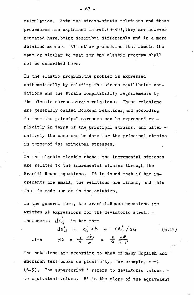
— 67 —
calculation. Both the stress-strain relations and these
procedures are explained in ref.(3-49),they are however
repeated here,being described differently and in a more
detailed manner. All other procedures that remain the
same or similar to that for the elastic program shall
not be described here.
In the elastic program,the problem is expressed
mathematically by relating the stress equilibrium con-
ditions and the strain compatibility requirements by
the elastic stress-strain relations. These relations
are generally called Hookean relationsiand according
to them the principal stresses can be expressed ex -
plicitly in terms of the principal strains, and alter 4WD
natively the same can be done for the principal strains
in termsodf the principal stresses.
In the elastic-plastic state, the incremental stresses
are related to the incremental strains through the
Prandtl-Reuss equations. It is found that if the in-
crements are small, the relations are linear, and this
fact is made use of in the solution.
In the general form, the Prandtl-Reuss equations are
written as expressions for the deviatoric strain
increments (1/4) in the form
delei c1)\ dereji
with d k = a cep a dr" 2 2 7
-(6.15)
The notations are according to that of many English and
American text books on plasticity, for example, ref,
(6-5). The superscript ' refers to deviatoric values,
to equivalent values. H' is the slope of the equivalent

-68- GOT
stress against plastic equivalent-strain curve,i.e. deFe
Because of the simplified stress system at a shell
of revolution, a reduced set of equations can be formed.
A shell element with a complete symmetry of geometry
and loading will have the system of forces shown in
Fig.6-2A. Taking a smaller element at a certain
distance from the shell mid-wall, the general system
of stresses is reduced to Fig.6-2b, with the other
stresses zero.. According to the mathematical model of
yielding, this element will yield when the equivalent
stress Fr reaches a certain value Y.
A further simplification is made by neglecting the
contribution of Ciandl;to yielding. c has always
been neglected in all developments of the basic thin-
walled shell theory. C exists because of the bending
of the shell element and varies parabolically across
the wall thickness with zero values at the shell wall
surfaces and maximum values at mid-wall. In first-
order thin-walled shell theories 1 -C12 is assumed to
have no contribution to the deformation. Its con-
tribution to yielding is also neglected here in the
elastic-plastic program.
There are thus only the two direct stresses 61 and
6i that are also the principal stresses. The corresponding
principal strains are el) e and e3 in the three
fixed directions.
Expanding eq.(6.15) for such a state of stress and strain)
this results in

- 69dei V 3 degP i , d61
_ cte, = -5- T 1r + - - 1 E I=
de 3 ,c7t Ti. ,
a / 4 d61 _ dui a = a--- tj E E
The von Mises yield-criterion gives the expression for
the equivalent stress for a three-dimensional stress-
state as
=(0-1 0-2)2÷ 0-2 - -( 6.17)
This for the case here of 0-1-3 = 0, becomes
= ( 6-1 2- + d, (1-2. + 6r, )427 -(6.18)
Equation (6.15)gives an explicit expression giving the
strain increments del and dezin terms of the stress
increments and the present state of stress. In the
elastic-plastic calculation the opposite relations 4
also required giving the stress increments dr, , and
dui. in terms of the strain increments. Ref.(3-49 )
shows that this is done by inverting the coefficient
matrix formed by both equations (6.16) and anO.additional
equation, this being the von Mises yield criterion in
the form of an implicit differential
3T,'ar, +362 / dr,. = 2 F =er- 1-11 61.jt, -(6.19)
The resulting matrix equations is
I9 tr, 1
----ff --..y.
t _-: E 12. -,zi.
-(6.16)
3 e ~-
_ H r
•••
do--1
(JO;
del
dez
da-i)
-(6.2o)
Inversion of this coefficient matrix is done at the
computer resulting in coefficients referred to by
Marcal as 'partial stiffness-coefficients' for plastic
straining
1̀5-1) c)61 (/ \ (1Tis :Yet' 1p ) Ae2.4, ) ) • c ez 3e, le aez.
Similar coefficients for points which are completely

— 70 —
elastic can be formed directly,being,
301) ,4 \ ()we. ce2_Jt
4)6; N cel — V' —(6.21)
It is of interest to note that becently Yamada et.al.(6-6)
have derived the values of these elastic-plastic
coefficients directly, i.e. without inversion on the
computer, both for the general three-dimensional stress-
state and for the above plane stress state.
Transition Point
A solution of the states of stress and strain is
obtained at each increments of load. In the process
of integration, each mesh point in each shell element
is tested to see whether the point is Mastic or has
yielded at the previous load. If the point has already
yielded, elastic-plastic coefficients as defined above
are used to obtain the stress increments from the strain
increments. If the point is elastic,it is further
tested if it remains so after the load increment, in
which case the elastic coefficients are Used: If it
is otherwise, these points that yield during the load
increment, called transition points, are to be treated
specially. The process for this is mentioned below.
The feature of a transition point is that at a certain
portion of the load increment the point remains elastic,
while at the remaining portion of the increment, the
point behaveelastic-plastically. Since this ratio
cannot be determined directly,but by iterations of the
the solution of the complete shell, the elastic-plastic
calculation has to be planned accordingly.

- 71 - Consider one such point where,at a certain increment,
the strain changes from eto +SE. If the portion
of the strain increment Se that is elastic is oCirE ,
where d 1, then the elastic-plastic part is
Marcal assumes that.for small load-increments, the firtt
approximation can be made that the ratio al for the
strain increments gel has the same value as 0(2_ for Sez
and thus both of them are the same as the ratioo(for SE . Using the elastic and the plastic partial-stiffness-
coefficients, the stress increments are aGn
J e = 1,2. 2 -(6.22)
An overall coefficient can thus be defined,being
367: v. J \ \ 3e,;)
36-: \ 1) . 0( asi)e. + (1-'4) (les; -(6.23)
cp< i We now proceed to explain how mLs determined. Let
the transition point hagea current condition of 6-1) 5-2.)
e ) e 2. , they being elastic have the relations
and
F( , ) =
6-12 — C5-2_
E
s _ .11 a ( .e )
0.7„ - v., ( e., + )
In the next load increment, we make certain guess for
the values of the strain increments S-el , and EeL , and
assume first that they are the correct values. The
elastic portion of these increment are thus 04;S es
and a Set , with the corresponding elastic stress
increment, for direction I, as
E r Ecde, + (.2 z ( e -+ Je„)
e, 4 Ye,_) -(6.24a)
= 0(6c

-72-
If we call for convenience, TIT;_( gel + gezias
This is a fictitious value,being the stress increment
if ge and Ce are elastic which they are not.
Similarly for direction 2, E fc- Drie. e2. + = oC (5-Cr! -(6.24h)
By definition of yielding,
+ of s-0-, f 1 611- .4 s‘61. } and y = c"4 Er' Z - ( -1-..t&cf)( 6", catiie) ( + of EGO This gives aoez C = 0 -(6.25)
with a = F 10'2. + Se 4 Elf
= - 6-1 r?- r2
The roots for the quadratic equation (6.25) are
( 4ac) ii- 24.
They are as mentioned above) based on'the estimated
values of lei , and Eex. If these values are suf-
ficiently close to the correct values, there should be
only one root which lies between 0 and 1, and this is
t=.• taken as the estimated value for fromwhich the over-
all partial-stiffness-coefficient of (6.23) can be
calculated.
Knowing the partial-stiffness-coefficients of the
elastic points, plastic points and transition points,
the complete relations between all incremental stresses
and incremental strains can be obtaiffed. Tne normal
integration can thus be made to obtain the solution
throughout the shell. Any such solution is necessailly
based on the current estimated values of Ee, , and Eez
at a number of transition points. An iteration process

- 73 -
is thus necessary here when, after each solution, a
better one can be obtained by using at each transition
point the previously calculated value of to get a
better estimate of , and ge2_ . The first of these
iterations started off with g5= 1.0 for all transition
points.
Yield Stress
Mention should also be given here of the derivation of
the yield-stress value Y. In the program, Y is not
necessarily a constant, but can vary at each point in ,
the shell according to the amount of plastic strain er .
It thus means that the material need not be perfectly
plastic. The form of the relation between Y and `er
used in the program is
y k -e-r̀ -(6.26) 2.. 0
A perfectly-plastic material,for example,would thus
have the form
Y =k0
while a linearly strain-hardening material is expressed
by
Y =k0 + k1 -67p.
Other Useful Informations
Detailed flow-charts have again been drawn for the first
two subroutines of the program,, one being the main
routine and the other being the main flow and control
subroutine called MASTER. They are given in Appendix
A.
A list of the errata and other nessary corrections to
ref.(3-49) by Marcal and Pilgrim describing the program
has been drawn up, and is given in the same appendix.

- 74 7
7. ACCURACY TESTS FOR ELASTIC PROGRAM
Notations
This list.is in addition to that in Ch.6.
r radius vector of a point in shell
a radius of revolution for toroidal shell,
cylinder radius for cylindrical shell.
b radius of torus cross-section for toroidal
shell, sphere radius for spherical shell.
k integration constant for cylinder equations,
4k4 = 3(1 - 2) / a2 h2
integration constant for
'2 =
sphere equations,
accuracy in integration procedure.
accuracy in boundary control procedure.
Mt 4* meridional,circumferential bending moments
per unit length
The following accuracy tests on the elastic program
PVA1 were performed by the author in parallel with the
development,coding and error detection of the program.
7.1 Size of Problem For Converging Solution
The first test consists of a determination of the size
of the problem that can be accurately analysed by the
program. The term size is taken here in the context
of the numerical-analysis procedure, and not on the
physical size of the shell to be analysed. This size
is also not related to the storage size in the computer
since the program uses fixed storage location for the
matrides necessary in the computation. The 32,000-word
core store of the IBM 7090 or 7094 computer allows the
shell problem to have a maximum of 4 branches, each
branch with a maximum of 10 elements and 300 interval

-75-
points. These limitations are larger than are
necessary for most problems that have to be solved.
It was found on using the program for shell analysis
that there was a limitation to the length of the branch
of a specific shell geometry, beyond which the boundary-
control procedure loss its accuracy and converged very
slowly or not at all. Similar observation has since
been reported by Kalnins (3-31). This loss of accuracy
is not due to cumulative errors in the integration
process. It is basically due to the subtraction of
very large, almost equal numbers in the solution of
the unknown initial variables XA during the boundary-
control process.
In an analytic solution to shell problems, it is very
often noticed that the complementary solution can be
expressed in terms of two types of functions. Of these,
one type of functions decays exponentially while the
other type of function grows exponentially with the
meridianal length 1 of the shell. Thus the coefficients
Cjim,defined by the relations between the initial and
end values of a branch,equation (6.7),
Gjm = LI" c•J;.4•1 XA.im = 0 im
increase as the length of the shell branch increases.
The final solution of the unknown initial values XA
requires inverting a matrix with the values Cjim as
coefficients. During this inversion, the coefficients
are multiplied and subtracted from each other. If the
values Cjim are exceedingly large, such that the sig-
nificant figures are lost during subtraction, the in-
vertion would either loose its accuracy or break down

- 76 -
completely in some cases.
To test this phenomenon and to check its accuracy, a
large number of ' numerical experiments ' are per-
formed on the computer varying the length, diameter and
thickness of a cylindrical shell with built-in ends
under internal pressure. Analytical solution to the
cylindrical problem (see for example,Chapter 4 of Ref.
(6-3))reveals that the exponentially increasing function
is the term ekl(A cos kl + A2sin kl ) which is always
smaller in value than (A1 + A2) ekl
* k in this problem
has the relations 4 k4 = 3(1- V 2 )/ a2• h2 , with a =
radius and h= semi-thickness of the cylinder. Al and A2
are constants of integration. Thus we have /
kl = 1 (i Fa; which is approximately 0.91 j Arc-kTi for =0.3.
The range of integration in the program is a branch of
the shell. Thus the length of a branch rather than the
length of a complete shell is the parameter that has to
be limited. From these experiments on the cylindrical
shell, it was observed that, on the IBM 7090 or 7094
when jz.* - tt- of a cylindrical shell branch is greater than 15, the boundary-control process cannot make the
boundary functions converge to the desired zero values.
This factor represent a magnification ratio of the order
of e :61 xl15 • — 106
This limiting value of 15 for LF-i-1- should be dependent
only on the cylindrical geometry of the shell and not
on the loading and the boundary arrangements. Further
tests have been made on this using the problem of an
open-ended cylindrical shell under internal pressure,

- 77 -
with one half of it at a different thickness from the
other. Each half is thus considered as,branch with
the junction point at the discontinuity. Discontinuity
stresses occur at and near thejunction, and die away
towards the open end. Because of the difference in
thickness t , the length 1 to give the same value
to the parameter TT,T.-- is different. From a number
of calculationswith different lengths supplied to earth
branch, it was found that slow or break down of con—
vergency occurred at approximately the same value of 15.
Shells of other geometries are expected to have other
limiting criterion. The case of a shallow spherical—
shell was next investigated. Again the complementary
solution to the governing equations consists of a rapidly
increasing function and a rapidly decreasing one. The
former is not an exponential function, but consists of
Kelvin Functions (see, for example, Chapter 4 of Ref.
6-3). It is of the form A i beril 112. 14i. jrj where q 1 1 x [ * (l_ep x
r4-1T , 1 = meridional
length,b = radius of curvature, h = semi—thickness
For 1) = 0.3 j = /Tx 0.91 x 1 Again the influencing parameter is (1171
71 There would
be a different critical value for this parameter. In
the case of the shallow spherical shell with a central
hole, it is found that this value varies with the
diameter of the hole making it impossible to draw up a
convenient rule to determine the critical value.
7.2 Cylinders Under Internal Pressure
The same problem as in section 7.1 above, of a circular
cylindrical—shell with built—in ends and under internal
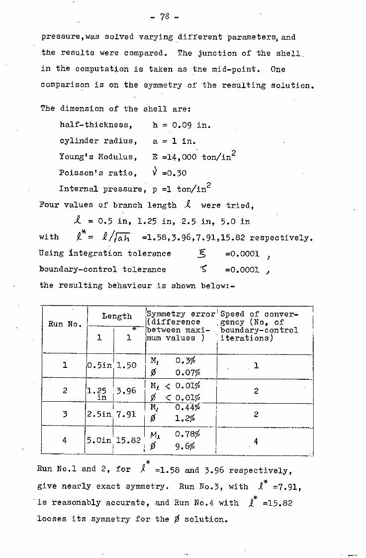
Symmetry error'Speed of conver- (difference :gency (No, of between maxi- boundary-control mum values ) iterations)
Run No. Length
1
MI 0.3% 0.5in 1.50 0 0.07%
1.25 3.96 in 0 < 0.01°A
MI 0.44% 2.5in 7.91 0 1.2% i
i /4/4 0.78% 5.0in 15.82
I 9.6%
1
2 MI < 0.01%
2
4
3
4
2
- 78 -
pressure,was solved varying different parameters, and
the results were compared. The junction of the shell
in the computation is taken as the mid-point. One
comparison is on the symmetry of the resulting solution.
The dimension of the shell are:
half-thickness, h = 0.09 in.
cylinder radius, a = 1 in.
Young's Modulus, E =14,000 ton/in2
Poisson's ratio, ) =0.30
Internal pressure, p =1 ton/in2
Four values of branch length were tried,
= 0.5 in, 1.25 in, 2.5 in, 5.0 in
with Q. 1/FT; =1.58,3.96,7.91,15.82 respectively.
Using integration tolerance .1; =0.0001
boundary-control tolerance -5 =0.0001 , the resulting behaviour is shown below:-
Run No.1 and 2, for X =1.58 and 3.96 respectively,
give nearly exact symmetry. Run No.3, with 1 =7.91,
.is reasonably accurate, and Run No.4 with / =15.82
looses its symmetry for the 0 solution.

Symmetry Error Speed of Convergency Run
0.03% 0.01% 3b 2
-79- Decreasing next the tolerance for the case of
it*
=7.91, to =0.00001, =0.0001,give the
following improved behaviour,
Run
Symmetry Error Speed of Convergency
0.14%
3a 0.07% 2
For the case. "5 =0.0001, =0.40001, the result is
Complete analytical solution to this problem can be
obtained from -solving the governing differential equation eF
+ 4k2 F = 0, F = radial shear force per 3(1--
unit circumference, k = a parameter, where 4k4=
The expressions for the solution are directly evaluated
on the computer and considered as the exact solution.
.The above numerical-analysis results are compared against
it.
Run 4 * A
Error(%) I
Branch 1 .
. Branch 2
Max Mi; + 1.13 + 0.88 1 1.58
. Max 0 + 2.04 + 1.98
• Max Mx + 0.48 + 0.02
3 7.91 Max 0 - 0.49 + 0.72
Max 14.2 + 0.77 - 0.02 4 15.82
. . Max 0 + 6.57 .- 3.71

- 80 -
It is seen that except for the case 2 =15.82,both the
cases with 1 =1.58 and 7.91 give results that agree to
within 2% of the exact solution.
7.3 Comparison With Published Results
The program PVA1 was tested over a wide range of shell
shapes and parameters,and comparisons were made with a
selected number of published results. The range of
Problems covers those encountered in pressure vessel
j. analysis. The results are shown in Fig. 7-1 to 7-5.
In all cases the dimensions of the shell structure are
shown in the figures.
Cylinders with Abrupt Thickness Chab7e
A number of thin-walled cylinders with an abrupt change
in wall thickness and loaded under internal pressure
have been carefully machined and analysed experimentally
by Morgan and Bizon(4-5). In all cases the results were
compared with theoretical analysis based on the analytical
methods of Johns and Orange (7-1), where the equations
are also first-approximation ones according to Timoshenko
and Woinowsky-Kkieger (3-7). The same theory is thus
used as in the present computer program although the
source of the equations fist: different.
Program PVA1 was used to analyse one of the above
cylinders with the two parts of thicknesses 0.082 in
and 0.205 in and having the same mid-wall diameter of
5.785 in. Fig.7-1 shows the stress distributions. The
two theoretical solutions 66incide at all location on
this plot of the distribution and are shown as the same
lines.

-81- Toriconical Heads Under Internal Pressure
Morgan and Bizon did a further series of experimental
analyses on toriconical heads (4-17). The same care
have been taken on these tests as on those above. Two
heads of the same shape were tested. The larger one
was spun from an aluminium sheet, while the smaller one
was more accurately contour-machined from an aluminium
billet and found to have a very accurate geometry, the
contour being within 0.002 in of the true shape out of
a 12 in diameter vessel. Again they comtred the results
with theoretical results based on the same analytical
methods; for the solution of the conical portion, tables
of Bessel-Kelvin functions were used.
The results of the contour-machined head were compared
with the solution using PVA1. In this case the vessel
is quite thin,making the shell meridianal-length
parameter re too large for accurate analysis by the
program. Fortunately the regions of discontinuity at
the cone-sphere and at the sphere-cylinder intersections
are sufficiently remote that there is a region in between
where the stress falls to a near membrane condition.
The problem is thus solved by two computations - one for
a cone-on-sphere geometry and one for a sphere-on-
cylinder geometry. The results again nearly coincide
with the published theoretical results. They are both
plotted as the same lines in Fig.7-2.
Expansions Bellows Under Axial Thrust
Turner and Ford reported in 1957 (7-2) experimental
studies of the stress and deflecion of a number of
pipeline expansion-bellows under axial loading.

- 82
Theoretical analysis was also presented based on an
approximate theory using a series solution for the
minimum strain-energy. A torus geometry,given by the
expression
r = a d= b cos 6
was used for the convolution, with
a = radius of revolution
b = radius of the torus cross-section.
In the analysis it was assumed that a >>b so that terms
of the form r a. ± 6 cas 6
were approximated to unity.
In a subsequent paper in 1959 (6-2), Turner reduced the
governing shell-equations for a toroidal geometry to
two second-order differential equations each of which
was a special case of the Mathieu equation. The same
approximation that a >".>13 was used. The solutions were
obtained through influence coefficients by tabulating
the Mathieu functions. Using the theory, detailed
comparisons were made in Ref.(7-3) of the stress and
deflection of a few selected bellows units tested in
Ref.7-2.
Two typical shapes of expansion bellows have been
analysed with the program PVAI. The first is a flat-
plate bellows unit shown in Fig.7-3a . Extensive
strain ganging was made during the original test and
from it stress results were obtained at different
positions. Two calculations were made to give a full
analysis, one analysing the convolution attached to the
end of the bellows, and the other analysing the middle

- 83 - root convolution. Different end-conditions were
simulated in the computation. For the other end of
the end-convolution, an extension pipe estimated to be
of similar stiffness to the actual arrangement was
assumed. Otherwise an assumption of a condition of
symmetry of 0 =0, and F=O, can be made.
Figures 7-3a and b show the stresses from computation
compared with both the strain gauge test results and
the theoretical solution of Turner in 1959. The two
theoretical results were in good agreemtnt with each
other. Moderate agreement was found between the theories
and the experiment. The experimental stress values have,
according to Ref.7.2, anaccuracy of + 10%
The other bellows unit is called bellows C, shown in
Fig.7-4. There are six quarter-convolutions, forming
one middle crest and two adjacent toots both of which
are each carried further by a quarter-convolution to
end at a thick end-plate. Both the strain and the
deflection values were studied with the computer program.
For the prediction of the axial deflection, exact idea-
lisation must be used in the computation. For this
purpose, one half of the bellows is analysed with one
end of the shell terminating with a fixed-end condition
of u =0, and 0 =0, and the other end, being the middle
crest, terminating with a symmetry condition of 0 = 0 ,
F = O. The circumferential strain distribution between
the root and the middle crest is preserited in Fig.7-4,.
and is shown together with the strain gauge test.points,
and the theoretical results of Turner in 1959 which only
give the midwall value (for a thin shell, the midwall

- 8h. -
-value should be the average of the external surface and
internal surface values). The agreement between these
results are good.
The axial deflection from computation is shown below
with the other two results.
Deflection between roots,per ton load:
Measured 0.0071 in.
Calculated,Turner 1959 0.0071 in.
Present program 0.00718 in.
Again very good agreement is obtained.
7.4 Comparison With Other Pressure Vessel Programs
In Ref.3-37,H. Kraus made a review and evaluation of
pressure vessel programs, and critically compare the
results obtained from four of them using three complex
shell problems, all of them shells of revolution under
axisymmetric loading.
Four Other Pressure Vessel Programs
The first program originated from R.K. Penny (3-24,3-38)
who was with the Central Electricity Generating Board.
It solves the axisymmetric problem using the Love-
Meissner equations and by the method of finite-difference.
The next program, by A.Kalnins (3-31) who was with the
Yale University,can analysis symmetric and non-symmetric
loads. The equations are reduced to a system of first-
order differential equations, and salved by the Adams-
Bashforth stepwise integration method along each shell
segment, of which, a maximum of ten is allowed. Con-
tinuity'conditions are then applied to the variables
at the end-points of the segments, to give a simultaneous

- 55' -
system of equations which is solved by Gaussian
elimination to complete the solution. The third
program originated from Radkowski and others (3-26)
at the AVCO corporation. It solves the standard
axisymmetric problem allowing of temperature and
material properties varying through the shell wall.
Multi-branch junctions of 1,1p to three shells can be
analysed. The differential equations derived by E.
Reissner for shells of revolution are solved by the
finite-difference method. These three programs,although
differing in their generality and in methods of solution,
use basically the same class of first-approximation
thin-walled shell theory for shells of revolution.
The fourth program,by Friedrich (3-36) of the Westing-
house Bettis Atomic -'ower Laboratories ,solves the
standard axisymmetric problem with additional conside-
ration of thick-shell effects. The method of solution
is the finite-element method. This approximates the
generating curves of the shell of revolution by ellip-
soidal finite-elements of shell where middle surface
shifts between the elements are allowed. Instead of
proceeding from the governing differential-equation of
shells, a stiffness matrix is calculated from the strain
energy by the principal of virtual work. The thick-
shell effect is introduced by determing the contribution
to the strain energy from both the normal stress and
the shear deflection,both of these are neglected in Love's
first approximation theory.
Two of three problems used by Kraus for comparing the
above programs are solved with the present program.

— 86,s. —
Test Problem 1 - Spherical Cap
The first one is a 60° semi-angle spherical cap with
20 in means-radius and 1 in thickness, simply supported
at the edge. At the support a condition of zero radial-
displacement and zero meridianal-moment is assumed.
The top of the shell is closed. Most computer programs
have difficulty in analysing this closed condition
since the shell differential-equations are singular at
the closed apex, this is unless special facilities are
added. The first three programs by Kalnins, Radkowski
et.al. and Penny have such a facility. The fourth
program by Friedrich cannot analyse a closed end, and
Kraus left a small hole at the apex of the shell. Kraus
abserved that this was a valid procedure since the dis-
turbance caused by the hole was very localized. Program
PVAI can analyse a closed vessel, although ho output
is shown for the very last point, and depending on the
particular problem and the accuracy specified, a loss
of accuracy in the results may be found at the last one
or few points. Kraus presented the results of stresses
and displacements for only certain key locations in
the vessel considered.
Using 120 steps for the integration, the elastic program
PVA1 gave the following results, for 1 lb/in2 internal
pressure:
Running time on IBM 7094,min less than 0.12
Outside stress at apex, lb/in2 9.864
Inside stress at apex, lb/in2 10.035
Normal displacement at apex,10-6in 5.224
Outside axial stress at support,lb/in2 9.636
Inside axial stress at support,lb/in2 9.636

- 87 -
Outside circ.stress at support,lb/in2 3.5032
Inside circ.stress at support,lb/in2 2.2786
Rotation at support,10 6 radian 14.140
Peak stress (axial outside),1b/in2 14.431
Location of peak stress,degress from support 8.5
This table is so constructed that a direct value by value
comparison can be made Agth the results from other pro-
grams listed in Ref.(3-37). There is very good agreement
with the results from the other first-order programs, on
the stresses as well as the deflection and rotation-values.
In general,the results from PVA1 are closer to that of
both the Penny and the kalnins programs, agreement being
to the third and fourth significant figures. The results
from the higher-order Friedrich program are slightly
different from all others.
Test Problem 2- Hemispherical Vessel Head
The other vessel was a closed hemispherical pressure-
vessel head under internal pressure. The mean diameter
was 20in , and the thickness for both the head and the
vessel body was 1 in. The cylinder part of the vessel
had a length of 40in which is sufficiently long for the
discountinuity stress at the vessel head to die away to
a very small value.
The problem was solved with both UVAI. and the elastic-
plastic program PLINTH. The same E and ) were used
and the pressure was again 1 lb/in2
BUZ PLINTH Number of separate output points 144 124
Outside stress at aPPc.lb/in2 9.990 9.956
Inside stress at apex.lb/in2 10.010 10.050

- Normal displacement at apex.lb/in
2
Outside axial stress at junction,lb/in2
Inside axial stress at junction,lb/in2
9.711
10.007
9.993
9.732
10.007
9.993
Outside circ.stress at junction,lb/in2 14.996 14.996
Inside circ.stress at junction,lb/in2 14.992 14.992
Normal displacement at junction,l0-bin 7.996 7.996
Rotation at junction,10-7rad. 9.600 9.600
Outside axial stress at end,lb/in2 10.026 9.988
Inside axial stress at end,lb/in2 9.974 10.012
Outside circ.stress at end,lb/in2 20.007 20.040
Inside circ.stress at end,lb/in2 19.992 20.048
. Normal displacement at end,10 6 In 11.330 11.363
Peak stress in cyl.(circ.outside)lb/in2 20.638 20.641
Location,in.from junction 6.5 6.67
The axial displacement values are relative to the end
of the vessel.
In addition to the results from the four programs pre-
sented in Ref.(3-37). Kraus aubsequatly presented in
Chapter 10 of Ref.(3-8)*, analytical results for this
problem based on Watts and Lang,1953 (3-11).
Comparing these altogether seven sets of results, it can
be seen that again the results of the Friedrich program
are slightly different from all others because it is
based on a different class of theory. The present results
from PVA1 and PLINTH agree closely with the remaining
four, the largest difference being only of the order of
0.50. The closest set of results to the present results
* Fig.10.12 of Ref(3-8) shows the vessel with an inner diameter of 20.0" rather than a mean diameter of that same value which was used in the calculations in Ref. (3-37). The author believes that it is this diagram that is in error, and that the calculations were all on identical vessels.

-89-
are those of the Kalnins program which happen to use
also the predictor-corrector step-by-step integration
procedure.
7.5 Conclusions
The comparisons above show that there is nearly exact
agreement between the results of the program PVA1 and
other theoretical results. The heimspherical-head
results and toriconical-head results using the Johns
and Orange aftalysis procedure, are all stress results.
These analyses do not give the displacement and rotation
values. The computer program of Penny and Kalnins using
numerical procedures of finite-difference and prediter-
correcter integration do give them, and in these cases
it is found that there is again nearly exact agreement
between these numerical results.. All these suggest that
the present computer program PVA1 does not give error in
the process of transcribing Love's thin.:valled first-
approximation theory into the analysis of general pressure
vessel.
The particular problems studied above are governed by
the availability of published results of sufficient
detail and accuracy. They are however selected such that
they cover the range of problem encountered in most
pressure vessel analysis. They have included the toroidal
element,the bellows convolution the closed-apex problem,
and the p-r
Both
internal pressure loading and axial thrust loading have
been studied.
Greater discrepencies were, as expected,found between
the theoretical results of PVA1 and the experimental

-90-
results. This is because there are at least two-ad-
ditional sources of discrepency. Inaccuracy can occur
at the experiment, this includes deviations in the shell
from the ideal geometry and possible errors in the
measuring techniques. The theories can also be in error
if the assumptions behind them are not precise enough,
for example,the most well-knowassumption that cannot Kurt ba
always be followed is that the shell wall is not.
sufficiently thin.
If we consider inaccuracies during the experiment,
Accuracy of the measuring techniques can in many cases
be estimated by calibration. In the bellows tests of
Turner, the actual measured dimensions,found to be
different from the nominal ones, were used in the cal-
culations. Smaller inCaccuracy caused by geometry would
be expected for this. The two tests of Morgan and Bizon
were conducted with special care to reduce errors caused
by deviation in the shell geometry. The test vessels
were machined to the prescribed geometry. During the
tests on toriconical heads, Morgan and Bizon confirmed
that this geometrical inaccuracy can greatly affect the
final accuracy of results. It thus pays to put in extra
effort to get accurate geometry if exact comparison of
results is desired.

-91- 8 ACCURACY TESTS FOR ELASTIC-PLASTIC FROGRAM
8- 1 Previous Comparisons
A number of tests on this elastic-plastic program PLINTH
have already been conducted and published. They are all
compared against the published experiments of vessels
or vessel components. A brief summary of these tests
is presented below.
Marcal and Pilgrim,1966
In the same paper (3-49) that Marcal and Pilgrim presented
the elastic-plastic program,they also presented two cal-
culations,one on a toroidal bellows labelled S tested
by Marcal and Turner (8-5), the other on a torispherical
pressure-vessel head tested by Stoddart (8-10). Both
are of mild steel and the mechanical proporties as
reported with the tests were used in the calculations.
The bellows unit was loaded axially, Strain and deflection
readings were obtained beyond its limit of plastic be-
haviour. Only two appropriate curves from the calculation
were shown compared with the experiment. The first is
the curve of load maximum surface-strain. The
agreement on this is very good. The other is the curve
of load•, axial-deflection. Here the calculated deflection
results were higher at low loads by about one fifth.
The collapse load from the calculation was taken as the
load when the convergency of the numerical process become
very slow.
The torispherical head was tested under pressure,beyond
yield, and until the head nearly collapsed. The elastic
stresses from the calculation were compared in detail
with the test results and good agreement was found in

-92-
nearly all positions. For the elastic-plastic behaviour,
the curve of pressure ./ stress for one maximum stress
location of the head was compared. The agreement here
is less than that of the bellows test. There was during
the test a sudden increase in stress at the external
gauges (although,surprisingly, the internal gauges which
were at the same location did not show any sudden change
of behaviour at the same-'pressure), and this behaviour
was not shown on the calculated curves. There was no
explanation of how the collapse pressure from the cal-
culation was arrived at.
Marcal and Turner
Marcal and Turner (8-13) presented a modified procedure
to the solution of the thin-walled shell theory to
predict more realistically the local behaviour of flush
nozzles in spherical pressure vessels. This modified
procedure was incorporated into the program PLINTH and
a few calculations were again made to compare with a
few published tests.
The first tests that were compared, were by Cloud(5-8),
who tested three nozzles with no fillet-weld nor rein-
forcement. The nozzles were loaded under pressure
until collapse. The second tests were by Dinno and Gill
(4-10), who_in a similar manner tested two nozzles with
fillet-weld. Calculations were made using the normal
thin-walled shell theory and the modified theory. Com-
parisons were made on the deflection behaviour and the
behaviour of the maximum meridianal-strain. On the Cloud
nozzles, the modification did not affect the deflection
values but there was little agreement between the

- 93 -
calculation and the experiment. The calculated strain
results of the same nozzles were greatly affected by the
theory used. Because of these two reasons it was not
possible to judge whether the elastic-plastic program
gave good results or not. On the two nozzles with weld wed by 4)-f Dinno and Gill, the two theories g' different values
of elastic deflection, with that 6f the modified theory
closer to the experimental deflection. After initial
yielding, the modified theory gave deflection values which
started to increase rapidly from a lower load than ex-
periment, and further gave,after that, a load which, for
the same deflection, is 10 to 25% lower than the measured
load. No comparison can be made of the behaviour of load
against strain, since the experimental results were not
shown.
These comparison of results for the nozzles were com-
plicated by the presence of local effects at the nozzle
junction which is also the location of maximum stress.
The modified theory is thus necessary to take this into
account. However, this means that the above elastic-
plastic comparisons are not straight-forward tests of
the accuracy of the program. No conclusion can thus be
drawn in this case on this latter point.
8712 Use of Elastic-Plastic Result°
Both the literatures and Ch.7 show that the accuracy of
prediction of stresses by elastic thin-shall theory is
fairly well established for many shapes of shells of
interest to pressure vessel designers. It is probable
that carefully machined vessel and accurately conducted
tests can even reveal the accuracy or otherwise of the
assumptions behind the theories. The prediction of

- 94 - elastic-plastic stresses and strains is still in its
infancy. We have seen in Sec.8.1 that many more factors
influence the accuracy of such predictions than is the
case for elastic calculations. It was thus difficult
to compare the results in detail.
Two methods can be adopted to tackle this problem. The
first is to eliminate, as far as possible,those sub-
sidiary factors that may affect the experimental results
( by subsidiary factors is meant those that cannot be
included in elastic-plastic calculations as limited by
the theory). ThWincludes, for example, trying to re-
move any residual stresses and any difference in hardness
of the material, a-0-4.44A-6.4
f the vessel geometry
as tested1and using the actual geometry in the calculations.
Details of this are given in Ch.11 which gives the pre -
parations to the author's vessel test. The second method
is-to find out,what uses these calculations may be put
i#e to help with design and discuss the accuracy or
other wise of the results in the context of these probable
uses. For this purpose, the vessel research and vessel
design interests of these elastic-plastic calculations
are reviewed below, followed by a discussion of the kind
of results that may be required.
In the design against excessive deformation and collapse,
elastic-plastic calculations can (8-1) fill the gaps
left by limit analysis,where at present approximate
solutions to only torispherical heads(5-4) and sym -
metrical nozzles (see Ref.802), are possible. Study can
also be extended to the solution of shells with various
strain-hardening material properties. In the design of

- 95 -
components under reversed loadings,such as expansion
bellows and pipe bends, the design can be made more
economical by allowing alternating plasticity rather
than limiting the working load to one giving no yielding,
Here design to some low cyole fatigue life N requires
the plastic strain e (8-3). One commonly used relation
(8-4) is eP 14:2- = constant. Other relations with the
total strain et have been proposed for small plastic
strain. To predict the maximum value of e or et on
such vessel components, elastic-plastic computation is
required (8-5),(8-6) using a 'cydlic' rather than the
oridinary 'monotonic' stress-strain curve of the material.
Loading direction does not reverse with components loaded
only under pressure , but in most cases there is a suf-
ficient number of loading and unloading cycles in general
service to justify the consideration of shakedown under
repeated load(8-7),(8-8) rn additidn2t6Jd6Ilapse:11.1While
one procedure to obtain shakedown load, applicable to
symmetric nozzles, requires only elastic analysis (5-17),
(5-18), the elastic-plastic solution up to not greater
than twice the first yield load is required in another
procedure applicable to the general shell(8-1),(8-8),(8-9).
From this brief review, it appears that interest is on
the prediction of collapse load, of shakedown load, and
of fatigue life.
Where low cycle fatigue is of interest,Ref.(8-5) and
(8-6) pointed out that elastic-plastic calculations using
the value of settled cyclic yield-stress for non-work-
hardening material,or settled cyclic yield-curve for
workhardening material were used instead of the ordinary

- 96 -
'monotonic' stress-strain curve. The strain ral:::e of
interest should be less than 2.5 times the maximum
elastic range except for very short fatigue-life.
Where elastic-plastic calculation is used (8-1) to
predict shakedown pressures, stresses at less than twice
the first-yield pressure are requiredthese being abet- iUA-4-
2.5 or 3.0 times the first yield stArcosco.
In the prediction of collapse, this can be observed
either through the strain results or the deflection
results. The component may be judged to be in a state
of collapse when there is a sudden change in slope of
the load-strain or load-deflection curve, or when the
strain or deflection has reached a certain large value.
The final interest is on the load value at this condition
and no consideration of repeated load behaviour is
necessary.
Closely allied to the prediction of collapse is the
prediction of excessive deformation. This is important
in applications where close fitting of the vessel com-
ponent is necessary, as in the case of standpipes for
fuel rods in nuclear reactor vessels and of high pressure
turbine, compressor and pump casings. Again the value
of the load is required.
8;3 Further Comparisons
Since the present research was planned, the author noticed
two pieces of experimental work that could serve as basis
for a further detailed comparison of the results of the
elastic-plastic program. Both of them involved testing
pressure vessels beyong yield to a state of collapse,
while strain measurements were made with eiMtrical strain

- 97 -
gauges. As mentioned in Sec.5.3,Stoddart (8-10) carried
out, at the now University of Newcastle-upon-Tyne,elastic
and plastic tests on two identical torispherical pressure-
vessel heads,made of mild steel yin thick, and of 24in
mean diameter. Extensive gauging of both the inside
and the outside surfaces was made. Kemper et.al.(5-12)
of the APV Ltd. and of the Firth-Vickers Stainless Steel
Ltd. tested two pressure vessels of identical geometry,
but made of stainless steels differently heat-treated.
Only nine strain gauges at the outside of each vessel
were used, since the purpose of their test was to show,
the advantage of one of the steels that had been warm -
worked to a higher proof-strength,and thus gauges were
used only to record the general vessel behaviour until
collapse. The vessels had mean diameter of 41* in. and thicknesses of iin at the body and 5/16in at the head.
The heads of the Kemper vessels are slightly less than
twice the size of that of the other vessels, but both
have similar height/diameter and knuckle-radius/diameter
ratios. They can be classified as medium-thick pressure-
vessel heads. The following Table 8-1 gives detail of
their geometry and some other useful information. (Also
shown on this table are the geometry and information
of the author's vessel to be described later in Ch.11
and 12.)

-98- Table 8-1 Details of Test Vessel Heads
Author's tests Head A Head B
Stoddart I Ref.(8-10)
Kemper Ref.(5-12)
Head dimension(in.) Shell diameter D 23.678 23.848 24.000 41.125 Crown radius R 20.474 19.444 24.125 41.844 Knuckle radius r 3.839 4.344 2.000 3.156 Head thickness t 0.322 0.312 0.250 0.310 Shell thicknessT 0.322 0.312 0.250 0.250 Head height h (see note below) h/D
5.890 6.384
0.249 0.268
4.387
0.183
7.295
0.177 t/D .1/73.5 1/76.3 1/96.0 1/132 r/D 16.21% 18.22% 8.33% 7.67%
Strain gauging, Gauge lengths 2mm, 5mm, 10mm 1 in. 3mm,5mm Gauge location Inside and out - Inside & Outside
side surface outside surface
surface
Material Stainless Steel Mild Steel Stainless steel
Heat treatment After f4riCa - tion,900 C
After fabrica-tion
None
Note:D,R, r and h are mid-wall values. No significance is
implied in the number of figures as these are the values used
in the calculations.
84 Tests by Stoddart
Stoddart's vessel was analysed with the elastic-plastic
program using values,as quoted in Ref.(8-10), of Young's
Modulus of 30.354 x 10⁶ lb/in2 and Poisson's ratio of
0.31. An elastic perfectly-plastic stress-strain be-
haviour was assumed with a yield stress of 40,197 lb/in2
this value being obtained from a tensile test specimen
from the same plate as used for the vessel head and
subjected to the same heat treatment. The calculation

-99- gave a theoretical first-yield at 213 lb/in
2*. Four
peak strain values at three strain-gauge locations were
plotted alongside the corresponding experimental curves
and are shown in Fig.8-1. The inside meridional strain
at the 45° station was maximum for the whole vessel.
The curves for this strain value show that the elastic
values agree very well while the theoretical plastic-
strains increase more rapidly with pressure than the
experimental values. The agreement is different with
the other pairs of curves. Here, while all the experimental
curves bend down sharply at around 375 lb/in2, the
theoretical ones show a more gradual change of slope
making it difficult to intepret a corresponding pressure
at which the vessel starts to deform rapidly. A quan-
titative comparison of the collapse pressure is however
very useful, and two methods are proposed here to intepret
this value.
Definition of Collapse
In the first method a tangent is drawn to the plastic
part of the load-strain or load-deflection curve, and
its intersection point with the elastic line is used
as a criterion of the start of collapse. (In what follows,
the tangent is drawn at a point on the curve where the
actual strain, or deflection is three times the value
expeffted for that load had the response remained elastic).
This stems from the observation (8-11) that simple
structures of linear-hardening material behave such that
* The complete elastic-plastic computation took 20 minutes on the IBM 7094 computer, this includes calculation at every load increment, each at20.2 of the yield pressure, until a pressure of 468 lb/in .

-100-
a tangent to the nearly straight part of the load-
deflection curve intersects the elastic line at the
same point as that for a perfectly-plastic material.
For these structureg,this point both marks physically
the start of rapid deformation and coincides with the
results from a limit analysis.
The second deTinition tries to indicate the load where
signs of physical collapse, in the form of excessive
straining,actually occur. It is chosen as the pressure
giving a maximum total strain of 0.5% at the vessel out-
side surface.
Comparison
Table 8-2 below compares the collapse pressures thus
obtained from the test curves and from the calculation.
The tangent method for collapse was applied to the
experimental curve for the maximum meridional strain.
The value from the test results is 380 lb/in2 and happens
to agree with the value where the strain readings increased
suddenly. The collapse values from calculation is higher,
at 410 lb/in2. A limit analysis, assuming also perfectly-
plastic material and according to Shield and Drucker (5-4),
gives upper bound pressure of 465 lb/in2 and lower .bound
of 375 lb/in2.
The tangent method gives collapse loads within the bounds
of the limit analysis, while the 0.5% strain criterion
gives as expected, a higher collapse, although the
difference is not large (21% for the test curve and 13%
for the calculated curve),

- 101 -
Table 8-2 First yield and collapse pressure for
Mild steel pressure vessel head, Stoddart
(8-10).
Test results Ref.(8410)
Elastic-plastic calculation
First yield
Collapse Method 1 (tangent) Method 2 (.5% strain)
250 lb/in2
380 470
213 lb/in2
410 about 490
81;5 Test by Kemper Et.Al.
Stress-strain Curve
Material properties were also give in the report on the
tests by Kemper et.al., (5-12). They were obtained from
tests in general on the two types of steels used, but not
specifically on the individual plates used to fabricate
the vessels. This is unfortunate, since, as is shown in
Fig.3,Ref.(5-12), the proof stress can vary over a wide
range even for the same type of steel. Two representative
stress-strain curves, one for the high-proof steel and
one for the normally used low-proof steel,are given in
the Fig:land 2:of'Ref;(5=12). The curves were used in
the present calculations as data for the elastic-plastic
pressure-vessel program PLINTH. There is a high degree
of strain-hardening,and a perfectly-plastic calculation
would not be accurate. In the program PLINTH strain-
hardening in the stress-strain curve is defined through
the coefficients of an algebraic polynomial. In this
way, the measured curve, with any amount of strain-
hardening,can be approximated and used in the calculation.
For this purpose, a least-square curve-fitting program

- 102 -
was written, based on Ref.(8-12), for fitting an
algebraic polynomial of specified order to a set of
unequally spaced data points. The supplied curve for
the low-proof material, within the range 0 to 2% plastic
strain, was converted to a second-order polynomial.
The elastic-plastic calculation for this problem took
a total of 20 minutes on the IBM 7094, the pressure
increment, after the initial yielding at 95.7 lb/in2,
was 0.4 of this value until a pressure of 287 lb/in2
was obtained. Fig.8-2 shows the elastic strain dis-
tribution. The maximum straining occurs near mid-knuckle,
on the internal surface,giving a strain-concentration -
factor of about 4.0 over the vessel-body circumferential
strain.
Sources of Possible Error
Beforecomparing the theoretical and test results, it
should be noted that the former had assumed a uniform
material property throughout the vessel as given by the
assumed YounSts Modulus, Poisson's Ratio and the
approximated stress-strain curve. The test vessels had
however not been heat-treated after fabrication as in
the Stoddart test. The vessel plates would certainly
suffer a certain amount of work-hardening during fabrication.
The most severe hardening would occur at the knuckle
region of the heads where 5/16 in. thick plate was rolled
into 3 in. knuckle radii.
The two test vessels were nominally indentical,and the
measured elastic strain from both are expected to be the
same or similar. They are however fcund to disagree in
nearly all cases and to disagree also with the corresponding

- 103 -
calculated values. The following Table 8-3 compares
the strain values at five gauge locations, the measured
values were obtained from the slope of the elastic part
of the curves plotted on the appropriate figures of
Ref.(5-12).
Table 8-3 Elastic Strains
10-6per 100 lb/in2pressure
Position Gauge No. o.
Measured Strain Ref.(5-12) Corresponding
Calculated Strains Low-proof
Fig.9 High-proof Fig10 Fg.11
Crown centre 9 22 13 17 16
Mid-knuckle Circ. Merid.
8 5
-43 -8
-60 -28
-55 -29
Vessel body Circ. Merid. a
2 3
18 . 5 .
-
- 86 24 24
This disagreement in elastic strains makes it impossible
to get a meaningful comparison of the elastic-plastic
strain values. Only the theoretical strains are thus
shown in Pig.8-3 where the peak strain values labelled
A to D in Fig.8-2 were plotted against pressure. A few
of these readings are internal ones whose.Thehaviour
could not be observed during the experiment. The axial
deflection of the crown centre relative to mid-vessel
was also plotted and is shown as curve S .
Comparison
The theoretical first-yield using the properties of the
low-proof steel is at 95.7 lb/in 2, and at 150 lb/in2 all
the peak strain curves get progressively non-linear.

— 1014. —
Fig.9 of Ref.(5-12) gives the strain behaviour of the
low-proof vessel during the test. This figure is
repeated here as Fig.8-4 for convenience of comparison.
Of the nine strain gauges in the test, two, No.6 and 7,
were on the junction of the nozzles and were not plotted.
The other gauges plotted were on the vessel head or the
vessel body. The plastic behaviour of these other seven
gauges showed a progressively non-linear response after
300 lb/in2,expecially for gauges No.4,8 and 2,the former
twalocated at the mid-knuckle and the last at the vessel
body. After 500 lb/in2, a rapid increase at No.2 and 1,
both of which were at the vessel body, At this pressure,
the other mid-knuckle gauges,showed only a steady increase,
which is a continuation of their previous behaviour.
Table 8-4 below compares the elastic-plastic behaviour
as observed from the external strain gauges and as
predicted by calculation.
Table 8-4 Stainless Steel Vessels, Kemper Et.Al.
Test Ref.5-12
Elastic-plastic calculation
Low-proof vessel First-yield pressure Collapse pressure
Method 1 (tangent)
Method 2 (.5% strain)
200 lb/in2
270
530
115 lb/in2
j190 1190 240
High-proof vessel First-yield pressure 300 200 Collapse pressure Method 1 (tangent) 690 040
1340 Method 2 (.5% strain) 590 420
Since only external strain gauges were used in the tests,
and in order to give a fair comparison,only external
strain results are used to give the calculated values

- 105 -
of the first-yield pressures and the collapse pressures
by the tangnnt method. Two values for each vessel are
listed against the collapse pressure by the tangent
method, they are obtained from the maximum external
meridional-strain and the maximum external circumferential-
strain curves respectively. In this calculation the
values agree with each other.
Only seven strain gauge results are available for each
test vessel, and of these only two were positioned near
the- location of maximum straining of the vessel head,
at the centre of the knuckle radius surface. - The yield
and collapse pressures from these test results are thus
expected to be higher than what would actually happened.
The table shows that first yield and collapse as predicted
from the calculation do occur at a lower pressure than NON-
that from the test. Two other factors, un-uniform degrees
of yield and work-hardeningland disagreement at the
elastic results, have already been mentioned above that
would throw doubt to an elastic-plastic comparison. It
is thus not possible to judge the value of this comparison.

-106-
9 AXIAL LOADING TESTS OF FLUSH NOZZLES
9-1 Nozzle Configuration
Nozzles can be attached to pressure vessels in different
manners, and different methods of reinforcement can be
used to reduce the weakness of having openings in vessels.
From operating experience, and from special researches
into nozzles and openings, good design configurations
have gradually replaced the bad ones. Design codes can
prevent both extreme over- and under-reinforcements, and
according to these practices certain bad methods of
arrangement of welds have been eliminated from important
types of pressure vessels. Reinforcing pads and partial-
penetration welds are at present commonly used because
of their convenience during manufacturing. Specially
machined reinforcements and through-penetration welds
are however the better practice, both as regardsA9
better distribution of stresses and for easier analysis
by photoelasticity or by theoretical prediction.
Junction Arrangements
Many pressure vessel nozzles are fabricated leaving
fillet welds at the junctions. Experimental analyses
of such nozzles with strain gauges are possible only
as far as the edge of the welds. The unknown stress-
concentration due to the weld arrangement would be added
to the peak stress at the junction, and thus no exact
estimate of the local condition can be made. This is
of course not a disadvantage in the many cases where only
the load-holding-strength of the nozzle is important.
The stresses are very local in nature and the ductility
of the pressure vessel material is usually adequate for
taking up such stresses.

- 107 -
As safety and economy are both of importance in the design
of pressure vessels, increasing number of design con-
siderations will be brought in,and stricter designs will
be imposed. Better knowledge of the local but high stresses
at the nozzle junction will be necessary for the design
of nozzles. Already this is a requirement for the design
of many nuclear vessels. The ASME Boiler Code, Section
III, for nuclear vessels (9-1), specifies that nozzle
welds should not be left as welded, but the corner and
fillet are to be ground and machined to specific radii.
A few recommended shapes are given in the Code, according
to which the designs can be based, In such cases, definite
stress indices can be used in the design of such nozzles
against fatigue failure. Nozzles not according to these
recommended shapes must be designed with stress indices
obtained from specially conducted experimental stress
analysis.
It was mentioned in Section 14.3 that the Pressure Vessel
Research Committee launched a major program of experimental
study of pressure vessel nozzles and their reinforcements
(9-2),(9-3). All the nozzle configurations that were
analysed were of these smoothened types. It was felt
that they would be the only configurations used in
advanced nozzle design of the future, and that such a big
research effort should be directed towards these con-
figurations and not to any less-advanced shapes. For
the very same reasons, the author's present test is on
the smooth nozzles.
A complete vessel is not necessary for conducting axial
load tests on nozzles. The bending stresses and strains

- 108 -
are local in nature and an enclosed container is not
necessary, as would be required in a pressure test. Two
mild-steel spherical caps with flat bases were used.
Branch pipes of sufficient length were welded on top to
simulate the condition of a nozzle on a spherical vessel
or on the centre of a torispherical vessel. The nominal
dimensions of. the two test components are shown in Pig.
9-1. These two test components will be referred to as
the Thick Cap and the Thin Cap.
The base plates of both Caps are 24 in. in diameter and
the base circles of the spheres are approximately 22 in.
diameter. Both nozzles are of the same diameter and
thickness,being machined out of a 4 in. outside diameter,
in.thick, mild-steel tube.
This diameter of nozzle was selected so that the nozzle 111-4)
was/ small for sticking and manipulating strain-gauges .
inside the nozzle bore, but not too large as to cause
interference between the bending stresses originating
both from the nozzle junction and from the base plate.
The weld preparation and the final machining of the nozzle
are shown in Fig.9-24-. This weld• preparation is in
accordance with that recommended for Flush Set-through
Nozzles in the three British Standards for Carbon-Steel
Pressure Vessels,(9-14) to (9-6). It was selected because
the weld zone, being situated on the vessel side, is
slightly away from the fillet and corner regions, and
*Hot finish seamless steel tubing,according to BS 3601, steel 22.
+Dried,low hydrogen FORTEX 30 (i.e.30 ton/in2 UTS) elec-trodes,kindly supplied by MUREX Welding Processes Ltd. was used.

- 109- because it has been found by observing other experimental
results that the maximum stress may occur nearer the
nozzle end of the above regions. The nominal radius at
the fillet, this being the same for both caps, was
selected to be the same as the nozzle nominal thickness
of -A- in. Any smaller value for this radius would cause
great difficulties in the satisfactory strain measurement
of this region by strain gauges. The corner radii, on
the other hand, have different nominal values for the
two caps. In each case it was selected to equal the
sum of the values, cap thickness and nominal fillet
radius. This is not the normal practice, but the reason,
for doing it is that it will result in a shape similar
_to that used in the theoretical analysis which will be
explained later in Ch.10.
942 Strain Gauge Techniques
It was noticed, from previous experience of other
colleagues at Imperial College, that the strain-range
required of the gauges, for elastic-plastic tests of
pressure vessel components until or near collapse, is
in the range of a few percent. -Crdinary gauge and
adhesive combination may break or become gradually non-
linear within this strain range. Specially manufactured
post-yield wire gauges called TMI, has been found by
other colleagues to be suitable for such high strains.
Two types of gauges of this make were used in the tests
here, a linear post-yield gauges of 5mm gauge-length
for the high strain regions, and a 5 mm, 900 overlapping
* By Tokyo Sokki Kenkyujo Co.Ltd. Tokyo.

- 110 -
rosette-gauge for the other regions. Apart from having
the distinction of being designed for high and low strains,
the former type of gauge has a backing which is more
flexible and can follow a surface contour reasonably
well, unless the contour is a doubly-curved one. The
latter type of gauge can only be applied to a flat
surface or a slightly curved one.
After some initial trial, it was found later that gauges
of even smaller gauge-length and size were necessary at
the fillet position. Most stress analysis experiments
on nozzles that uses strain gauges neglect any measurement
at the fillet position, because, with a sharp fillet or
a fillet weld at that position, it is extremely difficult,
if not impossible, to find accurately the strains there
with strain gauges. The author however considers that
a knowledge of the fillet strain is very important, for
the very reason that, in most cases, the maximum strain
resides there. The present fillet has, as mentioned, a
smooth surface of radius about -A- in. The 5 mm gauge,
5 mm being about 0.20 in, is too large and was found
difficult to fit around this small radius. Notgauge:
of smaller size was available in this range of TML
post-yield gauges, and a KYOWA foil gauge with 2mm
gauge-length was selected. In addition to being
available in this small size, the KYOWA foil gauges were
supplied with lead-wires already attached, a very useful
arrangement in the present circumstances.
.A rapid setting adhesive was used on all gauges, called
cyanoacrylate (with the trade name of Eastman 910). No
By Kyowa Electionies Instruments Co.Ltd1 Tokyo.

- 111 -
mixing nor heating is required for its use. The gauge
to be positioned has only to be held down by finger
pressure, since the setting time is only from one to a
few minutes. A certain amount of skill is however
needed, since any wrong positioning, or any uneven
pressure in the first few instants of contact between
the gauge and the prepared surface, cannot be remedied
without much trouble•;removing the gauge and replacing
by a new one. This adhesive was however very necessary
for this job because many gauges were, of necessity,
close to each other and. some had to be positioned at
awkward locations or unflat surfaces.
All the different types of gauges used were checked for
their gauge factors and the linearity at different strain
ranges. The strain values at breaking point were also
observed. The same adhesive, the same surface pre-
paration procedure, and the same strain recording
arrangement were used as in the actual tests. Further
details of these techniques are given in Section 9.4
below.
The gauge factors at small strain values were measured
using a four-point beam-bending rig designed for such
calibrating purposes. Within the range of 0.1% strain,
which is the range possible for this calibrating
arrangement, the response of the gauges were all linear
and the gauge factors were very close to the manufacturer's
value and within the accuracy expected from the test.
For calibrating at higher strains, a 4 in. by i in.
stainless-steel bar pulled in tension was used. The
gauges were all positioned on the same side of the bar

- 112 -
to prevent errors caused by bending of the bar under
off-centre loadings. The strain values were checked
by taking accurate measurements with a travelling-
microscope of the length between two transversely
scribed lines, on the same side of the bar as the gauges.
With this travelling-microscope arrangement there was
no limit to the strain range that could be measured.
Two gauges of each type were tested. The two rosette-
gauges failed both at about 1.7% strain by a complete
slipping of the adhesive bond. The two linear post--
yield gauges failed by a gradual peeling-off of the
backing from the metal surface, and the response became
non-linear after strains of 6% and 7.5% . The two 2mm
foil-gauges both failed by an excessive stretching of
the foils near the weld tags until the foils necked and
broke. Their failure strains were around 2.3% .
The gauge readings were all plotted against the strain
calculated by the microscope measurement,to determine
:the gauge factors and to observe the linearity. A small
amount of scatter existed at small strains below. about
0.3%,because the microscope arrangement is not suitable
for such small strains. A similar pattern of behaviour
was observed on all gauges, in that the plots showed a
very slight deviation from a straight line at around
the range of 0.5 to 0.7% , but settled to another
straight line with a different gauge factor all the way
afterwards. In view of the slight scatter below 0.3%
it is hard to obtain accurately the gauge factor at low
strains, but lines according to the manufacturer's closely
value do fit very /the points below 0.5 to 0.7% strain.
At higher strains, all the wire gauges have a lower gauge

— 113 —
factor with between 6 to 8% difference, while the foil
gauges have a higher gauge factor with a 13% difference.
943 Material Properties
A knowledge of the material properties is necessary for
elastic-plastic calculation. The static stress-strain
curve of the material beyong yield was needed as data
for the computation. The strain range of interest was
within 4 per cent. It was also useful to know the
ultimate tensile-stress.
Test Specimens
The nozzles of the two components were made from the
same piece of pipe, but the spherical caps may have
different properties. The arrangement of the nozzle
weld was such that the actual junction,espacially the
zone where most of the yielding occurs, consists com-
pletely of the pipe material. It was thus decided to
prepare test specimens and to conduct measurements on
the material properties on only the pipe materials. A
spare piece of pipe material was taken and heat-treated
together with the two completed nozzle and cap com-
ponents, the procedure being desdribed in Section 9.4
below.
From theoretical analysis of the elastic strains, done
beforehand - , it had been found that the maximum strain
of the whole test component would occur as a compression
in the meridional direction, which would. be very nearly
the axial direction of the nozzle. The maximum value
for tensile strains also occurred in the same direction.
The pipe was i in. thick, 4 in. outside diameter.
Tensile-test specimens were machined from this in the

-114- axial direction. Two types of plane strain compression
specimens, designed for test with the platen in the axial
and the hoop directions were also made.
Tensile Tests
The tensile test was easy to conduct. The tensile
specimens were designed to fit between the shackles of
the Hounsfield Tensometer, but were actually loaded at
a slow and constant strain-rate in a Instron Universal
Testing Machine. The stress-strain curve from tensile
tests on mild steel, with its upper and lower yield
point, is very sensitive to the loading and the measuring
arrangements and to the strain rate (9-7). The Instron
machine has a long and free linkage behind the shackles
thus reducing any non-axiality in the test set-up. It
would be preferable to be able to measure the extension
of the uniform portion of the specimens. Unfortunately
the space between the ends of the two shackles,.when
locked around a specimen, is very small, with a clear
gap of only about in. Attempts had been made to insert
and take measurements with some home-made " clip-gauges",
bent strips of spring steel with the change of curvature
detected and measured by resistance strain gauges. This
however was not successful. It was thus decided to
record the cross-head movement as an indication of the
plastic straining of the specimens. The calculated elastic
straining of a specimen, which could be quite small
compared with the plastic one, was then added to find the
total strain. The Instron machine's own autographic
plotter was used, the extension being plotted against the
load value recorded by a load cell. Two tensile specimens
were tested.

Table 9-1 Tensile Test Results
Initial Dimensions (in) Load Values (lb) Stress Values(lb/in2)
Average Diam.
d
. Eff. gauge length L
Upper Lower Ult. yield yield tensile load load load U.Y.L. L.Y.L. U.T.L.
U.Y.S. L.Y.S. U.T.S.
•
1 0.1255 0.90 592 568 779 47,900 45,900 62,900
2 0.1255 0.92 590 550 775 47,500 44,500 62,500
Average 47,800 45,200 62,800
Table 9-1 gives the test results of the two speCimens. The ratio of yield/ ultimate stress is about 75%. The load-extension curves near the yield points are show in a and b.

- 116 -
Compression Tests
The technique of the plane-strain compression test
(9-8),(9-9) as originally developed by Watts and Ford
(9-10) and commonly used on relatively thin strips and
sheets, is normally suitable for finding the compression
stress-strain behaviour at high strains, from 5% to 80%
reduction or even higher. With the usual procedurel the
test strip is compressed between two narrow tool-steel
plat4, and after a certain increment of load, it is
removed and the resulting strip thidkness is read by a
micrometer. The strain range of interest in our case
is however only 4%. At small strain ranges, the re-
duction in thickness is small and scatter of the
results can occur.
An alternate procedure finally adopted is to dispense
with the micrometer for thickness measurement, and to
measure the movement of the plates during loading. A
home-made Clip Gauge, mentioned above, was used, with
the ends of the gauge inserted between the shoulders
of the platens. The loading on the strip can thus be
made continuously and, unless the clip gauge is disturbed
in-between readings, one continuous run is sufficient
for one set of readings, corresponding to one stress-
strain curve.
It was mentioned that the maximum compressive strain
at the nozzle would be in the axial direction. These
plane-strain compression tests result in a maximum
strain in the through-thickness direction, and may not
be representative of the desired axial-direction pro-
perties. They can however serve as a rough check on the
uniformity of material properties in the two important

- 117 -
hoop and axial-directions. The load-deflection curves
of the three tests performed with the platen perpen-
dicular to the hoop direction, and the two tests with
the platen perpendicular to the axial direction, are
presented in Fig.9-4 to 9-6. It can be seen that the
value of the yield stress at each group of test is
fairly consistent; the slope of the plastic lines are
however not so. The reason for the latter may be caused
by the different amounts of friction between the strips
and the platen.
9.4 Test Arrangements and Preparations
Residual stresses would be left at and around the nozzle
junction after the welding fabrication. While this
may not affect the strain gauge readings'in the elastic
ranges of the shell, the yielding load and yielding
pattern may be altered as a result. For this reason,
the two shells were both giyen a stress-relieving heat-
treatment after welding at a temperature of 650° E,
(see Ref.(9-11)). As mentioned in Section 9.3, the
spare piece of pipe needed for preparing test specimens
was heat treated at the same time.
An important aim of these tests is to obtain accurate
measurements of the strain distribution of the shells,
especially around the nozzle junctions. Strain gauges
were applied on both surfaces of the shell. The geometry
and loading should be symmetrical, and the principal
strain directions were known at the axial and meridional
directions of the shell. Gauge locations were chosen
along a. particular cross-sectional plane of the shell.
At each location, two linear gauges or one right-angled

-118- rosette gauge were positioned in the two principal-
strain directions. Two further planes were selected,
one diametrically opposite and one at right angles to
:the measurement plane. One these latter two planes,
strain gauges were positioned at a selected few of the
locations to check on the symmetry of the arrangement.
It is important to measure accurately the straining at
the fillet .and. corner radii surfaces. Three pairs of
5 mm post-yield wire gauges were positioned on each
surface, one pair at the centre of the curve and two
pairs at the ends. From theoretical prediction, the
meridional strains nearer the nozzle-end of the fillet
were found to have the highest values and,furthermore,
found to have a sharp gradient. Three 2mm foil-gauges
were positioned there, all in the meridional direction.
Two of them were placed at the corresponding locations
of the 5mm gauges,i.e. at the centre and at the nozzle-
end of the fillet radius curve, and the third one was
placed in-between.
The normal surface-preparation procedure was used. The
surfaces of the spherical caps were rough and slightly
pitted, probably as a reault of the hot-pressing process
generally used for making such caps and dished-ends.
The 650° heat-treatment applied to the shells further
left the caps and nozzles with coatings of oxide. Thus,
at and around the strain gauge loactions, they were given
machine-sanding with a sanding-drum attached to a portable
electric-drill. At rough places on the caps, a light
carbide-wheel grinding had to be used.
Cementing of gauges was mostly done on the surfaces as

- 119 -
was left after machine sanding,because it was felt
that extra polishing by hand was not necessary.
Cleaning and degreasing of the metal surfaces and the
back of the gauges was done using carbon tetrachloride.
Acetone was also tried,but was finally not used for
this purpose because the cement cyanocarylate was found
to be slightly soluble in it. Acetone was however useful
for cleaning the metal surfaces from spare cement left
by neighbouring gauges,or by a previous gauge that
had been found defective and been removed.
The strains were recorder using a mult-channel automatic
strain-recorder made by Solatron Ltd, Plate 9-l,designed
for measuring static strain. The basic bridge-circuit
of each chan42 is shown in Fig.9-7. It is a direct-
current, Wheatstone bridge circuit with the electric
potential drbn from a constant voltage electronic power-
pack. A digital voltmeter reads the out-of-balance
voltage. Fifty bridges are provided in the recorder
unit, each with its own balancing unit, thus giving 50
available channels. A commutator unit selects the
channels,either repeatedly or in turn, and the voltage
reading is displayed each time on the digital voltmeter
and printed on to paper tape through a fast printer for
permanent record.
The maximum selection speed of the unit is 10 channels
per second. It is thus possible for a set of 50 readings
to be recorded within 5 seconds from the moment of
trigger. The loading during experiment could however
be held relatively constant for a reasonable period of
time. A slower speed of 5 channels per second was used

-120-
throughout this series of tests.
Since a d.c. bridge circuit is used in the recorder, the
considerations of accuracy of readings are very much
simplified. The normal precautions as necessary for
any resistance strain-gauge measurements using d.c.
bridge circuits were taken here. These include the
balancing of lead wires, temperature compensation with
the same type of dummy gauges on the same metal surfaces,
testing that sufficient insulating resistance to earth
exists at each gauge,etc. There were more than 50 gauges
on each shell. Two terminal boxes were thus connected
to each shell. One box was connected to the gauges
around the nozzle junction, and the other to the gauges
necessary for checking the axisymmetry of the arrangement
during loading. Since the bridges in the recorder are
separated from each other, each active gauge must be
provided with a corresponding dummy gauge. This would
normally ald to the financial expense of any test that
involve many gauges. Fortunately two shells were being
tested here with all the gauges on one duplicated onihe
other. It was thus arranged that while one shell was
being tested the gauges or the other were used as dummies.
Two of the channels of the strain recorder were used for
special purposes. One channel was connected to a thermo-
couple,arranged to detect the temperature difference
between the two shells. Two distinct thermocouple
junctions were made, each attached on to the surface of
a cap and connected through the commutator unit to the
digital voltmeter,by-passing the bridge. Any difference
in the temperature of the shells would be detected as

-121-
• • *fm thermo-e• difference at the voltmeter, and be recorded
together with the set of strain readings. The same
voltage range at the voltmeter could be used for both
purposes.
Connected to the other channel was a separate pair of
gauges with the active one kept under constant strain
throughout the test. The same four-point beam-loading
rig as used for the gauge-factor calibration (Section
9.2) was used here to supply the constant strain. This
served as a check against any drift of the whole gauge-
bridge-recorder system. This precaution was taken
because the whole series of loading and reading of each
shell, with all the necessary interruptions,took between
half to a whole working day.
The value of the excitation voltage was fixed at 2.00
volts to give a direct reading at the digital voltmeter
and printer. The last digit of the voltmeter and printer
has a value of 10 A4V and 0.02 V4.- 20 MV respectively.
Comparing with the uniaxial yield-strain of the shell
material of about 1500 /tstrain (i.e.1500/LV), the
resolution and the accuracy are sufficiently small,except
probably for measurements much below yield.
The loading was performed on an Olsen Universal Testing
Machine. Vertical load could be transmitted to the
Crosshead through four screws located at the four corners
This direct reading is strictly correct only if all the gauge factors are 2.00. The quoted gauge factors of the manufacturers have values of 1.94 to 2.08,according to the different batches of gauges. This variation has however been neglected, because the purposes of the test were more to survey the strain distribution and to observe their variation under plastic loading, and not as much to obtain precise strain readings.

-122-
of the horizontal load sensing table,leaving a wide
and clear table-space for positioning the shell. The
arrangement during test is shown in Plate 9-2. Com-
pression loading was applied. The shell under test
was supported on three blocks and lightly clamped on
to the table. The loading force acted from the cross-
head,through a conical anvil and a hardened steel ball,
which, in turn, sat on a central hole drilled in the end-
flange of the nozzle, Fig.9-1.
At two diametrically opposite positions at the junction,
displacement dial-gauges fixed with right-angled at-
. tachments were used to measure the axial deflection of
the nozzle junction relative to the base of the cap.
The test loading,during which the final measurements
of the test were to be made,must be the first one to
cause any yielding after the post-weld stress-relieving.
This was a necessary measure to prevent the unknown
effects of residual stresses and to get a true comparison
with the predictions of the elastic-plastic shell program.
Before the test loading, a number of elastic loadings were
however made to the shells for the purpose of checking
for the correct connection of all the hundred and odd
gauge-circuits, for the linearity of response of the
gauges, and for the symmetry of the shell loading-
arrangements. These loading were all kept within the
range of elastic response of the shells.
Gauges that were found to be defective were removed and
replaced. In addition to being checked for the correct
alignment and location,they were visually inspected
with the aid of a strong light and magnifying glass,for

-123—
any air bubbles or voids under the gauge wires pr gauge
foils. Such air bubbles could give fictitious strain
readings to the gauges. The final check for this
defect required an elastic loading, and all bad gauges
that gave non-linear responses were replaced.
The symmetry of the shell and the arrangements was
checked Using the three sets of gauges positioned around
each shell for this purpose. In both shells the readings
from the three sets were in agreement.
9.5 Test Procedure and Results
The Thin Cap
The Thin Cap was the first one to be loaded beyong yield
to obtain the plastic and the collapse behaviours.
Initally, readings were taken at every 1000 lb.interval.
During each interval the load was held steady for about
One minute and the readings were taken, this consisting
of triggering the scanner of the strain recorder and
reading the two dial gauges. At a load of about 5000 lbs,
the highest strain reading showed signs of deviating
from a linear relation with load. Subsequently and until
9000 lbs the load increment was decreased to 500 lbs.
At about 14,000 lbs, the rate of straining had to be
increased because the corresponding rate of increase of
load had slowed down. The load reached a maximum at
14,210 lbs, when the load started to drop even for a
further increase of the rate of straining Of the loading
machine. Straining was thus finally stopped and the-
load relaxed, this occured at about a deflection of 0.1
inch at .the nozzle junction. During the unloading, the
recording of the readings was continued at larger intervals.

- 124 -
All the strain readings were individually plotted against
the load and the gradient of the initial, linear part of
the graphs were measured and taken as the elastic strain
value. The elastic strain distribution around the nozzle
junction,could thus be obtained. The meridional and
the circumferential strain distributions are given in
Fig.9-8 and 9-9 respectively. The readings of the foil
gauges,with their smaller gauge-length of 2mm, are shown
differently, the circular symbol having aniadditional
cross. The highest strain is a meridional one at the
external fillet radius of the nozzle junction. It can
be seen that thiS high strain is very local in nature
and the strain changes very rapidly across this region.
It is also interesting to note that the circumferential
strains at the nozzle have the same value on both shell
surfaces, indicating that no circumferential bending
strains existed there.
A selected few strain readings were taken and plotted
in Fig.9-10 against load, to show the initial plastic
behaviour. The curves are numbered according to the
channel number of the gauges at the recorder. These
numbers are also shown in Fig.9-8 and 9-9. No.2 is
the gauge giving the highest strain reading. This
gauge recorded a deviation from a linear relation with
load at about 5500 lbs. This is a foil gauge. No.7, a
wire gauge next to it, has the next highest strain
reading. Its curve deviates from a straight line at a
slightly higher load, and this is as expected. This
* In these figures, and all other figures giving experimental results of the nozzles, the strains are given the same sign as the load, and thus compressive strains are shown positive.

-125-
similarity of their behaviours confirms that this non-
linearity is a true indication of the yielding of the
shell, and not due to any misbehaviour of the gauge
readings. Gauges No.28 and 6 give the peak meridional
strains at the corner radius and the peak circumferential
strain at the fillet radius respectively. They happen
to have the same elastic reading and their curves remain
straight until about 7500 lbs although their subsequent
plastic readings are different. Gauges No.40 and 48 are
plotted to represent the behaviour of the part of the
shell away from the nozzle junction. No.48 at the nozzle
wall, gives a very straight plot, while the curve of
No.40 at the shell wall is nearly so. It is interesting
to note the behaviour of gauge No.19 which lies on the
nozzle side quite near to the region of high plastic
straining; the strain there actually decreased after a
load of about 6500 lbs.
The complete collapse behaviour of the Thin Cap is
represented in Fig.9-11 using the few representative
strain readings and the axial deflection of the nozzle
junction indicated by the curve E . The bend in the
No.2 curve is quite sharp at first yeild, but subsequently
settles to a near-straight line at about 1/12th of the
elastic slope. The axial-deflection curve does not
deviate much from a straight line, and at 13,000 lb load
has a value of 36.5 thousandth inch, which is only about
40 percent more than the extrapolated elastic value.
After recording the set of readings obtained at 13,000
lb load, the next two sets of readings at 14,000 lbs and
14,120 lbs were unfortunately lost, in the sense that they

- 126 -
are unusable. This explains the trucation of the
curves before reaching the maximum load of 14,120 lbs.
It was found after the test that the last two sets of
strain readings were shifted by large but varying
amounts, even the readings of the constant-strain
channel.*
The unfortunate outcome of this is that the
strain variationsat final collapse of the shell cannot
now be seen.
The Thick Cap
The Thick Cap was next tested. As mentioned in Section
9-4, the gauges of the Thin Cap were used as dummies.
A few gauges of the latter had been broken under the
excessive straining they had suffered. They were re-
placed by ordinary resistors with the same resistance
of 120 ohms; because of this there was for these channels
no temperature-compensation property inherent in the
circuit. As a precaution, a longer warming-up time was
allowed for the whole electrical circuit, so that the
circuitfr especially the gauges and resistors, could
stabilize to a constant temperature under the balancing
influence of I2R heating and of natural cooling. Very
little additional precaution could be taken against a
change of the surrounding air temperature, but the
laboratory in which the tests were conducted has no
windows and very little natural draught.
* The reason for this very probably lie with the strain recorder, and may be connected with the necking failure of foil gauges 1 and 2 observed after the test. Such failure caused an open-circuit to the active bridge arm and resulted in a large reading equal to the bridge excitation-voltage. On the strain recorder, any such extraordinarily large readings on a data channel usually causes confusion to the readings of the following channels.

-127- Load was increased in steps of 500 lbs with the same
holding time of about one minute. After about 8000 lb
loading, the gauges No.1 and 2 with the highest readings
began to behave non-linearly with the load. After 24,000
lbs, readings were taken at every 1000 lb interval. Here
the maximum strain reading,gauge No.2,increased nearly •
linearly with load, but at a smaller slope of about one
fifth of the elastic slope. After 30,000 lbs this strain
increased even faster with load. Loading was stopped
at 34,000 lbs when the peak strain exceeded 4 per cent.
The different strain readings were plotted against load,
and similarly the gradients of the initial linear part
of the curves were used to get the elastic strain values.
Pigs.9-12 and 9-13 show their distribution. Gauges 1
and 2 are the 2mm foil gauges. The general pbttern is
similar to that of the Thin Cap, with the highest strain
at the fillet radius and in the meridional direction.
This peak strain is,as expected,lower than that of the
Thin Cap owing to theextra thickness and the larger
curvature radius of the Thick Cap.
The initial plastic behaviour of the shell is given in Fig.
9-14,and again the behaviour is similar to that of the
ThinT,Qap. This shell also showed a decrease in strain at
the region next to the peak strain region at the fillet
radius. This is seen in the behaviour of gauge No19. The
complete behaviour of the shell up to the maximum load is
given in Fig.9-15. No.2 gauge is the maximum for the
whole shell. No.42 is the other peak strain at the corner
radius in the meridional direction. No.18 is the cir-
cumferential strain at the fillet radius. No.48
represents the behaviour of the nozzle away,from the

-128-
junction region, and this remained linear as expected.
The positions of these gauges can also be seen in Figs.
9-12 and 9-13.
After 30,000 lbs, both the No.18 and No.42 lines curve
down sharply showing a non-linear response of the whole
junction in addition to the very local region around
No.2 gauge. This is a clear sign that the shell was
beginning to collapse, and is confirmed by the similar
behaviour of the axial deflection curve labelled 6
Fig.9-15 shows also the behaviour of gauges No.2 and
42 during unloading of the shell. The first part of
the unloading curve is,as expected, linear and has a
very similar slope to the elastic part of the loading
curve. After unloading through half the load range,
the behaviour however became slightly non-linear with
the strain relaxing at a faster rate than the first
part of the curve.
Cycling
A few more reloading cycles were applied to both shells.
It was observed in both shells that the previous maximum
load could not be attained again. The probable reason
for this comes from the geometrical change suffered by
the spherical shell, which under compressive loadings
always results in a weaker shape than before. The change
in geometry of the Thin Cap was especially pronounced
with the top (or centre) part of the cap becoming
noticeably flattened.
No visible cracks appeared at or around the two nozzle
junctions during and after the loading.

- 129 -
10. THEORETICAL SOLUTIONS TO COMPARE AXIAL TEST RESULTS
10.1 Approximations to the Nozzle Junction Configuration
Theoretical methods of stress analysis at nozzlea in
pressure vessels have, in the past, used the approximation
of unreinforced cir6ular openings in flat plates (10-1)
and, later on, of circular openings in hemispherical
shells (10-2). Various loadings are applied to the edge
of the openings to simulate the different kinds of
loadings,usually pressure or external loads on the
nozzles. Small-diametered or thick-walled nozzles can
be treated as solid cylinders for analysing the stresses
from external loadings(10-5),(10-4).
barge diameter and/or thin-walled nozzle can only be
accurately approximated by considering the nozzle also
to be a shell. Leckie and Penny (10-5) have analysed
the problem as the intersection of a cylindrical shell
and a spherical shell with its appropriate hole. The
thin-walled shell theory was solved with the aid of the
digital computer, and the equilibrium of.forces and the
compatibility of displacements and rotations at the
shell intersection were allowed for. The results
obtained clearly showed the influence of the strength
of the nozzle on the stress concentration on the vessel.
The present computer program PVA1 and PLINTH can con-
veniently analyse such shell intersection problems,
since it was designed as a general purpose shell program
treating the shell structure as a combination of a
number of shell elements of varying shapes.
A certain amount of experimental results have been pub-
lished giving the stresses and/or strains of pressure

- 130 -
vessel nozzles (10-6),(10-8). The author has made rough
comparisons using the above shell-intersection analyses
to check their accuracy and for any errors in the above
programs. In general the stress and strain distributions
have been satisfactory on both the nozzle and the
spherical vessel. There are however discrepancies on
the local peak stresses at the nozzle junction. These
stresses are local and secondary in nature, and in normal
cases accuracy cannot be expected from both the experimental
analysis and the thin-walled shell theoretical analysis.
Unfortunately, in this case of pressure vessel nozzles,
the accuracy of these local stresses are most important
since the stress concentration factors for the nozzle
components are calculated from them.
Further comparisons were made with other published experi-
mental results that included stresses at the local
junction region. Most of the theoretical results were
found to give a high stress concentration, although a
few were satisfactory. To quote two specific examples,
the two shells tested here were theoretically analysed
using the mentioned shell-intersection procedure and
the results plotted as curves No.III, labelled as "Simple"
in Figs.9-8 and 9-9, and Fig.9-12 and 9-13. The circum-
ferential strains give reasonable agreement. The higher
strains are meridional ones, and here it is noticed that,
vh.ereas-3 the distributions in general are satisfactory,
the peak values are very much higher than the strain
gauge results. A fuller discussion of this is given
in Section 10.3, in connection with the comparison of
all the theoretical results.

— 131 —
One possible explanation of this high prediction is the
phenomenon of discontinuity stresses at changes in shell
thicknesses. At any sudden change of thickness in a
shell, local stress concentrations are often found which
decay rapidly away from the discontinuity. The magnitude
of these concentrations depend on how abrupt and how
much the thickness is altered. The less sudden the
change, the smaller is the local concentration. In our
theoretical model, the two intersecting shells have in
general different thicknesses, and a sudden change is
assumed. In actual nozzles, the rate of transition
depends on the junction detail and its fabrication
arrangements.
It is believed that the ultimate theoretical tool for
analysing the many possible shapes and sizes of the
junction configuration,especially the many possible
arrangements for local reinforcements, is the numerical
method of finite-elements (10-9) . However this method,
at present, is not well developed for analysing thin
shells of revolution of varying shapes and thicknesses.
The author thus decided instead to apply the existing
thin-walled shell, computer program to this nozzle
problem in the best possible way.
The present program can, as mentioned, calculate with
shell elements of the shape of a toroidal surface. Such
an element with a very tight radius is positioned in
between the cylindrical shell representing the nozzle
and the spherical shell representing the vessel. The
complete shell thus consists of three elements instead
of two. The torus is given a uniform taper of the

— 132 —
correct amount so that the thicknesses at its two ends
agree with that of the nozzle and of the vessel. Under
this method of representation, there is no abrupt change
of thickness nor change of direction of shell wall in
passing from the vessel to the nozzle.
One parameter of this torus element can be varied at
will. This is its meridional radius of curvature rm
which is defined in the program as that of its mid-
surface. In the procedure adopted here, a value for
rm is chosen such that the smallest radius of curvature
of the element's concave surface (corresponding to the
fillet surface) agrees with the actual fillet radius,
see Pig.10-1. A smaller curvature would be left at the
convex surface corresponding to the corner. This
procedure is adopted in all the following calculations
and is called the Smooth Representation of the nozzle.
At the subsequent comparison, improvements are noticed
in the theoretical results of all the nozzles compared.
The Simple Representation gives very bad prediction for
the few nozzles where the nozzle thickness near the
junction is very different from that of the vessel. At
such nozzles the improvement is especially noticeable.
More details of these comparisons with published photo-
elastic results are given in Appendix B, where the
difference in accuracy between the Simple Representation
and the Smooth Representation can be seen,
* There is also an alternative procedure whereby the volume of material at the junction is kept the same as that of the actual junction; but here a lot of trial and error adjustments are necessary in the process of approximation, and is not used here.

— 133 —
10.2 Modification to the Computer grogram
The torus element used in the Smooth Representation has,
in most cases,a small radius comparable in magnitude
to its thickness, and falls outside the range within
which the thin-shell theory can be accurately applied.
It is highly probable that further improvements in the
theoretical results can be obtained if some kind of
thick-walled-shell modification is made.
Various thick-shell theories or methods have been proposed
in the paSt, mostly based on the thin-walled shell theory.
Either fundamental alterations were made to the equations,
or the results were modified according to empirical re-
lations or from physical intuition. The former method
should be more reliable if the theory is well based,but
here there is at present no clear consensus of opinion
on what equations are the best ones to be used.
One of these theories has been written into a pressure
vessel program for axisymmetrical shells. This is due
to the work of Friedrich at the Bettis Atomic Power
Laboratory,Pittsburgh (10-10). Thick curved shell
elements are linked up and solved by a finite-element
procedure. Among the problems analysed to check the
program was a reinforced nozzle with rounded fillet and
corner, on which carefully executed photoelastic analysis
had been made. Five such curved elements of changing
thicknesses were used in the calculation to fit the
junction shape. The results gave very good agreement.
The highest and the second highest peak streeses gave
differences of -6.9% and 1.70 respectively, and these
differences are of similar order of magnitude to the

-134- possible errors in the photoelastic analyses.
The author has applied the present thin-shell program
PVAl-to this problem using a single torus element in
the Smooth Representation. This gave differences of
7.3% and 21% to the same mentioned peak stresses, which
is a reasonable result. It is thus seen that if a thick-
shell modification is made to this program, the results
should be further improved and could be used for reasonable
prediction of nozzle stresses.
Thin shell or thin beam theories assume that the stresses
are distributed linearly across the thickness. This is
however not true for thick and curved shells or beams.
In the case of pure bending, the stresses at the concave
side are higher and that at the convex side are lower
than predicted from thin shell or thin beam theories.
This non-linear distribution can be observed in photo-
elastic tests by taking slices at different layers across
the thickness, and this has actually been observed and
reported in connection with photoelastic tests of nozzles.
A complete elasticity solution of the problems should
also predict this phenomenon.
A quite accurate solution to the thick-curved-beam pro-
blem can be obtained by relaxing the requirement that the
strains and stresses vary linearly, but keeping the assump-
tion that plane sections across the beam thickness remain
plane after bending. The procedure for this method is
* See for example Chapter 16 of "Advanced Mechanics of Materials" by Hugh Ford, Longmans,Green & Co.,Ltd.1963.

-135-
usually attributed to E.Winkler. A beam,originally
of curvature radius 1)0 at the middle axis and being
bent to a hew radius b, would have a bending strain
distribution at the fibre distant z from the middle
axis, of bo z
( e bo - z o
If z/b0-a.01 the strain would vary linearly with z ,i.e.
linearly across the thickness. In the simple beam theory
this is assumed from the start of the derivation,and
thus giving
e = 1 b
z
Assuming no stress in the lateral direction, the stress
in the same longitudinal direction is thus
a = E e E( 1_ 1 ) z bo b.
Shell elements have, in general, curvatures in two prin-
cipal directions. A similar modification as the above
could be made to thick-curved-shell elements. Plane
sections of the elements normal to the two principal
directions are assumed to remain plane under loading.
Again no linearity is assummed for the stresses and
strains. Tangential displacements of the fibre along
the principal directions would vary linearly with the
perpendiCular distance z from the shell mid-surface.
Rotations of this fibre perpendicular to the sectional
'planes would thus be constant across the thicknesaf., In
deriving strain values from such displacements and
rotations, the thickness and z can not now be assumed
small compared with the two radii of curvature bl and
b2 •

- 136 -
A modification of this nature has been made to the elastic-
plastic version PLINTH of the thin-walled shell program.
Details of the modifications involved in the equations
are given in Appendix C. The program integrates four
first-order differential equations along the generator
of the shell of revolution to obtain the solution. These
equations are obtained directly and without many changes
from the equilibrium equations. The other stress-strain
relations and strain-displacement relations are also used
in the program without many changes to obtain the different
working parameters, or to calculate one parameter from
the others. The modification here involves, at the basic
level, the alteration of the strain-displacement relations
to included terms that contain the ratio y/R. At junction
of nozzles, only the meridional curvature is severe; the
circumferential curvature has the same order of magnitude
as the thickness, as in other thin shell problems. Thus
bearing in mind only nozzle problems, only the terms z/b1
(b1 being the meridional radius of curvature) is added.
Any other expressions and equations that require the use
of the above strain-displacement relations would also be
appropriately modified, and because of this, many additional
coefficients and terms in the program that were previously
zero have to be specifically defined.
The modified program is called the C program, C standing
for the Curved-element. No fundamental change is required,
but additional terms have been added to many equation and
expressions used in the original program. To check the
program, three problems were used. Two of the problems
contain no toroidal or spherical elements and the results
were checked against that using the unmodified program

- 137 -
PLINTH. The third problem has a thick toroidal element
with meridional curvature radius very small compared
with the circumferential radius. The result for this
can be compared with a Winkler Solution for a thick
curved cylindrical element. Details of the comparison
are given in the Appendix D . For the first two problems,
the elastic and the elastic-plastic solutions agree
exactly confirming the basic accuracy of the C program
after modification. For the third problem, the results
of the modified program are very close(to the second
figure) although not in exact agreementwiththe analytical
Winkler Solution for cylindrical ring. The results for
this problem using the original program are however out
by a large amount, indicating the vast improvement with
the C program.
10.3 Comparison of Results
Accurate measurements of the dimensions of the two shells
are required to give correct geometrical data in the
computer program. The thicknesses of the dap and the
nozzle shells were measured with ha/id micrometers before
the shells were welded together, and uniform thickness
was assumed in the calculation at each of the shell walls.
The curvatures of the spherical caps were measured with
drawing-office radius templates. The Thick Cap was found
to have fairly constant meridional curvatures from the
top to the base, and a single spherical shell element was
used for the cap in the calculation. The centre portion
of the Thin Cap was found to have a smaller meridional
radius than the rest of the cap, and to be flatter there
than a true spherical shape. As these shells are usually
formed by hot-pressing over spherical dies, it is

-138-
probable that the centre portion had suffered some de-
formation prior to its use in this experiment. The data
in the dalculation for this shell were thus adjusted to
be according to its actual shape. This results in a
toroidal shell element with a near-spherical shape being
used near the centre, and this element is joined at its
outer edge to a spherical shell element of a larger
radius of curvature. The fillet and corner radii of
the two nozzle junctions were accurately measured with
workshop radius gauge, and these values were used to
calculate the mid-;•call radii of curvature of the
toroidal shell elements needed in the Smooth Representation.
Using the terminology used to describe the data for the
computer program as described in Ch.6 and more fully in
the program's manual 10-11, the nozzle shell was taken in
the calculation as one branch of the complete shell, and
the cap shell as the other. Boundary conditions in the
form of displacements or forces were required at the
end of each branch. A membrane state of stress was
taken at the end of the nozzle branch, with
0 = 0
and 0 = 0 d 1
This signifies that no rotation exists at the edge of
the shell nor change of rotation with respect to the
shell meridian. The length of this nozzle branch was
taken sufficiently long to ensure that the resulting
stresses and strains would actually die away asymptotically
to this membrane condition. The cap branch was given
its actual meridional length, and terminated with a
fixed-end condition of

- 139 -
u = 0 ,
0 = 0
u being the radial displacement. The base ring and the
weld between it and the shell were considered sufficiently
rigid.
10.3.1 Elastic Results
The elastic behaviour of the shells was first compared
before domparisons were made to their plastic behaviour.
Altoggther three methods of representing the junctions
were tried with this pressure vessel program. The
predicted strain distributions were plotted on the same
figures as the experimental strain gauge results, these
being on 2ig.9-8,9-9,9-12 and 9-13.
Around the Junction Region
The Simple Representation of the nozzle junction is
where the normal shell-theory procedure for shell inter-
sections is used. Its results are show as +he set of
curves labelled No.III. In both shells the circumferential
strains give good agreement with experiment whether at
the junction or away from it. A very high meridional
strain value is however predicted at the nozzle side of
the junction, the discrepancy being very large for the
Thin Cap.
Due to Marcal(8-13), the program has also an additional
facility to overcome,for this nozzle problem,this high
predicted strain from a Simple Representation. This
procedure, also referred to in Section 8-1, assumes in
the calculation that the force transmitted between the
intersecting shells is spread over a circumferential
band of finite width, rather than over the mid-shell-

-140-
wall line. The resulting strain distribution using
this facility, called here the 'Band Representation',
is plotted as curves No.IV in the same figures. A
reduction is found in'the value of the high. meridional
Strain at the nozzle. The peak strain value for the
Thick Cap is now lower than the experimental value ,
but that for the Thin Cap is still very high.
In the Smooth Representation both the results using the
original version of the pressure vessel program PLINTH,
and that using the modified C program are presented.
They are plotted as the curves II and curves I res-
pectively; in many areas the two curves coincide. The
circumferential strains shown in Figs.9-9 and 9-13
again show good agreement with experiment, and actually
improve on the slight over-prediction of the other
representations at the shell-end of the junction. The
meridional strains at the external surface of the Thin
Cap, in Fig.9-8, show very good agreement even at the
peak strain region at the fillet, this being the maximum
strain for the whole shell. The C Program gives better
agreement for this peak strain value. On the internal
surface, the two programs give the same result and reduce
the previous predicted peak strain value by nearly a
half and a third. This predicted peak strain is none
the less still 2.4 times the highest strain gauge reading
at that vicinity, that of gauge No.28. This difference
can partly be accounted for by the probable chance that
this gauge might not necessarily lie at the narrow peak
strain region, since the gauges there were not as close
together as those at the fillet region of the external
surface. It is also probable that the theoretical

-143.-
approximation or the geometrical representation is not
sufficiently refined, or thirdly that the gauge No.28
might be at fault. Fig.9-12 shows the meridional strain
distribution for the Thick Cap. Here the prediction of
the highest junction strain,also at the external fillet,
is not as good as that for the Thin Cap. This strain
value is 210 lower for the C Program and 320 lower for
PLINTH. On the other hand agreement is very good for
the internal surface strain values including the peak
one.
Away from the Junction Region
We now turn to a comparison of the strain distributions
at the other parts of the shells not at the junction
regions. The strains are thus not local strains. The
geometry of the Caps are such that the stresses are
expected to fall, as we move away from the junction, to
the membrane states of stress of a cylinder or of a
sphere. Thus the parts of the shells near the junctions
are still regions of interest. The stresses there would
not be influenced by the detail shape of the fillet or
corner, but are stresses caused by discontinuity of the
shell junction.
At the nozzle the calculated strains are found in general
to lie quite close to the measured ones. The strains
vary rapidly along the shell because the shell wall there
is thin, but all the calculated strains follow this
variation quite well. The single exception to this is
* Although stress is mentioned here, the same also applies to strain which is what was measured and what has been compared.

- 142 -
in the Simple Representation calculation on the Thick
Cap, where the bending strain component seems to be less
than that of the others. At the spherical shell, the
strain vary less rapidly. The agreement here in general
is reasonable but not as good as that at the nozzle.
On the Thin Cap, the Smooth Representation calculation
gives very close predictions. The Simple and the Band
Representation calculations on the same shell give
curves that are parallel to but slightly displaced from
the measured ones. At the cap shell of the Thick Cap
the comparison is similar in most respects.
The better strain predictions at the nozzle shell than
at the cap shell is very probably because the nozzle is
machined and thus has a true circular cylindrical shape
and a uniform thickness at all points. If this is the
case, this shows the sensitivity of the strains to the
variation in the shell geometries. The slight superiority
of the Smooth Representation results, even away from the
junction region, deserves some comments as well. This
shows that,even disregarding the local stresses, the
stresses obtained by the normal shell-intersection
procedure,i.e., the Simple Represenation,can be improved
upon by a better representation of the actual junction.
The probable reason is that the Simple Representation
does not give the correct stiffhess to the junction
region. The Smooth Representation,because it approximates
closer to the actual shape of the junction,give a better
prediction bf'notlpnly the local stresses,but also the
elastic stiffness of the region.
Equivalent Stress

- 143 -
A comparison is also made of the equivalent stress
intensity which governs the yielding of the shell
material. The same von Mises Criterion as uaed in the
calculations is used,
1') Cr =- ( 171-,2
z- - - Crx .)
where 61 and 0-2 are the principal stresses on the shell
surfaces. The third through-thickness stress 63 is
zero under the assumptions of the thin shell.theory.
The stress distributions on the two Caps are plotted
in the same way as previously, and shown in Fig$.10-2
and 10-3. To compare this, the calculated equivalent
stress from the C Program is also plotted. The location
of the maximum stress should be where the shell first
starts to yield. This is found to be the same in both
shells, at the nozzle end of the external fillet radius.
It can be seen that the predicted peak stress of the
Thi4 Cap agrees quite closely with the measured one,
but that at the Thick Cap is 17% too low.
A plot of the equivalent stress is useful not only
because the engineer is more accustomed to thinking in
terms of stresses, but also because it can show where
the first yielding of the shell occurs, and thirdly
because it combines the results of two curves into one
making the comparison of results an easier task.
Deflection
Next to be studied is the shell deflection. The computer
program can also give solutions for the axial and radial
deflections at every interval-points of each shell branch.
This information has been asked for in each of the-above

- 144 - calculations, in order that a comparison can be made
with the measured vertical,i.e.axial,deflection of the
nozzle junction. The two dial gauges used to measure
the latter were fixed on to the loading table. They
were located at diametrically opposite positions of the
nozzle, and were found to give nearly the same readings
oneach of the two series of loadings of each Cap, sig,=,
nifying the absence of any tilting deflections of the
nozzles. The delfection readings were plotted against
load, and the slope of the straight portion of each graph
is measured to give the elastic deflection of the nozzle
junctions. The measured and calculated deflections are
listed in the table below; in thousandth inch per 1000
lb load.
Thick Cap Thin Cap
Measured 1.7 2.0
Calculated
Smooth,C Program 0.8 2.5
Simple 1.1 3.0
Band 1.1 3.2
The results of the different calculations are consistent
among themselves, in the sense that the Smooth Representation
gives the stiffest junction,while the calculations with
the Simple and Band Representations give a slightly less
stiff junction. There are differences of 36% and of
26% in deflection between the stiffest and the weakest
junction.
The measured and calculated deflections,show,in both
shells,a great discrepancy. The geometries of the caps
were however a bad one for getting a good deflection
prediction. The deflection was found to be very sensitive

7 145 -
to the amount of restraint at the base of the cap shell,
as well as to the latter's height and curvature. This
was observed from a further number of calculations where
these factors were changed. For example,rather than
having a fixed-end condition at the base of the cap
shell giving it a high degree of rigidity, the end con-
dition can be assumed to be a freely supported one with
zero meridional bending moment and zero meridional force
at the edge,i.e.Me = 0, and F= 0. .Mere the support
offers no restraint to the cap shell. The actual support
must therefore be at a condition in between these two.
The free-end condition increases the calculated deflection
to 1.51 thousandth inch for the Thick Cap, and 2.86
thousandth inch for the Thin Cap.
A further numerical experiment has also been tried
changing the shape of the Thin Cap. Based on measurements,
the shape of the cap shell has been assumed in the cal-
culations to have a spherical radius of 16.1 inches with
the top part assumed to be flattened to a torus of radius
12.1 inches. The axact height of the shell has unfor-
tunately not been measured before the test and there
is thus no way of confirming whether this assumed shape
is exact or not. If instead of the above shape,the
extreme shape of a single spherical shell of 12.1 inches
radius is assumed in the calculation,the axial deflection
is found to be drastically reduced to a value of 0.78
.thousandth inch instead of 2.51 thousandth inch.
This change of support gives only a slight alteration to the strain distribution at and around the junction region, and the conclusions drawn above from the com-parison of strains would not be affected.

-346-
10.3.2 Elastic-Plastic and Collapse Results
The Thin Cap
For the purpose of comparing the elastic-plastic behaviour,
only the results of the C program calculations are used.
Fig.9-11 gives the variation against load of the meridional
and calculated peak strain values and the deflection
values for the Thin Cap. The highest experimental
strain is that of gauge No.2, which starts to deviate
from a linear relation with load at 5000 lb, and this
deviatiori starts to become noticeable at 6000 lb. The
corresponding curve for the calculation is labelled EM
on the same figure, and this has a first-yield load
of 4550 lb. Their elastic-values are similar, and it
is seen that their elastic-plastic behaviour compares
very well, with the calculated value being slightly
lower. The peak meridional strain at the internal
corner has a calculated value of nearly twice the
experimental value. The corresponding calculated elastic-
plastic curve, labelled IM, is much more non-linear than
the curve of the strain gauge No.28, the former bending
down noticeably after 7000 lb while the latter only
becoming so after 11,000 lb. The calculated circum-
ferential strain has the same elastic peak value both
on the internal and on the external surfaces and has
also the same elastic-plastic behaviour on these two
surfaces. They are shown together as the curve labelled
C. The corresponding experimental curve is that of
gauge No.6. Here the elastic calculated and measured
value are nearly the same and their elastic-plastic
behaviours are also found to be similar. The calculation
gives an,.elastic axial deflection about 25% higher than

- 147 -
the experiment, and if this difference is taken into
account their elastic-plastic behaviours are found to
be similar.
The Thin Cap collapsed during test at a loading of
14,120 lbs. Since, during the test, no readings could
be obtained near this collapse load, their values can-
not be plotted on the graph, but it is known that all
the peak strains near the junction and the axial de-
flection did increased very rapidly with load. No
similar collapse behaviour could however be seen in
the calculation, which was carried on until a load of
18,200 lb and stopped when the computing has taken a
full 45 minutes on the IBM 7090 computer.
The Thick Can.
The Thick Cap, as expected,proved to be stronger than
the Thin Cap. Fig.9-15 shows that the first sign of
non-linearity during test was at 8000 lbs; this
occurred at strain gauge No.2 which gave the highest
reading. The calculation predicted a first yield at
8710 lbs, which is higher,although it should be pointed
out that the calculation predicted a smaller ,elastic
peak strain. Presumably becadse of the difference of
elastic strain values, the corresponding elastic-
plastic strain values, shown as the curves labelled
No.2 and EM, differ more and,more as the loading is
increased. The peak meridional strains at the internal
surface have nearly the same elastiE values from the
experiment and from the calculation. Their elastic-
plastic behaviour,shown by the curves labelled No.42
and IM, are similar in shape, ignoring for the moment

- 148-
the region above 30,000 lbs. The calculated elastic-
plastic strain has a slightly higher value,by about
25% at a load of 18,000 lbs. The circumferential peak
strain curves are labelled C and No.18, and here both
the elastic and plastic values coincide until the
beginning of collapse. The deflections are difficult
to compare; the elastic values differ by a large amount
and become more so at larger loads.
On this test of the Thick Cap, readings have been
obtained all the way until the maximum load of 34,200
lbs. The curves from these readings clearly show a
large increase as the load approaches this maximum.
Again no such collapse behaviour Can be seen in the
calculation which is carried on until 40,000 lbs.
Discussions on Collapse
Collapse of shells of the type where circumferential
plastic hinges are formed have been predicted in the
past using this elastic-plastic shell program, and,
although more comparisons are still needed, the pre-
diction of this collapse value has been reasonable
successful. The failure here in :this respect for b6th
shells,tempts one to believe that there may be other
influencing factors that do not exist elsewhere.
It is noticed that the loading used here was a com-
pressive one which tended to inwardly deform the spherical
load-supporting shell. The stiffness of such a flatter
deformed shell gets less, and so does its load holding
resistance. Internal pressure loading, on the other
hand would push:the shell around the nozzle outwards.
During the test on the Thin Cap, there was an axial

-149-
deflection of 85 thousandth inch, about 3/32 inch,
before the deformation started to get increasingly non-
linear and finally collapsed, in the sense that no load
increase could be withstood. The corresponding deflection
for the Thick Cap was about 60 thousandth inch,-about
1/16th inch. These deformations were sufficient to
decrease the radii of curvature of the shells near the
nozzle junctions,to decrease the shells' resistance
against such loading,and to contribute to an earlier
collapse than would be expected from an ideal rigid
shell that would not change its shape according to load.
It is possible to test directly this drop in load-holding
capacity of the shell. For this purpose the Thin Cap
was loaded a second time. This shell had already
suffered a permanent axial-deflection of 62 thousandth
inch after the first loading with a 14,120 lb maximum.
The reloading was, as expected, reasonably linear until
about 12,500 lbs when the deformation became increasingly
non-linear. A maximum load of only 13,000 lbs was
attained; this is a drop of 8 per cent. In a third
loading, the straining rate of the-loading machine cross-
head was xept constant, thus giving a constant cross-
head velocity. A continuous record of the load and the
deflection was Kept. Straining and recording was main-
tained even after the maximum load was reached. The
variation of load against time, and of deflection against
time,are shown in Fig.10-4. The deflection-time curve
is nearly linear,as expected. A maximum load 12,900
lbs was attained at a deflection of about 40 thousandth
inch, after which the load dropped. At 80 thousandth
inch, the load was about 12,000 lbs; and at 160

- 150 -
thousandth inch,11,000 lbs.
10.4 Conclusions
These tests were performed in order that the elastic-
plastic pressure vessel program might be compared and
checked. They also have the role of helping to develop
and try out testing techniques in preparation for a
further more *detailed pressure test of a specially
built model vessel described later in Ch.11 and 12.
The tests are found to. be successful on the latter
purpose,but the conclusion is mixed as to the first.
The post-yield strain gauges and the miniature foil
gauge both stood up well to the purposes for which
they were being used. In common with other small
strain .gauges, a certain amount of skill is necessary
for their satisfactory operation and the casualty rate
dropped rapidly with increasing experience. The use
of the fast-action cyanoacfylate cement, and of the
automatic strain-gauge recorder,enables many more gauges 1/"44-4"1-12-
to be used than wouldAbe possible for the same man-
hours. This made it possible to have more detailed
survey of the strain distribution and a clearer picture
of the local stress variation through the nozzle junction
region.
Accurate measurement of the material's stress-strain
curve was important, as the calculation could only be
as accurate as the material properties with which the
program was supplied. Elastic-plastic calculations are
especially sensitive to the value 6fthe yield stress.
Tensile tests on small specimens were found to be the
only method suitable for thin-walled materials, and

- 151 -
they seemed to give satisfactory results.
It was known that the normal shell-intersection procedure
would not give accurate local stress results at the shell
joints. The:Band Representation procedure mentioned in
Marcal and Turner (8-13) was expected and was found to
improve on the calculated local strain or stress at the
nozzle junction. The suggested Smooth Representation,
gave even better improvement for the two nozzles tested,
both of them have had the corners and the fillets
ground smooth. When these methods of representation
were compared with each other, there emerged the important
finding that the different methods allotted different
contributions of the local region to the overall shell
stiffness. This was noticed by the fact that they gave
different calculated strains away from the junction
region, and gave different shell deflections. The best
local representation was found to give the better pre-
diction for the general strain values.
The Smooth Representation still cannot predict reliably
the value of the highest strain although this strain is
very local in nature. In a modification to the program
F,LINTH, the assumption of a linear stress variation
across the shell thickness at sharp curvature regions
was removed. This gave improvement to the predicted
value of the highest strain, but still did not seem to
provide the full answer. Whether this double improvement
is considered sufficient will depend ultimately on the
requirements of the designer, since it is this that
governs how impOrtant is the absolute value of this very
local stress.

- 152 -
The accuracy of the elastic-plastic strain prediction
was found to depend on that of the elastic strain
prediction, It is encouraging to note that in most of
the cases where the elastic peak strains agree between
calculation and measurement, the elastic-plastic strains
also agree or have very similar behaviour. This result
will increase the confidence in any futher use of such
an elastic-plastic strain calculation.
The calculations failed to predict two things, the
collapse behaviour and the deflection value of the
shell. It is likely that the unsuitable arrangement
of the loading can account for the former and the proximity
of the base of the cap shell can account for the latter.
Whether they can account for the whole discrepancy can-
not of course be known until further tests giving
affirmative conclusions are available.

-153-
11. PRESSURE TEST OF VESSEL: PREPARATION
11.1 Introduction
Elastic analysis of torispherical pressure-vessel heads
is in general possible and is increasingly becoming
familiar to designers. The reason for this is the
advance in the development and solution of thin-walled
shell theories, and the introduction of the digital
computer. These vessel heads have also been successfully
analysed with the method of limit analysis making it
possible to find the plastic collapse pressure,assuming
the heads fail under severe plastic bending. Elastic-
plastic analysis can, however, give an understanding
of how the heads behave in the intermediate stages. It
can also serve other useful purposes.
It,can,for example,provicle a complete picture of the
stresses and deflections,which the limit analysis cannot.
The numerical method can also be programmed on the
computer to accept work-hardening stress-strain pro-
perties not possible with limit analysis; this is
important for materials like stainless steel and aluminium.
The usefulness of this analysis actually extends beyong
the design against vessel failures under steady loading,
for example, during hydrostatic test. The important
future application of this analysis lies in the design
against repeated loading that has very often been ignored
in the past.
A torispherical head has a shape that is easier to be
accurately stress analysed by a shell analysis program,
than a vessel with a cylindrical nozzle. This is because
the former does not have local geometrical details that

- 154 -
are at the same time stress raisers. The stress con-
centrations that exist on a head are due to overall
change in shape from one part of the head to another.
Good accuracy has already been shown possible for the
elastic stress analysis of such heads by computer
programs using thin-walled shell theory,the analysis
and the expected accuracy must of course be within the
limitations of the theory and the numerical process.
The torispherical head is thus a better shell component
to be used for checking the accuracy of an elastic-
plastic analysis. There should, in this case,be less
uncertainty about the cause of any inaccuracy, than in
the case of symmetrical nozzles.
To get an elastic-plastic calculation, a knowledge of
the material's stress-strain curve beyong yield is
required. Mild steel, the commonpressure vegsel material
which was also used in the nozzle tests in Ch.9 and 10,
has during a tensile test,unfortunately, an unstable
region after the first yielding. This behaviour cannot
be approximated in detail in the calculation and has
thus been neglected in the nozzle calculation, A material
without this instability would be more suitable. For
this reason, stainless steel is used in the present
vessel test.
11.2 Vessel Design
Torispherical heads can be tested and stress analysed
in the laboratory in two arrangements. One can either
use a single head which is closed by a thick flange (as P-/0 #-/
used, for example, in Ref.1±=t-and 1t2), or use two
heads forming a complete vessel with possibly a side

- 155 -
opening for access ( as used in Ref.±±=3). The latter
arrangement was used in this test.
A 24 in. diameter stainless steel vessel, Fig.11-1, was
built under normal manufacturing standards to a design
pressure of 360 lb/in2 * and according to BS 1500,class
1. Two torispherical dished ends with the same nominal
dimensions were used as heads, one of which had a
centrally attached unreinforced nozzle 3.642 in. bore
and * in. thick, for stress analysis purposes. For
access to the vessel interior, a 10 in. nominal bore,
palkeinforced opening was made at the side. The former
test nozzle, Fig.11-2, had the same thickness and
junction arrangement as the mild-steel nozzles that were
tested. For identification, the dished end without
nozzle is called A, and the other dished end called B.
The steel was austentic 18/8 chromium-hickelte7e1
stabilised by the addition of titanium. The plates
making up the body and heads, made according to ICI
specifications MI53H class 'A' (1958) (1/8/Ti), had
the following chemical composition:-
Carbon 0.15% max.
Chromium 17.5% min.
Nickel 7.5% min.
Titanium C x 4 min. and 1% max.
Silicon 1.2% max.
Manganese 2% max.
Sulphur 0.05% max.
.Phosphorus 0.05% max.
All pressure readings in connection with these vessel tests are gauge pressures.

- 156 -
These plates were supplied in the fully annealed con-
dition, being cooled or quenched from a temperature of
950/1150° C,
During vessel fabrication a certain amount of work-
hardening was expected because of the forming and welding
operations. This change of properties might vary at
different parts of the vessel. The mathematical assumption
of uniform material property, including the stress-strain
curve, would thus be inexact. The vessel was thus given
an annealing stress-relief at a temperature of 900° C,
this being after an hydraulic test to only the design
pressure of 360 lb/in2.
11.3 Measurements
The stress-strain curves of the vessel steels were also
determined by obtaining the instantaneous tensile load-
'deflection curve on the Instron universal testing machine.
The test pieces were machined from three test plates,one
being a piece from the same pipe making up the end nozzle,
the second being from the same plate making up the vessel
body, and the third being from this same plate but which
has,in addition,been roll-formed to a cylindrical shape
of the same diameter as the vessel. No plane-strain
compression tests were made.
The vessel dimensions were measured after being received
from the manufacturer. The diameter, of the vessel body
was measured with a pair of hand-held calipers for
fabrication tolerances. Only the vertical and the
horizontal diameters were taken. The average outside
diameter was found to be 23.84 in. with the maximum and
minimum readings being + 0.75% and - 0.8% respectively

-157-
of this value. The maximum difference for any one cross-
section was 1.4%. Since according to BS 1500, the
maximum out-of-roundness for any one cross-section for:::a
24 in.vessel must not be greater than 1.0%, it can be
seen that the vessel shell was not an accurately
fabricated cylinder.
The shell thickness is an important data for the cal-
culation, but it could not be known for sure that the
dished ends,after the hot-pressing and edge-rolling,
operations, would keep to the nominal thickness accurately.
For this reason,a survey was taken of the thicxness with
ultrasonics. An ultrasonic flaw-detector which could
double as a measuring instrument for the thickness of
metallic plates,was used. The closed dished end A was
found to have an average thickness of 0.322 in.with
maximum difrences of + 3.4% and - 2.2%. The other dished
end B with the nozzle, had corresponding values of
0.323 in, + 2.5% and - 4.3%. The vessel body had an
average thickness of 0.331 in. and better tolerance.
The nominal thickness for all three is 5/16 in.(0.313 in.)
The shape of the dished ends governs their stress dis-
tributions and it was important that they should be
measured accurately. A precision plate camera was used
to obtain, at distances between six and eight feet,
silhouette photographs of the two ends. The images were
enlarged to full sixe. Besot torispherical shapes
were then constructed following these profiles, and used
as geometrical data for calculations.
11.4 Strain And Deflection Gauging
Strain Gauging

- 158 -
The same strain gauge technique was used. With a few
exceptions, 5mm,post-yield strain gauges of the wire
type with epoxy backing were used for the high strain
regions, and 5mm, 900 overlapping rosette gauges were
used in other regions. Three 10mm gauges were used to
measure the circumferential strains around the vessel
body.
The junction of the test nozzle had smooth radii left
at both the fillet and the corner, and the strain there
was also measured by 2mm foil gauges.
The rapid setting adhesive,cyanoacrylate, was used on
all gauges.
The gauges inside the vessel did not require careful
water-proofing since the pressurising liquid was to be
hydraulic oil with sufficiently good insulating pro-
perties. Preliminary tests had also shown that, over
a reasonable period of time, the gauge and, the adhesive
were not damaged nor attacxed by the oil.. Nevertheless,
a coating of epoxy resin was applied over these gauges
and around the end of the lead wires where they joined
the gauges. These lead wires were led tnrough the
cover flange of the 10 in. side-opening with the help
of two sealing glands,specially made by the Conax Corp.
for such purposes.
The same arrangement for recording the strain readings
was used. The Solatron multi-channel automatic strain-
recorder was used to scan,display and record the strain
Conax Corporation, 2300 Walden Ave., Buffalo, New York.

- 159 -
at each gauge. This recorder had,since the nozzle tests,
been enlarged to take 100 channels; it was otherwise the
same. No special set of gauges was prepared as dummy,
but instead the gauges already on one of the mild-steel
shells tested above were used for this purpose. Mild
steel may have different temperature coefficient of
expansion to stainless steel. The readings many thus
• be prone to slight drifting when the temperature changes.
Additional precautions were thus necessary during test,
firstly to have a long warm-up period before every test,
and secondly to ensure that the room temperature remined
constant. The first was kept during the tests and the
second was found to be true as mentioned later. Nearly
all the strain gauges were positioned on the same
vessel meridian,which was on the horizontal plane at
right angles'to the plane containing the centre of the
side opening. Their lo.-2:4 tions are given in Fig.11-3.
Four gauges are not shown in this figure, they are at
. meridians 90° and 180° away in order to check the sym-
metry of the arrangement.
Gauges were placed nearer together at three main areas
of interest. One of these was the junction of the.test
nozzle, and the other two were the knuckles of the two
dished ends. Otherwise, the dual restrictions of finance
and of number of gauge channels, required that an economy
of gauges had to be made to obtain the stress picture
of the whole vessel. The selection of gauge locations
was based on theoretical elastic analysis, presumed
correct, and judgement was made such that the important
strain peaks would be recorded, and that the strain
distributions at the areas of interest would be observed

- 160 -
in detail.
Deflection Gauging
Fig.11-4 shows the twelve displacement dial gauges
positioned around the vessel to detect the vessel wall
deflection. The easiest way to observe the collapse,
if any, of a vessel is through its deformation. These
dial gauges were in the same horizontal plane as that
of the strain gauges,and were attached to a rigid frame
built around the vessel and supported independently of
it. Their readings should also serve to check the
theoretical deflection results:
Preliminary Tests
After the usual visual and physical inspection of the
btrain gauges and balancing of all the Wheatstone bridge
circuits, the vessel was first subjected to a pneumatic
test under low pressure from the shop-air supply. The
plan was to check the linearity of the strain-gauge
response under elastic straining of the vessel. Un-
fortunately this was not successful, and because of
this, the internal gauges and their bond could not be
strain checked prior to their being immersed under oil,
after which no replacements would be possible.
The vessel was then filled with oil, bled as far as
possible of all air bubbles, and then pressurised.
Pressure of less than 160 lb/in2 was kept throughout
these preliminary. tests. Both the internal and the
external gauges were checked for their linearity of
response. Three of the external gauges were found to
be unsatisfactory. They were subsequently replaced,:.
checked,and found to be satisfactory. Five of the

- 161 -
sixteen internal gauges were fouhd to be sufficiently
non-linear to have to be rejected,and' from then on,
only the remaining eleven internal gauges were used
for measurements.
11.5 Oil Circuit
A common hydraulic oil was used for the test. The oil
pressure was measured with pressure gauges of the
Bourdon-tube type. Two gauges were used, according to
the pressure in use, one with a face 12 inch diameter
measuring up to 1000 lb/in2 gauge in 10 lb/in2 divisions,
the other with a face 6 inch diameter measuring up to
1500 lb/in2 in 50 lb/in2 divisions. Both gauges had
been dead-weight calibrated before putting in Ilse.
A diagram of the complete oil circuit is shown in Fig.
11-5. The pump consists of two Madan airhydro pumps
in series, capable of working to a pressure of 2400 lb/in2
and of maintaining reasonably constant pressure within
the range 60 lb/in2 to 2400 lb/in2. Normal shop-air
supply could be and was used for working the pumps. A
plunger in the pumps acts both as a pressure intensifier
and as the pumping piston. Since the air pressure can
be regulated and kept constant within fine limits by
a regulating value, the oil pressure can be maintained
constant for long periods, even with slow leakage from
the pressure circuit. No circulating of oil is involved
in this process. Rotary pumps, on the other hand,
normally circulates the liquid continuously during periods
of constant pressure, and may thus raise the liquid
temperature, making this a grave disadvantage in the
present application where the strain gauge measurements

- 162 -
demand both a long holding time and a constant oil
temperature.
The volume of oil required for raising the pressure can
be measured on a 6.ft. long measuring tube, 3 inch bore.
This actually measured the volume of oil supplied to
the pump. However, with all the air inside the pressure
part of the oil circuit removed as far as possible,the
volume of oil required for erastit deformation of the
vessel was found to be sufficiently small so that the
elastic-plastic vessel-deformation should be detected
easily on the pressure-volume curve. This measuring
arrangement can only measure the pumping volume. During
unloading of the vessel, the oil was slowly released
from the shut-off value at the exit, and no oil mea-
surement of this could be. made.

- 163 -
12. PRESSURE TEST CP VESSEL - TEST AND COMPARISON
12.1 Elastic Test
During the initial setting up, calibration,and trial
of the strain gauges and circuit, the pressure in the
vessel had been kept not higher than 160 lb/in2 so that
no plastic straining of the test regions might occur.
Elastic strain values were obtained by taking the vessel
to 160 lb/in2 and back to zero, and recording the strain
reading at each 20 lb/in2. The readings from each
individual gauge were plotted against pressure, and
the slope of the straight line portion of each plot was
interpreted as the elastic strain. 46 gauges were con-
sidered satisfactory and used at the subsequent elastic-
plastic tests.
Figs.12-1 to 12-4 show the strain distribution with the
strain values plotted against the meridional distance
along the vessel wall. The highest strain concentration
occurred at the nozzle junction where the gradient of
the local strain was very high. The highest strain value
was at the meridional gauge No.7 at the middle of the
external fillet radius. Another strain concentration
occurred, as expected, at the knuckle of the torispherical
heads. The highest strain here was the meridional one
on the inside surface, where the pressure load caused
a high tensile strain. Gauges Nos.12,13,14 and Nos.23,
24,25 were grouped each at the same meridional location
but were on different circumferential positions from the
others in the group. The results showed that there was
reasonable symmetry of the vessel.
12.2 Elastic Calculations

- 164 -
The heads were then each analysed elastically using the
pressure vessel programs. Young's Modulus was taken
as 30 x 106 lb/in2 and Poisson's ratio 0.3. The shape
of the heads were measured from the profiles obtained
by photographic technique mentioned in Section 11.3.
The nearest torispherical shapes were used in the cal-
culation. Following the procedure used for the axial
load tests,the nozzle junction was represented in the
calculation by a small toroidal element to fit the actual
machined radii. For the same reason that the curvature
there was not large compared with the wall thickness,
the modified version of PLINTH,Program C, was used,which
took into account the non-linear nature of the stress
across the shell wall at such regions.
The closed end A of the vessel was analysed with the
normal version PLINTH since the problem of small curvature
radius did not arise here. The resulting distribution
of strain are plotted in the same Figs. 12.1-1 and 12-2 as
the measured strain values. The calculated peak strains
are in general higher than the few measured strain values
near these locations. The one exception is at the centre
of the crown where the two measured strain values,both
at the outside surface, are higher. In general,however,
there is reasonable agreement between the results,con-
* There is an inherent fault with the programs t1 they may loose accuracy when the shell closed in on itself, which means that the shell meridians meet at the axis of rotation. This is believed to be because the numerical process used cannot give accurate solution at very small values of r - the radius vector from the shell axis, because the differential equations become singular. For-tunately it was- noticed, from experience with the programs, that this loss of accuracy would affect only the results at a narrow region near the shell axis, and the overall results were not affected. In plotting the calculated strains, this narrow region was thus neglected.

165 -
sidering that both the location of the strain gauges
and the shape of the head cannot be measured with suf-
ficient accuracy.
The Vessel head B with the test nozzle was analysed
with Program C and shown also on Figs.12-1 to 12-4.
There are two regions of stress concentration,the
knuckle and the nozzle junction. At and around the
knuckle, the picture is a similar one to the other
knuckle mentioned above,with the calculated strain values
also larger than the measured ones, although the agreement
here is relatively better. At and around the nozzle
junction, there is good agreement in general,with perhaps
one exception, and-an important one, which is at the
highest measured strain reading at gauge No.7 which
measured the meridional strain at the external fillet
radius. Here the calculated strain is lower,being only
60 per cent of the measured value. It should now be
recollected that at the axial test comparison, the
Winkler modification to the program was .made in order
to improve the correlation of this particular strain
value at the external fillet radius, and an improvement
was found,although not sufficiently to give a good
agreement. It is seen here that again good agreement
cannot be obtained in the present pressure test.
Stress concentration factors of the knuckle and the
nozzle junction are calculated taking the theoretical
membrane stress at the vessel body as unity. The factors
are expressed either as ratios of the direct stresses
or of the equivalent stresses, the equivalent stresses
being based on the von Mises yield criterion. They are
listed below,
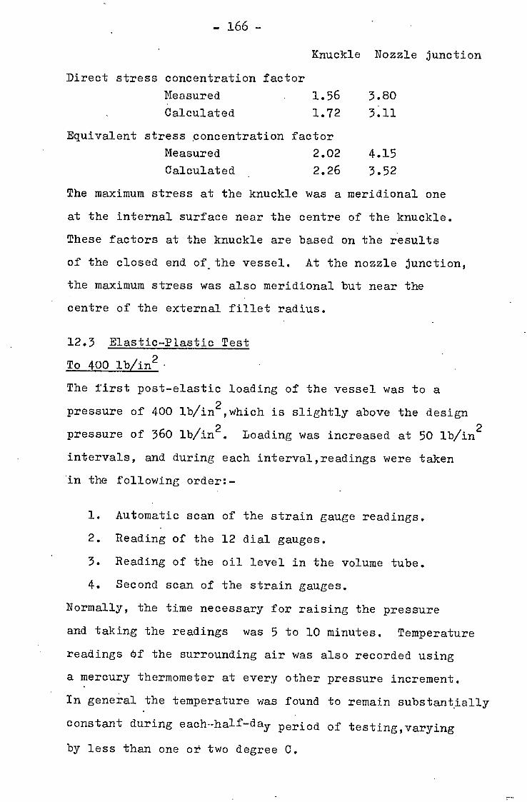
- 166 -
Direct stress concentration factor
Knuckle Nozzle junction
Measured 1.56 3.80
Calculated 1.72 3.11
Equivalent stress concentration factor
Measured 2.02 4.15 Calculated 2.26 3.52
The maximum stress at the knuckle was a meridional one
at the internal surface near the centre of the knuckle.
These factors at the knuckle are based on the results
of the closed end of the vessel. At the nozzle junction,
the maximum stress was also meridional but near the
centre of the external fillet radius.
12.3 Elastic-Plastic Test
To 400 lb/in2 •
The first post-elastic loading of the vessel was to a
pressure of 400 lb/in2,which is slightly above the design
pressure of 360 lb/in2. Loading was increased at 50 lb/in2
intervals, and during each interval,readings were taken
in the following order:-
1. Automatic scan of the strain gauge readings.
2. Reading of the 12 dial gauges.
3. Reading of the oil level in the volume tube.
4. Second scan of the strain gauges.
Normally, the time necessary for raising the pressure
and taking the readings was 5 to 10 minutes. Temperature
readings Of the surrounding air was also recorded using
a mercury thermometer at every other pressure increment.
In general the temperature was found to remain substantially
constant during each--half-day period of testing,varying
by less than one or two degree C.

-167-
The pressure was then reduced in steps back to zero,by
a gradual release of the oil. No volume measurements
were possible during such pressure reduction, although
the other readings were still taken. At zero pressure
most of the strain and deflection readings returned to
zero.
To 870 lb/in2
The next and subsequent reloading were made without read-
justing the dial gauges or rebalancing the strain-gauge
bridges. Pressure was raised, again in 50 lb/in2 in-
crements, to 700 lb/in2. At this pressure,the highest
strain reading,at gauge No.7, was 0.6%. This reading
and a number of other high strain readings had already
shown a high degree of non-linearity with load. There-
after,smaller pressure increments were made until loading
stopped at 870 lb/in2.
Throughout this loading,the pressure had always been
kept steady or increasing. Only once did the pressure
drop, at 800 lb/in2, when,due to flange leakage at the
side opening,the pressure dropped back to 750 lb/in2
before the leakage was remedied by tightening of the
holding bolts. Pigs.12-5 and 12-6 show two typical
readings, at the nozzle junction, one deflection and
one strain reading,plotted against pressure, It can be
seen that the load reduction causes little, if any,
deviation to the normal trend of the curves.
At 870 lb/in2 the pressure was then reduced in steps to
zero as before. This is followed by reloading to only
870 lb/in2, with readings being taken all the time at
selected intervals. This cycle of unloading and loading

- 168 -
to 870 lb/in2 was made altogether seven times. The
effect of this is also shown on Figs.12-5 and 12-6.
The strain and deformation increased progressively by
small amounts during each cycle, but the amount of
increment decreased steadily, and at the seventh cycle
lium)armr very small and fell within the accuracy of
measurement. Typical values of deflection and maximum
strain,after each cycle, at zero pressure, are shown
in Table 12-1a.
In each case, the increment between the 6th and 7th cycles
was about, or less than,I-per cent of the actual value.
Since the nozzle and the dished-end knuckle had the most
severe deformation in the vessel, it is expected that
other parts of the vessel suffer less incremental de-
formation. During each cycle a narrow loop can be
observed on the load-strain or load-deflection curves,
similar in shape to the hysteresis loop of a stress-
strain curve of a metal. The loops did not in general
narrow down and disappear when the incremental deformation
was gradually reduced to zero. Table 12-la also shows
the loop width of representative strain.
To 1070 lb/in2
The next increase of maximum pressure was to 1070 lb/in2 .
During this increase,slow leaking occurred again at the
gasket of the side opening,and was remedied in the same
way. The further increase in volume of the vessel can
be seen in Fig.12-7 where the volume of oil added to
the gessel is plotted against pressure.
Another seven cycles of the pressure were made between
zero and this maximum pressure of 1070 lb/in2. The

Table 12 - la. Change in Strain and Deflection Readings at Zero Pressure after Pressure Cycling.
Cycles of 0-870 lb/in2
Cycle No. 1 2 3 4 5 6 7
Guage 38, head A max. strain (%) 0.214 0.232 0.241 0.248 0.252 0.255 0.257
(hysteresis loop width/range) (%) 8.3 5.9 5.3 NA* NA NA
Guage 44, head B max. strain (%) 0.234 0.248 0.257 0.263 0.267 0.268 0.270
Head A deflection (thou.) 46 48 50 51.-- 52 52 53 I
Head B deflection at opening (thou.) 156 164 168 172 173 174 175 aN coo
Table 12 - lb. Cycles of 0-1,070 lb/in2
Cycle No. 1 2 3 4 5 6 7 I
Guage 38 (%) 0.648 . 0.688 0.709 0.724 0.733 0.743 0.752
Guage 44 (%) 0.645 0.677 0.695 0.708 0.714 0.722 0.728
Head A deflection (thou.) 100 107 109 111 111 112 114
Head B deflection at opening (thou.) 350 368 375 382 386 389 394
*Not available

— 169 —
increment of the same strains and deformations can be
seen from Table 12-16.
The increments dropped to 1-2 per cent of the actual
values.
Final Increase to 1165 lb/in2
The next and last load increment brought the pressure
to 1165 lb/in2 which is 3.2 times the design pressure
of 360 lb/in2. At this maximum pressure the total axial
movement of the test nozzle was more than 1/2 inch relative
to mid-vessel, and a regio f the nozzle within 1/2 inch
of the junction had clearly bulged outwards such that
this region was no longer cylindrical but conical in
shape. The experiment was thus stopped, since it had
not been the intention to fail the vessel but only to
observe its elastic-plastic behaviour until collapse.
Final Results
Typical variations of Strain and defleftioft with pressure
over the total range, 0 to 1165 lb/in2, are shown on
Figs.12-8 to 12-15. Detailed explanation and discussion
of these curves are given later in connection with com-
parisons with the--calculated results.
The experimental readings of two representatives strain
gauges No.28 and No.24, are plotted in greater details
than the others in Figs.12-8 and 12-16 respectively,
one shows the behaviour of the dished-end and the other
that of the vessel body. Onj each graph the three loading
curves were drawn separately, and gaps exist where the
strain values were increased under load cycling. Both
of them show that the unloading and the cycling appear:•

- 170 -
to make no difference to the overall plastic behaviour
of these strain values. This behaviour was found to
be the same for the other strain and deflection readings
plotted in these and other figures. For this reason,
only the envelope to the curves were plotted for all
the other readings. Also, in the subsequent discussions,
the vessel will be treated as being loaded under a
monotonically increasing pressure,with the unloading
parts neglected.
These plastic loads-strain curves are identified by
labelling them with strain gauge numbers which are
shown both in Fig.11-3,which gives the physical location
of these gauges, and in Figs.12-1 to 12-4,which give
the elastic strain distribution. Readings for strain
gauges No.7 and 6 came adrift before the end of the
test due to peeling off of the gauge backings. In
general, each curve, of either strain or deflection
reading,shows first a deviation from linearity, followed
• at higher pressures by an increasing change of slope,
which then slows down giving a more or less constant
slope. The pressures where these changes occur vary
for different gauges, and probably also vary according
to the elastid values.
12.4 'Elastic-Plastic Calculations
The comparison of these experimental results with the
elastic-plastic calculations is one of the main interest
of this study. To do these calculations. the stress-strain
curves of the shell material are required as data.
Similar.to the procedure used in the calculation of the
stainless steel APP vessel,two second-order algebraic

- 171 -
polynomials were approximated to the measured stress-
strain curves,one belonging to that of the 5/16 in.
steel plate used for the vessel heads and the body, and
the other to that of the steel pipe used for the end
nozzle. The former curve is shown on Fig.12-16,where
the polynomial equation is
5= 3.34996 x 10⁴ + 1.33691 x 1066T 2 - 1.81592 x 10⁷ep lb/in2
The latter curve is shown on Fig.12-17,where the
polynomial equation is,
T=3.92603 x 10⁴ + 1.23774 x 106613 -1.63857 x 1075 2 lb/in2
These curves are great improvements over the approximation
of perfect plasticity. Their proof stresses can be
compared below. 0.2% proof 1% proof
Vessel Steel
.
Measured
Equation
39,170 lb/in2
37,000 lb/in2
47,100 lb/in2
45,000 lb/in2
Nozzel Steel Measured
Equation
45,000 lb/in
41,700 lb/in2
d 51,800 lb/in
50,000 lb/in2
The same Young's Modulus of 30 x 106 lb/in2, and
Poisson's ratio of 0.3, were used as in the elastic
calculations.
The calculation of the closed dished-end A predicted a
first (local) yield at 464 lb/in2, occurring at the
inner surface of the knuckle near its centre. Thereafter
the calculation was repeated at load increments of 100 lb/in'
and subsequently at 50 lb/in2 increment. The final cal-
culation was at 964 lb/in2 when the defdrmation became
very large. The total computing time was 30 minutes
on the IBM 7094.
The calculation on the nozzle-end B of the vessel,using

-172-
the modified version of the program and the appropriate
stress-strain curves for the two parts of the shell,
predicted a first yield at 368 lb/in2 at the external
surface on the fillet radius of the nozzle. There-
after loading was increased at 0.2 of this yield pressure
until 809 lb/in2. This computing also took 30 minutes.
The calculated results were plotted against pressure
on the same graphs as the experimental results in Figs.
12-8 to 12-16. Each calculated curve is paired with the
measured curve obtained from a strain gauge or a dial
gauge, the former curve,/ being the curve of the corres-
ponding values at the location of the gauge;.
12.5 Discussion on Strain and Displacement
For the stress concentration area near the knuckles,
there is generally good agreement between calculatedn
and measured strain values. Fig.12-8 and 12-9 show the
strains around the knuckle of the closed dished-end A.
The calculated strains at all gauge locations agree
very well at the initial elastic-plastic stage until
about 800 lb/in2, which is 1.7 times the theoretical
first yield. This is true even for gauges 38 and 33
where the elastic agreement is not close. After 800 lb/in2
the theory predicted a higher strain. When expressed
as strain difference, this is appreciable; but because
of the flatness of most of the curves, the pressure
difference for the same strain appears less formidable,
say 15 per cent differente gt2:11:ttarze,ent:-.gtrailn for the
point of maximum strain (gauge 38). It is difficult
to interpret the meaning of this difference because
firstly, at such large straining the stiffening of the

173 --
actual vessel due to geometry change would become
noticable, and secondly, the difference in the elastic•-
values ( for all peak strains in Fig.12-8 and 12-9, the
theory gives higher values ) is magnified increasingly
at large plastic strains. Both these effects tend to
make the calculation over-estimate the strain values,
but the contribution of each cannot be conveniently
determined.
The strains at the knuckle of the other dished-end B
are shown in Fig.12-10 and 12-11. The elastic agreement
is not as good as the above dished-end, and neither is
the agreement of the elastic-plastic strain.
The strains at the nozzle junction of this dished-end
are given in Fig.12-12 and 12-13. At gauge locations
6,42 and 43, good elastic agreement is found. The cor-
responding elastic-plastic strains agree closely until
about 560 lb/in2 (1.5 times first yield), after which
the predicted strains become larger than that measured.
The strains at lower stress regions of the vessel - the
barrel, and the centre of the closed end - did not agree
as closely with the predicted values as those already
described at the knuckle regions. At the centre of the
dished-end A, Fig.12-15, gauges 35 and 36 showed some
non-linearity as low as 400 lb/in21 and by 700 lb/in2
non-linearity was very well developed, whereas the pre-
dicted strains were linear until 950 lb/in2. A similar
discrepancy was shown by the circumferential strain at
the barrel (Fig.12-15) where the measured strain showed

- 174 -
non-linearity from 500 lb/in2 upwards*, while the
calculated strain remained linear until a much higher
pressure of 950 lb/in2. These discrepancies can be
partly accounted far by the stress-strain approximation
which has a 30 per cent higher proportional limit. This
difference of proportional limit would not by itself
affect noticeably the solution at a bending region of
shell, but tend to show up in the above regions which
have little bending component of stresses.
The predicted displacements of the heads relative to
mid-vessel (Fig.12-14) .shows i quite good agreement,
although they also go non-linear at a higher pressure
than that observed.
In order to observe the effect of different stress-
strain behaviour, and for another reason connected with
collapse load described below, a calculation was repeated
for head A but with a non-hardening material. A yield
stress of 34,900 lb/in2 was used, obtained from the
experimental curves by the same 'tangent' method to
find the collapse load mentioned both below and in
Section 8.4 above. This value also happens to be
approximately the 0.1 per cent proof-stress. The
solution for any other yield stress values should vary
proportionately. The resulting behaviour is also plotted
in Figs.12-8,12-9 and 12-14 with first yield occurring
at 482 lb/in2. The top parts of the curves are flatter
This is actually shown on two of the three circumferential strain gauges. The third one remained linear throughout the test because it happened to rest on weld material which presumably has a much higher yield point.

- 175 -
as expected, and the itrariiitTonS-: from the elastic
lines are slighly sharper.
12.6 Discussion On Collapse Load
The vessel steel has a high degree of strain hardening
and it can be seen from the vessel behaviour that col-
lapse cannot be clearly defined. Two different methods
were used previously in Section 8.4 to define collapse,
the first being the intersection point of the elastic
line and a tangent to the strain or deformation curve
and the second being the load where a maximum strain
of 0.5 per cent occurs at the outside surface of the
vessel head or nozzle.
Table 12-2 compares the collapse pressure thus obtained
from the two vessel heads and from the end nozzle. The
first yield pressure is also cited for reference. The
tangent method for collapse gives different values
according to the curves used. As far as possible, three
curves are used, namely that for the maximum meridional
and the maximum circumferential strains, and that for
the axial deformation. The limit pressure,also quoted
at the bottom, assumes perfectly-plastic materials.
The results are according to the theory by Shield and
Drucker for the head A and according to the theory by
Gill for the nozzle. In the latter case, only the
lower bound is available and the two values quoted for
this, at the bottom of the last column are based on
the first yield stresses of the theoretical approximation
to the two stress-strain curves onefor the vessel steel
and the other for the end-nozzle steel.

Vessel head A Vessel head B (with nozzle
End Nozzle
Comparisons Of Collapse Pressure (lb/in2) As Measured And As Predicted By Different Methods
.••• •
Test Results ____ ___
First (local) yield pressure 360 320 340 Collapse pressure by
810 725 610 (P, (a) Method 1 (tangent) (b) 850 780 610
(c) 820 640 640 Method 2 (0.5% strain) about 1210 920 660
Elastic—plastic Calculation (d) (e) (d) (f) First yield pressure 464 482 515 368 Collapse pressure by
(a) 810 816 NA 560 Method 1 (tangent) (b) 840 865 NA 590
• (c) 880 $90 660 640 Method 2 (0.5% strain) about 980 920 NA 660
Limit Analysis • Upper Bound i&g NA (NA Lower Bound 765 NA 613-718

-177—
... Continued from Table 4
Note:NA - Not available
(a) - From max.merid.strain curve
(b) - From max.circ.strain curve
(c) - From head deflection curve
(d) - Based on fitted (0.20) stress-strain curve
(e) - Based on non-hardening yield stress
of 34,900 lb/in2
(f) - Based on non-hardening yield stress
of 40,200 lb/in2
The heads of the present vessel are nominally identical
and as shown above give similar elastic strains at the
knuckles. Table 12-2 shows,hoWever,that their plastic
collapse behaviours are different, the weaker head
being head B with the opening. It is noted here that
the nozzle is not reinforced.
The vessel head A, with no opening,gives good agreement
for collapse loads derived by the tangent method as
between the test results and the calculation,using the
fitted stress-strain curve(column (d),Table 12-2).
Similar agreement is also found for the calculation
using a perfectly-plastic stress-strain curve based on
a yield of 34,900 lb/in2 ( column (e),Table 12-2). In
both cases the collapse load based on the calculated
deflection curve is higher than that observed. The
limit load using a yield of 34,900 lb/in2 agrees well
with the above collapse loads.
At 0.5 per cent maximum outside strain, a large amount
of work-hardening has already occurred, and calculation
(e) based on a perfectly-plastic property is expected

- 2.78 -
to give a low prediction. This is found to be true.
It is found that calculation (d) also predicts a lower
load of about 980 lb/in2, compared with the load of
about 1,210 lb/in2 observed from the test where the
change of shape of the vessel head may strengthen it
substantially.
The presence of an:end-nozzle on vessel head B made it
fail by collapse at lower loads. The collapse based
on the calculated deflection compares well with observation.
No other comparison is possible because the calculation
did not go to a 2high:- enough load for this purpose.
10 limit load can be obtained because the theory can-
not conveniently account for weakening caused by an
end nozzle.
The collapse loads of the end nozzle obtained by the
same procedures give fair agreement betweem calculation
and observation. Worth noticing is the agreement of.
the 0.5 per cent strain collapse values. At this low
pressure the change of geometry is small and its effect
is probably negligible.
12.7 Conclusions
In the last few chapters,we have seen how the pressure
vessel programs were checked in various ways for their
accuracy. The elastic program was found to be free from
basic errors and its solution could give accuracy to
three or four significant figures from the thin-walled
shell theory. The two preliminary comparisons with the
published plastic tests by Stoddart and by Kemper of
pressure vessel heads gave,first and foremost,more
understanding of the different behaviours of mild steel

- 179 -
heads and stainless steel heads. The large amount of
strain-hardening of stainless steels allow such vessels
to withstand higher pressure after an initial yielding.
The actual comparisons gave mixed results.
Great care was taken in the preparation and conduction
of the present stainless-steel vessel test. The care
taken appeared to be well rewarded. The strain gauging
of the vessel interior lientwithout much trouble despite
the.few rejected gauges. The use of hydraulic oil for
applying the pressure,airhydro pump for maintaining
constant pressure, and the specially made Conax sealing
gland for the strain gauge lead wires,made the pre-
paration and testing an easier task.
During the test,the vessel was unloaded and given
repeated loading cycles, both action being common in
the life of pressure vessels including those in boiler,
chemical and nuclear reactor plants. These actions were
found to interrupt, but not to affect, the general trend
of the increasing elastic-plastic strains or deflections
of the vessel. It can be seen more clearly here that
the large amount of strain-hardening of the steel caused
the vessel to show a slow transition into rapid straining,
thus giving slightly more warning than other vessels
of the on-coming collapse. Even after this transition,
there was a reserve of strength since the increasing
hardening of the material caused the load resistance
to increase with increasing straining.
The'calculated elastic results compared well with
experiment. At the dished ends the calculated peak
strains were in general slightly higher. At the nozzle

- 180 -
junction,where there was a severe stress concentration,
there was good agreement,except unfortunately the
largest measured strain value where the corresponding
calculated value was very much lower. With small
amount of plastic straining, it is seen that the cal-
culation predicted the behaviour with fair accuracy.
Agreement is less satisfactory at larger strain, where
geometry change from large deformation undoubtedly
influences the behaviour,although this gives lower
predicted loads and thus conservative estimates for
vessel heads and nozzles under internal pressure.
There is no sharply defined .collapse load for this
vessel, both because of the high degree of strain-
handening and because of the relatively large kunckle
radius (16 for dished-end A and l8 for dished-end
B). The previously suggested procedure to define the
start of collapse by drawing tangents to the load-
strain or load-deflection curves is found to work well
good agreement,although in most applications the method
may not be convenient.to use.

-181-
13. OTHER GENERAL DISCUSSIONS
13.1 Pressure Vessel Programs
Theoretical Basis of Programs
The shell equations used in the programs are from small
deformation,thin-walled shell theory. This gives a
limitation to the possible accuracy from the programs.
However there is a wide range of medium thick vessels,
say, of thickness to diameter ratio from 1:10 to 1:100,
depending on the vessel geometry and on the application,
where the elastic-plastic program is of great use. The
programs can of course analyse thinner vessels than
the above,although the change of actual geometry under
load may in this case give noticeable change to the
stress distribution, throwing doubts on the results at
large amount of deformation. ,On even thinner vessels,
the interest would be on buckling where completely
different theories would have to be used.
Another limitation arising from the theory used is on
the accuracy of the local stress and strain at shell
discontinuities. Shell discontinuities are normally
assumed in calculations on pressure vessel nozzles, and
in many cases they give inaccurate results at the junction
of the nozzle and vessel shells. To reduce this in-
accuracy, the shell discontinuity was in the present
investigation removed and the nozzle shell was joined
to the vessel shell using a small toroidal shell element.
This is the method of Smooth Representation. The im-
provement as a result can be seen in Appendix B. A
further attempt to improve this was made in modifying
the thin-walled shell assumption resulting in the C
Program. These efforts were however found to be in-

- 182 -
sufficient. The comparison of the nozzle junction
stress calculations with the three nozzle test results
showed that the accuracy achieved was less than that
at other parts of the shells. Possibly more accurate
solutions can be obtained with finite-element stress-
analyses programs capable of analysing solids of re-
volution, but this would be an academin exercise until
more study is made of the meaning of these very high
but local stress at nozzle junctions, and of the design
use to which the stress results are to be put. Designers
in the past did not have to face this problem since
substantial reinforcement was placed at the nozzle
junctions using the area replacement rule. Present
methods proposed to design to limit ( or collapse ) load,
or to shakedown load do not require the knowledge of
the local stress intensity; Designing against ordihary
and low-cycle fatigue will however require the value
of the stress intensity, and here one may find it pro-
fitable to investigate in detail the local stress in-
tensity at nozzle junctions.
The method of obtaining elastic-plastic solution was
developed by Marcal. This is the tangent modulus method,
as it is now commonly called. With this method,problems
of extreme non-linearity can be analysed and the solution
for large amount of plastic stressing can be obtained.
There is another method by Mendelson that has also been
applied to elastic-plastic analyses of plates and shells.
This method is very efficient in computing time, but it
is not able to solve very non-linear problems, and is
thus not suitable for calculating the collapse behaviour
or that at large amount of stress and strain.-.- One

-163-
cause of the relative inefficiency of the Marcal
procedure is the large number of iterations necessary
at transition points. At points which have already
yielded, it was noticed that the calculation procedure
can determine reasonable estimates of the stress and car"
strain from the tangent, H' = DT, of the stress-strain
curve, and reasonable rate of convergency can be obtained.
At transition points, however,good estimates of the strain
increment cannot in general be made and this slows down
the rate of iteration convergency during each load
increment.
At and near the shell axis the computer program is found
to give slow integration convergency or inaccurate result;;
This is a property of the method of numerical analysis
of the shell equations when the distance from the shell
axis approaches zero. This phenomenon has also been
noticed by originators of some other pressure vessel
programs, because in some of them,special facilities were
written into the program to remedy this, for example,
by using special shallow spherical shell equations at
the region near the shell axis. In the present programs,
a proviion is also made to remedy this slow convergency,
but it has been found that in some problems this May:not
give a sufficiently accurate solution near the apex.
Indeed the misbehaviour was very noticable during the
calculation on the dlosed pressure vessel head A, where
the calculated results at the apex, i.e. the region very
near the shell axis, has to be neglected. It is also
seen in Pig. 12-15A that the elastic-plastic results for
this region seem to behave differently from what would
be expected.

- 184 -
Usage of the Programs
The computer programs are found to be very flexible,
and capable of analysing a large range and variety of
shell geometry and loadings. One of the few drawbacks
is that it cannot analyse directly ellipsoidal shell
elements and thus cannot conveniently analyse, for
example t ellipsoidal pressure vessel heads. The other
disadvantage is the limitation on the length of shell
branches. The Spera toriconica.l head compared in Ch.7
has to be analysed as two problems,one consisting of a
cone on a sphere and other of a sphere on a cylinder.
The Thin Cap and the pressure vessel head B with nozzle
are both just within the limits of shell length for
reasonable rate of convergency.
There are ways of overcoming this disadvantage. One • Ref 3-30
is to adopt the method of Kalninsxspliting the shell
into a number of sections, each section of a length
within the limit eapable of being analysed by the step-
by-step integration procedure. Independentlyl influence
coefficients are obtained for each section, after which
these influence coefficients for all shell section are
then analysed by matrix procedure to obtained solution
for the complete shell. This however involves the
development and writing of a new program. Another simple
method is to use a computer that uses longer 'word-length'.
The IBM 7090 & 7094 computers, used on all the above
calculations,use floating-point values defined by 48
binary bits giving an accuracy for each variable of 7
to 8 significant decimal figures. Computers that use
longer.'word-length' than 48 bits can store numerical
values to a higher accuracy. This should increase the

' 185 -
limiting shell-length of the program in a ratio of the
number of significant figures of a working variable.
The elas'tic program PVA1 is for most problems quite
convenient to use. It is of course necessary to check
that the branch length is within the limiting length.
Also, at areas of stress discontinuity, like that caused
by geometry change or by local loading, the integration
interVal length has to be reduced, but, in general, the
allowable maximum for the number of intervals is more
than sufficient. The program has a large number of
error messages if the data is found to be wrong, and
,many diagnostic messages if the problem cannot converge.
The two manuals explaining the program and its use are
found by many to be convenient to use. The author, for
example, knows of instances where engineers unfamiliar
with the program have, with little or no help, used the
program to analyse problems without great difficulty.
The elastic-plastic program PLINTH is in general less
convenient to use than the elastic program. The de-
velopment work on this program was terminated in a
shorter time than expected,and there was, compared with
PVA1,less tidying-up efforts,less provision for automatic
check,diagnostic and error messagesland user's manual
was less well prepared. Compared with elastic problems,
the elastic-plastic problems are much more complex and
have more factors influencing the convergency of the
solution. In general each problem has to be tried a
first time and sometimes a second time or more before
a successful final run, giving aatisfactory solution
beyond collapse of the shell, can be obtained.

- 186 -
The computing time needed for a complete elastic-plastic
calculation to collapse is many times more than a elastic
calculation. This is due mainly to two reasons. The
first one is due to the large number of iterations
required. In the elastic-plastic calculation,solutions
have to be obtained at a number of small increments of
loading, and during each loading a number of iterations,
each similar to a elastic calculation have to be made
to lterat'w for the correct plastic strains. Thus a
complete elastic-plastic calculation is equivalent to
a large number of simple elastic calculations. The
second reason comes from the increased storage required
on the computer. The elastic-plastic program requires
many more parameters than the elastic program, and the
former, in its final form, uses subsidiary store in the
form of magnetic tapes or magnetic discs for storing
the elastic-plastic stiffness coefficients. This use
of subsidiary store increases very much the execution
time of the calculation. The final result of these is
that on the IBM 7094, where most of the computation was
done, a typical elastic calculation uses about 0.5 to
1.0 minutes for execution while a typical elastic-plastic
calculation takes 20 to 45 minutes.
13.2 Vessel Behaviour
From the test conducted and from the other test reported,
it is not possible to get a simple rule to predict which
vessel head may collapse with a sudden increase in strain
and deformation,or may strain gradually until the defor-
mation becomes very large. There appears to be a number
of factors involved.

- 187 -
The Stoddart vessel head and the Kemper vessel head
have similar shape and height-to-diameter ratio,but the see Tetd f/ 8-/, p.?S'
latter vessel is thinneri However Stoddart observed a
sharp increase of strain and deformation near collapse
while this was not observed by Kemper. The cause of
this difference in behaviour is thus very probably the
large amount of strain hardening of the stainless steel
in Kemper's vessel. As to the calculation, it was
noticed that the theoretical solution for the Stoddart
test did not show a similar sudden increase of strain
and deformation at collapse. Since a perfectly plastic
material is already assumed in the calculation, the
evidence seems to point to inaccuracy in the solution.
If one reviews in detail the tangent modulus method of
elastic-plastic calculation by Marcal, it appears that
by taking the tangent modulus over a finite load increment,
any rapid change of strain would be smoothened over in
the process. If this is true,there may be some application
of the program where this inaccuracy may not be unimportant.
Further confirmation of this finding is necessary and
desirable.
The axial load tests condticted on the two mild steel
nozzles showed a final physical collapse in the form of
a sudden increase in the strain rate. This collapse was
not observed in the calculations. The mild steel leas?
negligable strain-hardening until the strain is very
large. While this difference may again be due to the
failure of the calculation.to predict a sharp change of
strain rate, there is an additional factor here in that
the axial loading on the spherical shell was .compr.essive
i.e. inwards, and at large deformation the instability

- 188 -
load may be lowered because of the changed geometry.
It is thus not possible to judge whether the results
of the elastic-plastic calculation are at fault here.
Geometry change may also be the reason for the under-
estimation in the calculation of the pressure resistance
of the stainless steel test vessel. The calculation
predicted at high loads a much higher straining than that
observed. The change of geometry of torispherical heads
under internal pressure normally increases their pressure
resistance.
In spite of these two possible errors of the elastic-
plastic calculation at large deformation of vessels, the
proposed method of tangent for obtaining collapse leads is
found to work well for correlating the actual and predicted
collapse loads, and the twO errors do not seem to affect
their agreement.
The test vessel was twice given repeated loading and un-
loading cycling during the tests. One of the observations
was that these cyclings did not interrupt the general
load-strain and load-deformation curves. One other
observation can be made here from these repeated loadings.
This comes from the fact that the strain and deformation
increased during each load cyclepbut the rate was found
to decrease gradually with increasing number of cycles.
If the increase of strain and deformation fell to zero,
this would either e a shakedown or an alternating
plasticity behaviour. In the plasticity theory of ideal
materials,there is a ci4ar-cut difference between shake-
down and alternating plasticity, but in actual metals
the distinction is not so precise. The above repeated
loading method can thus be used as an

189 -
experimental observation of the maximum shakedown load;
this may beihterpreted as the highest repeated load
value where the maximum strain increment after a large
number of cycles decreased sufficiently to zero and at
the same time the hysteresis loop of maximum strain
becomes sufficiently narrow.
13.3 Design Interest
The near future design interest on elastic-plastic
calculations depends on what approach is used for pressure
vessel design. The ASME boiler and pressure vessel codes
require the determination of stress level at different
parts of the vessel to be used as the major criterie.il-
of design. The stress has to be separated into different
categories: membrane,primary and secondary. Different
criterions are given to the maximum permissible stress
leveIsfor each type of stresses. These stress levels
are of course elastic stress leve14, although this is not
to imply that elastic-plastic strains are not of.interest.
Investigations with elastic-plastic calculation could
be used indirectlyl sayito obtain better criteria for
the stress levels andto give additinnal limitations for
different modes of failures and for different component.
The British Standards for pressure vessel design consider
separately the design of different vessel components.
It is here that investigations by elastic-plastic cal-
culation of specific components, like the vessel head6
and axisytmetric nozzles considered in this thesis, can
get more direct application. Individual pressure vessel
components can fail in a number of manners. Most of
these failure modes involve plastic straining before

- 190 -
final failure occurs , and in such cases a better under-
standing of the failure can be achieved through the use
of elastic-plastic calculations.
Plastic Collapse
Plastic collapse is a common butseve're mode of failure
for both pressure vessel heads and nozzles. Destructive
testing is of course the best procedure for ensuring
a safe design. Theoretical procedure for determining
this plastic collapse load has been attempted by using
the limit analysis method.
limit solutions that can be
design are for axisymmetric
and protruding type, and on
solutions are claimed to be
toriconical heads. However
At present the available
applied to pressure vessel
nozzles of both the flush
torispherical heads whose
similarly applicable to
from the above investigations
with elastic-plastic calculations, it can be seen that,
- the gap of knowledge of collapse load on other shell
geometries and on non-typical geometries can immediately
be filled by such calculations. Examples of other
geometries,which must of course be axisymmetricrare flat
heads, ellipsoidal heads,concial heads,different types
of "shell-reducers", and toroidal expansion bellows.
Assumptions of non-work-hardening in collapse load:, cal-
culation make the solution over-conservative in the case
of annealed stainless steels and some non-ferrous metals
with a large amount of strain hardening. One remedy
is to assume a higher yield stress in the calculation,
say, the one percent proof stress. Design of vessels
of such materials whenthe collapse load is the limiting
criterion can however be more realistic and accurate if

- 191 -
the strain-hardening could be taken into account. There
is a large scope for the use of elastic-plastic calculation
here. The effeft of strain-hardening on collapse load
has so far not been investigated.
Shakedown
Loadings on pressure vessels are never constant during
their working life and very often is repetitive in
nature. Shakedown considerations may be required when
local yielding occurs many times during the life time
of the component. When the yielded zone is well
surrounded by material that remains elastic, LangeriRef.W-3)
suggested that shakedown should occur under any repeated
loading when the maximum load is less than twice that
causing the maximum strained region to start yield.
This is a convenient rule to apply and is used in the
ASME Section III Code for nuclear vessels, to limit the
level of secondary stress at the working load. The
actual maximum - shakedown load of course vary according.:
to the geometry of the vessel component,with the factor
2.0 being the upper ceiling for the ratio to first yield
load.
Theoretical analysis of pressure vessel nozzles, flush
and protruding, was made by Leckie. In this case only
the elastic solution is required to obtain the shake-
down solution. This is because pressure vessel nozzles
have in gene±al--_Smarrow zone of high stress with the
location of this zone accurately known to be on the
junction between vessel and nozzle. Pressure vessel
heads have however a less concentrated region of high
stress and this property makes it impossible for vessel

- 192 -
heads to be analysed for shakedown by the same method
using elastic solutionS. To obtain the shakedown pressure, ,Ref.
a method used by CrispAmakes use of solutions obtained
by the method of elastic-plastic analysis. This is one
of the immediate applications of the elastic-plastic
analysis. From a survey of shakedown solution of a range
of torispherical pressure vessel heads, he observed that
the average shakedown pressure is about 1.66 of the
pressure to cause first yield, and none of them, as
expected, exceeded twice the first-yield pressure. This
same procedure could equally well be applied to many
other pressure vessel components, especially those with-
out abrupt changes of gitpetry that give rise to narrow
regions of stress concentration, Ellipsoidal heads and
pipe-line toroidal expansion-bellows are examples of
gtpetries that can be thus used to obtain shakedown
solutions.
Low-Cycle Fatigue
Low-cycle fatigue (also called high-stain fatigue) is
a mode of failure where plastic straihing plays an
essential role. Strictly speaking, a vessel component,
when designed so that it will shakedown,would only
require elastic fatigue considerations. There are how-
ever many cases where designers,for good reasons)may
be interested in low-cycle fatigue. First example occurs
when one finds a range of standard design of vessel
components that has in the past been used satisfactorily
outside the shakedown load, and there is thus no
justification to limit them in future to a lower load
from shakedown consideration. Secondly, thcrc arc power
station that may be started-up once-. a 'day would subject

- 193 -
its equipments, in a working life of say 20 or 25 years,
to working-load cycles of less than 10,000. Thus in
some such instances, reasonable saving can be obtained
by designing equipments to this 10,000-cycle working
life. Thirdly the designer may very often come across
materials with a large amount of work-hardening, and
shakedown design using the proportional limit to the
stress-strain curve would not make good use of the
reserve of work-hardening strength of the material. a
The alternate solutio f using/higher proof-stress value
is an acceptable compromise,but this has to be confirmed
by actual testing since the shakedown theorem,in its
present form,assumes,non-workhardening behaviour. The
better alternative in such :a case may be to design to
low-cycle fatigue.
The contribution to low-cycle-fatigue analysisjof
methods of elastic-plastic analysis of shell components)
lies in their ability to predict the elastic-plastic
strain concentration at different loads. Assuming that
the correlation between the fatigue life of specimen and
pf actual structure is known, one can determine from
specimens the strain-range and fatigue-life relations,
and use elastic-plastic analysis to calculate the
maximum strain in the actual shell component andthus
predict its fatigue life. The same procedure is of course
used to predict high-cycle or elastic fatigue life of
structures using elastic analysis instead of elastic-
plastic analysis. One difficulty that arises is because
the plastic straining in the actual structure is caused
by cylic loading while the elastic-plastic analyses
assume a steady increasing load. On this point, it has

- 194 -
been suggested that the use of a cyclic stess-strain
curve in the method of analysis should give a true
prediction:of the strain concentration under cyclic
loading. The cyclic stress-btrain curve, each to be
defined for an infinite or a specific number of loading
cycles, is a curve of the cyclic strain-range against
the corresponding cyclic.stress-range at the specified
number of cycles, and this is usually obtained by
cyclically testing small loading specimens of the gfec ? is, e
material under constant strain-rangeeach4for a different
strain-range. This procedure of predicting low-cycle
fatigue life has been tried with success but more con-
firmation of the validity of the procedure under
different circumstances is required.
The strain-range of interest for this application is
higher than that for the shakedown appliction,but both
should be of similar of order of magnitude; hence the
required plastic strain for both is thus of similar
magnitude to the elastic strain. The load range for
this application is again higher than that for shake-
down, but here there is an upper ceiling since the low-
cycle fatigue load cannot be greater than the collapse
load.
* Blatherwick A.D. & Lazan B.J. The effect of changing cyclic modulus on bending fatigue strength. Proc. ASTM 56,1012,1956.

-195-
14. CONCLUSIONS
Literature Review
The following findings are revealed, helping to set the
course of investigation in this thesis :
a) The elastic-plastic analysis of the stress and liNie
behaviour of axisymmetric pressure vessel shells
by numerical computation forms a useful and logical
extension to the early,p and current, theoretical
study of thin-walled pressure vessels.
b) Such methods of analysis developed by Marcal,and by
others, have not been sufficiently compared in detail
against appropriate and accurate expeirments.
c) The possible applications into design of elastic-
plastic solution have not been sufficiently investigated,
and thus not well exploited.
d) Medium thick pressure vessel heads, commonly in the
the shape of torispheres3 can be analysed elastically.
Howeverfor some common modes of failure, it is
inappropriate to design according to elastic analysis,
and application into design by elastic-plastic theory may
be of immediate interest.
e) On the possible design of 'pressure vessel nozzles,
using these and other more accurate procedures,
greatela urgency is required to attain a 4419-r-43 wide-
spread adoption of better and consistant arrangement
of nozzle reinforcements, to obtain a better prediction
of the very local peak-stresses at nozzle junctions,
and to achieve a better understanding of the role
these peak stresses play in different modes of
failures.

- 196 -
Design Interests of Elastic-Plastic Analysis
The possible design interests vary according to the
modes of failure, andto a lesser degree, according to
the vessel component.
f) Design against excessive deformation of nozzles
requiring accurate alignment, requires the value
of deformation. In many other cases,this excessive
deformation failure may be a plastic collapse, where
the collapse load is required as the ceiling of
hydraulic proof-test pressure and any occassional
over-load of vessels in service. For vessel heads'
under internal pressure, this load is about 1.5 -
2.2 of the first-yield load.
g) Failure under repeated loading can be prevented by
designing for shakedown or against low-cycle fatigue.
The load range of interest in shakedown design is
less than that for design against collapse. A
proposed method,where elastic-plastic analysis can
usefully be applied,would require the values and the
ratios of the peak stresses at small amount of
plastic straining.
h) The load range of interest in design against low- also
cycle fatigue is og-cin smaller than that for design
against collapse. At the failure load,the amount of
plastic straining in the elastic-plastic calculation
is of similar magnitude to that in the calculation
needed to predict shakedown. These calculations would
however be on strain-hardening material since the
cyclic stress-strain curve would be used. What is-1
i.:eqiiiredtfrom-these...calculations would be the peak-

- 197 -
strain value, either the total strain, or its plastic
component.
Elastic Behaviour of Nozzles and Heads
i) The elastic solutions from the computer: programs,
PVA1 and PLINTH,used in this investigation are
found to be reliable and accurate for normal vessel
shell calculations, with geometry and loading with-
in the assumptions of the theory, and with no
intersections of shells where the thickness and the
direction of the shell-meridian change across the
intersection.
j) Tests conducted to check the accuracy of the
programs have to be carefully planned and executed
to eliminate a number of other sources of dis- oetN0
agreements. Especially important is4an accurate
shell geometry since this is found to affect very
much the resulting deflection and stress-distribution.
The axial deflections, for example,of the two nozzle-
on-spherical-cap specimens are found to depend very
much on the precise shape and edge-restraint of the
caps.
k) The programs have difficulty in conveging to an
accurate solution at the crown centre of some tori-
spherical-head problems, including that of the
stainless steel test-vessel head A. Other than this,
however, the elastic solution gives good prediction
of the maximum stresses and the stress distribution.
11 The programs cannot give similar accuracy for
asisymmetric nozzle problems. It is known,and con-
firmed)that the normal shell-theory procedure to
approximate a nozzle-on-vessel by intersedting shells

- 198 -
gives over-estimation of the peak junction stress,
especially when nozzle and vessel have very different
thicknesses. The two attmepts to improve on the
results, one by the method of Smooth Representation,
the other by modifying the program to approximate
better to thick curved shells, both give substantial
improvement for the three test nozzles, but are not
sufficient. to give good agreement with the maximum
strain gauge readings. The Smooth Representaion
applies only to flush nozzles with no partial
penetration welds.
Vessel Behaviour and Elastic-Plastic Analysis
m) The accuracy of elastic-plastic predictions depends
on a number of factors. During the vessel test,
reasonable precautions were taken, based on earlier
experience, to achieve a uniform yield-stress pro-
perty together with an accurate mathematical re-
production of the actual stress-strain curve, and
to obtain an accurate elastic-stress prediction.
However nothing could be done about possible error
caused by geometry change at large deformation of
the shells. It was found difficult to allocate the
share of each of the above factors causing the
difference in the calculated and measured results,
and equally difficult to judge how far the calculated
results are in error, due to the program andAthe
theory used.
At the crown centre of torispherical heads.) where
the elastic results are in error, the comparison
of the vessel head A shows that the elastic-plastic

- 199 -
results are also wrong. Comparison' of the
Stoddart test results shows that the computation
process does not converge sufficiently to the
correct solution/ when the strain-rate (i.e.
change of strain per unit load increase) changes
rapidly, and thus tend to smoothen out any sudden
change of slope in the load-strain and load-de-
formation curves. This however needs further con-
firmation.
Whether or not any inaccuracy from the present
program can be easily reduced, the present results
look more favourable, however, when judged as to
their possible design use. The two interests in
this case are/ the behaviour at small plastic
straining/ and the collapse load. Allowing for
inaccuracies caused by the differences in the
elastic results, the peak-strain and deflection
results show good agreement at small amount of
plasticity. The axial tests on the mild-steel
nozzles are not suitable for comparing collapse
because of the proximity of the vessel-base and the
nozzle. For the vessel test, good agreement is
obtained for the collapse loadl as defined by the
proposed method of intersection of tangent lines
to the load-strain and load-deformation curves.
Agreement is also obtained for this collapse load
when the calculation is compared against the
Stoddart vessel test.
6) The collapse values as defined by this method of
tangents showlpt only good agreement, for the two
vessel heads and one nozzle, between that ftomtthe

- 200 -
theoretical curves and the experimental curves,they
also show reasonable agreement to the limit-analysis
results using appropriate yield-stress values. The
method gives values that are not very sensitive as
to which peak strain curves are used, these. peak
strains must of course be near the collapse zones.
Values.from the overall deflection curves are also
in reasonable agreement. The method is also not
very sensitive to errors due to inaccurate stress-
strain curve, or to geometrical change of the real
vessel. It is less convenient to use than that
based on a certain value of peak strain, but it
deserves further investigation into its consistency
and applications.
p) The test vessel continues to hold pressure many
times the first yield preSsure, and the design
pressure of 360 lb/in2. ( Testing stopped at
1165 lb/in2.) This comes from the large amount of
ducitility of the anneal led stainless steel used.
Kemper and his co-worker observed the same
phenomenon during their vessel tests.
q) Cycling the test vessel at'870 lb/in2 and at 1070
lb/in2 ( 2.6, 3.1 times respectively the observed
first yield of the nozzle and 2.4, 3.0 times
respectively the observed first yield of vessel
head A ) did not cause noticeable incremental
straining at the 7th cycle. Any effect these
cycling may cause to the overall load-strain and
load-deflection curves is undetectab16,:.

- 201 -
REFERENCES

- 202 -
2-1 THCMPSON,S.J.Boilers-past and present.
Proc.I.Mech.E.148,4,p132,1942. 2-2 .REEMANg.F.Notes on the development of the steam
boiler. Proc.I.Mech.E.147,p72,1942. 2-3 BACH,C. Untersuchungen aber die Formnrlerungen
und die Anstrengun gewalbter BOden. (Investigations into the stresses and deformations of curved plates.) VDI 43, 51, 1585-1594,1613-1625,1899.
2-4 HOEHN,E. and HUGGENBERGER,A. Uber die Festigkeit der geAlbten BOden und der zylinderschale. (Monograph),Springer,Berlin,1927.
2-5 ENGINEERING. The Strength of Dished Ends. Engineering,128,1-4,July 5,1929.
2-6 MEISSNER,E.Das Elastizitatsproblem fur dilnne Schalen von Ringflgchen-, Kugel-oder Kegelform, (in German). Physik,l4, 343pp. 1913. ( Also TMB Translation 238, The elasticity problem for thin shells of toroidal, spherical,or conical shape. 1951.)
2-7 COATES,W.M. States of stresses in full heads of pressure vessels.Trans. ASME.,52,22,117-131,1930.
2.11-8 PRESSURE VESSEL RESEARCH COMMITTEE. Report on the design of pressure vessel heads,.Appendix 1, History of the design of heads for pressure vessels. Welding J.Res. Supp1.41S-48S,Jan.1953.
2-9 SIEBEL,E. and ORBER,F. Versuche ilber die Anstrengung und die Formanderugen gewolbter Kesselboden mit und ohne Ivlannloch bei der Beanspruchung durch inneren Druck.-Mitt.K.W.Inst. Eisenforsch.,7,10,113-177,1926,and 8, 1,1-51,1926.
2-10 TAYLOR,J.H.and WATERS,E.O.Effect of openings in pressure vessels. Trans. ASME,56,3,119-140,1934.
2-11 EVERETT,F.L. and MCCUTCHAN,A. Investigation of
stress conditions in a full-size welded branch connection. Trans. ASME,60,p.399,1938.
2-12 BESKIN,L.Strengthening of circular holes in plates under edge loads. Trans.ASME,66,p.A-140,1944.
2-13 INGLIS,C.E. Engineering 95,p.415,1913.
2-14 KOOISTRA,L.F.and BLASER,R.U. Experimental
technique in pressure vessel testing. Trans.ASME

- 203 -
72,579-587,1950. 2-15 GROSS,N. Research on welded pressure vessels and
pipelines. Brit. Weld. J.1,4,149-160,1954. 2-16 DRUCKER,D.C. Three-dimensional photoelasticity.
Ch.l7,part II of Hetenyi,M.(ed.) Handbook of Experimental Stress Analysis. New York,Wiley, 1950.
2-17 GLASGOW,ROYAL COLLEGE OF SCIENCE AND TECHNOLOGY. Nuclear Reactor Containment Buildings and Pressure Vessels. Proc.sym.organised by Dept.of Mech.,Civil, and Chem.Eng., Royal Coll. Sci.Tech.,Glasgow,l7-20th May 1960. London,Butterworths,1960.
2-18 INSTITUTION OF MECHANICAL ENGINEERS. Proc.Sym. on Pressure Vessel Research Towards Better Design. 18th and 19th Jan.1961: arranged by I.Mech.E. and B.W.R.A.,London,Inst.Mech.Engrs.,1962.

- 204 -
3-6 REISSNER,E.A new derivation of the equations for the deformation of elastic shells. Amer. J.Math,63,177-184,1941.
3-7 TIMOSHENKO,S. and WOINOiISKY-KRIEGER,S. Theory of plates and Shells. McGraw-Hi11,1959.
3-8 KRAUS,H. Thin Elastic Shells. London,Wiley,1967. 3-9 WATTS,G.W. and LANG,H.A. Stresses in a pressure
vessel with a conical head. Trans. ASME,74,315-326,1952.
3-10 TAYLOR,C.E. and WENK,E.Jr. Analysis of stresses in the conical elements of shell structures. Proc.2nd.U.S.Nat.Cong.Appl.Mech.,ASME,323-331,
1955. 3-11 WATTS,G.W.and LANG,H.A. Stresses in a pressure
vessel with a hemispherical head. Trans.ASME,75, 83-89,1953.
3-12 GALLETLY,G.D. Influence coefficients for hemispherical shells with small opening at the vertex, J.Appl.Mech.22,20-24,1955.
3-13 GALLETLY,G.D. Influence coefficients for open-crown hemispheres. Trans.ASME 82A,73-81,1960.
3-14 GECKELER,J.W. Uber die Festigkeit achsen-symetrischer Schalen. Forschungsarb. Ingwes., Berlin,276,1-52,1926.
3-15 NAGHDI,P.M. and DESILVA,C.N. Deformation of elastic ellipsoidal shells of revolution. Proc 2nd U.S. National Cong.Appl.Mech.,ASME,333-343, 1955.
3-16 DESILVA,C.N. Deformation of elastic paraboloidal shells of revolution. J.Appl. Mech.24,397-404, 1957.
3-17 LECKIE,F.A. Localized loads applied to spherical shells. J.Mech.Eng.Sci.3,111-118,1961.
3-18 LECKIE,F.A. and PENNY,R.K. A dritical study of the solutions for the axisymmetric bending of spherical shells. Weld. Res. Council Bull. No. 90,1963.
3-19 FLUGGE,W. Statik and Dynamik der Schalen. Berlin, Julius Springer Verlag,1934.
3-20 LUR'E,A.I. The general theory of thin elastic
shells,Prikl. Mat. Mekh.4,7,1940.
3-21 HILDEBRAND,F.B.,REISSNER,E. and THOMAS,G.B.

- 205 -
Notes on the foundations of the theory of small displacements of orthortropic shells. NACA-TN-
. 1833, March 1949. 3-22 NAGHDI,P.M. On the theory of thin elastic shells,
Q.Appl. Math.14,369-380,1957. 3-23 KLOSNER,J.M. and LEVINE,H.S. Further comparison
of elasticity and shell theory solutions. AIAA Journal 4,467-480,1966.
3-24 PENNY,R.K. Symmetric bending of the general shell of revolution by finite difference methods. J.Mech.Eng.Sci.3,369-377,1961.
3-25 SEPETOSKI,W.K.,PEARSON,C.E.,DINGWELL,I.W. and ADKINS,A.W. A digital computer program for the general axisymmetric thin shell problems. J.Appl. Mech.29,655-661,1962.
3-26 RADKOWSKI,P.P.,DAVISI R.M. and BOLDUC,M.R. Numerical analysis of equations of thin shells of revolution. Amer. Rocket Soc. J.32,36-41,1962.
3-27 BUDIANSKY,B. and RADKOWSKI,P.P. Numerical analysis of unsymmetrical bending of shells of revolution. AIAA J.1,1833-1842,1963.
3-28 GALLETLY,G.D. Bending of open crown ellipsoidal shells. Weld. Res.Council Bull.54.1959.
3-29 GALLETLY,G.D. Edge influence coefficients for toroidal shells. Trans.ASME,82B,60-64,65-68,1960.
3-30 MIRABAL,J.A. and DIGHT,D.G. SOR-II, a program to perform stress analysis of shells of revolution. KAPL-M-EC-19,Knolls Atomic Power Lab., Schenectady,N.Y.,1962.
3-31 KALNINS,A. Analysis of shells of revolution subjected to symmetrical and non-symmetrical loads. J.Appl. Mech.31, 467-476,1964.
3-32 PILGRIM,W.R.,CHEUNG,J.S.T. and MARCAL,P.V. Computer program for elastic analysis of pressure vessels. RD-C-N-22, Central Elect. Generating Board,London,June,1965.
3-33 NATIONAL PHYSICAL LABORATORY Modern Computing Methods. London, Her Majesty's Stationery Office, 1961.
3-34 FOX,L.(ed) Numerical Solution of Ordinary and Partial Differential Equations. London,Pergamon-v, 1962.

- 206 -
3-35 GRAFTON,P.E. and STROME,D.R. Analysis of axisymmetrical shells by the direct stiffness method. AIAA J.1,2342-2347,1963.
3-36 FRIEDRICH,C.M.SEAL-SHELL 2, a computer program for the stress analysis of a thick shell of revolution with axisymmetric pressure,tem-peratures and distributed loads. WAPD-TM-38, Bettis Atomic Power Lab., Pittsburgh,Pa.,1963.
3-37 KRAUS,H. A review and evaluation of computer programs for the analysis ofsttess.es in pressure vessels. Weld. Res. Council Bull.108,11-28,1965.
3-38 PENNY,R.K. and.PERRYMAN,K.R. VESSIL, 1,IBM 7090 program for computing stresses in shells of revolution. Central Elect. Generating Board, Computing Dept., London,1962.
3-39 GALLETLY,G.D. Analysis of discontinuity stresses adjacent to a central circular opening in a hemispherical shell. Report 870,David Taylor Model Basin, Washington,D.C., May,1956.
3-40 ROSE,R.T. and THOMPSON,J.M.T. Calculated stress concentration factor for nozzles in spherical pressure vessels. Paper 1 of (3-5).
3-41 LECKIE,F.A. and PENNY,R.K. Solution for the stresses at nozzles in pressure vessels, Paper 2. Stress concentration factors for the stresses at nozzle intersections in pressure vessels, Paper 3. Welding Res. Council Bull.90, Sept.1963.
3-42 O'CONNELL,J.M. and CHUBB,E.J. An Improved method of calculating stresses at the intersection of a cylindrical nozzle and a spherical shell. Paper 5 Applied Mechanies Convention, Proc.I.Mech.E. 178,3J,224-230,1963-64.
3-43 DRUCKER,D.C. Limit analysis of cylindrical shells under axially-symmetric loading. Proc. 1st. Midw. Conf. Solid Mech.(Urbana,1953)158-163,1954.
3-44 ONAT,E.T. and PRAGER,W. Limit analysis of shells of revolution. Proc. Roy. Netherlands Acad.Sci. B57,534-548,1954.
3-45 •HODGE,P.G.Jr. Yield conditions for rotationally symmetric shells under axisymmetric loading. J. Appl. Mech.27,323-331,1960.

- 207 -
3-46 HOPKINS,H.G. and PRAGER,W. The load carrying capacities of circular plates. J.Mech.Phys. Solids,2,1-13,1953.
3-47 HODGE,P.G.Jr. Yield point load of an annular plate. J.Appl.Mech.26,454-455,1959.
3-48 HODGE,P.G.Jr. Limit-Analysis of Rotationally Symmetric Plates and Shells. Prentice-Hal1,1963.
3-49 MARCAL,P.V. and PILGRIM,W.R. A stiffness method for elastic-plastic shells of revolution. J. Strain Analysis,1,4,339-350,1966.
3-50 SPERA,D.A. Analysis of elastic-plastic shells of revolution containing discontinuities. AIAA J.1,11,2583-2589,1963.
3-51 BIJLAARD,P.P. Stresses from radial loads in cylindrical pressure vessels. Weld. J.33,615S-6235,1954.
3-52 BIJLAARD,P.P. Stresses from radial loads and external moments in cylindrical pressure vessels. Weld.J.,34,6085-617S,1955.
3-53 WICHMAN,K.R.,HOPPER,A.G. and MERSHON,J.L. Local stresses in spherical and cylindrical shells due to external loadings. Weld.Res.Council Eu11.107, 1965.
3-54 LUR1 E,A.I. Concentration of stresses in the vicinity of an aperture in the surface of a circular cylinder ( in Russian). Priki.Mat.Mek. 10,397-406,1946. Also, English Trans. IMM-NYU 280,New York University,Inst. of Math.Sciences, Nov.1960.
3-55 WITHUM,D. The circular cylindrical shell with circular section cut out under shear stress. (In German). Ing.Archiv.26,435-446,1958. Also,
translation,C.E. Trans. 2728,Central Elect. Generating Board,Central Tech. Infor-mation Service,London,S.E.1.
3-56 REIDELBACH,W. The state of stress at the per-peAdicular intersection of two right circular cylinders .(in German). Ing. Archiv.30,5,1961. English trans.. by M.M.Stanisic,General Tech. Copr., Tech. note 3-1,1962.
3-57 ERINGEN,A.C., NAGHDI,A.K. and THIEL,C.C. State

- 208 -
of stress in a circular cylindricial shell with a circular hole. Weld. Res. Council Bull.102, Jan.1965.
3-58 MINGEN,A.C. and SUHUBI,E.S. Stress distribution at two normally intersecting cylindrical shells. Nuclear Struct. Engg.2,253-270,1965.
3-59 CLOUGH,R.W. and JOHNSON,C.P. A finite element approximation for the analysis of thin shells. Int. J. Solids Struct.4,1,p43,1968.

- 209 - 4-1 JONES,N. An appraisal of the stress-probing
method. Engineer,218,5675,715-716,Oct.1964. 4-2 SWANSON,S.A.V. and FORD,H. Stresses in thick-
walled plane pipe bends. J.Mech.Eng.Sci.1,2, 103-112,1959.
4-3 MANTLE,K.G. and PROCTER,E. Use of resistance strain gauges. Engineer,March 25,1960,527-528.
4-4 RILEY,W.F. Experimental determination of stress distributions in thin walled cylindrical and spherical pressure vessels with circular nozzles. NASA CR 53580,Dec.1963.
4-5 MORGAN,W.C. and TaZON,P.T. Experimental investigation of stress distributions near abrupt change in wall thickness in thin-walled pressurized cylinders. NASA TN-D-1200. June 1962.
4-6 WELLS,A.A.,LANE,P.H.R.,and ROSE,R.T. Stress analysis of nozzles in cylindrical pressure vessels. taper 2,21 of (2-17).
4-7 KOOISTRA,L.F. and LEMCOE,M.M. Low cycle fatigue research on full-size pressure vessels. Weld. Res. Suppl. 41,p297S,July 1962.
4-8 KITCHING,R. and DUFFIELD,N.A. Stresses due to axial loads and internal pressure on forged nozzles in a spherical pressure vessel. Int. J.Mech.Sci. 6,77-103)-1964.
4-9 ROSE,R.T. Stress analysis on nozzles in thin walled cylindrical pressure vessels. Brit. Welding J.12,2,80-89,1965.
4-10 DINNO,K.S. and GILL,S.S. An experimental investi-gation into the plastic behaviour of flush nozzles in spherical pressure vessel. Int. J.Mech.Sci.7, 817-839,1965.
4-11 PERRY,C.C. and.LISSNER,H.R. The Strain Gage Primer,HcGraw Hi11,2nd lid., 1962.
4-12 BERMAN,J. and PAI,D.H. An experimental investi-gation of stresses in an HY-80 marine boiler drum. Welding Res. Supplement,p307-S,July,1962.
4-13 ANDERSON,B.R. Low-cost technique for stress-analysis of solid-rocket cases. Proc. Soc. Expt. Stress Analysis, 20,1,14-21,1963.
4-14 BOWDEN,A.T. and DRUMM,J.C. Design and testing of

- 210 -
large gas ducts. Proc. I.Mech.E.174,3,119-158, 1960.
4-15 CRANCH,E.T. An experimental investigation of stresses in the neighbourhood of attachments to a cylindrical shell.. Weld.Res.Council Bull.No. 60,May 1960.
4-16 LANE,P.H.R. and ROSE,R.T.Comparative performance of pressure vessel nozzles under pulsating pressure. Paper 4 of (2-17).
4-17 MORGAN,W.C. and BIZON,P.T. Experimental evaluation of theoretical elastic stress distributions for cylinder-to-hemisphere and cone-to-sphere junctions in pressurized shell structures. NASA TN D-1565, Feb.1963.
4-18 FESSLER,H, and ROSE,R.T. Photoelastic deter- mination of stresses in a cylindrical shell. Brit.J.Appl. Physics 4,3,76-79,1953.
4-19 FESSLER,H. and LEWIN,B.H. Stress distribution in a tee junction of thick pipe. Brit.J.Appl. Physics.7,p76,1956.
4-20 FESSLER,H. and LAKSHIMINARAYANA,C.N. Stresses in hemispherical drum heads. Paper 8 of (2-17).
4-21 FESSLER,H. and STANLEY,P. Stresses in tori- spherical drumheads-a photoelastic investigation. J. Strain Analysis 1,1,p69,1965.
4-22 LEVEN,M.M. Photelastic analysis of reinforced openings and transition sections in spherical and cylindrical vessels subjected to internal pressure. Westinghouse Res. Report 907-5900- R1, June 1961.
4-23 KENNY,B. Effect of Poisson's ratio on stress distribution. Engineer 218,5675,706-712, Oct.30,1964
4-24 DUNDURS,J. Dependence of stress on Poisson's ratio in plane elasticity. Int. J.Solids Struct. 3,1013-1021,1967.
4-25 FESSLER,H. and STANLEY,P. Stresses in tori- spherical drumheads,2: A critical evaluation. J. Strain Analysis.1,2,89-1011966.
4-26 MacLAUGHLIN,T.F. Photoelastic stress analysis of thick-walled closed-end cylinders. Expt. Mech.5,129-134,1965.

- 211 -
4-27 MARGOLIS,A.I. (Original paper
Acad. Sci.40,3,35-371-1960. 4-28 MERSHON,J.L. PVRC Research on
openings in pressure vessels. Buli.77,May,1962.
4-29 LANGER,B.F. PVRC interpretive
in Russian). Inst.
reinforcement of Weld. Res. Council
report of pressure vessel research, Section 1- Design considerations, Weld. Res. Council Bull.95, Apri1,1964.
4-30 KITCHING,H. and JONES,N. Effect of bending moments on nozzles with forged transition pieces. Proc. I.Mech. E.178,3J,p211,1963-64.
4-31 KITCHING,R.and OLSEN,B.E. Further experiments with forged nozzles in pressure vessels. Proc.
I. Mech. E.,179,1,29,907-930,1964-65. 4-32 KAUPMAN,A. and SPERA,D.A Investigation of the
elastic-plastic stress state around a reinforced opening in a spherical shell. NASA TN-D- 2672, Feb.1965.

- 212 -
5-1 NEAL,B.G. The Plastic Methods of Structural Analysis. London,Chapman & Hall, 1st ed.1956.
5-2 HODGE,P.G.Jr. Plastic Analysis of Structures. McGraw-Hi11,1959.
5-3 DRUCKER,D.C. and SHIELD,R.T. Limit analysis of symmetrical loaded thin shells of revolution. J. Appl. Mech.61-68, March 1959.
5-4 SHIELD,R.T. and DRUCKER,D.C. Limit strength of thin walled pressure vessel with an ASME standard torispherical head. Proc. 3rd U.S. Nat. Congress Appl. Mech.665-6724958.
5-5 SHIELD,R.T. and DRUCKER,D.C. Design of thin - walled torispherical and toriconical pressure -vessel heads. J. Appl. Mech. 28, 292-297,June 1961.
5-6 GILL, S.S. The limit pressure for a flush cylin-drical nozzle in a spherical pressure vessel. Int. J. Mech. Sci. 6, 105-115,1964.
5-7 DINNO,K.S. and GILL,S.S. The limit analysis of a pressure vessel consisting of the junction of a cylindrical and spherical shell. Int. J. Mech. Sci., 7, 21-42,1965.
5-8 CLOUD, R.L. The limit pressure of radial nozzles in spherical shells. Nuc. Struct. Engg. 1,4,403-413, April 1965.
5-9
COTTAM,W.J. and GILL,S.S. Experimental investigation of the behaviour beyond the elastic limit of flush nozzles in cylindrical pressure vessels. J. Mech. Eng. Sci. 8, 3, 330-350,1966.
5-10 CLOUD,R.L. and RODABAUGH,E.C. Approximate analysis of the plastic limit pressure of nozzles in cylindrical shells. J. Engg. Power, Trans. ASME, 67-WA/PVP-4.
5-11 STODDART,J.S. A study of the initial yield and ultimate collapse of torispherical pressure vessel heads. Ph.D. Thesis, Univ. Durham, May 1967.
5-12 KEMPER,M., MORLEY,J.I., McWILLIAM,J.A. and SLATER, D. Pressure vessels of high proof strength warm worked stainless steel. Proc. I. Mech. E. 181,1, 7,137-168,1966-67.
5-13 NEAL,B.G. and SYMONDS,P.S. A method for cal - culating the failure load for a framed structure

- 213 -
subjected to fluctuating loads. J. Inst.Civil. Engrs. 35, p186,1950.
5-14 SIMONDS,P.S. and PRAGER,W. Elastic-plastic analysis of structures subjected to loads varying arbitrarily between prescribed limits. J. App. Mech.17, p315,1950.
5-15 KOITER,W.T. A new general theorem on shake-down of elastic-plastic structures. Proc.k.14ed. Akad. Wet.(1),59,24,1956.
5-16 SYMONDS,P.S. Shakedown in continuous media. J. Appl. Mech. 85-89, March 1951.
5-17 LECKIE,F.A. Shakedown pressures for flush cylinder-sphere shell intersections. J. Mech. Eng.Sci. 7, 4, p367,1965.
5-18 LECKIE,F.A. & PENNY,R.K. Shakedown loads for radial nozzles in spherical pressure vessels. Int. J. Solid Struct. 3, 743-755,1967.
5-19 PARKES,E.W. Incremental collapse due to thermal stress. Aircraft Engg. 28, 395,1956.
5-20 EDMUNDS, H.G. and BEER,F.J. Notes on incremental collapse in pressure vessels. J. Mech. Eng. Sci. 3,3,187-199,1961.

- 214 -
6-1 PILGRIM,W.R. and MARCAL,P.V. Computer program for elastic analysis of pressure vessels, Users' manual. Report RD/C/N/36, Central Electricity Generating Board,Computing Branch, London Oct.1965.
6-2 TURNER,C.E. Study of the symmetrical elastic loading of some shells of revolution with special reference to toroidal elements. J.Mech. Eng.Sci.
1,2,1959. 6-3 TURNER,C.E. Introduction to Plate and Shell
Theory. London,Longmans,1965.. 6-4 FOX,L. The Numerical Solution of Two-point
Boundary Problems in Ordinary Differential Equations. Oxford, Claradon'Press, 1957.
6-5 FORD,H. and ALEXANDER,J.M. Advanced Mechanics of Materials. London,Longmans,1963.
6-6 YAMADA,Y., YOSHIMURA,N. and SAKURAI,T. Plastic stress-strain matrix and its application for the solution of elastic-plastic problems by the finite element method. Int. J.Mech.Sci. 10,5, 343-354, May 1968.

- 215 - 7-1 JOHNS,R.H. and ORANGE,T.W. Theoretical elastic
stress distributions arising from discontinuities and edge loads in several shell-type structures. NASA TR-R-103,1961.
7-2 TURNER,C.E. and FORD,H. Stress and deflexion studies in pipe line expansion bellows. Proc. Inst. Mech. Engr. 171,15,526-544,1957.
7-3 TURNER,C.E. Stress and deflection studies of flat-plate and toroidal expansioli. bellows, subjected to axial, eccentric or internal pressure loading. J. Mech. Eng. Sci. 1,2,130-143,1959.

- 216 -
8-1 CRISP,R.J. A computer survey of the behaviour of torispherical drum heads under internal pressure loading,Part 11, The elastic-plastic analysis. To be published.
8-2 RODABAUGH,E.C. and CLOUD,R.L. Assessment of the plastic strength of pressure vessel nozzles. Trans. ASIDE, J. Engg. Industry,90,636-643,1968.
8-3 LANGER,B.F. Design of pressure vessels for low- cycle fatigue. Trans. ASME,J. Basic Engg. 84, 389,1962..
8-4 COFFIN,L.F. Jr. A study of the effects of cyclic thermal stresses in ductile metals. Trans.ASME, 1.§., 931-950,1954.
8-5 MARCAL,P.V. and TURNER,C.E. Limited life of shells of revolution subjected to severe local bending. J. Mech. Eng. Sci. 1,4,408-423,1965.
8-6 BLOMFIELD,J.A. and JACKSON,P.B.M. Fatigue tests on some cupro-nickel pipe bends and a comparison of some failure prediction methods. Accepted for Int. Conf. Pressure Vessel Tech., Delft, ASME-KIVI, 2, paper 38,1969.
8-7 LECKIE,F.A. and PAYNE,D.J. Some observations on the design of spherical pre ssure vessels with flush cylindrical nozzles. Proc. Inst. Mech. Eng. 180,1,20,497-512,1965-66.
8-8 FINDLAY,G.E. and SPENCE,J. Applying the shake- down concept to pressure ve ssel design. Engineer, 226,63,12th July 1968.
8-9 PROCTER,E. and FLINDERS,R.F. Shakedown investigations *on partial penetration welded nozzles in a spherical shell. Nuc. Eng. Design. 8,1,171-185,1968.
8-10 STODDART, J.S. A study of the initial yield and ultimate collapse of torispherical pressure vessel heads. Ph.D. Thesis, Univ. Durham,May 1967.
8-11 HODGE,P.G. Limit Analysis of Rotationally Symmetric Plates and Shells.Ch.9. London,Prentic- Hal1,1963.
8-12 McCRACKEN,D.R. & DORN,W.S. Numerical Methods and Fortran Programming. Ch.8. New York, Wiley.1954.
8-13 MARCAL,P.V. and TURNER,C.E. Elastic-plastic be- haviour of flush nozzles in spherical pressure
vessels. J. Mech. Eng.Sci.9,3,182-189,1967.

-217-
9-1 AMERICAN SOCIETY OF MECHANICAL ENGINEERS. Nuclear vessels, Boiler and Pressure Vessel Code, Sec.III,
1965. 9-2 MERSHON,J.L. PVRC research on reinforcement of
openings in pressure vessels. Weld. Res. Council
Bull. No.77,May 1962. 9-3 MERSHON,J.L. Preliminary evaluation of PVRC photo-
elasticity data on reinforced openingsiin pressure
vessels. Ibid. No.113, Apri1,1966. 9-4 BRITISH STANDARDS INSTITUTION. Fusion Welded
Pressure Vessels For Use In The Chemical, Petroleum And Allied Industries, Part 1, Carbon And Low Alloy Steel. BS 1500 Part 1,1958.
9-5 BRITISH STANDARDS INSTITUTION. Fusion Welded rressure Vessels ( Advanced Design And Construction) For Use In The Chemical, Petroleum And Allied Industries, Part 1, Carbon And Ferritic Alloy Steels. BS 1515, Part 1.1965.
9-6 BRITISH STANDARDS INSTITUTION. Carbon And Low Alloy Steel Pressure Vessels For Primary Circuits Of Nuclear Reactors. BS 3915,1965.
9-7 MORRISON,J.L.M. The yield of mild steel with particular reference to the effect of size. of specimen. Proc. Inst. Mech. Eng. 142,193-223, 1939.
9-8 ALEXANDER,J.M. & BREWER,R.C. Medhanical Properties
of Materials, Section 1.3.2. Van Nostrand,1963. 9-9 JOHNSON,W. and MELLOR,P.B. Plasticity for
Mechanical Engineers,Section 6.6. Van Nostrand,
1962. 9-10 WATTS,A.B. and FORD,H. An experimental investigation
of the yielding of strips between smooth dies.
Proc. I. Mech. E., 1B,p.448,1952. 9-11 KOENIGSBERGER,F. Design for Welding in Mechanical
Engineering, Ch.6. Longmans Green,1948.

-218-
10-1 BESKIN,L. Strengthening of circular holes in plates under edge loads. Trans.ASME 66,p.A-140, 1944.
10-2 GALLETLY,G.D. Analysis of discontinuity stresses adjacent to a central cirdular opening in a hethi-spherical shell. Report 870. David Taylor Model Basin, Washington, D.C.1956..
10-3 BIJLAARD, P.P. Local stresses in spherical shells from radial or moment loadings. Weld.J. Res. Supp. May 1957.
10-4 BIJLAARD,P.P. On the stresses from local loads on spherical pressure vessels and pressure vessel heads. Weld. Res. Council Bull. No.34. March 1957.
10-5 LECKIE,F.A. and PENNY,R.K. Solutions for the stresses at a nozzle. in pressure vessels. Ibid. N0.90. Sept.1963.
10-6 TAYLOR,C.E. and SCHWEIKER, J.W. A- 3-dimensional photoelastic investigation of the stresses near a reinforced opening in a reactor pressure vessel. Proc. Soc. Expt. Stress Analysis. 17, p.25,1959.
10-7 LEVEN,M.M. Photoelastic analysis of reinforced openings in cylindrical,spherical, and tori-sphe'rical shells subjected to internal pressure. Res. Report 63-917-514-RI. .Westinghouse Res. Lab., Pittsburgh, Penn. Feb.1963.
10-8 RILEY,W.F. Experimental determination of stress distribution in thin walled cylindrical and spherical pressure vessels-with circular nozzles. NASA CR-53580. Dec.1963.
10-9 ZIENKIEWICZ,O.C. and CHEUNG,Y.K. The Finite Element Method in Structural and Continuum Mechanics. McGraw-Hill.1967.
10-10 FRIEDRICH,C.M. SEAL-SHELL-2 -A Computer program for the stress analysis of a thick shell of revolution with axisymmetric pressures, tem - peratures, and distributed loads. WAPD-TM-398. Bettis Atomic Power Lab., Pittsburgh,Pa.,Dec.1963.
10-11 PILGRIM,W.R.,CHEUNG,J.S.T. and MARCAL,P.V. Computer program for elastic analysis of pressure vessels'. RD-C-N-22, Central Elect. Generating Board,London,
June,1965.

APPENDICES

- 220 -
Appendix A
Item A-1 Flow diagram of elastic shell program
A-2 Flow diagrams for elastic-plastic shell
program 'PLINTH', (a) Main program,(b) Main
control routine 'MASTER',
A-3 Errata and correction to Ref.(3-49) con-
cerning description of elastic-plastic
program.

r 'GEOM. RETURN, AHEAD OF STEP
DETERMINE VALUES OF VARIABLES ASSEMBLE FROM VESSEL DATA VECTORS DESCRIBING VESSEL GEOMETRY (CALL GEOM.
NO OK
YE CALL RITE9
I
<NO OF ITERATIONS ?-• 'ITRATC?
ENO
(ETURN)
- 221 -
FLOW DIAGRAM OF ELASTIC
r ANT DATA
YES
(READ-IN NEXT SET OF DATA I -
CHECK FOR ERROR IN DATA YES
MAIN PROGRAM , PVA
"PRINT ERROR MESSAGES]
'SUMMER'
EOK
PRINT-OUT DATA
1 INITIALISATION OF VARIABLES
DETERMINE GEOMETRY AND LOADING PARAMETERS OF NEXT STEP
DETERMINE CURRENT VALUES OF VARIABLES BEHIND STEP
CALL 'INTRO'
O
L
(CALL'EPAI')
. . EPA!
i
INTRO 1
ERMINE DERIVATIVES OF VARIABLE ROM EQUILIBRIUM EQUATIONS
r
SET -UP INITIAL GUESSES OF VARIABLES AT JUNCTION
r
--(INJECT
(CALL 'INJECT' ,
ADJUST INITIAL VALUES IF BETTER APPROXIMATION SUPPLIED
(RETURN
CHECK INTEGRATION ACCURACY
OK I
NO OF ITERATIONS TOFRO ? NO
YES
SET COUNTER
PRINT ERROR MESSAGE
INTEGRATE ALONG NEXT BRANCH CALL 'SUMMER'
• <LAST BRANCH? N D IVES
TEST FOR CONVERGENCY OF BOUNDARY VALUES CALL 'EXAM'
(RETURN)
'EXAM
\END OF BRANCH?, NO YES
RECORD BOUNDARY VALUES,
RETURN
INCREASE EACH INITIAL VALUE BY II.
si---(INTEGRATE ALONG NEXT BRANCH CALL 'SUMMER'
FORM BOUNDARY FUNCTIONS FROM BOUNDARY VALUES
(INTERMEDIATE PRINT-OUT) CALL 'INTRIM'
'INT RIM
PRINT-OUT ALL INITIAL VALUES AND THE TWO BOUNDARY FUNCTIONS FOR A BRANCH
INVERT'
TEST SINGULARITY OK
INVERT MATRIX
FIND SOLUTION Of MATRIX EQUATION'
(,RETURN
L — _J
(LAST BRANCH, N
E YES
NO<L AST VALUE 7> EYES
FROM TWO SETS OF BOUNDARY VALUES SET-UP BOUNDARY CONTROL MATRIX
I SET-UP RHS OF MATRIX EQUATIONS'
SOLVE EQUATIONS CALL 'INVERT'
<SINGULAR i>YES RAISE FACTOR TO 105.1 ENO
ADJUST GUESSES OF INITIAL VALUES
CHECK ACCURACY OF FUNCTIONS WITH RHS OF ALL BOUNDARY CONTROL EQUATIONS
_ -I
ANY OUTPUT OPTION' EYES
IS IT 'GRAPH? NO
IPRINT-OUT SPECIFIED VALUES
AT EAFH POINT AND EACH BRANCH
NO \LAST BRANNC YES
(RETURN)
(RETURN TO Id
INSTRUCTION IN MAIN PROGRAM
L
'RITE'
r 'SETUP
SET-UP ORDINATE, ABSCISSA AND SCALING FACTOR
ACCORDING TO VALUE CF 'PLOT'
(CALL CRPGR)
'LINE r
'CRPGFe
(CALCI.n±E)
PRINT-OUT GRAPHICAL DISPLAY
ES CALL SET-UP
RETURN (RETURN)
-1
,Other subroutines BLOCK —A Block Data Subroutine
and diadtefsinevsarior program parameters n
displacement antes.
MERGER—RequiredB
when va values of
axial d la
is specified Superposition two solutions. •RBAND •}
—Required for O'Connell modification
'BANDER' iinetnspare adnindgaito;idniillete,:- Ittir at junction
b'BOUND —A Function Subroutine Determines
Boundary Function for any solution
This Is a basic flow diagram, and does not include the following special cases: 1 Loading through fixed axial displacement 2 Loading at junction, Body force loading,
Point loading 3. *C1 Connell modification of load interaction
at the junction
J.S T Cheung Nov 1966

/CHECK DATA, ERROR?
INO
Y PRINT BASIC DATA
1 READ FURTHER DATA FOR
PLASTIC OPERATION
<CHECK DATA, ERROR?
EXIT, CALL 'MASTER'
STOP
H PRINT ERROR MESSAGES
STOP
YES
YES
READ BASIC INPUT DATA FOR ELASTIC OPERATION
PRINT ERROR MESSAGES
- 222 -
MAIN PROGRAM e NOZLE"

YES YES
YES LAST LOAD INCREMENT ?
( HALF LOAD INCREMENT AND INITIAL VALUES
CALL 'LODE' NO
( CALCULATE NEW STIFFNESS COEFFICIENTS CALL 'STIFF'
HALF LOAD INCREMENT AND INITIAL VALUES
CA LL LODE'
IS THIS FOURTH TIME LOAD INCREMENT REQUIRES HALVING?
INSPECT CODE WORD KZTEST i.e. IS STIFFNESS CHANGING RAPIDLY ?
LAST ITERATION OF STIFFNESS ALLOW ED
YES
( SET UP SOLUTION AND PRINT ACCORDING TO OUTPUT OPTIONS
' CA LL 'SCALE'
YES IS SHELL ELASTIC ?)-4
SHELL ELASTIC?)-or YES
(INTEGRATE ALONG EACH BRANCH IN TURN CALL 'SUMMER'
N
LAST BRANCH?
TEST FOR CONVERGENCE OF BOUNDARY • FUNCTIONS
CALL'EXAM'
YES
7 2'23 —
Subroutine MASTER
INITIATION OF CODE WORDS AND PARAMETERS
( 441 ) INITIATION OF PARAMETERS FOR
ELASTIC SOLUTION
(CALL IN BETTER GUESSES OF INITIAL VALUES. IF ANY SUPPLIED
CALL 'INJECT'
CONVERGED?
NO
... SET UP INITIAL GUESSES FOR (....... PLASTIC SOLUTION AND TEST FOR
A CHANGE OF LOAD PATTERN CALI:LODE'
<IS SHELL ELASTIC ? NO • YES
N
'YES
'STORE NEW BOUNDARY VALUES
NO
<HALVING LOAD INCREMENT REQUIRED ?
SET UP ELASTIC SOLUTION AND PRINT ACCORDING TO
(
OUTPUT OPTIONS CALL 'SCALE'
YES <LAST BOUNDARY ITERATION> ALLOWED ?
IND
INCREASE EACH INITIAL VALUE IN TURN BY 1%
(INTEGRATE ALONG EACH BRANCH IN TURN> CALL -SUMMER'
LAST BRANCH
LAST VALUE? > ins
SET UP BOUNDARY CONTROL MATRIX AND RHS OF EQUATIONS
(SOLVE EQUATIONS)
CALL 'INVERT'
PRINT SOLUTION ie REOD CHANCES OF INITIAL VALUES
COMPARE CHANGE WITH ORIGINAL VALUES
ERASE PREVIOUS CODE WORD `KZTEST'
SET 'KZTEST'IF RATIO OF CHANGE > ALLOW ERROR
I CORRECT INITIAL VALUES'

- 224 -
A-3 Errata and Correction to Ref.(3-49).
The following errata and corrections are necessary
to Ref.(3-49) by Narcal and Pilgrim in the Journal
of Strain Analysis,1966.
341 Line 7 should read,"where m = additional
strain required to cause yield/strain
caused by".
Line 4, last paragraph of 'Generalized
Stiffness COefficients' should read,
"divided into a maximum of ten equal
intervals through the thickness and%
Page 347 Last line of page should read "branch j
withstartingvalues. A i..„ 1 to 4."
Page 348 Last line,paragraph 3, should read "
i.e. by f; (Xt ) = 0.1gj ( Xij ) = 0 . Next paragraph,the two derivatives should
rr )-e• ai .read, -7;$7- V A 01"-i Following lines,same paragraph,eq.(31a)
(31a)
4 ; ‘, A = — (Y ‘i 4
(3m)
Next but one paragraph,lines (a) and (b)
should read,
" (a) u is common for all branches,
i.e. XA 1 = Xti , j 2 to M. 1
(b) 0 is common for all branches, i.e. X21 = 21 2j j = 2 to M.
Page
and (31b) should read, 4 e-F. .A r-- (X1.1 )

- 225 -
Appendix B
Two Methods of Approximating Nozzle Junction Geometry
With Thin-Walled Shell Elements, And A Comparison of
Their Accuracy With Photoelasticity Results.
B.1 Simple and Smooth Representation of Nozzle Geometry
The thin-walled shell theory for shells of revolution,
on which all the analysis with the computer programs
are based, defines a shell according to the generating
line of the shell mid-wall surface and the shell thickness,
this being the perpendicular distance between the exter-
ior and interior walls. A shell with two portions of
different shapes is assumed to be joined at the inter-
section of these mid-wall lines. Because of this a
pressure vessel nozzle is commonly represented as a
cylinder intersecting a convex end, the latter being
usually spherical. This we shall call the 'simple
geometrical representation' of the junction,to distingusih
from other refined representations. The shells are
here assumed to end at the point of intersection-of the
mid-wall lines. From Fig.B-1,it can be seen that the
corner of the actual junction is not represented while
the location of the fillet is not clear. For these
reasons it has always been difficult to give meaning to
the stress calculated at the junction in terms of their
actual loaction. This is a serious drawback of the
simple representation sinceo in most caseso the stresses
at the junction are the crital ones.
' Prom calculations based on shell theories, it is known
that stresses at a change of shell thickness are un-
realistically high when an abrupt change is assumed. The
stresses actually measured are very often found to be

mp •RE PXE SENTATI ON
Si 4 a oTH &PRES-Z. TATI DIV
FIG 8--/ g771 CF Pi OX !MAT/ N4
NOZZLE JI-IN CT/ ON 61-014E TIZ

- 227 -
lower. A similar situation should exist between nozzle.
calculations and'experimental measurements. The nozzle
has in general a different thickness to that of the
vessel. The simple representation for such cases will
thus alsoliaveanabrupt change of thickness through the
junction, while the actual juflction may be left with a
fillet weld or may be subsequently rounded or even may
be constructed with a forged ring reinforcement. Thus
it is not surprising that such calculations give higher
values of stresses.
A small torus element of tapering thickness inserted
between the cylinder and the sphere would remove both
the thickness discontinuity and slope discontinuity of
the meridian line,(see Fig.B-1). The nozzle thus re-
presented in calculations is said to have a 'smooth
junction representation'. No change to PVAl,the
program being used)is necessary to specify this. Both
a uniformly tapered element,and tori of positive as well
as negative curvature areallowed in the specification
of geometrical data. There is however one difficulty
in the representation. The actual junction in general
can be rounded to different fillet and corner radii.
Unless these radii have a special relations to each other,
the smooth representation by the torus can only follow
one of them. Mershon in interpretating a comprehensive
series of experimental results carried out at the United
States has noted that the stresses in the corner zone
the almost independent of the fillet and corner radii.
For this reason the fillet radius of the actual vessel
is used to define the curvature of the torus. Although
this is still not a perfect approximation, but any

- 228 -
further attempts at a better fit would be impractical.
Point by point matching would have to be used l and the
method will definitely be too cumbersome for normal
design investigations.
When nozzles are designed against fatigue failures,both
elastic or more often low-cycle fatigue actions, it is
very desirable that nozzles be attached by full penetration
welds and with corner and fillet rounded to adequate
radii. In the 1965 British Standard 1515, they are left
to the discretion of the designers. However in the 1963
A S M E Nuclear Vessel Code, these are laid down as
necessary requirements for nozzle attachments. Except
for minor attachments with no piping reactions and under
small thermal stresses, full penetration welds are to
be used in all cases. A radius not less than i of the
vessel thickness is required at the corner of flush
nozzles. Fillet welds are to be ground to a smooth
surface with transition radius not less than i of the
thickness of the thinner part being joined. For flush
nozzles thus designed, the above mentioned method of
representation can be used with ease,and should give
satisfactory approximation of the true shape.
B.2 Comparison with Photoelasticity Results
Program PVA1 is based on thin-wall shell'theory according
to Turner. A comprehensive test of its reliability and
accuracy has been conducted and reported in Ref.3-32
and Ch.7. It was concluded that the program was reliable
and accurate to within the assumptions of the shell theory,
and the accuracy of the shell geometrical representation
and loading specification.

229 -
The ultimate test of any method of theoretical stress
analysis must be made against actual measurements.
Hence to establish this method of calculating nozzle
stresses, the method must be checked against stress
measurements of actual pressure vessel nozzles. For
obtsining the latteri both strain gauge analysis and three
dimensional photoelasticity can be used. It is however
found that many published experimental results of
pressure vessel nozzles are not suitable for this purpose.
The peak stresses of interest are usually concentrated
Over small areas and many experiments were not conducted
to measure accurately these stresses. Many of the other
available results are not accurate enough for fine com-
parisons.
The Pressure Vessel Research Committee of the United
States sponsored a series of programs of photoelastic
tests on nozzles. Although many of these tests were on
thick-wall vessels not accurately covered by the thin-
wall theory on which PAV1 was based, a sufficient number
of the rest remains to enable a good selection of a
variety of shapes and dimensional parametric ratios.
Nozzles WN-10D, WS-1LB, S-2AZ, N4-E and N4-A (labelled
here nozzles 1,2,3,4 and 5) all tested photoelastically
under internal pressure were chosen and compared against
computations using the two representations.
Fig.B-2 shows the cross-sectional shapes of the five
nozzle models. They are not drawn to the same scale,
but are proportioned to have the same inside diameter
of the spherical vessel. The dimensional ratios of these
nozzles are given,Table B-i below.Di,di are the inside

- 230 -
am..•••••••
. tV N rUD
TicT 8-2 (7- ,E0P/ET&Y Of Pf-/cToELACT/C A/GlE LS

Nozzle Code No. Di . . d1 d. 1 t ro r. 1 T t D. 1 T T T
1 WN-10D 24.1 11.7 0.20 0.41 1.56 0.56
2 WS-1LB 24.2 11.5 0.05 0.105 2.95 0.25
3 S-2AZ 72.0 35.4 0.129 0.261 0.25 0.25
4.4 r 1.23 4 N4-E 27.0 0.20
{ 0.77 0.77
114.0 0.39
5 N4-A 24.8 11.5 0.20 0.43 0.58 0.58
Table B-1 Dimension Ratios for Axisymmetric Nozzles

- 232 -
diameters of the vessel and nozzle respectively; T, t
are their respective thicknesses. ro and ri are the
(outside) fillet radius and the (inside) corner radius
of the junction. Nozzles, 1,2 and 3 have normal rounded
corner and fillet. Among them the latter two have the
same ro and ri,but the former twu have larger fillet
radius ro than ri. Nozzles 4 and 5 have each a different
type of local reinforcement. liere because of the
additional reinforcements the contribution of the fillet
to the reinforcing effect is negligible small, although
it still has a definite radius. Nozzles.1,2,4 and 5
have similar diameter/thickness ratio to each other.
They are reasonably thick walled (with nozzle di/t ratio
between 11 and 12) and lie in the transitional zone where
the thin-wall theory may begin to lose accuracy. Never-
theless there is no reason to assume that this probable
loss of accuracy may alter, to different degrees, the
accuracy of results of the two different junction re-
presentations. Thus comparisons can still be made between
the two representations. Nozzles 3 has thinner walls
than the others.
Table B-2 gives the results of the calculations tested
alongside the experimental results. The stresses are
expressed as stress concentration factors. The membrane
circumferential stress of the sphere is used as unit
stress. The maximum stress peaks and minimum stress
troughs for the whole shell are tabulated for the external
and internal surfaces, and in the meridional and circumferential
directions. Spaces are left blank when such peaks or
troughs do not exist, or when the peaks do not exceed the
membrane value. The maximum values for nozzle and

Table B-2 Axisymmetric Nozzles Under Internal Pressure:
Stress concentration factor obtained from different methods of analysis
Nozzle Method of Analysis
External Surface Internal Surface Error ( )
Ref. Circ. Merid. Circ. Merid. No. Code Max. Min. Max. Min. Max. Min. Max. Min.
Photoelastic 1.68 0.80 1.15 0.20 1.91 0.98 --- -.033 1 B-1 1 WN-10D PVAl,simple 4.53 0.81 4.66 -0.12 1.98 0.97 --- -3.64 +140
PVAl,smooth 2.43 0.87 1.61 0.06 1.88 0.99 --- -0.33 + 27
0.13 B-i Photoelastic 1.07 1.13 -0.14 2.03 0.21 --- -0.17 2 WS-1LB PVAl,simple 3.49 0.82 3.12 -0.01 1.78 0.87 --- -2.13 + 70
PVAl,smooth 1.77 0.04 1.49 -0.55 1.78 0.43 --- -0.04 - 12
B-2 Photoelastic 4.75 NA 3.00 NA 2.50 NA NA. -2.50 3 S-2AZ PVAl,simple 6.26 0.71 7.07 -0.39 2.37 -0.31 1.41 -6.07 + 50
PVAl,smooth 5.11 0.71 4.40 -0.40 2.39 -0.94 1.40 -3.40 + 8
1.73 0.14 1.68 -0.20 0.53 --- -0.12 B-3 Photoelastic 1.68 4 N4-E PVAl,simple 2.15 0.15 1.88 -0.36 1.21 0.46 --- -0.82 + 24
PVAl,smooth 2.06 0.13 1.71 -0.43 1.48 0.48 --- -0.38 + 19
1.79 0.23 1.74 -0.23 1.77 --- B-4 Photoelastic --- -0.09 SEAL-SHELL 2 1.66 0.39 1.50 -0.23 1.80 --- --- -0.03 + 1 B-5
5 N4-A PVAl,simple 2.21 0.39 1.62 -0.25 1.26 --- --- -0.18 + 23 PVAl,smooth 1.92 0.12 1.65 -0.37 1.40 --- --- -0.27 + 7

- 234 -
vessel are underlined. The difference between this
maximum value and the corresponding experimental value
is expressed as a percentage error shown on the column
on the right—hand side.
The two methods of representation were both calculated
with program PVAl. In the simple representation a
discontinuity of the shell wall direction was allowed
at the junction as in Pig. B-1. When necessary,shell
walls with tapered thickness were used as in nozzle 4
and 5. The smooth representation calculations differ
only by the geometrical specification at the junction.
The results 'show in general that calculations with simple
representation give a maximum stress at the junction
higher than that actually found. This is especially so
for nozzles 1, 2, and 3 where the different calculated
stresses are very much different from the actual stresses.
Prediction errors of 140%,70% and 50% tespectively occur
for the maximum tensile stresses. The calculations also
show high compressive stresses in the meridional direction
at the inner wall, but no such stress concentrations are
found at the actual vessels. All these erroneously high
stress peaks lie at the common discontinuity point
between the nozzle and vessel, locating more often on
the vessel side. It is further noticed that the three
nozzles with very bad predicted results have, adjascent
to the junction, a greater change of shell thickness than
the others. All these evidence seem to show that the
sudden change of shell thickness necessary in using the
simple representation will give unrealistic stress peaks.
The calculations with smooth junctions show a marked

- 235-
improvement. The greatest error is 22% for nozzle 1
whereas the simple representation gives a 140% error
for the same case. The calculations all predect a stress
slightly above that found by experiment. The only
exception is nozzle 2;this nozzle is unusually proportioned
with the fillet radius very much greater than the corner
radius, and thus the method of representation cannot
approximate closely to the shape with a tapered torus.
Since the repre6entation follows the value of the fillet
radius, this results in an over-rounded corner and a
low prediction of stresses. Nevertheless the calculation
for this nozzle is only out by 12%. This shows that
the method of representation can safely be used for a
wide range of junction geometry.

- 236 -
B.3 References
B-1 LEVEN,M.M. Photoelastic analysis of reinforced openings in cylindrical,spherical, and toro-spherical shells subjected to internal pressure. Westinghouse Res.Lab. Report 63-917-514-R1,N63-23497, Feb.1963.
B-2 MERSHON,J.L. PVRC research on reinforcement of openings in pressure vessels. Weld. Res.Council Bull.77, May 1962.
B-3 TAYLOR,C.E. and SCHWEIKER,J.W. A three-dimensional photoelastic investigation of the stresses near a reinforced opening in a reactor pressure vessel. Proc. Soc. Expt. Stress Analysis,17,1,25-36,1960.
B-4 TAYLOR,C.E.,LIND,N.C. and SCHWEIKER,J.W. A three-dimensional photoelastic study of stress around reinforced outlets in pressure vessels. Weld. Res. Council Bull.51, June,1959.
B-5 FRIEDRICH,C.M. SEAL-SHELL-2. A computer program for the stress analysis of a thick shell of re-volution with axisymmetric pressures, temperatures, and distributed loads. Bettis Atomic Power Lab., Pittsburgh. WAPD-TM-398, Dec.1963.

- 237 -
Appendix C
Modifications to Elastic-Plastic Program PLINTH to
Accept for a Better Approximation Solution Shells
With Large Meridional Curvature.
D.1 Basic Difference of Better Approximation Theory
The linear thin-walled shell equationd by Turner (6-3)
used in the pressure vessel programs assumed not only
that the wall thickness 2h is small compared with the
circumferential radius of rotation r , but also that
2h is small compared with the two radii of curvature.
The derivation of the equations are given in Ref.6-3,
and with minor modifications to the notations and sign
conventions, these equations are repeated in Refs.3-32
and 3-49 in the forms as used in the two programs. The
following discussions considers the modifications
necessary to the basic sets of equations to give a
better approximation solution when the meridional
curvature radius b is not large compared with thick-
ness 2h.
Equilibrium Equations
Turner's shell element, see Fig.6-1, is straight sided
in the meridional direction. In general the shell
equations express the conditions of equilibrium between
the generalised interal forces S (i.e. direct force,
shear force and bending moment ) and the external and
body loading L on the element. Three equations are
necessary, two giving the equilibrium conditions of the
two possible translatory movements, and the third for
possible rotational movement, all along a radial plane
through the shell central axis.

- 238 -
fl (S , L ) =0
f2 (s, L ) = 0
f3
(S, - L ) = 0
The equations should contain terms governed by the
shape of this assumed infinitesimal shell element, since
the element shape and its alignment govern the direction
of actionof these generalised internal forces S.
The basic linear theory assumes, Fig.6-1, that the
element is straight along the meridian and curved along
the circumference, with lengths dl and rd// respectively.
When an element is flat and has all sides straight, as
that used in plate theory, the direct force on the sides
would not contribute to the resistance against pressure
or .outward-directed body force, and the full resistance
against them would be taken by the transverse shear.
. With the curved circumferential edge, the shell element
here alloWs the circumferential direct force Np to con-
tribute to this resistance, while the straight meridional
edge means that the contribution of the meridional direct
force Ne is neglected in companison with the action of
transverse shear. To a first order of accuracy, this
being a linear first order theory, this is true. In
applying this theory, inaccuracy should not arise flats
non-shallow shells, where the transverse pressure and
body forces do not give rise to large stretching forces
and for shells with straight or near-straight meridian -
i.e. those approximating to a cylinder, cone or disc. *
* An important observation from these discussion,although not of immediate interest here, is that the crown regions of torispherical and elliptical vessel heads do not come under these two categories, and the basic theory may not be adequate for accurate solution unless special shallow shell equations are used. This possible inaccuracy affects of course the solution near to this region and not otherwise.

- 239 -
There are two alternatives open to the.proposed modified
theory. The more accurate alternative is to allow of
a non-linear stress distribution across the shell thick-
ness and at the same time use a shell element with curved
meridional edge. The simplier alternative allows of a
non-linear stress distribution, but the element remains
the same shape. After preliminary investigation into
both, it was found that the first one requires a com-
pletely new derivation of the shell equations. Also,
the second alternative is found to have the same limitation
as the basin theory, that good accuracy would be obtained
only for non-shallow or straight sided shells, but a good
accuracy of solution for a small curvature radius b should
be attained if, in the numerical calculation, dl is small
compared with b.
The second alternative is thus used in this investigation,
because of the much smaller amount of work involved, in
the alternation. The same shell element i8 used, with
modifications to the internal stress distribution. For
this element, the basic expressions for the equilibrium
equation should be the same as before. This is because
the shell equations, as observed, depend on the shape
and alignment of the elements and on the arrangement of
the generalised forces and loadings, and not on how the
internal stress is distributed to give the generalised
forces.
Geometry of Deformation
(a) Mid-wall Strains
In the basic theory, the mid-wall strains -di? and 170 are
related to the displacements u v and rotation 0 , see

- 240 -
Fig. 6-1, by the expressions
= r
dt,tica = cos + ee sitle
Under the new assumptions, the expression for circumferential
strain ey, would not be affected, since this is independent
of the curvature of the shell element. The mid-wall
circumfernetial circle increases in length during straining,
from 27-cr to 2 ii ( u ), and causes a strain of
= Z11.(1-+u) -- .21Tr a-71'r
ti
r
The expression for mid-wall meridional strain "Fe is
obtained by equating the change of radial displacement
du to the components caused by meridional straining and
rotational straining. Consider.what happens if, for
accuracy, one takes a curved meridional edged element
Fig. C-2, with a change of inclination from 0 at the
bottom edge to 9 + 0(0 at the top edge, giving
de -= - dI/b . After straining, the displacements
at the bottom edge are u and v, while that at the top
edge are u + du and v + dv. As in the derivation of
'go in the basic theory, du and dv consist of a com-
bination of meridional straining, To dl in the direction
8 + de of the top edge, and of rotational movement,
0 dl in,Terpendicular direction. Resolving components
in the radial direction,
du = -43 cos(0-f- c(6)dk + ey siii ( +de)ca
The effect of de is of second order and can be neglected,
leaving
ctvidk = ckcos + sei^e

- 241 - which is the same expression as the basic theory.
(b) Strains at a General Shell Fibre.
At a general shell fibre, Fig. 0-1, at distance z
perpendicular to the shell element mid-strface, the
basic theory relates the general strains ey, and e0
at this .fibre to "gy and eo by
ey, = "ey + z si" c I cc
ee = -ea + z
It can be seen that here the meridional strain e
varies linearly across the shell wall, since
eo - ee coc
This is not necessarily so when the meridional curvature
is not large relative to the thickness, b not >> 2h.
In a better first appnnimation to such a case, only the
more basic assumption is made that the cross-sectional
planes'at the top and bottom edges of the shell element
remain plane during deformation. Consider temporarily
again the initially curved element, Fig. C-2,with
curvature radius b, b being positive when the centre is
inside the shell of revolution.
A general fibre at distance z from mid-surface has a
meridional length (b + z ) (dl/b) = (1 + z/b) dl .
Under dtrain, the mid-surface fibre extends by -60d1.
In addition, the element suffers a rotation of 0 at the
bottom edge and 0 + d0 at the top edge, causing an
extension- at the general fibre of zd0. The total charge
in length of this general fibre is
-eist dl + zd0
The corresponding strain is thus

- 242 -
ORtar NAL
POSIT-1W
r
-i- -e-a)ct-t tt
Fi G C— / y OF ..7)EFov-tA riaN
Posiricw
OF ,grg,9//iT Sipe.° Z-LE/EAIT
FICA nig VE I) Sl-DED ELEMENT

- 243 -
j-4 e = 0
(1 -1- 3113) at
(E0 + 3 °4 )/( 1+ sig)
This is different to the basic expression by the factor
(1 + z/b ).
The circumfekential strain e can be obtained by de-
termining the radial displacement of the general fibre.
The mid-surface fibre has a radial displacement given
by u . Due to a rotation 0 , the additional dis-
placement at the general fibre is z0 sine , giving
a total displacement u + z0 sine
Original length of a circumferential circle through
point z is 2 Tr ( r + z cos° ).
Under straining, this length is. 21i ( r + z cos 4+ u +
z0 sine ). The circumferential strainiis thus
— I Q-77- ( g ae) 0-)
OA+ 1.43.9-1:1A0) /(1- t s cue) sip
i.e. e. = (et, j r 43)7( I-t- 71- cose)
In the basic theory, it is taken that r tC 1., and
since the better approximation considered here only
deals with cases k/b not -(1( 1 and not other cases)
thus the term:: cos 8 is here neglected in the
denominator*, leaving
* The neglect of this term is not justified when either kt/I^ not 4:.< 1, or e not aproaching 90°. This
happens at the apex of, a uloded shell when the closure is in the form of a cone whose semi-included-angle is not near to 90
o .

- 244 -
eq, = eli,+ z (sie03/r) 0
which is the same as that of the basic theory.
Stress-strain Relations
The stress-strain relations, elastic or elastic-plastic,
are for the condition at a local fibre and the expressions
are unrelated to the shape and geometry of the shell
element. They should thus be the same in the modified
theory.
Conclusions
To accommodate a better approximation for the case of
shells with large meridional curvatures, only one
expression has to be altered among the set of basic
equations of equilibrium , of compatibility at the
mid-wall, of compatibility at a general fibre, and of
the stess-strain relations. The new expression defines
the meridional strain eeat a general fibre, and is in
the form
z OMR) /( 1+ )
( z Eh)
which reverts back to the basic form when 1.00 << 1 .
C.2 Modifications to the Tangent Modulus Method for
Elastic-Plastic Shells of Revolution.
The tangent modulus method as used in the elastic-plastic
shell program has been reported by Marcel and Pilgrim,
Ref.3-49. In an elastic-plastic analysis, numerical
calOulations are performed on small increments of loading,
each giving the corresponding incremental stress, strain,
force, moment and displacements. The relations between

0(21
- 245 -
these latter parameters are not straight forward expressions.
For the convenience of numerical mainpulation, these
relations are expressed in matrix form and the coefficients
are called stiffness coefficients and generalised stiffness
coefficients. For example, the stress-strain relations
for a shell fibre can be written as
,. 1{ (5 el
oe Sep,
where the of coefficients are called the stiffness co-
efficients. Also, for the stress state at a shell
element, the force and moment system consists of N0 ,
Ny MO , MW . The strain state of the same element
can be defined completely by four paraetezzJ5e,
0' ,0 . Again using the increment of these parameters,
then relations can be written as
, A l2.
.24
A41
A 14
•
A44
The A's are Balled the generalised stiffness coefficients.
As mentioned above in C-1, the stress-strain relations,
are not changV.tin the modified method, thus the 0,08
would remain the same. The expression for go is how-
ever changed and this results in a different set of
relations defining the generalised stiffness coefficients
(G S C ). The following discussions give the derivation
of these G S C under the modified method.
The E N's and SM's are forces and moments at the edges
of a shell element, and can be calculated by integrating

- 246 -
the direct stresses
gNo = fSC© dZ -
Ng,
EN G
Emq, = f"6-0-4, z d z
In the basic
S9, through the thickness. ti
f C o 6ee e(2 Se(,) dz. h
oz2., Eee, z‘12, 5e(F) dz
h Cam,, gee ± 062. Je q,) z
J 0(21 Eeo + c eq.) zdz
theory
See = See Rh 2 54'
S. eLy . SST + i‘h
2 S S(13
However in the_ modified theory,
'See =(661? Z C))1) /( 1+ 3/1D) while S.eq, remains the same.
•
These result in the relations, (drVloping the incremental
notation S,for convenience
Ne (I + z/b) e.41/ az*—
°-(11 ci z
43if oeit z c/z -r , TAss r,e.
2./6) 062. z dz.
Nip = 0(24 CIZ
2112 f a22 c12 r zdz rk Ci 2J,4) -7- S z z
M =., c 1/2 9 f
04 (j + z/ b) f CN112 CI Z
d), r 21,A.a
. 4- 0
4) _1062 Z Z dZ
_ jr c(„_, -zdz ee
(i + z(b) (pi Z2dZ
CIS 2/
ce z dz
S'I'm • 1^
f of z Z2 d z
The program considers separately the cases when the
element is at an elastic state and at a elastic-plastic
state. The stiffness coefficients at an elastic state

2 I — •a-
r dz.
r z dz. J 1+ 2-iL
r2 r
can be evaluated directly,
f d k
f2ctz
= 2 h
= 0
some in series form.
- 247 -
can all be calculated directly as is shown below.
The elastic stress-strain relations for a plane stress
system can be written as
A11 =
Al2 =
A13 =
A14 =
A31 =
A32 =
A33 =
A34 =
1 — 0 2-
) E 1—
E f d 1 + z /,
1E f d Z
E f z 612. - i 211, E rw.e
J 2. d z 1- tl r
C zdz J 2110
f z CIZ
I +.2./13
f 2.2-dz
0 22
= a 21
, A21
, A22
, A23
,A24
' A41
' A42
' A43
' A44
r zdz ( /1z)
E f z z
)E 17-47- J (+246
E si'he r 2zd z
ire =
=
e0 HE I P.
which give directly, 4C11
0412
e0 -+
Listing the G S C's, we have
The integrations are all from z = - h to z = h. They
§ h3

- 248 -
=2 h D HF i(4W+ +
=2 h b E-- :1-(4)x- S (4)4 =2 h b2 [ Mir45(4)44
I + V13 ti 2 dz
j + 2/6 (4% 2.2-d z
J 1-{- 2-/b
(11 03)2- < 1
when
This leaves A14 ' A24 ' A33 ' A43 zero, while in the
basic theory A13 , A23 , A31 , A41 are also zero. Thus
additional terms have to be kept in all expressions
making use of these G S C's.
For the elastic-plastic element, the coefficients can-
not be expressed in simple formulas since the o('s
giving the stress strain relations vary from fibre to
fibre through,ithe element thickness, depending on the
stress state. A numerical integration is made in this
case for each individual element, and the procedure for
this is the same in the modified method as in the
original method.

- 249 -
AtTendix D
Accuracy Tests of The C Program
The C Program as described in Section 10.2 is a
modified version of the elastic-plastic program PLINTH.
When a shell to be analysed by the program has a meridional
radius of curvature which is not large compared with
the shell thickness, by an approximation, the program
takes into account the resulting non-linear distribution
of stress across the shell wall. To check for accuracy
of such a modification a few problems were analysed.
Three simple problems were used to check the program.
The first problem,shown in Fig.D11, is that of a thick-
walled toroidal ring with a complete slit in the plane
of the ring, at the position either of maximum distance
or of minimum distance from the ring central-axia. Load
is applied to the sides of the slit to open the ring.
The similar problem of a split cylindricalyrather than
toroidalfring can be easily solved analytically by the
Winkler procedure; the two solutions can thus be compared.
The diameter /thickness ratio,2b/2h, is fixed at a value
of 2.0 while radius a is varied for different calculations.
It is-found that the circumferential stresses and strains
of the shell, i.e. those perpendicular to the sectional
plane in Fig. D-1,decrease as radius a is increased.
Thus by increasing radius a sufficiently, the condition
of the meridional stress and strain distribution on this
sectional plane approaches that of a plane-stress con-
dition, which is that of a cylindrical ring. The sense
of the circumferential strains follows that of the radial
displacement. They are compressive for the outside
slitted ring, and tensile for the inside slitted one.

ra 1001
b h~ o•5
FIGURE J. Mick- AIALLED ToRoiDAL RAG
RING kJITH OtATS1DE SLIT
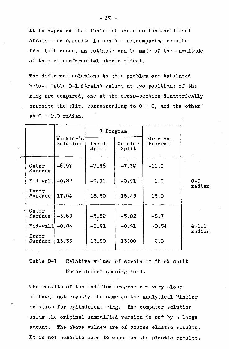
- 251 -
It is expected that their influence on the meridional
strains are opposite in sense, and,comparing results
from both cases, an estimate can be made of the magnitude
of this circumferential strain effect.
The different solutions to this problem are tabulated
below, Table D-1.Straink values at two positions of the
ring are compared, one at the cross-section diametrically
opposite the slit, corresponding to 6 = 0, and the other
at 0 = 11.0 radian.
Winkler's' Solution
C program Original Program Inside
Split Outside Split
Outer -6.97 -7.36 -7.37 -11.0 Surface
Mid-wall -0.82 -0.91 -0.91 1.0
Inner Surface 17.64 18.80 18.45 13.0
Outer Surface -5.60 -5.82 -5.82 -8.7
Mid-wall -0.86 -0.91 -0.91 -0.54
Inner Surface 13.35 13.80 13.80 9.8
9=0 radian
8=1.0 radian
Table D-1 Relative values of strain at thick split
Under direct opening load.
The results of the modified program are very close
although not exactly the same as the analytical Winkler
solution for cylindrical ring. The computer solution
using the original unmodified version is out by a large
amount. The above values are of course elastic results.
It is not possible here to check on the plastic results.

- 252 -
The other two problems used to check the program contain
no toroidal elements, nor spherical elements, since
this is a special case of a toroidal one. They are
designed to check whether the modified program would
give the same results as the original one to ensure that
no error has crept in unnoticed from the many alterations
necessary to the program subroutines and instructions.
Both the elastic solution and the plastic solution are
compared. The first vessel is a uniform circular
cylinder with fixed ends under internal pressure load.
The C Program solution is found to be exactly symmetrical
about the mid position, and the elastic as well as the
plastic solutions are found to be exactly the same as
that of the original program. The second vessel con—
sists of a 45° conical pressure vessel head with rein—
forcements at the vessel side of the corner in the shape
of a taper where the thickness increases towards the
corner. The taper is being used here so that the terms
connected with changes in thicknesses can be checked.
Again in the final form of the modified program the
solutions agree exactly.

- 253 -
LIST OF ILLUSTRATIONS
Figures
1-1 Torispherical Pressure Vessel Head. 6-1 Axisymmetric Thin-Walled Shell Element. 6-2 Force and Stress System of Shell Element. 7-1 Stress Distribution, Cylinder Under Internal
Pressure. 7-2 Stress Distribution, Toriconical Head Under
Internal Pressure. 7-3 a) Circumferential Stresses, Flat Plate Bellows.
b) Meridional Stresses, Flat Plate Bellows. 7-4 Circumferential Strains, Bellows C. 8-1 Mild Steel Torispherical Head, Stoddart. 8-2 Stainless Steel Vessels, Kemper, Theoretical Elastic
Strains. 8-3 Stainless Steel Vessels, Kemper, Theoretical Plastic
Strains.
8-4 Strain Gauge Readings of Low Proof Vessel, Kemper. 9-1 Nominal Dimensions of Thick Cap and Thin Cap. 9-2 Welding and Machining Details of Nozzles. 9-3 a) Tensile Tests, Load-Crosshead.1 Movement,
Specimen 1.
b) Tensile Tests, Load-Crosshead Movement,Specimen 2. 9-4 9-5. 9-6 9-7 Basic Bridge Circuit of Recorder. 9-8 Meridional Strains at Nozzle of Thin Cap. 9-9 Circumferential Strain at Nozzle of Thin Cap. 9-10 Plastic Behaviour of Thin Cap, Strain Gauge Readings. 9-11 Collapse Behaviour of Thin Cap.
9-12 Meridional Strains at Nozzle of Thick Cap. 9-13 Circumferential Strains at Nozzle of Thick Cap. 9-14 Plastic Behaviour of Thick Cap, Strain Gauge Readings. 9-15 Collapse Behaviour of Thick Cap. 10-1 'Smooth' Representation of Nozzle Junction.
10-2 Equivalent Stress Intensity at Nozzle of Thin Cap. 10-3 Equivalent Stress Intensity at Nozzle of Thick Cap. 10-4 Constant Strain-Rate Loading of Thin Cap.
Plane Plane Plane
Strain Compression Tests, Strain Compression Tests, Strain Compression Tests,
Hoop Hoop Axial
Specimen 1 & Specimen 3. Specimen 1 &
2.
2.

- 254 -
11-1 Test Vessel Nominal Dimensions. 11-2 Details of Test Nozzle, 11-3 Position of Strain Gauges on Test Vessel. 11-4 Position of Dial Gauges on Test Vessel. 11-5 Pressure Circuit.
12-1 Elastic Circumferential Strain Distribution on Test Vessel Heads.
12-2 Elastic Meridional Strain Distribution on Test Vessel Heads.
12-3 Elastic Circumferential Strain, Nozzle End of Test Vessel (Head B).
12-4 Elastic Meridional Strain, Nozzle End of Test Vessel (Head B).
12-5 Axial Deflection at End Nozzle Junction. 12-6 Circumferential Strain At End Nozzle Junction. 12-7 Pressure-Volume Curve. 12-8 Circumferential Strain Around Kunckle of Closed
Dished End (Head A). 12-9 Meridional Strains Around Kunckle of Closed Dished
End (Head A). 12-10 Circumferential Strains Around Kunckle of Dished
End with Nozzle (Head B).
12-11 Meridional Strains Around Kunckle of Dished End with Nozzle (Head B).
12-12 Circumferential Strains at Junction of End Nozzle. 12-13 Meridional Strains at Junction of 'End Nozzle. 12-14 Axial Deflections Relative to Mid-Vessel. 12-15 a) Strains Near Crown Centre of Closed Dished End
(Head A). •b) External Circumferential Strains at Vessel Body.
12-16 Equivalent Stress-Strain Curves for Test Vessel. 12-17 Equivalent Stress-Strain Curves for End Nozzle.
Plates
9-1 Multi-Channel Strain Recorder. 9-2 Test Arrangement.

- 255 -
Fia 1- 1 TeR tEPHERIcAL
PRkSSuRE i/s..s7EL MEAD

11- v
w-i- v1Y-8/
dkia Mi r --ca-- 811
dr- gi
St
1
w
FaRce Pft/9 /14
DISPLAcERZ-Nr py3cR,4,4
Ff6 6-- f AXISYlt-fl-IETRIC THIN — WILLED SHELL ZLE/4674 T

(6)
CcL)
- 257 -
FIG 6- 2 fokck- A/vD STREss SYsTEM OF SMELL 4-2.EMENT

• Ott2u—'1,11, —
"
0"
CYLi j INT
/Crib EXT
•
- 258 -
EXT.
aiv INT • 8. 0-1.1
MEASOR.VIENTS ARE 7-414E 721 th 0.0x1 I N . EX'T
•
cs-t 114T .••••••• o
°b 65 INT
'N's• Crt EXT.
32 to12.345 -PISTAWCZ reol-i TilicgAJESS ClIANCE iNCRES)
EXPEkIMENT P1OkaAt1 /41 24. BI2oN RE.
— • 0 — CMCIAMFERENTML ST'RE'SS Arr. rtif:FACE
EXT. S CAP-FACE
CA LC ULATI ON . MOXOAN 73120A) REF 0—.0/ AND PVAI
. 7— i STRESS 2vs FRIh'cf T,onl CYLIA DEla MNDE/2 AITERNAL. PREYSTRI
_ 4 I 5 4-
Cl — HER.I.PIONAL STR.t.SS Crt, --- - CikccuurEkENriAL sr4ths
HEP-IPtONAL ST.C.ESS 1

27.5
141 20•0— % qe
EXPERIMENT ROgaiiN 2 gizoN / REF(4-a) L.,
I7 HER to. .2,eEss j
c-1 17.5 6v, 0 C/a c, STRkS5 • 1 ce egi
_ AN -51/RfAct ()... c.i 0z 16•0
Cri, tri) CfRe. S-rRE..s s 1 lixT. SligrAcE '''' cc) I HER, D. STR E SS Cr r2
CALcULATidAl frioRatlitil Bi2dttyrEt(4-104
hf+d) • ?VA I I-- 10.0
2.5
MACHIMSO HEAD MO
25 c—CyL1uDE S? 6•S 5•57 A )___
225 i•c171- ia, 0
CO 54,..,1
F•c1-2:10_L),..1
/14CHES
12,5
16.14T.
tEXT •
a °COVE
5.S.1 LO }.1:71
sie.r
ExT
0 INT
(3,.?
tr —6—
it
,:k"'"
0
-7-4—t---,`
,
L 0/ 6 I
0./ .,..'
\
o, i
ExT
CI
I
r
/
a:: to,,----
U ' I t
A
IL/13 9
I I I 1 o 2 2 I 0 I 2 3 4- MERIDIMIAL DISiAticE FRol,A SHELL 7LnACTiotas
(tt.1) SHECZE 5.57ncYLIWOER
4••C.9" L01,3G,
F I G 7-2_
STRESS .1)1 ST RIB trl" I 0 N TOR.1 CONICAL I-JE /11) LIAIDE12. rER.N4L PIUS'S VRE

. $7
;.cl.
41f I ... .
INTERNAL
/ .. 0•2..
i_ I:1 ---....z.
Cr Ii 1i *•..A ir
,
, / \/' AN.1,J, / j......tu/
,,/ 1/ ,"
ri---2:-'-- I t , P
INCV,ES . ''..____.......4..:`'::...c....i...6 RAOWS
d r , I - / I
0 , •
',,, ' DEcillEES L
J, r ,
- A c,r __evii.t,
. /.- '
EXTERVIAL
.
. ...
%
-..... ,- r
• j iviicvz. . 1, C ,.ii
' 93/ "
•
14
Z
14
-18
-16
- 260 —
'0 CURVED PLIATE
RA I. PLATE CURVED Lai PLATE v.
EXPERIMENT TuRAIER_X- r Okb J 43EF (7- 2)
_ O — EXTERNAL SrREss END 1/4 CoNVOLUT14N
— A — INTERNAL STRESS
— 0 — INTERNAL STRESS MO ALE '/4 coNvoLvrioN
CALcutArrom Tclizniz , REF (( - -Z) P 1/141
Fla 7- 3 (a) C/RCWI FE REA1TML STRESS.,
FLAT PLATE BELL 0 iv_s
41•••••••=1M,

24
1G
k
rin - I G
24
f \
—I l 7 ,,---,\ fit -\s%
IL-1"-e= 1 te I hriL'
r J
S, <
• .,,s,,, ‘s s '• \ \ • . A
INTERNAL PN N ;. '" - - - -, ,,, C2---C)
i
DEGREVS a•lo C.,,0 90 1 1 •LI.,
• • • •
• • • r ,f,.,-,
1Y 0 7
./17 ,,,,,,
90 Go
U, 0 \
0 Bo 0
5 G !NICHES RADIOS
7 0
N.N. • • • •
• . .
B
P/'
/
%
I
-%
t
t / UTERWAL
%. .
... .
sse ,
1 t
0 k . I t
**1:1-( \ ,-)
*32 ti
-261-
SIG 7-3(b) MLR I.Dionbc-iL STRESSES ,
FLAT PL/)TL BELLoNS
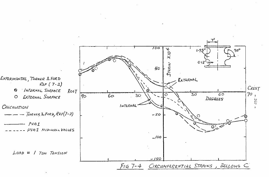
S3:78Diq
Sly1077.P.F -SW /W/_2S 7 vi1N.73/3,Yhin,-.)0
/V CI /Sp,' Fl / civo-r
S P1 7 (i/1 -7 7 6%7 -11 11 rvid -- r find
— ,Nowin7,2-40
.7,V2Y17S 7 Afaigi X-5 _boy yottgyns tI.W?ig-PY/
( ) CL g 71/1P13N1213c1X

MENEM MI.
411=01.1M 01111.101. minn•••• gown...b
OuTsIDE WALL l"
,Aeoo
OuTSIDE WALL
bikiaMSBOALS ( I AletIES) O U Ts I DE WALL
= 45 ° N.)
•••••••••••
noo ISor t4 trJ
loo400
CP =45 0 WALL
MERstaxED Srovow i? (e- to)
CilLccItArip „ PLINTH
200 11•••••• •••••• 0.110 •1110
FiG s-1 M ILE? STEEL TORISPHERICAL STOI3DART I00
STA (I'& CZ,4T) ' 6
244 R I R
I/4 Mgt
/

1.••••••••• ••••••••• — I NrERVAI Srmim
/0
CmcaistarEizforma
EXTEANAL EnvaiAl
CftoW
411116:111:111.0 CalIGLIIMMINONW
Zo
HER/Dimwit.
DisTimice Vasszz. iagi.ohga (iticitiss)
1
llassaz, acov
Fla S-2 STAWLESS S'TI&L tlEsszts KkylikEn es. Temo.22riicA.,, f4r:ric ST/.AINS —
I I 1

0
A (4vEi 8
200
ISO
I I I I SCALE 2 , HIGH PAW VESSEL CL4119.......
SCALE 1, Law PaooF licisso...
RE
ESU
RE
AXIAL DEFLECTIOAI VE.TVL REA) PEAR. SWAIMS ARnliALD kivsicg.LE , EXTERNAL. $'NziPACa
A 8 C ItiLaIDIONAL. CIACmt-itea.aEMTi.11..
V
FIG 8-3 STAINLESS STEEL. VESSELS , KE MPE A
TI4E0P.F.TICAL PLAsTIC BEI/AV/Ova
DaFiacrie/4 ( ini
•3 .4 •S *6 • 7 °g .9 sreM i Pi ( PER CEA! 7)
.1 .2 1.0

loo_ g, J4 -2, 3, I
ALL ExT. ariES AT
CPowiu C
1-1 1D—by c(c KLt
t/s'5' EL BdPy
3$0
30 0
25o
F/CT g — _TTR.13 in; 6-4 tIcE D Iv 2 0 0
F Lc t%; PX co F tits SEL
STkfl (PEk CENT)
111-
15'0

4
FiG. 1 NOMINA L ..DIME.IVS/ON D F
TI-I ICk CA P TH IV CAP
//
8
311
R (Thin) 5,,
R (Thick)
24" DIA.
4"Dia.
/ /
/ /
5" I.D.
16"R (Thin) 261/ R (Thick)
1 or
I 7. Dia. 1,
1 R

1" 8 R .
,ft R (Thin), t(Thick)
Z.,"...5°
ji:(Thin), i(Thick )
Cap
L
311o.
0.125 ±•002"
r \
1 11 44 0.D. x Thick mild
steel tube.
FIG.9-2 WELDING AND MACHINING DETAILS OF NOZZLES.

—UTL 780 LB.
ELASTIC DEFLECTION LIN ZERO SPECIMEN DEFLECTION LINE. -
-UYL 592 LB —LYL 568 LB
t800
700
600
500 2 4% TO TAL STRAIN LINE. 0
< 0 -J
400
300
-.
200 — SPECIMEN 1. EFFECTIVE GAUGE LENGTH 0.90" INITIAL X-SECTIONAL AREA 001238 in2
1
100
0 0.5 04 03 02 01 0
DEFLECTION READINGS (INCH )
FIG 5-3A TENSILE TESTS 3 LOAD •---' CROSSHEAD MOVEMENT.

SPECIMEN 2. EFFECTIVE GAUGE LENGTH 0.92" INITIAL X-SECTION AL AREA 0.0123 8 in2
600
700
500 c.1 0 <cr) -J
400
800
300
200
100
UYL 590 LB.
LYL 550 LB
ZERO SPECIMEN DEFLECTION LINE.
ELASTIC DEFLECTION LINE
4 %TOTAL STRAIN LINE
UTL775 LB
- 270 -
• 05 •04 •03 .02 . • 01 DEFLECTION READINGS (INCH)
F IG.9-3B TENSILE TESTS, LOAD ^, CROSSHEAD MOVEMENT.

0 •
0
LO A
D (
TONS )
4
SPECIMEN #1 AVERAGE THICKNESS 0.1242" GAUGE CALIBRATION 1 THOU=2.0 DIV/ EXTRAPOLATED YIELD = 50200 LB/IN" EQUIVALENT Y = 43500 L BilN2
rr o PLASTIC SLOPE = 9.6
SPECIMEN 2 AVERAGE THICKNESS 0.1242
o
GAUGE CALIBRATION 1 THOU =2.0 DIV 2 EXTRAPOLATED YIELD = 49000 LB /IN EQUIVALENT Y = 42400 L B I IN2
// PLASTIC SLOPE .11•3
10 12 14 16 18 GAUGE METER READING, RELATIVE ( DIVISIONS)
FIG 9-4 PLANE STRAIN • COMPRESSION TESTS , HOOP SPECIMEN 41. 2 .
20 22 24.

8 4. 00
28
24
20
0
_s 12
AVERAGE THICKNESS 0.1242 7
GAUGE CALIBRATION 1 THOU =5.0 DIV
/EXTRAPOLATED YIELD = 4.8000 LBIIN 2 EQUIVALENT Y = 41500 L Bj IN2
" SLOPE —11.9
12 16 20 24 28 32 36 40
GAUGE METER READING ( DIVISIONS ) 0
0
FIG. 9-5 PLANE STRAIN COMPRESSION TEST , HOOP SPECIMEN 4c3

80
70
60
co -J O O
50
-J 4.0
30
AVERAGE THICKNESS = 0,1915" GAUGE CALIBRATION, 1 THOU = 4-88 DIV
EXTRAPOLATED • Y1ELD = 50600 LB/IN2 4.3900 LBIIN2
PLASTIC SLOPE = 15.7
#2 0.1856 / 4.77 DIV /
52000 /
45000 /
8-2
20
EQUVALENT Y
12 16 20 24 28 32 36 40 44
GAUGE METER READING, RELATIVE ( DIVISIONS)
10/ —
0
0 4 8
FIGS-6 PLANE STRAIN COMPRESSION TEST , AXIAL SPECIMEN 1 4 2 .

ACTIVE STRAIN GAUGE.
DUMMY STRAIN GAUGE.
TO COMMUTATOR AND DIGITAL VOLTMETER.
120 n
- 27,1
TO CONSTANT D.C. VOLTAGE I • SOURCE • I L _ J
BALANCE 10 KIL
FIG9-7 BASIC BRIDGE CIRCUIT OF STRAIN RECORDER.
•2

FIGURA9-8
MERIDIONAL STRAINS
AT NOZZLE OF
THIN CAP
ELASTIC STRAINS IN PERCENT
PER 1000 LS LOAD
0
•
-•01 STRAIN GAUGE READINGS
TI-~ECRETI CAL
I 514607 H C PROGRAM
.5140ori N PROGRAM
SIAIPLE
IlL 3141‘1_,D
0
-•13 2
- •03
04
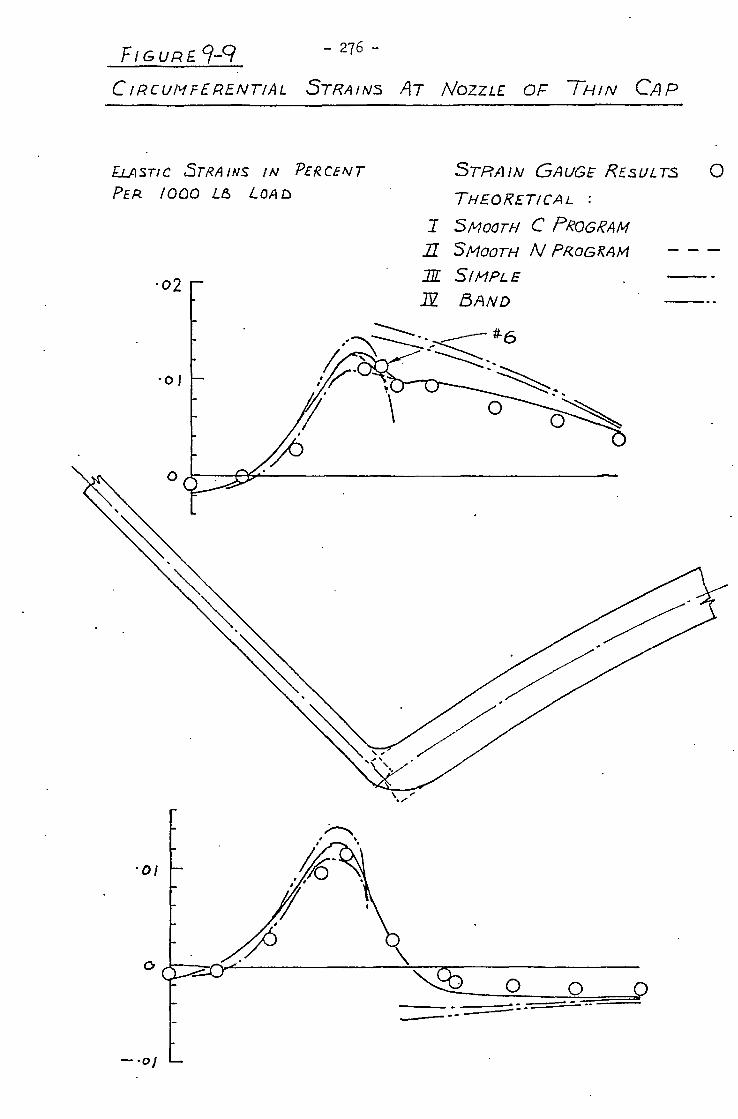
0 Q
- F. IGURE9-9 - 276 CIRCUMFERENTIAL STRAINS IIT NOZZLE OF 11-II N CAP
STRAIN GAUGE RESULTS 0
THEORETICAL :
I 5Modril C PROGRAM 11 SMOOTH /1/ PROGRAM — — — 71L SIMPLE R BAND
. X46 --- z.s
• • • 0 I • • ----,
ELASTIC STRA INS IN PERCENT
PER /000 1.8 LOAD
• 0

0 I1 CQ
Q8 000
7000
FIGURE1-10...
PLASTIC BEHAVIOUR OF THIN CAP
STRAIN GAUGE READINGS
• 05 .10 '15 .20 .25 •30 STRAIN ( PERCENT)

440
GAUGE °28
, /
FIRST YIELD LOAD BY THEORY
4550 L&S
/4/ ' 11(.4E #Z
--
4 000
400
i'000
/ 2000
i_XPERIMENTAL
MA wry! ukt LOAD /4120 L8
FIGUIRE9-// COLLAPSE BEHAVIOUR OF
THIN CAP
STRAIN DEFLECT/01V
EX PERIM E iVT
7-11 EO RV
1(600
14000
000
0 00
IO 20 30
.2. *6
40 .5'o 6o 70
•Es
1.0 1.7 /.4
DEFLECTION ( X000 INCH So STD /oo /•6 1.8 20 .

FIG. • 9-12 MERIDIONAL STRAINS AT
NOZZLE (:) THicr< CAP
- 279 -
ELASTIC STRAINS IN PERCENT
PER. 1003 La LOAD
• 005
O
STRAIN GAUGE READINGS
THEORETt CAL SmooTH C PRoaivim
71 SmoorH N PR °GRAM Tff SIMPLE
28 1E BAND
- • 005
-- • 0
0
•••••••11,

ELASTIC STRAINS IN PERCVVT STRAIN GAUGE READINGS 0 PER WOO LB LOAD
THEORETICAL
I SMoorH C PROGRAM 7.1 SMOOTH N PROGRAM
21L SIMPLE
112 BAND
- 280 -
FrGuRE943
CIRCUMFERENTIAL STRAINS
AT NOZZLE OF THICK CAP

-
2. SZ. 50. 1 1 1 I , I I
S9N/C7 H_3&
NlVaLS" 3111/9
del/70111VHJ
> I gliLL.D1f5V7c/
7>1-63dr791-11
11111 / .•
, ry /! /
/1/ „pp, 7 ,_,7 / , 1 -
SIB 9170 ett
0
o 7
00,
0009'
00o. g
000 0/
000 V
00017/
r- 0009lt;
oo o 0Z

35 000
3o000
A tz:/_. 000
/ d / 1
I/ /
/ /
/
I
r/
GAII6E #z
-4
k I
cc /
20 000 -1 i / / / /
/ / t
/ / / i /6-0 00 -- / /
i 1 / I/
1/ 1
i0000 I
z V
/
FIGURE 9-15 COLLAPSE gEHAVIouR of THICK CAP
STRAIN .DEFLEcTioN
EXPERIMENTAL MAX. LOAD 3426.6 LES
cn
5000
0 10
EXPERIMENT
THEORY
FIRST YIELD By THEORY
2710 Lgs
.20 30 As
40
a- 0
on.•••• ••••••••• a•m• • OM en et OD ••• MID ••••
60 6.0 3-0
DEFLECTION (IA 000 tAtcH) 70 go 90 too
4.0 s s•0 S. RA Iv PE RC

ACTUAL NOZZLE t SMODTH I REPRESENTATION
IN CALCULATION
± t .....11.. I
CYLINDER ELEMENT
TAPERED ToRUS ELEMENT
VI
SPHERE ELEMEAJT
T
rrte= ro + y 1 IF t< T
r A 11 I 11 I "F
t ro I- --5 .- j tF T < t
FIGURE 10- 1 i SMOOTH 1 REPRESENTATION OF NOZZLE cTUNCTIoN

- 234 -
FIGURE IQ -
EQUIVALENT STRESS INTENSITY
AT NOZZLE OF THIN CAP
IN 1000 L8/iN 2
PER 1000 LB LOAD
EXPERIMENTAL 0
THEORETICAL ( SMOOTH, C PRoGRA/4)
/0
8
6
2
10
8
MEMBRANE STRESS AT NOZZLE -
6
4
2 0

- 285 -
0 FIGURE 10 - 3
GQUJVALENT STRESS INTENSITY
AT No ZZL E OF THICK CAP
iN /000 L8//N 2 PER 1 000 L8 Lo AD
EXPERIMENTAL 0 THEoRETIcAL
(.SMOOTH, C PRoGRAM)
0 0
MEMBRANE STRESS
AT NO2ZLE

0
.DEF
LECTI
0A1
(1 A
L Tt
ioav
iNor
t/!A
/CH
) o
S'97 0 Z-1-17/
13Iv Vo'I7 11,13.53Yd
o 0
- 99Z -
37zEoN dv No 1.1,777.13g 1 tin( V 3h9li a1io7 7VIX V
N-
0
0
O
iy 0 1.13.3-a7g

r 3 "
77iNeANT LINE
0.KI4r.,
0 Accs-s /110.22LE
SizE / 0"
TErr Na2ZLE
Pig_ DEMILE SEE na
1 gaire r•r/naLtss f EEL
bEstaiv P/?E.S.cliifE 36 18/IN=
No co
7r TEK
1
ELEVATION
SELT LENcry • • p
31- Il g IMpieox. ZEivarAl
rig /1-
TEST 1/Ers- _DIMEA/SION3

- 288 -
•
( t
tiF
-s" 7-6- C. F. WELD
1}" F. WELD
16
!cur RALIK n SOUND
VESSEL NERD METAL FIND REWELD
.ras IfwALL s. C.24" f iDitl
AFTER. (AIELDIN6 INTO HEAD TYPE To BE HficioNzo DOWN
Jciwr TO BE ilhciovED To 75 DIMENSIONS E1101/1A1
RADII EfIdaill 4s 4rcaRi3nty FR014 4' O/D/4 X 3.1.24”1/DiA PIPE
As PasgoiS N
-76111ZAD
VESSEL HEAD
Fl NISH Z•t) NOZZLE
WELD PREP/Mir-10N
Fia 11-2 LS OF TEST NOZZLE

s-tvw_Lispd 1,117.1.V6r. 140V-1 9rip7or 3,YV Nr4011,5 ('S7&'
-79rni5' 7fiNolo3in/ -14
3.9)16",9
..7.7 &dams 7 73eis
0 Fvnti.9
la164-19' 6 S .7N H7d lv/ -11'g 1-76v Fz")- 53917t/9
rvPuisoci p-vEts z 0 s3.9nE/9
1
7 3SS.7/1 No S2.911(719 dO NO/1.1soj E -// • 2 /-/
1Z,A1 /0- (1-2Y-int littlerq
-kr 0-7•0
0-kv '0"-v „-F-S•L
-17-1-1/ „-7•12
ti
grvu7d 7d1NOZ)?I'H
fi

17 -11 912 7 3-TS -Ls NO NO ..73'nifi 7 7C/JOr zIO NP/-USOG/
NV7cil
i
0 C1 C\I
I
7 W-075(.2 u/..wai v NQ 5,v &'7J 7 E/1 NOT.:12/21-/ 31-1.2 .14/
0' 7-LIV 4 Ply go fl S 3,M1,9 7e/(1

PRESSIME RGGuLATog
On. TANK Pump
YE:SSEL PiZESSuRE GAUGE OIL hate.)
R.EauLATDIZ
SHUT-OFF VALVE
HEA-SugING 7746k- A-ND RULE
SHOP AM SUPPLy
OIL LEVZL
Tisr VESSEL
RYDRAuLie UsED 044 CrACtiir
FIG 11-5 PI SIRE CiWcti/T

i l HEAD 8 -,_ / i -4. • ot0
tti C.3
10
Cilt..CuLATED MEASURE Z
8 /0 12. 14
/ liEssEL &Is Foa
I .
.•010
EXTERNAL hkingNAL 01111•••••• 4101•11
.SHELL
HEAD HEAD A 0
HEAD &MD 0,v HEASuRED GaoNdraMs
/2-/ ELASTIC CliZet47-1FERIENTIA4
D/ST.2/eVriON OM TEST / 47 VESS1L MeADs

ST
RA
IN P
R 1
00 L
ON
2 cE
pir)
,
0
a a
o o o 0 0
0
6 0
c) ....
-6
III
00
L
ti
Vf - r-
S
a
4.11
11ftf
tim
i 11
•11.
1.,m
11
skit
to
13
0 v
T
14
0 C
I*
,0
fv
ED
0 i
lr 11
1 S
D
pa
1,
sollO
P"."6
6 ..a
spra
ll"
arre
adar
ews$
ex
pia.1
.4"Ir I
C
0
6;
.0,
-- ---'
..--02
tri 6
I
CO
\ N
s
2—it.
4
0 r-
a!
0 11
o Z
>
i3
?, <
Z
it;
tiff
0
r*
0
U)
U)
Na NCIfidleiViTia
is
1 pi
al
N„.
I I
t'll
I I
I
- C. 6
i7

CTR4
IN
PF
/
LehA/2
(Pliz
ctiv
r)
6;
—0 0 1-)
u.)
0
I
O
O
7
1 I
I
;.., Di
o
C--1 il
1 .
NA
Rr
71
a0
tA)

NMQ,Y7 TV C.J.L
Ha- g 733-3-34

- 296 -
`10 Ctea 410.1 .11 7 87o Who
A
a
PRZ
a
SOD
F/G
AX L DEFLECTION 47" .tIVD, NOZZLE -TO Ak77 ON
MEASURED (.DIFFiRENcE OF AsEADIA4g, 219L Ne ?3,5)
a0 — - CALCti LA 7E2
I coo
2f3 7
/041 /50
OZFLEcrioni (0000 ta) 02.00

7o L 6/IN 2
0
- 297 -
goo CYCLE No. I 2 3
00'
o
F/G• 12- 6 CiRCUMFERENTML ETRA1NS
Ar END No22LE JUNCTION
340 „
MEASURED (GAucE 43, TEAissiON)
C.44CtizATED aoa
• .2 CYCLE No. /
• g 1.0 SIT72/3/A1 (f L. CENT)

1 t(6.t. Le/mig
1 3RD C. OA D/Ala
;000 ‘,2 AID L M DING / 0 7 L 8 /IN
870 1-8//N I sr L o A DIAJ6 800
Coo
FIG PRESSURE VOLUME CURVE'
LEVc-L MEASURING TilSe (IN) . 30zs 35 0
too ISO L.0 011- VOME (IA13) 0 ,
400
200

- 2 99 -
1
is ( 1-94R CHT)
3
0
0
0
ci 0
0
1/4.0
rt tv f /Ey 7 ) 32lols37.7 Yci
0
0

10 0
mat)
.2 - 111/: 1..1); °NAIL giRAINS
hiZObinfi) kNack.LE OF CLosET) Ots.HE.:o,AND
( EAh .4)
klE4S0 RED
CALCWATED WITH Firao 3' Tx? Es's-.c ,4fd Cu v WIT11 PEIZFECTLY /LAS ric CtiRVE.
t
Fok ExT. 6,que.c.3 33 ) .27 , -29 /NT. Cfiuci 351
• • .4 ./ • .3 • 4- JS .6 7 ,
,c---7-K• /l /iv 0.-4 it re% Ai 7 )

S TRA A.1( PLC CL-Ai 7-)
— CI-J Cu 1.11 TED
4-7 FOR ,SAT tie; E A/7: 64 it cE
'l5 25 I 1 3 3 S i • i• O
iler 1.2-10 CheciAn-frER_NrIAL .3-r1X1 /AJE
o 0
F00
600
1)ko tf N .1) </v IA Ck LE OF S AIL kb TA/ A la 2 2 LZ.-
1--/EAD
/flEA S u E.

Err. GA. ticZ
\CI / NT. gA t i cE
•
t ti
ills-Ri p/ oh' --AL
Ake ItivD Kiv t 4 C-KLE
ry
Q3*
0
- 30
2 -
o
0
0
0
0
o
0
,$) 1
1
6 IV //F., 7) JAW
S'S (V

1.2 1 , 0 , (.2
Fl C/ R. Cu mrEREA177A-L YrRAInis
AT J UNCTI ON OF t/V.b Ai d 22LE 43
43
LAST READ1N& CA ttGE 6
— C4 L Cti LI) Tr-
FoR tx T, 64tcaz- 1N T. 64 [ACE 412
-.E7R7-)IN (/)E, CF_ /vr)
POO
g

Eriz AIN ( F 4R. c,_,,,j .6 D.. 6
A
FIG NIERIDioniAL Ril ALS
AT cAvC.71 ON CF -6it/JD A; (I 22 L.k."7 Toro
42
?6
LAST R&M)/ Ai6
Fok GAME 7
ME MS ciRLD
CI) LA?ED
rOR. amtaE 7 /NT. 6"
1• t /,2. I /• 11- I • 6 11112 ,21111=11=1=1=1=12116 a. 11 01=LICJ.MALSGSOMINIONOWIMIMMININOLIMI.040/1~101RMIMMORMIRO)
Coo

Mr CENTRE OF CLoSE0 HEAD
AT JG1NcTiON OF ENDA/Da-2LE-
1
FICT X M C DEFLECT/ OnI_S
RL.,4 To 1/C" SsEL_
frlEAS tl.RE D
CALCULATED
20
FrrED CuRire.'
PER rEcn V PLI)Sric ea gv
100 /20 /4-o /O .2.00 1 22o 124.0
1).EFLL-.-C7-10N (I loco IA).)

HEAsuRED
C,eLCuLAT)D
foA. EXT. 6-.914cEs•
o
a 3 6
)20°
35.
a
LW Y6
6:14
LU
F1 r7 1.2- /5 A .CTRANs NEAR ("yea N naTRE
OF CLOSEb DiShED END (HEAP .4)
• OS ,15 • 2z .3 STRA MI (i)t_R ezew

.23 -23/.24-.25
fic, 1.2-158
go EXTERNAL. C/AZ CON FERE/ti Til?
STRA 1N S 1.)-7" V E SSE L Bo. y
4c o MEASURED
aLet(LATED
,2CC1
FOR EXT. G-13t4ais .23/ .24- 2 _25
4 if • g
12ECENT) S77011,1

-71.1 MEASuREDZom TleikE£ TE,VS'iLE
— — SZST FIT CURVE
TE p WIT/- -2ND ORDER ogLeE131ZhIc d tifrIL Om /Ai R. zi-ArGE 0 - 4 ?LzR cENT •
= 3.3+19 x r6 xio (Ep x I (1.7 6132
/ IN//NJ
10 0 Axis fog 2e 1-10S -ric S7X13IN
pc: ErR4inl &k.C4-7 T

cr 1.2- 17 E& UIvi L LAJT S* 7-RtcS SrieMN CuR vCS Fak END Alc
IlEAStIRED FROM 11,10 MNSiLZ TE sr5
EEST FIT CURVE
lip 24/4 0.ADE& ALCE4Rafc 1.y/vom L_ Iti triY IA) ietyiv‘z- 0- 4-LS
.:.-_ 3. 7.2 663)( 10 t (.23774 X io — I. /32s7.x/67 Fp 2. Tr ( g iv2) , e (/ ti/
0 .S /.0 .2r iJ
3. 0 4
3
I0
P.!_hl ST/ e Si- ',A Jr. (J cENTJ

Plate 1 Multi-channel Strain Recorder

ial re t
Top Related
Copyright © 2022 FDOKUMEN

