Dow

nloa

ded

from

asc

elib

rary

.org

by

Mcg

ill U

nive

rsity

on

04/1

6/15

. Cop

yrig

ht A

SCE

. For

per

sona

l use

onl

y; a

ll ri

ghts

res

erve

d.

Semianalytical Model for Shear Stress Distribution in Simpleand Compound Open Channels

A. R. Zarrati1; Y. C. Jin2; and S. Karimpour3

Abstract: Semianalytical equations were derived for distribution of shear stress in straight open channels with rectangular, trapezoidal,and compound cross sections. These equations are based on a simplified streamwise vorticity equation that includes secondary Reynoldsstresses. Reynolds stresses were then modeled and their different terms were evaluated based on the work of previous researchers andexperimental data. Substitution of these terms into the simplified vorticity equation yielded the relative shear stress distribution equationalong the width of different channel cross sections. In compound channels the effect of additional secondary flows due to the shear layerbetween the main channel and the flood plain were also considered. Comparisons between predictions of the model and experimental data,predictions of other analytical or three dimensional numerical models with advanced turbulent closures, were made with good agreement.

DOI: 10.1061/�ASCE�0733-9429�2008�134:2�205�

CE Database subject headings: Shear stress; Anisotropy; Secondary flow; Analytical techniques; Channels; Boundary shear.

Introduction

Water flowing in ducts and open channels exerts longitudinalshear stress on the wetted periphery, which is not distributed uni-formly. Distribution of boundary shear stress depends upon theshape of the cross section, the structure of the secondary flowcells, and nonuniformity in the boundary roughness.

Boundary shear stress distribution is important in predictingflow resistance, sediment transport, and cavitation. It is essentialfor practicing river engineers to understand the shear stress dis-tribution in open channels periphery for the prediction of rivermorphology as well as for the protection of river bed, river banks,and flood control structures.

The flow in straight open channels is accompanied by the sec-ondary flows, perpendicular to the main flow direction. Althoughthe secondary flow velocity is only 2 to 3% of the primary meanvelocity, it has important consequences on the flow. Secondaryflows convect momentum from the mean flow to the corners,which increases the boundary shear toward the corners. Trans-verse turbulence anisotropy and nonhomogeneity, which areformed near the solid boundaries, have dominant effects on thegeneration of the secondary flows �Nezu and Nakagawa 1993�.The free surface in an open-channel flow makes this problemmore complicated. As turbulence parameters are difficult to mea-sure accurately near the free surface, these parameters are poorly

1Associate Professor, Dept. of Civil and Environmental Engineering,Amirkabir Univ. of Technology, Tehran, Iran.

2Visiting Professor, Dept. of Hydraulic and Ocean Engineering,National Cheng Kung Univ., Taiwain and Professor, Faculty of Engineer-ing, Univ. of Regina, Regina, SK Canada.

3Post Graduate Student, Dept. of Civil and Environmental Engineer-ing, Amirkabir Univ. of Technology, Tehran, Iran.

Note. Discussion open until July 1, 2008. Separate discussions mustbe submitted for individual papers. To extend the closing date by onemonth, a written request must be filed with the ASCE Managing Editor.The manuscript for this paper was submitted for review and possiblepublication on September 7, 2006; approved on June 19, 2007. This paperis part of the Journal of Hydraulic Engineering, Vol. 134, No. 2,

February 1, 2008. ©ASCE, ISSN 0733-9429/2008/2-205–215/$25.00.

JOURNA

J. Hydraul. Eng. 2008

understood even from an experimental point of view. In com-pound channels the strong shear layer between the faster flow inthe main channel and flow in the flood plain also causes thegeneration of additional secondary flows.

A considerable amount of experimental work has been carriedout on the distribution of boundary shear in straight triangularducts �Aly et al. 1978�, in square ducts �Gessner 1964; Gessnerand Emery 1980�, in rectangular ducts �Knight and Patel 1985;Rhodes and Knight 1994�, in rectangular open channels �Knightet al. 1984�, in trapezoidal open channels �Tominaga et al. 1989;Flintham and Carling 1988�, and in compound open channels�Knight and Hamed 1984; Rajaratnam and Ahmadi 1981; Knightand Shiono 1990; Myers and Elsawy 1975; Tominaga and Nezu1991�.

Several two- and three-dimensional numerical models havebeen developed to predict flow characteristics such as shear stressdistribution in triangular ducts �Aly et al. 1978�, in rectangularopen channels �Keller and Rodi 1988; Cokljat and Younis 1995�,and in compound channels �Krishnappan and Lau 1986; Kawa-hara and Tamai 1988; Noat et al. 1993a,b; Pezzinga 1994; Tho-mas and Williams 1995; Cokljat and Younis 1995; Sofilidas andPrinos 1998, 1999; Rameshwaran and Naden 2003�.

Correlations of the distribution of boundary shear to geometricfactors of the channel cross section in simple and irregular chan-nels �Rajaratnam and Ahmadi 1981; Khodashenas and Paquier1999� have been proposed. Knight et al. �1984�, Flintham andCarling �1988�, and Rhodes and Knight �1994� presented empiri-cal equations for the distribution of shear force in the cross sec-tion of trapezoidal and compound channels. These equations givethe average boundary shear on the wall and bed of the channelcross section.

An analytical model was developed by Shiono and Knight�1991� in compound channels. This model, starting from thedepth-averaged momentum equation, assumed an apparent shearstress, which included the effects of lateral turbulence shear andsecondary flows, to be quantified later by experimental data. Thismodel is not effective in predicting the distribution of boundaryshear in the corner region where secondary flows are very strong

�Shiono and Knight 1991�.

L OF HYDRAULIC ENGINEERING © ASCE / FEBRUARY 2008 / 205

.134:205-215.

Dow

nloa

ded

from

asc

elib

rary

.org

by

Mcg

ill U

nive

rsity

on

04/1

6/15

. Cop

yrig

ht A

SCE

. For

per

sona

l use

onl

y; a

ll ri

ghts

res

erve

d.

Zheng and Jin �1998� presented an analytical model to predictshear stress distribution in the corner region of rectangular ductsand open channels. This model was developed based on the sim-plified stream-wise vorticity equation. Jin et al. �2004� developedthis method to calculate shear stress distribution in triangularducts and across the walls and corner region of rectangular andtrapezoidal open channels.

Another analytical model was presented by Yang and McCor-quodale �2004� to predict shear stress distribution across the bedand walls of rectangular open channels. In this method an order ofmagnitude analyses is used to simply relate lateral and verticalterms of momentum equation and to obtain an equation for shearstress distribution. However, the final equation for shear stressdistribution does not depend on the geometry of the channel.

Secondary flows may have large effects on the shear stressdistribution. Transverse anisotropy is crucial to the study of thesecondary flows that will be described in the following sections. Itis very difficult to model the anisotropy behavior of turbulence.The use of three-dimensional models together with advanced tur-bulence models is also complex and requires extensive program-ming and computational efforts. Therefore, it is desired to use asimple analytical model in which the effect of secondary flows isconsidered.

In the present study semianalytical equations are derived fordistribution of shear stress in channels with different cross sec-tions. In the first step the secondary flow mechanism in simplechannels is studied. Subsequently, the vorticity equation is sim-plified by considering the effect of secondary flows. Differentterms of the simplified vorticity equation are then evaluated basedon the work of previous researchers and experimental data. Insimple channels the method of Zheng and Jin �1998� and Jin et al.�2004� is extended for calculation of shear stress across the wholechannel cross section. This method is then developed for com-pound channels by considering the effect of additional secondaryflows, which are due to the shear layer between the main channeland the flood plain. Comparison of the results obtained by thepresent method with experimental data and numerical predictionsshows the validity of the present analytical model.

Model Development

After extensive review of experimental work and turbulence mod-els describing secondary flows in noncircular ducts, Demuren andRodi �1984� concluded that it is the streamwise vorticity equationwhich governs the process of streamwise vorticity generation,which in turn leads to secondary flows. For a fully developedturbulent flow in straight ducts and channels, the vorticity equa-tion in the x-direction can be reduced to �Gerard 1978�

�2

�y � z�vv − ww� = � �2

�y2 −�2

�z2�vw �1�

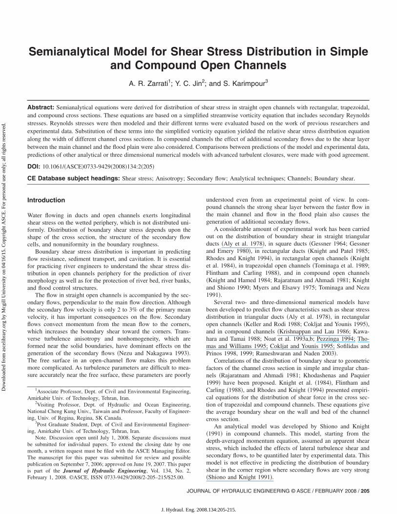
in which the x-direction is defined as the primary flow direction,y is vertical to the channel bed, z is lateral to flow direction, andu, v, and w�turbulent fluctuation components in x-, y-, andz-directions, respectively �see Fig. 1�.

Perkins �1970� suggested the following universal function todescribe the relationship between the transverse anisotropy and

the boundary shear stress:

206 / JOURNAL OF HYDRAULIC ENGINEERING © ASCE / FEBRUARY 200

J. Hydraul. Eng. 2008

�vv − ww�u*

2 = − �1 −y

L� �2�

where u*2�local friction velocity, and L�distance from the wall

where the effect of wall on turbulence anisotropy becomes negli-gible. Therefore, the right-hand side of the Eq. �1� can be written:

�2

�y � z�vv − ww� =

�

�z�u*

2

L� �3�

Perkins �1970� also considered that the secondary shear stress iscomposed of two parts:

vw = vw1 + vw2 �4�

The first part �vw1� is due to the transverse gradient of mainsecondary velocities and considering anisotropic eddy viscositycoefficients can be written as

vw1 = − �y

�W

�y− �z

�V

�z�5�

where �y and �z�eddy viscosity coefficients in y- andz-directions, respectively. By using mixing length theory, theseare modeled as

�y = ��y�2� �W

�y�, �z = ��z�2� �V

�z� �6�

where ��von Kármán constant. The secondary flow streamlinesare assumed circular, such that

�V

�z= −

�W

�y�7�

and hence

� �2

�y2 −�2

�z2��vw1� = − 4�2� �W

�y� �W

�y�8�

The second term of the secondary shear stress �vw2� is dependenton the proximity between boundaries, being induced through thedistortion of the direct stress field by the changing of the bound-ary. As the existence of boundaries is the reason for the existenceof secondary flow, the gradient of this term can be considered asa coefficient of turbulence anisotropy gradient:

� �2

�y2 −�2

�z2��vw2� = B1

�2

�y � z�vv − ww� �9�

Fig. 1. Direction of axes

Therefore Eq. �1� can be rewritten as

8

.134:205-215.

Dow

nloa

ded

from

asc

elib

rary

.org

by

Mcg

ill U

nive

rsity

on

04/1

6/15

. Cop

yrig

ht A

SCE

. For

per

sona

l use

onl

y; a

ll ri

ghts

res

erve

d.

�

�z�u*

2

L� = B� �W

�y� �W

�y�10�

where B=−2�2�1−B1�. In Eq. �10�, if W and L can be obtained,the distribution of friction velocity, which is proportional to shearstress, can be achieved.

Boundary Shear in Trapezoidal and RectangularOpen Channels

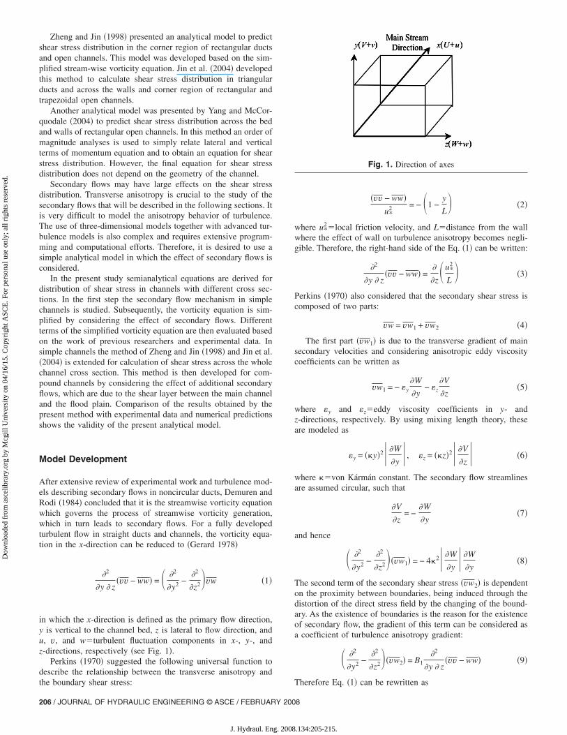
To determine shear stress distribution in a simple channel, thewetted periphery is divided into two parts. One part is the cornerregion and the other is the outer region that is not affected by themechanism that occurs near the corner region. Experimental datagiven by Tominaga et al. �1989� show that secondary flows arestrong near the corner region within a distance equal to 0.65H�Fig. 2�, where H�flow depth. Secondary flows have no effect onthe flow mechanism in the outer region and therefore L, which isa characteristic of turbulent flow, has a constant value across theouter region equal to 0.65H. However, the distribution of L in thecorner region is strongly affected by secondary flows. The follow-ing section is to determine L in the corner region of a simplechannel.

Transverse Anisotropy

It is proposed that the distribution of �v*v*−w*w*� along thecorner bisector follows a universal function, where v* andw*�turbulent velocity fluctuations along the corner bisector, y*,and perpendicular to it, z* �see Fig. 2�. By analyzing data insquare ducts presented by Gessner �1964� where the corner angle�=90°, the following relationship was found:

�v*v* − w*w*�u*T

2 = − 0.5�1 −y*

L*� �11�

where L*�distance along the corner point to a point where an-isotropy of turbulence becomes negligible. For a trapezoidal sec-tion L*=0.65H /sin�� /2� and u*T�average shear velocitybetween z=0 and z=a. In fact L*�point of intersection of thebisector of the corner angle and y=0.65H and a=0.65H / tan�� /2� so that a�width of corner region �see Fig. 2�.If the shear stress on the corner point is assumed as u*cr, bycomparing Eq. �11� with the general form of universal function,

2 2

Fig. 2. Geometric parameters of a trapezoidal channel

Eq. �2�, will show that u*cr=0.5u*T. Considering this relationship

JOURNA

J. Hydraul. Eng. 2008

and two extreme cases when the corner angle is zero and �, itmay be postulated that

u*cr

2 = sin2��/2�u*T

2 �12�

Along the corner bisector, the relationship between turbulenceanisotropy in Cartesian coordinates and a coordinate system or-thogonal to that �y* and z* as shown in Fig. 2� can be written as

�vv − ww� = − cos����v*v* − w*w*� �13�

Combining Eqs. �11�–�13� yields the following equation for trans-verse anisotropy in base Cartesian coordinate along the cornerbisector:

��vv − ww��z*=0,y*=z/cos��/2� = cos � sin��/2�u*T

2 �1 −z/cos��/2�

L*�

�14�

Comparing Eq. �14� and Eq. �2� and noticing that y=z tan�� /2�, ageneral relationship is obtained for L as

L =z tan��/2�

1 +cos���sin2��/2�u*T

2 �1 − z/a�

u*2

�15�

Hence:

�

�z�u*

2

L� =

�

�z�u*

2 + cos���sin2��/2�u*T

2 �1 − z/a�

z tan��/2�� �16�

Model of Transverse Secondary Flows

The secondary flows profile in a square duct presented by Gessner�1964� shows that the W component of secondary flow variesapproximately linearly along the y-direction. In addition, the re-sults of Hoagland �1960� indicate that near secondary flow cellboundaries streamlines are approximately equidistant except inthe vicinity of the corner. Hence W near the solid boundary isapproximated by the secondary flow along the corner bisector andthe following equation can be written:

�W

�y=

�1 + cos��/2��Vcb

z�17�

where Vcb�secondary flow velocity along the corner bisector incorner region. Zheng and Jin �1998� suggested the following re-lationship:

Vcb

u*= 0.38

z

z +0.02a

tan��/2�

�18�

In the outer region as the characteristic of turbulent flow “L” hasa constant value, the distribution of �W /�y�same as that of thepoint of intersection of the outer corner regions.

Derivation of Equations for Shear StressDistribution and Boundary Conditions

To find a relationship for stress distribution, Eq. �10� can be inte-grated along the bed and wall of the channel section, using theexpressions found for L and W. It is also assumed that the average

2

bed-shear stress at the corner region �u*Tis proportional to aver-

L OF HYDRAULIC ENGINEERING © ASCE / FEBRUARY 2008 / 207

.134:205-215.

Dow

nloa

ded

from

asc

elib

rary

.org

by

Mcg

ill U

nive

rsity

on

04/1

6/15

. Cop

yrig

ht A

SCE

. For

per

sona

l use

onl

y; a

ll ri

ghts

res

erve

d.

age shear stress along the total bed and/or wall. The followingboundary conditions can be used to calculate the coefficients ofthe derived equations:1. Shear stress is continuous and therefore unique at points be-

tween different regions.2. Gradient of shear stress should be continuous and therefore

unique at points between different regions.3. The average shear stress along the wall or bed can be calcu-

lated by integrating the equation of shear stress distribution.4. On the corner point, i.e., the conjunction of the bed and wall,

shear stress calculated from equations given for bed and wallshould be equal.

Lateral Stress Distribution along the Bed ofTrapezoidal and Rectangular Channels

Integrating Eq. �10� noticing that L=0.65H in the outer region thefollowing equations would result for shear stress distributionalong the channel bed:

�b

�̄b

= − k�1 −z

a� + A1

2z

b

2z

b+

2a

b1

+ C1

2z

b, 0 � z � a �19�

�b

�̄b

= A2

2z

b+ C2, a � z � b/2 �20�

where =cos � sin2�� /2�, and 1=0.02 / tan�� /2�. Using theboundary conditions, and if bed-shear stress at midchannel isknown, for example from the chart given by Chow �1959�,��b�cl /�gHS=k1 �where k1 could be found from a chart� coeffi-cients k, A1, A2, C1, and C2 in Eqs. �19� and �20� can be calcu-lated. Calculated coefficients are given in the Appendix. Theaverage shear stress along the bed can be estimated from an em-pirical equation, for example, equations given by Knight et al.�1984, 1994�.

Lateral Shear Distribution along the Wall ofTrapezoidal and Rectangular Channels

Due to the approximately symmetric characteristic of secondaryflow cells along the corner bisector, Eq. �19� can also be used forcorner region of the wall:

�s

�̄s

= − k��1 −zt

a� + A1�

zt

S

zt

S+

a

S1

+ C1�zt

S, 0 � zt � a �21�

Tominaga et al. �1989� have argued that, when the angle betweena sidewall and the free surface was less than 90°, a new vortexwould also be generated near the junction of the free surface andthe wall. If the boundary is imagined by mirroring the sidewallalong the free surface, the free surface is a corner bisector of theangle between the solid boundary of the sidewall and the imagi-nary boundary. Thus, the vortex near the free surface is analogousto the vortex near the corner region and consequently the shear

stress in this region takes the form of Eq. �21�:

208 / JOURNAL OF HYDRAULIC ENGINEERING © ASCE / FEBRUARY 200

J. Hydraul. Eng. 2008

�s

�̄s

= − k��1 −1

a�1 −

zt

S�� + A2�

1 −zt

S

1 −zt

S+

S − a

S2

+ C2��1 −zt

S�, a � zt � S �22�

where 2=0.02 / tan � and k�=0 because shear stress is zero onthe conjunction point of free surface and the wall. Eqs. �21� and�22� are used to calculate shear stress distribution along the chan-nel wall. Coefficients A1�, A2�, C1�, C2�, k� can be estimated using theboundary conditions and are given in the Appendix. Using em-pirical equations given by Knight et al. �1984, 1994� for averageshear stress along the channel wall, shear stress distribution canbe calculated.

Boundary Shear in Compound Open Channels

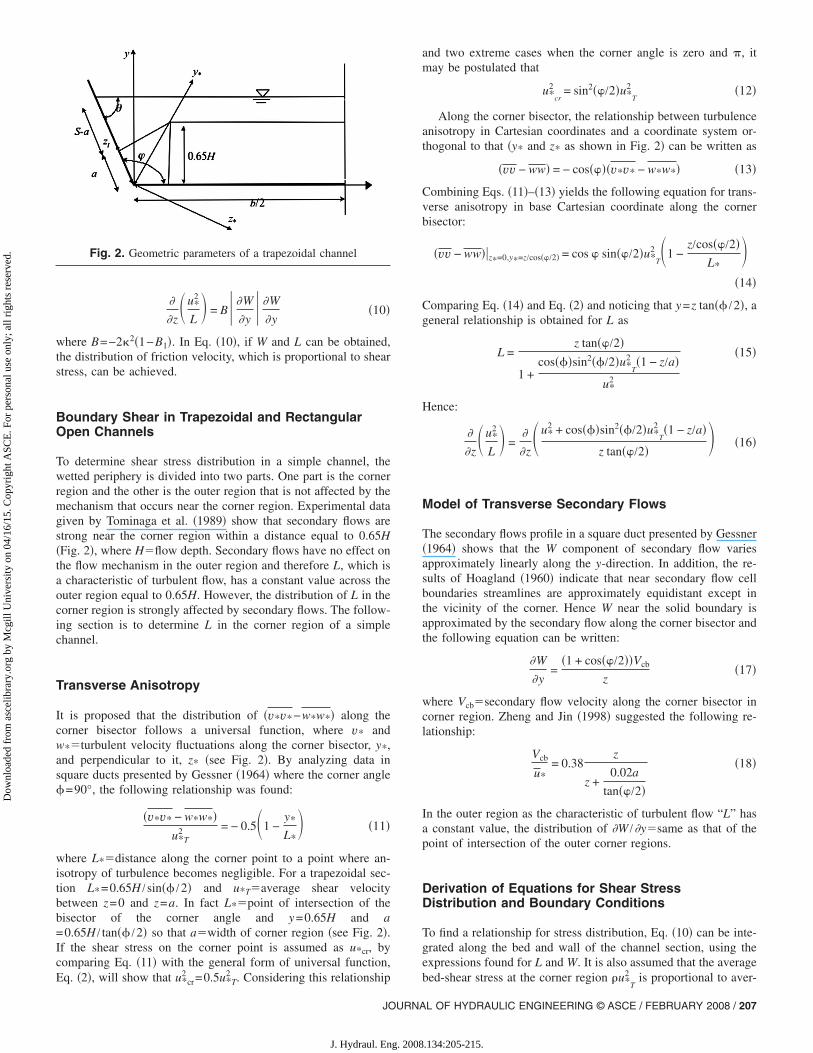
In compound channels in addition to the effect of the channelsurface and free surface, the strong shear layer between the floodplain and the main channel affects turbulence anisotropy. Theshear layer is generated because of the differences between veloc-ity in the main channel and the flood plain. The shear layer causesmomentum transfer between the main channel and the flood plainand generates two secondary flows. The region that is stronglyaffected by shear layer is called the interaction region. By con-sidering the effect of wall, bed, free surface, and shear layer, thewetted periphery of a compound channel can be divided into dif-ferent parts that are shown in Fig. 3.

Measurements show that near the zone of interaction, bed-

Fig. 3. Geometric parameters of compound channel

shear stress suddenly increases �Shiono and Knight 1991�. Studies

8

.134:205-215.

Dow

nloa

ded

from

asc

elib

rary

.org

by

Mcg

ill U

nive

rsity

on

04/1

6/15

. Cop

yrig

ht A

SCE

. For

per

sona

l use

onl

y; a

ll ri

ghts

res

erve

d.

by Shiono and Knight also demonstrated that the effect of shearlayer on shear stress distribution decreases �shear stress distribu-tion becomes more uniform� as the relative depth, that is, floodplain depth divided by the main channel depth, increases. Byusing the shear stress distribution given by Rajaratnam and Ah-madi �1981� for different relative depths �h /H�, the width of theinteraction zone �z0�, can be correlated to the width of flood plain�bfp� and relative depth as follows:

z0 = 0.026827�e�−2.812148�h/H−1�� − 1�bfp �23�

Lateral Stress Distribution along the Bed of FloodPlain

The bed of the flood plain is divided into three parts. The first partis a corner region that is not affected by the shear layer anddistribution of �ww−vv� is like that of a simple channel. Thesecond part is the outer region with no effect from the shear layerand the corner region and the third part is the interaction regionthat is strongly affected by the shear layer. For the distribution of�ww−vv� in a compound channel, only one set of experimentaldata is available �Tominaga and Nezu 1991�. Based on these dataL has a constant value in the outer region of the flood plain and alinear distribution for L is assumed in the interaction region.

Also, the distribution of W can be attained by a formula givenby Tominaga et al. �1989�:

W = Wmax�1 −2y

h� �24�

Considering that Wmax is a function of average shear stress alongthe flood plain bed, Eq. �10� can be integrated to find the follow-ing equation for the bed of the flood plain:

�bfp

�bfp= A1� z

z0�2

+ B1� z

z0� + C1, 0 � z � z0 �25�

�bfp

�bfp= A2� z

z0� + B2, z0 � z � b − a �26�

�bfp

�bfp= A3

−z − b

b

−z − b

b+ 0.02

a

b

− B3

z − b

b, b − a � z � b �27�

Eqs. �25�–�27� are used to calculate shear stress distribution alongthe flood plain bed. Coefficients A1, A2, A3, B1, B2, B3, and C1 canbe estimated from the boundary conditions and shear stress at themidpoint of the flood plain which can be calculated as follows.

As the flood plain is usually wide, the effect of shear layer isthus negligible at the midpoint of the flood plain. Therefore, arelationship like the exponential equation given by Knight et al.�1984� is derived here from data of Rajaratnam and Ahmadi�1981� for shear stress at the midpoint of the flood plain:

�cl

�ghSf= 1.37�1 − e−�bfp/2h�0.55

� �28�

where ��fluid density; g�gravitational acceleration; and Sf�isfriction slope. From the boundary conditions and Eq. �28�, six ofseven unknown coefficients can be determined. Comparison ofthe results of the developed model with experimental data given

by Rajaratnam and Ahmadi �1981� showed that A3 can be as-

JOURNA

J. Hydraul. Eng. 2008

sumed to have a constant value of 0.75 for the whole rangeof experiments. All calculated coefficients are given in theAppendix.

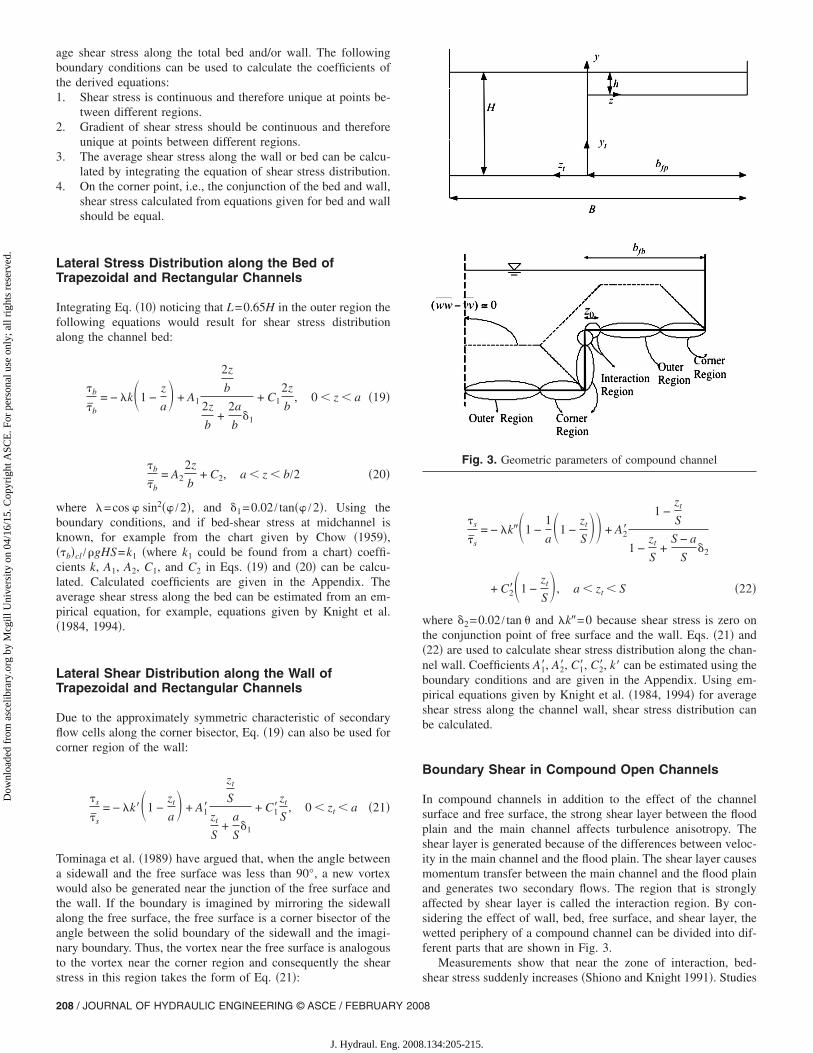
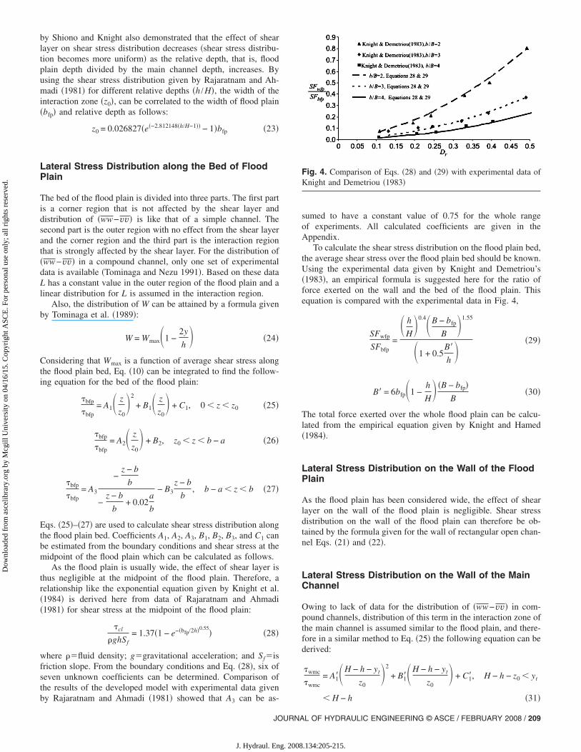
To calculate the shear stress distribution on the flood plain bed,the average shear stress over the flood plain bed should be known.Using the experimental data given by Knight and Demetriou’s�1983�, an empirical formula is suggested here for the ratio offorce exerted on the wall and the bed of the flood plain. Thisequation is compared with the experimental data in Fig. 4,

SFwfp

SFbfp=� h

H�0.4�B − bfp

B�1.55

�1 + 0.5B�

h� �29�

B� = 6bfp�1 −h

H� �B − bfp�

B�30�

The total force exerted over the whole flood plain can be calcu-lated from the empirical equation given by Knight and Hamed�1984�.

Lateral Stress Distribution on the Wall of the FloodPlain

As the flood plain has been considered wide, the effect of shearlayer on the wall of the flood plain is negligible. Shear stressdistribution on the wall of the flood plain can therefore be ob-tained by the formula given for the wall of rectangular open chan-nel Eqs. �21� and �22�.

Lateral Stress Distribution on the Wall of the MainChannel

Owing to lack of data for the distribution of �ww−vv� in com-pound channels, distribution of this term in the interaction zone ofthe main channel is assumed similar to the flood plain, and there-fore in a similar method to Eq. �25� the following equation can bederived:

�wmc

�wmc= A1��H − h − yt

z0�2

+ B1��H − h − yt

z0� + C1�, H − h − z0 � yt

Fig. 4. Comparison of Eqs. �28� and �29� with experimental data ofKnight and Demetriou �1983�

� H − h �31�

L OF HYDRAULIC ENGINEERING © ASCE / FEBRUARY 2008 / 209

.134:205-215.

Dow

nloa

ded

from

asc

elib

rary

.org

by

Mcg

ill U

nive

rsity

on

04/1

6/15

. Cop

yrig

ht A

SCE

. For

per

sona

l use

onl

y; a

ll ri

ghts

res

erve

d.

By simulating the corner region of the main channel with thecorner region of a rectangular channel with a=H−h−z0 �Fig. 3�,shear stress on this region can be written as

�wmc

�wmc= A2�

yt

H − h

yt

H − h+

H − h − z0

H − h1

+ C2�yt

H − h, 0 � yt � H − h − z0

�32�

Like previous equations, coefficients of these equations can beobtained by applying the boundary conditions and are given in theAppendix. From the boundary conditions, however, only four offive unknown coefficients can be determined. Through compari-son with experimental data given by Rajaratnam and Ahmadi�1981�, the fifth coefficient, C2�, was calculated to be equal to0.75.

As before, the average shear stress on the main channel bedand wall are necessary to be known. By using Knight and Dem-etriou’s �1983� experimental data average shear stress on wall andbed of the main channel can be calculated.

Lateral Stress Distribution on the Bed of the MainChannel

The effect of the shear layer on shear stress distribution along thebed of the main channel is only limited to the corner secondaryflow. Hence for calculating bed-shear stress of the main channel,Eqs. �19� and �20� for shear stress distribution along the rectan-gular channel bed can be used by substituting a=H−h−z0.

Comparison of Results with Experimental andNumerical Data

Rectangular Channels

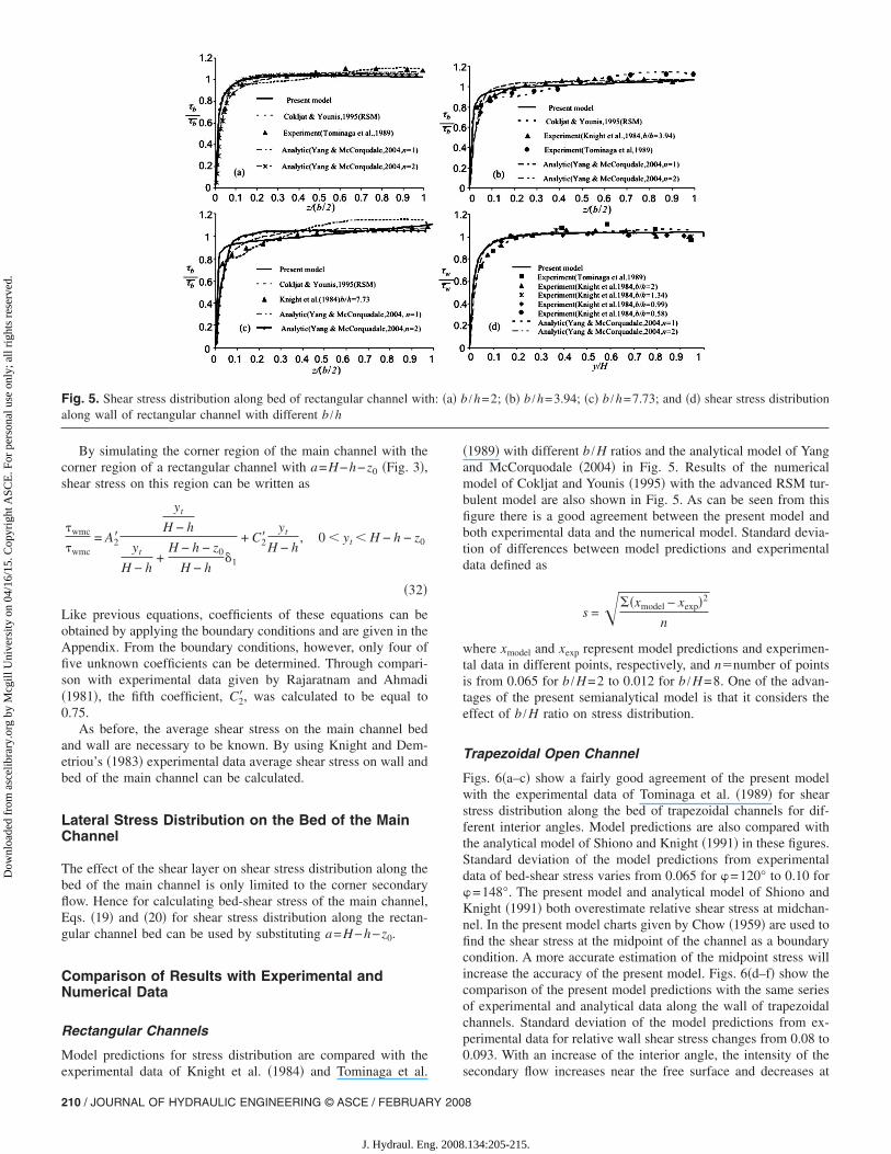
Model predictions for stress distribution are compared with the

Fig. 5. Shear stress distribution along bed of rectangular channel withalong wall of rectangular channel with different b /h

experimental data of Knight et al. �1984� and Tominaga et al.

210 / JOURNAL OF HYDRAULIC ENGINEERING © ASCE / FEBRUARY 200

J. Hydraul. Eng. 2008

�1989� with different b /H ratios and the analytical model of Yangand McCorquodale �2004� in Fig. 5. Results of the numericalmodel of Cokljat and Younis �1995� with the advanced RSM tur-bulent model are also shown in Fig. 5. As can be seen from thisfigure there is a good agreement between the present model andboth experimental data and the numerical model. Standard devia-tion of differences between model predictions and experimentaldata defined as

s =� �xmodel − xexp�2

n

where xmodel and xexp represent model predictions and experimen-tal data in different points, respectively, and n�number of pointsis from 0.065 for b /H=2 to 0.012 for b /H=8. One of the advan-tages of the present semianalytical model is that it considers theeffect of b /H ratio on stress distribution.

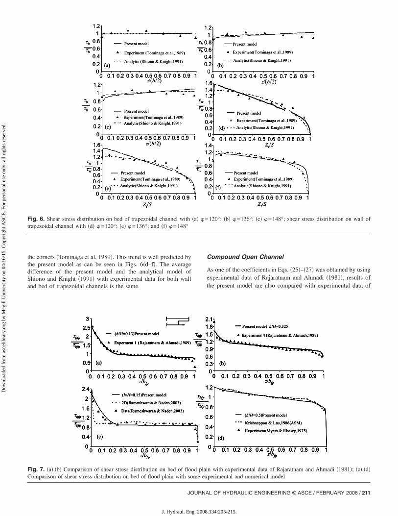
Trapezoidal Open Channel

Figs. 6�a–c� show a fairly good agreement of the present modelwith the experimental data of Tominaga et al. �1989� for shearstress distribution along the bed of trapezoidal channels for dif-ferent interior angles. Model predictions are also compared withthe analytical model of Shiono and Knight �1991� in these figures.Standard deviation of the model predictions from experimentaldata of bed-shear stress varies from 0.065 for �=120° to 0.10 for�=148°. The present model and analytical model of Shiono andKnight �1991� both overestimate relative shear stress at midchan-nel. In the present model charts given by Chow �1959� are used tofind the shear stress at the midpoint of the channel as a boundarycondition. A more accurate estimation of the midpoint stress willincrease the accuracy of the present model. Figs. 6�d–f� show thecomparison of the present model predictions with the same seriesof experimental and analytical data along the wall of trapezoidalchannels. Standard deviation of the model predictions from ex-perimental data for relative wall shear stress changes from 0.08 to0.093. With an increase of the interior angle, the intensity of the

/h=2; �b� b /h=3.94; �c� b /h=7.73; and �d� shear stress distribution

: �a� b

secondary flow increases near the free surface and decreases at

8

.134:205-215.

Dow

nloa

ded

from

asc

elib

rary

.org

by

Mcg

ill U

nive

rsity

on

04/1

6/15

. Cop

yrig

ht A

SCE

. For

per

sona

l use

onl

y; a

ll ri

ghts

res

erve

d.

the corners �Tominaga et al. 1989�. This trend is well predicted bythe present model as can be seen in Figs. 6�d–f�. The averagedifference of the present model and the analytical model ofShiono and Knight �1991� with experimental data for both walland bed of trapezoidal channels is the same.

Fig. 6. Shear stress distribution on bed of trapezoidal channel withtrapezoidal channel with �d� �=120°; �e� �=136°; and �f� �=148°

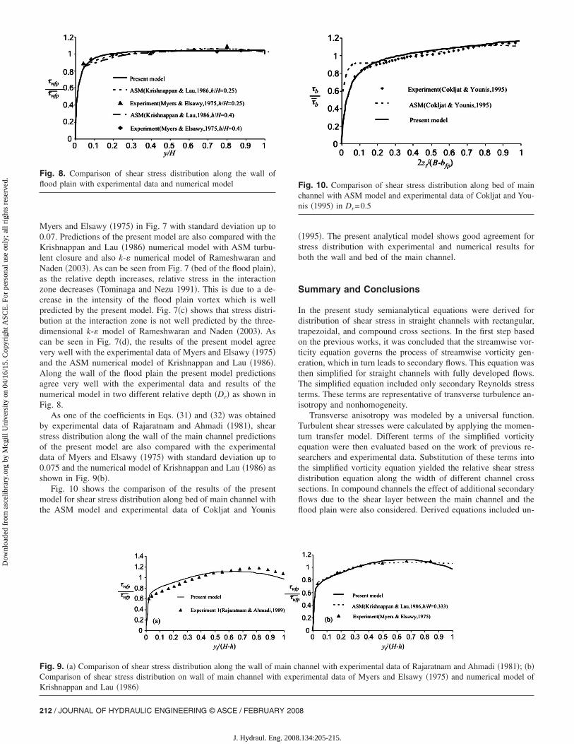
Fig. 7. �a�,�b� Comparison of shear stress distribution on bed of flooComparison of shear stress distribution on bed of flood plain with so

JOURNA

J. Hydraul. Eng. 2008

Compound Open Channel

As one of the coefficients in Eqs. �25�–�27� was obtained by usingexperimental data of Rajaratnam and Ahmadi �1981�, results ofthe present model are also compared with experimental data of

120°; �b� �=136°; �c� �=148°; shear stress distribution on wall of

n with experimental data of Rajaratnam and Ahmadi �1981�; �c�,�d�perimental and numerical model

�a� �=

d plaime ex

L OF HYDRAULIC ENGINEERING © ASCE / FEBRUARY 2008 / 211

.134:205-215.

Dow

nloa

ded

from

asc

elib

rary

.org

by

Mcg

ill U

nive

rsity

on

04/1

6/15

. Cop

yrig

ht A

SCE

. For

per

sona

l use

onl

y; a

ll ri

ghts

res

erve

d.

Myers and Elsawy �1975� in Fig. 7 with standard deviation up to0.07. Predictions of the present model are also compared with theKrishnappan and Lau �1986� numerical model with ASM turbu-lent closure and also k-� numerical model of Rameshwaran andNaden �2003�. As can be seen from Fig. 7 �bed of the flood plain�,as the relative depth increases, relative stress in the interactionzone decreases �Tominaga and Nezu 1991�. This is due to a de-crease in the intensity of the flood plain vortex which is wellpredicted by the present model. Fig. 7�c� shows that stress distri-bution at the interaction zone is not well predicted by the three-dimensional k-� model of Rameshwaran and Naden �2003�. Ascan be seen in Fig. 7�d�, the results of the present model agreevery well with the experimental data of Myers and Elsawy �1975�and the ASM numerical model of Krishnappan and Lau �1986�.Along the wall of the flood plain the present model predictionsagree very well with the experimental data and results of thenumerical model in two different relative depth �Dr� as shown inFig. 8.

As one of the coefficients in Eqs. �31� and �32� was obtainedby experimental data of Rajaratnam and Ahmadi �1981�, shearstress distribution along the wall of the main channel predictionsof the present model are also compared with the experimentaldata of Myers and Elsawy �1975� with standard deviation up to0.075 and the numerical model of Krishnappan and Lau �1986� asshown in Fig. 9�b�.

Fig. 10 shows the comparison of the results of the presentmodel for shear stress distribution along bed of main channel withthe ASM model and experimental data of Cokljat and Younis

Fig. 8. Comparison of shear stress distribution along the wall offlood plain with experimental data and numerical model

Fig. 9. �a� Comparison of shear stress distribution along the wall of mComparison of shear stress distribution on wall of main channel witKrishnappan and Lau �1986�

212 / JOURNAL OF HYDRAULIC ENGINEERING © ASCE / FEBRUARY 200

J. Hydraul. Eng. 2008

�1995�. The present analytical model shows good agreement forstress distribution with experimental and numerical results forboth the wall and bed of the main channel.

Summary and Conclusions

In the present study semianalytical equations were derived fordistribution of shear stress in straight channels with rectangular,trapezoidal, and compound cross sections. In the first step basedon the previous works, it was concluded that the streamwise vor-ticity equation governs the process of streamwise vorticity gen-eration, which in turn leads to secondary flows. This equation wasthen simplified for straight channels with fully developed flows.The simplified equation included only secondary Reynolds stressterms. These terms are representative of transverse turbulence an-isotropy and nonhomogeneity.

Transverse anisotropy was modeled by a universal function.Turbulent shear stresses were calculated by applying the momen-tum transfer model. Different terms of the simplified vorticityequation were then evaluated based on the work of previous re-searchers and experimental data. Substitution of these terms intothe simplified vorticity equation yielded the relative shear stressdistribution equation along the width of different channel crosssections. In compound channels the effect of additional secondaryflows due to the shear layer between the main channel and theflood plain were also considered. Derived equations included un-

annel with experimental data of Rajaratnam and Ahmadi �1981�; �b�rimental data of Myers and Elsawy �1975� and numerical model of

Fig. 10. Comparison of shear stress distribution along bed of mainchannel with ASM model and experimental data of Cokljat and You-nis �1995� in Dr=0.5

ain chh expe

8

.134:205-215.

Dow

nloa

ded

from

asc

elib

rary

.org

by

Mcg

ill U

nive

rsity

on

04/1

6/15

. Cop

yrig

ht A

SCE

. For

per

sona

l use

onl

y; a

ll ri

ghts

res

erve

d.

known coefficients resulting from integration and simplifying as-sumptions. Most of these coefficients were calculated from theboundary conditions.

Predictions of the model when compared with experimentaldata of rectangular, trapezoidal, and compound open channelsshowed good agreement. Results of the model were also com-pared with predictions of other analytical as well as three-dimensional numerical models with k-� and RSM closure withgood agreement. This supports the validity of the model assump-tions and the ability of the model to predict shear stress distribu-tion in different open channel cross sections similar to complexnumerical models.

Acknowledgments

This research was supported in part by the Natural Science andEngineering Research Council of Canada. A student grantawarded to this work by the Ministry of Power in Iran is alsoappreciated.

Appendix. Summary of Coefficients

Coefficients of Eqs. �19� and �20�:

A1 =

1 +k

2−

K1

K2

2m

n+

�n − 4 − 21�2n

, A2 =K1

K2− C2

C1 =K1

K2+ k�1 −

n

2� −

A1

�1 + 1�2�1n

2+ 1�, C2 =

A1

�1 + 1�2 − k

K1 =��b�cl

�gHSf, K2 =

�̄b

�gHSf

j =2m

n+

n − 4 − 21

2n, f = n + n − , n =

b

a,

m = 1 − 1 ln�1 +1

1�, k = ko =

1 + �− 0.5 +j

e�

f j

e−

2

= cos���sin2��/2�

Coefficients of Eqs. �21� and �22�:

A1� =q

rf��1 + 2�2 −k�e�

f�, A2� =

1

��1 − A1�� +

k�

2�

C1� = A2�1

q�1 + 2�+ C2�

1 − q

q−

A1�

q�1 + 1�,

C2� =A1�

�1 + 12�0.5 − k� + A2�

�− 1 − 2 + q��1 − q��1 + 2�2

K2 =�̄b , K3 =

�̄s

�gHSf �gHSf

JOURNA

J. Hydraul. Eng. 2008

q =a

S= 1.3 cos2 ��/2�, m� = 1 − 2 ln�1 +

1

2�,

m = 1 − 1 ln�1 +1

1�, k� =

K2

K3k

� = qm −q

2�1 + 1�+

1 − q

2�1 + 1�2

� = m��1 − q� +q

2�1 + 2�+

�− 1 − 2 + q�2�1 + 2�2

f� =1 + q

�1 + 1�2 − 2m +q�

��1 + 2�2 e� = 2 + 2 − q −q

2��1 + 2�2

Coefficients of Eqs. �25�–�27�:

A1 =3bfp

z0�1 −

k1fp

k2fp� − n�

2z0

bfp� A3

�1 + 1�−

k1fp

k2fp�

A2 =2z0

bfp� A3

�1 + 1�2 −k1fp

k2fp�

A3 = 0.75, B1 = A2 − 2A1

B2 =k1fp

k2fp− A2

bfp

2z0, B3 = − 1

k1fp

k2fp

bfp

a− A2

2abfp + 1bfp2

2az0

C1 = A1 +k1fp

k2fp− A2

bfp

2z0

k1fp =�cl

�ghSf= 1.37�1 − e�−� bfp

2h�0.55��, k2fp =

�̄bfp

�ghSf

m = 1 − 1 ln�1 +1

1�, � = 1 −

a

b�1 − m�1 + 1�2 + 0.51�

n� = 0.25a

z0�− 2 + 2m�1 + 1�2 − 1�

Coefficients of Eqs. �31� and �32�:

A1� = C1� − C2� − A1�t, A2� =− 1

t��1 − C1�

t

3+ C2�

3 − 2t

6�

B1� =− z0

H − h�C2� +

A1�1

�1 − t��1 + 1�2� − 2A1�

C1� = C1�̄bfp

�wmc, C2� = 0.75

t� = �1 − t�m +tt�

6+

t

2�1 + 1�, t� =

1 + 1 − t

�1 − t��1 + 1�2 , t =z0

H − h

Notation

The following symbols are used in this paper:A1, B1, C1, A2, B2, C2, A3, B3, C3

� bed-shear stress distribution coefficients;A1�, B1�, C1�, A2�, B2�

� wall shear stress distribution coefficients;

L OF HYDRAULIC ENGINEERING © ASCE / FEBRUARY 2008 / 213

.134:205-215.

Dow

nloa

ded

from

asc

elib

rary

.org

by

Mcg

ill U

nive

rsity

on

04/1

6/15

. Cop

yrig

ht A

SCE

. For

per

sona

l use

onl

y; a

ll ri

ghts

res

erve

d.

a � width of comer region;B � half of compound channel width;b � bed width of rectangular or trapezoidal

channel;bfp � flood plain width;

g � gravitational acceleration;H � flow depth;h � flow depth in flood plain;

k, k� � ratio of average shear stress in the cornerregion to average shear stress on bed andsidewall;

L � characteristic length where �vv-ww�=0;L* � distance along the corner point to a point

where isotropic turbulence occurs;ly, lz � mixing length y- and z-directions;

p � pressure;S � wall length;

Sf � friction slope;SFwfp, SFbfp � force exerted on the wall and the bed of the

flood plain, respectively;s � wall slope of trapezoidal channel;

U, V, W � time averaged velocity components along x-,y-, and z-directions;

u* � averaged shear velocity;u, v, w � turbulent fluctuation components along x-,

y-, and z-directions, respectively;u* � friction velocity;

u*dc� average friction velocity at corner region;

u*cr � shear stress on the corner point;u*T

� average shear velocity at corner region;Vcb � secondary flow velocity along the corner

bisector in corner region;v*, w* � turbulent fluctuation components along the

corner bisector and perpendicular to thebisector;

zo � width of the interaction zone in thecompound channel;

2 � function of free surface angle with thesidewall;

�y, �z � eddy viscosity coefficients in y- andz-directions;

� � free surface angle with the sidewall;� � von Kármán constant;

, l � function of corner angle;� � fluid density;

�b, �s � average bed and side wall shear stress;�wfp, �bfp � average shear stress along wall and bed of

the flood plain;�wmc, �bmc � average shear stress along wall and bed of

the main channel;�b, �s � bed and side wall shear stress;

�cl � shear stress at the midpoint of the floodplain;

�wfp, �bfp � shear stress at wall and bed of the floodplain;

�wmc, �bmc � shear stress at wall and bed of the mainchannel; and

� � corner angle.

References

Aly, A. M. M., Trupp, A. C., and Gerard, A. D. �1978�. “Measurement

and prediction of fully developed turbulent flow in an equilateral tri-

214 / JOURNAL OF HYDRAULIC ENGINEERING © ASCE / FEBRUARY 200

J. Hydraul. Eng. 2008

angular duct.” J. Fluid Mech., 85�1�, 57–83.Chow, V. T. �1959�. Open channel hydraulics, McGraw-Hill, New York.Cokljat, D., and Younis, B. A. �1995�. “Second-order closure study of

open-channel flows.” J. Hydraul. Eng., 121�2�, 94–107.Demuren, A. O., and Rodi, W. �1984�. “Calculation of turbulent-driven

secondary motion in non-circular ducts.” J. Fluid Mech. Digit. Arch.,140, 189–222.

Flintham, T. P., and Carling, P. A. �1988�. “The prediction of mean bedand wall boundary shear stress in uniform and compositely roughchannels.” Proc., Int. Conf. on River Regime, W. R. White, ed., Wiley,Chichester, 267–287.

Gerard, R. �1978�. “Secondary flow in non-circular conduits.” J. Hydraul.Eng., 104�5�, 755–773.

Gessner, F. B. �1964�. “Turbulence and mean flow characteristics in rect-angular channels.” Ph.D. thesis, Purdue Univ., West Lafayette, Ind.

Gessner, F. B., and Emery, A. F. �1980�. “Numerical prediction of devel-oping turbulent flow in rectangular duct.” J. Fluids Eng., 103�3�,445–455.

Hoagland, L. C. �1960�. “Fully developed turbulent flow in straight rect-angular ducts-secondary flow, its cause and effect on the primaryflow.” Ph.D. thesis, Dept. of Mechanical Engineering, MIT,Cambridge.

Jin, Y. C., Zarrati, A. R., and Zheng, Y. �2004�. “Boundary shear distri-bution in straight ducts and open channels.” J. Hydraul. Eng., 130�9�,924–928.

Kawahara, Y., and Tamai, N. �1988�. “Numerical calculation of turbulentflows in compound channels with an algebraic stress turbulencemodel.” Proc., 3rd Int. Symp. on Refined Flow Modeling and Turbu-lence Measurements, Y. Iwasa, N. Tamai, and A. Wada, eds., Tokyo,527–536.

Keller, R. J., and Rodi, W. �1988�. “Prediction of flow characteristics inmain channel flood plain flows.” J. Hydraul. Res., 26�4�, 425–441.

Khodashenas, S. R., and Paquier, A. �1999�. “A geometrical method forcomputing the distribution of boundary shear across irregular straightopen channels.” J. Hydraul. Res., 37�3�, 381–388.

Knight, D. W., and Demetriou, J. D. �1983�. “Flood plain and main chan-nel flow interaction.” J. Hydraul. Eng., 109�8�, 1073–1092.

Knight, D. W., Demetriou, J. D., and Hamed, M. E. �1984�. “Boundaryshear in smooth rectangular channels.” J. Hydraul. Eng., 110�4�, 405–422.

Knight, D. W., and Hamed, M. E. �1984�. “Boundary shear in symmetri-cal compound channel.” J. Hydraul. Eng., 110�10�, 1412–1430.

Knight, D. W., and Patel, H. S. �1985�. “Boundary shear in smooth rect-angular ducts.” J. Hydraul. Eng., 111�1�, 29–47.

Knight, D. W., and Shiono, K. �1990�. “Turbulent measurements in ashear layer region of a compound channel.” J. Hydraul. Res., 28�2�,175–196.

Knight, D. W., Yuen, K. W. H., and Alhamid, A. A. �1994�. “Boundaryshear stress distribution in open channel flow.” Mixing and transportin the environment, K. J. Beven, P. C. Chatwin, and J. H. Millbank,eds., Wiley, New York, 51–87.

Krishnappan, B. G., and Lau, Y. L. �1986�. “Turbulence modeling offlood plain flows.” J. Hydraul. Eng., 112�4�, 251–266.

Myers, W. R. C., and Elsawy, E. M. �1975�. “Boundary shear in channelwith flood plain.” J. Hydr. Div., 101�7�, 933–946.

Naot, D., Nezu, I., and Nakagawa, H. �1993a�. “Calculation ofcompound-open-channel flow.” J. Hydraul. Eng., 119�12�, 1418–1426.

Naot, D., Nezu, I., and Nakagawa, H. �1993b�. “Hydrodynamic behaviorof compound rectangular open channels.” J. Hydraul. Eng., 119�3�,390–408.

Nezu, I., and Nakagawa, H. �1993�. Turbulence in open channel flows,IAHR Series, A. A. Balkema, Rotterdam, The Netherlands.

Perkins, H. J. �1970�. “The formation of streamwise vorticity in turbu-lence flow.” J. Fluid Mech., 44�4�, 721–740.

Pezzinga, G. �1994�. “Velocity distribution in compound channel flowsby numerical modeling.” J. Hydraul. Eng., 120�10�, 1176–1198.

Rajaratnam, N., and Ahmadi, R. �1981�. “Hydraulics of channels with

8

.134:205-215.

Dow

nloa

ded

from

asc

elib

rary

.org

by

Mcg

ill U

nive

rsity

on

04/1

6/15

. Cop

yrig

ht A

SCE

. For

per

sona

l use

onl

y; a

ll ri

ghts

res

erve

d.

flood-plains.” J. Hydraul. Res., 19�1�, 43–60.Rameshwaran, P., and Naden, P. S. �2003�. “Three-dimensional numerical

simulation of compound channel flows.” J. Hydraul. Eng., 129�8�,645–652.

Rhodes, D. G., and Knight, D. W. �1994�. “Distribution of shear force onboundary of smooth rectangular channels.” J. Hydraul. Eng., 120�7�,787–806.

Shiono, K., and Knight, D. W. �1991�. “Turbulent open channel flow withvariable depth across the channel.” J. Fluid Mech. Digit. Arch., 222,617–646.

Sofialidis, D., and Prinos, P. �1998�. “Compound open-channel flow mod-eling with nonlinear low-Reynolds k-� models.” J. Hydraul. Eng.,124�3�, 253–261.

Sofialidis, D., and Prinos, P. �1999�. “Numerical study of momentum

exchange in compound open channel.” J. Hydraul. Eng., 125�2�,

JOURNA

J. Hydraul. Eng. 2008

152–164.Thomas, T. G., and Williams, J. J. R. �1995�. “Large eddy simulation of

turbulent flow in an asymmetric compound channel.” J. Hydraul.Res., 33�1�, 27–41.

Tominaga, A., and Nezu, I. �1991�. “Turbulent structure in compoundopen channel flows.” J. Hydraul. Eng., 117�1�, 21–41.

Tominaga, A., Nezu, I., Ezaki, K., and Nakagawa, H. �1989�. “Three-dimensional turbulent structure in straight open channel flows.” J.Hydraul. Res., 27�1�, 149–173.

Yang, S.-Q., and McCorquodale, J. A. �2004�. “Determination of bound-ary shear stress and Reynolds shear stress in smooth rectangular chan-nel flows.” J. Hydraul. Eng., 130�5�, 458–462.

Zheng, Y., and Jin, Y. C. �1998�. “Boundary shear in rectangular ducts

and channels.” J. Hydraul. Eng., 124�1�, 86–89.

L OF HYDRAULIC ENGINEERING © ASCE / FEBRUARY 2008 / 215

.134:205-215.