


Bahasa
Halaman
Hukum

Elsevier Editorial System(tm) for Remote Sensing of Environment Manuscript Draft Manuscript Number: RSE-D-10-00458R1 Title: Satellite-based estimates of groundwater storage variations in large drainage basins with extensive floodplains Article Type: Short Communication Keywords: groundwater; remote sensing; hydrological modelling Corresponding Author: Dr. Frédéric Frappart, PhD Corresponding Author's Institution: Université de Toulouse First Author: Frédéric Frappart, PhD Order of Authors: Frédéric Frappart, PhD; Fabrice Papa, PhD; Andreas Güntner, PhD; Susanna Werth, PhD; Joecila Santos da Silva, PhD; Javier Tomasella, PhD; Frédérique Seyler, PhD; Catherine Prigent, PhD; William B Rossow, PhD; Stéphane Calmant, PhD; Marie-Paule Bonnet, PhD
hal-0
0582
647,
ver
sion
1 -
3 Ap
r 201
1Author manuscript, published in "Remote Sensing of Environment / Remote Sensing of the Environment 115, 6 (2011) 1588-1594"
DOI : 10.1016/j.rse.2011.02.003

Ref.: RSE-D-10-00458
Total water storage decomposition and estimates of groundwater variations in the Negro
River Basin
Dear Frédéric,
Two reviews of your paper follow. The third reviewer has evidently moved and left no
forwarding address, so we will not have a review from him and will rely on these two.
They are quite positive, but Reviewer #1 recommends some refocus and that the
evidence that the modeling is accurate needs to be stronger.
Please carefully consider the comments and recommendations below and make
appropriate changes to the paper. Publication depends on revision and/or rebuttal of
the criticisms made. Further review and revision may be necessary before a final
decision can be made.
When you submit your revised paper, please provide a summary of the changes you
have made and your responses to the review comments and recommendations.
To submit a revision, go to http://ees.elsevier.com/rse/ and log in as an Author. You will
see a menu item called "Submission Needing Revision." You will find your submission
record there. Please remove any items that have changed or are no longer needed before
uploading your revised manuscript.
Please upload your original files, not PDF files. If you have any problems or questions
when uploading your revised manuscript, please contact Betty Schiefelbein at:
I hope that you will undertake the necessary revisions and will look forward to receiving
your revised paper.
Sincerely,
Marvin Bauer
Editor-in-Chief
Remote Sensing of Environment
Dear Marvin Bauer,
Editor-in-Chief
Remote Sensing of Environment
Please find enclosed the revised version of our manuscript now entitled "Satellite-based
estimates of groundwater storage variations in large drainage basins with extensive
floodplains ". We have taken into account their constructive comments to improve the quality
of the manuscript.
As suggested by Reviewer 1, we modified the title of the manuscript and added a new figure
presenting a) the annual amplitude of the GRACE-based GW seasonal amplitude, b) the
hydrologeological of Brazil from the Departamento Nacional da Produção Mineral (1983) to
show the reader the similarities between our estimates and the hydrogeological structures in
Response to reviews and summary of revisionsha
l-005
8264
7, v
ersi
on 1
- 3
Apr 2
011
the Negro River basin. We explained why this comparison is relevant to validate qualitatively
our approach. If the seasonal amplitudes of groundwater storage variations will most probably
change with the climate forcing of a particular period, i.e., decrease during an El Niño event
as in our case, the spatial patterns of variations will persist even for non-average conditions.
We also added in the introduction some sentences on the important role of the floodplains in
the hydrological cycle.
We responded Reviewer 3 concerning the type of approach used to filter the GRACE data and
added some information about the characteristics of the Negro River basin.
We responded on the scale problem concerning the comparison between the GRACE-derived
GW anomalies and the in situ measurements pointed out by the two Reviewers.
We hope these modifications will satisfy the Reviewers comments.
We are looking forward to hearing from you.
Sincerely yours,
Frédéric Frappart, Fabrice Papa, Andreas Güntner, Susanna Werth, Joecila Santos da Silva,
Javier Tomasella, Frédérique Seyler, Catherine Prigent, William B. Rossow, Stéphane
Calmant, Marie-Paule Bonnet
==============================
Comments from the Reviewers:
Reviewer #1:
This study combines a variety of data and models regarding water levels in various
components of the water system in the Negro Basin, South America during 2003-2004.
The study starts from GRACE measurements of total water storage (TWS) variations
during this time. Then these variations are broken up into variations occurring in the
surface water (SW), root zone (RZ), and groundwater (GW) reservoirs (as in equation
1). In particular, SW is constrained by satellite measurements and in situ observations,
and RZ from a hydrological model. The authors are then able to solve for GW by
removing RZ and SW from the TWS measurements of GRACE. To verify the solution
for groundwater, the authors compare to hydrological maps to see if the results seem
reasonable.
The authors have thus outlined a method for detecting temporal variations in
groundwater storage using GRACE satellite measurements and a variety of additional
measurements and models to remove the contributions from SW and RZ. Although
similar methods have been used to constrain groundwater variations on a basin-scale
(for example, the authors cite Yeh et al., 2006; Rodell et al, 2009; Leblanc et al 2009),
this is the first time this method has been performed in a region dominated by wetlands.
The manuscript is reasonably well-written. However, I am concerned about a few issues
that relate to verification of the method and to importance with respect to the broader
hydrological community. First, it seems to me that this manuscript describes a method
for estimating groundwater variations in a wetland environment, but it is presented as
an investigation of the hydrology of the Negro basin. In fact, I don't think the
manuscript tells us anything new about the Negro basin, and therefore I think the focus
of the paper should be altered. I describe my thoughts on this in more detail in points 1
hal-0
0582
647,
ver
sion
1 -
3 Ap
r 201
1

and 2 below. Second, the method that the authors describe should, in principle, be able
to constrain variations in groundwater in a wetland basin (otherwise their method is not
useful). However, the authors only compare ground water variations obtained using
their method to a hydrogeological map of Brazil (and don't show the map), and to
groundwater measurements in a single location (the Asu catchment) for which the fit is
not that great (see Fig. 3a). Thus, I think the authors need to do a better job in
demonstrating that their method is accurately constraining actual variations in
groundwater. I describe these concerns below in points 3-5 below.
If the issues I list below can be addressed, then I think that the manuscript could be
published. In the meantime, I am recommending "major revision".
We would like to thank Reviewer 1 for carefully reading our manuscript and for providing us
with useful/interesting comments, which helped us to improve our paper.
1. This study was performed in the Negro Basin, South America during 2003-2004,
because this is a location and time period for which sufficient data exists. I am not aware
of an alternative reason for estimating the groundwater variations in this time and
location - if there is some other reason for choosing the Negro Basin (e.g., there is
persistent aquifer depletion there, or a drought), then the authors should stress this
more clearly. If the authors are not addressing any groundwater issues related to the
Negro basin, then they should stress that the point of this study is method development
and verification, and they are just using the Negro Basin to test their method. Also, in
this case, I think that the title the authors chose is slightly misleading because of its
mention of the Negro Basin. Instead, the title should be something like "A method for
estimating basin-scale groundwater storage variations in a wetland". The authors could
add "A case study from the Negro Basin 2003-2004" at the end.
Reviewer 1 is right: we present here a methodology to estimate groundwater variations in a
large river basin covered with extensive floodplains, and to our knowledge, this is the first
attempt in a such environment. We now mentioned this, both in the introduction and, in the
conclusion. The aim of this paper is not to address any groundwater issues specifically related
to the Rio Negro, but we chose the Negro River basin as a case study for our method because
we already successfully applied our methodology to estimate surface water volume variations
combining information on inundation extent from satellite images and water levels from radar
altimetry in this basin (Frappart et al., 2005; 2008).
As suggested by Reviewer 1, we modified the title of the paper to “Satellite-based estimates
of groundwater storage variations in large basins with extensive floodplains”.
2. Furthermore, given that others have estimated groundwater storage variations by
combining GRACE and surface water measurements, the angle that is new in this
manuscript is the application to a drainage basin dominated by wetlands. Thus, I think
that the authors need to stress some of the challenges that are presented by the
application to wetlands. Why is performing this type of analysis in a wetland different
from performing it in a desert or other environment? I think that this is because much
more accurate estimates of surface water fluctuations are necessary in a wetland region.
This should be stated clearly. For this study to be useful, the minimum requirements for
constraints on surface water variations should also be mentioned - how can a reader
hal-0
0582
647,
ver
sion
1 -
3 Ap
r 201
1
determine if their constraints on surface water variations are sufficient? Finally, I think
that a sentence or two about the need for better constraints on groundwater variations
in wetland regions is necessary - what are the major applications of such measurements,
and why is remote detection better than in situ measurements (wells)?
This paper follows two previous studies on the estimate of surface water storage in the Negro
basin, the first one on the methodology (Frappart et al., 2005), the second one on the
monitoring of the surface waters on the basin over 1993-2002 (Frappart et al., 2008), as
mentioned in part 3.1 Monthly water level maps.
The datasets used in this paper are very similar to the ones from Frappart et al. (2008): the
same multisatellite inundation product but which has been extended to the period 2003-2004,
a denser network of altimetry stations with more accurate water levels as ENVISAT RA-2
measurements are used instead of Topex/Poseidon.
In this previous study we found a maximum error of 23% of the annual surface water
variations. In this new study, taking into account the different sources of error, the maximum
error is reduced to ~ 11%. (See the part on surface water error estimates in 3.1 Water volume
variations for details on how this error was estimated (lines 188-200)).
We added in the introduction (lines 55-64) a paragraph on the role of floodplains and the
interest of using remote sensing information for large river basins instead of in situ as
generally for this information is missing for most of the tropical basin, such as the Amazon:
“Although wetlands and floodplains cover only 6% of the Earth surface, they have a
substantial impact on flood flow alteration, sediment stabilization, water quality, groundwater
recharge and discharge (Maltby, 1991; Bullock and Acreman, 2003). Moreover, floodplain
inundation is an important regulator of river hydrology owing to storage effects along channel
reaches. Reliable and timely information about the extent, spatial distribution, and temporal
variation of wetlands and floods as well as the amount of water stored is crucial to better
understand their relationship with river discharges, and also their influence on regional
hydrology and climate. Remote sensing techniques are a unique mean for monitoring large
drainage basins climate and hydrology where in situ information is lacking (as, for instance,
over floodplains and wetlands or for groundwater monitoring)”.
Moreover, wells, especially in tropical areas are very sparse and will never provide a
complete view of GW variations nor resolve its variations on shorter "weather-like" time
scales, which we want to determine in order to investigate processes.
Besides, wells will never provide a complete map of GW for large areas nor, unless
continuously monitored, resolve its variations on shorter "weather-like" time scales, which we
want to determine in order to investigate processes.
3. I am concerned about the data and method that the authors use to verify their results.
The authors estimate the amplitude of groundwater variations (Fig. 1f) by removing SW
and RZ from TWS - this seems to be their main result. How can the authors know if
these results are correct? They compare their results to a hydrogeological map of the
Negro River Basin (see text, near line 197) and find that the GW variation pattern
"perfectly matches" the hydrological map. This is a qualitative result at best, especially
since the text in the sentences following line 197 is the only comparison that the authors
present. Only gross generalizations of the spatial variations in the seasonal cycle of
groundwater are presented and compared to the model predictions. I think that at a
minimum, some sort of quantitative measure of the groundwater variations should be
presented. For example, do the amplitudes of the estimated variations for 2003-2004
match those that are "predicted" by the hydrogeological map? Better, a reproduction of
hal-0
0582
647,
ver
sion
1 -
3 Ap
r 201
1
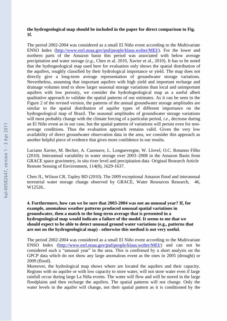
the hydrogeological map should be included in the paper for direct comparison to Fig.
1f.
The period 2002-2004 was considered as a small El Niño event according to the Multivariate
ENSO Index (http://www.esrl.noaa.gov/psd/people/klaus.wolter/MEI/). For the lower and
northern parts of the Amazon basin this period was associated with below average
precipitation and water storage (e.g., Chen et al. 2010, Xavier et al., 2010). It has to be noted
that the hydrogeological map used here for evaluation only shows the spatial distribution of
the aquifers, roughly classified by their hydrological importance or yield. The map does not
directly give a long-term average representation of groundwater storage variations.
Nevertheless, assuming that important aquifers with high yield and important recharge and
drainage volumes tend to show larger seasonal storage variations than local and unimportant
aquifers with low porosity, we consider the hydrologeological map as a useful albeit
qualitative approach to validate the spatial patterns of our estimates. As it can be seen in the
Figure 2 of the revised version, the patterns of the annual groundwater storage amplitudes are
similar to the spatial distribution of aquifer types of different importance on the
hydrogeological map of Brazil. The seasonal amplitudes of groundwater storage variations
will most probably change with the climate forcing of a particular period, i.e., decrease during
an El Niño event as in our case, but the spatial patterns of variations will persist even for non-
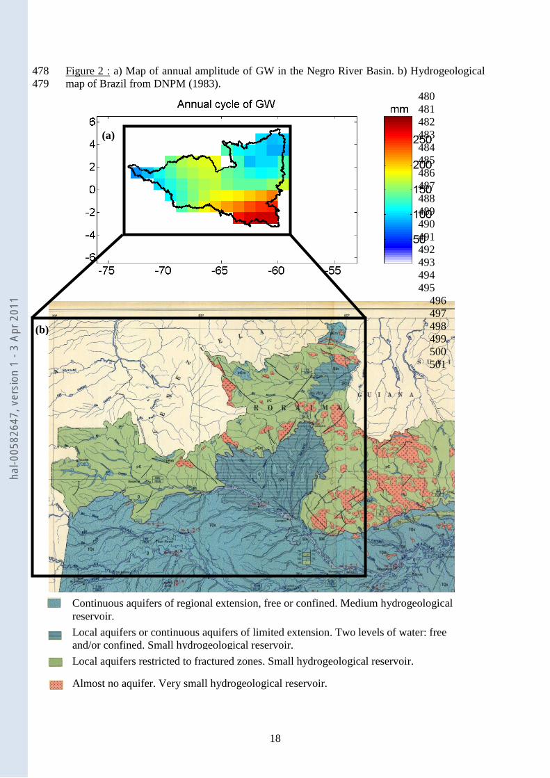
average conditions. Thus the evaluation approach remains valid. Given the very low
availability of direct groundwater observation data in the area, we consider this approach as
another helpful piece of evidence that gives more confidence in our results.
Luciano Xavier, M. Becker, A. Cazenave, L. Longuevergne, W. Llovel, O.C. Rotunno Filho
(2010). Interannual variability in water storage over 2003–2008 in the Amazon Basin from
GRACE space gravimetry, in situ river level and precipitation data Original Research Article
Remote Sensing of Environment, 114(8), 1629-1637.
Chen JL, Wilson CR, Tapley BD (2010). The 2009 exceptional Amazon flood and interannual
terrestrial water storage change observed by GRACE, Water Resources Research, 46,
W12526..
4. Furthermore, how can we be sure that 2003-2004 was not an unusual year? If, for
example, anomalous weather patterns produced unusual spatial variations in
groundwater, then a match to the long-term average that is presented in a
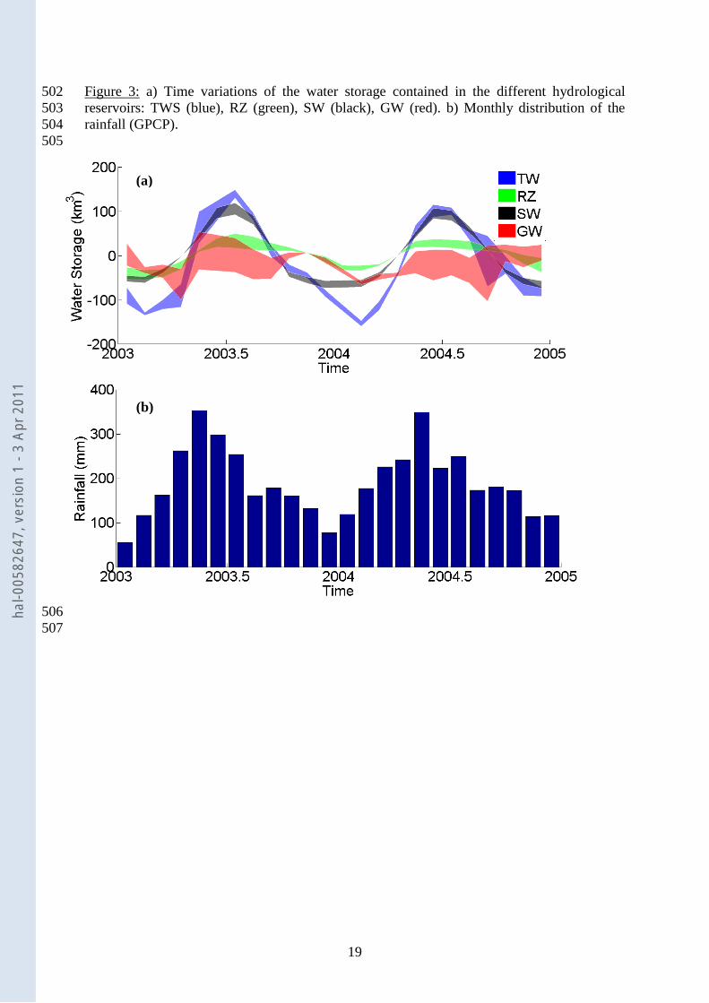
hydrogeological map would indicate a failure of the model. It seems to me that we
should expect to be able to detect unusual ground water variations (e.g., patterns that
are not on the hydrogeological map) - otherwise this method is not very useful.
The period 2002-2004 was considered as a small El Niño event according to the Multivariate
ENSO Index (http://www.esrl.noaa.gov/psd/people/klaus.wolter/MEI/) and can not be
considered such a “unusual year” in the area. This is confirmed by a short analysis on the
GPCP data which do not show any large anomalous event as the ones in 2005 (drought) or
2009 (flood).
Moreover, the hydrological map shows where are located the aquifers and their capacity.
Regions with no aquifer or with low capacity to store water, will not store water even if large
rainfall occur during large La Niña events. The water will flow and will be stored in the large
floodplains and then recharge the aquifers. The spatial patterns will not change. Only the
water levels in the aquifer will change, not their spatial pattern as it is conditioned by the
hal-0
0582
647,
ver
sion
1 -
3 Ap
r 201
1

storage capacity of the soil. As it can be seen in the Figure 2 of the revised version, the
patterns of the annual groundwater storage amplitudes are consistent with the spatial
distribution of aquifer types on the hydrogeological map of Brazil.
5. The authors do compare their results to in situ measurements of groundwater
variations from wells at the Asu micro-catchment. This direct comparison (Fig. 3a) is
exactly the type of constraints on the method that are needed. Yet, the authors' method
shows a very small variation in groundwater during 2003 (about 100 mm) when in fact
there was about 600 mm of variation. Although the method did much better in 2004, the
failure to predict 1 out of the 2 groundwater cycles does not give the reader a lot of
confidence in the method.
Unfortunately, we found only one small area where groundwater time variations are available.
The Asu micro-catchment has a drainage area of ~ 7 km² and is not directly connected to the
Negro River. As explained in the manuscript, we can not expect a perfect match between this
point-measurement and the GRACE encompassing gridpoint with area of ~10,000 km². The
interest of this comparison is to see that the timing is similar between the two datasets and that
the range of variations is similar. This is what we observe in Figure 4a.
Other points about the paper:
-- Line 100 - I think the figure callout should be Fig. 1b.
We added Fig. 1b to the callout and changed the legend of the other panels and the figure
caption. We modified the text accordingly.
-- Section 2.6. The authors describe how they use a hydrological model to constrain the
root zone water storage variations. It is unclear to the reader what inputs go into this
model, and what the uncertainty about the outputs - I think additional detail that
describes these aspects should be added. This is potentially important because I expect
there are tradeoffs between root zone storage and groundwater storage.
In this study, we did not pretend to have run neither WGHM nor LaD models. We are directly
using outputs from these two hydrological models. We suggest the readers to refer to the
articles describing these two models to obtain the information concerning the resolution of the
water balance equation and the allocation in the different water reservoirs (the references are
given in the text). No uncertainty is provided with the hydrological model estimates, however,
we followed a similar approach to the one proposed in previous studies such as Yeh et al.,
Water Resources Research, 2006; Rodell et al., Hydrogeology Journal, 2007; Strassberg et
al., Geophysical Research Letters, 2007; Leblanc et al., Water Resources Research, 2009;
Rodell et al., Nature, 2009; Sun et al., Geophysical Research Letters, 2010 and maybe some
others. The only difference is we use the outputs from two hydrological models instead of a
single one. The outputs of these two models exhibit very similar spatial and temporal patterns,
and also have similar amplitude differences. We used their extrema in equations (1) and (2) to
present a mean behaviour and a range of variations.
-- Line 137 - I think that the word "bathymetry" is usually used to mean "seafloor
hal-0
0582
647,
ver
sion
1 -
3 Ap
r 201
1

topography", and not the "unflooded land surface". I think that "land surface" would
be a better term here.
We changed bathymetry into land surface as suggested by Reviewer 1.
-- Line 206 (and earlier in the paragraph) - The authors describe the relative
"importance" of aquifers. This is a rather unquantitative term - I expect that there are
better ways of comparing the groundwater storage variations (see point 3 above)
We also wish we could use more quantitative data to compare our groundwater storage
variations. Unfortunately, it is the way the acquifers are mentioned on the one and only
hydrogeological map of Brazil which gives the boundaries of the aquifers and their relative
importance. We used it to evaluate the spatial patterns of our estimates. See our response to
point 3 above.
-- Fig. 3- For parts b and c, it is unclear to me from the caption whether the SW and GW
estimates are measured or inferred from the GW=TWS-SW-RZ method described here.
Furthermore, the authors state in the text that these two quantities should be the same
(since the water table is above the surface), but in that case, shouldn't SW already be
subtracted from out, and the GW should be zero?
To make it clearer, we modified Figure 4 (former Figure 3) caption as follows:
“Figure 4: a) Time variations of the GW storage in the Asu catchment (in situ - grey) and in
the corresponding GRACE gridcell (satellite-based - black). b) and c) Time variations of the
surface water levels (altimetry-derived - grey) and the groundwater for the corresponding
GRACE gridcell (satellite-based - black) in the swamps of Caapiranga and Morro da Água
Preta respectively”.
It is not exactly what is written in the text. In these two areas, the water table reach the
surface, so the surface water and the groundwater should present similar variations. So
GW=TWS-SW-RZ ~ SW. It is what is observed on Figure 4 b) and c).
=========================
Reviewer #3:
This is a very interesting study that combines satellite data and modeling analyses to
understand temporal variations in water storage in different components of the system.
The strength of the paper comes from the multisatellite data and comparison with model
results. I hope the following minor comments improve the manuscript. It seems that
GRACE measures changes in water storage, I think it is important to indicate this.
Throughout the manuscript it often refers to water storage measurements, rather than
specifying changes in water storage. I did not see the area of the basin mentioned in the
paper. Maybe I missed it.
We would like to thank both Reviewers for carefully reading our manuscript and for
providing us with interesting comments, which helped us to improve our paper.
hal-0
0582
647,
ver
sion
1 -
3 Ap
r 201
1

GRACE measures the total mass variations of the Earth at monthly or submonthly timescales.
This measurement is converted into anomalies of TWS by removing the static gravity field
obtained as a multi-year average of the monthly gravity field. We added several times in the
paper the term anomaly to make it clearer to the reader.
We also added the area of the Negro basin (~ 700,000 km²), which represents 12% of the
Amazon basin (line 57).
The authors indicate that the destriped filter with 300 km smoothing provided the best
results, but did not indicate relative to what other approaches that were done?
Werth et al. (2009) evaluated six post-processing filter methods for derivation of regionally
averaged water mass variations from GRACE’s global gravity field solutions against
hydrological model outputs, and, for each filter method, a wide range of values for the
parameters that define the degree of smoothing were tested. These filters are:
- the isotropic Gaussian filter (Jekeli, 1981),
- two degree-order dependent methods (Swenson & Wahr, 2002)
- a time-dynamic filter (Seo et al., 2006)
- an empirical method know as destriping method (Swen and Whar, 2006)
- an anisotropic method (Kusche, 2007).
For the Negro basin, the best choice according to this methodology was found to be the
destriped and smoothed at 300 km post-processing method. We suggest the readers to refer to
the Werth et al. (2009) paper already mentioned in the reference list.
We added to the paragraph:
“among six different filtering methods and different parameters (see Werth et al. (2009) for
the filters employed and the values of the parameters that define the degree of smoothing
used)” (lines 156-157).
Jekeli, C., 1981. Alternative methods to smooth the Earth’s gravity field, Tech. Rep. 327,
Department of Geodetic Science and Surveying, Ohio State Univ., Columbus, OH.
Kusche, J., 2007. Approximate decorrelation and non-isotropic smoothing of time-variable
GRACE-type gravity field models, J. Geodesy, 81(11), 733–749.
Seo, K.W., Wilson, C.R., Famiglietti, J.S., Chen, J.L. & Rodell, M., 2006. Terrestrial water
mass load changes from Gravity Recovery and Climate Experiment (GRACE), Water Resour.
Res., 42, W05417,doi:10.1029/2005WR004255.
Swenson, S. & Wahr, J., 2002. Methods for inferring regional surface-mass anomalies from
Gravity Recovery and Climate Experiment (GRACE) measurements of time-variable gravity,
J. geophys. Res., 107(B9), doi:10.1029/2001JB000576.
Swenson, S. & Wahr, J., 2006. Post-processing removal of correlated errors in GRACE data,
Geophys. Res. Lett., 33, L08402, doi:10.1029/2005GL025285.
Line 227: the paper indicates that groundwater levels were assumed to be below 2 m
depth; however, the following paragraph (line 236) indicates that the groundwater table
permanently reached the land surface?
hal-0
0582
647,
ver
sion
1 -
3 Ap
r 201
1
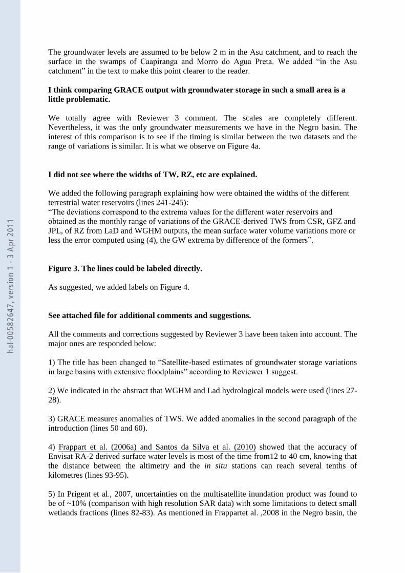
The groundwater levels are assumed to be below 2 m in the Asu catchment, and to reach the
surface in the swamps of Caapiranga and Morro do Agua Preta. We added “in the Asu
catchment” in the text to make this point clearer to the reader.
I think comparing GRACE output with groundwater storage in such a small area is a
little problematic.
We totally agree with Reviewer 3 comment. The scales are completely different.
Nevertheless, it was the only groundwater measurements we have in the Negro basin. The
interest of this comparison is to see if the timing is similar between the two datasets and the
range of variations is similar. It is what we observe on Figure 4a.
I did not see where the widths of TW, RZ, etc are explained.
We added the following paragraph explaining how were obtained the widths of the different
terrestrial water reservoirs (lines 241-245):
“The deviations correspond to the extrema values for the different water reservoirs and
obtained as the monthly range of variations of the GRACE-derived TWS from CSR, GFZ and
JPL, of RZ from LaD and WGHM outputs, the mean surface water volume variations more or
less the error computed using (4), the GW extrema by difference of the formers”.
Figure 3. The lines could be labeled directly.
As suggested, we added labels on Figure 4.
See attached file for additional comments and suggestions.
All the comments and corrections suggested by Reviewer 3 have been taken into account. The
major ones are responded below:
1) The title has been changed to “Satellite-based estimates of groundwater storage variations
in large basins with extensive floodplains” according to Reviewer 1 suggest.
2) We indicated in the abstract that WGHM and Lad hydrological models were used (lines 27-
28).
3) GRACE measures anomalies of TWS. We added anomalies in the second paragraph of the
introduction (lines 50 and 60).
4) Frappart et al. (2006a) and Santos da Silva et al. (2010) showed that the accuracy of
Envisat RA-2 derived surface water levels is most of the time from12 to 40 cm, knowing that
the distance between the altimetry and the in situ stations can reach several tenths of
kilometres (lines 93-95).
5) In Prigent et al., 2007, uncertainties on the multisatellite inundation product was found to
be of ~10% (comparison with high resolution SAR data) with some limitations to detect small
wetlands fractions (lines 82-83). As mentioned in Frappartet al. ,2008 in the Negro basin, the
hal-0
0582
647,
ver
sion
1 -
3 Ap
r 201
1

multisatellite product is not adequately detecting the small floodplains upstream of the Negro
and its two major tributaries (see Frappart et al., 2008 for more details). However, all these
informations about the uncertainty are used to compute the error bars on the surface water
estimates (see above).
hal-0
0582
647,
ver
sion
1 -
3 Ap
r 201
1

1
Satellite-based estimates of groundwater storage variations in large 1
drainage basins with extensive floodplains 2
3
Frédéric Frappart (1), Fabrice Papa (2,3), Andreas Güntner (4), Susanna Werth (4), 4
Joecila Santos da Silva (5), Javier Tomasella (6), Frédérique Seyler (7), Catherine 5
Prigent (8), William B. Rossow (2), Stéphane Calmant (3), Marie-Paule Bonnet (1) 6
7
1 Université de Toulouse ; CNRS ; IRD ; OMP LMTG; F-31400 Toulouse, France 8
2 Université de Toulouse ; CNES ; CNRS ; IRD ; OMP LEGOS; F-31400 Toulouse, France 9
3 NOAA-CREST, City College of New York, New York, USA 10
4 GFZ, Telegrafenberg, Potsdam, Germany 11
5 UEA, CESTU, Manaus/AM, Brazil 12
6 INPE/Centro de Ciência do Sistema Terrestre, Cachoeira Paulista/SP, Brazil 13
7 IRD, US ESPACE, Montpellier, France 14
8 LERMA, Observatoire de Paris, CNRS, Paris, France 15
16
17
18
19
20
21
Revised version submitted to Remote Sensing of Environment the 17 January 2011 22
23
24
*Manuscriptha
l-005
8264
7, v
ersi
on 1
- 3
Apr 2
011
2
Abstract: 25 26
This study presents monthly estimates of groundwater anomalies in a large river basin 27
dominated by extensive floodplains, the Negro River basin, based on the synergistic analysis 28
using multisatellite observations and hydrological models. For the period 2003-2004, changes 29
in water stored in the aquifer is isolated from the total water storage measured by GRACE by 30
removing contributions of both the surface reservoir, derived from satellite imagery and radar 31
altimetry, and the root zone reservoir simulated by WGHM and LaD hydrological models. 32
The groundwater anomalies show a realistic spatial pattern compared with the 33
hydrogeological map of the basin, and similar temporal variations to local in situ groundwater 34
observations and altimetry-derived level height measurements. Results highlight the potential 35
of combining multiple satellite techniques with hydrological modelling to estimate the 36
evolution of groundwater storage. 37
38
39
Keywords: groundwater, remote sensing, hydrological modelling 40
41
hal-0
0582
647,
ver
sion
1 -
3 Ap
r 201
1
3
1. Introduction 42
43
The water cycle of large tropical river basins is strongly influenced by seasonal and 44
interannual variability of rainfall and streamflow, affecting all the components of the water 45
balance (Ronchail et al., 2002; Marengo et al., 2009). The Terrestrial Water Storage (TWS), 46
which represents an integrated measurement of the water stored in the different hydrological 47
reservoirs and is the sum of the surface water, root zone soil water, snowpack and 48
groundwater, is a good indicator of the changes that occur in hydrological conditions globally 49
and at basin scales. Nevertheless, TWS is difficult to measure due to the lack of in situ 50
observations of the terrestrial hydrological compartments. 51
The Gravity Recovery And Climate Experiment (GRACE) mission, launched in 2002, detects 52
tiny changes in the Earth’s gravity field which can be related to spatio-temporal variations of 53
TWS at monthly or sub-monthly time-scales (Tapley et al., 2004). Previous studies provide 54
important information on changes in TWS over the Amazon (Crowley et al., 2008; Chen et 55
al., 2009). Variations in groundwater storage can be separated from the TWS anomalies 56
measured by GRACE using external information on the other hydrological reservoirs such as 57
in situ observations (Yeh et al., 2006), model outputs (Rodell et al., 2009), or both (Leblanc et 58
al., 2009). No similar studies have been undertaken yet for large river basins characterized by 59
extensive wetlands or floodplains. 60
Although wetlands and floodplains cover only 6% of the Earth surface, they have a 61
substantial impact on flood flow alteration, sediment stabilization, water quality, groundwater 62
recharge and discharge (Maltby, 1991; Bullock and Acreman, 2003). Moreover, floodplain 63
inundation is an important regulator of river hydrology owing to storage effects along channel 64
reaches. Reliable and timely information about the extent, spatial distribution, and temporal 65
variation of wetlands and floods as well as the amount of water stored is crucial to better 66
understand their relationship with river discharges, and also their influence on regional 67
hal-0
0582
647,
ver
sion
1 -
3 Ap
r 201
1

4
hydrology and climate. Remote sensing techniques are a unique mean for monitoring large 68
drainage basins climate and hydrology where in situ information is lacking (as, for instance, 69
over floodplains and wetlands or for groundwater monitoring). 70
In this study, a new technique is proposed to derive the spatio-temporal variations of water 71
volume anomalies in the aquifer of the Negro River basin, a large tropical basin dominated by 72
extensive floodplains (see Figure 1a and b for its location). The Negro River basin, with a 73
drainage area of 700,000 km², is indeed the second largest tributary to the Amazon River, 74
covering 12% of the Amazon basin, with a mean annual discharge of 28.400 m3.s
-1 (Richey 75
et al., 1989; Molinier et al., 1992). The method is based on the combination of multisatellite-76
derived hydrological products and outputs from global hydrology models. Water storage 77
anomalies in the different hydrological reservoirs are removed from the TWS anomalies 78
measured by GRACE to isolate the groundwater anomaly storage over 2003-2004. Results are 79
both evaluated and validated using a hydrogeological map of Brazil, in situ measurements of 80
groundwater level variations in a micro-catchment, and altimetry-derived water stages for 81
zones where the aquifers reach the land surface. 82
2. Datasets 83
84
2.1. GRACE-derived land water mass solutions 85
The Gravity Recovery And Climate Experiment (GRACE) mission, launched in March 2002, 86
provides measurements of the spatio-temporal changes in Earth’s gravity field. Several recent 87
studies have shown that GRACE data over the continents can be used to derive the monthly 88
changes of the total land water storage (Ramillien et al., 2005; 2008; Schmitt et al., 2008) 89
with an accuracy of ~1.5 cm of equivalent water thickness when averaged over surfaces of a 90
few hundred square-kilometres. We used the Level-2 land water solutions (RL04) produced 91
by GFZ, JPL (for these two first products, January 2003, June 2003 and January 2004 are 92
missing), and CSR (June 2003 and January 2004 are missing) with a spatial resolution of 93
hal-0
0582
647,
ver
sion
1 -
3 Ap
r 201
1

5
~333 km, destriped and smoothed by Chambers (2006) with an accuracy of 15-20 mm of 94
water thickness. They are available at ftp://podaac.jpl.nasa.gov/tellus/grace/monthly. 95
96
2.2. The multisatellite inundation extent 97
This dataset quantifies at global scale the monthly distribution of surface water extent and its 98
variations at ~25 km of resolution. The methodology which captures the extent (with an 99
accuracy of ~10%) of episodic and seasonal inundations, wetlands, rivers, lakes, and irrigated 100
agriculture over more than a decade, 1993–2004, is based on a clustering analysis of a suite of 101
complementary satellites observations, including passive (SSM/I) and active (ERS) 102
microwaves, and visible and near-IR (AVHRR) observations (Prigent et al., 2007; Papa et al., 103
2006; 2008; 2010). 104
105
2.3. Envisat RA-2 radar altimeter-derived water level heights over rivers and wetlands 106
Silva dos Santos et al. (2010) build 140 time series of water levels derived from RA-2 ranges 107
processed using the Ice-1 retracker over the Negro River drainage basin (see Figure 1c for 108
their locations), for the period 2002-2008, as suggested by Frappart et al. (2006a). The 109
uncertainty associated with the water level height ranges between 5–25 cm for high water 110
season to 12–40 cm during low water season (Frappart et al., 2006a; Santos da Silva et al., 111
2010). 112
113
2.4. In situ surface water levels 114
We used daily measurements of water stage from eight leveled in situ gauge stations from the 115
Brazilian Water Agency (Agência Nacional de Águas or ANA - http://www.ana.gov.br), see 116
Figure 1c for their location. 117
118
hal-0
0582
647,
ver
sion
1 -
3 Ap
r 201
1

6
2.5. In situ groundwater levels 119
The Asu micro-catchment, with a drainage area of 6.58 km², ~90 km north-northwest of 120
Manaus, was instrumented with dipwells in 2001 (see (Tomasella et al., 2008) for a complete 121
description of the catchment instrumentation). We used the well measurements to evaluate 122
our estimates of the groundwater storage variations at that location. 123
124
2.6. Root zone water storage outputs from hydrological models 125
Hydrological model outputs are widely used to analyze spatio-temporal variations of water 126
storage content at basin and global scales. We used water storage in the root zone from the 127
Land Dynamics (LaD) model (Milly and Shmakin, 2002) outputs and from the latest version 128
(Hunger and Döll, 2007) of the WaterGAP Global Hydrology Model (WGHM) (Döll et al., 129
2003). 130
131
2.7. Precipitation estimates from the Global Precipitation Climatology Project (GPCP) 132
These data quantify the distribution of precipitation over the global land surface (Adler et al., 133
2003). We used the monthly Satellite-Gauge Combined Precipitation Data product Version 2 134
data, available from January 1997 to present with a spatial resolution of 1° of latitude and 135
longitude. Over land surfaces, uncertainty in rate estimates from GPCP is generally less than 136
over the oceans due to the in situ gauge input (in addition to satellite) from the GPCC (Global 137
Precipitation Climatology Center). Over land, validation experiments have been conducted in 138
a variety of locations worldwide and suggest that while there are known problems in regions 139
of persistent convective precipitation, non precipitating cirrus or regions of complex terrain, 140
the uncertainty estimates range from 10 to 30% (Adler et al., 2003). 141
142
2.8. Hydrogeological map of Brazil 143
hal-0
0582
647,
ver
sion
1 -
3 Ap
r 201
1

7
We used a hydrogeological map from the Brazilian Department of Mineral Production 144
(DNPM, 1983) which provides the boundaries and the hydrogeological importance of the 145
aquifers of the whole Brazil. This map, holdings of ISRIC, is made available by the European 146
Commission - Joint Research Centre through the European Digital Archive of Soil Maps 147
(EuDASM) (Selvaradjou et al., 2005): 148
http://eusoils.jrc.ec.europa.eu/esdb_archive/EuDASM/EUDASM.htm 149
150
3. Methods 151
152
3.1. Monthly water level maps 153
154
Monthly maps of water level over the floodplains of the Negro River Basin have been 155
determined by combining the observations from a multi-satellite inundation dataset, RA-2 156
derived water levels, and the in situ hydrographic stations for the water levels over rivers and 157
floodplains (see Figure 1c for the location of altimetry-based and in situ stations). For a given 158
month during the flood season, water levels were linearly interpolated over the flooded zones 159
of the Negro River Basin. A pixel of 25 km x 25 km is considered inundated when its 160
percentage of inundated area is greater than 0. The elevation of each pixel of the water level 161
maps is given with reference to its minimum computed over the 2003-2004 period. This 162
minimum elevation represents either the land surface or very low water stage of the 163
floodplain. More details about the methodology used here can be found in Frappart et al. 164
(2005, 2006b, 2008). 165
166
3.2. GRACE leveling and time-shift 167
168
An optimum filter method was developed by analyzing the correspondence of GRACE basin-169
average water storage to the ensemble mean of hydrological models (WGHM, LaD) and by 170
analyzing the error budgets (satellite/leakage errors) and amplitude and phase biases for the 171
hal-0
0582
647,
ver
sion
1 -
3 Ap
r 201
1
8
different filter types. For the Negro River Basin, the destriped filter with 300 km smoothing 172
radius provides the best results among six different filtering methods and different parameters 173
(see Werth et al. (2009) for the filters employed and the values of the parameters that define 174
the degree of smoothing used). Only a very small bias in the seasonal phase of storage 175
changes resulted due to filtering. The GRACE products have been rescaled with a factor of 176
1.061 to account for amplitude smoothing due to filtering determined from smoothed and 177
unsmoothed basin-average model ensemble time series of water storage. 178
179
3.3. Groundwater storage estimates 180
181
The time variations of the TWS expressed as anomalies are the sum of the contributions of the 182
different reservoirs present in a drainage basin: 183
TWS SW RZ GW (1) 184
where SW represents the total surface water storage including lakes, reservoirs, in-channel 185
and floodplains water; RZ is the water contained in the root zone of the soil (representing a 186
depth of 1 or 2 m), GW is the total groundwater storage in the aquifers. These terms are 187
generally expressed in volume (km3) or mm of equivalent water height. 188
The GW anomaly over 2003-2004 is obtained in (1) by calculating the difference between the 189
TWS anomaly estimated by GRACE and the SW level anomaly maps previously derived 190
from remote sensing and the RZ anomaly derived from hydrological models outputs. The 191
TWS and RZ monthly anomalies are the average anomalies of respectively the Level-2 192
GRACE CSR, GFZ and JPL destriped and smoothed solutions at 300 km of averaging radius, 193
and the outputs from LaD and WGHM, resepctively. 194
195
3.4. Water volume variations 196
For a given month t, the regional water volume of TWS, SW, RZ or GW storage δV(t) in a 197
basin with surface area S, is simply computed from the water heights δhj, with j = 1, 2, . . . 198
hal-0
0582
647,
ver
sion
1 -
3 Ap
r 201
1
9
(expressed in mm of equivalent water height) inside S, and the elementary surface Re2 199
sinθjδλδθ (and the percentage of inundation Pj for SW): 200
2( ) ( , , )sin je j j j j
j S
V t R P h t
(2) 201
where λj and θj are co-latitude and longitude, δλ and δθ are the grid steps in longitude and 202
latitude (generally δλ= δθ), and Re the mean radius of the Earth (6378 km). The surface and 203
total water volume variations are expressed in km3. 204
Error on anomalies of surface water volumes were computed in the Negro basin using (3) : 205
n
i
iiii hdShdSdV1
(3) 206
where dV is the error on the monthly water volume anomaly (V), Si the ith
elementary 207
surface, δhi the ith
elementary water level variation between two consecutive months, dSi the 208
error on the ith
elementary surface, and dδhi the error on the ith
elementary water level 209
variation between two consecutive months. 210
The error sources include misclassifications, altimetry measurements and the linear 211
interpolation method. The maximum error on the volume variation are monthly estimated as: 212
)( maxmaxmaxmaxmax hShSV (4) 213
where: ΔVmax is the maximum error on the water monthly volume anomaly, Smax is the 214
maximum monthly flooded surface, δhmax is the maximum water level variation between two 215
consecutive months, ΔSmax is the maximum error for the flooded surface, and Δ(δhmax) is the 216
maximum error for the water level between two consecutive months. 217
218
4. Results & Discussion 219
220
Monthly estimates of water storage in the different hydrological reservoirs are computed for 221
two years (2003-2004) for which the different datasets overlap in time. Maps of annual 222
amplitudes of TWS, SW, RZ and GW are respectively presented in Figure 1 d to g. They were 223
hal-0
0582
647,
ver
sion
1 -
3 Ap
r 201
1
10
obtained by fitting simultaneously the temporal trend, the amplitudes of the annual and semi-224
annual cycles by least-square adjustment at each grid point. The amplitude of the annual cycle 225
for TWS is maximum along the Negro River, and the downstream part of the Branco River, 226
and also over the non flooded areas in the northwest of the Branco River (see Frappart et al. 227
(2005) for a classification of the vegetation and flood extent in the Negro River Basin), 228
reaching 300 mm in the downstream part (Figure 1d). This area corresponds also to the 229
maximum of amplitude of the SW (Figure 1e), clearly related to substantial backwater effects 230
produced at the Negro-Solimões confluence (Filizola et al., 2009). The amplitude of the 231
annual cycle for RZ (Figure 1f) is small except in the upstream part of the Branco River sub-232
basin, where large precipitation occurred without significant flood events. The largest 233
amplitudes of the annual cycle for the GW (Figure 1g) were observed along the Negro River 234
stream, peaking at 250 mm, i.e., ~72% of the TWS, in the downstream part of the basin. In 235
contrast, small amplitudes were obtained in the Branco and Uaupes Basins. The pattern of 236
GW storage variations observed in Figure 2a tends to be similar to the hydrogeological 237
structures of the Negro River Basin (Figure 2b). For important aquifers, higher yield, recharge 238
and drainage volumes and thus larger seasonal storage variations can be expected than for 239
local and unimportant aquifers with low porosity. According to the hydrogeological map of 240
Brazil (DNPM, 1983), the lower part of the basin (longitude -67° and latitude 0°), where 241
the amplitude of the GRACE-based GW seasonal cycle is the largest, is characterized by 242
continuous aquifers of medium hydrogeological importance. The Uaupes Basin, which only 243
contains local aquifers of relatively small importance, and the Branco Basin, which presents a 244
mixture of local aquifers and small continuous aquifers of relatively small importance, and 245
zones with almost no aquifers, correspond to the smallest amplitudes of the GW seasonal 246
cycle. Note that a secondary maximum of the amplitude of the GW seasonal cycle (66°W, 247
hal-0
0582
647,
ver
sion
1 -
3 Ap
r 201
1
11
2°N) can be observed in the upper part of the Negro River which is in good agreement with 248
the presence of two small aquifers of medium importance (DNPM, 1983). 249
Figure 3a shows the time variations (and deviation at each time step) of the water storage 250
anomalies in the TWS, SW, RZ and GW reservoirs for 2003 and 2004. The deviations 251
correspond to the extrema values for the different water reservoirs and obtained as the 252
monthly range of variations of the GRACE-derived TWS from CSR, GFZ and JPL, of RZ 253
from LaD and WGHM outputs, the mean surface water volume variations more or less the 254
error computed using (4), the GW extrema by difference of the formers. The TWS signal is 255
dominated during high waters (May to July) by SW variations. The RZ varies in phase with 256
both TWS and SW and the amplitude of its variations represents a third of the amplitude of 257
TWS variations, which is similar to what was obtained by Kim et al. [2009] for the whole 258
Amazon basin. The resulting GW variations exhibit a more complex profile with two peaks. 259
Its time variations follow the bimodal distribution of the precipitation resulting from the 260
geographical location of the basin in both hemispheres (Figure 3b). A large variability, 261
reaching several months, is observed in the timing the extrema across the basin: GW storage 262
is maximum (minimum) in July-August (December-March) in the western part (Uaupes and 263
west of the Negro), in June-July (February to April) in the centre of the basin and the 264
downstream of the Branco, in August-September in the upper part of the Branco, and in May-265
June (October to December) for the downstream part of the Negro basin. These results are 266
consistent with in situ measurements from sites located in the downstream part of the Negro 267
basin (Do Nascimento et al., 2008; Tomasella et al., 2008) and closely related to the timing of 268
GW recharge and soil thickness. In Manaus, the time-lag between the maxima of rainfall and 269
GW is 3 months, which is similar to what is observed with in situ measurements. 270
hal-0
0582
647,
ver
sion
1 -
3 Ap
r 201
1

12
Figure 4 compares in situ measurements of GW levels from the Asu catchment and water 271
levels from the Caapiranga and Morro da água preta swamps with the estimated anomalies of 272
GW. 273
The GW levels in the Asu micro-catchment (below 2m) were converted into GW storage 274
using a specific yield of 0.17 as in Tomasella et al. (2008). Figure 4a shows the 2003-2004 275
time variations of the GW storage of the Asu catchment and the encompassing GRACE 276
gridcell. They show similar temporal variations. Very good agreement is found between mid 277
2003 and 2004. Nevertheless, the increase in GW starts later in 2003 for the in situ 278
measurements and the maximum value is three times lower. A less pronounced decrease can 279
also be observed for 2004. Two main factors can account for these differences: the respective 280
sizes (7 km² against 10,000 km²), and the fact that the Asu catchment is not directly connected 281
to the Negro River, so the recharge processes may be different. 282
The groundwater table permanently reaches the surface in several parts of the Negro River 283
Basin. Two of these regions, the Caapiranga and Morro da água preta swamps (Figure 1c), are 284
flooded and can be monitored using radar altimetry. In these cases, we expect GW to have 285
similar time variations as surface water levels. Time series of SW and corresponding GW 286
anomalies over 2003-2004 are presented in Figures 4b and c for Caapiranga and Morro da 287
água preta respectively. Except for February 2004, where the SW derived from radar altimetry 288
present an abnormally low level (larger errors on altimetry-derived stages during 289
the low water season, due to the presence of dry land or vegetation in the 290
satellite field of view have also been reported by other studies, see for instance Frappart et al., 291
(2006a) or Santos da Silva et al., (in press), both time 292
series agree well (R=0.76 for Caapiranga and 0.73 for Água do Morro Preta) and exhibit 293
similar temporal patterns and amplitudes. The comparisons in Figure 4 give 294
confidence in the groundwater variations derived by the approach presented here. 295
hal-0
0582
647,
ver
sion
1 -
3 Ap
r 201
1

13
5. Conclusion 296
297
This study presents the first attempt to estimate time variations of GW anomalies using 298
GRACE-based TWS in combination with other remote sensing measurements and model 299
outputs for a large river basin characterized by extensive inundation. Both spatial and 300
temporal patterns of ground water storage anomalies exhibit realistic behaviour. Comparisons 301
with scarce in situ and satellite information show good agreement, in spite of the difference in 302
spatial scales. This promising study will be soon extended to the entire Amazon basin and for 303
more years as all datasets will soon be available over a longer period of time (2002 to 304
present). Extending this method to characterize the evolution of water storage in other large 305
river basins, especially in semi-arid regions, is also important as it will provide regional 306
estimates of groundwater variations, a key variable for water resource management. 307
308
Acknowledgements 309
310
This work was partly supported by the foundation STAE in the framework of the CYMENT 311
project and the ANR CARBAMA. Two authors (F. Papa and W.B. Rossow) are supported by 312
NASA Grant NNXD7AO90G. The authors would like to thank the Centre de Topographie 313
des Océans et de l’Hydrosphère (CTOH) at Laboratoire d’Etudes en Géophysique et 314
Oc´eanographie Spatiales (LEGOS), Observatoire Midi-Pyrénées (OMP), Toulouse, France, 315
for the provision of the ENVISAT RA-2 GDR dataset. They wish to thank an anonymous 316
reviewer for helping us in editing the manuscript to improve its quality. 317
318
References 319
320
Adler, R. F., et al. (2003). The Version 2 Global Precipitation Climatology Project (GPCP) 321
Monthly Precipitation Analysis (1979-Present). Journal of Hydrometeorology, 4,1147-1167. 322
323
Bullock, A., & Acreman, M. (2003). The role of wetlands in the hydrological cycle, 324
Hydroogy and. Earth Sysem. Science,7, 358– 389, doi: 10.5194/hess-7-358-2003. 325
hal-0
0582
647,
ver
sion
1 -
3 Ap
r 201
1

14
326
Chambers, D.P. (2006). Evaluation of New GRACE Time-Variable Gravity Data over the 327
Ocean. Geophysical Research Letters, 33, LI7603, doi:10.1029/2006GL027296. 328
329
Chen, J. L., Wilson, C. R., Tapley, B. D., Yang, Z. L., & Niu, G. Y. (2009). 2005 drought 330
event in the Amazon River basin as measured by GRACE and estimated by climate models, 331
Journal of Geophysical Research, 114, B05404, doi:10.1029/2008JB006056. 332
333
Crowley, J. W., Mitrovica, J. X., Bailey, R. C., Tamisiea, M. E., & Davis, J. L. (2008). 334
Annual variations in water storage and precipitation in the Amazon Basin. Journal of 335
Geodesy, 82(1), 9– 13, doi:10.1007/s00190-007-0153-1. 336
337
Departamento Nacional da Produção Mineral/DNPM (1983). Mapa hidrogeológico do Brasil, 338
escala 1:5,000,000. 339
340
Döll, P., Kaspar, F., & Lehner, B. (2003). A global hydrological model for deriving water 341
availability indicators: Model tuning and validation. Journal of Hydrology, 270, 105– 134. 342
343
Do Nascimento, N.R., Fritsch, E., Bueno, G.T., Bardy, M., Grimaldi, C., & Melfi, A. J. 344
(2008). Podzolization as a deferraltization process: dynamics and chemistry of ground and 345
surface waters in an Acrisol – Podzol sequence of the upper Amazon basin. European Journal 346
Soil Science, 59, 911-924, doi: 10.1111/j.1365-2389.2008.01049.x. 347
348
Filizola, N., Spínola, N. , Arruda, W., Seyler, F. , Calmant, S., & Silva, J. (2009). The Rio 349
Negro and Rio Solimões confluence point – hydrometric observations during the 2006/2007 350
cycle. In: River, Coastal and Estuarine Morphodynamics - RCEM 2009, Carlos Vionnet, 351
Marcelo H. García, E.M. Latrubesse, G.M.E. Perillo. (eds.). Taylor & Francis Group, 352
London, 1003-1006. 353
354
Frappart, F., Martinez, J. M., Seyler, F., León, J. G., & Cazenave, A. (2005). Floodplain water 355
storage in the Negro River basin estimated from microwave remote sensing of inundation area 356
and water levels. Remote Sensing of Environment, 99, 387-399, 357
doi:10.1016/j.rse.2005.08.016. 358
359
Frappart, F., Calmant, S., Cauhopé, M., Seyler, F., & Cazenave, A. (2006a). Preliminary 360
results of ENVISAT RA-2 derived water levels validation over the Amazon basin. Remote 361
Sensing of Environment, 100, 252-264, doi:10.1016/j.rse.2005.10.027. 362
363
Frappart, F., Do Minh, K., L’Hermitte, J., Cazenave, A., Ramillien, G., Le Toan, T., & 364
Mognard-Campbell, N. (2006b). Water volume change in the lower Mekong basin from 365
satellite altimetry and imagery data. Geophysical Journal International, 167 (2), 570-584, 366
doi:10.1111/j.1365-246X.2006.03184.x. 367
368
Frappart, F., Papa, F., Famiglietti, J. S., Prigent, C., Rossow, W. B., & Seyler, F. (2008). 369
Interannual variations of river water storage from a multiple satellite approach: A case study 370
for the Rio Negro River basin. Journal of Geophysical Research, 113, D21104, 371
doi:10.1029/2007JD009438. 372
373
Hunger, M., & Döll, P. (2007). Value of river discharge data for global-sale hydrological 374
modelling. Hydrology and Earth System Science Discussion, 4, 4125– 4173. 375
hal-0
0582
647,
ver
sion
1 -
3 Ap
r 201
1

15
376
Kim, H., P. J.-F., Yeh, T., Oki, and S. Kanae (2009), Role of rivers in the seasonal variations 377
of terrestrial water storage over global basins, Geophys. Res. Lett., 36, L17402, doi: 378
10.1029/2009GL039006. 379
380
Leblanc, M. J., P. Tregoning, G. Ramillien, S. O. Tweed, and A. Fakes (2009), Basin-scale, 381
integrated observations of the early 21st century multiyear drought in southeast Australia, 382
Water Resour. Res., 45, W04408, doi:10.1029/2008WR007333. 383
384
Maltby, E. (1991). Wetland management goals: Wise use and conservation, Landscape Urban 385
Planning, 20, 9– 18. 386
387
Marengo, J.A. (2009), Long-term trends and cycles in the hydrometeorology of the Amazon 388
basin since the late 1920s, Hydrol. Process., 23, 3236-3244, doi:10.1002/hyp.7396. 389
390
Milly, P. C. D., and A.B. Shmakin (2002), Global modeling of land water and energy 391
balances: 1. The Land Dynamics (LaD) model. J. Hydrometeorol. 3, 283–299. 392
393
Molinier, M. (1992). Régionalisation des débits du basin amazonien, In: VII Journées 394
Hydrologiques, Régionalisation des débits en hydrologie et application au développement, 395
ORSTOM, Montpellier, 489-502. 396
397
Papa, F., C. Prigent, F. Durand, and W. B. Rossow (2006), Wetland dynamics using a suite of 398
satellite observations: A case study of application and evaluation for the Indian Subcontinent, 399
Geophys. Res. Lett., 33, L08401, doi:10.1029/2006GL025767. 400
401
Papa, F., Güntner, A., Frappart, F., Prigent, C., & Rossow, W.B. (2008). Variations of surface 402
water extent and water storage in large river basins: A comparison of different global data 403
sources. Geophysical Research Letters, 35, L11401, doi:10.1029/2008GL033857. 404
405
Papa, F., Prigent, C., Aires, F., Jimenez, C., Rossow, W.B., & Matthews, E. (2010). 406
Interannual variability of surface water extent at global scale. Journal of Geophyical. 407
Research, 115, D12111, doi:10.1029/2009JD012674. 408
409
Prigent, C., Papa, F., Aires, F., Rossow, W. B., & Matthews, E. (2007). Global inundation 410
dynamics inferred from multiple satellite observations. 1993–2000, Journal of Geophysical 411
Research, 112, D12107, doi:10.1029/2006JD007847. 412
413
Ramillien, G., Frappart, F., Cazenave, A., & Güntner, A. (2005). Time variations of the land 414
water storage from an inversion of 2 years of GRACE geoids. Earth and Planetary Science 415
Letters, 235, 283–301, doi:10.1016/j.epsl.2005.04.005. 416
417
Ramillien, G., Famiglietti, J.S., & Wahr, J. (2008). Detection of continental hydrology and 418
glaciology signals from GRACE: A review. Surveys in Geophysics, 29(4-5), 361-374, doi: 419
10.1007/s10712-008-9048-9. 420
421
Richey, J.E., Nobre, C., & Deser, C. (1989). Amazon river discharge and climate variability. 422
Nature, 246, 101-103. 423
424
hal-0
0582
647,
ver
sion
1 -
3 Ap
r 201
1
16
Roddel, M., Velicogna, I., & Famiglietti, J. (2009). Satellite-based estimates of groundwater 425
depletion in India. Nature, 460, 999-1003, doi:10.1038/nature08238. 426
427
Ronchail, J., Cochonneau, G., Molinier, M., Guyot, J-L., Goretti de Miranda Chaves, A., 428
Guimarães, V., & Oliveira E. de (2002). Interannual rainfall variability in the Amazon basin 429
and sea-surface temperatures in the equatorial Pacific and the tropical Atlantic oceans. 430
International Journal of Climatology, 22(13), 1663-1686. 431
432
Santos da Silva, J., Calmant, S., Seyler, F., Rottuno Filho, O.C., Cochonneau, G., Mansur, 433
W.J. (2010). Water levels in the Amazon basin derived from the ERS 2 and ENVISAT radar 434
altimetry missions. Remote Sensing of Environment, doi:10.1016/j.rse.2010.04.020. 435
436
Santos da Silva, J., Seyler, F., Calmant, S., Rottuno Filho, O.C., Roux, E., Araújo, A. A. M., 437
& Guyot, J. L. (in revision). Water Level Dynamics of Amazon Wetlands at the Watershed 438
Scale by Satellite Altimetry. International Journal of Remote Sensing. 439
440
Schmidt, R., Flechtner, F., Meyer, U., Neumayer, K.-H., Dahle, Ch., Koenig, R., & Kusche, J. 441
(2008). Hydrological Signals Observed by the GRACE Satellites. 442
Surveys in Geophysics, 29, 319 – 334, doi: 10.1007/s10712-008-9033-3. 443
444
Selvaradjou, S-K., L. Montanarella, O. Spaargaren and D. Dent (2005). European Digital 445
Archive of Soil Maps (EuDASM) - Soil Maps of Latin America and Carribean Islands (DVD-446
Rom version). EUR 21822 EN. Office of the Official Publications of the European 447
Comunities, Luxembourg. 448 449 Swenson, S. & Wahr, J., 2006. Post-processing removal of correlated errors in GRACE data, 450
Geophys. Res. Lett., 33, L08402, doi:10.1029/2005GL025285. 451
Tapley, B. D., Bettadpur, S., Watkins, M.M., & Reigber, C. (2004). The Gravity Recovery 452
and Climate Experiment; mission overview and early results. Geophysical Research Letters, 453
31(9), L09607, doi:10.1029/2004GL019920. 454
455
Tomasella, J., Hodnett, M. G., Cuartas, L. A., Nobre, A. D., Waterloo, M. J., & Oliveira, S. 456
M. (2008). The water balance of an Amazonian micro-catchment: the effect of interannual 457
variability of rainfall on hydrological behaviour. Hydrological Processes, 22, 2133-2147, 458
doi:10.1002/hyp.6813. 459
460
Werth, S., Güntner, A., Schmidt, R., & Kusche, J. (2009). Evaluation of GRACE filter tools 461
from a hydrological perspective. Geophysical Journal International, 179, 1499-1515, 462
doi:10.1111/j.1365-246X.2009.04355.x 463
464
Yeh, P. J.-F., Swenson, S. C., Famiglietti, J. S., & Rodell, M. (2006). Remote sensing of 465
groundwater storage changes in Illinois using the Gravity Recovery and Climate Experiment 466
(GRACE). Water Resources Research, 42, W12203, doi:10.1029/2006WR005374. 467
468
469
hal-0
0582
647,
ver
sion
1 -
3 Ap
r 201
1

17
Figure 1: a) Overview map of South America with the location of the Negro River Basin (b)). 470
c) Map of the Negro River sub-basin extracted from SRTM DEM. Each thin line of black dots 471
represents a ENVISAT track. Yellow dots represent in situ gauge stations, and red dots 472
represent altimetry stations. d), e), f) and g) Maps of amplitude of the annual cycle for TWS, 473
SW, RZ and GW respectively. 474
475
476
477 (c)
(d) (e)
(f) (g)
(b)
hal-0
0582
647,
ver
sion
1 -
3 Ap
r 201
1
18
Figure 2 : a) Map of annual amplitude of GW in the Negro River Basin. b) Hydrogeological 478
map of Brazil from DNPM (1983). 479
480
481
482
483
484
485
486
487
488
489
490
491
492
493
494
495
496
497
498
499
500
501
Almost no aquifer. Very small hydrogeological reservoir.
Local aquifers restricted to fractured zones. Small hydrogeological reservoir.
Local aquifers or continuous aquifers of limited extension. Two levels of water: free
and/or confined. Small hydrogeological reservoir.
Continuous aquifers of regional extension, free or confined. Medium hydrogeological
reservoir.
(b)
(a)
hal-0
0582
647,
ver
sion
1 -
3 Ap
r 201
1
19
Figure 3: a) Time variations of the water storage contained in the different hydrological 502
reservoirs: TWS (blue), RZ (green), SW (black), GW (red). b) Monthly distribution of the 503
rainfall (GPCP). 504
505
506
507
(b)
(a)
hal-0
0582
647,
ver
sion
1 -
3 Ap
r 201
1

20
Figure 4: a) Time variations of the GW storage in the Asu catchment (in situ - grey) and in the 508
corresponding GRACE gridcell (satellite-based - black). b) and c) Time variations of the 509
surface water levels (altimetry-derived - grey) and the groundwater for the corresponding 510
GRACE gridcell (satellite-based - black) in the swamps of Caapiranga and Morro da Água 511
Preta respectively. 512
513
-400
-200
0
200
400
600
2003 2003.5 2004 2004.5 2005
Date
Gro
un
dw
ate
r sto
rag
e (
mm
)
514
-600
-400
-200
0
200
400
2003 2003.5 2004 2004.5 2005
Date
Wate
r le
vel (m
m)
515
-600
-400
-200
0
200
400
2003 2003.5 2004 2004.5 2005
Date
Wate
r le
vel (m
m)
516
(a)
(b)
(c)
- Satellite-based GW
- In situ GW
- Satellite-based GW
- altimetry-derived SW
- Satellite-based GW
- altimetry-derived SW
hal-0
0582
647,
ver
sion
1 -
3 Ap
r 201
1
Top Related
Copyright © 2022 FDOKUMEN

