REVIEW ARTICLE OPEN

Recent advances and applications of machine learning in solid-state materials scienceJonathan Schmidt 1, Mário R. G. Marques 1, Silvana Botti2 and Miguel A. L. Marques1

One of the most exciting tools that have entered the material science toolbox in recent years is machine learning. This collection ofstatistical methods has already proved to be capable of considerably speeding up both fundamental and applied research. Atpresent, we are witnessing an explosion of works that develop and apply machine learning to solid-state systems. We provide acomprehensive overview and analysis of the most recent research in this topic. As a starting point, we introduce machine learningprinciples, algorithms, descriptors, and databases in materials science. We continue with the description of different machinelearning approaches for the discovery of stable materials and the prediction of their crystal structure. Then we discuss research innumerous quantitative structure–property relationships and various approaches for the replacement of first-principle methods bymachine learning. We review how active learning and surrogate-based optimization can be applied to improve the rational designprocess and related examples of applications. Two major questions are always the interpretability of and the physicalunderstanding gained from machine learning models. We consider therefore the different facets of interpretability and theirimportance in materials science. Finally, we propose solutions and future research paths for various challenges in computationalmaterials science.

npj Computational Materials (2019) 5:83 ; https://doi.org/10.1038/s41524-019-0221-0

INTRODUCTIONIn recent years, the availability of large datasets combined withthe improvement in algorithms and the exponential growth incomputing power led to an unparalleled surge of interest in thetopic of machine learning. Nowadays, machine learning algo-rithms are successfully employed for classification, regression,clustering, or dimensionality reduction tasks of large sets ofespecially high-dimensional input data.1 In fact, machine learninghas proved to have superhuman abilities in numerous fields (suchas playing go,2 self driving cars,3 image classification,4 etc). As aresult, huge parts of our daily life, for example, image and speechrecognition,5,6 web-searches,7 fraud detection,8 email/spam filter-ing,9 credit scores,10 and many more are powered by machinelearning algorithms.While data-driven research, and more specifically machine

learning, have already a long history in biology11 or chemistry,12

they only rose to prominence recently in the field of solid-statematerials science.Traditionally, experiments used to play the key role in finding

and characterizing new materials. Experimental research must beconducted over a long time period for an extremely limitednumber of materials, as it imposes high requirements in terms ofresources and equipment. Owing to these limitations, importantdiscoveries happened mostly through human intuition or evenserendipity.13 A first computational revolution in materials sciencewas fueled by the advent of computational methods,14 especiallydensity functional theory (DFT),15,16 Monte Carlo simulations, andmolecular dynamics, that allowed researchers to explore thephase and composition space far more efficiently. In fact, the

combination of both experiments and computer simulations hasallowed to cut substantially the time and cost of materialsdesign.17–20 The constant increase in computing power and thedevelopment of more efficient codes also allowed for computa-tional high-throughput studies21 of large material groups in orderto screen for the ideal experimental candidates. These large-scalesimulations and calculations together with experimental high-throughput studies22–25 are producing an enormous amount ofdata making possible the use of machine learning methods tomaterials science.As these algorithms start to find their place, they are heralding a

second computational revolution. Because the number of possiblematerials is estimated to be as high as a googol (10100),26 thisrevolution is doubtlessly required. This paradigm change is furtherpromoted by projects like the materials genome initiative(Materials genome initiative) that aim to bridge the gap betweenexperiment and theory and promote a more data-intensive andsystematic research approach. A multitude of already successfulmachine learning applications in materials science can be found,e.g., the prediction of new stable materials,27–35 the calculation ofnumerous material properties,36–51 and the speeding up of first-principle calculations.52

Machine learning algorithms have already revolutionized otherfields, such as image recognition. However, the development fromthe first perceptron53,54 up to modern deep convolutional neuralnetworks was a long and tortuous process. In order to producesignificant results in materials science, one necessarily has notonly to play to the strength of machine learning techniques butalso apply the lessons already learned in other fields.

Received: 26 February 2019 Accepted: 17 July 2019

1Institut für Physik, Martin-Luther-Universität, 06120 Halle-Wittenberg, Halle (Saale), Germany and 2Institut für Festkörpertheorie und -optik, Friedrich-Schiller-Universität Jena,Max-Wien-Platz 1, 07743 Jena, GermanyCorrespondence: Miguel A. L. Marques (miguel.marques@physik.uni-halle.de)

www.nature.com/npjcompumats

Published in partnership with the Shanghai Institute of Ceramics of the Chinese Academy of Sciences

As the introduction of machine learning methods to materialsscience is still recent, a lot of published applications are quite basicin nature and complexity. Often they involve fitting models toextremely small training sets or even applying machine learningmethods to composition spaces that could possibly be mappedout in hundreds of CPU hours. It is of course possible to usemachine learning methods as a simple fitting procedure for smalllow-dimensional datasets. However, this does not play to theirstrength and will not allow us to replicate the success machinelearning methods had in other fields.Furthermore, and as always when entering a different field of

science, nomenclature has to be applied correctly. One example isthe expression “deep learning”, which is responsible for a majorityof the recent success of machine learning methods (e.g., in imagerecognition and natural language processing55). It is of coursetempting to describe one’s work as deep learning. However,denoting neural networks with one or two fully connected hiddenlayer as deep learning56 is confusing for researchers new to thetopic, and it misrepresents the purpose of deep-learningalgorithms. The success of deep learning is rooted in the abilityof deep neural networks to learn descriptors of data with differentlevels of abstraction without human intervention.55,57 This is, ofcourse, not the case in two-layer neural networks.One of the major criticisms of machine learning algorithms in

science is the lack of novel laws, understanding, and knowledgearising from their use. This comes from the fact that machinelearning algorithms are often treated as black boxes, as machine-built models are too complex and alien for humans to understand.We will discuss the validity of the criticism and differentapproaches to this challenge.Finally, there have already been a number of excellent reviews

of materials informatics and machine learning in materials sciencein general,13,58–62 as well as some other covering specificallymachine learning in the chemical sciences,63 in materials design ofthermoelectrics and photovoltaics,64 in the development oflithium-ion batteries,65 and in atomistic simulations.66 However,owing to the explosion in the number of works using machinelearning, an enormous amount of research has already beenpublished since the past reviews and the research landscape hasquickly transformed.Here we concentrate on the various applications of machine

learning in solid-state materials science (especially the most recentones) and discuss and analyze them in detail. As a starting point,we provide an introduction to machine learning, and in particularto machine learning principles, algorithms, descriptors, anddatabases in materials science. We then review numerousapplications of machine learning in solid-state materials science:the discovery of new stable materials and the prediction of theirstructure, the machine learning calculation of material properties,the development of machine learning force fields for simulationsin material science, the construction of DFT functionals bymachine learning methods, the optimization of the adaptivedesign process by active learning, and the interpretability of, andthe physical understanding gained from, machine learningmodels. Finally, we discuss the challenges and limitations machinelearning faces in materials science and suggest a few researchstrategies to overcome or circumvent them.

BASIC PRINCIPLES OF MACHINE LEARNINGMachine learning algorithms aim to optimize the performance of acertain task by using examples and/or past experience.67 Generallyspeaking, machine learning can be divided into three maincategories, namely, supervised learning, unsupervised learning,and reinforcement learning.Supervised machine learning is based on the same principles as

a standard fitting procedure: it tries to find the unknown functionthat connects known inputs to unknown outputs. This desired

result for unknown domains is estimated based on the extrapola-tion of patterns found in the labeled training data. Unsupervisedlearning is concerned with finding patterns in unlabeled data, as,e.g., in the clustering of samples. Finally, reinforcement learningtreats the problem of finding optimal or sufficiently good actionsfor a situation in order to maximize a reward.68 In other words, itlearns from interactions.Finally, halfway between supervised and unsupervised learning

lies semi-supervised learning. In this case, the algorithm isprovided with both unlabeled as well as labeled data. Techniquesof this category are particularly useful when available data areincomplete and to learn representations.69

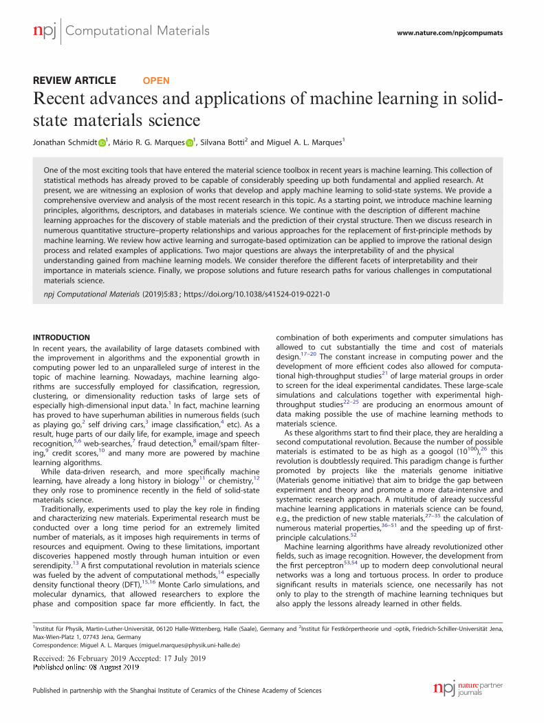
As supervised learning is by far the most widespread form ofmachine learning in materials science, we will concentrate on it inthe following discussion. Figure 1 depicts the workflow applied insupervised learning. One generally chooses a subset of therelevant population for which values of the target property areknown or creates the data if necessary. This process isaccompanied by the selection of a machine learning algorithmthat will be used to fit the desired target quantity. Most of thework consists in generating, finding, and cleaning the data toensure that it is consistent, accurate, etc. Second, it is necessary todecide how to map the properties of the system, i.e., the input forthe model, in a way that is suitable for the chosen algorithm. Thisimplies to translate the raw information into certain features thatwill be used as inputs for the algorithm. Once this process isfinished, the model is trained by optimizing its performance,usually measured through some kind of cost function. Usually thisentails the adjustment of hyperparameters that control thetraining process, structure, and properties of the model. The dataare split into various sets. Ideally, a validation dataset separatefrom the test and training sets is used for the optimization of thehyperparameters.

Fig. 1 Supervised learning workflow

J. Schmidt et al.

2

npj Computational Materials (2019) 83 Published in partnership with the Shanghai Institute of Ceramics of the Chinese Academy of Sciences

1234567890():,;

Every machine learning application has to consider the aspectsof overfitting and underfitting. The reason for underfitting usuallylies either in the model, which lacks the ability to express thecomplexity of the data, or in the features, which do not adequatelydescribe the data. This inevitably leads to a high training error. Onthe other hand, an overfitted model interprets part of the noise inthe training data as relevant information, therefore failing toreliably predict new data. Usually, an overfitted model containsmore free parameters than the number required to capture thecomplexity of the training data. In order to avoid overfitting, it isessential to monitor during training not only the training error butalso the error of the validation set. Once the validation error stopsdecreasing, a machine learning model can start to overfit. Thisproblem is also discussed as the bias-variance trade off in machinelearning.70,71 In this context, the bias is an error based on wrongassumptions in the trained model, while high variance is the errorresulting from too much sensitivity to noise in the training data. Assuch, underfitted models possess high bias while overfittedmodels have high variance.Before the model is ready for applications, it has to be evaluated

on previously unseen data, denoted as test set, to estimate itsgeneralization and extrapolation ability.Different methods ranging from a simple holdout, over k-fold

cross-validation, leave-one-out cross-validation, Monte Carlo cross-validation,72 up to leave-one-cluster-out cross-validation73 can beused for the evaluation. All these methods rely on keeping somedata hidden from the model during the training process. For asimple holdout, this is just performed once, while for k-fold cross-validation the dataset is separated into k equally sized sets. Thealgorithm is trained with all but one of these k subsets, which isused for testing. Finally, the process is repeated for every subset.For leave-one-out cross-validation, each sample is left out of thetraining set once and the model is evaluated for that sample. It hasto be noted that research in chemistry has shown that this form ofcross-validation is insufficient to evaluate adequately the pre-dictive performance of quantitative structure–property relation-ship and should therefore be avoided.74,75 Monte Carlo cross-validation is similar to k-fold cross-validation in the sense that thetraining and test set are randomly chosen. However, here the sizeof the training/test set is chosen independently from the numberof folds. While this can be advantageous, it also means that asample is not guaranteed to be in the test/training set. Leave-one-cluster-out cross-validation73 was specifically developed formaterials science and estimates the ability of the machinelearning model to extrapolate to novel groups of materials thatwere not present in the training data. Depending on the targetquantity, this allows for a more realistic evaluation and a betterunderstanding of the limitations of the machine learning model.Leave-one-cluster-out cross-validation removes a cluster ofmaterials and then considers the error for predictions of thematerials belonging to the removed cluster. This is, for example,consistent with the finding in ref. 76 that models trained onsuperconductors with a specific superconducting mechanism donot have any predictive ability for superconductors with othermechanisms.Before discussing various applications of machine learning in

materials science, we will give an overview of the differentdescriptors, algorithms, and databases used in materialsinformatics.

DatabasesMachine learning in materials science is mostly concerned withsupervised learning. The success of such methods depends mainlyon the amount and quality of data that is available, and this turnsout to be one of the major challenges in material informatics.77

This is especially problematic for target properties that can only bedetermined experimentally in a costly fashion (such as the critical

temperature of superconductors—see section “Prediction ofmaterial properties—superconductivity”). For this reason, data-bases such as the materials project,78 the inorganic crystalstructure database,79 and others (Materials genome initiative,The NOMAD archive, Supercon, National Institute of MaterialsScience 2011)80–92 that contain information on numerous proper-ties of known materials are essential for the success of materialsinformatics.In order for these databases and for materials informatics to

thrive, a FAIR treatment of data93 is absolutely required. A FAIRtreatment encompasses the four principles: findability, accessi-bility, interoperability, and repurposability.94 In other words,researchers from different disciplines should be able to find andaccess data, as well as the corresponding metadata, in acommonly accepted format. This allows the application of thedata for new purposes.Traditionally, negative results are often discarded and left

unpublished. However, as negative data are often just asimportant for machine learning algorithms as positive results,28,95

a cultural adjustment toward the publication of unsuccessfulresearch is necessary. In some disciplines with a longer tradition ofdata-based research (like chemistry), such databases alreadyexist.95 In a similar vein, data that emerges as a side productbut are not essential for a publication are often left unpublished.This eventually results in a waste of resources as other researchersare then required to repeat the work. In the end, every singlediscarded calculation will be sorely missed in future machinelearning applications.

FeaturesA pivotal ingredient of a machine learning algorithm is therepresentation of the data in a suitable form. Features in materialscience have to be able to capture all the relevant information,necessary to distinguish between different atomic or crystalenvironments.96 The process itself, denoted as feature extractionor engineering, might be as simple as determining atomicnumbers, might involve complex transformations such as anexpansion of radial distribution functions (RDFs) in a certain basis,or might require aggregations based on statistics (e.g., averageover features or the calculation of their maximum value). Howmuch processing is required depends strongly on the algorithm.For some methods, such as deep learning, the feature extractioncan be considered as part of the model.97 Naturally, the bestchoice for the representation depends on the target quantity andthe variety of the space of occurrences. For completeness, wehave to mention that the cost of feature extraction and of targetquantity evaluation must never be comparable.Ideally, descriptors should be uncorrelated, as an abundant

number of correlated features can hinder the efficiency andaccuracy of the model. When this happens, further featureselection is necessary to circumvent the curse of dimensionality,98

simplify models, and improve their interpretability as well astraining efficiency. For example, several elemental properties suchas the period and group in the periodic table, ionization potential,and covalent radius, can be used as features to model formationenergies or distances to the convex hull of stability. However, itwas shown that, to obtain acceptable accuracies, often only theperiod and the group are required.99

Having described the general properties of descriptors, we willproceed with a listing of the most used features in materialsscience. Without a doubt, the most studied type of features in thisfield are the ones related to the fitting of potential energysurfaces. In principle, the nuclear charges and the atomic positionsare sufficient features, as the Hamiltonian of a system is usuallyfully determined by these quantities. In practice, however, whileCartesian coordinates might provide an unambiguous descriptionof the atomic positions, they do not make a suitable descriptor, as

J. Schmidt et al.

3

Published in partnership with the Shanghai Institute of Ceramics of the Chinese Academy of Sciences npj Computational Materials (2019) 83

the list of coordinates of a structure are ordered arbitrarily and thenumber of such coordinates varies with the number of atoms. Thelatter is a problem, as most machine learning models require afixed number of features as an input. Therefore, to describe solidsand large clusters, the number of interacting neighbors has to beallowed to vary without changing the dimensionality of thedescriptor. In addition, a lot of applications require that thefeatures are continuous and differentiable with respect to atomicpositions.A comprehensive study on features for atomic potential energy

surfaces can be found in the review of Bartó et al.100. Importantpoints mentioned in their work are: (i) the performance of themodel and its ability to differentiate between different structuresdo not depend directly on the descriptors but on the similaritymeasurement between them; (ii) the quality of the descriptors isrelated to the differentiability with respect to the movement ofthe atoms, completeness of the representation, and invariance tothe basis symmetries of physics (rotation, reflection, translation,and permutation of atoms of the same species). For clarification, aset of invariant descriptors qi, which uniquely determines anatomic environment up to symmetries, is defined as complete. Anovercomplete set is then a set that includes more features thannecessary.Simple representations that show shortcomings as features are

transformations of pairwise distances,101–103 Weyl matrices,104 andZ-matrices.105 Pairwise distances (and also reciprocal or exponen-tial transformations of these) only work for a fixed number ofatoms and are not unique under permutation of atoms. Theconstrain on the number of atoms is also present for polynomialsof pairwise distances. Histograms of pairwise atomic distances arenon-unique: if no information on the angles between the atoms isgiven, of if the ordering of the atoms is unknown, it might bepossible to construct at least two different structures with thesame features. Weyl matrices are defined by the inner productbetween neighboring atoms positions, forming an overcompleteset, while permutations of the atoms change the order of the rowsand columns. Finally, Z-matrices or internal coordinate representa-tions are not invariant under permutations of atoms.In 2012, Rupp et al.106 introduced a representation for

molecules based on the Coulomb repulsion between atoms Iand J and a polynomial fit of atomic energies to the nuclearcharge

MIJ ¼0:5Z2:4

I for I ¼ JZIZJ

jRI�RJ j for I ≠ J

(: (1)

The ordered eigenvalues (ε) of these “Coulomb matrices” arethen used to measure the similarity between two molecules.

dðε; ε0Þ ¼ffiffiffiffiffiffiffiffiffiffiffiffiffiffiffiffiffiffiffiffiffiffiffiffiffiXi

εi � ε0i�� ��2s

: (2)

Here, if the number of atoms is not the same in both systems, εis extended by zeros. In this representation, symmetricallyequivalent atoms contribute equally to the feature function, thediagonalized matrices are invariant with respect to permutationsand rotations, and the distance d is continuous under smallvariations of charge or interatomic distances. Unfortunately, thisrepresentation is not complete and does not uniquely describeevery system. The incompleteness derives from the fact that notall degrees of freedom are taken into account when comparingtwo systems. The non-uniqueness can be demonstrated using asan example acetylene (C2H2).

107 In brief, distortions of thismolecule can lead to several geometries that are described bythe same Coulomb matrix.Faber et al.108 presented three distinct ways to extend the

Coulomb matrix representation to periodic systems. The first ofthese features consists of a matrix where each element represents

the full Coulomb interaction between two atoms and all theirinfinite repetitions in the lattice. For example:

Xij ¼ 1NZiZj

Xk;l

φðjRk � Rl jÞ; (3)

where the sum over k (l) is taken over the atom i (j) in the unit celland its N closest equivalent atoms. However, as this double sumhas convergence issues, one has to resort to the Ewald trick: Xij isdivided into a constant and two rapidly converging sums, one forthe long-range interaction and another for the short-rangeinteraction. Another extension by Faber et al. considers electro-static interactions between the atoms in the unit cell and theatoms in the N closest unit cells. In addition, the long-rangeinteraction is replaced by rapidly decaying interaction. In theirfinal extension, the Coulomb interaction in the usual matrix isreplaced by a potential that is symmetric with respect to thelattice vectors.In the same line of work, Schütt et al.109 extended the Coulomb

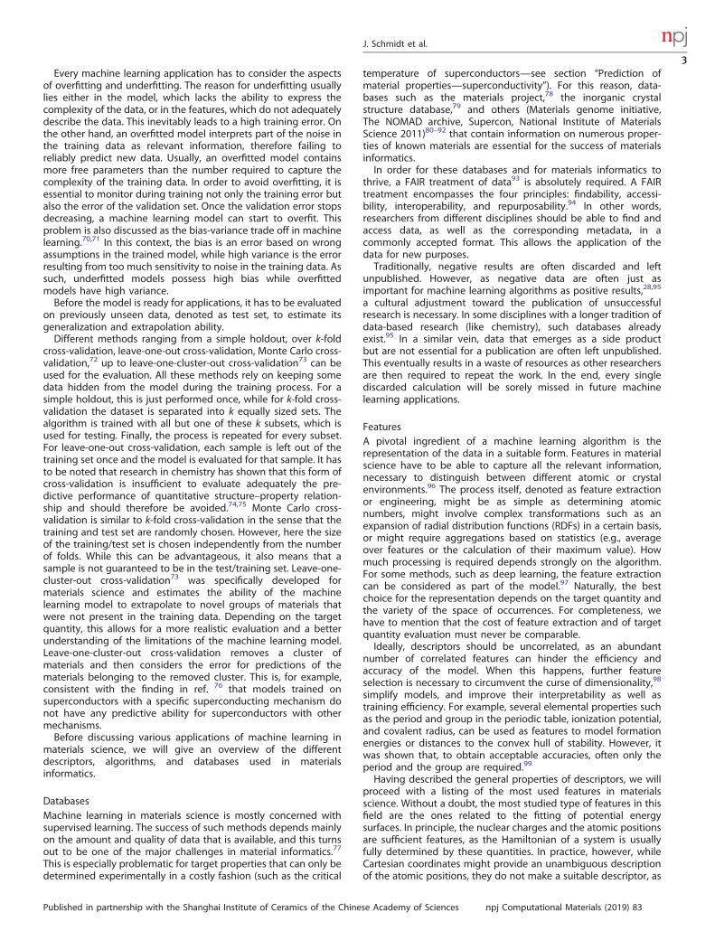
matrix representation by combining it with the Bravais matrix.Unfortunately, this representation is plagued by a degeneracyproblem that comes from the arbitrary choice of the coordinatesystem in which the Bravais matrix is written. Another representa-tion proposed by Schütt et al. is the so called partial radialdistribution function, which considers the density of atoms β in ashell of width dr and radius r centered around atom α (see Fig. 2):

gαβðrÞ ¼ 1NαVr

XNα

i

XNβ

j

θðdαiβj � rÞθðr þ dr � dαiβj Þ: (4)

Here Nα and Nβ are the number of atom of types α and β, Vr isthe volume of the shell, and dαβ are the pairwise distancesbetween two atom types.Another form for representing the local structural environment

was proposed by Behler and Parrinelo.110 Their descriptors111

involve an invariant set of atom-centered radial

Gri ðfRigÞ ¼

Xneighbors

j≠i

grðRijÞ; (5)

and angular symmetry functions

Gai ðfRigÞ ¼

Xneighbors

j≠i

gaðθijkÞ; (6)

where θijk is the angle between Rj− Ri and Rk− Ri. While theradial functions Gr

i contain information on the interaction betweenpairs of atoms within a certain radius, the angular functions Ga

icontains additional information on the distribution of the bondangles θijk. Examples for atom-centered symmetry functions are

Gri ¼

Xneighbors

j≠i

fcðRijÞe�ηðRij�RsÞ2 (7)

Fig. 2 Two crystal structure representations. (Left) A unit cell withthe Bravais vectors (blue) and base (pink) represented. (Right)Depiction of a shell of the discrete partial radial distribution functiongαβ(r) with width dr. (Reprinted with permission from ref. 109.Copyright 2014 American Physical Society

J. Schmidt et al.

4

npj Computational Materials (2019) 83 Published in partnership with the Shanghai Institute of Ceramics of the Chinese Academy of Sciences

and

Gai ¼ 21�ζ

Xneighbors

jki≠j≠k

ð1þ λ cos θijkÞζe�ηðR2ijþR2ikþR2jkÞ ´ fcðRijÞfcðRikÞfcðRjkÞ:

(8)

Here fc is a cutoff function, leading to the neglect of interactionsbetween atoms beyond a certain radius Rc. Furthermore, ηcontrols the width of the Gaussians, Rs is just a parameter thatshifts the Gaussians, λ determines the positions of the extrema ofthe cosine, and ζ controls the angular resolution. The sum overneighbors enforces the permutation invariance of these symmetryfunctions. Usually, 20–100 symmetry functions are used per atom,constructed by varying the parameters above. Beside atomcentered, these functions can also be pair centered.112

A generalization of the atom-centered pairwise descriptor ofBehler was proposed by Seko et al.113 It consists of simple basisfunctions constructed from the multinomial expansion of theproduct between a cutoff function (fc) and an analytical pairwisefunction (fn) (for example, Gaussian, cosine, Bessel, Neumann,polynomial, or Gaussian-type orbital functions)

bi;jn;p ¼Xk

fnðRijkÞ � fcðRijkÞ" #p

; (9)

where p is a positive integer, and Rijk indicates the distancebetween atoms j and k of structure i. The descriptor then uses thesum of these basis functions over all the atoms in the structureP

jbi;jn;p

!.

A similar type of descriptor is the angular Fourier series (AFS),100

which consists of a collection of orthogonal polynomials, like theChebyshev polynomials Tl(cos θ)= cos (lθ), and radial functions

AFSnl ¼Xi;j>i

gnðriÞgnðrjÞcosðlθijÞ: (10)

These radial functions are expansions of cubic or higher-orderpolynomials

gnðrÞ ¼Xα

WnαϕαðrÞ; (11)

where

ϕαðrÞ ¼ ðrc � rÞαþ2=Nα: (12)

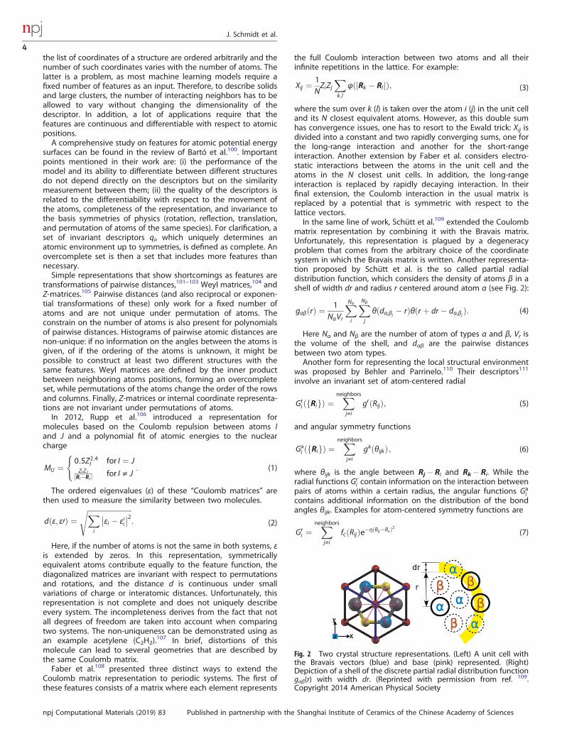
A different approach for atomic environment features wasproposed by Bartok et al.100,114 and leads to the power spectrumand the bispectrum. The approach starts with the generation of anatomic neighbor density function

ρðrÞ ¼ δðr0Þ þXi

δðr� riÞ; (13)

which is projected onto the surface of a four-dimensional spherewith radius r0. As an example, Fig. 3 depicts the projection for 1and 2 dimensions. Then the hyperspherical harmonic functionsUjm0m can be used to represent any function ρ defined on the

surface of a four-dimensional sphere115,116

ρ ¼X1j¼0

Xjm;m0¼�j

cjm0mUjm0m: (14)

Combining these with the rotation operator and the transfor-mation of the expansion coefficients under rotation leads to theformula

Pj ¼Xj

m0;m¼�j

cj�m0mcjm0m (15)

for the SO(4) power spectrum. On the other hand, the bispectrumis given by

Bj j1 j2 ¼Xj1

m10 ;m1¼�j1

cj1m10m1

Xj2m20;m2¼�j2

cj2m20m2´Xj

m0;m¼�j

Cj j1 j2mm1 m2

Cj j1 j2m0m01 m02c

j�m0m;

(16)

where Cj j1 j2mm1 m2 are the Clebsch–Gordon coefficients of SO(4). We

note that the representations above are truncated, based on theband limit jmax in the expansion.Finally, one of the most successful atomic environment features

is the following similarity measurement

Kðρ; ρ0Þ ¼ kðρ; ρ0Þffiffiffiffiffiffiffiffiffiffiffiffiffiffiffiffiffiffiffiffiffiffiffiffiffiffiffiffiffiffikðρ; ρÞkðρ0; ρ0Þp

" #ζ(17)

also known as the smooth overlap of atomic positions (SOAP)kernel.100 Here ζ is a positive integer that enhances the sensitivityof the kernel to changes on the atomic positions and ρ is theatomic neighbor density function, which is constructed from asum of Gaussians, centered on each neighbor:

ρðrÞ ¼Xi

e�αjr�ri j2 : (18)

In practice, the function ρ is then expanded in terms of thespherical harmonics. In addition, k(ρ, ρ′) is a rotationally invariantkernel, defined as the overlap between an atomic environmentand all rotated environments:

kðρ; ρ0Þ ¼Z

dRZ

dr ρðrÞρ0ðRrÞ: (19)

The normalization factorffiffiffiffiffiffiffiffiffiffiffiffiffiffiffiffiffiffiffiffiffiffiffiffiffiffiffiffiffiffikðρ; ρÞkðρ0; ρ0Þp

ensures that theoverlap of an environment with itself is one.The SOAP kernel can be perceived as a three-dimensional

generalization of the radial atom-centered symmetry functionsand is capable of characterizing the entire atomic environment atonce. It was shown to be equivalent to using the power orbispectrum descriptor with a dot-product covariance kernel andGaussian neighbor densities.100

A problem with the above descriptors is that their numberincreases quadratically with the number of chemical species.Inspired by the Behler symmetry functions and the SOAP method,Artrith et al.117 devised a conceptually simple descriptor whosedimension is constant with respect to the number species. This isachieved by defining the descriptor as the union between twosets of invariant coordinates, one that maps the atomic positions(or structure) and another for the composition. Both of thesemappings consist of the expansion coefficients of the RDFs

RDFiðrÞ ¼Xα

cRDFα ϕαðrÞ for 0 � r � Rc (20)

and angular distribution functions (ADF)

ADFiðθÞ ¼Xα

cADFα ϕαðθÞ for 0 � r � Rc: (21)

in a complete basis set ϕα (like the Chebyshev 94% average cross-

Fig. 3 Mapping of a flat space in one and two dimensions onto thesurface of a sphere in one higher dimension. (Reprinted withpermission from ref. 100. Copyright 2013 American Physical Society.)

J. Schmidt et al.

5

Published in partnership with the Shanghai Institute of Ceramics of the Chinese Academy of Sciences npj Computational Materials (2019) 83

validation error). The advantage of stability

cRDFα ¼XRj

ϕαðRijÞfcðRijÞwtj (22)

and

cADFα ¼XRj ;Rk

ϕαðθijkÞfcðRijÞfcðRijÞwtjwtk : (23)

Here fc is a cut-off function that limits the range of theinteractions. The weights wtj and wtk take the value of one for thestructure maps, while the weights for the compositional mapsdepend on the chemical species, according to the pseudo-spinconvention of the Ising model. By limiting the descriptor to twoand three body interactions, i.e., radial and angular contributions,this method maintains the simple analytic nature of theBehler–Parrinelo approach. Furthermore, it allows for an efficientimplementation and differentiation, while systematic refinement isassured by the expansion in a complete basis set.Sanville et al.118 used a set of vectors, each of which describes a

five-atom chain found in the system. This information includesdistances between the five atoms, angles, torsion angles, andfunctions of the bond screening factors.119

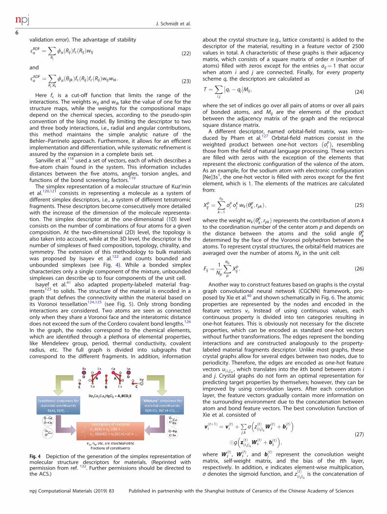
The simplex representation of a molecular structure of Kuz’minet al.120,121 consists in representing a molecule as a system ofdifferent simplex descriptors, i.e., a system of different tetratromicfragments. These descriptors become consecutively more detailedwith the increase of the dimension of the molecule representa-tion. The simplex descriptor at the one-dimensional (1D) levelconsists on the number of combinations of four atoms for a givencomposition. At the two-dimensional (2D) level, the topology isalso taken into account, while at the 3D level, the descriptor is thenumber of simplexes of fixed composition, topology, chirality, andsymmetry. The extension of this methodology to bulk materialswas proposed by Isayev et al.122 and counts bounded andunbounded simplexes (see Fig. 4). While a bonded simplexcharacterizes only a single component of the mixture, unboundedsimplexes can describe up to four components of the unit cell.Isayef et al.41 also adapted property-labeled material frag-

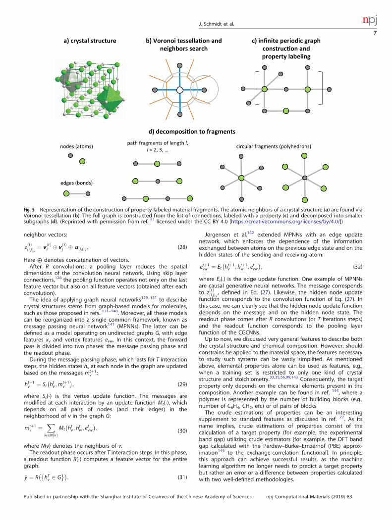
ments123 to solids. The structure of the material is encoded in agraph that defines the connectivity within the material based onits Voronoi tessellation124,125 (see Fig. 5). Only strong bondinginteractions are considered. Two atoms are seen as connectedonly when they share a Voronoi face and the interatomic distancedoes not exceed the sum of the Cordero covalent bond lengths.126

In the graph, the nodes correspond to the chemical elements,which are identified through a plethora of elemental properties,like Mendeleev group, period, thermal conductivity, covalentradius, etc. The full graph is divided into subgraphs thatcorrespond to the different fragments. In addition, information

about the crystal structure (e.g., lattice constants) is added to thedescriptor of the material, resulting in a feature vector of 2500values in total. A characteristic of these graphs is their adjacencymatrix, which consists of a square matrix of order n (number ofatoms) filled with zeros except for the entries aij= 1 that occurwhen atom i and j are connected. Finally, for every propertyscheme q, the descriptors are calculated as

T ¼Xi;j

qi � qj�� ��Mij; (24)

where the set of indices go over all pairs of atoms or over all pairsof bonded atoms, and Mij are the elements of the productbetween the adjacency matrix of the graph and the reciprocalsquare distance matrix.A different descriptor, named orbital-field matrix, was intro-

duced by Pham et al.127 Orbital-field matrices consist in theweighted product between one-hot vectors opi

� �, resembling

those from the field of natural language processing. These vectorsare filled with zeros with the exception of the elements thatrepresent the electronic configuration of the valence of the atom.As an example, for the sodium atom with electronic configuration[Ne]3s1, the one-hot vector is filled with zeros except for the firstelement, which is 1. The elements of the matrices are calculatedfrom:

Xpij ¼

Xnpk¼1

opi okj wkðθpk ; rpkÞ; (25)

where the weight wkðθpk ; rpkÞ represents the contribution of atom kto the coordination number of the center atom p and depends onthe distance between the atoms and the solid angle θpkdetermined by the face of the Voronoi polyhedron between theatoms. To represent crystal structures, the orbital-field matrices areaveraged over the number of atoms Np in the unit cell:

Fij ¼ 1Np

XNp

p

Xpij : (26)

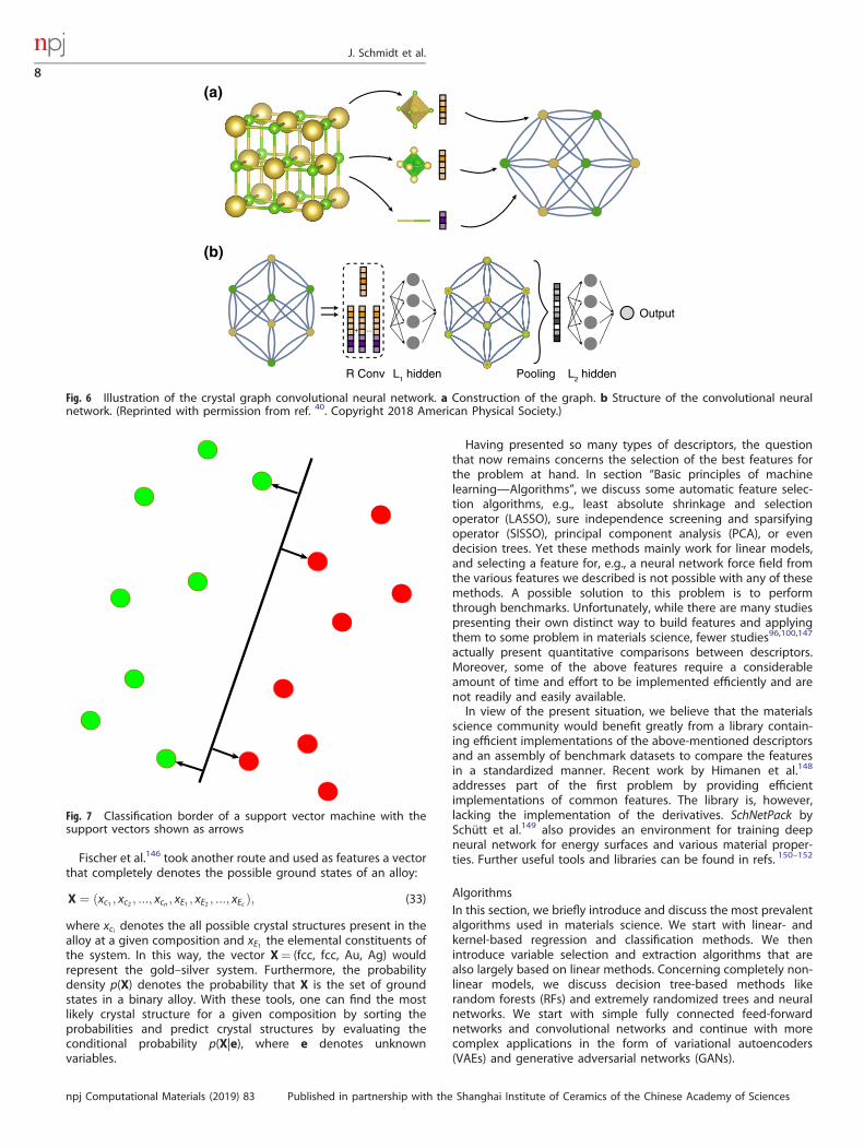
Another way to construct features based on graphs is the crystalgraph convolutional neural network (CGCNN) framework, pro-posed by Xie et al.40 and shown schematically in Fig. 6. The atomicproperties are represented by the nodes and encoded in thefeature vectors vi. Instead of using continuous values, eachcontinuous property is divided into ten categories resulting inone-hot features. This is obviously not necessary for the discreteproperties, which can be encoded as standard one-hot vectorswithout further transformations. The edges represent the bondinginteractions and are constructed analogously to the property-labeled material fragments descriptor. Unlike most graphs, thesecrystal graphs allow for several edges between two nodes, due toperiodicity. Therefore, the edges are encoded as one-hot featurevectors uði;jÞk , which translates into the kth bond between atom iand j. Crystal graphs do not form an optimal representation forpredicting target properties by themselves; however, they can beimproved by using convolution layers. After each convolutionlayer, the feature vectors gradually contain more information onthe surrounding environment due to the concatenation betweenatom and bond feature vectors. The best convolution function ofXie et al. consisted of

vðtþ1Þi ¼ vðtÞi þP

j;kσ zðtÞði;jÞkW

ðtÞf þ bðtÞf

� �

�g zðtÞði;jÞkWðtÞs þ bðtÞs

� �;

(27)

where W ðtÞf , W ðtÞ

s , and bðtÞi represent the convolution weightmatrix, self-weight matrix, and the bias of the tth layer,respectively. In addition, e indicates element-wise multiplication,σ denotes the sigmoid function, and zðtÞði;jÞk is the concatenation of

Fig. 4 Depiction of the generation of the simplex representation ofmolecular structure descriptors for materials. (Reprinted withpermission from ref. 122. Further permissions should be directed tothe ACS.)

J. Schmidt et al.

6

npj Computational Materials (2019) 83 Published in partnership with the Shanghai Institute of Ceramics of the Chinese Academy of Sciences

neighbor vectors:

zðtÞði;jÞk ¼ vðtÞi � vðtÞj � uði;jÞk ; (28)

Here ⊕ denotes concatenation of vectors.After R convolutions, a pooling layer reduces the spatial

dimensions of the convolution neural network. Using skip layerconnections,128 the pooling function operates not only on the lastfeature vector but also on all feature vectors (obtained after eachconvolution).The idea of applying graph neural networks129–131 to describe

crystal structures stems from graph-based models for molecules,such as those proposed in refs. 131–140. Moreover, all these modelscan be reorganized into a single common framework, known asmessage passing neural network141 (MPNNs). The latter can bedefined as a model operating on undirected graphs G, with edgefeatures xv and vertex features evw. In this context, the forwardpass is divided into two phases: the message passing phase andthe readout phase.During the message passing phase, which lasts for T interaction

steps, the hidden states hv at each node in the graph are updatedbased on the messages mtþ1

v :

htþ1v ¼ St htv ;m

tþ1v

� �; (29)

where St(⋅) is the vertex update function. The messages aremodified at each interaction by an update function Mt(⋅), whichdepends on all pairs of nodes (and their edges) in theneighborhood of v in the graph G:

mtþ1v ¼

Xw2NðvÞ

Mt htv ; htw ; e

tvw

� �; (30)

where N(v) denotes the neighbors of v.The readout phase occurs after T interaction steps. In this phase,

a readout function R(⋅) computes a feature vector for the entiregraph:

y ¼ R hTv 2 G� � �

: (31)

Jørgensen et al.142 extended MPNNs with an edge updatenetwork, which enforces the dependence of the informationexchanged between atoms on the previous edge state and on thehidden states of the sending and receiving atom:

etþ1vw ¼ Et htþ1

v ; htþ1w ; etvw

� �; (32)

where Et(.) is the edge update function. One example of MPNNsare causal generative neural networks. The message correspondsto zðtÞði;jÞk , defined in Eq. (27). Likewise, the hidden node updatefunction corresponds to the convolution function of Eq. (27). Inthis case, we can clearly see that the hidden node update functiondepends on the message and on the hidden node state. Thereadout phase comes after R convolutions (or T iterations steps)and the readout function corresponds to the pooling layerfunction of the CGCNNs.Up to now, we discussed very general features to describe both

the crystal structure and chemical composition. However, shouldconstrains be applied to the material space, the features necessaryto study such systems can be vastly simplified. As mentionedabove, elemental properties alone can be used as features, e.g.,when a training set is restricted to only one kind of crystalstructure and stoichiometry.33,35,56,99,143 Consequently, the targetproperty only depends on the chemical elements present in thecomposition. Another example can be found in ref. 144, where apolymer is represented by the number of building blocks (e.g.,number of C6H4, CH2, etc) or of pairs of blocks.The crude estimations of properties can be an interesting

supplement to standard features as discussed in ref. 77. As itsname implies, crude estimations of properties consist of thecalculation of a target property (for example, the experimentalband gap) utilizing crude estimators [for example, the DFT bandgap calculated with the Perdew–Burke–Ernzerhof (PBE) approx-imation145 to the exchange-correlation functional]. In principle,this approach can achieve successful results, as the machinelearning algorithm no longer needs to predict a target propertybut rather an error or a difference between properties calculatedwith two well-defined methodologies.

Fig. 5 Representation of the construction of property-labeled material fragments. The atomic neighbors of a crystal structure (a) are found viaVoronoi tessellation (b). The full graph is constructed from the list of connections, labeled with a property (c) and decomposed into smallersubgraphs (d). (Reprinted with permission from ref. 41 licensed under the CC BY 4.0 [https://creativecommons.org/licenses/by/4.0/])

J. Schmidt et al.

7

Published in partnership with the Shanghai Institute of Ceramics of the Chinese Academy of Sciences npj Computational Materials (2019) 83

Fischer et al.146 took another route and used as features a vectorthat completely denotes the possible ground states of an alloy:

X ¼ ðxc1 ; xc2 ; :::; xcn ; xE1 ; xE2 ; :::; xEc Þ; (33)

where xci denotes the all possible crystal structures present in thealloy at a given composition and xE1 the elemental constituents ofthe system. In this way, the vector X= (fcc, fcc, Au, Ag) wouldrepresent the gold–silver system. Furthermore, the probabilitydensity p(X) denotes the probability that X is the set of groundstates in a binary alloy. With these tools, one can find the mostlikely crystal structure for a given composition by sorting theprobabilities and predict crystal structures by evaluating theconditional probability p(X|e), where e denotes unknownvariables.

Having presented so many types of descriptors, the questionthat now remains concerns the selection of the best features forthe problem at hand. In section “Basic principles of machinelearning—Algorithms”, we discuss some automatic feature selec-tion algorithms, e.g., least absolute shrinkage and selectionoperator (LASSO), sure independence screening and sparsifyingoperator (SISSO), principal component analysis (PCA), or evendecision trees. Yet these methods mainly work for linear models,and selecting a feature for, e.g., a neural network force field fromthe various features we described is not possible with any of thesemethods. A possible solution to this problem is to performthrough benchmarks. Unfortunately, while there are many studiespresenting their own distinct way to build features and applyingthem to some problem in materials science, fewer studies96,100,147

actually present quantitative comparisons between descriptors.Moreover, some of the above features require a considerableamount of time and effort to be implemented efficiently and arenot readily and easily available.In view of the present situation, we believe that the materials

science community would benefit greatly from a library contain-ing efficient implementations of the above-mentioned descriptorsand an assembly of benchmark datasets to compare the featuresin a standardized manner. Recent work by Himanen et al.148

addresses part of the first problem by providing efficientimplementations of common features. The library is, however,lacking the implementation of the derivatives. SchNetPack bySchütt et al.149 also provides an environment for training deepneural network for energy surfaces and various material proper-ties. Further useful tools and libraries can be found in refs. 150–152

AlgorithmsIn this section, we briefly introduce and discuss the most prevalentalgorithms used in materials science. We start with linear- andkernel-based regression and classification methods. We thenintroduce variable selection and extraction algorithms that arealso largely based on linear methods. Concerning completely non-linear models, we discuss decision tree-based methods likerandom forests (RFs) and extremely randomized trees and neuralnetworks. We start with simple fully connected feed-forwardnetworks and convolutional networks and continue with morecomplex applications in the form of variational autoencoders(VAEs) and generative adversarial networks (GANs).

(a)

(b)

R Conv

+ ...

L1 hidden Pooling L2 hidden

Output

Fig. 6 Illustration of the crystal graph convolutional neural network. a Construction of the graph. b Structure of the convolutional neuralnetwork. (Reprinted with permission from ref. 40. Copyright 2018 American Physical Society.)

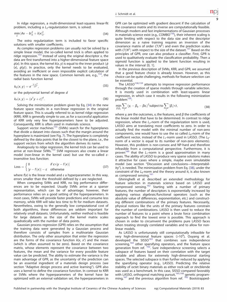
Fig. 7 Classification border of a support vector machine with thesupport vectors shown as arrows

J. Schmidt et al.

8

npj Computational Materials (2019) 83 Published in partnership with the Shanghai Institute of Ceramics of the Chinese Academy of Sciences

In ridge regression, a multi-dimensional least-squares linear-fitproblem, including a L2-regularization term, is solved:

minx

jAx � bj22 þ λjxj22: (34)

The extra regularization term is included to favor specificsolutions with smaller coefficients.As complex regression problems can usually not be solved by a

simple linear model, the so-called kernel trick is often applied toridge regression.153 Instead of using the original descriptor x, thedata are first transformed into a higher-dimensional feature spaceϕ(x). In this space, the kernel k(x, y) is equal to the inner product ⟨ϕ(x), ϕ(y)⟩. In practice, only the kernel needs to be evaluated,avoiding an inefficient or even impossible explicit calculation ofthe features in the new space. Common kernels are, e.g.,154, theradial basis function kernel

kGðx; yÞ ¼ e�jx�yj22σ2 ; (35)

or the polynomial kernel of degree d

kPðx; yÞ ¼ ðxTy þ cÞd: (36)

Solving the minimization problem given by Eq. (34) in the newfeature space results in a non-linear regression in the originalfeature space. This is usually referred to as kernel ridge regression(KRR). KRR is generally simple to use, as for a successful applicationof KRR only very few hyperparameters have to be adjusted.Consequently, KRR is often used in materials science.Support vector machines155 (SVMs) search for the hyperplanes

that divide a dataset into classes such that the margin around thehyperplane is maximized (see Fig. 7). The hyperplane is completelydefined by the data points that lie the closest to the plane, i.e., thesupport vectors from which the algorithm derives its name.Analogously to ridge regression, the kernel trick can be used to

arrive at non-linear SVMs.153 SVM regressors also create a linearmodel (non-linear in the kernel case) but use the so-called ε-insensitive loss function:

Loss ¼ 0 if ε> y � f ðxÞj jy � f ðxÞj j � ε otherwise

(37)

where f(x) is the linear model and ε a hyperparameter. In this way,errors smaller than the threshold defined by ε are neglected.When comparing SVMs and KRR, no big performance differ-

ences are to be expected. Usually SVMs arrive at a sparserrepresentation, which can be of advantage; however, theirperformance relies on a good setting of the hyperparameters. Inmost cases, SVMs will provide faster predictions and consume lessmemory, while KRR will take less time to fit for medium datasets.Nevertheless, owing to the generally low computational cost ofboth algorithms, these differences are seldom important forrelatively small datasets. Unfortunately, neither method is feasiblefor large datasets as the size of the kernel matrix scalesquadratically with the number of data points.Gaussian process regression (GPR) relies on the assumption that

the training data were generated by a Gaussian process andtherefore consists of samples from a multivariate Gaussiandistribution. The only other assumption that enter the regressionare the forms of the covariance function k(x, x′) and the mean(which is often assumed to be zero). Based on the covariancematrix, whose elements represent the covariance between twofeatures, the mean and the variance for every possible featurevalue can be predicted. The ability to estimate the variance is themain advantage of GPR, as the uncertainty of the prediction canbe an essential ingredient of a materials design process (seesection “Adaptive design process and active learning”). GPR alsouses a kernel to define the covariance function. In contrast to KRRor SVMs where the hyperparameters of the kernel have beoptimized with an external validation set, the hyperparameters in

GPR can be optimized with gradient descent if the calculation ofthe covariance matrix and its inverse are computationally feasible.Although modern and fast implementations of Gaussian processesin materials science exist (e.g., COMBO156), their inherent scaling isquite limiting with respect to the data size and the descriptordimension as a naive training requires an inversion of thecovariance matrix of order OðN3Þ and even the prediction scaleswith OðN2Þ with respect to the size of the dataset.157 Based on theprinciples of GPR, one can also produce a classifier. First, GPR isused to qualitatively evaluate the classification probability. Then asigmoid function is applied to the latent function resulting invalues in the interval [0, 1].In the previous description of SVMs, KRR, and GPR, we assumed

that a good feature choice is already known. However, as thischoice can be quite challenging, methods for feature selection canbe essential.The LASSO158,159 attempts to improve regression performance

through the creation of sparse models through variable selection.It is mostly used in combination with least-squares linearregression, in which case it results in the following minimizationproblem159:

minβ;β0

Xi

ðyi � β0 � βxiÞ2subject toXi

jβij<t; (38)

where yi are the outcomes, xi the features, and β the coefficients ofthe linear model that have to be determined. In contrast to ridgeregression, where the L2-norm of the regularization term is used,LASSO aims at translating most coefficients to zero. In order toactually find the model with the minimal number of non-zerocomponents, one would have to use the so called L0-norm of thecoefficient vector, instead of the L1-norm used in LASSO. (The L0-norm of a vector is equal to its number of non-zero elements).However, this problem is non-convex and NP-hard and thereforeinfeasible from a computational perspective. Furthermore, it isproven160 that the L1-norm is a good approximation in manycases. The ability of LASSO to produce very sparse solutions makesit attractive for cases where a simple, maybe even simulatablemodel (see section “Discussion and conclusions—Interpretabil-ity”), is needed. The minimization problem from Eq. (38), under theconstraint of the L0-norm and the theory around it, is also knownas compressed sensing.161

Ghiringhelli et al. described an extended methodology forfeature selection in materials science based on LASSO andcompressed sensing.162 Starting with a number of primaryfeatures, the number of descriptors is exponentially increased byapplying various algebraic/functional operators (such as theabsolute value of differences, exponentiation, etc.) and construct-ing different combinations of the primary features. Necessarily,physical notions like the units of the primary features constrainthe number of combinations. LASSO is then used to reduce thenumber of features to a point where a brute force combinationapproach to find the lowest error is possible. This approach ischosen in order to circumvent the problems pure LASSO faceswhen treating strongly correlated variables and to allow for non-linear models.As LASSO is unfortunately still computationally infeasible for

very high-dimensional feature spaces (>109), Ouyang et al.developed the SISSO163 that combines sure independencescreening,164 other sparsifying operators, and the feature spacegeneration from ref. 162. Sure independence screening selects asubspace of features based on their correlation with the targetvariable and allows for extremely high-dimensional startingspaces. The selected subspace is than further reduced by applyingthe sparsifying operator (e.g., LASSO). Predicting the relativestability of octet binary materials as either rock-salt or zincblendewas used as a benchmark. In this case, SISSO compared favorablywith LASSO, orthogonal matching pursuit,165,166 genetic program-ming,167 and the previous algorithm from ref. 162 Bootstrapped-

J. Schmidt et al.

9

Published in partnership with the Shanghai Institute of Ceramics of the Chinese Academy of Sciences npj Computational Materials (2019) 83

projected gradient descent168 is another variable selectionmethod developed for materials science. The first step ofbootstrapped-projected gradient descent consists in clusteringthe features in order to combat the problems other algorithms likeLASSO face when encountering strongly correlated features. Thefeatures in every cluster are combined in a representative featurefor every cluster. In the following, the sparse linear fit problem isapproximated with projected gradient descent169 for differentlevels of sparsity. This process is also repeated for variousbootstrap samples in order to further reduce the noise. Finally,the intersection of the selected feature sets across the bootstrapsamples is chosen as the final solution.PCA170,171 extracts the orthogonal directions with the greatest

variance from a dataset, which can be used for feature selectionand extraction. This is achieved by diagonalizing the covariancematrix. Sorting the eigenvectors by their eigenvalues (i.e., by theirvariance) results in the first principal component, second principalcomponent, and so on. The broad idea behind this scheme is that,in contrast to the original features, the principal components willbe uncorrelated. Furthermore, one expects that a small number ofprincipal components will explain most of the variance andtherefore provide an accurate representation of the dataset.Naturally, the direct application of PCA should be consideredfeature extraction, instead of feature selection, as new descriptorsin the form of the principal components are constructed. On theother hand, feature selection based on PCA can follow variousstrategies. For example, one can select the variables with thehighest projection coefficient from, respectively, the first nprincipal components when selecting n features. A more in-depth discussion of such strategies can be found in ref. 171.The previous algorithms can be considered as linear models or

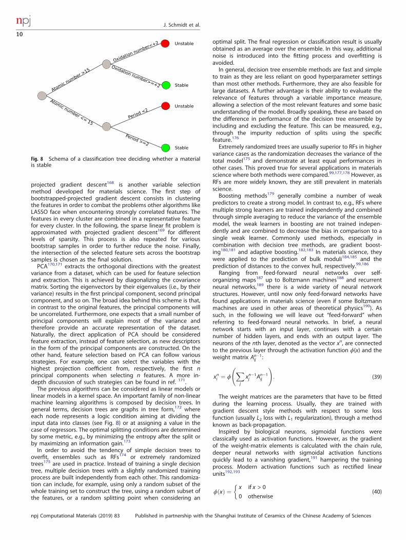
linear models in a kernel space. An important family of non-linearmachine learning algorithms is composed by decision trees. Ingeneral terms, decision trees are graphs in tree form,172 whereeach node represents a logic condition aiming at dividing theinput data into classes (see Fig. 8) or at assigning a value in thecase of regressors. The optimal splitting conditions are determinedby some metric, e.g., by minimizing the entropy after the split orby maximizing an information gain.173

In order to avoid the tendency of simple decision trees tooverfit, ensembles such as RFs174 or extremely randomizedtrees175 are used in practice. Instead of training a single decisiontree, multiple decision trees with a slightly randomized trainingprocess are built independently from each other. This randomiza-tion can include, for example, using only a random subset of thewhole training set to construct the tree, using a random subset ofthe features, or a random splitting point when considering an

optimal split. The final regression or classification result is usuallyobtained as an average over the ensemble. In this way, additionalnoise is introduced into the fitting process and overfitting isavoided.In general, decision tree ensemble methods are fast and simple

to train as they are less reliant on good hyperparameter settingsthan most other methods. Furthermore, they are also feasible forlarge datasets. A further advantage is their ability to evaluate therelevance of features through a variable importance measure,allowing a selection of the most relevant features and some basicunderstanding of the model. Broadly speaking, these are based onthe difference in performance of the decision tree ensemble byincluding and excluding the feature. This can be measured, e.g.,through the impurity reduction of splits using the specificfeature.176

Extremely randomized trees are usually superior to RFs in highervariance cases as the randomization decreases the variance of thetotal model175 and demonstrate at least equal performances inother cases. This proved true for several applications in materialsscience where both methods were compared.99,177,178 However, asRFs are more widely known, they are still prevalent in materialsscience.Boosting methods179 generally combine a number of weak

predictors to create a strong model. In contrast to, e.g., RFs wheremultiple strong learners are trained independently and combinedthrough simple averaging to reduce the variance of the ensemblemodel, the weak learners in boosting are not trained indepen-dently and are combined to decrease the bias in comparison to asingle weak learner. Commonly used methods, especially incombination with decision tree methods, are gradient boost-ing180,181 and adaptive boosting.182,183 In materials science, theywere applied to the prediction of bulk moduli184,185 and theprediction of distances to the convex hull, respectively.99,186

Ranging from feed-forward neural networks over self-organizing maps187 up to Boltzmann machines188 and recurrentneural networks,189 there is a wide variety of neural networkstructures. However, until now only feed-forward networks havefound applications in materials science (even if some Boltzmannmachines are used in other areas of theoretical physics190). Assuch, in the following we will leave out “feed-forward” whenreferring to feed-forward neural networks. In brief, a neuralnetwork starts with an input layer, continues with a certainnumber of hidden layers, and ends with an output layer. Theneurons of the nth layer, denoted as the vector xn, are connectedto the previous layer through the activation function ϕ(x) and theweight matrix An�1

ij :

xni ¼ ϕXj

xn�1j An�1

ij

!: (39)

The weight matrices are the parameters that have to be fittedduring the learning process. Usually, they are trained withgradient descent style methods with respect to some lossfunction (usually L2 loss with L1 regularization), through a methodknown as back-propagation.Inspired by biological neurons, sigmoidal functions were

classically used as activation functions. However, as the gradientof the weight-matrix elements is calculated with the chain rule,deeper neural networks with sigmoidal activation functionsquickly lead to a vanishing gradient,191 hampering the trainingprocess. Modern activation functions such as rectified linearunits192,193

ϕðxÞ ¼ x if x > 0

0 otherwise

(40)

Fig. 8 Schema of a classification tree deciding whether a materialis stable

J. Schmidt et al.

10

npj Computational Materials (2019) 83 Published in partnership with the Shanghai Institute of Ceramics of the Chinese Academy of Sciences

or exponential linear units194

ϕðxÞ ¼ x if x > 0

αðex � 1Þ otherwise

(41)

alleviate this problem and allow for the development of deeperneural networks.The real success story of neural networks only started once

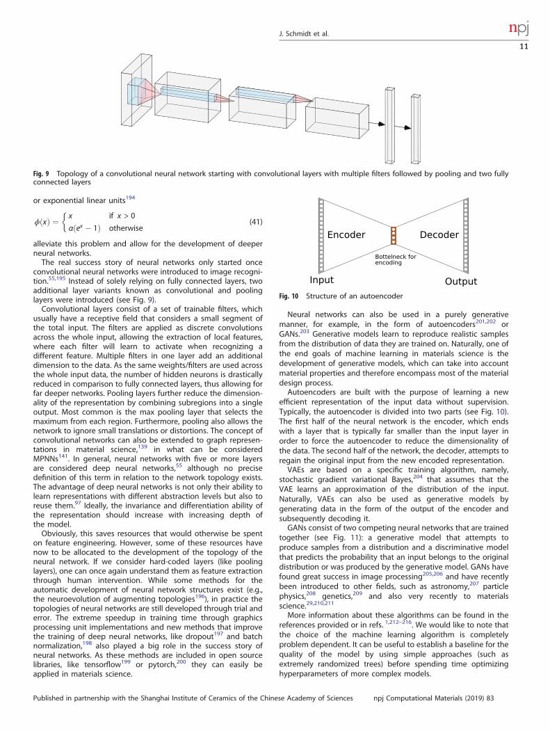
convolutional neural networks were introduced to image recogni-tion.55,195 Instead of solely relying on fully connected layers, twoadditional layer variants known as convolutional and poolinglayers were introduced (see Fig. 9).Convolutional layers consist of a set of trainable filters, which

usually have a receptive field that considers a small segment ofthe total input. The filters are applied as discrete convolutionsacross the whole input, allowing the extraction of local features,where each filter will learn to activate when recognizing adifferent feature. Multiple filters in one layer add an additionaldimension to the data. As the same weights/filters are used acrossthe whole input data, the number of hidden neurons is drasticallyreduced in comparison to fully connected layers, thus allowing forfar deeper networks. Pooling layers further reduce the dimension-ality of the representation by combining subregions into a singleoutput. Most common is the max pooling layer that selects themaximum from each region. Furthermore, pooling also allows thenetwork to ignore small translations or distortions. The concept ofconvolutional networks can also be extended to graph represen-tations in material science,139 in what can be consideredMPNNs141. In general, neural networks with five or more layersare considered deep neural networks,55 although no precisedefinition of this term in relation to the network topology exists.The advantage of deep neural networks is not only their ability tolearn representations with different abstraction levels but also toreuse them.97 Ideally, the invariance and differentiation ability ofthe representation should increase with increasing depth ofthe model.Obviously, this saves resources that would otherwise be spent

on feature engineering. However, some of these resources havenow to be allocated to the development of the topology of theneural network. If we consider hard-coded layers (like poolinglayers), one can once again understand them as feature extractionthrough human intervention. While some methods for theautomatic development of neural network structures exist (e.g.,the neuroevolution of augmenting topologies196), in practice thetopologies of neural networks are still developed through trial anderror. The extreme speedup in training time through graphicsprocessing unit implementations and new methods that improvethe training of deep neural networks, like dropout197 and batchnormalization,198 also played a big role in the success story ofneural networks. As these methods are included in open sourcelibraries, like tensorflow199 or pytorch,200 they can easily beapplied in materials science.

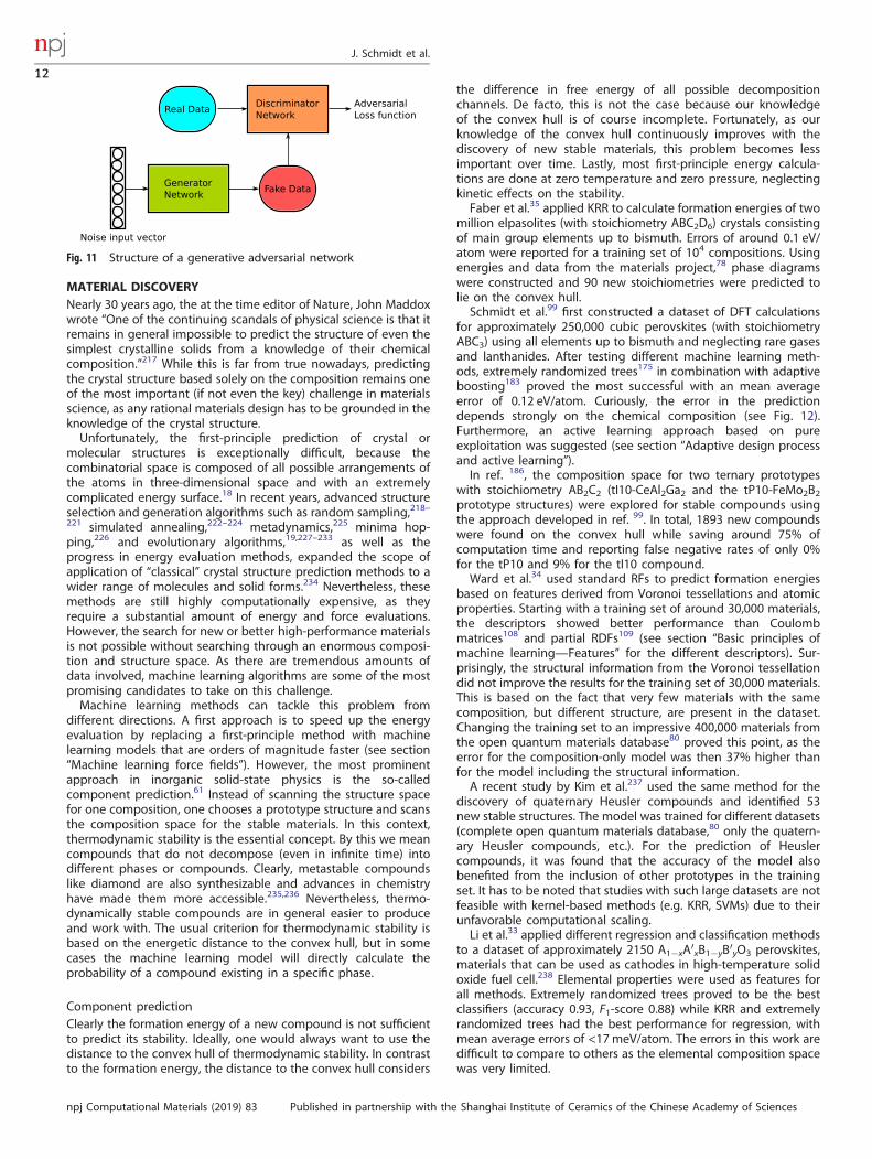
Neural networks can also be used in a purely generativemanner, for example, in the form of autoencoders201,202 orGANs.203 Generative models learn to reproduce realistic samplesfrom the distribution of data they are trained on. Naturally, one ofthe end goals of machine learning in materials science is thedevelopment of generative models, which can take into accountmaterial properties and therefore encompass most of the materialdesign process.Autoencoders are built with the purpose of learning a new

efficient representation of the input data without supervision.Typically, the autoencoder is divided into two parts (see Fig. 10).The first half of the neural network is the encoder, which endswith a layer that is typically far smaller than the input layer inorder to force the autoencoder to reduce the dimensionality ofthe data. The second half of the network, the decoder, attempts toregain the original input from the new encoded representation.VAEs are based on a specific training algorithm, namely,

stochastic gradient variational Bayes,204 that assumes that theVAE learns an approximation of the distribution of the input.Naturally, VAEs can also be used as generative models bygenerating data in the form of the output of the encoder andsubsequently decoding it.GANs consist of two competing neural networks that are trained

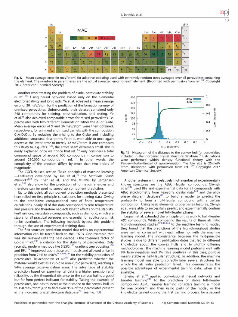
together (see Fig. 11): a generative model that attempts toproduce samples from a distribution and a discriminative modelthat predicts the probability that an input belongs to the originaldistribution or was produced by the generative model. GANs havefound great success in image processing205,206 and have recentlybeen introduced to other fields, such as astronomy,207 particlephysics,208 genetics,209 and also very recently to materialsscience.29,210,211

More information about these algorithms can be found in thereferences provided or in refs. 1,212–216. We would like to note thatthe choice of the machine learning algorithm is completelyproblem dependent. It can be useful to establish a baseline for thequality of the model by using simple approaches (such asextremely randomized trees) before spending time optimizinghyperparameters of more complex models.

Fig. 9 Topology of a convolutional neural network starting with convolutional layers with multiple filters followed by pooling and two fullyconnected layers

Fig. 10 Structure of an autoencoder

J. Schmidt et al.

11

Published in partnership with the Shanghai Institute of Ceramics of the Chinese Academy of Sciences npj Computational Materials (2019) 83

MATERIAL DISCOVERYNearly 30 years ago, the at the time editor of Nature, John Maddoxwrote “One of the continuing scandals of physical science is that itremains in general impossible to predict the structure of even thesimplest crystalline solids from a knowledge of their chemicalcomposition.”217 While this is far from true nowadays, predictingthe crystal structure based solely on the composition remains oneof the most important (if not even the key) challenge in materialsscience, as any rational materials design has to be grounded in theknowledge of the crystal structure.Unfortunately, the first-principle prediction of crystal or

molecular structures is exceptionally difficult, because thecombinatorial space is composed of all possible arrangements ofthe atoms in three-dimensional space and with an extremelycomplicated energy surface.18 In recent years, advanced structureselection and generation algorithms such as random sampling,218–221 simulated annealing,222–224 metadynamics,225 minima hop-ping,226 and evolutionary algorithms,19,227–233 as well as theprogress in energy evaluation methods, expanded the scope ofapplication of “classical” crystal structure prediction methods to awider range of molecules and solid forms.234 Nevertheless, thesemethods are still highly computationally expensive, as theyrequire a substantial amount of energy and force evaluations.However, the search for new or better high-performance materialsis not possible without searching through an enormous composi-tion and structure space. As there are tremendous amounts ofdata involved, machine learning algorithms are some of the mostpromising candidates to take on this challenge.Machine learning methods can tackle this problem from

different directions. A first approach is to speed up the energyevaluation by replacing a first-principle method with machinelearning models that are orders of magnitude faster (see section“Machine learning force fields”). However, the most prominentapproach in inorganic solid-state physics is the so-calledcomponent prediction.61 Instead of scanning the structure spacefor one composition, one chooses a prototype structure and scansthe composition space for the stable materials. In this context,thermodynamic stability is the essential concept. By this we meancompounds that do not decompose (even in infinite time) intodifferent phases or compounds. Clearly, metastable compoundslike diamond are also synthesizable and advances in chemistryhave made them more accessible.235,236 Nevertheless, thermo-dynamically stable compounds are in general easier to produceand work with. The usual criterion for thermodynamic stability isbased on the energetic distance to the convex hull, but in somecases the machine learning model will directly calculate theprobability of a compound existing in a specific phase.

Component predictionClearly the formation energy of a new compound is not sufficientto predict its stability. Ideally, one would always want to use thedistance to the convex hull of thermodynamic stability. In contrastto the formation energy, the distance to the convex hull considers

the difference in free energy of all possible decompositionchannels. De facto, this is not the case because our knowledgeof the convex hull is of course incomplete. Fortunately, as ourknowledge of the convex hull continuously improves with thediscovery of new stable materials, this problem becomes lessimportant over time. Lastly, most first-principle energy calcula-tions are done at zero temperature and zero pressure, neglectingkinetic effects on the stability.Faber et al.35 applied KRR to calculate formation energies of two

million elpasolites (with stoichiometry ABC2D6) crystals consistingof main group elements up to bismuth. Errors of around 0.1 eV/atom were reported for a training set of 104 compositions. Usingenergies and data from the materials project,78 phase diagramswere constructed and 90 new stoichiometries were predicted tolie on the convex hull.Schmidt et al.99 first constructed a dataset of DFT calculations

for approximately 250,000 cubic perovskites (with stoichiometryABC3) using all elements up to bismuth and neglecting rare gasesand lanthanides. After testing different machine learning meth-ods, extremely randomized trees175 in combination with adaptiveboosting183 proved the most successful with an mean averageerror of 0.12 eV/atom. Curiously, the error in the predictiondepends strongly on the chemical composition (see Fig. 12).Furthermore, an active learning approach based on pureexploitation was suggested (see section “Adaptive design processand active learning”).In ref. 186, the composition space for two ternary prototypes

with stoichiometry AB2C2 (tI10-CeAl2Ga2 and the tP10-FeMo2B2prototype structures) were explored for stable compounds usingthe approach developed in ref. 99. In total, 1893 new compoundswere found on the convex hull while saving around 75% ofcomputation time and reporting false negative rates of only 0%for the tP10 and 9% for the tI10 compound.Ward et al.34 used standard RFs to predict formation energies

based on features derived from Voronoi tessellations and atomicproperties. Starting with a training set of around 30,000 materials,the descriptors showed better performance than Coulombmatrices108 and partial RDFs109 (see section “Basic principles ofmachine learning—Features” for the different descriptors). Sur-prisingly, the structural information from the Voronoi tessellationdid not improve the results for the training set of 30,000 materials.This is based on the fact that very few materials with the samecomposition, but different structure, are present in the dataset.Changing the training set to an impressive 400,000 materials fromthe open quantum materials database80 proved this point, as theerror for the composition-only model was then 37% higher thanfor the model including the structural information.A recent study by Kim et al.237 used the same method for the

discovery of quaternary Heusler compounds and identified 53new stable structures. The model was trained for different datasets(complete open quantum materials database,80 only the quatern-ary Heusler compounds, etc.). For the prediction of Heuslercompounds, it was found that the accuracy of the model alsobenefited from the inclusion of other prototypes in the trainingset. It has to be noted that studies with such large datasets are notfeasible with kernel-based methods (e.g. KRR, SVMs) due to theirunfavorable computational scaling.Li et al.33 applied different regression and classification methods

to a dataset of approximately 2150 A1−xA′xB1−yB′yO3 perovskites,materials that can be used as cathodes in high-temperature solidoxide fuel cell.238 Elemental properties were used as features forall methods. Extremely randomized trees proved to be the bestclassifiers (accuracy 0.93, F1-score 0.88) while KRR and extremelyrandomized trees had the best performance for regression, withmean average errors of <17meV/atom. The errors in this work aredifficult to compare to others as the elemental composition spacewas very limited.

Fig. 11 Structure of a generative adversarial network

J. Schmidt et al.

12

npj Computational Materials (2019) 83 Published in partnership with the Shanghai Institute of Ceramics of the Chinese Academy of Sciences

Another work treating the problem of oxide–perovskite stabilityis ref. 56. Using neural networks based only on the elementalelectronegativity and ionic radii, Ye et al. achieved a mean averageerror of 30 meV/atom for the prediction of the formation energy ofunmixed perovskites. Unfortunately, their dataset contained only240 compounds for training, cross-validation, and testing. Yeet al.56 also achieved comparable errors for mixed perovskites, i.e.perovskites with two different elements on either the A- or B-site.Mean average errors of 9 and 26meV/atom were then obtained,respectively, for unmixed and mixed garnets with the compositionC3A2D3O12. By reducing the mixing to the C-site and includingadditional structural descriptors, Ye et al. were able to once againdecrease the latter error to merely 12 meV/atom. If one comparesthis study to, e.g., refs. 1,35, the errors seem extremely small. This iseasily explained once we notice that ref. 56 only considers a totalcompound space of around 600 compounds in comparison toaround 250,000 compounds in ref. 1. In other words, thecomplexity of the problem differs by more than two orders ofmagnitude.The CGCNNs (see section “Basic principles of machine learning

—Features”) developed by Xie et al.,40 the MatErials GraphNetworks132 by Chen et al., and the MPNNs by Jørgensenet al.142 also allow for the prediction of formation energies andtherefore can be used to speed up component prediction.Up to this point, all component prediction methods presented

here relied on first-principle calculations for training data. Owingto the prohibitive computational cost of finite temperaturecalculations, nearly all of this data correspond to zero temperatureand pressure and therefore neglects kinetic effects on the stability.Furthermore, metastable compounds, such as diamond, which arestable for all practical purposes and essential for applications, riskto be overlooked. The following methods bypass this problemthrough the use of experimental training data.The first structure prediction model that relies on experimental

information can be traced back to the 1920s. One example thatwas still relevant until the past decade is the tolerance factor ofGoldschmidt,239 a criterion for the stability of perovskites. Onlyrecently, modern methods like SISSO,163 gradient tree boosting,180

and RFs174 improved upon these old models and allowed a rise inprecision from 74% to >90%143,240,241 for the stability prediction ofperovskites. Balachandran et al.241 also predicted whether thematerial would exist as a cubic or non-cubic perovskite, reaching a94% average cross-validation error. The advantage of stabilityprediction based on experimental data is a higher precision andreliability, as the theoretical distance to the convex hull is a goodbut far from perfect indicator for stability. Taking the example ofperovskites, one has to increase the distance to the convex hull upto 150meV/atom just to find even 95% of the perovskites presentin the inorganic crystal structure database79 (see Fig. 13).

Another system with a relatively high number of experimentallyknown structures are the AB2C Heusler compounds. Oliynyket al.242 used RFs and experimental data for all compounds withAB2C stoichiometry from Pearson’s crystal data243 and the alloyphase diagram database88 to build a model to predict theprobability to form a full-Heusler compound with a certaincomposition. Using basic elemental properties as features, Olynyket al. were able to successfully predict and experimentally confirmthe stability of several novel full-Heusler phases.Legrain et al. extended the principle of this work to half-Heusler

ABC compounds. While comparing the results of three ab initiohigh-throughput studies37,244,245 to the machine learning model,they found that the predictions of the high-throughput studieswere neither consistent with each other nor with the machinelearning model. The inconsistency between the first-principlestudies is due to different publication dates that led to differentknowledge about the convex hulls and to slightly differingmethodologies. The machine learning model performs well with9% false negatives and 1% false positives (in this case, positivemeans stable as half-Heusler structure). In addition, the machinelearning model was able to correctly label several structures forwhich the ab initio prediction failed. This demonstrates thepossible advantages of experimental training data, when it isavailable.Zheng et al.36 applied convolutional neural networks and

transfer learning246 to the prediction of stable full-Heuslercompounds AB2C. Transfer learning considers training a modelfor one problem and then using parts of the model, or theknowledge gained during the first training process, for a second

Fig. 13 Histogram of the distance to the convex hull for perovskitesincluded in the inorganic crystal structure database.79 Calculationswere performed within density functional theory with thePerdew–Burke–Ernzerhof approximation. The bin size is 25meV/atom. (Reprinted with permission from ref. 99. Copyright 2017American Chemical Society.)

Fig. 12 Mean average error (in meV/atom) for adaptive boosting used with extremely random trees averaged over all perovskites containingthe element. The numbers in parentheses are the actual averaged error for each element. (Reprinted with permission from ref. 99. Copyright2017 American Chemical Society.)

J. Schmidt et al.

13

Published in partnership with the Shanghai Institute of Ceramics of the Chinese Academy of Sciences npj Computational Materials (2019) 83

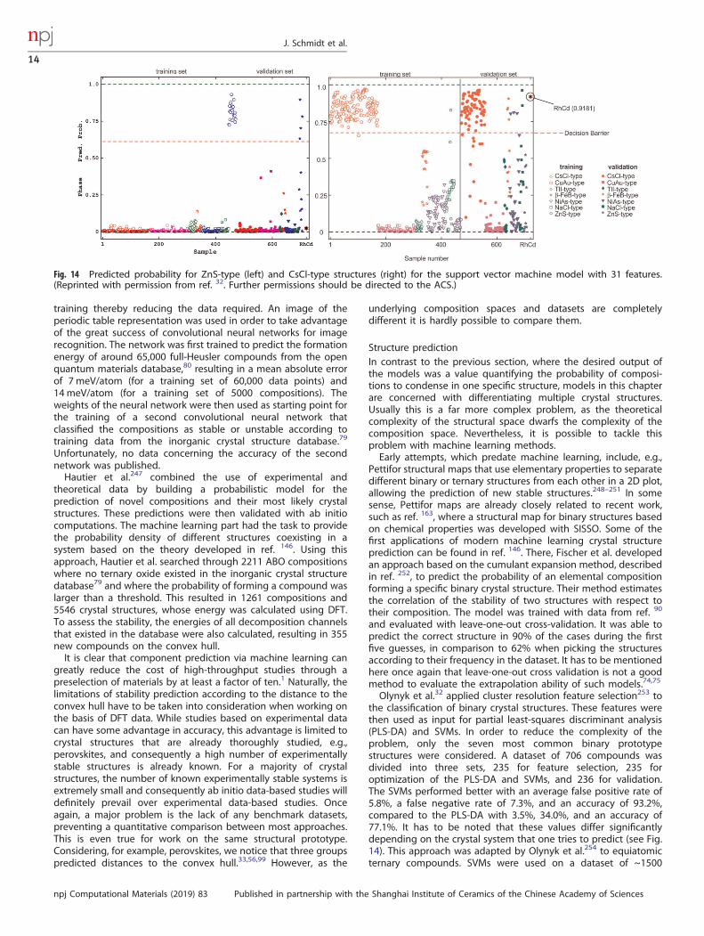
training thereby reducing the data required. An image of theperiodic table representation was used in order to take advantageof the great success of convolutional neural networks for imagerecognition. The network was first trained to predict the formationenergy of around 65,000 full-Heusler compounds from the openquantum materials database,80 resulting in a mean absolute errorof 7 meV/atom (for a training set of 60,000 data points) and14meV/atom (for a training set of 5000 compositions). Theweights of the neural network were then used as starting point forthe training of a second convolutional neural network thatclassified the compositions as stable or unstable according totraining data from the inorganic crystal structure database.79

Unfortunately, no data concerning the accuracy of the secondnetwork was published.Hautier et al.247 combined the use of experimental and

theoretical data by building a probabilistic model for theprediction of novel compositions and their most likely crystalstructures. These predictions were then validated with ab initiocomputations. The machine learning part had the task to providethe probability density of different structures coexisting in asystem based on the theory developed in ref. 146. Using thisapproach, Hautier et al. searched through 2211 ABO compositionswhere no ternary oxide existed in the inorganic crystal structuredatabase79 and where the probability of forming a compound waslarger than a threshold. This resulted in 1261 compositions and5546 crystal structures, whose energy was calculated using DFT.To assess the stability, the energies of all decomposition channelsthat existed in the database were also calculated, resulting in 355new compounds on the convex hull.It is clear that component prediction via machine learning can

greatly reduce the cost of high-throughput studies through apreselection of materials by at least a factor of ten.1 Naturally, thelimitations of stability prediction according to the distance to theconvex hull have to be taken into consideration when working onthe basis of DFT data. While studies based on experimental datacan have some advantage in accuracy, this advantage is limited tocrystal structures that are already thoroughly studied, e.g.,perovskites, and consequently a high number of experimentallystable structures is already known. For a majority of crystalstructures, the number of known experimentally stable systems isextremely small and consequently ab initio data-based studies willdefinitely prevail over experimental data-based studies. Onceagain, a major problem is the lack of any benchmark datasets,preventing a quantitative comparison between most approaches.This is even true for work on the same structural prototype.Considering, for example, perovskites, we notice that three groupspredicted distances to the convex hull.33,56,99 However, as the

underlying composition spaces and datasets are completelydifferent it is hardly possible to compare them.

Structure predictionIn contrast to the previous section, where the desired output ofthe models was a value quantifying the probability of composi-tions to condense in one specific structure, models in this chapterare concerned with differentiating multiple crystal structures.Usually this is a far more complex problem, as the theoreticalcomplexity of the structural space dwarfs the complexity of thecomposition space. Nevertheless, it is possible to tackle thisproblem with machine learning methods.Early attempts, which predate machine learning, include, e.g.,

Pettifor structural maps that use elementary properties to separatedifferent binary or ternary structures from each other in a 2D plot,allowing the prediction of new stable structures.248–251 In somesense, Pettifor maps are already closely related to recent work,such as ref. 163, where a structural map for binary structures basedon chemical properties was developed with SISSO. Some of thefirst applications of modern machine learning crystal structureprediction can be found in ref. 146. There, Fischer et al. developedan approach based on the cumulant expansion method, describedin ref. 252, to predict the probability of an elemental compositionforming a specific binary crystal structure. Their method estimatesthe correlation of the stability of two structures with respect totheir composition. The model was trained with data from ref. 90

and evaluated with leave-one-out cross-validation. It was able topredict the correct structure in 90% of the cases during the firstfive guesses, in comparison to 62% when picking the structuresaccording to their frequency in the dataset. It has to be mentionedhere once again that leave-one-out cross validation is not a goodmethod to evaluate the extrapolation ability of such models.74,75

Olynyk et al.32 applied cluster resolution feature selection253 tothe classification of binary crystal structures. These features werethen used as input for partial least-squares discriminant analysis(PLS-DA) and SVMs. In order to reduce the complexity of theproblem, only the seven most common binary prototypestructures were considered. A dataset of 706 compounds wasdivided into three sets, 235 for feature selection, 235 foroptimization of the PLS-DA and SVMs, and 236 for validation.The SVMs performed better with an average false positive rate of5.8%, a false negative rate of 7.3%, and an accuracy of 93.2%,compared to the PLS-DA with 3.5%, 34.0%, and an accuracy of77.1%. It has to be noted that these values differ significantlydepending on the crystal system that one tries to predict (see Fig.14). This approach was adapted by Olynyk et al.254 to equiatomicternary compounds. SVMs were used on a dataset of ~1500

Fig. 14 Predicted probability for ZnS-type (left) and CsCl-type structures (right) for the support vector machine model with 31 features.(Reprinted with permission from ref. 32. Further permissions should be directed to the ACS.)

J. Schmidt et al.

14

npj Computational Materials (2019) 83 Published in partnership with the Shanghai Institute of Ceramics of the Chinese Academy of Sciences

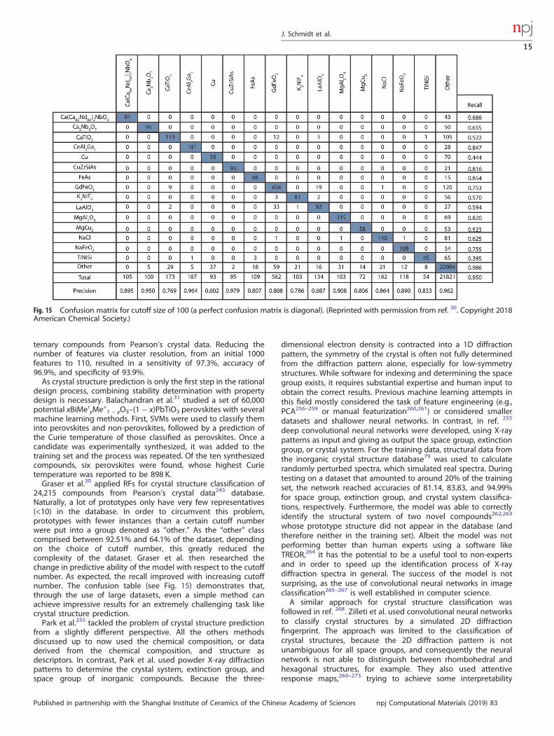
ternary compounds from Pearson’s crystal data. Reducing thenumber of features via cluster resolution, from an initial 1000features to 110, resulted in a sensitivity of 97.3%, accuracy of96.9%, and specificity of 93.9%.As crystal structure prediction is only the first step in the rational

design process, combining stability determination with propertydesign is necessary. Balachandran et al.31 studied a set of 60,000potential xBiMe′yMe″1− yO3–(1− x)PbTiO3 perovskites with severalmachine learning methods. First, SVMs were used to classify theminto perovskites and non-perovskites, followed by a prediction ofthe Curie temperature of those classified as perovskites. Once acandidate was experimentally synthesized, it was added to thetraining set and the process was repeated. Of the ten synthesizedcompounds, six perovskites were found, whose highest Curietemperature was reported to be 898 K.Graser et al.30 applied RFs for crystal structure classification of

24,215 compounds from Pearson’s crystal data243 database.Naturally, a lot of prototypes only have very few representatives(<10) in the database. In order to circumvent this problem,prototypes with fewer instances than a certain cutoff numberwere put into a group denoted as “other.” As the “other” classcomprised between 92.51% and 64.1% of the dataset, dependingon the choice of cutoff number, this greatly reduced thecomplexity of the dataset. Graser et al. then researched thechange in predictive ability of the model with respect to the cutoffnumber. As expected, the recall improved with increasing cutoffnumber. The confusion table (see Fig. 15) demonstrates that,through the use of large datasets, even a simple method canachieve impressive results for an extremely challenging task likecrystal structure prediction.Park et al.255 tackled the problem of crystal structure prediction

from a slightly different perspective. All the others methodsdiscussed up to now used the chemical composition, or dataderived from the chemical composition, and structure asdescriptors. In contrast, Park et al. used powder X-ray diffractionpatterns to determine the crystal system, extinction group, andspace group of inorganic compounds. Because the three-

dimensional electron density is contracted into a 1D diffractionpattern, the symmetry of the crystal is often not fully determinedfrom the diffraction pattern alone, especially for low-symmetrystructures. While software for indexing and determining the spacegroup exists, it requires substantial expertise and human input toobtain the correct results. Previous machine learning attempts inthis field mostly considered the task of feature engineering (e.g.,PCA256–259 or manual featurization260,261) or considered smallerdatasets and shallower neural networks. In contrast, in ref. 255

deep convolutional neural networks were developed, using X-raypatterns as input and giving as output the space group, extinctiongroup, or crystal system. For the training data, structural data fromthe inorganic crystal structure database79 was used to calculaterandomly perturbed spectra, which simulated real spectra. Duringtesting on a dataset that amounted to around 20% of the trainingset, the network reached accuracies of 81.14, 83.83, and 94.99%for space group, extinction group, and crystal system classifica-tions, respectively. Furthermore, the model was able to correctlyidentify the structural system of two novel compounds262,263

whose prototype structure did not appear in the database (andtherefore neither in the training set). Albeit the model was notperforming better than human experts using a software likeTREOR,264 it has the potential to be a useful tool to non-expertsand in order to speed up the identification process of X-raydiffraction spectra in general. The success of the model is notsurprising, as the use of convolutional neural networks in imageclassification265–267 is well established in computer science.A similar approach for crystal structure classification was

followed in ref. 268. Zilleti et al. used convolutional neural networksto classify crystal structures by a simulated 2D diffractionfingerprint. The approach was limited to the classification ofcrystal structures, because the 2D diffraction pattern is notunambiguous for all space groups, and consequently the neuralnetwork is not able to distinguish between rhombohedral andhexagonal structures, for example. They also used attentiveresponse maps,269–273 trying to achieve some interpretability

Fig. 15 Confusion matrix for cutoff size of 100 (a perfect confusion matrix is diagonal). (Reprinted with permission from ref. 30. Copyright 2018American Chemical Society.)

J. Schmidt et al.

15

Published in partnership with the Shanghai Institute of Ceramics of the Chinese Academy of Sciences npj Computational Materials (2019) 83

and visualization of the model. This will be further discussed insection “Discussion and conclusions—Interpretability”.Further interesting work concerning micro-structure and

material characterization, using machine learning-based imageprocessing, can be found in refs. 274–279.

If we consider structure prediction through machine learning,we also have to consider global structure prediction methods,where the whole energy surface has to be explored efficiently.This can also be considered as a surrogate-based optimizationproblem (see section “Adaptive design process and activelearning”), where the expensive experiment is the local geometryoptimization through DFT. Yamashita et al.280 started with a largeset of initial structures from which a random subset was locallyoptimized and used to train a Bayesian regressor to predict theenergy. Using Thompson sampling,281 structures from the initialset were sampled randomly according to their probability ofminimizing the energy. The approach was tested on NaCl andY2Co17 and reduced the average number of trials until finding theoptimal structure by, respectively, 31% and 39% when comparedto random structure selection.Lastly, we discuss two works that introduced modern neural

network architectures to crystal structure prediction and genera-tion. Both methods have also been used recently for micro-structures by Li et al.210,282

Ryan et al.28 applied VAEs (see section “Basic principles ofmachine learning—Algorithms”) to crystal structure prediction.The 42-layer VAEs develop a more efficient representation for theinput (see section “Basic principles of machine learning—

Features”). For training and testing, a dataset of around 50,000crystal structures from the inorganic crystal structure database79

and the crystallography open database89 were used. The encodingof the original descriptors was used as input for a five-layersigmoid classifier that predicts the most likely elements to formthe topology represented by the atomic fingerprints. A thirdauxiliary neural network, in this case a five-layer softmax classifier,combined the non-normalized atomic fingerprints and the outputof the sigmoid classifier that improves the prediction. To predictdirectly the crystal structure from this approach, one requirestraining data of negatives or, in other words, knowledge of crystalstructures that do not exist. Unfortunately, no such database isavailable in physics. In order to circumvent this problem, Ryanet al. calculated the likelihood of the existence of a structure as theproduct of the probabilities of elements existing at the singleatomic sites. Application to test data demonstrated a clearsuperiority of this approach in comparison with random choices.Nouira et al.29 introduced a GAN-based strategy (see section

“Basic principles of machine learning—Algorithms”) to crystalstructure generation in the form of CrystalGAN. Specifically, theycreated a novel GAN structure to generate stable ternarystructures on the basis of binary hydrides. Remarkably, themethod generates structures of higher complexity and is able toinclude constraints based on domain knowledge. However, as nodata about the stability of the generated structures werepublished, the evaluation of the usefulness of this approach isstill pending. A second application of GANs in materials science,and in particular in chemistry, can be found in ref. 211.

PREDICTION OF MATERIAL PROPERTIESMachine learning methods have proven to be successful in theprediction of a large number of material properties. An overviewof different properties that were predicted can be found in Table1. In the following, we discuss in depth a few properties, studied invarious works, which provide good examples for currentchallenges in computational materials science, and possiblestrategies to overcome them.

Band gapsDesign of functional materials for applications like light-emittingdiodes (LEDs), photovoltaics, scintillators, or transistors, alwaysrequires detailed knowledge of the band gap. Consequently, a lotof effort was invested in theoretical methods for high-throughputcalculations of this electronic property. It is well known thatstandard exchange correlation functionals, like the PBE,145

systematically underestimate band gaps in comparison toexperimental results. More modern functionals like the modifiedBecke–Johnson by Tran and Blaha332 or the strongly constrainedand appropriately normed meta-GGA333 by Jianwei et al. improveupon these results. However, the state-of-the-art higher-fidelitymethods still remain the many-body GW approximation or hybridfunctionals. Unfortunately, these usually come with a prohibitivelyhigh computational cost. Machine learning is one possibility toovercome this obstacle by either directly predicting band gapsbased on experimental or theoretical training data or by using theresults of low-fidelity methods to predict experimental or high-fidelity theoretical results.Zhuo et al.289 tried to circumvent the problems of the different

theoretical methods by directly predicting experimental bandgaps. Their approach started with a classification of the materialsas either metal or non-metal using SVM classifiers and thenprogressed by predicting the band gap with SVM regressors. Theperformance of the resulting models in predicting experimentalband gaps lies somewhere between basic functionals (like thePBE) and hybrid functionals. The error turns out to be comparableto, e.g., ref. 40,41. However, Zhuo et al. improved upon those earlier

Table 1. Summary of material properties predicted with machinelearning methods and corresponding references

Property References

Curie temperature 31,283–287

Vibrational free energy and entropy 288

Band gap 40,41,132,159,283,289–300

Dielectric breakdown strength 38,44,45

Lattice parameter 300

Debye temperature and heat capacity 41–43

Glass transition temperature 301,302

Thermal expansion coefficient 41

Thermal boundary resistance 303

Thermal conductivity 37,46–51,304,305

Local magnetic moments 127,306

Melting temperature 39,48,307

Magnetocaloric effects 283

Grain boundaries 308

Grain boundary energy 309–312

Grain boundary mobility 312

Interface energy 300

Seebeck coefficient 46,313,314

Thermoelectric figure of merit 315

Bulk and shear moduli 40–42,132,184,185,316

Electrical resistivity 46

Density of states 109,317,318

Fermi energy and Poisson ratio 40

Dopant solution energy 319

Metal–insulator classification 65

Topological invariants 320–326

Superconducting critical temperature 73,76,122,327–329

Li-ion conductivity and battery state-of-charge 65,330,331

J. Schmidt et al.

16

npj Computational Materials (2019) 83 Published in partnership with the Shanghai Institute of Ceramics of the Chinese Academy of Sciences

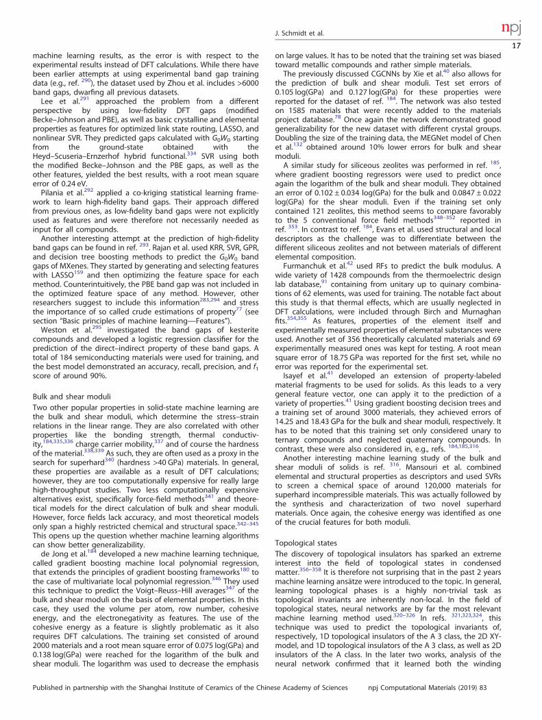
machine learning results, as the error is with respect to theexperimental results instead of DFT calculations. While there havebeen earlier attempts at using experimental band gap trainingdata (e.g., ref. 290), the dataset used by Zhou et al. includes >6000band gaps, dwarfing all previous datasets.Lee et al.291 approached the problem from a different

perspective by using low-fidelity DFT gaps (modifiedBecke–Johnson and PBE), as well as basic crystalline and elementalproperties as features for optimized link state routing, LASSO, andnonlinear SVR. They predicted gaps calculated with G0W0 startingfrom the ground-state obtained with theHeyd–Scuseria–Ernzerhof hybrid functional.334 SVR using boththe modified Becke–Johnson and the PBE gaps, as well as theother features, yielded the best results, with a root mean squareerror of 0.24 eV.Pilania et al.292 applied a co-kriging statistical learning frame-

work to learn high-fidelity band gaps. Their approach differedfrom previous ones, as low-fidelity band gaps were not explicitlyused as features and were therefore not necessarily needed asinput for all compounds.Another interesting attempt at the prediction of high-fidelity

band gaps can be found in ref. 293. Rajan et al. used KRR, SVR, GPR,and decision tree boosting methods to predict the G0W0 bandgaps of MXenes. They started by generating and selecting featureswith LASSO159 and then optimizing the feature space for eachmethod. Counterintuitively, the PBE band gap was not included inthe optimized feature space of any method. However, otherresearchers suggest to include this information283,294 and stressthe importance of so called crude estimations of property77 (seesection “Basic principles of machine learning—Features”).Weston et al.295 investigated the band gaps of kesterite

compounds and developed a logistic regression classifier for theprediction of the direct–indirect property of these band gaps. Atotal of 184 semiconducting materials were used for training, andthe best model demonstrated an accuracy, recall, precision, and f1score of around 90%.

Bulk and shear moduliTwo other popular properties in solid-state machine learning arethe bulk and shear moduli, which determine the stress–strainrelations in the linear range. They are also correlated with otherproperties like the bonding strength, thermal conductiv-ity,184,335,336 charge carrier mobility,337 and of course the hardnessof the material.338,339 As such, they are often used as a proxy in thesearch for superhard340 (hardness >40 GPa) materials. In general,these properties are available as a result of DFT calculations;however, they are too computationally expensive for really largehigh-throughput studies. Two less computationally expensivealternatives exist, specifically force-field methods341 and theore-tical models for the direct calculation of bulk and shear moduli.However, force fields lack accuracy, and most theoretical modelsonly span a highly restricted chemical and structural space.342–345

This opens up the question whether machine learning algorithmscan show better generalizability.de Jong et al.184 developed a new machine learning technique,

called gradient boosting machine local polynomial regression,that extends the principles of gradient boosting frameworks180 tothe case of multivariate local polynomial regression.346 They usedthis technique to predict the Voigt–Reuss–Hill averages347 of thebulk and shear moduli on the basis of elemental properties. In thiscase, they used the volume per atom, row number, cohesiveenergy, and the electronegativity as features. The use of thecohesive energy as a feature is slightly problematic as it alsorequires DFT calculations. The training set consisted of around2000 materials and a root mean square error of 0.075 log(GPa) and0.138 log(GPa) were reached for the logarithm of the bulk andshear moduli. The logarithm was used to decrease the emphasis

on large values. It has to be noted that the training set was biasedtoward metallic compounds and rather simple materials.The previously discussed CGCNNs by Xie et al.40 also allows for

the prediction of bulk and shear moduli. Test set errors of0.105 log(GPa) and 0.127 log(GPa) for these properties werereported for the dataset of ref. 184. The network was also testedon 1585 materials that were recently added to the materialsproject database.78 Once again the network demonstrated goodgeneralizability for the new dataset with different crystal groups.Doubling the size of the training data, the MEGNet model of Chenet al.132 obtained around 10% lower errors for bulk and shearmoduli.A similar study for siliceous zeolites was performed in ref. 185,

where gradient boosting regressors were used to predict onceagain the logarithm of the bulk and shear moduli. They obtainedan error of 0.102 ± 0.034 log(GPa) for the bulk and 0.0847 ± 0.022log(GPa) for the shear moduli. Even if the training set onlycontained 121 zeolites, this method seems to compare favorablyto the 5 conventional force field methods348–352 reported inref. 353. In contrast to ref. 184, Evans et al. used structural and localdescriptors as the challenge was to differentiate between thedifferent siliceous zeolites and not between materials of differentelemental composition.Furmanchuk et al.42 used RFs to predict the bulk modulus. A

wide variety of 1428 compounds from the thermoelectric designlab database,91 containing from unitary up to quinary combina-tions of 62 elements, was used for training. The notable fact aboutthis study is that thermal effects, which are usually neglected inDFT calculations, were included through Birch and Murnaghanfits.354,355 As features, properties of the element itself andexperimentally measured properties of elemental substances wereused. Another set of 356 theoretically calculated materials and 69experimentally measured ones was kept for testing. A root meansquare error of 18.75 GPa was reported for the first set, while noerror was reported for the experimental set.Isayef et al.41 developed an extension of property-labeled

material fragments to be used for solids. As this leads to a verygeneral feature vector, one can apply it to the prediction of avariety of properties.41 Using gradient boosting decision trees anda training set of around 3000 materials, they achieved errors of14.25 and 18.43 GPa for the bulk and shear moduli, respectively. Ithas to be noted that this training set only considered unary toternary compounds and neglected quaternary compounds. Incontrast, these were also considered in, e.g., refs. 184,185,316.Another interesting machine learning study of the bulk and

shear moduli of solids is ref. 316. Mansouri et al. combinedelemental and structural properties as descriptors and used SVRsto screen a chemical space of around 120,000 materials forsuperhard incompressible materials. This was actually followed bythe synthesis and characterization of two novel superhardmaterials. Once again, the cohesive energy was identified as oneof the crucial features for both moduli.

Topological statesThe discovery of topological insulators has sparked an extremeinterest into the field of topological states in condensedmatter.356–358 It is therefore not surprising that in the past 2 yearsmachine learning ansätze were introduced to the topic. In general,learning topological phases is a highly non-trivial task astopological invariants are inherently non-local. In the field oftopological states, neural networks are by far the most relevantmachine learning method used.320–326 In refs. 321,323,324, thistechnique was used to predict the topological invariants of,respectively, 1D topological insulators of the A 3 class, the 2D XY-model, and 1D topological insulators of the A 3 class, as well as 2Dinsulators of the A class. In the later two works, analysis of theneural network confirmed that it learned both the winding

J. Schmidt et al.

17

Published in partnership with the Shanghai Institute of Ceramics of the Chinese Academy of Sciences npj Computational Materials (2019) 83

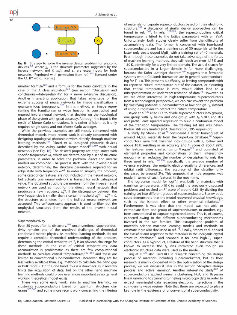
number formula321 and a formula for the Berry curvature in thecase of the A class insulators323 (see section “Discussion andconclusions—Interpretability” for a more extensive discussion).Another interesting application that takes advantage of theextreme success of neural networks for image classification isquantum loop topography.320 In this method, an image repre-senting the Hamiltonian or wave function is constructed andentered into a neural network that decides on the topologicalphase of the system with great accuracy. Although the input is theresult of Monte Carlo simulations, it is rather efficient, as it onlyrequires single steps and not Monte Carlo averages.While the previous examples are still mostly concerned with

theoretical models, more recent work is already concerned withdesigning topological photonic devices directly through machinelearning methods.325 Pilozzi et al. designed photonic devicesdescribed by the Aubry–André–Harper model359,360 with neuralnetworks (see Fig. 16). The desired property are edge states withspecific frequencies ωt, which are determined by a set of structureparameters. In order to solve the problem, direct and inversemodels are combined. The process starts with the inverse neuralnetwork, determining the structure parameters required for anedge state with frequency ωind

t . In order to simplify the problem,some categorical features are not included in the neural network,but actually one neural network is trained for each categoricalvalue. The obtained structure parameters from the inverse neuralnetwork are used as input for the direct neural network thatproduces a new frequency ωdir

t . If the discrepancy between thetwo frequencies is smaller than a certain threshold ωind

t � ωdirt < δ,

the structure parameters from the indirect neural network areaccepted. This self-consistent approach is used to filter out theunphysical structures from the results of the inverse neuralnetwork.

SuperconductivityEven 30 years after its discovery,361 unconventional superconduc-tivity remains one of the unsolved challenges of theoreticalcondensed matter physics. As machine learning methods do notrequire a complete theoretical understanding of the problem,determining the critical temperature Tc is an obvious challenge forthese methods. In the case of critical temperatures, dataaccumulation is problematic, as there are few computationalmethods to calculate critical temperatures,362–364 and these arelimited to conventional superconductors. Moreover, they are farless widely available than, e.g., methods to calculate the band gapor bulk moduli. On the one hand, this is a drawback as it severelylimits the acquisition of data, but on the other hand machinelearning methods could prove even more important as no generalworking theoretical model exists.There was some early work, akin to machine learning, on

clustering superconductors based on quantum structure dia-grams365,366 and some more recent work concerning the filtering

of materials for cuprate superconductors based on their electronicstructure.367 A discussion of similar design approaches can befound in ref. 368. In refs. 327,328, the superconducting criticaltemperature is fitted to the lattice parameters with an SVM.Unfortunately, both studies clearly suffer from the difficulty ofaccumulating data. The former is concerned with iron-basedsuperconductors and has a training set of 30 materials while thelatter only treats doped MgB2 with a training set of 40 materials.Even though these examples do not take advantage of the fortesof machine learning methods, they still reach an error 1.17 K and1.10 K, admittedly for a very limited domain. The actual search forsuperconductors in a larger domain is far more challenging,because the Kohn–Luttinger theorem369 suggests that fermionicsystems with a Coulomb interaction are in general superconduct-ing for T→ 0. This presents a difficulty, as leaving compounds withno reported critical temperature out of the dataset, or assumingthat critical temperature is zero, would either lead to amisrepresentation or underrepresentation of data.76 However, aswe are often interested in high-temperature superconductorsfrom a technological perspective, we can circumvent the problemby classifying potential superconductors as low or high TC, insteadof using a regressor to predict the critical temperature.Isayev et al.122 used RFs to divide superconductors into groups,

one group with TC below and one group with TC >20 K and RFsand partial least squared regression to build a continuous modelof the transition temperature. The training set size was never-theless still very limited (464 classification, 295 regression).A study by Stanev et al.76 considered a larger training set of

around 14,000 materials from the SuperCon database.82 Super-conductors were first classified into groups with Tc below andabove 10 K, resulting in an accuracy and F1 score of about 92%.The features were created using Magpie370 and consisted ofelemental properties and combinations of them. Interestinglyenough, when reducing the number of descriptors to only thethree used in refs. 365,366, specifically the average number ofvalence electrons, the metallic electronegativity differences, andorbital radii differences, the accuracy of the classifier onlydecreased by around 3%. This suggests that little progress wasmade in terms of such features in the meantime.The regression model for log(TC) was built for materials with

transition temperatures >10 K to avoid the previously discussedproblems and reached an R2 score of around 0.88. By dividing thetraining set into different groups of superconductors, Stanev et al.could demonstrate that the model recovered physical knowledge,such as the isotope effect or other empirical relations.371

Furthermore, it was clear that the model was not able toextrapolate from one group of superconductors to another, e.g.,from conventional to cuprate superconductors. This is, of course,expected owing to the different superconducting mechanismsinvolved in the two families. This extrapolation problem ofmaterials science machine learning models and methods toestimate it are also discussed in ref. 73. Finally, Stanev et al. appliedthe classifier and regressor to the materials in the inorganic crystalstructure database79 and scanned it for new high-TC super-conductors. As a byproduct, a feature of the band structure that isknown to increase the TC was recovered even though noelectronic structure data were used in the model.Ling et al.329 also used RFs in research concerning the design

process of materials including superconductors, but as theirresearch is mainly concerned with the optimization of the designprocess, we will discuss it later in the section “Adaptive designprocess and active learning”. Another interesting study372 ofsuperconductors applied k-means clustering, PCA, and Bayesianlinear unmixing to scanning tunneling microscopy data in order toextract meaningful data regarding electronic interactions in thespin-density wave regime. Note that these are expected to play akey role in the existence of unconventional superconductivity.

Fig. 16 Strategy to solve the inverse design problem for photonicdevices,325 where χ0 is the structure parameter suggested by theinverse network and ξ, m±

ij , and s± are extra inputs for bothnetworks. (Reprinted with permission from ref. 325 licensed underthe CC BY 4.0 cc license.)

J. Schmidt et al.

18

npj Computational Materials (2019) 83 Published in partnership with the Shanghai Institute of Ceramics of the Chinese Academy of Sciences

ADAPTIVE DESIGN PROCESS AND ACTIVE LEARNINGThe previous chapters were concerned with the prediction of thestability, atomic structure, and physical properties. Necessarily, allof these methods have the end goal of minimizing the time until anew optimal material with tailored properties is found. This caneither imply the minimization or maximization of a single propertyor the search for a material on the Pareto front in the case ofmultiple objectives. In order to reach this goal, we aim at reducingthe number of “experiments” that have to be carried out, as theseare the most time consuming and expensive segment of thediscovery process. In our case, experiment may denote compu-tationally expensive calculations, like the ones necessary to obtainthe phonon and electron transport properties required for thedesign of thermoelectrics. A more general discussion of suchoptimization problems can be found in the literature under thename of surrogate-based optimization373,374 and active learning.The adaptive design process consists of two interwoven tasks:

(i) A surrogate model has to be developed; (ii) Based on theprediction of the surrogate model, optimal infill points have to bechosen in order to retrain the surrogate model and finally find theoptimum.The challenge in this process is to balance the end goal of

finding the best material (exploitation) with the need to explorethe space of materials in order to improve the model.375 The mostnaive strategy is naturally pure exploitation, in which case thedesign algorithm always chooses the material with the highestprediction of the target value (lowest in the case of minimization).From other fields, e.g., drug design376,377 and quantitativestructure–activity relationship in chemistry,378,379 it is alreadyknown that such an unsophisticated approach is far from optimal.More sophisticated policies, such as maximum likelihood ofimprovement or maximum expected improvement, try to strikea balance between these strategies. However, choosing theoptimal experiment according to one’s strategy requires machinelearning models that not only return predictions but also theuncertainty of a prediction.Starting from this requirement, the most obvious algorithm

choice are Bayesian prediction models like Gaussian processes380

as they also provide the variance of the predicted function.Gaussian processes have been applied to a wide variety ofstructure optimization and design problems in materials science. Afew examples are optimizing thermal conductance in nanostruc-tures,47 predicting interface309 and crystal280 structures, optimiz-ing materials for thermoelectric381,382 and optoelectric382 devices,or optimizing GaN LEDs.383 Furthermore, these studies alreadyresulted in successfully synthesized materials.384,385 We alreadydiscussed in the section “Basic principles of machine learning—Algorithms” that the inherent scaling of Gaussian processes bothwith respect to training set size as well as feature dimension isquite bad.157 At the moment, a lot of adaptive design studies stilltreat extremely small datasets (see, e.g., ref. 384 with a training setsize of 22), in which case this is irrelevant. However, a largenumber of the previously discussed models for stability orproperty prediction use high-dimensional descriptors and aretherefore also unsuitable for Bayesian methods.329,386

One alternative to Bayesian predictors are standard machinelearning algorithms, like SVRs or decision tree methods, incombination with bootstrapping methods to estimate theuncertainty. In ref. 375, Balachandran et al. compared differentsurrogate models and strategies on a set of M2AX compounds forthe optimization of elastic properties. From a pure predictionperspective, SVRs with radial basis function slightly outperformedGaussian processes for training set sizes >120 materials. Differentdesign strategies were then used in combination with the SVR. Itturned out that efficient global optimization,387 as well asknowledge gradient,388 showed the best results. Xue et al.384

obtained similar results concerning the choice of algorithms for

the composition optimization of NiTi-based shape memory alloys.Starting with a set of 22 materials, Xue et al. successfullysynthesized 14 materials (from a total of 36 synthesized in totalduring 9 feedback loops), which were superior to the originaldataset.Balachandran et al.389 also applied SVRs in combination with

efficient global optimization to the maximization of the band gapof A10(BO4)6X2 apatites. In this case, the performance for twofeature sets, one containing the Shannon ionic radii and the otherone the Pauling electronegativity differences was compared.Interestingly, the design based on the ionic radii performed better,finding the optimal material after 22 materials (13 materials in theinitial training set, 9 chosen by the design algorithm) incomparison to 30 for the electronegativities, while having a farlarger error in the machine learning model (0.54 eV compared to0.19 eV for the electronegativities). The result is most likely due tothe fact that, of the three atomic species considered for the B-site(P, V, As), P provides clearly higher band gaps than the otherelements and has a different ionic radius while the electronega-tivity of P and As are nearly the same.389 Using this information,the algorithm eliminated all compositions without P on the B-site.This example demonstrates that sometimes the algorithm withthe highest predictive power will not necessarily lead to the bestoptimal design results. A combination of the two predictors leadsto even better results with the optimal composition after oneiteration; however, the mean absolute error of the model was stillslightly worse (0.21 eV) than the one of the purelyelectronegativity-based model.Ling et al.329 treated a high-dimensional (with respect to the

descriptor space) materials design problem with the RF frameworkFUELS.390 By adding a bias term to the uncertainty, whichaccounts for noise and missing degrees of freedom, theyexpanded upon previous uncertainty estimates from refs. 391,392.Tested on 4 datasets (magnetocaloric, thermoelectric, super-conductors, and thermoelectric) with higher descriptor number(respectively, 54, 54, 56, 22), FUELS compared favorably with theBayesian framework COMBO and random sampling, while beingroughly an order of magnitude faster. In order to evaluate variousselection strategies or model algorithms, different metrics wereused. In materials science, a commonly used metric is the numberof experiments until the optimal material is found. While thismetric has some merit, in most cases opportunity cost (thedistance of the current best from the overall best) or the numberof experiments until the current best is within a specific distance(e.g., 1%) is superior and is also used more often in theliterature.393,394

Monte Carlo tree searches395 are a second algorithm withsuperior scaling that has recently been introduced to materialsscience. The application is inspired by its success in go,2 where acombination of neural networks, reinforcement learning, andMonte Carlo tree search allowed for the first superhumanperformance in this ancient strategy game. Dieb et al.396

implemented a materials design version in the form of the opensource library MDTS. Using the test case of the optimal design ofthermoelectric Si-Ge alloys, they demonstrated that, althoughBayesian optimization has advantages for small problems due toits advanced prediction abilities, Monte Carlo tree search designtime stays close to constant (see Fig. 17) with increasing problemsize. Furthermore, and in contrast to genetic algorithms, it doesnot require the determination of hyperparameters. Owing to theunfavorable scaling of Bayesian optimization, at some point thecomputational effort of the design becomes larger than thecomputational effort of the experiments, at which point MonteCarlo methods become superior. For the interface structureoptimization in ref. 396, this is already the case for interfaces with>22 atoms. Further applications to the determination of grainboundary structures397 and the structure of boron-dopedgraphene398 also demonstrate the viability of the method for

J. Schmidt et al.

19

Published in partnership with the Shanghai Institute of Ceramics of the Chinese Academy of Sciences npj Computational Materials (2019) 83

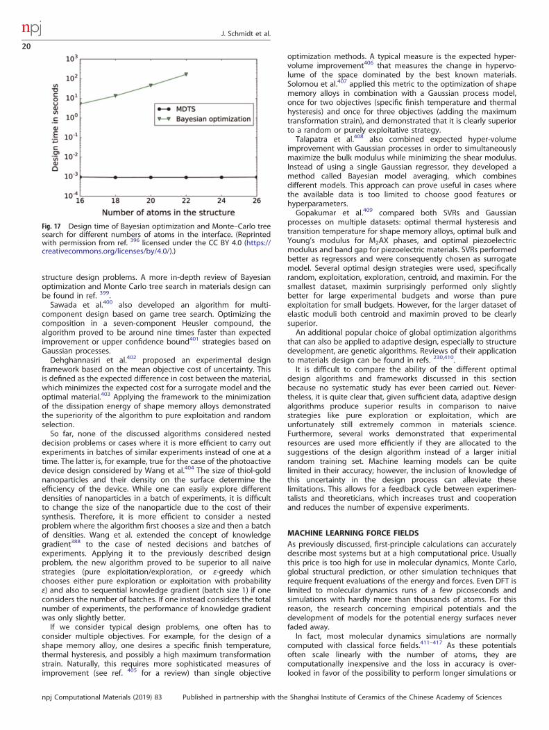
structure design problems. A more in-depth review of Bayesianoptimization and Monte Carlo tree search in materials design canbe found in ref. 399.Sawada et al.400 also developed an algorithm for multi-

component design based on game tree search. Optimizing thecomposition in a seven-component Heusler compound, thealgorithm proved to be around nine times faster than expectedimprovement or upper confidence bound401 strategies based onGaussian processes.Dehghannasiri et al.402 proposed an experimental design

framework based on the mean objective cost of uncertainty. Thisis defined as the expected difference in cost between the material,which minimizes the expected cost for a surrogate model and theoptimal material.403 Applying the framework to the minimizationof the dissipation energy of shape memory alloys demonstratedthe superiority of the algorithm to pure exploitation and randomselection.So far, none of the discussed algorithms considered nested

decision problems or cases where it is more efficient to carry outexperiments in batches of similar experiments instead of one at atime. The latter is, for example, true for the case of the photoactivedevice design considered by Wang et al.404 The size of thiol-goldnanoparticles and their density on the surface determine theefficiency of the device. While one can easily explore differentdensities of nanoparticles in a batch of experiments, it is difficultto change the size of the nanoparticle due to the cost of theirsynthesis. Therefore, it is more efficient to consider a nestedproblem where the algorithm first chooses a size and then a batchof densities. Wang et al. extended the concept of knowledgegradient388 to the case of nested decisions and batches ofexperiments. Applying it to the previously described designproblem, the new algorithm proved to be superior to all naivestrategies (pure exploitation/exploration, or ε-greedy whichchooses either pure exploration or exploitation with probabilityε) and also to sequential knowledge gradient (batch size 1) if oneconsiders the number of batches. If one instead considers the totalnumber of experiments, the performance of knowledge gradientwas only slightly better.If we consider typical design problems, one often has to

consider multiple objectives. For example, for the design of ashape memory alloy, one desires a specific finish temperature,thermal hysteresis, and possibly a high maximum transformationstrain. Naturally, this requires more sophisticated measures ofimprovement (see ref. 405 for a review) than single objective

optimization methods. A typical measure is the expected hyper-volume improvement406 that measures the change in hypervo-lume of the space dominated by the best known materials.Solomou et al.407 applied this metric to the optimization of shapememory alloys in combination with a Gaussian process model,once for two objectives (specific finish temperature and thermalhysteresis) and once for three objectives (adding the maximumtransformation strain), and demonstrated that it is clearly superiorto a random or purely exploitative strategy.Talapatra et al.408 also combined expected hyper-volume

improvement with Gaussian processes in order to simultaneouslymaximize the bulk modulus while minimizing the shear modulus.Instead of using a single Gaussian regressor, they developed amethod called Bayesian model averaging, which combinesdifferent models. This approach can prove useful in cases wherethe available data is too limited to choose good features orhyperparameters.Gopakumar et al.409 compared both SVRs and Gaussian

processes on multiple datasets: optimal thermal hysteresis andtransition temperature for shape memory alloys, optimal bulk andYoung’s modulus for M2AX phases, and optimal piezoelectricmodulus and band gap for piezoelectric materials. SVRs performedbetter as regressors and were consequently chosen as surrogatemodel. Several optimal design strategies were used, specificallyrandom, exploitation, exploration, centroid, and maximin. For thesmallest dataset, maximin surprisingly performed only slightlybetter for large experimental budgets and worse than pureexploitation for small budgets. However, for the larger dataset ofelastic moduli both centroid and maximin proved to be clearlysuperior.An additional popular choice of global optimization algorithms

that can also be applied to adaptive design, especially to structuredevelopment, are genetic algorithms. Reviews of their applicationto materials design can be found in refs. 230,410.It is difficult to compare the ability of the different optimal

design algorithms and frameworks discussed in this sectionbecause no systematic study has ever been carried out. Never-theless, it is quite clear that, given sufficient data, adaptive designalgorithms produce superior results in comparison to naivestrategies like pure exploration or exploitation, which areunfortunately still extremely common in materials science.Furthermore, several works demonstrated that experimentalresources are used more efficiently if they are allocated to thesuggestions of the design algorithm instead of a larger initialrandom training set. Machine learning models can be quitelimited in their accuracy; however, the inclusion of knowledge ofthis uncertainty in the design process can alleviate theselimitations. This allows for a feedback cycle between experimen-talists and theoreticians, which increases trust and cooperationand reduces the number of expensive experiments.

MACHINE LEARNING FORCE FIELDSAs previously discussed, first-principle calculations can accuratelydescribe most systems but at a high computational price. Usuallythis price is too high for use in molecular dynamics, Monte Carlo,global structural prediction, or other simulation techniques thatrequire frequent evaluations of the energy and forces. Even DFT islimited to molecular dynamics runs of a few picoseconds andsimulations with hardly more than thousands of atoms. For thisreason, the research concerning empirical potentials and thedevelopment of models for the potential energy surfaces neverfaded away.In fact, most molecular dynamics simulations are normally

computed with classical force fields.411–417 As these potentialsoften scale linearly with the number of atoms, they arecomputationally inexpensive and the loss in accuracy is over-looked in favor of the possibility to perform longer simulations or

Fig. 17 Design time of Bayesian optimization and Monte–Carlo treesearch for different numbers of atoms in the interface. (Reprintedwith permission from ref. 396 licensed under the CC BY 4.0 (https://creativecommons.org/licenses/by/4.0/).)

J. Schmidt et al.

20

npj Computational Materials (2019) 83 Published in partnership with the Shanghai Institute of Ceramics of the Chinese Academy of Sciences

simulations with hundreds of thousands or even millions of atoms.Another approach is DFT-based tight binding.418–420 Thisquantum–mechanical technique scales with the cube of thenumber of electrons but has a much smaller prefactor than DFT.Certainly, calculations performed with this method are not asaccurate as in DFT, but they are more reliable than classical forcefield calculations. In addition to the reduced precision, theconstruction of force fields and tight-binding parameters isunfortunately not straightforward.Neural networks were the first machine learning method used

in the construction of potential energy surfaces. As early as 1992,Sumper et al.421 used a neural network to relate the vibrationspectra of a polyethylene molecule with its potential energysurface. Unfortunately, the large amount of input data andarchitecture optimization required deemed this approach as toocumbersome and difficult to apply to other molecular systems. Itwas the work of Blank et al.422 in 1995 that really showed thepotential, and marked the birth, of machine learning force fields.Their work on the surface diffusion of CO/Ni(111) relied on neuralnetwork potentials, which mapped the energy of a system with itsstructure, mainly the lateral position of the center of mass, theangle of the molecular axis relative to the surface normal, and theposition of the center of mass. The training set was obtained fromelectronic structure calculations and no further approximationswere used. Their seminal study proved that neural networks couldbe used to make accurate and efficient predictions of the potentialenergy surface for systems with several degrees of freedom.Since then, many machine learning potentials were reported. As

several reviews on these potentials can be easily found in theliterature,112,423–425 here we discuss only the most prominent andrecent approaches related to materials science.One of the most successful applications of machine learning to

the creation of a reliable representation of the potential energysurface is the Behler and Parrinelo approach.110 Here the totalenergy of a system is represented as a sum of atomiccontributions Ei. This became the standard for all later machinelearning force fields, as it allows their application to very largesystems. In the Behler–Parrinelo approach, a multilayer perceptronfeedforward neural network is used to map each atom to itscontribution to the energy. Every atom of a system is described bya set of symmetry functions, which serve as input to a neuralnetwork of that element. Every element in the periodic table ischaracterized by a different network. As the neural networkfunction provides an energy, analytical differentiation with respectto the atomic positions or the strain delivers, respectively, forcesand stresses. This approach was originally applied to bulk silicon,reproducing DFT energies up to an error of 5 meV/atom.Furthermore, molecular dynamic simulations using this potentialwere able to reproduce the RDF of a silicon melt at 3000 K. Manyapplications of this methodology to the field of materials sciencehave appeared since then, for example, to carbon,426 sodium,427

zinc oxide,428 titanium dioxide,111 germanium telluride,429 cop-per,430 gold,431 and Al-Mg-Si alloys.432

Since its publication in 2007, several improvements were madeto the Behler and Parrinelo approach. In 2015, Ghasemi et al.proposed a charge equilibration technique via neural networks,433

where an environment-dependent atomic electronegativity isobtained from the neural networks and the total energy iscomputed from a charge equilibration method. This techniquesuccessfully reproduced several bulk properties of CaF2.

434 In2011, the cost function was expanded to include forceterms.424,428 This extension was first proposed by Witkoskieet al.435 and later extended and generalized by Pukrittayakameeet al.436,437 These works show that the inclusion of the gradients inthe training substantially improves the accuracy of the force fields,not only due to the increase of the size of the training set but alsodue to the additional restrictions in the training. Hajinazar et al.438

devised a strategy to train hierarchical multicomponent systems,

starting with elemental substances and going up to binaries,ternaries, etc. They then applied this technique to the calculationsof defects and formation energies of Cu, Pd, and Ag systems andwere able to obtain an excellent reproduction of phonondispersions. Another improvement concerns the replacement ofthe original Behler–Parrinelo symmetry functions by descriptorsthat can be systematically improved. One such descriptor is givenby Chebyshev polynomials,117 which also allow for the creation ofpotentials for materials with several chemical elements, due to itsconstant complexity with respect to the number of species.Potentials constructed with this descriptor are the reportedmachine learning potentials that can describe more chemicalspecies, with 11 so far.Artrith et al.439 proved the applicability of specialized neural

network potentials in their study of amorphous Li–Si phases. Theycompared the results obtained with two different samplingmethods. The first involved a delithiation algorithm, whichcoupled a genetic algorithm with a specialized potential trainedwith only 725 structures close to the crystalline LixSi1−x phase. Thesecond method consisted of an extensive molecular dynamicsheat-quench sampling and a more general potential. Figure 18shows the accuracy of the latter neural network potential.We note that not only machine learning methods are changing

the field of materials science but also machine learningmethodologies. The spectral neighbor analysis potential440 fromThompson et al. consists of a linear fit that associates an atomicenvironment, represented by the four-dimensional bispectrumcomponents, with the energies of solids and liquids. The firstapplication of these potential to tantalum showed promisingresults, as it was able to correctly reproduce the relative energy ofdifferent phases. Furthermore, in the application of this potentialto molybdenum by Chen et al.,441 PCA was used to examine thedistribution of the features in the space. This technique increasesthe efficiency of the fitting, as it ensures a good coverage of thefeature space and reduces the number of structures in the trainingset. Their potential achieved good accuracies for energies andstresses (9 meV and 0.9 GPa, respectively). Although the accuracyin the forces was considerably worse (0.30 eVÅ), they alsomanaged to reproduce correctly several mechanical propertiessuch as the bulk modulus, lattice constants, or phonon dispersions(see Fig. 19). Wood et al.442 proposed an improvement of the

Fig. 18 Phase diagram of 45,000 LixSi1−x structures depicting theformation energies predicted using the general neural networkpotential (green stars) and the density functional theory referenceformation energies (black circles). (Reprinted from ref. 439, with thepermission of AIP Publishing.)

J. Schmidt et al.

21

Published in partnership with the Shanghai Institute of Ceramics of the Chinese Academy of Sciences npj Computational Materials (2019) 83

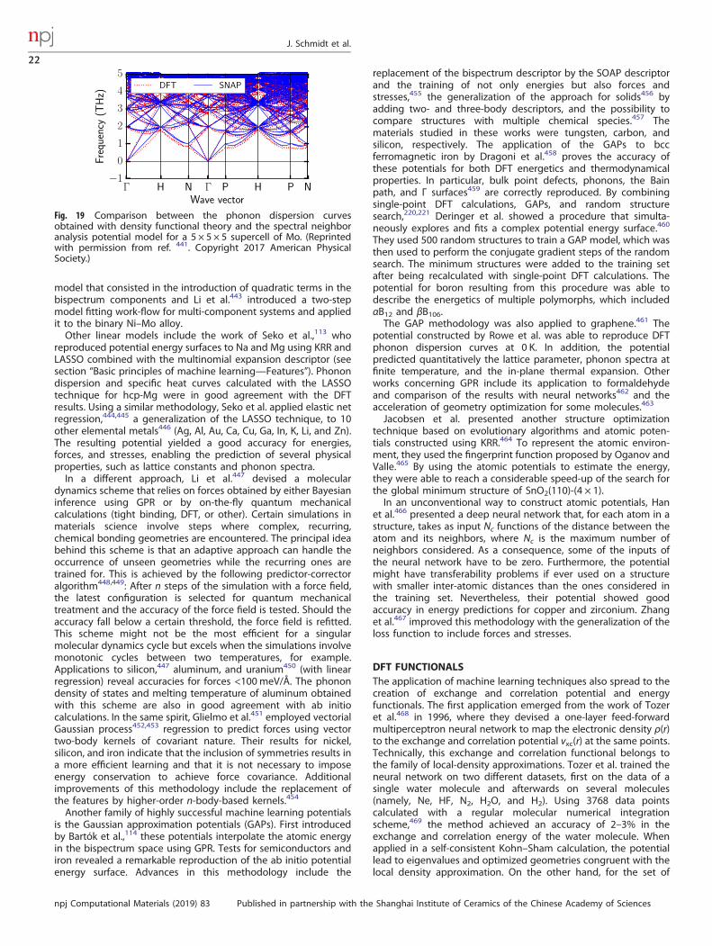
model that consisted in the introduction of quadratic terms in thebispectrum components and Li et al.443 introduced a two-stepmodel fitting work-flow for multi-component systems and appliedit to the binary Ni–Mo alloy.Other linear models include the work of Seko et al.,113 who

reproduced potential energy surfaces to Na and Mg using KRR andLASSO combined with the multinomial expansion descriptor (seesection “Basic principles of machine learning—Features”). Phonondispersion and specific heat curves calculated with the LASSOtechnique for hcp-Mg were in good agreement with the DFTresults. Using a similar methodology, Seko et al. applied elastic netregression,444,445 a generalization of the LASSO technique, to 10other elemental metals446 (Ag, Al, Au, Ca, Cu, Ga, In, K, Li, and Zn).The resulting potential yielded a good accuracy for energies,forces, and stresses, enabling the prediction of several physicalproperties, such as lattice constants and phonon spectra.In a different approach, Li et al.447 devised a molecular

dynamics scheme that relies on forces obtained by either Bayesianinference using GPR or by on-the-fly quantum mechanicalcalculations (tight binding, DFT, or other). Certain simulations inmaterials science involve steps where complex, recurring,chemical bonding geometries are encountered. The principal ideabehind this scheme is that an adaptive approach can handle theoccurrence of unseen geometries while the recurring ones aretrained for. This is achieved by the following predictor-correctoralgorithm448,449: After n steps of the simulation with a force field,the latest configuration is selected for quantum mechanicaltreatment and the accuracy of the force field is tested. Should theaccuracy fall below a certain threshold, the force field is refitted.This scheme might not be the most efficient for a singularmolecular dynamics cycle but excels when the simulations involvemonotonic cycles between two temperatures, for example.Applications to silicon,447 aluminum, and uranium450 (with linearregression) reveal accuracies for forces <100 meV/Å. The phonondensity of states and melting temperature of aluminum obtainedwith this scheme are also in good agreement with ab initiocalculations. In the same spirit, Glielmo et al.451 employed vectorialGaussian process452,453 regression to predict forces using vectortwo-body kernels of covariant nature. Their results for nickel,silicon, and iron indicate that the inclusion of symmetries results ina more efficient learning and that it is not necessary to imposeenergy conservation to achieve force covariance. Additionalimprovements of this methodology include the replacement ofthe features by higher-order n-body-based kernels.454

Another family of highly successful machine learning potentialsis the Gaussian approximation potentials (GAPs). First introducedby Bartók et al.,114 these potentials interpolate the atomic energyin the bispectrum space using GPR. Tests for semiconductors andiron revealed a remarkable reproduction of the ab initio potentialenergy surface. Advances in this methodology include the

replacement of the bispectrum descriptor by the SOAP descriptorand the training of not only energies but also forces andstresses,455 the generalization of the approach for solids456 byadding two- and three-body descriptors, and the possibility tocompare structures with multiple chemical species.457 Thematerials studied in these works were tungsten, carbon, andsilicon, respectively. The application of the GAPs to bccferromagnetic iron by Dragoni et al.458 proves the accuracy ofthese potentials for both DFT energetics and thermodynamicalproperties. In particular, bulk point defects, phonons, the Bainpath, and Γ surfaces459 are correctly reproduced. By combiningsingle-point DFT calculations, GAPs, and random structuresearch,220,221 Deringer et al. showed a procedure that simulta-neously explores and fits a complex potential energy surface.460

They used 500 random structures to train a GAP model, which wasthen used to perform the conjugate gradient steps of the randomsearch. The minimum structures were added to the training setafter being recalculated with single-point DFT calculations. Thepotential for boron resulting from this procedure was able todescribe the energetics of multiple polymorphs, which includedαB12 and βB106.The GAP methodology was also applied to graphene.461 The

potential constructed by Rowe et al. was able to reproduce DFTphonon dispersion curves at 0 K. In addition, the potentialpredicted quantitatively the lattice parameter, phonon spectra atfinite temperature, and the in-plane thermal expansion. Otherworks concerning GPR include its application to formaldehydeand comparison of the results with neural networks462 and theacceleration of geometry optimization for some molecules.463

Jacobsen et al. presented another structure optimizationtechnique based on evolutionary algorithms and atomic poten-tials constructed using KRR.464 To represent the atomic environ-ment, they used the fingerprint function proposed by Oganov andValle.465 By using the atomic potentials to estimate the energy,they were able to reach a considerable speed-up of the search forthe global minimum structure of SnO2(110)-(4 × 1).In an unconventional way to construct atomic potentials, Han

et al.466 presented a deep neural network that, for each atom in astructure, takes as input Nc functions of the distance between theatom and its neighbors, where Nc is the maximum number ofneighbors considered. As a consequence, some of the inputs ofthe neural network have to be zero. Furthermore, the potentialmight have transferability problems if ever used on a structurewith smaller inter-atomic distances than the ones considered inthe training set. Nevertheless, their potential showed goodaccuracy in energy predictions for copper and zirconium. Zhanget al.467 improved this methodology with the generalization of theloss function to include forces and stresses.

DFT FUNCTIONALSThe application of machine learning techniques also spread to thecreation of exchange and correlation potential and energyfunctionals. The first application emerged from the work of Tozeret al.468 in 1996, where they devised a one-layer feed-forwardmultiperceptron neural network to map the electronic density ρ(r)to the exchange and correlation potential vxc(r) at the same points.Technically, this exchange and correlation functional belongs tothe family of local-density approximations. Tozer et al. trained theneural network on two different datasets, first on the data of asingle water molecule and afterwards on several molecules(namely, Ne, HF, N2, H2O, and H2). Using 3768 data pointscalculated with a regular molecular numerical integrationscheme,469 the method achieved an accuracy of 2–3% in theexchange and correlation energy of the water molecule. Whenapplied in a self-consistent Kohn–Sham calculation, the potentiallead to eigenvalues and optimized geometries congruent with thelocal density approximation. On the other hand, for the set of

Fig. 19 Comparison between the phonon dispersion curvesobtained with density functional theory and the spectral neighboranalysis potential model for a 5 × 5 × 5 supercell of Mo. (Reprintedwith permission from ref. 441. Copyright 2017 American PhysicalSociety.)

J. Schmidt et al.

22

npj Computational Materials (2019) 83 Published in partnership with the Shanghai Institute of Ceramics of the Chinese Academy of Sciences

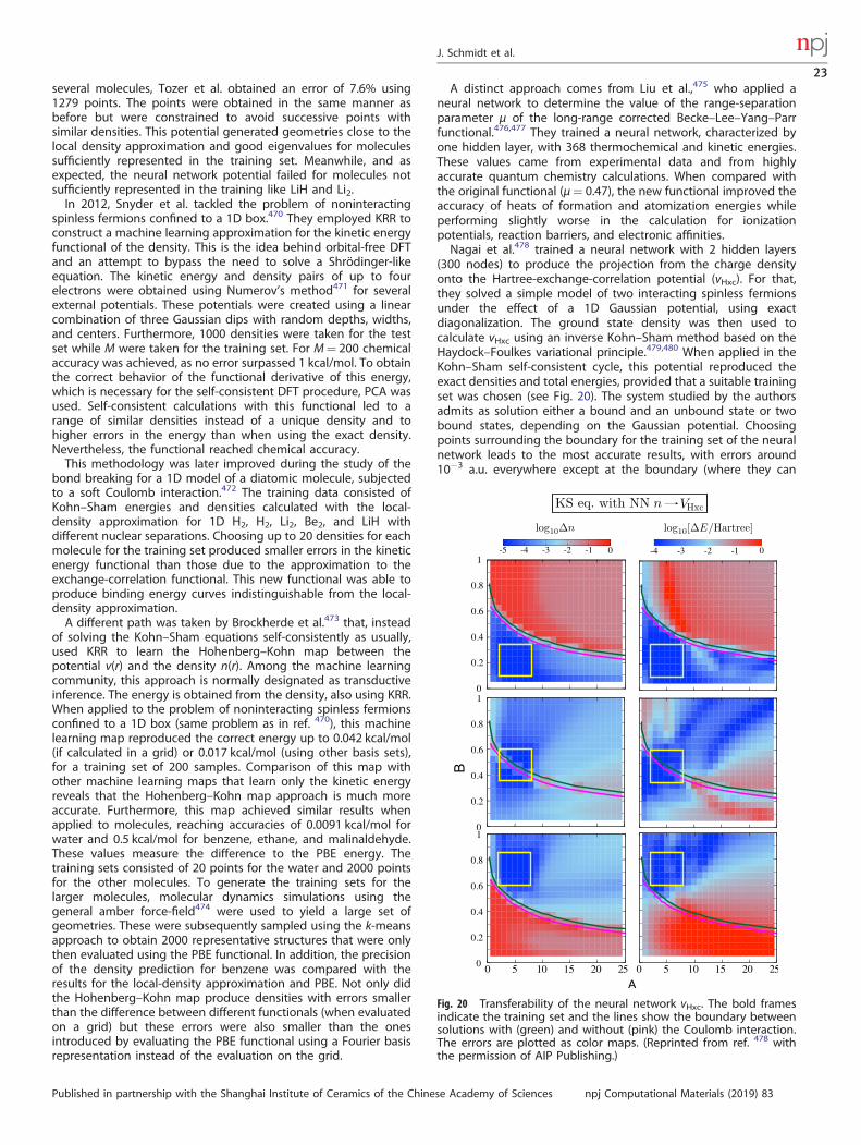
several molecules, Tozer et al. obtained an error of 7.6% using1279 points. The points were obtained in the same manner asbefore but were constrained to avoid successive points withsimilar densities. This potential generated geometries close to thelocal density approximation and good eigenvalues for moleculessufficiently represented in the training set. Meanwhile, and asexpected, the neural network potential failed for molecules notsufficiently represented in the training like LiH and Li2.In 2012, Snyder et al. tackled the problem of noninteracting

spinless fermions confined to a 1D box.470 They employed KRR toconstruct a machine learning approximation for the kinetic energyfunctional of the density. This is the idea behind orbital-free DFTand an attempt to bypass the need to solve a Shrödinger-likeequation. The kinetic energy and density pairs of up to fourelectrons were obtained using Numerov’s method471 for severalexternal potentials. These potentials were created using a linearcombination of three Gaussian dips with random depths, widths,and centers. Furthermore, 1000 densities were taken for the testset while M were taken for the training set. For M= 200 chemicalaccuracy was achieved, as no error surpassed 1 kcal/mol. To obtainthe correct behavior of the functional derivative of this energy,which is necessary for the self-consistent DFT procedure, PCA wasused. Self-consistent calculations with this functional led to arange of similar densities instead of a unique density and tohigher errors in the energy than when using the exact density.Nevertheless, the functional reached chemical accuracy.This methodology was later improved during the study of the

bond breaking for a 1D model of a diatomic molecule, subjectedto a soft Coulomb interaction.472 The training data consisted ofKohn–Sham energies and densities calculated with the local-density approximation for 1D H2, H2, Li2, Be2, and LiH withdifferent nuclear separations. Choosing up to 20 densities for eachmolecule for the training set produced smaller errors in the kineticenergy functional than those due to the approximation to theexchange-correlation functional. This new functional was able toproduce binding energy curves indistinguishable from the local-density approximation.A different path was taken by Brockherde et al.473 that, instead

of solving the Kohn–Sham equations self-consistently as usually,used KRR to learn the Hohenberg–Kohn map between thepotential v(r) and the density n(r). Among the machine learningcommunity, this approach is normally designated as transductiveinference. The energy is obtained from the density, also using KRR.When applied to the problem of noninteracting spinless fermionsconfined to a 1D box (same problem as in ref. 470), this machinelearning map reproduced the correct energy up to 0.042 kcal/mol(if calculated in a grid) or 0.017 kcal/mol (using other basis sets),for a training set of 200 samples. Comparison of this map withother machine learning maps that learn only the kinetic energyreveals that the Hohenberg–Kohn map approach is much moreaccurate. Furthermore, this map achieved similar results whenapplied to molecules, reaching accuracies of 0.0091 kcal/mol forwater and 0.5 kcal/mol for benzene, ethane, and malinaldehyde.These values measure the difference to the PBE energy. Thetraining sets consisted of 20 points for the water and 2000 pointsfor the other molecules. To generate the training sets for thelarger molecules, molecular dynamics simulations using thegeneral amber force-field474 were used to yield a large set ofgeometries. These were subsequently sampled using the k-meansapproach to obtain 2000 representative structures that were onlythen evaluated using the PBE functional. In addition, the precisionof the density prediction for benzene was compared with theresults for the local-density approximation and PBE. Not only didthe Hohenberg–Kohn map produce densities with errors smallerthan the difference between different functionals (when evaluatedon a grid) but these errors were also smaller than the onesintroduced by evaluating the PBE functional using a Fourier basisrepresentation instead of the evaluation on the grid.

A distinct approach comes from Liu et al.,475 who applied aneural network to determine the value of the range-separationparameter μ of the long-range corrected Becke–Lee–Yang–Parrfunctional.476,477 They trained a neural network, characterized byone hidden layer, with 368 thermochemical and kinetic energies.These values came from experimental data and from highlyaccurate quantum chemistry calculations. When compared withthe original functional (μ= 0.47), the new functional improved theaccuracy of heats of formation and atomization energies whileperforming slightly worse in the calculation for ionizationpotentials, reaction barriers, and electronic affinities.Nagai et al.478 trained a neural network with 2 hidden layers

(300 nodes) to produce the projection from the charge densityonto the Hartree-exchange-correlation potential (vHxc). For that,they solved a simple model of two interacting spinless fermionsunder the effect of a 1D Gaussian potential, using exactdiagonalization. The ground state density was then used tocalculate vHxc using an inverse Kohn–Sham method based on theHaydock–Foulkes variational principle.479,480 When applied in theKohn–Sham self-consistent cycle, this potential reproduced theexact densities and total energies, provided that a suitable trainingset was chosen (see Fig. 20). The system studied by the authorsadmits as solution either a bound and an unbound state or twobound states, depending on the Gaussian potential. Choosingpoints surrounding the boundary for the training set of the neuralnetwork leads to the most accurate results, with errors around10−3 a.u. everywhere except at the boundary (where they can

Fig. 20 Transferability of the neural network vHxc. The bold framesindicate the training set and the lines show the boundary betweensolutions with (green) and without (pink) the Coulomb interaction.The errors are plotted as color maps. (Reprinted from ref. 478 withthe permission of AIP Publishing.)

J. Schmidt et al.

23

Published in partnership with the Shanghai Institute of Ceramics of the Chinese Academy of Sciences npj Computational Materials (2019) 83

almost reach 1 a.u.). On the other hand, choosing points in one ofthe regions results in a poor description of the other region.

DISCUSSION AND CONCLUSIONSInterpretabilityWe already noted in the introduction that a major criticism ofmachine learning techniques is that their black-box algorithms donot provide us with new “physical laws” and that their innerworkings remain outside our understanding.481 For example,Ghiringhelli et al. argue that “a trustful prediction of newpromising materials, identification of anomalies, and scientificadvancement are doubtful,” if the scientific connection betweenfeatures and prediction is unknown.96 Johnson writes in thecontext of quantitative structure–activity relationships: “By notfollowing through with careful, designed, hypothesis testing wehave allowed scientific thinking to be co-opted by statistics andarbitrarily defined fitness functions.”378 The main concern is thatmodels not based on physical principles might fail in completelyunexpected cases (that are trivial for humans) while providing avery good result on average. Such cases can only be predicted andprevented if one understands the causality between the inputsand outputs of the model. Furthermore, especially in applicationswhere a single failure is extremely expensive or potentially deadly(as in medicine), the lack of trust in black-box machine learningmodels stops their widespread use even when they provide asuperior performance.273

As there are different concepts of interpretability, we will defineits various facets according to Lipton et al.482 To start with, we candivide interpretability into transparency and post hoc explana-tions, which consist of additional information provided by orextracted from a model.Transparency can once again be split into the concepts of

simulatability, decomposability, and algorithmic transparency.Simulatability is a partially subjective notion and concerns theability of humans to follow and retrace the calculations of themodel. This is, e.g., the case for sparse linear models such as theones resulting from LASSO,159 SISSO,163 or flat decision treemodels. Decomposability is closely related to the intelligibility of amodel and describes whether its various parts (input, parameters,calculations) allow for an intuitive interpretation. Algorithmictransparency considers our understanding of the error surface(e.g., whether the training will converge to a unique solution). Thisis clearly not the case for modern neural networks, for example.Post hoc interpretability considers the possibility to extract

additional information from the model. Examples for this arevariable importance from a decision tree model or active responsemaps, which highlight regions of a picture that were particularlyimportant for its classification by a convolutional neural network.Starting from these concepts of interpretability, it is obvious

that the notion of a complex model runs counter to the claim thatit is simulatable by a human. Furthermore, models that aresimulatable (e.g., low-dimensional linear models) and accurateoften require unintuitive highly processed features that reduce thedecomposability483 (e.g., spectral neighbor analysis potentialpotentials) in order to reach a comparable performance to amore complex model. In contrast, a complex model like a deepconvolutional neural network only requires relatively simple un-engineered features and relies on its own ability to extractdescriptors of different abstraction levels. In this sense, there is adefinite conflict between the complexity and accuracy of a model,on one hand, and a simulatable decomposable model on theother hand.The simplest examples of models that are simulatable are

techniques based in dimensionality reduction or feature selectionalgorithms, like SISSO.163 These are usually used in combinationwith linear fits and result in simple equations describing the

problem. An example is the estimation of the probability of amaterial to exist as a perovskite (ABX3), as given in ref. 143:

τ ¼ rXrB� nA nA � rA=rB

lnðrA=rBÞ� �

; (42)

where nA is the oxidation state of A and ri is the ionic radius of ioni. Another example is given by Kim et al.,38 who used LASSO, aswell as RF and KRR, to predict the dielectric breakdown field ofelemental and binary insulators, on the basis of eight featuresobtained from first-principle calculations (e.g. band gap, phononcutoff frequency, etc.). In the end, all three methods determinedthe same two features as optimal and demonstrated nearly thesame error. However, Kim et al. favored LASSO,159 because itprovided a simple analytical formula, even if no further knowledgewas gained from the formula. In any case, the knowledge of theanalytical formula and therefore the simulatability seems to be farless relevant than the knowledge of the most relevant physicalvariables. In general, we can even argue that simulatability is notrelevant for materials science as computational methods based onphysical reasoning, like DFT or tight binding, are even furtherremoved from simulatability than most machine learning models.A second method that provides a variable importance measure

(see section “Basic principles of machine learning—Features”) areRFs or other decision tree-based methods. Stanev et al. demon-strate the usefulness of this method for post hoc interpretability inref. 76, by recovering numerous known (e.g., isotope effect) andsome unknown rules and limits for the superconducting criticaltemperature. This was done by first reducing the number offeatures via variable importance measure (Gini importance) andsubsequently visualizing the correlation between the features andthe critical temperature (see Fig. 21).Pankajakshan et al.168 developed bootstrapped-projected gra-

dient descent as a feature selection method specifically formaterials science. The motivation came from some consistencyissues for correlated or linearly dependent variables (present, forexample, in LASSO), which bootstrapped-projected gradientdescent can alleviate through extra clustering and bootstrapping.In their work, Pankajakshan et al. used machine learning mostly tofind and understand descriptors, in order to improve the d-bandmodel of catalysts for CO2 reduction,484 instead of actually usingthe machine learning model for predictions. This can definitely bea reasonable approach in cases where datasets are too small andincomplete for any successful extrapolation. Notwithstanding, inmost cases it is questionable if a classical (in the sense of “non-machine learning”) model should be used directly when amachine learning model is superior, as in the case of the d-bandmodel.485 Of course, it is a bonus when a classical model exists, asit can be used to check for consistency issues or as a crudeestimation of property. However, in our opinion, pragmaticapplications of advanced materials design should always use thebest model.While RFs and linear fits are considered more accessible from a

interpretability point of view, deep neural networks are one of theprime examples for algorithms that are traditionally considered ablack box. While their complex nature often results in superiorperformance in comparison to simpler algorithms, an unwantedconsequence is the lack of simulatability and algorithmictransparency. As the lack of interpretability is one of the mainchallenges for a wider adoption of neural networks in industry andexperimental sciences, post hoc methods to visualize the responseand understand the inner workings of neural networks weredeveloped during the past years. One example are attentiveresponse maps for image recognition networks that highlightregions of the picture according to their importance in thedecision making process. Kumar et al.271 demonstrated that, bycombining the understanding gained from attentive responsemaps with domain knowledge and applying it to the design

J. Schmidt et al.

24

npj Computational Materials (2019) 83 Published in partnership with the Shanghai Institute of Ceramics of the Chinese Academy of Sciences

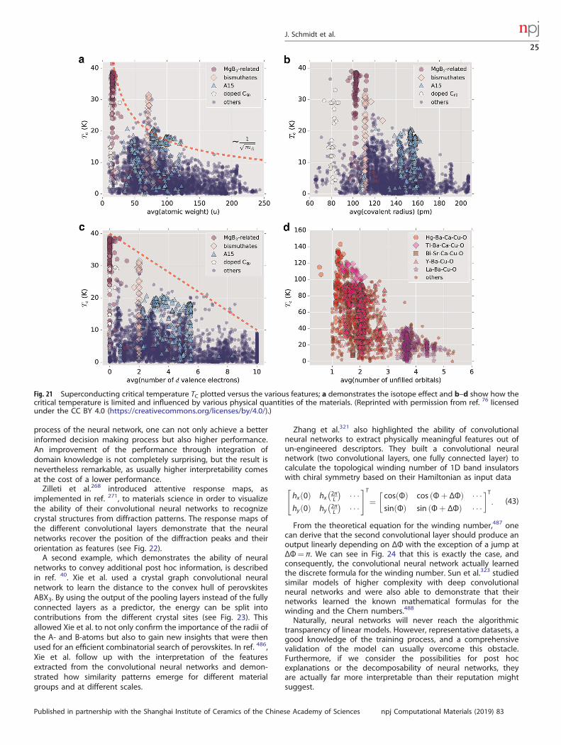
process of the neural network, one can not only achieve a betterinformed decision making process but also higher performance.An improvement of the performance through integration ofdomain knowledge is not completely surprising, but the result isnevertheless remarkable, as usually higher interpretability comesat the cost of a lower performance.Zilleti et al.268 introduced attentive response maps, as

implemented in ref. 271, to materials science in order to visualizethe ability of their convolutional neural networks to recognizecrystal structures from diffraction patterns. The response maps ofthe different convolutional layers demonstrate that the neuralnetworks recover the position of the diffraction peaks and theirorientation as features (see Fig. 22).A second example, which demonstrates the ability of neural

networks to convey additional post hoc information, is describedin ref. 40. Xie et al. used a crystal graph convolutional neuralnetwork to learn the distance to the convex hull of perovskitesABX3. By using the output of the pooling layers instead of the fullyconnected layers as a predictor, the energy can be split intocontributions from the different crystal sites (see Fig. 23). Thisallowed Xie et al. to not only confirm the importance of the radii ofthe A- and B-atoms but also to gain new insights that were thenused for an efficient combinatorial search of perovskites. In ref. 486,Xie et al. follow up with the interpretation of the featuresextracted from the convolutional neural networks and demon-strated how similarity patterns emerge for different materialgroups and at different scales.

Zhang et al.321 also highlighted the ability of convolutionalneural networks to extract physically meaningful features out ofun-engineered descriptors. They built a convolutional neuralnetwork (two convolutional layers, one fully connected layer) tocalculate the topological winding number of 1D band insulatorswith chiral symmetry based on their Hamiltonian as input data

hxð0Þ hx 2πL

� � � � �hyð0Þ hy 2π

L

� � � � �

" #T¼ cosðΦÞ cos ðΦþ ΔΦÞ � � �

sinðΦÞ sin ðΦþ ΔΦÞ � � � �T

: (43)

From the theoretical equation for the winding number,487 onecan derive that the second convolutional layer should produce anoutput linearly depending on ΔΦ with the exception of a jump atΔΦ= π. We can see in Fig. 24 that this is exactly the case, andconsequently, the convolutional neural network actually learnedthe discrete formula for the winding number. Sun et al.323 studiedsimilar models of higher complexity with deep convolutionalneural networks and were also able to demonstrate that theirnetworks learned the known mathematical formulas for thewinding and the Chern numbers.488

Naturally, neural networks will never reach the algorithmictransparency of linear models. However, representative datasets, agood knowledge of the training process, and a comprehensivevalidation of the model can usually overcome this obstacle.Furthermore, if we consider the possibilities for post hocexplanations or the decomposability of neural networks, theyare actually far more interpretable than their reputation mightsuggest.

Fig. 21 Superconducting critical temperature TC plotted versus the various features; a demonstrates the isotope effect and b–d show how thecritical temperature is limited and influenced by various physical quantities of the materials. (Reprinted with permission from ref. 76 licensedunder the CC BY 4.0 (https://creativecommons.org/licenses/by/4.0/).)

J. Schmidt et al.

25

Published in partnership with the Shanghai Institute of Ceramics of the Chinese Academy of Sciences npj Computational Materials (2019) 83

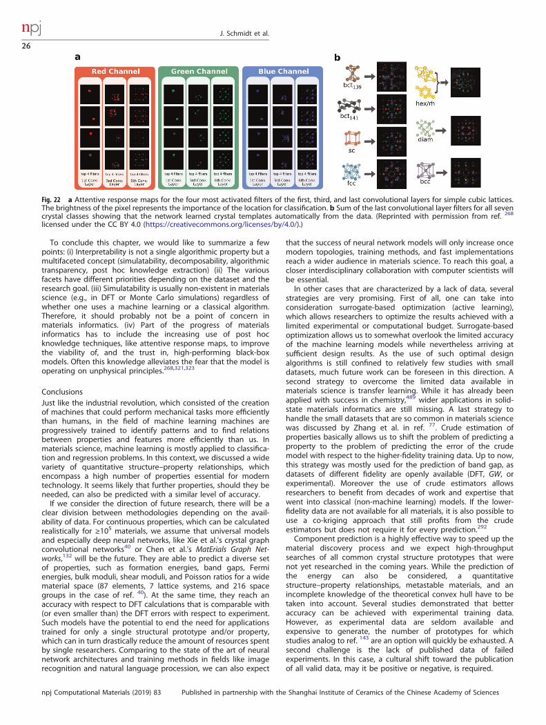
To conclude this chapter, we would like to summarize a fewpoints: (i) Interpretability is not a single algorithmic property but amultifaceted concept (simulatability, decomposability, algorithmictransparency, post hoc knowledge extraction) (ii) The variousfacets have different priorities depending on the dataset and theresearch goal. (iii) Simulatability is usually non-existent in materialsscience (e.g., in DFT or Monte Carlo simulations) regardless ofwhether one uses a machine learning or a classical algorithm.Therefore, it should probably not be a point of concern inmaterials informatics. (iv) Part of the progress of materialsinformatics has to include the increasing use of post hocknowledge techniques, like attentive response maps, to improvethe viability of, and the trust in, high-performing black-boxmodels. Often this knowledge alleviates the fear that the model isoperating on unphysical principles.268,321,323

ConclusionsJust like the industrial revolution, which consisted of the creationof machines that could perform mechanical tasks more efficientlythan humans, in the field of machine learning machines areprogressively trained to identify patterns and to find relationsbetween properties and features more efficiently than us. Inmaterials science, machine learning is mostly applied to classifica-tion and regression problems. In this context, we discussed a widevariety of quantitative structure–property relationships, whichencompass a high number of properties essential for moderntechnology. It seems likely that further properties, should they beneeded, can also be predicted with a similar level of accuracy.If we consider the direction of future research, there will be a

clear division between methodologies depending on the avail-ability of data. For continuous properties, which can be calculatedrealistically for ≥105 materials, we assume that universal modelsand especially deep neural networks, like Xie et al.’s crystal graphconvolutional networks40 or Chen et al.’s MatErials Graph Net-works,132 will be the future. They are able to predict a diverse setof properties, such as formation energies, band gaps, Fermienergies, bulk moduli, shear moduli, and Poisson ratios for a widematerial space (87 elements, 7 lattice systems, and 216 spacegroups in the case of ref. 40). At the same time, they reach anaccuracy with respect to DFT calculations that is comparable with(or even smaller than) the DFT errors with respect to experiment.Such models have the potential to end the need for applicationstrained for only a single structural prototype and/or property,which can in turn drastically reduce the amount of resources spentby single researchers. Comparing to the state of the art of neuralnetwork architectures and training methods in fields like imagerecognition and natural language procession, we can also expect

that the success of neural network models will only increase oncemodern topologies, training methods, and fast implementationsreach a wider audience in materials science. To reach this goal, acloser interdisciplinary collaboration with computer scientists willbe essential.In other cases that are characterized by a lack of data, several

strategies are very promising. First of all, one can take intoconsideration surrogate-based optimization (active learning),which allows researchers to optimize the results achieved with alimited experimental or computational budget. Surrogate-basedoptimization allows us to somewhat overlook the limited accuracyof the machine learning models while nevertheless arriving atsufficient design results. As the use of such optimal designalgorithms is still confined to relatively few studies with smalldatasets, much future work can be foreseen in this direction. Asecond strategy to overcome the limited data available inmaterials science is transfer learning. While it has already beenapplied with success in chemistry,489 wider applications in solid-state materials informatics are still missing. A last strategy tohandle the small datasets that are so common in materials sciencewas discussed by Zhang et al. in ref. 77. Crude estimation ofproperties basically allows us to shift the problem of predicting aproperty to the problem of predicting the error of the crudemodel with respect to the higher-fidelity training data. Up to now,this strategy was mostly used for the prediction of band gap, asdatasets of different fidelity are openly available (DFT, GW, orexperimental). Moreover the use of crude estimators allowsresearchers to benefit from decades of work and expertise thatwent into classical (non-machine learning) models. If the lower-fidelity data are not available for all materials, it is also possible touse a co-kriging approach that still profits from the crudeestimators but does not require it for every prediction.292

Component prediction is a highly effective way to speed up thematerial discovery process and we expect high-throughputsearches of all common crystal structure prototypes that werenot yet researched in the coming years. While the prediction ofthe energy can also be considered, a quantitativestructure–property relationships, metastable materials, and anincomplete knowledge of the theoretical convex hull have to betaken into account. Several studies demonstrated that betteraccuracy can be achieved with experimental training data.However, as experimental data are seldom available andexpensive to generate, the number of prototypes for whichstudies analog to ref. 143 are an option will quickly be exhausted. Asecond challenge is the lack of published data of failedexperiments. In this case, a cultural shift toward the publicationof all valid data, may it be positive or negative, is required.

Fig. 22 a Attentive response maps for the four most activated filters of the first, third, and last convolutional layers for simple cubic lattices.The brightness of the pixel represents the importance of the location for classification. b Sum of the last convolutional layer filters for all sevencrystal classes showing that the network learned crystal templates automatically from the data. (Reprinted with permission from ref. 268

licensed under the CC BY 4.0 (https://creativecommons.org/licenses/by/4.0/).)

J. Schmidt et al.

26

npj Computational Materials (2019) 83 Published in partnership with the Shanghai Institute of Ceramics of the Chinese Academy of Sciences

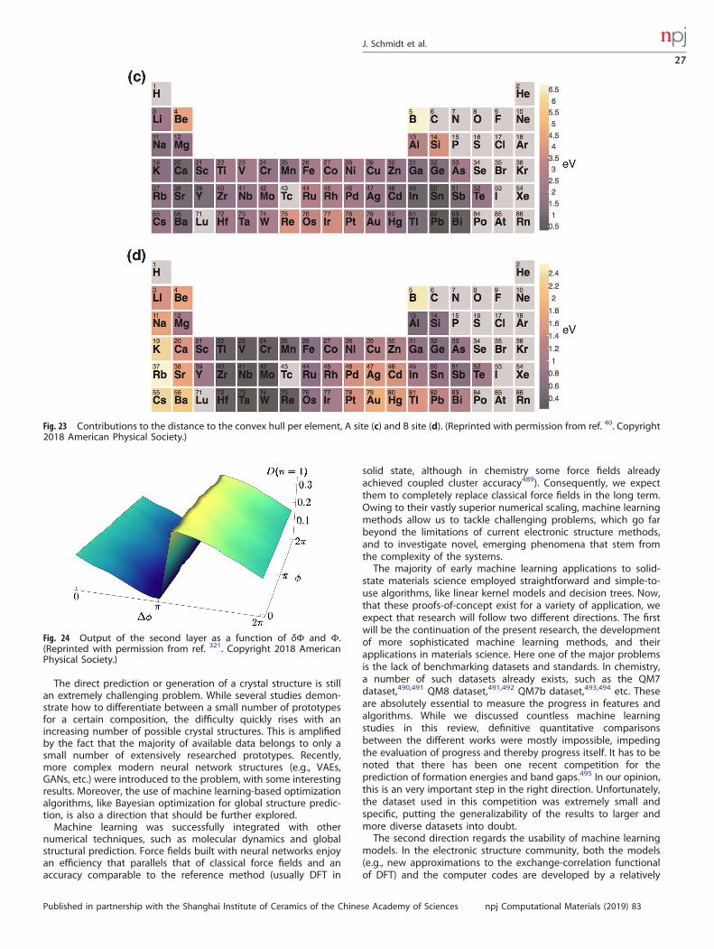
The direct prediction or generation of a crystal structure is stillan extremely challenging problem. While several studies demon-strate how to differentiate between a small number of prototypesfor a certain composition, the difficulty quickly rises with anincreasing number of possible crystal structures. This is amplifiedby the fact that the majority of available data belongs to only asmall number of extensively researched prototypes. Recently,more complex modern neural network structures (e.g., VAEs,GANs, etc.) were introduced to the problem, with some interestingresults. Moreover, the use of machine learning-based optimizationalgorithms, like Bayesian optimization for global structure predic-tion, is also a direction that should be further explored.Machine learning was successfully integrated with other

numerical techniques, such as molecular dynamics and globalstructural prediction. Force fields built with neural networks enjoyan efficiency that parallels that of classical force fields and anaccuracy comparable to the reference method (usually DFT in

solid state, although in chemistry some force fields alreadyachieved coupled cluster accuracy489). Consequently, we expectthem to completely replace classical force fields in the long term.Owing to their vastly superior numerical scaling, machine learningmethods allow us to tackle challenging problems, which go farbeyond the limitations of current electronic structure methods,and to investigate novel, emerging phenomena that stem fromthe complexity of the systems.The majority of early machine learning applications to solid-

state materials science employed straightforward and simple-to-use algorithms, like linear kernel models and decision trees. Now,that these proofs-of-concept exist for a variety of application, weexpect that research will follow two different directions. The firstwill be the continuation of the present research, the developmentof more sophisticated machine learning methods, and theirapplications in materials science. Here one of the major problemsis the lack of benchmarking datasets and standards. In chemistry,a number of such datasets already exists, such as the QM7dataset,490,491 QM8 dataset,491,492 QM7b dataset,493,494 etc. Theseare absolutely essential to measure the progress in features andalgorithms. While we discussed countless machine learningstudies in this review, definitive quantitative comparisonsbetween the different works were mostly impossible, impedingthe evaluation of progress and thereby progress itself. It has to benoted that there has been one recent competition for theprediction of formation energies and band gaps.495 In our opinion,this is an very important step in the right direction. Unfortunately,the dataset used in this competition was extremely small andspecific, putting the generalizability of the results to larger andmore diverse datasets into doubt.The second direction regards the usability of machine learning

models. In the electronic structure community, both the models(e.g., new approximations to the exchange-correlation functionalof DFT) and the computer codes are developed by a relatively

Fig. 23 Contributions to the distance to the convex hull per element, A site (c) and B site (d). (Reprinted with permission from ref. 40. Copyright2018 American Physical Society.)

Fig. 24 Output of the second layer as a function of δΦ and Φ.(Reprinted with permission from ref. 321. Copyright 2018 AmericanPhysical Society.)

J. Schmidt et al.

27

Published in partnership with the Shanghai Institute of Ceramics of the Chinese Academy of Sciences npj Computational Materials (2019) 83

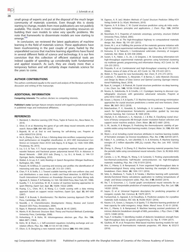
small group of experts and put at the disposal of the much largercommunity of materials scientists. Even though this is slowlystarting to change, models from most publications are not publiclyavailable. This results in most researchers spending resources onbuilding their own models to solve very specific problems. Wenote that frameworks to disseminate models are now starting toemerge.496

In conclusion, we reviewed the latest applications of machinelearning in the field of materials science. These applications havebeen mushrooming in the past couple of years, fueled by theunparalleled success that machine learning algorithms have foundin several different fields of science and technology. It is our firmconviction that this collection of efficient statistical tools areindeed capable of speeding up considerably both fundamentaland applied research. As such, they are clearly more than atemporary fashion and will certainly shape materials science forthe years to come.

AUTHOR CONTRIBUTIONSThe authors contributed equally to the search and analysis of the literature and to thediscussion and writing of the manuscript.

ADDITIONAL INFORMATIONCompeting interests: The authors declare no competing interests.

Publisher’s note: Springer Nature remains neutral with regard to jurisdictional claimsin published maps and institutional affiliations.

REFERENCES1. Marsland, S. Machine Learning (CRC Press, Taylor & Francis Inc., Boca Raton, FL,

2014).2. Silver, D. et al. Mastering the game of go with deep neural networks and tree

search. Nature 529, 484–489 (2016).3. Bojarski, M. et al. End to end learning for self-driving cars. Preprint at

arXiv:1604.07316 (2016).4. He, K., Zhang, X., Ren, S. & Sun, J. Delving deep into rectifiers: surpassing human-

level performance on ImageNet classification. In 2015 IEEE International Con-ference on Computer Vision (ICCV) (eds Bajcsy, R. & Hager, G.) 1026–1034 (IEEE,Piscataway, NJ, 2015).

5. Liu, S.-S. & Tian, Y.-T. Facial expression recognition method based on gaborwavelet features and fractional power polynomial kernel PCA. In Advances inNeural Networks - ISNN 2010 (eds Zhang, L., Lu, B.-L. & Kwok, J.) 144–151(Springer, Berlin, Heidelberg, 2010).

6. Waibel, A. & Lee, K.-F. (eds) Readings in Speech Recognition (Morgan Kaufmann,Burlington, MA, 1990).

7. Pazzani, M. & Billsus, D. Learning and revising user profiles: the identification ofinteresting web sites. Mach. Learn. 27, 313–331 (1997).

8. Chan, P. K. & Stolfo, S. J. Toward scalable learning with non-uniform class andcost distributions: a case study in credit card fraud detection. In KDD’98 Proc.Fourth International Conference on Knowledge Discovery and Data Mining (edsAgrawal, R., Stolorz, P. & Piatetsky, G.) 164–168 (AAAI Press, New York, NY, 1998).

9. Guzella, T. S. & Caminhas, W. M. A review of machine learning approaches tospam filtering. Expert Syst. Appl. 36, 10206–10222 (2009).

10. Huang, C.-L., Chen, M.-C. & Wang, C.-J. Credit scoring with a data miningapproach based on support vector machines. Expert Syst. Appl. 33, 847–856(2007).

11. Baldi, P. & Brunak, S. Bioinformatics: The Machine Learning Approach (The MITPress, Cambridge, MA, 2001).

12. Noordik, J. H. Cheminformatics Developments: History, Reviews and CurrentResearch (IOS Press, Amsterdam, 2004).

13. Rajan, K. Materials informatics. Mater. Today 8, 38–45 (2005).14. Martin, R. M. Electronic Structure: Basic Theory and Practical Methods (Cambridge

University Press, Cambridge, 2008).15. Hohenberg, P. & Kohn, W. Inhomogeneous electron gas. Phys. Rev. 136,

B864–B871 (1964).16. Kohn, W. & Sham, L. J. Self-consistent equations including exchange and cor-

relation effects. Phys. Rev. 140, A1133–A1138 (1965).17. Olson, G. B. Designing a new material world. Science 288, 993–998 (2000).

18. Oganov, A. R. (ed.) Modern Methods of Crystal Structure Prediction (Wiley-VCHVerlag GmbH & Co. KGaA, Weinheim, 2010).

19. Oganov, A. R. & Glass, C. W. Crystal structure prediction using ab initio evolu-tionary techniques: principles and applications. J. Chem. Phys. 124, 244704(2006).

20. Newnham, R. E. Properties of materials: anisotropy, symmetry, structure (OxfordUniversity Press, Oxford, 2005).

21. Curtarolo, S. et al. The high-throughput highway to computational materialsdesign. Nat. Mater. 12, 191–201 (2013).

22. Green, M. L. et al. Fulfilling the promise of the materials genome initiative withhigh-throughput experimental methodologies. Appl. Phys. Rev. 4, 011105 (2017).

23. Koinuma, H. & Takeuchi, I. Combinatorial solid-state chemistry of inorganicmaterials. Nat. Mater. 3, 429–438 (2004).

24. Suram, S. K., Haber, J. A., Jin, J. & Gregoire, J. M. Generating information-richhigh-throughput experimental materials genomes using functional clusteringvia multitree genetic programming and information theory. ACS Comb. Sci. 17,224–233 (2015).

25. Potyrailo, R. et al. Combinatorial and high-throughput screening of materialslibraries: review of state of the art. ACS Comb. Sci. 13, 579–633 (2011).

26. Walsh, A. The quest for new functionality. Nat. Chem. 7, 274–275 (2015).27. Lookman, T., Eidenbenz, S., Alexander, F. & Barnes, C. (eds) Materials Discovery

and Design by Means of Data Science and Optimal Learning (Springer Interna-tional Publishing, Basel, 2018).

28. Ryan, K., Lengyel, J. & Shatruk, M. Crystal structure prediction via deep learning.J. Am. Chem. Soc. 140, 10158–10168 (2018).

29. Nouira, A., Sokolovska, N. & Crivello, J.-C. Crystalgan: learning to discover crys-tallographic structures with generative adversarial networks. Preprint atarXiv:1810.11203 (2018).

30. Graser, J., Kauwe, S. K. & Sparks, T. D. Machine learning and energy minimizationapproaches for crystal structure predictions: a review and new horizons. Chem.Mater. 30, 3601–3612 (2018).

31. Balachandran, P. V., Kowalski, B., Sehirlioglu, A. & Lookman, T. Experimentalsearch for high-temperature ferroelectric perovskites guided by two-stepmachine learning. Nat. Commun. 9, 1668 (2018).

32. Oliynyk, A. O., Adutwum, L. A., Harynuk, J. J. & Mar, A. Classifying crystal struc-tures of binary compounds AB through cluster resolution feature selection andsupport vector machine analysis. Chem. Mater. 28, 6672–6681 (2016).

33. Li, W., Jacobs, R. & Morgan, D. Predicting the thermodynamic stability of per-ovskite oxides using machine learning models. Comput. Mater. Sci. 150, 454–463(2018).

34. Ward, L. et al. Including crystal structure attributes in machine learning modelsof formation energies via Voronoi tessellations. Phys. Rev. B 96, 024104 (2017).

35. Faber, F. A., Lindmaa, A., von Lilienfeld, O. A. & Armiento, R. Machine learningenergies of 2 million elpasolite (ABC2D6) crystals. Phys. Rev. Lett. 117, 135502(2016).

36. Zheng, X., Zheng, P. & Zhang, R.-Z. Machine learning material properties fromthe periodic table using convolutional neural networks. Chem. Sci. 9, 8426–8432(2018).

37. Carrete, J., Li, W., Mingo, N., Wang, S. & Curtarolo, S. Finding unprecedentedlylow-thermal-conductivity half-Heusler semiconductors via high-throughputmaterials modeling. Phys. Rev. X 4, 011019 (2014).

38. Kim, C., Pilania, G. & Ramprasad, R. From organized high-throughput data tophenomenological theory using machine learning: the example of dielectricbreakdown. Chem. Mater. 28, 1304–1311 (2016).

39. Seko, A., Maekawa, T., Tsuda, K. & Tanaka, I. Machine learning with systematicdensity-functional theory calculations: application to melting temperatures ofsingle- and binary-component solids. Phys. Rev. B 89, 054303 (2014).

40. Xie, T. & Grossman, J. C. Crystal graph convolutional neural networks for anaccurate and interpretable prediction of material properties. Phys. Rev. Lett. 120,145301 (2018).

41. Isayev, O. et al. Universal fragment descriptors for predicting properties ofinorganic crystals. Nat. Commun. 8, 15679 (2017).

42. Furmanchuk, A., Agrawal, A. & Choudhary, A. Predictive analytics for crystallinematerials: bulk modulus. RSC Adv. 6, 95246–95251 (2016).

43. Kauwe, S. K., Graser, J., Vazquez, A. & Sparks, T. D. Machine learning prediction ofheat capacity for solid inorganics. Integr. Mater. Manuf. Innov. 7, 43–51 (2018).

44. Kim, C., Pilania, G. & Ramprasad, R. Machine learning assisted predictions ofintrinsic dielectric breakdown strength of ABX3 perovskites. J. Phys. Chem. C 120,14575–14580 (2016).

45. Yuan, F. & Mueller, T. Identifying models of dielectric breakdown strength fromhigh-throughput data via genetic programming. Sci. Rep. 7, 17594 (2017).

46. Gaultois, M. W. et al. Perspective: Web-based machine learning models for real-time screening of thermoelectric materials properties. APL Mater. 4, 053213(2016).

J. Schmidt et al.

28

npj Computational Materials (2019) 83 Published in partnership with the Shanghai Institute of Ceramics of the Chinese Academy of Sciences

47. Ju, S. et al. Designing nanostructures for phonon transport via Bayesian opti-mization. Phys. Rev. X 7, 021024 (2017).

48. Seko, A., Hayashi, H., Nakayama, K., Takahashi, A. & Tanaka, I. Representation ofcompounds for machine-learning prediction of physical properties. Phys. Rev. B95, 144110 (2017).

49. Sosso, G. C., Deringer, V. L., Elliott, S. R. & Csányi, G. Understanding the thermalproperties of amorphous solids using machine-learning-based interatomicpotentials. Mol. Simul. 44, 866–880 (2018).

50. Wei, H., Zhao, S., Rong, Q. & Bao, H. Predicting the effective thermal con-ductivities of composite materials and porous media by machine learningmethods. Int. J. Heat. Mass Tran. 127, 908–916 (2018).

51. Wu, Y.-J., Sasaki, M., Goto, M., Fang, L. & Xu, Y. Electrically conductive thermallyinsulating Bi–Si nanocomposites by interface design for thermal management.ACS Appl. Nano Mater. 1, 3355–3363 (2018).

52. Jalem, R. et al. Bayesian-driven first-principles calculations for acceleratingexploration of fast ion conductors for rechargeable battery application. Sci. Rep.8, 5845 (2018).

53. Rosenblatt, F. The perceptron: a probabilistic model for information storage andorganization in the brain. Psychol. Rev. 65, 386 (1958).

54. McCulloch, W. S. & Pitts, W. A logical calculus of the ideas immanent in nervousactivity. Bull. Math. Biophys. 5, 115–133 (1943).

55. LeCun, Y., Bengio, Y. & Hinton, G. Deep learning. Nature 521, 436–444 (2015).56. Ye, W., Chen, C., Wang, Z., Chu, I.-H. & Ong, S. P. Deep neural networks for

accurate predictions of crystal stability. Nat. Commun. 9, 3800 (2018).57. Ren, Z. & Lee, Y. J. Cross-domain self-supervised multi-task feature learning

using synthetic imagery. In 2018 IEEE/CVF Conference on Computer Vision andPattern Recognition (eds Bai, Y., Zhang, Y., Ding, M. & Ghanem, B.) 762–771 (IEEE,Piscataway, NJ, 2018).

58. Rajan, K. Materials informatics: the materials gene and big data. Annu. Rev.Mater. Res. 45, 153–169 (2015).

59. Mueller, T., Kusne, A. G. & Ramprasad, R. in Reviews in Computational Chemistry(eds Parrill, A. L. & Lipkowitz, K. B.) Ch. 4 (John Wiley & Sons, Inc., Hoboken, NJ,2016).

60. Correa-Baena, J.-P. et al. Accelerating materials development via automation,machine learning, and high-performance computing. Joule 2, 1410–1420 (2018).

61. Liu, Y., Zhao, T., Ju, W. & Shi, S. Materials discovery and design using machinelearning. J. Mater. 3, 159–177 (2017).

62. Ward, L. et al. Strategies for accelerating the adoption of materials informatics.MRS Bull. 43, 683–689 (2018).

63. Butler, K. T., Davies, D. W., Cartwright, H., Isayev, O. & Walsh, A. Machine learningfor molecular and materials science. Nature 559, 547–555 (2018).

64. Butler, K. T., Frost, J. M., Skelton, J. M., Svane, K. L. & Walsh, A. Computationalmaterials design of crystalline solids. Chem. Soc. Rev. 45, 6138–6146 (2016).

65. Shi, S. et al. Multi-scale computation methods: Their applications in lithium-ionbattery research and development. Chin. Phys. B 25, 018212 (2016).

66. Ward, L. & Wolverton, C. Atomistic calculations and materials informatics: areview. Curr. Opin. Solid State Mater. Sci. 21, 167–176 (2017).

67. Alpaydin, E. Introduction to Machine Learning (The MIT Press, Cambridge, MA,2014).

68. Sutton, R. S. & Barto, A. G. Reinforcement Learning (The MIT Press, Cambridge,MA, 2018).

69. Nguyen, H., Maeda, S.-i. & Oono, K. Semi-supervised learning of hierarchicalrepresentations of molecules using neural message passing. Preprint atarXiv:1711.10168 (2017).

70. Geman, S., Bienenstock, E. & Doursat, R. Neural networks and the bias/variancedilemma. Neural Comput. 4, 1–58 (1992).

71. Sammut, C. & Webb, G. I. Encyclopedia of Machine Learning and Data Mining(Springer Publishing Company, Incorporated, New York, NY, 2017).

72. Picard, R. R. & Cook, R. D. Cross-validation of regression models. J. Am. Stat.Assoc. 79, 575–583 (1984).

73. Meredig, B. et al. Can machine learning identify the next high-temperaturesuperconductor? Examining extrapolation performance for materials discovery.Mol. Syst. Des. Eng. 3, 819–825 (2018).

74. Tropsha, A., Gramatica, P. & Gombar, V. K. The importance of being earnest:validation is the absolute essential for successful application and interpretationof QSPR models. QSAR Comb. Sci. 22, 69–77 (2003).

75. Golbraikh, A. & Tropsha, A. Beware of q2. J. Mol. Graph. Modell. 20, 269–276(2002).

76. Stanev, V. et al. Machine learning modeling of superconducting critical tem-perature. npj Comput. Mater. 4, 29 (2018).

77. Zhang, Y. & Ling, C. A strategy to apply machine learning to small datasets inmaterials science. npj Comput. Mater. 4, 25 (2018).

78. Jain, A. et al. Commentary: The materials project: a materials genome approachto accelerating materials innovation. APL Mater. 1, 011002 (2013).

79. F. H. Allen, G. G. & Sievers, R. (eds) Crystallographic Databases (InternationalUnion of Crystallography, Chester, 1987).

80. Saal, J. E., Kirklin, S., Aykol, M., Meredig, B. & Wolverton, C. Materials design anddiscovery with high-throughput density functional theory: the open quantummaterials database (OQMD). JOM 65, 1501–1509 (2013).

81. Kirklin, S. et al. The open quantum materials database (OQMD): assessing theaccuracy of DFT formation energies. npj Comput. Mater. 1, 15010 (2015).

82. Groom, C. R., Bruno, I. J., Lightfoot, M. P. & Ward, S. C. The Cambridge structuraldatabase. Acta Crystallogr. Sect. B Struct. Sci. Cryst. Eng. Mater. 72, 171–179(2016).

83. Hachmann, J. et al. The Harvard clean energy project: large-scale computationalscreening and design of organic photovoltaics on the world community grid. J.Phys. Chem. Lett. 2, 2241–2251 (2011).

84. Puchala, B. et al. The materials commons: a collaboration platform and infor-mation repository for the global materials community. JOM 68, 2035–2044(2016).

85. Mullin, R. Citrine informatics. CEN Glob. Enterp. 95, 34–34 (2017).86. de Jong, M. et al. Charting the complete elastic properties of inorganic crys-

talline compounds. Sci. Data 2, 150009 (2015).87. Zakutayev, A. et al. An open experimental database for exploring inorganic

materials. Sci. Data 5, 180053 (2018).88. Villars, P., Okamoto, H. & Cenzual, K. ASM Alloy Phase Diagrams Database (ASM

International, Materials Park, OH, 2006).89. Gražulis, S. et al. Crystallography open database (COD): an open-access collec-

tion of crystal structures and platform for world-wide collaboration. Nucleic AcidsRes. 40, D420–D427 (2011).

90. Villars, P. et al. The Pauling file, binaries edition. J. Alloy. Comp. 367, 293–297(2004).

91. Gorai, P. et al. TE design lab: a virtual laboratory for thermoelectric materialdesign. Comput. Mater. Sci. 112, 368–376 (2016).

92. Haastrup, S. et al. The Computational 2D Materials Database: high-throughputmodeling and discovery of atomically thin crystals. 2D Mater. 5, 042002 (2018).

93. Wilkinson, M. D. et al. The FAIR guiding principles for scientific data manage-ment and stewardship. Sci. Data 3, 160018 (2016).

94. Draxl, C. & Scheffler, M. NOMAD: the FAIR concept for big data-driven materialsscience. MRS Bull. 43, 676–682 (2018).

95. Raccuglia, P. et al. Machine-learning-assisted materials discovery using failedexperiments. Nature 533, 73–76 (2016).

96. Ghiringhelli, L. M., Vybiral, J., Levchenko, S. V., Draxl, C. & Scheffler, M. Big data ofmaterials science: critical role of the descriptor. Phys. Rev. Lett. 114, 105503(2015).

97. Bengio, Y., Courville, A. & Vincent, P. Representation learning: a review and newperspectives. IEEE Trans. Pattern Anal. Mach. Intell. 35, 1798–1828 (2013).

98. Bellman, R. E. Adaptive Control Processes: A Guided Tour (Princeton UniversityPress, Princeton, NJ, 2015).

99. Schmidt, J. et al. Predicting the thermodynamic stability of solids combiningdensity functional theory and machine learning. Chem. Mater. 29, 5090–5103(2017).

100. Bartók, A. P., Kondor, R. & Csányi, G. On representing chemical environments.Phys. Rev. B 87, 184115 (2013).

101. Raff, L., Komanduri, R. & Hagan, M. Neural Networks in Chemical ReactionDynamics (Oxford University Press, Oxford, 2012).

102. Braams, B. J. & Bowman, J. M. Permutationally invariant potential energy sur-faces in high dimensionality. Int. Rev. Phys. Chem. 28, 577–606 (2009).

103. Swamidass, S. J. et al. Kernels for small molecules and the prediction of muta-genicity, toxicity and anti-cancer activity. Bioinformatics 21, i359–i368 (2005).

104. Weyl, H. The Classical Groups: Their Invariants and Representations (PrincetonUniversity Press, Princeton, NJ, 1997).

105. Jensen, F. Introduction to Computational Chemistry (Wiley, New York, NY, 2013).106. Rupp, M., Tkatchenko, A., Müller, K.-R. & von Lilienfeld, O. A. Fast and accurate

modeling of molecular atomization energies with machine learning. Phys. Rev.Lett. 108, 058301 (2012).

107. Moussa, J. E. Comment on «fast and accurate modeling of molecular atomiza-tion energies with machine learning». Phys. Rev. Lett. 109, 059801 (2012).

108. Faber, F., Lindmaa, A., von Lilienfeld, O. A. & Armiento, R. Crystal structurerepresentations for machine learning models of formation energies. Int. J.Quantum Chem. 115, 1094–1101 (2015).

109. Schütt, K. T. et al. How to represent crystal structures for machine learning:towards fast prediction of electronic properties. Phys. Rev. B 89, 205118 (2014).

110. Behler, J. & Parrinello, M. Generalized neural-network representation of high-dimensional potential-energy surfaces. Phys. Rev. Lett. 98, 146401 (2007).

111. Artrith, N. & Urban, A. An implementation of artificial neural-network potentialsfor atomistic materials simulations: performance for TiO2. Comput. Mater. Sci.114, 135–150 (2016).

J. Schmidt et al.

29

Published in partnership with the Shanghai Institute of Ceramics of the Chinese Academy of Sciences npj Computational Materials (2019) 83

112. Behler, J. Perspective: Machine learning potentials for atomistic simulations. J.Chem. Phys. 145, 170901 (2016).

113. Seko, A., Takahashi, A. & Tanaka, I. Sparse representation for a potential energysurface. Phys. Rev. B 90, 024101 (2014).

114. Bartók, A. P., Payne, M. C., Kondor, R. & Csányi, G. Gaussian approximationpotentials: the accuracy of quantum mechanics, without the electrons. Phys. Rev.Lett. 104, 136403 (2010).

115. Khersonskii, V. K., Moskalev, A. N. & Varshalovich, D. A. Quantum Theory ofAngular Momemtum (World Scientific Publishing, Singapore, 1988).

116. Meremianin, A. V. Multipole expansions in four-dimensional hypersphericalharmonics. J. Phys. A Math. Gen. 39, 3099–3112 (2006).

117. Artrith, N., Urban, A. & Ceder, G. Efficient and accurate machine-learning inter-polation of atomic energies in compositions with many species. Phys. Rev. B 96,014112 (2017).

118. Sanville, E., Bholoa, A., Smith, R. & Kenny, S. D. Silicon potentials investigatedusing density functional theory fitted neural networks. J. Phys. Condens. Matter20, 285219 (2008).

119. Baskes, M. Determination of modified embedded atom method parameters fornickel. Mater. Chem. Phys. 50, 152–158 (1997).

120. Kuz’min, V. E. et al. Hierarchic system of QSAR models (1D–4D) on the base ofsimplex representation of molecular structure. J. Mol. Model. 11, 457–467 (2005).

121. Kuz’min, V. E., Artemenko, A. G. & Muratov, E. N. Hierarchical QSAR technologybased on the simplex representation of molecular structure. J. Comput. Aid. Mol.Des. 22, 403–421 (2008).

122. Isayev, O. et al. Materials cartography: representing and mining materials spaceusing structural and electronic fingerprints. Chem. Mater. 27, 735–743 (2015).

123. Ruggiu, F., Marcou, G., Varnek, A. & Horvath, D. ISIDA property-labelled fragmentdescriptors. Mol. Inform. 29, 855–868 (2010).

124. Blatov, V. A. Voronoi-Dirichlet polyhedra in crystal chemistry: theory andapplications. Crystallogr. Rev. 10, 249–318 (2004).

125. Carlucci, L., Ciani, G., Proserpio, D. M., Mitina, T. G. & Blatov, V. A. Entangled two-dimensional coordination networks: a general survey. Chem. Rev. 114,7557–7580 (2014).

126. Cordero, B. et al. Covalent radii revisited. Dalton Trans. 2832–2838 (2008).127. Pham, T. L. et al. Machine learning reveals orbital interaction in materials. Sci.

Technol. Adv. Mat. 18, 756–765 (2017).128. He, K., Zhang, X., Ren, S. & Sun, J. Deep residual learning for image recognition.

In 2016 IEEE Conference on Computer Vision and Pattern Recognition (CVPR) (edsBajcsy, R., Li, F.-F., & Tuytelaars, T.) 770–778 (IEEE, Piscataway, NJ, 2016).

129. Gori, M., Monfardini, G. & Scarselli, F. A new model for learning in graphdomains. Proc. 2005 IEEE Int. Jt. Conf. Neural Netw. 2005. 2, 729–734 (2005).

130. Scarselli, F., Gori, M., Tsoi, A. C., Hagenbuchner, M. & Monfardini, G. The graphneural network model. IEEE Trans. Neural Netw. 20, 61–80 (2009).

131. Li, Y., Tarlow, D., Brockschmidt, M. & Zemel, R. Gated graph sequence neuralnetworks. Preprint at arXiv:1511.05493 (2015).

132. Chen, C., Ye, W., Zuo, Y., Zheng, C. & Ong, S. P. Graph networks as a universalmachine learning framework for molecules and crystals. Chem. Mater. 31,3564–3572 (2019).

133. Schütt, K. T., Arbabzadah, F., Chmiela, S., Müller, K. R. & Tkatchenko, A. Quantum-chemical insights from deep tensor neural networks. Nat. Commun. 8, 13890(2017).

134. Kipf, T. N. & Welling, M. Semi-supervised classification with graph convolutionalnetworks. Preprint at arXiv:1609.02907 (2016).

135. Kearnes, S., McCloskey, K., Berndl, M., Pande, V. & Riley, P. Molecular graphconvolutions: moving beyond fingerprints. J. Comput. Aided Mol. Des. 30,595–608 (2016).

136. Bruna, J., Zaremba, W., Szlam, A. & LeCun, Y. Spectral networks and locallyconnected networks on graphs. Preprint at arXiv:1312.6203 (2013).

137. Battaglia, P. W., Pascanu, R., Lai, M., Rezende, D. & Kavukcuoglu, K. Interactionnetworks for learning about objects, relations and physics. Preprint atarXiv:1612.00222 (2016).

138. Defferrard, M., Bresson, X. & Vandergheynst, P. Convolutional neural networkson graphs with fast localized spectral filtering. Preprint at arXiv:1606.09375(2016).

139. Duvenaud, D. K. et al. Convolutional networks on graphs for learning molecularfingerprints. In Advances in Neural Information Processing Systems 28 (eds. Cortes,C., Lawrence, N. D., Lee, D. D., Sugiyama, M. & Garnett, R.) 2224–2232 (CurranAssociates, Inc., Red Hook, NY, 2015).

140. Schütt, K. T., Sauceda, H. E., Kindermans, P.-J., Tkatchenko, A. & Müller, K.-R.Schnet – a deep learning architecture for molecules and materials. J. Chem. Phys.148, 241722 (2018).

141. Gilmer, J., Schoenholz, S. S., Riley, P. F., Vinyals, O. & Dahl, G. E. Neural messagepassing for quantum chemistry. In Proc. 34th International Conference onMachine Learning, vol. 70 of Proc. Machine Learning Research (eds. Precup, D. &Teh, Y. W.) 1263–1272 (PMLR, International Convention Centre, Sydney, 2017).

142. Jørgensen, P. B., Jacobsen, K. W. & Schmidt, M. N. Neural message passing withedge updates for predicting properties of molecules and materials. Preprint atarXiv:1806.03146 (2018).

143. Bartel, C. J. et al. New tolerance factor to predict the stability of perovskiteoxides and halides. Preprint at arXiv:1801.07700 (2018).

144. Mannodi-Kanakkithodi, A., Pilania, G., Huan, T. D., Lookman, T. & Ramprasad, R.Machine learning strategy for accelerated design of polymer dielectrics. Sci. Rep.6, 20952 (2016).

145. Perdew, J. P., Burke, K. & Ernzerhof, M. Generalized gradient approximationmade simple. Phys. Rev. Lett. 77, 3865–3868 (1996).

146. Fischer, C. C., Tibbetts, K. J., Morgan, D. & Ceder, G. Predicting crystal structure bymerging data mining with quantum mechanics. Nat. Mater. 5, 641–646 (2006).

147. Jäger, M. O. J., Morooka, E. V., Canova, F. F., Himanen, L. & Foster, A. S. Machinelearning hydrogen adsorption on nanoclusters through structural descriptors.npj Comput. Mater. 4, 37 (2018).

148. Himanen, L. et al. Dscribe: library of descriptors for machine learning in materialsscience. Preprint at arXiv:1904.08875 (2019).

149. Schütt, K. T. et al. SchNetPack: a deep learning toolbox for atomistic systems. J.Chem. Theory Comput. 15, 448–455 (2018).

150. Ward, L. et al. Matminer: an open source toolkit for materials data mining.Comput. Mater. Sci. 152, 60–69 (2018).

151. Yao, K., Herr, J. E., Toth, D., Mckintyre, R. & Parkhill, J. The tensormol-0.1 modelchemistry: a neural network augmented with long-range physics. Chem. Sci. 9,2261–2269 (2018).

152. Ong, S. P. et al. Python materials genomics (pymatgen): a robust, open-sourcepython library for materials analysis. Comput. Mater. Sci. 68, 314–319 (2013).

153. Boser, B. E., Guyon, I. M. & Vapnik, V. N. A training algorithm for optimal marginclassifiers. In Proc. Fifth Annual Workshop on Computational learning theory -COLT’92 (ed Haussler, D.) 144–152 (ACM Press, New York City, NY, 1992).

154. Schölkopf, B., Tsuda, K. & Vert, J.-P. (eds.) Kernel Methods in ComputationalBiology (MIT Press, Cambridge, MA, 2004).

155. Devroye, L, Györfi, L. & Lugosi, G. in A Probabilistic Theory of Pattern Recognition.Stochastic Modelling and Applied Probability 187–213 (Springer, New York, NY,1996).

156. Ueno, T., Rhone, T. D., Hou, Z., Mizoguchi, T. & Tsuda, K. COMBO: an efficientBayesian optimization library for materials science. Mater. Des. 4, 18–21 (2016).

157. Deisenroth, M. P. & Ng, J. W. Distributed Gaussian processes. In ICML’15 Proc.32nd International Conference on International Conference on Machine Learning -Volume 37 (eds Bach, F. & Blei, D.) 1481–1490 (ICML, Lille, 2015).

158. Santosa, F. & Symes, W. W. Linear inversion of band-limited reflection seismo-grams. SIAM J. Sci. Stat. Comp. 7, 1307–1330 (1986).

159. Tibshirani, R. Regression shrinkage and selection via the lasso. J. R. Stat. Soc. Ser.B 58, 267–288 (1996).

160. Candès, E. J., Romberg, J. K. & Tao, T. Stable signal recovery from incomplete andinaccurate measurements. Commun. Pure Appl. Math. 59, 1207–1223 (2006).

161. Eldar, Y. C. & Kutyniok, G. (eds.) Compressed Sensing: Theory and Applications(Cambridge University Press, Cambridge, 2012).

162. Ghiringhelli, L. M. et al. Learning physical descriptors for materials science bycompressed sensing. New J. Phys. 19, 023017 (2017).

163. Ouyang, R., Curtarolo, S., Ahmetcik, E., Scheffler, M. & Ghiringhelli, L. M. SISSO: acompressed-sensing method for identifying the best low-dimensional descrip-tor in an immensity of offered candidates. Phys. Rev. Mater. 2, 083802 (2018).

164. Fan, J. & Lv, J. Sure independence screening for ultrahigh dimensional featurespace. J. R. Stat. Soc. Ser. B 70, 849–911 (2008).

165. Tropp, J. A. & Gilbert, A. C. Signal recovery from random measurements viaorthogonal matching pursuit. IEEE Trans. Inf. Theory 53, 4655–4666 (2007).

166. Pati, Y., Rezaiifar, R. & Krishnaprasad, P. Orthogonal matching pursuit: recursivefunction approximation with applications to wavelet decomposition. In Proc.27th Asilomar Conference on Signals, Systems and Computers (ed Singh, A.) 40–44(IEEE Comput. Soc. Press, Los Alamitos, CA, 1993).

167. Schmidt, M. & Lipson, H. Distilling free-form natural laws from experimentaldata. Science 324, 81–85 (2009).

168. Pankajakshan, P. et al. Machine learning and statistical analysis for materialsscience: stability and transferability of fingerprint descriptors and chemicalinsights. Chem. Mater. 29, 4190–4201 (2017).

169. Jain, P., Tewari, A. & Kar, P. On iterative hard thresholding methods for high-dimensional m-estimation. Adv. Neural Inf. Process. Syst. 27, 685–693 (2014).

170. Pearson, K. LIII. On lines and planes of closest fit to systems of points in space.Lond. Edinb. Dublin Philos. Mag. J. Sci. 2, 559–572 (1901).

171. Jolliffe, I. Principal Component Analysis (Springer-Verlag, Berlin, 2002).172. Quinlan, J. Simplifying decision trees. Int. J. Man. Mach. Stud. 27, 221–234 (1987).173. Quinlan, J. R. Induction of decision trees. Mach. Learn. 1, 81–106 (1986).174. Breiman, L. Random forests. Mach. Learn. 45, 5–32 (2001).175. Geurts, P., Ernst, D. & Wehenkel, L. Extremely randomized trees. Mach. Learn. 63,

3–42 (2006).

J. Schmidt et al.

30

npj Computational Materials (2019) 83 Published in partnership with the Shanghai Institute of Ceramics of the Chinese Academy of Sciences

176. Strobl, C., Boulesteix, A.-L., Zeileis, A. & Hothorn, T. Bias in random forest variableimportance measures: Illustrations, sources and a solution. BMC Bioinformatics 8,25 (2007).

177. Toyao, T. et al. Toward effective utilization of methane: machine learning pre-diction of adsorption energies on metal alloys. J. Phys. Chem. C 122, 8315–8326(2018).

178. Shandiz, M. A. & Gauvin, R. Application of machine learning methods for theprediction of crystal system of cathode materials in lithium-ion batteries.Comput. Mater. Sci. 117, 270–278 (2016).

179. Schapire, R. E. The strength of weak learnability. Mach. Learn. 5, 197–227 (1990).180. Friedman, J. H. Greedy function approximation: a gradient boosting machine.

Ann. Stat. 29, 1189–1232 (2001).181. Mason, L., Baxter, J., Bartlett, P. L. & Frean, M. R. in Advances in Neural Information

Processing Systems 12 (eds. Solla, S. A., Leen, T. K. & Müller, K.) 512–518 (MITPress, Cambridge, MA, 2000).

182. Freund, Y. & Schapire, R. E. A decision-theoretic generalization of on-linelearning and an application to boosting. J. Comput. Syst. Sci. 55, 119–139 (1997).

183. Drucker, H. Improving regressors using boosting techniques. In ICML ’97 Proc.Fourteenth International Conference on Machine Learning (ed Kaufmann, M.)107–115 (ICML, Lille, 1997).

184. de Jong, M. et al. A statistical learning framework for materials science: appli-cation to elastic moduli of k-nary inorganic polycrystalline compounds. Sci. Rep.6, 34256 (2016).

185. Evans, J. D. & Coudert, F.-X. Predicting the mechanical properties of zeoliteframeworks by machine learning. Chem. Mater. 29, 7833–7839 (2017).

186. Schmidt, J., Chen, L., Botti, S. & Marques, M. A. L. Predicting the stability ofternary intermetallics with density functional theory and machine learning. J.Chem. Phys. 148, 241728 (2018).

187. Kohonen, T. Self-Organizing Maps (Springer, Berlin, 2001).188. Ackley, D. H., Hinton, G. E. & Sejnowski, T. J. A learning algorithm for Boltzmann

machines. Cogn. Sci. 9, 147–169 (1985).189. Hochreiter, S. & Schmidhuber, J. Long short-term memory. Neural Comput. 9,

1735–1780 (1997).190. Carleo, G. & Troyer, M. Solving the quantum many-body problem with artificial

neural networks. Science 355, 602–606 (2017).191. Kolen, J. F. & Kremer, S. C. (eds). in A Field Guide to Dynamical Recurrent Networks.

Ch. 11 (Wiley-IEEE Press, Hoboken, NJ, 2001).192. Nair, V. & Hinton, G. E. in ICML’10 Proc. 27th International Conference on Inter-

national Conference on Machine Learning (eds Fürnkranz, J. & Joachims, T.)807–814 (Omnipress, Athens, 2010).

193. Glorot, X., Bordes, A. & Bengio, Y. Deep sparse rectifier neural networks. In Proc.Fourteenth International Conference on Artificial Intelligence and Statistics, vol. 15of Proc. Machine Learning Research (eds Gordon, G., Dunson, D. & Dudík, M.)315–323 (PMLR, London, 2011).

194. Clevert, D.-A., Unterthiner, T. & Hochreiter, S. Fast and accurate deep networklearning by exponential linear units (ELUs). Preprint at arXiv:1511.07289 (2015).

195. LeCun, Y. et al. Handwritten digit recognition with a back-propagation network.Adv. Neural Inf. Process. Syst. 2, 396–404 (1990).

196. Stanley, K. O. & Miikkulainen, R. Evolving neural networks through augmentingtopologies. Evol. Comput. 10, 99–127 (2002).

197. Srivastava, N., Hinton, G., Krizhevsky, A., Sutskever, I. & Salakhutdinov, R. Drop-out: a simple way to prevent neural networks from overfitting. J. Mach. Learn.Res. 15, 1929–1958 (2014).

198. Ioffe, S. & Szegedy, C. Batch normalization: Accelerating deep network trainingby reducing internal covariate shift. Preprint at arXiv:1502.03167 (2015).

199. Abadi, M. et al. TensorFlow: large-scale machine learning on heterogeneoussystems. arXiv:1603.04467. https://arxiv.org/abs/1603.04467 (2011).

200. Paszke, A. et al. Automatic differentiation in pytorch. In NIPS 2017 AutodiffWorkshop: The Future of Gradient-based Machine Learning Software and Techni-ques (2017).

201. Plaut, D. C. & Hinton, G. E. Learning sets of filters using back-propagation.Comput. Speech Lang. 2, 35–61 (1987).

202. Hinton, G. E. Reducing the dimensionality of data with neural networks. Science313, 504–507 (2006).

203. Goodfellow, I. et al. Generative adversarial nets. In Advances in Neural Infor-mation Processing Systems 27 (eds Ghahramani, Z., Welling, M., Cortes, C.,Lawrence, N. D. & Weinberger, K. Q.) (Curran Associates, Inc., Red Hook, NJ,2014).

204. Kingma, D. P. & Welling, M. Auto-encoding variational Bayes. Preprint atarXiv:1312.6114 (2013).

205. Isola, P., Zhu, J.-Y., Zhou, T. & Efros, A. A. Image-to-image translation with con-ditional adversarial networks. Preprint at arXiv:1611.07004 (2017).

206. Ledig, C. et al. Photo-realistic single image super-resolution using a generativeadversarial network. In 2017 IEEE Conference on Computer Vision and Pattern

Recognition (CVPR) (eds Chellappa, R., Zhang, Z. & Hoogs, A.) 105–114 (IEEE,Piscataway, NJ, 2017).

207. Schawinski, K., Zhang, C., Zhang, H., Fowler, L. & Santhanam, G. K. Generativeadversarial networks recover features in astrophysical images of galaxiesbeyond the deconvolution limit. Mon. Not. R. Astron. Soc. Lett. L110–L114 (2017).

208. Paganini, M., de Oliveira, L. & Nachman, B. CaloGAN: Simulating 3D high energyparticle showers in multilayer electromagnetic calorimeters with generativeadversarial networks. Phys. Rev. D 97, 014021 (2018).

209. Ghahramani, A., Watt, F. M. & Luscombe, N. M. Generative adversarial networksuncover epidermal regulators and predict single cell perturbations. bioRxiv.https://doi.org/10.1101/262501 (2018).

210. Li, X. et al. A deep adversarial learning methodology for designing micro-structural material systems. In ASME. International Design Engineering TechnicalConferences and Computers and Information in Engineering Conference, Volume2B: 44th Design Automation Conference, pp. V02BT03A008 (ASME, New York, NY,2018).

211. Sanchez-Lengeling, B., Outeiral, C., Guimaraes, G. L. & Aspuru-Guzik, A. Opti-mizing distributions over molecular space. an objective-reinforced generativeadversarial network for inverse-design chemistry (ORGANIC). ChemRxiv preprint5309668/3 (2017).

212. Géron, A. Hands-On Machine Learning with Scikit-Learn and TensorFlow (O’ReillyUK Ltd., Farnham, 2017).

213. Goodfellow, I., Bengio, Y. & Courville, A. Deep Learning (The MIT Press, Cam-bridge, MA, 2017).

214. Murphy, K. P. Machine Learning: A Probabilistic Perspective (MIT Press Ltd,Cambridge, MA, 2012).

215. Bishop, C. M. Pattern Recognition and Machine Learning (Springer-Verlag NewYork Inc., New York, NY, 2006).

216. Kelleher, J. D., Mac Namee, B. & D’Arcy, A. Fundamentals of Machine Learning forPredictive Data Analytics: Algorithms, Worked Examples, and Case Studies (MITPress Ltd, Cambridge, MA, 2015).

217. Maddox, J. Crystals from first principles. Nature 335, 201–201 (1988).218. Freeman, C. M. & Catlow, C. R. A. Structure predictions in inorganic solids. J.

Chem. Soc. Chem. Commun. 89–91 (1992).219. van Eijck, B. P. & Kroon, J. Structure predictions allowing more than one

molecule in the asymmetric unit. Acta Crystallogr. Sect. B 56, 535–542 (2000).220. Pickard, C. J. & Needs, R. J. High-pressure phases of silane. Phys. Rev. Lett. 97,

045504 (2006).221. Pickard, C. J. & Needs, R. J. Ab initio random structure searching. J. Phys. Con-

dens. Matter 23, 053201 (2011).222. Pannetier, J., Bassas-Alsina, J., Rodriguez-Carvajal, J. & Caignaert, V. Prediction of

crystal structures from crystal chemistry rules by simulated annealing. Nature346, 343–345 (1990).

223. Schön, J. C. & Jansen, M. First step towards planning of syntheses in solid-statechemistry: determination of promising structure candidates by global optimi-zation. Angew. Chem. Int. Ed. 35, 1286–1304 (1996).

224. Doll, K., Schön, J. C. & Jansen, M. Structure prediction based on ab initiosimulated annealing. J. Phys. Conf. Ser. 117, 012014 (2008).

225. Martońák, R., Laio, A. & Parrinello, M. Predicting crystal structures: the Parrinello-Rahman method revisited. Phys. Rev. Lett. 90, 075503 (2003).

226. Goedecker, S. Minima hopping: an efficient search method for the globalminimum of the potential energy surface of complex molecular systems. J.Chem. Phys. 120, 9911–9917 (2004).

227. Bush, T. S., Catlow, C. R. A. & Battle, P. D. Evolutionary programming techniquesfor predicting inorganic crystal structures. J. Mater. Chem. 5, 1269–1272 (1995).

228. Woodley, S. M. & Catlow, R. Crystal structure prediction from first principles. Nat.Mater. 7, 937–946 (2008).

229. Gottwald, D., Kahl, G. & Likos, C. N. Predicting equilibrium structures in freezingprocesses. J. Chem. Phys. 122, 204503 (2005).

230. Paszkowicz, W. Genetic algorithms, a nature-inspired tool: survey of applicationsin materials science and related fields. Mater. Manuf. Process. 24, 174–197(2009).

231. Glass, C. W., Oganov, A. R. & Hansen, N. USPEX–evolutionary crystal structureprediction. Comput. Phys. Commun. 175, 713–720 (2006).

232. Wang, Y., Lv, J., Zhu, L. & Ma, Y. Crystal structure prediction via particle-swarmoptimization. Phys. Rev. B 82, 094116 (2010).

233. Wang, Y., Lv, J., Zhu, L. & Ma, Y. CALYPSO: a method for crystal structure pre-diction. Comput. Phys. Commun. 183, 2063–2070 (2012).

234. Reilly, A. M. et al. Report on the sixth blind test of organic crystal structureprediction methods. Acta Crystallogr. Sect. B Struct. Sci. Cryst. Eng. Mater. 72,439–459 (2016).

235. Zakutayev, A. et al. Experimental synthesis and properties of metastableCuNbN2 and theoretical extension to other ternary copper nitrides. Chem. Mater.26, 4970–4977 (2014).

J. Schmidt et al.

31

Published in partnership with the Shanghai Institute of Ceramics of the Chinese Academy of Sciences npj Computational Materials (2019) 83

236. Shoemaker, D. P. et al. In situ studies of a platform for metastable inorganiccrystal growth and materials discovery. Proc. Natl Acad. Sci. USA 111,10922–10927 (2014).

237. Kim, K. et al. Machine-learning-accelerated high-throughput materials screen-ing: discovery of novel quaternary Heusler compounds. Phys. Rev. Mater. 2,123801 (2018).

238. Jacobs, R., Mayeshiba, T., Booske, J. & Morgan, D. Material discovery and designprinciples for stable, high activity perovskite cathodes for solid oxide fuel cells.Adv. Energy Mat. 8, 1702708 (2018).

239. Goldschmidt, V. M. Die gesetze der krystallochemie. Die Nat. 14, 477–485 (1926).240. Pilania, G., Balachandran, P. V., Gubernatis, J. E. & Lookman, T. Classification of

ABO3 perovskite solids: a machine learning study. Acta Crystallogr. Sect. B Struct.Sci. Cryst. Eng. Mater. 71, 507–513 (2015).

241. Balachandran, P. V. et al. Predictions of new ABO3 perovskite compounds bycombining machine learning and density functional theory. Phys. Rev. Mater. 2,043802 (2018).

242. Oliynyk, A. O. et al. High-throughput machine-learning-driven synthesis of full-Heusler compounds. Chem. Mater. 28, 7324–7331 (2016).

243. Villars, P. Pearson’s Crystal Data, Crystal Structure Database for Inorganic Com-pounds (ASM International, Materials Park, OH, 2007).

244. Ma, J. et al. Computational investigation of half-Heusler compounds for spin-tronics applications. Phys. Rev. B 95, 024411 (2017).

245. Zhang, X., Yu, L., Zakutayev, A. & Zunger, A. Sorting stable versus unstablehypothetical compounds: The case of multi-functional ABX half-Heusler filledtetrahedral structures. Adv. Funct. Mater. 22, 1425–1435 (2012).

246. Weiss, K., Khoshgoftaar, T. M. & Wang, D. A survey of transfer learning. J. BigData 3, 9 (2016).

247. Hautier, G., Fischer, C. C., Jain, A., Mueller, T. & Ceder, G. Finding nature’s missingternary oxide compounds using machine learning and density functional the-ory. Chem. Mater. 22, 3762–3767 (2010).

248. Pettifor, D. A chemical scale for crystal-structure maps. Solid State Commun. 51,31–34 (1984).

249. Pettifor, D. G. The structures of binary compounds. I. Phenomenological struc-ture maps. J. Phys. C Solid State Phys. 19, 285–313 (1986).

250. Pettifor, D. G. Structure maps for pseudobinary and ternary phases. Mater. Sci.Tech. 4, 675–691 (1988).

251. Glawe, H., Sanna, A., Gross, E. K. U. & Marques, M. A. L. The optimal onedimensional periodic table: a modified pettifor chemical scale from data mining.New J. Phys. 18, 093011 (2016).

252. Morita, T. Cluster variation method of cooperative phenomena and its gen-eralization II. quantum statistics. J. Phys. Soc. Jpn. 12, 1060–1063 (1957).

253. Sinkov, N. A. & Harynuk, J. J. Cluster resolution: a metric for automated, objectiveand optimized feature selection in chemometric modeling. Talanta 83,1079–1087 (2011).

254. Oliynyk, A. O. et al. Disentangling structural confusion through machine learn-ing: Structure prediction and polymorphism of equiatomic ternary phases ABC.J. Am. Chem. Soc. 139, 17870–17881 (2017).

255. Park, W. B. et al. Classification of crystal structure using a convolutional neuralnetwork. IUCrJ 4, 486–494 (2017).

256. Obeidat, S. M., Al-Momani, I., Haddad, A. & Yasein, M. B. Combination of ICP-OES,XRF and XRD techniques for analysis of several dental ceramics and theiridentification using chemometrics. Spectroscopy 26, 141–149 (2011).

257. MITSUI, T. & SATOH, M. Determination of ammonium nitrate in dynamitewithout separation by multivariate analysis using X-ray diffractometer. J. Chem.Softw. 4, 33–40 (1998).

258. Chen, Z. P. et al. Enhancing the signal-to-noise ratio of X-ray diffraction profilesby smoothed principal component analysis. Anal. Chem. 77, 6563–6570 (2005).

259. Matos, C. R. S., Xavier, M. J., Barreto, L. S., Costa, N. B. & Gimenez, I. F. Principalcomponent analysis of X-ray diffraction patterns to yield morphological classi-fication of brucite particles. Anal. Chem. 79, 2091–2095 (2007).

260. Tatlier, M. Artificial neural network methods for the prediction of frameworkcrystal structures of zeolites from XRD data. Neural Comput. Appl. 20, 365–371(2010).

261. Agatonovic-Kustrin, S., Wu, V., Rades, T., Saville, D. & Tucker, I. Ranitidinehydrochloride X-ray assay using a neural network. J. Pharm. Biomed. Anal. 22,985–992 (2000).

262. Park, W. B., Shin, N., Hong, K.-P., Pyo, M. & Sohn, K.-S. A new paradigm formaterials discovery: heuristics-assisted combinatorial chemistry involvingparameterization of material novelty. Adv. Funct. Mater. 22, 2258–2266 (2012).

263. Park, W. B., Singh, S. P. & Sohn, K.-S. Discovery of a phosphor for light emittingdiode applications and its structural determination, Ba(Si,Al)5(O,N)8:Eu

2+. J. Am.Chem. Soc. 136, 2363–2373 (2014).

264. Werner, P. E., Eriksson, L. & Westdahl, M. TREOR, a semi-exhaustive trial-and-errorpowder indexing program for all symmetries. J. Appl. Crystallogr. 18, 367–370(1985).

265. LeCun, Y. et al. Backpropagation applied to handwritten zip code recognition.Neural Comput. 1, 541–551 (1989).

266. Lecun, Y., Bottou, L., Bengio, Y. & Haffner, P. Gradient-based learning applied todocument recognition. Proc. IEEE 86, 2278–2324 (1998).

267. Krizhevsky, A., Sutskever, I. & Hinton, G. E. Imagenet classification with deepconvolutional neural networks. In Advances in Neural Information ProcessingSystems 25 (eds Pereira, F., Burges, C. J. C., Bottou, L. & Weinberger, K. Q.)1097–1105 (Curran Associates, Inc., Red Hook, NY, 2012).

268. Ziletti, A., Kumar, D., Scheffler, M. & Ghiringhelli, L. M. Insightful classification ofcrystal structures using deep learning. Nat. Commun. 9, 2775 (2018).

269. Zeiler, M. D. & Fergus, R. Visualizing and understanding convolutional networks.In Computer Vision — ECCV 2014 (eds Fleet, D., Pajdla, T., Schiele, B. & Tuytelaars,T.) 818–833 (Springer International Publishing, Basel, 2014).

270. Bach, S. et al. On pixel-wise explanations for non-linear classifier decisions bylayer-wise relevance propagation. PLoS ONE 10, e0130140 (2015).

271. Kumar, D., Menkovski, V., Taylor, G. W. & Wong, A. Understanding anatomyclassification through attentive response maps. In 2018 IEEE 15th InternationalSymposium on Biomedical Imaging (ISBI 2018) (eds Wang, F. et al.) 1130–1133(IEEE, Piscataway, NJ, 2018).

272. Montavon, G., Lapuschkin, S., Binder, A., Samek, W. & Müller, K.-R. Explainingnonlinear classification decisions with deep Taylor decomposition. PatternRecogn. 65, 211–222 (2017).

273. Kumar, D., Wong, A. & Taylor, G. W. Explaining the unexplained: a class-enhanced attentive response (CLEAR) approach to understanding deep neuralnetworks. In 2017 IEEE Conference on Computer Vision and Pattern RecognitionWorkshops (CVPRW) 1686–1694 (IEEE, Piscataway, NJ, 2017).

274. Dimiduk, D. M., Holm, E. A. & Niezgoda, S. R. Perspectives on the impact ofmachine learning, deep learning, and artificial intelligence on materials, pro-cesses, and structures engineering. Integr. Mater. Manuf. Innov. 7, 157–172(2018).

275. Kalinin, S. V., Sumpter, B. G. & Archibald, R. K. Big–deep–smart data in imagingfor guiding materials design. Nat. Mater. 14, 973–980 (2015).

276. Liu, Z. et al. Tomogan: low-dose X-ray tomography with generative adversarialnetworks. Preprint at arXiv:1902.07582 (2019).

277. Liu, R., Agrawal, A., Liao, W., Choudhary, A. & De Graef, M. Materials discovery:Understanding polycrystals from large-scale electron patterns. In 2016 IEEEInternational Conference on Big Data (Big Data) (ed Joshi, J.) 2261–2269 (IEEE,Piscataway, NJ, 2016).

278. Wang, B. et al. Deep learning for analysing synchrotron data streams. In 2016New York Scientific Data Summit (NYSDS) 1–5 (IEEE, 2016).

279. DeCost, B. L., Jain, H., Rollett, A. D. & Holm, E. A. Computer vision and machinelearning for autonomous characterization of am powder feedstocks. JOM 69,456–465 (2017).

280. Yamashita, T. et al. Crystal structure prediction accelerated by Bayesian opti-mization. Phys. Rev. Mater. 2, 013803 (2018).

281. Chapelle, O. & Li, L. An empirical evaluation of Thompson sampling. In Advancesin Neural Information Processing Systems 24 (eds Shawe-Taylor, J., Zemel, R. S.,Bartlett, P. L., Pereira, F. & Weinberger, K. Q.) 2249–2257 (Curran Associates, Inc.,Red Hook, NY, 2011).

282. Li, X. et al. A transfer learning approach for microstructure reconstruction andstructure-property predictions. Sci. Rep. 8, 13461 (2018).

283. Zhang, B. et al. Machine learning technique for prediction of magnetocaloriceffect in La(Fe,Si/Al)13-based materials. Chin. Phys. B 27, 067503 (2018).

284. Balachandran, P. V., Xue, D. & Lookman, T. Structure–Curie temperature rela-tionships in BaTiO3-based ferroelectric perovskites: Anomalous behavior of (Ba,Cd)TiO3 from DFT, statistical inference, and experiments. Phys. Rev. B 93, 144111(2016).

285. Sanvito, S. et al. Accelerated discovery of new magnets in the Heusler alloyfamily. Sci. Adv. 3, e1602241 (2017).

286. Zhai, X., Chen, M. & Lu, W. Accelerated search for perovskite materials withhigher Curie temperature based on the machine learning methods. Comput.Mater. Sci. 151, 41–48 (2018).

287. Dam, H. C. et al. Important descriptors and descriptor groups of Curie tem-peratures of rare-earth transition-metal binary alloys. J. Phys. Soc. Jpn. 87,113801 (2018).

288. Legrain, F., Carrete, J., van Roekeghem, A., Curtarolo, S. & Mingo, N. How che-mical composition alone can predict vibrational free energies and entropies ofsolids. Chem. Mater. 29, 6220–6227 (2017).

289. Zhuo, Y., Tehrani, A. M. & Brgoch, J. Predicting the band gaps of inorganic solidsby machine learning. J. Phys. Chem. Lett. 9, 1668–1673 (2018).

290. Dey, P. et al. Informatics-aided bandgap engineering for solar materials. Comput.Mater. Sci. 83, 185–195 (2014).

291. Lee, J., Seko, A., Shitara, K., Nakayama, K. & Tanaka, I. Prediction model of bandgap for inorganic compounds by combination of density functional theorycalculations and machine learning techniques. Phys. Rev. B 93, 115104 (2016).

J. Schmidt et al.

32

npj Computational Materials (2019) 83 Published in partnership with the Shanghai Institute of Ceramics of the Chinese Academy of Sciences

292. Pilania, G., Gubernatis, J. & Lookman, T. Multi-fidelity machine learning modelsfor accurate bandgap predictions of solids. Comput. Mater. Sci. 129, 156–163(2017).

293. Rajan, A. C. et al. Machine-learning-assisted accurate band gap predictions offunctionalized MXene. Chem. Mater. 30, 4031–4038 (2018).

294. Sparks, T., Kauwe, S. & Welker, T. Extracting knowledge from DFT: experimentalband gap predictions through ensemble learning. ChemRxiv preprint 7236029(2018).

295. Weston, L. & Stampfl, C. Machine learning the band gap properties of kesteriteI2−II−IV−V4 quaternary compounds for photovoltaics applications. Phys. Rev.Mater. 2, 085407 (2018).

296. Gu, T., Lu, W., Bao, X. & Chen, N. Using support vector regression for the pre-diction of the band gap and melting point of binary and ternary compoundsemiconductors. Solid State Sci. 8, 129–136 (2006).

297. Pilania, G. et al. Machine learning bandgaps of double perovskites. Sci. Rep. 6,19375 (2016).

298. Setyawan, W., Gaume, R. M., Lam, S., Feigelson, R. S. & Curtarolo, S. High-throughput combinatorial database of electronic band structures for inorganicscintillator materials. ACS Comb. Sci. 13, 382–390 (2011).

299. Lu, S. et al. Accelerated discovery of stable lead-free hybrid organic-inorganicperovskites via machine learning. Nat. Commun. 9, 3405 (2018).

300. Pilania, G. & Liu, X.-Y. Machine learning properties of binary wurtzite super-lattices. J. Mater. Sci. 53, 6652–6664 (2018).

301. Cassar, D. R., de Carvalho, A. C. & Zanotto, E. D. Predicting glass transitiontemperatures using neural networks. Acta Mater. 159, 249–256 (2018).

302. Liu, Y., Zhao, T., Yang, G., Ju, W. & Shi, S. The onset temperature (Tg) of As Se1glasses transition prediction: a comparison of topological and regression ana-lysis methods. Comput. Mater. Sci. 140, 315–321 (2017).

303. Zhan, T., Fang, L. & Xu, Y. Prediction of thermal boundary resistance by themachine learning method. Sci. Rep. 7, 7109 (2017).

304. Seko, A. et al. Prediction of low-thermal-conductivity compounds with first-principles anharmonic lattice-dynamics calculations and Bayesian optimization.Phys. Rev. Lett. 115, 205901 (2015).

305. van Roekeghem, A., Carrete, J., Oses, C., Curtarolo, S. & Mingo, N. High-throughput computation of thermal conductivity of high-temperature solidphases: the case of oxide and fluoride perovskites. Phys. Rev. X 6, 041061 (2016).

306. Pham, T.-L. et al. Learning structure-property relationship in crystalline materials:a study of lanthanide–transition metal alloys. J. Chem. Phys. 148, 204106 (2018).

307. Pilania, G., Gubernatis, J. E. & Lookman, T. Structure classification and meltingtemperature prediction in octet AB solids via machine learning. Phys. Rev. B 91,214302 (2015).

308. Kikuchi, S., Oda, H., Kiyohara, S. & Mizoguchi, T. Bayesian optimization for effi-cient determination of metal oxide grain boundary structures. Phys. B 532,24–28 (2018).

309. Kiyohara, S., Oda, H., Tsuda, K. & Mizoguchi, T. Acceleration of stable interfacestructure searching using a kriging approach. Jpn. J. Appl. Phys. 55, 045502(2016).

310. Kiyohara, S., Oda, H., Miyata, T. & Mizoguchi, T. Prediction of interface structuresand energies via virtual screening. Sci. Adv. 2, e1600746 (2016).

311. Zhu, Q., Samanta, A., Li, B., Rudd, R. E. & Frolov, T. Predicting phase behavior ofgrain boundaries with evolutionary search and machine learning. Nat. Commun.9, 467 (2018).

312. Rosenbrock, C. W., Homer, E. R., Csányi, G. & Hart, G. L. W. Discovering thebuilding blocks of atomic systems using machine learning: application to grainboundaries. npj Comput. Mater. 3, 29 (2017).

313. Furmanchuk, A. et al. Prediction of Seebeck coefficient for compounds withoutrestriction to fixed stoichiometry: a machine learning approach. J. Comput.Chem. 39, 191–202 (2017).

314. Abdellahi, M., Bahmanpour, M. & Bahmanpour, M. Modeling Seebeck coefficientof Ca3−xMxCo4O9 (M= Sr, Pr, Ga, Ca, Ba, La, Ag) thermoelectric ceramics. Ceram.Int. 41, 345–352 (2015).

315. Carrete, J., Mingo, N., Wang, S. & Curtarolo, S. Nanograined half-Heusler semi-conductors as advanced thermoelectrics: an ab initio high-throughput statisticalstudy. Adv. Funct. Mater. 24, 7427–7432 (2014).

316. Tehrani, A. M. et al. Machine learning directed search for ultraincompressible,superhard materials. J. Am. Chem. Soc. 140, 9844–9853 (2018).

317. Yeo, B. C., Kim, D., Kim, C. & Han, S. S. Pattern learning electronic density ofstates. Preprint at arXiv:1808.03383 (2018).

318. Broderick, S. R., Aourag, H. & Rajan, K. Classification of oxide compoundsthrough data-mining density of states spectra. J. Am. Ceram. Soc. 94, 2974–2980(2011).

319. Meredig, B. & Wolverton, C. Dissolving the periodic table in cubic zirconia: datamining to discover chemical trends. Chem. Mater. 26, 1985–1991 (2014).

320. Zhang, Y. & Kim, E.-A. Quantum loop topography for machine learning. Phys.Rev. Lett. 118, 216401 (2017).

321. Zhang, P., Shen, H. & Zhai, H. Machine learning topological invariants withneural networks. Phys. Rev. Lett. 120, 066401 (2018).

322. Deng, D.-L., Li, X. & Sarma, S. D. Machine learning topological states. Phys. Rev. B96, 195145 (2017).

323. Sun, N., Yi, J., Zhang, P., Shen, H. & Zhai, H. Deep learning topological invariantsof band insulators. Phys. Rev. B 98, 085402 (2018).

324. Beach, M. J. S., Golubeva, A. & Melko, R. G. Machine learning vortices at theKosterlitz-Thouless transition. Phys. Rev. B 97, 045207 (2018).

325. Pilozzi, L., Farrelly, F. A., Marcucci, G. & Conti, C. Machine learning inverse pro-blem for topological photonics. Commun. Phys. 1, 57 (2018).

326. Carrasquilla, J. & Melko, R. G. Machine learning phases of matter. Nat. Phys. 13,431–434 (2017).

327. Owolabi, T. O., Akande, K. O. & Olatunji, S. O. Prediction of superconductingtransition temperatures for Fe-based superconductors using support vectormachine. Adv. Phys. Theor. Appl. 35, 12–26 (2014).

328. Owolabi, T. O., Akande, K. O. & Olatunji, S. O. Estimation of superconductingtransition temperature tc for superconductors of the doped MgB2 system fromthe crystal lattice parameters using support vector regression. J. Supercond. Nov.Magn. 28, 75–81 (2014).

329. Ling, J., Hutchinson, M., Antono, E., Paradiso, S. & Meredig, B. High-dimensionalmaterials and process optimization using data-driven experimental design withwell-calibrated uncertainty estimates. Integr. Mater. Manuf. Innov. 6, 207–217(2017).

330. Sendek, A. D. et al. Machine learning-assisted discovery of solid Li-ion con-ducting materials. Chem. Mater. 31, 342–352 (2019).

331. Waag, W., Fleischer, C. & Sauer, D. U. Critical review of the methods for mon-itoring of lithium-ion batteries in electric and hybrid vehicles. J. Power Sources258, 321–339 (2014).

332. Tran, F. & Blaha, P. Accurate band gaps of semiconductors and insulators with asemilocal exchange-correlation potential. Phys. Rev. Lett. 102, 226401 (2009).

333. Sun, J., Ruzsinszky, A. & Perdew, J. P. Strongly constrained and appropriatelynormed semilocal density functional. Phys. Rev. Lett. 115, 036402 (2015).

334. Heyd, J., Scuseria, G. E. & Ernzerhof, M. Hybrid functionals based on a screenedCoulomb potential. J. Chem. Phys. 118, 8207–8215 (2003).

335. Snyder, G. J. & Toberer, E. S. Complex thermoelectric materials. Mater. Sustain.Energy 101–110 (2010).

336. Cahill, D. G., Watson, S. K. & Pohl, R. O. Lower limit to the thermal conductivity ofdisordered crystals. Phys. Rev. B 46, 6131–6140 (1992).

337. Yan, J. et al. Material descriptors for predicting thermoelectric performance.Energy Environ. Sci. 8, 983–994 (2015).

338. Liu, A. Y. & Cohen, M. L. Prediction of new low compressibility solids. Science245, 841–842 (1989).

339. Gilman, J. J. Electronic Basis of the Strength of Materials (Cambridge UniversityPress, Cambridge, 2001).

340. Kaner, R. B. Materials science: designing superhard materials. Science 308,1268–1269 (2005).

341. Kramer, G. J., Farragher, N. P., van Beest, B. W. H. & van Santen, R. A. Interatomicforce fields for silicas, aluminophosphates, and zeolites: derivation based on abinitio calculations. Phys. Rev. B 43, 5068–5080 (1991).

342. Cohen, M. L. Theory of bulk moduli of hard solids. Mater. Sci. Eng. A 105-106,11–18 (1988).

343. Xu, B., Wang, Q. & Tian, Y. Bulk modulus for polar covalent crystals. Sci. Rep. 3,3068 (2013).

344. Cohen, M. L. Calculation of bulk moduli of diamond and zinc-blende solids. Phys.Rev. B 32, 7988–7991 (1985).

345. Lam, P. K., Cohen, M. L. & Martinez, G. Analytic relation between bulk moduli andlattice constants. Phys. Rev. B 35, 9190–9194 (1987).

346. Loader, C. Local Regression and Likelihood (Springer-Verlag, Berlin, 1999).347. Hill, R. The elastic behaviour of a crystalline aggregate. Proc. Phys. Soc. Sect. A 65,

349–354 (1952).348. Sastre, G. & Gale, J. D. Derivation of an interatomic potential for germanium- and

silicon-containing zeolites and its application to the study of the structures ofoctadecasil, ASU-7, and ASU-9 materials. Chem. Mater. 15, 1788–1796 (2003).

349. Tsuneyuki, S., Tsukada, M., Aoki, H. & Matsui, Y. First-principles interatomic potentialof silica applied to molecular dynamics. Phys. Rev. Lett. 61, 869–872 (1988).

350. van Beest, B. W. H., Kramer, G. J. & van Santen, R. A. Force fields for silicas andaluminophosphates based on ab initio calculations. Phys. Rev. Lett. 64,1955–1958 (1990).

351. Gale, J. D. Analytical free energy minimization of silica polymorphs. J. Phys.Chem. B 102, 5423–5431 (1998).

352. Sanders, M. J., Leslie, M. & Catlow, C. R. A. Interatomic potentials for SiO2. J.Chem. Soc. Chem. Commun. 1271–1273 (1984).

353. Siddorn, M., Coudert, F.-X., Evans, K. E. & Marmier, A. A systematic typology fornegative Poisson’s ratio materials and the prediction of complete auxeticity inpure silica zeolite JST. Phys. Chem. Chem. Phys. 17, 17927–17933 (2015).

J. Schmidt et al.

33

Published in partnership with the Shanghai Institute of Ceramics of the Chinese Academy of Sciences npj Computational Materials (2019) 83

354. Birch, F. Finite elastic strain of cubic crystals. Phys. Rev. 71, 809–824 (1947).355. Murnaghan, F. D. The compressibility of media under extreme pressures. Proc.

Natl Acad. Sci. USA 30, 244–247 (1944).356. Wang, J. & Zhang, S.-C. Topological states of condensed matter. Nat. Mater. 16,

1062–1067 (2017).357. Hasan, M. Z. & Kane, C. L. Colloquium: topological insulators. Rev. Mod. Phys. 82,

3045–3067 (2010).358. Moore, J. E. The birth of topological insulators. Nature 464, 194–198 (2010).359. Aubry, S. & André, G. Analyticity breaking and Anderson localization in incom-

mensurate lattices. Ann. Isr. Phys. Soc. 3, 18 (1980).360. Harper, P. G. The general motion of conduction electrons in a uniform magnetic

field, with application to the diamagnetism of metals. Proc. Phys. Soc. Sect. A 68,879–892 (1955).

361. Bednorz, J. G. & Müller, K. A. Possible high Tc superconductivity in theBa–La–Cu–O system. Z. Phys. B Condens. Matter 64, 189–193 (1986).

362. Eliashberg, G. M. Interactions between electrons and lattice vibrations in asuperconductor. Sov. Phys. JETP 11:3, 7354388 (1960).

363. Lüders, M. et al. Ab initio theory of superconductivity. I. Density functionalformalism and approximate functionals. Phys. Rev. B 72, 024545 (2005).

364. Marques, M. A. L. et al. Ab initio theory of superconductivity. II. application toelemental metals. Phys. Rev. B 72, 024546 (2005).

365. Rabe, K. M., Phillips, J. C., Villars, P. & Brown, I. D. Global multinary structuralchemistry of stable quasicrystals, high-Tc ferroelectrics, and high-Tc super-conductors. Phys. Rev. B 45, 7650–7676 (1992).

366. Villars, P. & Phillips, J. Quantum structural diagrams and high-Tc super-conductivity. Phys. Rev. B 37, 2345–2348 (1988).

367. Klintenberg, M. & Eriksson, O. Possible high-temperature superconductors pre-dicted from electronic structure and data-filtering algorithms. Comput. Mater.Sci. 67, 282–286 (2013).

368. Norman, M. R. Materials design for new superconductors. Rep. Prog. Phys. 79,074502 (2016).

369. Kohn, W. & Luttinger, J. M. New mechanism for superconductivity. Phys. Rev.Lett. 15, 524–526 (1965).

370. Ward, L., Agrawal, A., Choudhary, A. & Wolverton, C. A general-purpose machinelearning framework for predicting properties of inorganic materials. npj Comput.Mater. 2, 16028 (2016).

371. Matthias, B. T. Empirical relation between superconductivity and the number ofvalence electrons per atom. Phys. Rev. 97, 74–76 (1955).

372. Ziatdinov, M. et al. Deep data mining in a real space: separation of intertwinedelectronic responses in a lightly doped BaFe2As2. Nanotechnology 27, 475706(2016).

373. Nguyen, A.-T., Reiter, S. & Rigo, P. A review on simulation-based optimizationmethods applied to building performance analysis. Appl. Energ. 113, 1043–1058(2014).

374. Forrester, A. I. & Keane, A. J. Recent advances in surrogate-based optimization.Prog. Aerosp. Sci. 45, 50–79 (2009).

375. Balachandran, P. V., Xue, D., Theiler, J., Hogden, J. & Lookman, T. Adaptivestrategies for materials design using uncertainties. Sci. Rep. 6, 19660 (2016).

376. Schneider, G. et al. Voyages to the (un)known: adaptive design of bioactivecompounds. Trends Biotechnol. 27, 18–26 (2009).

377. Bajorath, J. et al. Navigating structure–activity landscapes. Drug Discov. Today14, 698–705 (2009).

378. Johnson, S. R. The trouble with QSAR (or how i learned to stop worrying andembrace fallacy). J. Chem. Inf. Model. 48, 25–26 (2008).

379. Maggiora, G. M. On outliers and activity cliffs – why QSAR often disappoints. J.Chem. Inf. Model. 46, 1535–1535 (2006).

380. Rasmussen, C. E. & Williams C. K. I. Gaussian Processes for Machine Learning (MITPress Ltd, Cambridge, MA, 2005).

381. Yamawaki, M., Ohnishi, M., Ju, S. & Shiomi, J. Multifunctional structural design ofgraphene thermoelectrics by Bayesian optimization. Sci. Adv. 4, eaar4192 (2018).

382. Bassman, L. et al. Active learning for accelerated design of layered materials. npjComput. Mater. 4, 74 (2018).

383. Rouet-Leduc, B., Barros, K., Lookman, T. & Humphreys, C. J. Optimisation of GaNLEDs and the reduction of efficiency droop using active machine learning. Sci.Rep. 6, 24862 (2016).

384. Xue, D. et al. Accelerated search for materials with targeted properties byadaptive design. Nat. Commun. 7, 11241 (2016).

385. Xue, D. et al. Accelerated search for BaTiO3-based piezoelectrics with verticalmorphotropic phase boundary using Bayesian learning. Proc. Natl Acad. Sci. USA113, 13301–13306 (2016).

386. Shan, S. & Wang, G. G. Survey of modeling and optimization strategies to solvehigh-dimensional design problems with computationally-expensive black-boxfunctions. Struct. Multidiscip. Optim. 41, 219–241 (2009).

387. Jones, D. R., Schonlau, M. & Welch, W. J. Efficient global optimization ofexpensive black-box functions. J. Glob. Optim. 13, 455–492 (1998).

388. Frazier, P., Powell, W. & Dayanik, S. The knowledge-gradient policy for correlatednormal beliefs. INFORMS J. Comput. 21, 599–613 (2009).

389. Balachandran, P. V. et al. in Materials Discovery and Design 59–79 (SpringerInternational Publishing, Basel, 2018).

390. Hutchinson, M., Paradiso, S. & Ward, L. Citrine Informatics Lolo https://citrine.io/(2016).

391. Efron, B. Model Selection Estimation and Bootstrap Smoothing (Division of Bios-tatistics, Stanford University, Stanford, CA, 2012).

392. Wager, S., Hastie, T. & Efron, B. Confidence intervals for random forests: thejackknife and the infinitesimal jackknife. J. Mach. Learn. Res. 15, 1625–1651(2014).

393. Lindström, D. Evaluation of a surrogate based method for global optimization.Int. J. Comput. Electr. Autom. Control Inf. Eng. 9, 1636–1642 (2015).

394. Powell, W. B. & Ryzhov, I. O. Optimal Learning (John Wiley & Sons, Inc., Hoboken,NJ, 2012).

395. Browne, C. B. et al. A survey of Monte Carlo tree search methods. IEEE Trans.Comp. Intel. AI 4, 1–43 (2012).

396. Dieb, T. M. et al. MDTS: automatic complex materials design using Monte Carlotree search. Sci. Technol. Adv. Mat. 18, 498–503 (2017).

397. Kiyohara, S. & Mizoguchi, T. Searching the stable segregation configuration at thegrain boundary by a Monte Carlo tree search. J. Chem. Phys. 148, 241741 (2018).

398. Dieb, T. M., Hou, Z. & Tsuda, K. Structure prediction of boron-doped graphene bymachine learning. J. Chem. Phys. 148, 241716 (2018).

399. Dieb, T. M. & Tsuda, K. in Nanoinformatics 65–74 (Springer Singapore, Singapore,2018).

400. Sawada, R., Iwasaki, Y. & Ishida, M. Boosting material modeling using game treesearch. Phys. Rev. Mat. 2, 103802 (2018).

401. Okamoto, Y. Applying Bayesian approach to combinatorial problem in chem-istry. J. Phys. Chem. A 121, 3299–3304 (2017).

402. Dehghannasiri, R. et al. Optimal experimental design for materials discovery.Comput. Mater. Sci. 129, 311–322 (2017).

403. Yoon, B.-J., Qian, X. & Dougherty, E. R. Quantifying the objective cost ofuncertainty in complex dynamical systems. IEEE Trans. Signal Proces. 61,2256–2266 (2013).

404. Wang, Y., Reyes, K. G., Brown, K. A., Mirkin, C. A. & Powell, W. B. Nested-batch-mode learning and stochastic optimization with an application to sequentialmulti-stage testing in materials science. SIAM J. Sci. Comput. 37, B361–B381(2015).

405. Wagner, T., Emmerich, M., Deutz, A. & Ponweiser, W. On expected-improvementcriteria for model-based multi-objective optimization. In Parallel Problem Solvingfrom Nature, (eds Schaefer, R., Cotta, C., Kolodziej, J. & Rudolph, G.) PPSN XI718–727 (Springer, Berlin, Heidelberg, 2010).

406. Emmerich, M. T. M., Deutz, A. H. & Klinkenberg, J. W. Hypervolume-basedexpected improvement: monotonicity properties and exact computation. In2011 IEEE Congress of Evolutionary Computation (CEC) 2147–2154 (IEEE, Piscat-away, NJ, 2011).

407. Solomou, A. et al. Multi-objective Bayesian materials discovery: Application onthe discovery of precipitation strengthened NiTi shape memory alloys throughmicromechanical modeling. Mater. Des. 160, 810–827 (2018).

408. Talapatra, A. et al. Autonomous efficient experiment design for materials dis-covery with Bayesian model averaging. Phys. Rev. Mat. 2, 113803 (2018).

409. Gopakumar, A. M., Balachandran, P. V., Xue, D., Gubernatis, J. E. & Lookman, T.Multi-objective optimization for materials discovery via adaptive design. Sci.Rep. 8, 3738 (2018).

410. Johnson, D. D. in Informatics for Materials Science and Engineering 349–364(Elsevier, Amsterdam, 2013).

411. Tersoff, J. New empirical model for the structural properties of silicon. Phys. Rev.Lett. 56, 632–635 (1986).

412. Stillinger, F. H. & Weber, T. A. Computer simulation of local order in condensedphases of silicon. Phys. Rev. B 31, 5262–5271 (1985).

413. van Duin, A. C. T., Dasgupta, S., Lorant, F. & Goddard, W. A. ReaxFF: a reactiveforce field for hydrocarbons. J. Phys. Chem. A 105, 9396–9409 (2001).

414. MacKerell, A. D. et al. All-atom empirical potential for molecular modeling anddynamics studies of proteins. J. Phys. Chem. B 102, 3586–3616 (1998).

415. Daw, M. S. & Baskes, M. I. Embedded-atom method: derivation and applicationto impurities, surfaces, and other defects in metals. Phys. Rev. B 29, 6443–6453(1984).

416. Daw, M. S., Foiles, S. M. & Baskes, M. I. The embedded-atom method: a review oftheory and applications. Mater. Sci. Rep. 9, 251–310 (1993).

417. Becker, C. A., Tavazza, F., Trautt, Z. T. & de Macedo, R. A. B. Considerations forchoosing and using force fields and interatomic potentials in materials scienceand engineering. Curr. Opin. Solid State Mater. Sci. 17, 277–283 (2013).

418. Seifert, G. & Joswig, J.-O. Density-functional tight binding – an approximatedensity-functional theory method. Wiley Interdiscip. Rev. Comput. Mol. Sci. 2,456–465 (2012).

J. Schmidt et al.

34

npj Computational Materials (2019) 83 Published in partnership with the Shanghai Institute of Ceramics of the Chinese Academy of Sciences

419. Koskinen, P. & Mäkinen, V. Density-functional tight-binding for beginners.Comput. Mater. Sci. 47, 237–253 (2009).

420. Porezag, D., Frauenheim, T., Köhler, T., Seifert, G. & Kaschner, R. Construction oftight-binding-like potentials on the basis of density-functional theory: applica-tion to carbon. Phys. Rev. B 51, 12947–12957 (1995).

421. Sumpter, B. G. & Noid, D. W. Potential energy surfaces for macromolecules. aneural network technique. Chem. Phys. Lett. 192, 455–462 (1992).

422. Blank, T. B., Brown, S. D., Calhoun, A. W. & Doren, D. J. Neural network models ofpotential energy surfaces. J. Chem. Phys. 103, 4129–4137 (1995).

423. Handley, C. M. & Popelier, P. L. A. Potential energy surfaces fitted by artificialneural networks. J. Phys. Chem. A 114, 3371–3383 (2010).

424. Behler, J. Atom-centered symmetry functions for constructing high-dimensionalneural network potentials. J. Chem. Phys. 134, 074106 (2011).

425. Behler, J. First principles neural network potentials for reactive simulations of largemolecular and condensed systems. Angew. Chem. Int. Ed. 56, 12828–12840 (2017).

426. Khaliullin, R. Z., Eshet, H., Kühne, T. D., Behler, J. & Parrinello, M. Nucleationmechanism for the direct graphite-to-diamond phase transition. Nat. Mater. 10,693–697 (2011).

427. Eshet, H., Khaliullin, R. Z., Kühne, T. D., Behler, J. & Parrinello, M. Ab initio qualityneural-network potential for sodium. Phys. Rev. B 81, 184107 (2010).

428. Artrith, N., Morawietz, T. & Behler, J. High-dimensional neural-network potentialsfor multicomponent systems: applications to zinc oxide. Phys. Rev. B 83, 153101(2011).

429. Sosso, G. C., Miceli, G., Caravati, S., Behler, J. & Bernasconi, M. Neural networkinteratomic potential for the phase change material GeTe. Phys. Rev. B 85,174103 (2012).

430. Artrith, N. & Behler, J. High-dimensional neural network potentials for metalsurfaces: a prototype study for copper. Phys. Rev. B 85, 045439 (2012).

431. Boes, J. R., Groenenboom, M. C., Keith, J. A. & Kitchin, J. R. Neural network andReaxFF comparison for Au properties. Int. J. Quantum Chem. 116, 979–987(2016).

432. Kobayashi, R., Giofré, D., Junge, T., Ceriotti, M. & Curtin, W. A. Neural networkpotential for Al-Mg-Si alloys. Phys. Rev. Mater. 1, 053604 (2017).

433. Ghasemi, S. A., Hofstetter, A., Saha, S. & Goedecker, S. Interatomic potentials forionic systems with density functional accuracy based on charge densitiesobtained by a neural network. Phys. Rev. B 92, 045131 (2015).

434. Faraji, S. et al. High accuracy and transferability of a neural network potentialthrough charge equilibration for calcium fluoride. Phys. Rev. B 95, 104105 (2017).

435. Witkoskie, J. B. & Doren, D. J. Neural network models of potential energy sur-faces: prototypical examples. J. Chem. Theory Comput. 1, 14–23 (2005).

436. Pukrittayakamee, A., Hagan, M., Raff, L., Bukkapatnam, S. & Komanduri, R. inIntelligent Engineering Systems Through Artificial Neural Networks: Smart SystemsEngineering Computational Intelligence in Architecting Complex Engineering Sys-tems, Vol. 17, 469–474 (ASME Press, New York, NY, 2007).

437. Pukrittayakamee, A. et al. Simultaneous fitting of a potential-energy surface andits corresponding force fields using feedforward neural networks. J. Chem. Phys.130, 134101 (2009).

438. Hajinazar, S., Shao, J. & Kolmogorov, A. N. Stratified construction of neuralnetwork based interatomic models for multicomponent materials. Phys. Rev. B95, 014114 (2017).

439. Artrith, N., Urban, A. & Ceder, G. Constructing first-principles phase diagrams ofamorphous LixSi using machine-learning-assisted sampling with an evolutionaryalgorithm. J. Chem. Phys. 148, 241711 (2018).

440. Thompson, A., Swiler, L., Trott, C., Foiles, S. & Tucker, G. Spectral neighboranalysis method for automated generation of quantum-accurate interatomicpotentials. J. Comput. Phys. 285, 316–330 (2015).

441. Chen, C. et al. Accurate force field for molybdenum by machine learning largematerials data. Phys. Rev. Mater. 1, 043603 (2017).

442. Wood, M. A. & Thompson, A. P. Extending the accuracy of the SNAP interatomicpotential form. J. Chem. Phys. 148, 241721 (2018).

443. Li, X.-G. et al. Quantum-accurate spectral neighbor analysis potential models forNi–Mo binary alloys and fcc metals. Phys. Rev. B 98, 094104 (2018).

444. Zou, H. & Hastie, T. Regularization and variable selection via the elastic net. J.Roy. Stat. Soc. Ser. B 67, 301–320 (2005).

445. Hastie, T, Tibshirani, R. & Friedman, J. The Elements of Statistical Learning(Springer, New York, NY, 2009).

446. Seko, A., Takahashi, A. & Tanaka, I. First-principles interatomic potentials for tenelemental metals via compressed sensing. Phys. Rev. B 92, 054113 (2015).

447. Li, Z., Kermode, J. R. & Vita, A. D. Molecular dynamics with on-the-fly machinelearning of quantum-mechanical forces. Phys. Rev. Lett. 114, 096405 (2015).

448. Vita, A. D. & Car, R. A novel scheme for accurate MD simulations of largesystems. MRS Proc. 491, 473 (1997).

449. Csányi, G., Albaret, T., Payne, M. C. & Vita, A. D. Learn on the fly: a hybrid classicaland quantum-mechanical molecular dynamics simulation. Phys. Rev. Lett. 93,175503 (2004).

450. Kruglov, I., Sergeev, O., Yanilkin, A. & Oganov, A. R. Energy-free machine learningforce field for aluminum. Sci. Rep. 7, 8512 (2017).

451. Glielmo, A., Sollich, P. & Vita, A. D. Accurate interatomic force fields via machinelearning with covariant kernels. Phys. Rev. B 95, 214302 (2017).

452. Evgeniou, T., Micchelli, C. A. & Pontil, M. Learning multiple tasks with kernelmethods. J. Mach. Learn. Res. 6, 615–637 (2005).

453. Álvarez, M. A., Rosasco, L. & Lawrence, N. D. Kernels for vector-valued functions:a review. Found. Trends Mach. Learn. 4, 195–266 (2012).

454. Glielmo, A., Zeni, C. & Vita, A. D. Efficient nonparametric n-body force fields frommachine learning. Phys. Rev. B 97, 184307 (2018).

455. Szlachta, W. J., Bartók, A. P. & Csányi, G. Accuracy and transferability of Gaussianapproximation potential models for tungsten. Phys. Rev. B 90, 104108 (2014).

456. Deringer, V. L. & Csányi, G. Machine learning based interatomic potential foramorphous carbon. Phys. Rev. B 95, 094203 (2017).

457. De, S., Bartók, A. P., Csányi, G. & Ceriotti, M. Comparing molecules and solidsacross structural and alchemical space. Phys. Chem. Chem. Phys. 18,13754–13769 (2016).

458. Dragoni, D., Daff, T. D., Csányi, G. & Marzari, N. Achieving DFT accuracy with amachine-learning interatomic potential: thermomechanics and defects in bccferromagnetic iron. Phys. Rev. Mater. 2, 013808 (2018).

459. Vtek, V. Intrinsic stacking faults in body-centred cubic crystals. Philos. Mag. 18,773–786 (1968).

460. Deringer, V. L., Pickard, C. J. & Csányi, G. Data-driven learning of total and localenergies in elemental boron. Phys. Rev. Lett. 120, 156001 (2018).

461. Rowe, P., Csányi, G., Alfè, D. & Michaelides, A. Development of a machinelearning potential for graphene. Phys. Rev. B 97, 054303 (2018).

462. Kamath, A., Vargas-Hernández, R. A., Krems, R. V., Carrington, T. & Manzhos, S.Neural networks vs Gaussian process regression for representing potentialenergy surfaces: a comparative study of fit quality and vibrational spectrumaccuracy. J. Chem. Phys. 148, 241702 (2018).

463. Schmitz, G. & Christiansen, O. Gaussian process regression to accelerate geo-metry optimizations relying on numerical differentiation. J. Chem. Phys. 148,241704 (2018).

464. Jacobsen, T., Jørgensen, M. & Hammer, B. On-the-fly machine learning of atomicpotential in density functional theory structure optimization. Phys. Rev. Lett. 120,026102 (2018).

465. Oganov, A. R. & Valle, M. How to quantify energy landscapes of solids. J. Chem.Phys. 130, 104504 (2009).

466. Han, J., Zhang, L., Car, R. & Weinan, E. Deep potential: a general representationof a many-body potential energy surface. Commun. Comput. Phys. 23, 629(2018).

467. Zhang, L., Han, J., Wang, H., Car, R. & E, W. Deep potential molecular dynamics: ascalable model with the accuracy of quantum mechanics. Phys. Rev. Lett. 120,143001 (2018).

468. Tozer, D. J., Ingamells, V. E. & Handy, N. C. Exchange-correlation potentials. J.Chem. Phys. 105, 9200–9213 (1996).

469. Murray, C. W., Handy, N. C. & Laming, G. J. Quadrature schemes for integrals ofdensity functional theory. Mol. Phys. 78, 997–1014 (1993).

470. Snyder, J. C., Rupp, M., Hansen, K., Müller, K.-R. & Burke, K. Finding densityfunctionals with machine learning. Phys. Rev. Lett. 108, 253002 (2012).

471. Hairer, E, Nørsett, S. P. & Wanner, G. Solving Ordinary Differential Equations I:Nonsitff Problems (Springer, Berlin, 1993).

472. Snyder, J. C. et al. Orbital-free bond breaking via machine learning. J. Chem.Phys. 139, 224104 (2013).

473. Brockherde, F. et al. Bypassing the Kohn-Sham equations with machine learning.Nat. Commun. 8, 872 (2017).

474. Wang, J., Wolf, R. M., Caldwell, J. W., Kollman, P. A. & Case, D. A. Developmentand testing of a general amber force field. J. Comput. Chem. 25, 1157–1174(2004).

475. Liu, Q. et al. Improving the performance of long-range-corrected exchange-correlation functional with an embedded neural network. J. Phys. Chem. A 121,7273–7281 (2017).

476. Becke, A. D. Density-functional exchange-energy approximation with correctasymptotic behavior. Phys. Rev. A 38, 3098–3100 (1988).

477. Leininger, T., Stoll, H., Werner, H.-J. & Savin, A. Combining long-range config-uration interaction with short-range density functionals. Chem. Phys. Lett. 275,151–160 (1997).

478. Nagai, R., Akashi, R., Sasaki, S. & Tsuneyuki, S. Neural-network Kohn-Shamexchange-correlation potential and its out-of-training transferability. J. Chem.Phys. 148, 241737 (2018).

479. Kadantsev, E. S. & Stott, M. J. Variational method for inverting the Kohn-Shamprocedure. Phys. Rev. A 69, 012502 (2004).

480. Foulkes, W. M. C. & Haydock, R. Tight-binding models and density-functionaltheory. Phys. Rev. B 39, 12520–12536 (1989).

J. Schmidt et al.

35

Published in partnership with the Shanghai Institute of Ceramics of the Chinese Academy of Sciences npj Computational Materials (2019) 83

481. Vellido, A., Martn-Guerrero, J. D. & Lisboa, P. J. Making machine learning modelsinterpretable. In 20th European Symposium on Artificial Neural Networks, Com-putational Intelligence and Machine Learning (ESANN) 163–172 (Bruges (Bel-gium), 2012). Available from http://www.i6doc.com/en/livre/?GCOI=28001100967420.

482. Lipton, Z. C. The mythos of model interpretability. Queue 16, 30:31–30:57 (2018).483. Lipton, Z. C., Kale, D. C. & Wetzel, R. Modeling missing data in clinical time series

with RNNs. In Proc. Machine Learning for Healthcare 2016 (eds Doshi-Velez, F.,Fackler, J., Kale, D., Wallace, B. & Wiens, J.) 253–270 (Proceedings of MachineLearning Research, Children's Hospital LA, Los Angeles, CA, USA, 2016).

484. Kitchin, J. R., Nørskov, J. K., Barteau, M. A. & Chen, J. G. Role of strain and ligandeffects in the modification of the electronic and chemical properties of bime-tallic surfaces. Phys. Rev. Lett. 93, 156801 (2004).

485. Ma, X., Li, Z., Achenie, L. E. K. & Xin, H. Machine-learning-augmented chemi-sorption model for CO2 electroreduction catalyst screening. J. Phys. Chem. Lett.6, 3528–3533 (2015).

486. Xie, T. & Grossman, J. C. Hierarchical visualization of materials space with graphconvolutional neural networks. J. Chem. Phys. 149, 174111 (2018).

487. Alexander, J. W. Topological invariants of knots and links. Trans. Am. Math. Soc.30, 275–275 (1928).

488. Chern, S.-S. Characteristic classes of Hermitian manifolds. Ann. Math. 47, 85(1946).

489. Smith, J. S. et al. Outsmarting quantum chemistry through transfer learning.ChemRxiv preprint 6744440 (2018).

490. Ramakrishnan, R., Dral, P. O., Rupp, M. & von Lilienfeld, O. A. Quantum chemistrystructures and properties of 134 kilo molecules. Sci. Data 1, 140022 (2014).

491. Ruddigkeit, L., van Deursen, R., Blum, L. C. & Reymond, J.-L. Enumeration of 166billion organic small molecules in the chemical universe database GDB-17. J.Chem. Inf. Model. 52, 2864–2875 (2012).

492. Ramakrishnan, R., Hartmann, M., Tapavicza, E. & von Lilienfeld, O. A. Electronicspectra from TDDFT and machine learning in chemical space. J. Chem. Phys. 143,084111 (2015).

493. Blum, L. C. & Reymond, J.-L. 970 million druglike small molecules for virtualscreening in the chemical universe database GDB-13. J. Am. Chem. Soc. 131,8732–8733 (2009).

494. Montavon, G. et al. Machine learning of molecular electronic properties inchemical compound space. New J. Phys. 15, 095003 (2013).

495. Sutton, C. et al. Nomad 2018 kaggle competition: solving materials sciencechallenges through crowd sourcing. Preprint at arXiv:1812.00085 (2018).

496. Chard, R. et al. DLHub: model and data serving for science. Preprint atarXiv:1811.11213 (2018).

Open Access This article is licensed under a Creative CommonsAttribution 4.0 International License, which permits use, sharing,

adaptation, distribution and reproduction in anymedium or format, as long as you giveappropriate credit to the original author(s) and the source, provide a link to the CreativeCommons license, and indicate if changes were made. The images or other third partymaterial in this article are included in the article’s Creative Commons license, unlessindicated otherwise in a credit line to the material. If material is not included in thearticle’s Creative Commons license and your intended use is not permitted by statutoryregulation or exceeds the permitted use, you will need to obtain permission directlyfrom the copyright holder. To view a copy of this license, visit http://creativecommons.org/licenses/by/4.0/.

© The Author(s) 2019

J. Schmidt et al.

36

npj Computational Materials (2019) 83 Published in partnership with the Shanghai Institute of Ceramics of the Chinese Academy of Sciences