Download - Parametric population representation of retinal location: Neuronal interaction dynamics in cat primary visual cortex

Parametric Population Representation of Retinal Location:Neuronal Interaction Dynamics in Cat Primary Visual Cortex

Dirk Jancke,1 Wolfram Erlhagen,1 Hubert R. Dinse,1 Amir C. Akhavan,1,2 Martin Giese,1 Axel Steinhage,1 andGregor Schoner3

1Institut fur Neuroinformatik, Theoretische Biologie, Ruhr-Universitat, D-44780 Bochum, Germany, 2Keck Center forIntegrative Neuroscience, University of California, San Francisco, California 94143, and 3Centre de Recherche enNeurosciences Cognitives, Centre National de la Recherche Scientifique, F-13402 Marseille, France

Neuronal interactions are an intricate part of cortical informationprocessing generating internal representations of the environ-ment beyond simple one-to-one mappings of the input param-eter space. Here we examined functional ranges of interactionprocesses within ensembles of neurons in cat primary visualcortex. Seven “elementary” stimuli consisting of small squaresof light were presented at contiguous horizontal positions. Thepopulation representation of these stimuli was compared to therepresentation of “composite” stimuli, consisting of twosquares of light at varied separations. Based on receptive fieldmeasurements and by application of an Optimal Linear Estima-tor, the representation of retinal location was constructed as adistribution of population activation (DPA) in visual space. Thespatiotemporal pattern of the DPA was investigated by obtain-ing the activity of each neuron for a sequence of time intervals.We found that the DPA of composite stimuli deviates from the

superposition of its components because of distance-dependent (1) early excitation and (2) late inhibition. (3) Theshape of the DPA of composite stimuli revealed a distance-dependent repulsion effect. We simulated these findings withinthe framework of dynamic neural fields. In the model, thefeedforward response of neurons is modulated by spatialranges of excitatory and inhibitory interactions within the pop-ulation. A single set of model parameters was sufficient todescribe the main experimental effects. Combined, our resultsindicate that the spatiotemporal processing of visual stimuli ischaracterized by a delicate, mutual interplay between stimulus-dependent and interaction-based strategies contributing to theformation of widespread cortical activation patterns.

Key words: cat; interaction; neural ensembles; neural field;optimal linear estimator; population code; population dynamics;receptive field; striate cortex; visual field

During the recent years neurons of the visual cortex have beenextensively investigated according to a diversity of feature at-tributes. In search of optimal stimulus conditions, they wereclassified with respect to differing receptive field (RF) properties.However, RFs can exhibit complex, nonpredictive behavior de-pendent on further variations of the stimulus parameters. Inaddition, these complex spatiotemporal response properties canbe modified by stimulation displaced from the RF center or fromoutside the classical RF (Allman et al., 1985; Dinse, 1986; Gilbertand Wiesel, 1990; Sillito et al., 1995). These observations wereexplained with results from anatomical and physiological studiesrevealing extensive long-range horizontal intracortical connec-tions (Fisken et al., 1975; Creutzfeldt et al., 1977; Gilbert andWiesel, 1979, 1990; Kisvarday and Eysel, 1993; Bringuier et al.,1999). Accordingly, optical imaging techniques demonstrated thatthe cortical processing of even very small objects is associatedwith a widespread pattern of cortical population activation (Grin-vald et al., 1994; Godde et al., 1995).

Neural population analysis refers to the notion that large en-sembles of neurons contribute to the cortical representation of

sensory or motor parameters. Early formulations of this idea(Erickson, 1974) conceived of the representation of complexstimuli in terms of elementary feature detectors simply as acombination of the simultaneous levels of their activation. Inprimary motor cortex, ensembles of neurons broadly tuned to thedirection of movement have been shown to accurately representthe current value of that parameter (Georgopoulos et al., 1986,1993). These observations inspired renewed attempts to investi-gate sensory representations in terms of population codes (Stein-metz et al., 1987; Lee et al., 1988; Vogels, 1990; Young andYamane, 1992; Wilson and McNaughton, 1993; Nicolelis andChapin, 1994; Ruiz et al., 1995; Jancke et al., 1996; Kalt et al.,1996; Zhang, 1996; Groh et al., 1997; Sugihara et al., 1998; Zhanget al., 1998) and triggered theoretical work examining the formalbasis of coding by populations of neurons (Gielen et al., 1988;Vogels, 1990; Zohary, 1992; Gaal, 1993a,b; Seung and Sompolin-sky, 1993; Anderson, 1994a,b; Salinas and Abbott, 1994; Giese etal., 1997; Pouget et al., 1998; Zemel et al., 1998; Zhang et al., 1998).

In this paper we studied how small visual stimuli can berepresented by the joint activation of a population of neurons incat primary visual cortex and how neurons within such a popu-lation interact in terms of a common metric dimension, in ourcase, in visual space.

In a first step, we attempted to extract the contribution ofneurons to the representation of the location of small squares oflight, which we called “elementary” stimuli (Fig. 1A). We there-fore constructed distributions of population activation (DPAs)defined in the visual field that can be regarded as a subspace of

Received March 31, 1999; revised July 21, 1999; accepted Aug. 2, 1999.This work was supported by grants from the Deutsche Forschungsgemeinschaft

(Scho 336/4-2 to G.S. and Di 334/5-1,3 to H.D.). We thank Dr. Alexa Riehle andAnnette Bastian for discussion, Dr. Christoph Schreiner for helpful comments on anearlier version of this manuscript, and David Kastrup for proofreading.

Correspondence should be addressed to Dr. Dirk Jancke, Institut f ur Neuroin-formatik, Theoretische Biologie ND 04, Ruhr-Universitat Bochum, D-44780 Bo-chum, Germany.Copyright © 1999 Society for Neuroscience 0270-6474/99/199016-13$05.00/0

The Journal of Neuroscience, October 15, 1999, 19(20):9016–9028

the potentially high-dimensional space of visual stimulus at-tributes. The second step consisted of projecting the neural re-sponses to “composite” stimuli assembled from two squares oflight at varied separations (Fig. 1B) onto this subspace by ana-lyzing DPAs weighted with the responses to composite stimuli.Distance-dependent deviations of the DPAs from the superposi-tion of the corresponding elementary components reveal insightinto interaction processes within the representation of retinallocation at the population level. Such interaction may arise fromrecurrent connectivity within the cortical area as well as fromrecurrence within the network providing the sensory input. Aneural field model explicates how such mechanisms contribute tothe evolution of cortical activation within ensembles of neurons.

MATERIALS AND METHODSExperimental setupAnimals and preparation. Electrophysiological recordings from a total of178 cells were made extracellularly in the foveal representation of area 17in 20 adult cats of both sexes. Animals were initially anesthetized withKetanest (15 mg/kg body weight, i.m.; Parke-Davis, Courbevoie, France)and Rompun (1 mg/kg, i.m.; Bayer, Wuppertal, Germany). Additionally,atropin (0.1 mg/kg, s.c.; Braun) was given. After intubation with anendotracheal tube, animals were fixated in a stereotactic frame. Duringsurgery and recording, anesthesia was maintained by artificial respirationwith a mixture of 75% N2O and 25% O2 and by application of sodiumpentobarbital (Nembutal, 3 mg z kg 21 z hr 21, i.v.; Ceva). Treatment of allanimals was within the regulations of the National Institution of HealthGuide and Care for Use of Laboratory Animals (1987). Animals wereparalyzed by continuous infusions of gallamine triethiodide (2 mg/kg, i.v.

F

E3.84˚

response plane

1

3

RF-center

2.8˚

CA B

D

2.8˚

elementary stimuli composite stimuli

nasal temporal

[deg]2

4

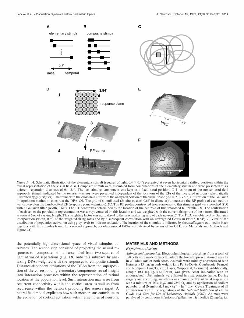
Figure 1. A, Schematic illustration of the elementary stimuli (squares of light, 0.4 3 0.4°) presented at seven horizontally shifted positions within thefoveal representation of the visual field. B, Composite stimuli were assembled from combinations of the elementary stimuli and were presented at sixdifferent separation distances of 0.4–2.4°. The left stimulus component was kept at a fixed nasal position. C, I llustration of the noncentered fieldapproach. Stimuli, indicated by the small gray square, were presented independent of the locations of the RFs of the measured neurons (schematicallyillustrated by gray ellipses). The frame with the cross-hair illustrates the analyzed portion of the visual space (2.8 3 2.0). D–F, I llustration of the Gaussianinterpolation method to construct the DPA. D1, The grid of stimuli used (36 circles, each 0.64° in diameter) to measure the RF profile of each neuronwas centered on the hand-plotted RF (response plane technique). D2, The RF profile constructed from responses to this stimulus grid was smoothed (D3)with a Gaussian filter (width, 0.64°). The RF center was determined as the location of the centroid of this smoothed RF profile. D4, The contributionof each cell to the population representations was always centered on this location and was weighted with the current firing rate of the neuron, illustratedas vertical bars of varying length. This weighting factor was normalized to the maximal firing rate of each neuron. E, The DPA was obtained by Gaussianinterpolation (width, 0.6°) of the weighted firing rates and by a subsequent convolution with an unweighted Gaussian (width, 0.64°). F, View of thedistribution of population activation using gray levels to indicate activation. The location of the stimulus is indicated by the small square outlined in blacktogether with the stimulus frame. In a second approach, one-dimensional DPAs were derived by means of an OLE; see Materials and Methods andFigure 2C.

Jancke et al. • Population Dynamics within Parametric Space J. Neurosci., October 15, 1999, 19(20):9016–9028 9017

bolus; 2 mg z kg 21 z hr 21 i.v., Sigma, St. Louis, MO). In addition, 5%glucose in physiological Ringer’s solution was continuously infused (3ml/hr; Braun). Heart rate, intratracheal pressure, expired CO2, bodytemperature, and EEG were monitored during the entire experiment.Respiration was adjusted for an end-tidal CO2 between 3.5 and 4.0%.The body temperature was kept at 37.5°C by means of a feedback-controlled heating pad. Contact lenses with artificial pupils (3 mm diam-eter) were used to cover the eyes, which were frequently rinsed withartificial eye liquid (Liquifilm; Pharm-Allergan). Pupils were dilated byatropine (5 mg/ml), and nictitating membranes were retracted by nor-epinephrine (Neosynephrin-POS, 50 mg/ml; Ursapharm). The bone anddura mater were removed over the central representation of area 17 inthe left hemisphere. The exposed cortex was covered with heavy siliconeoil. At the end of the experiments, animals were killed with an overdoseof sodium pentobarbital.

Data acquisition. We recorded responses of single units in the fovealrepresentation in area 17 of the left hemisphere. Stimuli were alwayspresented to the contralateral eye. Recordings were performed simulta-neously with two or three glass-coated platinum electrodes (resistancebetween 3.5 and 4.5 MV; Thomas Recording), which were advanced witha microstepper. The bandpass-filtered (500–3000 Hz) electrode signalswere fed into spike sorters based on an on-line principle componentanalysis (Gawne and Richmond, National Institutes of Health, Bethesda,MD). Their output TTL-pulses were stored on a personal computer(PC) with a time resolution of 1 msec. Raw analog recordings weredisplayed on oscilloscopes and on audio monitors. Digitized neuralresponses were displayed as poststimulus time histograms (PSTHs) on-line during the recording sessions.

Data were analyzed off-line in the Interactive Data Language graph-ical environment (Research Systems, Inc.).

Visual stimulation. Stimuli were displayed on a PC-controlled 21 inchmonitor (120 Hz, noninterlaced) positioned at a distance of 114 cm fromthe animal.

An identical set of common stimuli was presented to all neurons: (1)elementary stimuli (Fig. 1 A), small squares of light (size, 0.4 3 0.4°),were flashed at one of seven different horizontally contiguous locationswithin a fixed foveal reference frame; and (2) composite stimuli (Fig.1 B), two simultaneously flashed squares of light, were separated bydistances that varied between 0.4 and 2.4°. Each stimulus was flashed for25 msec. The interstimulus interval (ISI) was 1500 msec. There were atotal of 32 repetitions of each stimulus, arranged in pseudorandom orderacross the different conditions. Stimuli had a luminance of 0.9 cd/m 2

against a background luminance of 0.002 cd/m 2. The retinal position ofthese common stimuli was constant, irrespective of the RF location ofindividual neurons (non-RF-centered approach illustrated in Fig.1C,D4 ).

The profile of each individual RF was assessed quantitatively with aseparate set of stimuli, consisting of small dots of light (diameter, 0.64°)that were flashed in pseudorandom order (20 times) for 25 msec (ISI,1000 msec) on the 36 locations of an imaginary 6 3 6 grid, centered overthe hand-plotted RF (response plane technique, Fig. 1 D1). To control foreye drift, RF profiles were repeatedly measured during each recordingsession.

Construction of the DPAThe general idea behind constructing a population distribution is toextract the contributions of neurons to the representation of a particularstimulus parameter. To obtain entire distributions that are defined forvisual field location, two types of analysis were applied: (1) based on themeasured RF profiles (Fig. 1 D1,D2), the calculated RF centers (Fig.1 D3) served to construct two-dimensional DPAs by interpolating thenormalized firing rates of each contributing neuron with a Gaussianprofile (cf. Anderson, 1994a,b, for a related attempt) (Fig. 1E,F ); and (2)to minimize the reconstruction error for the elementary stimulus condi-tions, we extended the Optimal Linear Estimator (OLE) (Salinas andAbbott, 1994), resulting in one-dimensional DPAs (Fig. 2C).

Constructing two-dimensional DPAs by Gaussian interpolation. For eachlocation on the 6 3 6 grid, an average response strength was determinedfor each cell by averaging the firing rate in the time interval between 40and 65 msec after stimulus onset corresponding to the peak responses inthe PSTHs. RF profiles were obtained (Fig. 1 D2) and smoothed byconvolution with a Gaussian profile in two dimensions (half width, 0.64°;Fig. 1 D3). The center of the RF of each cell was then computed as thecenter of mass of that part of the RF profile that exceeded half of themaximal firing rate.

The firing rate, fn(s,t) of neuron number n to stimulus number s wasdefined as the firing rate in a 10 msec time interval beginning at time tafter stimulus onset, averaged over 32 stimulus repetitions. Spontaneousactivity, bn, was estimated as the mean firing rate accumulated overnonstimulus trials. For the purpose of constructing the population rep-resentation, the firing rate of each cell was normalized to its maximumfiring rate, mn, over all stimuli used to measure the response planes andduring any single 10 msec bin in the time interval from stimulus onset to100 msec after stimulus onset. This normalized firing rate:

Fn~s, t! 5fn~s, t! 2 bn

mn 2 bn(1)

was always well defined and positive (Fig. 1D4).The normalized firing rates, Fn(s,t), were depicted at the position of thecalculated RF center of each neuron. For interpolation of the data points,the width of the Gaussian profile was chosen equal to 0.6° in visual space(approximately corresponding to the average RF width of all neuronsrecorded) (Fig. 2 A). To correct for uneven sampling of visual space bythe limited number of RF centers, the distribution was normalized bydividing by a density function, which was simply the sum of unweightedGaussian profiles (width, 0.64°) centered on all RF centers. This proce-dure is illustrated in Figure 1, E and F.

Deriving the optimal linear estimator for the DPA. An optimal estimationof the DPA is based on the responses to elementary stimuli. For eachstimulus position si, the DPA, Ui(sk), is constructed as a linear combina-tion of contributions from each neuron (n 5 1, . . . , N ):

Ui~sk! 5 On51

N

cn~sk! fn~si!. (2)

The number M of sample points sk determines the degree of resolutionwith which the DPAs are sampled. The contribution of each neuron is abasis function, cn(sk), to be determined by optimization, multiplied withthe firing rate, fn(si), averaged over the time interval between 40 and 65msec after stimulus onset. The desired form of the DPA representationof these stimuli is explicitly chosen as a Gaussian, Ui(sk), centered oneach stimulus position, si:

Ui~sk! 5 expS2~sk 2 si!

2

2s2 D with sk [ @s1 2 s, s7 1 s#, k 5 1 . . . M.

(3)

The width s 5 0.6° was chosen such that Ui(sk) fits to the average RFprofile of all measured neurons (Fig. 2 A). To determine the basisfunctions we minimize the average reconstruction error Si (Ui (sk) 2Ui(sk)) 2 (Seung and Sompolinsky, 1993; Salinas and Abbott, 1994; Pougetet al., 1998), which leads to:

cn~sk! 5 Om51

N

Lm~sk!Qnm21. (4)

Here, Qnm is the correlation matrix between the firing rates of neuronsn and m for all stimuli:

Qnm 5 Oi51

7

fn~si! fm~si!, (5)

and Lm(sk) is:

Lm 5 Oi51

7

Ui~sk! fm~si!. (6)

This amounts to an OLE for a vector-valued stimulus parameter (Salinasand Abbott, 1994).

This estimator can then be extrapolated to obtain time-resolved DPAsby replacing the averaged firing rate fn(si) in Equation 2 by the firing ratein a particular time interval. The coefficients cn(sk), by contrast, remainfixed. This extrapolated DPA is the basis for investigating the nonlinearinteraction effects within the composite stimulus paradigm. We comparethe superpositions:

9018 J. Neurosci., October 15, 1999, 19(20):9016–9028 Jancke et al. • Population Dynamics within Parametric Space

Uijsup~sk , t! 5 Ui ~sk , t! 1 Uj ~sk , t! (7)

of the time-resolved DPAs for two elementary stimuli si and sj with thetime-resolved DPAs of composite stimuli

Uijmeas~sk , t! 5 O

n51

N

cn~sk! fn~si , sj , t!. (8)

Uijmeas (sk , t) is the extrapolated DPA that is based on replacing the rate

fn(si) in Equation 2 by the firing rates fn(si , sj , t) that are observed inresponse to the corresponding composite stimulus.

RESULTSExperimental resultsDistributions of population activation of elementary stimuliWe constructed DPAs in response to a set of small squares of lightthat only differ in their position along a virtual horizontal line andthat we termed elementary stimuli. The DPAs were defined invisual space and were based on single cell responses from 178neurons recorded in the foveal representation of cat area 17. Toobtain DPAs, we made use of two different approaches: (1) in atwo-dimensional Gaussian interpolation procedure, the RF cen-

ters were weighted with the normalized firing rate of each neuron(Fig. 1D–F). Corresponding to the average RF profile of allneurons recorded (compare Fig. 2A), the width of the Gaussianwas chosen uniformly to 0.6°; and (2) in addition, based on theassumption that the representation of visual location can beconsidered as a function of activation in parameter space, weminimized the error for reconstructing one-dimensional distribu-tions using the OLE procedure. This method is optimal in thesense that it extracts the available information from the firingrates under the condition of a least square fit.

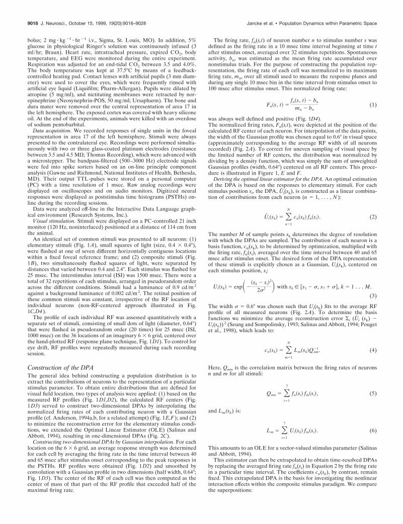
As a reference, we calculated DPAs in the time interval be-tween 40 and 65 msec after stimulus onset corresponding to thepeak responses in the PSTHs. Both approaches yielded equiva-lent results. The DPAs were monomodal and centered onto eachrespective visual field position. For each stimulus, Figure 2Bdepicts the two-dimensional DPAs of all seven elementary stimuliconstructed by Gaussian interpolation. Figure 2C shows the OLE-derived one-dimensional DPAs. The spatial arrangement of ac-tivity within these distributions implies that neurons in primaryvisual cortex contribute as an ensemble to the representation of

C

position [deg]

activ

iatio

n

3.84˚

A40 - 65 ms

40 - 65 ms

0.4˚

B

Figure 2. A, Average RF, corresponding to the tuning for location, of all 178 recorded neurons. Based on the peak responses in the PSTHs (40–65 msecafter stimulus onset) each RF profile was smoothed by convolution with a Gaussian in two dimensions (width, 0.64°). RF centers were derived bycalculating the centroid of each profile (compare Fig. 1D3). For summation, the smoothed profiles were added with respect to their RF centers. The SDwas 0.6° (calculated for that part of the resulting average RF profile, which exceeded half of the maximal amplitude). This value of average RF widthmatches the typical RF sizes found in area 17 of the cat (Orban, 1984). The vertical arrow indicates the spatial extension in terms of visual fieldcoordinates. B, Population representations of the elementary stimuli computed as two-dimensional DPAs over visual space after Gaussian interpolation(compare Fig. 1). The construction was based on the activity of 178 neurons. DPAs were computed in the time interval between 40 and 65 msec afterstimulus onset corresponding to the peak responses in the PSTHs. The activation level is shown in a color scale normalized to maximal activationseparately for each stimulus (calibration bar at bottom right). Red indicates high levels of activation. The frame outlined in white depicts the area of thevisual field investigated as described in Figure 1C. In addition, the stimulus is shown as a square outlined in white. Note that for each stimulus the focalzone of activation is approximately centered on the stimulus location. C, DPAs derived by means of an OLE for all seven elementary stimuli used. DPAswere assumed as Gaussian profiles centered on each respective stimulus position. As in the interpolation procedure, neural activity was integratedbetween 40 and 65 msec after stimulus onset. The width of the estimated Gaussian was chosen 0.6° to match the average RF width (tuning curve) of allneurons measured (compare Fig. 2A). The maxima of the OLE-derived distributions were aligned accurately on the position of each stimulus.


visual field location, although the RF of each neuron might bebroadly tuned to stimulus location.

For extrapolation, DPAs were obtained by replacing the neuralactivity observed in other time intervals or in response to com-posite stimuli.

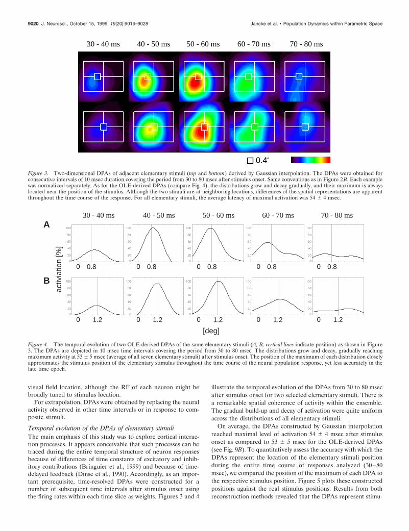
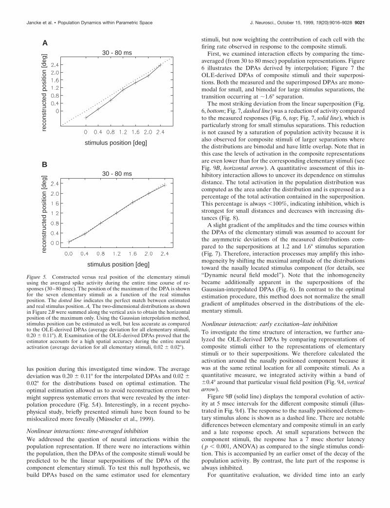
Temporal evolution of the DPAs of elementary stimuliThe main emphasis of this study was to explore cortical interac-tion processes. It appears conceivable that such processes can betraced during the entire temporal structure of neuron responsesbecause of differences of time constants of excitatory and inhib-itory contributions (Bringuier et al., 1999) and because of time-delayed feedback (Dinse et al., 1990). Accordingly, as an impor-tant prerequisite, time-resolved DPAs were constructed for anumber of subsequent time intervals after stimulus onset usingthe firing rates within each time slice as weights. Figures 3 and 4

illustrate the temporal evolution of the DPAs from 30 to 80 msecafter stimulus onset for two selected elementary stimuli. There isa remarkable spatial coherence of activity within the ensemble.The gradual build-up and decay of activation were quite uniformacross the distributions of all elementary stimuli.

On average, the DPAs constructed by Gaussian interpolationreached maximal level of activation 54 6 4 msec after stimulusonset as compared to 53 6 5 msec for the OLE-derived DPAs(see Fig. 9B). To quantitatively assess the accuracy with which theDPAs represent the location of the elementary stimuli positionduring the entire time course of responses analyzed (30–80msec), we compared the position of the maximum of each DPA tothe respective stimulus position. Figure 5 plots these constructedpositions against the real stimulus positions. Results from bothreconstruction methods revealed that the DPAs represent stimu-

30 - 40 ms 40 - 50 ms 50 - 60 ms 60 - 70 ms 70 - 80 ms

0.4˚

Figure 3. Two-dimensional DPAs of adjacent elementary stimuli (top and bottom) derived by Gaussian interpolation. The DPAs were obtained forconsecutive intervals of 10 msec duration covering the period from 30 to 80 msec after stimulus onset. Same conventions as in Figure 2 B. Each examplewas normalized separately. As for the OLE-derived DPAs (compare Fig. 4), the distributions grow and decay gradually, and their maximum is alwayslocated near the position of the stimulus. Although the two stimuli are at neighboring locations, differences of the spatial representations are apparentthroughout the time course of the response. For all elementary stimuli, the average latency of maximal activation was 54 6 4 msec.

30 - 40 ms 40 - 50 ms 50 - 60 ms 60 - 70 ms 70 - 80 msA

act

ivia

tion

[%]

B

[deg]

0 0.8 0 0.80 0.8 0 0.8 0 0.8

0 1.2 0 1.20 1.2 0 1.2 0 1.2

Figure 4. The temporal evolution of two OLE-derived DPAs of the same elementary stimuli (A, B, vertical lines indicate position) as shown in Figure3. The DPAs are depicted in 10 msec time intervals covering the period from 30 to 80 msec. The distributions grow and decay, gradually reachingmaximum activity at 53 6 5 msec (average of all seven elementary stimuli) after stimulus onset. The position of the maximum of each distribution closelyapproximates the stimulus position of the elementary stimulus throughout the time course of the neural population response, yet less accurately in thelate time epoch.


lus position during this investigated time window. The averagedeviation was 0.20 6 0.11° for the interpolated DPAs and 0.02 60.02° for the distributions based on optimal estimation. Theoptimal estimation allowed us to avoid reconstruction errors butmight suppress systematic errors that were revealed by the inter-polation procedure (Fig. 5A). Interestingly, in a recent psycho-physical study, briefly presented stimuli have been found to bemislocalized more foveally (Musseler et al., 1999).

Nonlinear interactions: time-averaged inhibitionWe addressed the question of neural interactions within thepopulation representation. If there were no interactions withinthe population, then the DPAs of the composite stimuli would bepredicted to be the linear superpositions of the DPAs of thecomponent elementary stimuli. To test this null hypothesis, webuild DPAs based on the same estimator used for elementary

stimuli, but now weighting the contribution of each cell with thefiring rate observed in response to the composite stimuli.

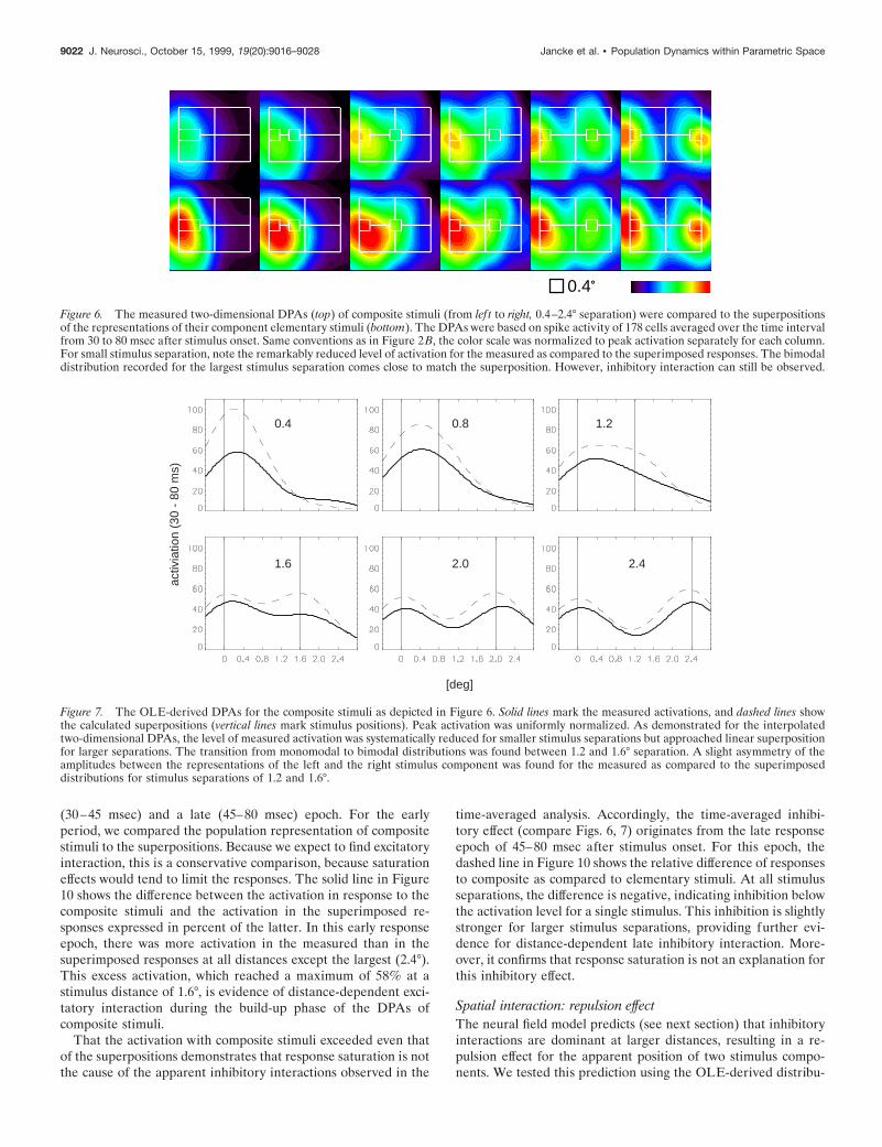
First, we examined interaction effects by comparing the time-averaged (from 30 to 80 msec) population representations. Figure6 illustrates the DPAs derived by interpolation; Figure 7 theOLE-derived DPAs of composite stimuli and their superposi-tions. Both the measured and the superimposed DPAs are mono-modal for small, and bimodal for large stimulus separations, thetransition occurring at ;1.6° separation.

The most striking deviation from the linear superposition (Fig.6, bottom; Fig. 7, dashed line) was a reduction of activity comparedto the measured responses (Fig. 6, top; Fig. 7, solid line), which isparticularly strong for small stimulus separations. This reductionis not caused by a saturation of population activity because it isalso observed for composite stimuli of larger separations wherethe distributions are bimodal and have little overlap. Note that inthis case the levels of activation in the composite representationsare even lower than for the corresponding elementary stimuli (seeFig. 9B, horizontal arrow). A quantitative assessment of this in-hibitory interaction allows to uncover its dependence on stimulusdistance. The total activation in the population distribution wascomputed as the area under the distribution and is expressed as apercentage of the total activation contained in the superposition.This percentage is always ,100%, indicating inhibition, which isstrongest for small distances and decreases with increasing dis-tances (Fig. 8).

A slight gradient of the amplitudes and the time courses withinthe DPAs of the elementary stimuli was assumed to account forthe asymmetric deviations of the measured distributions com-pared to the superpositions at 1.2 and 1.6° stimulus separation(Fig. 7). Therefore, interaction processes may amplify this inho-mogeneity by shifting the maximal amplitude of the distributionstoward the nasally located stimulus component (for details, see“Dynamic neural field model”). Note that the inhomogeneitybecame additionally apparent in the superpositions of theGaussian-interpolated DPAs (Fig. 6). In contrast to the optimalestimation procedure, this method does not normalize the smallgradient of amplitudes observed in the distributions of the ele-mentary stimuli.

Nonlinear interaction: early excitation–late inhibitionTo investigate the time structure of interaction, we further ana-lyzed the OLE-derived DPAs by comparing representations ofcomposite stimuli either to the representations of elementarystimuli or to their superpositions. We therefore calculated theactivation around the nasally positioned component because itwas at the same retinal location for all composite stimuli. As aquantitative measure, we integrated activity within a band of60.4° around that particular visual field position (Fig. 9A, verticalarrow).

Figure 9B (solid line) displays the temporal evolution of activ-ity at 5 msec intervals for the different composite stimuli (illus-trated in Fig. 9A). The response to the nasally positioned elemen-tary stimulus alone is shown as a dashed line. There are notabledifferences between elementary and composite stimuli in an earlyand a late response epoch. At small separations between thecomponent stimuli, the response has a 7 msec shorter latency( p , 0.001, ANOVA) as compared to the single stimulus condi-tion. This is accompanied by an earlier onset of the decay of thepopulation activity. By contrast, the late part of the response isalways inhibited.

For quantitative evaluation, we divided time into an early

30 - 80 msre

cons

truc

ted

posi

tion

[deg

]A

30 - 80 ms

reco

nstr

ucte

d po

sitio

n [d

eg]

B

stimulus position [deg]

stimulus position [deg]

Figure 5. Constructed versus real position of the elementary stimuliusing the averaged spike activity during the entire time course of re-sponses (30–80 msec). The position of the maximum of the DPA is shownfor the seven elementary stimuli as a function of the real stimulusposition. The dotted line indicates the perfect match between estimatedand real stimulus position. A, The two-dimensional distributions as shownin Figure 2B were summed along the vertical axis to obtain the horizontalposition of the maximum only. Using the Gaussian interpolation method,stimulus position can be estimated as well, but less accurate as comparedto the OLE-derived DPAs (average deviation for all elementary stimuli,0.20 6 0.11°). B, Examination of the OLE-derived DPAs proved that theestimator accounts for a high spatial accuracy during the entire neuralactivation (average deviation for all elementary stimuli, 0.02 6 0.02°).


(30–45 msec) and a late (45–80 msec) epoch. For the earlyperiod, we compared the population representation of compositestimuli to the superpositions. Because we expect to find excitatoryinteraction, this is a conservative comparison, because saturationeffects would tend to limit the responses. The solid line in Figure10 shows the difference between the activation in response to thecomposite stimuli and the activation in the superimposed re-sponses expressed in percent of the latter. In this early responseepoch, there was more activation in the measured than in thesuperimposed responses at all distances except the largest (2.4°).This excess activation, which reached a maximum of 58% at astimulus distance of 1.6°, is evidence of distance-dependent exci-tatory interaction during the build-up phase of the DPAs ofcomposite stimuli.

That the activation with composite stimuli exceeded even thatof the superpositions demonstrates that response saturation is notthe cause of the apparent inhibitory interactions observed in the

time-averaged analysis. Accordingly, the time-averaged inhibi-tory effect (compare Figs. 6, 7) originates from the late responseepoch of 45–80 msec after stimulus onset. For this epoch, thedashed line in Figure 10 shows the relative difference of responsesto composite as compared to elementary stimuli. At all stimulusseparations, the difference is negative, indicating inhibition belowthe activation level for a single stimulus. This inhibition is slightlystronger for larger stimulus separations, providing further evi-dence for distance-dependent late inhibitory interaction. More-over, it confirms that response saturation is not an explanation forthis inhibitory effect.

Spatial interaction: repulsion effectThe neural field model predicts (see next section) that inhibitoryinteractions are dominant at larger distances, resulting in a re-pulsion effect for the apparent position of two stimulus compo-nents. We tested this prediction using the OLE-derived distribu-

0.4˚

Figure 6. The measured two-dimensional DPAs (top) of composite stimuli (from lef t to right, 0.4–2.4° separation) were compared to the superpositionsof the representations of their component elementary stimuli (bottom). The DPAs were based on spike activity of 178 cells averaged over the time intervalfrom 30 to 80 msec after stimulus onset. Same conventions as in Figure 2B, the color scale was normalized to peak activation separately for each column.For small stimulus separation, note the remarkably reduced level of activation for the measured as compared to the superimposed responses. The bimodaldistribution recorded for the largest stimulus separation comes close to match the superposition. However, inhibitory interaction can still be observed.

activ

iatio

n (3

0 -

80 m

s)

[deg]

0.4 1.20.8

1.6 2.42.0

Figure 7. The OLE-derived DPAs for the composite stimuli as depicted in Figure 6. Solid lines mark the measured activations, and dashed lines showthe calculated superpositions (vertical lines mark stimulus positions). Peak activation was uniformly normalized. As demonstrated for the interpolatedtwo-dimensional DPAs, the level of measured activation was systematically reduced for smaller stimulus separations but approached linear superpositionfor larger separations. The transition from monomodal to bimodal distributions was found between 1.2 and 1.6° separation. A slight asymmetry of theamplitudes between the representations of the left and the right stimulus component was found for the measured as compared to the superimposeddistributions for stimulus separations of 1.2 and 1.6°.


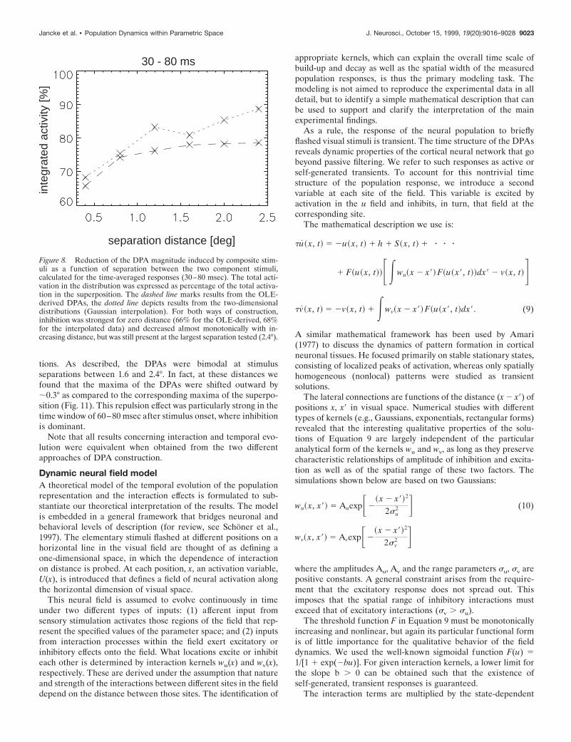
tions. As described, the DPAs were bimodal at stimulusseparations between 1.6 and 2.4°. In fact, at these distances wefound that the maxima of the DPAs were shifted outward by;0.3° as compared to the corresponding maxima of the superpo-sition (Fig. 11). This repulsion effect was particularly strong in thetime window of 60–80 msec after stimulus onset, where inhibitionis dominant.

Note that all results concerning interaction and temporal evo-lution were equivalent when obtained from the two differentapproaches of DPA construction.

Dynamic neural field modelA theoretical model of the temporal evolution of the populationrepresentation and the interaction effects is formulated to sub-stantiate our theoretical interpretation of the results. The modelis embedded in a general framework that bridges neuronal andbehavioral levels of description (for review, see Schoner et al.,1997). The elementary stimuli flashed at different positions on ahorizontal line in the visual field are thought of as defining aone-dimensional space, in which the dependence of interactionon distance is probed. At each position, x, an activation variable,U(x), is introduced that defines a field of neural activation alongthe horizontal dimension of visual space.

This neural field is assumed to evolve continuously in timeunder two different types of inputs: (1) afferent input fromsensory stimulation activates those regions of the field that rep-resent the specified values of the parameter space; and (2) inputsfrom interaction processes within the field exert excitatory orinhibitory effects onto the field. What locations excite or inhibiteach other is determined by interaction kernels wu(x) and wv(x),respectively. These are derived under the assumption that natureand strength of the interactions between different sites in the fielddepend on the distance between those sites. The identification of

appropriate kernels, which can explain the overall time scale ofbuild-up and decay as well as the spatial width of the measuredpopulation responses, is thus the primary modeling task. Themodeling is not aimed to reproduce the experimental data in alldetail, but to identify a simple mathematical description that canbe used to support and clarify the interpretation of the mainexperimental findings.

As a rule, the response of the neural population to brieflyflashed visual stimuli is transient. The time structure of the DPAsreveals dynamic properties of the cortical neural network that gobeyond passive filtering. We refer to such responses as active orself-generated transients. To account for this nontrivial timestructure of the population response, we introduce a secondvariable at each site of the field. This variable is excited byactivation in the u field and inhibits, in turn, that field at thecorresponding site.

The mathematical description we use is:

tu~ x, t! 5 2u~ x, t! 1 h 1 S~ x, t! 1 z z z

1 F~u~ x, t!!FEwu~ x 2 x9! F~u~ x9, t!!dx9 2 v~ x, t!Gt v~ x, t! 5 2v~ x, t! 1 Ewv~ x 2 x9! F~u~ x9, t!dx9. (9)

A similar mathematical framework has been used by Amari(1977) to discuss the dynamics of pattern formation in corticalneuronal tissues. He focused primarily on stable stationary states,consisting of localized peaks of activation, whereas only spatiallyhomogeneous (nonlocal) patterns were studied as transientsolutions.

The lateral connections are functions of the distance (x 2 x9) ofpositions x, x9 in visual space. Numerical studies with differenttypes of kernels (e.g., Gaussians, exponentials, rectangular forms)revealed that the interesting qualitative properties of the solu-tions of Equation 9 are largely independent of the particularanalytical form of the kernels wu and wv, as long as they preservecharacteristic relationships of amplitude of inhibition and excita-tion as well as of the spatial range of these two factors. Thesimulations shown below are based on two Gaussians:

wu~ x, x9! 5 AuexpF2~ x 2 x9!2

2su2 G (10)

wv~ x, x9! 5 AvexpF2~ x 2 x9!2

2sv2 G

where the amplitudes Au, Av and the range parameters su, sv arepositive constants. A general constraint arises from the require-ment that the excitatory response does not spread out. Thisimposes that the spatial range of inhibitory interactions mustexceed that of excitatory interactions (sv . su).

The threshold function F in Equation 9 must be monotonicallyincreasing and nonlinear, but again its particular functional formis of little importance for the qualitative behavior of the fielddynamics. We used the well-known sigmoidal function F(u) 51/[1 1 exp(2bu)]. For given interaction kernels, a lower limit forthe slope b . 0 can be obtained such that the existence ofself-generated, transient responses is guaranteed.

The interaction terms are multiplied by the state-dependent

separation distance [deg]

inte

grat

ed a

ctiv

ity [%

]

30 - 80 ms

Figure 8. Reduction of the DPA magnitude induced by composite stim-uli as a function of separation between the two component stimuli,calculated for the time-averaged responses (30–80 msec). The total acti-vation in the distribution was expressed as percentage of the total activa-tion in the superposition. The dashed line marks results from the OLE-derived DPAs, the dotted line depicts results from the two-dimensionaldistributions (Gaussian interpolation). For both ways of construction,inhibition was strongest for zero distance (66% for the OLE-derived, 68%for the interpolated data) and decreased almost monotonically with in-creasing distance, but was still present at the largest separation tested (2.4°).


sigmoidal signal F(u). This factor prevents the asymptotic tran-sient response to fall below resting level because only those sitesin the field that are sufficiently activated are susceptible to inhib-itory interaction.

The parameter t, Equation 9, determines the overall time scaleof build-up and decay of the field activity and can be adjusted toreproduce qualitatively the measured time course of populationactivity changes. In the numerical studies, we have used the valuet 5 15. A fixed criterion (5% above resting level) was used todefine the response onset in the experiments. For the simulations,the afferent transient stimulus S(x,t) at position x, applied for aduration Dt 5 25 msec, is a Gaussian profile characterized by itsstrength, As, and width parameter, 2s. The choice of s fixes thespatial units relative to the experimental space scale. All rangeparameters used in the model simulations were chosen as multi-ples of s 5 5, which represents 0.2° in visual space.

If this transient external input creates enough excitation withinthe field, the excitatory response develops a single spatial maxi-mum located at the center, x, of the stimulated segment. This isfollowed by a process of relaxation to the resting state driven byincreasing inhibition in the field. The activation level of this

resting state is a homogenous and stable solution of the modeldynamics, fixed by the parameter h , 0 (h 5 23 for the simula-tions shown here).

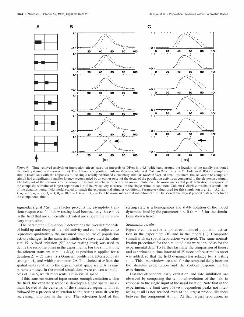
Simulation resultsFigure 9 compares the temporal evolution of population activa-tion in the experiment (B) and in the model (C). Compositestimuli with six spatial separations were used. The same normal-ization procedures for the simulated data were applied as for theexperimental data. To further facilitate the comparison of theoryand experiment, a time interval of 25 msec before stimulus onsetwas added, so that the field dynamics has relaxed to its restingstate. This time window accounts for the temporal delay betweenthe stimulus presentation and the cortical response in theexperiment.

Distance-dependent early excitation and late inhibition areobserved by comparing the temporal evolution of the field inresponse to the single input at the nasal location. Note that in theexperiment, the limit case of two independent peaks not inter-acting at all is not reached even at the largest probed distancesbetween the component stimuli. At that largest separation, an

A C

[ms][ms]

B

Figure 9. Time-resolved analysis of interaction effects based on integrals of DPAs in a 0.8° wide band around the location of the nasally positionedelementary stimulus (A, vertical arrow). The different composite stimuli are shown in column A. Column B contrasts the OLE-derived DPAs to compositestimuli (solid line) with the responses to the single nasally positioned elementary stimulus (dashed line). At small distances, the activation to compositestimuli had a significantly smaller latency accompanied by an earlier onset of the decay of the population activity as compared to the elementary stimuli.The late part of the responses to the composite stimuli was characterized by an overall inhibition. The arrow marks that peak activation in response tothe composite stimulus of largest separation is still below activity measured in the single stimulus condition. Column C displays results of simulationsof the dynamic neural field model scaled to match the experimental stimulus conditions. Parameter values used for this simulation are: Au 5 5.2, Av 54, su 5 15, sv 5 25, As 5 4, Bs 5 10, b 5 1, h 5 2 3, t 5 15. The arrow marks that inhibition can still be seen at the largest probed distances betweenthe component stimuli.


inhibition effect can still be seen in the time course of activation(Fig. 9B,C, horizontal arrows).

In the spatial domain, nonlinear interactions are observed as

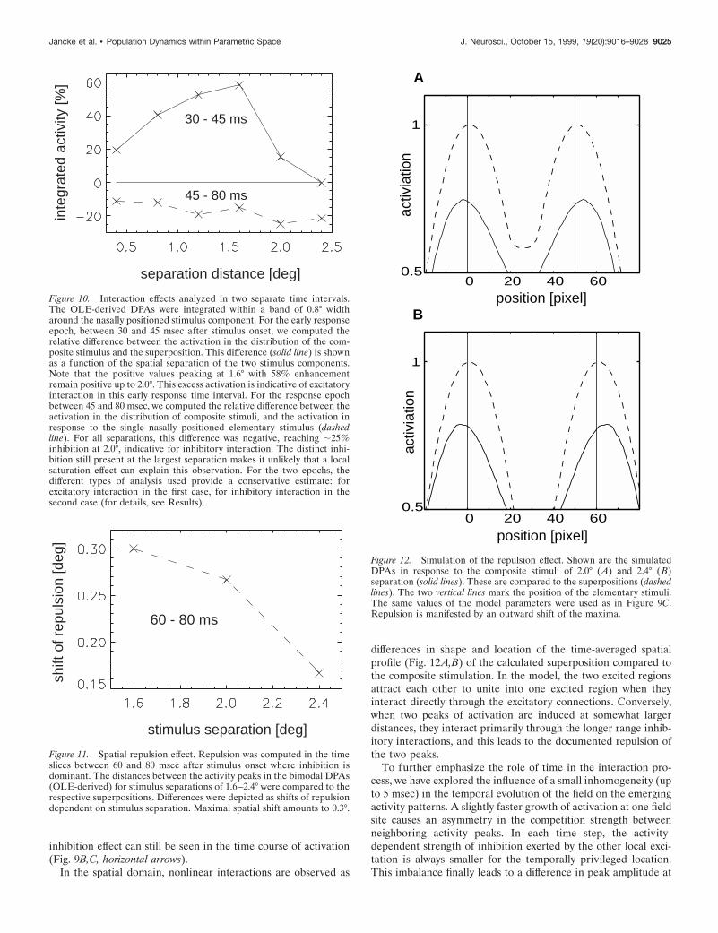
differences in shape and location of the time-averaged spatialprofile (Fig. 12A,B) of the calculated superposition compared tothe composite stimulation. In the model, the two excited regionsattract each other to unite into one excited region when theyinteract directly through the excitatory connections. Conversely,when two peaks of activation are induced at somewhat largerdistances, they interact primarily through the longer range inhib-itory interactions, and this leads to the documented repulsion ofthe two peaks.

To further emphasize the role of time in the interaction pro-cess, we have explored the influence of a small inhomogeneity (upto 5 msec) in the temporal evolution of the field on the emergingactivity patterns. A slightly faster growth of activation at one fieldsite causes an asymmetry in the competition strength betweenneighboring activity peaks. In each time step, the activity-dependent strength of inhibition exerted by the other local exci-tation is always smaller for the temporally privileged location.This imbalance finally leads to a difference in peak amplitude at

separation distance [deg]

inte

grat

ed a

ctiv

ity [%

]

30 - 45 ms

45 - 80 ms

Figure 10. Interaction effects analyzed in two separate time intervals.The OLE-derived DPAs were integrated within a band of 0.8° widtharound the nasally positioned stimulus component. For the early responseepoch, between 30 and 45 msec after stimulus onset, we computed therelative difference between the activation in the distribution of the com-posite stimulus and the superposition. This difference (solid line) is shownas a function of the spatial separation of the two stimulus components.Note that the positive values peaking at 1.6° with 58% enhancementremain positive up to 2.0°. This excess activation is indicative of excitatoryinteraction in this early response time interval. For the response epochbetween 45 and 80 msec, we computed the relative difference between theactivation in the distribution of composite stimuli, and the activation inresponse to the single nasally positioned elementary stimulus (dashedline). For all separations, this difference was negative, reaching ;25%inhibition at 2.0°, indicative for inhibitory interaction. The distinct inhi-bition still present at the largest separation makes it unlikely that a localsaturation effect can explain this observation. For the two epochs, thedifferent types of analysis used provide a conservative estimate: forexcitatory interaction in the first case, for inhibitory interaction in thesecond case (for details, see Results).

stimulus separation [deg]

shift

of r

epul

sion

[deg

]

60 - 80 ms

Figure 11. Spatial repulsion effect. Repulsion was computed in the timeslices between 60 and 80 msec after stimulus onset where inhibition isdominant. The distances between the activity peaks in the bimodal DPAs(OLE-derived) for stimulus separations of 1.6–2.4° were compared to therespective superpositions. Differences were depicted as shifts of repulsiondependent on stimulus separation. Maximal spatial shift amounts to 0.3°.

0 20 40 60 0.5

1

A

position [pixel]

activ

iatio

n

0 20 40 60 0.5

1

B

position [pixel]

activ

iatio

n

Figure 12. Simulation of the repulsion effect. Shown are the simulatedDPAs in response to the composite stimuli of 2.0° (A) and 2.4° (B)separation (solid lines). These are compared to the superpositions (dashedlines). The two vertical lines mark the position of the elementary stimuli.The same values of the model parameters were used as in Figure 9C.Repulsion is manifested by an outward shift of the maxima.


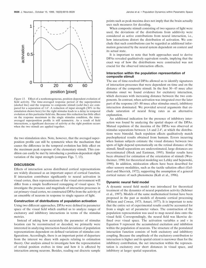
the two stimulation sites. Note, however, that the averaged super-position profile can still be symmetric when the mechanism thatcauses the difference in the temporal evolution has little effect onthe maximum peak response of the elementary stimuli. This con-dition can easily be met by introducing a position-dependent slightvariation of the input strength (compare Figs. 7, 13).

DISCUSSIONEffects of interaction across distributed cortical representationsare widely discussed as an important aspect of cortical function.If interaction contributes significantly to neural activation invisual cortex, then representations of the visual environment willdiffer from a simple feedforward remapping of visual space. Toinvestigate the presence and magnitude of interaction processes incat primary visual cortex, we constructed DPAs from the activity ofan ensemble of neurons in response to single squares of light.

Construction of distributions of population activationUsing two different approaches, DPAs were defined in parameterspace of the visual field which enabled us to analyze ranges ofexcitatory and inhibitory interactions in terms of the stimulusmetrics.

Instead of asking how accurately the parameter of stimuluslocation can be reconstructed or decoded, we primarily wereinterested in analyzing interaction-based deviations of populationrepresentations dependent on defined variations of stimulus con-figurations. Accordingly, there is an important point of departurefrom the interest we share with aspects relating to estimationtheory. Our analysis aimed to investigate how the representationof retinal position evolves in time and how it is affected byinteraction among neurons. Besides, reading out discrete sample

points such as peak maxima does not imply that the brain actuallyuses such measures for decoding.

When composite stimuli consisting of two squares of light wereused, the deviations of the distributions from additivity wereconsidered as active contributions from neural interaction, i.e.,how interactions distort the distribution of activation. We con-clude that such contributions can be regarded as additional infor-mation generated by the neural system dependent on context andits actual state.

It is important to note that both approaches used to deriveDPAs revealed qualitatively equivalent results, implying that theexact way of how the distributions were constructed was notcrucial for the observed interaction effects.

Interaction within the population representation ofcomposite stimuliThe use of time-resolved DPAs allowed us to identify signaturesof interaction processes that were dependent on time and on thedistance of the composite stimuli. In the first 30–45 msec afterstimulus onset we found evidence for excitatory interaction,which decreases with increasing distance between the two com-ponents. In contrast, when activation was integrated over the laterpart of the response (45–80 msec after stimulus onset), inhibitoryinteraction dominated. We provided several arguments that ex-clude saturation of neural firing rates as an alternativeexplanation.

An additional indication for the presence of inhibitory inter-action was found by analyzing the spatial shapes of the DPAs.Mutual repulsion of the maxima of the DPAs was observed atstimulus separations between 1.6 and 2.4°, at which the distribu-tions were bimodal. Such repulsion effects qualitatively matchpsychophysical results obtained from humans. Errors incurringwhen human subjects estimate the visual distance between twospots of light depend systematically on the retinal distance of thestimuli. Small separations are underestimated, large distances areoverestimated (Hock and Eastman, 1995). Similar results havebeen obtained for estimation of the orientation of stimuli (Wes-theimer, 1990; for theoretical modeling see Lehky and Sejnowski,1990). In addition, mislocation effects have been described forother sensory modalities, such as the tactile saltation effect (Gel-dard and Sherrick, 1972), supporting the assumption of a generalcortical nature of such phenomena (Kalt et al., 1996).

Dynamic neural field modelA dynamic neural field model was introduced for theoreticaltreatment of the dynamics of neural population activity (Schoneret al., 1997). Models of the same mathematical format have beenproposed in the past as models of dynamic cortical processing(Wilson and Cowan, 1973; Amari, 1977). It is important to notethat the entire set of experimental results could be accounted forfrom a single set of parameter values. The construction of thepopulation representation was used to map neural data onto thevisual field. Correspondingly, the neural field was likewise de-fined over visual space. The activation variables u and v inEquation 9 represent the accumulated excitation and inhibitionwithin the population of neurons. The structure of the postulatedinteraction function consists of both excitatory and inhibitorycoupling. Because the amplitude of the excitatory contribution tointeraction is higher and its spatial extent is narrower than for theinhibitory contribution, the net interaction within the represen-tation is excitatory over short distances in visual space, andinhibitory at larger spatial separation.

0 20 40 60 0

0.5

1

position [pixel]

activ

iatio

n

Figure 13. Effect of a nonhomogeneous, position-dependent evolution offield activity. The time-averaged response period of the superposition(dashed line) and the response to composite stimuli (solid line) are com-pared for a separation of 1.6°. A reduction of input strength (30% in thesimulation shown here) for the right stimulus leads to a delay in temporalevolution at this particular field site. Because this reduction has little effecton the response maximum in the single stimulus condition, the time-averaged superposition profile is still symmetric. As a result of fieldinteractions, a significant decrease of activity at the right position occurswhen the two stimuli are applied together.


The absolute values of range parameters used for the numericalstudies revealed that the excitatory and the inhibitory processesextend over a range of 0.6 and 1.0° of visual field, respectively.The strength of inhibition and excitation strongly influences thewidth of the emerging activity distribution, and thus the spatialseparation at which a transition from a monomodal to a bimodalrepresentation occurs. Our simulations showed that even thoserepresentations that overlap only for the smallest separation stillcan reveal the effect of late inhibition and early excitation, indi-cating that the width of the distributions has only little effects onthe time course of interaction. A small number of parameters weresufficient for modeling the complex spatiotemporal responses frommany different cell types combined at a population level.

Relationship of our results to single cell analysisInteraction profiles have been repeatedly examined at the level ofsingle cells (Movshon et al., 1978; Heggelund, 1981a,b; Nelson,1991; Tolhurst and Heeger, 1997). In those studies, the activity ofa cell induced by a single stimulus at the RF center was comparedto the activity of the cell in the presence of a second stimuluspresented at varied locations.

In contrast, the population approach used here performs twodifferent types of averages. First, because our stimuli were notRF-centered, we average across different spatial locations withinthe RFs (cf. Szulborski and Palmer, 1990). Outside the labora-tory, visual objects are similarly distributed in arbitrary waysacross RFs, so that this way of stimulus presentation and averag-ing is crucial for an understanding of how complex scenes arerepresented in visual cortex.

Second, we average across many different cell types. Neurons inarea 17 contribute potentially to the representations of manydifferent parameters such as retinal position, orientation, curva-ture, length, motion direction, etc. To characterize the contribu-tion of each neuron to the representation of stimulus location, onemight conceive of the high-dimensional space spanned by thesedifferent parameters. Each neuron could be thought of as a pointin this parametric space. This point corresponds to a set ofpreferred values for all represented parameters. By asking onlyhow the firing rate of the neuron depends on visual field position,the contributions of all neurons are averaged, although theirpreferred parameter set may be different along other dimensions.In this sense, the DPA is a projection from a potentially high-dimensional space onto a common neuronal space representingonly visual field position. The DPA could thus be viewed as aneural population receptive field of the inverted cortical point-spread function (“cortical spread-point function”).

The shape of the DPA mattersPopulation coding ideas have largely been centered on estimatingthe stimulus or task parameter from the activity of populations ofneurons (Georgopoulos et al., 1986, 1993; Vogels, 1990; Zohary,1992; Seung and Sompolinsky, 1993; Salinas and Abbott, 1994;Groh et al., 1997). Compared to vector-based population tech-niques, the current approach focused on the concept of an entiredistribution of population activation (Lee et al., 1988; Bastian etal., 1997; Pouget et al., 1998) (for related attempts, see Anderson,1994a,b; Zemel et al., 1998, in which they seek to recover aprobability distribution of activity over the encoded variable). Inour approach, the distribution is significant not only by a meanvalue of the represented parameter, but also through its shape.Consequently, asymmetric deformations of the DPA could bedetected, in which two peaks in the DPA are repelled from each

other at sufficiently large stimulus separations. This effect isobservable only by taking the shape of the constructed DPA intoaccount and would be detectable neither on the basis of PSTHresponses of individual cells nor in reconstructions that estimateonly single values or discrete samples of parameters.

Relationship of our results to cortical mapsIn principle, our time averaged two-dimensional DPAs are equiv-alent to activities recorded in functional imaging studies such asfunctional magnetic resonance imagine, positron emission to-mography, and optical imaging of intrinsic signals assuming aclean retinotopy. There are a number of differences, however.Besides the limitations of these techniques to resolve the milli-second time scale as accomplished by our single cell recordings,the main problem arises from the fact that the retinotopy is farfrom coming close to a clean representation of the visual field (cf.Das and Gilbert, 1997). This is particularly obvious at the spatialscale of our investigation, which differentiates between visualangles ,1° apart (Hubel and Wiesel, 1962; Albus, 1975). Analysisof the cortical point-spread function has shown that the process-ing of even very small stimuli is associated with a widespreadpattern of cortical activation (Grinvald et al., 1994; Godde et al.,1995; Chen-Bee and Frostig, 1996). In addition, imaging methodsas listed above do not solely reflect spike activity but includecontributions from glial cells and cerebral blood flow. Accord-ingly, comparison of DPAs spanned in parametric space withcortical activation maps recorded with such imaging techniquesmay allow separating neural and non-neural contributions.

A dynamically distributed processing over a large cortical areapossibly reflects a major role in neural strategies of cooperativeinteraction. Observations in real-time imaging studies supportedthis assumption because the firing of single neurons can bepredicted if the whole pattern of cortical population activation istaken into account (Arieli et al., 1996; Kenet et al., 1998). Be-cause our approach allows for a functional interpretation ofcortical activation patterns, it may serve to find transformationrules that map the multidimensional visual input onto corticalrepresentations.

REFERENCESAlbus K (1975) A quantitative study of the projection area of the central

and the paracentral visual field in area 17 of the cat. I. The precision ofthe topography. Exp Brain Res 24:159–179.

Allman J, Miezin F, McGuiness EL (1985) Stimulus specific responsesfrom beyond the classical receptive field. Annu Rev Neurosci8:407–430.

Amari S (1977) Dynamics of pattern formation in lateral-inhibition typeneural fields. Biol Cybern 27:77–87.

Anderson CH (1994a) Basic elements of biological computational sys-tems. Int J Modern Physics C 5:135–137.

Anderson CH (1994b) Neurobiological computational systems. In: Com-putional intelligence imitating life (Palaniswami M, Attkiouzel Y,Marks II RJ, Fogel D, Fukada T, eds), pp 219–222. New York: IEEE.

Arieli A, Sterkin A, Grinvald A, Aertsen A (1996) Dynamics of ongoingactivity: explanation of the large variability in evoked cortical re-sponses. Science 273:1868–1871.

Bastian A, Riehle A, Erlhagen W, Schoner G (1997) Prior informationpreshapes the population representation of movement direction inmotor cortex. NeuroReport 9:315–319.

Bringuier V, Chavane F, Glaeser L, Fregnac Y (1999) Horizontal prop-agation of visual activity in the synaptic integration field of area 17neurons. Science 283:695–699.

Chen-Bee CH, Frostig RD (1996) Variability and interhemisphericasymmetry of single-whisker functional representations in rat barrelcortex. J Neurophysiol 76:884–894.

Creutzfeldt OD, Garey LJ, Kuroda R, Wolff JR (1977) The distribution


of degenerating axons after small lesions in the intact and isolatedvisual cortex of the cat. Exp Brain Res 27:419–440.

Das A, Gilbert CD (1997) Distortions of visuotopic map match orienta-tion singularities in primary visual cortex. Nature 387:594–598.

Dinse HR (1986) Foreground-background-interaction - Stimulus depen-dent properties of the cat’s area 17, 18 and 19 neurons outside theclassical receptive field. Perception 15:A6.

Dinse HR, Kruger K, Best J (1990) A temporal structure of corticalinformation processing. Concept Neurosci 1:199–238.

Erickson RP (1974) Parallel population coding in feature extraction. In:The neurosciences (Schmitt FO, Worden FG, eds), pp 155–169. Cam-bridge: MIT.

Fisken RA, Garey CJ, Powell TPS (1975) The intrinsic, association andcommissural connections of area 17 of the visual cortex. Philos Trans RSoc Lond B Biol Sci 272:487–536.

Gaal G (1993a) Population coding by simultaneous activities of neuronsin intrinsic coordinate systems defined by their RF weighting functions.Neural Networks 6:499–515.

Gaal G (1993b) Calculation of movement direction from firing activitiesof neurons in intrinsic coordinate systems defined by their preferreddirections. J Theor Biol 162:103–130.

Geldard FA, Sherrick CE (1972) The cutaneous “rabbit”: a perceptualillusion. Science 178:178–179.

Georgopoulos AP, Schwartz AB, Kettner RE (1986) Neural populationcoding of movement direction. Science 233:1416–1419.

Georgopoulos AP, Taira M, Lukashin A (1993) Cognitive neurophysi-ology of the motor cortex. Science 260:47–52.

Gielen CCAM, Hesselmans GHFM, Johannesma PIM (1988) Sensoryinterpretation of neural activity patterns. Math Biosci 88:14–35.

Giese MA, Cubaleska B, Pagel M, Akhavan AC, Jancke D, Dinse HR,Schoner G (1997) Identification of feedforward and recurrent part ofthe neural dynamics of position representation in cat area 17. SocNeurosci Abstr 23:2364.

Gilbert CD, Wiesel TN (1979) Morphology and intracortical projectionsof functionally identified neurons in cat visual cortex. Nature280:120–125.

Gilbert CD, Wiesel TN (1990) The influence of contextual stimuli on theorientation selectivity of cells in primary visual cortex of the cat. VisionRes 30:1689–1701.

Godde B, Hilger T, von Seelen W, Berkefeld T, Dinse HR (1995)Optical imaging of rat somatosensory cortex reveals representationaloverlap as topographic principle. NeuroReport 7:24–28.

Grinvald A, Lieke EE, Frostig RD, Hildesheim R (1994) Cortical point-spread function and long-range lateral interactions revealed by real-time optical imaging of macaque monkey primary visual cortex. J Neu-rosci 14:2545–2568.

Groh JM, Born RT, Newsome WT (1997) How is a sensory map readout? Effects of microstimulation in visual area MT on saccades andsmooth pursuit eye movements. J Neurosci 17:4312–4330.

Heggelund P (1981a) RF organization of simple cells in cat striate cor-tex. Exp Brain Res 42:89–98.

Heggelund P (1981b) RF organization of complex cells in cat striatecortex. Exp Brain Res 42:99–107.

Hock HS, Eastman KE (1995) Context effects on perceived position:sustained and transient temporal influences on spatial interactions.Vision Res 35:635–646.

Hubel DH, Wiesel TN (1962) Receptive fields, binocular interaction andfunctional architecture in the cat’s visual cortex. J Physiol (Lond)160:106–154.

Jancke D, Akhavan AC, Erlhagen W, Schoner G, Dinse HR (1996)Reconstruction of motion trajectories using population representationsof neurons in cat visual cortex. Soc Neurosci Abstr 22:646.

Kalt T, Akhavan AC, Jancke D, Dinse HR (1996) Dynamic populationcoding in rat somatosensory cortex. Soc Neurosci Abstr 22:105.

Kenet T, Arieli A, Grinvald A, Shoham D, Pawelzik K, Tsodyks M(1998) Spontaneous and evoked firing of single cortical neurons arepredicted by population activity. Soc Neurosci Abstr 24:1138.

Kisvarday ZF, Eysel UT (1993) Functional and structural topography ofhorizontal inhibitory connections in cat visual cortex. Eur J Neurosci5:1558–1572.

Lee C, Rohrer WH, Sparks DL (1988) Population coding of saccadic eyemovements by neurons in the superior colliculus. Nature 332:357–360.

Lehky SR, Sejnowski TJ (1990) Neural model of stereoacuity and depthinterpolation based on a distributed representation of stereo disparity.J Neurosci 10:2281–2299.

Movshon JA, Thompson ID, Tolhurst DJ (1978) RF organization ofcomplex cells in the cat’s striate cortex. J Physiol (Lond) 283:79–99.

Musseler J, Van der Heijden AHC, Mahmud SH, Deubel H, Ertsey S(1999) Relative mislocalization of briefly presented stimuli in the ret-inal periphery. Percept Psychophys, in press.

Nelson SB (1991) Temporal interactions in the cat visual system. I.Orientation-selective suppression in the visual cortex. J Neurosci11:344–356.

Nicolelis MAL, Chapin JK (1994) Spatiotemporal structure of somato-sensory responses of many-neuron ensembles in the rat ventral poste-rior medial nucleus of the thalamus. J Neurosci 14:3511–3532.

Orban GA (1984) Neuronal operations in the visual cortex. In: Studies ofbrain function XI (Braitenberg V, ed). New York: Springer.

Pouget A, Zhang K, Latham PE (1998) Statistically efficient estimationusing population coding. Neural Comput 10:373–401.

Ruiz S, Crespo P, Romo R (1995) Representation of moving tactilestimuli in the somatic sensory cortex of awake monkeys. J Neurophysiol38:1403–1420.

Salinas E, Abbott LF (1994) Vector reconstruction from firing rates.J Comp Neurosci 1:89–107.

Schoner G, Kopecz K, Erlhagen W (1997) The dynamic neural fieldtheory of motor programming: arm and eye movements. In: Self-organization, computational maps and motor control (Morasso P, San-guineti V, eds), pp 271–310. Amsterdam: Elsevier Science.

Seung HS, Sompolinsky H (1993) Simple models for reading neuronalpopulation codes. Proc Natl Acad Sci USA 90:10749–10753.

Sillito AM, Grieve KL, Jones HE, Cudeiro J, Davis J (1995) Visualcortical mechanisms detecting focal orientation discontinuities. Nature378:492–496.

Steinmetz MA, Motter BC, Duffy CJ, Mountcastle VB (1987) Func-tional properties of parietal visual neurons: radial organization ofdirectionalities within the visual field. J Neurosci 7:177–191.

Sugihara T, Edelman S, Tanaka K (1998) Representation of objectivesimilarity among three-dimensional shapes in the monkey. Biol Cybern78:1–7.

Szulborski RG, Palmer LA (1990) The two-dimensional spatial struc-ture of nonlinear subunits in the RFs of complex cells. Vision Res30:249–254.

Tolhurst DJ, Heeger DJ (1997) Comparison of contrast-normalizationand threshold models of the responses of simple cells in cat striatecortex. Vis Neurosci 14:293–309.

Vogels R (1990) Population coding of stimulus orientation by striatecortical cells. Biol Cybern 64:24–31.

Westheimer G (1990) Simultaneous orientation contrast for lines in thehuman fovea. Vision Res 30:1913–1921.

Wilson HR, Cowan JD (1973) A mathematical theory of the functionaldynamics of cortical and thalamic nervous tissue. Kybernetik 13:55–80.

Wilson MA, McNaughton B (1993) Dynamics of the hippocampal en-semble code for space. Science 256:1055–1058.

Young MP, Yamane S (1992) Sparse population coding of faces in theinfero-temporal cortex. Science 256:1327–1331.

Zemel RS, Dayan P, Pouget A (1998) Probabilistic interpretation ofpopulation codes. Neural Comput 10:403–430.

Zhang K (1996) Representation of spatial orientation by the intrinsicdynamics of head direction cell ensemble: a theory. J Neurosci16:2112–2126.

Zhang K, Ginzburg I, McNaughton BL, Sejnowski TJ (1998) Interpret-ing neuronal population activity by reconstruction: unified frameworkwith application to hippocampal place cells. J Neurophysiol79:1017–1044.

Zohary E (1992) Population coding of visual stimuli by cortical neuronstuned to more than one dimension. Biol Cybern 66:265–272.
