


Bahasa
Halaman
Hukum


Optimal Design of a Gravity Survey Network and its Application
to Delineate the Jabera-Damoh Structure in the Vindhyan Basin,
Central India
RAVI PRAKASH SRIVASTAVA, NIMISHA VEDANTI, and V. P. DIMRI
Abstract—Fractal dimension analysis was carried out for optimal designing of 2-D gravity survey
network and to determine an optimum range of gridding interval to generate least aliased Bouguer
anomaly maps. As a test case, this method has been successfully applied to the Jabera-Damoh region of the
Vindhyan Basin, which is considered as a potential hydrocarbon bearing area. In particular, we aim to
delineate accurately the lateral extent of a possible hydrocarbon bearing structure. To achieve this aim,
fractal dimension of survey network was computed using 2-D distributions of observation points in the
planning phase of the survey so that the optimum station spacing for gravity survey can be obtained. A
range of optimum gridding interval for the gravity data set was suggested using the box-counting method
of fractal dimension determination. Bouguer anomaly maps of the region are prepared utilizing the
optimum gridding interval. For the first time, these anomaly maps clearly outline the gravity evidence of an
anomalous rifted structure, which is bounded by parallel faults on either side. This structure is interpreted
as a favorable basin for the occurrence of hydrocarbons. Another finding of this study has been the
delineation of an apparently small ridge-like structure running east-west, dividing this basin in two parts. A
subsurface geological model along a profile across the Jabera structure has also been presented.
Key words: Fractals, sampling, gridding, gravity anomaly, Vindhyan Basin.
Introduction
Design of a survey network plays an important role in optimizing the number of
data points. Most of the geophysical data sets, especially gravity observations, are
often irregularly distributed, thus survey design becomes a critical step, both to
obtain sufficient data at a minimum cost and to avoid problems related to survey
spacing (i.e., data sampling). Data sampling problems generally cannot be resolved
during processing and therefore must be dealt with at the survey design stage only. A
careful data acquisition can significantly streamline subsequent quality control tasks
and helps to minimize related processing costs. Processing and interpretation of
acquired 2-D gravity data requires interpolation of data at regular grid intervals.
National Geophysical Research Institute, Uppal Road, Hyderabad 500 007, India.E-mail: [email protected]
Pure appl. geophys. 164 (2007) 2009–20220033–4553/07/102009–14DOI 10.1007/s00024-007-0252-1
� Birkhauser Verlag, Basel, 2007
Pure and Applied Geophysics
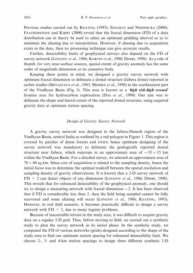
Previous studies carried out by KEATING (1993), SEDARAT and NISHIMURA (2000),
FEATHERSTONE and KIRBY (2000) reveal that the fractal dimension (FD) of a data
distribution can in theory be used to select an optimum gridding interval so as to
minimize the aliasing due to interpolation. However, if aliasing due to acquisition
exists in the data, then no processing technique can give accurate results.
Further, detectability limits of geophysical surveys also depend on the FD of
survey network (LOVEJOY et al., 1986; KORVIN et al., 1990; DIMRI, 1998). As a rule of
thumb, for very near-surface sources, spatial extent of gravity anomaly has the same
order of magnitude dimension as its causative body.
Keeping these points in mind, we designed a gravity survey network with
optimum fractal dimension to delineate a domal structure (Jabera dome) reported in
earlier studies (SRIVASTAVA et al., 1983; MISHRA et al., 1998) in the southeastern part
of the Vindhyan Basin (Fig. 1). This area is known as a ‘high risk-high reward’
frontier area for hydrocarbon exploration (DAS et al., 1999). Our aim was to
delineate the shape and lateral extent of the reported domal structure, using acquired
gravity data at optimum station spacing.
Design of Gravity Survey Network
A gravity survey network was designed in the Jabera-Damoh region of the
Vindhyan Basin, central India as outlined by a red polygon in Figure 1. This region is
covered by patches of dense forests and rivers; hence optimum designing of the
survey network was mandatory to delineate the geologically reported domal
structure near Jabera, which outcrops in an approximate area of �35� 15 km
within the Vindhyan Basin. For a detailed survey, we selected an approximate area of
70� 60 sq km. Since cost of acquisition is related to the sampling density, hence the
initial focus was to determine the optimal tradeoff between the spatial resolution and
sampling density of gravity observations. It is known that a 2-D survey network of
FD = 2 can detect objects of any dimension (LOVEJOY et al., 1986; DIMRI, 1998).
This reveals that for enhanced detectability of the geophysical anomaly, one should
try to design a measuring network with fractal dimension �2. It has been observed
that if FD is considerably less than 2, then the field being sampled cannot be fully
recovered and some aliasing will occur (LOVEJOY et al., 1986; KEATING, 1993).
However, in real field scenario, it becomes practically difficult to design a survey
network with FD = 2, due to many logistic problems.
Because of inaccessible terrain in the study area, it was difficult to acquire gravity
data on a regular 2-D grid. Thus, before moving to field, we carried out a synthetic
study to plan the survey network in its initial phase. In the synthetic study, we
computed the FD of various networks (grids) designed according to the shape of the
study area to find out optimum station spacing for enhanced detectability limit. We
choose 2-, 3- and 4-km station spacings to design three different synthetic 2-D
2010 R. P. Srivastava et al. Pure appl. geophys.,

networks. Fractal dimension (Fig. 2) of these synthetic grids was computed using the
well-known box-counting method (TURCOTTE, 1992). A comparative analysis based
on the cost of the survey and the detectability limit of these synthetic grids is shown
in Table 1. It is clear from Table 1 that FD of synthetic grid decreases with an
increase in station spacing. In this case one can prefer to acquire data at 2-km
spacing because of higher FD (dense coverage). Since it was difficult to acquire data
Figure 1
Geological map and location of the studied area in the Vindhyan Basin, central India. Red polygon is the
surveyed area. A profile AA’ across the target structure, Jabera dome is selected for the modeling.
Vol. 164, 2007 Optimum Design of Survey Network 2011
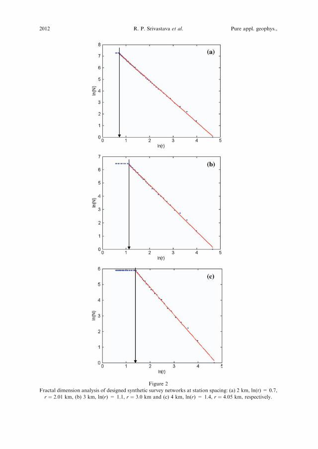
Figure 2
Fractal dimension analysis of designed synthetic survey networks at station spacing: (a) 2 km, ln(r) = 0.7,
r ¼ 2:01 km, (b) 3 km, ln(r) = 1.1, r ¼ 3:0 km and (c) 4 km, ln(r) = 1.4, r ¼ 4:05 km, respectively.
2012 R. P. Srivastava et al. Pure appl. geophys.,

at the regular grid of 2-km spacing in the study area, acquisition of data at 3-km grid
spacing is suggested in the studied region.
For comparative study, gravity data were also acquired at approximately 2- and
4-km spacing, though it was not suggested for practical purposes. The acquisition
pattern for 2-, 3- and 4-km station spacing is shown in Figure 3, where synthetic
observation points are shown in red color and actual observation points are shown
in blue color. Figure 3 shows that observed data points are quite close to the
designed grid points for 3- and 4-km station spacings. Computation of FD of a real
survey network with observation points approximately at 2-, 3- and 4-km spacing
respectively, is shown in Figure 4. The value of FD is obtained as 1.65, 1.66 and
1.67, respectively for 2-, 3- and 4-km station spacing. This slight increase in fractal
dimension with station spacing is observed because of the fact that the real data
acquired at approximately 2-, 3-and 4-km intervals is not at regular intervals, and
there are some blank patches as shown in the Figure 3. The gravity data acquired
at 4-km station spacing were more homogeneous and hence have high fractal
dimension.
Optimum Gridding of Gravity Data
Preparation of Bouguer anomaly maps requires interpolation of data using
statistical methods, which introduces aliasing. Hence, appropriate processing is
required to generate the least aliased anomaly maps. To overcome this problem,
KEATING (1993) suggested the use of well-known fractal dimension analysis to
determine an optimum gridding interval, exploiting the concept of scaling regime of
the data. The FD analysis is done using the box-counting method.
In the box-counting method, the area is subdivided into a number of equal size
squares with side length r. The logarithm of the number of such squares (ln NðrÞ),which have at least one observation point, is plotted against ln(r) and the slope of this
plot gives the value of the fractal dimension. The smallest length r at which the
scaling regime ceases to be constant gives the optimum sampling interval. It was
Table 1
Comparative study of designed survey networks using different station spacings and cost of the survey, which
corresponds to man-days to acquire the data. It is assumed that at 2-km spacing about 15 data points, at 3-km
about 12 data points, and at 4-km about 10 data points can be collected in a day, in a difficult terrain. This
assumption is based on practical experience in the field
Station
Spacing
FD of Designed 2-D
Grid
Detectability
limit (2-FD)
No. of Stations Man-Days
2 km 1.79 0.21 1436 95
3 km 1.75 0.25 636 53
4 km 1.74 0.26 357 36
Vol. 164, 2007 Optimum Design of Survey Network 2013

0 20 40 60 80 100 1200
20
40
60
80
100
120
X (km)
)mk(
Y
Designed Grid
Acquired Stations
(a)
(b)
(c)
0 20 40 60 80 100 1200
20
40
60
80
100
120
X (Km)
)m
K(Y
Designed GridAcquired Stations
0 20 40 60 80 100 1200
20
40
60
80
100
120
X (Km)
)m
K(Y
Designed GridAcquired Stations
Figure 3
Acquisition network with actual observation points plotted over: (a) Station spacing 2 km, (b) station
spacing 3 km, and (c) station spacing 4 km. Synthetic grid nodes are shown in red and actual observations
are shown in blue.
2014 R. P. Srivastava et al. Pure appl. geophys.,

0 1 2 3 4 50
1
2
3
4
5
6
7
ln(r)
)N(nl
(a)
0 1 2 3 4 50
1
2
3
4
5
6
7
ln(r)
)N(nl
(b)
0 1 2 3 4 50
1
2
3
4
5
6
ln(r)
)N(nl
(c)
Figure 4
Optimum gridding interval and fractal dimensional analysis of real data acquired at: (a) 2-km station
spacing, ln(r) = 1.07, r ¼ 2:92 km, FD = 1.65, (b) 3-km station spacing, ln(r) = 1.23, r ¼ 3:42 km, FD=
1.66, (c) 4-km station spacing, ln(r) = 1.41, r ¼ 4:09 km, FD = 1.67.
Vol. 164, 2007 Optimum Design of Survey Network 2015

observed that only in the case of synthetic data, one can get a unique gridding
interval which is equal to the station spacing (Fig. 2). Whereas, in the case of real
data (Figs. 4a, b), the scaling regime does not cease suddenly at a point, hence a
range for an optimum gridding interval is suggested from the curve. This range is
encircled in FD analysis plots (Fig. 4) obtained by using observed data at 2-, 3- and
4-km station spacing. We therefore suggest that instead of looking for an optimum
gridding interval, anomalies can be computed within an optimum interpolation
range. The interpolation range for the real data acquired in the studied region is
2:92� 0:5 for 2-km spacing, 3:42� 0:5 km for 3-km station spacing and
4:09� 0:5 km for 4-km station spacing as encircled in Figures 4 a,b,c.
Gridding/Interpolation Method
Interpolation is a procedure of predicting values of attributes at unsampled sites
from measurements made at point locations within the same area. Among several
techniques available for the interpolation of the data, kriging is found most suitable
for the interpolation of irregular spatial data (ECKSTEIN, 1989; ISHIDA and
KAWASHIMA, 1993; HUTCHINSON and GESSLER, 1994). The input data for kriging
are usually an irregularly-spaced sample of points. This technique is an exact
interpolator of the data. Exact interpolators honor the data points upon which the
interpolation is based. Keeping in view the robustness of the kriging for sparse data
we have used point kriging, which estimates the values of the points at the grid nodes
using commercial software ‘Surfer’, developed by Golden Software, Inc (www.gold-
ensoftware.com). The software ‘Surfer’ uses a linear variogram model as default for
point kriging and we have used the same for the interpolation of the data presented
in this paper.
Bouguer Anomaly Map of the Jabera-Damoh Region
Bouguer anomaly maps of the studied region are prepared using an interpolation
interval obtained by fractal dimensional analysis. The anomaly maps (Figs. 5a,c)
produced by the fractal method look more smooth and free from aliasing errors,
hence produce the best representation of the subsurface features of the study area
rather than the maps produced by the conventional method (Figs. 5b,d). In our view,
the conventional way of gridding the data is to take the interpolation/gridding
interval less than the actual spacing of the data locations. If the survey is done at a
random interval then the mean spacing of the data locations is normally used to grid
the data. In the fractal method we select the interpolation interval based on fractal
dimension analysis (KEATING, 1993) of the data location. It is clearly evident from
Figure 5 that the Bouguer anomaly map obtained by the fractal method is almost
2016 R. P. Srivastava et al. Pure appl. geophys.,
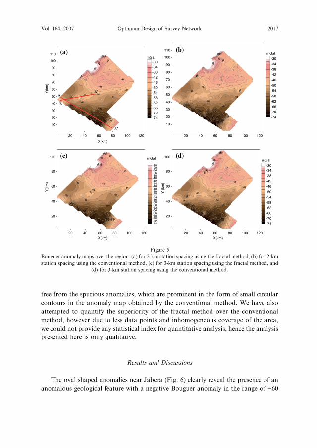
free from the spurious anomalies, which are prominent in the form of small circular
contours in the anomaly map obtained by the conventional method. We have also
attempted to quantify the superiority of the fractal method over the conventional
method, however due to less data points and inhomogeneous coverage of the area,
we could not provide any statistical index for quantitative analysis, hence the analysis
presented here is only qualitative.
Results and Discussions
The oval shaped anomalies near Jabera (Fig. 6) clearly reveal the presence of an
anomalous geological feature with a negative Bouguer anomaly in the range of )60
20 40 60 80
(a) (b)
(c) (d)
100 120 20 40 60 80 100 120
X(km)
20 40 60 80 100 120X(km)
20 40 60 80 100 120X(km)
10
20
30
40
50
60
70
80
90
100
110
Y(k
m)
Y(k
m)
-74-70-66-62-58-54-50-46-42-38-34-30
mGal
A’
R
AR’
10
20
30
40
50
60
70
80
90
100
110
-74
-70
-66
-62
-58
-54
-50
-46
-42
-38
-34
-30
mGal
20
40
60
80
100
-74-72-70-68-66-64-62-60-58-56-54-52-50-48-46-44-42-40-38-36-34-32-30
mGal
20
40
60
80
100
Y (
km)
-74
-70
-66
-62
-58
-54
-50
-46
-42
-38
-34
-30
mGal
Figure 5
Bouguer anomaly maps over the region: (a) for 2-km station spacing using the fractal method, (b) for 2-km
station spacing using the conventional method, (c) for 3-km station spacing using the fractal method, and
(d) for 3-km station spacing using the conventional method.
Vol. 164, 2007 Optimum Design of Survey Network 2017

to )74 mGal. The boundary of this structure is clearly demarcated by our study. The
delineated structure appears to be a rifted basin bounded by faults on either side.
Further, a new finding of this study is the delineation of an apparently small ridge-
like structure marked as RR’ in Figure 5a. This ridge-like structure running east-west
divides this region (basin) in two parts, which has not yet been observed in earlier
studies. It is also seen in the anomaly map that this basin extends further south-west
than hitherto known.
The anomaly pattern of the studied region does not conform to the geologically
reported domal structure near Jabera. This may be due to the fact that the particular
domal structure has a gentle dip of around 10�. This means that the domal structure
is not a deep-seated feature, rather it could be an erosional feature. It is further
observed that the Bouguer anomaly maps prepared at 2-km and 3-km spacing
convey the same geological information. This suggests that there is no loss of useful
information in acquiring data at 3-km spacing in this area, which was suggested in
the synthetic study.
Figure 6
Bouguer anomaly map of the region superimposed over the geological map of Jabera–Damoh region
extracted from Figure 1.
2018 R. P. Srivastava et al. Pure appl. geophys.,

For quantitative interpretation we selected a profile AA’ (Fig. 5a) across the
target structure and modeled the gravity data using the Marquardt inversion
approach with the help of SAKI program (WEBRING, 1985). The target structure is
shown in the geological map of the area (Fig. 1) and the profile AA’ across the
structure is not at the boundary, thus interpolation effects at the boundary will not
affect the modeling results and the best possible model of the target structure is
obtained. The proposed subsurface model along the profile AA’ is shown in Figure 7.
This profile is selected in order to estimate the tentative geological crosssection across
the conspicuous low gravity anomaly observed in the southern part of the study area.
Deep Seismic Sounding (DSS) studies (KAILA et al., 1989) indicate maximum
thickness of sediments in this part of the Vindhyan Basin. Since this area lies in the
vicinity of Jabera, we termed it as Jabera Basin.
Using constraints from the borehole data (DAS et al., 1999) and DSS studies
(MURTY et al., 2004) the inverse modeling of this profile (AA’) has been attempted.
The preliminary depth values of the major interfaces were obtained from the 2-D
Figure 7
Gravity model along the profile AA’.
Vol. 164, 2007 Optimum Design of Survey Network 2019
scaling spectral analysis (MAUS and DIMRI, 1994, 1995a,b, 1996) of the data. The
modeling result (Fig. 7) shows that the anomaly corresponds to a deep faulted basin
in the crystalline basement in which the upper layer with density value of 2.46 g/cc
corresponds to the upper Vindhyan rocks. This layer is underlain by 5.5-km thick
lower Vindhyan sediments. The layer of lower Vindhyan sediments is gently sloping
from NW to SE direction, which sits over the high density rocks possibly comprising
the Bijawar/Mahakoshal group. It was difficult to fit the observed anomaly pattern
without introducing this high density (2.80 g/cc) layer. In the absence of this layer,
the thickness of sediments would have increased to such an extent that it would have
not matched with the known seismic and well log results. It is also seen in the model
that the granite layer is missing in the right margin of the faulted basin whereas it has
a thin patch in its left side of the faulted segment. This conforms to the reported DSS
modeling (MURTY et al., 2004).
There is a possibility that the Bijawar/Mahakoshal groups of rocks were
deposited directly over the high-velocity (6.5 km/s) and high-density (2.93 g/cc)
exhumed lower crustal segment.
Concluding Remarks
The fractal approach of data interpolation reduces aliasing effects due to
interpolation and suggests an optimum grid interval value for interpolation of
randomly distributed data. In this case study, aliasing is reduced by optimum
designing of survey network in the Jabera-Damoh area of the Vindhyan Basin.
Modeling of the gravity anomaly along a profile across the target structure has been
done and the results reveal that the anomaly corresponds to a faulted basin in the
crystalline basement.
It is worth mentioning that the fractal dimensional analysis of finding an
optimum sampling interval is found very useful, which avoids unnecessary dense data
acquisition efforts. It is evident from the anomaly maps, produced by conventional
and fractal methods, that the later reduces spurious anomalies. Therefore use of
fractal dimensional analysis is recommended for the acquisition of data and
preparation of anomaly maps for a more realistic interpretation. However, before
designing a survey network, the following points must be taken in account:
1. Objective of survey, whether the survey target is a shallow or deep feature.
2. Station spacing should be properly judged based on the dimension of the target
and accessibility of the terrain.
3. Stations should be evenly distributed across the target to obtain a higher fractal
dimension rather than clustering them on easily accessible areas, because such
data points will add only modest information towards delineation of the target in
the case of the 2-D survey.
2020 R. P. Srivastava et al. Pure appl. geophys.,

We suggest that the fractal dimension study should be carried out in the planning
phase of gravity/magnetic surveys using synthetic stations. Well-designed surveys
with higher fractal dimension and optimum sampling intervals produce desired
gravity maps with the least or no aliasing, as has been demonstrated in this case
study.
Acknowledgements
The authors acknowledge the Department of Science and Technology, Govt. of
India for sponsoring this work. We are thankful to Drs. Stefan Maus and O.P.
Pandey for critically reading the manuscript. Comments of an anonymous reviewer
helped us to improve the quality of the manuscript.
REFERENCES
DAS, A.K., BARUAH, R.M., BISHT, S.S., and AGRAWAL, B. (1999), An integrated analysis of late Proterozoic
lower Vindhyan sediments for hydrocarbon exploration, J. Geol. India. 53, 239–253.
DIMRI, V.P. (1998), Fractal behavior and detectability limit of geophysical surveys, Geophys. 63, 1943–1947.
ECKSTEIN, B.A. (1989), Evaluation of spline and weighted average interpolation algorithms, Comp. Geosci.
15(1), 79–94.
FEATHERSTONE, W.E. and KIRBY, J.F. (2000), The reduction of aliasing in gravity anomalies and geoid
heights using digital terrain data, Geophys. J. Int. 141, 204–212.
HUTCHINSON, M.F. and GESSLER, P.E. (1994), Splines - more than just a smooth interpolator, Geoderma 62,
45–67.
ISHIDA, T. and KAWASHIMA, S. (1993), Use of Cokriging to Estimate Surface Air Temperature from
Elevation, Theor. Appl. Climatol. 47, 147–157.
KAILA, K. L., MURTHY, P. R. K., and MALL, D. M. (1989), The evolution of the Vindhyan Basin vis-‘a-vis
the Narmada–Son lineament, Central India, from deep seismic soundings; Tectonophysics 162, 277–289.
KEATING, P. (1993), The fractal dimension of gravity data sets and its implications for gridding, Geophys.
Prosp. 41, 983–993.
KORVIN, G., BOYD, D.M., and O’DOWD, R. (1990), Fractal characterization of the south Australian gravity
station network, Geophys. J. Int. 100, 535–539.
LOVEJOY, S., SCHERTZER, D., and LADOY, P. (1986), Fractal characterization of inhomogeneous geophysical
measuring networks, Nature 319, 43–44.
MAUS, S. and DIMRI, V.P. (1994), Fractal properties of potential fields caused by fractal sources, Geophys.
Res. Lett. 21, 891–894.
MAUS, S. and DIMRI, V.P. (1995a), Basin depth estimation using scaling properties of potential fields, J. Ass.
Expl. Geophys. 16, 131–139.
MAUS, S. and DIMRI, V.P. (1995b), Potential field power spectrum inversion for scaling geology, J. Geophys.
Res. 100, 12605–12616.
MAUS, S. and DIMRI, V.P. (1996), Depth estimation from the scaling power spectrum of potential fields?
Geophys. J. Int. 124, 113–120.
MISHRA, D.C., GUPTA, S.B., and RAO, M.R.K.P. (1998), Airborne magnetic lineament, groundwater
potentiality and basement structures in S-E part of Vindhyan Basin, J. Geol Soc. India 52, 195–202.
MURTY, A.S.N., TEWARI, H.C., and REDDY, P.R. (2004), 2-D crustal structure along Hirapur-Mandla
profile in Cental India: An update, Pure Appl. Geophys. 161, 165–184.
Vol. 164, 2007 Optimum Design of Survey Network 2021

SEDARAT, H. and NISHIMURA, D.G. (2000), On the optimality of the gridding reconstruction algorithm,
IEEE Transactions on Medical Imaging 19(4), 306–317.
SRIVASTAVA, B.N., RANA, M.S., and VERMA, N.K. (1983), Geology and hydrocarbon prospects of the
Vindhyan Basin, Petroleum Asia J. 179–189.
TURCOTTE, D.L. (1992), Fractals and Chaos in Geology and Geophysics (Cambridge University Press, 1992).
WEBRING, M., (1985), Semi-automatic Marquardt inversion of gravity and magnetic profiles, U.S.
Geological Survey Open File Report OF 85–122.
(Received October 1, 2006, accepted March 2, 2007)
To access this journal online:
www.birkhauser.ch/pageoph
2022 R. P. Srivastava et al. Pure appl. geophys.,
Top Related
Copyright © 2022 FDOKUMEN

