


Bahasa
Halaman
Hukum


Modelling the management of multiple-use
reservoirs: Deterministic or stochastic
dynamic programming?
Lap Doc Trana,b
,
Steven Schilizzia, Morteza Chalak
c and Ross Kingwell
a,d
a School of Agricultural and Resource Economics, The University of Western Australia, 35 Stirling Highway,
Crawley, Western Australia 6009, Australia
b Department of Economics, Nong Lam University, Thu Duc District, Ho Chi Minh City, Vietnam
c Centre for Environmental Economics and Policy, School of Agricultural and Resource Economics, The
University of Western Australia, 35 Stirling Highway, Crawley, Western Australia, 6009, Australia
d Department of Agriculture & Food, Western Australia, 3 Baron-Hay Court, South Perth, Western Australia
6151, Australia
Contributed paper prepared for presentation at the 56th AARES annual conference,
Fremantle, Western Australia, February7-10, 2012
Copyright 2012 by Authors names. All rights reserved. Readers may make verbatim copies of this document for
non-commercial purposes by any means, provided that this copyright notice appears on all such copies.

Modelling the management of multiple-use reservoirs:
Deterministic or stochastic dynamic programming?
Lap Doc Tran
Steven Schilizzi, Morteza Chalak, and Ross Kingwell1
Abstract
Modelling complex systems such as multiple-use reservoirs can be challenging. A legitimate
question for scientists and modellers is how best to model their management under uncertain
rainfall. This paper studies whether it is worth using a stochastic model that requires more
effort than a much simpler deterministic model. Both models are applied to the management
of a multiple-use reservoir in southern Vietnam. Although no single modelling approach is
universally superior, this study indicates that the desirable modelling approach is stochastic if
reservoir capacity and water use demands have a high enough impact on the optimal timing of
reservoir water use.
Keywords: deterministic dynamic proramming, stochastic dynamic programming, water
management, irrigation, fisheries, multiple-use reservoir
1. Introduction
There is a vast of literature on reservoir water management using dynamic optimization
models (Abdallah et al., 2003, Barros et al., 2003, Biere et al., 1972, Butcher et al., 1969,
Cervellera et al., 2006, Chaves et al., 2003, Georgiou et al., 2008, Ghahraman et al., 2002,
Karamouz et al., 1987, Nandalal et al., 2007, O'Loughlin, 1971, Reca et al., 2001a, Reca et
al., 2001b). These studies employed either stochastic or deterministic approaches to determine
optimal water release strategies for a reservoir. The approaches chosen to define the optimal
release strategies in these studies depended on available data sources, computing power, the
skills of the researchers and the time available to them. For example, O’Loughlin (1971) and
Dudley (1971) concluded that although using stochastic dynamic optimization took much
time, it yielded better results compared to a deterministic approach.
Due to developments in computer software and computing power over the past two decades,
the problems of time-consuming computations have lessened and facilitated the use of
stochastic dynamic optimization for reservoir management. However, this application of
stochastic dynamic optimization requires access to long-term rainfall and reservoir inflow
data in order to calculate meaningful probabilities for stochastic variables. Ensuring the
1 The authors gratefully acknowledge the provision of funding from the Australian Centre for International
Agricultural Research (ACIAR) for this research.

availability of such data is often difficult for researchers investigating reservoir management
in isolated areas of developing countries. The simpler method of deterministic dynamic
optimization, may be easier where data is limited.
This paper investigates the relative merits of the stochastic and deterministic approaches to
reservoir management, using multiple-use reservoirs in southern Vietnam to illustrate the
problem and highlight its relevance to decision-making.
This paper is structured as follows. The next section briefly describes a reservoir management
model based on either a stochastic or deterministic approach. Then parameter estimation and
data collection are presented. Finally, the model results are presented for a range of reservoir
configurations and reservoir management objectives, and conclusions are drawn about when a
particular modelling approach is likely to be most relevant.
2. A dynamic optimization model for managing multiple-use reservoirs
Tran et al. (2011) constructed a dynamic optimization model for managing multiple-use
reservoirs in southern Vietnam. The model addressed the problem of reservoir water
management for two competing uses of the water: crop irrigation and fish production. The
time horizon of the model included 8 stages (where each stage was 25 days long) covering 2
rice crop seasons (where each crop comprised 4 growth periods described as initial,
development, mid-season, and late-season), and a fish harvesting season from stage 4 to stage
7. The state variable was the amount of water in the reservoir at the beginning of an irrigation
season, as measured by the percentage of reservoir capacity (% RC). The decision variable
was the amount of water to be released at each stage (also expressed as % RC). Finally, the
objective function was to maximize the expected stream of the present value of profits
(ENPV) generated by the reservoir which included profits from rice and fish production.
The rice profits were calculated as follows:
rnrrrrn CYPAB (1)
where Brn represents rice profits (mVND); Ar is rice irrigated area (ha); Pr is the price of rice
(mVND/tonne); Yr is rice yields (tonnes) obtained in stage n; and Crn is total rice production
cost in stage n (mVND). The other rice production inputs, such as fertilizer, chemicals, and
labour, were assumed to be applied at optimal levels. In Eq.(1), rice yields Yr was determined
using a water production function (Paudyal et al., 1990):
8
1 0
11n n
yprW
WkYY
n
(2)
where Yr is the rice yield (tonnes/ha); Yp is the potential yield of rice (tonnes/ha); nyk is the
yield response factor to water at stage n; W0 is the rice water requirements (%RC); Wn is total
water supply at stage n (%RC).
fnnfnfn CPCETRB 1 (3)

where Bfn is fish profits (mVND); TRfn (mVND) is total fish return obtained from the BRAVO
model (Truong et al., 2010); Cfn is the total cost of fish production (mVND); and PCEn is the
physical concentration effects coefficient (Tran et al., 2011).
sY
ssAPCE
f
ttn
%)1()1(
0
(4)
where is the parameter obtained from the reservoir hypsographic equation, sAA 0 , which
indicates the relationship between reservoir surface area A (ha) and reservoir capacity s
(%RC); A0 is the reservoir surface area when the reservoir is full (ha); and are the
parameters obtained from Nguyen et al. (2001) who indicated the relationship between fish
yields and reservoir surface area as AY .The other fish production inputs, such as weight
of fingerlings and labour, are assumed to be applied at optimal levels.
The backward induction method was employed to find the optimal release strategy for
managing the reservoir for single-use rice or fish production, and joint production of rice and
fish. The model was validated for the Daton reservoir in southern Vietnam. The maximum
storage capacity of this reservoir was much greater than the water requirements it served. An
important modelling result obtained for the Daton reservoir (Tran et al., 2011) was that
variations in rainfall do not significantly affect the intra-year release strategy and benefits
generated by the reservoir. A legitimate question for the modelling approach then arose as to
whether it was worthwhile to employ a stochastic model, which involves complex
computations and a large amount of time for its construction. Would the use of a deterministic
model be preferable? In this study, we alter and revise the Tran et al. model to consider
various scenarios for water management and compare modelling results from stochastic and
deterministic models.
In the Tran et al. model, when the reservoir is managed solely for rice production, fish profits
are assumed to be zero; and rice profits are assumed to be zero if the reservoir is managed
purely for fish harvesting. However, in reality, when the reservoir is managed solely for the
use of one enterprise, the other enterprise can also benefit. For example, if the reservoir water
is managed purely for rice production, fish are still harvested to a limited degree. Fish profits
vary according to the storage levels of the reservoir which are determined by the optimal
water release for rice production. Similarly, when the reservoir is managed exclusively for
fish production, rice is still cultivated. Rice profits vary according to rainfall and the release
of water to facilitate fish harvesting.
The objective function of the Tran et al. model is:
Bn = Brn + Bfn (5)
where Bn is total profit, Brn is rice profit, and Bfn is fish profits All are measured in mVND.
Equation (5) becomes Bn = Brn if the reservoir water is managed for rice production, and is Bn
= Bfn if the reservoir is managed for fish harvesting. In the present study, the objective
function is extended as follows:
If the reservoir is managed solely for rice production, the objective function is:
Bn = B*
rn + B’fn (6a)

If the reservoir is managed solely for fish production, the objective function is:
Bn = B’rn + B
*fn (6b)
where B*
rn and B*fn are the maximum profits obtained from optimal release for rice production
and fish harvesting, respectively. B*
rn and B*
fn are found using the method proposed by Tran et
al. (2011). B’fn is fish profit determined by the optimal water release for rice production; and
B’rn is rice profit determined by the optimal water release for fish harvesting. All are measured
in mVND.
The objective function for the optimization model is to maximize the expected net present
value of profits (ENPV), and for the deterministic case the net present value (NPV) is
maximized. For convenience, total net profits (TNP) are used here to represent both ENPV
and NPV.
The objective function for stochastic optimization model is
m
k
k
n
k
nnnnn
k
n
k
nnnnn
k
nnu
nn iqeusViqeusBqpEMaxsVn 1
1 ,,,,,,,,
(7)
(n=8, ….,1)
(8)
where sn reservoir water level at the beginning of each stage; un is the release at stage n; en is
the evaporation at stage n; qn is rainfall at stage n; and in is the reservoir inflows at stage n. All
are expressed in %RC.
In addition to modifying the objective function of the Tran et al. model, the model structured
in the present study considers both deterministic and stochastic cases of reservoir water
management. In the stochastic model (Tran et al., 2011), the reservoir water level (state
variable) at the next stage was unknown depending on rainfall distribution in the previous
stages which was represented by the (14 x 8) rainfall distribution matrix (Eq. 8). The
objective function for the deterministic case is similar to (Eq.7) except that in the
deterministic case the probabilities of rainfall occurrences are not considered and rainfall
distribution matrix is replaced by a (1 x 8) vector of rainfall averages, one for each stage.
3. Parameter estimation for the reservoir water management model
3.1 Time horizon of the model
The Daton reservoir is used to irrigate two consecutive rice crops each of approximately 1000
hectares during the dry season from December to June. The first crop is grown from
December to March and the second crop is from April to July. Each crop lasts about 100 days
and is divided into four growth periods: the initial, development, mid and late season periods
as defined in the Cropwat 8.0 model (Swennenhuis, 2006). Each rice growth period as
modelled is 25 days long, consistent with the experimental results obtained by Le and Duong
m
k
k
nn qp1
1

(1998). To account for the two consecutive rice crops, each with four growing periods, a
model with eight 25-day stages was developed.
Harvesting of fish occurs when the reservoir water is at its lowest levels, during the period
from mid February to June (Nguyen, 2008a). In the eight-stage model the fish harvest season
covers four 25-day periods, starting in stage 4 and ending in stage 7.
3.2 Rainfall, evaporation, and hydrologic data
Rainfall data
Daily rainfall data from 2001 to 2008 was collected from the Daton irrigation branch (Dinh,
2008). This data was used to calculate rainfall probability density functions in each stage
(Table 1), the inflows of the reservoir, and the amount of water that the rice fields directly
received from rainfall.
Table 1 Rainfall
Rainfall Rainfall probability
(mm) Stage 1 Stage 2 Stage 3 Stage 4 Stage 5 Stage 6 Stage 7 Stage 8
0.0 0.955 0.98 0.98 0.95 0.865 0.745 0.635 0.545
37.5 0 0 0 0 0.005 0.005 0.015 0.03
87.5 0.005 0 0.01 0 0.015 0.01 0.035 0
137.5 0 0 0.005 0.015 0.01 0.03 0.025 0.025
187.5 0.01 0.005 0 0 0.025 0.01 0.035 0.04
237.5 0.005 0 0.005 0 0.03 0.005 0.01 0.035
287.5 0 0 0 0.005 0.005 0.01 0.015 0.02
337.5 0 0 0 0.01 0 0.01 0.02 0.03
387.5 0.005 0 0 0.015 0.005 0.02 0.005 0.03
437.5 0.01 0.01 0 0 0 0.01 0.01 0.005
487.5 0 0.005 0 0 0.01 0.02 0.02 0.03
537.5 0 0 0 0.005 0 0.005 0.01 0.02
587.5 0.005 0 0 0 0.005 0.005 0.015 0.015
625.0 0.005 0 0 0 0.025 0.115 0.15 0.175

Evaporation data
The average evaporation in each stage is estimated using the monthly evaporation data from
the Dong Nai province (1977 – 2006) provided by the Sub-Institute of Hydrometeorology and
Environment of South Vietnam. The average of monthly evaporation was calculated using the
evaporation data of the Dong Nai province. These values were then divided by 30 to obtain an
average daily evaporation for each month. The average evaporation value for each stage, 25
days, was then obtained by multiplying the average daily evaporation by 25 for the relevant
month. In cases where a stage bridges two months, the average evaporation of that stage was
considered to be the sum of the evaporation calculated for the number of days of each of the
corresponding months. For example, stage 1 lasts for 25 days from December 25th
to January
18th
; therefore, the average evaporation for this stage was the sum of seven days of average
evaporation for December and 18 days for January.
Hydrological data
The physical parameters of the reservoir were obtained from the Daton irrigation branch
(Dinh, 2008) including maximum and minimum storage capacity, discharge capacity,
reservoir surface area, reservoir catchment area, and reservoir inflows. The hypsographic
coefficient, which indicates the relationship between reservoir water availability and reservoir
surface area, was obtained from the hypsographic curve provided by the Daton irrigation
branch. All parameters are presented in Table 2.
Table 2 Parameters used in the model
Parameters Unit Value Descriptions
smax MCM 19.6 Maximum reservoir capacity
smin MCM 0.4 Minimum storage water level required for safety
DC m3/second 2.5 Reservoir discharge capacity
A0 ha 350
Reservoir surface area at full level of water
Rc km2
21
Reservoir catchment area
θ
no.
0.5732
Hypsographic coefficient
σ
no.
0.3
Reservoir inflow coefficient MCM = Million Cubic Metres, or m
310
6
3.3 Rice production data
A seasonal calendar for rice production and the actual cultivated area of rice were obtained
from the 2008 annual report of the local authority (Nguyen, 2008b). The maximum observed
yields over the period from 2001 to 2008 were used to indicate the potential yield of rice in
this area. It was 6.5 tonnes/ha for the first rice crop and 6 tonnes/ha for the second rice crop.
Irrigation efficiency, expressing the percentage of irrigation water used efficiently, was fixed
at 85% (Thang Pham, 2009, personal communication, 15 January). To simulate rice yields in
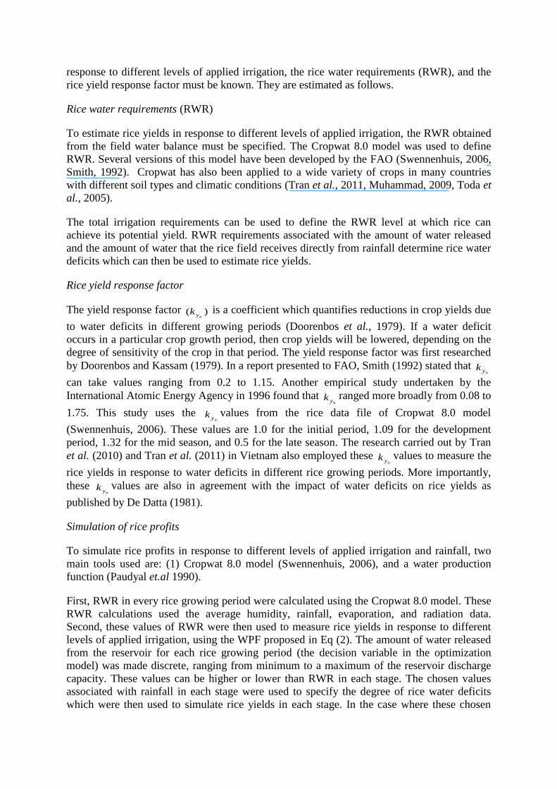
response to different levels of applied irrigation, the rice water requirements (RWR), and the
rice yield response factor must be known. They are estimated as follows.
Rice water requirements (RWR)
To estimate rice yields in response to different levels of applied irrigation, the RWR obtained
from the field water balance must be specified. The Cropwat 8.0 model was used to define
RWR. Several versions of this model have been developed by the FAO (Swennenhuis, 2006,
Smith, 1992). Cropwat has also been applied to a wide variety of crops in many countries
with different soil types and climatic conditions (Tran et al., 2011, Muhammad, 2009, Toda et
al., 2005).
The total irrigation requirements can be used to define the RWR level at which rice can
achieve its potential yield. RWR requirements associated with the amount of water released
and the amount of water that the rice field receives directly from rainfall determine rice water
deficits which can then be used to estimate rice yields.
Rice yield response factor
The yield response factor )(nyk is a coefficient which quantifies reductions in crop yields due
to water deficits in different growing periods (Doorenbos et al., 1979). If a water deficit
occurs in a particular crop growth period, then crop yields will be lowered, depending on the
degree of sensitivity of the crop in that period. The yield response factor was first researched
by Doorenbos and Kassam (1979). In a report presented to FAO, Smith (1992) stated that nyk
can take values ranging from 0.2 to 1.15. Another empirical study undertaken by the
International Atomic Energy Agency in 1996 found that nyk ranged more broadly from 0.08 to
1.75. This study uses the nyk values from the rice data file of Cropwat 8.0 model
(Swennenhuis, 2006). These values are 1.0 for the initial period, 1.09 for the development
period, 1.32 for the mid season, and 0.5 for the late season. The research carried out by Tran
et al. (2010) and Tran et al. (2011) in Vietnam also employed these nyk values to measure the
rice yields in response to water deficits in different rice growing periods. More importantly,
these nyk values are also in agreement with the impact of water deficits on rice yields as
published by De Datta (1981).
Simulation of rice profits
To simulate rice profits in response to different levels of applied irrigation and rainfall, two
main tools used are: (1) Cropwat 8.0 model (Swennenhuis, 2006), and a water production
function (Paudyal et.al 1990).
First, RWR in every rice growing period were calculated using the Cropwat 8.0 model. These
RWR calculations used the average humidity, rainfall, evaporation, and radiation data.
Second, these values of RWR were then used to measure rice yields in response to different
levels of applied irrigation, using the WPF proposed in Eq (2). The amount of water released
from the reservoir for each rice growing period (the decision variable in the optimization
model) was made discrete, ranging from minimum to a maximum of the reservoir discharge
capacity. These values can be higher or lower than RWR in each stage. The chosen values
associated with rainfall in each stage were used to specify the degree of rice water deficits
which were then used to simulate rice yields in each stage. In the case where these chosen

values were lower than RWR, water deficits occurred, causing reductions in rice yields in that
stage. Conversely, if the chosen values of water released were higher than RWR, then there
was a surplus of water. This surplus can be assumed to exit into rivers without a negative
effect on rice yields. There are two reasons for choosing values that are higher than RWR.
Firstly, an over-release may be reasonable when considering water releases for fish
harvesting. Secondly, in reality, an over-release will not affect rice yields because rice farmers
can control how much water is taken into their farms from the irrigation canals.
The average production cost and return per hectare of rice production was obtained from
surveying the farmers. The average production costs per hectare included the costs of seeding,
weeding, fertilizing, chemical use, labour, and harvest. The average production cost per
hectare for the first and the second rice crop were mVND 8.82 and 6.72, respectively. The
average return per hectare for rice production was estimated by multiplying the price of rice
(mVND 2.5 per tonne)2 by the rice yields. Total returns and total costs for the cultivated area
were estimated by multiplying these average values by the actual cultivated area. Total rice
profits in each stage were estimated by subtracting the total costs from the total returns.
3.4 Fish production data
The fish yields for each species harvested were estimated using the BRAVO model (Truong
and Schilizzi, 2010). All required input data for this model (such as weight of fingerlings,
stocking costs, and labour cost) was obtained from the 2008 annual report of the Daton
cooperative (Nguyen, 2008a). Tran et al. (2011) also used this data to estimate fish yields at
the Daton reservoir. The fish yield-reservoir area multiplicative factor (γ = 0.7422) and fish
yield-reservoir area power factor (ω = -0.7445) in equation (4) were obtained from Nguyen et
al. (2001)
Table 3 Weight and price of each fish species
Fish Prices Fish yields (tonnes) species (106VND
per tonne) Stage
1 Stage
2 Stage
3 Stage
4 Stage
5 Stage
6 Stage
7 Stage
8 Common Carp 16 0 0 0 3.506 3.026 2.636 2.262 0 Silver Carp 6 0 0 0 8.861 7.666 6.693 5.758 0 Grass Carp 8.5 0 0 0 7.043 6.239 5.573 4.887 0 Bighead Carp 6 0 0 0 4.477 3.93 3.479 3.027 0 Mrigal 8.5 0 0 0 4.154 3.584 3.121 2.678 0
2 The average price of rice in 2008 obtained from the survey

The total fish production cost in 2008 was mVND 615. The price of each fish species varies
according to fish size at harvest. In this study the price of each species (Table 3) was
represented by the fish price at its average size, which accounted for 70% to 80% of the total
weight of fish harvested (Nguyen, 2008a).
Simulation of fish profits
To simulate fish profits in response to fluctuations in the reservoir water level, the method
proposed above was employed. Total fish returns in each stage were estimated using the
BRAVO model. To examine the effects of the reservoir water fluctuations on fish production,
these total fish returns were then multiplied by the PCE coefficient (Tran et al., 2011). Fish
profits in response to the reservoir water fluctuations in each stage were obtained by
subtracting the total fish production cost from the total fish returns obtained under PCE.
4. Results and discussion
Reservoir water management is analysed for three production scenarios where the reservoir
water is used for: rice production only (scenario 1), fish production only (scenario 2) and joint
production of rice and fish (scenario 3).
The model is applied to Daton reservoir in southern Vietnam where the reservoir has a
maximum water storage capacity (RC) much greater than its current irrigation requirements
(IR). This model is then used to find the optimal water release strategy for other reservoir
configurations by modifying the Daton reservoir parameters. In particular, as each initial
water level of the Daton reservoir represents a full reservoir for different sizes, two groups of
reservoir configurations can be distinguished: R11 and R12 (see Table 5). The results obtained
from scenario 1 indicate that when the initial water level of the Daton reservoir is at 70% RC,
the amount of reservoir water available for irrigation is sufficient to fully satisfy the water
demand for 1000 hectares of rice production. Given this fixed irrigated area, as the initial
water level in the reservoir at the beginning of the irrigation season decreases, the
ratioIR
RCR decreases. In particular, when the initial water level is 70% RC (or fluctuates
around this level), the ratio R approaches 1. Therefore, 70% RC is a useful benchmark. In
addition, when the initial water level is at 50% RC, the reduction in irrigation increases the
magnitude of water deficits for rice, leading to a significant reduction in rice profits due to
reduced yields. Therefore, 50% RC is another benchmark point. For this reason, the following
sections use 50% RC, 70% RC and 100% RC as the benchmark water levels to define
reservoir configurations.
In the following sections, modelling results are presented for two ranges of initial water levels
(R11 and R12) of the Daton reservoir at the beginning of the irrigation season. R11 represents
the case when the initial water level is high, 70% - 100% RC. By contrast, R12 represents the
case when the initial water level is low, 50% - 70% RC (see Table 5).

Table 5 Reservoir configurations
Initial water
level
Reservoir
configurations
Descriptions
70%- 100% RC
(R ≥ 1)
R11 Reservoirs are full at the beginning of the irrigation
season and have RC greater than or equal to total IR
50% - 70% RC
(R < 1)
R12 Reservoirs are full at the beginning of the irrigation
season and have RC smaller than total IR

0
2000
4000
6000
8000
10000
12000
14000
16000
18000
40 50 60 70 80 90 100
TN
P (
mV
ND
)
Initial water level (% RC)
(a)
Scenario 1: Rice production
SDP model
DDP model
0
2000
4000
6000
8000
10000
12000
14000
16000
18000
40 50 60 70 80 90 100
TN
P (
mV
ND
)
Initial water level (% RC)
(b)
Scenario 2: Fish production
SDP model
DDP model
2000
4000
6000
8000
10000
12000
14000
16000
18000
40 50 60 70 80 90 100
TN
P (
mV
ND
)
Initial water level (% RC)
(c)
Scenario 3: rice and fish
SDP model
DDP model
Figure 1 Comparing total net profits (TNP) in the three production scenarios for the
DDP and SDP models

Scenario 1 – Rice production
For scenario 1, differences in total net profits (TNP) obtained from deterministic and
stochastic models vary according to the initial water level (Figure 1a). When the initial water
level is high (70% - 100% RC), or for R11–type reservoirs, the differences between the models
in TNP range from 0.2% to 0.5%. This is because within this range of the initial water level,
there is always sufficient reservoir water available for rice production. Therefore, rice yield is
independent of rainfall and the water releases do not differ between the two modelling
approaches (Figure 1 b, c). The absence of differences in TNP suggests that when the initial
water level is high, the simpler deterministic approach to RWM is more appropriate, as it
reduces the complexity of calculation and is less time consuming.
However, when the initial water level is low (50% - 70% RC), or for R12–type reservoirs, the
TNP of the two modelling approaches can differ by up to 24%. For any initial water level
lower than 70% RC, the TNP obtained from the DDP model is always higher than the TNP
obtained from the SDP model. At these low initial water levels there is insufficient water to
satisfy the full irrigation requirements of rice. For the deterministic model, the use of mean
rainfall data causes the stochastic impacts of low rainfall events to be overlooked. Therefore,
the release in the deterministic model is greater in some stages. However, this likely causes an
overestimation of TNP. For example, the deterministic model indicates that in stage 4 a
release of 7% RC should be made (Figure 1a). However, the stochastic model indicates that
water release should be lower in stage 4 to satisfy water requirements for rice production in
stages 5 to 7. The overstated releases from the deterministic model also occur in the last three
stages. This indicates that when the initial water level is low, using deterministic modelling
can produce overstated optimal release strategies or at least cause reservoir managers to take
higher risks than they might otherwise have taken when managing the reservoir. Therefore,
although the SDP modelling is more complex and time consuming, it may be more
appropriate than the DDP modelling, especially for reservoirs with a smaller size and where
security of rice production is required.

0
5
10
15
20
25
30
1 2 3 4 5 6 7 8
(% R
C)
Stage of DP
(a)
Initial water level at 50% RC
SDP model
DDP model
0
5
10
15
20
25
30
1 2 3 4 5 6 7 8
(% R
C)
Stage of DP
(b)
Initial water level at 70% RC
SDP model
DDP model
0
5
10
15
20
25
30
1 2 3 4 5 6 7 8
(% R
C)
Stage of DP
(c)
Initial water level at 100% RC
SDP model
DDP model
Figure 2 Comparing the optimal release for rice production between the DDP and SDP
models. The results were compared at three initial water levels: 50% RC (a), 70% RC
(b), and 100% RC (c)

Scenario 2 – Fish production
0
5
10
15
20
25
30
1 2 3 4 5 6 7 8
(% R
C)
Stage of DP
(a)
Initial water level at 50% RC
SDP model
DDP model
0
5
10
15
20
25
30
1 2 3 4 5 6 7 8
(% R
C)
Stage of DP
(b)
Initial water level at 70% RC
SDP model
DDP model
0
5
10
15
20
25
30
1 2 3 4 5 6 7 8
(% R
C)
Stage of DP
(c)
Initial water level at 100% RC
SDP model
DDP model
Figure 3 Comparing the optimal release for fish production between the DDP and SDP
models. The results were compared at three initial water levels: 50% RC (a), 70% RC
(b), and 100% RC (c)
For scenario 2, the TNP obtained from the DDP and SDP models are not significantly
different (4 to 5% difference), irrespective of the initial water level in the reservoir (Figure
1b). Although the optimal releases from stage 1 to 4 are significantly different for the two
models (Figure 2 a, b), the TNP for this scenario is unaffected (Figure 1b). This is because
regardless of how much water is available in the reservoir and how much rainfall occurs, the
optimal release is planned for the maximum water release prior to the fish harvest season
(stage 4) to enhance fish harvest efficiency. The absence of significant differences in TNP
obtained from the DDP and SDP models suggests the deterministic approach to RWM is
appropriate for managing the reservoir for fish production.
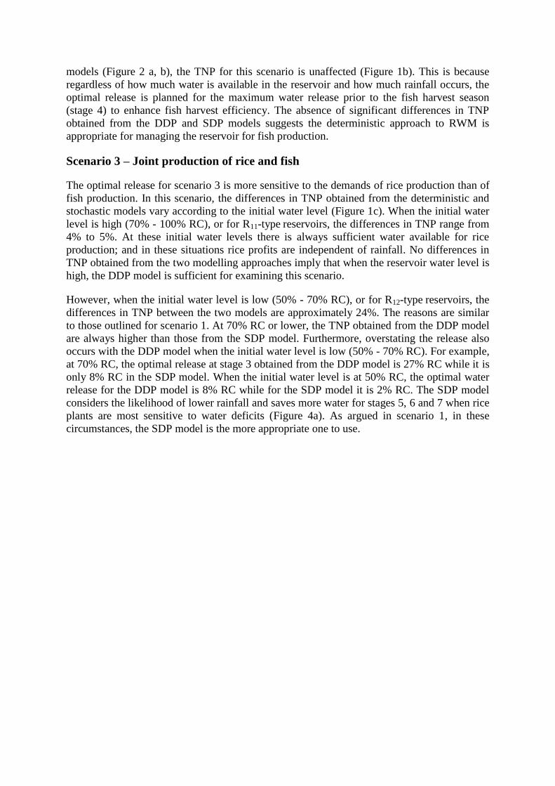
Scenario 3 – Joint production of rice and fish
The optimal release for scenario 3 is more sensitive to the demands of rice production than of
fish production. In this scenario, the differences in TNP obtained from the deterministic and
stochastic models vary according to the initial water level (Figure 1c). When the initial water
level is high (70% - 100% RC), or for R11-type reservoirs, the differences in TNP range from
4% to 5%. At these initial water levels there is always sufficient water available for rice
production; and in these situations rice profits are independent of rainfall. No differences in
TNP obtained from the two modelling approaches imply that when the reservoir water level is
high, the DDP model is sufficient for examining this scenario.
However, when the initial water level is low (50% - 70% RC), or for R12-type reservoirs, the
differences in TNP between the two models are approximately 24%. The reasons are similar
to those outlined for scenario 1. At 70% RC or lower, the TNP obtained from the DDP model
are always higher than those from the SDP model. Furthermore, overstating the release also
occurs with the DDP model when the initial water level is low (50% - 70% RC). For example,
at 70% RC, the optimal release at stage 3 obtained from the DDP model is 27% RC while it is
only 8% RC in the SDP model. When the initial water level is at 50% RC, the optimal water
release for the DDP model is 8% RC while for the SDP model it is 2% RC. The SDP model
considers the likelihood of lower rainfall and saves more water for stages 5, 6 and 7 when rice
plants are most sensitive to water deficits (Figure 4a). As argued in scenario 1, in these
circumstances, the SDP model is the more appropriate one to use.

0
5
10
15
20
25
30
1 2 3 4 5 6 7 8
(% R
C)
Stage of DP
(a)Initial water level at 50% RC
SDP model
DDP model
0
5
10
15
20
25
30
1 2 3 4 5 6 7 8
(% R
C)
Stage of DP
(b) Initial water level at 70% RC
SDP model
DDP model
0
5
10
15
20
25
30
1 2 3 4 5 6 7 8
(% R
C)
Stage of DP
(c) Initial water level at 100% RC
SDP model
DDP model
Figure 4 Comparing the optimal release for rice and fish production between the DDP
and SDP model. The results are shown at three initial water levels: 50% RC (a), 70%
RC (b), and 100% RC (c)
5. Conclusion
Profitable management of multiple-use reservoirs depends on many factors. Modelling
complex systems such as multiple-use reservoirs can be challenging. A legitimate question for
scientists and modellers is how best to model the management of a multiple-use reservoir.
This paper studies whether it is worthwhile to use a stochastic modelling approach that
requires more modelling effort, yet provides more realistic results compared to a deterministic
model that is simpler to construct. To compare the two modelling approaches we apply both
stochastic and deterministic models to the management of a multiple-use reservoir in southern
Vietnam.
The optimal strategy for release of reservoir water is determined for two types of reservoir:
(1) a reservoir full at the beginning of the irrigation season with a water holding capacity
greater than or equal to total irrigation requirements (R11-type reservoirs), and (2) a reservoir
full at the beginning of the irrigation season with a water holding capacity smaller than total
irrigation requirements (R12-type reservoirs). Three production scenarios are examined: a
focus on rice production, a focus on fish production, and lastly, focusing on joint production
of rice and fish. Key findings for the focus on either rice production or joint production of rice
and fish, are that for R11-type reservoirs there are few differences in total profits between the
stochastic versus deterministic models of the management of these reservoirs. These findings
suggest that the deterministic approach is appropriate for these reservoirs as it reduces the
complexity of calculations and is less time consuming.
However, the opposite is found for R12-type reservoirs: the deterministic approach overstates
optimal release strategies or at least may cause reservoir managers to take greater
management risks than they might otherwise do. When fish production is the management
focus, then the absence of significant differences in total profits obtained from the
deterministic and stochastic approaches for either R11- or R12-type reservoirs suggests that the
deterministic approach is appropriate for managing these reservoirs in these situations.
Hence, although no single modelling approach is universally superior, nonetheless the
desirable modelling approach is stochastic if reservoir capacity and water use demands have a
rather high impact on optimal temporal use of reservoir water.
Reference
Abdallah, B. A., Abderrazek, S., T.Jamila & Kamel, N. 2003. Optimization of Nebhana
Reservoir Water Allocation by Stochastic Dynamic Programming. Water Resources
Management, 17, 259-272.
Barros, M. T. L., Tsai, F. T. C., Yang, S.-L., Lopes, J. E. G. & Yeh, W. W. G. 2003.
Optimization of Large-Scale Hydropower System Operations. Journal of Water
Resources Planning & Management, 129, 178.
Biere, A. W. & Lee, I. M. 1972. A Model for Managing Reservoir Water Releases. American
Journal of Agricultural Economics, 54, 411-421.
Butcher, W., Haimes, Y. & Hall, W. 1969. Dynamic programming for the optimal sequencing
for water supply project. water resources research, 5, 1196-1204.
Cervellera, C., Chen, V. & Wen, A. 2006. Optimization of a large-scale water reservoir
network by stochastic dynamic programming with efficient state space discretization.
European journal of operational research, 171, 1139.
Chaves, P., Kojiri, T. & Yamashiki, Y. 2003. Optimization of storage reservoir considering
water quantity and quality. Hydrological Processes, 17, 2769-2793.
Datta, S. K. D. 1981. Principles and Practices of Rice Production, New York, John Wiley.
Dinh, C. T. 2008. The Daton reservoir operations - The 2008 annual report of the Daton
irrigation branch. Dong Nai, Vietnam: Unpublished results. Department of
Agricultural and Rural Development.
Doorenbos, J., Kassam, A. H. & Bentvelsen, C. I. M. 1979. Yield response to water

Georgiou, P. & Papamichail, D. 2008. Optimization model of an irrigation reservoir for water
allocation and crop planning under various weather conditions. Irrigation Science, 26,
487-504.
Ghahraman, B. & Sepaskhah, A.-R. 2002. Optimal allocation of water from a single purpose
reservoir to an irrigation project with pre-determined multiple cropping patterns.
Irrigation Science, 21, 127-137.
Karamouz, M. & Houck, M. H. 1987. Comparison of stochasitic and deterministic dynamic
programming for reservoir operating rule generation. JAWRA Journal of the American
Water Resources Association, 23, 1-9.
Le, S. & Duong, M. X. 1998. The preliminary studies of water requirement for rice at Eaphe-
Krongpak, Darklak province (Highland of Vietnam). In: NGUYEN, A. N., LE, S.,
CU, D. X. & HOANG, H. V. (eds.) Selected Research Results of Science and
Technologies of Southern Institute of Water Resources Research (SIWRR). Ho Chi
Minh City, Vietnam: Agricultural Publisher.
Muhammad, N. 2009. Simulation of maize crop under irrigated and rainfed conditions with
Cropwat model. ARPN Journal of Agricultural and Biological Science, 4, 68-73.
Nandalal, K. D. W. & Bogardi, J. J. 2007. Dynamic Programming Based Operation of
Reservoirs : Applicability and Limits. Leiden: Cambridge University Press.
Nguyen, Q. M. 2008a. The 2008 annual report of the Daton Cooperatives. Dong Nai,
Vietnam: Unpublished results. Department of Agricultural and Rural Development.
Nguyen, S. H., Bui, A. T., Le, L. T., Nguyen, T. T. T. & De Silva, S. S. 2001. The culture-
based fisheries in small, farmer-managed reservoirs in two Provinces of northern
Vietnam: an evaluation based on three production cycles. Aquaculture Research, 32,
975-990.
Nguyen, V. T. 2008b. The 2008 annual report of the Thanh Son Commune. Dong Nai:
Unpublished results. The People Committe of Thanh Son Commune, Tan Phu
Disctric, Dong Nai Province, Vietnam.
O'Loughlin, G. G. 1971. Optimal reservoir operation. A comparison of methods for finding
optimal reservoir release rules and an investigation of the properties and uses of
stochastic dynamic programming models. Doctor of Philosophy, University of New
South Wales.
Paudyal, G. N. & Manguerra, H. B. 1990. Tow-step dynamic programming approach for
optimal irrigation water allocation. Water Resources Management, 4, 187-204.
Reca, J., Roldán, J., Alcaide, M., López, R. & Camacho, E. 2001a. Optimisation model for
water allocation in deficit irrigation systems: I. Description of the model. Agricultural
Water Management, 48, 103-116.
Reca, J., Roldán, J., Alcaide, M., López, R. & Camacho, E. 2001b. Optimisation model for
water allocation in deficit irrigation systems: II. Application to the Bémbezar
irrigation system. Agricultural Water Management, 48, 117-132.
Smith, M. 1992. CROPWAT a computer program for irrigation planning and management.
Rome: FAO.
Swennenhuis, J. 2006. Cropwat Software Manual. 8.0 ed. Rome: Water Resources
Development and Management Service of F.A.O.
Toda, O., Yoshida, K., Hiroaki, S., Katsuhiro, H. & Tanji, H. 2005. Estimation of irrigation
water using Cropwat model at KM35 project site, in Savannakhet, Lao PDR. Role of
Water Sciences in Transboundary River Basin Management, Thailand, 2005.
Tran, L. D., Schilizzi, S., Chalak, M. & Kingwell, R. 2011. Optimizing Competitive Uses of
Water for Irrigation and Fisheries. Agricultural Water Management,, 30.

Tran, L. D., Schilizzi, S. & Kingwell, R. 2010. Dynamic Trade-offs in Water Use Between
Irrigation and Reservoir Aquaculture in Vietnam. Australian Agricultural and
Resource Economics Society 2010 Annual Conference. Adelaide Convention Centre,
SA, Australia.
Truong, T. D. & Schilizzi, S. G. M. 2010. Modeling the impact of goverment regulation on
the performance of reservoir aquaculture in Vietnam. Aquaculture Economics &
Management, 14, 120 - 144.
Top Related
Copyright © 2022 FDOKUMEN

