Comparison of deterministic and stochastic SIS and SIR ...

Comparison of deterministic and stochastic SIS and SIRmodels in discrete time

Linda J.S. Allen *,1, Amy M. Burgin

Department of Mathematics and Statistics, Texas Tech University, Lubbock, TX 79409-1042, USA

Received 2 June 1998; received in revised form 16 August 1999; accepted 25 August 1999

Abstract

The dynamics of deterministic and stochastic discrete-time epidemic models are analyzed and compared.The discrete-time stochastic models are Markov chains, approximations to the continuous-time models.Models of SIS and SIR type with constant population size and general force of infection are analyzed, thena more general SIS model with variable population size is analyzed. In the deterministic models, the valueof the basic reproductive number R0 determines persistence or extinction of the disease. If R0 < 1, thedisease is eliminated, whereas if R0 > 1, the disease persists in the population. Since all stochastic modelsconsidered in this paper have ®nite state spaces with at least one absorbing state, ultimate disease extinctionis certain regardless of the value of R0. However, in some cases, the time until disease extinction may bevery long. In these cases, if the probability distribution is conditioned on non-extinction, then when R0 > 1,there exists a quasi-stationary probability distribution whose mean agrees with deterministic endemicequilibrium. The expected duration of the epidemic is investigated numerically. Ó 2000 Elsevier ScienceInc. All rights reserved.

Keywords: Epidemic; Stochastic; Quasi-stationary; Markov process

1. Introduction

The extinction behavior exhibited by stochastic population models is frequently not charac-teristic of their deterministic analogs. Even the simple stochastic exponential growth model hasa ®nite probability of extinction (see e.g., [1]). It is the goal of this investigation to examinethe relationship between some stochastic and deterministic epidemic models. In particular,

Mathematical Biosciences 163 (2000) 1±33

www.elsevier.com/locate/mbs

* Corresponding author. Tel.: +1-806 742 2580; fax: +1-806 742 1112.

E-mail address: [email protected] (L.J.S. Allen).1 Partial support was provided by NSF grant DMS-9626417.

0025-5564/00/$ - see front matter Ó 2000 Elsevier Science Inc. All rights reserved.

PII: S0025-5564(99)00047-4

deterministic and stochastic SIS and SIR models with constant population size and general forceof infection and SIS models with variable population size are analyzed and compared. The modelsare formulated in terms of discrete-time approximations to the continuous-time models. In thedeterministic case, the model is formulated as a system of di�erence equations and in the sto-chastic case, the model is a Markov chain.

Some of the ®rst analyses of stochastic and deterministic continuous-time epidemic models aredue to Bailey [2] and Bartlett [3]. The Reed-Frost and Greenwood models are probably the mostwell-known discrete-time stochastic epidemic models [2]. In these Markov chain models, it isassumed that the discrete-time interval corresponds to the length of the incubation period and theinfectious period is assumed to have length zero. The contact process depends on the binomialdistribution and hence, these models are referred to as chain-binomial models. Zero, one, or morethan one infection may take place during the ®xed time interval. Some extensions of the Reed-Frost model are discussed in [4] and applied to diseases such as polio and in¯uenza. Ackerman etal. [4] performed extensive computer simulations of the epidemic models and studied the impact ofvarious vaccination strategies.

Continuous and discrete-time stochastic SI models were analyzed by West and Thompson [5]and their behavior compared to the analogous deterministic models. In the SI model, the sus-ceptible proportion eventually converges to zero; the entire population becomes infected. Westand Thompson [5] showed that deterministic and stochastic SI models have much di�erentconvergence behavior when the size of the susceptible population is varied and that the behaviorof the continuous and discrete-time stochastic models agree when the time steps are small.

Jacquez and O'Neill [6] and Jacquez and Simon [7] compared the behavior of a continuous-timestochastic SI epidemic model with recruitment and deaths to the analogous deterministic model.The extinction behavior of the stochastic model was demonstrated, a behavior not possible in theanalogous deterministic models. However, when the probabilities in the stochastic model wereconditioned on non-extinction, the deterministic and stochastic models were more closely related;a quasi-stationary state exists in the stochastic model whose mean is given by the deterministicendemic equilibrium.

Quasi-stationary distributions in discrete-time Markov chains were ®rst studied by Seneta andVere-Jones [8] and in continuous-time by Darroch and Seneta [9]. In an epidemic setting, quasi-stationary distributions in continuous time were ®rst studied by Kryscio and Lef�evre [10]. Re-cently, N�asell analyzed the quasi-stationary distribution for a continuous-time stochastic SISmodel with no births and deaths [11,12] and continuous-time stochastic SIR models with birthsand deaths [13]. He showed that the quasi-stationary distribution has di�erent forms dependingon the value of R0 and its relationship to N, the total population size. Three di�erent parameterregions determine the form of the quasi-stationary distribution. When R0 is less than 1, thedistribution is approximately geometric and when R0 is greater than 1, the distribution is ap-proximately normal. However, there exists a transition region when R0 is near 1, where the formof the distribution is more complex. The time to disease extinction is also determined by thesethree regions [13]. We investigate the form of the probability distribution for the number of in-fectives for our discrete-time models and note that the quasi-stationary distributions are ap-proximately normal when R0 > 1.

Due to the generality of the force of infection, the discrete-time deterministic and stochasticmodels in this investigation are new formulations. The stochastic formulations are more general

2 L.J.S. Allen, A.M. Burgin / Mathematical Biosciences 163 (2000) 1±33

than the models of West and Thompson [5] and N�asell [11±13] and are more closely tied to thedeterministic models than are the Reed-Frost models. If the time step is chosen su�ciently small,then the discrete-time deterministic and stochastic models approximate the behavior of the con-tinuous-time models. In particular, there is agreement between the behavior shown in special casesof our models and in the continuous-time stochastic models of Jacquez and O'Neill [6], Jacquezand Simon [7], and N�asell [11±13].

It is assumed that the time step is su�ciently small so that only one change in state is possibleduring the time step. A change may be either a birth or death of a susceptible or infected indi-vidual, recovery of an infected individual, or an infection of a susceptible individual. The tran-sition probabilities in our models approximate the Poisson process generally applied incontinuous-time models [14]. The probability of each event depends only on their state at thecurrent time interval; thus, making the stochastic processes Markovian. The discrete-time sto-chastic models are formulated as Markov chains and in the simple case of an SIS model withconstant population size, the entire transition matrix is given.

In the following sections, three models are discussed: SIS model with constant population size,SIR model with constant population size, and SIS model with variable population size. In eachsection, ®rst, a summary and analysis of the dynamics of the deterministic model are given.Second, the corresponding stochastic model is formulated, analyzed, and compared to the de-terministic model. The probability an epidemic occurs, the quasi-stationary distribution, themean, the quasi-stationary mean, and the mean duration of the epidemic are discussed. Third,numerical results from the deterministic and stochastic simulations are presented and discussed.

2. SIS model with constant population size

2.1. Deterministic SIS

The discrete-time deterministic SIS model has the form

S�t � Dt� � S�t��1ÿ k�t�Dt� � �bDt � cDt�I�t�; �1�I�t � Dt� � I�t��1ÿ bDt ÿ cDt� � k�t�DtS�t�;

where t � nDt; n � 0; 1; 2; . . . ; Dt is a ®xed time interval (e.g., 1 h, one day), S�0� > 0; I�0� > 0 andS�0� � I�0� � N . It is assumed that the parameters are positive, a > 0;b > 0 and c > 0. It followsthat S�t� � I�t� � N for all time; the total population size remains constant. The function k�t� isthe force of infection (number of contacts that result in infection per susceptible individual perunit time), bDt is the number of births or deaths per individual during the time interval Dt(number of births � number of deaths), and cDt is the removal number (number of individualsthat recover in the time interval Dt�. Individuals recover but do not develop immunity, they areimmediately susceptible. In addition, it is assumed that there are no deaths due to the disease, norecruitment, and no vertical transmission of the disease (all newborns are susceptible). Since birthscan be combined with recoveries, c0 � b� c, model (1) is equivalent to an SIS model without anybirths or deaths.

Model (1) generalizes epidemic models considered in [15] through the form of the force ofinfection. In [15], the force of infection was assumed to have the form

L.J.S. Allen, A.M. Burgin / Mathematical Biosciences 163 (2000) 1±33 3

k�t� � aN

I�t�; �2�

where a is the contact rate, the number of successful contacts made by one infectious individualduring a unit time interval. In this case, the incidence rate (number of new cases per unit time) k�t�S�t�is referred to as the standard incidence rate [16]. When the population size is constant, the standardincidence has the same form as the mass action incidence rate: constant I�t�S�t�. Another form for theforce of infection arises from the Poisson distribution. The ratio l � aIDt=N is the average numberof infections per susceptible individual in time Dt. The probability of k successful encounters re-sulting in a susceptible individual becoming infective is assumed to follow a Poisson distribution:

p�k� � exp�ÿl�lk

k!:

Only one successful encounter is necessary for an infection to occur; therefore, when there are nosuccessful encounters, the expression

p�0� � exp�ÿl� � exp

�ÿ aDt

NI�

represents the probability that a susceptible individual does not become infective. The number ofsusceptibles that do not become infective in time Dt is S�t� exp�ÿaDtI=N� and the number ofsusceptibles that do become infective is S�t��1ÿ exp�ÿaDtI=N��. Thus, another form for the forceof infection k�t�Dt is

1ÿ exp

�ÿ aDt

NI�t��: �3�

The force of infection in (3) was applied to discrete-time epidemic models studied by Cooke et al.[17]. The force of infection in (2) can be seen to be a linear approximation to the one given in (3).Other forms for the force of infection are discussed by Hethcote [16].

Several general assumptions are made regarding the force of infection which includes theparticular forms considered above:

(i) 0 < k�t� � k�I�t��6 aI�t�=N for I 2 �0;N �.(ii) k�I� 2 C2�0;N �;dk�I�=dI > 0; and d2k�I�=dI26 0 for I 2 �0;N �.(iii) k�I� jI�0� 0 and k0�I� jI�0� a=N .(iv) 0 < �b� c�Dt6 1 and 0 < aDt6 1.

The above assumptions imply that the force of infection increases with the number of infectives ata decreasing rate and is bounded above by a linear function of the number of infectives. Theincidence rate is bounded above by the standard incidence rate of infection. Conditions (i)±(iv) aresu�cient to guarantee non-negative solutions and asymptotic convergence to an equilibrium.However, they are not necessary conditions, for example, less restrictive assumptions on aDtguarantee convergence to an equilibrium in the case of (2) [15]. In the analogous stochasticmodel, even more restrictive conditions will be put on the parameters to guarantee that thetransition probabilities are true probabilities.

Model (1) with the force of infection given by (2) was analyzed by Allen [15] and the one withforce of infection (2) by Cooke et al. [17] and Sumpter [18]. For the more general model (1), it isstraightforward to show that conditions (i) and (iv) imply solutions are non-negative.


The basic reproductive number R0 determines asymptotic behavior of (1) and is expressed interms of the model parameters as

R0 � ab� c

:

The basic reproductive number is de®ned as the average number of secondary infections causedby one infective individual during his/her infective period in an entirely susceptible population[19].

Theorem 1. (i) If R06 1; then solutions to (1) approach the disease-free equilibriumlimt!1

I�t� � 0; limt!1

S�t� � N :

(ii) If R0 > 1, then solutions to (1) approach a unique positive endemic equilibrium

limt!1

I�t� � �I > 0; limt!1

S�t� � �S > 0:

Proof. Denote the right side of I�t � Dt� in (1) by g�I�g�I� � I�1ÿ bDt ÿ cDt� � k�I�Dt�N ÿ I�:

Note that

g0�I� � 1ÿ bDt ÿ cDt � k0�I�Dt�N ÿ I� ÿ k�I�Dt;

g00�I� � k00�I�Dt�N ÿ I� ÿ 2k0�I�Dt:

Since k00�I�6 0 and k0�I� > 0 for I 2 �0;N �, it follows that g00�I� < 0 for I 2 �0;N �.For case (i), where R06 1; g�0� � 0 and g0�0�6 1. Since g00�I� < 0; g0�I� < 1 or

g�I� < I for I 2 �0;N �. It follows that fI�t�g is a strictly decreasing sequence bounded below byzero and must approach a ®xed point of g on �0;N �. The only ®xed point of g on �0;N ] is 0; hence,limt!1 I�t� � 0.

For case (ii), where R0 > 1, it shown that there exists a unique �I > 0 such thatg��I� � �I; g�I� > I for I 2 �0; �I� and g�I� < I for I 2 ��I;N �. In this case, g�0� � 0; g�N� < N , andg0�0� > 1. Thus, there exists at least one ®xed point �I > 0; g��I� � �I. Let �I be the smallest positive®xed point, then g�I� > I for I 2 �0; �I�. It follows that g0��I�6 1. Since g00�I� < 0; g0�I� < g0��I�6 1 for I 2 ��I ;N �. Integration of the last inequality over the interval ��I ; I � shows thatg�I� < I for I > �I. Thus, g has a unique positive ®xed point �I .

The possibility of two-cycles, g�I1� � I2 and g�I2� � I1 is ruled out by showing that1� g0�I� > 0 for I 2 �0;N � [20]. If I1 < I2; I1; I2 2 �0;N�; then

0 <

Z I2

I1

�1� g0�I��dI � I2 ÿ I1 � g�I2� ÿ g�I1� � 0;

a contradiction. Now, for I 2 �0;N�; 1� g0�I� > 1ÿ k�I�Dt P 1ÿ aDtI=N P 1ÿ aDt P 0. Inaddition, McCluskey and Muldowney [20] proved that the condition 1� g0�I� 6� 0 impliesnon-existence of any m-cycle for m > 1. A result of Cull [21] can be applied. The di�erenceequation I�t � Dt� � g�I�t�� is a population model as de®ned by Cull [21]: g has a uniquepositive ®xed point �I > 0 such that g�I� > I for I 2 �0; �I� and g�I� < I for I 2 ��I;N �; g has aunique maximum, and is strictly increasing before the maximum and strictly decreasing after


the maximum. The non-existence of two-cycles for the population model I�t � Dt� � g�I�t��implies global stability of �I (Theorem 1, p. 143, [21]). �

The value of the endemic equilibrium depends on the form of the force of infection. With theforce of infection given by (2), the endemic equilibrium is

�I � N�1ÿ 1=R0�;which agrees with the analogous continuous-time model. With the force of infection (3), theendemic equilibrium is the positive implicit solution of

expÿaDt

N�I

� �� N ÿ �1� bDt � cDt��I

N ÿ �I:

2.2. Stochastic SIS

2.2.1. ModelThe discrete-time stochastic SIS model is a Markov chain with ®nite state space. The corre-

sponding continuous-time model is a Markov jump process with the jumps forming a Markovchain. In the discrete-time model, it is assumed that at most one event occurs in the time period Dt,either an infection, birth, death, or recovery which depends only on the values of the statevariables at the current time. Since the population size remains constant, a birth and death mustoccur simultaneously.

Let I and S denote random variables for the number of infectives and susceptibles, respec-tively, in a population of size N. The random variable I is integer-valued with state probabilitiespi�t� � ProbfI�t� � ig for i 2 f0; 1; . . . ;Ng and time t 2 f0;Dt; 2Dt; . . .g. Let the probability of anew infective in time Dt be PiDt � k�i�Dt�N ÿ i�; where k�i� denotes the force of infection, e.g., incase (2), k�i� � ai=N . If i 62 �0;N �, then Pi � 0: Let the probability of recovery or death in time Dtbe �b� c�iDt. Since I has a ®nite state space, in Refs. [6,7], the N in case (2) is replaced bys� iÿ 1, then s=�s� iÿ 1� is the proportion of susceptibles that can be infected by one infective.However, in the models considered here, it is assumed that s=�s� iÿ 1� � s=N � �N ÿ i�=N .Thus, the transition probabilities for the SIS model are

ProbfI�t � Dt� � i� 1 j I�t� � ig � PiDt;

ProbfI�t � Dt� � iÿ 1 j I�t� � ig � �b� c�iDt:

The probabilities pi�t� satisfy the following di�erence equations:

pi�t � Dt� � piÿ1�t�Piÿ1Dt � pi�1�t��b� c��i� 1�Dt

� pi�t��1ÿPiDt ÿ biDt ÿ ciDt��;p0�t � Dt� � p0�t�;

where i � 1; . . . ;N and pi�t� � 0 for i 62 f0; 1; . . . ;Ng:The above transition probabilities approximate the transition probabilities in a continuous-

time Markov jump process, where the transition probabilities follow a Poisson process and thetime between jumps is given by an exponential distribution with mean 1=�Pi � �b� c�i�. Theprobability of recovery or death of an infective in the continuous-time model satis®es


ProbfI�t � Dt� � iÿ 1 j I�t� � ig � �b� c�iDt � o�Dt�:If Dt! 0, the continuous-time model is obtained. For Dt su�ciently small, the discrete-timeprocess assumes that the transition probability is given by �b� c�iDt.

The di�erence equations for the discrete-time model can be expressed in matrix form with thede®nition of the N � 1� N � 1 transition matrix. Let

T �

1 �b� c�Dt 0 0 � � � 00 1ÿP1Dt ÿ �b� c�Dt 2�b� c�Dt 0 � � � 00 P1Dt 1ÿP2Dt ÿ 2�b� c�Dt 3�b� c�Dt � � � 0� � � � � � � �0 0 0 0 � � � N�b� c�Dt0 0 0 0 � � � 1ÿ N�b� c�Dt

0BBBBBB@

1CCCCCCA:and p�t�T � �p0�t�; p1�t�; . . . ; pN�t��. The probability density for I satis®es p�t � Dt� � Tp�t�.

To ensure that the elements of T are probabilities it is required that

PiDt � �b� c�iDt6 1:

The following restrictions on the parameters are su�cient to guarantee that the elements of T areless than 1:

N�a� b� c�2Dt6 4a if R0 > 1 and �b� c�NDt6 1 if R06 1: �4�These restrictions are satis®ed if Dt is su�ciently small. Note that they are stronger conditionsthan those imposed in the deterministic model.

Matrix T is a stochastic matrix with a single absorbing state, the zero state. From the theory ofMarkov chains, it follows that limt!1 p0�t� � 1 [14]. Eventually, there are no infectives in thepopulation, regardless of the threshold value R0. However, for R0 > 1; it may take a long time forthe disease to be completely eliminated. For the continuous-time stochastic SIS model withoutbirths and standard incidence, it has been shown by Kryscio and Lef�evre [10] and N�asell [11,12]that the time until absorption increases exponentially in N as N approaches in®nity when R0 > 1.

2.2.2. Quasi-stationary distributionA closer relationship between the stochastic and deterministic models can be seen through

examination of another probability distribution referred to as the quasi-stationary probabilitydistribution. De®ne

qi�t� � pi�t�1ÿ p0�t� ;

and q�t�T � �q1�t�; q2�t�; . . . ; qN �t��, where i � 1; . . . ;N . The probability q is conditioned on non-extinction. The quasi-stationary distribution has been studied in continuous-time stochastic SI,SIS, and SIR models with standard incidence of infection [6,7,11±13].

The di�erence equations for qi can be shown to satisfy

qi�t � Dt��1ÿ �b� c�q1�t�Dt� � qiÿ1�t�Piÿ1Dt � qi�1�t��b� c�Dt�i� 1��qi�t��1ÿPiDt ÿ �b� c�iDt�; �5�

where i � 1; . . . ;N and qi�t� � 0 if i 62 �1;N �. This equation agrees with the di�erence equation forthe probability function p with the exception of the factor �1ÿ �b� c�q1�t�Dt�.


A time-independent solution of (5) is a stationary or equilibrium solution,q�T � �q�1; q�2; . . . ; q�N �. It can be seen that a stationary solution satis®es the eigenvalue equation,Tx� � dx�, where x�T � �ÿ1; q�1; . . . ; q�N� and d is the eigenvalue �1ÿ �b� c�q�1Dt�. A similar rela-tionship was shown by Jacquez and Simon [7] and N�asell [11,12] for the continuous-time sto-chastic SIS model with standard incidence. After simpli®cation, the matrix equation, �T ÿ I�x�=Dt� ÿ�b� c�q�1x�; Dt 6� 0, is the same as the matrix equation satis®ed by the continuous-timemodel. N�asell describes an iterative procedure for calculating the quasi-stationary distribution.

Two approximations to the quasi-stationary distribution can be derived for q� which also agreewith the continuous-time approximations [7,10±12]. One approximation assumes there is no de-crease in the number of infectives when I�t� � 1. This ®rst approximation ~q is the positiveeigenvector associated with eigenvalue one of the reduced stochastic matrix ~T ; the ®rst row and®rst column of T are deleted and �b� c�Dt is set to 0 in the second row and second column of T:

~T �

1ÿP1Dt 2�b� c�Dt 0 � � � 0P1Dt 1ÿP2Dt ÿ 2�b� c�Dt 3�b� c�Dt � � � �� 0 0 0 � � � N�b� c�Dt0 0 0 � � � 1ÿ N�b� c�Dt

0BBBB@1CCCCA:

Matrix ~T is a transition matrix of a regular Markov chain. The eigenvector ~q is the stationarydistribution of ~T . The components of ~q can be shown to equal the following expressions:

~qn � ~q1

Pnÿ1Pnÿ2 � � �P1

n!�b� c�nÿ1; n � 2; . . . ;N ; 1 �

XN

i�1

~qn:

In the special case of standard incidence (2), the formulas for the approximate quasi-stationarydistribution simplify to those given by the continuous-time model [7,10±12]:

~qn � ~q1

�N ÿ 1�!n�N ÿ n�!

R0

N

� �nÿ1

; n � 2; . . . ;N ;

~q1 �XN

k�1

�N ÿ 1�!k�N ÿ k�!

R0

N

� �kÿ1" #ÿ1

: �6�

A second approximation to the quasi-stationary distribution assumes

ProbfI�t � Dt� � iÿ 1 j I�t� � ig � �b� c��iÿ 1�Dt:

In this second approximation, the approximate quasi-stationary distribution again satis®es~T ~q � ~q, where ~q is the stationary distribution of the regular Markov chain and

~T �

1ÿP1Dt �b� c�Dt 0 � � � 0P1Dt 1ÿP2Dt ÿ �b� c�Dt 2�b� c�Dt � � � 0� � � � � � �0 0 0 � � � �N ÿ 1��b� c�Dt0 0 0 � � � 1ÿ �N ÿ 1��b� c�Dt

0BBBB@1CCCCA:

In the case of standard incidence, the stationary distribution for this second approximation isgiven by


~qn � ~q1

�N ÿ 1�!�N ÿ n�!

R0

N

� �nÿ1

; n � 2; . . . ;N ;

~q1 �XN

k�1

�N ÿ 1�!�N ÿ k�!

R0

N

� �kÿ1" #ÿ1

: �7�

The approximate quasi-stationary distributions, ~q, given by (6) and (7) with the quasi-stationarydistribution q� calculated via the implicit relation �T ÿ I�x�=Dt � ÿ�b� c�q�1x�, are graphed inFigs. 1 and 2 for N � 50 and R0 � 1:5; 2; and 3. For R0 � 2 and 3, the distributions agree

Fig. 1. The quasi-stationary probability distribution and the approximate distribution given by (6) when N � 50 and

R0� 1.5, 2, and 3.

Fig. 2. The quasi-stationary probability distribution and the approximate distribution given by (7) when N � 50 and

R0� 1.5, 2, and 3.


reasonably well with the quasi-stationary distribution which assumes an approximate normalshape. However, for smaller values of N and R0 small, the approximations are not as good andthe distribution may not have a normal shape [11,12]. Also, note that as R0 increases, the varianceof the quasi-stationary distribution decreases.

2.2.3. Mean and quasi-stationary meanThe mean of the probability distributions of p and q satisfy

m�t� �XN

i�0

ipi�t�; m��t� �XN

i�1

iqi�t�:

Applying the di�erence equations for p and q, another set of di�erence equations for the mean,m�t�, and quasi-stationary mean, m��t�, can be derived:

m�t � Dt� ÿ m�t� �XN

i�0

PiDti

�ÿ bDt ÿ cDt

�ipi�t� � �b� c�Dt�R0n�t� ÿ 1�m�t�; �8�

m��t � Dt��1ÿ �b� c�q1�t�Dt� ÿ m��t� � �b� c�Dt�R0n��t� ÿ 1�m��t�;

where

n�t� �PN

i�0 pi�t�Pi

aPN

i�0 ipi�t�and n��t� �

PNi�1 qi�t�Pi

aPN

i�1 iqi�t�:

Note that Pi=i6 as=N ; thus, n�t� and n��t� are strictly less than 1.The asymptotic behavior of the mean, m�t�, depends on the basic reproductive number, R0.

When R06 1, it follows from (8) that the mean m�t� of the stochastic process is strictly decreasing,bounded below by zero, and therefore, must approach an equilibrium. Since the only non-neg-ative equilibrium for m�t� is 0, m�t� approaches 0. When R0 > 1; however, the mean m�t� has anadditional steady-state given by

n�t� � 1

R0

:

In the particular case of (2), where Pi � ais=N , the above expression can be written as

m�t� N 1

��ÿ 1

R0

�ÿ m�t�

�� r2�t�;

where r2�t� is the variance. The deterministic endemic equilibrium is �I � N�1ÿ 1=R0�. Hence, theabove inequality shows that when the mean of the stochastic process is approximately constant, itis less than the deterministic equilibrium.

The mean of the distribution of q� is calculated for various values of N and R0 in Table 1 and iscompared to the deterministic endemic equilibrium �I. There is closer agreement between the quasi-stationary mean of the stochastic process and the deterministic endemic equilibrium when R0 andN are large. The agreement is poorer when R0 is small. Also, note the quasi-stationary mean liesbelow the endemic equilibrium.


2.2.4. Relation to a random walkIf the population size N is su�ciently large, initially, the nonlinear stochastic process can be

approximated by a random walk on [0, 1) with an absorbing barrier at zero. If p denotes theprobability of moving to the right and q the probability of moving to the left, then the probabilityof eventual absorption beginning from position a > 0 is

qp

� �a

if q < p and 1 if q P p:

[14]. If p and q are interpreted in terms of the epidemic model, then p denotes the probability ofbecoming infected, PiDt, and q the probability of recovery or death, �b� c�iDt. When there are asmall number of infectives, s � N and Pi � ai, so that the probability of no epidemic is�q=p�a � ��b� c�=a�a, or approximately

1

R0

� �a

if R0 > 1 and 1 if R06 1;

where a is the initial number of infectives. The numerical examples show that the value of p0�t�(probability of no epidemic) approaches �1=R0�a at the outset of the epidemic.

2.2.5. Expected duration of the epidemicLet sj be the probability distribution for the time to extinction beginning with j infectives. A

system of di�erence equations for the expected duration of the epidemic, E�sj�, for the discrete-time model takes the form

E�sj� � Dt � j�b� c�DtE�sjÿ1� �PjDtE�sj�1�� 1ÿPjDt ÿ �b� c�jDt�E�sj�;

E�s1� � Dt �P1DtE�s2� � �1ÿP1Dt ÿ �b� c�Dt�E�s1�for j � 2; . . . ;N . Assuming that Dt 6� 0, the system above can be expressed in the same form as thecontinuous-time SIS model [12]:

E�sj� � 1

Pj � j�b� c� �Pj

Pj � j�b� c�E�sj�1� � j�b� c�Pj � j�b� c�E�sjÿ1�;

E�s1� � 1

P1 � �b� c� �P1

P1 � �b� c�E�s2��9�

for j � 2; . . . ;N . This system of linear equations can be solved explicitly for E�sj� [1,22]. It wasshown for the continuous-time SIS model with standard incidence that, when R0 > 1, the ex-pected duration of the epidemic increases exponentially in N [10±12]. This exponential increase inthe expected duration can be observed in the numerical examples in the next section.

Table 1

The quasi-stationary mean m� and the deterministic equilibrium �I ; �m�=�I�N R0 � 3 R0 � 2 R0 � 1.5

25 16.09/16.67 11.27/12.5 7.26/8.33

50 32.80/33.33 23.83/25 14.48/16.67


2.3. Numerical examples

Several numerical examples are simulated with various values for the population size, N, theinitial number of infectives, I, and the basic reproductive number, R0. In all the simulations, theincidence rate has the form of the standard incidence rate of infection, k�t�S�t� � aI�t�S�t�=N .

In the ®rst example, the behavior of individual sample paths of the stochastic model arecompared to the deterministic solution. Three sample paths of the stochastic model are graphedagainst the corresponding deterministic solution in Fig. 3. Initially, one infective is introduced into

Fig. 3. Three sample paths of stochastic SIS model are graphed with the deterministic solution when R0 � 2, I(0)� 1,

S(0)� 99, a � 1:6, b � 0:4 � c, and Dt � 0:01:

Fig. 4. The probability function, p(t), for the stochastic SIS model is graphed when R0 � 0:9, I(0) � 1, S(0) � 99,

a� 0.9, b� 0.5� c, and Dt� 0.01.


a population of size N � 100 with R0 � 2. The time step is Dt � 0:01 and the Time axis is thenumber of time steps, e.g., Time� 1000 means 1000 time steps and thus, an actual total time of1000Dt � 10. One of the sample paths reaches 0 very quickly and the other two sample paths varyabout the deterministic solution.

The probabilities for the number of infectives at each time step Dt can be obtained directly fromthe equation p�t � Dt� � Tp�t�. In Figs. 4±7, one infective is introduced into the population of size

Fig. 5. The mean, M, of the stochastic SIS model and the deterministic solution, Det I, are graphed for the probability

function and parameter values given in Fig. 4.

Fig. 6. The probability function, p�t�, for the stochastic SIS model is graphed when R0� 2, I�0�� 1, S(0)� 99,

a� 1.6, b� 0.4� c, and Dt � 0.01.


N� 100. When the basic reproductive number R0 � 0:9, the probability of no epidemic, p0�t�,quickly approaches 1 (see Fig. 4). The mean of the stochastic process and the deterministic so-lution both approach 0 (see Fig. 5). When the basic reproductive number R0� 2, the probabilitydistribution is bimodal (Fig. 6); one mode is at zero and the second mode is approximated by theendemic equilibrium; the endemic equilibrium is �I � 50, whereas the mean of the distribution isi � 46:8 at t � 1000Dt � 10. If the probability at zero is neglected, the remaining probabilitiesrepresent the quasi-stationary distribution, q�t�, which appears to be approximately normal. Themean of the probability density p�t�;M , and the mean of q�t�;M�, are graphed in Fig. 7 andcompared to the deterministic solution, Det I. It can be seen that the mean, M, lies below thedeterministic solution and the mean of the quasi-stationary distribution, M�, is less than but muchcloser than M to the deterministic solution.

The value of p0�t� initially approaches the value estimated from the random walk. In Fig. 6, theprobability that the disease is eliminated, p0�t�, is approximately 1=R0 � 0:5 for the time frameshown �p0�1000Dt� � p0�10� � 0:51�. In Fig. 8, the initial number of infectives is increased to ®veindividuals, then according to the estimate given by the random walk, p0�t� is approximately�1=R0�5� 0.03125, and p0�1000Dt� � p0�10� � 0:039.

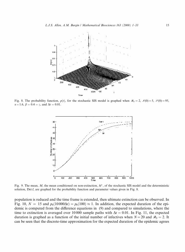
The mean and mean conditioned on non-extinction show closer agreement to the deterministicsolution as the population size and the initial number of infectives are increased. The mean andthe quasi-stationary mean for the state probabilities (with ®ve initial infectives), given in Fig. 8,are graphed in Fig. 9. Note that there is closer agreement between the means and the deterministicsolution; however, the means are always less than the deterministic solution.

If the time were continued for a su�ciently long period, then it would be possible to observelimt!1 p0�t�� 1 and limt!1m�t� � 0. For a population size of N� 100, absorption or completedisease extinction did not occur in the time frame shown in Figs. 4±9. However, if the size of the

Fig. 7. The mean, M, the mean conditioned on non-extinction, M�, of the stochastic SIS model and the deterministic

solution, Det I, are graphed for the probability function and parameter values given in Fig. 6.


population is reduced and the time frame is extended, then ultimate extinction can be observed. InFig. 10, N � 15 and p0�10000Dt� � p0�100� � 1. In addition, the expected duration of the epi-demic is computed from the di�erence equations in (9) and compared to simulations, where thetime to extinction is averaged over 10 000 sample paths with Dt � 0:01. In Fig. 11, the expectedduration is graphed as a function of the initial number of infectives when N� 20 and R0 � 2. Itcan be seen that the discrete-time approximation for the expected duration of the epidemic agrees

Fig. 8. The probability function, p�t�, for the stochastic SIS model is graphed when R0 � 2, I(0)� 5, S(0)� 95,

a� 1.6, b � 0:4 � c, and Dt � 0:01.

Fig. 9. The mean, M, the mean conditioned on non-extinction, M�, of the stochastic SIS model and the deterministic



with that obtained from the continuous-time model. Also, note that as the initial number of in-fectives increases, the expected duration approaches a constant. In Table 2, the expected durationwhen I�0� � 1 is calculated for various values of N when using formula (9) and compared to the

Fig. 10. The probability function, p�t�, for the stochastic SIS model is graphed when R0 � 2, I(0)� 1, S�0� � 14,

a � 1:6, b � 0:4 � c, and Dt � 0:01.

Fig. 11. The expected duration of an epidemic when N� 20, R0� 2, a� 1.6, and b� 0.4� c, as a function of the initial

number of infectives, I(0). The exact values for the expected duration (formula (9)) are graphed for the SIS model and

the approximate values calculated from an average of 10 000 sample paths when Dt� 0.01. The approximate duration is

calculated for the SIR model and the SIS model with variable population size when r� 0.25, K� 20, and initial total

population size N(0)� 20.


approximate duration calculated from an average of 10 000 sample paths. There is close agree-ment between the exact and approximate duration and it is evident that there is a large increase inthe expected duration with N.

In the next section, the SIR deterministic and stochastic models with constant population sizeare analyzed.

3. SIR model with constant population size

3.1. Deterministic SIR

In the SIR model, individuals develop an immunity to the disease, births and deaths are in-cluded but such that the population size remains constant. The discrete-time deterministic SIRmodel has the following form:

S�t � Dt� � S�t��1ÿ k�t�Dt� � �N ÿ S�t��bDt;

I�t � Dt� � I�t��1ÿ bDt ÿ cDt� � k�t�DtS�t�; �10�R�t � Dt� � R�t��1ÿ bDt� � cDtI�t�;

where t � nDt; n � 0; 1; 2; . . . ; S�0�; I�0� > 0;R�0�P 0; S�0� � I�0� � R�0� � N ; a > 0; b > 0;and c > 0. The conditions (i)±(iv) on the force of infection are assumed to hold. In this model,recovery leads to immunity. Newborns are susceptible.

It is clear that conditions (i) and (iv) imply solutions are non-negative andS�t� � I�t� � R�t� � N for all time. It can also be shown that the basic reproductive number de-termines the asymptotic behavior in some cases.

Theorem 2. (i) If R06 1, then solutions to (10) approach the disease-free state

limt!1

I�t� � 0; limt!1

R�t� � 0; limt!1

S�t� � N :

(ii) If R0 > 1, then there exists a unique positive endemic equilibrium and no cycles of period twoexist. For the force of infection given by (2), the positive equilibrium is locally asymptoticallystable.

Proof. Let the right-hand side of I�t � Dt� in (10) be denoted as g:

g�I ;R� � I�1ÿ bDt ÿ cDt� � k�t�Dt�N ÿ I ÿ R�:

Table 2

The expected duration of an epidemic for the SIS model as a function of N, R0 � 2; I�0� � 1; a � 1:6; b � 0:4 � c

N 5 10 15 20 25

Exact 3.68 8.26 17.73 39.01 88.68

Approximate 3.69 8.20 17.83 39.44 90.93


For case (i), R06 1, then

g�I ;R�6 I�1ÿ bDt ÿ cDt� � aDtI�N ÿ I ÿ R�=N 6 I � I�aÿ bÿ c�Dt6 I :

Thus, fI�t�g is a decreasing sequence bounded below by zero and has a limit �I. Also, it followsthat fR�t�g has a limit given by c�I=b. The limit is a ®xed point of g and must satisfy, g��I ; c�I=b� � �Ior �I is a solution to

�bDt � cDt�I � k�I�Dt�N ÿ I ÿ cI=b� � h�I�: �11�Now, h�0� � 0; h0�0� � aDt, and h00�I� < 0 which implies h�I� < aDtI for I > 0. Thus,h�I� < aDtI 6 �bDt � cDt�I for I > 0. The only ®xed point satisfying (11) is the origin; solutionsconverge to the disease-free state.

For case (ii), where R0 > 1, the endemic equilibrium also satis®es (11). In this case,h0�0� � aDt > �bDt � cDt�. In addition, h�0� � 0 and h�N� < 0. Thus, h�I� must cross the line(bDt � cDt�I at least once. Uniqueness follows from the properties of k�I� as in the proof ofTheorem 1.

Let f �S; I� and g�S; I� denote the right sides of S�t � Dt� and I�t � Dt� in (10), respectively. Theresults of McCluskey and Muldowney [20] can be applied to show there do not exist any cycles ofperiod 2. Cycles of period 2 do not exist if the matrix, I� J is strictly diagonally dominant forS � I 2 �0;N � excluding the equilibrium I � 0 and S � N [20]. Matrix I is the identity matrix andmatrix J is the 2� 2 Jacobian matrix of F � �f ; g�

I� J � 2ÿ k�I�Dt ÿ bDt ÿ k0�I�DtS

k�I�Dt 2ÿ bDt ÿ cDt � k0�I�DtS

!:

Note from conditions (i)±(iv) that k�I�Dt6 aDtI=N 6 1 and k0�I�DtS6 aDtS=N < 1. Diagonaldominance in the ®rst row of I + J follows from

2ÿ k�I�Dt ÿ bDt ÿ k0�I�DtS P 2ÿ bDt ÿ aDt�S � I�=N > 2ÿ bDt ÿ aDt P 0:

Diagonal dominance in the second row follows from

2ÿ bDt ÿ cDt � k0�I�DtS ÿ k�I�Dt P 2ÿ bDt ÿ cDt ÿ aDtS=N > 0:

The matrix I� J is strictly row diagonally dominant for all S � I 2 �0;N �; S 6� N and hence, theredo not exist any cycles of period 2.

Next, local stability of the positive equilibrium for the force of infection given by (2) is shown.The positive equilibrium is given by

�S � NR0

; �I � ba

N�R0 ÿ 1�:

The Jacobian matrix evaluated at the positive equilibrium is

Je � 1ÿ bDtR0 ÿ aDt=R0

bDt�R0 ÿ 1� 1ÿ bDt ÿ cDt � aDt=R0

� �:

For local stability, the Jury conditions must be satis®ed; the trace and determinant must satisfythe three conditions:


trace�Je� < 1� det�Je�; det�Je� < 1; ÿtrace�Je� < 1� det�Je�[23]. It is tedious but straightforward to show that the trace and determinant of Je satisfy the ®rsttwo inequalities when R0 > 1. The third inequality is satis®ed if

aDt < �4ÿ bDt�bDt � cDt�� bDt � cDtbDt�2ÿ bDt ÿ cDt� : �12�

The right side of the above inequality is greater than 3/2. Hence, it follows from condition (iv) thatthe third inequality is satis®ed. �

Weaker conditions on the force of infection may result in periodic solutions. When R0 > 1 andinequality (12) is not satis®ed, the model with the force of infection (2) exhibits periodic solutions[15].

The assumption b > 0 is important to the existence of the endemic state. If b � 0 andk�I� � aI=N or k�I� � aI, then limt!1 I�t� � 0 regardless of the magnitude of R0 [15]. The con-tinuous-time version of this model with mass action incidence �k�I�S � aIS� and b � 0 is theclassical SIR model studied by Kermack and McKendrick [24].

3.2. Stochastic SIR

The discrete-time stochastic SIR model is a Markov chain with ®nite state space. The analo-gous continuous-time model is a Markov jump process. The stochastic SIR model is a bivariateprocess dependent on the random variables I and R, the number of infected and immune in-dividuals, respectively. The stochastic SIR has a joint probability function,pir�t� � ProbfI�t� � i; R�t� � rg, where i; r � 0; 1; 2; . . . ;N and 06 i� r6N .

Let PirDt � k�i��N ÿ iÿ r�Dt denote the probability of a new infective in time Dt:

ProbfI�t � Dt� � i� 1; R�t � Dt� � r j I�t� � i; R�t� � rg � PirDt;

where k�i� satis®es conditions (i)±(iv). Let ciDt; biDt, and brDt denote the probability of recovery ofan infective and the probability of death of an infective or of an immune individual, respectively:

ProbfI�t � Dt� � iÿ 1; R�t � Dt� � r � 1 j I�t� � i; R�t� � rg � ciDt;

ProbfI�t � Dt� � iÿ 1; R�t � Dt� � r j I�t� � i; R�t� � rg � biDt;

ProbfI�t � Dt� � i; R�t � Dt� � r ÿ 1 j I�t� � i; R�t� � rg � brDt:

Each death is accompanied by a birth so that the population size remains constant. For example,a death of an immune individual is accompanied by a birth of a susceptible.

The di�erence equations satis®ed by the joint probability pir�t� are

pir�t � Dt� � piÿ1;r�t�Piÿ1;rDt � pi�1;rÿ1�t�cDt�i� 1� � pi�1;r�t�bDt�i� 1�� pi;r�1�t�bDt�r � 1� � pir�t��1ÿPirDt ÿ ciDt ÿ b�i� r�Dt�;

p0r�t � Dt� � p0r�t�;where i; r � 0; 1; . . . ;N ; i� r6N and pir�t� � 0 if i; r; 62 �0;N �. To ensure that the transitionprobabilities are positive and bounded by one, it is required that PirDt � ciDt � b�i� r�Dt6 1 fori� r � 0; 1; . . . ;N and i� r6N . The inequality is satis®ed if Dt is chosen su�ciently small. The


discrete-time stochastic model is a Markov chain, but in this case, the transition matrix cannot beexpressed in a simple form. There is a single absorbing state at the origin, I � 0 and R � 0.

3.2.1. Mean and quasi-stationary meanThe quasi-stationary distribution is de®ned by

qir�t� � pir�t�1ÿPN

r�0 p0r�t�for i � 1; . . . ;N ; r � 0; . . . ;N and i� r6N . The corresponding di�erence equations for qir�t� aregiven by

qir�t � Dt��1ÿ �b� c�q1�t�Dt� � qiÿ1;r�t�Piÿ1;rDt � qi�1;rÿ1�t�cDt�i� 1� � qi�1;r�t�bDt�i� 1�� qi;r�1�t�bDt�r � 1� � qir�t��1ÿPirDt ÿ ciDt ÿ b�i� r�Dt�

for i � 1; . . . ;N ; r � 1; . . . ;N , and i� r6N ; where qi�t� �PNÿi

r�0 pir�t�=�1ÿPNÿi

r�0 pir�t��.Note that the di�erence equations for the quasi-stationary distribution are similar to those for

the SIS model. In addition, the mean and the mean conditioned on non-extinction for I satisfydi�erence equations similar to those given for the SIS model.

Let mI�t� �PN

i;r�0 ipir�t� and m�I�t� �PN

i�1;r�0 iqir�t� denote the mean number of infectives andthe mean conditioned on non-extinction, respectively. In each case, the sum over i and r is un-derstood to mean i� r6N . Then

mI�t � Dt� ÿ mI�t� �XN

i;r�0

PirDti

�ÿ cDt ÿ bDt

�ipir�t� � �b� c�Dt�R0nI�t� ÿ 1�mI�t�; �13�

m�I�t � Dt��1ÿ �b� c�q1�t�Dt� ÿ m��t� � �b� c�Dt�R0n�I�t� ÿ 1�m�I�t�;

where

nI�t� �PN

i;r�0 pir�t�Pir

aPN

i;r�0 ipir�t�and n�I�t� �

PNi;r�0 qir�t�Pir

aPN

i;r�0 iqir�t�:

Note that Pir�t�=i6 as=N , where s � N ÿ iÿ r so that nI�t� < 1. When R06 1; it follows from(13) that fmIg is a monotone decreasing sequence which converges to 0. It can be seen from (13)that there are two steady-state solutions for the mean, the zero solution and the solution of

nI�t� � 1

R0

:

There is a similar relation to a random walk as in the stochastic SIS model when the initialnumber of infectives is small and the population size is large. Initially, the epidemic fades outquickly with probability �1=R0�a when R0 > 1. However, it persists with probability, 1ÿ �1=R0�a,where a is the initial number of infectives.

Approximations are given for the expected time to extinction from quasi-stationarity for thecontinuous-time SIR model with standard incidence by N�asell [13]. In the numerical examples, weapproximate the expected time to extinction for the corresponding discrete-time model.

For non-endemic SIR models, an important problem is to estimate the total size of the epidemicor the ®nal size distribution. Since our models are endemic �b > 0�, we do not investigate this


problem. Some references for the ®nal size distribution in non-endemic, discrete and continuous-time stochastic SIR models are given in the list of Refs. [25±28].


In the numerical examples, it is assumed that the incidence rate has the form of the standardincidence, k�t�S�t� � aI�t�S�t�=N . One initial infective is introduced into a population of size

Fig. 12. The probability function for the number of infectives I�t� in the stochastic SIR model is graphed when R0 � 2,

I�0�� 1, S(0)� 99, R(0)� 0, a � 1:6, b � 0:4 � c, and Dt � 0:01.

Fig. 13. The mean, M, the mean conditioned on non-extinction, M�, of the stochastic SIR model and the deterministic



N � 100; R0 � 2; and Dt � 0:01. The probability function for the number of infectives isgraphed in Fig. 12, pi�t� �

PNÿir�0 pir�t�. The probability function and its mean are calculated from

10 000 individual sample paths. The shape of the probability functions of the SIS and SIR modelsare similar; both are bimodal, with one mode at zero and one close to the endemic equilibrium ofthe deterministic model, �I � 25. Neglecting the probability at zero, the quasi-stationary distri-bution appears approximately normal. Initially, the disease is eliminated with probability close to1=R0 � 0:5. The deterministic solution of the SIR model is graphed with the mean and the meanconditioned on non-extinction in Fig. 13. Both means lie below the deterministic solution, al-though the mean conditioned on non-extinction is closer to the deterministic solution.

The expected duration of the epidemic is calculated numerically from an average of 10 000sample paths. Fig. 14 is a graph of the expected duration as a function of N for R0 equal to 2, 3and 4 with one initial infective. It can be seen that the expected duration appears to increaseexponentially with N. The expected duration for a population of size N � 20 and R0 � 2 as afunction of the initial number of infectives is graphed in Fig. 11 and compared to that of the SISmodel. Since individuals recover in an SIR model and are not reinfected, the duration is muchshorter for an SIR model than for an SIS model with the same parameter values.

4. SIS model with variable population size

In the SIS model with variable population size, it is assumed that the total population size is notconstant but varies with time, N � N�t�. Since the total population size satis®es N�t� � S�t� � I�t�,the model has two independent dynamic variables. The deterministic and stochastic SIS modelsare described in the next sections.

Fig. 14. The approximate expected duration of an SIR epidemic when I(0)� 1, b � 0:4 � c and R0 � 2, 3, and 4 as a

function of the total population size N. The duration is calculated from an average of 10 000 sample paths when

Dt � 0:01.


4.1. Deterministic SIS

The following di�erence equation models the growth of the population:

N�t � Dt� � N�t��f �N�t�� 1� � N�t�F �N�t�� g�N�t��; 0 < N�0� < K; �14�where F �N� � f �N� � 1 and NF �N� � g�N�. The functions f and g in (14) satisfy the followingthree conditions:

(v) f �N�; g�N� 2 C1�0;K�; f �N� > 0 for N 2 �0;K�;(vi) g�0� � 0 and g�K� � K, and(vii) g0�0� > 1; g0�N� > 0 for N 2 �0;K�.

Thus, F �N�N � g�N� implies F �K� � 1 and f �K� � 0. In addition, g�N� > N for N 2 �0;K�. Eq.(14) has two ®xed points, �N � 0 and �N � K. Since the population is initially below K, conditions(v)±(vii) guarantee that solutions N�t� increase monotonically to K, the carrying capacity. Suchtypes of conditions were imposed in di�erential equation epidemic models with variable popu-lation size (e.g., [29±32]). Two examples satisfying the above restrictions are the di�erenceequations for logistic growth:

N�t � Dt� � N�t� �rDt � 1�KK � rDtN�t� ; r > 0 �15�

or

N�t � Dt� � N�t� 1

�� rDt ÿ N�t�rDt�

K

�; 0 < rDt < 1:

The deterministic SIS model with variable population size has the form:

S�t � Dt� � S�t��F �N�t�� ÿ k�t�Dt� � �bDt � cDt�I�t�;I�t � Dt� � I�t��F �N�t�� ÿ bDt ÿ cDt� � k�t�DtS�t�; �16�

N�t � Dt� � N�t�F �N�t��;where F �N�t�� 1� f �N�t��; bDt is the per capita number of births, bDt ÿ f �N�t�� is the percapita number of deaths in time Dt; S�0� > 0; I�0� > 0, and N�0� � S�0� � I�0� < K.

Conditions (i)±(iv) are assumed to hold for the force of infection, but conditions (i)±(iii) aremodi®ed to account for the changing population size. Let i�t� � I�t�=N�t�. It is assumed that theforce of infection is a function of the proportion of infectives, i�t�, rather than the number ofinfectives, I�t�. The three modi®ed conditions are stated in terms of the proportion, i�t�:�i�0 k�t� � k�i�t��6 ai�t�; where i�t� � I�t�=N�t�.�ii�0 k�i� 2 C2�0; 1�; dk�i�=di > 0; and d2k�i�di26 0 for i 2 �0; 1�.�iii�0 k�i� ji�0� 0 and k0�i� ji�0� a.

With these restrictions, the incidence rate may take the form of the standard incidence given in (2)or the form in (3). However, the mass action incidence rate is not possible,k�t�S�t� 6� constant I�t�S�t�. Also, note that the restrictions �i�0±�iii�0 and (iv)±(vii) imply that so-lutions to (16) are non-negative.

The following theorem gives su�cient conditions that show the basic reproductive numberdetermines asymptotic behavior.


Theorem 3. (i) If R0 < 1, then solutions to (16) satisfy

limt!1

I�t� � 0; limt!1

S�t� � K:

(ii) If R0 > 1 and if the function h�x� � �1ÿ bDt ÿ cDt�x� �1ÿ x�k�x�Dt defined on [0, 1] has aunique positive fixed point x�; 0 < x� < 1; and 0 < x� < xM , where h�xM��max06 x6 1 h�x�, thensolutions to (16) satisfy

limt!1

I�t� � �I > 0; limt!1

S�t� � �S > 0;

where �I � x�K and �S � �I � K.

The conditions imposed on h in part (ii) of Theorem 3 seem restrictive but it can be easilyshown that they are satis®ed by the force of infection k�i�t�� ai�t�. In this case,x� � �aÿ bÿ c�=a <minf1; �1� �aÿ bÿ c�Dt�=�2aDt� � xMg.

Proof. The di�erence equation for I�t� can be expressed in terms of proportions, i�t� � I�t�=N�t�and s�t� � S�t�=N�t� � 1ÿ i�t�

i�t � Dt� � N�t�N�t � Dt� �i�t��f �N�t�� 1ÿ bDt ÿ cDt� � k�i�t��Dt�1ÿ i�t��:

For case (i), let � > 0 be chosen such that 0 < aDt=�cDt � bDt ÿ �� < 1. Since N�t� approaches Kand f �N�t�� approaches f �K� � 0 as t!1, choose t su�ciently large such that t P T implies0 < f �N�t�� < �. Then for t P T ,

i�t � Dt�6 N�t�N�t � Dt� �i�t��1� �ÿ bDt ÿ cDt� � aDt�1ÿ i�t��

6 i�t��1� aDt ÿ bDt ÿ cDt � �� ÿ aDt�i�t��26 i�t�:The sequence fi�t�g is monotone decreasing, bounded below by zero and must converge to a ®xedpoint of

h�i� � i�1ÿ bDt ÿ cDt� � k�i�Dt�1ÿ i�: �17�Note that

h0�i� � 1ÿ bDt ÿ cDt � k0�i�Dt�1ÿ i� ÿ k�i�Dt;

h00�i� � k00�i�Dt�1ÿ i� ÿ 2k0�i�Dt;

h00�i� < 0 for i 2 �0; 1�, and h0�0� � 1� aDt ÿ bDt ÿ cDt < 1. It follows that h�i� < i for i 2 �0; 1�.The only ®xed point of h for R0 < 1 is 0. Hence, i�t� converges to 0.

Let 0 < �1 < 1 and �2 > 0. Consider the function

h�x� � �1ÿ �1�x�1ÿ bDt ÿ cDt� � �1ÿ �1��1ÿ xÿ �1�k�x�Dt� h�x� ÿ �1�h�x� � �1ÿ �1�k�x�Dt�6 h�x�:

Also, the function

h�x� � x�1ÿ bDt ÿ cDt � �1� � �1ÿ x�k�x�Dt � h�x� � �1x P h�x�;where h is de®ned in (17). Note that h�0� � 0 � h�0� � 0.


The function h has the property that h0�i� � 0 for at most a single value of i 2 �0; 1�.Thus, h is strictly increasing for x < xM and strictly decreasing for x > xM . When R0 > 1 sothat h0�0� > 1, the solution x�t� to x�t � Dt� � h�x�t�� converges monotonically to x� fort > 0.

For case (ii), choose �1 su�ciently small such that h and h have unique positive ®xed points xand x, respectively, x < x < 1 such that jx� ÿ xj < �2 and jx� ÿ xj < �2. In addition, choose �1

su�ciently small such that h�x� and h�x� are strictly increasing for 0 < x < x, where x is some pointx < x < xM , h�x� > x for 0 < x < x, h�x� < x for x > x, h�x� > x for 0 < x < x, h�x� < x for x > x,and h�x� < xM for x 2 �0; 1� (possible since h and k are C1�0; 1� and h�x� < xM ). Thus,limt!1 h�x�t�� x and limt!1 h�x�t�� x.

Choose t su�ciently large such that t P T implies 0 < f �N�t�� < �1, 1ÿ i�t� ÿ s�t� < �1, and1ÿ �1 < N�t�=N�t � Dt�. Then for t P T

h�i�t��6 i�t � Dt�6 h�i�t��:If x�T � � i�T � � y�T �, then

x�T � Dt� � h�x�T �� h�i�T ��6 i�T � Dt�6 h�i�T �� h�y�T �� y�T � Dt� < xM :

Since h0�x� > 0 for x < xM , then

x�T � 2Dt� � h�x�T � Dt��6 h�x�T � Dt��6 h�i�T � Dt�� i�T � 2Dt�6 h�y�T � Dt��6 h�y�T � Dt�� y�T � 2Dt� < xM :

Continuing in this manner,

x�T � nDt� � h�x�T � �nÿ 1�Dt��6 i�T � nDt�6 h�y�T � �nÿ 1�Dt�� y�T � nDt�

for n � 2; . . .. Since x�t� converge to x and y�t� converges to x, it follows that

x� ÿ �26 x6 lim inft!1

i�t�6 lim supt!1

i�t�6 x6 x� � �2:

Since �2 can be made arbitrarily small, it follows that limt!1 i�t� � x�. �

4.2. Stochastic SIS

4.2.1. ModelThe discrete-time stochastic SIS model with variable population size is formulated as a Markov

chain. The stochastic process is bivariate. Let I and N denote the random variables for thenumber of infectives and total number of individuals. Let the joint probability function be de-noted as

pin�t� � ProbfI�t� � i; N�t� � ng:


There are ®ve di�erent transition probabilities in the discrete-time model:

ProbfI�t � Dt� � i� 1; N�t � Dt� � n j I�t� � i; N�t� � ng � PinDt;

ProbfI�t � Dt� � iÿ 1; N�t � Dt� � n j I�t� � i; N�t� � ng � ciDt;

ProbfI�t � Dt� � i; N�t � Dt� � n� 1 j I�t� � i; N�t� � ng � bnDt;

ProbfI�t � Dt� � iÿ 1; N�t � Dt� � nÿ 1 j I�t� � i; N�t� � ng � �bDt ÿ f �n��i;ProbfI�t � Dt� � i; N�t � Dt� � nÿ 1 j I�t� � i; N�t� � ng � �bDt ÿ f �n��nÿ i�

for i6 n, i; n � 0; 1; . . . ;M , where Pin � k�i=n��nÿ i�, i=n is the proportion of infectives, and f �n�is the function de®ned in the deterministic model (14). Assumptions (i)0±(iii)0, and (iv)±(vii) areassumed to hold. The population size may increase above carrying capacity, K; thus, the de®nitionof f needs to be extended to n > K and in addition, the population size should be bounded. Twomore conditions are made for the stochastic model:

(viii) There exists M > K such that f 2 C1�0;M �; f �n� < 0 for K < n6M .(ix) The probability of a birth, ProbfN�t � Dt� � n� 1 jN�t� � ng � 0 for n P M .

Conditions (viii) and (ix) assume that when K < n6M , the probability of a death is greater thanthe probability of a birth and that M is a bound on the population size.

The di�erence equations for the joint probability function pin�t� are given by

pin�t � Dt� � piÿ1;n�t�Piÿ1;nDt � pi�1;n�t�c�i� 1�Dt � pi;nÿ1�t�b�nÿ 1�Dt�pi�1;n�1�t��bDt ÿ f �n� 1��i� 1� � pi;n�1�t��bDt ÿ f �n� 1��n� 1ÿ i��pin�t��1ÿPinDt ÿ ciDt ÿ 2bnDt � f �n�n�;

p00�t � Dt� � p00�t�for i6 n6M ; i; n � 0; 1; . . . ;M and pin�t� � 0 for i; n 62 �0;M �. The probabilities must satisfyPinDt � ciDt � 2bnDt ÿ f �n�n6 1 for 06 i6 n; i; n � 0; 1; . . . ;M which is possible if Dt is su�-ciently small.

The only absorbing state is the state I � 0 and N � 0; eventually, the disease is eliminated andthe population becomes extinct. However, it may take a long time for total population extinctionto occur, especially for large initial values and large carrying capacity K.

4.2.2. Mean and quasi-stationary meanThe quasi-stationary probability distribution is de®ned by qin�t� � pin�t�=

�1ÿPMn�0 p0n�t�� for i; n � 1; 2; . . . ;M ; i6 n. The probabilities qin�t� satisfy the di�erence equa-

tions

qin�t � Dt� 1

"ÿPM

n�1 p1n�t��bDt � cDt ÿ f �n��1ÿPM

n�0 p0n�t�

#� qiÿ1;n�t�Piÿ1;nDt � qi�1;n�t�c�i� 1�Dt � qi;nÿ1�t�b�nÿ 1�Dt�qi�1;n�1�t��bDt ÿ f �n� 1��i� 1� � qi;n�1�t��bDt ÿ f �n� 1��n� 1ÿ i��qin�t��1ÿPinDt ÿ ciDt ÿ 2bnDt � f �n�n�

for i; n 2 f0; 1; . . . ;Mg; i6 n. The di�erence equations for the quasi-stationary distribution di�erfrom the SIS model with constant population size due to the presence of the term f �n�.


Di�erence equations for the mean and the mean conditioned on non-extinction also di�er fromthose of the stochastic SIS model with constant population size. The mean and mean conditionedon non-extinction satisfy the di�erence equations:

m�t � Dt� ÿ m�t� �XM

i;n�0

PinDti

�ÿ bDt ÿ cDt � f �n�

�ipin�t� � �b� c�Dt�R0nI�t� ÿ 1�m�t�;

m��t � Dt� 1

"ÿPM

n�1 p1n�t��bDt � cDt ÿ f �n��1ÿPM

n�0 p0n�t�

#ÿ m��t� � �b� c�Dt�R0n

�I�t� ÿ 1�m��t�;

where

nI�t� �PM

i;n�0�PinDt � f �n�i�pin�t�aDt

PMi;n�0 ipin�t�

;

n�I�t� �PM

i;n�0�PinDt � f �n�i�qin�t�aDt

PMi;n�0 iqin�t�

;

and the sum is over indices i6 n6M . For this stochastic process, the threshold R0 may notdetermine the asymptotic behavior of the mean. Another threshold relates the random walk to theprobability of disease elimination.

Initially, if there are a small number of infectives and a large population size, the probability ofdisease elimination can be approximated using the theory of random walks. Suppose s � n0,where n0 is the initial population size, ProbfN�0� � n0g � 1, then probability of infectionis Pin0

Dt � k�i=n0��n0 ÿ i�Dt � aiDt and the probability of recovery or death is ciDt��bDt ÿ f �n0��i. From the theory of random walks [14], the probability of ultimate absorption ordisease elimination is approximately

cDt � bDt ÿ f �n0�aDt

� �a

;

where a is the initial number of infectives. If n0 < K, then f �n0� > 0 and if n06K, then f �n0�P 0.If the initial population size is less than the carrying capacity, n0 < K, then the probability that thedisease is eliminated is less than in a population of constant size. In other words, a growingpopulation is more likely to experience an epidemic than a population that has stabilized at aconstant population size. However, in a population that is declining, n0 > K, the probability thatthe disease is eliminated is greater than in a population that has stabilized.

A possible reason for the di�erence between the constant and variable population size modelsis due to the death rate of infectives which changes with the population size. When the pop-ulation size is below carrying capacity, births exceed deaths, and the length of infectivity in-creases from 1=�cDt � bDt� to 1=�cDt � bDt ÿ f �n�� f �n� > 0�: This longer period of infectivitydue to a decreased death rate may result in more susceptibles becoming infective at the outset ofan epidemic.



Numerical examples are simulated for a growing population; the initial population size is belowcarrying capacity. In these examples, population growth follows the logistic equation (15):

f �n� � rDt�K ÿ n�K � rDtn

and the force of infection is k�i=n� � ai=n. The time step is Dt � 0:002, so that the actual timeframe extends from 0 to time �Dt� � 10000Dt � 20: The probabilities and means are calculatedfrom 10 000 individual sample paths.

In the ®rst example, one infective is introduced into a population of size n � 20 with carryingcapacity K � 100, maximum population size of M � 200, a basic reproductive number R0 � 2,and parameter values a � 1:5, b � 0:5, c � 0:25 and r � 0:25. In Figs. 15 and 16 the marginalprobabilities for I�t� and N�t� are given. The probability function for infectives is bimodal, onemode is at zero and the second mode is the quasi-stationary mean which is near the endemicequilibrium of the deterministic model. The probability function of the total population size isunimodal for the time frame shown; there is one mode approaching carrying capacity, K � 100.The probability that the disease is eliminated approaches a value close to that predicted by therandom walk in the time frame shown. The estimate for disease elimination in the random walk isgiven by

bDt � cDt ÿ f �n0�aDt

� 0:367;

which is close to the value of p0�20� � ProbfI�20� � 0g in Fig. 15. Initially, the probability ofdisease elimination is less than in the model with a constant population size due to the decreased

Fig. 15. The probability function for the number of infectives I�t� for the SIS model with variable population size is

graphed when R0 � 2, I(0)� 1, S(0)� 19, K� 100, a � 1:5, b � 0:5, c � 0:25, r � 0:25, M � 200, and Dt � 0:002.


death rate of infectives. The mean and the mean conditioned on non-extinction for the probabilitydistributions of I�t� and N�t� are graphed in Fig. 17.

In the next example, the carrying capacity is reduced to K � 15, the initial conditions areI�0� � 1 and S�0� � 4, and the parameter values are r � 0:25, a � 1:6, b � 0:4, c � 0:4, andDt � 0:002. The graph in Fig. 18 can be compared to Fig. 10. For a small carrying capacity,

Fig. 16. The probability function for the total population size N�t� is graphed for the SIS model with variable pop-

ulation size of the parameter values given in Fig. 15.

Fig. 17. The mean number of infectives, Mean I, the mean total population size, Mean N, the mean conditioned on

non-extinction for infectives Mean �I , and the deterministic solutions, Det I and Det N, for the SIS model with variable

population size are graphed for the probabilities and parameter values given in Figs. 15 and 16.


K � 15, and for a longer time frame, time �Dt� � 50000�0:002� � 100, ultimate disease elimina-tion can be observed. In Fig. 18, the disease is eliminated at a faster rate than in the SIS modelwith constant population size. This faster rate is probably due to the small population size and thesmall number of susceptibles, S�0� � 4 in Fig. 18 as opposed to S�0� � 14 in Fig. 10. In thisexample, it can also be observed that the total population size will eventually approach 0. InFig. 19, the probability function for the total population size, N�t�, shows that as time increases,the probability that the population size is 0 also increases.

Fig. 19. The probability function for the total population size N�t� for the SIS model with variable population size is

graphed for the parameter values given in Fig. 18.

Fig. 18. The probability function for the number of infectives I�t� for the SIS model with variable population size is

graphed when R0 � 2, I(0)� 1, S�0� � 4, K� 15, a� 1.6, b� 0.4� c, r� 0.25, M� 45, and Dt� 0.002.


In the last example, the expected duration of the epidemic is estimated by calculating the av-erage duration from 10 000 sample paths when K � 20, R0 � 2, and N�0� � K. In Fig. 11, theexpected duration is compared to the SIS model with constant population size when the initialnumber of infectives is varied from 1 to 20. It can be seen that the expected duration is shorter forthe variable population size model. This shortened duration may be due in part to the fact that thetotal size in the variable population size model is on the average less than K;N < K, but in theconstant population size model N � K.

5. Summary

Discrete-time deterministic and stochastic models are formulated and analyzed for three dif-ferent models: SIS model with constant population size, SIS model with variable population size,and SIR model with constant population size. These discrete-time models may be directly ap-plicable to particular diseases (e.g., [4,33]) or may be considered as approximations to the morewell-known continuous-time models. The discrete-time epidemic models are new formulationswhich generalize the form of the force of infection.

For the deterministic cases, Theorems 1±3 state asymptotic results for the three models. Thebasic reproductive number R0 determines whether the disease is eliminated or persists. In the caseof persistence, the endemic equilibrium depends on the form of the force of infection.

The discrete-time stochastic epidemic models are formulated as Markov chains which may beconsidered approximations to the continuous-time Markov jump processes. Restrictions are puton the size of the time step to ensure that the models give true probability distributions.

In the stochastic models, the probability of disease elimination ultimately approaches 1, in-dependent of the value of the basic reproductive number. However, as the population size in-creases, the time until absorption also increases. In these cases, the quasi-stationary distribution issigni®cant. Di�erence equations for the mean and quasi-stationary mean are obtained. The nu-merical examples illustrate the form of the the probability distribution and the quasi-stationarydistribution for the number of infectives. The probability distribution is bimodal when R0 > 1and the initial number of infectives is small. One mode is at I � 0. The second mode is the meanof the quasi-stationary distribution which is close to the deterministic endemic equilibrium. Theshape of the quasi-stationary distribution appears to be approximately normal for R0 > 1 and Nsu�ciently large, which agrees with continuous-time stochastic SIS and SIR models with standardincidence studied by N�asell [11±13]. In other examples, the behavior of the SIS Markov chainmodel agrees with that of the continuous-time SIS Markov jump process: the relation to a randomwalk and the expected duration of the epidemic. West and Thompson [5] also showed agreementbetween the behavior of the discrete and continuous-time stochastic SI models.

There is some distinction between the behavior of the SIS stochastic model with variablepopulation size and the model with constant population size. The expected duration is less and therate of convergence to extinction is faster in the variable population size model as illustrated inFigs. 10, 11 and 19. In the SIS model with variable population size, when the population size isless than the carrying capacity, births exceed deaths and the length of infectivity increases from1=�cDt � bDt� to 1=�cDt � bDt ÿ f �n�� f �n� > 0 when n > K�. However, the reverse occurs when


the population size is greater than the carrying capacity, deaths exceed births and the length ofinfectivity decreases since f �n� < 0 when n > K.

There remain some open questions in regard to the behavior of the epidemic models. The globalbehavior of the deterministic SIR model in the case R0 > 1 needs to be veri®ed. In addition,analytical approximations to the quasi-stationary distribution and the expected duration of theepidemic are needed for the stochastic SIR model and the SIS model with variable population size(see e.g., [11±13]).

Acknowledgements

We acknowledge the support of the NSF grant DMS-9626417. We thank anonymous refereesfor their helpful comments and suggestions.

References

[1] E. Renshaw, Modelling Biological Populations in Space and Time, Cambridge University, Cambridge, 1993.

[2] N.T.J. Bailey, The Mathematical Theory of Infectious Diseases and its Applications, Hafner, New York, 1957.

[3] M.S. Bartlett, Deterministic and stochastic models for recurrent epidemics, Proc. Third Berkeley Symp. Math. Stat.

Prob. 4 (1956) 81.

[4] E. Ackerman, L.R. Elveback, J.P. Fox, Simulation of Infectious Disease Epidemics, Charles C. Thomas Publisher,

Spring®eld, IL, 1984.

[5] R.W. West, J.R. Thompson, Models for the simple epidemic, Math. Biosci. 141 (1997) 29.

[6] J.A. Jacquez, P. O'Neill, Reproduction numbers and thresholds in stochastic epidemic models I. Homogeneous

populations, Math. Biosci. 107 (1991) 161.

[7] J.A. Jacquez, C.P. Simon, The stochastic SI model with recruitment and deaths I. Comparison with the closed SIS

model, Math. Biosci. 117 (1993) 77.

[8] E. Seneta, D. Vere-Jones, On quasi-stationary distributions in discrete-time Markov chains with a denumerable

in®nity of states, J. Appl. Prob. 3 (1966) 403.

[9] J.N. Darroch, E. Seneta, On quasi-stationary distributions in absorbing continuous-time ®nite Markov chains, J.

Appl. Prob. 4 (1967) 192.

[10] R.J. Kryscio, C. Lef�evre, On the extinction of the S-I-S stochastic logistic model, J. Appl. Prob. 26 (1989) 685.

[11] I. N�asell, On the quasi-stationary distribution of the stochastic logistic epidemic, Math. Biosci. 156 (1999) 21.

[12] I. N�asell, The quasi-stationary distribution of the closed endemic SIS model, Adv. Appl. Prob. 28 (1996) 895.

[13] I. N�asell, On the time to extinction in recurrent epidemics, J. Roy. Statist. Soc. B 61 (1999) 309.

[14] N.T.J. Bailey, The Elements of Stochastic Processes with Applications to the Natural Sciences, Wiley, New York,

1964.

[15] L.J.S. Allen, Some discrete-time SI, SIR and SIS epidemic models, Math. Biosci. 124 (1994) 83.

[16] H.W. Hethcote, A thousand and one epidemic models, in: S.A. Levin (Ed.), Frontiers in Mathematical Biology,

Lecture Notes in Biomathematics, vol. 100, Springer, Berlin, 1994, p. 504.

[17] K.L. Cooke, D.F. Calef, E.V. Level, stability or chaos in discrete epidemic models, in: V. Lakshmikantham (Ed.),

Nonlinear Systems and Applications, Academic Press, New York, 1977, p. 73.

[18] K.J. Sumpter, The dynamics of some epidemic models, Master's thesis, Texas Tech University, Lubbock, TX,

USA, 1995.

[19] H.W. Hethcote, Qualitative analyses of communicable disease models, Math. Biosci. 28 (1976) 335.

[20] C.C. McCluskey, J.S. Muldowney, Bendixson±Dulac criteria for di�erence equations, J. Dyn. Di�. Eq. 10 (1998)

567.


[21] P. Cull, Local and global stability for population models, Biol. Cybern. 54 (1986) 141.

[22] R.H. Norden, On the distribution of the time to extinction in the stochastic logistic population model, Adv. Appl.

Prob. 14 (1982) 687.

[23] L. Edelstein-Keshet, Mathematical Models in Biology, Birkh�auser Mathematics Series, Random House, New

York, 1988.

[24] W.O. Kermack, A.G. McKendrick, Contributions to the mathematical theory of epidemics, Proc. Roy. Soc. A 115

(1927) 700.

[25] F. Ball, A uni®ed approach to the distribution of total size and total area under the trajectory of infectives in

epidemic models, Adv. Appl. Prob. 18 (1986) 289.

[26] C. Lef�evre, P. Picard, A non-standard family of polynomials and the ®nal size distribution of Reed-Frost epidemic

processes, Adv. Appl. Prob. 22 (1990) 25.

[27] C. Lef�evre, P. Picard, The ®nal size distribution of epidemics spread by infectives behaving independently, in: J.-P.

Gabriel, C. Lef�evre, P. Picard (Eds.), Stochastic Processes in Epidemic Theory, Lecture Notes in Biomathematics,

vol. 86, Springer, New York, 1990, p. 155.

[28] D. Ludwig, Final size distributions for epidemics, Math. Biosci. 23 (1975) 33.

[29] L.J.S. Allen, P.J. Cormier, Environmentally driven epizootics, Math. Biosci. 131 (1996) 51.

[30] F. Brauer, Models for the spread of universally fatal diseases, J. Math. Biol. 28 (1990) 451.

[31] A. Pugliese, Population models for diseases with no recovery, J. Math. Biol. 28 (1990) 65.

[32] J. Zhou, H.W. Hethcote, Population size dependent incidence in models for diseases without immunity, J. Math.

Biol. 32 (1994) 809.

[33] L.J.S. Allen, M.A. Jones, C.F. Martin, A discrete-time model with vaccination for a measles epidemic, Math.

Biosci. 105 (1991) 111.


Comparison of deterministic and stochastic SIS and SIR ...

Documents

Transcript of Comparison of deterministic and stochastic SIS and SIR ...