


Bahasa
Halaman
Hukum


Institute of Farm Management
University of Hohenheim
Department of Farm Management
Prof. Dr. Drs. h.c. Jürgen Zeddies
MODELLING OF PARTICULATE MATTER AND AMMONIA
EMISSIONS FROM GERMAN AGRICULTURE
Dissertation
Submitted in fulfilment of the requirements for the degree “Doktor der Agrarwissenschaften”
(Dr.sc.agr. / Ph.D. in Agricultural Sciences)
to the
Faculty of Agricultural Sciences
presented by
Olga Beletskaya
Stavropol, Russian Federation
2016

This thesis was accepted as a doctoral dissertation in fulfilment of the requirements for the
degree “Doktor der Agrarwissenschaften” (Dr. sc. agr. / Ph.D. Agricultural Sciences) by the
faculty Agricultural Sciences of the university of Hohenheim on 10.11.2014.
Date of oral examination: 14.01.2015
Examination Committee
Supervisor and Reviewer Prof. Dr.Dr.h.c. Jürgen Zeddies
Co-Reviewer PD Dr. Eva Gallmann
Additional Examiner Prof. Dr. Reiner Doluschitz
Head of the Committee Prof. Dr. Stefan Böttinger

Dedicated to the dearest and beloved friend Juan Guillermo Cobo


v
ACKNOWLEDGEMENT
With all my heart and mind I am grateful to all those, who directly or indirectly has contri-
buted to this study. At first place I would like to thank my colleague and direct advisor Dr.
Elisabeth Angenendt and my doctoral thesis supervisor Prof. Dr. Jürgen Zeddies for support,
and sharp but reasonable critic and useful advice. Many thanks go to my colleague and co-
worker in the project framework, Dipl. Ing. Susanne Wagner (IER, University of Stuttgart)
for the best teamwork, informational support and encouragement. From the representatives of
the same institute, I would like to express my gratefulness to Jochen Teloke for helpful infor-
mative support and for the organization of efficient project meetings; and to Balendra Thiru-
chittampalam for a good collaboration. I also express my thanks to PD Dr. Eva Gallmann for
her agreement to be my second referee. For the readiness to play role of my third referee I
thank Prof. Dr. Reiner Doluschitz.
I want to thank my precursor, Dr. Steffen Triebe, for the introduction into the work and readi-
ness to answer any related questions. In the Institute for farm management, where I have
worked and conducted this study, there are and there were many people, which helped not on-
ly with practical advice, but charged me spiritually in everyday life: Prof. Dr. Frank Lizka,
Nicole Schönleber, Silvia Andres, Daniel Blank, Vasilina Nekrasova, Tatyana Vorontsova,
Angelika Konold, Tetyana Tonkoshkur, and Yulia Droganova. I am also grateful to: Caroline
Seeman and Johannes Empel for technical expert advice, Mr. Gamer for informational and
technical support, and Yannick Kühl for technical help as a system administrator.
For the close collaboration and subjective support I am grateful to Prof. Torsten Hinz, Ulrich
Dämmgen and Jochen Hahne from TI institution (former vTI and FAL), Prof. Roger Funk
from the University of Leipzig, Mr. Ewald Grimm (Dipl.-Ing. techn. Umweltschutz) from
KTBL, and Mr. Winfried Gramatte from DLG.
For the great support in organizational issues and for overall readiness to help, many warm
thanks to our institutional secretary Mrs. Ulla Held and to Mrs. Agnes Bardoll.
Further I would like to mention great support of my family and in this regard to express my
thanks to my parents and to my best friend Juan Cobo, who witnessed the most part of the
work process with patience and support. Mentioned and not mentioned here acquaintances
and friends, all directly or indirectly contributed to this project and study. Thank you for all
your reliance, assistance and encouragement.


vii
TABLE OF CONTENT
ACKNOWLEDGEMENT ....................................................................................................... v
TABLE OF CONTENT ......................................................................................................... vii
LIST OF FIGURES ................................................................................................................ xi
LIST OF TABLES ................................................................................................................ xiii
LIST OF APPENDIXES ...................................................................................................... xvii
LIST OF ABBREVIATIONS ............................................................................................... xix
1 GENERAL INTRODUCTION ............................................................................................ 1
1.1 Background .......................................................................................................................... 1
1.2 Problem Statement ............................................................................................................... 2
1.3 Goal and Objectives of the Study ......................................................................................... 3
1.4 Outline of the Study ............................................................................................................. 3
2 POLLUTANTS: ORIGINS AND IMPACTS ..................................................................... 5
2.1 Particulate Matter (PM) and Ammonia (NH3): Sources, Climate Impact
and Mitigation ..................................................................................................................... 5
2.1.1 Particulate Matter ....................................................................................................... 5
2.1.1.1 Sources and Levels of PM Emissions ............................................................ 6
2.1.1.2 Impact of PM on Climate ............................................................................ 10
2.1.1.3 Mitigation of PM Emissions ........................................................................ 11
2.1.2 Ammonia .................................................................................................................. 13
2.1.2.1 Sources and Levels of NH3 Emissions ........................................................ 14
2.1.2.2 Impact of NH3 Emission on the Environment ............................................. 17
2.1.2.3 Mitigation of NH3 Emission ........................................................................ 18
2.2 Impact of PM and NH3 Emissions on Human and Livestock Health ................................ 25
3 POLITICAL REGULATIONS .......................................................................................... 29
3.1 Common Agricultural Policy (CAP) .................................................................................. 29
3.1.1 Luxembourg Agricultural Reform ........................................................................... 29
3.1.2 Health Check ............................................................................................................ 31
3.1.3 Regional Programs ................................................................................................... 32
3.2 National Environmental Regulations and International Climate Policy ............................ 32
3.2.1 Convention on Long-range Transboundary Air Pollution ....................................... 34
3.2.2 Kyoto Protocol ......................................................................................................... 35
3.2.3 Gothenburg Protocol ................................................................................................ 35
3.2.4 EU Directive on Integrated Pollution Prevention and Control ................................ 36

viii
3.2.5 Other Directives ....................................................................................................... 37
4 STUDY REGIONS .............................................................................................................. 39
4.1 Brandenburg ....................................................................................................................... 39
4.2 Lower Saxony .................................................................................................................... 41
4.3 Baden-Württemberg ........................................................................................................... 43
5 MATERIALS AND METHODS ........................................................................................ 47
5.1 Choice of the Methodology ................................................................................................ 47
5.2 Data Collection and Processing .......................................................................................... 48
5.2.1 FADN Data .............................................................................................................. 49
5.2.2 Census (Statistical) Data .......................................................................................... 50
5.2.3 Sources of Additional Information ........................................................................... 51
5.2.4 Choice of PM Emission Factors ............................................................................... 53
5.2.5 Choice of NH3 Emission Factors ............................................................................. 58
5.3 Extrapolation ...................................................................................................................... 63
5.4 EFEM Structure and Approach .......................................................................................... 69
5.4.1 Farm Structure Module ............................................................................................ 70
5.4.2 Policy Module .......................................................................................................... 72
5.4.3 Emission Module ..................................................................................................... 72
5.5 Prognosis ............................................................................................................................ 73
5.6 Assumptions ....................................................................................................................... 74
5.7 Regional Policy Assumptions ............................................................................................ 77
6 MODELLING RESULTS .................................................................................................. 79
6.1 Reference Scenario ............................................................................................................. 79
6.2 Validation of Modelled Capacities ..................................................................................... 86
6.3 Validation of Modelled Emissions ..................................................................................... 88
6.4 Effect of Different Political Conditions on Modelling Results .......................................... 93
6.5 Sensitivity Analysis ............................................................................................................ 98
7 QUANTITATIVE ANALYSIS OF ABATEMENT OPTIONS .................................... 103
7.1 Abatement of NH3 Emission: Abdication of Urea from Mineral Fertilization Practises
(Scenario I) ...................................................................................................................... 103
7.2 Abatement of NH3 Emissions: Change of Housing System (Scenario II) ....................... 107

ix
7.3 Abatement of NH3 Emission: Protein Adjusted Feeding of Livestock (Scenario III) ..... 113
7.3.1 Pigs ......................................................................................................................... 114
7.3.2 Poultry .................................................................................................................... 117
7.3.3 Impact of the Scenario with CP-low Feeding (Scenario IIIa) ................................ 119
7.3.4 Different CP-low Feeding Strategies for Fattened Pigs (Scenario IIIb) ................ 126
7.4 Abatement of NH3 Emission: Environmentally Friendly Techniques for Liquid Manure
Storage and Land Application ......................................................................................... 129
7.4.1 Introduction of the Manure Storage Cover (Scenario IV) ..................................... 129
7.4.2 Manure Land Application (Scenario V) ................................................................. 137
7.5 Abatement of PM Emission: Reduced Tillage (Scenarios VIa and b) ............................. 141
7.6 Abatements of PM and NH3 Emissions: Exhaust Air Treatment ..................................... 147
7.6.1 Scenario VIIa ......................................................................................................... 148
7.6.2 Simulations of Emission Intensities (Scenario VIIb) ............................................. 158
7.6.3 Simulations of Costs for EATS’ Wastewater Storage (Scenario VIIc) ................. 160
7.7 Combination Scenario (Scenario VIII) ............................................................................ 162
8 DISCUSSION .................................................................................................................... 167
8.1 Uncertainties ..................................................................................................................... 167
8.2 Future Development and Policy Advise ........................................................................... 169
SUMMARY ........................................................................................................................... 181
ZUSAMMENFASSUNG ..................................................................................................... 187
LITERATURE CITED ........................................................................................................ 193
APPENDIXES ...................................................................................................................... 207


xi
LIST OF FIGURES
Figure 1 PM10 (a) and PM2.5 (b) emissions from the German agriculture between 1995
and 2007 and prognoses for 2010–2020 ............................................................. 9
Figure 2 NH3 emissions from agriculture in Germany for the year 2007,
Gg NH3 year-1
................................................................................................... 16
Figure 3 Shares of arable land under different crops (in %) for administrative regions of
Lower Saxony in 2003 ...................................................................................... 42
Figure 4 Shares of cattle, pigs, and poultry production (in %) for the administrative re-
gions of Lower Saxony in 2003 ........................................................................ 43
Figure 5 Shares of arable land under different crops (in %) for the administrative regions
of Baden-Württemberg in 2003 ........................................................................ 44
Figure 6 Shares of cattle, pigs, and poultry production (in %) for the administrative re-
gions of Baden-Württemberg in 2003 .............................................................. 45
Figure 7 Stages of the modelling procedure ................................................................... 49
Figure 8 Build-up of the core of EFEM, farm structure module .................................... 71
Figure 9 Correlation between livestock density (in LU per hectare of agricultural land)
and emissions of NH3-N, GHG, PM10 and PM2.5 (in kg per hectare of agricul-
tural area) for Lower Saxony ............................................................................ 84
Figure 10 Correlation between livestock density (in LU per hectare of agricultural land)
and emissions of NH3-N, GHG, PM10 and PM2.5 (in kg per hectare of agricul-
tural area) for Baden-Württemberg .................................................................. 85
Figure 11 Correlation between livestock density (in LU per hectare of agricultural land)
and emissions of NH3-N, GHG, PM10, and PM2.5 (in kg per hectare of agricul-
tural area) for Brandenburg .............................................................................. 85
Figure 12 Comparison of EFEM and NIR modelling results for NH3 (a) losses and PM
(b) emissions ..................................................................................................... 91
Figure 13 PM emissions (in Gg) resulting from the integration of different PM emission
intensities for harvesting and ploughing into EFEM, for Lower Saxony, Baden-
Württemberg, their administrative regions and Brandenburg .......................... 99

xii
Figure 14 Shares of PM emissions from arable farming, animal husbandry and other
sources (i.e., diesel and heating oil burning and upstream sector) in the total
PM losses for Lower Saxony (a), Baden-Württemberg (b), their administrative
regions and Brandenburg (b) .......................................................................... 101
Figure 15 Crop production for BAU and Scenario II in Tübingen (a), Lüneburg (b), and
Brandenburg (c) .............................................................................................. 111
Figure 16 Relative changes in NH3, PM, and GHG emissions and gross margin (in %)
resulting from Scenario IIIa and b for Weser-Ems (a), Stuttgart (b), and
Brandenburg (c) .............................................................................................. 127
Figure 17 Crop production (in 1000 ha) resulting from BAU and Scenarios VIa and b for
Weser-Ems (a), Karlsruhe (b), and Brandenburg (c) ...................................... 145
Figure 18 Area under the reduced tillage in BAU and resulted from Scenario VIa and b,
in the comparison to the total arable land ....................................................... 146
Figure 19 Emissions of PM and NH3 (in Gg) resulting from the incorporation of minimal,
medium and maximal EATS emission abatement ratios into EFEM, in Lüne-
burg (a), Karlsruhe (b), and Brandenburg (c) ................................................. 158
Figure 20 Average costs of PM and NH3 reduction (in EUR per kg of respective pollut-
ant) resulting from the incorporation of different EATS emission abatement ra-
tios, i.e., minimal, medium and maximal, into EFEM, in Lüneburg (a),
Karlsruhe (b), and Brandenburg (c) ................................................................ 159
Figure 21 Changes of average abatement costs due to the separate wastewater storage
construction versus the slurry storage enlargement (in %) and number of sows’
and fattened pigs’ places by different types of intensive farms in Lüneburg,
Karlsruhe, and Brandenburg ........................................................................... 161
Figure 22 Shares of the administrative region in total emissions and their abatement in
Lower Saxony (a) and Baden-Württemberg (b) due to the introduction of Sce-
nario VIII ....................................................................................................... 165

xiii
LIST OF TABLES
Table 1 24-hours and annual standards for PM10/2.5 in different countries, in µg
PM10/2.5 m-3
....................................................................................................... 26
Table 2 Land use in administrative regions of Brandenburg, Lower Saxony and Baden-
Württemberg in 2003, in 1000 ha ..................................................................... 40
Table 3 Original categories in FADN database and their aggregations for EFEM ....... 50
Table 4 Original categories in the census database and their aggregations in EFEM .. 52
Table 5 PM10/2.5 emission factors for livestock production in Germany, in kg PM10/2.5
animal-1
year* .................................................................................................... 54
Table 6 PM10/2.5 emission factors for tillage operations and diesel burning ................. 55
Table 7 PM10/2.5 emission factors for grain harvesting ................................................. 56
Table 8 General information on seeds moisture by harvesting (in %) .......................... 57
Table 9 PM emission factors for upstream agricultural production in Germany ......... 58
Table 10 Partial emission factors for NH3-N losses (in % from NH4-N) from cattle, pig
and poultry housing systems, manure storage and land application ................. 60
Table 11 NH3 emissions abatement potentials (in %) of different slurry storage covers in
comparison to open storage tanks ..................................................................... 61
Table 12 NH3 reduction potentials (in %) of various manure land application techniques
for different land managements and types of manure, in comparison to the
reference technique ........................................................................................... 62
Table 13 NH3 losses (in % from NH4-N) from the application of cattle, pig and poultry
manure to arable land and grassland ................................................................ 63
Table 14 Share of farming on a regular/sideline basis (full-/part-time) in Baden-
Württemberg, Brandenburg and Lower Saxony, in 2003 ................................. 64
Table 15 Typical farms resulting from the extrapolation procedure and extrapolation
factors for administrative regions of Lower Saxony, in 2003 .......................... 65
Table 16 Typical farms resulting from the extrapolation procedure and extrapolation
factors for administrative regions of Baden-Württemberg, in 2003 ................. 66

xiv
Table 17 Typical farms resulting from the extrapolation procedure and extrapolation
factors for Brandenburg, in 2003 ...................................................................... 67
Table 18 Distribution of farm types (in %) resulting from modelling (in brackets) and
according to census database, for Lower Saxony (a), Baden-Württemberg (b),
their administrative regions and Brandenburg (b), in 2003 .............................. 68
Table 19 Shares of various housing activities (in %) as weight average values for
Germany, with number of animal places1)
as a weighting factor .................... 75
Table 20 Assumptions on frequency distribution (in %) of farms with different housing
systems for laying hens by German federal states and for the years 2003
and 2015 ........................................................................................................... 76
Table 21 Shares of various manure storage and land application techniques (in %) as
weight average values for Germany, with manure quantity as a weighting
factor ................................................................................................................. 76
Table 22 Agricultural activity dependent subsidies introduced by regional environmental
programs ........................................................................................................... 77
Table 23 Average results of the reference scenario for different farm types in Lower
Saxony (a), Baden-Württemberg (b), and Brandenburg (c) and total outputs for
these federal states ....................................................................................... 80-81
Table 24 Contribution of different farm types to emissions in Lower Saxony (a), Baden-
Württemberg (b), and Brandenburg (c) in 2003 .......................................... 82-83
Table 25 Farms average modelling results and comparison of EFEM total outputs with
census data for Lower Saxony (a), Baden-Württemberg (b), and
Brandenburg (c) ........................................................................................... 86-87
Table 26 Comparison of capacities and emissions resulting from EFEM and GAS-EM,
for the year 2003 ............................................................................................... 89
Table 27 Individual farms’ modelling results for the reference scenario and BAU for
Hannover and Lower Saxony (a), Stuttgart and Baden-Württemberg (b), and
Brandenburg (c) ........................................................................................... 94-95
Table 28 Modelling results for the reference scenario and BAU for Lower Saxony (a)
and Baden-Württemberg (b), their administrative regions,
and Brandenburg (b) .................................................................................... 95-96

xv
Table 29 PM emission factors for the simulation of PM losses in the framework of
sensitivity analysis ............................................................................................ 99
Table 30 Nitrogen content in fertilizers (in %), NH3 emission factors
(in kg NH3-N kg N-1
), values of domestic sales (in 1000 tonnes) for mineral
fertilizers ......................................................................................................... 104
Table 31 Average emissions occurring from abdication of urea from mineral fertilization
practise by different farm types in Hannover and Lower Saxony (a), Freiburg
and Baden-Württemberg (b), and Brandenburg (c) ................................. 104-105
Table 32 Crucial EFEM assumptions for solid and slurry based housing systems ....... 108
Table 33 Results of the switch from slurry to solid manure based housing system at
farms in Lüneburg and Lower Saxony (a), Tübingen and Baden-Württemberg
(b), and Brandenburg (c) ......................................................................... 109-110
Table 34 Assumptions for Scenario III ........................................................................ 113
Table 35 Composition of CP-restricted diet for sows .................................................. 115
Table 36 Composition of CP-restricted diet for fattened pigs ....................................... 117
Table 37 Composition of CP-restricted diet for laying hens ......................................... 118
Table 38 Composition of CP-restricted diet for broilers ............................................... 119
Table 39 Number of animals by livestock intensive and mixed farms
in Weser-Ems (a) and Lower Saxony, Stuttgart and Baden-Württemberg (b),
and Brandenburg (c) ....................................................................................... 120
Table 40 Average emissions from CP-adjusted fodder by pigs and poultry for different
farm types in Weser-Ems and Lower Saxony (a), Stuttgart and Baden-
Württemberg (b), and Brandenburg (c) ................................................... 121-123
Table 41 Annual prices for different manure storage covers in 2003, in EUR year-1
... 130
Table 42 Results from application of particular type of manure storage covers by
different farm categories in Weser-Ems (a), Stuttgart (b),
and Brandenburg (c) ................................................................................ 131-134
Table 43 Costs of manure land application techniques (in EUR m-3
) and their NH3
reduction potential (in %) ............................................................................... 137

xvi
Table 44 Results from employment of particular type of manure land application
techniques by different farm categories in Weser-Ems (a), Stuttgart (b),
and Brandenburg (c) ................................................................................ 138-139
Table 45 Emissions abatement results from the introduction of reduced tillage, without
and with financial aid in Weser-Ems (a), Karlsruhe (b), and
Brandenburg (c) ....................................................................................... 142-144
Table 46 Mitigation potentials (in %) for PM and NH3 for different EATS types ....... 148
Table 47 Impact of EATS installation on the example of a typical intensive livestock
farm with the emphasis on pig production (861 fattened pigs’ and 153 sows’
places per farm) in Lüneburg .......................................................................... 151
Table 48 Impact of EATS installation on the example of a typical intensive livestock
farm with the emphasis on pig production (215 sows’ places per farm) (a) and
farm with the emphasis on poultry production (511 fattened pigs’ places per
farm) (b) in Karlsruhe ............................................................................. 152-153
Table 49 Impact of EATS installation on the example of a typical intensive livestock
farm with the emphasis on pig production (171 fattened pigs’ and 1,097 sows’
places per farm) (a) and farm with the emphasis on poultry production (3,124
fattened pigs’ and 476 sows’ places per farm) (b) in Brandenburg ......... 154-155
Table 50 The comparison between abatement costs and reduced costs of damage and net
benefit (EUR (×106)) resulting from different scenarios in Baden-Württemberg,
Lower Saxony, and Brandenburg ................................................................... 163
Table 51 Results of the combination scenario (VIII), for study regions ....................... 164
Table 52 Mitigation costs, costs of damage, and net benefits (in EUR (×106)) resulting
from the combination scenario (Scenario VIII) implementation in study
regions ............................................................................................................ 166
Table 53 Officially proposed reduction ratios for Germany and the best scenarios’
abatement results modelled with EFEM ......................................................... 178

xvii
LIST OF APPENDIXES
Appendix I Scenarios’ results for NH3, PM, and GHG emissions in Lower Saxony ........ 208
Appendix II Scenarios’ results for NH3, PM, and GHG emissions
in Baden-Württemberg ................................................................................... 213
Appendix III Scenarios’ results for NH3, PM, and GHG emissions
in Brandenburg ............................................................................................... 218


xix
LIST OF ABBREVIATIONS
a annum
AA Amino acids
ae aerodynamic diameter
ap animal place
BAT Best Available Techniques
BAU Business-as-usual
BB Brandenburg
BS Braunschweig
BW Baden-Württemberg
C/N ratio Carbon-nitrogen ratio
CAP Common Agricultural Policy
CC Cross Compliance
CEC Cation Exchange Capacity
CH4 Methane
CO Carbon monoxide
CO2 Carbon dioxide
CLRTAP Convention on Long-range Transboundary Air Pollution
CP Crude protein
Cu Copper
DFG Deutsche Forschungsgemeinschaft
EA Exhaust Air
EATS Exhaust Air Treatment System
EC European Community
EFEM Economic Farm Emission Model
EU European Union
FKW Perfluorinated organic compounds
FR Freiburg
H-FKW Halogenated fluorocarbon
H2S Hydrogen sulphide
HA Hannover
HC Health Check
IIASA International Institute for Applied Systems Analysis
IPPC Integrated Pollution Prevention and Control

xx
KR Karlsruhe
kt kilotons = 103 tons
GAS-EM name of model used for calculation of National Imission Inventory Report
(NIR) outputs
GHG Greenhouse gases
GWP100 Global Warming Potential for the time horizon of 100 years
LS Lower Saxony
LU livestock unit
LÜ Lüneburg
LRTAP Geneva Convention on Long-range Transboundary Air Pollution
MAC Maximum acceptable concentrations
ME Metabolized Energy
Mg Magnesium
Mn Manganese
N Nitrogen
NAU Niedersächsische Agrar- Umweltprogramme
NEC National Emission Ceilings
NIR National Imission Inventory Report
NMVOC Non-methane volatile organic components
NO, N2O Nitrous oxides
NO3 Nitrate
NOx Nitrogen oxides
NH3 Ammonia
KULAP Kulturlandschaftsprogramm
MEKA Marktentlastungs- und Kulturlandschaftsausgleich
pH measure of the acidity
PM10 Fine particles with an aerodynamic diameter of less than 10 µm
PM2.5 Fine particles with an aerodynamic diameter of less than 2.5 µm
POP persistent organic pollutants
SF6 Sulphur hexafluoride
SO2 Sulphur dioxide
SO4 Sulphate
TAN Total ammoniacal nitrogen
TiO2 Titanium dioxide/ titania
TSP Total suspended particulate matter
TÜ Tübingen

xxi
UBA Umweltbundesamt
UNEP United Nations Environment Program
VOC Volatile organic compounds
WE Weser-Ems
WHO World Health Organization
Zn zinc/ spelter
ZnO Zinc oxide


1
1 GENERAL INTRODUCTION
1.1 Background
Agriculture was, is, and will be an essential source of food for the whole humanity. Further-
more, it is an important basis of livelihood for more than 50% of the planet population (FAO,
2000). Nowadays, agricultural activities are expanded far beyond food sector, primarily in the
direction of the high profit oriented non-food products such as bio-fuel and biogas.
Beyond this, agriculture is regarded as the production sector causing environmental degrada-
tion and carrying the burden of its consequences. For example, improper land management
causes soil erosion, which, in turn, leads to yield reduction and air and water pollution. The
solutions for environmental problems have to be searched for in all areas, where particular
pollution arises, firstly, because of specific characters of pollution stemming from various
economy sectors, and secondly, as it is easier to combat pollution before it spreads far away
from its emission source.
Several studies have been conducted to understand the characters of environmental problems
caused by the agricultural sector and to find out better mitigation options. Thank to extensive
research, the contribution of the agricultural sector to negative environmental changes through
emissions of ammonia (NH3) and green house gases (GHG) is now evident. Moreover, it has
been revealed that the major pollutants (i.e., gas and dust) in agriculture result from natural
processes (UBA, 2005), although anthropogenic activities performed in the agricultural sector
are boosting the intensity of naturally occurred emissions.
If natural processes are hardly controllable, negative impacts of anthropogenic factors can be
minimized, e.g., through the introduction of the best farming practises and measures prevent-
ing erosion (UBA, 2005). Plenty of ideas, on how to abate emissions from agriculture, have
been generated, and even several of them have already been proven as efficient and taken into
everyday practise. Nevertheless, the current knowledge on the specific role of the agricultural
sector in environmental changes is not sufficient on the background of a continuously grow-
ing world population, an increasing demand for food and therefore enhanced anthropogenic
activities in agriculture. Hence, further research in this field is indispensable.
This study contributes to a better understanding of environmental problems caused by agricul-
ture and aims to deduct financially and environmentally efficient abatement strategies for PM
and NH3. The work has been conducted in the framework of the project “Modelling of sec-
toral, spatial disaggregated balances of particulate matter (PM) and GHG and assessment of

2
environmental protection strategies at the regional policy level” funded by the German Re-
search Foundation (DFG – Deutsche Forschungsgemeinschaft).
1.2 Problem Statement
Since state of environment and health become an acute problem, many political laws, proto-
cols, and measures (e.g., taxes, emission permits trade) are introduced for the national and in-
ternational encouragement to perform environment protective actions. Regardless these ef-
forts, environmental pollution continues to rise. Very often, the reason is costly environmental
protective services for the majority of small agricultural producers. Although considering
growing role of agriculture and presuming that, almost all farmers worldwide could conduct
the emission mitigation options, significant abatement results can be expected. In many de-
veloped countries, including Germany, regional governments provide financial support to mo-
tivate farmers for undertaking environmental protective actions.
Last German emission inventory introduced in the year 2009 is essential contribution to the
knowledge about effectiveness of mitigation activity in the country. It is also important to
consider an impact of current emission control legislation for successful assessment of cost-
effective range of emission reduction measures. However, this inventory neither says any-
thing about economic efficiency of abatement options nor considers political aspects, which
are essential for obtaining more precise emission results and making less uncertain projections
for the future.
The current work is based on linear optimization modelling approach and addresses analyses
of financial and abatement efficiency of environmental protection actions for German indi-
vidual farms and regions. Moreover, the study suggests cost-effective pollution control strate-
gies. In foreground of this research is the analysis of PM and NH3 emissions. The choice of
PM can be explained by increasing interest to the damaging effect of this pollutant on the en-
vironment and human health. Emissions of NH3 have been analysed in this work, because out
of all production sectors agriculture contributes the most to the total NH3 losses, which, in
turn, lead to deteriorations of environmental and health conditions. Moreover, NH3 released
increases PM load through active formation of secondary aerosols.

3
1.3 Goal and Objectives of the Study
The goal of the current study is, on the one hand, to actualize an existing modelling approach
for the economic optimization of the farming activities. In addition, this approach has been
developed for investigation of the mitigation and financial effectiveness of PM and NH3
abatement measures (e.g., through manure spreading with high-precision techniques, filter
installation in animal barn, etc.) at the farm and regional level in Germany as a case study. As
this approach is already assigned to GHG emission calculations for former studies (see AN-
GENENDT (2003), KAZENWADEL (1999) and SCHÄFER (2006)), changes in GHG losses result-
ing must be discussed in this work as a side effect from introduction of PM and NH3 mitiga-
tion options. On the other hand, this study is aimed to analyse an impact of regional environ-
mental legislation and economic feasibility of emission abatement and to propose and priori-
tise different potential abatement strategies. The objectives of this study are:
1) to investigate the current state of pollution in Germany and to make prognosis for at
least 10 years ahead on the basis of optimization modelling approach
2) to assess the mitigation and financial efficiency of various measures for PM and NH3
abatement at the farm and region level
3) to determine changes in emissions and the effect of uncertain factors’ alteration for the
economy of individual farms and whole regions; this is to be done in the framework of
sensitivity analyses
4) to compare practicability and feasibility of different mitigation options for PM and
NH3 emissions
5) to elaborate emission mitigation scheme, with possible and combinable options for
abatement of PM and NH3 emissions
6) to analyse the interlinkages between NH3, PM and GHG emissions in the course of
mitigation options analysis
1.4 Outline of the Study
Chapter 1 contextualizes the current study, discusses, and justifies its topic and objectives.
Chapter 2 presents contemporary state of knowledge about pollutants such as PM and NH3,
including the classification of their sources, discussion of the agricultural sector’s contribution
to the emissions, analysis of pollutants impact on human and livestock health and environ-

4
ment as well as deduction of possible abatement measures. National and international envi-
ronmental policy is discussed in Chapter 3. Chapter 4 includes a metadata analysis and gen-
eral introduction of study sites and specific character of their agricultural sector. Choice of the
model is justified in Chapter 5. The same chapter also presents a methodology with related
assumptions and all procedures of data collection and information processing. The modelling
results are presented for the reference year 2003 and forecasted for 12 years ahead (projection
period) in Chapter 6. Thereafter, the impacts of changes in policy conditions, model limita-
tions and emission factors are checked due to the comparison of the reference scenario and
prognosis results. Chapter 7 describes different model scenarios and relevant simulations aim-
ing to detect, how PM and NH3 losses change under certain conditions at the farm and region
level. This chapter continues with the presentation of the scenarios’ results and further on
elaboration of emissions abatement strategy, as a combination of several efficient mitigation
options. A general discussion on the emission states, both current and for the prognosis year,
as well as the abatement efficiency and uncertainties is carried out in Chapter 8. As conclu-
sion, policy recommendations based on the modelling results are specified (Chapter 9). Lit-
erature references, summaries (in English, German), and appendixes complete this manu-
script.

5
2 POLLUTANTS: ORIGINS AND IMPACTS
Due to lack of information, people used to believe that the industry is the only source of major
pollutions, and the establishment of environment friendly industrial production will solve the
pollution problem and might even stop climate change. However, despite all our attempts to
influence the cause of emission in order to reduce pollution, there are still natural emission
sources, which are the part of the self-regulatory system of the Earth and can hardly be con-
trolled (UBA, 2005). Therefore, before deciding about relevant mitigation options, particu-
larly in the agriculture, it is necessary to determine the origin of pollutants (natural or anthro-
pogenic), which are to be abated. This chapter provides the insight into character, properties
and impact of PM and NH3 emissions originated from agriculture.
2.1 Particulate Matter (PM) and Ammonia (NH3): Sources, Climate Impact and Mitiga-
tion
Particulate matter and ammonia are pollutants changing the physical and chemical state of the
atmosphere, meanwhile affecting the environment and causing climate change both independ-
ently and in interactions with each other and other gases. The impact of PM on the environ-
ment depends on its fraction size and chemical composition (in the case of aerosols), which in
turn is determined by the emission sources. In the atmosphere PM and NH3 are stemming ei-
ther directly from natural and anthropogenic sources (e.g., PM from wind erosion and land
tillage and NH3 from manure management in agriculture) or are resulted from chemical reac-
tions between various gases and volatile components suspended in the air (for instance, aero-
sols or secondary PM). Dominant factors affecting emission intensities, i.e., origin and char-
acter of PM and NH3 losses, are discussed in the following sections.
2.1.1 Particulate Matter
Particulate matter (PM), aerosols or fine particles, are tiny solid or liquid particulates sus-
pended in the air. The particles’ size and their chemical composition determine the properties
of PM. According to the classification by size, following PM fractions can be defined: super-
fine (dae1< 100 nm), fine (dae < 2.5 µm), rough (dae > 2.5 µm) and coarse (2.5 µm <dae < 10
µm) particles. Larger particles (dae > 10 µm) tend to settle to the ground by gravity, while the
smallest particles (dae < 1 µm) can stay in the atmosphere for weeks until they are removed
1 dae - aerodynamic diameter

6
by precipitation. Particles can be transported by wind to the distance, which depends on size
of PM fraction. Thus, the smaller particles, the longer distance they cover being suspended in
the air (UBA, 2005).
Beside PM differentiation by fraction size, particles can also be divided into primary and sec-
ondary. Primary PM comes directly from the emission source into the atmosphere. Secondary
particles (or aerosols) are the result of chemical reactions of gases and low-volatile products,
constituting PM (SPRING et al., 2006).Secondary PM constitutes significant share in total PM,
namely about 50-90%. About 50% of aerosols have been detected in the total mass of PM102
and PM2.5, respectively (ERISMAN et al., 2004).
Two primary fractions - PM10 and PM2.5 - are investigated in this work. This choice is mainly
reasoned by an international concern of health damaging effect of these factions (section 2.2).
Moreover, only primary PM emissions are regarded in this study, as consideration of secon-
dary PM requires detailed meteorological information and data on chemical processes, which
are far beyond the economic-ecological character of this thesis and its approach.
2.1.1.1 Sources and Levels of PM Emissions
There are diverse sources of air pollution with PM; they can eventually be classified into
natural and human/anthropogenic. Naturally occurred primary PM is emitted to the atmos-
phere in the form of volcano ash, burning products from forest and grassland fires, biologic
organic matters (e.g., pollen, spores, microorganisms) from living vegetation, particles from
windblown soil erosion, and seas. Natural sources of secondary PM are, e.g., CH4 from damp
regions, nitrous oxide (N2O) from biological activities in soils, gases out of volcanoes (i.e.,
NH3, sulphur dioxide (SO2), hydrogen sulphide (H2S), sulphate (SO4) out of seas and nitrate
(NO3) out of soils and waters (NASA EARTH OBSERVATORY, 2006; UBA, 2005).
The main natural cause of dust in the atmosphere is wind erosion. Depending on meteorologi-
cal conditions, suspension of soil particles in the air constitute ca. 5-20% of the total PM
(UBA, 2005). Wind changes natural surface cover while removing the most fertile portion of
the soil from the field. Soil particles stay in the atmosphere causing visibility problems, air
and water pollution, reduction in the crops’ performance, higher plants’ susceptibility to dis-
eases and transmission of plant pathogens (GON et al., 2007).
2 The definition PM10 is used to determine the particulate matter with dae 10 µm, PM2.5 is the particulate matter
with dae 2.5 µm.

7
Among anthropogenic sources of primary and secondary particles we can distinguish: com-
bustors for energy supply (e.g., power stations), waste burning facilities, combustion proc-
esses in agriculture, domestic fuel (i.e., gas, oil, and coal), industrial processes (for instance,
metal production), construction sites, handling of bulk materials and agricultural operations
(NASA EARTH OBSERVATORY, 2006; UBA, 2005).
Considering initially natural cause of wind erosion, it is important to mention that its intensity
and resulting PM atmospheric load are often deteriorated under the influence of anthropo-
genic factors. For instance, the problem of wind erosion becomes more acute on the back-
ground of improper land management. The direct dust release from arable land due to tillage
is generally much higher than dust emission from wind erosion (FUNK et al., 2007a). Atmos-
pheric conditions and soil properties determine the intensity of PM emissions from tillage op-
erations, e.g., in rainy seasons the emission is clearly much lower than in dry periods. The re-
sults of experiments conducted by FUNK et al. (2007a) showed higher emissions by sandy
than clay soils (by the same soil moisture). Beside soil properties, another factor affecting
dust release from agricultural soils is the type of tillage operation employed. For instance,
ploughing causes much higher PM emissions than land cultivation through harrowing or disk-
ing (FUNK et al., 2007a). Nevertheless, relatively high humidity eliminates the discrepancy
between PM emissions from various land cultivation operations due to low PM emission po-
tential (ÖTTL et al., 2007).
Combustion in agriculture is generally used by farmers either to prevent unwanted weeds or
to prepare an area (through removal of shrubs and trees) for livestock pastures and/or arable
production. Burning in agriculture releases into the atmosphere a wide variety of pollutants
(e.g., carbon monoxide (CO), CO2 and soot), which become airborne and are generally trans-
ported downwind (FUNK et al., 2007a). Another negative side-effect of agricultural burning is
the loss of organic matter, which leads to the soil degradation (USDA, 2006; UBA, 2005).
Agricultural combustion is still practised in several countries, where environmental pollution
is not a “number-one-concern” (e.g., USA and Russia). In Germany, however, agricultural
burning has been banned by the environmental law (WEGENER et al., 2006).
In animal husbandry, PM emitted from animals per se (e.g., skin, hairs, and faeces) can be
considered as naturally originated, but PM emissions stemming from fodder and litter prepa-
ration as well as from barn cleaning rank among anthropogenic activities. Particles stemming
from livestock management by up to 85% consist of organic material carrying gases, micro-

8
organisms, endotoxins3, and odours. Dust from animal husbandry is primarily emitted from
animal fodder (ca. 90%), bedding materials (55-68%), animal bodies (up to 12%) and faeces
(ca. 8%). Although these values may differ depending on animal type (HARTUNG et al., 2007).
Thus, if in poultry houses dust mainly originates from feathers and manure, and less from
feed, bedding material, micro-organisms, and fungi, PM in pig houses primarily stems from
feed, skin particles and faeces and less from bedding material (AARNINK et al., 2007). More-
over, PM composition varies depending on animal type and housing system. For instance, the
highest amount of protein and microorganisms was detected in poultry houses; there the con-
centration of bacteria was higher in aviary than in cage system. The highest concentration of
antibiotic residues was found in pig houses (HARTUNG et al., 2007).
The concentrations of inhalable and respirable dust are also different for various animal types.
The highest PM concentration during 24 hours was detected in poultry houses (ca. 10 and 1.2
mg m-3
of inhalable and respirable dust, respectively), followed by pig barns (about 5.5 and
0.46 mg m-3
of inhalable and respirable dust, correspondingly) and cattle houses (nearly 1.22
and 0.17 mg m-3
of inhalable and respirable dust, respectively) (SEEDORF et al., 2000).
Concentrations and, consequently, emissions of PM in livestock barns depend on following
interrelated factors: animal type, age and activity, housing system, duration of a housing pe-
riod, ventilation rate, seasonal changes, and farm management. Constructions, ventilation,
heating, and farm management vary from barn to barn and affect PM concentration; hence, it
is lower by a higher ventilation rate (NANNEN et al., 2007). An increasing animal activity
causes a raise in concentration of PM with dae higher than 2 µm (METHLING et al., 2002).
Farm management and animal activities are connected in a way that, for instance, animals
feeding boost up animal activities, which in turn enhance dust concentration (mainly of PM
with dae >= 10 µm) in the livestock house. Seasonal changes also affect PM emissions from
animal barn. Thus, dust emission in summer is higher than in winter due to a higher air vol-
ume flow (NANNEN et al., 2007).
3 Endotoxins are constitutes of the bacteria’s’ cell wall, which are released after the decay of the bacteria’s. En-
dotoxins are one of many inflammatory substances (AGENTUR FÜR ERNEUERBARE ENERGIEN, 2009).

9
Figure 1 PM10 (a) and PM2.5 (b) emissions from the German agriculture between 1995 and 2007 and prog-
noses for 2010–2020
Source: UBA (2009b)
According to UBA (2005) and SPRING et al. (2006) the contribution of agriculture into cumu-
lative PM emission is about 9% for PM10 and 7% for PM2.5, primarily through natural proc-
esses.
Figure 1 shows the development of the cumulative PM10/2.5 from agriculture in Germany be-
tween 1995 and 2007 and prognoses for PM emissions in 2010-2020. Losses of PM10 from
agriculture rose from 1995 till 2007 by 2%, by 0.05 Gg4 year
-1, while PM2.5 emissions de-
clined by 8%, with 0.03 Gg per year (UBA, 2009b). According to the prognosis 2010-2020,
PM10 emission will tend to rise although with a lower annual growth ratio (i.e., about +0.08%
comparing to +0.14% for the period 1995-2007). Although the average of PM2.5 emission
forecasted for 2010-2020 is slightly higher (by +0.2%) than the average value for the period
1995-2007, PM2.5 emission tends to decline with the yearly rate of ca. –0.24% versus –0.65%
between 1995 and 2007. However, UBA (2009b) does not provide any explanation, why fore-
seen trend is increasing for PM10 and decreasing for PM2.5 emissions.
Another projection of PM emission for 2010-2020 from JÖRß et al., (2007) shows constant
development over the forecasted period. Thus, according to the prognosis the amount PM10
released in 2010-2020 comparing to 1995 has to increase by +0.3%, while for PM2.5 emis-
sions the decline by more than –0.6% is expected. In contrast to the year 2007, the change of
forecasted emission equate to +0.4% and –0.8% for PM10 and PM2.5, correspondingly.
4 Gg – gigagram equivalent to kilotonne (kt)

10
Major part of PM10 emitted is stemming from agricultural soils (over 50%) and manure man-
agement (ca. 48%) (UBA, 2009b). According to UNECE (2009a) 32% and 57% of PM10 and
35% and 45% of PM2.5 emissions from animal husbandry stem from pig and poultry houses,
respectively. Thus, it has been estimated that livestock management produces 9-35% of total
PM10.
2.1.1.2 Impact of PM on Climate
After being emitted to the atmosphere, primary PM stays suspended in the air, meanwhile re-
acting with atmospheric gases. The speed of chemical reactions of PM in the air depends on
weather conditions (temperature, moisture, and electricity) and properties of particles (size
and composition), etc.
Fast formed secondary particles directly affect environment through either scattering or ab-
sorbing of solar and terrestrial radiation. This, in turn, changes cloud formation and atmos-
pheric temperature (NASA EARTH OBSERVATORY, 2006). Aerosols serve as a basis for forma-
tion of cloud droplets. Concentration of secondary PM increases within a cloud, and modu-
lates cloud properties, frequency of cloud occurrence, cloud thickness, rainfall amounts and
intensity of sunlight reflection. Smaller aerosol droplets stay longer in the atmosphere, while
larger ones sediment faster as a rainfall (GRID-ARENDAL, 2001).
In addition, the major aerosols have a "direct” cooling effect through sunlight reflection.
However, there are secondary particles yielding large positive radiative forcing and thus, pro-
ducing warming effects (KLOSTER et al., 2008; GRID-ARENDAL, 2001). Decreasing or in-
creasing of atmospheric temperature results from combination of both effects. However, it is
not only aerosols properties influencing climate change, they rather work in association with
other external factors such as changes in the atmospheric composition, alteration of surface
reflectance by land use, and variation in the sun radiation (NASA EARTH OBSERVATORY,
2006).
Both primary and secondary PM combined with other gases and chemical elements suspended
in the air, are the main precursors of smog and acid rain, which are harmful for any living be-
ing (NASA EARTH OBSERVATORY, 2006).
The transboundary character of PM emission atmospheric transport has become evident.
Thus, according to UN (2006), an average for Europe modelled transboundary contribution of
PM2.5 and PM10 constituted about 60% and 25%, respectively. However, it is important to

11
mention that the application of PM mitigation measures locally seems to be more efficient
rather than conducting abatement actions after particles are already spread in the atmosphere.
There, due to the chemical processes, PM is converted into easily changeable and hence more
difficult to neutralize aerosols. Additionally, spatial distribution of PM10 supports a regional
character on emission distribution, as coarse material sediments relatively rapidly and a fine
dust tends to stagnate in the atmosphere, especially by low wind speed. Therefore, PM of
various fractions is mainly deposited locally, e.g., due to fog or/and rainfall events. This sug-
gests that major PM emission mitigation plans need to take a regional approach (PUN et al.,
1999).
2.1.1.3 Mitigation of PM Emissions
Proper feeding management and sprinkling of oil-water suspension in animal barns are some
measures preventing high PM emission. Although AARNINK et al. (2007) proposed that PM
losses from dry feeding is as high as from liquid feeding, the majority of studies state that wet
feeding causes comparatively lower PM emissions (UNECE, 2009a; METHLING et al., 2002).
Humidification of hay, with high airborne organic dust emission potential, is an efficient
measure for reduction of PM losses from horse management. Thus, the use of silage/haylage
instead of dry hay and immersion of hay in the water for 30 minutes before animals feeding
reduce released respirable dust by up to 30-90% (CLEMENTS et al., 2007; GIRARD et al.,
2009).
Several studies disagree about PM abatement potential of fat addition into animal fodder sug-
gesting PM reduction from 10% to 100% (AARNINK et al., 2007). Regardless the mitigation
efficiency of this measure, its application is limited due to a negative impact on meat quality,
particularly by fattened pigs. Thus, fraction of soy bean and the rapeseed oil in the feeding
mixture should not exceed 1-1.5% and 2-3%, respectively (WEIß et al., 2005).
The form of provided fodder (e.g., meal or pallets) plays an important role for PM emissions
from animal feeding. Thus, the change from meal to pallets feeding reduces PM emissions by
over 30%. Moreover, type of fodder ingredients determines the intensity of dust release from
pig feeding. For instance, fodder components such as wheat, sorghum, and barley generate
higher PM emission than corn (AARNINK et al., 2007).
Besides feeding management, PM emission in barn depends on type of bedding material. For
instance, it is higher by peat than by straw bedding (JEPPSSON, 1999). However, the origin of
straw for bedding material has diverse impact on the PM losses: flax straw causes less dust

12
emission than “wheat, barley, rye, and hemp straw”. Moreover, the more humid straw bed, the
less PM is released from it (AARNINK et al., 2007).
Spraying of oil-water emulsion in pig houses has been proposed by TAKAI (2007) as an alter-
native for PM abatement. However, application rate must be at least 7 ml m-2
day-1
and oil
concentration in oil-water suspension no less than 20% in order to assure effective PM mitiga-
tion oil. The reduction of airborne PM in barn air with this technique is limited due to high
amount of water required and due to side effects as diffusion, electro static charge, turbulence,
and uneven distribution of dust particles in animal house.
To the end-of-pipe technologies of PM abatement applicable in animal barns belong filters. It
has been demonstrated that already the use of filters for removal of coarse airborne dust from
animal barn improves air quality and hence fattened pig performance (HARTUNG et al., 2007).
The separation of PM from the exhaust air is assured through the physical and biological
cleaning principles. The physical separation of the dust implies moisturising of air, leading it
through the filtering media and accumulating of smaller PM fractions into bigger dust parti-
cles. These particles sediment on the filtering material to be later washed out as into the sump
(SCHIER, 2005; KTBL, 2008b). The biological degradation of dust particles by the microor-
ganisms on the filter media guarantees removing of organic PM from the exhaust air (KTBL,
2008b). Exhaust air treatment systems (EATSs), such as trickling bed reactors, chemical and
biological scrubbers, assure emission reduction of the total dust by 70-90%. A know-how like
electrostatic filters may reduce PM10 emissions from the laying hens’ houses by 70-80%, al-
though they must be better developed for being installed in animal houses (MITCHELL et al.,
2007). Filters in animal barns are not considered as BATs in the EU because of their high
costs, ecological threats resulted from chemicals application and their discharge with filter
wastewater, and also due to unstable air cleaning performance (KTBL, 2008b; MELSE et al.,
2009b). Nevertheless, above-mentioned emission abatement efficiency of filters suggests that
cleaning of exhaust air is very important to comply with current and future PM10 and PM2.5
emission thresholds (UNECE, 2009a; AARNINK et al., 2007; MELSE et al., 2008).
The abatement of dust caused by land cultivation can be achieved either through reduction of
surface wind speed or increase of soil resistance. Thus, planting of shelterbelts reduces wind
speed over field surfaces, and therefore, relatively less amount of PM released due to tillage
operation is blown away. However, this technique can be regarded as supportive due to its
relatively high costs and requirements of long term maintenance (FUNK et al., 2007b). An-
other option to reduce PM emissions from tillage practises is application of land preparation

13
techniques causing less soil disturbance. Hence, remaining yield residues on field and applica-
tion of reduced tillage or no-tillage lead to significant reduction of soil loss ratio (by up to
100%). Moreover, beside decrease of soil loss, reduced tillage or conservation tillage aims to
protect biodiversity, preserve soil moisture, cut off air pollution (not only in terms of PM, but
also CO2 an SO2) and appears as an landscape forming factor (KERTÉSZ et al., 2010; PUTTE et
al., 2010; DUXBURY, 1994; FUNK et al., 2007b; GAMBA et al., 2004). Nevertheless, multiple
studies report negative side effects of reduced tillage such as possible yield reduction in short
term (by up to 30%) by various crops and soil types and qualities. Beyond this, type of tillage
technique determines yield reduction, as yield and tillage depth are negatively related. Thus,
the yield from no-tillage can be lower than one from reduced tillage due to a worse soil-seed
contact, soil water drainage, roots aeration, etc. (PUTTE et al., 2010; SILVA et al., 2010).
Taking into account dependency of PM emission from soil tillage on weather conditions it can
be advised to conduct tillage operations on humid soils, or at high air humidity, e.g., in morn-
ing hours or after small rain (especially relevant for sandy soils5) in order to reduce dust emis-
sions from land preparation.
2.1.2 Ammonia
Ammonia (NH3) is a “colourless gas, very pungent odour”, “much lighter than the air” and
extremely good soluble in water (WIBERG et al., 2001; PERRY et al., 1995). In nature, NH3
results from biosynthesis, when it is produced within nitrogen (N) fixation process. In the at-
mosphere NH3 is a potential basis for aerosols development due to its reaction with other at-
mospheric elements like sulphur oxides (SO2, SO3) and nitrogen oxides (NO, N2O), non-
methane volatile organic components (NMVOC), and other particulates suspended in the air
(DEFRA, 2002; SPRING et al., 2006; RENNER et al., 2007; SCHNELLE-KREIS et al., 2007). Re-
sulting aerosols (section 2.1.1) , e.g., ammonia sulphate and ammonia nitrate, are easily
breakable and transferable back to NH3 (DEFRA, 2002).
Regardless the fate of NH3 emissions in terms of secondary PM formation, this study is con-
centrated on NH3 losses before the formation of secondary aerosols.
5 Personal communication of Susanne Wagner, University of Stuttgart, and Roger Funk, ZALF, from 23.01.2008

14
2.1.2.1 Sources and Levels of NH3 Emissions
Most of gaseous losses of N constitute NH3 emissions. Agriculture and particularly livestock
farming contributes ca. 80-90% to NH3 losses in Europe. Ammonia in animal husbandry re-
sults from microbial decomposition of nitrogenous compounds (DEFRA, 2002). Nitrogen ex-
creted in form of urea in urine and undigested proteins in faeces contributes 70% and 30% to
the total N excreted by cows and pigs, respectively. However, these values can vary consid-
erably depending on animal performance, fodder, housing system, manure properties and
other factors (PRATT et al., 2004).
Under the influence of ambient temperature and manure pH ammonium (NH4) in manure or
litter is easy balancing between the liquid and gas phases before being emitted to the atmos-
phere as NH3. When manure pH is below 7, nearly all NH3 exists in a non-volatile form, i.e.,
NH4. By relatively higher temperatures NH4 brakes down into highly volatile NH3 (MEIS-
INGER et al., 2000).
Several factors on each stage of manure management affect NH3 losses. Emissions of NH3
from livestock housing losses depend on barn design (e.g., ventilation system and barn floor
design), manure properties, animal types, frequency of manure removal from the barn, etc.
Ventilation rate, ventilation system, and positioning of inlet and outlet openings determine the
airflow pattern. The airflow rate affects temperature and velocity of the air above the manure
surface; its increase may result in higher NH3 concentrations and thereafter, emissions (FERM
et al., 2005; KOERKAMP et al., 1998; SAHA et al., 2010).
Manure removal out of animal barn is an implicit part of the common farming techniques, but
frequencies of removal vary depending on livestock type. Thus, cattle solid manure is gener-
ally removed from barn daily (UNECE, 2007). In poultry houses with manure-belt, excreta
are not allowed to build up over time due to high possibility of damaging the entire manure-
removal system6. Hence, poultry dung is generally removed 1-2 times per week (varying from
farm to farm). In hens’ houses with deep pit for manure storage, as well as in broiler houses
with deep litter, removal of litter and excreta occurs principally once per year (BRADE et al.,
2008).
In general manure is transported from animal houses into specially assigned storage confine-
ments, where NH3 emissions and N-leaching should be prevented (BMJ, 2007). Alternatively,
manure can be used in biogas production plant. However, the potential of NH3 losses is higher
6 Personal communication from 06.10.09 with Prof. Dr. Werner Bessei, Institute for Farm Animal Ethology and
Poultry Production, University of Hohenheim

15
due to anaerobic digestion of the slurry in biogas-tanks, its higher pH and TAN7 concentration
(SOMMER, 1997). Biogas production reduces total GHG emissions, where 44%, 48%, and 8%
are attributed to the reduction of CO2, CH4, and N2O losses, respectively (NIELSEN et al.,
2004).
On the stage of manure storage, NH3 emissions depend on animal category and breed,
weather conditions (i.e., ambient air temperature, humidity and wind), manure characteristics
(e.g., dry matter content, temperature, and pH), size of manure surface, storage duration, and
preceding housing technique (BERG et al., 2003). Thus, manure from pig and cattle barns with
deep litter has a higher dry matter content and emits more NH3 than dung from animal houses
with less or even no straw (MEISINGER et al., 2000; BERG et al., 2003).
From the point of manure land application, it can be differentiated between NH3 losses during
and after spreading procedure. The volatilization of NH3 during manure spreading is esti-
mated as a bit higher than 1%. However, the highest rate of NH3 loss of around 40-70% oc-
curs in several hours after manure land application (MEISINGER et al., 2000; UNECE, 2007).
Factors such as manure dry matter content, soil condition (e.g., moisture, pH content, cation
exchange capacity (CEC), and infiltration rate), manure land application method used, and
weather conditions (e.g., temperature, wind speed, and rainfalls) have potentially significant
impact on NH3 losses from manure land application (BRASCHKAT et al., 1996; MEISINGER et
al., 2000). For instance, every increase of dry matter content of cattle and pig manure by 1%
is associated with the raise of NH3 losses from manure land application by ca. 5% (DEFRA,
2002).
Ammonia losses from pasture depend a lot on N-repletion of soil and thus N-concentration in
the grass. Oversaturation of soil and plants with N causes higher amount of N excreted with
urea of the grazing livestock. This, in turn results in a higher NH3 emission potential (DE-
FRA, 2002).
The content of easily acceptable by plants N per mass unit of mineral fertilizers is higher
comparing to animal excreta. By this reason, 1 kg of N is cheaper for mineral fertilizers. Due
to their higher N-content mineral N-fertilizers have to be applied onto the land very carefully,
as their application has greater danger of N leaching and therefore of increasing NH3 emis-
sions. Additionally, NH3 losses depend on the form of mineral fertilizers (i.e., liquid or solid)
applied. Emissions of N2O and NH3 are lower by liquid mineral fertilizers infiltrating faster
into the soil. Opposite is the emission situation by solid mineral fertilizers generally broad-
7 Total ammoniacal nitrogen (TAN = NH4-N (ammonium nitrogen) + NH3-N (ammonia nitrogen))

16
casted onto agricultural land and not always incorporated into the land shortly after spreading.
For instance, NH3 losses from urea granulates is much higher than the emission from liquid
urea (by 27% of NH3-N) (KUCEY, 1988). In addition, NH3 emission depends on the type of
mineral fertilizer: urea causes much higher NH3 losses than calcium ammonia nitrate
(DÄMMGEN et al., 2009). Weather and soil conditions (e.g., moisture and temperature) assure
additional impact on amount of NH3 released due to mineral fertilizers land application. For
instance, wind, low soil moisture and temperature coincide to relatively higher NH3 emissions
(PALMA et al., 1998).
In general, ca. 95% of total NH3 is released from German agriculture. Major part of these
losses stem from cattle farming (49%), particularly from managing dairy livestock. Pig hus-
bandry takes the second place for the amount of emitted NH3 (23%). Poultry contribution to
the total NH3 losses from German agriculture is only 9%. Non-animal agricultural, such as
use of fertilizer, is responsible for 14% of NH3 losses. Absolute values for NH3 emissions
from German agriculture in 2007 are presented in Figure 2.
Figure 2 NH3 emissions from agriculture in Germany for the year 2007, Gg NH3 year-1
Source: UBA (2009a)
Partial NH3 emissions8 from livestock production such as handling of manure in animal
houses, its storage in special capacities (ca. 50% of total NH3) and manure land application
(42% of total NH3) constitute the major NH3 emission. The contribution of grazing is only
about 9% (DÄMMGEN et al., 2009).
8 Partial NH3 emissions are emissions occurred due to the performance of different agricultural activities, like
handling of manure in animal barn, manure storage and manure land application, animal grazing. The total
NH3 emission is the sum of several partial NH3 emissions.

17
In Germany, between 1991 and 2007, no significant fluctuations have been observed in the
development of NH3 emissions, and NH3 losses levelled out at about 624.4 Gg (WAGNER et
al., 2009). According to UBA (2009a), the NH3 emission in Germany in 2010 still overcome
the ceiling established by the Gothenburg protocol for the year 2010, namely 550 kt, by 54 kt
or ca. 9.8%. Although the NH3 emission threshold 2020 for Germany has been set 0.8%
higher than the respective data for 2010, the emission ceiling for 2020 (566 kt) would still
overcome estimated emission values by ca. 7.6% or 43 kt (AMANN et al., 2008; UBA, 2009b).
2.1.2.2 Impact of NH3 Emission on the Environment
Many environmental problems as total acidification and eutrophication9 are caused by NH3
deposited from the atmosphere onto water and soil and that is why the topic of NH3 emission
is very crucial for agriculture (DEFRA, 2002).
Secondary PM, to which formation NH3 contributes, is generally removed from the atmos-
phere with the rainfall often causing acid rains (FERM et al., 2005; KOERKAMP et al., 1998;
MILES et al., 2004). In addition, ammonium salts, i.e., ammonium sulphate and ammonium
nitrate, neutralize acids in the atmosphere and NH3 accelerate the processes. However, am-
monium salts are easily breakable and transferable back to NH3 (DEFRA, 2002; KOERKAMP
et al., 1998).
Both a short lifetime of NH3 and its uneven distribution in the atmosphere cause large varia-
tions in NH3 deposition. Ammonia emission has a local character, but it can be changed by
several meteorological factors. Thus, rain and wind transport NH3 over long distances creat-
ing interregional damage (HEALTH CANADA, 2006).
Damages caused by NH3 are generally noticeable only after long time. For instance, soils ex-
haust its ability to neutralize N-based acids only over decades. Moreover, in medium and long
term, N-overenrichment of soil may lead to the replacement of valuable plants with weeds
(KOERKAMP et al., 1998; DEFRA, 2002). The fact that consequences of NH3 emissions be-
come obvious only after a while, does not mean that there is a lot of time before any of miti-
gation options to minimize NH3 losses is undertaken. The earlier we start applying the meas-
ures to prevent NH3 emissions, the higher are the chances to protect our future environment
from excess of NH3 and its results.
9 Eutrophication is a natural process, in which enrichment of water bodies with nutrients stimulates algal growth
and accumulation of organic matter (FERREIRA et al., 2007; KOTTA et al., 2009), causing air and water pollu-
tion.

18
2.1.2.3 Mitigation of NH3 Emission
Options for NH3 reductions on different stages of livestock production and manure manage-
ment are independent but not just additive in terms of their emission reduction. Therefore, to
be able to observe the efficiency of specific abatement strategy, a complete NH3-production
chain has to be taken into account. For instance, NH3 losses from housing and manure man-
agement vary between systems with liquid and solid manure; however their cumulative NH3
emission reduction is similar (BERG et al., 2003). It is important to consider mitigation prac-
tises for NH3 in interlinkages with PM and GHGs, because NH3 contributes to the formation
of secondary PM and has some common with GHGs sources in agriculture (BRINK et al.,
2005; MONTENY et al., 2006).
The abatement of NH3 losses from grazing animals implies operation of rotational rather than
of continuous grazing. In addition, shortage of grazing season leads to reduction of N2O
losses. However, the emission reductions greatly depend on the character of faeces distribu-
tion and soil and weather conditions (BUSSINK et al., 1998; CHADWICK et al., 2004).
The main principles for abatement of NH3 in animal houses are the improvement of barn ven-
tilation, employment of EATS, the reduction of the manure surface area and changing of ma-
nure properties, application of a bedding material, adjustment of animal feeding management,
and frequent slurry removal from animal barn to external storage capacities.
Inner environment of the livestock house, where the concentration of NH3 and other gases is
high, can hardly be controlled effectively only through conventional roof ventilation espe-
cially during the winter, when ventilation rate is quite low. In this situation employment of a
partial ventilation system, e.g., at the pit, reduces more efficiently a concentration of NH3 in
the air above the liquid manure surface (SAHA et al., 2010). High rates of forced ventilation
drying the dung collected on the belts in poultry battery houses lead to the reduction of the
poultry manure moisture and hence of NH3 losses (FERM et al., 2005). In pig houses, higher
ventilation rates decrease the effect of rising outside temperatures on the internal NH3 concen-
trations. However, higher ventilation rates also have side effects: beside boosting electricity
costs they increase an air velocity above manure surface, enhance NH3 evaporation, and pro-
voke dust emission (FERM et al., 2005; UNECE, 2007).
Two factors affecting NH3 losses, i.e., exhaust airflow rate and concentration, can potentially
be influenced to reduce NH3 emissions. However, changing of the flow rate is restricted
through the requirements to livestock well-being (JANSSEN et al., 1990). Thus, only the reduc-
tion of exhaust airflow concentration can be regarded as possible NH3 abatement option. In

19
this concern, it is important to mention EATS. Their installation is only plausible in the ani-
mal barns with forced ventilation (HAHNE et al., 2007). Biofilters do not suite for the reduc-
tion of NH3, which, however, can be removed from the exhaust air with trickle bed reactor
and chemical washers. Trickle bed reactors reduce NH3 (by 70-90%) through its oxidation
into nitrite and nitrate and their later discharged with the wastewater (KTBL, 2008b; SCHIER,
2005; MELSE et al., 2009c; SHERIDAN et al., 2002; MELSE et al., 2009a). Chemical scrubbers
abate NH3 emissions by ca. 95% converting gaseous NH3 into acid liquid, and after the reac-
tion with sulphuric acid into NH3 salt solution, which is eventually discharged (SCHIER, 2005;
MELSE et al., 2009c; SHERIDAN et al., 2002; MELSE et al., 2009a; KTBL, 2008b). Beside sin-
gle stage filters there are multi-pollutant filters, e.g., 2- and 3-stage EATS, where the stages
can be combined together in several ways. The higher the number of cleaning steps in the fil-
ter, the more pollutants can be abated and the more efficient is the emissions reduction. Nev-
ertheless, the multi-pollutant scrubbers are still running as experimental systems employed at
several farms in different countries (e.g., the Netherlands, Germany, and Denmark) (SCHIER,
2005; MELSE et al., 2009c).
Application of the EATS for the separation of CH4 is restricted by the low solubility of CH4.
However, significant removal of CH4 from the exhaust air might be achieved at a relatively
high dwell time of air in the filter media. Some N2O can be emitted as the side effect of deni-
trification and nitrification processes in the biotrickling filter. Although employment of the
EATS is costly, the filters appear to be a very perspective NH3 abatement technique due to its
high mitigation potential (MELSE et al., 2009a).
Reduction of the manure surface is another important way to decline in NH3 losses. It can be
achieved throughout the use of manure pans, gutters or/and small channels, a frequent re-
moval of manure from the barn floor with toothed scraper running over a slatted floor (e.g., in
cattle barn) or flashing of the barn floor with water. However, flashing of excreta from the
floor can cause more problems with animal slipping, raise of odour emissions and results in
ca. 50% higher slurry volume, that requires larger storage facilities (OOSTHOEK et al., 1990;
UNECE, 2007).
Changing properties of manure stored underneath the barn floor (e.g., in pig houses with fully
or partially slatted barn floor) through the reduction of manure and urine pH, manure dry mat-
ter content and temperature leads to the significant reduction NH3 losses from animal house
(MULVANEY et al., 2008; UNECE, 2007; PRATT et al., 2004). Manure cooling can be
achieved through the increasing depth of manure pit or installation of groundwater system,

20
what is not always possible and quite costly (UNECE, 2007). Mechanical separation or an-
aerobic digestion assures NH3 abatement by 50%. Disadvantages of this method are an in-
crease in NH3 emission due to extended storage periods of the solid material, higher NH3
losses occurring due to manure spreading and excessive capital and operational costs (O’SHEA
et al., 2009; UNECE, 2007; METHLING et al., 2002; AMON et al., 2004). Although anaerobic
digestion of slurry causes decrease of NH3 and CH4 emissions (by ca. 70%) and raise of N2O
losses (by over 30%), the net total GHG emission cuts off by nearly 60% (AMON et al., 2006).
An addition to the slurry of organic acids (e.g., lactic) or inorganic (e.g., nitric and sulphuric)
acids or a transparent and odourless TiO2 liquid solution) reduces pH up to 6-6.5. Emissions
of NH3 and CH4 losses are minimal at this pH value of slurry. Thus, treatment of slurry with
acids assures eightfold reduction of NH3 emissions comparing to untreated liquid manure.
Additional mixing of manure leads to 60 times higher reduction of NH3 released. However,
organic acids are not so efficient, because they are degrading rapidly and large quantities of
them are required and inorganic acids cause overfertilization with S or P. Moreover, acids
handling on the farm can be hazardous, and slurry treated with acids is to be applied onto the
land with a high caution (UNECE, 2007; MARCELLA et al., 2007; OOSTHOEK et al., 1990;
DÖHLER, 1990; MONTENY et al., 2004; BERG et al., 2004).
The choice of bedding material allows controlling NH3 emissions. Different types of peat ad-
sorb ca. 0.3 – 2.7% NH3 per dry matter weight of litter material, while barley straw absorbs
only 0.8%, oat straw 0.5% and 0.7% for long and chopped, respectively, wood shavings 0.8%
and sawdust 0.6% of NH3. Peat-straw chopped mixture reduces NH3 losses by nearly 57%
comparing to the long straw bedding. Although peat has high NH3 emission abatement poten-
tial due to a relatively low pH (nearly 3.0-4.5), high C/N ratio (about 91) and high water ab-
sorbing capacities (JEPPSSON, 1999), its application leads to a higher amount of PM released
(section 2.1.1).
Not only type but also amount of litter in the animal house has a significant impact on NH3
losses. Thus, comparing to slurry-based system, ca. 33% and 100% more straw for cattle and
pig house, respectively assures NH3 emission reduction of 50% and 18%, correspondingly
(GILHESPY et al., 2009). Nevertheless, regardless a positive control of temperature by animals
themselves and hence a lower energy demand for ventilation and heating, there are some
drawbacks. Among them are increasing N-content of manure and extra costs for straw supply
and handling (UNECE, 2007). Moreover, if a change from straw-based to the slurry-based
housing system result in lower N2O (by 2-5%) and CH4 (by 6-8%) losses, it causes a boost of
NH3 emissions (AMON et al., 2001; MONTENY et al., 2006; CHADWICK et al., 2004).

21
The adaptation of the diet is another alternative for reduction of NH3 released from animal
husbandry. For instance, an adjustment of fodder nutrient intake through the addition of ben-
zoic acid or minerals like Zn, Cu, Mg, and Mn into poultry diet slows down the process of
turning uric acid in poultry excreta into NH3 (KIM et al., 2003, 2004).
It is known that protein in animal faeces is a potential source of NH3 emission. Only about 20-
40% of the protein-N from livestock diet is found in animal and their products (meat, eggs,
milk, etc.), but the rest 80-60% of protein-N is excreted (DEFRA, 2002). From this perspec-
tive an optimisation of the crude protein (CP) level in livestock diets is regarded as a good
method for reduction NH3 emission from animal husbandry (KIRCHGEßNER, 2004; POWERS et
al., 2007). Reduction of CP, e.g. by 70%, may lead to about 30%-reduction of N in excreta,
comparing to the manure excreted by animals on a standard diet (DEFRA, 2002). However,
the ratio, by which NH3 emission can be reduced, is determined by the regional reference
feeding practises (without abatement attempts), dietary composition livestock fodder and
animal physiology (UNECE, 2007). Optimal CP-level in animal diet as well as its improved
digestion can also be obtained through the introduction of phase feeding, e.g., by fattened
pigs. This practise implies a gradual reduction of a general protein-N level and allows dietary
crude protein reduction by ca. 40% and hence NH3 emissions abatement by nearly 62.4%
(HAYES et al., 2004a). Regardless that CP-adjusted feeding assures reduction in NH3 and N2O
losses (by 10-30%) (BRINK et al., 2005; MONTENY et al., 2006), it may result in a higher
amount of CH4 and N2O released during manure storage and after manure land application
(MELSE et al., 2009a). Beside emission reductions, adjusted livestock diets affect animal per-
formance. In order to assure a positive impact, a right balancing of nutrients in livestock diets
is crucial (SINCLAIR et al., 2001; TOUCHETTE et al., 1998; KIM et al., 2009; MELUZZI et al.,
2001). KIM. et al. (2004) states, that an inclusion of ZnO into broilers’ diets shows relatively
higher performance. Also HAYES et al. (2004a) found that finishing pig average daily gain
changed only minimally due to the decrease of the dietary protein up to 13%, under the condi-
tion of addition to the ration of synthetic amino acids. According to KIRCHGEßNER (2004), an-
other advantage of feeding pigs with protein-reduced fodder is a lower intake of drinking wa-
ter by pigs and thereafter less slurry produced and stored. This is a precondition for a signifi-
cant NH3 emission reduction. Moreover, costs of manure land application decrease with to the
reduction of slurry amount.
Application of NH3 emission reducing techniques in animal house can be restricted due to
high costs of structural adjustments in animal barn and increasing energy requirements

22
(STMELF BAYERN, 2003; KIM et al., 2004). Thus, it is important to move manure from ani-
mal barn into specially adjusted storage confinements to assure a higher NH3 mitigation com-
paring to manure storage in a livestock house (STMELF BAYERN, 2003).
Well organized manure storage may lead to the reduction of NH3 emission by nearly 80% and
abatement of CH4 and N2O by ca. 90% and 99%, respectively (BRINK et al., 2005; MONTENY
et al., 2006). Natural crust formation is the least cost intensive way to abate NH3 losses from
the stored liquid manure. However, if natural crust appears relatively rapidly by cattle slurry
(in 4-6 weeks), it often does not appear on the surface of stored pig liquid manure due to its
very low viscosity. Beside this, crust does not develop for (anaerobically) digested slurry in
biogas tanks (SOMMER, 1997; DÖHLER et al., 2002; SCHÄFER, 2006; AMON et al., 2005). Also
encrustation of the stored slurry surface results in increasing N2O emissions (BERG et al.,
2004). Generally natural crust formation technique for NH3 abatement could be taken into
practise by farms, where liquid manure is added into tanks from its bottom and where slurry is
not spread frequently and natural crust is rarely disturbed (UNECE, 2007). The latter is not
always the case and introduction of slurry containers’ covers from different materials is
nowadays wide spread routine by German farmers. Utilization of solid cover for the liquid
manure tank (e.g., concrete cover and tent roof) is the most effective and relatively more ex-
pensive measure for NH3 emission reduction. Although application of artificial floating cov-
ers is less costly alternative, its NH3 mitigation efficiency depends on the manure manage-
ment, the type of stored manure, homogenization intervals, and external factors, i.e., air tem-
perature and solar radiations. Radiation contributes to the heating of the slurry surface, which
causes a significant disequilibrium in slurry between NH3 and TAN in favour of NH3. How-
ever, the introduction of granulate for slurry storage cover prevents the effect of solar radia-
tion and air temperature on the NH3 losses (DÖHLER et al., 2002; SOMMER, 1997). Beside
positive effect of manure storage covering on the reduction of NH3 emission, the same prac-
tise causes increase in N2O losses and rise of CH4 emission by nearly 10% (BRINK et al.,
2005; AMON et al., 2006). Moreover, at the results of conducted experiments BERG et al.
(2006) found out that N2O losses are higher from the manure surface covered with granulate
and straw (nearly 3 and 5 times, respectively) comparing to uncovered slurry storage. Addi-
tion of lactic acid to any type of slurry surface cover, except solid covers, reduces CH4 emis-
sions by 10-20% (BERG et al., 2004).
Comparing with the broadcasting different manure spreading techniques (e.g., band-spreading
trailing hose, band-spreading trailing shoe, and shallow injection) revealed some advantages
in NH3 abatement. Several of these techniques are effective in NH3 abatement due to an im-

23
plicit manure land incorporation or/and precise manure application. Slurry extirpators assure
precise application of slurry with following mixture of manure with the upper layer of the
soil, while slurry injectors introduce manure into middle level of the soil covering. Neverthe-
less, the employment of these manure spreading techniques is restricted due to their applica-
bility only onto arable land without vegetation, relatively high expenses for the machinery, a
low acreage performance and high drug force. From one side, soil disturbance occurring due
to injection of untreated slurry results in NH3 emissions reduction (by about 80%) and a boost
of N2O losses (by up to 100%) (MONTENY et al., 2006; BRINK et al., 2005; PERÄLÄ et al.,
2006; METHLING et al., 2002; CHADWICK et al., 2004). From another side, use of injection
increase fertilizer replacement values of organic manure, this speaks for reduction of CO2 and
N2O losses due to less mineral fertilizers applied to the land (WEISKE et al., 2004). According
to RODHE et al. (2002), employments of shallow injection on grassland may result in yield
reduction. Application of slurry with trailing hose and/or trailing shoe avoids soil disturbance
and efficiently reduce NH3 emissions: the first due to manure distribution in narrow bands and
the second due to precise manure application underneath the plants and into upper soil surface
(METHLING et al., 2002). However, according to MANNHEIM et al. (1997), these techniques
just significantly slow down NH3 emission, which boost up during several hours after slurry
land application.
In the case of manure land application techniques without implicit incorporation (i.e., broad-
band and trailing hose), either land cultivation before manure spreading or manure incorpora-
tion after land application can be conducted in order to minimize NH3 losses. Direct incorpo-
ration of manure into the soil during, e.g., next 4 hours after land application allows the reduc-
tion of NH3 emission by ca. 90-100% (DÄMMGEN et al., 2009). However, the NH3 abatement
efficiency of manure land incorporation depends on the NH3 amount emitted before the im-
plementation of this practise. That is why the time span between spreading and incorporation
is very important to consider: the longer the delay of incorporation the higher amount of NH3
emitted and the lower the NH3 abatement efficiency of the technique. Moreover, relatively
high PM emission could be expected from manure incorporation activity. However, there no
scientific data on the amount of PM emitted from ploughing the soil, where manure has been
applied to. MEISINGER et al. (2000) states that the manure incorporation has a positive side
effect on the yield, due to an improved N utilization by plants.
The type of land management influences the choice of manure spreading technique and there-
fore of NH3 abatement measure. Thus, spreading techniques, which are applicable for arable
land without vegetation or with crop residues, are not suitable for the grassland. For instance,

24
by perennial crops and grasslands, manure applied through broadcasting, band-spreading trail-
ing hose, band-spreading trailing shoe and shallow injection, but not through slurry tooth ex-
tirpator. Broadcasting of manure onto vegetation, even yield residues, increases plant con-
tamination and causes boosting NH3 emission (O’SHEA et al., 2009; UNECE, 2007). The
washing of the manure after application from leaves and stems into the soil with water may
lead to the reduction of NH3 emissions, although this measure is costly and causes alongside
environmental effects (e.g., surface run-off and leaching) (UNECE, 2007).
Abatement efficiency is dependant on manure properties (i.e., dry matter content, pH, etc.),
which adjustment may assure the reduction of NH3 losses. Thus, MEISINGER et al. (2000)
mentioned a proportional dependency of NH3 emission potentials on dry matter content of
spread manure. Manure dry matter content also determines the speed of NH3 volatilization,
which is initially slower by dry manure (e.g., poultry litter), but extends over several days
(MEISINGER et al., 2000). Dry matter content can be reduced in order to obtain higher manure
infiltration rate, for instance, through the dilution of manure with water or addition of slurry
to irrigation water at the rate of 1:50. Although this abatement practise reduces NH3 losses by
nearly 60%, there is the risk of plants contamination (DÖHLER, 1990; MANNHEIM et al., 1997;
MEISINGER et al., 2000; UNECE, 2007; MKHABELA et al., 2009). Moreover, slurry dilution
before application onto agricultural land is related to higher manure spreading costs caused by
increased amount of slurry-water mixture (METHLING et al., 2002).
Soil characteristics (e.g., cation exchange capacity (CEC), pH, moisture) have a crucial influ-
ence on the NH3 volatilization. The higher pH of soil leads to the higher TAN concentrations
and therefore higher NH3 emission potential. However, higher CEC can restrict pH increase
and reduce NH3 losses. Although soil type and its characteristics have a great influence on the
penetration of animal manure, it is rather plausible to match the technique for the manure land
application to the soil and surface type than to change above mentioned soil parameters. For
instance, for stony soils and sloping land without vegetation it is worth to apply the pressur-
ized injection of slurry (UNECE, 2007).
Timing of manure land application as well as weather conditions are crucial factors for deter-
mining NH3 emissions from manure land application. Thus, NH3 losses are negligible during
morning hours than in the afternoon and overnight, that is to say under cool and humid ambi-
ent circumstances. Alternatively, slurry may be spread before light rainfall (ca. 6 mm). Pre-
cipitations after manure application onto the soil lead to NH3 and CH4 emissions reduction,

25
but also too high amount N2O released (BRINK et al., 2005; MKHABELA et al., 2009; SHER-
LOCK et al., 2002; METHLING et al., 2002; DÖHLER, 1990).
In order to reduce NH3 losses from mineral fertilizers’ land application and considering the
variations in NH3 emission intensities by various fertilizer types (section 2.1.2.1), it makes
sense to choose fertilizers with lower NH3 emission potential. An additional irrigation during
the first 15 days after, e.g., urea land application assures significant decrease in NH3 released.
The NH3 reduction rate is proportional to irrigation water amount. However, application of
mineral fertilizers under wet conditions or with following irrigation will lead to higher N2O
losses. Moreover, it is important to apply synthetic N-fertilizers and organic manure not at the
same time; otherwise N2O losses increase (KUCEY, 1988; MONTENY et al., 2004; CHADWICK
et al., 2004).
2.2 Impact of PM and NH3 Emissions on Human and Livestock Health
The surrounding environment in the livestock houses has a great impact on stockman’s and
animal health and depends a lot on the farm management. In this section impacts of NH3 and
PM, originating from livestock barns, on human and animal welfare are discussed all together
for three reasons. Firstly, there are plenty of interlinkages between aerial pollutants at the
chemical and physical level and not all of them are fully known. Therefore, a separation of
their effects is hardly possible (DEFRA, 2002). Secondly, PM and NH3 can be the same haz-
ardous for livestock and stockman (WATHES, 1998). Thirdly, diseases caused by both pollut-
ants are of a great concern worldwide (HARTUNG et al., 2007).
Talking about impact of NH3 on human and livestock welfare, it is important to mention that
at concentration of 100 ppm gaseous NH3 causes inflammation of the mucous membrane in
the eye and the respiratory tract (WIBERG et al., 2001), and its high concentrations (e.g., 2,500
ppm) may even be fatal for both humans and animals (DEMMERS et al., 2003). Hence, the pol-
lutions thresholds, beyond which health of stockmen and animals is in danger, must be deter-
mined to control the emission. Maximum acceptable concentrations (MAC) are already estab-
lished for NH3 in animal barn; they generally lay below nationally defined levels, which vary
from 10 to 50 ppm depending on animal type, working time and country. For instance, in
England a higher limit is applied for short term exposures, i.e., 35 ppm over 15 min of work.
In Sweden the limit is stricter, namely 10 ppm for stockmen (AMANN, 2006). Concentrations
of NH3, often exceeding in poultry and pig houses, also vary between animal management

26
systems. For instance, exposure of stockmen in poultry houses is higher for free range (10.8
mg m-3
) than cage (4.8 mg m-3
) systems (KOERKAMP et al., 1998).
Health impact of PM may have different character, i.e., mechanical, chemical, toxic, infec-
tious, allergic, and immunosuppressive (KEDER, 2007). A growing number of epidemiological
studies have observed that even short term increases in PM air pollution is associated with
increased human and livestock mortality from respiratory and cardiovascular disease (HAR-
TUNG et al., 2007; PEREZ et al., 2008). According to UN (2006) the continuous exposure to
PM leads to average reduction in live expectancy in Europe by 8.6 months.
It has also been revealed that a long term exposure to PM2.5 rather than to PM10 effects the
mortality level due to higher toxicity per unit mass (DEFRA, 2007a; UN, 2006). Although
there is still no agreement about the degree of hazard from various fractions of PM, it is
known that PM fraction size determines, where the particles sediment in respiratory system
and which hazards they cause for human and animal health (KOLLER, 2005; WHO, 2005).
Some studies have disclosed that fine PM (less than PM2.5), or respirable fraction, is more
harmful for humans than coarse particles (between PM2.5 and PM10) or inhalable dust (KOER-
KAMP et al., 1998; KOLLER, 2005). However, there are still few practical evidences for con-
cluding about the influence of coarse PM on human health (PEREZ et al., 2008).
Beside fraction size, dust composition is also responsible for the health hazard. Thus, bacteria
spores and viruses can be bounded to the PM suspended in the barn air, and after sedimenta-
tion of dust particles in the respiratory tract of animals and humans they may cause infections
(METHLING et al., 2002).
Only few countries have established thresholds for PM emissions, below which no adverse
effects on human health are to be expected. They are presented in Table 1.
Table 1 24-hour and annual standards for PM10/2.5 in different countries, in µg PM10/2.5 m-3
Guidelines PM2.5 PM10
24-hours Annual 24-hours Annual USA 35 15 150 50
Canada 30 -- -- --
Mexico 65 15 -- --
Australia 25 8 50 --
WHO-Guidelines 25 10 50 --
European Commission -- 12a)
-17b)
25a)
-35b)
20a)
-28b)
Japan -- -- 100 --
China (Hong-Kong) -- -- 180 55
Notes: a)
50% of limit value; b)
70% of limit value; c)
WHO – World Health Organization
Sources: EUROPEAN PARLIAMENT (2008) and WHO (2005)

27
Tolerance limits for PM, showed in Table 1 are primarily based upon human exposure. The
World Health Organization (WHO) recommends that in order to avoid significant harmful
effects in the population, the PM2.5 24-hour (24-h) average should not exceed 25 µg m-3
and
that the annual average must not exceed 10 µg m-3
(GUSTAFSSON et al., 2007; KOERKAMP et
al., 1998; UN, 2006). According to the WHO, regardless the state-individual standards, the
health risks for PM2.5 and PM10 are likely to be similar in cities in developed and developing
countries (PEREZ et al., 2008).
Several countries have proposed maximal concentrations of total and respirable dust in animal
barns in a framework of national regulations (METHLING et al., 2002). For the former Democ-
ratic Republic of Germany the threshold was 6 mg/m3. Until now, however, there are no PM
thresholds values for Germany for concentration in animal barn, beyond which the working
and living conditions are not safe (DEMMERS et al., 2003; METHLING et al., 2002).
Very limited information on the interlinkages between aerial pollutants and animal health is
available (WHO, 2005; PEREZ et al., 2008; EUROPEAN PARLIAMENT, 2008). Nevertheless,
several studies show that chronic exposure of animals to aerial pollutants worsens the severity
of respiratory diseases and affects their well-being and performance (e.g., weight gain for fat-
tened pigs). Moreover, research gives the insight into an evolutionary instinct of livestock
such as animals’ preferences for fresh air. Thus, HARTUNG et al. (2007) discussed the ability
of pigs to detect NH3 in the barn air and avoid areas contaminated with irritants; although
animals could tolerate suddenly changed NH3 concentrations (e.g., up to 100 ppm) (SMITH et
al., 1996).
Beside PM emissions from animal barns, there are significant amount of PM emitted from
other agricultural activities, where mainly humans are exposed to the pollutants. Thus, diesel
exhaust PM (part of the emission from arable agriculture) is easily inhalable substance pro-
ducing chronic health problems, e.g., bronchitis, asthma, cardiovascular disease, and lung
cancer (JONES et al., 1998).


29
3 POLITICAL REGULATIONS
Political restrictions as an essential part of the economic-ecological modelling in this study
(section 5.3) assure better representativeness of a model, while providing a wide field for
simulations. The inclusion of policy measures into modelling procedure allows drawing plau-
sible conclusions from PM and NH3 emission analysis. This chapter provides an overview of
the European agricultural policy. In addition, main legislative framework addressing climate
policy regulations both at the national and international level is briefly discussed.
3.1 Common Agricultural Policy (CAP)
Since 1962, main postulates and orientations of the CAP have changed adjusting to current
problems and requirements of the European agricultural market. Thus, in 1970s prices inter-
vention policy reducing EU reliance on imported food was replaced by a taxation and subsidy
policy for agricultural imports and exports. These policies put EU food prices among the
highest prices in the world. Radical reforms came into force in 1990s and defined the era of
guaranteed prices and rural development. These reforms aimed to break the production de-
pendency on financial support, meanwhile developing rural economy (i.e., its structure and
competitiveness) satisfying consumer demands and high requirements to environment protec-
tion (RICHARD, 2000; EUROPEAN COMMISSION, 2010).
Common Agricultural Policy reforms are considered in this study, since economic-ecological
modelling is based on changes of economic issues. The most important political regulations
have been integrated into the modelling process in order to build a model as close to the real-
ity as possible. This work is based on the political information for the year 2003 and progno-
ses year 2015. Chapter 5 provides a detailed explanation of the years’ choice. Following sec-
tions introduce their main principles of the CAP 2003 and CAP Health Check (HC) Reform
2015 both individually and in comparison to draw conclusions about changes.
3.1.1 Luxembourg Agricultural Reform
All policy restrictions for the reference scenario are taken from the Luxembourg Agricultural
Reform 2003 (Council Regulation (EC) No 1782/2003) introduces. The core principles of the
Reform are decoupling of direct support schemes, Cross Compliance (CC), and reduction of a
financial aid overflow with a particular annual rate.

30
Decoupling assures separation of production from subventions in order to increase efficiency
of financial support throughout improvement of agricultural goods’ competitiveness, training
a market-oriented farmer and reduction agricultural prices. In addition to decoupling all indi-
vidual farm subsidies have to be merged together into a single cumulative payment (EU-
ROPÄISCHE KOMMISSION, 2003).
Member states can keep coupling to production but in limits avoiding adjustment of produc-
tion amounts. There also were some product specific direct payments untouched by the de-
coupling policy, e.g., annual subsidy of 45 EUR per each hectare of not fallow area under en-
ergy crops10
, direct payments for pulses, shell fruits and industrial potato (BMVEL, 2006).
With embracing of decoupling policy livestock subsidies were abolished. Although this put
livestock and fodder production in unfavourable financial situation, farmers learn to rely on
common market mechanism and own competitiveness and not on the state financial support.
The obligatory fallow land was kept in the framework of decoupling for direct payment. Fi-
nancial aid for the set-aside under economic crops was only proposed to farms with the share
of fallow land between 10% and 33% of a total farm agricultural area (EUROPÄISCHE KOM-
MISSION, 2003; BMVEL, 2006).
The connection between decoupled payments and fulfilment of standards in environmental
protection, alimentary products security, animal and plants health, animal welfare and job
safety assure realisation of the Cross-Compliance (CC) principle. According to it, agricultural
production has to be organized in a way, which both agricultural sector and environment will
profit from (EUROPÄISCHE KOMMISSION, 2003).
Modulation rule completes the CC principle. Modulation is an obligatory shortage of direct
payments for large-scale farms in order to release finances for rural development. In the
framework of modulation, funding is redistributed from the first pillar of the CAP (market
regulation and direct payments) into the second pillar (rural development). Transferred fi-
nances may be used by member states to reinforce programs in climate change, biodiversity,
renewable energy, water management, and innovations. Money accumulated due to the modu-
lation procedure has to be distributed over member states based on a size of agricultural area,
number of employees in agriculture, and relative income level (EUROPÄISCHE KOMMISSION,
2009a; BVEL, 2005, 2006; HÖLSCHER, 2006). In 2003, the modulation rate of 2% was op-
tional and applicable if cumulative support of farmer reached 10,000 EUR. In 2005, this ceil-
10
Energy crops from agriculture are processed to energy goods as befoul, electricity and heat (EUROPÄISCHE
KOMMISSION, 2003)

31
ing was cut down to 5,000 EUR and until 2006 the modulation rate equated to 3% (GÖMANN
et al., 2009).
In addition, market protection policy was adjusted within the CAP 2003; thus, intervention
price in cereal production sector was kept, but monthly financial aid in this sector had to be
reduced by 50%. Prices in milk sector had to be reduced asymmetrically: the intervention
price for butter by 25% during 4 years and for skimmed milk powder by 15% in the 3 years
period. Farmers got milk premium as a compensation payment for milk price reduction: the
premium amount depended on the milk yield until 2005 (EUROPÄISCHE KOMMISSION, 2003;
BVEL, 2006).
Beside pricing mechanism, the CAP 2003 also changed in quoting regulations: for instance,
milk contingent supposed to increase by 0.5% from the year 2006 to 2008 (HÖLSCHER, 2006).
3.1.2 Health Check
The discussion at the board of agricultural ministers in Brussels on 20 November 2008 about
European agricultural proceedings ended up with final decisions on a Health Check (HC)
Program of the CAP. It will come into force in 2015, and it aims to unify all farm premium
models. This reform assures several significant alterations of the CAP 2003.
First of all, the need for further financial support of energy crops is eliminated, as an increas-
ing demand for bio-energy on international markets is followed by rising prices and increas-
ing production. Moreover, due to foreseen abolishment of a minimal obligatory rate for the
follow land, the production of economic and energy crops have to increase (EUROPÄISCHE
KOMMISSION, 2009a; OSTERBURG et al., 2009).
Secondly, instead of optional modulation, obligatory modulation with slightly increase of
modulation rate and stable allowance will get into power.
Thirdly, the situation for milk and sugar contingents will change: thus, milk quota as well as
subdivision of sugar beet contingent on the European market into A and B quota have to be
abolished. According to a new sugar market directive from 2005, which is valid up to
2014/15, the minimal prices for sugar beet must decrease gradually by 39% and the sugar ref-
erence prices by 36% (EUROPÄISCHE KOMMISSION, 2009b; BMVEL, 2006).
Regardless substitution of individual direct payments with cumulative payment the EU-
members can save some historically reasonable coupled payments with some exceptions, i.e.,
suckler cows, goat, and sheep premiums (EUROPÄISCHE KOMMISSION, 2009a).

32
Despite the switch from the CAP 2003 to the HC Program 2015, many principles still stay
common for both CAP variants. For instance, in both reforms emphasize the development of
decoupling procedure and maintenance of CC principles. However, decoupling procedure of
direct payments will be extended and operation of single payment scheme for 2015 will be
simplified (GÖMANN et al., 2009). Although the CC regulation has already shown positive
results and there is an intention to keep it, justification of CC rules implementation by all EU
member states is only oriented on the cumulative effectiveness of certain standards and seems
to be complicated. In the framework of the HC reform standards, CC rules stay optional, but
not for member states (EUROPÄISCHE KOMMISSION, 2009a).
3.1.3 Regional Programs
Due to a very specific mergence of agricultural and environmental policies, the regional pro-
grams are established. Their objective is to support environment at the regional level and
hence to contribute to the emission mitigation targets at the national scale. In the framework
of the regional agro-environmental and compensation programs regions/federal states got a
financial support for these purposes.
As environmental problems are of high concern in Germany, several of its federal states have
their own environment and cultural landscapes protection programs, e.g., NAU11
in Lower
Saxony, KULAP12
in Brandenburg and Bavaria, MEKA13
in Baden-Württemberg. These re-
gional directives, introduced in the framework of regional agricultural policy and financed as
agro-environmental measures from agricultural political budget, are oriented on the achieve-
ment of political environmental targets and generally adapted to the particular regional re-
quirements.
3.2 National Environmental Regulations and International Climate Policy
Environmental pollution is subject to national and international laws, conventions and direc-
tives. All these levels are equally important considering a varying character of emission and
deposition of different pollutants. This section presents an overview of political programs and
11
NAU – (Germ., Niedersächsische Agrar- Umweltprogramme) Lower Saxony Agro-environmental Program. 12
KULAP – (Germ., Kulturlandschaftsprogramm) Cultural Landscape Programm. 13
MEKA – (Germ,. Marktentlastungs- und Kulturlandschaftsausgleich) Market relief and cultural lanscape regu-
lation.

33
regulations, controlling the activities fields in agriculture, which the PM, NH3 and GHG emis-
sions stem from.
In Germany, there are several national environmentally oriented management regulations: the
German Federal Imission Control Act 2002 (GFICA; Germ., Bundes-Imissionsgesetz –
BImSchG), the German Technical Guidelines on Air Quality Control (Technische Anleitung
zur Reinhaltung der Luft – TA Luft) and the Nitrate Directive (DÜV, 2007). These regulations
introduce rules and restrictions for farming practises, assure the establishment of closer con-
trol of on-going environmental protection processes and allow adjusting of existing interna-
tional directives to German legislation and specific emission situations. Thus, the GFICA is
aimed to prevent impacts of damaging environmental conditions such as air contamination
and noise on people, animals, soils, water, and the atmosphere. The GFICA regulates installa-
tion of different equipment on farms, approval of these equipment, emissions and imissions,
safety tests, condition and operation of motor vehicles, monitoring of air pollution and clean
air and noise abatement plans, etc. (BMJ, 2010; SCHIER, 2005).
In the framework of GFICA the regulation TA Luft was established. This regulation aims to
protect from impacts of damaging environmental conditions occurring due to air pollution.
The protection is assured through prescription of good practises and preventive measures
against contamination of air with multiple pollutants and odour. TA Luft defines emission
thresholds based on state of the art level for various emission sources felling into the category
requiring licensing of abatement equipment. TA Luft regulation also specifies emission do-
mains and pollutant types and prescribes minimal distance between pollutant sources and con-
structed areas and ecosystems. For instance, by 50 livestock units (LU) per livestock intensive
farm and total livestock density of 2 LU/ha, the minimal distance of 180 m from the nearest
settlement and 150 m from sensitive to nitrogen plants and ecosystems has to be kept
(SCHIER, 2005; BMU, 2002; METHLING et al., 2002).
According to the Nitrate Directive (ND), a minimal manure storing capacity (concrete or
steel, below-ground or above-ground circular tanks, or earth-banked lagoons) for German
farms must be equivalent to a 6-months excretion rate. The ND regiments the maximal
amounts of N from animal excreta, which can be applied to arable land and pastures, i.e., 230
and 170 kg N/ha, respectively. Throughout these thresholds, livestock density is also limited
with up to 3 LU per hectare of agricultural area (METHLING et al., 2002). The Directive indi-
cates the time spans of manure land application, when the nutrients supply to the soil would
fulfil crops requirements. Beside this, the ND also introduces time period and soil conditions

34
(e.g., water logger and frozen soils), when spreading of manure is banned for practical reasons
and environmental protection. However, the deadlines for manure spreading can be adjusted
to the specifics of regions (BMJ, 2007).
National environmental legislation is necessary but not sufficient. Transboundary character of
some pollutants (sections 1.2.1 and 1.2.2) highlights the importance of international agree-
ments about countries’ common actions in emission abatement. They eliminate additional fac-
tors affecting farmers’ competitiveness by means of redistribution of responsibilities, identifi-
cation of regulatory areas and establishing similar constrains and regulations for farmers in
different countries. This is how international environmental regulations push emissions miti-
gating efforts to the global level (OENEMA et al., 2004).
Since the first World Climate Conference in Geneva, Switzerland, in 1979, organized as a re-
action to a series of climate anomalies in the 1970s, a lot more attention has been attracted to
climate related aspects and problems. Additionally, many organizations, programs and
agreements of climate safeguarding character have gained legislative power. One of their ob-
jectives is to improve the knowledge on ongoing climate processes as well as on the state of
water, air and soil pollution, to find out the consequences of climate change for environment
and society and to elaborate plausible mitigation strategies (SCHÄFER, 2006). The most impor-
tant conventions, protocols and programs like convention on Long-range Transboundary Air
Pollution (LRTAP), Kyoto Protocol, EU directive on integrated pollution prevention and con-
trol (IPPC), and United Nations Environment Program (UNEP) aim environmental protection
across borders.
3.2.1 Convention on Long-range Transboundary Air Pollution
Understanding of linkage between sulphur emissions and acidification resulted in high con-
cern on ecosystem damage and, furthermore, led to the development of the Geneva Conven-
tion on Long-Range Transboundary Air Pollution (LRTAP), the first international legislative
instrument aiming to solve aerial pollution problems at the national and international level.
The LRTAP has ratified by 34 countries and the European Community (EC) in 1979 and en-
tered into force in 1983. It plays a leading role in abatement of NH3 and also addresses long-
range transport of sulphur dioxide (SO2), NOx, VOC, persistent organic pollutants (POP), and
heavy metals through a series of Protocols (SCHÄFER, 2006; DEFRA, 2007a; UNECE, 2005).
The Convention introduces two main ways to abate NH3 losses: carrying out of good agricul-
tural practise and introduction of specific NH3 reduction measures. These abatement options

35
include reduction of urea fertilizers application, employment of emission abating techniques
by slurry storage and land application, and incorporation of the solid manure into the soil dur-
ing 24 hours after its spreading over the arable land (GRIMM et al., 2005).
In 2004, the LRTAP’s field was extended for the control and abatement of PM emissions. The
work plan covers research for health impacts of fine particulates in collaboration with WHO,
through “the development of monitoring programmes for PM and its atmospheric transport
across the European region” (UNECE, 2005). This plan intends to evaluate interrelations be-
tween different emissions like PM and SO2, NOx, VOC, and NH3. Although modelling outline
as well as information from participating countries have been improved, there is still a neces-
sity for further studies on exposure to PM (UNECE et al., 2001). The LRTAP shows envi-
ronmental organizations and policy makers at a local level the way, how to act providing
proper knowledge and orientation for farmers.
3.2.2 Kyoto Protocol
A new stage of climate protective actions was marked by the world climate conference in
Kyoto, Japan, in 1997. Within the framework of the Kyoto Protocol, industrial countries
agreed for taking common responsibility to reduce GHG emissions (CO2, CH4, N2O, H-FKW,
FKW, and SF614
) between 2008 and 2012 by at least 5% comparing to 1990. The EU commit-
ted to the general reduction of 8%, although the obligations of EU member states differ from
country to country. Germany ratified the Kyoto Protocol on 27 April 2002, and agreed to re-
duce emissions of the previously mentioned 6 GHGs by 21% (SCHÄFER, 2006). The Protocol
assists to the accepted it parties in the achievement of their emission abatement targets, pro-
viding them with the insights into an international emissions trading system. The latter estab-
lishes the flexible mechanisms allowing each country to make progress in their commitments
under specific conditions (DEFRA, 2007a).
3.2.3 Gothenburg Protocol
The fist of December 1999 was marked with the ratification of a multi-componential “Proto-
col for abating of acidification, eutrophication and ground-level ozone” by 27 EU-member
states in Gothenburg. The aim of the protocol is to improve population’s health and state of
environment throughout the control and reduction of sulphur, NOx, VOC and NH3 emissions
14
H-FKW – halogenated fluorocarbon, FKW – perfluorinated organic compounds, SF6 – sulphur hexafluoride

36
caused by anthropogenic activities. Moreover, it has to ensure that atmospheric depositions
and concentrations do not exceed in a long and short term (UNECE, 2005).
The Gothenburg Protocol came into force and was approved by the EU, the USA and Canada
in 2005 (UNECE, 2005). The Protocol committed to reduce the emission of the sulphur diox-
ide by 63%, NOx by 41%, VOC by 40%, the ground-level ozone by 50% and NH3 by 17% to
2010 comparing to the year 1990. It is proposed that these reductions have to be reached
through the application of Best Available Techniques (BAT), e.g., no use of synthetic fertiliz-
ers and implementation of specific abatement measures on each stage of farm management
(e.g., manure handling, animal husbandry, and manure land application) (MELSE et al.,
2009b). Regardless common expectations from emission reduction practises, the Protocol de-
termines reduction targets for each country (party). For instance, Germany has agreed on re-
duction of NH3 emission from 746 Gg in 1990 to 550 Gg in 2010, i.e., by 28%. In addition,
reduction of NH3 emission stemming from fertilizers application must constitute 20% and be-
tween 20% and 40% for NH3 emission from animal housing and manure storage (UNECE,
2005; SCHÄFER, 2006). Beside these pollutants, the Gothenburg Protocol considers both sec-
ondary and primary PM (DEFRA, 2002).
3.2.4 EU Directive on Integrated Pollution Prevention and Control
The IPPC directive targets to minimize environmental impact of human activities through set-
ting rules for controlling industrial and agricultural activities. Based on control results (for air,
water and land pollutions, waste generation and energy utilization, complying with job safety
requirements, etc.) these activities get an operating permit. The permit is issued for the opera-
tor after proving the fact that Best Available Techniques (BAT) are employed under consid-
eration of local conditions (i.e., geographical, technical, and environmental). All measures
leading to the highest emission reduction and applicable under changing economic and tech-
nical conditions belong to the BAT category. However, these techniques are not always stan-
dard or widely available (EUROPEAN PARLIAMENT, 2001b; MELSE et al., 2009b).
According to the IPPC the abatement techniques assuring reduction of NH3 losses by at least
20%, should be employed in new-built animal barns, which do not comply with strict emis-
sion requirements. Abatement effects of above-mentioned techniques together with NH3 re-
duction from slurry storage confinements must result in at least 40% less NH3 emission
(GRIMM et al., 2005).

37
Even not advanced technologies are giving acceptable results with a good management.
Hence, good management practises are important preconditions for a high quality of advanced
technologies and techniques functioning. This implies a significant reduction of industrial and
agricultural impacts on environment, improvement of material flows management and rising
efficiency of energy use (MELSE et al., 2009b).
Cooperation of EU member states results in BAT reference documents (BREFs) describing
reference technique and informing about emissions and consumption levels, which follow the
application of techniques not complying with legally binding standards. “Reference Docu-
ment on Best Available Techniques for Intensive Rearing of Poultry and Pigs” is the BREF
devoted to good agricultural practises and techniques applied by intensive livestock farms
with more than 40,000 poultry places and/or 2,000 fattened pig places, and/or 750 breeding
sow places. The key topics of this document are “nutritional management, housing systems,
water and energy use, manure storage, manure processing”, and manure land application
(MELSE et al., 2009b).
3.2.5 Other Directives
In order to protect their environment, besides UNECE, many countries have ratified the Goth-
enburg Protocol, United Nations Framework Convention on Climate Change (UNFCCC), the
EC National Emission Ceiling Directive (NEC) and the Directive 2008/50/EC of the Euro-
pean Parliament and of the Council and others.
- United Nations Framework Convention on Climate Change (UNFCCC) was ratified
by 189 governments and it aims to stabilize GHG “concentrations in the atmosphere at
the level that would prevent dangerous anthropogenic interference with the climate
system” (DEFRA, 2007a).
- The NEC Directive came in force in November 2001. As the Gothenburg Protocol, it
sets the maximal limits for pollutants responsible for acidification, eutrophication and
ground-level ozone, i.e., SO2, NOx, VOCs and NH3, state to emit per year 2010
(EUROPEAN PARLIAMENT, 2001a).
- A new proposed Directive of the European Parliament and of the Council on the Re-
duction of National Emissions of Certain Atmospheric Pollutants and Amending Di-
rective 2003/35/EC has to replace The NEC Directive, while continuing to be based
on its principles. This directive binding reduction objectives for 2020 and 2030. The

38
reduction objectives are calculated in comparison with the basis year 2005. In addition
to the NEC Directive two additional pollutants are considered, namely PM2.5 and CH4
(BOURGUIGNON, 2015; EUROPEAN COMISSION, 2013).
- The Directive 2008/50/EC of the European Parliament and of the Council promotes
the development of environmental law at the international level through a created
framework for controlling and reducing damages caused by transboundary pollutants
to human health and environment. The Directive establishes 24-hours and annual
thresholds for PM10 and PM2.5 (section 1.2.3, Table 1). Additionally, this legal docu-
ment presumes a possibility for extension of time span for pollution minimization
(EUROPEAN PARLIAMENT, 2008).
- The aim of the Directive 96/62/EG from the 27th
September 1996 is the determination
and description of targets for preserving good air quality and for minimization of air
pollutants’ damaging effects on human and animal health and on the environment.
Many regional, national and international legal notes aimed to conduct and control environ-
mental protection measures and to assure protection of human and animal well-being. How-
ever, in this section only the most significant environmental legislative acts have been men-
tioned.

39
4 STUDY REGIONS
For emission analyses in this study, specific regions are chosen. They represent various but
common characters of German agriculture. In this work, Baden-Württemberg and Lower
Saxony with their respective administrative districts and Brandenburg are considered. In
Brandenburg arable agriculture is widespread; Lower Saxony is a region of intensive live-
stock production; and in Baden-Württemberg fodder-producing farms are well represented.
Regional diversification of agricultural production is important, especially when one consid-
ers that prevailing activities tend to be responsible for the major emissions. All required in-
formation to build-up the model for the analysis of emissions and emission abatement options
is obtained for the NUTS 1 and NUTS 215
levels (chapter 5).
Before calculating and presenting the results for the PM and NH3 emissions for each studied
German federal state and its administrative units, it makes sense to look at the situation of the
agricultural sector in Brandenburg, Lower Saxony, and Baden-Württemberg. Thus, the next
section will introduce the state of agricultural business in these areas for 2003 (reference year)
and describe natural characteristics of these regions influencing land use, e.g., average annual
temperature and precipitations.
4.1 Brandenburg
Brandenburg is the federal state with total area of 29.1×10³ km
2 and 2.54 million of popula-
tion (MLUV, 2010). Agricultural areas in Brandenburg (1,329×103 ha) are featured with
sandy soils and soil quality below 40 (in the scale from 10 – bad- to 100 - very good) accord-
ing to ROSCHKE (2004). This in addition to relatively low annual precipitations (of 500-600
mm) presents very complicated conditions for agricultural production.
Cropping or arable farms represent 37% of total farmers in Brandenburg and occupy nearly
39% of the total agricultural area, which 77.5% account for arable land and 22.1% for grass-
land. The share of land for other purposes is negligible (ca. 0.4%). Table 2 shows the crop
production structure of arable land.
15
NUTS - Nomenclature of territorial units for statistics – NUTS. It is a three-level hierarchical classification,
which subdivides each the EU-state into NUTS 1 regions (e.g., German federal states (Germ., “Länder”)),
which are in turn subdivided into NUTS 2 regions (German administrative regions (Germ., “Regierungsbe-
zirke”)) (BVEL, 2005).

40
Table 2 Land use in administrative regions of Brandenburg, Lower Saxony, and Baden-
Württemberg in 2003, in 1000 ha
BB LS
Total BW
Total BS HA LB WE ST KR FR TÜ
Agricultural land 1,329 385 494 812 930 2,620 477 205 335 437 1,455
Arable land 1031 335 414 497 570 1,816 317 144 146 231 837
Cereals 500 209 249 237 235 902 191 76.5 60.9 139 467
Oil crops 124 20.9 28.3 21.7 14.3 85.2 28.8 10.2 8.1 21.3 68.4
Tubers 14.1 54.0 43.3 44.9 6.1 148 17.5 5.5 1.8 1.6 26.4
Field fodder 139 8.5 28.6 92.9 146 276 36.1 12.4 18.0 38.6 105
Set-aside area 167 34.1 40.4 50.5 36.8 162 27.4 16.1 15.2 22.2 80.9
Others 87.4 8.7 24.4 49.5 133 243 16.1 22.8 42.1 8.5 89.5
Grassland 293 48.6 78.4 302 354 783 145 57.0 169 196 567
Notes: BB – Brandenburg, LS – Lower Saxony, BS – Braunschweig, HA – Hannover, LB – Lüneburg,
WE – Weser-Ems, BW – Baden-Württemberg, ST – Stuttgart, KR – Karlsruhe, FR – Freiburg, TÜ
– Tübingen
Source: FORSCHUNGSDATENZENTREN (2007) and DESTATIS (2008)
Cereals production takes the highest share of arable area, namely 48.6%. Under other impor-
tant crops such as oil plants, forage crops and tubers are 12%, 13.4% and 1.4% of arable land,
correspondingly. Share of set-aside is about 15%, which is equivalent to 151×103 ha
(DESTATIS, 2008; FORSCHUNGSDATENZENTREN, 2007).
The share of arable land under winter rapeseed increased in 2003 by ca. 7% comparing to
1999; in the same time forage crops cultivation reduced by nearly 14.5%. Potato production
takes only a minor part of a total arable area, mainly because of their insecure yield. Very few
agricultural land is matching by its properties for sugar beet cultivation (FORSCHUNGSDATEN-
ZENTREN, 2007).
Among cereals winter wheat and rye prevail in total arable production with 27.1% and 34.2%,
respectively. High rye production can be explained by secure yields even under unfavourable
climate and soil conditions. Although between 1999 and 2003 agricultural area under rye
crops was diminished by 62.3×10³ ha mainly due to low returns, a further increase of arable
land for rye production in Brandenburg due to the extension of the EU and comparatively
more favourable rye yields in this federal state is foreseen by LBV-BRANDENBURG (2010;
FORSCHUNGSDATENZENTREN, 2007).
Amount of land under cultivation of wheat, which requires better climate and soil conditions
than rye, increased between 1999 and 2003 by ca. 30×103 ha. Reasons for the expansion of
wheat production are higher returns and progress in wheat breeding activity (LBV-
BRANDENBURG, 2010). Winter rapeseed appears to be the prevailing culture among oil crops,

41
as it takes over 83% of land under oil plants; the remained area is under sunflower production.
The major part of arable land under fodder cultivation is covered by silage maize (up to 70%).
Within the reference year 2003 only about 12.3% of fallow land is under renewable primary
products (FORSCHUNGSDATENZENTREN, 2007).
In terms of animal production, Brandenburg has fewer cattle per hectare of agricultural used
land than other study regions. The livestock density is nearly 0.45 LU16
/ha (sections 3.3.2 and
3.3.3) (DESTATIS, 2008). In total Brandenburg posses 614×103 animals
17 in cattle category
and by 769×103 of pigs. Laying hens and broilers represent the major part of poultry produc-
tion (6,514×103 animals) (FORSCHUNGSDATENZENTREN, 2007).
Between 1992 and 2002 number of cattle in Brandenburg declined by ca. 15%, while animal
population density dropped off by more than 19 animals per 100 ha annually. In the same
time, the number of pigs declined by nearly 20% and livestock density cut off by almost 50
animals per 100 ha and year. Although pig husbandry is very important production branch,
steady market price fluctuations and increasing fodder costs are obstacles on the way of or-
ganization of profitable pig production. This and factors like transformation processes after
reunification of Eastern and Western Germany and omission of animal premium lead to fur-
ther decrease in number of animals. The reduction of cattle heads is caused by low revenue
from husbandry of some livestock categories, e.g., dairy cows (LBV-BRANDENBURG, 2010).
4.2 Lower Saxony
Lower Saxony is a German federal state with total area of 47.6×10³ km
2 and ca. 8 million of
population (NIEDERSACHSEN, 2008). Natural characteristics vary broadly across the federal
state (NMELV, 2006).
The best lands with yield potential of 0.1 tones per hectare of wheat represent one-fifth of the
agricultural area and are located in the south of the federal state, in the mountain foreland,
which belongs to the best arable areas of Germany. Three-fifth of the area is represented by
dry sandy and bog soils, good matching for rye cultivation. The costal region in the north of
Lower Saxony with a high level of groundwater is specialized on fodder growing (more than
43% of farms), occupying nearly 35% of agricultural area (NMELV, 2006).
16
each LU = 500 kg 17
Census data are performed in animal places (AP)

42
The climate of Lower Saxony is temperate, with the annual average temperatures of 8-9°C
and sufficient precipitations in average of 600-1000 mm per annum (DWD, 2010).
In Lower Saxony about 80% of land area is under agricultural production (2,620×103 ha)
(NMELV, 2006; DESTATIS, 2008), whereof 69.3% and 29.9% is occupied by arable land
and grassland, correspondingly. Table 2 shows land share under the most important crops in
the federal state. The segment of cereals production is ca. 50%, where 42% (386×103 ha) is
under wheat and around 21.4% (193×103 ha) under winter barley production. The cultivation
of forage crops occupies 13.4% of arable land, whereof ca. 84% (232×103 ha) is under silage
maize. Tubers growing accounts for 8.2%, oil crops for 4.7% and other cultures for 15.1% of
arable land. Fallow areas take about 9% of arable land (162×103 ha) (Figure 3).
Figure 3 Shares of arable land under different crops (in %) for administrative regions of Lower Saxony in
2003
Source: NMELV (2006)
In terms of livestock production livestock density in Lower Saxony is nearly 1.16 LU/ha.
Main animal management activity is pig husbandry, with an emphasis on piglets’ production.
Pig production is primarily located on the north-west of Lower Saxony (NMELV, 2006). Pigs
count for 7,795×103 animals, cattle for more than 2,661×10
3 animals, and poultry for
47,864×103 birds (FORSCHUNGSDATENZENTREN, 2007). Figure 4 demonstrates the shares of
different animal categories in the administrative regions of Lower Saxony.

43
Figure 4 Shares of cattle, pigs, and poultry production (in %) for the administrative regions of Lower
Saxony in 2003
Source: FORSCHUNGSDATENZENTREN (2007)
The highest share of pig production is situated in Braunschweig, while Weser-Ems is marked
through the prevailing intensive poultry production (Figure 4). The cattle husbandry, how-
ever, dominates in Lüneburg.
4.3 Baden-Württemberg
Baden-Württemberg has the total area of 35.8×10³ km
2 and ca. 10.8 million of population
(SLBW, 2010). Natural characteristics vary broadly across the federal state (NMELV, 2006).
The federal state of Baden-Württemberg covers 18 different soil landscapes. Fertile soils of
Northern Upper-Rhine low terraces and Alps foreland are basically used for pastures and pro-
duction of maize and vegetables. Loam soils in the north-west of Baden-Württemberg are
good for wine and fruit growing. Since long time favourable climatic conditions and fertile
soils in the Necare river basin are intensively used for fruit and vegetables production and
viniculture. Arable land and grassland share hilly central part of Baden-Württemberg. Agri-
cultural production, including cereal and grassland production, takes the major part of Allgäu
(MUNV, 2010).
The average annual temperatures in Baden-Württemberg vary from 6°C to 10.5°C and the av-
erage amount of precipitation differs along the federal state from 600 to 2,200 mm. Air
masses from the west stop by Black forest and Swabian Albs and are responsible for a rela-
tively higher precipitations in the western part of Baden-Württemberg (DWD, 2010).

44
In 2003 average farm size was 22.1 ha in Baden-Württemberg and this value tends to increase
over time (SLBW, 2010).
In Baden-Württemberg, two-third (57.6%) of agricultural area is under arable land and one-
third (39%) under grassland. The highest share of arable land is under cereal production
(467×103 ha), whereof winter wheat is leading accounting for 39.6% and winter and spring
barley for 21.6% for each crop category (DESTATIS, 2008).
Forage growing on arable land is the next important scope of arable agriculture in Baden-
Württemberg, where 48% of farms specialize on forage growing practised on ca. 40% of the
total agricultural land (1,455×103 ha). Forage production occupies 105×10
3 ha, with more
than 65% of land under silage maize production. Only about 10% of arable area is fallow land
(Figure 5).
Figure 5 Shares of arable land under different crops (in %) for administrative regions of Baden-
Württemberg in 2003
Source: FORSCHUNGSDATENZENTREN (2007)
Structural shifts in agriculture occur due to changes in general agricultural policy framework,
increasing farms’ specialization and high competitiveness on national, and international agri-
cultural markets. They are reflected in a decreasing number of agricultural farms between
1979 and 2005 (by ca. 50%) and (almost 2.5 times) higher average farm size (up to 23.9 ha).
For the same period livestock numbers per farm have risen by 2-6 times depending on animal
category (ARNDT, 2006).
Livestock density in Baden-Württemberg is nearly 0.8 LU ha-1
. Among all livestock catego-
ries poultry count for 2,662×103 animals, pigs for 2,302×10
3 animals, and cattle for 1,138×10
3
animals (DESTATIS, 2008). The contribution of individual administrative regions of Baden-

45
Württemberg to the management of different livestock types, i.e., cattle, pigs and poultry, is
presented in Figure 6.
Figure 6 Shares of cattle, pigs, and poultry production (in %) for the administrative regions of Baden-
Württemberg in 2003
Source: FORSCHUNGSDATENZENTREN (2007)
From the Figure 6 it can be seen that the uppermost share of pig production in Baden-
Württemberg is concentrated in Stuttgart and Tübingen, while the major part of poultry and
cattle production is situated in Karlsruhe and Freiburg, respectively.


47
5 MATERIALS AND METHODS
This chapter discusses the methodology choice throughout the comparison of advantages and
disadvantages of different approaches. Beside this, it presents chosen modelling structure, as-
sumptions and approach, including extrapolation procedure, and describes data collection and
processing. Also an overview of current estimates of PM and NH3 emissions from the various
agricultural sources, particularly livestock farming and land tillage operations, is an important
part of this chapter explaining choice of respective emission factors.
5.1 Choice of the Methodology
A mathematical model is required primarily for analysing current emission situation and its
future changes, for adopting emission rates to specific regional conditions (e.g., climate and
soil type) and capacities (e.g., size of arable land and livestock numbers). Additionally, with
the model the most coherent estimations at regional scale are possible, especially for regions
where direct measurements are not feasible from economic or technical perspective.
There are several models measuring environmental pollution, e.g., RAINS18
, RAUMIS19
,
GAS-EM20
, and EFEM21
.
A multisectoral model RAINS is based on non-linear approach and evaluating impact of pol-
lutants (i.e., SO2, NOx, NH3, and NMVOC), stemming from a wide range of activities, on
human health and ecosystem (IIASA, 2008).
An agricultural sector model, RAUMIS, is also based on a non-linear approach is created for
the analysis of relationships between agriculture and environment as well as for making po-
litical recommendations for German districts (Landkreise). The model analysis covers only N-
based emission, including NH3 (UNIVERSITY OF BONN, 2006).
An emission model for German agriculture GAS-EM is created to calculate emissions based
on statistical data (activities). However, GAS-EM modelling results do not reflect economi-
cally optimal farm organization. This policy model not just considers routine emission abate-
ment techniques, but also suggests new mitigation options at the farm level (DÄMMGEN et al.,
2009).
18
Regional Air Pollution Information and Simulation, 19
RAINS - regionalised information system for agriculture and environment in Germany (Germ., Regionalisier-
tes Agrar- und UmweltInformations System für Deutschland) 20
GAS-EM – GASeous Emissions (DÄMMGEN et al., 2009) 21
Economic Farm Emission Model

48
The model EFEM is elaborated in the University of Hohenheim, Institute for Farm Manage-
ment. As an integration of economic and ecosystem models, EFEM provides estimations of
disaggregated regional emissions and allows simulation of the effects occurring due to the
employment of different emission mitigation options. The model is adjusted to various farm-
structures and adapted for finding simultaneous solutions of multidimensional problems. Pri-
mary objective of EFEM is economic farm optimization and determination of financial and
abatement efficiency of multiple emission abatement alternatives. The model assures a realis-
tic detailed analysis of emissions at both farm and regional scales. Thank to continuously ex-
tension of key research issue, EFEM provides the basis for various projects. In this work the
analysis of PM and NH3 emissions from various agricultural systems is carried out (BELET-
SKAYA et al., 2007; NEUFELDT et al., 2004).
Not all above mentioned model approaches are compatible with the objectives of this study.
For instance, RAINS is a very complex model to assure a detailed estimation of the agricul-
tural sector. Controversially, RAUMIS provides a quite detailed analysis of agricultural sector
and related environmental problems, but analysing only N-based emissions among all range
of pollutants. GAS-EM models and predicts a wide range of emissions, but does not deter-
mine an economically optimized choice of agricultural activities causing these emissions and
financially preferable abatement measures. Models EFEM and RAUMIS are similar, as their
modelling approach is based on the static linear programming. The same as RAINS and GAS-
EM EFEM describes process-based relations between agriculture and environment. However,
EFEM is not only a model for the analysis of emissions and their abatement but also for the
determination of financially feasible emission abatement measures implemented by economi-
cally optimal agriculture processes (UNIVERSITY OF BONN, 2006; IIASA, 2008; BELETSKAYA
et al., 2007).
5.2 Data Collection and Processing
Comprehensive stages of the economic-ecological modelling procedure are presented in Fig-
ure 7. It shows all steps of emission calculation: 1) collection of respective emission informa-
tion, i.e., relevant bookkeeping and statistical data; 2) selection of typical farms; 3) adjust-
ment of the typical farms’ bookkeeping information to the census data through the extrapola-
tion procedure; 4) integration of emission factors and adjusted information on typical farms
into the model; 5) model emissions calculations for economically optimal solutions at the

49
farm level; 6) extrapolation of individual farms’ results to the regional level. All steps will be
discussed in detail in the following section.
Several databases are combined at the first stage of the modelling procedure. Information on
activities (e.g., land tilling, harvesting production of various crops, and crop rotation) and ca-
pacities (e.g., livestock heads and agricultural areas) is collected from statistical authorities.
The sections 2.2.1, 2.2.2 and 2.2.3 present the procedure of data collection from different
sources.
Figure 7 Stages of the modelling procedure
Data (census and bookkeeping data) for the year 2003 are chosen as a reference year for this
study, as for this year, comparing to later years, more complete fundamental data for the
model elaboration (i.e., results of agricultural survey, data from FADN database) were avail-
able to the beginning of the research. Beside this, the exogenous input data like subsidies and
policy restrictions are also taken for 2003.
5.2.1 FADN Data
The construction of a region-specific typical farm-model started with collection of bookkeep-
ing data for individual farms in the considered German federal states (Lower Saxony, Baden-
Württemberg and Brandenburg). This information is obtained from the Farm Accountancy
Data Network (FADN) (FORSCHUNGSDATENZENTREN, 2007). This database contains consis-
Bookkeeping farm data matched to the reality
1
FADN - bookkeep-
ing data
Statistical information (e.g., numbers
of animals, size of agricultural land)
Emission intensities (i.e. ani-
mal husbandry, arable farming,
manure management and ferti-
lizers production)
Extrapolation
2
Emissions on the farm level
Model calculations
Optimal solutions for different farm types
Extrapolation to regional level
Output: regional capacities and emissions
4
3
2
4
5 5
6

50
tent information on important agricultural products (meat, milk, crops, etc.), costs, prices, ar-
eas, and income for all selected regions and administrative districts of various countries.
However, FADN does not take into account any changes in intensities of a single production
process: input and production intensities are fixed throughout prices, costs and yields for a
certain farm-type. This means that the use of FADN data requires an analysis of changes of
agricultural management induced by deviations from original farm organization. This diver-
gence has significant influence on fertilizer application, cultivated crops and so forth
(VABITSCH, 2006). Bookkeeping FADN data have been categorized and aggregated to match
EFEM structure and parameters (Table 3).
Table 3 Original categories in FADN database and their aggregations for EFEM
1 FADN categories Animals Cattle Pigs Poultry A Male cattle, 12-24 months H Breeding sows J Laying hens, elder than 6 months
B Female cattle, 12-24 months I Fattened pigs K Broilers
C Male cattle above 24 months
D Breeding heifers
E Fattened heifers
F Dairy cows
G Other cows (incl. suckler cows)
2 FADN categories Arable agriculture and grassland
a Cereal f Tubers k Permanent grassland and pas-
tures
b Other arable cultures g Other forage plants l Untended pastures
c Fallow land h Temporary grass
d Forest land i Perennial crops
e Non-food oil plants j Orcharding
3a EFEM aggregated categories Animals
Cattle Pigs Poultry A+C Fattened bulls H Sows J Laying hens
B+D+E Heifers I Fattened pigs K Broilers
F Dairy cows
G Suckler cows
3b EFEM categories Arable agriculture and grassland
a+b+c+d-e+f+g+h+i-j Arable land
k+l Permanent grassland
5.2.2 Census (Statistical) Data
Information for the year 2003 (section 5.2.1), acquired from official regional and national sta-
tistical institutions, has been aggregated as shown in Table 4. The statistical data presents re-
gional factor endowments and capacities, but do not provide information on yearly livestock

51
number. This database rather demonstrates the amount of animal places22
per annum. The
later has been recalculated into number of livestock heads by the model implicitly. However,
results have been converted back to animal places to compare later with statistical data in the
framework of the validation procedure (section 8.2).
5.2.3 Sources of Additional Information
Beyond FADN and census data, further information is obtained from other sources. Thus,
price information built into EFEM has mainly been taken from ZMP (2002b, 2004a, 2004,
2004b, 2005a, 2005b) and partially from KTBL (2002) as well as from specifically oriented
publications as ZUCKERWIRTSCHAFT (2003) and STATISTISCHES JAHRBUCH (2006). The aver-
age prices for the years 2001, 2002, and 2003 have been built into the model. Technical data
for Brandenburg and Lower Saxony are presented by TRIEBE (2007). The technical informa-
tion for Baden-Württemberg is assumed to be the same as in Lower Saxony. The reason for
such approximation is a relatively small difference for the average plot size between Baden-
Württemberg (2-3 ha) and Lower Saxony (5 ha) (SCHÄFER, 2006; TRIEBE, 2007).
Information on yield of important crops as wheat, rye, rapeseed, maize, barley etc. is taken
from KTBL (2000-2003) for the above mentioned three years. A calculated arithmetic aver-
age and the processed information have been introduced into the model.
Expert knowledge has been used for many questionable cases and to obtain up-to-date or spe-
cific information.
22
The term “animal place” is used to describe the number of animals counted at a certain date, which is German
census practise. The term “place” does not describe the number of places in animal houses potentially used
for animal production (DÄMMGEN et al., 2009).

52
Table 4 Original categories in the census database and their aggregations in EFEM
1 Census categories Animals Cattle Pigs Poultry A Calves < than 6 months or weighting < than 220 kg M Piglets W Laying hens, above 6 months
B Young male cattle, from 6 months to 1 year N Young pigs lighter than 50 kg live weight X Laying hens, less than 6 months
C Young female cattle, from 6 months to 1 year O Fattened pigs, from 50 to 80 kg Y Broilers
D Young male cattle, 1 - 2 years P Fattened pigs, from 80 to 110 kg
E Young female cattle, 1 - 2 years, for slaughtering Q Fattened pigs heavier than 110 kg
F Young female cattle, 1 - 2 years, for replacement R Young sows gestating
G Male cattle above 2 years S Other sows gestating
H Female cattle above 2 years, for slaughtering T Young sows not gestating
I Female cattle above 2 years, replacement U Other sows not gestating
J Dairy cows V boars
K Suckler cows
L Cows for fattening and slaughtering
2 Census categories Arable agriculture and grassland
a Winter wheat k Early table potato u Silage maize
b Spring wheat l Intermediate and late table potato v Other plants
c Durum m Potato for food processing w Fallow land
d Triticale n Sugar beet without seed production x Arable land
e Rye o Winter rapeseed for grains production y Orchards
f Winter barley p Spring rapeseed z Permanent grassland
g Spring barley q Sunflower seeds aa Mow-pasture
h Oat r Clover, clover-grass, clover-lucern mixture ab Permanent pasture
i Corn to mature s Lucerne ac Mountain pastures
j Early, intermediate, late fodder & non-fodder potato t Grass growing on arable land ad Wetland meadows, herding areas
3a EFEM aggregated categories Animals
Cattle Pigs Poultry A Calves O+P+Q Fattened pigs W Laying hens
E+F Heifers R+S+T+U Sows Y Broilers
D+G Fattened bulls
J Dairy cows
K Suckler cow
3b EFEM categories Arable agriculture and grassland
k+l Potato q Sunflower seeds w Fallow land
n Sugar beet r Clover-grass x Arable land
o Winter rapeseed u Silage maize z Permanent grassland

53
5.2.4 Choice of PM Emission Factors
The choice of PM emission factors proposed some difficulties. Firstly, due to the lack of a
worldwide unique inventory system and harmonized sampling procedures an application of
emission factors in the modelling procedure is difficult and requires additional pre-processing
of emission data. Secondly, there is still not enough information to conclude about the contri-
bution of agricultural activities, e.g., arable farming with relevant operations (like land prepa-
ration, crop production and harvesting), to the PM emission. Thirdly, very few studies analyze
the uncertainty level of emission factors, and therefore, comparison of information on PM
emission from different researches does not give a clear picture of whether emission data are
overestimated or underestimated. Fourth problem is related to the drawing of an analogy be-
tween European and American (mainly stemming from California) emission information,
where sometimes neither difference in climate nor soil conditions is considered. The upper-
most reason for this comparison is the lack of relevant European investigation.
Regardless above mentioned difficulties, several studies have been compared in this work,
e.g., GRIMM (2007), SEEDORF et al. (2004), TAKAI et al. (1998), FUNK et al. (2007a). Gener-
ally, PM emission factors are found as a product of air exchange rates and concentrations,
where concentration of primary PM originated from animal barns is determined from dust
mass collected on specially assigned filters (SEEDORF, 2004; TAKAI et al., 1998).
Before being implemented into the model, PM emission rates have been evaluated with sev-
eral criteria. The first criterion is a relevance of emission information for Germany or at least
for European countries. Regardless the fact that several national studies, for instance, TAKAI
et al. (1998), and DEFRA (2002), demonstrate variation of PM emission rates inside of
Europe, it is important to limit the choice of PM emission intensities with the framework of
the EU. There the natural conditions and agricultural management does not vary drastically.
Thus, following selected studies meet the first criterion: KLIMONT et al. (2002), UNECE
(2006), DÄMMGEN et al. (2009), SEEDORF (2004), and TAKAI et al. (1998).
At the second stage methodological approaches of these studies have been compared. Thus,
UNECE (2006) has the same methodology for air exchange rate calculation as TAKAI et al.
(1998). However, the suitability of TAKAI et al. (1998) methodology for estimation of the
emission factors is questionable, as air exchange rate has not been measured, but rather
merely calculated with CO2-balancing method23
. Both emission rates calculation and measur-
23
Personal communication of Susanne Wagner, University of Stuttgart, and Friedhelm Schneider (GRIMM
company (producer of optical measuring devices), from 21.01.2008

54
ing techniques used by TAKAI et al. (1998) are different from those applied by SEEDORF
(2004). Additionally, SEEDORF (2004) suggests to take into account housing periods for vari-
ous livestock types as the way to reduce the uncertainty of PM emission factors’ estimations
and also demonstrated, how housing periods can be calculated.
Following the third comparison criterion, studies presenting measured PM fractions have been
favoured. Among them are the works of BERRY et al. (2005) (for PM10) and HAEUSSERMANN
et al. (2007) (for PM2.5). In major cases, however, emissions of different PM fractions are
rather determined based on PM size distribution. Thus, TAKAI et al. (1998) measured inhal-
able, respirable dust and total suspended particles (TSP). Results for PM10/2.5 have been de-
rived from these values (UNECE, 2006). SEEDORF (2004) suggests additional recalculation of
inhalable/respirable fractions into PM10/2.5 using transformation factors, which must to be ap-
plied very carefully, because of unclear correlation between above-mentioned dust fractions.
At the fourth stage of PM emission data selection, the information sources differentiating
emission factors for various animal types and housing systems has been chosen, as such de-
tailed disaggregation shown in Table 5 matches to the EFEM-approach.
Table 5 PM10/2.5 emission factors for livestock production in Germany, in kg PM10/2.5 ani-
mal-1
year*
Animal category Housing system PM10 PM2.5
Dairy cow Tie barn 0.70 0.45
Loose barn 0.36 0.23
Suckler cow Tie barn 0.70 0.45
Loose barn 0.36 0.23
Heifer Solid manure/litter 0.32 0.21
Liquid manure 0.24 0.16
Fattened bulls Solid manure/litter 0.32 0.21
Liquid manure 0.24 0.16
Calves Solid manure/litter 0.16 0.10
Breeding sow Solid manure/litter 0.58 0.09
Liquid manure 0.45 0.07
Fattened pigs Solid manure/litter 0.50 0.08
Liquid manure 0.42 0.07
Laying hens Cages 0.017 0.002
Aviary 0.084 0.016
Broilers 0.052 0.007
Note: *
PM emission caused by fodder mixing and supply constitute 80-90% of total PM emissions from
livestock husbandry and are integrated in emission rates for all animal categories (UNECE, 2009a)
Source: DÄMMGEN et al. (2009)
DÄMMGEN et al. (2009) or National Emission Inventory is the study meeting the major above
mentioned criteria. Moreover, in the framework of this study the choice of PM emission in-
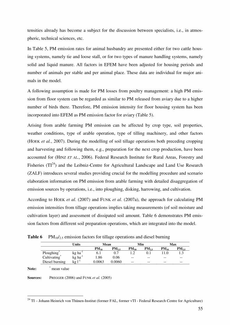
55
tensities already has become a subject for the discussion between specialists, i.e., in atmos-
pheric, technical sciences, etc.
In Table 5, PM emission rates for animal husbandry are presented either for two cattle hous-
ing systems, namely tie and loose stall, or for two types of manure handling systems, namely
solid and liquid manure. All factors in EFEM have been adjusted for housing periods and
number of animals per stable and per animal place. These data are individual for major ani-
mals in the model.
A following assumption is made for PM losses from poultry management: a high PM emis-
sion from floor system can be regarded as similar to PM released from aviary due to a higher
number of birds there. Therefore, PM emission intensity for floor housing system has been
incorporated into EFEM as PM emission factor for aviary (Table 5).
Arising from arable farming PM emission can be affected by crop type, soil properties,
weather conditions, type of arable operation, type of tilling machinery, and other factors
(HOEK et al., 2007). During the modelling of soil tillage operations both preceding cropping
and harvesting and following them, e.g., preparation for the next crop production, have been
accounted for (HINZ ET AL., 2006). Federal Research Institute for Rural Areas, Forestry and
Fisheries (TI24
) and the Leibniz-Centre for Agricultural Landscape and Land Use Research
(ZALF) introduces several studies providing crucial for the modelling procedure and scenario
elaboration information on PM emission from arable farming with detailed disaggregation of
emission sources by operations, i.e., into ploughing, disking, harrowing, and cultivation.
According to HOEK et al. (2007) and FUNK et al. (2007a), the approach for calculating PM
emission intensities from tillage operations implies taking measurements (of soil moisture and
cultivation layer) and assessment of dissipated soil amount. Table 6 demonstrates PM emis-
sion factors from different soil preparation operations, which are integrated into the model.
Table 6 PM10/2.5 emission factors for tillage operations and diesel burning
Units Mean Min Max
PM10 PM2.5 PM10 PM2.5 PM10 PM2.5
Ploughing* kg ha
-1 6.1 0.7 1.2 0.1 11.0 1.3
Cultivating* kg ha
-1 1.86 0.06 -- -- -- --
Diesel burning kg l-1
0.0063 0.0060 -- -- -- --
Note: * mean value
Sources: PREGGER (2006) and FUNK et al. (2005)
24
TI – Johann Heinrich von Thünen-Institut (former FAL, former vTI - Federal Research Centre for Agriculture)

56
Minimal and maximal emission values from ploughing, related to dry and moist weather con-
ditions, consequently, and single values for PM emissions from alternative tillage techniques
result from the above mentioned approach25
. Mean values for PM emissions from ploughing
have been integrated into EFEM alone with PM emission intensities for reduced-tillage to as-
sure comparability of emission factors between different types of land preparation (Table 6).
The next important source of PM emissions in arable farming after land preparation is har-
vesting and post-harvesting operations, i.e., unloading, cleaning, and drying. The PM10 emis-
sion factor for cereal harvesting is a sum of the partial emission rates for harvesting, drying,
cleaning, and unloading. Only the highest value for emission rate from harvesting is meas-
ured, whilst minimal and mean values are derived from the measured emission factor as 10%
and 50%, respectively. The average emission factor is matching to harvesting of dry grains;
the lowest emission rate corresponds to PM emissions from harvesting of humid grains; the
maximal value reflects PM emission from harvesting of yield under very dry weather condi-
tions. Controversially to emission factors from harvesting, the maximal and minimal PM
emission rates from post harvesting activities are measured. The highest PM emission values
for unloading, cleaning and drying of grains are resulting from humid grains, while the lowest
emission rate arise from dry grains. The reason for this is that at dry conditions major dust is
emitted from combine harvesting rather than crop drying. Table 7 presents the cumulative PM
emission rates for harvesting and following operations, and for burning of heating oil during
yield drying.
Table 7 PM10/2.5 emission factors for grain harvesting
Units Mean1)
Min2)
Max3)
PM10 PM2.5 PM10 PM2.5 PM10 PM2.5
Harvesting4)
kg ton-1
0.31 0.069 0.04 0.009 0.82 0.182
Uploading kg ton-1
0.02 0.004 0.03 0.007 0.04 0.002
Cleaning kg ton-1
0.03 0.007 0.05 0.011 0.01 0.002
Drying kg ton-1
0.08 0.018 0.12 0.027 0.01 0.009
Harvesting sum5)
kg ton-1
0.44 0.098 0.24 0.053 0.88 0.194
Heating oil use kg l-1
0.00031 0.00027 -- -- -- --
Notes: 1)
medium yield moisture is about 19%; 2)
wet –the water content in harvested seeds is nearly 25%;
3)dry – the moisture of harvested seeds is about 13-14%
4) post-harvesting activities are not in-
cluded (own calculations based on HOEK et al. (2007)); 5)
sum of emission rates for harvesting and
post-harvesting activities
Sources: HINZ (2004) and HOEK et al. (2007)
25
Personal communication of Susanne Wagner, University of Stuttgart, and Roger Funk, ZALF, from
23.01.2008

57
So far, measurements and estimations of PM emission factors from harvesting are performed
only for PM10. The assessment of PM2.5 emission rates is made based on assumptions on par-
ticle distribution. Thus, according to UIHLEIN et al. (2003), ratio of PM2.5 in total suspended
particles (TSP) constitutes 10.1%, while 45.4% belongs to PM10 (Table 7). It is to be consid-
ered that this approach may lead to uncertain results, particularly if PM10 and PM2.5 are poorly
correlated.
Emission intensities from harvesting and post-harvesting are available for cereals, but still
missing for other crops. For instance, no measurements of PM emissions are available yet for
maize harvesting. However, according to Hinz T.26
, PM emitted from this activity is coarse
(section 2.1) and sediment relatively fast. This is the reason for the assumption that maize
harvesting does not cause any PM10 and PM2.5 emissions. It is important to mention that major
dust from harvesting stems from plants per se; consequently, PM emission rate depends on
the yield rather than on weather conditions. Clover and silage maize are harvested when the
seeds’ water content is relatively high (more than 19%); hence, it is assumed that no PM is
emitted from silage maize and clover harvesting.
Due to the comparison of harvesting moisture conditions for different crops presented in Ta-
ble 8, it can be seen that average moisture levels for rapeseed and field beans are similar to
moisture rates for cereals. Therefore, emission from harvesting of field beans and winter rape-
seed is assumed to be the same as for cereals.
Table 8 General information on seeds moisture by harvesting (in %)
Plants Seeds moisture Sources
Cereals 14-25 HANUS et al. (2008)
Legumes 16-20 HANUS et al. (1999)
Rapeseed 15 HEYLAND et al. (2006)
To conclude it can be said that PM emission from grains and legumes harvesting is independ-
ent from soil type, because in major cases harvester does not disturb the soil. In the case of
tuber harvesting, PM is released rather from soil than from crops. However, soil types vary
greatly inside of one region; therefore, the application of correct PM emission rate from soils
in the modelling approach remains questionable.
In order to obtain PM emissions not only from various farms, but also from other industries
contributing to agricultural production, it is necessary to consider PM emission intensities
26
Personal communication of Susanne Wagner, University of Stuttgart, and Torsten Hinz, TI, from 30.01.2008

58
from the upstream sector. Particulate matter emissions from upstream sector occur from burn-
ing of heating oil, production of electricity and fertilizers, and production and preparation of
animal fodder. Respective emission intensities are demonstrated in Table 9.
Table 9 PM emission factors for upstream agricultural production in Germany
PM sources Units PM2.5 PM10
Heating oil burning kg l-1
5.3 8.4
Electricity production kg kWh-1
0.9 1.8
Fertilizer production, incl.
N-fertilizers
kg 100kg-1
0.204
0.215
P-fertilizers kg 100kg-1
0.0986 0.104
K-fertilizers kg 100kg-1
0.0779 0.082
Ca-fertilizers kg 100kg-1
0.0112 0.0286
Source: UIHLEIN et al. (2003)
Losses of PM occurring due to the livestock fodder production, which farmer buys to fulfil
nutritive requirements of livestock, are calculated on the basis of available PM emission rates
for arable farming (tillage, harvesting, electricity production and heating oil burning and utili-
zation) and data on crop yields for 2003 and 2015.
5.2.5 Choice of NH3 Emission Factors
There are more studies presenting measurements for NH3 losses than for PM emissions. Sev-
eral works, i.e., AMON et al. (2001), DÄMMGEN et al. (2009), DEFRA (2002), DEFRA
(2007b), KOERKAMP et al. (1998), MISSELBROOK et al. (2000), NICHOLSON et al. (2004),
UBA (2008), UNECE (2009a), have been reviewed for measured or assessed data on NH3
emissions. Variations in NH3 emissions are found for housing systems, animal types as well
as in time and between countries (KOERKAMP et al., 1998).
Countries based difference is the first decisive factor for selection of NH3 emission rates.
Thus, information sources providing estimations of NH3 emission factors from non-European
countries, e.g., USA, have not been considered due to differences in farm management and,
furthermore, in climate conditions. Although there is diverse contribution of various European
countries to partial27
and general NH3 released, emission intensities from European countries
are prioritized (KOERKAMP et al., 1998). It is found, that NH3 emission factor for cattle slurry
loose system from the UK is by nearly 30% higher than data for the same animal category and
housing system for Germany, but ca. 13% lower for cattle straw based systems
27
related to individual sources of NH3 emissions (e.g., animal housing and pasture)

59
(DEFRA, 2007b). However, German NH3 emission rates for cattle and pig housing appear to
be over 15% higher than Dutch data for identical system. Dutch NH3 emission factors for lay-
ing hens overcome German emission intensities by ca. 80% (UNECE, 2009a).
The second comparison criterion for information sources of NH3 emission data is the me-
thodological approach for emission calculation. On the one hand, there is emission informa-
tion resulting from unit approach, when independent measurements are taken from each
source and stage of manure management (AMON et al., 2001; KOERKAMP et al., 1998;
NICHOLSON et al., 2004). On the other hand, some emission estimates resulting from mass
flow approach, where NH3 losses from livestock farming are seen as a part of the N-flow and
the effect of emissions alteration on one stage will depend on preceding and following stages
of manure management (DÄMMGEN et al., 2009; DEFRA, 2002, 2007b; UNECE, 2009a). A
drawback of the unit approach is the difficulty to assess the effects of emission abating efforts
on earlier stages of the N-cycle (DEFRA, 2002). To avoid this shortcoming, emission infor-
mation from the studies using the mass flow method for calculation of NH3 emission rates is
chosen.
In EFEM emission factors for NH3 are differentiated for each animal category and housing
system. Table 10 shows selected NH3 emission rates presented as the percentage loss of NH3-
N from TAN28
in excreted, stored and spread animal manure. In the case of manure storage,
TAN is determined as a difference of TAN-value after excretion after deduction of ammo-
nium nitrogen looses during livestock housing. For manure land application stage in manure
management, TAN is determined as a TAN-value after deduction of NH3-N losses during
housing and storage.
Emission factors for NH3 emissions for cattle housing vary for different housing techniques,
explicitly for loose and tie systems. Though, tie housing of cattle is considered as less profit-
able for animal welfare comparing to loose system, it emits three times less NH3 than loose
houses due to a smaller surface covered with manure (UNECE, 2007; DÄMMGEN et al., 2009;
DÄMMGEN, 2007). The respective figures are presented in Table 10. As no data on NH3 emis-
sion from cattle housed in the system withleachate are available, it is assumed that NH3 emis-
sion factor for leachate is the same as for slurry (Table 10).
28
Total ammoniacal nitrogen (TAN = NH4-N (ammonium nitrogen) + NH3-N (ammonia nitrogen))

60
Table 10 Partial emission factors for NH3-N losses (in % from NH4-N) from cattle, pig and
poultry housing systems, manure storage and land application
Animal category NH3 source categories NH3-source sub-categories Emission rates
Cattle Housing system Tie system, slurry 7.8
Loose system, slurry 23.6
Tie system, solid manure 7.8
Loose system, solid manure 23.6
Tie system, leachate 7.8
Loose system, leachate 23.6
Storage Slurry 17.0
Solid manure 60.0
Leachate 25.0
Land application Arable land, slurry 50.0
Arable land, solid manure 90.0
Arable land, leachate 20.0
Grassland, slurry 60.0
Grassland, solid manure 90.0
Grassland, leachate 20.0
Grazing 7.5
Pigs Housing system Slurry based 25.5
Storage Slurry 15.0
Land application Arable land, slurry 25.0
Grassland, slurry 30.0
Laying hens Housing systems Aviary 10.1
Cages, dung belt with drying 4.3
Storage *)
Dry dung 5.8
Aviary 6.5
Land application Arable land 90.0
Broilers Housing systems Free range, solid manure 13.8
Storage *)
Broilers, litter 7.5
Land application Arable land 45.0
Source: DÄMMGEN et al. (2009); *)
own calculation based on DÄMMGEN (2007) and DÄMMGEN et al.
(2009)
Losses of NH3 for both breeding sows’ and fattened pigs’ housing systems are nearly the
same (24% and 27% of NH3-N from TAN, respectively); therefore, an average value is taken
for this study (Table 10). As no information on straw based housing systems for pigs is avail-
able for Germany, this type of pig management is not considered in the current study
(DÄMMGEN et al., 2009).
It is important to consider the difference in properties between pig and cattle liquid manure,
which, in turn, explains discrepancy in NH3 released. Thus, viscosity of pig slurry is lower
comparing to cattle liquid manure. Therefore, pig slurry stored in the open slurry tank can
easier be moved by the wind, which leads to higher NH3 losses. Also lower viscosity of pig
liquid manure assures its relatively faster infiltration into soil and, at the result, less NH3 re-
leased from manure land application (Table 10) (DE BODE, 1990; SCHÄFER, 2006). The effect
of the ambient temperature on NH3 losses from spreading pig and cattle liquid manure is dif-

61
ferent. Thus, if 30% of NH3 can be released from pig liquid manure land application by 20°C,
the same NH3 losses from spread cattle slurry occur already at the ambient temperature of
slightly higher than 0°C (DÖHLER, 1990).
Emission rate of NH3 for hens in cages with manure-belt system and without additional aera-
tion has not been included in this study, as this practise is considered to be rear in Germany
(Table 20, section 5.6).
In the conditions of continental climate, where cows spend more time in barns than grazing,
emission rate for NH3 from pasture is lower than emission intensities from cattle housing
(Table 10) (DEFRA, 2002).
In order to reduce NH3 emission at the stage of manure storage, German farmers generally
install different covers for manure storage tanks or allow a natural crust formation, when stir-
ring slurry less. The abatement potentials of various cover types for manure storage have been
compared with the reference technique, which implies an absence of surface cover for the
same type of storage (Table 11).
Table 11 NH3 emissions abatement potentials (in %) of different slurry storage covers in
comparison to open storage tanks
Covering material NH3 mitigation, %
General remarks Cattle slurry Pig slurry
Natural crust 30-80 20-70 Low efficiency in the case of frequent slurry application
Granulate 80-90 80-90 Adjustment of material losses is necessary1)
Hexa-Cover 2)
Not for cattle
manure 90-98
Only for pig slurry, without natural crust, long expected
useful life
Floating film 80-90 80-90
Low maintenance requirements; does not suit for big con-
tainers due to relatively high costs
Tent roof 85-95 85-95 Low maintenance requirements, no access for rain water
Concrete cover/
v.a. concrete cover3)
85-95 85-95 Low maintenance requirements, no access for rain water5)
Notes: 1)
10% of annual losses by granulate; 2)
synthetic floating elements; 3)
vehicle-access concrete
cover; 5)
diameter of storage tank is up to 15 m (KTBL, 2002)
Sources: KTBL (2005, 2002)
Amount of NH3 non-released during manure management in animal barn and manure storage
can be emitted during manure application onto agricultural land. This requires employment of
NH3 abating techniques for manure spreading, otherwise, much of the abatement benefit
gained due to the implementation of emission reduction techniques during manure storage
may be lost. Potentials of NH3 emission abatement for different ways of manure land applica-
tion are presented in Table 12. Efficiency of methods for NH3 reduction is demonstrated in
comparison to the reference technique, i.e., broadcasting.

62
Table 12 NH3 reduction potentials (in %) of various manure land application techniques for
different land managements and types of manure, in comparison to the reference
technique
Land application
techniques Animal type
Arable land Grassland
Solid
manure Slurry Leachate
Solid
manure Slurry Leachate
Broadcast, splash
plate
cattle, pigs,
poultry reference technique reference technique
Band-spreading
trailing hose
cattle n/a 102 10
2 n/a 30
2 10
2
pigs n/a 302 10
2 n/a 50
2 10
2
Band-spreading
trailing shoe
cattle n/a 601 -- n/a 40
2 --
pigs n/a 601 -- n/a 60
2 --
Shallow injection
open slot
cattle n/a n/a -- n/a 602 --
pigs n/a n/a -- n/a 802 --
Slurry tooth extirpa-
tor**
cattle n/a 801 -- n/a n/a --
pigs n/a 801 -- n/a n/a --
Notes: n/a – technique is not practised for particular land or manure type; * technique is mainly applicable
on grassland; **
technique is only applicable on arable land
Source: 1 UNECE (2009b);
2 DÄMMGEN (2009)
From Table 12 it can be seen that in case of manure spreading the range of measures for NH3
abatement for liquid manure is wider than for solid excreta. The common spreading tech-
niques for leachate are broadcast and spreading with trailing hose.
Type of the manure, ambient temperature and soil infiltration rate are taken into account for
modelling seasonal changes in NH3 emission from slurry land application. The basic monthly
information on temperatures and precipitations is obtained from German Meteorological Ser-
vice (DWD, 2010) for the years 2004, 2005, and 2007. The year 2006 is not considered, for
marginal alteration of its weather parameters from the average for Germany. Calculated aver-
age monthly temperatures are associated with certain time spans in a year, when particular
farming practises are conducted.
Infiltration rate in range from low to medium and high has been adjusted to particular manure
type based on knowledge about viscosity of slurry. Additionally, different slurry absorption
rates of soil were considered for manure application onto arable land and grassland. For grass-
land’s vegetation prevents rapid infiltration of leachate into soil, its intensity for pig liquid
manure to arable land is determined as high, but to grassland as medium. The absorption rates
for leachate are assumed to be the same. The infiltration rate of more viscous cattle slurry is
lower than of pig slurry, i.e., medium for both arable land and grassland.
Seasonal changes of weather conditions strongly influence the volatilized amount of NH3
(MULVANEY et al., 2008). Assumptions on alteration of NH3 potential losses under considera-

63
tion of weather conditions and infiltration intensities are taken from HORLACHER et al. (1989)
and further on calibrated with NH3 emission rates for manure land application from
DÄMMGEN et al. (2009). Ammonia emission rates for different farming block time spans re-
sulting from above-mentioned assumptions are shown in Table 13.
Table 13 NH3 losses (in % from NH4-N) from the application of cattle, pig and poultry ma-
nure to arable land and grassland
Source: HORLACHER et al. (1989)
Data on seasonal NH3 losses from leachate application onto agricultural land are available
only for cattle due to the general assumption that pigs are housed in barns with slurry based
systems (section 5.6), while leachate occurs as a product in solid manure based systems.
There is also no data on seasonal NH3 emissions for fermented pig slurry; hence, NH3 losses
from its land application are assumed to be equal to NH3 emission from pig slurry spreading.
However, in the case of cattle fermented slurry NH3 losses are 50% lower than respective
emissions from not-fermented cattle slurry.
5.3 Extrapolation
After collecting bookkeeping and census information, FADN data are checked for their repre-
sentativeness. For this reason bookkeeping information and regional statistics have been com-
pared and significant differences found. In general, FADN figures are lower than the respec-
tive data from regional statistics for identical parameters and regions. Beside this, data for
some agricultural categories, e.g., broilers and sugar beet, are absent in the FADN database.
There are at least three explanations for the mentioned disparities:
Slurry Leachate Fermented slurry
cattle pigs cattle cattle pigs
Arable land March 14.7 6.8 5.5 6.8 6.8
April-July 36.7 18.2 14.6 18.2 18.2
August 50.0 25.0 20.0 25.0 25.0
September-October 36.7 18.2 14.6 18.2 18.2
November-February 14.7 6.8 5.5 6.8 6.8
Grassland March 17.6 8.8 8.8 8.8 8.8
April-July 44.0 22.0 22.0 22.0 22.0
August 60.0 30.0 30.0 30.0 30.0
September-October 44.0 22.0 22.0 22.0 22.0
November-February 17.6 8.8 8.8 8.8 8.8

64
- Firstly, differences could possibly be caused by the exclusion of part-time farming out of
bookkeeping database. However, as it is shown in Table 14, the share of part-time farming
might be significant.
Table 14 Share of farming on a regular/sideline basis (full-/part-time) in Baden-
Württemberg, Brandenburg and Lower Saxony, in 2003
Individual
farms, thds.
Share of farms in
region, %
Full-time farms 21.9 34
Part-time farms 38.7 60
BW, total 64.5 100
Full-time farms 1.8 27
Part-time farms 3.4 51
BB, total 6.7 100
Full-time farms 30.5 54
Part-time farms 22.6 40
LS, total 56.3 100
Notes: BW – Baden-Württemberg, LS – Lower Saxony, BB – Brandenburg
Source: DESTATIS (2008)
- Secondly, absence of some specific data can be related to data security issues, when in-
formation on farm business is open only for limited authorities, e.g., in Baden-
Württemberg.
- Thirdly, it is possible that a large share of poultry management is situated at industrial
rather than agricultural enterprises. However, the FADN database only contains informa-
tion on agricultural units, that is, possibly, why animal category like broilers is not pre-
sented in FADN data for some administrative units, for instance Braunschweig, Karlsruhe,
and Freiburg.
Data lacking by any of all above mentioned reasons have not been estimated, but rather con-
sidered to be equal to zero. By the reason of a strong deviation of FADN data from regional
statistics extrapolation factors in a FADN database (number of representative farms of a cer-
tain type in a certain region) could not be taken for this study as weighting factors. Thus, in
order to calculate extrapolation factors matching for EFEM, the extrapolation procedure
elaborated according to the approach presented by SCHÄFER (2006) and KAZENWADEL (1999)
is conducted.
There are at least three ways to extrapolate farm results to the regional level in at least three
ways: 1) modelling of all farms in a region and extrapolation of results; 2) regarding a whole
region as a group of farms; 3) an extrapolation of individual farms’ capacity to census data.
The third option seems to be the most suitable for this study, as in this case requirements for

65
data are lower than in the other cases. Moreover, the third method allows the consideration of
different farm types in a study region (KAZENWADEL, 1999).
Extrapolation procedure is based on an optimization approach, which eases depiction of total
regional capacities through weighting of typical farms’ capacities. The basic principle of this
approach is that test-farms are averaged and assessed at the regional level. For each study re-
gion 5 typical farms with factor endowments close to average results are selected according to
the business administrative classification (Germ., BWA – Betriebswirtschaftliche Ausrich-
tung): arable, forage growing, mixed farms and two types of intensive livestock farms,
namely with the emphasis on the pig and poultry production. Typical farms have been ex-
trapolated to the regional level. Farm capacities and number of representative farms (extrapo-
lation factors) resulting from the extrapolation are shown in Tables 15-17.
Table 15 Typical farms resulting from the extrapolation procedure and extrapolation factors
for administrative regions of Lower Saxony, in 2003
Farm types
Ara
ble
lan
d
Gra
ss-
lan
d
Su
ga
r
beet
Ma
le
ca
ttle
≥ 1
yea
r
Heif
ers
Da
iry
co
w
Su
ck
ler
co
w
Fa
tten
ed
pig
s
Breed
ing
so
ws
Laying hens
Bro
ilers
Extrapo-
lation
factors free
ra
ng
e
ca
ges/
av
iary
Braunschweig
AF 95.6 -- 11.0 -- -- -- -- -- -- -- -- -- 2,226 FGF 31.5 36.8 -- 3 13 40 8 -- -- -- -- -- 865 ILF_ Pigs 94.8 -- 32.0 -- -- -- -- 156 25 -- -- -- 785 ILF_ Poultry 24.7 -- 4.0 -- -- -- -- 15 52 398 1,696 -- 75.5 MF 16.8 14.9 -- 3 5 -- -- -- -- -- -- -- 1,119
Hannover
AF 78.3 -- 12.0 -- -- -- -- -- -- -- -- -- 1,720 FGF 29.0 26.0 -- 5 15 34 3 -- -- -- -- -- 2,135 ILF_ Pigs 69.6 -- -- -- -- -- -- 706 139 -- -- -- 693 ILF_ Poultry 61.4 -- 4.0 -- -- -- -- 253 -- -- -- 16,696 204 MF 151 22.0 15.9 16 5 -- 5 -- -- 181 789 -- 1,041
Lüneburg
AF 91.1 -- 15.2 -- -- -- -- -- -- -- -- -- 1,604 FGF 23.6 39.2 -- 23 25 69 -- -- -- -- -- -- 3,833 ILF_ Pigs 26.9 -- -- -- -- -- -- 545 97 -- -- -- 1,092 ILF_ Poultry 80.2 -- -- -- -- -- -- -- -- -- -- 1,903 1,346 MF 31.1 38.5 -- 7 8 7 -- -- 47 198 -- 3,947
Weser-Ems AF 28.6 -- 0.3 -- -- -- -- -- -- -- -- -- 5,087 FGF 10.8 37.4 -- 19 19 43 -- -- -- -- -- -- 8,508 ILF_ Pigs 38.5 6.1 -- -- 3 -- 14 126 222 -- -- -- 1,747 ILF_ Poultry 48.3 -- -- -- -- -- -- 459 10 475 2,066 -- 4,533 MF 53.6 28.4 -- 72 13 12 3 -- -- -- -- 25,741 873
Notes: AF - arable farms, FGF – forage growing farms, ILF_Pigs/Poultry – intensive livestock farms with
emphasise on pig and poultry production, respectively, MF – mixed farms
In Lower Saxony, forage growing farms are prevailing (35%) followed by mixed farms (about
30%). Farm capacities are not evenly distributed among administrative regions. Thus, Braun-

66
schweig is the region with 41% of arable farms in Lower Saxony. Arable and forage growing
farms in Hannover account for a slightly lesser share, namely 31% and 36% of total farms,
respectively. Also, intensive livestock farming with emphasis on both pig and poultry produc-
tion plays a significant role in this region. The highest number of dairy cattle can be found in
Lüneburg, while in Weser-Ems intensive pig and poultry production farms prevail, constitut-
ing 30% of total farms in this region (Table 15).
Table 16 Typical farms resulting from the extrapolation procedure and extrapolation factors
for administrative regions of Baden-Württemberg, in 2003
Farm types
Ara
ble
lan
d
Gra
ss-
lan
d
Su
ga
r
beet
Ma
le
ca
ttle
≥ 1
yea
r
Heif
ers
Da
iry
co
w
Su
ck
ler
co
w
Fa
tten
ed
pig
s
Breed
ing
so
ws
Laying hens
Bro
ilers
Extrapo-
lation
factors free
ra
ng
e
ca
ges/
av
iary
Stuttgart
AF 55.1 -- 5.2 -- -- -- -- -- -- -- -- -- 2,840 FGF 15.9 34,6 -- 8 37 3 16 -- -- -- -- -- 1,920 ILF_ Pigs 48.7 -- -- -- -- -- -- 193 117 -- -- -- 1,495 ILF_ Poultry 35.1 4.5 -- 30 -- -- -- -- -- -- -- 9,156 49.7 MF 20.1 28.5 -- 5 16 4 7 -- -- 223 223 -- 2,745
Karlsruhe
AF 53.9 -- 3.1 -- -- -- -- -- -- -- -- -- 1,522 FGF 7.5 36.5 -- 5 25 2 11 -- -- -- -- -- 758 ILF_ Pigs 31.5 -- 2.1 -- -- -- -- -- 215 -- -- -- 66.1 ILF_ Poultry 20.7 44.7 -- 26 -- -- 21 511 -- 1,602 1,602 -- 99.2 MF 56.8 27.1 -- 4 10 7 3 -- -- -- -- -- 919
Freiburg
AF 65.3 -- -- -- -- -- -- -- -- -- -- -- 741 FGF 17.8 59.8 -- 8 35 -- 9 -- -- -- -- -- 2,229 ILF_ Pigs 32.9 -- -- -- -- -- -- 198 53 -- -- -- 342 ILF_ Poultry 13.1 -- -- -- -- -- -- -- -- 2,380 2,380 -- 107 MF 52.8 41.4 -- 4 -- 30 17 10 -- -- -- -- 861
Tübingen
AF 41.1 -- -- -- -- -- -- -- -- -- -- -- 3,009 FGF 14.5 50.6 -- 8 47 3 16 -- -- -- -- -- 3,439 ILF_ Pigs 13.8 -- -- -- -- -- -- -- 128 -- -- -- 723 ILF_ Poultry 38.3 -- 1.1 -- -- -- -- 349 -- -- -- 576 679 MF 17.0 17.6 -- 1 13 2 8 -- -- 240 240 -- 1,258
Notes: AF - arable farms, FGF – forage growing farms, ILF_Pigs/Poultry – intensive livestock farms with
emphasizes on pig and poultry production, respectively, MF – mixed farms
Table 16 shows that about 50% of all farms in Baden-Württemberg are forage growing farms,
while about 30% are mixed farms. Freiburg is the most representative region in terms of
number of forage growing farms (52%). Stuttgart and Tübingen are two administrative re-
gions with the highest endowments of arable land in Baden-Württemberg (65% of total arable
area), where arable farms represent 31% and 33%, correspondingly. Nevertheless, forage
growing farms are prevailing farm type in Tübingen (ca. 48%), while mixed farms are the ma-
jor farm type in Stuttgart (30%). Regardless the lowest share of arable land in Baden-

67
Württemberg (17%), arable farms in Karlsruhe account for 41% of all regional farm types.
Although, the spread of intensive livestock farming in Baden-Württemberg is hardly compa-
rable with the development of the same branch in Lower Saxony, intensive livestock farms
are relatively good represented in Stuttgart and Tübingen (pig production), and Freiburg
(poultry production). The number of intensive livestock farms for these regions constitute
over 85% of this farm type in total Baden-Württemberg (Table 16).
Table 17 Typical farms resulting from the extrapolation procedure and extrapolation factors
for Brandenburg, in 2003
Farm types
Ara
ble
lan
d
Gra
ss–
lan
d
Su
ga
r
beet
Ma
le
ca
ttle
>=
1
yea
r
Da
iry
co
w
Su
ck
ler
co
w
Heif
ers
Fa
tten
ed
pig
s
Breed
ing
so
ws
Laying hens
Bro
ilers
Extrapo-
lation
factors free
ra
ng
e
ca
ges/a
via
ry
AF 396 - 10.0 - - - - - - - - - 1,127 FGF 102 270 - 47 32 182 45 - - - - - 451 ILF_ Pigs 137 - - - 3 - - 171 1,097 - - - 62.0 ILF_ Poultry 48.0 - - - - - - 3,124 476 7,855 28,678 45,731 72.0 MF 546 180 - 19 74 103 74 - - - - - 964
Notes: AF - arable farms, FGF – forage growing farms, ILF_Pigs/Poultry – intensive livestock farms with
emphasizes on pig and poultry production, respectively, MF – mixed farms
As it can be seen from Table 17, arable farms represent 41% of total farms in Brandenburg.
Forage growing and particularly mixed farms are important for cattle husbandry. Intensive
livestock farms are not as widely spread in Brandenburg as in Lower Saxony and Baden-
Württemberg. These farm types constitute only ca. 5% of total number of farms in Branden-
burg (Table 17).
Due to the extrapolation approach, each regional capacity is weight with the respective gross
margin to guarantee that they are not overestimated. The relevance of this weighting proce-
dure is obvious. Thus, in the case of poultry farms several hundred and/or thousands of laying
hens and broilers are produced, however, the gross margin per animal is quite low (7-9 EUR
animal-1
and 1 EUR animal-1
for laying hens and broilers, respectively). The choice of gross
margin as a weighting factor can be explained by the predominant economic character of
EFEM. Indeed, if ecological aspects of analysis are of higher concern, other weighting factors
such as size of agricultural area or livestock numbers would be taken into account. After
weighting of farm capacities the sums of absolute under- and overestimations have to be
minimized through the optimization approach (KAZENWADEL, 1999).

68
The applied extrapolation procedure guarantees a well assessment of regional factor endow-
ments through the multiplication of the adjusted farms capacities with the weighting coeffi-
cient (or, in this case, number of representative farms). Extrapolation additionally assures that
farm shares in the selected federal states are well represented. Table 18 shows that a good
matching between statistical data and modelling results for both distribution of different farm
types in administrative regions and their distribution in the complete federal state could be
reached. In this table the modelled distributions are established in brackets and compared to
the real situation in Lower Saxony, Baden-Württemberg, and Brandenburg for the year 2003.
Table 18 Distribution of farm types (in %) resulting from modelling (in brackets) and ac-
cording to census database, for Lower Saxony (a), Baden-Württemberg (b), their
administrative regions and Brandenburg (b), in 2003
a) Regions
Farm types BS HA LÜ WE LS
AF 7 8 5 5 25
(7) (4) (7) (12) (29)
FGF 2 4 15 22 43
(2) (5) (9) (20) (35)
ILF 0 1 1 6 8
(0) (2) (3) (4) (8)
MF 2 5 6 12 25
(3) (3) (9) (12) (27)
NS 11 17 27 44 100
(12) (13) (27) (48) (100)
b) Regions
Farm types ST KR FR TÜ BW BB
AF 8 5 4 6 23 37
(11) (6) (3) (12) (31) (42)
FGF 12 4 17 15 48 34
(7) (3) (9) (13) (32) (17)
ILF 1 0 0 1 2 2
(6) (1) (2) (5) (14) (5)
MF 10 3 6 8 27 27
(11) (4) (3) (5) (23) (36)
BW/BB 31 12 27 30 100 100
(35) (13) (17) (35) (100) (100)
Notes: BS – Braunschweig, HA – Hannover, LÜ –Lüneburg, WE – Weser-Ems, ST – Stuttgart, KR –
Karlsruhe, FR – Freiburg, TÜ – Tübingen, LS – Lower Saxony, BW – Baden-Württemberg; BB –
Brandenburg; AF - arable farms, FGF – forage growing farms, ILF – intensive livestock farms,
MF – mixed farms
The fact that factor endowments in FADN data are higher than statistical average can serve as
the explanation of some deviations of modelling results from bookkeeping information.

69
Established typical farms are built into EFEM after implementation of extrapolation approach
and comparison of real data and modelling results.
5.4 EFEM Structure and Approach
The objective of economic analysis in EFEM corresponds to farmers interests and is oriented
on the maximization of individual farm gross margins. These farms are regarded as represen-
tative (typical) for all farms of the same type in the same region, and their objective function
can be expressed parametrically as follows:
max πk = (pi - ci) × xk, xk
s.t. Ak× xk≤ zk, xk ≥ 0,
where πk is the total gross margin of the k-th farm-type, pi and ci are n-vectors for the i-th sell-
ing price and variable costs of the i-th production activity, consequently, and xk is the n-vector
of command variables. The constraints faced by farm-type k are defined through Ak and zk,
determining m×n-input-output matrix and m-vector of capacities, respectively (DE CARA S. et
al., 2004).
Command variables in EFEM can be both endogenous and exogenous. Thus, area under cer-
tain crop (including grassland and set-aside area), quantity of purchased animal feeding and
total GHG emissions are endogenous; while, e.g., variables related to policy programs like
enrolment in environmental or set-aside programs, subsidies, etc. are examples of exogenous
variables.
Under Ak following constraints are defined: cropping area, crop rotation, animal housing
places, livestock nutritive requirements, quotas, restrictions imposed by policy and environ-
mental programs (DE CARA S. et al., 2004). In EFEM total land is fixed at an initial land en-
dowment of each farm-type. Crop rotation constraints in EFEM are presented as the maximal
shares of arable land under certain crops in a rotation process. The respective restrictions sub-
stitute dynamics in crop cultivation in the static modelling framework. These restrictions are
introduced on the base of statistical information for the reference year 2003, and further on
calibrated to reflect common practises of arable farming in the year 2015, which the projec-
tion is made for (section 5.5). Number of livestock heads is restricted by the availability of
animal places (DE CARA S. et al., 2004; DE CARA et al., 2005).

70
EFEM is a mixed integer model, one of special cases of linear programming, where the corre-
sponding variables can be included as both binary and integer. Model’s mathematical basis
connected to the solving algorithm in MS Excel spreadsheets application assures calculation
of optimal farming solutions. The given approach assures precise depiction of farms’ techni-
cal conditions, allows the choice between production options, make a detailed representation
of pollutants’ sources possible (ANGENENDT, 2003) and let farmers deal in mutually exclusive
policy programs with involvement of different obligations and payments (DE CARA S. et al.,
2004). However, beside the advantages, the modelling approach has a draw back, namely its
static character (ANGENENDT, 2003). Thus, no factor endowments (inclusive land size, restric-
tions of crop rotation and livestock numbers) are changing over time. This must be taken into
account by interpreting modelling results and making projections.
5.4.1 Farm Structure Module
An economic-ecological model EFEM is not only a combination of economic and ecological
factors. Indeed, it has a more complex structure composed of multiple sub-modules. They al-
low a representation of all relevant production processes of arable farming and grassland
management with related mechanization, animal husbandry with a disaggregated feeding
module, manure management, and N circulation.
The core of EFEM is a production module, where all sub-modules along with energy, emis-
sion, and stock flow parameters for the quantification of emissions stemming from agricul-
tural operations are merged together. Also emissions of NH3, PM and GHG are differentiated
for each production branch they are sourced from. A detailed build-up of the model core is
shown in Figure 8.

71
Figure 8 Build-up of the core of EFEM, farm structure module
Source: TRIEBE (2007), modified
All production activities presented in EFEM are disaggregated by the level of input-use and
performance. Thus, in general 14 different arable crops are integrated into EFEM, i.e., winter-
and spring wheat, winter- and spring-barley, oats, rye, winter rapeseed, sugar beets, potatoes,
field beans, sunflowers, grain maize and silage corn, as well as clover-grass. All main crops
analysed in EFEM are allocated into three categories: sold or consumed on farm, only for sel-
ling and only for on-farm consumption. The main crops for the farm-own consumption in-
clude mainly forage crops and grass from pastures for animal fodder. Therefore, the amount
of these crop types for farm-own purposes depends on their relative price and nutritional
value. Beside main crops, by-products are also analysed in EFEM on farm for feeding pur-
poses, litter, or green manure production and utilisation. Each crop production activity can be
combined with different fertilization intensities. In EFEM it is distinguished between two
grassland activities: meadow and pasture (DE CARA S. et al., 2004; TRIEBE, 2007).
Livestock production is subdivided according to levels of performance for main animal cate-
gories in selected regions. The part of the model devoted to animal husbandry includes data
on production of following animal types: dairy and suckler cows, calves, heifers, bulls, fat-
tened pigs, sows, sheep, laying hens, and broilers (TRIEBE, 2007). Animal feeding is deter-
mined endogenously in EFEM through establishment of nutritional requirements varying for
animal types. These requirements are established in such a way that maximal and minimal
values for digestible matter, energy, protein and lysine for each livestock category in the ani-
mal production module has to be met (DE CARA et al., 2005).
Production Production
module module
Farm structure module
Mechanisation
Arable production Grassland production
Animal
feeding Manure manage-
ment
Animal produc-
tion
N-cycle-N-output model
OUTPUT: economic results, production structure and quantities

72
5.4.2 Policy Module
The farm module is interrelated with the political module. Policy modelling assumes integra-
tion of relevant issues of the CAP, national German directives (e.g., Nitrate Directive), envi-
ronmental laws, and political programs into EFEM. This structure assures building of agricul-
tural production and resulted emissions maximally close to the reality and forecasting of the
consequences following political changes. Political issues mainly serve as restrictions for cer-
tain agricultural activities (like minimal and maximal share of fallow area), but also introduce
beneficial conditions for farmers as, e.g., in case of premiums for growing of renewable pri-
mary products. Parameters representing political constraints and supports have endogenous
character (section 3.1).
5.4.3 Emission Module
The calculation of emissions requires relevant activity data for respective year and emission
intensities. The product of these two components results in a total emission generated by a
certain activity. Hence, the emission module is closely bounded with the production module
of EFEM (Figure 8). Contribution to the emissions compiles input from: agricultural soils and
manure storage (N2O), enteric fermentation and manure management (CH4), manure man-
agement and mineral fertilizers land application (NH3), livestock management, land tillage,
fuel and heating oil burning (PM), fuel and electricity utilization (CO2).
Greenhouse gas emissions calculations follow the procedure of the IPCC Guidebook and par-
tially the methodology of the German National Emission Inventory. The GHG emission cal-
culation is done on the base of country-specific data on agricultural activities (like number of
livestock units and area assigned for certain crops) and emission intensities. All GHG emis-
sions, namely N2O and CH4 losses, are converted into CO2 equivalent by means of GWP fac-
tors, i.e., 298 and 25 for N2O and CH4, respectively. More information to the modelling of
GHG with EFEM can be found in SCHÄFER (2006) and TRIEBE (2007)
Both PM and NH3 emissions are modelled explicitly, with emission factors as exogenous pa-
rameters. This provides a wide field for model simulations. Analysis of the emission altera-
tions, which imply changing of any of exogenous and thereafter variations in endogenous fac-
tors, and relevant predictions for the future can be performed thanks to these simulations.

73
Computation of NH3 losses has been done with country-specific activity information and NH3
loss-fractions. Detailed information on the selection procedure for NH3 and PM emission fac-
tors is provided in sections 5.2.5 and 5.2.4, respectively.
Thus, computations of PM emissions have been performed through the following implicit
formula:
Et= EFt × xt,
where Et is PM emission stemmed from an agricultural activity t, EFt is PM emission factor
for the activity t (section 5.2.4) and xt is the quantitative expression of the activity t.
The methods for calculation of NH3 and PM losses in EFEM are different. Ammonia emis-
sion is computed with the mass flow approach. Thus, NH3 emission factors (section 5.2.5) are
combined in one chain of comprehensive calculations of NH3 losses from all stages of manure
management, i.e., manure storage in animal barn and special confinements and manure land
application.
Three different branches are considered in EFEM by calculation of NH3, PM, and GHG emis-
sions: upstream (buying of farm current assets like pesticides, mineral fertilizers, fuel, heating
oil and electricity) and agriculture (including all causing emission activities). EFEM is also
adjusted for computation of emissions from downstream (emission sourced from biogas and
bio-ethanol production). Although not for all pollutants (i.e., for PM) emission intensities for
downstream sector are available. By this reason and due to the initial intention to analyse, at
the first place, traditional agriculture oriented on the food and forage production, downstream
branch is excluded out of the modelling analysis.
5.5 Prognosis
Generally, inventories are needed within relatively short reference period (mainly a
year).Further analysis and investigations are based in the information projected from the cer-
tain reference year. Projections of future emission developments intend to support an actual
study results and to fill out the data gaps, which could not be eliminated for the reference
year. Thus, a “business-as-usual” (BAU) scenario is built to demonstrate how modelling re-
sults amend after several years, if neither technology nor land distribution, nor farm capaci-
ties, but rather market and political conditions change along with frequency distribution of
various farm activities. The year 2015 is chosen for BAU, primarily because the time span of
13 years allows staying in certain political framework determined by the CAP measures (sec-

74
tion 3.1). This entails forecast-uncertainty for the year 2020 and further years. The degree of
uncertainty increases under consideration of changing technological, market and economic
conditions.
Major alterations of the model for 2015 are conducted throughout integration of new political
measures and restrictions (section 3.1.2) and prices. The projection of prices for 2015 have
been provided by the TI29
, as well as some additional future outlooks for costs, i.e., for fertil-
izers, plant protection, seeds, etc. (OSTERBURG et al., 2009). Then predicted prices for 2015
have been calibrated with the respective figures from 2003 and then integrated into EFEM.
Projections 2015 are made for main crop yield changes by means of regression analysis of
crop yield data. Time series of 23 years for Lower Saxony and Baden-Württemberg and 16
years for Brandenburg have been taken for this analysis.
By making projections it is taken into account that requirements to a minimal share of arable
land under fallow practise have to be cancelled already before 2015. The maximal share of
production of renewable resources on arable land is another important change performed for
BAU comparing to the reference scenario 2003. According to AGENTUR FÜR ERNEUERBARE
ENERGIEN (2009), already 17% of arable land were under renewable primary products in
2009. A higher share of arable land used for the production of renewable resources is ex-
pected after consideration changing political regulations for supports of renewable resources
even. Thus, it has been assumed that farmers are able to produce renewable primary crops on
up to 20% of arable land.
5.6 Assumptions
Before starting with model calculations for the reference and business-as-usual (BAU) situa-
tions and scenarios, certain general modelling assumption have been made. Relevant informa-
tion on occurrence of housing systems, manure storage and spreading techniques is partially
taken from the agricultural sector model RAUMIS (OSTERBURG et al., 2009).
The occurrence of certain emission generating agricultural activities had to assure modelling
results close to the reality. Absence of the relevant information for the years 2003 and 2015
become a reason for several simplifications. Thus, data for 1999 have been taken for building
up EFEM reference-scenario 2003. BAU-scenario 2015 is elaborated based on the informa-
29
TI - Johann Heinrich von Thünen Institute, Federal Research Institute for Rural Areas (former FAL, former
vTI)

75
tion on frequency distribution for the year 2010. Moreover, the assumptions shown in Table
19 have been applied to the FADN and census data serving as a basis for EFEM calculations
(sections 5.2.1 and 5.2.2).
Table 19 Shares of various housing activities (in %) as weight average values for Germany,
with number of animal places1)
as a weighting factor
Animal type Housing system Manure type 2003 2015
Dairy cows Tie barn Solid 13 8
Tie barn Liquid 33 17
Loose barn Solid 3 5
Loose barn Liquid 51 70
Fattened bulls Tie barn Solid 2 1
Tie barn Liquid 3 0
Loose barn Solid 3 4
Loose barn Liquid 91 94
Suckler cows Tie barn Solid 7 7
Tie barn Liquid 2 2
Loose barn Solid 86 86
Loose barn Liquid 5 5
Heifers Tie barn Solid 8 8
Tie barn Liquid 17 17
Loose barn Solid 25 26
Loose barn Liquid 50 49
Fattened pigs Liquid 100 100
by 1-phase feeding2)
29 13
by 2-phase-feeding2)
62 76
by 3-phase/ multiphase-
feeding2)
9 11
Sows Liquid 100 100
Sources: 1)
MEISINGER et al. (2000) and UNECE (2007); 2)
personal communication with Mrs. Stefanie Ferle
from Agricultural consultancy service for pig husbandry and breeding (Germ., Beratungsdienst
Schweinehaltung und Schweinezucht), 14.12.2009.
Table 19 shows different housing systems for cattle considered during the modelling. Neither
the FADN nor the census databases give any information on occurrence of certain housing
system for cattle. Therefore, it is assumed that farms with livestock number over 20 animal
places cattle is housed in loose barn, otherwise in tie barns. Additionally, a hypothesis has
been made that 100% of dairy cows in Germany are situated in livestock houses during the
whole year, because the majority of German farmers (ca. 80%) keep their dairy cows in barns
(BERG et al., 2003). However, grazing occurrence by suckler cows (57%) allows the state-
ment that suckler cows and heifers spend grazing the most part of the year, except the winter
time, when they stay in animal house (OSTERBURG et al., 2009). Moreover, it is supposed that
suckler cows and heifers in barns are generally kept on a deep litter. There is only a relatively
small share of intensive pig farms with solid-manure based management, i.e., 24% and 7% in
2003 and 17% and 4% in 2010 for breeding sows and fattened pigs, respectively (OSTERBURG

76
et al., 2009). Also after STMELFBAYERN (2003) deep litter pig housing is almost out of prac-
tise in Germany, mainly due to costly labour and litter material, which must be renewed regu-
larly. Hence, it is stated that 100% of both pig types are kept in barns with slurry manage-
ment.
Assumptions for housing of laying hens are presented in Table 20. After competent advice of
Prof. Werner Bessei30
, a hypothesis has been made that all cages in German poultry farms in
2015 are equipped with additional aeration installations for manure belts (section 2.2.3).
Table 20 Assumptions on frequency distribution (in %) of farms with different housing sys-
tems for laying hens by German federal states and for the years 2003 and 2015
2003 2015
BW 1)
LS 2)
BB 3)
Germany 4)
Cages, manure belt with drying 50 81 78,5 0
Aviary, deep pit /free range 50 19 21,5 100
Notes: BW – Baden-Württemberg, LS – Lower Saxony, BB - Brandenburg
Sources: 1)
SLBW (2008); 2)
NLS (2005); 3)
IT.NRW (2007); 4)
EUROPÄISCHE KOMMISSION (2009b)
Assumptions on the occurrence of different manure application and storage techniques rele-
vant for calculation of NH3 emissions for both pigs and cattle are taken from OSTERBURG et
al. (2009) and demonstrated in Table 21. Straw shuffle is excluded from the list of covering
materials for slurry storage in EFEM, as this practise is seldom in Germany31
.
Table 21 Shares of various manure storage and land application techniques (in %) as weight
average values for Germany, with manure quantity as a weighting factor
Procedures Techniques Cattle manure Pig manure
2003 2015 2003 2015
Manure storage Slurry in barn underneath of slatted floor 35 29 31 35
Storage in outdoor confinements without cover 1 0 27 21
Outdoor storage, natural floating cover 42 46 13 12
Outdoor storage, artificial floating cover 7 11 13 16
Outdoor storage, concrete cover 15 15 16 16
Manure land application Broadcast on surface, splash plate 78 64 68 45
Band-spreading trailing hose 18 25 27 44
Band-spreading trailing shoe 1 2 1 2
Shallow injection open slot 2 5 2 3
Injection 1 4 2 6
Source: OSTERBURG et al. (2009)
30
Personal communication from 06.10.2009 with Prof. Dr. Werner Bessei, the Institute for Farm Animal Ethol-
ogy and Poultry Production, University of Hohenheim 31
Personal communication with Dr. Elisabeth Angenendt und Dipl.-ing. Susanne Wagner, form 25.09.2009

77
Different manure application techniques in EFEM are defined for various economic crops,
seasons (section 5.2.5), types of land management (arable land with and without vegetation
and grassland) and manure amount, which is adjusted according to crops’ optimal nutrients
intake. Total N content in organic manure and N losses during manure management are con-
sidered by calculation of eventual N amount available for plants (section 5.2.5). Amount of
manure applied meets requirements for maximal amount of N-input to the agricultural area
established by the Nitrate Directive (section 3.2). The possibility to extend land for manure
spreading on farms with higher than needed amount of N per hectare of agricultural land is
introduced into EFEM as a function of manure exchange (Germ., Güllebörse) for Branden-
burg and Lower Saxony. This implies that farmers can sell excess of organic manure to other
farms, where N limits are not reached yet.
As there is no information on share of land under mulching practises available, it has been
assumed that this type of agricultural activity is performed on over 10% of arable land (OS-
TERBURG et al., 2009).
Due to introduction of crop rotation by study regions, maximal deviation of EFEM crop pro-
duction structures from census results by 20% is accepted.
Modelling assumptions and simplifications serve as an important basis for economic-
ecological model, analysis of its results and their projection.
5.7 Regional Policy Assumptions
Measures of regional environmental programs, i.e., KULAP in Brandenburg, MEKA in Ba-
den-Württemberg, and NAU in Lower Saxony (section 3.2.5) are integrated into EFEM. Ta-
ble 22 presents subsidies for environmentally friendly and protective agricultural activities.
Table 22 Agricultural activity dependent subsidies introduced by regional environmental
programs
Programs
Measures Units KULAP NAU MEKA
20031)
20092)
20033)
20094)
II (2003)5)
III (2009)6)
Mulching EUR ha-1
-- -- 72 40 60 60
Environmentally friendly
manure land application
EUR LU-1
-- -- 15 15 -- --
EUR ha-1
-- -- max 30 max 30 207)
; 408)
30
Notes: 1)
valid from 1.07.2005 till 30.06.2006; 2)
valid from 1.01.2007 till 31.12.2010; 3)
valid from
21.07.2004 till 31.12.2009; 4)
valid from 1.01.2009 till 31.12.2015; 5)
valid from 1.01.2000; 6)
valid
from 1.01.2007; 7)
by 1 LU ha-1
; 8)
1-2 LU ha-1
46 m3 ha
-1, max 2 LU ha
-1
Sources: OSTERBURG et al. (2009)

78
Amount of financial aid varies not only between regions, but also in the framework of the
same regional programs over time. Thus, the information for 2003 and 2009 is shown in the
table above. The measures of regional environmental programs for 2009 are considered for
the prognosis.
Financial support for the introduction of mulching technique and environmentally friendly
land application of organic manure is provided only in Lower Saxony and Baden-
Württemberg, which land endowments and the livestock densities are higher than in Branden-
burg (chapter 4). It makes these regions vulnerable to negative effect of improper manure
management and crop production. No relevant policy measures exist in Brandenburg.

79
6 MODELLING RESULTS
This chapter presents main modelling results for farming activities and for stemming from
them PM, NH3, and GHG emissions. The modelling results have been validated through the
comparison of the modelled for the reference year (2003) activities (agricultural area, live-
stock number, etc.) with the reality (census data). Additionally the impact of the European
agricultural policy and regional environmental programs relevant for the study regions (chap-
ter 4) on emissions in 2003 and 2015 is examined and discussed in this chapter.
6.1 Reference Scenario
Reference scenario 2003 is calculated in EFEM with the agricultural activities data (section
5.2.1) and assumptions on occurrence of these activities for the year 2003 (section 5.6).
Farms are classified by their economic success, with gross margin as a classification criterion.
Economically optimized capacities of each farm type and each study region, like size of agri-
cultural areas and livestock density, reflect the character of agriculture in a region. In Tables
23a, b, and c emission outputs for PM, NH3, and GHG losses are aggregated as follows:
- “NH3 total” is the sum of NH3 losses from manure management, pastures, and mineral
fertilizers’ application. Emissions of NH3 from pastures are part of “NH3 cattle”.
- “PM10/2.5 arable” consists of emissions from land tillage, yield harvesting, post-harvesting
operations, burning of fuel and heating oil, including respective losses for fallow areas.
- “PM10/2.5 animals” is the sum of PM emissions from cattle, pigs, and poultry housing.
- Emissions of PM from agriculture and upstream sector are summed up in the category
“PM total”. The upstream sector includes production of mineral fertilizers, electricity,
fuel, and intermediate products for a further use in agriculture. Particulate matter released
from the agricultural sector also includes losses from agricultural machinery on grassland.
- Emissions of GHG are calculated as the sum of CH4 losses from agricultural production
and N2O and CO2 emissions from agriculture and upstream sector.
Primarily in the modelling procedure the modelling results for all administrative regions of
Lower Saxony, Baden-Württemberg, and Brandenburg have been classified by farm types. On
the second stage, a weight average for individual farm group has been calculated out of these
outputs using the number of representative farms in a respective category as weighting factors
(Tables 15, 16, and 17). The modelling outputs for each federal state are shown in Table 23 as
a sum of the absolute results for representative farms of each farm type.

80
Table 23 Average results of the reference scenario for different farm types in Lower
Saxony (a), Baden-Württemberg (b), and Brandenburg (c) and total outputs for
these federal states
a) AF FGF ILF_Pigs ILF_Poultry MF LS
Number of farms 10,438 15,743 3,914 5,453 5,051 40,599
Gross margin EUR (×10
3) 48.7 92.4 168 112 64.9 3,557,529
EUR ha-1
726 1,440 3,227 1,970 884 1,372
Agricultural area ha 67.0 64.2 52.1 56.6 73.4 2,593,681
Arable land ha 67.0 19.8 49.0 56.6 60.3 1,816,261
Grassland ha -- 44.4 3.1 -- 13.2 777,421
Livestock density LU* ha-1
-- 1.2 2.3 1.1 0.5 0.9
NH3 animal barn kg NH3-N -- 1,177 2,176 1,203 468 35,961,082
NH3 manure storage kg NH3-N -- 330 795 350 197 11,208,994
NH3 manure appl.** kg NH3-N -- 1019 642 859 618 26,355,419
NH3 grazing kg NH3-N -- 37.1 12.6 -- 18.0 806,777
NH3 min. fertiliz.*** kg NH3-N 351 58.6 159 133 301 7,455,793
NH3 total kg NH3-N 351 2,624 3,789 2,544 1,605 80,981,281
PM10 animals kg PM10 -- 30.4 244 289 256 4,301,438
PM2.5 animals kg PM2.5 -- 19.6 41.4 45.1 40.2 920,032
PM10 arable kg PM10 607 175 447 508 547 16,379,101
PM2.5 arable kg PM2.5 117 33.1 85.9 97.5 105 3,137,628
PM10 total kg PM10 626 232 946 1,416 1,085 27,086,586
PM2.5 total kg PM2.5 134 74.0 195 391 270 6,814,082
N2O total kg CO2e 129,823 174,969 78,574 72,478 80,326 5,596,701,064
CH4 total kg CO2e -- 408,031 29,757 32,283 40,954 5,334,234,580
CO2 total kg CO2e 52,156 82,483 99,498 112,210 46,684 4,102,586,017
GHG total kg CO2e 181,979 665,482 207,829 216,972 167,964 15,033,521,660
b) AF FGF ILF_Pigs ILF_Poultry MF BW
Number of farms 8,115 8,351 2,627 936 5,770 25,798
Gross margin EUR (×103) 32.2 74.2 101 79.3 48.5 1,500,693 EUR ha-1 637 1,174 2,777 2,081 836 1,069
Agricultural area ha 50.6 63.2 36.4 38.1 58.0 1,404,208
Arable land ha 50.6 15.1 36.4 33.4 30.2 837,362
Grassland ha -- 48.1 -- 4.8 27.8 566,845
Livestock density LU* ha-1 -- 1.0 1.8 1.3 0.6 0.6
NH3 animal barn kg NH3-N -- 859 1,204 442 152 11,620,020
NH3 manure storage kg NH3-N -- 241 372 125 190 4,198,101
NH3 manure appl.** kg NH3-N -- 765 363 402 422 10,149,930
NH3 grazing kg NH3-N -- 32.4 -- 1.0 31.6 489,195
NH3 min. fertiliz.*** kg NH3-N 314 43.5 90.3 167 153 4,186,061
NH3 total kg NH3-N 314 1,943 2,029 1,140 949 30,154,107
PM10 animals kg PM10 -- 22.1 108 224 33.3 870,595
PM2.5 animals kg PM2.5 -- 14.3 17.6 37.0 13.7 278,999
PM10 arable kg PM10 480 144 344 326 282 7,934,424
PM2.5 arable kg PM2.5 92.0 26.9 66.2 62.0 53.9 1,514,541
PM10 total kg PM10 507 189 594 829 423 10,463,964
PM2.5 total kg PM2.5 117 61.8 118 217 122 2,681,497
N2O total kg CO2e 130,470 88,120 35,492 11,267 68,913 2,712,437,093
CH4 total kg CO2e -- 206,711 9,711 5,907 65,998 2,339,696,149
CO2 total kg CO2e 63,924 46,101 46,597 16,986 41,533 1,745,801,021
GHG total kg CO2e 178,852 327,029 245,156 246,707 235,925 6,797,934,263

81
c)
AF FGF ILF_Pigs ILF_Poultry MF BB
Number of farms 1,127 451 62 72 964 2,677
Gross margin EUR (×103) 206 340 605 940 506 978,742 EUR ha-1 521 914 4,421 19,574 697 738
Agricultural area ha 396 372 137 48.0 726 1,325,923
Arable land ha 396 102 137 48.0 546 1,030,476
Grassland ha -- 270 -- -- 180 295,447
Livestock density LU* ha-1 -- 0.8 3.4 16.4 0.4 0.4
NH3 animal barn kg NH3-N -- 4,280 8,711 14,770 3,398 6,813,313
NH3 manure storage kg NH3-N -- 1,199 3,201 5,065 952 2,022,711
NH3 manure appl.** kg NH3-N -- 3,729 2,474 13,754 2,847 5,572,325
NH3 grazing kg NH3-N -- 260 -- -- 309 415,010
NH3 min. fertiliz.*** kg NH3-N 1,752 199 136 654 2,218 4,259,271
NH3 total kg NH3-N 1,752 9,666 14,521 34,242 9,724 18,667,620
PM10 animals kg PM10 -- 116 566 5,062 97.9 546,491
PM2.5 animals kg PM2.5 -- 74.6 91.8 748 62.9 153,880
PM10 arable kg PM10 3,353 921 1,161 406 4,607 8,738,179
PM2.5 arable kg PM2.5 620 179 215 75.0 861 1,628,273
PM10 total kg PM10 3,434 1,161 3,312 17,606 4,972 10,661,992
PM2.5 total kg PM2.5 695 370 639 5,524 1,175 2,520,966
N2O total kg CO2e 625,482 178,598 33,488 98,953 1,043,451 2,231,088,099
CH4 total kg CO2e -- 396,118 9,952 53,178 682,496 1,286,549,930
CO2 total kg CO2e 249,343 87,270 54,910 178,696 468,198 1,170,118,070
GHG total kg CO2e 874,825 661,986 98,350 330,826 2,194,146 4,687,756,099
Notes: *livestock unit (500 kg of life weight),
**manure land application,
***mineral fertilization; AF -
arable farms, FGF – forage growing farms, ILF_Pigs/Poultry – intensive livestock farms with em-
phasis on pig and poultry production, correspondingly, MF – mixed farms
Each hectare of agricultural land assures gross margin of 1,372 EUR in Lower Saxony, 1,069
EUR in Baden-Württemberg, and 779 EUR in Brandenburg. Among five farm types analysed
in this study intensive livestock farms with orientation on pig production bring relatively
higher financial gain per hectare and per farm in Lower Saxony (3,226 EUR/ha) and Baden-
Württemberg (2,777 EUR/ha) by the uppermost livestock density in these regions, i.e., 2.3
and 1.8 LU/ha, correspondingly. However, in Brandenburg, these are livestock intensive poul-
try producing farms with relatively higher monetary gain per hectare of agricultural land,
namely 19,574 EUR/ha (Table 23).
In Tables 23, it is shown that Lower Saxony contributes 81.0×10⁶ kg NH3-N (or 62%) to the
total NH3 released from three study regions (chapter 4). Meanwhile, the parts of Baden-
Württemberg and Brandenburg in NH3 emitted from animal husbandry are considerably less,
i.e., 30.2×10⁶ kg NH3-N (or 23%) and 18.7×10
6 kg NH3-N (or 14%), respectively. The high-
est share of NH3 losses stems from manure management: 92% in Lower Saxony, 88% in Ba-
den-Württemberg, and 79% in Brandenburg. Among the sources of NH3 emissions, animal
barns contribute the most to the NH3 released from livestock husbandry (48%, 44%, and 46%
for Lower Saxony, Baden-Württemberg, and Brandenburg, correspondingly). Manure land

82
application is on the second place with 35% for Lower Saxony and 38% for Baden-
Württemberg and Brandenburg. Less NH3 is released from manure storage and animal grazing
(16%, 18%, and 17% in Lower Saxony, Baden-Württemberg, and Brandenburg, respectively).
In Lower Saxony, Baden-Württemberg, and Brandenburg, 8%, 12%, and 21% of the total
NH3, correspondingly, is emitted due to the mineral fertilizers land application. Absolute con-
tribution of Lower Saxony to the NH3 losses from mineral fertilization is the uppermost
among study regions, i.e., 7.5×10⁶ kg NH3-N, due to higher amount of agricultural area.
For all study regions, the most part of PM10 and PM2.5 losses originates from arable agricul-
ture, i.e., of over 50-73% in average for both PM fractions, the lowest figure describes the
situation in livestock intensive Lower Saxony and the highest in arable Brandenburg. In study
regions with higher agricultural land endowments, as Lower Saxony and Baden-Württemberg,
arable farms contribute the uppermost share to the total PM emission. With nearly 30% con-
tribution rate livestock intensive poultry farms prevail in Lower Saxony, while arable farms
emit over 50% to the total PM emissions in Baden-Württemberg. In Brandenburg, mixed
farms contribute the most, namely 45% in average for both PM fractions to the total PM
losses (Tables 23a, b, c).Shares of PM from animal husbandry in the total PM in Lower
Saxony are uppermost comparing to the other study regions, i.e., 16% and 14% of PM10 and
PM2.5, respectively. This is consistent with 1.9 kg PM10/LU and 0.4 kg PM2.5/LU of total PM
by relatively high livestock density in Lower Saxony (Table 23a). The contribution of Lower
Saxony to GHG emissions is ca. 2-3 times higher than in other study regions, i.e., 15.0×10⁹ kg
CO2e. In these losses dominating shares belong to N2O and CH4, namely 37% and 35%, cor-
respondingly (Tables 23a, b, and c).
The absolute inputs of single farms to the total emissions have been extrapolated to the level
of federal state and the results presented in Tables 24a, b, and c.
Table 24 Contribution of different farm types to emissions in Lower Saxony (a), Baden-
Württemberg (b), and Brandenburg (c) in 2003
a)
Units AF FGF ILF_Pigs ILF_Poultry MF LS
Number of farms 10,438 15,743 3,914 5,453 5,051 40,599
NH3 total kg NH3-N (×103) 3,667 40,677 14,760 13,873 8,004 80,981
PM10 total kg PM10(×103) 6,530 3,656 3,700 7,722 5,478 27,086
PM2.5 total kg PM2.5(×103) 1,396 1,160 763 2,130 1,365 6,814
N2O total kg CO2e (×103) 1,355,132 1,826,376 820,176 756,552 838,464 5,596,701
CH4 total kg CO2e (×103) -- 4,259,151 310,616 336,982 427,486 5,334,235
CO2 total kg CO2e (×103) 544,423 860,984 1,038,586 1,171,287 487,305 4,102,586
GHG total kg CO2e (×103) 1,899,556 6,946,511 2,169,378 2,264,821 1,753,255 15,033,522

83
b)
Units AF FGF ILF_Pigs ILF_Poultry MF BW
Number of farms 8,115 8,351 2,627 936 5,770 25,798
NH3 total kg NH3-N (×103) 2,544 15,928 5,330 1,064 5,289 30,154
PM10 total kg PM10(×103) 4,111 1,579 1,559 776 2,437 10,464
PM2.5 total kg PM2.5(×103) 949 516 310 203 704 2,681
N2O total kg CO2e (×103) 1,058,723 715,070 288,005 91,432 559,207 2,712,437
CH4 total kg CO2e (×103) -- 1,677,399 78,802 47,937 535,558 2,339,696
CO2 total kg CO2e (×103) 518,728 374,094 378,121 137,835 337,024 1,745,801
GHG total kg CO2e (×103) 1,577,451 2,766,563 744,928 277,203 1,431,789 6,797,934
c)
Units AF FGF ILF_Pigs ILF_Poultry MF BB
Number of farms 1,127 451 62 72 964 2,677
NH3 total kg NH3-N (×103) 1,975 4,245 901 2,467 9,080 18,668
PM10 total kg PM10(×103) 3,869 524 205 1,268 4,795 10,662
PM2.5 total kg PM2.5(×103) 783 167 39.6 398 1,133 2,521
N2O total kg CO2e (×103) 704,810 201,249 37,735 111,503 1,175,791 2,231,088
CH4 total kg CO2e (×103) -- 446,357 11,215 59,922 769,056 1,286,550
CO2 total kg CO2e (×103) 280,967 98,338 61,874 201,360 527,579 1,170,118
GHG total kg CO2e (×103) 985,778 745,945 110,823 372,784 2,472,425 4,687,756
Notes: AF - arable farms, FGF – forage growing farms, ILF_Pigs/Poultry – intensive livestock farms with
emphasizes on pig and poultry production consequently, MF – mixed farms; LS – Lower Saxony,
BW – Baden-Württemberg; BB – Brandenburg
From the tables it follows that these are either forage growing farms in Lower Saxony and
Baden-Württemberg (with ca. 51% and 53%, respectively) or mixed farms in Brandenburg
(with 49%), which contributes the most to the total NH3-N emission. By above mentioned
forage growing and mixed farms 98% and 77% of NH3 losses, respectively stem from manure
management. Mixed farms in Brandenburg are also main contributors to the total NH3 re-
leased from mineral fertilization (by 2.1×10⁶ kg NH3-N), while in Lower Saxony and Baden-
Württemberg arable farms contribute the most to this NH3 emission category, i.e., 0.9 and
0.8×10⁶ kg NH3-N, correspondingly (Tables 23 and 24).
Table 24b demonstrates that arable farms in Baden-Württemberg are main contributors to the
total PM in the federal state, i.e., with 39% and 35% for PM10 and PM2.5, respectively. How-
ever, in Lower Saxony the uppermost part in total PM emissions take intensive poultry pro-
ducing farms, with 29% of PM10 and 31% of PM2.5, which reasonable share, i.e., 36% and
21% for PM10 and PM2.5, correspondingly, stems from livestock management. It can be ex-
plained by the fact that this farm category counts for ca. 52% of pigs places in the federal
state, 98% of which constitute fattened pigs, PM emission intensive animal category (Table
5). The contribution of the mixed farms in Brandenburg to the total PM emission is the high-
est among other farm types, i.e., 45% for both PM fractions, due to relatively high number of

84
suckler cows and heifers (nearly 78% and 83% of total number of animal places in the federal
state, respectively). However, PM released from animal husbandry by mixed farms in Bran-
denburg constitute only 2% and 6% of total PM10 and PM2.5, respectively by this farm type
(Tables 24a, c).
The same to NH3 emissions the major GHG losses in Lower Saxony and Baden-Württemberg
stem from forage growing farms, namely ca. 46% and 41%, respectively (Tables 23a, b and
24a, b). The uppermost part of GHG is released from respective farms as CH4, i.e., nearly
61% for each federal state. In Brandenburg about 2.3×10⁹ kg CO2e (or 49%) of GHGs,
whereof 51% are N2O losses from agricultural soils, are emitted from mixed farms (Tables
23c and 24c).
The correlation between livestock density and NH3, GHG, and PM emissions is shown by
Figures 9, 10, and 11 for three study regions (chapter 4).
Figure 9 Correlation between livestock density (in LU per hectare of agricultural land) and emissions of
NH3-N, GHG, PM10 and PM2.5 (in kg per hectare of agricultural area) for Lower Saxony
Note: LU – livestock unit

85
Figure 10 Correlation between livestock density (in LU per hectare of agricultural land) and emissions of
NH3-N, GHG, PM10 and PM2.5 (in kg per hectare of agricultural area) for Baden-Württemberg
Note: LU – livestock unit
Figure 11 Correlation between livestock density (in LU per hectare of agricultural land) and emissions of
NH3-N, GHG, PM10, and PM2.5 (in kg per hectare of agricultural area) for Brandenburg
Note: LU – livestock unit
Figures 9, 10, and 11 demonstrate a trade-off between NH3 and GHG emissions and livestock
density. The correlation between emissions per hectare of agricultural land and LU/ha is ex-
plained by the value of the coefficient of determination (R2): when it is close to 100% then
correlation is strong. In the case of NH3 losses, R2 explains 99% of variants in Lower Saxony,
71% in Baden-Württemberg, and 98% in Brandenburg. For GHG emissions, R2 equates to

86
0.99 for Lower Saxony, 0.88 for Baden-Württemberg, and 0.94 for Brandenburg. However,
livestock density is not a determinative factor for PM emissions in Lower Saxony and Baden-
Württemberg, for R2 is 22% and 6%, respectively. Nevertheless, there is a strong correlation
between LU/ha and kg PM10/2..5 in Brandenburg, i.e., R2 = 0.99; the latter results from fewer
observations for regression analysis (Figures 9, 10, and 11). In general, emission results are
consistent with the character of agricultural business in study regions. Hence, Baden-
Württemberg takes a middle position between Brandenburg with high emissions from arable
agriculture and Lower Saxony with prevailing losses from intensive livestock farming.
6.2 Validation of Modelled Capacities
The reference scenario, representing the actual political and production situation in agricul-
ture, has been validated to determine consistency of EFEM with the reality. For this model-
ling results have been compared, i.e., with metadata, i.e., census information. This chapter
describes validation approach and its results. Agricultural land endowments, number of ani-
mals and crop production structure from both above-mentioned sources of information are
presented in Table 25.
Table 25 Farms average modelling results and comparison of EFEM total outputs with cen-
sus data for Lower Saxony (a), Baden-Württemberg (b), and Brandenburg (c)
a) AF FGF ILF_Pigs ILF_Poultry MF LS
Weighting factor 10,438 15,743 3,914 5,453 5,051 EFEM Census data
ha 1000 ha
Agricultural land 85.5 67.0 58.8 63.2 80.9 2,594 2,620
Arable land 85.5 23.4 57.0 63.2 66.7 1,816 1,816
Grassland -- 43.5 1.8 -- 14.2 777 783
%
Winter grains 48.0 36.7 48.8 48.8 49.6 45.4 42.9
Summer cereals 11.9 1.1 10.8 10.8 10.9 10.2 8.3
Maize 4.8 -- 5.9 5.9 1.0 4.9 4.0
Tubers 12.1 4.1 14.0 14.0 7.4 8.2 8.2
Silage maize 1.9 38.8 2.9 2.9 5.4 9.1 12.8
Clover-grass -- 9.3 -- -- 0.6 1.7 0.1
Oil plants 7.6 -- 5.3 5.3 10.1 6.2 4.7
Others -- -- -- -- -- -- 18.9
Fallow 12.9 6.0 11.4 11.4 13.8 12.0 8.9
animal places 1000 animal places
Dairy cow -- 42 -- -- 3 702 748
Suckler cow -- 2 4 -- 6 72 74
Fattened bulls -- 12 -- -- 25 364 365
Heifers -- 22 -- -- 3 381 361
Breeding sows -- -- 135 16 -- 659 659
Fattened pigs -- -- 466 183 -- 3,560 3,560
Laying hens -- -- -- 1,151 390 13,660 13,669
Broilers -- -- -- 5,169 6,435 28,415 28,628

87
b) AF FGF ILF_Pigs ILF_Poultry MF BW
Weighting factor 8,115 8,351 2,627 936 5,770 EFEM Census data
ha 1000 ha
Agricultural land 53.8 59.3 29.8 38.1 65.4 1,404 1,455
Arable land 53.8 13.9 29.8 26.8 36.7 837 837
Grassland -- 45.4 -- 11.3 28.6 567 567
%
Winter grains 39.9 29.4 40.1 40.1 37.4 37.9 36.8
Spring grains 20.7 19.8 20.3 20.3 19.8 20.4 18.9
Maize 8.8 8.4 7.4 7.4 10.9 8.9 8.1
Tubers 5.6 1.6 0.1 0.1 -- 3.1 3.2
Silage maize 1.0 35.5 1.8 1.8 8.6 8.0 8.2
Clover-grass -- 2.1 -- -- 1.2 0.6 2.7
Oil plants 10.2 -- 12.6 12.6 6.5 8.2 8.2
Others -- -- -- -- -- -- 13.6
Fallow area 13.5 3.1 13.9 13.9 14.5 12.2 9.7
animal places 1000 animal places
Dairy cow -- 31 -- -- 9 340 398
Suckler cow -- 2 -- -- 11 63 63
Fattened bulls -- 7 -- 14 4 91 91
Heifers -- 17 -- 4 6 191 163
Breeding sows -- -- 128 -- -- 300 300
Fattened pigs -- -- 99 217 3 653 652
Laying hens -- -- -- 1,991 232 2,657 2,662
Broilers -- -- -- 2,410 -- 848 874
c) AF FGF ILF_Pigs ILF_Poultry MF BB
Weighting factor 1,127 451 62 72 964 EFEM Census data
ha 1000 ha
Agricultural land 342 268 235 253 324 1,326 1,329
Arable land 342 93.7 228 253 267 1,031 1,031
Grassland -- 174 7.0 -- 56.9 295 293
%
Winter grains 46.7 37.5 46.7 46.7 46.7 46.3 44.2
Spring grains 5.8 0.9 5.8 5.8 5.8 5.6 4.4
Maize 3.1 -- 3.1 3.1 -- 1.4 1.3
Tubers 2.5 1.5 2.2 2.2 0.4 1.4 1.4
Silage maize 3.3 23.8 3.3 3.3 6.8 6.0 9.5
Clover-grass -- 10.0 -- -- 1.4 1.2 0.4
Oil plants 16.6 13.4 16.6 16.6 16.6 16.5 12.9
Others -- -- -- -- -- -- 10.6
Fallow 18.8 8.9 18.9 18.9 19.5 18.8 16.2
animal places 1000 animal places
Dairy cow -- 35 -- -- 25 155 181
Suckler cow -- 11 -- -- 19 92 92
Fattened bulls -- 12 -- -- 5 40 40
Heifers -- 20 -- -- 15 92 86
Breeding sows -- -- 274 119 -- 102 102
Fattened pigs -- -- 43 787 -- 236 236
Laying hens -- -- -- 9,133 -- 2,632 2,632
Broilers -- -- -- 11,433 -- 3,295 3,295
Notes: AF - arable farms, FGF – forage growing farms, ILF_Pigs/Poultry – intensive livestock farms with
emphasizes on pig and poultry production consequently, MF – mixed farms; BW – Baden-
Württemberg, LS – Lower Saxony, BB – Brandenburg

88
As it has been stated in section 5.6, the deviation of EFEM results for crop production struc-
ture from respective census information must not exceed 20%. Table 25 shows that the ratios
of areas under certain plants are well represented. Small difference from statistics can be ex-
plained by the fact that areas not under arable farming and pastures are assigned to arable ar-
eas and grasslands in EFEM. Additionally, the character of EFEM as an economic optimiza-
tion model explains the deviations from census. Hence, small advantages in crop prices and
production costs often lead to changes in optimal solution in favour of certain crop.
Comparatively high is the divergence of modelling results from census data for silage maize
and forage crops by livestock intensive Lower Saxony and regions with big farm size and
high livestock numbers per farm, e.g., Brandenburg. However, for cereal crops, tubers, and oil
plants the deviations are minimal, i.e., in average up to 9%. There are slight overestimations,
namely 1.5%, by clover-grass in Brandenburg and Lower Saxony. It is compensated through
the underestimation of areas under silage maize, more costly comparing to clover-grass, by
ca. 0.2-3.7% (Table 25).
In the case of livestock husbandry, number of dairy cows is mainly underestimated due to
economic optimization process. Thus, because of the integrated into the model option allow-
ing to fulfil milk quota with less dairy cows having relatively high milk performance. How-
ever, a compensatory overestimation occurs by heifers, as due to the modelling restriction
heifers have to be grown on the farm. This must assure full balancing of emissions analysed
in this study (ZEDDIES et al., 2011). Lower number of dairy cattle causes underestimation of
areas under silage maize, a main forage crops for this animal category (Table 25).
6.3 Validation of Modelled Emissions
In this section emissions of NH3 and PM resulting from the modelling procedure are vali-
dated. A proper validation of emission results can be assured through the comparison of
EFEM emissions results with outputs of a reliable study. In this case we have chosen the offi-
cial National Imission Inventory Report for Germany (NIR32
) (DÄMMGEN et al., 2009), an
important element of climate modelling and policy assessment showing relative importance of
various emission sources and demonstrating effects of each abatement measures on them. Pre-
senting historic time-series of GHG and PM losses NIR projects these emissions for the year
2020. Outputs of NIR result from GAS-EM calculations (section 5.1). The validation proce-
dure is performed through the comparison of emissions from agricultural production com-
32
NIR – German National Emission Inventory

89
puted by EFEM and respective results of GAS-EM for the reference year 2003 (section 3.1).
Regional capacities, emissions, and relative difference of the EFEM results from the GAS-
EM outputs are shown in Table 26.
Table 26 Comparison of capacities and emissions resulting from EFEM and GAS-EM, for
the year 2003
Units LS BW BB
NIR1)
EFEM %2)
NIR EFEM % NIR EFEM %
Main crops Winter grain ha (×10
3) 780 825 5.8 317 317 -- 457 477 4.4
Spring grain ha (×103) 153 185 20.9 163 171 4.9 46.3 57.4 24.0
Maize ha (×103) 94.9 89.1 -6.1 72.7 74.4 2.3 15.3 14.2 -7.2
Silage maize ha (×103) 232 165 -28.9 68.8 66.6 -3.2 97.4 62.0 -36.3
Winter rapeseed ha (×103) 85.1 113 32.8 67.5 67.5 -- 103 138 34.0
Sugar beet ha (×103) 114 114 -- 20.6 20.4 -1.0 11.2 11.0 -1.8
Animal categories Dairy cows ap
*** (×10
3) 748 702 -6.1 398 339 -12.5 182 155 -12.5
Heifers ap (×103) 864 641 -25.8 396 246 -37.8 205 171 -16.9
Bulls ap (×103) 708 364 -48.6 187 91 -51.6 79 40 -49.8
Suckler cows ap (×103) 74 72 -2.7 63 63 0.2 92 92 --
Sows ap (×103) 659 659 -- 300 300 -- 102 102 --
Fattened pigs ap (×103) 4,623 3,560 -23.0 984 653 -33.6 349 236 -32.4
Laying hens ap (×103) 13,669 13,660 -0.1 2,567 2,657 3.5 2,435 2,632 8.1
Broilers ap (×103) 28,628 28,415 -0.7 874 848 -3.0 3,295 3,295 --
PM emissions PM10 arable tons PM10 2,856 16,381 474 1,318 7,813 493 1,617 8,738 440
PM2.5 arable tons PM2.5 110 3,138 2,753 51.0 1,493 2,827 62.0 1,628 2,526
PM10 livestock tons PM10 5,117 4,207 -17.8 1,121 834 -25.6 649 522 -19.6
PM2.5 livestock tons PM2.5 1,086 861 -20.7 343 256 -25.4 151 138 -8.6
PM10 total tons PM10 7,973 20,588 158 2,439 8,647 255 2,266 9,260 309
PM2.5 total tons PM2.5 1,196 3,999 234 394 1,749 344 213 1,766 729
NH3 emissions
NH3 cattle4)
tons NH3 62,710 54,087 -13.8 26,630 21,616 -18.8 14,390 13,492 -6.2
NH3 pigs tons NH3 38,530 27,766 -28.0 10,150 7,222 -28.8 3,770 2,745 -27.2
NH3 poultry tons NH3 11,260 8,100 -28.1 1,230 1,186 -3.6 1,650 1,306 -20.8
NH3 min.fertil.5)
tons NH3 17,000 9,063 -46.7 3,300 4,542 37.6 4,200 5,179 23.3
NH3 total tons NH3 129,500 99,016 -23.5 41,310 34,566 -16.3 24,010 22,722 -5.4
GHG emissions
CO2 tons CO2e (×103) 568 1,686 197 125 843 574 121 586 384
N2O tons CO2e (×103) 4,592 5,088 10.8 1,806 2,294 27.0 1,100 1,965 78.6
CH4 tons CO2e (×103) 5,607 5,334 -4,9 2,110 2,340 10.9 1,058 1,287 21.6
GHG tons CO2e (×103) 10,767 12,108 12.5 4,041 5,477 35.5 2,279 3,838 68.4
Notes: 1)
NIR – National Imission Inventory report for Germany; 2)
– deviations of EFEM results from the
NIR; 3)
ap – animal place; 4)
including NH3 losses from pasture; 5)
NH3 from mineral fertilizers’
land application; LS – Lower Saxony, BW – Baden-Württemberg, BB – Brandenburg
Sources: DÄMMGEN et al. (2009) and EFEM calculations

90
Emissions in the table are calculated as follows:
- For calculation of NH3 and PM losses from livestock management, CH4 emissions from
enteric fermentation, and CH4 and N2O losses from manure storage following animal
categories are taken: cattle (dairy cattle, calves, male beef bulls, and suckler cows), pigs
(sows and fattened pigs), poultry (laying hens and broilers). Emissions of NH3 from pas-
tures are part of “NH3 cattle”.
- “NH3 total” is the sum of NH3 losses from animal husbandry and mineral fertilization.
- “PM10/2.5 arable” for EFEM comprises emissions from land tillage, yield harvesting, post-
harvesting operations, burning of fuel and heating oil. The respective outputs in GAS-EM
are the products of a given emission factor per hectare of arable area and land endow-
ments.
- “PM total” is the sum of emissions results for “PM10/2.5 arable” and “PM10/2.5 animals”.
- Emissions of CO2 in EFEM are calculated as sum of losses from electricity use in animal
barns, diesel burning by agricultural machinery and oil burning due to the yield drying.
Carbon captured at the result of the sequestration process is not considered. In NIR total
CO2 emissions is the sum of losses from urea land application and liming in agriculture.
- N2O comprises direct and indirect emissions and losses from manure storage. Methane
(CH4) is the sum of losses from enteric fermentation and manure storage.
- In GHG emissions sum up above mentioned losses of CH4, N2O, and CO2.
Figures 12a and b show the two models’ PM and NH3 emission results aggregated into the
source categories (i.e., livestock husbandry, arable farming, and total).

91
a)
b)
Figure 12 Comparison of EFEM and NIR modelling results for NH3 (a) and PM (b) emissions
Notes: LS – Lower Saxony, BW – Baden-Württemberg, BB – Brandenburg, NIR – National Immission
Report; EFEM- Economic Farm Emission Model
Sources: DÄMMGEN et al. (2009) and EFEM calculations
Figure 12a shows that NH3 losses resulted from EFEM calculations are lower comparing to
the NIR emissions. Controversially, EFEM results for PM emissions are higher, with excep-
tion of PM emissions from animal husbandry (Figure 12b). Emissions of GHGs resulting

92
from EFEM tend to be overestimated comparing to the respective GAS-EM outputs, with the
exception of CH4 losses in Lower Saxony (Figure 12c).
Discrepancies between models’ results occur, firstly, due to models’ different characters and
objectives (section 5.1). Thus, building up of the agricultural capacities by EFEM and GAS-
EM is not alike. Land endowments and crop production structure modelled with GAS-EM are
very close to the census data, with exception of overestimated areas under rye, oat, and maize.
The respective EFEM results, contrary, deviate stronger from the census data, particularly for
land under winter and spring grains and maize (Table 26). Moreover, if EFEM outputs differ
slightly from census data due to the model optimizing character (section 5.4), GAS-EM re-
sults of are not adjusted during the modelling procedure.
Secondly, variations between resulting from two models animal capacities and emissions
from livestock husbandry occur due to different categorization and aggregation of input data.
Although number of animals modelled by GAS-EM is close to the respective census out-
comes, in EFEM the outputs for heifers, bulls, fattened pigs, and laying hens is underesti-
mated (Table 26). This mainly results from differences in aggregation of initial data in two
models, and it is only partially caused by the optimization character of EFEM (section 5.4)
(Tables 3 and 4 for EFEM and DÄMMGEN et al. (2009) for GAS-EM).
Thirdly, the dissimilarities between models’ emission outputs occur due to contrasts in meth-
odology for emission calculation. For instance, it is not clear, which operations of arable
farming are contributing to the emission factor for PM from arable agriculture in GAS-EM.
Controversially, in EFEM respective results are categorized into PM released from various
sources, which emission intensities are defined for (see details above in the text of this section
and section 5.2.4). In the case of NH3 emission calculation, there are some differences in the
implementation of the mass-flow approach caused by additional assumptions intended to im-
prove the emission calculation methodology in EFEM, e.g., on seasonal NH3 losses (section
5.2.5). This together with differences in aggregation and categorization explains lower NH3
emissions from animal husbandry in EFEM (by 20%, 21%, and 11% for Lower Saxony, Ba-
den-Württemberg, and Brandenburg, respectively). Emissions of CO2 resulting from EFEM
and GAS-EM are hardly comparable. Thus, in GAS-EM total CO2 emissions comprise CO2
released from urea land application and liming in agriculture, while the same emission cate-
gory in EFEM comprises losses from more sources (see details above in the text of this sec-
tion). In the case of CH4 and N2O emission calculation, the methodology slightly varies be-

93
tween EFEM and GAS-EM (for more information on EFEM see SCHÄFER (2006) and TRIEBE
(2007) and on GAS-EM see DÄMMGEN et al. (2009)).
In general, the calculation of PM losses from arable agriculture is more disaggregated and
process oriented in EFEM comparing to GAS-EM. Methodological approach for NH3 calcula-
tion only slightly differs between two models due to additional assumptions in EFEM aimed
to improve the approach making NH3 emissions results closer to real ones. Emissions of
GHGs resulted from EFEM are mainly overestimated comparing to respective GAS-EM out-
puts partially due to varying aggregation of input census information and partially at the result
of differences in emission calculations methodology.
6.4 Effect of Different Political Conditions on Modelling Results
In order to determine the efficiency of various abatement options in the future, the projection
of the reference year 2003 for the year 2015 has been performed (section 5.5). Modelling re-
sults for the reference scenario 2003 and BAU 2015 are presented in Table 27 and compared
with each other in order to reveal the impact of different political conditions and modelling
assumptions on the emissions (sections 5.5 and 5.6). One administrative region has been cho-
sen for each Lower Saxony and Baden-Württemberg, i.e., Hannover and Stuttgart, respec-
tively, for presentation and comparison of modelling outputs at the farm level (Table 27). The
table shows absolute results for gross margin, PM, NH3, and GHG emissions for the reference
year and BAU.

94
Table 27 Individual farms’ modelling results for the reference scenario and BAU for Han-
nover and Lower Saxony (a), Stuttgart and Baden-Württemberg (b), and Branden-
burg (c)
a) Units AF FGF ILF_Pigs ILF_Poultry MF HA LS
2003 Gross margin EUR/ha 841 1,296 3,372 1,662 835 1,221 1,372
NH3 total kg NH3-N/ha 5.8 31.5 67.2 39.1 10.8 20.7 31.2
PM10 total kg PM10/ha 9.5 4.6 16.4 34.5 11.1 10.1 10.4
PM2.5 total kg PM2.5/ha 2.0 1.3 3.2 7.8 2.9 2.4 2.6
N2O total kg CO2e/ha 2,099 1,806 2,569 2,856 2,606 2,261 2,158
CH4 total kg CO2e/ha -- 3,327 1,296 1,128 411 1,118 2.057
CO2 total kg CO2e/ha 742 861 4,651 3,166 1,228 1,378 1,582
GHG total kg CO2e/ha 2,841 5,993 8,516 7,149 4,245 4,756 5,796
2015
Gross margin EUR/ha 1,101 1,610 3,531 2,105 1,132 1,501 1,680
NH3 total kg NH3-N/ha 7.2 32.3 67.7 40.6 13.1 22.2 33.5
PM10 total kg PM10/ha 10.6 4.9 19.9 35.9 12.7 11.4 12.0
PM2.5 total kg PM2.5/ha 2.4 1.3 3.9 8.1 3.2 2.7 2.9
N2O total kg CO2e/ha 2,709 1,879 3,334 3,560 3,206 2,752 2,513
CH4 total kg CO2e/ha -- 3,505 1,201 1,109 421 1,155 2,114
CO2 total kg CO2e/ha 965 861 4,691 2,836 1,456 1,515 1,760
GHG total kg CO2e/ha 3,674 6,245 9,225 7,504 5,083 5,423 6,386
b)
Units AF FGF ILF_Pigs ILF_Poultry MF ST BW
2003 Gross margin EUR/ha 769 1,443 2,504 1,306 1,045 1,266 1,069
NH3 total kg NH3-N/ha 6.4 37.2 47.7 47.3 20.0 23.5 21.5
PM10 total kg PM10/ha 10.2 3.9 15.1 31.9 7.6 9.0 7.5
PM2.5 total kg PM2.5/ha 2.3 1.2 3.0 7.3 2.4 2.2 1.9
N2O total kg CO2e/ha 2,682 1,621 2,861 2,833 1,587 2,171 1,932
CH4 total kg CO2e/ha -- 3,802 734 1,889 2,226 1,569 1,666
CO2 total kg CO2e/ha 1,240 819 3,409 2,325 998 1,427 1,243
GHG total kg CO2e/ha 3,922 6,243 7,004 7,046 4,811 5,167 4,841
2015
Gross margin EUR/ha 854 1,736 3,059 1,871 1,381 1,544 1,323
NH3 total kg NH3-N/ha 6.3 39.9 47.6 46.2 20.0 24.0 21.9
PM10 total kg PM10/ha 10.7 3.8 13.9 32.8 7.9 9.1 7.8
PM2.5 total kg PM2.5/ha 2.4 1.1 2.8 7.5 2.3 2.2 1.9
N2O total kg CO2e/ha 2,677 1,748 3,147 2,922 1,260 2,147 1,967
CH4 total kg CO2e/ha -- 4,338 675 1,838 2,341 1,705 1,796
CO2 total kg CO2e/ha 1,172 799 2,359 2,298 899 1,206 1,093
GHG total kg CO2e/ha 3,849 6,884 6,180 7,058 4,500 5,058 4,856

95
c) Units AF FGF ILF_Pigs ILF_Poultry MF BB
2003
Gross margin EUR/ha 521 914 4,421 19,574 697 738
NH3 total kg NH3-N/ha 4.4 25.3 106 713 13.0 14.1
PM10 total kg PM10/ha 8.7 3.1 24.2 367 6.8 8.0
PM2.5 total kg PM2.5/ha 1.8 1.0 4.7 115 1.6 1.9
N2O total kg CO2e/ha 1,581 1,199 4,446 32,244 1,679 1,683
CH4 total kg CO2e/ha -- 2,660 1,321 17,328 1,098 970
CO2 total kg CO2e/ha 630 586 7,291 58,229 753 882
GHG total kg CO2e/ha 2,212 4,445 13,058 107,801 3,530 3,535
2015
Gross margin EUR/ha 686 1,089 7,021 25,211 841 923
NH3 total kg NH3-N/ha 5.9 25.0 104 825 14.7 15.7
PM10 total kg PM10/ha 10.8 3.3 23.1 441 8.3 9.7
PM2.5 total kg PM2.5/ha 2.2 0.9 4.5 129 1.9 2.2
N2O total kg CO2e/ha 2,119 1,320 4,448 33,196 2,154 2,132
CH4 total kg CO2e/ha -- 2,800 1,131 16,779 1,222 1,051
CO2 total kg CO2e/ha 819 562 6,891 69,105 917 1,055
GHG total kg CO2e/ha 2,938 4,681 12,470 119,079 4,294 4,239
Notes: AF - arable farms, FGF – forage growing farms, ILF_Pigs/Poultry – intensive livestock farms with
emphasizes on pig and poultry production consequently, MF – mixed farms; HA – Hannover, ST –
Stuttgart, BB – Brandenburg, LS – Lower Saxony, BW – Baden-Württemberg.
Table 28 demonstrates gross margin and emission results of the reference scenario and BAU
2015 for study regions and their administrative units.
Table 28 Modelling results for the reference scenario and BAU for Lower Saxony (a) and
Baden-Württemberg (b), their administrative regions, and Brandenburg (b)
a) Units BS HA LÜ WE LS
2003
Gross margin EUR/ha 1,008 1,221 1,193 1,755 1,372
NH3 total kg NH3-N/ha 10.9 20.7 27.3 48.5 31.2
PM10 total kg PM10/ha 8.9 10.1 7.3 13.9 10.4
PM2.5 total kg PM2.5/ha 2.0 2.4 1.8 3.7 2.6
N2O total kg CO2e/ha 2,214 2,261 1,966 2,246 2,158
CH4 total kg CO2e/ha 558 1,118 2,130 3,106 2,057
CO2 total kg CO2e/ha 968 1,378 1,146 2,318 1,582
GHG total kg CO2e/ha 3,740 4,756 5,242 7,670 5,796
2015
Gross margin EUR/ha 1,199 1,501 1,448 2,175 1,680
NH3 total kg NH3-N/ha 12.2 22.2 29.1 52.3 33.5
PM10 total kg PM10/ha 9.7 11.4 8.5 16.2 12.0
PM2.5 total kg PM2.5/ha 2.3 2.7 2.0 4.1 2.9
N2O total kg CO2e/ha 2,725 2,752 2,234 2,538 2,513
CH4 total kg CO2e/ha 572 1,155 2,242 3,153 2,114
CO2 total kg CO2e/ha 1,093 1,515 1,318 2,550 1,760
GHG total kg CO2e/ha 4,389 5,423 5,794 8,240 6,386

96
b) Units ST KR FR TÜ BW BB
2003
Gross margin EUR/ha 1,266 762 797 1,199 1,069 738
NH3 total kg NH3-N/ha 23.5 12.9 17.5 26.2 21.5 14.1
PM10 total kg PM10/ha 9.0 7.9 5.5 7.1 7.5 8.0
PM2.5 total kg PM2.5/ha 2.2 2.0 1.5 1.8 1.9 1.9
N2O total kg CO2e/ha 2,171 1,902 1,455 2,038 1,932 1,683
CH4 total kg CO2e/ha 1,569 904 1,524 2,234 1,666 970
CO2 total kg CO2e/ha 1,427 1,185 1,796 1,266 1,243 882
GHG total kg CO2e/ha 5,167 3,990 3,960 5,538 4,841 3,535
2015
Gross margin EUR/ha 1,544 958 1,029 1,472 1,323 923
NH3 total kg NH3-N/ha 24.0 13.5 17.5 26.9 21.9 15.7
PM10 total kg PM10/ha 9.1 8.8 6.0 7.4 7.8 9.7
PM2.5 total kg PM2.5/ha 2.2 2.1 1.5 1.8 1.9 2.2
N2O total kg CO2e/ha 2,147 2,051 1,484 2,089 1,967 2,132
CH4 total kg CO2e/ha 1,705 986 1,610 2,412 1,796 1,051
CO2 total kg CO2e/ha 1,206 1,063 1,606 1,148 1,093 1,055
GHG total kg CO2e/ha 5,058 4,101 3,965 5,649 4,856 4,239
Notes: BS – Braunschweig, HA – Hannover, LÜ – Lüneburg, WE – Weser-Ems, LS – Lower Saxony, ST
– Stuttgart, KR – Karlsruhe, FR – Freiburg, TÜ – Tübingen, BW – Baden-Württemberg, BB –
Brandenburg
The absolute values of gross margin increase by all farm types in BAU comparing to the ref-
erence year. This augmentation equates to ca. 23%, 22%, and 25% for Hannover, Stuttgart,
and Brandenburg, correspondingly. The highest increase of gross margin in Hannover and
Stuttgart is expected for mixed farms (36% and 43%, respectively). Although in Brandenburg
farms specializing on the pig production reveal the uppermost raise in gross margin (59%).
The financial gain grows with relatively small rate of 5% by farms with emphasise on pigs
husbandry in Hannover, due to reduction of area under relatively expensive spring grain and
maize and more land for cultivation of a cheaper rye. A moderate increase of gross margin of
11% by arable farms in Stuttgart can be explained by lower prices for sugar beet in 2015
comparing to 2003. The animal premium and milk quota elimination follows with relatively
lower increase of gross margin of 19% by forage growing farms in Brandenburg.
Gross margin increases at the regional level in a similar way as for individual farms. The
highest increase of gross margin in Lower Saxony is projected for Weser-Ems (24%), the re-
gion with intensive livestock farming. Gross margin growth rate is the uppermost for Baden-
Württemberg’s administrative regions with intensive poultry and cattle production, i.e., for
Karlsruhe (26%) and Freiburg (29%), respectively. Higher livestock density expected in 2015
due to the elimination of the obligatory minimum for fallow land (section 5.5) explains the
boost in financial gain by administrative regions with intensive livestock husbandry.

97
Over 30% of NH3 is released from forage growing and pig producing farms in Hannover and
Stuttgart, while nearly 50% of the respective emission in Brandenburg stems from mixed
farms. Table 27 shows the increase of total NH3 emissions for Hannover in 2015 comparing
to 2003 by 7.2%, with the highest growth rate for arable and mixed farms (24% and 21%, re-
spectively). Higher amount of NH3 released from arable farms occurs due to the abolition of
obligatory minimum for fallow lands and following increase the NH3 emission potential from
mineral fertilization. The total growth rate for NH3 emissions in Stuttgart is negligible (2%)
and results mainly from the forage growing farms activities, where emissions raise by 7% per
farm. Changes in optimal solution justify drop in NH3 losses by up to 2% by other farm types
in Stuttgart (Table 27).
Among the study regions the growth rate of NH3 losses is the uppermost in Brandenburg (9%)
comparing to Lower Saxony (6%) and Baden-Württemberg (3%). Boost in livestock number
in Tübingen in 2015 explains the highest increase of NH3 losses (8%) stemming mainly from
manure management. The elimination of obligatory minimum for fallow area and following
increase of area under mineral fertilization may justify the uppermost enhancement rate for
NH3 losses in Braunschweig (10%) (Table 28).
The elimination of obligatory minimum for fallow area and resulting increase of the land un-
der arable production and mineral fertilization explains relatively higher growth rate for PM
released from arable farms in 2015 in Hannover, Stuttgart, and Brandenburg (16%, 5%, and
23%, respectively in average for both PM fractions). By the same reason PM emission in-
creases with high rate by livestock intensive farms with the emphasis on pig production in
Hannover, poultry production farms in Stuttgart, and mixed farms in Brandenburg (with 22%,
3%, and 20%, correspondingly, in average for PM10 and PM2.5). However, PM losses by pig
producing farms drop by 7% in Stuttgart and 4% in Brandenburg partially due to the elimina-
tion of obligatory minimum for fallow area and therefore more forage produced than pur-
chased. Rise in PM emissions from animal husbandry in 2015 comparing to 2003 can be ex-
plained by the higher number of animals in 2015 resulted from the economic optimization
procedure.
At the level of federal state, PM losses rise with the uppermost rate for Weser-Ems and Lüne-
burg (ca. 14% in average for PM10 and PM2.5) in Lower Saxony und Karlsruhe (nearly 8% in
average for both PM fractions) in Baden-Württemberg. In Karlsruhe enhancement in PM re-
leased from animal husbandry and particularly intensive poultry production is bound with the
banning of cage housing systems starting from 2009 and poultry housing in aviary.

98
Similarly to the PM and NH3 emissions, higher GHG losses are projected for the year 2015
comparing to the reference situation in Hannover and Brandenburg (by 14% and 20%, respec-
tively). However, amount of GHG released from farms in Stuttgart decreases by slightly over
2%. As it is shown in Tables 27 and 28, CO2 emissions from upstream sector contribute the
major to augmentations in GHG losses for Hannover and Brandenburg and to their decline for
Stuttgart. Thus, the total GHG emissions increase in 2015 by 10% in Lower Saxony and 20%
in Brandenburg due to the positive changes in CO2, i.e., by 11% and 20% in Lower Saxony
and in Brandenburg, respectively. However, due to an increase of livestock number, extensive
fodder production and more agricultural land under prevailing manure land application CO2
losses drop by ca. 12% and CH4 emissions increase by 8% and the total GHG boost in Baden-
Württemberg only by 0.5%. In general, alterations in GHG losses are uneven, thus, in Stutt-
gart amount of GHG released from agriculture declines by ca. 2% and it increases in
Karlsruhe with the uppermost ratio in the federal state (by nearly 3%). Abolishment of the
required obligatory minimum of fallow area and resulting extension of land under arable agri-
culture in BAU explains the boost in direct, indirect and total N2O losses by 27% in Branden-
burg, 16% in Lower Saxony, and 2% in Baden-Württemberg (Table 28).
Summing up it can be noticed that total emissions of PM, NH3, and GHG at the farm and re-
gional level in BAU depend on the prevailing production directions. Beside this, increase of
agricultural area under both synthetic and organic fertilization, due to the elimination of the
obligatory minimum of fallow land, and boost in livestock number, comparing to the refer-
ence scenario, determine alterations in emissions of above-mentioned pollutants in BAU.
6.5 Sensitivity Analysis
The aim of sensitivity analysis is to show, how reference results for PM losses change, when
different emission intensities are taken for the modelling procedure. This is important to con-
sider during the elaboration of the emission abatement strategy.
Losses of PM from soil tillage and crop harvesting are analysed in this section. While emis-
sion results in EFEM are calculated with mean values of PM emission factors for above-
mentioned emission sources, minimal and maximal PM emission intensities have been addi-
tionally integrated into the model to perform the sensitivity analysis. Resulting minimal,
maximal, and mean emissions from harvesting and tillage operations for the reference year
have been compared between each other.

99
Availability of several emission factors for the same type of agricultural operations can be
explained by the vulnerability of aspects responsible for the uncertainty of emission potential.
Thus, in the case of tillage mainly soil and weather conditions determine variations in PM
emission intensity. For instance, relatively higher amount of PM is released from sandy soils
and/or by dry weather conditions. Controversially, tillage of clay or humid soil causes very
negligible PM losses. As during combine harvesting PM is mainly released from crops, PM
emission intensity from harvesting operations depends only on the weather before harvesting,
and thereafter on moisture of harvested seeds. Emission intensities taken for the sensitivity
analysis are presented in Table 29; their choice, particularities of measurement and calculation
are discussed in details in section 5.2.4.
Table 29 PM emission factors for the simulation of PM losses in the framework of sensiti-
vity analysis
PM10 PM2.5
min mean max min mean max
Harvesting1)
kg ton-1
0.10 0.24 0.44 0.05 0.19 0.88
Plouging2)
kg ha-1
1.20 6.10 11.00 0.10 0.68 1.30
Sources: 1)
HINZ (2004), HINZ et al. (2006) and HOEK et al. (2007) ; 2)
FUNK et al. (2005)
Figure 13 shows variations of total PM emissions resulting from the simulation at the level of
administrative regions and federal states.
Figure 13 PM emissions (in Gg) resulting from the integration of different PM emission intensities for har-
vesting and ploughing into EFEM, for Lower Saxony, Baden-Württemberg, their administrative re-
gions and Brandenburg
Notes: MIN, MEAN and MAX – minimal, mean and maximal values of PM emission factor

100
Integration of maximal or minimal PM emission factors into EFEM demonstrates the upper-
most alterations of PM losses in study regions with prevailing arable farming. Thus, in Bran-
denburg and Baden-Württemberg PM is mainly released from tillage and harvesting opera-
tions. Growth rate for PM losses due to the introduction of the maximal PM emission inten-
sity into EFEM reaches 55% for PM10 and 37% and for PM2.5 in Brandenburg and 49% and
31% for PM10 and PM2.5, correspondingly, in Baden-Württemberg. The reduction rate, result-
ing from the calculation of PM emissions with minimal emission factors is again the upper-
most in Brandenburg (45% for PM10 and 29% for PM2.5) and only slightly less in Baden-
Württemberg (41% for PM10 and 24% for PM2.5). The respective outputs for Lower Saxony
are comparatively lower due to a prevailing livestock management, revealing the increase of
39% for PM10 and 25% for PM2.5, respectively and the reduction of 33% and 22% for PM10
and PM2.5, correspondingly.
Among administrative regions, the dominating arable character of agricultural activities ex-
plains the uppermost augmentation of PM losses in Karlsruhe (53% for PM10 and 34% for
PM2.5) and Braunschweig (60% and 43% for PM10 and PM2.5, respectively) due to the emis-
sion calculations with the maximal PM emission intensities. The lowest raise in PM losses
occurs in study regions with prevailing livestock farming, i.e., Weser-Ems (25% for PM10 and
15% for PM2.5) and Stuttgart and Freiburg (ca. 48% and 29% for PM10 and PM2.5, correspond-
ingly). Alternatively, emissions calculations with minimal emission factors reveal the highest
PM emission abatement in Braunschweig (50% for PM10 and 33% for PM2.5) and Karlsruhe
(45% and 26% for PM10 and PM2.5, respectively) and the lowest in Weser-Ems (21% for PM10
and 12% for PM2.5) and Freiburg (41% for PM10 and 22% for PM2.5).
Figure 14 shows, how the contribution of main PM sources to the total PM losses change at
the regional level depending on a chosen PM emission intensity.

101
a)
b)
Figure 14 Shares of PM emissions from arable farming, animal husbandry and other sources (i.e., diesel and
heating oil burning and upstream sector) in the total PM losses for Lower Saxony (a), Baden-
Württemberg (b), their administrative regions and Brandenburg (b)
Notes: BS – Braunschweig, HA – Hannover, LÜ – Lüneburg, WE – Weser-Ems, LS – Lower Saxony, ST
– Stuttgart, KR – Karlsruhe, FR – Freiburg, TÜ – Tübingen, BB – Brandenburg
Both Figures 13 and 14 demonstrate a direct connection between changes in emission results
from implementation of different PM emission intensities and a character of agricultural man-
agement prevailing. Thus, livestock intensive regions (i.e., Weser-Ems, Stuttgart, and Tübin-
gen) response relatively weak to the introduction of different PM emission factors for harvest-
ing and ploughing into the model. Controversially, regions with intensive arable production
(e.g., Braunschweig and Karlsruhe) demonstrate stronger alterations in PM losses.


103
7 QUANTITATIVE ANALYSIS OF ABATEMENT OPTIONS
More is known about, how the exposure to aerial pollutants affects the health of animals and
stockmen. However, a wide spectrum of available relevant information has to be in tact with
the actions in elaboration of new emission abatement strategies. In this chapter, different
common and relatively new farming practises resulting in lower NH3 and PM losses are
checked for their emission mitigation efficiency. The idea of the model simulations or scenar-
ios is both cost-benefit analysis of the environmental programs and the quantitative assess-
ment of abatement option’s effect on the environment (cost-effectiveness analysis).
7.1 Abatement of NH3 Emission: Abdication of Urea from Mineral Fertilization Prac-
tises (Scenario I)
Mineral fertilization is an important mean to maintain soil nutrients content and ensure a
proper nutritional value of economic crops, when there is not enough organic manure avail-
able. However, application of fertilizers, particularly urea, to agricultural soils results in rela-
tively high NH3 emission. Beside environmental concern, the Scenario I implementation in-
tends to increase production efficiency, which may decline due to plant diseases occurring
from urea land application and following urea hydrolysis boosting soil pH and making it con-
ductive for some fungus (HILL et al., 2003).
The scenario objective is to determine environmental and financial efficiency of the urine ex-
clusion from mineral fertilization practise through the comparison of the scenario outputs with
the BAU results. Calcium ammonium nitrate and urea are taken for the analysis because of
their comparatively high share in domestic sales, i.e., 41.3% and 18.7%, correspondingly.
Other mineral fertilizers are not so wide applicable in Germany (STATISTISCHES JAHRBUCH,
2007). Additionally, types of land management, such as arable land or grassland, are consid-
ered by calculation of NH3 amount released due to mineral fertilization, as the difference in
land management boosts the climatologic discrepancy affecting NH3 emissions.
Mineral fertilizers’ prices for 2015 integrated into EFEM result from the regression analysis
for annual values calculated as arithmetic average of monthly prices for calcium ammonium
nitrate and urea in Germany. Monthly prices are taken for 9 years (from 2001 to 2009) from
DLZAGRARMAGAZIN (2010). Before being implemented into the model prices have been re-
calculated into EUR per kg of mineral N. Due to the lack of information on the applicability
of certain fertilizers in Germany, their annual prices and NH3 emission intensities have been

104
weight with their domestic sales values, resulting from the regression analysis from 1993 to
2008, and presented in Table 30.
Table 30 Nitrogen content in fertilizers (in %), NH3 emission factors (in kg NH3-N kg N-1
),
values of domestic sales (in 1000 tonnes) for mineral fertilizers
N-content,
in %1)
Emission factors, in kg
NH3-N kg N-1
Fertilizers’
domestic sales,
in 1000 t
Fertilizers’
prices, in EUR
per kg fertilizer
Fertilizers’
prices, in EUR
per kg N in
fertilizer
Arable
land2)
Grass-
land3)
20033)
20154)
2003 2015 2003 2015
Calcium ammo-
nium nitrate
27.0 0.006 0.016 835 462 14.3 31.8 55.1 122
Urea 46.0 0.115 0.230 308 445 17.7 38.7 38.0 83.1
Sources: 1)
LFL (2003)2)
DÄMMGEN et al. (2009); 3)
STATISTISCHES JAHRBUCH (2007); 4)
own calculations
based on STATISTISCHES JAHRBUCH (2007)
The Scenario I outputs compared to the BAU results are shown in Table 31 and Appendixes
I, II, and III. Relatively high amount of agricultural land available became a selection criterion
for the administrative units, which the scenario outcomes are demonstrated for (Table 31).
Table 31 Average emissions occurring from abdication of urea from mineral fertilization
practise by different farm types in Hannover and Lower Saxony (a), Freiburg and
Baden-Württemberg (b), and Brandenburg (c)
a) Farm type
Categories Units AF FGF ILF_Pigs ILF_Poultry MF HA LS
Agricultural area ha (×103) 145 122 48.3 12.5 164 492 2,599
Livestock density LU/ha1)
-- 1.0 2.1 0.9 0.2 0.5 0.9
Scenario results
Gross margin EUR/ha 1,051 1,604 3,517 2,078 1,103 1,486 1,670
NH3 total kg NH3-N (×103) 165 3,728 3,190 442 1,266 8,791 78,300
Changes to the reference
N fertilizers applied % -17.8 -6.2 -13.4 -1.6 -1.6 -5.3 -5.8
Gross margin % -0.5 -0.4 -0.4 -1.3 -2.6 -1.0 -0.6
PM10 total % -0.2 -0.5 0.0 0.0 -0.1 -0.1 -0.1
PM2.5 total % -0.6 -1.4 -0.4 -0.1 -0.2 -0.5 -0.1
NH3 organic2)
% -- 1.9 -0.1 -- -- 0.8 -0.5
NH3 mineral3)
% -88.5 -82.9 -79.8 -82.0 -82.0 -84.7 -84.6
N2O total % -4.2 -2.3 -5.7 -1.2 -1.4 -2.9 -2.9
CH4 total % -- 0.2 -- -- -12.7 -1.4 -0.1
CO2 total % -2.2 -1.9 -0.5 -0.3 -0.8 -1.1 -0.7
GHG total % -3.6 -0.8 -2.3 -0.7 -2.2 -2.0 -1.4
Average abatement costs
NH3 total EUR/kg NH3-N 0.6 2.1 6.2 3.4 3.6 2.3 2.4

105
b) Farm type
Categories Units AF FGF ILF_Pigs ILF_Poultry MF FR BW
Agricultural area ha (×103) 48.4 173 11.2 1.4 81.1 315 1,404
Livestock density LU/ha1)
-- 0.6 1.4 1.2 0.6 0.5 0.7
Scenario results
Gross margin EUR/ha 639 1,118 2,333 8,280 700 1,012 1,312
NH3 total kg NH3-N (×103) 65.7 3,544 490 220 834 5,154 28,186
Changes to the reference
N fertilizers applied % -10.4 -11.7 -20.2 -11.9 -9.1 -10.5 -13.8
Gross margin % -3.4 -0.2 -0.4 -0.1 -1.6 -0.8 -0.8
PM10 total % -0.1 -1.3 0.2 -- 0.1 -0.3 0.4
PM2.5 total % -0.5 -1.7 -0.5 -- -0.5 -0.8 0.1
NH3 organic2)
% -- -- -- -- -- -- 0.5
NH3 mineral3)
% -82.5 -83.9 -85.4 -83.7 -83.0 -83.0 -82.9
N2O total % -3.7 -2.5 -7.2 -2.3 -4.7 -3.8 -3.8
CH4 total % -- -- -- -- -- -- -0.1
CO2 total % -1.4 -1.0 -0.4 -0.2 -2.9 -1.4 0.3
GHG total % -2.9 -0.8 -3.1 -0.6 -2.8 -1.7 -1.5
Average abatement costs NH3 total EUR/kg NH3-N 3.5 3.2 3.0 3.3 3.4 3.4 3.6
c) Farm type
Categories Units AF FGF ILF_Pigs ILF_Poultry MF BB
Agricultural area ha (×103) 446 168 8.5 3.5 700 1,326
Livestock density LU/ha1)
-- 0.8 3.4 16.4 0.4 0.4
Scenario results
Gross margin EUR/ha 680 1,086 7,021 25,196 826 911
NH3 total kg NH3-N (×103) 393 4,065 882 2,836 8,194 16,370
Changes to the reference
N fertilizers applied % -24.3 -11.0 -- -- -8.5 -10.5
Gross margin % -0.9 -0.3 -- -- -1.8 -1.3
PM10 total % -0.2 -0.2 -- -- 0.1 0.0
PM2.5 total % -0.9 -0.6 -- -- -0.4 -0.5
NH3 organic2)
% -- -- -- -- 3.0 1.3
NH3 mineral3)
% -88.6 -83.7 -- -- -83.3 -85.1
N2O total % -7.8 -2.8 -- -- -5.5 -5.7
CH4 total % -- 0.0 -- -- 2.9 1.8
CO2 total % -3.7 -1.2 -- -- -2.2 -2.1
GHG total % -6.6 -0.9 -- -- -2.3 -2.9
Average abatement costs NH3 total EUR/kg NH3-N 0.9 3.2 -- -- 3.7 2.6
Notes: 1)
LU/ha – livestock units per hectare; 2)
NH3 losses from manure management; 3)
NH3 losses from
application of mineral fertilizers; AF - arable farms, FGF – forage growing farms,
ILF_Pigs/Poultry – intensive livestock farms with emphasizes on pig and poultry production con-
sequently, MF – mixed farms; HA – Hannover, LS – Lower Saxony, FR – Freiburg, BW – Baden-
Württemberg, and BB – Brandenburg
Although the price per kg of urea is higher than per 1 kg of calcium ammonium nitrate, the
price per 1 kg urea-N is relatively lower due to higher urea N-content, i.e., nearly 47% com-
paring to 26% in calcium ammonium nitrate. This explains the reduction of the gross margin
by all study regions and all farm types resulting from the scenario implementation. The gross

106
margin reduction reaches ca. 0.6–1.3%, with the highest rates for arable farms in Freiburg and
Baden-Württemberg (over 3.4%), mixed farms in Hannover and Lower Saxony (2.6%), and
poultry producing intensive livestock farms in Brandenburg (ca. 2%) (Table 31).
The substitution of urea with calcium ammonium nitrate leads to the reduction of NH3 emis-
sion from mineral fertilization by nearly 90% (Table 31), although the mitigation of total NH3
losses is comparatively low, i.e., 27%, 24%, and 12% for Brandenburg, Hannover, and
Freiburg, respectively. The strongest positive effect of the scenario implementation on the to-
tal amount of NH3 released from agriculture in Brandenburg can be explained by the inferior
livestock density (0.4 LU ha-1
) and thereafter a higher demand for mineral fertilizers in this
federal state. Nevertheless, 18%-increase of fertilizers’ price leads to a higher fertilizer re-
placement value of manure and thus, to less mineral fertilizers applied. Hence, in Hannover
and Brandenburg much less fertilizers have been applied onto the land at arable farms (by ca.
18% and 24%, correspondingly) and in Freiburg at pig producing farms (by nearly 20%). This
also results in changes of optimal solution for winter rye, winter rapeseed, and sunflowers in
favour of crops with fewer N-requirements. Less of fertilizers applied onto agricultural land
together with relatively low NH3 emission intension of fertilization without urea lead to the
NH3 abatement by ca. 89% for arable farms in Hannover and Brandenburg and by about 85%
pig producing farms in Freiburg. At the level of federal state, reduction of NH3 emission from
mineral fertilizers land application occurring due to the implementation of Scenario I reaches
85% in Brandenburg and Lower Saxony and 83% in Baden-Württemberg.
Scenario conditions cause alterations in optimal solution and hence both positive and negative
negligible changes in PM losses. Exclusion of urea from fertilization practises leads to less
fertilizers applied onto the land and therefore lower GHG emissions by all farm types and re-
gions, with uppermost emission diminution rate for Brandenburg (by ca. 3%). Mainly abate-
ment of N2O stemming from fertilizers production and application explains GHG reduction.
Abatement of NH3 emissions is the cheapest in the regions with a higher emission reduction
rate, namely in Hannover, Lower Saxony, and Brandenburg (2.3, 2.4, and 2.6 EUR/kg NH3-
N, correspondingly) and the most expensive for the regions with a relatively low NH3 emis-
sion reduction, i.e., in Freiburg and Baden-Württemberg (3.4 and 3.6 EUR/kg NH3-N, respec-
tively). At the farm level, average costs for NH3 abatement are the uppermost for mixed farms
in Brandenburg (up to 3.7 EUR/kg NH3-N), intensive pig producing farms in Hannover (ca.
6.2 EUR/kg NH3-N), and arable farms in Freiburg (3.5 EUR/kg NH3-N). Higher mitigation
costs result from lower reduction of the total NH3 losses. The fact that manure exchange func-

107
tion has not been considered by the modelling procedure for Baden-Württemberg, still an in-
creasing need for mineral fertilizers and thus relatively high gross margin reduction explain
costly NH3 emission mitigation by arable farms in Freiburg.
In general, it must be mentioned that abdication of urea from mineral fertilization practise is
efficient measure for reduction of NH3 released. Beyond this, scenario has a negative effect
for GHG emission development. The most efficient emission abatement occurs in the regions
and at the farms with larger land endowments, lower livestock density and thus higher amount
of mineral fertilizers applied.
7.2 Abatement of NH3 Emissions: Change of Housing System (Scenario II)
Within Scenario II it has been switched from slurry to solid manure based livestock housing
system. The scenario objective is to check, to which extend NH3 emission can be reduced,
under which costs and side effects for other pollutants. The main scenario condition is that all
cattle are housed on the (deep) litter and pigs and poultry - in liquid manure based systems
(section 5.6).
The change from solid to slurry based livestock management requires additional expenses,
varying depending on animal barn and adjustments performed. As this makes an estimation of
the total costs for modification of already existing livestock house problematic, it is assumed
that solid manure system is introduced in a new-built livestock house. In Table 32 straw
amount, costs for manure spreading, and levels of N and NH4 are compared between two live-
stock housing systems. As the table shows, additional expenses from introduction of solid
manure based system in a new built animal house occur mainly due to the purchase of straw
for floor bedding, and more expensive solid manure land application. Regardless compara-
tively higher content of total N in solid manure, amount of NH4-N, easily breakable into NH3,
and therefore NH3 emission potential are lower.

108
Table 32 Crucial EFEM assumptions for solid and slurry based housing systems
Units
Solid manure
system
Liquid manure
system
Straw amount1)
dairy cows 100 kg/LU 1.0 --
bulls and heifers 100 kg /LU 1.5 --
calves 100 kg /LU 0.3 --
Straw price EUR/100 kg 8.6 8.6
N content2)
dairy cows
kg N/t (m3)
6.5 3.8
heifers 4.3 3.8
suckler cows 6.0 5.5
calves & male cattle 5.0 4.8
NH4 content2)
dairy cows
kg NH4-N/t (m3)
2.1 2.3
heifers 1.8 2.3
suckler cows 2.1 3.4
calves & male cattle 2.1 3.1
Costs of manure spreading EUR/100kg (m3) 4.4
** 4.1
***
NH3 reduction due to manure land application % -- by up to 12****
Notes: *for straw spreading and excreta removing,
**average for three study regions,
***costs have been
calculated based on the frequency distribution assumptions for manure spreading techniques in
BAU (section 5.6) in average for three regions; ****
NH3 reduction has been calculated based on
assumptions for occurrence of manure spreading techniques in BAU (section 5.6).
Sources: 1)
KTBL (1998); 2)
LFL (2008); 3)
KTBL (2002)
The switch from slurry based to deep litter based livestock management system is not a sub-
ject to financial aid and limitations; exception is the common for all study regions restriction
on N-input to agricultural land (LFL, 2008). As the scenario application is restricted within
cattle management, a relatively higher cattle number has become the selection criterion for
administrative regions for the scenario results presentation. Number of cattle places as well as
Scenario II outputs are extrapolated to the regional level and presented in comparison to the
BAU results in Table 33 and Appendixes I, II, and III.

109
Table 33 Results of the switch from slurry to solid manure based housing system at
farms in Lüneburg and Lower Saxony (a), Tübingen and Baden-Württemberg
(b), and Brandenburg (c)
a) Farm type
Categories Units AF FGF ILF_Pigs ILF_Poultry MF LÜ LS
Number of animals
Dairy cows ap1)
-- 262,508 -- -- -- 262,508 746,057
Suckler cows ap -- 8,468 -- -- 18,216 26,684 72,492
Male cattle2)
ap -- 101,616 -- -- 11,592 113,208 361,637
Heifers ap -- 114,318 -- -- 14,904 129,222 364,237
Scenario results
Gross margin EUR/ha 930 1,513 5,160 935 1,079 1,405 1,638
PM10 total kg PM10 (×103) 1,790 1,851 1,039 1,055 1,181 6,916 32,090
PM2.5 total kg PM2.5 (×103) 390 512 204 242 316 1,665 7,826
NH3 total kg NH3-N (×103) 108 13,186 3,744 764 1,602 20,374 80,843
Changes to the reference
Gross margin % -- -5.0 -- -- -- -2.9 -2.5
PM10 arable % -- 1.2 -- -- -- 0.3 0.2
PM2.5 arable % -- 2.4 -- -- -- 0.7 0.3
PM10 animal % -- 10.1 -- -- -- 2.5 1.1
PM2.5 animal % -- 9.8 -- -- -- 5.4 3.2
NH3 organic3)
% -- -19.7 -- -- -- -14.9 -9.1
NH3 mineral4)
% -- -3.3 -- -- -- -0.6 0.4
N2O total % -- -15.4 -- -- -- -6.4 -4.0
CH4 total % -- -14.9 -- -- -- -13.6 -12.6
CO2 total % -- -9.2 -- -- -- -2.9 -0.8
GHG total % -- -14.4 -- -- -- -8.4 -6.0
Average abatement costs
NH3 total EUR/kg NH3-N -- 10.9 -- -- -- 10.9 15.3
b) Farm type
Categories Units AF FGF ILF_Pigs ILF_Poultry MF TÜ BW
Number of animals
Dairy cows ap1)
-- 161,613 -- -- 16,349 177,962 399,073
Suckler cows ap -- 10,316 -- -- 2,515 12,831 63,316
Male cattle2)
ap -- 27,509 -- -- 1,258 28,766 90,662
Heifers ap -- 55,017 -- -- 10,061 65,078 162,888
Scenario results
Gross margin EUR/ha 760 1,499 8,146 1,142 1,533 1,422 1,292
PM10 total kg PM10 (×103) 1,371 890 220 464 455 3,400 11,381
PM2.5 total kg PM2.5 (×103) 313 253 41.7 95.7 134 836 2,785
NH3 total kg NH3-N (×103) 850 6,996 1,108 528 1,124 10,606 29,531
Changes to the reference
Gross margin % -- -5.7 -- -0.2 -1.6 -3.4 -2.4
PM10 arable % -- 0.6 -- -- 2.9 0.4 0.3
PM2.5 arable % -- 1.0 -- -- 3.2 0.5 0.5
PM10 animal % -- 8.9 -- -- 1.4 2.8 2.2
PM2.5 animal % -- 8.7 -- -- 2.7 5.4 4.4
NH3 organic3)
% -- -14.2 -- -- 1.4 -10.6 -7.2
NH3 mineral4)
% -- 11.1 -- -- 38.0 3.8 5.0
N2O total % -- -14.8 1.0 -- 8.8 -5.2 -1.8
CH4 total % -- -14.1 -- -- -12.7 -13.5 -12.9
CO2 total % -- -4.6 -0.1 -- -- -1.4 -0.6
GHG total % -- -13.2 -- -- -3.5 -8.0 -5.6
Average abatement costs
NH3 total EUR/kg NH3-N -- 18.7 -- -- -25.75)
20.2 22.4

110
c) Farm type
Categories Units AF FGF ILF_Pigs ILF_Poultry MF BB
Number of animals
Dairy cows ap1)
-- 82,136 -- -- 99,336 181,472
Suckler cows ap -- 20,308 -- -- 71,367 91,676
Male cattle2)
ap -- 21,211 -- -- 18,324 39,535
Heifers ap -- 14,442 -- -- 71,367 85,809
Scenario results
Gross margin EUR/ha 686 1,036 7,024 25,207 812 901
PM10 total kg PM10 (×103) 4,792 547 196 1,526 5,717 12,778
PM2.5 total kg PM2.5 (×103) 980 158 38.0 445 1,327 2,948
NH3 total kg NH3-N (×103) 2,627 3,778 882 2,836 9,637 19,760
Changes to the reference
Gross margin % -- -4.9 -- -- -3.5 -2.4
PM10 arable % -- -3.1 -- -- -2.0 -1.2
PM2.5 arable % -- -1.8 -- -- -2.1 -1.2
PM10 animal % -- 8.5 -- -- 4.7 1.3
PM2.5 animal % -- 8.3 -- -- 4.5 3.0
NH3 organic3)
% -- -10.3 -- -- -12.5 -9.0
NH3 mineral4)
% -- -0.3 -- -- 8.9 4.6
N2O total % -- -12.1 -- -- 3.9 1.1
CH4 total % -- -12.9 -- -- -11.8 -11.6
CO2 total % -- -3.2 -- -- 11.2 4.9
GHG total % -- -11.5 -- -- 1.0 -1.1
Average abatement costs
NH3 total EUR/kg NH3-N -- 21.3 -- -- 31.9 27.3
Notes: 1)
ap – animal places; 2)
male cattle ≥1 year; 3)
NH3 losses from manure management; 4)
NH3 losses
from mineral fertilization; 5)
no NH3 emission reduction occurs; AF - arable farms, FGF – forage
growing farms, ILF_Pigs/Poultry – intensive livestock farms with emphasizes on pig and poultry
production consequently, MF – mixed farms; LÜ – Lüneburg, LS – Lower Saxony, TÜ – Tübin-
gen, BW – Baden-Württemberg, and BB – Brandenburg
Due to higher costs of solid manure based housing system (Table 32), the gross margin result-
ing from the scenario implementation decreases by 2.4-2.5% in total for all study regions with
the highest rate for forage growing farms in Tübingen (ca. 6%) and Lüneburg and Branden-
burg (nearly 5%). No changes in emissions occur due to the scenario implementation by
mixed farms in Lüneburg, as according to modelling assumptions suckler cows and heifers
there are initially situated in barns with solid manure management system (section 5.6).
The switch from slurry to solid manure based housing system has a negative effect for devel-
opment of PM emissions from animal barn, as the livestock management with deep litter, es-
pecially by male cattle and heifers, releases more PM (section 5.2.4). Analysis of PM losses
from livestock house at the regional level reveals the highest boost in PM losses in Tübingen
and Baden-Württemberg (ca. 5% and 3% in average for PM10 and PM2.5). Less is the increase
of PM emissions for livestock intensive Lüneburg and Lower Saxony (nearly 3% for both PM
fractions) and arable Brandenburg (ca. 1% for PM10 and 3% for PM2.5).

111
Similarly to the PM development at the regional level, PM released from animal husbandry at
the farm level increases with the uppermost rate by forage growing farms in Lüneburg (10.1
and 9.8% for PM10 and PM2.5, correspondingly), Tübingen and Brandenburg (ca. 9% in aver-
age for both PM fractions). This can be explained by the fact that by nearly 90% total cattle
places at these farms in Lüneburg are constituted by PM intensive bulls and heifers, while
dairy cows and male cattle, also causing comparatively high PM emissions, represent ca. 64%
and 11% of total livestock places at forage growing farms in Brandenburg.
Beside PM losses from livestock management, it is important to analyse the changes in PM
released from arable farming. They result from alterations in crop production structure occur-
ring due to the switch from slurry to solid manure based livestock housing systems and pre-
sented in Figure 15.
Figure 15 Crop production for BAU and Scenario II in Tübingen (a), Lüneburg (b), and Brandenburg (c)
Results demonstrated in Figure 15 reveal clear increase in PM from arable farming in Lower
Saxony and Baden-Württemberg and their administrative regions. This can be explained by
higher production of PM intensive cereal, maize, and oil plants. Thus, the area under winter
grains in Lüneburg and Lower Saxony reduces (by ca. 13% and 3%, respectively). However,
it is counterbalanced through more spring grains and oil crops produced in these regions, i.e.,
by nearly 20% and 46%, correspondingly, for Lüneburg and by 17% and 14%, respectively,
for Lower Saxony). The later causes the boost in PM emissions by 0.3% for PM10 and 0.7%
for PM2.5 in Lüneburg and by 0.3% in average for both PM fractions in Lower Saxony. In
Tübingen and Baden-Württemberg production of both winter grains increases (by 1.4% and
0.6%, correspondingly) as well as the area under cultivation of oil plants in Tübingen (by
about 10%) and maize and oil crops in Baden Württemberg (by ca. 63% and 11%, respec-
tively). Controversially in Brandenburg reduction of area under winter grains (by 8%) is more

112
considerable comparing to the increase in maize and cover crops production (by ca. 45.5 ha
and 30.3 ha, correspondingly), that results in 1.2% less PM emitted from arable farming (Fig-
ure 15 and Table 33).
Comparatively low NH4-content per kg of solid manure explains reduction of NH3 emitted
from manure management and of total NH3 losses (Table 32). Among the regions presented in
Table 33, the uppermost reduction of total NH3 is detected in Lüneburg (13%), comparing to
Tübingen and Brandenburg (with 9% and 5%, respectively). At the farm level, the highest re-
duction rates for NH3 losses from livestock management in Lüneburg and Tübingen is de-
tected by forage growing farms (ca. 20% and 14%, correspondingly). In Brandenburg NH3
abatement is more efficient by mixed farms (13%). Such considerable reduction of NH3 re-
leased from forage growing and mixed farms corresponds with comparatively higher livestock
number and hence increasing NH3 emission and abatement potential, due to the scenario as-
sumptions. In Tübingen a slight boost of the NH3 released from the management of organic
manure by mixed farms (+1.4%) can be explained by higher content of NH4 in mineral fertil-
izers and pigs’ liquid manure and lacking possibility to sell liquid manure through manure
exchange. The later results in the excess of solid manure to be stored until the moment of land
application; meanwhile emission abatement options applicable for storage of solid manure are
limited (section 2.1.2.3). A need for counterbalancing of lower NH4 content in solid manure
with additional N is one of the reasons for a raise of NH3 emissions from mineral fertilization
in all study regions, with highest rate in Baden-Württemberg. Another explanation for it is the
adjustment of the optimal solution to the scenario assumptions (Figure 15).
The overall reduction of GHG losses occurs mainly due to the abatement of CH4 emissions
from manure management (by 13% in Lower Saxony and Baden-Württemberg, and by 12%
in Brandenburg), with the uppermost rate for forage growing farms. Total GHG emissions
drop with the highest ratio in Lower Saxony and Baden-Württemberg (ca. 6%), while in
Brandenburg respective reduction is negligible (nearly 1%).
Average costs for total NH3 abatement through the change from slurry to solid manure based
housing systems varies from 10.9 to 27.3 EUR per kg NH3-N, with the highest costs attributed
to the regions and farms with the least reduction of NH3 released. Lower average costs for
NH3 mitigation in Lüneburg and Lower Saxony (10.9 and 15.3 EUR kg NH3-N-1
, respec-
tively) can be explained by lower NH3 emission potential of solid manure applied onto agri-
cultural land.

113
Overall, it can be said that the Scenario II implementation for a newly built livestock house
has a positive effect for NH3 and GHG emissions reduction, meanwhile leading to higher PM
losses. The abatement efficiency varies depending on region and farm type; thus, relatively
costly NH3 abatement corresponds with the low livestock density and land endowments.
7.3 Abatement of NH3 Emission: Protein Adjusted Feeding of Livestock (Scenario III)
An adjustment of animal fodder nutritional value in accordance with livestock needs and per-
formance is the crucial principle of optimal livestock diet and at the same time basic rule for
feeding with reduced content of crude protein (CP) (STMELF BAYERN, 2003). Employment
of CP-low ration is primarily intended to reduce N-content in animal excreta and therefore
NH3 emission potential (LINDERMAYER, 2002). Beside compliance with animal nutritional
requirements, animal diet also must assure higher nutrients ingestion and retention (URYNEK
et al., 2003; HÉLÈNE et al., 2005b; KIRCHGEßNER, 2004). This section describes specifics of
CP-low feeding strategy for sows, fattened pigs, laying hens and broilers. Introduction of CP-
restricted diet by cattle is not considered in this work, as there are not enough investigations
of different rations effect on livestock productivity and well-being.
Abatement for NH3 emissions resulted from the introduction of CP-adjusted feeding by dif-
ferent livestock categories is presented in Table 34.
Table 34 Assumptions for Scenario III
Reduction in N excreted in com-
parison with normal diet, in %
Breeding sows 7.7
Fattened pigs 10-25*
Laying hens 4.1
Broilers 15.8
Notes: * depending of the number of feeding phases, thus 10%-reduction is for one-phase-feeding and
25%-reduction is for three-phases-feeding
Sources: LEL (2009, 2008)
Reduction of NH3 losses is calculated with the information from LEL (2009) on nutrients con-
tent in excreta of animals on standard and CP-low rations. The nutritional values of different
dietary ingredients calculated based on their dry matter content, has been taken from DLG
(2005) and KIRCHGEßNER (2004). Prices for amino acids (AAs) and mineral fodder are ob-
tained from German agricultural fodder producer. According to LEL (2009), the employment

114
of CP-reduced feeding results in a comparatively lower protein-N content in animal excreta,
i.e., by ca. 4-25% depending on animal type and feeding practise (Table 34).
The objective of Scenario IIIa is to determine financial and environmental efficiency of CP-
adjusted diets by different types of intensive livestock farms. It has been assumed that the CP-
reduced feeding strategy is implemented by 100% of German farms.
In order to understand better functioning principle of the Scenario III, the EFEM modelling
of fodder supply to animals in BAU has to be explained. In a framework of animal module
livestock feeding is presented in a disaggregated way, i.e., as a combination of both ingredi-
ents of farm-own and purchased products. In BAU modelling of feeding strategies is based on
the idea of farmers’ freedom to choose the dietary ingredients of farm-own production. The
amount of dietary components for pigs and cattle is adjusted to the animals’ nutritional re-
quirements, i.e., to a minimal level of CP, lysine, metabolized energy (ME), and maximal dry
matter content. Moreover, combination of ingredients is determined individually for each
livestock production activity and animal type within the linear model optimization process.
Laying hens and broilers in BAU are fed only with the purchased universal fodder, which
amount is restricted through maximal dry matter intake per bird and per annum. Animals nu-
tritional requirements and nutritive values of feeding components are taken from DLG (2005),
KIRCHGEßNER (2004), and KTBL (2008a).
In contrast to BAU the scenario feeding rations are introduced into EFEM as a composition
or dietary ingredients, which partially are of non farm-own production. Setting of maximal
quantity for each feeding component allows some modelling flexibility in determination of
fodder ingredients’ amount based on their costs, nutrients content, and animal requirements.
The effect of Scenario III is revealed due to the comparison of its results for all relevant ani-
mal categories with the respective BAU outcomes.
As various feeding strategies lead to alteration in body organization and energy balance
(RAMSAY et al., 2008), individual CP-low diet chosen for each animal type in Scenario IIIa
had to comply with several criteria named in sections 7.3.1-2.
7.3.1 Pigs
Introduction of CP-low diet by sows is efficient if the feeding ration is adjusted to animals
nutritional requirements during two periods of breeding, i.e., lactation and gestation
(SPIEKERS et al., 1990). The feeding rations for pregnant sows on two stages of gestation are
taken from KIM et al. (2009), and for lactating pigs from HÉLÈNE et al. (2005b); both diets are

115
shown in Table 35. Feeding ration to implement into EFEM has been calculated as a weight
average of dietary compositions with periods for gestation and lactation, covering 77% and
23% of the sows’ production cycle, respectively, as weighting factors (KTBL, 2008a). Total
nutritional values of animal diets in Table 35 have been computed for the dry matter based
nutrients content of fodder plants and other elements (AA, soy bean oil, etc.).
Table 35 Composition of CP-restricted diet for sows
Categories Units CP-low diet for
gestating sows1)
CP-low diet for
lactating sows2)
Averaged dietary
composition
Feeding days 91 164 77 332
Corn % 74.21 74.30 50.25 68.70
Corn starch % -- -- 7.97 1.85
Soy bean meal, decupled % 10.08 10.01 1.53 8.06
Wheat % -- -- 30.00 6.96
Wheat bran % -- -- 3.00 0.7
Alfalfa meal, 17% CP % 5.00 5.00 -- 3.84
Salt % 0.35 0.35 0.45 0.37
Dicalcium phosphate % 2.20 2.20 2.30 2.22
Potassium chloride % 0.25 0.25 -- 0.19
Calcium carbonate % 0.53 0.5 0.48 0.50
Vegetable oil % 0.43 0.40 -- 0.32
L-Lysine HCl % 0.53 0.50 0.35 0.3
DL-Methionine % -- -- 0.02 0.0046
Tryptophan % -- -- 0.04 0.009
L-Threonine % 0.18 0.13 0.11 0.14
Molasses % 5.00 5.00 3.00 4.45
L-Arginine % -- 0.06 -- 0.03
Vitamin- & mineral premix % 1.50 1.50 0.50 1.27
Sum % 100.00 100.00 100.00 100.00
Nutrient compositions, calculated3)
ME MJ/kg 14.43 14.43 14.91 14.66
CP g/kg 152.79 152.51 115.58 144.02
Lysine g/kg 8.28 8.50 6.68 8.02
Notes: ME -metabolized energy, CP - crude protein
Source: 1)
KIM et al. (2009); 2)
HÉLÈNE et al. (2005b); 3)
own calculations based on DLG (2005),
KIRCHGEßNER (2004) and KTBL (2008a)
The criterion of reduction of N-excreted is fulfilled through lower content of soy bean meal in
sows ration, and its partial substitution with CP-low ingredients, like corn (Table 35). How-
ever, CP proportions in pigs’ diets on different breeding stages must be very well planned, as
a higher protein storage gained during gestation and farrowing lead to a low milk production
and quality (SINCLAIR et al., 2001; KIM et al., 2009; HÉLÈNE et al., 2005b). Therefore, the diet
chosen for pregnant sows has higher protein content than the lactation ration (Table 35).
Limitation of essential AAs is the major consequence of CP-low diet by sows, but addition of
AAs into pigs’ fodder must be performed with extra caution, since balance of AAs is easy to

116
disturb (KIM et al., 2001). The misbalance can lead to performance reductions by sows and
their litter, negatively affect animal health, and cause higher mortality (TOUCHETTE et al.,
1998). Due to higher ileal digestibility33
by gestating pigs (STEIN et al., 1999), dietary ration
chosen for sows on this stage content comparatively more AAs (Table 35).
High-energy diets for gestating pigs increase the risk of obesity and high weight loss during
lactation (KIM et al., 2009). By lactating sows high-energy diet maintains body fatness and
leads to a lower milk fat content, reducing farrows productivity (SINCLAIR et al., 2001).
Hence, a maximal ME of 15 MJ has been set for lactating ration (Table 35).
The reaction of sows on dietary modifications depends on pigs’ age, weight, breed, and ge-
netic. Here such feature of sow organism as forming of fat reserves during farrowing, that al-
lows maintaining of milk yield and quality, has to be taken into account (HÉLÈNE et al.,
2005b; HÉLÈNE et al., 2005a; SINCLAIR et al., 2001).
The main expectation from the introduction of rational feeding by fattened pigs is to favour an
optimal meat development and quality, to shorten the fattened period and to assure efficient
nutrient uptake. As for sows, fatteners’ ration has to be adjusted to nutritional requirements
depending on pigs’ age and weight (CANH et al., 1998; KIRCHGEßNER, 2004).
Fattened pigs’ CP-low diet is primarily results from the exclusion of high protein soy bean
meal out of animal ration. However, CP deficiency must be compensated through the higher
content of AAs, i.e., methionine, threonine, and tryptophan. This study analyses fatteners’
one-phase diet, when the same mixture of the ingredients (universal fodder) is provided dur-
ing pigs’ lifetime, as well as combinations of two, three or even more dietary compositions
over fattening period. Levels of protein and mineral fodder are generally reduced simultane-
ously and gradually for each following feeding phase, which allows meeting of pigs’ nutri-
tional requirements and lower N-content in excreta in the best way (KIRCHGEßNER, 2004;
SPIEKERS et al., 1990). Feeding strategies for fattened pigs are presented in Table 36. The ra-
tion for the incorporation into EFEM is calculated as a weight average of several dietary com-
positions, with days for each fattening phase as a weighting factor. Total nutritional value is
the sum of dry matter based value of all dietary components. Further on averaged feeding ra-
tion and its nutritional value is multiplied with the occurrence of feeding options (Table 19,
section 5.6).
33
digestibility of AAs

117
Table 36 Composition of CP-restricted diet for fattened pigs
Categories Units Universal
feeding1)
2-phase-
feeding
Average
ration for
2-phase-
feeding
3-phase-feeding Average
ration for
3-phase-
feeding
Weight range2)
kg 35-115 20-60 60-115 25-60 60-85 85-115
Fattening days 119 49 70 49 28 42
Soy bean meal % 16.00 21.40 10.90 15.20 14.40 6.30 0.70 7.70
Barley % 50.00 50.00 50.00 50.00 50.00 50.00 50.00 50.00
Wheat % 30.80 24.70 36.70 31.80 31.60 40.90 46.80 39.20
Vegetable oil % 1.00 1.20 0.70 0.90 1.00 0.50 0.50 0.70
L-Lysine HCl % 0.20 0.10 0.20 0.16 0.33 0.39 0.44 0.38
DL-Methionine % -- -- -- -- 0.03 0.03 0.03 0.03
L-Threonine % -- -- -- -- 0.07 0.05 0.07 0.07
Mineral fodder % 2.00 2.50 1.50 1.90 2.50 2.00 1.50 2.00
Sum % 100 100 100 100 100 100 100 100
Nutrient compositions, calculated3)
ME MJ/kg 13.01 12.95 13.05 13.01 12.96 12.98 13.03 12.97
CP g/kg 164 181 148 162 181 153 133 137
Lysine g/kg 11.09 12.38 9.75 10.83 12.41 10.21 8.71 10.08
Notes: 1)
one feeding ration during total fattening stage; 2)
corresponds to feeding phases; ME -
metabolized energy, CP - crude protein
Source: KIRCHGEßNER (2004); 3)
own calculations based on DLG (2005), KIRCHGEßNER (2004), and KTBL
(2008a)
The level of ME for each phase in the chosen diets only slightly differs from 13 MJ/kg, as
lower dietary ME may cause problems with N-retention. Moreover, rise in the lysine-ME ratio
under the sufficient energy intake may considerably improve N-retention. Amount of N in
excreta of fattened pigs on 2-phase and 3-phase low-protein diet is lower by 15% and 25%,
correspondingly, comparing to respective results from universal feeding (Table 34)
(KIRCHGEßNER, 2004; LEL, 2009).
7.3.2 Poultry
Contemporary poultry is mainly kept on the diets with high CP content. The introduction of
CP-limited diet by poultry is less financially and environmentally efficient than by pigs
mainly due to altering variability within birds flock. However, some poultry producers in ag-
riculture and industry apply CP-low feeding for laying hens and broilers out of ecological
concern (MELUZZI et al., 2001; LEL, 2009).
Different feeding schemes, i.e., phase feeding, protein-restricted diets, AAs supplementation,
etc., are applicable for laying hens, but for the study analysis the universal ration from ME-
LUZZI et al. (2001) has been chosen. This feeding ration is proved as assuring relatively higher

118
egg weight, and better food intake and N utilization (MELUZZI et al., 2001). Its dietary com-
position is demonstrated in Table 37.
Table 37 Composition of CP-restricted diet for laying hens
Ingredients Units Amount
Yellow maize % 64.9
Soy bean meal % 17.8
Wheat gluten % 2.0
Corn starch % 3.7
Soy bean oil % 0.2
Limestone % 7.6
Dicalcium phosphate % 2.0
Calcium propionate % 0.3
Vitamin- mineral premix % 0.4
L-Lysine HCl % 0.2
L-Tryptophan % 0.4
L-Cystine % 0.2
Sum % 100
Nutrient compositions, calculated*
ME MJ/kg 11.5
CP g/kg 155
Lysine g/kg 10.24
Notes: ME -metabolized energy, CP - crude protein
Source: MELUZZI et al. (2001); *
own calculations based on DLG (2005), KIRCHGEßNER (2004), and KTBL
(2008a)
If energy value of universal diet for laying hens exceeds 11.5 MJ/kg, daily weight gain in-
creases, feed ingestion worsens and feed intake changes. Thus, ME of the chosen diet does
not overcome the optimal level (KIRCHGEßNER, 2004).
According to LEL (2009), implementation of CP-low feeding by laying hens results in reduc-
tion of excreta-N content by ca. 4.1% (Table 34). However, MELUZZI et al. (2001) states that
the N reduction in laying hens’ manure may reach 11-14% depending on the type of the stan-
dard diet to compare with.
Although the possibility to introduce CP-limited diet by broilers is restricted due to birds’
short live span of about 4-8 weeks, there is still a chance to implement feeding ration assuring
better fodder ingestion and lesser N-excretion (IPEK et al., 2009).
Controversially to pigs, digestion of both protein and fat by broilers results in equal amount of
energy, and any limitation in these two nutrients may lead to significant birds’ performance
and health reduction (KIRCHGEßNER, 2004; MELUZZI et al., 2001; IPEK et al., 2009; ROSE-
BROUGH et al., 2008; YANG et al., 2009). However, several investigations show that the re-

119
duction of ME- and CP-content during the early life stage of broilers (starters) tends to im-
prove nutrients intake and meat quality. That’s why the phase feeding strategy with CP-low
feeding stage for starters is taken from YANG et al. (2009). The experiment carried out by
YANG et al. (2009) revealed that relatively more efficient utilisation of AAs by birds on CP-
restricted diet is a possible reason for lower N-content in broilers’ manure, which may be re-
duced by up to 15.8% (LEL, 2009) (Table 34).
Broilers’ CP-restricted diet to incorporate into EFEM is calculated as a weight average of full-
protein ration for starting broiler chicks, low-protein feeding, and normal diet for finishers,
with feeding days for each stage as weighting factors. Nutritional values of different feeding
stages and rations along with average outputs are presented in Table 38.
Table 38 Composition of CP-restricted diet for broilers
Categories Units CP-high diet for
starters
CP-low diet for
starters Finishers Average
ration Number of days 14 6 20
Maize % 48.6 60.0 60.2 56.1
Soy bean meal % 31.3 17.1 22.2 24.6
Maize gluten meal % 8.5 8.6 8.6 8.6
Wheat bran % -- 4.2 -- 0.6
Soy bean oil % 7.5 5.8 5.2 6.1
L-lysine HCl % -- 0.2 0.2 0.1
DL-methionine % 0.12 0.05 0.01 0.05
Choline chloride % 0.2 0.2 0.2 0.2
Dicalcium phosphate % 2.0 2.0 1.5 1.7
Limestone % 1.3 1.4 1.4 1.3
Salt % 0.3 0.3 0.3 0.3
Mineral premix % 0.1 0.1 0.1 0.1
Vitamin premix % 0.1 0.1 0.1 0.1
Maduramicin % 0.05 0.01 0.10 0.07
Total % 100 100 100 100
Nutrient compositions, calculated*
ME MJ/kg 15.0 14.5 14.6 14.8
CP g/kg 254 209 226 233
Lysine g/kg 12.2 9.6 10.9 11.2
Note: ME -metabolized energy, CP - crude protein
Source: YANG et al. (2009), * own calculations based on DLG (2005), KIRCHGEßNER (2004) and KTBL
(2008a)
7.3.3 Impact of the Scenario with CP-low Feeding (Scenario IIIa)
The Scenario IIIa outputs are demonstrated on the example of Weser-Ems, Stuttgart, and
Brandenburg. A number of farm animals serves as the selection criterion for study regions

120
shown in Table 39, particularly number of pigs, as this category emits the most NH3 (23.2%)
comparing to poultry (9.2%) (Figure 2, section 2.1.2.1).
Table 39 Number of animals by livestock intensive and mixed farms in Weser-Ems (a) and
Lower Saxony, Stuttgart and Baden-Württemberg (b), and Brandenburg (c)
a) Farm type
Categories Units ILF_Pigs ILF_Poultry MF WE LS
Number of animals
Fattened pigs ap* (×10
3) 220 2,081 -- 2,301 3,560
Breeding sows ap (×103)
388 45 -- 433 659
Laying hens ap (×103)
-- 11,518 -- 11,518 13,660
Broilers ap (×103)
-- -- 22,474 22,474 28,415
b) Farm type
Categories Units ILF_Pigs ILF_Poultry MF ST BW
Number of animals
Fattened pigs ap* (×10
3) 289 -- -- 289 653
Breeding sows ap (×103)
175 -- -- 175 300
Laying hens ap (×103)
-- -- 1,227 1,227 2,657
Broilers ap (×103)
-- 456 -- 456 848
c) Farm type
Categories Units ILF_Pigs ILF_Poultry MF BB
Number of animals
Fattened pigs ap* (×10
3) 11 225 -- 236
Breeding sows ap (×103)
68 34 -- 102
Laying hens ap (×103)
-- 2,632 -- 2,632
Broilers ap (×103)
-- 3,295 -- 3,295
Notes: *ap – animal place; AF – arable farms, FGF – forage growing farms, ILF_Pigs/Poultry – intensive
livestock farms with emphasizes on pig and poultry production consequently, MF – mixed farms;
WE – Weser-Ems, ST – Stuttgart, BB – Brandenburg
The scenario results for individual farms have been extrapolated to the regional level and
shown in Table 40 and Appendixes I, II, and III. The table demonstrates absolute NH3 emis-
sions, relative values for gross margin per hectare of agricultural land, relative changes of
emissions and absolute alteration of gross margin from the BAU outcomes. Average costs of
the overall NH3 emission mitigation serve as an indicator of CP-low diets’ financial and
abatement efficiency.

121
Table 40 Average emissions from CP-adjusted fodder by pigs and poultry for different farm types in Weser-Ems and Lower Saxony (a), Stutt-
gart and Baden-Württemberg (b), and Brandenburg (c)
a)
Farm type
Categories Units AF FGF
ILF_
Pigs
ILF_
Poultry MF WE LS AF FGF
ILF_
Pigs
ILF_
Poultry MF WE LS
Sows Fattened pigs Gross margin EUR/ha 864 1,884 6,551 2,720 2,181 2,190 1,688 864 1,884 6,300 2,782 2,181 2,190 1,688
NH3 total kg NH3-N (×103) 974 20,627 5,738 13,944 4,560 45,904 43,259 974 20,594 6,186 14,864 4,560 47,196 45,106
Changes to the reference Changes to the reference
Gross margin % -- -- 4.4 -0.2 -- 0.7 0.5 -- -- 0.4 2.1 -- 0.7 0.5
NH3 organic1)
% -- -- -7.1 -6.8 -- -6.9 -5.6 -- -- -- -0.2 -- -0.2 -0.2
NH3 mineral2)
% -- -- -22.8 2.5 -- 0.2 0.8 -- -- 0.1 0.2 -- 0.1 0.2
PM10 total % -- -- -6.9 -- -- -0.6 -0.3 -- -- -- -- -- -- --
PM2.5 total % -- -- -7.6 0.1 -- -0.4 -0.2 -- -- -- -- -- -- --
N2O total % -- -- -6.4 -2.1 -- -1.2 -0.4 -- -- -- -- -- -0.3 0.0
CH4 total % -- -- -2.6 -- -- -0.1 -0.1 -- -- -2.9 -10.7 -- -1.3 -0.9
CO2 total % -- -- -3.2 0.5 -- -0.3 -0.1 -- -- -- -- -- -- 0.1
GHG total % -- -- -4.5 -0.6 -- -0.7 -0.4 -- -- -0.5 -2.1 -- -0.6 -0.3
Average abatement costs Average abatement costs
NH3 total EUR/kg NH3-N -- -- -33.44)
1.0 -- -9.94)
-11.44)
-- -- -5094)
-4454)
-- -4464)
-3594)
Laying hens Broilers Gross margin EUR/ha 864 1,884 6,275 2,556 2,181 2,132 1,663 864 1,884 6,275 2,725 1,560 2,128 1,658
NH3 total kg NH3-N (×103) 974 19,277 6,195 14,376 4,560 45,363 85,352 974 19,292 6,186 14,891 4,229 45,548 84,692
Changes to the reference Changes to the reference
Gross margin % -- -- -- -6.2 -- -2.0 -1.0 -- -- -- -- -28.5 2.1 -1.3
NH3 organic1)
% -- -- -- -3.4 -- -2.4 -0.7 -- -- -- -- -7.3 -0.7 -1.2
NH3 mineral2)
% -- -- -- -3.9 -- -1.2 -0.3 -- -- -- -- -6.8 -0.4 -0.1
PM10 total % -- -- -- -35.2 -- -19.5 -11.2 -- -- -- -- -13.4 -2.1 -1.3
PM2.5 total % -- -- -- -51.8 -- -29.6 -17.6 -- -- -- -- -34.7 -5.1 -3.2
N2O total % -- -- -- -0.8 -- -0.2 -0.1 -- -- -- -- -5.2 -0.5 -0.2
CH4 total % -- -- -- -- -- -- 0.2 -- -- -- -- 1.5 0.1 0.2
CO2 total % -- -- -- 6.3 -- 3.3 1.8 -- -- -- -- 41.5 2.7 1.6
GHG total % -- -- -- 4.5 -- 1.1 0.7 -- -- -- -- 14.2 0.8 0.5
Average abatement costs Average abatement costs
NH3 total EUR/kg NH3-N -- -- -- 72.1 -- 72.6 84.0 -- -- -- -- 135 136 55.4

122
b)
Farm type
Categories Units AF FGF
ILF_
Pigs
ILF_
Poultry MF ST BW AF FGF
ILF_
Pigs
ILF_
Poultry MF ST BW
Sows Fattened pigs Gross margin EUR/ha 854 1,736 3,111 1,871 1,381 1,552 1,328 854 1,736 3,083 1,871 1,381 1,549 1,326
NH3 total kg NH3-N (×103) 979 3,652 3,237 82.1 2,722 10,577 14,634 979 3,652 3,471 82.3 2,722 10,961 14,983
Changes to the reference Changes to the reference
Gross margin % -- -- 1.7 -- -- 0.5 0.4 -- -- 0.8 -- -- 0.3 0.2
NH3 organic1)
% -- -- -7.6 -- -- -4.2 -3.4 -- -- -0.1 -- -- -0.1 -1.1
NH3 mineral2)
% -- -- 7.2 -- -- 1.4 0.6 -- -- 3.9 -- -- 0.8 0.4
PM10 total % -- -- 0.2 -- -- 0.1 0.1 -- -- -- -- -- -- 0.0 PM2.5 total % -- -- 1.0 -- -- 0.2 0.1 -- -- -- -- -- -- 0.0 N2O total % -- -- -1.8 -- -- -0.5 -0.3 -- -- 0.1 -- -- -- 0.0
CH4 total % -- -- 0.3 -- -- -- 0.1 -- -- -7.6 -- -- -0.4 -0.4
CO2 total % -- -- 2.7 -- -- 0.8 0.8 -- -- 0.1 -- -- -- 0.0
GHG total % -- -- 0.3 -- -- 0.1 -0.1 -- -- -0.9 -- -- -0.1 -0.1
Average abatement costs Average abatement costs
NH3 total EUR/kg NH3-N -- -- -16.64)
-- -- -16.74)
-18.84)
-- -- 222 -- -- 222 -46.34)
Laying hens Broilers Gross margin EUR/ha 854 1,736 3,059 1,871 1,345 1,533 1,316 854 1,736 3,057 1,338 1,382 1,542 1,322
NH3 total kg NH3-N (×103) 979 3,920 3,476 82.3 2,701 11,162 14,566 979 3,652 3,476 75.9 2,722 10,903 14,614
Changes to the reference Changes to the reference
Gross margin % -- -- -- -- -2.6 -0.7 -0.5 -- -- -- -28.5 -- -0.1 -0.1
NH3 organic1)
% -- -- -- -- -0.8 -0.3 -0.5 -- -- -- -8.9 -- 0.0 0.0
NH3 mineral2)
% -- -- -- -- 0.4 0.7 0.3 -- -- -- 3.8 -- 0.7 0.3
PM10 total % -- -- -- -- -29.8 -7.5 -6.2 -- -- -- -11.1 -- -0.2 -0.1
PM2.5 total % -- -- -- -- -39.4 -12.0 -9.7 -- -- -- -29.5 -- -0.4 -0.3
N2O total % -- -- -- -- -0.2 0.2 0.1 -- -- -- -1.9 -- 0.2 0.1
CH4 total % -- -- -- -- -0.5 -0.2 0.0 -- -- -- -- -- -- 0.0
CO2 total % -- -- -- -- 6.7 1.4 1.1 -- -- -- 29.7 -- 0.4 0.1
GHG total % -- -- -- -- 1.4 0.5 0.4 -- -- -- 14.3 -- 0.2 0.1
Average abatement costs Average abatement costs
NH3 total EUR/kg NH3-N -- -- -- -- 230 233 190 -- -- -- 149 -- 162 382

123
c)
Farm type
Categories Units AF FGF
ILF_
Pigs
ILF_
Poultry MF BB AF FGF
ILF_
Pigs
ILF_
Poultry MF BB
Sows Fattened pigs Gross margin EUR ha
-1 686 1,089 7,316 25,841 841 927 686 1,089 7,028 25,590 841 924
NH3 total kg NH3-N (×103) 2,627 4,194 814 2,746 10,284 20,665 2,627 4,194 882 2,849 10,284 20,836
Changes to the reference Changes to the reference
Gross margin % -- -- 4.2 2.5 -- 0.4 -- -- 0.1 1.5 -- 0.1
NH3 organic1)
% -- -- -7.6 -3.6 -- -1.1 -- -- -- -0.1 -- 0.0
NH3 mineral2)
% -- -- -24.0 -12.2 -- -0.1 -- -- -- 0.1 -- 0.0
PM10 total % -- -- -11.6 -0.6 -- -0.2 -- -- -1.0 -0.1 -- 0.0
PM2.5 total % -- -- -12.0 -0.7 -- -0.3 -- -- -0.9 -- -- 0.0
N2O total % -- -- -7.1 -4.7 -- -0.2 -- -- -- -- -- --
CH4 total % -- -- -4.8 -0.5 -- -0.1 -- -- -3.6 -7.1 -- -0.3
CO2 total % -- -- -8.5 -2.5 -- -0.6 -- -- -1.1 -0.2 -- -0.1
GHG total % -- -- -13.7 -5.3 -- -0.5 -- -- -1.1 -1.5 -- -0.1
Average abatement costs Average abatement costs
NH3 total EUR/kg NH3-N -- -- -36.34)
-20.24)
-- -26.84)
-- -- -195 -3834)
-- -3934)
Laying hens Broilers Gross margin EUR ha
-1 686 1,089 7,021 22,740 841 916 686 1,089 7,021 23,824 841 919
NH3 total kg NH3-N (×103) 2,627 4,194 882 2,821 10,284 20,808 2,627 4,194 882 2,803 10,284 20,791
Changes to the reference Changes to the reference
Gross margin % -- -- -- -9.8 -- -0.8 -- -- -- -5.5 -- -0.4
NH3 organic1)
% -- -- -- -1.1 -- -0.2 -- -- -- -1.7 -- -0.3
NH3 mineral2)
% -- -- -- -1.4 -- 0.0 -- -- -- -1.6 -- 0.0
PM10 total % -- -- -- -43.6 -- -5.2 -- -- -- -2.9 -- -0.3
PM2.5 total % -- -- -- -57.9 -- -8.8 -- -- -- -6.3 -- -1.0
N2O total % -- -- -- -1.1 -- 0.0 -- -- -- -1.3 -- 0.0
CH4 total % -- -- -- -- -- -- -- -- -- 0.1 -- 0.0
CO2 total % -- -- -- 7.3 -- 0.9 -- -- -- 3.7 -- 0.5
GHG total % -- -- -- 5.2 -- 0.3 -- -- -- 2.2 -- 0.1
Average abatement costs Average abatement costs
NH3 total EUR/kg NH3-N -- -- -- 271 -- 273 -- -- -- 97.4 -- 98.5
Notes: 1)
NH3 from organic manure management; 2)
NH3 from mineral fertilization; 3)
no NH3 emission reduction occurs; 4)
NH3 abatement is bound with profit; AF -
arable farms, FGF – forage growing farms, ILF_Pigs/Poultry – intensive livestock farms with emphasizes on pig and poultry production, correspondingly, MF –
mixed farms; WE – Weser-Ems, ST – Stuttgart, BB – Brandenburg

124
The implementation of Scenario IIIa for sows in study regions reveals overall positive
change in gross margin of up to 0.7%. At the farm level, the uppermost boost in a financial
gain of ca. 2-4% is detected for intensive livestock farms with the emphasis on pig produc-
tion. This can be explained by the fact that ca. 90% and 67% of sows in Weser-Ems and
Brandenburg, respectively, are concentrated at these farms (Table 39). The gross margin
growth rate resulting from feeding of sows with CP-restricted fodder is the uppermost by the
regions with the highest livestock density, i.e., Weser-Ems and Lower Saxony 1.4 and 0.9 LU
ha-1
, correspondingly). Controversially, the financial gain from the introduction of CP-low
ration by fattened pigs rises with the uppermost rate of 2% by intensive poultry producing
farms comprising 90% and 95% of fattened pigs in Weser-Ems and Brandenburg, correspond-
ingly. In Stuttgart all pig categories are only presented at farms with orientation on pig pro-
duction; there the gross margin increases due to the scenario implementation for fattened pigs
by up to 1% (Table 39 and 40). Boost in gross margin due to the scenario implementation by
both pigs’ categories results from the reduction in animals’ ration of soy bean meal, relatively
expensive and high in CP ingredient. This allows savings comparatively higher than expenses
for compensatory dietary additives (i.e., AAs and mineral fodder), although they constitute ca.
40.7 EUR per sow and 3.4 EUR per fattened pig. However, in this study only one dietary
combination has been considered for each animal type. It can be that other CP-limited feeding
compositions for pigs appear to be more expensive than normal nutrition, but possibly even
more efficient in terms of NH3 reduction and maintenance of animal productivity and per-
formance. Therefore, more investigations of different CP-limited diets are required.
Controversially to the pigs’ case, introduction of CP-low diet for both laying hens and broilers
is bound with the gross margin reduction. Moreover, for forage growing and arable regions,
like Baden-Württemberg and Brandenburg this decrease for laying hens is higher than for
broilers (ca. 0.8% versus 0.4%). Scenario relevant farms are either intensive poultry produc-
ing or mixed farms. Feeding of laying hens with CP-adjusted fodder in Weser-Ems results in
9.8% and 28.5% lower financial gain by intensive livestock and mixed farms, respectively.
This corresponds with the highest drop off in gross margin at the regional level. Compara-
tively less considerable is gross margin reduction for Baden-Württemberg and Brandenburg.
Although the expenses for dietary additives per laying hen (2.8 EUR ap-1
) are much lower
than those for pigs, total expenses are about 4 times higher than for sows due to high number
of birds in study regions (Table 39). In the case of broilers, the major costs are related to die-
tary ingredients different from supplementary constituents, e.g., relatively expensive maize
and soy bean meal.

125
Direct effect of Scenario IIIa is abatement of NH3 from animal barn attributed to lower N-
content in excreta of animals on CP-adjusted diet. The uppermost NH3 reduction rate of 7%
and 6% occurs due to CP-low feeding of sows in Weser-Ems and Lower Saxony, respec-
tively. The scenario introduction for fattened pigs results in NH3 mitigation effect of 0.1-
0.2%, which hardly differs between administrative regions presented in Table 40. However,
among federal states, Baden-Württemberg demonstrates the best abatement NH3 released
from bars of fattened pigs on CP-limited ration. Laying hens and broilers fed CP-low fodder
cause the highest NH3 emission reduction for Weser-Ems and Lower Saxony (2.4% and 0.7%,
respectively, for laying hens, 0.7% and 1.2%, correspondingly, for broilers) (Table 40).
Alteration in NH3 losses occurring due to mineral fertilization result from the Scenario IIIa
implementation, following changes in optimized crop production structure and a lesser N-
content in animal excreta. This together with relative value of organic manure defines the di-
rection for development of NH3 from mineral fertilization. Alterations in crop production
structure are minimal; major of them are caused by the pigs’ CP-low feeding and nearly no
changes arise from the scenario introduction for laying hens and broilers. Also the function of
manure exchange is important for justification of development of NH3 emissions from min-
eral fertilization. Manure exchange ensures farmers the flexibility in finding the most optimal
way to maintain soil fertility. Thus, luck of this function in EFEM for Baden-Württemberg
results in a boost of NH3 losses from mineral fertilizers land application (Table 40).
The total NH3 emission, comprising both NH3 losses from organic manure management and
mineral fertilization, generally declines due to practicing of CP-restricted feeding by pigs and
poultry. However, reduction rate for the total NH3 is lower than diminution of NH3 losses
stemming from manure management, and therefore, maximal and minimal abatement results
differ among study regions. Thus, the uppermost decrease for sows and fattened pigs is re-
vealed in Baden-Württemberg (2.3% and 0.6%, respectively), and for laying hens and broilers
in Lower Saxony (1.2% and 0.9%, correspondingly). In Brandenburg, total NH3 emission re-
duction by both pigs and poultry is less than 1% (Appendixes I, II, and III).
The CP-low diet by animals is only indirectly cause any alterations in PM emissions and can
primarily be explained with the changes of PM losses for the upstream production sector and
namely production of AAs and other additives for the CP-low dietary composition. Mainly
PM losses decrease with relatively high rate by scenario relevant intensive livestock and
mixed farms, i.e., 0.2-29.8% for PM10 and 1.0-39.4% for PM2.5 in Stuttgart, 0.0-35.2% for

126
PM10 and 0.0-51.8% for PM2.5 in Weser-Ems, and 0.6-43.6% for PM10 and 0.7-57.9% for
PM2.5 in Brandenburg (Table 40).
Total GHG losses in Lower Saxony, Baden-Württemberg, and Brandenburg reduce only due
to the Scenario IIIa implementation for pigs by negligible rates. Feeding of poultry with CP-
adjusted fodder results in the increase of total GHG emissions by less than 1% in all study re-
gions. The contribution of individual GHGs to the total emissions does not follow a clear
trend and depends on farm types and animal categories (Table 40).
The most efficient NH3 emission abatement is detected for livestock intensive Weser-Ems and
Lower Saxony, i.e., 72.6 and 84.0 EUR/kg NH3-N, correspondingly, for laying hens and 136
and 55.4 EUR/kg NH3-N, respectively, for broilers. Due to minimal NH3 emission abatement
and much higher costs of CP-adjusted dietary compositions, introduction of CP-low feeding
practise appears to be the most expensive for poultry in forage growing Baden-Württemberg
and arable Brandenburg, i.e., 190 and 273 EUR/kg NH3-N, correspondingly, for laying hens
and 55.4 and 382 EUR/kg NH3-N, respectively, for broilers. Profit from the scenario imple-
mentation for pigs on the background of relatively low total NH3 reduction speaks for finan-
cial gain due to the NH3 abatement. However, this would make any economic sense only
when reduced and not because of the gross margin reduction, but rather due to a higher NH3
mitigation.
7.3.4 Different CP-low Feeding Strategies for Fattened Pigs (Scenario IIIb)
The results of the CP-low diet introduction for fattened pigs differ depending on the number
of feeding stages and the occurrence of different feeding strategies, i.e., 1-phase, 2-phase, 3-
phase, and multi-phase feeding. In the framework of this section and due to the implementa-
tion of Scenario IIIb it has to be revealed, how modelling outcomes change due to the em-
ployment of each above-mentioned feeding strategy for fattened pigs at 100% of relevant
German farms. The scenario outputs have been compared to the results of BAU and presented
together with results of Scenario IIIa for fattened pigs. The occurrence of feeding practises is
discussed in section 5.6, and presented in Table 19. The Scenario IIIb results are introduced
in Figure 16 for Weser-Ems, Stuttgart, and Brandenburg.

127
a)
b)
c)
Figure 16 Relative changes in NH3, PM, and GHG emissions and gross margin (in %) resulting from Sce-
narios IIIa and b for Weser-Ems (a), Stuttgart (b), and Brandenburg (c).
Application of different CP-limited feeding strategies for fattened pigs is bound with financial
gain increase comparing to the BAU outputs, and can be explained by a gradual exclusion of
soy bean meal from animals diets (Table 36). Changes in optimal solution imply deterioration
of gross margin growth rate. Thus, the introduction of CP-adjusted ration in two stages as-
sures lower profit in Brandenburg comparing to financial outcomes of 1-phase feeding (Sce-
nario IIIa results). Meanwhile, in Weser-Ems the implementation of 3-stage feeding is com-
paratively more costly than feeding of fatteners of the same region in two stages. Following
the same criterion, the scenario implementation is the most profitable for 3-stage pig feeding

128
in Brandenburg. However, gross margin growth rates hardly differ for various feeding strate-
gies in Weser-Ems and Stuttgart reaching maximal 0.8% and 1%, respectively.
Figure 16 demonstrates negligible changes in NH3 emissions resulting from the scenario im-
plementation in Brandenburg, but even here the total NH3 losses boost up slightly comparing
to the BAU outcomes. However, in Weser-Ems, the study region with a relatively higher live-
stock density of 1.4 LU ha-1
, the 2-stage and multi-stage feeding of fattened pigs leads to the
reduction of NH3 losses, i.e., by nearly 2.0%. This can be explained by the different cumula-
tive results of the NH3 emitted from such sources as manure storage and land application for
each particular study region.
Similar to Scenario IIIa emissions of PM and GHG resulting from the implementation of
Scenario IIIb only slightly alter from BAU. Nevertheless, PM losses increase by ca. 1.5% for
Weser-Ems and decline by nearly 0.5% for Stuttgart in average for all feeding strategies. This
difference for both regions with a high livestock density can be justified by the fact that the
adjustments of the optimal solution to the scenario conditions are individual for each region.
GHG emissions decline in all study regions, but with different ratios: from 0.03% in Bran-
denburg to ca. 4% in Stuttgart. There are minimal changes for PM and GHG losses in Bran-
denburg.
Relatively high average abatement costs results from the introduction of multi-stage CP-low
diet for fattened pigs in Weser-Ems (ca. 31 EUR/kg NH3-N) and from feeding of animals with
CP-adjusted fodder in three stages in Stuttgart and Brandenburg (322 and 129 EUR/kg NH3-
N, respectively). Due to a higher financial gain and slight reduction of NH3 losses, strategies
with 2- and 3-phase feeding in Weser-Ems, more than one feeding phase in Stuttgart and
multi-phase feeing in Brandenburg result in profit for the reduction of NH3 emissions by 1 kg
(Table 40).
Highlighting the outputs of Scenarios IIIa and b, it has to be mentioned that results of CP-
adjusted diet introduction vary depending on the animal category, number of animals, farm
type, and region. Although CP-low feeding of pigs is related to the positive financial results,
the total NH3 abatement hardly exceeds 2%. As it was mentioned in the section 7.3.3, such
profit is welcome, when it does reflects both considerable financial and ecological efficiency,
and as ecological efficiency is preferential for this study, the emission abatement must be
much higher and resulting average profit much lower. Hence, more CP-low dietary composi-
tions and phase feeding strategies have to be investigated for a more ecologically efficient
CP-low feeding strategy.

129
7.4 Abatement of NH3 Emission: Environmentally Friendly Techniques for Liquid Ma-
nure Storage and Land Application
The idea that livestock excreta are residues of animal production over times was substituted
with the agricultural producers’ interest to the organic manure as a valuable mean to maintain
soil nutrients content. Moreover, soon it became clear that there are more manure produced
than it can be applied onto the land and that the excess of organic fertilizers not stored and
spread properly negatively affects animal and human health, local ecosystems, and climate
due to emissions of NH3 and GHG gases (RIEß et al., 1990). Nowadays, when the problems of
environmental protection and health safety are of a higher priority at the local and global
level, more measures are applied in manure management to minimize a negative ecological
effect. Following sections describe different options for environmentally friendly handling of
organic manure leading to NH3 abatement.
7.4.1 Introduction of the Manure Storage Cover (Scenario IV)
Minimization of NH3 losses from storage of livestock manure is the important measure allow-
ing preservation of manure N-content and therefore increasing amount of N potentially avail-
able for plants. The main Scenario IV assumption is that several types of covers for storage
of liquid organic manure are installed by 100% of German farms. In the scenario only storage
of untreated slurry is analysed; formation of natural crust and keeping of liquid manure un-
derneath slatted floor are not taken into account, as the first measure is mainly possible by cat-
tle and hardly controllable, and the second one is generally applied only during limited time
period. The scenario objective is to analyse environmental and financial efficiency of differ-
ent cover types installed by manure storage: tent roof, floating film, granulate, Hexa-cover,
concrete cover, and vehicle access concrete cover.
Annual prices for manure storage covers are calculated based on the data for investment re-
quirements, service life, maintenance, and interest for manure storage covers and for storage
capacities with diameters of 10, 15, 18.5, 25 and 33 meters. The data for the price calculation
is taken from KTBL (2002) and the results are calibrated with costs for manure storage con-
finements with the diameter 15 meters for the year 2003 from KTBL (2005). It is assumed
that the prices alter from 2003 to 2015 with the factor of 1.97 (equivalent to diesel price
change), calculated based on the information provided in OFFERMANN et al. (2009). The ca-
pacities vary from federal state to federal state and from farm to farm depending on the
amount of manure excreted during 6 months (minimal excreta amount, which the size of ma-

130
nure storage tanks must be adjusted to (section 3.2)). The prices for the manure storage covers
along with their NH3 abatement efficiency are presented in Table 41. Depending on the
amount of manure to store and thereafter, dimensions of manure storage confinement, their
prices in the table vary from 1 to 2 in Baden-Württemberg, from 2 to 3 in Lower Saxony and
from 4 to 5 in Brandenburg.
Table 41 Annual prices for different manure storage covers in 2003, in EUR year-1
Storage cover type Abatement
efficiency, %
Annual prices for storage capacities*, EUR year
-1
1 2 3 4 5
Granulate 85 185 313 568 1.125 2.274
Hexa-Cover 94 314 400 571 1.005 1.714
Floating film 85 540 662 1.046 1.763 2.962
Tent roof 90 537 663 1.114 2.042 3.846
Concrete cover 90 319 736 1.570 3.674 8.838
Vehicle-access concrete cover 90 336**
775**
-- -- --
Notes: *the information on storage capacities has been presented in following order: vol-
ume/height/diameter/width;**
own calculations based on the data from DÖHLER et al. (2002); 1 -
250m3/4m/10m/6.25m; 2 - 500m
3/4m/15m/8.3m; 3 – 1.000m
3/4m/18.5m/13.51m; 4 –
2.200m3/4m/25m/22m; 5 – 5.000m
3/4m/33m/37.9m.
Sources: KTBL (2002, 2005)
Results of Scenario IV in comparison to BAU outputs are presented in Table 42. For the
demonstration of the scenario outputs, livestock intensive administrative regions, i.e., Weser-
Ems and Stuttgart, have been selected.

131
Table 42 Results from application of particular type of manure storage covers by different farm categories in Weser-Ems (a), Stuttgart (b), and
Brandenburg (c)
a) Farm type
Categories Units AF FGF
ILF_
Pigs
ILF_
Poultry MF WE LS AF FGF
ILF_
Pigs
ILF_
Poultry MF WE LS
Granulate Floating film Gross margin EUR/ha 864 1,878 6,213 2,714 2,177 2,165 1,675 864 1,865 6,191 2,703 2,170 2,155 1,667
NH3 total kg NH3-N (×103) 974 20,998 5,371 13,432 4,443 45,219 80,769 974 19.225 5,318 13,432 4,412 43,361 78,559
Changes to the reference Changes to the reference Gross margin % -- -0.3 -1.0 -0.5 -0.2 -0.5 -0.3 -- -1.1 -1.4 -0.9 -0.5 -0.9 -0.8
NH3 organic1)
% -- -12.0 -13.8 -9.3 -2.8 -10.6 -9.2 -- -12..0 -13.6 -9.3 -2.8 -10.5 -10.4
NH3 mineral2)
% -- -10.4 17.1 -19.4 -3.8 -7.5 -2.6 -- -3.8 17.1 -19.4 -3.8 -6.5 -2.2
PM10 total % -- -- 0.3 0.0 -- 0.0 0.0 -- -- 0.3 0.0 -- 0.0 0.0
PM2.5 total % -- -0.1 1.6 -0.1 -- 0.0 0.0 -- -0.1 1.6 -0.1 -- 0.0 0.0
N2O total % -- -0.2 8.8 -3.0 0.1 0.0 0.1 -- 1.2 8.8 -3.0 0.1 0.5 0.4
CH4 total % -- -0.1 -- -- 0.1 -0.1 -0.2 -- -- -- -- 0.1 0.0 0.0
CO2 total % -- -0.4 2.6 -0.5 -0.5 0.1 0.0 -- -0.4 2.6 -0.5 -0.5 0.1 0.1
GHG total % -- -0.1 3.7 -1.0 0.0 0.0 0.0 -- 0.3 3.7 -1.0 -- 0.2 0.2
Average abatement costs Average abatement costs NH3 total EUR/kg NH3-N -- 1.0 4.1 2.0 1.8 1.8 2.0 -- 3.1 5.6 3.7 5.6 3.8 4.2
Tent roof Concrete cover Gross margin EUR/ha 864 1,864 6,182 2,701 2,169 2,154 1,667 864 1,861 6,196 2,710 2,167 2,155 1,668
NH3 total kg NH3-N (×103) 974 19,044 5,236 13,292 4,404 42,949 78,510 974 19982 5,233 13,292 4,404 43,885 80,027
Changes to the reference Changes to the reference Gross margin % - -1.1 -1.5 -1.0 -0.5 -1.0 -0.8 -- -1.2 -1.3 -0.7 -0.6 -0.9 -0.7
NH3 organic1)
% -- -12.9 -14.9 -10.2 -3.1 -11.4 -10.4 -- -8.4 -15.0 -10.2 -3.1 -9.3 -8.4
NH3 mineral2)
% -- -5.1 18.8 -21.3 -3.0 -7.2 -2.6 -- -11.1 18.8 -21.3 -3.0 -8.1 -2.7
PM10 total % -- 0.1 0.4 0.0 -- 0.0 0.0 -- 0.0 0.4 0.0 -- 0.0 0.0
PM2.5 total % -- 0.0 1.8 -0.1 -- 0.1 0.0 -- -0.1 1.8 -0.1 -- 0.0 0.0
N2O total % -- 1.1 9.2 -3.6 0.4 0.4 0.2 -- -- 10.2 -3.6 0.4 0.1 0.2
CH4 total % -- -0.1 -- -- -0.9 -0.1 0.0 -- -0.1 0.2 -- -0.9 -0.1 -0.1
CO2 total % -- -0.6 2.9 -0.5 0.4 0.2 0.1 -- -0.5 2.9 -0.5 0.4 0.2 0.1
GHG total % -- 0.2 4.0 -1.2 -0.1 0.1 0.1 -- 0.1 4.3 -1.2 -0.1 0.0 0.1
Average abatement costs Average abatement costs NH3 total EUR/kg NH3-N -- 2.9 5.6 3.6 5.6 3.6 4.3 -- 5.1 4.8 2.4 6.7 4.1 4.8

132
Farm type
Categories Units AF FGF
ILF_
Pigs
ILF_
Poultry MF WE LS AF FGF
ILF_
Pigs
ILF_
Poultry MF WE LS
Hexa-Cover Vehicle access concrete cover Gross margin EUR/ha 864 1,874 6,202 2,709 2,177 2,161 1,672 864 1,859 6,200 2,707 2,168 2,154 1,667
NH3 total kg NH3-N (×103) 974 20,216 5,314 13,432 4,412 44,348 80,414 974 18,763 5,288 13,292 4,407 42,723 77,855
Changes to the reference Changes to the reference
Gross margin % -- -0.5 -1.2 -0.7 -0.2 -0.6 -0.5 -- -1.3 -1.3 -0.7 -0.6 -1.0 -0.8
NH3 organic1)
% -- -7.4 -13.6 -9.3 -2.8 -8.4 -8.0 -- -15.5 -15.2 -10.2 -3.1 -12.6 -12.1
NH3 mineral2)
% -- -3.0 17.1 -19.4 -3.8 -6.4 -2.3 -- -5.1 18.8 -21.3 -3.0 -7.2 -2.6
PM10 total % -- -- 0.3 0.0 -- 0.0 0.0 -- 0.1 0.4 0.0 -- 0.0 0.2
PM2.5 total % -- -- 1.6 -0.1 -- 0.0 0.0 -- 0.0 1.8 -0.1 -- 0.1 0.0
N2O total % -- 1.5 8.8 -3.0 0.1 0.6 0.3 -- 1.0 9.2 -3.6 0.4 0.4 0.2
CH4 total % -- -- -- -- 0.2 -- 0.1 -- -0.1 -- -- -0.9 -0.1 -0.2
CO2 total % -- -0.5 2.6 -0.5 -0.5 0.1 0.1 -- -0.6 2.9 -0.5 0.4 0.2 0.0
GHG total % -- 0.3 3.7 -1.0 -- 0.2 0.1 -- 0.2 3.9 -1.2 -0.1 0.1 0.0
Average abatement costs Average abatement costs
NH3 total EUR/kg NH3-N -- 2.5 4.9 2.8 1.9 3.1 3.3 -- 3.1 4.8 2.8 6.8 3.3 3.6
b)
Farm type
Categories Units AF FGF
ILF_
Pigs
ILF_
Poultry MF ST BW AF FGF
ILF_
Pigs
ILF_
Poultry MF ST BW
Granulate Floating film Gross margin EUR/ha 854 1,731 3,058 1,867 1,378 1,542 1,320 854 1,717 3,044 1,847 1,364 1,533 1,311
NH3 total kg NH3-N (×103) 979 3,680 3,030 79.2 2,466 10,235 28,850 979 3,683 3,030 79.2 2,466 10,238 28,671
Changes to the reference Changes to the reference
Gross margin % -- -0.3 0.0 -0.2 -0.2 -0.1 -0.3 -- -1.1 -0.5 -1.3 -1.2 -0.7 -0.9
NH3 organic1)
% -- -5.4 -13.0 -3.9 -7.4 -8.4 -7.0 -- -5.4 -13.0 -3.9 -7.4 -8.4 -7.7
NH3 mineral2)
% -- -8.0 -5.8 -1.6 -4.8 -2.0 -1.2 -- -5.0 -5.8 -1.6 -4.8 -1.8 -1.1
PM10 total % -- -0.8 -0.1 -- 0.0 -0.1 0.0 -- -0.1 -0.1 -- 0.0 0.0 0.0
PM2.5 total % -- -2.0 -0.3 -- -0.1 -0.3 -0.1 -- -0.2 -0.3 -- -0.1 -0.1 -0.1
N2O total % -- 0.2 1.2 -0.2 -0.2 0.3 0.4 -- 0.8 1.2 -0.2 -0.2 0.4 0.5
CH4 total % -- 0.2 -- -- 0.1 0.2 0.0 -- -- -- -- -0.1 -0.1 0.0
CO2 total % -- -2.7 -1.0 -0.3 -0.6 -0.7 -0.4 -- -0.6 -1.0 -0.3 -0.6 -0.5 -0.3
GHG total % -- 0.0 0.4 -0.2 -0.1 0.1 0.1 -- 0.2 0.4 -0.2 -0.2 0.1 0.1
Average abatement costs Average abatement costs NH3 total EUR/kg NH3-N -- 2.5 0.2 2.2 1.8 1.2 2.0 -- 8.9 2.3 13.6 11.8 6.2 7.7

133
Farm type
Categories Units AF FGF
ILF_
Pigs
ILF_
Poultry MF ST BW AF FGF
ILF_
Pigs
ILF_
Poultry MF ST BW
Tent roof Concrete cover Gross margin EUR/ha 854 1,717 3,044 1,849 1,364 1,532 1,311 854 1,713 3,053 1,862 1,373 1,536 1,314
NH3 total kg NH3-N (×103) 979 3,437 2,989 78.7 2,433 9,917 28,698 979 3,437 2,989 78.7 2,433 9,916 28,695
Changes to the reference Changes to the reference
Gross margin % -- -1.1 -0.5 -1.2 -1.2 -0.8 -0.9 -- -1.3 -0.2 -0.5 -0.6 -0.5 -0.7
NH3 organic1)
% -- -11.8 -14.3 -4.6 -8.6 -11.8 -7.6 -- -11.8 -14.3 -4.6 -8.6 -11.8 -7.6
NH3 mineral2)
% -- -5.9 -6.4 -1.8 -5.6 -2.0 -1.2 -- -5.9 -6.4 -1.8 -5.6 -2.0 -1.3
PM10 total % -- -0.1 -0.1 -- 0.0 0.0 0.0 -- -0.1 -0.1 -- 0.0 0.0 0.0
PM2.5 total % -- -0.2 -0.4 -- -0.1 -0.1 -0.1 -- -0.2 -0.3 -- -0.1 -0.1 -0.1
N2O total % -- 0.6 1.0 -0.3 -0.3 0.3 0.4 -- 0.6 1.0 -0.3 -0.3 0.3 0.5
CH4 total % -- -- -- -- 0.4 0.2 0.0 -- -- -- 18.4 0.0 0.1 0.0
CO2 total % -- -0.7 -1.1 -0.4 -0.7 -0.5 -0.4 -- -0.7 -1.1 -0.4 -0.7 -0.5 -0.4
GHG total % -- 0.1 0.3 -0.2 0.0 0.1 0.1 -- 0.1 0.3 4.6 -0.2 0.1 0.1
Average abatement costs Average abatement costs NH3 total EUR/kg NH3-N -- 4.2 2.3 11.3 10.0 4.6 7.8 -- 4.7 0.8 5.0 4.6 3.1 6.6
Hexa-Cover Vehicle access concrete cover Gross margin EUR/ha 854 1,727 3,053 1,860 1,373 1,539 1,318 854 1,712 3,053 1,858 1,373 1,535 1,312
NH3 total kg NH3-N (×103) 979 3,683 3,030 79.2 2,466 10,238 29,185 979 3,730 2,989 78.7 2,433 10,210 28,995
Changes to the reference Changes to the reference Gross margin % -- -0.5 -0.2 -0.6 -0.6 -0.3 -0.4 -- -1.4 -0.2 -0.7 -0.6 -0.6 -0.8
NH3 organic1)
% -- -5.4 -13.0 -3.9 -7.4 -8.4 -5.8 -- -4.1 -14.3 -4.6 -8.6 -8.7 -6.5
NH3 mineral2)
% -- -5.0 -5.8 -1.6 -4.8 -1.8 -1.1 -- -5.9 -6.4 -1.8 -5.6 -2.0 -1.2
PM10 total % -- -0.1 -0.1 -- 0.0 0.0 0.0 -- -0.1 -0.1 -- 0.0 0.0 0.0
PM2.5 total % -- -0.2 -0.3 -- -0.1 -0.1 -0.1 -- -0.2 -0.4 -- -0.1 -0.1 -0.1
N2O total % -- 0.8 1.2 -0.2 -0.2 0.4 0.5 -- -0.8 1.0 -0.3 -0.3 0.3 0.4
CH4 total % -- -- -- -- -0.1 -0.1 0.0 -- -- -- -- -0.1 -0.1 0.0
CO2 total % -- -0.6 -1.0 -0.3 -0.6 -0.5 -0.3 -- -0.9 -1.1 -0.4 -0.7 -0.6 -0.4
GHG total % -- 0.2 0.4 -0.2 -0.2 0.1 0.1 -- 0.2 0.3 -0.2 -0.2 0.0 0.1
Average abatement costs Average abatement costs NH3 total EUR/kg NH3-N -- 4.0 0.8 6.0 5.5 2.7 4.8 -- 14.1 1.0 6.1 5.2 4.6 8.3

134
c)
Farm type
Categories Units AF FGF
ILF_
Pigs
ILF_
Poultry MF BB AF FGF
ILF_
Pigs
ILF_
Poultry MF BB
Granulate Floating film Gross margin EUR/ha 686 1,089 6,958 24,934 839 920 686 1,089 6,951 24,934 838 918
NH3 total kg NH3-N (×103) 2,627 3,661 747 2,637 9,528 19,200 2,627 3,661 747 2,658 9,528 19,221
Changes to the reference Changes to the reference Gross margin % -- -- -0.9 -1.1 -0.2 -0.3 -- -- -1.0 -1.1 -0.4 -0.5
NH3 organic1)
% -- -- -15.6 -7.8 -6.2 -5.6 -- -- -15.6 -7.1 -6.2 -5.4
NH3 mineral2)
% -- -- 19.0 8.2 -0.5 -0.2 -- -- 19.0 8.2 -0.5 -0.2
PM10 total % -- -- 0.5 0.1 0.0 0.0 -- -- 0.5 0.1 0.0 0.0
PM2.5 total % -- -- 1.7 0.3 -0.1 0.0 -- -- 1.7 0.3 -0.1 0.0
N2O total % -- -- 9.6 6.1 -- 0.4 -- -- 9.6 6.0 0.0 0.4
CH4 total % -- -- -- -- -- -0.2 -- -- -- -- -- --
CO2 total % -- -- 2.5 1.6 -0.2 0.2 -- -- 2.5 1.6 -0.2 0.2
GHG total % -- -- 4.1 2.2 0.0 0.2 -- -- 4.1 2.2 -0.1 0.2
Average abatement costs Average abatement costs NH3 total EUR/kg NH3-N -- -- 3.9 4.4 2.7 4.9 -- -- 4.5 5.1 5.3 7.5
Tent roof Concrete cover Gross margin EUR/ha 686 1,089 6,937 24,833 837 917 686 1,089 6,916 24,768 833 911
NH3 total kg NH3-N (×103) 2,627 3,661 735 2,618 9,451 19,091 2,627 3,661 735 2,618 9,451 19,091
Changes to the reference Changes to the reference
Gross margin % -- -- -1.2 -1.5 -0.5 -0.6 -- -- -1.5 -1.7 -1.0 -1.3
NH3 organic1)
% -- -- -17.1 -8.5 -7.2 -6.3 -- -- -17.1 -8.5 -7.2 -6.3
NH3 mineral2)
% -- -- 20.9 9.0 -0.6 -0.2 -- -- 20.9 9.0 -0.6 -0.2
PM10 total % -- -- 0.5 0.1 0.0 0.0 -- -- 0.5 0.1 0.0 0.0
PM2.5 total % -- -- 1.9 0.4 -0.1 0.1 -- -- 1.9 0.4 -0.1 0.1
N2O total % -- -- 10.0 6.3 -0.1 0.4 -- -- 10.1 6.4 -0.1 0.4
CH4 total % -- -- -- -- -- -- -- -- -- -- -- --
CO2 total % -- -- 2.7 1.8 -0.3 0.2 -- -- 2.7 1.8 -0.3 0.2
GHG total % -- -- 4.3 2.3 -0.1 0.2 -- -- 4.3 2.4 -0.1 0.2
Average abatement costs Average abatement costs NH3 total EUR/kg NH3-N -- -- 4.7 5.4 5.4 8.2 -- -- 6.0 6.1 11.2 16.9

135
Farm type
Categories Units AF FGF
ILF_
Pigs
ILF_
Poultry MF BB
Hexa-Cover Gross margin EUR/ha 686 1,089 6,962 24,919 840 914
NH3 total kg NH3-N (×103) 2,627 3,661 747 2,637 9,528 19,200
Changes to the reference
Gross margin % -- -- -0.9 -1.1 -0.2 -0.3
NH3 organic1)
% -- -- -15.6 -7.8 -6.2 -5.6
NH3 mineral2)
% -- -- 19.0 8.2 -0.5 -0.2
PM10 total % -- -- 0.5 0.1 0.0 0.0
PM2.5 total % -- -- 1.7 0.3 -0.1 0.0
N2O total % -- -- 9.6 6.0 0.0 0.4
CH4 total % -- -- -- -- -- --
CO2 total % -- -- 2.5 1.6 -0.2 0.2
GHG total % -- -- 4.1 2.2 -0.1 0.2
Average abatement costs NH3 total EUR/kg NH3-N -- -- 4.0 4.5 2.0 4.0
Notes: 1)
NH3 losses from manure management; 2)
NH3 losses from application of mineral fertilizers; 3)
no
reduction of NH3 emissions occurs; AF - arable farms, FGF – forage growing farms,
ILF_Pigs/Poultry – intensive livestock farms with emphasizes on pig and poultry production con-
sequently, MF – mixed farms; HA – Hannover, LS – Lower Saxony, FR – Freiburg, BW – Baden-
Württemberg, BB – Brandenburg.
The discrepancy in coverage prices and sizes of storage capacities determine changes of the
scenario’s financial effect. According to Table 42, the employment of granulate for covering
of slurry storage results in the lowest gross margin reduction in all study regions and their
administrative units, varying from -0.1% in Stuttgart to 0.5% in Weser-Ems. Financial gain
decreases with moderate rates of 0.3-0.6% due to the installation of Hexa-Cover. The upper-
most decrease of gross margin follows the introduction of tent roof by slurry tanks in Weser-
Ems and Stuttgart (nearly 1%) and Brandenburg (about 0.8%).The same expensive is the em-
ployment of floating film and vehicle-access concrete cover in the study regions (Table 42,
Appendixes I, II, and III). At the farm level, the strongest negative financial effect of Sce-
nario IV is detected for intensive pig farms in Weser-Ems (1.0-1.5%) and forage growing in
Stuttgart (0.3-1.4%). The gross margin reduction rate in Brandenburg is the highest for inten-
sive livestock farms with the orientation of poultry production, i.e., 1.1-1.7% depending on
the cover type. The scenario does not reveal any changes for the forage growing farms in
Brandenburg, as in BAU it is assumed that livestock there is housed on deep litter (section
5.6), and thus, abatement measures are not applicable to dung and leachate storage.
Covers’ NH3 reduction potentials in Table 41 are adjusted due the modelling procedure and,
particularly, scenario assumptions. Thus, the highest abatement of total NH3 emissions results
from the installation of vehicle-access concrete cover in Lower Saxony (ca. 11%), floating
film in Baden-Württemberg (about 7%), and tent roof and concrete cover in Brandenburg

136
(nearly 5%). Changes of total NH3 released due to the scenario implementation depend on
alteration of NH3 emissions from manure management and mineral fertilization. The upper-
most mitigation of NH3 from manure management results from the employment of tent roof
and concrete cover in Stuttgart (by about 12%) and floating film in Baden-Württemberg (ca.
8%). However, the most efficient emission reduction of 13% follows the slurry storage cover-
ing with vehicle-access concrete cover in Lower Saxony and Weser-Ems. Abatement of NH3
from manure management in Brandenburg is comparatively low, with the highest rate of 7%
due to tent roof and concrete cover installation (Table 42, Appendixes I, II, and III).
Emissions of NH3 from mineral fertilization decrease due to the scenario implementation by
up to 3% in Lower Saxony, over 1% in Baden-Württemberg and by negligible rate in Bran-
denburg (Table 42, Appendixes I, II, and III). This reduction follows the preservation of
stored slurry NH4-content and thus higher substitution value of organic N in excreta.
Changes of total PM and GHG losses are negligible and mainly results from slight alterations
of optimal crop production structure occurring due to the scenario assumptions (Table 42).
Introduction of granulate for covering of manure storage tanks is followed by the cheapest
NH3 abatement in all regions, i.e., up to 2.0 EUR/kg NH3-N in Lower Saxony and Weser-
Ems, and 2.1 and 1.2 EUR/kg NH3-N in Baden-Württemberg and Stuttgart, respectively.
More affordable NH3 mitigation of 4.0 EUR/kg NH3-N in Brandenburg is expected from the
use of Hexa-cover. Reduction of NH3 emissions is the most expensive for concrete cover in-
stallation in Weser-Ems and Lower Saxony (up to 5.0 EUR/kg NH3-N) and in Brandenburg
(ca. 17.0 EUR/kg NH3-N) and for veihicle-acess concrete cover and floating film in Baden-
Württemberg (over 8.0 EUR/kg NH3-N). At the farm level, the cheapest NH3 reduction is de-
tected for pigs producing intensive livestock farms in Stuttgart and Brandenburg (up to 2.3
and 6.0 EUR/kg NH3-N, correspondingly) and forage growing farms in Weser-Ems (up to 5.1
EUR/kg NH3-N).
Among the covering materials with relatively low NH3 reduction potential granulate leads to
the cheapest NH3 abatement due to its lower costs. However, the employment of Hexa-cover
is the most efficient and affordable in Brandenburg, with large storage confinements. The
higher livestock density and land endowments, the cheaper the scenario outputs, as in Lower
Saxony and Baden-Württemberg and other way round, as in Brandenburg.

137
7.4.2 Manure Land Application (Scenario V)
There is much higher NH3 emissions released due to manure land application comparing to
losses from animal barn and manure storage (section 5.2.5, Table 10). The employment of
environmentally friendly slurry spreading techniques results in considerably high NH3 abate-
ment. However, these abatement options must come up with state of the art and have to be
carried out at efficient management of time and manure amount to improve the nutrients use
by crops and prevents their washing out and hence contamination of the groundwater.
In Scenario V different NH3 abating manure application techniques like trailing shoe, slurry
tooth extirpator and shallow injector are checked for their ecological and financial efficiency.
For this sake, it is assumed that each technique is applied by 100% of German farms, and
slurry tooth extirpator can only be employed ones per year, namely after crop harvesting, and
only for unsown arable land. Financial aid for environmentally friendly manure land applica-
tion is not considered (section 5.6, Table 19).
Costs, NH3 emission abatement potentials for different techniques, and types of land man-
agement, i.e., arable farming and grassland, are presented in Table 43. The information stems
from KTBL (2002, 2004, 2005). Considering that operations of manure land application with
trailing shoe, slurry tooth extirpator and shallow injection are conducted through machinery
rings and contractors, the computed costs for manure spreading are calibrated with contrac-
tor’s prices 2003 and projected for the year 2015 with the factor of 1.97 (equivalent to the
price change for diesel) taken from OFFERMANN et al. (2009).
Table 43 Costs of manure land application techniques (in EUR m-3
) and their NH3 reduc-
tion potential (in %)
Federal states LS BW BB NH3 abatement, %*
2003 2015 2003 2015 2003 2015 Arable land Grassland
Broadband 2.35 3.48 2.68 3.98 1.92 2.85 -- --
Trailing shoe 4.00 5.94 4.50 6.68 3.50 5.20 60 40-60
Slurry tooth extirpator 4.50 6.68 5.00 7.43 4.00 5.94 80 --
Shallow injection 4.25 6.31 4.75 7.05 3.75 5.57 -- 60-80
Solid manure spreading 3.15 4.28 3.48 4.78 2.82 3.75 -- --
Note: LS – Lower Saxony, BW – Baden-Württemberg, BB – Brandenburg; * the abatement potential
depends on the manure and animal type (section 5.2.5)
Sources: DÖHLER (2002) and KTBL (2002, 2004)
Results of Scenario V are demonstrated for the administrative regions with relatively high
livestock number and therefore more organic manure produced. The scenario outputs for five
farm categories and for study regions are shown in Table 44 and in Appendixes I, II, and III.

138
Table 44 Results from employment of particular type of manure land application techniques by different farm categories in Weser-Ems (a),
Stuttgart (b), and Brandenburg (c)
a) Farm type
Categories Units AF FGF
ILF_
Pigs
ILF_
Poultry MF WE LS AF FGF
ILF_
Pigs
ILF_
Poultry MF WE LS
Trailing shoe Slurry tooth extirpator/ Shallow injector Gross margin EUR/ha 864 1,820 6,168 2,679 2,144 2,128 1,650 864 1,811 6,162 2,684 2,144 2,123 1,646
NH3 total kg NH3-N (×103) 974 16,906 5,724 14,131 4,092 41,828 75,190 974 16,370 5,673 14,115 4,045 41,177 73,840
Changes to the reference Changes to the reference
Gross margin % -- -3.4 -1.7 -1.4 -1.7 -2.2 -1.8 -- -3.9 -1.8 -1.5 -1.7 -2.4 -2.0
NH3 organic1)
% -- -22.6 -6.7 -5.2 -9.8 -13.9 -14.8 -- -25.0 -7.6 -5.3 -10.9 -15.3 -16.5
NH3 mineral2)
% -- -22.4 -- -3.8 -14.4 -5.2 -2.4 -- -23.1 -- -3.8 -14.7 -5.3 -2.4
PM10 total % -- -- -- -- -- 0.0 0.0 -- -- -- -- -- 0.0 0.0
PM2.5 total % -- -- -- -- -- 0.0 0.0 -- -- -- -- -- 0.0 0.0
N2O total % -- -4.1 0.4 -1.5 -4.0 -2.2 -1.6 -- -4.7 -0.2 -1.5 -4.0 -2.3 -1.7
CH4 total % -- 0.0 0.0 0.0 0.7 0.0 -0.1 -- 0.0 0.0 0.0 1.2 0.1 -0.1
CO2 total % -- -1.9 0.0 -0.2 -1.9 -0.5 -0.5 -- -2.0 0.0 -0.2 -2.2 -0.6 -0.6
GHG total % -- -1.1 0.1 -0.5 -1.2 -0.7 -0.8 -- -1.2 0.0 -0.5 -1.1 -0.8 -0.8
Average abatement costs Average abatement costs
NH3 total EUR/kg NH3-N -- 5.4 14.5 11.0 5.7 6.6 6.8 -- 5.5 13.3 11.3 5.4 6.7 6.7
b)
Farm type
Categories Units AF FGF
ILF_
Pigs
ILF_
Poultry MF ST BW AF FGF
ILF_
Pigs
ILF_
Poultry MF ST BW
Trailing shoe Slurry tooth extirpator/ Shallow injector Gross margin EUR/ha 854 1,680 3,013 1,845 1,353 1,516 1,298 854 1,672 3,010 1,845 1,351 1,515 1,295
NH3 total kg NH3-N (×103) 979 3,351 3,197 78.5 2,069 9,575 26,664 979 2,936 3,191 78.4 2,028 9,213 25,990
Changes to the reference Changes to the reference
Gross margin % -- -3.2 -1.5 -1.4 -2.0 -1.8 -1.9 -- -3.6 -1.6 -1.4 -2.2 -1.9 -2.1
NH3 organic1)
% -- -10.2 -8.0 -4.8 -21.9 -12.6 -15.0 -- -24.7 -8.2 -4.9 -26.1 -18.9 -17.5
NH3 mineral2)
% -- -20.0 -3.5 -1.9 -16.4 -3.3 -2.8 -- -20.1 -3.5 -2.0 -16.5 -3.3 -2.9
PM10 total % -- -- -- -- -- 0.0 0.0 -- -- -- -- -- 0.0 0.0
PM2.5 total % -- -- -- -- -- 0.0 0.0 -- -- -- -- -- 0.0 0.0
N2O total % -- -4.3 -1.7 -1.1 -5.4 -2.0 -1.9 -- -4.5 -1.7 -1.1 -5.5 -2.1 -1.9
CH4 total % -- 0.2 0.0 0.0 0.0 0.2 -0.1 -- 0.2 0.0 0.0 0.0 0.3 0.0
CO2 total % -- -4.2 -0.6 -0.4 -2.0 -1.1 -0.8 -- -4.2 -0.6 -0.4 -1.9 -1.1 -0.8
GHG total % -- -1.3 -1.0 -4.3 -1.8 -1.0 -1.0 -- -1.3 -1.0 -0.5 -1.5 -1.0 -0.9
Average abatement costs Average abatement costs
NH3 total EUR/kg NH3-N -- 8.5 12.3 12.4 6.3 8.3 9.0 -- 6.3 13.0 12.5 6.3 7.4 8.6

139
c) Farm type
Categories Units AF FGF ILF_Pigs ILF_Poultry MF BB AF FGF ILF_Pigs ILF_Poultry MF BB
Trailing shoe Slurry tooth extirpator/ Shallow injector Gross margin EUR/ha 686 1,089 6,930 24,782 827 914 686 1,089 6,923 24,858 825 912
NH3 total kg NH3-N (×103) 2,627 3,661 815 2,756 8,520 18,377 2,627 3,661 812 2,745 8,320 18,164
Changes to the reference Changes to the reference
Gross margin % -- -- -1.3 -1.7 -1.7 -1.0 -- -- -1.4 -1.4 -1.9 -1.2
NH3 organic1)
% -- -- -7.7 -3.4 20.1 -11.1 -- -- -8.0 -3.8 -22.9 -12.6
NH3 mineral2)
% -- -- -- -- -1.6 -0.8 -- -- -- -- -1.8 -1.0
PM10 total % -- -- -- -- -- 0.0 -- -- -- -- -- 0.0
PM2.5 total % -- -- -- -- -- 0.0 -- -- -- -- -- 0.0
N2O total % -- -- -0.2 -0.1 -1.6 -0.9 -- -- -0.2 -0.1 -1.7 -0.9
CH4 total % -- -- 0.0 0.0 -1.9 -1.2 -- -- 0.0 0.0 -1.9 -1.5
CO2 total % -- -- 0.0 0.0 -0.6 -0.3 -- -- 0.0 0.0 -0.7 -0.3
GHG total % -- -- -0.1 0.0 -1.4 -0.8 -- -- -0.1 0.0 -1.5 -0.9
Average abatement costs Average abatement costs
NH3 total EUR/kg NH3-N -- -- 11.3 11.3 6.7 7.7 -- -- 11.7 11.2 6.8 7.8
Notes: 1)
NH3 losses from manure management; 2)
NH3 losses from application of mineral fertilizers; 3)
no NH3 reduction occurs; AF - arable farms, FGF – forage
growing farms, ILF_Pigs/Poultry – intensive livestock farms with emphasizes on pig and poultry production consequently, MF – mixed farms; HA – Hannover,
LS – Lower Saxony, FR – Freiburg, BW – Baden-Württemberg, BB – Brandenburg

140
Environment friendly manure spreading is expensive NH3 emission abatement measure result-
ing in overall reduction of gross margin (Tables 43, 44). The reduction rate of scenario’s fi-
nancial effect for each study region hardly differs between trailing shoe and slurry injector. In
general gross margin reduction in arable Brandenburg is less comparing to the regions with
relatively high livestock density, namely Baden-Württemberg, Lower Saxony and their ad-
ministrative units. This can be explained by a higher amount of agricultural land under ma-
nure land application than in Brandenburg (chapter 4). At the farm level, the highest decrease
of gross margin is expected forage growing farms in Weser-Ems and Stuttgart (up to 2-4%)
and mixed farms in all study regions in Table 44 (up to 2%). No changes occur from the sce-
nario implementation for the forage growing farms in Brandenburg, as according to the BAU
assumption, livestock there is housed on a deep litter (section 5.6), and Scenario V assump-
tions do not match for spreading of dung and leachate.
Reduction rates of total NH3 losses increase gradually from comparatively cheap trailing shoe
to relatively expensive injector techniques. In Baden-Württemberg, the abatement rates are
uppermost, i.e., 14.1%, and 16.2% for the employment of trailing shoe and slurry injector,
respectively. Relatively low reduction of total NH3 emitted in Weser-Ems and Lower Saxony
results from higher livestock density, agricultural land endowments and hence greater NH3
emission potential (Appendixes I, II, and III). Similarly to livestock feeding and manure stor-
age stages of manure management, cut off in NH3 stemming from manure management is
slightly higher than abatement rates for total NH3 losses (Table 44).
Although total NH3 emission reduction occurs mainly due to the changes in the NH3 released
from manure management, abatement of NH3 released from mineral fertilization also contrib-
utes to the total NH3 abatement. It can be justified by a higher amount of N retained in the soil
due to the employment of environmentally friendly manure spreading techniques. The respec-
tive decrease resulting from trailing shoe and slurry extirpator use reaches 2%, 3%, and 1% in
Lower Saxony, Baden-Württemberg, and Brandenburg, correspondingly (Table 44).
Alterations in PM and GHG emissions resulting from the scenario implementation are negli-
gible and caused by adjustment of optimal solution to scenario conditions (Table 44).
Cost-benefit analysis reveals that the average abatement costs from the slurry spreading with
trailing shoe and injector employment hardly differ and reaches 6.8 and 7.8 EUR/kg NH4-N,
respectively, for Lower Saxony and Brandenburg. Controversially, in Baden-Württemberg
slurry injection into the arable land is cheaper then spreading of liquid manure with trailing
shoe, i.e., 8.6 versus 9.0 EUR/kg NH3-N. At the farm level, the cheapest NH3 abatement is

141
detected for forage growing and mixed farms, where the mitigation is the uppermost (Table
44).
Highlighting the content of this section, it can be mentioned that both financial and ecological
efficiency of the scenario for NH3 development varies between regions and farm types. Thus,
relatively higher land endowments and livestock density of Lower Saxony and Baden-
Württemberg speak for higher emission reduction and lower abatement costs. Regardless its
high price injector is the most efficient manure spreading technique, as it results in the lowest
NH3 mitigation costs.
7.5 Abatement of PM Emission: Reduced Tillage (Scenarios VIa and b)
Currently about 7% of total arable land is under no-tillage practises. The fact that European
farmers are generally not strongly affected by the consequences of soil degradation and/or wa-
ter loss is probably one of the main reasons why they are unlikely to adopt conservation till-
age (PUTTE et al., 2010; DUXBURY, 1994). The term of conservation tillage covers several soil
preparation practises, i.e., no-tillage and mulching. There are reverse opinions on, whether
reduced tillage fells into the category of conservation agriculture. Following PUTTE et al.
(2010), in this study we regard the reduced tillage as the pillar of conservation agriculture.
There are differences between no-tillage, mulching and reduced tillage to be explained: no-
tillage farming and mulching generally imply refusal of any soil disturbance (occurring, e.g.,
due to ploughing and/or harrowing), while by reduced tillage only ploughing is excluded.
In the framework of Scenarios VIa and b reduced tillage practise is checked for its financial
and emission abatement efficiency. Financial support per hectare of area under reduced tillage
is introduced in the framework of Scenario VIb. The funding of 40 EUR and 60 EUR per ha
of area under reduced tillage is provided in the framework of environmental regional pro-
grams in Lower Saxony and Baden-Württemberg, respectively (section 3.1.3). The share of
the area under reduced tillage is not restricted for the scenarios analysed in this section. How-
ever, one of the BAU assumptions is the employment reduced tillage by German farmers on
only 10% of arable land (section 5.6).
The scenario results compared with the BAU outputs are presented in Table 45 for farms in
Weser-Ems, Karlsruhe, their respective federal states, and Brandenburg. The size of arable
area is chosen as selection criterion for administrative regions.

142
Table 45 Emissions abatement results from the introduction of reduced tillage, without and
with financial aid in Weser-Ems (a), Karlsruhe (b), and Brandenburg (c)
a) Farm type
Categories Units AF FGF
ILF_
Pigs
ILF_
Poultry MF WE LS
Arable land ha (×103) 171 91.9 41.8 219 46.8 570 2,599
Scenario VIa Reduced tillage area ha (×10
3) 165 53.4 36.3 218 42.4 515 1,296
Gross margin EUR/ha 1,042 1,918 6,413 2,897 2,286 2,278 1,777
PM10 total kg PM10 (×103) 893 918 1,046 7,066 2,196 12,120 24,006
PM2.5 total kg PM2.5 (×103) 279 376 225 2,017 531 3,429 6,710
Changes to the reference
Gross margin % 20.6 1.8 2.2 6.3 4.0 4.8 5.8
PM10 total % -51.1 -24.7 -14.9 -14.3 -9.8 -19.0 -22.8
PM2.5 total % -30.0 -11.0 -9.6 -7.1 -5.8 -9.9 -12.1
NH3 total % 8.2 -0.5 1.7 0.1 -- 0.2 0.3
N2O total % 8.5 3.9 2.0 3.5 1.9 4.1 3.4
CH4 total % -- 0.6 6.0 -- -0.8 0.6 0.4
CO2 total % 8.2 -1.0 4.0 1.5 0.7 2.1 3.9
GHG without CO2
enclosure % 8.0 1.0 4.1 1.7 0.2 2.0 2.2
CO2 enclosure % 869 322 877 114 81.8 172 51.4
GHG total % -78.5 -5.6 -8.9 -38.3 -36.1 -21.3 -21.1
Average abatement costs
PM10 total EUR/kg PM10 -32.8 -45.2 -40.4 -32.0 -26.5 -33.8 -35.6
PM2.5 total EUR/kg PM2.5 -255 -296 -310 -244 -194 -254 -273
Scenario VIb
Reduces tillage area ha (×103) 165 53.7 37.7 218 42.4 517 1,298
Gross margin EUR/ha 1,081 1,922 6,444 2,935 2,292 2,294 1,798
PM10 total kg PM10 (×103) 893 919 1,104 7,066 2,196 12,179 24,063
PM2.5 total kg PM2.5 (×103) 279 376 234 2,017 531 3,438 6,720
Changes to the reference
Gross margin % 25.1 2.0 2.7 7.7 5.1 5.8 7.0
PM10 total % -51.1 -24.6 -10.1 -14.3 -9.8 -18.6 -22.6
PM2.5 total % -30.0 -10.9 -6.1 -7.1 -5.8 -9.7 -12.0
NH3 total % 8.2 -7.1 0.4 0.1 -- -3.0 -1.7
N2O total % 8.5 3.5 -0.1 3.5 1.9 3.7 3.3
CH4 total % -- 0.6 0.0 -- -0.8 0.3 0.1
CO2 total % 8.2 -1.0 3.0 1.5 0.7 1.9 3.9
GHG without CO2
enclosure % 8.0 1.1 1.6 1.7 0.2 1.7 2.1
CO2 enclosure % 869 323 934 115 81.8 173 258
GHG total % -78.5 -5.7 -12.0 -38.3 -36.2 -21.7 -21.3
Average abatement costs
PM10 total EUR/kg PM10 -39.8 -52.1 -73.5 -39.1 -33.4 -41.8 -43.3
PM2.5 total EUR/kg PM2.5 -310 -343 -602 -298 -244 -315 -332

143
b) Farm type
Categories Units AF FGF
ILF_
Pigs
ILF_
Poultry MF KR BW
Arable land ha (×103) 82.0 5.7 1.6 2.1 52.2 144 1,404
Scenario VIa
Reduced tillage area ha (×103) 76.8 3.1 1.1 2.0 50.9 134 719
Gross margin EUR/ha 789 1,394 7,879 1,772 883 1,013 1,368
PM10 total kg PM10 (×103) 436 55.0 28.4 175 283 978 6,842
PM2.5 total kg PM2.5 (×103) 134 21.2 5.6 51.0 95.6 307 2,110
Changes to the reference
Gross margin % 10.1 1.1 0.0 0.6 7.2 5.8 3.4
PM10 total % -51.0 -24.2 -17.3 -6.3 -51.9 -44.8 -37.6
PM2.5 total % -32.3 -11.7 -12.9 -3.4 -31.7 -27.0 -22.0
NH3 total % -5.8 1.5 1.4 0.2 -2.0 -1.0 1.6
N2O total % -3.2 1.6 -0.4 4.1 -1.6 -1.8 -2.4
CH4 total % -- -- -- 11.7 0.2 0.9 0.1
CO2 total % -3.7 -2.6 -- -1.1 -5.4 -3.8 -2.3
GHG without CO2
enclosure % -4.7 0.1 -0.1 3.6 -3.3 -2.6 -1.9
CO2 enclosure % 837 583 65.6 33.0 876 812 461
GHG total % -72.8 -7.7 -16.1 -8.8 -51.6 -46.7 -34.8
Average abatement costs
PM10 total EUR/kg PM10 -13.1 -27.9 -0.8 -6.2 -14.9 -13.9 -15.0
PM2.5 total EUR/kg PM2.5 -93.1 -174 -5.6 -41.3 -103 -97.5 -107
Scenario VIb
Reduced tillage area ha (×103) 82.0 3.4 1.4 2.0 51.1 140 778
Gross margin EUR/ha 848 8,221 7,923 5,647 1,362 1,473 1,401
PM10 total kg PM10 (×103) 402 52.7 26.7 175 283 940 6,596
PM2.5 total kg PM2.5 (×103) 129 20.9 5.4 51.0 95.5 302 2,084
Changes to the reference
Gross margin % 18.3 1.5 0.6 1.6 12.0 10.1 5.9
PM10 total % -54.8 -27.4 -22.3 -6.3 -52.0 -47.0 -39.9
PM2.5 total % -34.4 -13.0 -16.4 -3.4 -31.8 -28.1 -22.9
NH3 total % -5.8 1.6 1.2 1.8 -2.0 -0.8 0.2
N2O total % -3.2 1.6 -0.7 3.9 -1.5 -1.8 -2.8
CH4 total % -- -- -- 11.7 0.4 1.1 0.1
CO2 total % -3.9 -2.8 -0.3 -1.0 -5.4 -3.9 -1.4
GHG without CO2
enclosure % -4.8 0.1 0.2 3.6 -3.0 -11.6 -1.7
CO2 enclosure % 900 628 114 33 878 592 48.6
GHG total % -78.0 -8.3 -27.4 -8.8 -51.5 -48.9 -37.3
Average abatement costs
PM10 total EUR/kg PM10 -22.1 -34.3 -9.8 -15.2 -24.8 -23.2 -24.9
PM2.5 total EUR/kg PM2.5 -159 -220 -70.8 -101 -171 -163 -175

144
c) Farm type
Categories Units AF FGF
ILF_
Pigs
ILF_
Poultry MF BB
Arable land ha (×103) 446 46.0 8.5 3.5 527 1,030
Reduced tillage area ha (×103) 436 34.8 7.6 3.1 510 992
Gross margin EUR/ha 718 1,091 7,049 25,261 860 944
PM10 total kg PM10 (×103) 2,328 365 155 1,509 2,964 7,322
PM2.5 total kg PM2.5 (×103) 635 129 32.3 442 939 2,177
Changes to the reference
Gross margin % 4.6 0.2 0.4 0.2 2.2 2.3
PM10 total % -51.4 -34.0 -20.9 -1.1 -49.0 -43.1
PM2.5 total % -35.2 -16.3 -15.0 -0.5 -29.6 -26.2
NH3 total % -0.2 0.3 -1.0 -0.6 2.7 1.2
N2O total % -0.4 0.1 -1.0 -0.2 0.2 -0.1
CH4 total % -- -0.1 -- -- 3.6 2.2
CO2 total % -4.2 -0.5 -1.9 -0.1 -2.4 -2.5
GHG without CO2 en-
closure % -2.3 -0.2 -1.5 -0.1 0.1 -0.5
CO2 enclosure % 132 64.5 -24.8 -1.7 868 134
GHG total % -10.7 -1.8 0.8 0.4 -6.2 -6.1
Average abatement costs
PM10 total EUR/kg PM10 -5.7 -2.3 -5.7 -8.9 -4.6 -5.1
PM2.5 total EUR/kg PM2.5 -41.0 -16.8 -40.7 -64.5 -33.4 -36.4
Notes: AF – arable farms, FGF – forage growing farms, ILF_Pigs/Poultry – intensive livestock farms
with emphasizes on pig and poultry production consequently, MF – mixed farms; WE – Weser-
Ems, KR – Karlsruhe, BB – Brandenburg.
The employment of reduced tillage reveals overall increase of gross margin mainly due to a
lower diesel amount required for this practise. Because of different technical and production
conditions, the gross margin resulting from the Scenario VIa implementation in Weser-Ems
is more than 2 times higher than in Karlsruhe and Brandenburg. The strongest positive finan-
cial effect of the scenario is revealed for arable farms in all regions. The uppermost gross
margin growth rate in Karlsruhe, i.e., 6% versus 5% in Weser-Ems and ca. 2% in Branden-
burg, can be explained by a higher share of arable farms in total arable area in this region,
namely, 56% versus 30% in Weser-Ems and 43% in Brandenburg. The positive financial ef-
fect of the reduced tillage implementation becomes higher due to the introduction of the fi-
nancial aid for farmers in the framework of Scenario VIb. Comparing to the Scenario VIa
outputs the gross margin boosts up with a higher rate in Karlsruhe (4.2%) than Weser-Ems
(1%). This can be justified by the increase of area under reduced tillage, 4.0% in Karlsruhe
versus 0.4% in Weser-Ems (Figure 18).
Expected ecological effect of both scenarios is that PM emissions decrease. Abatement of PM
emission is higher in Karlsruhe (45% and 27% for PM10 and PM2.5, respectively) than in
Brandenburg (43% for PM10 and 26% for PM2.5) and Weser-Ems (19% and 10% for PM10 and
PM2.5, correspondingly), whereof up to 40-50% for PM10 and 30-40% for PM2.5 stem from

145
arable agriculture in all study regions (Appendixes I, II, and III). Total PM losses diminish
thank to the reduction of diesel amount for agricultural machinery and hence less PM emitted
from diesel upstream production. Mitigation ratios for PM emission after the premium intro-
duction (Scenario VIb) are higher comparing to the results without subventions (Scenario
VIa) by less than 1.0% in Weser-Ems and by ca. 1.3-3.5% in Karlsruhe.
Alterations in NH3 losses occur mainly due to the adjustment of optimal solution to scenarios’
assumptions. The optimized results for crop production structure in scenarios and BAU are
shown in Figure 17.
Figure 17 Crop production (in 1000 ha) resulting from BAU and Scenarios VIa and b for Weser-Ems (a),
Karlsruhe (b), and Brandenburg (c)
Important is the positive effect of the reduced tillage practises on the development of GHG
emissions. The uppermost GHG abatement resulting from Scenario VIa is revealed for
Karlsruhe and Baden-Württemberg, i.e., nearly 47% and 35%, respectively, and the lowest for
Weser-Ems and Lower Saxony, namely, ca. 21%. The introduction of financial support leads
to a higher reduction rate for GHG losses. The drop in total GHG emissions results mainly
from C-sequestration in soils and thus CO2 enclosure; it is nearly twofold higher for Weser-
Ems and Brandenburg and nearly 6 times higher in Karlsruhe than in BAU. Nevertheless,
without counting for carbon accumulation in soil, CO2 emissions and GHG losses from agri-
cultural and upstream sector increase by nearly 2% in Weser-Ems and Lower Saxony (Table
45). This can be explained by both adjustment of an optimal crop production structure, greater
land endowments available for economic crops and thus higher production of mineral fertiliz-
ers and amount of heating oil burned during yield drying (Figure 17).

146
Figure 17 demonstrates that due to the implementation of Scenario VIa and b, 50% less
spring grains, silage maize and cover crops and nearly 60% less oil crops are produced in We-
ser-Ems. The increase of area under less costly rye (by 16%) and clover (by over 100%) coun-
terbalance above-mentioned reductions. The less area under oil crops in Karlsruhe (by nearly
50%) is compensated through the double acreage under clover, 2% more area under winter
grains and less spring grains produced. In Brandenburg, the uppermost reduction is detected
for the area under silage maize (ca. 40%), meanwhile 4.4% more winter grains and 2.2% less
winter rapeseed are produced. The discrepancy between regions in the reaction on the sce-
nario assumptions stems from the balancing between crops for animal fodder and crops as
market product, and the changes are less in the regions with relatively lower livestock density,
e.g., Karlsruhe and Brandenburg (0.4 LU ha-1
) comparing to Weser-Ems (1.4 LU ha-1
). In ad-
dition, production of crops with relatively low requirements for fertilisers and higher area un-
der legumes and clover, maintaining soil N-content, diminishes the need for fertilization.
In Figure 18 effect of Scenarios VIa and b on the share of arable land under reduced tillage
in comparison to BAU for Weser-Ems, Karlsruhe, and Brandenburg is shown.
Figure 18 Area under the reduced tillage in BAU and resulted from Scenario VIa and b, in the comparison
to the total arable land
Notes: WE – Weser-Ems, KR – Karlsruhe, BB – Brandenburg
If, according to the BAU assumptions, reduced tillage is applied on 10% of arable land (57,
14 and 103 ha (×103) in Weser-Ems, Karlsruhe, and Brandenburg, correspondingly), unlim-
ited opportunity to implement this type of soil management is followed with tenfold increase
of the area under it in all regions. Additional provision of financial support results in a higher
increase in arable area under this land preparation practise, but this positive effect of premium

147
is negligible (Figure 18). Thus, the share of reduced tillage area in the total arable land, result-
ing from Scenario VIa, constitutes eventually 90% for Weser-Ems, 93% for Karlsruhe, and
96% for Brandenburg. The implementation of Scenario VIb leads to the boost of respective
values by 4% and 1% for Karlsruhe and Weser-Ems, respectively.
Generalising it can be said that employment of reduced tillage without restrictions for the area
under reduced tillage and with subvention per hectare of respective area assures ca. 50% less
PM released from arable farming in the study regions. The abatement of PM emission is re-
lated to the positive financial outcome and is the cheapest and the most efficient in the region
and farms with higher share of arable land under reduced tillage, like Karlsruhe. The impor-
tant consequence of reduced tillage practise is the abatement of GHG losses due to carbon se-
questration in soil. The mitigation rate for GHG released may reach up to 80% depending on
the region and farm type.
7.6 Abatements of PM and NH3 Emissions: Exhaust Air Treatment
Nowadays the construction of a new animal barn is only possible, when requirements of na-
tional and regional environmental law are met and additional pollution abatement options are
introduced in livestock houses (section 3.2). Exhaust air (EA) treatment is one of the most ef-
ficient measures for reduction of emissions stemming from animal barn. In Germany “Clop-
penburg guideline” (Germ., “Cloppenburger Leitfaden”) put an official start to the certified
practises for filtering of livestock buildings’ EA34
. This guideline established minimal re-
quirements to construction, maintenance and operation of exhaust air treatment systems
(EATS), and NH3, PM, and odour abatement. In 2005 “Cloppenburg guideline” was substi-
tuted with DLG Signumtest35
. Due to its optional character, employment of EATS in general
and certified36
ones particularly is rather limited to individual cases (HAHNE et al., 2007;
SCHIER, 2005).
34
Exhaust (EA) is the air, which leave animal barn through ventilation and air conditioning or free aeration sys-
tems. A release of the exhaust air out of the livestock house causes certain emissions, which depend on the
composition of air (SCHIER, 2005). 35
Germ., Baumuster- und Gebrauchswertprüfung zur Zertifizierung von Abluftreinigungsanlagen der DLG e.V. 36
Personal communication with Winfried Gramatte, contact person in the fields as job safety, quality manage-
ment, renewable energy, DLG, from 13.08.2010; personal communication with Jochen Hahne, TI, from
10.05.2010

148
7.6.1 Scenario VIIa
The objective of Scenario VIIa is to determine financial and abatement effect from employ-
ment of different EATSs in pig barns. Functioning of filters analysed in this scenario is based
on a primary air cleaning process, i.e., physical, chemical, and biological, and secondary prin-
ciple, e.g., physical air cleaning by bio-filter (SCHIER, 2005).
Abatement potentials for both PM and NH3 are taken from KTBL (2008b) for five filter types.
However, these data are very restrictive for future forecast of PM emission, as mitigation effi-
ciency for PM is presented for the total dust rather than for different fractions. To fill this gap,
additional assumptions on abatement of PM10 and PM2.5 are made and together with abate-
ment potentials for NH3 losses presented in Table 46.
Table 46 Mitigation potentials (in %) for PM and NH3 for different EATS types
Sources KTBL (2008b) own assumptions based on KTBL (2008b)
and personal communications*
PM NH3 PM10 PM2.5 NH3
Single stage biofilters >70 -- 70-90 30-90 --
Trickle bed reactors >70 >70 70-90 30-90 70-90
Single-stage chemical scrubber >70 70-95 70-90 30-90 70-95
Two-stage chemical scrubber >70 70-89 70-90 30-90 70-89
Three-stage chemical scrubber >70 70-95 70-90 30-90 70-95
Note: * more information is in the text.
Measurements of PM10 emissions can be characterized as relatively precise, and it is assumed
that at least 70% of PM10 is captured with EATS. Nevertheless, the same cannot be said about
the PM2.5 measurements, firstly, due to the novelty of the interest to PM2.5 emission, which
became a subject to discussions only in 2005. Secondly, there are still analytical obstacles re-
lated to measuring of PM2.5 captured by filters: release and following drying out of water
aerosols leads to salts’ deposition on the filter surface and hence increases dust load37
. This
can explain often resulting low or negative PM2.5 abatement potential. Therefore, minimal
PM2.5 emission reduction is assumed to be at least 30% and maximal abatement ratio equal to
90% for both PM fractions (Table 46). For comparison, MELSE et al. (2008) states that an av-
erage PM10 and PM2.5 abatement potential of multi-pollutant exhaust air scrubbers is about
62-93% and 47-90%, correspondingly. In general, NH3 and PM emissions reduction from fil-
tering of EA depends rather on a proper operation of EATS than on the filter type (OGINK et
al., 2007; KTBL, 2008b).
37
Personal communication with Jochen Hahne, TI, from 10.05.2010

149
Standard capacities of EATS for this scenario are chosen depending on number of pig places
from KTBL (2008b) and GRIMM (2010), their full installation and operation costs from KTBL
(2008b, 2005) (for chemical scrubbers), and GRIMM (2010) (for filtering capacities for 3000
animal places). This scenario operates with the costs of certified filters in new-built animal
barns. Expenses related to adjustment of livestock house for EATS’ installation may vary
widely depending on barn design and technical conditions (KTBL, 2008b). For instance, an
installation of filters in animal house with decentralized ventilation requires changing of a
whole ventilation system. This adjustment can be so expensive that the employment of EATS
may become unprofitable38
. OGINK et al. (2008) estimates additional costs for necessary
modification in existing animal barn for filter installation: they are higher by 31-41% for sows
and by 26-34% for fattened pigs than the costs for setting up of EATS in a new-built barn
(OGINK et al., 2008).
Annual EATS costs comprise fixed and variable costs. Fixed or investment costs including
depreciation and interest rate and depending on filter capacity can be subdivided into costs for
filter base construction and EATS mounting. Variable or operational costs are related to main-
tenance and utilization of electricity, water, acids, wastewater, and labour (KTBL, 2008b;
SCHIER, 2005; MELSE et al., 2009a). The investment and operational costs for fattened pigs in
litterless houses are recalculated for breeding sows (KTBL, 2008b). There is no information
on investment requirements for EATS installation in poultry houses and filter operational
costs for fattened pig barns cannot be calibrated for poultry39
due to different composition of
EA (KTBL, 2008b). This together with the fact that EATS are applied to lesser extend in
poultry barns, because of a high dust and feathers load (KTBL, 2008b, 2005) explains, why
the scenario is implemented only for pigs producing farms.
Due to operation of scrubbers and trickle bed reactors NH3 content in EA reduces and ca. 1.7
kg of N per fattened pig place per annum is accumulated in wastewater (KTBL, 2008b). The
scrubbing water serves as a potential fertilizer. To determine imputed income from saving on
mineral fertilizers, the prices per 1 kg of calcium ammonium nitrate and urea are calibrated
with their N-shares into prices for 1 kg of N. Resulting values are weight with the fertilizers’
domestic sale (Table 30) to obtain the average price of 1.04 EUR/kg N. It is assumed that the
same amount of N is accumulated in filter wastewater (ca. 1.7 kg N per animal place per an-
num) in barns with fattened pigs and breeding sows. Thus, the savings from land application
38,39
Personal communication with Ewald Grimm, Dipl.-Ing. techn. Umweltschutz, KTBL, from 13.08.2010

150
of this water instead of mineral fertilizers are equivalent to 1.84 EUR per pig place per an-
num. However, EATS wastewater must be stored, and in this scenario it is assumed that
scrubbing water from EA filtering is stored in slurry storage enlarged for 0.76 EUR per ani-
mal place (ap) per annum (a) (KTBL, 2008b) (section 7.6.3).
For Scenario VIIa it is assumed that 100% of German farms employ EATSs. Tables 47-49
and Appendixes I, II, and III demonstrate the results from installation of EATSs for intensive
livestock farms in chosen administrative units in Lüneburg, Karlsruhe, their federal states and
Brandenburg. High number of pig places per farm serves as a selection criterion for the study
regions. When both pigs categories are present at the intensive livestock farm, capacity of
EATSs are adjusted for each animal type. If fattened pig and sow production occurs at sepa-
rate farms, the results for two farm categories are shown (Tables 47-49).

151
Table 47 Impact of EATS installation on the example of a typical intensive livestock farm with the emphasis on pig production (861 fattened
pigs’ and 153 sows’ places per farm) in Lüneburg
Notes: 1)
2-stage filter with chemical and water cleaning; 2)
3-stage chemical scrubber with chemical, water and biofiltering stage; 3)
3-stage chemical scrubber with
chemical and 2× water cleaning steps; 4)
ap – animal places; 5)
annual costs calculated on the basis of KTBL (2008b), inclusive the costs for the slurry storage
enlargement; 6)
annual costs calculated on the basis of KTBL (2008b); 7)
NH3-N emissions sourced from manure management; 8)
NH3-N emissions from mineral
fertilizers land application
Units Trickle bed reac-
tor 2-stage system
1) 3-stage system
2) Biofilter
Chemical
scrubber 3-stage system
3)
Standard unit capacities ap4)
1,060 460 1,060 460 1,060 460 1,060 460 1,060 460 1,060 460
for fattened pigs × -- × -- × -- × -- × -- × --
for sows -- × -- × -- × -- × -- × -- ×
Gross margin EUR/ha 4,477 4,469 4,566 4,861 4,783 4,541
Investment costs5)
EUR/ap 7.2 22.1 11.5 28.2 7.1 21.8 3.1 7.5 6.0 13.6 7.8 24.0
Operational costs6)
EUR/ap 16.4 30.1 11.2 29.8 10.8 32.8 3.6 8.7 5.4 13.2 11.3 31.9
Total costs5)
EUR/ap 23.6 52.2 22.7 58.0 17.9 54.6 6.6 16.2 11.4 26.8 19.1 55.9
Scenario results
PM10 kg (×103) 801 801 801 804 801 801
PM2.5 kg (×103)
176 176 176 180 176 176
NH3 organic7)
kg (×103)
1,516 1,519 1,498 3,733 1,498 1,498
NH3 mineral8)
kg (×103)
439 440 439 519 439 439
Changes to the reference
Gross margin % -13.4 -13.5 -11.6 -5.9 -7.5 -12.1
PM10 % -26.1 -26.1 -26.1 -25.8 -26.1 -26.1
PM2.5 % -17.9 -17.9 -18.0 -16.3 -18.0 -18.0
NH3 org % -59.4 -59.3 -59.9 -- -59.9 -59.9
NH3 min % -15.4 -15.4 -15.5 -- -15.5 -15.5
N2O % -7.7 -7.7 -7.7 -- -7.7 -7.7
CH4 % -- -- -- -- -- --
CO2 % -3.0 -3.0 -3.0 -- -3.0 -3.0
GHG % -4.1 -4.1 -4.2 -- -4.2 -4.2
Average abatement costs
PM10 EUR/kg PM10 76.8 77.8 66.9 34.5 42.8 69.8
PM2.5 EUR/kg PM2.5 565 572 492 276 315 512
NH3 total EUR/kg NH3-N 9.5 9.6 8.2 -- 5.2 8.5

152
Table 48 Impact of EATS installation on the example of a typical intensive livestock farm with the emphasis on pig production (215 sows’
places per farm) (a) and farm with the emphasis on poultry production (511 fattened pigs’ places per farm) (b) in Karlsruhe
a)
Units Trickle bed
reactor 2-stage system
1) 3-stage system
2) Biofilter
Chemical
scrubber 3-stage system
3)
Standard unit capacity ap4)
460 460 460 460 460 460
Gross margin EUR/ha 7,255 7,222 7,243 7,484 7,414 7,233
Investment costs5)
EUR/ap 16.0 20.3 15.0 5.4 9.9 17.3
Operational costs6)
EUR/ap 21.4 21.2 23.3 6.2 9.4 22.7
Total costs5)
EUR/ap 37.4 41.5 38.3 11.5 19.3 40.0
Scenario results
PM10 total kg (×103) 23.2 22.9 23.2 22.9 23.2 23.2
PM2.5 total kg (×103)
4.8 4.7 4.8 4.7 4.8 4.8
NH3 organic7)
kg (×103)
108 109 107 175 109 113
NH3 mineral8)
kg (×103)
4.9 4.9 4.9 4.8 4.9 4.9
Changes to the reference
Gross margin % -7.9 -8.3 -8.0 -5.0 -5.8 -8.1
PM10 total % -20.6 -21.9 -20.6 -22.0 -20.6 -20.6
PM2.5 total % -13.9 -15.1 -13.9 -15.2 -13.9 -13.9
NH3 organic % -47.6 -46.7 -47.8 -14.8 -47.0 -45.1
NH3 mineral % -12.0 -12.0 -12.1 -13.8 -12.1 -12.1
N2O % -5.9 -4.3 -4.9 -6.0 -6.1 -4.3
CH4 % -- -1.7 -- -1.7 -- --
CO2 % -1.0 -2.6 -1.0 -2.7 -1.0 -1.0
GHG % -4.0 -4.3 -3.5 -4.4 -4.1 -3.1
Average abatement costs
PM10 total EUR/kg PM10 170 169 174 101 127 176
PM2.5 total EUR/kg PM2.5 1,323 1,287 1,349 765 984 1,369
NH3 total EUR/kg NH3-N 10.5 11.2 10.6 -- 7.9 11.4

153
b)
Units Trickle bed
reactor 2-stage system
1) 3-stage system
2) Biofilter
Chemical
scrubber 3-stage system
3)
Standard unit capacity ap4)
700 700 700 700 700 700
Gross margin EUR/ha 1,569 1,560 1,524 1,680 1,632 1,563
Investment costs5)
EUR/ap 12.0 13.8 14.4 6.0 9.4 12.6
Operational costs6)
EUR/ap 15.2 14.8 19.3 6.0 8.8 15.9
Total costs5)
EUR/ap 27.2 28.6 33.7 12.0 18.2 28.5
Scenario results
PM10 total kg (×103) 163 163 163 165 163 163
PM2.5 total kg (×103)
49.2 49.2 49.2 49.6 49.2 49.2
NH3 organic7)
kg (×103)
202 202 200 272 200 261
NH3 mineral8)
kg (×103)
0.3 0.3 0.3 0.2 0.3 0.2
Changes to the reference
Gross margin % -10.9 -11.4 -13.4 -5.0 -7.3 -11.3
PM10 total % -10.9 -10.9 -10.9 -9.9 -10.9 -10.9
PM2.5 total % -4.8 -4.8 -4.8 -4.1 -4.8 -4.8
NH3 organic % -34.2 -34.1 -34.9 -11.6 -34.9 -32.6
NH3 mineral % 31.8 31.6 32.8 344 32.8 --
N2O % -4.3 -4.3 -4.4 -4.7 -4.4 -1.9
CH4 % 10.3 11.8 10.3 10.8 10.3 10.3
CO2 % -- -- -- -- -- --
GHG % 3.1 3.7 3.1 3.2 3.1 3.7
Average abatement costs
PM10 total EUR/kg PM10 69.0 72.3 85.0 32.0 46.2 72.2
PM2.5 total EUR/kg PM2.5 552 579 680 271 369 577
NH3 total EUR/kg NH3-N 13.1 13.8 15.9 -- 8.6 14.1
Notes: 1)
2-stage filter with chemical and water cleaning; 2)
3-stage chemical scrubber with chemical, water and biofiltering stage; 3)
3-stage chemical scrubber with
chemical and 2× water cleaning steps; 4)
ap – animal places; 5)
annual costs calculated on the basis of KTBL (2008b), inclusive the costs for the slurry storage
enlargement; 6)
annual costs calculated on the basis of KTBL (2008b); 7)
NH3-N emissions sourced from manure management; 8)
NH3-N emissions from mineral
fertilizers land application

154
Table 49 Impact of EATS installation on the example of a typical intensive livestock farm with the emphasis on pig production (171 fattened
pigs’ and 1,097 sows’ places per farm) (a) and farm with the emphasis on poultry production (3,124 fattened pigs and 476 sows
places per farm) (b) in Brandenburg
a)
Units Trickle bed
reactor 2-stage system
1) 3-stage system
2) Biofilter
Chemical
scrubber 3-stage system
3)
Unit capacities ap4)
460 1180 460 1180 460 1180 460 1180 460 1180 460 1180
for fattened pigs × -- × -- × -- × -- × -- × --
for sows -- × -- × -- × -- × -- × -- ×
Gross margin EUR/ha 6,545 6,552 6,584 6,955 6,643 6,492
Investment costs5)
EUR/ap 19.8 7.3 25.3 10.6 19.6 7.0 6.7 4.1 12.2 8.4 21.5 11.7
Operational costs6)
EUR/ap 26.9 16.2 26.6 10.8 29.3 11.2 7.8 4.7 11.8 6.9 28.5 17.9
Total costs5)
EUR/ap 46.7 23.5 51.9 21.4 48.9 18.2 14.5 8.8 24.1 14.5 50.0 29.6
Scenario results
PM10 total kg (×103) 150 150 148 144 150 150
PM2.5 total kg (×103)
34.4 34.4 34.1 31.0 34.4 34.4
NH3 organic7)
kg (×103)
554 555 546 884 543 543
NH3 mineral8)
kg (×103)
155 155 155 88.5 155 155
Changes to the reference
Gross margin % -6.8 -6.7 -6.2 -0.9 -5.4 -7.5
PM10 total % -18.5 -18.5 -19.5 -21.8 -18.5 -18.5
PM2.5 total % -12.9 -12.9 -13.7 -21.5 -12.9 -12.9
NH3 organic % -47.8 -47.7 -48.6 -16.8 -48.8 -48.8
NH3 mineral % -12.4 -12.4 -12.5 -50.1 -12.5 -12.5
N2O % -6.4 -6.4 -6.4 -6.3 -6.4 -6.4
CH4 % -- -- -1.5 -1.5 -- --
CO2 % -4.2 -4.2 -5.1 -4.7 -4.2 -4.2
GHG % -5.0 -5.0 -5.7 -5.9 -5.0 -5.0
Average abatement costs PM10 total EUR/kg PM10 120 119 105 14.1 95.4 134
PM2.5 total EUR/kg PM2.5 804 792 696 66.5 637 892
NH3 total EUR/kg NH3-N 7.7 7.6 7.0 -- 6.0 8.4

155
b)
Units Trickle bed
reactor 2-stage system
1) 3-stage system
2) Biofilter
Chemical
scrubber 3-stage system
3)
Unit capacities ap4)
3000 700 3000 700 3000 700 3000 700 3000 700 3000 700
for fattened pigs × -- × -- × -- × -- × -- × --
for sows -- × -- × -- × -- × -- × -- ×
Gross margin EUR/ha 22,587 22,213 22,740 22,107 23,159 22,779
Investment costs5)
EUR/ap 7.3 12.9 7.7 14.8 5.6 15.4 6.0 5.6 6.9 10.1 6.4 13.4
Operational costs6)
EUR/ap 9.0 16.3 11.4 15.9 8.0 20.7 12.6 6.5 6.1 9.4 7.9 17.1
Total costs5)
EUR/ap 16.3 29.2 19.1 30.7 13.6 36.1 18.6 12.1 13.0 19.5 14.3 30.5
Scenario results
PM10 total kg (×103) 539 540 540 542 540 540
PM2.5 total kg (×103)
126 126 126 128 126 126
NH3 organic7)
kg (×103)
659 660 652 1,457 652 652
NH3 mineral8)
kg (×103)
280 280 280 331 280 280
Changes to the reference
Gross margin % -10.4 -11.9 -9.8 -12.3 -8.1 -9.7
PM10 total % -16.6 -16.4 -16.4 -16.0 -16.4 -16.4
PM2.5 total % -10.9 -10.8 -10.8 -9.1 -10.8 -10.8
NH3 organic % -54.8 -54.7 -55.2 -- -55.2 -55.2
NH3 mineral % -15.4 -15.4 -15.5 -- -15.5 -15.5
N2O % -6.9 -6.8 -6.9 -- -6.9 -6.9
CH4 % -0.3 -- -- -- -- --
CO2 % -4.3 -4.0 -4.0 -- -4.0 -4.0
GHG % -4.8 -4.6 -4.6 -- -4.6 -4.6
Average abatement costs
PM10 total EUR/kg PM10 46.5 53.8 44.4 57.0 36.8 43.7
PM2.5 total EUR/kg PM2.5 323 374 308 456 256 303
NH3 total EUR/kg NH3-N 5.9 6.7 5.5 -- 4.6 5.4
Notes: 1)
2-stage filter with chemical and water cleaning; 2)
3-stage chemical scrubber with chemical, water and biofiltering stage; 3)
3-stage chemical scrubber with
chemical and 2× water cleaning steps; 4)
ap – animal places; 5)
annual costs calculated on the basis of KTBL (2008b), inclusive the costs for the slurry storage
enlargement; 6)
annual costs calculated on the basis of KTBL (2008b); 7)
NH3-N emissions sourced from manure management; 8)
NH3-N emissions from mineral
fertilizers land application

156
Scenario analysis revealed that total annual EATS installation costs per livestock intensive
farm with emphasis on pig production in Lüneburg vary between 6.6 and 22.8 EUR per fat-
tening place, and 2.6 and 8.8 EUR per fattening cycle. This is cheaper comparing to the an-
nual costs per sow place, i.e., 16.2-58.0 EUR (Table 47). The filtering capacities vary be-
tween two types of intensive livestock farms in Karlsruhe and Brandenburg. Yearly EATS
installation cost for pig producing farms in Karlsruhe constitute around 11.5-41.5 EUR per
sow, between 12.0 and 33.7 EUR per fattened pig place or 4.7 and 13.1 EUR per fattening
cycle (Table 48a, b). Total filter costs by intensive livestock farms with the emphasis on pig
production in Brandenburg constitute ca. 14.5-51.9 EUR/ap for fatteners or 5.6-19.7 EUR per
fattening cycle and only for 8.8-29.6 EUR per sow place. Controversially, the EATS em-
ployment in pig house at intensive livestock farm with the orientation on poultry production is
more expensive for sows (in average 26.3 EUR/ap) than for fattened pigs (in average 19.0
EUR/ap or 7.3 EUR per fattening cycle) (Table 49a, b). Such discrepancy in annual EATS
costs between two animal types and farm categories can be justified by different number of
animal places: the higher the number of pig places the lower the respective costs. Independ-
ently on number of animal places, farm type, and region, the lowest annual costs results from
the installation of biofilters and the highest costs arise from the employment of trickle bed
rectors. The reduction of pig places by 50% assures the increase of relative costs by 100%.
The main sources of the total PM emissions are animal husbandry and upstream production.
After installation of different EATS at pig farms in Lüneburg, PM emission of 1.1 kg PM10/ap
and 0.3 kg PM2.5/ap reduces by up to 26% for PM10 and 18% for PM2.5 with slightly lower
ratios for biofilters. Sow production in Karlsruhe results in nearly 1.6 kg PM10/ap and 0.3 kg
PM2.5/ap and emission abatement of up to 22% and 15% for PM10 and PM2.5, respectively.
The respective figures for fattened pigs in Karlsruhe are higher, ca. 3.2 kg PM10/ap and 1.0 kg
PM2.5/ap, and correspond with lower PM losses cut off, ca. 11% for PM10 and 5% for PM2.5.
Emissions of PM per animal place in Brandenburg, i.e., 2.0 kg PM10/ap and 0.5 kg PM2.5/ap,
hardly differ between two intensive livestock farms. However, the abatement by the farm with
emphasis on poultry production is lower than for pig producing farms, i.e., 16% for PM10 and
11% for PM2.5 versus 19-22% for PM10 and 13-22% for PM2.5 (Table 49b). Employment of
biofilter at the farms with sow production in Karlsruhe and Brandenburg leads to higher PM
reduction comparing to the farms producing fattened pigs (Tables 48a, b and 49 a, b). This
can be explained by higher PM emission intensity of breeding sows.
Losses of NH3 from manure management constitute 2.2 kg NH3-N/ap in Lüneburg. Due to
relatively low number of pig places, respective emissions for sow and fattened pigs producing

157
farms in Karlsruhe (7.9 and 5.1 kg NH3-N/ap) are higher than in Brandenburg (7.0 and 2.5 kg
NH3-N/ap). As biofilters are primarily designed for only PM and odour abatement, their em-
ployment does not directly affect NH3 emissions (section 2.1.2.3). The alterations of total
NH3 released from the management of organic manure in Karlsruhe and Brandenburg can be
explained by adjustments of optimal modelling solution to scenario assumptions. Installation
of other EATS types in animal barns results in NH3 emission reduction of 54% in Lüneburg,
ca. 47% and 44% for sow producing farms and 35% and 48% for fattened pig producing
farms in Karlsruhe and Brandenburg, correspondingly. Total NH3 abatement depends on the
decrease of NH3 released from mineral fertilisation and manure management, where the re-
duction rates for the latter are slightly higher than for the total NH3 emission. Discrepancies in
NH3 mitigation between filter types are negligible (Tables 47-49, Appendixes I, II, and III).
Less NH3 losses from mineral fertilization are expected due to a partial substitution of mineral
fertilizers with filter wastewaters; the exception is employment of biofilters. Thereafter, the
amount of not easily breakable N retained after manure land application is higher comparing
to the respective BAU results by about 0.22% for livestock intensive farm with the emphasis
on pig production in Brandenburg and Lüneburg. Thus, up to 7.0 (×103) EUR and 24.7 (×10
3)
EUR for mineral fertilization can be saved annually by these farms in Brandenburg and Lüne-
burg. Controversially, in Karlsruhe, these expenses for mineral fertilisation increase by 1.5
(×103) EUR, for N content in manure applied to the land there declines by ca. 0.24% for sow
producing farms.
As it is mentioned in section 2.1.2.3, EATS analysed in this study and listed in Table 46 are
not designed for abatement of GHG emission. The reduction in GHG emissions by livestock
intensive farms in Lüneburg, Karlsruhe, and Brandenburg reaches 4-5%. Decrease in amount
of GHG released can be mainly justified by the cut off in N2O and CH4 losses occurring due
to the adjustment of EFEM conditions to scenario assumptions.
Financial results of emission abatement differ depending on type of farm and EATS. The
cheapest PM abatement for almost all intensive livestock farms in study regions occurs due to
biofilters employment, i.e., from 32 to 101 EUR/kg PM10 and from 276 to 765 EUR/kg PM2.5.
Exceptional case is the installation of biofilter at fattened pigs producing farms in Branden-
burg. In Karlsruhe and Brandenburg, the most costly PM and NH3 emission reduction follows
installation of 3-stage EATS, i.e., 85-134 EUR/kg PM10, 680-892 EUR/kg PM2.5 and 16-8
EUR/kg NH3-N. The abatement of both PM and NH3 is the cheapest in all regions due to
chemical scrubber employments, namely, 43-127 EUR/kg PM10, 315-984 EUR/kg PM2.5, and

158
5-8 EUR/kg NH3-N. In Lüneburg and Brandenburg the most costly PM and NH3 reduction
results from the installation of 2-stage filter: ca. 78 EUR/kg PM10, 572 EUR/kg PM2.5 and 10
EUR/kg NH3-N in Lüneburg and 47 EUR/kg PM10, 323 EUR/kg PM2.5 and 7 EUR/kg NH3-N
in Brandenburg (Tables 47-49).
7.6.2 Simulations of Emission Intensities (Scenario VIIb)
As it has already been mentioned before, EATSs’ abatement efficiency is determined by the
way to operate them. If in the Scenario VIIa mean values for emission reduction ratios have
been used for the calculation, the aim of Scenario VIIb is to show, how emission develop-
ment and average abatement costs change due to the employment of different filters by mini-
mal and maximal PM and NH3 abatement potentials. The scenario results along with BAU
outputs are presented in Figures 19 and 20.
Figure 19 Emissions of PM and NH3 (in Gg) resulting from the incorporation of minimal, medium and
maximal EATS emission abatement ratios into EFEM, in Lüneburg (a), Karlsruhe (b), and Bran-
denburg (c)

159
Emission of PM resulting from the modelling with minimal filter abatement efficiency devi-
ates from outcomes resulting from integration of the mean value of emission reduction poten-
tial (Scenario VIIa) into EFEM by +12%, +4%, and +7% for Lüneburg, Karlsruhe, and
Brandenburg, respectively. Particulate matter emissions increase with twofold lower rates due
to the EFEM calculations with the maximal abatement potential. Introduction of the maximal
PM mitigation rate of 90% assures the lowest PM emissions in all regions. In the case of NH3
mitigation the introduction of minimal NH3 reduction ratio into EFEM results in emission
outcomes variation of 13% for Karlsruhe to 22% for Brandenburg and 31% for Lüneburg
from results of modelling with mean NH3 abatement ratio (Figure 19).
Figure 20 Average costs of PM and NH3 reduction (in EUR per kg of respective pollutant) resulting from the
incorporation of different EATS emission abatement ratios, i.e., minimal, medium and maximal,
into EFEM, in Lüneburg (a), Karlsruhe (b), and Brandenburg (c)
Average costs for PM and NH3 emission abatement resulting from installation of different
EATSs differentiate more from each other than the absolute emissions. This can be justified
by higher deviation of EATS cost from one filter type to another. These costs are lower for
modelling with maximal mitigation ratios comparing to calculations with minimal abatement
rates by nearly 33%, 70%, and 30% for PM10, PM2.5, and NH3, respectively (Figure 20).

160
7.6.3 Simulations of Costs for EATS’ Wastewater Storage (Scenario VIIc)
Additional amount of N released with wastewater discharged due to EATS operation must be
stored. There are two alternatives for its storage: firstly, it can be added into slurry storage
confinement; this requires enlargement of slurry storage (section 7.6.1). Secondly, filter wash-
ing water can be placed in the separate storage; however, this is bound with much higher
costs. Functioning principle of trickle bed rector allows only direct discharge of wastewater
into slurry tank. The solution of ammonium sulphate is released due to the operation of
chemical/acid and multiple-stage filters with sulphuric acid addition during chemical stage.
Thus, the scrubbing water cannot be directly added to the slurry storage, due to the risk of
toxic substances’ microbial formation and CO2 release (KTBL, 2008b). In this case a separate
storage facility has to be constructed for wastewater storage. However, if non-sulphuric acid
is utilized during chemical stage, the scrubbing water can be directly added to slurry storage
tanks. The costs for slurry storage enlargement, i.e., 0.76 EUR per animal place per annum,
and construction of new storage, namely 2.61 EUR per animal place per annum, are taken
from KTBL (2008b).
Taking into account the amount of N per animal saved through inclusion of EATS washing
water into manure management (section 7.6.1), it is important to check, how each option for
wastewater storage affects the financial efficiency of abatement measure regarded in this sec-
tion. For previous scenarios (Scenarios VIIa and b) it was assumed that scrubbing water is
stored in enlarged slurry tanks. In the framework of Scenario VIIc, the results of introduction
of separate wastewater storage are compared with the Scenario VIIa and shown in Figure 21
along with the number of fattened pig and breeding sow places.

161
Figure 21 Changes of average abatement costs due to the separate wastewater storage construction versus the
slurry storage enlargement (in %) and number of sows’ and fattened pigs’ places by different types
of intensive farms in Lüneburg, Karlsruhe, and Brandenburg.
Notes: LÜ – Lüneburg, KR – Karlsruhe, BB – Brandenburg, ILF_Pigs and ILF_Poultry – intensive live-
stock farms with the emphasis on pigs and poultry production, correspondingly
As it can be seen from Figure 21 average abatement costs resulting from installation of sepa-
rate storage facility for filter scrubbing water are certainly higher than financial abatement
efficiency resulting from the enlargement of slurry storage. The costs augmentation ratios
vary between regions and intensive livestock farms and constitute ca. 11% for Lüneburg, 5-
8% for Karlsruhe, and 9-14% for Brandenburg. Farms with higher number of fattened pigs
demonstrate an increase in average abatement costs (Figure 21).
Underlying the results of all respective scenarios (VIIa, b and c) presented in section 7.6, it
has to be mentioned that EATSs effects differ between regions and types of intensive live-
stock farms. Although sows cause more PM released than fattened pig, PM released per fat-
tener place is higher considering fattened pigs number per animal place per annum (3 pigs).
Therefore, the reduction of PM emission is more efficient at farms with high number of fat-
tened pigs’ places. Minimal discrepancies in PM and NH3 emission reduction occurs for dif-
ferent filter types and results from the adjustment of optimal modelling solution to scenario
assumptions. Also the variation in average costs for PM and NH3 emissions abatement vary
between EATS types. The cheapest mitigation of both PM and NH3 results from the installa-
tion of 1-stage chemical scrubber in all study regions. With shifting of PM and NH3 reduction

162
rates from minimal to maximal values average emission abatement costs decrease by slightly
more than 30% for PM10 and NH3. Keeping filter wastewater in separate storage confinement
instead of adding it directly to slurry storage tank causes the increase of average costs for PM
and NH3 emission reduction by up to 50%.
7.7 Combination Scenario (Scenario VIII)
In the framework of all above described scenarios emission mitigation strategies are checked
for their environmental and economic efficiencies. The analysis is carried out under assump-
tion of ceteris paribus situation for all factors except subjects of particular scenarios.
Initially average abatement costs have serves as a determinative factor for scenarios’ effi-
ciency. However, implementation of several emission mitigation options resulting in financial
surplus for farmers may come up with low emission abatement, e.g., CP-limited pigs feeding,
but major costly abatement measures lead to a relatively high emission reduction. Moreover,
if average abatement costs are a sufficient criterion for efficiency assessment from farmer per-
spective, this approach seems to be limited at the regional level. Nevertheless, to work out the
efficient emission abatement strategy it is important to combine emission reduction options
meeting expectations of both farmers and policy makers. For this sake, avoided damage costs
are calculated with a special model elaborated at IER, University of Stuttgart, and provided
for this study in the framework of the DFG-project. It is done to estimate pollutants’ harmful
effect for the overall economy. Computed for each farm type avoided damage costs in com-
parison with mitigation costs and resulting net benefits are presented in Table 50. Net benefits
or monetarised externalities, in turn, result from the distraction of absolute change in gross
margin (abatement costs) from avoided costs of damage. Net benefits give a better under-
standing of emission mitigation option’s effect on health and terrestrial biodiversities (WAGN-
ER et al.).
Scenario VIII aims to find relatively more efficient abatement measures in order to combine
them together in a framework of the best mitigation scheme. The uppermost net benefit is the
selection criterion for each individual emission reduction option.

163
Table 50 The comparison between abatement costs and reduced costs of damage and net
benefit (EUR (×106)) resulting from different scenarios in Baden-Württemberg,
Lower Saxony, and Brandenburg
Scenario
BW LS BB
Mitigation
costs
Avoided
damage costs
Net
benefit
Mitigation
costs
Avoided
damage costs
Net
benefit
Mitigation
costs
Avoided
damage costs
Net
benefit
I 96.3 98.8 2.5 27.4 264 237 15.7 141 126
II 43.7 37.7 -6.0 109 158 49.1 29.5 25.5 -4.0
III Sows -6.6 7.7 14.3 -22.3 26.3 48.6 -4.9 4.9 9.8
Fattened pigs -4.0 1.7 5.7 -22.9 -18.3 4.6 -1.6 0.2 1.8
Broilers 1.7 0.3 -1.4 55.8 44.0 -11.8 5.2 2.9 -2.3
Laying hens 9.9 19.3 9.4 49.5 87.0 37.5 9.2 19.1 9.9
IV Granulate 3.8 43.5 39.7 14.5 166 152 3.9 17.8 13.9
Foil 16.1 47.4 31.3 34.8 185 150 5.9 17.3 11.4
Hexa-Cover 7.4 35.8 28.4 21.2 143 122 3.1 17.8 14.7
Tent roof 16.1 46.8 30.7 35.7 187 151 7.4 20.2 12.8
Concrete 13.6 46.8 33.2 32.1 152 120 15.3 20.2 4.9
V.a. concrete 14.7 40.1 25.4 34.7 217 182 -- -- --
V Trailing shoe 35.8 94.1 58.3 78.3 264 186 12.5 37.2 24.7
Injector 39.9 109 69.1 87.0 295 208 14.2 42.1 27.9
VI -63.4 68.4 132 -252 34.9 287 -28.1 64.9 93.0
VII Biofilter 26.5 36.0 9.5 29.3 173 144 6.0 9.1 3.1
Trickle bed reactor 53.2 86.9 33.7 174 391 217 9.1 33.2 24.1
1-stage chemical
scrubber 32.9 91.5 58.6 98.2 417 319 7.1 33.5 26.4
2-stage scrubber 58.0 76.5 18.5 188 373 185 9.7 33.1 23.4
3-stage filter1)
55.7 97.3 41.6 174 408 234 8.5 33.5 25.0
3-stage filter2)
56.1 93.2 37.1 178 330 152 9.2 33.5 24.3
Notes: I – Abdication of urea in mineral fertilizers; II –Switch for the solid manure based animal hus-
bandry system; III – CP-low fodder; IV – Covering of manure storage; V – Manure land applica-
tion; VI – Reduced tillage; VII – Exhaust air treatment; 1)
3 stage EATS with bio, chemical and
water cleaning stages; 2)
3-stage EATS with 1 chemical stage and 2 water stages
A negative sign of mitigation costs tells about positive financial outputs resulted from the im-
plementation of abatement measure. If the avoided damage costs are negative, then emissions
cause higher damage than in BAU. Measures with negative net benefits are economically in-
efficient. Hence, only abatement options with positive and higher net benefit are joined to-
gether in the course of abatement strategy’s suggestion and the Scenario VIII calculation. No
subventions in a framework of regional environmental programs are considered for this sce-
nario (section 3.1.3). The scenario results in comparison to respective BAU outputs for Ba-
den-Württemberg, Lower Saxony, and Brandenburg are presented in Table 51.
The scenarios with the highest net benefit differ between farms, administrative regions, and
federal states (Tables 50, 51). Thus, it cannot be stated that the vehicle access concrete cover
is most efficient measure for NH3 emission reduction for all regions and farms of Lower
Saxony. However, at this stage of work presentation of the results for federal states rather

164
than for farms and administrative regions is reasonable, as implementation of an elaborated
mitigation scheme can mainly be afforded at a higher administrative level.
Table 51 Results of the combination scenario (VIII), for study regions
Units BW LS BB
Scenario results
Gross margin EUR ha-1
1,291 1,642 895
PM10 total kg (×10-3
) 7,753 18,629 6,388
PM2.5 total kg (×10-3
)
2,151 5,062 1,841
NH3 total kg (×10-3
)
24,881 47,221 11,002
GHG total kg (×10-3
) 4,877,079 10,725,494 4,320,436
Changes to the reference
Gross margin EUR (×10-3
) -45,119 -98,785 -37,708
PM10 total % -29.3 -40.1 -50.4
PM2.5 total % -20.5 -33.7 -37.6
NH3 total % -20.4 -46.3 -47.2
N2O % -6.4 -9.5 -15.7
CH4 % -18.8 -6.9 -5.5
CO2 % 20.0 -4.5 -11.9
GHG % -23.6 -29.6 -20.2
Average abatement costs PM10 total EUR/kg PM10 9.5 7.9 5.8
PM2.5 total EUR/kg PM2.5 53.5 38.4 34.0
NH3 total EUR/kg NH3-N 3.8 2.4 3.8
GHG total EUR/kg CO2e 0.3 0.0 0.0
Notes: BW – Baden-Württemberg, LS – Lower Saxony, BB – Brandenburg
Due to the Scenario VIII calculations, the decrease in gross margin is the lowest in Lower
Saxony (slightly over 2%) and the uppermost in Baden-Württemberg (more than 21%). Bran-
denburg takes a middle position with 3% of gross margin reduction.
Total PM losses in Brandenburg decrease by nearly 50% for PM10 and 37% for PM2.5. This is
the highest reduction ratio comparing to Baden-Württemberg (ca. 29% and 21% for PM10 and
PM2.5, respectively) and Lower Saxony (about 40% for PM10 and 34% for PM2.5). Ammonia
emissions decline with the uppermost ratio in Brandenburg (47%) and Lower Saxony (46%).
Controversially to the development of other pollutants, GHG losses drop by the highest rate in
Lower Saxony (ca. 30%), comparing to Baden-Württemberg (24%) and Brandenburg (20%).
The average abatement costs are higher for Baden-Württemberg, due to a relatively moderate
emission reduction. There is a discrepancy between average costs of PM and NH3 abatement
in Lower Saxony and Brandenburg. It reflects the prevailing character of agricultural produc-
tion in these regions: higher livestock density in Lower Saxony results in a less costly NH3

165
abatement, while intensive arable production allow the highest reduction in PM losses stem-
ming from arable land in Brandenburg.
Figure 22 provides a basic insight into the contribution of administrative regions to the total
emissions in Lower Saxony and Baden-Württemberg.
Figure 22 Shares of the administrative region in total emissions and their abatement in Lower Saxony (a) and
Baden-Württemberg (b) due to the introduction of Scenario VIII.
Notes: BS – Braunschweig, HA – Hannover, LÜ – Lüneburg, WE – Weser-Ems, LS – Lower Saxony, ST
– Stuttgart, KR – Karlsruhe, FR – Freiburg, TÜ – Tübingen, BW – Baden-Württemberg
Where bars of abatement overcome the lines of emissions, there the regarded combination of
mitigation options is more efficient. The most efficient emission reduction in Lower Saxony
is detected for Weser-Ems, where livestock density is the highest (1.4 LU ha-1
). Moreover, in
Weser-Ems PM abatement resulting from the scenario is efficient, as the regional contribu-
tion to the overall PM cut off (57% and 66% for PM10 and PM2.5, respectively) prevails over
share of the administrative region in total PM emissions (42% for PM10 and 43% for PM2.5).
The contribution to the total PM losses is threefold higher for Braunschweig, comparing to
the regional share in PM emission reduction, therefore, abatement results cannot be regarded
as efficient there. Following the above mentioned criterion, mitigation of NH3 and GHG is
less efficient for Weser-Ems and Lüneburg, while GHG emissions reduction is efficient only
in Hannover (Figure 22a).
In Baden-Württemberg PM emission reduction is the most efficient for Stuttgart, as its share
in PM emission abatement (ca. 42% for both PM fractions) is higher than contribution to the
total PM losses. However, NH3 and GHG emissions reduction is the least efficient in this ad-
ministrative region, as its share in overall pollution in Baden-Württemberg is ca. 7% higher
than its contribution into NH3 and GHG emission reduction in this federal state. The least ef-

166
ficient PM emission abatement occurs in Tübingen, due to 13% higher contribution to federal
state’s overall PM released than to the cut off in PM losses. Karlsruhe contributes less to the
total PM and NH3 emissions in Baden-Württemberg, i.e., by 14% and 8%, respectively, than
other administrative regions. There 5-6% higher share in PM and NH3 emissions abatement
and lower input to overall pollution in Baden-Württemberg speak for efficient abatement of
these pollutants.
Costs of damage for national economics as well as net benefits from Scenarios VIII imple-
mentation are presented in Table 52.
Table 52 Mitigation costs, avoided costs of damage, and net benefits (in EUR (×106)) re-
sulting from the combination scenario (Scenario VIII) implementation in study
regions
BS HA LÜ WE LS ST KR FR TÜ BW BB
Mitigation costs 4.6 -9.9 -56.1 160 99.0 20.1 -3.3 3.9 24.4 45.1 37.7
Avoided damage
costs 82.1 162 245 489 1,107 136 67.6 58.2 121 353 327
Net benefits 77.5 172 301 329 1,008 116 70.9 54.3 96.6 306 289
Notes: BS – Braunschweig, HA – Hannover, LÜ – Lüneburg, WE – Weser-Ems, LS – Lower Saxony, ST
– Stuttgart, KR – Karlsruhe, FR – Freiburg, TÜ – Tübingen, BW – Baden-Württemberg, BB –
Brandenburg
The net benefits in Table 52 are comparatively higher for Lower Saxony and its administra-
tive region Weser-Ems, i.e., 1,008 and 329 EUR (×106), correspondingly.
In general, in this section it is shown that the combination of different abatement measures
may lead to the reduction of NH3 losses in the year 2015 by ca. 50%, depending on the re-
gion. Abatement of up to 50% and 40% can be expected for PM10 and PM2.5 emissions.
Moreover, GHG, which long term damaging effect on the environment is very high, decrease
by nearly 30% after combining of the most efficient abatement measures.

167
8 DISCUSSION
This study determines PM, NH3, and GHG emissions and their development at the farm and
regional level due to the changes in overall political, economic and environmental circum-
stances. Linear programming economic-ecological farm emission model (EFEM) is chosen as
a methodological approach for scenarios calculation. At the first place the results for reference
scenario (for the year 2003) and its projection for 2015 (BAU) are summarized. Further, out-
comes from the employment of different emission abatement instruments, i.e., exclusion of
urea from mineral fertilization practise and reduced tillage, CP-low animals’ feeding, envi-
ronmentally friendly manure storage and land application, and treatment of EA in pigs’
houses, are analysed in comparison with the modelled BAU outputs. The last section starts
with the discussion of the uncertainty and its various aspects and continues with political
strategy for emission reduction suggested based on the modelling outcomes.
8.1 Uncertainties
A necessary condition for accurate emission calculations with EFEM is the quality of basic
information, i.e., emission factors, activities, and census data. However, uncertainties occur in
structured way and it is important to understand their reasons.
The first type of uncertainty, which has been faced during this study, is the shortage of scien-
tific explanation due to the lack of measurements. Thus, there are not enough data on PM
emission intensities, e.g., for harvesting of various crops, tilling of different soil types and
employment of special land preparation techniques, i.e., harrowing, discing and soil prepara-
tion for sowing or planting. Moreover, the science of measuring emissions from construction
and industrial sectors, household activities (like fireworks, grilling, and cigarettes’ smokes)
and agriculture is still at its early development stage. For improving the situation it is crucial
to take more measurements of PM emissions during different seasons (UIHLEIN et al., 2003),
for various soil types (in case of tillage operations and sometimes harvesting), for both PM10
and PM2.5, and for as many crops and animal types as possible. Resulting wide data range will
allow assessment of emission factors with lower uncertainty rate. In addition, uncertainty re-
lated to the quality of taken measurements has to be minimized. For instance, measurements
of PM losses must be taken for whole 24-hours period (especially relevant for measuring PM
in animal barns) (HEYLAND et al., 2006).
In the case of NH3 emissions, both variations between emission rates and choice of emission
calculation method are responsible for uncertain estimates. Nevertheless, not all of them can

168
be explained by physical and chemical processes. Errors in estimation of NH3 losses may re-
sult from the sampling, i.e., definition of N-content (KOERKAMP et al., 1998). Moreover, con-
sidering instability of gases under varying ambient conditions, it can be said that even very
precise NH3 concentration measurements can hardly be interpolated to the higher scale (e.g.,
regional) avoiding uncertainty. According to AMON et al. (2001), NICHOLSON et al. (2004),
and KOERKAMP et al. (1998), the error in estimation of NH3 emission rates tends to be mini-
mal (less than 30%) for determination of NH3 factors from the topmost practised activities,
i.e., manure management in livestock houses, manure storage and land application. Lacking
attention of such sub-categories of manure management as storage of slurry and solid manure,
grazing and intensive poultry management can cause uncertainty level of over 30%.
There are some uncertainties, which arise from assumptions and simplifications. In this study
based on the modelling procedure, making assumptions and approximations is essential, and
related uncertainties have to be taken into account. For instance, the assumption that 100% of
fattened pigs are housed in barns with liquid manure systems is rough, for about 17-20% of
animals of this type are held on the deep litter.
As PM emission factors are not available for each crop type in EFEM, some relevant assump-
tions and approximations are performed. The assumptions on shares of PM10/2.5 in TSP taken
from UIHLEIN et al. (2003) may lead to uncertain results, particularly if PM10 and PM2.5 are
hardly correlated.
Unavailability of time series for emission factors for both PM and NH3 is another issue caus-
ing uncertainty for the future projection of emissions. The measurements of emission intensi-
ties are either few, like in the case of the PM losses, or are too general and independent on the
measurement year. For instance, more measurements of PM emission rates at different condi-
tions (i.e., weather and soil conditions, soil type, depth of the tillage, etc.) are necessary for
better analysis of the reduced tillage effect on PM released. Otherwise, PM losses are the
same for dissimilar study regions, where, in the reality, amount of PM released alters in a cer-
tain range depending on the above-mentioned circumstances.
Activities data, both from the statistical institutions and forecasted, imply significant uncer-
tainty. Thus, incompleteness of collected data, e.g., FADN, and thereafter, arisen difficulties
with the true situation description is a reason for uncertainties. In this study, this draw back is
eliminated through the application of the extrapolation procedure.
Emission development in medium and long term depends on economy structural changes,
population growth, changes in global domestic product (GDP), technological progress, and

169
the legislation. However, the fact that EFEM is a static partial equilibrium model does not al-
low taking into account the major of above-mentioned dynamics. This, in turn, causes uncer-
tainties, which are especially important to consider for the model projection demonstrating
emissions development in medium and long term.
Very few information sources provide uncertainty estimates. However, to quantify uncertain-
ties it is important to compare results of sensitivity analysis with outcomes of the alternative
modelled scenarios. But systematic quantification of uncertainties and caring out of sensitivity
analyses is very complex. By this reason after consideration of the development of European
air quality policy, it makes sense to introduce the national emission thresholds for pollutants
and to compare, how close are prognoses of different models to the established ceiling values
(JÖRß et al., 2007). This task gets complicated on the background of limited number of mod-
els similar in approach, character, covering the same levels of modelling, i.e., the farm, re-
gional, and country level, and analysing the same mitigation strategies. However, average
abatement costs resulting from the implementation of several emission reduction options are
compared between EFEM, GAS-EM, and RAINS) for order of magnitude. The comparison
reveals positive results.
8.2 Future Development and Policy Advise
In the period from 1995 to 2003 number of small farms decreased by about 26%, while
amount of big farms raised by ca. 17%. Moreover, intensive structural changes in agriculture,
in favour of large farms are expected to the year 2015. These variations together with prevail-
ing over time intensive character of agricultural business may speak for higher impact on the
environment, i.e., due to oversupply of nutrients to agricultural soils and higher emissions
from livestock management. Moreover, requirements to environmental and animal protection
and job safety standards get stricter. Orientation of livestock production toward animal wel-
fare means, for instance, changes from slurry based housing systems to deep litter systems;
the latter results in higher PM emissions from animal husbandry. This, in turn, requires im-
provement of already known abatement measures (GRIMM et al., 2005; FREDE, 2005).
To introduce a consistent environmental policy it is not enough to make political decisions
based only on the feelings of the reality. There are also must be the understanding of possible
and necessary. It is hard to meet combination of these abilities by politicians and agricultural
producers. As politics is the point of compromise between policy makers and farmers, their
collaboration is crucial (SCHULZ, 2005; DRALLE, 2005). To assure it, existing and proposed

170
political instruments supporting emissions abatement must meet several criteria. The first one
is enforceability implies an existence of obstacles like conflict of interests. For instance, poli-
ticians expect positive long term returns from the implementation of policy measures, their
contribution to sustainable development and synergy between different spheres of national
economy. However, these interests of politicians may conflict with interest of farmers, aiming
to build own capital from sufficient returns of production factors mainly in short and medium
terms. Other sub-targets, such as keeping of sustainable agricultural business for the next gen-
erations and carrying out of environmental protective activities, are conditioned by the above-
mentioned monetary target. Still the interests of policy makers and farmers may be two links
of the same chain. Low interest to emission abatement from the side of agricultural producers
may result from the fact that very few farmers know about contribution of agriculture to the
atmospheric pollution, believing that the major emissions stem from industry and traffic. The
lack of necessary knowledge on agricultural practise and its environmental aspects by policy
makers is counterbalanced with higher interest to socioeconomic and cultural issues, which
face agriculture in industrial countries, i.e., trade liberalization, food quality and safety, ani-
mal welfare, and rural development. Addressing their objectives, farmers choose proper man-
agement, but each farmer has an individual perception of organization with following unique
combination of various emission sources. This is an additional obstacle on the way for correct
political decision making about environmental issues (DÄMMGEN et al., 2004; DÖHLER et al.,
2002; OENEMA et al., 2004).
All emission abatement options are eventually bound with costs. Hence, their financial effi-
ciency is the second crucial evaluation criterion. In general, only relatively less costly emis-
sion abatement techniques can be considered as plausible by the farmer (BUSSINK et al.,
1998). Nevertheless, high mitigation potential of the emission abatement measures can be the
reason to accept relatively costly measures. The emission abatement is higher if the reduction
measure is implemented at the production stage rather than retailers and processors. However,
in this case the transaction costs are comparatively higher, as more actors involved in the
emission reduction procedure (CLEVELAND et al., 2002; OENEMA et al., 2004). The heteroge-
neity of average abatement costs, caused by variability of emission intensities, farming activi-
ties, and their substitutability, plays important role in the selection of an optimal mitigation
policy. Here environmental efficiency of emission reduction options has to be considered in
the combination with their effect for the total economy. In this sense average abatement costs
do give only narrow picture on the overall effect of individual measures. Therefore, net bene-

171
fit, calculated as the difference between avoided costs of damage and mitigation costs, was
analysed, as it compiles positive and negative effects of all emissions for the whole economy.
The technical character of mitigating options explains feasibility and controllability. The
emission reductions measures have to be plausible for single farms in order to be accepted,
but they must meet political targets at the same time. Both political objectives and acceptabil-
ity by farmers greatly depend on the regional specifics (DÖHLER et al., 2002; OENEMA et al.,
2004). In order to bring both points of view together in a structural way, it is necessary to
provide extension services for farmers (indirect environmental instrument) and proper stimu-
lating and rewarding and at the same time forbidding and penalizing environmental regulation
(direct environmental instrument). These instruments intend to make the polluter to face eco-
nomic results of non-environmentally friendly action vices (OENEMA et al., 2004; DÖHLER et
al., 2002). This study has suggested different farming options followed with the reduction of
certain emissions. This positive result could already be achieved through the organisation of
education and extension services for farmers.
In general, all interventions related to the emission abatement can be subdivided into mild,
moderate, and severe (CHADWICK et al., 2004). The PM and/or NH3 abatement scenarios pre-
sented in this study can be differentiated only for two types of interventions, i.e., mild and
moderate. Introduction of CP-low fodder for animals, changing livestock management sys-
tems, exclusion of urea from mineral fertilization practises, techniques for manure storage and
land application and introduction of reduced tillage to agricultural land belong to mild inter-
ventions. Use of additives for animal feeding or stored manure, employment of new tech-
niques for EA treatment can be classified as moderate interventions. Severe interventions im-
ply the impact on the source of emission through, e.g., reduction of livestock heads, closing
polluting farms, taking off higher acreage of arable land for fallow practises. Severe interven-
tions are results of decision making at the policy level and the task of this study is to avoid
them throughout provision of necessary information and suggestions on mild and moderate
interventions to assure economic and environmental conditions, which are more favourable
for our society.
The first abetment option analyzed in this study is the exclusion of urea from the mineral
fertilization practises. It is relatively costly measure, as it presumes exclusion of fertilizer
with comparatively lower costs for each kilogram of N, but followed with a considerable NH3
reduction. Resulted average abatement costs differ among farm categories, but in acceptable
for farmer range. The way to carry out this abatement technique is not complicated, as it just

172
requires changes of the farmers purchase preferences. From the politicians’ perspective this
option is efficient and applicable in major regions, as the resulting net benefit is positive and
high for some regions, i.e., 237 EUR (×106) in Lower Saxony and 126 EUR (×10
6) in Bran-
denburg. Farmers can accept this practise voluntary after introduction of some extension ser-
vices. However, there are always agricultural producers, who are against extra expenses for
something not related to direct short term returns. In this case, urea price can be additionally
increased so that the price of per 1 kg urea-N will be higher comparing to more environmen-
tally friendly fertilizers. Alternatively, introduction of taxes for urea application may push
farmers to conduct more environmentally friendly fertilizing practises. Establishment of the
manure exchange in all regions is very important, as it assures availability of organic alterna-
tive to mineral fertilization.
Changing from slurry to solid manure based livestock management system is undoubt-
edly efficient measure for NH3 emission abatement, but its reduction potential directly de-
pends on the number of livestock at farms, where this option is implemented. Mitigation of
NH3 losses from solid manure production can be very small or even negative due to its emis-
sion intensive storage and treatment of leachate. In addition, a higher straw amount applied
and long term keeping of manure in animal house lead to relatively high NH3 emissions. Also
problem related to high long term NH3 losses from the solid manure spread onto the field
arises. Moreover, precipitation does not cause the same positive effect on NH3 emission re-
duction from solid manure as from slurry land application. Immediate incorporation of solid
manure into the soil after spreading, if possible, assures minimization of NH3 losses by up to
100%, but may result in boos of PM and GHG emissions. Environmental problems caused by
solid manure land application have different effect on farms with different production specif-
ics, e.g., grassland and arable farms. Thus, for arable farming and extensive forage growing a
certain amount of solid manure is advantageous. However, environmentally friendly applica-
tion of organic manure by intensive grass production at forage growing farms is only possible
with slurry based manure system. Solid manure, with its high share of organically bounded N,
does not provide enough N to the grass in definite intervals and cause not only high NH3
losses, but also high NOx emissions (OTT, 1990; DÖHLER, 1990). Changing of slurry based
animal housing system in favour of solid manure based system may cause a negative devel-
opment of the PM emission from animal house, as for some animal categories (i.e., male cat-
tle, and heifers) housing on solid manure is associated with higher amount of PM released.
From the point of feasibility, the introduction of new system is related to additional costs for a
bedding material and labour for its regular renewal. Total costs vary depending on the fact,

173
whether the solid manure system is introduced in a newly constructed building (as it has been
assumed in this study) or it is established in the house with slurry based livestock manage-
ment system. The latter implies additional expenses, which in turn alter based on the type of
adjustment in animal barn (e.g., installation of a new system for manure floor-scrubbing and
adjustment of barn floor). Due to possible discrepancies in scenario results for various farms
the same measure will hardly be acceptable for all farm categories. Moreover, summed emis-
sion effects and financial results turned out into negative net benefit in Baden-Württemberg
and Brandenburg. This speaks for unacceptability of the switch from slurry to solid manure
based livestock hosing system for the overall economy.
Analysis of NH3 emission reduction measure such as feeding of pigs and poultry with CP-
limited fodder reveals more or less homogeneous emission reduction among animals by very
negligible rate, namely up to 2%. Although the absolute decrease in excreta-N content varies
from 4.1% to 25%. This idea is in contradiction with the several studies’ statements, e.g.,
POWERS et al. (2007), DEFRA (2002), UNECE (2007) and HAYES et al. (2004b), that the ad-
justment of CP-level in livestock diet assures reduction of N excreted by 30-45% and hence
significant abatement of total NH3 losses. For instance, according to HAYES et al. (2004b),
40% less CP in animal ration may result in NH3 emission abatement by 60%. This discrep-
ancy can be justified by the specifics of EFEM-approach for the calculation of N-emissions,
where all manure management stages and multiple sources of NH3 losses are taken into ac-
count. By this reason reduction ratio for N in livestock excreta is not significant on the back-
ground of the cumulative NH3 emissions stemming from several manure management stages.
The side effect of the NH3 abatement option on PM and GHG differs between regions and
farm types. The costs from this abatement option implementation vary between livestock
categories. Thus, if introduction of CP-low feeding strategy by pigs in all regions is bound
with profit, such dietary practise for poultry, especially broilers, is generally costly. Costs of
CP-adjusted diets include expenses for facilities, labour, special food additives, and relevant
knowledge. Not every farmer can afford implementation of CP-low feeding of livestock;
therefore, the decision about feeding livestock with CP-low diet is to be taken individually for
each region and even farm. However, positive net benefit results from introduction of CP-
adjusted diet by sows (14.4, 48.6, and 9.8 EUR (×106) for Baden-Württemberg, Lower
Saxony, and Brandenburg, respectively) and fattened pigs (5.7, 4.7, and 1.8 EUR (×106) for
Baden-Württemberg, Lower Saxony, and Brandenburg, correspondingly), and negative net
benefit by poultry, with some exceptions for laying hens. In general, this measure is much less
efficient than above regarded NH3 abatement options. Introduction of taxes for each exceed-

174
ing kg of N in animal excreta or quota for the respective N-content will only boost the costs of
CP-limited feeding practise, but not improve its emission reduction efficiency. Moreover, ex-
penses for control are expected to raise, that put introduction of CP-reduced diets beyond bor-
ders of financial efficiency. Under this consideration, additional measures related to animal
feeding and leading to NH3 and/or PM emission reduction are to be implemented together
with CP-low feeding. For instance, different additives can be introduced into animal fodder.
However, more investigations are required in this field.
Taking into the account the efficiency of different measures making manure management
more environmentally friendly, their affordability for farmers has to be taken into account. At
first place, farm size, production emphasis, and amount of agricultural land determine choice
of matching type of slurry storage cover and manure land application technique. At second
place, the financial aid to the farmers is the additional motivational factor for conducting of
these environment oriented agricultural practises. Manure storage cover is efficient, but
costly measure for NH3 abatement. The highest net benefit results from the manure storage
cover with granulate (39.7 EUR (×106)) in Baden-Württemberg, vehicle-access concrete
cover in Lower Saxony (82 EUR (×106)) and Hexa-cover in Brandenburg (14.6 EUR (×10
6)).
Utilization of environmentally friendly techniques for manure land application requires fol-
lowing of basic rules in order to reach expected NH3 emission reduction: manure is to be
spread under relatively lower temperatures and preferably shortly before the rain (DÖHLER,
1990). Among different manure land application techniques, employment of injector tech-
nique is the efficient for all study regions (69.5, 208, and 27.9 EUR (×106) for Baden-
Württemberg, Lower Saxony, and Brandenburg, respectively). Introduction of the premium
for 1 m3 of organic fertilizers applied to agricultural land with specific environment protecting
techniques encourages farmers for production of slurry rather than more NH3 emission inten-
sive solid manure. Taxation of 1 m3 of manure applied to the land with non-environmentally
friendly techniques may be bound with the restricted control options. To improve the scenario
effect and motivate farmers for introduction of environment friendly manure land application,
premium can be provided for additional practises, such as diluting of solid manure and its fur-
ther treatment. The financial aid then must at least cover additional expenses of water and
other additives. Alternatively, the amount of solid manure applied onto the land can be taxed.
The tax, in this case and generally, is higher than subvention, as it comprises the estimation of
damage for overall economy. Another important measure, beside farmers’ motivation, is the
optimization of institutional net allowing agricultural producers, especially in livestock inten-
sive regions, to sell the excess of farm manure. However, in case of manure storage cover and

175
manure land application farmers do not need to be told, which type of emission abating tech-
nique has to be employed, as it is dictated by farm capacities, factor endowments, and re-
gional conditions. For instance, introduction of immediate manure incorporation into the land
or slurry application with injectors are not always possible, e.g., due to the existence of vege-
tation cover, or because of stony soils.
Although conservation agriculture, with its important aspect, i.e., reduced tillage, is often
classified as an old fashioned agriculture (KERTÉSZ et al., 2010), nowadays more and more
farmers turn to this practise due to its environmentally friendly character. The main driving
force for employment of reduced tillage is economic one. Current study reveals that applica-
tion of reduced tillage is financially efficient. Moreover, due to this practise less amount of
PM and GHG is released. The net benefit from reduced tillage employment is positive and
high for all study regions (132, 287, and 93.0 EUR (×106) for Baden-Württemberg, Lower
Saxony, and Brandenburg, correspondingly). However, several investigations demonstrate
that reduced tillage practise may counteract with farmers expectation of high yield. The yield
changes following the employment of reduced tillage depend not only on the tillage depth, but
also on its endurance, soil type and quality (SILVA et al., 2010). Thus, regional and farms spe-
cifics must be analysed before taking decision about applicability of the reduced tillage. This
study shows that additional provision of subvention per hectare of arable land under conserva-
tion tillage increases this efficiency just slightly. Therefore, it can be substituted with invest-
ments in extension services for farmers.
With the extensive development of livestock husbandry, the distance between animal barns
and residential area, biotopes, forests and recreational areas situated close to the dwelling
zones progressively decrease. Due to the emissions stemming from animal houses, it becomes
difficult to build a new or even to extend existing livestock facility. This has resulted in the
political concern and future requirements to environmental protective character of the agricul-
tural activities, particularly for livestock management, promise to be stricter. On this back-
ground more efficient measure for emissions reduction is found, i.e., installation of filters.
Among different filter types analysed in this study the most efficient abatement of both PM
and NH3 losses and the highest net benefit result from the installation of 1-stage chemical
scrubber (58.6, 319, and 26.4 EUR (×106)) in Baden-Württemberg, Lower Saxony, and Bran-
denburg, respectively).
Employment of filters has several obstacles. Firstly, EATS’s installation and operation is ex-
pensive and therefore not affordable for all farmers. Its costs rise additionally for the installa-

176
tion in already build animal barn due to adjustments of building for filter mounting, introduc-
tion of extended slurry storage facilities or assuring separate storage of filter wastewater. Be-
cause of this EATSs do not belong to the state of art techniques. Hence, their installation is
only reasonable, when territorial extension is not possible due to established place specific
requirements (MELSE et al., 2009b; DRALLE, 2005). All the above-mentioned aspects make
this pollution abatement option unattractive for owners of relatively small livestock farms.
Here, a further technological improvement of filters in order to reduce operational costs may
assure wide application of EATS in the near future. This together with the fact that the
knowledge on filters’ abatement efficiencies is incomplete highlights the importance of sup-
port for a related research (JANSSEN et al., 1990). It is important to mention that the total
EATS costs do not depend on actual number of animal places, but rather on the filtering re-
quirements for initial amount of animals in the barn by the filter installation. Hence, introduc-
tion of such coordinal measures as reduction of livestock number due to any reasons, e.g.,
overproduction, emission reduction, and changes in market contingent, parallel to EATS in-
stallation negatively affects economic efficiency of EA filtering due to relatively high opera-
tional costs per animal place.
Second obstacle on the way of widespread filter installation is the existence of uncertified
EATSs, which do not guarantee proper mitigation of pollutants, on German market. The main
reason for it is an optional character of the certified EATS. Considering this fact, it is impor-
tant to motivate the producers of filters to certify their products. It is crucial to clarify that the
certification is a further important step on the way to a high quality product and to progressive
enterprise development.
Initially average abatement costs of different scenarios have been compared to the respective
BAU results to define scenarios’ financial efficiency in this study. As the environmental po-
licy aims to reduce pollutants damaging effect in long and medium term and with a maximum
positive effect for the overall economy, it implies the prevention of the shift into another envi-
ronmental problem. Thus, tradeoffs and interlinkages between different emissions must be
considered before suggestion and implementation of abatement strategy (DÖHLER et al., 2002;
DUXBURY, 1994; METHLING et al., 2002). This is done in the framework of the scenarios’ net
benefits calculations, when mitigation costs and avoided damage costs for different emissions
are considered. Net benefits for various scenarios are compared between each other and the
ones with the uppermost net benefits have been combined together in the framework of the
better abatement strategy (Scenario VIII).

177
To conclude about abatement efficiency of individual scenarios (Scenarios I – VII) and the
better abatement scheme (Scenario VIII) at the country and federal state level, NH3 and PM
emission reductions resulted from the scenarios’ implementation are compared with critical
binding national reduction objectives repealing current National Emission Ceilings (NEC)
values. These targets are set by the Directive of the European Parliament and of the Council
on the reduction of national emissions of certain atmospheric pollutants and amending Direc-
tive 2003/35/EC. These new targets are based on NEC-principles, but they are presented as
relative values to be met by 2020 and 2030 (section 3.2.5 and EUROPEAN COMISSION (2013).
The NEC-value for total NH3 in Germany in 2020 constitutes 566 kt. According to the reports
and prognoses of UBA (2009b, a), it cannot be reached under current policy for NH3 emission
reduction. An expected ratio for a total NH3 emission reduction suggested by the European
Commission in the framework of new directive equates to 5% per annum between 2020 and
2029 and 35% yearly starting from 2030 (BOURGUIGNON, 2015). As the major part of NH3
released stems from agricultural sector, particularly animal husbandry and manure manage-
ment (section 2.1.2.1), the assumption about the equivalence of the abatement value set for
total NH3 and ammonia stemming from agriculture has been made.
As it is determined in the Gothenburg Protocol, total PM2.5 emission in Germany has to reach
maximum 106 kt up to 2020. There are no NEC specified for PM10, therefore, it is assumed
that the abatement ratios of 26% between 2020 and 2029 and 43% starting from 2030 speci-
fied for PM2.5 count also for PM10 (BOURGUIGNON, 2015). The same as for NH3 it is assumed
that major part of PM is emitted from agriculture. Of course, this assumption is very rough, as
PM is emitted mainly by heating, industry and transport. This, however, have to be considered
by following comparison of expected reductions up to the set NEC-values with scenarios in-
dividual abatement results.
Set emission reduction targets for annual emissions in Germany and estimated values for
study regions, as well as shares of PM and NH3 in German emissions and scenarios’ abate-
ment results compared to the BAU outputs are presented in Table 53. In the case of scenarios
with various abatement alternatives, the one with the uppermost net benefit has been chosen
for this analysis.

178
Table 53 Officially proposed reduction ratios for Germany and the best scenarios’ abate-
ment results modelled with EFEM
BW BB LS Germany
Annual emission reduction commitments for Germany, comparing to 2005, in %
for PM10 between 2020 and 2029 -26.0 -26.0 -26.0 -26.0
for PM2.5 between 2020 and 2029 -26.0 -26.0 -26.0 -26.0
for NH3 between 2020 and 2029 -5.0 -5.0 -5.0 -5.0
for PM10 from 2030 -43.0 -43.0 -43.0 -43.0
for PM2.5 from 2030 -43.0 -43.0 -43.0 -43.0
for NH3 from 2030 -39.0 -39.0 -39.0 -39.0
Changes in PM10 emissions comparing to BAU, in %
Scenario I 0.4 0.0 -0.1 --
Scenario II 3.8 -0.7 3.3 --
Scenario III 0.1 -5.2 -11.2 --
Scenario IV 0.0 0.0 0.0 --
Scenario V 0.0 -0.1 0.0 --
Scenario VI -37.6 -43.1 -22.8 --
Scenario VII -3.5 -1.2 -5.6 --
Scenario VIII -43.5 -50.4 -40.1 --
Changes in PM2.5 emissions comparing to BAU, in %
Scenario I 0.1 -0.5 -0.1
Scenario II 3.0 0.0 2.5 --
Scenario III 0.1 -8.8 -17.6 --
Scenario IV -0.1 0.0 0.0 --
Scenario V 0.0 -0.1 0.0 --
Scenario VI -22.0 -26.2 -12.1 --
Scenario VII -1.8 -0.8 -3.0 --
Scenario VIII -31.2 -37.6 -33.7 --
Changes in NH3 emissions comparing to BAU, in %
Scenario I -13.3 -27.2 -14.8 --
Scenario II -5.5 -5.2 -8.1 --
Scenario III -2.3 -0.1 -1.2 --
Scenario IV -6.8 -5.7 -7.5 --
Scenario V -15.5 -12.7 -14.9 --
Scenario VI 1.6 1.2 0.3 --
Scenario VII -12.7 -7.0 -19.5 --
Scenario VIII -37.2 -47.2 -44.2 --
Notes: BW – Baden-Württemberg, LS – Lower Saxony, BB – Brandenburg, NEC – National Emission
Ceilings; I – abdication of urea in mineral fertilizers; II – switch to the solid manure based animal
husbandry system; III – CP-low fodder; IV – covering of manure storage; V – slurry land applica-
tion; VI – reduced tillage; VII – exhaust air treatment, VIII – combination scenario
Sources: own calculations based on DÄMMGEN et al. (2009) and resulting from the EFEM modelling
The information in Table 53 has to be analysed in a following way: the different pollutant
abatements are compared with the set targets for annual emission reduction for each study re-
gion and the whole Germany.
Thus, table shows that annual PM10/2.5 emission reductions expected form the employment of
the reduced tillage (Scenario VI) in Lower Saxony is closer to the moderate annual estimated

179
abatement targets between 2020 and 2029. In the same region, also PM emission reduction
from introduction of CP-low diets by laying hens is closer to the target 2020-2029. Mitigation
of PM losses resulting from the combination scenario (Scenario VIII) is overfulfilled in study
regions for the reduction target 2020-2029 set by the European Commission for overall Ger-
many. However, the modelled emission reduction of the most health relevant PM fraction
with diameter 2.5 µm, which the target is primarily established for, is less efficient comparing
to the proposed abatement value. Abatement of PM-losses resulting from the rest scenarios is
even lower than a moderate annual reduction rate suggested for any year between 2020 and
2029.
Comparison of the emission abatement values proposed by the European Commission and
EFEM outputs 2015 for NH3-N losses reveals that with some exceptions the commitment for
annual emission abatement for Germany 2020-2029 is much underestimated comparing to
scenarios’ mitigation outcomes. Differently looks the situation resulting from the comparison
of the modelling outputs with the ambitious reduction target valid from 2030: only the result
of the combination scenario is closer for Baden-Württemberg and overfulfilled for Branden-
burg and Lower Saxony comparing to the set emission reduction targets (Table 53).
Following the results of Table 53 for both PM and NH3 emissions, it can be said that applica-
tion of several individual and combination scenarios may assured a promising emission reduc-
tion even overfulfilment of the commitments suggested by the European Commission in the
proposed directive. However, in the case of such individual mitigation options, as the em-
ployment of the costly EATS (Scenario VII) for PM losses and introduction of CP-low fodder
by pigs and poultry (Scenario III) for NH3 emission reduction, abatement efficiency boost up
is necessary. This has to be achieved under consideration of the fact that efficiency of each
scenario varies from region to region. Therefore, local conditions have to be taken into ac-
count, while finding better policy measures for emissions abatement or improving existing
ones. For this, regardless considerable achievements in emission abatement practises in agri-
culture and improved over time understanding of negative pollutants impacts on environment
and human and livestock health, further research has to be conducted.


181
SUMMARY
Agricultural production comes along with numerous environmental effects, such as contribu-
tion to climate change, harmful to health emission impacts as well as eutrophication and
acidification of soils and waters. Political regulations and environmental protection measures
at the national and international level shall support development of sustainable agriculture.
The intention of this work is to analyze the alterations of PM (particulate matter), NH3 (am-
monia), and GHG (greenhouse gas) losses from German agriculture arising due to adaptations
in agricultural and environmental policy, and to find out efficient PM and NH3 emission
abatement options.
At the first place, the character of PM and NH3 emissions from agriculture and the ways for
their abatement are discussed. This production sector contributes approx. 95% to the overall
NH3 emissions. The respective estimates for PM10 and PM2.5 are lower and reach only 9% and
7%, correspondingly; such low contribution of agriculture to an overall PM emission can be
explained by the novelty of the topic and lack of measurements.
To show, how certain economic and political conditions and their adjustment over time do
affect amount of NH3, PM, and GHG released from agriculture and to evaluate emission miti-
gation options, economic-ecological static integer linear model, EFEM (Economic Farm
Emission Model), has been developed. This model is based on bottom-up-approach, when the
modelling results for individual farms can be projected to the regional level in the framework
of the extrapolation procedure. Integrated into EFEM NH3 and PM emission factors result
from the extensive literature review and experts consulting, while the activities data stem
from FADN (Farm Accountancy Data Network) and census databases. In EFEM farm struc-
ture, production activities and extrapolation tool are represented in the system of interrelated
modules for five farm types, i.e., arable farms, forage-growing, mixed and intensive livestock
farms (one with the emphasises on pig husbandry and another one specializing in poultry pro-
duction). The modelling is done for three German counties and each of them has focus re-
gions, which are exemplary for important sources of PM, NH3, and GHG emissions in agri-
culture. Thus, following study regions have been chosen: Baden-Württemberg characterized
by forage growing prevailing there, Lower Saxony marked by intensive livestock productions
and Brandenburg due to its sandy arable sites at risk of erosion. Although this study is per-
formed for Germany, its approach can be implemented for different countries, if secondary
information database is complete.

182
At first, the model calculations are carried out for the year 2003, as the optimized reference
situation, to define the emissions’ status-quo. The next step is the modelling for the projection
year 2015, as the BAU-scenario (business-as-usual scenario: updated frame conditions of ag-
ricultural policy), to demonstrate the emissions’ development under certain economic and po-
litical conditions. The EFEM calculations for Lower Saxony for the year 2003 amount to ca.
34 kg NH3-N/ha, 12 kg PM10/ha, 3 kg PM2.5/ha and 6,386 kg CO2e/ha. These emissions are
nearly 1.5-2 times higher than those once in Baden-Württemberg and Brandenburg. Valida-
tion of the reference outcomes for each study region through their comparison with figures of
the German National Imission Inventory (NIR) discloses the overestimation of modelled PM
and GHG emissions and underestimation of NH3 losses. Such deviations can be explained by
the following EFEM specifics: more disaggregated and process oriented modelling of the PM
released from arable agriculture, additional reality relevant assumptions for NH3 emissions
calculation and differing aggregation of input census information. Comparing to the reference
situation, the emission results for BAU 2015 are 4% to 20%, 2% to 10% and 2% to 20%
higher for PM, NH3, and total GHG, correspondingly. Lower Saxony demonstrates the up-
permost absolute emissions increase: ammonia losses boost up from 81.0 million to 87.1 mil-
lion kg NH3-N (ca. +7.6%), particulate matter emissions from 27.1 million to 31.1 million kg
for PM10 (+14.7%) and from 6.8 million to 7.6 million kg for PM2.5 (+12.0%) and amount of
GHG released from 15,033 million to 16,599 million kg CO2e (+10.4%). However, in Bran-
denburg the relative emission alterations are the highest: with +9.4% (from 18.7 million to
20.4 million kg NH3-N) for ammonia, +20.7% for PM10 and with +17.0% for PM2.5 (from
10.7 million to 12.9 million kg PM10 and from 2.5 million to 2.9 million kg PM2.5) for particu-
late matter, and +19.9% (from 4,687 million to 5,620 million kg CO2e) for GHG. Neverthe-
less, in Baden-Württemberg the alterations for analyzed emissions are minimal, i.e., amount-
ing to 0.5 million kg PM10 and 0.02 million kg PM2.5 (+4.8 and +0.9%, respectively) for parti-
culate matter, 0.6 million kg NH3-N (+2.0%) for ammonia and 20.9 million kg CO2e (+0.3%)
for GHG. These figures demonstrate that changing frame conditions of the agricultural policy
have the strongest negative effect for emissions in Brandenburg.
The efficiency of various NH3 and PM abatement measures is determined through the com-
parison of scenarios’ outputs with BAU results. The individual scenarios analyse the adjust-
ments of emission sources in the framework of the emission relevant agricultural production
practice, as exclusion of urea from mineral fertilization practices, switching from slurry to
solid manure based livestock housing systems, introduction of crude protein (CP) reduced
feeding by pigs and poultry production, environmentally friendly slurry storage and land ap-

183
plication, reduced tillage, and installation of exhaust air treatment systems (EATS) in pig
barns. Beside main scenario calculations for the CP-low feeding practices and mounting of
exhaust air filters, the EFEM simulations have been carried out to observe the change in
model behaviour for different values of some exogenous parameters.
Although the exclusion of urea from fertilization practice is easy to implement from the per-
spectives of both farmers and politicians, it is a relatively expensive NH3 emission abatement
measure especially for farms with relatively high livestock density. Thus, gross margin in
Lower Saxony and Brandenburg decreases for mixed farms with 476 million EUR (-1.6%)
and 576 million EUR (-1.8%), respectively, and for forage-growing farms with 1,722 million
EUR and 182 million EUR (-0.3% in both regions), correspondingly. Beside the fact that the
abdication of urea leads to a positive side effect for NO2 and GHG emissions reduction, this
option is bound with the highest, out of all abatement options analysed in this study, abate-
ment of NH3 released from mineral fertilization practices. The emission mitigation is particu-
larly high for arable farms, where it reaches 89% (5.6 million kg NH3-N in Lower Saxony, 2.8
million kg NH3-N in Baden-Württemberg und 3.0 million
kg NH3-N in Brandenburg). The
contribution of arable farms to the total regional reduction of NH3 losses reaches nearly 50%.
By the same reason, the average mitigation costs are the lowest for arable farms. At the
county level greater land endowments of Lower Saxony speak for more efficient NH3 reduc-
tion and lower average abatement costs, 2.4 EUR/ kg NH3-N, than in other study regions.
The costs of the switch from liquid to solid manure based housing system for cattle depend on
the adjustment to perform in the animal barn. The higher livestock density corresponds with
the highest contribution to the total NH3 abatement and the lowest average abatement costs.
The switch from liquid to solid manure based housing system for cattle at farms and in re-
gions with relatively high livestock density is followed with maximal NH3 and GHG emis-
sions reduction. However, this scenario implementation results in by up to 4% higher particu-
late matter emission. Among study regions, the average abatement costs of 15.3 EUR/ kg
NH3-N are lowest for Lower Saxony with a comparatively higher livestock density, i.e., 1.16
LU (livestock unit) per hectare.
Besides changing of housing system, there is a chance to reduce NH3 losses from livestock
barns via a gradual reduction of crude protein (CP) content in animal diet. Positive financial
effect of this mitigation measure for pigs producing farms can be partially explained by the
cutting off the amount of expensive high protein ingredients. At the farm level, livestock in-
tensive farms with the emphasis on the sows breeding demonstrate the most positive NH3

184
emission abatement scenario effect of up to 0.9 million kg NH3-N (-6.7%) for Lower Saxony,
0.3 million kg NH3-N (-6.6%) for Baden-Württemberg and 12.3 million
kg NH3-N (-7.8%) for
Brandenburg. However, the uppermost NH3 mitigation is negligible at the county level, i.e.,
1.2 million kg NH3-N (-1.5%) for broilers production in Lower Saxony, ca. 0.2 million
kg
NH3-N (-0.8%) and 0.3 million kg NH3-N (-2.4%) for breeding sows production in Branden-
burg and Baden-Württemberg, correspondingly. These low reduction rates for both NH3 and
GHG losses can barely motivate farmers to implement this feeding system.
The employment of environmentally friendly techniques for manure storage covering and
land application is common nowadays for the majority of German farmers. The techniques
analysed in the study results in NH3 emissions reduction improving from a cheaper to more
expensive abatement option. In all study regions, livestock intensive farms with the emphasis
on pig production and forage growing farms demonstrate the highest emission reduction due
to a relatively higher livestock density. Comparing to other techniques injection of liquid ma-
nure into the soil and covering manure storage with granulate follows with a higher NH3
abatement. Somewhat lower NH3 emission reduction and more costly covering of slurry stor-
age with granulate results in higher average abatement costs.
The area under conservation or reduced tillage in Germany as well as in EU is increasing.
Modelling reveals that reduced tillage employment leads to less PM released from arable ag-
riculture and results in financial surplus due to relatively lesser amount of diesel required for
these practices. At the farm level, it is arable farms contributing the highest share of nearly
55% and 24% to the total PM reduction in Baden-Württemberg (-2.2 million kg PM2.5 and -
0.3 million kg PM10) and Lower Saxony (-1.7 million kg PM10 and -0.2 million kg PM2.5),
respectively. Total GHG emissions decrease by up to 80% mainly due to CO2 enclosure, i.e.,
with 15.2 billion kg CO2e for Lower Saxony, 6.4 billion kg CO2e for Baden-Württemberg und
5.4 billion kg CO2e for Brandenburg.
Filters or Exhaust Air Treatment Systems (EATS) installation is costly, but efficient measure
for the reduction of NH3 and PM losses. Among multi-pollutant filters, installation of 1-stage
chemical scrubber follows with a relatively cheap PM and NH3 abatement. The sensitivity
analysis demonstrates that the NH3 emissions and average abatement costs are inversely cor-
related. Three levels of NH3 emission factors, i.e., minimal, mean and maximal, are consid-
ered for this analysis. Modelling with the maximal value of the emission intensity results with
up to 24% less NH3 released in comparison to the IS-scenario. At the same time, average
abatement costs are reduced by 30%. However, additional expenses for the building of sepa-

185
rate storage for filter wastewater cause the increase of average abatement costs by 30% in
contrast to the IS-situation, where it is assumed that the wastewater is stored together with
slurry. At the farm level, PM emission reduction is the uppermost for livestock intensive
farms with the emphasis on pig production, mainly due to higher amount of PM intensive
breeding sows there.
Net benefit, as the difference between reduced costs of damage for human health and envi-
ronment and mitigation costs, gives the insight into the effect of abatement measure for the
overall economy. Among all scenarios analysed in this study, the emission abatement options
assuring maximal net benefits and emissions reduction are combined together and suggested
as the abatement strategy at the farm and policy level.
With the ratification of Gothenburg Protocol Germany commits to reduce emissions to the
certain year up to the set National Emission Ceilling (NEC) values. The efficiency of any
emission abatement measure is clear through the comparison of scenario results with national
emission abatement ratios proposed by the European Commission for the years between 2020
and 2029. The efficiency of certain scenarios, however, varies for study regions due to their
individual conditions.
Increasing attention to environmental problems at the regional and global level requires
higher contribution of scientists from all over the world to the definition of pollution and
emission abatement status. This study demonstrates the relevance of further investigation of
PM and NH3 emissions in and from agriculture and of the ways to abate them.


187
ZUSAMMENFASSUNG
Die landwirtschaftliche Produktion ist mit zahlreichen Umweltwirkungen verbunden, z.B.
Beitrag zum Klimawandel, gesundheitsgefährdende Emissionsbelastungen sowie Eutrophie-
rung und Versauerung von Böden und Gewässern. Gesetzliche Regelungen und Umwelt-
schutzmaßnahmen auf nationaler und internationaler Ebene sollen eine nachhaltige Landwirt-
schaft fördern. Ziel der vorliegenden Arbeit ist es, die Änderung der Belastungen durch Fein-
staub (PM)40
, Ammoniak (NH3) und Treibhausgas (THG)-Emissionen aus der Landwirt-
schaft in Deutschland bei veränderter Landwirtschafts- und Umweltpolitik zu analysieren und
darauf basierend effiziente Vermeidungsoptionen für die Feinstaub- und Ammoniakemissio-
nen abzuleiten.
Zu Beginn werden die Feinstaub- und NH3-Belastungen aus der Landwirtschaft und deren
Vermeidungsmöglichkeiten erläutert. Allein der Anteil der Landwirtschaft beträgt bei den ge-
samten NH3-Emissionen rund 95%. Die entsprechenden Schätzwerte für PM10 und PM2.5 be-
tragen 9% bzw. 7%. Allerdings können diese Feinstaubwerte aus der Landwirtschaft bisher
nur ungenau kalkuliert werden, was an der Neuigkeit des Themas sowie an mangelnden
Messwerten liegt.
Um aufzuzeigen, inwiefern wirtschaftliche und politische Rahmenbedingungen und deren
Anpassungen im Laufe der Zeit die emittierten Mengen von Feinstaub, NH3, und THG aus
der Landwirtschaft und deren Vermeidungsoptionen beeinflussen, wurde das statische, öko-
nomisch-ökologische Integer-lineare Modell EFEM (Economic Farm Emission Model) ange-
wandt und für die spezifischen Fragestellungen weiterentwickelt und angepasst. Es ist ein
Bottom-Up-Modell, das auf Basis von einzelbetrieblichen Modellen, Regionen mit Hilfe von
Hochrechnungsfaktoren abbilden kann. Emissionsfaktoren für Feinstaub und NH3 wurden
durch umfangreiche Literaturrecherche und Expertenbefragungen ermittelt, während die
landwirtschaftlichen Produktionsdaten aus der INLB (InformationsNetz Landwirtschaftlicher
Buchführungen)-Datenbank und der Landwirtschaftszählung stammen. EFEM ist modular
aufgebaut und verfügt über ein Betriebsstruktur-, ein Produktionsverfahrens- und Hochrech-
nungsmodul. Für diese Studie werden fünf verschiedene Betriebstypen: Ackerbau-, Futter-
bau-, Gemischt- und Veredlungsbetriebe (jeweils Schweine- und Geflügelproduktion) abge-
bildet. Die Modellierung wird für drei deutsche Bundesländer durchgeführt. Jedes dieser
Bundesländer hat Schwerpunktregionen, die für wichtige landwirtschaftliche Quellen von
Feinstaub-, NH3- und THG-Emissionen beispielhaft sind. Untersucht werden Baden-
40
PM10 und PM2.5 (Engl. particulate matter) stehen für Feinstaub mit aerodynamischem Durchmesser von 10
bzw. 2.5 Mikrometer.

188
Württemberg, das durch intensive Futterbauregionen gekennzeichnet ist, weiterhin Nieder-
sachsen, geprägt durch intensive Veredlungsstandorte und Brandenburg, aufgrund sandigen
und damit erosionsgefährdeten Ackerbaustandorten. Obwohl die vorliegende Arbeit sich aus-
schließlich mit Deutschland befasst, kann das Modell auch für andere Länder eingesetzt wer-
den, sofern eine vollständige Datenbank mit den relevanten Sekundärdaten verfügbar ist.
In einem ersten Schritt wurde eine Referenzsituation für das Jahr 2003 modelliert, um den
Emissionen-Status-quo zu definieren. In einem weiteren Schritt wurden für das Jahr 2015, als
BAU-Szenario (Business as usual: aktualisierte agrarpolitische Rahmenbedingungen), Be-
rechnungen mit EFEM durchgeführt, um die Emissionsentwicklung bei bestimmten ökonomi-
schen und politischen Rahmenbedingungen darzustellen. Die mit EFEM berechneten Emis-
sionen für das Jahr 2003 belaufen sich für Niedersachsen auf ca. 34 kg NH3-N/ha, 12 kg
PM10/ha, 3 kg PM2.5/ha und 6.386 kg CO2äq/ha. Im Vergleich zu diesen modellierten Werten
sind die Modellergebnisse für Baden-Württemberg bzw. Brandenburg ca. 1,5 bis zweimal so
hoch. Vergleicht man diese Emissionen im Referenzscenario mit Werten aus dem nationalen
Emissionsinventar, zeigt der Vergleich eine Überschätzung der modellierten Feinstaub- und
Treibhausgasemissionen und eine Unterschätzung der NH3-Verluste. Dies kann durch die fol-
genden Modellbesonderheiten von EFEM erklärt werden: disaggregierte und prozessorientier-
te Modellierung der Feinstaubemissionen aus Ackerbau, zusätzliche, an die Realität angenä-
herte Annahmen für die Berechnung von NH3-Emissionen und abweichende Aggregation von
Informationen der Landwirtschaftszählung. Im Vergleich zur Referenzsituation sind die
Emissionsergebnisse der Untersuchungsregionen für das Jahr 2015 für Feinstaub um 4 bis
20%, für NH3 um 2 bis 10% und für THG insgesamt um 2 bis 20% höher. Niedersachsen
weist die höchsten absoluten Steigerungen auf: NH3-N ist von 81,0 Mio. kg auf 87,1 Mio. kg
(ca. +7,6%) gestiegen, Feinstaub von 27,1 Mio. auf 31,1 Mio. kg PM10 (+14,7%) und von
6,8 Mio. auf 7,6 Mio. kg PM2.5 (+12,0%) und für THG-Emissionen von 15.033 Mio. auf
16.599 Mio. kg CO2äq (+10,4%), wobei in Brandenburg die relative Emissionsänderung für
NH3-N mit +9,4% (von 18,7 Mio. auf 20,4 Mio. kg NH3-N), für Feinstaub mit +20,7% für
PM10 und +17,0% für PM2.5 (von 10,7 Mio. auf 12,9 Mio. kg PM10 und von 2,5 Mio. auf 2,9
Mio. kg PM2.5) und für THG mit +19,9% (von 4.687 Mio. auf 5.620 Mio. kg CO2äq) am höch-
sten ist. Allerdings zeigt Baden-Württemberg nur geringe Änderungsraten sowohl für PM10 in
Höhe von 0,5 Mio. kg PM10 und für PM2.5 im Umfang von 0,02 Mio. kg PM2.5 (+4,8% bzw.
+0,9%) als auch Ammoniak in Höhe von 0,6 Mio. kg NH3-N (+2,0%) und für THG in Höhe
von 20,9 Mio. kg CO2äq (+0,3%). Die Werte veranschaulichen, dass die Emissionssituation in

189
Brandenburg durch die Anpassung agrarpolitischer Rahmenbedingungen am stärksten negativ
beeinflusst wird.
Die Wirkung verschiedener Maßnahmen zur Reduktion von NH3- und Feinstaubbelastungen
wird durch den Ergebnisvergleich verschiedener Szenarien mit dem Szenario ‚BAU‘ darges-
tellt. Die einzelnen Szenarien untersuchen dabei Anpassungen einzelner Emissionsquellen
innerhalb emissionsrelevanter Produktionsverfahren, wie bspw. der Ausschluss von Harnstoff
bei der Mineraldüngerapplikation, der Umstieg von Flüssig- auf Festmist basierenden Tierhal-
tungssystemen, die Einführung von rohproteinreduzierten Futterrationen in der Schweine- und
Geflügelproduktion, umweltfreundliche Lagerungs- und Ausbringungssysteme von Flüssig-
mist, reduzierte Bodenbearbeitung sowie die Installation von Abluftreinigungsanlagen in
Schweineställen. Neben der Berechnung von Szenarien für die Einführung von rohproteinre-
duzierten Fütterung und Aufbau von Abluftreinigungsanlagen wurden auch Simulationen
durchgeführt, um die Anpassungen von Modellergebnissen durch die Änderungen von exoge-
nen Parametern abzuleiten.
Obwohl der Ausschluss von Harnstoff aus Düngeverfahren sowohl aus der Perspektive der
Landwirte als auch der Politiker relativ einfach umzusetzen wäre, ist das eine teure emis-
sionsmindernde Maßnahme in Bezug auf NH3-Emissionen - vor allem für Betriebe mit einer
relativ hohen Viehdichte. So sinkt der durch die Modellierung ermittelte Deckungsbeitrag für
Niedersachsen und Brandenburg von 476 Mio. EUR bzw. 576 Mio. EUR um entsprechend
1,6 bzw. 1,8% für Verbundbetriebe und von 1.722 Mio. EUR bzw. 182 Mio. EUR um etwa
jeweils 0,3% für Futterbaubetriebe. Diese Vermeidungsoption hat einen positiven Nebenef-
fekt, da weiterhin auch NO2- und THG-Emissionen gemindert werden. Darüber hinaus - im
Vergleich zu allen Szenarien der vorliegenden Arbeit - ergibt diese Szenariorechnung eine
maximale Senkung von NH3-Belastungen. Unter allen in dieser Studie untersuchten Emis-
sionsminderungsmaßnahmen führt der Ausschluss von Harnstoff aus Düngeverfahren, auf-
grund von mangelndem Ersatz von Mineraldünger durch organischen Dünger, zu einer maxi-
malen Reduktion des durch die Düngung freigesetzten NH3 um bis zu 89% in Ackerbaube-
trieben (5,6 Mio. kg NH3-N in Niedersachsen, 2,8 Mio. kg NH3-N in Baden-Württemberg und
3,0 Mio. kg NH3-N in Brandenburg). Ackerbaubetriebe leisten daher einen Beitrag von 50%
zur regionalen Vermeidung. Dementsprechend sind auch die durchschnittlichen Vermei-
dungskosten für Ackerbaubetriebe am niedrigsten. Die NH3-Emissionsreduktion ist am effi-
zientesten in Niedersachsen, wo die Flächenausstattungen höher und die Durchschnittsver-
meidungskosten um 2,4 EUR/kg NH3-N niedriger sind als vergleichsweise in Baden-
Württemberg und Brandenburg.

190
Die Kosten für die Umstellung von Flüssig- auf Festmist basierende Haltungssysteme in der
Rinderproduktion hängen von den baulichen Anpassungen der Stallgebäude ab. Die höhere
Viehbestandsdichte korrespondiert mit dem höchsten Beitrag der gesamten NH3-Vermeidung
und den niedrigsten durchschnittlichen Vermeidungskosten. Obwohl die Einführung dieser
Minderungsmaßnahme in Betrieben und Regionen mit einer vergleichsweise hohen Viehdich-
te zu einer Minderung von NH3- bzw. THG-Emissionen beiträgt, führt diese jedoch gleichzei-
tig zu einer bis zu 4% höheren Feinstaubbelastung. Von allen Untersuchungsregionen sind die
Durchschnittsvermeidungskosten dieser emissionsmindernden Maßnahme mit ca. 15,3
EUR/kg NH3-N in Niedersachsen am niedrigsten, das mit durchschnittlich 1,16 GVE (Groß-
vieheinheiten) je ha eine vergleichsweise hohe Viehdichte erreicht.
Neben Anpassungsmaßnahmen für Stallgebäude gibt es in Tierhaltungssystemen weitere
Möglichkeiten NH3-Verluste zu reduzieren, wie bspw. über eine schrittweise Verringerung
des Rohprotein-Gehalts in der Tierfütterung. In der Schweinproduktion können positive öko-
nomische Auswirkungen dieser Minderungsmaßnahme zumindest teilweise durch die Men-
genreduzierung der teuren Futtermittelinhaltstoffe mit hohem Anteil an Rohprotein erklärt
werden. Die intensiven Tierhaltungsbetriebe mit dem Schwerpunkt Schweineproduktion zei-
gen die höchste NH3-Emissionsverminderungseffekte in Höhe von 0,9 Mio. kg NH3-N
(-6,7%) für Niedersachsen, 0,3 Mio. kg NH3-N (-6,6%) für Baden-Württemberg und 12,3
Mio. kg NH3-N (-7,8%) für Brandenburg. Die resultierende NH3-Emissionsminderung fällt
jedoch für alle untersuchten Bundesländer gering aus. Maximal werden Minderungen von 1,2
Mio. kg NH3-N (-1,5%) in der Masthähnchenproduktion in Niedersachsen, etwa 0,2 Mio. kg
NH3-N (-0,8%) in der Zuchtsauenproduktion in Brandenburg bzw. 0,3 Mio. kg NH3-N
(-2,4%) in Baden-Württemberg erreicht. Diese vernachlässigbaren Reduktionsraten, sowohl
für NH3- als auch für THG-Emissionen, werden Landwirte kaum motivieren, rohproteinredu-
zierte Fütterungssysteme zu implementieren.
Heute ist der Einsatz von umweltfreundlichen Techniken für die Lagerung und Ausbringung
von Flüssigmist für die Mehrheit der deutschen Landwirte selbstverständlich. In der vorlie-
genden Arbeit werden verschiedene Techniken analysiert, die zu einer Reduzierung von NH3-
Emissionen führen, welche für kostengünstige relativ niedrig und für teurere Lösungsoptionen
relativ hoch ausfällt. Aufgrund der hohen Viehdichte zeigen intensive Tierhaltungsbetriebe
mit dem Schwerpunkt Schweineproduktion als auch Futterbaubetriebe die höchste Emis-
sionsvermeidung. Im Vergleich zu anderen Techniken folgt die Injektion von Flüssigmist di-
rekt in den Boden und die Abdeckung von Güllelagern mit Granulat mit einer vergleichsweise
höheren NH3-Minderung. Eine geringere Reduzierung von NH3-Emissionen bei höheren

191
Vermeidungskosten pro Jahr wurde für die Abdeckung von Flüssigmistlagern bei der Ver-
wendung von Granulat als Deckmaterial ermittelt.
Die landwirtschaftlich genutzte Fläche unter konservierender oder reduzierter Bodenbearbei-
tung nimmt sowohl in Deutschland als auch in der EU insgesamt zu. Diese Verfahren führen
zu geringeren Feinstaubbelastungen im Ackerbau und zu einer Steigerung des Deckungsbei-
trags aufgrund eines - im Vergleich zur konventionellen Bodenbearbeitung - geringeren Die-
selverbrauchs. In Baden-Württemberg und Niedersachsen ist der Beitrag der Ackerbaubetrie-
be zur regionalen Minderung der Feinstaubbelastung mit 55% bzw. 24% am höchsten (Ba-
den-Württemberg: -2,2 Mio. kg PM2.5 und -0,3 Mio. kg PM10; Niedersachsen: -1,7 Mio. kg
PM10 und -0,2 Mio. kg PM2.5). Die Treibhausgasemissionen insgesamt verringern sich vor
allem durch CO2-Bindung um bis zu 80%, d.h., um 15,2 Mrd. kg CO2äq für Niedersachsen,
6,4 Mrd. kg CO2äq für Baden-Württemberg und 5,4 Mrd. kg CO2äq für Brandenburg.
Die Anbringung von Filter- oder Abluftsystemen in Stallanlagen ist aufwendig, stellt jedoch
eine effiziente Maßnahme zur Reduzierung von NH3- und Feinstaubbelastungen dar. Inner-
halb der Multi-Schadstofffilter erzielt die Installation von einstufigen chemischen Wäschern
eine relativ kostengünstige Bekämpfung von Feinstaub- und NH3-Belastungen. Eine Sensiti-
vitätsanalyse zeigt, dass je höher die NH3-Emissionsinstensität ist, desto geringer sind die
NH3-Verluste und Durchschnittsvermeidungskosten. Bei der Sensitivitätsanalyse wurden drei
verschiedene NH3-Emissionsfaktorstufen berücksichtigt, ein minimaler, ein durchschnittlicher
sowie ein maximaler Wert. Die Modellrechnung mit dem maximalen NH3-Emissionsfaktor
resultiert im Vergleich zur IST-Situation, die mit dem durchschnittlichen NH3-
Emissionsfaktor abgebildet wurde, bis zu 24% geringere NH3-Belastungen. Die Durch-
schnittsvermeidungskosten reduzieren sich dabei um 30%. Allerdings verursacht der Mehr-
aufwand für den Bau von separaten Speichern für Filterabwasser wiederum einen Anstieg der
Vermeidungskosten um 30% im Vergleich zur IST-Situation, bei der unterstellt wurde, dass
Filterabwasser mit Flüssigmist zusammen gelagert wird. Auf der betrieblichen Ebene ist da-
durch die Senkung der Feinstaubbelastung für Tierhaltungsbetriebe mit dem Schwerpunkt
Schweineproduktion maximal, hauptsächlich aufgrund der höheren Anzahl von Zuchtsauen,
die relativ höhere Feinstaubemissionen verursachen.
Der Netto-Nutzen, als Differenz von eingesparten Kosten für menschliche Gesundheitsschä-
den und Umweltschäden und den landwirtschaftlichen Vermeidungskosten, gibt einen Ein-
blick auf die gesamtwirtschaftliche Wirkung von Minderungsmaßnahmen. Die in dieser Stu-
die analysierten Emissionsvermeidungsoptionen, die einen maximalen Netto-Nutzen und eine

192
maximale Emissionsminderung gewährleisten, wurden miteinander kombiniert und als Ver-
meidungsstrategie sowohl auf betrieblicher als auch politischer Ebene empfohlen.
Mit der Ratifizierung des Protokolls von Göteborg hat Deutschland sich verpflichtet, die
Emissionen innerhalb eines bestimmten Zeitraumes auf die national festgelegten Emissionso-
bergrenzen zu reduzieren. Die Wirksamkeit jeder Emissionsvermeidungsmaßnahmen wird
deutlich, indem die Szenario-Ergebnisse mit den nationalen Emissionsobergrenzen für die
Jahre zwischen 2020 und 2029, die von der Europäischen Kommission vorgeschlagen wur-
den, vergleicht. Die Effizienz von den Einzelszenarien variiert aufgrund der individuellen re-
gionalen Bedingungen.
Das zunehmende Interesse für Umweltprobleme auf regionaler und globaler Ebene erfordert
für die Statusbestimmung des Belastungsgrades und der Emissionsvermeidung mehr Beiträge
von Wissenschaftlern aus der ganzen Welt. Die vorliegende Studie und deren Modellierungs-
ergebnisse zeigen die Relevanz für weitere Untersuchungen von Feinstaub-und NH3-
Emissionen aus und in der Landwirtschaft und von Möglichkeiten, diese zu verringern.

193
LITERATURE CITED
AARNINK, A.J.A. and ELLEN, H.H. (2007) Processes and Factors Affecting Dust Emissions
from Livestock Production. DustConf 2007 – How to Improve Air Quality, pp. 12.
AGENTUR FÜR ERNEUERBARE ENERGIEN (2009) Anbau nachwachsender Rohstoffe in
Deutschland 2009. Deutschlands Informationsportal zu Erneuerbaren Energien, 2009,
http://www.unendlich-viel-energie.de/de/bioenergie/detailansicht/article/9/anbau-
nachwachsender-rohstoffe-in-deutschland-2008-1.html.
AMANN, M. (2006) A Focus on Particulate Matter. 2006
http://www.iiasa.ac.at/rains/pm.html?sb=5.
AMANN, M., BERTOK, I., COFALA, J., HEYES, C., KLIMONT, Z., RAFAJ, P., SCHÖPP, W. and
WAGNER, F. (2008) National Emission Ceilings for 2020 based on the 2008 Climate &
Energy Package. NEC Scenario Analysis Report Nr. 6.
AMON, B., BOXBERGER, J., AMON, T. and ALT, C. (2001) Emissions of NH3, N2O and CH4
from Dairy Cows Housed in a Farmyard Manure Tying Stall (Housing, Manure Stor-
age, Manure Spreading). Nutrient Cycling in Agroecosystems, 60, pp. 103-113.
AMON, B., KRYVORUCHKO, V., AMON, T. and BOXBERGER, J. (2005) Wirkung der Abdeckung
auf NH3-, N2O- und CH4-Emissionen während der Lagerung von Milchviehflüssig-
mist. Landtechnik. Fachzeitschrift für Agrartechnik und ländliches Bauen, 60, S. 216-
217
AMON, B., KRYVORUCHKO, V., AMON, T. and ZECHMEISTER-BOLTENSTERN, S. (2004) Meth-
ane, Nitrous Oxide and Ammonia Emissions during Storage and after Application of
Dairy Cattle Slurry and Influence of Slurry Treatment. Greenhouse Gas Emissions
from Agriculture Mitigation Options and Strategies, pp. 90-95.
AMON, B., KRYVORUCHKO, V., MOITZI, G., AMON, T. and ZECHMEISTER-BOLTENSTERN, S.
(2006) Methane, Nitrous Oxide and Ammonia Emissions during Storage and after
Application of Dairy Cattle and Pig Slurry and Influence of Slurry Treatment. Agri-
culture, Ecosystems & Environment, Special Issue "Mitigation of Greenhouse Gas
Emissions from Livestock Production", 112, pp. 153-162.
ANGENENDT, E.A. (2003) Entwicklung eines ökologisch-ökonomischen Modells für extensive
Futterbaubetriebe zur Abbildung der Emissionen klimarelevanter Gase aus der Land-
wirtschaft und zur Bewertung von Verminderungsstrategien. Agrarwirtschaft. Agri-
media, Sonderheft ; 176, S. 173.
ARNDT, J. (2006) Strukturen der baden-württembergischen Landwirtschaft 2005. Statistisches
Monatsheft Baden-Württemberg 3, S. 23-27.
BELETSKAYA, O., HUCK, I., ANGENENDT, E., THELOKE, J., ZEDDIES, J. and FRIEDRICH, R.
(2007) PM Emissions and Mitigation Options from Agricultural Processes in Germa-
ny. Particulate Matter in and from Agriculture, Sonderheft 308, pp. 165-172.
BERG, W., BRUNSCH, R. and PAZSICZKI, I. (2004) Green House Gas Emissions from Covered
Slurry Compared with Uncovered during Storage. Greenhouse Gas Emissions from
Agriculture Mitigation Options and Strategies, pp. 58-62.
BERG, W., BRUNSCH, R. and PAZSICZKI, I. (2006) Greenhouse Gas Emissions from Covered
Slurry Compared with Uncovered During Storage. Agriculture, Ecosystems & Envi-
ronment, 112, pp. 129-134.
BERG, W.E., BRUNSCH, R., EURICH-MENDEN, B., DÖHLER, H., DÄMMGEN, U., OSTENBURG, B.
and BERGSCHMIDT, A. (2003) Ammonia Emissions from German Animal Husbandry.
3rd International Conference on Air Pollution from Agriculture Operations, pp. 8.
BERRY, N.R., ZEYER, K., EMMENEGGER, L. and KECK, M. (2005) Emissionen von Staub
(PM10) und Ammoniak (NH3) aus traditionellen und neuen Stallsystemen mit Untersu-
chungen im Bereich der Mastschweinehaltung. Vertrag Nr. BUWAL/INT/501.01.16
(5.1.1), S. 108.

194
BMJ (2007) Bekanntmachung der Neufassung der Düngeverordnung (DüV). Bundesgesetz-
blatt, 1.
BMJ (2010) BImSchG. Gesetz zum Schutz vor schädlichen Umwelteinwirkungen durch
Luftverunreinigungen, Geräusche, Erschütterungen und ähnliche Vorgänge.
BMU (2002) Erste Allgemeine Verwaltungsvorschrift zum Bundes–Immissionsschutzgesetz
(Technische Anleitung zur Reinhaltung der Luft – TA Luft). S. 239.
BMVEL (2006) Die EU-Agrarreform –Umsetzung in Deutschland. S. 124.
BOURGUIGNON, D. (2015) Reducing Air Pollution. National Emission Ceilings for Air Pollut-
ants. EPRS (European Parliamentary Research Service), Members' Research Service.
pp. 10.
BRADE, W., FLACHOWSKY, G. and SCHRADER, L. (2008) Legehuhnzucht und Eiererzeugung.
Sonderheft 322, S. 260.
BRASCHKAT, J., MANNHEIM, T. and MARSCHNER, H. (1996) Estimation of Ammonia Losses
after Application of Liquid Cattle Manure on Grassland. Zeitschrift für Pflanzen-
ernährung und Bodenkunde, 160, pp. 117 - 123.
BRINK, C., IERLAND, E.V., HORDIJK, L. and KROEZE, C. (2005) Cost-effective Emission
Ebatement in Agriculture in the Presence of Interrelations: Cases for the Netherlands
and Europe. Ecological Economics, 53, pp. 59- 74.
BUSSINK, D.W. and OENEMA, O. (1998) Ammonia Volatilization from Dairy Farming Sys-
tems in Temperate Areas: a Review. Nutrient Cycling in Agroecosystems, 51, pp. 19-
33.
BVEL (2005) Meilensteine der Agrarpolitik. 156.
BVEL (2006) Die EU-Agrarreform –Umsetzung in Deutschland. 124.
CANH, T.T., AARNINK, A.J.A., SCHUTTE, J.B., SUTTON, A., LANGHOUT, D.J. and VERSTEGEN,
M.W.A. (1998) Dietary Protein Affects Nitrogen Excretion and Ammonia Emission
from Slurry of Growing-finishing Pigs. Livestock Production Science, 56, pp. 181-
191.
CHADWICK, D. and JARVIS, S. (2004) Greenhouse Gas Emission Reduction Measures and
Technologies. Greenhouse Gas Emissions from Agriculture Mitigation Options and
Strategies, pp. 68-74.
CLEMENTS, J.M. and PIRIE, R.S. (2007) Respirable Dust Concentrations in Equine Stables.
Part 2: The Benefits of Soaking Hay and Optimising the Environment in a Neighbour-
ing Stable. Research in Veterinary Science, 83, pp. 263-268.
CLEVELAND, C.J., STERN, D.I. and COSTANZA, R. (Eds.) (2002) The Economics of Nature and
Nature of Economics, Edward Elgar Publishing, Inc.
DÄMMGEN, U. (2007) Calculations of Emissions from German Agriculture - National Emis-
sion Inventory Report (NIR) 2007 for 2005. Introduction, Methods and Data (GAS-
EM). 1.
DÄMMGEN, U., STROGIES, M., HAENEL, H.-D., RÖSEMANN, C., CONRAD, J., LÜTTICH, M.,
DÖHLER, H., EURICH-MENDEN, B., LAUBACH, P., MÜLLER-LINDENLAUF, M. and OS-
TERBURG, B. (2009) Calculations of Emissions from German Agriculture - National
Emission Inventory Report (NIR) 2009 for 2007. 1, pp. 411.
DÄMMGEN, U. and WEBB, J. (2004) The Development of the EMEP/CORINAIR Guidebook
with Respect to the Emissions of Different C and N Species from Animal Production.
Greenhouse Gas Emissions from Agriculture Mitigation Options and Strategies, pp.
144-150.
DE BODE, M.J.C. (1990) Vergleich der Ammoniakemissionen aus verschiedenen Flüssigmist-
lagersystemen. Ammoniak in der Umwelt, S. 34.31-34.13.
DE CARA, S., HOUZÉ, M. and JAYET, P.-A. (2005) Methane and Nitrous Oxide Emissions from
Agriculture in the EU: A Spatial Assessment of Sources and Abatement Costs. Envi-
ronmental & Resource Economics, 32, pp. 551-583.

195
DE CARA S., BLANK D., CARRÉ-BONSCH F. and JAYET P.-A. (2004) A Two-model Compari-
son of GHG Emissions and Abatement Costs in Baden-Württemberg. Project Report
(FP 6).
DEFRA (2002) Ammonia in the UK. 91.
DEFRA (2007a) Air Quality and Climate Change: A UK Perspective. The 3rd Report Pro-
duced by the Air Quality Expert Group, pp. 272.
DEFRA (2007b) Nitrogen Output of Livestock Excreta. pp. 60.
DEMMERS, T.G.M., WATHES, C.M., RICHARDS, P.A., TEER, N., TAYLOR, L.L., BLAND, V.,
GOODMAN, J., ARMSTRONG, D., CHENNELLS, D., DONE, S.H. and HARTUNG, J. (2003)
A Facility for Controlled Exposure of Pigs to Airborne Dusts and Gases. Biosystems
Engineering, 84, pp. 217-230.
DESTATIS (2008) Regionaldatenbank Deutschland. 2007,
https://www.regionalstatistik.de/genesis/online/logon.
DLG (2005) Kleiner Helfer für die Berechnung von Futterrationen. Wiederkäuer und Schwei-
ne, DLG-Verlags-GmbH, Frankfurt-am-Main.
DLZ AGRARMAGAZIN (2010) Betriebsmittelpreise. Dünge- und Pflanzenschutzmittel.
http://www.dlz-agrarmagazin.de/sro.php?redid=36658&page=BPreise.
DÖHLER, H. (1990) Ammoniakverluste nach der Flüssigmistausbringung - Erfassung und
Minderungsmöglichkeiten. Ammoniak in der Umwelt, S. 41.41-41.49.
DÖHLER, H., EURICH-MENDEN, B., DÄMMGEN, U., OSTENBURG, B., LÜTTICH, N.,
BERGSHMIDT, A., BERG, W. and BRUNSCH, R. (2002) BMVEL/UBA-Ammoniak-
Emissionsinventar der deutschen Landwirtschaft und Minderungsszenarien bis zum
Jahre 2010. Forschungsbericht 299 42 245/02, Texte 5/02, S. 307.
DRALLE, M. (2005) Der tierhaltende Betrieb in zehn Jahren. Landwirtschaft - Visionen 2015,
S. 49-61.
DÜV (2007) Bekanntmachung der Neufassung der Düngeverordnung. Bundesgesetzblatt, 1.
DUXBURY, J.M. (1994) The Significance of Agricultural Sources of Greenhouse Gases. Fertil-
izer Research, 38, pp. 151-163.
DWD (2010) Deutscher Wetterdienst. Wetter und Klima. 2010, http://www.dwd.de.
ERISMAN, J.W. and SCHAAP, M. (2004) The Need for Ammonia Abatement with Respect to
Secondary PM Reductions in Europe. Environmental Pollution, 129, pp. 159-163.
EUROPÄISCHE KOMMISSION (2003) Verordnung (EG) Nr. 1782/2003 des Rates vom 29. Sep-
tember 2003 mit gemeinsamen Regeln für Direktzahlungen im Rahmen der Gemein-
samen Agrarpolitik und mit bestimmten Stützungsregelungen für Inhaber landwirt-
schaftlicher Betriebe und zur Änderung der Verordnungen (EWG) Nr. 2019/93, (EG)
Nr. 1452/2001, (EG) Nr. 1453/2001, (EG) Nr. 1454/2001, (EG) Nr. 1868/94, (EG) Nr.
1251/1999, (EG) Nr. 1254/1999, (EG) Nr. 1673/2000, (EWG) Nr. 2358/71 und (EG)
Nr. 2529/2001. S. 125.
EUROPÄISCHE KOMMISSION (2009a) Verordnung (EG) Nr. 73/2009 der Rates mit gemeinsa-
men Regeln für Direktzahlungen im Rahmen der gemeinsamen Agrarpolitik und mit
bestimmten Stützungsregelungen für Inhaber landwirtschaftlicher Betriebe und zur
Änderung der Verordnungen (EG) Nr. 1290/2005, (EG) Nr. 247/2006, (EG) Nr.
378/2007 sowie zur Aufhebung der Verordnung (EG) Nr. 1782/2003. 99.
EUROPÄISCHE KOMMISSION (2009b) Verordnung (EG) Nr. 73/2009 der Rates mit gemeinsa-
men Regeln für Direktzahlungen im Rahmen der gemeinsamen Agrarpolitik und mit
bestimmten Stützungsregelungen für Inhaber landwirtschaftlicher Betriebe und zur
Änderung der Verordnungen (EG) Nr. 1290/2005, (EG) Nr. 247/2006, (EG) Nr.
378/2007 sowie zur Aufhebung der Verordnung (EG) Nr. 1782/2003. S. 99.
EUROPEAN COMISSION (2013) Directive of the European Parliament and of the Council on the
Reduction of National Emissions of Certain Atmospheric Pollutants and Amending
Directive 2003/35/EC. pp. 17.

196
EUROPEAN COMMISSION (2010) The Common Agricultural Policy Explained. pp. 11.
EUROPEAN PARLIAMENT (2001a) Directive 2001/81/EC of the European Parliament and of the
Council of 23 October 2001 on National Emission Ceilings for Certain Atmospheric
Pollutants. OJ L 309, pp. 22.
EUROPEAN PARLIAMENT (2001b) Directive 2008/1/EC of the European Parliament and of the
Council of 15 January 2008 concerning integrated pollution prevention and control.
22.
EUROPEAN PARLIAMENT (2008) Directive 2008/50/EC of the European Parliament and of the
Council of 21 May 2008 on Ambient Air Quality and Cleaner Air for Europe. L 152,
pp. 44.
FAO (2000) The State of Food and Agriculture 2000. Agricultural and Development Eco-
nomics Working Papers - 32.
FERM, M., MARCINKOWSKI, T., KIERONCZYK, M. and PIETRZAK, S. (2005) Measurements of
Ammonia Emissions from Manure Storing and Spreading Stages in Polish Commer-
cial Farms. Atmospheric Environment, 39, pp. 7106-7113.
FORSCHUNGSDATENZENTREN (2007), http://www.forschungsdatenzentrum.de.
FREDE, H.-G. (2005) Betrieblich Existenz und Umweltschutz 2015 im Einlkang? Landwirt-
schaft - Visionen 2015, S. 110-113.
FUNK, R., ENGEL, W., HOFFMANN, C. and REUTER, H. (2007a) Influence of Soil Type and Soil
Moisture on PM Emissions from Soils during Tillage. Particulate Matter in and from
Agriculture, Sonderheft 308, pp. 157-163.
FUNK, R. and REUTER, H.I. (2005) Dust Emission by Agriculture. Wind Erosion and Tillage.
Internationales BMU/UBA Fachgespräch.
FUNK, R. and RIKSEN, M. (2007b) Measures to Reduce Wind Erosion and Related Dust Emis-
sions. DustConf 2007 – How to Improve Air Quality, pp. 11.
GAMBA, C. and PIOVANELLI, C. (2004) Carbon Dioxide and Nutrious Oxide Emissions in the
Atmosphere in Relation to Various Tillage Systems and Management of the Soils.
Greenhouse Gas Emissions from Agriculture Mitigation Options and Strategies, pp.
220-222.
GILHESPY, S.L., WEBB, J., CHADWICK, D.R., MISSELBROOK, T.H., KAY, R., CAMP, V., RET-
TER, A.L. and BASON, A. (2009) Will Additional Straw Bedding in Buildings Housing
Cattle and Pigs Reduce Ammonia Emissions? Biosystems Engineering, 102, pp. 180-
189.
GIRARD, M., LACASSE, Y. and CORMIER, Y. (2009) Hypersensitivity Pneumonitis. Allergy 64,
pp. 322-334.
GÖMANN, H., KLEINHANß, W., KREINS, P., LEDEBUR, O.V., OFFERMANN, F., OSTERBURG, B.
and SALAMON, P. (2009) Health Check der EU-Agrarpolitik - Auswirkungen der Be-
schlüsse. Arbeitsberichte aus der vTI-Agrarökonomie, 1.
GON, H.D.V.D., SCHAAP, M., VISSCHEDIJK, A. and HENDRIKS, E. (2007) A Methodology to
Constrain the Potential Source Strenth of Various Soil Dust Sources Contributing to
Atmospheric PM10 Concentrations. Particulate Matter in and from Agriculture, Son-
derheft 308, pp. 165-172.
GRID-ARENDAL (2001) Climate Change 2001: The Scientific Basis. 2009,
http://www.grida.no/publications/other/ipcc_tar/?src=/climate/ipcc_tar/vol4/english/w
g1figspm-3.htm.
GRIMM, E. (2007) Control of PM Emission from Livestock Farming Installations in Germany.
Particulate Matter in and from Agriculture, Sonderheft 308, pp. 179.
GRIMM, E. (2010) Abluftreinigung bei Tierhaltungsanlagen – Aktuelles zum Stand der Tech-
nik und zu den Kosten.

197
GRIMM, E., DÖHLER, H., EICHLER, F., EURICH-MENDEN, B. and DÄMMGEN, U. (2005) Interna-
tionale und europäische Klimaschutz- und Luftreinhaltepolitik - Stellenwert für die
Tierhaltung. Landwirtschaft - Visionen 2015, S. 83-101.
GUSTAFSSON, G. and WACHENFELT VON E. (2007) Airborne Dust Control for Floor Housing
Systems for Laying Hens. Particulate Matter in and from Agriculture, Sonderheft 308,
pp. 135-140.
HAEUSSERMANN, A., GÖTZ, M. and HARTUNG, E. (2007) Particulate Emissions from Deep-
bedded Growing-finishing Pigs. DustConf 2007 – How to Improve Air Quality, pp.
12.
HAHNE, J., HARTUNG, E., GRIMM, E. and DÖHLER, H. (2007) Abluftreinigung und weitere
Möglichkeiten zur Minderung von Emissionen aus Schweinestallungen - Stand der
Technik. Bautagung Raumberg-Gumpenstein, S. 31-39.
HANUS, H., KELLER, E.R. and HEYLAND, K.-U. (1999) Handbuch des Pflanzenbaus, Knollen-
und Wurzelfrüchte, Körner- und Futterleguminosen, Ulmer Verlag.
HANUS, H., KELLER, E.R. and HEYLAND, K.-U. (2008) Handbuch des Pflanzenbaues. Getreide
und Futtergräser. Vol. Band 2 Ulmer Verlag, S. 800.
HARTUNG, J. and SALEH, M. (2007) Composition of Dust and Effects on Animals. Particulate
Matter in and from Agriculture, Sonderheft 308, pp. 111-116.
HAYES, E.T., LEEK, A.B.G., CURRAN, T.P., DODD, V.A., CARTON, O.T., BEATTIE, V.E. and
O'DOHERTY, J.V. (2004a) The influence of diet crude protein level on odour and am-
monia emissions from finishing pig houses. Bioresource Technology, 91, 309-315.
HAYES, E.T., LEEK, A.B.G., CURRAN, T.P., DODD, V.A., CARTON, O.T., BEATTIE, V.E. and
O'DOHERTY, J.V. (2004b) The Influence of Diet Crude Protein Level on Odour and
Ammonia Emissions from Finishing Pig Houses. Bioresource Technology, 91, pp.
309-315.
HEALTH CANADA (2006) Let's Talk About Health And Air Quality. http://www.hc-
sc.gc.ca/ewh-semt/air/out-ext/effe/talk-a_propos_e.html, 2007.
HÉLÈNE, Q., CÉSAR, A.M.-G., ANNE, P., JEAN-YVES, D. and ARMELLE, P. (2005a) Dietary
Protein Restriction during Lactation in Primiparous Sows with Different Live Weights
at Farrowing: II. Consequences on Reproductive Performance and Interactions with
Metabolic Status. Reproduction Nutrition Development, 45, pp. 57-68.
HÉLÈNE, Q., CÉSAR, A.M.-G., JEAN-YVES, D., CHANTAL, F. and ARMELLE, P. (2005b) Dietary
Protein Restriction during Lactation in Primiparous Sows with Different Live Weights
at Farrowing: I. Consequences on Sow Metabolic Status and Litter Growth. Reproduc-
tion Nutrition Development, 45, pp. 39-56.
HEYLAND, K.-U. and HANUS, H.E.A. (2006) Ölfrüchte, Faserpflanzen, Arzneipflanzen und
Sonderkulturen, Ulmer Verlag.
HILL, W.J., HECKMAN, J.R., CLARKE, B.B. and MURPHY, J.A. (2003) Summer Patch Disease
Severity on Kentucky Bluegrass in Response to Fertilizer Source. Journal of Plant Nu-
trition, 26, pp. 1499-1512.
HINZ, T. (2004) Agricultural PM10 Emissions from Plant Production. PM Emission Invento-
ries, Workshop.
HINZ, T. and HOEK, K.V.D. (2006) PM Emissions from Arable Agriculture. UNECE Task
Force on Emission Inventories and Projections, Agriculture and Nature Panel.
HOEK, K.W. and HINZ, T. (2007) Particulate Matter Emissions from Arable Production - a
Guide for UNECE Emission Inventories. Particulate Matter in and From Agriculture,
Sonderheft 308, pp. 179.
HÖLSCHER, R. (2006) Nachrüstlösungen zur Emissionsminderung dezentral entlüfteter Stal-
lungen zur Schweinemast.

198
HORLACHER, D. and MARSCHNER, H. (1989) Schätzrahmen zur Beurteilung von Ammoniak-
verlusten nach Ausbringung von Rinderflüssigmist. Zeitschrift für Pflanzenernährung
und Bodenkunde, 153.
IIASA (2008) The RAINS Review 2004: The General Modelling Approach of the RAINS
Model. 2010, http://www.iiasa.ac.at/rains/review/index.html?sb=10.
IPEK, A., KARABULUT, A., SAHAN, U., CANBOLAT, O. and YILMAZ-DIKMEN, B. (2009) The
Effects of Different Feeding Management Systems on Performance of a Slow-growing
Broiler Genotype. British Poultry Science, 50, pp. 213 -217.
IT.NRW (2007) Rückgang in der Käfighaltung in Nordrhein-Westfalen.
JANSSEN, J. and KRAUSE, K.-H. (1990) Messung und Simulation von Ammoniakkonzentratio-
nen in Ställen. Ammoniak in der Umwelt, S. 21.21-21.12.
JEPPSSON, K.H. (1999) Volatilization of Ammonia in Deep-litter Systems with Different Bed-
ding Materials for Young Cattle. Journal of Agricultural Engineering Research, 73,
pp. 49-57.
JONES, J.B., WATHES, C.M. and WEBSTER, A.J.F. (1998) Operant Responses of Pigs to At-
mospheric Ammonia. Applied Animal Behaviour Science, 58, pp. 35-47.
JÖRß, W., HANDKE, V., LAMBRECHT, U. and DÜNNEBEIL, F. (2007) Emissionen und Maßnah-
menanalyse Feinstaub 2000 - 2020, Umweltbundesamt, Dessau-Roßlau.
KAZENWADEL, G. (1999) Ökonomisch/ökologische Beurteilung von regionalen Agrar- und
Umweltprogrammen in der Europäischen Union, AgriMedia Verlag, Stuttgart.
KEDER, J. (2007) An Assessment of Time Changes of the Health Risk of PM10 Based on
GRIMM Analyzer Data and Respiratory Deposition Model. Particulate Matter in and
from Agriculture, Sonderheft 308, pp. 57-62.
KERTÉSZ, Á., MADARÁSZ, B., CSEPINSZKY, B. and BENKE, S. (2010) The Role of Conserva-
tion Agriculture in Lanscape Protection. Hungarian Geographical Bulletin, 59, pp.
167-180.
KIM, S.W., BAKER, D.H. and EASTER, R.A. (2001) Dynamic Ideal Protein and Lmiting Amino
Acids for Lactating Sows: the Impact of Amino Acid Mobilization. Journal of Animal
Science, 79, pp. 2356-2366.
KIM, S.W., HURLEY, W.L., WU, G. and JI, F. (2009) Ideal Amino Acid Balance for Sows dur-
ing Gestation and Lactation. Journal of Animal Science, 87, pp. 123-132.
KIM, W.K. and PATTERSON, P.H. (2003) Effect of Minerals on Activity of Microbial Uricase
to Reduce Ammonia Volatilization in Poultry Manure. Poultry Science, 82, pp. 223-
231.
KIM, W.K. and PATTERSON, P.H. (2004) Effects of Dietary Zinc Supplementation on Broiler
Performance and Nitrogen Loss from Manure. Poultry Science, 83, pp. 34-38.
KIRCHGEßNER, M. (2004) Tierernährung, DLG-Verlags-GmbH, Frankfurt am Main.
KLIMONT, Z., COFALA, J., BERTOK, I., AMANN, M., HEYES, C. and GYARFAS, F. (2002) Model-
ling Particulate Emissions in Europe. A Framework to Estimate Reduction Potential
and Control Costs. Interim Report IR-02-076.
KLOSTER, S., DENTENER, F., FEICHTER, J., RAES, F., AARDENNE, J.V., ROECKNER, E., LOH-
MANN, U., STIER, P. and SWART, R. (2008) Influence of Future Air Pollution Mitiga-
tion Strategies on Total Aerosol Radiative Forcing. Atmospheric Chemistry and Phys-
ics, 8, pp. 6405–6437.
KOERKAMP, P.W.G.G., METZ, J.H.M., UENK, G.H., PHILLIPS, V.R., HOLDEN, M.R., SNEATH,
R.W., SHORT, J.L., WHITE, R.P., HARTUNG, J., SEEDORF, J., SCHRÖDER, M., LINKERT,
K.H., PEDERSEN, S., TAKAI, H., JOHNSEN, J.O. and WATHES, C.M. (1998) Concentra-
tions and Emissions of Ammonia in Livestock Buildings in Northern Europe. Journal
of Agricultural Engineering Research, 70, pp. 79-95.
KOLLER, U. (2005) Feinstaub - kleine Partikel mit großer Wirkung. Hintergrundpapier, S. 9.

199
KTBL (1998) Taschenbuch Landwirtschaft 1998/99, Kuratorium für Technik und Bauwesen
in der Landwirtschaft (KTBL).
KTBL (2000-2003) KTBL Datensammlung - Standarddeckungsbeiträge, CD.
KTBL (2002) Taschenbuch Landwirtschaft, Kuratorium für Technik und Bauwesen in der
Landwirtschaft (KTBL).
KTBL (2004) Betriebsplannung 2002/03, Kuratorium für Technik und Bauwesen in der
Landwirtschaft (KTBL).
KTBL (2005) Faustzahlen für die Landwirtschaft, KTBL.
KTBL (2008a) Betriebsplannung 2006/07, Kuratorium für Technik und Bauwesen in der
Landwirtschaft (KTBL).
KTBL (2008b) Exhaust Air Treatment Systems for Animal Housing Facilities. Techniques -
Performance - Costs, Kuratorium für Technik und Bauwesen in der Landwirtschaft
e.V., Darmstadt.
KUCEY, R.M.N. (1988) Ammonia Loss Following Surface Application of Urea Fertilizers to a
Calcareous Soil. Communications in Soil Science and Plant Analysis, 19, pp. 431 -
445.
LBV-BRANDENBURG (2010) Brandenburg & seine Bauern. Landwirtschafliche Daten. 2010,
http://www.lbv-brandenburg.de.
LEL (2008) Schweinemäster. http://www.landwirtschaft-mlr.baden-
wuerttemberg.de/servlet/PB/menu/1226731_l1/index1221750829191.html.
LEL (2009) Nährstoffvergleich (Nabi). http://www.landwirtschaft-mlr.baden-
wuerttem-
berg.de/servlet/PB//menu/1237485_l1/index1215773518694.html?showChilds=true&r
estartNavigationWith=1034709.
LFL (2003) Leitfaden für die Düngung von Acker- und Grünland. 7. überarbeitete Auflage, S.
85.
LFL (2008) Düngeverordnung 2009,
http://www.lfl.bayern.de/iab/duengung/mineralisch/15551/index.php.
LINDERMAYER, H. (2002) Einfluss der Fütterung auf den Nährstoffausstoß bei Mastschwei-
nen. S. 1-10.
MANNHEIM, T., BRASCHKAT, J., DORR, J. and MARSCHNER, H. (1997) Computergestützter
Schatzrahmen zur Ermittlung und Verminderung von Ammoniakemissionen nach
Flussigmistausbringung. Zeitschrift für Pflanzenernährung und Bodenkunde, 160, S.
133 - 140.
MARCELLA, G., ANNAMARIA, C. and DANIEL, B. (2007) A New Low Cost Technique to Re-
duce Concentration Pollutants in Animal Houses. DustConf 2007 – How to Improve
Air Quality, pp. 12.
MEISINGER, J.J. and JOKELA, W.E. (2000) Ammonia Volitilization from Dairy and Poultry
Manure. Managing Nutrients and Pathogens from Animal Agriculture, NRAES-130,
pp. 21.
MELSE, R., OGINK, N. and BOSMA, B. (2008) Multi-pollutant Scrubbers for Removal of Am-
monia, Odor, and Particulate Matter from Animal House Exhaust Air. Mitigating Air
Emissions from Animal Feeding Operations Conference, pp. 7.
MELSE, R.W., OGINK, N.W.M. and RULKENS, W.H. (2009a) Air Treatment Techniques for
Abatement of Emissions from Intensive Livestock Production. The Open Agriculture
Journal, 3, pp. 6-12.
MELSE, R.W., OGINK, N.W.M. and RULKENS, W.H. (2009b) Overview of European and Neth-
erlands' Regulations on Airborne Emissions from Intensive Livestock Production with
a Focus on the Application of Air Scrubbers. Biosystems Engineering, 104, pp. 289-
298.

200
MELSE, R.W. and TIMMERMAN, M. (2009c) Sustainable Intensive Livestock Production De-
mands Manure and Exhaust Air Treatment Technologies. Bioresource Technology,
100, pp. 5506-5511.
MELUZZI, A., SIRRI, F., TALLARICO, N. and FRANCHINI, A. (2001) Nitrogen Retention and Per-
formance of Brown Laying Hens on Diets with Different Protein Content and Con-
stant Concentration of Amino Acids and Energy. British Poultry Science, 42, pp. 213
— 217.
METHLING, W. and UNSHELM, J. (2002) Umwelt- und tiergerechte Haltung von Nutz-, Heim-
und Begleittieren, Parey Buchverlag, Berlin.
MILES, D.M., BRANTON, S.L. and LOTT, B.D. (2004) Atmospheric Ammonia Is Detrimental to
the Performance of Modern Commercial Broilers. Poultry Science 83, pp. 1650-1654.
MISSELBROOK, T.H., VAN DER WEERDEN, T.J., PAIN, B.F., JARVIS, S.C., CHAMBERS, B.J.,
SMITH, K.A., PHILLIPS, V.R. and DEMMERS, T.G.M. (2000) Ammonia Emission Fac-
tors for UK Agriculture. Atmospheric Environment, 34, pp. 871-880.
MITCHELL, B.W. and BAUMGARTNER, J.W. (2007) Electrostatic Space Charge System for Re-
ducing Dust in Poultry Production Houses and the Hatchery. DustConf 2007 – How to
Improve Air Quality, pp. 11.
MKHABELA, M.S., GORDON, R., BURTON, D., SMITH, E. and MADANI, A. (2009) The Impact
of Management Practices and Meteorological Conditions on Ammonia and Nitrous
Oxide Emissions Following Application of Hog Slurry to Forage Grass in Nova Sco-
tia. Agriculture, Ecosystems and Environment, 130, pp. 41-49.
MLUV (2010) Landesportal Brandenburg. 2010,
http://www.brandenburg.de/sixcms/detail.php/lbm1.c.379427.de.
MONTENY, G.-J. and BANNINK, A. (2004) Main Principles for GHG Abatement Strategies for
Animal Houses, Manure Storage and Manure Management. Greenhouse Gas Emis-
sions from Agriculture Mitigation Options and Strategies, pp. 38-44.
MONTENY, G.-J., BANNINK, A. and CHADWICK, D. (2006) Greenhouse Gas Abatement Strate-
gies for Animal Husbandry. Agriculture, Ecosystems and Environment, 112, pp. 163–
170.
MULVANEY, M.J., CUMMINS, K.A., WOOD, C.W., WOOD, B.H. and TYLER, P.J. (2008) Am-
monia Emissions from Field-Simulated Cattle Defecation and Urination. Journal of
Environmental Quality, 37, pp. 2022-2027.
MUNV (2010) Themenpark Umwelt. 2010, http://www.themenpark-umwelt.baden-
wuerttemberg.de/servlet/is/10089/.
NANNEN, C. and BÜSCHER, W. (2007) Particle Emissions from German Livestock Buildings -
Influences and Fluctuation Factors. Particulate Matter in and from Agriculture, Son-
derheft 308, pp. 39-44.
NASA EARTH OBSERVATORY (2006) Aerosols. 2006,
http://earthobservatory.nasa.gov/Library/7.
NEUFELDT, H., SCHÄFER, M. and ANGENENDT, E. (2004) Modelling Regional GHG Emissions
from Farm Production and Agricultural Soils with EFEM-DNDC. Greenhouse Gas
Emissions from Agriculture Mitigation Options and Strategies, pp. 165-171.
NICHOLSON, F.A., CHAMBERS, B.J. and WALKER, A.W. (2004) Ammonia Emissions from
Broiler Litter and Laying Hen Manure Management Systems. Biosystems Engineer-
ing, 89, pp. 175-185.
NIEDERSACHSEN (2008) 2008, http://www.niedersachsen.de.
NIELSEN, L.H. and HJORT-GREGERSEN, K. (2004) Greenhouse Gas Emission Reduction via
Centralised Biogas Co-digestion Plants in Denmark. Greenhouse Gas Emissions from
Agriculture Mitigation Options and Strategies, pp. 183-189.

201
NLS (2005) Schlachtungen Milcherzeugung und -verwendung Brut, Schlupf und Schlachtun-
gen von Geflügel Legehennenhaltung und Eiererzeugung. Statistische Berichte Nie-
dersachsen. Tierische Erzeugung 2003, S. 17.
NMELV (2006) Die Landwirtschaft in Niedersachsen.
O’SHEA, C.J., LYNCH, B., LYNCH, M.B., CALLAN, J.J. and O’DOHERTY, J.V. (2009) Ammonia
Emissions and Dry Matter of Separated Pig Manure Fractions as Affected by Crude
Protein Concentration and Sugar Beet Pulp Inclusion of Finishing Pig Diets. Agricul-
ture, Ecosystems and Environment, 131, pp. 154-160.
OENEMA, O., KUIKMAN, P. and VELTHOF, G. (2004) Assessment and Mitigation of Green-
house Gas Emissions at Farm Level. Greenhouse Gas Emissions from Agriculture
Mitigation Options and Strategies, pp. 172-178.
OFFERMANN, F., BROCKMEIER, M., GÖMANN, H., KLEINHANß, W., KREINS, P., LEDEBUR, O.V.,
OSTERBURG, B., PELIKAN, J. and SALAMON, P. (2009) vTI-Baseline 2008. S. 57.
OGINK, N.W.M. and BOSMA, B.J.J. (2008) Multi-phase Air Scrubbers for the Combined
Abatement of Ammonia, Odor and Particulate Matter Emissions American Society of
Agricultural and Biological Engineers.
OGINK, N.W.M. and HAHNE, J. (2007) Electrostatic Space Charge System for Reducing Dust
in Poultry Production Houses and the Hatchery. DustConf 2007 – How to Improve Air
Quality, pp.1.
OOSTHOEK, J., KROODSMA, W. and HOEKSMA, P. (1990) Betriebliche Maßnahmen zur Minde-
rung von Ammoniakemissionen aus Ställen. Ammoniak in der Umwelt, S. 29.21-
29.23.
OSTERBURG, B. and DÄMMGEN, U. (2009) Annahmen für die Prognose der Gasemissionen aus
der deutschen Landwirt-schaft im Jahr 2010, 2015 und 2020. Emissionen aus der deut-
schen Landwirtschaft - Nationaler Emissionsbericht (NIR) 2009 für 2007, S. 369-381.
OTT, A. (1990) Vergleich der Ammoniakabgabe bei Fest- und Flüssigmistsystemen. Ammo-
niak in der Umwelt, S. 27.21-27.26.
ÖTTL, D. and FUNK, R. (2007) PM Emission Factors for Farming Activities by Means of Dis-
persion Modelling. Particulate Matter in and from Agriculture, Sonderheft 308, pp.
173-177.
PALMA, R.M., SAUBIDET, M.I., RIMOLO, M. and UTSUMI, J. (1998) Nitrogen Losses by Vola-
tilization in a Corn Crop with Two Tillage Systems in the Argentine Pampa. Commu-
nications in Soil Science and Plant Analysis, 29, pp. 2865 - 2879.
PERÄLÄ, P., KAPUINEN, P., ESALA, M., TYYNELÄ, S. and REGINA, K. (2006) Influence of
Slurry and Mineral Fertiliser Application Techniques on N2O and CH4 Fluxes from a
Barley Field in Southern Finland. Agriculture, Ecosystems & Environment, 117, pp.
71-78.
PEREZ, P. and SALINI, G. (2008) PM2.5 Forecasting in a Large City: Comparison of Three
Methods. Atmospheric Environment, 42, pp. 8219-8224.
PERRY, D.L. and PHILLIPS, S.L. (1995) Handbook of Inorganic Compounds., CRC Press, New
York.
POWERS, W.J., ZAMZOW, S.B. and KERR, B.J. (2007) Reduced Crude Protein Effects on Aerial
Emissions from Swine. Applied Engineering in Agriculture, 23, pp. 539-546.
PRATT, E.V., ROSE, S.P. and KEELING, A.A. (2004) Effect of Moisture Content and Ambient
Temperature on the Gaseous Nitrogen Loss from Stored Laying Hen Manure. British
Poultry Science, 45, pp. 301-305.
PREGGER, T. (2006) Ermittlung und Analyse der Emissionen und Potenziale zur Minderung
primärer anthropogener Feinstäube in Deutschland. Doktor-Ingenieur, S. 177.
PUN, B.K. and SEIGNEUR, C. (1999) Understanding Particulate Matter Formation in the Cali-
fornia San Joaquin Valley: Conceptual Model and Data Needs. Atmospheric Envi-
ronment 33, pp. 4865-4875.

202
PUTTE, A.V.D., GOVERS, G., DIELS, J., GILLIJNS, K. and DEMUZERE, M. (2010) Assessing the
Effect of Soil Tillage on Crop Growth: A Meta-regression Analysis on European Crop
Yields under Conservation Agriculture. European Journal of Agronomy, 33, pp. 231-
241.
RAMSAY, T.G. and MITCHELL, A.D. (2008) Impact of Dietary Protein Content on Uncoupling
Protein mRNA Abundance in Swine. Comparative Biochemistry and Physiology Part
B: Biochemistry and Molecular Biology, 149, pp. 562-571.
RENNER, E. and WOLKE, R. (2007) Formation of Secondary Inorganic Aerosols by High Am-
monia Emissions Simulated by LM/MUSCAT. 29th NATO/CCMS International
Technical Meeting on Air Pollution Modelling and its Application, pp. 522-529.
RICHARD, H. (2000) The CAP: History and Attempts at Reform. Economic Affairs, 20, pp. 4-
10.
RIEß, R. and VÖHRINGER, H. (1990) Bewertung von Futterzusatzstoffen in Bezug auf ihr Sorp-
tionsvermögen. Ammoniak in der Umwelt, S. 25.21-25.26.
RODHE, L. and RAMMER, C. (2002) Application of Slurry to Ley by Band Spreading and In-
jection Methods. Biosystems Engineering 83, pp. 107–118.
ROSCHKE, M. (2004) Landwirtschaft, Gartenbau und Ernährung. Ackerbau und Grünland.
2010, http://www.mugv.brandenburg.de.
ROSEBROUGH, R.W., RUSSELL, B.A. and RICHARDS, M.P. (2008) Short Term Changes in the
Expression of Lipogenic Genes in Broilers (Gallus Gallus). Comparative Biochemistry
and Physiology - Part A: Molecular & Integrative Physiology, 149, pp. 389-395.
SAHA, C.K., ZHANG, G., KAI, P. and BJERG, B. (2010) Effects of a Partial Pit Ventilation Sys-
tem on Indoor Air Quality and Ammonia Emission from a Fattening Pig Room. Bio-
systems Engineering, 105, pp. 279-287.
SCHÄFER, M. (2006) Abschätzung der Emissionen klimarelevanter Gase aus der Ladwirtschaft
Baden-Würrtembergs und Bewertung von Minderungsstrategien unter Nutzung eines
ökonomisch-ökologischen Regionalmodells, Shaker Verlag, Aachen.
SCHIER, F. (2005) Verfahrenstechnische Bewertung mehrstufiger Abluftreinigungssysteme in
der Mastschweinehaltung und deren Zertifizierbarkeit. Hohe Landwirtschaftliche Fa-
kultät, Doktor der Agrarwissenschaften (Dr. agr.).
SCHNELLE-KREIS, J., SKLORZ, M., HERRMANN, H. and ZIMMERMANN, R. (2007) Atmosphäri-
sche Aerosole. Chemie in unserer Zeit. Special Issue: "Chemie der Atmosphäre", 41,
S. 220-230.
SCHULZ, S. (2005) Zukunft der EU-Förderung zur ländlichen Entwicklung. Landwirtschaft -
Visionen 2015, S. 33-37.
SEEDORF, J. (2004) An Emission Inventory of Livestock-related Bioaerosols for Lower
Saxony, Germany. Atmospheric Environment, 38, pp. 6565-6581.
SEEDORF, J. and DÄMMGEN, U. (2004) Particle Emissions from Animal Husbandry – a New
Chapter for the Atmospheric Emission Inventories Guidebook. UN ECE Task Force
on Emission Inventories and Projections, Agriculture and Nature Panel.
SEEDORF, J. and HARTUNG, J. (2000) Emission of Airborne Particulates from Animal Produc-
tion. Workshop "Livestock Farming and the Environment".
SHERIDAN, B.A., CURRAN, T.P. and DODD, V.A. (2002) Assessment of the Influence of Media
Particle Size on the Biofiltration of Odorous Exhaust Ventilation Air from a Piggery
Facility. Bioresource Technology, 84, pp. 129-143.
SHERLOCK, R.R., SOMMER, S.G., KHAN, R.Z., WOOD, C.W., GUERTAL, E.A., FRENEY, J.R.,
DAWSON, C.O. and CAMERON, K.C. (2002) Ammonia, Methane, and Nitrous Oxide
Emission from Pig Slurry Applied to a Pasture in New Zealand. Journal of Environ-
mental Quality, 31, pp. 1491-1501.

203
SILVA, A.P., BABUJIA, L.C., FRANCHINI, J.C., SOUZA, R.A. and HUNGRIA, M. (2010) Micro-
bial Biomass under Various Soil- and Crop-management Systems in Shortand Long-
term Experiments in Brazil. Field Crops Research, 119, pp. 20-26.
SINCLAIR, A.G., BLAND, V.C. and EDWARDS, S.A. (2001) The Influence of Gestation Feeding
Strategy on Body Composition of Gilts at Farrowing and Response to Dietary Protein
in a Modified Lactation. Journal of Animal Science, 79, pp. 2397-2405.
SLBW (2008) Legehennen liefern 713 Millionen Eier im Jahr 2007.
SLBW (2010) Landwirtschaft. Landesdaten. 2010, http://www.statistik-
portal.de/Landwirtschaft/Landesdaten/.
SMITH, J.H., WATHES, C.M. and BALDWIN, B.A. (1996) The Preference of Pigs for Fresh Air
over Ammoniated Air. Applied Animal Behaviour Science, 49, pp. 417-424.
SOMMER, S.G. (1997) Ammonia Volatilatilization from Tanks Containing Anaerobically Di-
gested Animal Slurry. Atmospheric Environment 31, pp. 863-868.
SPIEKERS, H. and PFEFFER, E. (1990) Emissionsminderung durch angepaßte Fütterung. Am-
moniak in der Umwelt, S. 24.21-24.16.
SPRING, C. and NEFTEL, A. (2006) Ammoniakemissionen aus der Landwirtschaft und Fein-
staub. AGRARForschung, 13, S. 392-397.
STATISTISCHES JAHRBUCH (2006) Statistisches Jahrbuch über Ernährung, LandwirtschaFt und
Forsten, Bundesministerium Für Ernährung, LandwirtschaFt und Forsten. Landwirt-
schaftsverlag., Münster-Hiltrup.
STATISTISCHES JAHRBUCH (2007) Statistisches Jahrbuch über Ernährung, LandwirtschaFt und
Forsten, Bundesministerium Für Ernährung, LandwirtschaFt und Forsten. Landwirt-
schaftsverlag., Münster-Hiltrup.
STEIN, H.H., AREF, S. and EASTER, R.A. (1999) Comparative Protein and Amino Acid Diges-
tibilities in Growing Pigs and Sows. Journal of Animal Science, 77, pp. 1169-1179.
STMELF BAYERN (2003) Verminderung gasförmiger Emissionen in der Tierhaltung. Ammo-
niak, Mathangas, Lachgas. Merkblatt, S. 26.
TAKAI, H. (2007) Factors Influencing Dust Reduction Efficiency of Spraying of Oil-water
Mixtures in Pig Buildings. DustConf 2007 – How to Improve Air Quality, pp. 12.
TAKAI, H., PEDERSEN, S., JOHNSEN, J.O., METZ, J.H.M., KOERKAMP, P.W.G.G., UENK, G.H.,
PHILLIPS, V.R., HOLDEN, M.R., SNEATH, R.W., SHORT, J.L., WHITE, R.P., HARTUNG,
J., SEEDORF, J., SCHRÖDER, M., LINKERT, K.H. and WATHES, C.M. (1998) Concentra-
tions and Emissions of Airborne Dust in Livestock Buildings in Northern Europe.
Journal of Agricultural Engineering Research, 70, pp. 59-77.
TOUCHETTE, K.J., ALLEE, G.L., NEWCOMB, M.D. and BOYD, R.D. (1998) The Use of Syn-
thetic Lysine in the Diet of Lactating Sows. Journal of Animal Science, 76, pp. 1437-
1442.
TRIEBE, S. (2007) Reduktion von Treibhausgasenissionen aus der Landwirtschaft, JOSEF
EUL Verlag, Lohmar.
UBA (2005) Hintergrundpapier zum Thema Staub/Feinstaub (PM). 2007,
http://www.umweltbundesamt.de/uba-info-presse/hintergrund/feinstaub.pdf.
UBA (2008) Intensive Viehhaltung und Aquakultur. PRTR-Leitfaden, S. 265-278.
UBA (2009a) German Informative Inventory Report. 2009, http://iir-
de.wikidot.com/emission-trends-ammonia.
UBA (2009b) Nationale Trendtabellen für die deutsche Berichterstattung atmosphärischer
Emissionen. National Trend Tables for the German Atmospheric Emission Reporting.
UIHLEIN, A., REINHARDT, G., BRASCHKAT, J., HÖPFNER, U., KNÖRR, W. and LAMBRECHT, U.
(2003) Analyse von Minderungspotenzialen der pertikelrelevanten Emissionen durch
die Landwirtschaft in Baden-Württemberg. Forschungsbericht FZKA-BWPLUS, S.
130.

204
UN (2006) Particulate matter. Report of the Second and Third Meetings of the Expert Group
on Particulate Matter by the Co-chairs in Collaboration with the Secretariat, pp. 11.
UNECE (2005) Protocol to the 1979 Convention on Long-range Transboundary Air Pollution
to Abate Acidification, Eutrophication and Ground-level Ozon. pp. 65.
UNECE (2006) EMEP/CORINAIR Emission Inventory Guidebook.
UNECE (2007) Guidance Document on Control Techniques for Preventing and Abating
Emissions of Ammonia. pp. 35.
UNECE (Ed.) (2009a) EMEP EEA Emission Inventory Guidebook, UNECE/EMEP TFEIP.
UNECE (2009b) Executive body for the Convention on Long-range Transboundary Air Pol-
lution - Progress in core activities.
UNECE and WHO (2001) Overview of Instruments Relevant to Transport, Environment and
Health and Recommendations for Further Steps. Synthesis Report, pp. 57.
UNIVERSITY OF BONN (2006) RAUMIS Modelling System. 2010, http://www.agp.uni-
bonn.de/agpo/rsrch/raumis_e.htm.
URYNEK, W. and BURACZEWSKA, L. (2003) Effect of Dietary Energy Concentration and Ap-
parent Ileal Digestible Lysine: Metabolizable Energy Ratio on Nitrogen Balance and
Growth Performance of Young Pigs. Journal of Animal Science, 81, pp. 1227-1236.
USDA (2006) Component I: Particulate Emissions 2006,
http://www.ars.usda.gov/research/programs/programs.htm?np_code=203&docid=317
&page=1.
VABITSCH, A.M. (2006) Qualitativer Vergleich von Modellen zur Bewertung von Klima-
schutzmaßnahmen in Europa unter besonderer Berücksichtigung der Landwirtschaft.,
S. 172.
WAGNER, S., ANGENENDT, E., BELETSKAYA, O. and ZEDDIES, J. Costs and Benefits of Am-
monia and Particulate Matter Abatement in German Agriculture Including Interactions
with Greenhouse Gas Emissions. Agricultural Systems, 141, 58-68.
WAGNER, S. and KLIMONT, Z. (2009) Exploring Implications of New EU Legislation for
Animal Welfare and of Trends in Organic Farming on Ammonia Emissions. Interim
report.
WATHES, C.M. (1998) Aerial Emissions from Poultry Production. World's Poultry Science
Journal, 54, pp. 243-251.
WEGENER, J., LÜCKE, W. and HEINZEMANN, J. (2006) Potentieller Beitrag der Landwirtschaft
zur Verminderung der Treibhausgasemissionen in Deutschland. Agrarwirtschaft, 55,
S. 196-203.
WEISKE, A., VABITSCH, A., OLESEN, J.E. and KASIMIR KLEMEDTSSON, A. (2004) Mitigation
measures of GHG emissions for European dairy farms Greenhouse Gas Emissions
from Agriculture Mitigation Options and Strategies, pp. 137-143.
WEIß, J., PABST, W., STRACK, K.E. and GRANZ, S. (2005) Tierproduktion, Parey, Berlin.
WHO (2005) Air Quality Guidelines Global Update. Report on a Working Group meeting.
WIBERG, N. and AYLETT, B.J. (Eds.) (2001) Inorganic Chemistry, Academic Press, San
Diego, California.
YANG, Y.X., GUO, J., YOON, S.Y., JIN, Z., CHOI, J.Y., PIAO, X.S., KIM, B.W., OHH, S.J.,
WANG, M.H. and CHAE, B.J. (2009) Early Energy and Protein Reduction: Effects on
Growth, Blood Profiles and Expression of Genes Related to Protein and Fat Metabo-
lism in Broilers. British Poultry Science, 50, pp. 218 - 227.
ZEDDIES, J., FRIEDRICH, R., ANGENENDT, E., THELOKE, J., BELETSKAYA, O. and WAGNER, S.
(2011) Grundlagenuntersuchungen zur Verminderung der Emissionen gesundheitsge-
fährdender Stoffe und klimarelevanter Gase aus der Landwirtschaft. Endbericht. DFG
Endbericht (not published).
http://gepris.dfg.de/gepris/OCTOPUS/;jsessionid=F851B780812C4690202558CAF25

205
E137D;jsessionid=65890B44FEF75C0BEF34345646A64CF6?context=projekt&id=2
7583001&module=gepris&selectedSubTab=2&task=showDetail, S. 19.
ZMP (2002b) ZMP-Marktbilanz Vieh und Fleisch.
ZMP (2004) ZMP-Marktbilanz Eier. - Zentrale Markt- und Preisberichtstelle
ZMP (2004a) ZMP-Marktbilanz Getreide, Ölsaaten, Futtermittel. - Zentrale Markt- und
Preisberichtstelle
ZMP (2004b) ZMP-Marktbilanz Vieh und Fleisch.
ZMP (2005a) ZMP-Marktbilanz Getreide, Ölsaaten, Futtermittel. - Zentrale Markt- und
Preisberichtstelle
ZMP (2005b) ZMP-Marktbilanz Vieh und Fleisch.
ZUCKERWIRTSCHAFT (2003) Taschenbuch, Dr. Albert Bartens, Berlin.


229
APPENDIXES

208
Appendix I Scenarios’ results for NH3, PM, and GHG emissions in Lower Saxony
Scen
ario
s
Gro
ss
ma
rg
in
NH
3
org
an
ic
NH
3
min
era
l
NH
3
PM
10
ara
ble
PM
2.5
ara
ble
PM
10
an
ima
ls
PM
2.5
an
ima
ls
PM
10
PM
2.5
N2O
CO
2
CH
4
GH
G
Average abatement
costs
Unit/
Farm type €/ha kg/ha kg CO2e/ha
€/kg
NH3
€/kg
PM10
€/kg
PM2.5
Refe
ren
ce
AF 1,000 -- 6.7 6.7 10.2 1.9 -- -- 10.6 2.3 2,551 900 -- 3,501 -- -- --
FGF 1,710 42.2 1.1 43.3 2.9 0.6 0.5 0.3 3.7 1.1 1,882 640 4,398 7,092 -- -- --
ILF_pigs 3,686 67.2 3.8 70.9 9.7 1.9 4.3 0.7 20.1 4.1 4,228 5,287 1,364 10,918 -- -- --
ILF_poultry 2,273 48.6 4.2 52.7 10.3 2.0 7.1 1.2 31.8 8.2 3,128 5,666 1,060 8,908 -- -- --
MF 1,289 18.1 5.2 23.3 8.3 1.6 3.7 0.6 15.9 3.9 2,699 4,629 1,180 5,329 -- -- --
LS 1,680 30.0 3.8 33.8 7.1 1.3 1.9 0.4 12.0 2.9 2,513 2,249 2,114 6,386 -- -- --
Changes against the reference, in %
I41
AF -0.7 -- -88.0 -88.0 0.6 0.7 -- -- 0.5 0.3 -4.9 -1.6 -- -4.0 0.9 -- --
FGF -0.2 -1.0 -82.6 -3.9 -0.1 -0.1 -- -- -0.2 -0.4 -1.2 -0.5 0.1 -0.3 2.6 -- --
ILF_pigs -0.8 -0.1 -72.5 -4.9 0.0 0.0 -- -- 0.0 -0.1 -1.4 -0.2 0.0 -0.6 8.5 -- --
ILF_poultry -0.7 0.0 -83.8 -8.7 0.0 0.0 -- -- -0.1 -0.2 -5.2 -0.7 0.0 -2.2 3.3 -- --
MF -1.6 0.0 -82.3 -22.7 0.0 0.0 -- -- -0.2 -0.2 -2.1 -0.9 -1.9 -1.7 3.5 -- --
LS -0.6 -0.5 -84.6 -14.8 0.2 0.3 -- -- 0.1 -0.1 -2.9 -0.7 -0.1 -1.4 2.4 -- --
II
42
AF -- -- -- -- -- -- -- -- -- -- -- -- -- -- -- -- --
FGF -5.8 -15.9 -3.7 -15.6 1.0 1.9 10.2 9.9 26.6 16.6 -14.0 -4.7 -14.6 -15.6 14.8 -- --
ILF_pigs -- -- -- -- -- -- -- -- -- -- -- -- -- -- -- -- --
ILF_poultry -- -- -- -- -- -- -- -- -- -- -- -- -- -- -- -- --
MF -1.7 5.6 4.0 -3.4 0.0 0.0 0.4 1.6 0.1 0.3 0.4 0.4 -9.7 -3.4 28.2 -- --
LS -2.5 -9.1 0.4 -8.1 0.2 0.3 1.1 3.2 3.3 2.5 -4.0 -0.8 -12.6 -6.0 15.3 -- --
III
43
(So
ws)
AF -- -- -- -- -- -- -- -- -- -- -- -- -- -- -- -- --
FGF -- -- -- -- -- -- -- -- -- -- -- -- -- -- -- -- --
ILF_pigs 3.0 -7.4 5.7 -6.7 -- -- -- -- -2.4 -2.6 -2.0 -1.3 -1.4 -2.8 -24.4 -- --
ILF_poultry -0.1 -6.5 1.4 -5.8 -- -- -- -- -- -- -1.6 0.5 0.0 -0.5 1.1 -- --
MF -- -- -- -- -- -- -- -- -- -- -- -- -- -- -- -- --
LS 0.5 -5.6 0.8 -1.8 -- -- -- -- -0.3 -0.2 -0.4 -0.1 -0.1 -0.4 -11.4 -- --
III
(Fa
tten
ed
pig
s) AF -- -- -- -- -- -- -- -- -- -- -- -- -- -- -- -- --
FGF -- -- -- -- -- -- -- -- -- -- -- -- -- -- -- -- --
ILF_pigs 1.2 -0.2 -- -0.2 -- -- -- -- -- -- 0.0 0.0 -8.7 -1.2 -431 -- --
ILF_poultry 1.8 -0.3 0.2 -0.2 -- -- -- -- -- -- 0.0 0.0 -10.2 -1.7 -348 -- --
MF -- -- -- -- -- -- -- -- -- -- -- -- -- -- -- -- --
LS 0.5 -0.2 0.2 -0.1 -- -- -- -- -- -- 0.0 0.1 -0.9 -0.3 -359 -- --
41
I – Scenario I: Abdication of urea in mineral fertilizers 42
II – Scenario II: Change of housing system 43
III – Scenarios III: Protein adjusted feeding of livestock, i.e., for pigs (sows and fattened pigs) and poultry (laying hens and broilers)

209
Appendix I Scenarios’ results for NH3, PM, and GHG emissions in Lower Saxony (continuation)
Scen
ario
s
Gro
ss
ma
rg
in
NH
3
org
an
ic
NH
3
min
era
l
NH
3
PM
10
ara
ble
PM
2.5
ara
ble
PM
10
an
ima
ls
PM
2.5
an
ima
ls
PM
10
PM
2.5
N2O
CO
2
CH
4
GH
G
Average abatement
costs
Unit/
Farm type
Changes against the reference, in % €/kg
NH3
€/kg
PM10
€/kg
PM2.5
III
44
(La
yin
g h
en
s) AF -- -- -- -- -- -- -- -- -- -- -- -- -- -- -- -- --
FGF -- -- -- -- -- -- -- -- -- -- -- -- -- -- -- -- --
ILF_pigs -- -- -- -- -- -- -- -- -- -- -- -- -- -- -- -- --
ILF_poultry -5.5 -3.3 -2.1 -3.2 -- -- -- -- -30.1 -45.0 -0.6 5.5 0.0 3.7 79.8 -- --
MF -1.6 -0.5 0.0 -0.4 -- -- -- -- -8.5 -13.3 -0.1 2.0 2.1 1.4 223 -- --
LS -1.1 -0.7 -0.3 -1.2 -- -- -- -- -11.2 -17.6 -0.1 1.8 0.2 0.7 84.0 -- --
III
(Bro
ilers)
AF -- -- -- -- -- -- -- -- -- -- -- -- -- -- -- -- --
FGF -- -- -- -- -- -- -- -- -- -- -- -- -- -- -- -- --
ILF_pigs -- -- -- -- -- -- -- -- -- -- -- -- -- -- -- -- --
ILF_poultry -1.5 -0.6 0.3 -0.5 -- -- -- -- -0.8 -2.0 -0.1 1.1 -- 0.8 141 -- --
MF -9.6 -4.7 -0.4 -3.9 -0.2 -0.2 -- -- -5.5 -13.4 -1.1 9.4 3.0 3.9 133 -- --
LS -1.3 -1.2 -0.1 -0.9 0.0 0.0 -- -- -1.3 -3.2 -0.2 1.6 0.2 0.5 55.4 -- --
IV
45
(Gra
nu
late
)
AF -- -- -- -- -- -- -- -- -- -- -- -- -- -- -- -- --
FGF -0.2 -8.7 -5.2 -8.6 -- -- 0.0 0.0 0.0 -0.1 0.2 -0.5 -0.1 0.0 1.1 -- --
ILF_pigs -0.8 -14.3 -5.1 -13.8 0.0 0.1 0.0 0.0 0.1 0.6 3.6 1.3 0.0 1.7 3.1 -- --
ILF_poultry -0.4 -8.9 -10.5 -9.1 -- -- 0.0 0.0 0.0 -0.1 -2.2 -0.4 0.0 -0.9 2.1 -- --
MF -0.2 -2.7 -0.3 -2.2 -- -- -- -- -- -- 0.0 -0.1 1.9 -0.5 5.2 -- --
LS -0.3 -9.2 -2.6 -8.5 -- -- -- -- -- -- 0.1 0.0 -0.2 0.0 2.0 -- --
IV
(Flo
ati
ng
fil
m) AF -- -- -- -- -- -- -- -- -- -- -- -- -- -- -- -- --
FGF -0.9 -10.9 -3.4 -10.7 0.0 0.0 -- -- 0.0 -0.2 0.8 -0.5 0.0 0.2 3.3 -- --
ILF_pigs -1.2 -14.2 -5.1 -13.7 0.1 0.1 -- -- 0.1 0.6 3.5 1.3 0.0 1.8 4.6 -- --
ILF_poultry -0.9 -8.9 -10.5 -9.1 0.0 0.0 -- -- 0.0 -0.1 -2.2 -0.4 0.0 -0.9 4.3 -- --
MF -0.9 -2.7 -0.3 -2.2 -- -- -- -- 0.0 0.0 0.0 -0.1 0.0 0.0 23.6 -- --
LS -0.8 -10.4 -2.2 -9.5 -- -- -- -- 0.0 0.0 0.4 0.1 0.0 0.2 4.2 -- --
IV
(Hex
a-c
ov
er) AF -- -- -- -- -- -- -- -- -- -- -- -- -- -- -- -- --
FGF -0.4 -6.4 -3.0 -6.3 0.0 0.0 -- -- 0.0 -0.1 1.0 -0.6 0.0 0.2 2.6 -- --
ILF_pigs -1.0 -14.2 -5.1 -13.7 0.0 0.0 -- -- 0.1 0.6 3.6 1.3 0.1 1.8 3.8 -- --
ILF_poultry -0.6 -8.9 -10.5 -9.1 0.0 0.0 -- -- 0.0 -0.1 -2.2 -0.4 0.0 -0.9 3.1 -- --
MF -0.4 -2.7 -0.3 -2.2 -- -- -- -- -- -- 0.0 -0.1 0.1 0.0 11.1 -- --
LS -0.5 -8.0 -2.3 -7.3 0.0 0.0 -- -- 0.0 0.0 0.3 0.0 0.0 0.1 3.3 -- --
44
III – Scenarios III: Protein adjusted feeding of livestock, i.e., for pigs (sows and fattened pigs) and poultry (laying hens and broilers) 45
IV – Scenario IV: Introduction of the manure storage cover (Scenario IV), i.e., granulate, floating film, Hexa-cover, tent roof, concrete cover, and vehicle-access concrete cover

210
Appendix I Scenarios’ results for NH3, PM, and GHG emissions in Lower Saxony (continuation)
Scen
ario
s
Gro
ss
ma
rg
in
NH
3
org
an
ic
NH
3
min
era
l
NH
3
PM
10
ara
ble
PM
2.5
ara
ble
PM
10
an
ima
ls
PM
2.5
an
ima
ls
PM
10
PM
2.5
N2O
CO
2
CH
4
GH
G
Average abatement
costs
Unit/
Farm type Changes against the reference, in %
€/kg
NH3
€/kg
PM10
€/kg
PM2.5
IV
46
(Ten
t ro
of)
AF -- -- -- -- -- -- -- -- -- -- -- -- -- -- -- -- --
FGF -0.9 -10.1 -4.1 -10.0 -- -- -- -- -- -- 0.7 -0.7 0.0 0.1 3.5 -- --
ILF_pigs -1.3 -15.6 -5.6 -15.0 0.0 0.1 -- -- 0.2 0.7 3.6 1.4 0.0 1.8 4.5 -- --
ILF_poultry -0.9 -9.8 -11.5 -9.9 0.0 0.0 -- -- 0.0 -0.1 -2.6 -0.4 0.0 -1.0 4.1 -- --
MF -0.9 -3.0 -0.3 -2.4 -- -- -- -- -- -- 0.0 0.0 -0.5 -0.1 21.6 -- --
LS -0.8 -10.4 -2.6 -9.5 0.0 0.0 -- -- 0.2 0.2 0.2 0.0 0.1 0.1 4.3 -- --
IV
(Co
ncrete
co
ver)
AF -- -- -- -- -- -- -- -- -- -- -- -- -- -- -- -- --
FGF -1.0 -6.5 -5.8 -6.5 0.0 0.0 -- -- 0.0 -0.2 0.3 -0.1 -0.1 0.0 6.2 -- --
ILF_pigs -1.1 -15.6 -5.6 -15.1 0.0 0.0 -- -- 0.2 0.7 3.9 1.4 0.1 2.0 3.7 -- --
ILF_poultry -0.6 -9.8 -11.5 -9.9 0.0 0.0 -- -- 0.0 -0.1 -2.6 -0.4 0.0 -1.0 2.6 -- --
MF -0.6 -3.0 -0.3 -2.4 -- -- -- -- -- -- 0.0 0.0 -0.5 -0.1 13.6 -- --
LS -0.7 -8.4 -2.7 -7.8 0.0 0.0 -- -- 0.0 0.0 0.2 0.1 0.1 0.1 4.8 -- --
IV
(V.-
a.
co
n-
crete
co
ver)
AF -- -- -- -- -- -- -- -- -- -- -- -- -- -- -- -- --
FGF -1.1 -13.3 -4.1 -13.1 0.0 0.0 -- -- 0.0 -0.1 0.7 -0.7 0.0 0.1 3.3 -- --
ILF_pigs -1.1 -15.7 -5.6 -15.1 0.0 0.0 -- -- 2.0 0.7 3.6 1.4 0.0 1.8 3.7 -- --
ILF_poultry -0.7 -9.8 -11.5 -9.9 0.0 0.0 -- -- 0.0 -0.1 -2.6 -0.4 0.0 -1.0 3.0 -- --
MF -0.6 -3.0 -0.3 -2.4 -- -- -- -- -- -- 0.0 0.0 -2.5 -0.5 14.3 -- --
LS -0.8 -12.1 -2.6 -11.1 0.0 0.0 -- -- 0.0 0.0 0.2 0.0 -0.2 0.0 3.6 -- --
V47
(Tra
ilin
g s
ho
e) AF -- -- -- -- -- -- -- -- -- -- -- -- -- -- -- -- --
FGF -3.0 -22.0 -14.4 -21.8 -- -- -- -- 0.0 0.0 -4.0 -2.1 0.0 -1.2 5.6 -- --
ILF_pigs -1.7 -7.0 -1.2 -6.7 -- -- -- -- 0.0 0.0 -0.3 -0.1 0.0 -0.2 13.5 -- --
ILF_poultry -1.2 -5.0 -2.1 -4.7 -- -- -- -- 0.0 0.0 -1.1 -0.2 0.0 -0.5 11.2 -- --
MF -0.8 -7.4 -0.9 -5.9 -- -- -- -- 0.0 0.0 -0.8 -0.4 1.6 -0.9 7.9 -- --
LS -1.8 -14.8 -2.4 -13.4 -- -- -- -- 0.0 0.0 -1.6 -0.5 -0.1 -0.8 6.8 -- --
V
(Slu
rry
ex
tirp
a-
tor)
AF -- -- -- -- -- -- -- -- -- -- -- -- -- -- -- -- --
FGF -3.5 -24.9 -15.0 -24.7 -- -- -- -- 0.0 0.0 -4.1 -2.2 0.0 -1.2 5.7 -- --
ILF_pigs -1.8 -7.6 -1.2 -7.2 -- -- -- -- 0.0 0.0 -0.5 -0.1 0.1 -0.2 13.3 -- --
ILF_poultry -1.3 -5.1 -2.1 -4.8 -- -- -- -- 0.0 0.0 -1.1 -0.2 0.0 -0.5 11.5 -- --
MF -0.9 -8.1 -0.9 -6.5 -- -- -- -- 0.0 0.0 -0.8 -0.5 -1.3 -0.8 7.7 -- --
LS -2.0 -16.5 -2.4 -14.9 -- -- -- -- 0.0 0.0 -1.7 -0.6 -0.1 -0.8 6.7 -- --
46
IV – Scenario IV: Introduction of the manure storage cover (Scenario IV), i.e., granulate, floating film, Hexa-cover, tent roof, concrete cover, and vehicle-access concrete cover 47
V – Scenario V: Manure land application, i.e., through the implementation of slurry spreading techniques as trailing shoe and slurry extirpator

211
Appendix I Scenarios’ results for NH3, PM and GHG emissions in Lower Saxony (continuation)
Scen
ario
s
Gro
ss
ma
rg
in
NH
3
org
an
ic
NH
3
min
era
l
NH
3
PM
10
ara
ble
PM
2.5
ara
ble
PM
10
an
ima
ls
PM
2.5
an
ima
ls
PM
10
PM
2.5
N2O
CO
2
CH
4
GH
G
Average abatement
costs
Unit/
Farm type Changes against the reference, in %
€/kg
NH3
€/kg
PM10
€/kg
PM2.5
VIa
48
AF 11.5 -- 2.3 2.3 -23.9 -18.6 -- -- -22.4 -13.3 2.9 -36.2* -- -30.0 -- -48.4 -371
FGF 2.6 -0.3 14.3 0.0 -42.4 -32.7 -- -- -33.2 -14.8 5.0 -41.4* 0.3 -9.2 -- -35.7 -263
ILF_pigs 3.7 0.7 -3.8 0.4 -52.9 -39.4 -- -- -22.7 -14.3 0.2 -16.1* 3.0 -20.1 -- -30.1 -233
ILF_poultry 7.7 0.0 5.2 0.4 -55.0 -40.7 -- -- -17.1 -8.6 4.1 -31.8* 0.0 -39.1 -- -32.1 -248
MF 9.3 0.1 2.7 0.6 -50.4 -37.9 -- -- -25.9 -13.6 3.1 -48.1* -0.6 -36.1 -- -29.1 -225
LS 5.8 -0.1 3.6 0.3 -39.9 -30.3 -- -- -22.8 -12.1 3.4 -32.6* 0.4 -21.1 -- -35.6 -273
VIb
49
AF 13.3 -- 2.3 2.3 -23.9 -18.6 -- -- -22.4 -13.3 2.9 -61.5* -- -30.0 -- -56.1 -430
FGF 3.1 -4.4 14.2 -3.9 -42.6 -32.8 -- -- -33.2 -14.7 4.8 -19.7* 0.4 -9.2 -- -42.8 -319
ILF_pigs 4.7 0.1 -3.8 -0.1 -53.2 -39.7 -- -- -21.3 -13.2 -0.5 -7.2* 0.0 -21.2 -- -40.7 -319
ILF_poultry 9.4 0.0 5.2 0.4 -55.0 -40.7 -- -- -17.1 -8.6 4.1 -48.0* 0.0 -39.0 -- -39.2 -302
MF 11.5 0.1 2.7 0.6 -50.4 -37.9 -- -- -25.9 -13.5 3.1 -58.2* -2.5 -36.4 -- -36.0 -278
LS 7.0 -2.4 3.6 -1.7 -40.0 -30.3 -- -- -22.6 -12.0 3.3 -37.0* 0.1 -21.2 -- -43.3 -332
VII
50
(Bio
filt
er)
AF -- -- -- -- -- -- -- -- -- -- -- -- -- -- -- -- --
FGF -- -- -- -- -- -- -- -- -- -- -- -- -- -- -- -- --
ILF_pigs -2.3 -12.2 -28.9 -14.6 -- -- -92.9 -68.7 -22.5 -16.8 -5.8 -8.2 3.2 -8.6 -- 18.9 119
ILF_poultry -2.1 -10.6 -10.2 -10.6 -- -- -39.1 -28.5 -7.1 -3.3 14.5 3.0 0.0 1.0 -- 22.3 188
MF -- -- -- -- -- -- -- -- -- -- -- -- -- -- -- -- --
LS -0.7 -7.4 -7.8 -7.4 -- -- -34.7 -20.3 -5.3 -3.0 0.9 -1.1 0.0 -1.3 -- 17.8 128
VII
(Tric
kle
bed
rea
cto
r)
AF -- -- -- -- -- -- -- -- -- -- -- -- -- -- -- -- --
FGF -- -- -- -- -- -- -- -- -- -- -- -- -- -- -- -- --
ILF_pigs -12.1 -49.6 -10.3 -44.0 -- -- -93.0 -69.0 -20.3 -13.0 -4.3 -2.3 2.0 -2.8 11.9 110 814
ILF_poultry -10.1 -48.3 -7.0 -45.1 -- -- -39.1 -28.5 -8.9 -4.4 -5.0 -0.8 0.0 -2.6 10.1 87.4 676
MF -- -- -- -- -- -- -- -- -- -- -- -- -- -- -- -- --
LS -3.9 -20.4 -2.9 -18.2 -- -- -34.7 -20.4 -5.6 -3.0 -1.1 -0.7 -0.1 -0.8 10.6 100 756
VII
(2-s
tag
e c
hem
i-
ca
l scru
bb
er) AF -- -- -- -- -- -- -- -- -- -- -- -- -- -- -- -- --
FGF -- -- -- -- -- -- -- -- -- -- -- -- -- -- -- -- --
ILF_pigs -12.7 -50.2 -10.3 -44.5 -- -- -93.0 -69.0 -20.3 -13.0 -4.8 -2.3 2.0 -3.0 12.4 116 855
ILF_poultry -11.3 -47.6 -7.0 -44.5 -- -- -39.1 -28.5 -8.9 -4.4 -5.0 -0.8 0.0 -2.6 11.5 97.8 757
MF -- -- -- -- -- -- -- -- -- -- -- -- -- -- -- -- --
LS -4.2 -19.4 -3.1 -17.3 -- -- -34.7 -20.4 -5.6 -3.0 -1.2 -0.8 0.1 -0.8 12.1 108 813
48
VIa – Scenario VIa: Reduced tillage, without financial aid 49
VIb – Scenario VIb: Reduced tillage with financial aid 50
VII – Scenario VII: Exhaust air treatment, i.e., through the application of biofilter, trickle-bed reactor, 2-stage and 1-stage chemical scrubber, 3-stage filter with 2 water stages,
and 3-stage filter with 1 water stage * – soil carbon sequestration is considered

212
Appendix I Scenarios’ results for NH3, PM, and GHG emissions in Lower Saxony (continuation)
Scen
ario
s
Gro
ss
ma
rg
in
NH
3
org
an
ic
NH
3
min
era
l
NH
3
PM
10
ara
ble
PM
2.5
ara
ble
PM
10
an
ima
ls
PM
2.5
an
ima
ls
PM
10
PM
2.5
N2O
CO
2
CH
4
GH
G
Average abatement
costs
Unit/
Farm type Changes against the reference, in %
€/kg
NH3
€/kg
PM10
€/kg
PM2.5
VII
51
(1-s
tag
e c
hem
i-
ca
l scru
bb
er) AF -- -- -- -- -- -- -- -- -- -- -- -- -- -- -- -- --
FGF -- -- -- -- -- -- -- -- -- -- -- -- -- -- -- -- --
ILF_pigs -7.2 -50.7 -10.4 -44.9 -- -- -93.0 -69.0 -20.3 -13.0 -4.8 -2.3 2.0 -3.0 6.9 65.0 481
ILF_poultry -5.2 -49.0 -7.1 -45.8 -- -- -39.1 -28.5 -8.9 -4.4 -5.1 -0.9 0.0 -2.7 5.2 45.3 350
MF -- -- -- -- -- -- -- -- -- -- -- -- -- -- -- -- --
LS -2.2 -21.9 -3.0 -19.5 -- -- -34.7 -20.4 -5.6 -3.0 -1.2 -0.7 0.1 -0.7 5.6 56.4 426
VII
(3-s
tag
e w
ith
2
wa
ter s
tag
es) AF -- -- -- -- -- -- -- -- -- -- -- -- -- -- -- -- --
FGF -- -- -- -- -- -- -- -- -- -- -- -- -- -- -- -- --
ILF_pigs -11.9 -50.7 -10.4 -44.9 -- -- -93.0 -69.0 -20.3 -13.0 -4.8 -2.3 2.0 -3.0 11.5 108 800
ILF_poultry -10.8 -34.1 -7.1 -32.0 -- -- -39.1 -28.5 -8.9 -4.4 -3.6 -0.9 0.0 -2.1 15.3 93.8 726
MF -- -- -- -- -- -- -- -- -- -- -- -- -- -- -- -- --
LS -4.0 -16.9 -3.2 -15.2 -- -- -34.7 -20.4 -5.6 -3.0 -1.1 -0.8 -0.1 -0.8 13.1 102 771
VII
(3-s
tag
e w
ith
1
wa
ter s
tag
e) AF -- -- -- -- -- -- -- -- -- -- -- -- -- -- -- -- --
FGF -- -- -- -- -- -- -- -- -- -- -- -- -- -- -- -- --
ILF_pigs -11.6 -49.2 -10.4 -43.6 -- -- -93.0 -69.0 -20.3 -13.0 -4.8 -2.3 2.0 -3.0 11.5 105 779
ILF_poultry -10.6 -49.0 -7.1 -45.8 -- -- -39.1 -28.5 -8.9 -4.4 -5.1 -0.9 0.0 -2.7 10.5 91.8 710
MF -- -- -- -- -- -- -- -- -- -- -- -- -- -- -- -- --
LS -3.9 -21.3 -3.2 -19.0 -- -- -34.7 -20.4 -5.6 -3.0 -1.3 -0.8 -0.1 -0.9 10.2 99.8 751
VIII
52
AF 7.1 -- -87.3 -87.3 -23.9 -18.6 -- -- -22.7 -14.5 -3.2 -1.4 -- -38.4 -12.1 -29.5 -210
FGF -2.4 -24.2 -81.9 -25.8 -41.8 -32.2 3.7 3.6 -33.3 -16.9 -5.4 -5.1 -5.1 -13.7 4.0 33.6 219
ILF_pigs -14.8 -64.1 -78.6 -64.9 -54.4 -40.5 -94.2 -74.1 -49.8 -35.7 -27.4 -20.7 -34.8 -52.8 11.8 54.4 370
ILF_poultry -0.8 -56.7 -78.0 -58.4 -55.3 -41.0 -39.1 -28.5 -55.0 -56.7 -18.4 2.5 -4.7 -40.9 0.6 1.1 4.1
MF 2.2 -35.5 -80.5 -45.6 -50.5 -38.1 0.3 1.0 -34.5 -27.1 -6.1 4.0 -9.3 -38.7 -2.6 -5.1 -26.4
LS -2.3 -39.1 -83.4 -44.2 -40.1 -30.4 -33.7 -19.4 -40.1 -33.7 -9.4 -4.5 -6.9 -29.6 2.6 8.0 38.5
Notes: AF – arable farm, FGF – forage growing farm, ILF_pigs and ILF_poultry – intensive livestock farms with the emphasis on pigs and poultry production respec-
tively, MF – mixed farms; LS – Lower Saxony.
51
VII – Scenario VII: Exhaust air treatment, i.e., through the application of biofilter, trickle-bed reactor, 2-stage and 1-stage chemical scrubber, 3-stage filter with 2 water stages,
and 3-stage filter with 1 water stage 52 VIII – Scenario VIII: Combination scenario, i.e., combination of different emissions abatement measures

213
Appendix II Scenarios’ results for NH3, PM, and GHG emissions in Baden-Württemberg
Scen
ario
s
Gro
ss
ma
rg
in
NH
3
org
an
ic
NH
3
min
era
l
NH
3
PM
10
ara
ble
PM
2.5
ara
ble
PM
10
an
ima
ls
PM
2.5
an
ima
ls
PM
10
PM
2.5
N2O
CO
2
CH
4
GH
G
Average abatement
costs
Unit/
Farm type €/ha kg/ha kg CO2e/ha
€/kg
NH3
€/kg
PM10
€/kg
PM2.5
Refe
ren
ce
AF 779 -- 6.4 6.4 10.3 1.9 -- -- 10.9 2.4 2,673 1,193 -- 3,861 -- -- --
FGF 1,450 30.8 0.7 31.5 2.3 0.4 0.4 0.2 3.0 0.9 1,403 755 3,443 5,496 -- -- --
ILF_pigs 3,587 51.7 3.1 54.8 10.5 2.0 3.0 0.5 15.2 3.0 3,235 4,161 746 6,929 -- -- --
ILF_poultry 1,575 27.1 4.6 31.7 9.1 1.7 6.6 1.1 25.1 6.3 2,651 4,832 1,326 7,450 -- -- --
MF 1,117 14.6 2.2 16.9 5.3 1.0 0.8 0.3 7.8 2.1 1,556 919 1,755 4,200 -- -- --
BW 1,323 19.3 3.0 22.3 6.1 1.1 0.7 0.2 7.8 1.9 1,967 1,258 1,797 4,856 -- -- --
Changes against the reference, in %
I53
AF -3.1 -- -82.8 -82.8 0.0 0.2 -- -- -0.1 -0.3 -5.8 -1.8 -- -4.5 3.4 -- --
FGF -0.2 0.8 -83.1 -1.6 -0.7 -1.2 -- -- -0.6 -0.5 -1.5 -0.2 -0.2 -0.5 5.1 -- --
ILF_pigs -0.3 0.0 -83.7 -5.4 0.0 0.1 -- -- 3.4 2.5 -4.4 5.2 0.0 0.4 3.5 -- --
ILF_poultry -1.1 0.0 -83.3 -15.2 0.0 0.1 -- -- 1.0 0.5 -5.6 2.0 0.0 -1.0 3.3 -- --
MF -0.8 0.0 -82.5 -13.8 -0.1 -0.2 -- -- -0.2 -0.4 -2.4 -1.2 0.2 -1.0 3.4 -- --
BW -0.8 0.5 -82.9 -13.3 -0.1 -0.1 -- -- 0.4 0.1 -3.8 0.3 -0.1 -1.5 3.6 -- --
II
54
AF -- -- -- -- -- -- -- -- -- -- -- -- -- -- -- -- --
FGF -5.1 -12.9 21.7 -12.1 0.5 1.5 9.1 8.8 24.7 15.4 -11.0 -3.1 -15.0 -12.6 19.3 -- --
ILF_pigs -- -- -- -- -- -- -- -- -- -- -- -- -- -- -- -- --
ILF_poultry -- -- -- -- -- -- -- -- -- -- -- -- -- -- -- -- --
MF -1.2 2.8 16.9 4.7 1.3 1.4 1.5 2.5 1.0 1.0 6.1 0.6 -8.9 -1.3 -17.6 -- --
BW -2.4 -7.2 5.0 -5.5 0.3 0.5 2.2 4.4 3.8 3.0 -1.8 -0.6 -12.9 -5.6 22.4 -- --
III
55
(So
ws)
AF -- -- -- -- -- -- -- -- -- -- -- -- -- -- -- -- --
FGF -- -- -- -- -- -- -- -- -- -- -- -- -- -- -- -- --
ILF_pigs 1.9 -7.4 7.2 -6.6 -- -- -- -- 0.6 1.2 -2.4 5.2 -1.0 -1.3 -19.2 -- --
ILF_poultry -- -- -- -- -- -- -- -- -- -- -- -- -- -- -- -- --
MF -- -- -- -- -- -- -- -- -- -- -- -- -- -- -- -- --
BW 0.4 -3.4 0.6 -2.3 -- -- -- -- 0.1 0.1 -0.3 0.8 0.1 -0.1 -18.8 -- --
III
(Fa
tten
ed
pig
s) AF -- -- -- -- -- -- -- -- -- -- -- -- -- -- -- -- --
FGF -- -- -- -- -- -- -- -- -- -- -- -- -- -- -- -- --
ILF_pigs 0.6 -0.1 3.5 0.1 -- -- -- -- -0.2 -0.1 0.8 -- -8.4 -0.7 783 -- --
ILF_poultry 2.7 -8.0 2.1 -6.6 -- -- -- -- 0.2 0.2 -1.2 0.6 -5.9 -1.3 -22.7 -- --
MF -- -- -- -- -- -- -- -- -- -- -- -- -- -- -- -- --
BW 0.2 -1.1 0.4 -0.6 -- -- -- -- 0.0 0.0 0.0 0.0 -0.4 -0.1 -46.3 -- --
53
I – Scenario I: Abdication of urea in mineral fertilizers 54
II – Scenario II: Change of housing system 55
III – Scenarios III: Protein adjusted feeding of livestock, i.e., for pigs (sows and fattened pigs) and poultry (laying hens and broilers)

214
Appendix II Scenarios’ results for NH3, PM, and GHG emissions in Baden-Württemberg (continuation)
Scen
ario
s
Gro
ss
ma
rg
in
NH
3
org
an
ic
NH
3
min
era
l
NH
3
PM
10
ara
ble
PM
2.5
ara
ble
PM
10
an
ima
ls
PM
2.5
an
ima
ls
PM
10
PM
2.5
N2O
CO
2
CH
4
GH
G
Average abatement
costs
Unit/
farm type Changes against the reference, in %
€/kg
NH3
€/kg
PM10
€/kg
PM2.5
III
56
(La
yin
g h
en
s) AF -- -- -- -- -- -- -- -- -- -- -- -- -- -- -- -- --
FGF -- -- -- -- -- -- -- -- -- -- -- -- -- -- -- -- --
ILF_pigs -- -0.2 3.3 0.0 -- -- -- -- 0.1 0.1 0.7 0.5 0.4 0.9 -31.2 -- --
ILF_poultry -4.8 -1.3 0.1 -1.1 -- -- -- -- -23.9 -18.0 -0.3 4.2 3.5 3.4 243 -- --
MF -1.9 -0.7 0.1 -0.6 -- -- -- -- -36.9 -25.0 -0.1 3.6 -0.3 0.9 221 -- --
BW -0.5 -0.5 0.3 -0.3 -- -- -- -- -6.2 -9.7 0.1 1.1 0.0 0.4 190 -- --
III
(Bro
ilers)
AF -- -- -- -- -- -- -- -- -- -- -- -- -- -- -- -- --
FGF -- -- -- -- -- -- -- -- -- -- -- -- -- -- -- -- --
ILF_pigs -- 0.2 3.3 -- -- -- -- -- -0.2 -0.1 0.7 0.1 -- 0.5 -2.0 -- --
ILF_poultry -2.6 -1.7 0.3 -1.4 -- -- -- -- -1.3 -3.2 -0.2 -1.7 3.0 1.8 101 -- --
MF -- -- -- -- -- -- -- -- -- -- -- -- -- -- -- -- --
BW -0.1 0.0 0.3 0.0 -- -- -- -- -0.1 -0.3 0.1 0.1 0.0 0.1 382 -- --
V57
(G
ra
nu
late
) AF -- -- -- -- -- -- -- -- -- -- -- -- -- -- -- -- --
FGF -0.3 -5.7 -5.3 -5.7 0.0 0.0 -- -- -0.2 -0.6 0.7 1.0 -- 0.1 2.5 -- --
ILF_pigs -0.1 -13.0 -6.0 -12.6 0.0 0.0 -- -- -0.1 -0.3 2.1 -0.9 -- 0.8 0.3 -- --
ILF_poultry -0.4 -6.1 -1.4 -5.4 -- -- -- -- -- -- 0.3 -0.2 -- 0.0 3.4 -- --
MF -0.3 -5.3 -1.2 -4.8 -- -- -- -- -- -- -0.1 -0.3 -- -0.1 3.8 -- --
BW -0.2 -7.0 -1.2 -6.2 0.0 0.0 -- -- 0.0 -0.1 0.4 -0.4 -- 0.1 2.0 -- --
IV
(Flo
ati
ng
fil
m) AF -- -- -- -- -- -- -- -- -- -- -- -- -- -- -- -- --
FGF -1.1 -6.9 -4.6 -6.8 0.0 0.0 -- -- 0.0 -0.1 0.8 -0.6 0.0 0.2 7.3 -- --
ILF_pigs -0.6 -12.9 -6.0 -12.5 0.0 0.0 -- -- -0.1 -0.3 2.1 -0.9 0.0 0.8 3.0 -- --
ILF_poultry -1.5 -6.2 -1.4 -5.5 -- -- -- -- -- -- 0.3 -0.2 3.7 0.7 13.7 -- --
MF -1.3 -5.3 -1.2 -4.8 -- -- -- -- -- -- -0.1 -0.3 -0.1 -0.1 19.4 -- --
BW -0.9 -7.7 -1.1 -6.8 0.0 0.0 -- -- 0.0 -0.1 0.5 -0.3 0.0 0.1 7.7 -- --
IV
(Hex
a-c
ov
er) AF -- -- -- -- -- -- -- -- -- -- -- -- -- -- -- -- --
FGF -0.5 -3.4 -4.6 -3.7 0.0 0.0 -- -- 0.0 -0.1 0.9 -0.6 0.0 0.2 6.3 -- --
ILF_pigs -0.2 -13.0 -6.0 -12.6 0.0 0.0 -- -- -0.1 -03 2.1 -0.9 0.0 0.8 1.2 -- --
ILF_poultry -0.7 -6.2 -1.4 -5.5 -- -- -- -- -- -- 0.3 -0.2 0.0 0.0 6.2 -- --
MF -0.6 -5.3 -1.2 -4.8 -- -- -- -- -- -- 0.1 -0.3 -0.1 -0.1 9.3 -- --
BW -0.4 -5.8 -1.1 -5.1 0.0 0.0 -- -- 0.0 -0.1 0.5 -0.3 0.0 0.1 4.8 -- --
56
III – Scenarios III: Protein adjusted feeding of livestock, i.e., for pigs (sows and fattened pigs) and poultry (laying hens and broilers) 57
IV – Scenario IV: Introduction of the manure storage cover (Scenario IV), i.e., granulate, floating film, Hexa-cover, tent roof, concrete cover, and vehicle-access concrete cover

215
Appendix II Scenarios’ results for NH3, PM, and GHG emissions in Baden-Württemberg (continuation)
Scen
ario
s
Gro
ss
ma
rg
in
NH
3
org
an
ic
NH
3
min
era
l
NH
3
PM
10
ara
ble
PM
2.5
ara
ble
PM
10
an
ima
ls
PM
2.5
an
ima
ls
PM
10
PM
2.5
N2O
CO
2
CH
4
GH
G
Average abatement
costs
Unit/
Farm type Changes against the reference, in %
€/kg
NH3
€/kg
PM10
€/kg
PM2.5
IV
58
(Ten
t ro
of)
AF -- -- -- -- -- -- -- -- -- -- -- -- -- -- -- -- --
FGF -1.1 -6.0 -5.4 -5.9 0.0 0.0 -- -- -0.1 -0.2 0.8 -0.7 0.0 0.2 8.5 -- --
ILF_pigs -0.6 -14.3 -6.6 -13.9 0.0 0.0 -- -- -0.1 -0.3 2.0 -1.0 0.0 0.7 2.8 -- --
ILF_poultry -1.5 -7.0 -1.5 -6.2 0.0 0.0 -- -- 0.0 -0.1 0.2 -0.2 0.0 0.0 12.2 -- --
MF -1.3 -6.2 -1.4 -5.6 0.0 0.0 -- -- 0.0 -0.1 -0.1 -0.3 -0.2 0.0 16.5 -- --
BW -0.9 -7.6 -1.2 -6.7 0.0 0.0 -- -- 0.0 -0.1 0.4 -0.4 0.0 0.1 7.8 -- --
IV
(Co
ncrete
co
ver)
AF -- -- -- -- -- -- -- -- -- -- -- -- -- -- -- -- --
FGF -1.2 -6.0 -5.4 -5.9 0.0 0.0 -- -- -0.1 -0.2 0.8 -0.7 0.0 0.2 9.6 -- --
ILF_pigs -0.3 -14.3 -6.7 -13.9 0.0 0.0 -- -- -0.1 -0.3 2.2 -0.9 0.0 0.8 1.2 -- --
ILF_poultry -0.9 -7.0 -1.5 -6.2 0.0 0.0 -- -- 0.0 -0.1 0.2 -0.2 1.3 0.2 7.3 -- --
MF -0.8 -6.2 -1.4 -5.6 0.0 0.0 -- -- 0.0 -0.1 -0.1 -0.3 0.0 -0.1 9.8 -- --
BW -0.7 -7.6 -1.3 -6.7 0.0 0.0 -- -- 0.0 -0.1 0.5 -0.4 0.0 0.1 6.6 -- --
IV
(V.-
a.
co
n-
crete
co
ver)
AF -- -- -- -- -- -- -- -- -- -- -- -- -- -- -- -- --
FGF -1.3 -4.1 -5.4 -4.1 0.0 0.0 -- -- -0.1 -0.2 0.9 -0.7 0.0 0.2 14.6 -- --
ILF_pigs -0.3 -14.2 -6.6 -13.8 0.0 0.0 -- -- -0.1 -0.3 2.0 -1.0 0.0 0.7 1.4 -- --
ILF_poultry -1.0 -6.9 -1.4 -6.1 0.0 0.0 -- -- -0.1 -0.1 0.3 -0.3 0.0 0.0 7.8 -- --
MF -0.9 -6.2 -1.4 -5.6 0.0 0.0 -- -- 0.0 -0.1 0.1 -0.3 -0.1 -0.1 10.7 -- --
BW -0.8 -6.5 -1.2 -6.7 0.0 0.0 -- -- 0.0 -0.1 0.4 -0.4 0.0 0.1 8.3 -- --
V59
(Tra
ilin
g s
ho
e) AF -- -- -- -- -- -- -- -- -- -- -- -- -- -- -- -- --
FGF -3.1 -17.2 -21.4 -17.3 -- -- -- -- 0.0 0.0 -4.5 -2.9 0.1 -1.3 8.3 -- --
ILF_pigs -1.5 -7.9 -3.6 -7.6 -- -- -- -- 0.0 0.0 -1.5 -0.4 0.0 -0.8 12.7 -- --
ILF_poultry -2.6 -4.4 -0.8 -4.0 -- -- -- -- 0.0 0.0 -0.6 -0.2 1.3 -0.1 33.9 -- --
MF -1.6 -17.2 -3.9 -15.4. -- -- -- -- 0.0 0.0 -2.5 -1.0 -0.7 -1.3 7.0 -- --
BW -1.9 -15.0 -2.8 -13.3 -- -- -- -- 0.0 0.0 -1.9 -0.8 -0.1 -0.9 8.7 -- --
V
(Slu
rry
ex
tir-
pa
tor)
AF -- -- -- -- -- -- -- -- -- -- -- -- -- -- -- -- --
FGF -3.4 -21.0 -21.6 -21.0 -- -- -- -- 0.0 0.0 -4.6 -2.9 0.1 -1.3 7.6 -- --
ILF_pigs -1.6 -7.9 -3.6 -7.6 -- -- -- -- 0.0 0.0 -1.5 -0.4 0.0 -0.8 13.7 -- --
ILF_poultry -2.8 -4.9 -0.5 -4.3 -- -- -- -- 0.0 0.0 -0.5 -0.6 0.0 -0.5 32.3 -- --
MF -1.8 -18.5 -3.9 -16.5 -- -- -- -- 0.0 0.0 -2.6 -0.9 -0.3 -1.2 7.4 -- --
BW -2.1 -17.5 -2.9 -15.5 -- -- -- -- 0.0 0.0 -1.9 -0.8 0.0 -0.9 8.4 -- --
58
IV – Scenario IV: Introduction of the manure storage cover (Scenario IV), i.e., granulate, floating film, Hexa-cover, tent roof, concrete cover, and vehicle-access concrete cover 59
V – Scenario V:Manure land application, i.e., through the implementation of slurry spreading techniques as trailing shoe and slurry extirpator

216
Appendix II Scenarios’ results for NH3, PM, and GHG emissions in Baden-Württemberg (continuation)
Scen
ario
s
Gro
ss
ma
rg
in
NH
3
org
an
ic
NH
3
min
era
l
NH
3
PM
10
ara
ble
PM
2.5
ara
ble
PM
10
an
ima
ls
PM
2.5
an
ima
ls
PM
10
PM
2.5
N2O
CO
2
CH
4
GH
G
Average abatement
costs
Unit/
Farm type Changes against the reference, in %
€/kg
NH3
€/kg
PM10
€/kg
PM2.5
VIa
60
AF 10.3 -- -8.6 -8.6 -52.4 -40.4 -- -- -49.7 -31.3 -6.5 -73.3* -- -72.5 -- -14.8 -104
FGF 1.5 5.1 -16.1 4.6 -38.2 -32.3 -- -- -30.2 -16.0 0.8 -49.7* -0.1 -11.8 -- -24.4 -151
ILF_pigs 1.4 1.3 -7.0 0.9 -46.0 -35.9 -- -- -26.9 -18.5 -1.6 -35.8* 0.0 -38.4 -- -11.9 -86.4
ILF_poultry 4.5 0.3 -0.7 0.1 -54.5 -42.9 -- -- -17.6 -10.1 1.0 -37.0* 4.0 -40.7 -- -16.0 -113
MF 3.2 -1.0 -6.1 -1.7 -50.7 -39.2 -- -- -34.3 -17.9 -0.8 -80.0* 0.3 -39.2 -- -13.3 -93.8
BW 3.4 3.1 -8.4 1.6 -49.4 -38.6 -- -- -37.6 -22.0 -2.4 -61.7* 0.1 -34.8 -- -15.4 -107
VIb
61
AF 17.6 -- -8.9 -8.9 -56.2 -43.0 -- -- -53.2 -33.4 -6.8 -79.0* -- -77.7 -- -23.7 -168
FGF 2.2 2.7 -10.3 2.4 -44.1 -36.3 -- -- -34.8 -17.5 1.5 -54.1* -0.1 -12.8 -- -30.5 -197
ILF_pigs 3.0 0.5 -26.8 -1.0 -53.9 -40.7 -- -- -25.2 -16.1 -6.2 -32.5* 0.0 -42.6 -- -27.7 -217
ILF_poultry 7.6 0.7 -0.7 0.5 -56.9 -44.5 -- -- -18.5 -10.5 0.9 -38.6* 3.9 -42.4 -- -25.9 -183
MF 5.7 -0.5 -6.0 -1.2 -52.6 -40.3 -- -- -35.6 -18.5 -0.8 -84.9* 0.4 -41.1 -- -23.1 -163
BW 5.9 1.7 -9.4 0.2 -53.5 -41.2 -- -- -39.9 -22.9 -2.8 -65.3* 0.1 -37.2 -- -24.9 -175
VII
62
(Bio
filt
er) AF -- -- -- -- -- -- -- -- -- -- -- -- -- -- -- -- --
FGF -- -- -- -- -- -- -- -- -- -- -- --
-- -- -- -- --
ILF_pigs -6.4 -15.9 41.6 -13.8 -- -- -94.0 -72.0 -18.9 -10.6 -2.7 4.5 0.0 1.5 -- 89.3 806
ILF_poultry -4.5 -21.3 19.4 -17.0 -- -- -48.0 -35.2 -12.5 -5.7 -2.4 3.1 0.3 2.2 -- 25.8 228
MF -- -- -- -- -- -- -- -- -- -- -- -- -- -- -- -- --
BW -1.4 -5.5 3.0 -4.4 -- -- -39.6 -15.9 -3.4 -1.5 -0.4 0.9 0.0 0.2 -- 71.3 657
VII
(Tric
kle
bed
rea
cto
r)
AF -- -- -- -- -- -- -- -- -- -- -- -- -- -- -- -- --
FGF -- -- -- -- -- -- -- -- -- -- -- -- -- -- -- -- --
ILF_pigs -12.6 -50.2 -2.3 -48.4 -- -- -94.0 -72.0 -19.2 -12.2 -4.9 -0.3 -0.2 -2.8 15.4 173 1,374
ILF_poultry -11.0 -29.3 0.1 -26.2 -- -- -48.0 -35.2 -12.9 -6.5 -1.9 0.0 4.6 0.4 22.0 61.3 490
MF -- -- -- -- -- -- -- -- -- -- -- -- -- -- -- -- --
BW -2.8 -12.9 -0.1 -11.3 -- -- -39.6 -15.9 -3.5 -1.8 -0.7 0.0 0.2 -0.2 14.6 140 1,113
VII
(2-s
tag
e c
hem
i-
ca
l scru
bb
er) AF -- -- -- -- -- -- -- -- -- -- -- -- -- -- -- -- --
FGF -- -- -- -- -- -- -- -- -- -- -- -- -- -- -- -- --
ILF_pigs -13.6 -49.6 -2.3 -47.8 -- -- -94.0 -72.0 -19.3 -12.2 -4.8 -0.3 -0.2 -2.8 16.9 187 1,489
ILF_poultry -12.1 -29.2 0.1 -26.1 -- -- -48.0 -35.2 -12.9 -6.5 -1.9 0.0 5.2 0.5 24.2 67.2 537
MF -- -- -- -- -- -- -- -- -- -- -- -- -- -- -- -- --
BW -3.1 -11.3 -0.1 -9.9 -- -- -39.6 -15.9 -3.5 -1.8 -0.6 0.0 0.2 -0.2 18.1 153 1,241
60
VIa – Scenario VIa: Reduced tillage, without financial aid 61
VIb – Scenario VIb: Reduced tillage with financial aid 62
VII – Scenario VII: Exhaust air treatment, i.e., through the application of biofilter, trickle-bed reactor, 2-stage and 1-stage chemical scrubber, 3-stage filter with 2 water stages,
and 3-stage filter with 1 water stage * – soil carbon sequestration is considered

217
Appendix II Scenarios’ results for NH3, PM, and GHG emissions in Baden-Württemberg (continuation)
Scen
ario
s
Gro
ss
ma
rg
in
NH
3
org
an
ic
NH
3
min
era
l
NH
3
PM
10
ara
ble
PM
2.5
ara
ble
PM
10
an
ima
ls
PM
2.5
an
ima
ls
PM
10
PM
2.5
N2O
CO
2
CH
4
GH
G
Average abatement
costs
Unit/
Farm type Changes against the reference, in %
€/kg
NH3
€/kg
PM10
€/kg
PM2.5
VII
63
(1-s
tag
e c
hem
i-
ca
l scru
bb
er) AF -- -- -- -- -- -- -- -- -- -- -- -- -- -- -- -- --
FGF -- -- -- -- -- -- -- -- -- -- -- -- -- -- -- -- --
ILF_pigs -7.8 -50.1 -2.4 -48.3 -- -- -94.0 -72.0 -19.2 -12.2 -4.6 -0.3 -0.2 -2.7 9.7 108 858
ILF_poultry -6.1 -29.6 0.1 -26.5 -- -- -48.0 -35.2 -12.9 -6.5 -1.9 0.0 4.6 0.4 12.1 34.0 272
MF -- -- -- -- -- -- -- -- -- -- -- -- -- -- -- -- --
BW -1.7 -13.6 -0.1 -11.9 -- -- -39.6 -15.9 -3.5 -1.8 -0.6 0.0 0.1 -0.2 8.5 86.6 705
VII
(3-s
tag
e w
ith
2
wa
ter s
tag
es) AF -- -- -- -- -- -- -- -- -- -- -- -- -- -- -- -- --
FGF -- -- -- -- -- -- -- -- -- -- -- -- -- -- -- -- --
ILF_pigs -13.2 -50.4 1.8 -48.5 -- -- -94.0 -72.0 -19.2 -12.1 -4.1 0.2 0.2 -2.0 16.2 182 1,453
ILF_poultry -11.7 -23.9 0.0 -21.4 -- -- -48.0 -35.2 -12.9 -6.5 -1.6 0.0 0.5 -0.5 28.6 65.2 521
MF -- -- -- -- -- -- -- -- -- -- -- -- -- -- -- -- --
BW -3.0 -13.9 0.1 -12.2 -- -- -39.6 -15.9 -3.5 -1.8 -0.6 0.1 0.1 -0.2 14.2 148 1,205
VII
(3-s
tag
e w
ith
1
wa
ter s
tag
e)
AF -- -- -- -- -- -- -- -- -- -- -- -- -- -- -- -- --
FGF -- -- -- -- -- -- -- -- -- -- -- -- -- -- -- -- --
ILF_pigs -13.0 -50.0 1.8 -48.1 -- -- -94.0 -72.0 -19.5 -12.4 -4.0 -0.3 -0.2 -2.3 16.1 176 1,403
ILF_poultry -12.0 -29.6 0.1 -26.5 -- -- -48.0 -35.2 -12.9 -6.5 -1.9 0.0 3.4 0.1 23.6 66.7 532
MF -- -- -- -- -- -- -- -- -- -- -- -- -- -- -- -- --
BW -3.0 -14.5 0.1 -12.7 -- -- -39.6 -15.9 -3.5 -1.8 -0.6 0.0 0.0 -0.2 13.5 145 1,180
VIII
64
AF 4.2 -- -82.3 -82.3 -52.4 -40.4 -- -- -49.9 -32.4 12.2 -9.3 -- -42.7 -6.3 -6.1 -42.0
FGF -4.9 -28.8 -78.0 -29.8 -22.8 -18.3 6.2 6.0 -3.9 -3.5 -12.5 -12.5 -10.8 -13.3 7.4 613 2,247
ILF_pigs -4.0 -38.5 -87.3 -41.3 -52.5 -39.2 -94.0 -72.0 -47.1 -30-6 -6.7 6.4 -7.7 -18.7 6.3 20.0 154
ILF_poultry 3.6 0.5 -85.7 -11.9 -54.6 -42.6 -48.0 -35.2 -45.1 -40.0 10.5 1.3 2.3 -10.6 -15.0 -5.0 -22.7
MF -2.5 -32.5 -85.8 -39.7 -51.7 -40.0 -0.5 -1.2 -53.5 -45.7 -2.2 -9.7 -0.6 -22.4 4.1 6.7 28.7
BW -2.4 -30.2 -83.1 -37.2 -48.1 -37.1 -38.5 -13.8 -43.5 -31.2 -0.2 -6.8 -8.1 -22.3 3.8 9.5 53.5
Notes: AF – arable farm, FGF – forage growing farm, ILF_pigs and ILF_poultry – intensive livestock farms with the emphasis on pigs and poultry production respec-
tively, MF – mixed farms; BW – Baden-Württemberg.
63
VII – Scenario VII: Exhaust air treatment, i.e., through the application of biofilter, trickle-bed reactor, 2-stage and 1-stage chemical scrubber, 3-stage filter with 2 water stages,
and 3-stage filter with 1 water stage 64 VIII – Scenario VIII: Combination scenario, i.e., combination of different emissions abatement measures

218
Appendix III Scenarios’ results for NH3, PM, and GHG emissions in Brandenburg
Scen
ario
s
Gro
ss
ma
rg
in
NH
3
org
an
ic
NH
3
min
era
l
NH
3
PM
10
ara
ble
PM
2.5
ara
ble
PM
10
an
ima
ls
PM
2.5
an
ima
ls
PM
10
PM
2.5
N2O
CO
2
CH
4
GH
G
Average abatement
costs
Unit/
Farm type €/ha kg/ha kg CO2e/ha
€/kg
NH3
€/kg
PM10
€/kg
PM2.5
Refe
ren
ce
AF 686 -- 5.9 5.9 10.4 1.9 -- -- 10.8 2.2 2,119 819 -- 2,938 -- -- --
FGF 1,089 24.0 1.0 25.0 2.8 0.5 0.3 0.2 3.3 0.9 1,320 562 2,800 4,681 -- -- --
ILF_pigs 7,021 103 1.0 104 10.2 1.9 4.1 0.7 23.1 4.5 4,448 6,891 1,131 12,470 -- -- --
ILF_poultry 25,211 811 14.0 825 10.3 1.9 145 24.0 441 129 33,196 69,105 16,779 119,079 -- -- --
MF 841 10.4 4.3 14.7 7.7 1.4 0.1 0.1 8.3 1.9 2,154 917 1,222 4,294 -- -- --
BB 923 11.3 4.4 15.7 8.0 1.5 0.5 0.1 9.7 2.2 2,132 1,055 1,051 4,239 -- -- --
Changes against the reference, in %
I65
AF -0.9 -- -88.6 -88.6 0.0 0.0 -- -- -0.2 -0.9 -7.8 -3.7 -- -6.6 0.9 -- --
FGF -0.3 0.0 -83.7 -3.9 -0.1 -0.1 0.0 0.0 -0.2 -0.6 -2.8 -1.2 0.0 -0.9 3.2 -- --
ILF_pigs -- -- -- -- -- -- -- -- -- -- -- -- -- -- -- -- --
ILF_poultry -- -- -- -- -- -- -- -- -- -- -- -- -- -- -- -- --
MF -1.8 3.0 -83.3 -26.1 0.2 0.1 4.8 4.9 0.1 -0.4 -5.5 -2.2 2.9 -2.3 3.7 -- --
BB -1.3 1.3 -85.1 -27.2 0.1 0.1 0.7 1.7 0.0 -0.5 -5.7 -2.1 1.8 -2.9 2.6 -- --
II
66
AF -- -- -- -- -- -- -- -- -- -- -- -- -- -- -- -- --
FGF -4.9 -10.3 -0.3 -9.9 -3.1 -1.8 8.5 8.3 -1.2 2.7 -12.1 -3.2 -12.9 -11.5 21.3 -- --
ILF_pigs -- -- -- -- -- -- -- -- -- -- -- -- -- -- -- -- --
ILF_poultry -- -- -- -- -- -- -- -- -- -- -- -- -- -- -- -- --
MF -3.5 -12.5 8.9 -6.3 -2.0 -2.1 4.7 4.5 -1.5 -0.4 3.9 11.2 -11.8 1.0 31.9 -- --
BB -2.4 -9.0 4.6 -5.2 -1.1 -1.2 1.3 3.0 -0.7 0.0 1.1 4.9 -11.6 -1.1 27.3 -- --
III
67
(So
ws)
AF -- -- -- -- -- -- -- -- -- -- -- -- -- -- -- -- --
FGF -- -- -- -- -- -- -- -- -- -- -- -- -- -- -- -- --
ILF_pigs 4.2 -7.6 -24.0 -7.8 -0.4 -0.5 -- -- -11.6 -12.0 -7.1 -8.5 -4.8 -13.7 -36.3 -- --
ILF_poultry 2.5 -3.6 -12.2 -3.7 -- -- -- -- -- -- -4.7 -2.5 -0.5 -5.3 -20.1 -- --
MF -- -- -- -- -- -- -- -- -- -- -- -- -- -- -- -- --
BB 0.4 -1.1 -0.1 -0.8 -- -- -- -- -0.2 -0.3 -0.2 -0.6 -0.1 -0.5 -26.8 -- --
III
(Fa
tten
ed
pig
s) AF -- -- -- -- -- -- -- -- -- -- -- -- -- -- -- -- --
FGF -- -- -- -- -- -- -- -- -- -- -- -- -- -- -- -- --
ILF_pigs 0.1 -- -- -- -- -- -- -- -1.0 -0.9 -- -1.1 -3.6 -1.1 -195 -- --
ILF_poultry 1.5 -0.1 0.1 -0.1 -- -- -- -- -0.1 0.0 -- -0.2 -7.1 -1.5 -380 -- --
MF -- -- -- -- -- -- -- -- -- -- -- -- -- -- -- -- --
BB 0.1 0.0 0.0 0.0 -- -- -- -- 0.0 0.0 -- -0.1 -0.3 -0.1 -393 -- --
65
I – Scenario I: Abdication of urea in mineral fertilizers 66
II – Scenario II: Change of housing system 67
III – Scenarios III: Protein adjusted feeding of livestock, i.e., for pigs (sows and fattened pigs) and poultry (laying hens and broilers)

219
Appendix III Scenarios’ results for NH3, PM, and GHG emissions in Brandenburg (continuation)
Scen
ario
s
Gro
ss
ma
rg
in
NH
3
org
an
ic
NH
3
min
era
l
NH
3
PM
10
ara
ble
PM
2.5
ara
ble
PM
10
an
ima
ls
PM
2.5
an
ima
ls
PM
10
PM
2.5
N2O
CO
2
CH
4
GH
G
Average abatement
costs Unit/
Farm type Changes against the reference, in %
€/kg
NH3
€/kg
PM10
€/kg
PM2.5
III
68
(La
yin
g h
en
s) AF -- -- -- -- -- -- -- -- -- -- -- -- -- -- -- -- --
FGF -- -- -- -- -- -- -- -- -- -- -- -- -- -- -- -- --
ILF_pigs -- -- -- -- -- -- -- -- -- -- -- -- -- -- -- -- --
ILF_poultry -9.8 -1.1 -1.4 -1.1 -- -- -- -- -43.6 -57.9 -1.1 7.3 -- 5.2 271 -- --
MF -- -- -- -- -- -- -- -- -- -- -- -- -- -- -- -- --
BB -0.8 -0.2 0.0 -0.1 -- -- -- -- -5.2 -8.8 0.0 0.9 0.0 0.3 273 -- --
III
(Bro
ilers)
AF -- -- -- -- -- -- -- -- -- -- -- -- -- -- -- -- --
FGF -- -- -- -- -- -- -- -- -- -- -- -- -- -- -- -- --
ILF_pigs -- -- -- -- -- -- -- -- -- -- -- -- -- -- -- -- --
ILF_poultry -5.5 -1.7 -1.6 -1.7 -- -- -- -- -2.9 -6.3 -1.3 3.7 0.1 2.2 97.4 -- --
MF -- -- -- -- -- -- -- -- -- -- -- -- -- -- -- -- --
BB -0.4 -0.3 0.0 -0.2 -- -- -- -- -0.3 -1.0 0.0 0.5 0.0 0.1 98.5 -- --
IV
69
(Gra
nu
late
)
AF -- -- -- -- -- -- -- -- -- -- -- -- -- -- -- -- --
FGF -- -- -- -- -- -- -- -- -- -- -- -- -- -- -- -- --
ILF_pigs -0.9 -15.6 19.0 -15.3 0.4 0.4 -- -- 0.5 1.7 9.6 -0.8 0.0 5.9 3.9 -- --
ILF_poultry -1.1 -7.8 8.2 -7.5 0.0 0.0 -- -- 0.1 0.3 6.1 0.1 0.0 3.0 4.4 -- --
MF -0.2 -6.2 -0.5 -4.5 -- -- -- -- -- -- 0.0 0.2 0.0 -0.1 2.7 -- --
BB -0.3 -5.6 -0.2 -4.0 0.0 0,0 -- -- 0.0 0.0 0.4 0.2 -0.2 0.2 4.9 -- --
IV
(Flo
ati
ng
fil
m) AF -- -- -- -- -- -- -- -- -- -- -- -- -- -- -- -- --
FGF -- -- -- -- -- -- -- -- -- -- -- -- -- -- -- -- --
ILF_pigs -1.0 -15.6 19.0 -15.3 0.0 0,0 -- -- 0.5 1.7 9.6 2.5 0.0 4.1 4.5 -- --
ILF_poultry -1.1 -7.1 8.2 -6.8 0.0 0,0 -- -- 0.1 0.3 6.0 1.6 0.0 2.2 5.1 -- --
MF -0.4 -6.2 -0.5 -4.5 0.0 0,0 -- -- 0.0 -0.1 0.0 -0.2 0.0 -0.1 5.3 -- --
BB -0.5 -5.4 -0.2 -3.9 0.0 0,0 -- -- 0.0 0.0 0.4 0.2 0.0 0.2 7.5 -- --
IV
(Hex
a-c
ov
er) AF -- -- -- -- -- -- -- -- -- -- -- -- -- -- -- -- --
FGF -- -- -- -- -- -- -- -- -- -- -- -- -- -- -- -- --
ILF_pigs -0.9 -15.6 19.0 -15.3 0.4 0.4 -- -- 0.5 1.7 9.6 2.5 0.0 4.1 4.0 -- --
ILF_poultry -1.1 -7.8 8.2 -7.5 0.0 0.0 -- -- 0.1 0.3 6.0 1.6 0.0 2.2 4.5 -- --
MF -0.2 -6.2 -0.5 -4.5 0.0 0.0 -- -- 0.0 -0.1 0.0 -0.2 0.0 -0.1 2.0 -- --
BB -0.3 -5.6 -0.2 -4.0 0.0 0.0 -- -- 0.0 0.0 0.4 0.2 0.0 0.2 4.0 -- --
68
III – Scenarios III: Protein adjusted feeding of livestock, i.e., for pigs (sows and fattened pigs) and poultry (laying hens and broilers) 69
IV – Scenario IV: Introduction of the manure storage cover (Scenario IV), i.e., granulate, floating film, Hexa-cover, tent roof, concrete cover, and vehicle-access concrete cover

220
Appendix III Scenarios’ results for NH3, PM, and GHG emissions in Brandenburg (continuation)
Scen
ario
s
Gro
ss
ma
rg
in
NH
3
org
an
ic
NH
3
min
era
l
NH
3
PM
10
ara
ble
PM
2.5
ara
ble
PM
10
an
ima
ls
PM
2.5
an
ima
ls
PM
10
PM
2.5
N2O
CO
2
CH
4
GH
G
Average abatement
costs Unit/
Farm type Changes against the reference, in %
€/kg
NH3
€/kg
PM10
€/kg
PM2.5
IV
70
(Ten
t ro
of)
AF -- -- -- -- -- -- -- -- -- -- -- -- -- -- -- -- --
FGF -- -- -- -- -- -- -- -- -- -- -- -- -- -- -- -- --
ILF_pigs -1.2 -17.1 20.9 -16.7 0.0 0.0 -- -- 0.5 1.9 10.0 2.7 0.0 4.3 4.7 -- --
ILF_poultry -1.5 -8.5 9.0 -8.2 0.0 0.0 -- -- 0.1 0.4 6.3 1.8 0.0 2.3 5.4 -- --
MF -0.5 -7.2 -0.6 -5.3 0.0 0.0 -- -- 0.0 -0.1 -0.1 -0.3 0.0 -0.1 5.4 -- --
BB -0.6 -6.3 -0.2 -4.5 0.0 0.0 -- -- 0.0 0.1 0.4 0.2 0.0 0.2 8.2 -- --
IV
(Co
ncrete
co
ver)
AF -- -- -- -- -- -- -- -- -- -- -- -- -- -- -- -- --
FGF -- -- -- -- -- -- -- -- -- -- -- -- -- -- -- -- --
ILF_pigs -1.5 -17.1 20.9 -16.7 0.4 0.5 -- -- 0.5 1.9 10.5 2.7 0.0 4.3 6.0 -- --
ILF_poultry -1.7 -8.5 9.0 -8.2 0.0 0.0 -- -- 0.1 0.4 6.4 1.8 0.0 2.4 6.1 -- --
MF -1.0 -7.3 -0.6 -5.3 0.0 0.0 -- -- 0.0 -0.1 0.1 -0.3 0.0 -0.1 11.2 -- --
BB -1.3 -6.3 -0.2 -4.5 0.0 0.0 -- -- 0.0 0.1 0.4 0.2 0.0 0.2 16.9 -- --
V71
(Tra
ilin
g
sh
oe)
AF -- -- -- -- -- -- -- -- -- -- -- -- -- -- -- -- --
FGF -- -- -- -- -- -- -- -- -- -- -- -- -- -- -- -- --
ILF_pigs -1.3 -7.7 0.0 -7.7 -- -- -- -- 0.0 0.0 -0.2 0.0 0.0 -0.1 11.3 -- --
ILF_poultry -1.3 -3.4 0.0 -3.4 -- -- -- -- 0.0 0.0 -0.1 0.0 0.0 0.0 11.3 -- --
MF -1.7 -20.1 -1.6 -14.6 -- -- -- -- 0.0 0.0 -1.6 -1.9 -1.9 -0.6 6.7 -- --
BB -1.0 -11.1 -0.8 -8.1 -- -- -- -- 0.0 0.0 -0.9 -1.2 -1.2 -1.4 7.7 -- --
V
(Slu
rry
ex
-
tirp
ato
r)
AF -- -- -- -- -- -- -- -- -- -- -- -- -- -- -- -- --
FGF -- -- -- -- -- -- -- -- -- -- -- -- -- -- -- -- --
ILF_pigs -1.4 -8.0 0.0 -7.9 -- -- -- -- 0.0 0.0 -0.2 0.0 0.0 -0.1 11.7 -- --
ILF_poultry -1.4 -3.8 0.0 -3.8 -- -- -- -- 0.0 0.0 -0.1 0.0 0.0 0.0 11.2 -- --
MF -1.9 -22.9 -1.8 -16.6 -- -- -- -- 0.0 0.0 -1.7 -0.7 -1.9 -1.5 6.8 -- --
BB -1.2 -12.6 -0.9 -9.2 -- -- -- -- 0.0 0.0 -0.9 -0.3 -1.5 -0.9 7.8 -- --
VIa
72
AF 4.6 -- -0.2 -0.2 -53.1 -41.2 -- -- -51.4 -35.2 -0.4 -15.1* -- -10.7 -- -5.7 -41.0
FGF 0.2 0.3 0.4 0.3 -41.0 -31.1 -- -- -34.0 16.3 0.1 -6.6* -0.1 -1.8 -- -2.3 -16.8
ILF_pigs 0.4 -1.0 0.0 -1.0 -47.2 -36.2 -- -- -20.9 -15.0 -1.0 -0.1* 0.0 0.8 -- -5.7 -40.7
ILF_poultry 0.2 -0.7 0.0 -0.6 -46.7 -35.4 -- -- -1.1 -0.5 -0.2 0.3* 0.0 0.4 -- -8.9 -64.5
MF 2.2 4.4 -1.3 2.7 -52.8 -40.7 -- -- -49.0 -29.6 0.2 -12.4* 3.6 -6.2 -- -4.6 -33.4
BB 2.3 2.0 -0.7 1.2 -52.3 -40.4 -- -- -43.1 -26.2 -0.1 -10.9* 2.2 -6.1 -- -5.1 -36.4
70
IV – Scenario IV: Introduction of the manure storage cover (Scenario IV), i.e., granulate, floating film, Hexa-cover, tent roof, concrete cover, and vehicle-access concrete cover 71
V – Scenario V: Manure land application, i.e., through the implementation of slurry spreading techniques as trailing shoe and slurry extirpator 72
VIa – Scenario VIa: Reduced tillage, without financial aid

221
Appendix III Scenarios’ results for NH3, PM, and GHG emissions in Brandenburg (continuation)
Scen
ario
s
Gro
ss
ma
rg
in
NH
3
org
an
ic
NH
3
min
era
l
NH
3
PM
10
ara
ble
PM
2.5
ara
ble
PM
10
an
ima
ls
PM
2.5
an
ima
ls
PM
10
PM
2.5
N2O
CO
2
CH
4
GH
G
Average abatement
costs Unit/
Farm type Changes against the reference, in %
€/kg
NH3
€/kg
PM10
€/kg
PM2.5
VII
73
(Bio
filt
er)
AF -- -- -- -- -- -- -- -- -- -- -- -- -- -- -- -- --
FGF -- -- -- -- -- -- -- -- -- -- -- -- -- -- -- -- --
ILF_pigs -0.9 -16.8 -50.1 -21.6 -- -- -94.0 -72.0 -21.8 -21.5 -16.3 -16.7 -1.5 -24.9 -- 14.1 66.5
ILF_poultry -12.3 0.0 0.0 0.0 -- -- -36.7 -32.0 -16.0 -9.1 0.0 0.0 0.0 0.0 -- 57.0 456
MF -- -- -- -- -- -- -- -- -- -- -- -- -- -- -- -- --
BB -0.5 -1.3 -1.5 -1.4 -- -- -29.4 -12.1 -1.2 -0.8 -0.4 -0.8 0.0 -1.8 -- 43.4 291
VII
(Tric
kle
bed
rea
cto
r)
AF -- -- -- -- -- -- -- -- -- -- -- -- -- -- -- -- --
FGF -- -- -- -- -- -- -- -- -- -- -- -- -- -- -- -- --
ILF_pigs -6.8 -47.8 -12.4 -42.8 -- -- -94.0 -72.0 18.5 -12.9 -6.4 -4.2 0.0 -5.0 9.6 111 824
ILF_poultry -10.4 -54.8 -15.4 -47.5 -- -- -36.7 -32.0 -16.6 -10.9 -6.9 -4.3 -0.3 -4.8 5.9 35.9 187
MF -- -- -- -- -- -- -- -- -- -- -- -- -- -- -- -- --
BB -0.8 -9.6 -1.2 -6.9 -- -- -29.4 -12.1 -1.2 -0.8 -0.3 -0.6 0.0 -0.4 6.3 62.2 413
VII
(2-s
tag
e c
hem
i-
ca
l scru
bb
er) AF -- -- -- -- -- -- -- -- -- -- -- -- -- -- -- -- --
FGF -- -- -- -- -- -- -- -- -- -- -- -- -- -- -- -- --
ILF_pigs -6.7 -47.7 -12.4 -42.7 -- -- -94.0 -72.0 -18.5 -12.9 -6.4 -4.2 0.0 -5.0 9.5 109 812
ILF_poultry -11.9 -54.7 -15.4 -47.4 -- -- -36.7 -32.0 -16.4 -10.8 -6.8 -4.0 0.0 -4.6 6.7 41.5 217
MF -- -- -- -- -- -- -- -- -- -- -- -- -- -- -- -- --
BB -0.8 -9.5 -1.2 -6.9 -- -- -29.4 -12.1 -1.2 -0.8 -0.3 -0.5 0.0 -0.3 6.7 67.1 447
VII
(1-s
tag
e c
hem
i-
ca
l scru
bb
er) AF -- -- -- -- -- -- -- -- -- -- -- -- -- -- -- -- --
FGF -- -- -- -- -- -- -- -- -- -- -- -- -- -- -- -- --
ILF_pigs -5.4 -48.8 -12.5 -43.6 -- -- -94.0 -72.0 -18.5 -12.9 -6.4 -4.2 0.0 -5.0 7.5 88.0 653
ILF_poultry -8.1 -55.2 -15.5 -47.9 -- -- -36.7 -32.0 -16.4 -10.8 -6.9 -4.0 0.0 -4.6 4.6 28.4 148
MF -- -- -- -- -- -- -- -- -- -- -- -- -- -- -- -- --
BB -0.6 -9.7 -1.2 -7.0 -- -- -29.4 -12.1 -1.2 -0.8 -0.3 -0.5 0.0 -0.3 4.9 49.3 328
VII
(3-s
tag
e w
ith
2
wa
ter s
tag
es) AF -- -- -- -- -- -- -- -- -- -- -- -- -- -- -- -- --
FGF -- -- -- -- -- -- -- -- -- -- -- -- -- -- -- -- --
ILF_pigs -7.5 -48.8 -12.5 -43.6 -- -- -94.0 -72.0 -18.5 -12.9 -6.4 -4.2 0.0 -5.0 10.5 123 915
ILF_poultry -9.7 -55.2 -15.5 -47.9 -- -- -36.7 -32.0 -16.4 -10.8 -6.9 -4.0 0.0 -4.6 5.4 33.6 176
MF -- -- -- -- -- -- -- -- -- -- -- -- -- -- -- -- --
BB -0.8 -9.7 -1.2 -7.0 -- -- -29.4 -12.1 -1.2 -0.8 -0.3 -0.5 0.0 -0.3 6.2 63.3 421
73
VII – Scenario VII: Exhaust air treatment, i.e., through the application of biofilter, trickle-bed reactor, 2-stage and 1-stage chemical scrubber, 3-stage filter with 2 water stages,
and 3-stage filter with 1 water stage

222
Appendix III Scenarios’ results for NH3, PM, and GHG emissions in Brandenburg (continuation)
Scen
ario
s
Gro
ss
ma
rg
in
NH
3
org
an
ic
NH
3
min
era
l
NH
3
PM
10
ara
ble
PM
2.5
ara
ble
PM
10
an
ima
ls
PM
2.5
an
ima
ls
PM
10
PM
2.5
N2O
CO
2
CH
4
GH
G
Average abatement
costs Unit/
Farm type Changes against the reference, in %
€/kg
NH3
€/kg
PM10
€/kg
PM2.5
VII
74
(3-s
tag
e w
ith
2
wa
ter s
tag
es) AF -- -- -- -- -- -- -- -- -- -- -- -- -- -- -- -- --
FGF -- -- -- -- -- -- -- -- -- -- -- -- -- -- -- -- --
ILF_pigs -7.5 -48.8 -12.5 -43.6 -- -- -94.0 -72.0 -18.5 -12.9 -6.4 -4.2 0.0 -5.0 10.5 123 915
ILF_poultry -9.7 -55.2 -15.5 -47.9 -- -- -36.7 -32.0 -16.4 -10.8 -6.9 -4.0 0.0 -4.6 5.4 33.6 176
MF -- -- -- -- -- -- -- -- -- -- -- -- -- -- -- -- --
BB -0.8 -9.7 -1.2 -7.0 -- -- -29.4 -12.1 -1.2 -0.8 -0.3 -0.5 0.0 -0.3 6.2 63.3 421
VIII
75
AF -0.5 -- -90.5 -90.5 -53.1 -41.2 -- -- -51.9 -37.4 -14.3 -16.3 -- -26.7 0.6 0.6 3.8
FGF -5.9 -24.0 -88.6 -26.4 -49.5 -34.6 7.3 7.0 -41.0 -18.8 -22.0 -21.0 -13.5 -16.7 9.7 47.5 372
ILF_pigs -3.8 -28.7 96.0 -27.5 -45.7 -34.3 -94.0 -72.0 -50.6 -30.7 14.6 2.5 -7.9 -0.1 9.4 22.9 194
ILF_poultry 1.5 -48.8 -37.4 -48.6 -46.7 -35.4 -20.6 -15.6 -51.6 -62.8 -31.4 -5.8 -3.4 -36.1 -0.9 -1.6 -4.5
MF -4.2 -30.7 -83.3 -45.9 -53.0 -40.5 -1.5 -1.6 -49.7 -31.7 -15.5 -11.1 -1.2 -17.4 5.2 8.5 58.1
BB -3.1 -32.1 -86.1 -47.2 52.8 -40.5 -19.5 -8.5 -50.4 -37.6 -15.7 -11.9 -5.5 -20.2 3.8 5.8 34.0
Notes: AF – arable farm, FGF – forage growing farm, ILF_pigs and ILF_poultry – intensive livestock farms with the emphasis on pigs and poultry production respec-
tively, MF – mixed farms; BB – Brandenburg
74
VII – Scenario VII: Exhaust air treatment, i.e., through the application of biofilter, trickle-bed reactor, 2-stage and 1-stage chemical scrubber, 3-stage filter with 2 water stages,
and 3-stage filter with 1 water stage 75
VIII – Scenario VIII: Combination scenario, i.e., combination of different emissions abatement measures
Top Related
Copyright © 2022 FDOKUMEN

