A Particulate Matter Risk Assessment for Philadelphia and Los ...
168
A Particulate Matter Risk Assessment for Philadelphia and Los Angeles 3 July 1996, Revised Prepared for Office of Air Quality Planning and Standards U.S. Environmental Protection Agency Research Triangle Park, NC Prepared by Leland Deck Ellen Post Matthew Wiener Kathy Cunningham Work funded through Contract No. 68-W4-0029 Work Assignments 9, 9-1, and 15-1 Eric Smith, Work Assignment Manager Cheryl Brown, Project Officer
-
Upload
khangminh22 -
Category
Documents
-
view
4 -
download
0
Transcript of A Particulate Matter Risk Assessment for Philadelphia and Los ...

A Particulate Matter Risk Assessment for Philadelphiaand Los Angeles
3 July 1996, Revised
Prepared forOffice of Air Quality Planning and StandardsU.S. Environmental Protection AgencyResearch Triangle Park, NC
Prepared byLeland DeckEllen PostMatthew WienerKathy Cunningham
Work funded throughContract No. 68-W4-0029Work Assignments 9, 9-1, and 15-1
Eric Smith, Work Assignment ManagerCheryl Brown, Project Officer

REVISED REPORT
This is a revised version of the report submitted to EPA on July 3, 1996. The revisionscorrect minor errata discovered in the tables presented in the July 3rd report. No new analysesare presented in this report. Only minimal revisions have been made to the text where necessaryto reflect the changes in the tables. The pagination has been changed somewhat to incorporatethese changes. Revised version submitted to EPA November, 1996 by Abt Associates Inc.

DISCLAIMER
This report is being furnished to the U.S. Environmental Protection Agency by AbtAssociates Inc. in partial fulfillment of Contract No. 68-W4-0029, Work Assignment No. 15-1. Some of the preliminary work for this report was completed under Work Assignments 9 and 9-1of the same contract. The opinions, findings, and conclusions expressed are those of the authorsand are not necessarily those of the Environmental Protection Agency. Inquiries should beaddressed to Mr. Harvey Richmond, U.S. EPA, Office of Air Quality Planning and Standards,MD-15, Research Triangle Park, North Carolina 27711.

ACKNOWLEDGEMENTS
The authors gratefully acknowledge the assistance of Brad Firley, Robert Funk, KevinPetrik, and Lily Valle, of Abt Associates Inc. in the production of this report.
The members of and consultants to the Clean Air Scientific Advisory Committee ofEPA’s Science Advisory Board provided suggestions and comments on drafts of this report. Dr.Kinley Larntz, in particular, provided valuable assistance on the statistical techniques used in theuncertainty analysis.
The Work Assignment Manager, Eric Smith, as well as Harvey Richmond, Karen Martin,and John Bachmann, all of the U.S. Environmental Protection Agency, provided a variety ofconstructive suggestions and comments and technical direction at all stages of work on thisreport.
Table of Contents
1. Introduction . . . . . . . . . . . . . . . . . . . . . . . . . . . . . . . . . . . . . . . . . . . . . . . . . . . . . . . . . . . . . . . . 1
2. Methods . . . . . . . . . . . . . . . . . . . . . . . . . . . . . . . . . . . . . . . . . . . . . . . . . . . . . . . . . . . . . . . . . 112.1. Overview . . . . . . . . . . . . . . . . . . . . . . . . . . . . . . . . . . . . . . . . . . . . . . . . . . . . . . . . . 112.2. Modeling attainment of alternative (or current) standards . . . . . . . . . . . . . . . . . . . 122.3. The concentration-response function and estimation of health effect
incidence changes . . . . . . . . . . . . . . . . . . . . . . . . . . . . . . . . . . . . . . . . . . . . . . . . 192.4. Calculating the aggregate health effects incidence on an annual basis from the
changes in daily health effects incidence . . . . . . . . . . . . . . . . . . . . . . . . . . . . . . 222.5. Baseline health effects incidence data . . . . . . . . . . . . . . . . . . . . . . . . . . . . . . . . . . . 242.6. Sensitivity analyses . . . . . . . . . . . . . . . . . . . . . . . . . . . . . . . . . . . . . . . . . . . . . . . . . 24
3. Assumptions and Caveats . . . . . . . . . . . . . . . . . . . . . . . . . . . . . . . . . . . . . . . . . . . . . . . . . . . . 273.1. Concentration-response functions . . . . . . . . . . . . . . . . . . . . . . . . . . . . . . . . . . . . . . 27
3.1.1. Accuracy of the estimates of concentration-response functions . . . . . . . . 273.1.2. Applicability of concentration-response functions in different locations
. . . . . . . . . . . . . . . . . . . . . . . . . . . . . . . . . . . . . . . . . . . . . . . . . . . . . . . . . 303.1.3. Extrapolation beyond observed air quality levels . . . . . . . . . . . . . . . . . . . 32
3.2. The air quality data . . . . . . . . . . . . . . . . . . . . . . . . . . . . . . . . . . . . . . . . . . . . . . . . . 333.2.1. Appropriateness of the PM indicator . . . . . . . . . . . . . . . . . . . . . . . . . . . . 333.2.2. Adequacy of PM air quality data . . . . . . . . . . . . . . . . . . . . . . . . . . . . . . . 33
3.3. Baseline health effects incidence rates . . . . . . . . . . . . . . . . . . . . . . . . . . . . . . . . . . 343.3.1. Quality of incidence data . . . . . . . . . . . . . . . . . . . . . . . . . . . . . . . . . . . . . 343.3.2. Lack of daily health effects incidence rates . . . . . . . . . . . . . . . . . . . . . . . 35
3.4. Further caveats . . . . . . . . . . . . . . . . . . . . . . . . . . . . . . . . . . . . . . . . . . . . . . . . . . . . . 363.4.1. Highly susceptible subgroups . . . . . . . . . . . . . . . . . . . . . . . . . . . . . . . . . . 363.4.2. Possible omitted health effects . . . . . . . . . . . . . . . . . . . . . . . . . . . . . . . . . 37
4. Air Quality Assessment: The PM Data . . . . . . . . . . . . . . . . . . . . . . . . . . . . . . . . . . . . . . . . . . 394.1. The Philadelphia County PM data . . . . . . . . . . . . . . . . . . . . . . . . . . . . . . . . . . . . . . 39

4.2. The Southeast Los Angeles County PM data . . . . . . . . . . . . . . . . . . . . . . . . . . . . . 44
5. Concentration-Response Functions . . . . . . . . . . . . . . . . . . . . . . . . . . . . . . . . . . . . . . . . . . . . 475.1. Concentration-response functions taken from the literature . . . . . . . . . . . . . . . . . . 475.2. Estimation of a distribution of $’s, estimation of $ in any given location, and
characterization of the uncertainty surrounding that estimate . . . . . . . . . . . . . . . 495.2.1. Estimation of the distribution of $’s . . . . . . . . . . . . . . . . . . . . . . . . . . . . . 515.2.2. Estimating $ in a given location . . . . . . . . . . . . . . . . . . . . . . . . . . . . . . . . 545.2.3. Pooled estimates of $ . . . . . . . . . . . . . . . . . . . . . . . . . . . . . . . . . . . . . . . . 55
5.2.3.1. Pooled analyses of mortality PM-10 concentration-responsefunctions . . . . . . . . . . . . . . . . . . . . . . . . . . . . . . . . . . . . . . . . . . . . 56
5.2.3.2. Pooled analyses of mortality PM-2.5 concentration-responsefunctions . . . . . . . . . . . . . . . . . . . . . . . . . . . . . . . . . . . . . . . . . . . . 58
5.2.3.3. Pooled analyses of morbidity concentration-response functions. . . . . . . . . . . . . . . . . . . . . . . . . . . . . . . . . . . . . . . . . . . . . . . . . . . 60
5.2.4. Quantitative assessment of uncertainty surrounding $’s applied toPhiladelphia and Los Angeles: results . . . . . . . . . . . . . . . . . . . . . . . . . . . 61
5.2.5. Translating a 90 percent credible interval for $ into a 90 percent credibleinterval for avoided health effect incidence . . . . . . . . . . . . . . . . . . . . . . . 64
6. Baseline Health Effects Incidence Rates . . . . . . . . . . . . . . . . . . . . . . . . . . . . . . . . . . . . . . . . 676.1. Sources of incidence data . . . . . . . . . . . . . . . . . . . . . . . . . . . . . . . . . . . . . . . . . . . . 68
7. Assessment of the Health Risks Associated with “As Is” PM Concentrations Above Background . . . . . . . . . . . . . . . . . . . . . . . . . . . . . . . . . . . . . . . . . . . . . . . . . . . . . . . . . . . 717.1. Results and sensitivity analyses . . . . . . . . . . . . . . . . . . . . . . . . . . . . . . . . . . . . . . . . 717.2. Uncertainty Analyses . . . . . . . . . . . . . . . . . . . . . . . . . . . . . . . . . . . . . . . . . . . . . . . 103
7.2.1. A Monte Carlo analysis: propagation of uncertainties from several sources104
8. Assessment of the Health Risk Reductions Associated with Attainment of Alternative PMStandards . . . . . . . . . . . . . . . . . . . . . . . . . . . . . . . . . . . . . . . . . . . . . . . . . . . . . . . . . . . . 1128.1. Results and sensitivity analyses . . . . . . . . . . . . . . . . . . . . . . . . . . . . . . . . . . . . . . . 1128.2 An assessment of the plausibility of linear rollbacks and associated sensitivity
analysis . . . . . . . . . . . . . . . . . . . . . . . . . . . . . . . . . . . . . . . . . . . . . . . . . . . . . . . . 1128.3. Uncertainty analyses . . . . . . . . . . . . . . . . . . . . . . . . . . . . . . . . . . . . . . . . . . . . . . . 126
9. Characterization of Risk Associated with PM Pollution: Interpreting the Results of the RiskAnalysis . . . . . . . . . . . . . . . . . . . . . . . . . . . . . . . . . . . . . . . . . . . . . . . . . . . . . . . . . . . . . 1299.1. Variability of predicted health risks . . . . . . . . . . . . . . . . . . . . . . . . . . . . . . . . . . . . 1309.2. Uncertainty surrounding predicted risks . . . . . . . . . . . . . . . . . . . . . . . . . . . . . . . . 1309.3. Importance of the measure of risk . . . . . . . . . . . . . . . . . . . . . . . . . . . . . . . . . . . . . 1329.4. Importance of the indicator of PM: PM-10 vs. PM-2.5 . . . . . . . . . . . . . . . . . . . . . 1339.5. Risk predictions based on concentration-response functions from long-term
exposure studies versus those from short-term exposure studies . . . . . . . . . . . 134

9.6. Dependence of results on the assumption that the concentration-responserelationship is applicable at low concentrations . . . . . . . . . . . . . . . . . . . . . . . . . . . . . . . . . . . . . . . . . . . . . . . . . . . . . . . . . . . . . . 136
Appendix 1: The Relationship Between the Ambient Concentration-Response Function and theIndividual Exposure-Response Function . . . . . . . . . . . . . . . . . . . . . . . . . . . . . . . . . . . . 137
Appendix 2: Pooling the Results of Different Studies . . . . . . . . . . . . . . . . . . . . . . . . . . . . . . . . 141
Appendix 3: The Concentration-Response Function and Relative Risk . . . . . . . . . . . . . . . . . . 147
Appendix 4: A Generalization of the Basic Concentration-Response Function . . . . . . . . . . . . 151
Appendix 5: Adjustment of Means and Standard Deviations of Distributions for Location-Specific $’s . . . . . . . . . . . . . . . . . . . . . . . . . . . . . . . . . . . . . . . . . . . . . . . . . . 155
References . . . . . . . . . . . . . . . . . . . . . . . . . . . . . . . . . . . . . . . . . . . . . . . . . . . . . . . . . . . . . . . . . 156

1Because of the lack of individual exposure data, epidemiological studies typically use ambientconcentration as a surrogate for individual exposure, effectively estimating the ambient concentration-responsefunction rather than the individual exposure-response function. While doing this may result in a biased estimate ofthe individual exposure-response function, it does not result in a biased estimate of the concentration-responsefunction, which is what is actually estimated. This is explained more fully in Appendix 1.
Abt Associates, Inc. p. 1 July 3, 1996, Revised
A PARTICULATE MATTER RISK ANALYSIS FOR PHILADELPHIA AND LOS ANGELES
1. Introduction
Assessing the impacts of ambient particulate matter (PM) on human health has been aconcern of epidemiological research and government policy for many years. Because PM isidentified as a “criteria pollutant” by the Environmental Protection Agency (EPA) under theClean Air Act, PM standards must be reevaluated periodically. An assessment of the currenthealth risks due to PM and the reduction in health risks associated with achieving alternative PMstandards is part of this process. This document reports the method and results of analyses toassess the risks associated with current levels of ambient PM in two selected locations and toestimate the risk reductions that might be achieved in those locations by attainment of alternativePM standards.
The Criteria Document (EPA, 1996a) and Staff Paper (EPA, 1996b) evaluate thescientific evidence on the health effects of PM, including information on exposure routes, thephysiological mechanisms by which PM might damage human health, and concentration-response components of risk assessment. The risk analysis described in this report builds on thatwork. It draws on the hazard identification and concentration-response information provided inthe Criteria Document in order to estimate the incidence of health effects associated with “as is”ambient PM concentrations and the incidence of health effects that might be avoided by theattainment of alternative PM standards or sets of standards.
The relationship between a health response and ambient PM concentration is referred toin this report as the (ambient) concentration-response relationship. It is the relationship betweenthe average ambient concentration of PM (in :g/m3) and the population response (number ofindividuals exhibiting the health response). In contrast, the relationship between a healthresponse and individual exposure to PM is referred to as an individual exposure-responserelationship. This is the relationship between the actual exposure to PM (in :g/m3) experiencedby the individual and the probability that that individual will exhibit the health response.
Both the individual exposure-response relationship and the ambient concentration-response relationship are of interest. The individual exposure-response relationship is of clearscientific interest. This is the relationship that epidemiological studies would presumablyestimate if data on individual exposure were available for each member of a population.1 However, for the National Ambient Air Quality Standards (NAAQS), which influence ambientconcentrations of PM (through environmental policies and regulations that lead to meeting the

2While “risk analysis” is used to refer to each separate analysis (e.g., for a particular location underparticular assumptions), the entire collection of risk analyses is referred to interchangeably as (the set of) “riskanalyses” or as a “risk analysis.”
3Risk is assessed for PM levels down to the lowest level observed in the study reporting theconcentration-response function, but not lower than background level in the sample location. If the lowestobserved PM level was not reported, risk is assessed down to background level in the sample location. Background PM level is the PM concentration in the absence of controllable anthropogenic sources in NorthAmerica. Background concentrations are treated in a manner consistent with the Criteria Document.
Abt Associates, Inc. p. 2 July 3, 1996, Revised
standards), the ambient concentration-response relationship is of primary regulatory interest. That is, it is important to predict the risk reduction associated with changing ambientconcentrations, rather than the risk reduction associated with changing individual exposure(which is not directly controlled by the NAAQS). It is therefore the concentration-responsefunctions which are appropriate to use in the PM risk analysis. The relationship between theindividual exposure-response function and the (ambient) concentration-response function isexamined formally in Appendix 1.
The risk analysis considers two different PM indicators. The indicator for the current airquality standard is defined as those particles of diameter less than or equal to 10 microns and isdenoted as PM-10. The Staff Paper (EPA, 1996b) recommends consideration of an indicatormeasuring fine particles, defined as those of aerodynamic diameter less than or equal to 2.5microns and denoted as PM-2.5. Both PM-10 and PM-2.5 are examined in the risk analyses.2
There are two major phases of the risk analysis. The first phase assesses the risksassociated with “as is” PM concentrations in a specified location.3 If the location is not inattainment of current standards, risk analyses are carried out in two ways: (1) daily PMconcentrations are left unadjusted, and (2) daily PM concentrations are first adjusted to simulateattainment of the current standards prior to the analysis. The method of adjustment is describedin Section 2.2 below. The basic question addressed in the first phase of the risk analysis is of thefollowing form:
For a given human health endpoint (mortality, hospital admissions, etc.),what is the estimated incidence of the health endpoint that may beassociated with “as is” PM concentrations?
The second phase of the risk analysis estimates the risk reductions that would beassociated with the attainment of alternative PM standards as opposed to attainment of currentstandards. Annual average PM-2.5 standards of 15 and 20 :g/m3 are each considered alone aswell as in combination with daily PM-2.5 standards of 65, 50, and 25 :g/m3, respectively. Attainment of a standard or set of standards is simulated by adjusting “as is” daily PMconcentrations to daily PM concentrations that would just meet the standard(s). The impact onhuman health is assessed by comparing the health risks associated with PM concentrations thatattain the alternative PM-2.5 standards with the health risks associated with the “as is” PM

4"Review of National Ambient Air Quality Standards for Ozone: Assessment of Scientific and TechnicalInformation” (EPA, 1996c), and “A Probabilistic Assessment of Health Risks Associated With Short-TermExposure to Tropospheric Ozone” (Whitfield et al., 1996).
Abt Associates, Inc. p. 3 July 3, 1996, Revised
concentrations that attain the current (PM-10) standards. The basic question addressed is of thefollowing form:
For a given reduction in PM concentrations and a given human healthendpoint (mortality, hospital admissions, etc.), what is the estimatedreduction in incidence of the health endpoint associated with thereduction in PM concentrations?
As in the first phase of the risk analysis, if the location is not in attainment of current standards,daily PM concentrations are adjusted to simulate attainment of current standards prior to theanalysis.
The PM risk analysis described in this report is not a national risk assessment, nor does itmodel micro-environment exposure (as was done as part of the risk assessment prepared for therecent review of the ozone NAAQS4). Extensive risk analyses are instead carried out for twosample locations by applying concentration-response functions from epidemiological studies todata on daily ambient PM-10 and PM-2.5 levels in each location (consistent with the generalapproach taken in the ozone risk analyses involving risk estimates based on epidemiologystudies).
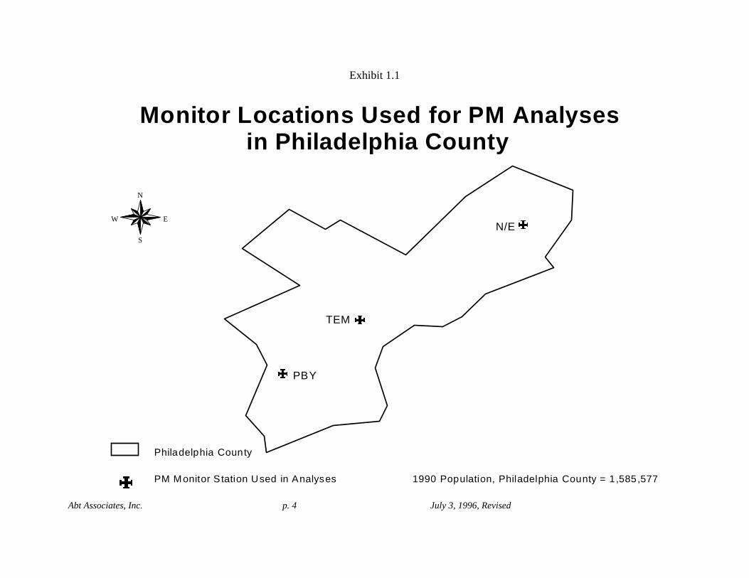
The two locations chosen for risk analysis are Philadelphia County, Pennsylvania andSoutheast Los Angeles County, California. The geographic region comprised, the populationencompassed within the region, and the placement of air quality monitors used in the riskanalysis are illustrated in Exhibit 1.1 for Philadelphia County and Exhibit 1.2 for Southeast LosAngeles County. A portion of southeastern Los Angeles County selected for use in the analysisincludes the portion of the county with the highest PM-10 levels. The region included in thisanalysis approximates the portion of the county reported to have an annual average PM-10 levelabove 40 :g/m3 in 1994 (from "Air Quality Standards Compliance Report," South Coast AirQuality Management District, 1995). The size and age distribution of the population livingwithin the selected region was estimated by totaling the population of U.S. Census block groupsfalling within the region. A block group is considered to be within the region if thepopulation-weighted centroid of the block group is within the boundary of the region.
Abt Associates, Inc. p. 4 July 3, 1996, Revised
N/E
PBY
TEM
N
EW
S
Monitor Locations Used for PM Analysesin Philadelphia County
Philadelphia County
1990 Population, Philadelphia County = 1,585,577PM Monitor S tation Used in Analyses
Exhibit 1.1

Abt Associates, Inc. p. 5 July 3, 1996, Revised
Diamond Bar
CentralLos Angeles
Lynwood
Pasadena
BurbankAzusa
West LosAngeles
Long Beach
N
EW
S
Geographic Region Used for PM Analysesin Southeast Los Angeles County
Los Angeles County
Boundary of PM Region
Other Monitoring Stations
1990 Population, LA County = 8,863,164
1990 Southeastern County Populationwithin Indicated Boundary = 3,635,984
PM Monitor Station Used in Analyses
Exhibit 1.2
Abt Associates, Inc. p. 6 July 3, 1996, Revised
Philadelphia County has virtually complete daily air quality data for both PM-10 andPM-2.5. For a one-year period from September 1992 through August 1993, monitor data forPM-10 are available for 98.6 percent of the days in the year, and monitor data for PM-2.5 areavailable for 96.4 percent of the days in the year. In addition, Philadelphia County has been thesite of extensive investigation of the health effects of air pollution.
Southeast Los Angeles County, a western location, provides a contrast to PhiladelphiaCounty in type of particulate matter. In addition, as in Philadelphia County, substantial airquality data for both PM-10 and PM-2.5 are available for Los Angeles. Finally, several healthstudies have been carried out in this city.
Numerous epidemiological studies are used in the risk analyses. Most studies focus onadverse effects associated with elevations in PM levels during short time periods. These studies,referred to as “short-term exposure” studies, draw current incidence levels primarily fromhospital and vital statistics records. The “long-term exposure” studies, on the other hand,evaluate mortality or morbidity in relation to long-term air quality, characterized by annual meanlevels of PM. These studies used large cohorts of adults with specifically defined characteristicswho were followed over years of observation. The health endpoints for which the largestnumber of studies are available are mortality, hospital admissions for pneumonia, hospitaladmissions for Chronic Obstructive Pulmonary Disease (COPD), and “total respiratory” hospitaladmissions. (The exact set of ICD codes included in “total respiratory” admissions varies fromstudy to study.)
In some cases, most notably in the case of mortality and PM-10, concentration-responserelationships have been estimated by several studies in the literature. For those health effects forwhich associations with PM have been estimated in several studies, ideally, the data sets fromthese studies could be combined and re-analyzed to produce a more robust estimate of PM healtheffects. When it is impossible to combine the data, however, there are various ways to pool theresults of the studies to derive a concentration-response function. One method, which is used inthis risk analysis, is described in Appendix 2.
In the first phase of the risk analysis, assessing the risk associated with “as is” ambientPM concentrations, the number of separate analyses is determined by the number of healthendpoint-PM indicator combinations for which concentration-response functions have beenestimated. In the second phase of the risk analysis, assessing the risk reduction associated withattaining possible alternative (sets of) standards, the number of separate analyses is determinedby the number of health endpoints and the number of (sets of) alternative standards considered. If there are N health endpoints and M sets of PM standards of interest, there is a maximum ofN*M analyses possible.

Abt Associates, Inc. p. 7 July 3, 1996, Revised
An overview of the major components of the PM risk analysis discussed in this report ispresented in Exhibit 1.3. Each separate analysis in the first phase of the risk analysis depends onthe following four basic components:
! air quality information,! information on the concentration-response relationship between the health endpoint of
interest and the PM indicator of interest in the location of interest;! baseline health incidence information for the location of interest; and! the size of the population living in the location of interest.
If the location is not in attainment of current PM standards (as in Los Angeles), the first phase ofthe risk analysis requires, prior to risk analysis,
! the simulation of attainment of current standards.
Each separate analysis in the second phase of the risk analysis depends on an additionalcomponent:
! the simulation of attainment of a set of alternative PM-2.5 standards.
There are substantive issues surrounding each of these components. These issues and approachesin the absence of complete information on any one or more of these risk analysis components arediscussed at length in the sections that follow.
The basic methods used in all the analyses, and methodological issues specific toparticular parts of the risk analysis (e.g., to one phase or the other), are discussed in Section 2. Because the risk analyses were carried out in the face of incomplete information, it wasnecessary to make assumptions at several points in the analysis process. These assumptions andthe various sources of uncertainty surrounding risk estimates are discussed in Section 3. Section4 discusses the Philadelphia County and Southeast Los Angeles County air quality data used inthe analyses, that is, the ambient PM-10 and PM-2.5 data from these locations. The PM-10 andPM-2.5 concentration-response functions used in the analyses are discussed in Section 5. Concentration-response functions in the epidemiological literature that were considered in therisk analysis are given in Section 5.1. The estimation of a distribution of concentration-responsefunctions (across locations), the estimation of a concentration-response function in any givenlocation, and the characterization of the uncertainty surrounding concentration-responsefunctions is discussed in Section 5.2. Section 6 presents baseline health effects incidence ratesfor each of the locations from vital statistics sources. These are the health effects incidence ratesassociated with “as is” PM levels.
In both phases of the risk analysis, there is substantial uncertainty. The results of theanalyses depend on a number of analytic choices and will change if different choices are made.

Abt Associates, Inc. p. 8 July 3, 1996, Revised
Exhibit 1.3 Major Components of Particulate Matter Health Risk Analysis
Ambient Population-oriented Monitoringfor Selected Cities
Air Quality AdjustmentProcedures
Alternative ProposedStandards
Changes inDistributionof PM AirQuality Risk Estimates:
• “As is”• “Alternative
Scenarios”
= Sensitivity Analysis: Analysis of effects of alternative assumptions, procedures or data occurs at these points.S
HealthRisk
Model
S
S
S
City-specific (or National)Baseline Health EffectsIncidence Rates (varioushealth endpoints)
S
Human EpidemiologicalStudies (various healthendpoints)
Concentration -ResponseRelationships
S S
“As is” Analysis

Abt Associates, Inc. p. 9 July 3, 1996, Revised
One way to assess the impact of particular analytic choices on the results of the risk analyses isthrough sensitivity analyses, in which the impact of different analytic choices on the results ofthe risk analysis is assessed.
The assessment of the risk associated with “as is” PM concentrations in PhiladelphiaCounty and Southeast Los Angeles (the first phase of the risk analysis) is presented in Section7. The results and associated sensitivity analyses are presented in Section 7.1. Monte Carlopropagation of uncertainty analyses, considering the uncertainty from several sources, arepresented in Section 7.2.
The assessment of the risk reduction associated with attaining possible alternative (setsof) standards in these two locations (the second phase of the risk analysis) is presented inSection 8. The results and associated sensitivity analyses are presented in Section 8.1. Othersensitivity analyses concerning the rollback method are presented in Sections 8.3. Alternativeforms of PM standards are considered in Section 8.3. Monte Carlo propagation of uncertaintyanalyses, considering the uncertainty from several sources, are presented in Section 8.4. Finally, issues of interpretation of the results of the risk analysis are discussed in Section 9.

Abt Associates, Inc. p. 10 July 3, 1996, Revised
Abt Associates, Inc. p. 11 July 3, 1996, Revised
2. Methods
This section describes the basic methods of the risk analysis. Conducting a risk analysisrequires substantial information. For each of the elements of the risk analyses described belowcomplete and certain information is not available, resulting in a significant degree ofuncertainty. The sources of uncertainty and the assumptions made to perform risk analyses inthe face of incomplete information are discussed in Section 3.
2.1. Overview
Each separate analysis in either the first phase or the second phase of the risk analysiscan be characterized as estimating the change in the incidence of a given health effect resultingfrom a given change in PM concentrations. In the first phase, risk analyses consider the healtheffects incidence associated with “as is” PM above either the lowest PM level observed in thestudy or background level. (In Los Angeles County, where “as is” concentrations do not meetcurrent PM standards, the health effects incidence associated with unadjusted “as is” PMconcentrations and the health effects incidence associated with “as is” PM concentrationsadjusted to simulate attainment of current standards are both considered.) This is equivalent toassessing the potential change in health effects incidence associated with a reduction in PMconcentrations from “as is” levels (in or out of attainment with current standards) to thespecified lower PM level (either the lowest observed in the study or background level).
In the second phase, risk analyses consider the change from “as is” PM concentrationsto those concentrations that would just attain a specified set of alternative PM standards. Themethod used in both phases of the risk analysis is therefore basically the same. The importantdifference between the two phases is in the specified alternative (lower) PM levels: in the firstphase the alternative air quality is either the lowest PM level observed in the study orbackground PM level, whereas in the second phase the alternative air quality is based onattainment of a set of alternative PM-2.5 standards. The first phase therefore requires either areported lowest observed PM level or an estimate of background PM (PM-10 and PM-2.5)level; the second phase requires that a method be developed to simulate attainment of thespecified standard(s). This method is applied to the first phase as well to simulate attainmentof current PM-10 standards where appropriate prior to risk analyses.
To estimate the change in the incidence of a given health effect resulting from a givenchange in ambient PM concentrations in a sample location, the following elements arenecessary:
(1) air quality data from the sample location to estimate both “as is” PMconcentrations and, for the second phase of the risk analysis, the concentrationsassociated with attainment of proposed PM standards;
(2) a concentration-response function estimating the relationship between ambientPM concentrations and the health endpoint in the sample location (preferably

Abt Associates, Inc. p. 12 July 3, 1996, Revised
derived in the same location, although functions estimated in other locations canbe used at the cost of increased uncertainty -- see Section 3.1.2); and
(3) an estimate of the baseline health effect incidence (rate) corresponding to “as is”PM levels (since most of the available concentration-response functions give apercent change in incidence rather than an absolute number of cases).
The change in the health endpoint may be measured as a daily change, corresponding tochanges in daily average ambient PM concentrations from “as is” levels to some alternativelevels (e.g., either background or those levels corresponding to attainment of a set ofstandards). Alternatively, the change in the health endpoint may be measured as an annualchange, corresponding to a change in the annual average PM concentration. Whenconcentration-response functions from short-term exposure studies are used, it is appropriate toassess daily effects. When concentration-response functions from long-term exposure studiesare used, it is appropriate to assess annual effects. When daily effects are calculated, thesedaily changes are aggregated, and, in the absence of PM data for all 365 days of the year,adjusted to reflect the total for the entire year, as described below. All changes in healtheffects, whether calculated on a daily or annual basis, are therefore aggregates for an entireyear. The risk analysis procedure described in more detail below is diagramed in Exhibit 2.1for analyses based on short-term exposure studies and Exhibit 2.2 for analyses based on long-term exposure studies.
Because there are substantive methodological issues involved in simulating theattainment of a set of standards (either current PM-10 standards or alternative PM-2.5standards), this is discussed separately in Section 2.2 below. The functional form of theconcentration-response relationships used in the risk analyses, and the prediction of changes inhealth effects incidence associated with changes in ambient PM concentrations using theseconcentration-response functions is described in Section 2.3. Issues involved in the calculationof annual health effects incidence are discussed in Section 2.4. A brief discussion of issuesinvolved in attaining baseline incidence rates is given in Section 2.5. Finally, the sensitivityanalyses carried out in both phases of the risk analysis, and any methodological issuespertaining to them, are described in Section 2.6.
2.2. Modeling attainment of alternative (or current) standards
Predicting the change in risk due to a change in air quality from an “as is” annual meanto meet a lower annual standard when using a concentration-response function from a long-term exposure study is straightforward: the “as is” mean is simply reduced to the standardlevel. In this case, simulating attainment of a standard does not involve generating analternative set of daily PM concentrations, because the concentration-response function

Abt Associates, Inc. p. 13 July 3, 1996, Revised
Flow Diagram of Typical Risk Analysis for Short-Term Exposure Studies
Obtain individual monitor PM
data
Identify background
PM Level
Identify functional form
Compute daily average PM
concentrations for available days
Compute change in PM on each dayPM concentration
is available Identify rollbackmethod or
cutpoint levels(for certain analyses)
Air Quality Data
Identify location- specificstudies
Obtain annuallocation-specific
baselinehealth incidence
Obtain populationexposed to
monitored PM
Identify Relative Risk
(RR) or slope coefficents (ß)
Calculate pooled
function(if necessary)
Convert RR to ß
(if necessary)
Concentration-Response Functions
Population
Baseline Health Incidence
Compute % changein health effectsassociated with
changes in PM foreach day on whichPM concentration
is available
Compute annual
# of cases
associated with
change in PM
Result:Percent change intotal incidence
Result:PM associatedincidence
Adjust to dailybaseline incidence
Compute total %change in health effects
by summing daily results, with missing
day corrections
Exhibit 2.1
Identify range of PM levels
in study

Abt Associates, Inc. p. 14 July 3, 1996, Revised
Flow Diagram of Typical Risk Analysis for Long-Term Exposure Studies
Obtain individual monitor PM
data
Identify background
PM Level
Identify functionalform
Compute daily average PM
concentrations for available days
Compute annualaverage
PM concentrations, with missing day
corrections
Compute changein annual
average PMIdentify rollback
method or cutpoint level
(for certainanalyses)
Air Quality Data
Identify location- specific studies
Obtain location-specific baselinehealth incidence
Obtain populationexposed to
monitored PM
Identify Relative Risk
(RR) or slope coefficents (ß)
Calculate pooled
function(if necessary)
Convert RR to ß
(if necessary)
Concentration-Response Functions
Population
Baseline Health Incidence
Compute % change
in health effectsassociated withchanges in PM
Compute # of cases
associated with
change in PM
Result:Percent change intotal incidence
Result:PM associatedincidence
Exhibit 2.2
Identify range of PM levels
in study

Abt Associates, Inc. p. 15 July 3, 1996, Revised
estimated in a long-term exposure study is based on annual, rather than daily PMconcentrations.
When a concentration-response function from a short-term exposure study is used,however, attainment of an alternative standard or set of standards is best simulated bychanging the distribution of daily PM concentrations. This section discusses the methods usedto change daily PM concentrations in a sample location to simulate the attainment of a newstandard or set of standards. The methods described below are also applicable to thesimulation of attainment of current standards when a location is not already in attainment, asdiscussed below.
An area is considered in attainment of a standard if all PM monitors in the area are inattainment. An area is in attainment of an annual standard if the annual average PMconcentration at each monitor in the area is at or below the standard. An area is in attainmentof a daily standard (which currently allows one exceedence) if no more than one monitor-dayexceeds the daily standard. Although it is possible to change the daily PM concentrations ateach monitor separately (to separate degrees) to simulate attainment, this would requireextensive analysis that is beyond the scope of this risk analysis. Therefore, although theamount or percent of reduction on a given day might be determined by the PM concentration ata single monitor on a single day, attainment is simulated by changing daily concentrationsaveraged over all monitors.
There are many different methods of reducing daily PM levels that would result inattainment of a given PM standard or set of standards. Preliminary analyses of historical PMdata found that year-to-year reductions in PM levels in a given location tended to be roughlylinear. That is, both high and low daily PM levels decreased proportionally. (This is discussedmore fully in the discussion of the sensitivity of results to the rollback method, in Section 8.)This suggests that, in the absence of detailed air quality modeling, it is reasonable to simulatePM reduction to bring a sample location into attainment of new proposed standards byproportional rollbacks (i.e., by decreasing PM levels on all days by the same percentage).
Proportional (linear) rollback is only one of many possible ways, however, to create analternative distribution of daily concentrations to meet new PM standards. One could, forexample, reduce the high days by one percentage and the low days by another percentage,choosing the percentages so that the new distribution achieves the new standard. At theopposite end of the spectrum from linear rollbacks, it is possible to meet a daily standard by“peak shaving.” The peak shaving method would reduce all daily PM concentrations above acertain concentration to that concentration (e.g., the standard) while leaving dailyconcentrations at or below this value unchanged. While a strict peak shaving method ofattaining a standard is unrealistic, it is illustrative of the principal that patterns different from aproportional rollback might be observed in areas attempting to come into compliance withrevised standards.

Abt Associates, Inc. p. 16 July 3, 1996, Revised
If the short-term exposure concentration-response functions were exactly linear, thenthe overall estimated change in health effects associated with short-term exposure woulddepend only on the total change in PM concentration (above the lowest level at which PMpollution causes health effects). Because the concentration-response functions beingconsidered are almost linear, the method by which daily PM concentrations are reduced tomeet annual standards makes almost no difference.
However, the method by which daily concentrations are reduced to meet dailystandards may make a sizeable difference, since it is the distribution of all the daily changes inair quality concentrations (above the lowest observed level at which PM pollution is associatedwith health effects) that results in the aggregate annual risk estimates. If one rollback methodresults in an air quality distribution with considerably more days with large changes in airquality than another method that also attains a given daily standard, the two methods willestimate significantly different health risks.
The estimated change in health effects based on short-term (daily) exposureconcentration-response functions, then, is sensitive to the reduction method only to the extentthat different reduction methods result in different total amounts of PM being removed fromthe atmosphere. Therefore, when the annual mean standard is the controlling standard (so agiven total amount of PM must be removed), results should be relatively insensitive todifferent reduction methods (and would be totally insensitive to the reduction method if theconcentration-response functions were exactly linear). When a daily standard is thecontrolling standard, however, results will be sensitive to different reduction methods.
Attainment of a set of standards was simulated by proportional rollback. That is,average daily PM concentrations were reduced by the same percentage on all days. Becausepollution abatement methods are applied largely to anthropogenic sources of PM, rollbackswere applied only to PM above estimated background levels. (Rollbacks were estimated onlyfor PM-2.5. Background PM-2.5 concentrations were estimated as 3.5 :g/m3 in PhiladelphiaCounty, and 2.5 :g/m3 in Southeast Los Angeles County. This is consistent with the approachof the Criteria Document.) The percent reduction was determined by the controlling standard. For example, suppose both an annual and a daily PM-2.5 standard are proposed. Suppose pa isthe percent reduction required to attain the annual standard, i.e., the percent reduction of dailyPM above background necessary to get the annual average at the monitor with the highestannual average down to the standard. Suppose pd is the percent reduction required to attain thedaily standard with one exceedence, i.e., the percent reduction of daily PM above backgroundnecessary to get the second highest monitor-day down to the daily standard. If pd is greaterthan pa, then all daily average PM concentrations above background are reduced by pd percent. If pa is greater than pd, then all daily average PM concentrations are reduced by pa percent. Information on controlling monitors and percent rollbacks necessary to simulate attainment ofalternative PM-2.5 standards in Philadelphia County and Southeast Los Angeles County isgiven in Exhibits 2.3 and 2.4.

Abt Associates, Inc. p. 17 July 3, 1996, Revised
Because the reduction method to attain a daily standard could have a significant impacton the risk analysis results, sensitivity analyses were conducted on different rollback methodsfor meeting proposed standards. The results of these analyses are presented in Section 8.
Exhibit 2.3. Controlling Monitors for Rollbacks to Attain Alternative PM-2.5 Standards
Monitor Site Weighted AnnualAverage PM-2.5Concentration*
Second DailyMaximum 24-Hour
PM-2.5Concentration*
Controlling Monitor
Philadelphia County
N/E 15.5 65.1
PBY 16.7 72.2 For daily standard
TEM 17.1 70.0 For annual standard
Southeast Los Angeles County
Central LA 24.1 91.1 For annual standard
Diamond Bar 21.9 101.7 For daily standardAll concentrations are given in :g/m3 .*Both weighted annual averages and second dailymaximum concentrations at the two monitors in Southeast Los Angeles County were adjustedto reflect attainment of the current PM-10annual standard of 50 :g/m3 and the current PM-10daily standard of 150 :g/m3. These standards are currently attained in Philadelphia County.

Abt Associates, Inc. p. 18 July 3, 1996, Revised
Exhibit 2.4. Controlling Standards and Percent Rollbacks Necessary to Attain Alternative PM-2.5 Standards
Alternative PM-2.5Standards
Philadelphia County Southeast Los Angeles County
Annual Avg.Standard
24-HourStandard
Controlling Standard and Percent Rollback*
Controlling Standard and Percent Rollback**
20 alone ---- Annual -- 18.8%
20 65 Daily -- 10.4% Daily -- 37.0%
20 50 Daily -- 32.3% Daily -- 52.1%
20 25 Daily -- 68.7% Daily -- 77.3%
15 alone Annual -- 15.5% Annual -- 42.0%
15 65 Annual -- 15.5% Annual -- 42.0%
15 50 Daily -- 32.3% Daily -- 52.1%
15 25 Daily -- 68.7% Daily -- 77.3%All concentrations are given in :g/m3 .*Based on controlling values for Philadelphia County of 17.1 :g/m3 for the annual standardand 72.2 :g/m3 for the daily standard.** Based on controlling values for Southeast Los Angeles County of 24.1 :g/m3 for the annualstandard and 101.7 :g/m3 for the daily standard.
The linear rollback methods described above to simulate attainment of alternative setsof PM-2.5 standards are also used to simulate attainment of current PM-10 standards prior toanalyses in both the first and second phases of the risk analysis for Southeast Los AngelesCounty, which is out of attainment for current standards. Analyses for PM-10 in the firstphase of the risk analysis use exactly the rollback method described above. Analyses for PM-2.5 in the first and second phases of the risk analysis assume that PM-2.5 is rolled backproportionately to PM-10 rollbacks. If, for example, daily PM-10 concentrations are decreasedby 10 percent to simulate attainment of current PM-10 standards, it is assumed that daily PM-2.5 concentrations decrease by 10 percent as well. It is these adjusted PM-2.5 concentrations,the “as is” PM-2.5 concentrations in attainment of current standards, that are then reducedagain by proportional rollback methods to simulate the attainment of alternative PM-2.5standards in the second phase of the risk analysis. The adjustment of PM-10 and PM-2.5concentrations in Southeast Los Angeles County to simulate attainment of current PM-10standards is summarized in Exhibit 2.5.

5Although, as noted above, epidemiological studies might prefer to estimate individual exposure-responserelationships, because of the lack of individual exposure data, these studies typically estimate the ambientconcentration-response relationship instead. Although this is not necessarily the relationship of ultimate interest tohealth scientists, it is the relationship that is appropriate to use in the PM risk analysis with ambient PM data.
Abt Associates, Inc. p. 19 July 3, 1996, Revised
Exhibit 2.5. Adjustment of PM Concentrations in Southeast Los Angeles County to Simulate Attainment of Current PM Standards
Unadjusted Concentrations Concentrations adjusted for compliance withcurrent PM-10 standards
(21.8 % rollback above background required toreduce second daily max. to the standard )
PM-10
Monitor Annual Mean 24-hr 2nd high Annual Mean 24-hr 2nd high
CELA 51.7 195.2 41.8 154.0
DBAR 46.1 170.7 37.4 134.8
Controlling 51.7 195.2 41.8 154.0
PM-2.5
Monitor Annual Mean 24-hr 2nd high Annual Mean 24-hr 2nd high
CELA 30.1 115.7 24.1 91.1
DBAR 27.3 129.3 21.9 101.7
Controlling 30.1 129.3 24.1 101.7All concentrations are given in :g/m3.The adjustment was performed assuming background concentrations of 6 :g/m3 for PM-10, and 2.5 :g/m3 for PM-2.5. Both the PM-10 annual mean and 2nd daily maximum PM-10 concentration exceed current standards: 50:g/m3 and 150 :g/m3 respectively. Since levels of 54 :g/m3 and 154 :g/m3 are de facto considered to be incompliance, meeting the annual standard requires no rollback. However, meeting the daily standard requires aproportional rollback of (195.2-154.0)/(195.2-6.0) = 21.8% of air quality concentrations above background. (The6.0 in the denominator takes into account that only concentrations above background are reduced.) This rollbackwas applied to the PM concentrations above 6 :g/m3, and to the PM-2.5 concentrations above 2.5 :g/m3.
2.3. The concentration-response function and estimation of health effect incidence changes
The concentration-response functions used in this risk analysis are empiricallyestimated relationships between average ambient concentrations of the pollutant of interest(PM-10 or PM-2.5) and the health endpoints of interest (e.g., mortality or hospital admissions)reported by epidemiological studies.5 The choice of studies is discussed in Section 5. In somecases, separate risk analyses were performed using the concentration-response functions fromseparate studies; in other cases, only a “pooled function” derived from several studies of thesame health endpoint was used.

6Poisson regression is essentially a linear regression of the natural logarithm of the dependent variable onthe independent variable, but with an error structure that accounts for the particular type of heteroskedasticity thatis believed to occur in health response data. What matters for the risk analysis, however, is simply the form of theestimated relationship, as shown in equation (1).
Abt Associates, Inc. p. 20 July 3, 1996, Revised
(1)
(2)
(3)
Although some epidemiological studies estimated linear concentration-responsefunctions, most of the studies used a method referred to as “Poisson regression” to estimateexponential concentration-response functions in which the natural logarithm of the healthendpoint is a linear function of PM6:
where x is the ambient PM level, y is the incidence of the health endpoint of interest at PMlevel x, $ is the coefficient of ambient PM concentration, and B is the incidence at x=0, i.e.,when there is no ambient PM. The relationship between a specified ambient PM level, x0, forexample, and the incidence (rate) of a given health endpoint associated with that level (denotedas y0) is then
Because the exponential form of concentration-response function (equation (1)) is by far themost common form, the discussion that follows assumes this form. However, because thecoefficients estimated by the epidemiology studies are extremely small, these exponentialfunctions are nearly linear. The consequences of this near-linearity are discussed below.
Ambient PM levels may be based on any averaging time, e.g., they may be dailyaverages or annual averages, as long as the health effect incidence corresponds to the PMaveraging time. For example, the concentration-response function may describe therelationship between daily average ambient PM concentrations and daily mortality, or it maydescribe the relationship between annual average ambient PM concentrations and annualmortality. Some concentration-response functions were estimated by using moving averagesof PM to predict daily health effects incidence. Such a function might, for example, relate theincidence of the health effect on day t to the average of PM concentrations on days t and (t-1). (This may be considered a variant on the short-term, or daily concentration-response function.) The discussion below does not indicate averaging times and simply assumes that the measureof health effect incidence, y, is consistent with the measure of ambient PM concentration, x.
The change in health effects incidence, )y = y0 - y, from y0 to the baseline incidencerate, y, corresponding to a given change in ambient PM levels, )x = x0 - x, can be derived fromequations (1) and (2) (as shown in Appendix 3) as

Abt Associates, Inc. p. 21 July 3, 1996, Revised
(4)
Alternatively, the change in health effects incidence can be calculated indirectly usingrelative risk. Relative risk (RR) is a well known measure of the comparative health effectsassociated with a particular air quality comparison. The risk of mortality at ambient PM levelx0 relative to the risk of mortality at ambient PM level x, for example, may be characterized bythe ratio of the two mortality rates: the mortality rate among individuals when the ambient PMlevel is x0 and the mortality rate among (otherwise identical) individuals when the ambient PMlevel is x. This is the relative risk for mortality associated with the difference between the twoambient PM levels, x0 and x. Given a concentration-response function and a particular changein ambient PM levels, )x, the relative risk associated with that change in ambient PM, denotedas RR)x, is equal to e$)x . The change in health effects incidence, )y, corresponding to a givenchange in ambient PM levels, )x, can then be calculated based on this relative risk:
Equations (3) and (4) are simply alternative ways of writing the relationship between a givenchange in ambient PM levels, )x, and the corresponding change in health effects incidence,)y. The derivation of equation (4) is shown in Appendix 3. These equations are the keyequations that combine air quality information, concentration-response information, andbaseline health effects incidence information to estimate ambient PM health risk.
Given a concentration-response function and air quality data (ambient PM values) froma sample location, then, the change in the incidence of the health endpoint ()y = y0 - y)corresponding to a change in ambient PM level of )x = x0 - x is determined. This can either bedone with equation (3), using the coefficient, $, from a concentration-response function, orwith equation (4), by first calculating the appropriate relative risk from the concentration-response function.
Because the estimated change in health effect incidence, )y, depends on the particularchange in PM concentrations, )x, being considered, the choice of PM concentration changeconsidered is important. These changes in PM concentrations are generally reductions from the current levels of PM (“as is” levels) to some alternative, lower level(s).
If a location is not in attainment of current PM standards, as is the case in SoutheastLos Angeles County, current levels may be characterized in two ways. It may be of interest tocompare health effects at “as is” PM concentrations (that do not attain the current standards)with health effects at some alternative PM level(s). Alternatively, it is also of interest tocompare health effects at those PM concentrations that just attain the current PM-10 standardswith health effects at those PM concentrations that just attain some alternative (PM.2.5)standards. This is an appropriate context for examining the potential risk reductions associatedwith revising the current standard.
The first and second phases of the risk analysis are distinguished primarily by thechoice of lower PM level(s). The second phase considers the changes in health effects

Abt Associates, Inc. p. 22 July 3, 1996, Revised
incidence associated with changes from PM concentrations that meet the current standards toPM concentrations that just meet alternative PM-2.5 standards.
When possible, the choice of lower PM level(s) in an analysis in the first phase of therisk analysis is the lowest PM concentration observed in the study that estimated theconcentration-response function used in the risk analysis. This is the lowest PM concentrationat which the concentration-response function is supported. However, many of the short-termexposure PM studies do not report the lowest observed PM concentration. (For example,many studies report the lowest decile or quartile values.) When the lowest observed PMconcentration is not reported (or if it is lower than background level), analyses in the firstphase of the risk analysis consider the range of “as is” PM concentrations in the samplelocation down to background PM concentration in that location.
In contrast to most short-term exposure studies, long-term exposure studies routinelyreport the lowest observed annual average PM concentration. Risk analyses that use long-termexposure concentration-response functions therefore consider the range of “as is” annualaverage PM in the sample location to the lowest annual average PM level observed in thestudy.
In both phases of the risk analysis, the ambient PM concentrations to which “as is”ambient PM concentrations are compared are generally lower than or equal to “as is”concentrations. Therefore )x = x0 - x is negative (or zero), and so the corresponding change inincidence of health effects, )y, is also negative (or zero). That is, there are fewer cases of anygiven health effect at lower ambient PM levels. Alternatively, -)y may be interpreted as thehealth effects attributable to PM concentrations between x0 and x.
Because different epidemiological studies report different estimated concentration-response functions for a given health endpoint, predicted changes in health effects incidencesdepend on the concentration-response function used. The uncertainty introduced into the riskanalyses by this is assessed both through sensitivity analyses and through Monte Carlomethods (see Section 9).
2.4. Calculating the aggregate health effects incidence on an annual basis from the changes in daily health effects incidence
To assess the daily health impacts of daily average ambient PM levels abovebackground or above the levels necessary to achieve a given standard, concentration-responsefunctions from short-term exposure studies were used together with estimated changes in dailyambient PM concentrations to calculate the daily changes in the incidence of the healthendpoint. Adding these changes over all the days in a year yields the annual change. (Alternative assumptions about the range of PM levels associated with health effects wereexplored in sensitivity analyses. When a minimum concentration for effects is considered,reductions below this concentration do not contribute attributable cases to the calculation. Only reductions down to this concentration contribute attributable cases to the calculation.)
Abt Associates, Inc. p. 23 July 3, 1996, Revised
After daily changes in health effects are calculated, an annual change is calculated bysumming the daily changes. However, there are some days for which no ambient PMconcentration information is available. The predicted estimated risks, based on those days forwhich air quality data are available, must be adjusted to take into account the full year.
In Philadelphia County, there are very few missing days, and these are distributedevenly throughout the year. In this case, the adjusted health effects incidence is the originalincidence multiplied by the number of days in a year and divided by the number of days forwhich data are available; that is, the figure is simply scaled for the fraction of days on whichthere are data. In Philadelphia County, for example, PM-10 data are available for 358 daysevenly distributed throughout the year. Suppose the sum of the daily premature deathsassociated with PM on those 358 days is 600, then the adjusted figure is 612 (i.e., 600 x365/358). This reflects the assumption that the distribution of PM concentrations on thosedays for which data are available accurately reflects the distribution of ambient PMconcentrations for the entire year, and that the concentration-response functions wereestimated using data from the entire year.
In Southeast Los Angeles County, however, the distribution of missing days variessignificantly in different periods of the year. During the first quarter of 1995, air qualitymonitoring was done on roughly one in six days; during the second quarter, it was done onroughly one in three days; and during the third and fourth quarters, it was done almost everyday. Because of this, adjustments were made separately in each quarter, and the results added. Adjustment of health effects incidence within a quarter in Southeast Los Angeles County wasdone with the same method used to adjust health effects incidence throughout the year inPhiladelphia County.
Some concentration-response functions are based on average PM levels during severaldays. When these concentration-response functions are used, the air quality data are averagedfor the same number of days. For example, a function based on two-day averages of PMwould be used in conjunction with two-day averages of PM in the sample location to predictthe incidence of the health effect in that location. In some cases, intervals of three or moreconsecutive days in a given location are missing data, and so no multi-day average is availablefor use with multi-day concentration-response functions. These cases were treated by multi-day functions just as individual missing days were treated by single-day functions: theycontributed no cases to the risk analysis, and figures were adjusted for the days on whichmulti-day averages were missing.
Concentration-response functions from long-term exposure studies were used to assessthe annual health impacts of changes in annual average ambient PM concentrations. In thiscase, the “as is” annual concentration is simply the average concentration for those days onwhich data are available, if missing days are evenly distributed throughout the year (as inPhiladelphia County), or a composite of quarterly averages if missing days are not evenlydistributed throughout the year (as in Southeast Los Angeles County).

Abt Associates, Inc. p. 24 July 3, 1996, Revised
Note that while the long-term exposure studies use annual average PM concentration asthe PM indicator, the studies were conducted in such a way that they may have detected effectsdue to PM exposure over some longer period. For example, average PM concentrations overthe course of five years might be the appropriate measure. It is therefore possible that the fullbenefits of reducing PM predicted by these studies would not appear in the first year afterreductions to attain a standard, but would be “phased in” gradually as concentrations duringsuccessive years were also reduced. If average PM concentrations over five years is theappropriate measure, for example, the benefits of a standard would gradually increase to theirfull level over the course of the five years after the new standard had been attained. The riskanalysis makes no attempt to determine the appropriate exposure period for long-termexposure studies. The estimated annual benefits of reduced long-term exposure are assumed tobe completely achieved by the future year for which attainment of the new standard is beingmodeled. The issue is partially addressed, however, in a sensitivity analysis which examinesthe effect of altering the “slope” parameter in the long-term exposure concentration-responsefunction.
2.5. Baseline health effects incidence data
Baseline health effects incidence rates (e.g., death rates) and population sizes (tocalculate baseline incidence levels) for the selected locations were obtained from vital statisticssources. Location-specific information was used whenever possible. However, location-specific baseline incidence data for hospital admissions and other morbidity endpoints are notas readily available as for mortality from national data sources. Where possible, local sourcesof data (e.g., from city, county or state health agencies) were obtained. However, such data arenot uniformly available, and alternative procedures were used in some instances. Forrespiratory symptom or illness health endpoints, routine surveillance and reporting is notgenerally conducted in metropolitan areas, in contrast to the data gathered on mortality andhospital admissions. For these endpoints, estimates of baseline incidence were derived fromthe studies themselves to provide what should be viewed as only a rough estimate ofmagnitude of potential effects, given the much greater degree of uncertainty concerningbaseline incidence information for these endpoints. The baseline health effects incidence dataare presented and discussed more fully in Section 6.
2.6. Sensitivity analyses
The predictions of the risk analyses depend on the input components discussed above. Changes in the values of these input components change the predictions of the analyses. Thisis an important issue in risk analysis because the true values of parameters necessary for suchanalyses, e.g., the location-specific concentration-response relationships and the location-specific baseline health effects incidence rates, are often not known exactly and must beestimated. The sensitivity of the results of an analysis to changes in the values of the input

Abt Associates, Inc. p. 25 July 3, 1996, Revised
components (or in assumptions or procedures that affect these values) is therefore an importantconsideration.
The uncertainty associated with having to estimate parameter values can be assessed byuncertainty analyses, in which the probability distribution of values for an input component isestimated, and the resulting distribution of possible outcomes is assessed. Uncertainty analysesto assess the uncertainty associated with key parameters of the risk assessment model, focusingprimarily on the concentration-response function, are discussed in Section 9.
Alternatively, sensitivity analyses can be used to illustrate the sensitivity of analysisresults to different possible input values or to different assumptions or procedures that mayaffect these input values. Although a sensitivity analysis is not as comprehensive as anuncertainty analysis, selecting only a few possible alternative values of an input componentrather than characterizing the entire distribution of these values, it is precisely the simplicity ofa sensitivity analysis that makes it preferable for illustrating the impact on results of usingdifferent input component values. Exhibit 2.6 lists the sensitivity analyses carried out for eachof the two phases of the risk analysis. The results of those sensitivity analyses pertaining tothe first phase of the risk analysis (the “as is” analyses) are presented in Section 7; the resultsof those sensitivity analyses pertaining to the second phase of the risk analysis (the alternativestandards analyses) are presented in Section 8.

Abt Associates, Inc. p. 26 July 3, 1996, Revised
Exhibit 2.6. Sensitivity Analyses
Sensitivity analyses associated with the “as is” risk analyses:
1. Sensitivity analysis of the effect of alternative assumed background levels on predicted health effects associated with “as is” PM (PM-10 and PM-2.5) above background.
2. Sensitivity analysis of the effect of using alternative “hockey stick” models on predicted short-term exposure health effects associated with “as is” PM concentrations above specified model cutpoints.
3. Sensitivity analysis of the effect of alternative cutpoints (PM levels below which health effects incidence is not considered) on predicted long-term exposure health effects associated with “as is” PM above cutpoint.*
4. Sensitivity analysis of the effect of combining different averaging times in pooled short-term exposure mortality concentration-response functions on predicted health effects associated with “as is” PM-10 concentrations above background.*
5. Sensitivity analysis of the effect of using concentration-response functions for short- term mortality from different individual studies on predicted health effects associated with “as is” PM-10 and PM-2.5**
6. Sensitivity analysis of the effect of copollutants in the concentration-response model on the predicted relative risk for a change in PM-10 concentration of 50 :g/m3 and a change in PM-2.5 concentration of 25 :g/m3.
7. Sensitivity analysis of the effect of copollutants in the concentration-response model on the predicted health effects associated with “as is” PM above background.
8. Sensitivity analysis of the effect of historical previous air quality on estimated mortality associated with long-term exposure to PM-2.5.*
Sensitivity analyses associated with the alternative standards analyses:
9. Sensitivity analysis of the effect of different background levels on rollbacks required to simulate attainment of alternative PM-2.5 standards.
10. Sensitivity analysis of the effect of different rollback methods to simulate attainment of alternative PM-2.5 standards.*
*Sensitivity analysis done for Philadelphia County only. With the exception of sensitivity analysis number 6,which is not specific to any location, other analyses were done for both Philadelphia County and Southeast LosAngeles County (see Exhibit 7.5).**A preliminary (unpublished) study of short-term exposure mortality has been conducted in Philadelphia for PM-2.5 (Dockery et al., Abstr., 1996). The results of this study are compared with the results obtained by using thepooled analysis function separately in Section 7. This study is not included, however, among the studies in thissensitivity analysis and is not included in the main results because it is not yet published.

Abt Associates, Inc. p. 27 July 3, 1996, Revised
3. Assumptions and Caveats
To carry any risk analysis to completion in the face of incomplete information, it isnecessary to make a variety of assumptions. The necessity of making simplifying assumptionscharacterizes most scientific analyses, because analysis is usually performed with only limitedinformation. Some of the assumptions necessary in the risk analyses are assumptionsgenerally made in scientific analyses (for example, that the model used to describe therelationship between variables does accurately describe this relationship). Other assumptionsare specific to these risk analyses. (Assumptions may be characterized instead as caveats: thevalidity of the results of the analysis depend in part on the extent to which the underlyingassumptions are valid.)
The risk analyses discussed in this report are only as good as the inputs to the analyses -- that is, the concentration-response functions, the air quality data, the health effects incidencerates, and the population sizes. The quality of each component is stated as an assumption or,alternatively, discussed as a caveat. Other assumptions/caveats concerning how each of thethree analysis components are used in the risk analyses are discussed below in turn. For manyof the uncertainties, it is not known whether the factors discussed might lead to over- or under-estimates of risk. Exhibit 3.1 summarizes some of the key uncertainties in the risk analysis,which are discussed in more detail below.
3.1. Concentration-response functions
The concentration-response function is a key element of risk assessment. The qualityof the risk analysis depends, in part, on (1) how well the concentration-response functions usedin the risk analyses have been estimated (e.g., whether they are unbiased estimates of therelationship between the health response and ambient PM concentration in the study locations),(2) how applicable these functions are to locations and times other than those in which theywere estimated, and (3) the extent to which these relationships apply beyond the range of thePM concentrations from which they were estimated. These issues are discussed in thesubsections below.
3.1.1. Accuracy of the estimates of concentration-response functions
The adequacy of the estimation of the relationships between PM and various healthendpoints in epidemiological studies has received considerable attention. A significant portionof this attention has focused on the issue of using average ambient PM concentration as ameasure of actual exposure to PM. Although they might prefer to estimate the individualexposure-response relationship, such studies are actually estimating the concentration-responserelationship, as discussed in Section 1. Concern that this practice may produce biasedestimates of individual exposure-response relationships may be valid. However, because therisk analysis examines the association between changes in health effects incidence and changesin ambient PM concentrations, (ambient) concentration-response functions, rather than

Abt Associates, Inc. p. 28 July 3, 1996, Revised
Exhibit 3.1. Key Uncertainties in the Risk Analysis
UncertaintyDirection of
PotentialError
Comments
Empirically estimatedconcentration-responserelationships
? Statistical association does not prove causation. Becauseconcentration-response functions are empirically estimated,there is uncertainty surrounding these estimates. Omittedconfounding variables could cause upward bias.
Functional form ofconcentration-responserelationship
? Statistical significance of coefficients in an estimatedconcentration-response function does not necessarily meanthat the mathematical form of the function is the best modelof the true concentration-response relationship.
Transferability of concentration-response relationships
? Concentration-response functions may not be valid in timesand places other than those in which they were estimated.
Extrapolation of concentration-response relationships beyondobserved data range
+ A concentration-response relationship estimated by anepidemiological study may not be valid at concentrationsoutside the range of concentrations observed during the study.
Adequacy of PMcharacterization
? Only particle mass per unit volume has been considered, andnot, for example, chemical composition or any other particlecharacteristics.
Accuracy of PM massmeasurement
? Possible differences in measurement error, losses of particularcomponents, and measurement method between the two riskanalysis locations and between these locations and theoriginal studies would be expected to add uncertainty toquantitative estimates of risk.
Adjustment of air qualitydistributions to reflect attainmentof proposed alternative standards
? There is uncertainty in the pattern and extent of reductions indaily PM concentrations that would take place to attainproposed standards.
Baseline health effects data ? Data may not be exactly appropriate for a variety of reasons. For example, location- and age-group-specific baseline ratesmay not be available in all cases. Baseline incidence maychange over time for reasons unrelated to PM.
Sensitive subgroups ? Populations in the sample locations may have more or fewermembers of sensitive subgroups than locations in whichfunctions were derived. Thus functions might not beappropriate. (This is a subset of the uncertainty associatedwith transferring concentration-response functions from onelocation to another (see above).
Omitted effects - Some health effects caused by PM may have been omitted.

Abt Associates, Inc. p. 29 July 3, 1996, Revised
individual exposure-response functions, are relevant to the analysis discussed in this report. The important question here, then, is whether epidemiological studies have produced accurate,unbiased estimates of ambient concentration-response functions.
The accuracy of an estimate of a concentration-response function reported by a studydepends on the study design. The Criteria Document has evaluated the substantial body of PMepidemiological studies. In general, critical considerations in evaluating the design of anepidemiological study include the adequacy of the measurement of average ambient PM, theadequacy of the health effects incidence data, and the consideration of potentially importanthealth determinants and causal factors such as:
! copollutant air quality;! exposure to other health risks, such as smoking and occupational exposure;! demographic characteristics, including age, sex, socioeconomic status, and
access to medical care; and! population health status independent of PM air quality.
Other specific characteristics of concern depend on the health endpoints in the studies. Studyselection for the risk analysis was guided by the evaluations in the PM Criteria Document(EPA, 1996a).
Concentration-response functions may not be identical for all members or all subgroupsof a population; however, the concentration-response functions used in the risk analysis reflectoverall population responses at air quality levels similar to those found in the sample locations(see Section 3.1.3).
To the extent that the studies did not address all critical factors, the concentration-response functions may be limited. They may result in either over- or underestimates of riskassociated with ambient PM concentrations in the locations in which the studies were done. Itis possible, then, that their application to the sample locations in the risk analyses might alsohave resulted in biased estimates of risk in those locations.
One possible source of bias in the estimation of concentration-response functionswarrants special note. A concentration-response function could be biased if the measurementof average ambient PM concentration is inaccurate in a systematic way. Most epidemiologicalstudies use the average PM levels reported at some number of PM monitors as the measure ofthe average ambient PM concentration (which, for the purposes of the studies, is itself asurrogate for individual exposure to PM). This may or may not yield accurate measurementsof the actual daily average ambient PM concentrations in the study city. Depending on howthe monitors are placed, it could yield systematically inaccurate, or biased measurements. What is important for the purpose of the risk analysis, in this case, is that the measurement ofdaily average ambient PM concentrations in the sample location be biased in the same way asin the study city. That is, a systematic bias in the measurement of daily average ambient PMconcentrations in the study city is not a problem for the risk analysis if there is the same

Abt Associates, Inc. p. 30 July 3, 1996, Revised
systematic bias in the measurement of daily average ambient PM concentrations in the samplelocation. Whether this is the case, however, is unlikely to be known.
3.1.2. Applicability of concentration-response functions in different locations The method described in Section 2 combines PM data from a single year in a specific
location (the sample location) with a concentration-response relationship estimated by anepidemiological study to predict the change in incidence of a given health endpoint associatedwith a given change in ambient PM concentrations in that location. Preferably, thisconcentration-response function is obtained from a study conducted in the sample locationitself. However, if no such study is available, a concentration-response function derived froma study that was performed in a different location (or a pooled analysis concentration-responsefunction derived from several such studies) is used. The precision of these predictionstherefore rests in part on the “transferability” of the concentration-response relationship fromone location to another. That is, it rests on the assumption that the relationship betweenambient PM (either PM-10 or PM-2.5) and a given health endpoint is the same in the twolocations.
The relationship between average ambient PM concentration and the incidence of agiven health endpoint, the concentration-response relationship, depends on (1) the relationshipbetween individual exposure and average ambient PM concentration and (2) the relationshipbetween the health response and individual exposure (as described formally in Appendix 1). One or both of these relationships may depend on the exposed population (for example, theextent of susceptible subgroups) and/or the composition of the PM and other air qualityindicators to which the population is exposed. Both the population and the composition of PMand other air quality indicators could vary significantly from one location to another. In thiscase, the concentration-response relationship could vary significantly from one location toanother as well. There are various reasons why one or both of the relationships upon whichthe concentration-response relationship depends might vary from one location to another.
The relationship between individual exposure and average ambient PM concentrationmight differ among locations if people’s behavior patterns differ significantly from onelocation to another. Suppose, for example, people in the study city spend a lot more timeoutdoors than people in the sample location. Suppose also that ambient (outdoor)concentrations of PM are greater in both locations than indoor concentrations. Then a givenambient PM concentration will be associated with higher individual exposures among peoplein the study location than among people in the sample location.
Suppose, alternatively, that coarse particles are less likely to infiltrate indoor air. Inthis case, PM-10 with a high proportion of coarse particles would result in lower indoorexposure than PM-10 with a high proportion of fine particles. If the percent of time spentindoors is the same in different locations, then the location with the coarser PM-10 would havelower individual exposure to PM-10 than the location with the finer PM-10.

Abt Associates, Inc. p. 31 July 3, 1996, Revised
The relationship between the health response and individual exposure might differamong locations if, for example, the population in one location has a higher proportion of asusceptible subgroup than another location. Closely matching populations used in studies tothe populations of the sample locations is not possible for many characteristics (for example,smoking status, workplace exposure, socioeconomic status, and the prevalence of highlysusceptible subgroups).
Alternatively, the PM-10 in one location may be largely fine particles (PM-2.5),whereas in another location it may be made up predominantly of coarse particles. If PM-2.5 ismore potent than coarse particles in causing the health effect, then there will be a greaterincidence of the health effect corresponding to a given level of individual exposure to PM-10in the first location, all else equal, than in the second location (see Appendix 4).
Other pollutants, such as carbon monoxide and ozone, may also play a role in causinghealth effects, either independently or in combination with PM. Interlocational differences inthese pollutants could also induce differences in the concentration-response relationshipbetween one location and another.
In summary, the concentration-response relationship in one location may not be thesame as the concentration-response relationship in another location. Even if the relationshipbetween the health response and individual exposure is the same in both locations, therelationship between individual exposure and ambient concentrations may differ between thetwo locations. Similarly, even if the relationship between individual exposure and ambientconcentrations is the same in both locations, the relationship between the health response andindividual exposure may differ between the two locations. In either case, the concentration-response relationship would differ.
Instead of a single concentration-response function that characterizes the relationshipbetween ambient PM (either PM-10 or PM-2.5) and a given health endpoint everywhere in theUnited States, then, a more realistic model may be a distribution of concentration-responsefunctions, or, equivalently, a distribution of values of the parameter $ in the concentration-response function. If concentration-response functions were available for all health endpointsfor each of the sample locations, the precision of the risk analyses would be improved. Thenecessity of applying concentration-response functions estimated in locations other than thesample locations for which risk is being analyzed introduces uncertainty into the results of therisk analyses. This is particularly apparent in the case of mortality, for which there are manyestimated concentration-response functions. The degree of this uncertainty is assessed byMonte Carlo methods, as described in Section 9.
The uncertainty associated with the application of concentration-response functionsfrom epidemiological studies to the sample locations is nonetheless smaller than theuncertainty associated with the use of concentration-response functions from animal studies. Such studies are often used in risk assessments, especially when epidemiological results arenot available, but are not used in the risk analysis described in this report.

7Although the concentration-response functions are exponential, they are practically linear. It is stillunlikely, however, that a linear function is appropriate over a very wide range of PM concentrations.
Abt Associates, Inc. p. 32 July 3, 1996, Revised
3.1.3. Extrapolation beyond observed air quality levels
Although a concentration-response function describes the theoretical relationshipbetween ambient PM and a given health endpoint for all possible PM levels (down to zero), theestimation of a concentration-response function is based on real ambient PM values that arelimited to the range of PM concentrations in the location in which the study was conducted. The actual shape of the concentration-response function is not known outside the observed airquality range. Several of the mortality studies discussed in the Criteria Document (EPA,1996a), including Pope et al.(1992), reported measured PM-10 levels as low as 4 :g/m3. Nonetheless, the concentration-response relationship may be less certain towards the lower endof the concentration range if few days had such low concentrations.
The risk analyses assume that the estimated concentration-response functionsadequately represent the true concentration-response relation down to background levels in thesample locations, in cases in which this background level is above the lowest concentrationsused to derive the concentration-response functions. For studies in which the lowestconcentrations studied are likely to be above background (e.g., the long-term exposure study ofPope et al. 1995) estimates of risk are not generated for concentrations below the minimumconcentrations observed in the studies. The estimates of risk for the lowest concentrationsconsidered are more uncertain than the estimates for concentrations in the middle of the rangeof study data.
The concentration-response relationship may also be less certain towards the upper endof the concentration range being considered in a risk analysis, particularly if the PMconcentrations in the sample location exceed the PM concentrations observed in the studylocation. Even though it may be reasonable to model the concentration-response relationshipas exponential over the ranges of PM concentrations typically observed in epidemiologicalstudies, it is unlikely to be exponential over a very wide range of PM levels.7 Rather, at veryhigh PM concentrations, the concentration-response function is likely to begin to flatten out. In a location such as Los Angeles, where pollution levels are generally higher than average inthe United States, and possibly substantially higher, it is possible that some PM concentrationsfall in the range in which the exponential function is no longer appropriate. To the extent thatthis is the case, it would contribute to overestimation of PM-related health effects incidence insuch a location.
The standards that EPA has chosen to evaluate in the second phase of the risk analysislie in the middle range of pollution levels observed in epidemiological studies. Applyinguniform linear rollbacks to the concentration distributions in the sample locations, however,will result in some modeled PM concentrations well below these levels. It is possible thatthere is a minimum concentration below which PM is not associated with health effects. Tothe extent that reducing concentrations below such a concentration is counted as reducing PM-

Abt Associates, Inc. p. 33 July 3, 1996, Revised
related health effects, the health benefits attributed in the risk analyses to reducing PM areoverestimated. The degree of overestimation depends on the frequency of modeled PMconcentrations that are lower than the lowest level at which effects actually occur, and howmuch lower the modeled PM concentrations are. Sensitivity analyses address the sensitivity ofthe results of the risk analysis to different assumptions about the minimum concentration atwhich health effects occur.
3.2. The air quality data
3.2.1. Appropriateness of the PM indicator
The ozone air quality risk analysis modeled people’s activity patterns and theirresulting exposure to different ozone micro-environments. This was of interest becausecontrolled experiments have measured people’s reactions to varying ozone concentrations. Nosuch controlled experiments for PM were used in the PM risk analyses. Instead, the PM riskanalysis used estimates of average ambient air quality in a given location as measured atmonitors. This matches the measure of exposure used in PM epidemiology studies.
PM is measured in units of mass per unit volume, typically in micrograms per cubicmeter, rather than in density of particles (i.e., in parts per million). The only distinction madebetween different kinds of particles in the risk analysis is one of size: PM-2.5 vs. PM-10. Thismay not be the only distinction of interest. The chemical composition of PM, for example,was not considered in any of the risk analyses (as it was not in most of the epidemiologicalstudies used in these analyses).
3.2.2. Adequacy of PM air quality data
The method of averaging data from monitors across a metropolitan area in the riskanalysis is similar to the methods used to characterize ambient air quality in most of theepidemiology studies. The important issue, however, is whether any biases in themeasurement of average daily ambient PM concentrations in the study location are matched inthe sample location, as discussed in Section 3.1.1. Ideally, the measurement of average dailyambient PM concentrations in the study location are unbiased. In this case, unbiased riskpredictions in the sample location depend, in part, on an unbiased measurement of averagedaily ambient PM concentrations in the sample location as well. If, however, the measurementof average daily ambient PM concentrations in the study location are biased, unbiased riskpredictions in the sample location are still possible if the measurement of average dailyambient PM concentrations in the sample location incorporate the same bias as exists in thestudy location measurements. Because this is not known, however, the adequacy of the PMmeasurements in the sample locations is a source of uncertainty in the risk analysis.
PM air quality data are not available for all days of the year chosen for risk analysis ineither of the sample locations. The change in the incidence of a health effect over the courseof the year corresponding to a given change in daily PM levels is calculated based on the

Abt Associates, Inc. p. 34 July 3, 1996, Revised
assumption that PM levels on those days with PM data are representative of levels on thosedays without PM data (see Section 2 for an explanation of the method of extrapolating changesin health effects incidence to an entire year). Where available concentration data are evenlydistributed throughout the year, the extrapolation can be performed in a single step. Whereavailable concentration data are unevenly distributed through the year, results from differentparts of the year are scaled separately, and the results added. This avoids bias due to seasonaldifferences in average PM levels and monitoring frequencies.
Because the PM data in each sample location are limited to a specific year, the resultsof the risk analyses are generalizable to the present only to the extent that ambient PM levels inthe available data are similar to current ambient PM levels. A substantial difference betweenPM levels in the years used in the risk analyses and current PM levels could imply asubstantial difference in predicted incidences of health effects. This is not expected to be alarge problem, however, because adequate PM-10 and PM-2.5 monitoring data are availablefor Philadelphia County for 1992-1993 and for Southeast Los Angeles County for 1995.
3.3. Baseline health effects incidence rates
3.3.1. Quality of incidence data
Local incidence data were obtained for mortality and for hospital admissions for bothPhiladelphia and Los Angeles (see Section 6). This is clearly preferable to using nonlocaldata, such as national incidence rates. As with any health statistics, however, misclassificationof disease, errors in coding, and difficulties in correctly assigning residence location arepotential problems. These same potential sources of error are present in most epidemiologicalstudies. In most cases, the reporting institutions and agencies utilize standard forms and codesfor reporting, and quality control is monitored.
When national rates are used, the estimated rates are generally considered reliable, dueto the large sample size available. As the source population becomes smaller and the eventrarer, the reliability may decrease, due the infrequency of occurrence. Most endpointsconsidered in this report are common occurrences and the locations are sufficiently large,however, that the statistics reported are likely to be adequately representative of theoccurrences, even though the data are limited to one year.
Incidence rates for some health endpoints (in particular, for lower respiratorysymptoms) were obtained from the studies reporting the concentration-response functions. There is greater uncertainty in the application of incidence data obtained from specific studiesto locations across the country, because the rates are specific to a certain location, time, andcohort. Where possible, baseline incidence rates were obtained for the age cohorts matchingthe populations studied. In addition, some rates taken from studies (for example, lowerrespiratory symptoms from Pope et al. 1991) are age-specific. Since actual rates for someendpoints (including lower respiratory symptoms) are known to vary with age, rates for some

Abt Associates, Inc. p. 35 July 3, 1996, Revised
age cohorts may not be accurately represented. For example, it is likely that lower respiratorysymptom rates are underestimated for young children.
Regardless of the data source, if actual incidence rates are higher than the incidencerates used risks will be underestimated. If incidence rates are lower than the incidence ratesused, then risks will be overestimated. For most of the concentration-response functions, theincidence rates affect the estimation of the changes in the number of cases associated withchanges in PM, but not the estimation of the percentage changes in PM-related cases. Theuncertainties in identifying the correct baseline incidence rates therefore affect only oneportion of the results.
Both morbidity and mortality rates change over time for various reasons. One of themost important of these is the age distribution of the population. The old and the extremelyyoung are more susceptible to many health problems than is the population as a whole. Themost recent available data were used in the risk analysis. However, the average age of thepopulation in many locations will increase as the post-WWII children age. Consequently, thebaseline incidence rates for some endpoints may rise, resulting in an increase in the number ofcases attributable to any given level of PM pollution. Alternatively, areas which experiencerapid in-migration, as is currently occurring in the south and west, may tend to have adecreasing mean population age and corresponding changes in incidence rates and risk. Although temporal changes in incidence are relevant to both morbidity and mortalityendpoints, however, the most recent available data were used in all cases, so temporal changesare not expected to be a large source of uncertainty.
3.3.2. Lack of daily health effects incidence rates
Both ambient PM levels and the daily health effects incidence rates corresponding toambient PM levels vary somewhat from day to day. Those risk analyses based onconcentration-response functions estimated by short-term exposure studies calculate dailychanges in incidence and sum them over the days of the year to predict an annual change inhealth effect incidence.
Most of the concentration-response functions calculate relative risk, that is, percentchange in health effects, which depends only on the change in PM levels (and not the actualvalue of either the initial or final PM concentration). This percent change is multiplied by abaseline incidence in order to determine the change in health effects incidence. That is,
where the relative risk (RR) depends only on the change in PM levels ()PM), not the actualvalues, and the baseline incidence may depend on the actual PM concentrations.
If PM does indeed affect health, then actual incidence rates can be expected to besomewhat higher than average on days with high PM concentrations, and somewhat lower than

Abt Associates, Inc. p. 36 July 3, 1996, Revised
average on days with low PM concentration. However, only annual average incidence rates areavailable from vital statistics sources. Daily incidence rates corresponding to “as is” daily PMlevels were therefore approximated by the average daily incidence rates, calculated from theannual figures:
The annual average baseline incidence rate is expected to be lower than the actual baselineincidence rate on days with high PM, and so the predicted change in incidence will also belower than it should be. Similarly, the annual average baseline incidence is expected to behigher than the actual baseline incidence rate on days with low PM, and so the predictedchange in incidence will also be higher than it should be. The change in health effectsincidence may therefore be slightly underestimated on days with high PM levels and slightlyoverestimated on days with low PM levels. Both effects are small, however, and shouldlargely cancel one another.
3.4. Further caveats
3.4.1. Highly susceptible subgroups
Highly susceptible subgroups, such as asthmatics and people with cardiovascular orpulmonary disease, are of particular concern with regard to PM pollution. These groupscomprise, presumably, a substantial portion of hospital admissions, deaths, and morbiditycounts enumerated in this risk analysis. To the extent that a location has a larger (smaller)proportion of people in these groups than the location in which a concentration-responsefunction was estimated, however, risk may be underestimated (overestimated). This is one ofthe reasons that concentration-response functions may not be transferable, as discussed inSection 3.1.2. In addition, the health effects experienced by a susceptible subgroup may bemuch greater than those experienced by the population at large. Given the lack of data on therepresentation of various potentially susceptible subgroups in specific locations, this questioncannot be addressed with certainty given available data.
3.4.2. Possible omitted health effects
Although this risk analysis method considers both mortality and a variety of morbidityhealth effects, it does not include all health effects which may result from PM exposure. Onlya subset of those endpoints that have been the subject of quantitative epidemiological studiesare enumerated. Other possible health effects reported to be associated with short-termexposures to PM-10 include emergency room visits for asthma (Schwartz et al. 1993),respiratory hospitalization in children (Pope et al. 1991), school absences (Ransom and Pope1992), symptoms of cough (Schwartz et al. 1994; Ostro et al. 1991), and asthma medicationusage (Pope et al. 1991). Other possible health effects reported to be associated with short-term exposures to PM-2.5 include respiratory-related restricted activity days and work lossdays in adults (Ostro et al. 1987). Health effects that have been associated with long-term

Abt Associates, Inc. p. 37 July 3, 1996, Revised
exposures to PM-10, not included in the risk analysis, are chronic bronchitis in adults (Abbeyet al. 1995a) and decreased lung function in children (Raizenne et al. 1996). Other possibleeffects of concern include cardiovascular and respiratory episodes and diseases not measuredin the hospitalization studies, and effects in those under 65 for health effects for which onlystudies on those over 65 are available. The omission of some endpoints may lead to anunderestimate of total risk to the population.

Abt Associates, Inc. p. 38 July 3, 1996, Revised

8 Proposed Methodology for PM Risk Analyses in Selected Cities. Abt Associates, February 1996.
Abt Associates, Inc. p. 39 July 3, 1996, Revised
4. Air Quality Assessment: The PM Data
This section describes the PM-10 and PM-2.5 data for Philadelphia County andSoutheast Los Angeles County used in the risk analysis. Average ambient PM-10concentration in a sample location on a given day is represented by the average of reportedPM-10 levels at the different monitors in that location on that day. The same approach is usedfor PM-2.5. This approach is consistent with what has been done in epidemiological studiesestimating PM concentration-response functions. Also, because people are often quite mobile(e.g., living in one part of a city and working in another), a city-wide average PM level may bea more meaningful measure of ambient PM concentration than PM levels at individualmonitors. Ito et al. 1995 found that averaging PM-10 concentrations reported at monitors indifferent places generally improved the significance of the association between PM-10 andmortality in Chicago, compared with using individual monitors.
Frequency graphs of average daily PM levels in each of the sample locations are shownfor both PM-10 and PM-2.5 for Philadelphia County in Exhibit 4.1, and for PM-10 and PM-2.5 in Southeast Los Angeles County in Exhibits 4.2 and 4.3, respectively.
4.1. The Philadelphia County PM data
Air pollution data were collected in Philadelphia County by the Harvard School ofPublic Health (HSPH) Exposure Assessment and Engineering Program for the EPA’sAtmospheric Research and Exposure Assessment Laboratory. Each monitor recordedpollution levels for PM-10 and PM-2.5. No monitor gave information on every day. Exhibit4.4 lists the monitors used. Exhibits 4.5 and 4.6 show the number of days on which PM-10and PM-2.5 concentration data were available at each monitor. Concentration data wereavailable almost every day in Philadelphia County (as compare with the situation in SoutheastLos Angeles County, described below). Exhibits 4.7 through 4.9 summarize the reported PM-10 and PM-2.5 concentrations at the three monitors used, and for a composite monitorassumed to report on each day the average of any concentrations reported by the threemonitors.
Because not all monitors report PM concentrations on all days, the effect of estimatingmissing concentrations was explored in a previous analysis8 of a data set including monitorswith many more days missing than those used in this analysis. Adding estimated values wherethere had been missing values proved to have virtually no effect on the distribution of PMconcentrations. Therefore, no such estimation was attempted in this analysis, and Philadelphiaair quality is represented on each day by the average of any concentrations reported by thethree monitors. The method used to adjust health effect incidence estimates from thosecorresponding to the number of non-missing days in the year to estimates corresponding to afull year is described in Section 2.

Abt Associates, Inc. p. 40 July 3, 1996, Revised
Exhibit 4.1Daily Average PM Concentration Frequencies
Philadelphia County, September 1992 - August 1993

Abt Associates, Inc. p. 41 July 3, 1996, Revised
Exhibit 4.2Daily Average PM-10 Concentration Frequencies
Southeast Los Angeles County, 1995

Abt Associates, Inc. p. 42 July 3, 1996, Revised
Exhibit 4.3Daily Average PM-2.5 Concentration Frequencies
Southeast Los Angeles County, 1995

Abt Associates, Inc. p. 43 July 3, 1996, Revised
Exhibit 4.4. Philadelphia County Monitor IDs and LocationsMonitor Code AIRS ID (if AIRS monitor) Location
N/E Philadelphia NE Airport: Grant/Ashton Roads
PBY 59th St. and Greenway Ave.
TEM 421010037 13th St. and Montgomery Ave.
Exhibit 4.5. Number of Days on which PM-10 Concentration Data are Available, byQuarter. Philadelphia, September 1992 - August 1993.
Q1 Q2 Q3 Q4 Year Total
N/E 52 87 77 35 251
PBY 88 88 90 84 350
TEM 47 83 70 31 231
Composite 87 91 92 88 358
Exhibit 4.6. Number of Days on which PM-2.5 Concentration Data are Available, byQuarter. Philadelphia, September 1992 - August 1993.
Q1 Q2 Q3 Q4 Year Total
N/E 52 81 76 34 243
PBY 81 84 87 86 338
TEM 43 89 71 35 238
Composite 84 91 90 88 353
Exhibit 4.7. PM-10 Concentrations by QuarterPhiladelphia, September 1992 - August 1993
Q1 Q2 Q3 Q4 WeightedYear Avg.
2nd DailyMax
N/E 15.7 21.3 26.2 18.7 20.5 70.7
PBY 18.6 24.3 29.0 19.6 22.9 72.3
TEM 18.6 25.0 30.3 23.9 24.5 76.8
Composite 18.1 23.7 27.1 20.1 22.2 67.2All concentrations are in :g/m3.

Abt Associates, Inc. p. 44 July 3, 1996, Revised
Exhibit 4.8. PM-2.5 Concentrations, by QuarterPhiladelphia, September 1992 - August 1993
Q1 Q2 Q3 Q4 WeightedYear Avg.
2nd DailyMax
N/E 12.9 16.3 20.0 13.2 15.6 65.1
PBY 14.3 17.6 21.8 14.2 17.0 72.6
TEM 13.6 17.3 22.0 15.6 17.1 70.0
Composite 13.8 17.0 20.9 14.1 16.5 69.3All concentrations are in :g/m3.
Exhibit 4.9. Percentile Points of Composite DistributionPhiladelphia, September 1992 - August 1993
10th 25th 50th 75th 90th Max
PM-10 10.4 14.2 19.7 28.2 44.2 72.6
PM-2.5 7.2 9.7 14.0 21.0 29.5 69.8All concentrations are in :g/m3.
4.2. The Southeast Los Angeles County PM data
Two California Air Resources Board monitors in Los Angeles County, designatedCentral Los Angeles (CELA) and Diamond Bar (DBAR) were selected to represent air quality.A portion of southeastern Los Angeles County selected for use in the analysis includes theportion of the county with the highest PM-10 levels. The region included in this analysisapproximates the portion of the county reported to have an annual average PM-10 level above40:g/m3 in 1994 (from "Air Quality Standards Compliance Report," South Coast Air QualityManagement District, 1995). The two monitors reported concentrations infrequently during thefirst quarter of 1995, somewhat more frequently in the second quarter of 1995, and almostevery day during the second and third quarters. Exhibits 4.10 and 4.11 show the number ofdays for which data were available in each quarter. Exhibits 4.12 and 4.13 show the averageconcentration reported in each quarter, as well as a weighted year average (weighted byquarter, as per the 1987 Federal Register notice, Vol. 52, No. 126, p. 24667 (July 1, 1987), andas used for annual average data reported in AIRS) and the second-highest reported value. Percentile points of the distributions are not provided, because the unequal distribution ofmonitor-days among quarters, even for the composite monitor, provides a skewed picture of airquality. All of the tables include statistics for the CELA and DBAR monitors, as well as for acomposite monitor, assumed to report on each day the average of whatever concentrationswere reported by the CELA and DBAR monitors.

Abt Associates, Inc. p. 45 July 3, 1996, Revised
Exhibit 4.10. Number of Days on which PM-10 Concentration Data are Available, byQuarter. Southeast Los Angeles County, 1995.
Q1 Q2 Q3 Q4 Year Total
CELA 12 26 83 85* 206
DBAR 10 26 82 81 199
Composite 13 27 86 89 215*One concentration, on October 30, was omitted as an obvious error.
Exhibit 4.11. Number of Days on which PM-2.5 Concentration Data are Available, byQuarter. Southeast Los Angeles County, 1995.
Q1 Q2 Q3 Q4 Year Total
CELA 12 26 80 83 201
DBAR 9 26 82 84 201
Composite 13 27 85 89 214
Exhibit 4.12. PM-10 Concentrations by QuarterSoutheast Los Angeles County, 1995
Q1 Q2 Q3 Q4 WeightedYear Average
2nd DailyMax
CELA 36.4 45.8 52.0 72.8 51.7 195.2
DBAR 30.4 40.0 43.2 72.2 46.4 170.7
Composite 32.6 42.4 47.5 72.4 48.7 193.4All concentrations are in :g/m3.
Exhibit 4.13. PM-2.5 Concentrations by QuarterSoutheast Los Angeles County, 1995
Q1 Q2 Q3 Q4 Weighted YearAverage
2nd DailyMax
CELA 21.6 26.0 27.0 45.6 30.1 115.7
DBAR 18.5 20.2 23.1 47.6 27.3 129.3
Composite 20.6 23.3 25.1 45.8 28.7 106.2All concentrations are in :g/m3.
5. Concentration-Response Functions
5.1. Concentration-response functions taken from the literature
Study selection decisions are among the most important subjective decisions that must

Abt Associates, Inc. p. 46 July 3, 1996, Revised
be made in a risk analysis. These judgements include decisions on which endpoints toconsider quantitatively, as well as decisions about which of the available scientific studiesshould be used for quantitative risk analysis. The concentration-response functions reportedby epidemiological studies are estimates of the relationships between PM-10 and PM-2.5 and avariety of health endpoints. The choice of functions for use in the risk analysis was guided by the PM Criteria Document (EPA 1996a, Tables 13-3 to 13-5).
The studies highlighted by the CD, and those used in this risk analysis to derivequantitative estimates of risk, used PM-10 or PM-2.5 mass (or other fine particle indicators) astheir indicator of PM. This eliminated, for example, the extensive studies of air pollution andmortality conducted in Philadelphia (e.g., Health Effects Institute 1995, Moolgavkar et al.1995a, Schwartz and Dockery 1992). In addition, two studies were omitted because otherstudies in the same locations were considered more appropriate for use in this risk analysis. Styer et al., 1995 estimated a concentration-response function for mortality in Chicago only forautumn; Ito and Thurston 1996 estimated a concentration-response function for mortality inChicago for the whole year, and was therefore preferable. Dockery et al. 1992 (St. Louis andEast Tennessee) was superseded by Schwartz et al. 1996, which considered much larger datasets in the same locations. Finally, for some studies of respiratory symptoms, the definitionsof cough and lower respiratory symptoms can overlap; thus for risk analyses using thesestudies only lower respiratory symptoms were evaluated.
The health endpoints and the epidemiology studies used to estimate concentration-response functions for these endpoints that have been considered in the risk analysis aresummarized in Exhibit 5.1.
As can be seen in Exhibit 5.1, most of the concentration-response functions were notestimated in either Philadelphia or Los Angeles. If the concentration-response relationship fora given combination of health endpoint and PM indicator were the same everywhere, then aconcentration-response function estimated in one location could be applied to another location,and the only uncertainty would be from the usual sampling error associated with any estimate. There is no reason to believe, however, that the concentration-response relationship is the sameeverywhere. If a concentration-response function has not been estimated for the location ofinterest (e.g., Philadelphia County or Southeast Los Angeles County), this presents theproblem of how to best estimate the concentration-response relationship in that location, basedon information from other locations. Even if a concentration-response function has beenestimated in the location of interest, the estimate of that location-specific function may beimproved by incorporating information from other locations into the estimate. The moresampling error there is around the location-specific

Abt Associates, Inc. p. 47 July 3, 1996, Revised
Exhibit 5.1. Studies of the Health Effects Associated with Particulate Matter PollutionUsed in the Risk Analysis
Endpoint Study City/Location PM Indicator
Short-Term ExposureMortality: Ito and Thurston, 1996 Chicago, IL PM-10
Schwartz et al., 1996a Six Cities PM-10
Pope et al. 1992 Utah Valley, UT PM-10
Schwartz, 1993 Birmingham, AL PM-10
Kinney et al . 1995 Los Angeles, CA PM-10
Schwartz et al., 1996a Six Cities PM-2.5
Long-Term Exposure Mortality: Pope et al. 1995 51 U.S. Cities PM-2.5
Hospital Admissions:
Respiratory Disease: Schwartz et al. 1995 Tacoma, WA PM-10
Schwartz et al. 1995 New Haven, CT PM-10
Schwartz, 1996 Spokane, WA PM-10
Thurston et al. 1994 Ontario, CA PM-2.5*
COPD: Schwartz, 1994a Birmingham, AL PM-10
Schwartz, 1994b Detroit, MI PM-10
Schwartz, 1994c Minneapolis, MN PM-10
Schwartz, 1996 Spokane, WA PM-10
Pneumonia: Schwartz, 1994a Birmingham, AL PM-10
Schwartz, 1994b Detroit, MI PM-10
Schwartz, 1994c Minneapolis, MN PM-10
Schwartz, 1996 Spokane, WA PM-10
Ischemic Heart Disease: Schwartz & Morris, 1995 Detroit, MI PM-10
Congestive Heart Failure: Schwartz & Morris, 1995 Detroit, MI PM-10
Respiratory Symptoms: Dockery et al., 1989 Six Cities PM-10
Pope et al. 1991 Utah Valley, UT PM-10
Ostro et al., 1995 Los Angeles, CA PM-10*Thurston et al.(1994) reports both a PM-10 and a PM-2.5 coefficient. In a later paper (Thurston and Kinney,1995), however, the authors interpret their findings as “clear that the FP [fine particle] portion of the mass(including particle strong acidity, H+) is driving the apparent relationships seen for the PM-10 and TSP metrics.” The risk analysis therefore uses only the PM-2.5 results from Thurston et al. (1994).
estimate, the greater will be the improvement achieved by incorporating information fromother locations. This is discussed below.

Abt Associates, Inc. p. 48 July 3, 1996, Revised
5.2. Estimation of a distribution of $’s, estimation of $ in any given location, andcharacterization of the uncertainty surrounding that estimate
The concentration-response function is an important component of the risk analysesand a source of substantial uncertainty in those analyses. The exponential concentration-response function (equation (1), Section 2) commonly assumed in the epidemiologicalliterature on particulate matter pollution health effects and used as the basis for the riskanalyses implies that the relationship between a given change in PM concentration, )x, and thecorresponding change in the health endpoint, )y,
(see Section 2 and Appendix 3), depends critically on the value of $. The larger the value of $,the greater the change in the health effect associated with a given change in PM concentration. For ease of discussion, the health endpoint is taken to be mortality. However, the discussionbelow applies to any health endpoint.
It is possible that there is only a single value of $, that is, that the concentration-response relationship between PM and mortality is the same everywhere. If this is the case,different estimates of $ reported by different epidemiological studies are all estimates of thesame underlying parameter and differ from each other only because of sampling error.
A more general and a more plausible model, however, is that there is not just a singleconcentration-response relationship between PM and mortality, but that this relationship variesfrom one location to another, depending on such factors as the composition of the PM and thecomposition of the exposed population. Even if the form of the concentration-responsefunction is the same everywhere, the value of $ may change from one location to another,reflecting differences in these factors. For example, it may be the case that in PhiladelphiaCounty,
whereas in Los Angeles,
with $1 … $2.
The concentration-response relationship between PM and mortality (for example,throughout the United States) may be characterized, then, by a distribution of $’s. For anygiven interval of possible values of $, this distribution describes the probability that $ (and

9This is technically referred to as a probability density function, but will be called a distribution here forsimplicity.
10Since the concentration-response relationship ($) in a given location is uncertain, the mortality predictedusing any given concentration-response relationship is also uncertain. Corresponding to the underlyingdistribution of $’s, there is a distribution of PM-related mortality, describing the probability that the incidence ofmortality associated with a given PM level falls within a given interval.
Abt Associates, Inc. p. 49 July 3, 1996, Revised
therefore the concentration-response relationship) at any particular location is within thatinterval.9,10
If there is an underlying distribution of $’s, then differences in reported estimates of $among studies carried out on a single population in a single location (using identical averagingtimes, methodology, etc.) would reflect only sampling error, because all such studies areestimating the same $. Differences in reported estimates among studies carried out ondifferent populations in different locations, however, may also reflect differences in the $’sbeing estimated. There are, then, two potential sources of variability among concentration-response estimates:
(1) within-study variability, or sampling error (so that even two studies estimatingthe same $ are likely to report different estimates), and
(2) between-study variability derived from the fact that studies may be estimatingdifferent underlying parameter values,
and associated with these two sources of variability is uncertainty about the correctconcentration-response function for a given location.
If the underlying distribution of $’s were known, this distribution could be used tocharacterize the uncertainty surrounding an estimate of $ applied to a given location (in theabsence of an estimated concentration-response function for that location). Suppose, forexample, that $0.05 is the 5th percentile of the distribution of $’s and $0.95 is the 95th percentile. Then, for a randomly selected location (e.g., for a sample location), there is a 90 percentprobability that $ in that location falls within the interval ($0.05, $0.95). The distribution of $’sthus allows uncertainty bounds to be associated with any estimate of $ applied to a particularlocation.

11Estimator A is better than estimator B if the mean squared error associated with estimator A is less thanthe mean squared error associated with estimator B.
Abt Associates, Inc. p. 50 July 3, 1996, Revised
5.2.1. Estimation of the distribution of $’s
The distribution of $’s is not known, however, and must be estimated. Once thedistribution is estimated, the interval from the 5th percentile to the 95th percentile of theestimated distribution, referred to as the “90 percent credible interval,” is used to characterizethe uncertainty associated with $ in any location for which a concentration-response functionhas not been estimated (and for which there is therefore no information more specific than thegeneral distribution of $’s).
If only a single study has estimated a concentration-response function for a givenendpoint, then the only available information about the distribution of $’s comes from thatstudy. Within the general case of n studies reporting $’s, this is just the special case in whichn=1. The discussion below refers to the general case of n studies (where n may be greater thanor equal to 1).
If each study were reporting the true concentration-response function for the locationstudied, then the set of reported $’s would be a sample from the underlying distribution of $’sand could therefore be used to help estimate this distribution. What each study reports,however, is an estimate of the concentration-response function (or, equivalently, an estimate of$) for the location studied. The reported $ for each study location therefore has some samplingerror associated with it.
Under the assumption that the true $’s in the various study locations are all drawn fromthe same distribution of $’s, an estimate of $ for a given study location that uses informationfrom all the study locations is generally better than an estimate that uses information from onlythe given study location (see, for example, Efron and Morris, 1973; Laird and Ware, 1982; andLaird and Ware, 1984).11 That implies that the estimates of $ reported for each study locationcan be improved upon. Suppose, for example, that the concentration-response function forPM-10 and mortality has been estimated in locations A, B, C, and D. Let MLEA denote themaximum likelihood estimate of $ in location A, MLEB the maximum likelihood estimate of $in location B, and so on. Let pooled(A,B,C,D) denote a pooled estimate of the concentration-response function, pooling the concentration-response functions in locations A through D. Then a weighted average of MLEA and pooled(A,B,C,D) is a better estimator of $ in locationA than MLEA, and similarly for locations B, C, and D.
A good estimate of the distribution of $’s, then, relies on first adjusting the $’sestimated in individual study locations by incorporating information from the other studylocations (if there is more than one study location). The estimation of the distribution of $’sfor a given combination of health endpoint and PM indicator is a three-step procedure whichefficiently uses the available information as follows:

Abt Associates, Inc. p. 51 July 3, 1996, Revised
In step 1, a random effects pooled estimate of $ is calculated, using the $’s reported bythose studies that estimated a concentration-response function for the given combination ofhealth endpoint and PM indicator. The random effects pooled estimate is based on theassumption that there is an underlying distribution of $’s, with variance 02. The pooledestimate is a weighted average of the reported $’s (which are assumed to be estimates of $’sdrawn from the distribution). The weights are a function of both the sampling error (thewithin-study variability) and 02 (the between-study variability). The calculation of the weightsis described in Appendix 2. The pooled estimates, calculated for all health endpoint PMindicator combinations for which there is more than one study, are given in Section 5.2.2.
In step 2, $ in each study location is re-estimated, using a weighted average of the $reported for that location and the random effects pooled estimate calculated in step 1. (Thisshifts the individual $’s towards the pooled estimate.) The standard error of the estimate of $is similarly recalculated. (This reduces the standard errors associated with the individual $’s.) The uncertainty associated with $ in the ith location is, as before the adjustment, described bya normal distribution. The adjustment in step 1 simply shifts the mean of that distribution fromthe $ reported by the study to the re-estimated $. (The adjustment also reduces the standarddeviation of this normal distribution by incorporating information from all study locations intothe estimate of $ in the ith study location.) The formulas for the adjusted mean and standarddeviations are given in Appendix 5.
In step 3, the underlying distribution of $’s is estimated as an (unweighted) average ofthe normal distributions derived in step 2. Suppose, for example, that three epidemiologystudies reported estimates of $ for PM and mortality, each in a different location. Theavailable information about what $ might be in a randomly selected location (not necessarilyone of the three for which $ has been estimated) is contained, then, in three normaldistributions, adjusted in step 2 above. These adjusted distributions, denoted f1, f2, and f3, arecentered at three different values, $1, $2, and $3 (the adjusted $’s). The underlying distributionof $’s is estimated as follows: For any possible value of $, x, the value of the distribution of$’s at x is estimated as
normalized so that the area under the distribution function integrates to 1. In general, theestimate of the distribution of $’s based on n studies is
normalized so that the distribution function, f(x), integrates to 1.

Abt Associates, Inc. p. 52 July 3, 1996, Revised
If n=1, that is, if there is only a single study for a given combination of health endpointand PM indicator, the estimated distribution of $’s is just the distribution for that study -- thatis, a normal distribution, with mean equal to the reported $ in the study and standard deviationequal to the reported standard error of the mean. (There is no pooled estimate when n=1, andtherefore no adjustment of the $ reported by the single study.)
The 5th and 95th percentiles of this estimated distribution, f(x), are then the 90 percentcredible interval -- that is, the estimate of the interval within which the true value of $ at arandomly selected location (e.g., the location of interest) lies with 90 percent probability.
The adjustment of the normal distributions in step 2 above may also be seen in aBayesian framework, in which the distributions reported by the studies are considered priordistributions, and the adjusted distributions are considered posterior distributions,incorporating the evidence of the random effects analysis. The procedure is referred to as an“empirical Bayes” estimation procedure because the prior distributions are based on empiricalevidence (see, for example, Efron and Morris, 1971; Efron and Morris, 1972a; Efron andMorris, 1972b; Efron and Morris, 1973; and Cox and Hinkley, 1974) . Exhibit 5.3 shows theprior and posterior distributions for the set of 10 functions relating short-term PM-10 exposureand mortality. The adjustment pulls all mean relative risk estimates towards the random-effects distribution average relative risk of 1.040, with those starting furthest from the averagebeing changed the most. In addition, the standard deviations are reduced, since thecombination of several coherent analyses reduces overall uncertainty.
The classic Monte Carlo technique, which consists of generating a large number ofobservations from a known distribution, is another technique often used to assess uncertainty. When there are several sources of uncertainty, or equivalently, several parameters in the modelwhose values are uncertain, Monte Carlo methods are often used to generate observations fromseveral distributions. On each of a large number of iterations, an observation is randomlydrawn from each of the distributions, and the model output based on the parameter valuesdrawn is calculated. (This is referred to as “propagating uncertainty through the model.”) Niterations thus generate N model output values. As N approaches infinity, the distribution ofoutput values approaches the distribution of output values consistent with the distributions ofinput parameter values. A ninety percent confidence interval around the model output can thenbe derived from the 5th and 95th percentiles of this distribution.
The distribution, f(x),whose derivation is discussed above, can be shown to be the limitdistribution of a Monte Carlo “propagation of uncertainty” procedure in which there is only asingle source of uncertainty (the concentration-response function). That is, this distributionwould have been approached by a Monte Carlo procedure analogous to the procedure used inthe typical “propagation of uncertain” exercise. Because there is only a single source ofuncertainty, the Law of Large Numbers allows the analytic calculation of the distributionreached in the limit, that is, as the number of trials in the Monte Carlo procedure approachesinfinity. The analytic limit distribution was used in these risk analyses.
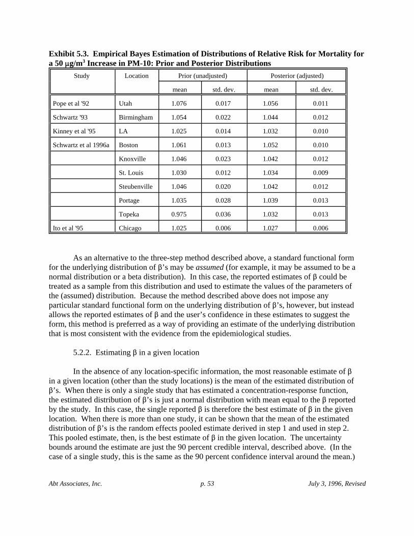
Abt Associates, Inc. p. 53 July 3, 1996, Revised
Exhibit 5.3. Empirical Bayes Estimation of Distributions of Relative Risk for Mortality fora 50 :g/m3 Increase in PM-10: Prior and Posterior Distributions
Study Location Prior (unadjusted) Posterior (adjusted)
mean std. dev. mean std. dev.
Pope et al '92 Utah 1.076 0.017 1.056 0.011
Schwartz '93 Birmingham 1.054 0.022 1.044 0.012
Kinney et al '95 LA 1.025 0.014 1.032 0.010
Schwartz et al 1996a Boston 1.061 0.013 1.052 0.010
Knoxville 1.046 0.023 1.042 0.012
St. Louis 1.030 0.012 1.034 0.009
Steubenville 1.046 0.020 1.042 0.012
Portage 1.035 0.028 1.039 0.013
Topeka 0.975 0.036 1.032 0.013
Ito et al '95 Chicago 1.025 0.006 1.027 0.006
As an alternative to the three-step method described above, a standard functional formfor the underlying distribution of $’s may be assumed (for example, it may be assumed to be anormal distribution or a beta distribution). In this case, the reported estimates of $ could betreated as a sample from this distribution and used to estimate the values of the parameters ofthe (assumed) distribution. Because the method described above does not impose anyparticular standard functional form on the underlying distribution of $’s, however, but insteadallows the reported estimates of $ and the user’s confidence in these estimates to suggest theform, this method is preferred as a way of providing an estimate of the underlying distributionthat is most consistent with the evidence from the epidemiological studies.
5.2.2. Estimating $ in a given location
In the absence of any location-specific information, the most reasonable estimate of $in a given location (other than the study locations) is the mean of the estimated distribution of$’s. When there is only a single study that has estimated a concentration-response function,the estimated distribution of $’s is just a normal distribution with mean equal to the $ reportedby the study. In this case, the single reported $ is therefore the best estimate of $ in the givenlocation. When there is more than one study, it can be shown that the mean of the estimateddistribution of $’s is the random effects pooled estimate derived in step 1 and used in step 2. This pooled estimate, then, is the best estimate of $ in the given location. The uncertaintybounds around the estimate are just the 90 percent credible interval, described above. (In thecase of a single study, this is the same as the 90 percent confidence interval around the mean.)
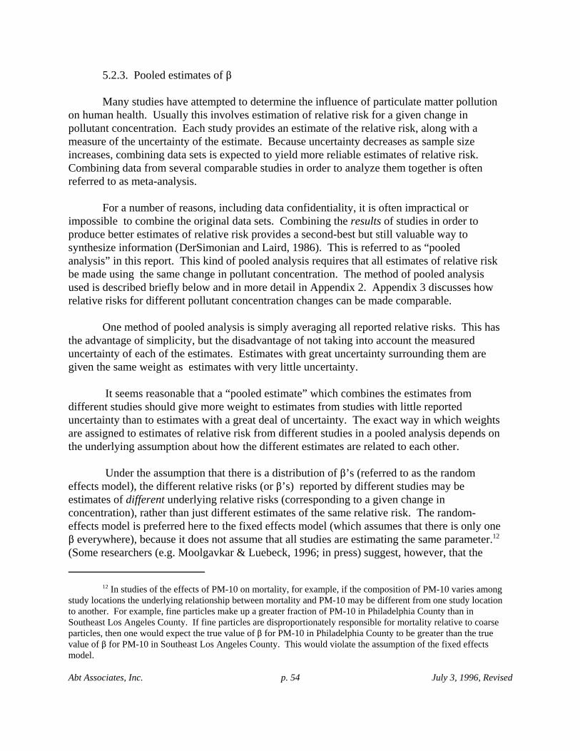
12 In studies of the effects of PM-10 on mortality, for example, if the composition of PM-10 varies amongstudy locations the underlying relationship between mortality and PM-10 may be different from one study locationto another. For example, fine particles make up a greater fraction of PM-10 in Philadelphia County than inSoutheast Los Angeles County. If fine particles are disproportionately responsible for mortality relative to coarseparticles, then one would expect the true value of $ for PM-10 in Philadelphia County to be greater than the truevalue of $ for PM-10 in Southeast Los Angeles County. This would violate the assumption of the fixed effectsmodel.
Abt Associates, Inc. p. 54 July 3, 1996, Revised
5.2.3. Pooled estimates of $
Many studies have attempted to determine the influence of particulate matter pollutionon human health. Usually this involves estimation of relative risk for a given change inpollutant concentration. Each study provides an estimate of the relative risk, along with ameasure of the uncertainty of the estimate. Because uncertainty decreases as sample sizeincreases, combining data sets is expected to yield more reliable estimates of relative risk. Combining data from several comparable studies in order to analyze them together is oftenreferred to as meta-analysis.
For a number of reasons, including data confidentiality, it is often impractical orimpossible to combine the original data sets. Combining the results of studies in order toproduce better estimates of relative risk provides a second-best but still valuable way tosynthesize information (DerSimonian and Laird, 1986). This is referred to as “pooledanalysis” in this report. This kind of pooled analysis requires that all estimates of relative riskbe made using the same change in pollutant concentration. The method of pooled analysisused is described briefly below and in more detail in Appendix 2. Appendix 3 discusses howrelative risks for different pollutant concentration changes can be made comparable.
One method of pooled analysis is simply averaging all reported relative risks. This hasthe advantage of simplicity, but the disadvantage of not taking into account the measureduncertainty of each of the estimates. Estimates with great uncertainty surrounding them aregiven the same weight as estimates with very little uncertainty.
It seems reasonable that a “pooled estimate” which combines the estimates fromdifferent studies should give more weight to estimates from studies with little reporteduncertainty than to estimates with a great deal of uncertainty. The exact way in which weightsare assigned to estimates of relative risk from different studies in a pooled analysis depends onthe underlying assumption about how the different estimates are related to each other.
Under the assumption that there is a distribution of $’s (referred to as the randomeffects model), the different relative risks (or $’s) reported by different studies may beestimates of different underlying relative risks (corresponding to a given change inconcentration), rather than just different estimates of the same relative risk. The random-effects model is preferred here to the fixed effects model (which assumes that there is only one$ everywhere), because it does not assume that all studies are estimating the same parameter.12 (Some researchers (e.g. Moolgavkar & Luebeck, 1996; in press) suggest, however, that the

13Although there are five studies, Schwartz et al. 1996a effectively conducted six separate studies in thesix cities listed. Following Schwartz et al., the pooled analyses treat these six cities as separate studies. There aretherefore ten PM-10 mortality studies on which pooled analyses were based.
Abt Associates, Inc. p. 55 July 3, 1996, Revised
heterogeneity in estimates of PM effects makes single estimates of risk difficult to estimate.)
Several pooled analyses, performed on a number of combinations of PM-10 studiesidentified in the Criteria Document for PM-10 (EPA, 1996a), are described below. Studieswere aggregated for analysis based upon the health endpoint of concern (only mortality andhospital admissions are considered) and the period of exposure evaluated (e.g., one day, threeday). In addition, a pooled function for mortality and PM-2.5, derived by Schwartz et al.1996afrom their studies in six cities, is also presented.
5.2.3.1. Pooled analyses of mortality PM-10 concentration-response functions
Pooled analyses were performed on various subsets of the following short-termexposure mortality studies cited in the Criteria Document for PM-10 (EPA, 1996a):13
! Ito and Thurston 1996 (Chicago, IL);! Kinney et al. 1995 (Los Angeles, CA);! Pope et al. 1992 (Utah Valley, UT);! Schwartz 1993 (Birmingham, AL);! Schwartz et al. 1996a (Boston; Knoxville, TN; St. Louis; Steubenville, OH;
Portage, WI; Topeka, KS)
Exhibit 5.4 shows the relative risks reported in the original studies for a change in PM-10concentration of 50 :g/m3. It is explained in Appendix 3 how the relative risk correspondingto one PM concentration change can be adjusted to reflect other concentration changes. Exhibit5.5 shows the studies included in each pooled analysis.
The "all averaging times" pooled analysis includes studies that used the average PMconcentration on a single day as the pollution indicator as well as studies that used the averagePM concentration over a 2-, 3- or 5-day period. Those studies which use multi-day averagesare in effect using a smoothed data set, comparing each day’s mortality to recent averageexposure rather than simply exposure on the same day. The averaging times applied

Abt Associates, Inc. p. 56 July 3, 1996, Revised
Exhibit 5.4. Relative Risks of Mortality Associated With a Change in PM-10 Concentration of 50 :g/m3.
Study LocationRelative
Risk Standard Error
Ito and Thurston, 1996 Chicago 1.025 0.006
Kinney et al., 1995 Los Angeles 1.025 0.014
Pope et al., 1992 Utah 1.076 0.017
Schwartz, 1993 Birmingham 1.054 0.022
Schwartz et al.,1996a Boston 1.061 0.013
Schwartz et al., 1996a Knoxville, TN 1.046 0.023
Schwartz et al., 1996a St. Louis 1.030 0.012
Schwartz et al., 1996aSteubenville,OH 1.046 0.020
Schwartz et al., 1996a Portage, WI 1.035 0.027
Schwartz et al., 1996a Topeka, KA 0.975 0.036
Exhibit 5.5. Studies Included in Each Pooled Analysis for PM-10
Study
all averaging
times
single-dayaveraging
only
2-day averaging
only
multi-day averaging
only
Ito et al. '95 T T
Kinney et al. '95 T T
Pope et al. '92 T T
Schwartz '93 T T
Schwartz et al. 1996a T T
to the PM data used in the risk analyses were chosen to correspond to the majority of functionsused in a pooled analysis. Because seven of the ten functions included in the “all averagingtimes” pooled analysis are based on two-day PM averages, two-day PM averages were usedwith this pooled function. Single-day PM concentrations were used with the one single-dayfunction; two-day PM averages were used with the two two-day functions; and five-day PMaverages were used with the two multi-day functions (one of which is a three-day function andthe other of which is a five-day function). The more nearly linear the concentration-responsefunction, however, the less difference it makes whether multi-day averaging functions are usedwith single-day PM data. (If the functions were perfectly linear, it would make no differenceat all.) The concentration-response functions considered here are nearly linear, as discussedabove. Because all of the studies in the "all averaging times" pooled analysis focus on theresults of short-term exposure to pollution (as opposed to long-term exposure, measured inyears), it is appropriate to consider these studies together.

Abt Associates, Inc. p. 57 July 3, 1996, Revised
Exhibit 5.6 shows the average relative risk of the mortality studies considered in eachpooled analysis, as well as the relative risk estimates (and standard errors) from pooledanalyses based on the fixed effects model and, where possible, the random effects model. Therandom effects model is preferred because it takes into account possible geographic variability,and pooled functions were based on the random effects model except when this was notpossible due to insufficient difference among the reported studies (see Appendix 2). Relativerisks are expressed for a 50 :g/m3 increase in PM-10 concentration. For the single-dayaveraging time study, it was not possible to calculate a random effects model estimate, and soonly the result based on the fixed effects model is shown. Exhibit 5.7 shows the relative riskresults of the original studies and the inverse variance weighting pooled analyses graphically,including the 95 percent confidence bounds.
Exhibit 5.6. Pooled Analyses of Mortality for PM-10 Relative Risk Estimates for a 50:g/m3 Increase in PM-10
Group N
ArithmeticAverage
Relative Risk
Fixed EffectsInverse Variance
Weighting
Random EffectsInverse Variance
Weighting
est. RR s.e. est. RR s.e.
All averaging times 10 1.037 1.035 0.004 1.040 0.007
Single-day averagingonly 1 1.025 1.025* 0.014* n/a n/a
2-day averaging only 7 1.031 1.032 0.005 1.035 0.007
>2 -day averaging only 2 1.065 1.068 0.013 n/a n/a*Although there is only one single-day averaging study (Kinney et al., 1995), and therefore no weighting ispossible, the figures in this column are presented to include the standard error.
Exhibits 5.6 and 5.7 illustrate that the selection of studies to include in the pooledanalysis is a critical choice. For example, pooling the two studies that use average PMconcentrations over three to five days increases the relative risk estimated for a 50 :g/m3
increase in PM-10, compared to that estimated by the pooled function based on studies that useaverage PM concentrations over only two days.
5.2.3.2. Pooled analyses of mortality PM-2.5 concentration-response functions
Exhibit 5.8 summarizes the available short-term exposure mortality studies that usePM-2.5 as the particulate matter indicator. Schwartz et al. 1996a reported relative riskestimates for six cities, along with an estimate for all six cities combined, based on a methodsimilar to the pooled analysis method described above. Exhibit 5.8 presents Schwartz et al.’srelative risk estimates for a 25 :g/m3 increase in PM-2.5 for each of the six cities separately aswell as the relative risk estimate based on the pooled function provided in the study.

Abt Associates, Inc. p. 58 July 3, 1996, Revised
0 . 8 5
0 . 9
0 . 9 5
1
1 . 0 5
1 . 1
1 . 1 5
Pool
ed F
unct
ion
(Ran
dom
Effe
cts)
(Fix
ed E
ffect
s)
Individual Studies
All
aver
agin
g tim
es
1 3 5 6 7 8 9 12 13
Pool
ed F
unct
ion
Schw
artz
et a
l., 1
996a
(Bos
ton)
Ito a
nd T
hust
on, 1
996
Kin
ney
et a
l., 1
995
Pope
et a
l., 1
992
Schw
artz
et a
l., 1
996a
(Kno
xvill
e, T
N)
Schw
artz
et a
l., 1
996a
(St.
Loui
s)
Schw
artz
et a
l., 1
996a
(Ste
uben
ville
, OH
)
Schw
artz
et a
l., 1
996a
(Por
tage
, WI)
Schw
artz
et a
l., 1
996a
(Top
eka,
KA
)
2-da
y av
erag
ing
time
> 2-
day
aver
agin
g tim
e
Schw
artz
, 199
3
Exhibit 5.7. Relative Risk of Mortality Associated with a Change in PM-10
Concentration of 50 µg/m3(Individual Studies and Pooled Analyses)
Rel
ativ
e R
isk
(95%
Con
fiden
ce In
terv
als)

Abt Associates, Inc. p. 59 July 3, 1996, Revised
Exhibit 5.8. Short-term Exposure Mortality Studies Using PM-2.5 as theIndicator of Particulate Matter, with Pooled Analyses.Relative Risk Estimates for a 25 :g/m3 Increase in PM-2.5
Study CityRelative Risk
(95% Confidence Interval) Source
Watertown, MA 1.056(1.038, 1.074)
Schwartz et al. 1996a
Knoxville, TN 1.035(1.005, 1.066)
Schwartz et al. 1996a
St. Louis, MO 1.028(1.010, 1.043)
Schwartz et al. 1996a
Steubenville, OH 1.025(0.998, 1.053)
Schwartz et al. 1996a
Portage, WI 1.030(0.993, 1.071)
Schwartz et al. 1996a
Topeka, KS 1.020(0.951, 1.092)
Schwartz et al. 1996a
Pooled function, using fixedeffects inverse variance weighting
1.038(1.028, 1.048)
Schwartz et al. 1996a
5.2.3.3. Pooled analyses of morbidity concentration-response functions
Exhibit 5.9 shows the results of pooled analyses performed on studies of various otherhealth effects of PM-10, as measured by hospital admissions. The four studies for hospitaladmissions for pneumonia and COPD come from Schwartz 1994a (Birmingham), Schwartz1994b (Detroit), Schwartz 1994c (Minneapolis/St. Paul), and Schwartz 1996 (Spokane). Thethree figures used for “total respiratory” hospital admissions are from Schwartz 1995 (NewHaven, CT and Tacoma, WA) and Schwartz 1996 (Spokane). A fourth study of respiratoryhospital admissions, using data from Cleveland, was excluded, because it considers 2-dayaverage PM-10 rather than same-day average PM-10 as the other studies do. (Including theCleveland study makes virtually no difference in the results.) In only one case was thevariation in results among the studies great enough to allow the use of a random-effects model. In the other cases, there is insufficient evidence that the different studies are estimatingdifferent underlying concentration-response functions.

14In those cases for which there is only a single study, the best estimates of the 5th and 95th percentiles ofthe distribution of $’s are the 5th and 95th percentiles of the normal distribution with mean equal to the $ reportedby the study and standard deviation equal to the standard error of the mean reported by the study. There istherefore no “analysis” necessary.
Abt Associates, Inc. p. 60 July 3, 1996, Revised
Exhibit 5.9. Pooled Analyses of Effects of PM-10 on Hospital Admissions Relative Risk Estimates for a 50 :g/m3 Increase in PM-10
Health Effect* N
ArithmeticAverage
Relative Risk
Fixed Effects InverseVariance Weighting
Random Effects InverseVariance Weighting
est. RR s.e. est. RR s.e.
hospital admissions- “totalrespiratory”
3 1.098 1.088 0.022 n/a n/a
hospital admissions-pneumonia
4 1.071 1.069 0.014 n/a n/a
hospital admissions-COPD
4 1.163 1.137 0.023 1.140 0.024
*All hospital admissions in this exhibit refer to individuals age 65 or older.
5.2.4. Quantitative assessment of uncertainty surrounding $’s applied to Philadelphia and Los Angeles: results
An uncertainty analysis (i.e., estimation of the distribution of $’s and calculation of a90 percent credible interval) was carried out in each case in which a pooled analysis wasperformed (see Section 5.2.3) -- that is, in each case in which there is more than one reportedestimate of the concentration-response function.14 (The one exception is the concentration-response function for PM-10 and mortality, based on 1-day averaging, for which there is onlyone study. This was included within the set of pooled analyses for mortality forcompleteness.)
The estimated distribution of $’s can be translated into a distribution of avoided healtheffects incidences corresponding to a given change in PM concentrations, as described above. Alternatively, it can be translated into a distribution of relative risks associated with a givenchange in PM concentrations, because each value of $ corresponds to a particular relative riskfor a given change in PM (see Section 2 and Appendix 3). The results of the uncertaintyanalyses, presented below, are in terms of relative risks associated with a 50 :g/m3 change inPM-10 or a 25 :g/m3 change in PM-2.5. The mean, the 95 percent credible interval (i.e., the2.5 and 97.5 percentile points), and the 90 percent credible interval (i.e., the 5 and 95percentile points) of the estimated distribution of relative risks for each uncertainty analysis arepresented in Exhibit 5.10. The 90 percent credible intervals are reported along with thequantitative estimates of risk. This approach is consistent with the 90 percent confidenceintervals used to characterize uncertainty in other Agency risk analyses, such as thoseconducted for ozone and lead. In addition, the 95 percent confidence intervals around thepooled analysis estimate of the mean of each underlying distribution of relative risks ispresented for comparison both with the uncertainties as reported in the original studies and

Abt Associates, Inc. p. 61 July 3, 1996, Revised
with the 95 percent credible interval from the estimated distribution of relative risks.
The distinction between a credible interval and the corresponding confidence intervalaround the pooled estimate is worth a further note for the sake of clarity. The 90 percentconfidence interval around the pooled estimate is derived from the standard error of theestimate of the mean, which is a measure of how good an estimate of the mean of theunderlying distribution the pooled analysis estimate is. The 90 percent confidence intervalaround the pooled estimate is the interval within which the true mean of the underlyingdistribution lies with 90 percent confidence. (For a precise definition of a confidence interval,see, for example, Mood et al., 1974, p. 375.) The confidence interval around the pooledestimate, then, comprises uncertainty bounds around the true mean of the distribution.
The 90 percent credible interval, consisting of the 5th and 95th percentiles of theestimated underlying distribution, comprises uncertainty bounds around the true value of $ (orthe true relative risk) in a particular location. In the absence of any further information aboutthat location, the 90 percent credible interval is an estimate of the interval within which $ inthat location will fall with 90 percent probability. This is the appropriate measure ofuncertainty surrounding the estimate of $ applied to a specific location.
The 90 percent credible interval will always be at least as wide as, and usually widerthan the 90 percent confidence interval around the pooled estimate of the mean. The greaterthe variance of the underlying distribution (i.e., the larger 02) the more of a discrepancy therewill be between the two types of uncertainty bounds. As 02 approaches zero, the 90 percentcredible interval approaches the 90 percent confidence interval around the pooled estimate ofthe mean. This is the case, for example, when there is only a single study. In this case, there isno evidence of differing $’s (because $ has been estimated in only a single location) andtherefore no evidence that 02 is positive. In this case, the 90 percent credible interval equalsthe 90 percent confidence interval around the estimate of the mean, which is based only on thewithin-study sampling error.
To illustrate the comparison between the confidence interval around the pooledestimate of the mean of the distribution of $’s and the corresponding credible interval for alocation-specific $, Exhibits 5.11 and 5.12 show graphically the normal distributionsrepresenting the within-study variability around the $’s reported by the ten “all averagingtimes” mortality PM-
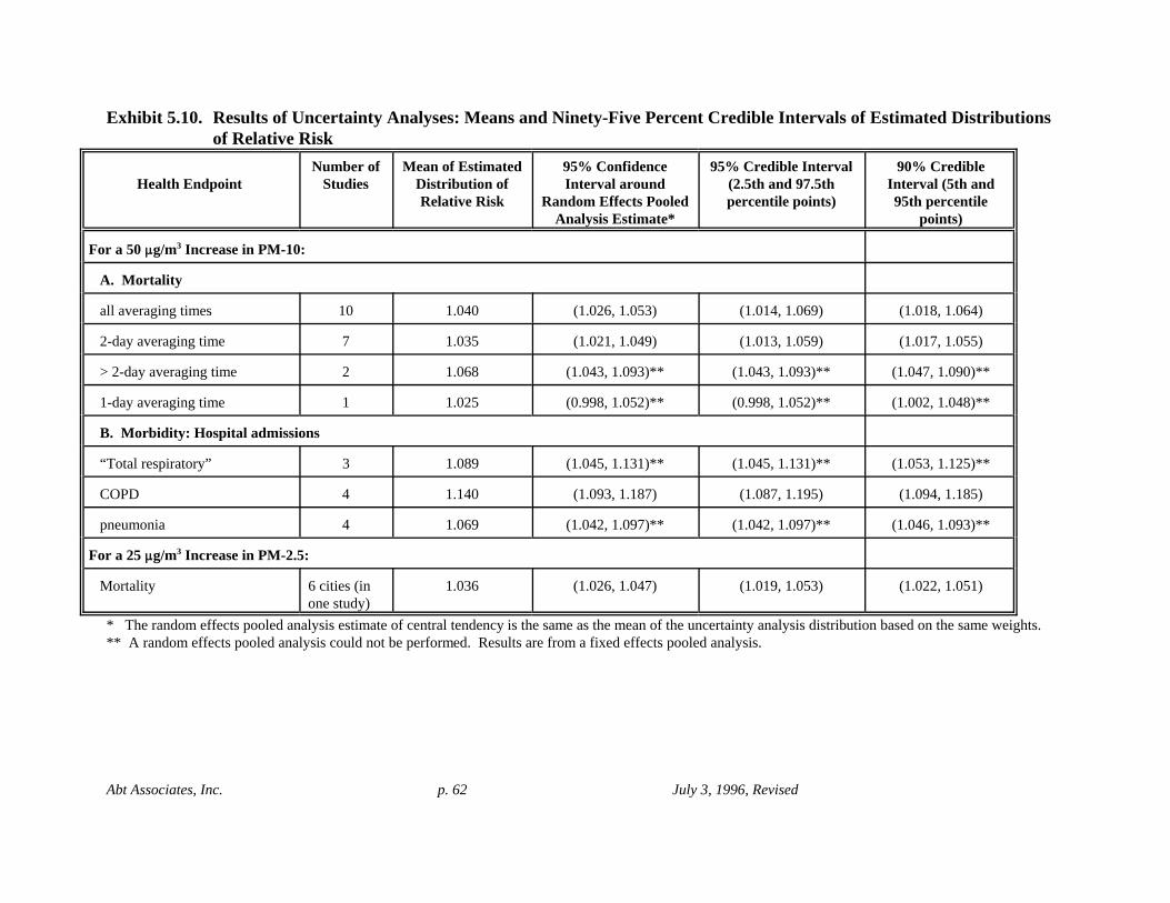
Abt Associates, Inc. p. 62 July 3, 1996, Revised
Exhibit 5.10. Results of Uncertainty Analyses: Means and Ninety-Five Percent Credible Intervals of Estimated Distributionsof Relative Risk
Health EndpointNumber of
StudiesMean of Estimated
Distribution ofRelative Risk
95% ConfidenceInterval around
Random Effects PooledAnalysis Estimate*
95% Credible Interval(2.5th and 97.5thpercentile points)
90% CredibleInterval (5th and95th percentile
points)
For a 50 :g/m3 Increase in PM-10:
A. Mortality
all averaging times 10 1.040 (1.026, 1.053) (1.014, 1.069) (1.018, 1.064)
2-day averaging time 7 1.035 (1.021, 1.049) (1.013, 1.059) (1.017, 1.055)
> 2-day averaging time 2 1.068 (1.043, 1.093)** (1.043, 1.093)** (1.047, 1.090)**
1-day averaging time 1 1.025 (0.998, 1.052)** (0.998, 1.052)** (1.002, 1.048)**
B. Morbidity: Hospital admissions
“Total respiratory” 3 1.089 (1.045, 1.131)** (1.045, 1.131)** (1.053, 1.125)**
COPD 4 1.140 (1.093, 1.187) (1.087, 1.195) (1.094, 1.185)
pneumonia 4 1.069 (1.042, 1.097)** (1.042, 1.097)** (1.046, 1.093)**
For a 25 :g/m3 Increase in PM-2.5:
Mortality 6 cities (inone study)
1.036 (1.026, 1.047) (1.019, 1.053) (1.022, 1.051)
* The random effects pooled analysis estimate of central tendency is the same as the mean of the uncertainty analysis distribution based on the same weights.** A random effects pooled analysis could not be performed. Results are from a fixed effects pooled analysis.

Abt Associates, Inc. p. 63 July 3, 1996, Revised
10 studies as well as both the estimated distribution of $’s and the corresponding pooledanalysis estimate of the mean of the distribution. Exhibit 5.11 shows the ten unadjustednormal distributions representing the within-study variability around each of the ten reported$’s. Exhibit 5.12 superimposes on the ten adjusted normal distributions (1) the pooled analysisestimate of the mean of the distribution of $’s and the normal distribution around this estimate,based on the standard error of the estimate, and (2) the estimated distribution of $’s generatedfrom the underlying ten adjusted normal distributions, using the three-step estimationprocedure described in Section 5.2.1.
Note that, even though the distributions around the reported estimates of $’s arenormal, the estimated distribution of $’s derived from them is not normal. As noted above, itdoes not have a standard functional form but instead reflects the evidence from the particularstudies on which it is based. Note also that it is possible, when sampling from the estimateddistribution of $’s, to select a negative number. The probability of doing so, however, isextremely small.
5.2.5. Translating a 90 percent credible interval for $ into a 90 percent credible interval for avoided health effect incidence
As in Section 5.2 above, the health effect will be taken to be mortality for ease ofdiscussion in this section. The discussion is, however, generalizable to any health effect. Fora given set of PM reductions in a given location, to any value of $ there corresponds apredicted avoided mortality. There is therefore a distribution of avoided mortalitycorresponding to the distribution of $’s. Ideally, the 5th and 95th percentiles of the estimateddistribution of avoided mortality would compose the 90 percent credible interval around apoint estimate of avoided mortality in the location of interest. If the concentration-responsefunction is linear, the mortality predicted by the concentration-response function evaluated atthe x percentile $ would be the same as the x percentile of the distribution of mortality. Thatis, if $x denotes the x percentile value of $ from the distribution of $’s, and )yx denotes the xpercentile value of the distribution of avoided mortality from the corresponding distribution,then
If, however, the concentration-response function is convex or concave, the equality becomesan inequality. Because the concentration-response functions are almost linear, however, thediscrepancy will be very small, and the 5th and the 95th percentile $’s from the estimateddistribution of $’s were applied to the air quality data in a given location (Philadelphia Countyor Southeast Los Angeles County) to obtain a close approximation to a 90 percent “credibleinterval” in avoided incidences of the given health effect in that location.
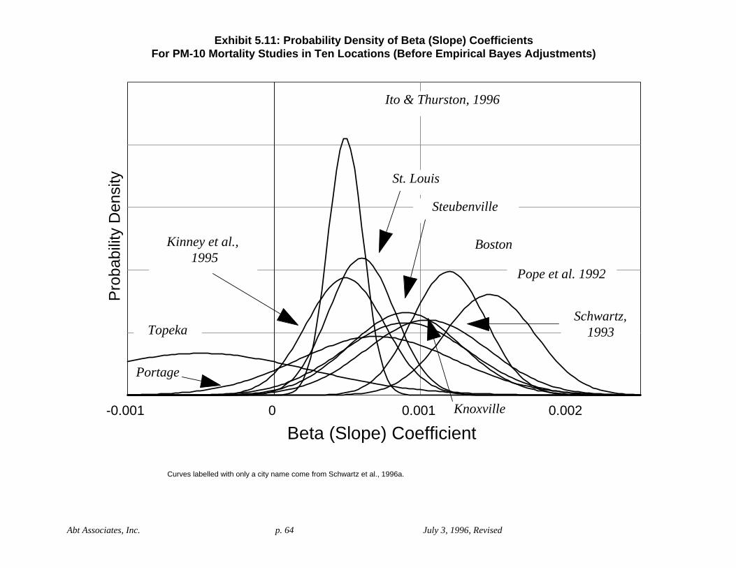
Abt Associates, Inc. p. 64 July 3, 1996, Revised
Pro
babi
lity
Den
sity
-0.001 0 0.001 0.002
Beta (Slope) Coefficient
Topeka
Ito & Thurston, 1996
Boston
Pope et al. 1992
Portage
St. Louis
Kinney et al., 1995
Steubenville
Schwartz,1993
Knoxville
Exhibit 5.11: Probability Density of Beta (Slope) CoefficientsFor PM-10 Mortality Studies in Ten Locations (Before Empirical Bayes Adjustments)
Curves labelled with only a city name come from Schwartz et al., 1996a.

Abt Associates, Inc. p. 65 July 3, 1996, Revised
Pro
babi
lity
Den
sity
-0.001 0 0.001 0.002
Pooled Analysis CentralTendency EstimateUncertainty Analysis
Estimated Distribution
(
w
i
t
h
s
u
r
r
o
u
n
d
i
n
g
nBeta (Slope)
abd c e
(with surrounding normal distribution,using standard error of estimate)
Exhibit 5.12: Mortality Studies from ten Locations (Adjusted Using Empirical Bayes Method),Pooled Analysis Central Tendency Estimate, and Uncertainty Analysis Estimated Distribution
Results Based on Random Effects Weighting
a = Pooled analysis central tendency estimate = mean of uncertainty analysis estimated distribution(b,c) = 95% confidence interval around the mean(d,e) = 95% “credible interval” from uncertainty analysis distribution (i.e., 2.5 and 97.5 percentiles of the distribution)

Abt Associates, Inc. p. 66 July 3, 1996, Revised

15 Incidence rates also vary within a geographic area due to the same factors; however, statistics regardingwithin-city variations are rarely available and are not necessary for this analysis.
Abt Associates, Inc. p. 67 July 3, 1996, Revised
6. Baseline Health Effects Incidence Rates
Incidence rates are required inputs for many, but not all, concentration-responsefunctions. Many of the epidemiology studies used in this analysis directly estimate thepercentage change in incidence (i.e., the relative risk), rather than the absolute number of casesfor an endpoint. To estimate the number of PM-associated cases using these studies, it isnecessary to know the baseline incidence, that is, the number of cases in a location before achange in PM air quality.
Incidence rates express the occurrence of a disease or event (e.g., asthma episode,death, hospital admission) in a specific period of time, usually per year. Rates are expressedeither as a value per population group (e.g., the number of cases in Philadelphia County) or avalue per number of people (e.g., number of cases per 10,000 residents), and may be age andsex specific. Incidence rates vary among geographic areas due to differences in populationcharacteristics (e.g, age distribution) and factors promoting illness (e.g., smoking, air pollutionlevels).15 The sizes of the populations in Philadelphia County and Southeast Los AngelesCounty that are relevant to the risk analyses reported here (i.e., the populations to which thebaseline incidences refer) are given in Exhibit 6.1.
Exhibit 6.1. Relevant Population Sizes for Philadelphia County and Southeast Los Angeles County
Population Philadelphia County Southeast Los Angeles County
Total 1,586,000 3,636,000
Ages $ 65 240,800 (15.2%) 322,100 (8.9%)
Children, ages 8-12 102,900 (6.5%) 282,100 (7.8%)
Children, ages 10-12 61,700 (3.9%) 165,800 (4.6%)
Asthmatic Children, ages 9-11
3,900* (0.25%) 10,700* (0.29%)
Asthmatic African-AmericanChildren, ages 7-12
-- 1,800* (0.05%)
*Incidences for asthmatic children were obtained using the national asthma prevalence among children (6.3%). The incidence of asthmatic African-American children ages 7-12 in Southeast L.A. County, for example, is3,636,000 multiplied by {0.0937 (the proportion of the population that is ages 7-12) x 0.085 (the proportion of thepopulation that is African-American) x 0.063 (the proportion of the national population of children that areasthmatic)}.

Abt Associates, Inc. p. 68 July 3, 1996, Revised
6.1. Sources of incidence data
Incidence rates are available for mortality (death rates) and for specific communicablediseases which state and local health departments are required to report to the federalgovernment. None of the morbidity endpoints in the risk analysis are required to be reportedto the federal government. In addition to the required federal reporting, many state and localhealth departments collect information on some additional endpoints. These most often arerestricted to hospital admission or discharge diagnoses, which are collected to assist inplanning medical services. Data may also be collected for particular studies of health issues ofconcern.
Although federal agencies collect incidence data on many of the endpoints covered inthis report, their data are often available only at the national level (national averages), or at theregional or state level. When possible, state and local health departments and hospitalplanning commissions were contacted to obtain location-specific rates.
Estimates of location-specific baseline mortality rates for Philadelphia County andSoutheast Los Angeles County were obtained from the National Center for Health Statistics(NCHS), a national repository for morbidity, mortality, and health services data. Baselineincidence rates for hospital admissions (for pneumonia, COPD, “total respiratory,” congestiveheart disease, and ischemic heart failure) were obtained for Philadelphia County from theDelaware Valley Hospital Council for 1993-1994 (fiscal year 1994), and for Los Angeles fromCalifornia’s Office of Statewide Health Planning and Development Data Users Support Group.Finally, in the absence of other sources of baseline incidence data for respiratory symptomsand acute bronchitis, baseline rates for these health endpoints were taken from the studieswhich estimated the concentration-response functions used for these endpoints in the riskanalysis.
Baseline health effects incidence rates used in the risk analysis are given in Exhibit 6.2. In all cases, the incidence rates listed correspond to the ages of the populations studied in therelevant epidemiology studies, e.g., individuals over 65 years of age. The national incidencerates given in Exhibit 6.2 may differ from those given in the Criteria Document for severalreasons, including differences in the years used and differences in the ICD codes includedwithin a health effects category.

Abt Associates, Inc. p. 69 July 3, 1996, Revised
Exhibit 6.2. Baseline Health Effects Incidence RatesHealth Effect Philadelphia
CountySoutheast Los
Angeles CountyNationalAveragea
Short-Term Exposure Mortalityb (per 100,000 general population/year)
1280 676 830
Long-Term Exposure Mortality (age 30 and older)(per 100,000 general population/year)
1154* 657* --
Morbidity:
A. Hospital Admissions (per 100,000 general population/year)
Total respiratory hospital admissionsc (all ages): ICD codes 466, 480-482, 485, 490-493
816 427 --
Total respiratory hospital admissions (65 and older): ICD codes 460-519
650 428 504
COPD admissions (65 and older): ICD codes 490-496 202 116 103
Pneumonia admissions (65 and older): ICD codes 480-487 257 205 229
Ischemic heart failure (65 and older): ICD codes 410-414 614 307 450
Congestive Heart Disease (65 and older): ICD code 428 487 197 231
B. Respiratory Symptoms (percent of relevant population)
Lower Respiratory Symptoms (LRS) in children, ages 8-12(number of cases of symptoms per day)
0.15%** 0.15%** --
Lower Respiratory Symptoms (LRS) in asthmatic children, ages9-11 (number of days of symptoms)
16%** 16%** --
Shortness of breath (number of days) in asthmatic African-American children, ages 7-12
-- 5.6%** --
(Doctor diagnosed) acute bronchitis in children ages 10-12 peryr.
6.5%** 6.5%** --
All incidence rates are rounded to the nearest unit.a. National rates for hospital admissions for patients over 64 years of age were obtained from Vital and HealthStatistics, Detailed Diagnoses and Procedures, National Hospital Discharge Survey, 1990. June, 1992. CDC.Hyattsville, Md. Each rate is based on the number of discharges divided by the 1990 population of 248,709,873 . b. Mortality figures exclude suicide, homicide, and accidental death, which corresponds to the measures used inthe epidemiological studies employed in this analysis.c. Although a baseline incidence rate is not needed for calculating the incidence of total respiratory hospitaladmissions associated with PM (because the concentration-response function predicts cases rather than percentchange), it is needed for calculating the PM-related percent change in total incidence.*Although county-specific total mortality incidences (over all ages) were available for both Philadelphia and LosAngeles, age-specific mortality incidences were not available. Baseline mortality incidences among individualsaged 30 and over in Philadelphia and Southeast Los Angeles Counties were therefore estimated by applyingnational age-specific death rates to county-specific age distributions, and adjusting the resulting estimated age-specific incidences so that the estimated total incidences (including all ages) equaled the actual county-specifictotal incidences. For example, if the total of the estimated age-specific incidences obtained in this way was 5%

Abt Associates, Inc. p. 70 July 3, 1996, Revised
higher than the actual total incidence for a county, then each of the estimated age-specific incidences wasmultiplied by (1/1.05). Using this method, the baseline mortality incidences among individuals aged 30 and overwere estimated to be 90% and 97% of the baseline incidences including all ages in Philadelphia County andSoutheast Los Angeles County, respectively. **Baseline incidence rates for respiratory symptoms were taken from the original studies.

Abt Associates, Inc. p. 71 July 3, 1996, Revised
7. Assessment of the Health Risks Associated with “As Is” PM Concentrations Above Background
7.1. Results and sensitivity analyses
The results of the first phase of the risk analysis, assessing the health risks associatedwith “as is” PM concentrations are given in Exhibit 7.1 for Philadelphia County in 1992-1993and Exhibits 7.2 and 7.3 for Southeast Los Angeles County in 1995. Because Southeast LosAngeles County was not in attainment of current PM-10 standards in 1995, the health risksassociated with “as is” PM concentrations in that location was assessed in two ways. First, theassessment was carried out using “as is” PM concentrations (Exhibit 7.2). Second, health riskswere assessed using daily PM concentrations adjusted to simulate attainment of currentstandards (Exhibit 7.3). The method of adjusting daily PM concentrations to simulateattainment of current standards is described in Section 2.2.
All estimated incidences were rounded to the nearest 10, except lower respiratorysymptoms, which are reported to the nearest 1000, and shortness of breath among African-American asthmatics, which is rounded to the nearest 100. All percentages were rounded toone decimal place. Rounding was done for convenience of presentation and is not intended toimply a particular level of precision.
There is substantial uncertainty surrounding all estimates of incidence associated with“as is” PM concentrations, in both Philadelphia County and Southeast Los Angeles County. The incidence of a health effect predicted to be associated with “as is” PM concentrations in agiven location depends on the concentration-response function in that location. Because thetrue concentration-response functions (for the relevant health effects) are not known, they mustbe estimated. If concentration-response functions had been estimated for Philadelphia Countyand Southeast Los Angeles County specifically, then the only uncertainty associated withusing these estimated concentration-response functions in the risk analyses for PhiladelphiaCounty and Southeast Los Angeles County would be the uncertainty as to how well theestimated concentration-response functions approximate the true concentration-responsefunctions in these locations. This uncertainty is typically expressed as a 90 or 95 percentconfidence interval around the estimate.
However, because concentration-response functions have, for most health endpoints,not been estimated for Philadelphia County or Southeast Los Angeles County specifically,concentration-response functions estimated in other locations, or a central tendency estimatederived by pooling these, have been used instead. This adds a second source of uncertainty tothe risk analyses. If there is true geographic variability in the concentration-response functionfor a given health effect, then it is uncertain how well the concentration-response function inone location (or the mean of concentration-response functions in several locations)approximates that for a different location. (This is discussed in more detail in Section 3 andSection 5.2.)

Abt Associates, Inc. p. 72 July 3, 1996, Revised
To assess the total uncertainty surrounding the concentration-response function appliedto a given location (e.g., Philadelphia County) in the risk analysis, in this case, the full range ofpossibilities of what the function in that location might be is characterized by estimating the distribution of possible values of the “slope” parameter, $, in the concentration-responsefunction. This distribution is estimated based on the limited information from studiesconducted in various locations throughout the U.S. Lacking further information, thisdistribution characterizes the range of possibilities of what the concentration-response functionmight be in a randomly selected location anywhere in the United States. If nothing more abouta location is known, then, it is estimated that with 90 percent probability, $ in that location liesbetween the 5th and the 95th percentiles of this estimated distribution of $’s. This interval isreferred to as the “90 percent credible interval” for any location in the U.S., includingPhiladelphia County or Southeast Los Angeles County. Each predicted PM-related incidenceand each predicted PM-related percent of total incidence is accompanied by its associated 90percent credible interval (in parentheses below it). In those cases in which the distribution of$’s is estimated from only a single study, this 90 percent credible interval coincides with the90 percent confidence interval around the estimate of the concentration-response function inthe study location. The estimation of the distribution of $’s from which to calculate the 90percent credible interval is described in Section 5.2.1.
PM-related health effects incidence and percent of total incidence predicted inSoutheast Los Angeles County are uniformly greater than those predicted in PhiladelphiaCounty. The generally higher pollution levels and greater population size in Southeast LosAngeles County are undoubtedly the primary reasons for this. In some instances (e.g., forlower respiratory symptoms among 8-12 year old children), however, the predictions of PM-related health effects incidence in Southeast Los Angeles County seem questionably high. It isimportant to bear in mind that most predictions are based on only a single study, and there arereasons to be cautious in accepting the results of any single study without corroboration fromother studies. In addition, pollution levels in Southeast Los Angeles County are notably high. PM concentrations in that location exceeded the range of PM observations on which theestimation of the concentration-response function for lower respiratory symptoms among 8-12year old children (Schwartz et al. 1994) was based. For example, the highest PM-10concentration observed in the Schwartz study was 117 :g/m3, as compared with a secondhighest PM-10 concentration of 193.4 :g/m3 in Southeast Los Angeles County (Exhibit 4.12). The highest PM-2.5 concentration observed in the Schwartz study was 86 :g/m3, as comparedwith a second highest PM-2.5 concentration of 106.2 :g/m3 in Southeast Los Angeles County(Exhibit 4.13). It is possible that the Los Angeles PM concentrations exceeded the range onwhich the estimated concentration-response relationship is a plausible model (see Section3.1.3). To the extent that this was the case, the incidence of PM-related health effects wouldhave been overestimated for Southeast Los Angeles County. The numbers of days on whichPM concentrations reported in Southeast Los Angeles County in 1995 exceeded maximum PMconcentrations observed in studies estimating concentration-response functions is given, foreach health endpoint considered in the risk analyses, in Exhibit 7.4.

Abt Associates, Inc. p. 73 July 3, 1996, Revised
Exhibit 7.1Estimated Annual Health Risks Associated with "As Is" PM Concentrationsin Philadelphia County, September 1992- August 1993 (for base case assumptions)
Health Effects Associated with PM-2.5 Above Background**Health Effects Associated with PM-10 Above Background**Percent of Total IncidenceIncidencePercent of Total IncidenceIncidenceHealth Effects*
1.8%3701.1%220(A) Associated with short-term exposure (all ages) Mortality (1.1 - 2.5)(230 - 510)(0.8 - 1.4)(160 - 290)
4.7%860-- -- ---- -- --(B) Assoc. with long-term exposure (age 30 and over)(2.9 - 6.4)(540 - 1170)-- -- ---- -- -- (51 locations)
2.0%260-- -- ---- -- --(C) Total RespiratoryHospital Admissions(0.5 - 3.5)(70 - 450)-- -- ---- -- -- (all ages)Respiratory
-- -- ---- -- --2.4%250(D) Total respiratory-- -- ---- -- --(1.5 - 3.3)(150 - 340) (>64 years old)-- -- ---- -- --3.7%120(E) COPD-- -- ---- -- --(2.5 - 4.7)(80 - 150) (>64 years old) -- -- ---- -- --1.9%80(F) Pneumonia-- -- ---- -- --(1.3 - 2.6)(50 - 100) (>64 years old)
0.7%700.8%80(G) Ischemic Heart Disease ***Hospital Admissions(0.3 - 1.2)(30 - 120)(0.3 - 1.3)(30 - 120) (>64 years old)Cardiac
1.3%1001.4%110(H) Congestive Heart Failure ***(0.6 - 2.0)(50 - 150)(0.7 - 2.1)(50 - 160) (>64 years old)
20.0%< 11000 >17.5%< 10000 >(I) Lower Respiratory Symptoms (# of cases)Lower Respiratory (10.3 - 28.2)(6000 - 15000)(15.3 - 19.6)(8000 - 11000) (8-12 year olds)Symptoms
-- -- ---- -- --6.8%< 16000 >(J) Lower Respiratory Symptoms (# of days) in Children****-- -- ---- -- --(2.4 - 10.9)(6000 - 25000) (9-11 year old asthmatics)-- -- ---- -- --0.3%< 190 >(K) Doctor-diagnosed Acute Bronchitis assoc--- -- ---- -- --( 0.0 - 0.6 )( 20 - 370 )iated with long-term exposure (10-12 year olds)
Sources of Concentration-Response (C-R) Functions:* Health effects are associated with short-term exposure to PM, unless otherwise specified.(A) PM-10 C-R function based on pooled results from ** Health effects incidence was quantified across the range of PM concentrations observed in each study, when possible, but not studies in 10 locations; PM-2.5 C-R function based on pool below background level. Background PM-10 is assumed to be 8 ug/m3; background PM-2.5 is assumed to be 3.5 ug/m3. results from studies in six locations.*** PM-2.5 results based on using PM-2.5 mass as PM-10 mass in the PM-10 functions.(B) Pope et al., 1995****Angle brackets <> indicate incidence calculated using baseline incidence rates reported in studies, with no adjustment for (C) Thurston, et al., 1994 location-specific incidence rates. This increases the uncertainty in the incidence estimates.(D) PM-10 C-R based on pooled results from 4 functions(E) PM-10 C-R based on pooled results from 4 functionsThe numbers in parentheses for pooled functions are NOT standard confidence intervals. (F) PM-10 C-R based on pooled results from 4 functionsAll the numbers in parentheses are interpreted as 90% credible intervals based on uncertainty analysis (G) Schwartz & Morris, 1995that takes into account both statistical uncertainty and possible geographic variability.(H) Schwartz & Morris, 1995See text in Chapter 7 for details.(I) Schwartz, et al., 1994(J) Pope et al., 1991(K) Dockery et al., 1989

Abt Associates, Inc. p. 74 July 3, 1996, Revised
Exhibit 7.2Estimated Annual Health Risks Associated with "As Is" PM Concentrationsin Southeast Los Angeles County, 1995* (for base case assumptions)
Health Effects Associated with PM-2.5 Above Background***Health Effects Associated with PM-10 Above Background***Percent of Total IncidenceIncidencePercent of Total IncidenceIncidenceHealth Effects**
3.7%9003.3%800(A) Associated withMortality (2.2 - 5.0)(540 - 1230)(2.3 - 4.1)(570 - 1020) short-term exposure (all ages)
-- -- ---- -- --1.6%400(B) Associated with short-term exposure-- -- ---- -- --(0.2 - 3.1)(40 - 750) (all ages; study done in Los Angeles)11.9%2,800-- -- ---- -- --(C) Associated with long-term exposure
(7.5 - 16.0)(1800-3800)-- -- ---- -- -- (age 30 and over; 51 locations)
7.7%1,200-- -- ---- -- --(D) Total RespiratoryHospital Admissions(2.1 - 13.4)(330 - 2080)-- -- ---- -- -- (all ages)Respiratory
-- -- ---- -- --6.9%1,070(E) Total Respiratory-- -- ---- -- --(4.2 - 9.4)(660 - 1460) (>64 years old)-- -- ---- -- --10.3%440(F) COPD-- -- ---- -- --(7.3 - 13.1)(310 - 560) (>64 years old) -- -- ---- -- --5.6%420(G) Pneumonia-- -- ---- -- --(3.9 - 7.3)(290 - 550) (>64 years old)
1.4%1602.3%260(H) Ischemic Heart Disease****Hospital Admissions(0.6 - 2.3)(60 - 260)(0.9 - 3.7)(100 - 420) (>64 years old)Cardiac
2.5%1804.1%290(I) Congestive Heart Failure****(1.2 - 3.8)(90 - 270)(2.0 - 6.1)(140 - 430) (>64 years old)
34.4%< 51000 >41.4%< 62000 >(J) Lower Respiratory Symptoms (# of cases)Lower Respiratory (19.1 - 45.7)(28000 - 68000)(37.2 - 45.2)(56000 - 68000) (8-12 year olds)Symptoms
-- -- ---- -- --18.4%< 115000 >(K) Lower Respiratory Symptoms (# of days)in Children *****-- -- ---- -- --(6.9 - 28.0)(43000 - 175000) (9-11 year old asthmatics)-- -- ---- -- --19.3%< 7200 >(L) Days of shortness of breath (7-12 year old-- -- ---- -- --(6.4 - 29.2)(2400 - 10900) African American asthmatics in Los Angeles)-- -- ---- -- --3.1%< 5090 >(L) Doctor-diagnosed Acute Bronchitis assoc--- -- ---- -- --(0.4 - 4.7)(680 - 7750)iated with long-term exposure (10-12 year olds)
Sources of Concentration-Response (C-R) Functions: * Southeast Los Angeles County was not in attainment of current PM-10 standards (50 ug/m3 annual average(A) PM-10 C-R function based on pooled results from standard and 150 ug/m3 daily standard) in 1995. Figures shown use the actual reported concentrations. studies in 10 locations; PM-2.5 C-R function based on pooled ** Health effects are associated with short-term exposure to PM, unless otherwise specified. results from studies in six locations. *** Health effects incidence was quantified across the range of PM concentrations observed in each study, when possible, but not(B) Kinney et al.,1995 below background level. Background PM-10 is assumed to be 6.0 ug/m3 and background PM-2.5 is assumed to be 2.5 ug/m3.(C) Pope et al., 1995 **** PM-2.5 results based on using PM-2.5 mass as PM-10 mass in the PM-10 functions.(D) Thurston, et al., 1994*****Angle brackets <> indicate incidence calculated using baseline incidence rates reported in studies, with no adjustment for(E) PM-10 C-R based on pooled results from 4 functions location-specific incidence rates. This increases the uncertainty in the incidence estimates.(F) PM-10 C-R based on pooled results from 4 functions(G) PM-10 C-R based on pooled results from 4 functions(H) Schwartz & Morris, 1995The numbers in parentheses for pooled functions are NOT standard confidence intervals. (I) Schwartz & Morris, 1995All numbers in parentheses are interpreted as 90% credible intervals based on uncertainty(J) Schwartz, et al., 1994analysis that takes into account both statistical uncertainty and possible geographic variability.(K) Pope et al., 1991See text in Chapter 7 for details.(L) Dockery et al., 1989

Abt Associates, Inc. p. 75 July 3, 1996, Revised
Exhibit 7.3Estimated Annual Health Risks Associated with Attainment of Current Standardsin Southeast Los Angeles County, 1995* (for base case assumptions)
Health Effects Associated with PM-2.5 Above Background***Health Effects Associated with PM-10 Above Background***Percent of Total IncidenceIncidencePercent of Total IncidenceIncidenceHealth Effects**
2.9%7102.6%630(A) Associated withMortality(1.7 - 3.9)(430 - 970)(1.8 - 3.3)(450 - 800) short-term exposure (all ages)
-- -- ---- -- --1.2%290(B) Associated with short-term exposure-- -- ---- -- --(0.1 - 2.2)(30 - 550) (all ages; study done in Los Angeles)8.6%2,050-- -- ---- -- --(C) Associated with long-term exposure
(5.4 - 11.7)(1250-2690)-- -- ---- -- -- (age 30 and over; 51 locations)
6.1%940-- -- ---- -- --(D) Total RespiratoryHospital Admissions(1.6 - 10.5)(250 - 1630)-- -- ---- -- -- (all ages)Respiratory
-- -- ---- -- --5.4%840(E) Total Respiratory-- -- ---- -- --(3.3 - 7.4)(520 - 1160) (>64 years old)-- -- ---- -- --8.2%350(F) COPD-- -- ---- -- --(5.8 - 10.5)(240 - 440) (>64 years old) -- -- ---- -- --4.4%330(G) Pneumonia-- -- ---- -- --(3.1 - 5.8)(230 - 430) (>64 years old)
1.1%1301.8%200(H) Ischemic Heart Disease****Hospital Admissions(0.4 - 1.8)(50 - 200)(0.7 - 2.9)(80 - 330) (>64 years old)Cardiac
2.0%1403.2%230(I) Congestive Heart Failure****(1.0 - 3.0)(70 - 210)(1.5 - 4.8)(110 - 340) (>64 years old)
28.7%< 43000 >34.8%< 52000 >(J) Lower Respiratory Symptoms (# of cases)Lower Respiratory (15.4 - 39.0)(23000 - 58000)(31.0 - 38.4)(46000 - 57000) (8-12 year olds)Symptoms
-- -- ---- -- --14.9%< 93000 >(K) Lower Respiratory Symptoms (# of days)in Children *****-- -- ---- -- --(5.5 - 23.0)(34000 - 143000) (9-11 year old asthmatics)-- -- ---- -- --14.1%< 5200 >(L) Days of shortness of breath (7-12 year old-- -- ---- -- --(4.6 - 21.8)(1700 - 8100) African American asthmatics in Los Angeles)-- -- ---- -- --2.3%< 3760 >(L) Doctor-diagnosed Acute Bronchitis assoc--- -- ---- -- --(0.3 - 3.7)(470 - 6190)iated with long-term exposure (10-12 year olds)
Sources of Concentration-Response (C-R) Functions: * Southeast Los Angeles County was not in attainment of current PM-10 standards (50 ug/m3 annual average(A) PM-10 C-R function based on pooled results from standard and 150 ug/m3 daily standard) in 1995. "As is" daily PM-10 concentrations were first rolled studies in 10 locations; PM-2.5 C-R function based on pooled back to simulate attainment of these standards. "As is" daily PM-2.5 concentrations were rolled back results from studies in six locations. by the same percent as daily PM-10 concentrations. See text in Chapter VI for details.(B) Kinney et al.,1995 ** Health effects are associated with short-term exposure to PM, unless otherwise specified.(C) Pope et al., 1995 *** Health effects incidence was quantified across the range of PM concentrations observed in each study, when possible, but not(D) Thurston, et al., 1994 below background level. Background PM-10 is assumed to be 6.0 ug/m3 and background PM-2.5 is assumed to be 2.5 ug/m3.(E) PM-10 C-R based on pooled results from 4 functions **** PM-2.5 results based on using PM-2.5 mass as PM-10 mass in the PM-10 functions.(F) PM-10 C-R based on pooled results from 4 functions*****Angle brackets <> indicate incidence calculated using baseline incidence rates reported in studies, with no adjustment for(G) PM-10 C-R based on pooled results from 4 functions location-specific incidence rates. This increases the uncertainty in the incidence estimates.(H) Schwartz & Morris, 1995(I) Schwartz & Morris, 1995The numbers in parentheses for pooled functions are NOT standard confidence intervals. (J) Schwartz, et al., 1994All numbers in parentheses are interpreted as 90% credible intervals based on uncertainty (K) Pope et al., 1991analysis that takes into account both statistical uncertainty and possible geographic variability.(L) Dockery et al., 1989See text in Chapter 7 for details.

Abt Associates, Inc. p. 76 July 3, 1996, Revised
Exhibit 7.4Number of Days on Which PM Concentration Reportedin Southeast Los Angeles County, 1995Exceeds Maximum Observed PM in Studies for Each Endpoint
Concentration Exceeds the Maximum Observed in StudiesNumber of days with AQ data on which Reported
Observed in StudyMaximum Concentration
PM-2.5PM-10(in ug/m3)Health Effects00251 (PM-10)(A) Associated withMortality (all ages)
170 (PM-2.5)** short-term exposuren/a2177 (PM-10)(B) Associated with short-term exposure
(study done in Los Angeles)falls within rangen/a34 (PM-2.5)(C) Associated with long-term exposure
(51 locations)22n/a66 (PM-2.5)(D) Total RespiratoryHospital Admissions
(all ages)Respiratory
123383 (PM-10)*(E) Total Respiratory* (>64 years old)
123383 (PM-10)*(F) COPD* (>64 years old)
123383 (PM-10)*(G) Pneumonia* (>64 years old)
123383 (PM-10)*(H) Ischemic Heart Disease*Hospital Admissions (>64 years old)Cardiac
123383 (PM-10)*(I) Congestive Heart Failure* (>64 years old)
1016117 (PM-10)(J) Lower Respiratory Symptoms (# of cases)Lower Respiratory 86 (PM-2.5) (8-12 year olds)Symptoms
n/a1195 (PM-10)(K) Lower Respiratory Symptoms (# of days)in Children (9-11 year old asthmatics)
n/a19101 (PM-10)(L) Days of shortness of breath (7-12 year old African American asthmatics in Los Angeles)
n/afalls within range59 (PM-10)***(L) Doctor-diagnosed Acute Bronchitis assoc-iated with long-term exposure (10-12 year olds)
Sources of Concentration-Response (C-R) Functions:Southeast Los Angeles AQ Data, 1995(A) PM-10 C-R function based on pooled results from Composite monitor studies in 10 locations; PM-2.5 C-R function based on pooled Annual average PM-10: 49 ug/m3 results from studies in six locations.Annual average PM-2.5: 29 ug/m3(B) Kinney et al.,1995Daily Max PM-10: 197 ug/m3(C) Pope et al., 1995Daily Max PM-2.5: 120 ug/m3(D) Thurston, et al., 1994(E) PM-10 C-R based on pooled results from 4 functions* Based on reported 90th percentile of distribution reported in study.(F) PM-10 C-R based on pooled results from 4 functions** Based on reported 95th percentile of distribution reported in study.(G) PM-10 C-R based on pooled results from 4 functions*** Based on reported PM-15 distribution.(H) Schwartz & Morris, 1995(I) Schwartz & Morris, 1995(J) Schwartz, et al., 1994(K) Pope et al., 1991(L) Dockery et al., 1989

Abt Associates, Inc. p. 77 July 3, 1996, Revised
Another reason that the estimated percentage of lower respiratory symptoms may be solarge is that the original study of lower respiratory symptoms among a general population of 8-12 year old children (Schwartz et al. 1994) restricted the analysis to a period from April toAugust. During these months, the respiratory symptoms incidences from other causes are at aminimum. Thus, applying the changes observed in the odds ratio associated with PM overthese months across an entire year could result in an overestimate of the percentage incidenceof new cases of respiratory symptoms overall.
The effect of other pollutants, such as ozone, as confounders or effects modifiers,would also be higher in the summer months and could possibly lead to some overestimation ofeffects. Schwartz et al.1994 indicates that a general consistency of findings in both summerstudies in the Six Cities and winter studies in Utah Valley suggests that the association withrespiratory symptoms is not limited to photochemically produced aerosols. However, theconsistency between studies is greater for cough than for lower respiratory symptoms, theendpoint examined in this analysis (Schwartz et at. 1994, Table 6). Thus questions still existas to whether factors such as the differing prevalence of respiratory symptoms between winterand summer or effects modification by ozone may play some role in the large odds ratio forlower respiratory symptoms predicted by the Six Cities study (Schwartz et al. 1994).
As seen in Exhibits 7.2 and 7.3, Pope et al. (1991) also examined lower respiratorysymptoms among asthmatic children (a possible sensitive subgroup) in the Utah Valley, andfound significantly lower PM-associated incidence. Ostro et al. (1995) examined shortness ofbreath among African-American asthmatic children and estimated a PM effect roughly 50percent stronger than that from the Utah Valley. Shortness of breath might be considered aless severe effect than “lower respiratory symptoms” (and therefore be exacerbated by lowerlevels of PM), and African-Americans may be a sensitive subgroup for PM effects onasthmatic symptoms. Both of these factors might lead one to expect a somewhat strong PMeffect on shortness of breath in African-American asthmatics, as observed. The results fromOstro et al. (1995) might therefore be considered consistent with the symptom resultspresented in Exhibits 7.2 and 7.3.
Although in most cases concentration-response functions estimated in the samplelocations were not available, for short-term exposure mortality there is a single preliminary(unpublished) study carried out in Philadelphia for PM-2.5 and a single (published) study(Kinney et al. 1995) carried out in Los Angeles for PM-10. The results from these functionsare compared with the results using the corresponding pooled analysis functions for short-termexposure mortality in Exhibit 7.5.

Abt Associates, Inc. p. 78 July 3, 1996, Revised
Exhibit 7.5. Comparison of Predicted Short-Term Exposure Mortality Incidence Using Pooled Analysis Functions and Location-Specific Functions
Concentration-Response Function
Health Effects Associated with PM-10Above Background in Southeast Los
Angeles County
Health Effects Associated with PM-2.5Above Background in Philadelphia
County
Incidence Percent of TotalIncidence
Incidence Percent of TotalIncidence
PM-10 pooledanalysis functionbased on 10 studies
800(570 - 1020)
3.3%(2.3 - 4.1) --- ---
Study done in LosAngeles (Kinney etal., 1995)
400(40 - 750)
1.6%(0.2 - 3.1) --- ---
PM-2.5 pooledanalysis functionbased on 10 studies
--- ---370
(220 - 510)1.8%
(1.1 - 2.5)
Study done inPhiladelphia(Dockery et al.,Abstract, 1996)*
--- ---510
(190 - 840)2.5%
(0.9 - 4.1)
*This study is as yet only in the form of an unpublished abstract and is therefore not included among the studies inthe Exhibits of results.
Exhibit 7.6 provides a different way of looking at the “as is” results for PhiladelphiaCounty. The histogram shows the number of days on which PM-2.5 is within a given range inthe Philadelphia County data. The line shows the number of deaths associated with PM-2.5 onthose days. The number of deaths associated with PM-2.5 depends both on the number of daysat a given concentration and on the concentration itself. Therefore the bulk of PM-relatedmortality is associated with PM-2.5 concentrations of between 12 and 24 :g/m3 simplybecause most days have concentrations in that range. The small number of days with largeconcentrations of PM-2.5, although they contribute more deaths per day, do not contribute aslarge a number of deaths overall.
Several sensitivity analyses were performed to assess the sensitivity of the results ofanalyses in the first phase of the risk analysis to various assumptions underlying the analyses.The sensitivity analyses and the exhibits presenting their results are summarized in Exhibit 7.7.

Abt Associates, Inc. p. 79 July 3, 1996, Revised
0
20
40
60
80
100
120
140
Freq
uenc
y of
Mea
n P
M-2
.5 C
once
ntra
tion
0
20
40
60
80
100
120
Ass
ocia
ted
Mor
talit
y (5
%, m
ean,
95%
)
4 8 12 16 20 24 28 32 36 40 44 48 52
Two-Day Mean PM-2.5 Conc. (ug/m3)
5th percentile mean value 95th percentile
mortality
conc. frequency
Exhibit 7.6Distributions of Two-Day Mean PM-2.5 Concentration
and of Mortality Associated Withthe Excess of Those Concentrations Above Background
Philadelphia, September 1992 - August 1993
The 5th percentile, mean, an 95th percentile mortality concentration-response functions (Betas) are fromthe distribution of Betas based on the empirical-Bayes-adjusted Betas (see Section 5.2.1) from Schwartzet al., 1996a.
Frequencies shown for the 364 days on which two-day mean PM-2.5concentrations were actuallyavailable. Bar width is 4 ug/m3, including allconcentrations less than the value indicated under the barand including,as the lower bound, the concentration value under the next lowest bar. Associatedmortalityfigures are for a full year, calculated assuming that the distributionof concentrations on days with availabledata is representative of thedistribution of concentrations for the entire year.

Abt Associates, Inc. p. 80 July 3, 1996, Revised
Exhibit 7.7. Summary of Sensitivity Analyses Associated with “As Is” Phase of RiskAnalysis
Sensitivity Analysis of: Exhibit(s)
the effect of alternative background levels on predicted health effectsassociated with “as is” PM-10 and PM-2.5 in Philadelphia County
Exhibits 7.9 and 7.10
the effect of alternative background levels on predicted health effectsassociated with “as is” PM-10 and PM-2.5 in Los Angeles County
Exhibits 7.11 and 7.12
the effect of alternative cutpoint models on predicted health effectsassociated with “as is” PM-10, using two different methods of slopeadjustment in Philadelphia County
Exhibits 7.13 and 7.14
the effect of alternative cutpoint models on predicted health effectsassociated with “as is” PM-2.5, using two different methods of slopeadjustment in Philadelphia County
Exhibits 7.15 and 7.16
the effect of alternative cutpoint models on predicted health effectsassociated with “as is” PM-10, using two different methods of slopeadjustment in Los Angeles County
Exhibits 7.17 and 7.18
the effect of alternative cutpoint models on predicted health effectsassociated with “as is” PM-2.5, using two different methods of slopeadjustment in Los Angeles County
Exhibits 7.19 and 7.20
the effect of combining different averaging times in pooled short-termexposure mortality functions on predicted health effects associatedwith “as is” PM-10 in Philadelphia County
Exhibit 7.21
the effect of using concentration-response functions for short-termmortality from different individual studies on predicted health effectsassociated with “as is” PM-10 and PM-2.5 in Philadelphia County
Exhibit 7.22
the effect of copollutants on relative risks for a change of 50 :g/m3
PM-10 or 25 :g/m3 PM-2.5*Exhibit 7.23
the effect of copollutants on predicted health effects associated with“as is” PM in Philadelphia County
Exhibit 7.24
the effect of copollutants on predicted health effects associated withPM after meeting current PM-10 standards in Los Angeles County
Exhibit 7.25
the effect of differing cutpoints on estimated mortality associated withlong-term exposure to PM-2.5 (no slope adjustment) in PhiladelphiaCounty
Exhibit 7.26
the effect of historical previous air quality on estimated mortalityassociated with long-term exposure to PM-2.5 (in PhiladelphiaCounty)
Exhibit 7.27
*This sensitivity analysis is not location-specific. It examines the effect of having copollutants in the modelsestimated by epidemiological studies on relative risks associated with specified changes in PM concentration.
The sensitivity analyses of alternative cutpoint models considered the effect of usingalternative concentration-response models. The exponential model estimated by mostepidemiological studies (and therefore used in most of the risk analyses (see Section 2,

Abt Associates, Inc. p. 81 July 3, 1996, Revised
equation 1)) assumes that there is no PM level at which the relationship between PM and thehealth effect fundamentally changes. Using the relative risk version of the model (seeAppendix 3, equation 9), this means that there is a linear relationship between the naturallogarithm of the relative risk, ln(RR), and PM, as shown in Exhibit 7.18. As an alternative tothis simple linear relationship, a “hockey stick” model was considered. The hockey stickmodel is determined by (1) a cutpoint, below which the model is a horizontal line (i.e., theslope is zero), and (2) the positive slope of the line corresponding to PM concentrations greaterthan the cutpoint. Changing the cutpoint and/or the positive slope results in different hockeystick models.
Exhibit 7.7a compares the results of using a cutpoint with no slope adjustment and ofusing a cutpoint while doubling the slope. In each case, there is no additional risk at or belowthe cutpoint; that is, the relative risk at or below the cutpoint is equal to one (so that the naturallogarithm of the relative risk is zero). Appendix E of the Staff Paper (EPA, 1996b) discussesthe choice of the particular cutpoints presented. Philadelphia “as is” results, and Los Angelesresults assuming attainment of current standards are examined. The base case results (whichrequire no slope adjustment, since no cutpoint is imposed) are provided for comparison. Doubling the slope roughly doubles the estimate of mortality associated with short-termexposure to PM-2.5.
Exhibit 7.7a. Comparison of the Effect of Cutpoints with and without Slope Adjustment. Mortality Associated with Short-Term Exposure to PM-2.5.
Cutpoint Philadelphia County Southeast Los Angeles County
no adjustment slope doubled no adjustment slope doubled
Background(“Base Case”)
1.8%(1.1, 4.4)
--- 2.9%(1.7, 3.9)
---
10 :g/m3 1.0%(0.6, 1.3)
1.9%(1.2, 2.6)
1.9%(1.1, 2.6)
3.7%(2.2, 5.0)
18 :g/m3 0.4%(0.2, 0.5)
0.7%(0.4, 1.0)
1.1%(0.7, 1.5)
2.2%(1.3, 3.0)
30 :g/m3 0.09%(0.06, 0.13)
0.2%(0.1, 0.3)
0.5%(0.3, 0.7)
1.0%(0.6, 1.4)
Exhibits 7.13 through 7.20 provide another perspective on slope adjustment. Twodifferent methods of adjusting the positive slope of the “hockey stick” concentration-responsefunction were used. The methods result in different slope adjustments being applied whendifferent cutpoints are selected.

Abt Associates, Inc. p. 82 July 3, 1996, Revised
The first slope adjustment method preserves the area of the triangle formed by (1) thex-axis, (2) a vertical line at the maximum observed PM concentration in the study thatestimated the original exponential concentration-response function, and (3) the originalconcentration-response function itself (i.e., the linear relationship between ln(RR) and PM). That is, the slope of the hockey stick is adjusted so that the area under the new line (down tothe x-axis and out to the vertical line at the maximum observed PM level in the study) is thesame as the corresponding area under the original function. The original function spans awider range on the x-axis, and a smaller range on the y-axis, than the adjusted function. Thatis, to compensate for fewer PM-associated health effects at low concentrations (and no effectsat all below the cutpoint), the adjusted function rises more quickly than does the originalfunction.
If the actual PM concentrations where the original function was estimated were evenlydistributed along the x-axis, then the area under the original function (the triangle describedabove) is an approximation of the total health effects predicted by the original function. Ingeneral, however, distributions of PM concentrations tend to be skewed to lowerconcentrations, with relatively long tails. A better approximation would take account of this. However, such an approximation would predict an even steeper slope than the method usedhere, since the days with lower PM concentrations would need to account for the health effectspreviously accounted for by days with high PM concentrations.
The second slope adjustment method assumes that the relative risk associated with themaximum observed concentration remains the same in the hockey stick model as in theoriginal model that did not assume a cutpoint. Thus the positive-sloped portion of the hockeystick extends from the cutpoint to the relative risk achieved by the original function at themaximum observed concentration. This method adjusts the slope by less than the first method.
Exhibit 7.8 illustrates the two slope adjustment methods. It is important to keep inmind that these adjustment methods are illustrative, rather than definitive. Different choices ofslope adjustments can yield substantially different results. Proper evaluation of the effect ofcutpoints would require re-analysis of original health and air quality data, as noted above.
Exhibits 7.22, 7.23, and 7.24 show the effect of including copollutants in the analysis. The figures presented in these exhibits derive from models that include PM and one otherpollutant at a time. No models considering three or more pollutants at a time are included.

Abt Associates, Inc. p. 83 July 3, 1996, Revised
Sensitivity Analysis: Slope Adjustment
Slope AdjustmentMethod 1
Original Function
Slope AdjustmentMethod 2
PM-10 Pooled Mortality Function
PM-10 Levels (µg/m3)
Ln(R
elat
ive
Ris
k) a
bove
Bac
kgro
und
EasternBackground
ExampleCutpoint
HighestObservedPM-10 Levelin Studies
Exhibit 7.8
Relative Risks shown are the risks associated with elevated PM-10 levels relative to therisks associated with the background PM level (8 µg/m3).
2512201253080
0.04
0.08
0.12
0.16
0.20
0.24

Abt Associates, Inc. p. 84 July 3, 1996, Revised
Exhibit 7.9Sensitivity Analysis: The Effect of Alternative Background Levels onPredicted Health Effects Associated With "As-Is" PM-10Philadelphia County, September 1992 - August 1993
Percent of Total Incidence Associated with PM-10 Above Background**
BackgroundBackgroundBackground BASE CASE
= 11 µg/m3 = 5 µg/m3 = 8 µg/m3 Health Effects*0.9%1.3%1.1%(A) Associated with short-term exposure Mortality (all ages)
(0.6 - 1.1 ) (1.0 - 1.7 ) (0.8 - 1.4 ) 1.9%2.87%2.4%(B) Total RespiratoryHospital Admissions
(1.2 - 2.7 ) (1.8 - 4.0 ) (1.5 - 3.3 ) (>64 years old)Respiratory3.0%4.4%3.7%(C) COPD
(2.1 - 3.8 ) (3.1 - 5.7 ) (2.5 - 4.7 ) (>64 years old) 1.6%2.3%1.9%(D) Pneumonia
(1.1 - 2.1 ) (1.6 - 3.1 ) (1.3 - 2.6 ) (>64 years old) 0.6%1.0%0.8%(E) Ischemic Heart DiseaseHospital Admissions
(0.2 - 1.0 ) (0.4 - 1.5 ) (0.3 - 1.3 ) (>64 years old)Cardiac1.1%1.7%1.4%(F) Congestive Heart Failure
(0.5 - 1.7 ) (0.8 - 2.5 ) (0.7 - 2.1 ) (>64 years old)14.2%20.8%17.5%(G) Lower Respiratory Symptoms (# of cases)Lower Respiratory
(12.4 - 15.9 ) (18.2 - 23.3 ) (15.3 - 19.6 ) (8 - 12 year olds)Symptoms in Children5.5%8.2%6.8%(H) Lower Respiratory Symptoms (# of days)
(2.0 - 8.8 ) (2.9 - 13.0 ) (2.4 - 10.9 ) (9-11 year old asthmatics)
Sources of Concentration-Response (C-R) Functions:* Health effects associated with short-term exposure to PM.(A) PM-10 C-R function based on pooled results from ** Health effects incidence was quantified across the range of PM concentrations observed in each study, studies in 10 locations. when possible, but not below background level. Background PM-10 is assumed to be 8 ug/m3 .(B) PM-10 C-R based on pooled results from 4 functions(C) PM-10 C-R based on pooled results from 4 functions(D) PM-10 C-R based on pooled results from 4 functionsThe numbers in parentheses for pooled functions are NOT standard confidence intervals. (E) Schwartz & Morris, 1995All numbers in parentheses are interpreted as 90% credible intervals based on(F) Schwartz & Morris, 1995uncertainty analysis that takes into account both statistical uncertainty and (G) Schwartz, et al., 1994possible geographic variability. See text in Chapter 7 for details.(H) Pope et al., 1991

Abt Associates, Inc. p. 85 July 3, 1996, Revised
Exhibit 7.10Sensitivity Analysis: The Effect of Alternative Background Levels onPredicted Health Effects Associated With "As-Is" PM-2.5Philadelphia County, September 1992 - August 1993
Percent of Total Incidence Associated with PM-2.5 Above Background**BackgroundBackgroundBASE CASE Background
= 5.0 µg/m3 = 2.0 µg/m3 = 3.5 µg/m3 Health Effects*1.6%2.1%1.8%(A) Associated with short-term exposure Mortality (all ages)
(1.0 - 2.2 ) (1.2 - 2.8 ) (1.1 - 2.5 ) 1.8%2.2%2.0%(B) Total RespiratoryHospital Admissions
(0.5 - 3.1 ) (0.6 - 3.9 ) (0.5 - 3.5 ) (all ages)Respiratory0.7%0.8%0.7%(C) Ischemic HeartHospital Admissions
(0.3 - 1.1 ) (0.3 - 1.3 ) (0.3 - 1.2 ) Disease***old)Cardiac (>64 years
1.2%1.5%1.3%(D) Congestive(0.6 - 1.8 ) (0.7 - 2.2 ) (0.6 - 2.0 ) Heart Failure***
17.8%22.2%20.0%(E) Lower Respiratory Symptoms Lower Respiratory (9.2 - 25.2 ) (11.5 - 31.1 ) (10.3 - 28.2 ) (# of cases) (8-12 years old)Symptoms in Children
Sources of Concentration- * Health effects associated with short-term exposure to PM.Response (C-R) Functions: ** Health effects incidence was quantified across the range of PM concentrations observed in each study,(A) PM-2.5 C-R function based on when possible, but not below background level. Background PM-2.5 is assumed to be 3.5 ug/m3. pooled results from 6*** PM-2.5 results based on using PM-2.5 mass as PM-10 mass in the PM-10 functions. locations.(B) Thurston, et al., 1994The numbers in parentheses for pooled functions are NOT standard confidence intervals. (C) Schwartz & Morris, 1995All the numbers in parentheses are interpreted as 90% credible intervals based on uncertainty (D) Schwartz & Morris, 1995analysis that takes into account both statistical uncertainty and possible geographic variability.(E) Schwartz, et al., 1994See text in Chapter 7 for details.
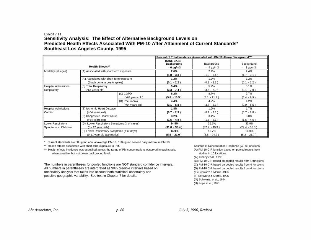
Abt Associates, Inc. p. 86 July 3, 1996, Revised
Exhibit 7.11Sensitivity Analysis: The Effect of Alternative Background Levels onPredicted Health Effects Associated With PM-10 After Attainment of Current Standards*Southeast Los Angeles County, 1995
Percent of Total Incidence Associated with PM-10 Above Background***
BackgroundBackgroundBackground BASE CASE
= 8 µg/m3 = 4 µg/m3 = 6 µg/m3 Health Effects**2.4%2.7%2.6%(A) Associated with short-term exposure Mortality (all ages)
(1.7 - 3.1 ) (1.9 - 3.4 ) (1.8 - 3.3 ) 1.2%1.2%1.2%(A') Associated with short-term exposure
(0.1 - 2.2 ) (0.1 - 2.2 ) (0.1 - 2.2 ) (Study done in Los Angeles)5.1%5.7%5.4%(B) Total RespiratoryHospital Admissions
(3.1 - 7.0 ) (3.5 - 7.9 ) (3.3 - 7.4 ) (>64 years old)Respiratory7.7%8.7%8.2%(C) COPD
(5.4 - 9.9 ) (6.1 - 11.1 ) (5.8 - 10.5 ) (>64 years old) 4.2%4.7%4.4%(D) Pneumonia
(2.9 - 5.5 ) (3.3 - 6.1 ) (3.1 - 5.8 ) (>64 years old) 1.7%1.9%1.8%(E) Ischemic Heart DiseaseHospital Admissions
(0.7 - 2.8 ) (0.7 - 3.1 ) (0.7 - 2.9 ) (>64 years old)Cardiac3.0%3.4%3.2%(F) Congestive Heart Failure
(1.5 - 4.5 ) (1.6 - 5.1 ) (1.5 - 4.8 ) (>64 years old)33.0%36.7%34.8%(G) Lower Respiratory Symptoms (# of cases)Lower Respiratory
(29.4 - 36.3 ) (32.7 - 40.3 ) (31.0 - 38.4 ) (8 - 12 year olds)Symptoms in Children14.0%15.7%14.9%(H) Lower Respiratory Symptoms (# of days)
(5.2 - 21.7 ) (5.8 - 24.2 ) (5.5 - 23.0 ) (9-11 year old asthmatics)
* Current standards are 50 ug/m3 annual average PM-10, 150 ug/m3 second daily maximum PM-10.Sources of Concentration-Response (C-R) Functions:** Health effects associated with short-term exposure to PM.(A) PM-10 C-R function based on pooled results from *** Health effects incidence was quantified across the range of PM concentrations observed in each study, studies in 10 locations. when possible, but not below background level. (A') Kinney et al., 1995(B) PM-10 C-R based on pooled results from 4 functions(C) PM-10 C-R based on pooled results from 4 functionsThe numbers in parentheses for pooled functions are NOT standard confidence intervals. (D) PM-10 C-R based on pooled results from 4 functionsAll numbers in parentheses are interpreted as 90% credible intervals based on(E) Schwartz & Morris, 1995uncertainty analysis that takes into account both statistical uncertainty and (F) Schwartz & Morris, 1995possible geographic variability. See text in Chapter 7 for details.(G) Schwartz, et al., 1994(H) Pope et al., 1991

Abt Associates, Inc. p. 87 July 3, 1996, Revised
Exhibit 7.12
Sensitivity Analysis: The Effect of Alternative Background Levels onPredicted Health Effects Associated With PM-2.5 After Attainment of Current Standards*Southeast Los Angeles County, 1995
Percent of Total Incidence Associated with PM-2.5 Above Background***BackgroundBackgroundBASE CASE
= 4.0 µg/m3 = 1.0 µg/m3Background = 3.5 µg/m3 Health Effects**
2.7%3.1%2.9%(A) Associated with Mortality (all ages)(1.6 - 3.7 ) (1.9 - 4.2 ) (1.7 - 3.9 ) short-term exposure
5.6%6.5%6.1%(B) Total RespiratoryHospital Admissions(1.5 - 9.7 ) (1.8 - 11.2 ) (1.6 - 10.5 ) (all ages)Respiratory
1.1%1.2%1.1%(C) Ischemic HeartHospital Admissions(0.4 - 1.7 ) (0.5 - 2.0 ) (0.4 - 1.8 ) Disease****Cardiac (>64 years old)
1.8%2.1%2.0%(D) Congestive(0.9 - 2.8 ) (1.0 - 3.2 ) (1.0 - 3.0 ) Heart Failure****
26.7%30.6%28.7%(E) Lower Respiratory Symptoms Lower Respiratory (14.4 - 36.3 ) (16.5 - 41.4 ) (15.4 - 39.0 ) (# of cases) (8-12 years old)Symptoms in Children
Sources of Concentration- * Current standards are 50 ug/m3 annual average PM-10, 150 ug/m3 second daily maximum PMResponse (C-R) functions: ** Health effects associated with short-term exposure to PM.(A) PM-2.5 C-R function *** Health effects incidence was quantified across the range of PM concentrations observed in each study,based on pooled results when possible, but not below background levelfrom 6 locations.**** PM-2.5 results based on using PM-2.5 mass as PM-10 mass in the PM-10 functions.(B) Thurston, et al., 1994(C) Schwartz & Morris, 1995The numbers in parentheses for pooled functions are NOT standard confidence intervals. (D) Schwartz & Morris, 1995All the numbers in parentheses are interpreted as 90% credible intervals based on (E) Schwartz, et al., 1994uncertainty analysis that takes into account both statistical uncertainty and possible
geographic variability. See text in Chapter 7 for details.

Abt Associates, Inc. p. 88 July 3, 1996, Revised
Exhibit 7.13Sensitivity Analysis: The Effect of Alternative Cutpoint Models onPredicted Health Effects Associated With "As-Is" PM-10Slope Adjustment Method 1*Philadelphia County, September 1992 - August 1993
Percent of Total Incidence Associated with PM-10 Above Cutpoint
CutpointCutpointCutpointBackgroundBASE CASE
= 40 µg/m3 = 30 µg/m3 = 20 µg/m3 = 8 µg/m3 Health Effects**0.1%0.2%0.4%1.1%(A) Associated with short-term exposure Mortality (all ages)
(0.0 - 0.1)(0.1 - 0.2)(0.3 - 0.6)(0.8 - 1.4 ) 0.4%0.7%1.3%2.4%(B) Total RespiratoryHospital Admissions
(0.2 - 0.5)(0.4 - 0.9)(0.8 - 1.7)(1.5 - 3.3 ) (>64 years old)Respiratory0.1%0.1%0.3%0.8%(C) Ischemic Heart DiseaseHospital Admissions
(0.0 - 0.1)(0.1 - 0.2(0.1 - 0.4)(0.3 - 1.3 ) (>64 years old)Cardiac0.1%0.2%0.5%1.4%(D) Congestive Heart Failure
(0.1 - 0.2)(0.1 - 0.1)(0.2 - 0.2)(0.7 - 2.1 ) (>64 years old)4.7%6.3%9.3%17.5%(E) Lower Respiratory Symptoms (# of cases)Lower Respiratory
(3.4 - 5.5)(3.9 - 8.1)(5.4 - 12.7)(15.3 - 19.6 ) (8-12 year olds)Symptoms in Children
* Two methods examine the potential impact of a concentration-response function having a steeper slope (i.e., larger coefficient) aboveSources of Concentration- specified cutpoints. In both methods the slope below the cutpoint is set = 0, while the slope above the cutpoint is set to be greater Response (C-R) functions: than the slope in the original study. In Adjustment Method 1, the cutpoint C-R relationship is modeled to intersect with the original(A) C-R function based on pooled relationship, exceeding the RRs predicted for the original study at higher concentrations. The relationship was modeled to match the reduction in results from 10 locations. the range of PM concentrations upon application of the cutpoint with an identical percentage increase in the risk observed(B) C-R function based on pooled at the highest concentration. Method 2 estimates a smaller increase in the slope. See text in Section 7 for details. results from 4 locations.**Health effects associated with short-term exposure to PM.(C) Schwartz & Morris, 1995(D) Schwartz & Morris, 1995The numbers in parentheses for pooled functions are NOT standard confidence intervals. (E) Schwartz, et al., 1994All numbers in parentheses are interpreted as 90% credible intervals based on
uncertainty analysis that takes into account both statistical uncertainty and possible geographic variability. See text in Chapter 7 for details.

Abt Associates, Inc. p. 89 July 3, 1996, Revised
Exhibit 7.14
Sensitivity Analysis: The Effect of Alternative Cutpoint Models onPredicted Health Effects Associated With "As-Is" PM-10Slope Adjustment Method 2*Philadelphia County, September 1992 - August 1993
Percent of Total Incidence Associated with PM-10 Above Cutpoint
CutpointCutpointCutpointBASE CASE Background = 40 µg/m3 = 30 µg/m3 = 20 µg/m3 = 8 µg/m3 Health Effects**
0.1%0.1%0.4%1.1%(A) Associated with short-term exposure Mortality (all ages)(0.0 - 0.1)(0.1 - 0.2)(0.3 - 0.5)(0.8 - 1.4 )
0.2%0.4%1.0%2.4%(B) Total RespiratoryHospital Admissions(0.1 - 0.3)(0.3 - 0.6)(0.6 - 1.3)(1.5 - 3.3 ) (>64 years old)Respiratory
0.0%0.1%0.3%0.8%(C) Ischemic Heart DiseaseHospital Admissions(0.0 - 0.1)(0.0 - 0.2)(0.1 - 0.4)(0.3 - 1.3 ) (>64 years old)Cardiac
0.1%0.2%0.5%1.4%(D) Congestive Heart Failure(0.0 - 0.1)(0.1 - 0.3)(0.2 - 0.7)(0.7 - 2.1 ) (>64 years old)
2.5%4.1%7.9%17.5%(E) Lower Respiratory Symptoms (# of cases)Lower Respiratory (1.5 - 3.2)(2.4 - 5.6)(4.5 - 11.0)(15.3 - 19.6 ) (8-12 year olds)Symptoms in Children
* Two methods examine the potential impact of a concentration-response function having a steeper slope (i.e., larger coefficient)Sources of Concentration- above specified cutpoints. In both methods the slope below the cutpoint is set = 0, while the slope above the cutpoint is set to Response (C-R) functions: be greater than the slope in the original study. In Adjustment Method 2, the slope is increased so that the new C-R function estimates(A) C-R function based on pooled the same health risk at the highest observed PM value as the original function. Method 1 estimates a larger increase in the slope. results from 10 locations. See text in Section 7 for details.(B) C-R function based on pooled results from 4 locations.**Health effects associated with short-term exposure to PM.(C) Schwartz & Morris, 1995(D) Schwartz & Morris, 1995The numbers in parentheses for pooled functions are NOT standard confidence intervals. (E) Schwartz, et al., 1994All numbers in parentheses are interpreted as 90% credible intervals based on
uncertainty analysis that takes into account both statistical uncertainty and possible geographic variability. See text in Chapter 7 for details.

Abt Associates, Inc. p. 90 July 3, 1996, Revised
Exhibit 7.15Sensitivity Analysis: The Effect of Alternative Cutpoint Models onPredicted Health Effects Associated With "As Is" PM-2.5Slope Adjustment Method 1*Philadelphia County, September 1992 - August 1993
Percent of Total Incidence Associated with PM-2.5 Above Cutpoint
CutpointCutpointBackground BASE CASE:
= 18 µg/m3 = 10 µg/m3 = 3.5 µg/m3 Health Effects**0.5%1.1%1.8%(A) Associated with Mortality (all ages)
(0.3 - 0.6)(0.7 - 1.5)(1.1 - 2.5 ) short-term exposure0.8%1.4%2.0%(B) Total RespiratoryHospital Admissions
(0.2 - 1.4)(0.4 - 2.4)(0.5 - 3.5 ) (all ages)Respiratory
0.2%0.4%0.7%Disease(C) Ischemic Heart
Hospital Admissions(0.1 - 0.3)(0.1 - 0.6)(0.3 - 1.2 ) (>64 years old)Cardiac
0.4%0.7%1.3%Failure(D) Congestive Heart
(0.2 - 0.5)(0.3 - 1.0)(0.6 - 2.0 ) (>64 years old)
9.9%13.2%20.0%Symptoms(E) Lower Respiratory
Lower Respiratory
(5.7 - 13.1)(7.2 - 18.6)(10.3 - 28.2 ) (8 - 12 years old)Symptoms in Children
Sources of Concentration- * Two methods examine the potential impact of a concentration-response function having a steeper slope (i.e., larger coefficient) aResponse (C-R) functions: specified cutpoints. In both methods the slope below the cutpoint is set = 0, while the slope above the cutpoint is set to be gre(A) C-R function based on pooled than the slope in the original study. In Adjustment Method 1, the cutpoint C-R relationship is modeled to intersect with the orig results from six locations. relationship, exceeding the RRs predicted for the original study at higher concentrations. The relationship was modeled to mat(B) Thurston, et al., 1994 the range of PM concentrations upon application of the cutpoint with an identical percentage increase in the risk observed(C) Schwartz & Morris, 1995 at the highest concentration. Method 2 estimates a smaller increase in the slope. See text in Section 7 for details.(D) Schwartz & Morris, 1995(E) Schwartz et al., 1994** Health effects associated with short-term exposure to PM.
The numbers in parentheses for pooled functions are NOT standard confidence intervals. All the numbers in parentheses are interpreted as 90% credible intervals based on uncertainty analysis that takes into account both statistical uncertainty and possible geographic variability.See text in Section 7 for details.

Abt Associates, Inc. p. 91 July 3, 1996, Revised
Exhibit 7.16
Sensitivity Analysis: The Effect of Alternative Cutpoint Models onPredicted Health Effects Associated With "As Is" PM-2.5Slope Adjustment Method 2*Philadelphia County, September 1992 - August 1993
Percent of Total Incidence Associated with PM-2.5 Above Cutpoint
CutpointCutpointCutpointBASE CASE: Background = 30 µg/m3 = 18 µg/m3 = 10 µg/m3 = 3.5 µg/m3 Health Effects**
0.1%0.4%1.0%1.8%(A) Associated with short-term exposure Mortality (all ages)(0.1 - 0.2)(0.3 - 0.6)(0.6 - 1.4)(1.1 - 2.5 )
0.2%0.6%1.2%2.0%(B) Total RespiratoryHospital Admissions(0.1 - 0.4)(0.2 - 1.1)(0.3 - 2.2)(0.5 - 3.5 ) (all ages)Respiratory
0.1%0.2%0.4%0.7%Disease(C) Ischemic Heart
Hospital Admissions(0.0 - 0.1)(0.1 - 0.3)(0.2 - 0.6)(0.3 - 1.2 ) (>64 years old)Cardiac
0.1%0.3%0.7%1.3%Failure(D) Congestive Heart
(0.0 - 0.1)(0.2 - 0.5)(0.3 - 1.0)(0.6 - 2.0 ) (>64 years old)
3.8%7.1%12.2%20.0%Symptoms(E) Lower Respiratory
Lower Respiratory
(2.4 - 4.7)(3.9 - 9.8)(6.5 - 17.3)(10.3 - 28.2 ) (8 - 12 years old)Symptoms
Sources of Concentration- * Two methods examine the potential impact of a concentration-response function having a steeper slope (i.e., larger coefficient)Response (C-R) functions: above specified cutpoints. In both methods the slope below the cutpoint is set = 0, while the slope above the cutpoint is set to (A) C-R function based on pooled be greater than the slope in the original study. In Adjustment Method 2, the slope is increased so that the new C-R function estimates results from six locations. the same health risk at the highest observed PM value as the original function. Method 1 estimates a larger increase in the slope.(B) Thurston, et al., 1994 See text in Section 7 for details.(C) Schwartz & Morris, 1995(D) Schwartz & Morris, 1995**Health effects associated with short-term exposure to PM.(E) Schwartz et al., 1994
The numbers in parentheses for pooled functions are NOT standard confidence intervals. All the numbers in parentheses are interpreted as 90% credible intervals based on uncertainty analysis that takes into account both statistical uncertainty and possible geographic variability.See text in Chapter 7 for details.
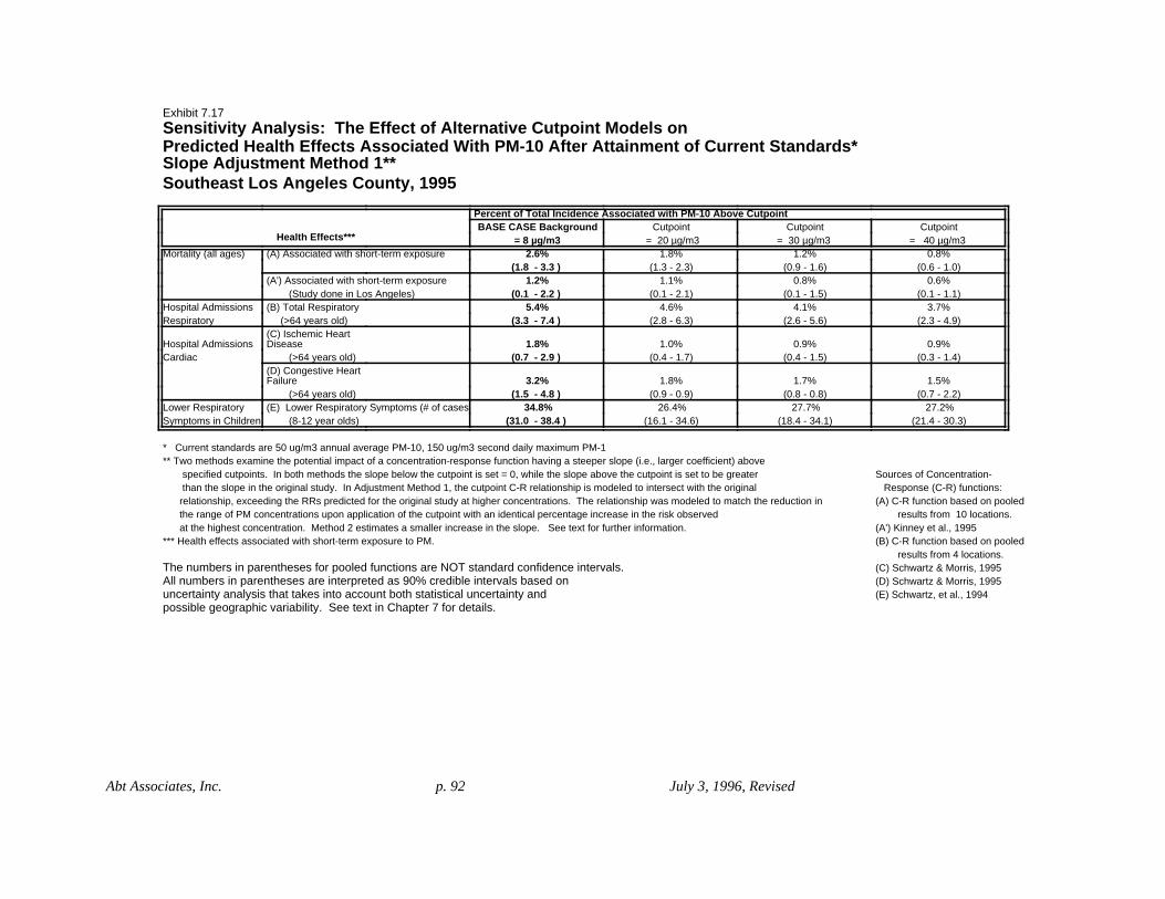
Abt Associates, Inc. p. 92 July 3, 1996, Revised
Exhibit 7.17Sensitivity Analysis: The Effect of Alternative Cutpoint Models onPredicted Health Effects Associated With PM-10 After Attainment of Current Standards*Slope Adjustment Method 1**Southeast Los Angeles County, 1995
Percent of Total Incidence Associated with PM-10 Above CutpointCutpointCutpointCutpointBASE CASE Background
= 40 µg/m3 = 30 µg/m3 = 20 µg/m3 = 8 µg/m3 Health Effects***0.8%1.2%1.8%2.6%(A) Associated with short-term exposure Mortality (all ages)
(0.6 - 1.0)(0.9 - 1.6)(1.3 - 2.3)(1.8 - 3.3 ) 0.6%0.8%1.1%1.2%(A') Associated with short-term exposure
(0.1 - 1.1)(0.1 - 1.5)(0.1 - 2.1)(0.1 - 2.2 ) (Study done in Los Angeles)3.7%4.1%4.6%5.4%(B) Total RespiratoryHospital Admissions
(2.3 - 4.9)(2.6 - 5.6)(2.8 - 6.3)(3.3 - 7.4 ) (>64 years old)Respiratory
0.9%0.9%1.0%1.8%Disease(C) Ischemic Heart
Hospital Admissions(0.3 - 1.4)(0.4 - 1.5)(0.4 - 1.7)(0.7 - 2.9 ) (>64 years old)Cardiac
1.5%1.7%1.8%3.2%Failure(D) Congestive Heart
(0.7 - 2.2)(0.8 - 0.8)(0.9 - 0.9)(1.5 - 4.8 ) (>64 years old)27.2%27.7%26.4%34.8%(E) Lower Respiratory Symptoms (# of cases)Lower Respiratory
(21.4 - 30.3)(18.4 - 34.1)(16.1 - 34.6)(31.0 - 38.4 ) (8-12 year olds)Symptoms in Children
* Current standards are 50 ug/m3 annual average PM-10, 150 ug/m3 second daily maximum PM-1** Two methods examine the potential impact of a concentration-response function having a steeper slope (i.e., larger coefficient) above
Sources of Concentration- specified cutpoints. In both methods the slope below the cutpoint is set = 0, while the slope above the cutpoint is set to be greater Response (C-R) functions: than the slope in the original study. In Adjustment Method 1, the cutpoint C-R relationship is modeled to intersect with the original(A) C-R function based on pooled relationship, exceeding the RRs predicted for the original study at higher concentrations. The relationship was modeled to match the reduction in results from 10 locations. the range of PM concentrations upon application of the cutpoint with an identical percentage increase in the risk observed(A') Kinney et al., 1995 at the highest concentration. Method 2 estimates a smaller increase in the slope. See text for further information.(B) C-R function based on pooled*** Health effects associated with short-term exposure to PM. results from 4 locations.(C) Schwartz & Morris, 1995The numbers in parentheses for pooled functions are NOT standard confidence intervals. (D) Schwartz & Morris, 1995All numbers in parentheses are interpreted as 90% credible intervals based on(E) Schwartz, et al., 1994uncertainty analysis that takes into account both statistical uncertainty and
possible geographic variability. See text in Chapter 7 for details.

Abt Associates, Inc. p. 93 July 3, 1996, Revised
Exhibit 7.18Sensitivity Analysis: The Effect of Alternative Cutpoint Models onPredicted Health Effects Associated With PM-10 After Attainment of Current Standards*Slope Adjustment Method 2**Southeast Los Angeles County, 1995
Percent of Total Incidence Associated with PM-10 Above CutpointCutpointCutpointCutpointBASE CASE Background
= 40 µg/m3 = 30 µg/m3 = 20 µg/m3 = 8 µg/m3 Health Effects***0.7%1.1%1.6%2.6%(A) Associated with short-term exposure Mortality (all ages)
(0.5 - 0.9)(0.8 - 1.4)(1.2 - 2.1)(1.8 - 3.3 ) 0.5%0.7%1.0%1.2%(A') Associated with short-term exposure
(0.0 - 0.9)(0.1 - 1.3)(0.1 - 2.0)(0.1 - 2.2 ) (Study done in Los Angeles)2.0%2.7%3.5%5.4%(B) Total RespiratoryHospital Admissions
(1.3 - 2.7)(1.7 - 3.7)(2.2 - 4.8)(3.3 - 7.4 ) (>64 years old)Respiratory
0.6%0.8%1.1%1.8%Disease(C) Ischemic Heart
Hospital Admissions(0.2 - 1.0)(0.3 - 1.3)(0.4 - 1.8)(0.7 - 2.9 ) (>64 years old)Cardiac
1.1%1.4%1.9%3.2%Failure(D) Congestive Heart
(0.5 - 1.6)(0.7 - 2.1)(0.9 - 2.8)(1.5 - 4.8 ) (>64 years old)16.7%19.4%22.9%34.8%(E) Lower Respiratory Symptoms (# of cases)Lower Respiratory
(11.3 - 20.5)(12.0 - 25.2)(13.7 - 30.5)(31.0 - 38.4 ) (8-12 year olds)Symptoms in Children
* Current standards are 50 ug/m3 annual average PM-10, 150 ug/m3 second daily maximum PM-1** Two methods examine the potential impact of a concentration-response function having a steeper slope (i.e., larger coefficient)
Sources of Concentration- above specified cutpoints. In both methods the slope below the cutpoint is set = 0, while the slope above the cutpoint is set to Response (C-R) functions: be greater than the slope in the original study. In Adjustment Method 2, the slope is increased so that the new C-R function estimates(A) C-R function based on pooled the same health risk at the highest observed PM value as the original function. Method 1 estimates a larger increase in the slope. results from 10 locations.(A') Kinney et al., 1995***Health effects associated with short-term exposure to PM.(B) C-R function based on pooled results from 4 locations.The numbers in parentheses for pooled functions are NOT standard confidence intervals. (C) Schwartz & Morris, 1995All numbers in parentheses are interpreted as 90% credible intervals based on(D) Schwartz & Morris, 1995uncertainty analysis that takes into account both statistical uncertainty and (E) Schwartz, et al., 1994possible geographic variability. See text in Chapter 7 for details.

Abt Associates, Inc. p. 94 July 3, 1996, Revised
Exhibit 7.19
Sensitivity Analysis: The Effect of Alternative Cutpoint Models onPredicted Health Effects Associated With PM-2.5 After Attainment of Current Standards*Slope Adjustment Method 1**Southeast Los Angeles County, 1995
Percent of Total Incidence Associated with PM-2.5 Above CutpointCutpointCutpointCutpoint BASE CASE:
= 30 µg/m3 = 18 µg/m3 = 10 µg/m3Backgrount = 3.5 µg/m3 Health Effects***
0.7%1.3%2.1%2.9%(A) Associated with Mortality (all ages)(0.4 - 1.0)(0.8 - 1.8)(1.3 - 2.8)(1.7 - 3.9 ) with short-term exposure
3.4%4.0%4.9%6.1%(B) Total RespiratoryHospital Admissions(0.9 - 5.9)(1.1 - 7.0)(1.3 - 8.5)(1.6 - 10.5 ) (all ages)Respiratory
0.4%0.6%0.7%1.1%(C) Ischemic HeartHospital Admissions
(0.2 - 0.7)(0.2 - 0.9)(0.3 - 1.1)(0.4 - 1.8 ) Disease (>64 years old)Cardiac0.7%1.0%1.2%2.0%(D) Congestive Heart Failure
(0.4 - 1.1)(0.5 - 1.5)(0.6 - 1.8)(1.0 - 3.0 ) (>64 years old)19.7%21.0%22.0%28.7%(E) Lower Respiratory SymptomsLower Respiratory
(17.0 - 20.9)(13.2 - 26.5)(12.5 - 29.7)(15.4 - 39.0 ) (8 - 12 years old) Symptoms in Children
* Current standards are 50 ug/m3 annual average PM-10, 150 ug/m3 second daily maximum PM-10** Two methods examine the potential impact of a concentration-response function having a steeper slope (i.e., larger coefficient) above specified cutpoints. In both methods the slope below the cutpoint is set = 0, while the slope above the cutpoint is set to be gre than the slope in the original study. In Adjustment Method 1, the cutpoint C-R relationship is modeled to intersect with the orig relationship, exceeding the RRs predicted for the original study at higher concentrations. The relationship was modeled to match the reduction in the range of PM concentrations upon application of the cutpoint with an identical percentage increase in the risk observed at the highest concentration. Method 2 estimates a smaller increase in the slope. See text for further information.
Sources of Concentration-*** Health effects associated with short-term exposure to PM.Response (C-R) functions:(A) C-R function based onThe numbers in parentheses for pooled functions are NOT standard confidence intervals. pooled results from All the numbers in parentheses are interpreted as 90% credible intervals based on uncertainty analysis six locationsthat takes into account both statistical uncertainty and possible geographic variability.(B) Thurston, et al., 1994(C) Schwartz & Morris, 1995See text in Section 7 for details.(D) Schwartz & Morris, 1995(E) Schwartz et al., 1994

Abt Associates, Inc. p. 95 July 3, 1996, Revised
Exhibit 7.20
Sensitivity Analysis: The Effect of Alternative Cutpoint Models onPredicted Health Effects Associated With PM-2.5 After Attainment of Current Standards*Slope Adjustment Method 2**Southeast Los Angeles County, 1995
Percent of Total Incidence Associated with PM-2.5 Above CutpointCutpointCutpointCutpointBASE CASE:
= 30 µg/m3 = 18 µg/m3 = 10 µg/m3Background = 3.5 µg/m3 Health Effects***
0.6%1.2%1.9%2.9%(A) Associated with Mortality (all ages)(0.4 - 0.8)(0.7 - 1.7)(1.2 - 2.7)(1.7 - 3.9 ) short-term exposure
2.0%3.1%4.4%6.1%(B) Total RespiratoryHospital Admissions(0.5 - 3.4)(0.8 - 5.4)(1.2 - 7.6)(1.6 - 10.5 ) (all ages)Respiratory
0.3%0.5%0.7%1.1%(C) Ischemic Heart Hospital Admissions
(0.1 - 0.5)(0.2 - 0.8)(0.3 - 1.2)(0.4 - 1.8 ) Disease (>64 years old)Cardiac0.5%0.9%1.3%2.0%(D) Congestive Heart
(0.2 - 0.8)(0.4 - 1.3)(0.6 - 1.9)(1.0 - 3.0 ) Failure (>64 years old)13.1%15.8%20.4%28.7%(E) Lower RespiratoryLower Respiratory
(9.1 - 15.5)(9.3 - 20.9)(11.5 - 27.9)(15.4 - 39.0 ) old)Symptoms (8 - 12 years
Symptoms in Children
* Current standards are 50 ug/m3 annual average PM-10, 150 ug/m3 second daily maximum PM- * Two methods examine the potential impact of a concentration-response function having a steeper slope (i.e., larger coefficien above specified cutpoints. In both methods the slope below the cutpoint is set = 0, while the slope above the cutpoint is s be greater than the slope in the original study. In Adjustment Method 2, the slope is increased so that the new C-R function estimates the same health risk at the highest observed PM value as the original function. Method 1 estimates a larger increase in the slope.**Health effects associated with short-term exposure to PM.
The numbers in parentheses for pooled functions are NOT standard confidence intervals. Sources of Concentration-All the numbers in parentheses are interpreted as 90% credible intervals based on uncertainty analysis Response (C-R) functions:that takes into account both statistical uncertainty and possible geographic variability.(A) C-R function based on See text in Chapter 7 for details.pooled results fromsix locations.(B) Thurston, et al., 1994(C) Schwartz & Morris, 1995(D) Schwartz & Morris, 1995(E) Schwartz et al., 1994

Abt Associates, Inc. p. 96 July 3, 1996, Revised
Exhibit 7.21
Sensitivity Analysis: Effect of Combining Different Averaging TimesIn Pooled Short-Term Exposure Mortality Functions onPredicted Health Effects Associated With "As-Is" PM-10Philadelphia County, September 1992 - August 1993
Percent of Total Incidence Associated with PM-10 Above Background*
average PMStudies using 3-5 day
average PMStudies using 2-day
average PMStudies using 1-day
Averaging TimesStudies Using All
BASE CASE**
(2 studies)(7 studies)(1 study)(10 studies)5-day average PM2-day average PM1-day average PM2-day average PMMatching study and data
1.8%1.0%0.4%1.1%averaging times(1.3 - 2.4 ) (0.5 - 1.5 ) (0.0 - 0.8 ) (0.8 - 1.4 )
2-day average PM2-day average PM2-day average PM2-day average PMUsing 2-day average PM data1.9%same0.4%same
(1.3 - 2.4 ) (0.0 - 0.8 ) 1-day average PMUsing 1-day average PM data
1.1%(0.8 - 1.4 )
5-day average PMUsing 5-day average PM data1.1%
(0.8 - 1.4 )
The studies that contribute to the pooled*Health effects incidence was quantified across the range of PM concentrations observed in each study,function are: when possible, but not below background level. Background PM-10 is assumed to be 8 ug/m3 .Kinney et al., 1995 (Los Angeles)1-day:Ito and Thurston, 1996 (Chicago)2-day:** The base case is a random-effects pooled function used with 2-day average PM data.Schwartz et al. 1996 (Boston, MA; All other pooled functions are also random effects, except the pooled function derived from Knoxville, TN; St. Louis, MO; studies using 3-5 day average PM data, for which a fixed effects model was used, since Steubenville, OH; Portage, WI;it is not possible to calculate a random effects model for those two functions. Topeka, KS)Schwartz 1993 (Birmingham, AL)3-day:The numbers in parentheses for pooled functions are NOT standard confidence intervaPope et al., 1992 (Utah Valley)5-day:All numbers in parentheses are interpreted as 90% credible intervals based on
uncertainty analysis that takes into account both statistical uncertainty and possible geographic variability. See text in Chapter 7 for details.
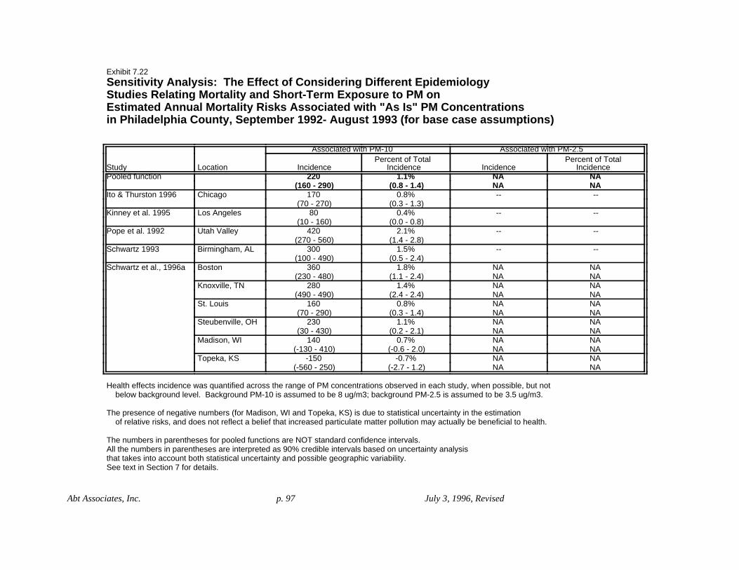
Abt Associates, Inc. p. 97 July 3, 1996, Revised
Exhibit 7.22Sensitivity Analysis: The Effect of Considering Different EpidemiologyStudies Relating Mortality and Short-Term Exposure to PM onEstimated Annual Mortality Risks Associated with "As Is" PM Concentrationsin Philadelphia County, September 1992- August 1993 (for base case assumptions)
Associated with PM-2.5Associated with PM-10
IncidencePercent of Total
IncidenceIncidencePercent of Total
IncidenceLocationStudyNANA1.1%220Pooled functionNANA(0.8 - 1.4)(160 - 290)----0.8%170ChicagoIto & Thurston 1996
(0.3 - 1.3)(70 - 270)----0.4%80Los AngelesKinney et al. 1995
(0.0 - 0.8)(10 - 160)----2.1%420Utah ValleyPope et al. 1992
(1.4 - 2.8)(270 - 560)----1.5%300Birmingham, ALSchwartz 1993
(0.5 - 2.4)(100 - 490)NANA1.8%360BostonSchwartz et al., 1996aNANA(1.1 - 2.4)(230 - 480)NANA1.4%280Knoxville, TNNANA(2.4 - 2.4)(490 - 490)NANA0.8%160St. LouisNANA(0.3 - 1.4)(70 - 290)NANA1.1%230Steubenville, OHNANA(0.2 - 2.1)(30 - 430)NANA0.7%140Madison, WINANA(-0.6 - 2.0)(-130 - 410)NANA-0.7%-150Topeka, KSNANA(-2.7 - 1.2)(-560 - 250)
Health effects incidence was quantified across the range of PM concentrations observed in each study, when possible, but not below background level. Background PM-10 is assumed to be 8 ug/m3; background PM-2.5 is assumed to be 3.5 ug/m3.
The presence of negative numbers (for Madison, WI and Topeka, KS) is due to statistical uncertainty in the estimation of relative risks, and does not reflect a belief that increased particulate matter pollution may actually be beneficial to health.
The numbers in parentheses for pooled functions are NOT standard confidence intervals. All the numbers in parentheses are interpreted as 90% credible intervals based on uncertainty analysis that takes into account both statistical uncertainty and possible geographic variability.See text in Section 7 for details.

Abt Associates, Inc. p. 98 July 3, 1996, Revised
Table 7.23
Sensitivity Analysis: Effect of CopollutantsRelative Risks for Change of 50 ug/m3 PM-10 or 25 ug/m3 PM-2.5
Relative Risk withRelative Risk withRelative Risk withRelative Risk withRelative riskdaily 1-hour maximumdaily averagedaily 1-hour maximumdaily average
O3O3COSO2no copollutantStudy, Pollutant, & LocationEndpoint1.021.02Ito & Thurston 1995, PM-10Mortality
(1.01 - 1.03)(1.02 - 1.04)Chicago1.021.021.02Kinney et al., 1995, PM-10
(1.00 - 1.05)(0.99 - 1.04)(1.00 - 1.05)Los Angeles1.191.141.11Pope 1994, PM-10
(1.00 - 1.43)(0.96 - 1.37)(0.95 - 1.31)Utah Valley, summer only0.045*0.086*Thurston et al., 1994, PM-2.5All respiratoryHospital
(-0.028 - 0.12 )(0.024 - 0.15 )Ontario, Canada(all ages)Admissions1.091.071.06Schwartz 1995, PM-10All respiratory
(1.01 - 1.18)(1.02 - 1.13)(1.01 - 1.12)New Haven(ages >64)1.121.111.10Schwartz 1995, PM-10
(0.99 - 1.26)(1.03 - 1.19)(1.04 - 1.16)Tacoma1.08Schwartz 1994, PM-10Pneumonia
(1.02 - 1.14)Minneapolis/St. Paul(ages >64)1.06Schwartz 1994, PM-10
(1.03 - 1.09)Detroit1.10Schwartz 1994, PM-10COPD
(1.06 - 1.16)Detroit(ages >64)1.0251.024**1.028Schwartz & Morris 1995, PM-10Ischemic Heart Disease
(1.007 - 1.044)(1.005 - 1.043)(1.011 - 1.047)Detroit1.0381.050Schwartz & Morris 1995, PM-10Congestive Heart Failure
(1.011 - 1.064)(1.024 - 1.077)DetroitResults presented in bold come from functions used in the base case analysis.The number of significant digits given for each relative risk is the same as the number reported in the original study.
* Thurston et al. 1994 provides a function relating changes in PM to changes in the number of cases. The relative risk calculated from this coefficient may vary widely from location to location, depending on baseline incidences. Therefore, the coefficient, adjusted to a rate per 100,000 people, is reported, instead of a relative risk.
** Based on 1-hour maximum SO2.
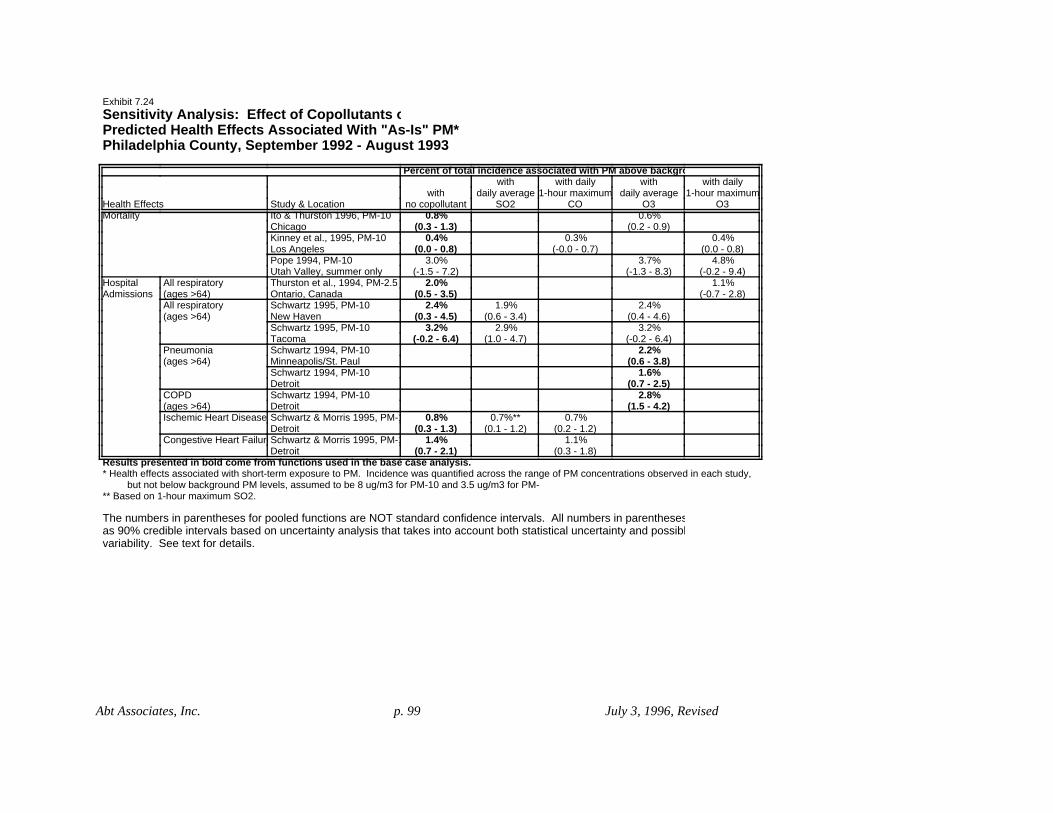
Abt Associates, Inc. p. 99 July 3, 1996, Revised
Exhibit 7.24Sensitivity Analysis: Effect of Copollutants oPredicted Health Effects Associated With "As-Is" PM*Philadelphia County, September 1992 - August 1993
Percent of total incidence associated with PM above backgrowith dailywithwith dailywith
1-hour maximumdaily average1-hour maximumdaily averagewithO3O3COSO2no copollutantStudy & LocationHealth Effects
0.6%0.8%Ito & Thurston 1996, PM-10Mortality(0.2 - 0.9)(0.3 - 1.3)Chicago
0.4%0.3%0.4%Kinney et al., 1995, PM-10(0.0 - 0.8)(-0.0 - 0.7)(0.0 - 0.8)Los Angeles
4.8%3.7%3.0%Pope 1994, PM-10(-0.2 - 9.4)(-1.3 - 8.3)(-1.5 - 7.2)Utah Valley, summer only
1.1%2.0%Thurston et al., 1994, PM-2.5All respiratoryHospital(-0.7 - 2.8)(0.5 - 3.5)Ontario, Canada(ages >64)Admissions
2.4%1.9%2.4%Schwartz 1995, PM-10All respiratory(0.4 - 4.6)(0.6 - 3.4)(0.3 - 4.5)New Haven(ages >64)
3.2%2.9%3.2%Schwartz 1995, PM-10(-0.2 - 6.4)(1.0 - 4.7)(-0.2 - 6.4)Tacoma
2.2%Schwartz 1994, PM-10Pneumonia(0.6 - 3.8)Minneapolis/St. Paul(ages >64)
1.6%Schwartz 1994, PM-10(0.7 - 2.5)Detroit
2.8%Schwartz 1994, PM-10COPD(1.5 - 4.2)Detroit(ages >64)
0.7%0.7%**0.8%Schwartz & Morris 1995, PM-1Ischemic Heart Disease(0.2 - 1.2)(0.1 - 1.2)(0.3 - 1.3)Detroit
1.1%1.4%Schwartz & Morris 1995, PM-1Congestive Heart Failure(0.3 - 1.8)(0.7 - 2.1)Detroit
Results presented in bold come from functions used in the base case analysis.* Health effects associated with short-term exposure to PM. Incidence was quantified across the range of PM concentrations observed in each study, but not below background PM levels, assumed to be 8 ug/m3 for PM-10 and 3.5 ug/m3 for PM-** Based on 1-hour maximum SO2.
The numbers in parentheses for pooled functions are NOT standard confidence intervals. All numbers in parenthesesas 90% credible intervals based on uncertainty analysis that takes into account both statistical uncertainty and possiblvariability. See text for details.

Abt Associates, Inc. p. 100 July 3, 1996, Revised
Exhibit 7.25Sensitivity Analysis: Effect of Copollutants onPredicted Health Effects Associated With PM* After Attainment of Current Standards**Southeast Los Angeles County, 1995
Percent of total incidence associated with PM above backgroundwith dailywithwith dailywith
1-hour maximumdaily average1-hour maximumdaily averagewithO3O3COSO2no copollutantStudy & LocationHealth Effects
1.3%1.9%Ito & Thurston 1996, PM-10Mortality(0.5 - 2.1)(0.7 - 3.1)Chicago
1.2%1.0%1.2%Kinney et al., 1995, PM-10(0.1 - 2.2)(-0.1 - 2.0)(0.1 - 2.2)Los Angeles
10.7%8.3%6.7%Pope 1994, PM-10(-0.4 - 20.1)(-3.0 - 17.9)(-3.6 - 15.7)Utah Valley, summer only
NANAThurston et al., 1994, PM-2.5All respiratoryHospitalNANAOntario, Canada(all ages)Admissions
5.5%4.4%5.5%Schwartz 1995, PM-10All respiratory(1.0 - 10.3)(1.3 - 7.6)(0.6 - 10.1)New Haven(ages >64)
7.2%6.6%7.2%Schwartz 1995, PM-10(-0.4 - 14.0)(2.2 - 10.5)(-0.4 - 14.0)Tacoma
5.1%Schwartz 1994, PM-10Pneumonia(1.5 - 8.4)Minneapolis/St. Paul(ages >64)
3.7%Schwartz 1994, PM-10(1.7 - 5.7)Detroit
6.4%Schwartz 1994, PM-10COPD(3.4 - 9.3)Detroit(ages >64)
1.6%1.5%***1.8%Schwartz & Morris 1995, PM-10Ischemic Heart Disease(0.4 - 2.8)(0.3 - 2.8)(0.7 - 2.9)Detroit
2.4%3.2%Schwartz & Morris 1995, PM-10Congestive Heart Failure(0.7 - 4.0)(1.5 - 4.8)Detroit
Results presented in bold come from functions used in the base case analysis* Health effects associated with short-term exposure to PM. Incidence was quantified across the range of PM concentrations observed in each study, but not below background PMlevels, assumed to be 6 ug/m3 for PM-10 and 2.5 ug/m3 for PM-2.5.** Current standards are 50 ug/m3 annual average PM-10, 150 ug/m3 second daily maximum PM-10.*** Based on 1-hour maximum SO2.
The numbers in parentheses for pooled functions are NOT standard confidence intervals. All numbers in parentheses are interpreted as 90% credible intervals based on uncertainty analysis that takes into account both statistical uncertainty and possible geographic variability. See text for details.

Abt Associates, Inc. p. 101 July 3, 1996, Revised
Exhibit 7.26
Sensitivity Analysis: The Effect of Differing Cutpoints on EstimatedMortality Associated with Long-term Exposure to PM-2.5Philadelphia County, September 1992 - August 1993
BASE CASE
Cutpoint = 18 ug/m3Cutpoint = 15 ug/m3Cutpoint = 12.5 ug/m3ug/m3Observed = 9
Lowest
0.0%1.0%2.5%4.7%(A) Mortality associated with(0.0 - 0.0)(0.6 - 1.3)(1.6 - 3.5)(2.9 - 6.4) long-term exposure
(A) Pope et al., 1995
Health effects incidence was calculated down to the lowest level observed in the study (9 ug/m3).No adjustments to the slope were performed.
The numbers in parentheses for pooled functions are NOT standard confidence intervals. All the numbers in parentheses are interpreted as 90% credible intervals based on uncertainty analysis that takes into account both statistical uncertainty and possible geographic variability.See text in Chapter 7 for details.

Abt Associates, Inc. p. 102 July 3, 1996, Revised
Exhibit 7.27Sensitivity Analysis: The Effect of Concentration-Response Function Slopeon Estimated Mortality Associated with Long-term Exposure to PM-2.5Philadelphia County, September 1992 - August 1993
BASE CASE
twice as high*Assuming relevant AQ
50% higher*Assuming relevant AQ
reportedAssuming AQ as
2.4%3.5%4.7%(A) Mortality associated with(1.5 - 3.3)(2.2 - 4.9)(2.9 - 6.4) long-term exposure
(A) Pope et al., 1995Health effects incidence was calculated down to the lowest level observed in the study* Adjusted function from Pope et al., 1995. Had historical air quality been 50% higher, the relative risk calculated by the study would have been two thirds of that reported. Had historical air quality been twice as high, the relative risk calculated would have been half that reported. See text for details.
The numbers in parentheses for pooled functions are NOT standard confidence intervals. All the numbers in parentheses are interpreted as 90% credible intervals based on uncertainty analysis that takes into account both statistical uncertainty and possible geographic variability.See text in Chapter 7 for details.

Abt Associates, Inc. p.103 July 3, 1996, Revised
7.2. Uncertainty Analyses
A set of risk analyses considering different sample locations, different PM indicators,different PM standards, different health endpoints, and different concentration-responsefunctions for each health endpoint can be expected to produce a set of results with a largedegree of variability. Some of this variability reflects actual variability in the underlyingpopulation parameters. For example, “as is” PM concentrations in one location may be muchgreater than in another location. Some of the variability in the outcomes of the risk analyses,however, reflects uncertainty about the true values of the parameters of the risk analyses. Thesubstantial variability generated by applying different concentration-response functions to agiven sample location, for example, does not reflect real variability that exists in that location,but instead reflects uncertainty about the actual concentration-response relationship betweenPM and the population response in that location.
There are several sources of possible uncertainty associated with the estimation of PM-related incidence in the risk analysis (as discussed in Section 3). These include, for example,uncertainty about the appropriate concentration-response function for a given location,uncertainty about the baseline health effect incidence rates in the location, uncertainty aboutaverage daily PM concentrations in the location, and uncertainty about the background PMconcentration in the location. In addition, there are sources of uncertainty inherent in anyempirical investigation, such as the uncertainty about the correct functional form of the(concentration-response) model.
Some of these analysis input components are likely to involve much greater degrees ofuncertainty than others. The concentration-response function, for example, is considered to bea source of substantial uncertainty. In contrast, because it was possible to obtain local baselineincidence rates for many of the health endpoints, the degree of uncertainty associated withthese incidence rates is considered to be quite small. Similarly, although there may be someuncertainty associated with average daily PM concentrations (especially related to those daysfor which no PM monitoring was done), the overall level of uncertainty associated with PMconcentrations is judged to be small relative to that associated with the concentration-responsefunction. First, the percent of days without monitoring was very small in Philadelphia Countyand fairly small in Southeast Los Angeles County. Second, if the uncertainty is associatedlargely with random measurement errors, then small errors in one direction on one day arelikely to be counterbalanced by small errors in the other direction on another day. Becausedaily incidences are totaled over the year, minor daily discrepancies related to PMmeasurement errors are likely to largely cancel each other out in the total.
In addition to differences in the degrees of uncertainty associated with differentcomponents of the analysis, there are differences in the degree to which these uncertainties canbe quantified. A sensitivity analysis (like those presented in Section 7.1) considers how theend result of an analysis varies as a particular input parameter value is varied. Such ananalysis requires only the possible alternative parameter values but does not require that theprobabilities of each possible input parameter value be known. In contrast, a quantitative

Abt Associates, Inc. p.104 July 3, 1996, Revised
assessment of the uncertainty associated with an input parameter requires either thedistribution of possible parameter values, or, at a minimum, some information on which tobase an estimate of this distribution.
The source of the largest amount of uncertainty in the risk analysis is likely to be theconcentration-response function. In addition, although the amount of information about thedistribution of possible values of the parameter in the concentration-response function variesfrom one function to another (e.g., for short-term exposure mortality there is substantialinformation, whereas for hospital admissions for respiratory illness there is much less), there issome information for each category of concentration-response function. For these reasons, theconcentration-response function is the primary focus of the uncertainty analysis. Uncertaintybounds characterizing the uncertainty associated with the concentration-response functionalone were derived for each combination of health endpoint and PM indicator. The methodsused to derive these uncertainty bounds are discussed in Section 5.2. The emphasis in thisdiscussion is on the general case when there is more than one study reporting a concentration-response function for a particular combination of health endpoint and PM indicator (e.g., short-term exposure mortality and PM-10). The results of these uncertainty analyses are shown inSection 5.2.4.
Other sources of uncertainty were sequentially added to the uncertainty associated withthe concentration-response function, using Monte Carlo propagation of uncertainty methods,which allow multiple sources of uncertainty to be considered simultaneously. The method andresults of this propagation of uncertainty are presented below.
7.2.1. A Monte Carlo analysis: propagation of uncertainties from several sources
The sensitivity analyses presented in Section 7.1 (and for meeting alternative standards,in Section 8 below) illustrate the dependence of the results of the risk analyses on certain keyparameters and assumptions. The uncertainty analysis presented in Sections 5.3.1 and 5.3.2attempts to quantify the uncertainty associated with a single parameter of the risk analysis,namely, the concentration-response function. While sensitivity analyses may help to identifythose parameters that most influence the results of an analysis, such analyses do not indicatethe likelihood that the true value of the parameter is any of those values considered. Inaddition, neither the sensitivity analyses nor the uncertainty analysis presented above considermore than one source of uncertainty at a time. This section presents a set of analyses intendedto more fully characterize the uncertainty surrounding the risk estimates presented in Sections7.1 and 8.1. The analyses use a Monte Carlo procedure to include uncertainty from severalsources simultaneously. These integrated uncertainty analyses are limited to consideration ofmortality associated with short-term and long-term exposure to PM-2.5.
As noted above, a Monte Carlo procedure refers to the drawing of observations from aknown distribution. Uncertainty from several sources may be propagated through the riskmodel by simultaneously drawing observations from a set of distributions, one for each source

Abt Associates, Inc. p.105 July 3, 1996, Revised
of uncertainty considered. Suppose, for example, there are three unknown parameters in theanalysis model, each of which has been estimated. Each parameter estimate is the mean of adistribution of possible values. On each iteration of the Monte Carlo procedure, anobservation is randomly selected from each of the three distributions. Each iteration thereforeproduces a triple -- three values, one for each unknown parameter. Given these three particularparameter values, there is a particular value of the endpoint of the analysis (e.g., a particularvalue of avoided mortality). On each of many iterations, the Monte Carlo procedure producesa randomly selected set of parameter values (selected from the distributions for these parameters) which in turn produces a particular value of the endpoint of the analysis. Theprocedure therefore produces a distribution of values of the analysis endpoint (e.g., adistribution of avoided mortality) corresponding to the set of distributions of parameter values. This distribution characterizes the uncertainty surrounding the analysis endpoint resulting fromthe uncertainty surrounding the input parameters considered.
Monte Carlo propagation of uncertainty analyses were carried out for both the short-term exposure mortality and the long-term exposure mortality risk analyses. The sources ofuncertainty included in the Monte Carlo analysis are listed in Exhibit 7.28, along withtheircorresponding distributions. Uncertainties were incorporated into the analysis one at atime in order to demonstrate the effect of each one.
The distributions of parameter values are not known but instead were estimated fromthe available information The estimation of the distribution of $ in the concentration-responsefunction, for example, is described in Section 5.2. The distributions for background PM-2.5were based on estimates of background PM-2.5 concentrations ranging from 2 :g/m3 to 5:g/m3 in the Eastern U.S. and from 1 :g/m3 to 4 :g/m3 in the Western U.S. With no furtherinformation about the distribution of background concentrations in the Eastern or WesternU.S., uniform distributions on these intervals seemed reasonable.
Not all uncertainties associated with the model are incorporated into the propagateduncertainty analysis. Some uncertainties, including, for example, the possible influence ofcopollutants, were excluded from this analysis due to a lack of sufficient quantitativeinformation from which to estimate a distribution. Despite a lack of quantitative information,cutpoints were included because of their key role in the analysis. Because there is noinformation on which to base an estimate of the distribution of values of a possible cutpoint, three alternative distributions, each consisting of weights for four discrete cutpoint values,were used to illustrate the impact on the risk estimates of alternative viewpoints about thelikelihood of a threshold existing above background PM-2.5 levels. The weighting schemes,which are included for illustrative purposes, are shown in Exhibit 7.29. Case I represents ajudgement that concentration-response functions are likely to be valid down to eitherbackground or 10 :g/m3; case III represents a judgement that concentration-response functionsare likely to have cutpoints at or above 18 :g/m3; and case II is intermediate between the othertwo.

Abt Associates, Inc. p.106 July 3, 1996, Revised
Exhibit 7.28. Summary of Uncertainties Incorporated into Integrated UncertaintyAnalysis
Uncertainty Distribution
Coefficient ($) in concentration-response function
Short-term exposure function (for which there were severalepidemiological studies): 200 points representing the estimateddistribution of $ for short-term exposure mortality, derived in Section5
Long-term exposure function: normal distribution based on results ofthe single study (Pope et al., 1995) used in the risk analysis
Cutpoints in concentration-responsefunction
4 cutpoints, 3 discrete weighting schemes,2 slope adjustment methods
Background PM-2.5 concentration uniform distributions on the intervals [2,5] and [1,4] (:g/m3) forPhiladelphia County and Los Angeles County, respectively(these are the ranges identified in the Criteria Document)
Form of PM reductions to achievealternative standards
130 points representing distribution of a certain kind of non-proportionality (described in Section 8)
Exhibit 7.29. Three weighting schemes for cutpoints in integrated uncertainty analyses: Mortality associated with short-term exposure to PM-2.5
Case I Case II Case III
Background 0.50 0.20 0.05
10 :g/m3 0.30 0.30 0.15
18 :g/m3 0.15 0.30 0.50
30 :g/m3 0.05 0.20 0.30
Ideally, to derive a concentration-response function with a cutpoint, the data on which theoriginal concentration-response function (without a cutpoint) was based would be re-analyzed,excluding those points falling below the selected PM level. If a threshold existed in the originaldata, this would presumably result in a different, steeper estimated function. Since the data onwhich the concentration-response functions were based are not readily available, two methods ofadjusting the slope of concentration-response functions (described in Section 7.1) wereconsidered. In the integrated uncertainty analyses, they are given equal weight.
Exhibits 7.30 and 7.31 show the integrated uncertainty analysis for mortality due toshort-term exposure for “as is” conditions in Philadelphia County, and results assumingattainment of current PM-10 standards in Southeast Los Angeles County, respectively. Each

Abt Associates, Inc. p.107 July 3, 1996, Revised
vertical bar represents an estimate of the health effects that includes a certain set ofuncertainties (identified below the bars). The mean estimate is shown, as well as the 5th, 25th,75th, and 95th percentiles. Note that in weighting case III, the 25th percentile becomes veryclose to the 5th percentile, and the 75th percentile becomes very close to the mean. This is aresult of the discrete nature of the distribution of cutpoints (as well as of the specific weightsassigned to each cutpoint). The lowest thirty percent of values in the distribution of estimatesfor Case III come from iterations when the cutpoint is assumed equal to 30 :g/m3. Iterationswhen the cutpoint is assumed to be lower give substantially higher values; therefore the 25thpercentile is very close to the 5th percentile (compared to the range of values). A jump wouldbe expected to occur around the 30th percentile. Similarly, since the next fifty percent ofvalues come from iterations when the cutpoint is assumed equal to 18 :g/m3, and since thesevalues are substantially lower than those predicted when the cutpoint is assumed to be lower,the 75th percentile value is close to the mean (again, compared to the range of values). If allthe individual values obtained were plotted, the graph would show clusters of points.
Because the lower cutpoints yield larger ranges of values (as well as larger values ingeneral; see Exhibits 7.15 and 7.16), Case I , which gives greater weight to the lower cutpoints,does not show this kind of bunching of the distribution. Case II is intermediate between CasesI and III. Similarly, because of Los Angeles County’s generally higher PM concentrations,this phenomenon is not as pronounced in Exhibit 7.31.

Abt Associates, Inc. p.108 July 3, 1996, Revised
0
100
200
300
400
500
600
Exhibit 7.30Uncertainty Analysis: Effect of Uncertainty of Relative Risks,
Background Concentrations, Cutpoint and Slope Adjustment Method
Mortality Associated With Short-Term Exposure to PM-2.5Philadelphia, September 1992 - August 1993
(Population: 1.6 Million)
RiskAssociated
with PM-2.5above
Cutpoint(Number ofDeaths and
as Percent ofTotal
Mortality)
Uncertainty in background concentration enters into these calculations only whenthe cutpoint is set equal to background. The other cutpoints are greater than thehighest background concentration considered. When a cutpoint other than backgroundis chosen, each of the two slope adjustment methods has a fifty percent chance of selection.
Cutpoint Weighting Schemes
95th % ile
75th % ile
Mean
25th % ile
5th % ile
Uncertainty in Just RR(Background= 3.5 µg/m3)
Uncertainty inRR and Background(cutpoint = background)
Case I Case II Case III
Uncertainty in RR, Background,Cutpoint, and Slope Adjustment Method
0.0%
0.5%
1.0%
1.5%
2.0%
2.5%
3.0%
Case I Case II Case IIIBackground 0.5 0.2 0.0510 μg/m3 0.3 0.3 0.1518 μg/m3 0.15 0.3 0.530 μg/m3 0.05 0.2 0.3

Abt Associates, Inc. p.109 July 3, 1996, Revised
0
100
200
300
400
500
600
700
800
900
1000
Exhibit 7.31Uncertainty Analysis: Effect of Uncertainty of Relative Risks,
Background Concentrations, Cutpoint and Slope Adjustment Method
Mortality Associated With Short-Term Exposure to PM-2.5After Meeting Current PM-10 Standards
Southeast Los Angeles County, 1995(Population: 3.6 Million)
RiskAssociated
with PM-2.5above
Cutpoint(Number ofDeaths and
as Percent ofTotal
Mortality)
Uncertainty in background concentration enters into these calculations only whenthe cutpoint is set equal to background. The other cutpoints are greater than thehighest background concentration considered. When a cutpoint other than background is chosen,each of the slope adjustment methods has a fifty percent chance of selection.
Cutpoint Weighting Schemes
Uncertainty in Just RR(Background= 2.5 µg/m3)
Uncertainty inRR and Background(cutpoint = background)
Case I Case II Case III
Uncertainty in RR, Background,Cutpoint, and Slope Adjustment Method
95th % ile
75th % ile
Mean
25th % ile
5th % ile
0.0%
0.5%
1.0%
1.5%
2.0%
2.5%
3.0%
3.5%
4.0%
Case I Case II Case IIIBackground 0.5 0.2 0.0510 μg/m3 0.3 0.3 0.1518 μg/m3 0.15 0.3 0.530 μg/m3 0.05 0.2 0.3

Abt Associates, Inc. p.110 July 3, 1996, Revised
A similar uncertainty analysis was carried out for mortality associated with long-termexposure. Exhibit 7.32 shows the cutpoint weighting schemes for this analysis. Like theweighting schemes for short-term exposure cutpoints (see Exhibit 7.29), these are used forillustrative purposes. Exhibit 7.33 shows the results of the uncertainty analysis for mortalityassociated with long-term exposure in Philadelphia County.
Exhibit 7.32. Three weighting schemes for cutpoints in integrated uncertainty analyses: Mortality associated with long-term exposure to PM-2.5
Case I Case II Case III
9 :g/m3 0.55 0.35 0.10
12.5 :g/m3 0.20 0.35 0.20
15 :g/m3 0.15 0.20 0.40
18 :g/m3 0.10 0.10 0.30

Abt Associates, Inc. p.111 July 3, 1996, Revised
0
200
400
600
800
1000
1200
Exhibit 7.33Uncertainty Analysis: Effect of Uncertainty of Relative Risk
and Cutpoint
Mortality Associated With Long-Term Exposure to PM-2.5Philadelphia, September 1992 - August 1993
(Population: 1.6 Million)
RiskAssociated
with PM-2.5above
Cutpoint(Number ofDeaths and
as Percent ofTotal
Mortality)
The lowest observed level in the long-term exposure mortality study (Pope et al., 1995) is9 μg/m3. Because this is above background PM-2.5 in Philadelphia, background does notenter into these calculations.
95th % ile
75th % ileMean
25th % ile
5th % ile
Uncertainty in Just RR(Cutpoint= 9 µg/m3)
Case I Case II Case III
Uncertainty in RR and Cutpoint
Cutpoint Weighting Schemes
Case I Case II Case III
9 μg/m3 0.55 0.35 0.1012.5 μg/m3 0.20 0.35 0.2015 μg/m3 0.15 0.20 0.4018 μg/m3 0.10 0.10 0.30
0.0%
1.0%
2.0%
3.0%
4.0%
5.0%
6.0%

Abt Associates, Inc. p.112 July 3, 1996, Revised
8. Assessment of the Health Risk Reductions Associated with Attainment of Alternative PM Standards
8.1. Results and sensitivity analyses
The results of the second phase of the risk analysis, assessing the health risk reductionsassociated with attaining alternative PM-2.5 standards (as opposed to current standards), aregiven in Exhibit 8.1 for Philadelphia County in 1992-1993 and Exhibit 8.2 for Southeast LosAngeles County in 1995. Because Southeast Los Angeles County is not in attainment ofcurrent PM-10 standards (and was not in attainment in 1995), PM-2.5 concentrations wereadjusted prior to the risk analyses, to simulate attainment of current standards. The method foradjusting daily PM-2.5 concentrations to simulate attainment of alternative PM-2.5 standardsand to simulate attainment of current PM-10 standards (in Southeast Los Angeles County) isdescribed in Section 2.2.
The results of the analyses in this second phase of the risk analysis follow a patternsimilar to that of the first phase. Predicted reductions in health effects incidence and predictedreductions in PM-related percent of total incidence associated with attaining alternative PM-2.5 standards in Southeast Los Angeles County are uniformly greater than those predicted inPhiladelphia County. The generally higher pollution levels and greater population size inSoutheast Los Angeles County are, as in the first phase of the risk analysis, the primaryreasons for this.
Because reduction of PM by the linear rollback method removes a given percent ofdaily PM over background, the amount of PM removed each day depends on what backgroundPM concentration is. Analyses were conducted to illustrate the sensitivity of predicted avoidedmortality to changes in assumed background PM concentration. The results are shown inExhibit 8.3 for Philadelphia County and Exhibit 8.4 for Southeast Los Angeles County.
8.2 An assessment of the plausibility of linear rollbacks and associated sensitivityanalysis
As described in Section 2.2, the method of adjusting daily PM concentrations tosimulate attainment of alternative standards could significantly influence the results of theseanalyses, especially when the alternative standard is a daily standard.
To assess the plausibility of the linear rollback method, analyses were carried out toevaluate the extent to which historical changes in PM-2.5 air quality can be modeled usinglinear rollbacks. The historic changes in PM-2.5 have not been the result of a PM-2.5 controlstrategy, however. The PM-2.5 changes likely result from control programs for otherpollutants (especially PM-10, ozone, and sulfates) and from weather variability. The pattern ofchanges that have occurred in the past, therefore, may not necessarily accurately estimate thechanges that may occur from future control programs.

Abt Associates, Inc. p.113 July 3, 1996, Revised
Exhibit 8.1
Estimated Changes in Health Risks Associated with Meeting Alternative PM-2.5 Standardsin Philadelphia County, September 1992 - August 1993 (for base case assumptions)The Daily Standards Allow One Exceedance at Each Monitor; the Annual Standards Apply to the Annual Average at Each Monitor#
PM-2.5-Associated
Reduction in Incidence Associated with Meeting Alternative StandardsIncidence20 ug/m3 annual20 ug/m3 annual20 ug/m3 annual20 ug/m3 annual associated withHealth Effects*
and 25 ug/m3 dailyand 50 ug/m3 dailyand 65 ug/m3 daily current standards**
260120400370(A) Associated with short-term exposure (all ages)Mortality (160 - 360 ) (70 - 170 ) (20 - 60 ) (0 - 0 ) (230 - 510 )
70.3%32.4%10.8%0.0%Percent Reduction in PM-Associated Incidence:***1.3%0.6%0.2%0.0%Percent Reduction in Total Incidence:****8605001700860(B) Associated with long-term exposure (age 30 and over)
(540-1170)(320-720)(130-290)(0 - 0 ) (540-1170)100.0%57.9%20.0%0.0%Percent Reduction in PM-Associated Incidence:
4.7%2.7%0.9%0Percent Reduction in Total Incidence:
18090300260Respiratory(C) Total
Hospital Admissions
(50 - 310 ) (20 - 150 ) (10 - 50 ) (0 - 0 ) (70 - 450 ) ages) (all
Respiratory69.2%34.6%11.5%0.0%Percent Reduction in PM-Associated Incidence:1.4%0.7%0.2%0.0%Percent Reduction in Total Incidence:
502010070(D) Ischemic Heart Disease*****Hospital Admissions
(20 - 80 ) (10 - 40 ) (0 - 10 ) (0 - 0 ) (30 - 120 ) years old) (>64
Cardiac7030100100(E) Congestive Heart Failure*****
(30 - 110 ) (20 - 50 ) (10 - 20 ) (0 - 0 ) (50 - 150 ) (>64 years old)70.0% - 71.4%28.6% - 30.0%10.0% - 14.3%0.0% - 0.0%Range of Percent Reductions in PM-Associated Incidence:
0.5% - 0.9%0.2% - 0.4%0.1% - 0.1%0.0% - 0.0%Range of Percent Reductions in Total Incidence:< 8000 >< 4000 >< 1000 >< 0 >< 11000 >(F) Lower Respiratory Symptoms (8-12 yr. olds) ******
(4000 - 11000 ) (2000 - 6000 ) (1000 - 2000 ) (0 - 0 ) (6000 - 15000 ) 72.7%36.4%9.1%0.0%Percent Reduction in PM-Associated Incidence:14.6%7.3%1.8%0.0%Percent Reduction in Total Incidence:
* Health effects are associated with short-term exposure to PM, unless otherwise specified.Sources of Concentration-Response (C-R) Functions: ** Health effects incidence was quantified across the range of PM concentrations observed in each study, when possible, but not below background (A) C-R function based on pooled PM-2.5 level. Background PM-2.5 is assumed to be 3.5 ug/m3 in Philadelphia County. results from studies in six locations. *** The percent reduction in PM-associated incidence achieved by attaining alternative standards as opposed to the current standards is the reduction in(B) Pope et al., 1995 incidence divided by the incidence associated with current standards. For example, the percent reduction in PM-associated incidence of mortality(C) Thurston, et al., 1994 associated with short-term exposure to PM-2.5 achieved by meeting both a 20 ug/m3 annual and a 65 ug/m3 daily standard is 40/370=10.8%.(D) Schwartz & Morris, 1995 **** The percent reduction in total incidence achieved by attaining current or alternative standards is the reduction in incidence achieved by attaining (E) Schwartz & Morris, 1995 the standard divided by the total (not only PM-associated) incidence.(F) Schwartz, et al., 1994***** PM-2.5 results based on using PM-2.5 mass as PM-10 mass in the PM-10 functions.
******Angle brackets <> indicate incidence calculated using baseline incidence rates reported in studies, with no adjustment for location-specific incidence rates. This increases the uncertainty in the incidence estimates.
The numbers in parentheses for pooled functions are NOT standard confidence intervals. All the numbers in parentheses are interpreted as 90% credible intervals based on uncertainty analysis that takes into account both statistical uncertainty and possible geographic variability. See text in Chapter 7 for details.
#The one exceedance form of the daily std. requires that the second highest concentration (the second daily max.) at each monitor (rounded to the nearest ug/m3) meets the std. The highest second daily maximum concentration at a monitor in Philadelphia is 72.6 ug/m3. The annual standard requires that the annual average at each monitor (rounded to the nearest 0.1 ug/m3) meets the std. The highest annual avg. at a monitor in Philadelphia is 17.1 ug/m3. Therefore the 20 ug/m3 annual standard is already met in Philadelphia.

Abt Associates, Inc. p.114 July 3, 1996, Revised

Abt Associates, Inc. p.115 July 3, 1996, Revised
Exhibit 8.1 (cont.)
Estimated Changes in Health Risks Associated with Meeting Alternative PM-2.5 Standardsin Philadelphia County, September 1992 - August 1993 (for base case assumptions)The Daily Standards Allow One Exceedance at Each Monitor; the Annual Standards Apply to the Annual Average at Each Monitor#
PM-2.5-AssociatedReduction in Incidence Associated with Meeting Alternative StandardsIncidence
15 ug/m3 annual15 ug/m3 annual15 ug/m3 annual15 ug/m3 annual associated withHealth Effects*
and 25 ug/m3 dailyand 50 ug/m3 dailyand 65 ug/m3 daily current standards**
2601206060370(A) Associated with short-term exposure (all ages)Mortality (160 - 360 ) (70 - 170 ) (40 - 80 ) (40 - 80 ) (230 - 510 )
70.3%32.4%16.2%16.2%Percent Reduction in PM-Associated Incidence:***1.3%0.6%0.3%0.3%Percent Reduction in Total Incidence:****860500230230860(B) Associated with long-term exposure (age 30 and over)
(540-1170)(5320-720)(170-380)(170-380)(540-1170)100.0%57.9%27.4%27.4%Percent Reduction in PM-Associated Incidence:4.7%2.7%1.3%1.3%Percent Reduction in Total Incidence:180904040260(C) Total RespiratoryHospital Admissions
(50 - 310 ) (20 - 150 ) (10 - 70 ) (10 - 70 ) (70 - 450 ) (all ages)Respiratory69.2%34.6%15.4%15.4%Percent Reduction in PM-Associated Incidence:1.4%0.7%0.3%0.3%Percent Reduction in Total Incidence:
5020101070(D) Ischemic Heart Disease*****Hospital Admissions(20 - 80 ) (10 - 40 ) (0 - 20 ) (0 - 20 ) (30 - 120 ) (>64 years old)Cardiac
70302020100(E) Congestive Heart Failure*****(30 - 110 ) (20 - 50 ) (10 - 20 ) (10 - 20 ) (50 - 150 ) (>64 years old)
70.0% - 71.4%28.6% - 30.0%14.3% - 20.0%14.3% - 20.0%Range of Percent Reductions in PM-Associated Incidence:0.5% - 0.9%0.2% - 0.4%0.1% - 0.3%0.1% - 0.3%Range of Percent Reductions in Total Incidence:
< 8000 >< 4000 >< 2000 >< 2000 >< 11000 >(F) Lower Respiratory Symptoms (8-12 yr. olds) ******(4000 - 11000 ) (2000 - 6000 ) (1000 - 3000 ) (1000 - 3000 ) (6000 - 15000 )
72.7%36.4%18.2%18.2%Percent Reduction in PM-Associated Incidence:14.6%7.3%3.6%3.6%Percent Reduction in Total Incidence:
* Health effects are associated with short-term exposure to PM, unless otherwise specified.Sources of Concentration-Response (C-R) Functions: ** Health effects incidence was quantified across the range of PM concentrations observed in each study, when possible, but not below background (A) C-R function based on pooled PM-2.5 level. Background PM-2.5 is assumed to be 3.5 ug/m3 in Philadelphia County. results from studies in six locations. *** The percent reduction in PM-associated incidence achieved by attaining alternative standards as opposed to the current standards is the reduction in(B) Pope et al., 1995 incidence divided by the incidence associated with current standards. For example, the percent reduction in PM-associated incidence of mortality(C) Thurston, et al., 1994 associated with short-term exposure to PM-2.5 achieved by meeting both a 15 ug/m3 annual and a 65 ug/m3 daily standard is 60/370=16.2%.(D) Schwartz & Morris, 1995 **** The percent reduction in total incidence achieved by attaining current or alternative standards is the reduction in incidence achieved by attaining (E) Schwartz & Morris, 1995 the standard divided by the total (not only PM-associated) incidence.(F) Schwartz, et al., 1994***** PM-2.5 results based on using PM-2.5 mass as PM-10 mass in the PM-10 functions.
******Angle brackets <> indicate incidence calculated using baseline incidence rates reported in studies, with no adjustment for location-specific incidence rates. This increases the uncertainty in the incidence estimates.
The numbers in parentheses for pooled functions are NOT standard confidence intervals. All the numbers in parentheses are interpreted as 90% credible intervals based on uncertainty analysis that takes into account both statistical uncertainty and possible geographic variability. See text in Chapter 7 for details.
#The one exceedance form of the daily std. requires that the second highest concentration (the second daily max.) at each monitor (rounded to the nearest ug/m3) meets the std. The highest second daily maximum concentration at a monitor in Philadelphia is 72.6 ug/m3. The annual standard requires that the annual average at each monitor (rounded to the nearest 0.1 ug/m3) meets the std. The highest annual avg. at a monitor in Philadelphia is 17.1 ug/m3. Therefore the 20 ug/m3 annual standard is already met in Philadelphia.

Abt Associates, Inc. p.116 July 3, 1996, Revised
Exhibit 8.2
Estimated Changes in Health Risks Associated with Meeting Alternative PM-2.5 Standardsin Southeast Los Angeles County, 1995* (for base case assumptions)The Daily Standards Allow One Exceedance at Each Monitor; the Annual Standards Apply to the Annual Average at Each Monitor#
Reduction in Incidence Associated with Meeting Alternative StandardsIncidence PM-2.5-Related
20 ug/m3 annual20 ug/m3 annual20 ug/m3 annual20 ug/m3 annual associated withHealth Effects
and 25 ug/m3 dailyand 50 ug/m3 dailyand 65 ug/m3 daily current standards**
550370270140710(A) Associated with short-term exposure (all ages)Mortality (330 - 750 ) (220 - 510 ) (160 - 370 ) (80 - 190 ) (430 - 970 )
77.5%52.1%38.0%19.7%Percent Reduction in PM-Associated Incidence:***2.2%1.5%1.1%0.6%Percent Reduction in Total Incidence:****2050158011305502050(B) Associated with long-term exposure (age 30 and over)
(1290 - 2770 ) (990-2150)(710-1550)(340 - 760 ) (1290-2770)100.0%77.3%55.5%27.0%Percent Reduction in PM-Associated Incidence:
8.6%6.6%4.8%2.3%Percent Reduction in Total Incidence:730490350180940(C) Total RespiratoryHospital Admissions
(200 - 1260 ) (130 - 850 ) (90 - 600 ) (50 - 310 ) (250 - 1630 ) (all ages)Respiratory77.7%52.1%37.2%19.1%Percent Reduction in PM-Associated Incidence:4.7%3.2%2.3%1.2%Percent Reduction in Total Incidence:100705020130(D) Ischemic Heart Disease *****Hospital Admissions
(40 - 160 ) (30 - 110 ) (20 - 80 ) (10 - 40 ) (50 - 200 ) (>64 years old)Cardiac110705030140(E) Congestive Heart Failure *****
(50 - 170 ) (40 - 110 ) (30 - 80 ) (10 - 40 ) (70 - 210 ) (>64 years old)76.9% - 78.6%50.0% - 53.8%35.7% - 38.5%15.4% - 21.4%Range of Percent Reductions in PM-Associated Incidence:
0.9% - 1.6%0.6% - 1.0%0.4% - 0.7%0.2% - 0.4%Range of Percent Reductions in Total Incidence:< 35000 >< 25000 >< 19000 >< 10000 >< 43000 >(F) Lower Respiratory Symptoms (8-12 yr. olds)******
(18000 - 49000 ) (13000 - 36000 ) (9000 - 27000 ) (5000 - 15000 ) (23000 - 58000 ) 81.4%58.1%44.2%23.3%Percent Reduction in PM-Associated Incidence:23.3%16.7%12.7%6.7%Percent Reduction in Total Incidence:
Health effects are associated with short-term exposure to PM, unless otherwise specified.Sources of Concentration-Response (C-R) Functions: * Los Angeles County was not in attainment of current PM-10 standards in 1995. Figures shown assume actual PM-10 concentrations(A) C-R function based on pooled results from are first rolled back to simulate attainment of these standards, and that actual PM-2.5 concentrations are rolled back by the same studies in 6 locations percent as PM-10. See text in Chapter VI for details.(B) Pope et al., 1995 ** Health effects incidence was quantified across the range of PM concentrations observed in each study, when possible, but not below background (C) Thurston, et al., 1994 PM-2.5 level. Background PM-2.5 is assumed to be 2.5 ug/m3 in Southeast Los Angeles County.(D) Schwartz & Morris, 1995 *** The percent reduction in PM-associated incidence achieved by attaining alternative standards as opposed to the current standards is the reduction in(E) Schwartz & Morris, 1995 incidence divided by the incidence associated with current standards. For example, the percent reduction in PM-associated incidence(F) Schwartz, et al., 1994 of mortality associated with short-term exposure to PM-2.5 achieved by meeting both a 20 ug/m3 annual and a 65 ug/m3
daily standard is 270/710 = 38.0%.**** The percent reduction in total incidence achieved by attaining current or alternative standards is the reduction in incidence achieved by attaining the standard divided by the total (not only PM-associated) incidence.***** PM-2.5 results based on using PM-2.5 mass as PM-10 mass in the PM-10 functions.******Angle brackets <> indicate incidence calculated using baseline incidence rates reported in studies, with no adjustment for location-specific incidence rates. This increases the uncertainty in the incidence estimates.
The numbers in parentheses for pooled studies are NOT standard confidence intervals. All the numbers in parentheses are interpreted as 90% credible intervalsbased on uncertainty analysis that takes into account both statistical uncertainty and possible geographic variability. See text in Chapter 7 for details.
#The one exceedance form of the daily std. requires that the second highest concentration (the second daily max.) at each monitor (rounded to the nearest ug/m3) meets the std. The highest second daily maximum concentration at a monitor in L.A. is 101.7 ug/m3 (after adjustment to simulate attainment of current stds). The annual standard requires that the annual average at each monitor (rounded to the nearest 0.1 ug/m3) meets the std. The highest annual avg. at a monitor in L.A. is 24.1 ug/m3 (after adjustment to simulate attainment of current stds).

Abt Associates, Inc. p.117 July 3, 1996, Revised
Exhibit 8.2 (cont.)
Estimated Changes in Health Risks Associated with Meeting Alternative PM-2.5 Standardsin Southeast Los Angeles County, 1995* (for base case assumptions)The Daily Standards Allow One Exceedance at Each Monitor; the Annual Standards Apply to the Annual Average at Each Monitor#
Reduction in Incidence Associated with Meeting Alternative StandardsIncidence PM-2.5-Related
15 ug/m3 annual15 ug/m3 annual15 ug/m3 annual15 ug/m3 annual associated withHealth Effects
and 25 ug/m3 dailyand 50 ug/m3 dailyand 65 ug/m3 daily current standards**
550370300300710(A) Associated with short-term exposure (all ages)Mortality (330 - 750 ) (220 - 510 ) (180 - 410 ) (180 - 410 ) (430 - 970 )
77.5%52.1%42.3%42.3%Percent Reduction in PM-Associated Incidence:***2.2%1.5%1.2%1.2%Percent Reduction in Total Incidence:****20501580122012602050(B) Associated with long-term exposure (age 30 and over)
(1290-2770)(990-2150)(790-1720)(790-1720)(1290-2770)100.0%77.3%61.6%61.6%Percent Reduction in PM-Associated Incidence:
8.6%6.6%5.3%5.3%Percent Reduction in Total Incidence:730490400400940(C) Total RespiratoryHospital Admissions
(200 - 1260 ) (130 - 850 ) (110 - 680 ) (110 - 680 ) (250 - 1630 ) (all ages)Respiratory77.7%52.1%42.6%42.6%Percent Reduction in PM-Associated Incidence:4.7%3.2%2.6%2.6%Percent Reduction in Total Incidence:100705050130(D) Ischemic Heart Disease *****Hospital Admissions
(40 - 160 ) (30 - 110 ) (20 - 90 ) (20 - 90 ) (50 - 200 ) (>64 years old)Cardiac110706060140(E) Congestive Heart Failure *****
(50 - 170 ) (40 - 110 ) (30 - 90 ) (30 - 90 ) (70 - 210 ) (>64 years old)76.9% - 78.6%50.0% - 53.8%38.5% - 42.9%38.5% - 42.9%Range of Percent Reductions in PM-Associated Incidence:
0.9% - 1.6%0.6% - 1.0%0.4% - 0.8%0.4% - 0.8%Range of Percent Reductions in Total Incidence:< 35000 >< 25000 >< 21000 >< 21000 >< 43000 >(F) Lower Respiratory Symptoms (8-12 yr. olds)******
(18000 - 49000 ) (13000 - 36000 ) (10000 - 30000 ) (10000 - 30000 ) (23000 - 58000 ) 81.4%58.1%48.8%48.8%Percent Reduction in PM-Associated Incidence:23.3%16.7%14.0%14.0%Percent Reduction in Total Incidence:
Health effects are associated with short-term exposure to PM, unless otherwise specified.Sources of Concentration-Response (C-R) Functions: * Los Angeles County was not in attainment of current PM-10 standards in 1995. Figures shown assume actual PM-10 concentrations(A) C-R function based on pooled results from are first rolled back to simulate attainment of these standards, and that actual PM-2.5 concentrations are rolled back by the same studies in 6 locations percent as PM-10. See text in Chapter VI for details.(B) Pope et al., 1995 ** Health effects incidence was quantified across the range of PM concentrations observed in each study, when possible, but not below background (C) Thurston, et al., 1994 PM-2.5 level. Background PM-2.5 is assumed to be 2.5 ug/m3 in Southeast Los Angeles County.(D) Schwartz & Morris, 1995 *** The percent reduction in PM-associated incidence achieved by attaining alternative standards as opposed to the current standards is the reduction in(E) Schwartz & Morris, 1995 incidence divided by the incidence associated with current standards. For example, the percent reduction in PM-associated incidence(F) Schwartz, et al., 1994 of mortality associated with short-term exposure to PM-2.5 achieved by meeting both a 15 ug/m3 annual and a 65 ug/m3
daily standard is 300/710 = 42.3%.**** The percent reduction in total incidence achieved by attaining current or alternative standards is the reduction in incidence achieved by attaining the standard divided by the total (not only PM-associated) incidence.***** PM-2.5 results based on using PM-2.5 mass as PM-10 mass in the PM-10 functions.******Angle brackets <> indicate incidence calculated using baseline incidence rates reported in studies, with no adjustment for location-specific incidence rates. This increases the uncertainty in the incidence estimates.
The numbers in parentheses for pooled studies are NOT standard confidence intervals. All the numbers in parentheses are interpreted as 90% credible intervalsbased on uncertainty analysis that takes into account both statistical uncertainty and possible geographic variability. See text in Chapter 7 for details.
#The one exceedance form of the daily std. requires that the second highest concentration (the second daily max.) at each monitor (rounded to the nearest ug/m3) meets the std. The highest second daily maximum concentration at a monitor in L.A. is 101.7 ug/m3 (after adjustment to simulate attainment of current stds). The annual standard requires that the annual average at each monitor (rounded to the nearest 0.1 ug/m3) meets the std. The highest annual avg. at a monitor in L.A. is 24.1 ug/m3 (after adjustment to simulate attainment of current stds).

Abt Associates, Inc. p.118 July 3, 1996, Revised
Exhibit 8.3
Sensitivity Analysis: The Effect of Alternative Background Levels onEstimated Changes in Health Risks Associated with Meeting a PM-2.5 Standard of 15 ug/m3 Annual, 50 ug/m3 Dailyin Philadelphia County, September 1992 - August 1993 (for base case assumptions)
PM-2.5-Associated
Reduction in Incidence Associated with Meeting StandardIncidence associated withBackgroundBackgroundBackgroundcurrent standards**Health Effects*= 5.0 ug/m3= 2.0 ug/m3= 3.5 ug/m3Background = 3.5 ug/m3
110130120370(A) Associated with short-term exposure (all ages)Mortality (70 - 150 ) (80 - 190 ) (70 - 170 ) (230 - 510 )
29.7%35.1%32.4%Percent Reduction in PM-Associated Incidence:***0.5%0.6%0.6%Percent Reduction in Total Incidence:****450540550860(B) Associated with long-term exposure (age 30 and over)
(300-650)(360-780)(500-720)(540-1170)52.6%63.2%57.9%Percent Reduction in PM-Associated Incidence:2.5%3.0%2.7%Percent Reduction in Total Incidence:
* Health effects are associated with short-term exposure to PM, unless otherwise specified. ** Health effects incidence was quantified across the range of PM concentrations observed in each study, when possible, but not below background PM-2.5 level. Background PM-2.5 is assumed to be 3.5 ug/m3 in Philadelphia County. *** The percent reduction in PM-associated incidence achieved by attaining alternative standards as opposed to the current standards is the reduction in incidence divided by the incidence associated with current standards. For example, the percent reduction in PM-associated incidence of mortality associated with short-term exposure to PM-2.5 achieved by meeting both a 15 ug/m3 annual and a 50 ug/m3 daily standard, assuming that background PM-2.5 concentration is 3.5 ug/m3 is 120/370 = 32.4%. **** The percent reduction in total incidence achieved by attaining current or alternative standards is the reduction in incidence achieved by attaining the standard divided by the total (not only PM-associated) incidence.
Sources of Concentration- Response (CR) functions:The numbers in parentheses for pooled functions (mortality associated with short-term exposure) are NOT standard (A) C-R function based on confidence intervals. All the numbers in parentheses are interpreted as 90% confidence intervals based on uncertainty pooled results from studiesanalysis that takes into account both statistical uncertainty and possible geographic variability. See text in Chapter 7 for details. in 6 locations.(B) Pope et al., 1995

Abt Associates, Inc. p.119 July 3, 1996, Revised
Exhibit 8.4
Sensitivity Analysis: The Effect of Alternative Background Levels onEstimated Changes in Health Risks Associated with Meeting a PM-2.5 Standard of 15 ug/m3 Annual, 50 ug/m3 DailySoutheast Los Angeles County, 1995
PM-2.5-Associated
Reduction in Incidence Associated with Meeting StandardIncidence associated withBackgroundBackgroundBackgroundcurrent standards**Health Effects*= 4.0 ug/m3= 1.0 ug/m3= 2.5 ug/m3Background = 2.5 ug/m3
350390370710(A) Associated with short-term exposure (all ages)Mortality (210 - 480 ) (240 - 540 ) (220 - 510 ) (430 - 970 )
49.3%54.9%52.1%Percent Reduction in PM-Associated Incidence:***1.4%1.6%1.5%Percent Reduction in Total Incidence:****1480167015802050(B) Associated with long-term exposure (age 30 and over)
(930-2030)(1050-2270)(990-2150)(1290-2770)72.5%81.5%77.3%Percent Reduction in PM-Associated Incidence:6.2%7.0%6.6%Percent Reduction in Total Incidence:
* Health effects are associated with short-term exposure to PM, unless otherwise specified. ** Health effects incidence was quantified across the range of PM concentrations observed in each study, when possible, but not below background PM-2.5 level. Background PM-2.5 is assumed to be 2.5 ug/m3 in Los Angeles County. *** The percent reduction in PM-associated incidence achieved by attaining alternative standards as opposed to the current standards is the reduction in incidence divided by the incidence associated with current standards. For example, the percent reduction in PM-associated incidence of mortality associated with short-term exposure to PM-2.5 achieved by meeting both a 15 ug/m3 annual and a 50 ug/m3 daily standard, assuming that background PM-2.5 concentration is 2.5 ug/m3 is 370/710 = 52.1%. **** The percent reduction in total incidence achieved by attaining current or alternative standards is the reduction in incidence achieved by attaining the standard divided by the total (not only PM-associated) incidence.
The numbers in parentheses for pooled functions (short-term exposure) are NOT standard confidence intervals. All the numbers in parentheses are interpreted as 90% credible intervals based on
Sources of Concentration-uncertainty analysis that takes into account both statistical uncertainty and possible geographic variability. See text in Chapter 7 for details. Response (CR) functions:(A) C-R function based on pooled results from studies in 6 locations.(B) Pope et al., 1995

16 Each decile was one tenth of the observations, rather than spanning one tenth of the concentrationrange.
17Analysis of data from several years in Pittsburgh indicated that most of the distribution was in any casefairly uniformly distributed, with significant variations only at the highest concentrations reported.
Abt Associates, Inc. p.120 July 3, 1996, Revised
The historic PM-2.5 data come from monitors operated by the California Air ResourcesBoard (CARB) and from the EPA’s National Aerometric Monitoring System (NAMS) and theHarvard monitoring system. Some monitors reported concentrations on only a few days in agiven year; such data were excluded. Only monitor-years represented by fifty or more dayswere included in the analysis. This corresponds to standard one-in-six monitoring, withallowances for a limited number of missed days. Exhibit 8.5 shows the number of daysavailable at each monitor for each year (blank entries indicate either no monitoring orinsufficient monitoring). In all, 230 monitor-years from 57 sites are represented.
Air quality data from different years at a single monitor could not be compared directly,because different years were represented by different numbers of days. Therefore, the reportedconcentrations from each monitor-year were grouped into deciles16, and all of the observationsin each decile were averaged to produce a representative concentration for that decile. Theaveraging (as opposed to selecting specific percentile values) was meant to promote stability ofresults between two monitor-years actually reporting the same air quality (with samplingerror).17 The second-highest reported concentration was also retained for each year. Eachmonitor-year was therefore represented by ten decile averages plus the second highest reportedconcentration.
To determine the extent to which the historic air quality changes were linear, thedeciles from one monitor-year were regressed against the corresponding deciles from anothermonitor-year. In the primary analyses consecutive years from single monitors were compared;these results were later compared to those comparing the years from a given site with highestand lowest average reported concentrations.
A regression gives a linear equation of the form
A linear rollback over background, however, is represented by an equation of the form
where x is the earlier year’s PM decile, y is the later year’s PM decile, and B is backgroundconcentration, which is subtracted from all PM concentrations, and therefore from each PMdecile, x. If the equations are to agree -- that is, if the relationship between one year’s PM

Abt Associates, Inc. p.121 July 3, 1996, Revised
Exhibit 8.5PM-2.5 Monitors with at Least Two Years In Which >50 Days Each Year Have Reported PM Concentrations: Number of Days with Reported Concentrations
94939291908988878685848382CARB Monitors
Monitor61605660Fresno, CA1000246576158555958El Centro, CA1300694
5252535856Lone Pine, CA14006995555555858Bakersfield, CA15002035756Taft College, CA1500250
6061Corcoran, CA16007155761Anderson Springs, CA17007205262Glenbrook, CA1700728
62605959Madera, CA2000002595958Mammoth Lakes, CA2600785
5452Truckee, CA2900794606056515455Rubidoux, CA3300144807366Sacramento, CA3400305
565253Trona, CA36001886060556256Stockton-Hazelton, CA39002526161595856San Jose, CA430038262606158Modesto, CA5000567606158535457Visalia, CA54005685858565358Azusa, CA70000606061605760North Long Beach, CA7000072
AIRS MonitorsMonitorCountyState
5760Fresno, CA51966060Long Beach, CA4002375457Rubidoux, CA8001655761Visalia, CA2002107
596161111141New Orleans, LA1071228551Presque Isle, ME1005323
921119574Acadia Nat'l Park, ME396687Augusta, ME111
90188Ware, MA400215256890Boston, MA225
59595761Clayton, MO (SL Co.)200318929586059575863173169104Ferguson, MO (SL Co.)50015961St. Ann, MO (SL Co.)7002
58586059Newark, NJ11133457535961Elizabeth, NJ439
5153New York City, NY566136525258New York City, NY69
5552565559New York City, NY7758575553Syracuse, NY101667
526054Winston-Salem, NC96737619159Canby, OR4541
575456Bend, OR117615859Central Point, OR100129
5860Medford, OR300157719165Portland, OR155158658260Portland, OR80
5556Pittsburgh, PA2134216415916716617117086Pittsburgh, PA27
596159Philadelphia, PA41018462Columbia, SC77945
115179164110San Antonio, TX36294881134164128El Paso, TX37141
9386Texas City, TX100216771146125111Harris Co., TX2420188160155112Corpus Christi, TX12355
132112Fort Worth, TX604395654Salt Lake Co., UT33549

Abt Associates, Inc. p.122 July 3, 1996, Revised
deciles and another year’s PM deciles is to be linear then it is necessary that A equal ", and
Since changes in air quality from year to year tend to be small, however (since A . 1),the denominator in the equation above is often close to zero. Therefore, small changes in theestimate of A lead to large changes in the estimated background, and regressions for differentyears estimate backgrounds differing by an order of magnitude (and in some casessubstantially higher than maximum PM-2.5 concentrations). In order to avoid this, theintercept was constrained to be zero in all regressions. When background concentrations wereconsidered, they were actually subtracted from all concentration measurements, andregressions again performed with the intercept constrained to be zero.
All estimated slope coefficients were significant at the 0.01 confidence level, and theregressions explained the vast majority of the variation in almost all year pairs. Exhibit 8.6describes the distributions of r2 values obtained in four sets of regressions. The first setincludes all consecutive years at single monitors. The second set considers a single pair ofyears from each monitor, the year with the lowest average concentration and the year with thehighest average concentration. These two sets assume no background concentration. The finaltwo sets consider consecutive year pairs in the eastern and western United States separately,incorporating an estimate of background concentration in each case. Note that includingreasonable estimates of background concentrations improves the predictive power of the worstof the regressions (a minimum r2 with estimated backgrounds of 0.71, as opposed to 0.61).
Exhibit 8.6. Distributions of r2 Statistics for Regressions on Different Sets of Year-Pairs
N Mean (St. Dev.)
Min 5th %-ile
95th%-ile
All, Consecutive Years (no background)
130 0.95(0.06)
0.61 0.86 0.99
All, High Year vs. Low Year(no background)
57 0.94(0.07)
0.63 0.79 0.99
East, Consecutive Years(background = 3.5 :g/m3)
45 0.96(0.04)
0.77 0.88 0.99
West, Consecutive Years(background = 2.0 :g/m3)
85 0.95(0.05)
0.71 0.86 0.99
The statistics in Exhibit 8.6 show that a linear rollback above some background canaccount for the vast majority of the change in PM concentrations between two years. However, predicting the proper slope (percent change) is more difficult. The percent change

Abt Associates, Inc. p.123 July 3, 1996, Revised
in the mean, as might be expected, is generally close to the percent change predicted by theregression. Therefore, rollbacks to meet annual standards present little problem. However, thepercent change necessary to bring the second highest value down to meet a standard is notparticularly well correlated (correlation coefficient . 0.66) with the percent change indicatedby the regression. Exhibit 8.7 gives some statistics on the distribution of the ratio of theregression slope to the ratio of second highest values. When the two percent changes are inagreement, the ratio is one. When the second high changes more than the distribution as awhole, the ratio is less than one, and when the second high changes less than the distribution asa whole, the ratio is greater than one.
Exhibit 8.7. Statistics on the Distribution of(Regression Slope)/(Ratio of Second High Values)All Consecutive Years (129 pairs)
Mean 1.02
Standard Deviation 0.18
1st percentile 0.66
5th percentile 0.72
25th percentile 0.90
50th percentile 1.03
75th percentile 1.12
95th percentile 1.27
99th percentile 1.62
These statistics, along with the correlation coefficient of 0.66, show that the regressionslopes are not well predicted by the ratio of second high values. (Linear regression accountsfor 43% of the variation; exponential and logarithmic forms do worse.)
A sensitivity analysis was carried out for Philadelphia County to examine the effect ofdifferent rollback methods on PM-related health effects. The results are given in Exhibits 8.8and 8.9. Rollbacks designed to meet annual standards, which remove the same total amount ofPM from the air no matter how the reductions are distributed, result in similar changes inincidence. They result in exactly the same reductions when the reductions are calculated usingfunctions relying on only the annual mean. The small differences produced by the differentmethods when reductions are measured using functions relying on daily PM concentrations aredue to the slight nonlinearity of the functions. (Linear functions would produce identicalresults under the three methods.)

Abt Associates, Inc. p.124 July 3, 1996, Revised
Rollbacks designed to simulate the attainment of daily standards, however, producenotably different results, since they result in the elimination of widely different amounts of PMfrom the air. The percent rollback necessary to bring the second highest value down to a givenvalue remains the same no matter what the rollback method; however, the amount of PMremoved from the lower 90% of the distribution changes. When the higher concentrations arereduced more than the lower, the result is that the lower concentrations are reduced less thanunder a strictly proportional rollback, so less PM is removed from the air and health effects arereduced less. Conversely, when higher concentrations are reduced less than lower ones, theresult is that the lower concentrations are reduced more than under a strictly proportionalrollback, so more PM is removed from the air and health effects are reduced more.
The degree to which these deviations from proportional rollbacks might be expected tobe observed in areas attempting to come into attainment with new standards is unclear,especially the case in which higher concentrations are reduced less than those in the bulk of thedistribution. For any sets of standards in which daily standards were controlling in an area, aset of control strategies that reduced high concentrations less than the overall distributionwould actually make achieving attainment more difficult, although this case mightapproximate an instance in which reducing high peaks was particularly difficult for somereason.

Abt Associates, Inc. p.125 July 3, 1996, Revised
Exhibit 8.8
Sensitivity Analysis: Effect of Alternative Rollback Methods on Mortality EstimatesShort-term Exposure (Pooled Function) and Long-term Exposure PM-2.5 Mortality FunctionsPhiladelphia County, September 1992 - August 1993
Initial Air Quality: 16.5 ug/m3 annual average, 69.3 ug/m3 2nd daily maximum
Alternative RollbackIncidence Reduction Achieved byPortion of Proportional Rollback
Percent Change in PM-Associated Incidence*
reduced lessconcentrations
Higher PM
moreconcentrations reduced
Higher PM
reduced lessconcentrations
Higher PM
moreconcentrations reduced
Higher PM
rolled back equallyAll PM concentrations
StandardAlternative
100.4%100.4%11.4%11.4%11.4%15 ug/m3 annual(A) Mortality associated with short-term exposure
131.3%72.6%39.0%21.5%29.7%50 ug/m3 daily
100.5%100.2%20.9%20.8%20.8%15 ug/m3 annual(B) Mortality associated with long-term exposure
131.1%72.6%70.5%39.1%53.8%50 ug/m3 daily
(A) C-R function based on studies in 6 cities* Health effects incidence was quantified across the range(B) Pope et al., 1995 of PM concentrations observed in each study, but not below
background PM-2.5 level, which is assumed to be 3.5 ug/m3.
In the alternative rollback cases, the upper 10% of the PM distribution was reduced by more or less than the lower 90%. See text in Section 8.2 for details.

Abt Associates, Inc. p.126 July 3, 1996, Revised
Exhibit 8.9
Sensitivity Analysis: Effect of Alternative Rollback Methods on Mortality EstimatesShort-term Exposure (Pooled Function) and Long-term Exposure PM-2.5 Mortality FunctionsPhiladelphia County, September 1992 - August 1993Details of Rollbacks for Proportional and One Alternative Rollback
Initial Air Quality: 16.5 ug/m3 annual average, 69.3 ug/m3 2nd daily maximum
Upper 10% of AQ distribution reduced moreEntire AQ distribution reduced equally
Alternative Rollback**Reduction Achieved by
Rollback IncidencePortion of Proportional
Incidence*PM-Associated
Percent Change in
2nd Daily Max)(Annual Mean /Resulting AQ
(upper / lower)AQ Rollback Required
Incidence*PM-Associated
inPercent change
2nd Daily Max)(Annual Mean /Resulting AQ
RequiredAQ Rollback
StandardAlternative
100.4%11.4%15.015.6%11.4%15.011.3%15 ug/m3 annual(A) Mortality associated with59.29.8%61.9 short-term exposure
72.6%21.5%13.729.4%29.7%12.729.4%50 ug/m3 daily50.018.4%50.0
100.2%20.8%15.015.6%20.8%15.011.3%15 ug/m3 annual(B) Mortality associated with59.29.8%61.9 long-term exposure
72.6%39.1%13.729.4%53.8%12.729.4%50 ug/m3 daily50.018.4%50.0
(A) C-R function based on studies in 6 cities* Health effects incidence was quantified across the range(B) Pope et al., 1995 of PM concentrations observed in each study, but not below
background PM-2.5 level, which is assumed to be 3.5 ug/m3.
** The percent of PM-associated incidence achieved by the alternative rollback method (i.e., the upper 10% of the air quality distribution being reduced by more than the lower 90% of the distribution). For example, in the second row 62.6% = 18.6%/29.7% x 100.

Abt Associates, Inc. p.127 July 3, 1996, Revised
8.3. Uncertainty analyses
Section 7.2 describes the integrated uncertainty analysis methods. Similar analyseswere conducted to assess the uncertainty surrounding estimates of avoided health effectsassociated with attaining alternative PM-2.5 standards. Results are presented in terms of thenumber of cases avoided, rather than the number of cases remaining.
Exhibit 8.10 shows the estimated health benefits associated with attaining an annualstandard of 15 :g/m3 and a daily standard of 50 :g/m3 in Southeast Los Angeles County,progressively including more sources of uncertainty from left to right in the diagram. The firstline shows the estimate when only uncertainty in relative risk is included. The next line showsthe estimate when uncertainty in relative risk and background (but not cutpoint) is included,and the next three lines show the estimates using the three cutpoint weighting cases. The fourlines on the right repeat the last four lines on the left, adding uncertainty in the form of therollback. The diagram shows that adding this uncertainty does not significantly change theuncertainty in the estimates produced by the model.
Exhibit 8.11 compares the benefits associated with meeting an annual standard of 15:g/m3 and either no daily standard or a daily standard of 65, 50, or 25 :g/m3 in Southeast LosAngeles County. For each standard, estimates are presented assuming that the cutpoint isequal to background, as well as for cutpoint weighting cases I, II, and III. All the estimatespresented in Exhibit 8.11 include uncertainty in the form of the rollback, as described inSection 8.2 and Exhibit 8.7.

Abt Associates, Inc. p.128 July 3, 1996, Revised
0.0%
0.5%
1.0%
1.5%
2.0%
2.5%
Just RR(background =
2.5 µg/m³)
RR andbackground
Case I Case II Case III RR andbackground
Case I Case II Case III
Exhibit 8.10Uncertainty Analysis: Effect of Uncertainty of Relative Risk, Background Concentration, Cutpoint, Slope Adjustment
Method, and Form of RollbackReduced Risk Associated with Meeting a PM-2.5 Standard of 15 μg/m3 Annual and 50 μg/m3 Daily
Mortality Associated With Short-term Exposure to PM-2.5Southeast Los Angeles County, 1995 (Population: 3.6 Million)
Reduced RiskAssociated
with MeetingPM-2.5
Standards(Number of
Deaths and as% ofTotal
Mortality)
Cutpoint = Background
RR, background, andCutpoint
Cutpoint Weighting Schemes Proportional Rollback
Cutpoint = Background
RR, background, and Cutpoint
Non-Proportional Rollback
95th % ile
Mean
5th % ile
0
100
200
300
400
500
600
Case I Case II Case IIIBackground 0.5 0.2 0.0510 μg/m3 0.3 0.3 0.1518 μg/m3 0.15 0.3 0.530 μg/m3 0.05 0.2 0.3
Mean Reduced Risk as % of Total PM-Associated RiskJust RR RR and Background Case I Case II Case III
Proportional 52.1% 52.3% 60.5% 69.5% 78.8%Non-Proportional -- 52.4% 60.7% 70.0% 79.2%

Abt Associates, Inc. p.129 July 3, 1996, Revised
Mean Reduced Risk as % of Total PM-Associated RiskRR and Background Case I Case II Case III
15 Annual only 42.2% 49.7% 57.9% 67.3%15 Annual/65 Daily 42.2% 49.7% 57.9% 67.3%15 Annual/50 Daily 52.4% 60.7% 70.0% 79.2%15 Annual/25 Daily 76.9% 83.6% 90.0% 95.4%
0.0%
0.5%
1.0%
1.5%
2.0%
2.5%
3.0%
3.5%
Background
Case I
Case II
Case III
Background
Case I
Case II
Case III
Background
Case I
Case II
Case III
Background
Case I
Case II
Case III
Exhibit 8.11Uncertainty Analysis: Effect of Uncertainty of Relative Risk, Background Concentration, Cutpoint, Slope Adjustment
Method, and Form of RollbackReduced Risk Associated with Meeting Alternative PM-2.5 Standards
Mortality Associated With Short-term Exposure to PM-2.5Southeast Los Angeles County, 1995 (Population: 3.6 Million)
15 μg/m3 annualno daily
15 μg/m3 annual65 μg/m3 daily
15 μg/m3 annual50 μg/m3 daily
15 μg/m3 annual25 μg/m3 daily
Reduced RiskAssociated
with MeetingPM-2.5
Standards(Number of
Deaths and as% ofTotal
Mortality)
95th % ile
Mean
5th % ile
0
100
200
300
400
500
600
700
800
Case I Case II Case IIIBackground 0.5 0.2 0.0510 μg/m3 0.3 0.3 0.1518 μg/m3 0.15 0.3 0.530 μg/m3 0.05 0.2 0.3
Cutpoint Weighting Schemes(μg/m3)

Abt Associates, Inc. p.130 July 3, 1996, Revised

Abt Associates, Inc. p.131 July 3, 1996, Revised
9. Characterization of Risk Associated with PM Pollution: Interpreting the Results of theRisk Analysis
This section discusses some issues related to the interpretation of the results of the riskanalyses presented above. Several risk analyses were carried out for each of the samplelocations (1) to assess the risks associated with “as is” PM levels and just attaining currentPM-10 standards, and with combinations of alternative daily and annual proposed standards;(2) for several different health endpoints; (3) considering PM-10 and PM-2.5; and (4) usingconcentration-response functions estimated by different studies as well as pooled analysisconcentration-response functions. The following points are discussed below:
(1) For any given concentration-response function, both the predicted health riskassociated with “as is” PM concentrations and the predicted risk reductions associated withattaining alternative standards differ substantially between the two sample locations;
(2) At each sample location, both the predicted health risk associated with “as is” PMconcentrations and the predicted risk reductions associated with attaining alternative standardsare surrounded by substantial uncertainty;
(3) The PM-related health risk in one location may appear greater or smaller than thePM-related health risk in another location, depending upon how PM-related health risk ismeasured -- as a percent of total incidence or in absolute number of cases. (This distinction isnot obvious from the particular two locations examined in this report, but could well occur incomparisons of PM-related health risks in other locations);
(4) The indicator of particulate matter (i.e., PM-10 vs. PM-2.5) may be very importantin assessing PM-associated health risks;
(5) The mortality associated with annual average PM-2.5, estimated using the long-term exposure studies, is notably greater than the mortality associated with daily average PM-2.5, estimated by the short-term exposure studies; the estimate of mortality associated withlong-term exposure is also more uncertain, given greater uncertainty surrounding pastexposures; and
(6) The health effects incidence estimated by a risk analysis is based on the assumptionthat the concentration-response relationship applies for all PM concentrations considered in theanalysis (e.g., down to the lowest PM level observed in the study which estimated theconcentration-response function or down to background level). If the relationship between PMand a given health effect does not extend as low as the lowest level considered in an analysis,then the predictions of incidence for that health effect will be overstated. Similarly, if the PMconcentrations considered in a risk analysis far exceed those observed in the study estimatingthe concentration-response function, it may be the case that the estimated concentration-response function is inappropriate for the very high PM concentrations considered in the riskanalysis. The reader must infer the projected impact of PM on a location’s public health based

Abt Associates, Inc. p.132 July 3, 1996, Revised
on his or her judgement of the lowest concentrations for which a relationship between PM andhealth can plausibly be drawn and the highest concentrations for which an exponentialconcentration-response function is an appropriate model.
Each of the above points is discussed in turn below.
9.1. Variability of predicted health risks
There are substantial differences in the PM-related health risks estimated inPhiladelphia County and in Southeast Los Angeles County, even when the same concentration-response function is used in both locations. When the measure of risk is the incidence ofhealth effects associated with “as is” PM concentrations or the incidence of health effectsassociated with attaining alternative PM standards, these differences reflect, to a large extent,the substantial differences in (1) the sizes of the exposed populations in Philadelphia County(population in 1990 = 1.6 million) and Southeast Los Angeles County (population in 1990 =3.6 million), (2) the baseline health effects incidence rates in the two locations, and (3)estimated PM levels in the two locations (as is in Philadelphia, assuming attainment of currentstandards in Los Angeles). When the measure of risk is in percentage terms (e.g., the numberof cases avoided due to attaining a standard divided by the total number of cases in the absenceof the standard), the difference in predicted risk based on a given concentration-responsefunction reflects only the difference in estimated PM levels between the locations (see Section9.3).
The differences discussed above do not include the differences that would be expecteddue to the fact that the concentration-response function for any given health endpoint probablyvaries from one location to another. The actual differences in PM-related risks between thesample locations could therefore be greater than the differences apparent in the risk analyses.(It is possible, but unlikely, that the concentration-response functions and PM exposureestimates would vary in such a way that the actual differences are less than the differencesapparent in the risk analyses.) The uncertainty surrounding the differences in risk estimatesbetween the two locations stems from the same sources of uncertainty surrounding riskestimations within each location, described below.
9.2. Uncertainty surrounding predicted risks
As noted in Section 2, the risk analysis requires knowledge about relationships betweenambient PM concentrations and health effects, information on ambient air quality, baselineincidence rates, and population sizes. Uncertainty in estimating each of these four factorscontributes to the uncertainty of predicted risks.
One of the primary quantifiable sources of uncertainty in the risk analyses is theconcentration-response function. The predictions of changes in health risks associated withchanges in PM concentrations (e.g., to attain an alternative standard) depend crucially on thisfunction. For example, there are two estimates of short-term exposure mortality associated

Abt Associates, Inc. p.133 July 3, 1996, Revised
with PM-10 above background in Southeast Los Angeles County (Exhibit 7.2), one using apooled analysis concentration-response function and the other using a concentration-responsefunction estimated by a study done in Los Angeles (Kinney et al., 1995). The PM-relatedincidence of mortality estimated by the former is twice that estimated by the latter.
There are two sources of uncertainty associated with the concentration-responsefunction in the risk analyses. First, a concentration-response function appropriate for onelocation may not be appropriate for another location. As discussed in Sections 3 and 9, trueunderlying values of $ in this function are likely to vary from one location to another. There istherefore uncertainty associated with applying concentration-response functions estimated instudy locations (or functions derived by pooling these functions) to the sample locations. Second, because the concentration-response functions are empirically estimated functions,there is uncertainty surrounding these estimates. The Monte Carlo analyses presented inSection 9, and the credible intervals (presented with all estimated incidences) derived fromthese Monte Carlo analyses indicate a substantial degree of both kinds of uncertainty.
One reason for the uncertainty surrounding estimates of concentration-responsefunctions is the difficulty of accounting for possible confounding factors, including weatherand other pollutants. Both of these are often highly correlated with elevated PMconcentrations, the first because weather conditions can keep PM in the air longer than usual(in inversions, for example), and the second because many pollution sources emit more thanone pollutant. As in any regression, it is difficult to determine the separate effects of highlycorrelated variables. In addition, a study recently reported by the Health Effects Institute (HEI1995) found that terms taking into account the interactions of multiple pollutants weresignificant predictors of health effects.
A concentration-response function could be biased if the measurement of averageambient PM concentration is inaccurate in a systematic way. Most epidemiological studies usethe average PM levels reported at some number of PM monitors as the measure of the averageambient PM concentration. This may or may not yield accurate measurements of the actualdaily average ambient PM concentrations in the study city. Depending on how the monitorsare placed, it could yield systematically inaccurate, or biased measurements. What isimportant for the purpose of the risk analysis, in this case, is whether the measurement of dailyaverage ambient PM concentrations in the sample location is biased in the same way as in thestudy city. That is, a systematic bias in the measurement of daily average ambient PMconcentrations in the study city is not a problem for the risk analysis if there is the samesystematic bias in the measurement of daily average ambient PM concentrations in the samplelocation. Unfortunately, whether this is the case is unlikely to be known. Uncertainty aboutthe degree to which this is the case is another uncertainty in the risk analyses.
Finally, the prediction of health effects incidence (e.g., associated with attainment of aPM standard or with “as is” PM concentrations) depends on the accuracy of the baselineincidence data used. Obviously, multiplying the baseline incidence of some health effect bysome factor will multiply the predicted PM health effects by the same factor. Because county-

Abt Associates, Inc. p.134 July 3, 1996, Revised
specific rates for mortality and hospital admissions are available from public health agenciesfor both Philadelphia County and Los Angeles County, these estimates are considered quitereliable. In the absence of city-specific rates for incidence of some respiratory symptoms, therisk analyses used rates from the epidemiological studies. This introduced another componentof uncertainty into the risk analyses.
9.3. Importance of the measure of risk
A PM-related health effect risk may be characterized in terms of the percent of the totalincidence of the health effect that is associated with PM concentrations above a certain level orthe actual number of cases (i.e., the incidence) of the health effect associated with PMconcentrations above a certain level. Both measures are presented in this report. The measureof risk used may affect the assessment of the degree of risk in one location relative to another. Suppose, for example, that location X has much higher PM levels than location Y. If PM-related mortality risk is measured in terms of the percent of total mortality associated with PM,location X will appear to have greater PM-related mortality risk than location Y. However, iflocation Y’s population is much larger than location X’s, it is quite possible that a greaterincidence of PM-related mortality will be predicted in location Y than location X. (Thispossibility was not apparent in the results from Philadelphia County and Southeast LosAngeles County because both the PM levels and the population of the latter exceed that of theformer.)
Unlike the incidence of PM-related mortality, the percent of total mortality that is PM-related is affected by neither the size of the exposed population nor the baseline health effectincidence rate. Given a concentration-response function (i.e., a $), this measure of risk isaffected only by the actual PM concentrations (relative to the alternative being considered). For an individual considering the PM-related risks to himself in one location versus another,the percent of the total incidence of the health effect is the appropriate measure of risk. Ityields an ordering of locations by their PM-related risk that is the same as the orderingachieved by simply measuring the PM concentrations in the different locations. PM levelswere higher in Southeast Los Angeles County than in Philadelphia County, so for any givenindividual the PM-related health risks are correspondingly higher in Southeast Los AngelesCounty than in Philadelphia County. (Compare, for example, the “percent of total incidence”columns for Philadelphia County, in Exhibit 7.1, with the corresponding columns for SoutheastLos Angeles County, in Exhibit 7.2.)
To measure risks to society, however, the number of affected individuals is important. Even if the risk per individual is higher in location A than location B, if many more individualsare exposed in location B, the total risk to society may be greater in location B. The actualnumber of PM-related cases and the percent of all cases that are PM-related are bothappropriate measures of risk that deal with different questions.

Abt Associates, Inc. p.135 July 3, 1996, Revised
9.4. Importance of the indicator of PM: PM-10 vs. PM-2.5
One important reason that the concentration-response relationship between PM-10 anda given health endpoint may vary from one location to another is that the composition of PM-10 varies significantly throughout the United States. In some areas, particulate matter iscomposed mostly of coarse particles; in other areas there is a much larger fine particle fraction. In Philadelphia County, for example, PM-2.5 comprises about 73 percent of PM-10 (seeExhibits 4.7 and 4.8), whereas in Southeast Los Angeles County, PM-2.5 comprises only about59 percent of PM-10 (Exhibits 4.12 and 4.13). If all particle sizes are equally harmful incausing a health effect, then this type of variability in PM-10 composition will not matter. Ifdifferent size particles are differentially harmful, however, a given concentration of PM-10 inone location may have a different impact on health than the same concentration of PM-10 inanother location. (The chemical composition of the PM may be important as well. Forexample, there has been some investigation of the health impacts of sulfates, a commonchemical component of PM pollution. However, particle size is one important factor and theone for which the most complete data are available.)
Suppose, for example, that only the fine fraction (PM-2.5) adversely affects humanhealth and the rest of PM-10 has no adverse effect at all. Suppose also that in location A, onlyfifty percent of PM-10 is PM-2.5 whereas in location B 90 percent of PM-10 is PM-2.5. Inthis case, 1 :g/m3 of PM-10 in location A translates into 0.5 :g/m3 of PM-2.5, whereas inlocation B 1 :g/m3 of PM-10 translates into 0.9 :g/m3 of PM-2.5. What appear to be equalexposures in the two locations when PM-10 is used as the indicator of particulate matterpollution exposure, are actually substantially different exposures to the only component thatactually affects health.
There are, then, two important issues for a risk analysis concerning the choice ofindicator of particulate matter pollution:
(1) different components of PM-10 may affect a health endpoint to different degrees (i.e., may be differentially “potent”), and (2) the ratios of these different components within PM-10 may change over time or from place to place, changing the health effects associated with particulate matter pollution.
If all particle sizes are equally potent in causing a given health effect, then therelationship between PM-10 and that health effect is adequately described by the basic modelintroduced in equation (1) in Section 2. If, however, PM-2.5 and the coarse fraction of PM-10are differentially potent, then that model may not adequately describe the relationship betweenPM-10 and the health effect, because a given concentration of PM-10 may be associated withdifferent levels of health effect depending on the composition of the PM-10.
A generalization of the basic exponential concentration-response relationship between ahealth effect and PM, either PM-10 or PM-2.5 presented in Section 2 (equation (1) is presented

Abt Associates, Inc. p.136 July 3, 1996, Revised
in Appendix 4. In this generalization, health effect incidence is a function of both PM-2.5 andthe coarse fraction of PM-10. The basic model (equation (1)) is then seen to be the specialcase in which PM-2.5 and the coarse fraction are equally potent. It is also shown that if PM-2.5 and the coarse fraction are not equally potent, then the relationship between PM-10 and agiven health endpoint will depend both on the relative potencies of the two fractions and on theratio of PM-2.5 to PM-10. If this ratio varies from one location to another, then the PM-10concentration-response function will vary as well, even if the exposed populations areidentical.
In the absence of such information, risk analyses considering PM-10 use only PM-10concentration-response functions (acknowledging the uncertainty introduced by the possibilitythat the composition of the PM-10 in the study location may differ from the composition of thePM-10 in the sample locations in which the function is applied). Risk analyses consideringonly PM-2.5 use PM-2.5 concentration-response functions when they are available. In a fewcases (e.g., for ischemic heart disease and congestive heart failure), PM-2.5 data are used withPM-10 functions (in the absence of PM-2.5 functions). The health effects incidencepredictions from such analyses are unlikely to overestimate the PM-2.5-related health risks.
9.5. Risk predictions based on concentration-response functions from long-termexposure studies versus those from short-term exposure studies
The long-term exposure study (Pope et al., 1995) estimates the apparent effect of PMon mortality to be much greater than do short-term exposure studies. This suggests that theeffects of long-term exposure may not merely be the sum of the effects of short-term exposuresover the course of a year. It is possible that the long-term exposure study is detecting mortalityrelated to long-term PM exposure, in addition to the mortality precipitated by short-term PMexposure. It is not unreasonable to suspect that prolonged exposure to elevated PM levels, aswell as exposure to short-term peak PM levels, might cause health problems. In addition, theeffects of the two types of exposure might be related.
While long-term exposure studies use long-term average PM concentration (which canbe approximated by annual average PM concentration) as the PM indicator, these studies aregenerally conducted in such a way that they may be detecting effects due to PM exposure oversome longer period. For example, average PM concentrations over the course of five yearsmight be the appropriate measure. Such possible discrepancies between the actual relevantexposure period (e.g., five years) and the exposure period considered by a long-term exposurestudy (e.g., one year) could have at least two effects.
It is possible that the full benefits of reducing PM predicted by such studies would notappear in the first year after reductions to attain a standard, but would be “phased in” graduallyas concentrations during successive years were also reduced. If average PM concentrationsover five years is the appropriate measure, for example, the benefits of a standard wouldgradually increase to their full level over the course of the five years after the new standard hadbeen attained. The risk analysis does not attempt to determine the appropriate exposure period

18Such a pattern of apparent mortality displacement of only a few days is often seen for some otherenvironmental effects, such as high temperature (Staff Paper, V-17).
Abt Associates, Inc. p.137 July 3, 1996, Revised
for the long-term exposure study on mortality. The estimated annual benefits of reduced long-term exposure are assumed to be completely achieved by the future year for which attainmentof the new standard is being modeled.
It is also possible that the predicted incidence of mortality that is associated with anannual average PM level could be either an over- or underestimation of risk. This could be thecase if the actual relevant exposure period is substantially different from one year, and theaverage PM levels over the relevant exposure period are substantially different from the annualaverage PM levels used in a long-term exposure study.
Finally, the prematurity of deaths associated with PM may be of crucial importance,whether the short-term exposure or the long-term exposure study is used. PM-related deathsthat are days or even weeks earlier than they would be at lower PM levels may cause lesspublic-health concern than PM-related deaths of individuals who could otherwise expect tolive many more years. Even finding that most of the people who die during PM episodes areseriously ill would not resolve the question, since without the additional stress of high PMconcentrations, some of those people might fully recover and live significantly longer. Thisissue so far has not been resolved in the epidemiological literature.
As indicated in the CD (EPA, 1996a) and the Staff Paper (EPA, 1996b), the publichealth burden of ambient PM-mediated mortality depends on both the number of deaths andthe shortening of life that PM exposure causes or promotes (CD, p. 13-44). Risk analysisestimates of percentage incidence (and incidence counts) of mortality associated with PMcould vary substantially depending on the general prematurity of death involved. For instance,if prematurity of death associated with short-term exposures to PM generally was only on theorder of days or weeks, then ambient PM concentrations in the two risk analysis locationswould be expected to have less of an impact on annual mortality incidence than indicated bythe base case analysis.18 In this case, PM would be temporally associated with the proportionof annual mortality events reported in the risk analysis, but PM would be associated with alower proportion of the overall mortality rate. This would result because many of the eventsthat PM would be associated with, if the assumption of little prematurity of death in general isaccurate, would have occurred in the absence of PM involvement days or weeks later. Thusthe absence or reduced concentrations of PM would not affect mortality rates to the sameextent to which PM was temporally associated with mortality events.
For this reason, the alternate health measure of Life Years Lost is often employed tomeasure the public health burden of environmental factors, rather than simply estimates ofmortality incidence. As the CD indicates, however, confident quantitative determination ofyears of life lost to ambient PM exposure is not yet possible (CD p. 13-44). A couple ofstudies of mortality from short-term exposures suggest that some portion of PM-inducedmortality may occur among individuals already so ill that they would soon die without PM
Abt Associates, Inc. p.138 July 3, 1996, Revised
exposure (Spix et al. 1993; Cifuentes and Lave 1996), while other studies (Dockery et al.1993; Pope et al. 1995) report associations between PM and changes in mortality rates,findings that cannot be solely explained by death-bed effects (i.e., mortality with littleprematurity) (Utell and Frampton 1995). A sustained reduction in particle levels in UtahValley over 14 months was also accompanied by a drop in mortality rates, consistent with thehypothesis that a substantial portion of PM-associated mortality may involve mortality ofsufficient prematurity to affect mortality rates.
Incomplete knowledge of the true excess mortality and prematurity of death associatedwith PM exposures complicates this risk analysis and adds uncertainty to the interpretation ofthe mortality risk estimates. This difficulty would be expected to most greatly complicateinterpretation of the estimates of mortality associated with short-term exposures compared tothe estimates of mortality associated with long-term exposures.
9.6. Dependence of results on the assumption that the concentration-responserelationship is applicable at low concentrations
The change in health effects incidence predicted by a risk analysis to be associated withreducing “as is” PM levels either to background or to concentrations that meet alternativestandards is based on the assumption that the concentration-response relationship applies downto the lowest concentration considered in the analysis. If the relationship between PM and agiven health effect does not extend to the lowest PM levels under consideration, then the predictions of health effects incidence will be biased. If, for example, there is a level abovethe lowest PM level considered below which there are no health effects, then the change inhealth effects incidence will be overstated. The degree of overstatement will depend on thediscrepancy between the lowest level considered and the lowest PM level at which there arePM-related health effects. In the absence of knowledge concerning the lowest level at whicheffects occur, the reader must infer the projected impact of particulate matter on a location’spublic health based on his or her judgement of the lowest concentrations for which the givenrelationship between PM and health can plausibly be drawn and the plausible shape of theconcentration-response function below that level. This issue has been partially explored in aseries of sensitivity and uncertainty analyses presented in Section 7.

19Each individual has an average exposure to PM over time (e.g., a daily average). The averageindividual exposure to PM is the average, over all individuals, of these time-averages. Because there are factorsother than average ambient PM concentration that affect individual exposure (as described in the model discussedbelow), average individual exposure to PM does not necessarily equal average ambient PM concentration.
20The average ambient PM concentration is an average over both time and space (e.g., the average over agiven geographic area of 24-hour averages).
Abt Associates, Inc. p.139 July 3, 1996, Revised
Appendix 1: The Relationship Between the Ambient Concentration-Response Function andthe Individual Exposure-Response Function
1. Individual exposure versus ambient concentration and the individual exposure-responserelationship versus the ambient concentration-response relationship
There has been persistent concern that epidemiological studies which use ambient PMconcentration data as a surrogate for individual exposure to PM may produce biased estimatesof individual exposure-response functions relating health effects to individual exposure. Thisis a valid concern. If such functions were used with individual exposure data from the studylocation, the predicted health responses could be biased, as discussed below. If such functionsare used with ambient PM concentration data from the study location, however, there is noreason to suspect that the predicted health responses would be biased (unless there are othersources of bias). The relationship estimated in the studies is, after all, between the populationhealth response and average ambient PM concentration.
To help clarify some potential confusion, two relationships are distinguished. Therelationship between a health response and individual exposure to PM is referred to as anindividual exposure-response relationship. On an individual level, this is the relationshipbetween the actual exposure to PM (in :g/m3) experienced by the individual and theprobability that that individual will exhibit the health response. On an aggregate level, it is therelationship between the average exposure to PM (in :g/m3) by individuals in the populationand the population response (number of individuals exhibiting the health response).19
The relationship between a health response and ambient PM concentration is referred toas the ambient concentration-response relationship. It is the relationship between the averageambient concentration of PM (in :g/m3) and the population response.20 Both the individualexposure-response relationship and the ambient concentration-response relationship are ofinterest. The individual exposure-response relationship is of clear scientific interest. This isthe relationship that epidemiological studies would presumably estimate if they had data onindividual exposure. Because the NAAQS influence ambient concentrations of PM, it is theambient concentration-response relationship that is of interest for this risk analysis, becausethe risk analysis examines the risk reduction associated with changing ambient concentrations,rather than the risk reduction associated with changing individual exposure (which is notdirectly controlled by the NAAQS).

Abt Associates, Inc. p.140 July 3, 1996, Revised
(16)
(17)
(18)
(19)
The two relationships (the individual exposure-response relationship and the ambientconcentration-response relationship) are related by the connection between individual exposureand ambient concentration, as detailed in the model below. Let
Z = average individual exposure to PM (in :g/m3),X = average ambient concentration of PM (in :g/m3),Y = the health response (e.g., mortality),Q = a vector of variables, other than ambient concentration, that affect individual exposure, (e.g., average percent of time spent indoors), andT = a vector of variables, other than individual exposure to PM, that affect the health
response.
For ease of illustration, certain functional forms are assumed. The relationship betweenindividual exposure and ambient concentration is assumed to be linear. The relationshipbetween the health response and individual exposure to PM is assumed to be log-linear. Inaddition, it is also assumed, for ease of discussion, that Q and T are each single variables.
The equations that follow are, as noted above, intended only to provide an example toillustrate the relationship between average individual exposure, average ambient concentration,and population health response. While deviations from any of the assumptions stated in thisexample may alter the particular functional forms of the equations presented below, they willnot affect the basic ideas discussed in this appendix.
The relationship between average individual exposure to PM (Z) and average ambientconcentration of PM (X) is given by
and the relationship between the population health response (Y) and average individualexposure (Z), the individual exposure-response relationship, is given by
Substituting equation (1) into equation (2) yields the ambient concentration-responserelationship:

Abt Associates, Inc. p.141 July 3, 1996, Revised
(20)
(22)
where
It is of scientific interest to estimate an individual exposure-response relationship,equation (2). Lacking data on individual exposure, Z, however, epidemiological studies useambient concentration, X, as a surrogate for individual exposure, Z. Such studies estimateequation (4), then, instead of equation (2). If the estimate of $ is an unbiased estimate of $,then it can also be an unbiased estimate of 8, the coefficient of individual exposure in theindividual exposure-response function, if and only if $o = 1. That is,
Therefore the source of the bias in estimating the coefficient of individual exposure, 8,does not exist for estimating the coefficient of ambient concentration, $. This is preciselybecause it is the ambient concentration-response relationship, rather than the individualexposure-response relationship that is being estimated in the epidemiological studies. Whereasthis may present a problem for the epidemiological studies that seek to estimate an individual exposure-response relationship, it should not present a problem for a risk assessment, forwhich it is the ambient concentration-response relationship that is of interest.
2. Other possible sources of bias in the estimate of the ambient concentration-response relationship and mitigating influences
Although epidemiological studies usually include in their models those variables thatare likely to affect the health response of interest (variables in the vector T, such astemperature and time trends), they do not necessarily include those variables that may affectindividual exposure (variables in the vector Q, such as the average percent of time spentindoors). While the actual ambient concentration-response relationship is equation (4), themodel estimated is more likely to be
That is, the model estimated may have omitted variables. This raises the possibility thatomitted variables could cause bias in the estimates of coefficients in the model. Thosevariables that are omitted, however, are likely to be highly correlated with the variables in thevector T -- in particular, with temperature. (For example, the percent of time spent indoorsshould be correlated with temperature.) While omission of these variables may cause bias inthe coefficient of temperature, then, it is unlikely to cause bias in the coefficient of X. In fact,the more highly correlated an omitted variable is with a variable in T, e.g., temperature, theless of a bias problem there is in estimating the coefficient of ambient concentration, $.
Abt Associates, Inc. p.142 July 3, 1996, Revised
Including variables such as temperature in the model, then, would tend to mitigate any biasproblem.
3. Transferability of a concentration-response relationship estimated in one location to another location
It is argued in sections 1 and 2 above that, while using ambient concentration as aproxy for individual exposure may produce a biased estimate of the individual exposure-response relationship in the study location, it should produce an unbiased estimate of theambient concentration-response relationship in that location. Applying ambient concentrationdata from the study location, then, should produce unbiased predictions of health response inthat location (barring any other possible sources of bias).
If ambient concentration data from a different location are applied to the estimatedambient concentration-response function from the study location, will the predicted healthresponse in that different location be biased? That depends on whether the ambientconcentration-response relationship in the study location is the same as that in the location towhich it is being applied. This is the issue of transferability.
Recall that the ambient concentration-response relationship estimated is
where $ = 8$o. If either 8 or $o differs between one location and another, then $ will differ,and the ambient concentration-response relationship will be different as well. $o might differamong locations if, for example, coarse particles are less likely to infiltrate indoor air. In thiscase, PM-10 with a high proportion of coarse particles would result in lower indoor exposurethan PM-10 with a high proportion of fine particles. If the percent of time spent indoors is thesame, then the location with the coarser PM-10 would have lower individual exposure to PM-10 than the location with the finer PM-10. 8 might differ among locations if, for example, thepopulation in one location has a higher proportion of a susceptible subgroup than anotherlocation. Another reason 8 might differ among locations is if the composition of the PMamong locations differs and the composition of the PM affects its toxicity (see Appendix 4).
While applying an ambient concentration-response function estimated in one locationto another location may give biased health response predictions, the direction or magnitude ofthe bias is not known, and will depend on the particular pair of locations. This issue is less oneof bias and more one of uncertainty and is addressed in Section 9 of the report.

Abt Associates, Inc. p.143 July 3, 1996, Revised
Appendix 2: Pooling the Results of Different Studies
Many studies have attempted to determine the influence of particulate matter pollutionon human health. Usually this involves estimation of a parameter $ in a concentration-response function, which may be linear or non-linear, as discussed above. Each study providesan estimate of $, along with a measure of the uncertainty of the estimate. Because uncertaintydecreases as sample size increases, combining data sets is expected to yield more reliableestimates of $. Combining data from several comparable studies in order to analyze themtogether is often referred to as meta-analysis.
For a number of reasons, including data confidentiality, it is often impractical orimpossible to combine the original data sets. Combining the results of studies in order toproduce better estimates of $ provides a second-best but still valuable way to synthesizeinformation (DerSimonian and Laird, 1986). This is referred to as pooling results in thisreport. Pooling requires that all of the studies contributing estimates of $ use the samefunctional form for the concentration-response function. That is, the $’s must be measuringthe same thing.
One method of pooling study results is simply averaging all reported $’s. This has theadvantage of simplicity, but the disadvantage of not taking into account the uncertainty of eachof the estimates. Estimates with great uncertainty surrounding them are given the same weightas estimates with very little uncertainty. For example, consider the three studies whose resultsare presented in Exhibit A2.1.
Exhibit A2.1. Three Sample Studies.
Study Estimate of $StandardDeviation Variance
Study 1 0.75 0.35 0.1225
Study 2 1.25 0.05 0.0025
Study 3 1.00 0.10 0.0100
The average of the three estimates is 1.0. However, the study 2 estimate has much lessuncertainty associated with it (variance = 0.0025) than either the study 1 or study 3 estimates. It seems reasonable that a pooled estimate which combines the estimates from all three studies should therefore give more weight to the estimate from the second study than to the estimatesfrom the first and third studies. A common method for weighting estimates involves usingtheir variances. Variance takes into account both the consistency of data and the sample sizeused to obtain the estimate, two key factors that influence the reliability of results.
The exact way in which variances are used to weight the estimates from differentstudies in a pooled estimate depends on the underlying model assumed. The next Section

Abt Associates, Inc. p.144 July 3, 1996, Revised
discusses the two basic models that might underlie a pooling and the weighting schemederived from each.
A2.1 The fixed effects model
The fixed effects model assumes that there is a single true concentration-responserelationship and therefore a single true value for the parameter $. Differences among $’sreported by different studies are therefore simply the result of sampling error. That is, eachreported $ is an estimate of the same underlying parameter. The certainty of an estimate isreflected in its variance (the larger the variance, the less certain the estimate). Pooling thatassumes a fixed effects model therefore weights each estimate under consideration inproportion to the inverse of its variance.
Suppose there are n studies, with the ith study providing an estimate $i with variance vi (I = 1, ..., n). Let
denote the sum of the inverse variances. Then the weight, wi , given to the ith estimate, $i , is
This means that estimates with small variances (i.e., estimates with relatively little uncertaintysurrounding them) receive large weights, and those with large variances receive small weights.
The estimate produced by pooling based on a fixed effects model, then, is just aweighted average of the estimates from the studies being considered, with the weights asdefined above. That is,
The variance associated with this pooled estimate is the inverse of the sum of the inversevariances:

Abt Associates, Inc. p.145 July 3, 1996, Revised
Exhibit A2.2 shows the relevant calculations for this pooling for the three sample studiessummarized in Exhibit A2.1.
Exhibit A2.2. Fixed Effect Model Calculations.
Study $i vi 1/vi wi wi*$i
1 0.75 0.1225 8.16 0.016 0.012
2 1.25 0.0025 400 0.787 0.984
3 1.00 0.0100 100 0.197 0.197
Sum 3 = 508.16 3 = 1.000 3 = 1.193
The sum of weighted contributions in the last column is the pooled estimate of $ based on thefixed effects model. This estimate (1.193) is considerably closer to the estimate from study 2(1.25) than is the estimate (1.0) that simply averages the study estimates. This reflects the factthat the estimate from study 2 has a much smaller variance than the estimates from the othertwo studies and is therefore more heavily weighted in the pooling.
The variance of the pooled estimate, vfe, is the inverse of the sum of the variances, or0.00197. (The sums of the $i and vi are not shown, since they are of no importance. The sumof the 1/vi is S, used to calculate the weights. The sum of the weights, wi , I=1, ..., n, is 1.0, asexpected.)
A2.2 The random effects model
An alternative to the fixed effects model is the random effects model, which allows thepossibility that the estimates $i from the different studies may in fact be estimates of differentparameters, rather than just different estimates of a single underlying parameter. In studies ofthe effects of PM-10 on mortality, for example, if the composition of PM-10 varies amongstudy locations the underlying relationship between mortality and PM-10 may be differentfrom one study location to another. For example, fine particles make up a greater fraction ofPM-10 in Philadelphia than in El Paso. If fine particles are disproportionately responsible formortality relative to coarse particles, then one would expect the true value of $ in Philadelphiato be greater than the true value of $ in El Paso. This would violate the assumption of thefixed effects model.
The following procedure can test whether it is appropriate to base the pooling on therandom effects model (vs. the fixed effects model):
A test statistic, Qw , the weighted sum of squared differences of the separate study estimatesfrom the pooled estimate based on the fixed effects model, is calculated as:

Abt Associates, Inc. p.146 July 3, 1996, Revised
Under the null hypothesis that there is a single underlying parameter, $, of which all the $i ’sare estimates, Qw has a chi-squared distribution with n-1 degrees of freedom. (Recall that n isthe number of studies in the meta-analysis.) If Qw is greater than the critical valuecorresponding to the desired confidence level, the null hypothesis is rejected. That is, in thiscase the evidence does not support the fixed effects model, and the random effects model isassumed, allowing the possibility that each study is estimating a different $.
The weights used in a pooling based on the random effects model must take intoaccount not only the within-study variances (used in a meta-analysis based on the fixed effectsmodel) but the between-study variance as well. These weights are calculated as follows:
Using Qw , the between-study variance, 02, is:
It can be shown that the denominator is always positive. Therefore, if the numerator isnegative (i.e., if Qw < n-1), then 02 is a negative number, and it is not possible to calculate arandom effects estimate. In this case, however, the small value of Qw would presumably haveled to accepting the null hypothesis described above, and the meta-analysis would be based onthe fixed effects model. The remaining discussion therefore assumes that 02 is positive.
Given a value for 02 , the random effects estimate is calculated in almost the same wayas the fixed effects estimate. However, the weights now incorporate both the within-studyvariance (vi) and the between-study variance ( 02). Whereas the weights implied by the fixedeffects model used only vi, the within-study variance, the weights implied by the randomeffects model use vi +02.
Let vi* = vi +02. Then

Abt Associates, Inc. p.147 July 3, 1996, Revised
and
The estimate produced by pooling based on the random effects model, then, is just a weightedaverage of the estimates from the studies being considered, with the weights as defined above. That is,
The variance associated with this random effects pooled estimate is, as it was for the fixedeffects pooled estimate, the inverse of the sum of the inverse variances:
The weighting scheme used in a pooling based on the random effects model is basicallythe same as that used if a fixed effects model is assumed, but the variances used in thecalculations are different. This is because a fixed effects model assumes that the variabilityamong the estimates from different studies is due only to sampling error (i.e., each study isthought of as representing just another sample from the same underlying population), while therandom effects model assumes that there is not only sampling error associated with each study,but that there is also between-study variability -- each study is estimating a different underlying$. Therefore, the sum of the within-study variance and the between-study variance yields anoverall variance estimate.
A2.3 An example
This Section demonstrates the relevant calculations for pooling using the example inExhibit A2.1 above.
First calculate Qw , as shown in Exhibit A2.3.

Abt Associates, Inc. p.148 July 3, 1996, Revised
Exhibit A2.3: Calculation of Qw
Study $i 1/vi 1/vi * ($i - $fe) 2
1 0.75 8.16 1.601
2 1.25 400 1.300
3 1.00 100 3.725
3 = Qw = 6.626
In this example the test statistic Qw = 6.626. The example considers three studies, so Qw isdistributed as a chi-square on two degrees of freedom. The critical value for the 5 percentlevel (i.e., corresponding to a 95 percent level of confidence) for a chi-square random variableon 2 degrees of freedom is 5.99. Because Qw = 6.626 > 5.99, hence the null hypothesis isrejected. That is, the evidence does not support the fixed effects model. Therefore assume therandom effects model is appropriate.
Then calculate the between-study variance:
From this and the within-study variances, calculate the pooled estimate based on the randomeffects model, as shown in Exhibit A2.4.
Exhibit A2.4. Random Effects Model Calculations.
Study $i vi + 02 1/(vi +02) wi* wi* x $i
1 0.75 0.1492 6.70 0.098 0.0735
2 1.25 0.0292 34.25 0.502 0.6275
3 1.00 0.0367 27.25 0.400 0.400
Sum 3 = 68.20 3 = 1.000 3 = 1.101
The random effects pooled estimate, $rand , is 1.101. It’s variance, vrand , is 1/(68.2) = 0.015.

21Because the Poisson regression form of concentration-response function (equation (1)) is by far the mostcommon form, the discussion that follows assumes that form.
Abt Associates, Inc. p.149 July 3, 1996, Revised
(35)
(36)
(37)
(38)
(39)
Appendix 3: The Concentration-Response Function and Relative Risk
The basic “Poisson regression” concentration-response relationship commonly found inthe epidemiological literature is
where x is the PM level, y is the incidence of the health endpoint of interest at PM level x, $ isthe coefficient of PM, and B is the incidence at x=0, i.e., when there is no particulate matter. (Either incidence or incidence rate may be used as long as y and B are consistent.)
If x denotes the actual (“as is”) PM level and y denotes the baseline incidence (rate) ofthe health endpoint, i.e., the incidence (rate) corresponding to the “as is” PM level, letting x0denote some specified alternative PM level and y0 denote the incidence (rate) associated withthat alternative PM level, then
The change in health effects incidence, )y = y0 - y, corresponding to a given change inPM levels, )x = x0 - x, can be derived from equations (1) and (2)21 as follows:
First, dividing equation (2) by equation (1) yields
Then multiplying through by y yields
Subtracting y from both sides gives
or

Abt Associates, Inc. p.150 July 3, 1996, Revised
(40)
(41)
(42)
(43)
(45)
Alternatively, the change in health effects incidence can be calculated using relativerisk. Relative risk (RR) is a well known measure of the comparative health effects associatedwith a particular exposure comparison. The risk of mortality at PM level x0 relative to the riskof mortality at PM level x, for example, may be characterized by the ratio of the two mortalityrates: the mortality rate among individuals exposed to PM level x0, i.e., y0, and the mortalityrate among (otherwise identical) individuals exposed to PM level x, i.e., y. This is the left-hand side of equation (3). That is,
or
Given a concentration-response function (i.e., a particular value for the coefficient, $),then, and a particular change in PM levels, )x, the relative risk associated with that change inPM, denoted as RR)x, can be calculated from equation (8). This is particularly significant,because it means that the relative risk corresponding to any change in PM levels is easilycalculated. In particular, using equation (8), it is straightforward to convert a relative riskcorresponding to one )x into a relative risk corresponding to a different )x. Suppose, forexample, that a relative risk from a study reflects the relative mortality risks associated withthe two PM levels, x0 and x1. Then from equation (8),
Solving for $ yields
Now the relative risk corresponding to )x=(x1 - x2) can be calculated, using $ and equation (8)again as
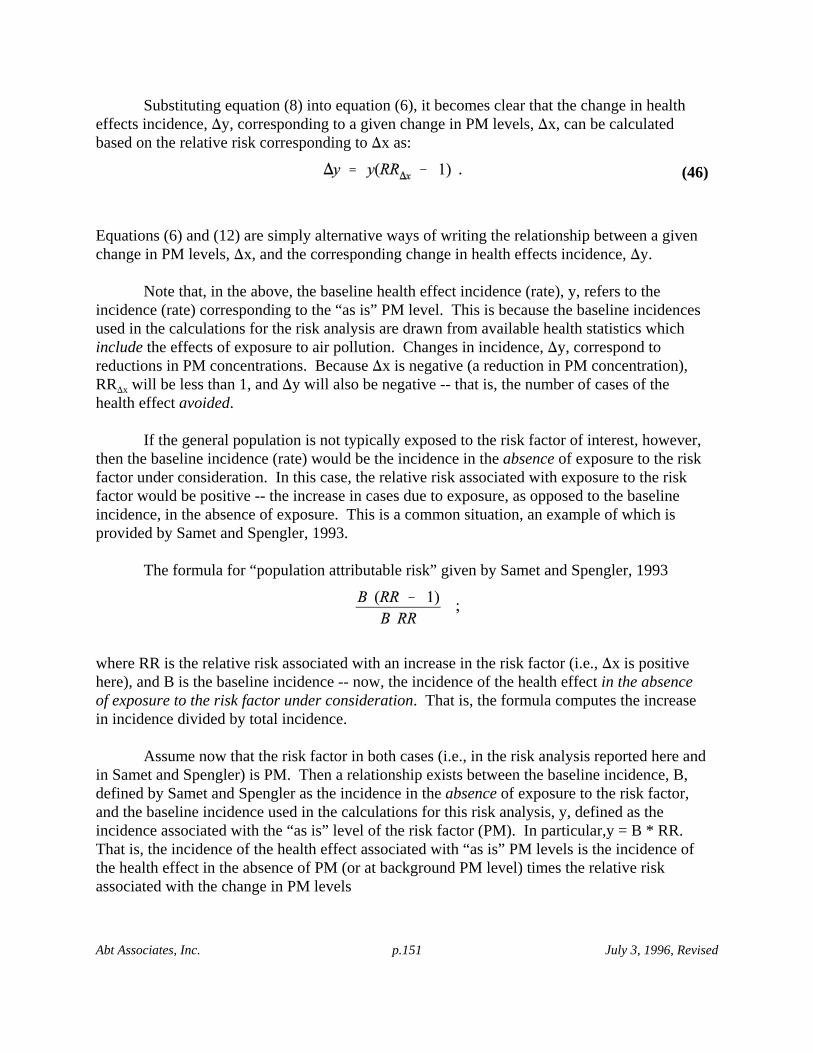
Abt Associates, Inc. p.151 July 3, 1996, Revised
(46)
Substituting equation (8) into equation (6), it becomes clear that the change in healtheffects incidence, )y, corresponding to a given change in PM levels, )x, can be calculatedbased on the relative risk corresponding to )x as:
Equations (6) and (12) are simply alternative ways of writing the relationship between a givenchange in PM levels, )x, and the corresponding change in health effects incidence, )y.
Note that, in the above, the baseline health effect incidence (rate), y, refers to theincidence (rate) corresponding to the “as is” PM level. This is because the baseline incidencesused in the calculations for the risk analysis are drawn from available health statistics whichinclude the effects of exposure to air pollution. Changes in incidence, )y, correspond toreductions in PM concentrations. Because )x is negative (a reduction in PM concentration), RR)x will be less than 1, and )y will also be negative -- that is, the number of cases of thehealth effect avoided.
If the general population is not typically exposed to the risk factor of interest, however,then the baseline incidence (rate) would be the incidence in the absence of exposure to the riskfactor under consideration. In this case, the relative risk associated with exposure to the riskfactor would be positive -- the increase in cases due to exposure, as opposed to the baselineincidence, in the absence of exposure. This is a common situation, an example of which isprovided by Samet and Spengler, 1993.
The formula for “population attributable risk” given by Samet and Spengler, 1993
where RR is the relative risk associated with an increase in the risk factor (i.e., )x is positivehere), and B is the baseline incidence -- now, the incidence of the health effect in the absenceof exposure to the risk factor under consideration. That is, the formula computes the increasein incidence divided by total incidence.
Assume now that the risk factor in both cases (i.e., in the risk analysis reported here andin Samet and Spengler) is PM. Then a relationship exists between the baseline incidence, B,defined by Samet and Spengler as the incidence in the absence of exposure to the risk factor,and the baseline incidence used in the calculations for this risk analysis, y, defined as theincidence associated with the “as is” level of the risk factor (PM). In particular,y = B * RR. That is, the incidence of the health effect associated with “as is” PM levels is the incidence ofthe health effect in the absence of PM (or at background PM level) times the relative riskassociated with the change in PM levels

Abt Associates, Inc. p.152 July 3, 1996, Revised
Substituting B = y/RR from above in the Samet and Spengler formula yields
or, now cancelling y,
which is the formula used in the calculations in the risk analysis. If the relative risk RR isassociated with an increase in pollution, )x, then a decrease in pollution, -)x, is associatedwith a relative risk 1/RR. Therefore, the formula used in these calculations computes thepercent change in incidence associated with a decrease in pollution from some previouslyexisting level (in this analysis, from observed concentrations to background or cutpointconcentrations). The percent is calculated with respect to the incidence at the existing level,that is, from the full incidence in the population.
As an example, assume that RR = 1.2. Then Samet and Spengler’s formula gives(1.2 - 1)/(1.2) = .167, that is, 16.7% of incidence attributable to the risk factor. Our formula is1- (1/1.2) = 1- .833 = .167, the same result given by Samet and Spengler..
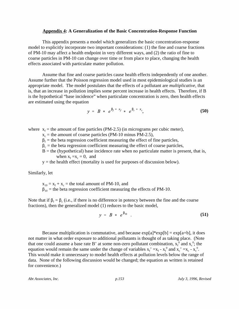
Abt Associates, Inc. p.153 July 3, 1996, Revised
(50)
(51)
Appendix 4: A Generalization of the Basic Concentration-Response Function
This appendix presents a model which generalizes the basic concentration-responsemodel to explicitly incorporate two important considerations: (1) the fine and coarse fractionsof PM-10 may affect a health endpoint in very different ways, and (2) the ratio of fine tocoarse particles in PM-10 can change over time or from place to place, changing the healtheffects associated with particulate matter pollution.
Assume that fine and coarse particles cause health effects independently of one another. Assume further that the Poisson regression model used in most epidemiological studies is anappropriate model. The model postulates that the effects of a pollutant are multiplicative, thatis, that an increase in pollution implies some percent increase in health effects. Therefore, if Bis the hypothetical “base incidence” when particulate concentration is zero, then health effectsare estimated using the equation
where xf = the amount of fine particles (PM-2.5) (in micrograms per cubic meter),xc = the amount of coarse particles (PM-10 minus PM-2.5), $f = the beta regression coefficient measuring the effect of fine particles, $c = the beta regression coefficient measuring the effect of coarse particles,B = the (hypothetical) base incidence rate when no particulate matter is present, that is,
when xf =xc = 0, and y = the health effect (mortality is used for purposes of discussion below).
Similarly, let
x10 = xf + xc = the total amount of PM-10, and $10 = the beta regression coefficient measuring the effects of PM-10.
Note that if $f = $c (i.e., if there is no difference in potency between the fine and the coarsefractions), then the generalized model (1) reduces to the basic model,
Because multiplication is commutative, and because exp[a]*exp[b] = exp[a+b], it doesnot matter in what order exposure to additional pollutants is thought of as taking place. (Notethat one could assume a base rate B’ at some non-zero pollutant combination, xf
0 and xc0; the
equation would remain the same under the change of variables xf’ =xf - xf0 and xc’ =xc - xc
0. This would make it unnecessary to model health effects at pollution levels below the range ofdata. None of the following discussion would be changed; the equation as written is retainedfor convenience.)

Abt Associates, Inc. p.154 July 3, 1996, Revised
(52)
(53)
(54)
(55)
(56)
(57)
Define
and
The parameter q is just the ratio of PM-2.5 to PM-10. The parameter r may be thought of asthe relative “potency” of coarse and fine particles in causing mortality (or, equivalently, as ameasure of their relative toxicities). If coarse and fine particles are equally potent in causingmortality (i.e., if particle size doesn’t matter), then r=1. If only fine particles matter, in whichcase $c = 0, then r=0. Assuming that fine particles cause at least their share of the mortalityassociated with PM-10, r will lie somewhere between 0 and 1.
Equation (2) implies
and therefore also
Equation (3) implies also that
Substituting equations (4), (5), and (6) back into the model (equation (1)) yields

Abt Associates, Inc. p.155 July 3, 1996, Revised
or, rearranging terms,
where
The factor [q + r(1 - q)] may be thought of as a “scaling” factor that, under theassumptions stated above, converts the PM-2.5 coefficient to the corresponding PM-10coefficient.
Even if the relationship between PM-2.5 and mortality (i.e., $f ) is the sameeverywhere, then, the relationship between PM-10 and mortality (i.e., $10) may vary from oneplace to another if the ratio of PM-2.5 to PM-10 (q) varies and/or the relative potencies of thefine and coarse fractions (r) varies.
Suppose, for example, that $f = 0.001 everywhere and that the relative potencies of thefine to coarse fractions (r) is 0.5 everywhere (i.e., the fine fraction is twice as harmful as thecoarse fraction everywhere). Suppose, however, that in Provo, Utah, only twenty percent ofPM-10 is fine particles whereas in Philadelphia, eighty percent is fine particles. Thecoefficient of PM-10 in Provo is then
$10,Provo = 0.001*[0.20 + 0.5(0.80)] = 0.0006
whereas in Philadelphia it is$10,Philadelphia = 0.001*[0.80 + 0.5(0.20)] = 0.0009.
Therefore, if the composition of PM-10 and/or the relative potencies of the fine andcoarse fractions of PM-10 varies significantly from one location to another, the PM-10concentration-response function estimated in one location may not be entirely applicable to adifferent location.
The generalized model (equation (1)) allows more specific analysis of alternativepolicy options. It also demonstrates that the PM-10 model, which does not distinguishbetween fine and coarse particles, may significantly misestimate the health effects associatedwith a given concentration of PM-10 if there really is a difference in the potency of PM-2.5and the coarse fraction and if the proportion of PM-10 that is fine particles varies significantlyfrom one location to another.

Abt Associates, Inc. p.156 July 3, 1996, Revised
Appendix 5: Adjustment of Means and Standard Deviations of Distributions for Location-Specific $’s
Location-specific estimates of $ are adjusted to take into account all the informationabout $ in all locations for which it has been estimated, assuming the random effects model inwhich location-specific $’s are regarded as a sample from an underlying distribution of $’s. Let
$i denote the estimate of $ in the ith location;Vi denote the variance of the estimate, $i ;02 denote the variance of the underlying distribution of $’s;$pooled denote the estimate of the mean of the distribution, derived by pooling the sample
of estimates of the $i’s ; and Vpooled denote the variance of the estimate of the mean, $pooled .
The unadjusted probability distribution describing the probability that the true value of $in the ith location is within any given interval is a normal distribution with mean equal to$i andvariance equal toVi.
The adjusted probability distribution is a normal distribution with mean equal to
and variance equal to
The adjusted mean is a weighted average of the original estimate, $i , and the pooledestimate of the mean of the distribution, $pooled . The larger the variance around the location-specific estimate, $i (i.e., the less certain it is), the less weight it has in the adjusted mean.
The first term in the adjusted variance combines the within study variance (Vi) and thebetween study variance, 02 . The second term in the adjusted variance is a correction for the factthat the mean of the distribution is not known but is only estimated (by $pooled ). This estimatetherefore has some variability associated with it.
Abt Associates, Inc. p.157 July 3, 1996, Revised
References
AIRS. Aerometric Information Retrieval System [database]. 1995. ResearchTriangle Park,NC. U.S. Environmental Protection Agency, Office of Air Quality Planning andStandards.
Abbey, D. E., Lebowitz, M.D., Mills, P.K., Petersen, F.F., Beeson, W.L., Burchette, R.J.1995. Long-term ambient concentrations of particulates and oxidants anddevelopment of chronic disease in a cohort of nonsmoking California residents. In:Phalen, R.F., Bates, D.V., eds. Proceedings of the colloquium on particulate airpollution and human mortality and morbidity; January 1994; Irvine, CA. InhalationToxicol. 7: 19-34.
American Lung Association. 1995. Dollars and Cents: The economic andhealth benefits ofpotenetial particulate matter reductions in the United States.
Cifuentes, L., Lave, L. 1996. Association of daily mortality and air pollution inPhiladelphia, 1983-1988. J. Air Waste Management Assoc. In press.
Cox, D., and Hinkley, D. 1974. Theoretical Statistics. Chapman and Hall, London.
DerSimonian, R. And N. Laird. 1986. Meta-analysis in clinical trials. Controlled ClinicalTrials 7:177-188.
Dockery, D.W., F.E. Speizer, D.O. Stram, J.H. Ware, J.D. Spengler, and B.G. Ferris, Jr. 1989. Effects of inhalable particles on respiratory health of children. Am. Rev.Respir. Dis. 139: 587-594.
Dockery, D.W., J. Schwartz, and J.D. Spengler. 1992. Air pollution and daily mortality: associations with particulates and acid aerosols. Environ Res. 59: 362-373.
Dockery, D.W., et al. 1993. An association between air pollution and mortality in six U.S.cities. The New England Journal of Medicine. 329 (24): 1753-1759.
Dockery, D.W. et al. 1996. Health effects of acid aerosols on North American children: respiratory symptoms. Env. Health Persp. Submitted.
Efron, B. and Morris, C. 1971. Limiting the risk of Bayes and empirical Bayes estimators. Part I: The Bayes case. J Am. Stat. Assoc. 66: 807-815.
Efron, B. and Morris, C. 1972a. Emprical Bayes on vector observations: An extension ofStein’s method. Biometrika 59: 335-347.
Efron, B. and Morris, C. 1972b. Limiting the risk of Bayes and empirical Bayes estimators. Part II: The empirical Bayes case. J Am. Stat. Assoc. 67: 130-139.

Abt Associates, Inc. p.158 July 3, 1996, Revised
Efron, B. and Morris, C. 1973. Stein’s estimation rule and its ccompetitors -- An empiricalBayes approach. J Am. Stat. Assoc. 68: 117-130.
Empire State Electric Energy Research Corporation (ESEERCO). 1994. New York StateEnvironmental Externalities Cost Study. Report 2: Methodology. Prepared by:RCG/Hagler, Bailly, Inc., November.
Graves, E.J. 1994. Detailed Diagnoses and Procedures National Hospital Discharge Survey1992. NCHS. Vital Health Statistics Series 13, No. 118. August. Figures do notinclude newborns.
Health Effects Institute. 1995. Particulate air pollution and daily mortality: replication andvalidation of selected studies. The phase I report of the Particle EpidemiologyEvaluation Project.
Ito, K., Kinney, P., and G.D. Thurston. 1995. Variations in PM10 concentrations within twometropolitan areas and their implications to health effects analyses. Inhalation Toxicol.,7:735-745.
Ito, K., and Thurston, G. 1996. Daily PM-10/Mortality Associations: An Investigation of At-Risk Sub-populations. J. Exposure Anal. and Environ. Epidemiol., to appear.
Kinney, P.L., Ito, K. and G.D. Thurston. 1995. A sensitivity analysis of mortality/PM10associations in Los Angeles. Inhalation Toxicology 7: 59-69.
Krupnick AJ, Harrington W, Ostro B. 1990. Ambient Ozone and Acute Health Effects: Evidence from Daily Data. Journal of Environmental Economics and Management18:1-18.
Mood, A., Graybill, F., and Boes, D. 1974. Introduction to the Theory of Statistics. McGrawHill, New York.
Moolgavkar, S.H., and E. G. Luebeck. 1996. Particulate Air Pollution and Mortality: ACritical Review of the Evidence. Epidemiology (in press).
Moolgavkar, S.H., Luebeck, E.G., Hall, T.A., Anderson E.L. 1995. Air Pollution and DailyMortality in Philadelphia. Epidemiology 6:476-484.
Ostro, B.D. 1987. Air pollution and morbidity revisited: a specification test. J. Eniron.Econ. Manage. 14: 87-98.
Ostro, B.D., Lipsett, M.J., Wiener, M.B., and J.C. Selner. 1991. Asthmatic responses toairborne acid aerosols. American Journal of Public Health 81: 694-702.

Abt Associates, Inc. p.159 July 3, 1996, Revised
Ostro, B.D., Lipsett M., Mann J., Braxton-Owens H., and White M.. 1995. Air pollutionand Asthma Exacerbations Among African-American Children in Los Angeles. In:Phalen, R.F., Bates, D. V., eds. Proceedings of the colloquium on particulate airpollution and human mortality and morbidity, part II; January, 1994; Irvine, CA. Inhalation Toxicol. 7:711-722.
Pope, C.A., III. 1991. Respiratory hospital admissions associated with PM10 pollution inUtah, Salt Lake, and Cache Valleys. Arch. Environ. Health 46: 90-97.
Pope, C.A., III. 1994. Particulate Pollution and Mortality in Utah Valley. Prepared for: Critical Evaluation Workshop on Particulate Matter - Mortality EpidemiologyStudies; Raleigh, North Carolina, November 9-11, 1994.
Pope, C.A., III, D.W. Dockery, J.D. Spengler, and M.E. Raizenne. 1991. Respiratory healthand PM10 pollution: a daily time series analysis. Am. Rev. Respir. Dis. 144: 668-674.
Pope, C.A., III, Schwartz, J., and M.R. Ransom. 1992. Daily mortality and PM10 in Utahvalley. Arch. Environ. Health 47: 211-217.
Pope, C.A., III, M.J. Thun, M.M. Namboodiri, D.W. Dockery, J.S. Evans, F.E. Speizer, andC.W. Heath, Jr. 1995. Particulate air pollution as a predictor of mortality in aprospective study of U.S. adults. Am. J. Respir. Crit. Care Med. 151: 669-674.
Raizenne, M., Neas, L., Damokosh, A., Dockery, D., Spengler, J., Koutrakis, P., Ware, J.,Speizer, F. 1996. Health effects of acid aerosols on North American children:pulmonary function. Environ. Health Perspect. Accepted.
Ransom, M. and Pope, C.A. III. 1992. Elementary school absences and PM-10 Pollution inUtah Valley. Environmental Research 58: 204-219.
Samet, J. And Spengler, J. Prevention of Respiratory Diseases from Indoor and Outdoor AirPollution. In Hirsch, A. et al., ed. 1993. Prevention of Respiratory Diseases. Marcel Dekker, Inc. New York.
Science Applications International (ICF Kaiser). 1995. Statistical Support for the PMNAAQS: Interim Report. SYF APP-95/039.
Schwartz, J. 1991. Particulate air pollution and daily mortality in Detroit. Environ. Res.56:204-213.
Schwartz, J. 1991/1992. Particulate air pollution and daily mortality: a synthesis. PublicHealth Rev. 19: 39-60.

Abt Associates, Inc. p.160 July 3, 1996, Revised
Schwartz, J. 1993. Air pollution and daily mortality in Birmingham, Alabama. Am. J.Epidemiol. 137: 1136-1147.
Schwartz, J. 1994a. Air Pollution and Hospital Admissions in Elderly Patients inBirmingham, Alabama. American Journal of Epidemiology 139:589-98.
Schwartz, J. 1994b. Air pollution and hospital admissions for the elderly in Detroit,Michigan. Am. J. Respir. Crit. Care Med. 150:648-55.
Schwartz, J. 1994c. PM10, Ozone and Hospital Admissions for the Elderly in Minneapolis-St. Paul, Minnesota. Archives of Environmental Health 49(5): 366-374.
Schwartz, J. 1995. Short term fluctuations in air pollution and hospital admissions of theelderly for respiratory disease. Thorax 50(5): 531-538.
Schwartz, J. 1996. Air Pollution and Hospital Admissions for respiratory disease. Epidemiology 7(1): 1-9.
Schwartz, J., D., Dockery, D.W., Neas, L.M., Wypij, D., Ware, J.H., Spengler, J.D.,Koutrakis, P., Speizer, F.E., Ferris, B.G., Jr. 1994. Acute Effects of Summer AirPollution on Respiratory Symptom Reporting in Children. Am. J. Respir. Crit. CareMed. 150: 648-655.
Schwartz, J., and D.W. Dockery. 1992a. Particulate air pollution and daily mortality inSteubenville, Ohio. Am. J. Epidemiol. 135: 12-19.
Schwartz, J., and D.W. Dockery. 1992b. Increased mortality in Philadelphia associatedwith daily air pollution concentrations. Am. Rev. Respir. Dis. 145: 600-604.
Schwartz, J., and R. Morris. 1995. Air pollution and cardiovascular hospital admissions. Am. J. Epidemiol., 142: 23-35.
Schwartz, J., Dockery, D., and L. Neas. 1996a. Is Daily Mortality Specifically AssociatedWith Fine Particles? J. Air & Waste Man. Assoc. (Accepted).
Schwartz, J., Dockery, D., Ware, J., Spengler, J., Wypij, D., Koutrakis, P., Speizer, F., andB. Ferris., Jr. 1989. Acute effects of acid aerosols on respiratory symptom reportingin children. USEPA, Boston, MA. For presentation at the 82nd Annual Meeting andExhibition. Anaheim, CA. pp. 1-10. June 25-30.
Schwartz, J., Dockery, D., Neas, L., Wypij, D., Ware, J., Spengler, J., Koutrakis, P., Speizer,F., and B. Ferris., Jr. 1994. Acute effects of summer air pollution on respiratorysymptom reporting in children. Am. J. Respir. Crit. Care Med. 150: 1234-1242.

Abt Associates, Inc. p.161 July 3, 1996, Revised
Schwartz, J., Slater, D., Larson, T., Pierson, T. and J. Koenig. 1993. Particulate AirPollution and Hospital Emergency Room Visits for Asthma in Seattle. Am Rev.Respir Dis 147: 826-831.
Spix, C., Heinrich, J., Dockery, D., Schwartz, J., Volksch, G., Schwinkowski, K., Collen, C.,Wichmann, H. 1993. Air pollution and daily mortality in Erfurt, East Germany,1980-1989. Env. Health Perspect. 101:518-526.
Styer, P., McMillan, N., Gao, F., Davis, J., and J. Sacks. 1994. The effect of airborneparticulate matter on daily death counts. Environ. Health Perspect. 103: 490-197.
Thurston, G. Ito, K., Hayes, C., Bates, D. and M. Lippmann. 1994. Respiratory HospitalAdmission and Summertime Haze Air Pollution in Toronto, Ontario: Consideration ofthe Role of Acid Aerosols. Environmental Research 65: 271-290.
Trijonis, J. C., et al. 1990. Visibility: Existing and Historical Conditions -- Causes andEffects. NAPAP Report 24.
U.S. Bureau of the Census (USBC). 1990. Statistical Abstract of the United States: 1990. 110th Edition. Washington D.C. U.S. Department of Commerce.
U.S. Bureau of the Census. 1992. Statistical Abstract of the United States (112th edition). Washington, DC. U.S. Department of Commerce.
U.S. Department of Commerce. 1994. County City Data Book.
U.S. Environmental Protection Agency (USEPA). 1986. Review of the National Ambient AirQuality Standards for Particulate Matte: Updated Assessment of Scientific andTechnical Information Addendum to the 1982 OAQPS Staff Paper. Prepared by theOffice of Air Quality Planning and Standards, Research Triangle Park, North Carolina. EPA 450/05-86-012.
U.U.S. Environmental Protection Agency (U.S. EPA). 1994. Review of the National Ambient AirQuality Standards for Sulfur Oxides: Assessment of Scientific and TechnicalInformation. Supplement to the 1986 OAQPS Staff Paper Addendum. Air QualityManagement Division, Office of Air Quality Planning and Standards. ResearchTriangle Park, NC. EPA Report No. EPA-452/R-94-013.
U.U.S. Environmental Protection Agency (U.S. EPA). 1996a. Air Quality Criteria forParticulate Matter. Office of Health and Environmental Assessment, Office ofResearch and Development. Research Triangle Park, NC.

Abt Associates, Inc. p.162 July 3, 1996, Revised
U.U.S. Environmental Protection Agency (U.S. EPA). 1996b. Review of the National AmbientAir Quality Standards for Particulate Matter: Policy Assessment of Scientific andTechnical Information. OAQPS Staff Paper. Office of Air Quality Planning andStandards. Research Triangle Park, NC.
U.U.S. Environmental Protection Agency (U.S. EPA). 1996c. Review of National Ambient AirQuality Standards for Ozone: Assessment of Scientific and Technical Information. AirQuality Management Division, Office of Air Quality Planning and Standards. Research Triangle Park, NC.
Utell, M., Frampton, M. 1995. Particles and mortality: a clinical perspective. In: Phalen, R.F., Bates, D. V., eds. Proceedings of the colloquium on particulate air pollution andhuman mortality and morbidity, part II; January 1994; Irvine, CA. Inhalation Toxicol.7: 645-655.
Whitfield, R. G. et al. 1996. A Probabilistic Assessment of Health Risks Associated WithShort-Term Exposure to Tropospheric Ozone. Report prepared for U.S. EPA Office ofAir Quality Planning and Standards. Research Triangle Park, NC.
Wood, Elaine. 1995. National Center for Health Statistics. Personal communication withMatthew Wiener, Abt Associates. October 31.