


Bahasa
Halaman
Hukum


Journal of Geomatics Vol. 15, No. 1, April 2021
© Indian Society of Geomatics
Investigation of flood (waterlog) flow pattern of University Road and Dan Fodio Boulevard in
Akoka, Yaba, Lagos, Nigeria
O.G. Omogunloye, O.A. Olunlade, O.E Abiodun, A.I. Moshood and O.A. Babatunde
Department of Surveying and Geoinformatics, University of Lagos, Akoka, Lagos, Nigeria.
Email: [email protected]
(Received: Jun 25, 2020; in final form: Apr 20, 2021)
Abstract: Flooding occurs when a river’s discharge exceeds its channel’s volume causing the river to overflow onto the
area surrounding the channel, known as the floodplain. The increase in discharge can be triggered by several events. The
most common cause of flooding (waterlog) is prolonged rainfall. If it rains for a long time, the ground will become
saturated and the soil will no longer be able to store water leading to increased surface runoff. Poor drainage system could
also make rainwater, not properly channelized, thereby leading to higher discharge levels and floods along the busy road.
The study investigated the vulnerability of flood along a route (2.64km) in the study area, alongside its’ drainage
architecture systems. The route (road) field survey, longitudinal profile and cross sections were carried out. The relative
elevation of points along the center line of a road is achieved through longitudinal profile while elevation of points across
the center line is achieved through the cross sections. The (X, Y, Z) coordinates, the longitudinal profile of the route and
the cross sections across the route, were used to determine the flow direction, flow accumulation, and the flow length
using ARCGIS 10.2 and plotting was achieved with the aid of AutoCAD 2012 at a horizontal scale of 1:5000 and vertical
scale of 1:100. The study showed that inadequacies in the depth of the two side drainages along the route, blockages by
sediments in form of refuse along the drainages, Ngoc and Lalit (2017), played a major role in the ill-free flow of water
along the drainages and the resultant over flow of water along the route during heavy downpour of rainfall.
Keyword: Runoff, Flood, Route, Flow, Drainages, Rainfall.
1. Introduction
Before investigation survey can be carried out successfully
on flooding, certain factors must be known. A survey
begins long before actual data collection starts, Josh et al.
(2019) and Firebrace et al, (1915). Some elements which
must be considered are: Exact area or location of the
survey (University Road, Akoka,Yaba, Lagos.); Type of
survey (reconnaissance or standard), scaled to meet
standards of map to be produced, (Elissavet et al. 2019 and
Kanetkar et al. 1966); Scope of the survey (short or long
term); Platforms available (aircraft, satellitesetc.); Support
work required (aerial or satellite photography, geodetics
etc.); and Limiting factors, (budget, politics, geographic or
operational constraints, positioning system limitations,
logistics).
Flooding is the unusual presence of water on land to a
depth, which affects normal activities (Mohamed et al.
2019). Flooding can arise from Overflowing Rivers (river
flooding); Heavy rainfall over a short duration (flash
floods); or An unusual inflow of seawater onto land (ocean
flooding). Ocean flooding can be caused by storms such as
hurricanes (storm surge), high tides (tidal flooding),
seismic events (tsunami) or large landslides (sometime
also called tsunami), (Addison, 1946).
Rainwater will enter the river much faster than it would if
the ground was not saturated leading to higher discharge
levels and floods (Sally et al. 2019).
The flood plain investigation along any route (road)
demands, the carrying out of proper route survey, in order
to determine the cause of flooding, as well as, the creation
of a 3D model map (Omogunloye, et al. 2013), that can
assist to proffer solution to the flooding (Davis, 1966).
Route surveying is one of the aspects of engineering
surveying, and could be pipeline, power-line, underground
cable or road survey. Route survey (road) comprises
longitudinal profile and cross sections (Clark, 1954). The
relative elevation of points along the Centre line of a road
is achieved through longitudinal profile while elevation of
points across the Centre line is achieved through the cross
sections. The two are important to civil engineers and
Surveyors to enable him realize the cut area and the fill
area depending on the purpose of the road (David, 1973).
The results of the project work are the route, the
longitudinal profile of the route and the cross sections
across the route. These were plotted with the aid of Auto
CAD 2012 at a horizontal scale of 1:5000 and vertical
scale of 1:100, (Omogunloye, O. G., et al 2011 and 2012).
At the end of the fieldwork and the plotting of the data, we
were able to find out that there were gullies at the Centre
of the route which could have been caused as a
consequence of erosion that dominates the environment.
Also we were able to find out that the route at the
beginning is at depression and as we progressed towards
the end of the route, the route tended to be elevated.
This study is to acquire information about the nature of the
surface of the flood plain along the University Road
Akoka, Yaba, Lagos Nigeria and produce a topographical
map in 3D depicting the longitudinal profile and cross-
sectioning of the various drainage system (canals and
gutters) affecting the different part of the study area as well
as analyzing changes that may have taken place over the
past immediate years, (Jingwei and Yixian, 2020;
Kanetkar et al. 1966 and Omogunloye, et al. 2017) and to
proffer a model that could be adopted in order to manage
and provide a lasting solution to forestall a reoccurrence.
16
Journal of Geomatics Vol. 15, No. 1, April 2021
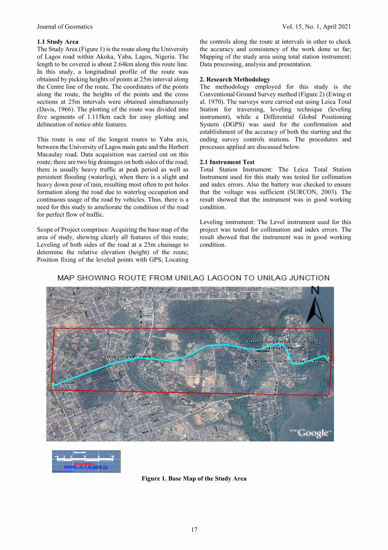
1.1 Study Area
The Study Area (Figure 1) is the route along the University
of Lagos road within Akoka, Yaba, Lagos, Nigeria. The
length to be covered is about 2.64km along this route line.
In this study, a longitudinal profile of the route was
obtained by picking heights of points at 25m interval along
the Centre line of the route. The coordinates of the points
along the route, the heights of the points and the cross
sections at 25m intervals were obtained simultaneously
(Davis, 1966). The plotting of the route was divided into
five segments of 1.115km each for easy plotting and
delineation of notice-able features.
This route is one of the longest routes to Yaba axis,
between the University of Lagos main gate and the Herbert
Macaulay road. Data acquisition was carried out on this
route; there are two big drainages on both sides of the road;
there is usually heavy traffic at peak period as well as
persistent flooding (waterlog), when there is a slight and
heavy down pour of rain, resulting most often to pot holes
formation along the road due to waterlog occupation and
continuous usage of the road by vehicles. Thus, there is a
need for this study to ameliorate the condition of the road
for perfect flow of traffic.
Scope of Project comprises: Acquiring the base map of the
area of study, showing clearly all features of this route;
Leveling of both sides of the road at a 25m chainage to
determine the relative elevation (height) of the route;
Position fixing of the leveled points with GPS; Locating
the controls along the route at intervals in other to check
the accuracy and consistency of the work done so far;
Mapping of the study area using total station instrument;
Data processing, analysis and presentation.
2. Research Methodology The methodology employed for this study is the
Conventional Ground Survey method (Figure 2) (Ewing et
al. 1970). The surveys were carried out using Leica Total
Station for traversing, leveling technique (leveling
instrument), while a Differential Global Positioning
System (DGPS) was used for the confirmation and
establishment of the accuracy of both the starting and the
ending survey controls stations. The procedures and
processes applied are discussed below.
2.1 Instrument Test
Total Station Instrument: The Leica Total Station
Instrument used for this study was tested for collimation
and index errors. Also the battery was checked to ensure
that the voltage was sufficient (SURCON, 2003). The
result showed that the instrument was in good working
condition.
Leveling instrument: The Level instrument used for this
project was tested for collimation and index errors. The
result showed that the instrument was in good working
condition.
Figure 1. Base Map of the Study Area
17

Journal of Geomatics Vol. 15, No. 1, April 2021
Figure 2. Research Methodology
2.2 Datum checks for the controls used
The control used (GME 04 & 05) were checked to
ascertain its stability or displacement from its original
position (Torge, 1991 and Omogunloye et al. 2017). At the
end of the checks, it was found to be stable and intact in its
original position,
2.3 Instrument / Materials used are
The instruments used for the study are made up of both
Hardware and software:
Hardware instrument used are: 1 no of Total station (Leica
TS 06) with accessories; A differential GPS with
accessories; A level instrument with accessories; Leveling
staff; Marker (paint); Reflector; 1 No. Plumb bob; 1 No.
Linen tape (100m); Field books; Nail and bottle corks; A
gallon of gloss paint; Brush; HP Computer System
(Laptop); 32GB Flash drive; and Hp Laser Jet Printer.
Software used are: Auto CAD software for plotting;
Google Earth Pro; Arc MAP 10.2; Suffer 15; Microsoft
office 2012 (Word, Excel, Power-Point); and Notepad
2.4 The Description of the Project Site and Detailing.
The project site is a route along the University road from
UNILAG Senate junction through the UNILAG main gate
to UNILAG junction Point, as shown in Figure (1).The
project started on a control Points, GME 04 and GME 05;
the project site forms a “T” junction with Herbert
Macaulay Way. The road comprises of two segments and
four lanes. The chainage of the centre line of the road starts
from the junction adjacent to UNILAG senate building at
25m interval, the cross section chainage was measured 9m
across to both left and right of the centre line. The road
surface is relatively flat with some certain undulations as
seen in all the longitudinal profiles in Figures (3, 4 & 5).
The highest point was recorded at a chainage 2+100m,
with a height of 11.946m above the reference datum. The
study area terminates at UNILAG junction, the traversing
was closed on the known control beacon marked SUG 04,
while the azimuth observation was closed on the
established control marked, SUG 05.
2.5 Field operation / data Acquisition
Traversing method was adopted to obtain the horizontal
alignment of the route along the Centre line at the specified
interval of 25m. Both the traversing and longitudinal data
acquisitions were carried out simultaneously. The two
field operations were closed on established pillar: SUG 04
and SUG 05. Acquired Data (X, Y, Z) coordinates of
points was stored in the Total Station instrument for the
traversing observation, while for that of the leveling, the
heights were recorded in a field book, and the processing
of the data was done in the office. An estimated length of
about 2.64Km was covered.
2.6 Data processing and reductions
Data processing is an intermediate stage between
fieldwork and Result presentation. At this stage, all the raw
data obtained from the field measurements were refined to
a more usable form to make them useful for other purposes
required by the study, Thomas (2010). Also all the
redundant data were filtered at this stage, Udabhor (2014).
2.7 Traverse Data Processing
Using the X, Y and Z data acquired from the Total Station,
an AutoCAD Script file was created in this format “_text
Easting’s, Northing’s text height
Height Point ID” as a layer, and the points where
connected according to the field book. Layers were also
created for other features in the AutoCAD. The X, Y and
Z coordinates of points were plotted using the AutoCAD
Civil 3D 2017 software and a map of the study area was
created in digital format.
2.8 Levelling Data Processing
Using the data acquired from Digital Level Instrument, the
heights of the corresponding points were computed using
the Height of Plane Collimation method of levelling
technique. A digital format level profile of the centre line
of the route was created using the AutoCAD Civil 3D 2017
software.
18

Journal of Geomatics Vol. 15, No. 1, April 2021
3. Results
3.1 Accuracy of the route survey result after
computation
A Linear accuracy of 1:23,000 for a distance of 2.64Km
was obtained against the minimum accuracy (1:3000)
required of a third-order job in accordance with SURCON
specifications on large scale cadastral and engineering
survey in Nigeria, Ewing et al, (1970).
At the end of project, SUG 04 was closed on. The
coordinates of the established SUG 04 using DGPS and
the coordinates of the measured SUG 04 as the closing
control are given in the table 1:
The minimum accuracy of third-order job required in
accordance with SURCON specifications on large scale
cadastral and engineering survey in Nigeria is 1:3000. The
formulae used in calculating the linear accuracy was: 1
√∆𝑁2 + ∆𝐸2
∑𝐷
Where
∆𝑁 = Misclosure in the Northing, between
coordinates of the closing control and
Observed.
∆𝐸 = Misclosure in Easting, between
coordinates of the closing control and the
Observed.
∑D = Summation of distances within the
network 1
√−0.0012 + 0.0022
2640
Table 1. The misclosures of closing controls
EASTINGS(m) NORTHINGS(m)
COORDINATES OF ESTABLISHED SUG
04 (DGPS)
540821.222 720233.804
COORDINATES OF MEASURED
SUG04(Total station)
540821.223 720233.806
MISCLOSURE -0.001 +0.002
Figure 3. Traverse Network (Autocad 2012)
Figure 4. Leveling Profile (Autocad, 2012)
19

Journal of Geomatics Vol. 15, No. 1, April 2021
3.2 Elevation Model (Tin)
A Triangulated Irregular Network (TIN) surface was
generated from surface source measurements on a point
feature, which contain elevations information. Points were
used as spot locations of elevations data, each color
showing the elevation range of each region. The highest
elevation is in red color which is around the Abule-Oja
area.
3.3 Flow Direction
This tool takes the kriging surface as input and outputs a
raster showing the direction of flow out of each cell
(Figure 6). There are eight valid output directions relating
to the eight adjacent cells into which flow could travel.
This approach is commonly referred to as an eight-
direction (D8) flow model (Addison, 1946).
This function is used to identify the water flow direction
on a surface, or identify the steepest descending direction
of each cell in a DEM (Figure 7) (Omogunloye et al. 2013).
The 8 cells surrounding the central cell are coded by the
powers of 2. From the right of the central cell, the cells are
coded as 2 to the power of 0, 1, 2, 3, 4, 5, 6, 7, that is 1, 2,
4, 8, 16, 32, 64, 128, thus represent the water flow direction
of the central cell to be east, southeast, south, southwest,
west, northwest, north and northeast, as the image below
shows.
Every central cell’s water flow direction is determined by
one of the eight values. For example, if a central cell’s
water flow direction is west, it will be given the value 16
(Omogunloye et al. 2012).
Figure 5. Showing the Triangulated Irregular Network of the Tarrain
Figure 6. Direction Coding
20

Journal of Geomatics Vol. 15, No. 1, April 2021
Figure 7. Showing The Flow Direction
3.4 Flow Accumulation
This function is used to create a network to show
accumulated flow into each cell, Figures (8, 9, 10, 11 &
12). The basic thoughts of Flow Accumulation is
supposing that there is one unit of water in each cell of the
raster data, and calculate the accumulated flow of each cell
through the Flow Direction Map. Gmn represent the cell at
row m, column n. G42 has 0 unit of water since there is no
cell which flow into it, G32 has 3 units of water since it
receives water from G41, G31 and G21. G22 has 1 unit of
water since it receives water from G11. G33 receives water
from three cells: G42, G32 and G22,
3+3+G42+G32+G22=7, therefore it has 7 units of water.
The result of Flow Accumulation is a raster of
accumulated flow to each cell, as determined by
accumulating the weight for all cells that flow into each
down slope cell.
Cells of undefined flow direction will only receive flow;
they will not contribute to any downstream flow. A cell
is considered to have an undefined flow direction, if its
value in the flow direction raster is anything other than
1, 2, 4, 8, 16, 32, 64, or 128.
The accumulated flow is based on the number of cells
flowing into each cell in the output raster. The current
processing cell is not considered in this accumulation.
Output cells with a high flow accumulation are areas of
concentrated flow and can be used to identify stream
channels.
Output cells with a flow accumulation of zero are local
topographic highs and can be used to identify ridges.
If the input flow direction raster is not created with the
Flow Direction tool, there is a chance that the defined
flow could loop. If the flow direction does loop, Flow
Accumulation will go into an infinite loop. Flow
Accumulation will go into an infinite loop and never
finish.
The Flow accumulation operation performs a cumulative
count of the number of pixels that naturally drain into
outlets. The operation can be used to find the drainage
pattern of a terrain.
Figure 8. Flow Direction to Flow Accumulation
21

Journal of Geomatics Vol. 15, No. 1, April 2021
Figure 9: How to Calculate Flow Direction
Figure 10. How to Calculate Flow Accumulation
Figure 11. Showing the Flow Accumulation
22

Journal of Geomatics Vol. 15, No. 1, April 2021
3.5 Flow Length
Every cell in a raster has a flow path which passes it. Flow
Length is used to calculate the length between each cell
and the outlet (or source) along the flow path, the result is
a Grid dataset. Flow Length is commonly used for flood
calculation, Omogunloye et al (2011), water flows can be
affected by factors such as slope, soil moisture and
vegetation cover, weight dataset is needed to model these
factors, Kanetkar et al, (1966). When it rains, a drop of
water landing somewhere in the basin must first travel
some distance before reaching the outlet. Assuming
constant flow velocities (an assumption we will relax later)
the pixel with the greatest flow length to the outlet
represents the hydrological most remote pixel. Its flow
length divided by the flow velocity represents a
representative lag time for the basin. The lag time
quantifies how long before the entire basin is contributing
to flow at the outlet and is a representative scale of the
basin.
In Flow Length Analysis, Flow Direction Data provides
the flow direction of streams; this dataset can be created
through Flow Direction Analysis. Weight dataset defines
the impedance of each cell in the raster.
There are two kinds of Flow Length Analysis:
Upstream: Calculate the length of the longest flow
path between each cell and its source cell on the
watershed boundary.
Downstream: Calculate the length of the flow path
between each cell and its corresponding outlet on
the edge of the raster.
Each colour showing the flood flow pattern of the route.
From regions with low flood pattern to regions with high
flood flow pattern.
The results obtained were analysed in detail. The following
are the inferences drawn from the analysis of the results;
Studying the flood flow pattern shows that areas with
high elevation height tend to have low flood, thus
causing water to tend to flow to places with low height
elevation. The elevation model also shows that the road is at the
same height with the drainages coupled with the fact
that there is no hole in the drainages to allow the flow
of water from the road.
Also, the regions with low height elevation drainages
are no longer functioning in other to channel the flow
of water into the neighbourhood canal, this tend to
cause stagnant water around the canal region. All things being equal, some regions in the map are
also liable to more flooding in the future, such as the
front of the emerald hall (Akoka Road).
It should be noted that this undulation is not primarily the
cause of flooding and water log on this route, rather after
proper investigation, it was noticed that flooding on this
route is cause due to the blockage of the drainages (canal,
gutter) along the route.
3.6 Result and Accuracy of the controls used
Table 2 and 3 shows the accuracy of the controls used
Figure 12. Showing The Flow Lenght
23

Journal of Geomatics Vol. 15, No. 1, April 2021
Table 2. Accuracy of the controls
CONTROL POINTS USED
Name Eastings (m) Northings (m) Orthometric
height (m)
GME 04 Components (m) 543891.542 720583.891 8.165
95 % Error 0.000 0.000 0.000
Status Control Fixed fixed fixed
Linear accuracy 1:100,000
Name Eastings(m) Northings(m) Orthometric
height(m)
GME 05 Components (m) 544028.845 720627.622 7.965
95 % Error 0.000 0.000 0.000
Status Control Fixed fixed fixed
Linear accuracy 1:100,000
Table 3. The coordinates and accuracies of the starting control points used for the project
NAME EASTING
(m)
NORTHING
(m)
ORTHOMETRIC
HIEGHT(m)
SUG 04 Components(m) 540821.222 720233.804 8.889 processed
(static)
95 % Error 0.000 0.001 0.004
Status Control processed (static) processed
(static)
processed (static)
Linear Accuracy 1:75,000
SUG 05 Components(m) 540875.703 720234.032 8.540
95 % Error 0.002 0.001 0.003
Status Control processed (static) processed
(static)
processed (static)
Linear Accuracy 1:33,000
4. Conclusions
Engineering survey is an essential aspect of Geo-
Information and a must for all engineering design and
construction. Flood assessment, monitoring and prediction
are crucial for environmental sustainability, particularly
within areas traversed by water logging. This study has
shown the need to compute flood (waterlog) flow analysis
and the usefulness of geographic information system (GIS)
as a spatial tool for inundation mapping within water
logged area. Also, the study has demonstrated the
importance of depicting the frequency of occurrence of
flood to the production of the aforementioned GIS-based
water logged zone mapping.
However, one of the most challenging issues in this study
is the choice of suitable flow length analysis. This
challenge has been surmounted in this study with
24

Journal of Geomatics Vol. 15, No. 1, April 2021
simultaneous examination of two established and widely
used methods of upstream and downstream flow length
techniques in GIS.
4.1 Recommendations
i. The government should ensure that some personnel
are put in charge of proper cleaning of drainage.
ii. Also the personnel should do a monthly check on the
status of the drainage and canal, due to unwanted
plants growing around this canal which also facilitate
stagnant water and flood along this route.
iii. The drainages should be reconstructed in other to
have a deeper drainage for proper channelling of
water.
iv. The Government should setup monitoring agency to
check indiscriminate deposit of waste into the
drainages.
v. Regular Engineering surveys should be encouraged
by both the Government and the Department in
charge of the proper management and maintenance
of the route and its environment.
References
Addison, H. (1946). Hydraulic Measurements, 2nd edition,
Chapman & Hall Ltd., London, pp 152.
Clarke, D. (1954). Plane and Geodetic Surveying, Vol. 1,
4th edition, Constable Publishers, London.
Clarke, D. (1973). Plane and Geodetic Surveying for
Engineers, Vol. II Sixth Edition, John Wiley Publishers,
USA.
Davis, R., Foote, F. and Kelly, J. (1966). Surveying, 5th
edition, McGraw-Hill, New York.
Firebrace, F. and Veale, C. J. (1915). Surveying, Part 1,
11th edition, Government press, Allahabad.
Elissavet, F., Ioannis, M. and Evangelos, B. (2019). Flood
vulnerability assessment using a GIS‐based multi‐criteria
approach—The case of Attica region,
https://doi.org/10.1111/jfr3.12563.
Jingwei, H. and Yixian, D. (2020). Spatial simulation of
rainstorm water logging based on a water accumulation
diffusion algorithm, Published online: 06 Jan 2020, pp 71-
87.
Josh, W., Jillian, C. L., Amanda, S. and Mofakkarul, I.
(2019). Barriers to the uptake and implementation of
natural flood management: A social‐ecological analysis,
Nottingham Trent University; NTSU Green Leaders; Trent
Regional Flood and Coastal Committee,
https://doi.org/10.1111/jfr3.12561.
Kanetkar, T.P. and Kulkarni, S. V. (1966). Surveying &
Levelling, Part 1, 22nd edition, A.V.G. press, India.
Ewing, C. E. and Mitchell, M. M. (1970). Introduction to
Geodesy Published by American Elsevier Company, Inc,
New York.
Mohamed, A. et al. (2019). Flash flood risk assessment in
urban arid environment: case study of Taibah and Islamic
universities’ campuses, Medina, Kingdom of Saudi
Arabia, Geomatics, Natural Hazards and Risk, 10(1),
Published online.
Ngoc, D. and Lalit, K. (2017). Application of remote
sensing and GIS-based hydrological modeling for flood
risk analysis: a case study of District 8, Ho Chi Minh city,
Vietnam, 1792-1811
Omogunloye, O. G., Ipadeola, A. O., Shittu, O. G. and
Ojegbile, B. M. (2017). Application of Iterative Weighted
Similarity Transformation (IWST) Deformation Detection
Method Using Coordinate Differences From Different
Observational Campaigns, Nigerian Journal of Surveying
& Geoinformatics, Peer Review Report-NJSG, 5(1), 61 –
75.
Omogunloye, O. G., Oladiboye, E. O., Quadri, J. A. and
Omogunloye, H. B. (2013). Determination of Spot Heights
of the University of Lagos Campus, Journal of
Environmental Science and Resource Management, 5(1),
97- 110
Omogunloye, O. G. and Ayeni, O. O. (2012). Geospatial
Analysis of Hotels in Lagos State with Respect to Other
Spatial Features, Research Journal in Engineering and
Applied Sciences 1(6), Emerging Academy Resources,
(ISSN-2276-8467), RJEA, 1(6), 393 – 403.
Omogunloye, O. G., Olaleye, J. B., Akande, S. H. and
Adekoya, O.O. (2011). A GIS Analysis for courier
companies in Lagos state (a case study of all Local
Government area), Journal of Geomatics, Indian Society
of Geomatics (ISG), 5(1), 47 – 51.
Sally, B., Matthew, P. W., Robert, J. N,, Ali, S., Zammath,
K., Jochen, H., Daniel, L. and Maurice V. M. (2019). Land
raising as a solution to sea‐level rise: An analysis of coastal
flooding on an artificial island in the Maldives,
https://doi.org/10.1111/jfr3.12567.
Surveyors Council of Nigeria (SURCON) (2003).
Specifications for large scale cadastral and engineering
survey in Nigeria.
Thomas, F. (2010). History of Mathematical Astronomy.
University of New Brunswick
Torge, W. (1991). Geodesy (3rd Edition), Published by de
Gruyter, New York.
Udabhor, G A. (2014). Potential Theory and Spherical
Harmonics Lecture Note, Department of Surveying and
Geoinformatics, University of Lagos.
25
Copyright © 2022 FDOKUMEN

