ORIGINAL ARTICLE

An integrated evolutionary approach for modellingand optimization of laser beam cutting process

D. Kondayya & A. Gopala Krishna

Received: 25 May 2011 /Accepted: 10 April 2012# Springer-Verlag London Limited 2012

Abstract This paper presents a new integrated methodologybased on evolutionary algorithms (EAs) to model and optimizethe laser beam cutting process. The proposed study is dividedinto two parts. Firstly, genetic programming (GP) approach isused for empirical modelling of kerf width (Kw) and materialremoval rate (MRR) which are the important performancemeasures of the laser beam cutting process. GP, being anextension of the more familiar genetic algorithms, recentlyhas evolved as a powerful optimization tool for nonlinearmodelling resulting in credible and accurate models. Designof experiments is used to conduct the experiments. Four prom-inent variables such as pulse frequency, pulse width, cuttingspeed and pulse energy are taken into consideration. The de-veloped models are used to study the effect of laser cuttingparameters on the chosen process performances. As the outputparameters Kw and MRR are mutually conflicting in nature, inthe second part of the study, they are simultaneously optimizedby using a multi-objective evolutionary algorithm called non-dominated sorting genetic algorithm II. The Pareto optimalsolutions of parameter settings have been reported that providethe decision maker an elaborate picture for making the optimaldecisions. The work presents a full-fledged evolutionary ap-proach for optimization of the process.

Keywords Laser beam cutting . Modelling . Geneticprogramming .Multi-objective optimization . NSGA-II

1 Introduction

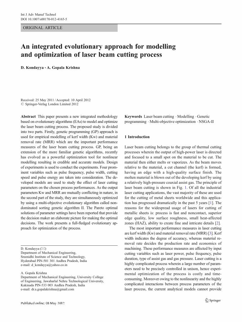
Laser beam cutting belongs to the group of thermal cuttingprocesses wherein the output of high-power laser is directedand focused to a small spot on the material to be cut. Thematerial then either melts or vaporizes. As the beam movesrelative to the material, a cut channel (the kerf) is formed,having an edge with a high-quality surface finish. Themolten material is blown out of the developing kerf by usinga relatively high-pressure coaxial assist gas. The principle oflaser beam cutting is shown in Fig. 1. Of all the industriallaser cutting applications, the vast majority of these are usedfor the cutting of metal sheets worldwide and this applica-tion has progressed dramatically in the past 5 years [1]. Thereasons for the widespread usage of lasers for cutting ofmetallic sheets is: process is fast and noncontact, superioredge quality, low surface roughness, small heat-affectedzones (HAZ), ability to create fine and intricate details [2].

The most important performance measures in laser cuttingare kerf width (Kw) andmaterial removal rate (MRR) [3]. Kerfwidth indicates the degree of accuracy, whereas material re-moval rate decides the production rate and economics ofmachining. These performance measures are affected by inputcutting variables such as laser power, pulse frequency, pulseduration, type of assist gas and gas pressure. Laser cutting is ahighly complicated process wherein a large number of param-eters need to be precisely controlled in unison, hence experi-mental optimization of the process is costly and time-consuming.Moreover owing to the nonlinearity and the highlycomplicated interactions between process parameters of thelaser process, the current analytical models cannot provide

D. Kondayya (*)Department of Mechanical Engineering,Sreenidhi Institute of Science and Technology,Hyderabad PIN-501 301 Andhra Pradesh, Indiae-mail: d_kondayya@yahoo.co.in

A. Gopala KrishnaDepartment of Mechanical Engineering, University Collegeof Engineering, Jawaharlal Nehru Technological University,Kakinada PIN-533 003 Andhra Pradesh, Indiae-mail: dr.a.gopalakrishna@gmail.com

Int J Adv Manuf TechnolDOI 10.1007/s00170-012-4165-5

accurate process prediction for better quality control and higherthroughput. Therefore an efficient method is needed to deter-mine the optimal parameters for best cutting performance. Theperformance measures as stated earlier viz. kerf width andmaterial removal rate are conflicting in nature, as lower valueof kerf width and higher value of material removal rate arepreferred.

The overall objective of this research is to apply a newprocess modelling and optimization methodology for thehighly nonlinear and complex manufacturing process of lasercutting. With this aim, accurate prediction models to estimateKw and MRR were developed from the experimental datausing a potential evolutionary modelling algorithm calledgenetic programming (GP). Subsequently, the developedmodels were used for optimization of the process. As thechosen objectives, Kw and MRR are opposite in nature, theproblem was formulated as a multi-objective optimizationproblem. Later, a popular evolutionary algorithm, non-dominated sorting genetic algorithm II (NSGA-II), was usedto retrieve the multiple optimal sets of input variables.

2 Literature review

Yousef et al. [4] have used artificial neural network (ANN) tomodel and analyse the nonlinear laser micro-machining pro-cess in an effort to predict the level of pulse energy needed tocreate a dent or crater with the desired depth and diameter onsurface of a material foil. Li et al. [5] have employed Taguchi’sexperimental method for examining the laser cutting quality ofa quad flat non-lead (QFN) package used in semiconductor

packaging technology. From the study they could observe that95.47 % of laser cutting quality is contributed from only threecontrol factors—laser frequency, cutting speed and drivingcurrent. Experimental design and artificial neural networkshave been used by Jimin et al. [6] for optimizing the parametersof 3D non-vertical laser cutting of 1-mm-thick mild steel.Dhara et al. [7] have adopted the artificial neural networksapproach to optimize themachining parameter combination forthe responses of depth of groove and height of recast layer inlaser micro-machining of die steel. Dubey andYadava [8] haveperformed the multi-response optimization of laser beam cut-ting process of thin sheets (0.5 mm thick) of magnetic materialusing hybrid Taguchi method and response surface method.The same authors [9] have performed the multi-objectiveoptimization of kerf quality using two kerf qualities such askerf deviation and kerf width using Taguchi quality loss func-tion for pulsed Nd:YAG laser cutting of thin sheet of alumin-ium alloy. The multiple regression analysis and the artificialneural network have been applied by Ming-Jong et al. [10] toestablish a predicting model for cutting 5×5 QFN packages byusing a diode-pumped solid-state laser system consideringcurrent, frequency and the cutting speed as input variablesand six laser cutting qualities as output variables of the QFNpackages, respectively. The genetic algorithm has been finallyapplied to find the optimal cutting parameters leading to lessHAZ width and fast cutting speed ensuing complete cutting.

Literature review infers considerable researchers conducteddistinctive investigations for improving the process perfor-mance of laser cutting. In this direction empirical modelsestablishing the relationships between the inputs and outputswere developed and these models were utilized as objective

Fig. 1 Laser beam cuttingprocess

Int J Adv Manuf Technol

functions and were optimized to obtain the machining condi-tions for the required responses. Literature review also revealsthat the dominant tools for modelling and optimization used todate have been Taguchi-based regression analysis, multipleregression method, response surface methodology and ANNs.

In multiple regression and response surface methodology, aprediction model has to be determined in advance and a set ofcoefficients has to be found. The prespecified size and shapeof the model imply that the model might not be able adequateto capture a complex relation between the influencing varia-bles and response parameters. Like the aforementionedapproaches, although ANNs have also been used extensivelyin the literature for modelling, they have the drawback of notbeing able to quantify explicitly the relationships betweeninputs and outputs. Though many research papers have beenpublished on Taguchi method and ANNs as per the authors’knowledge, very limited research work has been reportedpertaining to the literature on multi-objective optimization ofKw and MRR of laser beam cutting of steels. Hence, an efforthas been made in this paper, which confers the application ofevolutionary method for multi-objective optimization of lasercutting process.

3 Proposed methodology

In this paper, a novel approach is presented for modelling ofkerf width and material removal rate using GP. The distinc-tive aspect of GP as compared to traditional approaches isthat it does not make any presumption about the formulationto be made. Also the generated model helps directly toobtain an interpretation of the parameters affecting the pro-cess. More details of this methodology are discussed in

Section 4. The models developed by GP are subsequentlyused for optimization.

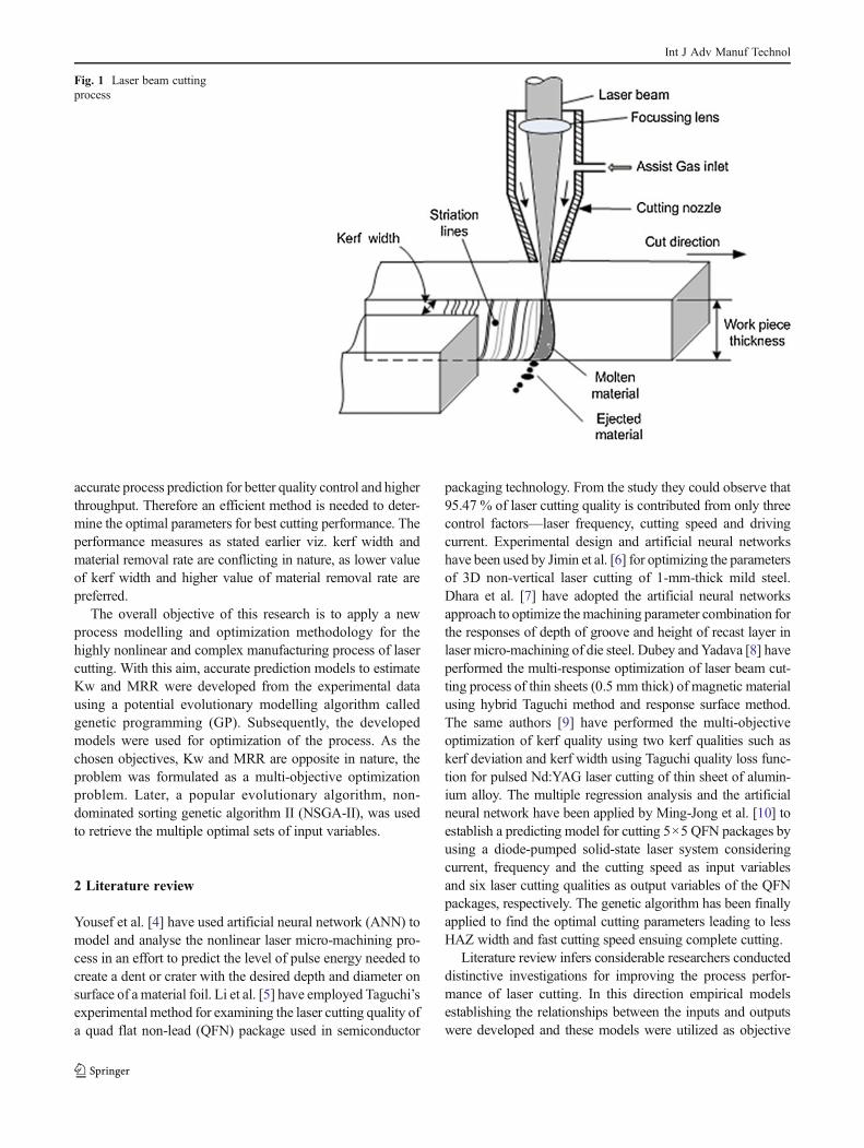
In the current study, unlike the previous approaches, theoptimization problem of laser beam cutting process is ex-plicitly formulated as a multi-objective optimization prob-lem, as the determination of the optimal machiningconditions involves a conflict between maximizing MRRand minimizing the kerf width. It can be noted that theclassical optimization methods (weighted sum methods,goal programming, min–max methods, etc.) are not efficientfor handling multi-objective optimization problems becausethey do not find multiple solutions in a single run, andtherefore, it is necessary for them to be applied as manytimes as the number of desired Pareto optimal solutions [11].The above-mentioned difficulty of classical optimizationmethods is eliminated in evolutionary algorithms, as theycan find the multiple solutions in a single run. As a result, amost commonly used evolutionary approach, the NSGA-II,is proposed in this paper for multi-objective optimization oflaser beam cutting process. GA-based multi-objective opti-mization methodologies have been widely used in the liter-ature to find Pareto optimal solutions. In particular, NSGA-II has proven its effectiveness and efficiency in finding well-distributed and well-converged sets of near Pareto optimalsolutions [12]. The proposed methodology of integrating GPand NSGA-II is depicted in Fig. 2.

4 Modelling using GP

GP [13] is an evolutionary optimization method that emu-lates the concepts of natural selection and genetics and is avariant of the more familiar genetic algorithm [14]. GP’s

Model building stage

Identification of input variables and

responses parameters

Conducting experiments and

recording responses

GP ModuleEmpirical models for MRR and Kerf

width

Formulation of multi-objective optimization problem:Maximize: MRRMinimize: KwS.T. feasible bounds of input variables

Pareto optimal

solution setMRR

Kw

NSGA-II module

Optimization stage

Fig. 2 Proposed methodology

Int J Adv Manuf Technol

ability to generate ingenious and insightful solutions hasbeen applied actively in numerous academic and industrialresearch areas. Successful results have been achieved invaried problem domains such as industrial robotics [15],fault detection [16], prediction of shear strength of beams[17] and machining [18].

The first step in GP implementation is to randomlygenerate the initial population for a given population size.For initialization, the ramped half and half method is usedwidely [19] as it generates parse trees of various sizes andshapes. Also this method renders a good coverage of thesearch space [13]. At each generation, new sets of modelsare evolved by applying the genetic operators: selection,crossover and mutation. These new models are known asoffspring, and they form the basis for the next generation.With each passing generation, it is presumed that the fit-ness of the best individual and that of the entire populationwill show improvement than in preceding generations.This process generally continues until an ideal individualhas been found or a stipulated number of generations havebeen processed.

5 Optimization using NSGA-II

Among the various EAs, GAs have been the most popularheuristic and global alternative approach to multi-objectivedesign and optimization problems [20]. These algorithmshave attracted significant attention from the research commu-nity over the last two decades because of their inherent ad-vantage in solving nonlinear objective functions. Of these, theelitist NSGA-II has received the most attention because of itslucidity and demonstrated excellence over other methods [21]for seeking Pareto optimal objective function fronts.

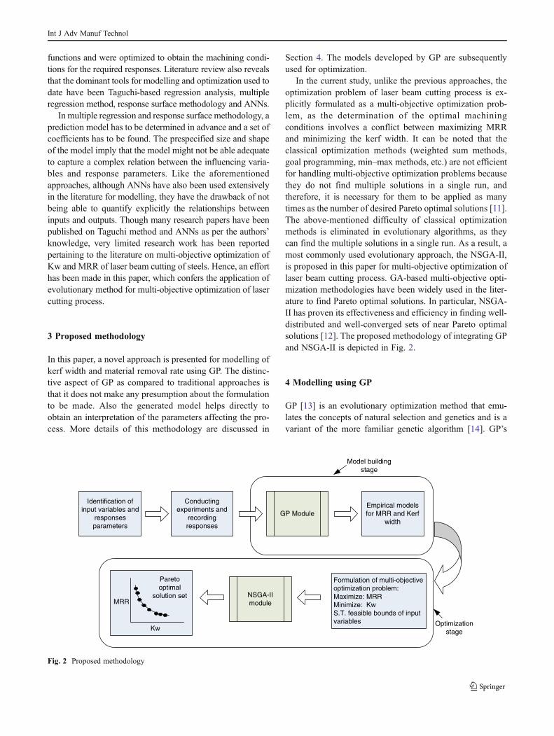
The various steps in NSGA-II based on the main frame-work of the algorithm [22] shown in Fig. 3 can be stated inthe following steps:

1. Set the initial run parameters for the algorithm, viz.population size (N), maximum number of generations(gmax), crossover probability (Pc), mutation probability(Pm; generation, g00).

2. Randomly create an initial population Pg of size N witha good coverage of the search space, and thereby havea diverse gene pool with potential to explore as muchof the search space as possible.

3. Evaluate the objective values and rank the populationusing the concept of domination. Each solution isassigned a fitness (or rank) equal to its non-dominationlevel (1 is the best level, 2 is the next best level and so on).

4. Perform the crowding sort procedure and include themost widely solutions by using crowding distance value.

5. The child populations Qg is produced from the parentpopulation Pg using binary selection, recombinationand mutation operators.

6. Then the two populations are combined together toproduce Rg (0Pg U Qg), which is of size 2N.

7. After this the population Rg undergoes non-dominatedsorting to achieve a global non-domination check.

8. The new population Pg+1 is filled based on the rankingof the non-dominated fronts.

9. Since the combined population is twice the size of thepopulation size N, all the fronts are not allowed to beused. Therefore a crowding distance sorting is performedin descending order and the population is filled. Thus forthis new population Pg+1, the whole process is repeated.

10. Update the number of generations, g0g+1.11. Repeat steps 3 to 10 until a stopping criterion is met.

Pg

Qg

Front 1

Rejected

Solutions [N+1, 2N]

R(g) = (Pg U Qg)

Pg+1Non-Dominated sorting

Crowding distance sorting

2N NFront 2

Front 3

Front 1

Front 2

Front 3

Geneticoperation

Offspringpopulation

Fig. 3 Main frame work of NSGA-II algorithm

Int J Adv Manuf Technol

6 Experimental details

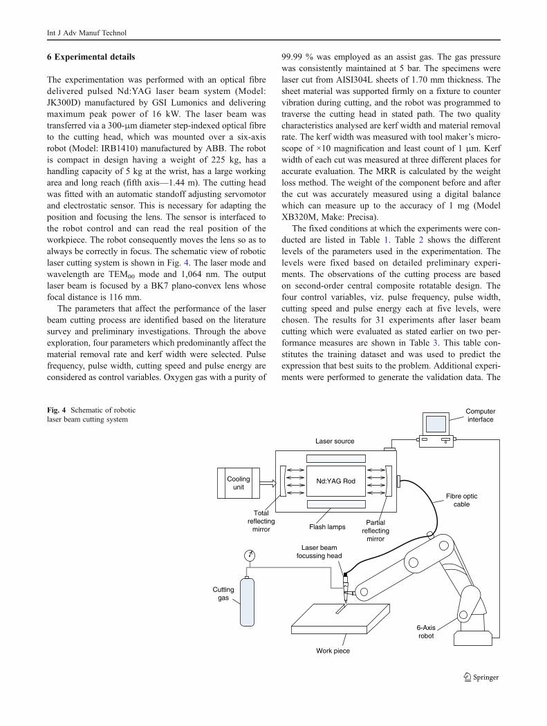
The experimentation was performed with an optical fibredelivered pulsed Nd:YAG laser beam system (Model:JK300D) manufactured by GSI Lumonics and deliveringmaximum peak power of 16 kW. The laser beam wastransferred via a 300-μm diameter step-indexed optical fibreto the cutting head, which was mounted over a six-axisrobot (Model: IRB1410) manufactured by ABB. The robotis compact in design having a weight of 225 kg, has ahandling capacity of 5 kg at the wrist, has a large workingarea and long reach (fifth axis—1.44 m). The cutting headwas fitted with an automatic standoff adjusting servomotorand electrostatic sensor. This is necessary for adapting theposition and focusing the lens. The sensor is interfaced tothe robot control and can read the real position of theworkpiece. The robot consequently moves the lens so as toalways be correctly in focus. The schematic view of roboticlaser cutting system is shown in Fig. 4. The laser mode andwavelength are TEM00 mode and 1,064 nm. The outputlaser beam is focused by a BK7 plano-convex lens whosefocal distance is 116 mm.

The parameters that affect the performance of the laserbeam cutting process are identified based on the literaturesurvey and preliminary investigations. Through the aboveexploration, four parameters which predominantly affect thematerial removal rate and kerf width were selected. Pulsefrequency, pulse width, cutting speed and pulse energy areconsidered as control variables. Oxygen gas with a purity of

99.99 % was employed as an assist gas. The gas pressurewas consistently maintained at 5 bar. The specimens werelaser cut from AISI304L sheets of 1.70 mm thickness. Thesheet material was supported firmly on a fixture to countervibration during cutting, and the robot was programmed totraverse the cutting head in stated path. The two qualitycharacteristics analysed are kerf width and material removalrate. The kerf width was measured with tool maker’s micro-scope of ×10 magnification and least count of 1 μm. Kerfwidth of each cut was measured at three different places foraccurate evaluation. The MRR is calculated by the weightloss method. The weight of the component before and afterthe cut was accurately measured using a digital balancewhich can measure up to the accuracy of 1 mg (ModelXB320M, Make: Precisa).

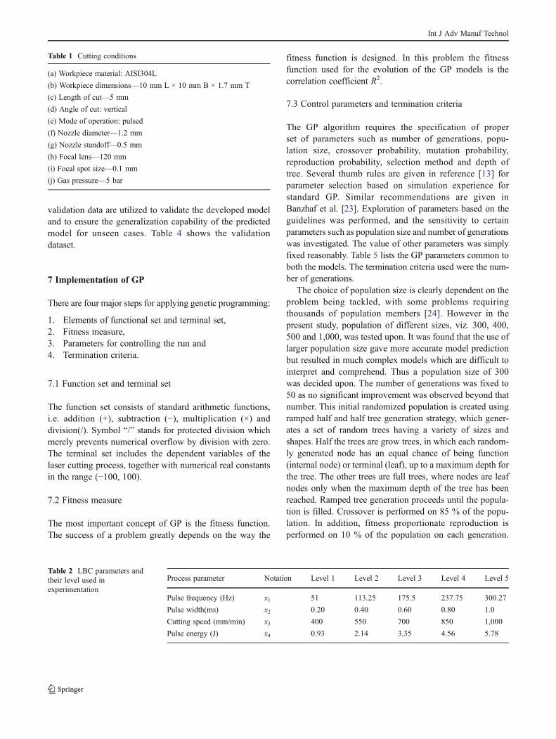
The fixed conditions at which the experiments were con-ducted are listed in Table 1. Table 2 shows the differentlevels of the parameters used in the experimentation. Thelevels were fixed based on detailed preliminary experi-ments. The observations of the cutting process are basedon second-order central composite rotatable design. Thefour control variables, viz. pulse frequency, pulse width,cutting speed and pulse energy each at five levels, werechosen. The results for 31 experiments after laser beamcutting which were evaluated as stated earlier on two per-formance measures are shown in Table 3. This table con-stitutes the training dataset and was used to predict theexpression that best suits to the problem. Additional experi-ments were performed to generate the validation data. The

Nd:YAG RodCoolingunit

Laser source

Flash lamps

Totalreflecting

mirror

Fibre opticcable

Computerinterface

Cuttinggas

6-Axisrobot

Work piece

Laser beamfocussing head

Partialreflecting

mirror

Fig. 4 Schematic of roboticlaser beam cutting system

Int J Adv Manuf Technol

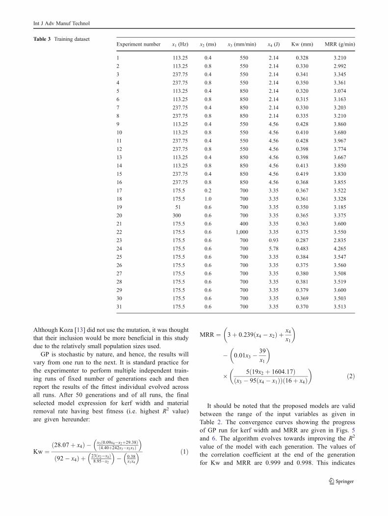
validation data are utilized to validate the developed modeland to ensure the generalization capability of the predictedmodel for unseen cases. Table 4 shows the validationdataset.

7 Implementation of GP

There are four major steps for applying genetic programming:

1. Elements of functional set and terminal set,2. Fitness measure,3. Parameters for controlling the run and4. Termination criteria.

7.1 Function set and terminal set

The function set consists of standard arithmetic functions,i.e. addition (+), subtraction (−), multiplication (×) anddivision(/). Symbol “/” stands for protected division whichmerely prevents numerical overflow by division with zero.The terminal set includes the dependent variables of thelaser cutting process, together with numerical real constantsin the range (−100, 100).

7.2 Fitness measure

The most important concept of GP is the fitness function.The success of a problem greatly depends on the way the

fitness function is designed. In this problem the fitnessfunction used for the evolution of the GP models is thecorrelation coefficient R2.

7.3 Control parameters and termination criteria

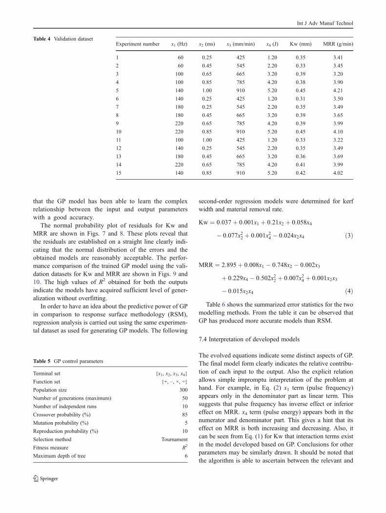
The GP algorithm requires the specification of properset of parameters such as number of generations, popu-lation size, crossover probability, mutation probability,reproduction probability, selection method and depth oftree. Several thumb rules are given in reference [13] forparameter selection based on simulation experience forstandard GP. Similar recommendations are given inBanzhaf et al. [23]. Exploration of parameters based on theguidelines was performed, and the sensitivity to certainparameters such as population size and number of generationswas investigated. The value of other parameters was simplyfixed reasonably. Table 5 lists the GP parameters common toboth the models. The termination criteria used were the num-ber of generations.

The choice of population size is clearly dependent on theproblem being tackled, with some problems requiringthousands of population members [24]. However in thepresent study, population of different sizes, viz. 300, 400,500 and 1,000, was tested upon. It was found that the use oflarger population size gave more accurate model predictionbut resulted in much complex models which are difficult tointerpret and comprehend. Thus a population size of 300was decided upon. The number of generations was fixed to50 as no significant improvement was observed beyond thatnumber. This initial randomized population is created usingramped half and half tree generation strategy, which gener-ates a set of random trees having a variety of sizes andshapes. Half the trees are grow trees, in which each random-ly generated node has an equal chance of being function(internal node) or terminal (leaf), up to a maximum depth forthe tree. The other trees are full trees, where nodes are leafnodes only when the maximum depth of the tree has beenreached. Ramped tree generation proceeds until the popula-tion is filled. Crossover is performed on 85 % of the popu-lation. In addition, fitness proportionate reproduction isperformed on 10 % of the population on each generation.

Table 1 Cutting conditions

(a) Workpiece material: AISI304L

(b) Workpiece dimensions—10 mm L × 10 mm B × 1.7 mm T

(c) Length of cut—5 mm

(d) Angle of cut: vertical

(e) Mode of operation: pulsed

(f) Nozzle diameter—1.2 mm

(g) Nozzle standoff—0.5 mm

(h) Focal lens—120 mm

(i) Focal spot size—0.1 mm

(j) Gas pressure—5 bar

Table 2 LBC parameters andtheir level used inexperimentation

Process parameter Notation Level 1 Level 2 Level 3 Level 4 Level 5

Pulse frequency (Hz) x1 51 113.25 175.5 237.75 300.27

Pulse width(ms) x2 0.20 0.40 0.60 0.80 1.0

Cutting speed (mm/min) x3 400 550 700 850 1,000

Pulse energy (J) x4 0.93 2.14 3.35 4.56 5.78

Int J Adv Manuf Technol

Although Koza [13] did not use the mutation, it was thoughtthat their inclusion would be more beneficial in this studydue to the relatively small population sizes used.

GP is stochastic by nature, and hence, the results willvary from one run to the next. It is standard practice forthe experimenter to perform multiple independent train-ing runs of fixed number of generations each and thenreport the results of the fittest individual evolved acrossall runs. After 50 generations and of all runs, the finalselected model expression for kerf width and materialremoval rate having best fitness (i.e. highest R2 value)are given hereunder:

Kw ¼28:07þ x4ð Þ � x3 0:09x4�x2þ29:38ð Þ

4:40þ242x3�x2x3ð Þ� �

92� x4ð Þ þ 23 x2�x4ð Þ8:95�x2

� �� 0:38

x1x4

� � ð1Þ

MRR ¼ 3þ 0:239 x4 � x2ð Þ þ x4x1

� �

� 0:01x3 � 39

x1

� �

� 5 19x2 þ 1604:17ð Þx3 � 95 x4 � x1ð Þð Þ 16þ x4ð Þ

� �ð2Þ

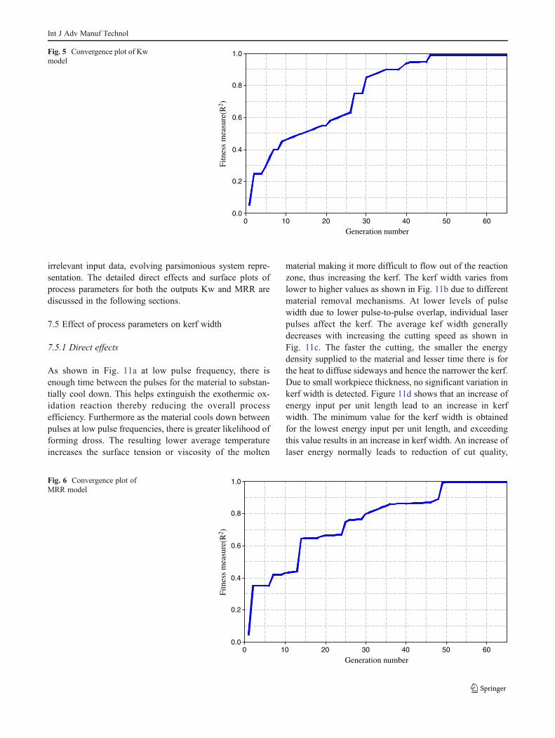
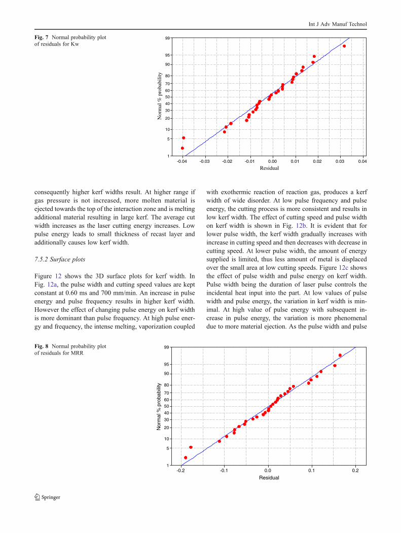
It should be noted that the proposed models are validbetween the range of the input variables as given inTable 2. The convergence curves showing the progressof GP run for kerf width and MRR are given in Figs. 5and 6. The algorithm evolves towards improving the R2

value of the model with each generation. The values ofthe correlation coefficient at the end of the generationfor Kw and MRR are 0.999 and 0.998. This indicates

Table 3 Training datasetExperiment number x1 (Hz) x2 (ms) x3 (mm/min) x4 (J) Kw (mm) MRR (g/min)

1 113.25 0.4 550 2.14 0.328 3.210

2 113.25 0.8 550 2.14 0.330 2.992

3 237.75 0.4 550 2.14 0.341 3.345

4 237.75 0.8 550 2.14 0.350 3.361

5 113.25 0.4 850 2.14 0.320 3.074

6 113.25 0.8 850 2.14 0.315 3.163

7 237.75 0.4 850 2.14 0.330 3.203

8 237.75 0.8 850 2.14 0.335 3.210

9 113.25 0.4 550 4.56 0.428 3.860

10 113.25 0.8 550 4.56 0.410 3.680

11 237.75 0.4 550 4.56 0.428 3.967

12 237.75 0.8 550 4.56 0.398 3.774

13 113.25 0.4 850 4.56 0.398 3.667

14 113.25 0.8 850 4.56 0.413 3.850

15 237.75 0.4 850 4.56 0.419 3.830

16 237.75 0.8 850 4.56 0.368 3.855

17 175.5 0.2 700 3.35 0.367 3.522

18 175.5 1.0 700 3.35 0.361 3.328

19 51 0.6 700 3.35 0.350 3.185

20 300 0.6 700 3.35 0.365 3.375

21 175.5 0.6 400 3.35 0.363 3.600

22 175.5 0.6 1,000 3.35 0.375 3.550

23 175.5 0.6 700 0.93 0.287 2.835

24 175.5 0.6 700 5.78 0.483 4.265

25 175.5 0.6 700 3.35 0.384 3.547

26 175.5 0.6 700 3.35 0.375 3.560

27 175.5 0.6 700 3.35 0.380 3.508

28 175.5 0.6 700 3.35 0.381 3.519

29 175.5 0.6 700 3.35 0.379 3.600

30 175.5 0.6 700 3.35 0.369 3.503

31 175.5 0.6 700 3.35 0.370 3.513

Int J Adv Manuf Technol

that the GP model has been able to learn the complexrelationship between the input and output parameterswith a good accuracy.

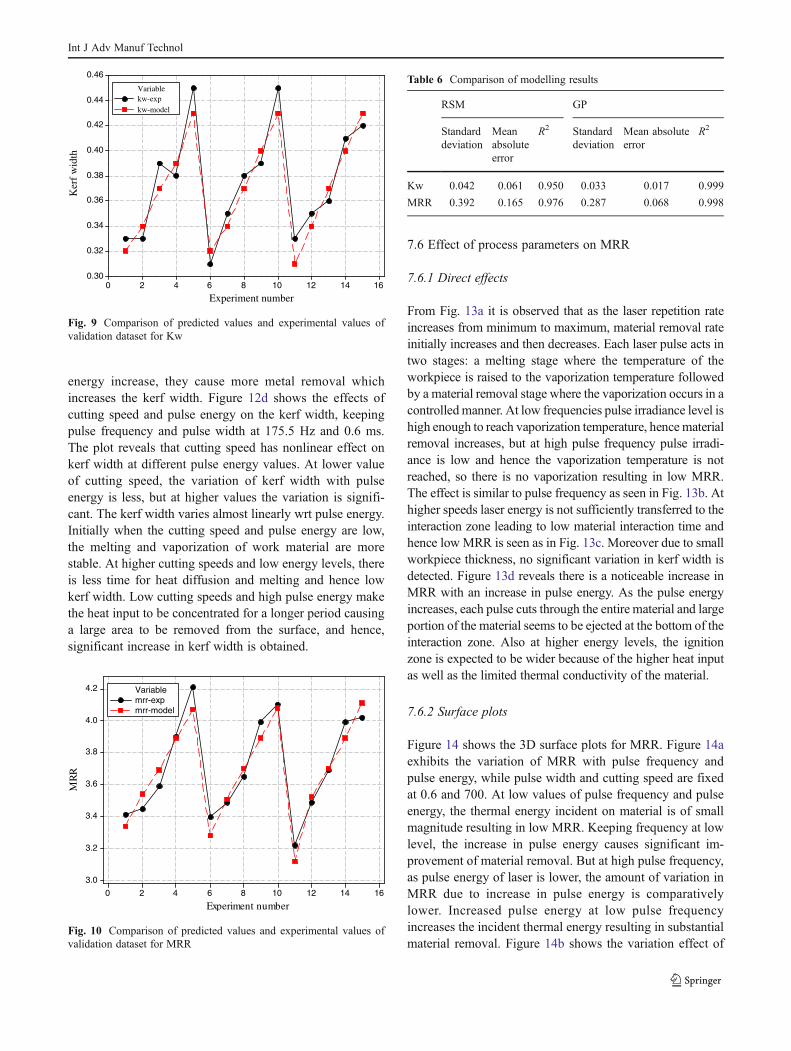
The normal probability plot of residuals for Kw andMRR are shown in Figs. 7 and 8. These plots reveal thatthe residuals are established on a straight line clearly indi-cating that the normal distribution of the errors and theobtained models are reasonably acceptable. The perfor-mance comparison of the trained GP model using the vali-dation datasets for Kw and MRR are shown in Figs. 9 and10. The high values of R2 obtained for both the outputsindicate the models have acquired sufficient level of gener-alization without overfitting.

In order to have an idea about the predictive power of GPin comparison to response surface methodology (RSM),regression analysis is carried out using the same experimen-tal dataset as used for generating GP models. The following

second-order regression models were determined for kerfwidth and material removal rate.

Kw ¼ 0:037þ 0:001x1 þ 0:21x2 þ 0:058x4

� 0:077x22 þ 0:001x24 � 0:024x2x4 ð3Þ

MRR ¼ 2:895þ 0:008x1 � 0:748x2 � 0:002x3

þ 0:229x4 � 0:502x22 þ 0:007x24 þ 0:001x2x3

� 0:015x2x4 ð4ÞTable 6 shows the summarized error statistics for the two

modelling methods. From the table it can be observed thatGP has produced more accurate models than RSM.

7.4 Interpretation of developed models

The evolved equations indicate some distinct aspects of GP.The final model form clearly indicates the relative contribu-tion of each input to the output. Also the explicit relationallows simple impromptu interpretation of the problem athand. For example, in Eq. (2) x1 term (pulse frequency)appears only in the denominator part as linear term. Thissuggests that pulse frequency has inverse effect or inferioreffect on MRR. x4 term (pulse energy) appears both in thenumerator and denominator part. This gives a hint that itseffect on MRR is both increasing and decreasing. Also, itcan be seen from Eq. (1) for Kw that interaction terms existin the model developed based on GP. Conclusions for otherparameters may be similarly drawn. It should be noted thatthe algorithm is able to ascertain between the relevant and

Table 4 Validation datasetExperiment number x1 (Hz) x2 (ms) x3 (mm/min) x4 (J) Kw (mm) MRR (g/min)

1 60 0.25 425 1.20 0.35 3.41

2 60 0.45 545 2.20 0.33 3.45

3 100 0.65 665 3.20 0.39 3.20

4 100 0.85 785 4.20 0.38 3.90

5 140 1.00 910 5.20 0.45 4.21

6 140 0.25 425 1.20 0.31 3.50

7 180 0.25 545 2.20 0.35 3.49

8 180 0.45 665 3.20 0.39 3.65

9 220 0.65 785 4.20 0.39 3.99

10 220 0.85 910 5.20 0.45 4.10

11 100 1.00 425 1.20 0.33 3.22

12 140 0.25 545 2.20 0.35 3.49

13 180 0.45 665 3.20 0.36 3.69

14 220 0.65 785 4.20 0.41 3.99

15 140 0.85 910 5.20 0.42 4.02

Table 5 GP control parameters

Terminal set {x1, x2, x3, x4}

Function set {+, –, ×, ÷}

Population size 300

Number of generations (maximum) 50

Number of independent runs 10

Crossover probability (%) 85

Mutation probability (%) 5

Reproduction probability (%) 10

Selection method Tournament

Fitness measure R2

Maximum depth of tree 6

Int J Adv Manuf Technol

irrelevant input data, evolving parsimonious system repre-sentation. The detailed direct effects and surface plots ofprocess parameters for both the outputs Kw and MRR arediscussed in the following sections.

7.5 Effect of process parameters on kerf width

7.5.1 Direct effects

As shown in Fig. 11a at low pulse frequency, there isenough time between the pulses for the material to substan-tially cool down. This helps extinguish the exothermic ox-idation reaction thereby reducing the overall processefficiency. Furthermore as the material cools down betweenpulses at low pulse frequencies, there is greater likelihood offorming dross. The resulting lower average temperatureincreases the surface tension or viscosity of the molten

material making it more difficult to flow out of the reactionzone, thus increasing the kerf. The kerf width varies fromlower to higher values as shown in Fig. 11b due to differentmaterial removal mechanisms. At lower levels of pulsewidth due to lower pulse-to-pulse overlap, individual laserpulses affect the kerf. The average kef width generallydecreases with increasing the cutting speed as shown inFig. 11c. The faster the cutting, the smaller the energydensity supplied to the material and lesser time there is forthe heat to diffuse sideways and hence the narrower the kerf.Due to small workpiece thickness, no significant variation inkerf width is detected. Figure 11d shows that an increase ofenergy input per unit length lead to an increase in kerfwidth. The minimum value for the kerf width is obtainedfor the lowest energy input per unit length, and exceedingthis value results in an increase in kerf width. An increase oflaser energy normally leads to reduction of cut quality,

Generation numberFi

tnes

s m

easu

re(R

2 )6050403020100

1.0

0.8

0.6

0.4

0.2

0.0

Fig. 5 Convergence plot of Kwmodel

Generation number

Fitn

ess

mea

sure

(R2 )

6050403020100

1.0

0.8

0.6

0.4

0.2

0.0

Fig. 6 Convergence plot ofMRR model

Int J Adv Manuf Technol

consequently higher kerf widths result. At higher range ifgas pressure is not increased, more molten material isejected towards the top of the interaction zone and is meltingadditional material resulting in large kerf. The average cutwidth increases as the laser cutting energy increases. Lowpulse energy leads to small thickness of recast layer andadditionally causes low kerf width.

7.5.2 Surface plots

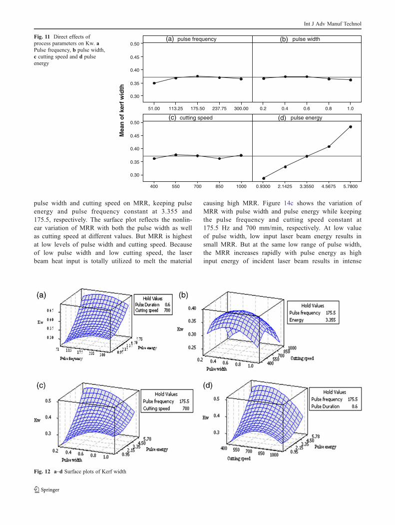
Figure 12 shows the 3D surface plots for kerf width. InFig. 12a, the pulse width and cutting speed values are keptconstant at 0.60 ms and 700 mm/min. An increase in pulseenergy and pulse frequency results in higher kerf width.However the effect of changing pulse energy on kerf widthis more dominant than pulse frequency. At high pulse ener-gy and frequency, the intense melting, vaporization coupled

with exothermic reaction of reaction gas, produces a kerfwidth of wide disorder. At low pulse frequency and pulseenergy, the cutting process is more consistent and results inlow kerf width. The effect of cutting speed and pulse widthon kerf width is shown in Fig. 12b. It is evident that forlower pulse width, the kerf width gradually increases withincrease in cutting speed and then decreases with decrease incutting speed. At lower pulse width, the amount of energysupplied is limited, thus less amount of metal is displacedover the small area at low cutting speeds. Figure 12c showsthe effect of pulse width and pulse energy on kerf width.Pulse width being the duration of laser pulse controls theincidental heat input into the part. At low values of pulsewidth and pulse energy, the variation in kerf width is min-imal. At high value of pulse energy with subsequent in-crease in pulse energy, the variation is more phenomenaldue to more material ejection. As the pulse width and pulse

Residual

Nor

mal

% p

roba

bilit

y0.040.030.020.010.00-0.01-0.02-0.03-0.04

99

95

90

80

70

60

50

40

30

20

10

5

1

Fig. 7 Normal probability plotof residuals for Kw

Residual

Nor

mal

% p

roba

bilit

y

0.20.10.0-0.1-0.2

99

95

90

80

70

60

50

40

30

20

10

5

1

Fig. 8 Normal probability plotof residuals for MRR

Int J Adv Manuf Technol

energy increase, they cause more metal removal whichincreases the kerf width. Figure 12d shows the effects ofcutting speed and pulse energy on the kerf width, keepingpulse frequency and pulse width at 175.5 Hz and 0.6 ms.The plot reveals that cutting speed has nonlinear effect onkerf width at different pulse energy values. At lower valueof cutting speed, the variation of kerf width with pulseenergy is less, but at higher values the variation is signifi-cant. The kerf width varies almost linearly wrt pulse energy.Initially when the cutting speed and pulse energy are low,the melting and vaporization of work material are morestable. At higher cutting speeds and low energy levels, thereis less time for heat diffusion and melting and hence lowkerf width. Low cutting speeds and high pulse energy makethe heat input to be concentrated for a longer period causinga large area to be removed from the surface, and hence,significant increase in kerf width is obtained.

7.6 Effect of process parameters on MRR

7.6.1 Direct effects

From Fig. 13a it is observed that as the laser repetition rateincreases from minimum to maximum, material removal rateinitially increases and then decreases. Each laser pulse acts intwo stages: a melting stage where the temperature of theworkpiece is raised to the vaporization temperature followedby a material removal stage where the vaporization occurs in acontrolledmanner. At low frequencies pulse irradiance level ishigh enough to reach vaporization temperature, hence materialremoval increases, but at high pulse frequency pulse irradi-ance is low and hence the vaporization temperature is notreached, so there is no vaporization resulting in low MRR.The effect is similar to pulse frequency as seen in Fig. 13b. Athigher speeds laser energy is not sufficiently transferred to theinteraction zone leading to low material interaction time andhence low MRR is seen as in Fig. 13c. Moreover due to smallworkpiece thickness, no significant variation in kerf width isdetected. Figure 13d reveals there is a noticeable increase inMRR with an increase in pulse energy. As the pulse energyincreases, each pulse cuts through the entire material and largeportion of the material seems to be ejected at the bottom of theinteraction zone. Also at higher energy levels, the ignitionzone is expected to be wider because of the higher heat inputas well as the limited thermal conductivity of the material.

7.6.2 Surface plots

Figure 14 shows the 3D surface plots for MRR. Figure 14aexhibits the variation of MRR with pulse frequency andpulse energy, while pulse width and cutting speed are fixedat 0.6 and 700. At low values of pulse frequency and pulseenergy, the thermal energy incident on material is of smallmagnitude resulting in low MRR. Keeping frequency at lowlevel, the increase in pulse energy causes significant im-provement of material removal. But at high pulse frequency,as pulse energy of laser is lower, the amount of variation inMRR due to increase in pulse energy is comparativelylower. Increased pulse energy at low pulse frequencyincreases the incident thermal energy resulting in substantialmaterial removal. Figure 14b shows the variation effect of

Experiment number

Ker

f w

idth

1614121086420

0.46

0.44

0.42

0.40

0.38

0.36

0.34

0.32

0.30

Variablekw-expkw-model

Fig. 9 Comparison of predicted values and experimental values ofvalidation dataset for Kw

Experiment number

MR

R

1614121086420

4.2

4.0

3.8

3.6

3.4

3.2

3.0

Variablemrr-expmrr-model

Fig. 10 Comparison of predicted values and experimental values ofvalidation dataset for MRR

Table 6 Comparison of modelling results

RSM GP

Standarddeviation

Meanabsoluteerror

R2 Standarddeviation

Mean absoluteerror

R2

Kw 0.042 0.061 0.950 0.033 0.017 0.999

MRR 0.392 0.165 0.976 0.287 0.068 0.998

Int J Adv Manuf Technol

pulse width and cutting speed on MRR, keeping pulseenergy and pulse frequency constant at 3.355 and175.5, respectively. The surface plot reflects the nonlin-ear variation of MRR with both the pulse width as wellas cutting speed at different values. But MRR is highestat low levels of pulse width and cutting speed. Becauseof low pulse width and low cutting speed, the laserbeam heat input is totally utilized to melt the material

causing high MRR. Figure 14c shows the variation ofMRR with pulse width and pulse energy while keepingthe pulse frequency and cutting speed constant at175.5 Hz and 700 mm/min, respectively. At low valueof pulse width, low input laser beam energy results insmall MRR. But at the same low range of pulse width,the MRR increases rapidly with pulse energy as highinput energy of incident laser beam results in intense

Mea

n o

f ke

rf w

idth

300.00237.75175.50113.2551.00

0.50

0.45

0.40

0.35

0.30

1.00.80.60.40.2

1000850700550400

0.50

0.45

0.40

0.35

0.30

5.78004.56753.35502.14250.9300

pulse frequency pulse width

cutting speed pulse energy

(a) (b)

(c) (d)

Fig. 11 Direct effects ofprocess parameters on Kw. aPulse frequency, b pulse width,c cutting speed and d pulseenergy

Fig. 12 a–d Surface plots of Kerf width

Int J Adv Manuf Technol

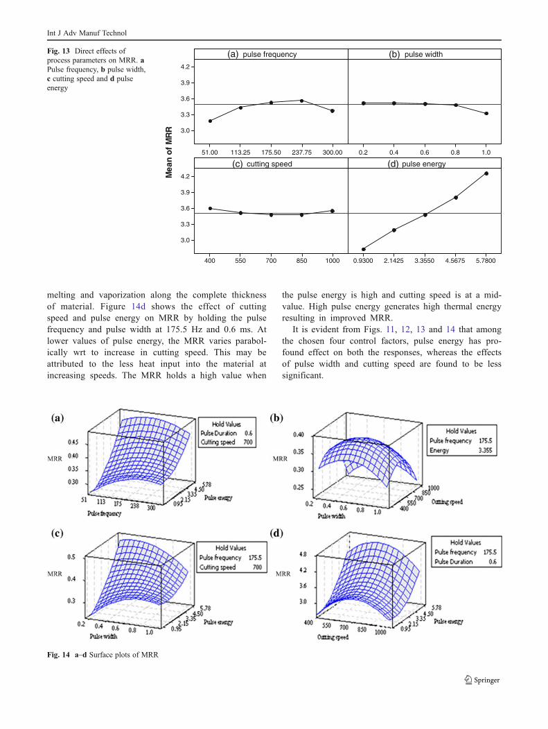
melting and vaporization along the complete thicknessof material. Figure 14d shows the effect of cuttingspeed and pulse energy on MRR by holding the pulsefrequency and pulse width at 175.5 Hz and 0.6 ms. Atlower values of pulse energy, the MRR varies parabol-ically wrt to increase in cutting speed. This may beattributed to the less heat input into the material atincreasing speeds. The MRR holds a high value when

the pulse energy is high and cutting speed is at a mid-value. High pulse energy generates high thermal energyresulting in improved MRR.

It is evident from Figs. 11, 12, 13 and 14 that amongthe chosen four control factors, pulse energy has pro-found effect on both the responses, whereas the effectsof pulse width and cutting speed are found to be lesssignificant.

Mea

n o

f M

RR

300.00237.75175.50113.2551.00

4.2

3.9

3.6

3.3

3.0

1.00.80.60.40.2

1000850700550400

4.2

3.9

3.6

3.3

3.0

5.78004.56753.35502.14250.9300

pulse frequency pulse width

cutting speed pulse energy

(a) (b)

(c) (d)

Fig. 13 Direct effects ofprocess parameters on MRR. aPulse frequency, b pulse width,c cutting speed and d pulseenergy

Fig. 14 a–d Surface plots of MRR

Int J Adv Manuf Technol

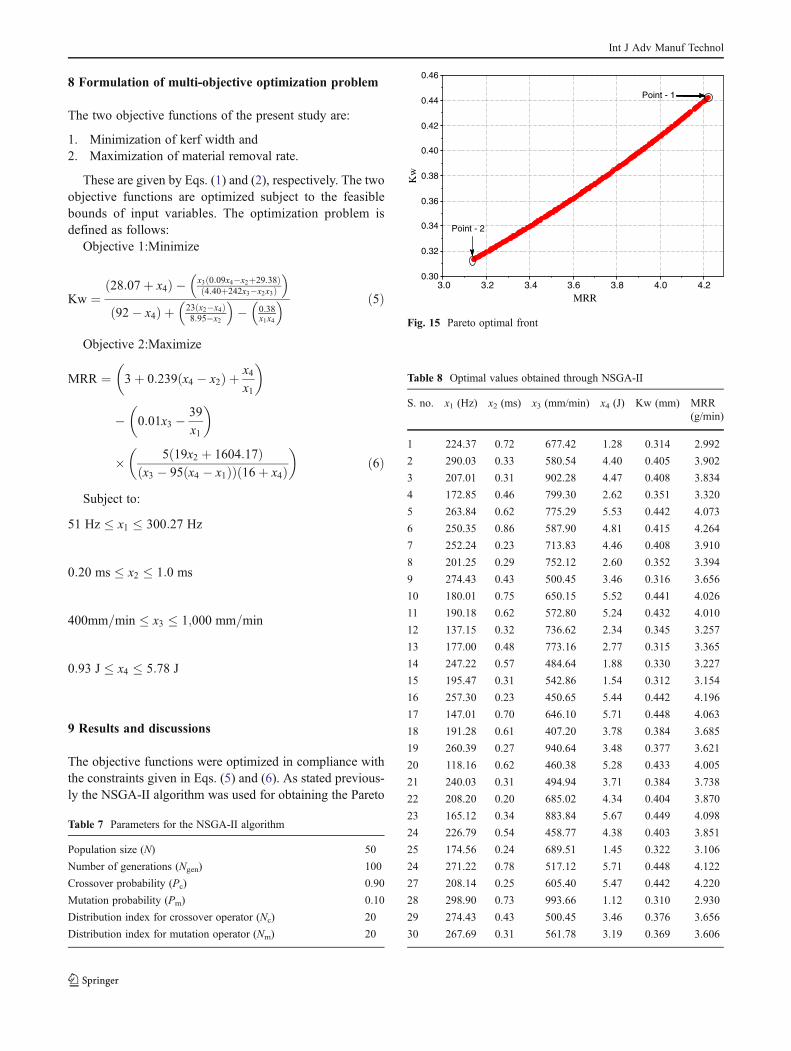
8 Formulation of multi-objective optimization problem

The two objective functions of the present study are:

1. Minimization of kerf width and2. Maximization of material removal rate.

These are given by Eqs. (1) and (2), respectively. The twoobjective functions are optimized subject to the feasiblebounds of input variables. The optimization problem isdefined as follows:

Objective 1:Minimize

Kw ¼28:07þ x4ð Þ � x3 0:09x4�x2þ29:38ð Þ

4:40þ242x3�x2x3ð Þ� �

92� x4ð Þ þ 23 x2�x4ð Þ8:95�x2

� �� 0:38

x1x4

� � ð5Þ

Objective 2:Maximize

MRR ¼ 3þ 0:239 x4 � x2ð Þ þ x4x1

� �

� 0:01x3 � 39

x1

� �

� 5 19x2 þ 1604:17ð Þx3 � 95 x4 � x1ð Þð Þ 16þ x4ð Þ

� �ð6Þ

Subject to:

51 Hz � x1 � 300:27 Hz

0:20 ms � x2 � 1:0 ms

400mm=min � x3 � 1;000 mm=min

0:93 J � x4 � 5:78 J

9 Results and discussions

The objective functions were optimized in compliance withthe constraints given in Eqs. (5) and (6). As stated previous-ly the NSGA-II algorithm was used for obtaining the Pareto

Table 7 Parameters for the NSGA-II algorithm

Population size (N) 50

Number of generations (Ngen) 100

Crossover probability (Pc) 0.90

Mutation probability (Pm) 0.10

Distribution index for crossover operator (Nc) 20

Distribution index for mutation operator (Nm) 20

MRR

Kw

4.24.03.83.63.43.23.0

0.46

0.44

0.42

0.40

0.38

0.36

0.34

0.32

0.30

Point - 1

Point - 2

Fig. 15 Pareto optimal front

Table 8 Optimal values obtained through NSGA-II

S. no. x1 (Hz) x2 (ms) x3 (mm/min) x4 (J) Kw (mm) MRR(g/min)

1 224.37 0.72 677.42 1.28 0.314 2.992

2 290.03 0.33 580.54 4.40 0.405 3.902

3 207.01 0.31 902.28 4.47 0.408 3.834

4 172.85 0.46 799.30 2.62 0.351 3.320

5 263.84 0.62 775.29 5.53 0.442 4.073

6 250.35 0.86 587.90 4.81 0.415 4.264

7 252.24 0.23 713.83 4.46 0.408 3.910

8 201.25 0.29 752.12 2.60 0.352 3.394

9 274.43 0.43 500.45 3.46 0.316 3.656

10 180.01 0.75 650.15 5.52 0.441 4.026

11 190.18 0.62 572.80 5.24 0.432 4.010

12 137.15 0.32 736.62 2.34 0.345 3.257

13 177.00 0.48 773.16 2.77 0.315 3.365

14 247.22 0.57 484.64 1.88 0.330 3.227

15 195.47 0.31 542.86 1.54 0.312 3.154

16 257.30 0.23 450.65 5.44 0.442 4.196

17 147.01 0.70 646.10 5.71 0.448 4.063

18 191.28 0.61 407.20 3.78 0.384 3.685

19 260.39 0.27 940.64 3.48 0.377 3.621

20 118.16 0.62 460.38 5.28 0.433 4.005

21 240.03 0.31 494.94 3.71 0.384 3.738

22 208.20 0.20 685.02 4.34 0.404 3.870

23 165.12 0.34 883.84 5.67 0.449 4.098

24 226.79 0.54 458.77 4.38 0.403 3.851

25 174.56 0.24 689.51 1.45 0.322 3.106

24 271.22 0.78 517.12 5.71 0.448 4.122

27 208.14 0.25 605.40 5.47 0.442 4.220

28 298.90 0.73 993.66 1.12 0.310 2.930

29 274.43 0.43 500.45 3.46 0.376 3.656

30 267.69 0.31 561.78 3.19 0.369 3.606

Int J Adv Manuf Technol

optimal solutions. The source code for NSGA-II is imple-mented in the VC++ programming language on WindowsXP platform. The optimization results are sensitive to algo-rithm parameters, typical of heuristic techniques. Hence, it isrequired to perform repeated simulations to find commen-surate values for the parameters. The best parameters for theNSGA-II, selected through 10 test simulation runs, are listedin Table 7. A population size of 100 was chosen withcrossover probability of 0.90 and mutation probability of0.10 along with other control parameters. NSGA-II gavegood diversity results and provided for a well-populatedPareto front of the conflicting objective functions as shownin Fig. 15.

Among the 100 non-dominated optimal solutions at theend of 100 generations, 30 optimal input variables and theircorresponding objective function values are presented inTable 8. By analysing the Pareto front, a decision makercan exploit it in accomplishing specific decisions based onthe requirements of the process. For instance at point 1 inFig. 15, laser cutting may be performed at maximum MRRbut the Kw will be a higher value and hence poor edgequality. On the other extreme of the front, i.e. point 2 lowKw with good edge quality may be obtained but the MRR isminimum. All the other points on the front are in between

cases. As can be observed from the graph, no solution in thefront is absolutely better than any other as they are non-dominated solutions; hence, any one of them is an accept-able solution. The choice of a particular solution has to bemade purely based on production requirements. For exam-ple if the manufacturer chooses to cut a component with Kwof 0.314 mm, the set of input variables may be selected fromthe first row of Table 8. Accordingly the MRR of 2.99 g/minwould be achieved. In another instance from the experimen-tal results of Table 3, 13th row, the set of input variablesleads to MRR of 3.66 and the corresponding Kw value is0.3985 mm. After optimization, the Kw value is reduced to0.316 mm (S. no. 9, Table 8) with almost the same value ofMRR.

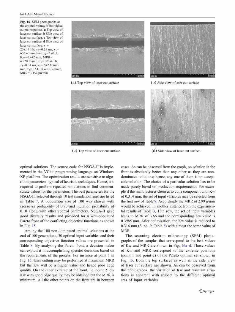
The scanning electron microscopy (SEM) photo-graphs of the samples that correspond to the best valuesof Kw and MRR are shown in Fig. 16a–d. Those valuesof Kw and MRR correspond to the extreme positions(point 1 and point 2) of the Pareto optimal set shown inFig. 15. Both the top surfaces as well as the side viewof laser cut surface are shown. As can be observed fromthe photographs, the variation of Kw and resultant stria-tions is apparent with respect to the different optimalsets of input variables.

(a) Top view of laser cut surface (b) Side view oflaser cut surface

(c) Top view of laser cut surface (d) Side view of laser cut surface

Fig. 16 SEM photographs atthe optimal values of individualoutput responses. a Top view oflaser cut surface. b Side view oflaser cut surface. c Top view oflaser cut surface. d Side view oflaser cut surface. x10208.14 Hz, x200.25 ms, x30605.40 mm/min, x405.47 J,Kw00.442 mm, MRR04.220 m/min, x10195.47Hz,x200.31 ms, x30 542.86mm/min, x401.54J, Kw00.320mm,MRR03.154gm/min

Int J Adv Manuf Technol

10 Conclusions

The laser cutting process is an important and widely usednontraditional manufacturing technology for rapid and pre-cise cutting of metallic sheets with complex shapes yieldingexcellent accuracy and quality. Being a complex process, itis very difficult and costly to determine the optimal param-eters based on trial and error or experience. The presentwork implements unique approach for laser cutting processbased on the integration of two evolutionary approaches,namely GP and NSGA-II. GP is a powerful evolutionarymodelling approach that can learn the complex underlyingrelationship between the input and response parameterseffectively, whereas NSGA-II is reliable and widely estab-lished tool for multi-objective optimization.

In this work, the most important performances of lasercutting, namelyMRR and kerf width, are considered. Initially,from the experimental training data, GP was used to model themathematical relations for the chosen performance measures.Then, the models developed by GP were tested for theiraccuracy and suitability using statistical methods. The indi-vidual effects and the surface plots of the input variables onthe chosen output parameters were also presented. Later, thevalidated mathematical models of GP were used by NSGA-IIto find the multiple sets of optimal solutions so as to enable amanufacturing engineer to choose a particular optimal operat-ing set of input variables according to the specific require-ments. The selection of optimum values is essential forprocess automation and implementation of a computer-integrated manufacturing system.

References

1. Walsh RA, Cormier DR (2006) McGraw-Hill machining and met-alworking handbook, 3rd edn. McGraw-Hill, New York

2. Prasad GVS, Siores E, Wong WCK (1998) Laser cutting of me-tallic coated sheet steels. J Mater Process Technol 74:234–242

3. Dubey AK, Yadava V (2008) Laser beam machining—a review.Int J Mach Tool Manuf 48:609–628

4. Yousef BF, George K, Knopf, Evgueni V, Bordatchev, Suwas K,Nikumb (2003) Neural network modeling and analysis of thematerial removal process during laser machining. Int J Adv ManufTechnol 22:41–53. doi:10.1007/s00170-002-1441-9

5. Li C-H, Tsaia M-J, Yang C-D (2007) Study of optimal laserparameters for cutting QFN packages by Taguchi’s matrix method.Optic Laser Tech 39:786–795

6. Jimin C, Yang J, Zhang S, Zuo T, Guo D (2007) Parameteroptimization of non-vertical laser cutting. Int J Adv Manuf Tech-nol 33:469–473. doi:10.1007/s00170-006-0489-3

7. Dhara SK, Kuar AS, Mitra S (2008) An artificial neural networkapproach on parametric optimization of laser micro-machining ofdie-steel. Int J Adv Manuf Technol 39:39–46. doi:10.1007/s00170-007-1199-1

8. Dubey AK, Yadava V (2008) Multi-objective optimisation of laserbeam cutting process. Optic Laser Tech 40(3):562–570

9. Avanish Kumar D, Vinod Y (2008) Optimization of kerf qualityduring pulsed laser cutting of aluminium alloy sheet. J MaterProcess Technol 204(11):412–418

10. Ming-Jong T, Chen-Hao Li, Cheng-Che C (2008) Optimal laser-cutting parameters for QFN packages by utilizing artificial neuralnetworks and genetic algorithm. J Mater Process Technol 208(1–3):270–283

11. Sardiñas RQ, Santana MR, Brindis EA (2006) Genetic algorithmbased multi-objective optimization of cutting parameters in turningprocesses. Eng Appl Artif Intell 19:127–133

12. Deb K, Pratap A, Agarwal S, Meyarivan T (2002) A fast and elitistmultiobjective genetic algorithm: NSGA-II. IEEE Trans EvolComput 6(2):182–197

13. Koza JR (1992) Genetic programming: on the programming ofcomputers by means of natural selection. MIT Press, Cambridge

14. Goldberg DE (1989) Genetic algorithms in search, optimisation,and machine learning. Addison-Wesley, Reading, MA

15. Dolinsky JU, Jenkinson ID, Colquhoun GJ (2007) Application ofgenetic programming to the calibration of industrial robots. Com-put Ind 58:255–264

16. Zhang L, Jack LB, Nandi AK (2005) Fault detection using geneticprogramming. Mech Syst Signal Proc 19(2):271–289

17. Ashour AF, Alvarez LF, Toropov VV (2003) Empirical modellingof shear strength of RC deep beams by genetic programming.Comput Struct 81(5):331–338

18. Kondayya D, Gopalakrishna A (2010) An integrated evolutionaryapproach for modelling and optimization of wire electrical dis-charge machining. Proc IME B J Eng Manufact 225:549–567.doi:10.1243/09544054JEM1975

19. Poli R, Langdon WB, McPhee NF (2010) A field guide to geneticprogramming. http://www.gp-field-guide.org.uk. Accessed Dec2010

20. Konak A, Coit DW, Smith AE (2006) Multi-objective optimizationusing genetic algorithms: a tutorial. Reliab Eng Syst Saf 91(9):992–1007

21. Deb, K.; Agarwal, S.; Pratap, A.; Meyarivan, T (2000) A fast elitistnondominated sorting genetic algorithm for multiobjective optimi-zation: NSGA II. In Proceedings of the Parallel Problem Solvingfrom Nature VI (PPSN-VI), Springer: NY, 849–858

22. Deb K, Pratap A, Agarwal S, Meyarivan T (2002) A fast and elitistmultiobjective genetic algorithm: NSGA-II. IEEE Trans EvolComput 6(2):182–197

23. Banzhaf W, Nordin P, Keller R, Francone F (1998) Geneticprogramming: an introduction. Morgan Kaufmann, San Francisco

24. Koza JR, Bennett FH III, Andre D, Martin A, Keane (1999)Genetic programming III: Darwinian invention and problem solv-ing. Morgan Kaufmann, San Francisco

Int J Adv Manuf Technol