


Bahasa
Halaman
Hukum

Implementation of a Hydraulic Routing Model forDendritic Networks with Offline Coupling to a
Distributed Hydrological ModelChi Chi Choi1; George Constantinescu2; and Ricardo Mantilla, M.ASCE3
Abstract: The authors present a new set of tools for solving the one-dimensional Saint-Venant equations (1D-SVEs) of flow transportthroughout dendritic river networks. The numerical solver is integrated with a set of geoprocessing tools, which include automatic cross-section selection, river bathymetry extraction, and a selection of model parameters, that facilitate the implementation of the 1D-SVE sim-ulation setup. In addition, geographic information systems (GIS)–based preprocessing tools are developed to provide a seamless coupling ofthe hydraulic model to a hydrological model, which provides estimates of surface and subsurface runoff from hill slopes and performs routingin river networks using simplified ordinary differential equations. The hill slope runoff and streamflow generated by CUENCAS are redis-tributed as lateral inflows to the channels modeled by the 1D-SVE hydraulic model. The coupling of the hydraulic and hydrologic (H-H)models enables the validation of the hydrological model at internal locations in the basin where stage measurements are made, instead of onlyat locations where streamflow is estimated. An application of the coupled H-H models is demonstrated in the Squaw Creek watershed, Iowa.Results show that the coupled H-H models serve to validate assumptions in the hydrological model related to the spatial and temporalproduction of runoff in the watershed and bolster confidence in the estimated discharges at ungauged locations. DOI: 10.1061/(ASCE)HE.1943-5584.0001152. © 2015 American Society of Civil Engineers.
Author keywords: Coupled hydrologic-hydraulic models; One-dimensional Saint-Venant equations (1D-SVEs); CUENCAS; Geographicinformation systems (GIS); Cross sections.
Introduction
A variety of mathematical methods have been developed to simu-late the routing of flows in open channels. These routing methodscan predict the timing of the peak flow, the peak flow magnitude,and the shape of a flood wave as it travels through a river network(Fread 1985). A broad categorization of these methods dividesthese flow-routing techniques between hydrologic and hydraulicrouting models. Hydrologic routing is based on the continuityequation and storage-discharge relationships that generate ordinarydifferential equations (ODEs). Examples include the Muskingummethods (McCarthy 1938; Nash 1959; Ponce 1979), linear reser-voir approximations (Nash 1957; Diskin et al. 1978), or simplifiednonlinear storage reservoirs (Mitchell 1962; Horn 1987; Mantillaet al. 2006). These routing tools can reproduce streamflow varia-tions accurately when the assumed storage-discharge relationshipsare an appropriate approximation of flow dynamics characteristic ina river network. However, because these relationships are based onestimations of residence time and in many cases are empiricallybased, they cannot capture key dynamic aspects of a flood wavesuch as the channel-floodplain interaction and backwater effects
due to downstream constrictions. In addition, because river geom-etries are not explicitly considered in hydrological routing methods,they only provide estimations of streamflow and not of stage.By contrast, based on a spatial description of the channels, hy-draulic routing simultaneously provides flow depths and stream-flow estimates.
Over the past several decades. reach-scale hydraulic modelsbased on the one-dimensional Saint-Venant equation (1D-SVE)have been successfully developed and used for natural river net-works (Hicks et al. 2005; Pramanik et al. 2010; Abshire 2012;Saleh et al. 2013). Results from these studies demonstrated thatthe accuracy of the river stage predictions correlates strongly withthe accuracy of the bathymetry data (e.g., channel bed profiles andriver geometry). Physically based 1D-SVE models are typicallyformulated as partial differential equations (PDEs), and these for-mulations can handle more complex unsteady flow dynamics inriver networks compared with hydrologic models because the gov-erning equations that are solved incorporate more physics. Thismotivated the development of streamflow routing algorithms basedon the 1D-SVE for large-scale river basins. Such applicationsrequire a large number of computational points to accurately de-scribe the river network and its dynamics under unsteady forcing(e.g., flood events) and a fast solver to obtain predictions in a rea-sonable amount of time. Given these requirements efforts have beenmade to (1) implement numerical algorithms that can solve largesystems of nonlinear equations in a robust and computationallyinexpensive way, (2) better parameterize the river geometry, and(3) better describe the channel-floodplain dynamics.
For example, Yamazaki et al. (2011) proposed a global hy-draulic routing model (CaMa-Flood), which can be coupled witha land surface model to simulate river and floodplain hydrodynam-ics at a continental or global scale. The river basin is discretized intounit catchments along with river network maps derived from the
1Graduate Student, IIHR-Hydrosicence and Engineering, Univ. of Iowa,Iowa City, IA 52242. E-mail: [email protected]
2Associate Professor, IIHR-Hydrosicence and Engineering, Univ. ofIowa, Iowa City, IA 52242. E-mail: [email protected]
3Assistant Professor, IIHR-Hydrosicence and Engineering, Univ. ofIowa, Iowa City, IA 52242 (corresponding author). E-mail: [email protected]
Note. This manuscript was submitted on June 6, 2014; approved onNovember 17, 2014; published online on March 19, 2015. Discussion per-iod open until August 19, 2015; separate discussions must be submitted forindividual papers. This paper is part of the Journal of Hydrologic Engi-neering, © ASCE, ISSN 1084-0699/04015023(14)/$25.00.
© ASCE 04015023-1 J. Hydrol. Eng.
J. Hydrol. Eng.
Dow
nloa
ded
from
asc
elib
rary
.org
by
Uni
v of
Iow
a L
ibra
ries
on
04/1
3/15
. Cop
yrig
ht A
SCE
. For
per
sona
l use
onl
y; a
ll ri
ghts
res
erve
d.

flow direction map that depicts the upstream-downstream relation-ship between each unit catchment. In addition, the topographicparameters of channel and floodplain (e.g., channel length, unit-catchment area, river bank altitude, and floodplain elevation pro-file) for each unit catchment were derived from the flow directionmaps and fine-resolution digital elevation models (DEMs). Thechannel width and depth were estimated from the empirical func-tion of river discharge (Yamazaki et al. 2013). The continuity equa-tion was formulated at the level of the control volume for each unitcatchment [i.e., change of total storage (channel and floodplain) =change of discharge between upstream and downstream + runoffinput from land surface model]. A diffusive wave equation wasused as a surrogate for the momentum equation (Yamazaki et al.2011). In other implementations, a local inertia equation was usedinstead of the diffusive wave equation (Yamazaki et al. 2013). Themodel was found to reproduce well the water level dynamics in theAmazon River basin (Yamazaki et al. 2012).
Paiva et al. (2013a, b) used a coupled hydrologic-hydraulicmodel (MGB-IPH and 1D-SVE) to model flow dynamics in theSolimoes River subbasin of the Amazon and in the entire AmazonRiver basin. The hydraulic model solves the full 1D-SVE for anarbitrary river network using an implicit finite-differences scheme.The linearized system of discrete equations is solved using aGauss elimination procedure algorithm based on a modified skylinestorage method. The availability of the detailed river bathymetryand floodplain topography data is fairly limited at large scales(e.g., continental scale). The model used a geographic informationsystem (GIS)–based algorithm to construct the required river net-work maps, the catchment discretization and the river cross sectionsdiscretization. It was also used to estimate the position of the chan-nel bottom and to construct the channel and floodplain parameter-izations based on the provided DEM (Paiva et al. 2011). The maindifference between this hydraulic model and CaMa-Flood is thateach subcatchment can be further divided into subfloodplain unitsthat coincide with the cross section discretization of the hydraulicmodel. As a result, the sum of the surface, subsurface, and baseflow obtained from using the hydrologic model for each floodplainunit is used to specify the lateral inflow in the hydraulic model. Thechannel cross section geometry is parameterized as a rectangular-shape channel. The channel width and depth are estimated througha geomorphologic relation, which is a function of the upstreamdrainage area and annual peak discharge. The flow exchange be-tween the channel and floodplain are simplified as a simple flood-plain storage model that correlates the flooded area and the waterlevel for every subfloodplain unit. These additional terms were thenadded as the lateral inflow terms in the continuity equation of the1D-SVE. The simulated hydrographs and the flood inundationwere found to agree well with the observed daily river dischargeand water levels and the Environmental Satellite (ENVISAT) altim-etry data. The other challenge is related to computing time neededfor large-scale applications. The Simulation Program for RiverNetworks (SPRINT) of Liu et al. (2014) solves the full 1D-SVEat regional to continental scales (105 grid elements) with an accept-able computational speed (the code computed the flow in a realflooding event approximately 330 times faster than the real timeover which the event occurred) on a desktop computer.
The method used for large-scale coupled hydrologic-hydraulicrouting models cannot be directly implemented for small-scale rivernetworks where the details of the river bathymetry are available. Insmall-scale studies, the detailed river bathymetry consists of multi-ple cross-sectional cuts. A first challenge is to correctly specify thediscretization of the cross sections (e.g., location, width). As dis-cussed by Ackerman (2009), their placement should follow severalrules: (1) the sections should not intersect, (2) the sections should
be close to perpendicular to the local flow direction, and (3) thesections should cross the stream centerline only once. By followingthese guidelines, the resulting cross section discretization used bythe hydraulic model may not always coincide with the catchmentdiscretization used by the hydrologic model. A second challengein small-scale studies is that the watershed scaling determinesthe acceptable level of accuracy for the simulated results. As such,the effects of the river geometry, floodplain bathymetry, and chan-nel bed profile on the accuracy of the modeled results are moresignificant for small-scale basin applications than for large-scaleriver basin applications. The mismatch associated with couplingthe hydrologic-hydraulic model at different scales creates a newresearch challenge that needs to be addressed. Consequently, thispaper proposes using a GIS-based method to streamline the cou-pling between a hydrologic model (CUENCAS) and a newly de-veloped hydraulic routing model based on the 1D-SVE.
The hydraulic routing model presented here is based on theclassical one-dimensional coupled continuity and momentum equa-tions known as the Saint-Venant equations (1D–SVEs). The solu-tion of the SVEs requires extensive physical-based data, such asriver geometries and topographic information, and in order forthe calculations made by the 1D-SVE to be accurate, the inflow-outflow boundary conditions and river bathymetric and topographicdata must relatively closely reflect reality. The acquisition of cross-section geometry and river bathymetry has improved significantlyin recent years with the advance of light detection and ranging(LIDAR) systems technology. One limitation of LIDAR maps isthat they do not capture the riverbed features because the laser can-not penetrate standing water (Cook et al. 2009), which results inerror-prone riverbed profiles. These inaccuracies can lead to verticaloffsets between the river stage measurement and the prediction. Inaddition, inflow boundaries (i.e., lateral runoff into channels) to the1D-SVE model, following a rainfall event, are not measurableeverywhere, and they are driven by complex processes that are as-sociated with hill slope surface runoff, soil water infiltration, andgroundwater seepage. Therefore, uncertainties of river bathymetricand inflow boundaries limit the use of hydraulic routing in complexriver networks. These limitations have been recognized by others.For example, Hicks et al. (2005) suggested three reasons that ac-counted for the limited use of hydraulic models for operationalstreamflow forecasting. First, there has not been strong enoughevidence to convince official agencies to invest more funds intothe large-scale implementation of hydraulic modeling. Second,hydraulic models are more difficult to set up and model stabilitycan be a concern. Third, forecasters have developed techniques toadjust hydrologic routing parameters to compensate for the models’inaccuracies.
Despite the previously mentioned complications, it is still ad-vantageous to solve the 1D-SVE because there can be flow situa-tions in which the backwater effects of local flow dynamics cannotbe correctly captured by unique storage-discharge relationships(Paiva et al. 2011). In addition, direct measurements of dischargeare sparse and difficult to obtain, while the deployment of stream-stage gauges is easier and less expensive (Royem et al. 2012). Thisis important because discharge measurements form the basis forhydrological routing model parameterization. In general, measure-ments of river stage are converted to discharge by means of a ratingcurve. These indirect estimates of river discharge data are subject touncertainties due to (1) the error in stage and discharge measure-ments, (2) the hysteresis effect of a looped rating curve, and (3) theextrapolation of the rating curve beyond the measurement range(Fread 1975; Di Baldassarre and Claps 2010). Moreover, the avail-ability of rating curves is usually limited to gauged sites along themain stem of a river network, which prohibits the direct comparison
© ASCE 04015023-2 J. Hydrol. Eng.
J. Hydrol. Eng.
Dow
nloa
ded
from
asc
elib
rary
.org
by
Uni
v of
Iow
a L
ibra
ries
on
04/1
3/15
. Cop
yrig
ht A
SCE
. For
per
sona
l use
onl
y; a
ll ri
ghts
res
erve
d.

between the simulated discharge hydrographs from the hydrolog-ical model and river stage measurements taken along the rivernetwork tributaries. Only hydraulic models, such as the 1D-SVEmodel presented here, can make direct use of stage measurementsfor the validation and calibration of parameters. Consequently, theoffline or online coupling of hydrological and hydraulic modelsemerges as an excellent alternative that takes advantage of the twoworlds of flow-routing modeling and offers the added benefit thatthe distributed stage measurements can be used to evaluate thespatial and temporal accuracy of the runoff field generated bythe rainfall-runoff component of hydrological models.
The goal of this paper is to document the development of aphysical-based 1D-SVE PDE solver that can be applied to calculateflood routing in river networks and that can be coupled with theODE-based hydrological model for the rainfall-runoff process. Thispaper will use the hydrological modeling framework CUENCASintroduced by Mantilla and Gupta (2005). The CUENCAS frame-work is divided into two sets of tools, which will be referred to asfollows: (1) CUENCAS-GIS refers to the set of tools that extractsand analyzes the river network morphology, and (2) 7) CUENCASHydrologic Models (CUENCAS-HM) refers to the set of toolsfor modeling flow in river networks. First, the 1D-SVE modeland the corresponding set of GIS-based geoprocessing tools thatcan simulate 1D unsteady flow through a dendritic river networkare described. The 1D-SVE code has been implemented as a set ofMATLAB libraries, which provides portability and ease of use forapplications ranging from classroom exercises to complex engi-neering applications. Subsequently, details of the ODE setup ofthe CUENCAS-HM hydrological model are given. The coupledhydrologic and hydraulic (H-H) model is then implemented andtested for a realistic rainfall event in the Squaw Creek upstreamfrom Ames, Iowa. The runoff field generated by CUENCAS-HM is used as inflow (discharge) to the 1D-SVE model. Thecoupled H-H model takes advantage of both stage and dischargedata for model validation. After calibration of the coupled H-Hmodel parameters, it is validated with measured data providedby the Iowa Flood Center (IFC) stream-stage sensor networksand USGS streamflow data. The improved flood predictive capabil-ity of the coupled H-H models is demonstrated for a watershed withmultiple stage gauging locations.
Coupled H-H Model’s Description and DataPreparation
Hydraulic Model: 1D-SVE Solver
The governing equations for the one-dimensional, unsteady, open-channel flow, known as 1D–SVEs, can be written as the continuityequation
∂A∂t þ
∂Q∂x − qlat ¼ 0 ð1Þ
and the momentum equation
∂Q∂t þ ∂ðβQ2
A Þ∂x þ gA
�∂h∂x þ Sf
�¼ 0 ð2Þ
where β = momentum correction factor; Q = discharge (m3=s);A = flow area; g = gravitational acceleration (m=s2); qlat = net lat-eral inflow per unit length of channel (m2=s); h = elevation of watersurface measured from a horizontal datum (m); Sf = frictionalslope; t = time (s); and x = distance measured along streamcenterline (m).
In the 1D-SVE code developed as part of the present work, thestandard four-point weighted Preissmann scheme (1961) is usedto solve the dynamic wave form of the 1D-SVE. The channel-floodplain interaction of the hydraulic routing was embedded in themodified 1D-SVE (Fread 1976). There are two major assumptionsassociated with this approach. First, the water-surface elevationis assumed to be the same across the channel and the floodplain.Second, the friction slopes in the channel and the floodplain areassumed to be equal. The reach lengths of the channel and the flood-plain can be different, but they are assumed to be equal in this paperfor the following reasons: (1) the delineation of the floodplain flowpath lines is humanly subjective, (2) the river cross sections withinthe in-channel and their dog-leg alignment over the floodplainare not easy to be automated and the authors’ geoprocessing (GIS)tools (see full description in “Model Setup and Model ParametersSelection”) does not include this capability; and (3) the channel-floodplain interaction is complex and multidimensional.
The modified forms of the 1D-SVE [Eqs. (1) and (2)] that in-clude the channel-floodplain interaction (Fread 1976; Fread andSmith 1978) are given as the continuity equation for the channel
∂Ac
∂t þ ∂Qc
∂xc ¼ 0 ð3Þ
the momentum equation for the channel
∂Qc
∂t þ∂�Qc
2
Ac
�∂xc þ gAc
�∂hc∂xc þ Sfc
�¼ 0 ð4Þ
where x = displacement in the main flow direction (m), the con-tinuity equation for the floodplain
∂Af
∂t þ ∂Qf
∂x 0j¼ 0 ð5Þ
and the momentum equation for the floodplain
∂Qf
∂t þ∂�Q2
f
Af
�∂x 0
fþ gAf
�∂hf∂x 0
fþ Sff
�¼ 0 ð6Þ
where x 0 = displacement in the floodplain direction (m).The subscript c denotes the variables pertaining to the river
channel and the subscript f denotes the variables pertaining to thefloodplain. For full details of the numerical algorithms, readers arereferred to Fread (1976).
Two internal boundaries conditions are imposed to solve flow inconfluences. The first is continuity at the junction node. The secondis the stage at all nodes coming into and exiting the junction are thesame. Because the 1D-SVE is written in MATLAB, the MATLABbuilt-in function (mldivide, \) is used to solve the systems of linearequation Ax ¼ C, where A is stored as sparse matrix format. Thediscretized form of 1D-SVE [Eqs. (3)–(6)] and the boundaryconditions are used to build the system of linear equations. TheNewton-Raphson method is used to solve the full systems of equa-tions of the 1D-SVE (Ax ¼ C, where x is the vector column for the2N unknowns, Qnþ1
i and hnþ1i for I ¼ 1,2; : : : ;N, where N is the
number of computation nodes). First, a set of initial values are as-signed to the unknownsQnþ1
i and hnþ1i and the iteration (k) is equal
to 1. The coefficient of the matrix on the left-hand side (A) and theresidual column (C) on the right-hand side is filled with the calcu-lated values based on the initial values of the unknowns. The cor-rections ðΔQi;ΔhiÞ obtained from column (x) are the solution ofthe system of linear equations (Ax ¼ C). The new values of the
© ASCE 04015023-3 J. Hydrol. Eng.
J. Hydrol. Eng.
Dow
nloa
ded
from
asc
elib
rary
.org
by
Uni
v of
Iow
a L
ibra
ries
on
04/1
3/15
. Cop
yrig
ht A
SCE
. For
per
sona
l use
onl
y; a
ll ri
ghts
res
erve
d.

unknowns calculated asQnþ1i and hnþ1
i for the next iteration (kþ 1)are expressed as follows:
ðQiÞkþ1 ¼ ðQiÞk þ ðΔQiÞk ðhiÞkþ1 ¼ ðhiÞk þ ðΔhiÞkThe iterative procedure terminates until the maximum value of
corrections ΔQi;Δhi column is reduced to the assigned thresholdvalues.
Coupling the Hydrologic and Hydraulic Models
Ideally, hydraulic models use the measured discharge hydrographat the basin outlet as a boundary condition, which limits the un-certainty of boundary conditions to stage-discharge relationships.However, the availability of measured data is sparse in ungaugedbasins. This restricts the use of the hydraulic model for a complexriver network. To compensate for the data scarcity, the simulateddischarge hydrographs from the hydrological model are used asthe inflow boundary conditions of the hydraulic model. In this pa-per, a realistic rainfall-runoff event is simulated by the hydrologicalmodel CUENCAS-HM, which is primarily written in Java. Therunoff generated from CUENCAS-HM is used as the inflow (dis-charge) of the cross section-based 1D-SVE solver. The flow trans-port in river networks in CUENCAS-HM is governed by a systemof ODEs that uses the mass conservation equation for a link, e,(Mantilla et al. 2006) as follows:
dSðe; tÞdt
¼ aeRðe; tÞ þ qðf1; tÞ þ qðf2; tÞ − qðe; tÞ ð7Þ
where Sðe; tÞ = storage in the link at time t; ae = total hill slope areainto which it is draining; Rðe; tÞ = runoff intensity per unit areafrom the hill slope; qðf1; tÞ þ qðf2; tÞ = flow from the two up-stream tributaries joining the link e; and qðe; tÞ = discharge at theoutlet of the link.
The channel storage, Sðe; tÞ, and discharge, qðe; tÞ, can bewritten as Sðe; tÞ ¼ lewedeðtÞ and
qðe; tÞ ¼ veðtÞwedeðtÞ ¼ veðtÞCA ð8Þwhere we = mean width of the link; deðtÞ = mean channel depth;CA = link average cross-sectional area; veðtÞ = flow velocity; andle = link length. Combining them gives
Sðe; tÞ ¼ qðe; tÞleveðtÞ
Letting veðtÞ ¼ v0qλ1Aλ2 ð9Þ
where v0 = initial velocity; and λ1 and λ2 = scaling exponents.The channel storage Sðe; tÞ ¼ ð1=v0Þqðe; tÞ1−λ1Aλ2 le is a func-
tion of discharge; then Eq. (7) becomes
dqðe; tÞdt
¼K½qðe; tÞ�½ahRðe; tÞþqðf1; tÞþqðf2; tÞ−qðe; tÞ� ð10Þ
where
K½qðe; tÞ� ¼ v0qðe; tÞλ1Aλ2
ð1 − λ1ÞleA simplified version of the runoff production from the hill slope
is given by
dSpdt
¼ RcpðtÞ − qpl ð11Þ
dSsdt
¼ ð1 − RcÞpðtÞ − qsl ð12Þ
Rðe; tÞ ¼ qpl þ qsl ð13Þ
dSðe; tÞdt
¼ ahðqpl þ qslÞ þ qðf1; tÞ þ qðf2; tÞ − qðe; tÞ ð14Þ
where qpl ¼ ½ðvhleÞ=ah�Sp and qsl ¼ ½ðvhleÞ=ðah × 290Þ�Ss; Rc =runoff coefficient; pðtÞ = rainfall time series; qpl = surface storage;qsl = subsurface storage; vh = velocity of the hill slope (m=s); Sp =storage volume from the surface (km3); ah = hill slope area drainingto the link (km2); and Ss = storage volume from the subsurface(km3). The link-based mass conservation Eq. (10) forms a systemof 3M nonlinear ODEs, where M is the number of links in thenetworks. Because the spatial distribution of the river networksand the storage-discharge relationship of the ODEs systems usedin CUENCAS-HM differ from the PDEs systems used in the1D-SVE solver, the geoprocessing tools (Choi 2013; Choi andMantilla 2015) are used to convert the tributary inflows fromthe ODEs systems into inflows for the 1D-SVE solver.
Study Site
Squaw Creek, which is upstream from Ames, Iowa (42.011°N93.596°W), was selected for this study. The Squaw Creek water-shed (SCW) is located in central Iowa where it drains approxi-mately 602 km2 and includes parts of Boone, Hamilton, Webster,and Story counties. It drains into the South Skunk River at Ames,Iowa, and ultimately discharges into the Mississippi River in south-east Iowa. There are a total of 5,143 km of streams in the basin,including ephemeral and perennial river pathways. The hydrologicmodel CUENCAS includes every one of those streams in its con-figuration. Of those streams, approximately 227 km form the per-ennial channel network, which is modeled by the 1D-SVE models(Fig. 1). The latter number agrees with the previously reportednetwork by Wendt (2007). The drainage has been transformedfrom slowly draining wetlands and depressions into rapidly drain-ing ditches and farm tiles (Squaw Creek Watershed PlanningCommittee 2004). Schilling et al. (2008) and Jha et al. (2010) pro-vide additional background on watershed characteristics as well asinformation on hydrologic, water quality, and biological monitor-ing data. Twenty-two bridge-mounted stage sensors that are oper-ated by the Iowa Flood Center (IFC) and a USGS streamflow gauge(#05470500) for river stage and discharge measurements (Fig. 1)are located in the watershed. The watershed recently experiencedsevere flooding in August 2010; a peak discharge of 634 m3=s andpeak stage of 5.53 m was recorded at the USGS streamflow gauge(#05470500), and the return period of the flood was estimatedto be between the 100- and 500-year flood interval (Barnes andEash 2012).
Fig. 1 shows the basin boundaries and river network delineatedusing CUENCAS-GIS. The Squaw Creek is an order-8 network.Only the higher order streams are selected for the 1D-HD modelimplementation for two reasons: (1) the hydrodynamic conditionsthat grant the implementation of 1D-HD models, including floodplain interactions and backwater effects from downstream con-strictions, typically occur in larger streams, and (2) many distrib-uted hydrological models include a routing component for thechannels in the networks, and the authors want to demonstratehow to connect the channel network where SVEs are solved withthe network that uses simplified routing methods. Routing inhydrological models typically entails simplified kinematic waveequations (Whitham 2011), ODE routing using nonlinear reser-voirs (Mein et al. 1974; Green 1979), or Muskingum routingschemes (McCarthy 1938; Nash 1959; Ponce 1979). The delin-eated river network (HD Model Streams), the river network
© ASCE 04015023-4 J. Hydrol. Eng.
J. Hydrol. Eng.
Dow
nloa
ded
from
asc
elib
rary
.org
by
Uni
v of
Iow
a L
ibra
ries
on
04/1
3/15
. Cop
yrig
ht A
SCE
. For
per
sona
l use
onl
y; a
ll ri
ghts
res
erve
d.

(CUENCAS-HM Streams), and the adjacent hill slope area ex-tracted by CUENCAS-GIS and the DEMs are the only inputsrequired by the tools that are presented in this paper. CUENCAS-GIS uses the classical D8 algorithm (O’Callaghan and Mark 1984)to determine drainage pathways.
Model Implementation Details for the Squaw CreekBasin
The first step in coupling the hydrologic and hydraulic models is toidentify how the river networks in the distributed hydrologic modelrelate to the network modeled by the hydraulic model. A short riversegment within the watershed is used to illustrate the steps neces-sary to assess the linkage. A requirement for linking the model isthat the channel centerlines in both models coincide relatively well.This condition can be easily achieved by burning the channel cen-terlines from the hydraulic model into the digital elevation model(5-m DEM) used for river network generation. As a result, the hillslope runoff generated from CUENCAS-HM can be matched asinflows for the cross section-based hydraulic model via automaticgeoprocessing tools. The process of linking the models is shownin Fig. 2.
The basin decomposition made by CUENCAS-GIS yields34,925 links and the corresponding adjacent hill slopes (LINK-ID),as depicted in Figs. 2(a–c). The automatically extracted river cross-section locations (points) are overlaid on the landscape partitiongiven by CUENCAS-GIS [Fig. 2(d)] to determine which hill slopesand what river channels drain directly into the channel segmentsthat are defined in the hydraulic model.
In order to correlate the river cross section locations and theLINK-ID in both models, the extracted values from the LINK-IDraster data generated by CUENCAS-GIS that lay within the 300-m-radius circle that surrounds the cross section points used by thehydraulic model are used. This is done for all of the cross sectionpoints except for the first upstream cross section [Fig. 2(e)]. Thisbuffering method is necessary because the channel centerlines inboth model setups do not match perfectly. The river networks usedin the hydraulic model are humanly digitized based on LIDAR-derived DEM (1 m), while the river network and its adjacent hillslope unit (equivalent to subcatchment unit in other models) used inCUENCAS are generated based on calculated flow direction gridsthrough the D8 algorithms derived from the resampled DEM (5 m).The D8 algorithm is not completely accurate, especially near hy-draulic structures such as roadway embankments or culverts thatcannot be well represented by LIDAR-derived DEM. Therefore,the LINK-IDs identified within a larger buffered domain can betraced to compensate for the small mismatch of the channel center-lines in both models. The extracted LINK-ID is then followeddownstream to the following cross section, ensuring that the ex-tracted values of the LINK-IDs for all the river cross sections areproperly connected. Once the correct LINK-ID of all the cross sec-tions has been identified, the inflows used for the 1D-HD modelscan be calculated. The inflow at the first river cross section is thedischarge hydrograph corresponding to the top LINK-ID, whilethe lateral inflows along the river segments are equal to the sum ofthe tributary inflows over the length interval between two consecu-tive cross sections [Fig. 2(f)]. By implementing this approach to allof the streams in the 1D-HD models, the runoff and storage releasegenerated by the distributed hydrologic model (CUENCAS-HM)can be automatically coupled with the cross section-based 1D-HDmodels.
Model Setup and Model Parameters Selection
Two significant flood events that occurred in August 2010 andMay 2013 in the Squaw Creek basin upstream from Ames, Iowa,were selected to validate the accuracy of the coupled H-H models.Because river stage data from IFC bridge-mounted sonic sensorsfor the 2010 event were not available, the authors used the 2013event for model validation and argue that if the coupled H-H modelcan perform well for multiple validation sites in the 2013 event,then the authors can expect that it will perform equally well forthe 2010 event using the same model parameters and model setup.Measurements of discharge at the USGS station (Ames, Iowa,#05404220) and measurements of stage at 22 IFC bridge-mountedsonic sensors were obtained to validate the authors’ modelingresults.
Four data inputs are required to set up the hydraulic model: (1) aset of centerlines with river labeling that will be modeled using the1D-SVE, (2) a 1-m LIDAR-based DEM, (3) a map of land coverto estimate roughness in the flood plain, and (4) the runoff andstreamflow space-time field generated by the hydrologic modelto be used as the inflow boundary condition. The LIDAR-derived1-m DEM topography used in this study is the result of a joint effortbetween the Iowa Department of Natural Resources (DNR), theIowa Department of Transportation (IDOT), the Natural ResourcesConservation Service (NRCS) and the Iowa Department of Agri-culture and Land Stewardship (IDALS). Floodplain roughnesscoefficients are estimated from the 30-m resolution land cover dataset [NLCD 2001 (Homer et al. 2007)]. A set of geoprocessing(GIS) tools are used to automate the cross section generation, rivergeometry extraction, and overbanks locations identification andcalculate the required inflows for the authors’ coupled H-H model
Fig. 1. (Color) Squaw Creek basin upstream from Ames, Iowa[Copyright © 2014 Esri (DNR, IDOT, NRCS and IDASLS). All rightsreserved]
© ASCE 04015023-5 J. Hydrol. Eng.
J. Hydrol. Eng.
Dow
nloa
ded
from
asc
elib
rary
.org
by
Uni
v of
Iow
a L
ibra
ries
on
04/1
3/15
. Cop
yrig
ht A
SCE
. For
per
sona
l use
onl
y; a
ll ri
ghts
res
erve
d.

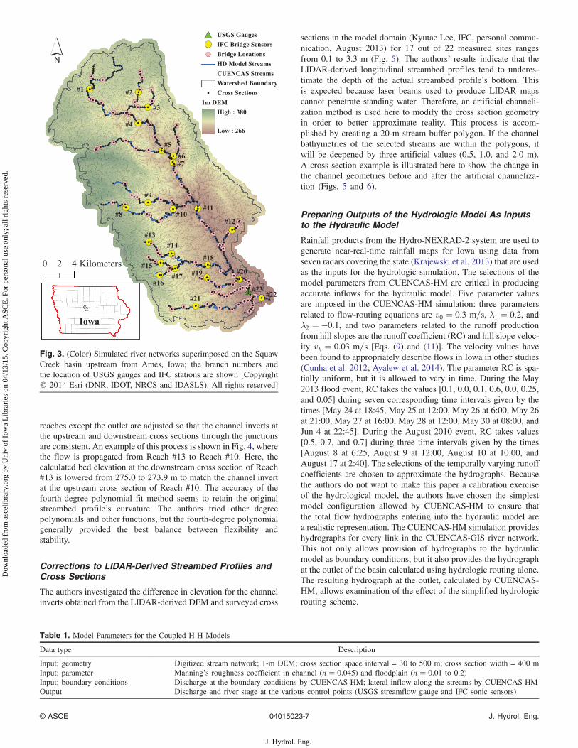
from files generated by the CUENCAS-HM hydrologic model.The cross sections selected follow some standard guidelines:(1) they do not overlap, (2) they intersect with the stream once,(3) they are not placed in river meandering zones, and (4) theydo not overlap at junctions. The details of the GIS tools are fullydescribed in another paper (Choi and Mantilla 2015). The authors’GIS tools generated a total of 486 cross sections along 33 individ-ual river reaches (a river reach refers to the river channel in betweentwo river junctions in the hydraulic model river network). The crosssection spacing is selected within a reasonable range (30 to500 m) so that a relatively smooth river bathymetric profile canbe obtained (Fig. 3). The cross section width is fixed at 400 mto include the floodplain topography. The cross sections are se-lected to satisfy the following criteria: (1) nonmeandering region,(2) at least 40-m distance to avoid overlapping cross sections atchannel junctions, and (3) at least one cross section for all thebridge crossings within the basin. The in-channel Manning’s
coefficients are assigned with values in the range of 0.03–0.05[typically clean, straight channel (Chow 1959)]. This case studyuses a constant value of 0.045 for every stream. The roughnesscoefficients for the left and right flood plains are the mean valueextracted from roughness coefficient grids derived from NLCD(2001) (Manning’s n value: 0.02 to 0.15). Table 1 summarizesthe required input parameters for the coupled H-H models.
One of the challenges associated with the automatic extractionof the river profile is that errors in the DEM can contaminate thestreambed bathymetry. These errors often create bumpy streambedprofiles along the thalweg, which are unrealistic and can affectthe numerical stability of hydrodynamic models. In order to avoidthese errors, the authors’ tools smooth out the streambed profile byfitting a fourth-degree polynomial (elevation versus downstreamdistance) to the bed profile of each reach in the model. The valuesgiven by the polynomial are used to determine the bed elevations ofall of the cross sections in that reach. The final bed profiles of all the
Fig. 2. (Color) Schematic diagram showing the step-by-step procedures of converting inflow from CUENCAS-HM to the 1D-SVE solver [Copyright© 2014 Esri (ESRI ArcGIS Online and data partners, including imagery from agencies supplied via the Content Sharing Program). All rightsreserved]
© ASCE 04015023-6 J. Hydrol. Eng.
J. Hydrol. Eng.
Dow
nloa
ded
from
asc
elib
rary
.org
by
Uni
v of
Iow
a L
ibra
ries
on
04/1
3/15
. Cop
yrig
ht A
SCE
. For
per
sona
l use
onl
y; a
ll ri
ghts
res
erve
d.
reaches except the outlet are adjusted so that the channel inverts atthe upstream and downstream cross sections through the junctionsare consistent. An example of this process is shown in Fig. 4, wherethe flow is propagated from Reach #13 to Reach #10. Here, thecalculated bed elevation at the downstream cross section of Reach#13 is lowered from 275.0 to 273.9 m to match the channel invertat the upstream cross section of Reach #10. The accuracy of thefourth-degree polynomial fit method seems to retain the originalstreambed profile’s curvature. The authors tried other degreepolynomials and other functions, but the fourth-degree polynomialgenerally provided the best balance between flexibility andstability.
Corrections to LIDAR-Derived Streambed Profiles andCross Sections
The authors investigated the difference in elevation for the channelinverts obtained from the LIDAR-derived DEM and surveyed cross
sections in the model domain (Kyutae Lee, IFC, personal commu-nication, August 2013) for 17 out of 22 measured sites rangesfrom 0.1 to 3.3 m (Fig. 5). The authors’ results indicate that theLIDAR-derived longitudinal streambed profiles tend to underes-timate the depth of the actual streambed profile’s bottom. Thisis expected because laser beams used to produce LIDAR mapscannot penetrate standing water. Therefore, an artificial channeli-zation method is used here to modify the cross section geometryin order to better approximate reality. This process is accom-plished by creating a 20-m stream buffer polygon. If the channelbathymetries of the selected streams are within the polygons, itwill be deepened by three artificial values (0.5, 1.0, and 2.0 m).A cross section example is illustrated here to show the change inthe channel geometries before and after the artificial channeliza-tion (Figs. 5 and 6).
Preparing Outputs of the Hydrologic Model As Inputsto the Hydraulic Model
Rainfall products from the Hydro-NEXRAD-2 system are used togenerate near-real-time rainfall maps for Iowa using data fromseven radars covering the state (Krajewski et al. 2013) that are usedas the inputs for the hydrologic simulation. The selections of themodel parameters from CUENCAS-HM are critical in producingaccurate inflows for the hydraulic model. Five parameter valuesare imposed in the CUENCAS-HM simulation: three parametersrelated to flow-routing equations are v0 ¼ 0.3 m=s, λ1 ¼ 0.2, andλ2 ¼ −0.1, and two parameters related to the runoff productionfrom hill slopes are the runoff coefficient (RC) and hill slope veloc-ity vh ¼ 0.03 m=s [Eqs. (9) and (11)]. The velocity values havebeen found to appropriately describe flows in Iowa in other studies(Cunha et al. 2012; Ayalew et al. 2014). The parameter RC is spa-tially uniform, but it is allowed to vary in time. During the May2013 flood event, RC takes the values [0.1, 0.0, 0.1, 0.6, 0.0, 0.25,and 0.05] during seven corresponding time intervals given by thetimes [May 24 at 18:45, May 25 at 12:00, May 26 at 6:00, May 26at 21:00, May 27 at 16:00, May 28 at 12:00, May 30 at 08:00, andJun 4 at 22:45]. During the August 2010 event, RC takes values[0.5, 0.7, and 0.7] during three time intervals given by the times[August 8 at 6:25, August 9 at 12:00, August 10 at 10:00, andAugust 17 at 2:40]. The selections of the temporally varying runoffcoefficients are chosen to approximate the hydrographs. Becausethe authors do not want to make this paper a calibration exerciseof the hydrological model, the authors have chosen the simplestmodel configuration allowed by CUENCAS-HM to ensure thatthe total flow hydrographs entering into the hydraulic model area realistic representation. The CUENCAS-HM simulation provideshydrographs for every link in the CUENCAS-GIS river network.This not only allows provision of hydrographs to the hydraulicmodel as boundary conditions, but it also provides the hydrographat the outlet of the basin calculated using hydrologic routing alone.The resulting hydrograph at the outlet, calculated by CUENCAS-HM, allows examination of the effect of the simplified hydrologicrouting scheme.
Fig. 3. (Color) Simulated river networks superimposed on the SquawCreek basin upstream from Ames, Iowa; the branch numbers andthe location of USGS gauges and IFC stations are shown [Copyright© 2014 Esri (DNR, IDOT, NRCS and IDASLS). All rights reserved]
Table 1. Model Parameters for the Coupled H-H Models
Data type Description
Input; geometry Digitized stream network; 1-m DEM; cross section space interval = 30 to 500 m; cross section width = 400 mInput; parameter Manning’s roughness coefficient in channel (n ¼ 0.045) and floodplain (n ¼ 0.01 to 0.2)Input; boundary conditions Discharge at the boundary conditions by CUENCAS-HM; lateral inflow along the streams by CUENCAS-HMOutput Discharge and river stage at the various control points (USGS streamflow gauge and IFC sonic sensors)
© ASCE 04015023-7 J. Hydrol. Eng.
J. Hydrol. Eng.
Dow
nloa
ded
from
asc
elib
rary
.org
by
Uni
v of
Iow
a L
ibra
ries
on
04/1
3/15
. Cop
yrig
ht A
SCE
. For
per
sona
l use
onl
y; a
ll ri
ghts
res
erve
d.

Results and Discussion
Hydrographs simulated by the coupled H-H models and byCUENCAS-HM are compared with observed stage and streamflowhydrographs provided by IFC and USGS sensors for the two majorflood events that occurred in August 2010 and May 2013. Themodel performance from two models is evaluated based on threestatistical measures used to compare the simulated and observedhydrographs: the root-mean-square error (RMSE), the correlationcoefficient (R), and the Nash-Sutcliffe coefficient (NS) (Table 2).The square root of discharge predicted from CUENCAS was usedas a surrogate of stage to compare model simulation results to stagemeasurements and direct discharge values at Gauge #23 wherestreamflow measurement are available.
An initial inspection of the streamflow hydrographs at the basinoutlet indicates that the timing of the flood peaks, the peak flow,and the shape of the simulated hydrographs are properly captured inthe two models (Figs. 7 and 8). In the case of the CUENCAS-HMsimulated hydrographs, the only opportunity for comparison withdata is at locations where streamflow estimates exist. The compari-son of the simulated hydrographs between the coupled H-H modeland CUENCAS-HM indicates that utilizing the coupled H-Hmodels offers a better estimate than using the CUENCAS-HMalone. The improvement can be attributed to the difference in theflow-routing mechanisms in both models. Physical-based equations(1D-SVE) used in the coupled H-H model can reproduce morecomplex flow dynamic conditions, such as flood plain interactionsand backwater effects, which are more likely to occur in the main
(a)
(b)
(c)
Fig. 4. (Color) (a) Squaw Creek basin upstream from Ames, Iowa [Copyright © 2014 Esri (DNR, IDOT, NRCS and IDASLS). All rights reserved];an example of bed elevation approximation of (b) Reach #13 and (c) Reach #10
Fig. 5. (Color) Comparison of LIDAR extracted channel bed elevations and surveyed river cross sections for 17 sites in the Squaw Creek basinupstream from Ames, Iowa [Copyright © 2014 Esri (DNR, IDOT, NRCS and IDASLS). All rights reserved]
© ASCE 04015023-8 J. Hydrol. Eng.
J. Hydrol. Eng.
Dow
nloa
ded
from
asc
elib
rary
.org
by
Uni
v of
Iow
a L
ibra
ries
on
04/1
3/15
. Cop
yrig
ht A
SCE
. For
per
sona
l use
onl
y; a
ll ri
ghts
res
erve
d.

stem of the river network. At smaller scales, the uncertainties as-sociated with the parameterization of the hydraulic routing model(i.e., cross sections and lateral roughness) are significant enough tobe comparable in accuracy to the purely hydraulic routing method.
Direct comparisons of model performance with respect to dataat interior basin locations can only be made for the coupled H-Hmodel. In general, the H-H model matches well the stage hydro-graphs of the main stem of the river and the tributaries, but thereis better performance along the main stem of a river network(Locations #7, #11, and #22) than on the tributaries (Locations#5, #18 and #21), as shown in Fig. 9. The lower accuracy for sim-ulation in small tributaries that drain small subbasins can be partlyattributed to the fact that there is more uncertainty in the computedrunoff field provided by the hydrological model. At those scales,hydrological models are more susceptible to errors in the radar-derived rainfall field (Mandapaka et al. 2010). In addition, the mea-surements used to benchmark the model are more prone to error insmall tributaries because the range of fluctuation is a lot smaller(i.e., 1 versus 4 m), which also imposes uncertainty in the mea-sured data.
Also in Fig. 9 the square root of the discharge estimated byCUENCAS-HM has been plotted using an inverted axis. Fluctua-tions of the square root of discharge are surrogates for stage be-cause the exponent of rating curves is close to 0.5 (Fenton 2001).These plots allow for indirect comparisons of model performance.
Fig. 6. (Color) Artificial channelization for 17 sites in the Squaw Creek basin upstream from Ames, Iowa [Copyright © 2014 Esri (DNR, IDOT,NRCS and IDASLS). All rights reserved]
Fig. 7. (Color) Simulated and observed discharge hydrographs at con-trol point #23 in the Squaw Creek basin upstream from Ames, Iowa,for a flood event that occurred in May 2013
Fig. 8. (Color) Simulated and observed discharge hydrographs atcontrol point #23 in the Squaw Creek basin upstream from Ames, Iowa,for a flood event occurred in August 2010
Table 2. Performance Measures of the Coupled H-H Model at MultipleControl Points for the May 2013 and August 2010 Flood Events
Controlpoint
Stage (May 2013) ordischarge (May 2013or August 2010)
RMSE(m=CMS)
R(H-H)
R(CUENCAS)
NS(H-H)
1 Stage 0.37 0.68 0.66 0.132 Stage 0.26 0.60 0.48 −0.434 Stage 0.31 0.82 0.60 0.695 Stage 0.27 0.80 0.52 −0.156 Stage 0.29 0.84 0.72 0.327 Stage 0.30 0.84 0.44 0.698 Stage 0.31 0.78 0.67 0.0210 Stage 0.46 0.88 0.53 0.0811 Stage 0.41 0.87 0.42 0.5912 Stage 0.24 0.76 0.63 −0.0413 Stage 0.11 0.90 0.84 0.4214 Stage 0.12 0.90 0.86 0.7915 Stage 0.11 0.90 0.73 0.4316 Stage 0.11 0.60 0.67 −1.3218 Stage 0.18 0.82 0.65 0.6119 Stage 0.17 0.67 0.50 0.1720 Stage 0.34 0.93 0.49 0.8021 Stage 0.18 0.58 0.60 −0.1422 Stage 0.45 0.92 0.51 0.6823 Discharge (May 2013) 7.54 0.97 0.95 0.9223 Discharge (August 2010) 23.53 0.97 0.93 0.78R̄ — — 0.81 0.64 —
© ASCE 04015023-9 J. Hydrol. Eng.
J. Hydrol. Eng.
Dow
nloa
ded
from
asc
elib
rary
.org
by
Uni
v of
Iow
a L
ibra
ries
on
04/1
3/15
. Cop
yrig
ht A
SCE
. For
per
sona
l use
onl
y; a
ll ri
ghts
res
erve
d.

In particular, it can be seen in Fig. 9 that the timing of peaks pre-dicted by both the coupled H-H models and CUENCAS-HM forthe tributaries are close, but the same prediction for the main stemfavor the coupled H-H model’s prediction (Figs. 7 and 8). By com-paring the correlation coefficients calculated from the two models,the coupled H-H model performs better than CUENCAS at multi-ple sites with a higher average correlation coefficient value of 0.81for the coupled H-H model and 0.64 for CUENCAS (Table 2).Given that the stage-discharge relationships at various locationsmay not be well represented by the one-to-one exponential function(
ffiffiffiffiQ
p ¼ h), this indirect comparison can bias the interpretation, buta visual inspection of the results corroborates the conclusion thathydraulic routing based on the 1D-SVE is a more appropriate alter-native for flow routing in complex flow situations. However, theauthors recognize that more testing needs to be done to make adefinitive conclusion.
The authors also recognized that both the coupled H-H modeland CUENCAS-HM fail to reproduce the secondary exponentialrecession (Q ¼ Q0e−kt) during the falling limb of the simulatedflood events. This is attributed to physical processes such as tiledrainage that are not being modeled by the hydrological model.
The total volumes of the predicted discharge are slightly less thanthe observed discharge hydrograph at the outlet (Figs. 7 and 8)during the recession period. One of the possible reasons is thatthe tile drainage has not been considered in this study, which pos-sibly constitutes the missed outflow volume. The tile drainage(perforated tubes underground) enhances the movement of excesswater in the subsurface and lowers the water table for crop pro-duction. Because the majority of the land use within the SquawCreek watershed is cropland [80% in 2005 (Osmond et al. 2012)]and it is estimated that 25–35% of all cropland is artificiallydrained (Schilling et al. 2008), the tile drainage reduces the stor-age capability of soil and therefore increases the amount of sub-surface flow entering the channel after the storm event has ended,which results in an underestimation of discharge hydrographsduring the recession period.
An additional comparison to illustrate the spatial differencesof the two models can be made by contrasting the channel veloc-ities predicted by both models. The difference was evaluated basedon the correlation coefficient (R) and bias (BIAS) [i.e., BIAS ¼EðvCUENCAS−HM=vH−HMODELÞ]. The automatic geoprocessing toolswere used to associate cross sections in the hydraulic model with
Fig. 9. (Color) Simulated and observed stage hydrographs at 8 control points in the Squaw Creek basin upstream from Ames, Iowa [Copyright© 2014 Esri (DNR, IDOT, NRCS and IDASLS). All rights reserved]
© ASCE 04015023-10 J. Hydrol. Eng.
J. Hydrol. Eng.
Dow
nloa
ded
from
asc
elib
rary
.org
by
Uni
v of
Iow
a L
ibra
ries
on
04/1
3/15
. Cop
yrig
ht A
SCE
. For
per
sona
l use
onl
y; a
ll ri
ghts
res
erve
d.

the stream LINK-ID of CUENCAS-GIS. The average channelvelocities estimated by CUENCAS-HM are based on the flow-routing Eq. (9), and the average channel velocities estimated by thecoupled H-H models are obtained by dividing the total dischargeby the cross-sectional area. The comparison is performed in twostages. First the reach-based estimates of the two models are com-pared by averaging the cross section-based values for each individ-ual river reach. The reach-based average velocities estimated by thecoupled H-H model cover a larger range of velocities (0 to 2 m=s)than those estimated by CUENCAS-HM (0 to 0.5 m=s). Channelvelocity differences are more correlated and less biased (close tounity) in smaller tributaries (#23, #25, and #26) than in largerstreams (#6, #14, and #18) (Fig. 10). Second, the spatial distribu-tion of the difference for every cross section was evaluated. It wasobserved to follow similar behavior to reach-based measures, butthe differences are less correlated and more biased (away fromunity) near the channel junctions and for larger channels in the rivernetwork. The majority of streams have correlation coefficients(0.6 to 1) and bias values less than one, which indicates that theaverage velocities estimated by the two models are correlated wellwith a similar shape and timing of peak, but there are consistentbiases in estimating the peak velocities (Fig. 11).
The large fluctuations in the channel velocities that wereestimated by the coupled H-H model can be attributed to the flow-routing mechanism of the coupled H-H models that are physical-based 1D-SVEs that depend on the channel geometries, the rivermorphology, and the shape of inflow hydrographs and are indepen-dent of the flow-routing parameters selected from the hydrologicalmodel. Although there are no direct channel velocity measurementsfor a model validation of the two models, the accuracy of thecoupled H-H model has been validated with multiple stage mea-surements. As a result, the average velocities predicted by thecoupled H-H model can serve to validate the assumption in thehydrological model related to the spatial and temporal productionof runoff in the watershed. This observation confirms the claimthat the coupled H-H models can more effectively capture the back-water effect near the channel junctions and flow dynamic character-istics for large streams.
The main advantage of using the physical-based coupled H-Hmodel is that it can provide both stage and discharge prediction(i.e., unsteady rating curve) at any intermediate site for a watershedwith multiple discharge and stage gauging locations. Becausethe selection of these site locations are automated in this paper’smodels, one can insert additional points of interest (e.g., bridge
Fig. 10. (Color) Comparison of average velocities for seven reaches by both models in the Squaw Creek basin upstream from Ames, Iowa [Copyright© 2014 Esri (DNR, IDOT, NRCS and IDASLS). All rights reserved]
© ASCE 04015023-11 J. Hydrol. Eng.
J. Hydrol. Eng.
Dow
nloa
ded
from
asc
elib
rary
.org
by
Uni
v of
Iow
a L
ibra
ries
on
04/1
3/15
. Cop
yrig
ht A
SCE
. For
per
sona
l use
onl
y; a
ll ri
ghts
res
erve
d.

locations in the authors’ models) into the model’s configuration.Another interesting application is the development of model-basedrating curves (Di Baldassarre and Montanari 2009; Lang et al.2010; Neppel et al. 2010; Di Baldassarre and Claps 2010) that canbe used as an alternative to empirically based rating curves or toextend those beyond the range of existent measurements. Althoughthe uncertainties of the hydraulically derived rating curve are com-plex and site specific, the proposed framework of the coupled H-Hmodels is capable of providing a rating curve at multiple locationswithin a certain confidence interval.
Conclusions
This study presents a new set of tools for solving the 1D–SVEsof flow transport throughout dendritic river networks. The numeri-cal 1D-SVE solver is integrated with a set of geoprocessing tools,including cross section selection, river bathymetry, and modelparameters, that facilitate the implementation of the 1D-SVE sim-ulation setup. The tools are capable of linking two different rivernetworks modeled by the CUENCAS-HM distributed hydrologicmodel and the 1D-SVE hydraulic model together, and thus providean offline coupling between the two models. Estimated runoff fromthe hydrological model from hill slopes and streams are treated aslateral inflows to the channel network modeled by the 1D-SVE hy-draulic model. An application example is presented for the SquawCreek basin upstream from Ames, Iowa. Simulated hydrographswithin the basin compare well with observations. These resultsdemonstrate the ability of the coupled H-H model to reproduce theflood routing accurately throughout dendritic river networks, in-cluding situations with complex flow dynamics (e.g., backwatereffects near junctions, floodplain interactions).
This paper allowed identification of several advantages of usingcoupled H-H models that can simultaneously provide stage and dis-charge prediction (i.e., unsteady rating curve) in watersheds withmultiple discharge and stage gauging locations. First, the couplingcreates the possibility for a validation of the hydrological modelusing stage measurements at internal watershed locations whereonly stage measurements are available. Second, the spatial and tem-poral variations of the channel velocities provided by the two differ-ent routing mechanisms can be used to provide a theoretical basisfor empirically based hydraulic routing methods. Third, the strongconstraint of lateral inflows imposed by the hydrological model
reduces the possibility of calibration of certain 1D-SVE modelparameters such as Manning coefficients. For example, in the im-plementation presented in this paper, it was necessary to impose achannel streambed elevation correction to match observations ratherthan adjusting the Manning coefficients, which would be outside ofthe parameter values typically observed in open channels.
The reason for using the Squaw Creek watershed as an exam-ple is that it contains multiple measurements for model validation.The authors recognize that some of the watershed characteristics(relatively small upstream drainage area, 603 km2, and gentle ter-rain) may not be a good place to demonstrate the significance of thebackwater effects modeled by the 1D-SVE model. However, thesimulations provide some evidence of this claim and the authorsplan to further investigate this issue as part of future communica-tions. The authors are currently implementing the model in somelarger basins in Iowa [Middle Raccoon (1; 533 km2), Turkey River(4; 144 km2), and several others] and for basins that drain directlyinto larger rivers [Walnut Creek (67 km2)].
An interesting area of future research that derives from the workpresented here is the use of simulation results to develop model-based rating curves that can be used as an alternative to empiricallybased rating curves or to extend rating curves beyond the rangeof existent measurement [e.g., Di Baldassarre and Montanari(2009), Lang et al. (2010), Neppel et al. (2010), and Di Baldassarreet al. (2010)]. Although there are confidence limits on model-basedrating curves, the authors’ modeling results indicate that these es-timates can be accurate enough for a range of applications.
Acknowledgments
The authors acknowledge financial and operational support fromthe Iowa Department of Transportation (IDOT) and the Iowa FloodCenter (IFC) to conduct this study. Digital elevation model dataand stream centerlines were supplied by the Iowa Department ofNatural Resources (IDNR) and IFC. The authors wish to thankDr. Larry Weber, IIHR, and others for their constructive comments.
Notation
The following symbols are used in this paper:A = flow area;ae = total hill slope area;CA = link average cross sectional area;
deðtÞ = mean channel depth;e = index for a stream link in CUENCAS-HM;h = elevation of water surface measured from a horizontal
datum;le = link length;
pðtÞ = rainfall time series;Q = discharge;
qðe; tÞ = discharge at the outlet of the link;qlat = net lateral inflow per unit length of channel;qpl = surface storage;qsl = subsurface storage;Rc = runoff coefficients;
Rðe; tÞ = runoff intensity per unit area from the hill slope;Sðe; tÞ = storage in the link at time t;
Sf = frictional slope;Sp = storage volume from the surface;Ss = storage volume from the subsurface;t = time;
veðtÞ = flow velocity of link e;vh = velocity of the hillslope;
Fig. 11. (Color) Spatial distribution of the difference of average velo-cities by both models in the Squaw Creek basin upstream from Ames,Iowa [Copyright © 2014 Esri (DNR, IDOT, NRCS and IDASLS). Allrights reserved]
© ASCE 04015023-12 J. Hydrol. Eng.
J. Hydrol. Eng.
Dow
nloa
ded
from
asc
elib
rary
.org
by
Uni
v of
Iow
a L
ibra
ries
on
04/1
3/15
. Cop
yrig
ht A
SCE
. For
per
sona
l use
onl
y; a
ll ri
ghts
res
erve
d.

v0 = initial velocity;we = mean width of the link;x = displacement in the main flow direction;x 0 = displacement in the floodplain direction; and
λ1, λ2 = scaling exponents.
References
Abshire, K. E. (2012). “Impacts of hydrologic and hydraulic model con-nection schemes on flood simulation and inundation mapping in theTar River basin.” M.S. thesis, Duke Univ., Durham, NC.
Ackerman, C. T. (2009). HEC-GeoRAS GIS tools for support of HEC-RAS using ArcGIS user’s manual version 4.2, U.S. Army Corps ofEngineers Institute for Water Resources Hydrologic EngineeringCenter (HEC), Davis, CA.
Ayalew, T. B., Krajewski, W. F., Mantilla, R., and Small, S. J. (2014).“Exploring the effects of hillslope-channel link dynamics and excessrainfall properties on the scaling structure of peak-discharge.” Adv.Water Resour., 64, 9–20.
Barnes, K. K., and Eash, D. A. (2012). “Flood of August 11–16, 2010,in the South Skunk River basin, central and southeast Iowa.” Open-FileRep. 2012-1202, U.S. Dept. of the Interior, U.S. Geological Survey,Reston, VA.
Choi, C. C. (2013). “Coupled hydrologic and hydraulic models and appli-cations.” M.S. thesis, Univ. of Iowa, Iowa City, IA.
Choi, C. C., and Mantilla, R. (2015).“Development and analysis of GIStools for the automatic implementation of 1D hydraulic models coupledwith distributed hydrological models.” J. Hydrol. Eng., in press.
Chow, V. T. (1959). Open-channel hydraulics, McGraw-Hill, New York.Cook, A., and Merwade, V. (2009). “Effect of topographic data, geometric
configuration and modeling approach on flood inundation mapping.”J. Hydrol., 377(1), 131–142.
Cunha, L. K. D. (2012). “Exploring the benefits of satellite remote sensingfor flood prediction across scales.” Ph.D. thesis, Univ. of Iowa, IowaCity, IA.
Di Baldassarre, G., and Claps, P. (2010). “A hydraulic study on the appli-cability of flood rating curves.” Hydrol. Res., 42(1), 10–19.
Di Baldassarre, G., and Montanari, A. (2009). “Uncertainty in riverdischarge observations: A quantitative analysis.” Hydrol. Earth Syst.Sci., 13(6), 913–921.
Diskin, M. H., Oben-Nyarko, K., and Ince, S. (1978). “Parallel cascadesmodel for urban watersheds.” J. Hydraul. Div., 104(2), 261–276.
Fenton, J. D. (2001). “Rating curves: Part 2—Representation and approxi-mation.” Proc., Conf. on Hydraulics in Civil Engineering, Institute ofEngineer Australia, Hobart, Dept. of Civil Engineering, CooperativeResearch Centre for Catchment Hydrology, VIC, Australia, 319–328.
Fread, D. L. (1975). “Computation of stage-discharge relationships affectedby unsteady flow.” Water Resour. Bull., 11(2), 213–228.
Fread, D. L. (1976). “Flood routing in meandering rivers with flood plains.”Proc., Rivers ‘76 Symp. on Inland Waterways for Navigation, FloodControl, and Water Diversion, Vol. 1, ASCE, New York, 164–197.
Fread, D. L. (1985). “Channel routing.” Hydrological forecasting,M. G. Anderson, and T. P. Burt, eds., Wiley, New York, 437–503.
Fread, D. L., and Smith, G. F. (1978). “Calibration technique for 1-Dunsteady flow models.” J. Hydraul. Div., 104(7), 1027–1044.
Green, C. S. (1979). “An improved subcatchment model for the River Dee.”Rep. No. 58, Institute of Hydrology, Wallingford, U.K.
Hicks, F. E., and Peacock, T. (2005). “Suitability of HEC-RAS for floodforecasting.” Can. Water Resour. J., 30(2), 159–174.
Homer, C., et al. (2007). “Completion of the 2001 National LandCover database for the conterminous United States.” Photogramm.Eng. Remote Sens., 73(4), 337–341.
Horn, D. R. (1987). “Graphic estimation of peak flow reduction inreservoirs.” J. Hydraul. Eng., 10.1061/(ASCE)0733-9429(1987)113:11(1441), 1441–1450.
Jha, M. K., Schilling, K. E., Gassman, P. W., and Wolter, C. F. (2010).“Targeting land-use change for nitrate-nitrogen load reductions in anagricultural watershed.” J. Soil Water Conserv., 65(6), 342–352.
Krajewski, W. F., Kruger, A., Singh, S., Seo, B. C., and Smith, J. A. (2013).“Hydro-NEXRAD-2: Real-time access to customized radar-rainfall forhydrologic applications.” J. Hydroinf., 15(2), 580–590.
Lang, M., Pobanz, K., Renard, B., Renouf, E., and Sauquet, E. (2010).“Extrapolation of rating curves by hydraulic modelling, with applica-tion to flood frequency analysis.” Hydrol. Sci. J., 55(6), 883–898.
Liu, F., and Hodges, B. R. (2014). “Applying microprocessor analysismethods to river network modelling.” Environ. Modell. Softw., 52,234–252.
Mandapaka, P. V., Villarini, G., Seo, B. C., and Krajewski, W. F. (2010).“Effect of radar-rainfall uncertainties on the spatial characterizationof rainfall events.” J. Geophys. Res., 115(D17110).
Mantilla, R., and Gupta, V. K. (2005). “A GIS numerical framework tostudy the process basis of scaling statistics in river networks.” IEEEGeosci. Remote Sens. Lett., 2(4), 404–408.
Mantilla, R., Gupta, V. K., and Mesa, O. J. (2006). “Role of coupled flowdynamics and real network structures on Hortonian scaling of peakflows.” J. Hydrol., 322(1–4), 155–167.
MATLAB [Computer software]. Natick, MA, MathWorks.McCarthy, G. T. (1938). “The unit hydrograph and flood routing.” Conf.
of the North Atlantic Division U.S. Army Corps of Engineers, U.S.Engineering Office, Providence, RI.
Mein, R. G., Laurenson, E. M., and McMahon, T. A. (1974). “Simplenonlinear model for flood estimation.” J. Hydraul. Div., 100(11),1507–1518.
Mitchell, W. D. (1962). “Effect of reservoir storage on peak flow.” U.S.Geological Survey Water-Supply Paper, 1580-C, U.S. GeologicalSurvey, Washington, DC.
Nash, J. E. (1957). “The form of the instantaneous unit hydrograph.” Int.Assoc. Sci. Hydrol., 45(3), 114–121.
Nash, J. E. (1959). “A note on the Muskingum flood-routing method.”J. Geophys. Res., 64(8), 1053–1056.
Neppel, L., et al. (2010). “Flood frequency analysis using historical data:Accounting for random and systematic errors.” Hydrol. Sci. J., 55(2),192–208.
O’Callaghan, J. F., and Mark, D. M. (1984). “The extraction of drainagenetworks from digital elevation data.” Comput. Vision Graphics ImageProcess., 28(3), 323–344.
Osmond, D., et al. (2012). “Walnut Creek and Squaw Creek watersheds,Iowa: National Institute of Food and Agriculture-Conservation EffectsAssessment Project.” How to build better agricultural conservationprograms to protect water quality, D. L. Osmond, D. W. Meals, D.L. K. Hoag, and M. Arabi, eds., Soil and Water Conservation Society,Ankeny, IA, 201–220.
Paiva, R. C., Collischonn, W., and Tucci, C. E. (2011). “Large scale hydro-logic and hydrodynamic modeling using limited data and a GIS basedapproach.” J. Hydrol., 406(3), 170–181.
Paiva, R. C. D., et al. (2013a). “Large scale hydrological and hydrodynamicmodelling of the Amazon River basin.” Water Resour. Res., 49(3),1226–1243.
Paiva, R. C. D., Collischonn, W., and Buarque, D. C. (2013b). “Validationof a full hydrodynamic model for large scale hydrologic modellingin the Amazon.” Hydrol. Processes, 27(3), 333–346.
Ponce, V. M. (1979). “Simplified Muskingum routing equation.”J. Hydraul. Div., 105(1), 85–91.
Pramanik, N., Panda, R., and Sen, D. (2010). “One dimensional hydro-dynamic modeling of river flow using DEM extracted river cross-sections.” Water Resour. Manage., 24(5), 835–852.
Preissmann, A. (1961). “Propagation of translator waves in channels andrivers.” First Congress of the French Association for Computation,AFCAL, Grenoble, France, 433–442 (in French).
Royem, A. A., Mui, C. K., Fuka, D. R., and Walter, M. T. (2012).“Technical note: Proposing a low-tech, affordable, accurate stream stagemonitoring system.” Trans. ASABE, 55(6), 237–242.
Saleh, F., Ducharne, A., Flipo, N., Oudin, L., and Ledoux, E. (2013). “Im-pact of river bed morphology on discharge and water levels simulatedby a 1D Saint–Venant hydraulic model at regional scale.” J. Hydrol.,476, 169–177.
© ASCE 04015023-13 J. Hydrol. Eng.
J. Hydrol. Eng.
Dow
nloa
ded
from
asc
elib
rary
.org
by
Uni
v of
Iow
a L
ibra
ries
on
04/1
3/15
. Cop
yrig
ht A
SCE
. For
per
sona
l use
onl
y; a
ll ri
ghts
res
erve
d.

Schilling, K. E., and Helmers, M. (2008). “Effects of subsurface drainagetiles on streamflow in Iowa agricultural watersheds: Exploratory hydro-graph analysis.” Hydrol. Processes, 22(23), 4497–4506.
Squaw Creek Watershed Planning Committee. (2004). “Squaw Creekwatershed management plan May, 2004.” ⟨http://www.lakecountyil.gov/Stormwater/LakeCountyWatersheds/FoxRiver/Documents/Squaw%20Creek%20Watershed%20Plan_2004.pdf⟩ (Jun. 5, 2014).
Wendt, A. A. (2007). “Watershed planning in central Iowa: An integratedassessment of the Squaw Creek watershed for prioritization ofconservation practice establishment.” M.S. thesis, Iowa State Univ.,Ames, IA.
Whitham, G. B. (2011). Linear and nonlinear waves, Wiley, New York.Yamazaki, D., et al. (2012). “Analysis of the water level dynamics simu-
lated by a global river model: A case study in the Amazon River.”WaterResour. Res., 48(9).
Yamazaki, D., Almeida, G. A., and Bates, P. D. (2013). “Improving com-putational efficiency in global river models by implementing the localinertial flow equation and a vector-based river network map.” WaterResour. Res., 49(11), 7221–7235.
Yamazaki, D., Kanae, S., Kim, H., and Oki, T. (2011). “A physically baseddescription of floodplain inundation dynamics in a global river routingmodel.” Water Resour. Res., 47(4).
© ASCE 04015023-14 J. Hydrol. Eng.
J. Hydrol. Eng.
Dow
nloa
ded
from
asc
elib
rary
.org
by
Uni
v of
Iow
a L
ibra
ries
on
04/1
3/15
. Cop
yrig
ht A
SCE
. For
per
sona
l use
onl
y; a
ll ri
ghts
res
erve
d.
Top Related
Copyright © 2022 FDOKUMEN

