Download - GIS-based high-resolution spatial interpolation of precipitation in mountain–plain areas of Upper Pakistan for regional climate change impact studies

ORIGINAL PAPER

GIS-based high-resolution spatial interpolation of precipitationin mountain–plain areas of Upper Pakistan for regional climatechange impact studies

Muhammad Waseem Ashiq & Chuanyan Zhao &

Jian Ni & Muhammad Akhtar

Received: 4 July 2008 /Accepted: 14 April 2009 /Published online: 5 May 2009# Springer-Verlag 2009

Abstract In this study, the baseline period (1960–1990)precipitation simulation of regional climate model PRECISis evaluated and downscaled on a monthly basis fornorthwestern Himalayan mountains and upper Indus plainsof Pakistan. Different interpolation models in GIS environ-ment are used to generate fine scale (250×250 m2)precipitation surfaces from PRECIS precipitation data.Results show that the multivariate extension model of

ordinary kriging that uses elevation as secondary data isthe best model especially for monsoon months. Modelresults are further compared with observations from 25meteorological stations in the study area. Modeled datashow overall good correlation with observations confirm-ing the ability of PRECIS to capture major precipitationfeatures in the region. Results for low and erraticprecipitation months, September and October, are howevershowing poor correlation with observations. Duringmonsoon months (June, July, August) precipitation patternis different from the rest of the months. It increases fromsouth to north, but during monsoon maximum precipita-tion is in the southern regions of the Himalayas, andextreme northern areas receive very less precipitation.Modeled precipitation toward the end of the twenty-firstcentury under A2 and B2 scenarios show overall decreaseduring winter and increase in spring and monsoon in thestudy area. Spatially, both scenarios show similar patternbut with varying magnitude. In monsoon, the Himalayansouthern regions will have more precipitation, whereasnorthern areas and southern plains will face decrease inprecipitation. Western and south western areas will sufferfrom less precipitation throughout the year except peakmonsoon months. T test results also show that changes inmonthly precipitation over the study area are significantexcept for July, August, and December. Result of this studyprovide reliable basis for further climate change impactstudies on various resources.

1 Introduction

The impact of climate change due to changes in theatmospheric greenhouse gas concentrations has serious

Theor Appl Climatol (2010) 99:239–253DOI 10.1007/s00704-009-0140-y

M. W. Ashiq (*)Punjab Forest Department,Lahore, Pakistane-mail: [email protected]

M. W. Ashiq :M. AkhtarInstitute of Geology, University of the Punjab (PU),Lahore, Pakistan

C. ZhaoKey Laboratory of Arid and Grassland Agroecologyof Ministry of Education, Lanzhou University,Lanzhou, China

J. NiMax Planck Institute for Biogeochemistry,Jena, Germany

Present Address:J. NiAlfred Wegener Institute for Polar and Marine Research,Potsdam, Germany

Present Address:M. W. AshiqCentre for Forest Conservation Genetics,Department of Forest Sciences,University of British Columbia (UBC),Vancouver, Canada

implications for the management of resources and thesustainable development of the societies concerned.Though General Circulation Models (GCMs) provide goodoverview of the current climate and predict future climatechanges at global level, their suitability for climate changeimpact assessment on various natural and managed systemsat regional or local scale is questioned due to their courseresolution (Grotch and MacCracken 1991; von Storch et al.1993; Ciret and Sellers 1998; Hellström and Chen 2003;Gaffin et al. 2004; Linderson et al. 2004). Some crucialparameters like altitude that significantly contribute indetermining climate are not fully captured in coarseresolution GCMs, as these can vary across very shortdistances. Downscaling of GCM outputs is thereforeneeded to get situation-specific information about climateand to further investigate the impacts in climate changesituations (Li and Sailor 2000; van Vuuren et al. 2007).Downscaling, a technique to bridge the gap of GCMprediction skill over different scales is carried out by twodistinct methods: (1) dynamical downscaling—by nestinghigh-resolution Regional Climate Models (RCM) withGCM (Giorgi 1990; Giorgi and Mearns 1991); and (2)statistical downscaling—by finding the relationship be-tween observed large-scale and regional climate, andapplying that to the GCM output (Karl et al. 1990). Detailsabout theory and applications of these methods are welldescribed in the literature (Murphy 1999; von Storch 1999;Xu 1999; Zorita and von Storch 1999; Yarnal et al. 2001;Linderson et al. 2004).

Among various climatic variables, precipitation is theone that is essentially required for a number of applicationslike natural resource management, agriculture management,irrigation scheduling, ecosystem modeling, and hydrologi-cal modeling. Understanding of its temporal and spatialdistribution is also important for undertaking climatechange impact studies on various systems (Busuioc et al.2001). However, high degree of inherent variability due toregional and local atmospheric processes that is not fullycaptured by the GCM make it difficult to directly use theGCM output for further reliable application (Karl et al.1990). Both downscaling methods (dynamical and statisti-cal) have therefore been applied independently or in ahybrid (Charles et al. 1999; Fuentes and Heimann 2000;Hellström and Chen 2003) to improve the GCM outputwith a varying degree of results. Compared to statisticaldownscaling, nesting of the RCM within the GCM issupported due to the assumption that the large-scale climateis well simulated by the GCM, and further, finer resolutionof RCM will better represent the near-surface small-scalevariability (Hellström and Chen 2003). However, due tosome uncertainty in the modeling, it is still necessary toassess RCM output with the present-day observed precip-itation before further application. The method described for

GCM in Busuioc et al. (2001) can also be applied to RCMoutput by comparing it with the long-term mean ofobserved precipitation data over the study area. Again, theapplication of RCM output is limited in certain casesbecause of its resolution (∼0.5°×0.5°) that requires furtherdownscaling to a scale appropriate for a specific study. Toenhance the ability to quantify effects of climate (andclimate variability) and to forecast the possible impacts ofclimate change, a variety of interpolation algorithms areavailable (Price et al. 2000). The most common of these isThiessen Polygon (Thiessen 1911) which has been widelyapplied to the interpolation of point measurements (Tabiosand Salas 1985; Dirks et al. 1998). Recently, GIS-basedinterpolation techniques are also being widely used for theinterpolation of point climatic variable data (observed ormodeled). Agnew and Palutikof (2000) provide a goodoverview of such studies in Europe and Mediterranean.Lloyd (2005) compared the performance of five differentinterpolation methods and concludes that methods includ-ing elevation as secondary data perform better than othersbecause of the relationship between precipitation andelevation. This relationship has already been reported byBrunsdon et al. (2001) with regional variations.

As there is lack of literature and reliable precipitationdata for Pakistan to carry out landscape scale climatechange impact assessments, the present study is designedwith the objectives to: (1) validate the outputs of PRECIS(Providing REgional Climate for Impact Studies) RCMrun for South Asia domain in terms of its ability toreproduce the observed precipitation patterns in the studyarea (2) compare various GIS-based interpolation techni-ques for interpolation of PRECIS modeled precipitation;and (3) generate fine-scale monthly precipitation data forthe baseline period as well as IPCC A2 and B2 futurescenarios for further use in climate change impact studieson various sectors especially forestry, agriculture, andhydrology.

2 Study area

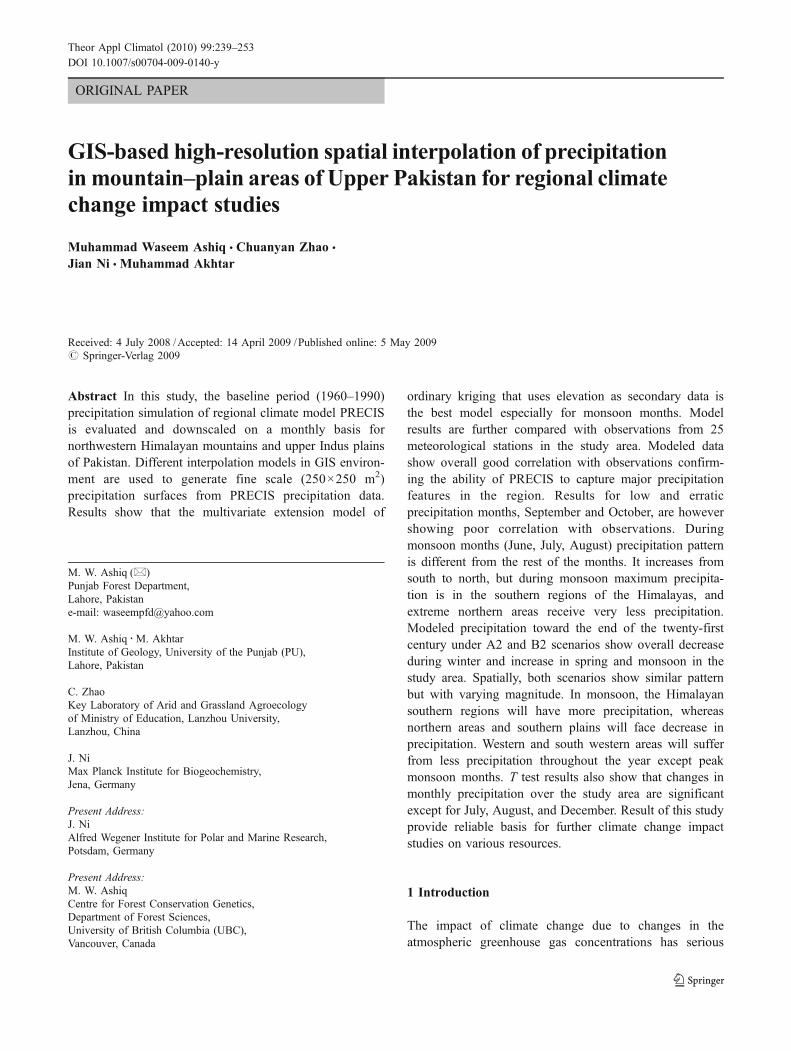
Situated between 69°20′–75°28′ E and 27°52′–35°42′ N,the landscape of the study area characterizes great diversityfrom biodiversity-rich Himalayan mountains in the north toflat agricultural plains of mighty Indus river system in thesouth. Elevation ranges from 61 to 6,126 m above sea level.In addition to hydrological functions and agriculturalproduction, the area also plays important roles of ecological,social, and protective nature.

It is also one of the most populated areas in the regionand administratively consists of Punjab Province, part ofNorth Western Frontier Province (NWFP) and Azad Jammuand Kashmir (AJK) valley in Pakistan (Fig. 1).

240 M. W. Ashiq et al.

3 Data and methods

Two sets of precipitation data (modeled and observational)are used in this study. Modeled precipitation data for thestudy area is obtained from a PRECIS run by Akhtar et al.(2008). PRECIS is a high-resolution atmospheric and landsurface model that is forced at its lateral boundaries by thesimulations of high-resolution (150 km×150 km) atmo-spheric component (HadAM3P atmosphere only GCM) ofthe HadCM3 coupled GCM model. For the baseline period(1961–1990), climate HadAM3P is driven with the ob-served sea surface temperature, and for future scenarios(2071–2100) sea surface temperature conditions are con-structed by adding anomalies from a transient simulation ofHadCM3 to observations (Gordon et al. 2000; Jones et al.2003; Wilson et al. 2005). The atmospheric dynamicsmodule of PRECIS is a hydrostatic version of the fullprimitive equations and uses horizontal and verticalcoordinates. There are 19 vertical levels, the lowest at825 hPa and the highest at 0.5 hPa. To control theaccumulation of noise and energy at the grid scale,horizontal diffusion is also applied. The land surface

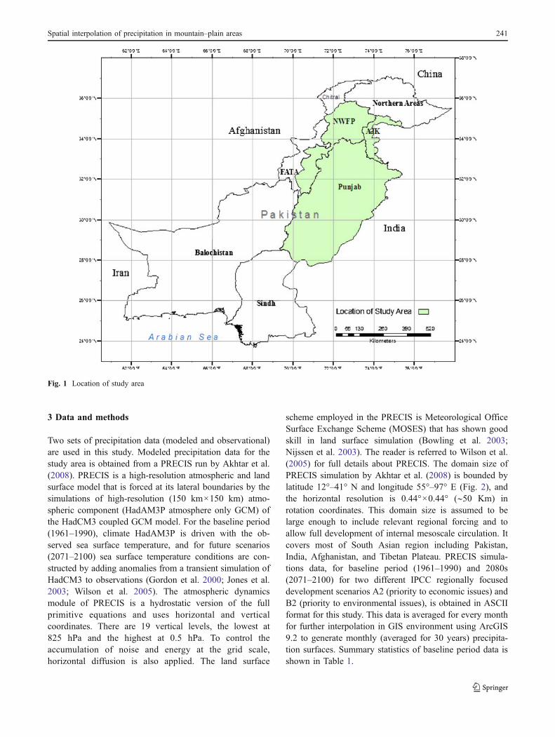
scheme employed in the PRECIS is Meteorological OfficeSurface Exchange Scheme (MOSES) that has shown goodskill in land surface simulation (Bowling et al. 2003;Nijssen et al. 2003). The reader is referred to Wilson et al.(2005) for full details about PRECIS. The domain size ofPRECIS simulation by Akhtar et al. (2008) is bounded bylatitude 12°–41° N and longitude 55°–97° E (Fig. 2), andthe horizontal resolution is 0.44°×0.44° (∼50 Km) inrotation coordinates. This domain size is assumed to belarge enough to include relevant regional forcing and toallow full development of internal mesoscale circulation. Itcovers most of South Asian region including Pakistan,India, Afghanistan, and Tibetan Plateau. PRECIS simula-tions data, for baseline period (1961–1990) and 2080s(2071–2100) for two different IPCC regionally focuseddevelopment scenarios A2 (priority to economic issues) andB2 (priority to environmental issues), is obtained in ASCIIformat for this study. This data is averaged for every monthfor further interpolation in GIS environment using ArcGIS9.2 to generate monthly (averaged for 30 years) precipita-tion surfaces. Summary statistics of baseline period data isshown in Table 1.

Fig. 1 Location of study area

Spatial interpolation of precipitation in mountain–plain areas 241

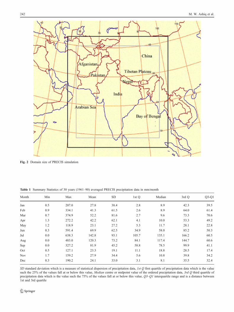
Table 1 Summary Statistics of 30 years (1961–90) averaged PRECIS precipitation data in mm/month

Month Min Max Mean SD 1st Q Median 3rd Q Q3-Q1

Jan 0.5 207.0 27.8 38.4 2.8 8.9 42.3 39.5

Feb 0.9 334.1 41.3 61.5 2.6 8.9 64.0 61.4

Mar 0.7 374.9 52.2 81.6 2.7 9.6 73.3 70.6

Apr 1.3 272.2 42.2 62.1 4.1 10.0 53.3 49.2

May 1.2 118.9 23.1 27.2 5.3 11.7 28.1 22.8

Jun 0.3 591.4 69.9 62.5 34.9 58.0 85.2 50.3

Jul 0.0 638.3 142.8 93.1 105.7 135.1 166.2 60.5

Aug 0.0 483.0 120.3 73.2 84.1 117.4 144.7 60.6

Sep 0.0 327.2 81.9 45.2 58.8 78.5 99.9 41.1

Oct 0.5 127.1 23.3 19.1 11.1 18.8 28.5 17.4

Nov 1.7 159.2 27.9 34.4 5.6 10.8 39.8 34.2

Dec 0.3 190.2 24.1 33.0 3.1 8.1 35.5 32.4

SD standard deviation which is a measure of statistical dispersion of precipitation data, 1st Q first quartile of precipitation data which is the valuesuch the 25% of the values fall at or below this value, Median centre or midpoint value of the ordered precipitation data, 3rd Q third quartile ofprecipitation data which is the value such the 75% of the values fall at or below this value, Q3–Q1 interquartile range and is a distance between1st and 3rd quartile

Fig. 2 Domain size of PRECIS simulation


Observational precipitation data is used to validate theresults of the modeled data interpolation for baselineperiod. For this purpose, total monthly precipitation dataof 25 Meteorological stations of Pakistan MeteorologicalDepartment is used. Location of observational stations isshown in Fig. 3. Out of these, data for 21 stations is

available for the entire baseline period (1961–90), whereasrecords of precipitation for four stations, namely, Dir, SaduSharif, Rafiqui, and Bhawalnagar are available for shorterperiods (Table 2). These stations are included to increasethe coverage of the validation data points. Monthly data isaveraged for the baseline/available period, and the basic

Fig. 3 Topography (DEM) of the study area and location of observational stations


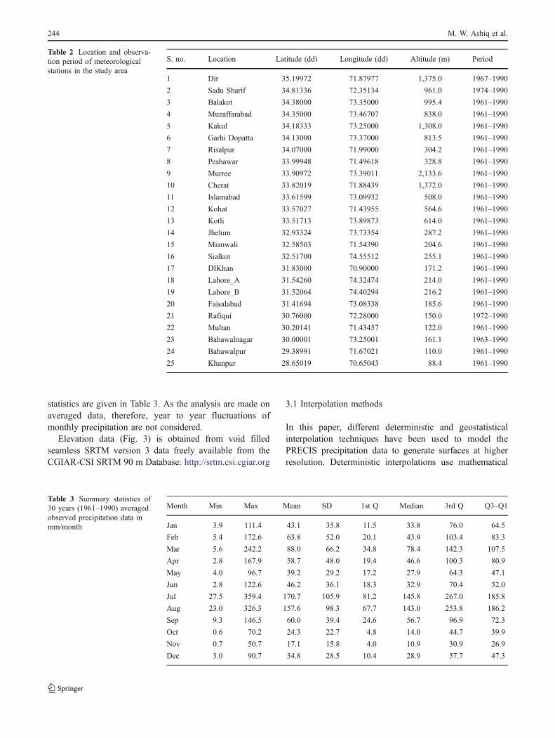
statistics are given in Table 3. As the analysis are made onaveraged data, therefore, year to year fluctuations ofmonthly precipitation are not considered.

Elevation data (Fig. 3) is obtained from void filledseamless SRTM version 3 data freely available from theCGIAR-CSI SRTM 90 m Database: http://srtm.csi.cgiar.org

3.1 Interpolation methods

In this paper, different deterministic and geostatisticalinterpolation techniques have been used to model thePRECIS precipitation data to generate surfaces at higherresolution. Deterministic interpolations use mathematical

Month Min Max Mean SD 1st Q Median 3rd Q Q3–Q1

Jan 3.9 111.4 43.1 35.8 11.5 33.8 76.0 64.5

Feb 5.4 172.6 63.8 52.0 20.1 43.9 103.4 83.3

Mar 5.6 242.2 88.0 66.2 34.8 78.4 142.3 107.5

Apr 2.8 167.9 58.7 48.0 19.4 46.6 100.3 80.9

May 4.0 96.7 39.2 29.2 17.2 27.9 64.3 47.1

Jun 2.8 122.6 46.2 36.1 18.3 32.9 70.4 52.0

Jul 27.5 359.4 170.7 105.9 81.2 145.8 267.0 185.8

Aug 23.0 326.3 157.6 98.3 67.7 143.0 253.8 186.2

Sep 9.3 146.5 60.0 39.4 24.6 56.7 96.9 72.3

Oct 0.6 70.2 24.3 22.7 4.8 14.0 44.7 39.9

Nov 0.7 50.7 17.1 15.8 4.0 10.9 30.9 26.9

Dec 3.0 90.7 34.8 28.5 10.4 28.9 57.7 47.3

Table 3 Summary statistics of30 years (1961–1990) averagedobserved precipitation data inmm/month

S. no. Location Latitude (dd) Longitude (dd) Altitude (m) Period

1 Dir 35.19972 71.87977 1,375.0 1967–1990

2 Sadu Sharif 34.81336 72.35134 961.0 1974–1990

3 Balakot 34.38000 73.35000 995.4 1961–1990

4 Muzaffarabad 34.35000 73.46707 838.0 1961–1990

5 Kakul 34.18333 73.25000 1,308.0 1961–1990

6 Garhi Dopatta 34.13000 73.37000 813.5 1961–1990

7 Risalpur 34.07000 71.99000 304.2 1961–1990

8 Peshawar 33.99948 71.49618 328.8 1961–1990

9 Murree 33.90972 73.39011 2,133.6 1961–1990

10 Cherat 33.82019 71.88439 1,372.0 1961–1990

11 Islamabad 33.61599 73.09932 508.0 1961–1990

12 Kohat 33.57027 71.43955 564.6 1961–1990

13 Kotli 33.51713 73.89873 614.0 1961–1990

14 Jhelum 32.93324 73.73354 287.2 1961–1990

15 Mianwali 32.58503 71.54390 204.6 1961–1990

16 Sialkot 32.51700 74.55512 255.1 1961–1990

17 DIKhan 31.83000 70.90000 171.2 1961–1990

18 Lahore_A 31.54260 74.32474 214.0 1961–1990

19 Lahore_B 31.52064 74.40294 216.2 1961–1990

20 Faisalabad 31.41694 73.08338 185.6 1961–1990

21 Rafiqui 30.76000 72.28000 150.0 1972–1990

22 Multan 30.20141 71.43457 122.0 1961–1990

23 Bahawalnagar 30.00001 73.25001 161.1 1963–1990

24 Bahawalpur 29.38991 71.67021 110.0 1961–1990

25 Khanpur 28.65019 70.65043 88.4 1961–1990

Table 2 Location and observa-tion period of meteorologicalstations in the study area


http://srtm.csi.cgiar.org

functions to generate surfaces from the measured points,based on either the extent of similarity or the degree ofsmoothing (Johnston et al. 2001). Among various deter-ministic interpolation techniques, inverse distance weight-ed, local polynomial interpolation, and radial basisfunctions are used to generate models. These techniquesare well described in literature (Hardy 1971; Bouhamidi2001; Johnston et al. 2001; Hofierka et al. 2002; Lloyd2005; Zhao et al. 2005; Sarra 2006).

Geostatistic interpolations are based on the theory ofregionalized variables and rely on both statistical andmathematical functions. These use a variogram model todescribe the spatial continuity of the input data to estimatevalues at unsampled locations. From this group, ordinarykriging and its multivariate extension ordinary cokrigingare used to generate models. Ordinary kriging depends onmodels of spatial autocorrelation formulated in terms of

covariance or semivariogram functions. The main charac-teristics of these models are sill, range, and nugget. Sillrepresents the total variation in the data, and range is thedistance where autocorrelation vanishes. Nugget effectrefers to the situation when sampling locations are closeto each other but difference between measurements is notzero. This occurs in semivariogram/covariance model dueto either measurement errors or variations at scales too fineto detect. The reader is referred to Isaaks and Srivastava(1989) and Clark and Harper (2000) for basic theory andmodeling details. Among various variogram models, onlythree (spherical, exponential, and rational quadratic) modelswith the nugget effect are used in this study. Elevation datais used as secondary data (Goovaerts 2000) in ordinaryCokriging models. Models with nugget effect that providethe optimal fit to the semivariance points are selected forfurther evaluation with observational data.

Month Deterministic models Geostatistical models

IDW LPI RBF_swt RBF_mq OK_sph OK_exp OK_rqd

Jan 15.83 15.34 15.27 15.31 15.62 15.68 15.54

Feb 24.97 24.22 24.12 24.18 24.68 24.79 24.54

Mar 31.86 30.96 30.84 30.86 31.24 31.35 31.11

Apr 24.08 24.06 23.92 23.92 23.92 23.94 23.88

May 11.25 11.23 11.03 11.45 11.49 11.48 11.44

Jun 36.68 35.91 35.62 36.15 35.41 35.89 35.31

Jul 53.54 53.75 53.32 54.4 53.38 53.68 53.29

Aug 40.45 40.65 40.37 41.18 40.41 40.46 40.41

Sep 23.74 23.58 23.53 23.55 23.51 23.47 23.45

Oct 7.84 7.97 7.91 7.81 7.89 7.92 7.88

Nov 14.45 14.27 14.26 14.27 14.37 14.47 14.32

Dec 14.41 14.00 14.00 14.04 14.26 14.39 14.16

Table 4 Comparison ofcross-validated root meansquare prediction errors(RMSE) in mm/month

0.0

20.0

40.0

60.0

80.0

100.0

120.0

140.0

160.0

180.0

Months

Pre

cip

itat

ion

Mea

n (

mm

)

Station

PRECIS

0.0

20.0

40.0

60.0

80.0

100.0

120.0

Months

Pre

cip

itat

ion

St

Dev

(m

m)

321 4 5 6 7 8 9 10 11 12 2 3 4 5 6 7 8 9 10 11 121

a bStation

PRECIS

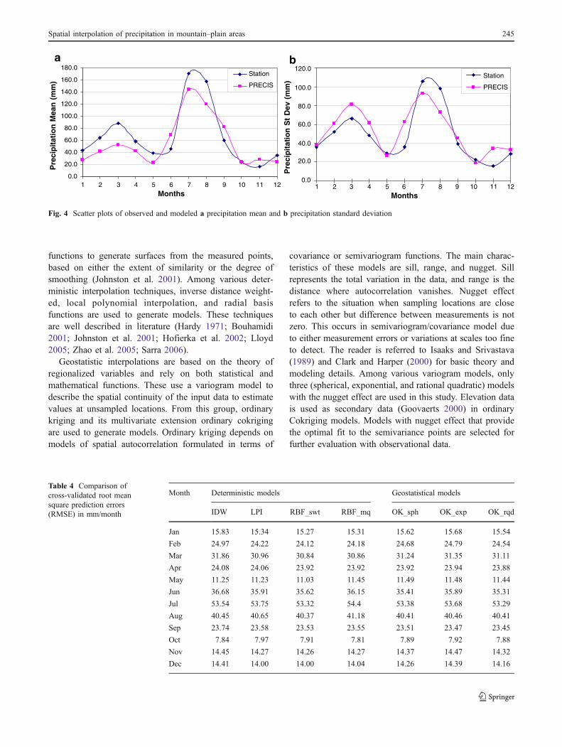
Fig. 4 Scatter plots of observed and modeled a precipitation mean and b precipitation standard deviation


4 Results and discussions

4.1 Quality checking of RCM output

To check the suitability of the PRECIS simulation outputfor further interpolation and generation of precipitationsurfaces for the study area, station data and PRECIS outputare compared (Fig. 4a, b) for mean value and standarddeviation derived from the mean monthly precipitation ofbaseline period. Results show overall good agreement. Patternof mean precipitation for both data sets is similar duringdifferent months except for November and December, and thesame is the case with SD. PRECIS overpredicted the meanprecipitation during June, September, and November. Themaximum difference is during March, whereas minimal isnoted for the month of October. Standard deviation ofPRECIS data is higher compared to the station data exceptfor the months May, July, August, and October. June is themonth with highest difference, whereas May has leastdifference.

4.2 Interpolation of PRECIS data

Initially, seven interpolation models in ArcGIS 9.2 havebeen used to generate the monthly precipitation surfaces

from the PRECIS baseline data. Out of these four models,namely, inverse distance weighted (IDW), local polynomialinterpolation (LPI), spline with tension radial basic function(RBF_swt), and multiquadric radial basic function(RBF_mq) belong to the deterministic models, whereasthe remaining three models, namely, OK_sph (OrdinaryKriging with Spherical variogram), OK_exp (OrdinaryKriging with Exponential variogram) and OK_rqd (Ordi-nary Kriging with Rational Quadratic variogram) aregeostatistical models. Interpolation model results are com-pared on the basis of cross-validated root mean squarederror (RMSE) of interpolated data. Cross-validated RMSEis the square root of the average of squared differencesbetween the measured and predicted values. This isobtained from calculations repeated for total number ofdata points’ time, while omitting one different data pointevery time (Wilks 2008). Results are tabulated in Table 4.

Since deterministic and geostatistical modeling are basedon different concepts, therefore, both model sets areevaluated separately for their interpolation performance.Overall, the performance of all the models is comparable.However, the best results in the form of least RMSE arefrom OK_rqd in geostatistical models and from RBF_swtmodel with exception of the month of October indeterministic models. Interpolation of October is better

Table 5 Cross-validated root mean square prediction errors (RMSE) in mm/month of monthly surfaces of precipitation generated by OCK_rqdand OK_rqd models

Model Jan Feb Mar Apr May Jun Jul Aug Sep Oct Nov Dec

OCK_rqd 15.49 24.29 30.61 22.91 10.85 36.49 54.98 41.33 24.17 8.02 13.97 13.98

OK_rqd 15.54 24.54 31.11 23.88 11.44 35.31 53.29 40.41 23.45 7.88 14.32 14.16

0.00

0.10

0.20

0.30

0.40

0.50

0.60

0.70

0.80

0.90

1.00

Jan Feb Mar Apr May Jun Jul Aug Sep Oct Nov Dec

Months

r2 v

alu

e

RBF_swt Model

OK_rqd Model

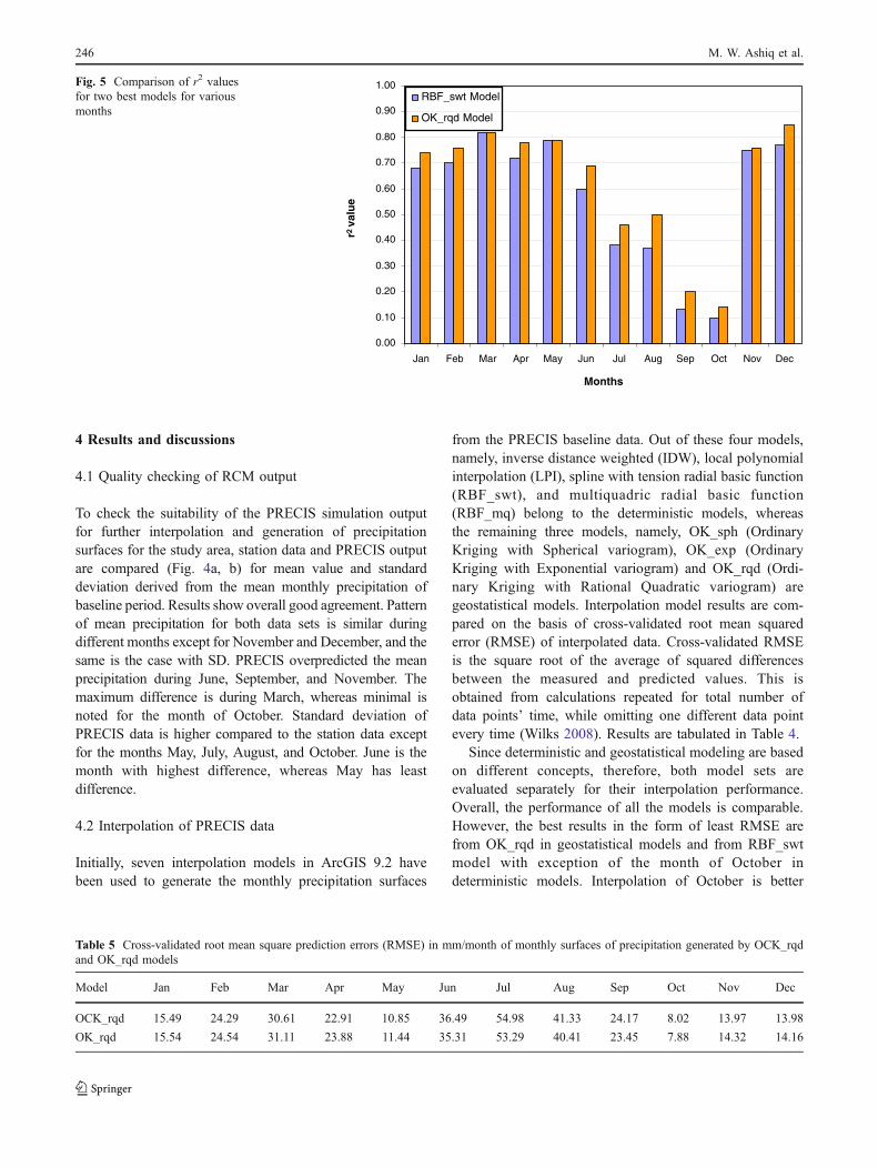
Fig. 5 Comparison of r2 valuesfor two best models for variousmonths


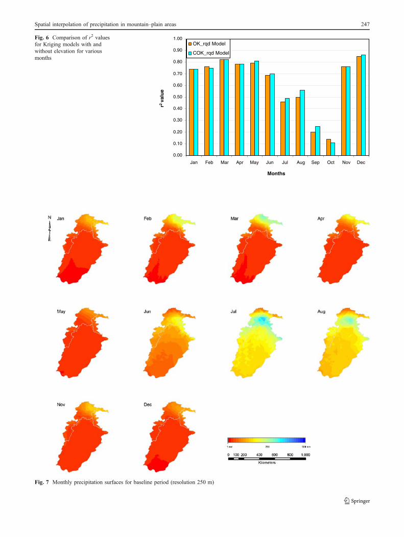
Fig. 7 Monthly precipitation surfaces for baseline period (resolution 250 m)

0.00

0.10

0.20

0.30

0.40

0.50

0.60

0.70

0.80

0.90

1.00

Jan Feb Mar Apr May Jun Jul Aug Sep Oct Nov Dec

Months

r2 val

ue

OK_rqd Model

COK_rqd Model

Fig. 6 Comparison of r2 valuesfor Kriging models with andwithout elevation for variousmonths


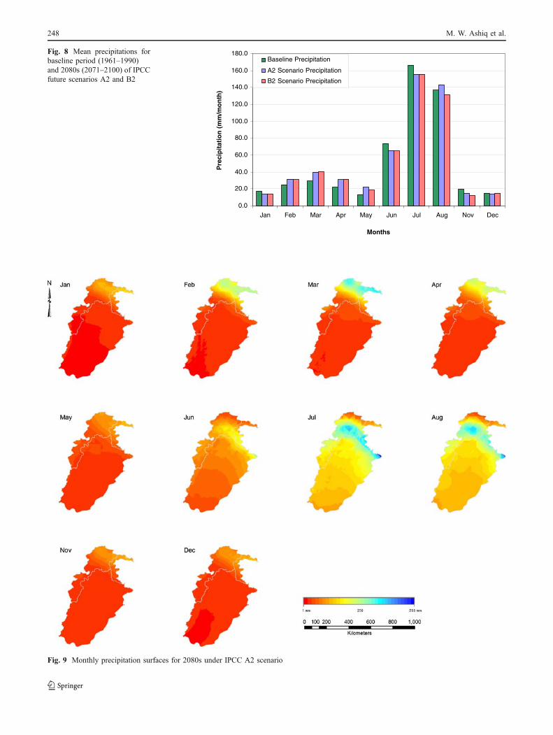
Fig. 9 Monthly precipitation surfaces for 2080s under IPCC A2 scenario

0.0

20.0

40.0

60.0

80.0

100.0

120.0

140.0

160.0

180.0

Jan Feb Mar Apr May Jun Jul Aug Nov Dec

Months

Pre

cip

itat

ion

(m

m/m

on

th)

Baseline Precipitation

A2 Scenario Precipitation

B2 Scenario Precipitation

Fig. 8 Mean precipitations forbaseline period (1961–1990)and 2080s (2071–2100) of IPCCfuture scenarios A2 and B2


achieved by RBF_mq instead of RBF_swt. This may beattributed to the distribution of data with least standarddeviation and minimal difference of third and first quartileamong all the months as shown in Table 1. Best modelresults for monthly surfaces in both model types are thenfurther compared for their performance with validation(observational) data. Modeled mean precipitation values forthe location of the climatic stations are compared with therecorded mean precipitation and evaluated with the coeffi-cient of determination (r2). Results presented in Fig. 5 showthat the r2 values of OK_rqd (geostatistical model)interpolated surfaces are better than the RBF_swt (deter-ministic model) for all months which is in accordance withthe results of Goovaerts (2000) who also found betterperformance of geostatistical models for spatial prediction ofprecipitation. The results for the months from July to Octoberare comparatively poor. Out of these, July and August are themonsoon months with maximum rainfall as shown in Table 3.

r2 values for these months are 0.46 and 0.50, respectively.The performance is worst for the months September andOctober with r2 values 0.20 and 0.14, respectively.

To further investigate the influence of elevation on thespatial and temporal distribution of precipitation, anothermodel OCK_rqd (Ordinary Cokriging with Rationale Qua-dratic variogram) is applied. In this method, the elevationdata from the SRTM is used as secondary variable togenerate the monthly surfaces. Selection of final monthlysurfaces is based on the same criteria of least cross-validatedRMSE values. RMSE values are presented in Table 5.

Months from January to May, November and Decembershow decrease in RMSE whereas months from June toOctober show increase in RMSE. This increased RMSE forthe months June to October is due to weak correlation ofPRECIS simulated data with the elevation (r2 values 0,0.08, 0.08, 0.05, and 0.09, respectively). When validated,these monthly interpolated surfaces with the observational

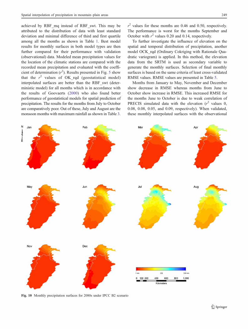
Fig. 10 Monthly precipitation surfaces for 2080s under IPCC B2 scenario


station data, r2 values for the months June to Septemberimproved because observational data has reasonable corre-lation with elevation (r2 values 0.44, 0.25, 0.32, and 0.43,respectively). Figure 6 shows the increase in r2 values from0.69 to 0.70, 0.46 to 0.49, 0.50 to 0.56, and 0.20 to 0.25 forthe months of June, July, August, and September, respec-tively, when compared with OK_rqd model. For the rest ofthe months, there is no significant change in r2 valuesexcept for the month of October where it drops to 0.11.Improvement in the results for the monsoon months withthe inclusion of elevation data confirms that elevation is animportant factor in the distribution of rainfall during thisseason. This is also in accordance with the results of somestudies carried out in different parts of the world (Phillips etal. 1992; Goovaerts 2000; Agnew and Palutikof 2000) thatelevation is a strong determinant of climate. The leastcorrelation of the interpolated precipitation with theobservations is during the month of October. Detailed

investigation of the data reflects that traces of precipitationwith high frequency are reported by the PRECIS, andperhaps, such small quantities are not recorded as signifi-cant precipitation at the observational stations. This resultedinto weak correlation between both data sets. Poorperformance of interpolation methods for the month ofSeptember can again be attributed to the limitation of thePRECIS to capture the precipitation pattern.

4.3 High-resolution baseline precipitation

Monthly precipitation surfaces for the baseline periodexcept for September and October at a resolution of250 m generated by OCK_rqd geostatistical interpolationmethod are presented in Fig. 7. Spatial pattern of precipi-tation is similar for the winter (November, December, andJanuary) and spring (February, March, April, and May). It islowest in the southern parts and increases as we move toward

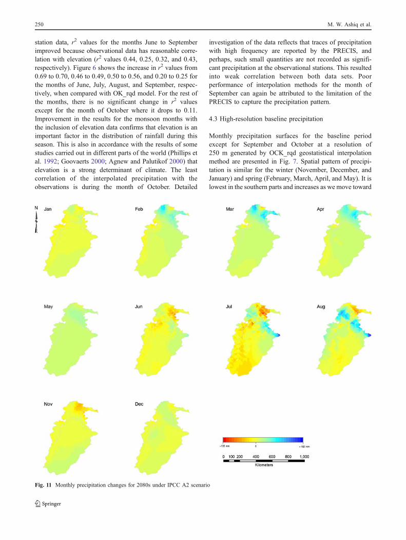
Fig. 11 Monthly precipitation changes for 2080s under IPCC A2 scenario


northern areas with the increasing altitude. In contrary,monsoon months (June, July, and August) present a differentpattern of precipitation increasing from south toward north,but maximum in southern Himalayan region, and to furthernorth it decreases with the least precipitation in extremenorth. This is because of the reason that HimalayanMountains serve as barriers to the monsoon winds comingfrom the south and yield maximum rainfall in southernranges of Himalayas. Northern areas receive precipitationfrom western cyclonic disturbances originating in theMediterranean.

4.4 High-resolution climate change scenario precipitation

Amajor caveat in any estimation of climate change is the factthat parameters for modeling are fitted to the current climaticconditions but are not known to remain valid under changedclimate. However, it is assumed that if the estimates of a

modeling adequately represent the current climate, we canuse its climate change estimates with confidence. Based onthis assumption, precipitation data of PRECIS for climatechange scenarios A2 and B2 for the period 2080 s (2071–2100) is interpolated using the model OCK_rqd to generatesurfaces. September and October months are excludedbecause of their poor results for baseline period. Resultsare presented in Fig. 8. These indicate decrease inprecipitation during winter, increase in spring and mon-soon. For August, A2 scenario shows increase in precipi-tation, whereas B2 scenario shows decrease.

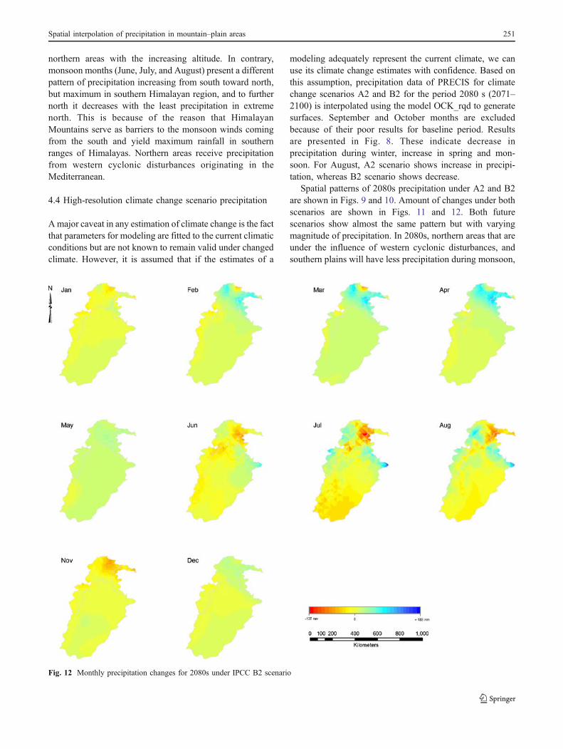
Spatial patterns of 2080s precipitation under A2 and B2are shown in Figs. 9 and 10. Amount of changes under bothscenarios are shown in Figs. 11 and 12. Both futurescenarios show almost the same pattern but with varyingmagnitude of precipitation. In 2080s, northern areas that areunder the influence of western cyclonic disturbances, andsouthern plains will have less precipitation during monsoon,

Fig. 12 Monthly precipitation changes for 2080s under IPCC B2 scenario


whereas Himalayan southern regions will have moreprecipitation. Overall western and southwestern areas willreceive less precipitation throughout the year except for peakmonsoon months.

Further, results of t test at 95% confidence interval showthat changes in precipitation over the study area aresignificant for all months except July, August, andDecember. P values for these months are 0.170, 0.450,0.494 (under A2 scenario) and 0.140, 0.248, 0.131 (underB2 scenario), respectively.

5 Conclusion

Among important climatic variables, precipitation is difficultto represent due to high inherent variability in its spatial andtemporal patterns. It is even more difficult in the study area inwhich different mechanisms are responsible for its occurrence.In this paper, PRECIS-RCM-generated precipitation surfacesare evaluated with the observational data and furtherdownscaled for more detailed regional information(250 m×250 m) to further conduct climate change impactassessments in various sectors. Although the results haveassociated uncertainties, these provide good evidence that(1) PRECIS capture pattern of current precipitation for mostof months; (2) the usefulness of GIS-based interpolationtechnique (Ordinary Cokriging) for the fine-scale spatialinterpolation precipitation; and (3) patterns of precipitationvary temporally and spatially significantly at small scale.

It is also noted that the systematic errors of RCM or drivingGCM cannot be improved by the interpolation techniquesused. This is the case with the months of September andOctober precipitation that need to be improved in RCMsimulations for the study area. This methodology can also beapplied for the fine-scale spatial distribution of other climaticvariables such as temperature in the study area.

Acknowledgement The present study is a part of the researchfunded by Higher Education Commission of Pakistan (PIN no. 041221461B-057) and also supported by National Natural ScienceFoundation of China (nos. 40671067 and 30770387). Authors arethankful to Nasir Ahmed (PU), Sally Aitken (UBC) and Tongli Wang(UBC) to facilitate this research and improve the manuscript. Thanksare also due to Pakistan Meteorological Department and CGIAR-Consortium for Spatial Information for making the data available forthis study. We also gratefully acknowledge the anonymous reviewersfor critical reviews of the manuscript.

References

Agnew MD, Palutikof JP (2000) GIS based construction of baselineclimatologies for the Mediterranean using terrain variables. ClimRes 14:115–127

Akhtar M, Ahmad N, Booij MJ (2008) Use of regional climate modelsimulations as input for hydrological models for the Hindukush–Karakorum–Himalaya region. Hydrology and Earth SystemSciences Discussions 5:865–902

Bouhamidi A (2001) Hilbertian approach for univariate spline withtension. Approx Theory its Appl 17(4):36–57

Bowling LC, Lettenmaier DP, Nijssen B, Graham LP, Clark DB,Maayar ME, Essery R, Goers S, Habets F, Bvd H, Jin J, KahanD, Lohmann D, Mahanama S, Mocko D, Nasonova O,Samuelsson P, Shmakin AB, Takata K, Verseghy D, Viterbo P,Xia Y, Ma X, Xue Y, Yang ZL (2003) Simulation of high latitudehydrological processes in the Torne–Kalix basin: PILPS Phase 2(e): 1. Experiment description and summary intercomparisons.Glob Planet Change 38(1–2):1–30

Brunsdon C, McClatchey J, Unwin DJ (2001) Spatial variations in theaverage rainfall–altitude relationship in Great Britain: an approachusing geographically weighted regression. Int J Climatol 21:455–466

Busuioc A, Chen D, Hellström C (2001) Performance of statisticaldownscaling models in GCM validation and regional climatechange estimates: application for Swedish precipitation. Int JClimatol 21:557–578

Charles SP, Bates BC, Whetton PH, Hughes JP (1999) Validation ofdownscaling models for changed climate conditions: case studyof southwestern Australia. Clim Res 12:1–14

Ciret C, Sellers AH (1998) Sensitivity of ecosystem models to thespatial resolution of the NCAR Community Climate ModelCCM2. Clim Dyn 14:409–429

Clark I, Harper WV (2000) Practical geostatistics 2000. Ecosse NorthAmerica Llc, Columbus, OH

Dirks KN, Hay JE, Stow CD, Harris D (1998) High-resolution studiesof rainfall on Norfolk Island Part II: interpolation of rainfall data.J Hydrol 208(3–4):187–193

Fuentes U, Heimann D (2000) An improved statistical-dynamicaldownscaling scheme and its application to the alpine precipita-tion climatology. Theor Appl Climatol 65:119–135

Gaffin S, Xing X, Yetman G (2004) Downscaling and geo-spatialgridding of socio-economic projections from the IPCC SpecialReport on Emissions Scenarios (SRES). Glob Environ Change14(2):105–123

Giorgi F (1990) Simulation of regional climate using a limited areamodel nested in a general circulation model. J Clim 3:941–963

Giorgi F, Mearns L (1991) Approaches to the simulation of regionalclimate change: a review. Review of Geophysics 29:191–216

Goovaerts P (2000) Geostatistical approaches for incorporating elevationinto the spatial interpolation of rainfall. J Hydrol 228:113–129

Gordon CC, Cooper C, Senior CA, Banks H, Gregory JM, MitchellJFB, Wood RA (2000) The simulation of SST, sea ice extents andocean heat transport in a version of the Hadley centre coupledmodel without flux adjustment. Clim Dyn 16(2–3):1147–1168

Grotch SL, MacCracken MC (1991) The use of general circulationmodels to predict regional climate change. J Clim 4:286–303

Hardy RL (1971) Multiquadratic equations of topography and otherirregular surfaces. J Geophys Res 76(8):1905–1915

Hellström C, Chen D (2003) Statistical downscaling based ondynamically downscaled predictors: application to monthlyprecipitation in Sweden. Adv Atmos Sci 20(6):951–958

Hofierka J, Parajka J, Mitasova H, Mitas L (2002) Multivariateinterpolation of precipitation using regularized spline withtension. Trans GIS 6(2):135–150

Isaaks EH, Srivastava RM (1989) An introduction to appliedgeostatistics. Oxford University Press, New York

Johnston K, VerHoef JM, Krivoruchko K, Lucas N (2001) Using ArcGISGeostatistical Analyst- GIS by ESRI, United States of America

Jones TC, Gregory JM, Ingram WJ, Johnson CE, Jones A, Lowe JA,Mithcell JFB, Roberts DL, Sexton DMH, Stevenson DS, Tett


SFB, Woodage MJ (2003) Anthropogenic climate change for1860–2100 simulated with the HadCM3 model under updatedemissions scenarios. Clim Dyn 20:583–612

Karl TR, Wang WC, Schlesinger ME, Knight RW, Portman D (1990)A method of relating general circulation model simulated climateto observed local climate. Part I: Seasonal statistics. J Climate3:1053–1079

Li X, Sailor D (2000) Application of tree structured regression forregional precipitation prediction using general circulation modeloutput. Clim Res 16:17–30

Linderson ML, Achberger C, Chen D (2004) Statistical downscalingand scenario construction of precipitation in Scania, southernSweden. Nord Hydrol 35(3):261–287

Lloyd CD (2005) Assessing the effect of integrating elevation datainto the estimation of monthly precipitation in Great Britain. JHydrol 308B:128–150

Murphy J (1999) An evaluation of statistical and dynamical techniquesfor downscaling local climate. J Clim 12(8):2256–2284

Nijssen B, Bowling LC, Lettenmaier DP, Clark DB, Maayar ME,Essery R, Goers S, Gusev YM, Habets F, Hurk BVD, Jin J,Kahan D, Lohmann D, Ma X, Mahanama S, Mocko D,Nasonova O, Niu GY, Samuelsson P, Shmakin AB, Takata K,Verseghy D, Viterbo P, Xia Y, Xue Y, Yang ZL (2003)Simulation of high latitude hydrological processes in theTorne–Kalix basin: PILPS Phase 2(e): 2: Comparison of modelresults with observations. Global Planet Change 38(1–2):31–53

Phillips DL, Dolph J, Marks D (1992) A comparison of geostatisticalprocedures for spatial analysis of precipitation in mountainousterrain. Agriculture and Forest Meteorology 58:119–141

Price DT, McKenney DW, Nalder IA, HutchinsonMF, Kesteven JL (2000)A comparison of two statistical methods for spatial interpolation ofCanadian monthly mean climate data. Agric For Meteorol 101:81–94

Sarra SA (2006) Integrated multiquadric radial basis functionapproximation methods. ComputMath Appl 51(8):1283–1296

Tabios GQ, Salas JD (1985) A comparative analysis of techniques forspatial interpolation of precipitation. Water Resource Bulletin 21(3):365–380

Thiessen AH (1911) Precipitation averages for large areas. MonWeather Rev 39(7):1082–1084

vanVuuren DP, Lucas PL, Hilderink H (2007) Downscaling drivers ofglobal environmental change: Enabling use of global SRESscenarios at the national and grid levels. Glob Environ Change17:114–130

vonStorch H (1999) The global and regional climate system. In:vonStorch H, Flöser G (eds) Anthropogenic climate change.Springer Verlag, Berlin, pp 3–36

vonStorch H, Zorita E, Cubash U (1993) Downscaling of globalclimate change estimates to regional scales: an application toIberian rainfall in wintertime. J Clim 6:1161–1671

Wilks DS (2008) High-resolution spatial interpolation of weathergenerator parameters using local weighted regressions. Agric ForMeteorol 148:111–120

Wilson S, Hassell D, Hein D, Jones R, Taylor R (2005) Installingand using the Hadley Centre regional climate modellingsystem, PRECIS (version 1.4), Met Office Hadley Centre,Exeter, UK

Xu CY (1999) From GCMs to river flow: a review of downscalingmethods and hydrologic modelling approaches. Prog Phys Geogr23(2):229–249

Yarnal B, Comrie CC, Frakes B, Brown P (2001) Developmentsand prospects in synoptic climatology. Int J Climatol 21:1923–1950

Zhao C, Nan Z, Cheng G (2005) Methods for modelling of temporaland spatial distribution of air temperature at landscape scale insouthern Qilian mountains, China. Ecolo Model 189:209–220

Zorita E, vonStorch H (1999) The analog method as a simplestatistical downscaling technique: comparison with more com-plicated methods. J Clim 12(8):2474–2489
