Download - Dispersion due to wall interactions in microfluidic separation systems

Dispersion due to wall interactions in microfluidic separation systemsSubhra Dattaa and Sandip GhosalDepartment of Mechanical Engineering, Northwestern University,2145 Sheridan Road, Evanston, Illinois 60208, USA

Received 4 June 2007; accepted 1 November 2007; published online 29 January 2008

The transport of a solute in a straight microchannel of axially variable cross-sectional shape in thepresence of an inhomogeneous flow field and an adsorption-desorption process on the wall isstudied, motivated by applications to capillary electrophoresis and open-channel capillaryelectrochromatography. An asymptotic approach based on the long time limit is adopted that reducesthe problem to the solution of a one-dimensional transport equation. The reduced model is integratednumerically to study the effects of inhomogeneous electro-osmotic flow and adsorption-desorptionkinetics on solute migration and dispersion in a rectangular microchannel. The accuracy of theasymptotic equations is checked by the direct numerical solution of the original three-dimensionaltransport problem. © 2008 American Institute of Physics. DOI: 10.1063/1.2828098

I. INTRODUCTION

The problem of transport of a solute that can interactwith channel walls is encountered very often in microfluidicchemical analysis techniques such as capillary electrophore-sis CE and open-channel capillary electrochromatographyCEC.1,2 In the latter, the interaction of a solute with a coat-ing bonded to the channel wall serves as the separationprinciple;3,4 in the former, it is often an undesirable effect.5–7

In both techniques, electro-osmotic flow EOF is commonlyemployed to transport both the solvent and the solute in themicrofluidic channels. The EOF is generated by externallyapplied electric fields that can act on the net charges presentnear a liquid-solid interface.8 In this paper, we study thetransport of a solute in inhomogeneous flows in the presenceof adsorption and desorption on the wall, motivated by ap-plications in CE and CEC under EOF.

The thickness of the diffuse charge layer at a liquid-solidinterface is characterized by the Debye length D, which isof the order of 1–10 nm for most solvents used in CE andCEC at room temperature.8 If the width of a channel is muchlarger than D and all properties are uniform, the EOF in thechannel is to a good approximation a “plug flow” or uniformflow.8 However, there are situations when the EOF is axiallyand radially inhomogeneous, for example, as a consequenceof the variation of zeta potential and microchannel crosssection,9 or due to finite Debye layer effects.10 While an inertsolute in a uniform “plug” flow spreads solely on account ofmolecular diffusion, the presence of inhomogeneities in theflow leads to enhanced spreading of solute bands by theTaylor-Aris dispersion mechanism.11,12 The effective diffu-sivity is inversely proportional to the molecular diffusivity ofthe solute in the analysis medium, and, for pressure-drivenflow, is more significant at higher flow rates.11 The analysisin this article is motivated by the problem of solute transportunder nonideal electro-osmosis conditions in microfluidicdevices.13 However, it is more general in scope as it canaccount for any axially variable flow and cross-sectionalshape changes,14,15 provided they take place on a slow timeand spatial scale in the axial direction.

Owing to the large surface to volume ratio of microflu-idic channels, solute adsorption and desorption on channelwalls is often a source of undesirable consequences like lossof sample16,17 and loss of resolution2 in techniques like CEand CEC. Specific studies relevant to modeling band broad-ening in CEC include Ref. 4 and Refs. 18–21. For studiesrelevant to CE, see e.g., Refs. 7 and 22, the reviews Ref. 9and Ref. 23, and the references therein. When both adsorp-tion and desorption are fast enough compared to the analysistime, the wall interactions can be characterized by the theoryof chromatography.24–26 Wall retention in chromatographictechniques, besides serving as the principle of separation25 isalso in itself a source of enhanced dispersion.24,27 Dispersiondue to retention and Taylor-Aris dispersion are coupled to-gether in most modes of chromatography that employ inho-mogeneous flow e.g., gas chromatography28 GC and liquidchromatography29 LC.

We provide here a generalized treatment of an arbitrarywall reaction kinetic function. Unlike most theories ofchromatography,25 the analysis does not require that the de-partures from a state of “chemical equilibrium” to be small.Consequently, it can be used to study dispersion at muchshorter times from the start of chemical analysis than avail-able chromatography theories and is also applicable forslower and nearly irreversible adsorption processes encoun-tered in proteomic applications of CE.16,30 In the special caseof fast linear kinetics, the analysis reaffirms known resultsfrom the theory of chromatography25 and can also predictchromatographic dispersion in complex microfluidic cross-sectional shapes like rectangle and trapezoid under variousflow conditions, such as, electrokinetic flow with finiteDebye layers,31 pressure-driven flow,25 the shear flow usedto transport solutes in shear-driven chromatography,32

and electro-osmotic micropump driven circularchromatography.33 The analysis also resolves the three-dimensional distribution of the solute in the microchannel, afeature that is absent in analyses based on method ofmoments26 or its generalizations.34 There are previous worksthat provide asymptotic approximations for the concentration

PHYSICS OF FLUIDS 20, 012103 2008

1070-6631/2008/201/012103/14/$23.00 © 2008 American Institute of Physics20, 012103-1

http://dx.doi.org/10.1063/1.2828098

http://dx.doi.org/10.1063/1.2828098

field as well as area averaged concentration in a channel,35–37

but none of them treat simultaneously inhomogeneous flows,arbitrary cross sections, and arbitrary wall kinetics, like thepresent work.

Owing to the small width to length ratio of microchan-nels, direct numerical solution of the three-dimensionaltransport problem for the concentration c of the solute in themicrochannel is expensive and gives rise to a “stiffsystem.”38 We use an asymptotic theory to obtain a formula-tion that requires only the solution of one-dimensional partialdifferential equations for the area averaged concentration ofthe solute c. The concentration distribution c can be calcu-lated explicitly in terms of c and its spatial derivative in theaxial direction. Thus, complete information of the concentra-tion distribution in three dimensions may be obtained at onlya fraction of the computational cost involved in direct nu-merical simulation of the full transport problem.

The asymptotic theory presented in this paper general-izes the theoretical development in Ref. 7 which is appli-cable to axisymmetric cylindrical capillaries of constantcross section. In its present form, the analysis can account forarbitrary cross-sectional shapes and a slow axial variation incross section. The solution starting from arbitrary initial con-ditions is accurate, except possibly during a short transientphase of duration of the order of the cross-channel diffusiontime. As in Ref. 7 the form of the wall reaction kinetics is leftarbitrary, but unlike Ref. 7, transverse as well as axial varia-tion of unadsorbed and adsorbed solute on the wall is admit-ted. The requirement of “slow reactions” in Ref. 7 is relaxedthereby extending the applicability of the theory to chro-matographic techniques, in addition to CE.

Several specific examples of the asymptotic theory willbe discussed, all involving transport of the solute in rectan-gular microchannels.39,40 These problems will be studied si-multaneously with both three-dimensional direct numericalsimulation and the asymptotically reduced equations, in or-der to check the accuracy of the asymptotic approach.

In Sec. II, we develop the asymptotic theory for disper-sion in axially variable flows and geometries with arbitrarywall reaction kinetics. In Sec. III, we consider the specialcase of linear adsorption/desorption kinetics and furtherstudy an interesting limit encountered in chromatographywhen both adsorption and desorption processes are nearly atequilibrium. We also describe the procedure to specialize ourmodel to specific flow types and geometries in this section.In Sec. IV, we solve the three-dimensional equations govern-ing transport and adsorption-desorption in a rectangular mi-crochannel numerically and compare the results with thosefrom the solution of the asymptotically reduced model. Wepresent our main conclusions in Sec. V.

II. ASYMPTOTIC EQUATIONS FOR SLOW AXIALVARIATION

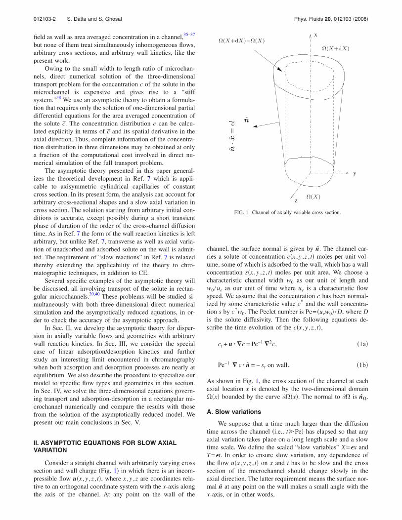
Consider a straight channel with arbitrarily varying crosssection and wall charge Fig. 1 in which there is an incom-pressible flow ux ,y ,z , t, where x ,y ,z are coordinates rela-tive to an orthogonal coordinate system with the x-axis alongthe axis of the channel. At any point on the wall of the

channel, the surface normal is given by n. The channel car-ries a solute of concentration cx ,y ,z , t moles per unit vol-ume, some of which is adsorbed to the wall, which has a wallconcentration sx ,y ,z , t moles per unit area. We choose acharacteristic channel width w0 as our unit of length andw0 /ue as our unit of time where ue is a characteristic flowspeed. We assume that the concentration c has been normal-ized by some characteristic value c* and the wall concentra-tion s by c*w0. The Peclet number is Pe= uew0 /D, where Dis the solute diffusivity. Then the following equations de-scribe the time evolution of the cx ,y ,z , t,

ct + u · c = Pe−1 2c , 1a

Pe−1 c · n = − st on wall. 1b

As shown in Fig. 1, the cross section of the channel at eachaxial location x is denoted by the two-dimensional domainx bounded by the curve x. The normal to is n.

A. Slow variations

We suppose that a time much larger than the diffusiontime across the channel i.e., tPe has elapsed so that anyaxial variation takes place on a long length scale and a slowtime scale. We define the scaled “slow variables” X=x andT=t. In order to ensure slow variation, any dependence ofthe flow ux ,y ,z , t on x and t has to be slow and the crosssection of the microchannel should change slowly in theaxial direction. The latter requirement means the surface nor-mal n at any point on the wall makes a small angle with thex-axis, or in other words,

y

z

x

n

n·x

=εl

Ω(X)

Ω(X+dX)

Ω(X+dX)−Ω(X)

FIG. 1. Channel of axially variable cross section.

012103-2 S. Datta and S. Ghosal Phys. Fluids 20, 012103 2008

n = lx + 1 − 2l2n, 2

where n is the unit normal at the boundary X of the2D domain x.41 If the axial velocity u is O1 fromthe requirements of continuity of flow, the cross flow veloc-ity components v and w must be O. So, we write,u=Ux+vy+wz=Ux+U and construct the followingasymptotic expansion for the velocity field:

u = UX,y,z,T; = U0 + U1 + ¯ , 3a

vy + wz = U = U0 + 2U

1 + ¯ . 3b

Changing variables from x and t to X and T, Eq. 1 becomes

cT + UcX + U · c − 2 Pe−1 cXX = Pe−1 2 c , 4a

Pe−11 − 2l2c · n + 2lcX = − sT, 4b

where is the two-dimensional gradient operator in thedomain . The variables c and s can be expanded in powersof ,

c = c0 + c1 + ¯ , 5a

s = s0 + s1 + ¯ 5b

and substituted in Eqs. 4a and 4b. Equating coefficients oflike powers of we get a succession of boundary value prob-lems, which we consider next.

B. Order 0

At O1 we have

Pe−1 2 c0 = 0, 6a

− Pe−1 c0 · n = 0. 6b

This implies that c0 is independent of the cross-sectionalcoordinates y and z, that is, c0= c0X ,T. A bar over aquantity indicates an average defined at each axial location Xand time T: for quantities defined within the channel e.g., cthe average is over the two-dimensional region X, forquantities defined on the wall of the channel e.g., s theaverage is over the one-dimensional bounding curve X.Equations 6a and 6b however, do not determine c0

uniquely because it is satisfied by any function c0X ,T of Xand T. To determine this function, we must now consider theboundary value problem at the next order.

C. Order

At O we have

Pe−1 2 c1 = cT

0 + U0cX0, 7a

− Pe−1 c1 · n = sT0. 7b

1. Solvability condition

Equations 7a and 7b have no solutions unless a solv-ability condition is satisfied by the lower order solution. In-tegrating both sides of Eq. 7a in the region X,

Pe−1 2 c1dA = AcT

0 + AU0cX0. 8

Using the two-dimensional Gauss Divergence Theorem thearea integral on X is converted to a line integral along thecurve X. Thus,

Pe−1 c1 · ndS

= Pe−1 2 c1dA = AcT

0 + AU0cX0 9

dA and dS denote the differential area element and arclength. Finally, using Eq. 7b in the integrand on the left-hand side of the equality and rearranging, we get

cT0 + U0cX

0 = − sT0, 10

where X is defined as the ratio of the perimeter mea-sured in w0 units and dimensionless area A measured in w0

2

units of the cross section at any X.

2. Solution for c„1…

Equation 10 is a necessary condition for nontrivial so-lutions of Eqs. 7a and 7b to exist. If it is satisfied, then wemay proceed to the next step, which is, determining thestructure of this solution. First, Eq. 10 can be used to re-write Eq. 7 as follows:

Pe−1 2 c1 = − sT

0 + U0 − U0cX0, 11a

− Pe−1 c1 · n = sT0. 11b

Solutions to Eq. 11a satisfying the boundary condition inEq. 11b may in general be written as

c1 = c1 + Pe− sT0f 0 + U0cX

0g0 . 12

Here, f 0 is defined by the following boundary value prob-lem:

2 f 0 = 1, 13a

f 0 · n =1

sT0

sT0 , 13b

f 0 = 0. 13c

Equation 13c is imposed in order to eliminate the arbitrari-ness of f 0 up to a constant. Similarly, g0 is defined by theboundary value problem,

2 g0 =

U0

U0− 1, 14a

g0 · n = 0, 14b

g0 = 0. 14c

D. Order 2

At order O2 we have

012103-3 Dispersion due to wall interactions Phys. Fluids 20, 012103 2008

Pe−1 2 c2 = cT

1 + U0cX1 + U1cX

0 + U0 · c1

− Pe−1 cXX0 , 15a

− Pe−1 c2 · n = sT1 + Pe−1 lcX

0. 15b

1. Solvability condition

Integrating both sides of Eq. 15a over the region Xas before, we derive

− sT1 = − Pe−1AcXX

0 − cX0

ldS +

U0cX1dA

+

U0 · c1dA + AU1cX

0 + AcT1. 16

The terms enclosed in brackets in Eq. 16 can be simplifiedusing the geometrical result see Appendix A,

FdA X

=

FXdA −

FldS , 17

the equation of continuity, UX+ ·U=0 and the conditionof no flow through the wall, u · n=0.

The terms enclosed in brackets in Eq. 16 become

AcXX0 − cX

0

ldS = AcX0X, 18a

U0cX1dA +

U0 · c1dA = Ac1U0X. 18b

Substituting this in Eq. 16 we get the following solvabilitycondition for the problem at O2:

− AsT1 = − Pe−1AcX

0X + Ac1U0X + AU1cX0

+ AcT1. 19

E. Reconstitution

We can obtain a single equation for c=c0+c1

+O2 by combining Eqs. 10 and 19: adding A times Eq.10, with times Eq. 19 and inserting the O2 terms2Ac1U1X and −2 Pe−1Ac1

XX doing so does not affectthe asymptotic validity of the resultant equation up to Owe get

− As0 + s1T = − Pe−1Ac0 + c1XX

+ Ac0 + c1U0 + U1X

+ Ac0 + c1T + O2 . 20

To get the form of the second term on the right-hand sideof Eq. 20 we have made use of the fact that the velocityfield u is solenoidal, so that

UAx = AU0 + U1 + 2U2 + ¯ x = 0. 21

Finally, reverting back to independent variables t=T / andx=X / and substituting c=c0+c1+O2 and s=s0

+s1+O2,

− Ast = − Pe−1Acxx + Acux + Act 22

with an error of O2. Combining c0= c0 and Eq. 12 andreverting to t and x,

c = c + Pe− st f + u cxg , 23

where f = f 0+O and g=g0+O are calculated bymodifying the boundary value problems in Eqs. 13 and14,

2 f = 1, 24a

f · n =1

st

st

, 24b

f = 0, 24c

2 g =

u

u− 1, 25a

g · n = 0, 25b

g = 0. 25c

Equation 23 can be substituted in Eq. 22. Defining thecoefficients and by

u = − fu , 26a

u = − gu 26b

we get

Act + Au cx = − Ast + AD*cxx − PeAu stx,

27a

D* = Pe−1 + Pe u2. 27b

Equations 23 and 27 are our asymptotic equations fordetermining c. They have an error of O3 or higher.

III. APPLICATIONS

The surface concentration must be specified by a kineticlaw of the following form:

st = hcw,s, . . . , 28

where cw denotes the solute concentration on the wall andthe … indicate parameters such as kinetic coefficients thatmay or may not have a space time dependence. The functionh in Eq. 28 can be expanded in Taylor series around c usingEq. 23,


st = hc,s, . . . + hcwcw=c Pe− st fw + u cxgw + O2 .

29

Here, fw and gw stand for the value of the functions f and gon the wall and hcw

cw=c indicates partial derivative of hwith respect to cw evaluated at cw= c.

A. Linear kinetics with constant coefficients

A linear reaction law of the form,

st = hcw,s,,K = Kcw − s 30

will now be specified, where is the rate constant of desorp-tion from the wall and K is the equilibrium constantof the adsorption-desorption process. The combinationK is the rate constant of adsorption. For such linear kinet-ics, hcw

cw=c=K. Averaging Eq. 29 specialized to linearkinetics along the bounding curve x and rearranging,

1 + K Pe fwst + s = Kc + Pe u cxgw + O2 .

31

Here, it has been assumed that and K do not vary along the

curve x. The notation fw and gw indicate fw and gw av-eraged over x. The asymptotically reduced equationsEqs. 27 and 31 can be solved simultaneously to find anasymptotic approximation to the axial distribution of c. Thethree-dimensional distribution of c can be calculated fromthe axial distribution of c, using Eq. 23.

B. The limit of fast reactions

Further analytical simplification of Eq. 27 is possiblewhen reactions at the wall happen on a time scale that isshort compared to the analysis time. Thus, adsorption anddesorption are nearly in equilibrium over most of the timeinterval over which knowledge of the analyte concentrationis of interest. The scaling that best describes this situation isKO1. In order to get a simple result, we further as-sume that the flow is homogeneous in the axial direction andthe cross section of the channel does not vary in shape orarea in the axial direction. Under these conditions A, , ,and are independent of x and t and u is a constant. So, Eq.27 can be rewritten as

ct + u cx = − st + Pe−1 + Pe u2cxx − Pe u stx

32

with an error of O3. In the long time limit, t1 /, theorder of magnitude of the terms in Eq. 31 can be estimatedas follows: the second term on the left-hand side of theequality and the first term on the right-hand side of the equal-ity are both O1 and the remaining terms are O or less.So, the leading order balance in Eq. 31 may be written as

s = Kc + O . 33

We note that from Eq. 27 at leading order

ct + u cx = − st + O2 . 34

Using Eq. 33 in Eq. 34, we get

ct = −u

1 + Kcx + O2 . 35

Differentiation of Eq. 33 with respect to t leads to st=Kct

+O2 in the long time limit, this can be used to replace theterms with st in Eq. 31 without the loss of asymptotic ac-curacy. On rearrangement of the resultant expression, we get

s = Kc − K

+ Pe K2 fw ct + K Pe gwu cx + O2 . 36

Using Eq. 35 in Eq. 36 we get

s = Kc + u cx K

1 + K+ Pe

K2

1 + Kfw + K Pe gw

+ O2 . 37

Differentiating Eq. 37 with respect to t and noting thatcxt= ctx can be calculated by differentiation of Eq. 35 withrespect to x we get

st = Kct − K

1 + K2 + K2 fw

1 + K2

+Kgw

1 + KPeu2cxx + O3 . 38

The st calculated by Eq. 38 can be used in Eq. 32 to arriveat the effective equation in the limit of fast reactions. Sincethe last term −Pe u stx of Eq. 32 is of the order of O2,it is sufficient to use an O accurate approximation of Eq.38 in approximating this term,

st = Kct + O2 = −K

1 + Ku cx + O2 , 39

where Eq. 35 has been used to obtain the second equality.The first term −st on the right-hand side of Eq. 32 is O,so in approximating it by Eq. 38, all terms of Eq. 38 haveto be retained. After this substitution to Eq. 38, we get onrearrangement,

ct +u

1 + Kcx = Deffcxx, 40

where K=K and

Deff = Deffchrom =

Pe−1

1 + K+

1 + K+

2K

1 + K2

+K2 fw

1 + K3Pe u2 +K

1 + K3 u2. 41

In the above gw= has been used. A proof of this is pre-sented in Appendix B.

In the analysis presented in this section, we assumed thescalings K1. If the adsorption and desorption reac-tions are even faster, that is, chemical equilibrium is estab-lished on a time scale much shorter than the cross channeltransport time, then K1 / is an appropriate scaling. Ifthe analysis presented in this section is repeated using

= /, where is independent of , then it is easily verified


that one recovers Eqs. 40 and 41, except for the last termin Eq. 41 which drops out. One could also arrive at Eqs.40 and 41 by reversing the two limiting procedures, thatis, invoking the “quasiequilibrium” assumption before theasymptotic analysis describing the Taylor regime as in thework of Golay24 and others. The other possibilities involvingfast reactions are A K1 / and 1; B K1 and1 /. In case A almost all of the analyte is adsorbed inthe first few capillary diameters and in case B retention isnegligible. In both cases though, Eq. 41 correctly describesthe appropriate limiting situation.

C. Shape functions in different flows and geometries

In order to proceed further with the asymptotically re-duced problem, it is essential to calculate the shape functionsf and g. This enables us to calculate the quantities , , and

fw appearing in the equations derived so far for c and s andalso to find the concentration variation across a given crosssection through Eq. 23.

The function f calculated by solving Eq. 24 dependsonly on the geometry of the channel if the kinetic coeffi-cients of adsorption-desorption and initial conditions on s arethe same for all points on the curve and can be calculatedby solving Eq. 24 with the right-hand side of Eq. 24b setto 1 / see Appendix B. Planar, rectangular, and trapezoidalmicrochannels are some common shapes of interest.40

The function g calculated by solving Eq. 25 dependsboth on the type of flow and geometry. Some interesting anduseful flows for which the function g and the coefficients and are relevant are

i Purely pressure-driven flow employed in liquid andgas chromatography25 and used for theoretical model-ing of axially variable electro-osmotic flow.42

ii Shear-driven Couette flow for novel techniquessuch as chromatography with electro-osmoticmicropumping33 and shear-driven chromatography.32

iii Electrokinetic flow with finite Debye layer effects tobe studied in Sec. IV under problem B.

All the above flow profiles are axially homogeneous, so thequantities and are evaluated to be constant coefficients.In an axially inhomogeneous flow, like problem C, as shownlater in Sec. IV, these quantities are a function of the axialcoordinate x.

Table I shows the quantities fw, , and calculated forpressure-driven flow in channels with uniform kinetic coef-ficients of adsorption-desorption for some cross sections ofinterest in microfluidics gap between planes, circle, square,and trapezoid. Except for the trapezoidal cross section forwhich f and g was obtained numerically, analytical solutionsto Eqs. 24 and 25 can be readily calculated or obtainedfrom the literature.36,43–45 Table I will be referred to in solv-ing the asymptotically reduced forms of the test problems inthe next section. The information in Table I when used in Eq.41 reaffirms classical results for the effective dispersioncoefficient in chromatography with plane and roundchannels.24–26

The gap between parallel planes can be used to approxi-mate the microfluidic channels used in shearchromatography32 and electro-osmotic micropumping.46 Theflow profile in either case is, then linear in the coordinate

across the channel width. In this case, we obtain fw=1 /3,=1 /12 and =1 /30 on solving Eqs. 24 and 25. Whilecalculating f , care should be taken to account for the fact thatshear chromatography and chromatography with electro-osmotic micropumping employ an adsorptive coating onlyon the passive electrode-free32 or stationary33 wall. Use of

these values of fw, , and in Eq. 41 reaffirms the expres-sion for effective dispersion coefficient derived in Ref. 32using the Method of Moments.26

The shape function g for electrokinetic flows with finiteDebye layers can be obtained numerically, given the analyti-cal expression for the flow field.10 Details of calculation ofthe coefficients when wall adsorption is present and inthis case will be presented in Sec. IV C.

IV. NUMERICAL SIMULATIONS

A complete solution of the problem of transport gener-ally involves solving Eq. 1 in three dimensions. The modeldeveloped in the last section requires solution of only one-dimensional equations. For the purpose of brevity, the formerapproach will be called the “three-dimensional model” andthe latter approach will be called the “asymptotically reducedmodel.” In this section, three specific test problems will besolved numerically using both of these methods and the re-sults compared to ascertain the accuracy of the asymptoticreduction.

A. Test problems

The test problems pertain to transport of the solute underelectro-osmotic flow. Additionally, the following specificconditions common to all the test problems to be describedwill be assumed:

i The microchannel has an axially invariant squarecross section of side 2b. With the choice w0=2b, thegeometric constant =4.

ii Wall reaction, when present, is of the linear form asdescribed by Eq. 30 with and K invariant on thewall.

TABLE I. The coefficients fw, , and calculated for an axially homoge-neous and purely pressure-driven flow in a plane channel gap betweenparallel plates and in channels with circular, square, and trapezoidal crosssection. The isosceles trapezoid in the last column is one for which thedistance between the parallel sides equals half the sum of the parallel sides.The reference length-scale w0 is the diameter for the circle and the distancebetween the parallel sides for the other geometrical shapes.

Channel type Plane Circular Square Trapezoidal

fw112

132

124

0.113

160

196

0.0155 0.052

1210

1192

0.0084 0.0329


iii Initially, there is no wall adsorbed concentration,s=0 at t=0.

iv The initial concentration of the solute cx ,y ,z , t=0 isuniform across the channel and has a Gaussian distri-bution along the channel.

v At any fixed axial location, x, the zeta potential doesnot vary over the bounding curve x.

The velocity scale ue for each test problem is chosen to en-sure that the dimensionless speed u is unity. We consider thefollowing test problems:

Problem A (EOF with wall reaction and infinitely thinDebye layers): The solute is transported by a uniform plugflow with adsorption and desorption on the walls. In Eq.30, the dimensionless equilibrium constant K will be heldconstant at the value K=1 and will be varied to study theeffect of varying wall reaction rates. This test problem is ofrelevance to separations by CEC,18 as well as to the issue ofband broadening due to wall-adsorption of charged species inCE.17 The uniform flow profile arises in situations where thechannel width is much larger than the Debye length and thewall properties are uniform. It also applies when the analyteis transported by electrophoresis alone in a channel whereEOF has been suppressed. The Peclet number is Pe=10 andthe numerical domain size in the x direction is L / 2b=40.

Problem B (EOF with wall reaction and finite Debyelayers): Transport of a neutral solute in a channel with finitesized Debye layer will be analyzed, when an adsorption-desorption process K=1 and K Pe=1 is present on thewall. The Debye layer thickness nondimensionalized by thewidth of the channel will be varied. The Peclet number isPe=10 and numerical domain size in the x direction isL / 2b=40.

Problem C (EOF with variable potential): Dispersionunder an axially varying EOF generated by a periodic zetapotential distribution =0+ cos2x / on all four wallsof the square channel in absence of wall reactions will be

studied by varying and . The Reynolds number of theflow is zero, the Peclet number is Pe=5 and the numericaldomain size in the x direction is L / 2b=128.

B. Numerical methods

The three-dimensional partial differential equation for cgiven by Eq. 1 was solved in a rectangular box of size2b 2b L. At each time step, the boundary condition Eq.1b was used to couple the c calculation from Eq. 1 to thes calculation from Eq. 30. The s calculation used explicitRunge Kutta 4 RK4 time stepping.38 An unconditionallystable implicit time integration scheme Crank Nicholsonmethod and spatial discretization, both of second order nu-merical accuracy,47 were used for advancing the c field. Thenumerical grid size used was x=y=z=0.033 for prob-lems A and B and 0.5x=y=z=0.05 for problem C. In allcases dt=0.01. The finite axial length L of the numericaldomain was chosen large enough so that cx=0 andcx=L remained essentially zero not larger than 10−10 atall times. A zero total flux sum of diffusive and convectivecomponents boundary condition was applied at the ends ofthe channel. For solution to the flow field in problem C, theSIMPLER algorithm48 was used see Refs. 39 and 49 fordetails. The shape functions f and g and the quantities , ,

and fw for the trapezoidal cross section listed in Table I werecalculated using a commercially available package MatlabPDE Toolbox employing the finite element method.47 Forsolving the asymptotically reduced one-dimensional prob-lem, RK4 time stepping and eighth order compact finite dif-ferences were used, similar to that in Ref. 7. A typical ratioof run times on a 2 GHz-512 Mbyte computer for the one-dimensional effective problem and the three-dimensionalproblem was of the order of 10−2. This considerable runtimeeconomy is a practical benefit of the asymptotically reducedmodel developed here.

0 1 2 3 4 5 6 7 80

0.1

0.2

0.3

0.4

0.5

0.6

0.7

0.8

t u/2b

Def

f/(2

bu)

λ K Pe=10

λ K Pe=5

λ K Pe=1

λ K Pe=3

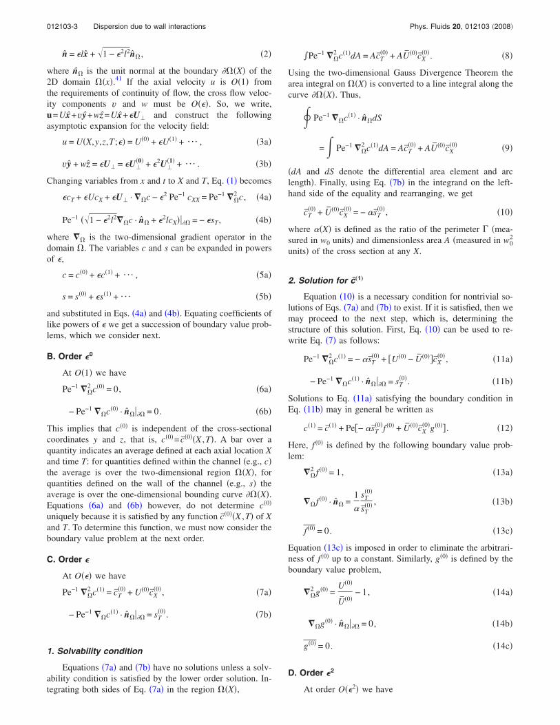
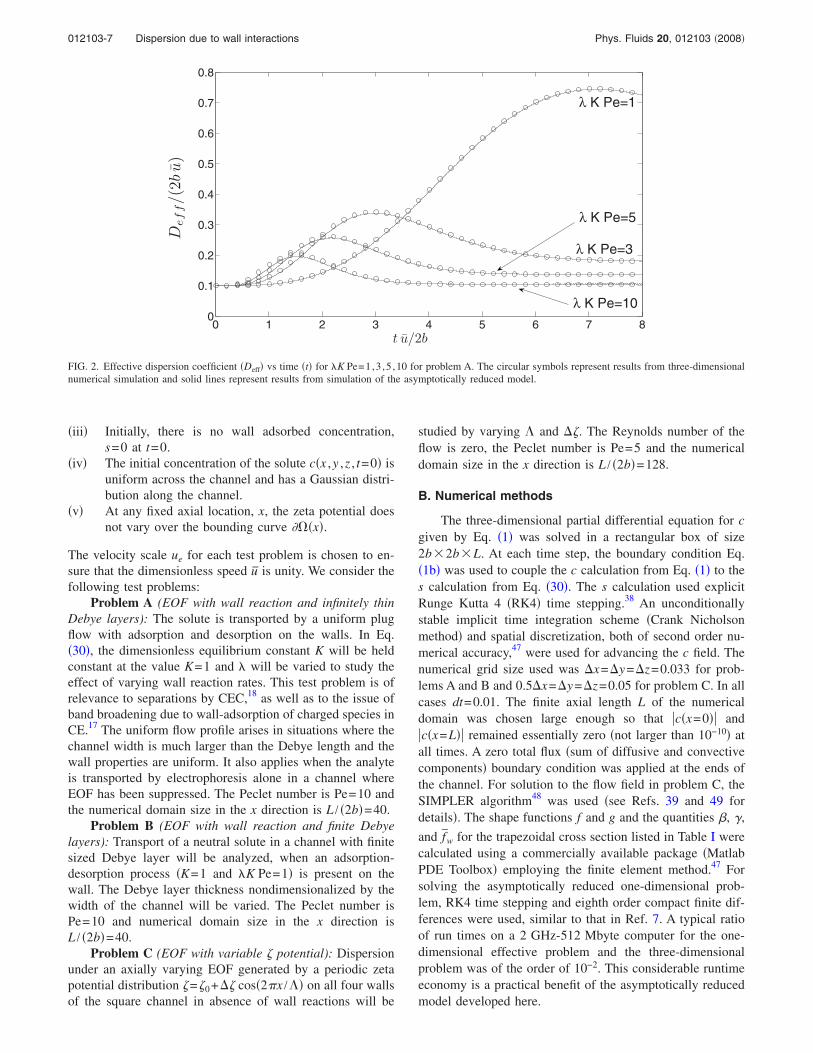
FIG. 2. Effective dispersion coefficient Deff vs time t for K Pe=1,3 ,5 ,10 for problem A. The circular symbols represent results from three-dimensionalnumerical simulation and solid lines represent results from simulation of the asymptotically reduced model.


C. Results

In the results to be described below, an effective disper-sion coefficient Deff is used as a measure of the instantaneousrate of spreading of the solute in the axial direction. It isdefined as follows:

Deff =1

2

d2

dt, 42

where the variance of the plug is defined as 2

= x−x*2c / c and x* is the position of the centroid of thedistribution, x*= xc / c. In the above equation and hence-forth, … indicates axial average. Note, that in general Deff

evaluated from Eq. 42 is a time dependent quantity. Thefigures in this section use dimensionless variables. In particu-lar, the concentration c is rendered dimensionless by dividingby the characteristic value c0=1 / 2b3cx ,y ,z , t=0dVwhere the volume integral is over the entire computationaldomain.

1. Problem A: EOF with wall reaction and infinitelythin Debye layers

The three-dimensional model for problem A involvessolving Eq. 1 together with Eq. 30 and the one-dimensional model requires solving Eqs. 31 and 32. Forthe current problem, ==0, the function g=0 everywhere

and f = 6y2+6z2−1 /24. Therefore, fw=1 /24 as noted inTable I for square cross section. If only small departuresfrom local equilibrium between the suspended and adsorbedphase is assumed, Eq. 41 may be used to calculate theeffective dispersion. Though the parameter alone is varied,results are presented in terms of the combination K Perepresenting a ratio of the characteristic adsorption time tothe characteristic diffusion time. Figure 2 shows the timeevolution of Deff calculated from the asymptotically reducedequations and the full three-dimensional equations for

K Pe=1,3 ,5 ,10 with K=1 and Pe=10 held fixed. The twosets of computational results are in excellent agreement.Qualitatively, Deff approaches a steady value after goingthrough a transient phase. The transient phase is the mostprolonged for K Pe=1, because, slow reactions take alonger time to achieve the quasiequilibrium characteristic ofchromatography. The asymptotically reduced model accu-rately represents the transient as well as the final equilibriumstate for all four reaction speeds studied, whereas, the ana-lytical estimate Deff

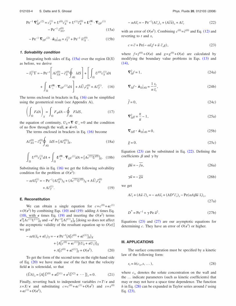
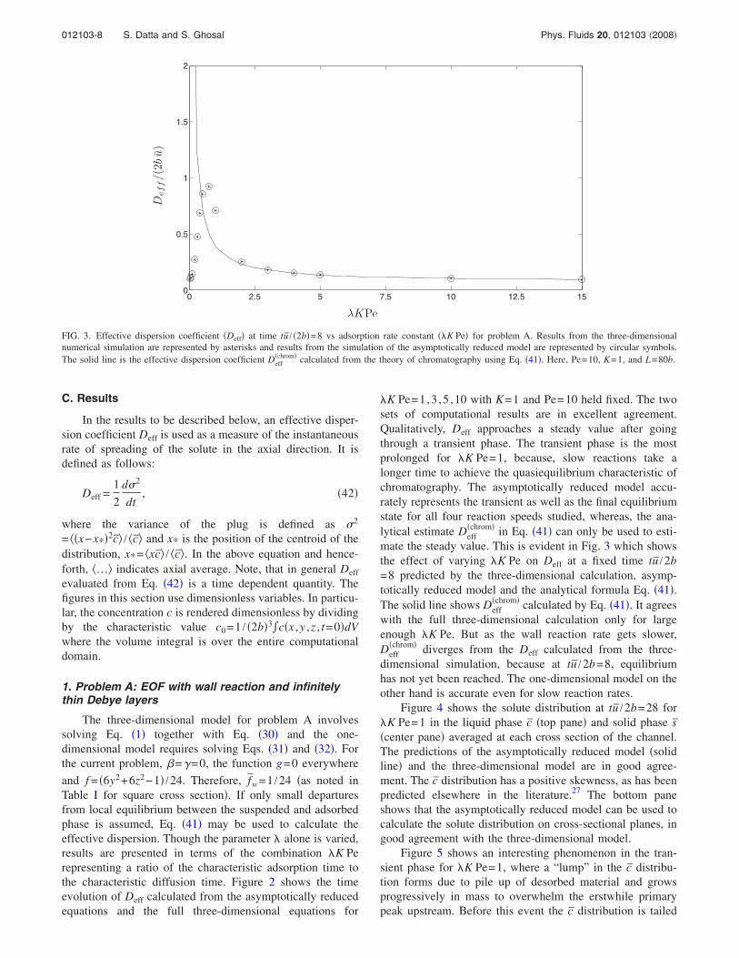
chrom in Eq. 41 can only be used to esti-mate the steady value. This is evident in Fig. 3 which showsthe effect of varying K Pe on Deff at a fixed time tu /2b=8 predicted by the three-dimensional calculation, asymp-totically reduced model and the analytical formula Eq. 41.The solid line shows Deff

chrom calculated by Eq. 41. It agreeswith the full three-dimensional calculation only for largeenough K Pe. But as the wall reaction rate gets slower,Deff

chrom diverges from the Deff calculated from the three-dimensional simulation, because at tu /2b=8, equilibriumhas not yet been reached. The one-dimensional model on theother hand is accurate even for slow reaction rates.

Figure 4 shows the solute distribution at tu /2b=28 forK Pe=1 in the liquid phase c top pane and solid phase scenter pane averaged at each cross section of the channel.The predictions of the asymptotically reduced model solidline and the three-dimensional model are in good agree-ment. The c distribution has a positive skewness, as has beenpredicted elsewhere in the literature.27 The bottom paneshows that the asymptotically reduced model can be used tocalculate the solute distribution on cross-sectional planes, ingood agreement with the three-dimensional model.

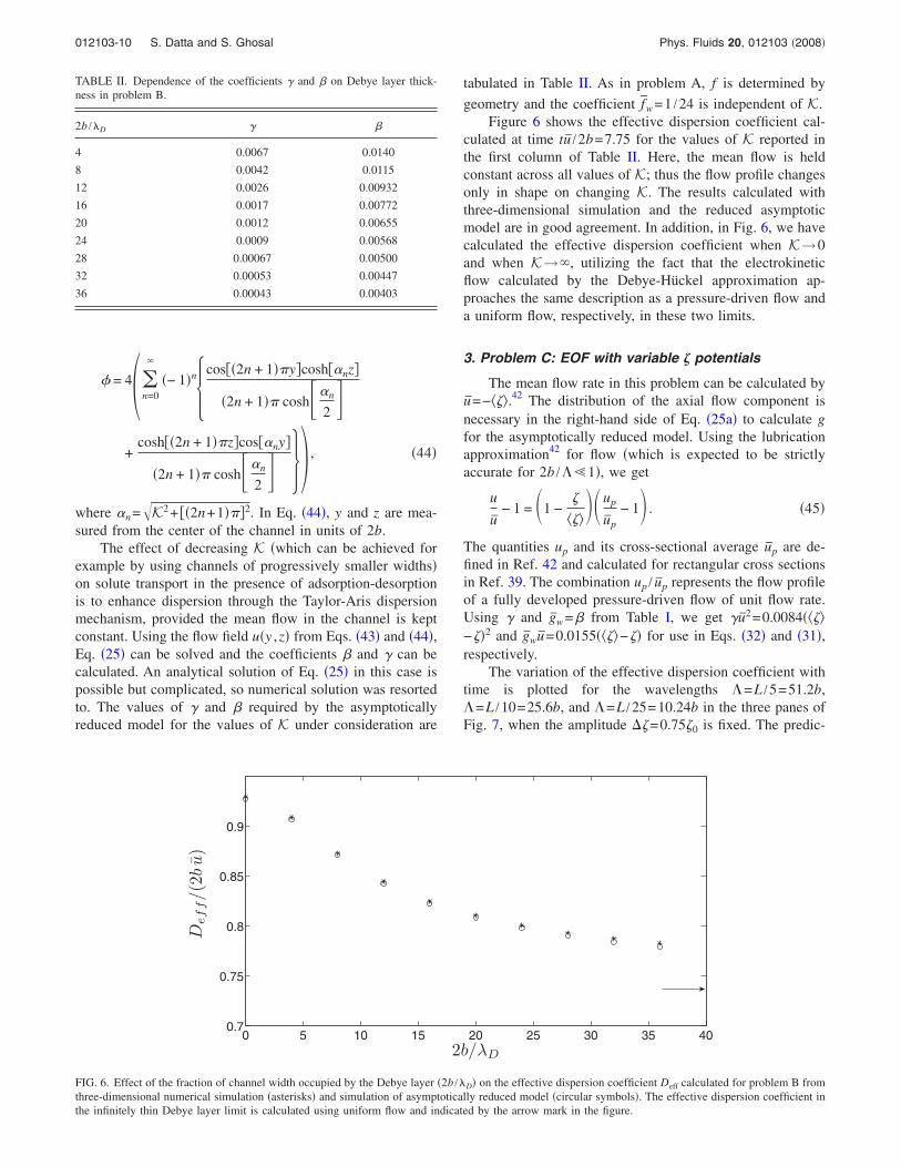
Figure 5 shows an interesting phenomenon in the tran-sient phase for K Pe=1, where a “lump” in the c distribu-tion forms due to pile up of desorbed material and growsprogressively in mass to overwhelm the erstwhile primarypeak upstream. Before this event the c distribution is tailed

0 2.5 5 7.5 10 12.5 150

0.5

1

1.5

2

λKPe

Deff/(2

bu)

FIG. 3. Effective dispersion coefficient Deff at time tu / 2b=8 vs adsorption rate constant K Pe for problem A. Results from the three-dimensionalnumerical simulation are represented by asterisks and results from the simulation of the asymptotically reduced model are represented by circular symbols.The solid line is the effective dispersion coefficient Deff

chrom calculated from the theory of chromatography using Eq. 41. Here, Pe=10, K=1, and L=80b.


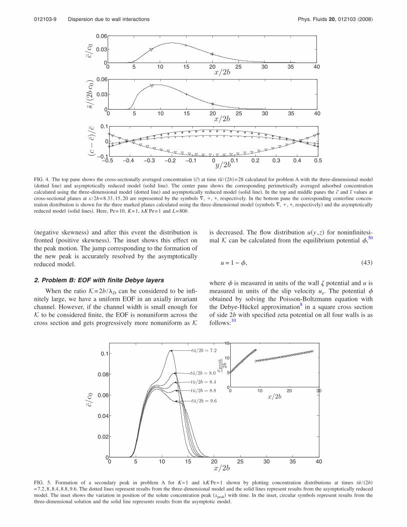
negative skewness and after this event the distribution isfronted positive skewness. The inset shows this effect onthe peak motion. The jump corresponding to the formation ofthe new peak is accurately resolved by the asymptoticallyreduced model.

2. Problem B: EOF with finite Debye layers

When the ratio K=2b /D can be considered to be infi-nitely large, we have a uniform EOF in an axially invariantchannel. However, if the channel width is small enough forK to be considered finite, the EOF is nonuniform across thecross section and gets progressively more nonuniform as K

is decreased. The flow distribution uy ,z for noninfinitesi-mal K can be calculated from the equilibrium potential ,50

u = 1 − , 43

where is measured in units of the wall potential and u ismeasured in units of the slip velocity ue. The potential obtained by solving the Poisson-Boltzmann equation withthe Debye-Hückel approximation8 in a square cross sectionof side 2b with specified zeta potential on all four walls is asfollows:10

0 5 10 15 20 25 30 35 400

0.03

0.06

x/2b

c/c 0

0 5 10 15 20 25 30 35 400

0.03

0.06

x/2b

s/(2

bc 0

)

−0.5 −0.4 −0.3 −0.2 −0.1 0 0.1 0.2 0.3 0.4 0.5−0.1

0

0.1

y/2b

(c−

c)/c

FIG. 4. The top pane shows the cross-sectionally averaged concentration c at time tu / 2b=28 calculated for problem A with the three-dimensional modeldotted line and asymptotically reduced model solid line. The center pane shows the corresponding perimetrically averaged adsorbed concentrationcalculated using the three-dimensional model dotted line and asymptotically reduced model solid line. In the top and middle panes the c and s values atcross-sectional planes at x /2b=8.33,15,20 are represented by the symbols , , , respectively. In the bottom pane the corresponding centerline concen-tration distribution is shown for the three marked planes calculated using the three-dimensional model symbols , , , respectively and the asymptoticallyreduced model solid lines. Here, Pe=10, K=1, K Pe=1 and L=80b.

0 5 10 15 20 25 30 35 400

0.02

0.04

0.06

0.08

0.1

x/2b

c/c 0

0 10 20 300

5

10

15

x/2b

xpea

k2b

tu/2b = 7.2

tu/2b = 8.0

tu/2b = 8.8

tu/2b = 9.6

tu/2b = 8.4

FIG. 5. Formation of a secondary peak in problem A for K=1 and K Pe=1 shown by plotting concentration distributions at times tu / 2b=7.2,8 ,8.4,8.8,9.6. The dotted lines represent results from the three-dimensional model and the solid lines represent results from the asymptotically reducedmodel. The inset shows the variation in position of the solute concentration peak xpeak with time. In the inset, circular symbols represent results from thethree-dimensional solution and the solid line represents results from the asymptotic model.


= 4n=0

− 1n cos2n + 1ycoshnz

2n + 1 coshn

2

+cosh2n + 1zcosny

2n + 1 coshn

2 , 44

where n=K2+ 2n+12. In Eq. 44, y and z are mea-sured from the center of the channel in units of 2b.

The effect of decreasing K which can be achieved forexample by using channels of progressively smaller widthson solute transport in the presence of adsorption-desorptionis to enhance dispersion through the Taylor-Aris dispersionmechanism, provided the mean flow in the channel is keptconstant. Using the flow field uy ,z from Eqs. 43 and 44,Eq. 25 can be solved and the coefficients and can becalculated. An analytical solution of Eq. 25 in this case ispossible but complicated, so numerical solution was resortedto. The values of and required by the asymptoticallyreduced model for the values of K under consideration are

tabulated in Table II. As in problem A, f is determined by

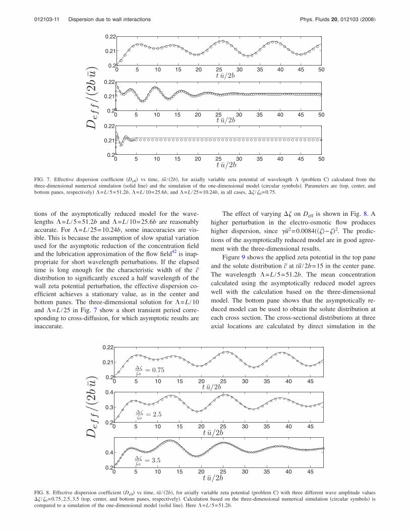
geometry and the coefficient fw=1 /24 is independent of K.Figure 6 shows the effective dispersion coefficient cal-

culated at time tu /2b=7.75 for the values of K reported inthe first column of Table II. Here, the mean flow is heldconstant across all values of K; thus the flow profile changesonly in shape on changing K. The results calculated withthree-dimensional simulation and the reduced asymptoticmodel are in good agreement. In addition, in Fig. 6, we havecalculated the effective dispersion coefficient when K→0and when K→, utilizing the fact that the electrokineticflow calculated by the Debye-Hückel approximation ap-proaches the same description as a pressure-driven flow anda uniform flow, respectively, in these two limits.

3. Problem C: EOF with variable potentials

The mean flow rate in this problem can be calculated byu=−.42 The distribution of the axial flow component isnecessary in the right-hand side of Eq. 25a to calculate gfor the asymptotically reduced model. Using the lubricationapproximation42 for flow which is expected to be strictlyaccurate for 2b /1, we get

u

u− 1 = 1 −

up

up

− 1 . 45

The quantities up and its cross-sectional average up are de-fined in Ref. 42 and calculated for rectangular cross sectionsin Ref. 39. The combination up / up represents the flow profileof a fully developed pressure-driven flow of unit flow rate.Using and gw= from Table I, we get u2=0.0084−2 and gwu=0.0155− for use in Eqs. 32 and 31,respectively.

The variation of the effective dispersion coefficient withtime is plotted for the wavelengths =L /5=51.2b,=L /10=25.6b, and =L /25=10.24b in the three panes ofFig. 7, when the amplitude =0.750 is fixed. The predic-

TABLE II. Dependence of the coefficients and on Debye layer thick-ness in problem B.

2b /D

4 0.0067 0.0140

8 0.0042 0.0115

12 0.0026 0.00932

16 0.0017 0.00772

20 0.0012 0.00655

24 0.0009 0.00568

28 0.00067 0.00500

32 0.00053 0.00447

36 0.00043 0.00403

0 5 10 15 20 25 30 35 400.7

0.75

0.8

0.85

0.9

2b/λD

Def

f/(2

bu)

FIG. 6. Effect of the fraction of channel width occupied by the Debye layer 2b /D on the effective dispersion coefficient Deff calculated for problem B fromthree-dimensional numerical simulation asterisks and simulation of asymptotically reduced model circular symbols. The effective dispersion coefficient inthe infinitely thin Debye layer limit is calculated using uniform flow and indicated by the arrow mark in the figure.


tions of the asymptotically reduced model for the wave-lengths =L /5=51.2b and =L /10=25.6b are reasonablyaccurate. For =L /25=10.24b, some inaccuracies are vis-ible. This is because the assumption of slow spatial variationused for the asymptotic reduction of the concentration fieldand the lubrication approximation of the flow field42 is inap-propriate for short wavelength perturbations. If the elapsedtime is long enough for the characteristic width of the cdistribution to significantly exceed a half wavelength of thewall zeta potential perturbation, the effective dispersion co-efficient achieves a stationary value, as in the center andbottom panes. The three-dimensional solution for =L /10and =L /25 in Fig. 7 show a short transient period corre-sponding to cross-diffusion, for which asymptotic results areinaccurate.

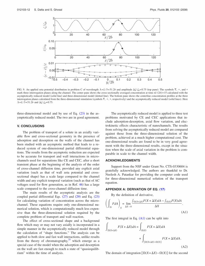
The effect of varying on Deff is shown in Fig. 8. Ahigher perturbation in the electro-osmotic flow produceshigher dispersion, since u2=0.0084−2. The predic-tions of the asymptotically reduced model are in good agree-ment with the three-dimensional results.

Figure 9 shows the applied zeta potential in the top paneand the solute distribution c at tu /2b=15 in the center pane.The wavelength =L /5=51.2b. The mean concentrationcalculated using the asymptotically reduced model agreeswell with the calculation based on the three-dimensionalmodel. The bottom pane shows that the asymptotically re-duced model can be used to obtain the solute distribution ateach cross section. The cross-sectional distributions at threeaxial locations are calculated by direct simulation in the

0 5 10 15 20 25 30 35 40 45 500.2

0.21

0.22

t u/2b

0 5 10 15 20 25 30 35 40 45 500.2

0.21

0.22

t u/2b

Def

f/(2

bu)

0 5 10 15 20 25 30 35 40 45 500.2

0.21

0.22

t u/2b

FIG. 7. Effective dispersion coefficient Deff vs time, tu / 2b, for axially variable zeta potential of wavelength problem C calculated from thethree-dimensional numerical simulation solid line and the simulation of the one-dimensional model circular symbols. Parameters are top, center, andbottom panes, respectively =L /5=51.2b, =L /10=25.6b, and =L /25=10.24b, in all cases, /0=0.75.

0 5 10 15 20 25 30 35 40 450.2

0.21

0.22

t u/2b

Def

f/(

2bu)

0 5 10 15 20 25 30 35 40 450.2

0.3

0.4

t u/2b

0 5 10 15 20 25 30 35 40 450.2

0.4

t u/2b

∆ζζ0

= 2.5

∆ζζ0

= 3.5

∆ζζ0

= 0.75

FIG. 8. Effective dispersion coefficient Deff vs time, tu / 2b, for axially variable zeta potential problem C with three different wave amplitude values /0=0.75,2.5,3.5 top, center, and bottom panes, respectively. Calculation based on the three-dimensional numerical simulation circular symbols iscompared to a simulation of the one-dimensional model solid line. Here =L /5=51.2b.


three-dimensional model and by use of Eq. 23 in the as-ymptotically reduced model. The two are in good agreement.

V. CONCLUSIONS

The problem of transport of a solute in an axially vari-able flow and cross-sectional geometry in the presence ofadsorption and desorption on the walls of the channel hasbeen studied with an asymptotic method that leads to a re-duced system of one-dimensional partial differential equa-tions. The results from the asymptotic reduction are expectedto be accurate for transport and wall interactions in micro-channels used for separations like CE and CEC, after a shorttransient phase at the beginning of the analysis of the orderof cross-channel diffusion time, provided any explicit axialvariation such as that of wall zeta potential and cross-sectional shape has a scale large compared to the channelwidth and any explicit temporal variation such as that of ACvoltages used for flow generation, as in Ref. 46 has a largescale compared to the cross-channel diffusion time.

The main results of the asymptotic analysis are thecoupled partial differential Eqs. 27 and 29 and Eq. 23for calculating variation of concentration across the micro-channel. These equations require only one-dimensional nu-merical solution, which is computationally much less expen-sive than the three-dimensional solution required by thecomplete problem of transport and wall reaction.

The effect of cross-sectional shape and a backgroundflow which may or may not vary axially is incorporated in asimple manner in the asymptotically reduced model throughthe calculation of “shape functions.” The analysis can beapplied to both slow and fast wall interactions, unlike resultsfrom the theory of chromatography,25 which emerge as aspecial case of the model when the adsorption and desorptionon the wall are fast enough to reach a state of “quasiequilib-rium” within the time of analysis.

The asymptotically reduced model is applied to three testproblems motivated by CE and CEC applications that in-clude adsorption-desorption, axial flow variation, and elec-trokinetic effects characteristic of nanochannels. The resultsfrom solving the asymptotically reduced model are comparedagainst those from the three-dimensional solution of theproblem, achieved at a much higher computational cost. Theone-dimensional results are found to be in very good agree-ment with the three-dimensional results, except in the situa-tion when the scale of axial variation in the problem is com-parable in scale to the channel width.

ACKNOWLEDGMENTS

Support from the NSF under Grant No. CTS-0330604 isgratefully acknowledged. The authors are thankful to Dr.Neelesh A. Patankar for providing the computer code usedfor three-dimensional numerical solution of the transportequation.

APPENDIX A: DERIVATION OF EQ. „17…

By the definition of derivative,

FdA X

= limX→0

X+XFX + XdA − XFXdA

X.

A1

The first integral in Eq. A1 can be split into

X+X

FX + XdA = X

FX + XdA

+ X+X−X

FX + XdA .

A2

The domain of integration X+X−X for the second

0 20 40 60 80 100 120

0.05

0.10

x/2b

c/c 0

−0.5 −0.4 −0.3 −0.2 −0.1 0 0.1 0.2 0.3 0.4 0.5−0.01

0.00

0.01

y/2b

(c−

c)/c

0 20 40 60 80 100 1200

1

2

x/2b

ζ/ζ 0

FIG. 9. An applied zeta potential distribution in problem C of wavelength =L /5=51.2b and amplitude /0=0.75 top pane. The symbols , , and

mark three interrogation planes along the channel. The center pane shows the cross-sectionally averaged concentration at time tu / 2b=15 calculated with theasymptotically reduced model solid line and three-dimensional model dotted line. The bottom pane shows the centerline concentration profiles at the threeinterrogation planes calculated from the three-dimensional simulation symbols , , , respectively and the asymptotically reduced model solid lines. Here=L /5=51.2b and /0=0.75.


integral above is a thin annulus on the X+X plane, isshown in Fig. 1. The differential area element of this annulusis −ldXdS, if the channel cross section varies slowly. There-fore,

X+X−X

FX + XdA

= X

FXldS + OX2. A3

Using Eq. A3 in Eq. A2 and the result in Eq. A1 we get

FdA X

=

FXdA −

FldS A4

after utilizing the definition of the derivative of the functionFX in variable X.

APPENDIX B: DERIVATION OF gw=

In the left-hand side of the mathematical identity,

f2 g − g

2 fdA = fg · n − gf · ndS

B1

we use Eqs. 24a, 24c, 25a, and 25c; this simplifies theleft-hand side to fu / udA.

For simplifying the first term in the right-hand side ofEq. B1, the right-hand of side of Eq. 24b which is re-quired to be only O1 accurate, by virtue of Eq. 13b canbe replaced by 1 /. This is because, s= s to O1 providedthe kinetic coefficients and the initial distribution of s do notvary on . Indeed, the evolution equation for s, st=hc ,s+O ensures that if s= s+O at t=0, it will remain so atfuture times.

The second term on the right-hand side is zero owing toEq. 25b. Utilizing the definition of by Eq. 26a and= P /A, we get

=1

A f

u

udA =

1

P gdS = gw. B2

1H. A. Stone, A. D. Stroock, and A. Ajdari, “Engineering flows in smalldevices: Microfluidics toward a lab-on-a-chip,” Annu. Rev. Fluid Mech.36, 381 2004.

2J. A. Wilkins and C. Horváth, “Capillary electrochromatography of pep-tides and proteins,” Electrophoresis 25, 2242 2004.

3Electrokinetic Phenomena: Principles and Applications in AnalyticalChemistry and Microchip Technology, edited by A. S. Rathore and A.Guttman Marcell Dekker, New York, 2004.

4M. Pačes, J. Kosek, M. Marek, U. Tallarek, and A. Seidel-Morgenstern,“Mathematical modelling of adsorption and transport processes in capil-lary electrochromatography: Open-tubular geometry,” Electrophoresis 24,380 2003.

5J. K. Towns and F. E. Regnier, “Impact of polycation adsorption on effi-ciency and electro-osmotically driven transport in capillary electrophore-sis,” Anal. Chem. 64, 2473 1992.

6M. R. Schure and A. M. Lenhoff, “Consequences of wall adsorption incapillary electrophoresis: Theory and simulation,” Anal. Chem. 65, 30241993.

7S. Ghosal, “The effect of wall interactions on capillary zone electrophore-sis,” J. Fluid Mech. 491, 285 2003.

8R. Probstein, Physicochemical Hydrodynamics Wiley, New York, 1994.

9S. Ghosal, “Electrokinetic flow and dispersion in capillary electrophore-sis,” Annu. Rev. Fluid Mech. 38, 309 2006.

10C. Yang and D. Li, “Analysis of electrokinetic effects on the liquid flow inrectangular microchannels,” Colloids Surf., A 143, 339 1998.

11G. I. Taylor, “Dispersion of soluble matter in solvent flowing slowlythrough a tube,” Proc. R. Soc. London, Ser. A 219, 186 1953.

12R. Aris, “On the dispersion of a solute in a fluid flowing through a tube,”Proc. R. Soc. London, Ser. A 235, 67 1956.

13S. Devasenathipathy, J. G. Santiago, and K. Takehara, “Particle trackingtechniques for electrokinetic microchannel flows,” Anal. Chem. 74, 37042002.

14A. Ajdari, “Electro-osmosis on inhomogeneously charged surfaces,” Phys.Rev. Lett. 75, 755 1995.

15A. Ajdari, “Generation of transverse fluid currents and forces by an elec-tric field: Electro-osmosis on charge-modulated and undulated surfaces,”Phys. Rev. E 53, 4996 1996.

16J. K. Towns and F. E. Regnier, “Capillary electrophoretic separations ofproteins using nonionic surfactant coatings,” Anal. Chem. 91, 11261992.

17M. S. Munson, M. S. Hasenbank, E. Fu, and P. Yager, “Suppression ofnonspecific adsorption using sheath flow,” Lab Chip 4, 438 2004.

18S. C. Jacobson, R. Hergenroeder, L. B. Koutny, and J. M. Ramsey, “Openchannel electrochromatography on a microchip,” Anal. Chem. 66, 23691994.

19J. H. Knox, “Thermal effects and band spreading in capillary electro-separation,” Chromatographia 26, 329 1988.

20U. Tallarek, E. Rapp, T. Scheenen, E. Bayer, and H. Van As, “Electroos-motic and pressure-driven flow in open and packed capillaries: Velocitydistributions and fluid dispersion,” Anal. Chem. 72, 2292 2000.

21M. C. Breadmore, M. Boyce, M. Macka, N. Avdalovic, and P. R. Haddad,“Peak shapes in open tubular ion-exchange capillary electrochromatogra-phy of inorganic anions,” J. Chromatogr., A 892, 303 2000.

22K. Shariff and S. Ghosal, “Peak tailing in electrophoresis due to alterationof the wall charge by adsorbed analytes: Numerical simulations andasymptotic theory,” Anal. Chim. Acta 507, 87 2003.

23S. Ghosal, “Fluid mechanics of electro-osmotic flow and its effect on bandbroadening in capillary electrophoresis,” Electrophoresis 25, 214 2004.

24M. J. E. Golay, “Theory of chromatography in open and coated tubularcolumns with round and rectangular cross sections,” in Gas Chromatog-raphy 1958: Proceedings of the Second Symposium, Amsterdam, May19–23, 1958, edited by D. H. Desty Butterworths Scientific, London,1958, pp. 36–45.

25J. C. Giddings, Dynamics of Chromatography, Part I, Principles andTheory Marcel Dekker, New York, 1965.

26R. Aris, “On the dispersion of a solute by diffusion, convection and ex-change between phases,” Proc. R. Soc. London, Ser. A 252, 538 1959.

27J. C. Giddings, “Generation of variance, “theoretical plates,” resolution,and peak capacity in electrophoresis and sedimentation,” Sep. Sci. 4, 1811969.

28J. R. Conder and C. L. Young, Physicochemical Measurement by GasChromatography Wiley, Chichester, 1979.

29L. R. Snyder and J. J. Kirkland, Introduction to Modern Liquid Chroma-tography Wiley, New York, 1979.

30B. Verzola, C. Gelfi, and P. G. Righetti, “Protein adsorption to the baresilica wall in capillary electrophoresis quantitative study on the chemicalcomposition of the background electrolyte for minimizing the phenom-enon,” J. Chromatogr., A 868, 85 2000.

31A. T. Conlisk, J. McFerran, Z. Zheng, and D. Hansford, “Mass transferand flow in electrically charged micro- and nanochannels,” Anal. Chem.74, 2139 2002.

32G. Desmet and G. V. Baron, “On the possibility of shear-driven chroma-tography: a theoretical performance analysis,” J. Chromatogr., A 855, 571999.

33S. Debesset, C. J. Hayden, C. Dalton, J. C. T. Eijkel, and A. Manz, “An acelectro-osmotic micropump for circular chromatographic applications,”Lab Chip 4, 396 2004.

34H. Brenner and D. A. Edwards, Macrotransport Processes Butterworth-Heinemann, Boston, 1993.

35R. Sankarasubramanian and W. N. Gill, “Unsteady convective diffusionwith interphase mass transfer,” Proc. R. Soc. London, Ser. A 333, 1151973.

36E. M. Lungu and H. K. Moffatt, “The effect of wall conductance on heatdiffusion in duct flow,” J. Eng. Math. 16, 121 1982.


37G. N. Mercer and A. J. Roberts, “A centre manifold description of con-taminant dispersion in channels with varying flow properties,” SIAM J.Appl. Math. 50, 1547 1990.

38G. Dahlquist, Numerical Methods Courier Dover, New York, 2003, pp.349.

39S. Datta, S. Ghosal, and N. A. Patankar, “Electro-osmotic flow in a rect-angular channel with variable wall zeta-potential: Comparison of numeri-cal simulation with asymptotic theory,” Electrophoresis 27, 611 2006.

40D. Dutta and D. T. Leighton, “A low dispersion geometry for microchipseparation devices,” Anal. Chem. 74, 1007 2002.

41The factor 1−22 was missed in Ref. 42, though the final equations areunaffected since the correction does not have contributions at the level oflubrication theory.

42S. Ghosal, “Lubrication theory for electro-osmotic flow in a channel ofslowly varying cross-section and wall charge,” J. Fluid Mech. 459, 1032002.

43M. R. Doshi, P. M. Daiya, and W. N. Gill, “Three dimensional laminar

dispersion in open and closed rectangular conduits,” Chem. Eng. Sci. 33,795 1978.

44P. C. Chatwin and P. J. Sullivan, “The effect of aspect ratio on longitudinaldiffusivity in rectangular channels,” J. Fluid Mech. 120, 347 2006.

45R. Datta and V. R. Kotamarthi, “Electrokinetic dispersion in capillaryelectrophoresis,” AIChE J. 36, 916 1990.

46A. Ajdari, “Electrokinetic ‘ratchet’ pumps for microfluidics,” Appl. Phys.A: Mater. Sci. Process. 75, 271 2002.

47J. H. Ferziger and M. Peric, Computational Methods for Fluid DynamicsSpringer, New York, 2002.

48S. V. Patankar, Numerical Heat Transfer and Fluid Flow Hemisphere,Washington, 1980, p. 126.

49N. A. Patankar and H. H. Hu, “Numerical simulation of electro-osmoticflow,” Anal. Chem. 70, 1870 1998.

50B. J. Kirby and E. F. Hasselbrink, “Zeta potential of microfluidic sub-strates: 1. Theory, experimental techniques, and effects on separations,”Electrophoresis 25, 187 2004.
