Analysis of Software Fault Removal Policies Using a NonHomogeneous Continuous Time Markov Chain

Swapna S. Gokhale1 Michael R. Lyu2 Kishor S. Trivedi3

Abstract

Software reliability is an important metric that quantifies the quality of a software product and is

inversely related to the residual number of faults in the system. Fault removal is a critical process

in achieving desired level of quality before software deployment in the field. Conventional software

reliability models assume that the time to remove a fault is negligible and that the fault removal process

is perfect. In this paper we examine various kinds of fault removal policies, and analyze their effect on

the residual number of faults at the end of the testing process, using a non–homogeneous continuous

time Markov chain. The fault removal rate is initially assumed to be constant, and it is subsequently

extended to cover time and state dependencies. We then extend the non–homogeneous continuous

time Markov chain (NHCTMC) framework to include imperfections in the fault removal process. A

method to compute the failure intensity of the software in the presence of explicit fault removal is also

proposed. The fault removal scenarios can be easily incorporated using the state–space view of the

non–homogeneous Poisson process.

1

1 Introduction

The residual faults in a software system directly contribute to its failure intensity, causing software

unreliability. Therefore, the problem of quantifying software reliability can be approached by obtain-

ing the estimates of the residual number of faults in the software. The number of faults that remain

in the code is also an important measure for the software developer from the point of view of plan-

ning maintenance activities. This is especially true for the developer of a commercial off-the-shelf

software application that is expected to run on thousands of individual systems. In the case of such

applications, users routinely report the occurrence of a specific failure to the software development

organization, with the presumption of getting the underlying fault fixed, so that the failure does not

recur. Thus commercial software organizations focus on the residual number of faults, in addition to

reliability as a measure of software quality [Kenney, 1993].

Most of the black-box software reliability models [Farr, 1996] reported in the literature assume

that a software fault is fixed immediately upon detection, and no new faults are introduced during

the fault removal process. This assumption of instantaneous and perfect fault removal is imprac-

tical [Defamieet al., 1999, Wood, 1997], and should be amended in order to present more realistic

testing scenarios. The time lag between the detection and removal of a fault is not explicitly accounted

for in the traditional software reliability models, as it complicates the stochastic process significantly,

making it impossible to obtain closed-form expressions for various metrics of interest. However, the

estimates of the residual number of faults in the software is influenced not only by the detection pro-

cess, but also by the time required to remove the detected faults. Fault removal process thus affects the

number of faults remaining in the software and consequently its reliability, and makes a direct impact

on the quality of a software product. The other stringent assumption is that of perfect fault removal.

Studies have shown that most of the faults encountered by customers are the ones that are reintroduced

during the removal of the faults detected during testing. Thus imperfect fault removal also affects the

residual number of faults in the software, and can at times be a major cause of its unreliability and

hence customer dissatisfaction [Levendel, 1990].

Conventional software reliability growth models (SRGMs) seek to obtain a closed form analytical

solution for various metrics of interest because of which they cannot incorporate explicit and imperfect

fault removal. However, the non–homogeneous Poisson process (NHPP) that underlies these SRGMs

can also be regarded as a non–homogeneous continuous time Markov chain (NHCTMC), where the

evolution of the process is represented in the form of state transitions. As a result, NHCTMC is often

referred to as the “state–space view” of NHPP. By resorting to a numerical solution of the NHCTMC,

we incorporate explicit and imperfect fault removal into SRGMs. We also analyze the effect of various

fault removal strategies on the residual number of faults using the NHCTMC framework. We also

describe how the framework could be used to incorporate imperfections in the fault removal process.

We propose a method to compute the failure intensity of the software in the presence of fault removal.

The layout of this paper is as follows: Section 2 provides a brief overview of finite failure NHPP

models. Section 3 presents the state–space view of non–homogeneous Poisson process, and describes

a numerical technique to obtain the solution of a NHPP. Section 4 describes various fault removal

strategies, presents a framework to incorporate fault removal activities into the finite failure software

reliability growth models, extends the framework to include imperfect fault removal and proposes a

method to compute the failure intensity of the software in the presence of fault removal. Section 5

presents some numerical results. Section 6 concludes the paper.

2 Finite failure NHPP models

This section provides an overview of the finite failure non–homogeneous Poisson process software

reliability models. This class of models is concerned with the number of faults detected in a given

time and hence are also referred to as “fault count models” [Goel and Okumoto, 1979].

Software failures are assumed to display the behavior of a non–homogeneous Poisson process

(NHPP), the stochastic process{N(t), t ≥ 0}, with a rate parameterλ(t) that is time–dependent. The

functionλ(t) denotes the instantaneous failure intensity.

Givenλ(t), the mean value functionm(t) = E[N(t)], wherem(t) denotes the expected number of

faults detected by timet, satisfies the relation:

m(t) =∫ t

0λ(s)ds (1)

and,

λ(t) =dm(t)

dt(2)

The random variableN(t) follows a Poisson distribution with parameterm(t), that is, the probability

thatN(t) takes a given non–negative integer valuen is determined by:

P{N(t) = n} =[m(t)]n ∗ e−m(t)

n!n = 0, 1, . . . ,∞ (3)

The time domain models which assume the failure process to be a NHPP differ in the approach they

use for determiningλ(t) or m(t). The NHPP models can be further classified into finite failures and

infinite failures models. We will be concerned only with finite failure NHPP models in this paper.

Finite failures NHPP models assume that the expected number of faults detected during an infinite

amount of testing time will be finite and this number is denoted bya [Farr, 1996]. The mean value

functionm(t) in case of finite failure NHPP models can be written as [Gokhaleet al., 1996]:

m(t) = aF (t) (4)

whereF (t) is a distribution function.

The failure intensityλ(t) for finite failure NHPP models can be written as:

λ(t) = aF′(t) (5)

The failure intensityλ(t) can also be written as:

λ(t) = [a−m(t)]F (t)

1− F ′(t)(6)

where

h(t) =F (t)

1− F ′(t)(7)

is the failure occurrence rate per fault or the hazard rate. Referring to Equation (6),[a − m(t)] rep-

resents the expected number of faults remaining, and hence is a non–increasing function of testing

time. Thus, the nature of the failure intensity is governed by the nature of the failure occurrence

rate per fault [Gokhale and Trivedi, 1999]. Popular finite failure NHPP models can be classified

according to the nature of their failure occurrence rate per fault. The Goel Okumoto software re-

liability growth model has a constant failure occurrence rate per fault [Goel and Okumoto, 1979],

the Generalized Goel Okumoto model can exhibit an increasing or a decreasing failure occurrence

rate per fault [Goel, 1985], the S–shaped model exhibits an increasing failure occurrence rate per

fault [Yamadaet al., 1983], and the log–logistic model exhibits an increasing/decreasing failure oc-

currence rate per fault [Gokhale and Trivedi, 1998].

3 State-space view of NHPP

The NHPP models described above provide a closed-form analytical expression for the expected num-

ber of faults detected given by the mean value function,m(t). However, the mean value functionm(t)

can also be obtained using numerical techniques. In this section we present a brief overview of ho-

mogeneous and non–homogeneous Poisson process, and describe a method to obtain a solution of the

NHPP processes using numerical techniques.

A discrete state, continuous-time stochastic process{N(t), t ≥ 0} is called a Markov chain if

for any t0 < t1 < . . . < tn < t, the conditional probability mass function ofN(t) for given val-

ues ofN(t0), N(t1), . . . , N(tn), depends only onN(tn). Mathematically the above statement can be

expressed as [Trivedi, 2001]:

P [N(t) = x|N(tn) = xn, . . . , N(t0) = x(t0)] = P [N(t) = x|N(tn) = xn] (8)

Equation (8) is known as the Markov property.

A Markov chain{N(t), t ≥ 0} is said to be time-homogeneous, if the following property holds:

P [N(t) = x|N(tn) = xn] = P [N(t− tn) = x|N(0) = xn] (9)

Equation (9) also known as the property of stationary increments implies that the next state of the

system depends only on the present state and not on the time when the system entered that state. Thus

in case of a homogeneous continuous time Markov chain (CTMC), the holding time in each state is

exponentially distributed.

Markov chains which do not satisfy the property of stationary increments given by Equation (9)

are called as non–homogeneous Markov chains [Kulkarni, 1995]. For a non–homogeneous CTMC,

the holding time distribution in state0 is 1 − e−m(t), whereas the distribution of the holding times in

the remaining states is fairly complicated.

A homogeneous Poisson process is a homogeneous continuous time Markov chain, whereas a

non–homogeneous Poisson process is a non–homogeneous continuous time Markov chain. Figure 1

shows the representation of a non–homogeneous Poisson process by a non–homogeneous continuous

time Markov chain (NHCTMC). In the figure, the state of the process is given by the number of events

observed. When the NHCTMC is used to model the fault detection process, each event represents fault

detection and hence the state of the process is given by the number of faults detected. The process starts

in state0, since initially at timet = 0 which marks the beginning of the testing process no faults are

detected. Upon the detection of the first fault, the process transitions to state1, and the rate governing

this transition is the failure intensity functionλ(t). Similarly, upon the detection of the second fault

the process transitions to state 2 and so on. Note that the time origin of a transition rate emanating

from any state is the beginning of system operation (this is called global time) and not from the time

of entry into that state (the so called local time). Globally time dependent transition rates imply a

non–homogeneous Markov chain as in the present case whilst locally time dependent transition rates

would imply a semi-Markov process.

The expected number of faults detected given by the mean value functionm(t) can also be com-

puted numerically by solving the Markov chain shown in Figure 1 using SHARPE [Sahneret al., 1996].

SHARPE stands for Symbolic Hierarchical Automated Reliability and Performance Evaluator, and is

a poweful tool that can be used to solve stochastic models of performance, reliability and performa-

bility. SHARPE was first developed in 1986 for three groups of users, namely, practicing engineers,

researchers in performance and reliability modeling, and students in science and engineering courses.

Since then several revisions have been made to SHARPE to fix bugs and to adopt new requirements.

Details of SHARPE can be obtained from [Sahneret al., 1996]. While using SHARPE to solve the

chain, two issues need to be resolved.

The first issue is that the chain in Figure 1 has an infinite number of states. In order to overcome

this issue, the chain can be truncated toθ states. Assuming that we are unlikely find more faults than

six times the expected number of faults present in the beginning, we use:

θ = 6dae (10)

wherea is the expected number of faults that can be detected given infinite testing time as in case

of Equation (4). The second issue is that SHARPE is designed to solve homogeneous CTMCs. We get

around this problem using the time-stepping techniques by dividing the time axis uniformly into small

sub-intervals, where within each time sub-interval, the failure intensity,λ(t), can be assumed to be

constant. Thus, within each time sub-interval, the non–homogeneous continuous time Markov chain

reduces to a homogeneous continuous time Markov chain which can then be solved using SHARPE.

This value ofλ(t) is used to obtain the state probability vector of the Markov chain at the end of that

time sub-interval. These state probabilities then form the initial probability vector for the next time

sub-interval. Letpi(t) denote the probability of being in statei at timet. The mean value function,

m(t), can then be computed as:

m(t) =θ∑

i=0

i ∗ pi(t) (11)

The accuracy of the solution produced by solving the NHCTMC using SHARPE will be influ-

enced by the length of the time sub-interval used to approximate the value of the failure intensity

functionλ(t). In general, the smaller the sub-interval, the better will be the accuracy. However, as the

length of the sub-interval decreases, the computational cost involved in obtaining a solution increases.

Thus, an appropriate choice of the length of the time sub-interval is a matter of tradeoff between the

computational cost and the desired accuracy of the solution.

We demonstrate the computational equivalence of the mean value function obtained using the ex-

pressions presented in Section 2 (referred henceforth as the closed-form analytical method) and the nu-

merical solution method, using the NTDS data [Goel and Okumoto, 1979, Jelinski and Moranda, 1972].

The NTDS data is from the U.S. Navy Fleet Computer Programming Center consisting of errors in the

development of software for a real-time, multicomputer complex which forms the core of the Naval

Tactical Data System (NTDS). The NTDS software consisted of 38 different modules. Each module

was supposed to follow three stages: the production (development) phase, the test phase, and the user

phase. The parameters of the four NHPP models described above were estimated from the NTDS data

using SREPT [Ramaniet al., 1998], and then the mean value function is computed for each of these

models by solving the Markov chain in Figure 1. Figure 2 shows the closed-form mean value function

and the one obtained using a numerical solution of the non–homogeneous continuous time Markov

chain (NHCTMC) for Goel Okumoto, Generalized Goel Okumoto, S-shaped, and log-logistic models

respectively.

As observed from Figure 2, the numerical solution of the mean value function obtained using

the state–space view of the non–homogeneous Poisson process gives us a very good approximation

to the analytical solution. In the next section, we describe how we exploit the flexibility offered by

the state–space view to incorporate more realistic features into the NHPP software reliability models,

which were initially based on oversimplifying assumptions in order to ensure mathematical tractability.

4 Fault removal into finite failure NHPP models

In this section we discuss the various fault removal strategies and the incorporation of explicit fault

removal into the finite failure NHPP models. We then extend the NHCTMC framework with explicit

fault removal to include imperfect fault removal. We also propose a method to compute the failure

intensity of the software in the presence of fault removal.

4.1 Fault removal policies

We assume that the testing process is unaffected by fault removal activity, i.e., testing continues even

during fault removal. The detected faults are queued to be removed. The fault detection rateλ(n, t)

depends on the number of faults detected, or time, or both. The fault removal rateµ(j, t), also depends

on time, or the number of faults queued to be removed, or both. Thus at timet, if the number of

faults detected isn, and the number of faults pending to be removed isj, thenn − j faults have been

removed1.

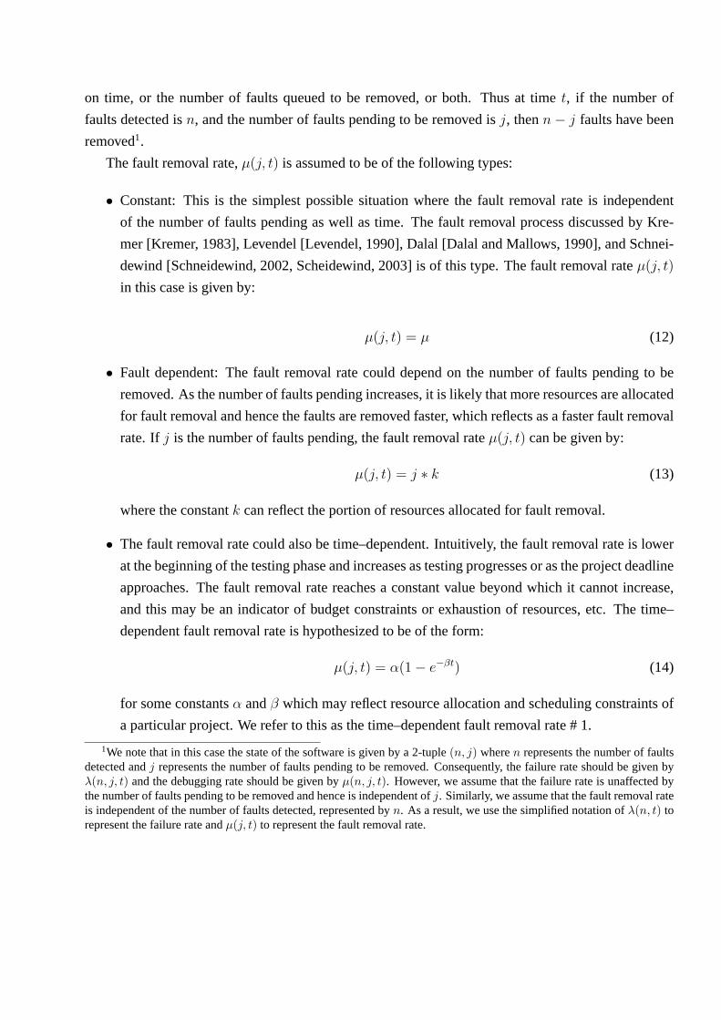
The fault removal rate,µ(j, t) is assumed to be of the following types:

• Constant: This is the simplest possible situation where the fault removal rate is independent

of the number of faults pending as well as time. The fault removal process discussed by Kre-

mer [Kremer, 1983], Levendel [Levendel, 1990], Dalal [Dalal and Mallows, 1990], and Schnei-

dewind [Schneidewind, 2002, Scheidewind, 2003] is of this type. The fault removal rateµ(j, t)

in this case is given by:

µ(j, t) = µ (12)

• Fault dependent: The fault removal rate could depend on the number of faults pending to be

removed. As the number of faults pending increases, it is likely that more resources are allocated

for fault removal and hence the faults are removed faster, which reflects as a faster fault removal

rate. Ifj is the number of faults pending, the fault removal rateµ(j, t) can be given by:

µ(j, t) = j ∗ k (13)

where the constantk can reflect the portion of resources allocated for fault removal.

• The fault removal rate could also be time–dependent. Intuitively, the fault removal rate is lower

at the beginning of the testing phase and increases as testing progresses or as the project deadline

approaches. The fault removal rate reaches a constant value beyond which it cannot increase,

and this may be an indicator of budget constraints or exhaustion of resources, etc. The time–

dependent fault removal rate is hypothesized to be of the form:

µ(j, t) = α(1− e−βt) (14)

for some constantsα andβ which may reflect resource allocation and scheduling constraints of

a particular project. We refer to this as the time–dependent fault removal rate # 1.

1We note that in this case the state of the software is given by a 2-tuple(n, j) wheren represents the number of faultsdetected andj represents the number of faults pending to be removed. Consequently, the failure rate should be given byλ(n, j, t) and the debugging rate should be given byµ(n, j, t). However, we assume that the failure rate is unaffected bythe number of faults pending to be removed and hence is independent ofj. Similarly, we assume that the fault removal rateis independent of the number of faults detected, represented byn. As a result, we use the simplified notation ofλ(n, t) torepresent the failure rate andµ(j, t) to represent the fault removal rate.

• Fault removal rate could also be time–dependent in the case of latent faults, which are inherently

harder to remove, and can be hypothesized to be:

µ(j, t) = αe−βt (15)

We refer to this as the time–dependent fault removal rate # 2.

• Time–dependent fault removal rate could also have any other functional form as dictated by the

process of a particular software project.

Fault removal activities can also be delayed to a later point in time in case of some software

development scenarios. Fault removal can be delayed based on the following two constraints:

• Fault removal can be delayed till a certain numberφ of faults are detected and are pending to be

removed.

• Fault removal may be suspended for a certain average amount of time1/µ1 after the detection

of the fault, or in other words there is an average time lag of1/µ1 units between the detection of

the fault and the initiation of its removal. Fault removal can also be delayed for a certain period

of time after testing begins, and once initiated it can proceed as per any of the fault removal

policies described above.

The fault removal rate could have any of the forms described above in case of deferred fault re-

moval.

4.2 Incorporating explicit fault removal

The finite failure NHPP models represented as a non–homogeneous continuous time Markov chain

(NHCTMC) in Section 3 are extended in this section to incorporate the various fault removal strategies

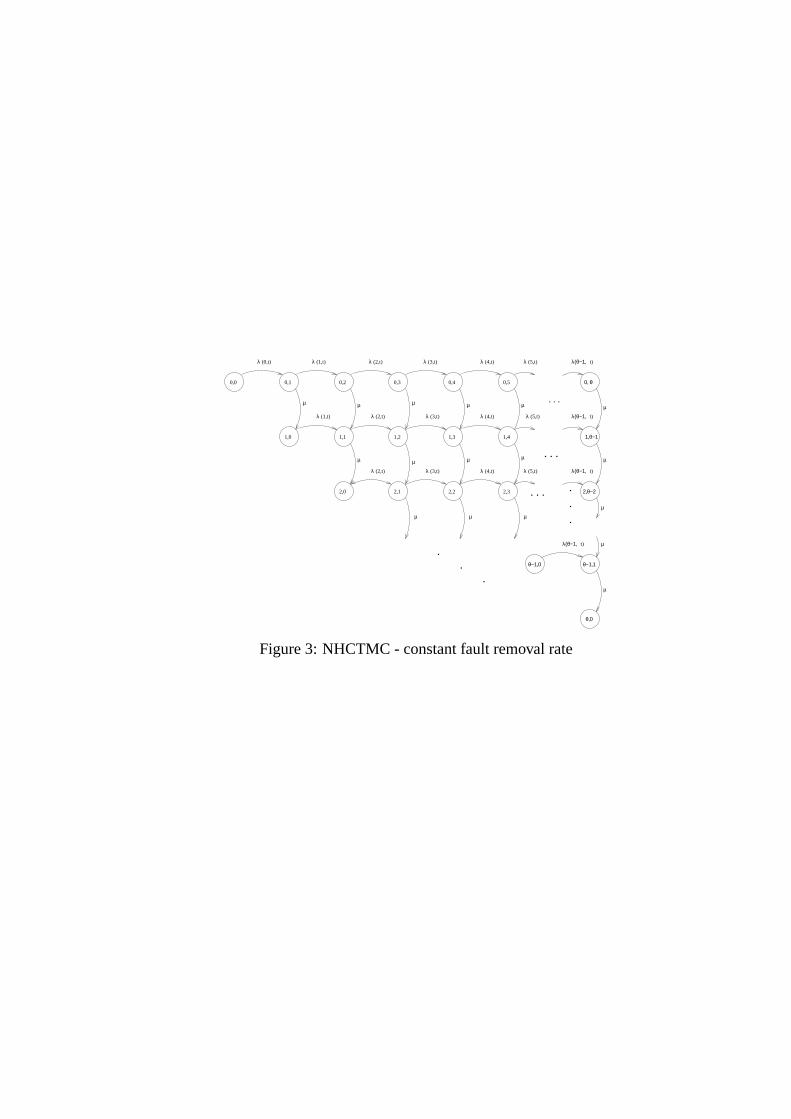
described above. The state–space of the NHCTMC in this case is a tuple(i, j), wherei is the number

of faults removed andj is the number of faults detected, and pending to be removed. The faults are

removed one at a time, and thus the detected faults form a queue up to a maximum ofθ − i, where

i is the number of faults removed andθ is as given in Equation (10). Figure 3 shows the NHCTMC

with a constant fault removal rate and Figure 4 shows the NHCTMC with a fault dependent removal

rate. Expressions for the expected number of faults removed,mR(t) and the expected number of faults

detected,mD(t), by timet in case of Figures 3, and 4 are given by Equations (16) and (17) respectively.

mR(t) =θ∑

i=0

θ−i∑

j=0

i ∗ pi,j(t) (16)

mD(t) =θ∑

i=0

θ−i∑

j=0

(i + j) ∗ pi,j(t) (17)

NHCTMC model with delayed fault removal, where the fault removal activities are delayed until a

certain numberφ of the faults are removed (fault dependent delay) is shown in Figure 5. The expected

number of faults removed,mR(t), and the expected number of faults detected,mD(t), in this case are

given by Equation (16) and Equation (17) respectively.

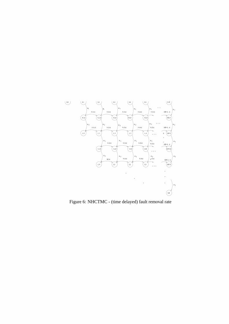
Delayed fault removal, where the fault removal activities are suspended till a certain time is elapsed

after the detection of a fault can be incorporated in the NHCTMC model using a phase type distribu-

tion [Kulkarni, 1995]. Figure 6 shows the NHCTMC where the removal is carried out in two phases.

The mean time spent in phase 1 or the idle phase is given by1/µ1, and the mean time spent in phase 2

or the phase where the actual removal activities are carried out is given by1/µ2. Thus, the mean fault

removal time1/µ is given by:

1

µ=

1

µ1

+1

µ2

(18)

In Figure 6, state (i, j, d) implies thati faults have been removed,j faults have been detected and

are queued for removal, and “d” implies intermediate phase of repair. The expected number of faults

removed,mR(t) and the expected number of faults detected,mD(t) is given by Equations (19) and

(20) respectively.

mR(t) =θ∑

i=0

θ−i∑

j=0

i ∗ (pi,j(t) + pi,j,d(t)) (19)

mD(t) =θ∑

i=0

θ−i∑

j=0

(i + j) ∗ (pi,j(t) + pi,j,d(t)) (20)

As mentioned earlier in Figures 3 through 5 ,i is the number of faults removed andj is the num-

ber of faults detected, and pending to be removed. The NHCTMC transitions either in the horizontal

direction or in the vertical direction depending on whether a fault is detected or removed. In state(i, j)

when a fault is detected the NHCTMC transitions to statej + 1, since the number of faults pending

to be removed increases by1. On the other hand, in state(i, j) if a fault is removed the NHCTMC

transitions to state(i + 1, j − 1). The former transition is governed by the failure intensity function

λ(t), and the latter transition is governed by the fault removal rate. Similar arguments hold for the

transitions shown in Figure 6, except that the state representation is given by a 3–tuple.

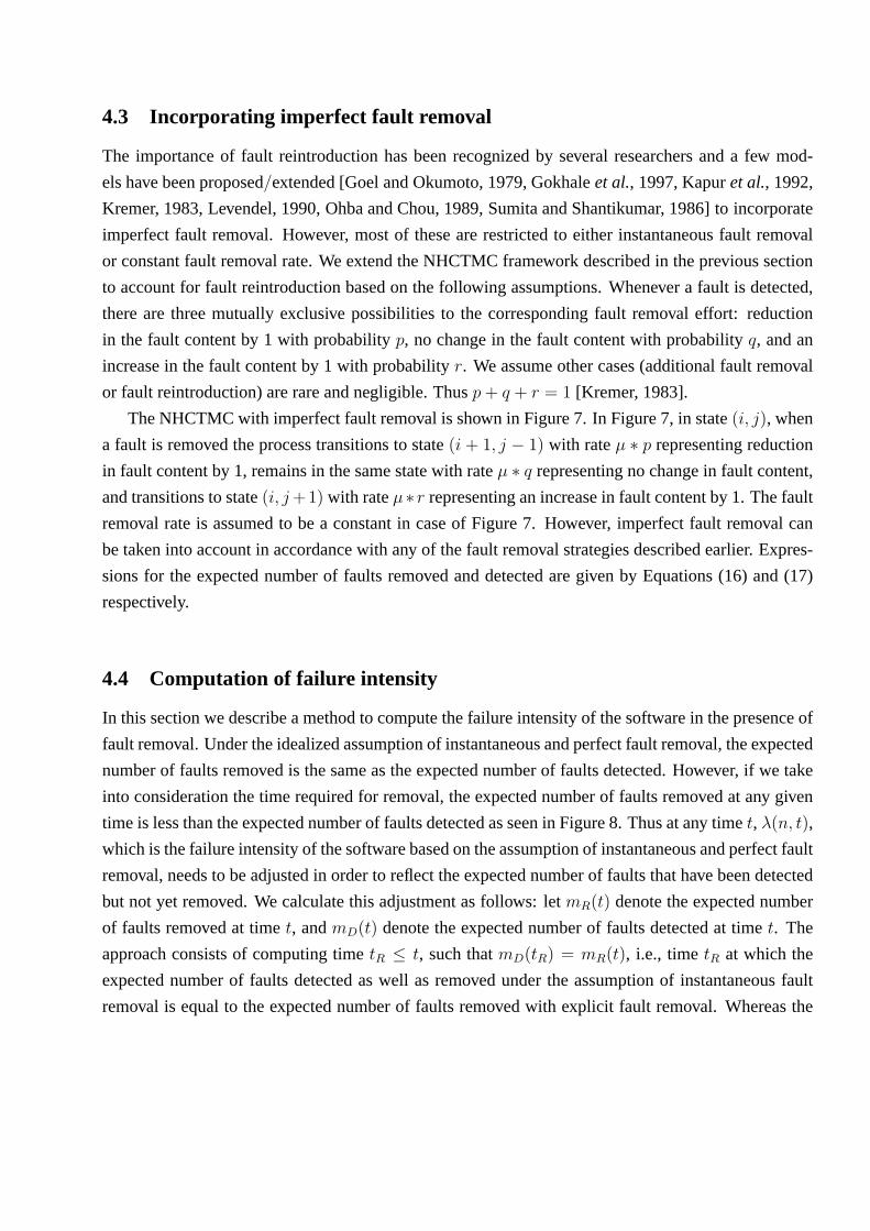
4.3 Incorporating imperfect fault removal

The importance of fault reintroduction has been recognized by several researchers and a few mod-

els have been proposed/extended [Goel and Okumoto, 1979, Gokhaleet al., 1997, Kapuret al., 1992,

Kremer, 1983, Levendel, 1990, Ohba and Chou, 1989, Sumita and Shantikumar, 1986] to incorporate

imperfect fault removal. However, most of these are restricted to either instantaneous fault removal

or constant fault removal rate. We extend the NHCTMC framework described in the previous section

to account for fault reintroduction based on the following assumptions. Whenever a fault is detected,

there are three mutually exclusive possibilities to the corresponding fault removal effort: reduction

in the fault content by 1 with probabilityp, no change in the fault content with probabilityq, and an

increase in the fault content by 1 with probabilityr. We assume other cases (additional fault removal

or fault reintroduction) are rare and negligible. Thusp + q + r = 1 [Kremer, 1983].

The NHCTMC with imperfect fault removal is shown in Figure 7. In Figure 7, in state(i, j), when

a fault is removed the process transitions to state(i + 1, j − 1) with rateµ ∗ p representing reduction

in fault content by 1, remains in the same state with rateµ ∗ q representing no change in fault content,

and transitions to state(i, j +1) with rateµ∗ r representing an increase in fault content by 1. The fault

removal rate is assumed to be a constant in case of Figure 7. However, imperfect fault removal can

be taken into account in accordance with any of the fault removal strategies described earlier. Expres-

sions for the expected number of faults removed and detected are given by Equations (16) and (17)

respectively.

4.4 Computation of failure intensity

In this section we describe a method to compute the failure intensity of the software in the presence of

fault removal. Under the idealized assumption of instantaneous and perfect fault removal, the expected

number of faults removed is the same as the expected number of faults detected. However, if we take

into consideration the time required for removal, the expected number of faults removed at any given

time is less than the expected number of faults detected as seen in Figure 8. Thus at any timet, λ(n, t),

which is the failure intensity of the software based on the assumption of instantaneous and perfect fault

removal, needs to be adjusted in order to reflect the expected number of faults that have been detected

but not yet removed. We calculate this adjustment as follows: letmR(t) denote the expected number

of faults removed at timet, andmD(t) denote the expected number of faults detected at timet. The

approach consists of computing timetR ≤ t, such thatmD(tR) = mR(t), i.e., timetR at which the

expected number of faults detected as well as removed under the assumption of instantaneous fault

removal is equal to the expected number of faults removed with explicit fault removal. Whereas the

perceived failure intensity at timet, under the assumption of instantaneous and perfect fault removal

is λ(n, t), we postulate that the actual failure intensity (failure intensity after adjustment), denoted by

λ′(n, t), can be approximately given byλ(n, tR), wheretR ≤ t. The conditiont = tR represents

the situation of instantaneous and perfect fault removal. This can be considered as a “roll-back” in

time, and is like saying that accounting for fault detection and fault removal separately up to timet is

equivalent to instantaneous and perfect fault removal up to timetR.

We illustrate this approach with the help of an example. Referring to the left plot in Figure 8,

the expected number of faults detected,mD(t), at timet = 200 is 23.16, while the expected num-

ber of faults removed at timet, mR(t) is 17.64. The failure intensity for this particular example is

assumed to be of the Goel Okumoto model and is given byλ(n, t) = 34.05 ∗ 0.0057 ∗ e−0.0057∗t.

The value oftR computed using these values is128.1. Thus if the software is released att = 200,

its perceived failure intensity would be0.0622, whereas the actual failure intensity after adjustment

would be0.093. The method discussed here was repeated for every time stepdt, and the plot on the

right in Figure 8 shows the perceived as well as the actual failure intensities for the entire time interval.

5 Numerical results

In this section we demonstrate the utility of the state–space technique to generate fault detection and

fault removal profiles, with the help of some case studies. Without loss of generality, we use the failure

intensity of the Goel Okumoto model for the case studies in this section. We estimate the parameters

of the failure intensity function of the Goel Okumoto model using data set obtained from Charles

Stark Draper Laboratories using CASRE [Lyu and Nikora, 1992]. The failure intensity used is given

by λ(n, t) = 39.0082 ∗ 0.0037 ∗ e−0.0037∗t.

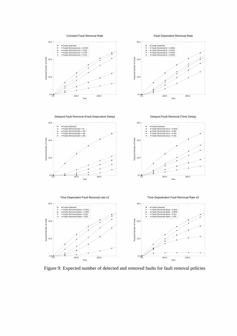
The expected number of faults detected and removed for the various fault removal policies is shown

in Figure 9. Initially, we obtain the expected number of faults detected and removed for various values

of constant fault removal rate,µ. The values of the fault removal rateµ, were set to be approximately

100%, 70%, 35% and17.5% of the maximum fault detection rate. The expected number of faults

removed decreases asµ decreases, and expectedly so. The cumulative fault removal curve has a form

similar to the cumulative fault detection curve, and as the fault removal rate increases, the fault re-

moval curve almost follows the fault detection curve. We then obtain the expected number of faults

removed as a function of time, when the fault removal rate depends on the number of pending faults

(Equation(13)). The expected number of faults removed is directly related to the proportionality con-

stantk in Equation (13). The fault removal rate in this case does not have a closed form expression but

can be computed by assigning appropriate reward rates to the states of the NHCTMC. Ask increases,

the expected number of faults removed increases. The expected number of faults detected and removed

as a function of time for time–dependent fault removal rate #1 as given by Equation (14) was obtained

next. The value ofα is held at0.15, which is approximately the maximum value of the fault detection

rate. The cumulative fault removal curve in this case is also similar to the cumulative fault detection

curve, and the difference between the expected number of detected and removed faults depends on the

value ofβ. Asβ increases, the fault removal rate increases and the expected number of faults removed

increases. The expected number of faults removed for time–dependent fault removal rate #2 as given

in Equation (15) was then obtained. In this case, as the value ofβ increases, the fault removal rate

decreases and the expected number of faults removed decreases. The expected number of faults de-

tected and removed as a function of time for delayed fault removal, where the expected delay between

the detection of the fault and the initiation of its removal isµ1 units, was obtained next. The expected

number of faults removed decreases with increasingµ1. The expected number of faults detected and

removed for delayed fault removal where fault removal begins only after a certain number of faultsφ

are accumulated was obtained next, for different values ofφ, setting the fault removal rateµ to be0.1.

As φ increases, the expected number of faults removed decreases.

Figure 9 depicts that for higher values of fault removal rates, the fault removal profile follows the

fault detection profile very closely, and the estimates of the residual number of faults based on the

idealized assumption of instantaneous fault removal are close to the ones with explicit fault removal.

However, as the fault removal rate increases the fault removal resources could be under utilized. For

the sake of illustration, we measure the utilization of the fault removal resources in case of the con-

stant fault removal rate. This can be achieved easily by assigning proper rewards to the states of the

NHCTMC. The utilization is shown in Figure 10. As seen from the figure, for higher values ofµ,

the utilization is low, and the debugging resources are not used up to their complete capacity for an

extended period of time. This may not be very cost effective, especially with increasing budget and

deadline constraints facing modern software development organizations. Incorporating explicit fault

removal into the software reliability growth models can thus be used to guide decision making about

the allocation of resources to the crucial, but perhaps the most important activity of fault removal,

so that a maximum number of faults are detected and removed before the shipment of the software

product in a cost effective manner.

Figure 11 shows the expected number of faults removed for different values ofp, q andr, in case

of imperfect fault removal. The figure shows that the expected number of faults removed decreases as

the probability of perfect fault removalp decreases.

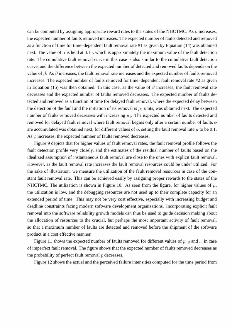
Figure 12 shows the actual and the perceived failure intensities computed for the time period from

t = 0 to t = 275 using the method explained in Section 4.4. As can be seen from the figure, the actual

failure intensity which accounts for fault removal is higher than the perceived failure intensity which

relies on the assumption of instantaneous repair. Thus if the software were to be released att = 275

time units its actual failure intensity would be0.0633 while its perceived failure intensity would be

0.0522.

The key points observed from the numerical results can be summarized as follows:

• The fault removal profile closely follows the fault detection profile for high values of fault re-

moval rates. However, for very high fault removal rates the fault removal resources are severely

under utilized which could lead to an inefficient use of the overall resources.

• The number of faults removed decreases as the probability of perfect fault removal decreases.

Thus, the residual fault density in the software depends not only on the fault detection and fault

removal rates, but is also affected by the probability of perfect fault removal.

• The actual failure intensity of the software (taking into account explicit fault removal) is higher

than the perceived failure intensity of the software, which does not consider the effects of fault

removal process explicitly. As a result, budget and software release time decisions based on the

perceived failure intensity rather than the actual failure intensity may tend to be optimistic.

The NHCTMC framework incorporating explicit and imperfect fault removal could be used in a

variety of ways. At the end of the testing phase it could be used to obtain an estimate of the residual

number of faults in the software. More importantly, it could be used to obtain a realistic estimate of the

optimal testing time, when costs justify the stop test decision [Gokhale, 2003]. The framework could

also be used for predictive or forecasting purposes to analyze the impact of various factors such as the

impact of additional testing, and the impact of delayed or deferred fault removal. For such analysis,

the solution of the model can be obtained for the desired parameter values. These parameters include

the length of the time interval of testing, the fault removal rate, and the duration of the interval for

which fault removal is to be deferred.

6 Conclusions

In this paper we have proposed a framework to account for explicit fault removal along with fault

reintroduction into the finite failure software reliability growth models. This framework is based on

the state–space view of non–homogeneous Poisson processes, and relies on numerical techniques to

obtain the mean value function of the NHPP. An analysis of different fault removal strategies is also

presented. We describe a method to compute the failure intensity of the software taking into consider-

ation explicit fault removal, which accounts for the faults which have been detected but not removed.

Models with explicit fault removal can be used to obtain realistic estimates of the residual number of

faults in the software, as well as the failure intensity of the software and hence guide decision making

about the allocation of resources in order to achieve timely release of the software.

References

[Dalal and Mallows, 1990] S. R. Dalal and C. L. Mallows. “Some graphical aids for deciding when

to stop testing software”.IEEE Trans. on Software Engineering, 8(2):169–175, February 1990.

[Defamieet al., 1999] M. Defamie, P. Jacobs, and J. Thollembeck. “Software reliability: Assump-

tions, realities and data”. InProc. of International Conference on Software Maintenance, September

1999.

[Farr, 1996] W. Farr.Handbook of Software Reliability Engineering, M. R. Lyu, Editor, chapter “Soft-

ware Reliability Modeling Survey”, pages 71–117. McGraw-Hill, New York, NY, 1996.

[Goel and Okumoto, 1979] A. L. Goel and K. Okumoto. “Time–dependent error–detection rate mod-

els for software reliability and other performance measures”.IEEE Trans. on Reliability, R-

28(3):206–211, August 1979.

[Goel, 1985] A. L. Goel. “Software reliability models: Assumptions, limitations and applicability”.

IEEE Trans. on Software Engineering, SE-11(12):1411–1423, December 1985.

[Gokhale and Trivedi, 1998] S. Gokhale and K. S. Trivedi. “Log-logistic software reliability growth

model”. In Proc. of High Assurance Systems Engineering (HASE 98), pages 34–41, Washington,

DC, November 1998.

[Gokhale and Trivedi, 1999] S. Gokhale and K. S. Trivedi. “A time/structure based software reliability

model”. Annals of Software Engineering, 8:85–121, 1999.

[Gokhaleet al., 1996] S. Gokhale, T. Philip, P. N. Marinos, and K. S. Trivedi. “Unification of finite

failure non-homogeneous Poisson process models through test coverage”. InProc. Intl. Sypmosium

on Software Reliability Engineering (ISSRE 96), pages 289–299, White Plains, NY, October 1996.

[Gokhaleet al., 1997] S. Gokhale, P. N. Marinos, K. S. Trivedi, and M. R. Lyu. “Effect of repair

policies on software reliability”. InProc. of Computer Assurance (COMPASS 97), pages 105–116,

Gatheirsburg, Maryland, June 1997.

[Gokhale, 2003] S. Gokhale. “Optimal software release time incorporating fault correction”. InProc.

of 28th IEEE/NASA Workshop on Software Engineering, Annapolis, MD, December 2003.

[Jelinski and Moranda, 1972] Z. Jelinski and P. B. Moranda.Statistical Computer Performance Eval-

uation, ed. W. Freiberger, chapter Software Reliability Research, pages 465–484. Academic Press,

New York, 1972.

[Kapuret al., 1992] P. K. Kapur, K. D. Sharma, and R. B. Garg. “Transient solutions of software

reliability model with imperfect debugging and error generation”.Microelectronics and Reliability,

32(1):475–478, April 1992.

[Kenney, 1993] G. Q. Kenney. “Estimating defects in commercial software during operational use”.

IEEE Trans. on Reliability, 42(1):107–115, January 1993.

[Kremer, 1983] W. Kremer. “Birth and death bug counting”.IEEE Trans. on Reliaability, R-32(1):37–

47, April 1983.

[Kulkarni, 1995] V. G. Kulkarni.Modeling and Analysis of Stochastic Systems. Chapman-Hall, New

York, 1995.

[Levendel, 1990] Y. Levendel. “Reliability analysis of large software systems: Defect data modeling”.

IEEE Trans. on Software Engineering, 16(2):141–152, February 1990.

[Lyu and Nikora, 1992] M. R. Lyu and A. P. Nikora. “CASRE-A computer-aided software reliability

estimation tool”. InCASE ’92 Proceedings, pages 264–275, Montreal, Canada, July 1992.

[Ohba and Chou, 1989] M. Ohba and X. Chou. “Does imperfect debugging affect software reliability

growth ?”. InProc. of Intl. Conference on Software Engineering, pages 237–244, April 1989.

[Ramaniet al., 1998] S. Ramani, S. Gokhale, and K. S. Trivedi. “SREPT: Software Reliability Esti-

mation and Prediction Tool”. In10th International Conference on Modelling Techniques and Tools

for Computer Performance Evaluation - Performance Tools 98, pages 27–36, Palma de Mallorca,

Spain, September 1998.

[Sahneret al., 1996] R. A. Sahner, K. S. Trivedi, and A. Puliafito.Performance and Reliability Anal-

ysis of Computer Systems: An Example-Based Approach Using the SHARPE Software Package.

Kluwer Academic Publishers, Boston, 1996.

[Scheidewind, 2003] N. F. Scheidewind. “Fault correction profiles”. InProc. of Intl. Symposium on

Software Reliability Engineering, pages 257–267, Denver, CO, November 2003.

[Schneidewind, 2002] N. F. Schneidewind. “An integrated failure detection and fault correction

model”. InProc. of Intl. Conference on Software Maintenance, pages 238–241, December 2002.

[Sumita and Shantikumar, 1986] U. Sumita and G. Shantikumar. “A software reliability model with

multiple-error introduction and removal”.IEEE Trans. on Reliability, R-35(4):459–462, October

1986.

[Trivedi, 2001] K. S. Trivedi.Probability and Statistics with Reliability, Queuing and Computer Sci-

ence Applications. John Wiley, 2001.

[Wood, 1997] A. Wood. “Software reliability growth models: Assumptions vs. reality”. InProc.

of Eigth Intl. Symposium on Software Reliability Engineering, pages 136–141, Albuquerque, NM,

November 1997.

[Yamadaet al., 1983] S. Yamada, M. Ohba, and S. Osaki. “S-shaped reliability growth modeling for

software error detection”.IEEE Trans. on Reliability, R-32(5):475–485, December 1983.

...0 1 2λ λ λ(t) (t) (t)

Figure 1: Non-homogeneous Markov chain for NHPP models

0 100 2000

10

20

30

Exp

ecte

d N

umbe

r of

Fau

lts

GO Model

AnalyticalNHCTMC

0 100 200Time

0

10

20

30

Exp

ecte

d N

umbe

r of

Fau

lts

Generalized GO Model

AnalyticalNHCTMC

0 100 2000

10

20

30

Exp

ecte

d N

umbe

r of

Fau

lts

S−shaped model

AnalyticalNHCTMC

0 100 200Time

0

10

20

30

Exp

ecte

d N

umbe

r of

Fau

lts

Log−logistic Model

AnalyticalNHCTMC

Figure 2: Comparison of analytical and numerical mean value functions

0,0 0,1 0,2 0,3 0,4 0,5

1,0 1,1 1,2 1,3 1,4

2,0 2,1 2,2 2,3

λ λ λ λ λ λ

λ λ λ λ λ

λ λ λ λ

µ µ µ µ µ µ

µ µ µ µ

µ

µ

µ

µ

µ µ µ

. . .

. . .

..

.

. . . .

.

.

0, θ

2,θ−2

θ−1,1

θ,0

θ−1,0

1,θ−1

(0,t) (1,t) (2,t) (3,t) (4,t) (5,t) λ(θ−1, t)

(1,t) (2,t) (3,t) (4,t) (5,t) λ(θ−1, t)

(2,t) (3,t) (4,t) (5,t) λ(θ−1, t)

λ(θ−1, t)

Figure 3: NHCTMC - constant fault removal rate

0,0 0,1 0,2 0,3 0,4 0,5

1,0 1,1 1,2 1,3 1,4

2,0 2,1 2,2 2,3

λ λ λ λ λ λ

λ λ λ λ λ

λ λ λ λ

. . .

. . .

..

.

. . . .

.

.

2 3 4 5 a

2 3 4 (a-1)

2 3 (a-2)

2

µ µ µ µ µ µ

µ µ µ µ µ

µ µ µ µ

µ

µ

0,θ

2,θ−2

1,θ−1

θ−1,1

θ, 0

θ−1,0

(0.t) (1,t) (2,t) (3,t) (4,t) (5,t)

(1,t) (2,t) (3,t) (4,t) (5,t)

(2,t) (3,t) (4,t) (5,t)

λ(θ−1, t)

λ(θ−1, t)

λ(θ−1, t)

λ(θ−1, t)

Figure 4: NHCTMC - fault dependent removal rate

0,0 0,1 0,2

µ µ µ

µ µ µ

µ

µ

µ µ

µ

. . .

. . .

. . .

.

.

.

. . .

0,θ

1,θ−1

θ−1,1

0.θ

θ−1,0

0,φ

1,φ−1 1,φ

φ,0 φ,1

0,φ+1

φ,θ−φ

λ λ(0,t) (1,t) λ(φ−1, t) λ(φ, t) λ(φ+1, t) λ(θ−1, t)

λ(θ−1, t)λ(φ, t) λ(φ+1, t)

λ(φ, t) λ(φ+1, t) λ(θ−1, t)

λ(θ−1, t)

Figure 5: NHCTMC - delayed (fault dependent delay) fault removal rate

0,0 0,1 0,2 0,3 0,4 0,5

λ λ λ λ λ λ

λ λ λ λ λ

λ λ λ λ

µ µ µ µ µ µ

µ µ µ µµ

µ µ µ

. . .

. . .

. . . .

.

.

0,1,d 0,.2,d 0,3,d 0,4,d 0,5,d

λ

1, 0 1, 1 1, 2 1, 3 1, 4

1,1,d 1,2,d 1,3,d 1,4,d

2, 0 2,1 2,2 2,3

µ

µ µ µ µ µ

1 1 1 1 1

1 1 1 1

2 2 2 2 2

2 2 2 2 2µ 2

λ λ λ λ

λ λ λ λ

µ 1

µ 2

. . .

. . .

.

.

..

.

.

.

.

0. θ

0,θ, d

1,θ−1

1,θ−1,d

2,θ−2

0.θ

1

(0,t) (1,t) (2,t) (3,t) (4,t) (5,t)

(1,t) (2,t) (3,t) (4,t) (5,t)

(1,t) (2,t) (3,t) (4,t) (5,t)

(2,t) (3,t) (4,t) (5,t)

(2,t) (3,t) (4,t) (5,t)

λ(θ−1, t)

λ(θ−1, t)

λ(θ−1, t)

λ(θ−1, t)

λ(θ−1, t)

Figure 6: NHCTMC - (time delayed) fault removal rate

0,0 0,1 0,2 0,3 0,4 0,5

1,0 1,1 1,2 1,3 1,4

2,0 2,1 2,2 2,3

a-1,0

λ λ λ λ λ λ

λ λ λ λ λ

λ λ λ λ

µ

µ

µ

µ

µ

µ µ µ

µ µ µ µ µ

µ µ µ µ

µ µ µ

µ

µ µ µ µ µ

µ µ µ µ2

µ

µ

µ

µ

. . .

. . .

. . .

..

.

.

.

.* p

* r * r * r * r * r * r

* r * r* r* r* r

* r * r * r * r

* r

* p * p * p * p * p

* p * p * p * p

* p * p * p

* p

* p

* p

* p

* p

0,θ

1,θ

2,θ−2

θ−1,1

θ,0

(0.t) (1,t) (2,t) (3,t) (4,t) (5,t)

(1,t) (2,t) (3,t) (4,t) (5,t)

(2,t) (3,t) (4,t) (5,t)

λ(θ−1, t)

λ(θ−1, t)

λ(θ−1, t)

λ(θ−1, t)

Figure 7: NHCTMC with imperfect repair

0 100 2000

10

20

30

Exp

ecte

d N

umbe

r of

Fau

lts

Expected Number of Faults vs. Time

Faults detectedFaults removed

0 100 2000

0.05

0.1

0.15

0.2

Fai

lure

inte

nsiti

es

Actual and Perceived Failure Intensities

PerceivedActual

Figure 8: An example for failure intensity adjustment

0.0 100.0 200.0Time

0.0

10.0

20.0

30.0

Exp

ecte

d N

umbe

r of

Fau

lts

Constant Fault Removal Rate

Faults DetectedFaults Removed (mu = 0.025)Faults Removed (mu = 0.05)Faults Removed (mu = 0.10)Faults Removed (mu = 0.15)

0.0 100.0 200.0Time

0.0

10.0

20.0

30.0

Exp

ecte

d N

umbe

r of

Fau

lts

Fault Dependent Removal Rate

Faults DetectedFaults Removed (k = 0.006)Faults Removed (k = 0.012)Faults Removed (k = 0.018)Faults Removed (k = 0.024)

0.0 100.0 200.0Time

0.0

10.0

20.0

30.0

Exp

ecte

d N

umbe

r of

Fau

lts

Delayed Fault Removal (Fault Dependent Delay)

Faults DetectedFaults Removed (phi = 5)Faults Removed (phi = 10)Faults Removed (phi = 15)Faults Removed (phi = 20)

0.0 100.0 200.0Time

0.0

10.0

20.0

30.0

Exp

ecte

d N

umbe

r of

Fau

lts

Delayed Fault Removal (Time Delay)

Faults DetectedFaults Removed (mu1 = 0.025)Faults Removed (mu1 = 0.05)Faults Removed (mu1 = 0.10)Faults Removed (mu1 = 0.15)

0.0 100.0 200.0Time

0.0

10.0

20.0

30.0

Exp

ecte

d N

umbe

r of

Fau

lts

Time Dependent Fault Removal rate #1

Faults DetectedFaults Removed (beta = 0.001)Faults Removed (beta = 0.005)Faults Removed (beta = 0.01)Faults Removed (beta = 0.05)

0.0 100.0 200.0Time

0.0

10.0

20.0

30.0

Exp

ecte

d N

umbe

r of

Fau

lts

Time Depedndent Fault Removal Rate #2

Faults DetectedFaults Removed (beta = 0.001)Faults Removed (beta = 0.005)Faults Removed (beta = 0.01)Faults Removed (beta = 0.05)

Figure 9: Expected number of detected and removed faults for fault removal policies

0.0 100.0 200.0Time

0.0

0.2

0.4

0.6

0.8

1.0

Util

izat

ion

Utilization vs. Time

mu = 0.025mu = 0.05mu = 0.1mu = 0.15

Figure 10: Utilization for constant fault removal rate

0.0 100.0 200.0Time

0.0

10.0

20.0

30.0

Exp

ecte

d N

umbe

r of

Fau

lts

Imperfect Fault Removal

p=1.0p=0.8, q=0.2p=0.8, q=0.1p=0.4, r=0.5

Figure 11: Expected number of faults removed for imperfect fault removal

0 100 2000

0.02

0.04

0.06

0.08

0.1

0.12

0.14

0.16

0.18

0.2

Fai

lure

Inte

nsity

Actual and Perceived Failure Intensity

ActualPerceived

Figure 12: Actual and perceived failure intensities

Biographies

Swapna S. Gokhalereceived B.E.(Hons.) in Electrical and Electronics Engineering and Computer

Science from the Birla Institute of Technology and Science, Pilani, India in June 1994, and MS and

PhD in Electrical and Computer Engineering from Duke University in September 1996 and Septem-

ber 1998 resectively. Currently, she is an Assistant Professor in the Dept. of Computer Science and

Engineering at the University of Connecticut. Prior to joining UConn, she was a Research Scientist

at Telcordia Technologies in Morristown, NJ. Her research interests include software reliability and

performance, software testing, software maintenance, program comprehension and understanding, and

wireless and multimedia networking.

Dr. Michael R. Lyu is currently an Associate Professor at the Computer Science and Engineering

department of the Chinese University of Hong Kong. He worked at the Jet Propulsion Laboratory

as a Technical Staff Member from 1988 to 1990. From 1990 to 1992 he was with the Electrical and

Computer Engineering Department at the University of Iowa as an Assistant Professor. From 1992 to

1995, he was a Member of the Technical Staff in the Applied Research Area of the Bell Communi-

cations Research (Bellcore). From 1995 to 1997 he was a research Member of the Technical Staff at

Bell Labs., which was first part of AT&T and later became part of Lucent Technologies. Dr. Lyu’s

research interests include software reliability engineering, distributed systems, fault-tolerant comput-

ing, wireless communication networks, Web technologies, digital library, and electronic commerce.

He has published over 90 refereed journal and conference papers in these areas.

Kishor S. Trivedi received the B.Tech. degree from the Indian Institute of Technology (Bombay), and

M.S. and Ph.D. degrees in computer science from the University of Illinois, Urbana-Champaign. He

holds the Hudson Chair in the Department of Electrical and Computer Engineering at Duke University,

Durham, NC. He also holds a joint appointment in the Department of Computer Science at Duke. His

research interests are in reliability and performance assessment of computer and communication sys-

tems. He has published over 300 articles and lectured extensively on these topics. He has supervised

37 Ph.D. dissertations. He is the author of a well known text entitled, Probability and Statistics with

Reliability, Queuing and Computer Science Applications, originally published by Prentice-Hall, with

a thoroughly revised second edition being published by John Wiley. He is a Fellow of the Institute of

Electrical and Electronics Engineers. He is a Golden Core Member of IEEE Computer Society.