


Bahasa
Halaman
Hukum

Heriot-Watt University Research Gateway
A reconfigurable multi-mode mobile parallel robot
Citation for published version:Tian, Y, Zhang, D, Yao, YA, Kong, X & Li, Y 2017, 'A reconfigurable multi-mode mobile parallel robot',Mechanism and Machine Theory, vol. 111, pp. 39-65.https://doi.org/10.1016/j.mechmachtheory.2017.01.003
Digital Object Identifier (DOI):10.1016/j.mechmachtheory.2017.01.003
Link:Link to publication record in Heriot-Watt Research Portal
Document Version:Peer reviewed version
Published In:Mechanism and Machine Theory
General rightsCopyright for the publications made accessible via Heriot-Watt Research Portal is retained by the author(s) and /or other copyright owners and it is a condition of accessing these publications that users recognise and abide bythe legal requirements associated with these rights.
Take down policyHeriot-Watt University has made every reasonable effort to ensure that the content in Heriot-Watt ResearchPortal complies with UK legislation. If you believe that the public display of this file breaches copyright pleasecontact [email protected] providing details, and we will remove access to the work immediately andinvestigate your claim.
Download date: 13. Feb. 2022
1
Abstract—In this paper we put forward the idea of deforming the
geometry of a parallel mechanism such that it can operate either as an
equivalent rolling robot or quadruped robot. Based on it, we present a
novel mobile parallel robot that can change its locomotion modes via
different equivalent mechanisms. The robot is in essence a four-arm
parallel mechanism in which each arm contains five revolute (R) joints.
The axes of the three internal R joints in any arm are parallel and are
orthogonal to those of the end joints. Based on singularity and
deformation analysis, we show that the upper platform has four
practical operation modes, (i.e., translation, planar, rotational, and
locked-up modes). Using these operation modes, the robot can realize
rolling, tumbling and quadruped locomotion modes by deforming into
switching states. The switching configurations of the robot are further
identified in which the robot can switch among different locomotion
modes, such that the robot can choose its mode to adapt complex
terrains. To verify the functionality of the robot, we present the results
of a series of simulations, and perform the locomotion modes’
experiments on a manufactured prototype.
Index Terms—Parallel mechanism, folding mechanism,
quadruped robot, reconfigurable robot, rolling motion, multiple
locomotion modes.
I. INTRODUCTION
HERE are many classes of mobile robots with different
characteristics. Legged robot can achieve walking,
crawling, running and jumping by alternatively changing
the supporting legs on the ground. This enables it to flexibly
explore different environments, but its walking efficiency is
lower and the control system is usually very complicated [1-3].
To enhance the walking capability of the robot in different
working environments, hybrid robot was presented that
constructed by integrating different walking devices together
(e.g., wheel-legged robots [4-10], track-legged robots [11],
wheel-track-legged robots [12]). But such a combination
usually increases the weight and volume of the robot, which
makes it less swift [3].
This work has been supported by National Natural Science Foundation of
China (51175030), and the Natural Sciences and Engineering Research Council
of Canada (NSERC).
Y. B. Tian is with Faculty of Engineering and Applied Science, University of Ontario Institution of Technology (UOIT), Canada.
(email:[email protected])
Dan Zhang, Y. A. Yao and Y. Z. Li are with the School of Mechanical, Electronic and Control Engineering in Beijing Jiaotong University, Beijing
100044, China (e-mail: [email protected], yayao@bjtu,edu.cn;
[email protected]). X. W, Kong is with the Department of Engineering and Physical Sciences,
Heriot-Watt University, United Kingdom (email: [email protected])
* Corresponding author
Different from hybrid robots, several mobile robots can
realize different locomotion modes by using reconfigurable
methods, which can switch among the locomotion modes of
rolling, walking and snake-like crawling, by changing the
topology of the robot properly [13-16]. However, the DOFs of a
these robots are usually very large, and the modules are
required to divide and re-connect to change their locomotion
modes. This highly limits the switching speed and increases the
control difficulty.
Without modular units, some deformable mobile robots can
obtain multiple locomotion modes by deforming their bodies or
entire shapes into various topology structures. For example,
soft robots composed of multiple loops, can roll, crawl, or jump
by changing the shapes of loops [17, 18]. Some legged robots
can switch their locomotion modes by deforming the legs into a
wheel [19], disk [20] or sphere [21], such that the legged robots
can achieve wheeled or spherical rolling motion.
In additional, parallel mechanisms have also been used to
realize different locomotion modes (e. g., walking mode
[22-24], biped mode [25-28], rolling mode [29-33], crawling
mode [34, 35], and worm-like mode [36]). However, the
locomotion mode of each of these mobile robots is fixed and the
working space is very small, that strictly limits the robot in
accommodating different road conditions. To improve the
capability of parallel mechanisms, a plenty of parallel
mechanisms with multiple operation modes were presented [37,
38]. Several lower DOF parallel robots can realize multiple
motion modes, e.g. rotational, translation, planar, or spherical
motions etc. Based on different operation modes, we further
presented two mobile parallel robots with two different
locomotion modes [39, 40]. We also used metamorphic
methods to make single loop linkages realize different
locomotion modes by changing their gestures. For example, we
presented a mobile parallelogram mechanism that can slide or
crawl on the ground [41], and used a spatial 8R linkage to
realize biped and rolling locomotion [42].
In this paper, we present a parallel robot that can deform into
a rolling and quadruped robot, which can significantly improve
the capability of a mobile robot. We mainly focus on the
mechanical design and the locomotion analysis of the robot.
We will show that the robot can be deformed into equivalent
open-chain mechanisms or planar closed-loop mechanisms by
controlling its singularity positions. Using different
mechanisms, this robot can mobile by rolling, tumbling, and
quadruped modes. Each of these modes can be quickly
switched at its singularity positions for adapting different
environments. Furthermore, our robot can be folded into three
compact forms, which may be useful for storage or hiding itself
A Reconfigurable Multi-mode Mobile Parallel
Robot
Yaobin Tian, Dan Zhang*, Yan-An Yao
*, Xianwen Kong, and Yezhuo Li
T
2
in performing some dangerous tasks.
The rest of the paper is organized as follows. The design and
operation modes analysis of the parallel mechanism are
introduced in Sec. 2. Section 3 analyzes the different
locomotion modes of the robot. Section 4 gives the switching
methods of the rolling, tumbling and quadruped modes. Section
5 presents the results of locomotion tests and folding functions
on a physical prototype. The conclusions and brief discussions
close the paper in Sec. 6.
II. MECHANISM DESIGN
In this section, we first introduce the design of the mobile
parallel robot. Then, based on the mobility and singularity
analysis, we show that the upper platform has four typical
operation modes. Using these modes, the robot can be viewed
as a parallel manipulator to realize some special movements.
A. Description of mechanism
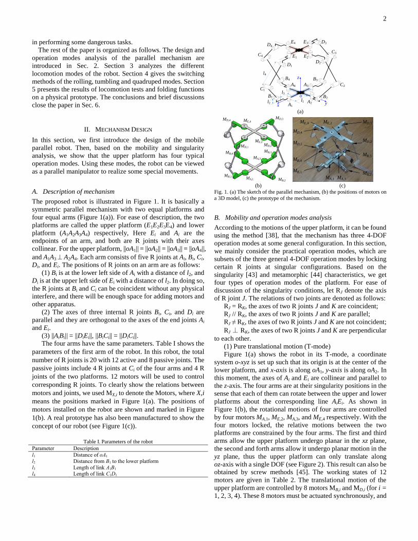
The proposed robot is illustrated in Figure 1. It is basically a
symmetric parallel mechanism with two equal platforms and
four equal arms (Figure 1(a)). For ease of description, the two
platforms are called the upper platform (E1E2E3E4) and lower
platform (A1A2A3A4) respectively, Here Ei and Ai are the
endpoints of an arm, and both are R joints with their axes
collinear. For the upper platform, ||oA1|| = ||oA2|| = ||oA3|| = ||oA4||,
and A1A3 A2A4. Each arm consists of five R joints at Ai, Bi, Ci,
Di, and Ei. The positions of R joints on an arm are as follows:
(1) Bi is at the lower left side of Ai with a distance of l2, and
Di is at the upper left side of Ei with a distance of l2. In doing so,
the R joints at Bi and Ci can be coincident without any physical
interfere, and there will be enough space for adding motors and
other apparatus.
(2) The axes of three internal R joints Bi, Ci, and Di are
parallel and they are orthogonal to the axes of the end joints Ai
and Ei.
(3) ||AiBi|| = ||DiEi||, ||BiCi|| = ||DiCi||.
The four arms have the same parameters. Table I shows the
parameters of the first arm of the robot. In this robot, the total
number of R joints is 20 with 12 active and 8 passive joints. The
passive joints include 4 R joints at Ci of the four arms and 4 R
joints of the two platforms. 12 motors will be used to control
corresponding R joints. To clearly show the relations between
motors and joints, we used MX,i to denote the Motors, where X,i
means the positions marked in Figure 1(a). The positions of
motors installed on the robot are shown and marked in Figure
1(b). A real prototype has also been manufactured to show the
concept of our robot (see Figure 1(c)).
Table I. Parameters of the robot
Parameter Description
l1 Distance of oA1
l2 Distance from B1 to the lower platform
l3 Length of link A1B1 l4 Length of link C1D1
(a)
(b) (c)
Fig. 1. (a) The sketch of the parallel mechanism, (b) the positions of motors on
a 3D model, (c) the prototype of the mechanism.
B. Mobility and operation modes analysis
According to the motions of the upper platform, it can be found
using the method [38], that the mechanism has three 4-DOF
operation modes at some general configuration. In this section,
we mainly consider the practical operation modes, which are
subsets of the three general 4-DOF operation modes by locking
certain R joints at singular configurations. Based on the
singularity [43] and metamorphic [44] characteristics, we get
four types of operation modes of the platform. For ease of
discussion of the singularity conditions, let RJ denote the axis
of R joint J. The relations of two joints are denoted as follows:
RJ = RK, the axes of two R joints J and K are coincident;
RJ // RK, the axes of two R joints J and K are parallel;
RJ ≠ RK, the axes of two R joints J and K are not coincident;
RJ ⊥ RK, the axes of two R joints J and K are perpendicular
to each other.
(1) Pure translational motion (T-mode)
Figure 1(a) shows the robot in its T-mode, a coordinate
system o-xyz is set up such that its origin is at the center of the
lower platform, and x-axis is along oA1, y-axis is along oA2. In
this moment, the axes of Ai and Ei are collinear and parallel to
the z-axis. The four arms are at their singularity positions in the
sense that each of them can rotate between the upper and lower
platforms about the corresponding line AiEi. As shown in
Figure 1(b), the rotational motions of four arms are controlled
by four motors MA,1, ME,2, MA,3, and ME,4 respectively. With the
four motors locked, the relative motions between the two
platforms are constrained by the four arms. The first and third
arms allow the upper platform undergo planar in the xz plane,
the second and forth arms allow it undergo planar motion in the
yz plane, thus the upper platform can only translate along
oz-axis with a single DOF (see Figure 2). This result can also be
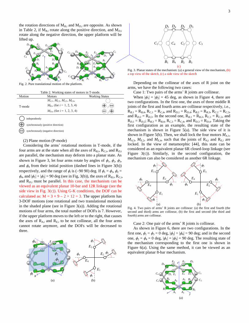
obtained by screw methods [45]. The working states of 12
motors are given in Table 2. The translational motion of the
upper platform are controlled by 8 motors MB,i and MD,i (for i =
1, 2, 3, 4). These 8 motors must be actuated synchronously, and
x y
z
o
A1A2
A3A4
B1 B2
B3B4
D1
C2
C3C4
D2
D3D4
E1 E2
E4
C1
E3
l1
l3
l2
l4
MA,1
MA,3
MB,1
MB,2
MB,3MB,4
MD,4MD,3
MD,2MD,1
ME,4
ME,2
MA,1 MA,3
ME,2ME,4
MB,1
MD,1
MB,2
MD,2
MD,4
MD,3
MB,4
MB,3
3
the rotation directions of MB,i and MD,i are opposite. As shown
in Table 2, if MB,i rotate along the positive direction, and MD,i
rotate along the negative direction, the upper platform will be
lifted up.
Fig. 2. Pure translational motion of the platform.
Table 2. Working states of motors in T-mode.
Motion Motors Working States
T-mode
MA,1, ME,2, MA,3, ME,4,
MB,i, (for i = 1, 2, 3, 4) /
MD,i, (for i = 1, 2, 3, 4) /
(2) Plane motion (P-mode)
Considering the arms’ rotational motions in T-mode, if the
four arms are at the state when all the axes of RB,i, RC,i, and RD,i
are parallel, the mechanism may deform into a planar state. As
shown in Figure 3, let four arms rotate by angles of 1, 2, 3,
and 4 from their initial position (dashed lines in Figure 3(b))
respectively, and the range of i is (90 90) deg. If 1 = 3, 2 =
4, and |1| + |2| = 90 deg (see in Fig, 3(b)), the axes of RB,i, RC,i,
and RD,i must be parallel. In this case, the mechanism can be
viewed as an equivalent planar 10-bar and 12R linkage (see the
side view in Fig. 3(c)). Using G-K conditions, the DOF can be
calculated as: M = 3 × 9 2 × 12 = 3. The upper platform has
3-DOF motions (one rotational and two translational motions)
in the shaded plane (see in Figure 3(a)). Adding the rotational
motions of four arms, the total number of DOFs is 7. However,
if the upper platform moves to the left or to the right, that causes
the axes of RA,i and RE,i to be not collinear, all the four arms
cannot rotate anymore, and the DOFs will be decreased to
three.
(a) (b)
(c)
Fig. 3. Planar states of the mechanism: (a) a general view of the mechanism, (b) a top view of the sketch, (c) a side view of the sketch
Depending on the collinear of the axes of R joint on the
arms, we have the following two cases:
Case 1: Two pairs of the arms’ R joints are collinear.
When |1| = |2| = 45 deg, as shown in Figure 4, there are
two configurations. In the first one, the axes of three middle R
joints of the first and fourth arms are collinear respectively, i.e.,
RB,1 = RB,4, RC,1 = RC,4, and RD,1 = RD,4; RB,2 = RB,3, RC,2 = RC,3,
and RD,2 = RD,3. In the second one, RB,1 = RB,2, RC,1 = RC,2, and
RD,1 = RD,2; RB,3 = RB,4, RC,3 = RC,4, and RD,3 = RD,4. Taking the
first configuration as an example, the resulting state of the
mechanism is shown in Figure 5(a). The side view of it is
shown in Figure 5(b). Then, we shall lock the four motors MA,1,
MA,3, ME,2, and ME,4, such that the joints of RA,i and RE,i are
locked. In the view of metamorphic [44], this state can be
considered as an equivalent planar 6R closed-loop linkage (see
Figure 3(c)). Similarly, in the second configuration, the
mechanism can also be considered as another 6R linkage.
(a) (b)
Fig. 4. Two pairs of arms’ R joints are collinear: (a) the first and fourth (the second and third) arms are collinear, (b) the first and second (the third and
fourth) arms are collinear.
Case 2: One pair of the arms’ R joints is collinear.
As shown in Figure 6, there are two configurations. In the
first one, 1 = 3 = 0 deg, |2| = |4| = 90 deg; and in the second
one, 2 = 4 = 0 deg, |1| = |3| = 90 deg. The resulting state of
the mechanism corresponding to the first one is shown in
Figure 6(a). Using the same method, it can be viewed as an
equivalent planar 8-bar mechanism.
(a)
z
yx yx
z
o
A1A2
A3
A4
B1
B2
B3B4
D1
C2
C3
C4
D2
D3D4
E1
E2
E4
C1
o
E3
A1A2
A3
A4
B1 B2
B3
B4
D1
C2
C3C4
D2
D3
D4
E1 E2
E4
C1
E3
independently
synchronously (positive direction)
synchronously (negative direction)
y
z
x
o1
2
3
4
1
2
3
4
E1
E2
E3
E4
x y
z
oA1 A2
A3A4
B1
B2
B3
B4
D1C2
C3
C4
D2
D3
D4
E1 E2
E4
C1
E3
B1 B3
C3
D3D1
C1
B4
C4
B2
D2
C2
D4
1
2
3
4
E1
E2
E3
E4
1
4
3
2
E1
E4
E3
E2
x y
z
o
A1 A2
A3A4
B1 B2
B3B4
D1
C2
C3C4 D2
D3
D4
E1E2
E4
C1
E3
4
(b) (c) Fig. 5. (a) Deform into a planar mechanism, (b) a side view of the mechanism,
(c) an equivalent planar 6R linkage.
(a) (b)
Fig. 6. One pair of arms’ R joints is collinear: (a) the second and fourth arms are
collinear, (b) the first and third arms are collinear.
(a) (b)
Fig. 7. (a) Deform into a planar mechanism on the yz plane, (b) an equivalent planar 8-bar mechanism.
Based on the above description, during P-mode, the four
arms are locked. For the motors at the coincident joints, they
need to be actuated synchronously. The details of 12 motors’
working states in P-mode are shown in Table 3.
Table 3. Working states of motors in P-mode.
P-mode Motors Working States
Each case MA,1, ME,2, MA,3, ME,4,
Case 1: (a)
MB,1 and MB,4
MD,1 and MD,4
MB,2 and MB,3
MD,2 and MD,3
Case 1: (b)
MB,1 and MB,2
MD,1 and MD,2
MB,3 and MB,4 MD,3 and MD,4
Case 2: (a) MB,2 and MB,4
MD,2 and MD,4
Case 2: (b) MB,1 and MB,3
MD,1 and MD,3
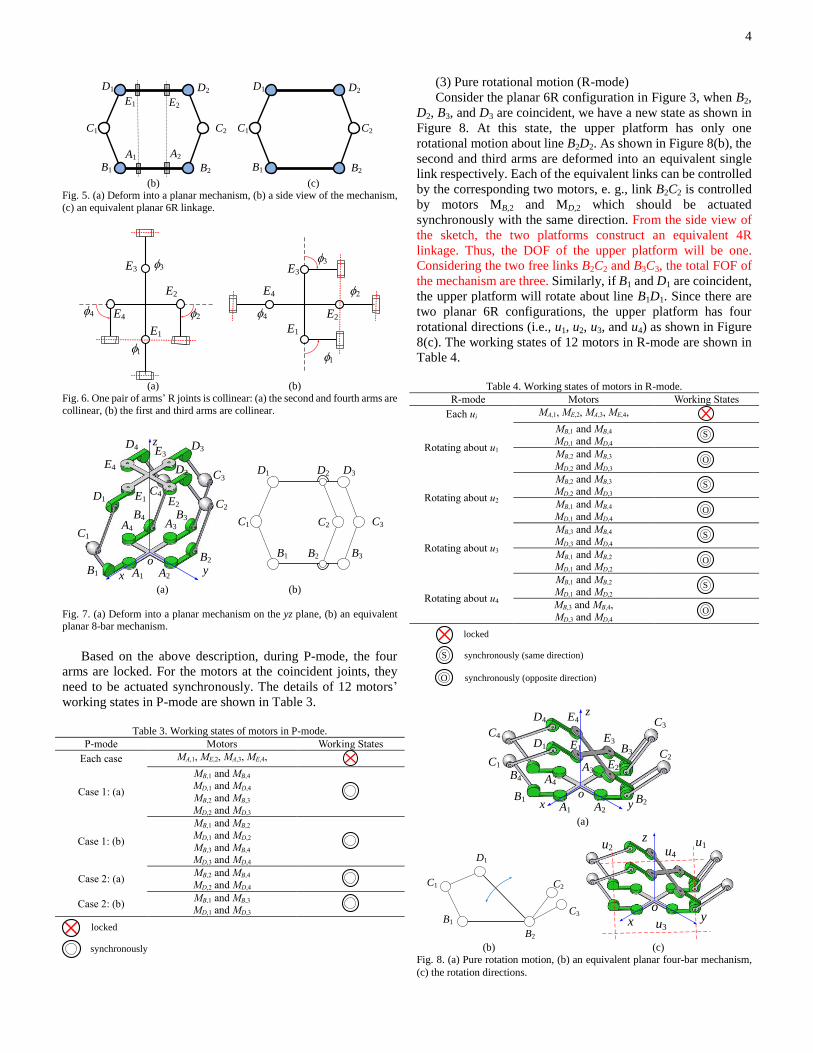
(3) Pure rotational motion (R-mode)
Consider the planar 6R configuration in Figure 3, when B2,
D2, B3, and D3 are coincident, we have a new state as shown in
Figure 8. At this state, the upper platform has only one
rotational motion about line B2D2. As shown in Figure 8(b), the
second and third arms are deformed into an equivalent single
link respectively. Each of the equivalent links can be controlled
by the corresponding two motors, e. g., link B2C2 is controlled
by motors MB,2 and MD,2 which should be actuated
synchronously with the same direction. From the side view of
the sketch, the two platforms construct an equivalent 4R
linkage. Thus, the DOF of the upper platform will be one.
Considering the two free links B2C2 and B3C3, the total FOF of
the mechanism are three. Similarly, if B1 and D1 are coincident,
the upper platform will rotate about line B1D1. Since there are
two planar 6R configurations, the upper platform has four
rotational directions (i.e., u1, u2, u3, and u4) as shown in Figure
8(c). The working states of 12 motors in R-mode are shown in
Table 4.
Table 4. Working states of motors in R-mode.
R-mode Motors Working States
Each ui MA,1, ME,2, MA,3, ME,4,
Rotating about u1
MB,1 and MB,4 MD,1 and MD,4
MB,2 and MB,3 MD,2 and MD,3
Rotating about u2
MB,2 and MB,3 MD,2 and MD,3
MB,1 and MB,4 MD,1 and MD,4
Rotating about u3
MB,3 and MB,4 MD,3 and MD,4
MB,1 and MB,2 MD,1 and MD,2
Rotating about u4
MB,1 and MB,2 MD,1 and MD,2
MB,3 and MB,4, MD,3 and MD,4
(a)
(b) (c)
Fig. 8. (a) Pure rotation motion, (b) an equivalent planar four-bar mechanism,
(c) the rotation directions.
B1 B2
C2
D2D1
C1
A1 A2
E1 E2
B1 B2
C2
D2D1
C1
1
2
3
4
E1
E2
E3
E4
1
2
3
4E1
E2
E3
E4
x y
z
oA1 A2
A3A4
B1
B2
B3B4
D1C2
C3
C4
D2
D3D4
E1 E2
E4
C1
E3
B1 B3
C3
D3D1
C1
B2
C2
D2
locked
synchronously
S
O
S
O
S
O
S
O
locked
synchronously (same direction)
synchronously (opposite direction)
S
O
x
z
oA1 A2
A3
A4
B1 B2
B3
B4
D1
C2
C3
C4
D4
E1
E2
E4
C1
E3
y
D1
B1
B2
C2
C3
C1
y
z
xo
u1u2
u3
u4

5
(4) Lock-up motion (L-mode)
During the T-mode, if the upper platform is moving down
to the base one, when all RB,i and RD,i are coincident as shown in
Figure 9(a), each of the four arms is at a spatial singularity
position. At this moment, the two motors at RB,i and RD,i can be
actuated synchronously (the same direction or opposite
directions). If the two motoes are in opposite directions, the
upper platform will be lifted up. If the motors’ directions are the
same, links BiCi and CiDi will be controlled as a single link. In
this case, each arm is folded into an equivalent serial arm with
2-DOF (see Figure 9(b)). That also leads the two platforms to
be locked together. The DOF of the robot will be eight. The
working states of 12 motors in L-mode are shown in Table 5.
Table 5. Working states of motors in L-mode.
L-mode Motors Working States
L-mode
MA,1, ME,2, MA,3, ME,4
MB,1 and MD,1
MB,2 and MD,2
MB,3 and MD,3
MB,4 and MD,4
(a)
(b)
(c)
Fig. 9. (a) The upper platform is fixed with lower platform, (b) switching position, (c) an equivalent four legged robot.
(5) Switching states
Based on the motions analysis of the upper platform, we
have obtained four typical modes. According to their positions,
we give a general sketch of the relations of the four modes (see
Fig. 10). One mode can be changed into the other modes via
some special states. We call these states switching states, which
are the singularity positions of the mechanisms. The singularity
positions can be obtained when some axes of R joints are
coincident. As shown in Table 6 in Appendix, we show the
details motions of the upper platform and the conditions of the
singularity positions. The figures in Table 6 are also the
switching states, at which the motions of mechanism can be
changed to other modes. Based on it, we can find the rapid way
to switch the motion modes. For example, the T-mode and
L-mode can be switched freely at any position.
Fig. 10. The switching functions of the motion modes.
III. LOCOMOTION MODES ANALYSIS
In this section, based on the four operation modes presented
in Section 2, we will use different equivalent mechanisms to
establish rolling, tumbling and quadruped locomotion modes.
The simulations are also performed based on a computational
3D-model to show the locomotion modes.
A. Rolling locomotion
Rolling is a very efficient manner of locomotion on flat
ground. Yim et al. first introduced a kind of locomotion modes
called tracked-rolling with a plenty of modules [13]. Sastra et al.
further presented a fast and efficient rolling gait based on a
closed-loop mechanism with numbers of modules [46]. Liu et
al. [47] and Yamawaki et al. [33] designed mobile robots with
rolling functions with planar 4R and 5R closed-loop
mechanisms respectively. Each of such rolling robots changes
the shapes of its loop (and therefore the position of its mass
center) such that it can roll on the ground by changing its
supporting edge (foot) alternatively.
Based on the analysis in section 2.2, during the P-mode, the
mechanism can be deformed into a single-loop 6R linkage (see
Figure 5). Our purpose is to realize rolling locomotion by
changing the shape of the loop.
Note that the DOF of the 6R linkage is three, we can use
four pairs of motors to control the 6R linkage in Figure 11(a): (i)
MB,1 and MB,4 to control , (ii) MD,1 and MD,4 to control , (iii)
MB,2 and MB,3 to control ; (iv) MD,2 and MD,3 to control .
Among the four pairs of motors, one pair of motors is redundant.
To simplify the control method, we shall let = , and = for
symmetry reason. Then, the configuration of linkage is
determined by only two independent variables ( and , see
Figure 11(b)). Due to the symmetric configuration, C1D1C2B2 is
S
S
S
S
synchronously (same direction)S
independently
x y
z
o
A1 A2
A3A4
B1B2
B3B4
D1
C2
C3C4
D2
D3D4
E4
C1
E3
xy
z
o
B1B2
B3
B4
D1
C2
C3C4
D2
D3
D4
E1
E2
E4 E3
A1A2
A3A4
C1
A1A2
A3A4
B1B2
B3B4
D1
D2
D3
D4
E1
E2
E4 E3
C1
C2
C3
C4
xy
z
o
T-mode L-mode
P-mode R-mode
Swtiching
state
Swtiching
state
Swtiching
state
Swtic
hing
stat
e
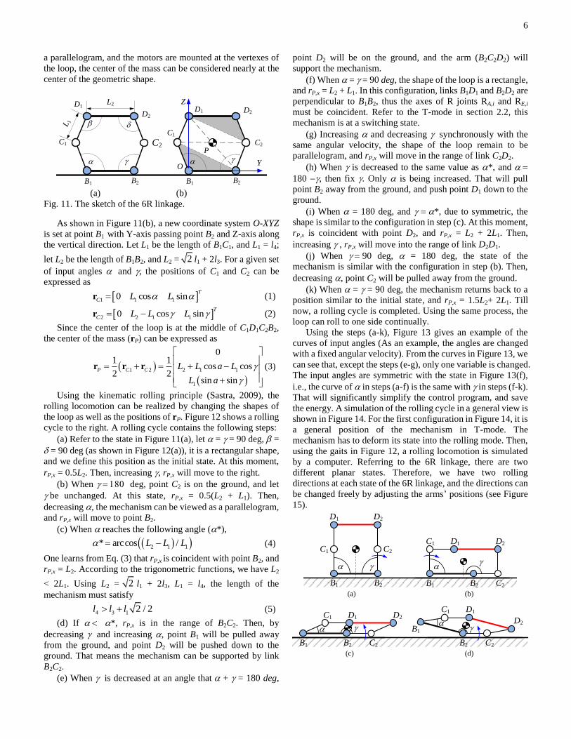
6
a parallelogram, and the motors are mounted at the vertexes of
the loop, the center of the mass can be considered nearly at the
center of the geometric shape.
(a) (b)
Fig. 11. The sketch of the 6R linkage.
As shown in Figure 11(b), a new coordinate system O-XYZ
is set at point B1 with Y-axis passing point B2 and Z-axis along
the vertical direction. Let L1 be the length of B1C1, and L1 = l4;
let L2 be the length of B1B2, and L2 = 2 l1 + 2l3. For a given set
of input angles and , the positions of C1 and C2 can be
expressed as
1 1 10 cos sinT
C L L r (1)
2 2 1 10 cos sinT
C L L L r (2)
Since the center of the loop is at the middle of C1D1C2B2,
the center of the mass (rP) can be expressed as
1 2 2 1 1
1
01 1
cos cos2 2
sin sin
P C C L L a L
L a
r r r (3)
Using the kinematic rolling principle (Sastra, 2009), the
rolling locomotion can be realized by changing the shapes of
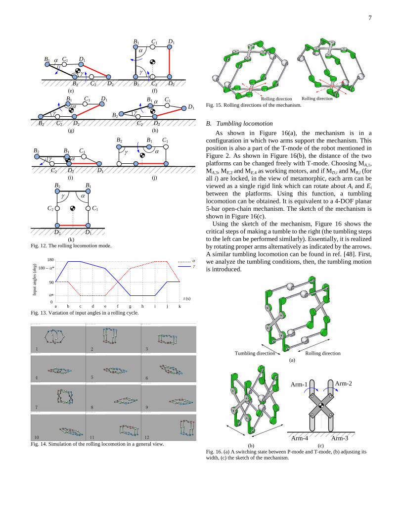
the loop as well as the positions of rP. Figure 12 shows a rolling
cycle to the right. A rolling cycle contains the following steps:
(a) Refer to the state in Figure 11(a), let = = 90 deg, =
= 90 deg (as shown in Figure 12(a)), it is a rectangular shape,
and we define this position as the initial state. At this moment,
rP,x = 0.5L2. Then, increasing , rP,x will move to the right.
(b) When 1 deg, point C2 is on the ground, and let
be unchanged. At this state, rP,x = 0.5(L2 + L1). Then,
decreasing , the mechanism can be viewed as a parallelogram,
and rP,x will move to point B2.
(c) When reaches the following angle (*),
2 1 1* arccos /L L L (4)
One learns from Eq. (3) that rP,x is coincident with point B2, and
rP,x = L2. According to the trigonometric functions, we have L2
< 2L1. Using L2 = 2 l1 + 2l3, L1 = l4, the length of the
mechanism must satisfy
4 3 1 2 / 2l l l (5)
(d) If *, rP,x is in the range of B2C2. Then, by
decreasing and increasing , point B1 will be pulled away
from the ground, and point D2 will be pushed down to the
ground. That means the mechanism can be supported by link
B2C2.
(e) When is decreased at an angle that + = 180 deg,
point D2 will be on the ground, and the arm (B2C2D2) will
support the mechanism.
(f) When = = 90 deg, the shape of the loop is a rectangle,
and rP,x = L2 + L1. In this configuration, links B1D1 and B2D2 are
perpendicular to B1B2, thus the axes of R joints RA,i and RE,i
must be coincident. Refer to the T-mode in section 2.2, this
mechanism is at a switching state.
(g) Increasing and decreasing synchronously with the
same angular velocity, the shape of the loop remain to be
parallelogram, and rP,x will move in the range of link C2D2.
(h) When is decreased to the same value as *, and
180 , then fix . Only is being increased. That will pull
point B2 away from the ground, and push point D1 down to the
ground.
(i) When = 180 deg, and *, due to symmetric, the
shape is similar to the configuration in step (c). At this moment,
rP,x is coincident with point D2, and rP,x = L2 + 2L1. Then,
increasing , rP,x will move into the range of link D2D1.
(j) When 90 deg, = 180 deg, the state of the
mechanism is similar with the configuration in step (b). Then,
decreasing , point C2 will be pulled away from the ground.
(k) When = = 90 deg, the mechanism returns back to a
position similar to the initial state, and rP,x = 1.5L2+ 2L1. Till
now, a rolling cycle is completed. Using the same process, the
loop can roll to one side continually.
Using the steps (a-k), Figure 13 gives an example of the
curves of input angles (As an example, the angles are changed
with a fixed angular velocity). From the curves in Figure 13, we
can see that, except the steps (e-g), only one variable is changed.
The input angles are symmetric with the state in Figure 13(f),
i.e., the curve of in steps (a-f) is the same with in steps (f-k).
That will significantly simplify the control program, and save
the energy. A simulation of the rolling cycle in a general view is
shown in Figure 14. For the first configuration in Figure 14, it is
a general position of the mechanism in T-mode. The
mechanism has to deform its state into the rolling mode. Then,
using the gaits in Figure 12, a rolling locomotion is simulated
by a computer. Referring to the 6R linkage, there are two
different planar states. Therefore, we have two rolling
directions at each state of the 6R linkage, and the directions can
be changed freely by adjusting the arms’ positions (see Figure
15).
(a) (b)
(c) (d)
B1 B2
C2
D2D1
C1
P
Y
Z
O
B1 B2
C2
D2
D1
C1
L2
L 1
D2D1
C2C1
B2B1
B2B1 C2
D1C1 D2
B2B1 C2
D1C1 D2
B2 C2
D2
D1C1
B1
D2D1
C2C1
B2B1
B2B1 C2
D1C1 D2
B2B1 C2
D1C1 D2
B2 C2
D2
D1C1
B1
7
(e) (f)
(g) (h)
(i) (j)
(k)
Fig. 12. The rolling locomotion mode.
Fig. 13. Variation of input angles in a rolling cycle.
Fig. 14. Simulation of the rolling locomotion in a general view.
Fig. 15. Rolling directions of the mechanism.
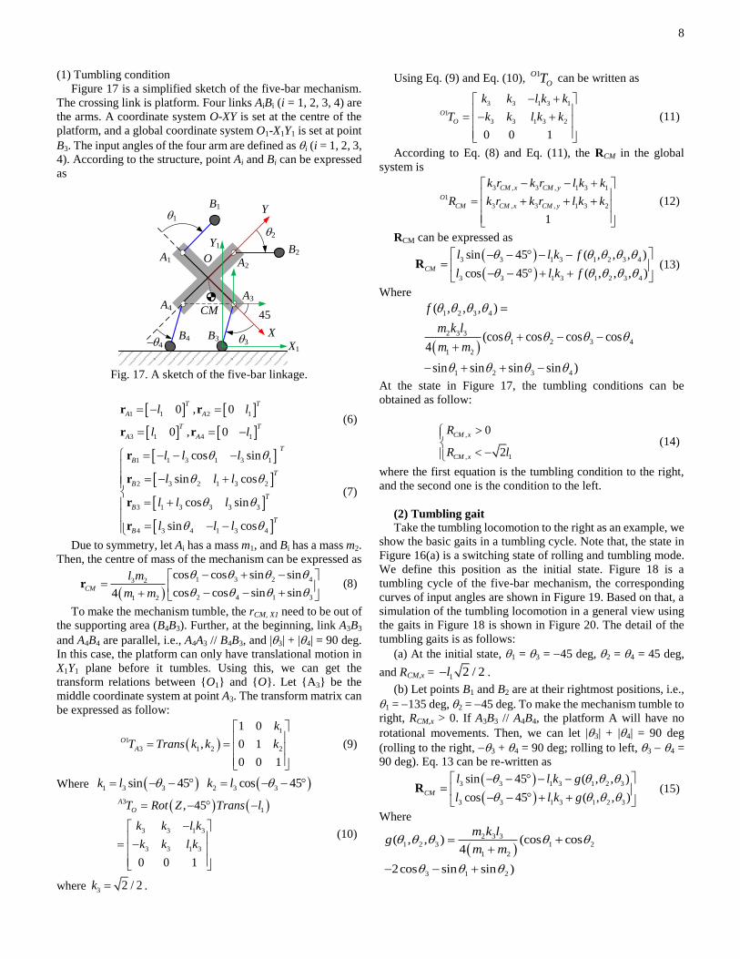
B. Tumbling locomotion
As shown in Figure 16(a), the mechanism is in a
configuration in which two arms support the mechanism. This
position is also a part of the T-mode of the robot mentioned in
Figure 2. As shown in Figure 16(b), the distance of the two
platforms can be changed freely with T-mode. Choosing MA,1,
MA,3, ME,2 and ME,4 as working motors, and if MD,i and MB,i (for
all i) are locked, in the view of metamorphic, each arm can be
viewed as a single rigid link which can rotate about Ai and Ei
between the platforms. Using this function, a tumbling
locomotion can be obtained. It is equivalent to a 4-DOF planar
5-bar open-chain mechanism. The sketch of the mechanism is
shown in Figure 16(c).
Using the sketch of the mechanism, Figure 16 shows the
critical steps of making a tumble to the right (the tumbling steps
to the left can be performed similarly). Essentially, it is realized
by rotating proper arms alternatively as indicated by the arrows.
A similar tumbling locomotion can be found in ref. [48]. First,
we analyze the tumbling conditions, then, the tumbling motion
is introduced.
(a)
(b) (c)
Fig. 16. (a) A switching state between P-mode and T-mode, (b) adjusting its width, (c) the sketch of the mechanism.
B2 C2 D2
B1 C1 D1
B2 C2 D2
B1 C1 D1
B2
C2 D2
B1 C1
D1
B2 C2 D2
B1 C1 D1
B2 C2 D2
B1 C1 D1
B2 C2 D2
B1 C1 D1
B2
C2 D2
B1 C1
D1
B2 C2 D2
B1 C1 D1
B2
C2 D2
B1 C1
D1
B2
C2 D2
B1 C1
D1
B1B2
C1C2
D1D2
B2
C2 D2
B1 C1
D1
B2
C2 D2
B1 C1
D1
B1B2
C1C2
D1D2
Inp
ut
ang
les
(deg
)
t (s)
90
0
180
a b c d e f g h
*
180 *
i j k
1 2
12
3
4 5 6
7 8 9
10 11
Rolling direction Rolling direction
Tumbling direction Rolling direction
Arm-1 Arm-2
Arm-3Arm-4 Arm-4 Arm-3
Arm-2Arm-1
Arm-4
Arm-3
Arm-1
Arm-2
Arm-1 Arm-2
Arm-3Arm-4
Arm-4 Arm-3
Arm-2Arm-1
8
(1) Tumbling condition
Figure 17 is a simplified sketch of the five-bar mechanism.
The crossing link is platform. Four links AiBi (i = 1, 2, 3, 4) are
the arms. A coordinate system O-XY is set at the centre of the
platform, and a global coordinate system O1-X1Y1 is set at point
B3. The input angles of the four arm are defined as i (i = 1, 2, 3,
4). According to the structure, point Ai and Bi can be expressed
as
Fig. 17. A sketch of the five-bar linkage.
1 1 2 1
3 1 4 1
0 , 0
0 , 0
T T
A A
T T
A A
l l
l l
r r
r r (6)
1 1 3 1 3 1
2 3 2 1 3 2
3 1 3 3 3 3
4 3 4 1 3 4
cos sin
sin cos
cos sin
sin cos
T
B
T
B
T
B
T
B
l l l
l l l
l l l
l l l
r
r
r
r
(7)
Due to symmetry, let Ai has a mass m1, and Bi has a mass m2.
Then, the centre of mass of the mechanism can be expressed as
1 3 2 43 2
2 4 1 31 2
cos cos sin sin
cos cos sin sin4CM
l m
m m
r (8)
To make the mechanism tumble, the rCM, X1 need to be out of
the supporting area (B4B3). Further, at the beginning, link A3B3
and A4B4 are parallel, i.e., A4A3 // B4B3, and |3| + |4| = 90 deg.
In this case, the platform can only have translational motion in
X1Y1 plane before it tumbles. Using this, we can get the
transform relations between {O1} and {O}. Let {A3} be the
middle coordinate system at point A3. The transform matrix can
be expressed as follow:
1
1
3 1 2 2
1 0
, 0 1
0 0 1
O
A
k
T Trans k k k
(9)
Where 1 3 3sin 45k l 2 3 3cos 45k l
3
1
3 3 1 3
3 3 1 3
, 45
0 0 1
A
OT Rot Z Trans l
k k l k
k k l k
(10)
where 3 2 / 2k .
Using Eq. (9) and Eq. (10), 1O
OT can be written as
3 3 1 3 1
1
3 3 1 3 2
0 0 1
O
O
k k l k k
T k k l k k
(11)
According to Eq. (8) and Eq. (11), the RCM in the global
system is
3 , 3 , 1 3 1
1
3 , 3 , 1 3 2
1
CM x CM y
O
CM CM x CM y
k r k r l k k
R k r k r l k k
(12)
RCM can be expressed as
3 3 1 3 1 2 3 4
3 3 1 3 1 2 3 4
sin 45 ( , , , )
cos 45 ( , , , )CM
l l k f
l l k f
R (13)
Where
1 2 3 4
2 3 3
1 2 3 4
1 2
1 2 3 4
( , , , )
(cos cos cos cos4
sin sin sin sin )
f
m k l
m m
At the state in Figure 17, the tumbling conditions can be
obtained as follow:
,
, 1
0
2
CM x
CM x
R
R l
(14)
where the first equation is the tumbling condition to the right,
and the second one is the condition to the left.
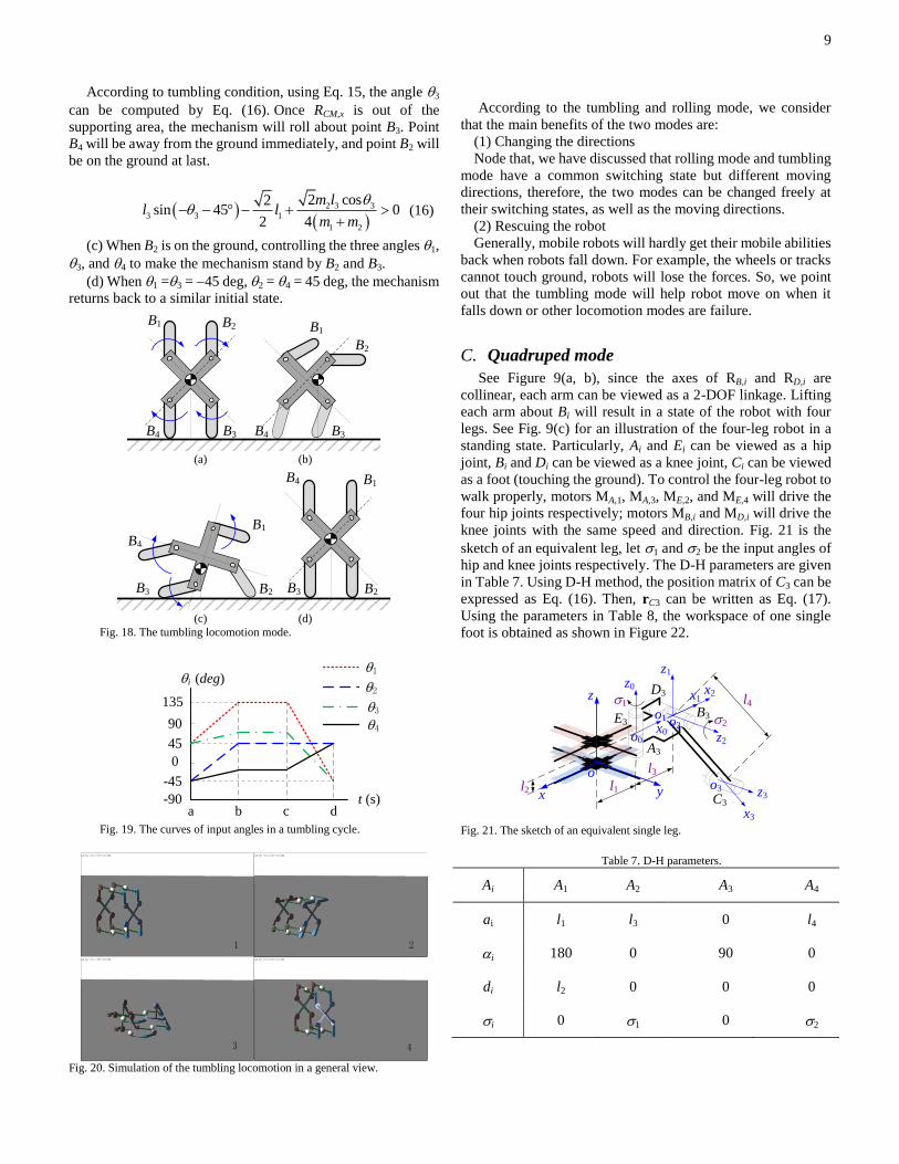
(2) Tumbling gait
Take the tumbling locomotion to the right as an example, we
show the basic gaits in a tumbling cycle. Note that, the state in
Figure 16(a) is a switching state of rolling and tumbling mode.
We define this position as the initial state. Figure 18 is a
tumbling cycle of the five-bar mechanism, the corresponding
curves of input angles are shown in Figure 19. Based on that, a
simulation of the tumbling locomotion in a general view using
the gaits in Figure 18 is shown in Figure 20. The detail of the
tumbling gaits is as follows:
(a) At the initial state, 1 = 3 = 45 deg, 2 = 4 = 45 deg,
and RCM,x = 1 2 / 2l .
(b) Let points B1 and B2 are at their rightmost positions, i.e.,
1 = 135 deg, 2 = 45 deg. To make the mechanism tumble to
right, RCM,x > 0. If A3B3 // A4B4, the platform A will have no
rotational movements. Then, we can let |3| + |4| = 90 deg
(rolling to the right, 3 + 4 = 90 deg; rolling to left, 3 4 =
90 deg). Eq. 13 can be re-written as
3 3 1 3 1 2 3
3 3 1 3 1 2 3
sin 45 ( , , )
cos 45 ( , , )CM
l l k g
l l k g
R (15)
Where
2 3 3
1 2 3 1 2
1 2
3 1 2
( , , ) (cos cos4
2cos sin sin )
m k lg
m m
A3
1
2
43
A4
B1
A2
B3B4
OB2
A1
Y
X
X1
Y1
45CM
9
According to tumbling condition, using Eq. 15, the angle 3
can be computed by Eq. (16).Once RCM,x is out of the
supporting area, the mechanism will roll about point B3. Point
B4 will be away from the ground immediately, and point B2 will
be on the ground at last.
2 3 3
3 3 1
1 2
2 cos2sin 45 0
2 4
m ll l
m m
(16)
(c) When B2 is on the ground, controlling the three angles 1,
3, and 4 to make the mechanism stand by B2 and B3.
(d) When 1 =3 = 45 deg, 2 = 4 = 45 deg, the mechanism
returns back to a similar initial state.
(a) (b)
(c) (d)
Fig. 18. The tumbling locomotion mode.
Fig. 19. The curves of input angles in a tumbling cycle.
Fig. 20. Simulation of the tumbling locomotion in a general view.
According to the tumbling and rolling mode, we consider
that the main benefits of the two modes are:
(1) Changing the directions
Node that, we have discussed that rolling mode and tumbling
mode have a common switching state but different moving
directions, therefore, the two modes can be changed freely at
their switching states, as well as the moving directions.
(2) Rescuing the robot
Generally, mobile robots will hardly get their mobile abilities
back when robots fall down. For example, the wheels or tracks
cannot touch ground, robots will lose the forces. So, we point
out that the tumbling mode will help robot move on when it
falls down or other locomotion modes are failure.
C. Quadruped mode
See Figure 9(a, b), since the axes of RB,i and RD,i are
collinear, each arm can be viewed as a 2-DOF linkage. Lifting
each arm about Bi will result in a state of the robot with four
legs. See Fig. 9(c) for an illustration of the four-leg robot in a
standing state. Particularly, Ai and Ei can be viewed as a hip
joint, Bi and Di can be viewed as a knee joint, Ci can be viewed
as a foot (touching the ground). To control the four-leg robot to
walk properly, motors MA,1, MA,3, ME,2, and ME,4 will drive the
four hip joints respectively; motors MB,i and MD,i will drive the
knee joints with the same speed and direction. Fig. 21 is the
sketch of an equivalent leg, let 1 and 2 be the input angles of
hip and knee joints respectively. The D-H parameters are given
in Table 7. Using D-H method, the position matrix of C3 can be
expressed as Eq. (16). Then, rC3 can be written as Eq. (17).
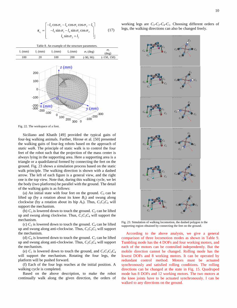
Using the parameters in Table 8, the workspace of one single
foot is obtained as shown in Figure 22.
Fig. 21. The sketch of an equivalent single leg.
Table 7. D-H parameters.
Ai A1 A2 A3 A4
ai
l1
l3
0 l4
i
180 0 90 0
di
l2
0 0 0
i
0 1
0 2
B3B4
B2B1
B3B4
B2
B1
B2
B1
B4
B3
B4
B2
B1
B3
B3B4
B2B1
B3B4
B2
B1
B2
B1
B4
B3
B4
B2
B1
B3
i (deg)
t (s)
0
135
a b c d
90
45
-45
-90
1
2
34
1 2
3 4
A3
B3
D3
E3
C3x y
z
o
x0
z0
o0
x1
z1
o1
x2
z2
o2
o3
x3
z3l2 l1
1
2
l3
l4
10
3
3 1 4 1 2 1
3 1 4 1 2
4 2 2
cos cos cos
sin sin cos
sin
c
l l l
l l
l l
r (17)
Table 8. An example of the structure parameters.
l1 (mm) l2 (mm) l3 (mm) l4 (mm) 1 (deg) 2
(deg)
100 20 100 200 (-90, ) (-150, 150)
Fig. 22. The workspace of a foot.
Siciliano and Khatib [49] provided the typical gaits of
four-leg walking animals. Further, Hirose et al. [50] presented
the walking gaits of four-leg robots based on the approach of
static walk. The principle of static walk is to control the four
feet of the robot such that the projection of the mass center is
always lying in the supporting area. Here a supporting area is a
triangle or a quadrilateral formed by connecting the feet on the
ground. Fig. 23 shows a simulation process based on the static
walk principle. The walking direction is shown with a dashed
arrow. The left of each figure is a general view, and the right
one is the top view. Note that, during this walking cycle, we let
the body (two platforms) be parallel with the ground. The detail
of the walking gaits is as follows:
(a) An initial state with four feet on the ground. C3 can be
lifted up (by a rotation about its knee B3) and swung along
clockwise (by a rotation about its hip A3). Thus, C1C2C4 will
support the mechanism.
(b) C3 is lowered down to touch the ground. C2 can be lifted
up and swung along clockwise. Thus, C1C3C4 will support the
mechanism.
(c) C2 is lowered down to touch the ground. C4 can be lifted
up and swung along anti-clockwise. Thus, C1C2C3 will support
the mechanism.
(d) C4 is lowered down to touch the ground. C1 can be lifted
up and swung along anti-clockwise. Thus, C2C3C4 will support
the mechanism.
(e) C1 is lowered down to touch the ground, and C1C2C3C4
will support the mechanism. Rotating the four legs, the
platform will be pushed forward.
(f) Each of the four legs reaches at the initial position. A
walking cycle is completed.
Based on the above description, to make the robot
continually walk along the given direction, the orders of
working legs are C3-C2-C4-C1. Choosing different orders of
legs, the walking directions can also be changed freely.
Fig. 23. Simulation of walking locomotion, the dashed polygon is the
supporting region obtained by connecting the feet on the ground.
According to the above analysis, we give a general
comparison of three locomotion modes as shown in Table 9.
Tumbling mode has the 4 DOFs and four working motors, and
each of the motors can be controlled independently. But the
mobile direction cannot be changed. Rolling mode has the
lowest DOFs and 8 working motors. It can be operated by
redundant control method. Motors must be actuated
synchronously and satisfied rolling conditions. The rolling
directions can be changed at the state in Fig. 15. Quadruped
mode has 8 DOFs and 12 working motors. The two motors at
the knee joints have to be actuated synchronously. I can be
walked to any directions on the ground.
-300-200
-1000
-300-200
-1000
100200
300
-200
-100
0
100
200
x (mm)y (mm)
z (mm)
o
C1
C2
C3
C4
C1
C2
C3
C4
C1
C2
C3
C4
C1
C2
C3
C4
C1
C2
C3
C4
C1
C2
C3
C4
C1
C2
C3
C4
C1
C2
C3
C4
C1
C2
C3
C4
C1
C2
C3
C4
C1
C2
C3
C4
C1
C2
C3
C4
C1
C2
C3
C4
C1
C2
C3
C4
C1
C2
C3
C4
C1
C2
C3
C4
C1
C2
C3
C4
C1
C2
C3
C4
C1
C2
C3
C4
C1
C2
C3
C4
C1
C2
C3
C4
C1
C2
C3
C4
C1
C2
C3
C4
C1
C2
C3
C4
11
Table 9. Comparison of three locomotion modes
Modes DOFs Working motors Mobile Directions
Rolling 3 8 Two
Tumbling 4 4 One Quadruped 8 12 Omnidirectional
IV. SWITCHING FUNCTION
In this section, we discuss the switching functions between
the three locomotion modes. Based on the locomotion gaits,
Figure 24 shows the relations of the locomotion modes. The
key steps are finding the right switching states of the motion
mode, which can be easily obtained from Table 6 in Appendix
B. Then, we can get a rapid way for changing the locomotion
mode. This function is very useful for the robot working in
complexed out-door environments. It can switch its locomotion
modes and therefore adapt different road conditions. For
example, rolling mode will have a faster speed on flat ground;
tumbling mode can be used for climbing stairs; and quadruped
mode will be more useful on rough ground.
Fig. 24. The switching function of locomotion modes.
(1) Rolling and tumbling modes
As shown in Figure 25(b), this state is a typical switching
state. If motors at Ai and Ei are working motors, the mechanism
will have a tumbling mode (see Figure 25(c)); or if motors at Bi
and Di are working motors, it will have a rolling mode (see
Figure 25(a)). Thus, the two modes can be directly switched at
this state.
(2) Rolling and quadruped modes
When one platform is on the ground (see Figure 26(a)), the
mechanism can deform into a switching state of L-mode (see
Figure 26(b)). Then, we get the quadruped modes (see Figure
26(c)) by folding the arms at Bi. It can be seen that the two
modes can be directly switched at the state in Figure 26(b).
(3) Tumbling and quadruped modes
Since the arms are always on the ground during a tumbling
mode, tumbling and quadruped mode cannot be switched in a
single state. As shown in Figure 27, there are three steps:
1) Making the platform on the ground using T-motion (see
Figure 27(a-c));
2) Deforming into a switching state of L-mode (see Figure
27(c-e));
3) Expanding the legs (see Figure 27(f)).
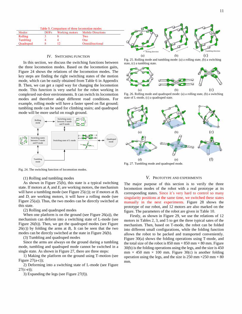
(a) (b) (c) Fig. 25. Rolling mode and tumbling mode: (a) a rolling state, (b) a switching
state, (c) a tumbling state.
(a) (b) (c) Fig. 26. Rolling mode and quadruped mode: (a) a rolling state, (b) a switching state of L-mode, (c) a quadruped state.
(a) (b) (c)
(d) (e) (f) Fig. 27. Tumbling mode and quadruped mode.
V. PROTOTYPE AND EXPERIMENTS
The major purpose of this section is to verify the three
locomotion modes of the robot with a real prototype at its
corresponding states. Since it’s very hard to control so many
singularity positions at the same time, we switched these states
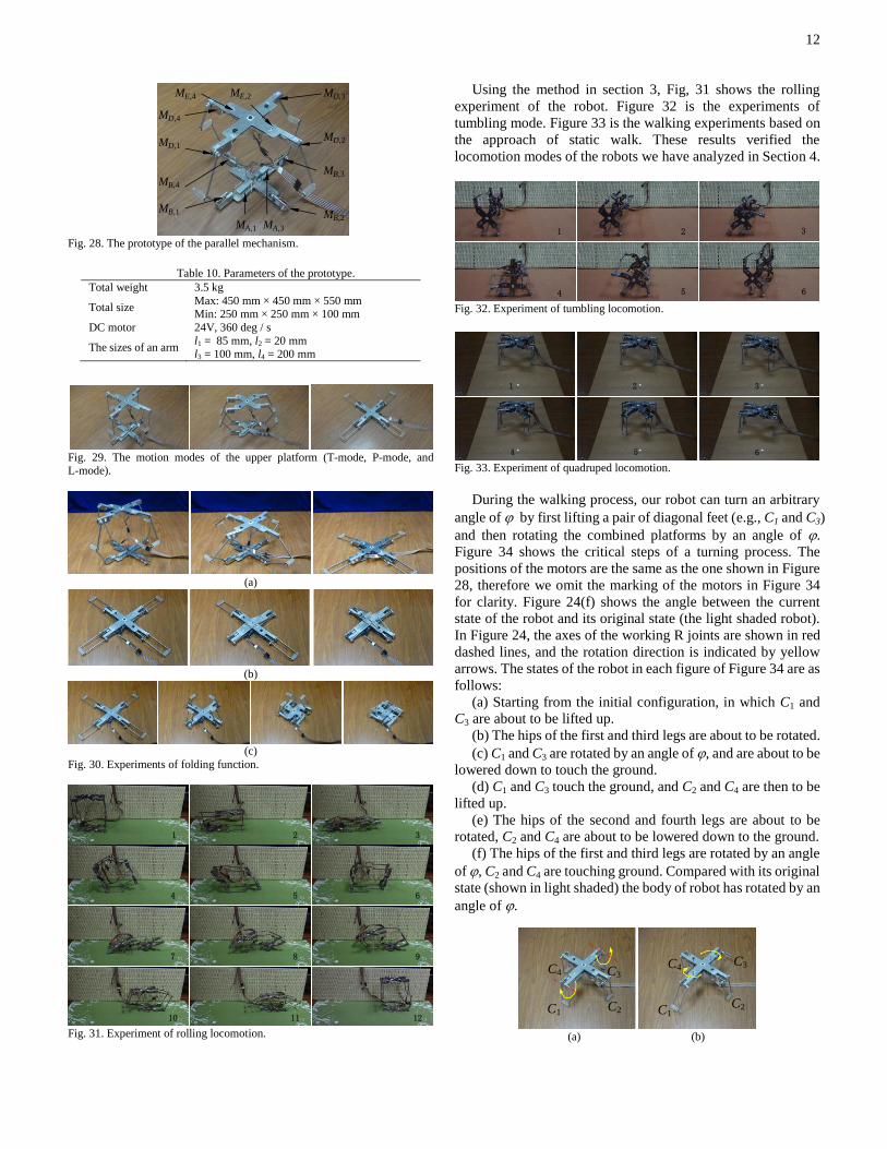
manually in the next experiments. Figure 28 shows the
prototype of our robot, and 12 motors are also marked on the
figure. The parameters of the robot are given in Table 10.
Firstly, as shown in Figure 29, we use the relations of 12
motors in Tables 2, 3, and 5 to get the three typical sates of the
mechanism. Then, based on T-mode, the robot can be folded
into different small configurations, while the folding function
allows the robot to be packed and transported conveniently.
Figure 30(a) shows the folding operations using T-mode, and
the total size of the robot is 850 mm × 850 mm × 80 mm. Figure
30(b) is the folding operations using the legs, and the size is 450
mm × 450 mm × 100 mm. Figure 30(c) is another folding
operation using the legs, and the size is 250 mm ×250 mm × 80
mm.
Switching states
between T-mode
and P-mode
Switching state of L-mode
Rolling
mode
Quadruped
mode
Tumbling
mode
Switching states
between T-mode
and P-mode
Rolling direction Tumbling direction
12
Fig. 28. The prototype of the parallel mechanism.
Table 10. Parameters of the prototype.
Total weight 3.5 kg
Total size Max: 450 mm × 450 mm × 550 mm Min: 250 mm × 250 mm × 100 mm
DC motor 24V, 360 deg / s
The sizes of an arm l1 = 85 mm, l2 = 20 mm l3 = 100 mm, l4 = 200 mm
Fig. 29. The motion modes of the upper platform (T-mode, P-mode, and L-mode).
(a)
(b)
(c)
Fig. 30. Experiments of folding function.
Fig. 31. Experiment of rolling locomotion.
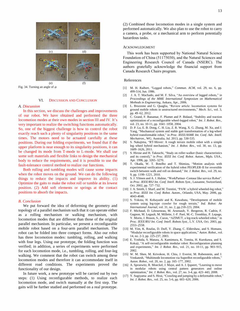
Using the method in section 3, Fig, 31 shows the rolling
experiment of the robot. Figure 32 is the experiments of
tumbling mode. Figure 33 is the walking experiments based on
the approach of static walk. These results verified the
locomotion modes of the robots we have analyzed in Section 4.
Fig. 32. Experiment of tumbling locomotion.
Fig. 33. Experiment of quadruped locomotion.
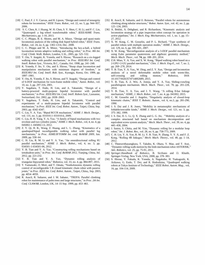
During the walking process, our robot can turn an arbitrary
angle of by first lifting a pair of diagonal feet (e.g., C1 and C3)
and then rotating the combined platforms by an angle of .
Figure 34 shows the critical steps of a turning process. The
positions of the motors are the same as the one shown in Figure
28, therefore we omit the marking of the motors in Figure 34
for clarity. Figure 24(f) shows the angle between the current
state of the robot and its original state (the light shaded robot).
In Figure 24, the axes of the working R joints are shown in red
dashed lines, and the rotation direction is indicated by yellow
arrows. The states of the robot in each figure of Figure 34 are as
follows:
(a) Starting from the initial configuration, in which C1 and
C3 are about to be lifted up.
(b) The hips of the first and third legs are about to be rotated.
(c) C1 and C3 are rotated by an angle of , and are about to be
lowered down to touch the ground.
(d) C1 and C3 touch the ground, and C2 and C4 are then to be
lifted up.
(e) The hips of the second and fourth legs are about to be
rotated, C2 and C4 are about to be lowered down to the ground.
(f) The hips of the first and third legs are rotated by an angle
of , C2 and C4 are touching ground. Compared with its original
state (shown in light shaded) the body of robot has rotated by an
angle of .
(a) (b)
MA,1 MA,3
ME,2ME,4
MB,1
MD,1
MB,2
MD,2
MD,4
MD,3
MB,4
MB,3
1 2 3
4 5 6
7 8 9
10 11 12
1 2 3
4 5 6
1 2 3
5 64
C1C2
C3C4
C1C2
C3C4
13
(c) (d)
(e) (f)
Fig. 34. Turning an angle of
VI. DISCUSSION AND CONCLUSION
A. Discussion
In this section, we discuss the challenges and improvements
of our robot. We have obtained and performed the three
locomotion modes at their own modes in section III and IV. It’s
very important to realize the switching functions automatically.
So, one of the biggest challenge is how to control the robot
exactly reach such a plenty of singularity positions in the same
times. The motors need to be actuated carefully at these
positions. During our folding experiments, we found that if the
upper platform is near enough to its singularity positions, it can
be changed its mode from T-mode to L-mode. We shall use
some soft materials and flexible links to design the mechanical
body to reduce the requirements, and it is possible to use the
fault-tolerance control method to realize our functions.
Both rolling and tumbling modes will cause some impacts
when the robot moves on the ground. We can do the following
things to reduce the impacts and improve its ability. (1)
Optimize the gaits to make the robot roll or tumble at its lowest
position. (2) Add soft elements or springs at the contact
positions to absorb the impacts.
B. Conclusion
We put forward the idea of deforming the geometry and
topology of a parallel mechanism such that it can operate either
as a rolling mechanism or walking mechanism, with
locomotion modes that are different than those of the original
parallel mechanism. In particular, we present a reconfigurable
mobile robot based on a four-arm parallel mechanism. The
robot can be folded into three compact forms. Also our robot
has three locomotion modes: tumbling, rolling, and walking
with four legs. Using our prototype, the folding function was
verified; in addition, a series of experiments were performed
for each locomotion mode, i.e., tumbling, rolling, and four-leg
walking. We comment that the robot can switch among these
locomotion modes and therefore it can accommodate itself in
different road conditions. The experiments proved the
functionality of our design.
In future work, a new prototype will be carried out by two
steps: (1) Using reconfigurable methods, to realize each
locomotion mode, and switch manually at the first step. The
gaits will be further studied and performed on a real prototype.
(2) Combined those locomotion modes in a single system and
performed automatically. We also plan to use the robot to carry
a camera, a probe, or a mechanical arm to perform potentially
hazardous tasks.
ACKNOWLEDGMENT
This work has been supported by National Natural Science
Foundation of China (51175030), and the Natural Sciences and
Engineering Research Council of Canada (NSERC). The
authors gratefully acknowledge the financial support from
Canada Research Chairs program.
References
[1] M. H. Raibert, “Legged robots,” Commun. ACM, vol. 29, no. 6, pp.
499-514, Jun. 1986.
[2] J. A. T. Machado, and M. F. Silva, “An overview of legged robots,” in
Proceedings of the MME International Symposium on Mathematical
Methods in Engineering, Ankara, Apr., 2006.
[3] L. Bruzzone and G. Quaglia, “Review article: locomotion systems for ground mobile robots in unstructured environments,” Mech. Sci., vol. 3,
pp. 49–62, 2012.
[4] C. Grand, F. Banamar, F. Plumet and P. Bidaud, “Stability and traction optimization of a reconfigurable wheel-legged robot,” Int. J. Robot. Res.,
vol. 23, no. 10-11, pp. 1041–1058, 2004.
[5] D. P. Lu, E. B. Dong, C. H. Liu, Z. R. Wang, X. G. Zhang, M. Xu, and J. Yang, “Mechanical system and stable gait transformation of a leg-wheel
hybrid transformable robot,” in Proc. IEEE/ASME Int. Conf. Adv. Intell.
Mechatron., WG. Australia, Jul. 2013, pp. 530-535. [6] S. Nakajima, “RT-Mover: A rough terrain mobile robot with a simple
leg–wheel hybrid mechanism,” Int. J. Robot. Res., vol. 30, no. 13, pp.
1609–1626, 2011. [7] S. Hirose and H. Takeuchi, “Study on roller-walker (basic characteristics
and its control),” in Proc. IEEE Int. Conf. Robot. Autom., Mpls. USA.,
Apr. 1996, pp. 3265–3270.
[8] T. Okada, W. T. Botelho and T. Shimizu, “Motion analysis with
experimental verification of the hybrid robot PEOPLER-II for reversible
switch between walk and roll on demand,” Int. J. Robot. Res., vol. 29, no. 9, pp. 1199–1221, 2010.
[9] S. J. Ylönen and A. J. Halme, “WorkPartner–Centaur like service Robot”.
in Proc. IEEE/RSJ Int. Conf. Intell. Robots Syst., Lausanne, Switzerland, Oct. 2002, pp. 727–732.
[10] J. A. Smith, I. Sharf, and M. Trentini, “PAW: a hybrid wheeled-leg robot,”
in Proc. IEEE Int. Conf. Robot. Autom., Orlando, USA, May. 2006, pp. 4043-4048.
[11] S. Yokota, H. Kobayashi and K. Kawabata, “Development of mobile system using leg-type crawler for rough terrain,” Ind. Robot: An
International Journal, vol. 31, no. 2, pp.218-223, 2004.
[12] F. Michaud, D. Létourneau, M. Arsenault, Y. Bergeron, R. Cadrin, F. Gagnon, M. Legault, M. Millette, J.-F. Paré, M.-C. Tremblay, P. Lepage,
Y. Morin, J. Bisson, S., Caron, “AZIMUT, a leg-track-wheeled robot,” in
Proc. IEEE/RSJ Int. Conf. Intell. Robots Syst., L.V. USA, Oct. 2003, pp. 2553–2558.
[13] M. Yim, K. Roufas, D. Duff, Y. Zhang, C. Eldershaw, and S. Homans,
“Modular reconfigurable robots in space applications,” Auton. Robot., vol. 14, no. 2-3, pp. 225-237, 2003.
[14] E. Yoshida, S. Matura, A. Kamimura, K. Tomita, H. Kurokawa, and S.
Kokaji, “A self-reconfigurable modular robot: Reconfiguration planning and experiments,” Int. J. Robot. Res., vol. 21, no. 10-11, pp. 903–915,
2002.
[15] W. M. Shen, M. Krivokon, H. Chiu, J. Everist, M. Rubenstein, and J. Venkatesh, “Multimode locomotion via SuperBot reconfigurable robots,”
Auton. Robot., vol. 20, no. 2, pp. 165–177, 2002.
[16] A. Sproewitz, R. Moeckel, J. Maye, and A. J. Ijspeert, “Learning to move in modular robots using central pattern generators and online
optimization,” Int. J. Robot. Res., vol. 27, no. 3-4, pp. 423–443, 2008.
[17] Y. Sugiyama and S. Hirai, “Crawling and jumping by a deformable robot,” Int. J. Robot. Res., vol. 25, no. 5-6, pp. 603–620, 2006.
C1C2
C3C4
C1C2
C3C4
C1
C2
C3C4
C1C2
C3C4
C1
C2
C3
C4
C1
C2
C3
C4
14
[18] C. Paul, F. J. V. Cuevas, and H. Lipson, “Design and control of tensegrity
robots for locomotion,” IEEE Trans. Robot., vol. 22, no. 5, pp. 944–957,
2006.
[19] S. C. Chen, K. J. Huang, W. H. Chen, S. Y. Shen, C. H. Li, and P. C. Lin,
“Quattroped: a leg–wheel transformable robot,” IEEE/ASME Trans.
Mechatronics, pp. 1-10, 2013. [20] C. C. Phipps, B. E. Shores, and M. A. Minor, “Design and quasi-static
locomotion analysis of the rolling disk biped hybrid robot,” IEEE Trans.
Robot., vol. 24, no. 6, pp. 1302-1314, Dec. 2008. [21] C. C. Phipps and M. A. Minor, “Introducing the hex-a-ball, a hybrid
locomotion terrain adaptive walking and rolling robot,” in Proc. 8th Int.
Conf. Climb. Walk. Robots, London, U.K., 2005, pp. 525–532. [22] Y. Ota, Y. Inagaki, K. Yoneda, and S. Hirose, “Research on a six-legged
walking robot with parallel mechanism,” in Proc. IEEE/RSJ Int. Conf.
Intell. Robots Syst., Victoria, B.C., Canada, Oct. 1998, pp. 241–248. [23] K. Yoneda, F. Ito, Y. Ota, and S. Hirose, “Steep slope locomotion and
manipulation mechanism with minimum degrees of freedom,” in
IEEE/RSJ Int. Conf. Intell. Rob. Syst., Kyongju, Korea, Oct. 1999, pp. 1897–1901.
[24] Y. Ota, K. Yoneda, F. Ito, S. Hirose, and Y. Inagaki, “Design and control
of 6-DOF mechanism for twin-frame mobile robot,” Auton. Robot., vol.
10, no. 3, pp. 297-316, 2001.
[25] Y. Sugahara, T. Endo, H. Lim, and A. Takanishi, “Design of a
battery-powered multi-purpose bipedal locomotor with parallel mechanism,” in Proc. IEEE/RSJ Int. Conf. Intell. Robots Syst., Lausanne,
Switzerland, Oct. 2002, pp. 2658–2663.
[26] Y. Sugahara, T. Endo, H. Lim, and A. Takanishi, “Control and experiments of a multi-purpose bipedal locomotor with parallel
mechanism,” in Proc. IEEE Int. Conf. Robot. Autom., Taipei, China, Sep.
2003, pp. 4342-4347. [27] C. Liu, Y. A. Yao, “Biped RCCR mechanism,” ASME J. Mech. Design.,
vol. 131, no. 3, pp. 031010.1–031010.6, 2009.
[28] C. Liu, H. H. Yang, Y. A, Yao, “A family of biped mechanisms with two revolute and two cylindric joints,” ASME J. Mech. Robot., vol, 4, no. 4, pp.
045002-1–045002-13, 2012.
[29] Z. Y. Qi, H. B., Wang, Z. Huang, and L. L. Zhang, “Kinematics of a quadruped/biped reconfigurable walking robot with parallel leg
mechanisms,” in Proc. ASME/IFTOMM Int. conf. ReMAR 2009, Jun.
2009, pp. 558–64.
[30] C. H. Liu, R. M. Li and Y. A. Yao, “An omnidirectional rolling 8U
parallel mechanism,” ASME J. Mech. Robot., vol, 4, no. 3, pp.
034501-1-034501-06, 2012. [31] Y. B. Tian and Y. A. Yao, “Constructing rolling mechanisms based on
tetrahedron units,” in Proc. Int. Conf. ReMAR 2012, Tianjing, China, Jul.
2012, pp. 221-232. [32] Y. B. Tian and Y. A. Yao, “Dynamic rolling analysis of
triangular-bipyramid robot,” Robotica, vol. 33, no. 4, pp. 884-897, 2015.
[33] T. Yamawaki, O. Mori, and T. Omata, “Nonholonomic dynamic rolling control of reconfigurable 5 R closed kinematic chain robot with passive
joints,” in Proc. IEEE Int. Conf. Robot. Autom., Taipei, China,, Sep. 2003, pp. 4054–4059.
[34] R. Aracil, R. Saltaren, and J. M. Sabater, “TREPA: Parallel climbing
robot for maintenance of palm trees and large structures,” in Proc. 2th Int.
Conf. CLAWAR, London, UK, 1415 Sep. 1999, pp. 453–461.
[35] R. Aracil, R. Saltarén, and O. Reinoso, “Parallel robots for autonomous
climbing along tubular structures,” Robot. Auton. Syst., vol. 42, no. 2, pp.
125–134, 2003.
[36] A. Bekhit, A. Dehghani, and R. Richardson, “Kinematic analysis and
locomotion strategy of a pipe inspection robot concept for operation in
active pipelines,” Int. J. Mech. Eng. Mechatronics, vol. 1, no. 1, pp. 15–27, 2012.
[37] X. W. Kong, C. M. Gosselin, and P. L. Richard, “Type synthesis of
parallel robots with multiple operation modes,” ASME J. Mech. Design., vol. 129, no. 6, pp. 595–601, 2007.
[38] X. W. Kong, “Reconfiguration analysis of a 3-DOF parallel mechanism
using Euler parameter quaternions and algebraic geometry method,” Mech. Mach. Theor., vol. 74, pp. 188–201, 2014.
[39] Z.H. Miao, Y. A. Yao, and X. W. Kong, “Biped walking robot based on a
2-UPU+2-UU parallel mechanism,” Chin. J. Mech. Eng-E., vol. 7, no. 2, pp. 269–278, 2014.
[40] Y. B. Tian, Y. A. Yao,, W. Ding, and Z. Y. Xun, “Design and locomotion
analysis of a novel deformable mobile robot with worm-like, self-crossing and rolling motion,” Robotica, DOI:
10.1017/S0263574714002689, 2015.
[41] Y. B. Tian, X. Z. Wei, A. Joneja, and Y. A. Yao, Sliding-crawling
parallelogram mechanism. Mech. Mach. Theor., vol. 78, pp. 201-228,
2014.
[42] Y. B. Tian, Y. A. Yao, and J. Y. Wang, “A rolling 8-bar linkage mechanism,” ASME, J. Mech. Robot., vol. 7, no. 4, pp. 041002, 2015.
[43] C. M. Gosselin and J. Angeles, “Singularity analysis of closed-loop
kinematic chains,” IEEE T. Robotic. Autom., vol. 6, no.3, pp. 281-290, 1990.
[44] J. S. Dai and J. R. Jones, “Mobility in metamorphic mechanisms of
foldable/erectable kinds,” ASME J. Mech. Design., vol. 121, no. 3, pp. 375–382, 1999.
[45] J. S. Dai, D. L. Li, Q. X. Zhang and G. G. Jin, “Mobility analysis of a
complex structured ball based on mechanism decomposition and
equivalent screw system analysis,” Mech. Mach. Theor., vol. 39, no. 4, pp.
445–458, 2004. [46] J. Sastra, S. Chitta, and M. Yim, “Dynamic rolling for a modular loop
robot,” Int. J. Robot. Res., vol. 28, no. 6, pp. 758-773, 2009.
[47] C. H. Liu, Y. A. Yao, R. M. Li, Y. B. Tian, N. Zhang, Y. Y. Ji, and F. Z. Kong, “Rolling 4R linkages,” Mech. Mach. Theory., vol. 48, pp. 1–14,
2012.
[48] C. Theeravithayangkura, T. Takubo, K. Ohara, Y. Mae, and T. Arai, “Dynamic rolling-walk motion by the limb mechanism robot ASTERISK,”
Adv. Robotics, vol. 25, pp. 75-91, 2011.
[49] Springer.Handbook of Robotics, B. Siciliano and O. Khatib, Springer-Verlag, New York, USA, 2008, pp. 378–383.
[50] S. Hirose, Y. Fukuda, K. Yoneda, A. Nagakubo, H. Tsukagoshi, K.
Arikawa, G. Endo, T. Doi, and R. Hodoshima, “Quadruped walking robots at Tokyo Institute of Technology,” IEEE Robot. Autom. Mag., vol,
16, pp. 104-114, 2009.
15
Appendix
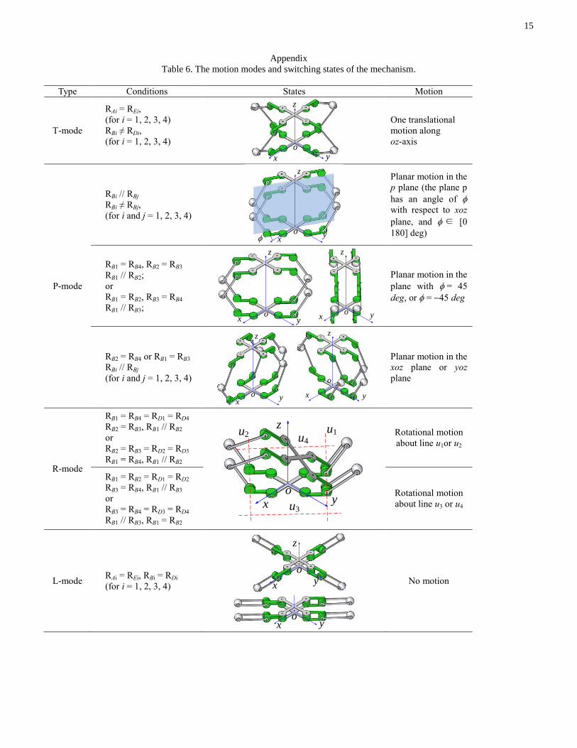
Table 6. The motion modes and switching states of the mechanism.
Type Conditions States Motion
T-mode
RAi = REi,
(for i = 1, 2, 3, 4)
RBi ≠ RDi,
(for i = 1, 2, 3, 4)
One translational
motion along
oz-axis
P-mode
RBi // RBj
RBi ≠ RBj,
(for i and j = 1, 2, 3, 4)
Planar motion in the
p plane (the plane p
has an angle of
with respect to xoz
plane, and ∈ [0
180] deg)
RB1 = RB4, RB2 = RB3
RB1 // RB2;
or
RB1 = RB2, RB3 = RB4
RB1 // RB3;
Planar motion in the
plane with = 45
deg, or = 45 deg
RB2 = RB4 or RB1 = RB3
RBi // RBj
(for i and j = 1, 2, 3, 4)
Planar motion in the
xoz plane or yoz
plane
R-mode
RB1 = RB4 = RD1 = RD4
RB2 = RB3, RB1 // RB2
or
RB2 = RB3 = RD2 = RD3
RB1 = RB4, RB1 // RB2
Rotational motion
about line u1or u2
RB1 = RB2 = RD1 = RD2
RB3 = RB4, RB1 // RB3
or
RB3 = RB4 = RD3 = RD4
RB1 // RB3, RB1 = RB2
Rotational motion
about line u3 or u4
L-mode RAi = REi, RBi = RDi
(for i = 1, 2, 3, 4)
No motion
y
z
x
o
y
z
xo
y
z
xo y
z
xo
y
z
xo y
z
x
o
y
z
xo
u1u2
u3
u4
y
z
xo
y
z
x
o
Top Related
Copyright © 2022 FDOKUMEN

