


Bahasa
Halaman
Hukum

TECHNISCHE UNIVERSITAT BERLIN
A Measurement-Based Joint Power and Rate Controller
for IEEE 802.11 Networks
vorgelegt von
Thomas Huhn (Dipl.-Wirtsch.-Ing.)
von der Fakultat IV – Elektrotechnik und Informatik
der Technischen Universitat Berlin
zur Erlangung des akademischen Grades
DOKTOR DER INGENIEURWISSENSCHAFTEN (DR.-ING.)genemigte Dissertation
Promotionsausschuss:
Vorsitzender des PA: Prof. Dr.-Ing. Adam Wolisz, TU BerlinPrufer der Dissertation: Prof. Anja Feldmann, Ph. D., TU Berlin
Prof. Dr. rer. nat. Jens-Peter Redlich, HU BerlinDr. Cigdem Sengul, Oxford Brookes University
Tag der wissenschaftlichen Aussprache: 11.01.2013
Berlin 2013D 83

Abstract
IEEE 802.11 (WiFi) networks are used to provide Internet access anywhere anytime. However, their
performance is far below the achievable limits when multiple participants share the same frequency
spectrum in an uncoordinated manner. The major reason behind such inefficiency is the lack of practical
resource allocation algorithms that adapt well to the current conditions in a wireless network dynam-
ically and select the appropriate transmission parameters such as transmission rates and power levels.
Most current practical schemes are rather simplistic and only change a single transmission parameter.
For instance, Transmit Power Control (TPC) works at the WiFi PHY layer and commonly assigns a
static and rather high power level to all packets. A per-link or packet scheme is expected to provide
better performance, but typically increases complexity and requires higher-layer information, such as
medium access state from the Medium Access Control (MAC) layer. Therefore, although performance
improvements have been shown in theory, these ideas are largely uninvestigated in practice.
In this thesis, our main goal is to understand the feasibility and performance impact of a joint and
per-link rate and power controller in a real WiFi system. To this end, we first enabled cross-layer
communication of transmission power between the WiFi PHY and MAC layers in the Linux mac80211
subsystem. Based on our Atheros WiFi hardware, we also developed the in-kernel monitoring tool
‘RegMon’ that enables understanding and troubleshooting MAC and PHY-layer operations with a fine-
grained time resolution across different Linux drivers.
We designed and implemented a distributed rate and power control algorithm, Minstrel-Blues, which
does not rely on signal strength or channel state information, but uses local statistics from periodic
sampling of different rate and power combinations. Essentially, Minstrel-Blues can run on any WiFi
hardware that supports packet-level power and rate control capabilities. Minstrel Blues decides the data-
rate, and consequently, the minimum power-level to support the chosen rate using a two-attribute utility
function based on the throughput and power consumption of all rates. To expose the trade-off between
throughput and network interference, we also introduced a weight parameter for the utility function,
which tunes the importance of throughput in utility decisions.
Our results show that if the goal is on maximizing the per-link throughput, Minstrel-Blues can sig-
nificantly reduce transmission power necessary to communicate per link, while maintaining the same
throughput achieved with maximum transmit power. We call this mode of operation - Minstrel Pi-
i

ano. Based on experiments in BOWL, at 5Ghz, Minstrel-Piano shows significant overall throughput
enhancements due to increasing spatial reuse. Our performance analysis concludes with experiments
with different weight factors in a home network scenario, with 2-laptops and one access point. These
experiments were run in the 2.4 GHz ISM band, and hence, they also show that our controller works
well in an typical scenarios. As more and more WiFi Access Points are deployed and with upcoming
IEEE 802.11 n and ac devices using wider channel widths, resource allocation is expected to become
even more important to manage interference efficiently. To this end, our work significantly contributes
to the understanding of rate, power and carrier-sense control in practice.
ii
Zusammenfassung
Die weite Verbreitung heutiger IEEE 802.11 (WiFi) Systeme untermauert das große Potential dezen-
traler Funknetzwerke nahezu uberall und zu jeder Zeit einen Internetzugang bereitstellen zu konnen.
Jedoch besteht eine signifikante Differenz zwischen der theoretisch moglichen und derzeit erreichten
Datenubertragungsleistung, wenn sich mehrere Benutzer gemeinsam einen Funkkanal teilen.
Eine der Hauptursachen liegt in der ineffizienten Ausnutzung des Frequenzspektrums begrundet. Es
fehlen praxisnahe Algorithmen zur dynamischen Ressourcenallokation, die geeignete Parameter, wie
z. B. Ubertragungsrate und Sendeleistungeine an den aktuellen Zustand des drahtlosen Netzwerks an-
passen. Gegenwartige Verfahren zur Ressourcenallokation in WiFi Systemen sind von sehr einfacher
Struktur und beschranken sich auf die Anpassung genau eines Parameters innerhalb der Funkubertra-
gung. Ubliche Praxis ist das Festsetzen einer statischen und vergleichsweise hohen Sendeleistung fur
alle zu ubertragenden Datenpakete. Praktische Verfahren zur dynamischen und verteilten Sendeleis-
tungsregelung auf der physikalischen Schicht (PHY-layer) des IEEE 802.11 Standards gibt es derzeit
nicht. Gleichwohl versprechen solche Allokationsschemen, die pro Paket bzw. pro Kommunikations-
verbindung gezielt Ressourcen zuweisen konnen, eine wesentliche Steigerung der Gesamtdatenrate in-
nerhalb eines drahtlosen Netzwerks. Jedoch steigen mit ihnen typischerweise die Komplexitat und auch
der Informationsbedarf aus hoheren Netzwerkschichten, wie beispielsweise der aktuelle Status des Me-
dienzugriffs aus der Schicht zur Medienzugriffssteuerung (MAC-layer). Deshalb sind derartige Ansatze,
trotz ihres in theoretischen Arbeiten belegten Potentials zur Leistungssteigerung, in praktischen WiFi
Systemen weitgehend unerforscht.
Der Schwerpunkt dieser wissenschaftlichen Arbeit liegt auf der Analyse zur Realisierbarkeit und zur
Leistungsfahigkeit einer gemeinsamen Regelung von Ubertragungsrate und Sendeleistung pro Kommu-
nikationsverbindung unter Verwendung realer IEEE 802.11 Hardware. Zu diesem Zweck haben wir
das Linux mac80211 Subsystem erweitert, so dass eine schichtubergreifende (cross-layer) Kommunika-
tion uber die Sendeleistung pro Datenpaket zwischen PHY-layer und MAC-layer ermoglicht wird. Im
nachsten Schritt haben wir analysiert, inwieweit die relevanten Regelungsparameter Ubertragungsrate
und Sendeleistung in unserem Forschungsnetzwerk “Berlin Open Wireless Lab (BOWL)” parametrisier-
bar sind und welche Wechselwirkungen zwischen ihnen bestehen. Auf der Grundlage unserer Atheros
WiFi Hardware entwickelten wir das neues Monitoringtool “RegMon” fur verschiedene Linux Kernel
iii

Treiber. Mit dessen Hilfe konnen wir die dynamischen Vorgange auf dem PHY-layer, als auch auf dem
MAC-layer der WLAN Netzwerkarte mit hoher zeitlichen Auflosung analysieren, auswerten und zur
Fehlerdiagnose nutzen.
In der vorliegenden Arbeit haben wir den verteilten Algorithmus “Minstrel-Blues” zur dynamischen
Ressourcenallokation von Ubertragungsrate und Sendeleistung entwickelt und implementiert. Unser Al-
gorithmus basiert auf der Auswertung lokaler Statistiken, die Paketerfolgswahrscheinlichkeiten aktiv
getesteter Kombinationen aus Ubertragungsrate und Sendeleistung beinhalten. Daruber hinaus werden
keine zusatzlichen Informationen wie z.B. die Signalstarke der empfangenen Pakete oder Kanalzus-
tandsbeschreibungen benotigt. Tatsachlich funktioniert Minstrel-Blues auf jeder beliebigen IEEE 802.11
Hardware, die eine Unterstutzung zur Regelung der Ubertragungsrate und Sendeleistung pro Datenpaket
bietet. Unter Berechnung einer additiven Nutzenfunktion, die sich aus dem aktuellen Datendurchsatz und
der notwendigen Sendeleistung pro unterstutzter Datenrate zusammensetzt, entscheidet Minstrel-Blues
welche Kombination aus Datenrate und Sendeleistung die hochste Praferenz erhalt. Um die Auswirkun-
gen des Zielkonflikts zwischen der Maximierung des Datendurchsatzes und der Minimierung der Inter-
ferenz im Funknetzwerk analysieren zu konnen, haben wir einen Gewichtungsfaktor in unsere Nutzen-
funktion integriert.
Unsere Ergebnisse zeigen, dass ein auf die Maximierung des Datendurchsatzes gewichteter Minstrel-
Blues in der Lage ist, die fur einen gleichbleibenden Datendurchsatz notwendig Sendeleistung, im Ver-
gleich zur maximalen Sendeleistung, signifikant zu verringern. Diese spezielle Funktionsweise beze-
ichnen wir als “Minstrel-Piano”. Basierend auf unseren Experimenten in BOWL, konnten wir bei der
Nutzung des 5 GHz ISM Frequenzbandes (IEEE 802.11a) belegen, dass Minstrel-Piano den Gesamt-
durchsatz des Datenverkehrs im Funknetzwerk, aufgrund seiner effizienterer Nutzung des Frequen-
zspektrums, maßgeblich erhoht. Unsere Analyse endet mit experimentellen Untersuchungen zu unter-
schiedlichen Gewichtungsfaktoren in einer typischen WiFI Umgebenung im Heimnetzwerk, bestehend
aus zwei Laptops und einer WLAN Basisstation. Anhand dessen konnten wir zeigen, dass unsere dy-
namische Regelung von Datenrate und Sendeleistung auch im lizenzfreien 2,4 GHz Frequenzspektrum
gut funktioniert. Mit steigender Dichte von WiFi Geraten und der kontinuierlichen Vergroßerung der
genutzten Bandbreite, durch die aktuellen Standards IEEE 802.11 n und 802.11 ac, gehen wir davon aus,
dass eine dynamische Ressourcenallokation eine Schlusselrolle zur effizienten Nutzung des Spektrum
bzw. zum Interferenzmanagement einnehmen wird. Zu diesem Zweck leistet diese Dissertations einen
entscheidenden Beitrag zum theoretischen Verstandnis und der praktischen Umsetzung einer dynamis-
chen Regelung von Ubertragungsrate, Sendeleistung und Carrier Sensing in IEEE 802.11 Systemen.
iv

Acknowledgments
At first, I want to thank my girlfriend Anja Werner for all her patience and endless support. Without her
love and respect I would not have finished this thesis.
I wish to express my sincere thanks to my advisor, Professor Anja Feldmann for guiding me during my
PhD.
A big thank you goes out to all senior researchers for working with me. Roger Karrer, Cigdem Sengul
and Ruben Merz - it was a remarkable experience for me to work with you during the MagNets and the
BOWL project.
I also would like to thank the entire FGINET group, student workers and friends that shared all kinds
of thought, ideas, discussion, coffees and intensive rounds of Kicker games during those five years in
BOWL. My greatest appreciation goes to this substantial list of my friends and fellows: Steve Uhlig,
Jan Bottger, Dan Levin, Florin Ciucu, Amir Mehmood, Andreas Wundsam, Slawomir Stanczak, Mario
Goldenbaum, Holger Taubig, Alexander Scheidler, Thomas Wohner, Peter Bank, Rainer May, Bernd
May, Harald Schioberg, Doris Schioberg, Nadi Sarrar, Britta Schneider, Bernhard Ager, Thorsten Fis-
cher, Britta Schneider, Mustafa Al-Bado, Lalith Suresh, Julius Schulz-Zander, Robin Kuck, Benjamin
Vahl, Tobias Steinicke, Theresa Enghardt, Felix Fietkau, Jae-Yong Yoo, Alina Friedrichsen and Adel
Aziz.
Especially while the last months, my whole family was always supporting me. My special thanks go to
Mum, Dad, Hannchen and Roxie.
v

vi
Contents
Resume iii
Acknowledgments v
1 Introduction 1
1.1 Problem Statement . . . . . . . . . . . . . . . . . . . . . . . . . . . . . . . . . . . . . 2
1.2 Contributions . . . . . . . . . . . . . . . . . . . . . . . . . . . . . . . . . . . . . . . . 3
1.3 Dissertation outline . . . . . . . . . . . . . . . . . . . . . . . . . . . . . . . . . . . . . 5
2 Resource Allocation in WiFi Networks 7
2.1 A Short Overview of IEEE 802.11 with Respect to Power, Rate, and Carrier Sense Control 8
2.2 Resource Allocation Based on Only Power, Rate or Carrier-Sense Control . . . . . . . . 11
2.2.1 Transmission Power Control (TPC) . . . . . . . . . . . . . . . . . . . . . . . . 11
2.2.2 Transmission Rate Control (TRC) . . . . . . . . . . . . . . . . . . . . . . . . . 15
2.2.3 Carrier-Sense Control - CSC . . . . . . . . . . . . . . . . . . . . . . . . . . . . 22
2.3 Joint Resource Allocation . . . . . . . . . . . . . . . . . . . . . . . . . . . . . . . . . . 24
2.4 Summary . . . . . . . . . . . . . . . . . . . . . . . . . . . . . . . . . . . . . . . . . . 27
3 An Inside Look at Our Testbed and Atheros IEEE 802.11 Radios 29
3.1 Our Testbed: Berlin Open Wireless Lab . . . . . . . . . . . . . . . . . . . . . . . . . . 29
3.1.1 Hardware Setup . . . . . . . . . . . . . . . . . . . . . . . . . . . . . . . . . . . 29
3.1.2 Software Setup . . . . . . . . . . . . . . . . . . . . . . . . . . . . . . . . . . . 31
3.2 IEEE 802.11 Radio Characteristics . . . . . . . . . . . . . . . . . . . . . . . . . . . . . 33
3.2.1 Atheros Hardware Design . . . . . . . . . . . . . . . . . . . . . . . . . . . . . 33
3.2.2 Rate and Power Control Capabilities . . . . . . . . . . . . . . . . . . . . . . . . 35
3.2.3 Carrier Sense Details . . . . . . . . . . . . . . . . . . . . . . . . . . . . . . . . 40
3.2.4 Noise Handling . . . . . . . . . . . . . . . . . . . . . . . . . . . . . . . . . . . 43
3.3 Summary . . . . . . . . . . . . . . . . . . . . . . . . . . . . . . . . . . . . . . . . . . 45
vii
4 Wireless MAC and PHY Layer Monitoring 474.1 Wireless Monitoring and its Limitations . . . . . . . . . . . . . . . . . . . . . . . . . . 47
4.2 RegMon - Design, Implementation and Performance . . . . . . . . . . . . . . . . . . . 49
4.2.1 In-Kernel MAC-Layer Monitoring . . . . . . . . . . . . . . . . . . . . . . . . . 49
4.2.2 Calculating MAC states . . . . . . . . . . . . . . . . . . . . . . . . . . . . . . 51
4.2.3 Validation and Performance . . . . . . . . . . . . . . . . . . . . . . . . . . . . 53
4.3 Summary . . . . . . . . . . . . . . . . . . . . . . . . . . . . . . . . . . . . . . . . . . 60
5 Development of a Joint Power-Rate Controller 615.1 Design and Implementation of a Cross-Layer Power-Rate Control Interface . . . . . . . 62
5.1.1 Linux mac80211 framework . . . . . . . . . . . . . . . . . . . . . . . . . . . . 62
5.1.2 Extending mac80211 for TPC . . . . . . . . . . . . . . . . . . . . . . . . . . . 65
5.2 Joint Power and Rate Control Algorithm: MINSTREL-BLUES . . . . . . . . . . . . . . 66
5.2.1 Validating Power-Rate and Throughput Relationships . . . . . . . . . . . . . . . 67
5.2.2 Design Properties and Functionality . . . . . . . . . . . . . . . . . . . . . . . . 67
5.2.3 Utility Function for Joint Decisions . . . . . . . . . . . . . . . . . . . . . . . . 72
5.3 Performance Evaluation . . . . . . . . . . . . . . . . . . . . . . . . . . . . . . . . . . . 74
5.3.1 Piano Power Control in a Single Link Scenario . . . . . . . . . . . . . . . . . . 74
5.3.2 Piano Power Control in a Multi-Link Scenario . . . . . . . . . . . . . . . . . . 77
5.3.3 Compatibility Experiment with Minstrel-Blues . . . . . . . . . . . . . . . . . . 86
5.4 Summary . . . . . . . . . . . . . . . . . . . . . . . . . . . . . . . . . . . . . . . . . . 91
6 Conclusion and Outlook 936.1 Summary . . . . . . . . . . . . . . . . . . . . . . . . . . . . . . . . . . . . . . . . . . 93
6.2 Future Directions . . . . . . . . . . . . . . . . . . . . . . . . . . . . . . . . . . . . . . 95
Bibliography 96
List of Figures 111
List of Tables 114
viii
Chapter 1
Introduction
Wireless networks have the potential to realize the long-standing vision of ubiquitous high-speed Internet
access. Today’s standard for wireless Internet access is currently the IEEE 802.11 Wireless Local Area
Networking (WLAN) technology [1]. Also known as WiFi, this technology is integrated, by default, in
every modern laptop, tablet, or mobile phone and it is used as a typical way to connect to the Internet in
all areas of our daily life: Today’s deployments cover, for example, homes, coffee shops, airports, and
university campuses, and continue to expand. One of the key factors underlying the broad acceptance
of WiFi is its simplicity and robustness, and the fact that it allows Internet access at low infrastructure
costs. These factors also position WiFi as a technology that fosters Internet availability in rural areas
(e.g., in India 1). This has significant potential to close the digital divide, as the investments for running
cables are no longer necessary. Hence, wireless networks will continue revolutionizing the society.
Despite its promise, WiFi networks bring many challenges. Current IEEE 802.11 networks op-
erate in a bandwidth-limited, license-free spectrum within the ISM band. The communication chan-
nel is a broadcast medium accessed in a shared manner, which exhibits much higher dynamics and is
interference-bounded in contrast to a wired-based communication system. Hence, the overall perfor-
mance of such a wireless system is significantly below the possible capacity when multiple participants
share the medium in an uncoordinated manner. Therefore, efficient and fair resource allocation is es-
sential for any performance improvements. The most important mechanisms for resource allocation and
interference management in wireless networks are: congestion control at the transport layer, routing
in the network later, link scheduling in the MAC (Medium Access Control) layer, and power control
in the PHY (Physical) layer [2]. There is also substantial theoretical work on cross-layer approaches,
that leverage information from different layers of the protocol stack to jointly control them e.g., joint
scheduling and routing (e.g., [3] and references therein).
To the best of our knowledge, none of the theoretical cross-layer approaches have been realized
1http://drupal.airjaldi.com/
1
2 1. Introduction
in practical WiFi systems. Most practical resource allocation algorithms realized in commodity WiFi
hardware focus on rate control. Most carrier-sense control solutions are vendor-specific as there is no
agreed-upon standard and power control is often considered infeasible [4, 5, 6].
In contrast to analytical and simulated approaches, wireless systems research lacks applying and
evaluating theoretical ideas for the following reasons: (1) There is no standard for communication across
layers. (2) While some of the theoretical work is not applicable to WiFi, others require disruptive
changes to the MAC (e.g., introducing a new frame type; see Chapter 2). (3) In real networks, not all
elements can be under the full control of a single operator (e.g., stations or access points (AP) belong to
other networks and also compete for common resources), and hence, centralized solutions are typically
infeasible. (4) Some solutions require network-wide state distribution or synchronization, which is
challenging to realize in practice due to their high control overhead.
In this thesis, we attempt to change this picture by investigating the feasibility and the potential gains
of fine-grained resource allocation in terms of rate, power and carrier-sense control based on commodity
WiFi hardware. Our main goal is to understand whether the promising gains from theoretical analysis
can be realized when their assumptions meet a real wireless system.
1.1 Problem Statement
The critical design factors that determine the quality of a wireless network are performance, reliability,
and scalability. Performance of a wireless network is affected by many factors. At the physical layer, the
hardware and the corresponding wireless technology define the maximal capacity of a link. Today’s WiFi
cards and access points achieve throughputs ranging from 54 Mbps as defined by the IEEE 802.11a/g [1]
standard up to 450 Mbps with IEEE 802.11n [7], when directional and smart antennas as well as MIMO
and multiradio/multichannel systems are used. Thus, it seems that at least the lower layers are on a
good path towards Gbps speeds. But how much of this capacity is available at the application level?
As measurements in our Berlin Open Wireless Lab (BOWL) indoor testbed confirmed, the protocol
overhead of the network stack accounts for roughly 50% of the capacity, implying that, for instance,
approximately 30 Mbps out of 54Mbps can be achieved in reality. These results are also confirmed
in our BOWL outdoor, where link speeds reach up to 30 Mbps on some links over 500 m with omni-
directional antennas [8]. However, out of the 48 nodes in our BOWL testbed, only 8 links fulfill the
multiple necessary conditions to achieve this high throughput, which are perfect line of sight, sufficient
antenna gains, and no interference. During our measurements with the outdoor BOWL testbed [9], we
have found up to 30 interfering networks in the neighborhood of one access point – per channel! With
increasing penetration of WiFi in residential areas (e.g., currently, 500 million households worldwide
deploy WiFi nodes [10]), chaotic unplanned deployments are becoming the norm where access points
and stations operate on the same or nearby channels either due to lack of coordination or insufficient
Contributions 3
available frequencies. Therefore, any centralized approach to control resource allocations is infeasible.
Given the rate of deployment, wireless interference is becoming one key component for perfor-
mance degradation due to the broadcast nature of wireless communication and limited unlicensed ISM
bandwidth. Regulators around the world are currently discussing rules and requirements that will allow
for mass-market access to unused UHF spectrum, referred to as ‘TV White Spaces’ [11]. Although
this might relieve interference, we believe throwing more resources on problem does only provide a
temporary solution and we need better resource allocation mechanisms. On the other hand, existing
resource allocation techniques do not scale to the growing demands for wireless capacity [12]. While
non-interfering channels are typically created by dividing time, frequency, code, etc., spatial reuse is
essential for improving capacity, especially, in co-channel interference limited environments [13]. This
also follows from the fact that the aggregate data transport capacity of a wireless network is proportional
to the number of simultaneous active communications it can support.
To improve spatial reuse in IEEE 802.11 networks, there are orthogonal approaches: (1) directional
transmissions and/or (2) specific choice of rate, power, and carrier sense parameters. Directional an-
tennas and beam-forming can be used to focus radio transmissions towards a certain direction, limiting
the interference from transmissions. However, the majority of today’s WiFi devices are equipped with
omni-directional antennas. Directional antennas, which require manual alignment to ensure link quality,
are mainly used in wireless backbone networks [9]. Furthermore, spatial gains from software based
beamforming mechanisms in recent 802.11n MIMO hardware are promising but their true potential is
yet to be understood [14]. In terms of rate, power and carrier sense control, current default WiFi config-
uration is to transmit all packets at the constant maximum power and only adapt the transmission rate,
while there is no standard strategy for adapting carrier sense settings. Jointly adjusting the transmission
power and rate at the wireless sender, and understanding its performance under different carrier sense
settings is mostly unexplored. In this thesis, we contribute to close this gap.
1.2 Contributions
In order to achieve efficient rate and power control in WiFi networks, a key requirement is to understand
the degree of their controllability, the interactions of the relevant factors, and their impact on channel
utilization and network throughput. Improper power, rate, and carrier sense adjustments in IEEE 802.11
wireless networks can lead to under-utilizing or attempting to over-utilize medium, which can stall
communication, or in the worst case result in network breakdowns. To this end, we first implemented
a new in-kernel monitoring tool, which allows us to observe significant effects and interactions at the
MAC layer in addition to common packet trace analysis. Next, we implemented an abstract power
control interface between the Linux MAC and PHY subsystem. To the best of our knowledge, we are
the first to implement such an interface, which enables realizing different power control approaches
4 1. Introduction
using today’s WiFi hardware. Using our implementation, it becomes possible to annotate per-packet
power levels based on hardware capabilities: power-level per packet in IEEE 802.11abg, and four power
levels per packet for retries in IEEE 802.11n. The PHY layer part of our implementation covers several
Atheros-based WiFi chips but it can easily be extended to other hardware drivers.
Finally, based on our cross-layer interface, we designed, implemented, and validated a joint power
and rate controller: Minstrel-Blues. Our controller uses cross-layer information from both PHY and
MAC layer. Our main design goal was to tune transmission power and rate to reduce unnecessary
interference and increase spatial reuse while keeping good throughput performance. Minstrel-Blues
operates in a decentralized manner without additional message passing to allow low overhead.
In summary, the main contributions of this thesis are:
• Tools
– Design and implementation of measurement tool RegMon to collect direct MAC and PHY
layer information: In order to be able to analyze the impact from different rate, power, and
carrier sensing settings, we needed direct measurements from the MAC and PHY layer. The
tool allows us to observe the different states of the wireless hardware, which is not possi-
ble from packet-level measurements. Substantial information about operation state of the
Atheros hardware is stored in hardware registers, such as sending, receiving, energy detect-
ing or idling durations of the transceiver unit. RegMon allow fine-grained measurements of
all possible registers up to a sample speed of 20000 Hz for the Madwifi, the ath5k, and the
ath9k Linux drivers.
• Algorithm & Implementation
– Linux mac80211 sublayer extension to enable power, rate and retry allocation per data
packet: In the current mac80211 subsystem of the Linux kernel, it is possible to specify
four rates per packet (multi-rate retries). To enable a power-level setting per packet within
the MAC layer, we restructured the mac80211 Linux subsystem to provide the necessary
space in the control data structure to allow a power level setting for each of the four rates
per packet. With this extension, we enable a general abstraction to annotate the transmission
power at the MAC layer in the Linux kernel. More specifically, we modified the transmission
path in the ath5k and ath9k drivers to support TPC at the MAC layer.
– Design and implementation of our joint power & rate controller, Minstrel-Blues: We de-
signed and implemented a joint rate and power controller within the Linux kernel. Minstrel-
Blues is a decentralized sampling-based controller that does not require additional control
messages between a WiFi transmitter and a receiver, e.g., to obtain received signal strength
information. Our algorithm supports selecting different throughput-interference trade-offs

Dissertation outline 5
through a tunable weight factor. This enables us to analyze different utilities based on
throughput and interference objectives. We refer to the case where throughput is the main
objective as Minstrel-Piano.
• Measurements
– Feasibility of parameter control and its constraints: We explore the capabilities of today’s
WiFi hardware in terms of rate, power and carrier sense control. In terms of rate control,
we explored the ability to set different modulation rates per packet and different rates per
packet retry attempts (multi-rate retries). For broadcast and unicast data packets, we vali-
date the range of adjustable transmission power per packet and show that the adjustment of
the transmission power for acknowledgment packets can only be done in a global manner.
Finally, we decompose the carrier sensing into its parts that influence the packet detections
mechanisms.
– Validation and Performance Analysis of Minstrel-Blues: We perform several validation ex-
periments that confirm that Minstrel-Bluse is able to adapt data rate and power levels when
operating with different IEEE 802.11a and 802.11g devices. We also validate the correct op-
eration of our utility function to realize different preferences for data rate and transmission
power. The performance analysis of Minstrel-Piano covers measurements of three differ-
ent carrier sense settings with UDP and TCP traffic within the 5 GHz band of our BOWL
testbed. Our results show the feasibility of joint rate and power control and a better spectral
efficiency through increased spatial reuse.
1.3 Dissertation outline
The rest of this thesis is organized as follows:
• In Chapter 2, we discuss the theoretical and practical approaches to resource allocation. We also
present the relevant background information on the IEEE 802.11 standard as well as the related
work in power, rate and carrier-sense control. We conclude with a table that summarizes the
current approaches, their objectives, assumptions and applicability to today’s WiFi networks.
• In Chapter 3, we present our Berlin Open Wireless Testbed (BOWL) in detail. As most of our
experiments are based on this testbed, we provide all the necessary details to understand the set-
up and measurement infrastructure. We also provide a detailed look at the capabilities of our
Atheros WiFi hardware. We dissect the controllability of power, rate and carrier-sense parameters
as well as their operational details.
• In Chapter 4, we present our in-kernel MAC state monitoring tool that enables direct observations
of the WiFi MAC layer. We end this chapter with the results from our investigation of the impacts

6 1. Introduction
of noise-floor calibration mechanisms on wireless experiments.
• In Chapter 5, we present the cross-layer design, the Linux mac80211 implementation, the valida-
tion and performance evaluation of our joint rate and power controller, Minstrel-Blues.
• In Chapter 6, we summarize the contributions and limitations of our systems, and outline several
directions for future work.
Chapter 2
Resource Allocation in WiFi Networks
Nowadays, WiFi network interface cards are part of almost all devices, including printers, beamers,
radios, and music players. All these devices share the WiFi unlicensed spectrum with a plethora of other
technologies, such as Bluetooth headsets, cordless phones, game controllers, and wireless video-link
systems. Even non-communicating appliances, such as microwave ovens, leak energy into the spectrum
and can cause interference with WiFi communication at 2.4GHz [15]. WiFi and non-WiFi interference
both affect how much of the nominal bandwidth is available to users, as bandwidth is determined by the
interference level and location with respect to the interference sources [3]. For instance, it was shown in
the Orbit testbed [16] with more than 100 WiFi nodes that the aggregate throughput of a typical TCP-
dominant workload is characterized by the number of interfering access points (and not by the number
of active clients). Therefore, handling interference among access points is a fundamental challenge to
improve performance, in particular, in uncoordinated and decentralized IEEE 802.11 deployments.
The conventional approaches to mitigate inter-cell interference in WiFi networks are resource allo-
cation schemas, which include control of transmission power, modulation, coding, channel frequency,
channel width, and physical carrier sense parameters at the PHY layer, and scheduling at the MAC
layer. Furthermore, routing and congestion control at the network layer [2] also impacts wireless re-
source allocation. Each of these approaches typically operate oblivious to the others, thus ignoring
possible interactions that degrade their performance. This also results in ignoring potential performance
gains through joint optimization [3]. In this chapter, we present an overview of previous theoretical and
practical work on resource allocation with a special focus on power, rate and carrier sense control. Our
main goal is to understand, highlight the underlying assumptions of the theoretical work and check their
applicability to a real WiFi system. To this end, we start with a short overview of the IEEE 802.11
standard and then present the state-of-the-art of the control approaches. Next, we discuss the current
work on joint control. Finally, we conclude with a summary and open problems.
7
8 2. Resource Allocation in WiFi Networks
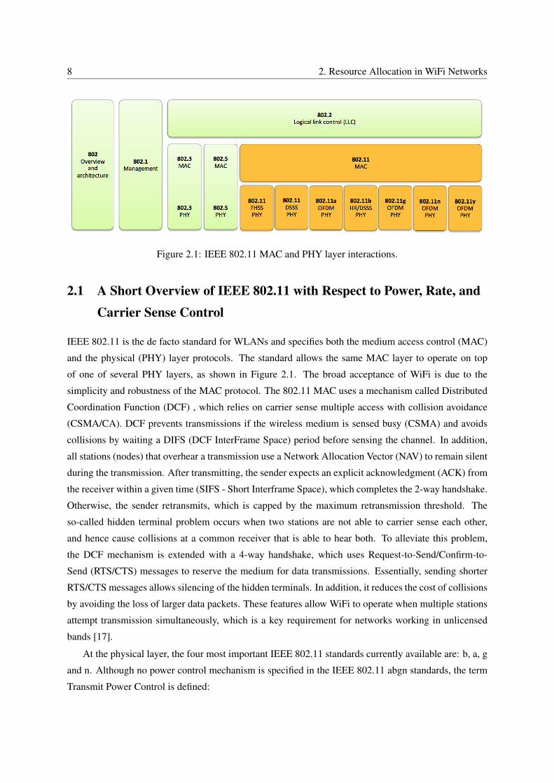
Figure 2.1: IEEE 802.11 MAC and PHY layer interactions.
2.1 A Short Overview of IEEE 802.11 with Respect to Power, Rate, andCarrier Sense Control
IEEE 802.11 is the de facto standard for WLANs and specifies both the medium access control (MAC)
and the physical (PHY) layer protocols. The standard allows the same MAC layer to operate on top
of one of several PHY layers, as shown in Figure 2.1. The broad acceptance of WiFi is due to the
simplicity and robustness of the MAC protocol. The 802.11 MAC uses a mechanism called Distributed
Coordination Function (DCF) , which relies on carrier sense multiple access with collision avoidance
(CSMA/CA). DCF prevents transmissions if the wireless medium is sensed busy (CSMA) and avoids
collisions by waiting a DIFS (DCF InterFrame Space) period before sensing the channel. In addition,
all stations (nodes) that overhear a transmission use a Network Allocation Vector (NAV) to remain silent
during the transmission. After transmitting, the sender expects an explicit acknowledgment (ACK) from
the receiver within a given time (SIFS - Short Interframe Space), which completes the 2-way handshake.
Otherwise, the sender retransmits, which is capped by the maximum retransmission threshold. The
so-called hidden terminal problem occurs when two stations are not able to carrier sense each other,
and hence cause collisions at a common receiver that is able to hear both. To alleviate this problem,
the DCF mechanism is extended with a 4-way handshake, which uses Request-to-Send/Confirm-to-
Send (RTS/CTS) messages to reserve the medium for data transmissions. Essentially, sending shorter
RTS/CTS messages allows silencing of the hidden terminals. In addition, it reduces the cost of collisions
by avoiding the loss of larger data packets. These features allow WiFi to operate when multiple stations
attempt transmission simultaneously, which is a key requirement for networks working in unlicensed
bands [17].
At the physical layer, the four most important IEEE 802.11 standards currently available are: b, a, g
and n. Although no power control mechanism is specified in the IEEE 802.11 abgn standards, the term
Transmit Power Control is defined:

A Short Overview of IEEE 802.11 with Respect to Power, Rate, and Carrier Sense Control 9
TPC: Radio regulations may require radio local area networks (RLANs) operating in the
5 GHz band to use transmitter power control, involving specification of a regulatory max-
imum transmit power and a mitigation requirement for each allowed channel, to reduce
interference with satellite services. The TPC service is used to satisfy this regulatory re-
quirement.
Since 2003, the IEEE 802.11h [18] transmit power extension specifies two spectrum management
services: Dynamic Frequency Selection (DFS) and TPC in order to be able to use certain parts of the
5Ghz spectrum at certain power levels and not interfere with other services, such as military radar
systems, satellite, and radio tracking. In order to enable the spectrum management service, the standard
defines new elements and messages (e.g., TPC capability) as extensions to existing management packets
(e.g., beacons, probe responses). These extensions allow the client and the AP to exchange the minimum
and maximum allowable transmission power information during the association or re-association of a
station to the access point, or at another station. Based on this exchange of information, transmission
power is adapted according to the link gains and margins. However, an algorithm for dynamically tuning
the transmit power is not defined by the IEEE 802.11h extension.
In the course of European harmonization of technical standards, the European Commission has de-
cided to unify the technical specifications for wireless networks from IEEE 802.11a [19] and 802.11h [18].
The current version of this harmonized European standard [20] allows different maximal transmission
power levels for each of the two 5GHz sub-bands according to TPC capability of the device. The first
sub-band ranges from 5,150 GHz to 5,350 GHz and is to be used in indoor environments. The sec-
ond sub-band from 5,470 GHz to 5,725 GHz targets outdoor usage. This European directive allows a
maximal output power level of 30dBm (respectively 1000 mW) in the second 5 GHz sub-band if the
following two conditions are met:
(i) Use of a TPC control range from 6 dB to 30 dBm
(ii) Use Dynamic Frequency Selection (DFS) when radar patterns are detected
Without such transmit power control (see (i)), devices are only allowed to use a maximum power
level of 27 dBm (respectively 500 mW). Note that the current Linux mac802.11 subsystem does not
fully support the IEEE 802.11h extensions. While DSF functionality is supported by some experimental
driver specific implementations (i.e., Atheros ath9k), TPC functionality is missing. To the best of our
knowledge there is currently no hardware vendor providing TPC, which fulfills the 6dB adaptation
range required by IEEE 802.11h. Instead, they operate at the decreased maximal output power levels.
Given these shortcomings in practice, we present mostly theoretical approaches to power control in
Section 2.2.1.
While power control support is non-existent in IEEE 802.11abgn standards, there is multi-rate sup-
10 2. Resource Allocation in WiFi Networks
port. Each IEEE 802.11 standard significantly increased the maximum net data rate: 11 Mbit/s in IEEE
802.11b, 54 Mbit/s in IEEE 802.11ag and 600 Mbit/s in IEEE 802.11n. Here, each rate represents a
distinct combination of symbol modulation (e.g., PSK, QAM, etc) and coding redundancy (e.g., 12 , 3
4 ).
While different modulation coding schemes are available with each standard, dynamically selecting a
modulation and coding scheme according to the current channel quality, i.e., automatic rate adaptation, is
left out of scope of the standards. We review the currently used rate control approaches in Section 2.2.2.
Finally, in addition to power level and rate selection, an IEEE 802.11 radio must implement a
packet/signal detection mechanism and a carrier sensing mechanism to support CSMA/CA. More specif-
ically, the Clear Channel Assessment (CCA) component aims at detecting the presence of ongoing trans-
missions to decide whether the channel is busy or not. The IEEE 802.11 standard specifies also a virtual
carrier sensing mechanism through the use of RTS and CTS messages and a Network Allocation Vector
(NAV) [1], but we focus on physical carrier sensing. Ramachandran categorizes all possible methods of
CCA into three: Energy Detection (ED), Preamble Detection (PD) and Decorrelation-based CCA [21].
802.11 systems use two out of the three methods: preamble detection and energy detection [1]. All
wireless frames across the entire 802.11abgn standards have a common unique preamble sequence at
the beginning of each frame. Hence, the transceiver can sense an ongoing transmission by detecting the
preamble sequence (preamble detection) or sense the carrier busy by detecting any kind of a signal with
signal strength higher than the CCA threshold (energy detection). The operation of CCA and selection
of its parameters play a fundamental role in communication in the presence of interference, and there-
fore, is essential to understanding the performance of WiFi networks. Carrier sense is a core part of
many wireless MAC protocols and has long been known to be an imperfect solution. Note that carrier
sense uses measurements of the wireless channel at the senders to decide whether to transmit, but at the
physical layer, channel conditions at the receivers determine the outcome of a transmission. When all
nodes are tightly clustered in a compact, isolated network, this might be expected to work well, because
channel conditions at all nodes are highly correlated. But, for any network large enough to allow spatial
reuse, the use of carrier sense is arguable [22, 23, 24, 25, 26]. In these networks, two classic failures may
occur: (1) the exposed terminal problem and (2) the hidden terminal problem. In the case of exposed
terminals, nodes that do not transmit at the same time when they could do so and therefore, missing the
potential of spatial reuse cause the problem. The hidden terminal problem, as described earlier, appears
when nodes that should not transmit concurrently do so and interfere with each other. Overall, carrier
sense control is a challenging problem, and hence, current carrier sense research is mostly theoretical.
Furthermore, these works typically consider a single parameter, the so-called carrier-sense threshold,
which does not truly reflect how carrier sensing is implemented in the current hardware. We present
these works in Section 2.2.3. Additionally, we show the details of the carrier sense mechanism imple-
mented in a typical WiFi radio, and its performance under external noise (e.g., from microwave ovens)
and temperature variations in Chapter 3.
Resource Allocation Based on Only Power, Rate or Carrier-Sense Control 11
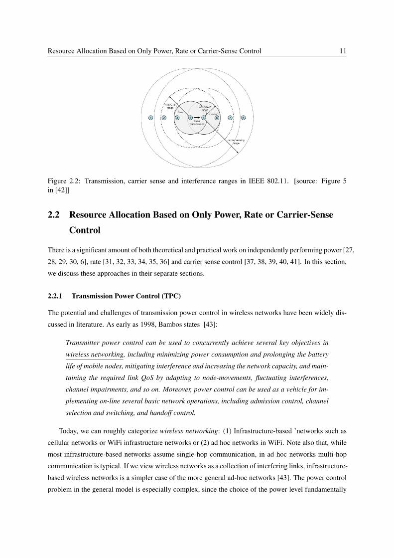
Figure 2.2: Transmission, carrier sense and interference ranges in IEEE 802.11. [source: Figure 5in [42]]
2.2 Resource Allocation Based on Only Power, Rate or Carrier-SenseControl
There is a significant amount of both theoretical and practical work on independently performing power [27,
28, 29, 30, 6], rate [31, 32, 33, 34, 35, 36] and carrier sense control [37, 38, 39, 40, 41]. In this section,
we discuss these approaches in their separate sections.
2.2.1 Transmission Power Control (TPC)
The potential and challenges of transmission power control in wireless networks have been widely dis-
cussed in literature. As early as 1998, Bambos states [43]:
Transmitter power control can be used to concurrently achieve several key objectives in
wireless networking, including minimizing power consumption and prolonging the battery
life of mobile nodes, mitigating interference and increasing the network capacity, and main-
taining the required link QoS by adapting to node-movements, fluctuating interferences,
channel impairments, and so on. Moreover, power control can be used as a vehicle for im-
plementing on-line several basic network operations, including admission control, channel
selection and switching, and handoff control.
Today, we can roughly categorize wireless networking: (1) Infrastructure-based ’networks such as
cellular networks or WiFi infrastructure networks or (2) ad hoc networks in WiFi. Note also that, while
most infrastructure-based networks assume single-hop communication, in ad hoc networks multi-hop
communication is typical. If we view wireless networks as a collection of interfering links, infrastructure-
based wireless networks is a simpler case of the more general ad-hoc networks [43]. The power control
problem in the general model is especially complex, since the choice of the power level fundamentally
12 2. Resource Allocation in WiFi Networks
affects many aspects of the network operation [44]:
• Received signal quality at the receiver (PHY layer)
• Carrier sensing and data transmission ranges (see Figure 2.2), hence, the number of nodes con-
tending for channel access (MAC layer)
• Transmission range, and hence, the number of hops in routing (Network layer).
• Interference with other receivers, therefore, congestion (Transport layer).
Note that in infrastructure WiFi networks, TPC does not affect the routing layer. Furthermore, in cellular
networks, the impact of TPC on the MAC layer is less of an issue due to the use of FDD (Frequency
Division Duplex) or TDD (Time Division Duplex) schemes for medium access. The capacity gains
of distributed power control in the context of cellular networks have been well studied in the litera-
ture [45] . However, these solutions for cellular networks cannot be directly applied to WiFi networks,
infrastructure-based, or ad hoc, as WiFi uses CSMA/CA MAC. In the rest of this section, we focus on
TPC for WiFi networks.
Due to its effect on multiple layers of the protocol stack, TPC directly affects throughput, capacity,
delay, and fairness in the network and, may also affect energy consumption and network connectiv-
ity. However, it is typically not possible to achieve multiple performance objectives, e.g., both high
throughput and low energy consumption, simultaneously. Therefore, the majority of the work in power
control, e.g., [46, 47, 48] use these performance objectives as key classifications. We follow the same ap-
proach and consider three main TPC classes: energy-oriented, topology-oriented and capacity-oriented.
Table 2.1 summarizes the related work on TPC.
The main goal of energy-oriented power control schemes is to reduce energy consumption, while
throughput is treated as a secondary objective. For instance, Jung et al [58] present a power control
protocol which does not degrade throughput and yields energy savings. Their nodes use maximum
transmission power to send RTS/CTS packets and minimum power to transmit data packets. To ensure
high throughput, data transmissions periodically are sent at maximum power to mitigate the loss of
ACK packets due to collisions. Gomez et al [49] introduce a power-aware routing system, PARO, to
minimize transmission power needed to forward packets in an ad-hoc network. There are also power-
aware routing protocols, which use transmission power as a routing metric, with the goal of increasing
network lifetime [59]. However, in today’s WiFi systems, energy savings from the proposed solutions
may not be realized. For instance, Piazza et al [60] show that TPC offers marginal energy savings
compared to the average power consumption of IEEE 802.11g WiFi cards. Their results show savings
from 10% to 20% by reducing transmission power from 15dBm to 0dBm (e.g., 32 mW to 1 mW),
assuming the device is constantly sending. Also Halperin et al [61] conclude, after analyzing energy
consumption of the latest IEEE 802.11n devices, that reducing the radiated power via TPC by 97%
still leads to only 10% in overall energy savings. In summary, it can be concluded that TPC does not
bring energy savings with today’s WiFi devices and, therefore, we do not consider reducing energy

Resource Allocation Based on Only Power, Rate or Carrier-Sense Control 13
Table 2.1: Summary of Transmit Power Control (TPC) Algorithms
Protocol Obj.1 Granularity Type of Control PHY layer assumptions Validation
PARO [49] E Per-packet Dist. Sym2, ideal comm.3,omni4 –
Compow [50] T Per-network Cent. Sym, ideal comm.,omni X(Routing)
ClusterPow [51] T Per-cluster Cent. Sym, ideal comm.,omni X(Routing)
PCMA [52] C Per-packet Dist. Sym, ideal comm., omni –
POWMAC [27] C Per-packet Dist. Sym, ideal comm., omni –
CONTOUR [53] C Per slot Cent., synch. Omni XClick [54] (P)
MIDAS [55] C Per packet Dist. Directional5 X(MAC,WARP)
DIRC [56] C Per slot Cent. Directional X(MAC,Madwifi)
SPEED [57] C Per slot Cent. Directional X(Multi-radio)1 Abbreviations: Obj: Objective, E: Energy, T: Topology, C: Capacity, Dist.: Distributed, Cent.:Centralized, synch: Synchronized, P:
Prototype2 Interference/fading conditions in rx and tx directions are similar in space and time.3 Ideal comm: Overhearing any transmissions is possible by other nodes, hence interference-free MAC (as long a minimum signal level
is reached). Furthermore, any node is capable of measuring received SNR of overheard packets and quantify this as a standard metric.4 Omni-directional antennas are considered.5 Directional antennas with a typical angle of vertical radiation beams between 5◦to 120◦are considered.
consumption as an objective in this thesis.
In the second class of topology-oriented power control schemes, the main objective is to control the
topological properties of the network, such as reducing interference from low-degree nodes while main-
taining overall connectivity [62]. Wattenhofer et al. [63] propose a scheme, where global connectivity
is guaranteed while the resulting network topology leads to an increase in network lifetime. Topology
control is intimately connected with routing in multi-hop wireless ad hoc networks. For instance, COM-
POW [50] selects a common power level to ensure bi-directional links between all nodes by running
several routing daemons, each at a different power level. The minimum power level, which achieves
the same level of network connectivity as the maximum power level is chosen as the common network
power. The authors later extend this work, and propose CLUSTERPOW [51] to avoid settling on an un-
necessarily high common power level in non-homogeneous network deployments. Here, while a higher
power may be used to connect two clusters, the power level used within clusters can be significantly
lower. In this thesis, we focus on single hop communication, and therefore, the TPC impact on and
interaction with routing are left as future work.
The third class, capacity-oriented power control schemes try to increase overall network capacity
while improving end-to-end delay and realizing fair throughput allocation [47]. Power control can im-
prove network throughput in two ways: (1) by reducing interference and (2) by increasing network
spatial reuse. For (1), consider a hidden terminal situation, where two senders are not able to carrier
14 2. Resource Allocation in WiFi Networks
sense each other, but their transmissions collide at one or both of the receivers. If the senders trans-
mit packets at an optimal power level, it may be possible to guarantee successful packet delivery while
minimizing interference. The collision probability is reduced and consequently, the number of retrans-
missions, which allows the bandwidth to be used effectively. For (2), remember that IEEE 802.11 does
not allow two simultaneous transmissions if the transmitters can carrier sense each other. Reducing the
transmission power may increase the number of simultaneous transmissions and increasing the overall
throughput. It must be noted that power control is not the only approach for avoiding interference and
increasing spatial reuse. Directional transmissions via directed antennas or beam-forming also improve
spatial reuse (e.g., DIRC [56], SPEED [57], [12], MIDAS [55]). However, such approaches require
extensive changes to the upper layers, including the MAC layer. Furthermore, access points with direc-
tional antennas are untypical for current deployments and hence, these approaches are out of the scope
of this thesis.
To improve spatial reuse as well as throughput, Monks et. al present Power Controlled Multiple
Access (PCMA) protocol [52], which allows different nodes to have different transmission power levels
and per-packet selection of transmit power. PCMA uses two channels, one channel for busy tones, and
the other for all other packets. While a node is receiving a data packet, it periodically sends a busy tone
to advertise its interference tolerance level. This bounds the maximum transmission power that can be
used for other transmissions. To this end, the busy tone is transmitted at the power level equal to the
maximum additional noise the node can tolerate. Any node wishing to transmit a packet first waits for
a fixed duration (determined by the frequency with which nodes transmit busy tones when receiving
data), and senses the channel for busy tones from other nodes. The signal strength of the busy tones
received by a node is used to determine the highest power level at which this node may transmit without
interfering with other on-going transmissions. This way, simultaneous transmissions can take place and
hidden terminals do not pose a problem as transmission power levels are bounded. However, PCMA
requires extensive modifications at the MAC layer.
The work of Muqattash and Krunz, POWMAC [48], does not require out-of-band signaling. How-
ever, it still requires significant changes to the MAC layer. POWMAC uses an access window (AW) to
allow for a series of RTS/CTS exchanges to take place before it schedules multiple concurrent data trans-
missions if they create tolerable interference to each other. Hence, the protocol activates multiple links
concurrently while satisfying the interference constraints. Each node maintains a power constraint list
about the surrounding active nodes. This information include node address, channel gain derived from
RSS measurements of the control packets, start time and duration of transmission activities, maximum
tolerable interference and the transmit power level used by the node. Based on simulations, the authors
show that POWMAC improves network throughput up to 50% by increasing spatial reuse in random-
grid topologies. However, POWMAC is not applicable to standard WiFi systems due to proposed MAC
changes. These are often not feasible due to the hardware limitations. Similarly, Countour [53] tries
Resource Allocation Based on Only Power, Rate or Carrier-Sense Control 15
to increase the spatial reuse through a slotted symmetric power control framework. In this framework,
all access points are assumed to be synchronized and they are expected to operate at the same power
level at any given instant and follow a sequence of power levels, called an envelope. A centralized
controller computes and distributes the envelope. Different than these approaches, in this thesis, we
investigate the feasibility of a fully-distributed capacity-oriented (or interference-aware) TPC scheme,
which works over the existing IEEE 802.11 standard and current WiFi hardware, and does not require
synchronization.
2.2.2 Transmission Rate Control (TRC)
Rate (Mb/s) Modulation Coding
Rate
IEEE 802.11
Standard
IEEE 802.11
Standard
IEEE 802.11
StandardRate
(Mb/s) Modulation Coding Rate
b g a1 DBPSK 1/11 X X2 DQPSK 1/11 X X
5,5 CCK 4/8 X X6 BPSK 1/2 X X9 BPSK 3/4 X X
11 CCK 8/8 X X12 QPSK 1/2 X X18 QPSK 3/4 X X24 16-QAM 1/2 X X36 16-QAM 3/4 X X48 64-QAM 2/3 X X54 64-QAM 3/4 X X
RateSelection
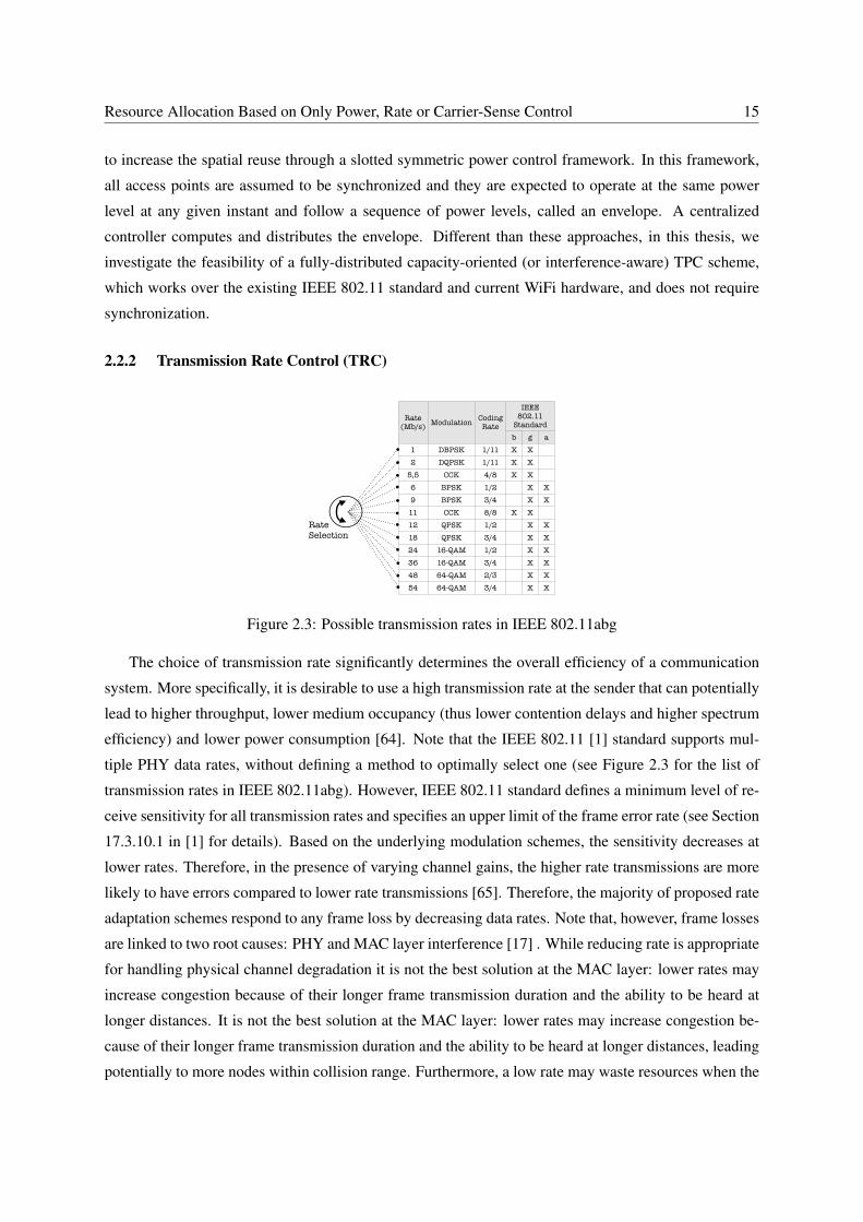
Figure 2.3: Possible transmission rates in IEEE 802.11abg
The choice of transmission rate significantly determines the overall efficiency of a communication
system. More specifically, it is desirable to use a high transmission rate at the sender that can potentially
lead to higher throughput, lower medium occupancy (thus lower contention delays and higher spectrum
efficiency) and lower power consumption [64]. Note that the IEEE 802.11 [1] standard supports mul-
tiple PHY data rates, without defining a method to optimally select one (see Figure 2.3 for the list of
transmission rates in IEEE 802.11abg). However, IEEE 802.11 standard defines a minimum level of re-
ceive sensitivity for all transmission rates and specifies an upper limit of the frame error rate (see Section
17.3.10.1 in [1] for details). Based on the underlying modulation schemes, the sensitivity decreases at
lower rates. Therefore, in the presence of varying channel gains, the higher rate transmissions are more
likely to have errors compared to lower rate transmissions [65]. Therefore, the majority of proposed rate
adaptation schemes respond to any frame loss by decreasing data rates. Note that, however, frame losses
are linked to two root causes: PHY and MAC layer interference [17] . While reducing rate is appropriate
for handling physical channel degradation it is not the best solution at the MAC layer: lower rates may
increase congestion because of their longer frame transmission duration and the ability to be heard at
longer distances. It is not the best solution at the MAC layer: lower rates may increase congestion be-
cause of their longer frame transmission duration and the ability to be heard at longer distances, leading
potentially to more nodes within collision range. Furthermore, a low rate may waste resources when the
16 2. Resource Allocation in WiFi Networks
channel conditions support a higher rate [65].
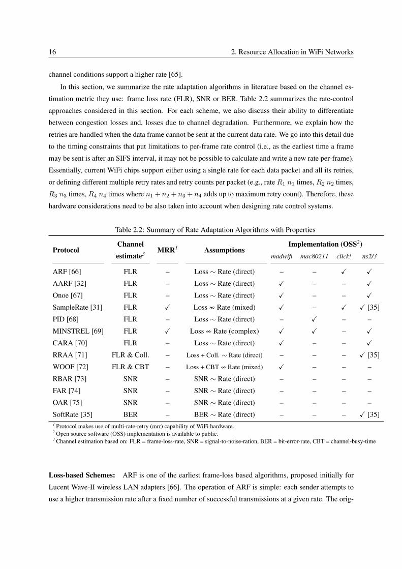
In this section, we summarize the rate adaptation algorithms in literature based on the channel es-
timation metric they use: frame loss rate (FLR), SNR or BER. Table 2.2 summarizes the rate-control
approaches considered in this section. For each scheme, we also discuss their ability to differentiate
between congestion losses and, losses due to channel degradation. Furthermore, we explain how the
retries are handled when the data frame cannot be sent at the current data rate. We go into this detail due
to the timing constraints that put limitations to per-frame rate control (i.e., as the earliest time a frame
may be sent is after an SIFS interval, it may not be possible to calculate and write a new rate per-frame).
Essentially, current WiFi chips support either using a single rate for each data packet and all its retries,
or defining different multiple retry rates and retry counts per packet (e.g., rate R1 n1 times, R2 n2 times,
R3 n3 times, R4 n4 times where n1 + n2 + n3 + n4 adds up to maximum retry count). Therefore, these
hardware considerations need to be also taken into account when designing rate control systems.
Table 2.2: Summary of Rate Adaptation Algorithms with Properties
ProtocolChannel
MRR1 AssumptionsImplementation (OSS2)
estimate3 madwifi mac80211 click! ns2/3
ARF [66] FLR – Loss ∼ Rate (direct) – – X X
AARF [32] FLR – Loss ∼ Rate (direct) X – – X
Onoe [67] FLR – Loss ∼ Rate (direct) X – – X
SampleRate [31] FLR X Loss � Rate (mixed) X – X X [35]
PID [68] FLR – Loss ∼ Rate (direct) – X – –
MINSTREL [69] FLR X Loss � Rate (complex) X X – X
CARA [70] FLR – Loss ∼ Rate (direct) X – – X
RRAA [71] FLR & Coll. – Loss + Coll. ∼ Rate (direct) – – – X [35]
WOOF [72] FLR & CBT – Loss + CBT � Rate (mixed) X – – –
RBAR [73] SNR – SNR ∼ Rate (direct) – – – –
FAR [74] SNR – SNR ∼ Rate (direct) – – – –
OAR [75] SNR – SNR ∼ Rate (direct) – – – –
SoftRate [35] BER – BER ∼ Rate (direct) – – – X [35]1 Protocol makes use of multi-rate-retry (mrr) capability of WiFi hardware.2 Open source software (OSS) implementation is available to public.3 Channel estimation based on: FLR = frame-loss-rate, SNR = signal-to-noise-ration, BER = bit-error-rate, CBT = channel-busy-time
Loss-based Schemes: ARF is one of the earliest frame-loss based algorithms, proposed initially for
Lucent Wave-II wireless LAN adapters [66]. The operation of ARF is simple: each sender attempts to
use a higher transmission rate after a fixed number of successful transmissions at a given rate. The orig-
Resource Allocation Based on Only Power, Rate or Carrier-Sense Control 17
inal ARF algorithm decreases the current rate and starts a timer when two consecutive transmissions fail
in a row. When the timer expires or the number of successfully received per-packet acknowledgments
reaches 10, the transmission rate is increased and the timer is reset. Simulations and experimental results
show that ARF only performs well in comparison to other rate selection algorithms when the channel
conditions support sending at the highest rate [76]. In fact, ARF finds the best rate very fast and without
any feedback from the receiver side (i.e., without the complexity of implementing feedback algorithms).
While ARF responds well to short term channel variation, the way it increases the rate limits its use in
stable environments where long-term channel variations are common. To address this problem, Lacage
et. al [32] proposed Adaptive Auto Rate Fallback (AARF), which uses binary exponential back-off to
adapt the threshold used to increase the rate. In AARF, if the first attempt to switch the rate up fails, then
the next attempt should only be made after doubling the threshold. If the situation persists, the threshold
is doubled again thus reducing the number of rate changes [64].
The practical relevance of rate control algorithms increased with the spread of Open-wrt based em-
bedded router platforms. Especially, the partial open-source driver Madwifi [77] of Atheros WiFi chips
is commonly used in research testbeds. The earliest open source rate adaptation protocol in FreeBSD
and Linux that got integrated into Madwifi was Onoe [67]. The objective of Onoe is to find the highest
rate that provides a loss ratio less than 50%. This rate control algorithm is less sensitive to individual
packet failures as compared to ARF as it accumulates performance credits per link and bitrate. If less
than 10% of data packets require a retry, the number of credits of the corresponding rate is increased.
Every second, a check is performed to see whether the amount of credits add up to a target threshold of
10 or more to switch to the next higher rate. In the case of errors, the number of credits for that rate is
decremented. Whenever the average number of retries is greater than one for 10 or more consecutive
packets, the rate is decreased to the next lower rate.
ARF, AARF and Onoe switch sequentially between a sorted list of available rates to react to channel
dynamics. These protocols assume that there is a linear relationship among rates, which is questionable
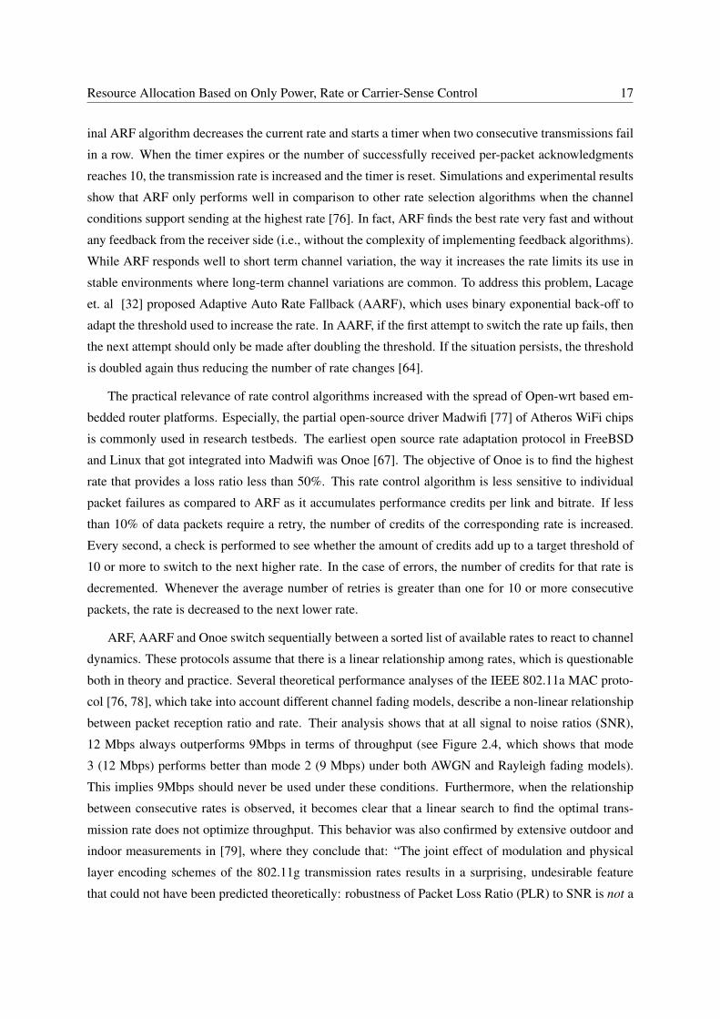
both in theory and practice. Several theoretical performance analyses of the IEEE 802.11a MAC proto-
col [76, 78], which take into account different channel fading models, describe a non-linear relationship
between packet reception ratio and rate. Their analysis shows that at all signal to noise ratios (SNR),
12 Mbps always outperforms 9Mbps in terms of throughput (see Figure 2.4, which shows that mode
3 (12 Mbps) performs better than mode 2 (9 Mbps) under both AWGN and Rayleigh fading models).
This implies 9Mbps should never be used under these conditions. Furthermore, when the relationship
between consecutive rates is observed, it becomes clear that a linear search to find the optimal trans-
mission rate does not optimize throughput. This behavior was also confirmed by extensive outdoor and
indoor measurements in [79], where they conclude that: “The joint effect of modulation and physical
layer encoding schemes of the 802.11g transmission rates results in a surprising, undesirable feature
that could not have been predicted theoretically: robustness of Packet Loss Ratio (PLR) to SNR is not a
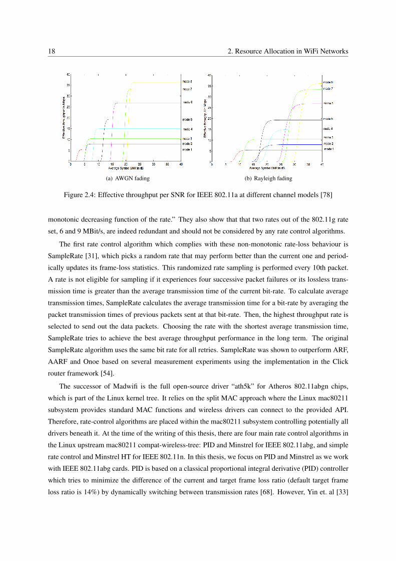
18 2. Resource Allocation in WiFi Networks
(a) AWGN fading (b) Rayleigh fading
Figure 2.4: Effective throughput per SNR for IEEE 802.11a at different channel models [78]
monotonic decreasing function of the rate.” They also show that that two rates out of the 802.11g rate
set, 6 and 9 MBit/s, are indeed redundant and should not be considered by any rate control algorithms.
The first rate control algorithm which complies with these non-monotonic rate-loss behaviour is
SampleRate [31], which picks a random rate that may perform better than the current one and period-
ically updates its frame-loss statistics. This randomized rate sampling is performed every 10th packet.
A rate is not eligible for sampling if it experiences four successive packet failures or its lossless trans-
mission time is greater than the average transmission time of the current bit-rate. To calculate average
transmission times, SampleRate calculates the average transmission time for a bit-rate by averaging the
packet transmission times of previous packets sent at that bit-rate. Then, the highest throughput rate is
selected to send out the data packets. Choosing the rate with the shortest average transmission time,
SampleRate tries to achieve the best average throughput performance in the long term. The original
SampleRate algorithm uses the same bit rate for all retries. SampleRate was shown to outperform ARF,
AARF and Onoe based on several measurement experiments using the implementation in the Click
router framework [54].
The successor of Madwifi is the full open-source driver “ath5k” for Atheros 802.11abgn chips,
which is part of the Linux kernel tree. It relies on the split MAC approach where the Linux mac80211
subsystem provides standard MAC functions and wireless drivers can connect to the provided API.
Therefore, rate-control algorithms are placed within the mac80211 subsystem controlling potentially all
drivers beneath it. At the time of the writing of this thesis, there are four main rate control algorithms in
the Linux upstream mac80211 compat-wireless-tree: PID and Minstrel for IEEE 802.11abg, and simple
rate control and Minstrel HT for IEEE 802.11n. In this thesis, we focus on PID and Minstrel as we work
with IEEE 802.11abg cards. PID is based on a classical proportional integral derivative (PID) controller
which tries to minimize the difference of the current and target frame loss ratio (default target frame
loss ratio is 14%) by dynamically switching between transmission rates [68]. However, Yin et. al [33]
Resource Allocation Based on Only Power, Rate or Carrier-Sense Control 19
showed that operation of PID leads to significant oscillation in rate selection and throughput.
The most commonly used rate control algorithm for IEEE 802.11abg is Minstrel [69]. It builds on
SampleRate and also incorporates several experiences from real WiFi systems into its design. The main
goal of Minstrel is to address responsiveness and reliability issues seen with the other rate algorithms
available in open-source drivers. Briefly, Minstrel operates as follows: It maintains a table of the es-
timated success probability per neighbor and rate. The success probability is calculated as the ratio
of the number of acknowledgements to transmission attempts for a given rate. Every 100ms, Minstrel
evaluates this statistics table and uses Exponential Weighted Moving Average (EWMA) to smooth the
success history of each rate, R, as follows:
p+success[R] = ((1− α)× success[R]
attempt[R]) + (α× psuccess[R]), (2.1)
where p+success[R] is the new success probability, psuccess[R] is the old success probability, success[R]
is the number of packets sent successfully in the current interval, and attempt[R] is the number of
attempts. Here, α is the smoothing factor. Given p+success[R], the maximum achievable throughput is
calculated as R× p+success[R]. This table is used to find the best performing rate and the rates to be used
for the retries (i.e., multi-rate retry chain) in the next interval. To update these statistics, a fixed amount
(10% by default) of the data packets are used to probe a randomly chosen rate out of the possible rate
set. Minstrel’s sampling therefore depends on the data traffic in terms of packet rate and packet length
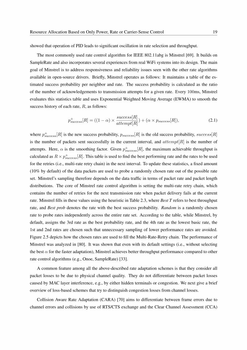
distributions. The core of Minstrel rate control algorithm is setting the multi-rate retry chain, which
contains the number of retries for the next transmission rate when packet delivery fails at the current
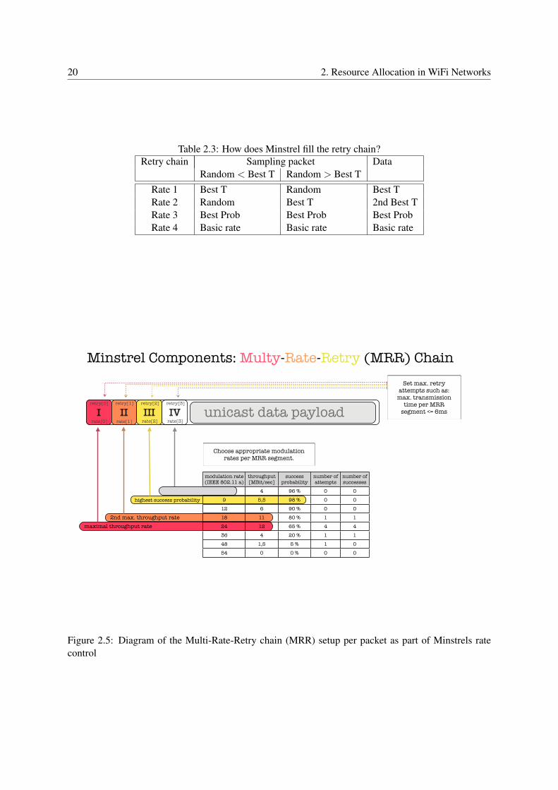
rate. Minstrel fills in these values using the heuristic in Table 2.3, where Best T refers to best throughput
rate, and Best prob denotes the rate with the best success probability. Random is a randomly chosen
rate to probe rates independently across the entire rate set. According to the table, while Minstrel, by
default, assigns the 3rd rate as the best probability rate, and the 4th rate as the lowest basic rate, the
1st and 2nd rates are chosen such that unnecessary sampling of lower performance rates are avoided.
Figure 2.5 depicts how the chosen rates are used to fill the Multi-Rate-Retry chain. The performance of
Minstrel was analyzed in [80]. It was shown that even with its default settings (i.e., without selecting
the best α for the faster adaptation), Minstrel achieves better throughput performance compared to other
rate control algorithms (e.g., Onoe, SampleRate) [33].
A common feature among all the above-described rate adaptation schemes is that they consider all
packet losses to be due to physical channel quality. They do not differentiate between packet losses
caused by MAC layer interference, e.g., by either hidden terminals or congestion. We next give a brief
overview of loss-based schemes that try to distinguish congestion losses from channel losses.
Collision Aware Rate Adaptation (CARA) [70] aims to differentiate between frame errors due to
channel errors and collisions by use of RTS/CTS exchange and the Clear Channel Assessment (CCA)
20 2. Resource Allocation in WiFi Networks
Table 2.3: How does Minstrel fill the retry chain?Retry chain Sampling packet Data
Random < Best T Random > Best TRate 1 Best T Random Best TRate 2 Random Best T 2nd Best TRate 3 Best Prob Best Prob Best ProbRate 4 Basic rate Basic rate Basic rate
Minstrel Components: Multy-Rate-Retry (MRR) Chain
maximal throughput rate2nd max. throughput rate
highest success probability
I II III IV unicast data payload
Basic rate
Set max. retry attempts such as:
max. transmission time per MRR
segment <= 6ms
modulation rate (IEEE 802.11 a)
throughput[MBit/sec]
success probability
number of attempts
number of successes
6 4 96 % 0 0
9 5,5 98 % 0 0
12 6 90 % 0 0
18 11 80 % 1 1
24 12 65 % 4 4
36 4 20 % 1 1
48 1,5 5 % 1 0
54 0 0 % 0 0
rate[0]
retry[0]
rate[1]
retry[1]
rate[2]
retry[2]
rate[3]
retry[3]
Choose appropriate modulation rates per MRR segment.
Figure 2.5: Diagram of the Multi-Rate-Retry chain (MRR) setup per packet as part of Minstrels ratecontrol

Resource Allocation Based on Only Power, Rate or Carrier-Sense Control 21
functionality of the IEEE 802.11. To handle collision-based losses, first, CARA turns on RTS upon a
frame loss and turn off RTS upon a frame success. The second method to differentiate collisions from
channel errors is called CCA Detection. After a node finishes its data transmission, it starts assessing
the wireless channel using CCA. Since the node expects an ACK within an SIFS, if the wireless channel
is busy and the expected ACK reception does not start, the station concludes that a collision has hap-
pened. In both cases, data transmission rate is not reduced. Similarly, Robust Rate Adaptation Algorithm
(RRAA) [71] consists of two components: rate adaptation (loss ratio estimation and rate selection) and
collision elimination. The basic idea is again to leverage the per-frame RTS option in the IEEE 802.11
standard, and selectively turn on RTS/CTS exchange to suppress collision losses. However, Wong et al
argue that CARA suffers from the drawback of RTS oscillation: In the worst case, when one of every
two frames is lost, this results in more than 50% throughput reduction. Therefore, RRAA uses adaptive
RTS to reduce collision losses. To this end, RRAA maintains an RTS-window (RTSwnd) similar to TCP
(Transmission Control Protocol) congestion window. Within an RTS window, all frames are sent with
RTS on. RTSwnd is initially set as 0, which disables RTS. It is then adapted as follows. When the last
frame was lost without RTS, RTSwnd is incremented by one as this suggests a collision loss. When
the last frame transmission was lost with RTS, or succeeded without RTS, RTSwnd is halved because
the packet did not experience collisions. When the last frame succeeded with RTS on, RTSwnd is kept
unchanged.
Finally, Wireless cOngestion Optimized Fallback (WOOF) [72] monitors channel busy time (us-
ing Atheros-based hardware) and relies on this metric to estimate the probability of congestion-based
packet loss. The data rate selection is based on SampleRate calculation of expected transmission time.
However, the congestion loss probability is used to adjust the expected transmission time, so that the
congestion-related losses do not play a significant role in rate selection. The authors show that WOOF
outperforms SampleRate and is able to follow the static best rate selection. However, it is not clear,
compared to the previous approaches, how WOOF performs in the presence of hidden terminals.
SNR-based approaches: Receiver Based Auto Rate (RBAR) [73] is the first SNR-based rate adap-
tation protocol that takes advantage of the RTS/CTS control frames transmitted at the basic rate. This
requires modifying the IEEE 802.11 standard in two ways: (1) RTS/CTS messages have to include
packet size and rate, instead of transmission duration; (2) an additional RSH message is sent before the
data frame to finalize the handshake. While RBAR is of little practical interest because it cannot be
deployed in existing 802.11 networks, it is still important because it serves as a baseline for SNR-based
approaches.
The existence of stations that use different rates creates challenging problems. Sadeghi et al [75]
showed that while standard IEEE 802.11 ensures access fairness among competing stations, this leads to
unfair use of the channel by slow transmitters. They propose Opportunistic Auto Rate (OAR) to ensure
22 2. Resource Allocation in WiFi Networks
time fairness among competing stations. Similar to RBAR, OAR probes possible rates by exchanging
RTS/CTS packets and it differs in its opportunistic transmission of data frames. Over periods of good
channel conditions, nodes that are able to use higher rates, send multiple consecutive data packets that
sum up to the time it would take to send a single packet at slower rates, e.g., the basic rate [81]. OAR,
unfortunately, shares the same practicality issues with RBAR.
Full Auto Rate (FAR) [82] attempts to achieve full data rate adaptation - rate adaptation for control
packets as well as data packets. The authors argue that, if RTS/CTS packets are transmitted at a higher
data rate, rather than the basic rate, better performance should be achieved because transmission at
basic rate underutilizes the wireless channel. In FAR, an idle station which overhears frames from its
neighbor stations uses its received signal strength to estimate the rate to the neighbor station. Then,
when this station needs to transmit an RTS, it uses the pre-estimated rate. If the RTS is transmitted
successfully, FAR follows the strategy similar of RBAR to estimate the rate for a data frame during the
RTS/CTS exchange. If RTS fails, it is retransmitted at a lower rate.
In summary, using receiver feedback is both an advantage and disadvantage for SNR-based ap-
proaches: while their information about what the receiver might be experiencing is more accurate, they
require a feedback mechanism to acquire such information. In [83], it is shown indeed that SNR-based
protocols are more robust compared to loss-based protocols. However, they also conclude that SNR-
based protocols require in-situ training to ensure such robustness.
BER-based approaches: BER-based rate adaption schemes, e.g., SoftRate [35], promise throughput
gains and shorten response time for rapidly varying channel conditions. It differentiates between inter-
ference and channel errors caused by attenuation or fading. The BER-based rate adaptation reduces the
bit rate accordingly only in the latter case. However, in order to use BER-based rate control schemes,
the PHY layer must be able to provide BER measurements or estimates. This is not the case in the
standard 802.11 PHY. This is due to having only a fixed set of error correcting codes to ensure the entire
frame is correct or it should be retransmitted. Therefore, typically, BER-based schemes are realized
using software-defined radios (SDRs). Using a customized firmware on the micro-controller, Han et al.
realized time-critical operations such as blockwise error correction over 802.11 frames but these novel-
ties are very hardware specific [84]. Therefore, the potential of BER-based approaches will be unlocked
as SDRs become more prominent but unfortunately, these approaches do not apply to current hardware.
2.2.3 Carrier-Sense Control - CSC
In addition to selecting a certain power-level and bit-rate to transmit a data packet, an IEEE 802.11 ra-
dio must implement a packet/signal detection mechanism and a carrier sensing mechanism to support
CSMA/CA. Among many wireless MAC protocols carrier sense is a key component of their operation.
Its main objective is to regulate concurrency in wireless medium access by achieving a balance between
Resource Allocation Based on Only Power, Rate or Carrier-Sense Control 23
interference protection and spatial reuse. Two types of carrier sensing are used, a mandatory physical
carrier sensing and an optional virtual carrier sensing, which is not our focus. Physical carrier sense is
known to be imperfect as a sender is only able to observe its environment and decides to transmit or
not, while the transmission success is actually determined by receiver-side conditions. The underlying
assumption is that channel conditions are highly correlated at all nodes. We observe this might be true
only in artificial cases of tightly clustered nodes in compact and isolated networks. Today’s WiFi de-
ployments contrast these assumptions, as they are not clustered but chaotic, not isolated but overlapping,
not compact but city wide.
Two problems with carrier sense have been identified in the literature: (1) the exposed terminal
problem, where nodes that could have transmitted simultaneously, miss the opportunity of spatial reuse,
and (2) the hidden terminal problem, where nodes that should hold back their transmission, do not and
interfere with others [85]. To address these issues, earlier work looked at tuneable carrier sensing, which
improves network throughput by maximising spatial reuse. Similarly, Schmidt et al. [86] propose a
CCA threshold adaptation but for a different context: vehicular networks. They propose to adapt CCA
threshold stepwise based on the time a packet has waited for channel access. Their approach enables the
possibility to find a sweet spot, where both the collisions and the channel access delays are reduced.
However, these theoretical works assume carrier sense is controlled via a single parameter, CCA
threshold, and adjust it in discrete and absolute steps [39, 87, 86]. Carrier sense that is implemented
on hardware is based on the interplay of different detection mechanisms. For instance, in the case of
Atheros hardware, it is possible adjust up to 6 parameters regarding the operation of carrier sensing.
Furthermore, the computation of the optimal threshold requires strong assumptions, such as all receivers
at a given distance are subject to the same interference [39, 87]. It is assumed that links either interfere or
sense each other. Yet recent experimental results show a more complex relationship: rather than on-off,
a probabilistic transition range (i.e., gray-zone) between interfering or carrier sensing links [88, 89].
The work based on WiFi experiments shows that there is room for improvement for carrier sense.
Jamieson et al. [23] present an experimental study, where they show that carrier sense performance is
poor in the presence of exposed terminals, multiple interferers, or when capture is possible (the receiver
is able to switch to receiving a stronger signal even though it is locked onto another). They argue that
especially at low bit rates, the capture effect allows concurrent transmissions. Furthermore, their results
indicate that carrier sense might be unnecessary at high loads, as nodes cannot keep up with carrier
sensing for each packet and transmissions slow down. Overlay MAC Layer (OML) [90], which was
implemented on top of the IEEE 802.11 MAC, allows scheduling transmissions so that ”unfavorable
interactions” between senders are avoided. The scheduling is based on an interference graph and their
results show significant improvement in fairness, and comparable results in throughput. Vutukuru et
al. [24] address the issue raised in [23] about exposed terminals, by allowing nodes to compute a conflict
map in a distributed manner. Nodes use empirical observations of packet losses to populate their own
24 2. Resource Allocation in WiFi Networks
piece of conflict map and keep track of those nodes they are able to transmitt to concurrently. This is
done with the help of receivers, which use headers and trailers of colliding packets to identify which
nodes cause a collision. All nodes periodically announce their interferer lists to all others. Note that,
however, all these improvements highly depend on the underlying network graph and the distribution of
traffic.
To better understand the performance of carrier sense in theory, recent work from Brodsky et al. [85]
focuses on both short and long range network links, and considers multi-rate radios. Their model applies
to the common two-sender case, assuming nodes roughly reach Shannon capacity through bit-rate adap-
tation. They consider carrier sensing as a function that switches between concurrent transmissions and
time-division multiplexing. Their analysis shows that carrier sense performance is close to optimal for
radios with adaptive bit-rate (only 15% below optimal). Most importantly, this performance is achieved
in a decentralized manner, and further tweaking offers only limited benefits. Their key results stem from
the observation that interference is a global phenomenon, affecting, to some extent, all nodes everywhere
and benefits from carrier sense adaptation seems to be limited. Compared to the aforementioned work,
their model suggests that hidden and exposed terminals usually cause modest reductions in throughput
rather than dramatic decreases. However, their model provides worst-case analysis and assumes opti-
mal concurrency, which provides interesting performance limits but with little practical relevance (i.e.,
their simple radio propagation models does not take into account the effect of shadowing and noise floor
calibrations, see [21] for an overview of different hardware technics to perform carrier sensing).
In summary, even though major steps have been taken in understanding carrier sense both in theory
and practice, the conclusions do not resolve the question whether carrier sense control is necessary or
not. Therefore, we consider carrier sense control an open problem.
2.3 Joint Resource Allocation
Todays strict layering approach of the protocol stack where fundamental services such as access to the
medium (link layer), routing (network layer), and congestion control (transport layer) are hierarchically
defined and independently provided has been proven as a very successful design paradigm for wired
networks [91]. Srivastava et. al [92] distinguish three main reasons why the presence of wireless links
within a network motivate protocol designers to violate the traditional layered network architecture:
the unique problems created by wireless links, the possibility of opportunistic communication, and the
new modalities of communication offered by the wireless medium. Essentially, the capacity of wireless
networks is not fixed but rather time- and space-varying caused by channel impairments, mobility and
interference [93]. The achievable capacity depends upon local resource allocation decisions: transmit
power and transmit rate adjusted at the WiFi sender and carrier sense settings at the WiFi receiver.
Here, significant inter-dependencies exist. For instance, a rate control mechanism searches for the best
Joint Resource Allocation 25
transmission rate under varying channel quality. A packet can be transmitted at a high rate if the SNR
(Signal to Noise Ratio) at the receiver is high and otherwise, a lower transmit rate achieves more robust
communication. Hence, the transmit rate adaptation algorithms in the literature [32, 31] take packet
loss into account as an indicator to adapt the current rate. However, through transmit power control,
the transmit power can be dynamically tuned, which consequently affects the SNR at the receiver and
hence, whether the rate chosen by the rate control algorithm works or not. Furthermore, using packet
loss as an indicator may lead to wrong decisions, as packet losses occur not only due to low SNR but also
due to congestion. Observing that nodes should not adapt their rates due to losses during congestion,
channel busy time (i.e., the fraction of the time the medium is utilized) is proposed as a new metric [72].
Note that, in this case, the measurements of channel busy time are dependent on the underlying physical
carrier sense mechanisms, which play a fundamental role in avoiding collisions. More specifically,
the channel is declared busy when (i) energy detected exceeds a certain threshold, (ii) a valid IEEE
802.11 signal is detected, or (iii) a combination of both (virtual carrier sensing is excluded here). Again,
this is also affected by transmit power control. Finally, in theory, one can improve spatial reuse, and
consequently network capacity, by reducing the power or increasing the carrier sense threshold. This
intuitively means “if you want to shout, you need to listen more carefully so as not to disturb those who
are whispering” [94]. Hence, given these interactions among the three mechanisms, it is essential to
design joint rate, power and carrier-sense mechanisms to maximize the network capacity [95]. In this
section, we survey recent theoretical and practical work on joint control mechanisms.
While theoretical works show significant potential from joint solutions, their shortcoming is the un-
realistic assumptions they make to simplify the analysis. For instance, they require significant amount
of channel state information, which is challenging to collect, if not infeasible, in practice. An example is
the well-known joint PHY rate and transmit power adaptation mechanism of Miser [96]. The key idea of
Miser is to compute an optimal rate-power combination table with respect to local power consumption
in an off-line fashion and use these pre-calculated results at runtime for each data frame transmission
by a simple table lookup. While Miser shows significant energy savings in simulations, the scheme re-
quires IEEE 802.11h as a pre-requisite for an implementation. Additionally, MISER needs to model the
wireless channel apriori to be able to calculate the rate-power combination offline and requires knowing
the number of contending stations in the network. Thus, it is not much of a practical interest [81].
Interference management schemes (e.g., multi-user MIMO) where interference is not always treated as
source of performance degradation also has several shortcomings [97].
Much of the existing work also considers IEEE 802.11 extensions, where existing messages are
extended or additional handshake messages are proposed. For instance, the RTS/CTS scheme is used
to estimate channel state information, which is further exploited for transmit power and rate adaptation.
In [98] a similar extension of the 802.11 DCF is proposed. However, instead of probing the link quality,
location information is included in the RTS/CTS handshake. By using a propagation model, the nodes

26 2. Resource Allocation in WiFi Networks
are able to make better interference predictions, which increase the achieved throughput. In contrast,
in [87], it was shown that in the case of discrete data rates, and a sufficient number of adjustable power
levels, tuning the tranmission power offers several advantages compared to carrier sense control. And
spatial reuse depends only on the ratio of transmit power level to carrier sense threshold. This, again,
requires the receiver to piggyback this information to the transmitter, which might be achieved by IEEE
802.11h [18], but is not implemented in any of the current device drivers.
Given the difficulty in changing standards and forcing driver implementations, local algorithms are
more relevant. For instance, in [99], both transmit power and rate adaptation are performed based
on the successful or unsuccessful reception of an ACK at the sender. If an ACK is not received, the
sender concludes that the signal quality was insufficient and it increases the transmit power or lowers
the data rate. If several ACKs are received successfully for several transmissions, the transmit power
is lowered or the data rate is increased. In our proposed joint rate-power controller Minstrel-Blues,
we also build on their strategy of selecting the highest possible data rate and adjusting the transmit
power accordingly. Similarly, in [100], PARF and PERF were proposed, where the authors extend ARF
(as in [101]) and ERF (Estimated Rate Fallback) to work with TPC. Note that ERF is the SNR-based
version of ARF, where each packet contains its power level and the path loss and noise estimate of the
last packet received. Based on this, ERF senders estimate SNR and set the highest transmission rate
that supports this SNR. The authors of [100] have observed that PARF did not perform well when the
receiver decreased the power for ACK transmissions. Essentially, this led to incorrect power decrease
decisions at the transmitter when these ACK frames were lost. They obtain more stable performance
with PERF, where power and rate decisions are based on the measured SNR values. These results
are in-line with [83], which shows that SNR-based protocols are more robust compared to loss-based
protocols. However, they also conclude that SNR-based protocols require in-situ training to ensure such
robustness.
Local approaches were also proposed for joint control that involves carrier sensing. In [101], the
spatial back-off concept was introduced, which allows dynamic tuning of carrier sense threshold together
with ARF (Auto-Rate Fallback) algorithm to achieve high throughput. While the algorithm uses local
search to make rate and carrier sense decisions, the authors assume that carrier sense can be controlled
with a single threshold adjustment. In [102], a joint transmit power and carrier sense adaptation is
proposed relying on a mechanism that differentiates congestion and interference related losses. It is
shown that by tuning the carrier sense threshold, it becomes possible to eliminate interference related
losses, when the interference signal arrives prior to the data signal. On the other hand, power control
suppresses losses when interference occurs after the arrival of the data signal. However, new trade-offs
are introduced when rate control is considered in addition to power and carrier sense control [103, 23].
Here, it becomes necessary to understand the trade-off between spatial reuse and the rate that can be
supported.
Summary 27
The closest work to our work is Symphony [104]. The authors implement a two-phase power and
rate controller in the Linux Madwifi driver. Similar to our work, Symphony also targets at keeping
the throughput performance at the same level as maximum power provides (REF phase), when a actual
lower power (OPT phase) is used. To take care of the hidden terminal situations arising due to the use
of lower power, they employ adaptive RTS/CTS to verify whether losses are due to collisions or channel
degradations. It must be noted that Symphony periodically switches between REF and OPT phases, to
confirm the performance expectations at the REF phase. This requires synchronisation among access
points, as well as additional messages to be broadcasted to client nodes in order to inform them about
those phase change. This is contrary to our work, which does not require synchronisation among nodes
nor additional message passing. Nevertheless, Symphony presents an example where theoretical work
is carried into practice, and our contribution, also lies in further reducing this gap.
2.4 Summary
In this section, we gave an overview of the research on both theoretical and practical power control, rate
control and carrier sense control, as well as joint control approaches. We observe that compared to the-
oretical work, the amount of practical work on these is limited, where rate control may be considered as
an exception. For instance, most interference-aware power control schemes predict interference by using
mathematical or prediction-based models [105]. Clearly, when using such models, the accuracy and the
achieved gains of the proposed power control schemes cannot be achieved due to the imperfection of the
derived models. Therefore, we believe there is a strong demand for testbed implementations to verify
the true potential and the feasibility of performing transmission power control. Furthermore, among the
three, the theoretical work on carrier sense stands out as the least representative of the reality. Indeed,
transmit power control as well as rate control require adapting to a single parameter (i.e., power-level,
and bit-rate or modulation-coding-combination, respectively), which takes a discrete and finite set of
values. The theoretical work on carrier sense also tries to tune a single parameter, CCA threshold, and
adjust it in discrete steps [39, 87]. In contrast, carrier sense control implemented on hardware is based
on the interplay of different detection mechanisms. For instance, in the case of Atheros hardware, it is
possible adjust up to six parameters to tune the operation of carrier sensing. Therefore, it is required to
adapt multiple inter-dependent parameters. The operation of carrier sense adaptation should be consid-
ered as relative to the current noise-floor, which is a time-varying process (it is periodically calibrated by
hardware). In the next chapter, we explain the parameters open to adaptation in carrier sense as well as
power and rate control in Atheros hardware. In addition, we take a closer look at the noise-floor process
in indoor and outdoor environments and its influence on carrier sensing.

28 2. Resource Allocation in WiFi Networks
Chapter 3
An Inside Look at Our Testbed andAtheros IEEE 802.11 Radios
Building practical joint rate and power control mechanisms requires a clear understanding of transmis-
sion and reception processes performed at the PHY layer, and access and control mechanisms performed
at the MAC layer in current hardware and drivers. To this end, in this chapter, we briefly describe our
testbed, the Berlin Open Wireless Lab (BOWL) testbed, which is the environment we have built, val-
idated, and tested our rate and power controller. Next, we present IEEE 802.11 radios in our set-up
and describe Atheros-specific features that affect our implementation and experimentation. Specifically,
we explain the Atheros receiver unit, its two packet detection mechanisms and the different modes of
carrier sense operation. We also discuss the importance of the noise-floor calibration process of the
CMOS-based wireless hardware as it forms the basis of the carrier sense operation.
3.1 Our Testbed: Berlin Open Wireless Lab
Wireless testbeds are invaluable for researchers to test their solutions under real system and network
conditions. Different than typical testbeds, the Berlin Open Wireless Lab (BOWL) project at Technische
Universitat Berlin (TUB) maintains an indoor and outdoor WiFi network which is used both for Internet
access and as a testbed for wireless research. In addition to these networks, the BOWL project includes
a smoketest network, for early development and testing. In the next two sections, we summarize the
hardware setup and software components of BOWL.
3.1.1 Hardware Setup
The large fraction of the BOWL network [106], formerly MagNets [8, 107], resides in the TU-Berlin
campus. From 2006 on, we have deployed more than 60 nodes on the rooftops of TUB buildings. Fig-
29
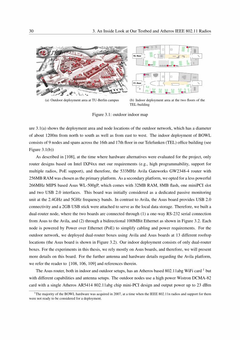
30 3. An Inside Look at Our Testbed and Atheros IEEE 802.11 Radios
(a) Outdoor deployment area at TU-Berlin campus
17. floor
16. floor
16-5
16-416-3 16-2
16-1
17-4
17-117-317-2
(b) Indoor deployment area at the two floors of theTEL-building
Figure 3.1: outdoor indoor map
ure 3.1(a) shows the deployment area and node locations of the outdoor network, which has a diameter
of about 1200m from north to south as well as from east to west. The indoor deployment of BOWL
consists of 9 nodes and spans across the 16th and 17th floor in our Telefunken (TEL) office building (see
Figure 3.1(b))
As described in [108], at the time where hardware alternatives were evaluated for the project, only
router designs based on Intel IXP4xx met our requirements (e.g., high programmability, support for
multiple radios, PoE support), and therefore, the 533MHz Avila Gateworks GW2348-4 router with
256MB RAM was chosen as the primary platform. As a secondary platform, we opted for a less powerful
266MHz MIPS based Asus WL-500gP, which comes with 32MB RAM, 8MB flash, one miniPCI slot
and two USB 2.0 interfaces. This board was initially considered as a dedicated passive monitoring
unit at the 2.4GHz and 5GHz frequency bands. In contrast to Avila, the Asus board provides USB 2.0
connectivity and a 2GB USB stick were attached to serve as the local data storage. Therefore, we built a
dual-router node, where the two boards are connected through (1) a one-way RS-232 serial connection
from Asus to the Avila, and (2) through a bidirectional 100MBit Ethernet as shown in Figure 3.2. Each
node is powered by Power over Ethernet (PoE) to simplify cabling and power requirements. For the
outdoor network, we deployed dual-router boxes using Avila and Asus boards at 13 different rooftop
locations (the Asus board is shown in Figure 3.2). Our indoor deployment consists of only dual-router
boxes. For the experiments in this thesis, we rely mostly on Asus boards, and therefore, we will present
more details on this board. For the further antenna and hardware details regarding the Avila platform,
we refer the reader to [108, 106, 109] and references therein.
The Asus router, both in indoor and outdoor setups, has an Atheros based 802.11abg WiFi card 1 but
with different capabilities and antenna setups. The outdoor nodes use a high power Wistron DCMA-82
card with a single Atheros AR5414 802.11abg chip mini-PCI design and output power up to 23 dBm
1The majority of the BOWL hardware was acquired in 2007, at a time when the IEEE 802.11n radios and support for themwere not ready to be considered for a deployment.
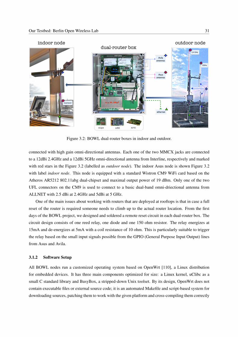
Our Testbed: Berlin Open Wireless Lab 31
dual-router box
ethernet
5GHz
2,4 GHz
Avila antennas
Asus antennas
outdoor nodeindoor node
dual-band
armmips x86
Figure 3.2: BOWL dual-router boxes in indoor and outdoor.
connected with high gain omni-directional antennas. Each one of the two MMCX jacks are connected
to a 12dBi 2.4GHz and a 12dBi 5GHz omni-directional antenna from Interline, respectively and marked
with red stars in the Figure 3.2 (labelled as outdoor node). The indoor Asus node is shown Figure 3.2
with label indoor node. This node is equipped with a standard Wistron CM9 WiFi card based on the
Atheros AR5212 802.11abg dual-chipset and maximal output power of 19 dBm. Only one of the two
UFL connectors on the CM9 is used to connect to a basic dual-band omni-driectional antenna from
ALLNET with 2.5 dBi at 2.4GHz and 5dBi at 5 GHz.
One of the main issues about working with routers that are deployed at rooftops is that in case a full
reset of the router is required someone needs to climb up to the actual router location. From the first
days of the BOWL project, we designed and soldered a remote reset circuit in each dual-router box. The
circuit design consists of one reed relay, one diode and one 150 ohm resistor. The relay energizes at
15mA and de-energizes at 5mA with a coil resistance of 10 ohm. This is particularly suitable to trigger
the relay based on the small input signals possible from the GPIO (General Purpose Input Output) lines
from Asus and Avila.
3.1.2 Software Setup
All BOWL nodes run a customized operating system based on OpenWrt [110], a Linux distribution
for embedded devices. It has three main components optimized for size: a Linux kernel, uClibc as a
small C standard library and BusyBox, a stripped-down Unix toolset. By its design, OpenWrt does not
contain executable files or external source code; it is an automated Makefile and script-based system for
downloading sources, patching them to work with the given platform and cross-compiling them correctly
32 3. An Inside Look at Our Testbed and Atheros IEEE 802.11 Radios
for the chosen router platform. We chose OpenWrt due to the following [110]:
..., if a new kernel is released, a simple change to one of the Makefiles will download the
latest kernel, patch it to run on the embedded platform and produce a new firmware image
– there’s no work to be done trying to track down an unmodified copy of the existing kernel
to see what changes had been made, the patches are already provided and the process ends
up almost completely transparent. This doesn’t just apply to the kernel, but to anything
included with OpenWrt – It’s this one simple understated concept, which is what allows
OpenWrt to stay on the bleeding edge with the latest compilers, latest kernels and latest
applications.
The OpenWrt build system typically produces a minimally configured image that needs to be configured
and distributed to our BOWL nodes.
In our dual-router set-up, the Avila boards were used both for wireless experimentation as well as
providing an access interface to Internet users. Therefore, early on, a lot effort has been put into automat-
ing the configuration of the Avila image and managing its distribution to the nodes [108]. We report on
our experience on managing this dev-ops network (i.e., development and operations network) in [109].
On the other hand, the Asus boards were not used for access and did not face the same challenges.
Therefore, I, single-handedly, maintained the OpenWrt system on the Asus routers and therefore, the
Asus image followed closely the latest development of OpenWrt, its so-called ‘trunk’ version. Such
early adoption to OpenWrt brings several advantages and disadvantages. The major advantage is the
close relation between OpenWrt trunk development and the Atheros driver development: several Open-
Wrt maintainers provide up-to-date patch sets for all three major Atheros device drivers. Since our
objective was to implement a joint power and rate controller in-kernel, a prerequisite was to get early
support from other kernel developers to work on a common and current code base. The main disad-
vantage is, expectedly, the need to constantly adapt the set of local patches to the trunk version. In
Chapter 5, we relate more on our experiences of getting our kernel development accepted into the Linux
upstream codebase.
For device drivers, in 2007, we started using Madwifi driver under OpenWrt. In 2010, the successor
driver, ath5k, became more stable, and we switched to using this fully open source driver which provides
more flexibility and operation transparency compared to any Madwifi version. Additional discussion
about the differences of those two drivers are presented in Chapter 5. On a final note, these open drivers
are the main force behind Atheros-based WiFi hardware to be widely used in research testbeds, creating
a more comparable experimentation landscape.
IEEE 802.11 Radio Characteristics 33
3.2 IEEE 802.11 Radio Characteristics
In this section, we summarize IEEE 802.11 radio [1] operations in terms of rate, power and carrier sense
based on our Atheros WiFi hardware. We first go into the details of Atheros hardware operation as well
as the registers providing important information about the MAC layer states and adjustable registers
that can be controlled to alter the operation of the card. Some of the features that we describe here are
IEEE 802.11a specific, however, most of the discussion applies to IEEE 802.11 in general. While we
mainly focus on rate, power and carrier sensing capabilities in a typical IEEE 802.11 hardware, we also
summarize several Atheros-based optimizations, such as Adaptive Noise Immunity (ANI), which have
significant impact on experimental measurements and therefore, which should be treated carefully [111].
Finally, we conclude with a discussion that noise floor calibration is an important hardware process that
acts as one of the determining factors of packet reception.
3.2.1 Atheros Hardware Design
In Figure 3.3 we have linked several sources of information about Atheros chip design [112, 113, 114,
115] together. In contrast to other WiFi chips like Broadcom BCM4712 or Intel 5300, Atheros chips
do not have a firmware running on a micro-controller (excluding Atheros USB WiFi) but rather 802.11
functions are split into hardware state-machines and software operation [112]. Functions that require
critical timing such as channel access, checksum generation, periodic beacons, and ACKs, are handled
within the protocol control unit (PCU). Other non time-critical functions, such as sending and receiving
of data frames and fragmentation, are performed by the device driver on the host system connected
via PCI bus to the WiFi card. On the sending path, the driver assembles a list of transmit frames in
host memory and passes a pointer to the list of transmit descriptors to the DMA engine (marked as
yellow line in Figure 3.3). The DMA engine traverses this pointer list, fetches the remaining data from
the host memory and passes it to the PCU to follow the 802.11 CSMA/CA access procedure to gain
access to the channel and then forwards the frame (further baseband and radio details can be found in
[112]). On the receiving path (shown as green line in Figure 3.3), after successful packet de-modulation,
the PCU extracts the frame type, verifies the checksum, and generates a response frame (i.e., ACK),
if appropriate, and passes the received frame to the DMA engine, which interprets a series of receive
descriptors to transfer the frame data to the host memory.
Besides the outlined data-path, Atheros MAC design has a dedicated control logic based on 32-bit
registers as shown in Figure 3.3. There are two types of registers: configuration registers that allow
updates, and status registers that allow monitoring of current hardware states [113]. Transmit power and
carrier sense operation are typical examples of function blocks that can be controlled by changing a set of
control register values (e.g., ACK transmission power in dBm or enable preamble-based (weak) signal
detection). The possible usage of each Atheros register value is well-documented (within the Linux

34 3. An Inside Look at Our Testbed and Atheros IEEE 802.11 Radios
CPU
driver
Memory-Controller /PCI Bridge
RAM
tx-data
Txdescriptors
*Rx-descriptors
tx-data txfifo
rxfifo
CarrierSense
Transmit
DAC
DAC
ADC
ADC
Filte
rFi
lter
Transmitter
Receiver
AGC
Freq. Synthesizer
TPC
diversityswitch
RF-Transreceiver
OffsetControl
SensitivityControl
EDPD
SignalDetection
Viterbi
Auto-correlate
FFT
IFFT
PowerDetector
Receive
MAC state-machine
Baseband
ProtocolControl
Unit(PCU)
crypto engine
checksumlogic
DMA EngineHost HIU
rx-data
tx-fifo
rx-fifo
*
* rx-data
PCIBus
mac80211
Status & ControlRegisters
user-space
Antenna
RegMon
Atheros WiFi hardware
tx-data+
variable gain amplifier (VGA)
frequency mixer
clockrate
PA
noise-floorcalibration
loop
ACK
BEACON
Figure 3.3: Design and interconnections between host and Atheros 802.11 interface with MAC and PHYlayer functions
codebase in file reg.h for 802.11 abg [116] and 802.11 n [117] chips). The status registers represent
the dynamics of the MAC transceiver state-machine (shown in Figure 3.3 in the PCU box) and provide
other useful information. Registers of interest depend on the overall monitor/measurement objective and
within this thesis, we have used:
i Noise threshold is stored with the main energy detection threshold (i.e., the minimum energy
level that triggers the correlation-based signal detection) in a single register. Monitoring it allows
analyzing the noise calibration process in the card, and the interference conditions.
ii Timing Synchronization Function (TSF) is split across an upper and lower 32-bit TSF register.
The TSF is based on a 1-MHz clock and can be used to measure time intervals in microseconds
precision.
iii Receive signal strength indicator (RSSI)
iv The number of successfully received frames
v Mac states: The radio can be in only one of these states at any point in time.
• TX: the radio is actively transmitting.
• RX: the packet/signal detection mechanism triggered a demodulation attempt.
IEEE 802.11 Radio Characteristics 35
• BUSY: there is sufficient in-band signal energy on the medium but the packet detection mech-
anism does not trigger. This can happen due to interference, e.g., it can be triggered by an
out-of-band activity such as a microwave oven, a Bluetooth transmission or transmissions of
IEEE 802.11 packets on adjacent channels.
• IDLE: if no other state applies.
There are four corresponding MAC state registers reside in the same hardware memory addresses
for all Atheros 802.11 abg chips as well as for newer Atheros 802.11n chips. The actual count of
overall clock cycles at a given clock rate (drafted as clock symbol in the middle of Figure 3.3) is
stored in a separate register that is used as reference point. Additionally, through a dedicated MIB
freeze register, it is possible to stop counting these registers. The ability to freeze the Mac state
registers before reading their content ensures reading consistency among the different states (i.e.,
Clock Cycles, TX, RX and BUSY counters).
We make use of these registers in order to set-up as well as analyse our measurement experiments. To the
best of our knowledge, it is currently not possible to obtain the instantaneous MAC state of the Atheros
radio. We will try to overcome these limitations through a sampling approach in the next section.
3.2.2 Rate and Power Control Capabilities
In this section, we summarize the current rate and power control capabilities of WiFi (IEEE 802.11) ra-
dios. Each IEEE 802.11 frame contains a preamble, which is used for signal detection by the receiving
radio as well as for timing acquisition in order to find out when the payload actually begins. The pream-
ble header also contains information about the used transmission mode, which defines a transmission
rate that corresponds to a particular modulation order and channel coding rate. Note that, management
frames, e.g., ACK frames, are typically sent at the lowest basic rate. The IEEE 802.11ag [1] standard
defines also two additional higher rates, 12 and 24 Mbps for ACKs. For data packets, the current radios
are able to adjust their transmission rate per packet but not for retransmissions, i.e., a rate-lookup is not
performed for retransmissions. In Atheros-based radios, for each data packet, it is possible to specify a
so-called multi-rate retry chain (MRR) within the tx-descriptor that contains four different rates and their
corresponding number of maximal retries. Once the packet is successfully transmitted, the remainder of
the retry chain is ignored. For instance, it is possible to retry sending a packet first at 54 Mbps 4 times,
next at 24 MBps 3 times, next at 9 Mbps 2 times, and finally, at 6 Mbps again 2 times. Essentially, only
a few rate control algorithms (e.g., Minstrel, see Section 2.2.2) operate based on this ability to configure
the entire retry chain for each data packet. Based on the current compat-wireless codebase in Linux, we
find the maximal supported retry rate stages is four and Atheros is the only vendor that supports this (for
chipsets 5212 and later). Therefore, in our case, Wistron CM9 (chip 5212) and DMCA-82 (chip 5413)
support a MRR chain with four stages. On the other hand, Broadcom hardware using b43, b43legacy

36 3. An Inside Look at Our Testbed and Atheros IEEE 802.11 Radios
and brcmsmac drivers (i.e., 802.11 abgn) support two, Ralink supports three and Intel supports one MRR
stage. However, as we do not have access to the source-code of the firmware running on these devices it
might be possible that a retry rate control is hidden from our view of the codebase.
While rate control per-packet transmission is typical, per-rate power control is not typical. Only sev-
eral chipset vendors, in particular Atheros, have documented implementations that permit adjustment per
packet [4]. It was validated in [118] that with Atheros chipsets it is possible to perform per-packet power
control with a granularity of 0.5 dBm and switching latency of 1 ms. Our experience with the Atheros
5212 and 5413 chipsets also confirms this, and we build our joint rate-power controller, presented in
Chapter 5, based on these capabilities. Note that these chipsets support one power level per data packet
(i.e., all possible retries are also done in the same power level). With newer 802.11n chips from Atheros,
like the AR938X, it is also possible to use four different power levels per retry chain entry. Finally,
ACK frames can only use a single power level per device. The range of adjustable power level values (in
case of Atheros hardware) starts at 0 dBm (lower power levels are not yet supported by the driver). The
upper bound depends on the specific WiFi card, where typical values are 16 to 23 dBm. The power can
be adjusted with a granularity of 0.5 dB. Other vendors seem to support even lower transmission power
levels, as mentioned in [119], Intel 5300 3x3 MiMo 802.11n WiFi cards enable transmit power levels
from −10 dBm to 16 dBm, also in steps of 0.5 dB.
Interaction between Rate and Power: In terms of joint controllability, both rate and power are not
mutually independent but rather exhibit a clear interaction in regions near the maximum output power.
There is a complex trade-off between the following three objectives: (1) sufficient output power (and
therefore sufficient transmission range/coverage), (2) high data rates to realize good network perfor-
mance and (3) low and efficient power consumption with respect to battery usage. Todays power am-
plifiers (PA) in WiFi radios (class A and AB are typical designs) can only achieve two of the three
objectives at the same time. They can work quite efficiently if the point of operation is near the maxi-
mum power saturation level (about 80 % max. efficiency). A key challenge is the power amplifier design
since in OFDM modulation, the resulting RF signal has a large peak-to-average power ratio, which can
theoretically have an amplitude as high as 17 dB and in practice, up to 10 dB [112]. Essentially, the PA
for OFDM systems must be sized to support possible peak power levels, but operate on average up to
10dB below this peak and therefore, at much lower efficiency levels for most of the time (at about 10%
average efficiency) [112]. There are two requirements that restrict the actual power level to stay below
its maximum amplification potential: (1) each device must meet the spectral mask given by the 802.11
abgn standard and any applicable regulatory requirements and (2) an individual transmit signal quality
per modulation rate specified by an error vector magnitude limit (EVM) must be met [1, 7, 112]. With
higher order modulation schemes (in terms of encoded bits per symbol), the EVM requirements defined
in the IEEE 802.11 standard get stricter. This translates into rate specific demands of linear amplification
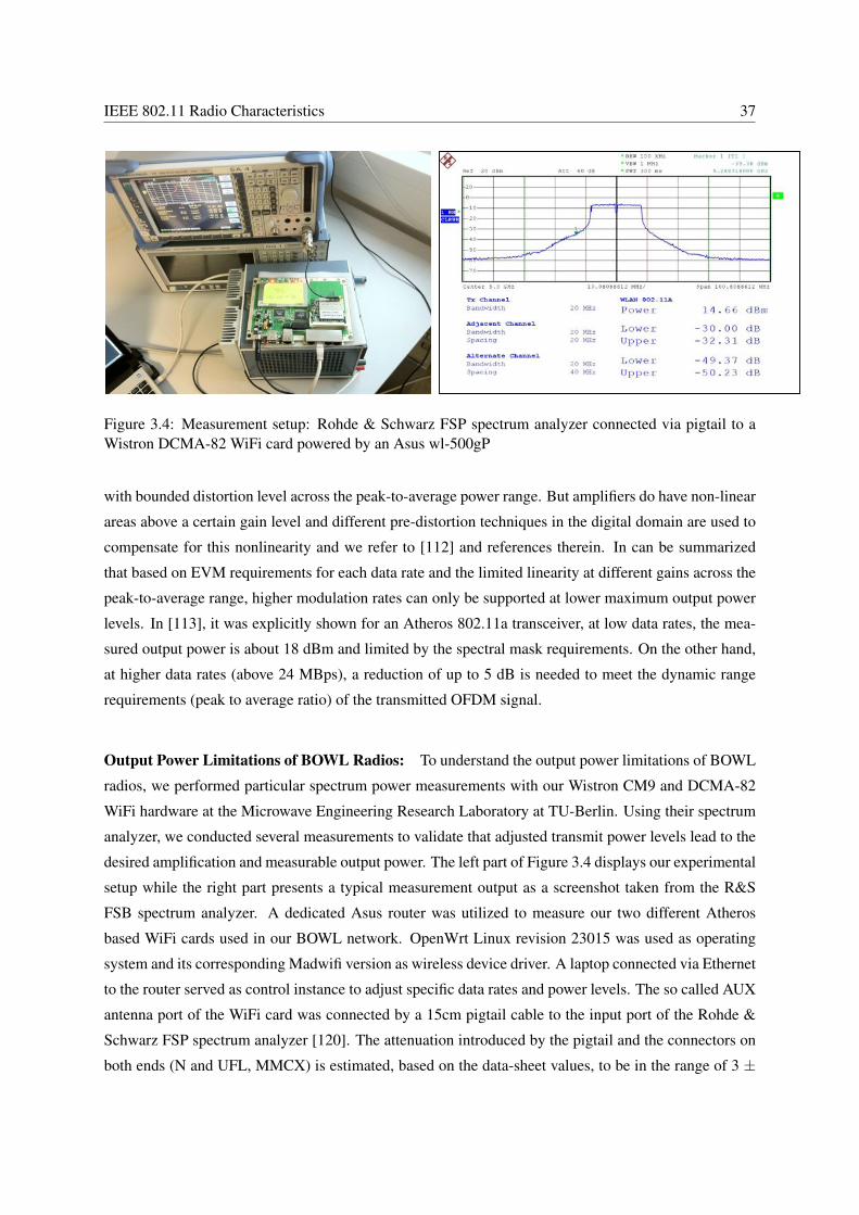
IEEE 802.11 Radio Characteristics 37
Figure 3.4: Measurement setup: Rohde & Schwarz FSP spectrum analyzer connected via pigtail to aWistron DCMA-82 WiFi card powered by an Asus wl-500gP
with bounded distortion level across the peak-to-average power range. But amplifiers do have non-linear
areas above a certain gain level and different pre-distortion techniques in the digital domain are used to
compensate for this nonlinearity and we refer to [112] and references therein. In can be summarized
that based on EVM requirements for each data rate and the limited linearity at different gains across the
peak-to-average range, higher modulation rates can only be supported at lower maximum output power
levels. In [113], it was explicitly shown for an Atheros 802.11a transceiver, at low data rates, the mea-
sured output power is about 18 dBm and limited by the spectral mask requirements. On the other hand,
at higher data rates (above 24 MBps), a reduction of up to 5 dB is needed to meet the dynamic range
requirements (peak to average ratio) of the transmitted OFDM signal.
Output Power Limitations of BOWL Radios: To understand the output power limitations of BOWL
radios, we performed particular spectrum power measurements with our Wistron CM9 and DCMA-82
WiFi hardware at the Microwave Engineering Research Laboratory at TU-Berlin. Using their spectrum
analyzer, we conducted several measurements to validate that adjusted transmit power levels lead to the
desired amplification and measurable output power. The left part of Figure 3.4 displays our experimental
setup while the right part presents a typical measurement output as a screenshot taken from the R&S
FSB spectrum analyzer. A dedicated Asus router was utilized to measure our two different Atheros
based WiFi cards used in our BOWL network. OpenWrt Linux revision 23015 was used as operating
system and its corresponding Madwifi version as wireless device driver. A laptop connected via Ethernet
to the router served as control instance to adjust specific data rates and power levels. The so called AUX
antenna port of the WiFi card was connected by a 15cm pigtail cable to the input port of the Rohde &
Schwarz FSP spectrum analyzer [120]. The attenuation introduced by the pigtail and the connectors on
both ends (N and UFL, MMCX) is estimated, based on the data-sheet values, to be in the range of 3 ±
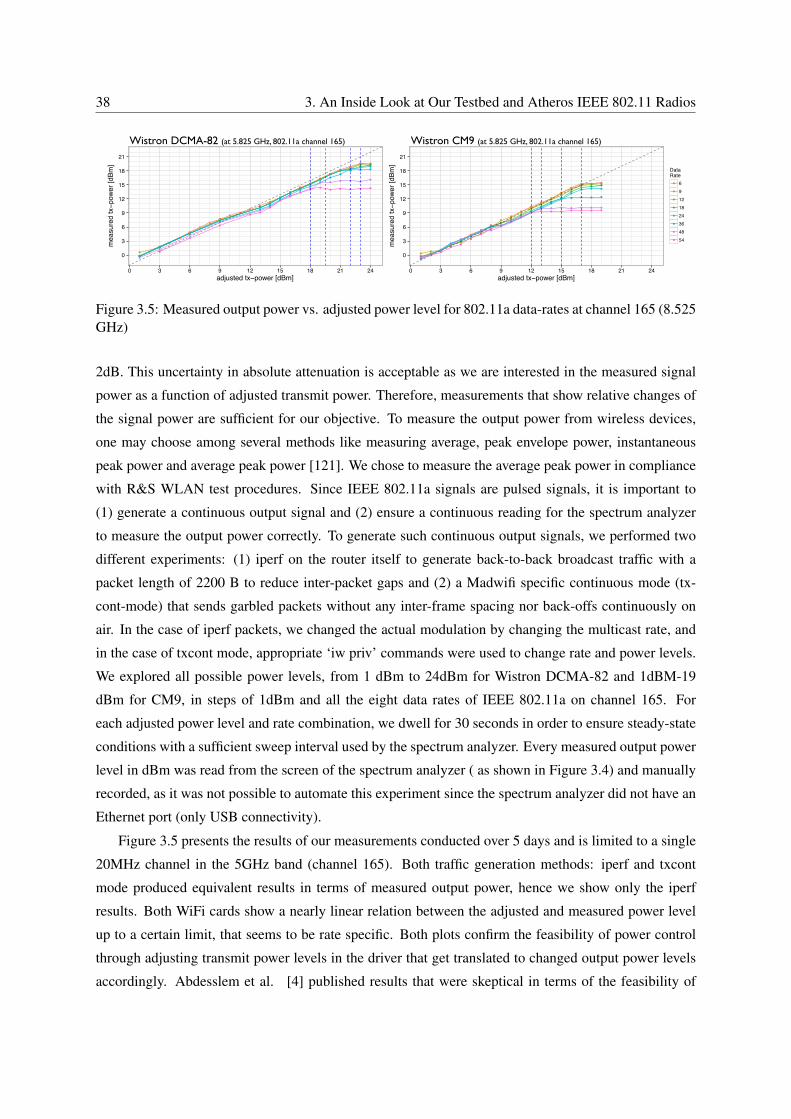
38 3. An Inside Look at Our Testbed and Atheros IEEE 802.11 Radios
●
●
●
●
●
●
●
●
●
●●
●
●
●
●
●
●
●
●
●
●●
● ●
●
●
●
●
●
●
●
●
●
●
●
●●
● ●
●
●
●
●
●
●
●
●
●
●
●
●●
● ●
●
●
●
●
●
●
●
●
●
●
●
●
● ●
●●
●
●
●
●
●
●
●
●
●
●
●
●
● ●● ●
●
●
●
●
●
●
●
●
●
●
●
●●
● ● ●
●
●
●
●
●
●
●
●
●●
● ● ● ● ●●
●
●
●
●●
●
●
●
●
● ●● ● ● ● ●
0
3
6
9
12
15
18
21
0 3 6 9 12 15 18 21 24adjusted tx−power [dBm]
mea
sure
d tx−p
ower
[dBm
]
DataRate
●
●
●
●
●
●
●
●
69121824364854
●●
●
●
●
●
●
●●
●
●
●
●
●
●
●
● ● ●
●●
●
●
●
●
●
●
●
●
●
●
●
●
●
●
● ● ●
●
●●
●●
●
●
●
●
●
●
●
●
●
●
●
● ● ●
●●
●
●
●
●
●
●
●●
●
●
●
●
●
●
● ● ●
●
●
●
●
●
●
●
● ●
●
●
●
●
●
●
●
● ● ●
●
●
●
●
●
●
●
● ●
●
●
●
●
●
● ● ● ● ●
●
●
●
●
●
●
● ●
●
●
●
●
● ● ● ● ● ● ●
● ●
●
●●
●
●
●●
●
●
● ● ● ● ● ● ● ●
0
3
6
9
12
15
18
21
0 3 6 9 12 15 18 21 24adjusted tx−power [dBm]
mea
sure
d tx−p
ower
[dBm
]
DataRate
●
●
●
●
●
●
●
●
69121824364854
Wistron CM9 (at 5.825 GHz, 802.11a channel 165)Wistron DCMA-82 (at 5.825 GHz, 802.11a channel 165)
Figure 3.5: Measured output power vs. adjusted power level for 802.11a data-rates at channel 165 (8.525GHz)
2dB. This uncertainty in absolute attenuation is acceptable as we are interested in the measured signal
power as a function of adjusted transmit power. Therefore, measurements that show relative changes of
the signal power are sufficient for our objective. To measure the output power from wireless devices,
one may choose among several methods like measuring average, peak envelope power, instantaneous
peak power and average peak power [121]. We chose to measure the average peak power in compliance
with R&S WLAN test procedures. Since IEEE 802.11a signals are pulsed signals, it is important to
(1) generate a continuous output signal and (2) ensure a continuous reading for the spectrum analyzer
to measure the output power correctly. To generate such continuous output signals, we performed two
different experiments: (1) iperf on the router itself to generate back-to-back broadcast traffic with a
packet length of 2200 B to reduce inter-packet gaps and (2) a Madwifi specific continuous mode (tx-
cont-mode) that sends garbled packets without any inter-frame spacing nor back-offs continuously on
air. In the case of iperf packets, we changed the actual modulation by changing the multicast rate, and
in the case of txcont mode, appropriate ‘iw priv’ commands were used to change rate and power levels.
We explored all possible power levels, from 1 dBm to 24dBm for Wistron DCMA-82 and 1dBM-19
dBm for CM9, in steps of 1dBm and all the eight data rates of IEEE 802.11a on channel 165. For
each adjusted power level and rate combination, we dwell for 30 seconds in order to ensure steady-state
conditions with a sufficient sweep interval used by the spectrum analyzer. Every measured output power
level in dBm was read from the screen of the spectrum analyzer ( as shown in Figure 3.4) and manually
recorded, as it was not possible to automate this experiment since the spectrum analyzer did not have an
Ethernet port (only USB connectivity).
Figure 3.5 presents the results of our measurements conducted over 5 days and is limited to a single
20MHz channel in the 5GHz band (channel 165). Both traffic generation methods: iperf and txcont
mode produced equivalent results in terms of measured output power, hence we show only the iperf
results. Both WiFi cards show a nearly linear relation between the adjusted and measured power level
up to a certain limit, that seems to be rate specific. Both plots confirm the feasibility of power control
through adjusting transmit power levels in the driver that get translated to changed output power levels
accordingly. Abdesslem et al. [4] published results that were skeptical in terms of the feasibility of

IEEE 802.11 Radio Characteristics 39
power control on WiFi chips (Atheros included). Their concerns have been disproved by Kowalik et al.
[118] by demonstrating that power control is feasible and can be implemented in current IEEE 802.11
cards with per-packet granularity and low power switching latency. Our results confirm those findings in
terms of feasibility. Furthermore, we confirm the results of [113] that a rate dependent maximal output
power level and the 5 dB difference between the highest modulation rate of 54MBits and the lowest
6MBits.
In order to ensure that both spectral and EMV limits are respected, the device driver itself ensures that
the power level annotation per packet does not exceed those power level limits stored in its EEPROM.
During device initialization, driver-level functions read eight supporting points stored in EEPROM that
provide maximal allowed power levels in 0.5 dBm steps as a function of the frequency and data rate. In
case of IEEE 802.11a, out of the eight possible data rates, the first five rates (6 to 24 MBits) are grouped
and have one common maximal power limit per frequency. The remaining three higher modulation rates
(36, 48 and 54 MBits) have individual limits that support less maximal output power.
Based on our output power results, we were able to find and fix a critical driver bug in the ath5k code
that caused unnecessary low throughput. In all of our experiments using the ath5k driver, we observed
that link throughput even on a small scale desktop setup was limited to approximately 15 MBits when
802.11a 5GHz channels above a center frequency of 5.720 GHz (typically 5GHz outdoor channels)
were used. Regardless of which type of Wistron model we tried (CM9 or DCMA-82), the rate set that
provided the maximal link throughput was always lower than or equal to 24 MBits. Our guess, which
turned out to be true, was that the rates higher than 24 MBits did not perform as expected due to high
amplification gain, which consequently led to signal distortion above the EVM requirements. When we
lowered the global transmit power limit in the ath5k driver from default 17dBm to 12 dBm in the case
of CM9 model and from 23dBm to 18 dBm in the case of DCMA-82 model, the throughput increased
significantly up to 26 MBits and, all the data rates up to 54 MBits performed as expected. We discovered
that this was caused by erroneous EEPROM readings, which led to assigning maximum power level to
all data rates. We fixed this problem and our ath5k driver patch is included in Linux kernel version 3.6 2
(since 21st of August 2012).
In order to understand the distribution of those power limitations across different Atheros cards,
we patched the ath5k diver to print EEPROM readings. We analyzed again the two different hardware
models: (i) Wistron DMCA-82 WiFi cards and (ii) Wistron CM9 WiFi cards. All cards from the same
model showed identical EEPROM values. Our results for both hardware models are shown in Figure 3.6.
Comparing the maximum power levels at the lower data rates, the DCMA-82 supports up to 24 dBM
(i.e., 251 mW) in the 802.11a band while the CM9 is limited to 19 dBm (i.e., 79 mW). In reference
to the highest data rate of 54 MBits, the maximal allowed output power of the DCMA-82 is limited
down to 18 dBm, while the CM9 goes down to 12 dBm. Furthermore the maximum transmit power
2https://git.kernel.org/cgit/linux/kernel/git/next/linux-next.git/commit/?id=3a245cbef6a9e4398456bd733b0b4b7cb3f11994
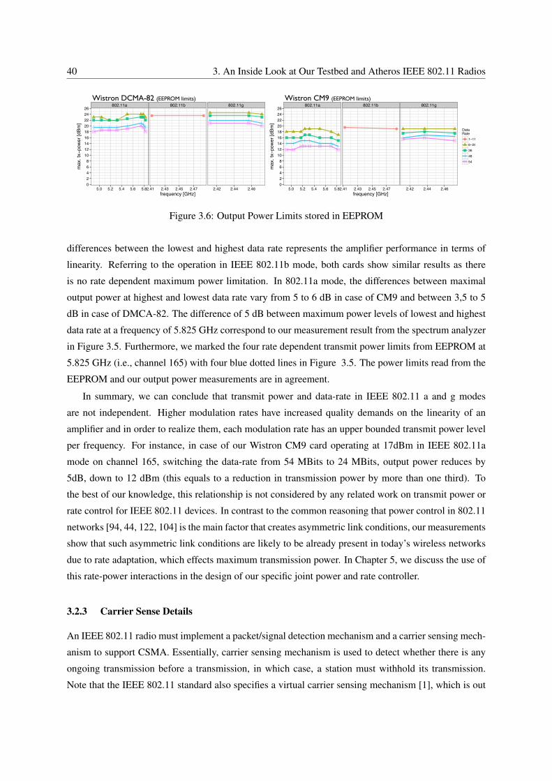
40 3. An Inside Look at Our Testbed and Atheros IEEE 802.11 Radios
802.11a 802.11b 802.11g
02468
101214161820222426
5.0 5.2 5.4 5.6 5.82.41 2.43 2.45 2.47 2.42 2.44 2.46frequency [GHz]
max
. tx−
powe
r [dB
m]
DataRate
1−116−24364854
Wistron DCMA-82 (EEPROM limits)802.11a 802.11b 802.11g
02468
101214161820222426
5.0 5.2 5.4 5.6 5.82.41 2.43 2.45 2.47 2.42 2.44 2.46frequency [GHz]
max
. tx−
powe
r [dB
m]
DataRate
1−116−24364854
Wistron CM9 (EEPROM limits)
Figure 3.6: Output Power Limits stored in EEPROM
differences between the lowest and highest data rate represents the amplifier performance in terms of
linearity. Referring to the operation in IEEE 802.11b mode, both cards show similar results as there
is no rate dependent maximum power limitation. In 802.11a mode, the differences between maximal
output power at highest and lowest data rate vary from 5 to 6 dB in case of CM9 and between 3,5 to 5
dB in case of DMCA-82. The difference of 5 dB between maximum power levels of lowest and highest
data rate at a frequency of 5.825 GHz correspond to our measurement result from the spectrum analyzer
in Figure 3.5. Furthermore, we marked the four rate dependent transmit power limits from EEPROM at
5.825 GHz (i.e., channel 165) with four blue dotted lines in Figure 3.5. The power limits read from the
EEPROM and our output power measurements are in agreement.
In summary, we can conclude that transmit power and data-rate in IEEE 802.11 a and g modes
are not independent. Higher modulation rates have increased quality demands on the linearity of an
amplifier and in order to realize them, each modulation rate has an upper bounded transmit power level
per frequency. For instance, in case of our Wistron CM9 card operating at 17dBm in IEEE 802.11a
mode on channel 165, switching the data-rate from 54 MBits to 24 MBits, output power reduces by
5dB, down to 12 dBm (this equals to a reduction in transmission power by more than one third). To
the best of our knowledge, this relationship is not considered by any related work on transmit power or
rate control for IEEE 802.11 devices. In contrast to the common reasoning that power control in 802.11
networks [94, 44, 122, 104] is the main factor that creates asymmetric link conditions, our measurements
show that such asymmetric link conditions are likely to be already present in today’s wireless networks
due to rate adaptation, which effects maximum transmission power. In Chapter 5, we discuss the use of
this rate-power interactions in the design of our specific joint power and rate controller.
3.2.3 Carrier Sense Details
An IEEE 802.11 radio must implement a packet/signal detection mechanism and a carrier sensing mech-
anism to support CSMA. Essentially, carrier sensing mechanism is used to detect whether there is any
ongoing transmission before a transmission, in which case, a station must withhold its transmission.
Note that the IEEE 802.11 standard also specifies a virtual carrier sensing mechanism [1], which is out
IEEE 802.11 Radio Characteristics 41
of the scope of this thesis.
IEEE 802.11 standard dictates several minimum requirements for the operation of a receiver. For
instance, the sensitivity for the minimum transmission mode should be −82 dBm for a 20 MHz channel
and the carrier sensing function should declare the medium busy for any signal 20 dBm above the
minimum sensitivity requirement (hence,−62 dBm for a 20 MHz channel). Note that the channel might
be busy due to transmission from other stations (i.e., station interference) or due to noise interference in
physical medium. Station interference is mainly seen as MAC-layer interference and noise interference
as PHY-layer interference.
Weak and Strong Signal Detection: A comprehensive summary about possible signal detection al-
gorithms, their performance and energy tradeoffs are given in [21]. In the context of wideband systems
they define the term carrier sensing (CS) to specifically indicate methods of coherent detection based
on suitable signal properties and distinguish it from non-coherent energy detection (ED). Non-coherent
ED is known to be a robust and universal mechanism that can be performed anywhere within the packet
without requiring any knowledge of the type of underlying signal structure at the physical layer [21].
However, 802.11abgn systems are wideband, where the signal power is much more spread around the
carrier frequency, which leads to signal power spectral density near the noise floor, and hence, ED is of-
ten not sufficient to detect the presence of a packet [123]. Wideband radio systems implement therefore
more reliable coherent detection methods such as preamble detection (PD) or decorrelation-based de-
tection. To this end, each packet is preceded with a known preamble, typically consisting of repetitions
of a sequence of symbols designed for a near-ideal autocorrelation property when the receiver varies the
time offsets during preamble detection. Both the 802.11abg and 802.11n support different length and
types of preamble sequences and need therefore specific detection capabilities in each radio.
A comprehensive source of information about Atheros methods to detect and demodulate packets
are patents [124, 125, 126, 127]. Based on these patents, we conclude that Atheros radio chipsets are
able to perform ED and PD signal detection concurrently [127], which are named as strong and weak
signal detection, respectively. The objective after packet detection is to maximize the received signal
size at the analog digital converter (ADC, shown in Figure3.3 to provide a good dynamic sampling
range. This is achieved by amplifying the received signal within the automatic gain control unit (AGC)
while providing headroom for adjacent channel interference and the peak-to-average-ratio of OFDM
symbols. A chart of possible state transitions and all background details about baseband detection and
gain operations can be found in [127] and references therein. Briefly, strong signal detection attempts to
detect incoming packets by monitoring sudden changes of the received raw signal power, especially the
saturation at the ADC. The start of a new packet is assumed when the measured signal power exceeds an
adjustable threshold above the current noise floor. The abrupt power increment triggers the Automatic
Gain Control (AGC) unit to reduce the amplifier gain so that the size of the received signal is forced to
42 3. An Inside Look at Our Testbed and Atheros IEEE 802.11 Radios
fall between two predefined thresholds. When the signal strength drops down from the lower threshold,
the WiFi card assumes the end of the packet and the AGC unit increases the amplifier gain, hence, its
sensitivity to catch new packets. Our experiments with Atheros hardware reproduced findings in [111],
which showed that Atheros ED only starts detecting packets successfully if the reported SNR is above
14dB. Several thresholds that control the energy detection part can be specified via the proc filesystem
in Madwifi and ath5k, resulting in the same control register triggers described hereafter.
Besides energy detection, Atheros hardware uses preamble-based weak signal detection, that, in case
of 802.11a, measures the significance of auto-correlated power with a period of 0.8µs (short symbol du-
ration) and enables packet detection with signal power levels near the noise floor [126]. The detection
of packet boundaries is provided through a 2-round correlation process using multiple thresholds, which
are independently configured for OFDM and CCK preambles when 802.11b/802.11g modes are sup-
ported. It can be concluded that the Atheros relies on a complex orchestration of several values and
thresholds to adjust signal amplification, filtering, self-correlation significance and off-set timings in or-
der to adjust the parallel operation of energy (strong) and preamble-based (weak) packet detection. Both
Madwifi and ath5k drivers support five levels of so-called interference immunity specified within the
debugfs filesystem. These are empirically determined combinations of multiple gain and filter thresh-
olds in order to change the overall sensitivity of the radio receiver with respect to incoming signals and
interference [125]. Furthermore, both drivers support the ability to enable or disable preamble-based
(weak) packet detection, hence pure energy detection operation. Within standard specific mode of op-
eration, the lowest sensitivity corresponds to the highest interference immunity index (e.g., level 4) in
combination with disabling preamble-based (weak) packet detection and enabling only energy detection.
The highest possible sensitivity is achieved by enabling preamble-based (weak) detection and using the
lowest interference immunity index (e.g., level 0). In our work on adjusting and monitoring carrier sense
operations [95] we validate a Madwifi driver patch provided by [128] to disable carrier sensing hence
any signal detection.
Capture Effect: Atheros radios also implement capture, which allows aborting the reception of an
ongoing frame, if a new stronger signal is detected. If the in-band power is measured to be above the
strong signal detection, the receiver logic is reset and strong signal detection for the new packet is started.
This is often referred to as “capture effect” in the literature. Capture may have a profound impact on
communication performance, however, it is a significant challenge to dissect the existence of capture
during transmissions. This is the reason why we do not attempt this in out work.
Adaptive Noise Immunity (ANI): Madwifi and ath5k drivers have both implemented their version
of a so called Adaptive Noise Immunity (ANI) algorithm [125, 111]. Its objective is to adapt receiver
sensitivity parameters such that rate of false packet detections are minimized [125]. A false detection
occurs when interference triggers the signal detection unit to believe that a packet is present. In both ANI

IEEE 802.11 Radio Characteristics 43
implementations receiver sensitivity is dynamically adjusted by changing the aforementioned 5-level
interference immunity index as well as enabling or disabling preamble based (weak) signal detection.
Measurements in [111] showed that enabling ANI may cause high variations in packet detection rate and
reported SNR values. In most of our experiments we switch ANI off and specify a static carrier sense
setting in the driver configuration.
3.2.4 Noise Handling
The achievable receive sensitivity of any communication system is fundamentally limited by noise.
Signal quality is typically measured as the ratio of the power of the received signal and the noise (Signal
to Noise Ratio - SNR) [129]. A common definition of SNR for any modulation scheme can be found
in [130]:
SNR =average received signal energy per symbol time
noise energy per symbol time
Note that, SNR is a function of (1) the output power of the transmitter, (2) the antenna gains on both
the sender and receiver side, (3) the path loss of the wireless channel and (4) the receiver noise. The
receiver noise floor, shown in Figure 3.7, is a time varying process of measured noise energy, which
is the sum of all noise sources in a measurement system. The circuit itself generates internal noise
for instance, by the random motion of electrons in a conductor, which is positively correlated with
temperature (i.e., an increase in temperature leads to higher agitation of electrons and thus an increase
in thermal noise). Typical internal sources of noise are thermal noise, shot noise and flicker noise, while
external noise sources are atmospheric noise and man-made noise [131]. A large proportion of external
noise originates from sources such as televisions, radios, mobile phones or microwave ovens.
It is typically understood that a higher SNR means lower bit error rate, and therefore, it makes
it possible to increase the bit-rate, which consequently improves throughput. However, an important
issue of high density, multi-user networks such as current WiFi deployments, is that transmissions are
significantly affected by interference from neighboring transmissions. Although the underlying IEEE
802.11 MAC aims at scheduling one transmission per time slot to avoid concurrent transmissions (i.e.,
MAC-layer interference), outside the carrier sense range, PHY-layer interference will be created from
simultaneous transmissions. Thus, in low-density networks, transmission errors are typically due to
low SNR, which is referred to as noise-limited regime. On the other hand, in high density networks,
transmission errors are due to low signal to interference and noise ratio (SINR), also referred to as
interference limited regime [132]. As illustrated on the right part of the Figure 3.7, SINR is defined
as [130]:
SINR =received signal energy
noise energy +∑N
link=1 Interference(link)
In IEEE 802.11 networks, performance is well understood when transmissions are noise-limited, but in
the interference-limited case network performance is considerably less well understood.
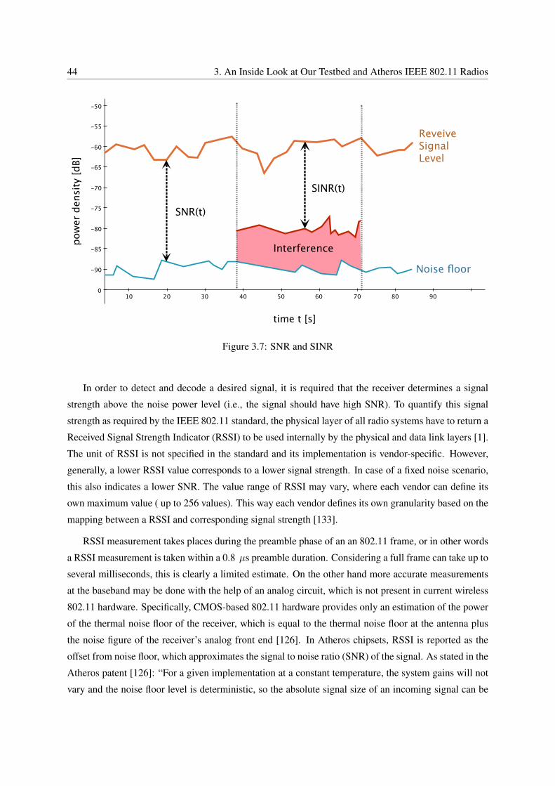
44 3. An Inside Look at Our Testbed and Atheros IEEE 802.11 Radios
10 20 30 40 50 60 70 80 90
-90
-85
-80
-75
-70
-65
-60
-55
-50
0
time t [s]
pow
er d
ensi
ty [d
B]
ReveiveSignalLevel
Noise floor
SNR(t)
Interference
SINR(t)
Figure 3.7: SNR and SINR
In order to detect and decode a desired signal, it is required that the receiver determines a signal
strength above the noise power level (i.e., the signal should have high SNR). To quantify this signal
strength as required by the IEEE 802.11 standard, the physical layer of all radio systems have to return a
Received Signal Strength Indicator (RSSI) to be used internally by the physical and data link layers [1].
The unit of RSSI is not specified in the standard and its implementation is vendor-specific. However,
generally, a lower RSSI value corresponds to a lower signal strength. In case of a fixed noise scenario,
this also indicates a lower SNR. The value range of RSSI may vary, where each vendor can define its
own maximum value ( up to 256 values). This way each vendor defines its own granularity based on the
mapping between a RSSI and corresponding signal strength [133].
RSSI measurement takes places during the preamble phase of an an 802.11 frame, or in other words
a RSSI measurement is taken within a 0.8 µs preamble duration. Considering a full frame can take up to
several milliseconds, this is clearly a limited estimate. On the other hand more accurate measurements
at the baseband may be done with the help of an analog circuit, which is not present in current wireless
802.11 hardware. Specifically, CMOS-based 802.11 hardware provides only an estimation of the power
of the thermal noise floor of the receiver, which is equal to the thermal noise floor at the antenna plus
the noise figure of the receiver’s analog front end [126]. In Atheros chipsets, RSSI is reported as the
offset from noise floor, which approximates the signal to noise ratio (SNR) of the signal. As stated in the
Atheros patent [126]: “For a given implementation at a constant temperature, the system gains will not
vary and the noise floor level is deterministic, so the absolute signal size of an incoming signal can be
Summary 45
computed directly from the relative computed RSSI value”. This is arguable, however, due to expected
temperature variability at different time scales (due to the effects from changes of seasons, night/day, cpu
load changing chip temperature). Furthermore, the true noise process is estimated by cyclic sampling,
which triggers an implementation-specific noise floor calibration. We present this process in more detail,
next.
Noise Floor Calibration: Noise calibration in the Atheros hardware is performed periodically by
measuring the minimum received in-band power, calculating a moving average and storing this value
in an Atheros hardware register. This value is used to calculate RSSI values per packet and therefore
affects all decisions that rely on the signal strength, noise level or both. Each time a noise calibration is
triggered, the hardware places the receive/transmit switch in an open position to ensure that any power
received at the antenna does not impact the calibration process. Hence, the noise calibration method
assumes that there exist inter-packet gaps between packet transmissions when no surrounding nodes send
packets. This assumption is necessary because during such a calibration, packet reception degrades and
weak signals may not be received nor processed. The whole noise floor calibration, which averages over
certain number of samples, takes less time than a SIFS duration. Since inter-packet gaps are unknown
in advance and may occur at unknown times, multiple noise floor measurements are taken within a time
window that is shorter than an inter-packet gap. However, it may not be possible to determine the true
noise floor when other continuous noise sources are present in the environment (i.e., no inter-packet
gaps). In this case, the calibration interval starts playing an important role and it becomes essential to
determine an interval which does not degrade packet reception and which provides reasonable noise
estimations.
3.3 Summary
In this section, we gave an overview of our testbed, and radio hardware, which play a significant role
in our tool development, experimentation, and performance evaluation. By combining multiple sources
of information with dedicated measurements we were able to understand the design, operation, and
limitations of our Atheros based WiFi hardware with respect to rate, power and carrier sense control.
For both of our WiFi cards deployed in BOWL, we analyzed the interaction between data rate and
transmit power. Our results validate that the maximum power level to send packets is a function of the
data rate. The next sections builds on the background information from chapter 3, and go into deeper
detail about how we monitor different radio functions. With this understanding, we develop a controller
for joint power and rate control.

46 3. An Inside Look at Our Testbed and Atheros IEEE 802.11 Radios

Chapter 4
Wireless MAC and PHY LayerMonitoring
To design, analyze, evaluate and debug our controller, a deep and precise understanding of the radio
behavior under different conditions is required. In addition, it is crucial to be able to build correct
cause-and-effect chain. Therefore, measurement and monitoring systems play a vital role in our design.
In this section, we briefly discuss the state of the wireless measurement tools for monitoring wireless
MAC-layer parameters and their limitations. The main part of this section presents our new open-source
measurement tool RegMon, which significantly extends the PHY and MAC layer monitoring of Atheros-
based WiFi cards. We describe our implementation of RegMon for all tree major Linux device divers,
namely Madwifi [67], ath5k [134] and ath9k [135] and describe its monitoring capabilities and usage
instructions. We conclude this section with the validation and performance evaluation of RegMon.
4.1 Wireless Monitoring and its Limitations
In general, monitoring approaches can roughly be divided into active and passive solutions. Passive mon-
itoring approaches deploy monitoring nodes to complement main node deployment and, collect network
information, for example, packet traces. Passive monitoring is not intrusive and hence can be incremen-
tally deployed without interrupting ongoing data transmissions. While passive monitoring approaches
have been shown to be successful for troubleshooting [136, 137, 25, 138], they may lack precision due
to the following reasons: (1) hardware differences between the monitoring nodes and main nodes in
the deployed area (e.g., WiFi card, antenna specifications), (2) location of the monitor nodes not rep-
resenting the channel conditions experienced by the deployment nodes, (3) strict time synchronization
requirements to be able to correlate events (especially under heavy traffic conditions [139]). Addition-
ally, protocol information that can not be directly measured by the monitoring nodes, has to be inferred.
47
48 4. Wireless MAC and PHY Layer Monitoring
Such information includes vital statistics about noise floor, the radio busy times, or queue lengths. Thus,
the accuracy of passive monitoring is not typically sufficient to understand protocol behavior in detail.
In [140], we presented PaPMo, an active monitoring tool, which generates measurement packets and
captures snapshots of the protocol status as packets pass through the different layers and over distributed
nodes. PaPMo consists of 3 components: time synchronization via broadcast packets, in-kernel protocol
sniffers as part of Madwifi driver and TCP kernel module, and trace processing and merging in user
space. By merging and correlating the captured information, PaPMo is able to provide packet-level
network behavior accurately like in simulators. Specifically, PaPMo is able to correlate MAC-layer
events, such as packet loss due to queue overflow with TCP congestion control behavior at the accuracy
of microseconds. Nevertheless, being an active measurement tool, PaPMo is quite intrusive, affecting the
system under measurement and it requires a specific wired network set-up to guarantee the synchronized
time stamping of packets.
Dujovne et al [141] published a comprehensive taxonomy about measurable IEEE 802.11 wireless
parameters with available open source measurement tools, mostly for Linux. All of the 10 open source
measurement tools use information provided by APIs or libraries accessed from user-space. 9 out of 10
tools utilize packets or packet headers as information source, and only one tool, WaveMon, makes use of
the deprecated Linux Wireless Extensions (WEXt) and Wireless Tools (WT) to access aggregated driver
statistics. This implies that certain parameters, e.g., carrier sense, can only be estimated by combining
header information, which obviously requires packet reception. Lately, Rayanchu et al. developed two
monitor systems: Airshark [142] and WiFiNet [15]. Their objective is to detect, localize, and quantify
the interference from various non-WiFi interference sources using commodity Atheros 802.11n WiFi
hardware. To this end, they utilize the special spectral scan mode - which is a feature in Atheros chip
AR9280 and later, but is not yet documented or implemented in the open source Linux (ath9k) nor BSD
driver code base. This mode enables the reception and processing of raw FFT samples from the Atheros
PHY and could be of great use for understanding the benefits of having channel state information (CSI)
or at least for verifying certain PHY layer operations. Also Halperin et al. [119] use detailed PHY
layer measurements of CSI and effective SNR provided by a commodity 3x3 MiMo Intel 5300 802.11
abgn WiFi card. In contrast to Airshark and WiFiNet, this measurement tool, which enables the debug
mode of the Intel 5300 firmware, is made available to the public [143]. Nevertheless, open source
measurement tools that allow wireless MAC and PHY layer monitoring are rare and generally tailored
to specific hardware.
One of the well-known open source tools is Wprobe, released with OpenWrt Linux kernel package
in 2009 [144]. It provides a distributed way to monitor a set of PHY and MAC layer parameters from a
Madwifi-driven Atheros card and enables data collection via IPFIX [145] protocol. Wprobe monitors the
operation of Atheros Mac state-machine by periodic sampling of the relevant 32-bit hardware registers,
described in Section 3.2.1, and outputs the fraction of time the radio spent at each state (i.e., transmitting,

RegMon - Design, Implementation and Performance 49
receiving, busy or idle). It also provides SNR and noise statistics per wireless link. The maximum
sampling resolution of Wprobe is limited to 10 register samples per second (10Hz). In [95], we analyzed
and validated different carrier sense scenarios with our modified version of Wprobe, which provides
higher sampling rates up to 1000 Hz. However, as Wprobe monitoring worked only with Madwifi, we
decided to create a Atheros register monitoring tool that works on all drivers (i.e., Madwifi, ath5k, and
ath9k). In the next section, we present our Atheros-specific monitoring tool RegMon.
4.2 RegMon - Design, Implementation and Performance
RegMon is implemented as a single kernel driver patch for each of the supported three drivers, without
the need for additional modules, daemons or user-space applications. All main functions of RegMon
and their interactions are shown in Figure 4.1. These functions are explained in detail next.
4.2.1 In-Kernel MAC-Layer Monitoring
To perform the monitoring, we leverage the lightweight kernel-to-userspace debug file system called
debugfs (colored as the green line in Figure 4.1). This serves two purposes: (1) it enables a a simple
file-based configuration of RegMon for its in-kernel operations from the userspace and, (2) the actual
trace-file from the kernel can be accessed via standard file read (e.g., with tail, cat) from the userspace.
For the actual measurements, it is possible to access Atheros control and status registers stored in the
card memory through the PCI bus. Each of the Linux drivers (i.e., Madwifi, ath5k and ath9k) has
its own C functions or macros to access the memory-mapped 32-bit register content, as shown at the
bottom of Figure 4.1. The Linux kernel function readl() is called to read the current register value at
the memory address that was passed to it, respecting different host endianness and memory mapping
specifics [146]. For every register read, we store the current timestamp and the raw hexadecimal register
values. Each column, except the first one holding the current timestamp, represents a register address
specified through debugfs from the user-space. In our current implementation, we can monitor up to 11
registers in parallel. The main limiting factor for the number of registers is the memory footprint of the
data structure to hold these values in the kernel.
The in-kernel register sampling consists of three parts (in Figure 4.1, labeled as (1) in-kernel register
sampling):
i. Reading registers (read registers() ):
• The function getnstimeofday() is called to get current UNIX time in nanoseconds and store the
returned timestamp.
• Iterating through the register file list in debugfs, each register’s own memory address is used
to call the corresponding driver’s read register function and store the returned register content.
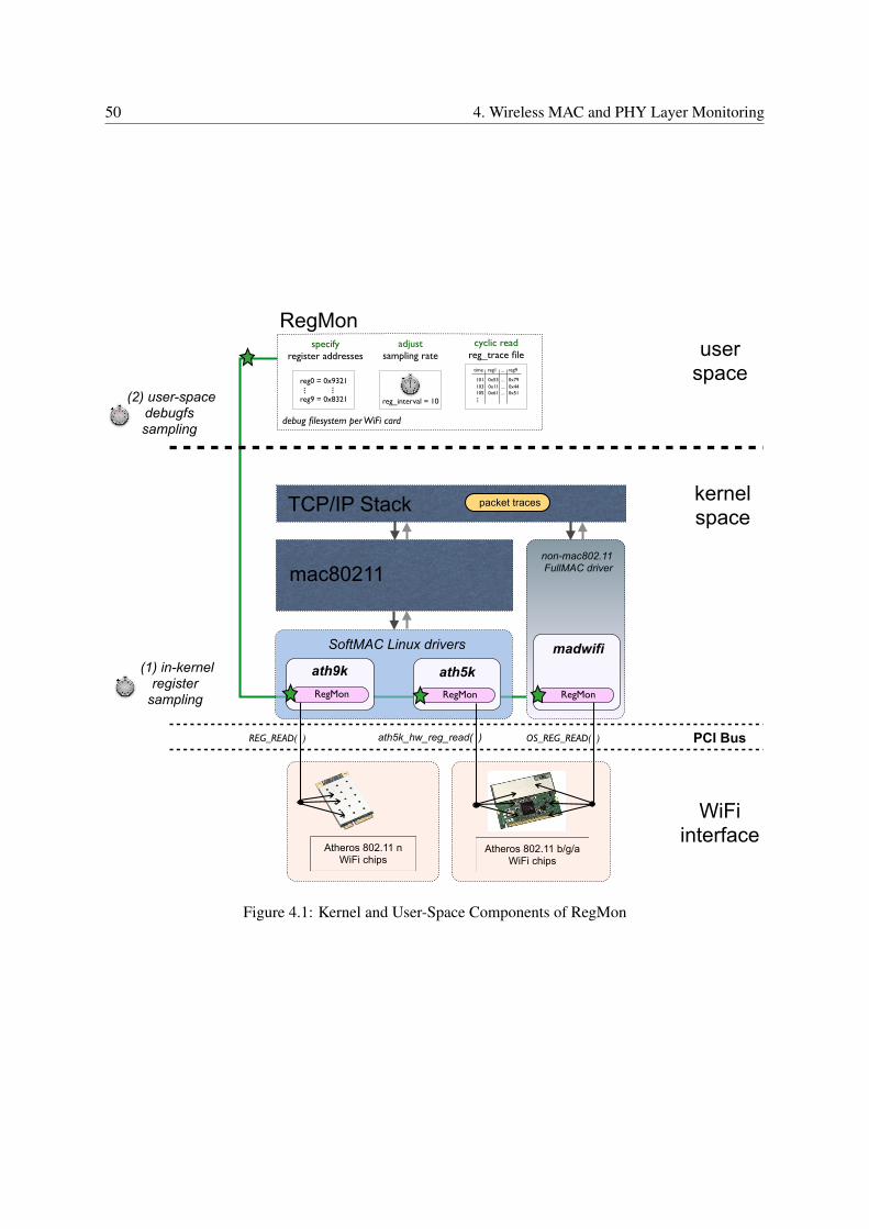
50 4. Wireless MAC and PHY Layer Monitoring
userspace
mac80211
ath5k
SoftMAC Linux drivers
ath5k_hw_reg_read( )
Atheros 802.11 b/g/a WiFi chips
ath9k
Atheros 802.11 nWiFi chips
non-mac802.11 FullMAC driver
RegMonRegMon RegMon
madwifi
OS_REG_READ( )REG_READ( )
debug filesystem per WiFi card
reg0 = 0x9321
reg9 = 0x8321 reg_interval = 10
cyclic readreg_trace file
specify register addresses
...
adjustsampling rate
...
time reg1 ... reg9
103 0x11 ... 0x44101 0x53 ... 0x79
105 0x61 ... 0x51
...
TCP/IP Stack kernelspace
packet traces
RegMon
WiFiinterface
(1) in-kernelregister
sampling
(2) user-spacedebugfssampling
PCI Bus
Figure 4.1: Kernel and User-Space Components of RegMon

RegMon - Design, Implementation and Performance 51
• Reading sampling resolution via debugfs, a new timer to read registers is registered. The
reading of registers will be triggered via a kernel timer event. In the case jiffies event is used,
sampling rate is bounded by the kernel timer frequency (max 4000 Hz). In the case high
resolution timers are used, sampling rates of 20.000Hz and more are feasible.
ii. Assembling the userspace output is triggered when a read operation to debugfs file is requested
from the userspace. Then, all the new rows are written as formatted string into a debugfs log file.
iii. Initialization and de-initialization
• At device initialization, each WiFi interface creates its own debugfs RegMon folder and files.
• All data structures and initial timer event registrations are performed.
• At device de-initialization, all data structures are freed and all debugfs entries are removed.
Userspace debugfs sampling is shown as (2) in Figure 4.1. Here, by reading the debugfs log file, we
get access to the content of the desired registers. We store these values in a ring buffer between kernel
and user-space. This allows compensating for slower and possibly non-deterministic read cycles in the
user-space while the content of the array is constantly updated in-kernel. Our current implementation
uses 30000 rows, which was under all circumstances sufficiently large to support register reading rates
up to 30 kHz. The trace-file generated by RegMon is currently formatted as space separated list of
measurement values, which turned out to be a sufficient format to parse and process the trace file for
further analysis.
4.2.2 Calculating MAC states
Based on the statistics collected with RegMon, we are able to calculate the percentage of the time spent
in each MAC state during a given observation duration Tobs. Shown in Figure 4.2 is a simplified repre-
sentation of the three most important blocks associated with packet reception and carrier sensing. The
first two blocks address signal detection and are described in more details below. The third block is an
energy detection block parameterized by a threshold (thr62 on Figure 4.2). The output of these blocks
is a binary {0, 1} signal sampled at the specific clock rate of the system. There are four corresponding
32-bit hardware registers of profiling the MAC baseband interface:
• CYCLE counter reg(CLOCK) (cc) increases with the number of clock cycles at a given clock
speed.
• TX counter register reg(TX) counts the number of cycles the transmission unit is active.
• RX counter register reg(RX) is incremented only if any of the two signal detection block outputs
is positive.
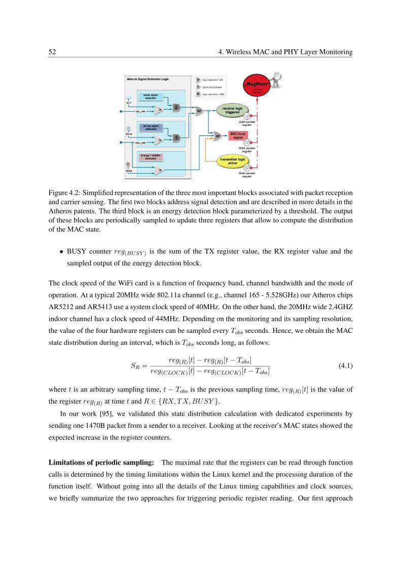
52 4. Wireless MAC and PHY Layer Monitoring
„RegMon“in-kernelmonitorin
Figure 4.2: Simplified representation of the three most important blocks associated with packet receptionand carrier sensing. The first two blocks address signal detection and are described in more details in theAtheros patents. The third block is an energy detection block parameterized by a threshold. The outputof these blocks are periodically sampled to update three registers that allow to compute the distributionof the MAC state.
• BUSY counter reg(BUSY ) is the sum of the TX register value, the RX register value and the
sampled output of the energy detection block.
The clock speed of the WiFi card is a function of frequency band, channel bandwidth and the mode of
operation. At a typical 20MHz wide 802.11a channel (e.g., channel 165 - 5.528GHz) our Atheros chips
AR5212 and AR5413 use a system clock speed of 40MHz. On the other hand, the 20MHz wide 2.4GHZ
indoor channel has a clock speed of 44MHz. Depending on the monitoring and its sampling resolution,
the value of the four hardware registers can be sampled every Tobs seconds. Hence, we obtain the MAC
state distribution during an interval, which is Tobs seconds long, as follows:
SR =reg(R)[t]− reg(R)[t− Tobs]
reg(CLOCK)[t]− reg(CLOCK)[t− Tobs](4.1)
where t is an arbitrary sampling time, t − Tobs is the previous sampling time, reg(R)[t] is the value of
the register reg(R) at time t and R ∈ {RX,TX,BUSY }.In our work [95], we validated this state distribution calculation with dedicated experiments by
sending one 1470B packet from a sender to a receiver. Looking at the receiver’s MAC states showed the
expected increase in the register counters.
Limitations of periodic sampling: The maximal rate that the registers can be read through function
calls is determined by the timing limitations within the Linux kernel and the processing duration of the
function itself. Without going into all the details of the Linux timing capabilities and clock sources,
we briefly summarize the two approaches for triggering periodic register reading. Our first approach
RegMon - Design, Implementation and Performance 53
is based on the mature Linux timer framework. Jiffies is the duration of one tick of the system timer
interrupt with a minimum duration defined by the frequency of the system ticks. The system frequency
can be specified in the Linux kernel build environment. Typical choices are 100 Hz, 250 Hz, or 1000
Hz, which lead to a maximal tick resolution of 10 ms, 4 ms, and 1 ms respectively. We were able to
successfully patch the kernel of our MIPS based Asus Router platform to a maximum of 4096Hz, which
represents the upper bound in sampling rate using jiffies.
In order to get higher sampling speed through more precise timer resolutions, we implemented a
second alternative based on the more recent high resolution timer subsystem (hr timers). High resolution
timers measure time at nanosecond-level resolution whereas standard Linux timers measure time at
millisecond-level resolution [146]. The usage of the hr timer subsystem depends on the hardware that
needs to provide sufficient precise clock sources, which our Asus WL-500gP router does. The changes
necessary to switch from using jiffies to hr timers were straightforward to implement, and did not include
any design changes. This way, we were able to increase the maximum sampling rate to 20.000 Hz.
Similar to any possible change to RegMon monitoring parameter, the sampling rate can also be changed
in an online fashion.
4.2.3 Validation and Performance
In this section, we validate basic functions of our RegMon implementation on different platforms and
drivers to ensure its correct operation and analyze its limitations. Specifically, we start with sampling
accuracy, the impact on cpu and network load, and execution time for register sampling.
Our validation experiments are performed on two different hardware platforms: (1) Asus WL-500gP
and (2) Ubiquity RouterStation pro (RSpro) both equipped with a Wistron CM9 Atheros 5212 WiFi
miniPCI card. Both platforms are driven by the same version of OpenWrt ‘Attitude Adjustment’ re-
vision 31101 using Linux kernel version 3.3. The Asus router platform is based on a Broadcom SoC
(BCM4704) MIPS with 264MHz, 32MB RAM, 1x miniPCI socket and Fast Ethernet. The RSpro is
more powerful compared to the Asus. It is based on an Atheros SoC (AR7161) MIPS 24K with 680MHz
CPU, 128MB RAM, 3x miniPCI sockets and Gigabit Ethernet. We use these two platforms to be able to
detect possible measurement limitations and errors within RegMon trace file generation and collection.
The performance of RegMon was evaluated by collecting trace files over Ethernet and not locally on
an USB stick. Note that the read/write performance of the ASUS USB interface would be much more
restricted compared to Ethernet.
In order to validate RegMon operation, we analyzed the following:
• Accuracy of sampling intervals: The distribution of error between specified sampling interval and
the measured interval
• CPU and network load: The impact of sampling interval to CPU and network load with and
without compression
54 4. Wireless MAC and PHY Layer Monitoring
• Register reading delay: The execution time of read registers()
• Packet reconstruction limitations: The limitations of reconstructing packet traces from Mac state
traces
Our validation is based on the following experiments. We connected Rspro directly to an IBM X200
Thinkpad laptop via an Ethernet cable and used it as a measurement sink. A customized bash script
running on the laptop triggered parameter changes on the router while we performed the following over
a duration of 60 seconds:
• RegMon trace file collection on the router and transfer via Ethernet to the laptop sink
• Cpusage [147] trace file collection on the router and transfer via Ethernet to the laptop sink
• Packet trace collection via tcpdump on the laptop
We repeated the same experiment with Asus.
Different sampling rates with and without on-line trace file compression were performed and ana-
lyzed. Based on the 22 Asus routers deployed across the BOWL network, the shortest possible interrupt
duration reported by the hr timer subsystem via dmesg output is 56 µs (equivalent to a sampling rate of
18 kHz). In case of the Ubiquity Routerstation PRO (RSpro), the hr timer subsystem reports a minimal
duration of 33 µs (equivalent to a sampling rate of 30 kHz). Based on these lower limits of the hr timer
subsystem, we choose sampling intervals starting from the lower bound of the given system up to 1000
µs in steps of 5 to 10 µs.
Accuracy of Sampling Intervals: To analyze the accuracy of specified sampling intervals, we used
our RegMon implementation based on the hr timer framework, which allows lower intervals to be set
compared to the jiffies implementation. In RegMon, we monitor two independent time sources: the
Linux system time and the TSF time based on the hardware clock within the Atheros WiFi card, both
with a granularity of 1 µs. In the optimal case, the measurement interval at which RegMon performs
periodic register readings should be of the same duration as the system time difference (or TSF time
difference) between two consecutive measurement records in RegMon trace file. As we described earlier
in 3.2.1, the TSF value is monitored through a register reading of the corresponding Atheros status
register and its value stored in the trace file along with the system time.
Figure 4.3 shows our first validation result based on RSpro router. The box whisker plot shows the
relation between the adjusted RegMon sampling interval in µs on the x-axis and the measured TSF time
difference (labeled as measured kernel interval) in µs between two successive register readings on the
y-axis. Each box-whisker summarizes the distribution of register readings, and in red points, we depict
the outliers that are more than 1.5 times the inter-quartile range away from the lower and upper quartiles.
The blue dashed line represents the optimal 1:1 linear relation between adjusted and measured interval.
Note that in our experiments, an interval of 200 µs between two measurements corresponds to a sampling
rate of 5000 Hz and therefore about 300000 samples are taken within those 60 seconds. Therefore, the
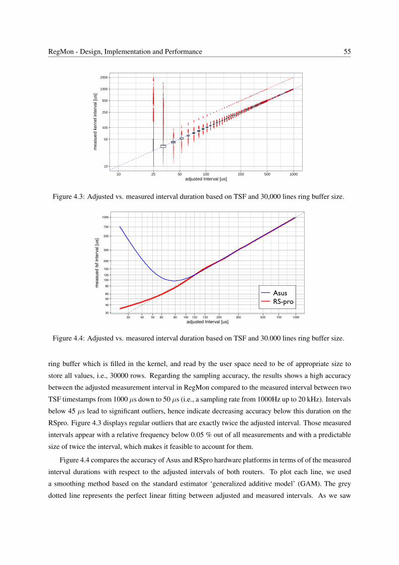
RegMon - Design, Implementation and Performance 55
●●●●●●●●●●●●●●●●●●●●●●●●●●●●●●●●●●●●●●●●●●●●●●●●●●●●●●●●●●●●●●●●●●●●●●●●●●●●●●●●●●●●●●●●●●●●●●●●●●●●●●●●●●●●●●●●●●●●●●●●●●●●
●
●●●●●
●●●●●●●●●●●●●●●●●●●●●●●●●●●●●●●●●●●●●●●●●●●●●●●●●●●●●●●●●●●●●●●●●●●●●●●●●●●●●●●●●●●●●●●●●●●●●●●●●●●●●●●●●●●●●●●●●●●●●●●●●●●●●●●●●●●●●●●●●●●●●●●●●●●●●●●●●●●●●●●●●●●●●●●●●●●●●●●●●●●●●●●●●●●●●●●●●●●●●●●●●●●●●●●●
●●●
●
●●●●●●●●●●●●●●●●●
●
●
●
●
●
●
●
●
●
●
●
●
●●
●●●●●●●●●●●●●●●●●●●●●●●●●●●●●●●●●●●●●●●●●●●●●●●●●●●●●
●●●●●●●●●●●●●●●●●●●●●●●●●●●●●●●●●●●●●●●●●●●●●●●●●●●●●●●●●●●●●●●●●●●●●●
●●●
●
●●●●●●●
●●●●●●
●●●●●●●●●●●●●●●●●●●●●●●●●●●●●●●●●●●●●●●●●●●●●●●●●●●●●●●●●●●●●●●●●●●●●●●●●●●●●●●●●●●●●●●●●●●●●●●●●●●●●●●●●●●●●●●●●●●●●●●●
●●
●●●●●●●●●
●
●●●
●●●
●
●
●●●●●
●
●
●
●
●
●
●
●
●
●
●
●●
●●●●●●●●●●●●●●●●●●●●●●●●●●●●●●●●●●●●●●●●●●●●●●●●●●●●●●●●●●●●●●●●●●●●●●●●●●●●●●●●●●●●●●●●●●●●●●●●
●●●●●●●●●●●●●●●●●●●●●●●●●●●●●●●●●●●●●●●●●●●●●●●●●●●●●●●●●●●●●●●●●●●●●●●●●●●●●●●●●●●●●●●●●●●●●●●●●●●●●●●●●●●●●●●●●●●
●●●●●●●●●
●●●●
●●●●●●
●●●●
●●●
●●
●
●●
●●
●
●
●
●
●●●●●●
●
●
●
●
●
●
●
●
●
●
●
●●●●●●●●●●●●
●●●●●●●●●●●●●●●
●
●●
●
●
●
●
●
●
●●●●●●●●●●●●
●●●●●●●●●●●●●●●●●●●●●
●●●●
●●●●
●●●●●●●●●●●●●●●●●
●●●●●●●●●●●●●●●
●●●●
●
●
●●●●●●●●●●●●●●
●●●●●●●●●●●●●●●●●●●
●●●
●●●●●●●●●●●●●●●●●●●●
●●●●●●●●●●●●●
●●●●
●●●●●●●●●●●●●●●
●●●●●●●●●●●●●●●●●●
●●●●
●
●●●●●●●●●●●●●●●●●●●
●●●●●●●●●●●●●
●●●●
●
●●●●●●●●●●●●●
●●●●●●●●●●●●●●●●●●
●●●●●
●●●●●●●●●●●●●●●●●●
●●●●●●●●●●●●
●●
●
●●●●●●●●●●●●
●●●●●●●●●●●●●●●●●
●●●●
●●●●●●●●●●●●●●●●
●●●●●●●●●●●●
●●●
●●●●●●●●●●●●
●●●●●●●●●●●●●●●●●
●●●●
●●●●●●●●●●●
●●●●●●●●●●●●●●●●●
●●●●
●●●●●●●●●●●●●●●●
●●●●●●●●●●●●●
●●●
●●●●●●●●●●●●●●●●●
●●●●●●●●●●●●●
●●
●●●●●●●●●●●
●●●●●●●●●●●●●●●●●●●●
●●●
●●●●●●●●●●●●●●
●●●●●●●●●
●●
●●●●●●●●●●●●
●●●●●●●●●●●●●●●●●●
●
●●●●●●●●●●●●●●●●●
●●●●●●●●●●●●
●●●
●●●●●●●●●●
●●●●●●●●●●●●●●●●
●
●●●●●●●●●●●●●●●●●
●●●●●●●●●●●●
●
●●●●●●●●●●
●●●●●●●●●●●●●●●●
●
●●●●●●●●●●●●●●●●●●●●
●●●●●●●●●●●●●●
●
●●●●●●●●●●●●
●●●●●●●●●●●●●●●●●
●●
●●●●●●●●●●●●
●●●●●●●
●●
●●●●●●●●●●●
●●●●●●●●●●●●●●●●●
●●●
●●●●●●●●●●●●●●●●●●
●●●●●●●●●●●●●●●
●●●
●●●●●●●●●●●●
●●●●●●●●●●●●●●●●●●●
●●
●●●●●●●●●●●●●
●●●●●●●●
●
●●●●●●●●●●
●●●●●●●●●●●●●●●●●
●●●●
●●●●●●●●●●●●●●●●
●●●●●●●●●●●●●
●●
●●●●●●●●●●●
●●●●●●●●●●●●●●●●●●
●
●●●●●●●●●●●●
●●●●●●●●●●
●●
●●●●●●●●●●●
●●●●●●●●●●●●●●●●
●●
●●●●●●●●●●●●●●●
●●●●●●●●●●
●
●●●●●●●●●
●●●●●●●●●●●●●●●●
●●
●●●●●●●●●●●●●●
●●●●●●●●●●
●
●●●●●●●●●●
●●●●●●●●●●●●●●●
●●
●●●●●●●●●●●●●●
●●●●●●●●
●●●●
●●●●●●●●●
●●●●●●●●●●●●●●
●
●●●●●●●●●●●●
●●●●●●●
●
●●●●●●●●●●●●
●●●●●●●●●●●●●●●●●
●●
●●●●●●●●●●●●●●
●●●●●●●●●●
●
●●●●●●●●●●●●
●●●●●●●●●●●●●●●●●●●
●●
●●●●●●●●●●●
●●●●●●●●
●●
●●●●●●
●●●●●●●●●●●●
●
●●●●●●●●●
●●●●●●●
●
●●●●●●
●●●●●●●●●●●
●
●●●●●●●●●●
●●●●●●
●
●●●●●●●●●●
●●●●●●●●●●●●●●●●●
●●
●●●●●●●●●●●●●●●●
●●●●●●●●●●●●●
●●
●●●●●●●●●
●●●●●●●●●●●●
●
●●●●●●●●●●●
●●●●●●●
●
●●●●●●●●●●
●●●●●●●●●●●●●●●●
●
●●●●●●●●●●●●
●●●●●●●●●
●
●●●●●●●●
●●●●●●●●●●●●
●
●●●●●●●●
●●●●●●
●●
●●●●●●●
●●●●●●●●●●●●●●
●●●
●●●●●●●●●●●●
●●●●●●●
●●
●●●●●●●
●●●●●●●●●●●●
●●
●●●●●●●●●●●
●●●●●●●
●
●●●●●●●●●●
●●●●●●●●●●●●●●●
●●
●●●●●●●●●●●●●●
●●●●●●●●●
●
●●●●●
●●●●●●●●
●●
●●●●●●●●
●●●●●
●
●●●●●
●●●●●●●●●●●●
●
●●●●●●●●●●
●●●●●●●
●
●●●●●
●●●●●●●●
●
●●●●●●●●●●●
●●●●●
●
●●●●●●
●●●●●●●●●●●●●
●●
●●●●●●●
●●●●●●●●●●
●
●●●●●●●
●●●●
●
●●●●●●●●●●
●●●●
●
●●●●●●●
●●●●●●●●●●●●●●
●
●●●●●●●
●●●●
●
●●●●●●●●●
●●●●●●●●●●●●●
●
●●●●●●●●●●●
●●●●●●●●
●
●●●●●●●
●●●●●●●●
●
●●●●●●●●●●
●●●●●●●●●●●●●●
●
●●●●●●●●●●●
●●●●●●●●
●
●●●●●●●●
●●●●●●●
●
●●●●●
●●●●●●●●●
●
●●●●●●●●●●●●●
●●●●●●●
●
●●●●●●●●
●●●●●●●●●●●●●
●
●●●●●●●●●●
●●●●●
●
●●●●●
●●●●●●●●●●
●
●●●●●●●●●●●●●●●
●
●●●●●●●●●●●●●●●●●
●
●●●●●●●●
●●●●●●
●
●●●●●●●●●●●●●●●
●
●●●●●●●●●●●●●●●●●●
●
●●●●●●●●●●●●●●●●
●
●●●●●●●●●●●●●●●●●●●●●●●●●●●●●●●●●●●
●
●●●●●●●●●●●●●●●●●●●●●●●●●●●
●
●●●●●●●●●●●●●●●●●●●●●●●●
●
●●●●●●●●●●●●●●●●●●●●●●●●●●●●●●●●●●●
●
●●●●●●●●●●●●●●●●●●●●●●●●●●●●●●●●
●
●●●●●●●●●●●●●●●●●●●●●●●●●●●●●●
●
●●●●●●●●●●●●●●●●●●●●●●●●●●●●
●
●●●●●●●●●●●●●●●●●●●●●●●●
●
●●●●●●●●●●●●●●●●●●●●●●●●●●●●●●
●
●●●●●●●●●●●●●●●●●●●●●●●●●●●●●●●●●
●
●●●●●●●●●●●●●●●●●●●●●●●●●●●●
●
●●●●●●●●●●●●●●●●●●●●●●●●●●●●●●●●
●
●●●●●●●●●●●●●●●●●●●●●●●●●●●●●●●●●●●●●●●
●
●●●●●●●●●●●●●●●●●●●●●●●●●●●●●●●●●●
●●
●●●●●●●●●●●●●●●●●●●●●●●●●●●●●●●●●
●
●●●●●●●●●●●●●●●●●●●●●●●●●●●
●
●●●●●●●●●●●●●●●●●●●●●●●●●●●●●●●●●●●
●
●●●●●●●●●●●●●●●●●●●●●●●●●●●●●●●●●●●●●●●●●
●
●●●●●●●●●●●●●●●●●●●●●●●●●●●●●●
●
●●●●●●●●●●●●●●●●●●●●●●●●●●●●
●
●●●●●●●●●●●●●●●●●●●●●●●●●●●●●●●●●●
●
●●●●●●●●●●●●●●●●●●●●●●●●●●●●●●●●●●●●●●●●
●
●●●●●●●●●●●●●●●●●●●●●●●●●●●●●●●
●
●●●●●●●●●●●●●●●●●●●●●●●●●●●●●●
●
●●●●●●●●●●●●●●●●●●●●●●●●●●●●
●
10
50
100
250
500
1000
2000
10 25 50 100 250 500 1000adjusted Interval [us]
mea
sued
ker
nel i
nter
val [
us]
Figure 4.3: Adjusted vs. measured interval duration based on TSF and 30,000 lines ring buffer size.
30
40
5060
80
100120
150
200
300
500
700
1000
30 40 50 60 80 100 120 150 200 300 500 700 1000adjusted Interval [us]
mea
sued
tsf i
nter
val [
us]
AsusRS-pro
Figure 4.4: Adjusted vs. measured interval duration based on TSF and 30.000 lines ring buffer size.
ring buffer which is filled in the kernel, and read by the user space need to be of appropriate size to
store all values, i.e., 30000 rows. Regarding the sampling accuracy, the results shows a high accuracy
between the adjusted measurement interval in RegMon compared to the measured interval between two
TSF timestamps from 1000 µs down to 50 µs (i.e., a sampling rate from 1000Hz up to 20 kHz). Intervals
below 45 µs lead to significant outliers, hence indicate decreasing accuracy below this duration on the
RSpro. Figure 4.3 displays regular outliers that are exactly twice the adjusted interval. Those measured
intervals appear with a relative frequency below 0.05 % out of all measurements and with a predictable
size of twice the interval, which makes it feasible to account for them.
Figure 4.4 compares the accuracy of Asus and RSpro hardware platforms in terms of of the measured
interval durations with respect to the adjusted intervals of both routers. To plot each line, we used
a smoothing method based on the standard estimator ‘generalized additive model’ (GAM). The grey
dotted line represents the perfect linear fitting between adjusted and measured intervals. As we saw
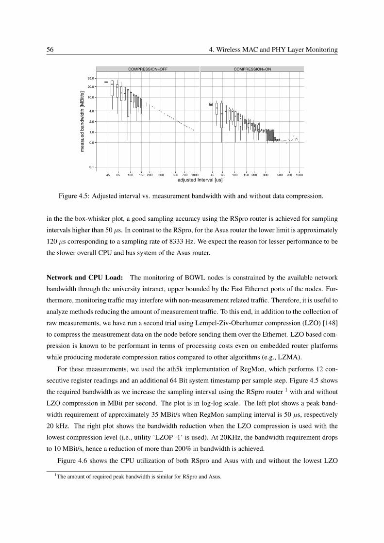
56 4. Wireless MAC and PHY Layer Monitoring
COMPRESSION=OFF COMPRESSION=ON
0.1
0.5
1.0
2.0
4.0
10.0
20.0
35.0
45 65 100 150 200 300 500 700 1000 45 65 100 150 200 300 500 700 1000adjusted Interval [us]
mea
sued
ban
dwid
th [M
Bit/s
]
Figure 4.5: Adjusted interval vs. measurement bandwidth with and without data compression.
in the the box-whisker plot, a good sampling accuracy using the RSpro router is achieved for sampling
intervals higher than 50 µs. In contrast to the RSpro, for the Asus router the lower limit is approximately
120 µs corresponding to a sampling rate of 8333 Hz. We expect the reason for lesser performance to be
the slower overall CPU and bus system of the Asus router.
Network and CPU Load: The monitoring of BOWL nodes is constrained by the available network
bandwidth through the university intranet, upper bounded by the Fast Ethernet ports of the nodes. Fur-
thermore, monitoring traffic may interfere with non-measurement related traffic. Therefore, it is useful to
analyze methods reducing the amount of measurement traffic. To this end, in addition to the collection of
raw measurements, we have run a second trial using Lempel-Ziv-Oberhumer compression (LZO) [148]
to compress the measurement data on the node before sending them over the Ethernet. LZO based com-
pression is known to be performant in terms of processing costs even on embedded router platforms
while producing moderate compression ratios compared to other algorithms (e.g., LZMA).
For these measurements, we used the ath5k implementation of RegMon, which performs 12 con-
secutive register readings and an additional 64 Bit system timestamp per sample step. Figure 4.5 shows
the required bandwidth as we increase the sampling interval using the RSpro router 1 with and without
LZO compression in MBit per second. The plot is in log-log scale. The left plot shows a peak band-
width requirement of approximately 35 MBit/s when RegMon sampling interval is 50 µs, respectively
20 kHz. The right plot shows the bandwidth reduction when the LZO compression is used with the
lowest compression level (i.e., utility ‘LZOP -1’ is used). At 20KHz, the bandwidth requirement drops
to 10 MBit/s, hence a reduction of more than 200% in bandwidth is achieved.
Figure 4.6 shows the CPU utilization of both RSpro and Asus with and without the lowest LZO
1The amount of required peak bandwidth is similar for RSpro and Asus.
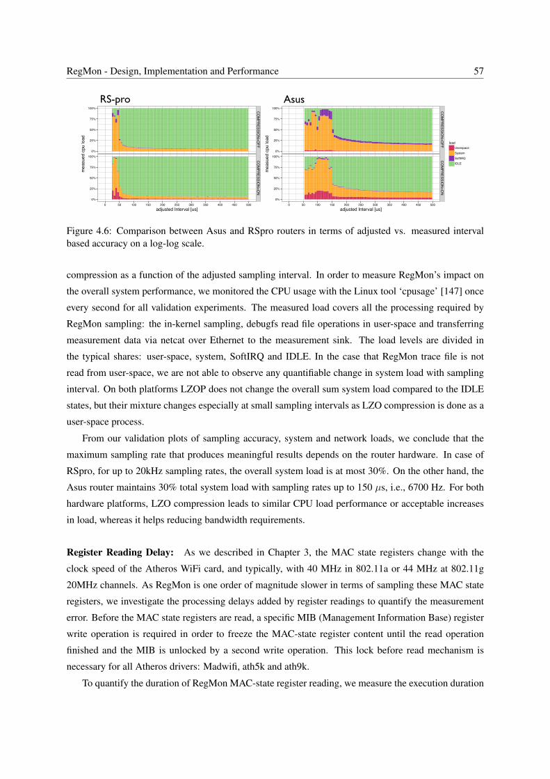
RegMon - Design, Implementation and Performance 57
0%
25%
50%
75%
100%
0%
25%
50%
75%
100%
CO
MPR
ESSION
=OFF
CO
MPR
ESSION
=ON
0 50 100 150 200 250 300 350 400 450 500adjusted Interval [us]
mea
sued
cpu
load
loadUserspaceSystemSoftIRQIDLE
0%
25%
50%
75%
100%
0%
25%
50%
75%
100%
CO
MPR
ESSION
=OFF
CO
MPR
ESSION
=ON
0 50 100 150 200 250 300 350 400 450 500adjusted Interval [us]
mea
sued
cpu
load
loadUserspaceSystemSoftIRQIDLE
RS-pro Asus
Figure 4.6: Comparison between Asus and RSpro routers in terms of adjusted vs. measured intervalbased accuracy on a log-log scale.
compression as a function of the adjusted sampling interval. In order to measure RegMon’s impact on
the overall system performance, we monitored the CPU usage with the Linux tool ‘cpusage’ [147] once
every second for all validation experiments. The measured load covers all the processing required by
RegMon sampling: the in-kernel sampling, debugfs read file operations in user-space and transferring
measurement data via netcat over Ethernet to the measurement sink. The load levels are divided in
the typical shares: user-space, system, SoftIRQ and IDLE. In the case that RegMon trace file is not
read from user-space, we are not able to observe any quantifiable change in system load with sampling
interval. On both platforms LZOP does not change the overall sum system load compared to the IDLE
states, but their mixture changes especially at small sampling intervals as LZO compression is done as a
user-space process.
From our validation plots of sampling accuracy, system and network loads, we conclude that the
maximum sampling rate that produces meaningful results depends on the router hardware. In case of
RSpro, for up to 20kHz sampling rates, the overall system load is at most 30%. On the other hand, the
Asus router maintains 30% total system load with sampling rates up to 150 µs, i.e., 6700 Hz. For both
hardware platforms, LZO compression leads to similar CPU load performance or acceptable increases
in load, whereas it helps reducing bandwidth requirements.
Register Reading Delay: As we described in Chapter 3, the MAC state registers change with the
clock speed of the Atheros WiFi card, and typically, with 40 MHz in 802.11a or 44 MHz at 802.11g
20MHz channels. As RegMon is one order of magnitude slower in terms of sampling these MAC state
registers, we investigate the processing delays added by register readings to quantify the measurement
error. Before the MAC state registers are read, a specific MIB (Management Information Base) register
write operation is required in order to freeze the MAC-state register content until the read operation
finished and the MIB is unlocked by a second write operation. This lock before read mechanism is
necessary for all Atheros drivers: Madwifi, ath5k and ath9k.
To quantify the duration of RegMon MAC-state register reading, we measure the execution duration

58 4. Wireless MAC and PHY Layer Monitoring
ACK receiver
sender
ACK
Data Data
preamble + signal24 µs
16 µs SIFS
16 µs SIFS20 µstime
shortest interval
Figure 4.7: 802.11a MAC frame and ack sequence in the case of packet bursts or fragmentation.
by comparing the TSF timestamp before and after the actual register reading takes place. A full cycle,
which includes freezing all MAC-state registers, reading each of the four registers and unfreezing them,
takes approximately 7 µs in all of our measurements and, across all drivers and also with both Asus and
RSpro hardware. As TSF is measured with an accuracy of 1 µs, the absolute error of a full read cycle
of all four MAC-state registers is 7 ± 1 µs. The impact of this error depends on the sampling interval
used, e.g., if MAC-state registers are sampled at 20kHz, which corresponds to a sampling interval of 50
µs, this translates to a relative error of 16%. However, most of our power control experiments need a
RegMon sampling speed of at most 1000Hz, which introduces a relative error of about 0.9 %.
Packet Reconstruction Limitations: Based on router capabilities, RegMon MAC-layer monitoring
can achieve a sampling rate of 20kHz, for instance in the case of our RSpro. Based on the Nyquist
sampling theorem [149] this resolution time is sufficient to perfectly reconstruct any packet process
with frequency lower than or equal to 10kHz, i.e., with duration shorter than or equal to 100 µs. The
minimum time between two frame transmissions in IEEE 802.11a occurs during a packet burst, when
fragmented packets are sent back to back. The Inter Frame Spacing (IFS) between these packets is a
SIFS duration, which is 16 µs (note that no back-off takes place during a packet burst). Such a packet
sequence is sketched in Figure 4.7 as an example. The shortest interval corresponds to the time between
two fragmented data packets plus the duration of the actual data part, determined by the packet length
in bytes (B) and the modulation. The minimum time interval between two frames is two SIFS intervals
plus ACK duration, which is 56µs. The smallest packet size defined in RFC 894 is 64 B, which will lead
to a transmission duration at the highest 802.11a modulation of 54 MBps of 16 µs (i.e., four symbols,
4 µs each, are needed to encode 64 B data + 36 B SNAT header). This frame is preceded by a 20µs
preamble. To sum, the worst case packet interval is as short as 92 µs (56+16+20) or about 10.9 kHz for
fragmented 802.11a packets. In order to allow a perfect packet process reconstruction, RegMon should
at least sample with about 21.7 kHz or 46 µs sampling interval. This is not feasible with the Asus router,
and in the case of the RSpro platform, such a high sampling rate can still be performed but the point of
operation is a bit below our 20kHz recommendation.
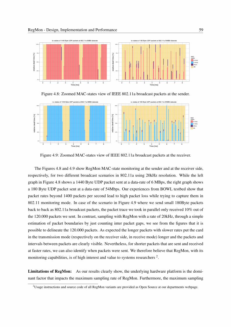
RegMon - Design, Implementation and Performance 59
0%
25%
50%
75%
100%
0 1 2 3 4 5 6 7 8Time [ms]
rela
tive
dwel
l tim
e [%
]
MACstates
tx−busyrx−busyothersidle
tx−states of 1440 Byte UDP packets at 802.11a 6MBit datarate
0%
25%
50%
75%
100%
0 1 2 3 4 5 6 7 8Time [ms]
rela
tive
dwel
l tim
e [%
]
MACstates
tx−busyrx−busyothersidle
tx−states of 180 Byte UDP packets at 802.11a 54MBit datarate
Figure 4.8: Zoomed MAC-states view of IEEE 802.11a broadcast packets at the sender.
0%
25%
50%
75%
100%
0 1 2 3 4 5 6 7 8Time [ms]
rela
tive
dwel
l tim
e [%
]
MACstates
tx−busyrx−busyothersidle
rx−states of 1440 Byte UDP packets at 802.11a 6MBit datarate
0%
25%
50%
75%
100%
0 1 2 3 4 5 6 7 8Time [ms]
rela
tive
dwel
l tim
e [%
]
MACstates
tx−busyrx−busyothersidle
rx−states of 180 Byte UDP packets at 802.11a 54MBit datarate
Figure 4.9: Zoomed MAC-states view of IEEE 802.11a broadcast packets at the receiver.
The Figures 4.8 and 4.9 show RegMon MAC-state monitoring at the sender and at the receiver side,
respectively, for two different broadcast scenarios in 802.11a using 20kHz resolution. While the left
graph in Figure 4.8 shows a 1440 Byte UDP packet sent at a data-rate of 6 MBps, the right graph shows
a 180 Byte UDP packet sent at a data-rate of 54Mbps. Our experiences from BOWL testbed show that
packet rates beyond 1400 packets per second lead to high packet loss while trying to capture them in
802.11 monitoring mode. In case of the scenario in Figure 4.9 where we send small 180Byte packets
back to back as 802.11a broadcast packets, the packet trace we took in parallel only received 10% out of
the 120.000 packets we sent. In contrast, sampling with RegMon with a rate of 20kHz, through a simple
estimation of packet boundaries by just counting inter packet gaps, we see from the figures that it is
possible to delineate the 120.000 packets. As expected the longer packets with slower rates put the card
in the transmission mode (respectively on the receiver side, in receive mode) longer and the packets and
intervals between packets are clearly visible. Nevertheless, for shorter packets that are sent and received
at faster rates, we can also identify when packets were sent. We therefore believe that RegMon, with its
monitoring capabilities, is of high interest and value to systems researchers 2.
Limitations of RegMon: As our results clearly show, the underlying hardware platform is the domi-
nant factor that impacts the maximum sampling rate of RegMon. Furthermore, the maximum sampling
2Usage instructions and source code of all RegMon variants are provided as Open Source at our departments webpage.
60 4. Wireless MAC and PHY Layer Monitoring
rate is limited by the number of wireless cards in a router that are monitored with RegMon. The 20kHz
sampling rate limit at the RSpro platform is an upper bound on the entire PCI bus meaning that the sum
of RegMon sampling rates for multiple WiFi cards can not exceed this sampling limit. Measurements
on newer WiFi cards that use PCI-express bus interfaces to connect to the host platform are left as future
work.
The presented RegMon tool does not perform any processing nor parsing of measurement data in
kernel. Its design is focused on fast register readings. But it might be feasible and also an interesting
path for future development to extend the online data processing that can, e.g., calculate statistics on mac
states. It should also be noted that the current RegMon design uses the same sampling rate for all register
readings. We expect it feasible to extend the current monitoring to individually assigned sampling rates
per register reading.
4.3 Summary
In this chapter, we presented the design, validation and performance of our Atheros specific monitoring
tool RegMon. RegMon enables sampling and analysis of hardware registers with high accuracy. It’s
sampling rate can be set up to 20 kHz depending on the measurement hardware. RegMon is implemented
and validated for all three major drivers of Atheros WiFi cards, namely Madwifi, ath5k and ath9k and
two alternative sampling methods based on Linux jiffies and hr timer. Our measurement tool enables
wireless researchers to access new information sources and is part of the default monitoring setup of the
BOWL network. It proved to be an accurate and reliable source for MAC and PHY layer measurements,
which were used in several research works [150, 151, 152, 153, 95]. In this thesis, RegMon is used
to carry out MAC layer measurements to develop, troubleshoot and analyse our joint rate and power
controller Minstrel-Blues, presented in the next chapter.

Chapter 5
Development of a Joint Power-RateController
In this chapter, we present the design of our power and rate controller, describe our implementation,
and discuss our validation and performance evaluation results. According to [43], a practical controller
should be:
• Distributed: To allow autonomous execution with minimal (if any) network communication re-
sources for control signals.
• Simple: To enable real time implementation with low computational overhead.
• Robust: To be able to adapt to diverse and uncertain inputs.
• Agile: For fast tracking of channel changes and node mobility.
• Scalable: To maintain high performance at networks of various sizes.
To support distributed operation, we propose a simple controller, which relies on local collection of
frame error statistics. This makes our controller scalable. To provide robust operation, the controller
does not react to random fluctuations, but to only the average trends reflecting the channel changes.
To this end, the controller updates power and rate at a timescale significantly larger than transmission
time (e.g., while periodic rate updates occur at each 100 ms, periodic power updates are performed at
slower or equal rates). To achieve agile operation, we check for conditions such as significant drops in
throughput during periodic rate updates and react with power adaptation. However, we do not consider
changes due to fast fading (e.g., mobility faster than walking speed).
Our controller builds on the new interface we introduce, which enables direct communication be-
tween IEEE 802.11 MAC and PHY layer to exchange information about transmit power levels. As
we want to implement a joint power and rate controller for current WiFi devices, we need the ability to
change and add new functionality to the operating system, more precisely, at the network stack and hard-
ware driver level. Given this constraint, Linux and BSD are our best choices. In this thesis our design and
61

62 5. Development of a Joint Power-Rate Controller
implementation will follow the Linux kernel. First we present the design of a cross-layer interface for
the Linux kernel, and propose our joint power and rate control algorithm, Minstrel-Blues, which takes
advantage of this new interface. We conclude with a performance evaluation to show Minstrel-Blues
operation under various settings, and environmental and network conditions.
5.1 Design and Implementation of a Cross-Layer Power-Rate ControlInterface
The implementation of IEEE 802.11 MAC layer typically uses a combination of dedicated hardware and
software [81]. Today, there exist two common designs for splitting the 802.11 MAC into two parts. On
the one hand, WiFi chip designers like Broadcom and Intel support on-chip micro-controllers, where part
of the time-critical code execution happens in firmware, and others are transferred to the host system.
On the other hand, Atheros 802.11 agn miniPCI and miniPCIe chips (besides the USB-based chips) do
not have a general firmware-driven micro-controller, but rather map certain functionalities directly onto
their hardware design. The exact architecture of the MAC layer, i.e., how much of its functionality is
implemented in hardware or in software, depends on the device itself, the device driver and the operating
system (OS) in use.
Historically IEEE 802.11 MAC implementations started as so-called FullMAC schemes, where con-
trol of MAC layer functions is mapped to the individual WiFi hardware or specific firmware or both.
FullMac designs can involve a firmware to be loaded into the chipset memory, e.g., Atheros 802.11n
USB WiFi sticks based on ath6kl [154]. However, due to the difficulty of developing and maintaining
the code for these FullMAC devices, in recent years, software implementations (i.e., SoftMAC) have
emerged. Now, a set of primitives such as authentication, association, beaconing, and functions such as
rate control are implemented at the OS level. For instance, SoftMAC design allows abstract rate control
algorithms to be used across multiple WiFi hardware from different vendors. In this section, we first give
an overview of Linux MAC 802.11 framework, which has SoftMAC capabilities, and next, describe the
extensions we have implemented to support per-packet transmit power and rate control.
5.1.1 Linux mac80211 framework
The Linux mac80211 subsystem provides different SoftMAC capabilities within the kernel [155]. The
main tasks of mac80211 are: (1) to translate between data frame protocols along the receiving (rx) path
(from the driver upwards) and along the transmitting (tx) path (from upper layers downwards), (2) to
control IEEE 802.11 management operations and (3) to provide an interface to perform per packet rate
adaptation. It supports different IEEE 802.11 standards (e.g., abgn), different interface modes (e.g.,
access point, station, ad hoc) and also certain QoS extensions such as 802.11e. An overview of the
current blocks of the Linux IEEE 802.11 part is depicted in Figure 5.1.
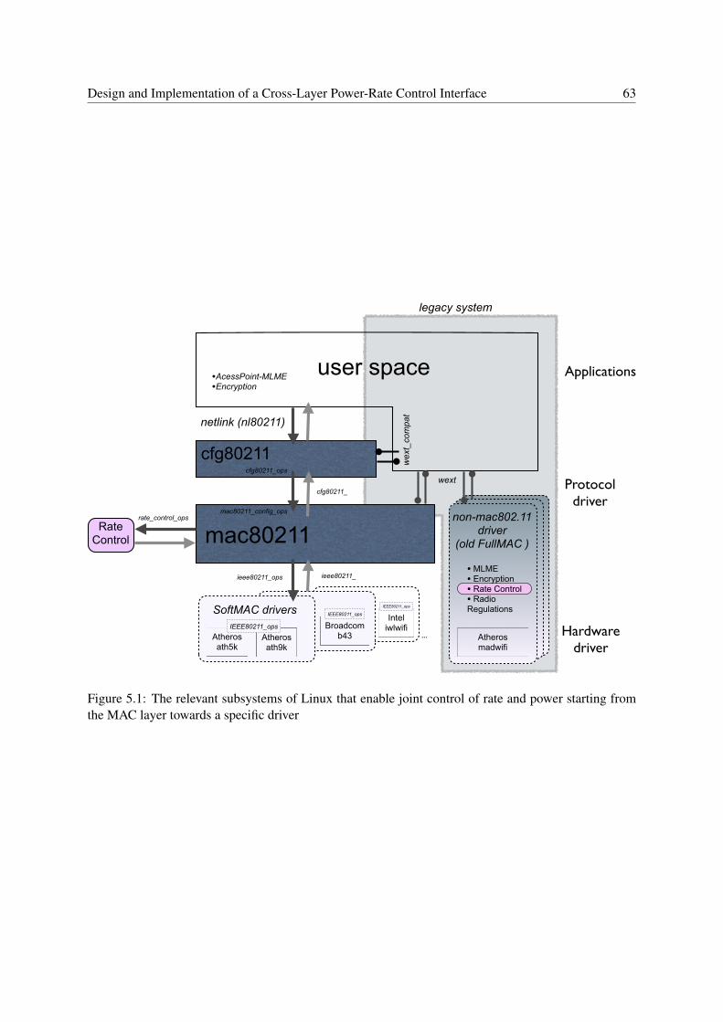
Design and Implementation of a Cross-Layer Power-Rate Control Interface 63
cfg80211
user space
mac80211
Atherosath5k
Atherosath9k
...
Protocoldriver
Hardwaredriver
Applications
netlink (nl80211)
cfg80211_ops
Broadcomb43
Inteliwlwifi
SoftMAC driversIEEE80211_ops
Atherosmadwifi
non-mac802.11driver
(old FullMAC )
cfg80211_
mac80211_config_ops
wext
wex
t_co
mpa
t
rate_control_opsRate
Control
legacy system
• MLME• Encryption• Rate Control• Radio Regulations
•AcessPoint-MLME•Encryption
IEEE80211_ops
IEEE80211_ops
ieee80211_ops ieee80211_
Figure 5.1: The relevant subsystems of Linux that enable joint control of rate and power starting fromthe MAC layer towards a specific driver
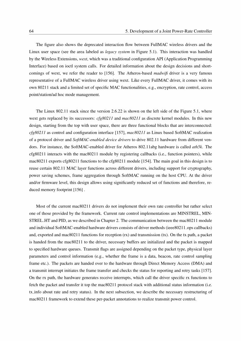
64 5. Development of a Joint Power-Rate Controller
The figure also shows the deprecated interaction flow between FullMAC wireless drivers and the
Linux user space (see the area labeled as legacy system in Figure 5.1). This interaction was handled
by the Wireless Extensions, wext, which was a traditional configuration API (Application Programming
Interface) based on ioctl system calls. For detailed information about the design decisions and short-
comings of wext, we refer the reader to [156]. The Atheros-based madwifi driver is a very famous
representative of a FullMAC wireless driver using wext. Like every FullMAC driver, it comes with its
own 80211 stack and a limited set of specific MAC functionalities, e.g., encryption, rate control, access
point/station/ad hoc mode management.
The Linux 802.11 stack since the version 2.6.22 is shown on the left side of the Figure 5.1, where
wext gets replaced by its successors: cfg80211 and mac80211 as discrete kernel modules. In this new
design, starting from the top with user space, there are three functional blocks that are interconnected:
cfg80211 as control and configuration interface [157], mac80211 as Linux based SoftMAC realization
of a protocol driver and SoftMAC-enabled device drivers to drive 802.11 hardware from different ven-
dors. For instance, the SoftMAC-enabled driver for Atheros 802.11abg hardware is called ath5k. The
cfg80211 interacts with the mac80211 module by registering callbacks (i.e., function pointers), while
mac80211 exports cfg80211 functions to the cfg80211 module [154]. The main goal in this design is to
reuse certain 802.11 MAC layer functions across different drivers, including support for cryptography,
power saving schemes, frame aggregation through SoftMAC running on the host CPU. At the driver
and/or firmware level, this design allows using significantly reduced set of functions and therefore, re-
duced memory footprint [156] .
Most of the current mac80211 drivers do not implement their own rate controller but rather select
one of those provided by the framework. Current rate control implementations are MINSTREL, MIN-
STREL HT and PID, as we described in Chapter 2. The communication between the mac80211 module
and individual SoftMAC-enabled hardware drivers consists of driver methods (ieee80211 ops callbacks)
and, exported and mac80211 functions for reception (rx) and transmission (tx). On the tx path, a packet
is handed from the mac80211 to the driver, necessary buffers are initialized and the packet is mapped
to specified hardware queues. Transmit flags are assigned depending on the packet type, physical layer
parameters and control information (e.g., whether the frame is a data, beacon, rate control sampling
frame etc.). The packets are handed over to the hardware through Direct Memory Access (DMA) and
a transmit interrupt initiates the frame transfer and checks the status for reporting and retry tasks [157].
On the rx path, the hardware generates receive interrupts, which call the driver specific rx functions to
fetch the packet and transfer it top the mac80211 protocol stack with additional status information (i.e.
tx info about rate and retry status). In the next subsection, we describe the necessary restructuring of
mac80211 framework to extend these per-packet annotations to realize transmit power control.

Design and Implementation of a Cross-Layer Power-Rate Control Interface 65
5.1.2 Extending mac80211 for TPC
To control the per-packet rate levels, the Linux kernel uses a control structure (in addition to the packet
buffer), which carries the rate and retry annotations of a given data packet on its way to the driver for
transmission (tx-path). We extended this control structure to support power annotations at the MAC
layer. On receiving the control structure, the driver, in our case, the Atheros device driver, forms a tx-
descriptor that represents the rate and power settings to be used by the WiFi hardware. After a packet is
sent, this structure is overwritten with the status annotation (tx-info), which contains at which rate and
after how many retries the packet succeeded (if at all).
Our implementation can be logically divided into the following parts:
1) Restructuring in order to free up the necessary space and add tx info to support transmit power level
annotation.
This enables a per-packet annotation of one power level (dBm) per multi-rate-retry stage.
2) Introduction of TPC hardware capability flags.
Based on these flags, the driver specifies its different transmit power control capabilities.
• IEEE80211 TPC NONE: This is the default operation, where TPC is not supported and there
is a single fixed transmit power setting.
• IEEE80211 TPC PER DATA PACKET: In this case, power levels are set per-packet. Note that
in this case, the retries are also sent with the same power.
• IEEE80211 TPC PER DATA MRR: Multiple power levels per multi-rate-retry stage are sup-
ported. This works similar to the multi-rate retry.
• IEEE80211 TPC ACK POWER GLOBAL: In this case, a single power level for ACK packets
is set.
3) Add support to change power-level of acknowledgement packets.
A global power level to be used in ACK packets extends the hardware configuration structure. When-
ever a change in ACK power occurs (i.e., through a user space configuration call), MAC sets the new
configuration flag IEEE80211 CONF CHANGE ACK POWER to signal a change to the driver. For
the ACK power to take effect, the driver registers a callback function with this flag, which reads the
new ACK power from the hardware configuration flags.
4) Adapt the source code in the sending path (tx-path) of all effected drivers.
TPC support is added to mac80211 by restructuring of struct ieee80211 tx info. Therefore the tx-
path of all effected drivers is modified to respect the new tx info structure. Linux wireless drivers that
we needed to modify were: ath9k, ath5k, iwl3954, iwl4965, iwl-agn, mwl8k, carl9170, ath9k-htc,
p54, rt2x00, rtl8180, rtl8087, hwsim, b43, b43legacy, brcmsmac and zd1211rw.
As a side effect of our implementation efforts, we also fixed several driver bugs, including race condi-
tions and pointer referencing issues. This mac80211 restructuring implementation is already accepted
in Linux kernel tree (since 31.07.2012). In the next sub-section we leverage our mac80211 extension to
66 5. Development of a Joint Power-Rate Controller
modulation rate (IEEE 802.11 a)
throughput[MBit/sec]
success probability
number of attempts
number of successes
6 4 99 % 0 0
9 5,5 90 % 0 0
12 6 70 % 0 0
18 11 80 % 1 1
24 12 65 % 4 4
36 4 20 % 1 1
48 1,5 5 % 1 0
54 0 0 % 0 0
∑
Minstrel component: update statistics
36MBit
90%unicast
broad- & m
ulticast
10%
24MBit
24MBit
18MBit
24MBit
48MBit
24MBit
ACKACK ACK ACK ACKACK
∑
Calculate exponential weighted moving average (EWMA) ofsuccess probability.
ACK
compute
senderdata
receiver
Figure 5.2: The statistics update is part of Minstrels rate control. To calculate per-rate success proba-bilities, Minstrel collects statistics from all packet transmission attempts. It also uses 10% of the datapackets as sampling packets to try random rates.
implement a joint power and rate controller.
5.2 Joint Power and Rate Control Algorithm: MINSTREL-BLUES
In this section, we present our controller solution that brings together the Minstrel rate control algorithm
and our power control algorithm. To control the transmission rate per-packet, the data-rate and retry an-
notations on the tx-path are performed by Minstrel. This algorithm is explained in detail in Section 5.2.2
and its operation is illustrated in Fig 5.2 summarizing the operation of Minstrel. In addition, we propose
the Blues algorithm to perform per-packet power control. In this section, we first present our validation
of power-rate relationship, which forms the foundation of our algorithms. Next, we present the Blues
algorithm, which enables a trade-off between achievable throughput and spatial reuse. Specifically, this
trade-off allows us to select lower transmission powers, which improves spatial-reuse but may degrade
throughput, which is controlled by using a throughput utility function. For performance evaluation, we
first present detailed validation and performance results on a specific case of Blues, which maintains
throughput equal to the one achieved at maximum power level. This version of Minstrel-Blues is called
Minstrel-Piano. We conclude with results of Minstrel-Blues in our indoor network at 5GHz, and in a
home network with two laptops and one access-point at 2.4GHz.
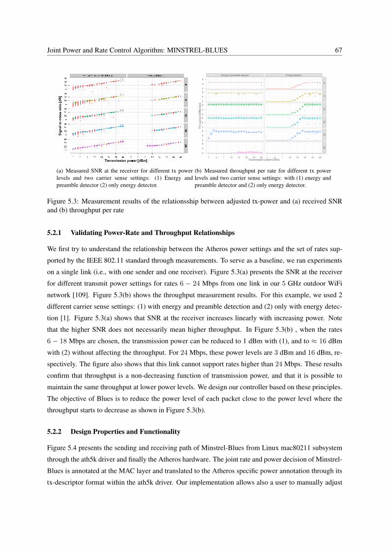
Joint Power and Rate Control Algorithm: MINSTREL-BLUES 67
(a) Measured SNR at the receiver for different tx powerlevels and two carrier sense settings: (1) Energy andpreamble detector (2) only energy detector.
(b) Measured throughput per rate for different tx powerlevels and two carrier sense settings: with (1) energy andpreamble detector and (2) only energy detector.
Figure 5.3: Measurement results of the relationsship between adjusted tx-power and (a) received SNRand (b) throughput per rate
5.2.1 Validating Power-Rate and Throughput Relationships
We first try to understand the relationship between the Atheros power settings and the set of rates sup-
ported by the IEEE 802.11 standard through measurements. To serve as a baseline, we ran experiments
on a single link (i.e., with one sender and one receiver). Figure 5.3(a) presents the SNR at the receiver
for different transmit power settings for rates 6 − 24 Mbps from one link in our 5 GHz outdoor WiFi
network [109]. Figure 5.3(b) shows the throughput measurement results. For this example, we used 2
different carrier sense settings: (1) with energy and preamble detection and (2) only with energy detec-
tion [1]. Figure 5.3(a) shows that SNR at the receiver increases linearly with increasing power. Note
that the higher SNR does not necessarily mean higher throughput. In Figure 5.3(b) , when the rates
6 − 18 Mbps are chosen, the transmission power can be reduced to 1 dBm with (1), and to ≈ 16 dBm
with (2) without affecting the throughput. For 24 Mbps, these power levels are 3 dBm and 16 dBm, re-
spectively. The figure also shows that this link cannot support rates higher than 24 Mbps. These results
confirm that throughput is a non-decreasing function of transmission power, and that it is possible to
maintain the same throughput at lower power levels. We design our controller based on these principles.
The objective of Blues is to reduce the power level of each packet close to the power level where the
throughput starts to decrease as shown in Figure 5.3(b).
5.2.2 Design Properties and Functionality
Figure 5.4 presents the sending and receiving path of Minstrel-Blues from Linux mac80211 subsystem
through the ath5k driver and finally the Atheros hardware. The joint rate and power decision of Minstrel-
Blues is annotated at the MAC layer and translated to the Atheros specific power annotation through its
tx-descriptor format within the ath5k driver. Our implementation allows also a user to manually adjust

68 5. Development of a Joint Power-Rate Controller
Minstrel-Blues
mac80211
SoftMACdrivers (ath5k)
txpath
ieee80211_ops.tx
statistics
look-upupdate
rxpath
compose tx-controldescriptor
processrx-status
descriptor
Atheros WiFi chip
hardware
PCI/PCIe via dma access
tx
rxack
per neighbor
data
data
sk_buff
sk_buff->cb48-Byte
data
fill sk_buff->cb withieee80211_tx_info->tx-status
•rates[4]• vif• hw_keys
fill sk_buff->cb withieee80211_tx_info->control
rxdata
failed
failedfailed
ok
Beacons
fail
failfail o
•rate•retry•power
Figure 5.4: Minstrel-Blues’s tx- and rx-path between mac80211 subsystem, ath5k driver and Atheroshardware.
a static power level and or a static data-rate via Linux debug file system (debugfs). This enables flexible
experimentation with different constants and variables.
To decide at which power level to operate, Blues uses 3 types of packets:
• Reference packets, which are sent at a reference power (typically a high power level).
• Sample packets, which are sent for power-level exploration of different power levels.
• Data packets, which are sent at a power level equal to sample power level plus a constant, ∆
(∆ = 2 dB in our experiments).
By sending packets at different power levels, Blues aims to understand the impact of transmission power
changes on packet success probability. Using these three different types of packets, the algorithm oper-
ates in two parts: (1) It records number of successes and attempts obtained from the transmission feed-
back (see COLLECT STATS in Minstrel-Blues pseudocode depicted in Fig. 5.5), and (2) if enough packets
are sampled for a given rate (determined by the min update parameter), an update mechanism adjusts
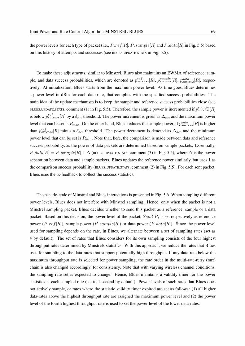
Joint Power and Rate Control Algorithm: MINSTREL-BLUES 69
the power levels for each type of packet (i.e., P ref [R], P sample[R] and P data[R] in Fig. 5.5) based
on this history of attempts and successes (see BLUES UPDATE STATS in Fig. 5.5).
To make these adjustments, similar to Minstrel, Blues also maintains an EWMA of reference, sam-
ple, and data success probabilities, which are denoted as prefsuccess[R], psamplesuccess[R], pdatasuccess[R], respec-
tively. At initialization, Blues starts from the maximum power level. As time goes, Blues determines
a power-level in dBm for each data-rate, that complies with the specified success probabilities. The
main idea of the update mechanism is to keep the sample and reference success probabilities close (see
BLUES UPDATE STATS, comment (1) in Fig. 5.5). Therefore, the sample power is incremented if psamplesuccess[R]
is below prefsuccess[R] by a δinc threshold. The power increment is given as ∆inc and the maximum power
level that can be set is Pmax. On the other hand, Blues reduces the sample power, if pdatasuccess[R] is higher
than prefsuccess[R] minus a δdec threshold. The power decrement is denoted as ∆dec and the minimum
power level that can be set is Pmin. Note that, here, the comparison is made between data and reference
success probability, as the power of data packets are determined based on sample packets. Essentially,
P data[R] = P sample[R] + ∆ (BLUES UPDATE STATS, comment (3) in Fig. 5.5), where ∆ is the power
separation between data and sample packets. Blues updates the reference power similarly, but uses 1 as
the comparison success probability (BLUES UPDATE STATS, comment (2) in Fig. 5.5). For each sent packet,
Blues uses the tx-feedback to collect the success statistics.
The pseudo-code of Minstrel and Blues interactions is presented in Fig. 5.6. When sampling different
power levels, Blues does not interfere with Minstrel sampling. Hence, only when the packet is not a
Minstrel sampling packet, Blues decides whether to send this packet as a reference, sample or a data
packet. Based on this decision, the power level of the packet, Send P , is set respectively as reference
power (P ref [R]), sample power (P sample[R]) or data power (P data[R]). Since the power level
used for sampling depends on the rate, in Blues, we alternate between a set of sampling rates (set as
4 by default). The set of rates that Blues considers for its own sampling consists of the four highest
throughput rates determined by Minstrels statistics. With this approach, we reduce the rates that Blues
uses for sampling to the data-rates that support potentially high throughput. If any data-rate below the
maximum throughput rate is selected for power sampling, the rate order in the multi-rate-retry (mrr)
chain is also changed accordingly, for consistency. Note that with varying wireless channel conditions,
the sampling rate set is expected to change. Hence, Blues maintains a validity timer for the power
statistics at each sampled rate (set to 1 second by default). Power levels of such rates that Blues does
not actively sample, or rates where the statistic validity timer expired are set as follows: (1) all higher
data-rates above the highest throughput rate are assigned the maximum power level and (2) the power
level of the fourth highest throughput rate is used to set the power level of the lower data-rates.
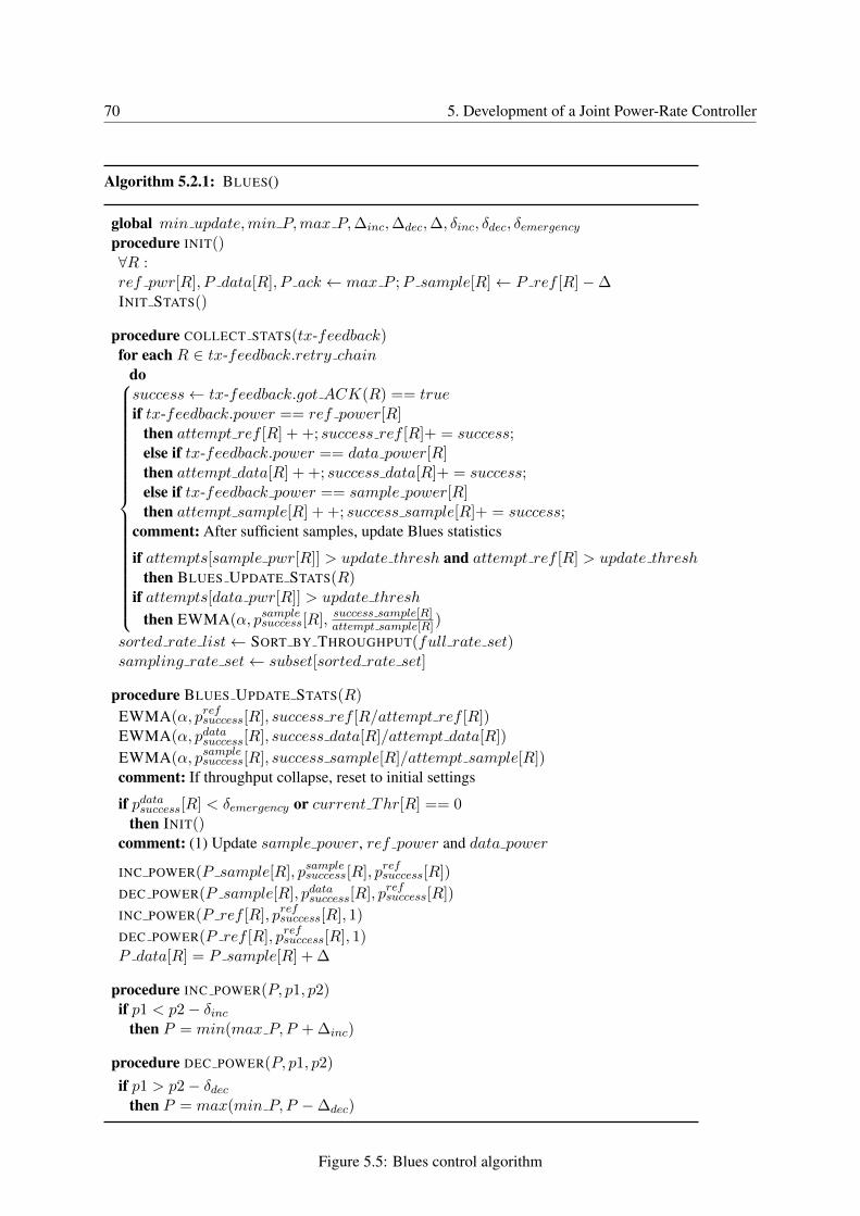
70 5. Development of a Joint Power-Rate Controller
Algorithm 5.2.1: BLUES()
global min update,min P,max P,∆inc,∆dec,∆, δinc, δdec, δemergency
procedure INIT()∀R :ref pwr[R], P data[R], P ack ← max P ;P sample[R]← P ref [R]−∆INIT STATS()
procedure COLLECT STATS(tx-feedback)for each R ∈ tx-feedback.retry chain
do
success← tx-feedback.got ACK(R) == trueif tx-feedback.power == ref power[R]
then attempt ref [R] + +; success ref [R]+ = success;else if tx-feedback.power == data power[R]then attempt data[R] + +; success data[R]+ = success;else if tx-feedback power == sample power[R]then attempt sample[R] + +; success sample[R]+ = success;
comment: After sufficient samples, update Blues statistics
if attempts[sample pwr[R]] > update thresh and attempt ref [R] > update threshthen BLUES UPDATE STATS(R)
if attempts[data pwr[R]] > update thresh
then EWMA(α, psamplesuccess[R], success sample[R]
attempt sample[R])
sorted rate list← SORT BY THROUGHPUT(full rate set)sampling rate set← subset[sorted rate set]
procedure BLUES UPDATE STATS(R)
EWMA(α, prefsuccess[R], success ref [R/attempt ref [R])EWMA(α, pdatasuccess[R], success data[R]/attempt data[R])
EWMA(α, psamplesuccess[R], success sample[R]/attempt sample[R])
comment: If throughput collapse, reset to initial settings
if pdatasuccess[R] < δemergency or current Thr[R] == 0then INIT()
comment: (1) Update sample power, ref power and data power
INC POWER(P sample[R], psamplesuccess[R], prefsuccess[R])
DEC POWER(P sample[R], pdatasuccess[R], prefsuccess[R])
INC POWER(P ref [R], prefsuccess[R], 1)
DEC POWER(P ref [R], prefsuccess[R], 1)P data[R] = P sample[R] + ∆
procedure INC POWER(P, p1, p2)if p1 < p2− δinc
then P = min(max P, P + ∆inc)
procedure DEC POWER(P, p1, p2)
if p1 > p2− δdecthen P = max(min P, P −∆dec)
Figure 5.5: Blues control algorithm
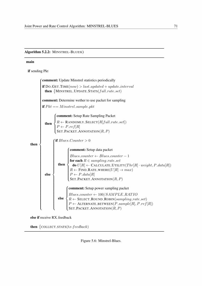
Joint Power and Rate Control Algorithm: MINSTREL-BLUES 71
Algorithm 5.2.2: MINSTREL-BLUES()
main
if sending Pkt
then
comment: Update Minstrel statistics periodically
if DO GET TIME(now) > last updated+ update intervalthen
{MINSTREL UPDATE STATS(full rate set)
comment: Determine wether to use packet for sampling
if Pkt == Minstrel sample pkt
then
comment: Setup Rate Sampling Packet
R← RANDOMLY SELECT(R[full rate set])P ← P ref [R]SET PACKET ANNOTATION(R,P )
else
if Blues Counter > 0
then
comment: Setup data packet
Blues counter ← Blues counter − 1for each R ∈ sampling rate set
do U [R]← CALCULATE UTILITY(Thr[R] · weight, P data[R])R← FIND RATE WHERE(U [R]→ max)P ← P data[R]SET PACKET ANNOTATION(R,P )
else
comment: Setup power sampling packet
Blues counter ← 100/SAMPLE RATIOR← SELECT ROUND ROBIN(sampling rate set)P ← ALTERNATE BETWEEN(P sample[R], P ref [R])SET PACKET ANNOTATION(R,P )
else if receive RX feedback
then{
COLLECT STATS(tx-feedback)
Figure 5.6: Minstrel-Blues.

72 5. Development of a Joint Power-Rate Controller
5.2.3 Utility Function for Joint Decisions
Based on several experiments with Blues running on a single link, we often observed in the statistics
collected by Minstrel and Blues that the throughput difference between the highest and the second high-
est data-rate is below 10% while the power-level difference can be more than 6dB (a reduction of more
then 75%). A reduction in transmission power leads to less effected radiated power and therefore, less
interference to potential surrounding transceivers. To expose the trade-off between the throughput and
interference to other transmissions, we introduced a linear utility function, U(w, ratei), where w de-
notes the weight that is given to throughput achieved at a ratei. For instance, if the goal is maximizing
throughput, than the weightw = 10. We call this case, which finds the necessary power level to maintain
the throughout at maximum power, as Minstrel-Piano.
To decide which rate and power level should be assigned to data packets, Minstrel-Blues periodically
calculates the utility function for each combination of the four highest data-rates and their power levels,
and uses the combination with the highest utility value for all data packets. The utility function uses two
attributes: benefit of a rate, benefit(ratei) and costs of a rate cost(ratei). We define benefit(ratei)
based on its estimated throughput and the maximal throughput:
benefit(ratei) =throughput(ratei)
throughput(ratemax thr)× 100 (5.1)
We scale the ratio of two throughput values with 100 to ease the kernel-level computations.
The cost factor is used to represent the interference costs of achieving a certain throughput at a given
rate, and hence, a power level. The interference cost is essentially a function of the area affected by the
interference and duration of the interference. The area is determined by the transmit power level, which,
in our case, is chosen as power(ratei) and path loss based on environmental and network settings.
However, as modelling such affects are quite complex, we approximate the interference area with only
power(ratei). Similarly, the duration can be approximated as 1/throughput(ratei). Based on these
approximations, we define the cost of a ratei, cost(ratei), with respect to maximal throughput and the
corresponding power:
cost(ratei) =power(ratei)
throughput(ratei)× throughput(ratemax thr)
power(ratemax thr)× 100 (5.2)
Note that, power levels are maintained in dB in Blues, therefore, we convert them first into Watts (i.e.,
power(Watt) = 10power(dB)/10). To avoid the anti-log calculation each time, we build a look-up table,
and use this table for the necessary conversion (i.e., all dBm values from 0 to 30 dBm are precalculated
in mW).
Based on the benefit(ratei) and cost(ratei), utility of rate i, U(ratei) is defined as:
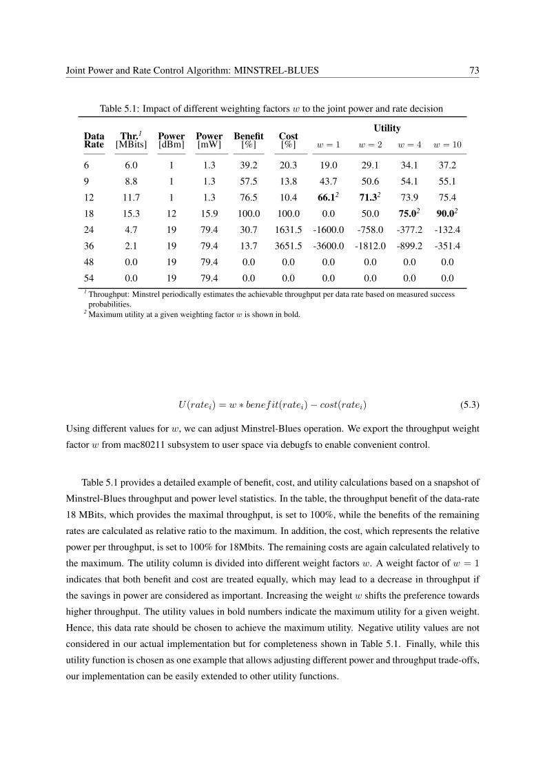
Joint Power and Rate Control Algorithm: MINSTREL-BLUES 73
Table 5.1: Impact of different weighting factors w to the joint power and rate decision
Data Thr.1 Power Power Benefit CostUtility
Rate [MBits] [dBm] [mW] [%] [%] w = 1 w = 2 w = 4 w = 10
6 6.0 1 1.3 39.2 20.3 19.0 29.1 34.1 37.2
9 8.8 1 1.3 57.5 13.8 43.7 50.6 54.1 55.1
12 11.7 1 1.3 76.5 10.4 66.12 71.32 73.9 75.4
18 15.3 12 15.9 100.0 100.0 0.0 50.0 75.02 90.02
24 4.7 19 79.4 30.7 1631.5 -1600.0 -758.0 -377.2 -132.4
36 2.1 19 79.4 13.7 3651.5 -3600.0 -1812.0 -899.2 -351.4
48 0.0 19 79.4 0.0 0.0 0.0 0.0 0.0 0.0
54 0.0 19 79.4 0.0 0.0 0.0 0.0 0.0 0.01 Throughput: Minstrel periodically estimates the achievable throughput per data rate based on measured success
probabilities.2 Maximum utility at a given weighting factor w is shown in bold.
U(ratei) = w ∗ benefit(ratei)− cost(ratei) (5.3)
Using different values for w, we can adjust Minstrel-Blues operation. We export the throughput weight
factor w from mac80211 subsystem to user space via debugfs to enable convenient control.
Table 5.1 provides a detailed example of benefit, cost, and utility calculations based on a snapshot of
Minstrel-Blues throughput and power level statistics. In the table, the throughput benefit of the data-rate
18 MBits, which provides the maximal throughput, is set to 100%, while the benefits of the remaining
rates are calculated as relative ratio to the maximum. In addition, the cost, which represents the relative
power per throughput, is set to 100% for 18Mbits. The remaining costs are again calculated relatively to
the maximum. The utility column is divided into different weight factors w. A weight factor of w = 1
indicates that both benefit and cost are treated equally, which may lead to a decrease in throughput if
the savings in power are considered as important. Increasing the weight w shifts the preference towards
higher throughput. The utility values in bold numbers indicate the maximum utility for a given weight.
Hence, this data rate should be chosen to achieve the maximum utility. Negative utility values are not
considered in our actual implementation but for completeness shown in Table 5.1. Finally, while this
utility function is chosen as one example that allows adjusting different power and throughput trade-offs,
our implementation can be easily extended to other utility functions.

74 5. Development of a Joint Power-Rate Controller
5.3 Performance Evaluation
In this section, we describe the performance of Minstrel-Blues in different scenarios, ranging from single
link to two or more links that operate in parallel. We run these experiments in our BOWL network
using the 5GHz frequency band and a residential location using the 2.4GHz frequency band. For traffic
generation, we used Iperf version 2.0.5, running single-threaded to generate UDP or TCP traffic. In
addition, the senders continuously ping their respective receivers every 2s to maintain connectivity. The
Iperf client and server ran either on dedicated BOWL servers that are connected to each wireless router
via Ethernet, or on the access-point and the client itself. Our experiments in this section are based on
our Minstrel-Blues implementation that runs on two different router platforms Asus wl-500gP and PC-
Engines Alix 3d2. Our evaluations take three different carrier-sense settings into account: (1) energy
and preamble detection, (2) only energy detection, and (3) automatic carrier sense control through ANI
(for details of these settings, see Section 3.2). To evaluate the performance with common metrics, we
monitor different sources across network layers: As shown in Figure 5.7 we use tree different monitoring
sources: (1) RegMon in order to monitor the MAC-layer states and consequently the interference, (2)
tcpdump to determine throughput and received SNR from packet traces and (3) statistics via debugfs to
monitor Minstrel-Blues control behavior in terms of chosen data-rates and power levels. All trace files
are stored while the experiment is running, and analyzed afterwards. Minstrel-Blues monitoring sources
5.3.1 Piano Power Control in a Single Link Scenario
In the initial design of our algorithm, we only considered supporting the same rate, and hence, the
throughput that Minstrel achieves, with the lowest power possible. In our current design, Minstrel-
Piano is a special configuration of Minstrel-Blues, where the weight factor, w, is set to 10, so that only
throughput influences the utility calculation, and the power level is negligible. This approach has a clear
two-step decision sequence: first the rate decision is made by Minstrel based on the estimated throughput
and second, Piano decides the power level based on the loss ratio with the rate set composed of the four
highest throughput rates of Minstrel.
The goal of the following measurement results is to show the ability of Minstrel-Piano to reduce
transmission power while maintaining the same throughput [153]. The traffic is UDP traffic with a
constant datagram size of 1420 B and a rate of 32 Mbps to make sure that all lower layers, including
the wireless MAC layer, are always saturated. We first validate the Piano operation using fixed rates.
Then, we validate the Minstrel-Piano operation, with the goal of showing that Piano is able to work with
Minstrel well.
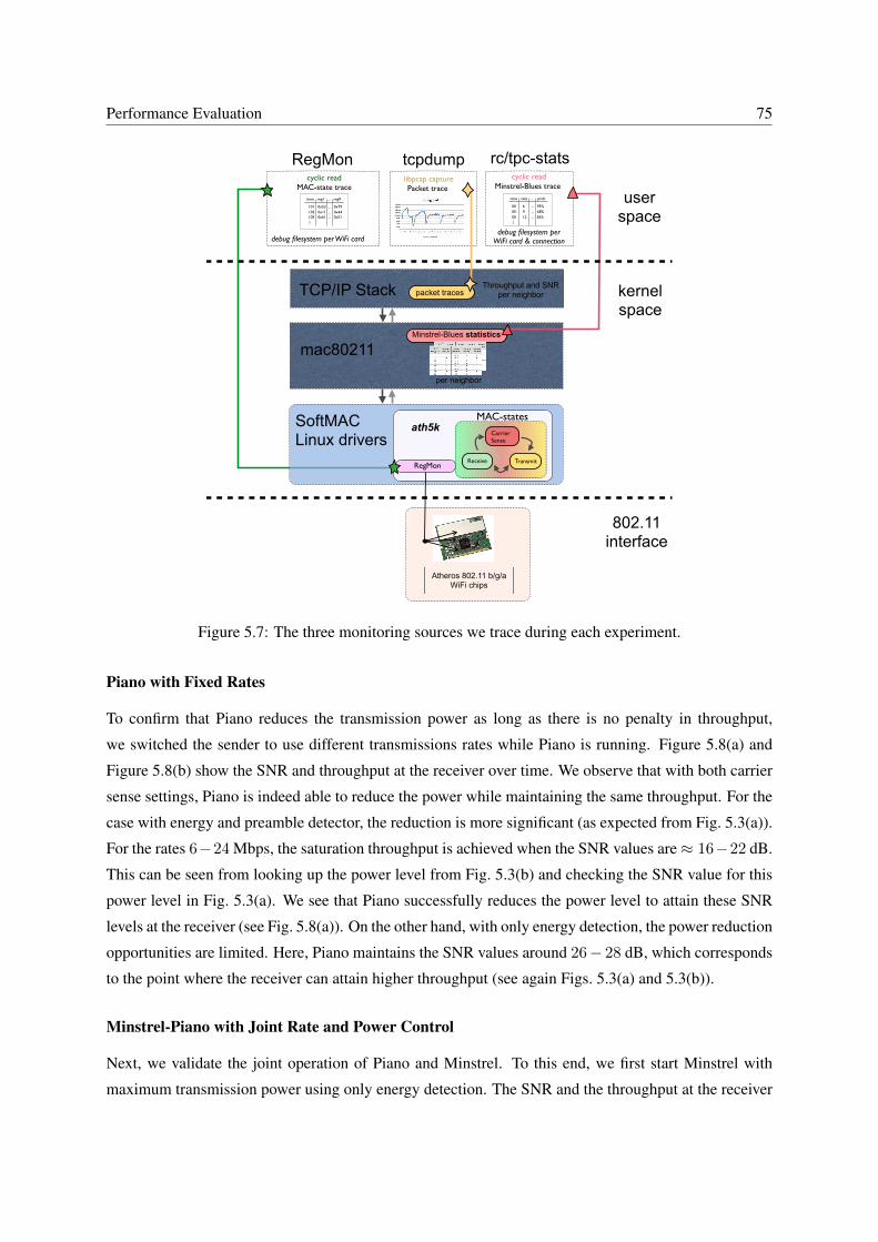
Performance Evaluation 75
userspace
mac80211
ath5kSoftMACLinux drivers
Atheros 802.11 b/g/a WiFi chips
RegMon
debug filesystem per WiFi card
cyclic readMAC-state trace
time reg1 ... reg9
103 0x11 ... 0x44101 0x53 ... 0x79
105 0x61 ... 0x51
...
Minstrel-Blues statistics
time rate ... prob
101 9 ... 68%101 6 ... 95%
...
101 12 ... 56%
cyclic readMinstrel-Blues trace
TCP/IP Stack kernelspace
debug filesystem perWiFi card & connection
packet traces
RegMon rc/tpc-stats
802.11interface
per neighbor
tcpdump
CarrierSense
TransmitReceive
MAC-states
libpcap capturePacket trace
Throughput and SNR per neighbor
Figure 5.7: The three monitoring sources we trace during each experiment.
Piano with Fixed Rates
To confirm that Piano reduces the transmission power as long as there is no penalty in throughput,
we switched the sender to use different transmissions rates while Piano is running. Figure 5.8(a) and
Figure 5.8(b) show the SNR and throughput at the receiver over time. We observe that with both carrier
sense settings, Piano is indeed able to reduce the power while maintaining the same throughput. For the
case with energy and preamble detector, the reduction is more significant (as expected from Fig. 5.3(a)).
For the rates 6−24 Mbps, the saturation throughput is achieved when the SNR values are≈ 16−22 dB.
This can be seen from looking up the power level from Fig. 5.3(b) and checking the SNR value for this
power level in Fig. 5.3(a). We see that Piano successfully reduces the power level to attain these SNR
levels at the receiver (see Fig. 5.8(a)). On the other hand, with only energy detection, the power reduction
opportunities are limited. Here, Piano maintains the SNR values around 26− 28 dB, which corresponds
to the point where the receiver can attain higher throughput (see again Figs. 5.3(a) and 5.3(b)).
Minstrel-Piano with Joint Rate and Power Control
Next, we validate the joint operation of Piano and Minstrel. To this end, we first start Minstrel with
maximum transmission power using only energy detection. The SNR and the throughput at the receiver
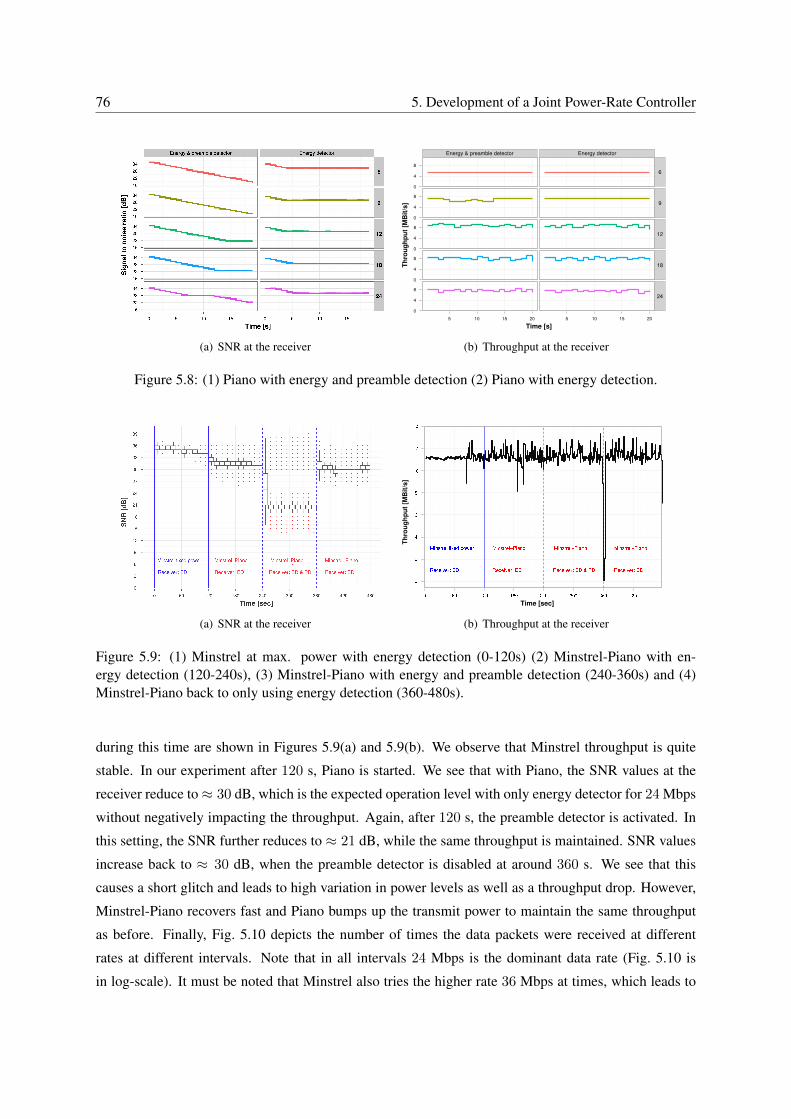
76 5. Development of a Joint Power-Rate Controller
(a) SNR at the receiver
Time [s]
Th
rou
gh
pu
t [M
Bit
/s]
0
4
8
0
4
8
0
4
8
0
4
8
0
4
8
Energy & preamble detector
5 10 15 20
Energy detector
5 10 15 20
6
9
12
18
24
(b) Throughput at the receiver
Figure 5.8: (1) Piano with energy and preamble detection (2) Piano with energy detection.
(a) SNR at the receiver (b) Throughput at the receiver
Figure 5.9: (1) Minstrel at max. power with energy detection (0-120s) (2) Minstrel-Piano with en-ergy detection (120-240s), (3) Minstrel-Piano with energy and preamble detection (240-360s) and (4)Minstrel-Piano back to only using energy detection (360-480s).
during this time are shown in Figures 5.9(a) and 5.9(b). We observe that Minstrel throughput is quite
stable. In our experiment after 120 s, Piano is started. We see that with Piano, the SNR values at the
receiver reduce to≈ 30 dB, which is the expected operation level with only energy detector for 24 Mbps
without negatively impacting the throughput. Again, after 120 s, the preamble detector is activated. In
this setting, the SNR further reduces to ≈ 21 dB, while the same throughput is maintained. SNR values
increase back to ≈ 30 dB, when the preamble detector is disabled at around 360 s. We see that this
causes a short glitch and leads to high variation in power levels as well as a throughput drop. However,
Minstrel-Piano recovers fast and Piano bumps up the transmit power to maintain the same throughput
as before. Finally, Fig. 5.10 depicts the number of times the data packets were received at different
rates at different intervals. Note that in all intervals 24 Mbps is the dominant data rate (Fig. 5.10 is
in log-scale). It must be noted that Minstrel also tries the higher rate 36 Mbps at times, which leads to
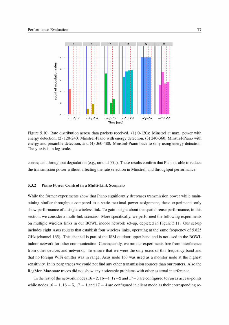
Performance Evaluation 77
Figure 5.10: Rate distribution across data packets received. (1) 0-120s: Minstrel at max. power withenergy detection, (2) 120-240: Minstrel-Piano with energy detection, (3) 240-360: Minstrel-Piano withenergy and preamble detection, and (4) 360-480: Minstrel-Piano back to only using energy detection.The y-axis is in log-scale.
consequent throughput degradation (e.g., around 90 s). These results confirm that Piano is able to reduce
the transmission power without affecting the rate selection in Minstrel, and throughput performance.
5.3.2 Piano Power Control in a Multi-Link Scenario
While the former experiments show that Piano significantly decreases transmission power while main-
taining similar throughput compared to a static maximal power assignment, these experiments only
show performance of a single wireless link. To gain insight about the spatial reuse performance, in this
section, we consider a multi-link scenario. More specifically, we performed the following experiments
on multiple wireless links in our BOWL indoor network set-up, depicted in Figure 5.11. Our set-up
includes eight Asus routers that establish four wireless links, operating at the same frequency of 5.825
GHz (channel 165). This channel is part of the ISM outdoor upper band and is not used in the BOWL
indoor network for other communication. Consequently, we run our experiments free from interference
from other devices and networks. To ensure that we were the only users of this frequency band and
that no foreign WiFi emitter was in range, Asus node 163 was used as a monitor node at the highest
sensitivity. In its pcap traces we could not find any other transmission sources than our routers. Also the
RegMon Mac-state traces did not show any noticeable problems with other external interference.
In the rest of the network, nodes 16−2, 16−4, 17−2 and 17−3 are configured to run as access-points
while nodes 16− 1, 16− 5, 17− 1 and 17− 4 are configured in client mode as their corresponding re-
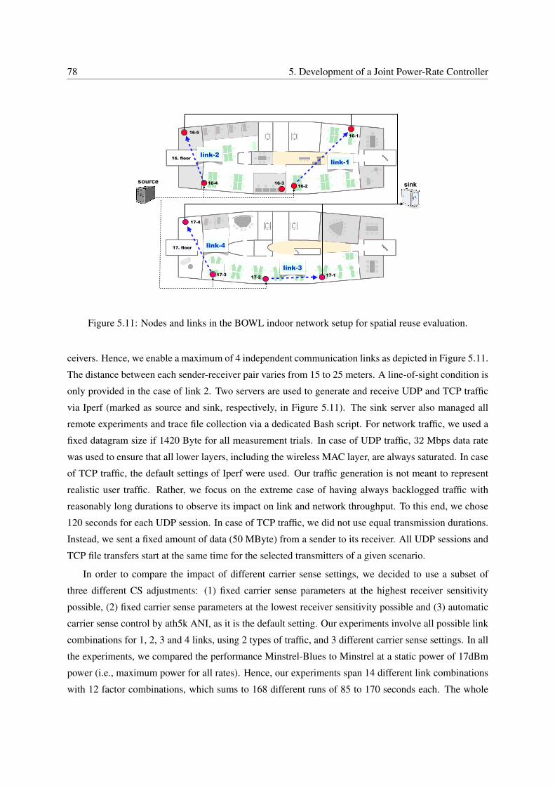
78 5. Development of a Joint Power-Rate Controller
17. floor
16. floor
16-5
16-4 16-316-2
16-1
17-4
17-117-3 17-2
sinksource
link-2link-1
link-3
link-4
Figure 5.11: Nodes and links in the BOWL indoor network setup for spatial reuse evaluation.
ceivers. Hence, we enable a maximum of 4 independent communication links as depicted in Figure 5.11.
The distance between each sender-receiver pair varies from 15 to 25 meters. A line-of-sight condition is
only provided in the case of link 2. Two servers are used to generate and receive UDP and TCP traffic
via Iperf (marked as source and sink, respectively, in Figure 5.11). The sink server also managed all
remote experiments and trace file collection via a dedicated Bash script. For network traffic, we used a
fixed datagram size if 1420 Byte for all measurement trials. In case of UDP traffic, 32 Mbps data rate
was used to ensure that all lower layers, including the wireless MAC layer, are always saturated. In case
of TCP traffic, the default settings of Iperf were used. Our traffic generation is not meant to represent
realistic user traffic. Rather, we focus on the extreme case of having always backlogged traffic with
reasonably long durations to observe its impact on link and network throughput. To this end, we chose
120 seconds for each UDP session. In case of TCP traffic, we did not use equal transmission durations.
Instead, we sent a fixed amount of data (50 MByte) from a sender to its receiver. All UDP sessions and
TCP file transfers start at the same time for the selected transmitters of a given scenario.
In order to compare the impact of different carrier sense settings, we decided to use a subset of
three different CS adjustments: (1) fixed carrier sense parameters at the highest receiver sensitivity
possible, (2) fixed carrier sense parameters at the lowest receiver sensitivity possible and (3) automatic
carrier sense control by ath5k ANI, as it is the default setting. Our experiments involve all possible link
combinations for 1, 2, 3 and 4 links, using 2 types of traffic, and 3 different carrier sense settings. In all
the experiments, we compared the performance Minstrel-Blues to Minstrel at a static power of 17dBm
power (i.e., maximum power for all rates). Hence, our experiments span 14 different link combinations
with 12 factor combinations, which sums to 168 different runs of 85 to 170 seconds each. The whole
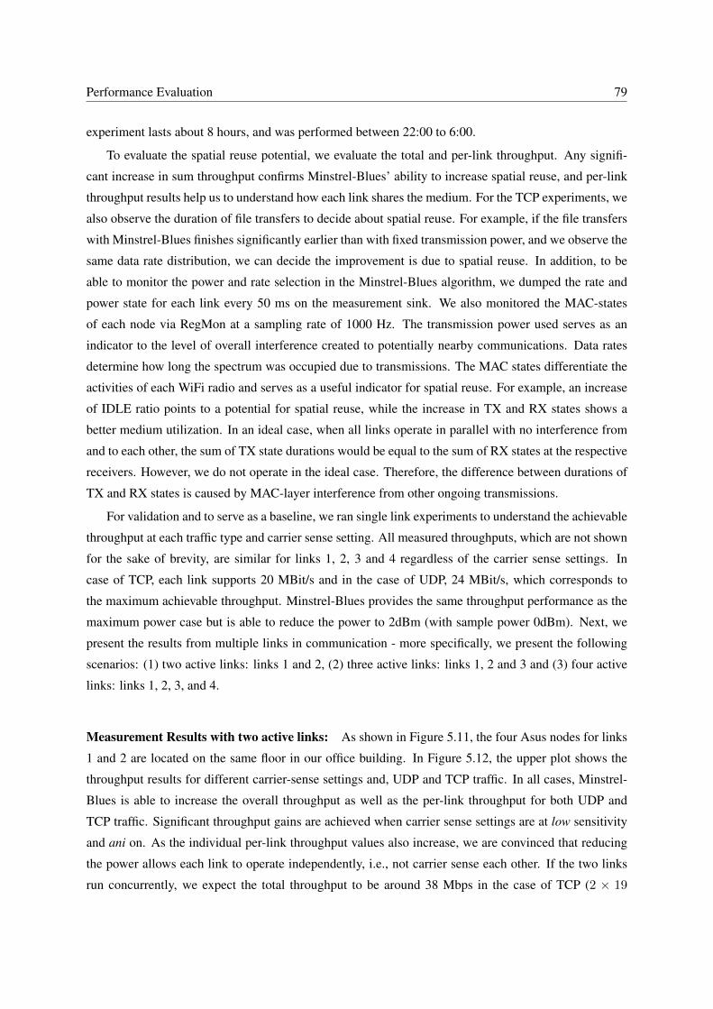
Performance Evaluation 79
experiment lasts about 8 hours, and was performed between 22:00 to 6:00.
To evaluate the spatial reuse potential, we evaluate the total and per-link throughput. Any signifi-
cant increase in sum throughput confirms Minstrel-Blues’ ability to increase spatial reuse, and per-link
throughput results help us to understand how each link shares the medium. For the TCP experiments, we
also observe the duration of file transfers to decide about spatial reuse. For example, if the file transfers
with Minstrel-Blues finishes significantly earlier than with fixed transmission power, and we observe the
same data rate distribution, we can decide the improvement is due to spatial reuse. In addition, to be
able to monitor the power and rate selection in the Minstrel-Blues algorithm, we dumped the rate and
power state for each link every 50 ms on the measurement sink. We also monitored the MAC-states
of each node via RegMon at a sampling rate of 1000 Hz. The transmission power used serves as an
indicator to the level of overall interference created to potentially nearby communications. Data rates
determine how long the spectrum was occupied due to transmissions. The MAC states differentiate the
activities of each WiFi radio and serves as a useful indicator for spatial reuse. For example, an increase
of IDLE ratio points to a potential for spatial reuse, while the increase in TX and RX states shows a
better medium utilization. In an ideal case, when all links operate in parallel with no interference from
and to each other, the sum of TX state durations would be equal to the sum of RX states at the respective
receivers. However, we do not operate in the ideal case. Therefore, the difference between durations of
TX and RX states is caused by MAC-layer interference from other ongoing transmissions.
For validation and to serve as a baseline, we ran single link experiments to understand the achievable
throughput at each traffic type and carrier sense setting. All measured throughputs, which are not shown
for the sake of brevity, are similar for links 1, 2, 3 and 4 regardless of the carrier sense settings. In
case of TCP, each link supports 20 MBit/s and in the case of UDP, 24 MBit/s, which corresponds to
the maximum achievable throughput. Minstrel-Blues provides the same throughput performance as the
maximum power case but is able to reduce the power to 2dBm (with sample power 0dBm). Next, we
present the results from multiple links in communication - more specifically, we present the following
scenarios: (1) two active links: links 1 and 2, (2) three active links: links 1, 2 and 3 and (3) four active
links: links 1, 2, 3, and 4.
Measurement Results with two active links: As shown in Figure 5.11, the four Asus nodes for links
1 and 2 are located on the same floor in our office building. In Figure 5.12, the upper plot shows the
throughput results for different carrier-sense settings and, UDP and TCP traffic. In all cases, Minstrel-
Blues is able to increase the overall throughput as well as the per-link throughput for both UDP and
TCP traffic. Significant throughput gains are achieved when carrier sense settings are at low sensitivity
and ani on. As the individual per-link throughput values also increase, we are convinced that reducing
the power allows each link to operate independently, i.e., not carrier sense each other. If the two links
run concurrently, we expect the total throughput to be around 38 Mbps in the case of TCP (2 × 19

80 5. Development of a Joint Power-Rate Controller
aniBlues: off
aniBlues: on
highBlues: off
highBlues: on
lowBlues: off
lowBlues: on
0
10
20
30
40
0
10
20
30
40
tcpudp
0 40 80 120 0 40 80 120 0 40 80 120 0 40 80 120 0 40 80 120 0 40 80 120
Time [s]
Thro
ughp
ut [M
Bit/s
]
link12total
active links: 12
TCP UDP
0
3
6
9
12
15
18
0
3
6
9
12
15
18
TX−L1TX−L2
0 20 40 60 80 100 120 0 20 40 60 80 100 120Time [s]
tx−P
ower
Lev
el [d
Bm]
powerlevel
datareference
tx−power level used at each sender active links: 12 rx−sensitivity: low
BLUES=OFF BLUES=ON
0%
50%
100%
0%
50%
100%
0%
50%
100%
0%
50%
100%
TX1−link
RX
1−linkTX
2−linkR
X2−link
0 20 40 60 80 100 0 20 40 60 80 100Time [s]
rela
tive
dwel
l tim
e [%
]
MACstates
tx−busyrx−busyidleothers
active links: 12 protocol: tcp CS−sensitivity: low
Time [s]
Throughput with active Links: 1, 2
TX-Power Data-Rate
MAC-states
TX1-link
TX2-link
TX link−1BLUES=OFF
TX link−1BLUES=ON
TX link−2BLUES=OFF
TX link−2BLUES=ON
5448
36
241812
6
5448
36
241812
6
5448
36
241812
6
1st−best2nd−best
high−pr
0 40 80 120 0 40 80 120 0 40 80 120 0 40 80 120Time [s]
802.
11a
data
rate
Minstrel−Blues data rates of each sender active links: 12 proto: TCP rx−sensitivity: lowTX-Data-rate
Figure 5.12: Both links 1 and 2 are active.
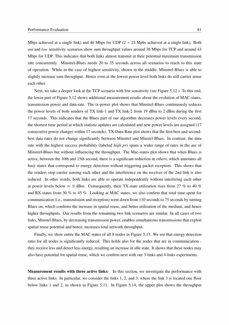
Performance Evaluation 81
Mbps achieved at a single link) and 46 Mbps for UDP (2 × 23 Mpbs achieved at a single link). Both
ani and low sensitivity scenarios show sum throughput values around 36 Mbps for TCP and around 43
Mbps for UDP. This indicates that both links almost transmit at their potential maximum transmission
rate concurrently. Minstrel-Blues needs 20 to 35 seconds across all scenarios to reach to this state
of operation. While in the case of highest sensitivity, shown in the middle, Minstrel-Blues is able to
slightly increase sum throughput. Hence even at the lowest power level both links do still carrier sense
each other.
Next, we take a deeper look at the TCP scenario with low sensitivity (see Figure 5.12 ). To this end,
the lower part of Figure 5.12 shows additional measurement results about the evolution of MAC-states,
transmission power and data-rate. The tx-power plot shows that Minstrel-Blues continuously reduces
the power levels of both senders of TX link-1 and TX link-2 from 19 dBm to 2 dBm during the first
17 seconds. This indicates that the Blues part of our algorithm decreases power levels every second,
the shortest time period at which statistic updates are calculated and new power levels are assigned (17
consecutive power changes within 17 seconds). TX-Data-Rate plot shows that the first-best and second-
best data rates do not change significantly between Minstrel and Minstel-Blues. In contrast, the data
rate with the highest success probability (labeled high pr) spans a wider range of rates in the ase of
Minstrel-Blues but without influencing the throughput. The Mac-states plot shows that when Blues is
active, between the 10th and 15th second, there is a significant reduction in others, which annotates all
busy states that correspond to energy detection without triggering packet reception. This shows that
the senders stop carrier sensing each other and the interference on the receiver of the 2nd link is also
reduced. In other words, both links are able to operate independently without interfering each other
at power levels below ≈ 9 dBm. Consequently, their TX-state utilization rises from 27 % to 40 %
and RX-states from 30 % to 45 %. Looking at MAC states, we also confirm that total time spent for
communication (i.e., transmission and reception) went down from 110 seconds to 75 seconds by turning
Blues on, which confirms the increase in spatial reuse, and better utilisation of the medium, and hence
higher throughputs. Our results from the remaining two link scenarios are similar. In all cases of two
links, Minstel-Blues, by decreasing transmission power, enables simultaneous transmissions that exploit
spatial reuse potential and hence, increases total network throughput.
Finally, we show entire the MAC states of all 8 nodes in Figure 5.13. We see that energy detection
ratio for all nodes is significantly reduced. This holds also for the nodes that are in communication -
they receive less and detect less energy, resulting an increase in idle state. It shows that these nodes may
also have potential for spatial reuse, which we confirm next with our 3-links and 4-links experiments.
Measurement results with three active links: In this section, we investigate the performance with
three active links. In particular, we consider the links 1, 2, and 3, where the link 3 is located one floor
below links 1 and 2, as shown in Figure 5.11. In Figure 5.14, the upper plot shows the throughput
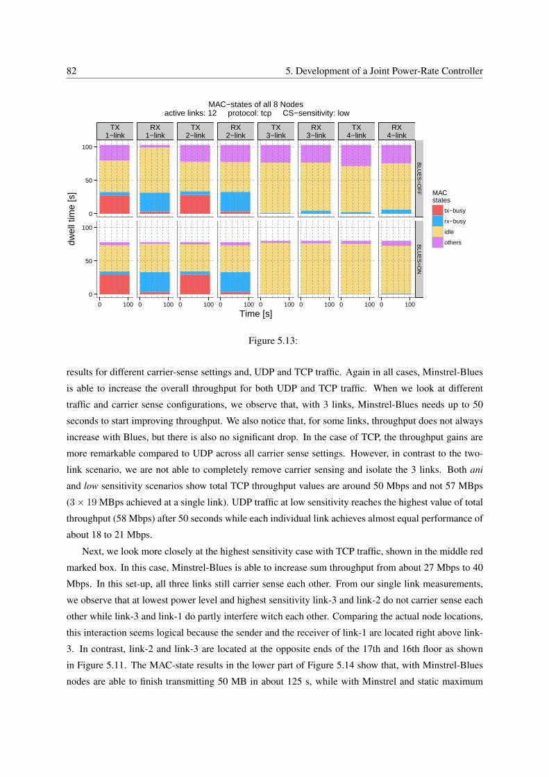
82 5. Development of a Joint Power-Rate Controller
TX1−link
RX1−link
TX2−link
RX2−link
TX3−link
RX3−link
TX4−link
RX4−link
0
50
100
0
50
100
BLU
ES
=O
FF
BLU
ES
=O
N
0 100 0 100 0 100 0 100 0 100 0 100 0 100 0 100
Time [s]
dwel
l tim
e [s
] MACstates
tx−busy
rx−busy
idle
others
MAC−states of all 8 Nodes active links: 12 protocol: tcp CS−sensitivity: low
Figure 5.13:
results for different carrier-sense settings and, UDP and TCP traffic. Again in all cases, Minstrel-Blues
is able to increase the overall throughput for both UDP and TCP traffic. When we look at different
traffic and carrier sense configurations, we observe that, with 3 links, Minstrel-Blues needs up to 50
seconds to start improving throughput. We also notice that, for some links, throughput does not always
increase with Blues, but there is also no significant drop. In the case of TCP, the throughput gains are
more remarkable compared to UDP across all carrier sense settings. However, in contrast to the two-
link scenario, we are not able to completely remove carrier sensing and isolate the 3 links. Both ani
and low sensitivity scenarios show total TCP throughput values are around 50 Mbps and not 57 MBps
(3× 19 MBps achieved at a single link). UDP traffic at low sensitivity reaches the highest value of total
throughput (58 Mbps) after 50 seconds while each individual link achieves almost equal performance of
about 18 to 21 Mbps.
Next, we look more closely at the highest sensitivity case with TCP traffic, shown in the middle red
marked box. In this case, Minstrel-Blues is able to increase sum throughput from about 27 Mbps to 40
Mbps. In this set-up, all three links still carrier sense each other. From our single link measurements,
we observe that at lowest power level and highest sensitivity link-3 and link-2 do not carrier sense each
other while link-3 and link-1 do partly interfere witch each other. Comparing the actual node locations,
this interaction seems logical because the sender and the receiver of link-1 are located right above link-
3. In contrast, link-2 and link-3 are located at the opposite ends of the 17th and 16th floor as shown
in Figure 5.11. The MAC-state results in the lower part of Figure 5.14 show that, with Minstrel-Blues
nodes are able to finish transmitting 50 MB in about 125 s, while with Minstrel and static maximum
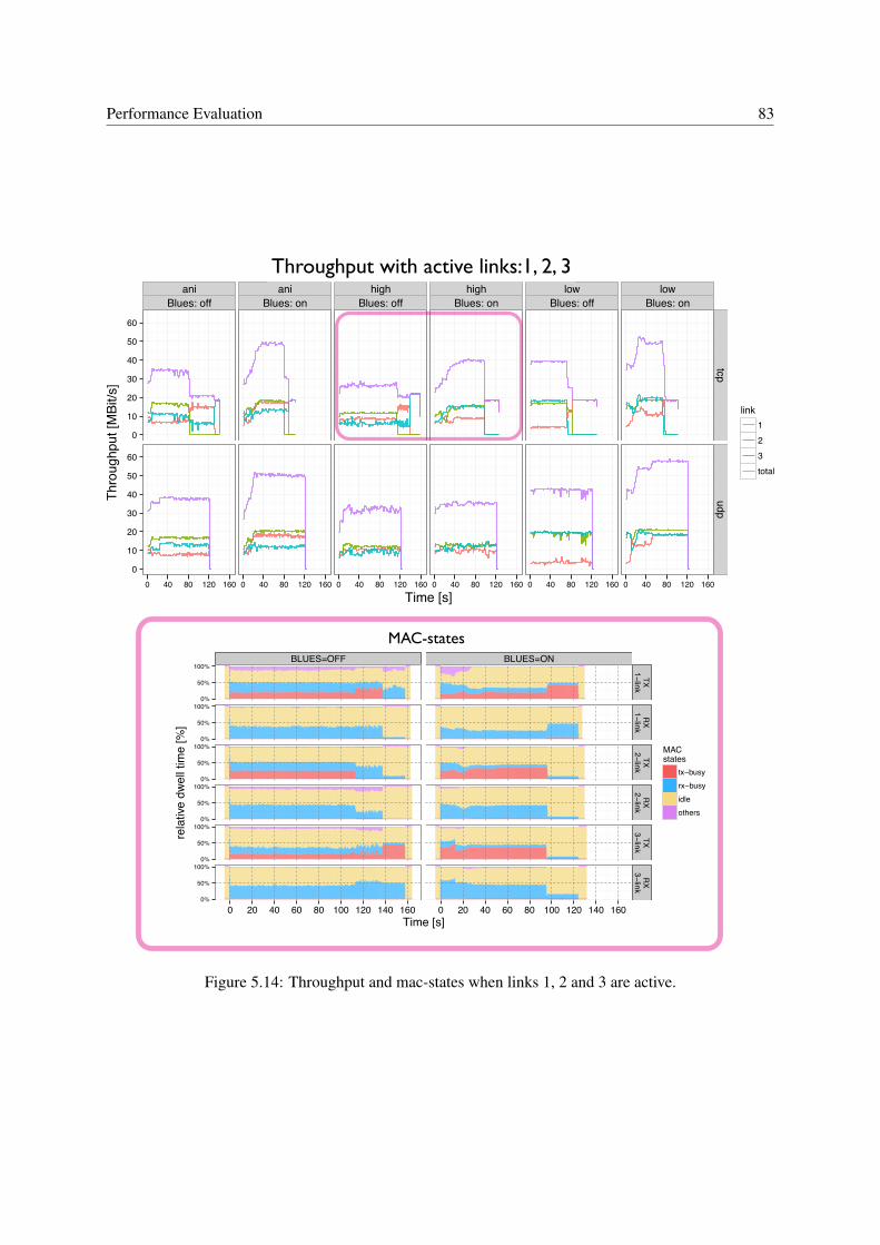
Performance Evaluation 83
aniBlues: off
aniBlues: on
highBlues: off
highBlues: on
lowBlues: off
lowBlues: on
0
10
20
30
40
50
60
0
10
20
30
40
50
60
tcpudp
0 40 80 120 160 0 40 80 120 160 0 40 80 120 160 0 40 80 120 160 0 40 80 120 160 0 40 80 120 160
Time [s]
Thro
ughp
ut [M
Bit/s
]
link123total
active links: 123Throughput with active links:1, 2, 3
BLUES=OFF BLUES=ON
0%
50%
100%
0%
50%
100%
0%
50%
100%
0%
50%
100%
0%
50%
100%
0%
50%
100%
TX1−link
RX
1−linkTX
2−linkR
X2−link
TX3−link
RX
3−link
0 20 40 60 80 100 120 140 160 0 20 40 60 80 100 120 140 160Time [s]
rela
tive
dwel
l tim
e [%
]
MACstates
tx−busyrx−busyidleothers
active links: 123 protocol: tcp CS−sensitivity: highMAC-states
Figure 5.14: Throughput and mac-states when links 1, 2 and 3 are active.
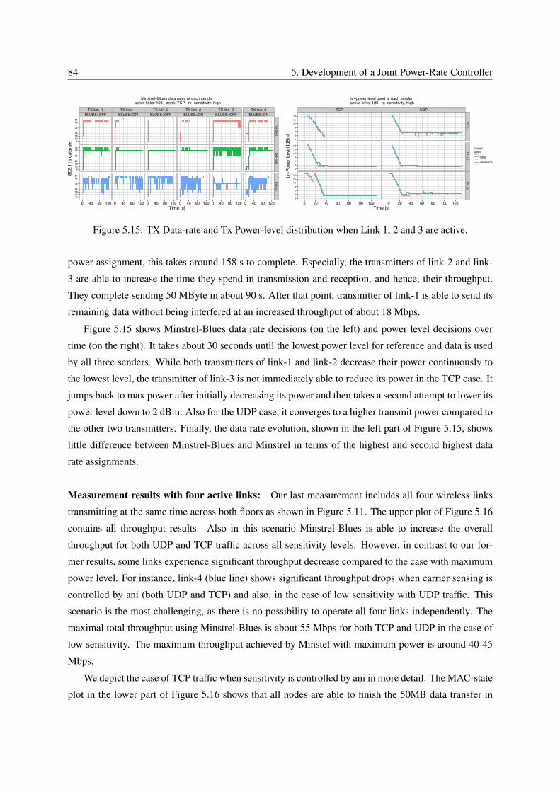
84 5. Development of a Joint Power-Rate Controller
TX link−1BLUES=OFF
TX link−1BLUES=ON
TX link−2BLUES=OFF
TX link−2BLUES=ON
TX link−3BLUES=OFF
TX link−3BLUES=ON
5448
36
241812
6
5448
36
241812
6
5448
36
241812
6
1st−best2nd−best
high−pr
0 40 80 120 0 40 80 120 0 40 80 120 0 40 80 120 0 40 80 120 0 40 80 120Time [s]
802.
11a
data
rate
Minstrel−Blues data rates of each sender active links: 123 proto: TCP rx−sensitivity: high
TCP UDP
0369
121518
0369
121518
0369
121518
TX−L1TX−L2
TX−L3
0 20 40 60 80 100 120 0 20 40 60 80 100 120Time [s]
tx−P
ower
Lev
el [d
Bm]
powerlevel
datareference
tx−power level used at each sender active links: 123 rx−sensitivity: high
Figure 5.15: TX Data-rate and Tx Power-level distribution when Link 1, 2 and 3 are active.
power assignment, this takes around 158 s to complete. Especially, the transmitters of link-2 and link-
3 are able to increase the time they spend in transmission and reception, and hence, their throughput.
They complete sending 50 MByte in about 90 s. After that point, transmitter of link-1 is able to send its
remaining data without being interfered at an increased throughput of about 18 Mbps.
Figure 5.15 shows Minstrel-Blues data rate decisions (on the left) and power level decisions over
time (on the right). It takes about 30 seconds until the lowest power level for reference and data is used
by all three senders. While both transmitters of link-1 and link-2 decrease their power continuously to
the lowest level, the transmitter of link-3 is not immediately able to reduce its power in the TCP case. It
jumps back to max power after initially decreasing its power and then takes a second attempt to lower its
power level down to 2 dBm. Also for the UDP case, it converges to a higher transmit power compared to
the other two transmitters. Finally, the data rate evolution, shown in the left part of Figure 5.15, shows
little difference between Minstrel-Blues and Minstrel in terms of the highest and second highest data
rate assignments.
Measurement results with four active links: Our last measurement includes all four wireless links
transmitting at the same time across both floors as shown in Figure 5.11. The upper plot of Figure 5.16
contains all throughput results. Also in this scenario Minstrel-Blues is able to increase the overall
throughput for both UDP and TCP traffic across all sensitivity levels. However, in contrast to our for-
mer results, some links experience significant throughput decrease compared to the case with maximum
power level. For instance, link-4 (blue line) shows significant throughput drops when carrier sensing is
controlled by ani (both UDP and TCP) and also, in the case of low sensitivity with UDP traffic. This
scenario is the most challenging, as there is no possibility to operate all four links independently. The
maximal total throughput using Minstrel-Blues is about 55 Mbps for both TCP and UDP in the case of
low sensitivity. The maximum throughput achieved by Minstel with maximum power is around 40-45
Mbps.
We depict the case of TCP traffic when sensitivity is controlled by ani in more detail. The MAC-state
plot in the lower part of Figure 5.16 shows that all nodes are able to finish the 50MB data transfer in
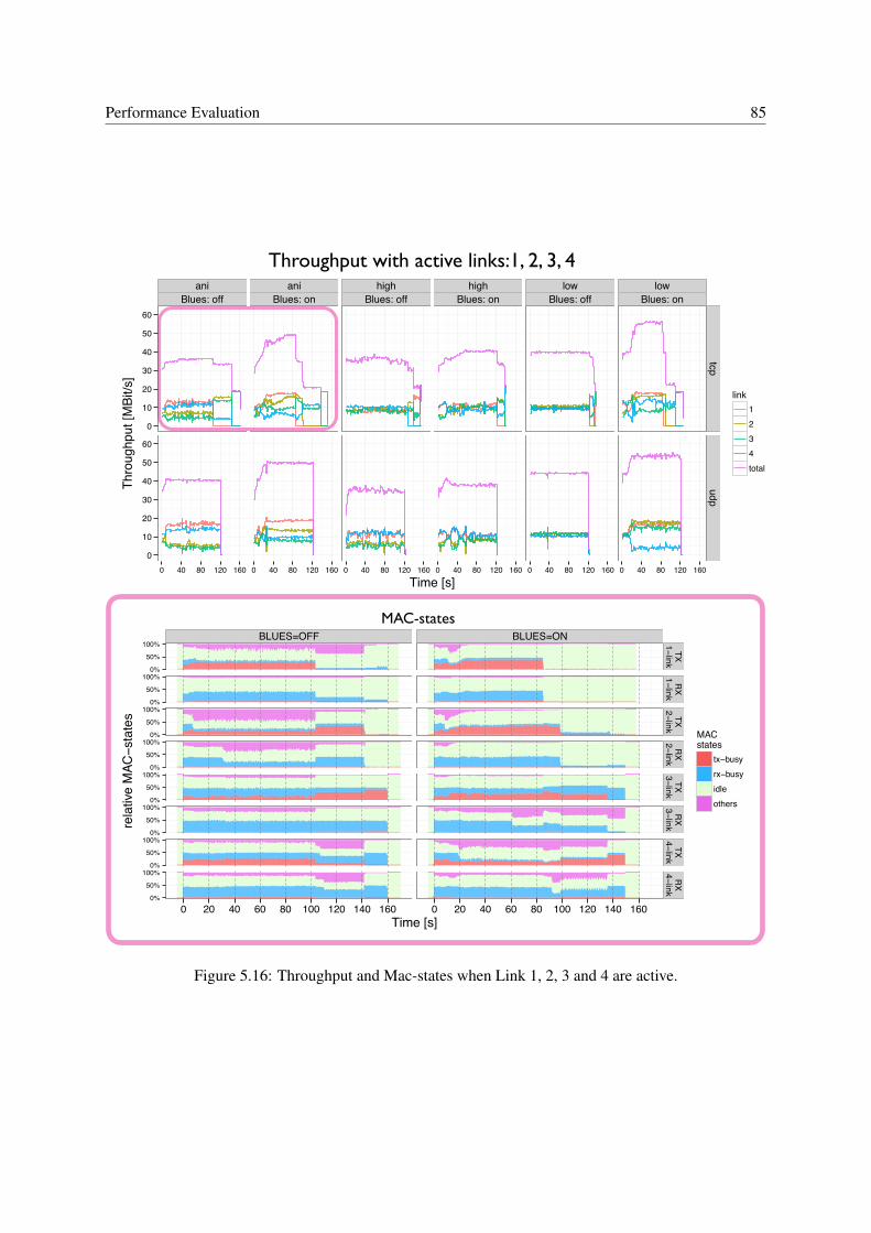
Performance Evaluation 85
BLUES=OFF BLUES=ON
0%
50%
100%
0%
50%
100%
0%
50%
100%
0%
50%
100%
0%
50%
100%
0%
50%
100%
0%
50%
100%
0%
50%
100%
TX1−link
RX
1−linkTX
2−linkR
X2−link
TX3−link
RX
3−linkTX
4−linkR
X4−link
0 20 40 60 80 100 120 140 160 0 20 40 60 80 100 120 140 160Time [s]
rela
tive
MAC
−sta
tes
MACstates
tx−busyrx−busyidleothers
active links: 1234 protocol: tcp CS−sensitivity: ani
aniBlues: off
aniBlues: on
highBlues: off
highBlues: on
lowBlues: off
lowBlues: on
0
10
20
30
40
50
60
0
10
20
30
40
50
60
tcpudp
0 40 80 120 160 0 40 80 120 160 0 40 80 120 160 0 40 80 120 160 0 40 80 120 160 0 40 80 120 160
Time [s]
Thro
ughp
ut [M
Bit/s
]
link1234total
active links: 1234Throughput with active links:1, 2, 3, 4
MAC-states
Figure 5.16: Throughput and Mac-states when Link 1, 2, 3 and 4 are active.
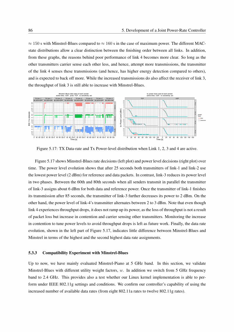
86 5. Development of a Joint Power-Rate Controller
≈ 150 s with Minstrel-Blues compared to ≈ 160 s in the case of maximum power. The different MAC-
state distributions allow a clear distinction between the finishing order between all links. In addition,
from these graphs, the reasons behind poor performance of link 4 becomes more clear. So long as the
other transmitters carrier sense each other less, and hence, attempt more transmissions, the transmitter
of the link 4 senses these transmissions (and hence, has higher energy detection compared to others),
and is expected to back off more. While the increased transmissions do also affect the receiver of link 3,
the throughput of link 3 is still able to increase with Minstrel-Blues.
TX link−1BLUES=OFF
TX link−1BLUES=ON
TX link−2BLUES=OFF
TX link−2BLUES=ON
TX link−3BLUES=OFF
TX link−3BLUES=ON
TX link−4BLUES=OFF
TX link−4BLUES=ON
5448
36
241812
6
5448
36
241812
6
5448
36
241812
6
1st−best2nd−best
high−pr
0 40 80 120 0 40 80 120 0 40 80 120 0 40 80 120 0 40 80 120 0 40 80 120 0 40 80 120 0 40 80 120Time [s]
802.
11a
data
rate
Minstrel−Blues data rates of each sender active links: 1234 proto: TCP rx−sensitivity: ani
TCP UDP
0369
121518
0369
121518
0369
121518
0369
121518
TX−L1TX−L2
TX−L3TX−L4
0 20 40 60 80 100 120 140 160 0 20 40 60 80 100 120 140 160Time [s]
tx−P
ower
Lev
el [d
Bm]
powerlevel
datareference
tx−power level used at each sender active links: 1234 rx−sensitivity: ani
Figure 5.17: TX Data-rate and Tx Power-level distribution when Link 1, 2, 3 and 4 are active.
Figure 5.17 shows Minstrel-Blues rate decisions (left plot) and power level decisions (right plot) over
time. The power level evolution shows that after 25 seconds both transmitters of link-1 and link-2 use
the lowest power level (2 dBm) for reference and data packets. In contrast, link-3 reduces its power level
in two phases. Between the 60th and 80th seconds when all senders transmit in parallel the transmitter
of link-3 assigns about 6 dBm for both data and reference power. Once the transmitter of link-1 finishes
its transmission after 85 seconds, the transmitter of link-3 further decreases its power to 2 dBm. On the
other hand, the power level of link-4’s transmitter alternates between 2 to 3 dBm. Note that even though
link 4 experiences throughput drops, it does not ramp up its power, as the loss of throughput is not a result
of packet loss but increase in contention and carrier sensing other transmitters. Monitoring the increase
in contention to tune power levels to avoid throughput drops is left as future work. Finally, the data rate
evolution, shown in the left part of Figure 5.17, indicates little difference between Minstrel-Blues and
Minstrel in terms of the highest and the second highest data rate assignments.
5.3.3 Compatibility Experiment with Minstrel-Blues
Up to now, we have mainly evaluated Minstrel-Piano at 5 GHz band. In this section, we validate
Minstrel-Blues with different utility weight factors, w. In addition we switch from 5 GHz frequency
band to 2.4 GHz. This provides also a test whether our Linux kernel implementation is able to per-
form under IEEE 802.11g settings and conditions. We confirm our controller’s capability of using the
increased number of available data rates (from eight 802.11a rates to twelve 802.11g rates).

Performance Evaluation 87
Lenovo Thinkpad T520OS = Ubuntu 12.04WiFi = Intel Ultimate-N 6300
802.11 a/g/n 450MBitdriver = iwlwifi
ASUS Eee PC 1005HAOS = Windows 7 homeWiFi = Atheros AR2427
802.11 b/gdriver = Windows specific
monitorinterface
accessinterface
-- ca. 5m --
-- ca. 3m --
PC-Engines Alix 3d2OS = OpenWrt rev. 33027WiFi = 2x Wistron CM9
802.11 a/b/gdriver = Ath5k + Minstrel-Blues
channel = 1 (2,412 GHz)date = 11.07.2012time = 22:00location = residence in Berlin
Figure 5.18: Node and Link Setup of Minstrel-Blues Compatibility Scenario.
For these experiments, we use a different measurement setup that consists of two client devices (a
laptop and a netbook) connected to one Minstrel-Blues enabled access-point in a residential house in
Berlin (see Figure 5.18). The WiFi card of the laptop is based on an Intel IEEE 802.11n chip powered
by a recent Ubuntu version. The netbook is equipped with an IEEE 802.11n Atheros chip and a recent
Windows version as its operating system. In contrast to the formerly used Asus MIPS hardware, the
access point is a x86 based PC-Engines Alix 3d2 router running a current version of OpenWrt. It
includes two Atheros based Wistron CM9 WiFi cards that are driven by the ath5k driver including our
Minstrel-Blues implementation. And a common 5 dBi indoor omni-directional antenna is attached to
each wireless interface. One WiFi cards serves as an access point on channel 1 (2.412 GHz) and the
other WiFi card is used as the monitoring interface to capture packets. Both clients and the access
point are located in one living room with direct line of sight to each other. The approximate distance of
communication links is annotated in Figure 5.18 and are rather short.
We generate traffic with Iperf, where the access point starts sending: (1) two UDP flows and (2) two
TCP flows to each client at the same time. To ensure that both flows start at the same time, the actual
measurement script is executed on the Alix router. The packet size is set to 1420 Byte. We collect MAC-
state traces at 1000Hz via RegMon, tcpdump traces from the monitoring interface, and Minstrel-Blues
data rate and power level assignments periodically via proc filesystem. The 8 GB CF card on the router
is sufficiently large to store all the monitoring data.
The whole experiment consists of six measurement runs (three weight factors of 10, 4 and 2, and
two traffic types of UDP and TCP) and lasts about 70 minutes. The impact of these weight factors were
shown and explained earlier in Table 5.1. Each experiment lasts for 10 minutes while we change from
Minstrel-Blues to Minstrel with maximum power (and vice versa) every 150 seconds. We start with
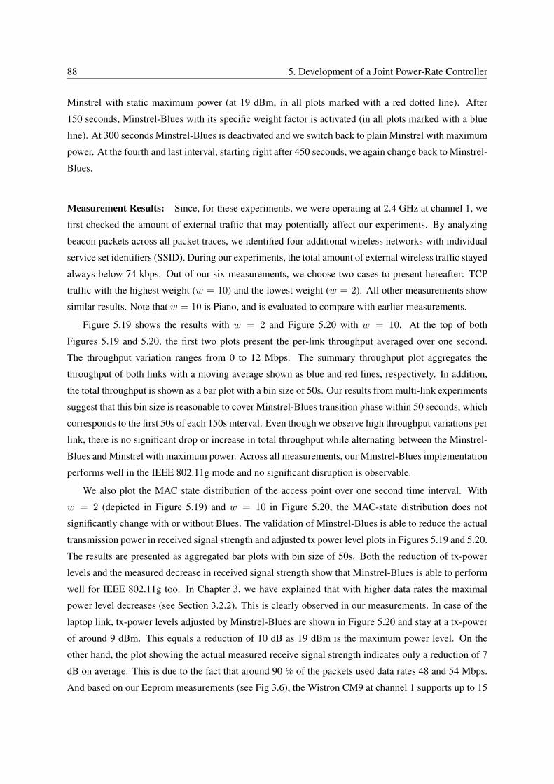
88 5. Development of a Joint Power-Rate Controller
Minstrel with static maximum power (at 19 dBm, in all plots marked with a red dotted line). After
150 seconds, Minstrel-Blues with its specific weight factor is activated (in all plots marked with a blue
line). At 300 seconds Minstrel-Blues is deactivated and we switch back to plain Minstrel with maximum
power. At the fourth and last interval, starting right after 450 seconds, we again change back to Minstrel-
Blues.
Measurement Results: Since, for these experiments, we were operating at 2.4 GHz at channel 1, we
first checked the amount of external traffic that may potentially affect our experiments. By analyzing
beacon packets across all packet traces, we identified four additional wireless networks with individual
service set identifiers (SSID). During our experiments, the total amount of external wireless traffic stayed
always below 74 kbps. Out of our six measurements, we choose two cases to present hereafter: TCP
traffic with the highest weight (w = 10) and the lowest weight (w = 2). All other measurements show
similar results. Note that w = 10 is Piano, and is evaluated to compare with earlier measurements.
Figure 5.19 shows the results with w = 2 and Figure 5.20 with w = 10. At the top of both
Figures 5.19 and 5.20, the first two plots present the per-link throughput averaged over one second.
The throughput variation ranges from 0 to 12 Mbps. The summary throughput plot aggregates the
throughput of both links with a moving average shown as blue and red lines, respectively. In addition,
the total throughput is shown as a bar plot with a bin size of 50s. Our results from multi-link experiments
suggest that this bin size is reasonable to cover Minstrel-Blues transition phase within 50 seconds, which
corresponds to the first 50s of each 150s interval. Even though we observe high throughput variations per
link, there is no significant drop or increase in total throughput while alternating between the Minstrel-
Blues and Minstrel with maximum power. Across all measurements, our Minstrel-Blues implementation
performs well in the IEEE 802.11g mode and no significant disruption is observable.
We also plot the MAC state distribution of the access point over one second time interval. With
w = 2 (depicted in Figure 5.19) and w = 10 in Figure 5.20, the MAC-state distribution does not
significantly change with or without Blues. The validation of Minstrel-Blues is able to reduce the actual
transmission power in received signal strength and adjusted tx power level plots in Figures 5.19 and 5.20.
The results are presented as aggregated bar plots with bin size of 50s. Both the reduction of tx-power
levels and the measured decrease in received signal strength show that Minstrel-Blues is able to perform
well for IEEE 802.11g too. In Chapter 3, we have explained that with higher data rates the maximal
power level decreases (see Section 3.2.2). This is clearly observed in our measurements. In case of the
laptop link, tx-power levels adjusted by Minstrel-Blues are shown in Figure 5.20 and stay at a tx-power
of around 9 dBm. This equals a reduction of 10 dB as 19 dBm is the maximum power level. On the
other hand, the plot showing the actual measured receive signal strength indicates only a reduction of 7
dB on average. This is due to the fact that around 90 % of the packets used data rates 48 and 54 Mbps.
And based on our Eeprom measurements (see Fig 3.6), the Wistron CM9 at channel 1 supports up to 15
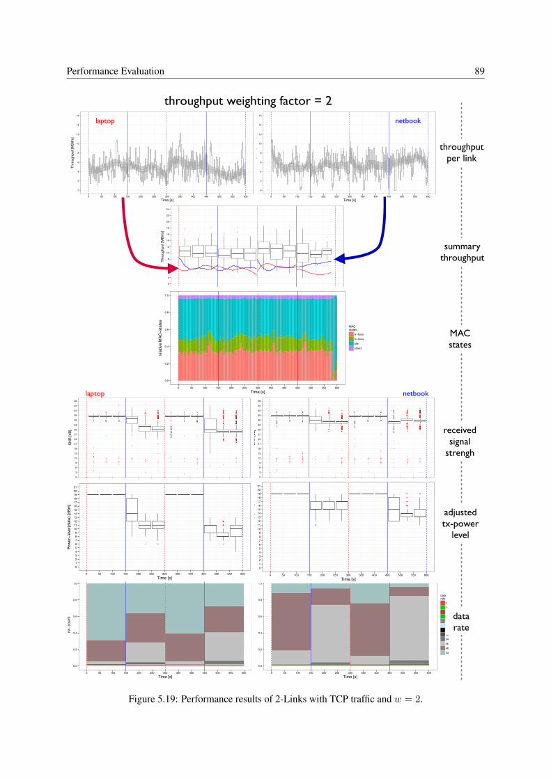
Performance Evaluation 89
0.0
0.2
0.4
0.6
0.8
1.0
0 50 100 150 200 250 300 350 400 450 500 550 600Time [s]
rel.
coun
t
datarate
125.56911121824364854
0
2
4
6
8
10
12
14
16
0 50 100 150 200 250 300 350 400 450 500 550 600Time [s]
Thro
ughp
ut [M
Bit/s
]
throughput weighting factor = 2
0.0
0.2
0.4
0.6
0.8
1.0
0 50 100 150 200 250 300 350 400 450 500 550 600Time [s]
rel.
coun
t
datarate
125.56911121824364854
●
●
●
●
●
●●
●
●
●
●
●
0
2
4
6
8
10
12
14
16
18
20
22
24
0 50 100 150 200 250 300 350 400 450 500 550 600Time [s]
Thro
ughp
ut [M
Bit/s
]
0
2
4
6
8
10
12
14
16
0 50 100 150 200 250 300 350 400 450 500 550 600Time [s]
Thro
ughp
ut [M
Bit/s
]
laptop netbook
summary throughput
throughputper link
receivedsignal
strengh
adjustedtx-power
level
datarate
MACstates
0.0
0.2
0.4
0.6
0.8
1.0
0 50 100 150 200 250 300 350 400 450 500 550 600Time [s]
rela
tive
MAC
−sta
tes
MACstates
tx−busyrx−busyidleothers
●
●
●
●
●
●
●●●
●●●
●
●
●●
●●
●●
●
●●
●
●
●
●
●
●●
●
●
●●
●●●
●
●
●●●●●●●●
●
●
●●●●
●●●●
●
●
●
●●
●
●
●●
●
●
●●●
●
●
●
●●
●
●
●
●●●
●
●
●●●●
●●
●●●
●
●●
●
●●
●
●
●
●
●●
●●
●●●
●●●
●
●
●●
●
●●●●●●●
●●
●
● ●
●
●
●
●●●●●●●
●
●
●
●
●●●
●
●
●
●
●
●●●●●
●
●●●
●
●
●
●
●
●
●●
●
●●●
●
●
●
●
●
●
●
●●
●
●
●●
●
●●
●
●
●
●
●
●●
●
●
●
●
●●●●
●
●
●●
●
●
●
●
●
●●●●●
●●
●
●●●●●●●●●●●●●●●●●●●●●●●●●●●●●●●●●●●●●●●●●●
●
●●●●
●
●●
●
●●●●●●●●●●
●
●
●
●●●
●
●●●
●
●●●
●
●●
●
●
●
●
●
●●
●
●
●
●●●
●
●●●●●●
●
●●●●
●
●●●●●●●●
●
●
●
●
●
●
●
●●
●
●●
●
●●
●
●
●
●●
●●
●
●
●
●●●●
●
●●
●
●
●
●●
●
●●
●
●
●
●
●●●
●●●
●
●
●●
●
●
●
●●
●
●
●
●
●
●●
●
●
●
●
●
●
●●
●
●
●
●●●●
●●
●
●
●
●
●
●
●
●
●
●
●
●
●
●●
●
●●
●●●
●
●
●●●
●
●
●
●
●
●
●●●●
●●
●
●●
●●●●●●●
●
●
●
●●●
●
●
●
●
●●
●●●●
●
●
●
●●●
●
●
●●●●●●●●
●
●
●●
●
●
●
●●●●
●●●
●
●●
●
●
●●
●●
●
●
●
●
●
●●
●
●●●
●
●
●●
●●●●
●
●
●
●●
●
●
●
●
●
●●●●●●
●
●●
●
●●
●
●
●
●●●●●●●
●
●
●
●
●●●●●
●
●
●
●
●●●●
●●●●●
●
●
●
●
●
●
●
●
●
●●
●
●
●
●
●
●
●
●
●
●
●
●
●●
●
●●●●●●
●
●●
●
●
●
●●●●●●
●
●
●
●
●●
●●
●●●
●
●
●
●
●
●
●●
●
●●
●
●●
●●
●
●
●
●
●
●●●●
●
●
●●●
●
●
●
●
●
●
●
●
●
●●●●
●
●
●
●●●●
●●
●
●
●●
●●●
●●●
●
●
●
●
●
●
●●
●
●●
●
●
●
●
●●●
●●
●
●
●●●
●
●
●●●
●
●
●
●●●●●
●●
●●
●
●
●
●
●
●
●●●●
●
●
●
●●●
●●
●●
●
●●●●
●
●●●●
●●●
●
●●●
●
●
●●
●●●●
●
●
●
●●●●●
●
●
●
●
●●
●
●
●
●
●
●●
●
●●●
●
●●●●
●●●●●
●
●●
●
●
●
●
●
●
●
●
●●
●
●
●
●●●
●
●●●
●
●●●
●
●
●
●●●●
●
●
●
●
●
●
●
●
●
●
●●●
●
●
●
●
●
●
●●●
●●
●
●
●
●
●●
●
●
●●
●
●
●
●
●
●
●
●
●●●●●
●●
●
●
●
●
●
●
●
●●
●
●●
●
●
●
●●
●
●●
●
●
●
●
●
●
●
●
●
●
●
●
●●
●
●
●
●
●
●
●
●
●
●
●
●●●●●
●
●
●
●
●●
●●●●●●
●
●●
●
●
●
●
●●●●
●
●●●
●
●●●
●
●
●●
●
●
●●●●
●
●
●
●●
●
●●●●
●
●●
●
●
●●●
●
●
●
●●
●
●
●
●●
●
●
●
●
●
●
●
●
●●●
●
●
●
●●
●●●●●
●
●
●●
●
●
●
●●
●●
●
●
●
●
●
●
●
●
●
●
●
●
●
●
●●
●●
●
●
●
●●●
●●●
●
●
●
●●●
●●
●
●●
●●
●●
●
●●
●
●
●
●
●
●
●●
●●
●●●●
●
●●●
●●
●
●●
●
●●●●
●
●
●
●●●
●
●
●●
●●●
●
●
●
●
●
●
●
●
●●●●●
●●●
●
●●
●
●
●
●
●
●
●●●
●
●
●●
●●●●●
●
●●
●
●
●
●●●
●
●●
●●●
●●●
●●●●●
●●●
●
●
●●●●
●
●●
●
●●●
●
●●●●●●●
●
●●●●
●
●●
●●
●●
●●
●●●
●●●
●●
●●●●●
●
●
●
●●●
●
●
●●●
●●
●
●
●
●●
●
●●
●
●
●
●
●
●
●●●●
●
●●●
●●●
●
●●
●●
●●
●
●●
●●
●
●
●
●●
●●
●
●
●
●
●
●●
●●
●
●
●●●
●●
●
●
●
●
●●
●
●●●
●
●
●
●
●
●●
●
●
●
●
●
●
●
●
●
●●●
●
●
●●
●
●
●●
●●●
●●
●
●
●
●
●
●
●●
●●●
●
●
●
●
●●
●
●
●
●
●
●
●●
●
●
●
●
●
●
●
●
●
●●●●●
●
●
●
●
●●
●●●
●●●●●
●
●●●●●
●
●●●●
●
●
●●
●
●
●
●
●
●
●
●●
●●
●
●
●●
●
●●●●
●
●
●
●●●●
●
●
●●
●
●
●
●
●
●●
●
●●●
●●●●●
●
●
●●
●
●●●
●●●●●
●
●●●●●
●●●
●●
●
●
●
●
●
●
●●
●●●
●●
●
●●
●
●
●
●
●
●●
●
●
●●
●
●●
●
●●
●
●
●
●
●
●
●
●
●
●
●
●
●
●●●●●●●●●●●●●●
●
●●●●●●●●●●●●●●●●●●●●●●●●●●●
●
●●●
●
●●
●●●
●●
●●●●●●
●
●●●
●
●●●●
●
●●●●●●
●●
●●●
●●
●
●●
●
●●●●●●●●●
●
●
●●●●●●
●
●●●●●●●
●
●●●●●●●●●●
●●
●
●
●●●●●●●●●
●
●
●
●●●●●
●
●●●●
●
●
●
●
●●
●
●
●
●●
●●
●●●●●●●
●
●●●●●●●●
●
●●●●●●
●●
●●●●
●
●●●●●
●
●
●●
●
●●●●●●●●●●●●●●●●
●
●
●
●
●●●●
●
●
●●
●●●●●●
●●
●●●●
●●
●
●
●
●
●
●
●●
●
●●
●●●
●
●●
●
●
●●
●
●
●
●
●
●
●
●
●
●
●
●
●●
●●●●●
●
●
●●
●
●
●
●
●
●
●
●
●
●
●
●
●
●
●●
●●●●
●
●●
●
●
●
●
●●
●
●
●
●●●●●
●
●
●
●
●
●●
●
●
●
●●●
●●
●
●
●●●●
●
●
●●●
●
●●
●
●
●
●●●
●
●
●●
●●●●
●
●
●
●●
●●
●
●●●
●●●
●
●
●●
●●
●
●●●●●●
●●
●●●●
●
●●●●
●
●
●●
●
●
●
●
●
●
●
●●●●
●●●
●●●●●●●
●
●
●
●
●
●
●
●●
●
●●●●
●
●
●
●
●
●
●
●●
●
●
●●●
●
●●●
●
●
●●●●
●●
●
●●
●
●●●
●●
●
●
●
●
●
●
●
●●
●
●●
●
●
●●
●●
●
●●
●
●
●
●●●
●●
●●
●
●●
●
●
●●●●
●●●●●
●
●
●●
●
●
●
●●●
●●
●●●
●
●
●●
●
●
●
●●
●
●●●●●
●●
●●●
●
●●●●
●
●
●●
●
●
●
●
●
●
●
●●
●
●
●
●●
●
●●●●●
●
●
●
●
●
●●
●
●
●
●
●●
●
●●
●
●
●
●●
●
●
●
●
●
●
●
●●●●
●●
●
●●
●
●
●
●●
●
●
●●●●●
●
●
●
●
●●
●●
●
●
●
●
●
●
●●●●
●
●
●
●
●
●●●●●●●●
●
●
●
●
●●●●
●
●
●
●
●
●
●
●
●
●
●
●
●
●
●
●●
●
●
●
●●●
●●
●
●
●
●
●
●
●
●●●●
●●
●●
●
●●
●
●
●
●
●
●
●●
●●
●●
●●
●
●●
●
●●
●
●
●●
●
●●
●●
●
●
●●●
●
●
●
●
●●
●
●●
●
●
●●
●
●
●
●
●●
●
●
●
●
●
●
●
●
●
●●
●
●●
●
●
●
●
●
●
●●
●●
●
●
●
●●
●
●●
●
●●
●
●
●
●●●●●
●
●●●●
●●
●
●
●
●
●
●
●
●
●
●
●
●
●●
●
●
●
●
●
●●
●
●
●
●●
●
●
●
●
●●●
●●●●●
●
●
●
●●
●●
●
●●●●
●●
●
●
●
●
●
●●
●
●
●
●
●
●●●
●●
●
●
●●
●
●●
●
●
●●
●
●
●●
●●
●
●
●
●
●
●●
●●
●
●
●
●
●
●●
●
●
●
●
●
●●●
●
●
●
●
●
●
●●
●
●
●●
●●
●●●●
●●
●
●
●
●●●
●
●●
●
●●●
●●●
●●●●●
●
●
●●
●
●
●●●
●●
●
●●●
●
●●●●●●
●
●
●●●
●●
●
●●●
●
●●●●
●
●●●●●
●
●
●
●
●●
●●
●●
●
●
●●●
●
●●●
●
●
●●●
●
●●●
●
●
●●●
●
●
●●●●●●
●
●●
●
●
●
●●●
●●
●●
●●
●
●●
●
●
●●
●●●●●
●●
●
●●
●●●●
●●
●
●
●
●
●
●
●
●●
●●
●
●
●
●●
●
●
●
●●
●●
●
●
●●
●
●●●
●
●●
●
●
●●
●
●
●
●
●
●
●
●
●
●
●●
●
●●●●
●
●
●
●
●
●
●
●●●●●●
●●
●
●
●
●●
●
●
●●
●●
●
●
●
●●●●●●
●●●●●
●
●●
●
●
●●
●●●
●●●
●
●●●●●●●●●
●
●
●
●●●
●
●
●
●●
●●
●
●●●
●
●
●
●●
●●●
●
●
●
●
●
●
●
●
●●●
●●
●●
●●
●
●
●
●●
●
●
●●●
●
●
●●●●
●
●●
●
●●
●
●
●●
●●
●
●
●●●
●
●
●
●●
●●●
●
●
●
●
●●●●
●
●
●●
●
●●●
●
●●
●
●
●
●●
●
●●
●
●
●●●
●●
●●
●●●●●
●
●
●
●
●●●●●●●●
●●
●●
●●●
●
●
●●
●
●●
●
●●
●
●●
●●●
●
●
●
●
●●●●
●
●
●
●
●
●
●●
●
●
●●
●
●
●●
●●●
●
●●
●
●
●
●
●●
●
●●●
●
●●
●
●
●
●
●
●●
●
●
●●
●●
●
●
●
●
●●
●
●
●●
●●
●
●
●
●
●●●
●
●
●
●●
●
●
●●
●
●●
●●
●
●●
●
●●
●●●
●●
●
●
●
●
●●●
●
●
●
●●
●●
●●●●
●●
●●
●
●●
●
●
●
●
●
●
●●
●
●
●
●●
●
●
●
●
●●
●
●
●
●
●
●●
●
●●
●
●
●
●
●●
●
●
●
●●
●
●
●
●●●●
●●
●
●
●
●
●
●
●
●●●
●
●
●
●
●●
●
●●●●
●
●
●
●
●
●
●●
●●
●
●●
●
●
●
●
●●
●
●
●●●
●●
●●
●
●
●
●
●
●
●
●●●●
●
●
●
●●
●
●●●
●●
●
●
●
●
●
●●●●
●
●●
●
●●
●
●
●
●
●
●
●●
●
●
●
●●
●
●●
●
●
●
●
●●●●
●
●
●
●
●
●
●
●
●
●●
●
●
●●
●●
●
●
●
●●
●
●●
●
●●●
●
●
●
●
●
●●●
●
●
●
●
●
●●
●
●
●
●●●●
●
●●
●
●●
●
●●●
●
●
●●
●
●●●
●
●
●
●●●
●
●●●
●●
●
●
●
●
●●●●
●
●
●
●
●
●
●
●
●●
●●●●●
●
●
●
●
●●●●●
●
●
●●
●
●●
●
●
●●●
●
●
●
●●●
●
●
●●
●
●
●●●●●
●
●●●●
●●
●
●
●●●●
●
●
●●
●
●●●●
●
●
●
●
●●●
●●
●●
●
●
●
●●●
●
●●
●
●●
●●
●
●
●●
●
●
●
●●
●
●
●
●
●
●
●
●●
●
●
●
●●●
●●●
●
●
●
●
●
●
●●●
●
●●
●
●
●
●●
●
●●●
●
●
●
●
●
●
●
●
●
●
●
●●●
●
●
●
●●
●
●
●
●
●
●
●
●
●
●
●●
●●●
●
●
●
●
●
●
●
●
●
●●
●
●
●
●
●●●●
●
●
●●●
●
●●●
●
●
●
●
●
●
●●
●
●
●
●
●●
●
●
●
●
●●
●●
●
●
●
●
●●
●
●●●●
●●●
●
●
●
●●
●
●
●●●
●●
●
●●●
●
●●
●
●●
●
●●
●
●
●
●●
●●●
●
●●
●
●
●
●●●
●●
●●
●
●●
●
●
●
●●
●●●●●●●●●
●
●
●
●●●●●
●
●
●●●
●
●●
●●●
●●
●
●●
●●
●●
●
●
●
●
●
●●
●
●
●
●●●
●
●
●
●
●
●
●
●
●
●
●
●
●
●
●
●
●●●
●
●
●
●●●●
●
●●
●●●●
●
●●
●●●●
●
●
●●
●●
●
●
●●●
●
●●●
●
●●●●
●
●
●
●
●
●
●●
●●●
●
●
●
●●●
●●●
●●
●
●
●●
●●
●
●
●
●●
●
●
●
●●
●
●
●
●
●
●
●
●
●●
●●
●
●●
●●
●
●
●
●
●
●
●
●●●●
●
●
●
●
●
●●
●●●
●
●
●●
●
●●
●●
●
●
●
●
●●●
●
●●
●
●
●
●
●●
●
●
●●●
●●
●
●●
●
●
●
●
●
●
●●
●●●
●
●
●●
●
●●
●
●
●
●
●
●
●●●●●
●
●
●
●
●
●●
●
●
●
●●
●
●
●●
●●●
●
●
●●●
●●●
●
●
●
●
●●
●●
●
●
●
●●●
●
●
●
●●
●
●
●●
●
●
●
●
●
●
●●●
●●
●
●
●
●●●
●●●
●●
●
●
●
●
●
●●
●
●●●
●●
●●●
●●
●
●●●
●●●
●
●
●
●
●
●
●
●
●
●●
●●●
●●
●
●●●
●●●●●●●
●
●
●
●
●
●
●
●
●
●
●●
●●
●●●●
●
●
●
●
●
●
●
●●
●●●
●
●
●●●
●
●●●
●●
●
●
●●●
●
●●●
●●●●
●
●●●
●
●
●●
●
●
●●●
●●●●●
●
●
●●●●●●●
●●
●●●●
●
●
●
●●●●●●●
●●
●
●
●
●●●●●
●
●●●
●●●
●
●●●●
●
●●●●●
●
●●
●●
●
●●●●●●●●●
●
●
●
●
●●●●●
●●
●
●●
●
●●
●
●
●
●
●
●
●
●
●
●●
●●●●●
●●
●●
●
●
●●●
●
●
●
●●
●
●
●
●●
●
●
●
●
●
●
●●
●
●
●●
●●●●
●
●
●
●●
●
●●
●
●
●●
●●
●
●
●
●●●●
●●●
●
●
●
●
●●●●●●
●
●
●
●●●
●
●
●●●
●●●●●●●●
●
●●●
●
●●
●●●
●
●●●
●●●●●●●●●●
●
●●
●●●●●
●
●
●
●
●
●
●●●●●●●●●●●
●●
●
●●●
●●
●●●
●●
●
●
●●●●●
●
●●●●
●
●
●●●●●●●
●
●●●●●●●●●●●●●●●●●
●
●●●●●●●●●●●●●●●●
●
●
●
●
●
●●
●●●●●
●
●●●●●●●●●
●
●
●
●●●●●●
●
●●●●●●●●●●
●●●
●
●
●●●●
●
●●●●●●●
●
●●●●●●●●
●
●●●●
●
●
●●
●
●●●●●●●●●
●
●●●●●●●●●●●
●
●●●●●●●●
●
●
●
●
●
●●●
●
●●
●
●●
●
●
●●
●
●●●●●●●●●●●●●●
●
●
●
●
●●
●●●●●●●●●●●●
●
●●●●●
●
●
●●●
●
●
●●●●●●●
●
●●●●●
●
●
●●●●●
●
●●●●●
●
●●●●●●●
●
●●●
●
●●●
●●●●●
●
●●
●
●
●●
●
●●●●●●●●
●
●●●●●●●●
●●
●●●●●●●●●●
●
●●
●
●
●
●●●●●
●●
●●●●●●●
●
●●●●
●●●●●●●●
●
●●
●
●
●
●
●●●●●
●
●●
●●
●
●
●
●●●●●●●●●●●●●●●●●●●●
●
●●●●●
●
●
●
●●●●●●●●
●
●
●
●
●●●
●
●
●
●
●
●
●
●●
●
●●●●●
●
●
●●
●
●
●
●
●
●●
●
●●
●
●
●
●●
●
●
●
●●●●
●
●
●●
●
●
●
●●●
●●●●
●
●●●
●
●●●●
●
●●●●●●
●
●
●
●
●
●●●
●
●
●
●
●●
●●
●
●
●
●
●
●
●●●●●
●●
●●
●
●
●●
●
●
●●●
●
●
●
●●
●
●
●
●
●
●●●●●●
●
●●
●
●
●
●●
●
●●
●
●●●●
●
●
●
●
●●
●
●●
●
●●●●
●●●●
●
●●
●●
●
●
●
●●
●
●●
●●
●●●
●
●
●
●
●●
●
●●●●
●
●
●●
●●
●
●●●●
●
●
●
●●●●
●●●
●
●●
●●
●●●●●
●
●
●
●●
●●
●
●●
●
●●●
●●●
●●●●
●
●●●●●
●●●●●
●
●
●●●●●●
●●●●●●
●
●
●
●
●●
●
●
●
●
●
●
●●●
●
●●
●
●
●
●●●●●
●●●
●●
●●●
●●●
●●●●●●
●
●
●
●●
●●●●●
●●
●
●●
●●
●
●
●
●
●●
●
●
●
●●
●
●
●
●
●●●●●
●●●●
●●●●
●●
●
●
●
●
●●●●●●
●●
●
●●●●●●●●●
●●
●●
●●●●
●
●
●●●
●●
●●
●
●●●●
●
●●
●
●
●
●●
●●
●●●
●
●
●
●●●●
●
●
●●●
●
●●●
●●●●
●●
●
●
●
●
●
●●●
●●
●
●
●●●●●●
●
●●
●●
●
●●●
●
●
●
●●
●
●
●●●●●●
●
●
●
●
●
●
●●
●
●●
●●
●●●
●●
●●●●●●
●
●●●●●
●
●
●
●
●●
●
●
●
●
●●
●●
●
●
●
●
●
●
●
●
●
●●●
●
●
●
●
●
●●
●
●●
●●
●●
●●
●
●
●
●●●
●●
●
●●●●●●●
●
●●●
●
●●
●
●
●
●●
●
●●
●
●●●●●●
●
●
●
●
●
●
●
●
●
●●
●
●
●●
●●●
●
●●●●●
●●
●
●●●
●
●●
●●●
●
●●●●
●
●●
●
●●
●●
●
●
●
●
●●
●●●
●
●
●
●●
●
●
●
●
●
●
●
●
●
●
●●●
●●●●●●●●●●
●
●
●
●
●●●
●
●
●●●●
●
●
●
●●
●
●●●●●●●●●●●●●●
●
●
●●●●●●
●
●●●●●●●●●●●●
●
●●●
●
●●●
●
●●●
●
●●●●●●●●●●
●
●●●●●
●
●●●●●●●●●●●●●●●●
●
●●
●●●●●●●●●●●●●●
●
●
●
●●
●
●
●
●●●●●●●●●●
●
●●
●
●●●●●
●
●
●●●●●●●
●
●
●
●
●●●●●●
●
●●●●●●●●●●●
●
●
●
●
●
●
●●●
●●●
●
●
●
●●●●
●●
●●●
●●●
●●
●
●
●
●●
●●
●●
●
●●●●●●●●
●
●
●
●
●●●●●
●
●●
●
●
●
●
●
●●●●●●
●
●
●●●
●
●●●
●
●●●
●
●●●●●●●●
●
●●●●●●●●
●●
●
●
●●●●
●●
●●●●●●●●●
●
●
●
●●●●●
●
●●●●●●
●
●
●●●●●
●
●●●
●
●
●
●●●●●●
●●●●
●●
●
●
●
●●●
●●
●
●●●●
●
●
●
●
●
●
●
●
●●
●●●
●●
●●●●
●
●
●●●
●●●●●●●●●●●●
●●
●
●
●●●●●
●
●●●●●●●●●●●●
●●
●
●●●●●
●
●●●
●●
●
●●
●
●
●●●
●
●●
●
●
●
●●●●
●
●●●
●
●
●
●●●●
●
●●●●●●
●●
●
●●●●●
●●●●
●●●●●●●
●●●●
●
●
●
●
●●●●
●
●●●●●●●
●
●
●●
●●●●●
●
●●●●
●
●
●●
●
●
●
●
●●●
●
●●●●
●
●●●●
●
●●●●●
●
●
●
●●
●
●●●●●●
●
●●
●
●●●●
●
●●
●
●●●●
●
●●●
●
●
●
●●●●●●●●●●●
●
●
●
●
●
●●●●
●
●●●●●●●●●●●●
●●
●
●●●●●●●●
●
●●●●●●●●●●●●
●
●
●
●●●●●●●●●
●
●●●●
●
●●●●●●●●●●●
●
●
●
●
●●●●●
●
●●
●●●●
●
●●●●
●
●●●●●
●
●
●
●
●
●●●●●
●
●●●●●●●
●
●
●
●●●●●
●
●●●●●●●
●●
●
●
●
●●●●●●●●●●●●●
●
●●●●●●
●
●●●
●
●
●
●●●●●●
●
●
●
●
●●
●
●
●
●
●
●
●
●
●
●
●
●●●
●
●●
●
●
●●
●
●
●
●
●●
●
●●
●
●●●●●●●
●
●●●●●●●●●●●
●
●
●
●
●
●
●
●
●
●●●●
●
●●●●●●●●●
●
●●●●●●●●●●●
●
●●●●● ●●●●●●●●
●
●●●●
●
●●●●●●●
●
●
●●
●
●●●●
●
●●
●
●
●
●
●●●
●
●●●●●
●
●●●●●
●
●●
●
●●●●
●
●
●
●
●●
●
●●●●●●●●●●●
●
●
●●●
●
●●
●
●
●
●
●
●
●●●●●
●●●
●
●●●
●
●
●●
●
●
●
●
●
●●
●
●●●●
●
●●●
●
●●●
●
●
●
●
●
●●
●
●
●●●
●●
●
●●
●●
●
●
●
●●
●
●
●
●
●
●
●
●
●
●●
●
●●
●
●
●●
●
●
●
●
●●
●●
●
●
●
●
●
●
●
●
●●●
●
●●
●
●
●
●
●
●●●
●
●●●
●
●●●
●
●
●
●
●
●
●●
●
●●
●
●●●
●
●
●●
●
●
●●
●●●●
●
●
●
●
●
●●●
●●
●
●
●
●●
●●●●
●
●●
●●
●
●●●●●
●●
●
●●
●
●
●
●
●●
●
●
●●
●●
●
●
●
●
●●●
●
●●
●●
●●●●
●●●
●
●
●
●●
●
●●
●
●●●●●
●●
●
●
●
●
●●●
●●
●
●●●●●
●
●
●●
●●
●
●
●
●●
●
●●
●
●
●
●●
●●●
●
●●
●●●
●
●
●●
●
●
●●●
●
●
●●
●
●●●●●
●
●●●●●
●
●
●
●●●●●●●●●●
●●
●●●●
●
●
●
●
●●
●
●
●●
●●
●●
●
●
●●
●●
●●
●
●
●
●
●
●●●
●●
●
●
●●●●●
●
●
●
●
●●
●
●
●
●
●
●●
●●
●●
●
●
●●●
●
●
●
●●
●●●●●●
●
●
●●●
●
●●
●●
●
●
●
●●
●
●
●
●
●●●●
●●
●
●●●
●●
●
●●●
●
●
●
●
●●
●
●
●
●
●●
●
●●
●
●●
●●●
●●
●
●●●
●
●
●
●●●●●
●
●●●●
●
●
●
●●
●●●
●
●
●
●●
●
●
●●
●●
●●
●
●●
●
●
●
●
●
●●
●
●●●
●
●
●●
●●
●●
●●
●●●●
●●
●
●
●
●
●
●●●
●
●
●
●
●
●●
●
●
●
●
●
●●●
●
●
●
●●
●
●
●
●
●
●●●
●●●●●●●●
●●●
●
●
●
●●●●
●
●●
●
●
●
●●
●
●●●●●
●
●●●
●
●
●●●●
●
●●●
●
●●●
●
●●●
●
●
●
●
●
●
●●
●●●●
●●
●●
●
●
●
●
●
●
●
●●
●●
●
●
●●●
●
●
●
●
●
●●●●
●●
●●●
●
●
●
●
●●
●
●
●●●●●●
●●
●
●
●●●
●●
●
●
●
●
●●
●●●
●
●
●●●
●
●●●●
●
●●
●
●
●
●●
●●
●
●
●●
●
●
●
●
●
●
●●●
●
●●
●
●
●●●●
●
●
●●
●
●
●
●
●
●
●
●
●
●
●
●
●●●●●
●
●
●
●●
●
●
●
●
●
●
●
●●●
●●●●
●
●
●
●●
●
●
●
●
●
●
●
●●●●●●
●●
●
●
●●
●
●
●
●●●
●
●
●●●●●●●●
●●
●
●
●
●●
●●●●
●
●
●
●●
●●●●●
●
●●
●
●●●●●
●
●
●
●●●
●●
●●
●●
●
●●
●●
●●
●
●●●
●
●●●●
●
●●
●
●
●
●●
●
●
●
●
●●
●
●
●●●
●●
●
●●●●
●●●
●●
●
●
●●
●
●●●
●
●●
●●●
●
●
●
●●
●
●●
●
●
●
●
●
●
●●
●
●
●
●●
●
●●●●
●
●
●
●
●
●
●
●●●
●
●●●
●
●
●●●
●
●
●
●
●●
●
●
●
●
●●
●●●
●
●
●●●●
●●
●●
●
●
●●
●
●
●
●
●
●●
●●
●
●●●●
●
●
●
●●●●
●
●●●
●●
●
●
●
●
●●
●
●
●
●
●
●
●
●●
●●
●
●
●●
●
●
●
●
●
●●●●●
●
●
●
●
●
●
●
●●
●
●
●
●●
●●●
●
●
●●●
●
●●
●
●●
●
●●●●●●●
●●
●●●●●●●
●
●
●●●●●
●
●
●
●
●
●●
●
●
●
●
●●●
●
●
●
●
●●●
●
●
●
●
●
●●●
●
●
●
●
●●●
●
●
●●
●
●
●
●
●
●
●
●●
●
●
●
●●
●
●
●●●
●
●
●
●
●●
●
●
●
●
●●
●●●●
●
●
●
●●
●●●
●
●●
●●
●
●●
●●●
●
●
●
●●●
●●
●●
●●
●
●
●
●
●
●
●
●
●
●
●
●●
●
●
●●
●
●
●
●
●
●●●
●●
●
●
●
●
●
●●●●●
●●●
●●
●
●●
●
●
●●●●
●
●
●
●
●●
●
●●
●●
●
●
●
●
●
●
●
●●
●●
●●
●●
●
●●
●
●
●
●●
●●
●
●
●●●●
●●●●●
●
●
●
●●●●
●●
●●●●
●
●
●
●
●
●
●
●
●●
●
●
●●●●●
●
●
●
●
●●●
●●
●●●
●
●
●●●●
●
●
●
●●●
●●
●
●●●
●
●●●●
●
●
●●
●
●
●
●
●
●●
●
●
●
●
●●
●
●●●
●
●
●●●
●
●
●
●●●
●
●●
●●●
●
●
●●●
●
●
●●●●
●
●
●●
●●●
●
●●●
●
●
●
●●
●●●
●
●
●●
●
●
●●
●●●
●
●●●●●
●
●
●
●
●●
●
●
●
●●●●
●
●●●●
●
●
●
●
●●●●
●
●●●
●
●
●
●
●
●
●
●●●●●
●
●●
●●●
●
●
●
●●●●
●
●
●
●●
●
●
●
●●●●
●
●
●●●
●●●●
●
●
●●
●
●●●
●●
●
●●●●●●●
●●●●
●●
●
●
●
●
●
●●
●
●●
●●
●●●
●
●●
●
●●
●●
●●
●
●
●●
●
●
●
●●
●
●●●●
●●
●●●
●●
●
●
●
●
●
●
●
●
●●●
●
●
●●
●
●
●
●●●●
●
●
●
●●
●●
●●●
●
●●
●
●●●●
●●
●
●●●
●
●●●●
●
●
●
●
●
●●●
●
●
●●●●●●
●
●
●
●
●●●●
●●
●
●
●
●●
●
●
●●
●
●
●●
●
●
●●
●
●●●●
●
●
●
●
●●
●
●
●
●
●
●
●
●●●
●
●
●
●
●
●
●
●
●
●
●
●
●●●●
●
●●
●●●●
●
●●
●
●
●
●
●
●●●●●
●
●
●
●
●●●●
●
●
●
●
●
●
●
●
●●●
●
●●●
●
●
●●●
●
●●
●
●
●●
●
●
●
●●
●●
●
●
●
●
●
●
●
●
●●●●●●●●●●●
●
●
●
●
●
●●
●
●
●●
●●●
●●●●
●●●
●
●
●
●
●
●
●
●●
●
●
●●●●●
●
●
●
●●●
●●
●
●
●●●
●●
●●
●
●●
●●●●●
●●
●
●●●
●●
●
●●
●●●
●
●
●●●
●
●
●
●
●
●
●
●
●
●
●
●
●
●
●
●●
●●●
●
●
●
●
●
●
●●
●
●●●●●
●●
●
●
●
●●
●
●
●
●
●●●
●
●●
●
●
●
●
●●
●
●
●
●
●●●●●●●●
●
●
●
●
●
●
●
●
●
●●
●
●
●●●
●
●
●●
●●●
●
●
●
●
●
●
●
●
●
●●●
●
●
●
●
●
●●●
●
●
●
●
●●
●●
●
●
●
●
●●
●
●●●
●
●
●
●●
●
●●
●●
●
●
●
●
●
●
●
●
●
●
●●
●
●
●
●
●●●
●
●
●
●
●
●●
●
●
●
●●
●
●●●
●●●●●
●●
●
●
●
●
●
●
●●
●
●●
●
●●●
●
●
●
●
●
●
●●
●
●●
●●
●●
●
●
●
●
●
●
●
●
●
●
●
●
●
●●●
●●●
●
●●●
●
●●
●
●
●
●
●
●
●●●●
●●
●●
●
●
●●
●
●
●
●
●
●●
●●
●●
●
●
●
●●
●
●
●
●
●
●●●●●●●●●●
●●●●
●
●●
●
●●●●●
●
●
●
●
●
●●
●
●
●●
●●●
●
●●
●
●
●
●
●
●●
●
●●
●
●
●
●
●
●
●●
●
●
●
●
●
●●
●
●
●
●●●●
●●●
●
●
●
●
●●
●●
●
●
●
●●●
●
●
●●●●●
●
●
●
●
●
●
●●●
●
●
●
●●●
●●
●
●●●
●
●
●
●●●
●
●●●●●●
●
●●
●●●
●
●
●
●
●
●
●
●●
●
●●●
●●
●
●
●●
●●
●
●
●
●●
●●●●
●●
●
●●
●
●
●
●●
●
●
●
●●
●
●
●
●●
●
●
●
●●
●
●
●
●
●
●●●●
●
●●
●
●
●
●●●
●●
●
●●
●
●
●
●
●
●●●●●
●
●
●●●●
●
●
●
●
●
●
●
●
●
●
●●●●●
●
●●
●
●
●
●
●●
●●
●●
●●
●●●●●
●
●
●
●●●
●
●
●
●
●
●
●
●●
●●●
●●●
●
●
●●●●●
●
●
●
●●
●
●
●●●
●●●●
●
●●●
●
●●●
●●
●
●
●
●●●●●●
●●
●
●
●
●
●
●
●
●
●
●●●
●
●●
●
●
●
●
●
●
●
●●●●
●●
●●
●
●
●●●●
●●
●
●
●●●
●●●
●
●
●
●
●●
●
●
●●
●
●
●●
●
●
●
●●●
●
●
●
●
●
●●●●●●●●●
●
●
●
●●●●
●●●
●●●
●
●
●
●●●●
●
●
●●●●●●●
●
●
●
●
●●●
●
●●●●
●
●
●
●
●
●●
●
●●
●
●
●
●●
●
●
●
●
●
●
●
●
●
●
●
●
●
●
●
●
●
●●
●●
●●●
●
●
●
●
●
●●●●●
●
●●
●●●●
●●
●●●●●●
●●
●
●●
●
●
●
●
●
●●●
●
●
●
●
●
●
●●●●
●
●
●
●●●●
●
●●●●●
●
●
●●
●
●●●●
●●
●
●●
●
●
●●
●
●
●●
●
●●●
●
●
●
●
●●●
●●
●
●
●●●●●
●
●
●
●
●
●●
●
●●●●
●
●
●
●●●
●
●
●●●
●●
●●●
●
●●
●
●
●●●
●
●●●●
●●
●
●
●
●
●
●
●
●
●●
●
●
●
●●●●●●
●
●
●
●
●●
●●
●●
●
●
●
●
●
●●
●
●●
●
●
●
●●●●●
●
●
●
●●●●
●●
●
●●
●
●
●
●●●
●
●
●
●
●
●
●●●
●
●●
●●
●
●
●
●●
●
●
●
●●
●●●
●
●
●●
●
●●
●●●●
●
●●●
●
●
●●
●
●●
●●●
●●●●
●●
●●●
●●
●
●
●
●
●
●●●
●
●
●
●
●●
●●●●●●●
●
●●●
●
●
●●●●
●
●
●●
●●
●
●
●●●
●
●●
●
●
●●
●
●●
●●
●●
●
●
●
●●
●
●
●
●●
●
●
●
●
●●●
●
●
●
●●
●
●●
●
●
●
●
●
●●●
●
●
●
●●
●
●
●
●
●●●
●
●
●
●
●●
●●
●
●
●
●
●
●
●
●
●
●●
●
●
●●●
●
●●
●
●
●
●
●
●
●
●
●
●
●●
●
●
●●
●●
●
●
●●
●●
●
●
●
●●●●●
●
●●●●●●
●●
●
●●
●
●●●●
●●●
●●
●
●
●
●
●
●
●
●
●●
●
●
●
●
●
●●●●
●
●
●●●●●
●●●●●●●
●
●●
●●●●
●
●
●
●●●●●
●
●●●
●
●
●●●●●
●
●
●
●
●●
●
●
●
●●●●
●●●
●
●●
●
●
●
●
●●
●
●
●●●●●
●●●
●
●●●
●●●●●●
●●
●
●●
●
●●
●
●
●●
●
●●
●
●
●
●
●
●●
●●
●
●●●
●
●
●●●●
●
●●
●
●
●
●●●
●
●●
●
●
●
●
●
●
●
●
●●
●
●
●
●●●●●
●
●
●
●
●
●●●
●●
●
●●
●●
●
●●
●●
●
●●
●
●
●●
●
●●●●●
●
●●●
●●●●
●●●●
●
●●
●
●●
●
●
●
●
●●
●
●●
●
●
●
●●●
●●
●●
●●
●●
●
●
●
●●
●●
●●
●
●
●●●●●
●●●
●
●●
●●
●●●●
●●●
●●
●●
●
●●
●●●
●
●●●●
●
●●●●
●
●
●●●●●●●●●●●●
●●●●●●
●
●
●●
●●
●●●●●
●
●●
●●
●
●
●
●
●
●●
●
●
●
●
●
●●
●●●
●
●
●
●
●
●
●
●
●
●
●●
●
●
●●●
●●
●●●
●
●
●
●
●
●●
●
●●
●
●●●●●
●
●●
●
●
●
●●●
●
●
●
●
●
●
●●●●●●
●
●
●
●●
●
●●
●
●●●●●●
●●
●
●
●
●
●●●●●
●
●
●
●●
●
●●
●
●
●
●●●●●●●●●
●
●
●
●
●●
●
●
●
●●
●
●●
●
●
●●
●
●●
●
●
●
●
●●
●
●
●●
●●
●
●
●
●
●
●
●
●
●●
●
●
●●●
●
●●
●
●
●
●●●●●●●●●●●●
●
●
●●
●
●
●
●
●●
●
●
●
●
●
●●●●●
●
●
●
●
●
●
●●
●
●
●●●●●
●
●●●●
●
●
●●●●●●●●●●●
●
●●
●
●●
●
●●
●
●●
●
●●
●
●
●
●●●●
●
●
●●●
●
●
●
●
●●●●●●
●
●
●
●
●●
●
●
●●
●●
●
●
●
●
●
●●
●
●
●
●●
●●
●●●
●
●●●●●●●●
●
●●●
●●
●
●●●●●●●
●
●
●
●
●●●●●●●
●
●
●
●
●
●
●
●
●
●
●
●
●●●●
●
●
●●●●●
●
●
●
●
●●●●●
●●●
●
●●●●
●●
●
●
●●
●●
●●●●
●
●●
●
●●
●●●
●
●
●●
●
●
●
●
●
●
●●
●●●●●●
●●●●
●
●
●
●
●
●
●●●
●●●
●
●●●●●●●●
●
●
●
●
●
●
●●
●●●
●
●
●
●●
●●
●
●●●
●
●
●●●
●
●
●●
●●●●●●
●
●●
●
●
●●
●
●
●●●
●●●●●
●
●●
●●●
●
●●●
●
●
●●●●●●●
●
●
●●
●
●
●
●
●
●
●
●●
●
●●
●●●●●●●●
●●
●
●●
●●
●●●
●
●
●
●
●
●
●●●
●
●
●
●
●
●
●
●
●
●
●
●
●●●
●●●●
●
●
●●
●
●●●
●●
●
●
●
●
●
●
●
●
●
●●
●
●●●●
●
●
●●●
●
●●●●
●
●
●
●●●●●
●
●
●
●
●●●●
●
●●
●
●●●●●
●
●●
●
●
●●
●
●
●
●
●●●●●
●
●
●
●●●●●●
●
●
●
●
●●●●●●
●
●●●●
●
●
●
●
●
●
●
●
●
●
●
●
●●
●
●
●
●●●●●
●●●
●
●
●
●
●
●●●●
●
●●
●
●●●●●●●
●
●
●
●
●
●
●●●●●●
●
●
●●●●
●
●●
●●●
●
●
●●
●
●●●●●
●
●
●
●
●
●●●
●
●
●●●
●
●
●
●●
●●●●●●●●●●●●●●●●
●
●●
●
●●
●
●●
●
●
●
●●
●
●
●
●●
●
●
●●●
●●
●
●
●●
●
●
●
●
●
●
●●●
●
●
●●●
●
●
●
●
●
●
●●
●
●●●●●●
●
●●●
●
●●●●●●●●●●●●●●
●●●
●
●
●●
●
●●●●●
●
●
●
●
●
●
●
●
●●
●●
●
●
●●●●●
●●●
●●●●
●●●
●
●●●
●●
●
●
●●
●
●
●
●
●
●
●
●●
●
●
●
●
●
●
●
●
●
●●
●
●
●
●
●
●●
●
●●
●
●●
●
●
●●●
●●
●
●
●
●
●
●
●
●●●●●
●
●
●
●●
●
●
●
●
●
●
●●●
●●●
●
●●●●●
●
●
●
●
●
●
●
●
●
●●●
●
●
●
●
●
●
●
●
●
●
●
●
●
●
●
●
●
●
●
●
●
●
●
●
●
●
●
●●
●
●
●
●
●
●
●
●
●
●●
●
●
●
●●
●
●●●
●
●
●
●●●●●●●●●●
●
●●
●
●●●●●
●●
●
●
●
●●
●
●
●
●
●●
●●
●●●●
●●
●
●
●
●
●
●●
●●
●
●●
●
●●●●
●●
●●●●
●
●
●
●
●●
●
●
●
●●●●
●
●
●
●●●
●
●
●
●●●
●●
●
●●
●●
●●
●●●
●
●●●●●●●●●
●
●●●●●
●●●●●●●
●●
●
●
●●
●
●
●
●●
●
●●
●
●●
●
●●●
●
●
●
●
●●●●●
●●●●
●●
●
●●●●●
●●
●●●●●
●
●
●
●●●
●
●
●●
●
●
●
●●
●●
●●●
●
●
●●
●
●●●●●●
●
●
●●
●●
●
●
●
●●●●●●
●●●●
●●
●
●
●
●
●
●●●
●
●●
●●
●
●
●
●●
●
●●
●●
●
●
●
●
●
●
●
●
●●●●●
●
●
●●
●
●●●●●●●●
●
●●●●●●●●●●●●
●
●●●●
●
●●●●●●●●●
●●
●●●●●
●
●
●
●●●●●●●●●
●
●●●●●
●
●
●●
●●●●●●●
●
●
●●
●
●●
●●
●●●
●
●
●
●
●
●
●
●
●
●
●
●
●
●
●
●
●
●
●
●
●●
●
●
●
●
●●
●
●
●
●●
●
●
●●
●
●
●
●
●●
●
●
●●
●
●
●
●
●●
●
●●
●
●
●●
●
●
●●●
●
●
●
●
●
●
●
●
●
●●
●
●●●
●
●
●
●
●
●
●
●
●
●
●●●
●
●
●
●
●
●
●
●
●
●
●
●●
●
●
●
●●●●●
●●
●
●●
●
●
●
●●●
●●●●●
●●
●
●●
●
●
●
●●●●
●
●
●
●●●●●
●●●●
●
●
●
●
●●●●●●●
●
●●●●●●●
●
●
●
●
●
●
●●
●
●●●●●
●●
●
●●●
●●
●
●
●
●●
●●
●
●
●
●
●●
●
●●
●
●
●
●
●
●
●●
●●
●
●
●●●●
●
●
●
●
●
●
●
●●●●●●●●
●●
●
●
●
●
●
●
●●
●
●
●
●
●●
●●
●
●●●
●
●
●
●
●
●
●
●
●
●●●●●●
●
●
●
●
●
●
●●●●
●
●
●●
●
●
●
●
●
●●●●●●●
●
●●
●●●
●
●
●
●
●
●
●●
●
●●
●
●
●
●●
●
●
●
●
●
●
●
●
●
●
●
●
●
●
●
●
●●
●
●●
●
●
●
●
●
●
●
●
●●
●
●
●
●●●
●
●●
●
●●
●
●
●●●
●●
●●
●
●
●
●●●●●
●●
●
●●●
●●●
●
●●●●
●
●
●●
●●
●
●
●
●●●
●●
●●
●●
●●
●
●
●
●
●●●●
●●●
●●●●●●
●
●
●●
●●●●●
●
●●●●
●
●●●●●●●
●
●
●
●
●●●●●●●●●●●
●●
●●
●
●
●
●
●
●●
●●
●
●
●
●●
●●
●
●●
●
●●●●
●●●●
●●
●
●●●●
●
●
●
●
●
●
●
●●●
●
●●
●
●
●
●●
●●
●●●
●
●
●
●
●●●
●
●
●●
●
●●●●●●●
●
●
●
●
●
●
●
●
●
●
●
●
●
●
●
●
●
●●
●
●
●●●
●
●
●
●●●
●
●
●
●
●●●
●
●
●
●●●
●
●
●
●
●●●
●
●
●
●
●●
●
●
●●●
●
●
●●●●●
●
●
●●
●
●●
●
●
●
●
●●●●●
●
●●●●
●
●●●●●●●●
●
●●
●●●●
●●
●●
●
●●
●
●●●●●
●
●
●●
●●●●
●
●●
●
●●●●
●
●●●●●●●●●●
●
●●●
●
●
●●●●●●●●●●●
●
●●●
●
●●
●
●●●
●●●
●
●
●●●●
●
●
●●
●
●●●●●●●●●
●
●●●●●●●●
●
●
●
●
●●●●●●●●●●●●●●●●●●●●●●
●
●●
●
●●●●●●●
●
●
●●●
●●●●
●
●
●
●
●●
●
●●
●
●●●
●
●
●
●
●●●●
●
●●●●●
●
●
●
●
●
●●
●
●
●
●
●
●●
●
●●●●●●
●
●
●
●
●●
●
●
●●
●
●
●●●●
●
●●
●
●
●
●
●
●●
●●
●●
●●●●●●
●
●
●●●●●
●
●
●
●●
●
●●●
●●
●
●
●●●●●●
●●●
●
●●
●
●●●●●●●
●
●
●●●
●●
●
●●●
●
●●
●
●●●●●
●
●
●●
●
●
●
●●●●●
●●
●
●●
●●
●
●●●●●●●
●
●●●
●
●
●
●
●●●●●●●
●
●●
●
●●
●●
●●
●●●●●
●
●
●
●
●
●
●
●●●
●
●●
●
●
●
●
●●●●●●●●●●●●●
●
●
●
●●
●
●
●
●
●
●●●
●
●
●
●
●
●
●
●●●●●●●●●
●
●●
●
●
●●●●
●
●●●●
●●
●●●●●●
●
●●●
●
●●
●●●
●
●
●●
●
●●●●●
●●
●●
●
●●
●●
●●●●●
●
●
●●●●●
●
●
●●
●
●●
●●●●●
●
●
●●●●
●●●●
●
●
●●●●●●
●
●
●
●●
●●●●
●
●
●
●●●●●●
●●
●
●●●
●
●●●●●
●
●●●●●●●●●●●●●●●●●●●●●●●●●●
●
●●●
●●
●●●●●●●●●●●
●
●●
●
●
●●●●●●●●●●●●
●
●●●●●●●●●●●●
●
●●●●●●●●●●●●●
●●
●
●●
●
●
●
●●
●●●●●●●●
●
●
●●●●●●●●●●●●●●●
●
●
●
●
●
●●
●
●●●
●
●●●●
●●
●
●●●
●
●●●●
●
●
●
●
●●
●
●●●
●
●●●
●
●●●
●
●
●
●
●
●
●
●
●
●
●●
●
●
●
●●
●●
●
●
●
●●●
●●
●●●
●●●
●●●
●
●●
●
●
●●
●
●
●●
●●
●
●
●
●●●●
●
●
●
●●●●
●
●●
●●
●
●
●
●●●●
●
●●●●●●●●●●
●
●●●●●●●●●●●●●●●●●●●●●●
●
●●●●●●●●
●●
●●●●●●●●●●●
●●
●●●
●
●●
●
●
●
●
●
●
●
●●●●
●
●●●●●●●●●
●
●●
●
●
●
●
●
●●
●
●●
●
●●
●●
●●●
●●
●●
●●●
●●
●
●
●●●
●
●●●
●
●●
●
●
●
●●●●●●
●
●
●
●●
●
●●●●●●
●
●
●
●
●●
●
●●
●
●●
●●
●●●●
●
●
●
●
●●
●●●
●●
●●●
●
●
●
●
●●
●
●●
●●●
●
●●●
●●
●●
●
●●
●
●
●
●
●
●●●●●
●
●●●
●●
●●
●●
●
●●
●●●●●
●●
●
●●
●●
●
●
●●
●
●●●●●●●
●
●
●●●●
●●●
●●
●
●●●
●
●
●●●●●●
●●
●
●
●
●●
●
●●
●●
●●
●
●●
●●
●
●●●
●●●●
●●●
●●●
●
●●●
●●●●
●
●
●●
●●
●
●●●
●●●●●
●
●
●
●
●●
●●
●●
●
●●●●
●
●●
●
●
●●
●
●●
●●
●
●●●●
●
●
●●
●●●
●
●
●
●
●
●
●
●●
●●●
●
●
●
●
●
●
●
●
●
●●
●
●
●
●
●●
●
●
●●●●
●
●
●
●
●
●●
●
●
●
●
●
●
●
●●
●●
●
●
●●●
●
●
●●●
●
●●
●
●
●
●●●
●
●●
●
●
●
●●
●
●
●●
●
●
●
●
●
●●●●●
●
●●●
●
●●
●
●
●
●
●
●
●
●
●●
●
●●●●
●
●
●
●
●
●
●
●
●●
●
●
●
●●
●●●●
●●
●
●
●●●
●●
●●●●
●
●●●●●
●
●
●
●
●
●
●
●●●●●●●
●●●●●
●
●●
●
●●●
●●●
●
●
●
●
●
●●●●●
●●●●●
●
●
●
●●
●
●
●
●
●●●●●●
●●
●●
●
●
●
●●●●●
●
●
●
●●
●
●
●
●
●
●●
●
●●●●●●
●
●
●
●
●
●
●●
●●●●●
●
●●
●
●
●
●
●
●
●
●●●●
●
●●●
●
●●
●●●
●
●
●
●●●
●
●●●●
●
●●
●
●●●
●●●
●●
●
●
●
●
●
●
●
●
●●●
●
●
●
●●
●
●
●●
●●
●
●
●
●●●●
●●●●
●●
●●
●
●
●
●●●●
●
●
●●
●
●
●●●
●
●
●●
●
●
●
●
●
●
●
●
●
●
●
●
●●●
●
●●
●●
●
●
●
●●
●
●
●
●●●
●
●
●●
●
●
●●●●
●
●
●●●●●
●
●
●
●
●●
●
●
●
●●●
●
●●
●
●
●
●●●●
●
●●
●●
●
●
●
●
●
●●●
●●
●
●●●●●
●
●
●
●
●●
●
●●●
●
●
●
●
●
●●
●●
●●
●●
●
●●
●
●
●●●
●
●
●
●●●●
●
●●
●●
●
●●●
●
●
●
●●●
●
●●
●
●
●
●
●
●●
●
●●
●
●
●
●
●
●
●
●
●
●
●●
●
●
●●
●●●
●
●
●
●
●●●
●
●
●●
●
●
●
●
●
●
●
●
●
●
●●●●
●
●●
●
●
●●●●●●
●
●
●
●
●●
●
●
●
●
●●●●
●
●●
●●
●
●
●●
●
●●
●●
●
●●
●
●●●
●
●
●●●
●●●
●
●
●
●
●
●
●
●
●
●
●
●
●
●
●
●
●
●●●●
●
●●
●
●●
●
●●
●
●
●
●●
●
●●●
●
●
●
●
●●
●
●
●
●
●
●●
●
●
●
●
●●
●
●●
●
●●
●
●●●
●
●
●
●
●
●
●●
●
●●
●
●
●
●
●
●
●
●
●●●
●
●
●
●●
●
●
●●
●
●
●
●●●
●
●
●
●
●●
●
●
●
●
●●
●
●
●
●●●●●
●
●●●●●●
●●●●
●●
●
●
●
●
●●●
●
●
●●●
●
●●
●
●
●
●
●
●
●
●
●
●
●
●●●
●
●●
●
●
●●
●●●●
●
●
●
●
●
●
●
●
●
●●●●●●
●
●●●
●
●
●●
●●
●
●
●●●
●
●
●●●●
●●
●
●
●
●
●
●
●●●●
●
●●●
●
●
●●
●
●●●
●
●
●
●
●●
●
●
●●●
●
●●●●●●●●
●●●●
●●●●
●
●●
●
●
●
●●
●
●
●
●●●●●●
●
●●●
●
●
●●●
●●
●
●
●
●
●
●●●●
●
●
●
●
●
●
●●●●●●●●
●
●
●
●
●
●
●
●
●
●
●
●●
●
●
●
●
●●●●
●●
●●
●●
●
●
●●
●
●●
●●●●
●
●
●●
●
●
●
●
●
●
●
●●●●
●
●
●●●
●
●●
●●●●
●
●●●●●●●
●
●●●●
●
●●
●
●●●●●●●●
●
●●●●●●●
●●
●●●
●
●●●●●
●●
●
●
●●
●
●
●●
●
●
●
●●●
●
●●
●
●
●
●●
●
●●●●●
●
●
●●●●●●
●
●
●●●
●
●●●●●●●
●
●●
●
●
●●
●
●●●●
●●
●●
●
●
●
●
●
●●●●●●
●
●●●●●
●●
●
●
●
●●
●
●
●
●●●
●
●
●●
●
●
●
●●
●●
●●
●
●●
●
●
●
●
●
●
●
●●●
●
●●●
●
●●
●
●
●
●●●
●
●
●
●
●
●
●
●
●
●
●●
●●
●
●
●
●●
●
●
●●●
●●
●
●
●
●
●●●●●
●●●
●
●
●
●
●
●
●
●
●
●
●
●
●●●
●●●
●●
●●
●
●●
●
●
●
●
●●
●
●●
●
●
●
●●
●
●●●●
●
●●●●●●●●●●●●
●
●
●
●●●●●
●
●
●●
●
●●●●●
●
●●●
●
●
●
●●
●
●
●
●●●●●●
●
●●●
●●●●●●●●
●
●●●●●
●●●●●●●
●
●●●●
●●●
●
●●●●●●●●●●●●
●
●●
●
●
●●●●●●
●
●
●
●
●●●●
●
●●●●●●●●●●●●●●●●●
●●
●●●●●
●
●
●
●●●●
●
●●
●●●●●●●●●●●●●●●●●
●●
●
●
●
●●●●●
●
●
●●●●●●●●
●
●●●●●●
●
●●●
●●●●●
●
●●●●●
●
●
●
●
●●●
●
●
●●
●●
●●●
●
●●●●●
●
●
●
●
●
●●●●●●
●
●●●●●
●
●●●●
●
●●
●●
●
●●●●●●●●●●
●●
●
●●●●●●●●
●●●
●
●●●●
●●●
●
●●●●●●
●
●
●●
●
●●●●●●●
●
●●●●●●●
●
●
●●
●
●●
●
●●●
●
●
●
●
●●●●●●●●●●●●●●●●●
●
●
●
●●●●
●
●
●
●●●
●
●●●●●●●●●●●●●●●●●●●●
●●
●
●●●●●
●
●
●●●
●
●
●
●
●
●
●●
●
●
●●
●●●●●
●
●●
●
●●●●●
●
●●
●●
●●
●●●
●
●
●
●
●
●
●●
●
●
●
●
●
●
●
●●●
●
●
●
●●
●
●
●●
●
●
●
●●●●
●●●
●
●●
●
●
●
●
●●●
●
●
●
●
●
●●
●●
●
●
●
●●●
●
●
●
●
●●●●●●
●●
●●●
●
●
●●
●
●
●
●
●●●
●●●
●
●
●●●●●
●
●●
●
●
●
●
●
●
●
●
●
●
●
●
●●●
●
●
●
●●
●
●●
●●
●
●●
●
●
●
●
●
●●
●●●
●●●
●
●●
●●●
●
●
●●●●●
●
●
●
●●
●
●●
●
●●●
●●
●
●
●●●●
●
●
●●
●●
●
●
●
●
●
●
●
●●●●●
●
●
●
●●●●●
●
●
●●
●
●
●
●
●
●
●●●●●●●
●●
●
●
●
●●
●
●
●
●
●
●
●
●
●
●●
●
●
●
●
●
●
●
●●
●
●
●
●●●●●
●
●●●
●●
●
●
●●●●●●●●
●●●
●●
●
●●●●●
●
●
●
●
●
●
●
●
●
●●●
●
●
●
●●●●●●●●●●
●
●●
●
●
●
●●●
●●
●
●●
●
●
●●
●
●
●●
●
●
●
●●●●●●●●
●
●
●
●●
●
●●
●●●●●●
●
●
●
●
●●●●●●●●●●●●●
●
●
●
●
●●●
●●
●●
●
●
●
●●
●
●
●
●
●
●●●
●
●●
●
●
●●●●
●
●
●
●
●
●●
●●●
●
●●●
●●
●●●
●
●
●
●
●●●●
●
●●
●
●
●●●
●●●
●
●
●●
●
●●
●●●
●
●
●●
●
●●
●
●
●
●●
●
●●●●
●●
●●●
●
●
●
●
●
●
●
●●
●
●
●
●
●
●
●●
●
●
●
●
●
●
●
●
●
●
●
●
●
●●
●●
●
●
●●
●●
●
●
●●
●
●●
●●
●●
●●
●
●
●●●●
●
●●
●
●●
●
●●
●
●●
●
●
●●
●
●
●
●
●
●
●
●
●
●
●
●
●
●
●
●●
●
●●●●●
●
●
●
●
●●
●
●
●
●●●
●●
●●●
●
●
●
●
●
●
●●
●
●
●●●●
●
●
●
●●
●
●
●
●
●●
●
●
●●●
●
●
●●●
●
●
●
●●
●●●
●
●
●●
●●
●●
●●●●●
●●
●
●
●
●●●
●
●
●●●●
●
●
●
●
●
●
●
●●
●
●
●
●●
●
●
●●
●
●
●
●
●
●●
●●●●●
●
●●
●
●●●●
●
●●
●●
●
●
●●
●
●●●
●
●●
●
●
●●
●●●
●
●
●
●●●
●
●
●●●
●
●●●
●
●
●●
●
●
●
●●
●
●●
●
●
●
●
●
●
●
●
●●
●
●
●●
●
●
●
●●
●●●●
●●
●
●
●
●
●
●
●
●
●●
●
●●
●●●
●
●
●●●
●●
●
●
●
●
●
●●●●●
●●
●
●
●●
●
●
●
●●
●
●
●
●●●●●
●
●●
●
●
●●
●
●
●
●
●
●●●
●
●●●●
●
●
●
●
●
●
●●●
●
●
●●●●●●●
●
●
●
●●
●
●
●
●
●●
●
●
●●
●
●
●
●
●●
●●
●●●
●
●●
●
●
●
●●●●
●●●
●
●
●
●
●
●
●●●
●
●
●
●
●
●
●
●
●●●
●
●●
●
●
●
●
●●●
●●●●●●
●
●
●
●
●●
●
●
●
●
●●
●
●
●
●●
●
●
●
●
●
●
●
●
●
●●●
●
●
●
●
●●
●
●●
●
●●
●
●
●
●●
●
●●
●
●
●●
●
●
●●
●
●
●
●
●
●●
●
●●
●
●
●
●●
●
●
●
●
●
●
●
●
●
●●
●
●
●●●
●
●
●
●
●
●●●●●
●
●●●●●
●
●
●●●●●
●
●
●●●
●
●
●
●
●●●●●●
●
●●
●
●
●●
●●
●
●●●●
●●●
●●●●●
●●
●●
●●
●●
●
●
●
●●
●
●●
●
●●
●
●●
●●●●
●
●
●
●●●
●
●
●●●●●●●●●●●
●
●
●●●●
●
●
●●
●●
●●
●
●
●
●
●
●
●
●
●●
●
●
●
●
●●●●
●
●
●
●
●●
●●●●
●
●●
●
●
●
●●●
●
●
●
●●●●
●
●
●
●●
●
●
●●●●
●
●●●●
●●
●
●
●●
●
●●●●
●
●
●●●●
●
●●●●
●
●●●
●
●●
●
●
●●
●
●●
●
●
●
●●●
●
●
●●
●●
●
●●●
●
●●●●
●
●●●●●
●
●
●●
●●
●●●
●
●●●●●●●●●●●●●
●●
●
●
●●
●
●
●●
●
●
●●
●●●
●
●
●
●
●
●●
●●
●
●●●
●
●
●
●●
●
●●
●●●
●
●
●●●●
●
●
●
●
●
●●●●
●
●
●
●
●
●
●●●●
●
●
●
●
●
●
●
●
●●
●
●
●●
●●
●
●
●
●
●
●
●
●●
●●
●
●
●
●
●
●
●
●●●●
●●●
●
●
●●●●
●●
●
●●
●
●●
●●
●
●
●
●●●●
●●
●●●●
●●
●●
●
●
●
●●●
●
●
●
●●●
●●
●●●●
●●
●●
●●●
●
●
●
●●
●●
●
●●
●
●●
●
●
●●
●
●
●●●●●
●
●
●●●
●
●
●●●
●●
●
●
●
●●
●
●
●
●
●●
●
●
●
●
●
●
●
●●●
●
●●●●●
●
●
●
●
●●●
●
●
●
●
●
●
●
●
●
●●●●●
●
●●
●
●●
●
●
●
●●
●
●●●
●
●●●●
●
●●●
●
●●
●
●
●●
●●●●
●
●
●
●●
●
●
●
●
●●
●●●●
●
●●●●
●
●
●
●
●
●
●
●
●●
●
●
●
●
●●
●●●●●
●
●●●
●
●
●●
●●
●
●
●
●
●
●
●
●
●
●
●
●
●
●
●
●
●●
●●
●
●
●
●
●
●●
●
●●●
●●●
●
●
●●
●
●
●
●
●●
●
●
●
●●
●
●●
●●●●●
●
●●●
●
●
●●
●
●●
●
●
●
●●
●
●
●
●
●
●●●
●●
●
●
●●●●
●●●●●●●
●
●●●●●
●
●●●●●●●●
●
●●●●●●●●●
●
●
●
●●●●●●●
●
●●●●●●●●●●●
●●
●●●●●●●
●
●●●●●●●
●
●
●
●
●●●
●
●
●●
●
●
●
●
●●●
●●●
●●
●●
●●
●●
●
●
●●●●
●
●
●
●
●
●●●
●
●●
●
●
●
●●●●●●●
●
●●
●
●
●
●
●●●●●●●●
●
●
●●●●●●●●●●
●
●
●
●
●
●
●
●
●
●
●
●
●●
●
●
●●
●●
●
●●●●
●
●
●●●
●
●
●●●●
●
●
●
●●
●●
●●●
●●●●
●
●
●
●
●●●
●
●
●
●
●
●●●●●●
●
●
●●
●●
●
●
●
●
●●●●●●●
●
●
●
●
●●
●●
●●
●●
●
●
●
●
●●
●
●
●
●
●
●
●●
●
●●
●
●
●
●●
●
●●●
●
●●●●
●●
●
●
●
●
●●
●●
●●
●●●●●●●●●●
●●
●●●●●
●
●
●
●
●●●●●●●●●
●
●
●
●●
●
●●●
●
●
●
●
●●
●
●
●●
●
●
●
●
●
●●
●●
●●●●
●
●●
●
●●
●
●
●●●●
●●
●●
●
●
●
●
●
●
●
●●
●
●
●
●
●
●
●
●
●
●●
●
●
●●
●
●●●
●
●
●
●
●
●
●●●
●●●●
●
●
●●●●●
●●
●●●●
●
●●●●●●●●●
●
●
●
●
●●●●●●
●
●
●
●
●
●
●
●●●●
●
●
●
●
●
●
●
●
●
●
●●
●●
●●●
●
●●
●
●●
●●
●
●
●
●●
●
●
●●●
●
●
●
●
●●●
●●
●
●●
●
●
●●●
●
●
●●●●
●
●●●●●●
●
●●●●●●●●●●●●●
●
●●●●
●
●●●●●●●●
●
●●●●●
●
●●●●●●●
●
●●●●●●
●
●
●
●
●
●
●
●
●
●
●
●
●
●
●
●●
●
●
●●
●●●●
●
●●
●
●
●
●●●●●●●●
●
●●●
●
●
●
●
●
●
●
●
●
●●●●●●
●
●●●
●
●●
●
●
●
●●●●
●●●●●
●
●●
●
●
●
●●●●●●
●
●●
●
●
●
●
●●
●
●
●
●
●●●●●
●●●
●
●●●
●●●●
●
●●
●
●
●
●
●
●
●
●
●
●
●●
●
●
●
●●
●
●
●
●●●
●
●●●●
●
●
●●
●●
●
●
●●
●
●
●●●●
●●●
●
●●
●●
●
●
●
●
●
●
●●
●●●●●
●
●
●
●
●
●
●
●●●●
●
●
●
●
●
●
●
●
●
●●●●●
●
●●
●
●●●●
●
●
●●●●●●●●●
●
●
●
●
●●●
●
●●●
●
●
●
●●
●
●●
●●
●
●
●
●
●
●
●
●
●
●
●
●●●
●
●●●●●
●
●
●
●●
●
●
●
●●
●●●●●
●
●●●●●●●●
●
●
●
●
●●
●
●●
●
●●●●
●●
●
●
●
●
●
●●●
●
●●
●
●●●●●
●
●
●
●
●
●
●●
●
●
●
●
●
●
●
●
●
●
●
●
●
●
●
●
●●●●
●
●
●
●
●
●
●
●●●
●
●
●
●
●
●
●●
●
●
●
●
●
●
●
●
●
●
●
●
●
●
●
●
●
●
●
●●
●
●●
●
●●
●●
●●
●
●●
●
●●●
●
●
●
●
●
●
●●
●
●
●
●
●
●
●●●
●
●●
●●
●
●
●
●●
●
●
●●●
●
●
●
●
●●
●
●
●●●
●
●
●
●●
●
●
●
●●●
●●
●●●●●●●
●
●●●●
●●
●
●●
●
●
●
●
●
●
●
●
●●
●●
●
●
●●
●
●
●●●●
●
●
●
●●
●
●
●
●
●●●●
●
●●●●●
●
●
●●●
●
●●
●
●
●●●
●
●
●
●
●●
●
●●●
●
●●
●
●
●●
●
●●
●
●
●
●●
●
●●
●
●
●
●
●
●
●●
●●
●
●●
●●
●
●●
●
●●
●
●
●
●●●●●●●●
●
●
●
●
●
●
●
●
●
●
●
●
●
●
●
●
●
●●
●
●●
●
●
●
●
●
●
●
●
●
●
●
●
●
●
●
●
●
●
●
●
●●
●
●
●
●
●
●
●
●
●
●
●
●
●
●
●●
●
●
●
●●
●●
●●
●
●
●
●
●●
●●
●
●
●
●●●●
●
●
●
●●
●
●●●
●
●●
●
●
●
●●●●
●
●●●
●
●●
●
●●
●●
●
●
●
●●●
●●●
●●
●
●
●●
●
●
●
●
●●●●
●
●
●
●
●
●
●
●
●●●
●
●
●
●●●●
●
●
●
●
●●
●●
●
●
●●
●
●
●●
●
●
●
●
●●
●
●
●
●
●
●
●●●●●
●
●
●
●
●
●
●
●
●●●
●●●
●
●
●●
●
●
●
●
●
●
●
●
●
●●●
●
●
●
●
●
●
●●
●
●
●
●
●
●
●
●
●
●●●
●
●
●
●●
●●●●●
●
●
●
●●●●●
●●
●●
●●
●
●
●●●
●
●●●●●●●●●
●●
●●●●●●
●●●●●
●
●
●
●●●●●
●
●●●●
●
●
●●
●
●
●●●●
●
●●●●●●●
●
●
●
●
●●●
●
●
●●●●●
●●
●
●●
●
●●●
●
●●
●
●●●●●●
●
●●●●
●●●
●
●●●●
●
●●●
●
●●●●●●●●●●
●
●●●●●
●●
●●
●
●●●●●
●●
●
●
●●●●●●●●
●
●●●●●
●
●●●●●●●
●●
●
●●●●●
●
●●●●●●●●●●●●●
●
●
●
●
●
●●●●
●
●●
●
●●●●
●
●●●●●
●
●
●●●●●●●●●●●●●●●●●●
●●●●
●
●●●
●
●●●●
●
●●●
●●
●
●●●●●●●●●
●
●●●
●
●●
●
●
●
●●●●●●●●●●●●●
●
●
●●
●
●●
●
●●
●
●●
●
●●●
●
●●●
●●
●●●●●
●
●●●●
●
●●●●●●
●
●
●●●●●●
●
●
●●●●
●
●
●●●●●●●
●
●●●●
●
●●●●●●●
●
●
●
●
●
●
●
●
●
●
●
●●●●
●
●●●●●●●●●●
●
●●
●
●●●
●
●
●●●●
●
●
●
●
●●
●
●
●
●
●●
●
●
●●●●
●
●
●●
●
●
●
●●
●
●●●
●
●
●
●
●●●●
●
●●●
●●●●●●
●
●●●●●●
●
●
●
●●
●
●
●
●
●
●●●
●
●●●●●
●
●
●
●●
●
●
●
●●●●●●●●●●●●●●●●●●●
●
●●●●●
●●
●●●●
●
●●
●
●
●
●●●●
●
●●●●
●
●
●
●●●
●
●
●●●●●●
●
●●●●●●●●●●●●
●
●
●●●●
●
●
●
●●●●●
●●
●
●
●●●●●●
●
●●
●●
●●
●
●
●
●
●
●
●●
●
●
●
●
●
●
●
●
●
●
●●
●
●●●●
●
●●●
●
●●
●●
●
●
●
●
●
●●
●
●
●●●
●
●
●●
●
●
●
●
●
●
●
●
●
●
●
●
●●
●●
●
●
●●
●
●
●
●
●
●
●
●●●
●●
●●●
●
●●
●●●
●●
●
●●●
●
●●
●
●
●
●
●
●
●●
●
●
●
●
●
●
●●●●
●
●
●
●●
●
●●●●
●
●●
●●●
●
●
●
●
●
●●●●
●
●●●
●
●●
●
●
●
●
●
●●●
●
●
●●
●●
●
●
●
●●●
●
●●
●
●
●
●
●
●
●
●●
●
●
●●
●
●
●
●
●
●
●
●
●●●
●●●●
●●
●
●
●
●●
●
●
●
●
●●●●●
●
●
●
●
●
●
●●●
●
●
●●
●
●●●●
●●●
●●
●
●
●●
●●●●
●
●
●●●
●
●
●
●
●
●
●
●
●●
●
●
●
●
●
●●●
●
●
●
●
●●
●
●
●●
●
●●●
●
●
●
●●
●●●
●
●
●
●
●
●●
●●
●●
●
●●
●●
●●●●●●
●
●
●
●
●●
●
●
●
●●●
●●
●●
●●●
●
●●
●
●
●
●
●
●
●
●
●
●●
●●
●
●
●
●●●
●
●
●
●
●●
●
●●
●
●
●●
●
●
●●
●●●
●
●●
●
●
●
●
●
●
●
●
●●
●
●
●
●●●
●
●
●
●
●
●●
●
●
●
●
●
●
●●
●
●
●
●
●
●
●
●
●●●
●
●●
●
●
●
●
●
●
●
●
●
●
●
●
●
●
●●
●●
●●●
●
●●
●
●
●
●
●
●●●●●●
●
●●●
●
●
●●
●●
●
●
●
●
●
●
●
●
●
●●●●●
●
●●
●
●
●●●●
●
●●
●
●
●
●
●
●●
●●
●●●
●●
●
●
●
●
●●
●
●
●●
●
●
●
●
●●
●●●
●
●
●
●
●
●
●
●●
●
●
●
●
●
●
●●
●
●●●●
●
●●
●
●
●●
●
●
●
●●
●
●
0
3
6
9
12
15
18
21
24
27
30
33
36
39
42
45
48
0 50 100 150 200 250 300 350 400 450 500 550 600Time [s]
SNR
[dB]
netbook
●
●●●
●
●●●●●●●●●●●●●●●
●
●●
●
●
●
●
●●
●
●●●
●
●
●●●●●●● ●
●
●●●●●●●●●●●●●●●●●●●●
●
●●●●●●●●●
●
●
●
●●●●●●●●●●
●
●●●
●
●●●●
●
●
●
●
●
●●●
●
●●●●●●
●
●●●●●●●●●●
●
●●●●●●●●●●●●●●●●●●●●●●●●●●● ●●
●
●●●
●
●●
●
●
●
●
●
●
●●●●●●
●
●●●●●
●
●
●●
●
●
●
●●●●●●●
●
●
●
●
●
●
●
●
●●
●
●●●
●
●●●
●
●
●●●●●●
●
●
●
●
●●●
●
●
●
●●
●●
●
●●●●
●
●
●
●
●●
●
●
●
●●●
●●
●●●●●
●●
●
●
●
●●
●●●
●
●
●
●
●
●●
●
●
●
●●
●
●●
●
●●
●●●●●
●
●
●
●●●●
●
●
●
●●●●●
●
●
●
●
●
●
●
●
●
●
●
●●
●●
●
●
●
●
●
●●
●●
●●
●●
●
●
●
●
●
●
●●
●
●●
●
●
●
●
●
●●●●
●
●●
●
●●
●
●●●●
●
●
●
●●
●
●●
●
●
●
●
●
●
●●
●
●●
●
●
●
●
●
●
●●
●●●
●●●●
●
●●●●
●
●
●
●●●●●●
●
●●
●
●●●
●
●
●
●
●
●
●●
●●●●●●●
●
●●
●
●●
●●●●●
●
●
●
●●●●●●
●●
●●●
●●
●
●
●
●●
●
●
●
●
●
●
●
●●●
●
●
●
●
●
●●
●
●●●●●
●
●
●●●
●●●
●
●
●
●●
●●
●●●
●●●●
●
●●
●●●●
●
●
●
●
●
●●●●
●
●●
●●
●
●●
●
●
●
●
●●●
●●
●
●
●●●
●
●●
●
●
●●
●
●
●
●
●
●
●
●●
●●●●●
●
●
●
●●
●
●
●
●●
●
●
●●
●●
●
●●
●●
●●
●●
●●
●
●
●
●
●●●●
●●
●●●●
●
●
●
●
●
●●
●●●●●
●●
●●●
●
●
●●
●
●
●
●●
●●●●●
●
●
●●●
●
●
●●
●
●●
●
●
●
●
●
●●●
●
●
●●
●
●●●
●
●
●
●
●
●
●
●
●
●
●
●
●
●
●
●
●●
●●●
●
●
●●
●
●
●
●●
●
●
●●
●●
●●
●
●
●●
●
●
●●●
●
●
●●
●
●●
●●●
●●
●
●
●
●
●
●
●
●
●
●
●
●
●●
●
●
●
●
●
●●
●
●●●
●
●●●●●●●
●
●
●●●●●●
●
●
●
●
●
●
●
●
●
●●
●●●●●
●
●●
●●
●
●●
●
●●●●
●
●
●
●●
●
●
●●●
●
●
●
●●●●
●
●●●
●
●
●
●
●●
●
●●●●
●
●●●●
●
●●
●●
●●●
●
●
●
●
●
●●
●●
●
●
●
●
●
●
●
●
●
●
●
●
●●
●●
●●
●
●
●●●
●
●
●
●
●●●
●●●●
●
●
●
●
●
●●●
●
●●●
●
●●
●
●●●
●
●
●
●●●
●
●
●
●
●●●●
●
●●●
●
●
●
●●●
●
●
●
●
●
●●
●
●●●
●
●
●●
●●●●●●●
●
●
●●●●
●
●
●●●●●
●●●
●
●
●
●
●
●
●●
●●●
●
●
●●●
●
●●
●●●
●
●
●
●
●●●
●
●
●
●
●●●
●●
●
●
●●
●●●●
●
●
●
●
●
●
●
●●
●●●●●
●
●
●●●
●
●●
●●
●
●
●
●
●
●
●
●
●
●●●
●
●●
●
●●
●
●
●●●
●●
●
●
●●
●
●
●
●
●
●
●●
●●●
●
●
●
●
●●●
●
●●
●●
●●●●
●
●●
●
●
●
●
●●
●●●
●
●●●
●
●●
●
●
●
●
●
●●●
●
●●●●●
●
●
●
●
●
●
●●●●●
●
●
●
●
●
●
●
●
●
●●●●
●
●●●
●●
●●●●
●
●
●
●
●
●●
●
●●
●
●
●
●●●●●
●●
●●
●●
●
●
●
●●
●●
●
●
●
●
●●
●●●
●
●
●●●●
●●●
●
●
●●
●
●
●
●●●●
●
●
●
●
●
●
●
●●
●
●
●
●
●
●●●
●
●
●●
●
●
●●●●●
●●●
●
●
●●
●
●●●●●●●●
●
●
●
●●●
●
●
●
●●
●
●
●
●
●●●●●●
●
●
●●
●
●
●
●
●
●●●
●
●
●
●
●
●●
●
●
●
●
●●
●
●
●
●●●
●●●
●
●
●
●
●
●
●●●●●●●●
●●●●●
●●●●●●●●●
●
●
●
●
●●
●
●
●
●
●
●
●
●
●●
●
●●
●
●
●
●●●●
●
●
●●
●
●
●
●●●
●
●
●
●
●●
●●
●●
●
●
●
●
●
●●
●
●
●●●●
●●
●●●●●
●
●
●●●
●
●●●●
●
●
●
●
●
●●●●●
●
●
●●●
●●●●
●
●●
●
●●
●
●●●●●●●●
●●
●●
●
●
●●●●●●●●
●
●●
●●
●
●
●
●
●●●
●
●
●
●●●
●
●
●●
●
●
●
●●
●
●
●
●●●
●
●
●
●●●
●
●●●●
●●
●
●
●●●
●●
●●●
●
●●
●●
●
●
●
●
●●
●
●●
●
●
●
●
●●●
●
●
●
●
●
●
●●●
●
●
●
●
●
●
●
●
●
●
●
●
●●
●●
●
●●●
●
●
●
●
●●
●
●
●●●●
●
●
●
●●●
●
●
●
●●
●
●
●
●
●●●
●
●
●
●●●●●
●
●
●
●
●
●●●●
●
●
●
●
●
●●
●●
●
●●
●●
●●
●
●
●
●
●
●
●
●
●●
●
●
●●●
●
●
●
●●
●
●
●
●
●●●●●
●
●
●
●
●
●
●
●●
●
●
●●
●
●●●
●
●
●
●
●
●
●
●
●●
●●●
●
●●
●
●
●
●
●●
●
●●●●●●
●●●●
●
●●
●●
●●
●
●
●
●●
●
●●●
●
●●●●●
●
●●●●●●
●
●
●●●
●
●●
●
●
●●
●●●●●●
●●●
●●●●●●
●●
●
●
●●●●
●
●
●
●
●
●
●●●●●
●
●●●●●
●
●●
●●
●●
●
●
●●
●
●●●●●●●●
●
●
●
●●●●
●●●●
●●●
●
●
●
●
●●●●●●
●●
●●
●●●
●
●
●●
●●●●●
●
●●
●
●
●
●
●
●●●●
●
●
●
●●
●
●
●●
●
●
●
●●●●
●
●●
●●
●
●
●
●●●
●
●●●
●
●●●●●●●●●
●
●
●●●●●
●
●●
●
●●●●●●●●
●
●
●
●
●
●
●
●
●
●
●
●●
●
●
●
●
●●
●
●
●●●
●
●●●●
●
●●
●
●
●●●●
●
●●
●
●
●
●
●
●
●●
●●
●
●●●
●
●
●
●
●
●●●
●●
●●●●
●●
●
●
●
●●
●●●
●●
●
●
●
●
●
●●●●
●
●
●●●●●
●
●●
●
●●●●
●
●●
●●
●●●
●
●●●●
●
●
●●●
●●
●●
●
●●
●
●
●
●●
●
●●●
●
●●
●
●●
●
●●●●●
●●●
●
●
●
●●
●
●●
●
●●●●
●
●
●●
●●●
●
●●
●●
●
●
●●
●
●
●●●●
●
●
●●
●
●
●
●
●●
●
●●●
●
●
●●
●●
●●
●
●●
●
●
●●
●
●●●●
●
●●●
●
●
●●●●
●
●●●●●●●
●
●
●
●
●●
●
●
●●
●●
●
●
●
●●
●
●
●●
●
●
●
●
●●
●
●●
●
●
●
●
●
●●
●●
●
●●●
●●
●
●●
●
●
●
●●
●
●●
●
●
●
●
●
●
●
●
●
●
●
●
●●
●●●●●●●●
●
●●●
●
●
●
●●●
●
●●●
●●
●
●●
●●●
●●●
●
●●●●●
●
●●●
●
●
●
●
●
●
●●
●
●●●●●●●
●●
●
●
●●
●
●
●
●
●
●
●
●
●
●
●
●
●
●
●
●
●
●●●●
●●
●●
●●●●
●●●
●
●●●●●●●
●
●
●
●●●
●
●●●
●
●●
●
●●
●
●
●
●
●●●●●
●
●
●
●
●
●
●●
●
●
●
●
●
●
●
●
●
●●
●●
●●
●
●
●
●
●
●
●
●
●
●
●
●
●●
●
●
●
●●●
●●
●●
●
●
●
●●●
●
●
●
●
●
●
●
●
●
●●
●●
●
●
●●
●
●
●
●
●
●
●
●
●
●●●●
●
●
●
●●
●●●
●●●
●●
●
●
●●●
●
●●
●
●
●
●
●
●●
●
●
●●●●●
●
●●●●
●
●
●
●●●
●
●
●
●●●●●●●
●●●●
●●●
●
●●●●●●●●●●
●
●●●●
●
●
●
●
●
●
●
●
●
●
●
●
●
●
●
●
●●
●
●
●●
●
●
●●●
●
●
●●
●
●
●●●
●
●●
●
●
●●●
●●
●●●
●
●●
●●
●
●●
●
●
●
●
●
●
●●
●●●
●
●
●●●●●●●●
●
●●●●
●
●●
●●
●
●
●
●●●
●
●●●●●●●●●●
●
●
●●●●●
●●●
●
●●
●
●
●
●
●
●
●
●●●
●
●
●
●
●
●
●
●
●
●
●
●
●
●
●
●●
●
●
●●
●
●
●●
●
●
●
●
●
●
●●●
●
●
●
●
●●●●●●
●
●
●●●
●●
●
●
●
●
●●
●
●●
●
●
●
●●
●
●
●●
●
●
●●●
●●
●
●
●
●
●
●●
●
●
●
●
●
●●
●
●
●
●
●
●●●
●
●●
●
●
●
●
●
●
●
●●
●
●
●
●
●
●
●
●
●
●
●
●
●
●
●
●
●●
●
●●
●
●●
●
●
●
●●
●
●
●
●●
●
●
●
●
●●●
●
●
●
●●
●
●
●
●●●
●
●
●●
●●
●●
●
●●●
●
●
●
●
●
●●●
●
●
●
●
●
●
●
●
●
●
●
●
●
●
●
●●
●●●●●●●●●
●
●●●
●
●●●●●
●
●●
●
●●
●
● ●●●
●
●●●●●●●●●●
●
●●●●●●●●●
●
●●●●
●
●●●●●
●
●●●●●●●●●●●●●●●●
●
●●●●●●●●
●
● ●●
●
●●
●
●
●
●
●
●●●●●
●
●●●●
●
●●●
●
●
●
●●●●●●●●●●
●
●●●●●
●
●●●●●●●●
●
●●
●
●●●●●●●●●●●●●●●
●
●●●●●●●●●●●●●●●●●●
●
●●●●●●●
●
●●
●
●●
●
●●●●●●●
●
●
●●●
●
●●
●
●●●●●●
●
●●●●●●●●●
●
●●●●●●●
●
●
●●
●●
●
●
●
●
●
●
●●
●●●
●●
●
●
●●
●
●
●
●
●
●●
●●●
●
●
●
●
●
●●●
●
●●●●
●●
●●
●
●
●
●
●●
●
●
●
●
●
●
●
●
●
●●●
●
●
●●
●
●
●●●
●
●●
●
●
●
●●
●
●
●
●
●
●●●●●
●
●
●
●
●
●●●
●
●●●
●●●
●
●
●●
●●●
●●
●
●●●●●
●●
●
●
●
●
●
●●
●
●
●
●
●
●
●
●
●●●●
●
●
●
●●●●
●
●
●
●
●●
●●
●
●●
●
●
●
●
●●
●
●
●
●
●
●
●
●●
●●
●
●
●
●
●
●
●●
●
●
●●●
●
●
●
●
●
●●
●●●●●●
●●
●●●
●
●●●
●●
●●
●●
●
●
●
●
●●
●
●
●
●
●
●
●●●
●
●
●
●●●
●
●
●●
●
●●
●
●●
●
●
●
●
●●
●
●●
●●●●●
●
●●
●
●
●●
●
●
●
●
●
●
●
●●
●
●●●
●
●
●
●
●
●
●●
●
●
●
●
●
●
●
●
●
●
●
●
●
●
●●
●
●
●●●
●
●
●●
●●●
●
●
●
●
●●
●●
●
●
●●
●
●
●
●
●●●●
●
●
●●
●
●●●
●
●
●●
●
●●
●●
●●
●
●●●●
●
●●●●
●
●
●
●●●
●
●●
●●
●
●
●●
●
●
●
●
●
●●
●●
●
●
●
●
●
●●
●●●●
●
●●
●
●●●●
●
●
●
●●
●
●●
●●
●
●
●
●
●
●●●
●
●
●
●●●
●
●●
●
●
●
●
●
●●
●
●
●
●●
●
●●●
●
●
●●●●
●
●●
●●
●●●●●
●
●●
●
●
●●●●
●
●
●●
●
●
●
●
●
●●●
●
●●
●●●●●
●
●●
●●
●
●
●
●
●
●
●
●●
●
●
●
●
●
●●
●
●
●
●●●●
●
●●
●
●●●●●●
●
●●
●
●●
●
●●
●●
●●●●●
●
●●
●
●
●
●
●
●
●
●
●
●
●
●●
●
●
●
●●
●●
●
●
●
●●
●
●
●
●
●●
●●●
●
●
●
●
●
●
●●
●●●●
●●
●●●●
●
●
●
●
●●
●
●
●
●
●●
●
●
●●
●
●
●
●
●●
●
●●
●●
●
●
●
●
●
●●
●●●●●
●●
●●●●
●
●
●●
●
●
●●●●
●
●●●●
●
●
●●
●
●●
●
●
●●●●●
●●
●●●●●
●
●
●
●●
●
●●
●
●●
●
●
●
●
●
●
●●●
●
●
●
●●
●
●●●
●
●
●
●●
●
●
●
●●
●
●
●
●
●
●
●
●
●
●
●
●
●
●
●
●●●
●●●
●
●●
●●
●
●
●●
●
●
●●●●
●
●
●
●
●●
●
●
●●
●
●●
●
●
●
●
●
●
●
●
●
●
●
●
●
●
●●
●
●
●
●
●
●
●●●●
●
●●
●
●●
●
●
●
●●
●●
●
●
●
●
●
●
● ●
●●●●●
●●
●
●
●
●●
●
●
●
●●●
●
●
●
●●●●●
●
●
●
●●●●●
●
●●
●
●●●
●●
●●
●
●●●●●●●
●
●
●
●
●●
●
●
●
●
●●
●
●●●●●
●●
●
●●●
●
●
●
●●●
●
●●●
●
●
●●●
●
●●
●
●●
●
●
●●●●●
●
●
●
●●
●●●●●
●
●
●●●●●
●
●
●
●
●●
●
●●●●
●
●●●
●
●
●
●
●
●
●
●
●●
●
●
●●
●●
●
●●●●
●●
●
●●●
●
●●
●
●
●
●●●●●●
●
●
●●
●●
●
●
●●●
●
●●●●●●●●●●●●●●●
●
●●●
●
●●
●
●
●
●●●●●●
●
●●●
●●
●●
●
●
●
●
●●●●●●●
●
●●
●
●
●
●
●
●
●
●●●●
●
●●
●
●●●●
●
●
●●●●
●
●●●
●
●
●
●
●●●●●●●●
●
●●●●
●
●●●
●●
●●●●●●
●
●
●
●●●●●
●
●●
●
●
●
●●●●●●●●●
●●
●
●
●●
●
●●●●
●
●●
●
●●
●
●●●●●
●
●
●
●●●
●
●●●●●●●
●●
●
●
●●●
●
●
●
●●●
●
●
●
●●
●
●
●
●
●
●●●●
●●
●
●●●●●●
●
●
●
●
●
●
●
●
●
●●●
●
●●
●●
●●
●
●●●●●
●
●●●●●●●
●
●
●
●
●
●
●
●
●●●●●●●●●●●●●
●
●
●●
●
●
●
●●●●●●●
●
●●
●
●
●
●
●
●●●●●●●●●●●●●
●
●●●●
●
●
●
●
●
●
●●●
●
●
●●
●
●●●●
●
●
●●●●●
●
●●●
●●
●●
●
●
●
●
●
●●●●
●
●
●
●
●●●
●●●●●●●
●
●●●●●●
●
●
●
●
●
●
●
●●●●
●●●
●
●●
●
●●●
●
●
●
●
●●
●
●
●
●
●
●
●●
●
●
●●
●●
●
●●
●
●
●●
●
●●
●●●
●●●
●
●
●
●
●
●●●
●
●
●
●
●
●
●
●●●●
●
●●●
●
●
●
●
●
●
●
●
●
●●
●●●
●
●
●●
●●
●●
●
●
●●
●
●
●●●
●●●
●
●
●
●
●●
●
●
●
●●●
●●●●●
●
●
●●
●
●
●●
●
●
●●
●●●●
●
●
●●●●●
●
●
●
●
●●●●●●●●●●●●
●
●●●
●
●●
●
●●
●
●●●
●
●●●
●
●●
●
●
●
●●
●
●
●●
●●
●
●
●
●
●
●●
●
●
●
●
●
●
●
●●
●●●
●
●
●●●
●
●●
●
●
●●
●●●
●
●●●●
●
●
●●
●●
●●
●
●
●
●●
●
●
●
●
●●●●
●●
●
●
●
●●●
●
●
●
●
●●
●
●●
●
●●●●
●
●
●●
●
●●●
●
●●●
●●
●●●●●●
●
●
●
●
●●●●
●
●●
●●
●●●●
●
●
●●
●
●
●
●
●●
●
●●●
●
●
●
●
●
●
●
●
●
●●●
●
●
●
●
●●
●
●
●
●●●
●
●●
●
●●
●
●●
●
●
●
●●●
●●●
●
●
●●●●
●
●
●●
●
●
●
●
●
●
●
●
●
●●
●
●
●
●●●
●
●
●
●●●
●
●
●
●
●●
●
●
●●
●
●
●
●
●
●
●●
●●
●●
●
●
●
●●●●
●
●●●
●
●●
●
●●●
●●
●
●
●
●●
●
●
●
●
●●
●
●
●
●
●●
●
●
●
●
●●
●
●
●
●
●
●
●
●
●
●●
●
●●
●●●
●
●
●●
●
●●●
●●
●●
●
●
●●
●
●
●●
●
●
●
●
●
●
●●
●
●
●
●●
●
●●●●
●
●
●●
●
●
●
●
●
●●
●
●
●
●
●
●
●●
●
●
●●●●
●
●
●
●
●●
●●●
●●●●
●
●
●
●●●●
●●
●●●●
●
●●●
●
●●
●●
●●●
●
●
●
●●●●●●
●
●
●
●
●
●
●●
●
●●
●
●
●●●
●●●●●●●●●
●
●
●●●
●
●
●
●
●
●
●
●
●
●
●
●●
●
●
●
●●
●
●●
●
●
●
●
●●●●●●
●
●●●●
●
●
●●●
●
●●
●
●
●●
●
●
●
●●●
●
●●
●
●●●
●
●●
●●●
●
●
●●●●
●
●
●
●
●
●●
●
●
●
●●
●●
●
●●●●
●
●●●
●
●●
●
●
●
●●
●●
●
●
●
●
●
●
●
●
●●●
●●
●
●
●
●●
●
●
●
●
●
●
●
●
●
●●
●
●
●
●
●
●
●
●
●
●
●●
●
●●
●●
●●
●
●
●
●
●●
●●
●●●●●●
●
●●●
●
●●●●●●●●●●●●●●
●
●
●
●
●●
●
●●
●
●
●●●
●
●
●
●
●
●●●
●
●●
●●
●
●●
●
●●●
●
●
●
●
●
●●●
●
●●●
●
●
●
●●
●
●
●
●●●
●
●●●●●●
●
●
●
●
●
●●
●
●
●
●
●●
●
●●
●
●
●
●●
●●●
●
●
●
●
●●●
●
●●
●
●
●
●
●
●
●
●●
●
●
●●
●
●●
●●
●
●
●
●●
●●
●●
●●●
●
●●●●
●●
●
●
●
0
3
6
9
12
15
18
21
24
27
30
33
36
39
42
45
48
0 50 100 150 200 250 300 350 400 450 500 550 600Time [s]
SNR
[dB]
laptop
●●●●●●●●
●●●●
●●●●
●●
●●●
●
●
●●●●
●●●●●
●●●●●●●●●●●●●●●●●●●●●●●●●●●●●●●●●●●●●
0123456789
101112131415161718192021
0 50 100 150 200 250 300 350 400 450 500 550 600Time [s]
Powe
r−le
vel(d
ata)
[dBm
]
●● ●●●
●●●●●●●●●●●●●●●●●●●●●●●●●●●●●●
●●●●●●●●●●●●●●●●●●
●●●●●●●●●
●●
0123456789
101112131415161718192021
0 50 100 150 200 250 300 350 400 450 500 550 600Time [s]
Powe
r−le
vel(d
ata)
[dBm
]
Figure 5.19: Performance results of 2-Links with TCP traffic and w = 2.
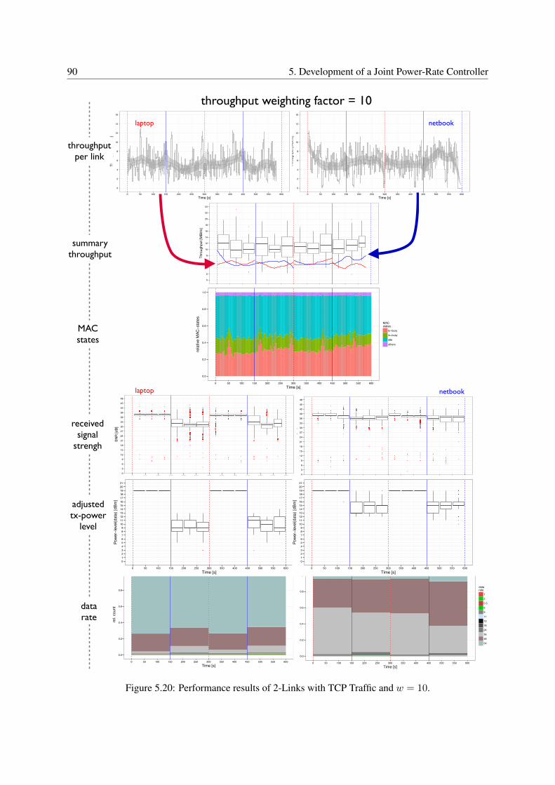
90 5. Development of a Joint Power-Rate Controller
0
2
4
6
8
10
12
14
16
0 50 100 150 200 250 300 350 400 450 500 550 600Time [s]
Thro
ughp
ut [M
Bit/s
]
●
●●
●
●
●
●
●
●
0
2
4
6
8
10
12
14
16
18
20
22
24
0 50 100 150 200 250 300 350 400 450 500 550 600Time [s]
Thro
ughp
ut [M
Bit/s
]
0.0
0.2
0.4
0.6
0.8
1.0
0 50 100 150 200 250 300 350 400 450 500 550 600Time [s]
rela
tive
MAC
−sta
tes
MACstates
tx−busyrx−busyidleothers
throughput weighting factor = 10
0.0
0.2
0.4
0.6
0.8
1.0
0 50 100 150 200 250 300 350 400 450 500 550 600Time [s]
rel.
coun
t
datarate
125.56911121824364854
0.0
0.2
0.4
0.6
0.8
1.0
0 50 100 150 200 250 300 350 400 450 500 550 600Time [s]
rel.
coun
t
datarate
125.56911121824364854
0
2
4
6
8
10
12
14
16
0 50 100 150 200 250 300 350 400 450 500 550 600Time [s]
Thro
ughp
ut [M
Bit/s
]
laptop netbook
summary throughput
throughputper link
receivedsignal
strengh
adjustedtx-power
level
datarate
MACstates
●●●●●●
●
●
●
●●●
●
●●●●●●●●●●●●●●●●●●●●●●●●●●●
●
●●●●●●●●●●●●●●●●●●●●●●●●●●●●●●●●●●●●●●●●●●●●●●●●●●●●●●●●●●●
●
●●●●●●●●
●
●●
●
●●●●●●●
●
●●●●●●●●●●●●●●●●●●●●●●●●●●●●●●●●●●●●●●●●●●●●
●
●●●●●●●●●●
●●
●●
●●
●●●●●●●●●●●●●●●●
●
●●●
●
●●●●●
●
●●●●●●●●●●●●●●●●●●●● ●●●●●
●
●●●●●●●●●●
●
●●●●
●
●●●●●●●●●●●●●●
●
●●●●●●●●●●●●●●●●●●●●
●
●●●●●●●●●●●●●●●●●●
●
●●●●●●●●●●●●●●●●●●●●●●
●●
●●●●●●●●●●●●●●●●●●●●●●●●●●●●●●●●●●●●●●●●●●●
●
●●●●●●●●●●●●●●●●●●●●●●●●●●●●●●●●●●●●●●●●●●●●●●●●●●●●●●●●●●●●●●●●●●●●●●●●●●●●●●●●●●●●●●●●●●●●●●●●
●
●●●●●●●●●●●●●●●●●●●●●●●●●●●●●●●●●●●●●●●●●●●●●●●●●●●●●●●●●●●●●●●●●●●●●●●●●●
●
●
●●
●
●
●●●
●
●
●●●
●●
●
●●●●●
●●●
●●●●●●
●
●
●
●●●
●
●
●
●●●
●
●
●
●●
●
●
●
●●
●
●
●
●
●
●
●
●
●●●
●
●●●
●●
●
●●●
●●
●
●
●●●
●
●●
●
●
●
●
●
●●●
●●
●
●
●
●
●
●
●●●●
●
●
●●
●
●
●●
●●●
●●
●
●
●●●●●●●●●●●●●●
●●
●
●●●●●●●●●●●
●
●●
●●●●
●●●●
●●
●●●●●●
●
●●
●
●●●●
●
●
●●●●
●
●●●
●●
●●
●●●●
●●
●
●
●
●
●●●
●
●
●
●●●
●●
●
●
●●
●●
●●●●
●
●
●
●
●●●●
●●●
●
●
●
●
●●●
●●
●
●●
●
●●
●●●
●
●●
●●
●●●●●●●●●●●●
●●
●●
●●
●●
●●
●
●●●●
●
●
●
●●
●
●●
●●●●●
●●●
●●
●●
●
●
●●●
●●
●●●●●●●
●
●●●●●
●
●●●●●●
●
●
●●
●●
●
●
●●
●
●
●
●
●●●
●
●
●
●●●●●●●●●●
●
●●●
●
●●
●
●
●
●●●
●
●
●●
●●
●
●
●●
●
●●●
●
●●
●●
●
●●●●●●●●●●
●
●●●●●●●●●●●●
●●
●●●●●●●●●●●●●●●●●●●●
●
●
●
●●●●●●●●●
●
●●●●●●●●●
●
●●●●●●●●●●●●●●●● ●●●
●
●●
●
●●●●●●●●●●●●●●●●●●●●
●
●
●
●
●●●●●●●●●●●
●
●
●
●●●●●
●
●●●●●●●●●●●●●●●●●●●●●●●●●●●●●●●●●●●●●●●●●●●●●●●●●●●●●●●●●●●●●●●●●●●●●●●●●●●●●●●●●●●●●●●●●●●●●●●●●●●●●●●●●●●●●●●●●●●●●●●●●●●●●●●●●●●●●●●●●●●●●●●
●●
●●●●●●●●●●●●●●●●●●●●●●●●●●●●●●●●●●●●●●●●●●●●●●●●
●
●●●●●●●●●●●●●●
●
●
●●●●●●●●●●●●●
●
●●●●●
●
●●●●●●●●●●●●●●●●●●
●
●●●●●●●●●●●●●●●●●●●●●●●●●●●●●●●●●●●●●●●●●●●●●●●●●●●●●●●●●●●●●●●●●●●●●●●●●●●●●●●●●●●●●●●●●●●●●●●●●●●●●●●●●●●●●●●●●●●●●●●●●●●●●●●●●●●●●●●●●●●●●●●●●●●●●●●●●●●●●●●●●●●●●●●●●●●●●
●
●●●●●●●●●●●●●●●●●●●●●●●●●●●●
●
●●●●●●●●●●●●●●●●●●●●●●●●●●●●●●●●●●●●●●●●●●●●●●●●●●●●●●●●●●●●●●●●●●●●●●●●●●●●●●●●●●●●●●●●●●●●●●●●●●●
●
●●●●●●●●●●●●●●●●●●●●●●●●●●●●●●●●●●●●●●●●●●●●●●●●●●●●●●●●●●●
●
●●●●●●●●●●●●●●●●●●●●●●●●●●●●●●●●●●●●●●●●●●●
●
●●●●●●●●●●
●
●●●●●●●●
●●●●●●●●●●
●
●●●●
●
●●●●●●
●
●●●●●●●
●
●
●
●
●
●●●●
●
●●●
●
●●
●
●●●●
●
●●●●●●●●
●
●●●
●
●●●
●●
●●●●●●●●●●●●●●●●●●
●
●●●●●●●●●●●●●●●●●●●●●●●
●
●●●●●
●
●●●●●●●●●●●●●●●●●●●●●●●●●●●●
●
●●●●●●●●●●●●●●●●●●●●●
●
●●●●●●●●●●●●●●●●●●●●●
●
●●●●●●●●●●●●●●●●●●●●●●●●●●●●●●●
●
●
●
●●
●
●●●●●●●●●●●●●●●●●●●●●●●●●●●●●●●●●●●●●●●●●●
●●●●●●●●●
●
●●●●
●
●
●
●●●●●
●
●●
●
●●●
●●
●
●●●●●●●●●●
●
●●●●●
●
●●●
●
●●●●
●
●
●●●●
●
●
●
●●●
●
●
●●●●●●●
●
●
●
●
●
●
●
●●●●●
●
●●●
●
●●●●●●●●●●
●
●●
●
●
●
●●
●
●●●
●
●●
●●●●●
●
●
●●●●●●●
●●●●●●●●●
●
●
●●
●●●
●
●●●●●●●●●●●●●●●●●●●●●
●
●●●
●
●●●●●●●●●●●
●
●
●●●●●●●●
●
●●●●●●
●●
●●●●
●
●●●●●
●
●●●●●
●●
●●●●●●●●●
●
●
●
●
●
●●●●●
●●
●●●●
●
●
●
●
●●●●
●
●●●●●●●●●●●
●
●
●
●
●
●
●●●●
●●
●
●
●
●
●
●
●
●
●●●●●●●●●
●
●●●●●●●●
●
●●●●●
●
●●●●●●●
●
●●●●
●
●●●●●●●
●
●●●●●●●
●
●
●
●●●●
●
●
●
●●●●●●●●●●●●●●●●●●
●
●
●
●●●
●
●●●●●●●●●
●
●●●●
●
●
●
●
●
●●●
●●●
●
●●●●●●
●
●●●
●
●●●
●
●●●●●●●●●●●●●●
●
●
●
●
●●●●●●●
●
●
●
●
●●●●
●
●
●
●●
●
●
●●●●●●●●
●
●●●
●
●
●
●
●●●●●●●●●●●●●●●
●
●●●●●●●
●
●●●●●
●
●●●
●
●●●●●●●●
●
●●●●●●
●
●●●●
●
●
●●●●●
●
●●
●
●●
●
●●
●
●●●●●●●
●●●
●
●
●
●
●●●●●
●
●●●
●
●●●●●
●
●
●●●●
●
●
●
●●
●
●●
●
●●●●●
●
●●●●●●●
●
●●●●●●●●
●
●
●●●
●
●●●●●●●●●●
●
●
●
●
●
●●●
●
●●●●●●●●●
●
●●●●
●
●
●●●
●
●●
●
●●●●●
●
●●●●●●●●●●●●●●●
●
●●●●●●●●
●
●
●●●●
●●
●
●●
●●
●●●●●●●
●
●●●●●●●●●●
●●●
●●●●
●
●●
●
●●
●●
●●●
●
●●●●●●
●●
●●●
●
●●
●
●●
●
●
●
●●●●●●
●
●●●
●
●●●●●●●●●
●
●●●
●
●
●
●●●●●
●
●●●●●●●
●
●●●●●●●●●●
●
●●●●●●●●●●●
●
●
●
●
●
●●●●●
●
●
●
●●●●
●
●
●
●
●
●
●
●●●●●●●
●
●
●
●
●●●●●
●
●
●
●●
●
●●●●●●
●
●●●●●●
●
●
●●●●●●●●
●
●●
●●
●
●
●●●●●●●●●●
●
●●●●●●●●
●
●●●●●●●●
●
●●●●●
●
●
●
●
●
●●●
●
●●●●
●
●
●
●●●●●
●●
●●●●●●
●
●●●●●●●
●
●●●
●
●●
●
●
●
●
●
●
●
●●●●●●●●●●●
●
●
●
●●●●●●
●●
●●●●●
●
●●●●●●●●
●
●●●●●●●●●●●●●●●
●
●
●
●●●●
●
●●●●●●●●●
●
●●●●●
●
●●
●
●●●
●●
●●
●
●●●●●●
●
●●●●●●●●●●●●●●●●●●
●
●
●●●●●●●●●
●●
●
●
●
●
●
●●
●
●
●
●
●
●
●
●●●●●●●
●
●●●●●●
●
●
●
●●
●
●
●
●●●●●
●
●●
●●
●●
●
●●●●●●●
●
●●●●
●
●
●
●
●●●●
●
●
●●
●
●
●
●
●
●
●
●
●
●
●●
●
●●
●
●●
●
●
●
●
●●●
●
●
●
●
●●
●
●
●
●
●
●●●●●●●●●●●●●●
●●
●●●●●●●●●
●
●●●●●●●●●
●
●
●
●
●
●●
●
●
●
●
●
●
●
●●●●●●●●●●●●●
●
●●
●
●●
●
●●●●●●●●●●
●
●●●●●●●●
●
●●●
●●
●●●●●●●●●●
●
●
●●
●●
●●●●
●
●●●●
●
●●●●
●
●●●●●●●
●
●●
●
●●
●
●
●
●●●
●
●
●●●
●
●
●
●
●●●●
●
●
●
●●●●
●
●●●●●
●
●●●●●●●●●●
●
●●●
●
●●●●
●
●●●●●●●●
●●
●●●●
●
●●●●●
●
●
●●●●●●●
●
●●
●
●●●
●
●
●●●●●●●●●
●
●
●●
●●●●
●
●●●●
●
●●
●
●●
●
●●●
●
●●●●●
●
●●●●
●
●
●
●●●●●●●●●●
●
●●●●●●
●
●●●●
●●
●
●
●●
●
●●
●
●●●●●●●
●
●●●●●●
●
●
●●●●●●●●●●●
●
●●●●●●●●
●
●●●●●●●●●●●●●●●●
●●
●
●
●●
●●
●
●
●
●
●
●
●●
●●
●●
●●●
●
●
●
●
●
●●●
●
●●
●
●●●●●●●●●
●
●
●
●●●●●●●●
●
●●●●●●
●
●●●
●
●●●●●
●
●●●●●●●●●●
●
●●●●
●
●
●
●●●●●●●●
●
●●●●●●●
●
●●●●●●●●●
●
●●●●●●
●
●
●
●●
●
●●●●●
●
●
●
●
●
●
●
●
●
●●
●
●
●
●
●●
●●
●●●
●
●
●●
●
●
●
●
●
●●●●●●●●●●●●
●
●●
●
●●●●●●
●
●●●●●
●
●●
●
●●●●●
●
●●●●●●●
●●
●●
●
●●●
●
●●●●●●●●
●
●●●●●●
●
●●
●●
●●●●●●●●●●●●●●
●●
●●●●
●
●●●●●●●●●
●
●●●●●●●●●●●●●
●
●
●
●
●●●
●
●●●●●●
●
●●●●●●●●●●●●●
●
●
●
●●●●●●●●●●
●●
●●
●
●●●●●●●
●
●
●●●
●
●●●●●
●
●●●●●●●●●●●●
●
●
●
●
●●
●
●●●●●●●
●
●●●●●●●●●●●●●
●●
●●●
●
●●
●
●
●
●
●
●
●●●
●
●
●●
●
●
●●
●
●
●
●
●
●
●
●
●
●
●
●●
●
●●●●●●●
●
●●●●●●●●●●●●●
●
●●●●●●●
●●
●
●●
●●●●●●●
●
●●●●●●●●●●●●●●●●●●●●●●●
●
●●
●
●●
●
●●●●●●●●●●●●●●
●●
●●●●●●●●●●●
●
●●●●●●●●
●
●●●●●
●
●
●
●
●
●
●
●●●●
●
●●●●●●
●
●●●●●●●●●●●●●●●●●●●●●●●●●
●●●
●●●●
●
●
●
●●●●●●●●●●●●●●●
●
●●●●●●●
●
●●●●●●●
●
●●●●●●●●●●
●
●●●
●
●●
●
●●●●●●●●●
●
●●
●
●●●●●●●●●
●
●●●●●●●
●
●●●●●●●
●
●●
●
●●
●●
●●●●●
●
●●
●
●●
●
●●●●
●
●●●●●●
●
●
●
●
●
●
●●
●
●●
●
●
●●●
●
●
●
●
●●●●●
●
●
●●●●●
●
●●
●●●
●
●
●●●●●●●
●
●
●
●●
●●●●●
●
●●●
●●
●
●
●
●
●●●●
●
●●●●●●
●●
●
●
●●●●●
●
●
●
●
●●
●
●●●●●
●
●
●
●●●
●
●
●●
●
●
●●
●
●●
●
●
●
●●
●●●●
●
●●
●
●
●
●
●
●●●●
●
●●
●
●
●
●●●●
●
●●●
●
●
●
●
●
●
●●●
●
●
●
●
●
●
●
●●●
●
●●
●
●
●
●●●
●
●●●
●
●●●●
●
●●
●
●
●
●
●●●
●
●●●
●
●●●●
●
●
●
●
●●●●
●
●
●●●●
●●●
●
●
●●
●●
●●
●
●
●
●
●
●
●●●●
●
●
●
●●
●
●●●
●
●●●
●
●●
●
●
●●
●
●●●●●●
●
●●●●
●
●●
●
●●
●
●
●●●●
●
●
●●
●●●
●
●●●●●●
●
●●●
●
●
●
●
●
●
●●
●
●
●
●
●
●
●
●
●●
●●●●●
●
●
●
●
●
●
●●
●
●
●
●
●
●●
●●
●
●●
●
●●●●●
●
●●●
●
●
●
●
●
●●●●●●
●
●●●
●●
●●
●●
●●●
●
●●●●
●
●
●●
●
●
●
●
●
●
●
●●
●
●●
●
●
●●●●●●●●●
●
●
●●●
●●●
●●
●●
●
●
●
●
●
●
●
●●
●
●●●●●●●●●
●
●●●
●
●
●
●●
●
●●●
●
●●
●
●
●●●●●●●●●●●●●
●
●●●
●
●●
●
●
●
●●●●
●●
●
●
●
●
●●●●●●●●●●●●
●
●
●
●
●●●●●●●
●
●
●
●
●
●●●●●
●
●●●●
●●
●●●●
●
●●●●●●
●
●
●
●
●
●
●
●●●
●
●●
●
●
●
●●●●
●
●
●●
●
●
●●
●
●●●●
●
●●
●●●●
●●
●
●
●
●●
●
●●●
●●
●
●
●
●
●●
●●
●
●
●
●●
●
●
●
●●
●
●
●
●●●●
●●
●
●●●
●
●
●
●
●
●
●
●
●●
●
●
●●●
●●
●
●●
●
●●
●●
●●●●
●
●
●
●
●●●
●
●
●●
●●●●
●
●
●●●
●
●●●
●
●
●●●
●●
●
●
●●
●
●●
●
●
●
●●●
●●
●
●
●
●
●
●●
●
●●
●
●●●
●
●●
●
●
●●●●●
●
●●
●●●
●●●●●
●●
●
●●
●
●
●
●
●
●
●
●
●
●
●
●●
●●
●
●●●
●
●●
●●●●
●●●●
●
●●●●
●●●●
●●●●●●
●
●●●
●
●●
●●
●●
●
●
●●
●
●
●
●
●●●
●
●
●
●
●●
●●
●
●
●
●
●
●
●
●
●●
●
●
●●
●
●
●
●●●●●
●
●
●
●●
●●●
●●●●
●●●
●●●
●●●●●
●
●
●●●●●●●●●●●
●●
●
●
●
●●
●
●
●
●●
●●
●
●
●
●
●
●
●
0
3
6
9
12
15
18
21
24
27
30
33
36
39
42
45
48
0 50 100 150 200 250 300 350 400 450 500 550 600Time [s]
SNR
[dB]
●
●●●●●●●●●●●●●●●●
●
●●●●●●●●●●●●●●●●●●●●●●●●●●●●
●
●●●●●●●●
●
●●●●●●
●
●●●●●●●
●
●●●●●
●
●●●●●●●●●
●
●●● ●●●●●●●●●●
●
●●●●●●●●●●●●●●●●●●●●●●●●●●●●●●●●●●●●●●●●●
●
●●●●●●●●●
●
●●●●●●●●●●
●
●●●●●●
●
●●●●●●●●●
●
●●●●
●●
●●●●
●
●●●●
●
●●●●●●●● ●●
●
●
●
●●●●
●
●●●●
●
●
●●●●●●●●
●
●
●
●
●
●
●
●●●●●●●
●
●●●●●●
●
●●●●●●●●●●●●●●●●●●●●●●●●
●
●●●●●●●●●●●●
●
●●●●●●●●●●●●●●●●●●●●●●●●●●●●●●●●●●●●●●
●
●●●●●●●●●●●●
●
●●●●●
●
●●●●●
●
●●●●●
●
●●●●●●●●●●●●●●●●●●●●●●●●●●●
●
●●●●
●
●
●●
●
●
●●●●
●●●
●
●
●●
●●
●●
●
●
●
●●
●
●
●
●
●
●
●●●
●
●
●
●
●
●
●
●
●
●
●
●
●●
●
●
●
●
●
●
●
●
●
●
●
●
●●
●
●●
●
●
●
●
●
●
●
●
●
●
●●●
●●
●
●
●
●
●●
●
●
●
●
●
●
●
●
●
●●●
●
●●
●
●
●
●
●
●●
●
●●
●
●●
●
●
●
●
●
●
●
●
●
●
●●●
●
●
●
●
●
●●
●●
●
●●●●
●
●
●
●
●
●
●
●●
●●●
●●
●●
●
●
●
●
●
●
●
●
●
●
●
●●
●
●
●
●
●
●●●●●
●●●
●
●
●
●
●
●●
●
●●
●
●
●●
●
●
●●
●
●
●
●
●
●
●
●
●
●●
●
●
●
●
●
●
●
●●
●
●
●
●
●●●
●●●
●
●
●
●
●
●
●●
●
●●
●
●
●
●
●
●●●●
●
●
●●
●
●
●
●●
●
●●
●●
●
●
●
●●●
●
●
●
●
●
●
●●
●
●
●
●
●
●
●
●
●
●●
●
●
●
●
●●
●●
●
●
●
●
●
●
●●
●
●
●
●
●
●
●
●
●●
●
●●
●
●
●●
●
●
●●●
●
●
●
●●
●
●
●●
●●
●
●●
●
●
●
●
●
●
●
●●●
●
●
●●
●
●●
●
●
●●
●
●
●
●
●
●
●●
●
●●
●
●●
●
●
●
●
●
●
●●●●
●
●●
●
●
●
●●
●
●
●
●
●
●
●
●
●●●
●
●
●
●●
●
●●
●
●
●
●
●
●●
●
●
●●●
●●●
●
●
●
●
●
●
●
●●●
●
●
●
●
●
●
●
●
●
●●●
●
●
●
●
●
●
●
●●
●
●
●●
●
●●●
●
●
●●●
●●●
●●●
●
●●
●
●
●
●
●
●●●
●
●
●
●●
●
●
●
●
●●
●
●●●
●
●
●
●
●
●●
●
●●●●●
●
●
●
●
●
●●
●
●
●
●●
●
●●●
●
●●●
●●
●●
●
●●●●
●
●●
●
●
●
●
●
●●
●
●
●
●
●
●
●
●
●
●
●
●
●●
●
●
●
●
●
●
●
●
●
●
●
●
●
●●●
●
●
●
●
●
●●
●
●
●
●
●
●
●
●
●
●
●
●
●
●●●
●
●
●●
●●
●
●
●
●
●●
●
●
●
●
●●
●
●
●
●
●
●
●●
●
●●
●●
●
●
●
●●
●
●●●
●
●
●
●
●
●
●
●
●
●●●
●
●
●
●
●
●
●
●
●
●
●
●
●
●
●
●
●
●
●
●
●
●
●●
●
●
●●
●
●
●
●
●
●
●
●●
●●●●
●●●●
●
●
●
●
●●
●
●●
●
●●●●
●
●
●
●
●
●●
●
●●●●●
●
●
●
●
●●
●
●●●●
●
●●
●●
●
●
●
●
●●
●
●
●
●
●
●
●●
●●●
●
●
●
●
●
●
●
●
●
●
●
●
●
●
●
●
●
●
●
●●
●
●
●
●
●
●●
●
●●
●●
●
●
●
●
●
●
●
●
●●●●
●
●
●
●
●●
●
●●
●
●
●
●●
●
●
●
●
●
●
●●
●●
●
●
●
●
●
●
●
●
●
●
●
●
●
●
●
●●
●
●
●
●
●●
●
●
●
●
●
●
●
●
●
●●
●●
●
●
●
●●
●
●
●
●
●
●●
●
●
●
●
●
●
●
●●
●
●
●
●
●●
●●
●
●
●
●
●
●
●
●
●
●
●
●
●
●
●
●
●
●
●
●●
●●
●●
●●●●●●
●
●
●
●●
●
●
●●
●
●
●
●
●
●
●●●
●
●
●
●
●
●
●●
●
●●
●
●
●
●
●
●
●
●
●
●
●
●
●
●
●●
●
●
●
●●
●●
●
●
●
●
●
●
●
●
●
●
●
●
●
●
●
●
●
●
●
●
●
●●
●
●
●●
●
●
●
●
●
●
●
●
●
●
●
●
●
●
●
●
●
●
●
●
●
●●
●
●
●
●●
●
●
●●●●●
●
●
●
●
●●
●
●
●
●
●
●
●●●
●
●●●●●●
●
●
●
●
●●
●
●
●
●
●●
●●
●●●
●
●
●
●●●●●
●
●
●
●●●●
●●●●
●
●●●
●●●●●●
●
●●
●
●
●
●
●●
●●
●●
●●●
●
●
●
●
●
●
●
●●
●●●
●
●
●
●
●●
●
●
●
●
●
●●●●
●
●
●
●
●
●●●
●
●
●●
●
●
●
●
●
●
●
●●
●
●
●●
●
●
●
●
●
●●●●●
●
●
●●
●
●
●●
●
●●●
●
●●
●
●
●
●
●
●●
●
●●●●●
●
●
●●●●●
●
●
●
●
●●
●
●
●
●●●
●
●●
●
●
●
●●
●
●
●
●
●
●
●
●●
●
●●
●
●●●●
●
●●
●
●
●
●●
●●
●●
●●●
●
●
●
●
●
●
●●●●
●
●
●
●
●
●
●●●
●
●
●●
●●
●
●
●
●
●
●
●●
●
●
●
●
●
●
●
●
●
●
●●
●
●
●
●
●
●
●●●●●
●
●
●●
●
●
●
●
●●
●
●
●
●
●●
●
●●
●
●
●
●
●●●
●
●
●
●
●
●
●
●
●
●
●
●
●
●
●
●
●
●
●●
●
●
●
●
●
●
●
●●
●
●●
●
●
●
●
●
●
●
●
●●
●
●
●●●
●
●
●
●
●
●
●●
●
●
●
●
●
●
●
●
●
●
●
●
●
●
●
●
●●
●
●
●
●
●
●
●
●
●
●
●●●
●
●
●●
●●
●●
●
●
●
●●●●●●●●●
●
●
●
●
●
●
●●●●●●●●●
●
●●●●●●●
●
●●●●●●
●
●●
●
●●
●
●
●●
●
●●
●
●
●●
●
●●●●●●●●●●
●
●●●●●●●●●●●●
●
●
●●
●
●●●●
●
●●
●
●
●
●●
●
●●●●●●
●
●
●●●●
●●●●●
●●
●
●●
●●
●
●
●●●
●
●
●
●●
●
●
●
●●
●
●
●●●
●
●
●
●
●
●
●
●
●
●
●
●
●
●
●
●●
●
●●
●
●●●●
●●●
●●●●●
●
●
●
●
●
●●
●
●
●
●
●●
●
●●●●
●
●●
●●
●
●●
●●
●
●
●
●●
●
●●●●●
●
●●●
●
●●
●●
●
●
●●●●●●●
●
●●●
●
●
●
●●
●
●●
●
●●
●●
●
●
●
●●
●
●●●●●●
●
●
●
●
●●
●●●●●●●●●
●
●
●
●
●
●●
●
●●●●●●●●●●●
●
●●●●●●
●
●●●●●
●
●
●
●
●
●
●
●
●
●
●
●
●
●
●●
●
●●●
●
●
●
●●●
●
●●●
●
●
●●
●
●
●●●
●
●
●
●
●
●
●
●●
●
●●●
●
●●
●
●
●
●
●
●●
●●
●
●
●
●●●●
●
●
●
●●
●●
●
●
●●
●
●●
●
●
●
●●
●
●
●
●
●
●
●
●
●
●
●●
●
●
●●
●
●
●
●
●
●
●●
●
●
●●●
●●●●●
●●
●
●
●
●
●
●●●
●●●
●
●
●●●
●●●
●
●
●
●
●
●
●●
●●
●●
●
●
●●●
●
●●●
●
●
●
●
●
●
●●
●●
●
●
●
●
●
●
●
●
●
●
●
●
●
●
●
●
●
●
●●●●
●
●
●
●
●
●
●●
●
●
●
●●●●●
●
●
●●
●●
●
●
●
●
●
●●
●
●
●
●
●●●●●●
●
●●●
●
●
●
●
●
●
●
●
●
●
●
●●
●
●●
●
●
●
●
●
●
●●●●
●●●
●
●
●
●
●●●
●●●●●●
●
●●
●
●
●
●
●
●
●
●
●
●
●●
●
●
●●●
●
●
●
●
●●
●
●
●
●
●●
●
●●
●
●●
●
●
●
●
●
●
●●●●
●●●
●
●
●
●●
●●
●●
●
●
●
●●●
●
●●
●
●
●
●
●
●●
●
●
●●●
●
●
●●●●●
●●●
●
●
●
●
●●
●●
●
●
●
●●
●
●
●
●
●●
●●●
●
●
●
●●
●●●
●
●
●
●
●●●
●
●●●●●●●
●
●
●
●
●
●
●
●●
●
●
●
●
●
●●
●
●●
●
●
●
●●●●
●
●
●
●
●●
●
●
●
●●
●●
●
●
●●●
●
●
●
●
●
●
●
●
●
●
●
●
●
●
●
●
●
●
●
●
●●
●
●●
●
●●
●
●
●
●
●
●
●
●●●
●
●
●●
●
●●●
●
●
●
●
●
●●
●
●
●
●
●
●
●
●
●
●●
●●●●
●
●●
●
●●
●
●●●●
●●
●●
●
●
●●●●
●
●
●
●
●●
●
●
●
●
●
●
●●
●
●
●
●
●●
●
●
●
●
●
●●
●●●
●
●
●
●●
●●●
●
●
●
●
●
●
●
●●
●
●●
●
●
●
●
●●
●
●
●
●
●
●●
●●
●
●
●●●
●
●
●●
●●
●●●
●
●
●
●
●●
●
●
●
●●
●
●
●
●●
●
●
●
●
●
●
●
●
●
●
●
●●●
●
●
●
●
●
●
●
●
●
●
●
●
●
●●
●●●
●
●
●●
●
●
●●
●
●
●
●
●
●
●
●●
●
●
●
●
●
●●
●●
●
●
●
●
●
●
●
●
●●
●
●●●●
●
●
●
●
●●
●
●●
●●
●●
●●
●
●
●
●
●●●●
●
●●
●
●
●
●●●
●●
●
●
●
●
●
●
●
●
●
●
●●●
●
●
●●
●●●
●
●
●
●
●
●●●
●●
●●
●
●
●●●
●
●
●●
●●
●
●
●●●●
●
●●
●
●●
●●
●
●●●
●
●
●
●●●●
●
●
●
●
●
●
●
●●●●
●●●●●
●●
●
●
●
●
●●
●
●
●
●
●
●●●●
●●●
●
●
●
●
●
●●
●
●
●●●
●●
●
●
●
●
●
●
●
●
●
●
●
●
●
●●
●
●
●
●
●●
●
●
●
●●
●
●
●
●
●
●
●
●
●
●●●
●
●
●●●
●●●
●
●
●
●●
●
●
●
●
●●●
●●
●
●
●●●
●
●●
●
●
●
●
●
●
●●
●
●
●
●
●●●●●
●
●
●
●●●●
●
●●
●
●●
●
●
●●●
●
●
●●
●
●●
●●●
●●
●
●●●
●●●●
●
●●
●●
●●
●
●
●
●●●
●
●
●●
●
●●●
●●●
●
●
●
●●●
●
●
●
●●
●
●
●
●
●
●●
●
●
●
●●
●
●
●
●●
●
●
●●
●
●
●
●●
●
●
●●
●
●
●●●
●●
●
●
●
●
●
●
●
●
●
●
●
●●
●
●●●
●
●
●●●
●
●
●●
●●
●
●●●●●●●●
●
●
●
●●●
●
●
●
●●●
●
●●
●
●●●
●
●●
●
●
●
●
●
●
●●●
●
●
●
●●●●
●
●
●
●
●
●
●
●
●
●
●
●
●●
●
●
●
●
●
●
●
●
●●●●
●
●
●
●●
●
●
●
●●
●●●●
●
●
●
●
●●●●●
●
●●
●
●●●●●●●
●●
●●
●
●●●
●
●
●
●
●
●●
●
●●●●●
●
●●●
●
●
●
●
●
●●
●
●●
●
●●
●
●●
●
●
●
●
●
●
●
●
●
●
●●●●●●●
●
●
●●
●
●
●
●●
●
●
●
●●
●
●
●
●
●●●●
●
●
●
●●●●
●
●●●
●
●
●
●
●●●
●
●●
●●●●●
●●
●●
●●
●
●
●●●●●
●
●●●
●●
●
●●
●
●●●●●●
●●
●
●●●●●
●
●
●
●
●
●
●
●
●
●
●
●●
●
●●
●
●
●●●
●
●●
●
●●●
●●
●●
●
●
●
●●
●●
●
●
●●
●
●
●
●
●●
●
●
●
●
●
●
●
●●●
●●
●
●
●
●
●●
●
●
●
●●
●●
●
●●
●
●
●
●
●
●
●
●●●
●
●●●
●
●
●
●●●
●
●●●●
●
●
●
●
●
●
●●
●
●
●
●
●
●●
●
●●●
●
●
●
●
●
●●●
●
●●
●
●●
●
●
●
●
●●●●
●●
●●
●
●
●
●●
●●
●●●●
●
●
●
●
●
●
●
●
●
●●
●
●
●
●
●
●
●
●
●●●
●
●
●
●●●
●
●
●
●●
●
●●
●
●●
●●
●
●
●
●●
●
●●
●
●●
●
●
●
●●
●
●
●
●●
●
●●●
●
●●●
●
●●
●
●
●
●
●●
●
●●
●
●
●
●●●●
●
●
●●
●
●
●
●
●
●
●
●
●
●
●
●
●
●
●
●
●
●
●●●●●●
●
●
●
●
●
●
●
●
●
●●
●●
●●
●●
●●
●
●
●●●●●
●
●
●
●
●
●
●
●
●●
●
●
●
●
●
●
●●●●
●
●●●
●
●
●
●●●●
●
●
●
●
●●●●
●
●●●●●●
●
●●
●
●
●
●
●
●●●●
●
●
●
●
●●●●●●●
●
●
●
●
●
●
●
●
●
●
●
●
●
●
●
●●●
●●●
●
●
●●●
●
●
●
●●●
●
●
●
●
●
●●
●
●
●
●
●
●●
●
●
●●●
●
●●●
●
●
●
●
●
●●●●●●
●
●
●
●
●●
●
●
●
●
●
●
●●●●
●●
●●
●
●
●
●
●
●●
●
●
●
●
●
●●●
●
●●
●
●
●
●
●
●
●
●
●
●
●
●
●
●●
●
●
●
●●
●
●●
●●
●
●
●
●●
●
●
●
●●●●
●
●●
●
●●●
●●
●
●
●
●
●
●●●●●●
●
●
●
●
●●●●
●
●
●
●●
●●
●
●
●
●
●
●
●
●
●
●
●●●
●
●
●
●
●
●
●●
●
●
●
●●●
●
●●●●
●
●●
●
●
●
●●
●●
●
●
●
●
●
●●
●
●
●
●
●
●
●
●●
●
●
●
●●
●●●
●
●●
●
●
●
●
●
●
●
●
●
●
●●
●●
●
●
●●
●
●●
●●
●●●●
●●
●
●
●
●
●
●
●
●
●
●
●
●
●●
●
●
●●
●
●
●
●
●
●
●●●●
●
●
●●
●
●
●
●●
●
●
●●●●●●
●
●●●
●
●
●
●
●
●
●
●
●
●
●
●
●
●
●●●●●●●
●
●
●
●
●●
●●
●
●
●
●●
●
●
●●
●
●
●
●●●
●
●●
●
●
●
●
●
●
●
●
●
●●
●
●
●
●
●
●
●●
●
●
●
●
●●●●
●
●●●
●
●
●
●●●
●
●●
●
●
●
●●
●
●
●●●
●●
●
●
●●●●●
●
●●
●
●
●
●
●●
●
●
●
●
●
●
●
●
●●
●
●
●●●●●
●
●●
●
●
●
●
●
●
●
●
●
●
●
●
●
●
●●
●
●
●
●
●
●●
●●●
●
●
●
●●
●●
●
●
●
●●●
●
●
●
●
●
●
●
●
●
●●
●
●
●●
●
●
●
●
●
●●
●●
●●●●
●●●
●●
●
●
●
●
●
●●
●
●●
●
●
●
●
●
●●●●●
●
●●
●
●
●
●
●
●
●
●
●●●
●
●●
●
●
●
●
●
●●●
●
●
●
●
●●●●
●
●
●
●●●
●
●
●●
●
●
●
●
●
●
●●
●●
●●●●●
●●●
●
●●●●
●
●●
●
●
●
●
●
●
●
●
●
●
●
●
●
●
●●
●
●
●
●
●
●
●
●●
●●
●●●
●
●
●
●●●
●
●
●
●●
●
●
●
●●●●
●
●●
●●
●
●●
●
●
●
●●
●
●●
●
●●
●
●
●
●●●
●
●
●●
●
●
●
●
●
●●●●
●
●
●
●●●
●
●
●
●
●●●
●
●●
●
●
●
●
●
●
●
●
●
●
●
●
●
●
●
●●●
●
●
●
●
●
●●●●
●
●●
●●
●
●
●
●
●●
●
●
●●
●
●
●●●
●
●●
●
●
●
●
●
●
●
●
●
●●●
●
●
●
●●
●
●
●
●●
●
●
●●
●
●●
●
●
●
●
●●
●
●
●
●●
●
●
●
●
●
●
●
●
●
●●●
●
●●●●●
●●
●
●●
●
●
●
●●
●
●
●
●
●
●
●
●●●●
●
●
●●
●
●
●
●●
●
●●
●
●
●
●
●●
●
●
●●
●
●
●
●
●●●
●
●
●●●
●
●
●●●
●
●
●
●
●●
●
●
●
●
●
●
●●
●
●
●●●
●
●
●
●
●
●
●
●●
●
●
●
●
●
●
●●
●●●
●●
●●
●
●
●●
●●
●
●
●●
●
●●●●●
●
●
●
●●
●●
●
●●●●
●
●
●●
●
●
●
●
●
●●●●●
●
●●●●
●
●
●●●
●
●
●
●
●
●
●
●
●
●
●●●●●
●●●
●
●
●●
●
●
●
●
●
●●●●
●
●
●
●
●
●●
●
●
●●
●
●
●
●
●
●
●●●●
●●●
●●
●●●●
●
●
●
●●
●
●
●●
●●
●
●
●●●
●
●●●
●
●●
●
●
●
●
●
●
●
●
●
●
●
●
●
●●
●
●
●
●●●
●
●
●
●
●●●●
●
●●
●●
●
●
●●●●●●●
●
●
●
●
●●●●
●
●
●●●●●●●●●●●
●
●●●●●●
●
●●
●
●
●
●
●
●
●●●●
●
●
●●●●●
●●●●●
●
●●●●●●
●
●
●●●
●
●●●●●●●
●
●
●
●
●●●●●
●
●
●
●●●●
●
●
●
●
●
●●
●●
●
●
●●
●●
●
●
●●
●●●●●●
●
●●●●
●
●
●
●●
●
●
●●
●
●●
●
●
●●●
●
●
●
●●●●●
●
●●
●
●●
●
●
●
●
●
●●●●
●
●
●
●
●
●
●
●
●
●●
●
●
●●
●●
●
●
●
●
●
●
●
●
●
●●
●
●
●
●
●
●
●●
●●
●
●
●●
●
●●
●
●●●
●
●
●
●
●
●
●
●
●●
●●●
●
●
●
●●●●●●●●
●
●
●
●●●●●●●●●●●●●●●●●
●●●●
●●
●
●●●●●●●●●●●●●
●
●●●
●
●
●
●●
●
●●
●
●
●
●
●●
●●●●●●●●
●
●●●●
●
●●●●●●●
●
●
●●●
●●●●●●
●
●
●
●●●●●●●●●●
●
●
●●●
●●
●●
●
●●●●
●
●
●
●●
●●
●●●● ●
●
●●
●
●●●
●
●
●●
●●●●●
●
●●●
●
●●
●
●
●
●●●●
●
●●●●●●●●●●
●●
●
●
●
●●
●
●
●
●
●●●●
●
●●●●
●
●
●
●
●●
●●●●●
●
●
●
●
●
●●●
●
●
●
●●
●●●●
●●●●
●
●●
●
●●
●●
●
●●
●
●
●
●
●●
●●●
●
●
●
●
●
●
●
●●
●●●●●
●
●●
●
●●
●
●
●
●
●
●
●
●
●●
●●●●●
●●●
●
●●
●
●●●●
●●●
●
●
●
●●●●●●●●
●
●
●●
●
●●
●
●
●
●●●
●
●●
●
●
●
●
●
●
●●
●●●●●●
●●
●
●
●
●●
●
●
●
●
●●●●
●
●
●
●●●
●
●
●●
●
●
●
●●
●●
●
●●●●●●●
●
●
●●
●
●●●
●
●●●●
●●
●●
●
●
●
●●●
●
●●
●
●
●
●
●●
●●
●●●
●
●
●●
●●●
●
●●
●●●
●
●
●
●
●
●
●●
●●
●●
●●●●●
●●
●
●
●●●
●
●
●
●
●●
●●●
●
●●●●
●
●
●●●●●
●
●
●
●
●
●●●●
●
●
●
●●
●
●
●●●
●
●●
●
●
●
●
●●
●●●●
●
●
●
●●
●●
●●
●
●
●
●●
●
●●●●
●●●●
●●
●
●●
●
●●
●●
●
●●●●
●●●
●
●●●●
●
●
●
●●●●
●
●
●●
●
●●
●
●
●
●
●
●
●●●
●
●●
●
●●●●●
●
●●●●●●
●
●●
●
●
●
●●●
●
●●
●●●
●●●
●●●●
●
●
●
●
●
●
●●
●●
●●
●●
●
●●●●
●
●●
●
●●
●●
●●●●●●
●
●●●●
●
●●
●●
●●
●
●
●
●●●●●
●
●●●●
●
●●
●
●
●●
●
●
●
●
●●
●
●
●
●
●●●
●
●●●
●
●
●
●
●●
●●
●
●●●
●
●
●
●
●●
●
●●
●
●●●●●
●
●
●
●●
●●●●●
●
●
●
●
●
●
●
●●●●
●
●●●
●●
●
●
●
●●
●
●
●●●●
●
●
●
●●
●
●
●
●●
●●
●
●
●
●●
●
●
●
●●●●●
●
●
●●
●●●●●●
●
●
●●
●●●
●●●
●●
●●●
●
●●
●
●●●●
●●●●●
●
●●●●●●●●
●●
●●
●●●●
●
●●●●●
●
●●
●
●●●
●
●●●
●
●
●●
●
●●
●●
●●
●●●●
●
●
●
●●
●
●
●
●
●
●●
●●●●
●
●
●
●
●
●
●
●
●
●
●
●●
●
●
●
●●
●
●●
●●●●●●●
●●●●●
●
●
●
●
●
●
●
●●●
●
●
●
●●●
●
●●●
●
●
●●
●
●●
●
●
●●
●●●
●●
●
●●
●
●●
●
●●●
●
●●●●
●
●
●
●
●
●
●●
●
●●
●●
●●●
●
●
●
●
●
●
●
●
●
●●
●
●
●
●
●●
●
●●
●
●●
●
●●
●
●●●●●●●●●●
●●●
●●
●●●●●●●●●
●
●
●
●
●
●●●
●
●●
●●●●●
●
●
●
●●●
●
●●
●
●●
●●●●●●●●
●
●
●
●
●
●
●
●
●
●
●
●
●
●●●●●
●
●
●
●
●●●
●●
●
●
●
●
●●
●
●
●●●
●
●●●
●●
●●
●
●●●
●
●
●
●
●
●●
●
●
●
●●●●●
●
●●
●
●●●
●●●
●
●
●●
●●
●●
●
●
●●●
●
●●●
●
●
●●●●
●
●
●
●
●●●●●●●
●
●
●●●
●●
●
●
●●
●●
●
●●
●●●
●●
●●●●●
●
●
●
●
●
●
●
●
●●
●
●
●●●●●
●●
●●●
●●●
●●●●●
●●●●
●
●
●
●
●●●
●
●●
●
●
●●
●
●●
●
●
●
●●●●●
●
●●
●●●●●
●●
●●
●●
●●
●
●●●
●●
●
●
●
●●●
●
●
●
●
●
●
●●
●
●●●●●●●●●●●●●
●
●●●●●●●
●
●●●●●●●●●●●●●●
●
●●●●●●●●●●●●●●●●●●
0
3
6
9
12
15
18
21
24
27
30
33
36
39
42
45
48
0 50 100 150 200 250 300 350 400 450 500 550 600Time [s]
SNR
[dB]
laptop netbook
●● ●
0123456789
101112131415161718192021
0 50 100 150 200 250 300 350 400 450 500 550 600Time [s]
Powe
r−le
vel(d
ata)
[dBm
]
●
●
●●●
●●●
●●●●●●●●●●●●●●●●●●●●●●●●●●●●●●●●●●●●●●●
●●
●●●●●●●●
●
●
●
●●●●●●●●●●●●●●●●
●
●●●●●●●●
●●●●●●●●
0123456789
101112131415161718192021
0 50 100 150 200 250 300 350 400 450 500 550 600Time [s]
Powe
r−le
vel(d
ata)
[dBm
]
Figure 5.20: Performance results of 2-Links with TCP Traffic and w = 10.
Summary 91
dBm at 54 Mbps and 16 dBm at 48 Mbps. This explains the difference of 3 dB between the adjusted and
measured reduction in power.
The data rate plots in Figures 5.19 and 5.20 show the relative count of all 12 IEEE 802.11g data-rates
that Minstrel-Blues actually used to send data packets for each interval of 150 seconds. By comparing
rate distributions per interval it can be seen that when w = 2, Minstrel-Blues prefers lower data rates,
while with w = 10, Minstrel-Blues uses the same data rates with Minstrel with maximum power level.
In case of the netbook and w = 2, the dominant date rate changes from 48 Mbps to 36 Mbps as shown
in Figure 5.19. The same observation holds for the laptop. It is to be noted that the actual power level
reduction with the laptop link and w = 10 is slightly higher compared to w = 2. We assume this is due
to the fact that the wireless channel conditions changed, as there was a 30 minute time gap between the
experiments.
From our results, we conclude that Minstrel-Blues operates as expected at 2.4 GHz with IEEE
802.11g hardware. It does significantly reduce actual transmission power while achieving similar per-
formance in throughput for both the netbook and laptop clients. The ability to adjust Minstrel-Blues’
utility function and therefore, influence data-rate and power selection by different weighting factors has
also been validated.
5.4 Summary
In this chapter, we presented the design, implementation, and performance evaluation of our joint rate
and power controller, Minstrel-Blues. In the first part, we explained our modifications to the Linux
mac80211 subsystem to annotate transmission power levels per packet. Building upon this, we described
our heuristic approach to minimize transmission power by sampling different, discrete power levels and
use the resulting success ratios for control decisions. Additionally, we enabled the TPC capabilities of
Atheros WiFi chips by extending the Linux ath5k driver. We motivated and introduced a utility function
to realize different preferences for combinations of achievable throughput per data rate and its necessary
transmission power. The special configuration of Minstrel-Blues, where only throughput influences the
utility calculation, is called Minstrel-Piano.
Several validation experiments confirmed Minstrel-BLUES is able to adapt data rates and power lev-
els, while operating with different IEEE 802.11a and 802.11g devices. The design and implementation
of our controller within the Linux kernel shows good performance. It allows to fully utilize the trans-
mission capacity at the highest data rate. Furthermore, our algorithm is able to reduce the transmission
power according to statistics of packet success probabilities, while maintaining the same throughput.
Hence, it reduces the amount of overall interference in the network.
In our performance evaluation in the BOWL testbed we showed that Minstrel-Piano significantly
increases the total network throughput through spatial reuse. Our measurements cover three different

92 5. Development of a Joint Power-Rate Controller
receiver sensitivities with UDP and TCP traffic at 5 GHz.
Limitations: In this chapter, we analyzed our joint rate and power controller with its ability to increase
spatial reuse, and thus total network throughput. Our current experimentation setup does not cover
mixed traffic, different packet sizes, or multiple packet flows and distributions. Therefore, additional
measurements would be necessary to explore the effects of realistic user traffic in terms of spatial reuse
potentials.
Any sampling based rate and power control algorithm needs sufficient sample attempts to realize
reasonable control decisions based on up-to-date statistics. Both, Minstrel as well as Minstrel-Blues,
currently use a fixed share of common data packets from the IP-layer and above to sample success
ratios of different data rates and power levels. The trade-off between accuracy and overhead of different
sampling methods in WiFi networks is unexplored.
As Minstrel-Blues operation depends on different thresholds to control power adjustments, different
intervals to periodically update success statistics, and other implementation specific parameters, the set
of default values to be chosen needs further study. In terms of agility, our power control settings are
conservative. Minstrel-Blues decreases power levels using smaller steps (currently 1 dB) and increases
power using larger steps (currently 2 dB). In other words, if the channel conditions get worse, we in-
crease power levels faster as compared to the case of good channel conditions, where we decrease the
power.
Finally, it must be stated that our current implementation of Minstrel-Blues is able to perform on
the latest Atheros 802.11n hardware but does not yet take advantage of its enhanced power control
capabilities at per pmulti-rate-retry stage.
Chapter 6
Conclusion and Outlook
6.1 Summary
We started by asking three questions: (1) What are the necessary prerequisites in order to achieve ef-
ficient rate and power control in real WiFi networks? (2) How do we design and implement transmit
power control in addition to existing rate control? (3) What are the conditions that allow joint rate and
power control to increase total throughput in WiFi networks?.
Chapter 3 and 4 answer the first question based on Atheros WiFi hardware. In this chapter we
present, in detail, the practical operation and limitations of Atheros WiFi cards and the specific interac-
tions between data rate and maximal power level. Our results validate that the maximum power level to
send packets is a function of the data rate and actual WiFi hardware. Both of the tested WiFi cards show
a nearly linear relation between the adjusted and measured power level up to a certain data rate specific
limit. This study allowed us to understand the necessary details of the Atheros hardware, essential for
our controller design.
In order to achieve efficient rate and power control in IEEE 802.11 wireless networks, an impor-
tant requirement is to understand their impact on channel utilization and network throughput. Improper
power, rate, and carrier sensing adjustments can lead to under-utilizing or attempting to over-utilize
medium, which can stall communication, or in the worst case result in network breakdowns. As packet
level traces are insufficient to directly monitor medium utilization at the MAC-layer, we created a new
wireless monitoring tool for Linux. In Chapter 4, we present the in-kernel design, validation and per-
formance of our Atheros specific monitoring tool RegMon. RegMon enables sampling, and analysis of
hardware registers with a high accuracy through a sampling rate up to 20 kHz depending on the mea-
surement hardware. It is implemented and validated for all three major drivers of Atheros WiFi cards,
namely Madwifi, ath5k and ath9k as well as two alternative sampling methods to support a wide range of
IEEE 802.11abgn hardware. Our measurement tool enables wireless researchers to access new informa-
93
94 6. Conclusion and Outlook
tion sources and is part of the default monitoring setup in our BOWL network. textitRegMon essentially
provides us with MAC layer measurements that help develop, troubleshoot and analyze our joint rate
and power controller.
Chapter 5 aims at answering the remaining two questions on the design and implement of a joint
rate and power controller. In the first part, we explained our modifications to the Linux mac80211
subsystem to annotate transmission power levels per packet. To enable a power-level setting per packet
in the MAC layer, we restructured the mac80211 Linux subsystem to provide the necessary space in
the control data structure to allow a power level setting for each of the four rates per packet. With this
extension, we enable a general abstraction to annotate the transmission power at the Linux MAC layer.
More specifically, we modified the Linux drivers from Atheros: ath5k and ath9k in their transmission
path to support TPC. To the best of our knowledge, we are the first to implement such an interface, which
enables realizing different power control approaches using today’s WiFi hardware. Building upon this,
we described our heuristic approach to minimize transmission power by sampling different, discrete
power levels and use the resulting success ratios for control decisions.
Using our implementation, it becomes possible to annotate per-packet power levels based on hard-
ware capabilities: one power-level for all retries in IEEE 802.11abg, and four power levels corresponding
to the four retries in IEEE 802.11n. Our implementation takes into account different hardware capabili-
ties, e.g., data and MAC acknowledgment (ack) packets differ in terms of controllability of power levels.
The PHY layer part of our implementation covers several Atheros-based WiFi chips but it can easily be
extended to other hardware drivers.
Finally, based on our cross-layer interface, we designed, implemented, and validated a joint power
and rate controller: Minstrel-Blues. Our controller respects the trade-off between packet delivery suc-
cess and interference to other ongoing transmissions. It uses cross-layer information from both PHY
and MAC layers (power and rate) and operates at the PHY layer. It is a decentralized sampling-based
controller that does not require additional control messages between a WiFi transmitter and a receiver,
e.g., to obtain received signal strength information.
Several validation experiments confirmed Minstrel-Blues capability of adapting data rate and power
levels, while operating with different IEEE 802.11a and 802.11g devices. The design and in-kernel im-
plementation of our controller provides sufficient performance to fully utilize the transmission capacity
at the highest data rate. Furthermore, our algorithm is able to reduce the transmission power according
to statistics of packet success probabilities, while maintaining the same throughput. Hence, it reduces
the amount of overall interference in the network. By evaluating the performance within the BOWL
testbed, we showed that Minstrel-Blues is able to significantly increase the total network throughput
through spatial reuse.
Future Directions 95
6.2 Future Directions
In our performance evaluation, we analyzed our joint rate and power controller in terms of its ability to
increase spatial reuse, and thus, total network throughput. While we have shown significant throughput
gains using Minstrel-Blues, our experiment setup is limited and does not cover mixed traffic, differ-
ent packet sizes, or multiple packet flows and distributions. Therefore, additional measurements are
necessary to explore the effects of realistic user traffic on spatial reuse potential.
At the time of writing this thesis both standards, IEEE 802.11a and 802.11g, are somehow out-of-
date and IEEE 802.11n as well as 802.11 ac are their successors. Hende, we plan to extend Minstrel-
Blues capabilities to support multiple input multiple output (MIMO) WiFi devices. Furthermore, current
Atheros 802.11n cards promise enhanced power control abilities. They support individual power levels
per multi rate retry stage, which could be incorporated into our current sampling approaches. As there
exists already a follow-up of Minstrel rate control, called Minstrel HT, we are confident that the power
controller Blues can be merged with this new 802.11n rate control algorithm.
With IEEE 802.11n comes also an increase in available data rates (up to 32 MCS rates with two
different guard intervals and channel width). The overall search space of possible power and rate com-
binations grows significantly and hence, efficient sampling of these rates and power levels becomes the
challenge.
Any sampling based rate and power control algorithm needs sufficient sample attempts to realize
reasonable control decisions based on up to date statistics. Both, Minstrel as well as Minstrel-Blues use
currently a fixed share of common data packets coming from the IP-layer and above to sample success
ratios of different data rates and power levels. The trade-off between accuracy and overhead of different
sampling approaches in current WiFi networks should be explored.
Another venue that requires investigation is our utility implementation in Blues, which provides
different mappings of user preferences for the joint decision process. A performance analysis in mixed
and also multi-hop scenarios when using different weight factors is also on our future work list.
Finally, one of the interesting paths that we plan to explore in the near future are the necessary steps
to ensure Minstrel-Blues operation together with non power-controlled WiFi routers. Therefore, we are
going put the necessary effort to get Minstrel-Blues committed into the mainline Linux kernel. Our
experiences when pushing our new data structure into the mac80211 subsystem convinced us that this
is not only nice-to-have but also a must to ensure comparability and repeatability of WiFi experiments.
This needs constant effort and probably an ”attitude adjustment” to realize that pros outweigh the cons.

96 Bibliography

Bibliography
[1] IEEE, Wireless LAN Medium Access Control (MAC) and Physical Layer (PHY) Specifications
(ANSI/IEEE Std 802.11, 1999 Edition (R2007)), Institute of Electrical and Electronics Engineers,
Inc., June 2007.
[2] A. Goldsmith and S. Wicker, “Design challenges for energy-constrained ad hoc wireless net-
works,” Wireless Communications, IEEE, vol. 9, no. 4, pp. 8 – 27, Aug. 2002.
[3] S. Stanczak, M. Wiczanowski, and H. Boche, Fundamentals of Resource Allocation in Wireless
Networks: Theory and Algorithms, 2nd ed. Springer Publishing Company, Incorporated, 2009.
[4] F. B. Abdesslem, L. Iannone, M. D. D. Amorim, K. Kabassanov, and S. Fdida, “On the feasibility
of power control in current ieee 802.11 devices,” in in PERCOMW ’06: Proceedings of the 4th
annual IEEE international conference on Pervasive Computing and Communications Workshops.
IEEE Computer Society, 2006, p. 468.
[5] V. Shrivastava, D. Agrawal, A. Mishra, S. Banerjee, and T. Nadeem, “On the (in)feasibility of fine
grained power control,” SIGMOBILE Mob. Comput. Commun. Rev., vol. 11, no. 2, pp. 65–66, Apr.
2007.
[6] V. Shrivastava, D. Agrawal, A. Mishra, S. Banerjee, and T. Nadeem, “Understanding the limi-
tations of transmit power control for indoor wlans,” in Proceedings of the 7th ACM SIGCOMM
conference on Internet measurement, ser. IMC ’07. New York, NY, USA: ACM, 2007, pp.
351–364.
[7] IEEE, Wireless LAN Medium Access Control (MAC)and Physical Layer (PHY) Specifications
Amendment 5: Enhancements for Higher Throughput (IEEE Std 802.11n-2009), Institute of Elec-
trical and Electronics Engineers, Inc., 2009.
[8] A. Botta, I. Matyasovszki, A. Pescape, and R. Karrer, “Performance evaluation of the magnets
backbone,” Deutsche Telekom Laboratories and University of Napoli ”Federico II”, Tech. Rep.,
Jul. 2006, http://www.grid.unina.it/Traffic/pub/TR-DTLab-UoN-2006.pdf.
97
98 Bibliography
[9] R. Karrer, A. Pescape, and T. Huhn, “Challenges in second-generation wireless mesh networks,”
EURASIP Journal on Wireless Communications and Networking, vol. 2008, August 2008, article
ID 274790, 10 pages.
[10] K. Thota, “Broadband and wi-fi households global forecast 2012,” Strategy Analytics, Tech. Rep.,
Marz 2012.
[11] M. Mueck and D. Noguet, “TV white space standardization and regulation in europe,” in Wireless
Communication, Vehicular Technology, Information Theory and Aerospace Electronic Systems
Technology (Wireless VITAE), 2011 2nd International Conference on, Mar. 2011, pp. 1 –5.
[12] X. Liu, D. Anderson, and K. Papagiannaki, “Maximizing spatial reuse in indoor environments,”
Ph.D. dissertation, School of Computer Science Carnegie Mellon University, 2011.
[13] X. Guo, S. Roy, and W. Conner, “Spatial reuse in wireless ad-hoc networks,” in Vehicular Tech-
nology Conference, 2003. VTC 2003-Fall. 2003 IEEE 58th, vol. 3, Oct. 2003, pp. 1437 – 1442
Vol.3.
[14] S. Lakshmanan, K. Sundaresan, S. Rangarajan, and R. Sivakumar, “Practical beamforming based
on RSSI measurements using off-the-shelf wireless clients,” in Proceedings of the 9th ACM SIG-
COMM conference on Internet measurement conference, ser. IMC ’09. New York, NY, USA:
ACM, 2009, pp. 410–416.
[15] S. B. Shravan Rayanchu, Ashish Patro, “Catching whales and minnows using wifinet: Decon-
structing non-wifi interference using wifi hardware,” in USENIX NSDI. ACM, 2012.
[16] M. A. Ergin, K. Ramachandran, and M. Gruteser, “Understanding the effect of access point den-
sity on wireless LAN performance,” in Proceedings of the 13th annual ACM international con-
ference on Mobile computing and networking, ser. MobiCom ’07. New York, NY, USA: ACM,
2007, pp. 350–353.
[17] I. Tinnirello and G. Bianchi, “Interference estimation in IEEE 802.11 networks,” Control Systems,
IEEE, vol. 30, no. 2, pp. 30 –43, Apr. 2010.
[18] IEEE, Wireless LAN Medium Access Control (MAC) and Physical Layer (PHY) specifications,
Amendment 5: Spectrum and Transmit Power Management Extensions in the 5 GHz band in
Europe (IEEE Std 802.11h-2003), Institute of Electrical and Electronics Engineers, Inc., 2003.
[19] IEEE, Wireless Medium Access Control (MAC) and physical layer (PHY) specifications, Amend-
ment: High Speed Physical Layer in the 5 GHz band, (IEEE Std 802.11a-1999), Institute of
Electrical and Electronics Engineers, Inc., 1999.

Bibliography 99
[20] ETSI, Broadband Radio Access Networks (BRAN); 5 GHz high performance RLAN; Harmonized
EN covering the essential requirements of article 3.2 of the R&TTE Directive (ETSI EN 301 893
V1.7.0), European Telecommunications Standards Institute, Januar 2012.
[21] I. Ramachandran and S. Roy, “Clear channel assessment in energyconstrained wideband wireless
networks,” IEEE Wireless Communications, vol. 14, no. 3, pp. 70 –78, Jun. 2007.
[22] V. Bharghavan, A. Demers, S. Shenker, and L. Zhang, “MACAW: a media access protocol for
wireless LAN’s,” SIGCOMM Comput. Commun. Rev., vol. 24, no. 4, pp. 212–225, Oct. 1994.
[23] K. Jamieson, B. Hull, A. Miu, and H. Balakrishnan, “Understanding the real-world performance
of carrier sense,” in Proceedings of the 2005 ACM SIGCOMM workshop on Experimental ap-
proaches to wireless network design and analysis. Philadelphia, Pennsylvania, USA: ACM,
2005, pp. 52–57.
[24] M. Vutukuru, K. Jamieson, and H. Balakrishnan, “Harnessing exposed terminals in wireless net-
works,” in Proceedings of the 5th USENIX Symposium on Networked Systems Design and Imple-
mentation, ser. NSDI’08. Berkeley, CA, USA: USENIX Association, 2008, pp. 59–72.
[25] Y.-C. Cheng, J. Bellardo, P. Benko, A. C. Snoeren, G. M. Voelker, and S. Savage, “Jigsaw: solving
the puzzle of enterprise 802.11 analysis,” SIGCOMM Comput. Commun. Rev., vol. 36, no. 4, pp.
39–50, Aug. 2006.
[26] L. Scalia, I. Tinnirello, and D. Giustiniano, “Side effects of ambient noise immunity techniques
on outdoor IEEE 802.11 deployments,” in Global Telecommunications Conference, 2008. IEEE
GLOBECOM 2008. IEEE, Dec. 2008, pp. 1 –6.
[27] A. Muqattash and M. Krunz, “A single-channel solution for transmission power control in wire-
less ad hoc networks,” in Proceedings of the 5th ACM international symposium on Mobile ad hoc
networking and computing, ser. MobiHoc ’04. New York, NY, USA: ACM, 2004, pp. 210–221.
[28] D. Son, B. Krishnamachari, and J. Heidemann, “Experimental study of the effects of transmission
power control and blacklisting in wireless sensor networks,” in Sensor and Ad Hoc Communica-
tions and Networks, 2004. IEEE SECON 2004. 2004 First Annual IEEE Communications Society
Conference on, Oct. 2004, pp. 289 – 298.
[29] M. Sha, G. Xing, G. Zhou, S. Liu, and X. Wang, “C-MAC: Model-Driven concurrent medium
access control for wireless sensor networks,” in INFOCOM 2009, IEEE, Apr. 2009, pp. 1845
–1853.

100 Bibliography
[30] N. Ahmed and S. Keshav, “SMARTA: a self-managing architecture for thin access points,” in
Proceedings of the 2006 ACM CoNEXT conference, ser. CoNEXT ’06. New York, NY, USA:
ACM, 2006, pp. 9:1–9:12.
[31] J. Bicket, “Bit-rate selection in wireless networks,” Master’s thesis, Massachusetts Institute of
Technology, 2005.
[32] M. Lacage, M. Manshaei, and T. Turletti, “IEEE 802.11 rate adaptation: A practical approach,”
in Proceedings of the 7th ACM international symposium on Modeling, analysis and simulation of
wireless and mobile systems, ser. MSWiM ’04. ACM, 2004.
[33] W. Yin, P. Hu, J. Indulska, and K. Bialkowski, “Performance of mac80211 rate control mech-
anisms,” in MSWiM ’11: Proceedings of the 14th ACM international conference on Modeling,
analysis and simulation of wireless and mobile systems. ACM Request Permissions, Oct. 2011.
[34] W. Yin, K. Bialkowski, J. Indulska, and P. Hu, “Evaluations of MadWifi MAC layer rate control
mechanisms,” in Quality of Service (IWQoS), 2010 18th International Workshop on, Jun. 2010,
pp. 1 –9.
[35] M. Vutukuru, H. Balakrishnan, and K. Jamieson, “Cross-layer wireless bit rate adaptation,” SIG-
COMM Comput. Commun. Rev., vol. 39, no. 4, pp. 3–14, Aug. 2009.
[36] K. L. K. L. LaCurts, “Measurement and analysis of real-world 802.11 mesh networks,” Thesis,
Massachusetts Institute of Technology, 2010, thesis (S.M.)–Massachusetts Institute of Technol-
ogy, Dept. of Electrical Engineering and Computer Science, 2010.
[37] J. Zhu, B. Metzler, X. Guo, and Y. Liu, “Adaptive CSMA for scalable network capacity in High-
Density WLAN: a hardware prototyping approach,” in INFOCOM 2006. 25th IEEE International
Conference on Computer Communications. Proceedings, Apr. 2006, pp. 1 –10.
[38] X. Yang and N. Vaidya, “On physical carrier sensing in wireless ad hoc networks,” in INFO-
COM 2005. 24th Annual Joint Conference of the IEEE Computer and Communications Societies.
Proceedings IEEE, vol. 4, Mar. 2005, pp. 2525 – 2535 vol. 4.
[39] J. Zhu, X. Guo, L. Yang, and W. Conner, “Leveraging spatial reuse in 802.11 mesh networks with
enhanced physical carrier sensing,” in Communications, 2004 IEEE International Conference on,
vol. 7, Jun. 2004, pp. 4004 – 4011 Vol.7.
[40] K. Park, J. Hou, T. Basar, and H. Kim, “Noncooperative carrier sense game in wireless networks,”
Wireless Communications, IEEE Transactions on, vol. 8, no. 10, pp. 5280 –5289, Oct. 2009.

Bibliography 101
[41] H. Ma, R. Vijayakumar, S. Roy, and J. Zhu, “Optimizing 802.11 wireless mesh networks based
on physical carrier sensing,” IEEE/ACM Trans. Netw., vol. 17, no. 5, pp. 1550–1563, 2009.
[42] F. Dressler, “A study of self-organization mechanisms in ad hoc and sensor networks,” Computer
Communications, vol. 31, no. 13, pp. 3018 – 3029, 2008.
[43] N. Bambos, “Toward power-sensitive network architectures in wireless communications: con-
cepts, issues, and design aspects,” Personal Communications, IEEE, vol. 5, no. 3, pp. 50 –59,
Jun. 1998.
[44] V. Kawadia and P. Kumar, “Principles and protocols for power control in wireless ad hoc net-
works,” Selected Areas in Communications, IEEE Journal on, vol. 23, no. 1, pp. 76 – 88, Jan.
2005.
[45] G. Foschini and Z. Miljanic, “A simple distributed autonomous power control algorithm and its
convergence,” Vehicular Technology, IEEE Transactions on, vol. 42, no. 4, pp. 641 –646, Nov.
1993.
[46] Y. Wang, J. C. S. Lui, and D. Chiu, “Understanding the paradoxical effects of power control on
the capacity of wireless networks,” Trans. Wireless. Comm., vol. 8, no. 1, pp. 406–413, Jan. 2009.
[47] M. Krunz, A. Muqattash, and S. Lee, “Transmission power control in wireless ad hoc networks:
challenges, solutions and open issues,” Network, IEEE, vol. 18, no. 5, pp. 8 – 14, Oct. 2004.
[48] A. Muqattash and M. Krunz, “POWMAC: a single-channel power-control protocol for throughput
enhancement in wireless ad hoc networks,” Selected Areas in Communications, IEEE Journal on,
vol. 23, no. 5, pp. 1067 – 1084, May 2005.
[49] J. Gomez, A. T. Campbell, M. Naghshineh, and C. Bisdikian, “PARO: supporting dynamic power
controlled routing in wireless ad hoc networks,” Wirel. Netw., vol. 9, no. 5, pp. 443–460, Sep.
2003.
[50] S. Narayanaswamy, V. Kawadia, R. S. Sreenivas, and P. R. Kumar, “Power control in Ad-Hoc
networks: Theory, architecture, algorithm and implementation of the COMPOW protocol,” in in
European Wireless Conference, 2002, pp. 156–162.
[51] V. Kawadia and P. R. Kumar, “Power control and clustering in ad hoc networks,” in In Proc. IEEE
INFOCOM 2003, 2003.
[52] J. Monks, V. Bharghavan, and W. Hwu, “A power controlled multiple access protocol for wireless
packet networks,” in INFOCOM 2001. Twentieth Annual Joint Conference of the IEEE Computer
and Communications Societies. Proceedings. IEEE, vol. 1, 2001, pp. 219 –228 vol.1.
102 Bibliography
[53] V. Navda, R. Kokku, S. Ganguly, and S. Das, “Slotted symmetric power control in managed
wireless lans,” Technical report, State University of New York at Stony Brook, 2008, Tech. Rep.,
2009.
[54] E. Kohler, R. Morris, B. Chen, J. Jannotti, and M. F. Kaashoek, “The click modular router,” ACM
Transactions on Computer Systems, vol. 18, pp. 263–297, 2000.
[55] A. Amiri Sani, L. Zhong, and A. Sabharwal, “Directional antenna diversity for mobile devices:
characterizations and solutions,” in Proceedings of the sixteenth annual international conference
on Mobile computing and networking, ser. MobiCom ’10. New York, NY, USA: ACM, 2010,
pp. 221–232.
[56] X. Liu, A. Sheth, M. Kaminsky, K. Papagiannaki, S. Seshan, and P. Steenkiste, “DIRC: increasing
indoor wireless capacity using directional antennas,” in Proceedings of the ACM SIGCOMM 2009
conference on Data communication, ser. SIGCOMM ’09. New York, NY, USA: ACM, 2009,
pp. 171–182.
[57] X. Liu, A. Sheth, M. Kaminsky, K. Papagiannaki, S. Seshan, and P. Steenkiste, “Pushing the
envelope of indoor wireless spatial reuse using directional access points and clients,” in Proceed-
ings of the sixteenth annual international conference on Mobile computing and networking, ser.
MobiCom ’10. New York, NY, USA: ACM, 2010, pp. 209–220.
[58] E. Jung and N. H. Vaidya, “A power control MAC protocol for ad hoc networks,” in Proceedings
of the 8th annual international conference on Mobile computing and networking, ser. MobiCom
’02. New York, NY, USA: ACM, 2002, pp. 36–47.
[59] A. Spyropoulos and C. Raghavendra, “Energy efficient communications in ad hoc networks using
directional antennas,” in INFOCOM 2002. Twenty-First Annual Joint Conference of the IEEE
Computer and Communications Societies. Proceedings. IEEE, vol. 1, 2002, pp. 220 – 228 vol.1.
[60] F. I. Piazza, S. Mangione, and I. Tinnirello, “On the effects of transmit power control on the
energy consumption of WiFi network cards,” in Quality of Service in Heterogeneous Networks,
ser. Lecture Notes of the Institute for Computer Sciences, Social Informatics and Telecommuni-
cations Engineering, N. Bartolini, S. Nikoletseas, P. Sinha, V. Cardellini, A. Mahanti, O. Akan,
P. Bellavista, J. Cao, F. Dressler, D. Ferrari, M. Gerla, H. Kobayashi, S. Palazzo, S. Sahni, X. S.
Shen, M. Stan, J. Xiaohua, A. Zomaya, and G. Coulson, Eds. Springer Berlin Heidelberg, 2009,
vol. 22, pp. 463–475.
[61] D. Halperin, B. Greenstein, A. Sheth, and D. Wetherall, “Demystifying 802.11n power consump-
tion,” in HotPower’10: Proceedings of the 2010 international conference on Power aware com-
puting and systems. USENIX Association, Oct. 2010.

Bibliography 103
[62] V. Rodoplu and T. Meng, “Minimum energy mobile wireless networks,” Selected Areas in Com-
munications, IEEE Journal on, vol. 17, no. 8, pp. 1333 –1344, Aug. 1999.
[63] R. Wattenhofer, L. Li, P. Bahl, and Y. Wang, “Distributed topology control for power efficient
operation in multihop wireless ad hoc networks,” in INFOCOM 2001. Twentieth Annual Joint
Conference of the IEEE Computer and Communications Societies. Proceedings. IEEE, vol. 3,
2001, pp. 1388 –1397 vol.3.
[64] S. Khan, “Design of rate-adaptive MAC and medium aware routing protocols for multi-rate,
multi-hop wireless networks,” Thesis, Brunel University School of Engineering and Design PhD
Theses, 2010.
[65] S. Biaz and S. Wu, “Rate adaptation algorithms for IEEE 802.11 networks: A survey and com-
parison,” in Computers and Communications, 2008. ISCC 2008. IEEE Symposium on, Jul. 2008,
pp. 130 –136.
[66] A. Kamerman and L. Monteban, “WaveLAN R©-II: a high-performance wireless LAN for the
unlicensed band,” Bell Labs Technical Journal, vol. 2, no. 3, pp. 118–133, 1997.
[67] Madwifi - wireless driver documentation. [Online]. Available: http://madwifi-project.org/wiki/
DevDocs/Branches
[68] S. Brivio. PID - rate control. http://linuxwireless.org/en/developers/Documentation. [Online].
Available: http://wireless.kernel.org/en/developers/Documentation/mac80211/RateControl/PID
[69] (2012, Juli) /madwifi/trunk/ath rate/minstrel/minstrel.txt - madwifi-project.org - trac.
http://madwifi-project.org/browser/madwifi/trunk/ath rate/minstrel/minstrel.txt.
[70] J. Kim, S. Kim, S. Choi, and D. Qiao, “CARA: collision-aware rate adaptation for IEEE 802.11
WLANs,” in INFOCOM 2006. 25th IEEE International Conference on Computer Communica-
tions. Proceedings, Apr. 2006, pp. 1 –11.
[71] S. H. Y. Wong, H. Yang, S. Lu, and V. Bharghavan, “Robust rate adaptation for 802.11 wireless
networks,” in Proceedings of the 12th annual international conference on Mobile computing and
networking, ser. MobiCom ’06. New York, NY, USA: ACM, 2006, pp. 146–157.
[72] P. Acharya, A. Sharma, E. Belding, K. Almeroth, and K. Papagiannaki, “Rate adaptation in con-
gested wireless networks through Real-Time measurements,” Mobile Computing, IEEE Transac-
tions on, vol. 9, no. 11, pp. 1535 –1550, Nov. 2010.
[73] G. Holland, N. Vaidya, and P. Bahl, “A rate-adaptive MAC protocol for multi-Hop wireless net-
works,” in Proceedings of the 7th annual international conference on Mobile computing and
networking, ser. MobiCom ’01. New York, NY, USA: ACM, 2001, pp. 236–251.

104 Bibliography
[74] Z. Li, A. Das, A. Gupta, and S. Nandi, “Full auto rate MAC protocol for wireless ad hoc net-
works,” Communications, IEE Proceedings-, vol. 152, no. 3, pp. 311 – 319, Jun. 2005.
[75] B. Sadeghi, V. Kanodia, A. Sabharwal, and E. Knightly, “Opportunistic media access for multirate
ad hoc networks,” in Proceedings of the 8th annual international conference on Mobile computing
and networking, ser. MobiCom ’02. New York, NY, USA: ACM, 2002, pp. 24–35.
[76] D. Qiao, S. Choi, and K. Shin, “Goodput analysis and link adaptation for IEEE 802.11a wireless
LANs,” Mobile Computing, IEEE Transactions on, vol. 1, no. 4, pp. 278 – 292, Dec. 2002.
[77] About the history of the madwifi driver. [Online]. Available: http://madwifi-project.org/wiki/
About/History
[78] S. Choudhury and J. Gibson, “Payload length and rate adaptation for throughput optimization in
wireless LANs,” in Vehicular Technology Conference, 2006. VTC 2006-Spring. IEEE 63rd, vol. 5,
May 2006, pp. 2444 –2448.
[79] K. Huang, D. Malone, and K. Duffy, “The 802.11g 11 mb/s rate is more robust than 6 mb/s,”
Wireless Communications, IEEE Transactions on, vol. 10, no. 4, pp. 1015 –1020, Apr. 2011.
[80] W. Yin, P. Hu, J. Indulska, and K. Bialkowski, “A method to improve adaptability of the minstrel
MAC rate control algorithm,” in Proceedings of the 7th international conference on Ubiquitous
intelligence and computing, ser. UIC’10. Berlin, Heidelberg: Springer-Verlag, 2010, pp. 504–
518.
[81] E. D. Stic, S. Informatique, M. H. Manshaei, E. Planete, I. S. Antipolis, T. Walid, D. T. Turletti,
M. H. Manshaei, and M. H. Manshaei, “Cross layer interactions for adaptive communications in
ieee 802.11 wireless lans,” Ph.D. dissertation, INRIA Sophia Antipolis, France, 2005.
[82] Z. Li, A. Das, A. Gupta, and S. Nandi, “Full auto rate mac protocol for wireless ad hoc networks,”
Communications, IEEE, vol. 152, no. 3, pp. 311 – 319, june 2005.
[83] J. Camp and E. Knightly, “Modulation rate adaptation in urban and vehicular environments: cross-
layer implementation and experimental evaluation,” in Proceedings of the 14th ACM international
conference on Mobile computing and networking, ser. MobiCom ’08. New York, NY, USA:
ACM, 2008, pp. 315–326.
[84] B. Han, A. Schulman, F. Gringoli, N. Spring, B. Bhattacharjee, L. Nava, L. Ji, S. Lee, and
R. Miller, “Maranello: practical partial packet recovery for 802.11,” in Proceedings of the 7th
USENIX conference on Networked systems design and implementation, ser. NSDI’10. Berkeley,
CA, USA: USENIX Association, 2010, pp. 14–14.
Bibliography 105
[85] M. Z. Brodsky and R. T. Morris, “In defense of wireless carrier sense,” SIGCOMM Comput.
Commun. Rev., vol. 39, no. 4, pp. 147–158, Aug. 2009.
[86] R. K. Schmidt, A. Brakemeier, T. Leinmuller, F. Kargl, and G. Schafer, “Advanced carrier sensing
to resolve local channel congestion,” in Proceedings of the Eighth ACM international workshop
on Vehicular inter-networking, ser. VANET ’11. New York, NY, USA: ACM, 2011, pp. 11–20.
[87] T. Kim, H. Lim, and J. C. Hou, “Improving spatial reuse through tuning transmit power, carrier
sense threshold, and data rate in multihop wireless networks,” in Proceedings of the 12th annual
international conference on Mobile computing and networking, ser. MobiCom ’06. New York,
NY, USA: ACM, 2006, pp. 366–377.
[88] M. Kurth and J.-P. Redlich, “Carrier sensing and receiver performance in indoor IEEE 802.11b
mesh networks,” in Proceedings of the 2009 International Conference on Wireless Communica-
tions and Mobile Computing: Connecting the World Wirelessly, ser. IWCMC ’09. New York,
NY, USA: ACM, 2009, pp. 726–732.
[89] W. Kim, J. Lee, T. Kwon, S.-J. Lee, and Y. Choi, “Quantifying the interference gray zone in wire-
less networks: A measurement study,” in IEEE International Conference on Communications,
2007. ICC ’07, Jun. 2007, pp. 3758 –3763.
[90] A. Rao and I. Stoica, “An overlay MAC layer for 802.11 networks,” in Proceedings of the 3rd
international conference on Mobile systems, applications, and services, ser. MobiSys ’05. New
York, NY, USA: ACM, 2005, pp. 135–148.
[91] F. Foukalas, V. Gazis, and N. Alonistioti, “Cross-layer design proposals for wireless mobile net-
works: a survey and taxonomy,” Communications Surveys Tutorials, IEEE, vol. 10, no. 1, pp. 70
–85, 2008.
[92] V. Srivastava and M. Motani, “Cross-layer design: a survey and the road ahead,” Communications
Magazine, IEEE, vol. 43, no. 12, pp. 112 – 119, Dec. 2005.
[93] Y. Zhang, J. Luo, and H. Hu, Wireless Mesh Networking: Architectures, Protocols and Standards.
Auerbach Pubn, Dec. 2006.
[94] V. Mhatre, K. Papagiannaki, and F. Baccelli, “Interference mitigation through power control in
high density 802.11 WLANs,” in INFOCOM 2007. 26th IEEE International Conference on Com-
puter Communications. IEEE, May 2007, pp. 535 –543.
[95] T. Huehn, R. Merz, and C. Sengul, “Joint transmission rate, power, and carrier sense settings:
An initial measurement study,” in Wireless Mesh Networks (WIMESH 2010), 2010 Fifth IEEE
Workshop on, 2010, pp. 1–6.

106 Bibliography
[96] D. Qiao, S. Choi, A. Jain, and K. G. Shin, “MiSer: an optimal low-energy transmission strat-
egy for IEEE 802.11a/h,” in Proceedings of the 9th annual international conference on Mobile
computing and networking, ser. MobiCom ’03. New York, NY, USA: ACM, 2003, pp. 161–175.
[97] “Report: NSF workshop on future wireless communication research| whitepapers | TechRepub-
lic,” 2009.
[98] T. Nadeem, L. Ji, A. Agrawala, and J. Agre, “Location enhancement to IEEE 802.11 DCF,” in
Proceedings IEEE INFOCOM 2005. 24th Annual Joint Conference of the IEEE Computer and
Communications Societies, vol. 1, Mar. 2005, pp. 651 – 663 vol. 1.
[99] P. Chevillat, J. Jelitto, and H. L. Truong, “Dynamic data rate and transmit power adjustment in
IEEE 802.11 wireless LANs,” International Journal of Wireless Information Networks, vol. 12,
no. 3, pp. 123–145, 2005.
[100] A. Akella, G. Judd, S. Seshan, and P. Steenkiste, “Self-management in chaotic wireless deploy-
ments,” in Proceedings of the 11th annual international conference on Mobile computing and
networking, ser. MobiCom ’05. New York, NY, USA: ACM, 2005, pp. 185–199.
[101] X. Yang and N. Vaidya, “A spatial backoff algorithm using the joint control of carrier sense
threshold and transmission rate,” in Sensor, Mesh and Ad Hoc Communications and Networks,
2007. SECON ’07. 4th Annual IEEE Communications Society Conference on, Jun. 2007, pp. 501
–511.
[102] H. Ma, J. Zhu, S. Roy, and S. Y. Shin, “Joint transmit power and physical carrier sensing adapta-
tion based on loss differentiation for high density IEEE 802.11 WLAN,” Comput. Netw., vol. 52,
no. 9, pp. 1703–1720, Jun. 2008.
[103] F. A. Tobagi and M. M. Hira, “Joint optimization of physical layer parameters and routing in
wireless mesh networks,” in Ad Hoc Networking Workshop (Med-Hoc-Net), 2010 The 9th IFIP
Annual Mediterranean, Jun. 2010, pp. 1 –8.
[104] K. Ramachandran, R. Kokku, H. Zhang, and M. Gruteser, “Symphony: synchronous two-phase
rate and power control in 802.11 WLANs,” IEEE/ACM Trans. Netw., vol. 18, no. 4, pp. 1289–
1302, Aug. 2010.
[105] B. Alawieh, Y. Zhang, C. Assi, and H. Mouftah, “Improving spatial reuse in multihop wireless
networks - a survey,” IEEE Communications Surveys Tutorials, vol. 11, no. 3, pp. 71 –91, 2009.
[106] R. Merz, H. Schioberg, and C. Sengul, “Design of a configurable wireless network testbed with
live traffic,” in Testbeds and Research Infrastructures. Development of Networks and Communi-
ties - 6th International ICST Conference, TridentCom 2010, Berlin, Germany, May 18-20, 2010,

Bibliography 107
Revised Selected Papers, ser. Lecture Notes of the Institute for Computer Sciences, Social Infor-
matics and Telecommunications Engineering, T. Magedanz, A. Gavras, H.-T. Nguyen, and J. S.
Chase, Eds., vol. 46. Springer, 2010, pp. 189–198.
[107] R. Karrer, I. Matyasovszki, A. Botta, and A. Pescape, “MagNets - experiences from deploying a
joint research-operational next-generation wireless access network testbed,” in 3rd International
Conference on Testbeds and Research Infrastructure for the Development of Networks and Com-
munities, 2007. TridentCom 2007, May 2007, pp. 1 –10.
[108] H. Schioberg, “Interactions of legacy internet traffic with multihop wireless networks,” Ph.D.
dissertation, Technical University Berlin, 2012.
[109] T. Fischer, T. Huhn, R. Kuck, R. Merz, J. Schulz-Zander, and C. Sengul, “Experiences with
bowl: Managing an outdoor wifi network (or how to keep both internet users and researchers
happy?),” in Proceedings of the 25th Large Installation System Administration Conference (LISA
’11). Usenix, December 2011, pp. 287–292.
[110] Openwrt project homepage. [Online]. Available: www.openwrt.org
[111] I. Tinnirello, D. Giustiniano, L. Scalia, and G. Bianchi, “On the side-effects of proprietary so-
lutions for fading and interference mitigation in IEEE 802.11b/g outdoor links,” Comput. Netw.,
vol. 53, no. 2, pp. 141–152, Feb. 2009.
[112] J. Thomson, B. Baas, E. Cooper, J. Gilbert, G. Hsieh, P. Husted, A. Lokanathan, J. Kuskin, D. Mc-
Cracken, B. McFarland, T. Meng, D. Nakahira, S. Ng, M. Rattehalli, J. Smith, R. Subramanian,
L. Thon, Y.-H. Wang, R. Yu, and X. Zhang, “An integrated 802.11a baseband and MAC proces-
sor,” in Solid-State Circuits Conference, 2002. Digest of Technical Papers. ISSCC. 2002 IEEE
International, vol. 1, 2002, pp. 126 –451 vol.1.
[113] D. Su, M. Zargari, P. Yue, S. Rabii, D. Weber, B. Kaczynski, S. Mehta, K. Singh, S. Mendis, and
B. Wooley, “A 5 GHz CMOS transceiver for IEEE 802.11a wireless LAN,” in Solid-State Circuits
Conference, 2002. Digest of Technical Papers. ISSCC. 2002 IEEE International, vol. 1, 2002, pp.
92 –449 vol.1.
[114] W. McFARLAND and J. THOMSON, “Method and system for detecting false packets in wireless
communication systems,” U.S. Patent WO 2003 028 272 A3R4, Apr., 2003.
[115] J. S. U. THOMSON and W. J. U. MCFARLAND, “Method and system for testing and optimizing
the performance of a radio communication device,” U.S. Patent 7 447 163, Nov., 2008.
[116] Ath5k hardware registers. [Online]. Available: http://lxr.free-electrons.com/source/drivers/net/
wireless/ath/ath5k/reg.h
108 Bibliography
[117] Ath9k registers documentation. [Online]. Available: http://lxr.free-electrons.com/source/drivers/
net/wireless/ath/ath9k/reg.h
[118] K. Kowalik, M. Bykowski, B. Keegan, and M. Davis, “Practical issues of power control in IEEE
802.11 wireless devices,” in Telecommunications, 2008. ICT 2008. International Conference on,
Jun. 2008, pp. 1 –5.
[119] D. Halperin, W. Hu, A. Sheth, and D. Wetherall, “Predictable 802.11 packet delivery from wire-
less channel measurements,” SIGCOMM Comput. Commun. Rev., vol. 40, no. 4, pp. 159–170,
Aug. 2010.
[120] R&S R©FSP spectrum analyzer (Rohde & schwarz international - products - test & measurement
- signal & spectrum analyzers). [Online]. Available: http://www.rohde-schwarz.com/en/product/
fsp-productstartpage 63493-8043.html
[121] M. Briggs, J. Martinez, and D. Bare, “Power measurements of OFDM signals,” in Electromag-
netic Compatibility, 2004. EMC 2004. 2004 InternationalSymposium on, vol. 2, Aug. 2004, pp.
485 – 488 vol.2.
[122] V. Shah and S. Krishnamurthy, “Handling asymmetry in power heterogeneous ad hoc networks: A
cross layer approach,” in Proceedings of the 25th IEEE International Conference on Distributed
Computing Systems, ser. ICDCS ’05. Washington, DC, USA: IEEE Computer Society, 2005,
pp. 749–759.
[123] I. Ramachandran and S. Roy, “On the impact of clear channel assessment on MAC performance,”
in Global Telecommunications Conference, 2006. GLOBECOM ’06. IEEE, Dec. 2006, pp. 1 –5.
[124] W.-J. U. CHOI, J. M. U. GILBERT, Y.-H. U. WANG, and X. U. ZHANG, “Spur mitigation
techniques,” U.S. Patent 7 321 631, Jan., 2008.
[125] P. J. U. HUSTED, H. U. YE, and A. U. SINGLA, “Adaptive interference immunity control,” U.S.
Patent 7 349 503, Mar., 2008.
[126] P. J. Husted and W. J. McFarland, “Method and system for noise floor calibration and receive
signal strength ...” U.S. Patent 7 643 810, Jan., 2010, U.S. Classification: 455/226.1.
[127] P. J. U. HUSTED and W. J. U. MCFARLAND, “Method and apparatus for selective disregard of
co-channel transmissions on a medium,” U.S. Patent 7 522 669, Apr., 2009.
[128] E. Anderson, G. Yee, C. Phillips, D. Sicker, and D. Grunwald, “Commodity AR52XX-Based
wireless adapters as a research platform,” Colorado Computer Systems Research Group, Tech.
Rep., Apr. 2008.
Bibliography 109
[129] T. H. Lee, The Design of CMOS Radio-Frequency Integrated Circuits, Second Edition, 2nd ed.
Cambridge University Press, Dec. 2003.
[130] D. Tse and P. Viswanath, Fundamentals of Wireless Communication. Cambridge University
Press, Jul. 2005.
[131] G. Fritzsche, Theoretische Grundlagen der Nachrichtentechnik 1. UTB fur Wissenschaft, Nov.
1984.
[132] V. Sridhara, H. Shin, and S. Bohacek, “Performance of 802.11b/g in the interference limited
regime,” Comput. Commun., vol. 31, no. 8, pp. 1579–1587, May 2008.
[133] J. Bardwell, “You believe you understand what you think i said,” Connect802 Corporation, Tech.
Rep., 2004.
[134] ath5k - linux wireless driver. [Online]. Available: http://wireless.kernel.org/en/users/Drivers/
ath5k
[135] ath9k - linux wireless driver. [Online]. Available: http://wireless.kernel.org/en/users/Drivers/
ath9k
[136] P. Bahl, J. Padhy, L. Ravindranath, M. Singh, A. Wolman, and B. Zill, “Dair: a framework for
managing enterprise wireless networks using desktop infrastructure,” in Proc. HotNets, College
Park, MD, Nov. 2005.
[137] Y.-C. Cheng, M. Afanasyev, P. Verkaik, P. Benko, J. Chiang, A. C. Snoeren, S. Savage, and G. M.
Voelker, “Automating cross-layer diagnosis of enterprise wireless networks,” in Proc. SIGCOMM,
Kyoto, Japan, Aug. 2007.
[138] R. Mahajan, M. Rodrig, D. Wetherall, and J. Zahorjan, “Analyzing the mac-level behavior of
wireless networks in the wild,” in Proc. SIGCOMM, Pisa, Italy, Aug. 2006.
[139] A. Schulman, D. Levin, and N. Spring, “On the fidelity of 802.11 packet traces,” in Proc. PAM,
Cleveland, OH, Apr. 2008.
[140] A. Aziz, T. Huhn, R. Karrer, and P. Thiran, “Model validation through experimental testbed: the
fluid flow behavior example,” in Proceedings of 4th International Conference on Testbeds and Re-
search Infrastructures for the Development of Networks and Communities (TRIDENTCOM ’08).
Brussels, Belgium: ICST (Institute for Computer Sciences, Social-Informatics and Telecommu-
nications Engineering), March 2008, pp. 1–6.
110 Bibliography
[141] D. Dujovne, T. Turletti, and F. Filali, “A taxonomy of IEEE 802.11 wireless parameters and open
source measurement tools,” Communications Surveys Tutorials, IEEE, vol. 12, no. 2, pp. 249
–262, 2010.
[142] S. Rayanchu, A. Patro, and S. Banerjee, “Airshark: detecting non-WiFi RF devices using com-
modity WiFi hardware,” in Proceedings of the 2011 ACM SIGCOMM conference on Internet
measurement conference, ser. IMC ’11. New York, NY, USA: ACM, 2011, pp. 137–154.
[143] D. Halperin, W. Hu, A. Sheth, and D. Wetherall, “Tool release: gathering 802.11n traces with
channel state information,” SIGCOMM Comput. Commun. Rev., vol. 41, no. 1, pp. 53–53, 2011.
[144] S. L. Felix Fietkau and S. Pirwitz, “Wireless probe, distributed measurement of link status in-
formation using ipfix and openimp,” Fraunhofer Institude for Open Communication Systems,
Technical Report TR-2009-0216-Wireless Probe Link Status Measurement, 2009.
[145] Ip flow information export: charter-ietf-ipfix-07. [Online]. Available: http://datatracker.ietf.org/
doc/charter-ietf-ipfix/
[146] J. Corbet, A. Rubini, and G. Kroah-Hartman, Linux Device Drivers, 3rd Edition. O’Reilly
Media, Inc., 2005.
[147] F. Schneider. Linuxtool: Cpusage. [Online]. Available: http://www.net.t-labs.tu-berlin.de/∼fabian/software de
[148] M. F. Oberhumer. LZO real-time data compression library. [Online]. Available: http:
//www.oberhumer.com/opensource/lzo/
[149] H. Nyquist, “Certain topics in telegraph transmission theory,” American Institute of Electrical
Engineers, Transactions of the, vol. 47, no. 2, pp. 617 –644, Apr. 1928.
[150] J. Schulz-Zander, “Quantitative analysis of physical layer and link layer measurements in wifi
networks,” Diplomarbeit, Technische Universitat Berlin, Berlin, Germany, September 2011.
[151] T. Juhre, “Wireless noise analysis and modeling for bowl network,” Diplomarbeit, Technische
Universitat Berlin, Berlin, Germany, March 2012.
[152] B. Vahl, F. Luque, T. Huehn, and C. Sengul, “Bowlmap: Network monitoring and debugging
through measurement visualization,” in The 4th IEEE Workshop on Hot Topics in Mesh Network-
ing (IEEE HotMESH 2012), San Francisco, USA, Jun. 2012.
[153] T. Huehn and C. Sengul, “Practical power and rate control for WiFi,” in 21st International Confer-
ence on Computer Communications and Networks (ICCCN 2012), Munich, Germany, Jul. 2012.
Bibliography 111
[154] P. Salvador, S. Paris, C. Pisa, P. Patras, Y. Grunenberger, X. Perez-Costa, and J. Gozdecki, “A
modular, flexible and virtualizable framework for IEEE 802.11,” in Future Network and Mobile-
Summit 2012 Conference Proceedings. Berlin: IIMC International Information Management
Corporation, Jul. 2012.
[155] (2012, May) mac80211 - linux wireless subsystem. [Online]. Available: http://linuxwireless.org/
en/developers/Documentation/mac80211
[156] J. W. Linville, “Tux on the air: The state of linux wireless networking,” in Ottawa Linux Sympo-
sium, Ottawa, Jul. 2008.
[157] M. Vipin and S. Srikanth, “Analysis of open source drivers for IEEE 802.11 WLANs,” in Inter-
national Conference on Wireless Communication and Sensor Computing, 2010. ICWCSC 2010,
Jan. 2010, pp. 1 –5.

112 Bibliography
List of Figures
2.1 IEEE 802.11 MAC and PHY layer interactions. . . . . . . . . . . . . . . . . . . . . . . 8
2.2 Transmission, carrier sense and interference ranges in IEEE 802.11. [source: Figure 5
in [42]] . . . . . . . . . . . . . . . . . . . . . . . . . . . . . . . . . . . . . . . . . . . 11
2.3 Possible transmission rates in IEEE 802.11abg . . . . . . . . . . . . . . . . . . . . . . . 15
2.4 Effective throughput per SNR for IEEE 802.11a at different channel models [78] . . . . 18
2.5 Diagram of the Multi-Rate-Retry chain (MRR) setup per packet as part of Minstrels rate
control . . . . . . . . . . . . . . . . . . . . . . . . . . . . . . . . . . . . . . . . . . . . 20
3.1 outdoor indoor map . . . . . . . . . . . . . . . . . . . . . . . . . . . . . . . . . . . . . 30
3.2 BOWL dual-router boxes in indoor and outdoor. . . . . . . . . . . . . . . . . . . . . . . 31
3.3 Design and interconnections between host and Atheros 802.11 interface with MAC and
PHY layer functions . . . . . . . . . . . . . . . . . . . . . . . . . . . . . . . . . . . . 34
3.4 Measurement setup: Rohde & Schwarz FSP spectrum analyzer connected via pigtail to
a Wistron DCMA-82 WiFi card powered by an Asus wl-500gP . . . . . . . . . . . . . . 37
3.5 Measured output power vs. adjusted power level for 802.11a data-rates at channel 165
(8.525 GHz) . . . . . . . . . . . . . . . . . . . . . . . . . . . . . . . . . . . . . . . . . 38
3.6 Output Power Limits stored in EEPROM . . . . . . . . . . . . . . . . . . . . . . . . . . 40
3.7 SNR and SINR . . . . . . . . . . . . . . . . . . . . . . . . . . . . . . . . . . . . . . . 44
4.1 Kernel and User-Space Components of RegMon . . . . . . . . . . . . . . . . . . . . . . 50
4.2 Simplified representation of the three most important blocks associated with packet re-
ception and carrier sensing. The first two blocks address signal detection and are de-
scribed in more details in the Atheros patents. The third block is an energy detection
block parameterized by a threshold. The output of these blocks are periodically sampled
to update three registers that allow to compute the distribution of the MAC state. . . . . 52
4.3 Adjusted vs. measured interval duration based on TSF and 30,000 lines ring buffer size. 55
4.4 Adjusted vs. measured interval duration based on TSF and 30.000 lines ring buffer size. 55
4.5 Adjusted interval vs. measurement bandwidth with and without data compression. . . . 56
113
114 Bibliography
4.6 Comparison between Asus and RSpro routers in terms of adjusted vs. measured interval
based accuracy on a log-log scale. . . . . . . . . . . . . . . . . . . . . . . . . . . . . . 57
4.7 802.11a MAC frame and ack sequence in the case of packet bursts or fragmentation. . . 58
4.8 Zoomed MAC-states view of IEEE 802.11a broadcast packets at the sender. . . . . . . . 59
4.9 Zoomed MAC-states view of IEEE 802.11a broadcast packets at the receiver. . . . . . . 59
5.1 The relevant subsystems of Linux that enable joint control of rate and power starting
from the MAC layer towards a specific driver . . . . . . . . . . . . . . . . . . . . . . . 63
5.2 The statistics update is part of Minstrels rate control. To calculate per-rate success prob-
abilities, Minstrel collects statistics from all packet transmission attempts. It also uses
10% of the data packets as sampling packets to try random rates. . . . . . . . . . . . . . 66
5.3 Measurement results of the relationsship between adjusted tx-power and (a) received
SNR and (b) throughput per rate . . . . . . . . . . . . . . . . . . . . . . . . . . . . . . 67
5.4 Minstrel-Blues’s tx- and rx-path between mac80211 subsystem, ath5k driver and Atheros
hardware. . . . . . . . . . . . . . . . . . . . . . . . . . . . . . . . . . . . . . . . . . . 68
5.5 Blues control algorithm . . . . . . . . . . . . . . . . . . . . . . . . . . . . . . . . . . . 70
5.6 Minstrel-Blues. . . . . . . . . . . . . . . . . . . . . . . . . . . . . . . . . . . . . . . . 71
5.7 The three monitoring sources we trace during each experiment. . . . . . . . . . . . . . . 75
5.8 (1) Piano with energy and preamble detection (2) Piano with energy detection. . . . . . . 76
5.9 (1) Minstrel at max. power with energy detection (0-120s) (2) Minstrel-Piano with en-
ergy detection (120-240s), (3) Minstrel-Piano with energy and preamble detection (240-
360s) and (4) Minstrel-Piano back to only using energy detection (360-480s). . . . . . . 76
5.10 Rate distribution across data packets received. (1) 0-120s: Minstrel at max. power
with energy detection, (2) 120-240: Minstrel-Piano with energy detection, (3) 240-360:
Minstrel-Piano with energy and preamble detection, and (4) 360-480: Minstrel-Piano
back to only using energy detection. The y-axis is in log-scale. . . . . . . . . . . . . . . 77
5.11 Nodes and links in the BOWL indoor network setup for spatial reuse evaluation. . . . . . 78
5.12 Both links 1 and 2 are active. . . . . . . . . . . . . . . . . . . . . . . . . . . . . . . . . 80
5.13 . . . . . . . . . . . . . . . . . . . . . . . . . . . . . . . . . . . . . . . . . . . . . . . 82
5.14 Throughput and mac-states when links 1, 2 and 3 are active. . . . . . . . . . . . . . . . 83
5.15 TX Data-rate and Tx Power-level distribution when Link 1, 2 and 3 are active. . . . . . . 84
5.16 Throughput and Mac-states when Link 1, 2, 3 and 4 are active. . . . . . . . . . . . . . . 85
5.17 TX Data-rate and Tx Power-level distribution when Link 1, 2, 3 and 4 are active. . . . . 86
5.18 Node and Link Setup of Minstrel-Blues Compatibility Scenario. . . . . . . . . . . . . . 87
5.19 Performance results of 2-Links with TCP traffic and w = 2. . . . . . . . . . . . . . . . . 89
5.20 Performance results of 2-Links with TCP Traffic and w = 10. . . . . . . . . . . . . . . 90

List of Tables
2.1 Summary of Transmit Power Control (TPC) Algorithms . . . . . . . . . . . . . . . . . . 13
2.2 Summary of Rate Adaptation Algorithms . . . . . . . . . . . . . . . . . . . . . . . . . 16
2.3 How does Minstrel fill the retry chain? . . . . . . . . . . . . . . . . . . . . . . . . . . . 20
5.1 Impact of different weight factors w on the joint power and rate decision . . . . . . . . . 73
115

116 Bibliography
Copyright © 2022 FDOKUMEN

