Download - A COMPARATIVE ANALYSIS OF TECHNIQUES FOR SPATIAL INTERPOLATION OF PRECIPITATION

VOL. 21, NO. 3 WATER RESOURCES BULLETIN

AMERICAN WATER RESOURCES ASSOCIATION JUNE 1985

A COMPARATIVE ANALYSIS OF TECHNIQUES FOR SPATIAL INTERPOLATION OF PRECIPITATION'

Guillermo Q. Tabios III and Jose D. Salas'

ABSTRACT: One of the problems which often arises in engineering hydrology is to estimate data at a given site because either the data are missing or the site is ungaged. Such estimates can be made by spatial interpolation of data available at other sites. A number of spatial interpolation techniques are available today with varying degrees of complexity. It is the intent of this paper to compare the applicability of various proposed interpolation techniques for estimating annual precipitation at selected sites.

The interpolation techniques analyzed include the commonly used Thiessen polygon, the classical polynomial interpolation by least- squares or Lagrange approach, the inverse distance technique, the multiquadric interpolation, the optimal interpolation and the Kriging technique. Thirty years of annual precipitation data at 29 stations located in the Region I1 of the North Central continental United States have been used for this study. The comparison is based on the error of estimates obtained at five selected sites. Results indicate that the Kriging and optimal interpolation techniques are superior to the other techniques. However, the multiquadric technique is almost as good as those two. The inverse distance interpolation and the Thiessen polygon gave fairly satisfactory results while the polynomial interpolation did not produce good results. (KEY TERMS: optimal interpolation; Kriging analysis; spatial estimation.)

INTRODUCTION The analysis of the spatial variability of hydrologic pro-

cesses in general and precipitation processes in particular have been of interest to water resources planners and man- agers for quite some time. Such analyses have applications in such hydrological studies as data transposition, water balance computations, flood forecasting via rainfall-runoff relationships and hydrometeorologic network design.

A number of techniques for spatial interpolation of hydrologic data have been suggested in the literature. The classical work of Thiessen (191 1) to estimate areal averages of precipitation has been commonly applied in hydrology. However, this technique does not provide a continuous representation of the hydrologic process involved. The earliest attempts to analyze the spatial variations of a process over an area were done by Drozdov and Sephelevskii (1946) in

studies to establish an error criterion for spatial interpolation and network density design. Unfortunately, due to problems of translation, they did not receive much attention in the western science. It was not until the mid-sixties that part of their work has been made available in the west by Gandin (1965) and Belousov, er aL (1971). The works of the latter two formalized the technique called optimal interpolation to describe spatial variations of a process.

Another classical work in data analysis is that of Matheron (1971) who introduced the theory of regionalized variables to estimate areal averages considered as realizations of stochastic processes. This theory led to the development of the Kriging technique which is a modified optimal interpolation technique of Russian origin. The difference between the two is the use of the so-called variogram in the former and the use of a spatial correlation function in the latter. Delfiner and Delhomme (1975) and Delhomme (1978) applied the Kriging technique for spatial interpolation and areal averaging. They also presented some alternative models to represent the variogram. Likewise, Delhomme (1979), Gam- bolati and Volpi (1979a), and Volpi and Garnbolati (1979) discussed the application of Kriging technique in groundwater hydrology.

Mejia and Rodriguez-Iturbe (1 974) and Rodriguez-Iturbe and Mejia (1974) presented extensions of the use of optimal error criteria for areal averaging, generation or synthesis of spatial data and network design focusing on rainfall process. Similar papers were presented by Lenton and Rodriguez- Iturbe (1977a, 1977b) dealing with rainfall averages and rainfall network analysis using a multidimensional model. Spatial interpolation based on multidimensional modeling attempts to preserve the spatial covariance structure of the process in addition to the mean. The approach requires that the area of interest is considered as a stochastic random field. The hydrologic phenomenon considered as a stochastic process is represented by a) random variables as a function of time, b) parameters characterizing the process, and c) coordinates of the points in two-dimensional space. The use

'Paper No. 84117 of the Water Resources Bulletin. Discussions are open until February 1, 1986. 'Respectively, Professor of Civil Engineering and Research Associate, Colorado State University, ERC, Fort Collins, Colorado 80523. (Professor

Salas is presently on sabbatical leave at the Istituto di Idraulica, Universita di Genoa, Italy.)

365 WATER RESOURCES BULLETIN

Tabios and Salas

of multidimensional models provides a better representation of the hydrologic phenomena as opposed to the classical multivariate models where the effect of coarse discretization over the area may not adequately approximate the physical process involved. The reader is referred to the foregoing re- ferences for a more detailed treatment on the subject.

The classical techniques of polynomial interpolation and inverse distance method are commonly found in the literature dealing with mapping or contouring problems. The reader is referred to Brodlie (1980), Belousov, el aZ. (1971)' Delfiner and Delhomme (1975) and Gambolati and Volpi (1979b) for some discussions of these techniques. Likewise, the multiquadric interpolation proposed by Hardy (1971) has been commonly used in geophysical processes, although its applicability to hydrology still remains to be evaluated. This paper is intended to examine the validity and applicability of some spatial interpolation techniques available to hydrologists. These techniques include the commonly used Thiessen polygon, the classical polynomial interpolation by Lagrange or least-squares method, the inverse distance method, multiquadric interpolation, optimal interpolation, and Kriging interpolation. An excellent reference in this regard is the paper by Creutin and Obled (1982).

INTERPOLATION TECHNIQUES Let xj and y, denote the coordinates of a point j in two-

dimensional space and hj, a function of xj and yj, denotes the observed process at n sampling points, j=1,2, . . . p. An estimate of the process ho at any point with coordinates xo and yo can be represented by a weighted linear combination of the observed values

where w. = weight of sampling point j . Equation (1) is the general form of the interpolation function used throughout this paper. It will be noted later that the different interpolation techniques differ only in evaluating the weights wj.

Thiessen Polygon Method This method is primarily based on proximal mapping (i.e.,

nearest distance neighbor). The estimate of the process ho at any point of interest is equal to the observed value of the nearest sampling point in the area. Let

(2) doj = (xo - xj) 2 + (yo - yj) 2 , j=1, . . . , n

and doi = min(do1, . . . ,don). That is, the subscript i is determined by searching for the minimum point-station distance, so that

w. = 0 for j # i J

366

and

w. = 1 for j = i J

Polynomial Interpolation In this techmique, a global equation is fitted to the study

area of interest using either an algebraic or trigonometric polynomial function. The general form of the polynomial function is written as

(3)

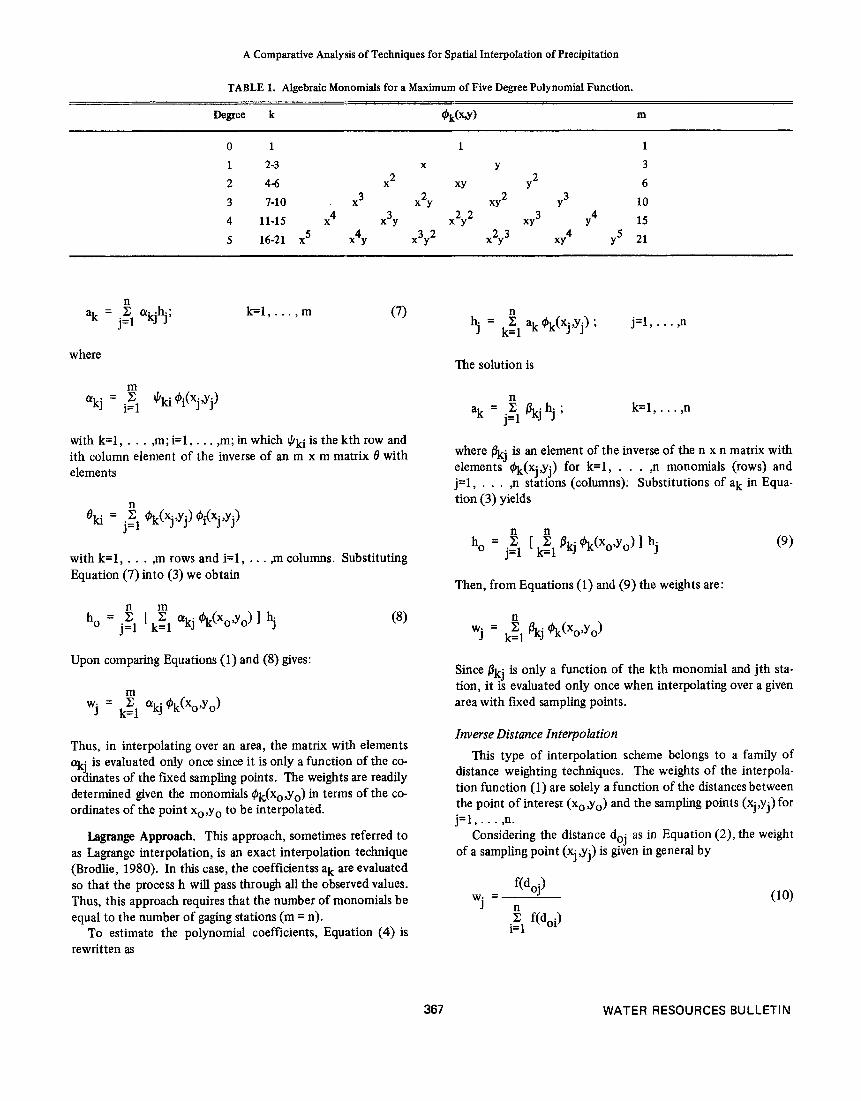
where ho is the interpolated value at any point (xo,yo), ak is the kth polynomial coefficient, @&-,,yo) the kth monomial in terms of xo and yo coordinates and m is the total number of monomials determined from the degree of polynomial function fitted in Equation (3). The algebraic monomials in terms of the x. and y coordinates are given in Table 1. Since the interpolation function (1) is in terms of weights, it is con- venient to express the polynomial Equation (3) in the form of (1). Two approaches are available for this purpose.

Least-Squares Approach. This approach provides an estimate of ho for processes having a trend surface characteristic. A requirement in this approach is that the number of sampling stations n be greater than the number of monomials m.

Let h, be the measured quantity of the process h at sampling stations j=1, . . . ,n and &. be the estimates of the same process based (on a model as in Elquation (3). Then

j = l , . . .

where the a's are defined previously and @k(Xj,yj) is the kth monomial in terms of the coordinates x. and y of station j. We want to estimate the parameter set ak, k=l , . . . ,m by minimizing the sum of the square errors given by

J J

n

j=1 F = Z [hj-\]*

By taking the derivatives of F with respect to ak, k=l , . . . ,m and equating this to zero gives

Note that the second summation term of the left hand side of Equation (6) :is only a function of the coordinates of the fixed sampling points given the form of the polynomial function in Equation (4). Thus, the polynomial coefficients, ak's can be obtained as

WATER RESOURCES BULLETIN

A Comparative Analysis of Techniques for Spatial Interpolation of Precipitation

TABLE 1. Algebraic Monomials for a Maximum of Five Degree Polynomial Function.

Degree k d)kk(W) m

0 1 1 1

1 2-3 X Y 3

6 2 4-6 X XY Y 10 3 7-10 . x

15 4 11-15 X 4 5 16-21 x5 x y

2 2

3 Y 2

XY

2 3

2 X Y

3 2

3 4 Y 3

XY 2 2

X Y 3

X Y 4

XY y5 21 X Y X Y

where

with k=l, . . . ,m; i=l, . . . ,m; in which J'h is the kth row and ith column element of the inverse of an m x m matrix 8 with elements

with k=l , . . . ,m rows and i=l , . . . ,m columns. Substituting Equation (7) into (3) we obtain

Upon comparing Equations (1) and (8) gives:

Thus, in interpolating over an area, the matrix with elements oqq is evaluated only once since it is only a function of the coordinates of the fixed sampling points. The weights are readily determined given the monomials @k(Xo,yo) in terms of the coordinates of the point xo,yo to be interpolated.

Lagrange Approach. This approach, sometimes referred to as Lagrange interpolation, is an exact interpolation technique (Brodlie, 1980). In this case, the coefficientss ak are evaluated so that the process h will pass through all the observed values. Thus, this approach requires that the number of monomials be equal to the number of gaging stations (m = n).

To estimate the polynomial coefficients, Equation (4) is rewritten as

367

n hj = kzl ak $(xj,yj) ; j=1 , . . . ,n

The solution is

k=l, . . . ,n

where akj is an element of the inverse of the n x n matrix with elements &(xj,yj) for k=l , . . . p monomials (rows) and j=1, . . . p stations (columns): Substitutions of ak in Equa- tion (3) yields

Then, from Equations (1) and (9) the weights are:

Since flkj is only a function of the kth monomial and jth station, it is evaluated only once when interpolating over a given area with futed sampling points.

Inverse Distance Interpolation This type of interpolation scheme belongs to a family of

distance weighting techniques. The weights of the interpolation function (1) are solely a function of the distances between the point of interest (xo,yo) and the sampling points (x,,y,) for j = 1 , . . . ,n.

Considering the distance d . as in Equation (2), the weight ?J of a sampling point (xj ,y,) is given in general by


Tabios and Salas

where f(do,) represents a given function of the distance doj. A commonly used form of the function f(*) is

where b is an appropriate constant. Note that the weight w J approaches zero as the distance d and/or the parameter b in- crease. When the parameter b takes on values of 1 or 2, the technique is referred to as the reciprocal distance interpolation or the inverse square distance interpolation, respectively.

One major drawback of the inverse distance interpolation approach is that when two or more sampling points are close to each other (in the absence of measurement errors), the re- dundant information from these stations are not discriminated against (Delfiner and Delhomme, 1975).

Multiquadric Interpolation In multiquadric interpolation, the influence of each sam-

pling point is represented by quadric cones as a function of the coordinates of these points (Hardy, 1971). The estimate for a given point (xo,yo) is thus obtained by the sum of the con- tributions from all those quadric cones. This is mathemati- cally expressed as

where ci = multiquadric coefficient of sampling point (xi,yi) and doi is the distance between points (xo,yo) and (xi,yi). To estimate the coefficients ci and express Equation (1 1) in terms of the weights as in Equation (l), we use Equation (11) for each point (xj ,yj) as

j=1,2, . . . ,n

Then, the coefficients ci are determined by

n ci = Z: 6-h- j=1 ‘J J i=1,2,. . . ,n

where 6ij is an element of the inverse of the n x n interstation distance matrix with elements die, j=1, . . . ,n and i=l, . . . , n.

Substitution of Equation (12j into (1 1) yields

or

368

Again, from Equations (1) and (13), the weights are:

j=1,. . . ,n

Optimal Interpolation Consider that ho is the process to be determined and Equa-

tion (1) is used to estimate ho. Let KO be the estimate of ho, as given by Equation (1). Then, in the optimal interpolation approach the weights are determined by minimizing the variance of the error of interpolation ue which is given by 2

A n (14)

2 ue = var[lno - ho] = var [ho - Z: w.h. j=1 J J ]

where var [ * ] stands for error-variance. Expanding Equation (14) gives

n u: = u2 -- 2 .Z w. cov(h h.) J=1 O J

(15)

where o2 is tlhe variance of the process ho and cov(hihj) represents the covariance between hi and hj. Minimizing the above equation with respect to the weights w, for j=1, . . . ,n stations and equating each of them to zero, yields

Considering :homogeneity in the variances, the covariance terms of Equation (1 6 ) can be replaced by

and

cov(hohj) = u2p(hoh$ (18)

where p(hihj) and p(hohi) are spatial correlation coefficients. In order to estimate these correlation coefficients, it is neces- sary to define a spatial correlation function. Considering a homogeneous and isotropic spatial correlation structure, p(hihj) may tie written as a function of distance only. Then, p(hihj) becomes p(dij) in which dij is the distance between points (xi,yi) and (x- y) .

Therefore, Equation I’ J (16) can now be written as

j=1,. . . ,n (19)



and the weights are obtained by solving the linear system of Equation (19).

The variance of the error for the optimal interpolation at point (xo,yo) may be obtained by substituting Equations (16) through (19) into Equation (15). The result is:

A The estimator h, will be unbiased by constraining the sum

of the weights to one. Then, n z w . = l

j=1 J

In this case, by combining Equations (15) and (20), a new set of weights may be obtained by minimizing the function:

n

J= 1 t 2 h [ . Z wj-11

where X is a Lagrange multiplier which is multiplied by 2 for mathematical convenience. Minimizing this function with respect to the weights gives

n Z wi cov(hhj) t h = cov(h h.) ; i=l 0 3

j=1, . . . ,n

which in terms of the isotropic correlations, becomes

and

n

i=l z w i = l

The linear system of Equation (22) must be solved simultaneously to obtain the weights. For the purpose of this paper, the weights obtained from Equation (22) will be referred to as constrained optimal interpolation to distinguish from those obtained from Equation (19). Likewise, the variance of the error for the optimal interpolation may be readily obtained as

369

The spatial correlation function p(d) can be assumed to be one of several forms. Assuming homogeneity and isotropicity , the most common correlation functions are (Yevjevich and Karplus, 1973):

(a) The reciprocal model, p(d) = 1/(1 + d/co);

(b) The square-root model,p(d) = l / d m o , and

(c) The exponential model, p(d) = exp(-d/co) where co is a parameter to be estimated which is sometimes called the characteristic radius.

To fit the spatial correlation functions, we first estimate the sample correlations between stations. For stations i and j, the sample correlation coefficient is given by

where hk(t) represents the time series observations of the process at station k, mk and. Sk are the corresponding estimates of the mean and standard deviation, respectively, and N is the total number of observations. The distance 4, between the stations are computed from Equation (2). Thus, for a total of n stations, there are n(n-1)/2 station pairs which will be used in fitting the spatial correlation functions.

Kriging Interpolation Various forms of Kriging techniques have been proposed

and applied for hydrological studies. Kriging is similar to optimal interpolation except that the spatial correlation function is replaced by the so-called variogram. As in optimal interpolation, Kriging interpolation requires that the observed process is second-order stationary. Essentially, this assumes homogeneity in the means, variances and covariances. In addition, we assume an isotropic spatial covariance structure. Then, as previously stated, the point variance is represented by var(hi) = a2; i=l , . . . p stations and the covariance between stations i and j is represented by cov(hih,) = cov(d-). Now, the homogeneous and isotropic semivariogram is de f ined as

y(d..) = - 1 var[+ - $1 1J 2

or

i,j=l,. . . p (23) 7(di,) = 2 - cov(d..) 1J ,

in which 7(di,) is the semivariogram as a function of the distance d.. between points i and j.

Therefore, rewriting Equation (15) by substituting Equa- tion (23) for cov(hihj) = cov(dij) gives

9


Tabios and Salas

2 n u2 = u2-2 Z w-[a -y(d .)I

€ j= l J OJ

Minimizing Equation (24) with respect to the weights yields

2 n Z: wi [ y(dij) - a*] = y(doj) - a ;

i= 1 j=1, . . . ,n (25)

which must be solved simultaneously to estimate the weights Wi.

As in the previous case, the variance of the error of interpolation 6: may be obtained by combining Equations (24) and (25), so that

A Furthermore, ho will be unbiased if a constraint as in

Equation (20) is added. Thus, in this case, the equations to be solved become

n C wi y(dij) + = y(doj) ; j=1,. . . ,n (26a)

i= 1

and

n

i= 1 2 w i = 1

which must be solved simultaneously to obtain the weights. In this case, the variance of the error of interpolation becomes

n n2 = Z: w. y(doj)+ X

j = l J

Other schemes of Kriging interpolation have been proposed in the literature. In an attempt to incorporate nonhomo- geneity in the mean of the process, Delfiner and Delhomme (1975) proposed the so-called universal Kriging technique. In this technique, the mean mo at a given point (xo,yo) is represented as a linear combination of the observed station means mj, as in Equation (l) , such that

n mo = Z w.m. (27) j=1 J J

where wj is the weight of station j for j = l , . . . p stations. Since the means are unknown, they may be represented by a polynomial trend as in Equation (3). Rewriting Equation (27) in terms of the polynomial trend gives

or alternatively,

Thus, the kth monomial at point (xo, yo) is

Imposing €quatiom (28) as Lagrange constraints in Equa- tion (24) [Equation (28) includes the constraint that the sum of the weights; must be equal to one in order to obtain a solution which is independent of $1 , the resulting function to be minimized is

n

j=l a: = 2 - 2 Z wj[a2 - -y(doj)]

Then, minimizing Equation (29) with respect to the weights and the Lagrange multipliers A's, the w e i g h and multipliers are obtained bly solving the following equations:

j = l , . . . ,n (30)

n Z: w. = I. j=1 J

where n is the number of stations and m is the number of monomials. Likewise, the variance of the error of interpolation is:

Volpi and Gambolati (1978), and Gambolati and Volpi (1979a, 1979b) claimed that specifying arbitrarily the degree of the polynomial function to represent the mean may lead



to inappropriate assessment of the variogram. In fact, increasing the degree of the polynomial results in an increasing error of interpolation. Instead, they proposed assessing a priori the mean m., j=O,l, . . . p “outside the frame of the kriging technique” (Gambolati and Volpi, 1979a). In addition, a constant mean (lack of trend) may be recommended some times.

Then, considering the relation of means of Equation (27) as a constraint in Equation (24), plus the constraint that the sum of the weights must be equal to one, the resulting system of linear equations to be solved are:

J

n z wi y(dij) + X, t Xlmj = y(dOj) ; j=l , . . . i= 1

n

i=l z w i = l

n X wimi = mo

i= 1

The corresponding variance of the error of interpolation is given by

As indicated before, Kriging interpolation requires the estimation of the variogram. Considering homogeneous and isotropic variograms for describing the spatial characteristics of the process of interest, a number of variogram models have been suggested in the literature (David, 1977; Delhomme, 1978). Some of these models are:

(a) the linear model,

y(d) = a d

(b) the polynomial model,

(c) the exponential model,

d d ) = w[l -exp(-ard)] ,a> 0

(d) the Gaussian model,

d d ) = w[l - exp(-cud2)] , a > 0 and

(e) the spherical model,

y(d) = w[3d/a - (d/a)3] , d G a

-Xd) = w , d > a

where w and a are appropriate constants and d is the distance between two points.

In fitting the foregoing variogram models, we first estimate the sample variogram $(d$ between stations i and j as:

l N %dij) = - 2 {[hi (t) - 41 - [hj (t) - Gj]} 2N t=l

where hk(t) represents the time series of observations at station k, &k is the estimated mean, and N is the total number of observations. The distance dij between two points is computed as in Equation (2). Thus, for a total of n stations, there are n(n-1)/2 pairs of points to use in fitting the model variograms.

VALIDATION PROCEDURES The validity and applicability of the foregoing interpola-

tion techniques is examined by the so-called “fictitious-point” method (Delhomme, 1978). This is done by suppressing one (station) sampling point and values for that point are interpolated based on the remaining (n-1) points. Then, the interpolated values are compared with those observed for that point. The same procedure is followed for some selected points in the network.

The criteria for comparison is: 1) Comparison of the mean and variance of the interpolated

2) The sum of square errors between the observed and in- and observed values.

terpolated values:

A where N = number of observed and interpolated values, ho(t) = interpolated value at sampling point (xo,yo) and &(t) = observed value at sampling point (xo.yo).

3) The proportion of the variance of the observed values accounted for by the interpolator, called the coefficient of efficiency, is

E = S

SO

where S o , the sum of the square differences between the observed values and the mean at point (xo,yo) is given by

4) Another measure of association between the observed and interpolated values is the coefficient of determination obtained by simple regression.

5) The standard deviation of the error of interpolation are also computed by using Equation (15) except for optimal

37 1 WATER RESOURCES BULLETIN

Tabios and Salas

interpolation and Kriging techniques in which specific expres- sions are available in each case.

In addition, a qualitative analysis is performed to assess the ability of some interpolation techniques in representing the process in space. Areal representations of the process are thereby provided.

APPLICATION TO ANNUAL PRECIPITATION

Study Area Description The area selected for this study is Region I1 in the North

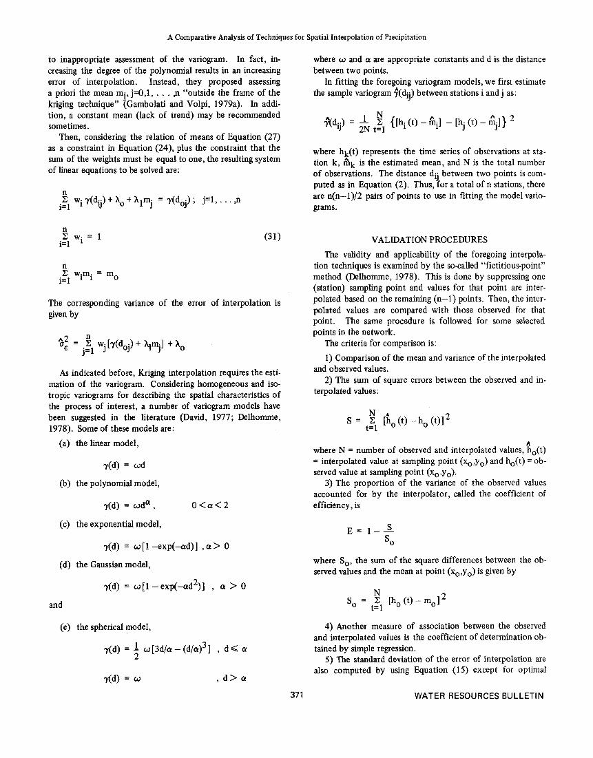
Central Continental United States with a total area of about 52,000 sq. kms. It is located between 96.0 and 99.5 degrees west longitude and 40.0 and 42.5 degrees north latitude. Re- gion I1 has 29 precipitation stations located east of Nebraska and some in northern Kansas. This region is considered a topographically homogeneous area and has relatively uniform spatial variability of some statistical parameters (Yevjevich and Karplus, 1973). The location of the region within the U.S.A. is shown in Figure 1.

99. 50° W I 96.0OoW

Figure 1. Location of the Study Area Within U.S.A.

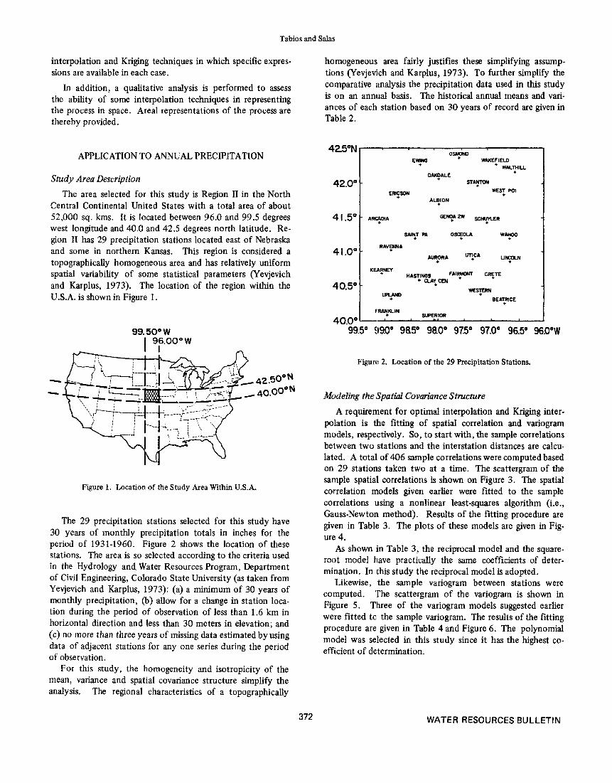
The 29 precipitation stations selected for this study have 30 years of monthly precipitation totals in inches for the period of 1931-1960. Figure 2 shows the location of these stations. The area is so selected according to the criteria used in the Hydrology and. Water Resources Program, Department of Civil Engineering, Colorado State University (as taken from Yejevich and Karplus, 1973): (a) a minimum of 30 years of monthly precipitation, (b) allow for a change in station location during the period of observation of less than 1.6 km in horizontal direction and less than 30 meters in elevation; and (c) no more than three years of missing data estimated by using data of adjacent stations for any one series during the period of observation.

For this study, the homogeneity and isotropicity of the mean, variance and spatial covariance structure simplify the analysis. The regional characteristics of a topographically

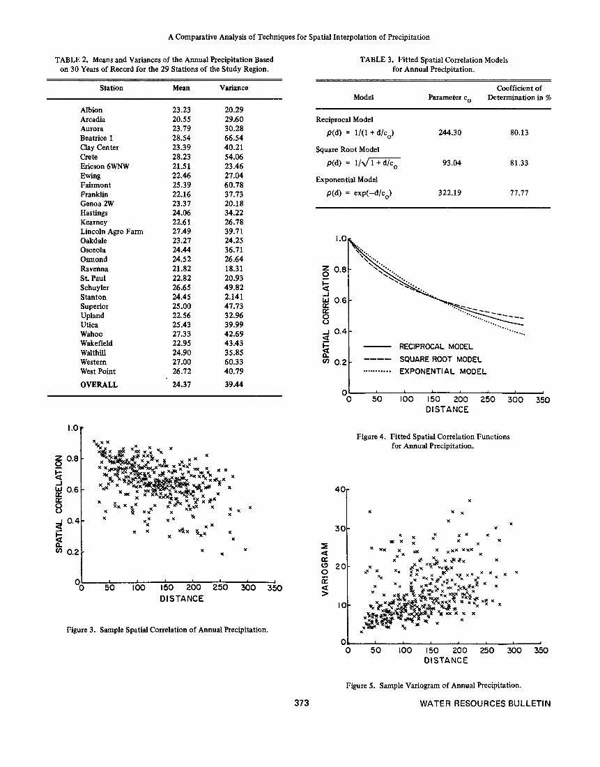
homogeneous area fairly justifies these simplifying assump- tions (Yevjevich and Karplus, 1973). To further simplify the comparative analysis the precipitation data used in this study is on an annual basis. The historical annual means and variances of each station based on 30 years of record are given in Table 2.

WAKEFIELO

OAYALE

WEy POI =v

SCH!?LER

Om+- " Y o WN,T m

425"N

42.0"

RAV$WA

41.0'1 AUrSpRA "IcA L1-N

Figure 2. Location of the 29 Precipitation Stations.

Modeling the (Spatial Covariance Structure A requirement for optimal interpolation and Kriging inter-

polation is the fitting of spatial correlation and variogram models, respectively. So, to start with, the sample correlations between two stations and the interstation distances are calculated. A total of 406 sample correlations were computed based on 29 stations taken two at a time. The scattergram of the sample spatial correlations is shown on Figure 3. The spatial correlation models given earlier were fitted to the sample correlations using a nonlinear least-squares algorithm (i.e., Gauss-Newton method). Results of the fitting procedure are given in Table 3. The plots of these models are given in Fig- ure 4.

As shown in Table 3, the reciprocal model and the sqaare- root model have practically the same coefficients of determination. In this study the reciprocal model is adopted.

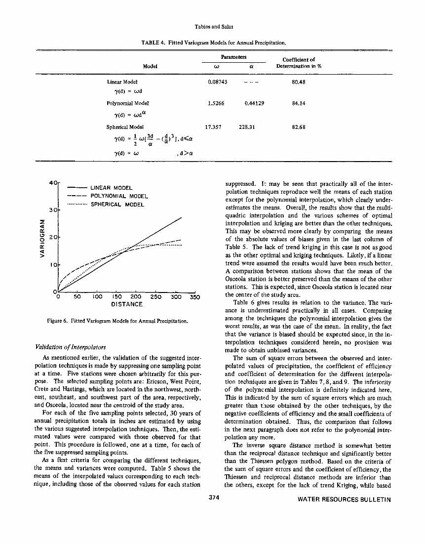
Likewise, the sample variogram between stations were computed. The scattergram of the variogram is shown in Figure 5. Three of the variogram models suggested earlier were fitted to the sample variogram. The results of the fitting procedure are given in Table 4 and Figure 6 . The polynomial model was selected in this study since it has the highest coefficient of determination.



J 0.4- 5 cn 0 .2 -

TABLE 2. Means and Variances of the Annual Precipitation Based on 30 Years of Record for the 29 Stations of the Study Region.

-... --...

- RECIPROCAL MODEL SQUAREROOT MODEL EXPONENTIAL MODEL

---- . . . . .. . . . . .

TABLE 3. Fitted Spatial Correlation Models for Annual Precipitation.

Station M W Variance

Albion Arcadia Aurora Beatrice 1 Clay Center Crete Ericson 6WNW Ewing Fairmont Franklin Genoa 2W Hastings Kearne y Lincoln Ago Farm Oakdale Osceola Osmond Ravenna St. Paul Schu yler Stanton Superior Upland Utica wahoo Wake field Walthill Western West Point

OVERALL

23.23 20.29 20.55 29.60 23.79 30.28 28.54 66.54 23.39 40.21 28.23 54.06 21.51 23.46 22.46 27.04 25.39 60.78 22.16 37.73 23.37 20.18 24.06 34.22 22.6 1 26.78 27.49 39.71 23.27 24.25 24.44 36.71 24.52 26.64 21.82 18.31 22.82 20.93 26.65 49.82 24.45 2.141 25.00 47.73 22.56 32.96 25.43 39.99 27.33 42.69 22.95 43.43 24.90 35.85 27.00 60.33 26.72 40.79 24.37 39.44

,

I .Oy

Z 0.8 - 0 %

8

J W 0.6 - lK a

Oe2 t X X I:

O:, 50 160 I50 200 250 360 3b 0 I S TA NC E

Figure 3. Sample Spatial Correlation of Annual Precipitation.

37 3

Coefficient of Model Parameter co Determination in %

Reciprocal Model P(d) = N 1 + d/co) 244.30 80.13

Square Root Model

PW = l / m 93.04 81.33

Exponential Model

P(d) = exp(-d/co) 322.19 77.77

"0 50 100 150 200 250 300 350 DISTANCE

Figure 4. Fitted Spatial Correlation Functions for Annual Precipitation.

40[ x

30

X

X X

X X

X

x x x x xx - - 1 * * x x x X

c L x xx x .& x x x x x x x U

X

0 50 100 150 200 250 300 350 DISTANCE

Figure 5 . Sample Variogram of Annual Precipitation.


Tabios and Salas

TABLE 4. Fitted Variogram Models for Annual Precipitation.

Model Parameters Coefficient of

0 a Determination in %

80.48 Linear Model 0.08743 - _ _ r(d) = a d

Polynomial Model 1.5266 0.44129 84.14

r(d) = o d a

Spherical Model 17.357 228.31 82.68 7(d) = 1 0[g -(5) d 3 ],a<&

r(d) = 0 , d > a 2 a

LINEAR MODEL ---- POLYNOMIAL MODEL . . . . . . . . . .. . SPHERICAL MODEL

30

DISTANCE

Figure 6. Fitted Variogram Models for Annual Precipitation.

Validation of Interpolators As mentioned earlier, the validation of the suggested inter-

polation techniques is made by suppressing one sampling point at a time. Five stations were chosen arbitrarily for this purpose. The selected sampling points are: Ericson, West Point, Crete and Hastings, which are located in the northwest, north- east, southeast, and southwest part of the area, respectively, and Osceola, located near the centroid of the study area.

For each of the five sampling points selected, 30 years of annual precipitation totals in inches are estimated by using the various suggested interpolation techniques. Then, the estimated values were compared with those observed for that point. This procedure is followed, one at a time, for each of the five suppressed sampling points.

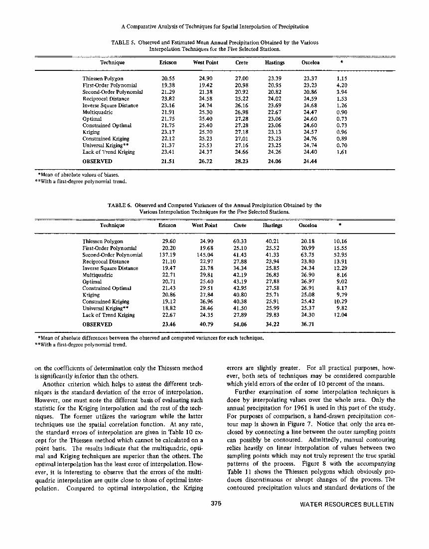
As a first criteria for comparing the different techniques, the means and variances were computed. Table 5 shows the means of the interpolated values corresponding to each technique, including those of the observed values for each station

suppressed. It may be seen that practically all of the interpolation techniques reproduce well the means of each station except for the polynomial interpolation, which clearly under- estimates the means. Overall, the results show that the multiquadric interpolation and the various schemes of optimal interpolation and kriging are better than the other techniques. This may be observed more clearly by comparing the means of the absolute values of biases given in the last column of Table 5. The lack of trend kriging in this case is not as good as the other optimal and kriging techniques. Likely, if a linear trend were assumed the results would have been much better. A comparison between stations shows that the mean of the Osceola station is better preserved than the means of the other stations. This is expected, since Osceola station is located near the center of the study area.

Table 6 gives results in relation to the variance. The variance is underestimated practically in all cases. Comparing among the techniques the polynomial interpolation gives the worst results, iis was the case of the mean. In reality, the fact that the variance is biased should be expected since, in the interpolation techniques considered herein, no provision was made to obtain unbiased variances.

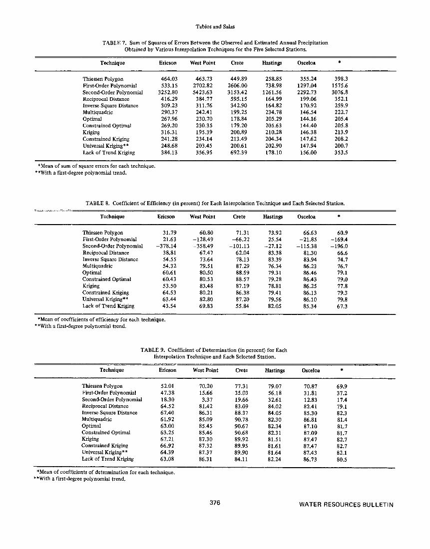
The sum of square errors between the observed and interpolated values of precipitation, the coefficient of efficiency and coefficient of determination for the different interpolation techniques are given in Tables 7,8, and 9. The inferiority of the polynomial interpolation is definitely indicated here. This is indicated by the sum of square errors which are much greater than tlhose obtained by the other techniques, by the negative coefficients of efficiency and the small coefficients of determination obtained. Thus, the comparison that follows in the next paragraph does not refer to the polynomial interpolation any more.

The inverse square distance method is somewhat better than the reciprocal distance technique and significantly better than the Thiessen polygon method. Based on the criteria of the sum of square errors and the coefficient of efficiency, the Thiessen and reciprocal distance methods are inferior than the others, ex,cept for the lack of trend Kriging, while based



TABLE 5. Observed and Estimated Mean Annual Precipitation Obtained by the Various Interpolation Techniques for the Five Selected Stations.

Technique Ericson West Point Crete Hastings Osceloa *

Thiessen Polygon First-Order Polynomial Second-Order Polynomial Reciprocal Distance Inverse Square Distance Multiquadric Optimal Constmined Optimal Kriging Constrained Kriging Universal Kriging** Lack of Trend Kriging

OBSERVED

20.55 19.38 21.29 23.82 23.16 21.91 21.75 21.75 23.17 22.12 21.37 23.41 21.51

24.90 19.42 21.38 24.58 24.74 25.30 25.40 25.40 25.70 25.23 25.53 24.37 26.72

27.00 20.98 20.92 25.22 26.16 26.98 27.28 27.28 27.18 27.01 27.16 24.66 28.23

23.39 20.95 20.82 24.02 23.69 22.67 23.06 23.06 23.13 23.23 23.25 24.26 24.06

23.37 23.23 20.86 24.59 24.68 24.47 24.60 24.60 24.51 24.76 24.74 24.40 24.44

1.15 4.20 3.94 1.53 1.26 0.90 0.73 0.73 0.96 0.89 0.70 1.61

*Mean of absolute values of biases. **With a first-degree polynomial trend.

TABLE 6. Observed and Computed Variances of the Annual Precipitation Obtained by the Various Interpolation Techniques for the Five Selected Stations.

Technique Ericson West Point Crete Hastings Osceloa *

Thiessen Polygon First-Order Polynomial Second-Order Polynomial Reciprocal Distance Inverse Square Distance Multiquadric optimal Constrained Optimal I iging Constrained Kriging Universal Kriging** Lack of Trend Kriging

OBSERVED

29.60 20.20

137.19 21.10 19.47 22.71 20.71 21.43 20.86 19.12 18.82 22.67 23.46

24.90 19.68

145.04 22.97 23.78 29.81 25.40 29.51 27.84 26.96 28.46 24.35 40.79

60.33 25.10 41.43 27.88 34.34 42.19 43.19 42.95 40.80 40.38 41.50 27.89 54.06

40.21 25.52 41.33 23.94 25.85 26.83 27.88 27.58 25.71 25.91 25.99 29.83 34.22

20.18 20.99 63.75 23.80 24.34 26.90 26.97 26.91 25.08 25.42 25.37 24.30 36.71

10.16 15.55 52.95 13.91 12.29 8.16 9.02 8.17 9.79

10.29 9.82

12.04

*Mean of absolute differences between the observed and computed variances for each technique. **With a first-degree polynomial trend.

on the coefficients of determination only the Thiessen method is significantly inferior than the others.

Another criterion which helps to assess the different techniques is the standard deviation of the error of interpolation. However, one must note the different basis of evaluating such statistic for the Kriging interpolation and the rest of the techniques. The former utilizes the variogram while the latter techniques use the spatial correlation function. At any rate, the standard errors of interpolation are given in Table 10 except for the Thiessen method which cannot be calculated on a point basis. The results indicate that the multiquadric, optimal and Kriging techniques are superior than the others. The optimal interpolation has the least error of interpolation. How- ever, it is interesting to observe that the errors of the multiquadric interpolation are quite close to those of optimal interpolation. Compared to optimal interpolation, the Kriging

375

errors are slightly greater. For all practical purposes, however, both sets of techniques may be considered comparable which yield errors of the order of 10 percent of the means.

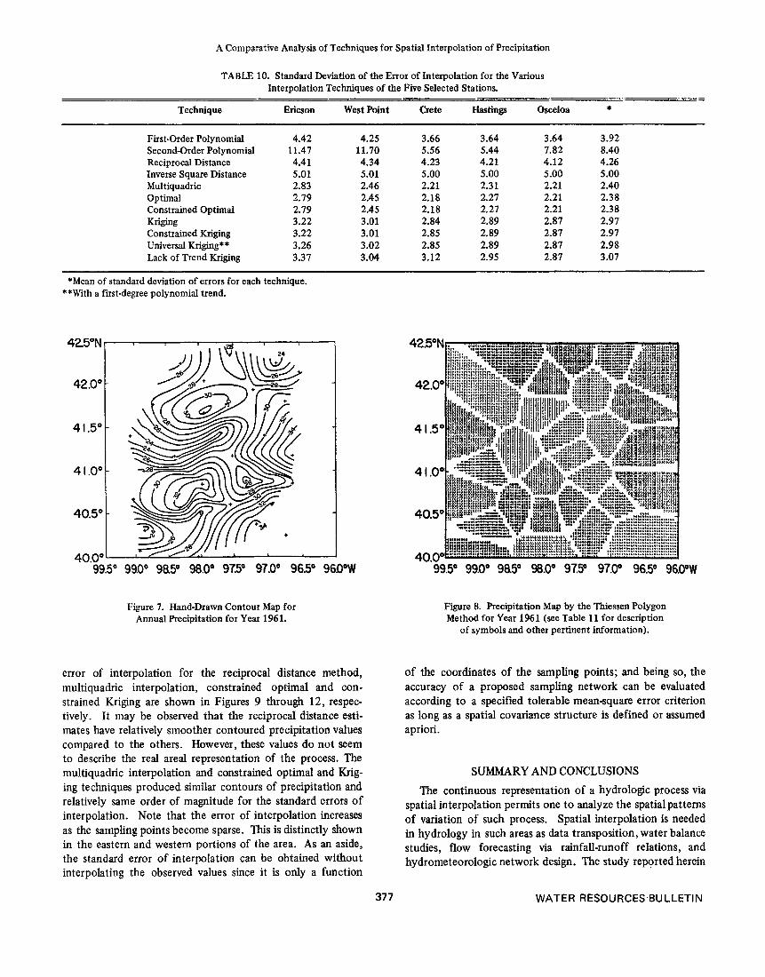
Further examination of some interpolation techniques is done by interpolating values over the whole area. Only the annual precipitation for 1961 is used in this part of the study. For purposes of comparison, a hand-drawn precipitation contour map is shown in Figure 7. Notice that only the area en- closed by connecting a line between the outer sampling points can possibly be contoured. Admittedly, manual contouring relies heavily on linear interpolation of values between two sampling points which may not truly represent the true spatial patterns of the process. Figure 8 with the accompanying Table 11 shows the Thiessen polygons which obviously pro- duces discontinuous or abrupt changes of the process. The contoured precipitation values and standard deviations of the


Tabios and Salas

TABLE 7. Sum of Squares of Errors Between the Observed and Estimated Annual Precipitation Obtained by Various Interpolation Techniques for the Five Selected Stations.

Technique Ericson West Point Crete Hasting Osceloa *

Thiessen Polygon First-Order Polynomial Second-Order Polynomial Reciprocal Distance Inverse Square Distance Multiquadric Optimal Constrained Optimal Kriging Constrained Kriging Universal Kriging** Lack of Trend Kriging

464.03 533.15

3252.80 416.29 309.23 290.37 267.96 26 9.20 316.31 241.28 248.68 384.13

463.73 2702.82 5423.63

384.77 311.76 242.41 230.70 230.35 195.39 234.14 203.45 356.95

449.89 2606.00 3153.42

595.15 342.90 199.25 178.84 179.20 200.89 213.49 200.61 692.39

258.85 738.98

1261.56 164.99 164.82 234.78 205.29 205.63 210.28 204.34 202.90 178.10

355.24 1297.04 2292.73

199.06 170.92 146.54 144.16 144.40 146.38 147.62 147.94 156.00

398.3 1575.6 3076.8 352.1 259.9 222.7 205.4 205.8 213.9 208.2 200.7 353.5

*Mean of sum of square errors for each technique. **With a first-degree polynomial trend.

TABLE 8. Coefficient of Efficiency (in percent) for Each Interpolation Teclhnique and Each Selected Station.

Technique Ericson West Point Crete Hasting Osceloa *

Thiessen Polygon First-Order Polynomial Second-Order Polynomial Reciprocal Distance Inverse Square Distance Multiquadric Optimal Constrained Optimal Kriging Constrained Kriging Universal Kriging* * Lack of Trend Kriging

31.79 21.63

-378.14 38.81 54.55 54.32 60.61 60.43 53.50 64.53 63.44 43.54

60.80 -128.49 -358.49

67.47 73.64 79.51 80.50 80.53 83.48 80.21 82.80 69.83

71.31 -66.22 -101.13

62.04 78.13 87.29 88.59 88.57 87.19 86.38 87.20 55.84

73.92 25.54

83.38 83.39 76.34 79.3 1 79.28 78.81 79.41 79.56 82.05

-27.12

66.63 -21.85

-115.38 81.30 83.94 86.23 86.46 86.43 86.25 86.13 86.10 85.34

60.9 -169.4 -196.0

66.6 74.7 76.7 79.1 79.0 77.8 79.3 79.8 67.3

*Mean of coefficients of efficiency for each technique. **With a first-degree polynomial trend.

TABLE 9. Coefficient of Determination (in percent11 for Each Interpolation Technique and Each Selected Station.

Technique Ericson West Point Crete Hastings Osceloa * ~~ ~~ ~~~ ~ __

Thiessen Polygon 52.01 70.20 77.31 79.07 70.87 69.9 First-Order Polynomial 47.38 15.66 35.03 56.18 31.81 37.2 Second-Order Polynomial 18.30 3.37 19.66 32.61 12.83 17.4 Reciprocal Distance 64.52 81.42 83.09 84.02 82.41 79.1 Inverse Square Distance 67.40 86.31 88.37 84.05 85.30 82.3 Multiquadric 61.92 85.09 90.78 82.30 86.81 81.4 Optimal 63.00 85.45 90.67 82.34 87.10 81.7 Constrained Optimal 63.25 85.46 90.68 82.3 1 87.09 81.7 Kriging 67.21 87.30 89.92 81.51 87.47 82.7 Constrained Kriging 66.92 87.32 89.95 81.61 87.47 82.7 Universal Kriging** 64.39 87.37 89.90 81.64 87.43 82.1 Lack of Trend Kriging 63.08 86.3 1 84.11 82.24 86.73 80.5

*Mean of coefficients of determination for each technique. **With a fiist-degree polynomial trend.



TABLE 10. Standard Deviation of the Error of Interpolation for the Various Interpolation Techniques of the Five Selected Stations.

Technique Ericson West Point Crete Hastings Osceloa * ~~

First-Order Polynomial Second-Order Polynomial Reciprocal Distance Inverse Square Distance Multiquadric Optimal Constrained Optimal Kriging Constrained Kriging Universal Kriging** Lack of Trend Kriging

4.42 11.47 4.4 1 5.01 2.83 2.79 2.79 3.22 3.22 3.26 3.37

4.25 11.70 4.34 5.01 2.46 2.45 2.45 3.01 3.01 3.02 3.04

3.66 5.56 4.23 5.00 2.21 2.18 2.18 2.84 2.85 2.85 3.12

3.64 5.44 4.21 5.00 2.31 2.27 2.21 2.89 2.89 2.89 2.95

3.64 7.82 4.12 5.00 2.21 2.21 2.21 2.87 2.81 2.87 2.87

3.92 8.40 4.26 5.00 2.40 2.38 2.38 2.97 2.97 2.98 3.07

*Mean of standard deviation of errors for each technique. **With a first-degree polynomial trend.

425"N r 1

42.0"

4 I .5"

4 I .oo

40.5"

40 0" . -.- 99.5" 99.0' 985" 98.0" 97.5" 97.0" 96.5" 96D"W

Figure 7. Hand-Drawn Contour Map for Annual Precipitation for Year 1961.

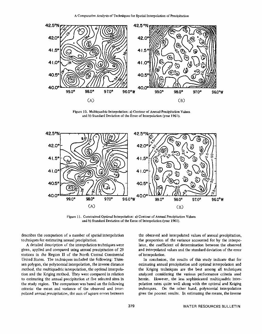
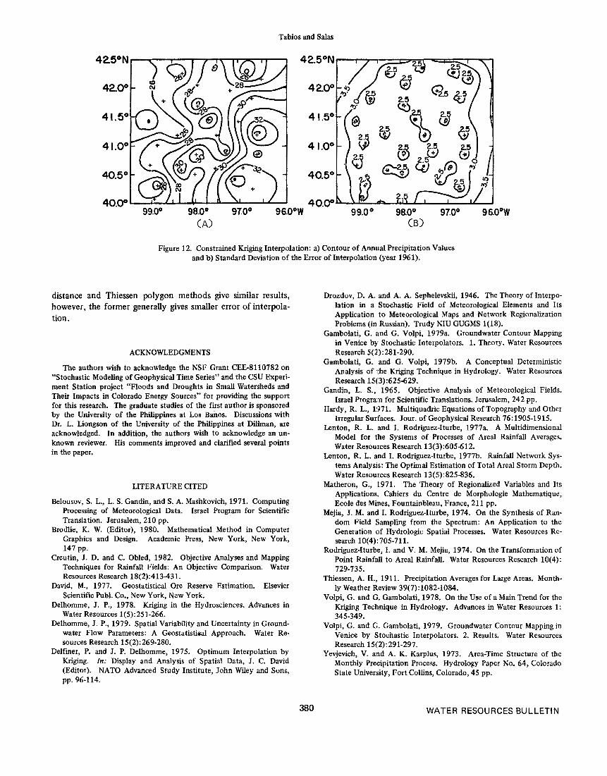
error of interpolation for the reciprocal distance method, multiquadric interpolation, constrained optimal and constrained Kriging are shown in Figures 9 through 12, respectively. It may be observed that the reciprocal distance estimates have relatively smoother contoured precipitation values compared to the others. However, these values do not seem to describe the real areal representation of the process. The multiquadric interpolation and constrained optimal and f i g - ing techniques produced similar contours of precipitation and relatively same order of magnitude for the standard errors of interpolation. Note that the error of interpolation increases as the sampling points become sparse. This is distinctly shown in the eastern and western portions of the area. As an aside, the standard error of interpolation can be obtained without interpolating the observed values since it is only a function

. 99.5" 99.0" 985" 98.0" 97.5" 97.0" 96.5' 96.0"W

Figure 8. Precipitation Map by the Thiessen Polygon Method for Year 1961 (see Table 11 for description

of symbols and other pertinent information).

of the coordinates of the sampling points; and being so, the accuracy of a proposed sampling network can be evaluated according to a specified tolerable mean-square error criterion as long as a spatial covariance structure is defined or assumed apriori.

SUMMARY AND CONCLUSIONS

The continuous representation of a hydrologic process via spatial interpolation permits one to analyze the spatial patterns of variation of such process. Spatial interpolation is needed in hydrology in such areas as data transposition, water balance studies, flow forecasting via rainfall-runoff relations, and hydrometeorologic network design. The study reported herein

377 WATER RESOURCES.BU LLETl N

Tabios and Salas

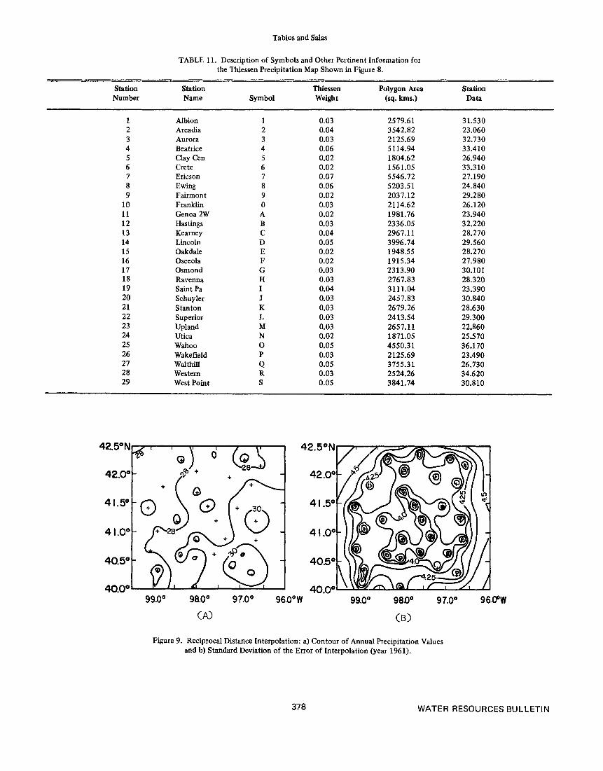
TABLE 11. Description of Symbols and Other Pertinent Information for the Thiessen Precipitation Map Shown in Figure 8.

Station Station Thiessen Polygon Area Station Number Name Symbol Weight (sq. kms.) Data

1 Albion 1 0.03 25 79.6 1 31.530 2 Arcadia 2 0.04 3542.82 23.060 3 Aurora 3 0.03 2125.69 32.730 4 Beatrice 4 0.06 5114.94 33.410 5 Clay Cen 5 0.02 1804.62 26.940 6 Crete 6 0.02 156 1.05 33.310 7 Ericson 7 0.07 5546.72 27.190 8 Ewing 8 0.06 5203.51 24.840 9 Fairmont 9 0.02 2037.12 29.280

10 Franklin 0 0.03 2114.62 26.120 11 Genoa 2W A 0.02 1981.76 23.940 12 Hastings B 0.03 2336.05 32.220 13 Kearney C 0.04 2967.11 28.270 14 Lincoln D 0.05 3996.74 29.560 15 Oakdale E 0.02 1948.55 28.270

17 Osmond G 0.03 2313.90 30.101 18 Ravenna H 0.03 2767.83 28.320 19 Saint Pa I 0.04 3 11 1.04 23.390 20 Schuyler J 0.03 2457.83 30.840

28.630 21 Stanton K 0.03 22 Superior L 0.03 2413.54 29.300 23 Upland M 0.03 2657.11 22.860 24 Utica N 0.02 1871.05 25.570 25 wahoo 0 0.05 4550.31 36.170 26 Wakefield P 0.03 2125.69 23.490 27 Walthilt Q 0.05 3755.31 26.730 28 Western R 0.03 2524.26 34.620 29 West Point S 0.05 3 84 1.74 30.810

16 Osceola F 0.02 1915.34 27.980

2679.26

99.0' 98.0' 97.0' 96.0'W 99.0" 980' 97.0' 96.U'W

(A> (B)

Figure 9. Reciprocal Distance Interpolation: a) Contour of Annual Precipitation Values and b) Standard Deviation of the Error of Interpolation (year 1961).



99.00 9800 97.00 9 6 . 0 0 ~ 99.0° 98.0' 97.0' 961)OW

Figure 10. Multiquadric Interpolation: a) Contour of Annual Precipitation Values and b) Standard Deviation of the Error of Interpolation (year 1961).

Figure 11. Constrained Optimal Interpolation: a) Contour of Annual Precipitation Values and b) Standard Deviation of the Error of Interpolation (year 1961).

describes the comparison of a number of spatial interpolation techniques for estimating annual precipitation.

A detailed description of the interpolation techniques were given, applied and compared using annual precipitation of 29 stations in the Region I1 of the North Central Continental United States. The techniques included the following: Thies- sen polygon, the polynomial interpolation, the inverse distance method, the multiquadric interpolation, the optimal interpolation and the Kriging method. They were compared in relation to estimating the annual precipitation at five selected sites in the study region. The comparison was based on the following criteria: the mean and variance of the observed and interpolated annual precipitation, the sum of square errors between

the observed and interpolated values of annual precipitation, the proportion of the variance accounted for by the interpolator, the coefficient of determination between the observed and interpolated values and the standard deviation of the error of interpolation.

In conclusion, the results of this study indicate that for estimating annual precipitation and optimal interpolation and the Kriging techniques are the best among all techniques analyzed considering the various performance criteria used herein. However, the less sophisticated multiquadric interpolation rates quite well along with the optimal and Kriging techniques. On the other hand, polynomial interpolation gives the poorest results. In estimating the means, the inverse


Tabios and Salas

99.0’ 98.0’ 97.0’ 96.0’W 99.0° 98.00 97.0’ 96.0’W

Figure 12. Constrained Kriging Interpolation: a) Contour of Annual Precipitation Values and b) Standard Deviation of the Error of Interpolation (year 1961).

distance and Thiessen polygon methods give similar results, however, the former generally gives smaller error of interpolation.

ACKNOWLEDGMENTS

The authors wish to acknowledge the NSF Grant CEE-8110782 on “Stochastic Modeling of Geophysical Time Series” and the CSU Experi- ment Station project “Floods and Droughts in Small Watersheds and Their Impacts in Colorado Energy Sources” for providing the support for this research. The graduate studies of the first author is sponsored by the University of the Philippines at Los Bahos. Discussions with Dr. L. Liongson of the University of the Philippines at Diliman, are acknowledged. In addition, the authors wish to acknowledge an unknown reviewer. His comments improved and clarified several points in the paper.

LITERATURE CITED

Belousov, S. L., L. S. Gandin, and S. A. Mashkovich, 1971. Computing Processing of Meteorological Data. Israel Program for Scientific Translation. Jerusalem, 210 pp.

Mathematical Method in Computer Graphics and Design. Academic Press, New York, New York, 147 pp.

Creutin, J. D. and C. Obled, 1982. Objective Analyses and Mapping Techniques for Rainfall Fields: An Objective Comparison. Water Resources Research 18(2):413431.

David, M., 1977. Geostatistical Ore Reserve Estimation. Elsevier Scientific Publ. Co., New York, New York.

Delhomme, J. P., 1978. Kriging in the Hydrosciences. Advances in Water Resources l(5): 25 1-266.

Delhomme, J. P., 1979. Spatial Variability and Uncertainty in Ground- water Flow Parameters: A Geostatistieal Approach. Water Re- sources Research 15(2):269-280.

Delfiner, P. and J. P. Delhomme, 1975. Optimum Interpolation by Kriging. fn: Display and Analysis of Spatial Data, J. C. David (Editor). NATO Advanced Study Institute, John Wiley and Sons,

Brodlie, K. W. (Editor), 1980.

pp. 96-114.

Drozdov, D. A. and A. A. Sephelevskii, 1946. The Theory of Interpo- lation in a Stochastic Field of Meteorological Elements and Its Application to Meteorological Maps and Network Regionalization Problems (in Russian). Trudy NIU GUGMS l(18).

Gambolati, G. and G. Volpi, 1979a. Groundwater Contour Mappmg in Venice by Stochastic Interpolators. 1. Theory. Water Resources Research 5(2):281-290.

A Conceptual Deterministic Analysis of the Kriging Technique in Hydrology. Water Resources Research 13 3) :6 25-6 29.

Gandin, L. S., 1965. Objective Analysis of Meteorological Fields. Israel Program for Scientific Translations. Jerusalem, 242 pp.

Hardy, R. L., 1971. Multiquadric Equations of Topography and Other Irregular Surfaces. Jour. of Geophysical Research 76:1905-1915.

Lenton, R. L. and I. Rodriguez-Iturbe, 1977a. A Multidimensional Model for the Systems of Processes of Areal Rainfall Averages. Water Resources Research 13(3):605612.

Lenton, R. L. and I. Rodriguez-Iturbe, 1977b. Rainfall Network Sys- tems Analysis: The Optimal Estimation of Total Areal Storm Depth. Water Resources Research 13(5):825-836.

Matheron, G., 1971. The Theory of Regionalized Variables and Its Applications. Cahiers du Centre de Morphologie Mathematique, Ecole des Mines, Fountainbleau, France, 21 1 pp.

Mejia, J. M. and I. Rodriguez-Iturbe, 1974. On the Synthesis of Ran- dom Field !;ampling from the Spectrum: An Application to the Generation of Hydrologic Spatial Processes. Water Resources Re- search lO(4) :705-711.

Rodriguez-Iturbe, I. and V. M. Mejia, 1974. On the Transformation of Point Rainfadl to Areal Rainfall. Water Resources Research lO(4):

Thiessen, A. H., 1911. Precipitation Averages for Large Areas. Month- ly Weather Review 39(7):1082-1084.

Volpi, G. and C. Gambolati, 1978. On the Use of a Main Trend for the Kriging Technique in Hydrology. Advances in Water Resources 1 : 345-349.

Volpi, G. and GL Gambolati, 1979. Groundwater Contour Mapping in Venice by Stochastic Interpolators. 2. Results. Water Resources Research 15(2):291-297.

Yevjevich, V. and A. K. Karplus, 1973. Area-Time Structure of the Monthly Precipitation Process. Hydrology Paper No. 64, Colorado State University, Fort Collins, Colorado, 45 pp.

Gambolati, G. and G. Volpi, 1979b.

729-735.
