Zipf's Law, Music Classification, and Aesthetics

Manaris, Bill.Romero, Juan.Machado, Penousal.

Computer Music Journal, Volume 29, Number 1, Spring 2005,pp. 55-69 (Article)

Published by The MIT Press

For additional information about this article

Access Provided by NTNU, Universitetsbiblioteket i Trondheim at 09/27/10 11:21AM GMT

http://muse.jhu.edu/journals/cmj/summary/v029/29.1manaris.html

Manaris et al.

Zipf’s Law, MusicClassification, andAesthetics

55

The connection between aesthetics and numbersdates back to pre-Socratic times. Pythagoras, Plato,and Aristotle worked on quantitative expressions ofproportion and beauty such as the golden ratio.Pythagoreans, for instance, quantified “harmo-nious” musical intervals in terms of proportions (ra-tios) of the first few whole numbers: a unison is 1:1,octave is 2:1, perfect fifth is 3:2, perfect fourth is4:3, and so on (Miranda 2001, p. 6). The Pythagoreanscale was refined over centuries to produce well-tempered and equal-tempered scales (Livio 2002,pp. 29, 186).

Galen, summarizing Polyclitus, wrote, “Beautydoes not consist in the elements, but in the harmo-nious proportion of the parts.” Vitruvius stated,“Proportion consists in taking a fixed nodule, ineach case, both for the parts of a building and for thewhole.” He then defined proportion as “the appro-priate harmony arising out of the details of the workitself; the correspondence of each given detailamong the separate details to the form of the designas a whole.” This school of thought crystallizedinto a universal theory of aesthetics based on “unityin variety” (Eco 1986, p. 29).

Some musicologists dissect the aesthetic experi-ence in terms of separable, discrete sounds. Othersattempt to group stimuli into patterns and studytheir hierarchical organization and proportions(May 1996; Nettheim 1997). Leonard Meyer statesthat emotional states in music (sad, angry, happy,etc.) are delineated by statistical parameters such asdynamic level, register, speed, and continuity (2001,p. 342).

Building on earlier work by Vilfredo Pareto, Al-fred Lotka, and Frank Benford (among others),George Kingsley Zipf refined a statistical techniqueknown as Zipf’s Law for capturing the scaling prop-erties of human and natural phenomena (Zipf 1949;Mandelbrot 1977, pp. 344–345).

We present results from a study applying Zipf’sLaw to music. We have created a large set of metricsbased on Zipf’s Law that measure the proportion ordistribution of various parameters in music, such aspitch, duration, melodic intervals, and harmonicconsonance. We applied these metrics to a large cor-pus of MIDI-encoded pieces. We used the generateddata to perform statistical analyses and train artifi-cial neural networks (ANNs) to perform variousclassification tasks. These tasks include author at-tribution, style identification, and “pleasantness”prediction. Results from the author attribution and

Computer Music Journal, 29:1, pp. 55–69, Spring 2005© 2005 Massachusetts Institute of Technology.

Bill Manaris,* Juan Romero,† PenousalMachado,‡ Dwight Krehbiel,§ Timothy Hirzel,*

Walter Pharr,* and Robert B. Davis¶

*Computer Science Department, College ofCharleston66 George Street, Charleston, SC 29424 USA{manaris, hirzel, pharr}@cs.cofc.edu†Creative Computer Group, RNASA LabFaculty of Computer Science, University of ACoruña, Spainjj@udc.es‡Centre for Informatics and Systems Department ofInformatic Engineering Polo II-University of Coimbra3030 Coimbra, Portugalmachado@dei.uc.pt§Psychology Department, Bethel CollegeNorth Newton, KS 67117 USAkrehbiel@bethelks.edu¶Department of Mathematics and Statistics, MiamiUniversityHamilton, OH 45011, USAdavisrb@muohio.edu

style identification ANN experiments have ap-peared in Machado et al. (2003, 2004) and Manariset al. (2003), and these results are summarized inthis article. Results from the “pleasantness” predic-tion ANN experiment are new and therefore dis-cussed in detail. Collectively, these results suggestthat metrics based on Zipf’s Law may capture essen-tial aspects of proportion in music as it relates tomusic aesthetics.

Zipf’s Law

Zipf’s Law reflects the scaling properties of manyphenomena in human ecology, including naturallanguage and music (Zipf 1949; Voss and Clarke1975). Informally, it describes phenomena wheresmall events are quite frequent and large events arerare. Once a phenomenon has been selected forstudy, we can examine the contribution of eachevent to the whole and rank it according to its “im-portance” or “prevalence” (see linkage.rockefeller.edu/wli/zipf). For example, we may rank uniquewords in a book by their frequency of occurrence,visits to a Web site by how many of them originatedfrom the same Internet address, and so on.

In its most succinct form, Zipf’s Law is expressedin terms of the frequency of occurrence (i.e., countor quantity) of events, as follows:

F ~ r–a (1)

where F is the frequency of occurrence of an eventwithin a phenomenon, r is its statistical rank (posi-tion in an ordered list), and a is close to 1. In thebook example above, the most frequent word wouldbe rank 1, the second most frequent word would berank 2, and so on. This means that the frequency ofoccurrence of a word is inversely proportional to itsrank. For example, if the first ranked word appears6,000 times, the second ranked word would appearapproximately 3,000 times (1/2), the third rankedword approximately 2,000 times (1/3), and so on.

Another formulation of Zipf’s Law is

P(f) ~ 1/fn (2)

where P(f) denotes the probability of an event ofrank f, and n is close to 1. In physics, Zipf’s Law is a

special case of a power law. When n is 1 (Zipf’s ideal),the phenomenon is called 1/f noise or pink noise.

Zipf distributions (e.g., 1/f noise) have been dis-covered in a wide range of human and naturally oc-curring phenomena including city sizes, incomes,subroutine calls, earthquake magnitudes, thicknessof sediment depositions, extinctions of species, traf-fic jams, and visits to Web sites (Schroeder 1991;Bak 1996; Adamic and Huberman et al. 2000; seealso linkage.rockefeller.edu/wli/zipf).

In the case of music, we can study the “impor-tance” or “prevalence” of pitch events, durationevents, melodic interval events, and so on. For in-stance, consider Chopin’s Revolutionary Etude. Todetermine if its melodic intervals follow Zipf’s Law,we count the different melodic intervals in thepiece, e.g., 89 half steps up, 88 half steps down, 80unisons, 61 whole steps up, and so on. Then we plotthese counts against their statistical rank on a log-log scale. This plot is known as the rank-frequencydistribution.

In general, the slope of the distribution may rangefrom 0 to –∞, with –1 denoting Zipf’s ideal. In otherwords, this slope corresponds to the exponent n inEquation 2. The R2 value can range from 0 to 1, with1 denoting a straight line. This value gives the pro-portion of y-variability of data points with respectto the trend line.

Figure 1a shows the rank-frequency distributionof melodic intervals for Chopin’s RevolutionaryEtude. Melodic intervals in this piece approximate aZipfian distribution with slope of –1.1829 and R2 of0.9156. Figure 1b shows the rank-frequency distri-bution of chromatic-tone distance for Bach’s Air onthe G String. The chromatic-tone distance is thetime interval between consecutive repetitions ofchromatic tones. In this piece, the chromatic-tonedistance approximates a Zipfian distribution withslope of –1.1469 and R2 of 0.9319. It should be notedthat the less pronounced fit at the tails (high andlow ranking events) is quite common in Zipf plotsof naturally occurring phenomena.

In many cases, the statistical rank of an event is in-versely related to the event’s size. Informally, smallerevents tend to occur more frequently, whereas largerevents tend to occur less frequently. For instance,the statistical rank of chromatic-tone distance in

56 Computer Music Journal

distribution of chromatic-tone distance for Bach’sOrchestral Suite No. 3 in D,movement no. 2, Air onthe G String, BWV 1068.

Figure 1. (a) Rank-frequency distribution ofmelodic intervals forChopin’s RevolutionaryEtude, Op. 10 No. 12 in Cminor; (b) rank-frequency

Manaris et al.

Mozart’s Bassoon Concerto in B-flat Major is in-versely related to the length of these time intervals(Zipf 1949, p. 337). In other words, plotting the countsof various distances against the actual distances(from smaller to larger) produces a near-Zipfian line.

Using size instead of rank on the x-axis generatesa size-frequency distribution. This is an alternativeformulation of Zipf’s Law that has found applica-tion in architecture and urban studies (Salingarosand West 1999). This formulation is also used in thebox-counting technique for calculating the fractaldimension of phenomena (Schroeder 1991, p. 214).

Zipf’s Law has been criticized on the grounds that1/f noise can be generated from random statisticalprocesses (Li 1992, 1998; Wolfram 2002, p. 1014).However, when studied in depth, one realizes thatZipf’s Law captures the scaling properties of a phe-nomenon (Mandelbrot 1977, p. 345; Ferrer Cancho

and Solé 2003). In particular, Benoit Mandelbrot, anearly critic, was inspired by Zipf’s Law and went onto develop the field of fractals. He states:

Natural scientists recognize in “Zipf’s Laws” thecounterparts of the scaling laws which physicsand astronomy accept with no extraordinaryemotion—when evidence points out their valid-ity. Therefore physicists would find it hard toimagine the fierceness of the opposition whenZipf—and Pareto before him—followed thesame procedure, with the same outcome, in thesocial sciences. (Mandelbrot 1977, pp. 403–404)

Zipf-Mandelbrot Law

Mandelbrot generalized Zipf’s Law as follows:

P(f) ~ 1/(1 + b)f(1 + c) (3)

where b and c are arbitrary real constants. This isknown as the Zipf-Mandelbrot Law. It accounts fornatural phenomena whose scaling properties are notnecessarily Zipfian.

Zipf’s Law in Music

Zipf himself reported several examples of 1/f distri-butions in music. His examples were processedmanually, because computers were not yet avail-able. Zipf’s corpus consisted of Mozart’s BassoonConcerto in B-flat; Chopin’s Etude in F minor, Op.25, No. 2; Irving Berlin’s Doing What Comes Natu-rally; and Jerome Kern’s Who. This study focusedon melodic intervals and the distance between repe-titions of notes (Zipf 1949, pp. 336–337).

Richard Voss and John Clarke (1975, 1978) con-ducted a large-scale study of music from classical,jazz, blues, and rock radio stations recorded continu-ously over 24 hours. They measured several param-eters, including output voltage of an audio amplifier,loudness fluctuations of music, and pitch fluctua-tions of music. They discovered that pitch and loud-ness fluctuations in music follow Zipf’s distribution.Additionally, Voss and Clarke developed a computerprogram to generate music using three different ran-

57

(a)

(b)

dom number generators: a white-noise (1/f0) source,a pink-noise (1/f) source, and a brown-noise (1/f2)source. They used independent random-number gen-erators to control the duration (half, quarter, eighth)and pitch (various standard scales) of successivenotes. Remarkably, the music obtained through thepink-noise generators was much more pleasing tomost listeners. In particular, the white-noise genera-tors produced music that was “too random,” whereasthe brown-noise generators produced music that was“too correlated.” They noted, “Indeed the sophisti-cation of this ‘1/f music’ (which was ‘just right’) ex-tends far beyond what one might expect from such asimple algorithm, suggesting that a ‘1/f noise’ (per-haps that in nerve membranes?) may have an essen-tial role in the creative process” (1975, p. 318) .

John Elliot and Eric Atwell (2000) failed to findZipf distributions in notes extracted from audio sig-nals. However, they used a small corpus of musicpieces and were looking only for ideal Zipf distribu-tions. On the other hand, Kenneth Hsu and AndrewHsu (1991) found 1/f distributions in frequency in-tervals of Bach and Mozart compositions. Finally,Damián Zanette found Zipf distributions in notes

extracted from MIDI-encoded music. Moreover, heused these distributions to demonstrate that as mu-sic progresses, it creates a meaningful context similarto the one found in human languages (see http://xxx.arxiv.org/abs/cs.CL/0406015).

Zipf Metrics for Music

Currently, we have a set of 40 metrics based onZipf’s Law. They are separated into two categories:simple metrics and fractal metrics.

Simple Metrics

Simple metrics measure the proportion of a particu-lar parameter, such as pitch, globally. Table 1 showsthe complete set of simple metrics we currentlyemploy (Manaris et al. 2002). Obviously, there aremany other possibilities, including size of move-ments, volume, timbre, tempo, and dynamics.

For instance, the harmonic consonance metricoperates on a histogram of harmonic intervals

58 Computer Music Journal

Table 1. Our Current Set of 20 Simple Metrics Based On Zipf’s Law

Metric Description

Pitch Rank-frequency distribution of the 128 MIDI pitchesChromatic tone Rank-frequency distribution of the 12 chromatic tonesDuration Rank-frequency distribution of note durations (absolute duration in seconds)Pitch duration Rank-frequency distribution of pitch durationsChromatic-tone duration Rank-frequency distribution of chromatic tone durationsPitch distance Rank-frequency distribution of length of time intervals between note (pitch)

repetitionsChromatic-tone distance Rank-frequency distribution of length of time intervals between note (chromatic

tone) repetitionsHarmonic interval Rank-frequency distribution of harmonic intervals within chordHarmonic consonance Rank-frequency distribution of harmonic intervals within chord based on music-

theoretic consonanceMelodic interval Rank-frequency distribution of melodic intervals within voiceHarmonic-melodic interval Rank-frequency distribution of harmonic and melodic intervalsHarmonic bigrams Rank-frequency distribution of adjacent harmonic interval pairsMelodic bigrams Rank-frequency distribution of adjacent melodic interval pairsMelodic trigrams Rank-frequency distribution of adjacent melodic interval tripletsHigher-order intervals Rank-frequency distribution of higher orders of melodic intervals; first-order met-

ric captures change between melodic intervals; second-order metric captureschange between first-order intervals, and so on up to sixth order

Manaris et al.

within each chord in a piece. It counts the numberof occurrences of each interval modulo multiples ofthe octave, and it plots them against their conso-nance ranking. In essence, this metric measures theproportion of harmonic consonance, or statisticalbalance between consonance and dissonance in apiece. We use a traditional music-theoretic rankingof harmonic consonance: unison is rank 1, P5 is rank2, P4 is rank 3, M3 is rank 4, M6 is rank 5, m3 isrank 6, m6 is rank 7, M2 is rank 8, m7 is rank 9, M7is rank 10, m2 is rank 11, and the tritone is rank 12.

Simple Zipf metrics are useful feature extractors.However, they have an important limitation. Theyexamine a music piece as a whole, ignoring poten-tially significant contextual details. For instance, thepitch distribution of Bach’s Air on the G String has aslope of –1.078. Sorting this piece’s notes in increas-ing order of pitch would produce an unpleasant mu-sical artifact. This artifact exhibits the same pitchdistribution as the original piece. Thus, simple met-rics could be easily fooled in the context of, saycomputer-aided music composition, where such met-rics could be used for fitness evaluation. However, inthe context of analyzing culturally sanctioned music,this limitation is not significant. This is because cul-turally sanctioned music tends to be well-balancedat different levels of granularity. That is, the balanceexhibited at the global level is usually similar to thebalance exhibited at the local level, down to a smalllevel of granularity, as will be explained shortly.

Fractal Metrics

Fractal metrics handle the potential limitation ofsimple metrics in the context of music composi-tion. Each simple metric has a corresponding fractalmetric (Manaris et al. 2003). Whereas a simple met-ric calculates the Zipf distribution of a particular at-tribute at a global level, the corresponding fractalmetric calculates the self-similarity of this distribu-tion. That is, the fractal metric captures how manysubdivisions of the piece exhibit this distribution atmany levels of granularity.

For instance, to calculate the fractal dimension ofpitch distribution, we recursively apply the simplepitch metric to the piece’s half subdivisions, quarter

subdivisions, etc., down to the level of single mea-sures. At each level of granularity, we count howmany of the subdivisions approximate the globaldistribution. We then plot these counts against thelength of the subdivision, producing a size-frequencydistribution. The slope of the trend line is the frac-tal dimension, D, of pitch distribution for this piece.This allows us to identify anomalous pieces that, al-though balanced at the global level, may be quiteunbalanced at a local level. This method is similarto the box-counting technique for calculating thefractal dimension of images (Schroeder 1991, p. 214).

Taylor et al. (1999) used the box-counting tech-nique to authenticate and date paintings by JacksonPollock. Using a size-frequency plot, they calcu-lated the fractal dimension, D, of Pollock’s paint-ings. In particular, they discovered two differentslopes: one attributed to Pollock’s dripping process,and the other attributed to his motions around thecanvas. Also, they were able to track how Pollockrefined his dripping technique: the slope decreasedthrough the years, from approximately –1 in 1943 to–1.72 in 1952.

Experimental Studies: Zipf-MandelbrotDistributions in MIDI-Encoded Music

Inspired by the work of Zipf (1949) and Voss andClarke (1975, 1978), we conducted two studies toexplore Zipf-Mandelbrot distributions in MIDI-encoded music. The first study used a 28-piece cor-pus from Bach, Beethoven, Chopin, Debussy, Handel,Mendelssohn, Schönberg, and Rodgers and Hart. Italso included seven pieces from a white-noise gen-erator as a control group (Manaris et al. 2002). Thesecond study used a 196-piece corpus from variousgenres, including Baroque, Classical, Romantic,Modern, Jazz, Rock, Pop, and Punk Rock. It also in-cluded 24 control pieces from DNA strings, whitenoise, and pink noise (Manaris et al. 2003).

Methodology

Zipf (1949, pp. 336–337) worked with compositiondata, i.e., printed scores, whereas Voss and Clarke(1975, 1978) studied performance data, i.e., audio

59

recorded from radio stations. Our corpus consistedmostly of MIDI-encoded performances from theClassical Music Archives (available online atwww.classicalarchives.com).

We identified a large number of parameters ofmusic that could possibly exhibit Zipf-Mandelbrotdistributions. These attributes included pitch, dura-tion, melodic intervals, and harmonic intervals,among others. Table 1 shows a representative sub-set of these metrics.

Results

Most pieces in our corpora exhibited near-Zipfiandistributions across a wide variety of metrics. In thefirst study, classical and jazz pieces averaged near-Zipfian distributions and strong linear relationsacross all metrics, whereas random pieces did not.Specifically, the across-metrics average slope formusic pieces was –1.2653. The corresponding R2

value, 0.8088, indicated a strong average linear rela-tion. The corresponding results for control pieceswere –0.4763 and 0.6345, respectively.

Table 2 shows average results from the secondstudy. In particular, the 196 music pieces exhibitedan overall average slope of –1.2023 with standarddeviation of 0.2521. The average R2 is 0.8233 with astandard deviation of 0.0673. The 24 pieces in the

control group exhibited an average slope of –0.6757with standard deviation 0.2590. The average R2 is0.7240 with a standard deviation of 0.1218. Thissuggests that some music styles could possibly bedistinguished from other styles and from non-musical data through a collection of Zipf metrics.

Music as a Hierarchical Dynamic System

Mandelbrot observed that Zipf-Mandelbrot distri-butions in economic systems are “stable” in that,even when such systems are perturbed, their slopestend to remain between 0 and –2. Systems withslopes less than –2, when perturbed, exhibit chaoticbehavior (1977, p. 344). The same stability has alsobeen observed in simulations of sand piles and vari-ous other natural phenomena. Phenomena exhibit-ing this tendency are called self-organizedcriticalities (Bak et al. 1987; Maslov et al. 1999).This tendency characterizes a complex system thathas come to rest. Because the system has lost en-ergy, it is bound to stay in this restful state, hencethe “stability” of these states.

Mandelbrot states that, because these stable dis-tributions are very widespread, they are noticed andpublished, whereas chaotic distributions tend not tobe noticed (1977, p. 344). Accordingly, in physics, all

60 Computer Music Journal

Table 2. Average Results Across Metrics for Various Genres from a Corpus of 220 Pieces

Genre Slope R2 Slope Std. Dev. R2 Std. Dev.

Baroque –1.1784 0.8114 0.2688 0.0679Classical –1.2639 0.8357 0.1915 0.0526Early Romantic –1.3299 0.8215 0.2006 0.0551Romantic –1.2107 0.8168 0.2951 0.0609Late Romantic –1.1892 0.8443 0.2613 0.0667Post Romantic –1.2387 0.8295 0.1577 0.0550Modern Romantic –1.3528 0.8594 0.0818 0.0294Twelve-Tone –0.8193 0.7887 0.2461 0.0964Jazz –1.0510 0.7864 0.2119 0.0796Rock –1.2780 0.8168 0.2967 0.0844Pop –1.2689 0.8194 0.2441 0.0645Punk Rock –1.5288 0.8356 0.5719 0.0954DNA –0.7126 0.7158 0.2657 0.1617Random (Pink) –0.8714 0.8264 0.3077 0.0852Random (White) –0.4430 0.6297 0.2036 0.1184

“natural” distributionfrom the interpretation ofthis piece as performed byharpsichordist JohnSankey.

Figure 2. (a) Rank-frequency distribution ofnote durations from thescore of Bach’s Two-PartInvention No. 13 in A mi-nor, BWV 784; (b) the more

Manaris et al.

distributions with slope less than –2 are collectivelycalled black noise, as opposed to brown noise (slopeof –2), pink noise (slope of –1, i.e., Zipf’s ideal), andwhite noise (slope of 0). (See Schroeder 1991, p. 122.)

The tendency of music to exhibit rank-frequencydistribution slopes between 0 and –2, as observed inour experiments with hundreds of MIDI-encodedmusic pieces, suggests that perhaps composing mu-sic could be viewed as a process of stabilizing a hier-archical system of pitches, durations, intervals,measures, movements, etc. In this view, a com-pleted piece of music resembles a dynamic systemthat has come to rest.

For a piece of music to resemble black noise, itmust be rather monotonous. In the extreme case,this corresponds to a slope of negative infinity (–∞),i.e., a vertical line. Other than the obvious “mini-malist” exceptions, such as John Cage’s 4'33", mostperformed music tends to have some variabilityacross different parameters such as pitch, duration,melodic intervals, etc. Figure 2a shows an exampleof black noise in music. It depicts the rank-frequency distribution of note durations from theMIDI-encoded score of Bach’s Two-Part InventionNo. 13 in A minor. This MIDI rendering has an un-natural, monotonous tempo. The Zipf-Mandelbrotslope of –3.9992 reflects this monotony. Figure 2bdepicts the rank-frequency distribution of note du-rations for the same piece, as interpreted by harpsi-chordist John Sankey. The Zipf-Mandelbrot slope of–1.4727 reflects the more “natural” variability ofnote durations found in the human performance.

Music Classification and Zipf’s Law

There are numerous studies on music classification,such as Aucouturier and Pachet (2003), Pampalk etal. (2004), and Tzanetakis et al. (2001). However,we have found no references to Zipf’s Law in thiscontext.

Zipf’s Law has been used successfully for classifi-cation in other domains. For instance, as mentionedearlier, it has been used to authenticate and datepaintings by Jackson Pollock (Taylor et al. 1999). Ithas also been used to differentiate among immunesystems of normal, irradiated chimeric, and athymic

mice (Burgos and Moreno-Tovar 1996). Zipf’s Lawhas been used to distinguish healthy from non-healthy heartbeats in humans (see arxiv.org/abs/physics/0110075). Finally, it has been used to distin-guish cancerous human tissue from normal tissueusing microarray gene data (Li and Yang 2002).

Experimental Studies

We performed several studies to explore the applica-bility of Zipf’s Law to music classification. Thestudies reported in this section focused on authorattribution and style identification.

Author Attribution

In terms of author attribution, we conducted fiveexperiments: Bach vs. Beethoven, Chopin vs. De-

61

(a)

(b)

bussy, Bach vs. four other composers, and Scarlattivs. Purcell vs. Bach vs. Chopin vs. Debussy(Machado et al. 2003, 2004).

We compiled several corpora whose size rangedacross experiments from 132 to 758 music pieces.Our data consisted of MIDI-encoded performances,the majority of which came from the online Classi-cal Music Archives. We applied Zipf metrics to ex-tract various features for each piece. The number offeatures per piece varied across experiments, rangingfrom 30 to 81. This collection of feature vectors wasused to train an artificial neural network. Our train-ing methodology is similar to one used by Mirandaet al. (2003); in particular, we separated feature vec-tors into two data sets. The first set was used fortraining, and the second set was used to test theANN’s ability to classify new data. We experimentedwith various architectures and training regimensusing the Stuttgart Neural Network Simulator (seewww-ra.informatik.uni-tuebingen.de/SNNS).

Table 3 summarizes the ANN architectures usedand results obtained from the Scarlatti vs. Purcellvs. Bach vs. Chopin vs. Debussy experiment. Thesuccess rate across the five-author attribution ex-periments ranged from 93.6 to 95 percent. Thissuggests that Zipf metrics are useful for author at-tribution (Machado et al. 2003, 2004).

The analysis of the errors made by the ANN indi-cates that Bach was the most recognizable com-poser. The most challenging composer to recognize

was Debussy. His works were often misclassified asscores of Chopin.

Style Identification

We have also performed statistical analyses of thedata summarized in Table 2 to explore the potentialfor style identification (Manaris et al. 2003). Wehave discovered several interesting patterns.

For instance, our corpus included 15 pieces bySchönberg, Berg, and Webern written in the twelve-tone style. They exhibit an average chromatic-toneslope of –0.3168 with a standard deviation of 0.1801.The corresponding average for classical pieces was–1.0576 with a standard deviation of 0.5009, whereasfor white-noise pieces it was 0.0949 and 0.0161, re-spectively. Clearly, by definition, the chromatic-tonemetric alone is sufficient for identifying twelve-tonemusic. Also, DNA and white noise were easily iden-tifiable through pitch distribution alone. Finally, allgenres commonly referred to as classical music ex-hibited significant overlap in all of the metrics; thisincluded Baroque, Classical, and Romantic pieces.This is consistent with average human competencein discriminating between these musical styles.

Subsequent analyses of variance (ANOVA) re-vealed significant differences among some genres.For instance, twelve-tone music and DNA wereidentifiable through harmonic-interval distributionalone. Similarly to author attribution, we expect

62 Computer Music Journal

Table 3. Author Attribution Experiment with Five Composers from Various Genres

SCARLATTI VS. PURCELL VS. BACH VS. CHOPIN VS. DEBUSSY

Test Set MSE

Train Patterns (%) Test Patterns (%) Architecture Cycles Errors Success Rate (%) Train Test

652 (86%) 106 (14%) 81-6-5 10000 6 94.4 0.00005 0.070004000 6 94.4 0.00325 0.10905

81-12-5 10000 6 94.4 0.00313 0.110064000 5 95.3 0.00321 0.10201

541 (71%) 217 (29%) 81-6-5 10000 11 95 0.00386 0.090764000 11 95 0.00199 0.10651

81-12-5 10000 14 93.6 0.00194 0.141954000 11 95 0.00388 0.09459

MSE = Mean-Square Error.

Manaris et al.

that a combination of metrics will be sufficient forstyle identification. To validate this hypothesis, weare currently conducting a large ANN-based style-identification study.

Aesthetics and Zipf’s Law

Arnheim (1971) proposes that art is our answer toentropy and the Second Law of Thermodynamics.As entropy increases, so do disorganization, ran-domness, and chaos. In Arnheim’s view, artists sub-consciously tend to produce art that creates abalance between chaos and monotony. According toSchroeder, this agrees with George Birkhoff’s The-ory of Aesthetic Value:

[F]or a work of art to be pleasing and interesting,it should neither be too regular and predictablenor pack too many surprises. Translated to math-ematical functions, this might be interpreted asmeaning that the power spectrum of the func-tion should behave neither like a boring ‘brown’noise, with a frequency dependence 1/f2, nor likean unpredictable white noise, with a frequencydistribution of 1/f0. (Schroeder 1991, p. 109)

As mentioned earlier, in the case of music, Vossand Clarke (1975, 1978) have shown that classical,rock, jazz, and blues music exhibits 1/f power spec-tra. Also, in our study, 196 pieces from various genresexhibited an average Zipf-Mandelbrot distributionof approximately 1/f1.2 across various music attri-butes (Manaris et al. 2003).

In the visual domain, Spehar et al. (2003) haveshown that humans show an aesthetic preferencefor images exhibiting a Zipf-Mandelbrot distribu-tion between 1/f1.3 and 1/f1.5. Finally, Mario Livio(2002, pp. 219–220) has demonstrated a connectionbetween a Zipf-Mandelbrot distribution of 1/f1.4 andthe golden ratio (0.61803 . . . ).

Zipf’s Law and Human Physiology

Boethius believed that musical consonance “pleasesthe listener because the body is subject to the samelaws that govern music, and these same proportions

are to be found in the cosmos itself. Microcosm andmacrocosm are tied by the same knot, simultaneouslymathematical and aesthetic” (Eco 1986, p. 31).

One connection between near-1/f distributions inmusic and human perception is the physiology ofthe human ear. The basilar membrane in the innerear analyzes acoustic frequencies and, through theacoustic nerve, reports sounds to the brain. Interest-ingly, 1/f sounds stimulate this membrane in justthe right way to produce a constant-density stimu-lation of the acoustic nerve endings (Schroeder1991, p. 122). This corroborates Voss and Clarke’sfinding that 1/f music sounds “just right” to humansubjects, as opposed to 1/f0 music, which sounds“too random,” and 1/f2 music, which sounds “toomonotonous” (Voss and Clarke 1978).

Functional magnetic resonance imaging (fMRI)and other measurements are providing additionalevidence of 1/f activity in the human brain (Zhangand Sejnowski 2000; see also arxiv.org/PS_cache/cond-mat/pdf/0208/0208415.pdf). According to CarlAnderson, to perceive the world and generate adap-tive behaviors, the brain self-organizes via sponta-neous 1/f clusters or bursts of activity at variouslevels. These levels include protein chain fluctua-tions, ion channel currents, synaptic processes, andbehaviors of neural ensembles. In particular,“[e]mpirical fMRI observations further support theassociation of fractal fluctuations in the temporallobes, brainstem, and cerebellum during the expres-sion of emotional memory, spontaneous fluctua-tions of thought and meditative practice” (Anderson2000, p. 193).

This supports Zipf’s proposition that composersmay subconsciously incorporate 1/f distributionsinto their compositions because they sound right tothem and because their audiences like them (1949,p. 337). If this is the case, then in certain styles suchas twelve-tone and aleatoric music, composers maysubconsciously avoid such distributions for artisticreasons.

Experimental Study: “Pleasantness” Prediction

We conducted an ANN experiment to explore thepossible connection between aesthetics and Zipf-

63

Mandelbrot distributions at the level of MIDI-encoded music. In this study, we trained an ANNusing Zipf-Mandelbrot distributions extracted froma set of pieces, together with human emotional re-sponses to these pieces. Our hypothesis was thatthe ANN would discover correlations between Zipf-Mandelbrot distributions and human emotionalresponses and thus be able to predict the “pleasant-ness” of music on which it had not been trained.

Methodology

We used a corpus of twelve excerpts of music. Thesewere MIDI-encoded performances selected by amember of our team with an extensive music the-ory background. Our goal was to identify six piecesthat an average person might find pleasant and sixpieces that an average person might find unpleas-ant. All excerpts were less than two minutes long tominimize fatigue for the human subjects. Table 4shows the composer, name, and duration of eachexcerpt.

We collected emotional responses from 21 sub-jects for each of the twelve excerpts. These subjectswere college students with varied musical back-grounds. The experiment was double-blind in thatneither the subjects nor the people conducting the

experiment knew which of the pieces were presumedas pleasant or unpleasant.

Subjects were instructed to report their own emo-tional responses during the music by using themouse to position an “X” cursor within a two-dimensional space on a computer monitor. The hor-izontal dimension represented “pleasantness,” andthe vertical dimension represented “activation” orarousal. The system recorded the subject’s cursorcoordinates once per second. Positions wererecorded on scales of 0–100 with the point (50, 50)representing emotional indifference or neutral reac-tion. Table 4 shows the average pleasantness ratingand standard deviation.

Much psychological evidence indicates that“pleasantness” and “activation” are the fundamen-tal dimensions needed to describe human emotionalresponses (Barrett and Russell 1999). Following es-tablished standards, the emotion labels “excited,”“happy,” “serene,” “calm,” “lethargic,” “sad,”“stressed,” and “tense” were placed in a circlearound the space to assist the subjects in the task.These labels, in effect, helped the subjects discernthe semantics of the selection space. Similar meth-ods for continuous recording of emotional responseto music have been used elsewhere (Schubert 2001).It is worth emphasizing that the subjects were not

64 Computer Music Journal

Table 4. Twelve Pieces Used for Music Pleasantness Classification Study

Human Rating

Composer Piece Duration Average Std. Dev.

Beethoven Sonata No. 20 in G, Opus 49. No. 2 1'00" 72.84 11.83Debussy Arabesque No. 1 in E (Deux Arabesques) 1'34" 78.30 17.96Mozart Clarinet Concerto in A, K.622 (first movement) 1'30" 67.97 12.43Schubert Fantasia in C minor, Op. 15 1'58" 68.17 13.67Tchaikovsky Symphony 6 in B minor, Op. 36, second movement 1'23" 68.59 13.52Vivaldi Double Violin Concerto in A minor, F. 1, No. 177 1'46" 63.12 15.93Bartók Suite, Op. 14 1'09" 42.46 14.58Berg Wozzeck (transcribed for piano) 1'38" 35.75 15.79Messiaen Apparation de l’Eglise Eternelle 1'19" 39.75 17.12Schönberg Pierrot Lunaire (fifth movement) 1'13" 44.00 15.85Stravinksy Rite of Spring, second movement (transcribed for piano) 1'09" 43.19 15.58Webern Five Songs (1. “Dies ist ein Lied”) 1'26" 39.74 13.04

The first six pieces were rated by subjects as “pleasant” overall; the last six pieces were rated as “unpleasant” overall.(Neutral is 50.)

Manaris et al.

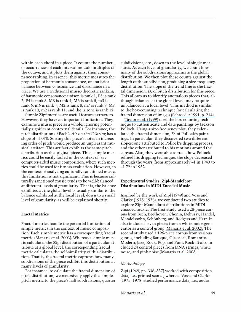
reporting what they liked or even what they judgedas beautiful. We are not aware of any studies relat-ing how one’s musical preferences or formal train-ing might affect one’s reporting of pleasantness.However, there is evidence that pleasantness andliking are not the same (Schubert 1996). Also, it hasbeen shown that pleasantness represents a moreuseful predictor of emotions than liking when usingthe above selection space in the music domain (Ri-tossa and Rickard 2004).

For the ANN experiment, we divided each musicexcerpt into segments. All segments started at 0:00and extended in increments of four seconds. That is,the first segment extended from 0:00 to 0:04, thesecond segment from 0:00 to 0:08, the third seg-ment from 0:00 to 0:12, and so on. We applied Zipfmetrics to extract 81 features per music increment.Each feature vector was associated with a desiredoutput vector of (1, 0) indicating pleasant and (0, 1)indicating unpleasant. This generated a total of 210training vectors.

We conducted a twelve-fold, “leave-one-out,”cross-validation study. This allowed for twelve pos-sible combinations of eleven pieces to be learnedand one piece to be tested. We experimented withvarious ANN architectures. The best one was afeed-forward ANN with 81 elements in the input

layer, 18 in the hidden layer, and two in the outputlayer. Internally, the ANN was divided into two 81× 9 × 1 “Siamese-twin” pyramids, both sharing thesame input layer. One pyramid was trained to recog-nize pleasant music, the other unpleasant. Classifi-cation was based on the average of the two outputs.

Results

Table 5 shows the results from all 12 experiments.The ANN performed extremely well with an aver-age success rate of 98.41 percent. All pieces wereclassified with 100 percent accuracy, with one ex-ception: Berg’s piece was classified with only 80.95percent accuracy. The ANN was considered suc-cessful if it rated a music excerpt within one stan-dard deviation of the average human rating; thiscovers 68 percent of the human responses.

There are two possibilities for this “failure” of theANN. Either our metrics fail to capture essential as-pects of Berg’s piece, or the other eleven pieces donot contain sufficient information to enable the in-terpretation of Berg’s piece.

Figure 3a displays the average human ratings forVivaldi’s Double Violin Concerto in A minor, F. 1.,No. 177. Figure 3b shows the pleasantness ratingspredicted by the ANN for the same piece. The

65

Table 5. Summary of Results from Twelve-Fold, Cross-Validation ANN Experiment, Listed by Composer ofTest Piece

MSE

Composer Success Rate (%) Cycles Train Test

Beethoven 100.00 32200 0.008187 0.003962Debussy 100.00 151000 0.001807 0.086451Mozart 100.00 222200 0.004430 0.003752Schubert 100.00 592400 0.001982 0.004851Tchaikovsky 100.00 121400 0.004268 0.004511Vivaldi 100.00 431600 0.003870 0.009643Bartók 100.00 569200 0.001700 0.008536Berg 80.95 4600 0.015412 0.100619Messiaen 100.00 35200 0.008392 0.001315Schönberg 100.00 8000 0.016806 0.015803Stravinksy 100.00 311200 0.004099 0.002693Webern 100.00 468600 0.002638 0.013540

Average 98.41 245633 0.006133 0.021306Std. Dev. 5.27 212697 0.004939 0.032701

of 50 denotes a neutral re-sponse. (b) Pleasantnessclassification by ANN ofthe same piece havingbeen trained on the other11 pieces.

Figure 3. (a) Average pleas-antness (o) and activation(x) ratings from 21 humansubjects for the first 1 min,46 sec of Vivaldi’s DoubleViolin Concerto in A mi-nor, F. 1, No. 177. A rating

ANN prediction approximates the average humanresponse.

Relevance of Metrics

The analysis of ANN weights associated with eachmetric gives an indication of its relevance for a par-ticular task. A large median value suggests that, forat least half of the ANNs in the experiment, themetric was useful in performing the particular task.There were 13 metrics that had median ANNweights of at least 7. Table 6 lists these metrics indescending order with respect to the median. It alsolists the mean ANN weights, standard deviations,and the ratio of standard deviation and mean.

Among the metrics with the highest medians,two of them stand out: harmonic consonance andchromatic tone. This is because they have a highmean and relatively small standard deviation, as in-dicated by the last column of Table 6. It can be ar-gued that these metrics were most consistentlyrelevant for “pleasantness” prediction across alltwelve experiments.

As mentioned earlier, harmonic consonance cap-tures the statistical proportion of consonance anddissonance in a piece. “Pleasant” pieces in our cor-pus exhibited similarities in their proportions ofharmonic consonance: the slope ranged from–0.8609 (Schubert, 0:08 sec) to –1.8087 (Beethoven,0:40) with an average of –1.2225 and standard devia-tion of 0.1802. “Unpleasant” pieces in our corpusalso exhibited similarities in their proportions ofharmonic consonance; in this case, however, theslope ranged from –0.2284 (Schönberg, 0:24) to–0.9919 (Berg, 0:20) with an average of –0.5343 andstandard deviation of 0.1519. Owing to the overlapbetween the two ranges, the ANN had to rely on ad-ditional metrics for disambiguation.

Chromatic tone captures the uniform distribu-tion of pitch, which is characteristic of twelve-toneand aleatoric music. Such music was rated consis-tently by our subjects as rather “unpleasant.” Thechromatic tone slope for “unpleasant” pieces rangedfrom –0.0578 (Webern, 0:48) to –1.4482 (Stravinsky,0:32), with an average of –0.6307 and standard devi-ation of 0.3985. On the other hand, the chromatictone slope for “pleasant” pieces ranged from –0.4491(Debussy, 0:16) to –1.8848 (Mozart, 0:68), with anaverage of –1.3844 and standard deviation of 0.3075.The chromatic tone metric was less relevant forclassification than harmonic consonance owing tothe greater overlap in the ranges of slopes between“pleasant” and “unpleasant” pieces. Other relevantmetrics include chromatic-tone distance, pitch du-ration, harmonic interval, harmonic and melodicinterval, harmonic bigrams, and melodic bigrams.

Discussion

These results indicate that, in most cases, the ANNis identifying patterns that are relevant to humanaesthetic judgments. This supports the hypothesis

66 Computer Music Journal

(a)

(b)

Manaris et al.

that there may be a connection between aestheticsand Zipf-Mandelbrot distributions at the level ofMIDI-encoded music.

It was interesting to note that harmonic conso-nance approximated a 1/f distribution for piecesthat were rated as pleasant and a more chaotic 1/f0.5

distribution for pieces that were rated as unpleas-ant. Because the emotional responses used in thisstudy were actually psychological self-report mea-sures, this suggests the influence of a higher level oforganization. Also, because an emotional measureis involved, this likely reflects some higher-levelpattern of intellectual processing that exhibits 1/forganization. This processing likely draws uponother, non-auditory information in the brain.

Conclusions

We propose the use of Zipf-based metrics as a basisfor author- and style-identification tasks and for theassessment of aesthetic properties of music pieces.The experimental results in author-identificationtasks, where an average success rate of more than94 percent was attained, show that the used set ofmetrics, and accordingly Zipf’s Law, capture mean-ingful information about the music pieces. Clearly,the success of this approach does not imply thatother metrics or approaches are irrelevant.

As noticed by several researchers, culturally sanc-tioned music tends to exhibit near-ideal Zipf distri-butions across various parameters. This suggeststhe possibility that combinations of Zipf-based met-rics may represent certain necessary but not suffi-cient conditions for aesthetically pleasing music.This is supported by our pleasantness study wherean ANN succeeds in predicting human aestheticjudgments of unknown pieces with more than 98percent accuracy.

The set of 40 metrics used in these studies repre-sent only a small subset of possible metrics. Theanalysis of ANN weights indicates that harmonicconsonance and chromatic tone were related to hu-man aesthetic judgments. Based on this analysisand on additional testing, we are trying to deter-mine the most useful metrics overall and to developadditional ones.

It should be emphasized that the metrics pro-posed in this article offer a particular description ofthe musical pieces, where traditional musical struc-tures such as motives, tonal structures, etc., are notmeasured explicitly. Statistical measurements, suchas Zipf’s Law, tend to focus on general trends andthus can miss significant details. To further explorethe capabilities and limitations of our approach, weare developing an evolutionary music generationsystem in which the proposed classificationmethodology will be used for fitness assignment.

67

Table 6. Statistical Analysis of ANN Weights for Metrics Used in the “Pleasantness” Prediction ANN Ex-periment (Ordered by Median)

Metric Median Mean Std. Dev. Std. Dev./Mean

Harmonic-melodic interval (simple slope) 57.43 64.22 45.09 0.70Harmonic consonance (simple slope) 44.54 44.48 17.13 0.39Harmonic bigram (simple slope) 37.76 41.37 31.88 0.77Pitch duration (simple slope) 32.34 32.53 20.01 0.62Harmonic interval (simple R2) 23.54 23.25 15.18 0.65Chromatic-tone distance (simple slope) 21.82 27.69 16.00 0.58Chromatic tone (simple slope) 19.93 21.83 7.75 0.36Melodic bigrams (simple slope) 15.74 20.83 17.82 0.86Duration (simple R2) 9.38 10.23 7.60 0.74Harmonic interval (simple slope) 8.39 8.21 5.90 0.72Fourth high order (fractal slope) 8.16 8.26 4.86 0.59Melodic interval (fractal slope) 7.81 8.37 3.42 0.41Harmonic bigram (simple R2) 7.46 10.28 11.64 1.13

Once developed, this system will be included in ahybrid society populated by artificial and humanagents, allowing us to perform further testing in adynamic environment.

In closing, our studies show that Zipf’s Law, asencapsulated in our metrics, can be used effectivelyin music classification tasks and aesthetic evalua-tion. This may have significant implications formusic information retrieval and computer-aidedmusic analysis and composition, and may provideinsights on the connection among music, nature,and human physiology. We regard these results aspreliminary; we hope they will encourage furtherinvestigation of Zipf’s Law and its potential applica-tions to music classification and aesthetics.

Acknowledgments

This project has been partially supported by an in-ternal grant from the College of Charleston and adonation from the Classical Music Archives. Wethank Renée McCauley, Ramona Behravan, andClay McCauley for their comments. WilliamDaugherty and Marisa Santos helped conduct theANN experiments. Brian Muller, Christopher Wag-ner, Dallas Vaughan, Tarsem Purewal, Charles Mc-Cormick, and Valerie Sessions helped formulate andimplement Zipf metrics. Giovanni Garofalo helpedcollect human emotional response data for theANN pleasantness experiment. William Edwards,Jr., Jimmy Wilkinson, and Kenneth Knuth providedearly material and inspiration.

References

Adamic, L. A., and B. A. Huberman. 2000. “The Nature ofMarkets in the World Wide Web.” Quarterly Journal ofElectronic Commerce 1(1):5–12.

Anderson, C. M. 2000. “From Molecules to Mindfulness:How Vertically Convergent Fractal Time FluctuationsUnify Cognition and Emotion.” Consciousness & Emo-tion 1:2:193–226.

Arnheim, R. 1971. Entropy and Art: An Essay on Disor-der and Order. Berkeley: University of California Press.

Aucouturier, J.-J., and F. Pachet. 2003. “Representing Mu-sical Genre: A State of the Art.” Journal of New MusicResearch 32(1):83–93.

Bak, P. 1996. How Nature Works: The Science of Self-Organized Criticality. New York: Springer-Verlag.

Bak, P., C. Tang, and K. Wiesenfeld. 1987. “Self-OrganizedCriticality: An Explanation for 1/f Noise.” Physical Re-view Letters 59:381–384.

Barrett, L. F., and J. A. Russell. 1999. “The Structure ofCurrent Affect: Controversies and Emerging Consen-sus.” Current Directions in Psychological Science8(1):10–14.

Burgos, J. D., and P. Moreno-Tovar. 1996 “Zipf-ScalingBehavior in the Immune System.” Biosystems 39(3):227–232.

Eco, U. 1986. Art and Beauty in the Middle Ages. H.Bredin, trans. New Haven: Yale University Press.

Elliot, J., and E. Atwell. 2000. “Is Anybody Out There?The Detection of Intelligent and Generic Language-Like Features.” Journal of the British InterplanetarySociety 53(1/2):13–22.

Ferrer Cancho, R., and R. V. Solé. 2003. “Least Effort andthe Origins of Scaling in Human Language.” Proceed-ings of the National Academy of Sciences, U.S.A100(3):788–791.

Hsu, K. J., and A. Hsu. 1991. “Self-Similarity of the ‘1/fNoise’ Called Music.” Proceedings of the NationalAcademy of Sciences, U.S.A. 88(8):3507–3509.

Li, W. 1992. “Random Texts Exhibit Zipf’s-Law-LikeWord Frequency Distribution.” IEEE Transactions onInformation Theory 38(6):1842–1845.

Li, W. 1998. “Letter to the Editor.” Complexity 3(5):9–10.Li, W., and Y. Yang. 2002. “Zipf’s Law in Importance of

Genes for Cancer Classification using MicroarrayData.” Journal of Theoretical Biology 219:539–551.

Livio, M. 2002. The Golden Ratio. New York: BroadwayBooks.

Machado, P., et al. 2003. “Power to the Critics—A Frame-work for the Development of Artificial Critics.” Pro-ceedings of 3rd Workshop on Creative Systems, 18thInternational Joint Conference on Artificial Intelli-gence (IJCAI 2003). Coimbra, Portugal: Center forInformatics and Systems, University of Coimbra,pp. 55–64.

Machado, P., et al. 2004. “Adaptive Critics for Evolution-ary Artists.” Proceedings of EvoMUSART2004—2ndEuropean Workshop on Evolutionary Music and Art.Berlin: Springer-Verlag, pp. 437–446.

Manaris, B., T. Purewal, and C. McCormick. 2002. “Pro-gress Towards Recognizing and Classifying BeautifulMusic with Computers: MIDI-Encoded Music and the

68 Computer Music Journal

Manaris et al.

Zipf-Mandelbrot Law.” Proceedings of the IEEE South-eastCon 2002. New York: Institute of Electrical andElectronics Engineers, pp. 52–57.

Manaris, B., et al. 2003. “Evolutionary Music and theZipf-Mandelbrot Law: Progress towards Developing Fit-ness Functions for Pleasant Music.” Proceedings ofEvoMUSART2003—1st European Workshop on Evolu-tionary Music and Art. Berlin: Springer-Verlag,pp. 522–534.

Mandelbrot, B. B. 1977. The Fractal Geometry of Nature.New York: W. H. Freeman.

Maslov, S., C. Tang, and Y.-C. Zhang. 1999. “1/f Noise inBak-Tang-Wiesenfeld Models on Narrow Stripes.”Physical Review Letters 83(12):2449–2452.

May, M. 1996. “Did Mozart Use the Golden Section?”American Scientist 84(2):118.

Meyer, L. B. 2001. “Music and Emotion: Distinctions andUncertainties.” In P. N. Juslin and J. A. Sloboda, eds.Music and Emotion—Theory and Research. Oxford:Oxford University Press: 341–360.

Miranda, E. R. 2001. Composing Music with Computers.Oxford: Focal Press.

Miranda, E. R., et al. 2003. “On Harnessing the Electroen-cephalogram for the Musical Braincap.” Computer Mu-sic Journal 27(2):80–102.

Nettheim, N. 1997. “A Bibliography of Statistical Appli-cations in Musicology.” Musicology Australia 20:94–106.

Pampalk E., S. Dixon, and G. Widmer. 2004. “ExploringMusic Collections by Browsing Different Views.”Computer Music Journal 28(2):49–62.

Ritossa, D. A., and N. S. Rickard. 2004. “The RelativeUtility of ‘Pleasantness’ and ‘Liking’ Dimensions inPredicting the Emotions Expressed in Music.” Psychol-ogy of Music 32(1):5–22.

Salingaros, N. A., and B. J. West. 1999. “A Universal Rulefor the Distribution of Sizes.” Environment and Plan-ning B: Planning and Design 26:909–923.

Schroeder, M. 1991. Fractals, Chaos, Power Laws: Min-utes from an Infinite Paradise. New York: W. H. Free-man.

Schubert, E. 1996. “Enjoyment of Negative Emotions inMusic: An Associative Network Explanation.” Psy-chology of Music 24(1):18–28.

Schubert, E. 2001. “Continuous Measurement of Self-Report Emotional Response to Music.” In P. N. Juslinand J. A. Sloboda, eds. Music and Emotion—Theoryand Research. Oxford: Oxford University Press,pp. 393–414.

Spehar, B., et al. 2003. “Universal Aesthetic of Fractals.”Computers and Graphics 27:813–820.

Taylor, R. P., A. P. Micolich, and D. Jonas. 1999. “FractalAnalysis Of Pollock’s Drip Paintings.” Nature399:422.

Tzanetakis, G., G. Essl, and P. Cook. 2001. “AutomaticMusical Genre Classification of Audio Signals.” Pro-ceedings of 2nd Annual International Symposium onMusic Information Retrieval. Bloomington: Universityof Indiana Press, pp. 205–210.

Voss, R. F., and J. Clarke. 1975. “1/f Noise in Music andSpeech.” Nature 258:317–318.

Voss, R. F., and J. Clarke. 1978. “1/f Noise in Music: Mu-sic from 1/f Noise.” Journal of the Acoustical Societyof America 63(1):258–263.

Wolfram, S. 2002. A New Kind of Science. Champaign,Illinois: Wolfram Media.

Zhang, K., and T. J. Sejnowski. 2000. “A Universal ScalingLaw between Gray Matter and White Matter of Cere-bral Cortex.” Proceedings of the National Academy ofSciences, U.S.A 97(10):5621–5626.

Zipf, G. K. 1949. Human Behavior and the Principle ofLeast Effort. New York: Addison-Wesley.

69