ж сжсыв ы ь з ттжс ьс п я рь жщ ы п р ся ьжщ
37
http://www-fourier.ujf-grenoble.fr/ ˜demailly/documents.html R´ esum´ e: L’objectif de ce texte est de proposer une piste pour un enseignement logiquement rigoureux et cependant assez simple de la g´ eom´ etrie euclidienne au coll` ege et au lyc´ ee. La g´ eom´ etrie euclidienne se trouve ˆ etre un domaine tr` es privil´ egi´ e des math´ ematiques, ` a l’int´ erieur duquel il est possible de mettre en uvre d` es le d´ epart des raisonnements riches, tout en faisant appel de mani` ere remarquable ` a la vision et ` a l’intuition. Notre pr´ eoccupation est d’autant plus grande que l’´ evolution des programmes scolaires depuis 3 ou 4 d´ ecennies r´ ev` ele une diminution tr` es marqu´ ee des contenus g´ eom´ etriques en- seign´ es, en mˆ eme temps qu’un affaiblissement du raisonnement math´ ematique auquel l’enseignement de la g´ eom´ etrie permettait pr´ ecis´ ement de contribuer de fa¸ con essen- tielle. Nous esp´ erons que ce texte sera utile aux professeurs et aux auteurs de manuels de math´ ematiques qui ont la possibilit´ e de s’affranchir des contraintes et des pre- scriptions trop indigentes des programmes officiels. Les premi` eres sections devraient id´ ealement ˆ etre maˆ ıtris´ ees aussi par tous les professeurs d’´ ecole, car il est ` a l’´ evidence tr` es utile d’avoir du recul sur toutes les notions que l’on doit enseigner ! Mots-cl´ es : g´ eom´ etrie euclidienne Resumen : El objetivo de este art´ ıculo es presentar un enfoque riguroso y a´ un razonablemente simples para la ense˜ nanza de la geometr´ ıa euclidiana elemental a nivel de educaci´ on secundaria. La geometr´ ıa euclidiana es una ´ area privilegiada de las matem´ aticas, ya que permite desde un primer nivel practicar razonamientos rigurosos y ejercitar la visi´ on y la intuici´ on. Nuestra preocupaci´ on es que las numerosas reformas de planes de estudio en las ´ ultimas 3 d´ ecadas en Francia, y posiblemente en otros pa´ ıses occidentales, han llevado a una disminuci´ on preocupante de la geometr´ ıa, junto con un generalizado debilitamiento del razonamiento matem´ atico al que la geometr´ ıa contribuye espec´ ıficamente de manera esencial. Esperamos que este punto de vista sea de inter´ es para los autores de libros de texto y tambi´ en para los profesores que tienen la posibilidad de no seguir exactamente las prescripciones sobre los contenidos menos relevantes, cuando est´ an por desgracia impuestos por las autoridades educativas y por los planes de estudios. El contenido de las primeras secciones, en principio, deber´ ıa tambi´ en ser dominado por los profesores de la escuela primaria, ya que siempre es recomendable conocer m´as de lo que uno tiene que ense˜ nar, a cualquier nivel ! Palabras clave : Geometr´ ıa euclidiana
-
Upload
khangminh22 -
Category
Documents
-
view
2 -
download
0
Transcript of ж сжсыв ы ь з ттжс ьс п я рь жщ ы п р ся ьжщ

A rigorous dedu tive approa h to
elementary Eu lidean geometry
Jean-Pierre Demailly
Universit�e Joseph Fourier Grenoble I
http://www-fourier.ujf-grenoble.fr/ demailly/documents.html
Resume :
L’objectif de ce texte est de proposer une piste pour un enseignement logiquementrigoureux et cependant assez simple de la geometrie euclidienne au college et au lycee.La geometrie euclidienne se trouve etre un domaine tres privilegie des mathematiques,a l’interieur duquel il est possible de mettre en uvre des le depart des raisonnementsriches, tout en faisant appel de maniere remarquable a la vision et a l’intuition. Notrepreoccupation est d’autant plus grande que l’evolution des programmes scolaires depuis3 ou 4 decennies revele une diminution tres marquee des contenus geometriques en-seignes, en meme temps qu’un affaiblissement du raisonnement mathematique auquell’enseignement de la geometrie permettait precisement de contribuer de facon essen-tielle. Nous esperons que ce texte sera utile aux professeurs et aux auteurs de manuelsde mathematiques qui ont la possibilite de s’affranchir des contraintes et des pre-scriptions trop indigentes des programmes officiels. Les premieres sections devraientidealement etre maıtrisees aussi par tous les professeurs d’ecole, car il est a l’evidencetres utile d’avoir du recul sur toutes les notions que l’on doit enseigner !
Mots-cles : geometrie euclidienne
Resumen :
El objetivo de este artıculo es presentar un enfoque riguroso y aun razonablementesimples para la ensenanza de la geometrıa euclidiana elemental a nivel de educacionsecundaria. La geometrıa euclidiana es una area privilegiada de las matematicas,ya que permite desde un primer nivel practicar razonamientos rigurosos y ejercitarla vision y la intuicion. Nuestra preocupacion es que las numerosas reformas deplanes de estudio en las ultimas 3 decadas en Francia, y posiblemente en otrospaıses occidentales, han llevado a una disminucion preocupante de la geometrıa, juntocon un generalizado debilitamiento del razonamiento matematico al que la geometrıacontribuye especıficamente de manera esencial. Esperamos que este punto de vista seade interes para los autores de libros de texto y tambien para los profesores que tienenla posibilidad de no seguir exactamente las prescripciones sobre los contenidos menosrelevantes, cuando estan por desgracia impuestos por las autoridades educativas y porlos planes de estudios. El contenido de las primeras secciones, en principio, deberıatambien ser dominado por los profesores de la escuela primaria, ya que siempre esrecomendable conocer mas de lo que uno tiene que ensenar, a cualquier nivel !
Palabras clave : Geometrıa euclidiana

2 A rigorous dedu tive approa h to elementary Eu lidean geometry
0. Introdu tion
The goal of this article is to explain a rigorous and still reasonably simple approach toteaching elementary Euclidean geometry at the secondary education levels. Euclideangeometry is a privileged area of mathematics, since it allows from an early stage topractice rigorous reasonings and to exercise vision and intuition. Our concern is thatthe successive reforms of curricula in the last 3 decades in France, and possibly in otherwestern countries as well, have brought a worrying decline of geometry, along with aweakening of mathematical reasoning which geometry specifically contributed to in anessential way. We hope that these views will be of some interest to textbook authorsand to teachers who have a possibility of not following too closely the prescriptionsfor weak contents, when they are unfortunately enforced by education authorities andcurricula. The first sections should ideally also be mastered by primary school teachers,as it is always advisable to know more than what one has to teach at any given level !
Keywords : Euclidean geometry
1. On axiomati approa hes to geometry
As a formal discipline, geometry originates in Euclid’s list of axioms and the work ofhis successors, even though substantial geometric knowledge existed before.
An excerpt of Euclid’s book
The traditional teaching of geometry that took place in France during the period 1880-1970 was directly inspired by Euclid’s axioms, stating first the basic properties ofgeometric objects and using the “triangle isometry criteria” as the starting point ofgeometric reasoning. This approach had the advantage of being very effective and ofquickly leading to rich contents. It also adequately reflected the intrinsic nature ofgeometric properties, without requiring extensive algebraic calculations. These choicesechoed a mathematical tradition that was firmly rooted in the nineteenth century,aiming to develop “pure geometry”, the highlight of which was the development ofprojective geometry by Poncelet.
Euclid’s axioms, however, were neither complete nor entirely satisfactory from a logical

1. On axiomati approa hes to geometry 3
perspective, leading mathematicians as Hilbert and Pasch to develop the system ofaxioms now attributed to Hilbert, that was settled in his famous memoir Grundlagender Geometrie in 1899.
David Hilbert (1862–1943 ), in 1912
It should be observed, though, that the complexity of Hilbert’s system of axiomsmakes it actually unpractical to teach geometry at an elementary level(1). The result,therefore, was that only a very partial axiomatic approach was taught, leading to asituation where a large number of properties that could have been proved formally hadto be stated without proof, with the mere justification that they looked intutivelytrue. This was not necessarily a major handicap, since pupils and their teachersmay not even have noticed the logical gaps. However, such an approach, eventhough it was in some sense quite successful, meant that a substantial shift had tobe accepted with more contemporary developments in mathematics, starting alreadywith Descartes’ introduction of analytic geometry. The drastic reforms implementedin France around 1970 (with the introduction of “modern mathematics”, under thedirection of Andre Lichnerowicz) swept away all these concerns by implementing anentirely new paradigm : according to Jean Dieudonne, one of the Bourbaki founders,geometry should be taught as a corollary of linear algebra, in a completely general andformal setting. The first step of the reform implemented this approach from “classede seconde” (grade 10) on. A major problem, of course, is that the linear algebraviewpoint completely departs from the physical intuition of Euclidean space, wherethe group of invariance is the group of Euclidean motions and not the group of affinetransformations.
(1)Even the improved and simpli�ed version of Hilbert's axioms presented by Emil Artin in his famous
book �Geometri Algebra� an hardly be taught before the 3
rd
or 4
th
year at university.

4 A rigorous dedu tive approa h to elementary Eu lidean geometry
from Descartes (1596-1650 ) to Dieudonne (1906-1992 ) and Lichnerowicz (1915-1998 )
The reform could still be followed in a quite acceptable way for about one decade,as long as pupils had a solid background in elementary geometry from their earliergrades, but became more and more unpractical when primary school and junior highschool curricula were themselves (quite unfortunately) downgraded. All mathematicalcontents of high school were then severely axed around 1986, resulting in curriculaprescriptions that in fact did not allow any more the introduction of substantialdeductive activity, at least in a systematic way.
We believe however that it is necessary to introduce the basic language of mathematics,e.g. the basic concepts of sets, inclusion, intersection, etc, as soon as needed, mostcertainly already at the beginning of junior high school. Geometry is a very appropriategroundfield for using this language in a concrete way.
2. Geometry, numbers and arithmeti operations
An important issue is the relation between geometry and numbers. Greek mathemati-cians already had the fundamental idea that ratios of lengths with a given unit lengthwere in one to one correspondence with numbers : in modern terms, there is a natu-ral distance preserving bijection between points of a line and the set of real numbers.This viewpoint is of course not at all in contradiction with elementary education sincemeasuring lengths in integer (and then decimal) values with a ruler is one of of thefirst important facts taught at primary school. However, at least in France, severalreforms have put forward the extremely toxic idea that the emergence of electroniccalculators would somehow free pupils from learning elementary arithmetic algorithmsfor addition, subtraction, multiplication and division, and that mastering magnitudeorders and the “meaning” of arithmetic operations would be more than enough tounderstand society and even to pursue in science. The fact is that one cannot con-ceptually separate numbers from the operations that can be performed on them, andthat mastering algorithms mentally and in written form is instrumental to realizingmagnitude orders and the relation of numbers with physical quantities. The first con-tact that pupils will have with “elementary physics”, again at primary school level,is probably through measuring lengths, areas, volumes, weights, densities, etc. Un-derstanding the link with arithmetic operations is the basic knowledge that will be

3. First steps of the introdu tion of Eu lidean geometry 5
involved later to connect physics with mathematics. The idea of a real number as apossibly infinite decimal expansion then comes in a natural way when measuring agiven physical quantity with greater and greater accuracy. Square roots are forcedupon us by Pythagoras’ theorem, and computing their numerical values is also a verygood introduction to the concept of real number. I would certainly recommend to(re)introduce from the very start of junior high school (not later than grade 6 and7), the observation that fractions of integers produce periodic decimal expansions, e.g.1/7 = 0.142857142857 ... , while no visible period appears when computing the squareroot of 2. In order to understand this (and before any formal proof can be given, asthey are conceptually harder to grasp), it is again useful to learn here the hand andpaper algorithm for computing square roots, which is only slightly more involved thanthe division algorithm and makes it immediately clear that there is no reason the resulthas to be periodic – unfortunately, this algorithm is no longer taught in France sincea long time. When all this work is correctly done, it becomes really possible to give aprecise meaning to the concept of real number at junior high school – of course manymore details have to be explained, such as the identification of proper and improperdecimal expansions, e.g. 1 = 0.99999 ... , the natural order relation on such expansions,decimal approximations with at given accuracy, etc. In what follows, we propose anapproach to geometry based on the assumption that pupils have a reasonable under-standing of numbers, arithmetic operations and physical quantities from their primaryschool years – with consolidation about things such infinite decimal expansions andsquare roots in the first two years of junior high school ; this was certainly the situa-tion that prevailed in France before 1970, but things have unfortunately changed forthe worse since then. Our small experimental network of schools SLECC (“Savoir LireEcrire Compter Calculer”), which accepts random pupils and operates in random partsof the country, shows that such knowledge can still be reached today for a very largemajority of pupils, provided appropriate curricula are enforced. For the others, ourviews will probably remain a bit utopistic, or will have to be delayed and postponedat a later stage.
3. First steps of the introdu tion of Eu lidean geometry
3.1. Fundamental concepts
The primitive concepts we are going to use freely are :
• real numbers, with their properties already discussed above ;
• points and geometric objects as sets of points : a point should be thought of as ageometric object with no extension, as can be represented with a sharp pencil ; aline or a curve are infinite sets of points (at this point, this is given only for intuition,but will not be needed formally) ;
• distances between points.
Let us mention that the language of set theory has been for more than one centurythe universal language of mathematicians. Although excessive abstraction should beavoided at early stages, we feel that it is appropriate to introduce at the beginningof junior high school the useful concepts of sets, of inclusion, the notation x ∈ E,

6 A rigorous dedu tive approa h to elementary Eu lidean geometry
operations on sets such as union, intersection and difference ; geometry and numbersalready provide rich and concrete illustrations.
A geometric figure is simply an ordered finite collection of points Aj and sets Sk
(vertices, segments, circles, arcs, ...)
Given two points A, B of the plane or of space, we denote by d(A,B) (or simply by AB)their distance, which is in general a positive number, equal to zero when the points Aand B coincide – concretely, this distance can be mesured with a ruler. A fundamentalproperty of distances is :
3.1.1. Triangular inequality. For any triple of points A,B,C, their mutual distancesalways satisfy the inequality AC 6 AB +BC, in other words the length of any side ofa triangle is always at most equal to the sum of the lengths of the two other sides.
Intuitive justification.
A
B
C
H
A
B
CH
Let us draw the height of the triangle joining vertex B to point H on the oppositeside (AC).
If H is located between A and C, we get AC = AH + HC ; on the other hand, ifthe triangle is not flat (i.e. if H 6= B), we have AH < AB and HC < BC (sincethe hypotenuse is longer than the right-angle sides in a right-angle triangle – this willbe checked formally thanks to Pythagoras’ theorem). If H is located outside of thesegment [A,C], for instance beyond C, we already have AC < AH 6 AB, thereforeAC < AB 6 AB +BC.
This justification(2) shows that the equality AC = AB + BC holds if and only if thepoints A, B, C are aligned with B located between A and C (in this case, we haveH = B on the left part of the above figure). This leads to the following intrinsicdefinitions that rely on the concept of distance, and nothing more(3).
3.1.2. Definitions (segments, lines, half-lines).
(a) Given two points A, B in a plane or in space, the segment [A,B] of extremitiesA, B is the set of points M such that AM +MB = AB.
(2)This is not a real proof sin e one relies on unde�ned on epts and on fa ts that have not yet been
proved, for example, the on ept of line, of perpendi ularity, the existen e of a point of interse tion
of a line with its perpendi ular, et ... This will a tually ome later (without any vi ious ir le, the
justi� ations just serve to bring us to the appropriate de�nitions!)
(3)As far as they are on erned, these de�nitions are perfe tly legitimate and rigorous, starting from our
primitive on epts of points and their mutual distan es. They would still work for other geometries
su h as hyperboli geometry or general Riemannian geometry, at least when geodesi ar s are uniquely
de�ned globally.

3. First steps of the introdu tion of Eu lidean geometry 7
(b) We say that three points A, B, C are aligned with B located between A and C ifB ∈ [A,C], and we say that they are aligned (without further specification) if oneof the three points belongs to the segment determined by the two other points.
(c) Given two distinct points A, B, the line (AB) is the set of points M that arealigned with A and B ; the half-line [A,B) of origin A containing point B is the setof points M aligned with A and B such that either M is located between A and B,or B between A and M . Two half-lines with the same origin are said to be oppositeif their union is a line.
In the definition, part (a) admits the following physical interpretration : a line segmentcan be realized by stretching a thin and light wire between two points A and B :when the wire is stretched, the points M located between A and B cannot ”deviate”,otherwise the distance AB would be shorter than the length of the wire, and the lattercould still be stretched further . . .
We next discuss the notion of an axis : this is a line D equipped with an origin O anda direction, which one can choose by specifying one of the two points located at unitinstance from O, with the abscissas +1 and −1 ; let us denote them respectively by Iand I ′. A point M ∈ [O, I) is represented by the real value xM = +OM and a point Mon the opposite half-line [O, I ′) by the real value xM = −OM . The algebraic measureof a bipoint (A,B) of the axis is defined by AB = xB − xA, which is equal to +AB or−AB according to whether the ordering of A, B corresponds to the orientation or toits opposite. For any three points A, B, C of D, we have the Chasles relation
AB +BC = AC.
This relation can be derived from the equality (xB − xA) + (xC − xB) = (xC − xA)after a simplification of the algebraic expression.
Building on the above concepts of distance, segments, lines and half-lines, we can nowdefine rigorously what are planes, half-planes, circles, circle arcs, angles . . .(4)
3.1.3. Definitions.
(a) Two lines D, D′ are said to be concurrent if their intersection consists of exactlyone point.
(b) A plane P is a set of points that can be realized as the union of a family of lines(UV ) such that U describes a line D and V a line D′, for some concurrent linesD and D′ in space. If A, B, C are 3 non aligned points, we denote by (ABC) theplane defined by the lines D = (AB) and D′ = (AC) (say)(5).
(4)Of ourse, this long series of de�nitions is merely intended to explain the sequen e of on epts in a
logi al order. When tea hing to pupils, it would be ne essary to approa h the on epts progressively,
to give examples and illustrations, to let the pupils solve exer ises and produ e related onstru tions
with instruments (ru2ler, ompasses . . .).
(5)In a general manner, one ould de�ne by indu tion on n the on ept of an a�ne subspa e Sn of
dimension n : this is the set obtained as the union of a family of lines (UV ), where U des ribes a line
D and V des ribes an a�ne subspa e Sn−1
of dimension n − 1 interse ting D in exa tly one point.
Our de�nitions are valid in any dimension (even in an in�nite dimensional ambient spa e), without
taking spe ial are !

8 A rigorous dedu tive approa h to elementary Eu lidean geometry
(c) Two lines D and D′ are said to be parallel if they coincide, or if they are both
contained in a certain plane P and do not intersect.
(d) A salient angle {BAC (or a salient angular sector) defined by two non oppositehalf-lines [A,B), [A,C) with the same origin is the set obtained as the union of thefamily of segments [U, V ] with ∈ [A,B) and V ∈ [A,C).
(e) A reflex angle (or a reflex angular sector) BAC is the complement of the corre-
sponding salient angle {BAC in the plane (ABC), in which we agree to include thehalf-lines [A,B) and [A,C) in the boundary.
(f) Given a line D and a point M outside D, the half-plane bounded by D containing
M is the union of the two angular sectors {BAM and {CAM obtained by expressingD as the union of two opposite half-lines [A,B) and [A,C) ; this is the union of allsegments [U, V ] such that U ∈ D and V ∈ [A,M). The opposite half-plane is theone associated with the half-line [A,M ′) opposite to [A,M). In that situation, wealso say that we have flat angles of vertex A.
(g) In a given plane P, a circle of center A and radius R > 0 is the set of points M inthe plane P such that d(A,M) = AM = R.
(h) A circular arc is the intersection of a circle with an angular sector, the vertex ofwhich is the center of the circle.
(i) The measure of an angle (in degrees) is proportional to the length of the circular arcthat it intercepts on a circle whose center coincides with the vertex of the angle, insuch a way that the full circle corresponds to 360◦. A flat angle (cut by a half-planebounded by a diameter of the circle) corresponds to an arc formed by a half-circleand has measure 180◦. A right angle is one half of a flat angle, that is, an anglecorresponding to the quarter of a circle, in other words, an angle of measure equalto 90◦.
(j) Two half-lines with the same origin are said to be perpendicular if they form a rightangle.(5)
The usual properties of parallel lines and of angles intercepted by such lines (“corre-sponding angles” vs “alternate angles”) easily leads to establishing the value of thesum of angles in a triangle (and, from there, in a quadrilateral).
Definition (i) requires of course a few comments. The first and most obvious commentis that one needs to define what is the length of a circular arc, or more generally of acurvilign arc : this is the limit (or the upper bound) of the lengths of polygonal lineinscribed in the curve, when the curve is divided into smaller and smaller portions (cf.2.2)(5). The second one is that the measure of an angle is independent of the radius Rof the circle used to evaluate arc lengths; this follows from the fact that arc lengths areproportional to the radius R, which itself follows from Thales’ theorem (see below).
(5)The on epts of right and �at angles, as well as the notion of half angle are already primary s hool
on erns. At this level, the best way to address these issues is probably to let pupils pra ti e paper
folding (the notion of horizontality and verti ality are relative on epts, it is better to avoid them
when introdu ing perpendi ularity, so as to avoid any potential onfusion).
(5)The de�nition and existen e of limits are di� ult issues that annot be addressed before high s hool,
but it seems appropriate to introdu e this idea at least intuitively.

3. First steps of the introdu tion of Eu lidean geometry 9
Moreover, a proportionality argument yields the formula for the length of a circulararc located on a circle of radius R : a full arc (360◦) has length 2πR, hence the lengthof an arc of 1◦ is 360 times smaller, that is 2πR/360 = πR/180, and an arc of measurea (in degrees) has length
ℓ = (πR/180)× a = R × a× π/180.
3.2. Construction with instruments and isometry criteria for triangles
As soon as they are introduced, it is extremely important to illustrate geometricconcepts with figures and construction activities with instruments. Basic constructionswith ruler and compasses, such as midpoints, medians, bissectors, are of an elementarylevel and should be already taught at primary school. The step that follows immediatelynext consists of constructing perpendiculars and parallel lines passing through a givenpoint.
At the beginning of junior high school, it becomes possible to consider conceptuallymore advanced matters, e.g. the problem of constructing a triangle ABC with a givenbase BC and two other elements, for instance :
(3.2.1) the lengths of sides AB and AC,
(3.2.2) the measures of angles {ABC and {ACB,
(3.2.3) the length of AB and the measure of angle {ABC.
A
B
C
A
B
CA
B
C
In the first case, the solution is obtained by constructing circles of centers B, C andradii equal to the given lengths AB and AC, in the second case a protractor is used todraw two angular sectors with respective vertices B and C, in the third case one drawsan angular sector of vertex B and a circle of center B. In each case it can be seen thatthere are exactly two solutions, the second solution being obtained as a triangle A′BCthat is symmetric of ABC with respect to line (BC) :
A′B
C
A′B
C
A′
B
C
One sees that the triangles ABC and A′BC have in each case sides with the samelengths. This leads to the important concept of isometric figures.

10 A rigorous dedu tive approa h to elementary Eu lidean geometry
3.2.4. Definition.
(a) One says that two triangles are isometric if the sides that are in correspondencehave the same lengths, in such a way that if the first triangle has vertices A, B, Cand the corresponding vertices of the second one are A′, B′, C′, then A′B′ = AB,B′C′ = BC, C′A′ = CA.
(b) More generally, one says that two figures in a plane or in space are isometric,the first one being defined by points A1, A2, A3, A4 . . . and the second one bycorresponding points A′
1, A′2, A
′3, A
′4 . . . if all mutual distances coincide.
The concept of isometric figures is related to the physical concept of solid body : abody is said to be a solid if the mutual distances of its constituents (molecules, atoms)do not vary while the object is moved; after such a mo
ve, atoms which occupied certain positions Ai occupy new positions A′i and we have
A′iA
′j = AiAj. This leads to a rigorous definition of solid displacements, that have a
meaning from the viewpoints of mathematics and physics as well.
3.2.5. Definition. Given a geometric figure (or a solid body in space) defined bycharacteristic points A1, A2, A3, A4 . . ., a solid move is a continuous succession ofpositions Ai(t) of these points with respect to the time t, in such a way that all distancesAi(t)Aj(t) are constant. If the points Ai were the initial positions and the points A′
i arethe final positions, we say that the figure (A′
1A′2A
′3A
′4 . . .) is obtained by a displacement
of figure (A1A2A3A4 . . .).(6)
Beyond displacements, another way of producing isometric figures is to use a reflection(with respect to a line in a plane, or with respect to a plane in space, as obtained bytaking the image of an object through reflection in a mirror)(6). This fact is alreadyobserved with triangles, the use of transparent graph paper is then a good way ofvisualizing isometric triangles that cannot be superimposed by a displacement without“getting things out of the plane” ; in a similar way, it can be useful to constructelementary solid shapes (e.g. non regular tetrahedra) that cannot be superimposed bya solid move.
3.2.6. Exercise. In order to ensure that two quadrilaterals ABCD and A′B′C′D′
are isometric, it is not sufficient to check that the four sides A′B′ = AB, B′C′ = BC,C′D′ = CD, D′A′ = DA possess equal lengths, one must also check that the twodiagonals A′C′ = AC and B′D′ = BD be equal ; equaling only one diagonal is notenough as shown by the following construction :
(6)The on ept of ontinuity that we use is the standard ontinuity property for fun tions of one real
variable - one an of ourse introudu e this only intuitively at the junior high s hool level. One an
further show that an isometry between two �gures or solids extends an a�ne isometry of the whole
spa e, and that a solid move is represented by a positive a�ne isometry, see Se tion 10. The formal
proof is not very hard, but ertainly annot be given before the end of high s hool (this would have
been possible with the rather strong Fren h urri ula as they were 50 years ago in the grade 12 s ien e
lass, but doing so would be nowadays ompletely impossible).
(6)Conversely, an important theorem - whi h we will show later (see se tion 10) says that isometri �gures
an be dedu ed from ea h other either by a solid move or by a solid move pre eded (or followed) by a
re�e tion.

3. First steps of the introdu tion of Eu lidean geometry 11
A
B
C
D′
D
The construction problems considered above for triangles lead us to state the followingfundamental isometry criteria.
3.2.7. Isometry criteria for triangles(7). In order that two triangles be isometric,it is necessary and sufficient to check one of the following cases
(a) that the three sides be respectively equal (this is just the definition), or
(b) that they possess one angle with the same value and its adjacent sides equal, or
(c) that they possess one side with the same length and its adjacent angles of equalvalues.
One should observe that conditions (b) and (c) are not sufficient if the adjacency spec-ification is omitted - and it would be good to introduce (or to let pupils perform)constructions demonstrating this fact. A use of isometry criteria in conjunction withproperties of alternate or corresponding angles leads to the various usual characteriza-tions of quadrilaterals - parallelograms, lozenges, rectangles, squares . . .
3.3. Pythagoras’ theorem
We first give the classical “Chinese” proof of Pythagoras’ theorem, which is derivedby a simple area argument based on moving four triangles (represented here in green,blue, yellow and light red). Its main advantage is to be visual and convincing(7).
b
a
b
a
a b
a b
c
c
a2
b2 b
a
a
b
a b
b a
c
c
c
c
c2a2 + b2 = c2
(7)A rigorous formal proof of of these 3 isometry riteria will be given later, f. Se tion 8.
(7)Again, in our ontext, the argument that will be des ribed here is a justi� ation rather than a formal
proof. In fa t, it would be needed to prove that the quadrilateral entral �gure on the right hand side
is a square - this ould ertainly be he ked with isometry properties of triangles - but one should not
forget that they are not yet really proven at this stage. More seriously, the argument uses the on ept
of area, and it would be needed tp prove the existen e of an area measure in the plane with all the
desired properties : additivity by disjoint unions, translation invarian e . . .

12 A rigorous dedu tive approa h to elementary Eu lidean geometry
The point is to compare, in the left hand and right hand figures, the remaining greyarea, which is the difference of the area of the square of side a + b with the area ofthe four rectangle triangles of sides a, b, c. The equality of the grey areas impliesa2 + b2 = c2.
Complement. Let (ABC) be a triangle and a, b, c the lengths of the sides that areopposite to vertices A, B, C.
(i) If the angle C is smaller than a right angle, we have c2 < a2 + b2,
(ii) If the angle C is larger than a right angle, we have c2 > a2 + b2.
Proof. First consider the case where (ABC) is rectangle : we have c2 = a2+ b2 and theangle is equal to 90◦.
a
bc
c′c′′
B
AA′ A′′
C
If angle C is < 90◦, we have c′ < c.
If angle C is > 90◦, we have c′′ > c.
We argue by either increasing or decreasing the angle : if angle C is < 90◦, we havec′ < c ; if angle C is > 90◦, we have c′′ > c. By this reasoning, we conclude :
Converse of Pythagoras’ theorem. With the above notation, if c2 = a2 + b2, thenangle C must be a right angle, hence the given triangle is rectangle in C.
4. Cartesian oordinates in the plane
The next fundamental step of our approach is the introduction of cartesian coordinatesand their use to give formal proofs of properties that had previously been taken forgranted (or given with a partial justification only). This is done by working inorthonormal frames.
4.1. Expression of Euclidean distance
x x′
y
y′
M
M ′

4. Cartesian oordinates in the plane 13
Pythagoras’ theorem shows that the length MM ′ of the hypotenuse is given by theformula MM ′2 = (x′ − x)2 + (y′ − y)2, as the two sides of the right angle are x′ − xand y′ − y (up to sign). The distance from M to M ′ is therefore equal to
(4.1.1) d(M,M ′) = MM ′ =√
(x′ − x)2 + (y′ − y)2.
(It is of course advisable to first present the argument with simple numerical values).
4.2. Squares
Let us consider the figure formed by points A (u ; v), B (−v ; u), C (−u ; −v),D (v ; −u).
O
A (u ; v)
B (−v ; u)
C (−u ; −v)
D (v ; −u)
Formula (4.1.1) yields
AB2 = BC2 = CD2 = DA2 = (u+ v)2 + (u− v)2 = 2(u2 + v2),
hence the four sides have the same length, equal to√2√u2 + v2. Similarly, we find
OA = OB = OC = OD =√u2 + v2,
therefore the 4 isoceles triangles OAB, OBC, OCD and ODA are isometric, and as aconsequence we have {OAB = {OBC = {OCD = {ODA = 90◦ and the other angles areequal to 45◦. Hence {DAB = {ABC = {BCD = {CDA = 90◦, and we have proved thatour figure is a square.
4.3. “Horizontal and vertical” lines
The set D of points M(x ; y) such that y = c (where c is a given numerical value) is a“horizontal” line. In fact, given any three points M , M ′, M ′′ of abscissas x < x′ < x′′
we haveMM ′ = x′ − x, M ′M ′′ = x′′ − x′, MM ′′ = x′′ − x

14 A rigorous dedu tive approa h to elementary Eu lidean geometry
and therefore MM ′ +M ′M ′′ = MM ′′. This implies by definition that our points M ,M ′, M ′′. If we consider the line D1 given by the equation y = c1 with c1 6= c, this isanother horizontal line, and we have clearly D ∩D1 = ∅, therefore our lines D and D1
are parallel.
Similarly, the set D of points M(x ; y) such that x = c is a “vertical line” and the linesD : x = c, D1 : x = c1 are parallel.
4.4. Line defined by an equation y = ax + b
We start right away with the general case y = ax + b to avoid any unnecessaryrepetitions, but with pupils it would be of course more appropriate to treat first thelinear case y = ax.
x1
x2 x3
y1
y2
y3
M1
M ′1
M ′′1
M2
M3
Consider three points M1 (x1 ; y1) , M2 (x2 ; y2), M3 (x3 ; y3) satisfying the relationsy1 = ax1 + b, y2 = ax2 + b and y3 = ax3 + b, with x1 < x2 < x3, say. Asy2 − y1 = a(x2 − x1), we find
M1M2 =√
(x2 − x1)2 + a2(x2 − x1)2 =√
(x2 − x1)2(1 + a2) = (x2 − x1)√1 + a2,
and likewise M2M3 = (x3 − x2)√1 + a2, M1M3 = (x3 − x1)
√1 + a2. This shows that
M1M2 +M2M3 = M1M3, hence our points M1, M2, M3 are aligned. Moreover(8), wesee that for any point M ′
1 (x, y′1) with y′1 > ax1 + b, then this point is not aligned withM2 and M3, and similarly for M ′′
1 (x, y′′1 ) such that y′′1 < ax1 + b.
Consequence. The set D of points M (x ; y) such that y = ax+ b is a line.
The slope of line D is the ratio between the “vertical variation” and the “horizontal
(8)A rigorous formal proof would of ourse be possible by using a distan e al ulation, but this is mu h
less obvious thanwhat we have done until now. One ould however argue as in § 5.2 and use a new
oordinate frame to redu e the situation to the ase of the horizontal line Y = 0 , in whi h ase the
proof is mu h easier.

4. Cartesian oordinates in the plane 15
variation”, that is, for two points M1 (x1 ; y1), M2 (x2 ; y2) of D the ratio
y2 − y1x2 − x1
= a.
A horizontal line is a line of slope a = 0. When the slope a becomes very large, theinclination of the line D becomess intuitively close to being vertical. We thereforeagree that a vertical line has infinite slope. Such an infinite value will be denoted bythe symbol ∞ (without sign).
Consider two distinct points M1 (x1, y1), M2 (x2, y2). If x1 6= x2, we see that thereexists a unique line D : y = ax+ b passing through M1 and M2 : its slope is given bya = y2−y1
x2−x1
and we infer b = y1 − ax1 = y2 − ax2. If x1 = x2, the unique line D passingthrough M1, M2 is the vertical line of equation x = x1.
4.5. Intersection of two lines defined by their equations
Consider two lines D : y = ax+b and D′ : y = a′x+b′. In order to find the intersectionD ∩ D
′ we write y = ax + b = a′x + b′, and get in this way (a′ − a)x = −(b′ − b).Therefore, if a 6= a′, there is a unique intersection point M(x ; y) such that
x = − b′ − b
a′ − a, y = ax+ b =
−a(b′ − b) + b(a′ − a)
a′ − a=
ba′ − ab′
a′ − a.
The intersection of D with a vertical line D′ : x = c is still unique, as we immediatelyfind the solution x = c, y = ac+ b. From this discussion, we can conclude :
Theorem. Two lines D and D′ possessing distinct slopes a, a′ have a unique
intersection point : we say that they are concurrent lines.
On the contrary, if a = a′ and moreover b 6= b′, there is no possible solution, henceD ∩D′ = ∅, our lines are distinct parallel lines. If a = a′ and b = b′, the lines D andD′ are equal, and they are still considered as being parallel.
Consequence 1. Consequence 1. Two lines D and D′ of slopes a, a′ are parallel ifand only if their slopes are equal (finite or infinite).
Consequence 2. If D is parallel to D′ and if D′ is parallel to D
′′, then D is parallelto D′′.
Proof. In fact, if a = a′ and a′ = a′′, then a = a′′.
We can finally prove “Euclid’s parallel postulate” (in our approach, this is indeed arather obvious theorem, and not a postulate !).
Consequence 3. Given a line D and a point M0, there is a unique line D′ parallel to
D that passes through M0.
Proof. In fact, if D has a slope a and if M0(x0 ; y0), we see that
• for a = ∞, the unique possible line is the line D′ of equation x = x0 ;
• for a 6= ∞, the line D′ has an equation y = ax+ b with b = y0 − ax0, therefore D′
is the line that is uniquely defined by the equation D′ : y − y0 = a(x− x0).

16 A rigorous dedu tive approa h to elementary Eu lidean geometry
4.6. Orthogonality condition for two lines
Let us consider a line passing through the origin D : y = ax. Select a point M(u ; v)located on D, M 6= O, that is u 6= 0. Then a = v
u. We know that the point
M ′ (u′ ; v′) = (−v ; u) is such that the lines D = (OM) and (OM ′) are perpendicular,thanks to the construction of squares presented in section 4.2. Therefore, the slope ofthe line D′ = (OM ′) perpendicular to D is given by
a′ =v′
u′=
u
−v= −u
v= −1
a
if a 6= 0. If a = 0, the line D coincides with the horizontal axis, its perpencular throughO is the vertical axis of infinite slope. The formula a′ = − 1
ais still true in that case
if we agree that 10 = ∞ (let us repeat again that here ∞ means an infinite non signed
value).
Consequence 1. Two lines D and D′ of slopes a, a′ are perpendicular if and onlyif their slopes satisfy the condition a′ = − 1
a⇔ a = − 1
a′(agreeing that 1
∞ = 0and 1
0 = ∞)).
Consequence 2. If D ⊥ D′ and D′ ⊥ D′′ then D and D′′ are parallel.
Proof. In fact, the slopes satisfy a = − 1a′
and a′′ = − 1a′
, hence a′′ = a.
4.7. Thales’ theorem
We start by stating a “Euclidean version” of the theorem, involving ratios of distancesrather than ratios of algebraic measures.
Thales’ theorem. Consider two concurrent lines D, D′ intersecting in a point O,
and two parallel lines ∆1, ∆2 that intersect D in points A, B, and D′ in points A′, B′ ;we assume that A, B, A′, B′ are different from O. Then the length ratios satisfy
OB
OA=
OB′
OA′=
BB′
AA′.
OA
B
A′
B′
D′
D
∆1
∆2

4. Cartesian oordinates in the plane 17
Proof. We argue by means of a coordinate calculation, in an orthonormal frame Oxysuch that Ox is perpendicular to lines ∆1, ∆2, and Oy is parallel to lines ∆1, ∆2.
O
AB
A′
B′
D′
D
∆1
∆2
x
y
In these coordinates, lines ∆1, ∆2 are “vertical” lines of respective equations
∆1 : x = c1, ∆2 : x = c2
with c1, c2 6= 0, and our linesD,D′ admit respective equationsD : y = ax,D′ : y = a′x.Therefore
A (c1, ac1), B (c2, ac2), A′ (c1, a′c1), B′ (c2, a
′c2).
By Pythagoras’ theorem we infer (after taking absolute values) :
OA = |c1|√1 + a2, OB = |c2|
√1 + a2, OA′ = |c1|
√1 + a′2, OB′ = |c2|
√1 + a′2,
AA′ = |(a′ − a)c1|, BB′ = |(a′ − a)c2|.We have a′ 6= a since D and cD′ are concurrent by our assumption, hence a′ − a 6= 0,and we then conclude easily that
OB
OA=
OB′
OA′=
BB′
AA′=
|c2||c1|
.
In a more precise manner, if we choose orientations on D, D′ so as to turn them intoaxes, and also an orientation on ∆1 and ∆2, we see that in fact we have an equality ofalgebraic measures
OB
OA=
OB′
OA′=
BB′
AA′.
Converse of Thales’ theorem. Let D, D′ be concurrent lines intersecting in O. If∆1 intersects D, D′ in distinct points A, A′, and ∆2 intersects D, D′ in distinct pointsB, B′ and if
OB
OA=
OB′
OA′

18 A rigorous dedu tive approa h to elementary Eu lidean geometry
then ∆1 and ∆2 are parallel.
Proof. It is easily obtained by considering the line δ2 parallel to ∆1 that passes throughB, and its intersection point β′ with D′. We then see that Oβ′ = OB′, hence β′ = B′
and δ2 = ∆2, and as a consequence ∆2 = δ2 // ∆1.
4.8. Consequences of Thales and Pythagoras theorems
The conjunction of isometry criteria for triangles and Thales and Pythagoras theoremsalready allows (in a very classical way !) to establish many basic theorems of elementarygeometry. An important concept in this respect is the concept of similitude.
Definition. Two figures (A1A2A3A4 . . .) and (A′1A
′2A
′3A
′4 . . .) are said to be similar
in the ratio k (k > 0) if we have A′iA
′j/AiAj = k for all segments [Ai, Aj] and [A′
i, A′j]
that are in correspondance.
An important case where similar figures are obtained is by applying a homothety witha given center, say point O : if O is chosen as the origin of coordinates and if to eachpoint M(x ; y) we associate the point M ′(x′ ; y′) such that x′ = kx, y′ = ky, thenformula (4.1.1) shows that we indeed have A′B′ = |k|AB, hence by assigning to eachpoint Ai the corresponding point A′
i we obtain similar figures in the ratio |k| ; thissituation is described by saying that we have homothetic figures in the ratio k ; thisratio can be positive or negative (for instance, if k = −1, this is a central symmetrywith respect to O). The isometry criteria for triangles immediately extend into criteriafor similarity.
Similarity criteria for triangles. In order to conclude that two triangles are similar,ii is necessary and sufficient that one of the following conditions is met :
(a) the corresponding three sides are proportional in a certain ratio k > 0 (this is thedefinition);
(b) the triangles have a corresponding equal angle and the adjacent sides are propor-tional ;
(c) the triangles have two equal angles in correspondence.
An interesting application of the similarity criteria consists in stating and proving thebasic metric relations in rectangle triangles : if the triangle ABC is rectangle in A andif H is the foot of the altitude drawn from vertex A, we have the basic relations
AB2 = BH ·BC, AC2 = CH · CB, AH2 = BH · CH, AB ·AC = AH ·BC.
A B
C
H

4. Cartesian oordinates in the plane 19
In fact (for example) the similarity of rectangle triangles ABH and ABC leads to theequality of ratios
AB
BC=
BH
AB=⇒ AB2 = BH ·BC.
One is also led in a natural way to the definition of sine, cosine and tangent of an acuteangle in a rectangle triangle.
Definition. Consider a triangle ABC that is rectangle in A. One defines
cos{ABC =AB
BC, sin{ABC =
AC
BC, tan{ABC =
AC
AB.
In fact, the ratios only depend on the angle {ABC (which also determines uniquely
the complementary angle {ACB = 90◦ − {ABC), since rectangle triangles that sharea common angle else than their right angle are always similar by criterion (c).Pythagoras’ theorem then quickly leads to computing the values of cos, sin, tan forangles with “remarkable values” 0◦, 30◦, 45◦, 60◦, 90◦.
4.9. Computing areas and volumes
It is possible – and therefore probably desirable – to justify many basic formulasconcerning areas and volumes of usual shapes and solid bodies (cylinders, pyramids,cones, spheres), just by using Thales and Pythagoras theorems, combined withelementary geometric arguments(9). We give here some indication on such techniques,in the case of cones and spheres. The arguments are close to those developed byArchimedes more than two centuries BC (except that we take here the liberty ofreformulating them in modern algebraic notations).
Volume of a cone
The volume of a cone with an arbitrary plane base of area A and altitude h is given by
(4.9.1) W =1
3Ah
One can indeed argue by a dilation argument that the volume V is proportional to h,and one also shows that is is proportional to A by approximating the base with a unionof small squares. The proof is then reduced to the case of an oblique pyramid (i.e. tothe case when the base is a rectangle). The coefficient 1
3is justified by observing that
a cube can be divided in three identical oblique pyramids, whose summit is one ofthe vertices of the cube and the bases are the 3 adjacent opposite faces. The altitudeof these pyramids is equal to the side of the cube, and their volume is thus 1
3 of thevolume of the cube.
(9)We are using here the word �justify� rather than �prove� be ause the ne essary theoreti al foundations
(e.g. measure theory) are missing � and will probably be missing for 5-6 years or more. But in reality,
one an see that these justi� ations an be made perfe tly rigorous on e the foundations onsidered
here as intuitive are rigorously established. The on ept of Hausdor� measure, as brie�y explained in
(11.3), an be used e.g. to give a rigorous de�nition of the p-dimensional measure of any obje t in a
metri spa e, even when p is not an integer.

20 A rigorous dedu tive approa h to elementary Eu lidean geometry
Archimedes formula for the area of a sphere of radius R
Since any two spheres of the same radius are isometric, their area depends only onthe radius R. Let us take the center O of the sphere as the origin, and consider the“vertical” cylinder of radius R tangent to the sphere along the equator, and moreprecisely, the portion of cylinder located between the “horizontal” planes z = −R andz = R. We use a “projection” of the sphere to the cylinder : for each point M ofthe sphere, we consider the point M ′ on the cylinder which is the intersection of thecylinder with the horizontal line DM passing by M and intersecting the Oz axis. Thisprojection is actually one of the simplest possible cartographic representations of theEarth. After cutting the cylinder along a meridian (say the meridian of longitude 180◦),and unrolling the cylinder into a rectangle, we obtain the following cartographic map.
2R
2πR
We are going to check that the cylindrical projection preserves areas, hence that thearea of the sphere is equal to that of the corresponding rectangular map of sides 2Rand 2πR :
(4.9.2) A = 2R × 2πR = 4πR2.
In order to check that the areas are equal, we consider a “rectangular field” delimitedby parallel and meridian lines, of very small size with respect to the sphere, in such away that it can be seen as a planar surface, i.e. to a rectangle (for instance, on Earth,one certainly does not realize the rotundity of the globe when the size of the field doesnot exceed a few hundred meters).

4. Cartesian oordinates in the plane 21
O O
zz
Oz
R
r
R
r
a
a′
bb′
ab
a′b′
lateral view
view from above
DM
M
M ′
zoom 4×
Let a, b be the side lengths of our “rectangular field”, respectively along parallel linesdirection and meridian lines direction, and a′, b′ the side lengths of the correspondingrectangle projected on the tangent cylinder.
In the view from above, Thales’ theorem immediately implies
a′
a=
R
r.
In the lateral view, the two triangles represented in green are homothetic (they share acommon angle, as the adjacent sides are perpendicular to each other). If we apply againThales’ theorem to the tangent triangle and more specifically to the sides adjacent tothe common angle, we get
b′
b=
adjacent small side
hypotenuse=
r
R.
The product of these equalities yields
a′ × b′
a× b=
a′
a× b′
b=
R
r× r
R= 1.

22 A rigorous dedu tive approa h to elementary Eu lidean geometry
We conclude from there that the rectangle areas a×b and a′×b′ are equal. This impliesthat the cylindrical projection preserves areas, and formula (4.9.2) follows.
5. An axiomati approa h to Eu lidean geometry
Although we have been able to follow a deductive presentation when it is compared tosome of the more traditional approaches – almost all of the statements were “proven”from the definitions – it should nevertheless be observed that some proofs relied merelyon intuitive facts – this was for instance the case of the “proof” of Pythagoras’ Theorem.The only way to break the vicious circle is to take some of the facts that we feelnecessary to use as ”axioms”, that is to say, to consider them as assumptions fromwhich we first deduct all other properties by logical deduction ; a choice of otherassumptions as our initial premises leads to non-Euclidean geometries (see section 10).
As we shall see, the notion of a Euclidean plane can be defined using a single axiom,essentially equivalent to the conjunction of Pythagoras’ Theorem - which was onlypartially justified - and the existence of Cartesian coordinates - which we had notdiscussed either. In case the idea of using an axiomatic approach would look frightening,we want to stress that this section may be omitted altogether – provided pupils are insome way brought to the idea that the coordinate systems can be changed (translated,rotated, etc.) according to the needs.
5.1. The “Pythagoras/Descartes” model
In our vision, plane Euclidean geometry is based on the following “axiomatic defini-tion”.
Definition. What we will call a Euclidean plane is a set of points denoted P, for whichmutual distances of points are supposed to be known, i.e. there is a predefined function
d : P× P −→ R+, (M,M ′) 7−→ d(M,M ′) = MM ′> 0,
and we assume that there exist “orthonormal coordinate systems” : to each point onecan assign a pair of coordinates, by means of a one-to-one correspondence M 7→ (x ; y)satisfying the axiom(10)
(Pythagoras/Descartes) d(M,M ′) =√
(x′ − x)2 + (y′ − y)2
for all points M (x ; y) and M ′ (x′ ; y′).
It is certainly a good practice to represent the choice of an orthonomal coordinatesystem by using a transparent sheet of graph paper and placing it over the paper sheetthat contains the working area of the Euclidean plane (here that area contains twotriangles depicted in blue, above which the transparent sheet of graph paper has beenplaced).

5. An axiomati approa h to Eu lidean geometry 23
O
x
yP
This already shows (at an intuitive level only at this point) that there is an infinitenumber of possible choices for the coordinate systems. We now investigate this in moredetail.
5.1.1. Rotating the sheet of graph paper around O by 180◦
A rotation of 180◦ of the graph paper around O has the effect of just changing theorientation of axes. The new coordinates (X ; Y ) are given with respect to the oldones by
X = −x, Y = −y.
Since (−u)2 = u2 for every real number u, we see that the formula
(∗) d(M,M ′) =√
(X ′ −X)2 + (Y ′ − Y )2
is still valid in the new coordinates, assuming it was valid in the original coordinates(x ; y).
5.1.2. Reversing the sheet of graph paper along one axis
If we reverse along Ox, we get X = −x, Y = y and formula (∗) is still true. Theargument is similar when reversing the sheet along Oy, we get the change of coordinatesX = x, Y = −y in that case.
5.1.3. Change of origin
Here we replace the origin O by an arbitrary point M0 (x0 ; y0).

24 A rigorous dedu tive approa h to elementary Eu lidean geometry
O
x
y
x0
y0
X
Y
M0
M (x ; y)
The new coordinates of point M (x ; y) are given by
X = x− x0, Y = y − y0.
For any two points M , M ′, we get in this situation
X ′ −X = (x′ − x0)− (x− x0) = x′ − x, Y ′ − Y = (y′ − y0)− (y − y0) = y′ − y
and we see that formula (∗) is still unchanged.
5.1.4. Rotation of axes
We will show that when the origin O is chosen, one can get the half-line Ox to passthrough an aribrary point M1 (x1 ; y1) distinct from O. This is intuitively obvious by“rotating” the sheet of graph paper around point O, but requires a formal proof relyingon our “Pythagoras/Descartes” axiom. This proof is substantially more involved thanwhat we have done yet, and can probably be jumped over at first – we give it here toshow that there is no logical flaw in our approach. We start from the algebraic equalitycalled Lagrange’s identity
(au+ bv)2 + (−bu+ av)2 = a2u2 + b2v2 + b2u2 + a2v2 = (a2 + b2)(u2 + v2),
which is valid for all real numbers a, b, u, v. It can be obtained by developpingthe squares on the left and observing that the double products annihilate. As aconsequence, if a and b satisfy a2 + b2 = 1 (such an example is a = 3/5, b = 4/5)and if we perform the change of coordinates
X = ax+ by, Y = −bx+ ay

5. An axiomati approa h to Eu lidean geometry 25
we get, for any two points M , M ′ in the plane
X ′ −X = a(x′ − x) + b(y′ − y), Y ′ − Y = −b(x′ − x) + a(y′ − y),
(X ′ −X)2 + (Y ′ − Y )2 = (x′ − x)2 + (y′ − y)2
by Lagrange’s identity with u = x′ − x, v = y′ − y. On the other hand, it is easy tocheck that
aX − bY = x, bX + aY = y,
hence the assignment (x ; y) 7→ (X ; Y ) is one-to-one. We infer from there that in thesense of our definition, (X ; Y ) is indeed an orthonormal coordinate system. If we nowchoose a = kx1, b = ky1, the coordinates of point M1 (x1 ; y1) are transformed into
X1 = ax1 + by1 = k(x21 + y21), Y1 = −bx1 + ay1 = k(−y1x1 + x1y1) = 0,
and the condition a2 + b2 = k2(x21 + y21) = 1 is satisfied by taking k = 1/
√x21 + y21 .
Since X1 =√
x21 + y21 > 0 and Y1 = 0, the point M1 is actually located on the half-line
OX in the new coordinate system.
5.2. Revisiting the triangular inequality
The proof given in 3.1.1, which relied on facts that were not entirely settled, can nowbe made completely rigorous.
A = O
B (u ; v)
C (c ; 0)x
y
H
A = O
B
CH
x
y
Given three distinct points A, B, C distincts, we select O = A as the origin and thehalf line [A,C) as the Ox axis. Our three points then have coordinates
A (0 ; 0), B (u ; v), C (c ; 0), c > 0,
and the foot H of the altitude starting at B is H (u ; 0). We find AC = c and
AB =√
u2 + v2 > AH = |u| > u, BC =√
(c− u)2 + v2 > HC = |c− u| > c− u.
Therefore AC = c = u+(c−u) 6 AB+BC in all cases. The equality only holds whenwe have at the same time v = 0, u > 0 and c− u > 0, i.e. u ∈ [0, c] and v = 0, in otherwords when B is located on the segment [A,C] of the Ox axis.
5.3. Axioms of higher dimensional affine spaces
The approach that we have described is also appropriate for the introduction ofEuclidean geometry in any dimension, especially in dimension 3. The starting point isthe calculation of the diagonal δ of a rectangular parallelepiped with sides a, b, c :
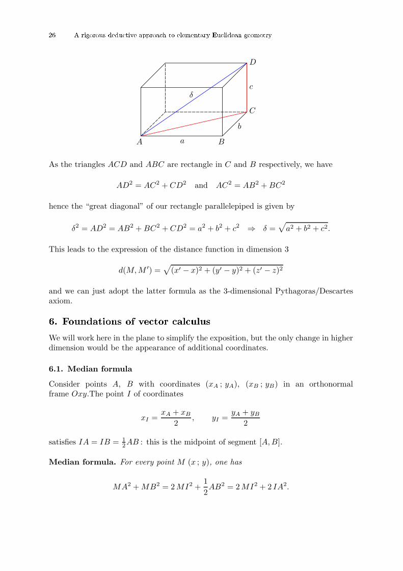
26 A rigorous dedu tive approa h to elementary Eu lidean geometry
A a B
b
C
c
D
δ
As the triangles ACD and ABC are rectangle in C and B respectively, we have
AD2 = AC2 + CD2 and AC2 = AB2 +BC2
hence the “great diagonal” of our rectangle parallelepiped is given by
δ2 = AD2 = AB2 +BC2 + CD2 = a2 + b2 + c2 ⇒ δ =√
a2 + b2 + c2.
This leads to the expression of the distance function in dimension 3
d(M,M ′) =√
(x′ − x)2 + (y′ − y)2 + (z′ − z)2
and we can just adopt the latter formula as the 3-dimensional Pythagoras/Descartesaxiom.
6. Foundations of ve tor al ulus
We will work here in the plane to simplify the exposition, but the only change in higherdimension would be the appearance of additional coordinates.
6.1. Median formula
Consider points A, B with coordinates (xA ; yA), (xB ; yB) in an orthonormalframe Oxy.The point I of coordinates
xI =xA + xB
2, yI =
yA + yB2
satisfies IA = IB = 12AB : this is the midpoint of segment [A,B].
Median formula. For every point M (x ; y), one has
MA2 +MB2 = 2MI2 +1
2AB2 = 2MI2 + 2 IA2.

6. Foundations of ve tor al ulus 27
A
B
I
M
Proof. In fact, by expanding the squares, we get
(x− xA)2 + (x− xB)
2 = 2x2 − 2(xA + xB)x+ x2A + x2
B ,
while
2(x− xI)2 +
1
2(xB − xA)
2 = 2(x2 − 2xIx+ x2I) +
1
2(xB − xA)
2
= 2(x2 − (xA + xB)x+
1
4(xA + xB)
2)+
1
2(xB − xA)
2
= 2x2 − 2(xA + xB)x+ x2A + x2
B.
Therefor we get
(x− xA)2 + (x− xB)
2 = 2(x− xI)2 +
1
2(xB − xA)
2.
The median formula is obtained by adding the analogous equality for coordinates yand applying Pythagoras’ theorem.
It follows from the median formula that there is a unique point M such that MA =MB = 1
2 AB, in fact we then find MI2 = 0, hence M = I. The coordinate formulasthat we initially gave to define midpoints are therefore independent of the choice ofcoordinates.
6.2. Parallelograms
A quadrilateral ABCD is a parallelogram if and only if its diagonals [A,C] and [B,D]intersect at their midpoint :
A
B
C
D
I
In this way, we find the necessary and sufficient condition
xI =1
2(xB + xD) =
1
2(xA + xC), yI =
1
2(yB + yD) =
1
2(yA + yC),
28 A rigorous dedu tive approa h to elementary Eu lidean geometry
which is equivalent to
xB + xD = xA + xC , yB + yD = yA + yC
or, alternatively, t
xB − xA = xC − xD, yB − yA = yC − yD,
in other words, the variation of coordinates involved in getting from A to B is the sameas the one involved in getting from D to C.
6.3. Vectors
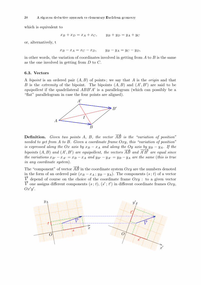
A bipoint is an ordered pair (A,B) of points ; we say that A is the origin and thatB is the extremity of the bipoint. The bipoints (A,B) and (A′, B′) are said to beequipollent if the quadrilateral ABB′A′ is a parallelogram (which can possibly be a“flat” parallelogram in case the four points are aligned).
A
B
B′
A′
I
Definition. Given two points A, B, the vector−−→AB is the “variation of position”
needed to get from A to B. Given a coordinate frame Oxy, this “variation of position”is expressed along the Ox axis by xB − xA and along the Oy axis by yB − yA. If the
bipoints (A,B) and (A′, B′) are equipollent, the vectors−−→AB and
−−−→A′B′ are equal since
the variations xB′ −xA′ = xB −xA and yB′ − yA′ = yB − yA are the same (this is truein any coordinate system).
The “component” of vector−−→AB in the coordinate system Oxy are the numbers denoted
in the form of an ordered pair (xB − xA ; yB − yA). The components (s ; t) of a vector−→V depend of course on the choice of the coordinate frame Oxy : to a given vector−→V one assigns different components (s ; t), (s′ ; t′) in different coordinate frames Oxy,Ox′y′.
O
x
y
O
x′
y′
−→V −→
V
s
s′
t
t′

7. Cartesian equation of ir les and trigonometri fun tions 29
6.4. Addition of vectors
A
B
C
D
The addition of vectors is defined by means of Chasles’ relation
(6.4.1)−−→AB +
−−→BC =
−→AC
for any three points A, B, C : when one takes the sum of the variation of positionrequired to get from A to B, and then from B to C, one finds the variation of positionto get from A to C ; actually, we have for instance
(xB − xA) + (xC − xB) = xC − xA
for the component along the Ox axis. Equivalently, if ABCD is a parallelogram, onecan also put
(6.4.2)−−→AB +
−−→AD =
−→AC.
That (6.4.1) and (6.4.2) are equivalent follows from the fact that−−→AD =
−−→BC in
parallelogram ABCD. For any choice of coordinae frame Oxy, the sum of vectorsof components (s ; t), (s′ ; t′) has components (s+ s′ ; t+ t′).
For every point A, the vector−→AA has zero componaents : it will be denoted simply
−→0 .
Obviously, we have−→V +
−→0 =
−→0 +
−→V =
−→V for every vector
−→V . On the other hand,
Chasles’ relation yields −−→AB +
−−→BA =
−→AA =
−→0
for all points A, B. Therefore we define
−−−→AB =
−−→BA,
in other words, the opposite of a vector is obtained by exchanging the origin andextremity of any corresponding bipoint.
6.5. Multiplication of a vector by a real number
Given a vector−→V of components (s ; t) in a coordinate frame Oxy and an arbitrary
real number λ, we define λ−→V as the vector of components (λs ; λt).
This definition is actually independent of the coordinate frame Oxy. In fact if−→V =
−−→AB 6= −→
0 and λ > 0, we have λ−−→AB =
−→AC where C is the unique point located
on the half-line [A,B) such that AC = λAB. On the other hand, if λ 6 0, we have−λ > 0 and
λ−−→AB = (−λ)(−−−→
AB) = (−λ)−−→BA.
Finally, it is clear that λ−→0 =
−→0 . Multiplication of vectors by a number is distributive
with respect to the addition of vectors (this is a consequence of the distributivity ofmultiplication with respect to addition in the set of real numbers).

30 A rigorous dedu tive approa h to elementary Eu lidean geometry
7. Cartesian equation of ir les and trigonometri fun tions
By Pythagoras’ thorem, the circle of center A (a, b) and radius R in the plane is theset of points M satisfying the equation
AM = R ⇔ AM2 = R2 ⇔ (x− a)2 + (y − b) = R2,
which can also be put in the form x2 + y2 − 2ax− 2by + c = 0 with c = a2 + b2 −R2.Conversely, the set of solutions of such an equation defines a circle of center A (a ; b)and of radius R =
√a2 + b2 − c if c < a2 + b2, is reduced to point A if c = a2 + b2, and
is empty if c > a2 + b2.
The trigonometric circle C is defined to be the unit circle centered at the origin in anorthormal coordinate system Oxy, that is, the of pointsM (x ; y) such that x2+y2 = 1.Let U be the point of coordinates (1 ; 0) and V the point of coordinates (0 ; 1). Theusual trigonometric functions cos, sin and tan are then defined for arbitrary anglearguments as shown on the above figure(10) :
θ
x = cos(θ)
y = sin(θ)
y
x= tan(θ)
O U
VM
T
The equation of the circle implies the relation (cos θ)2 + (sin θ)2 = 1 for every θ.
8. Interse tion of lines and ir les
Let us begin by intersecting a circle C of center A and radius R with an arbitraryline D. In order to simplify the calculation, we take A = O as the origin and we takethe axis Ox to be perpendicular to the line D. The line D is then “vertical” in thecoordinate frame Oxy. (We start here right away with the most general case, but, onceagain, it would be desirable to approach the question by treating first simple numericalexamples . . .).
(10)It seems essential at this stage that fun tions os, sin, tan have already been introdu ed as the ad ho
ratios of sides in a right triangle, i.e. at least for the ase of a ute angles, and that their values for the
remarkable angle values 0
◦, 30
◦, 45
◦, 60
◦, 90
◦are known.

8. Interse tion of lines and ir les 31
C
O
x0
Rx
y
D
This leads to equation
C : x2 + y2 = R2, D : x = x0,
hencey2 = R2 − x2
0.
As a consequence, if |x0| < R, we have R2 − x20 > 0 and there are two so-
lutions y =√R2 − x2
0 and y = −√
R2 − x20, corresponding to two intersection
points(x0,√R2 − x2
0) and (x0,−√R2 − x2
0) that are symmetric with respect to theOx axis. If |x0| = R, we find a single solution y = 0 : the line D : x = x0 is tangent tocircle C at point (x0 ; 0). If |x0| > R, the equation y2 = R2 − x2
0 < 0 has no solution ;the line D does not intersect the circle.
Consider now the intersection of a circle C of center A and radius R with a circle C′ ofcenter A′ and radius R′. Let d = AA′ be the distance between their centers. If d = 0the circles are concentric and the discussion is easy (the circles coincide if R = R′, andare disjoint if R 6= R′). We will therefore assume that A 6= A′, i.e. d > 0. By selectingO = A as the origin and Ox = [A,A′) as the positive x axis, we are reduces to the casewhere A (0 ; 0) and A′ (d ; 0). We then get equations
C : x2 + y2 = R2, C′ : (x− d)2 + y2 = R′2 ⇐⇒ x2 + y2 = 2dx+R′2 − d2.
For any point M in the intersection C ∩ C′, we thus get 2dx+R′2 − d2 = R2, hence
x = x0 =1
2d(d2 +R2 −R′2).
This shows that the intersection C∩C′ is contained in the intersection C∩D of C withthe line D : x = x0. Conversely, one sees that if x2 + y2 = R2 and x = x0, then (x ; y)also satisfies the equation
x2 + y2 − 2dx = R2 − 2dx0 = R2 − (d2 +R2 −R′2) = R′2 − d2

32 A rigorous dedu tive approa h to elementary Eu lidean geometry
which is the equation of C′, hence C ∩D ⊂ C ∩ C′ and finally C ∩ C
′ = C ∩D.
A
x0
A′
x
y
D
C
C′
The intersection points are thus given by y = ±√
R2 − x20. As a consequene, we have
exactly two solutions that are symmetric with respect to the line (AA′) as soon as−R < x0 < R, or equivalently
−2dR < d2 +R2 −R′2 < 2dR ⇐⇒ (d+R)2 > R′2 et (d−R)2 < R′2
⇐⇒ d+R > R′, d−R < R′, d−R > −R′,
i.e. |R−R′| < d < R+R′. If one of the inequalities is an equality, we get x0 = ±R andwe thus find a single solution y = 0. The circles are tangent internally if d = |R −R′|and tangent externally if d = R +R′.
Note that these results lead to a complete and rigorous proof of the isometry criteria fortriangles : up to an orthonormal change of coordinates, each of the three cases entirelydetermines the coordinates of the triangles modulo a reflection with respect to Ox (inthis argument, the origin O is chosen as one of the vertices and the axis Ox is takento be the direction of a side of known length). The triangles specified in that way arethus isometric.
9. S alar produ t
The norm ‖−→V ‖ of a vector−→V =
−−→AB is the length AB = d(A,B) of an arbitrary bipoint
that defines−→V . From there, we put
(9.1)−→U · −→V =
1
2
(‖−→U +
−→V ‖2 − ‖−→U ‖2 − ‖−→V ‖2
)
in particular−→U · −→U = ‖−→U ‖2. The real number
−→U · −→V is called the inner product
of−→U and
−→V , and
−→U · −→U is also defined to be the inner square of
−→U , denoted
−→U
2.
Consequently we obtain−→U
2=
−→U · −→U = ‖−→U ‖2.

10. More advan ed material 33
By definition (9.1), we have
(9.2) ‖−→U +−→V ‖2 = ‖−→U ‖2 + ‖−→V ‖2 + 2
−→U · −→V ,
and this formula can also be rewritten
(9.2′) (−→U +
−→V )2 =
−→U
2+−→V
2+ 2
−→U · −→V .
This was the main motivation of the definition : that the usual identity for the squareof a sum be valid for inner products. In dimension 2 and in an orthonormal frame
Oxy, we find−→U
2= x2 + y2 ; if
−→V has components (x′ ; y′), Definition (9.1) implies
(9.3)−→U · −→V =
1
2
((x+ x′)2 + (y + y′)2 − (x2 + y2)− (x′2 + y′2)
)= xx′ + yy′.
In dimension n, we would find similarly
−→U · −→V = x1x
′1 + x2x
′2 + . . .+ xnx
′n.
From there, we derive that the inner product is “bilinear”, namely that
(k−→U ) · −→V =
−→U · (k−→V ) = k
−→U · −→V ,
(−→U1 +
−→U2) · −→V =
−→U1 · −→V +
−→U2 · −→V ,
−→U · (−→V1 +
−→V1) =
−→U · −→V1 +
−→U · −→V2.
if−→U ,
−→V are two vectors, we can pick a point A and write
−→U =
−−→AB, then
−→V =
−−→BC, so
that−→U +
−→V =
−→AC. The triangle ABC is rectangle if and only if we have Pythagoras’
relation AC2 = AB2 +BC2, i.e.
‖−→U +−→V ‖2 = ‖−→U ‖2 + ‖−→V ‖2,
in other words, by (9.2), if and only if−→U · −→V = 0.
Consequence. Tw vectors−→U and
−→V are perpendicular if and only if
−→U · −→V = 0.
More generally, if we fix an origin O and a point A such that−→U =
−→OA, one can also
pick a coordinate system such that A belongs to the Ox axis, that is, A = (u ; 0). For
every vector−→V =
−−→OB (v ; w) in Oxy, we then get
−→U · −→V = uv
whereas‖−→U ‖ = u, ‖−→V ‖ =
√v2 + w2.
As the half-line [O,B) intersects the trigonometric circle at point (kv ; kw) withk = 1/
√v2 + w2, we get by definition
cos({−→U ,
−→V ) = cos({AOB) = kv =
v√v2 + w2
.
This leads to the very useful formulas
(9.4)−→U · −→V = ‖−→U ‖ ‖−→V ‖ cos(
{−→U ,
−→V ), cos(
{−→U ,
−→V ) =
−→U · −→V
‖−→U ‖ ‖−→V ‖.

34 A rigorous dedu tive approa h to elementary Eu lidean geometry
10. More advan ed material
At this point, we have all the necessary foundations, and the succession of conceptsto be introduced becomes much more flexible – much of what we discuss below onlyconcerns high school level and beyond.
One can for example study further properties of triangles and circles, and graduallyintroduce the main geometric transformations (in the plane to start with) : transla-tions, homotheties, affinities, axial symmetries, projections, rotations with respect to apoint ; and in space, symmetries with respect to a point, a line or a plane, orthogonalprojections on a plane or on a line, rotation around an axis. Available tools allow mak-ing either intrinsic geometric reasonings (with angles, distances, similarity ratios, . . .),or calculations in Cartesian coordinates. It is actually desirable that these techniquesremain intimately connected, as this is common practice in contemporary mathematics(the period that we describe as “contemporary” actually going back to several centuriesfor mathematicians, engineers, physicists . . .)
It is then time to investigate the phenomenon of linearity, independently of any distanceconsideration. This leads to the concepts of linear combinations of vectors, lineardependence and independence, non orthonormal frames, etc, in relation with theresolution of systems of linear equations. One is quickly led to determinants 2 × 2,3× 3, to equations of lines, planes, etc. The general concept of vector space providesan intrinsic vision of linear algebra, and one can introduce general affine spaces, bilinearsymmetric forms, Euclidean and Hermitian geometry in arbitrary dimension. What wehave done before can be deepened in various ways, especially by studying the generalconcept of isometry.
10.1. Definition. Let E and F be two Euclidean spaces and let s : E → F be anarbitrary map between these. We say that s is an isometry from E to F if for everypair of points (M,N) of E, we have d(s(M), s(N)) = d(M,N).
Isometries are closely tied to inner product via the following fundamental theorem.
10.2. Theorem. If s : E → F is an isometry, then s is an affine transformation, andits associated linear map σ :
−→E → −→
F is an orthogonal transform of Euclidean vectorspaces, namely a linear map preserving orthogonality and inner products :
(10.3) σ(−→V ) · σ(−→W ) =
−→V · −→W
for all vectors−→V ,
−→W ∈ −→
E .
In the same vein, one can prove the following result, which provides a rigorousmathematical justification to all definitions and physical considerations appeared insection 3.2.
10.4. Theorem. Let (A1A2A3A4 . . .) and (A′1A
′2A
′3A
′4 . . .) be two isometric figures
formed by points Ai, A′i of a Euclidean space E. Then there exists an isometry s of the
entire Euclidean space E such that A′i = s(Ai) for all i.

10. More advan ed material 35
Non Eu lidean geometries.
Bernhard Riemann (1826–1866 )
In contemporary mathematics, non Euclidean geometries are best seen as a specialinstance of Riemannian geometry, so called in reference to Bernhard Riemann, one ofthe founders of modern complex analysis and differential geometry [Rie]. A Riemannianmanifold is by definition a differential manifold M , namely a topological space thatadmits local differentiable systems of coordinates x = (x1 ; x2 ; . . . ; xn), equipped withan infinitesimal metric g of the form
(10.5) ds2 = g(x) =∑
16i,j6n
aij(x) dxidxj .
By integrating the infinitesimal metric along paths, one obtains the geodesic distancewhich is used as a substitute of the Euclidean distance (in physics, general relativityalso arises in a similar way by considering Lorentz-like metrics of the form ds2 =dx2
1+dx22+dx2
3− c2 dt2). On the unit disk D = {z ∈ C ; |z| < 1} in the complex plane,denoting z = x + iy, one considers the so-called Poincare metric (named after HenriPoincare, 1854-1912, see [Poi])
(10.6) ds =|dz|
1− |z|2 ⇔ ds2 =dx2 + dy2
(1− (x2 + y2))2.
The associated geodesic distance can be computed to be
(10.7) dP(a, b) =1
2ln
1 + |b−a||1−ab|
1− |b−a||1−ab|
.
When substituting this distance to the Pythagoras/Descartes axiom, one actuallyobtains a non Euclidean geometry, which is a model of the hyperbolic geometrydiscovered by Nikolai Lobachevski (1793-1856). In this geometry, there are actuallyinfinitely many parallel lines to a given line D through a given point p exterior to D,so that Euclid’s fifth postulate fails !

36 A rigorous dedu tive approa h to elementary Eu lidean geometry
D
p ∆
Lobachevski’s hyperbolic geometry and the failure of Euclid’s fifth postulate
On some ideas of Felix Hausdor� and Mikhail Gromov.
We first describe a few important ideas due to Felix Hausdorff (1868 - 1942), one ofthe founders of modern topology [Hau]. The first one is that the Lebesgue measure ofRn can be generalized without any reference to the vector space structure, but just byusing the metric. If (E, d) is an arbitrary metric space, one defines the p-dimensionalHausdorff measure of a subset A of E as
(10.8) Hp(A) = limε→0
Hp,ε(A), Hp,ε(A) = infdiamAi6ε
∑
i
(diamAi)p
where Hp,ε(A) is the least upper bound of sums∑
i(diamAi)p running over all
countable partitions A =⋃Ai with dimAi 6 ε. For p = 1 (resp. p = 2, p = 3)
one recovers the usual concepts of length, area, volume, and the definition even workswhen p is not an integer (it is then extremely useful to define the dimension of fractalsets). Another important idea of Hausdorff is the existence of a natural metric structureon the set of compact subsets of a given metric space (E, d). If K, L are two compactsubsets of E, the Hausdorff distance of K and L is defined to be
(10.9) dH(K,L) = max{maxx∈K
miny∈L
d(x, y),maxy∈L
minx∈K
d(x, y)}.
The study of metric structures has become today one of the most active domainsin mathematics. We should mention here the work of Mikhail Gromov (Abel prize2009) on length spaces and “moduli spaces” of Riemannian manifolds. If X and Y aretwo compact metric spaces, one defines their Gromov-Hausdorff distance dGH(X, Y )to be the infimum of all Hausdorff distances dH(f(X), f(Y )) for all possible isometricembeddings f : X → E, g : Y → E of X and Y in another compact metric space E.This provides a crucial tool to study deformations and degenerations of Riemannianmanifolds.

10. More advan ed material 37
Referen es
[Art℄ Emil Artin, Geometri Algebra, Inters ien e publishers In ., New York, 1957, download at
http://ia700300.us.ar hive.org/24/items/geometri algebra033556mbp/
geometri algebra033556mbp.pdf
[Des℄ Ren�e Des artes, La G�eom�etrie, appendix of Dis ours de la m�ethode, available from Proje t
Gutenberg http://www.gutenberg.org/files/26400/26400-pdf.pdf
[Die℄ Jean Dieudonn�e, Alg�ebre lin�eaire et g�eom�etrie �el�ementaire, Hermann, 1968, 240 pages
[Eu ℄ Eu lid, Eu lid's elements of geometry, English translation from Greek by Ri hard Fitzpatri k,
http://farside.ph.utexas.edu/eu lid/Elements.pdf
[Gro℄ Mikhail Gromov, Stru tures m�etriques pour les vari�et�es riemanniennes, edited by J. La-
fontaine and P. Pansu, Textes Math�ematiques, no. 1, CEDIC, Paris, 1981, translated by S.M.
Bates, Metri Stru tures for Riemannian and Non-Riemannian Spa es, Birkh �auser, 1999
[Hau℄ Felix Hausdor�, Dimension und �ausseres Mass, Mathematis he Annalen 79, 1-2 (1919) 157-
179, and Grundz �uge der Mengenlehre, Leipzig, 1914. viii + 476 pages, English translation Set
Theory, Ameri an Mathemati al So ., 1957, 352 pages
[Hil℄ David Hilbert, Grundlagen der Geometrie, Teubner, Leipzig, 1899, English translation The
Foundations of Geometry, by E.J. Townsend (2005), available from proje t Gutenberg,
http://www.gutenberg.org/files/17384/17384-pdf.pdf
[Lob℄ Nikolai Loba hevski, Geometri al resear hes on the theory of parallels,
http://quod.lib.umi h.edu/u/umhistmath/AAN2339.0001.001/1?rgn=full+text;view=pdf
[Pas℄ Moritz Pas h, Vorlesungen �uber neuere Geometrie, Teubner, Leipzig, 1882, download at
https://ia700308.us.ar hive.org/32/items/vorlesungenbern00pas goog/
vorlesungenbern00pas goog.pdf
[Poi℄ Henri Poin ar�e, Å�uvres, tome 2, 1916 - Fon tions fu hsiennes, et Les g�eom�etries non
eu lidiennes http://www.univ-nan y2.fr/poin are/bhp/
[Pon℄ Jean-Vi tor Pon elet, Trait�e des propri�et�es proje tives des �gures, Gauthier-Villars, Paris,
1866, download at http://galli a.bnf.fr/ark:/12148/bpt6k5484980j
[Rie℄ Bernhard Riemann, Grundlagen f �ur eine allgemeine Theorie der Funktionen einer ver �ander-
li hen omplexen Gr �osse, Inauguraldissertation, G �ottingen, 1851, and Ueber die Hypothe-
sen, wel he der Geometrie zu Grunde liegen, Habilitationss hrift, 1854, Abhandlungen der
K �onigli hen Gesells haft der Wissens haften zu G �ottingen, 13 (1868), English translation On
the Hypotheses whi h lie at the Bases of Geometry, http://www.emis.de/ lassi s/Riemann/


![[Рец.] C. П. Лопушанская. Развитие и функционирование древнерусского глагола. Волгоград, 1990 // Славяноведение.](https://static.fdokumen.com/doc/165x107/63155c7b511772fe45105073/rets-c-p-lopushanskaya-razvitie-i-funktsionirovanie.jpg)