М УЦ Ь ТУ ЛУР Ц Ж ЩШЦ ТУ ЬФ Ц С ТШ Т ШЧ Л ТШ РР ...
320
-
Upload
khangminh22 -
Category
Documents
-
view
0 -
download
0
Transcript of М УЦ Ь ТУ ЛУР Ц Ж ЩШЦ ТУ ЬФ Ц С ТШ Т ШЧ Л ТШ РР ...

The Borexino Solar Neutrino Experiment
and its Scintillator Containment Vessel
Laura Cadonati
A dissertation
presented to the faculty
of Princeton University
in candidacy for the degree
of Doctor of Philosophy
Recommended for acceptance
by the department of Physics
January 2001

c Copyright by Laura Cadonati, 2001. All rights reserved.
Abstract
Thirty years ago, the �rst solar neutrino detector proved fusion reactions power the Sun.
However, the total rate detected in this and all subsequent solar neutrino experiments is
consistently two to three times lower than predicted by the Standard Solar Model. Current
experiments seek to explain this \solar neutrino puzzle" through non-standard particle
properties, like neutrino mass and avor mixing, within the context of the MSW theory.
The detection of the monoenergetic 7Be solar neutrino is the missing clue for the solution of
the solar neutrino problem; this constitutes the main physics goal of Borexino, a real-time,
high-statistics solar neutrino detector located under the Gran Sasso mountain, in Italy.
In the �rst part of this thesis, I present a Monte Carlo study of the expected performance
of Borexino, with simulations of the neutrino rate, the external background and the �=�=
activity in the scintillator. The Standard Solar Model predicts a solar neutrino rate of
about 60 events/day in Borexino in the 0.25-0.8 MeV window, mostly due to 7Be neutrinos.
Given the design scintillator radiopurity levels (10�16g/g 238U and 232Th and 10�14g/g K),
Borexino will detect such a rate with a � 2:4% statistical error, after one year. In the MSW
Small (Large) Angle scenario, the predicted rate of �13 (33) events/day will be detected
with 8% (4%) error. The sensitivity of Borexino to 8B and pp neutrinos and to a Galactic
supernova event is also discussed.
The second part of this dissertation is devoted to the liquid scintillator containment
vessel, an 8.5 m diameter sphere built of bonded panels of 0.125 mm polymer �lm. Through
an extensive materials testing program we have identi�ed an amorphous nylon-6 �lm which
meets all the critical requirements for the success of Borexino. I describe tests of tensile
strength, measurements of 222Rn di�usion through thin nylon �lms and of optical clarity. I
discuss how the materials' radiopurity and mechanical properties a�ect the detector design
and physics potential and present models that, incorporating the measured properties, yield
a containment vessel that will safely operate for the ten-year lifetime of Borexino.
iii

Acknowledgments
There are many people I would like to acknowledge for all they have taught me and for the
support, the friendship and the encouragement they gave me during these past few years.
Nick Darnton, my husband, my friend and a colleague who has been close to me in
many invaluable ways, through useful discussions on the physics, help with the experimental
setups, readproo�ng this thesis and, most important, his moral support and patience, from
the moment we met in Gran Sasso through all my years in Princeton. I would not have
made it without you.
My beautiful little girl, Chiara, who gave me a whole new prospective on what is really
important in life and who made everything so much more interesting.
My parents, Angela and Luciano Cadonati, and my sister and best friend, Stefania, who
constantly supported me from overseas and always believed in me and in my potential. You
made me the person I am and then granted me the freedom to chose a path that would
take me so far away from you; I will never thank you enough.
My in-laws, Susan and Robert Darnton, with Margaret and Kate, who welcomed me in
a warm family when I moved here from Italy and always treated me like a daughter.
My advisor, professor Frank Calaprice, who encouraged me to apply for graduate school
and who has been a great mentor during all these years. Thank you for all the precious
advice, for the encouragement and for the way you always trusted me.
My friends in Princeton, in particular, the members of my study group, thanks to whom
studying for generals has not been such a bad experience, after all: Nick Darnton, Olgica
Bakajin, Diego Casa, Eric Splaver, Matt Hedman and Ken Nagamine. And thanks also to
Rich Simon, who always made sure we had food during our night study sessions. I would
like to give a special thanks to Indi Riehl and Omar Saleh for being such wonderful friends
in this past year: we shared happy and diÆcult moments, you have been a great help since
Chiara was born and I really appreciate it.
My friends and colleagues of the Princeton Borexino group. Thanks to professors Mark
iv

Chen, Tom Shutt and Bruce Vogelaar, who were always available for discussions and help.
Mark, thanks to you and Martha and Cassie for all the friendship and the support; we miss
you in Princeton. My compatriots, Cristiano Galbiati, Aldo Ianni and Andrea Pocar: it
has been nice to have our own \little Italy" in the B-level of Jadwin. Fred Loeser, who has
been such an asset from the moment I came to Princeton: thank you for always �nding
time to help me in my work and for being a friend. Beth Harding, Richard Fernholz, Ernst
de Haas, Mike Johnson, Allan Nelson, Jim Semler: it has been great working with you all.
My italian colleagues in the Borexino collaboration and the LNGS sta�, too many to
be listed here, who have become good friends during these years. I will always remember
with great a�ection the time spent at the Gran Sasso Laboratories, it has been a wonderful
experience, both professionally and personally.
Last, but not least, the whole Princeton Physics department sta�, with a particular
mention to Cynthia Murphy, Sue Oberlander and Laurel Lerner: I have always found a
helping hand and a smile, thank you.
v

to Chiara Maria Darnton
vi

Contents
Abstract iii
Acknowledgments iv
1 Solar Neutrino Physics 1
1.1 Solar Neutrinos . . . . . . . . . . . . . . . . . . . . . . . . . . . . . . . . . . 2
1.1.1 The Standard Solar Model . . . . . . . . . . . . . . . . . . . . . . . 2
1.1.2 Experimental Status . . . . . . . . . . . . . . . . . . . . . . . . . . . 5
1.2 The Solar Neutrino Puzzle . . . . . . . . . . . . . . . . . . . . . . . . . . . . 12
1.2.1 Astrophysical Solutions to the Solar Neutrino Puzzle . . . . . . . . . 13
1.2.2 Non-Standard Neutrino Physics . . . . . . . . . . . . . . . . . . . . 18
1.3 Where Do We Stand Now? . . . . . . . . . . . . . . . . . . . . . . . . . . . 24
2 The Borexino Experiment 31
2.1 Overview of the Borexino Project . . . . . . . . . . . . . . . . . . . . . . . . 31
2.2 Detector Structure . . . . . . . . . . . . . . . . . . . . . . . . . . . . . . . . 33
2.2.1 The Scintillator . . . . . . . . . . . . . . . . . . . . . . . . . . . . . . 35
2.2.2 The Nylon Vessels . . . . . . . . . . . . . . . . . . . . . . . . . . . . 40
2.2.3 The Bu�er Fluid . . . . . . . . . . . . . . . . . . . . . . . . . . . . . 41
2.2.4 The Stainless Steel Sphere . . . . . . . . . . . . . . . . . . . . . . . . 42
2.2.5 The External Water Tank and the Water Bu�er . . . . . . . . . . . 43
2.2.6 The Phototubes and the Muon Detector . . . . . . . . . . . . . . . . 43
2.2.7 The Scintillator Puri�cation System . . . . . . . . . . . . . . . . . . 45
vii

2.2.8 The Water Puri�cation System . . . . . . . . . . . . . . . . . . . . . 47
2.2.9 Electronics and DAQ . . . . . . . . . . . . . . . . . . . . . . . . . . . 48
2.2.10 Calibration . . . . . . . . . . . . . . . . . . . . . . . . . . . . . . . . 49
2.3 The Counting Test Facility for Borexino . . . . . . . . . . . . . . . . . . . . 50
2.3.1 Structure of the CTF Detector . . . . . . . . . . . . . . . . . . . . . 51
2.3.2 Results from CTF-I . . . . . . . . . . . . . . . . . . . . . . . . . . . 53
2.3.3 CTF-II . . . . . . . . . . . . . . . . . . . . . . . . . . . . . . . . . . 57
3 Monte Carlo Study of Backgrounds in Borexino 59
3.1 Monte Carlo code for Borexino . . . . . . . . . . . . . . . . . . . . . . . . . 59
3.1.1 GENEB: GEneration of NEutrino and Background . . . . . . . . . . 59
3.1.2 Tracking . . . . . . . . . . . . . . . . . . . . . . . . . . . . . . . . . . 61
3.1.3 Reconstruction . . . . . . . . . . . . . . . . . . . . . . . . . . . . . . 62
3.2 Neutrino Energy Spectra in Borexino . . . . . . . . . . . . . . . . . . . . . . 65
3.3 External Background . . . . . . . . . . . . . . . . . . . . . . . . . . . . . . . 68
3.3.1 Environmental Radioactivity . . . . . . . . . . . . . . . . . . . . . 68
3.3.2 External Background Sources in Borexino . . . . . . . . . . . . . . . 73
3.3.3 Behavior of External Background . . . . . . . . . . . . . . . . . . . . 75
3.3.4 Monte Carlo Simulation . . . . . . . . . . . . . . . . . . . . . . . . . 76
3.3.5 Alternative Geometries . . . . . . . . . . . . . . . . . . . . . . . . . 84
3.4 Internal Background . . . . . . . . . . . . . . . . . . . . . . . . . . . . . . . 88
3.5 Cosmogenic Backgrounds . . . . . . . . . . . . . . . . . . . . . . . . . . . . 93
4 The Physics Potential of Borexino 96
4.1 Solar Neutrino Physics from Borexino . . . . . . . . . . . . . . . . . . . . . 96
4.1.1 Neutrino Rates . . . . . . . . . . . . . . . . . . . . . . . . . . . . . . 96
4.1.2 Seasonal Variations . . . . . . . . . . . . . . . . . . . . . . . . . . . . 98
4.1.3 Day-Night Asymmetry . . . . . . . . . . . . . . . . . . . . . . . . . . 102
4.2 Sensitivity to the 7Be Signal in Borexino . . . . . . . . . . . . . . . . . . . . 106
4.3 Sensitivity to the 8B Solar Neutrino . . . . . . . . . . . . . . . . . . . . . . 109
viii

4.4 Sensitivity to the pp Solar Neutrino - Low Energy Spectrum in Borexino . . 115
4.5 Physics Beyond Solar Neutrinos . . . . . . . . . . . . . . . . . . . . . . . . . 120
4.5.1 ��e Detection . . . . . . . . . . . . . . . . . . . . . . . . . . . . . . . . 120
4.5.2 Double-� Decay with Dissolved 136Xe . . . . . . . . . . . . . . . . . 121
4.5.3 Neutrino Physics with MCi Sources . . . . . . . . . . . . . . . . . . 122
4.6 Supernova Neutrino Detection in Borexino . . . . . . . . . . . . . . . . . . . 122
4.6.1 Supernova Neutrino Spectrum . . . . . . . . . . . . . . . . . . . . . 123
4.6.2 Supernova Neutrino Signatures in Borexino . . . . . . . . . . . . . . 124
4.6.3 Consequences of Non-Standard Neutrino Physics . . . . . . . . . . . 128
4.6.4 Conclusions . . . . . . . . . . . . . . . . . . . . . . . . . . . . . . . . 136
5 The Scintillator Containment Vessel for Borexino 137
5.1 Historical Note . . . . . . . . . . . . . . . . . . . . . . . . . . . . . . . . . . 137
5.2 Thin Nylon Film . . . . . . . . . . . . . . . . . . . . . . . . . . . . . . . . . 139
5.2.1 Nylon Molecular Structure . . . . . . . . . . . . . . . . . . . . . . . 139
5.2.2 Nylon Film Physical Structure . . . . . . . . . . . . . . . . . . . . . 142
5.2.3 Nylon Compatibility with Water . . . . . . . . . . . . . . . . . . . . 144
5.2.4 Candidate Materials . . . . . . . . . . . . . . . . . . . . . . . . . . . 147
5.3 Mechanical Properties . . . . . . . . . . . . . . . . . . . . . . . . . . . . . . 149
5.3.1 Measurements of Tensile Strength and Chemical Compatibility of Ny-
lon with Various Fluids . . . . . . . . . . . . . . . . . . . . . . . . . 151
5.3.2 Creep . . . . . . . . . . . . . . . . . . . . . . . . . . . . . . . . . . . 158
5.3.3 The Stress-Cracking Problem . . . . . . . . . . . . . . . . . . . . . . 160
5.4 A New Measurement Campaign . . . . . . . . . . . . . . . . . . . . . . . . . 162
5.5 Technical Aspects of the Vessel Fabrication . . . . . . . . . . . . . . . . . . 163
5.5.1 Design and Construction . . . . . . . . . . . . . . . . . . . . . . . . 163
5.5.2 Cleanliness . . . . . . . . . . . . . . . . . . . . . . . . . . . . . . . . 166
5.6 The Hold-Down System . . . . . . . . . . . . . . . . . . . . . . . . . . . . . 168
ix

6 Radon Di�usion 172
6.1 The Radon Problem . . . . . . . . . . . . . . . . . . . . . . . . . . . . . . . 172
6.2 Mathematical Model for 222Rn Di�usion and Emanation . . . . . . . . . . . 174
6.2.1 Permeation . . . . . . . . . . . . . . . . . . . . . . . . . . . . . . . . 175
6.2.2 Emanation . . . . . . . . . . . . . . . . . . . . . . . . . . . . . . . . 176
6.3 Measurements of 222Rn Di�usion . . . . . . . . . . . . . . . . . . . . . . . . 177
6.3.1 222Rn Di�usion Detector Design . . . . . . . . . . . . . . . . . . . . 178
6.3.2 Measurement Procedure . . . . . . . . . . . . . . . . . . . . . . . . . 180
6.3.3 Detector Performances . . . . . . . . . . . . . . . . . . . . . . . . . . 182
6.3.4 Expected Di�usion Pro�les . . . . . . . . . . . . . . . . . . . . . . . 185
6.3.5 Data Analysis . . . . . . . . . . . . . . . . . . . . . . . . . . . . . . . 188
6.3.6 Results . . . . . . . . . . . . . . . . . . . . . . . . . . . . . . . . . . 190
6.4 222Rn Di�usion and Emanation in CTF . . . . . . . . . . . . . . . . . . . . 196
7 Optical Properties 200
7.1 Light Crossing a Thin Film: Luminous Transmittance and Haze . . . . . . 200
7.1.1 Surface E�ects . . . . . . . . . . . . . . . . . . . . . . . . . . . . . . 201
7.1.2 Volume E�ects . . . . . . . . . . . . . . . . . . . . . . . . . . . . . . 203
7.2 Optical Measurements on Nylon Films . . . . . . . . . . . . . . . . . . . . . 203
7.2.1 Transmittance . . . . . . . . . . . . . . . . . . . . . . . . . . . . . . 203
7.2.2 Light Scattering and Haze Measurements . . . . . . . . . . . . . . . 207
7.3 Consequences for Borexino . . . . . . . . . . . . . . . . . . . . . . . . . . . . 212
8 Radiopurity Issues 216
8.1 Nylon Film for the Inner Vessel . . . . . . . . . . . . . . . . . . . . . . . . . 217
8.1.1 Measured 238U, 232Th and 40K Content in Nylon . . . . . . . . . . . 217
8.1.2 Estimated Background from the Nylon Film in Borexino . . . . . 221
8.1.3 Radon Emanation and Internal Background . . . . . . . . . . . . . . 224
8.1.4 Surface Contamination . . . . . . . . . . . . . . . . . . . . . . . . . . 228
8.2 The Outer Vessel . . . . . . . . . . . . . . . . . . . . . . . . . . . . . . . . . 229
x

8.2.1 External Background and -ray Shielding . . . . . . . . . . . . . . . 230
8.2.2 Radon Permeation Through the Nylon Vessels . . . . . . . . . . . . 232
8.3 Auxiliary Components of the Inner Vessel . . . . . . . . . . . . . . . . . . . 233
8.3.1 Endcap Radiopurity . . . . . . . . . . . . . . . . . . . . . . . . . . . 236
8.4 Ropes for the Hold Down System . . . . . . . . . . . . . . . . . . . . . . . . 238
9 Stress Studies and Shape Analysis 241
9.1 Thin Shell Theory . . . . . . . . . . . . . . . . . . . . . . . . . . . . . . . . 241
9.1.1 The Stress Tensor . . . . . . . . . . . . . . . . . . . . . . . . . . . . 241
9.1.2 The Strain Tensor . . . . . . . . . . . . . . . . . . . . . . . . . . . . 243
9.1.3 Hooke's Law . . . . . . . . . . . . . . . . . . . . . . . . . . . . . . . 244
9.1.4 Membrane Stresses in Shells . . . . . . . . . . . . . . . . . . . . . . . 245
9.1.5 Thin Shell Theory for Shells of Revolution . . . . . . . . . . . . . . . 246
9.1.6 Symmetrically Loaded Spherical Shells of Revolution . . . . . . . . . 248
9.2 Membrane Theory and the Borexino Inner Vessel . . . . . . . . . . . . . . . 250
9.2.1 Sphere Supported by a Ring . . . . . . . . . . . . . . . . . . . . . . . 252
9.2.2 Supporting Membrane Around the Sphere . . . . . . . . . . . . . . . 257
9.3 Shape Analysis in Presence of Strings . . . . . . . . . . . . . . . . . . . . . 265
9.3.1 Test of the Single String Model on a 4 m Diameter Vessel . . . . . . 267
9.3.2 The n-string Model . . . . . . . . . . . . . . . . . . . . . . . . . . . . 275
9.3.3 Is the Model Complete? . . . . . . . . . . . . . . . . . . . . . . . . . 292
9.3.4 Stress Revisited . . . . . . . . . . . . . . . . . . . . . . . . . . . . . . 295
9.4 Conclusion . . . . . . . . . . . . . . . . . . . . . . . . . . . . . . . . . . . . 296
Bibliography 298
xi

Chapter 1
Solar Neutrino Physics
\Cosmic Gall"
Neutrinos, they are very small.
They have no charge and have no mass
And do not interact at all.
The earth is just a silly ball
To them, through which they simply pass,
Like dustmaids down a drafty hall
Or photons through a sheet of glass.
They snub the most exquisite gas,
Ignore the most substantial wall,
Cold-shoulder steel and sounding brass,
Insult the stallion in his stall,
And, scorning barriers of class,
In�ltrate you and me! Like tall
And painless guillotines, they fall
Down through our heads into the grass.
At night, they enter at Nepal
And pierce the lover and his lass
From underneath the bed - you call
It wonderful; I call it crass.
(John Updike, 1961)
Once considered a poltergeist in the world of particle physics, the neutrino still represents
one of the most intriguing of nature's particles, yet it is probably the most diÆcult to study.
The 1961 poem by John Updike [1] well summarizes its essence. According to the
Standard Model, the neutrino is a weakly interacting, chargeless and massless lepton, in
three avors: the electron neutrino �e, the muon neutrino �� and the tau neutrino �� , each
associated to a charged lepton (e�, �� and �� respectively). The neutrino is also one of the
1

Chapter 1: Solar Neutrino Physics 2
most abundant particles in the Universe: within one single human being, there are some
107 relic neutrinos from the Big Bang, 1014 from the Sun and 103 that are produced by
cosmic rays in the Earth's atmosphere, a circumstance that apparently o�ended Updike.
And yet, because neutrinos only interact weakly, they are so elusive that almost a quarter
of a century passed between the time Pauli \invented" them in 1930 [2], as a last desperate
attempt to save energy conservation in � decay, and the time of their experimental discovery
by Reines and Cowan in 1953 [3].
Half a century later, neutrinos and their mass still represent one of the major riddles
in particle physics. Evidences of a non-zero neutrino mass are appearing in the latest
experimental developments, opening the door to a deeper insight into Grand Uni�cation, but
we still do not know the particle-antiparticle conjugation properties of neutrinos and there
are still many open questions about the role of neutrinos in cosmology and astrophysics.
Several experiments are now exploring the world of neutrinos through the detection of
their ux from di�erent sources (atmospheric, reactor generated, solar). In the context of
this work, we will focus on neutrinos of solar origin.
1.1 Solar Neutrinos
1.1.1 The Standard Solar Model
Life on our planet would not be possible without the Sun and the ux of energy that has
irradiated the Earth during its whole lifetime. The question of what powers the Sun, �rst
raised in the 19th century, has been the object of studies during the 1920's and the 1930's [4],
but the �rst explanation of the energy production inside the Sun was provided in 1939 by
Hans Bethe [5]. His theory states that the only sources capable of powering the Sun over
its 4.7 billion years lifetime are thermonuclear processes occurring in the Sun's core.
The fundamental process is the fusion of Hydrogen atoms into � particles, with the
associated production of positrons and neutrinos:
4p! � + 2e+ + 2�e + 26:7 MeV: (1.1)

Chapter 1: Solar Neutrino Physics 3
Table 1.1: The pp cycle, producing most of the thermonuclear energy in the Sun.
Reaction Termination(%)1 Q E�e hq�ei[MeV] [MeV] [MeV]
p+ p!2 H+ e+ + �e (pp) 99.77 1.442 � 0.420 0.265orp+ e� + p!2 H + �e (pep) 0.23 1.442 1.442 1.442
2H+ p!3 He + 100 5.494
3He+3He! �+ 2p 84.92 12.860or3He+4He! 7Be+ 15,08 1.586
7Be+ e� !7 Li + �e (7Be) 15.07 0.862 (90%) 0.862 0.8620.383 (10%) 0.383 0.383
7Li + p! 2� 15.07 17.347or7Be+p!8B+ 0.01 0.1378B! 8Be� + e+ + �e (8B) 0.01 17.980 � 15 6.71
or3He+ p! 4He+e+ + �e (hep) 10�5 19.795 � 18.8 9.27
1 percentage of terminations for the pp chain in which each reaction takes place. The results are averages
over the present Standard Solar Model.
Chapter 1: Solar Neutrino Physics 4
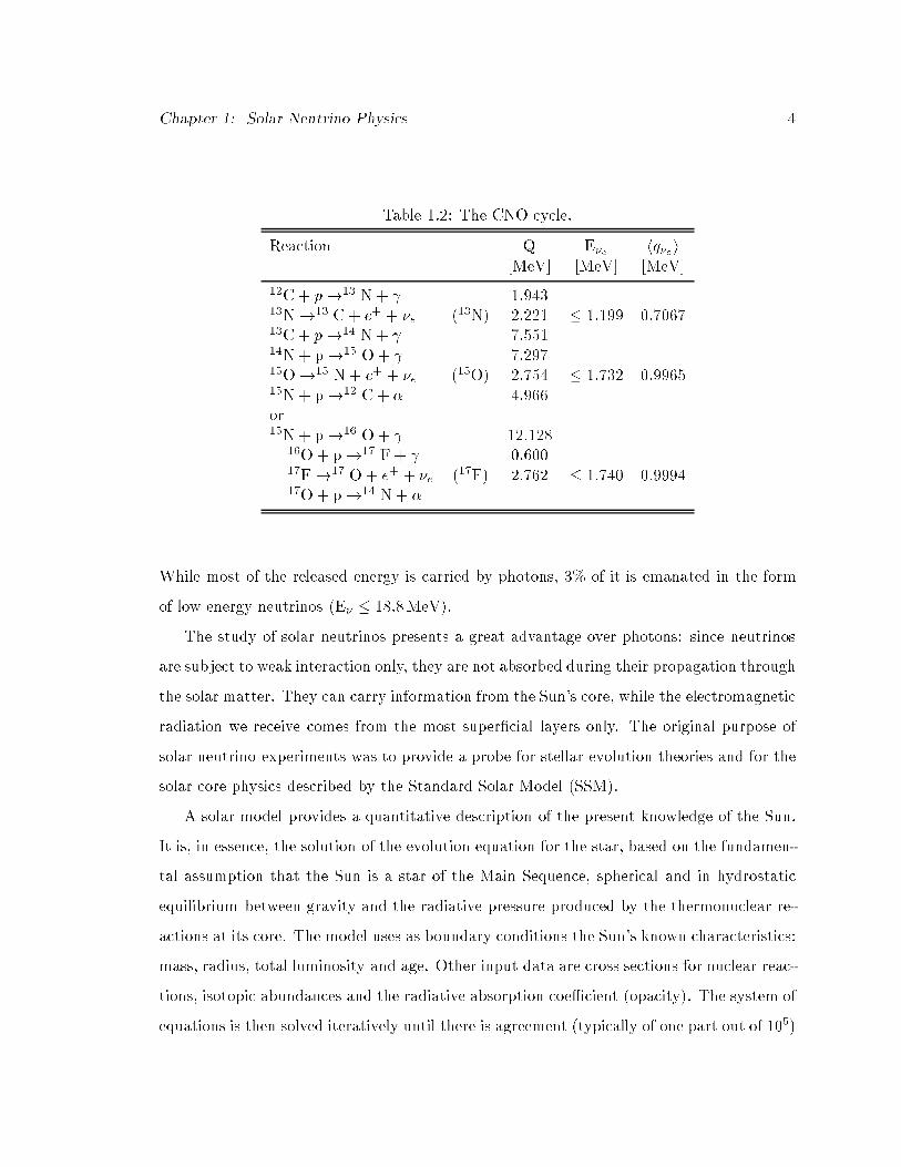
Table 1.2: The CNO cycle.
Reaction Q E�e hq�ei[MeV] [MeV] [MeV]
12C+ p!13 N+ 1.94313N!13 C+ e+ + �e (13N) 2.221 � 1:199 0.706713C+ p!14 N+ 7.55114N+ p!15 O+ 7.29715O!15 N+ e+ + �e (15O) 2.754 � 1:732 0.996515N+ p!12 C+ � 4.966or15N+ p!16 O+ 12.128
16O + p!17 F+ 0.60017F!17 O + e+ + �e (17F) 2.762 � 1:740 0.999417O + p!14 N+ �
While most of the released energy is carried by photons, 3% of it is emanated in the form
of low energy neutrinos (E� � 18:8MeV).
The study of solar neutrinos presents a great advantage over photons: since neutrinos
are subject to weak interaction only, they are not absorbed during their propagation through
the solar matter. They can carry information from the Sun's core, while the electromagnetic
radiation we receive comes from the most super�cial layers only. The original purpose of
solar neutrino experiments was to provide a probe for stellar evolution theories and for the
solar core physics described by the Standard Solar Model (SSM).
A solar model provides a quantitative description of the present knowledge of the Sun.
It is, in essence, the solution of the evolution equation for the star, based on the fundamen-
tal assumption that the Sun is a star of the Main Sequence, spherical and in hydrostatic
equilibrium between gravity and the radiative pressure produced by the thermonuclear re-
actions at its core. The model uses as boundary conditions the Sun's known characteristics:
mass, radius, total luminosity and age. Other input data are cross sections for nuclear reac-
tions, isotopic abundances and the radiative absorption coeÆcient (opacity). The system of
equations is then solved iteratively until there is agreement (typically of one part out of 105)

Chapter 1: Solar Neutrino Physics 5
between the model and the observed values of luminosity and solar radius. The model can
thus output the initial values for the mass ratios of hydrogen, helium and heavy elements,
the present radial distribution of mass, temperature, density, pressure and luminosity inside
the sun, the frequency spectrum for acoustic oscillations on the Sun's surface and the solar
neutrino spectrum and ux. Several model results have been published by di�erent authors
[6, 7, 8, 9, 10]: for a comparison between the di�erent models, I refer to the paper by Bahcall
and Pinssonneault [6]. They are all essentially in agreement; from here on, when talking of
SSM I will refer to the 1998 model by Bahcall, Basu and Pinsonneault (BP98 SSM [11]).
The Standard Solar Model allows us to deduce the present values of the solar neutrino
uxes. In Bethe's seminal work, two mechanisms were discussed: the so-called proton-
proton or pp reaction cycle, shown in table 1.1, and the carbon-nitrogen-oxygen or CNO
cycle, described in table 1.2. Today, the pp process is thought to be responsible for the
production of more than 98% of the Sun's energy. Both cycles culminate in the fusion
reaction described by eq. 1.1, the main di�erence being that the CNO cycle involves atoms
of carbon, nitrogen and oxygen as catalysts.
There are, overall, eight nuclear processes that produce neutrinos: the pep reaction
(p+ e� + p! 2H + �e) and the 7Be decay produce monoenergetic neutrinos, while all the
other sources generate neutrinos with a continuos energy spectrum. Table 1.3 reports the
uxes calculated in the BP98 SSM and �gure 1.1 shows the corresponding energy spectrum.
1.1.2 Experimental Status
All solar neutrino experiments present some common characteristics, due to the signal's low
rate. A solar neutrino detector needs to satisfy the following requirements:
- a large mass, in order to increase statistics;
- the use of high radiopurity materials, in order to minimize the background;
- a deep underground location, in order to shield from cosmic rays.
The experiments are essentially of two types:

Chapter 1: Solar Neutrino Physics 6
0.1 1.0 10.0Neutrino Energy (MeV)
101
102
103
104
105
106
107
108
109
1010
1011
1012
Flux
(/c
m2 /s
or
/cm
2 /s/M
eV)
Solar Neutrino SpectrumBahcall-Pinsonneault SSMpp
13N
15O
17F
7Be
7Be
pep
8B
hep
Figure 1.1: Solar neutrino spectra predicted by the BP98 SSM [11].

Chapter 1: Solar Neutrino Physics 7
Table 1.3: Prediction of the BP98 SSM [11]: the �rst column reports the solar neutrino uxfor each source, while the last two columns show the predicted neutrino capture rate in thechlorine and in the gallium experiments. The neutrino capture rates are measured in SolarNeutrino Unit (SNU), equivalent to 10�36 captures per target atom per second.
Source Flux Cl Ga�1010 cm�2 s�1
�[SNU] [SNU]
pp 5.94 0.0 69.6pep 1:39� 10�2 0.2 2.8hep 2:10� 10�7 0.0 0.07Be 4:80� 10�1 1.15 34.48B 5:15� 10�4 5.9 12.413N 6:05� 10�2 0.1 3.715O 5:32� 10�2 0.4 6.017F 6:33� 10�2 0.0 0.1
Total 7.7+1:2�1:0 129+8�6
1. radiochemical experiments: these employ neutrino capture reaction on speci�c
targets and later count the reaction products. They do not convey any information
on the time and the energy of the events.
2. real time experiments: these detect each neutrino interaction in the detector on
an event by event basis and they can record its energy, time and position.
At this point in time, �ve experiments have been measuring neutrino uxes from the sun.
I will now give a brief overview of each of them and a summary of their results.
The Chlorine experiment [12, 13]
The pioneer solar neutrino experiment was started in 1968 by R. Davis et al. in the
Homestake Gold Mine in Lead, South Dakota, at the depth of 4100 meters of water
equivalent (mwe). For almost two decades it was the only operating solar neutrino
detector.
The detector consists of a tank �lled with 615 tons of C2Cl4 (perchloroethylene), that
Chapter 1: Solar Neutrino Physics 8
o�ers about 2:2� 1030 37Cl atoms as targets for �e capture in the inverse 37Ar decay:
�e +37 Cl! e� +37 Ar: (1.2)
This is a radiochemical experiment; the reaction capture proceeds through weak
charged current and it is sensitive only to electron neutrinos with energy above the
threshold (Ethr = 0:814MeV); the main signal comes from 7Be and 8B neutrinos.
Every two months, the 37Ar atoms are extracted with an eÆciency of 90{95% and
counted in low background proportional counters: 37Ar decays by electron capture
(�1=2 = 35 d) in 37Cl, with production of 2{3 keV Auger electrons.
The SSM prediction for the capture rate in the Homestake experiment is reported in
table 1.3:
Rth = 7:7+1:2�1:0 SNU;
where one Solar Neutrino Unit (SNU) is equivalent to 10�36 neutrino captures per
target atom per second. Of this rate, 5.9 SNU come from 8B neutrinos and 1.15 SNU
are from 7Be neutrinos.
The measured counting rate, averaged over 25 years of data taking (1970{1995) is
roughly one third of the predicted value:
R = [2:56� 0:16� 0:16] SNU:
Gallium experiments: SAGE [14], GALLEX [15] and GNO [16]
These radiochemical experiments exploit the �e capture reaction on 71Ga:
�e +71 Ga! e� +71 Ge: (1.3)
The energy threshold for this reaction (Ethr = 0:233MeV) is low enough to allow the
detection of pp solar neutrinos. The SSM predictions for solar neutrinos capture rates
on 71Ga are reported in table 1.3: the main contribution comes from pp neutrinos
(54%), followed by 7Be neutrinos (27%) and 8B neutrinos (10%). The total expected
rate is:
129+8�6 SNU:

Chapter 1: Solar Neutrino Physics 9
The SAGE experiment is located in the underground Baksan Laboratory, in Northern
Caucasus, at 4300 mwe depth; the target consists of 60 tons of metallic gallium.
The GALLEX experiment is located in Hall A at the Gran Sasso National Labora-
tories, at a depth of 4000 mwe. Its target is 30 tons of gallium in a 60 m3 GaCl3
solution.
GNO (Gallium Neutrino Observatory) is the successor project of GALLEX, which
continuously took data between 1991 and 1997. The gallium mass in the GNO project
will be gradually increased, in the next years, from the present 30 tons up to 100 tons.
With di�erent chemical procedures, both SAGE and GALLEX (GNO) rely on the
periodic extraction of the 71Ge nuclides produced in the reaction described in eq. 1.3.
Their subsequent electronic capture decay in 71Ga (�1=2 = 11:43 d) is detected in low
background proportional counters.
The solar neutrino rates detected by the gallium experiments are roughly one half of
the prediction:
SAGE : R = [75� 7(stat)� 3(syst)] SNU;
and
GALLEX : R = [78� 6(stat)� 3(syst)] SNU:
GNO has recently made public results for the �rst two years of data (May 1998 {
January 2000): R = [66� 10� 3] SNU:
Water �Cerenkov detectors: Kamiokande [17] and SuperKamiokande [18]
Kamiokande (Kamioka Nucleon Decay Experiment) and SuperKamiokande, its suc-
cessor, are experiments looking for proton decay. Their sensitive mass consists of ultra-
pure water: ultrarelativistic charged particles crossing the water produce �Cerenkov
light observed by photomultiplier tubes. The two experiments are located in the
Kamioka mine, Japan, at 2700 mwe depth.
Chapter 1: Solar Neutrino Physics 10
Kamiokande was the second solar neutrino detector in chronological order, starting
in 1986. Its �ducial mass consisted of 680 tons of water, observed by 948 photomulti-
plier tubes. In 1994 Kamiokande was shut down and replaced by SuperKamiokande,
a larger scale clone detector. The �ducial mass of SuperKamiokande amounts to
22.5 kilotons of water, observed by 11000 photomultiplier tubes. Both experiments
performed excellent measurements on atmospheric and solar neutrinos.
The detection reaction for neutrino is elastic scattering on electrons:
�x + e� ! �x + e�: (1.4)
Elastic scattering is sensitive to any leptonic avor, with the di�erence that the cross
section for �� is about 6 times lower than that for �e, at the energy of 10 MeV.
The reaction is studied with a software energy threshold relatively high: 7.5 MeV in
Kamiokande and 6.5 MeV in SuperKamiokande; this limit, set by the background,
allows the detection of 8B and hep neutrinos only.
Despite the high energy threshold, the water �Cerenkov detectors o�er some important
advantages to the radiochemical experiments: they allow to record the time of the
event and to observe possible temporal uctuations in the signal. In addition, by
recording the energy of the recoil electron, they provide information on the spectral
energy of the incoming neutrinos. Finally, thanks to the high directionality of the
�Cerenkov e�ect, it is possible to establish a direct correlation between the neutrino
events and the Sun.
The ux measured by Kamiokande between 1986 and 1995 amounts to:
�(8B)exp = [2:8� 0:2� 0:3]cm�2s�1; (1.5)
and it compares with the predicted value as:
�(8B)exp
�(8B)theor= 0:54� 0:08: (1.6)
Chapter 1: Solar Neutrino Physics 11
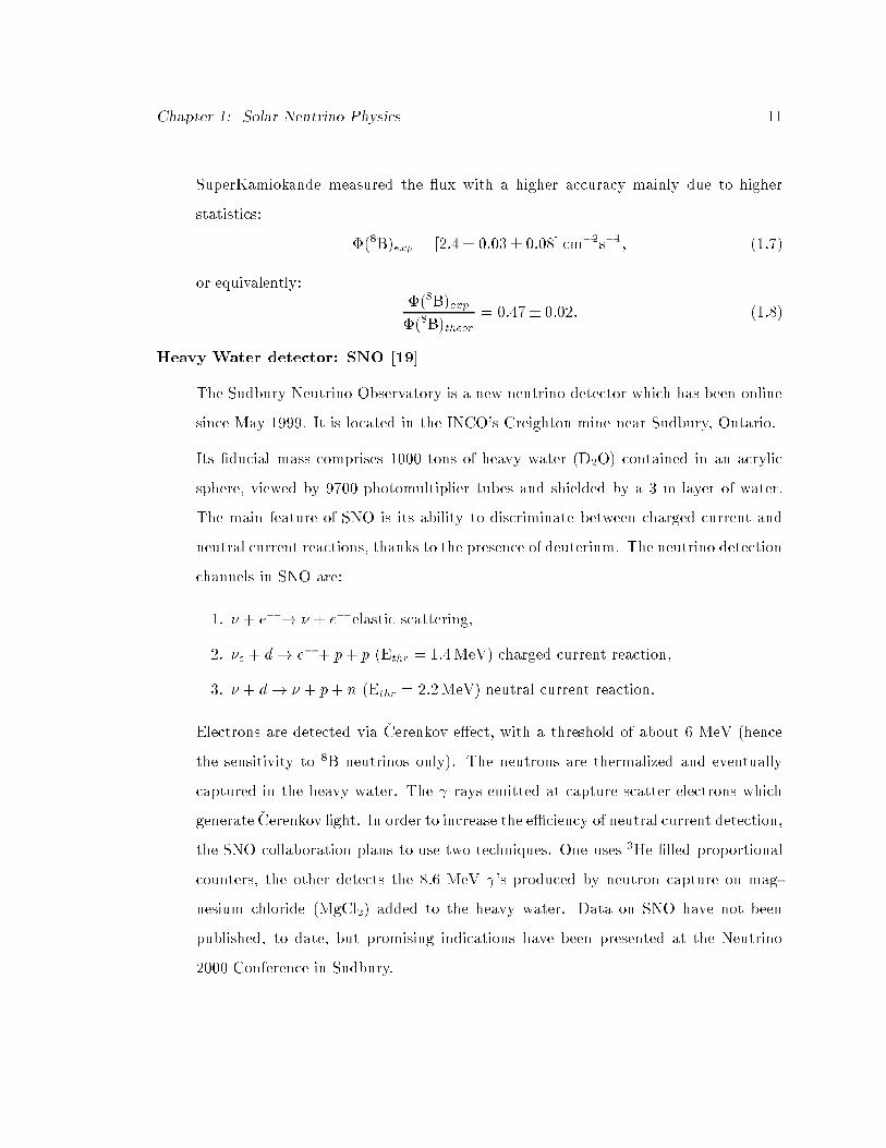
SuperKamiokande measured the ux with a higher accuracy mainly due to higher
statistics:
�(8B)exp = [2:4� 0:03� 0:08] cm�2s�1; (1.7)
or equivalently:�(8B)exp
�(8B)theor= 0:47� 0:02: (1.8)
Heavy Water detector: SNO [19]
The Sudbury Neutrino Observatory is a new neutrino detector which has been online
since May 1999. It is located in the INCO's Creighton mine near Sudbury, Ontario.
Its �ducial mass comprises 1000 tons of heavy water (D2O) contained in an acrylic
sphere, viewed by 9700 photomultiplier tubes and shielded by a 3 m layer of water.
The main feature of SNO is its ability to discriminate between charged current and
neutral current reactions, thanks to the presence of deuterium. The neutrino detection
channels in SNO are:
1. � + e� ! � + e� elastic scattering,
2. �e + d! e� + p+ p (Ethr = 1:4MeV) charged current reaction,
3. � + d! � + p+ n (Ethr = 2:2MeV) neutral current reaction.
Electrons are detected via �Cerenkov e�ect, with a threshold of about 6 MeV (hence
the sensitivity to 8B neutrinos only). The neutrons are thermalized and eventually
captured in the heavy water. The rays emitted at capture scatter electrons which
generate �Cerenkov light. In order to increase the eÆciency of neutral current detection,
the SNO collaboration plans to use two techniques. One uses 3He �lled proportional
counters, the other detects the 8.6 MeV 's produced by neutron capture on mag-
nesium chloride (MgCl2) added to the heavy water. Data on SNO have not been
published, to date, but promising indications have been presented at the Neutrino
2000 Conference in Sudbury.

Chapter 1: Solar Neutrino Physics 12
Figure 1.2: The three Solar Neutrino Problems: comparison of the prediction of the standardsolar model with the total observed rates in the �ve solar neutrino experiments: Homestake,Kamiokande, SuperKamiokande, GALLEX and SAGE. From reference [20].
1.2 The Solar Neutrino Puzzle
Figure 1.2 is a graphical illustration of the solar neutrino puzzle: the measured solar neutrino
uxes are, in all instances, lower than the predictions of the Standard Solar Model, combined
with the Standard Model of Electroweak interaction. The discrepancy between the predicted
and the measured rates goes beyond the range of uncertainties: this constitutes the \�rst"
neutrino problem.
There is, then, a \second" neutrino problem, as Bahcall and Bethe pointed out in 1990:
the 8B rate observed by the �Cerenkov detectors exceeds the total measured rate in the
chlorine experiment. This is puzzling, if the solar neutrino energy spectrum is not modi�ed
by some non standard neutrino process, since both 7Be and 8B neutrinos are expected to
Chapter 1: Solar Neutrino Physics 13
contribute to the chlorine rate. The signal directionality and the qualitative shape of events
in Kamiokande and SuperKamiokande leave no doubt that they have solar origin and they
obey the 8B energy spectrum.
A \third" solar neutrino problem emerges from the gallium detectors results: the mea-
sured rate is all accounted for by the pp neutrinos and, again, there is no room for 7Be
neutrinos. This is often referred to as \the problem of the missing 7Be neutrino".
The need for a justi�cation to the solar neutrino de�cit has driven e�orts in two di-
rections: astrophysical solutions and new neutrino physics solutions. In the next sections,
I will present the main theories that have been proposed and the solutions that now look
most promising.
1.2.1 Astrophysical Solutions to the Solar Neutrino Puzzle
The Standard Solar Model, built to give an estimate to the Sun's parameters, makes use
of a number of simplifying hypothesis, but the accuracy of its predictions can be tested
against experimental data.
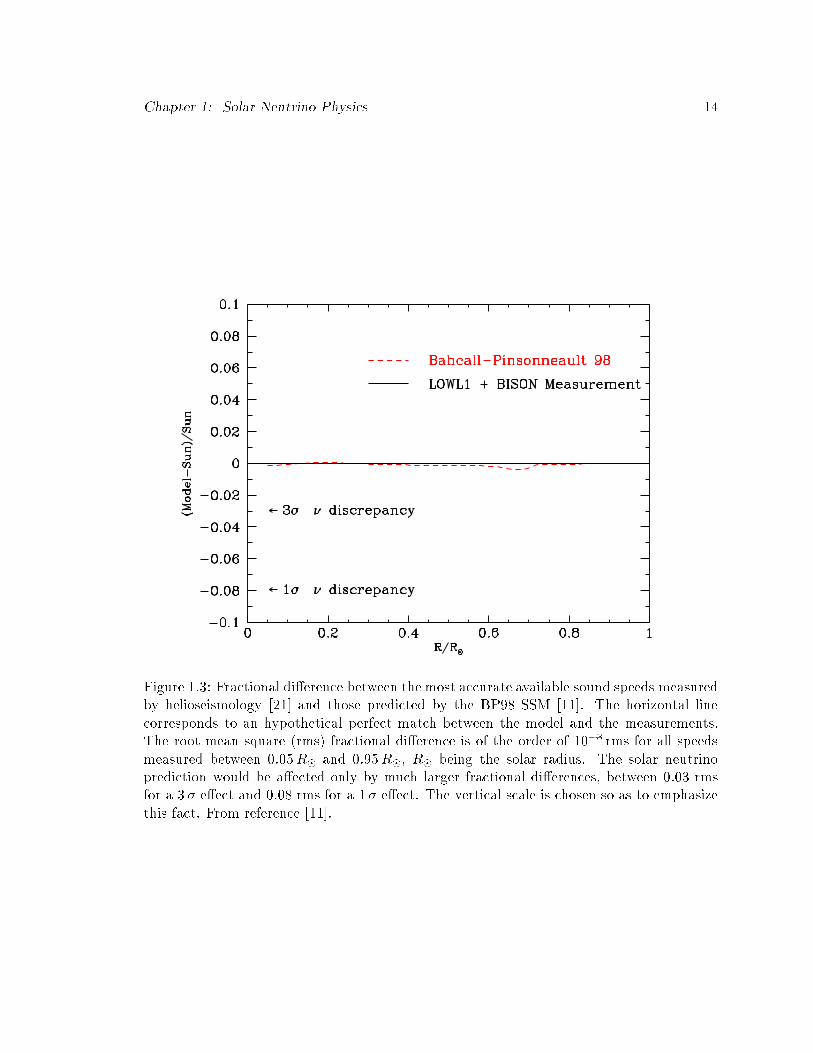
Helioseismic activity has been observed, in the past few years, by �ve di�erent experi-
ments: LOWL1, BISON, GOLF, GONG, MDI [21, 22, 23, 24]. These experiments measured
the radial distribution of the sound speed inside the Sun, providing results that are in excel-
lent agreement, at the level of 0.2%, with the predictions of the BP98 SSM [11]. Figure 1.3
shows how the fractional di�erence between the measured and the calculated distributions
is much smaller than any change in the model that could signi�cantly a�ect the prediction
of the solar neutrinos uxes.
The principal ingredients in the SSM calculations now seem to be well established. The
main uncertainty still lies in the input parameters, especially the nuclear cross sections that
have been measured in laboratories at much higher energies and later extrapolated to the
energies of interest for the Sun's fusion reactions. For instance, a low energy resonance in
the 3He+3He system would induce a signi�cant suppression of the 7Be and 8B neutrinos.
Other nuclear cross sections that would a�ect the 7Be and 8B neutrinos and that are not
well known at the energies of interest are 3He(�; )7Be and 7Be(p; )8B. Then there are
Chapter 1: Solar Neutrino Physics 14
Figure 1.3: Fractional di�erence between the most accurate available sound speeds measuredby helioseismology [21] and those predicted by the BP98 SSM [11]. The horizontal linecorresponds to an hypothetical perfect match between the model and the measurements.The root mean square (rms) fractional di�erence is of the order of 10�3 rms for all speedsmeasured between 0:05R� and 0:95R�, R� being the solar radius. The solar neutrinoprediction would be a�ected only by much larger fractional di�erences, between 0.03 rmsfor a 3 � e�ect and 0.08 rms for a 1 � e�ect. The vertical scale is chosen so as to emphasizethis fact. From reference [11].

Chapter 1: Solar Neutrino Physics 15
Figure 1.4: Response of the pp, 7Be and 8B uxes to variations of the SSM input parametersas a function of the resulting core temperature. The models that have been consideredchanged the input parameters for pp nuclear cross section Spp, opacity, mass ratios and age.From Castellani et al. [25].
uncertainties in calculated quantities such as the solar matter opacity, which depends on
the initial chemical and isotopic composition of the Sun. A possible explanation to the
solar neutrino puzzle can in principle be obtained by changing the input parameters of
the model, reducing, for instance, the opacity or lowering S17, the cross section for the
7Be(p; )8B reaction.
Another possibility, still in the astrophysical solution context, is to invoke mechanisms
that the model does not include, such as a strong central magnetic �eld, rapid rotations of
the core, instability phenomena or hypothetical WIMPs (Weak Interacting Massive Parti-
cles) that replace neutrinos as carriers for part of the Sun's energy.
Chapter 1: Solar Neutrino Physics 16
0.0 0.5 1.0φ(
7Be) / φ(
7Be)SSM
0.0
0.5
1.0
φ(8 B
) / φ
(8 B) SS
M
Monte Carlo SSMsTL SSMLow ZLow opacityWIMPLarge S11
Small S34
Large S33
Mixing modelsDar-Shaviv model
T C power law
BP SSM
No oscillationsCombined fit ofcurrent data90, 95, 99% C.L.
Smaller S17
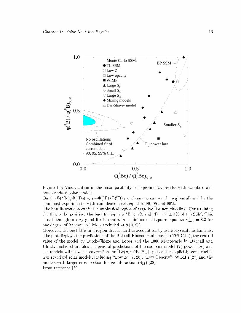
Figure 1.5: Visualization of the incompatibility of experimental results with standard andnon-standard solar models.On the �(7Be)=�(7Be)SSM ��(8B)=�(8B)SSM plane one can see the regions allowed by thecombined experiments, with con�dence levels equal to 90, 95 and 99%.The best �t would occur in the unphysical region of negative 7Be neutrino ux. Constrainingthe ux to be positive, the best �t requires 7Be< 7% and 8B = 41 � 4% of the SSM. Thisis not, though, a very good �t: it results in a minimum chisquare equal to �2min = 3:3 forone degree of freedom, which is excluded at 93% CL.Moreover, the best �t is in a region that is hard to account for by astrophysical mechanisms.The plot displays the predictions of the Bahcall-Pinsonneault model (90% C.L.), the centralvalue of the model by Turck-Chieze and Lopes and the 1000 Montecarlo by Bahcall andUlrich. Included are also the general predictions of the cool sun model (Tc power law) andthe models with lower cross section for 7Be(p; )8B (S17), plus other explicitly constructednon standard solar models, including \Low Z" [7, 26], \Low Opacity", WIMPs [27] and themodels with larger cross section for pp interaction (S11) [28].From reference [29].

Chapter 1: Solar Neutrino Physics 17
From a phenomenological point of view, all the new suggested processes a�ect the neu-
trino ux through a variation of the core temperature of the Sun (Tc). It is then possible to
treat Tc as a phenomenological parameter to represent di�erent solar models. An approxi-
mate correlation between the neutrino uxes from di�erent sources and Tc has been derived
by Bahcall and Ulrich: �(8B)� T18c , �(7Be)� T8
c and �(pp) � T�1:2c [7]. A reduction of Tc
(Cool Sun Model) could in principle work towards a solution for the solar neutrino puzzle.
The problem is the ratio �(7Be)=�(8B) would be pushed towards values that are higher
than the SSM prediction, while the experimental results go in the opposite direction. This
physics has been illustrated by Castellani et al. [25] in �gure 1.4.
The strongest argument against an astrophysical solution to the solar neutrino puzzle
is the incompatibility with experimental data. The results of existing experiments are
routinely compared to the model predictions with the �tting procedure described in detail
in ref [30]. The combined �t is a least square minimization of a �2, de�ned as:
�2 =Xi;j
�Rtheoryi �Rexper
i
�Vi;j
�Rtheoryj �Rexper
j
�(1.9)
where Ri is the measured or predicted event rate in the ith experiment and Vi;j is the error
matrix, that includes all the uncertainties in the model and the statistical and systematic
errors in the experiment.
Several �ts have been performed without satisfying results: no value of Tc can simulta-
neously justify all the experimental results [29, 31, 32]. Figure 1.5 [29] is a good visualization
of the incompatibility of experimental results with standard and non-standard solar mod-
els: while the experimental data indicate a preferential suppression of 7Be neutrinos, all
astrophysical and nuclear physical explanations predict a larger suppression for 8B than for
7Be and no signi�cant deformation of the 8B spectrum.
An astrophysical solution to the three solar neutrino problems is, at this point, largely
unfavorable. The explanation does not seem to lie in the Sun, where neutrinos are produced.
More likely something happens to them on the way to the detectors.

Chapter 1: Solar Neutrino Physics 18
1.2.2 Non-Standard Neutrino Physics
An alternative and more likely path towards the solution of the Solar Neutrino Puzzle
explores new neutrino physics, outside the boundaries of the Standard Model of electroweak
interaction. The basic idea is that neutrinos can have intrinsic properties that the Standard
Model does not foresee, such as mass, magnetic moment and a non zero avor mixing angle.
If this is the case, neutrinos take part in di�erent physical processes that can lower their
rate of detection and distort their energy spectrum.
Suggested particle physics solutions of the solar neutrino problem include neutrino oscil-
lations, neutrino decay and neutrino magnetic moments. I will provide below a description
of the most plausible models: avor oscillations in vacuum and in matter.
Flavor Oscillations in Vacuum
The idea that neutrinos can oscillate between leptonic avors was �rst suggested by Bruno
Pontecorvo, in 1967. This is a non standard phenomenon that takes place only if at least
one of the neutrino states has non zero mass and if the leptonic number is not conserved:
these properties are postulated in the Great Uni�cation Theory, or GUT, an extension of
the Standard Model.
In these hypotheses, the set of electroweak eigenstates ( avor eigenstates) �e, �� e ��
can be expressed as a combination of the mass eigenstates �m that describe free particle
propagation in vacuum:
j��i =Xm
h�mj��i j�mi; (1.10)
where j��i is the leptonic eigenstate, j�mi are mass eigenstates and h�mj��i are the massmatrix elements for neutrinos, a direct analog of the Kobayashi-Maskawa matrix in the
charged current Hamiltonian for quarks. In the case of mixing between leptonic avors,
this matrix is non-diagonal.
The di�erent mass components of a neutrino of de�nite avor propagate at di�erent
speeds: this leads to neutrino oscillations in vacuum, that is the transformation of a neutrino
of one avor into one of di�erent avor as the neutrino moves through empty space.

Chapter 1: Solar Neutrino Physics 19
In a simpli�ed two lepton model, the mixing matrix is a 2� 2 rotation and the mixing
can be expressed in term of a mixing angle �:
( j�ei = cos �j�1i+ sin �j�2ij�xi = � sin �j�1i+ cos �j�2i
: (1.11)
An electron neutrino j�ei with momentum p will propagate as superposition of the two mass
eigenstates and, after time t, the beam wavefunction will have evolved into:
j�e(x; t)i = cos �j�1ie�i(E1t�px) + sin �j�2ie�i(E2t�px); (1.12)
where Ej =qp2 + m2
j ' p + m2j=2p, in the hypothesis that the masses are much smaller
than the momentum. If �m2 = m22 �m2
1 and p ' E, eq. 1.12 can be rewritten as:
j�e(x; t)i =24cos �j�1i+ sin �j�2ie�i
�m2
2E
35 ei (E1t�px): (1.13)
The wavefunction describing neutrinos in free propagation has di�erent components, with
phases that depend on time and distance, and there is a non zero probability to detect
neutrinos of di�erent avors at any time during the propagation. Such probability has a
periodic behavior:
8<:P (�e ! �e; R) = jh�ej�e(R; t)ij2 = 1� sin2 2� sin2
��RLv
�P (�e ! �x; R) = jh�xj�e(R; t)ij2 = sin2 2� sin2
��RLv
� ; (1.14)
where R is distance from the source, Lv =4�p
�m2is the oscillation length and � is the mixing
angle.
Another way to describe the process is that, for a given moment p, the lighter eigen-
states in �e travel faster than the heavier ones. The di�erent components of the beam get
out of phase and during the trip from source to detector the beam acquires components
corresponding to di�erent avors, after a distance equal to the oscillation length. This is a
violation of the conservation of the leptonic number.
A solar neutrino detector should observe a periodic correlation between the neutrino
signal and the distance R from the source. The detectable neutrino ux would depend on

Chapter 1: Solar Neutrino Physics 20
the mixing angle and oscillation phase in equation 1.14. The electron neutrino signal can
be largely suppressed if the phase is:
� =�R
Lv=
�k +
1
2
��; (1.15)
with k integer. This happens if the Sun{Earth distance is equal to:
R =
�k +
1
2
�Lv =
�k +
1
2
�4�E
�m2 : (1.16)
Given the average value of R = 150� 104 km, we obtain:
�k +
1
2
�= 6:07
1
E[MeV]
�m2
10�10: (1.17)
If the mixing angle � is suÆciently large and if k is small enough, we can have a situation
where the 1 MeV neutrinos convert in a di�erent avor, while the higher energy neutrinos
from 8B do not. If k is large, avor conversion happens throughout the solar neutrino
spectrum and the signal from �e is at a minimum (about 0.5 SSM).
Note that the vacuum oscillation scenario requires, to solve the solar neutrino puzzle,
mixing angle values that are much larger than the corresponding mixing angles between
quarks and a very �ne tuning of the relation between neutrino masses, their energy and the
Sun-Earth distance.
Flavor Oscillations in Matter: the MSW E�ect
An alternative solution to the solar neutrino puzzle, originally proposed in 1978 by Wolfen-
stein [33] and later revived by Mikheyev and Smirnov in 1985 [34], accounts for the di�erent
way neutrinos propagate in matter, due to weak scattering with electrons.
Electron neutrinos interact with matter both through charged and neutral current weak
interactions, while �� and �� are subject to neutral current interactions only. The interaction
of neutrinos with the matter �elds can be accounted for by the introduction of a refraction
index n in the propagating wave function:
j��i =Xm
h�mj��i j�mi e�i(Emt�pnx): (1.18)

Chapter 1: Solar Neutrino Physics 21
The refraction index depends on the electron density Ne and the forward elastic scattering
amplitude for neutrinos f(0) as:
n = 1 +2�Nef(0)
p2: (1.19)
The di�erence between forward scattering amplitude for electron neutrinos and the other
avors determines a density-dependent splitting of the diagonal elements in the mass matrix;
in other words, the mass eigenstates that propagate in matter are di�erent from the ones
propagating in vacuum. The splitting is given by [35]:
fe(0)� fx(0) = �f(0) = �p2GFp
2�; (1.20)
where GF is the Fermi coupling constant. In virtue of this, the electron neutrino wave
function has an additional phase term that does not appear in the wave function for other
avors:
j�ei / e�ip2xNeGF: (1.21)
The oscillation length for �e is de�ned as the length at which the above phase term equals
2�. It depends on the electron density as:
Lm =2�p2NeGF
' 1:7� 107 m
�[g=cm3]hZ=Ai: (1.22)
This value is equal to � 200 km in the Sun's core and � 104 km inside Earth.
The mixing angle inside the solar matter �m is related to the one in vacuum by the
relation:
sin2 2�m =sin2 2�
(cos 2� � Lv=Lm)2 + sin2 2�
; (1.23)
where, again, Lv and Lm are the neutrino oscillation lengths in vacuum and in matter.
Equation 1.23 presents a resonant feature: let us assume that, along the path from the
Sun's core (where they are produced) to the external layers, neutrinos run into a region
with such density as to have:Lv
Lm= cos 2�:
In this case, sin2 2�m = 1, and there is local maximal mixing even though the mixing angle
in vacuum � can be very small. Provided the neutrino beam encounters a region with the

Chapter 1: Solar Neutrino Physics 22
mi2
2E
(xc)0
| L> | > | L> | e>
| H> | e>(x) /2
| H> | >(x) v
Figure 1.6: Schematic illustration of the MSW e�ect. The dashed line corresponds to theelectron-electron and the muon-muon diagonal elements of the M2 matrix in the avorbasis. Their intersection de�nes the critical density �c. The solid lines describe the lightand heavy local mass eigenstates as a function of matter density. If �e is produced in ahigh density region, as the Sun's core, and propagates adiabatically, it will follow the heavymass trajectory and emerge from the Sun as a ��. From reference [36].
\right" electron density, the conversion becomes resonant. The critical density is the point
where the splitting between mass eigenvalues reaches its minimum and it is equal to:
�c =1
2p2GF
cos 2��m2
E: (1.24)
The phenomenon of matter enhanced oscillation is known as the MSW e�ect.
According to the solar models [6, 7, 9, 37], the matter density inside the Sun monoton-
ically decreases between � 150 g=cm3 at the core and � 0 at the outside. The change in �
is followed by a change of �m and of the nature of the avor mixing.
The assumption underlying an MSW explanation to the solar neutrino problem is that
when a �e is generated in a high density region (� > �c), it is mainly constituted by the
heavier eigenstate, �2 = �H , while in vacuum it is closer to the lighter state �1 = �L. In the
critical density region, �m ! �4 and �H is composed by �e and �� in equal parts, while as
�! 0 it is mostly ��. If the neutrino beam crosses the Sun adiabatically (that is, without

Chapter 1: Solar Neutrino Physics 23
introducing transitions between �L and �H), it is mainly constituted by the heavier state �H
all the way. The net result is that, when it emerges Sun, the beam will be mostly constituted
by ��, non detectable by the radiochemical experiments and only partially detected by the
�Cerenkov detectors. This process is illustrated in �gure 1.6.
In the adiabatic hypothesis, the conversion of �e in �� is almost total. The survival
probability for a �e is:
P(�e ! �e)adiab =1
2(1 + cos 2� cos 2�m;i) � sin2 �; (1.25)
where �m;i � �2 is the mixing angle in matter, evaluated at the production site. A notable
remark is that, in the Sun, the conversion is more complete for smaller values of the mixing
angle in vacuum.
The adiabatic condition is satis�ed only if the resonance width is larger than the os-
cillation length in matter. For a 10 MeV neutrino, this condition is veri�ed, in the Sun,
if: (�m2 � 10�4eV2
sin2 2� < 4� 10�4:
For smaller masses and larger mixing angles, there is no adiabaticity and the conversion is
only partial.
In the non-adiabatic case, the survival probability for a �e with energy E is given by the
Parke relation [38, 39]:
P (E) =1
2+1
2cos 2�m;i cos 2� (1� 2Phop) ; (1.26)
Phop = e��; � =��m2 sin2 2�
4E cos 2�
���� Ne
dNe=dr
����resonance
: (1.27)
Phop is the Landau-Zener probability for a jump between the mass eigenstates. It accounts
for non adiabatic corrections, so that higher energy neutrinos have higher survival proba-
bility.
The MSW e�ect is, thus, extremely exible: depending on the values assumed by the
parameters �m2 and sin2 2�, it can preferentially suppress the higher energy neutrinos from
8B or the lower energy neutrinos from 7Be and pp or, again it can deplete the lower energy
portion of the 8B spectrum and the 7Be while safeguarding the pp ux.

Chapter 1: Solar Neutrino Physics 24
Table 1.4: Best-�t global oscillation parameters and con�dence limits for the currentlyallowed neutrino oscillation solutions. The active neutrino solutions are from Fig. 1.7. Thedi�erences of the squared masses are given in eV2. From reference [42].
Scenario �m2 sin2(2�) C.L.
LMA 2:7� 10�5 7:9� 10�1 68%SMA 5:0� 10�6 7:2� 10�3 64%LOW 1:0� 10�7 9:1� 10�1 83%VACS 6:5� 10�11 7:2� 10�1 90%VACL 4:4� 10�10 9:0� 10�1 95%Sterile 4:0� 10�6 6:6� 10�3 73%
The phenomenon of neutrino oscillation in matter can also take place inside the Earth.
As a consequence, electron neutrinos that have been converted in �x inside the Sun, by
MSW e�ect, can regenerate and recover their electron avor while crossing Earth in their
trip to the detector. Paraphrasing the title of Bahcall's paper [40], we could say that the
Sun appears brighter at night in neutrinos.
This e�ect would induce a daily variation of the detected rate; for details on the physics
and the calculations, we refer to [40, 41] and references therein. An experimental, statisti-
cally robust observation of a day � night asymmetry would be a very convincing proof of
the validity of the MSW e�ect.
1.3 Where Do We Stand Now?
The second generation of solar neutrino experiments, with larger detector masses and im-
proved sensitivities, has already started.
After the Neutrino 98 conference, when the SuperKamiokande data were �rst announced,
new �ts have been performed. A complete overview of the �ts and allowed solution is of-
fered in ref. [42]. Figure 1.7, from [42], shows the two allowed regions for vacuum oscillation
(VACL and VACS) and the three MSW allowed regions: LMA (large mixing angle solu-
tion), SMA (small mixing angle solution) and LOW (low mass). The best �t values and

Chapter 1: Solar Neutrino Physics 25
(a) (b)
Figure 1.7: Global oscillation solutions. The input data include the total rates in theHomestake, Sage, Gallex, and SuperKamiokande experiments, as well as the electron recoilenergy spectrum and the day-night e�ect measured by SuperKamiokande in 825 days of datataking. Figure 1.7-a shows the global solutions for the allowed MSW oscillation regions,known, respectively, as the SMA, LMA, and LOW solutions [42]. Figure 1.7-b shows theglobal solution for the allowed vacuum oscillation regions. The C.L. contours correspond,for both �gures, to �2 = �2min + 4:61(9:21), representing 90% ( 99%) C.L. relative to eachof the best-�t solutions (marked by dark circles) given in Table 1.4. The best vacuum�t to the SuperKamiokande electron recoil energy spectrum is marked in Fig. 1.7-b at�m2 = 6:3� 10�10 eV2 and sin2 2� = 1. From reference [42].

Chapter 1: Solar Neutrino Physics 26
1 10 102
103
104
105
0
0.5
1
1.5
L/Eν (km/GeV)
Dat
a / M
onte
Car
lo
e-like
µ-like
Figure 1.8: Ratio of observed and predicted events, in SuperKamiokande, as a functionof the natural oscillation parameter L=E� . Electrons show no evidence for oscillation,while muons exhibit a strong drop with L=E� . This is consistent with �� � �� oscillationswith maximal mixing and �m2 = 0:0032 eV 2, as indicated by the dashed lines from thesimulations. From reference [43].
con�dence limits for the di�erent models are reported in table 1.4, always from [42]. The
table also reports another solution that is presently being considered: oscillation of �e in
sterile neutrinos �s. The allowed region is similar to the SMA region, in �gure 1.7.
The SuperKamiokande data is contributing new pieces of information to the overall solar
neutrino picture, with increasing statistics. The main results can be summarized as follows:
Evidence for neutrino oscillation. The SuperKamiokande collaboration announced in
1998 new evidence for muon neutrino disappearance in the measured ux of atmo-
spheric neutrino [44]. They observed a up-down asymmetry and a reduced ux for
muon neutrinos, but not for electron neutrinos; such anomaly can be used as di-
agnostic for neutrino oscillation. The evidence points to neutrino oscillation in the
channel �� ! �� , with �m2 = 2� 7 � 10�3 eV2 and sin 2�V � 1 (see �g. 1.8). For a
complete discussion of the atmospheric neutrino anomaly and neutrino oscillation in

Chapter 1: Solar Neutrino Physics 27
SuperKamiokande, I refer to [43].
Spectral distortion above 13 MeV. The recoil energy spectrum measured by Super-
Kamiokande shows evidence for an enhanced event rate above a total electron energy
of 13 MeV. The detected spectrum and its ratio to the predictions of the BP98 SSM
are shown in �g. 1.9, from reference [45]. Several possible explanations have been
suggested for this anomaly, including:
1. an enhanced ux of hep neutrinos [46, 47];
2. a real upturn in the survival probability. Berezinsky et al. [48] pointed out that
there exists a vacuum oscillation solution that can explain the spectrum deforma-
tion and solve the solar neutrino puzzle at the same time (�m2 = 4:2�10�10 ev2,sin2 2� = 0:93, labelled by the authors HEE-VO, High-Energy Excess vacuum
oscillation). The HEE-Vo solution presents as its most distinct signature a semi-
annual seasonal variation of the 7Be neutrino ux, with maximal amplitude. This
e�ect needs to be con�rmed by a real-time detection of the 7Be neutrinos.
3. the excess could be a consequence of the small statistics or of small systematic
errors in the energy calibration. We will �nd out whether this is the case once
SNO will have collected enough statistics, since SNO is also sensitive to the
detection of this anomaly.
The most recent SuperKamiokande data, presented at the Neutrino 2000 confer-
ence [49], is still showing a high energy excess, but the evidence appears less con-
vincing, with higher statistics. A at spectrum is posible with �2flat = 13:7=17 dof
and 69% CL. The �t with 8B+hep neutrino spectra yields:
hep ux < 13:2 SSM (best �t : 5:4� 4:6 SSM):
Evidence for a day-night e�ect. A day/night asymmetry in the SuperKamiokande data
has been suggested at the Neutrino 2000 conference [49]:
2D �N
D +N= �0:034� 0:022stat� 0:013sys:

Chapter 1: Solar Neutrino Physics 28
10-1
1
10
6 8 10 12 14Energy (MeV)
Eve
nts
/ day
/ 22
.5kt
/ 0.
5MeV Super-Kamiokande 504day 6.5-20MeV
Solar neutrino MC (BP98 SSM)
Observed solar neutrino events
stat. error
stat.2+syst.2
0
0.1
0.2
0.3
0.4
0.5
0.6
0.7
0.8
0.9
1
6 8 10 12 14Energy(MeV)
Dat
a/S
SM
BP
98
Super-Kamiokande 504day 6.5-20MeV
stat. error
stat.2+syst.2
Figure 1.9: Top: recoil electron energy spectrum of solar neutrinos measured by Su-perKamiokande in the �rst 504 days, between 6.5 and 20 MeV, compared to the BP98SSM predictions. Below is a plot of the ratio between data and SSM prediction. Fromreference [45].

Chapter 1: Solar Neutrino Physics 29
This indication is still statistically weak (� 1:3 �), but, if con�rmed with higher
statistical signi�cance, it will indicate the occurrence of Earth regeneration for the 8B
solar neutrinos.
While the previous �ts tended to favor the SMA MSW solution, these new data from
SuperKamiokande, both by themselves and in combination with chlorine and gallium
experiments, tend to favor the LMA and LOW regions of the parameter space [41].
According to Fogli et al. [50], there is a tension between the total rates, which are
in favor of the SMA solution, and the at spectrum observed by SuperKamiokande
(the SMA predicts spectral deformation). However, a compromise between these
discordant indications is still reached in the global �t and all 3 solutions are still valid
at the 95% CL. As far as discrimination between the LOW and the LMA solutions,
Fogli et al. [50] propose to compare the day-night asymmetries in two separate energy
ranges: L (5{7.5 MeV) and H (7.5{20). Once enough statistics have been collected
both by SuperKamiokande and SNO, the sign of the parameter:
� =
�N �D
N +D
�H��N �D
N +D
�L
(1.28)
will allow to discriminate between LMA and LOW, since Earth regeneration e�ect is
stronger at low energy for LOW and at high energy for LMA.
SNO started its data taking about one year ago: at Neutrino 2000, very recently, they
have shown everything is working properly, the spectral shape can be scaled to the SSM
spectrum of 8B but the scaling coeÆcient has not been disclosed yet. The next few months
of data will shed some light on the questions opened by SuperKamiokande.
GNO will continue measuring the pp neutrino ux, with a larger mass, hence larger
statistics, than Gallex did. For the moment, it is working with the same sensitive mass, so
there is not much more information to add. It will be particularly interesting to see whether
a seasonal variation of the rate will emerge, with larger statistics, in view of the HEE-VO
model proposed by Berezinsky et al. [48].
But the missing key to a complete understanding of the solar neutrino puzzle is a direct,
real time measurement of the monoenergetic 7Be solar neutrino ux. Borexino is a new

Chapter 1: Solar Neutrino Physics 30
detector speci�cally designed to answer the question that is still pending: \where do all the
7Be neutrinos go?"
In the next three chapters, I will describe the detector and its new technology, I will
investigate background sources and expected performances and I will review the contribution
that Borexino can provide to the solution of the solar neutrino problem.

Chapter 2
The Borexino Experiment
2.1 Overview of the Borexino Project
The existing \second generation" solar neutrino detectors will produce high statistics neu-
trino signals and will provide precious information for the understanding of the solar neu-
trino physics, but the ultimate solution to the solar neutrino problem will come only once
we have an answer to the question of what happens to the 7Be solar neutrinos. A detector
speci�cally designed to count them is the missing key in this puzzle; Borexino is such a
detector.
Evolving from an original proposal by R. Raghavan1, the Borexino project relies on the
e�orts of an international collaboration whose principal institutions are from the United
States, Italy and Germany. The detector is now under construction in the underground
facility of the Gran Sasso National Laboratories (LNGS), under the Italian Apennines, at
a depth of 3800 mwe. Its main scienti�c goal is to provide a real time measurement of the
7Be neutrino ux, insulating it from the other components of the solar neutrino spectrum,
and to observe possible periodic variations of the signal.1The original Borex project was initiated in 1987 as a solar neutrino detector for neutral and charged
current interactions of 8B neutrinos on 11B in the target. The design required a 1000-ton �ducial mass of the
boron compound trimethylborate as scintillator, from which the project's name originated. Borexino was
�rst planned as a prototype for Borex, with only 100-ton �ducial mass. It was soon realized, though, that
Borexino was large enough to become a unique high rate detector for the more intense 7Be neutrinos, provided
the background at low energy could be reduced. The detection of 7Be neutrinos became the project's new
goal and trimethylborate was replaced by pseudocumene as scintillator, but the name remained.
31

Chapter 2: The Borexino Experiment 32
Borexino is an unsegmented detector whose sensitive mass consists of 300 tons of or-
ganic liquid scintillator, one third of which will be used as �ducial mass. The fundamental
detection reaction is the elastic scattering of neutrinos on electrons:
� + e! � + e: (2.1)
The energy of the recoil electron will be detected through the scintillation light it produces
as it comes to rest in the scintillator, by means of 2200 phototubes. The scattering reaction
is sensitive to all leptonic avors, but there is no signature that discriminates between
charged current (�e) and neutral current (�x) interactions. The only di�erence is the cross
section, which is about 5 times higher for �e than for the other avors.
The liquid scintillator (see x2.2.1) is a mixture of pseudocumene (PC) and uors (PPO),
with relatively high yield: � 104 photons are generated per MeV of deposited energy and
� 400 of them are detected. For this reason, Borexino is in principle able to detect recoil
electrons with energies down to a few tens of keV. In reality, the e�ective threshold is limited
by background considerations. The presence of the low energy � emitter 14C (Q = 156
keV) in the scintillator, chemically bound to the organic molecules, sets the lower detectable
neutrino ux at 250 keV.
The predicted counting rate for solar neutrinos in a 100 ton �ducial volume and above the
250 keV energy threshold is 63 events/day, 46 of which are from 7Be neutrinos, according to
the BP98 SSM [11]. Borexino does not o�er an event-by-event signature or any directional
information for �-e scattering events; the signal can be distinguished from the background
only statistically.
There is, however, a spectral signature for 7Be solar neutrinos: owing to the monochro-
matic nature of the 7Be neutrino radiation, the energy spectrum of the recoil electrons in
Borexino (eq. 2.1) will feature a sharp Compton-like edge at the energy of 665 keV. There
is also a temporal signature for the solar neutrino ux: the eccentricity of Earth's orbit
provokes a 7% annual variation of the neutrino rate (1=R2 e�ect).
The lack of an event-by-event signature makes it critically important to minimize the
rate and understand the spectrum of background events. The requirement for background

Chapter 2: The Borexino Experiment 33
in the energy range 250{800 keV (also known as the "neutrino window") is an upper limit
of 0:05 events/day/ton, or 5 � 10�10Bq/kg. Achieving this goal constitutes the ultimate
challenge and the key to the success of the Borexino project.
2.2 Detector Structure
The Borexino detector structure consists of several concentric regions, organized in the shell
pattern shown in �gure 2.1. The design has been driven by the following considerations:
Neutrino count rate. The number of detected neutrinos depends linearly on the volume
of target scintillator. In order to have a SSM neutrino count rate of about 50 ev/day
in a pseudocumene scintillator, the detector �ducial mass needs to be equal to at least
100 tons.
Solar neutrino signatures in Borexino. There are two principal ways Borexino will es-
tablish that it has seen solar neutrinos { one is to identify the \edge" due to 7Be
neutrinos in the electron recoil energy spectrum at 665 keV, the second is to observe
the 1=R2 annual variation in neutrino rate from the Sun (a 7% e�ect). Our ability to
detect either e�ect will depend critically on the degree of background suppression we
are able to achieve.
Signal to background ratio. Due to the strict requirements on the background rate (see
discussion in {3), extraordinary puri�cation procedures need to be implemented, both
for the active scintillator and for the surrounding shields. Very stringent requirements
are also placed on the construction materials used throughout Borexino { from the
scintillator containment vessel, to the phototube glass, to the metallic support vessels
(see x3.3). Measures must be employed to maintain cleanliness during assembly and
an eÆcient veto for cosmic-ray muons needs to be implemented.
Detector resolution. Maximizing the amount of collected scintillation light leads not
only to an improved energy resolution, vital for the identi�cation of the recoil elec-
tron edge, but also for a superior �=� discrimination and a better spatial position

Chapter 2: The Borexino Experiment 34
Stainless Steel Water Tank18m ∅
Stainless SteelSphere 13.7m ∅
2200 8" Thorn EMI PMTs
WaterBuffer
100 ton fiducial volume
Borexino Design
PseudocumeneBuffer
Steel Shielding Plates8m x 8m x 10cm and 4m x 4m x 4cm
Scintillator
Nylon Sphere8.5m ∅
Holding Strings
200 outward-pointing PMTs
Muon veto:
Nylon filmRn barrier
Figure 2.1: Schematics of the Borexino detector at Gran Sasso. 300 tons of liquid scintil-lator are shielded by 1040 tons of bu�er uid. The scintillation light is detected by 2200phototubes. Reconstruction of the position of point-like events allows the determinationof a 100 ton �ducial mass. Outwards pointing phototubes on the steel sphere surface actas muon veto detector, using the �Cerenkov light produced by muons intersecting the outerwater bu�er, which in addition shields against external radiation.

Chapter 2: The Borexino Experiment 35
reconstruction. This has driven the selection of the scintillator mixture (minimize
light attenuation while maximizing the yield) and the design of the light collection
apparatus (maximize the photomultiplier area coverage and further improve collection
with light concentrating cones).
While keeping these motivations in mind, I will now provide an overview of the vari-
ous detector components. Details on material radiopurity measurements/requirements and
background issues will be given in {3 and a speci�c discussion of the scintillation contain-
ment vessel will be o�ered in chapters {5{{9.
2.2.1 The Scintillator
The liquid scintillator solution for Borexino consists of pseudocumene (PC, 1,2,4-trimethyl-
benzene, C6H3(CH3)3), as a solvent and the uor PPO (2,5-diphenyloxazole, C15H11NO)
as a solute, at a concentration of 1.5 g/l (� 0.5%). This mixture has been extensively
studied in laboratory and in the Counting Test Facility (CTF). A summary of the main
results of CTF is presented in x2.3; a more complete discussion on them can be found in
references [51, 52]. The physical properties of pseudocumene are reported in table 2.1, while
the main characteristics of the liquid scintillator for Borexino can be summarized as follows:
� the primary light yield is equal to � 104 photons/MeV;
� the peak emission wavelength is equal to 430 ns (see emission spectra of PC and
PC+PPO in �gure 2.2), well above the sensitivity threshold of the phototubes (�
350 nm);
� the light mean free path in the scintillator, at the peak emission wavelength, exceeds
7 m;
� the scintillator decay lifetime does not exceed 4 ns, as it is required for a good spatial
resolution;

Chapter 2: The Borexino Experiment 36
Table 2.1: Physical properties of pseudocumene (1,2,4-trimethylbenzene).
Molecular formula C9H12
Chemical Structure C6H3(CH3)3Molecular weight 120.2Melting point -43.8oCBoiling point 169oCVapor density 4.15 (air = 1)Vapor pressure 2.03 mm Hg at 25oCDensity 0.876 g/cm3
Flash point 48oCWater solubility 57 mg/L at 20oCIndex of refraction 1.505Safety stable, ammable when heated
incompatible with strong oxidizing agents
250 300 350 400 450 500 5500
20
40
60
80
100
120
wavelength (nm)
PC PC+PPO
Figure 2.2: Normalized emission spectra of pseudocumene (PC) and of the scintillatormixture (PC+PPO) [53].

Chapter 2: The Borexino Experiment 37
� the large di�erence on the tail of the decay time distributions for � and � excita-
tion modes allows a very eÆcient �=� discrimination, as was proved in laboratory
experiments and also in the CTF (see x 2.3.2).
� the �-quenching factor exceeds 10 in the energy range 5{6 MeV, constraining the
�-equivalent energies for most of the 238U chain � decays below 0.5 MeV and hence
out of the range of the \Compton-like" 7Be edge. The �-quenching as a function of
the energy has been measured in laboratory to be [54]:
Q(E) = 20:3� 1:3E[MeV]:
� the necessary bulk radiopurity in the scintillator (10�16 g/g of 238U and 232Th) is
attainable on a large mass scale, as has been shown in the CTF (see x2.3.2).
The importance of good �=� discrimination will be emphasized in x3.4. Here I summa-
rize the basic principles of � quenching and �=� discrimination in organic scintillators. A
more complete discussion of this topic can be found in reference [55].
The electronic levels of an organic molecule with a �-electron system can be represented
schematically as in �gure 2.3. In organic scintillators, uorescence light is emitted by
radiative transitions between the �rst excited singlet � electron state S1 and the ground
state S0 or their vibrational sub-levels. The typical radiative lifetime of the �-singlet state
S1 is of the order of 10�8 � 10�9 s.
The absorption transition from the ground state S0 to the triplet states Ti is spin-
forbidden. Nevertheless, the triplet states can be populated by other means, such as the
collisional interaction between excited molecules. T1 is a long-lived state, with a radiative
lifetime that can range up to few seconds. Phosphorescence is the phenomenon of radiative
transitions from T1 to S0.
An alternative process is that of delayed uorescence, which takes place when two
molecules in the lowest excited �-triplet state T1 collide and result in a molecule in the
�rst excited �-singlet state S1 and one in the ground state S0. The molecule in S1 subse-
quently decays to the ground state, with the same spectrum of the main S1{S0 radiative

Chapter 2: The Borexino Experiment 38
SINGLETS
3
S2
S1
TRIPLET
T3
T2
T1
PhosphorescenceFluorescenceAbsorption
Inter-systemcrossing
S0
Ιπ
Figure 2.3: �-electronic energy levels of an organic molecule. S0 is the ground state. S1,S2, S3 are excited singlet states. T1, T2, T3 are excited triplet states. The thin lines arevibrational sublevels. I� is the �-ionization energy. From [55].
transition, but with a delay that is determined by the rate of collisions between T1 excited
molecules. In some scintillators, this slow component can last up to 1�s.
Scintillation light quenching may results frommolecular interactions between the excited
�-states and other excited or ionized molecules. Quenching depends on the density of
excitons and ionized molecules, resulting in a non-linear relationship between the deposited
energy and the emitted scintillation light. Quenching is a larger e�ect for � particles than
for electrons, because �'s have a larger energy loss per unit pathlength.
The relative intensity of the fast and the slow scintillation components also depends on
the energy loss per unit length, since the slow component is less a�ected by quenching. This
dependence results in a relative intensity for the slow emission which is larger for � than for

Chapter 2: The Borexino Experiment 39
Table 2.2: Decay times and probabilities for the di�erent scintillation components, in caseof excitation by either � or � � radiation. From a laboratory measurement [56].
1st component 2nd component 3rd component�1 [ns] q1 [%] �2 [ns] q2 [%] �3 [ns] q3 [%]
� rays 2.30 58.36 15.15 25.84 100 15.80� � rays 1.71 88.17 10.46 10.73 83 1.10
Figure 2.4: Time decay distribution of the scintillator for emission excited by � or � � radiation. From a laboratory measurement [56].

Chapter 2: The Borexino Experiment 40
� particles, thus allowing to discriminate between the two types of radiation on the basis
of the decay time distribution.
The distribution of the scintillation decay time is usually described phenomenologically
by a sum of exponential decay curves where the exponential with the shortest meanlife
corresponds to the main scintillation component:
f(t) =X
i
qi�ie�
t�i ;
X
i
qi = 1: (2.2)
Table 2.2 reports the parameters for the scintillator decay time distribution in the case of
� or � � radiation, measured on small scale samples of the scintillator for Borexino [56].
Figure 2.4 shows the scintillator decay time distribution measured in laboratory for � and
� particles. The ability to discriminate between � and � � radiation is based on the
di�erence in the tail of the time distributions of the scintillator decay.
2.2.2 The Nylon Vessels
The scintillator containment vessel (inner vessel) in Borexino is a spherical bag with an 8:5m
diameter. The material of construction for the inner vessel must meet stringent requirements
of cleanliness (see {8), optical clarity (see {7), mechanical strength and chemical resistance
to the scintillator (see {5). Radiopurity is particularly important, since the inner vessel is
the only component that is in direct contact with the scintillator; 222Rn emanating from the
inner vessel material potentially constitutes the ultimate source of background for Borexino
(see discussion in {6 and {8).
Selection and testing of various materials led to the choice of a nylon-6 �lm 125�m
thick. A second nylon vessel will be installed outside the inner vessel in order to insulate
it from 222Rn and other impurities that might otherwise di�use into the vicinity of the
sensitive volume from the outer regions of the detector, thereby increasing the background.
The second vessel will have an 11m diameter and will be built with the same transparent
nylon-6 �lm used for the inner vessel. {5 in the present dissertation will be devoted to
a complete description of the scintillator containment vessel and the characteristics of the
material of choice.

Chapter 2: The Borexino Experiment 41
2.2.3 The Bu�er Fluid
The inner shield layer for Borexino is a bu�er uid that �lls the region between the scintilla-
tor containment vessel and the stainless steel sphere. The uid of choice is pseudocumene,
which is also the solvent for the scintillator solution. Pseudocumene, as a bu�er uid,
presents a series of advantages:
� its density matches that of the scintillator within 1 part in 103, which is fundamen-
tal to minimize mechanical stresses on the inner vessel. This is a neutral buoyancy
con�guration;
� its index of refraction matches that of the scintillator within 1%. This way, the
scintillation light is minimally disturbed during its propagation and we can have better
position identi�cation;
� the light attenuation length and the scattering mean free path length exceed 5m at
the scintillation light wavelength (430 nm).
Pseudocumene, without uors, has a scintillation light yield � 20 times lower than
that of the scintillator solution. Even with this small light yield, a signi�cant number of
scintillation events in the inner bu�er would be detected with energies comparable to that of
the 7Be neutrinos, due to the ux of high energy -rays from various detector components,
mainly the phototubes (see x3.3). The probability of misinterpreting the scintillation events
produced in the bu�er as coming from the �ducial volume is small, thanks to the event
position reconstruction. However, in order to reduce the primary acquisition rate in the
neutrino energy window (250{800 keV), we plan to add 5 g/l dimethylphthalate (DMP) as
quencher to the inner bu�er. The quencher o�ers a further suppression of the scintillation
light yield in the bu�er by a factor of � 10 [57]. This way, the inner bu�er will really be a
passive shield and the detected events will only have taken place inside the scintillator.
The light mean free path lengths and the �Cerenkov light emission yield, important for
the muon veto, are not a�ected by the presence of the DMP quencher in the bu�er.

Chapter 2: The Borexino Experiment 42
2.2.4 The Stainless Steel Sphere
A stainless steel sphere (SSS) with 13.7 m diameter separates the pseudocumene bu�er
from the external 2 m shield layer of ultrapure water. The sphere also functions as support
structure for the 2200 phototubes, which are directly mounted on its internal surface. On
the sphere's outside there are 200 additional phototubes that detect the �Cerenkov radiation
produced by cosmic rays in the water, as a part of the muon veto system.
In the neutral buoyancy con�guration, the mechanical stress due to the density di�erence
between water (� = 1:0 g/cm3) and pseudocumene (� = 0:87 g/cm3) is acting solely on the
stainless steel sphere (water outside and pseudocumene inside, for a total buoyancy force
Fb = 1:7�109N), while the more delicate nylon inner vessel is unstressed. The sphere design
is based on the requirement that it be safe in a �lled, free-standing mode (full gravity load)
and also in its normal operating mode, with water outside. The sphere is made of 8mm
thick plates in the top hemisphere and 10mm thick plates in the bottom hemisphere, for
a total mass of � 45 tons. It is supported by 20 legs welded to the base plate of the water
tank.
In order to assure a high level of cleanliness, especially from particulates, the internal
surface of the stainless steel sphere has been pickled and passivated [58]. The result is
a matte �nish that di�usely re ects � 40% if the incident light. Light re ecting from
the sphere back to the phototubes has the potential to shift the time distribution for the
detected photons in � events; this would result in a degradation of the �=� discrimination.
The simulations show that if the re ection is di�use, rather than specular, most of the
re ected light will be trapped behind the light cones and will not signi�cantly disrupt the
�=� discrimination.
During the phototube mounting phase, the air within the sphere will be �ltered to
provide clean-room conditions, while during the �nal installation of the nylon vessels, special
synthetic radon-free air will be pumped into the stainless steel sphere, to prevent build-up
of radon daughters on the nylon vessels.
Chapter 2: The Borexino Experiment 43
2.2.5 The External Water Tank and the Water Bu�er
The most external shell in Borexino is the the water tank, a stainless steel domed cylinder
with 18 m diameter and 16.5 m high.
The water tank contains the external shielding layer in Borexino, a 2 m bu�er of ul-
trapure water. This shield absorbs the and the neutron ux emanated from the rocks of
the experimental hall (see x3.3). A 15 cm steel plate has been installed under the tank; its
purpose is to compensate for the reduced shield provided by the water at the bottom of the
tank, since the sphere is not vertically centered (see �gure 2.1).
The water shield also functions as a �Cerenkov detector for cosmic rays, as a part of
the muon veto system. In order to increase the cosmic ray detection eÆciency, the water
tank internal wall is covered by Tyvek sheets which re ect and di�use the �Cerenkov light
radiated by cosmic rays crossing the water bu�er [59, 60].
2.2.6 The Phototubes and the Muon Detector
The scintillation light from a neutrino interaction in the scintillator vessel will be detected
by an array of 2200 photomultiplier tubes [61] mounted on the inside surface of the stainless
steel sphere.
The phototubes are 20 cm diameter Thorn-EMI 9351. Their sensitivity threshold is
350 nm and their peak quantum eÆciency is at 420 nm (see �g. 2.5). Their timing jitter
(transit time spread) is 1 ns, the dark noise rate is about 1 kHz, afterpulsing is roughly
2.5% and their ampli�cation is 107 at the working voltage of 1400 V. The back-end seals of
the phototubes have been designed to be compatible for operation both in pseudocumene
and in water [62].
Massive e�orts have been spent in minimizing the radioactive contamination of the
phototube components. Nevertheless, the low radioactivity cathode glass Schott 8346 still
represents the only exception to the basic design concept that the background produced by
each material layer cannot exceed the background induced in its position by more external
sources. The phototubes, in fact, constitute the major source of external background in

Chapter 2: The Borexino Experiment 44
Figure 2.5: Quantum eÆciency of the phototubes for Borexino.
Borexino (see x3.3).
A directional light concentrator, similar to the \Winston cone" [63], is mounted on
1800 PMTs. The cones restrict the phototube �eld of view to the inner vessel and increase
by a factor � 3 their eÆciency for detecting the light coming from the scintillator. Their
shape is designed to produce an uniform response to all scintillation events; they have a
length of 28 cm and a maximum diameter of 35 cm. The e�ective coverage for the inner
vessel is equal to about 30%.
The remaining 400 PMTs will not employ the light concentrators, so that they will have
a wider solid angle acceptance and they will be able to detect �Cerenkov photons produced
in the bu�er by the muons, at the cost of a reduced eÆciency in detection of photons from
regular scintillation events. This system acts as an \internal muon veto" [59, 60]: the ratio
of photons detected by the phototubes with cones compared to those without cones provides
a selection criterion for muon identi�cation.
Beside the 400 PMTs with the cylindrical light guides, the muon detector will also use an
external detector consisting of an array of 200 phototubes mounted on the outside surface
Chapter 2: The Borexino Experiment 45
of the stainless steel sphere. Their task is to detect the �Cerenkov light produced in the 2 m
of water between the outer tank and the sphere. These 200 phototubes are of the same
model as the other 2200 and, again, they are not coupled to light guides, in order to obtain
a wider solid angle acceptance.
The necessity of a muon veto system in Borexino has been justi�ed by the experience
in the Counting Test Facility (x2.3): even though the underground location massively sup-
presses the cosmic ray ux intersecting the detector, the surviving muons produce a prompt
background of low energy events in the energy window of interest for the detection of solar
neutrinos. Such events mainly arise from muons that produce �Cerenkov radiation when
crossing the bu�er region [51].
Using the ratio of the total pulse height in the inner and outer detector as a cut, muon
tracks in the bu�er region can be discriminated from point-like events in the scintillator.
The time pattern of muon tracks is also very di�erent from the point-like events in the
scintillator - this can further improve their identi�cation. The muon veto system has been
designed to reduce this background to a levels of < 0.5 events/day [59, 60].
2.2.7 The Scintillator Puri�cation System
The most troublesome sources of radioactive impurities in Borexino can be classi�ed as
follows:
� suspended dust, containing 40K, 238U and 232Th(see x3.4);
� 222Rn emanating from the materials of construction (see discussion in {6);
� 210Pb deposited on the surface of the scintillator containment vessel (see x8.1.4);
� 40K in the uor;
� 85Kr in nitrogen or in the scintillator;
� cosmogenic radioisotopes as 7Be.

Chapter 2: The Borexino Experiment 46
Table 2.3: Radiopurity requirements and puri�cation techniques for Borexino. From refer-ence [64].
Isotope Source Typical conc. Tolerable level Strategy
14C cosmogenic14C12C
� 10�1214C12C
� 10�18 use petroleum
(from 14N) derivate(old carbon)
7Be cosmogenic 3� 10�2Bq/ton < 10�6Bq/ton distillation or(from 12C) underground
storage of scintillator
222Rn Air and emanation 100 222Rn atoms 1 222Rn atom Nitrogen strippingfrom materials per cm3 air per ton PC
210Pb IV surface minimum exposurecontamination event position ident.
238U suspended dust 2� 10�5g/g < 10�16g/g water extraction232Th in dust in PC distillation
Knat dust or uor 2� 10�6g/g < 10�13g/g water extractioncontamination in dust in scintillator
Argon Air 1 Bq/m3 N2 stripping85Kr Air 1 Bq/m3 N2 stripping
The scintillator puri�cation system focuses on the removal of these contaminants from the
scintillator solution. Requirements and techniques for di�erent contaminants are summa-
rized in table 2.3. The table was extracted from reference [64], where the reader can �nd a
complete description of the system.
The puri�cation system is composed of four di�erent units; a complex uid-handling
system can manage the scintillator in order to purify it either through one single unit or
through several of them in series. The units are intended for pre-�lling as well as online
puri�cation of the scintillator and, if needed, of the bu�er uid:
1. N2 counter-current stripping column to remove dissolved gas impurities, particularly
222Rn and 85Kr;
2. water extraction unit, e�ective at removing ionic impurities, such as metals uranium,

Chapter 2: The Borexino Experiment 47
Table 2.4: Radiopurity requirements for water in Borexino and in its Counting Test Facility,compared to the output of the Water Puri�cation Plant.
238U,232Th [g/g] Knat[g/g]222Rn [Bq/m3]
Borexino 10�10 10�7 1CTF 10�13 10�10 10�3
Raw Gran Sasso water 10�10 10�7 104
Output of the water purif. plant 3� 10�14 < 5� 10�11 < 3� 10�3
thorium and potassium;
3. vacuum distillation unit, to remove low volatility and non ionic contaminants, as dust
particles and degraded solvent molecules;
4. �ltration system, to remove suspended dust particles larger than 0:05�m.
The puri�cation techniques have been successfully tested in the CTF (x2.3.2).
2.2.8 The Water Puri�cation System
There are several uses, in Borexino, for ultra-pure water. In the most external detector
layers, it serves the function of shield for and n radiation from the rocks and of �Cerenkov
radiator for cosmic rays. In the scintillator puri�cation system, it plays a fundamental role
in the water extraction process. During the installation phases, it is used to clean all of the
detector's components (cables, phototubes, etc.). Finally, it constitutes the sole shielding in
the Counting Test Facility for Borexino (x2.3), where it comes in contact with the sensitive
volume.
A water puri�cation system has been operating since the startup of the CTF, in 1994;
it puri�es the water from the Gran Sasso mountain reservoir, achieving the levels reported
in table 2.4, where the requirements are also summarized.
The water puri�cation plant is composed of several units running in series; all the pipes
and connections are built of PVC and te on coated steel. The water is processed by reverse
osmosis, a continuous deionization unit, ultra�ltration and an ion exchanger. The �nal
Chapter 2: The Borexino Experiment 48
step in the water puri�cation process is radon stripping with nitrogen, in a counter-current
column 5 m tall, for the removal of 222Rn.
The plant can operate in two di�erent modes, at the rate of 2 m3/h. In production
mode, it puri�es the raw Gran Sasso water; in recirculation mode, it re-processes the water
that is already in the tank.
A complete and detailed description of the water plant, of its components and of the
techniques can be found in references [65, 66].
2.2.9 Electronics and DAQ
The design of an electronic chain for Borexino has been driven by the following requirements:
� a good energy resolution, in order to identify the neutrino edge in the energy spectrum.
With an average of 400 hits per MeV and 2200 phototubes, the electronics needs to
be able to discriminate single photoelectron signals and record the pulse height for
all the hits, including multiple hits on the same PMT. The dynamic range shall allow
unambiguous detection also for solar neutrinos at higher energies (Emax � 15MeV).
� a good time resolution, which is needed to reconstruct the event position (with time
of ight and triangulation techniques) and to disentangle � and � events (using the
scintillator time response). The electronics needs to be able to measure the arrival
time of each photomultiplier hit.
� ability to record multiple sequences of events with delay times as short as 100 ns (such
sequences are also called delayed coincidences and provide unreplaceable tools for the
identi�cation of background events, as I will discuss in x3.4);
� a fully-programmable trigger processor that allows various general phototube hit re-
quirements to be set.
The electronics for data acquisition in Borexino is constructed from custom designed
modules, by our Italian collaborators in Genoa [67], and it is fabricated by a commercial
electronics manufacturer (Laben, s.p.a.).
Chapter 2: The Borexino Experiment 49
2.2.10 Calibration
The calibration program for Borexino [68] covers the energy and time response of the detec-
tor using built-in systems, active tags of trace impurities in the scintillator and the insertion
of known radioactive sources.
1. The pulse timing and gain of each phototube is calibrated by a laser system. Photons
from a laser source are carried by thin quartz �bers connected to each optical con-
centrator, with a light yield corresponding to single photoelectron signals. The outer
muon veto detector is calibrated by a set of blue light LEDs mounted on the inside
wall of the external tank.
2. Natural calibration sources, that can be used to continuously monitor the energy
response, are provided by the 14C present in the scintillator and the 2:2MeV �ray
emitted in the capture of cosmogenic neutrons on protons.
3. Optical sources will be used to monitor the scintillator behavior and its transparency.
Light of several di�erent wavelengths will be carried into di�erent regions of the de-
tector by optical �bers coupled to external lasers.
4. In order to interpret the signal strength in terms of an energy, we need a detector
calibration with a point-like source located at a known position. This source can also
be used to calibrate the position reconstruction algorithm. The plan is to insert a small
encapsulated source that can be moved to known positions inside the scintillator, like
the 222Rn source that has been used in the CTF [69].
5. An unambiguous, straightforward test of the overall detector response will be pro-
vided by a calibration with an arti�cial sub-MeV neutrino source with activities in
the megaCurie range. A candidate source is the 51Cr source used by Gallex for its
calibration. It emits a neutrino with 740 keV energy, close to the 7Be neutrino. The
source would be inserted in an existing tunnel under the detector.
Chapter 2: The Borexino Experiment 50
2.3 The Counting Test Facility for Borexino
The real technological challenge for Borexino is the achievement of the low radioactivity
levels required for all the construction materials and the scintillator solution. In order to
prove its ability to satisfy the purity requirements for Borexino, in 1992 the Collaboration
decided to build a Counting Test Facility (CTF). The CTF is a small scale prototype of
Borexino, designed to achieve the following goals:
1. measurement of the 238U and 232Th contamination in the liquid scintillator with an
upper limit of 5� 10�16 g/g;
2. measurement of the Knat contamination in the liquid scintillator with an upper limit
of 10�13 g/g;
3. measurement of the 14C contamination in the liquid scintillator with an upper limit
of 10�18 for the relative concentration 14C /12C;
4. radioactivity screening of the construction materials;
5. test of methods for the puri�cation of scintillator and bu�er uids;
6. determination of the scintillator optical properties;
7. implementation of cleaning methods during construction and installation of the de-
tector and of the auxiliary plants.
The Counting Test Facility is not designed to detect neutrinos; in fact, the background
sources for Borexino constitute the signal in CTF. The limited dimensions of the CTF do not
allow us to de�ne a �ducial volume or to measure the total internal counting rate at the level
of 7Be neutrino interactions (0.5 counts/day/ton). Nevertheless, during the running of CTF
we developed analysis techniques to study the total background rate, overcoming as much
as possible the lack of a �ducial volume de�nition. Exploiting the spatial reconstruction of
the events, these techniques allowed to push the CTF sensitivity to � 15 times the neutrino
interaction rate.
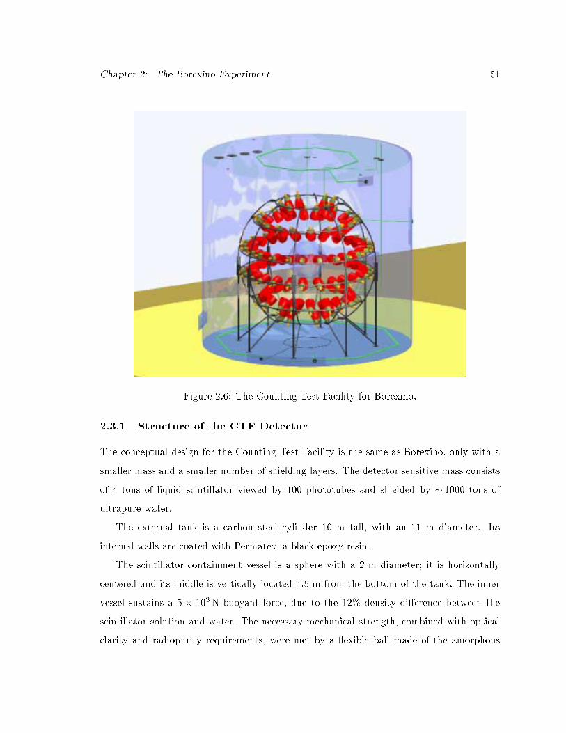
Chapter 2: The Borexino Experiment 51
Figure 2.6: The Counting Test Facility for Borexino.
2.3.1 Structure of the CTF Detector
The conceptual design for the Counting Test Facility is the same as Borexino, only with a
smaller mass and a smaller number of shielding layers. The detector sensitive mass consists
of 4 tons of liquid scintillator viewed by 100 phototubes and shielded by � 1000 tons of
ultrapure water.
The external tank is a carbon steel cylinder 10 m tall, with an 11 m diameter. Its
internal walls are coated with Permatex, a black epoxy resin.
The scintillator containment vessel is a sphere with a 2 m diameter; it is horizontally
centered and its middle is vertically located 4.5 m from the bottom of the tank. The inner
vessel sustains a 5 � 103N buoyant force, due to the 12% density di�erence between the
scintillator solution and water. The necessary mechanical strength, combined with optical
clarity and radiopurity requirements, were met by a exible ball made of the amorphous

Chapter 2: The Borexino Experiment 52
nylon-6 copolymer Durethan C38F. Nylon sheets 0.5 mm thick were cut in an orange slice
pattern and solvent welded over a spherical frame. An extensive description of the material
properties and the construction procedure will be provided in {5.
The scintillator solution used in CTF is a mixture of PC as solvent and a scintillation
uor, PPO, as solute at a concentration of 1.5 g/l. After its test in CTF the solution has
been adopted as scintillator for Borexino. A description of the main physical and optical
characteristics has been presented in x2.2.1; more details on the light propagation in CTF
can be found in reference [70].
The scintillator mixture is puri�ed by a combination of distillation and water extraction,
for the removal of particulate, and a counter-current ow of Nitrogen (stripping) for the
removal of 222Rn. A description of the system is provided in reference [64].
The uor is puri�ed with water extraction before being mixed with pseudocumene.
The main concern is potassium in PPO, measured at levels of 2 ppm Knat in the uor as
purchased. Contacting the solid PPO with water did not show to remove potassium; the pu-
ri�cation is then performed on a concentrated solution with pseudocumene (200 mg/l) [64].
After a three-fold water extraction, the pseudocumene can be evaporated and the recov-
ered PPO contains 0.4 ppb Knat [71], which contributes about 7 � 10�13 g/g Knat in the
scintillator.
The scintillation light detection is performed by 100 phototubes of the same type as
the ones for Borexino [61] coupled to light concentrators shaped as \Winston cones"[63] of
57 cm length and 50 cm maximum diameter.
The phototubes are mounted on a geodesic open structure, built with electropolished
stainless steel tubes. Unlike Borexino, CTF does not have an inner/outer bu�er structure
and the inner vessel is directly immersed in water. Given the larger surface{volume ratio,
under certain aspects CTF is actually a more delicate experiment than Borexino, since the
inner vessel surface contamination is a more critical issue and the water purity requirements
are higher.
The shield ultrapure water is produced by the same water puri�cation plant that has
been discussed in x2.2.8. Its main function is the reduction of the external background from

Chapter 2: The Borexino Experiment 53
the rocks. The dominant -rays are emitted by 208Tl (E = 2:6MeV). Since the minimum
path in water is 4.5 m and the absorption length for the 2.6 MeV rays in water is 20 cm,
the minimum reduction factor achieved by the bu�er is 10�9.
The readout electronics is designed so that the trigger signal is given by 6 photomultiplier
hits within a time window of 20 ns. There are 64 channels, 28 linked to single phototubes
and 36 linked to two coupled phototubes. For each channel, an ADC collects and digitizes
the charge signal and a TDC measures the time between the trigger and the signal hit.
Additional features are the acquisition and storage of the shape of the overall pulse, ob-
tained through the analog sum of all the outputs, the pulse shape discrimination, used to
discriminate between � and � events, and the capability to measure the delay between two
subsequent triggers, within 8 ms, using a long range TDC. This feature allows the identi�-
cation of the delayed coincidences between 214Bi and 214Po in the 238U chain (�1=2 = 164�s)
and 212Bi and 212Po in the 232Th chain (�1=2 = 0:3�s). Such correlated events are used to
identify the 238U and 232Th content of the scintillator.
2.3.2 Results from CTF-I
The �rst run of the Counting Test Facility (CTF-I) took place between January 1995 and
July 1997, when the detector was shut down for refurbishing and upgrading. A few interest-
ing results are available from that set of data; here I will summarize only the main results,
while for more details on the technology and on the data analysis I refer to the various
papers published in the past three years [51, 52, 72, 73].
Detector performances. The yield in CTF is equal to 300 photoelectrons per MeV, which
results in an energy resolution of 9% at 751 keV (214Po line). The spatial resolution,
at the same energy, is 12 cm.
�=� separation. The �=� discrimination has been performed, in CTF, by examining the
pulse shape from an analog sum of the signals from all the phototubes. The ratio of
the pulse tail (48{500 ns) versus the total charge collected in the 0{500 ns interval
can be used as a tag to separate � and � events. Figure 2.7 shows a typical scatter

Chapter 2: The Borexino Experiment 54
0
0.1
0.2
0.3
0.4
0.5
0.6
0.7
0.8
0.9
1
200 300 400 500 600 700 800 900 1000
Figure 2.7: Scatter plot of tail/total charge ratio versus energy in CTF. The �'s from 214Po(Equenched = 751 keV) can be easily separated from the continuous 214Bi � � spectrum(charge ratio � 0:2� 0:3). From reference [74].
R a d i u s (m)
0
200
400
600
800
1000
1200
0.00 0.50 1.00 1.50
ExternalInternalScintillator
Figure 2.8: Radial distribution of scintillation events in CTF, after puri�cation, comparedto the typical distribution of internal events (obtained with 222Rn insertion in the scin-tillator) and external events (obtained with 222Rn insertion in the water shield). Theradial distribution of scintillator events clearly resembles the external distribution. Fromreference [74].

Chapter 2: The Borexino Experiment 55
plot of the tail/total ratio versus energy: the �'s from 214Po can be easily separated
from the continuous 214Bi � � spectrum. At the energy of 214Po (751 keV), the
� rejection eÆciency is �97%, with � misidenti�cation of �2.5%. At lower energies
(300{600 keV), the � identi�cation ranges between 90 and 97%, with an associated �
misidenti�cation of 10% [51].
Measurement of scintillator radiopurity. The Counting Test Facility measured the
scintillator radiopurity at previously unachieved levels.
The concentration of 238U has been inferred from its daughters, using the correlation
214Bi(�)�214 Po(�) with �1=2 = 164�s. There were, however, strong indications that
the observed coincidence rate was not due to the scintillator intrinsic radiopurity, but
rather to the di�usion of 222Rn from the water through the nylon vessel (see x6.4).
The measured delayed coincidence counts due to the combination of intrinsic 238U
and di�used 222Rn is [51]:
238U = (3:5� 1:3)� 10�16 g=g:
The concentration of 232Th was measured through the decay of its daughters and the
delayed coincidence 212Bi (�)�212 Po (�) with �1=2 = 0:30�s. The result is [51]:
232Th = 4:4+1:5�1:2� 10�16 g=g:
The 14C concentration has been determined by measuring the count rate between 70
and 150 keV and �tting it with the Monte Carlo prediction [73]:
14C=12C = (1:94� 0:09)� 10�18 g=g:
Light propagation. Several measurements have been carried out to better understand
the main features of light propagation in a large scintillation detector. Of special
interest has been the investigation of the absorption and re-emission of light by the
uor (inelastic scattering). This process a�ected �44% of the detected light, with a
corresponding increase of the scintillation decay time, from the 3.5 ns measured in a
small-scale laboratory measurement to 5.5 ns in CTF [70].

Chapter 2: The Borexino Experiment 56
0
20
40
60
80
100
120
140
160
180
200
200 400 600 800 1000 1200 1400
Energy (keV)
Eve
nts
per
day
Before Purification
After Purification
Figure 2.9: Reduction of 210Po due to water extraction as observed in the energy spectrumfrom CTF. From reference [74].
Discrimination between internal and external background. The principal source of
background in CTF was activity in the shield water, due to 222Rn and its daughters
dissolved in the shield water at a concentration of about 30 mBq/m3. Such contri-
bution is classi�ed as \external" background, while \internal" background in CTF is
composed of the internal singles rate which includes all other backgrounds not tagged
by coincidence events. The discrimination between internal and external sources has
been performed using the spatial reconstruction and a �t with radial pro�les. Fig. 2.8
shows the radial distributions of internal and external activity, obtained experimen-
tally by an arti�cial enhancement of the radon concentration either in the scintillator
or in the water bu�er. The activity in the scintillator, after puri�cation, is then
compared to these distributions and clearly resembles external (or surface) activity.
The analysis results in < 30 events per day (1�) in the 250{800 keV energy window,
con�rming that there is no evidence for any internal activity at the level of the CTF
sensitivity [74].
Test of the puri�cation system. The CTF activity proved the puri�cation procedures
Chapter 2: The Borexino Experiment 57
e�ective at trace levels of contamination. Evidence for the e�ectiveness came from
both singles and coincidence data.
Fig. 2.9 shows the energy spectrum before and after the puri�cation procedure. The
internal background fell from � 600 events per day to its �nal value of < 30 per day.
The peak at 400 keV that was removed with puri�cation is believed to be due to
210Po which had built up during the scintillator's exposure to radon; the remaining
activity in the �gure is consistent with external activity produced by the known
222Rn concentration in the CTF water.
Using coincidence techniques, we saw the initial trace amount of 85Kr being reduced
by puri�cation, as well. 85Kr has a 0.43% decay branch to the 514 keV isomeric state
in 85Rb (t1=2 = 1:0 �s) giving rise to a � � coincidence. Nitrogen stripping reduced
the coincidence rate from 1:1� 0:2 per day to 0:2� 0:2 per day [52].
Muons. The muon rate in the experimental hall, equal to 1/m2/h, caused a detectable
�Cerenkov production in the water. Special pattern recognition algorithms were deve-
loped in order to identify such events. On the basis of these �ndings, a high eÆciency
muon veto has been included in Borexino [59, 60].
2.3.3 CTF-II
After undergoing some design reviews, the upgraded Counting Test Facility (CTF-II)
will be used as a quality control facility for Borexino, in order to test the purity of each
4 ton scintillator batch before its introduction into the larger detector.
The upgrades have been mainly focused towards a reduction of the \singles" rate seen
in CTF-I and, hence, an improvement in its sensitivity.
The main background source in CTF-I has been identi�ed as the 222Rn concentration
in the water shield, measured at levels of 10� 30mBq/m3.
Such a concentration is enough to justify 222Rn di�usion through the nylon vessel and
into the scintillator (see {6), at a level consistent with the measured 214Bi-214Po coincidence
rate. The inferred result for 238U (x2.3.2) is, then, really an upper limit and we still do not

Chapter 2: The Borexino Experiment 58
know the actual scintillator radiopurity and the limits of the puri�cation system. As I will
discuss in {3, the sensitivity of Borexino to the di�erent mixing scenario will be greatly
enhanced if the 238U level is lower, at the level of 10�17g/g.
Another problem related to 222Rn in the water is the high background in the scin-
tillator, which dominated the energy spectrum in CTF-I and e�ectively impaired any kind
of energy spectroscopy analysis. In particular, an important and still unsolved question is
that of the 40K content in the scintillator: the only signature to identify it is in the energy
spectrum. 40K decays � with 89:3% BR, with Q=1.3 MeV, and in the remaining 10:7%
BR produces a 1.46 MeV gamma. The high external background rate did not allow us
to identify either the � shape or the peak; an upper limit has been calculated from the
absence of a peak at 1.46 MeV and it is [75]:
Knat < 2:4� 10�11g=g (90% C:L:): (2.3)
This limit is two order of magnitude higher than the goal (set at 10�13g/g). The only way to
improve it is to maintain a low singles rate, which is possible only if the 222Rn concentration
in the water outside the scintillator vessel is maintained at levels of 1 mBq/m3 or lower. Note
that a lower limit on the potassium content in the CTF scintillator, after distillation and
water extraction, has been measured by our Munich collaborators with neutron activation
analysis [71]:
Knat < 4� 10�12g=g: (2.4)
The method used in CTF-II to control the 222Rn level in water consists of installing a
nylon screen between the scintillator vessel and the phototubes. This second vessel will act
as a barrier against the 222Rn that emanates from the various detector components (mainly,
the phototubes and Permatex, the resin coating the tank walls). At that point, the ultimate
limit to the 222Rn concentration in water will come from the water's own 226Ra content.
A second major upgrade consists of a partial muon veto, built with upward looking
phototubes mounted on the oor of CTF, for a more eÆcient identi�cation of the muon
events [76].
Chapter 3
Monte Carlo Study of Backgrounds
in Borexino
3.1 Monte Carlo code for Borexino
This chapter reviews the results of a Monte Carlo study of the expected neutrino signal
and background in the Borexino detector. The Monte Carlo code for event simulation
in Borexino has been developed in Milan and it is divided in three parts. GENEB [77,
78] simulates the physical events in terms of energy deposits in the scintillator, while the
tracking code [79] transforms the energy deposits into emitted photons and propagates them
throughout the detector. Once the event is simulated as a charge and time signal at the
phototubes, the �tter code [80] can be used to reconstruct the original event position, with
the same procedure that will be followed for the real data. The fundamental assumptions
behind the three portions of the Monte Carlo code are summarized here.
3.1.1 GENEB: GEneration of NEutrino and Background
Solar neutrinos interact in Borexino via the scattering reaction �xe� ! �xe
�, which pro-
duces electrons with kinetic energy ranging from 0 to approximately 18 MeV; the upper
limit is set by the hep neutrino interaction. In addition to this signal, the natural radioac-
tivity of the scintillator and the materials of construction of the detector induce background
events of type � + (energy range: 0{5 MeV) and � (energy range: 3{9 MeV).
59

Chapter 3: Monte Carlo Study of Backgrounds in Borexino 60
GENEB propagates individual particles and provides a detailed study of electromagnetic
showers in Borexino:
� particles: given their high stopping power, we can assume they deposit all their energy
at once in the position where they are produced. No \propagation" is, thus, necessary;
� and particles : they both produce electromagnetic showers. GENEB uses EGS4 [81]
to carry out their propagation inside the detector.
Processes that are taken into account for electrons are:
� M�oller scattering (e�e� ! e�e�);
� Bhabha scattering (e�e+ ! e�e+);
� positron annihilation (e�e+ ! );
� Bremstrahlung emission (e�N ! e� N);
� elastic scattering from atoms (e�N ! e�N);
� ionization energy loss (e�N ! e�N�e�).
EGS4 propagates electrons until they reach the cuto� energy of 10 keV. In the energy
range of interest for Borexino, the most relevant processes are M�oller and multiple
elastic scattering; Bremstrahlung a�ects only a few percent of the events. The typical
path length for a 1 MeV electron is of the order of � 1 cm, which we can consider
negligible in Borexino, given the resolution (13 cm at 1 MeV). For this reason, electrons
that do not undergo Bremstrahlung are treated as point-like.
Processes that a�ect photons in EGS4 are:
� photoelectric e�ect ( N ! e�N�);
� Compton scattering e� ! e�, largely dominant in the energy region of interest
for Borexino;
� pair production ! e+e�.

Chapter 3: Monte Carlo Study of Backgrounds in Borexino 61
The cuto� energy for photon propagation is 5 keV. In the detector, gamma rays
generate large, extended showers: the average dimension of a shower generated by a
1 MeV ray is 40 cm.
neutrino events : they are simulated in GENEB according to the theoretical energy
distribution of the Standard Solar Model [8]. Once the energy E� is chosen, the
program decides whether the interaction took place, according to the integrated cross
section:
�tot =
Z Tmax
0
d�(q; T )
dTdT; (3.1)
where Tmax is the maximum kinetic energy of the recoil electron and the di�erential
cross section is given by eq. 3.3. If the interaction does take place, GENEB proceeds
with the propagation of the scattered electron through EGS4.
3.1.2 Tracking
The tracking code converts energy deposits in the scintillator into optical photons and
follows each of them in its propagation inside the detector, until it is absorbed or it reaches
the phototubes. The tracking procedure takes into account the processes studied in CTF
and described in reference [70]:
{ scintillation decay with four decay components, as indicated in equation 2.2,
{ absorption/reemission process in the scintillator,
{ photon absorption,
{ Rayleigh elastic scattering in the scintillator and in the bu�er,
{ re ection on surfaces and the quantum eÆciencies of pseudocumene, PPO and the
phototubes.
The light collected on the photocathodes is then converted into a time and charge signal,
thus simulating the real data collection.

Chapter 3: Monte Carlo Study of Backgrounds in Borexino 62
0.2 0.4 0.6 0.8 1 1.2 1.40
2.5
5
7.5
10
12.5
15
energy (MeV)
DE
/E (
%)
Figure 3.1: Fractional energy resolution in Borexino, simulated for electron, point-likeevents.
Figure 3.1 shows how the resulting energy resolution of electron events varies, in Borex-
ino, as a function of their energy, while table 3.1 summarizes some of the main parameters
included in the simulation.
3.1.3 Reconstruction
In order to perform �ducial volume cuts and external background reductions, it is important
to have a good position �tter code that, given the charge and time signal at the phototubes
for each event, calculates the event position.
The existing �tter is essentially a vertex reconstruction, based on the principle that the
shape of the time signal distribution depends on the distance between the event and the
detector's center. The idea is to use the phototube hit time signal to calculate the event
coordinates from the photons' time of ight and to maximize (with the resources of the

Chapter 3: Monte Carlo Study of Backgrounds in Borexino 63
Table 3.1: Parameters in the Monte Carlo tracking code.
Photomultiplier Tubes:
cathode radius 0.095 mcurvature radius 0.11 mtime jitter 1 nsquantum eÆciency 20%Practical coeÆcient 0.6
Light Guides:Radius of entry aperture 0.157 mRadius of exit aperture 0.095 mLength 0.230 mRe ection coeÆcient 90%E�ective coverage 30.6%
Liquid Scintillator:Formula PC+PPO (1.5 g/l)Refractive index 1.505Photon yield 1:2� 104 photons/MeVAbsorption length:� = 340 nm �abs = 3:1 m� = 380 nm �abs = 5:1 m� = 420 nm �abs = 7:8 m� = 460 nm �abs = 8:2 mRayleigh elastic scattering:� = 340 nm �scatt = 1:6 m� = 380 nm �scatt = 4:1 m� = 420 nm �scatt = 6:6 m� = 460 nm �scatt = 11:1 m
Scintillator decay curve S(t) =P
iqi�ie�t=�i
response to � and excitations:�1 (q1) 3.574 ns (89.5%)�2 (q2) 17.61 ns (6.3%)�3 (q3) 59.49 ns (2.9%)�4 (q4) 330.4 ns (1.2%)
response to � excitations:�1 (q1) 3.254 ns (63.0%)�2 (q2) 13.49 ns (17.8%)�3 (q3) 59.95 ns (11.9%)�4 (q4) 279.1 ns (7.3%)
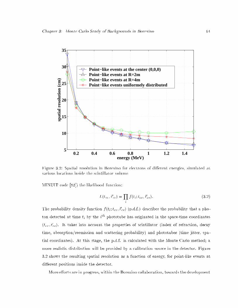
Chapter 3: Monte Carlo Study of Backgrounds in Borexino 64
0.2 0.4 0.6 0.8 1 1.2 1.45
10
15
20
25
30
35
energy (MeV)
spat
ial r
esol
utio
n (c
m)
Point−like events at the center (0,0,0) Point−like events at R=2m Point−like events at R=4m Point−like events uniformely distributed
Figure 3.2: Spatial resolution in Borexino for electrons of di�erent energies, simulated atvarious locations inside the scintillator volume
MINUIT code [82]) the likelihood function:
L(tev; ~rev) =Yi
f(ti; tev ; ~rev): (3.2)
The probability density function f(ti; tev ; ~rev) (p.d.f.) describes the probability that a pho-
ton detected at time ti by the ith phototube has originated in the space-time coordinates
(tev ; ~rev). It takes into account the properties of scintillator (index of refraction, decay
time, absorption/reemission and scattering probability) and phototubes (time jitter, spa-
tial coordinates). At this stage, the p.d.f. is calculated with the Monte Carlo method; a
more realistic distribution will be provided by a calibration source in the detector. Figure
3.2 shows the resulting spatial resolution as a function of energy, for point-like events at
di�erent positions inside the detector.
More e�orts are in progress, within the Borexino collaboration, towards the development
Chapter 3: Monte Carlo Study of Backgrounds in Borexino 65
of methods to improve the reconstruction of events close to the surface and the identi�cation
of extended electromagnetic showers, typical of external background.
3.2 Neutrino Energy Spectra in Borexino
The main sources of neutrino production in the Sun are the pp reaction (Emax = 0:42MeV),
7Be electronic capture (E1 = 0:383MeV and E2 = 0:861MeV) and 8B decay (Emax =
15MeV). Borexino is designed to have a high sensitivity for 7Be neutrinos; 8B neutrinos
can be detected, despite the low statistics, with energy threshold of 3.5 MeV (see x4.3),
while the pp neutrino signal is in an energy region dominated by 14C background.
The solar neutrinos interact in the detector by electron scattering:
� + e� ! � + e�;
where an electron of energy in the range 0{15 MeV is produced in the �nal state. Therefore,
any interaction involving an electron or a in this energy range is a potential \neutrino
candidate". Events induced by natural radioactivity in the scintillator or in the materials
surrounding it are e�ective background sources for neutrino detection.
The neutrino-electron scattering cross sections are well known in the Standard Model.
The �rst order di�erential cross section formula for ��e scattering was originally calculated
by t'Hooft in 1971 [83]:
d�
dT= �0
"g2L + g2R
�1�
T
q
�2� gLgR
T
q2
#; (3.3)
where:
gR = sin2 �W ;
gL = +1
2+ sin2 �W for �e � e� interactions;
gL = �1
2+ sin2 �W for �� � e� interactions:
T is the kinetic energy for the scattered electron, q is the neutrino energy, sin2 �W = 0:23
and
�0 =2GF
2m2e
��h4= 88� 10�46 cm2:
Chapter 3: Monte Carlo Study of Backgrounds in Borexino 66
For a given neutrino of momentum q, the total cross section is given by:
�(q) =
Z Tmax
0
d�
dT:
Radiative corrections have not been introduced in the code, yet; they would result in a
modi�cation of the recoil electron spectrum and of the integrated cross section of the order
of 2% or less.
In the case of neutrino oscillations, the solar energy spectrum of the neutrino for a given
source, predicted by the Solar Standard Model, is multiplied by a survival probability P(E):
���(E)on earth = [1� P (E)]�(E)sun;
��e(E)on earth = P (E)�(E)sun:(3.4)
GENEB has been implemented with the capability to simulate the neutrino signal in Borex-
ino in the following scenarios [84]:
MSW Small Angle: �m2 = 5:4� 10�6 eV 2, sin2 2� = 5:5� 10�3;
MSW Large Angle: �m2 = 1:8� 10�5 eV 2, sin2 2� = 0:76;
MSW LOW: �m2 = 7:9� 10�8 eV 2, sin2 2� = 0:96;
vacuum oscillations: �m2 = 6:5� 10�11 eV 2, sin2 2� = 0:75.
The expected neutrino signal rates and energy spectra in Borexino, calculated from the
theoretical ux predictions of the BP98 SSM [11] are shown in table 3.2 and in �gure 3.10,
where the 7Be neutrino manifests its Compton shoulder. Given these spectra, two energy
windows have been identi�ed: the \neutrino window", between 0.25 and 0.8 MeV, for 7Be
neutrinos and the \pep window", between 0.8 and 1.3 MeV.
The SSM ux of 7Be �e would give rise to 46 events/day in a �ducial volume of 100
metric tons, in the energy window 0.25{0.8 MeV. In the avor oscillation scenarios, where
some of the �e ux has been converted into another avor, the count rate will be smaller
since the ��; �� scattering cross-sections are about a factor of 5 lower. The two best-�t MSW
solutions which satisfy the existing experiments predict signal rates of 26 events/day for
the large-angle MSW solution and 10 events/day in the case of small-angle MSW mixing.
In the latter, practically all of the �e ux at the 7Be energy has been resonantly converted
into either �� or �� .

Chapter 3: Monte Carlo Study of Backgrounds in Borexino 67
Table 3.2: Predicted solar neutrino event rates in Borexino in three energy windows for4 scenarios: the Standard Solar Model (SSM), large mixing angle MSW solution (LMA),small mixing angle MSW solution (SMA) and LOW. The rates are calculated for the meanSun-Earth distance, in a 100-ton �ducial volume. The theoretical uxes, with their 1�uncertainties, are taken from the BP98 SSM [11].
Recoil Energy Neutrino ux SSM LMA SMA LOWMeV Source 1010 cm2s�1 ev/day ev/day ev/day ev/day
all E pp 5.94 (� 1%) 197 137 167 1117Be 0.480 (� 9%) 80 45 18 44pep 0.0139 (� 1%) 4.5 2.2 0.9 2.313N 0.0605 (� 19%) 8.3 4.8 1.9 4.315O 0.0532 (� 22%) 11 5.7 2.3 5.717F 6:33� 10�4 (� 12%) 0.13 0.07 0.03 0.078B 5:15� 10�4 (� 19%) 1.15 0.43 0.56 0.58
total 302 195 191 168
0.25{0.8 pp 1.3 1.0 0.6 0.67Be 45.7 26.0 9.7 25.1pep 2.0 1.0 0.4 1.013N 4.2 2.3 0.9 2.315O 5.5 2.8 1.1 2.817F 0.07 0.03 0.01 0.038B 0.10 0.04 0.05 0.05
total 59 33 13 32
0.8{1.3 pep 1.5 0.7 0.3 0.813N 0.2 0.10 0.04 0.1115O 1.9 0.9 0.3 1.017F 0.02 0.011 0.004 0.0118B 0.07 0.03 0.04 0.05
total 3.6 1.8 0.7 1.9

Chapter 3: Monte Carlo Study of Backgrounds in Borexino 68
It is interesting to consider also the monoenergetic pep neutrinos. If in Borexino one
were to look for electron recoils with energy 0.8{1.3 MeV, the calculated signal rate for the
SSM-predicted pep neutrino ux would be 1.5 events/day in a target mass of 100 metric
tons. Thus, a measurement of the pep neutrino ux in Borexino could be feasible if the
backgrounds turn out to be suÆciently low in this energy window. Note that the neutrinos
produced by the CNO cycle also create electron recoils in this energy window, with a rate
of 2 events/day, and make the pep neutrino signature even harder to discern. Table 3.5 lists
the neutrino interaction rates for several physics scenarios and for several �ducial volume
sizes.
3.3 External Background
The Borexino detector has been designed with the goal of screening the �ducial volume
from environmental radioactivity. The strategy we employed consists of constructing
the detector with materials of progressively higher radiopurity as we approach the �ducial
volume at the center of the detector. We de�ne as \external" the background due to
radioactivity in materials outside the inner vessel.
3.3.1 Environmental Radioactivity
The main background source in Borexino is the naturally occurring uranium, thorium and
potassium in any material. Figures 3.3 and 3.4 show the radioactive chains of 238U and
232Th: each contains several -emitting daughters. The overall spectrum for both families
is shown in �gure 3.5, where secular equilibrium is assumed within the chain.
The most relevant peaks are 208Tl at 2.6 MeV and 228Ac at 0.9 MeV in the 232Th chain
and the 214Bi lines at 1.7 and 1.1 MeV in the 238U chain.
40K is also a concern for external background, with its 1.46 MeV line (10.7% B.R.).
Although potassium is a widespread contaminant, due to its chemical aÆnity with sodium,
the radioactive isotope 40K has a relatively low abundance, equal to 0.0117%; as the si-
mulation will show, it represents a problem only in sources close to the inner vessel, such

Chapter 3: Monte Carlo Study of Backgrounds in Borexino 69
238
92U
234
90Th
234
91Pa
234
92U
230
90Th
226
88Ra
222
86Rn
218
84Po
214
82Pb
214
83Bi
214
84Po
210
82Pb
210
83Bi
210
84Po
206
82Pb
α
β
β
α
α
α
α
α
β
β
α
β
β
α
E=4.196 MeVτ1/2=4.46 109 y
E=0.109 MeV (65%)τ1/2=24 d
E=2.29 MeV (98%)τ1/2=1.17 m
E=4.77 MeVτ1/2=2.45 105 y
E=4.69 MeVτ1/2=7.54 104 y
E=4.78 MeV (94%)τ1/2=1622 103 y
E=5.49 MeVτ1/2=3.825 d
E=6.02 MeVτ1/2=3.11 m
E=0.72 MeVτ1/2=26.8 m
E=1.51 MeV (40%)τ1/2=19.8 m
E=7.69 MeVτ1/2=163 µs
E=0.015 MeV (81%)τ1/2=22.3 y
E=1.17 MeVτ1/2=5.01 d
E=5.3 MeVτ1/2=138.4 d
Figure 3.3: 238U radioactive chain.

Chapter 3: Monte Carlo Study of Backgrounds in Borexino 70
232
90Th
228
88Ra
228
89Ac
228
90Th
224
88Ra
220
86Rn
216
84Po
212
82Pb
212
83Bi
212
84Po208
81Tl
208
82Pb
α
β
β
α
α
α
α
β
β
α
α
β
E=4.01 MeVτ1/2=1.4 1010 y
E=0.053 MeVτ1/2=5.76 y
E=1.11 MeV (53%)τ1/2=6.13 h
E=5.423 MeV (73%)τ1/2=1.9 y
E=5.685 MeV (95%)τ1/2= 3.66 d
E=6,288 MeVτ1/2=55.6 s
E=6.778 MeVτ1/2=150 ms
E=0.33 MeV (88%)τ1/2=10.64 h
E=2.25 MeV (64%)τ1/2=60.6 m
E=8.79 MeVτ1/2=298 ns
E=6.04 MeV (36%)τ1/2= 60.6 m
E=1.8 MeVτ1/2=3.03 m
Figure 3.4: 232Th radioactive chain.

Chapter 3: Monte Carlo Study of Backgrounds in Borexino 71
0
1000
2000
3000
4000
5000
6000
7000
0.5 1 1.5 2 2.5 3
energy (MeV)
214Bi 214Bi
238U chain in secular equilibrium - 1.4 x 10⁴ U decays
5.0 x 10⁵ γ events
6.1 x 10⁵ γ rays
0
2000
4000
6000
8000
10000
0.5 1 1.5 2 2.5 3
energy (MeV)
208Tl228Ac
232Th chain in secular equilibrium - 1.2 x 10⁴ Th decays 5.0 x 10⁵ γ events
7.6 x 10⁵ γ rays
Figure 3.5: spectra of the 238U and 232Th families, in the hypothesis of secular equilibriumwithin the chains. For each decay of the progenitor, there are, on average, 3.62 events with emission in the 238U chain and 4.14 in the 232Th chain. A good portion of these eventsemit multiple 's, hence the total average number of -rays produced per each decay of theprogenitor is 4.4 in the 238U chain and 6.3 in the 232Th chain.

Chapter 3: Monte Carlo Study of Backgrounds in Borexino 72
40K19
40Ca20
40Ar18
4- 1.277x10⁹ y
0+
0+
E.C.10.72%
β-89.28%
Q(β-) =1311.09 keVQ(EC) =1504.9 keV
Figure 3.6: Decay schemes for 40K and 60Co.

Chapter 3: Monte Carlo Study of Backgrounds in Borexino 73
Table 3.3: ray ux from the walls in Hall C [85].
Isotope Energy (MeV) Flux (m�2�d�1)
40K 1.460 3:8� 107214Bi 1.120 1:4� 107214Bi 1.764 1:7� 107228Ac 0.911 0:48� 107208Tl 2.614 1:35� 107
Total 8:7� 107
(n, ) reactions � 8 � 1:0� 102
as the nylon endcaps and the ropes for the hold-down system (see also discussion in x8.3).
Another potential danger comes from 60Co: it typically can be found in stainless steel
and it produces two lines with energies of 1.33 and 1.17 MeV. The decay schemes for 40K
and 60Co are shown in �gure 3.6.
3.3.2 External Background Sources in Borexino
The activity emanated from the rock walls of the laboratory has been measured [85] and
the total ux is equal to 1:5� 108 =m2=d. Among these, the only penetrating components
are a few high energy lines, mainly from 208Tl, 214Bi and 40K, that contribute 54% of the
total ux; they are listed in table 3.3. The table also reports a higher energy component
(� 8MeV), due to neutron capture in the rocks; its ux is several orders of magnitude lower
than the others.
All of the detector components, such as the phototubes, the vessel material and the
bu�er uids, also need to be included in the estimation of the external background in
Borexino. Table 3.4 summarizes all the known or assumed radiopurity levels, while �gure
3.7 shows the distribution of sources inside the detector.

Chapter 3: Monte Carlo Study of Backgrounds in Borexino 74
Component
238U
232Th
Knat
60Co
activity
mass
[g/g]
[g/g]
[g/g]
[mBq/kg]
[ /d(1) ]
Nylonbag
2�10�12
4�10�12
1�10�8
0:5�103
3:2�104g
Holddownropes(2)
5�10�11
5�10�11
1�10�6
2:5�103
4:5�103g
I.V.Nylonendcaps(2)
5�10�11
5�10�11
7�10�7
5:6�103
1:2�104g
I.V.-O.V.Nylonpipe(2)
5�10�11
5�10�11
7�10�7
2:0�103
4:2�103g
O.V.Steelendcaps(2)
1�10�9
2�10�9
7�10�8
10
1:1�105
1:5�104g
Pseudocumenebu�er
1�10�15
1�10�15
1�10�12
5:0�103
103m3(3)
Lightguides(4)
1�10�8
1:3�10�7
6�10�6
2:6�108
6�106g
Phototubes
3�10�8
1�10�8
2�10�5
1:2�109
9�106g
StainlessSteelSphere
7�10�10
3�10�9
7�10�8
100
1:1�109
7�107g
222Rninthebu�er(5) :
1mBq/m3
2:2�105
103m3(3)
(1)
Takingintoaccountthewhole
energyspectrum.
(2)
Realisticassumption,basedonmeasurementsreportedinx8.3.
(3)
TotalvolumeinsidetheStainlessSteelSphere.
(4)
The
232Thconcentrationinthelightconesisanaverageover50%\Highpural"and50%regularAlcones(seetext).
(5)Conservativeassumption.
Table3.4:RadioactiveimpuritiesintheBorexinomaterials,contributingtotheexternalbackground
(I.V.andO.V.are,respectively,innerandoutervessel).

Chapter 3: Monte Carlo Study of Backgrounds in Borexino 75
radius (m)
gam
ma
even
ts/d
ay
IV+endcap
steel OV endcap
LGs
PMTsSSS
1mBq/m3 Radon in buffer
4.5 5 5.5 6 6.5
100
102
104
106
108
1010
Figure 3.7: Radial distribution of \external" sources in Borexino, in the region betweenthe inner vessel and the stainless steel sphere. IV and OV are the inner and outer vessels,LGs are the light cones, PMTs the phototubes and SSS the stainless steel sphere. The totalactivity from each component is reported in table 3.4.
3.3.3 Behavior of External Background
Each ray propagating through the detector generates an electromagnetic shower and de-
posits its energy in several di�erent interaction points. Typical average values of electromag-
netic shower extension, attenuation length in pseudocumene and number of interactions
for 's at di�erent energies are:
energy shower extension attenuation length number of interactions
0.5 MeV 35 cm 19.5 cm 19.51.0 MeV 39 cm 26 cm 221.46 MeV (40K) 40 cm 27.5 cm 241.76 MeV (214Bi) 41.5 cm 30 cm 252.6 MeV (208Tl) 43 cm 36 cm 30

Chapter 3: Monte Carlo Study of Backgrounds in Borexino 76
While a few high energy rays can reach the scintillator with their full energy, most of
the external background consists of tail of electromagnetic showers that start outside the
inner vessel and contribute only low energy interactions in the most external regions of the
sensitive volume.
The position of an external background event is not that of a point-like interaction, as
it is for � or � or � events, but it can be described as a shower energy-weighted \center of
gravity", where each interaction point is weighted by the number of detected photoelectrons
it originates. The event position provides us with an essential handle on external background
events, allowing us to reject them with a �ducial volume cut. This concept is illustrated in
�gure 3.9, where one can see the radial distribution of the external background activity and
of the SSM neutrino signal for events which deposited energy between 0.25 and 0.8 MeV.
3.3.4 Monte Carlo Simulation
I performed a detailed Monte Carlo simulation of all the expected sources of external back-
ground. The simulation follows the propagation of rays throughout the detector. For
the outer sources, that is the rocks, the stainless steel sphere, the phototubes and the light
cones, the propagation of each photon proved to be a very expensive process and it was dif-
�cult to achieve a signi�cant simulation statistics in reasonable computing times. I solved
this problem implementing a modi�cation to the GENEB code. The GENROX method
consists of propagating the rays one by one, with EGS4, in a layer of, typically, 1 m of
material in the outer detector regions and then record the residual energy spectrum and the
distribution of the initial direction of propagation for the 's that have not been absorbed
by the 1 m layer. These spectra can then be used as input for a new generation, starting
at the position where the previous ended. This way, the simulation statistics can be greatly
ampli�ed. Figure 3.8 shows a comparison of the energy spectra and the radial distributions
obtained with this method and with the direct EGS4 propagation of 5 � 107 2.6 MeV
events from 208Tl (232Th chain) in the phototubes. The agreement is better than 10%. For
rays generating within 1 m from the inner vessel this has not been necessary and I could
obtain a good simulation statistics in reasonable computing times.

Chapter 3: Monte Carlo Study of Backgrounds in Borexino 77
1
10
10 2
10 3
0 0.5 1 1.5 2 2.5Energy (MeV)
energy spectrum in 300 tons
energy spectrum in 200 tons
10-1
1
10
10 2
10 3
0 0.5 1 1.5 2 2.5 3 3.5 4
Radial distribution
250 - 800 keV
R (m)
Figure 3.8: Simulation of 2.6 MeV events in the phototubes, performed with the GEN-ROX method (continuous line) and with direct EGS4 propagation (marks). The GENROXsimulation has been normalized to the statistics of the direct propagation (5� 107 events).The error bars are based on Poisson statistics for the direct propagation.Top: comparison of the energy spectra in 300 tons (whole sensitive volume) and in 200 tons(large �ducial volume). The agreement is better than 10%.Bottom: comparison of radial distributions for events that deposited in the scintillator anenergy in the 0.25{0.8 MeV window. The position is an energy-weighted average of theshower interaction points.

Chapter 3: Monte Carlo Study of Backgrounds in Borexino 78
10-2
10-1
1
10
10 2
0 50 100 150 200 250 300 350 400
R (cm)
coun
ts/d
ay/5
cm
neutrino events (SSM rates)
external background
Figure 3.9: Radial distribution of external background and of neutrino SSM events in theenergy window 0.25{0.8 MeV.
The resulting external background event rates in di�erent �ducial volumes, compared
to the predicted neutrino signal in Borexino, are reported in table 3.5, while �gure 3.10
shows the corresponding energy spectra in a 100 ton �ducial volume. The position cuts are
performed on the center of gravity of the detected light.
Figure 3.11 is a graphical representation of the external background behavior: it consists
of a position-energy distribution of external background events collected over ten days of
data acquisition. The dotted box constitutes the residual area, on this scatter plot, after
energy and �ducial volume cuts. The fact that it is empty (less that 10�4 events in each
50 keV{5 cm bin is recorded as zero) is an illustration of the e�ectiveness of the �ducial
volume cut in rejecting external background counts.
The major contribution to the total external background rate comes from the photomul-
tiplier tubes (see table 3.5). They account for about half of the total external background in
the \neutrino" window 0.25{0.8 MeV. By placing the phototubes far from the inner vessel
and with a proper choice of the other components for low radioactivity, we have reduced the

Chapter 3: Monte Carlo Study of Backgrounds in Borexino 79
E
>
250keV
250�
800keV
800�
1300keV
Component
100t
130t
160t
200t
300t
100t
130t
160t
200t
300t
100t
130t
160t
200t
300t
Nylon�lm
0.05
0.2
0.8
4
147
0.002
0.006
0.03
0.4
56
0.002
0.013
0.08
0.5
40
Ropes
0.35
1.6
6.7
31
977
0.003
0.015
0.16
1.8
250
0.03
0.08
0.4
2.7
319
IV{OVPipe
0.08
0.3
1.1
5
118
{
{
0.05
0.7
50
{
0.09
0.3
1.4
35
IVPlate
0.56
3.8
15
65
2045
{
0.05
0.40
4.0
567
{
0.30
1.0
5.8
661
OVPlate
0.12
0.9
2.9
11
159
0.013
0.03
0.30
2.6
88
0.013
0.18
0.5
2.5
38
Bu�er
0.02
0.1
0.4
2
45
{
0.006
0.04
0.4
24
{
0.015
0.08
0.4
10
Rninbu�er
1.3
4.3
19
86
2482
0.017
0.33
2.5
22
1429
0.25
0.80
4.3
20
500
Lightguides
5.8
19
60
193
2226
0.054
0.34
2.3
18
896
0.43
1.9
8.3
35
494
Phototubes
5.2
16
56
199
2691
0.081
0.39
3.6
28
1294
0.54
2.4
11.1
50
658
SSSphere
1.7
5.3
19
65
927
0.005
0.20
1.6
12
496
0.26
1.0
3.9
16
207
Rocks
0.11
0.3
1.0
3
36
{
0.003
0.05
0.3
13
0.003
0.020
0.12
0.5
8
Total
15.2
52
182
665
11853
0.18
1.4
11
89
5163
1.5
6.7
30
135
2969
stat.err.
�0.4
�0.8
�2
�3
�11
�0.05
�0.1
�0.4
�1
�8
�0.15
�0.3
�0.6
�3
�5
Solar�scatteringrates:
BP98SSM
64
81
101
124
179
59
75
94
115
165
3.4
4.6
5.8
7.0
10.4
MSW
LMA
35
44
56
69
99
33
42
52
64
93
1.8
2.2
2.8
3.5
5.0
MSW
SMA
14
18
22
27
40
13
16
20
25
36
0.7
0.9
1.1
1.4
2.0
Table3.5:Expected backgroundrates(events/day)indi�erent�ducialvolumes(100,130,160and200tons)orinthe
wholescintillatorvolume(300tons),inthehypothesisofaperfectresolutiondetector.Thequotederrorsarestatistical,
only.Foracomparison,thepredictedneutrinoratesfordi�erentscenariosarereported,aswell.
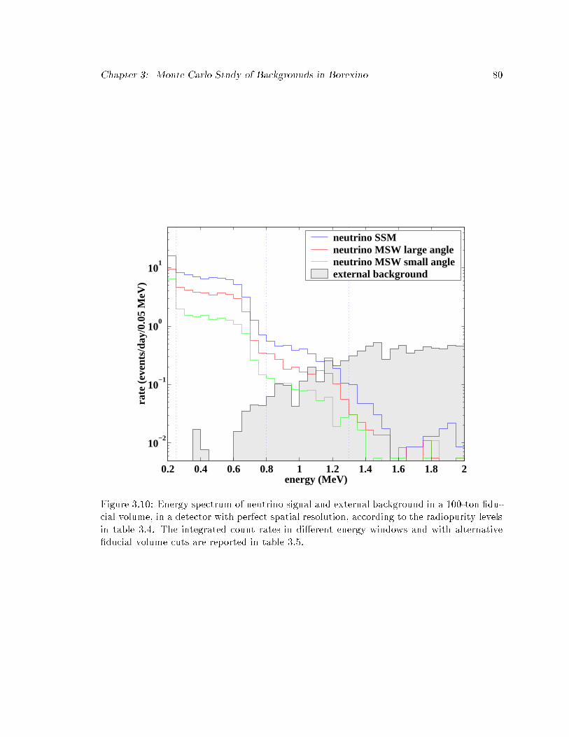
Chapter 3: Monte Carlo Study of Backgrounds in Borexino 80
energy (MeV)
rate
(ev
ents
/day
/0.0
5 M
eV)
0.2 0.4 0.6 0.8 1 1.2 1.4 1.6 1.8 2
10−2
10−1
100
101
neutrino SSM neutrino MSW large angleneutrino MSW small angleexternal background
Figure 3.10: Energy spectrum of neutrino signal and external background in a 100-ton �du-cial volume, in a detector with perfect spatial resolution, according to the radiopurity levelsin table 3.4. The integrated count rates in di�erent energy windows and with alternative�ducial volume cuts are reported in table 3.5.

Chapter 3: Monte Carlo Study of Backgrounds in Borexino 81
−3
−2
−1
0
1
2
3
4
0.5
1
1.5
2
2.5
3
250 300 350 400Radial position (cm)
Ene
rgy
(MeV
)
Figure 3.11: Position{energy distribution of external background events collected over tendays of data acquisition. The dotted box at the lower left corresponds to the window ofinterest for 7Be neutrinos in Borexino. The color code on the right is the log10 of theexpected number of events in each 50 keV{5 cm bin.

Chapter 3: Monte Carlo Study of Backgrounds in Borexino 82
Table 3.6: Expected background rates from the light cones (events/day). I assumed10 ppb 238U, 6 ppm Knat and a 232Th concentration of 50 ppb for the \Highpural", 220 ppbfor the regular Al and 135 ppb for the current design, with 50% cones form each type of Al.For comparison, I also report the background from the phototubes.
250� 800keV 800� 1300keVComponent 100 t 130 t 160 t 200 t 300 t 100 t 130 t 160 t 200 t 300 t
\Highpural" 0.02 0.14 1.0 8 377 0.18 0.8 3.5 15 205Regular Al 0.09 0.54 3.7 28 1414 0.68 2.9 13.2 55 78350% design 0.05 0.34 2.3 18 896 0.43 1.9 8.3 35 494
Phototubes 0.08 0.39 3.6 28 1294 0.54 2.4 11.1 50 658
external background rate to the desired, acceptable level; it was the phototube placement
that dictated the necessary geometry for the detector.
We recently realized that the light collectors constitute a more serious background source
than originally thought. Our German collaborators have identi�ed a high purity aluminum,
\Highpural", with 50 ppb 232Th, 10 ppb 238U equivalent (below and including 226Ra) and
<6 ppm Knat. The secular equilibrium in the 238U chain is broken, at the level of 226Ra, and
only the lower part of the chain emits penetrating rays. This material would represent a
good choice for the light collectors; unfortunately, not enough material is available for the
production of 1870 light cones and, due to schedule and budget constraints, we will probably
be forced to use a di�erent type of Al, with a 4.2 times higher 232Th concentration (220 ppb).
This contamination is measured with Ge counters, which detect the 2.6 MeV line and
calculate the 232Th equivalent concentration; due to this 2.6 MeV line, 232Th dominates
the external background from the cones. The current proposal is to use 50% of the clean,
\Highpural" material and 50% of the regular Al. I report in table 3.6 the Monte Carlo
predictions for the external background from the light cones as a function of the material
used, compared to that from the phototubes. The increased 232Th activity of the light
collectors makes them a background source comparable to the phototubes.
The radiopurity of the inner vessel and its auxiliary components are discussed in larger
detail in x8.1 and in x8.3. To the purposes of this discussion I have quoted, in table 3.4,
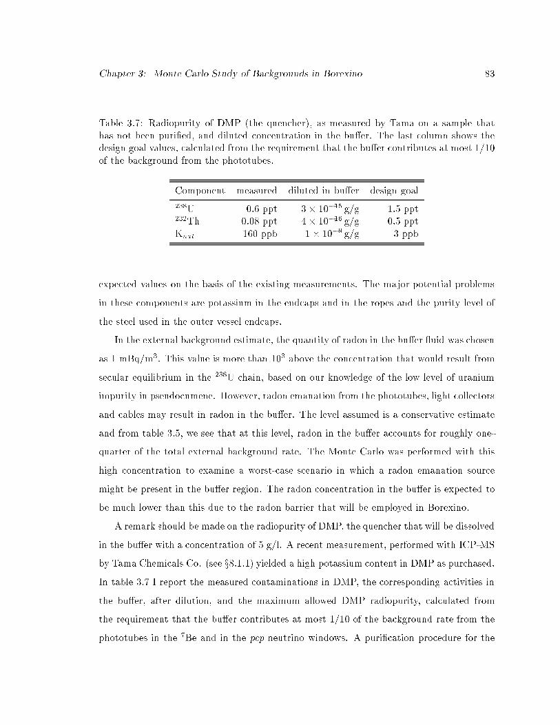
Chapter 3: Monte Carlo Study of Backgrounds in Borexino 83
Table 3.7: Radiopurity of DMP (the quencher), as measured by Tama on a sample thathas not been puri�ed, and diluted concentration in the bu�er. The last column shows thedesign goal values, calculated from the requirement that the bu�er contributes at most 1/10of the background from the phototubes.
Component measured diluted in bu�er design goal
238U 0.6 ppt 3� 10�15 g/g 1.5 ppt232Th 0.08 ppt 4� 10�16 g/g 0.5 pptKnat 160 ppb 1� 10�9 g/g 3 ppb
expected values on the basis of the existing measurements. The major potential problems
in these components are potassium in the endcaps and in the ropes and the purity level of
the steel used in the outer vessel endcaps.
In the external background estimate, the quantity of radon in the bu�er uid was chosen
as 1 mBq/m3. This value is more than 103 above the concentration that would result from
secular equilibrium in the 238U chain, based on our knowledge of the low level of uranium
impurity in pseudocumene. However, radon emanation from the phototubes, light collectors
and cables may result in radon in the bu�er. The level assumed is a conservative estimate
and from table 3.5, we see that at this level, radon in the bu�er accounts for roughly one-
quarter of the total external background rate. The Monte Carlo was performed with this
high concentration to examine a worst-case scenario in which a radon emanation source
might be present in the bu�er region. The radon concentration in the bu�er is expected to
be much lower than this due to the radon barrier that will be employed in Borexino.
A remark should be made on the radiopurity of DMP, the quencher that will be dissolved
in the bu�er with a concentration of 5 g/l. A recent measurement, performed with ICP-MS
by Tama Chemicals Co. (see x8.1.1) yielded a high potassium content in DMP as purchased.
In table 3.7 I report the measured contaminations in DMP, the corresponding activities in
the bu�er, after dilution, and the maximum allowed DMP radiopurity, calculated from
the requirement that the bu�er contributes at most 1/10 of the background rate from the
phototubes in the 7Be and in the pep neutrino windows. A puri�cation procedure for the

Chapter 3: Monte Carlo Study of Backgrounds in Borexino 84
DMP is now being tested, in order to reduce its potassium content by at least a factor 50.
3.3.5 Alternative Geometries
I investigated the advantages and the feasibility of a larger sensitive volume. This could be
achieved either by enlarging the inner vessel or by mixing the inner bu�er with uors in-
stead of quencher. In principle, a larger scintillator volume would only be an improvement,
sensibly increasing the statistics for solar neutrinos and other sources, such as geophysical
or Supernova neutrinos. The internal background (see x3.4) would scale with the scintil-
lator volume and the total signal/noise ratio would change only because of the external
background.
With a larger sensitive volume, the passive shielding layer would be thinner and there
would obviously be an overall increase of the external background rate. However, the
added scintillator layer would work as an \active veto" for the external 's, detecting energy
deposits in its outer regions. In this scenario, the rays that penetrate in the �ducial volume
have more energy than the 7Be neutrinos; all the others produce an energy-weighted center
of gravity shifted to a larger radius. Consequently, the background spectral shape in the
inner regions would be depleted of low energy events, and we would be allowed to consider
a much larger �ducial volume.
There are complications related to the handling of a larger mass of ultrapure liquid
scintillator; a possible alternative to enlarging the inner vessel is to replace the quencher
with uors, in the inner bu�er. This way, the stricter purity requirements would apply
to the 300 tons inside the inner vessel and not to the extended scintillator volume. In
this con�guration, the ultimate limit to the allowed �ducial volume would be set at 4 m,
25 cm away from the inner vessel (a source itself), for a �ducial mass and, consequently,
a statistics 2.4 times higher than in the 100-ton presently considered.
Figure 3.12 is an illustration of this concept: for di�erent values of the scintillator radius,
here labeled as RIV , I plot the signal to noise ratio in the 250{800 keV energy window. The
signal is the SSM prediction for 7Be neutrino, while the noise is the external background.
A nylon vessel at R = 4:25m is included in the calculation. As one can see, in the present

Chapter 3: Monte Carlo Study of Backgrounds in Borexino 85
SSM neutrino vs γ external background, signal/noise ratio - 0.25-0.8 MeV
10-2
10-1
1
10
10 2
10 3
10 4
10 5
3 3.2 3.4 3.6 3.8 4 4.2 4.4
Radius fiducial volume (m)
Sign
al/N
oise
rat
io
RIV = 4.25 m
RIV = 4.75 m
RIV = 5.25 m
RIV = 5.50 m
Figure 3.12: Signal (SSM neutrino) to noise (external background) ratio, in Borexino, as afunction of the �ducial volume radius, for di�erent values of the scintillator radius.
design, with RIV = 4:25m, the ratio becomes smaller than 1 at a �ducial volume radius of
3.9 m, but if we have a scintillating volume between inner and outer vessel (RIV = 5:25m
in the plot) the ratio is still equal to 10 at a �ducial volume radius of 4 m.
All this is meaningful in a detector with perfect spatial resolution. In reality, there are
two major problems:
1. In the current design, a larger scintillator volume would result in a very inhomoge-
neous detector. Figure 3.13 shows a Monte Carlo simulation of point-like events at
di�erent positions inside the detector. The �gures are scatter plots of the number
of photoelectron (that is, detected energy) versus the position of the source events,

Chapter 3: Monte Carlo Study of Backgrounds in Borexino 86
(a) Inner vessel radius = 4.25 m (b) Inner vessel radius = 5.25 m
Figure 3.13: Simulation of the detector response to monoenergetic point-like events gen-erated at di�erent position in the vessel. In abscissa is the radius at which the eventsare generated, in ordinate is the signal intensity, expressed as number of detected photo-electrons. The response starts falling at around R=4.25 m, with the existing light conedesign.
for a 4.25 and a 5.25 m inner vessel radius. The energy response is very similar in
the two cases, in the inner volume, but it becomes very inhomogeneous in the region
outside 4.25 m. An interpretation of events in this region would be very diÆcult. This
problem could in principle be solved by changing the shape of the light cones, in order
to get an homogeneous response in the larger vessel, at the cost of a loss in coverage
and, consequently, in energy resolution [86]:
scintillator cone cone coverageradius length radius
4.25 m 22.9 cm 15.7 cm 30.6%4.50 m 20.8 cm 15.1 cm 28.1%5.25 m 13.9 cm 13.1 cm 20.7%

Chapter 3: Monte Carlo Study of Backgrounds in Borexino 87
−5
0
5
−6−4
−20
24
6
−6
−4
−2
0
2
4
6
no hits 1 2 3 4 5 or more
−6 −4 −2 0 2 4 6 −5 0 5
−6
−4
−2
0
2
4
6
no hits 1 2 3 4 5 or more
(a) (b)
Figure 3.14: event display for a 1.46 MeV originated by 40K in the phototubes, from twodi�erent view angles. The vertical line and the yellow dots mark the 4.25 m inner vesselposition, while the magenta dots are the phototubes. The larger blue dots are phototubeswith one hit. The black star is the center of gravity of detected light, while the red star,shifted towards the center, is the reconstructed position.
2. The position resolution from the existing reconstruction code is not suÆcient for low
energy external background events close to the vessel; with a larger vessel, there is a
noticeable increase of the number of events that are badly reconstructed and pushed
to the center of the detector. Figure 3.14 shows one of such events: it is a simulated
1.46 MeV from 40K in the phototubes. It released most of its energy in the inner
bu�er, with a center of gravity at 4.50 m. The energy actually released in the 4.25 m
scintillator was 0.13 MeV, all close to the vessel surface, with a photoelectron center
of gravity at 4.16 m (black star in the event display). The reconstruction code pushed
this event at the center of the detector, at 2.28 m radius (red star in the event display).
It turns out that with the larger scintillator volume the signal to noise ratio is actually
worse, if the �ducial volume cut is performed on the reconstructed position. This
statement is illustrated in �gure 3.15. This problem will hopefully be solved with

Chapter 3: Monte Carlo Study of Backgrounds in Borexino 88
300 350 400 45010
−2
10−1
100
101
102
103
104
RIV
= 425 cm (geneb only)
RIV
= 475 cm (geneb only)
Radius fiducial volume (cm)
SSM neutrino / PMT background (250 − 800 keV)
S/N
rat
io
RIV
= 450 cm (rec)
RIV
= 425 cm (rec)
Figure 3.15: SSM prediction vs external background from the phototubes, as a function ofthe �ducial volume radius, for the 4.25 m vessel and for a larger inner vessel, with �ducialvolume cuts performed on the center of gravity of the light (continuous lines) or on thereconstructed position (dashed lines). The signal to noise ratios, in the second case, areworse for the larger vessel.
an improved p.d.f. in the reconstruction code and with the implementation of more
complex tags for the external background.
These combined considerations have convinced the collaboration not to change the light
cone geometry and the composition of the inner bu�er uid.
3.4 Internal Background
The background from internal radioactivity, intrinsic to the scintillator, is a more critical
concern than the external 's. The �ducial volume cut used to reject external backgrounds
is very powerful and could be made even more restrictive by shrinking the �ducial volume.

Chapter 3: Monte Carlo Study of Backgrounds in Borexino 89
Although there are some cuts, in the data analysis, that reject a good portion of internal
background counts, in principle the internal radioactivity can be really reduced only by
puri�cation.
The most signi�cant sources of internal activity in Borexino are likely to be 238U, 232Th
and 40K. I estimated the internal background rates and spectra in Borexino, using the
concentration of metal impurities measured in CTF [51]:
- 238U and 232Th � 10�16 g/g;
- Knat at 10�14 g/g (this limit was not actually proven);
- 14C/12C= 10�18 [73].
In addition to rays, the � and � activity in the scintillator must be included. Table
3.8 lists the contribution from each source of internal background, showing all the daugh-
ter isotopes in the 238U and 232Th chain individually; the rates are given in background
counts/day, both in the 7Be neutrino window and the pep neutrino window. In the following
discussion, the focus will be on the 7Be neutrino window, 0.25{0.8 MeV.
The raw background count rate is high, coming mostly from the large � activity in the
238U and 232Th chains. In liquid scintillators, the light output is quenched by a factor of
about 10 for � particle scintillation; as a result, an � with energy around 5 MeV resembles
a 500 keV electron energy deposit, thus appearing in the neutrino window.
In the data analysis, three techniques are used to reject some of the internal background
counts.
1. correlated events (CE): the method consists of tagging delayed coincidences in the
U and Th decay chains. In the U chain, there is a �{� decay sequence from 214Bi{
214Po, separated by t1=2 = 164 �s. In the Th chain, the delayed coincidence is for �{�
from 212Bi{212Po, separated by t1=2 = 0:30 �s. These were the delayed coincidences
used in CTF to identify U and Th impurities in the scintillator. In Borexino, these
events (both � and �) are easily rejected when they are observed as a coincident
signal. In table 3.8, a detection eÆciency of 95% for the delayed coincidence was

Chapter 3: Monte Carlo Study of Backgrounds in Borexino 90
Table 3.8: Internal background and di�erent cuts: rates (events/day) in the 100-ton �ducialvolume, assuming a perfect spatial resolution detector and the following scintillator contam-inations: 238U and 232Th at 10�16 g/g; Knat at 10
�14 g/g. The applied cuts are describedin the text.
250� 800keV 800� 1300keVisotope raw CE PSD SS raw CE PSD SS
(95%) (90%) (95%) (95%) (90%) (95%)
� + :234Th 0 0 0 0 0 0 0 0234Pa 3.9 3.9 3.9 3.9 3.4 3.4 3.4 3.4214Pb 9.3 9.3 9.3 0.5 1.0 1.0 1.0 0.05214Bi 0.5 0.02 0.02 0.02 0.5 0.02 0.02 0.02210Pb 0 0 0 0 0 0 0 0210Bi 6.4 6.4 6.4 6.4 0.8 0.8 0.8 0.8228Ra 0 0 0 0 0 0 0 0228Ac 0.3 0.3 0.3 0.3 1.1 1.1 1.1 1.1212Pb 3.1 3.1 3.1 0.2 0 0 0 0212Bi 0.8 0.04 0.04 0.04 0.7 0.04 0.04 0.04208Tl 0 0 0 0 0 0 0 040K 1.5 1.5 1.5 1.5 0.4 0.4 0.4 0.4
total � + : 25.8 24.6 24.6 12.9 7.9 6.8 6.8 5.8
�:238U 10.6 10.6 1.1 1.1 0 0 0 0234U 10.6 10.6 1.1 1.1 0 0 0 0230Th 10.6 10.6 1.1 1.1 0 0 0 0226Ra 10.6 10.6 1.1 1.1 0 0 0 0222Rn 10.6 10.6 1.1 0.05 0 0 0 0218Po 10.6 10.6 1.1 0.05 0 0 0 0214Po 3.2 0.2 0.02 0.02 7.4 0.4 0.04 0.04210Po 10.6 10.6 1.1 1.1 0 0 0 0232Th 3.4 3.4 0.3 0.3 0 0 0 0228Th 3.5 3.5 0.4 0.4 0 0 0 0224Ra 3.5 3.5 0.4 0.02 0 0 0 0220Rn 3.5 3.5 0.4 0.02 0 0 0 0216Po 3.5 3.5 0.4 0.02 0 0 0 0212Po 0 0 0 0 2.2 0.1 0.01 0.01212Bi 1.3 1.3 0.1 0.01 0.06 0.06 0.01 0
total �: 96.1 93.1 9.7 6.4 9.7 0.6 0.1 0.1
total events/day: 122 118 34 19 18 7.4 6.9 5.9

Chapter 3: Monte Carlo Study of Backgrounds in Borexino 91
assumed and the background rates are listed after this cut is applied. Note also that
in the Th chain, an additional delayed coincidence to consider could be the �{� from
220Rn{216Po, separated by t1=2 = 0:15 s. The longer time window required to identify
these coincidences might allow for too high an accidental coincidence probability for
this to be used (not employed in table 3.8).
2. pulse-shape discrimination (PSD): this technique will be used for identifying
and rejecting the � internal background counts. In organic liquid scintillators, the
pulse shape is di�erent between � and � scintillations; an � gives rise to greater light
emission in the longer time components of the scintillation pulse (resulting from a
greater excitation probability by � particles for the longer-lived triplet states). Using
a conservative estimate of 90% identi�cation probability for � counts, we can suppress
this component of the internal background, as seen in table 3.8.
3. statistical subtraction (SS): after tagging the Bi-Po delayed coincidence events in
both U and Th, one knows also the activity of the parent isotopes that precede the
coincidence in the decay chain, if they are in equilibrium, a valid assumption only
for short-lived and non-mobile isotopes. Using this knowledge we can subtract away
the spectra that would result from these parent activities. In the 238U chain, this can
be done back up to the mobile 222Rn isotope; in the 232Th chain, this can be done
back to 224Ra. Used for both � and � activity, this subtraction assists in removing �
counts from 214Pb.
This subtraction can be done reliably; however, it does not have the event-by-event
rejection feature of the CE and PSD cuts. It must be performed last, after suÆcient
statistics (total counts and tagged delayed coincidences) have been accumulated. In
table 3.8, the eÆciency of the statistical subtraction (SS) is 95%, identical to the CE
detection eÆciency.
In �g. 3.16 I show an estimate of the internal background spectral shape after all cuts
have been employed. Superimposed is the recoil electron spectrum arising from the SSM
ux of 7Be neutrinos. As one can see, the internal background spectrum presents a peak

Chapter 3: Monte Carlo Study of Backgrounds in Borexino 92
10-2
10-1
1
10
10 2
10 3
10 4
0 0.2 0.4 0.6 0.8 1 1.2 1.4
E (MeV)
coun
ts/d
ay/0
.05M
eV
SSM predictionInternal background
14C
residual alphasafter PSD (90% efficiency)
7Be neutrinorecoil edge (SSM)
dominant contribution: 234Pa
Figure 3.16: Estimate of internal background spectrum and SSM neutrino signal in a 100-ton �ducial volume.
feature in the 7Be neutrino window, due to the residual �'s in the high part of the 238U and
232Th chains. The ability to identify and reject these events, through �=� discrimination,
is fundamental for the identi�cation of the neutrino signal.
The sensitivity to pep is a�ected, instead, by the presence of 234Pa, in the high portion
of the 238U chain. This isotope decays � with an endpoint at 2.3 MeV and it has a at
spectral feature that could mask the pep neutrino signal.
In the uranium chain, it is important to single out 222Rn as a critical item. Because radon
is mobile and fairly long-lived (t1=2 = 3:82 days), it can be far out of equilibrium with the rest
of the uranium chain. In the scintillator, there might be an elevated 222Rn concentration
(compared to the amount of 238U) if radon di�uses out of the nylon vessel and into the
scintillator or if it originates from the outside and di�uses through the nylon �lm. This
was the limiting factor in the CTF measurement of the uranium (radium) concentration; in

Chapter 3: Monte Carlo Study of Backgrounds in Borexino 93
CTF, our measurement was ultimately just one of the equilibrium \ oor level" for 222Rn
in that detector. If in Borexino it turns out once again that radon is the contaminant and
not actually 238U, then it might be that the estimated internal background rate could be
halved, since the \out of equilibrium" 222Rn progenies only includes 3 � decays, versus the 8
�'s in the 238U chain, and there would be no 234Pa in the pep window. For a more complete
discussion of the background induced by 222Rn, I refer to x8.1.3.
At the contamination levels assumed for the simulations discussed in this section, one
�nds a signal-to-background ratio that leaves some room for improvement. Ideally, one
would like to achieve U and Th levels less than 10�17 g/g. This may indeed have been
the case, but the CTF was not capable of such a measurement due to radon. The linear
correlation between the internal delayed coincidence rates and the singles rate originating
from radon in the water bu�er suggested strongly that the CTF measurement of the delayed
coincidence rate in the 238U chain was the result of radon di�usion through the nylon
membrane (see x6.4).
The dominant internal backgrounds in Borexino may not come solely (or at all) from
uranium and thorium. For example, accidental exposure to air could result in the introduc-
tion of 85Kr in the scintillator, as occurred in CTF. Krypton is a noble gas; the 85Kr isotope
is not present in nature but it is present in the atmosphere as a product of nuclear �ssion
in nuclear reactors. Its activity in central Europe is � 1Bq/m3. 85Kr decays with 99:57%
B.R. to 85Rb emitting a � particle with Q = 687 keV and �1=2 = 10:7 years. The krypton
could be removed by the nitrogen stripping component of the scintillator puri�cation plant
in CTF; more details on this analysis can be found in reference [52].
3.5 Cosmogenic Backgrounds
Other potential sources of backgrounds, of cosmogenic nature, include backgrounds from
muons and muon-induced spallation products, neutrons, and cosmogenic radioactivity for
materials that have been exposed at the surface. These backgrounds have been evaluated
and are negligibly small, contributing less than 0.5 counts/day in the energy region between
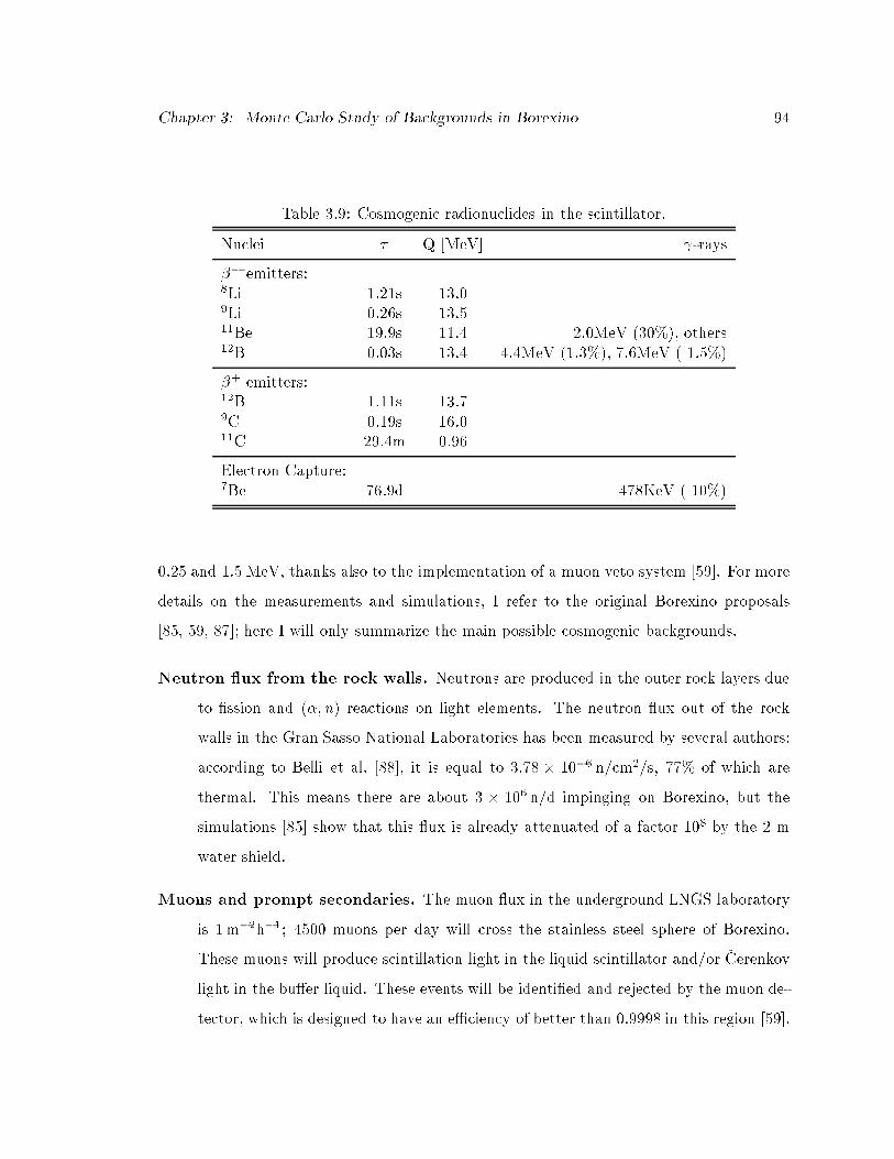
Chapter 3: Monte Carlo Study of Backgrounds in Borexino 94
Table 3.9: Cosmogenic radionuclides in the scintillator.
Nuclei � Q [MeV] -rays
�� emitters:8Li 1.21s 13.09Li 0.26s 13.511Be 19.9s 11.4 2.0MeV (30%), others12B 0.03s 13.4 4.4MeV (1.3%), 7.6MeV ( 1.5%)
�+ emitters:12B 1.11s 13.79C 0.19s 16.011C 29.4m 0.96
Electron Capture:7Be 76.9d 478KeV ( 10%)
0.25 and 1.5 MeV, thanks also to the implementation of a muon veto system [59]. For more
details on the measurements and simulations, I refer to the original Borexino proposals
[85, 59, 87]; here I will only summarize the main possible cosmogenic backgrounds.
Neutron ux from the rock walls. Neutrons are produced in the outer rock layers due
to �ssion and (�; n) reactions on light elements. The neutron ux out of the rock
walls in the Gran Sasso National Laboratories has been measured by several authors:
according to Belli et al. [88], it is equal to 3:78 � 10�6 n/cm2/s, 77% of which are
thermal. This means there are about 3 � 106 n/d impinging on Borexino, but the
simulations [85] show that this ux is already attenuated of a factor 108 by the 2 m
water shield.
Muons and prompt secondaries. The muon ux in the underground LNGS laboratory
is 1m�2h�1; 4500 muons per day will cross the stainless steel sphere of Borexino.
These muons will produce scintillation light in the liquid scintillator and/or �Cerenkov
light in the bu�er liquid. These events will be identi�ed and rejected by the muon de-
tector, which is designed to have an eÆciency of better than 0.9998 in this region [59].

Chapter 3: Monte Carlo Study of Backgrounds in Borexino 95
-rays from capture of cosmogenic neutrons. Energetic neutrons are produced by ul-
trarelativistic muons primarily in hadronic showers, occurring with a frequency of the
order of a few 10�2/m of path in water or scintillator [52, 89]. Neutrons are therma-
lized by inelastic and elastic collisions and then captured by protons in the reaction:
n + p!2 H + (2:216MeV): (3.5)
Neutrons have a capture mean time of about 300�s in pseudocumene. In Borexino,
we expect 100 neutrons/day, one third of them in the �ducial volume. Virtually, all of
these pulses fall outside the energy range of interest; moreover, they can be completely
suppressed by means of the 3 ms time correlation between the neutron capture and
the preceding muon event.
Radionuclides produced by muons in the scintillator. The muon induced nuclear
cascades that produce neutrons also produce radioactive nuclei in reactions involv-
ing the carbon atoms of the scintillator. A list of cosmogenic radionuclides produced
in the scintillator is reported in table 3.9.
Recently, data from an accelerator experiment [90, 91] gave a precise estimate of the
production rate of these nuclei. The estimate for the total background rate is one third
of the neutron rate: 30 events/day in the scintillator and 10 events/day in the �ducial
volume. Owing to the high endpoint energies, none of the very short lived isotopes is
expected to give a background of more than 1 event/day, even without further cuts.
Their contribution can still be reduced by time correlation with preceding muons.
11C poses a special problem. Its 30 m meanlife is too long for a time correlation with
the preceding muon. Since 11C is a �+ emitter, it deposits in the scintillator an energy
in the range of 1{2 MeV, due to the 1.022 MeV positron-electron annihilation energy.
These events fall outside the neutrino window, but they could limit the sensitivity
to the solar pep neutrinos. The expected rate, according to [90], is of about 7 11C
events/day in the 0.8{1.3 MeV energy window and in the 100-ton �ducial volume.

Chapter 4
The Physics Potential of Borexino
4.1 Solar Neutrino Physics from Borexino
The main focus of the physics program for Borexino is the measurement of the 7Be solar
neutrino ux and the investigation of neutrino oscillations as a solution to the solar neutrino
problem. Several oscillation scenarios have been identi�ed, based on the combined results of
the existing solar neutrino experiments (see x1.3 and �gure 1.7). In this section, I summarizethe predictions various authors have made on the impact Borexino will have on the solar
neutrino puzzle.
4.1.1 Neutrino Rates
Figure 4.1 shows the expected rates in Borexino, calculated for di�erent scenarios [42, 92,
93]. These predictions are based solely on the requirement of consistency with the results
from the existing solar neutrino experiments.
The �e scattering in the liquid scintillator for Borexino is driven by both charged (CC)
and neutral (NC) weak currents, while �� and �� scattering occur only via NC. Even without
conversion, in the 7Be energy window the counting rate exclusively due to NC interaction
is � 23% of the total rate. It follows that even in the case of complete conversion of 7Be
solar �e's into a di�erent avor, Borexino can record a signi�cant signal from the ��'s and
�� 's. In other words, the NC interaction sets a lower limit on the signal to be detected in
Borexino.
96

Chapter 4: The Physics Potential of Borexino 97
0
2
4
6
8
CNO Sun
0
0.2
0.4
0.6
0.8
1
νmassless
sterileMSW
SMAMSW
LMAMSW
LOWMSW
VacuumJust-so
Rat
e/SS
M
Figure 4.1: The expected rates in Borexino for various physics scenarios, expressed asa fraction of the SSM-predicted rate. In each scenario, the error bars show the rangesthat could be observed by Borexino and that would still be consistent with the existingsolar neutrino experiments (99% C.L.). Note that neutral current scattering for �� and ��contribute to the observed rate, even in the scenario of total MSW conversion. Data fromrefs. [42, 92, 93].
If neutrinos are massless and behave as prescribed by the Standard Model, with no avor
oscillations, then the existing experiments suggest that the rate in Borexino will be equal
to zero. This would be in con ict with the present understanding of the solar model and it
would imply that some unexpected physics is responsible for the solar neutrino de�cit.
Another scenario in which Borexino is expected to have virtually zero signal is that of
conversion into sterile neutrinos (right-hand helicity �s). In this case, a good �t with the
combined experiments is possible only for small mixing angle MSW [42, 92]. In light of recent
SuperKamiokande data and global �ts, pure �e ! �s seems to be excluded, but Barger et
al. [94] suggest that all the data are consistent with a four-neutrino model (�e; ��; �� ; �s)
and that oscillations into a sterile neutrino is not yet ruled out.

Chapter 4: The Physics Potential of Borexino 98
Figure 4.1 illustrates the expected rates in Borexino for the small (SMA) and large
(LMA) mixing angle MSW e�ect: a measurement of the 7Be ux in Borexino can distinguish
between these two solutions. The expected rate for the LOW MSW solution is very similar
to the large angle one; as I will discuss in the next paragraphs, the real signature for the
LOW MSW is the day/night asymmetry. The ability to discriminate between SMA and
LMA/LOW MSW is complementary to the capabilities of SNO and SuperKamiokande; by
looking at the distortion of the 8B neutrino energy spectrum, these two experiments can
only observe evidence for small mixing angle MSW oscillations.
A \CNO solution" [93] is also included in �gure 4.1. A measure of the recoil electron
rate and of the spectral shape at low energy (<1.5 MeV) enables an empirical identi�cation
of which cycle, CNO or pp, is responsible for most of the energy production in the Sun.
Finally, if Borexino were to observe the full SSM-calculated ux of 7Be neutrinos, it
would imply that one or more of the existing experiments is incorrect. This would also be
an interesting and valuable result.
4.1.2 Seasonal Variations
The annual variation of the measured rate in Borexino represents a distinctive signature
that the detected neutrinos have solar origin. The solar neutrino rate is subject to a 1=R2
modulation, due to the fact that the distance between the Earth and the Sun changes
during one orbital revolution. The magnitude of this annual variation is � 7%, peak-to-
peak. Given the signal-to-background estimates outlined in {3 and the BP98 SSM neutrino
ux, this e�ect will have greater than 5 � statistical signi�cance after three years of data-
taking (see �gure 4.2 from reference [74]). In the case of an unexpectedly high internal
background in Borexino, extending the size of the �ducial volume will increase both signal
and background; since only the signal presents the annual periodicity, this can increase
the statistical strength of the annual variation signature. Of course, this time-periodicity
analysis will only be possible provided the detector response is very stable. Size and shape
of the �ducial volume must be known and the detection eÆciency must be constantly
monitored; this is one of the goals of the calibration program for Borexino.

Chapter
4:
ThePhysics
Poten
tialofBorex
ino
99
3600
3800
4000
4200
4400
4600
4800
0200
400600
8001000tim
e (days)
counts/60 days
Figu
re4.2:
Theannualvaria
tionof
therate
inBorex
ino,after
three
years.
Theperio
dicity
isasig
natu
rethatthedetected
neutrin
oshave
solarorigin
.From
reference
[74].
Figu
re4.3
:Season
alvaria
tionof
the7B
eneutrin
o uxandof
theGNO
Galliu
mdetector
signal
fortheVO
(Vacu
um
Oscillation
,�m
2=
6:5�
10�11eV
2,sin
22�=
0:75[42])
and
HEE-VO
(High
Energ
yExcess
Vacu
um
Oscillation
,�m
2=
4:2�
10�10eV
2,sin
22�=
0:93
[48])
solutio
ns.
Thesurvival
prob
ability
P(�
e !�e )for
7Beneutrin
osisrep
resented
bythedash
edandthe
solidcurvefor
theVOandtheHEE-VOsolu
tions,as
afunction
oftim
e.Tisoneorbita
lperio
d(1
year).From
reference
[48].

Chapter 4: The Physics Potential of Borexino 100
In addition to the solar signature, the fact that the Earth{Sun distance varies during
the course of a year allows discrimination between the vacuum oscillation and the MSW
scenarios.
The \just-so" vacuum oscillation solution predicts that, given the allowed �m2 and
sin2 2� parameters, the neutrino oscillation length is just of the order of the Earth-Sun
distance. A change in R is followed by a change in the �e survival probability. Once the
solid angle dependence (/ 1=R2) has been subtracted from the data, vacuum oscillations
induce an annual variation of the signal as large as 25% at the best �t point [92].
This solution can be either established or excluded by the seasonal variation of the 7Be
neutrino rate in Borexino (see, for instance, reference [95]), since the monochromatic 7Be
neutrinos are expected to show the strongest seasonal dependence [96]. The e�ect is reduced
for the other uxes with a continuous spectrum, like 8B, because of the average over the
phases of neutrinos with di�erent energies and, consequently, di�erent survival probabilities.
On the other hand, no seasonal variation other than the 1=R2 modulation is expected
in the MSW oscillation scenario.
As mentioned in x1.3, Berezinsky et al. [48] proposed a particular vacuum oscillation
solution that could test the excess of high energy events (> 13 MeV) in SuperKamiokande:
HEE-VO, or High Energy Excess Vacuum Oscillation, with �m2 = 4:2 � 10�10 eV2 and
sin2 2� = 0:93. If this solution is valid, Borexino will detect a semiannual periodicity of its
signal, as it is shown in �gure 4.3, where the prediction for GNO is also shown.
Finally, a Fourier analysis of the real time distribution of neutrino interactions in the
detector allows us to probe a broader range of vacuum oscillation solutions than SNO and
SuperKamiokande. Borexino is sensitive to deviations of the Fourier discrete transform
values, from the non-oscillation case, up to the third harmonic, while both SNO and Su-
perKamiokande are sensitive to deviations of the �rst harmonic only (see �gure 4.4, from
reference [97]). A vanishing value for the deviation of the �rst harmonic corresponds to a
non vanishing value for the second harmonic, allowing Borexino to probe almost all of the
parameter region for the vacuum oscillation scenario.

Chapter 4: The Physics Potential of Borexino 101
Figure 4.4: Deviation from the no-oscillation case for the �rst three harmonics of the neu-trino real time distribution in SNO, SuperKamiokande and Borexino, in the vacuum oscil-lation scenario. These results are valid for a statistics of 105 neutrinos, with no background.The shadowed bar represents the sensitivity due to the statistical error only. Its absolutewidth is equal in the three plots.In presence of a background rate B constant in time, if S is the signal rate and T is thedata collection time, the error would scale with the factor
p(1 + f2n + B=S)=(ST) (fn is the
nth Fourier coeÆcient).The deviation is ten times larger in Borexino because the neutrino source has a discreteenergy spectrum. In SuperKamiokande and SNO the average of the survival probabilityover the continuous energy spectrum reduces the sensitivity. From reference [97].
Chapter 4: The Physics Potential of Borexino 102
4.1.3 Day-Night Asymmetry
Borexino, as a real time experiment, also has the capability of detecting day{night asymme-
tries in the neutrino event rate. Such e�ect would be a \smoking gun" signature for MSW:
the coherent forward scattering of neutrinos with matter causes a regeneration of the �e
species as the neutrino ux crosses Earth at nighttime [98, 99, 100].
Bahcall and Krastev have performed a detailed analysis of the detectability of a day-
night asymmetry e�ect in SuperKamiokande, SNO and Borexino [101]. The main point
of interest for Borexino is that the day/night asymmetry is particularly enhanced in the
MSW LOW scenario for low energy neutrinos (E� < 1MeV), as it is shown in �gure 4.5,
from reference [101]. This provides Borexino with the ability to discriminate between the
MSW LOW scenario and all other MSW scenarios. Figure 4.7 shows day-night asymmetry
contours calculated for Borexino by Gouvea et al. [102].
A recent paper by Foot [104] shows that the day-night asymmetry prediction for Borex-
ino is similar to the one for SuperKamiokande, except it is shifted to lower mass values (this
is because the oscillation depends on E=�m2 and the energy for Borexino is one order of
magnitude lower than that of SuperKamiokande). The asymmetry result for 7Be and 8B
neutrinos in the case of maximal oscillation �e ! ��;� is presented in �gure 4.6, where the
asymmetry parameter is de�ned as:
An�d =N �D
N +D(4.1)
N and D are the nocturnal and diurnal event rates, respectively. Assuming maximal os-
cillation, Borexino should see night-day asymmetry as low as An�d � 0:02 or lower after
a couple of years of data. The maximal neutrino oscillation solution leads to a signi�-
cant (An�d > 0:02) night-day asymmetry in Borexino and/or SuperKamiokande for the
parameter range:
10�8eV2 � �m2 � 4� 10�5eV2: (4.2)
Given the present asymmetry result from SuperKamiokande (see x1.3 and reference [49]):
2D �N
D +N= �0:034� 0:022stat� 0:013sys;

Chapter 4: The Physics Potential of Borexino 103
Figure 4.5: Survival probability for �e in the three MSW solutions.The solid line refers to the average survival probabilities computed taking into account re-generation in the earth and the dotted line refers to calculations for the daytime that do notinclude regeneration. The dashed line includes regeneration at night. From reference [42].
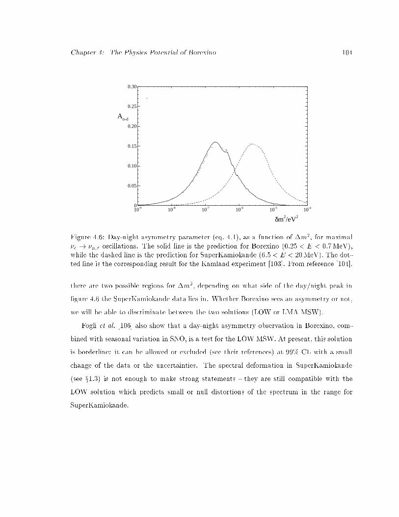
Chapter 4: The Physics Potential of Borexino 104
10-9 10-8 10-7 10-6 10-5 10-40
0.05
0.10
0.15
0.20
0.25
0.30
.
δm2/eV2
An-d
Figure 4.6: Day-night asymmetry parameter (eq. 4.1), as a function of �m2, for maximal�e ! ��;� oscillations. The solid line is the prediction for Borexino (0:25 < E < 0:7MeV),while the dashed line is the prediction for SuperKamiokande (6:5 < E < 20MeV). The dot-ted line is the corresponding result for the Kamland experiment [103]. From reference [104].
there are two possible regions for �m2, depending on what side of the day/night peak in
�gure 4.6 the SuperKamiokande data lies in. Whether Borexino sees an asymmetry or not,
we will be able to discriminate between the two solutions (LOW or LMA MSW).
Fogli et al. [106] also show that a day-night asymmetry observation in Borexino, com-
bined with seasonal variation in SNO, is a test for the LOW MSW. At present, this solution
is borderline: it can be allowed or excluded (see their references) at 99% CL with a small
change of the data or the uncertainties. The spectral deformation in SuperKamiokande
(see x1.3) is not enough to make strong statements - they are still compatible with the
LOW solution which predicts small or null distortions of the spectrum in the range for
SuperKamiokande.

Chapter 4: The Physics Potential of Borexino 105
105 x-6
10x1 -5
10x1 -6
10x1 -7
105 x-8
10x1 -8
105 x-7
105 x-6
10x1 -5
10x1 -6
10x1 -7
105 x-8
10x1 -8
105 x-7
10.05 0.50.10.010.005
22
∆m(e
V )
at BorexinoD/N asymmetry
sin 2 θ
0.5%
1%5%
10%
Figure 4.7: Constant day-night asymmetry contours (10%, 5%, 1% and 0.5%) in the �m2�sin2 � plane for 7Be neutrinos in Borexino. The vertical dashed line indicates sin2 � = 1
2 ,where the neutrino vacuum mixing is maximal. The authors assumed a 7Be neutrino rateof 53 ev/day and a constant background rate of 29 ev/day in the 100-ton �ducial volume forBorexino, in the neutrino window. A very similar result has been obtained for the Kamlandexperiment, with a 600 ton �ducial volume. From reference [102].Note that the authors use, in this plot, sin2 �, instead of sin2 2�, in order to show \the darkside" of the vacuum oscillation parameter space, � > �=4, normally not considered [105].

Chapter 4: The Physics Potential of Borexino 106
4.2 Sensitivity to the 7Be Signal in Borexino
This section presents an estimate of Borexino's sensitivity to the 7Be solar neutrino, based
on the signal and background simulation results presented in {3.The major limit to Borexino's sensitivity is the intrinsic 238U, 232Th and 40K content of
the scintillator (internal background). For the purpose of this calculation, I am assuming
the design values of 10�16 g/g 238U and 232Th and 10�14 g/g Knat in the scintillator and
one year of statistics.
The �tting procedure evolves in the following steps:
1. Monte Carlo generation of signal and background spectra with 1 year statistics and
50 keV energy bins.
2. Application of the standard cuts: �rst, identi�cation and rejection of Bi-Po correlated
events (95% eÆciency assumed) and of the � events (90% eÆciency assumed). Then,
bin-by-bin statistical subtraction from the residual energy distribution (error=pNbin)
of 214Pb, 212Pb and the remaining �'s in equilibrium with the Bi-Po events.
3. Background determination: the 234Pa+CNO plateaux is modeled with a linear �t in
the 0.8{1.4 MeV energy range. This line is then extrapolated as background in the
neutrino window.
4. The �t: the � peak is modeled with a Gaussian, with �xed centroid at 0.37 MeV and
� = 0:077MeV, which I assumed to be known from the behavior of the �'s directly
identi�ed by pulse shape discrimination. The only free parameter is the Gaussian
amplitude, proportional to the number of �'s that have not been identi�ed. The
neutrino 7Be shoulder is modeled by a line, between 0.3 and 0.6 MeV. The residual
spectrum can then be �t with a three parameters curve, sum of the at background
extrapolated from higher energies (�xed), the �'s (Gaussian with �xed centroid and
width) and the 7Be neutrinos (line).
This procedure has been applied to three scenarios, the SSM, the MSW LMA and the
MSW SMA. The �t results are shown in �gure 4.8 and summarized in table 4.8. The

Chapter 4: The Physics Potential of Borexino 107
0
500
1000
1500
2000
2500
3000
3500
4000
0.4 0.6 0.8 1 1.2 1.4 1.6 1.8 2E (MeV)
even
ts /
year
/ 0.
05 M
eV
7Be solar ν in BorexinoSSM prediction1 year statistics
0
200
400
600
800
1000
1200
1400
1600
1800
0.4 0.6 0.8 1 1.2 1.4 1.6 1.8 2E (MeV)
even
ts /
year
/ 0.
05 M
eV 7Be solar ν in Borexino
SMA MSW model1 year statistics
Figure 4.8: Energy spectrum �t in the neutrino window (0.25{0.8 MeV), given a one yearstatistics and in two scenarios: full SSM (top) and small mixing angle MSW oscillation(bottom).The dotted line is the neutrino spectrum, the dashed line is the residual background, afterthe cuts described in x3.4, and the marks are the sum spectrum, with error bars correspond-ing to a one year statistics. Overlapped is the �t result.

Chapter 4: The Physics Potential of Borexino 108
Table 4.1: Energy spectrum �t in the neutrino window (0.25{0.8 MeV), given a one yearstatistics and in three scenarios: full SSM, large and small mixing angle MSW oscillation.The number of neutrino events is extracted with a �t in the 0.25{0.6 MeV region. The �tincludes a at background level (extrapolated from the spectral behavior at higher energies),a Gaussian peak for the residual �'s and a line for the 7Be Compton shoulder. The resulting� event number is is agreement, within the error, with the number of events that were put inthe simulation. After one year, the neutrino rate will be quoted with 2.4% error, in case ofthe full SSM, 4% error, in the MSW LMA solution or 8% error in the MSW SMA solution.
SSM MSW LMA MSW SMA
events/year in 0.25{0.8 MeV 28416 � 169 18880 � 137 11590 � 108 at background 5330 � 258 4024 � 243 3256 � 232residual �'s/year 1895 � 405 2966 � 365 3265 � 2977Be � events/year 21188 � 509 11889 � 459 5069 � 393
� events/day 58.0 � 1.4 32.6 � 1.3 13.9 � 1.1simulated: 58.8 � 0.4 32.6 � 0.3 12.7 � 0.2
prediction is that, given a scintillator purity level of 10�16 g/g U, Th and 10�14g/g Knat,
with one year of data Borexino will quote a rate for 7Be neutrino with 2.4% precision in
the SSM scenario, 4% in the MSW large angle solution and 8% precision in the MSW small
angle solution.

Chapter 4: The Physics Potential of Borexino 109
4.3 Sensitivity to the 8B Solar Neutrino
The 8B solar neutrino energy spectrum has an endpoint at 15.1 MeV. The spectral shape,
according to the SSM prediction, is linear in its central region; a deformation would provide
a signature for conversion e�ects. Borexino has the capability to detect the 8B spectrum
with an energy threshold that depends on the background, potentially lower than in Su-
perKamiokande and SNO. Figure 4.9 shows the BP98 SSM prediction for the 8B neutrino
and the following background sources at > 3 MeV:
external background: the spectra in �gure 4.9 include the contribution of the phototubes
(distant sources) and of the inner vessel (close source). Without �ducial volume cuts,
the low energy threshold for 8B is limited by the background from the inner vessel.
A �ducial volume cut at R = 3:75 m is enough to suppress the surface background.
Going to a smaller �ducial volume would not contribute a signi�cant gain in sensitivity
to 8B �'s, because of the shape of the background from the phototubes (a \vertical
wall" at around 3 MeV). A lower limit to the energy threshold for 8B �'s is set by the
external background:
Ethr � 3:5 MeV:
The current threshold for SuperKamiokande is 5 MeV.
internal background: I used the design value of 10�16 g/g 238U and 232Th. In the 238U
chain, the only possible contribution at high energy comes from 214Bi (peaks at 2.3
MeV) and 234Pa (� spectrum with endpoint at 2.2 MeV), but they intersect the 8B
neutrino spectrum at about 3 MeV, hence they do not increase the threshold. The
internal background from 238U does not really a�ect the sensitivity to 8B neutrinos.
The dominating contribution at the higher energies of interest for 8B neutrinos comes
from 208Tl, with a large peak at 4 MeV. 208Tl e�ectively constitutes a limiting factor
for the 8B � sensitivity; in order for it not to be a problem, we need a two order of
magnitude lower level, consistent with 10�18g/g 232Th in the scintillator. Note that
the 208Tl may be a \taggable" background: its decay follows the � decay of 212Bi and

Chapter 4: The Physics Potential of Borexino 110
energy (MeV)
rate
(ev
ents
/day
/0.0
5 M
eV)
2 4 6 8 10 12 1410
−4
10−3
10−2
10−1
100
101
102
total signal external background from phototubes external background from nylon internal backgr. 208Tl − 10−16 g/g 232Th internal backgr. 214Bi 234Pa − 10−16 g/g 238U − 95% Bi−PoSSM neutrino from 8B
events/day in 300 tons
energy (MeV)
rate
(ev
ents
/day
/0.0
5 M
eV)
2 4 6 8 10 12 1410
−4
10−3
10−2
10−1
100
101 total signal
external background from phototubes external background from nylon internal backgr. 208Tl − 10−16 g/g 232Th internal backgr. 214Bi 234Pa − 10−16 g/g 238U − 95% Bi−PoSSM neutrino from 8B
events/day in 200 tons F.V.
Figure 4.9: Energy spectra, in Borexino, above 2 MeV, in the whole detector (top) and ina 200 ton �ducial volume.

Chapter 4: The Physics Potential of Borexino 111
a coincidence between an � and a high energy � � event, with �1=2 = 3:03minutes,
can be used for a direct identi�cation of the 208Tl events. Since the eÆciency for
this identi�cation still needs to be evaluated, in this study I followed a conservative
approach and I did not apply such direct identi�cation cut.
All the other known background sources are at lower energy (< 3MeV). There are some
cosmogenic isotopes that have end spectrum at more than 10 MeV, but given the eÆciency
of the muon veto system, all these events should be taggable and not a�ect the 8B neutrino
sensitivity (see x3.5).The plots in �gure 4.9 show how, once the �ducial volume cut is applied, the only real
limit to the threshold is the 208Tl peak. In the hypothesis of 10�16 g/g 232Th in equilibrium
with 208Tl, the spectral shape of 8B can be detected without any data manipulation only
above 5 MeV. This is a very conservative assumption, though, if we consider that the 208Tl
events can be removed by direct identi�cation and statistical subtraction.
A way to estimate the 8B rate below 5 MeV is to use the spectral features of the 208Tl
and the 8B neutrino to statistically separate the two components. Using an approach similar
to the one described in x4.2, I simulated the statistics of 3 years of data in Borexino, in a
200 ton �ducial volume (R=3.75 m). I modeled the 8B neutrino spectrum in the 3.5{9 MeV
region with a straight line and the 208Tl peak with a Gaussian. The line, from the �t, can
be used to estimate the 8B neutrino rate in the 3.5{5 MeV energy window. In alternative,
the Gaussian can be subtracted from the data, bin-by-bin, and the residual spectrum above
3.5 MeV can be attributed to 8B neutrinos.
Figure 4.10 shows the result of this analysis for 3 years of statistics, according to the
BP98 SSM or to the SMA and LMA MSW scenarios. The continuous red line is the
simulated 8B � energy distribution. The points with error bars are the residual spectrum
after subtraction of the Gaussian �t from the total signal. The straight line between 3.5 and
9 MeV is the �t result for the modeled 8B spectrum in that region. The numerical results
are summarized in table 4.2. The 8B neutrino rate in the 3.5{5 MeV energy region is well
described by the linear �t; in the SSM scenario, after 3 years, it will be known with 16%

Chapter 4: The Physics Potential of Borexino 112
0
20
40
60
80
100
120
140
2 4 6 8 10 12 14E (MeV)
8B solar ν in Borexino - SSM3 year statistics
0
20
40
60
80
100
120
140
2 4 6 8 10 12 14E (MeV)
MSW Small Angle8B solar ν in Borexino
3 year statistics
0
20
40
60
80
100
120
140
2 4 6 8 10 12 14E (MeV)
MSW Large Angle8B solar ν in Borexino
3 year statistics
Figure 4.10: 8B solar neutrinos in Borexino: the distribution is the simulated 8B � spectrum,the line is what the �t attributes to 8B � in the 2.5{9 MeV energy region and the pointsrepresent the residual spectrum after subtraction of the Gaussian peak for 208Tl from the�t, in the SSM, MSW SMA and LMA scenarios. The statistics is for three years of data.
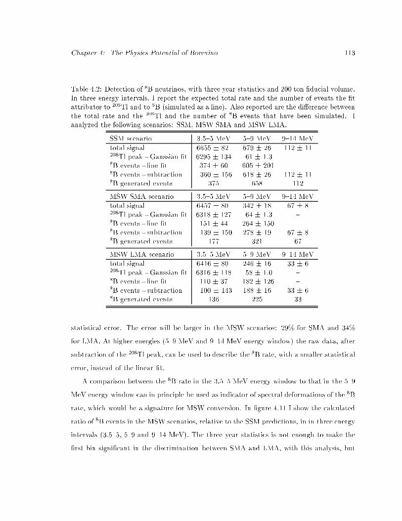
Chapter 4: The Physics Potential of Borexino 113
Table 4.2: Detection of 8B neutrinos, with three year statistics and 200 ton �ducial volume.In three energy intervals, I report the expected total rate and the number of events the �tattributes to 208Tl and to 8B (simulated as a line). Also reported are the di�erence betweenthe total rate and the 208Tl and the number of 8B events that have been simulated. Ianalyzed the following scenarios: SSM, MSW SMA and MSW LMA.
SSM scenario 3.5{5 MeV 5{9 MeV 9{14 MeV
total signal 6655 � 82 679 � 26 112 � 11208Tl peak - Gaussian �t 6295 � 134 61 � 1.3 {8B events - line �t 374 � 60 605 � 201 {8B events - subtraction 360 � 156 618 � 26 112 � 118B generated events 375 658 112
MSW SMA scenario 3.5{5 MeV 5{9 MeV 9{14 MeV
total signal 6457 � 80 342 � 18 67 � 8208Tl peak - Gaussian �t 6318 � 127 64 � 1.3 {8B events - line �t 151 � 44 264 � 150 {8B events - subtraction 139 � 150 278 � 19 67 � 88B generated events 177 321 67
MSW LMA scenario 3.5{5 MeV 5{9 MeV 9{14 MeV
total signal 6416 � 80 246 � 16 33 � 6208Tl peak - Gaussian �t 6316 � 118 58 � 1.0 {8B events - line �t 110 � 37 182 � 126 {8B events - subtraction 100 � 143 188 � 16 33 � 68B generated events 136 225 33
statistical error. The error will be larger in the MSW scenarios: 29% for SMA and 34%
for LMA. At higher energies (5{9 MeV and 9{14 MeV energy window) the raw data, after
subtraction of the 208Tl peak, can be used to describe the 8B rate, with a smaller statistical
error, instead of the linear �t.
A comparison between the 8B rate in the 3.5{5 MeV energy window to that in the 5{9
MeV energy window can in principle be used as indicator of spectral deformations of the 8B
rate, which would be a signature for MSW conversion. In �gure 4.11 I show the calculated
ratio of 8B events in the MSW scenarios, relative to the SSM predictions, in in three energy
intervals (3.5{5, 5{9 and 9{14 MeV). The three year statistics is not enough to make the
�rst bin signi�cant in the discrimination between SMA and LMA, with this analysis, but

Chapter 4: The Physics Potential of Borexino 114
0
0.1
0.2
0.3
0.4
0.5
0.6
0.7
4 6 8 10 12 14E (MeV)
R_M
SW/R
_SSM
MSW Large Angle
MSW Small Angle
Figure 4.11: The plot reports, in three energy intervals, the calculated rate of 8B events inthe MSW scenario, relative to the SSM prediction. I included both the SMA (squares) andthe LMA (dots) solutions. The error bars are calculated with a statistics of 3 years.
the errors could be signi�cantly reduced with less conservative assumptions on the 208Tl
direct identi�cation eÆciency.
In conclusion, this study shows that Borexino has the potential to detect 8B neutrinos
with a low energy threshold of 3.5 MeV, although the statistical signi�cance of the 3.5{5
MeV window has relevance only if the 208Tl signal is 1-2 orders of magnitude less than what
expected by 10�16 g/g 232Th in equilibrium.

Chapter 4: The Physics Potential of Borexino 115
4.4 Sensitivity to the pp Solar Neutrino - Low Energy Spec-
trum in Borexino
The neutrino scattering reaction in the liquid scintillator does not have an energy threshold.
With a trigger threshold of 6 hits, Borexino can detect events as low as 15 keV, including
the pp solar neutrino interactions. Nevertheless, the 14C content of the scintillator is a
major obstacle to the detection of this channel. 14C emits a low energy � (Q = 0:156MeV
and �1=2 = 5730 years) that dominates the energy spectrum below the so-called \neutrino
window". If we apply to Borexino the CTF result:
14C=12C = (1:94� 0:09)� 10�18;
in a �ducial volume of 100 tons (RFV = 3:00 m) we will have about 3�106 14C events each
day due to 14C beta decay. This signal is clearly overwhelming, as a whole, if compared
to the expected event rate of pp neutrinos in Borexino: 199 events per day in the 100-ton
�ducial volume, according to the BP98 SSM. The study I am about to report is an attempt
to establish whether the contribution of the pp solar neutrino can be extracted from the
Borexino energy spectra with statistical methods in the energy window 0.1{0.3 MeV.
Fig. 4.12 shows a Monte Carlo simulation of the energy spectra of the 14C � and of
the pp solar neutrino, with a 6 month statistics. In order to separate the two contributions,
it is absolutely necessary to know the 14C spectrum with great accuracy, with all the
experimental distortion e�ects (such as pile-ups, electron quenching in the scintillator [107]
and non Gaussian behaviors that are not included in the simulation). One way to achieve
this goal is to add a known amount of 14C to the scintillator and take data for a �xed length
of time. In this work I assumed a data acquisition period of 6 months, but it could be longer.
At the end of this period, we will have two spectra, one with 14C+ pp + background, and
the other with X �14 C+14 C+ pp+background, where X is the additional amount of 14C .
By taking the di�erence of the two spectra, we are left with an experimentally determined
spectrum of 14C that can be used in the �t to separate the pp spectrum.
We also need a spectrum for pp neutrinos: we trust that a comparison of the theoretical

Chapter 4: The Physics Potential of Borexino 116
1
10
10 2
10 3
10 4
10 5
10 6
10 7
0.1 0.15 0.2 0.25 0.3 0.35 0.4 0.45 0.5energy(MeV)
even
ts /
10 k
eV /
6 m
onth
s
pp neutrino
14C spectrum
0
200
400
600
800
1000
1200
1400
1600
0.1 0.15 0.2 0.25 0.3 0.35 0.4 0.45 0.5energy(MeV)
even
ts /
10 k
eV /
6 m
onth
s
pp neutrino
background
no α/β
90% α rejection
Figure 4.12: Top: energy spectra of 14C and pp neutrino Bottom: background spectra withand without 90% �=� discrimination. Both plots refer to a 100-ton �ducial volume and 6months' statistics.

Chapter 4: The Physics Potential of Borexino 117
14C � spectrum to the experimental one will provide information on the actual energy
resolution and possible spectral distortions at low energy, so that we will be able to correct
the Monte Carlo pp spectrum and use that to �t the data.
As for the background, in the 100-ton �ducial volume, at low energies, the external
background is not an issue. The main problem at E< 0:3MeV are tails of �'s and low-
energy 's (mainly 228Ra) in the radioactive chains of 238U and 232Th. There could be
other unexpected background sources, but the main point is that in the 0.1{0.3 MeV energy
window there is not an emerging spectral structure. With the hypothesis of 1�10�16g/g 238U
and 232Th in the scintillator, the background energy spectrum is similar to that in �g. 4.12,
once we apply the correlated coincidence and the statistical subtraction cuts described in
section 3.4. There still are some questions about the eÆciency of �=� discrimination at
these low energies; the �gure shows the two extremes of zero and 90% eÆciency for �
rejection. In both cases, in the small energy window used for the �t, the background can
be �t with a horizontal line.
With these inputs, it is possible to perform a three parameter �t on the low energy
spectrum. I tested this theory on a simulation of 6 months of data in Borexino that includes:
- 14C=12C = 1:94� 10�18 [73];
- 238U and 232Th= 1� 10�16g/g;
- pp neutrino rate from the BP98 SSM [11].
I also simulated a di�erent set of 6 month statistics, where the amount of 14C had been
doubled, and subtracted the two distributions to obtain an \experimental" 14C spectrum.
An independent theoretical pp spectrum was also simulated, for the �t. The error bars on
the �tting functions have been combined in the spectrum to be �t.
Table 4.3 is a summary of the �t results in the two cases: if the �'s are not identi�ed and
rejected, we are forced to use a smaller energy window in the �t, because of the di�erent
background shape (it is at in a smaller region).
Starting with 3:57� 104 pp events in input, the �t recovers (4:3� 0:4)� 104 events if
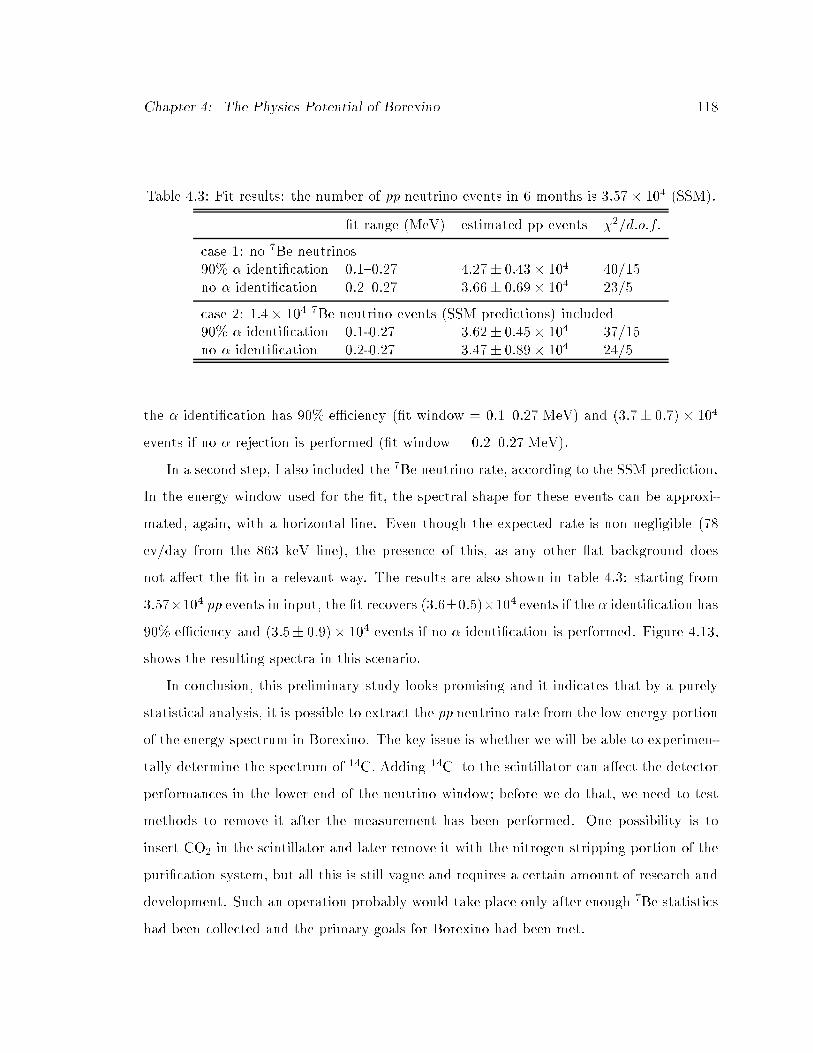
Chapter 4: The Physics Potential of Borexino 118
Table 4.3: Fit results: the number of pp neutrino events in 6 months is 3:57� 104 (SSM).
�t range (MeV) estimated pp events �2=d:o:f:
case 1: no 7Be neutrinos90% � identi�cation 0.1{0.27 4:27� 0:43� 104 40/15no � identi�cation 0.2{0.27 3:66� 0:69� 104 23/5
case 2: 1:4� 104 7Be neutrino events (SSM predictions) included90% � identi�cation 0.1-0.27 3:62� 0:45� 104 37/15no � identi�cation 0.2-0.27 3:47� 0:89� 104 24/5
the � identi�cation has 90% eÆciency (�t window = 0.1{0.27 MeV) and (3:7� 0:7)� 104
events if no � rejection is performed (�t window = 0.2{0.27 MeV).
In a second step, I also included the 7Be neutrino rate, according to the SSM prediction.
In the energy window used for the �t, the spectral shape for these events can be approxi-
mated, again, with a horizontal line. Even though the expected rate is non negligible (78
ev/day from the 863 keV line), the presence of this, as any other at background does
not a�ect the �t in a relevant way. The results are also shown in table 4.3: starting from
3:57�104 pp events in input, the �t recovers (3:6�0:5)�104 events if the � identi�cation has
90% eÆciency and (3:5� 0:9)� 104 events if no � identi�cation is performed. Figure 4.13,
shows the resulting spectra in this scenario.
In conclusion, this preliminary study looks promising and it indicates that by a purely
statistical analysis, it is possible to extract the pp neutrino rate from the low energy portion
of the energy spectrum in Borexino. The key issue is whether we will be able to experimen-
tally determine the spectrum of 14C. Adding 14C to the scintillator can a�ect the detector
performances in the lower end of the neutrino window; before we do that, we need to test
methods to remove it after the measurement has been performed. One possibility is to
insert CO2 in the scintillator and later remove it with the nitrogen stripping portion of the
puri�cation system, but all this is still vague and requires a certain amount of research and
development. Such an operation probably would take place only after enough 7Be statistics
had been collected and the primary goals for Borexino had been met.
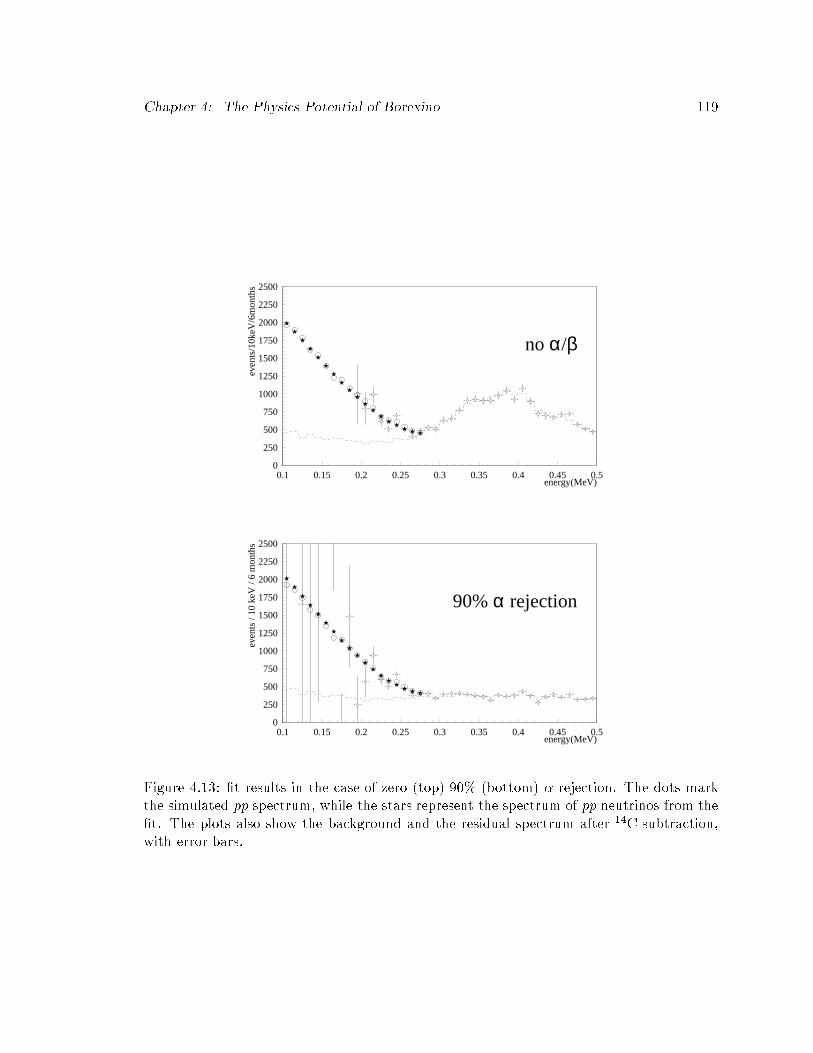
Chapter 4: The Physics Potential of Borexino 119
0
250
500
750
1000
1250
1500
1750
2000
2250
2500
0.1 0.15 0.2 0.25 0.3 0.35 0.4 0.45 0.5
no α/β
energy(MeV)
even
ts/1
0keV
/6m
onth
s
0
250
500
750
1000
1250
1500
1750
2000
2250
2500
0.1 0.15 0.2 0.25 0.3 0.35 0.4 0.45 0.5
90% α rejection
energy(MeV)
even
ts /
10 k
eV /
6 m
onth
s
Figure 4.13: �t results in the case of zero (top) 90% (bottom) � rejection. The dots markthe simulated pp spectrum, while the stars represent the spectrum of pp neutrinos from the�t. The plots also show the background and the residual spectrum after 14C subtraction,with error bars.

Chapter 4: The Physics Potential of Borexino 120
4.5 Physics Beyond Solar Neutrinos
Borexino is an ultra-low background detector, whose potential goes beyond the detection of
solar neutrinos. In this section I will present the additional scienti�c objectives for Borexino,
referring, for details, to the published and submitted papers. A separate section (x4.6) willbe devoted to the detection of supernova neutrinos in Borexino, a study that I conducted
and that promises to disclose interesting new results.
4.5.1 ��e Detection
The detection of ��e in Borexino proceeds via the classic Reines reaction of capture by
protons in the organic liquid scintillator:
��e + p! n+ e+; Q = 1:8MeV: (4.3)
The positron energy is related to the ��e energy as: E(e+) = E(��e) � Q + 1:02MeV. The
neutron capture induces emission of a 2:2MeV after 0:2ms. The delayed coincidence
between e+ and provides a de�nite signature for the detection of ��e, with a sensitivity of
a few events per year.
There are several interesting ��e sources: the Sun, Earth and nuclear power reactors,
which can be distinguished from each other mainly by their energy.
Solar ��e
While current solar astrophysics o�ers no room for solar antineutrinos, there is room for
them in a non-standard mechanism that involves an o�-diagonal magnetic moment for
Majorana neutrinos [85]. The current upper limit on the solar ��e ux is 5�104 cm�2s�1 [108],
which corresponds to a rate of 110 ��e per year in Borexino. The energy range for these events
is 7{15 MeV.

Chapter 4: The Physics Potential of Borexino 121
Geophysical ��e from the Earth
Borexino could be the �rst experiment to detect antineutrinos emitted by the radioactive
elements in the mantle and the crust of Earth, primarily 238U and 232Th. This would
establish important geophysical constraints on the heat generation within the Earth and
probe the radiochemical composition of Earth. Depending on the geophysical model, ��e
rates between 10 and 30 events per year, in the energy range 0{3.3 MeV, can be expected
in Borexino [109, 110].
Long-Baseline ��e's from European Reactors
Nuclear power reactors are strong sources of antineutrinos, emitted in the � decay of various
isotopes produced in the �ssion of Uranium. These ��e are produced with a known ux and
spectrum, at energies up to 8 MeV. Borexino is sensitive to the ux generated by nuclear
power reactors in France, Germany and Switzerland and the predicted event rate is of about
30 ��e per year. Evidence for neutrino oscillations would come from the disappearance of
these neutrinos and from distortions in their spectral shape. The combination of Borexino
and the European reactors, with their well de�ned experimental setup, makes an ideal
terrestrial long-baseline experiment for a model-independent search for vacuum neutrino
oscillation [111].
4.5.2 Double-� Decay with Dissolved 136Xe
Double-� decay o�ers the only mean to identify the Majorana neutrino. It has been tra-
ditionally carried out on target masses of the order of a few tens of kg. Borexino has the
potential to enhance this search on the multi-ton scale [112, 113]. Noble gases, as 136Xe are
highly soluble in the liquid scintillator and do not a�ect the radiopurity or the scintillator
eÆciency. The plan could be �rst tested in CTF2, adding 10 kg of 136Xe, in order to as-
sess signal quality and backgrounds. If successful, the measurement could be extended to
Borexino, with � 2 tons 136Xe.

Chapter 4: The Physics Potential of Borexino 122
4.5.3 Neutrino Physics with MCi Sources
The recoil electron pro�le in the �e � e scattering at low energies deviates from the weak
interaction predictions if the neutrino carries a static magnetic moment �� . Borexino is
sensitive to the search for �� using high intensity arti�cial sources of �e (51Cr) and ��e
(90Sr) [85, 114]. The sensitivity to a neutrino magnetic moment in Borexino is �� =
5 � 10�11 �B (Bohr magneton) for a 1 MCi 51Cr source, and �� = 3 � 10�11�B (Bohr
magneton) for a 1 MCi 90Sr source.
4.6 Supernova Neutrino Detection in Borexino
Type II supernovae result from the gravitational collapse of red giant stars with masses
larger than about eight solar masses. Their colossal explosion releases a typical binding
energy "B � 3 � 1053 ergs [115]. The total light emitted in the supernova outburst is only
about 1% of this energy; the remainder 99% of the binding energy comes o� in the form of
neutrinos, all within a few seconds.
The �eld of extrasolar neutrino astrophysics was born when neutrinos from SN1987A in
the Large Magellanic Cloud were detected by the IMB [116] and Kamiokande [117] neutrino
detectors. These pioneering observations contributed signi�cantly to the understanding
of the mechanisms involved in a supernova explosion and provided interesting limits on
neutrino properties. The next galactic supernova will prove even more valuable owing to
the abundance of neutrino events produced by the closer source and the variety of reactions
that will be available to study these neutrinos.
I estimated the sensitivity of Borexino to a Type II supernova at the center of our
galaxy (that is, at a distance of 10 kpc) - I will summarize here only the main points,
referring, for details, to the submitted paper [118] and a memo written for the Borexino
collaboration [119].

Chapter 4: The Physics Potential of Borexino 123
4.6.1 Supernova Neutrino Spectrum
Let us consider a stellar gravitational collapse releasing "B � 3 � 1053 ergs binding en-
ergy [115]. Most of the binding energy is carried by the ��� pairs produced during the
thermal cooling phase of the hot remnant core.
At core collapse temperatures and densities exceeding 1011 g=cm3 matter is not trans-
parent to neutrinos. Scattering interactions thermalize the neutrinos though their mean free
path remains large; in e�ect, neutrinos become the energy transport agents in the collapsed
stellar core. They emerge from the cooling core or \neutrinosphere" after they decouple.
The temperature at the time of decoupling determines the energy distribution of the emitted
neutrinos. Neutrinos of � and � avor decouple at higher temperature, since they interact
in ordinary matter only via the neutral-current weak interaction, whereas charged-current
scattering can occur for �e and ��e. Moreover, the neutrino decoupling takes place in neutron
rich matter, which is less transparent to �e than ��e. The temperature hierarchy is, then:
T�e < T��e < T�x , where �x denotes ��;� and ���;� . Each spectrum can be considered as a
Fermi-Dirac distribution with zero chemical potential [120]:
dN
dE�=
0:5546
T3
E2�
1 + eE�=TN0; (4.4)
with the following parameters:
�e : T = 3:5MeV; hE�i = 11MeV; (4.5)
��e : T = 5MeV; hE�i = 16MeV; (4.6)
��;� ���;� : T = 8MeV; hE�i = 25MeV: (4.7)
Based upon equipartition, the prediction is that all of the neutrino species are produced
in the cooling core with the same luminosity [115]. This implies that the number of �e's
will be greater than �� and �� , since their average energy is lower.

Chapter 4: The Physics Potential of Borexino 124
4.6.2 Supernova Neutrino Signatures in Borexino
� � e� scattering
Supernova neutrino interact with electrons by elastic scattering:
�i + e� ! �i + e�:
This is the same process employed in the detection of solar neutrinos. The standard elec-
troweak cross section, with E� � me, is:
� =2G2
FmeE�
�
�c2L +
1
3c2R
�; (4.8)
where the coupling constants depend on the neutrino species considered. The total cross
sections for � � e� scattering are linearly proportional to the neutrino energy, and appear
with appropriate parameters as:
�(�ee! �ee) = 9:20� 10�45E� [MeV] cm2; (4.9)
�(��ee! ��ee) = 3:83� 10�45E� [MeV] cm2; (4.10)
�(��;�e! ��;�e) = 1:57� 10�45E� [MeV] cm2; (4.11)
�(���;�e! ���;�e) = 1:29� 10�45E� [MeV] cm2: (4.12)
For all of the neutrino species from a typical supernova at 10 kpc, the calculated event rate
in Borexino is about 5 events from neutrino-electron scattering. These events do not have a
particular signature in Borexino; they can be identi�ed only through their time distribution.
��e + p reaction
The large cross section, low threshold, and abundance of target protons makes this the
dominant channel for detection of supernova neutrinos. The inverse � decay of the proton:
��e + p! e+ + n; (4.13)
has a reaction threshold of Ethres = 1:80MeV. At low energies, the total cross section can
be approximated as:
� =G2FpeEe
�
���cos2 �c���2"1 + 3
�gAgV
�2#; (4.14)

Chapter 4: The Physics Potential of Borexino 125
which can be re-written with appropriate parameters as:
�(E�) = 9:5� 10�44(E� [MeV] � 1:29)2 cm2: (4.15)
Integrating this cross section with the ��e spectrum gives an event rate of about 79 neutrinos
in Borexino from a typical supernova burst.
The signature from these events is a delayed coincidence between the prompt positron
and the 2.2 MeV ray emitted in the neutron capture on a proton (� = 0:25ms). This
signature is essentially free of background within the few second time interval of a supernova
explosion.
12C reactions
The abundance of carbon in an organic liquid scintillator provides an additional, interesting
target for neutrino interactions [121].
Neutrino reactions on the 12C nucleus (J� = 0+;T = 0) include the superallowed tran-
sitions to the A=12 triad (J� = 1+;T = 1) of 12B (ground state), 12C� (15:1MeV) and
12N (ground state). Another very interesting reaction would be the excitation of the
(J� = 1+; T = 0) level of 12C (12.7 MeV), with the following 3� decay to the ground state
of 8Be. In Borexino, a coincidence of 3 � events would have a very clear signature. Unfor-
tunately, the (0+; 0) ! (1+; 0) transition is forbidden in neutral current reactions, unless
strange quarks are present in nucleons. The A=12 isobar level scheme is shown in Fig. 4.14.
The neutrino reactions of interest are:
1. charged-current capture of ��e:
��e +12 C!12 B + e+ Q = 14:39MeV; (4.16)
12B!12 C+ e� + ��e �1=2 = 20:20ms; (4.17)
2. charged-current capture of �e:
�e +12 C!12 N + e� Q = 17:34MeV; (4.18)
12N!12 C+ e+ + �e �1=2 = 11:00ms; (4.19)

Chapter 4: The Physics Potential of Borexino 126
125B
127N
126C
Qβ- = 13.369 MeV
QEC = 17.338 MeV
1+ 1
1+ 1
1+ 1
0+ 0
1+ 0
(0)+ 0
0+ 0
2+ 0
12.7 MeV
10.3 MeV
7.65 MeV
4.44 MeV
15.1 MeV
0
0
0
stable
τ=20.20 ms
τ=11.00 ms
Figure 4.14: Level diagram for the 12C, 12N, 12B triad.
3. neutral-current inelastic scattering of � or �� :
� +12 C!12 C� + �0 Q = 15:11MeV; (4.20)
12C� !12 C+ (15:11MeV): (4.21)
All of the reactions on carbon o�er a detection signature in Borexino. The charged-
current reactions have the delayed coincidence of a � decay following the interaction. The
neutral-current events have a monoenergetic ray at 15:1MeV.
The cross sections for these reaction are relatively large and well established. In the
low-energy limit (E� 250MeV) only superallowed and allowed transitions are signi�cant;
the charged-current cross section is given by:
� =G2F
�cos2 �c
Xi
jMij2peEeF(Z;Ee) (4.22)

Chapter 4: The Physics Potential of Borexino 127
Table 4.4: Supernova neutrino events in Borexino from a supernova at 10 kpc, with "B =3 � 1053 ergs binding energy release. The cross sections are averaged over the incidentneutrino spectrum.
reaction channel hE�i [MeV] h�i [cm2] Nevents
�e � e 11 1:02� 10�43 2.37��e � e 16 6:03� 10�44 0.97�x � e 25 3:96� 10�44 0.81��x � e 25 3:25� 10�44 0.67
total � � e 4.82
��e + p! e+ + n 16 2:70� 10�41 79
12C(�e; e�)12N 11 1:85� 10�43 0.6512C(��e; e
+)12B 16 1:87� 10�42 3.8
neutral-current excitation�e +
12 C 11 1:33� 10�43 0.4��e +12 C 16 6:88� 10�43 1.5�x +
12 C 25 3:73� 10�42 20.6
total 12C(�; � 0)12C� 22.5
where jMij2 are the nuclear matrix elements squared and F(Z;Ee) is the Fermi function,
accounting for Coulomb corrections in � decays. For the neutral current reaction only the
isovector axial current contributes to the interaction; the cross section is given by:
� =G2F
�
Xi
jMij2(E� � Ei)2: (4.23)
The cross sections for the neutrino-carbon reactions have been investigated theoretically
and experimentally over the past 20 years and are now well established. The nuclear matrix
element is the Gamow-Teller matrix element, determined at q2 = 0 by the � decay rates,
in the Elementary Particle Treatment [121, 122, 123]. The resulting cross sections are
con�rmed also by the other two theoretical approaches: the Shell Model [124, 125, 126, 127,
128] and the Random Phase Approximation [129, 130, 131].
Table 4.4 summarizes our results; we estimate 23 neutral-current events, 4 events due
to ��e capture on 12C and less than one event due to �e capture, from a typical galactic

Chapter 4: The Physics Potential of Borexino 128
supernova at 10 kpc.
Neutral Current Detection in Borexino
The neutrino burst from a supernova rises steeply and decays exponentially in time: L� �e�t=�� , with �� � 3 s [132]. In a low-background solar neutrino detector, a burst of 100
events in a time window of 10 seconds is easily identi�able. The ability to separate the
neutral-current events from the ��e � p reactions determines whether interesting neutrino
physics can be explored.
The inverse � decay of the proton produces a neutron. In Borexino, this neutron ther-
malizes and walks in the detector until it is captured by hydrogen: n + p ! d + , with
a mean capture time � = 250�s and E = 2:2MeV. The large homogeneous detection
volume in Borexino ensures eÆcient neutron capture and eÆcient detection of the 2:2MeV
. These events can be tagged by the delayed coincidence.
EÆcient detection and resolution of the 15:1MeV will also be possible in Borexino.
Fig. 4.15 depicts an example of the singles spectrum from all supernova neutrino events that
would occur in Borexino within a time window of 10 seconds. Even if the ��e � p positrons
are not tagged, the 15:1 MeV peak is well resolved on top of the positron spectrum. The
energy resolution in Borexino, simulated here with the design light collection statistics of
400 photoelectrons/MeV, allows the neutral-current events to be identi�ed.
4.6.3 Consequences of Non-Standard Neutrino Physics
Massive Neutrinos
The present limits on neutrino mass, obtained by laboratory experiments, are high for ��
and �� : m�e < 3:9 eV, m�� < 170 keV and m�� < 18:2MeV [133]. By studying the arrival
time of neutrinos of di�erent avors from a supernova, mass limits on �� and �� down to
the tens of eV level can be explored.
Consider a supernova neutrino ux composed of two species, one massive and the other

Chapter 4: The Physics Potential of Borexino 129
02.5
57.510
12.515
17.520
0 0.5 1 1.5 2 2.5 3 3.5 4Energy (MeV)
Eve
nts
/ 0.0
5 M
eV
00.20.40.60.8
11.21.41.61.8
10 15 20 25 30 35 40 45 50Energy (MeV)
Eve
nts
/ 0.0
5 M
eV
Figure 4.15: Singles spectrum from supernova neutrinos in Borexino, in two energy windows.The �rst plot shows is the 2.2 MeV peak from the neutron capture that follows the ��einteraction on protons. The second plot shows, 10{50 MeV energy range, the well resolved15:1MeV rays from neutral-current excitation of carbon. Underneath is the continuumspectrum of the ��e + p interaction.

Chapter 4: The Physics Potential of Borexino 130
0
0.025
0.05
0.075
0.1
0.125
0.15
0.175
0.2
0.225
0 5 10 15 20 25 30 35 40 45 50energy (MeV)
neut
rino
dis
trib
utio
n (1
057)
νe
ν–
e
νµ+ντ+ν–
µ+ν–
τ
0 5 10 15 20 25 30 35 40 45 50
νe
ν–
e
νµ+ντ+ν–
µ+ν–
τ
energy threshold15.1 MeV
energy (MeV)
(a) N(E�) (b) N(E�) �(E�)
Figure 4.16: Contribution of the di�erent neutrino avors to the neutral-current reaction12C(�; � 0)12C�(15:11MeV): (a) supernova neutrino energy spectra and (b) their productwith the cross section above threshold. The solid line is the �e distribution; the dashed lineis the ��e pro�le; and the dotted line is the summed contribution of the other avors (��,�� , ��� and ��� ). The reaction threshold is represented by the vertical line.

Chapter 4: The Physics Potential of Borexino 131
0
0.005
0.01
0.015
0.02
0.025
0.03
0.035
0 5 10 15 20 25time (s)
m = 0 eV
m = 50 eV
m = 100 eV
m = 150 eV
0
0.005
0.01
0.015
0.02
0.025
0.03
0.035
0 5 10 15 20 25time (s)
m = 0 eV
m = 50 eV
m = 100 eV
m = 150 eV
(a) only m�� 6= 0 (b) m�� 6= 0; m�� 6= 0
Figure 4.17: Time distribution for the 12C(�; �0)12C� events, for two cases: (a) 46% of theevents are from massive neutrinos (�� + ��� ); (b) 91% of the events are massive (�� + ���and �� + ��� ).
essentially massless. The massive neutrinos will reach Earth with a time delay:
�t =D
2c
�m�
E�
�2(4.24)
with respect to the massless species, where D is the distance to the supernova. Measuring
this time delay requires being able to distinguish the massive species from the massless
neutrino interactions. Ideally, knowledge of the emission time distribution is also required
as is a precise measurement of E� .
In Borexino, the neutral-current excitation is dominated by ��, ���, �� and ��� , due
to their higher average energy. 91% of the neutral-current events come from the \heavy
avor" neutrinos. Their relative contribution to the neutral-current event rate is illustrated
in Fig. 4.16. The ��e � p charged-current events provide the time stamp for the \massless"
species. Thus, in Borexino, determining the time delay between the neutral-current and
charged-current events provides a handle on the mass of �� and/or �� .
Beacom and Vogel have shown [134, 135] that model-speci�c details relating to the

Chapter 4: The Physics Potential of Borexino 132
0
0.01
0.02
0.03
0.04
0.05
0.06
0.07
0 2 4 6 8 10 12 14time (s)
m = 0 eVm = 50 eV
m = 100 eV
m = 150 eV
0
0.01
0.02
0.03
0.04
0.05
0.06
0.07
0 2 4 6 8 10 12 14time (s)
m = 0 eV
m = 50 eV
m = 100 eV
m = 150 eV
(a) only m�� 6= 0 (b) m�� 6= 0; m�� 6= 0
Figure 4.18: Monte Carlo distribution of the average time of the 12C(�; � 0)12C� events, fora sample of 105 supernovae at 10 kpc (in this model, t = 3 s is the average arrival time ofthe massless neutrinos).
emission time pro�le of neutrinos from a supernova do not have a pronounced e�ect on the
arrival time distribution. A model-independent limit on the neutrino mass can be inferred
from the behavior of averaged quantities, such as:
�t = htiNC � htiCC : (4.25)
We considered a model for a supernova neutrino burst that rises linearly, reaching max-
imum in the �rst 20ms. This is followed by an exponential decay with � = 3 s [132].
Fig. 4.17 shows the expected time distribution of the 12C(�; � 0)12C� events in Borexino, for
two scenarios:
(a) �� is massless and �� is massive ) 46% of the 12C(�; �0)12C� events are delayed;
(b) �� and �� are both massive ) 91% of the 12C(�; � 0)12C� events are delayed.
Fig. 4.18 show the results of a Monte Carlo simulation of 105 supernovae (at a 10 kpc

Chapter 4: The Physics Potential of Borexino 133
0
20
40
60
80
100
120
140
-2 0 2 4 6 8 10 ∆t (s)
neut
rino
mas
s (e
V)
99% C.L.95% C.L.90% C.L.
0
20
40
60
80
100
120
140
-2 0 2 4 6 8 10 ∆t (s)
neut
rino
mas
s (e
V)
99% C.L.95% C.L.90% C.L.
(a) only m�� 6= 0 (b) m�� 6= 0; m�� 6= 0
Figure 4.19: Contour probability plots relating the average delay of 12C(�; � 0)12C� eventsto the neutrino mass, in the two scenarios.
distance) producing 12C neutral-current events in Borexino. The arrival times for the av-
erage of 23 events were drawn from the distributions shown in Fig. 4.17. Time zero is the
theoretical instant of the earliest possible arrival. The �gure shows the distribution of av-
erage time of arrival of the 12C(�; � 0)12C� events, for di�erent values of the heavy neutrino
mass. To obtain �t, we subtract the average arrival time of the light neutrinos, that is
htiCC = 3 s.
Fig. 4.19 shows the probability contour plots for neutrino mass as a function of average
arrival time delay. Di�erent probability contours are included in the �gure. In scenario (a),
where only �� is massive, 46% of the neutral-current events are delayed. From the data
set, the average arrival time of the charged-current events is subtracted from the average
arrival time of the neutral-current events, giving a value for �t. A measured delay (or lack
thereof) allows one to set a mass limit, such that:
if �t = �0:5 s, then m�� < 46 eV (90% CL);

Chapter 4: The Physics Potential of Borexino 134
if �t = 0 s, then m�� < 79 eV (90% CL);
if �t = +0:5 s, then m�� < 103 eV (90% CL).
Similarly, for scenario (b) in which both �� and �� are massive, with m�� ' m�� , mass
limits are extracted such that:
if �t = �0:5 s, then m�� �< 33 eV (90% CL);
if �t = 0 s, then m�� �< 55 eV (90% CL);
if �t = +0:5 s, then m�� < 71 eV (90% CL).
Conversely, a measured average arrival time delay of �t = +1:0 s allows one to exclude
a massless �� at greater than 90% con�dence level.
These limits are only slightly worse than what might be achievable in SuperKamiokande
(a sensitivity of 50 eV) [134], and in SNO (a sensitivity of 30 eV) [135]. It is remarkable
that the limits in Borexino are comparable, given the much higher statistics expected in
these much larger detectors. Since �t / m2, and the error on �t is proportional to the
square root of the number of detected events, the error on the neutrino mass will, in the
end, be proportional only to the fourth root of the number of detected events. This aspect
combined with the higher \heavy- avor fraction" in the neutral-current events in Borexino
allow �� mass limits in the cosmologically-signi�cant range to be reached.
Neutrino Oscillations
Neutrinos oscillations can be probed by comparing the supernova neutrino event rates for
di�erent reactions. The extent of limits on �m2 depend on the L=E ratio which, for distances
of kiloparsecs, is many orders of magnitude lower than present regions explored (e.g. solar
neutrino vacuum oscillations).
We will consider, as an example, the implications of vacuum oscillations in the solar
neutrino sector on the detection of supernova neutrinos in Borexino. Since the actual phase
of the oscillation can be any value (varies rapidly over this distance scales) we take an
average value of: hsin2(�L=�osc)iL = 0:5.

Chapter 4: The Physics Potential of Borexino 135
0
5
10
15
20
25
30
35
0 0.1 0.2 0.3 0.4 0.5 0.6 0.7 0.8 0.9 1β=αµ+ατ
expe
cted
eve
nt n
umbe
r
NC events
CC events
12C(ν–
e,e+)12B
12C(νe,e-)12N
Figure 4.20: Number of NC and CC events on 12C, as a function of an overall conversionprobability � = �� + �� , where �� = P(�e $ ��) and �� = P(�e $ �� ). The error bandsrefer to the case of a supernova at 10 kpc with "B = 3� 1053 ergs.

Chapter 4: The Physics Potential of Borexino 136
The main consideration is that higher energy �� could oscillate into �e, resulting in an
increased event rate since the expected �e energies are just at or below the charged-current
reaction threshold. The cross section for 12C(�e; e�)12N increases by a factor of 40 if we
average it over a �e distribution with T = 8MeV, rather than 3:5MeV. The gain in event
rate for 12C(��e; e+)12B is a factor of 5. The large increase in the �e induced reaction rate is
a pseudo-appearance signature for oscillations.
We assign the probability �� to �e $ �� conversion and �� to be the �e $ �� con-
version probability, and de�ne � = �� + �� . Thus, depending on the value of �, we have
the combinations of event numbers reported in and displayed in Fig. 4.20; the number of
charged-current and neutral-current events, as a function of the parameter � are shown
with an error band corresponding to the statistics for a supernova at 10 kpc. The constant
neutral-current rate �xes the avor-independent luminosity. Though the statistics are low,
the e�ect on the charged-current rates are signi�cant.
4.6.4 Conclusions
The Borexino detector will be sensitive to neutrinos from a Type II supernova in our galaxy.
A typical supernova at a distance of 10 kpc will produce about 80 events from ��e capture
on protons and about 30 events from reactions on 12C, mostly from �� and �� neutral-
current events. As a large homogeneous volume liquid scintillator, identi�cation of the
neutral-current events via detection of the monoenergetic 15:1MeV enables Borexino to
explore non-standard neutrino physics. Neutrino masses in the tens of eV range can be
explored for �� and �� by measuring the delayed arrival of the neutral-current signal which
is predominantly due to the interactions of �� and �� . The charged-current and neutral-
current reactions on 12C also o�er an important tool for probing neutrino oscillations.

Chapter 5
The Scintillator Containment
Vessel for Borexino
5.1 Historical Note
The scintillator containment vessel for Borexino and the Counting Test Facility is one of the
most challenging components of the Borexino detector, due to the diverse and demanding
requirements for a successful long-term operation of the experiment.
1. In order not to a�ect the signal detection, the construction material must eÆciently
transmit light in the 350{500 nm range.
2. It must be chemically resistant to aromatic hydrocarbons like pseudocumene. In the
case of CTF, resistance to water is also required.
3. The radiopurity requirements are more stringent than those of all the other detector
components, after the scintillator itself.
4. The vessel must be mechanically strong enough to withstand the stress induced by
the buoyant force. This is particularly diÆcult in the case of CTF.
5. Its permeability for aromatics, water and radon must be low.
6. The fabrication and installation must be performed in a clean environment, in order
to avoid surface contamination.
137
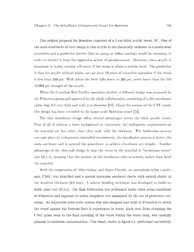
Chapter 5: The Scintillator Containment Vessel for Borexino 138
The original proposal for Borexino consisted of a 2 cm thick acrylic vessel [85]. One of
the main drawbacks of such design is that acrylic is not chemically resistant to concentrated
aromatics and a protective barrier (like an epoxy or te on coating) would be necessary in
order to protect it from the aggressive action of pseudocumene. Moreover, when acrylic is
immersed in water, crazing will occur if the stress is above a certain level. The prediction
is that for acrylic without joints, we can have 10 years of craze-free operation if the stress
is less than 500 psi. With joints the limit falls down to 300 psi, much lower than the full
10,000 psi strength of the acrylic.
When the Counting Test Facility operation started, a di�erent design was proposed by
the Princeton group and approved by the whole collaboration, consisting of a thin membrane
nylon bag, 0.5 mm thick and with 2 m diameter [87]. Given the success of the CTF vessel,
this design has been extended to the larger scale Borexino vessel [74].
The thin membrane design o�ers several advantages versus the thick acrylic vessel.
First of all, it induces a lower background or, conversely, the radiopurity requirements on
the material are less strict, since they scale with the thickness. The fabrication process
can take place in a cleanroom controlled environment, the installation process is faster, the
costs are lower and in general the procedures to achieve cleanliness are simpler. Another
advantage of the thin-wall design is that the stress in the material is \membrane stress"
(see x9.1.4), meaning that the tension on the membrane tries to stretch, rather than bend
the material.
With the cooperation of Miles-Mobay and Bayer Chemie, an amorphous nylon copoly-
mer, C38F, was identi�ed and a special extrusion produced sheets with optical clarity at
the required thickness (0.5 mm). A solvent bonding technique was developed to build re-
liable joins (see x5.5.1). The �nal fabrication was performed under clean room conditions
at Princeton and exposure to radon daughters was minimized by the use of protective cov-
erings. An adjustable hold-down system was also designed and built at Princeton to retain
the vessel against the buoyant force it experiences in water. Each step, from obtaining the
C38F nylon resin to the �nal unveiling of the vessel within the water tank, was carefully
planned to minimize contamination. The vessel, shown in �gure 5.1, performed successfully
Chapter 5: The Scintillator Containment Vessel for Borexino 139
during the 2 year CTF operation.
The fabrication techniques and knowledge acquired in CTF have been extended to the
Borexino vessel. The scintillator containment vessel for Borexino will be a 8.5 m diameter
sphere made of nylon �lm with a thickness of 0.125 mm.
One of the main upgrades planned for CTF2 and Borexino consists of a second nylon
vessel (the outer vessel), concentric to the inner vessel and with a � 1m larger radius.
It will serve as a barrier to protect the sensitive volume from 222Rn and other possible
contaminants emanated by the more distant detector components (see discussion in x8.2).
5.2 Thin Nylon Film
Our material of choice is nylon �lm: 0.5 mm thick for the CTF inner vessel and 0.1{0.125mm
thick for the CTF2 outer vessel and for the two Borexino vessels. Mylar (PET) has also
been considered, since it is chemically resistant to aromatic hydrocarbons and optically
transparent, but it was discarded due to the diÆculties encountered in the development of
a bonding method for strong joints.
Nylon is the material that best satis�es all our requirements. It can be extruded in
thin �lms with good optical properties (see {7) and it maintains high radiopurity levels
for 238U, 232Th and 40K (see discussion in {8). It is strong enough to stand the stress
induced by buoyancy (see {9) and is chemically compatible with aromatic hydrocarbons
like pseudocumene (see x5.3). The compatibility with water is a delicate issue, discussed
in detail in x5.2.3. The speci�c e�ect of water on radon di�usion in nylon is subject of the
dedicated {6 in this dissertation. This section will provide a summary of the basic chemical
and physical properties of nylon �lms; a complete treatment can be found in reference [136].
5.2.1 Nylon Molecular Structure
A nylon molecule can be visualized as a long chain sequence of fundamental units, called
monomers. Free monomers have amine nature (�NH2) on one end and acid (�COOH) on

Chapter 5: The Scintillator Containment Vessel for Borexino 140
Figure 5.1: The inner vessel in CTF.

Chapter 5: The Scintillator Containment Vessel for Borexino 141
H N
H
C
H
H
C
O
N
H
C
H
H
C
O
5
N
H
C
H
H
C
O
55
O
H
monomer
Figure 5.2: Molecular structure of the homopolymer PA-6 (also known as nylon-6 or poly-caprolactam).
the other; they bond with an amidation reaction of the type:
H [NH(R)CO]OH + H [NH(R)CO]OH! H [NH(R)CONH(R)CO]OH + H2O; (5.1)
where (R) is a block that characterizes the monomer. The result is a polymer with recurring
amide groups (�CONH�), also referred to as polyamide. A nylon with useful properties as
a plastic will be composed by about 100 monomers and will have a molecular weight higher
than 10,000.
Homopolymers are polymers built with a single type of monomers, while copolymers are
polymers where some of the monomer blocks are replaced by a di�erent molecule, which
could be another type of monomer or a more complex structure. Blends are mixtures of
at least 2 types of polymer and/or copolymer molecules, each constituting at least 2%
of the total weight. In the blend, each macromolecular component maintains its original
composition.
We follow the notation presented in reference [136], according to which symbols (numbers
or abbreviations) separated by a slash identify the components of a copolymer, while the
repetition of PA- after the slash indicates a blend of polymers:
PA-x: homopolymer HhHN (CH2)x�1CO
inOH. The monomer is constituted by (x-1) CH2
blocks, for a total of x carbon atoms;
PA-6 or nylon-6: polycaprolactam, H [HN (CH2)5CO]nOH, shown in �gure 5.2;

Chapter 5: The Scintillator Containment Vessel for Borexino 142
PA-yx: homopolymer HhHN (CH2)yNHCO (CH2)x�2CO
inOH. The monomer contains
two groups of CH2, separated by an amide group, for a total of x+y carbon atoms;
PA-66 or Nylon-66: H [HN (CH2)6NHCO (CH2)4CO]nOH, poly(hexamethylene adipa-
mine);
PA-6/66: a copolymer made from a combination of the monomers for PA-6 and PA-66;
PA-6/PA-66: a blend of PA-6 and PA-66 polymers;
PA66/6I/6T: a copolymer made of nylon-66 with the addition of isophthalic acid (6I) and
terephthalic acid (6T).
5.2.2 Nylon Film Physical Structure
Polymer molecules have a tendency to arrange themselves in a crystalline structure. Fig-
ure 5.3, from reference [136], is a schematic representation of the crystallographic units of
PA-6. In the fundamental � crystal structure, the polymer chains are fully extended in a
planar zig-zag conformation. They form sheets of hydrogen-bonded molecules, stacked one
upon another. Chains have no directionality, parallel and antiparallel chains are equiva-
lent. In the alternative structure, the chains are twisted and the hydrogen bonds are not
coplanar to the chain.
Most nylon �lms are only partially crystalline; they are usually described in terms of a
two-phase model, with an amorphous and a crystalline part. The relative amount of the
latter is the percent crystallinity wc, usually expressed as weight fraction. This parameter
can be determined by x-ray di�raction, thermal, infrared or density measurements. Ho-
mopolymer nylons typically have a 50% crystallinity. This parameter is relevant for us,
since it a�ects the optical quality of the �lm, haze in particular (see x7.1).
The crystalline portion consists of crystallites of di�erent size and perfection. Most
often the crystals do not possess a distinct boundary surface, because of tie molecules to
neighboring crystals and cilia that terminate in the amorphous phase. The unit cell of the
lattice has dimensions in the range of 0.2 nm to 3 nm. The polymer chain may fold at

Chapter 5: The Scintillator Containment Vessel for Borexino 143
Figure 5.3: Schematic representation of the crystallographic repeat units of PA-6, showingboth parallel and antiparallel disposition of the chains. The dashed lines are hydrogenbonds between molecules. From reference [136].
the surface of the crystals to create chain-folded lamellae with typical thickness of 5 nm
to 200 nm. The lamellae will in turn, usually form larger aggregates, spherulites with
dimensions of 1 �m to 100 �m. The spherulitic structure is set by the thermal history of
the �lm.
There are two kinds of thermal transitions of interest in polymers:
�rst order thermodynamic transitions between phases are associated with the crys-
talline regions in nylon. A typical example is melting of a crystal to form a liquid,
characterized by the melting point Tm, the temperature at which crystal and melt are
in equilibrium.
viscoelastic relaxations re ect the onset of various kinds of internal motions of the ny-
lon molecules with increasing temperature, associated with the amorphous regions in
nylon �lms. A typical example is the �-transition, or glass-rubber transition, charac-
terized by the glass transition temperature Tg.

Chapter 5: The Scintillator Containment Vessel for Borexino 144
Semicrystalline nylons have distinct melting points (Tm = 223oC for PA-6) and retain
some sti�ness up to Tm; when cooled, they freeze in a reproducible manner.
Amorphous nylons, instead, do not have a melting point but they exhibit a distinct
glass temperature Tg, above which they lose all mechanical integrity and become viscous
uids. The glass transition temperature can vary between 0oC and 100oC and it is a�ected
by several environmental factors, such as the presence of plasticizers, substances like free
monomers and water that decrease Tg in the �lm [137]. Reference [136] quotes for dry PA-6
a value of Tg � 60oC; this value can decrease linearly by 80oC when going from dryness to
water saturation.
The physical properties of nylon �lms are also a�ected by the molecular orientation, a
preferential arrangement of the crystals in the crystalline region or of the molecules in the
amorphous region. Orientation results from operations such as drawing or rolling of the
�lm, inducing a partial breakup of lamellae and spherulites and forming new structures,
called �brils. Stress orientation can also be found in amorphous chains. Orientation is
usually restricted to a surface layer as a result of the high shear rates near the surface,
during processing.
5.2.3 Nylon Compatibility with Water
Water signi�cantly a�ects the properties of nylon; this is a well known fact that we had to
take into account while choosing a material for the CTF inner vessel. The action of water
on nylon proceeds on two separate timescales and di�erent considerations apply to each
case.
The plasticizing e�ect of water
Water breaks the hydrogen bonds between nylon molecules; this is a short term e�ect that
can easily be seen in small scale tests. The change in the mechanical properties of nylon
due to the plasticizing e�ect of water was a known e�ect in 1992, when a nylon inner vessel
for CTF was �rst proposed. The tests showed a reduction of the yield strength and an
increase in the creep rate, when the �lm is in contact with water, but the e�ect was deemed

Chapter 5: The Scintillator Containment Vessel for Borexino 145
safe for the operating parameters of CTF [87]. Later we learned about the enhanced rate of
di�usion of gasses such as 222Rn through the nylon; this phenomenon limited the sensitivity
of CTF (see x6.4).
Water e�ectively lowers the glass transition temperature Tg in the nylon; this plasticizing
e�ect happens as quickly as the water di�uses into the nylon. It is also reversible when the
nylon is dried. This e�ect of water on the long nylon polymer molecules is much like adding
olive oil to spaghetti. The spaghetti strings slide on each other more easily, but are not
broken, changing the bulk strength properties.
Amorphous nylons are particularly a�ected by this phenomenon, since the hydrogen
bonds are all that keeps the molecules together. Crystalline nylons also have lattice forces
and are less a�ected, so in principle they would hold better against the plasticizing action
of water. But crystallinity a�ects the optical properties of nylon, so that a semicrystalline
nylon �lm is not a good option for Borexino (see {7).
Hydrolysis
The long term degradation of nylon is a complex e�ect, resulting from a combination of
di�erent phenomena: hydrolysis, oxidation, photolytic degradation, thermal degradation,
presence of impurities and degradation products formed during manufacture. The main
concern for our experiment is the degradation induced by hydrolysis.
Hydrolysis is the opposite of amidation, the reaction of an amine and an acid to form
an amide:
amidation
(R)NH2 +HOOC(R0) *) (R)NHCO(R0) + H2O:
hydrolysis
(5.2)
Polymeric molecules are formed from condensation reactions like this. The reaction can
proceed in either direction; the presence of excess water unbalances the polycondensation
reaction and induces hydrolysis, cutting the long polymer molecules at the joint between
monomers. The result is a shorter, low molecular weight chain and thus a weaker and more
brittle material (in order to exhibit the characteristic strength of nylon, the polymers need

Chapter 5: The Scintillator Containment Vessel for Borexino 146
to be constituted by at least 100 monomers).
Hydrolysis a�ects the polymer molecular structure and it can take place over timescales
of months or years. At a given temperature, the equilibrium is given by:
Kc(T) =[NHCO] [H2O]
[NH2] [COOH]: (5.3)
This means that, for a given nylon, the direction of the reaction is a�ected by two factors:
the ratio of concentration of water versus amine and acid ([H2O] = [NH2] [COOH]) and the
temperature. Polyamidation is an exothermic process; a decrease in temperature favors the
amidation, at constant water concentration.
Of course, some nylons are more subject to hydrolysis than others. For instance, the
hydrolyzation rate is a�ected by the [CH2]/[CONH] ratio in the molecule and the loss in
molecular mass is greater in PA-6 and PA-66 (ratio=5:1) than, say, in PA-12 (ratio=11:1).
In other words, the resistance to hydrolyzation increases with the hydrocarbon character of
the nylon.
We chose PA-6 for the Borexino inner vessel (see x5.2.4), because it is the easiest to
handle during the vessel fabrication process and it can be extruded without extra additives,
thus minimizing the contamination in U/Th/K. Also, it has all the required mechanical and
optical properties. But PA-6 and its copolymers are also the nylons that are most subject to
water degradation; they become brittle in water at high temperatures - this is a well known
e�ect. In all industrial applications of nylon it is customary to add glass �bers to the melt,
at processing, in order to make the material hydrolysis-resistant (see x11.5 in [136]). This
is a step we cannot take, in Borexino, because of radiopurity concerns.
It is diÆcult to estimate the possible long term damage to nylon by hydrolysis e�ects
in CTF, where the �lm is in contact with water at a temperature of 10 � 15oC. There
are no available long-term studies of the behavior of nylon in 100% relative humidity in
this temperature range. A study on PA-66 reports a large and clear hydrolysis e�ect for
elevated temperatures (60� 80oC): within a few months the yield strength drops by more
than a factor of two and the material becomes brittle in 2 months at 100% humidity and
T = 66oC [138]. PA-6 and its copolymers are expected to behave in a similar way [136].
Chapter 5: The Scintillator Containment Vessel for Borexino 147
An extrapolation of the data for PA-66 at 66oC, 82oC and 93oC reported in [138] to
the Borexino temperature of 10oC yields that brittleness will happen after 10 years in
water, if the process is regulated by the Arrhenius law. To make matters more complicated,
the damage by hydrolysis and other processes is accelerated when the materials are under
stress [139] and the hydrolysis process itself produces acids that accelerate the process
(see x3.6.1 in [136]). Any extrapolation is unreliable unless data are taken close to the
actual operating conditions [138].
The possible e�ect of hydrolysis on a nylon vessel has been considered for CTF but,
because of the long time scale involved, it was judged that a nylon vessel is safe.
A di�erent consideration applies to Borexino: in the present design, the vessel is in
contact with pseudocumene (and uor or quencher) and hydrolysis is not a real danger. An
alternative design has been proposed, though, where the scintillator is PXE (1-phenyl-1-
xylylethane, � = 0:985 g=cm3) and the bu�er is water. In this case, a careful reevaluation
of the long term safety of nylon in water must be made since, in order to look for annual
variations in the signal in Borexino, the detector must be stable for several years. As a
rough �gure of merit, the requirement is that the nylon vessels be absolutely safe from
degradation by hydrolysis for an operating time of 10 years. In this scenario, we should
consider the use of other nylons such as PA-12, since nylons based on larger monomers are
less sensitive to water. PA-12 copolymer �lms present very good optical qualities, but they
are much sti�er than the PA-6 based �lms. This would present a challenge for fabrication
by the method we are planning to use (see x5.5.1).
5.2.4 Candidate Materials
Although semicrystalline nylon �lms are less a�ected by the presence of plasticizers and
they are, in general, stronger than the amorphous nylons, we need to consider the e�ect of
crystallinity on the �lm optical quality. Light scattering at the boundaries of spherulites
reduces light transmission and induces opacity. Our search is then limited to amorphous
nylons.
The food packaging industry has developed transparent, strong and low permeability

Chapter 5: The Scintillator Containment Vessel for Borexino 148
COOH
COOH
COOH
COOH
m-xylylenediamineor isophthalic acidnonparallel
terephthalic acidparallel
Figure 5.4: Molecular structure of isophthalic and terephthalic acids, commonly used incopolymers of PA-6 and PA-66. The ring structure disturbs the formation of crystallineunits and the resulting �lm is amorphous.
thin nylon �lms (25-50 �m thick). We took advantage of the existing plastics technology and
reduced our material search problem to �nding a facility that can custom extrude thicker
�lm for us, with special care to our extreme cleanliness and optical quality requirements.
After a survey of all the commercially available materials, we focused on the following four
options:
C100: PA-6 Capron B73ZP (Allied Signal/Honeywell). Nylon-6 �lm is normally semicrys-
talline, but it can be obtained in amorphous form by quenching the temperatures
at extrusion: if the melt temperature is lowered fast enough, there is no time for
formation of crystalline structures and the resulting �lm is amorphous;
C90: Blend of 10% Selar PA3426 (DuPont) and 90% PA-6 Capron B73ZP. The Selar
molecules prevent formation of crystalline structures. We tested di�erent concentra-
tions and we settled on a 10%-90% blend with PA-6 Capron B73ZP. We observed that
a blend with an higher percentage of resin made the extruded �lm unstable;
ADS40T: PA-6 copolymer Sniamid ADS40T (Nyltech), with proprietary formula. The
copolymers are amorphous by design; they are complex engineered resins where the
insertion of ring structures in the molecules disrupts the formation of crystallites.

Chapter 5: The Scintillator Containment Vessel for Borexino 149
Typical copolymerization agents are isophthalic acid and terephthalic acid, shown in
�gure 5.4;
C38F: Durethan C38F (Bayer), another PA-6 copolymer with proprietary formula.
We purchased pellets of each material from the producers and custom extruded the �lm.
C38F was extruded in 1993 at Miles-Mobay in 0.125, 0.1 and 0.5 mm thicknesses and it
was used for the CTF inner vessel. The other �lms have been produced in a test extrusion
performed in summer 1998 at American Leistriz, a New Jersey producer of extrusion ma-
chinery that gave us access to their equipment. All four �lms are optically clear and have
been tested for mechanical properties and radiopurity; details are provided in dedicated
sections of this dissertation.
5.3 Mechanical Properties
The mechanical properties of thin nylon �lms are suitable for the requirements of the Borex-
ino scintillator containment vessel. Details on the stress loads acting on the �lm will be
provided in x9.2; in this context it is useful to mention that in the CTF design, with pseu-
documene (� = 0:88 g/cm3) inside the vessel and water outside, the maximum stress acting
on the membrane is equal to 3.4 MPa (500 psi), at the top. In Borexino, where the buoyancy
will only be due to density uctuations inside and outside the vessel, we expect a maximum
stress load of 2 MPa (300 psi).
The Stress-Strain Curve
The stress-strain curve provides fundamental information on the �lm mechanical properties.
A typical example of the behavior of nylon is shown in �gure 5.5. The initial linear region
represents the elastic regime, described by Hooke's law:
� = E " (5.4)
where � is the stress (load per unit cross-sectional area) acting on the �lm and " is the
strain (relative elongation). The constant of proportionality E is the Young's modulus, or

Chapter 5: The Scintillator Containment Vessel for Borexino 150
elastic region plastic region
yield point break point(failure)
stressσ [MPa]
strainε [%]
Figure 5.5: Typical stress-strain curve for nylon.
tensile modulus of elasticity, an index of the material's sti�ness.
The elastic region in the stress-strain plot is followed by a plastic region, where the
elongation increases without an increase in stress, up to the point where the material breaks.
The yield point marks the transition between elastic and plastic regimes. Nylon �lms behave
as typical polymers: the stress load peaks at the yield point and then drops to a constant
value, as elongation develops, until failure.
The tensile strength of a �lm is the ratio of the maximum load to the initial �lm cross
section; it can be calculated at the yield point or at the break point. If the material
exhibits high extensibility, stress calculations are not meaningful beyond the yield point,
due to extensive reduction in the cross sectional area.
Young's modulus and tensile strength measurements for several nylon strips have been
performed following the procedure of ASTM D882 [140]. We used a Tinius Olsen machine,
which forces a controlled elongation of thin plastic strips and records the force applied to
induce the elongation, thus producing a stress-strain curve. Note that the rate of strain
(change in tensile strain per unit time), specimen parameters and aws may cause large
variation in the results.

Chapter 5: The Scintillator Containment Vessel for Borexino 151
5.3.1 Measurements of Tensile Strength and Chemical Compatibility of
Nylon with Various Fluids
Before undertaking the construction of the �rst CTF inner vessel [87], several pull tests
have been performed on 0.25 mm thick C38F �lm strips. The result is that when the �lm is
in air or in PC, its strength varies in the range of 55-70 MPa (8000-10000 psi), while when
the �lm is in water, its strength drops to 14{20 MPa (2000{3000 psi). The uctuations
were due to the di�erent strain rates applied at the machine and to the relative humidity
at measurement.
In order to test mechanical strength and chemical compatibility, we performed pull tests
of thin nylon strips (2:5� 25 cm, nominal thickness = 0.125�m) that have been soaking for
several weeks in di�erent uids: pseudocumene (PC), PXE, PC+DMP+water, PC+DMP
and PC+PPO. Some strips have been kept in a jar with Drierite and nitrogen. Most of the
jars have been kept at room temperature, while some jars have been heated at 35oC. All
the samples have been prepared in an oxygen-free environment; the strips have been kept
in amber colored jars (to protect them from photolytic degradation) stored in a glove box
with nitrogen ow and all the uids have been subject to nitrogen sparging, for the removal
of oxygen. The pseudocumene had been distilled.
The results obtained after a month of soak test of nylon strips (with and without a
resorcinol joint) are reported in table 5.1, where for each test the errors are standard de-
viation over 3-5 samples. The table reports both tensile strength at yield and Young's
modulus. Figures 5.6 and 5.7 summarize the results obtained after longer soak time. As a
dry material, C38F tends to be stronger than the other three �lms, but they all otherwise
show a similar behavior.

Chapter 5: The Scintillator Containment Vessel for Borexino 152
Table 5.1: Tensile strength at yield and Young's modulus for the 4 candidate �lms, after 1month of immersion in di�erent uids. Results for nylon strips with a joint, after 3 months,are reported in the lower section of the table.
Fluid C100 C90 ADS40T C38F
Standard strips, 1 month immersion
Dry nitrogen � 67� 5 69� 3 66� 5 70� 4E 1704� 74 1750� 93 1606� 99 1677� 81
PC � 29� 1 35� 1 39� 2 36� 1E 741� 57 941� 39 1127� 117 744� 148
PXE � 27� 2 31� 1 33� 1 33� 2E 665� 77 831� 58 877� 26 875� 93
PC+PPO � 55� 2 57� 5 55� 5 73� 5E 1428� 104 1548� 62 1375� 119 1730� 77
PC+PPO hot � 37� 2 45� 1 42� 1 54� 3E 1001� 33 1262� 83 1277� 85 1519� 130
PC+PPO 12N � 60� 3 61� 2 61� 3 71� 3E 1573� 146 1572� 36 1540� 90 1723� 19
PC+DMP � 38� 1 47� 1 45� 1 55� 1E 1086� 29 1347� 48 1400� 100 1619� 59
PC+DMP+water � 18� 1 20� 3 21� 3 17� 1E 314� 5 372� 93 407� 85 298� 9
PC+DMP+water hot � 23� 1 20� 1 19� 2 18� 1E 358� 44 321� 21 346� 59 303� 36
water � 20� 2 18� 1 18� 2 17� 2E 296� 48 306� 24 308� 20 308� 20
water hot � 26� 2 22� 1 23� 2 22� 1E 380� 54 370� 28 372� 28 343� 69
Strips with a joint, 3 month immersion
Dry nitrogen � 59� 3 66� 3 58� 8 75� 1E 2137� 385 1962� 214 1965� 276 1930� 40
PC+PPO � 37� 2 53� 2 44� 2 47� 2E 1371� 67 1656� 95 1529� 87 1350� 73
PC+DMP+water � 22� 1 20� 1 21� 1 19� 2E 485� 51 363� 35 428� 22 339� 78

Chapter 5: The Scintillator Containment Vessel for Borexino 153
0 50 100 150 200 2500
10
20
30
40
50
60
70
80C100
time (days)
Yie
ld s
tren
gth
(MP
a)
0 50 100 150 200 2500
10
20
30
40
50
60
70
80C90
time (days)
Yie
ld s
tren
gth
(MP
a)
dry air PC+PPO PC+DMP PC+DMP+H2OH2O PC
0 50 100 150 200 2500
10
20
30
40
50
60
70
80ADS40T
time (days)
Yie
ld s
tren
gth
(MP
a)
0 50 100 150 200 2500
10
20
30
40
50
60
70
80C38F
time (days)
Yie
ld s
tren
gth
(MP
a)
Figure 5.6: Yield strength as a function of soaking time for the 4 candidate �lms in di�erent uids, at room temperature. The dotted lines refer to samples that have been immersed at35oC.

Chapter 5: The Scintillator Containment Vessel for Borexino 154
0 50 100 150 200 2500
200
400
600
800
1000
1200
1400
1600
1800
2000
C100
time (days)
You
ng m
odul
us (
MP
a)
0 50 100 150 200 2500
200
400
600
800
1000
1200
1400
1600
1800
2000
C90
time (days)
You
ng m
odul
us (
MP
a)
dry air PC+PPO PC+DMP PC+DMP+H2OH2O PC
0 50 100 150 200 2500
200
400
600
800
1000
1200
1400
1600
1800
2000
ADS40T
time (days)
You
ng m
odul
us (
MP
a)
0 50 100 150 200 2500
200
400
600
800
1000
1200
1400
1600
1800
2000
C38F
time (days)
You
ng m
odul
us (
MP
a)
Figure 5.7: Young's modulus as a function of soaking time for the 4 candidate �lms indi�erent uids, at room temperature. The dotted lines refer to samples that have beenimmersed at 35oC.

Chapter 5: The Scintillator Containment Vessel for Borexino 155
Water. The tests con�rm the reduction of mechanical strength in water, from � 70 MPa
to � 20 MPa. The e�ect is reversible: samples that had been immersed in water for 1
month recovered their full strength after 1 month in nitrogen and Drierite. We did not
observe any evident hydrolysis degradation after 6 months.
C90 �lm D.I. water water, then dry dry1 month 1 month + 1 month 1 month
� 18� 1MPa 67� 1MPa 69� 3MPaE 306� 24MPa 1827� 101MPa 1750� 93MPa
PC+PPO. When nylon is immersed in PC and in PC+PPO, it is expected to retain its
\dry as molded" mechanical strength. The C90 �lm exhibited a particularly low strength
(� 40 MPa) after 3 months in PC+PPO. We now believe this e�ect is due to the presence
of a small amount of water in the uid. Samples of the same �lm were prepared in two
di�erent jars (#2 and #6), on the same day, using di�erent batches of pseudocumene.
The �rst jar had been opened and closed twice, to extract the samples measured at 1 and 3
months. The mechanical strength of these strips was lower than the one of dry material. The
second jar was left undisturbed. We put both jars in the freezer compartment of a regular
refrigerator (�18oC): in the �rst jar, we observed the formation of small white structures,
likely ice crystal. Nothing appeared in the second jar. The samples from the second jar are
signi�cantly stronger than the ones from the �rst and equal to the dry samples.
C90 �lm Jar #2 Jar #6 dry4 samples 3 samples 2 samples184 days 183 days 168 days
� 43� 2MPa 71� 2MPa 72� 0:3MPaE 1129� 73MPa 1748� 41MPa 1698� 29MPa
We now have more nylon samples that have been soaking in PC+PPO for more than a
year: we will measure their strength once we have �nalized a method to evaluate the water
content in the scintillator solution, in the framework of the new program outlined in x5.4.

Chapter 5: The Scintillator Containment Vessel for Borexino 156
PC+DMP. We performed two tests of compatibility of nylon with PC+DMP: the original
idea was to reproduce the scenario where a leak in the stainless steel sphere causes a deposit
of water at the bottom of the sphere. For this purpose, we inserted 5 cc of water in the 1 l
jars, leaving it as a puddle at the bottom. The obvious result is that the puddle acts as a
water reservoir for the nylon strips, which exhibit the usual behavior of wet nylon (yield
strength � 20 MPa).
A test without adding water shows that the nylon still has a reduced strength (�
40 MPa), but in the light of the results with PC+PPO this is not a statement of chemical
incompatibility of nylon with DMP, rather it could be a problem of water in solution at
trace levels. It is fundamental for us to solve this uncertainty; the new measurement cam-
paign outlined in x5.4 is addressing the problem by decoupling the e�ect of water and of
the DMP.
PC. The samples soaking in PC were also weaker than the dry ones (yield strength �
40 MPa), a result that we found very puzzling at �rst. As above described, we put the jar
with C90 strips and PC in a freezer and we observed large white formations that melted
within an hour of being removed from the freezer, likely ice. After 4 months of immersion
in this jar, the last remaining 3 strips were moved to one with nitrogen and Drierite. A pull
test, two weeks later, showed they had recovered their full strength. This is consistent with
the hypothesis of water pollution in the PC jar.
C90 �lm in PC in PC in PC, then dry dry1 month 3 months 4 months + 2 weeks
� 35� 1MPa 33� 2MPa 74� 9MPa 69� 3MPaE 941� 39MPa 852� 45MPa 1856� 67MPa 1750� 93MPa
We then put 10 new strips in the same jar, with the same uid, in order to repeat the
test. We used strips with joints, but the result is nevertheless valid. After 2 weeks in the
jar, the strips were as strong as the dry ones, as if the water had disappeared.
One hypothesis to interpret this result is that the water contamination inside the jar
was below the saturation level of both PC and nylon, but because of the higher aÆnity
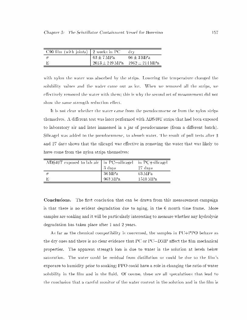
Chapter 5: The Scintillator Containment Vessel for Borexino 157
C90 �lm (with joints) 2 weeks in PC dry
� 63� 7MPa 66� 3MPaE 2013� 249MPa 1962� 214MPa
with nylon the water was absorbed by the strips. Lowering the temperature changed the
solubility values and the water came out as ice. When we removed all the strips, we
e�ectively removed the water with them; this is why the second set of measurement did not
show the same strength reduction e�ect.
It is not clear whether the water came from the pseudocumene or from the nylon strips
themselves. A di�erent test was later performed with ADS40T strips that had been exposed
to laboratory air and later immersed in a jar of pseudocumene (from a di�erent batch).
Silicagel was added to the pseudocumene, to absorb water. The result of pull tests after 3
and 27 days shows that the silicagel was e�ective in removing the water that was likely to
have come from the nylon strips themselves:
ADS40T exposed to lab air in PC+silicagel in PC+silicagel3 days 27 days
� 36MPa 63MPaE 963MPa 1510MPa
Conclusions. The �rst conclusion that can be drawn from this measurement campaign
is that there is no evident degradation due to aging, in the 6 month time frame. More
samples are soaking and it will be particularly interesting to measure whether any hydrolysis
degradation has taken place after 1 and 2 years.
As far as the chemical compatibility is concerned, the samples in PC+PPO behave as
the dry ones and there is no clear evidence that PC or PC+DMP a�ect the �lm mechanical
properties. The apparent strength loss is due to water in the solution at levels below
saturation. The water could be residual from distillation or could be due to the �lm's
exposure to humidity prior to soaking; PPO could have a role in changing the ratio of water
solubility in the �lm and in the uid. Of course, these are all speculations that lead to
the conclusion that a careful monitor of the water content in the solution and in the �lm is
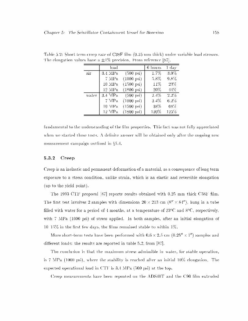
Chapter 5: The Scintillator Containment Vessel for Borexino 158
Table 5.2: Short term creep rate of C38F �lm (0.25 mm thick) under variable load stresses.The elongation values have a �1% precision. From reference [87].
load 6 hours 1 day
air 3.4 MPa (500 psi) 1.7% 3.0%7 MPa (1000 psi) 5.8% 9.8%10 MPa (1500 psi) 11% 23%12 MPa (1800 psi) 20% 44%
water 3.4 MPa (500 psi) 2.4% 2.2%7 MPa (1000 psi) 3.4% 6.2%10 MPa (1500 psi) 38% 68%12 MPa (1800 psi) 120% 125%
fundamental to the understanding of the �lm properties. This fact was not fully appreciated
when we started these tests. A de�nite answer will be obtained only after the ongoing new
measurement campaign outlined in x5.4.
5.3.2 Creep
Creep is an inelastic and permanent deformation of a material, as a consequence of long term
exposure to a stress condition, unlike strain, which is an elastic and reversible elongation
(up to the yield point).
The 1993 CTF proposal [87] reports results obtained with 0.25 mm thick C38F �lm.
The �rst test involves 2 samples with dimensions 20� 213 cm (800 � 8400), hung in a tube
�lled with water for a period of 4 months, at a temperature of 23oC and 8oC, respectively,
with 7 MPa (1000 psi) of stress applied. In both samples, after an initial elongation of
10{15% in the �rst few days, the �lms remained stable to within 1%.
More short-term tests have been performed with 0:6� 2:5 cm (0:2500� 100) samples and
di�erent loads: the results are reported in table 5.2, from [87].
The conclusion is that the maximum stress admissible in water, for stable operation,
is 7 MPa (1000 psi), where the stability is reached after an initial 10% elongation. The
expected operational load in CTF is 3.4 MPa (500 psi) at the top.
Creep measurements have been repeated on the ADS40T and the C90 �lm extruded

Chapter 5: The Scintillator Containment Vessel for Borexino 159
0 10 20 30 40 50 60 700
1
2
3
4
5
6
7
8ADS40T
time (days)
cree
p (%
)
1000 psi750 psi 500 psi 250 psi
0 10 20 30 40 50 60 700
1
2
3
4
5
6
7
8C90
time (days)
cree
p (%
)
1000 psi750 psi 500 psi 250 psi
Figure 5.8: Creep measurements for 110 mm long strips of ADS40T (top) and C90 (bot-tom). The samples have been loaded with di�erent stress values (1.7, 3.4, 5 and 7 MPa) inpseudocumene exposed to air, at room temperature.

Chapter 5: The Scintillator Containment Vessel for Borexino 160
at Leistriz in summer 1998, with a 70 day and 50 day test, respectively, in pseudocumene
exposed to air and humidity, at room temperature. The results are shown in �gure 5.8: the
two �lms exhibit a similar behavior, reaching a plateaux in about 10 days. The plateaux
value depends on the applied stress: � 1% at 1.7 MPa (250 psi) and � 7% at 7 MPa
(1000 psi). The operational load in Borexino is expected to be 1.8 MPa (see x9.2) and the
resulting vessel radius change, due to creep, is expected to be of the order of 0.25%.
5.3.3 The Stress-Cracking Problem
The inner vessel for CTF2 has been built with the same nylon �lm used in CTF1 (C38F
0.5 mm thick), while the outer vessel used commercially extruded PA-6 Capran �lm by
Allied Signal, 0.1 mm thick.
After the vessels were installed in October 1999, the CTF tank has been closed, with a
dry nitrogen ow. Two months later we noticed the inner vessel was broken. The primary
failure consisted of two � 4 cm long cracks near two of the buttons used to route the hold
down strings; a secondary problem were small leaks at the north and south pole joints.
The vessel was repaired with cast nylon patches and the CTF tank was �lled with water
in March 2000 for some tests; a new set of vessels for CTF2 is now under construction and
they will be installed by the end of 2000.
It is diÆcult to understand the exact cause of the CTF2 vessel failure, which was proba-
bly the result of a combination of di�erent e�ects. The contributing factors we have by now
identi�ed are the extreme dry conditions the vessel was exposed to during the two month
period, pressure variations that allowed the vessel to ex, stress at the buttons, aging of
the C38F �lm and formic acid fumes (see below).
Stress cracking is the failure of a material due to the simultaneous e�ect of stress and
hostile environmental conditions [141]. The failure can take the form of cracks, e�ective
tears in the material, or crazes, microscopic cracks (micro�brils) in a network on or under
the �lm surface. Unlike macroscopic cracks, crazes can still stand the stress load, but they
typically a�ect the �lm optical quality and they may appear as a white band. Transparent
nylons like C38F are generally less stress-cracking resistant than the semicrystalline ones,

Chapter 5: The Scintillator Containment Vessel for Borexino 161
particularly under bending loads (x11.4.5 in [136]).
Pressure variations caused the vessel to change its shape and fold, forming creases.
When the vessel is folded for shipping and installation, it is kept deliberately moist, so that
the creases do not cause damage. But when the �lm is very dry, the �lm is not able to
conform to the crease and cracks can form.
Another key point for CTF2 was the exposure to formic acid fumes during the �nal
assembly of the outer vessel in the CTF tank, when a nylon paste containing formic acid
was used to seal the �nal parts. Formic acid fumes evaporated while the past was drying
and cam into contact with the inner vessel. Exposure to acids is one of the environmental
factors a�ecting stress cracking. In CTF1 this did not happen, since there was no outer
vessel and the inner vessel was not exposed to the same extreme dryness conditions.
Note that the �lm thickness has played a role in the failure. When a 0.5 mm thick nylon
�lm is folded over a radius of curvature comparable with its thickness, the �lm might craze
or crack. This does not happen with a thinner �lm. The critical thickness can be de�ned
as the value at which the folding energy equals the crazing energy; it is strongly related to
the moisture content in the nylon.
Finally, we learned that the �lm history of exposure to water has an e�ect on the �nal
�lm performances. The consensus among vendors and nylon experts is that when nylon is
soaked in water for many days the plasticizers (typically, residual monomers) are leached
out by the water. This is something we saw by just leaving nylon samples in water for
several weeks: after about one month, a white material came o� all the samples. When
the �lm is dried, water and dissolved plasticizers are removed, leaving a �lm that is strong,
sti� and very brittle. A slight increase in temperature accelerates the process; one thin �lm
sample sample that had been conditioned by immersion in water at 50oC for seven days and
later dried for ten days in a glove box with nitrogen ow became very brittle and literally
shattered as it was touched. This leaching does not take place if the �lm stays in contact
with water vapor, even at 100% RH. The relevance of this e�ect for Borexino still has to
be tested.
The discussion on material choice has been reopened after the CTF2 vessel failure.

Chapter 5: The Scintillator Containment Vessel for Borexino 162
Copolymer nylons like C38F and ADS40T are now slightly disfavored: secondary crystal-
lization in copolymers contributes brittleness [136]. They also tend to have a higher 238U,
232Th and 40K content than the simpler PA-6. We also considered moving our choice to dif-
ferent nylons, like PA-612 or nylon with tougheners, but we ruled them out because weaker
and with poor optical quality. Our �nal selection is the amorphous PA-6 �lm produced by
quenching the temperature at extrusion, to inhibit crystallinity. The result is a transparent
nylon with lower radioactivity. ADS40T is still being considered as a backup material.
5.4 A New Measurement Campaign
A new measurement campaign has been started, in order to evaluate in a more systematic
way how the �lm history, in terms of exposure to water, a�ects its performance.
The literature reports that PA-6 �lm \dry as molded" contains 0.2% water in weight; at
50% R.H. (relative humidity) and 23oC this concentration raises to 2.8% and when the �lm
is immersed in water the saturation level is 9.5% in weight [136]. When the �lm is exposed
to less than 10% R.H., it can become extremely brittle, while at higher water concentration
the overall strength and 222Rn permeability properties are a�ected. We need to estimate
a valid operating range of humidity level for a safe vessel and we also need to determine
which will be the actual relative humidity the vessel will be exposed to in Borexino.
The new measurements are concentrating on a relative humidity monitor facility. Mea-
surement of water in nylon and PC is performed with the Computrac 3000 by Arizona In-
strument. The instrument heats a sample of test material and passes the volatiles through
a cold trap to an analysis cell where the moisture content of the owing gas is measured by
a moisture transducer. The plan is to perform the following tests:
1. water content in nylon in di�erent uids (air, PC, PC+DMP) at di�erent relative
humidity;
2. tensile yield strength and Young modulus as a function of the R.H. and the water
content in the �lm;

Chapter 5: The Scintillator Containment Vessel for Borexino 163
3. fracture toughness of the �lm after exposure to di�erent uids at di�erent R.H.;
4. shear strength in �lm with di�erent histories of exposure to water;
5. heat capacity.
Pull tests and all handling procedures will take place in a glove box with controlled relative
humidity.
5.5 Technical Aspects of the Vessel Fabrication
5.5.1 Design and Construction
The basic design of the inner and outer vessel structure for Borexino, with restrain ropes
and the tubes for �ll and access, is shown in �gure 5.9.
The construction method for the nylon vessels has long been established [74]. Both inner
and outer vessel in Borexino will be made by bonding 36 panels together, like segments of
an orange.
In the Borexino inner vessel, we need to create over 200 m of leak-free joints between the
di�erent panels. The method employed in the seam fabrication is, chemically, the same that
has been successfully tested on the CTF vessel. It consists of solvent bonding of the nylon
panels, using a mixture of water, resorcinol and ethanol. Ethanol increases the solubility
of resorcinol in water and also serves to soften the nylon. A weak organic acid, resorcinol
dissolves nylon and allows good adhesion between the panels. The joint is cured at room
temperature and under three atmospheres of pressure. If properly made, the joints are as
strong as the normal nylon material.
The CTF vessel was fabricated in its spherical shape, which required an inner spherical
support structure to react against the clamping pressure. For Borexino, with 4.5 m radius,
this becomes harder. Rather than being assembled as spheres, the vessels for Borexino will
be fabricated with the \ at-pack" technique: the panels are �rst folded in half along their
length, then bonded one by one on a long table, with the panels laying at and ending up
as a long prefolded pack.
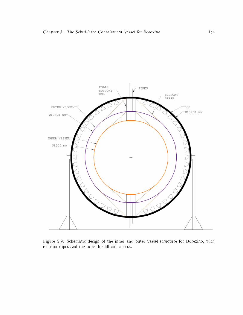
Chapter 5: The Scintillator Containment Vessel for Borexino 164
Ø13700 mmØ10500 mm
OUTER VESSEL SSS
SUPPORTSTRAP
POLARSUPPORTROD
PIPES
Ø8500 mm
INNER VESSEL
Figure 5.9: Schematic design of the inner and outer vessel structure for Borexino, withrestrain ropes and the tubes for �ll and access.

Chapter 5: The Scintillator Containment Vessel for Borexino 165
Figure 5.10: Present design of the north pole endcaps for the inner and outer vessel, withthe connections to the stainless steel sphere and the external tank.
Chapter 5: The Scintillator Containment Vessel for Borexino 166
The 36 panels cannot extend all the way to the pipe at the poles without becoming
inconveniently narrow; they need to be terminated at a ring with a diameter of about 1 m.
When the vessel is being installed at the stainless steel sphere, the envelope will hang from
this ring, so it is attached robustly to a central collar with a set of spokes. Nylon �lm will
cover the region between spokes, while the entire \wagon wheel" assembly will be machined
from a single piece of bulk nylon. A single solid plate, 1 m diameter, was ruled out based
on a Monte Carlo simulation of its optical e�ects: events near the plate would su�er a large
light blockage and some are so poorly reconstructed as to appear to be from the �ducial
volume, placing unreasonable radiopurity constraints on the plate material. The connection
to the bulk nylon end assembly pieces is made with nylon clamps and a formic acid solvent.
Attached to the central collar will be the 4" pipe that connects the inner vessel to the
external plumbing. An additional 8" concentric pipe attaches to the outer vessel end plate
and feeds the inner bu�er region (between the two vessels).
5.5.2 Cleanliness
During and after its extrusion from nylon pellets, the nylon �lm for the Borexino inner vessel
is vulnerable to surface contamination. The most likely forms of contamination are dust
particles and radioactive radon daughters. These same contamination issues were addressed
during the construction of the CTF inner vessel. Our strategy includes the following steps:
Film cleaning procedure. During the fabrication of the CTF, the �lm was extruded un-
der a tent that reproduced a cleanroom environment, thus limiting exposure to dust.
The entire extrusion process subjected it to only a few minutes of ambient radon.
It was immediately rolled and sealed in a radon-tight container. For Borexino this
is not very practical, given the larger width of the �lm and the machinery; cost is
also an issue. The new strategy involves extrusion with only partial tenting and a
subsequent �lm cleaning procedure. The procedure involves ultrasonic break-up and
electrostatic removal of dust particles and will be performed by KNF Clean Room
Products, Inc.. PA-6 �lm extruded with no special precautions has been measured

Chapter 5: The Scintillator Containment Vessel for Borexino 167
being approximately class 100, where the class for surface cleanliness is de�ned ac-
cording to military standard 1246C [142]. KNF performed a test cleaning on this
�lm, obtaining less than class 50; their expectation is to reach class 25 or better
with repeated �lm cleaning. A conservative estimation yields that, assuming all the
particulate washes o� in PC, a �lm at class 25 would contribute the equivalent of
� 10�17 g/g U/Th in the Borexino scintillator. The measured washo� of dust in PC
is actually 2� 1% [143].
Fabrication in clean room. The 2 m diameter inner vessel for CTF was built in its
spherical shape in a class 100 cleanroom. Thanks to the \ at-pack" method, both
inner and outer vessel for Borexino can also be built in the new, larger class 100 clean-
room speci�cally built at Princeton. The cleanroom serves a double task: it protects
the vessel from dust contamination and it facilitates the manufacturing process, since
its controlled humidity and temperature environment can maintain the nylon �lm
pliability. The cleanroom speci�cations provide a temperature range of (20 � 1)oC
and humidity range of (45 � 2)% R.H.. Aged, radon free water will be used for the
re-humidi�cation of the dry makeup air.
The nylon �lm handling has been simpli�ed as much as possible. The inner and outer
vessel will �rst be separately constructed without endcaps. With the \ at-pack"
construction technique, most of the vessel will be folded on itself, so that sensitive
inner surfaces will face only about one hour exposure to clean-room air; this way,
the risk of contamination from 210Pb, 238U and 232Th in dust is minimized. The
folded inner vessel will later be inserted in the outer vessel and then have its endcaps
attached, sealing the sensitive inner volume. The vessel will be placed in a 222Rn free
bag, boxed, shipped and installed. It will be rein ated with ultrapure N2 in situ in the
experiment just prior to �lling with scintillator. In order to prevent stress cracking in
the �lm, the vessel will be kept between 50 and 100% relative humidity.
Radon scrubbing system. The clean room will be equipped with a radon mitigation
system, to reduce its radon levels by at least a factor 10 below normal ambient levels.

Chapter 5: The Scintillator Containment Vessel for Borexino 168
The design speci�es the room be sealed, with a fully enclosed air handling system
and metal walls, ceiling and oor. This way, it requires only 0.1% of its volume in
makeup air per minute (170 m3/h). A radon �ltering system for the supply air has
been designed, based on VSA (Vacuum Swing Adsorption) on an activated charcoal
bed [144, 145]. A prototype VSA 222Rn �lter, handling a 1.7 m3/h air ow, achieved
a reduction factor better than 104; the full scale system is now under construction.
5.6 The Hold-Down System
The inner vessel for Borexino is ideally subject to a neutral buoyancy situation, with pseu-
documene both inside and outside. In reality, there is a small but non zero density di�er-
ence between PC+PPO (the scintillator) and PC+DMP (the quenched bu�er uid). At
T = 15oC [146]:
PC : � = 0:8772 g=cm3; (5.5)
PC + PPO : � = 0:8780 g=cm3; (5.6)
PC +DMP : � = 0:8788 g=cm3: (5.7)
This means there is at least a 0.09% density di�erence between the uids inside and outside
the vessel; the net result being an upwards buoyancy force.
Moreover, a temperature gradient between the scintillator and the bu�er, due to seasonal
temperature variations, causes an additional density uctuation. The temperature in the
experimental hall varies by up to 5oC; in the worst case scenario, such temperature gradient
is concentrated on the two sides of either vessel. The consequent density gradient can be
estimated from the volumetric expansion coeÆcient for pseudocumene [146]:
1
�
d�
dT= 0:09%=oC: (5.8)
The density uctuation induced by the temperature gradient can be in either direction,
while the one due to the presence of uor and quencher in the two solutions is always in the
same direction (the scintillator is lighter than the bu�er uid). As a design parameter, we

Chapter 5: The Scintillator Containment Vessel for Borexino 169
assume that the buoyancy on the Borexino vessel is the one associated to 1oC temperature
gradient, while the hold down system is designed to withstand a 5oC temperature gradient.
The hold-down system for the Borexino inner vessel will consist of two sets of 18 ropes
wrapping around the sphere, one set going upwards and one downwards. A similar system
is designed to hold the outer vessel.
The search for a rope material is still in progress. We have been investigating the
following categories of low-stretch �bers:
Liquid crystal polymers. The only commercially available brand is Vectran, a �ber with
very low stretch and very low creep, claimed to be unmeasurable at 50% breaking
strength (commercial literature). It also has very high chemical resistance. This
material was our original choice, but it has recently been discarded because of its high
potassium content (see x8.4).
Para-amids. These �bers are made from highly oriented polymers, derived from poly-
amides but incorporating aromatic ring structures. The result is a high strength, high
modulus �ber with very low stretch and low creep (0.02-0.05% creep at 50% of the
breaking load, according to the commercial literature). Known brands are Kevlar
(homopolymer) and Technora (copolymer).
High-density polyethylene (HDPE). These �bers have a very low stretch and a mo-
derate creep (1.7-5% creep at 50% of the breaking load). We examined Spectra and
Tensylon, which is our present tentative choice.
Polyphenylenebenzobisoxazole (PBO). These also have high modulus and tensile
strength and very low stretch and creep (virtually zero). Their chemical resistance
is expected to be inferior to the liquid crystal polymers and the HDPE's. The only
existing brand is Zylon, produced by a Japanese �rm.
For all four types, the elongation at break is about the same, namely 2-5%.
Another option, commercially available, are carbon �bers, which we did not explore
because of their need for an epoxy coating, which could pose a problem of incompatibility

Chapter 5: The Scintillator Containment Vessel for Borexino 170
with the pseudocumene. An open option are wire ropes, made with stainless steel (SS),
copper or Monel (nickel{copper alloy).
The rope size is determined by the requirement to withstand the buoyancy force induced
by a 5oC temperature gradient: 1270 kg (2800 lbs) for the inner vessel with radius 4.25 m
and 2400 kg (5300 lbs) for the outer vessel with radius 5.25 m. Taking into account the
angle at which the ropes leave the vessel (angle factor: sin 36o = 0:59), we calculate that
the yield strength has to be equal to, at least:
60 kg (130 lbs) for the inner vessel ropes; (5.9)
115 kg (250 lbs) for the outer vessel ropes: (5.10)
Another factor we need to take into account is creep: the data shown in x5.3.2 suggest
that, for a 5oC temperature gradient on the two sides of the inner vessel, stable for a few
days (this is a conservative assumption), the vessel change in radius due to creep will be
of the order of 1%. If the ropes creep more than the vessel, the overall performance of the
hold down system will be signi�cantly reduced, since no mechanism is foreseen to adjust
the ropes length after they are installed. This means the ropes need to have a maximum
creep of about 1% at the load of 60 kg (130 lbs).
We learned that HPDE, in particular, can creep to failure; the rule of thumb is that
failure occurs at 5% total stretch. This problem can be bypassed with a a proper rope sizing,
since creep depends on the ratio of operational and full load. In the case of Tensylon, an
extrapolation performed by the manufacturers on the basis of their measured creep data
yields that the time to failure (5% creep) is between 35 and 100 years if the operating load
is � 10% of the full load. This timescale is safe for Borexino. Other �bers are less a�ected
by this problem.
The criteria for the rope design can then be reduced to the following:
1. sizing by modulus: the elastic stretch at 60 kg (130 lbs) should not exceed 1%;
2. sizing by strength: the fraction of full load allowed for Tensylon ropes is 10%. This
requirement takes into account both the actual rope strength and the creep. Based on

Chapter 5: The Scintillator Containment Vessel for Borexino 171
0 1 2 3 4 50
5
10
15
20
25
Sized by modulus − g/m
Siz
ed b
y st
reng
th −
g/m
TensylonSpectra PBO Vectran Kevlar SS Cu Monel
Figure 5.11: Design mass density of ropes for the hold-down system built with di�erentmaterials, if the ropes are sized according to the strength or to the modulus requirements.From reference [147].
commercial literature information, the maximum allowed fraction for Spectra is 5%,
for Vectran, para-amids and PBO it is 30% and for the wire ropes it is 60%.
Figure 5.11, from reference [147], shows the resulting required rope mass (g/m): in abscissa
there is the mass needed to satisfy the modulus requirement, in ordinate there is the mass
needed to satisfy the strength requirement. The �nal rope size will depend on a compromise
between the design rope mass and radiopurity constraints (see x8.4).

Chapter 6
Radon Di�usion
6.1 The Radon Problem
Radon produces some of the strongest environmental radioactivity. It is a noble gas, pro-
duced in the 238U, 235U and and 232Th decay chains. Its di�usion capability through layers
of solid and liquid matter make it a critical limiting factor for low activity detectors such
as Borexino and its Counting Test Facility.
The most dangerous Radon isotope is 222Rn, from the 238U chain. 219Rn (235U chain)
and 220Rn (232Th chain) are short-lived and do not constitute a serious threat, since their
decays take place before they can di�use too deeply in any material. 222Rn is produced
in the decay of 226Ra (�1=2 = 1622y) and its daughters include 8 radioactive elements, as
shown in table 6.1.
An underground experiment as Borexino has to face the problem of 222Rn emanation
from the rock walls of the experimental hall. The 222Rn concentration in Hall C at Gran
Sasso can reach values as high as 1500 Bq/m3, while the outdoor 222Rn concentration are
normally two orders of magnitude lower. Thanks to a powerful ventilation system, this level
has been reduced to �30 Bq/m3. Still, a massive e�ort has been undertaken to maintain
the detector and all the auxiliary plants radon-tight.
Another important factor in Borexino and in CTF is the 222Rn emanation frommaterials
inside the detector, such as the phototubes, their supporting structure, cables, the external
vessel and the bu�er uid. A 226Ra content of 1 � 10�19g/g in the water bu�er may
172

Chapter 6: Radon Di�usion 173
Table 6.1: 222Rn and its daughters.
Nuclide Decay Energy (MeV) Half-life
222Rn � 5.49 3.825 d218Po � 6.02 3.11 m214Pb � + 1.03 26.8 m214Bi � + 3.20 19.8 m214Po � 7.69 164 �s210Pb � + 0.06 22.3 y210Bi � 1.16 5.01 d210Po � 5.30 138.4 d
constitute a signi�cant 222Rn source for CTF. The resulting 222Rn content in the shield
water of CTF1, right outside the inner vessel, was (24 � 5)mBq/m3 [51]. This 222Rn
concentration has represented the limiting factor for the sensitivity of the �rst CTF run,
for two reasons:
1. rays produced in the water propagated through the detector, into the scintillator,
and constituted the majority of the count rate (external background);
2. 222Rn outside the Inner vessel can di�use through the nylon bag and get directly in the
scintillator, a�ecting the estimate of internally produced 222Rn due to the scintillator
238U content (internal background).
This last e�ect has led to the argument that the estimated 238U level in the �rst run
of the Counting Test Facility was only an upper limit, and that the scintillator radiopurity
could actually be much better. There is a direct indication that the e�ect is real: in
December 1995 222Rn was arti�cially introduced in the CTF water shield and an increase in
the \internal" count rate (222Rn in the scintillator) was soon observed (see x6.4). It became
clear that we needed a quantitative estimation of this e�ect, with a direct measurement of
222Rn di�usion through nylon membranes, in order to validate the CTF results and con�rm
the feasibility of Borexino.
Chapter 6: Radon Di�usion 174
6.2 Mathematical Model for 222Rn Di�usion and Emanation
The di�usion of a non-decaying substance in isotropic and homogeneous media is described
by Fick's law:
~�+D~r� = 0 (6.1)
which, together with the continuity equation:
~r � ~�+ @t� = 0; (6.2)
gives the di�usion equation:
@t� = Dr2�: (6.3)
In most applications of interest for Borexino, there is a preferential direction of propagation
and the more general problem of eq. 6.3 can be restricted to the one-dimensional di�usion:
@�
@t= D
@2�
@x2: (6.4)
In the case of 222Rn, we need to account for radioactive decay and modify eq. 6.4 as follows:
@�
@t= D
@2�
@x2� ��; (6.5)
where:
� = local concentration of the di�using substance (atoms/cm3);
� = atomic ow (atoms/cm2/s);
D = di�usion coeÆcient (cm2/s);
� = decay constant (s�1).
A stationary solution is meaningful in situations in which the system is undisturbed for
a time longer than the 222Rn lifetime (5.5 days) and than the time needed to reach di�usion
equilibrium. In this case we can require that the time derivative be zero and solve the
di�usion equation, after imposing the proper boundary conditions.

Chapter 6: Radon Di�usion 175
Out:
ρ=ρ0
Barrier In:
ρ≈0
0 xd
ρ0
Sρ0
ρ(x)
MaterialVacuum
ρ≈0
0 x
ρ(x)
α-1
(a) (b)
Figure 6.1: Concentration pro�les for 222Rn di�usion through a barrier (a) and 222Rnemanation from a surface (b).
6.2.1 Permeation
If, in particular, we are interested in the di�usion of 222Rn through a barrier of thickness
d, with constant 222Rn concentration � = �0 on one side and negligible concentration � � 0
on the other (see �g. 6.1-a), the stationary solution is:
�(x) = S�0sinh[�(d� x)]
sinh(�d); (6.6)
where:
S = relative solubility (membrane material versus medium);
��1 =pD=� = characteristic di�usion length for 222Rn atoms in the membrane material.
The permeability of a membrane is, in general, de�ned as the product of solubility
and di�usion coeÆcient:
P = DS: (6.7)
Chapter 6: Radon Di�usion 176
Since 222Rn atoms decay while traveling through the membrane, an e�ective permeability
can be de�ned as:
Pe� = DS�d
sinh�d: (6.8)
The time lag is de�ned as the average time 222Rn atoms take to cross the barrier. It
depends on di�usion coeÆcient and barrier thickness as:
T =d2
6D: (6.9)
Finally, the 222Rn ux into and out of the membrane is given by:
�in = �(0) = �D@�
@x
����x=0
= �0DS�
sinh �dcosh�d = �0
Pe�d
cosh�d; (6.10)
�out = �(d) = �D@�
@x
����x=d
= �0DS�
sinh �d= �0
Pe�d
: (6.11)
This solution can be used to describe the 222Rn di�usion through the inner vessel, both
in Borexino and in CTF, where the 222Rn concentration outside the vessel can be assumed
constant in time scales of months, while the concentration inside the scintillator is negligible
in comparison.
We can de�ne a barrier attenuation factor as the ratio of the 222Rn concentration on the
two sides of the membrane. In the Borexino and CTF spherical geometry, the attenuation
factor is:
� =[222Rn]in
[222Rn]out= Pe�
3
Rd�: (6.12)
6.2.2 Emanation
The same formalism can be used to describe 222Rn emanation from a material containing
226Ra (see �g. 6.1-b). In this case, we need to take into account, in the di�usion equation,
the continuous production of 222Rn atoms due to 226Ra decay inside the material. Eq. 6.5
can be modi�ed as:@�
@t= D
@2�
@x2� ��+A; (6.13)
where A is the speci�c 226Ra activity (Bq/m3), equal to the 222Rn production rate density.
Again, on the timescale of months, the search can be limited to stationary solutions. The

Chapter 6: Radon Di�usion 177
simpli�ed problem is:
D@2�
@x2� ��+ A = 0 with
8><>:
� = 0 for x � 0
� = A� for x!1
: (6.14)
These boundary conditions describe a situation where the 222Rn concentration deep inside
the material is constant, equal to the decay rate of 226Ra, while it is negligible at the
emanation surface. The solution for the 222Rn density is:8><>:
�(x) = 0 for x � 0
�(x) = A� (1� e��x) for x > 0
: (6.15)
The 222Rn atom ux outside the material is, then:
j�outj =
�����D@�
@x
����x=0
= D�A
�= A��1 (atoms=s=cm2): (6.16)
That is: on the average, only the 222Rn atoms produced in a surface layer of thickness
equal to the di�usion length ��1 are emanated from the material. All the rest decay before
escaping.
6.3 Measurements of222Rn Di�usion
The di�usion and solubility coeÆcients of 222Rn in polymers are not generally available
in literature. Refs. [148, 149, 150] report measurements performed within the SNO collab-
oration or by our collaborators in MPI-Heidelberg; other e�orts in the selection of radon
barriers are reported in ref. [151].
In particular, we are interested in the di�usion properties of nylon membranes as the
one used to build the CTF inner vessel or the candidate material for the Borexino vessels.
Samples of PA-6 and C38F have been measured by M. W�ojcik et al. in Krak�ov. Their
apparatus is built to detect radon permeating through a thin membrane in a dry air envi-
ronment. Their results (see table 6.2 for a comparison with other materials) indicate these
nylon foils are good barriers when the relative humidity is � 0%.
We discussed in x5.2.3 how water can act as a plasticizer and a�ect the mechanical
properties of a polymer. Permeability to gases is a�ected as well: commercial �lm data
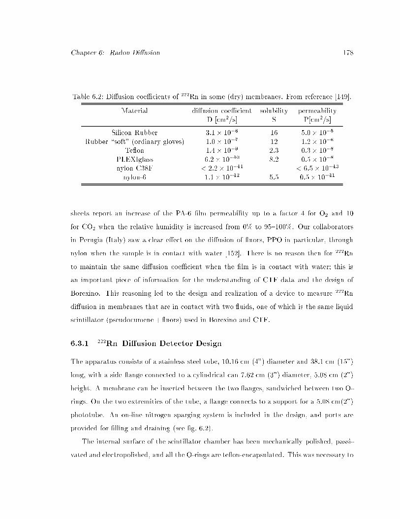
Chapter 6: Radon Di�usion 178
Table 6.2: Di�usion coeÆcients of 222Rn in some (dry) membranes. From reference [149].
Material di�usion coeÆcient solubility permeabilityD [cm2/s] S P[cm2/s]
Silicon Rubber 3:1� 10�6 16 5:0� 10�5
Rubber \soft" (ordinary gloves) 1:0� 10�7 12 1:2� 10�6
Te on 1:4� 10�9 2.3 0:3� 10�8
PLEXIglass 6:2� 10�10 8.2 0:5� 10�8
nylon C38F < 2:2� 10�11 < 6:5� 10�13
nylon-6 1:1� 10�12 5.5 0:5� 10�11
sheets report an increase of the PA-6 �lm permeability up to a factor 4 for O2 and 10
for CO2 when the relative humidity is increased from 0% to 95{100%. Our collaborators
in Perugia (Italy) saw a clear e�ect on the di�usion of uors, PPO in particular, through
nylon when the sample is in contact with water [152]. There is no reason then for 222Rn
to maintain the same di�usion coeÆcient when the �lm is in contact with water; this is
an important piece of information for the understanding of CTF data and the design of
Borexino. This reasoning led to the design and realization of a device to measure 222Rn
di�usion in membranes that are in contact with two uids, one of which is the same liquid
scintillator (pseudocumene + uors) used in Borexino and CTF.
6.3.1 222Rn Di�usion Detector Design
The apparatus consists of a stainless steel tube, 10.16 cm (4") diameter and 38.1 cm (15")
long, with a side ange connected to a cylindrical can 7.62 cm (3") diameter, 5.08 cm (2")
height. A membrane can be inserted between the two anges, sandwiched between two O-
rings. On the two extremities of the tube, a ange connects to a support for a 5.08 cm(2")
phototube. An on-line nitrogen sparging system is included in the design, and ports are
provided for �lling and draining (see �g. 6.2).
The internal surface of the scintillator chamber has been mechanically polished, passi-
vated and electropolished, and all the O-rings are te on-encapsulated. This was necessary to

Chapter 6: Radon Di�usion 179
water
PC +PPO
Nylon membrane
0.2 l
2.6 l
PMT
Figure 6.2: 222Rn di�usion detector: apparatus design.

Chapter 6: Radon Di�usion 180
prevent the aggressive action of pseudocumene. Moreover, the polishing provides a mirror-
�nish surface inside the scintillator chamber: this increases light re ection from �40% to
�80% and improves the eÆciency of light collection (see table 6.3).
Radioactive decays of 222Rn and its daughters inside the scintillator produce optical
photons that are collected by the two phototubes. The solid angle coverage is poor, hence the
analog signal cannot provide information on the deposited energy and no spectral analysis
is possible with this apparatus. The signature for 222Rn di�used in the liquid scintillator is
the delayed coincidence 214Bi �214 Po with hal ife �1=2 = 164�s.
The task of event identi�cation is performed by a logic chain (see �g. 6.3), designed to
count event pairs taking place in a time window of 800�s and record the delay between the
two events. The distribution of arrival times for the second event will follow the exponential
decay of 214Po (�1=2 = 164�s) superimposed on a distribution of accidental coincidences.
6.3.2 Measurement Procedure
The scintillator solution consists of about 3 l of pseudocumene, distilled and mixed with
uors: 2 g/l PPO ( uor) and 30 mg/l bis-MSB (wavelength shifter). Once the mixture is
placed in the detector, online nitrogen sparging is used to remove dissolved radon (in order
to minimize background) and oxygen (because of its quenching e�ects). Before proceeding
with the 222Rn insertion, the background activity is counted for a few days.
Once the background activity has been measured, the uid contained in the side can
(water or pseudocumene) is loaded with 222Rn. I used a 222Rn gas ow-through source: an
enclosed volume (106 ml) containing 21.4 kBq 226Ra (�1=2 = 1622 y). The system is then
sealed and radon di�usion through the membrane is monitored for about one week.
At the end, the radon-loaded uid is transferred from the side can into the scintillator
chamber: the process takes place in a completely sealed way. This allows a measurement
of the original amount of radon in the uid. If the uid is pseudocumene, it immediately
mixes with the scintillator. If it is water, which is heavier than the scintillator, it falls to
the bottom of the chamber and radon is exchanged between the two uids. The process
of 222Rn transfer, from water to PC is considered eÆcient: the scintillator volume is about
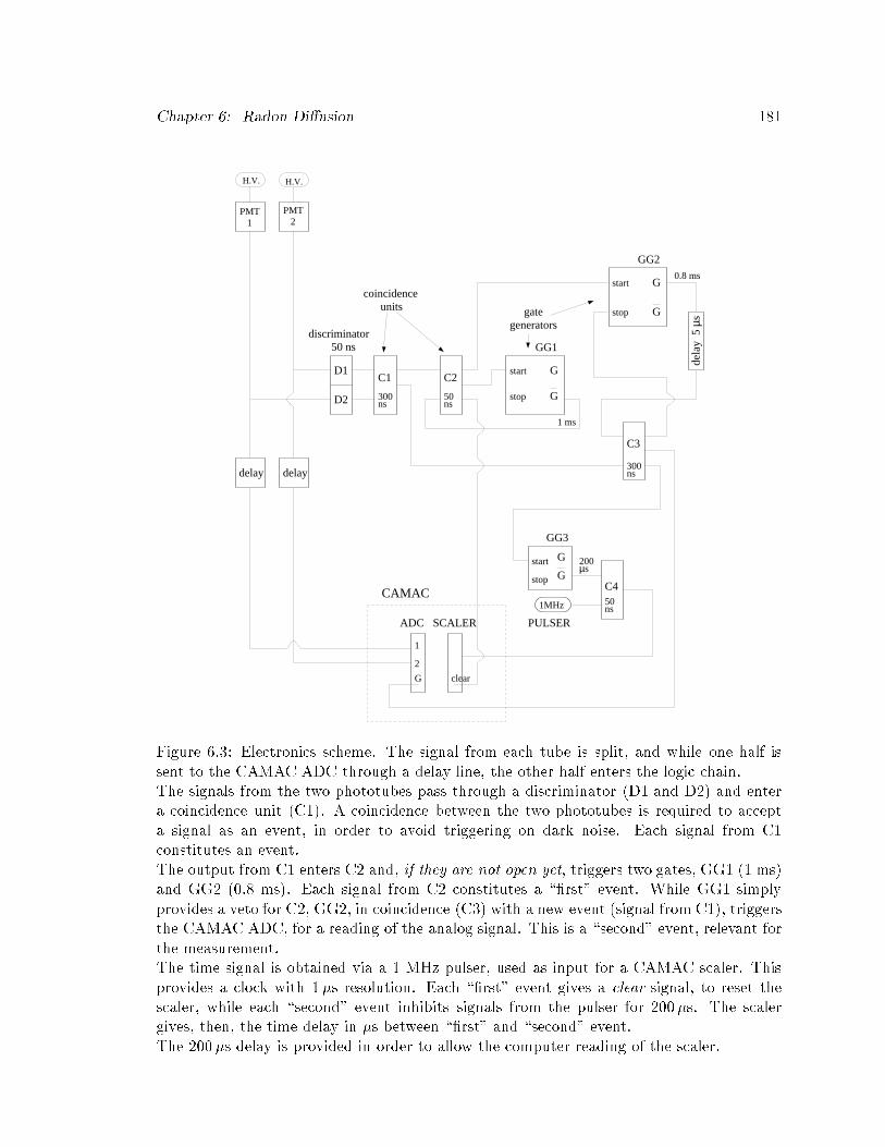
Chapter 6: Radon Di�usion 181
H.V. H.V.
PMT 1
PMT 2
delay delay
discriminator 50 ns
coincidence units
D1
D2
C1 C2
gategenerators
start
stop
GG1
G
G
G
Gstart
stop
GG2
dela
y 5
µs
C3
GG3
start
stop G
G
C4
PULSER
1MHzCAMAC
ADC SCALER
1
2
G clear
50 ns
300 ns
50 ns
300 ns
1 ms
0.8 ms
200 µs
Figure 6.3: Electronics scheme. The signal from each tube is split, and while one half issent to the CAMAC ADC through a delay line, the other half enters the logic chain.The signals from the two phototubes pass through a discriminator (D1 and D2) and entera coincidence unit (C1). A coincidence between the two phototubes is required to accepta signal as an event, in order to avoid triggering on dark noise. Each signal from C1constitutes an event.The output from C1 enters C2 and, if they are not open yet, triggers two gates, GG1 (1 ms)and GG2 (0.8 ms). Each signal from C2 constitutes a \�rst" event. While GG1 simplyprovides a veto for C2, GG2, in coincidence (C3) with a new event (signal from C1), triggersthe CAMAC ADC, for a reading of the analog signal. This is a \second" event, relevant forthe measurement.The time signal is obtained via a 1 MHz pulser, used as input for a CAMAC scaler. Thisprovides a clock with 1�s resolution. Each \�rst" event gives a clear signal, to reset thescaler, while each \second" event inhibits signals from the pulser for 200�s. The scalergives, then, the time delay in �s between \�rst" and \second" event.The 200�s delay is provided in order to allow the computer reading of the scaler.

Chapter 6: Radon Di�usion 182
number of detected photons per event, top tube
0
250
500
750
1000
1250
1500
1750
2000
0 1000 2000 3000
number of detected photons per event, bot tube
0
200
400
600
800
1000
1200
1400
1600
1800
0 1000 2000 3000
Figure 6.4: Simulated distribution of the number of photons reaching the top and the bottomphototubes, for 800 keV events, assuming a light yield of 104 =MeV. Only geometricale�ects are included.
10 times the water volume, and the solubility ratio is �50 (222Rn is much more soluble in
pseudocumene than in water): only 0.2% of the 222Rn remains in water. Each measurement
takes about two weeks.
6.3.3 Detector Performances
The detection of light emitted in the sensitive volume is performed by two phototubes only;
the dimensions were chosen in order to optimize the volume ratio between the two media
and a compromise had to be reached for coverage and energy resolution. In this geometry,
it is impossible to perform spectroscopy and identify energy peaks.
The e�ect of geometry on the eÆciency has been estimated through a Monte Carlo
simulation; results are summarized in table 6.3, while �g. 6.4 shows the expected energy
spectrum for the 214Po � (Q = 7:9MeV, quenched energy in PC+PPO = 750KeV). Pol-
ishing the tube's internal surface dramatically increased the light collection eÆciency.
Tests have been performed with an external 60Co source and by introducing 222Rn in
the scintillator as an internal source.
Fig. 6.5 shows the individual phototube spectra and the summed spectrum obtained
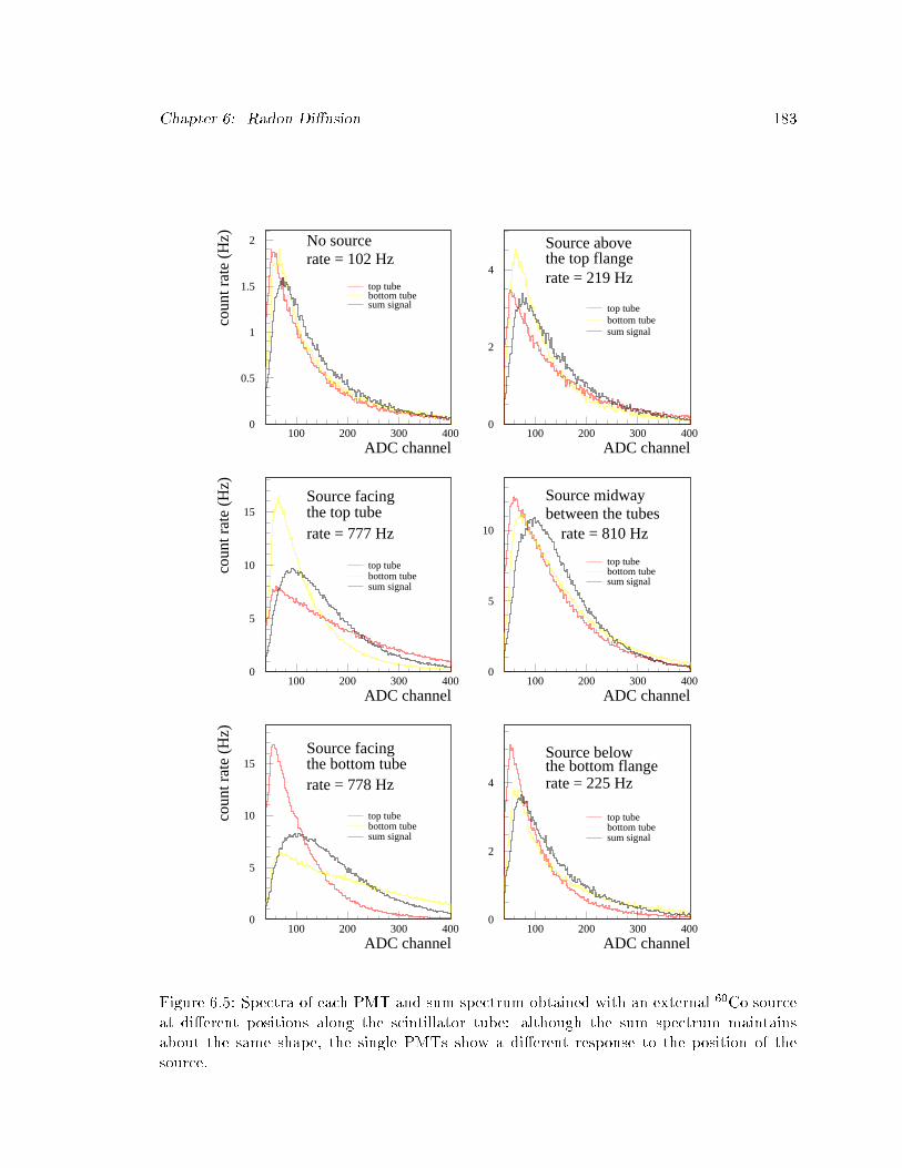
Chapter 6: Radon Di�usion 183
0
0.5
1
1.5
2
100 200 300 400
ADC channel
coun
t rat
e (H
z) No sourcerate = 102 Hz
top tubebottom tubesum signal
0
2
4
100 200 300 400
Source abovethe top flangerate = 219 Hz
top tubebottom tubesum signal
ADC channel
0
5
10
15
100 200 300 400
Source facingthe top tuberate = 777 Hz
top tubebottom tubesum signal
ADC channel
coun
t rat
e (H
z)
0
5
10
100 200 300 400
Source midwaybetween the tubes
rate = 810 Hz
top tubebottom tubesum signal
ADC channel
0
5
10
15
100 200 300 400
Source facingthe bottom tuberate = 778 Hz
top tubebottom tubesum signal
ADC channel
coun
t rat
e (H
z)
0
2
4
100 200 300 400
Source belowthe bottom flangerate = 225 Hz
top tubebottom tubesum signal
ADC channel
Figure 6.5: Spectra of each PMT and sum spectrum obtained with an external 60Co sourceat di�erent positions along the scintillator tube: although the sum spectrum maintainsabout the same shape, the single PMTs show a di�erent response to the position of thesource.

Chapter 6: Radon Di�usion 184
Table 6.3: EÆciency in light collection (Monte Carlo calculation).
percentage of photonsreaching either phototube
direct propagation (no re ections) 4%40% 4� re ection (stainless steel, non polished) 6%80% mirror re ection (stainless steel, mirror �nish) 15%
when a 60Co source is placed in di�erent positions along the chamber. No peaks are ob-
served, but the detector shows a response to the source position.
This test can be used to determine the eÆciency in detection of the rays emitted in
the side-can volume. The 60Co source emits two 's in cascade (1.17 MeV and 1.33 MeV),
its activity is 0:17�Ci and the rate increases of about 700 Hz. The eÆciency is then about
12.5% for 1.2{1.3 MeV rays (including the absorption in the steel walls of the chamber).
After introducing 222Rn in the main volume, I checked the energy spectrum of the 214Po
events, identi�ed via the delayed coincidence. There was no evident spectral structure.
Since no spectroscopy is possible with this apparatus, the 222Rn detection inside the
scintillator volume relies completely on the time correlation between 214Bi and 214Po events.
EÆciency does not constitute a serious bias, since the 222Rn content in the side can and in
the scintillator are both measured with the same technique, and the results depend only on
relative activities.
An example of what the 222Rn data look like is shown in �g. 6.6: the �rst plot is the
distribution of the delay time between coincidence events, in the internal source test. The
shape has been �t with an exponential plus a constant, to account for accidental triggers
in the 800 �s time window: the exponential component gives an estimation of the 222Rn
content in the scintillator. As a con�rmation of the nature of this signal, the second plot
shows how the estimated 222Rn content varies in time: the activity decays exponentially, in
good agreement with the 222Rn half-life.

Chapter 6: Radon Di�usion 185
0
0.05
0.1
0.15
0.2
0.25
0.3
0.35
0 200 400 600
fit function: A + Be-λt λ=0.0042 MHzχ2 = 0.886
rate in a 700µs window = 23.8 Hz∆t=14330 s
estimated Radon activity 15.48 ± 0.06 Bq
estimated accidental rate = 11.14 ± 0.06 Hz
coincidence time (µs)
rate
(co
unts
/sec
/4µs
)
0
2.5
5
7.5
10
12.5
15
17.5
20
22.5
25
0 50 100
time (hours)R
adon
act
ivity
(B
q)
fit with Radon decay curveRadon = 21 Bq χ2=0.709
Figure 6.6: 222Rn inside the scintillator tube: this in an example of the delay time distri-bution obtained in a 700�s time window, due to accidental coincidences and Bi-Po events.On the right, the estimated radon in scintillator is plotted versus time (222Rn decay curvewith �1=2 = 3:8 d).
6.3.4 Expected Di�usion Pro�les
The formalism introduced in x6.2 can be used to model the apparatus, once the proper
boundary conditions are imposed. The problem to be solved is the 1-dimensional di�usion
equation corrected for 222Rn decay (eq. 6.5), with the following boundary conditions:
8><>:
�(0) = S�0
�(x 6= 0) = 0at t = 0
Atot(t) = �0�Vse��t at t > 0
where:
� = local concentration of the di�using substance (atoms/cm3);
�0 = initial 222Rn concentration in the test uid (atoms/cm3);
S = relative solubility (nylon versus the uid in the side can);
Atot(t) = total 222Rn activity (Bq) in the system at time t;
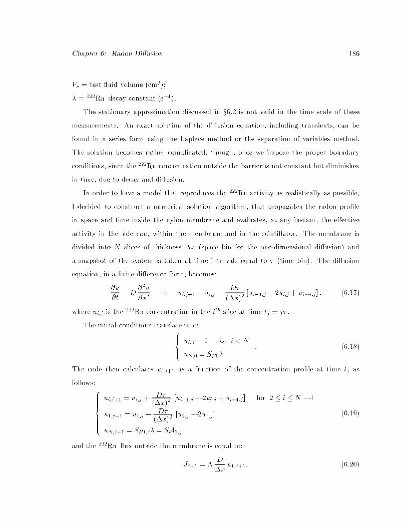
Chapter 6: Radon Di�usion 186
Vs = test uid volume (cm3);
� = 222Rn decay constant (s�1).
The stationary approximation discussed in x6.2 is not valid in the time scale of these
measurements. An exact solution of the di�usion equation, including transients, can be
found in a series form using the Laplace method or the separation of variables method.
The solution becomes rather complicated, though, once we impose the proper boundary
conditions, since the 222Rn concentration outside the barrier is not constant but diminishes
in time, due to decay and di�usion.
In order to have a model that reproduces the 222Rn activity as realistically as possible,
I decided to construct a numerical solution algorithm, that propagates the radon pro�le
in space and time inside the nylon membrane and evaluates, at any instant, the e�ective
activity in the side can, within the membrane and in the scintillator. The membrane is
divided into N slices of thickness �x (space bin for the one-dimensional di�usion) and
a snapshot of the system is taken at time intervals equal to � (time bin). The di�usion
equation, in a �nite di�erence form, becomes:
@u
@t= D
@2u
@x2) ui;j+1 � ui;j =
D�
(�x)2[ui+1;j � 2ui;j + ui�1;j ] ; (6.17)
where ui;j is the 222Rn concentration in the ith slice at time tj = j� .
The initial conditions translate into:8><>:
ui;0 = 0 for i < N
uN;0 = S�0�: (6.18)
The code then calculates ui;j+1 as a function of the concentration pro�le at time tj as
follows:8>>>>><>>>>>:
ui;j+1 = ui;j +D�
(�x)2[ui+1;j � 2ui;j + ui�1;j ] for 2 � i � N � 1
u1;j+1 = u1;j +D�
(�x)2[u2;j � 2u1;j ]
uN;j+1 = S�1;j� = SA1;j
(6.19)
and the 222Rn ux outside the membrane is equal to:
Jj+1 = AD
�xu1;j+1; (6.20)

Chapter 6: Radon Di�usion 187
0 100 200 300
time (hours)
D=1*10-9 cm2/s
D=1*10-10 cm2/s
D=1*10-11 cm2/s
D=1*10-12 cm2/s
film thicknessd=25µm
0 100 200 300
time (hours)
D=1*10-9 cm2/s
D=1*10-11 cm2/s
D=1*10-10 cm2/s
film thicknessd=125µm
Figure 6.7: Di�usion pro�les expected for a membrane with thickness d = 25�m (left)and d = 125�m (right) as a function of the di�usion coeÆcient D. The normalization isarbitrary.
where A1;j = S�1;j is the222Rn concentration outside the membrane at time tj = j� and
A is the interface area.
The 222Rn decay is included by multiplying all the activities by the same exponential factor:8><>:Atot;j+1 = Atot;j e
���
ui;j+1 = ui;j+1 e���
: (6.21)
The total amount of 222Rn in the system is then distributed as follows:8>>>><>>>>:A2;j+1 = A2;j e
��� +A D��x u1;j+1 di�used in the scintillator;
Ain;j+1 = A�xPN
i=1 ui;j+1 in the membrane;
A1;j+1 = Atot;j+1 �A2;j+1 � Ain;j+1 in the uid outside the membrane:
(6.22)
When the decay equilibrium between 222Rn and its daughters is included, the �nal
result is the count rate pro�le (as a function of time) expected inside the scintillator, given
a certain �lm thickness and a certain di�usion constant.
Fig. 6.7 shows how sensitive the apparatus is to the value of the di�usion coeÆcient:
the delay in the count rate increase (time lag) gives a direct indication of the value of D.

Chapter 6: Radon Di�usion 188
The initial concentration of 222Rn in the side can must be known to determine the relative
solubility (nylon versus uid) and the membrane permeability.
6.3.5 Data Analysis
The distribution of delayed coincidence times is collected for periods of about 10 hours.
The result is a time spectrum that can be �t by the calculated distribution for Bi-Po events
plus a background distribution that describes the rate of accidental coincidences, similar to
the one in �gure 6.6-a.
The background is ruled by the Poisson distribution: if R is the total event rate, the
probability of having n events in time t is equal to:
P (n) =(Rt)ne�Rt
n!: (6.23)
An accidental coincidence is registered in our spectrum if, given an event, another hap-
pens within the T = 800�s window. Using the Poisson distribution, we get that the
probability of having at least one event between time t and T and no events before t is:
P = e�Rt�1� e�R(T�t)
�= e�Rt � e�RT ; (6.24)
while the probability of having an event between t and t + dt is:
P (t)dt = Re�Rtdt: (6.25)
Hence, in a plot with bin size dt = � for a measurement that lasts tm, the background due
to accidental coincidences is:
N(t) = (Rtm) �Re�Rt � � = R2tm� e
�Rt: (6.26)
For a total rate R � 100 ev/s, in the time window of 0.8 s this distribution is, in a �rst
order approximation, at.
For each run, the time distribution is �t with the 2-parameter function:
f(t) = ae��t + R2tm� e�Rt; (6.27)

Chapter 6: Radon Di�usion 189
0
1
2
3
4
5
6
7
8
9
0 50 100 150 200time (hours)
Dif
fuse
d R
adon
(B
q)
25 µm PA-6 film b.o.
D = (9.3 ± 1.2) 10-10 cm2/s
S = 2.1 ± 0.4
4
5
6
7
8
9
10
11
12
13
6 8 10 12 D (10-10 cm2/s)
χ2
χ2 min = 5.66 for 18 d.o.f.
normalized χ2 min = 0.315
minimum χ2
1σ
2σ
Figure 6.8: On the left, time pro�le of 222Rn in the scintillator, with the resulting functional�t, for a 25 �m biaxially oriented PA-6 �lm in the water/scintillator con�guration. On theright, scan of �2 dependence on the di�usion coeÆcient.
with ��1 = 237�s (Bi-Po mean life). Given the proper normalization, the parameter a
gives the 222Rn content of the scintillator.
Once the measurement is terminated, the time pro�le of 222Rn content in the scintillator
is �t with the model calculated curves, for di�erent values of the di�usion coeÆcient D.
The best estimate of D is the value that gives the minimum �2 in the �t. I assumed Poisson
statistics in the raw data and used, as error on the estimated 222Rn, the one provided by
the MINUIT �t [82]. The error on D is obtained looking for the D-pro�les that �t the
222Rn time pro�le with �2 = �2min + 1 (see �g. 6.8).
The total count rate in the scintillator is a�ected by rays from 222Rn daughters in the
side can. The eÆciency for their detection has been measured by recording the total rate
when the side can was �lled with 222Rn enriched pseudocumene. The same uid was then
mixed with the scintillator and the residual 222Rn counted. The procedure was repeated
three times, yielding:
" = 0:149� 0:025:
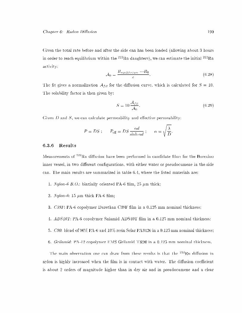
Chapter 6: Radon Di�usion 190
Given the total rate before and after the side can has been loaded (allowing about 3 hours
in order to reach equilibrium within the 222Rn daughters), we can estimate the initial 222Rn
activity:
A0 =Requilibrium �R0
": (6.28)
The �t gives a normalization Afit for the di�usion curve, which is calculated for S = 10.
The solubility factor is then given by:
S = 10Afit
A0: (6.29)
Given D and S, we can calculate permeability and e�ective permeability:
P = DS ; Pe� = DS�d
sinh �d; � =
s�
D:
6.3.6 Results
Measurements of 222Rn di�usion have been performed in candidate �lms for the Borexino
inner vessel, in two di�erent con�gurations, with either water or pseudocumene in the side
can. The main results are summarized in table 6.4, where the listed materials are:
1. Nylon-6 B.O.: biaxially oriented PA-6 �lm, 25 �m thick;
2. Nylon-6: 15 �m thick PA-6 �lm;
3. C38F: PA-6 copolymer Durethan C38F �lm in a 0.125 mm nominal thickness;
4. ADS40T: PA-6 copolymer Sniamid ADS40T �lm in a 0.125 mm nominal thickness;
5. C90: blend of 90% PA-6 and 10% resin Selar PA3426 in a 0.125mm nominal thickness;
6. Grilamid: PA-12 copolymer EMS Grilamid TR90 in a 0.125 mm nominal thickness.
The main observation one can draw from these results is that the 222Rn di�usion in
nylon is highly increased when the �lm is in contact with water. The di�usion coeÆcient
is about 2 orders of magnitude higher than in dry air and in pseudocumene and a clear
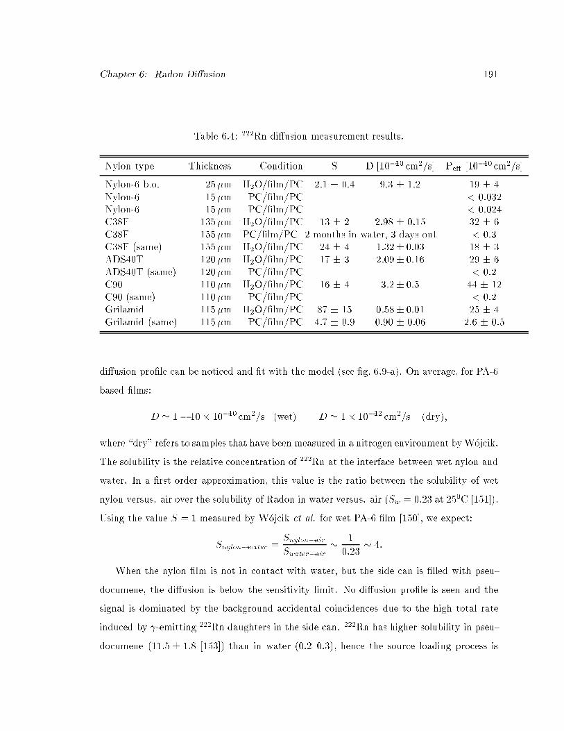
Chapter 6: Radon Di�usion 191
Table 6.4: 222Rn di�usion measurement results.
Nylon type Thickness Condition S D [10�10 cm2/s] Pe� [10�10 cm2/s]
Nylon-6 b.o. 25�m H2O/�lm/PC 2.1 � 0.4 9.3 � 1.2 19 � 4Nylon-6 15�m PC/�lm/PC < 0.032Nylon-6 15�m PC/�lm/PC < 0.024C38F 135�m H2O/�lm/PC 13 � 2 2.98 � 0.15 32 � 6C38F 155�m PC/�lm/PC 2 months in water, 3 days out < 0.3C38F (same) 155�m H2O/�lm/PC 24 � 4 1:32� 0:03 18 � 3ADS40T 120�m H2O/�lm/PC 17 � 3 2:09� 0:16 29 � 6ADS40T (same) 120�m PC/�lm/PC < 0.2C90 110�m H2O/�lm/PC 16 � 4 3:2� 0:5 44 � 12C90 (same) 110�m PC/�lm/PC < 0.2Grilamid 115�m H2O/�lm/PC 87 � 15 0:58� 0:01 25 � 4Grilamid (same) 115�m PC/�lm/PC 4.7 � 0.9 0.90 � 0.06 2.6 � 0.5
di�usion pro�le can be noticed and �t with the model (see �g. 6.9-a). On average, for PA-6
based �lms:
D ' 1� 10� 10�10 cm2=s (wet) D ' 1� 10�12 cm2=s (dry);
where \dry" refers to samples that have been measured in a nitrogen environment byW�ojcik.
The solubility is the relative concentration of 222Rn at the interface between wet nylon and
water. In a �rst order approximation, this value is the ratio between the solubility of wet
nylon versus. air over the solubility of Radon in water versus. air (Sw = 0:23 at 250C [151]).
Using the value S = 1 measured by W�ojcik et al. for wet PA-6 �lm [150], we expect:
Snylon�water =Snylon�airSwater�air
�1
0:23� 4:
When the nylon �lm is not in contact with water, but the side can is �lled with pseu-
documene, the di�usion is below the sensitivity limit. No di�usion pro�le is seen and the
signal is dominated by the background accidental coincidences due to the high total rate
induced by -emitting 222Rn daughters in the side can. 222Rn has higher solubility in pseu-
documene (11:5 � 1:8 [153]) than in water (0.2{0.3), hence the source loading process is

Chapter 6: Radon Di�usion 192
0
0.25
0.5
0.75
1
1.25
1.5
1.75
2
0 50 100 150 200 250time (hours)
Dif
fuse
d R
adon
(B
q)
A0 = 247 Bq
135 µm C38F film
D = (2.98 ± 0.15) 10-10 cm2/s
S = 13 ± 2
0
0.2
0.4
0.6
0.8
1
1.2
1.4
1.6
1.8
0 25 50 75 100 125 150 175 200 225time (hours)
Dif
fuse
d R
adon
(B
q) A0 = 1700 Bq (≈ 8.5×10³ Bq/l)
background
fit with DS =(3.0 ± 0.4) × 10-12 cm2/s
expected profile ifD = 5×10-11 cm2/s, S=0.4
expected profile ifD = 1×10⁻¹⁰ cm2/s, S=0.4
Limit on permeability:Peff < 3×10-12 cm2/s
(a) water (b) pseudocumene
Figure 6.9: Typical di�usion pro�les obtained in the two con�gurations. (a) is 135�mC38F �lm in contact with water and scintillator, while (b) is 15�m PA-6 �lm in contactwith pseudocumene and scintillator.
much more eÆcient, in this case. For the same reason, though, the relative solubility on
nylon is smaller: using the value measured by W�ojcik et al. for PA-6 �lm [150], we expect:
Snylon�water =Snylon�airSwater�air
�5
11:5� 0:4:
Fig. 6.9-b shows the result obtained with the thinnest PA-6 membrane I measured. Over-
lapped to the data are the radon decay curve (labeled \background") and the expected
di�usion curves with di�erent assumptions for the permeability; from these data we can
only derive an upper limit on the membrane e�ective permeability. Such limit is obtained
using the formula:
Pe� ' wd�Amax
A0e�tmax ; (6.30)
where w is the side-can width, Amax is the maximum di�used activity and tmax is the time
at which that value is seen. This formula is obtained from the stationary solution for the
ux through the membrane, allowing for radioactive decay. It is not very precise because

Chapter 6: Radon Di�usion 193
0
0.5
1
1.5
2
2.5
3
3.5
4
0 50 100 150 200 250time (hours)
Dif
fuse
d R
adon
(B
q) A0 = 687 ± 117 Bq
Fit with diffusion profiles :D = (5.79 ± 0.12) 10-11 cm2/sS = 87 ± 15
0
0.2
0.4
0.6
0.8
1
1.2
0 25 50 75 100 125 150 175 200 225time (hours)
Dif
fuse
d R
adon
(B
q) A0 = 1600 Bq
Fit with diffusion profiles :D = (8.96 ± 0.55) × 10-11 cm2/sS = 4.7 ± 0.9
(a) water (b) pseudocumene
Figure 6.10: PA-12 copolymer, 115�m thick: the same sample has been measured in thetwo con�gurations.
it neglects the time lag before the di�usion onset, but it is useful in cases when the pro�le
is not evident and the �t procedure does not work. For PA-6 based �lms, the best limit is:
Pe� < 2� 10�12 cm2=s (d = 15�m):
A more de�nite measurement for PA-6 �lm in contact with pseudocumene on one side
and pseudocumene vapor on the other has been obtained by W�ojcik et al. [150]:
D = (2:5� 1:2)� 10�12 cm2=s ; S = 1:0:
We found that this pattern of high permeability in water and low permeability in pseu-
documene is the same for the PA-6 �lm, for the PA-6 copolymers C38F and ADS40T and
for the PA-6 based blend C90.
A very di�erent result has been obtained for the PA-12 copolymer: in this case, the dif-
fusivity is actually higher in pseudocumene than in water, consistently with the expectation
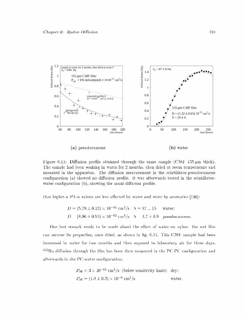
Chapter 6: Radon Di�usion 194
0
0.2
0.4
0.6
0.8
1
1.2
60 80 100 120 140 160 180 200time (hours)
Dif
fuse
d R
adon
(B
q) sample in water for 2 months, then dried at room TA0 = 2900 Bq
background(222Rn decay)
expected profile ifD = 5×10-11 cm2/s, S=0.4
155 µm C38F film:Peff = DS αd/sinh(αd) < 3×10-12 cm2/s
0
0.2
0.4
0.6
0.8
1
1.2
1.4
0 50 100 150 200 250time (hours)
Dif
fuse
d R
adon
(B
q)
A0 = 407 ± 69 Bq
155 µm C38F film
D = (1.32 ± 0.03) 10-10 cm2/s S = 24 ± 4
(a) pseudocumene (b) water
Figure 6.11: Di�usion pro�le obtained through the same sample (C38F 155�m thick).The sample had been soaking in water for 2 months, then dried at room temperature andmounted in the apparatus. The di�usion measurement in the scintillator-pseudocumenecon�guration (a) showed no di�usion pro�le. It was afterwards tested in the scintillator-water con�guration (b), showing the usual di�usion pro�le.
that higher-n PA-n nylons are less a�ected by water and more by aromatics [136]:
D = (5:79� 0:12)� 10�11 cm2=s S = 87� 15 water;
D = (8:96� 0:55)� 10�11 cm2=s S = 4:7� 0:9 pseudocumene:
One last remark needs to be made about the e�ect of water on nylon: the wet �lm
can recover its properties, once dried, as shown in �g. 6.11. This C38F sample had been
immersed in water for two months and then exposed to laboratory air for three days.
222Rn di�usion through the �lm has been then measured in the PC-PC con�guration and
afterwards in the PC-water con�guration:
Pe� < 3� 10�11 cm2=s (below sensitivity limit) dry;
Pe� = (1:8� 0:3)� 10�9 cm2=s water:

Chapter 6: Radon Di�usion 195
In view of our latest �ndings on the water e�ects on nylon (see x5.4), it is important to note
that what I refer to as \dry" is not a 0% R.H. condition. Three days of exposure to the
laboratory air, with its relative humidity, were not enough to bring the �lm to a \superdry"
condition. More likely, this �lm was in the humidity level that can realistically be achieved
in the experimental conditions, after the vessel will be exposed to a humid environment
during fabrication, transportation and installation (to avoid stress-cracking) and later dried
with a nitrogen ow in the stainless steel sphere. It is important, though, to know exactly
which is the humidity level we can allow in the �lm and in the pseudocumene, in order
for 222Rn emanation not to be a problem for Borexino. For this reason, I am planning to
start a new measurement campaign, where I will measure 222Rn di�usion in presence of
pseudocumene only and, at the same time, monitor the humidity level in the uids and in
the �lm using the technique described in x5.4.

Chapter 6: Radon Di�usion 196
6.4 222Rn Di�usion and Emanation in CTF
A measurement of 222Rn permeation through nylon has also been possible in CTF1. A
radon-in-water test was performed in December 1995 in order to study the external back-
ground contribution of 222Rn dissolved in the water shield. Five tons of water were inserted
in the bu�er without undergoing nitrogen stripping. The nominal 222Rn activity of this
water was � 103Bq/m3; its insertion brought the average 222Rn concentration outside the
inner vessel from � 0:03Bq/m3 up to � 5Bq/m3. The trigger rate grew to 20Hz and the
signal from 222Rn in the water bu�er dominated the whole energy spectrum.
The activity of 222Rn and its daughters in the external water was monitored by counting
the events in the energy window between 1.5 and 2.7 MeV, the \external Rn window".
Figure 6.12 shows the count rate in such window for a period of 40 days, starting from the
beginning of the test. The plot is �tted with a constant plus an exponential with half-life
equal to the one of 222Rn.
The number of Bi-Po events inside the scintillator also increased: this was an evidence
of 222Rn permeating through the inner vessel membrane. Figure 6.13-a shows the net
increase of the internal radon level as a function of time. I analyzed these data using the
same numerical model developed for the laboratory measurements, and the �t result is
overlapped to the data. The resulting di�usion coeÆcient is larger than the one measured
in laboratory on C38F �lm:
D = (6:7� 0:5)� 10�10 cm2=s:
A major uncertainty in this evaluation is represented by the inner vessel membrane
thickness. Its nominal value is 0.5 mm, but an increase in the sphere volume was measured in
CTF, since the very beginning; this increase corresponds to 5% in radius and 10% in surface
area. As a consequence, the stretched membrane became 10% thinner and the permeability
to 222Rn increased. This variation has been included in the �t, but further stretching might
have taken place as a consequence of the stress load acting on the vessel. Another e�ect
could have been the temperature change induced by the scintillator puri�cation procedure,
which would a�ect di�usivity. Moreover, it is possible that the e�ect of water on nylon is

Chapter 6: Radon Di�usion 197
Figure 6.12: Count rate in the energy window 1.5-2.7 MeV measured during the radon-in-water test of CTF. The plot is �tted with a constant plus an exponential with half-life equalto that of 222Rn.
0
50
100
150
200
250
300
350
0 200 400 600 800 1000time (hours)
Bi-
Po c
ount
rat
e (e
vent
s/da
y)
CTF Data: Radon in water test D = (6.7 ± 0.5) 10-10 cm2/s
42
43
44
45
46
47
48
6 7 8 D (10-10 cm2/s)
χ2
χ2 min = 42.5 for 32 d.o.f.
normalized χ2 min = 1.33
minimum χ2
1σ
2σ
Figure 6.13: On the left: CTF data for 222Rn inside the inner vessel, during the radon test.The �t with the di�usion pro�le is superimposed to the data. On the right: scan of the �2
dependence on the di�usion coeÆcient.

Chapter 6: Radon Di�usion 198
not limited to a sudden initial increase of permeability (up to two orders of magnitude),
but slowly progresses in time. The combined result is an observed increase of the estimated
222Rn content in the scintillator: from 1:5� 0:6 events/day (spring '95) to 5� 1 events/day
(fall '95, after puri�cation procedures).
The solubility value can be calculated with an assumption on the 222Rn level in water:
assuming the inserted 222Rn was uniformly distributed in the 1000m3 tank, one can assume
the concentration in water was about 4-5 Bq/m3. This would give a relative solubility (wet
nylon versus water) equal to:
S = 4� 1:
The uncertainty on this number is very high: 222Rn could have been not uniformly dis-
tributed, and the estimate of the amount of inserted 222Rn is only approximate.
The di�usion length and e�ective permeability, at the time of this test, can be calculated
from D and S:
��1 ' 180�m ; Pe� ' 1:1� 10�9 cm2=s:
Given these results, we can use the formalism introduced in section 6.2 to calculate the
amount of 222Rn permeating from the water bu�er through the inner vessel, if the water
222Rn concentration is equal to (24� 5)mBq/m3:
222Rndi� = 35� 10�Bq ) 3� 1 ev=day:
The high di�usion not only a�ects the permeation of 222Rn dissolved in the water bu�er
but also the 222Rn emanation from the nylon vessel itself. Given an 238U content in the
nylon of (1:2� 0:4)� 10�12 g/g (see x8.1.1) and 180�m di�usion length, we can calculate:
222Rnemanation = 38� 13�Bq ) 3� 1 ev=day: (6.31)
Figure 6.14 shows the expected Bi-Po rate in CTF as a function of the di�usion coeÆcient
and solubility S, including both emanation and permeation. The plot assumes an 238U
concentration in the nylon vessel equal to (1:2�0:4)�10�12 g/g and (24�5)mBq/m3 222Rn
in water. Overlapped are the measurements from CTF: (1:5� 0:6) events/day as measured

Chapter 6: Radon Di�usion 199
1 2 3 4 5 6 7 8 9 100
1
2
3
4
5
6
7
8
9
10
D (10−10 cm2/s)
Bi−
Po
rat
e (e
ven
ts/d
ay)
emanation only
S=1
S=5
S=10 S=20
Figure 6.14: Prediction of Bi-Po event rate in CTF assuming (24 � 5)mBq/m3 in water,as a function of the 222Rn di�usion coeÆcient in nylon, for di�erent values of solubility.The horizontal lines mark the measured rates: 1:5 � 0:6 events/day in spring '95 and 5 �1 events/day in fall '95.
in spring '95 and (5 � 1) events/day in fall '95. It is evident from the plot that the lower
count rate measured in spring '95 can well be explained by radon di�usion and emanation
and this determines the ultimate sensitivity limit of CTF to 238U in the scintillator. The
worse results obtained in the fall could be due either to a further deterioration of the vessel
or to a scintillator contamination added during the puri�cation test procedures.

Chapter 7
Optical Properties
Optical clarity is an important requirement for the Borexino inner vessel. The signal in
Borexino is carried by optical photons, collected by an array of 2200 phototubes. The energy
of an event is calculated from the number of detected photoelectrons, while its position is
reconstructed from the distribution of photoelectron arrival times. There are two ways
the inner vessel membrane can pose a problem. A loss of photons, due to absorption by
the inner vessel, induces a loss of energy resolution. A deviation in their path, due to
light scattering, induces a perturbation in the arrival time distribution and, consequently, a
degradation of the spatial resolution. We want to minimize these e�ects, in order to achieve
the best possible detector resolution. For this purpose, it is important to choose a material
that presents high transmittance and low haze, in the wavelength region between 350 and
500 nm, where the scintillator emission peak is located (�g. 2.2).
7.1 Light Crossing a Thin Film: Luminous Transmittance
and Haze
A light beam going through a thin �lm is subject to deviation or attenuation both at the
interfaces (surface e�ects) and while crossing the �lm material (volume e�ects).
Direct and total transmittance are de�ned as:
Td =IdI0
direct transmittance;
T =Id + Is;f
I0total transmittance;
(7.1)
200

Chapter 7: Optical Properties 201
where Id is the light ux transmitted directly, without being deviated by the �lm and Is;f
is the ux undergoing forward scattering.
Haze is de�ned as the percentage of transmitted light which in passing through the �lm
deviates more than 2.5o from the incident beam by forward scattering:
H =(Is)2:5o�90o
Id + Is;fhaze: (7.2)
The visible e�ect of haze is a loss of contrast, induced by large angle light scattering, while
light scattering at low angles a�ects clarity, the degree to which �ne details are resolved.
7.1.1 Surface E�ects
When a light beam hits the boundary surface between two substances with di�erent indices
of refraction, one part of it will re ect from the surface while the remainder will cross the
interface and undergo refraction.
Irradiance, or radiant ux density I, is de�ned as the average value of the power per
unit area crossing a surface in vacuum:
~S = c2"0 ~E � ~B; (7.3)
I =< S >=c "0
2E2
0
�W
m2
�: (7.4)
For a beam incident on a surface at an angle �i, the portion of energy incident normal to a
unit area, per unit time, is equal to Ii cos �i. We can de�ne:
R =Ir cos �rIi cos �i
=Ir
Iire ectance; (7.5)
where �r = �i is the re ection angle, and:
T =It cos �tIi cos �i
transmittance; (7.6)
where �t is the refraction angle, related to the incidence angle and the indices of refraction
of the two media by Snell's law:
ni sin �i = nt sin �t: (7.7)
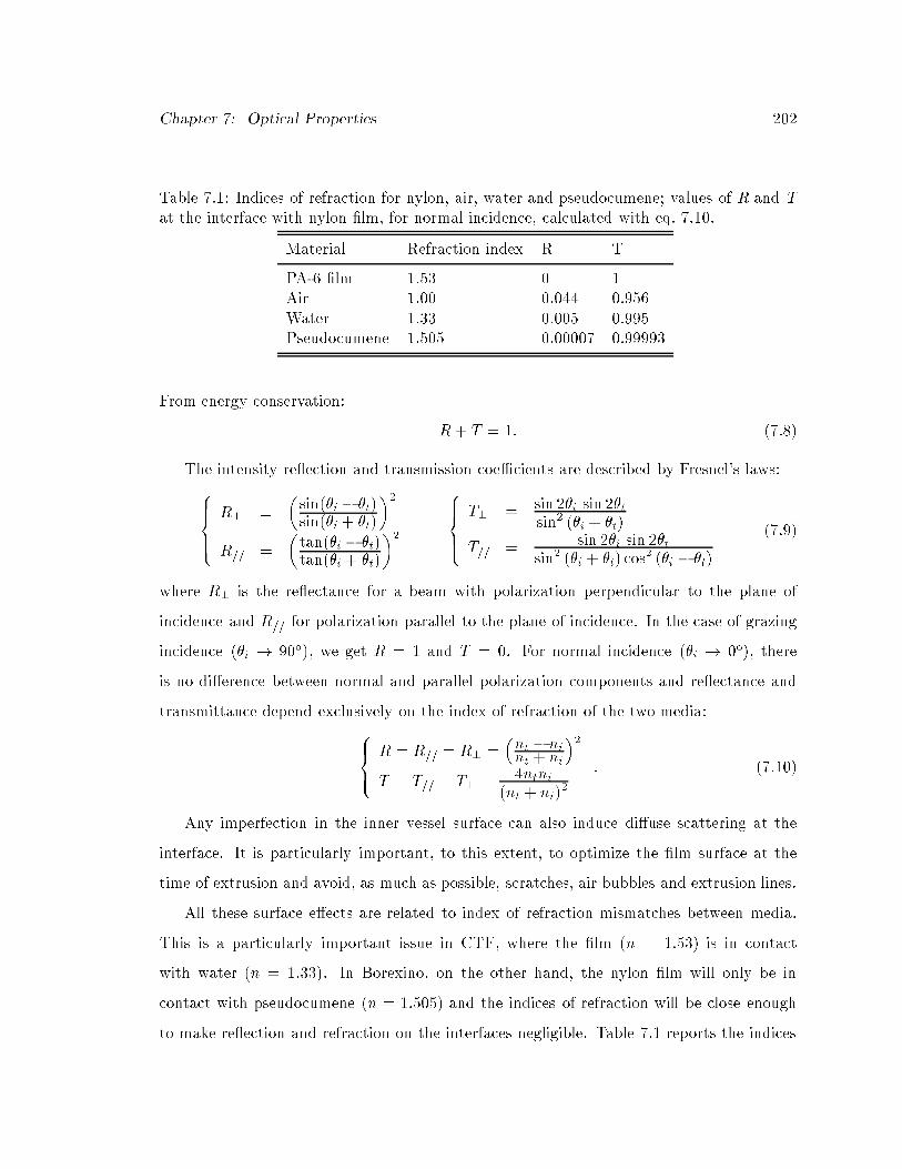
Chapter 7: Optical Properties 202
Table 7.1: Indices of refraction for nylon, air, water and pseudocumene; values of R and Tat the interface with nylon �lm, for normal incidence, calculated with eq. 7.10.
Material Refraction index R T
PA-6 �lm 1.53 0 1Air 1.00 0.044 0.956Water 1.33 0.005 0.995Pseudocumene 1.505 0.00007 0.99993
From energy conservation:
R+ T = 1: (7.8)
The intensity re ection and transmission coeÆcients are described by Fresnel's laws:8>><>>:
R? =
�sin(�i � �t)sin(�i + �t)
�2
R== =
�tan(�i � �t)tan(�i + �t)
�2
8>><>>:
T? = sin 2�i sin 2�tsin2 (�i + �t)
T== = sin 2�i sin 2�tsin2 (�i + �t) cos
2 (�i � �t)
(7.9)
where R? is the re ectance for a beam with polarization perpendicular to the plane of
incidence and R== for polarization parallel to the plane of incidence. In the case of grazing
incidence (�i ! 90o), we get R = 1 and T = 0. For normal incidence (�i ! 0o), there
is no di�erence between normal and parallel polarization components and re ectance and
transmittance depend exclusively on the index of refraction of the two media:8><>:
R = R== = R? =�nt � nint + ni
�2
T = T== = T? = 4ntni(nt + ni)
2
: (7.10)
Any imperfection in the inner vessel surface can also induce di�use scattering at the
interface. It is particularly important, to this extent, to optimize the �lm surface at the
time of extrusion and avoid, as much as possible, scratches, air bubbles and extrusion lines.
All these surface e�ects are related to index of refraction mismatches between media.
This is a particularly important issue in CTF, where the �lm (n = 1:53) is in contact
with water (n = 1:33). In Borexino, on the other hand, the nylon �lm will only be in
contact with pseudocumene (n = 1:505) and the indices of refraction will be close enough
to make re ection and refraction on the interfaces negligible. Table 7.1 reports the indices

Chapter 7: Optical Properties 203
of refraction for the media of interest and the values of R and T at the interface with nylon
�lm, for normal incidence, calculated with eq. 7.10.
7.1.2 Volume E�ects
As light crosses the nylon �lm, part of the light will be absorbed and converted into heat.
The remaining is subject to light scattering, caused by uctuations of the index of refraction
within the bulk material [154, 155, 156, 157]. This phenomenon is typically induced by the
presence of crystallites in semicrystalline solids such as the PA-6 �lm or substructures in
amorphous polymers like the PA-6 copolymers [136].
Most of the semicrystalline nylons are nearly opaque in thicknesses over 2.5 mm and
transparent to visible light, with a milky appearance, in thicknesses below 0.5 mm [136]. The
ultraviolet cuto� wavelength is below 300 nm (see measurements reported in x7.2.1), making
nylon �lms a viable choice for the Borexino inner vessel. The best optical quality is achieved
with amorphous nylon �lms, which can be obtained either through copolymerization or
through a rapid cooling of the material at the time of extrusion (see x5.2.4).
7.2 Optical Measurements on Nylon Films
7.2.1 Transmittance
The luminous transmittance of di�erent nylon �lms has been measured with an absorption
spectrometer. The instrument measures absorbance as a function of the beam wavelength,
where absorbance is de�ned as:
A = � logT: (7.11)
Figure 7.1 shows the results obtained in Princeton by M. Johnson for two di�erent
thicknesses of C38F and for commercially extruded PA-6 �lm Capran DF400 (Allied Signal).
These measurements have been performed in air; the uctuations at small wavelengths are
noise due to re ections inside the instrument. Figure 7.2 shows similar measurements
performed by our collaborators in Perugia, on a wider range of samples. These spectra have

Chapter 7: Optical Properties 204
200 250 300 350 400 450 500 550 6000
0.1
0.2
0.3
0.4
0.5
0.6
0.7
0.8
0.9
1
wavelength (nm)
tran
smitt
ance
C38F 0.125 mm C38F 0.500 mm PA−6 Capran DF400 (hazy) 0.100 mm
Figure 7.1: Transmittance versus wavelength in di�erent nylon strips, measured in air [158].
been obtained with � 1 cm nylon strips immersed in an open quartz cell containing water
and normalized to a reference beam that only goes through air. In both cases, the incident
light beam was perpendicular to the �lm and the measurements included only the direct
transmittance; scattering at large angles was not accounted for.
Figure 7.3 shows the results of measurements that I performed with a simpler apparatus,
consisting of a deuterium light source (wavelength < 350 nm) and a portable diode array
spectrometer (World Precision Instruments SD2000). Optical �bers mounted perpendicular
to the �lm convey the incident and the transmitted light beams. The angular acceptance
for the �bers is of the order of 6o. I focused my attention on on the behavior of PA-6 from
di�erent extrusions: commercially extruded Capran DF400, with hazy appearance, and
clear PA-6 Capron B73ZP, custom extruded at Leistriz, NJ in July 1998 and at Honeywell,
PA in May 1999. For comparison, I also measured a sample of C38F �lm.
The measurements show that the amorphous PA-6 copolymers C38F and ADS40T have
an ultraviolet transmittance cuto� between 295 and 300 nm, de�nitely lower than the PPO
emission peak (365 nm). The 0.125 mm C38F �lm is more transparent than the 0.5 mm

Chapter 7: Optical Properties 205
200 250 300 350 400 450 500 550 6000
0.1
0.2
0.3
0.4
0.5
0.6
0.7
0.8
0.9
1
wavelength (nm)
tran
smit
tanc
e
C38F 0.125 mm C38F 0.500 mm ADS40T 0.125 mm PA−6 Capran DF400 (hazy) 0.100 mm PA−6 Capron B73ZP −Leistriz(clear) 0.125 mm
Figure 7.2: Transmittance versus wavelength in di�erent nylon strips, measured in wa-ter [159].
�lm as it is expected for volume e�ects.
The PA-6 �lms show an interesting behavior. All three sets of measurements include
a sample of PA-6 Capran DF400 by Allied Signal, which we purchased as a 0.1 mm thick
sheet. Its appearance is milky, hazy, as expected for semicrystalline materials. The mea-
sured transmittance is lower than what obtained with amorphous materials, but the light
scattering measurements reported in x7.2.2 indicate this is partly due to the fact that the
spectrometer detects only direct transmittance, while there is a signi�cant component of
scattered light that is lost in these measurements.
We also purchased PA-6 Capron B73ZP pellets and extruded them twice, at Leistriz
in July 1998 and at Honeywell in May 1999. The di�erence between these sample is most
evident in �gure 7.3. The �rst �lm, extruded at Leistriz, already presented good optical
clarity, but thanks to the experience of the Honeywell technicians in extruding amorphous
PA-6, the most recent �lm presents the highest transmission in the ultraviolet spectrum,
even better than the copolymers, because of the lower cuto� wavelength. The only di�erence

Chapter 7: Optical Properties 206
0
0.1
0.2
0.3
0.4
0.5
0.6
0.7
0.8
0.9
1
220 240 260 280 300 320 340
PA-6 0.125 mm Capron B73ZPHoneywell extrusion
PA-60.125 mm
Capron B73ZPLeistriz extrusion
PA-6 copolymerC38F 0.125 mm
PA-60.100 mm
Capran DF400commercial extrusion, hazy
wavelength (nm)
tran
smitt
ance
Figure 7.3: Transmittance versus wavelength in di�erent nylon strips, measured in air, inthe ultraviolet spectrum (< 350 nm).

Chapter 7: Optical Properties 207
between this �lm and the Capran DF400 happened at extrusion, the chemical composition
of the two �lms is the same, only the crystallinity is di�erent.
7.2.2 Light Scattering and Haze Measurements
I performed a �rst attempt at measuring the light scattering o� nylon �lm using the appara-
tus shown in �gure 7.4. The light source is a tungsten lamp in series with a monochromator
(Oriel 7271) and a light chopper. The monochromatic beam goes through a set of 5 col-
limating slits and hits the sample, mounted on a rotating platform. The angular position
of the platform determines the incidence angle. The transmitted light is detected by a
phototube (Oriel 77340) mounted on a second arm attached to the rotating platform. By
moving the arm, it is possible to measure the light scattered at di�erent angles. In order
to separate the signal from background stray light, I used a lock-in ampli�er in coincidence
with the light chopper.
Figure 7.5 shows the results obtained with a 0.125 �m C38F �lm and normal light beam
incidence. The plot shows the fraction of detected light as a function of the angle between
incoming beam and detector mount. The measurement has been performed both with the
�lm unsupported and sandwiched between two microscope glass slides, with pseudocumene
as immersion uid. The blank measurements are shown as well. These data are subject to
measurement errors, high noise and background. From a qualitative standpoint, it is clear
there is some scattering induced by the �lm.
A much more reliable, quantitative estimation can be obtained through a measurement
of the �lm haze, that is the integrated scattered light signal. Haze measurements have been
performed with an integrating sphere (Newport Mod. 819-IS-4), following the procedure
outlined in ASTM D1003 [160]. The apparatus is shown in �gure 7.6. Its core is a 4"
diameter hollow sphere, internally coated by a white thermoplastic material with high
di�usion re ectance at all wavelengths, exceeding 90% in the 250{2500 nm range (98%
re ectance from 310 to 2100 nm). The light source and the detector are the same described
above. Light entering the sphere makes di�use re ection on the walls. After multiple
re ections on the sphere walls, about 10% of the light is collected by a photomultiplier tube

Chapter 7: Optical Properties 208
Lock-in amplifier
source +mono-chromator
lightchopper
sample (on a rotating platform)
phototubedetector
collimating slits
collimating slits
Figure 7.4: Apparatus for detection of light scattering from a nylon �lm.
−50 0 5010
−8
10−6
10−4
10−2
100
scattering angle (deg)
unsupported filmsupported film glass slides incoming light
Figure 7.5: Fraction of light scattered at di�erent angles by a 0.125 mm C38F �lm, unsup-ported and supported by glass microscope slides. The incident light was 366 nm wavelength.

Chapter 7: Optical Properties 209
PM
Light Trap
lightsource
film sample
integrating sphere coated with highly reflective material (diffusor)
Figure 7.6: Apparatus for haze and transmittance measurements.
mounted on a port at 90o from the entrance port. A ba�e is used to shield the detector
from non-integrated transmission.
Transmittance is measured by using the integrating sphere to collect the radiation trans-
mitted by a sample held at the entrance port. The sample is irradiated by a monochromatic
collimated light beam at normal incidence and the result is compared to the one obtained
without the sample. Figure 7.7 shows results obtained for di�erent �lms at several wave-
lengths in the region of interest for Borexino. The plot also includes, as comparison, the
transmittance measured in a regular glass microscope slide.
Measurements of haze (total integrated scattered light) can be performed using a light
trap to remove the unscattered component. The trap is mounted on a port directly in front
of the �lm sample, as shown in �gure 7.6. I measured the integrated scattered light at two
di�erent angles, by adjusting the size of the light trap:
- H1 = haze at more than 3.5o, using a light trap with 0:500 diameter;
- H2 = haze at more than 7o, using a light trap with 100 diameter.
The following quantities are measured:
I0 = incident light (re ectance standard in position);
It = total light transmitted by the sample (re ectance standard and sample in position);

Chapter 7: Optical Properties 210
320 330 340 350 360 370 380 390 4000.7
0.75
0.8
0.85
0.9
0.95
1
wavelength (nm)
tran
smit
ted
light
glass slide C38F 0.125 mm C38F 0.5 mm PA−6 Capran DF400 0.1 mm
Figure 7.7: Transmittance measured in air with the integrating sphere apparatus, at di�er-ent wavelengths in C38F, PA-6 Capran DF400 and a glass microscope slide.
Ib = light scattered by the instrument (light trap in position);
Is = light scattered by instrument and sample (light trap and sample in position).
From these we can calculate:
Tt =ItI0
total transmittance;
Td =1I0
hIs � Ib
ItI0
idi�use transmittance;
H = TdTt� 100 haze:
(7.12)
The measurements are performed in air. In order to use these results in a more general
way and extrapolate the consequences for Borexino, we need to apply a correction for the
re ection on the surface, due to index of re ection mismatch, as discussed in x7.1.1. To
a �rst order, we can neglect multiple re ections inside the membrane and apply Fresnel's
formula for normal incidence on the two �lm surfaces:
Tmeasured =
"4n1n2
(n1 + n2)2
#2
Tabs; (7.13)

Chapter 7: Optical Properties 211
Table 7.2: Haze measurements with 366 nm incident light.
Sample thickness Haze Haze Tair Tpc
mm H2 (> 7o) H1 (> 3:5o) (corrected)
ADS40T 0.125 (0:056� 0:004)% (0:37� 0:04)% (87:9� 0:5)% (97:6� 0:6)%C38F 0.125 (0:054� 0:002)% (0:28� 0:04)% (88:5� 0:5)% (98:3� 0:6)%C38F 0.5 (0:065� 0:007)% (0:32� 0:11)% (84:3� 0:7)% (93:6� 0:7)%Capran 0.1 (0:41� 0:15)% (9� 3)% (83:5� 0:6)% (91:3� 0:7)%Capran NW 0.1 (1:1� 0:2)% (14:9� 0:9)% (84:5� 1:0)% (92:4� 1:1)%Te on 0.125 (0:14� 0:02)% (1:01� 0:17)% (91:3� 0:4)% (95:5� 0:4)%
Table 7.3: Haze measurements with 550-600 nm incident light.
Sample Haze Haze Tair Tpc
H2 (> 7o) H1 (> 3:5o) (corrected)
C38F (0:29� 0:04)% (0:45� 0:05)% (91:2� 0:8)% (101� 1)%Honeywell (0:19� 0:08)% (0:23� 0:08)% (92:2� 0:8)% (100:5� 1)%Honeywell conditioned (0:47� 0:06)% (0:76� 0:07)% (91:3� 0:8)% (99:5� 1)%Leistriz (0:75� 0:08)% (0:84� 0:07)% (90:2� 0:8)% (98� 1)%Capran (1:74� 0:10)% (4:65� 0:17)% (87:3� 0:8)% (95� 1)%
where Tabs is the intrinsic transmittance due to bulk e�ects, while n1 and n2 are the indices
of refraction of nylon and air, respectively. In Borexino the nylon �lm will be in contact
with pseudocumene; the corrected transmittance will then be:
Tcorr = Tmeas
"4n1n0
(n1 + n0)2
(n1 + n2)2
4n1n2
#2
= Tmeasn20
n22
�n1 + n2
n1 + n0
�4
; (7.14)
where n0 = 1:505 is the refraction index of pseudocumene, n2 = 1:00 is the refraction
index of air and n1 is that of nylon. We can use the value n1 = 1:53 for PA-6 �lm, like
Capran DF400 and Capron B73ZP, and n1 = 1:59 for the amorphous copolymers C38F and
ADS40T. With these values, the scaling factor is 1.09 for PA-6 and 1.11 for the copolymers.
Table 7.2 summarizes results obtained with the two copolymers, with PA-6 and with
te on �lm DuPont FEP 500L, for 366 nm wavelength light. The amorphous copolymers
C38F and ADS40T both present a similar behavior, with transmittance in air equal to

Chapter 7: Optical Properties 212
88% (98% in pseudocumene, after correcting for the index of refraction mismatch) and a
scattered component H2 < 1%. There is no clear dependence of haze on the sample thick-
ness, while the overall transmittance is, as expected, lower for the thicker C38F �lm. PA-6
semicrystalline Capran DF400 �lm has lower transmittance (84% in air, 91% in pseudoc-
umene, with the index of refraction correction applied) and higher scattering. The table
reports two results: the one labeled NW was obtained with �lm that had been exposed to
the environment for a few months, possibly coated with dust particles, while the other was
the same �lm after being washed in water. The higher scattered component detected in the
�rst case seems to imply that the exposure to dust contamination increased light dispersion.
Table 7.3 reports the results obtained in a more recent set of measurements performed
with visible light (550{600 nm). This set includes the amorphous PA-6 Capron B73ZP
extruded at Leistriz and that extruded in May '99 at Honeywell. The latter has also
been measured after being \conditioned" by 8 hours of immersion in deionized water. The
exposure to water slightly increased the haze. The e�ect has not deteriorated with longer
exposure to water, at least not as much as to make the haze visible by naked eye (as it is
for the Capran DF400).
7.3 Consequences for Borexino
The overall e�ect of light transmittance and scattering in the inner vessel membrane needs to
be considered in conjunction with all the other phenomena that a�ect the Borexino detector
resolution. For this purpose, I performed a Monte Carlo simulation of monoenergetic, �-
like events in Borexino, using the light tracking and event reconstruction codes developed
in Milan.
I added a subroutine to the light tracking code in order to simulate haze in nylon, an
e�ect that was not originally included in the code. The routine changes the direction of
propagation of the transmitted photons once they hit the vessel membrane. The probability

Chapter 7: Optical Properties 213
for a photon to be de ected by an angle �s is assumed equal to:
P (�s) =
8><>:
H1 �H2 if 3:5o < �s < 7o
H2 if 7o < �s < 90o; (7.15)
where H1 and H2 are the measured values for haze at more than 3:5o and 7o, respectively.
I simulated 3 models, corresponding to the laboratory measurement results:
A. T = 97:5%,H1 = 0:3% and H2 = 0:1%, as with the amorphous copolymer �lm 125�m
thick;
B. T = 92%, H1 = 9% and H2 = 0:4%, as in the washed PA-6 semicrystalline �lm,
100�m micron thick ;
C. T = 92%, H1 = 15% and H2 = 1%, the worse case measured, PA-6 �lm 100�m thick,
without any pre-treatment.
I tested di�erent energies and positions inside the detector. The spatial resolution in the
cartesian coordinates x, y and z is about 0.5 cm worse with the semicrystalline nylon than
with the amorphous nylon, which in principle does not constitute a major problem for the
experiment.
The worse e�ect seen, in the model that includes haze, is a deterioration of the non
Gaussian tails of the reconstructed position distributions. Table 7.4 and �gure 7.8 show,
as a function of energy, the percentage of events whose distance between reconstructed
and generated position is larger than 4�, where � is the spatial resolution obtained with a
Gaussian �t of the x, y and z distributions. The �rst set of data has been obtained with
events generated at the center of the detector, while the second applies to events generated
on a spherical shell at R = 4m, close to the inner vessel position. The simulation shows
a 20 � 30% increase in the number of \tail events", throughout the energy spectrum, for
the semicrystalline and hazy PA-6 �lm (models B and C), compared to the behavior of
amorphous �lms (model A).
The conclusion we can draw from these calculations is that using a hazy, semicrystalline
nylon-6 �lm is risky from the standpoint of non-Gaussian tails in the position reconstruction.

Chapter 7: Optical Properties 214
Table 7.4: Results of a simulation of monoenergetic �-like events generated at the center andon a spherical shell at R = 4m in Borexino. For each model, the table reports � (Gaussianresolution in x, y and z) and the percentage of events whose reconstructed position is morethan 4� away from the generated position. Statistics of 105 events for each simulated energyand position.
E = 0.2 MeV �x;y;z events with j~Rrec � ~Rgenj > 4�x;y;z
Model Rgen = 0m Rgen = 4m Rgen = 0m Rgen = 4mA 19.5 cm 18.2 cm (1:93� 0:04)% (1:32� 0:04)%B 20.1 cm 18.7 cm (2:73� 0:05)% (1:54� 0:04)%C 20.2 cm 18.7 cm (2:82� 0:05)% (1:61� 0:04)%
E = 0.3 MeV �x;y;z events with j~Rrec � ~Rgenj > 4�x;y;z
Model Rgen = 0m Rgen = 4m Rgen = 0m Rgen = 4mA 15.3 cm 14.7 cm (0:82� 0:03)% (0:67� 0:03)%B 15.7 cm 15.1 cm (1:17� 0:03)% (0:87� 0:03)%C 15.8 cm 15.1 cm (1:13� 0:03)% (0:91� 0:03)%
E = 0.4 MeV �x;y;z events with j~Rrec � ~Rgenj > 4�x;y;z
Model Rgen = 0m Rgen = 4m Rgen = 0m Rgen = 4mA 13.1 cm 13.0 cm (0:51� 0:02)% (0:42� 0:06)%B 13.5 cm 13.4 cm (0:75� 0:03)% (0:73� 0:03)%C 13.5 cm 13.4 cm (0:78� 0:03)% (0:72� 0:03)%
E = 0.5 MeV �x;y;z events with j~Rrec � ~Rgenj > 4�x;y;z
Model Rgen = 0m Rgen = 4m Rgen = 0m Rgen = 4mA 11.6 cm 11.9 cm (0:25� 0:02)% (0:40� 0:06)%B 12.0 cm 12.3 cm (0:34� 0:02)% (0:46� 0:04)%C 12.0 cm 12.4 cm (0:39� 0:02)% (0:52� 0:02)%
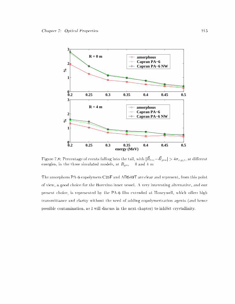
Chapter 7: Optical Properties 215
0.2 0.25 0.3 0.35 0.4 0.45 0.50
1
2
3
R = 0 m
%
amorphous Capran PA−6 Capran PA−6 NW
0.2 0.25 0.3 0.35 0.4 0.45 0.50
1
2
3
energy (MeV)
%
R = 4 m amorphous Capran PA−6 Capran PA−6 NW
Figure 7.8: Percentage of events falling into the tail, with j~Rrec� ~Rgenj > 4�x;y;z , at di�erentenergies, in the three simulated models, at Rgen = 0 and 4 m
The amorphous PA-6 copolymers C38F and ADS40T are clear and represent, from this point
of view, a good choice for the Borexino inner vessel. A very interesting alternative, and our
present choice, is represented by the PA-6 �lm extruded at Honeywell, which o�ers high
transmittance and clarity without the need of adding copolymerization agents (and hence
possible contamination, as I will discuss in the next chapter) to inhibit crystallinity.

Chapter 8
Radiopurity Issues
An overview of backgrounds in Borexino has been presented in {3. In this chapter I will
provide a deeper insight into the radiopurity and background issues related to the scintil-
lator containment vessel, including measurements, simulations and references to the CTF
experience. There are three major background concerns that have driven the inner vessel
material and design choices.
1. rays from 40K and from the 238U and 232Th radioactive chains penetrate into the
�ducial volume and contribute to the external background rate, while � and � decays
only produce \surface" background.
2. 222Rn produced in the 238U chain di�uses out of the nylon into the scintillator volume.
This has the potential to limit Borexino's sensitivity to the solar neutrino signal.
3. Depending on the history of the �lm's exposure to 222Rn, 210Pb (�1=2 = 22 years)
builds up on the vessel surface and later washes out in the Borexino sensitive volume.
Its daughters, 210Bi (�) and 210Po (�) contribute a non-taggable internal background
in the neutrino energy window.
I will discuss each item separately in x8.1 and then add a few considerations regarding the
outer vessel in x8.2 and on the auxiliary components (endplates, pipes, ropes) in x8.3.
216

Chapter 8: Radiopurity Issues 217
Table 8.1: Nylon radiopurity measurements performed with NAA by R. Von Hentig andT. Riedel, Munich, 1998-1999 [163]
Material brand name 238U (ppt) 232Th (ppt) Knat (ppb) Na (ppb)
Sniamid ADS40T pellets < 5.5 < 33 1.6 7.25Sniamid ADS40T pellets < 445 < 8 14Sniamid ADS40T �lm (Leistriz) < 63 < 8 72Selar PA3426 pellets < 24 < 29 49 0.23Capron B73ZP pellets < 11 < 10 25Capron B73ZP �lm (Leistriz) 115� 16 342� 70 500� 142C90 �lm (Leistriz) < 300 < 11 25
8.1 Nylon Film for the Inner Vessel
8.1.1 Measured 238U, 232Th and 40K Content in Nylon
Throughout the material selection campaign performed for Borexino, radiopurity measure-
ments in the nylon for the inner vessel have proven to be the most challenging. Before
choosing the most suitable material, we needed to know the 238U and 232Th content in the
�lm with a sensitivity of 1 ppt in mass (10�12 g/g) and Knat with a sensitivity of 1 ppb in
mass (10�9 g/g). The only other material in Borexino with a stricter requirement than this
is the scintillator itself, for which we built the Counting Test Facility.
Most other detector components have been characterized by germanium detectors in-
stalled in the LNGS underground laboratory [161, 162]. These detectors can reach a maxi-
mum sensitivity of about 0.2 mBq/kg, that is � 2�10�11 g/g 238U and 232Th or 6�10�8 g/g
Knat, not good enough for the nylon �lm.
Our German collaborators in Munich performed several measurement with their Neutron
Activation Analysis (NAA) facility [71], which was designed and optimized for the detection
of impurities in liquid scintillators. Their results, reported in table 8.1, are mostly upper
limits; they never achieved the required sensitivity with a nylon matrix.
The best sensitivity has been reached with Inductively Coupled Mass Spectrometry
(ICP-MS). Measurements of nylon pellets and �lm have been performed for us by Tama

Chapter 8: Radiopurity Issues 218
Table 8.2: Measurement performed by Tama Chemicals in 1993 with ICP-MS and GF-AAS.The quoted error is the standard deviation over three measurements. [164]
Material brand name sample form 238U (ppt) 232Th (ppt) Knat (ppb) Na (ppb)
Durethan C38F pellets 1.2 � 0.4 2.6 � 0.3 0.6 � 0.2 43 � 7Durethan C38F �lm 2.4 � 0.6 2.6 � 0.5 2.9 � 0.5 31.5 � 1.2Durethan B40F pellets 0.6 � 0.1 1.6 � 0.3 < 0.5 0.7Ultramid B36F pellets 42 � 1 4.2 � 0.3 3.9 � 0.6 17 � 2.3Grilamid TR55 pellets < 1.0 < 1.0 < 0.5 52 � 3.6Selar PA3426 pellets 6.1 � 0.8 7.5 � 0.2 6.3 � 2.8 130 � 12isophthal powder 91 35 25 26
Chemicals Co., a Japanese company specialized in the production of ultra-pure chemicals,
with an U.S. branch at Moses Lake Industries, WA. Their measurement technique involves
a cleaning pre-treatment with a detergent and with an ultrasonic bath, in order to re-
move dust particles that could contaminate the measurement. After cleaning, the samples
have been decomposed, or digested, through the addition of high purity sulfuric, nitric and
perchloric acid [164] and then measured in the mass spectrometer. Each result has been
compared to that obtained with a reagent blank measurement. A �rst measurement cam-
paign has been performed in 1993 for CTF: at that time, the company also measured Knat
and Na with Graphite Furnace Atomic Absorption Spectroscopy (GF-AAS); those results
are summarized in table 8.2. A new set of measurements, reported in table 8.3, has been
performed in November 1999 on candidate �lm and pellets for the Borexino inner vessel.
The measurements show, as a general trend, that all the candidate materials have good
radiopurity properties:
1. Sniamid ADS40T pellets contain 1.1 ppt 238U and 1.6 ppt 232Th, according to Tama
Chemicals (table 8.3). The Knat content has been measured in Munich and it is of
the order of 14 ppb.
2. Durethan C38F pellets contain 1.2 ppt 238U, 2.6 ppt 232Th and 0.6 ppb Knat (ta-
ble 8.2).

Chapter 8: Radiopurity Issues 219
Table 8.3: Measurements performed by Tama Chemicals in 1999 by ICP-MS. The quotederrors are the standard deviations over 5 measurements for each sample. [164]
Material brand name sample form 238U (ppt) 232Th (ppt)
Sniamid ADS40T pellets 1.1 � 0.0 1.6 � 0.1Sniamid ADS40T �lm (Leistriz) 2.8 � 0.1 3.8 � 0.2Capron B73ZP pellets 0.46 � 0.04 1.1 � 0.1Selar PA3426 pellets 0.22 � 0.02 0.65 � 0.17C90 (90% Capron, 10% Selar) �lm (Leistriz) 1.6 � 0.2 2.9 � 0.1C38F �lm (Mobay) 1.7 � 0.2 3.9 � 0.5
3. PA-6 pellets (Capron B73ZP and Durethan B40F) contain about half the radioim-
purities that are found in the copolymers: 0.5 ppt 238U and 1 ppt 232Th. The Knat
content of Capron B73ZP pellets is of the order of 15 ppb. The Selar PA3426 resin
also has a low 238U and 232Th content (less than 1 ppt). Any blend of Selar PA3426
with nylon-6 will be cleaner than the copolymers.
The measurement of isophthalic acid performed by Tama Chemicals (table 8.2) indicates
that the copolymerization agents are responsible for the higher 238U content, even though
they are only at the level of 1% in mass. This result highlights the advantage of using plain
PA-6, instead of the copolymers. Our favorite candidate is now the amorphous �lm extruded
by Honeywell from pellets of PA-6 Capron B73ZP (Allied Signal). We are in the process of
obtaining �nal batches of nylon pellets, which will be sent to Tama for measurement.
The �lm samples consistently show higher 238U and 232Th content. The results in
table 8.3 indicate that both the �lm extrusion performed at Leistriz in summer 1998 and
the one at Miles Mobay in 1993 added about 1 ppt 238U and 2 ppt 232Th to the material.
This is likely to be due to dust particles falling into the melt, at the time of extrusion,
despite the plastic tent and the HEPA air �lters that we installed around the machinery,
to reproduce a clean room environment. This is a bulk contamination that we will not be
able to remove once the extrusion is completed; the only way to minimize it is to protect
the melt from dust.
Chapter 8: Radiopurity Issues 220
Another potential problem for Borexino are surface dust deposits. Mineral dust particles
typically have a high U and Th content, of the order of 1 ppm 238U and 232Th for limestone
and sandstone and between 5 and 10 ppm in granite [165]. Few invisible dust particles
deposited on the vessel surface could contribute an overwhelming background in Borexino.
The Munich NAA measurements (table 8.1) found a very high level of 238U, 232Th and
Knat in one of the �lm samples (PA-6 Capron B73ZP). While all the other results were only
upper limits, this measurement found contamination values �100 times higher than those
obtained by ICP-MS. We learned, though, that the sample had not been cleaned before
the measurement. Surface dust contaminations is likely to have taken place at the time
of extrusion and while the sample was being handled for packaging and shipping, because
of exposure to room air. Tama is presently performing measurements of 238U, 232Th and
Knat on three samples of the amorphous PA-6 �lm extruded at the Honeywell plant. One
of the samples is being measured as received from the extruder, one has been throughly
rinsed with deionized water and the third is being pre-treated with an aggressive cleaning
procedure. A comparison of the three result will tell us whether the surface contamination
on the �lm is at acceptable levels and, if not, whether cleaning with deionized water is
enough to remove the dust contaminant. Unfortunately, the results are still not available,
at this time.
A third and independent attempt at measuring the radiopurity of nylon is in progress in
Heidelberg, where our collaborators from MPI Heidelberg and the University of Krak�ov are
measuring 222Rn emanation from nylon in presence of water vapors. As I discussed in {6,
water enhances 222Rn di�usion through the nylon, so that the di�usion length becomes
comparable to the �lm thickness (�0.1 mm). A 9.7 kg roll of 0.1 mm nylon �lm Capran
DF400 was placed in a 80 l emanation chamber for a period of 5 weeks and absorbed 1.3 l
of ultraclean water. The wet nylon was then left in the evacuated chamber for a few extra
weeks and 222Rn emanating from the material collected on charcoal traps and measured
with proportional counters, with the method described in refs. [166, 167]. The result is a

Chapter 8: Radiopurity Issues 221
226Ra concentration of the order of:
A226Ra = 5:6� 10�4Bq=kg ) 46 ppt 238U equivalent:
This particular �lm sample has been commercially extruded and the �lm roll has been
cut and prepared for the measurement in a class 100 clean room. Possible dust surface
contamination has taken place at the time of extrusion: we had no control on this. I
performed a dust particle count on a sample of the same �lm, in a clean room. The result
was 4.6 particles/mm2 with a diameter of � 10�m. On a 0.1 mm thick �lm, with two faces
exposed, and using the contamination value of 10�6 g/g 238U(mineral dust particles [165]),
this would contribute a 222Rn emanation comparable to that of 200 ppt 238U in the nylon
�lm (20�Bq/m3 222Rn in the scintillator). Of course these numbers are only approximative
and some of the dust particle I saw on the �lm are probably nylon fragments rather than
mineral particles, but this is an indication that the Heidelberg result, as well as the Munich
result, are a�ected by the presence of dust on the �lm surface, since the measured �lm
sample had not been pre-cleaned.
The conclusion we can draw from all these measurements is that the nylon �lm is
suÆciently clean for our requirements if we control the amount of dust particles falling in
the melt at extrusion and carefully maintain a clean surface during the vessel fabrication
and installation. Our strategy for cleanliness is outlined in x5.5.2.
8.1.2 Estimated Background from the Nylon Film in Borexino
I performed a Monte Carlo simulation of the background induced by the inner vessel in
Borexino if the contamination is the one measured by Tama Chemicals for the �lm samples:
238U = 2ppt; 232Th = 4 ppt; Knat = 10 ppb:
The simulation has been performed with the codes described in x3.1. It takes into
account rays emitted by the 238U and the 232Th chains and the 1.46 MeV ray emitted
by 40K in the bulk material of the nylon vessel. Spatial cuts have been performed using the
center of gravity of the detected light as event position. Table 8.4 quotes the expected daily

Chapter 8: Radiopurity Issues 222
energy (MeV)
rate
(ev
ents
/day
/0.0
5 M
eV)
0.2 0.4 0.6 0.8 1 1.2 1.4 1.6 1.8 210
−4
10−2
100
102
104
backgr. from PMTs − total backgr. from nylon − total backgr. from PMTs − in 100 tons backgr. from nylon − in 100 tons
Figure 8.1: Background spectra from the nylon of the inner vessel and from the phototubes,in the whole sensitive volume and in the 100-ton �ducial volume. The spatial cut is per-formed on the position of the center of gravity of detected light. Note, in the inner vesselbackground spectra, the peak due to the 1.46 MeV line from 40K.

Chapter 8: Radiopurity Issues 223
Table 8.4: Estimated background from the nylon vessel, with 2 ppt 238U, 4 ppt 232Thand 10 ppb Knat, compared to the one from 2200 phototubes, each with 112�g 238U, 50�g232Th and 62mg Knat. The units are counts/day.
E > 250 keV 238U 232Th 40K total I.V. total PMT
RF:V: = 3.00 m 0.012 0.02 0.02 0.05 53.50 m 0.2 0.2 0.4 0.8 564.00 m 8 6 9 22 7744.25 m 56 41 51 147 2691
E = 250� 800 keV 238U 232Th 40K total I.V. total PMT
RF:V: = 3.00 m < 0:01 0.002 < 0:01 < 0:01 0.08 � 0.043.50 m 0.025 0.004 < 0:01 0.03 3.64.00 m 3.0 1.3 0.6 5 2164.25 m 29 19 8 56 1294
E = 800� 1300 keV 238U 232Th 40K total I.V. total PMT
RF:V: = 3.00 m < 0:01 < 0:01 0.002 < 0:01 0.5 � 0.13.50 m 0.02 0.04 0.02 0.08 114.00 m 1.2 1.7 1.0 4 2164.25 m 10 11 19 40 658
rates in the di�erent energy windows of interest for the solar neutrino, compared to the
background from the phototubes. Figure 8.1 shows the background spectra from the vessel
and from the phototubes, with and without �ducial volume cut. Even in the most external
regions of the vessel, the background from the phototubes is about 20 times higher than
that from the nylon.
Conversely, the numbers in table 8.4 can be used to estimate the maximum allowed
radiopurity levels in the �lm, from the requirement that the background from each con-
taminant be less than or equal to 1/10 of the phototube signal; in the 300-ton sensitive
volume:
238U < 8 ppt; 232Th < 24 ppt; Knat < 30 ppb: (8.1)
The numbers reported in table 8.4 refer to background only. There are, of course, also
� and � decays taking place in the nylon �lm. The main di�erence is that � particles and
electrons do not penetrate into the scintillator like rays do; the average path of a 1 MeV

Chapter 8: Radiopurity Issues 224
electron is 1 cm, so even though they punch through the vessel, they remain con�ned in a
region close to the vessel surface. How much these events contribute to the background rate
in the �ducial volume depends on the spatial resolution of the event position reconstruction.
Based on the CTF experience and tests run with the present reconstruction code, we can
expect a spatial resolution of about 11 � 13 cm for events in the neutrino window. This
means that, assuming a Gaussian behavior, less than 1% of the point-like events taking
place next to the vessel surface will be reconstructed at R<3.85 m. There could be also an
e�ect from non-Gaussian tails in the reconstructed position distribution, but this cannot be
evaluated until we know the actual detector performance. Despite these uncertainties, we
can pretty safely assume that the overall �+ � background does not penetrate the �ducial
volume.
8.1.3 Radon Emanation and Internal Background
The formalism for Radon emanation from the nylon has been described in detail in {6. In
this section, I will apply it to the case of Borexino, in order to set an upper limit to the
allowed inner vessel radiopurity.
Let us assume, for a moment, that the only 222Rn source in Borexino is 226Ra in equilib-
rium with the bulk 238U content of the nylon �lm. 222Rn is a gas and can di�use out of the
material; once it is inside the inner vessel, it decays and becomes a source of internal back-
ground. The 222Rn concentration pro�le inside the nylon �lm is described by the stationary
solution for the di�usion problem (eq. 6.13) with boundary condition �(0) = �(d) = 0,
where d is �lm thickness:
�(x) =A
�
"1�
e�x � e��x
e�d � e��d+e�(x�d) � e��(x�d)
e�d � e��d
#: (8.2)
A is the speci�c activity of 226Ra in nylon and ��1 =pD=� is the di�usion length, the
average distance a 222Rn atom travels inside the material before decaying. As shown in x6.2,
the e�ective amount of 222Rn di�using out of the nylon into the inner vessel is that produced
in a surface layer of thickness equal to the di�usion length ��1. In the spherical geometry of
Borexino, assuming all the 222Rn that di�uses out of the nylon is swept away by conduction

Chapter 8: Radiopurity Issues 225
currents and uniformly redistributed in the scintillator volume, the equilibrium activity is:
A222Rn = A226Ra innylon3��1
R; (8.3)
where A222Rn is the speci�c activity of 222Rn di�used in the scintillator and R is the inner
vessel radius. A226Ra, the226Ra speci�c activity in nylon, can be calculated from the
measured 238U concentration, in the hypothesis of secular equilibrium inside the material:
1 ppt 238U = 10�12 g=g 238U = 1:235� 10�5Bq=kg = 1:4� 10�8Bq=cm3 (8.4)
(the typical density for nylon-6 is equal to 1.13 g/cm3). In order to calculate ��1, we need
to know the di�usion coeÆcient D. With the value measured by M. W�ojcik, for nylon in
pseudocumene [150]:
D = (2:0� 0:5)� 10�12cm2s�1 ) ��1 = 9:8� 10�4cm: (8.5)
If this radon is uniformly distributed inside the inner vessel, the concentration of emanated
222Rn will be:
A222Rn = Nppt � 1:0� 10�7Bq=m3; (8.6)
where Nppt is the number of 238U ppt's in the nylon bulk.
The resulting internal background is a much more critical problem than the back-
ground from the bulk of the nylon. Fig. 8.2 shows how the neutrino signal in the MSW
small angle scenario compares to the 222Rn chain activity in the 100-ton �ducial volume,
given 2 ppt 238U in the nylon �lm.
The eÆciency of software cuts will be fundamental in allowing the identi�cation of a
neutrino spectrum. The cuts shown in �g. 8.2 are applied in the following order:
1. Bi-Po correlated events allow a direct identi�cation of 214Bi events with 95% eÆciency,
while the �'s from 214Po will be detected on a separate channel;
2. � events will be directly identi�ed via Pulse Shape Discrimination - the plots assume
a 90% identi�cation eÆciency;

Chapter 8: Radiopurity Issues 226
energy (MeV)
rate
(ev
ents
/day
/0.0
5 M
eV)
0.2 0.4 0.6 0.8 1 1.2 1.4 1.6 1.8 210
−4
10−3
10−2
10−1
100
101
102
neutrino rate (MSW small angle)all background events (gr1+gr2)after Bi−Po identification after alpha cut after statistical subtraction
Figure 8.2: Neutrino events in Borexino, in the MSW small angle model, compared to thebackground induced by 2 ppt 238U in nylon (radon emanation), before and after applyingbackground cuts.

Chapter 8: Radiopurity Issues 227
Table 8.5: case of 2 ppt 238U in nylon: internal background rates (events/day) due toemanated 222Rn, neutrino rates and signal to noise ratios in the 100-ton �ducial volume.
E> 250 keV 250� 800 keV 800� 1300 keV
all 26 20 1.3CE 95% 16 15.5 0.5PSD 90% 6.4 5.7 0.5SS 95% 1.1 0.8 0.04
SSM 64 59 3.4MSW LA 35 33 1.8MSW SA 14 13 0.7
S/N ratio with all the cuts: case of 2 ppt 238U in nylon
SSM 59 74 77MSW LA 32 41 40MSW SA 13 16 17
3. the knowledge of the number of Bi-Po events allows a statistical subtraction of the
activities from other 222Rn daughters; assumed 95% eÆciency.
If these eÆciencies are realized, we can substantially increase the signal/background ratio
even in the MSW small angle scenario (see table 8.5) and with the assumption of 2 ppt 238U
in nylon. Without software cuts, the neutrino/background ratio in the neutrino window
becomes comparable to 1.
The design goal is to keep the 238U content of the nylon �lm at the level of 1 ppt; if we
fail in this goal and the 238U level becomes higher than 2-3 ppt, only an eÆcient background
identi�cation will allow a clean identi�cation of the neutrino signal. The ultimate limit is:
238U < 10 ppt; (8.7)
above which the neutrino identi�cation will be allowed only through sophisticated algo-
rithms. Note that if the nylon �lm were to be wet, the 222Rn emanation would be about
ten times more intense, due to the e�ect of water on nylon described in {6. In that case,

Chapter 8: Radiopurity Issues 228
the ultimate limit to the 238U content of the nylon would drop to 1 ppt. This is an un-
likely scenario for Borexino, but it proves the importance of a deeper understanding of the
dependence of 222Rn di�usivity on the humidity level in the �lm and in the scintillator.
8.1.4 Surface Contamination
Although 222Rn is relatively short-lived and most of its progeny is in equilibrium with it at
any time, one of its products can pose a time-delayed background threat for Borexino. 210Pb
has half life �1=2 = 22:3 years; its decay is followed by 210Bi (� with end-point energy at 1.16
MeV and �1=2 = 5:01 days) and 210Po (� with E=5.3 MeV �1=2 = 138:4 days). Exposure of
the nylon �lm to 222Rn, at any time between extrusion and installation, results in a deposit
of 210Pb on the surface. Part of it will later wash out into the scintillator and will contribute
a long term, non taggable background signal.
In order to understand the consequences of this plate-out e�ect, we can consider the
following worst case assumptions:
- the nylon �lm is exposed for � 1 hour to air at 20 Bq/m3 222Rn;
- all the 210Pb in a 3-m column of air above the �lm plates out on the unprotected
nylon surface;
- there is no scrubbing/cleaning procedure;
- all the 210Pb then washes out in the scintillator.
If all these conditions are satis�ed, the concentration of 210Pb dissolved into the scintillator
becomes 1:5 � 10�4 Bq/m3, which translates in � 1:5 � 103 events/day for each daughter
in the 100-ton �ducial volume. Of course, this calculation is much too conservative, but
it gives us a goal of a factor 1000 reduction, which would give � 1:5 � 10�7Bq/m3 or
1.5 events/day/isotope in the 100-ton �ducial volume. In order to achieve this goal, we are
taking a number of steps, including minimization of the 222Rn exposure, cleaning procedures
and a campaign of plate-out and wash-o� measurements. More details and references are
provided in x5.5.2.

Chapter 8: Radiopurity Issues 229
energy (MeV)
rate
(ev
ents
/day
/0.0
5 M
eV)
0.2 0.4 0.6 0.8 1 1.2
10−2
10−1
100
101
102
103
104
neutrino rate (MSW small angle) identified 210Po alphas (90% PSD)1.5x10⁻⁴ Bq/m3 210Pb identified 210Po alphas (90% PSD)1.5x10⁻⁷ Bq/m3 210Pb
Figure 8.3: Background spectra in the 100-ton �ducial mass produced by 210Pb dissolvedin the scintillator, in the worse-case scenario and after the suppression. The shaded areasare 210Po �s, directly identi�ed via pulse shape discrimination (90% eÆciency assumed).Overlapped is the expected � signal in the MSW small angle scenario.
Fig. 8.3 shows how, after the reduction, the expected background is safely below the
expected neutrino signal.
8.2 The Outer Vessel
The need for a second nylon vessel became clear during the CTF �rst run. The results,
quoted in [51] and summarized in table 8.2, show that the 222Rn content of the shielding
water (25 � 30 mBq/m3) absolutely dominated the count rate, in the form of external
background. Its contribution has been identi�ed and separated from the surface and internal
background through a �t of the radial distribution. Moreover, the detector sensitivity was
limited by 222Rn: the measured 238U content in the scintillator, (3:5 � 1:3) � 10�16 g/g,
is consistent with the di�usion of 222Rn from the water, through the inner vessel, into the
Chapter 8: Radiopurity Issues 230
Table 8.6: CTF measured backgrounds in the neutrino window (250-800 keV) [51]
before puri�cation after puri�cation
External background (counts/day) 1700� 270 2050� 100Surface background (counts/day) 350� 190 170� 60Internal background (counts/day) 470� 90 21� 47
sensitive volume (see x6.4).
A second nylon bag for CTF2 was suggested as a solution to the radon problem in CTF.
Its purpose is to create a bu�er region outside the inner vessel in CTF2, with ultrapure
water and a lower 222Rn content. The idea has been extended to Borexino, where the
di�usion issues are less dramatic, but the external background due to radon dissolved in
the bu�er liquid is still an issue.
8.2.1 External Background and -ray Shielding
In the absence of a bu�er region, the rays generated by 222Rn daughters have a high
probability of entering the sensitive volume and dominating the signal, in the form of
external background, as occurred in the CTF. The e�ect of an ideally sealed second nylon
vessel is to keep the sources (222Rn daughters) away from the detector sensitive volume.
The bu�er region will act as a passive shield.
The inner vessel will have radius RIV = 4:25m, while the outer vessel will have radius
R2 = 5:25m. They will both be built of PA-6 amorphous �lm with a � 0:125mm thickness.
Table 8.7 shows the results of a Monte Carlo simulation where the rays from 222Rn
daughters in di�erent regions of the bu�er have been treated separately. As one would
expect, the bu�er region attenuates rays produced outside the second vessel by a factor
of � 200. This means that the background produced by 1 mBq/m3 outside the I.V. is
equivalent to the background produced by � 200 mBq/m3 outside the second vessel.
In order to establish the 222Rn concentration we can a�ord to have outside the second
vessel, in Borexino, we can compare the numbers reported in table 8.7 with the background

Chapter 8: Radiopurity Issues 231
Table 8.7: Results of a Monte Carlo simulation of the background rate (events/day)induced by a uniform concentration of 222Rn equal to 1 mBq/m3 in the Borexino bu�er uid. The contribution of 222Rn in di�erent spherical shells is analyzed separately.
Shell radius start (m) 4.25 4.85 5.05 5.25 5.45 5.65Shell radius stop (m) 4.85 5.05 5.25 5.45 5.65 5.85shield thickness (m) 0 0.60 0.80 1.00 1.20 1.40
events/day due to 1 mBq/m3 uniform 222Rn
> 0:25 MeV 2368 70 27 11 4 20:25� 0:8 MeV 1364 40 15 6 2 10:8� 1:3 MeV 473 16 6 3 1 0.5
shield attenuation factor for 's 1 0.03 0.011 0.005 0.002 0.001equivalent activities (mBq/m3) 1 33 90 200 500 1000
Table 8.8: Background rate from 222Rn compared to the background rate from the PMTs.No spatial cuts have been applied.
Source 1 mBq/m3 222Rn 20 mBq/m3 222Rn PMTsoutside the I.V. outside the second vessel total
E > 0:25MeV (ev/day) 2:4� 103 2:1� 102 2:7� 103
0.25 - 0.8 MeV 1:4� 103 1:2� 102 1:3� 103
0.8 - 1.3 MeV 4:7� 102 5:2� 101 6:6� 102

Chapter 8: Radiopurity Issues 232
from the phototubes: as one can see in table 8.8, the background from 1 mBq/m3 222Rn in
the bu�er is consistent with the overall background from the phototubes. This means that
in principle, if the second vessel is perfectly sealed, we can a�ord a level of � 20 mBq/m3
outside the second vessel and still have � 1/10 of the background from the phototubes.
8.2.2 Radon Permeation Through the Nylon Vessels
The work on 222Rn di�usion through nylon, discussed in {6, showed that this is less of a
concern in Borexino than it is in CTF2, since both inner and outer vessel will be in contact
with pseudocumene and the 222Rn permeability should remain low.
Assuming the vessels are perfectly sealed, we can calculate how much 222Rn would get
into the bu�er and the scintillator, using the formalism for radon di�usion introduced in {6.
The ratio of 222Rn concentration inside and outside each vessel can be calculated as follows:
=[Rn]in[Rn]out
= Pe�1
�d2VnylonVin
; (8.8)
where:
Pe� = DS�d
sinh �d= e�ective permeability: (8.9)
In the 3- uid con�guration of Borexino, let's de�ne:
- A1 =222Rn concentration inside the Inner Vessel;
- A2 =222Rn concentration in the bu�er (between the two bags);
- A3 = 222Rn concentration in the region between the second vessel and the stainless
steel sphere.
If we use d1 = d2 = 0:125mm for the inner and outer vessel thickness and the di�usion
parameters D = 2:5� 10�12 cm2/s, S=1.0 [150], then:
��1 = 0:011mm; Pe� = 6:6� 10�16 cm2=s; (8.10)
and the barrier factors for the two bags are, respectively:
1 = A1=A2 ' 2� 10�10 for the inner vessel; (8.11)
2 = A2=A3 ' 3� 10�10 for the outer vessel: (8.12)

Chapter 8: Radiopurity Issues 233
We can then conclude that the 222Rn di�usion through the nylon �lm in Borexino is negli-
gible.
Of minor relevance is also the emanation of radon from the second bag: if the 238U
content in nylon is Nppt � 10�12g/g and the 222Rn di�usion length is the one quoted above,
we have, in the bu�er region:
Abu�er = Nppt � 1:13� 10�4 mBq=m3: (8.13)
The 222Rn production in the bu�er itself, due to 238U, is not a concern, either, if the
bu�er purity is at the level we are aiming for: 10�16g/g 238U is equivalent to 10�3mBq/m3
222Rn.
The only potential 222Rn problem, in this design, are leaks in the outer vessel or in the
uid recirculation system. The �nal goal is to maintain a level of 0.1 mBq/m3 in the region
between the two vessels, in order to keep the external 222Rn background at � 1=10 of that
from the phototubes.
8.3 Auxiliary Components of the Inner Vessel
The inner vessel is mostly nylon �lm, but the hold-down ropes, the endcaps and the pipes
attached to them are also a background source close to the sensitive volume.
The design for the endcap region is now approaching its �nal stage, although there is
still some uncertainty on the material and its mass. More details on the mechanical design
are provided in x5.5.1 and a drawing of the present design of the north pole endcaps for the
inner and outer vessel, with the connections to the stainless steel sphere and the external
tank, is shown in �gure 5.10. In this context it is enough to say the idea is to use endcaps
of solid nylon, with a total mass of 12 kg. Attached to the endcap is a 1 m nylon pipe with
a 10 cm (4") diameter and a total mass of 4.2 kg. The outer vessel endplates are at a 1 m
distance from the vessel, which is enough to shield the activity from their nylon parts. There
are, though, also some steel parts, for a total mass of 15 kg at R = 5:25m. The material
for the hold-down ropes is now being de�ned; details on the candidate materials and their

Chapter 8: Radiopurity Issues 234
Table 8.9: Monte Carlo simulation of background from the auxiliary components of theinner vessel, based on our best radiopurity knowledge and on the present design mass values.Both event rates in the 200-ton large �ducial volume and the 300-ton sensitive volume arereported. The rates are expressed as events/day.
Mass 238U 232Th Knat60Co 0.25{0.8 MeV 0.8{1.3 MeV 1.3{1.6 MeV
kg ppb ppb ppm mBq/kg 200 t 300 t 200 t 300 t 200 t 300 t
Phototubes 28 1294 50 658 56 500inner vessel nylon plate12 0.05 0.05 0.7 4 567 6 661 51 1108pipe inner-outer vessel4.2 0.05 0.05 0.7 0.7 50 1.4 35 3 45outer vessel steel plate15 1 2 0.07 10 3.5 116 2.5 38 2.5 20�ber ropes4.5 0.05 0.05 1 2 250 3 320 26 567
tensile properties are provided in x5.6. Our best option at this moment is Tensylon, with a
total mass of 4.5 kg.
The radiopurity requirements on these materials are less stringent than those on the
nylon �lm and 238U and 232Th are normally below our goal limits (de�ned in table 8.10).
The major problem we need to face is that of potassium, which is a major contaminant
both in bulk nylon (x8.3.1) and in the �bers for the hold-down ropes (x5.6). The steel parts
at the level of the outer vessel endcap are also a concern, especially for 60Co.
Table 8.9 reports the results of a Monte Carlo simulation of background from each
component, compared to that of the phototubes. The quoted radiopurities are based on
our present best knowledge; more information on the status of measurements is provided
in the dedicated subsections. In order to compare to the rest of the external background, I
quote both the total rate in 300 ton and in a 200 ton \large" �ducial volume.
Based on these simulations, I determined the ultimate allowed radiopurity limits, from
the requirement that each component contribute at most 1/10 of the background from the
phototubes in the 200 ton �ducial volume, both in the 7Be neutrino window (0.25{0.80MeV)

Chapter 8: Radiopurity Issues 235
Table 8.10: Maximum allowed radiopurity levels in the auxiliary components of the innervessel, derived from the requirement that each contaminant contribute at most 1/10 thebackground from the phototubes in the 7Be neutrino window and in the pep window, in the200-ton \large" �ducial volume. For each contaminant, the corresponding activity is alsoreported, expressed in terms of -Bq or events/sec.
Component 238U 232Th Knat60Co
ppb -Bq ppb -Bq ppm -Bq mBq/kg -Bq
inner vessel endplates:nylon, 12 kg 0.06 0.032 0.23 0.046 1 0.040best measured < 0.05 < 0.05 0.7
pipes inner-outer vessel:nylon, 4.2 kg 0.5 0.094 1.5 0.106 3.5 0.048best measured < 0.05 < 0.05 0.7
outer vessel endplates:steel 15 kg 6 4 5.5 1.3 12 0.6 20 0.6measured (for SSS) 1 2 0.07 10
ropes:Tensylon �ber, 4.5 kg 0.17 0.033 0.45 0.034 3 0.046measured < 0.05 < 0.05 1
and in the pep window (0.80{1.30 MeV).
In the speci�c case of potassium, a high 40K level produces a high background rate
in the 1.30{1.60 MeV energy window, where the 1.46 MeV peak is located. Although
this is not an ideal situation, a reasonable increase of background in that energy window,
due to an excess of external potassium, will not a�ect the sensitivity to the solar neutrino
signal, since it is above the pep region and below the sensitivity limit for 8B neutrinos. The
requirement of having external potassium contribute at most 1/10 of the phototube rate
in the 0.25{1.3 MeV energy region makes the background in the 1.3{1.6 MeV region of the
same order as that from the phototubes. The results are reported in table 8.10.
The requirements become stricter if applied to the whole 300 tons, because of the di�er-
ent radial distributions for external background from near and far sources. The endcaps and
Chapter 8: Radiopurity Issues 236
the ropes emit several low energy rays that are absorbed in the �rst 50 cm of scintillator.
These should not be included in the comparison with the phototubes, which, on the other
hand, provide only penetrating, higher energy ray that have survived the 2 m passive
bu�er.
The table also includes the corresponding activity from each contaminant and its
daughters. In the hypothesis of secular equilibrium, for each decay of the progenitor there
are on average 3.62 emitting events in the 238U chain and 4.144 in the 232Th chain, while
the branching ratio for decay of 40K is 0.107 and each 60Co decay contributes two 's.
8.3.1 Endcap Radiopurity
The bulk nylon to be used in the endcaps and in the pipes between inner and outer vessel
can be processed in two ways: casting or extrusion. In both cases, there is a high potential
for potassium contamination. In the procedure for casting nylon, Na salts are added to the
mixture. In extrusion and injection molding, there is a need to add mold release agents,
which are also often based on Na and sometimes on K. Potassium is chemically similar
to sodium and is often present in signi�cant amount wherever sodium is, for this reason
many surfactants and detergents are potential carriers of potassium. This problem is not
present in the extrusion of thin �lms, because mold releases are not required in that kind
of operation.
Table 8.11 reports the results of measurements obtained in a screening campaign that
started in May 2000 and is still in progress. We collaborated with two di�erent facilities:
the Missouri University Research Reactor (MURR) performs Instrumental Neutron Acti-
vation Analysis (INAA) on potassium, while ACSLabs (a company based in Houston, TX)
measures uranium and thorium with ICP-MS (sensitivity of 50 ppt), and potassium with
ICP-AXIAL (sensitivity of 5 ppb). The key point is that potassium is present in all the
samples, with a concentration that varies between 0.4 and 4 ppm.
The way samples are handled before measurement is, of course, very important: �nger-
prints can easily produce a high potassium contamination, at the ppm level. The samples
have been cleaned in di�erent ways, the most eÆcient being immersion in an ultrasonic bath
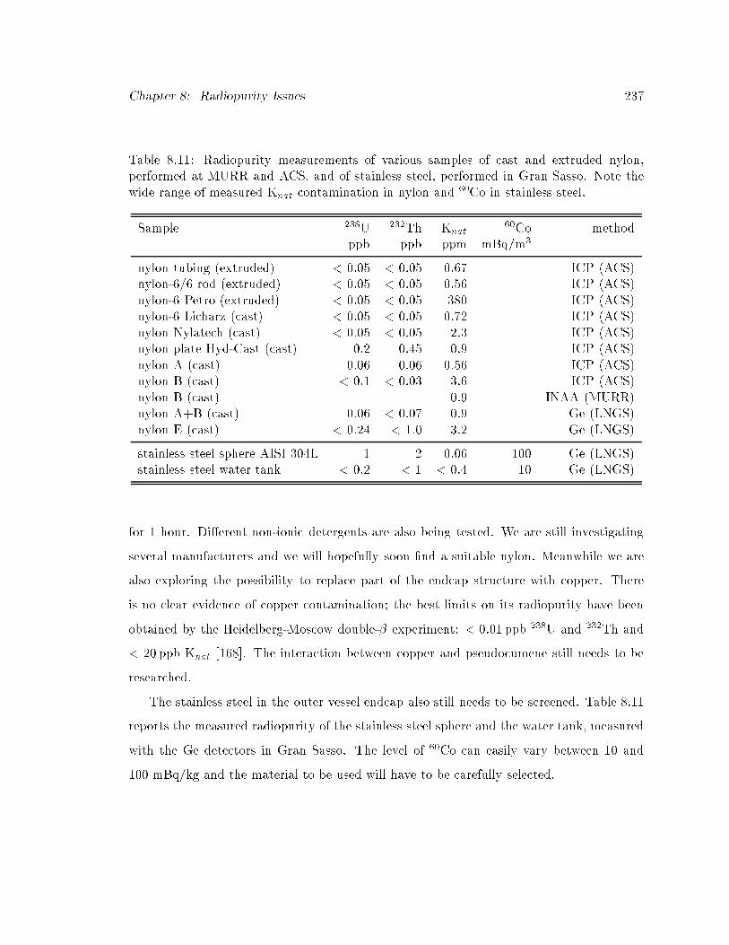
Chapter 8: Radiopurity Issues 237
Table 8.11: Radiopurity measurements of various samples of cast and extruded nylon,performed at MURR and ACS, and of stainless steel, performed in Gran Sasso. Note thewide range of measured Knat contamination in nylon and 60Co in stainless steel.
Sample 238U 232Th Knat60Co method
ppb ppb ppm mBq/m3
nylon tubing (extruded) < 0.05 < 0.05 0.67 ICP (ACS)nylon-6/6 rod (extruded) < 0.05 < 0.05 0.56 ICP (ACS)nylon-6 Petro (extruded) < 0.05 < 0.05 380 ICP (ACS)nylon-6 Licharz (cast) < 0.05 < 0.05 0.72 ICP (ACS)nylon Nylatech (cast) < 0.05 < 0.05 2.3 ICP (ACS)nylon plate Hyd-Cast (cast) 0.2 0.45 0.9 ICP (ACS)nylon A (cast) 0.06 0.06 0.56 ICP (ACS)nylon B (cast) < 0.1 < 0.03 3.6 ICP (ACS)nylon B (cast) 0.9 INAA (MURR)nylon A+B (cast) 0.06 < 0.07 0.9 Ge (LNGS)nylon E (cast) < 0.24 < 1.0 3.2 Ge (LNGS)
stainless steel sphere AISI 304L 1 2 0.06 100 Ge (LNGS)stainless steel water tank < 0.2 < 1 < 0.4 10 Ge (LNGS)
for 1 hour. Di�erent non-ionic detergents are also being tested. We are still investigating
several manufacturers and we will hopefully soon �nd a suitable nylon. Meanwhile we are
also exploring the possibility to replace part of the endcap structure with copper. There
is no clear evidence of copper contamination; the best limits on its radiopurity have been
obtained by the Heidelberg-Moscow double-� experiment: < 0:01 ppb 238U and 232Th and
< 20 ppb Knat [168]. The interaction between copper and pseudocumene still needs to be
researched.
The stainless steel in the outer vessel endcap also still needs to be screened. Table 8.11
reports the measured radiopurity of the stainless steel sphere and the water tank, measured
with the Ge detectors in Gran Sasso. The level of 60Co can easily vary between 10 and
100 mBq/kg and the material to be used will have to be carefully selected.

Chapter 8: Radiopurity Issues 238
Table 8.12: Radiopurity measurements of �bers.
Fiber 238U 232Th Knat methodppb ppb ppm
Vectran (Liquid crystal polymer) < 0.1 < 0.03 45 ICP (ACS)Vectran (Liquid crystal polymer) 90 INAA (MURR)
Technora (Aramid) 27 41 5 ICP (ACS)Technora (Aramid) 27 INAA (MURR)
Zylon (PBO) < 0.05 < 0.05 10.5 ICP (ACS)Zylon (PBO) 34 � 12 INAA (MURR)
Spectra (HDPE) 0.6 0.9 13 ICP (ACS)Spectra (HDPE) 15 INAA (MURR)Spectra (HDPE) < 2.3 < 3 6 � 2 Ge (LNGS)Spectra (HDPE) not washed < 2.2 < 5 52 � 3 Ge (LNGS)
Tensylon powder (HDPE) < 0.05 < 0.05 0.36 � 0.18 ICP (ACS)Tensylon �ber (HDPE) < 0.05 < 0.05 1.1 ICP (ACS)Tensylon �ber (HDPE) 6 INAA (MURR)
8.4 Ropes for the Hold Down System
The material of choice for the hold-down system (see x5.6) is now being de�ned on the
basis of our radiopurity and strength requirements. The high performance �bers we have
considered, together with their mechanical properties, are listed in x5.6.
Our initial choice was Vectran, because of its high strength and its virtually null creep.
Vectran strings have been installed in CTF2, where a large peak at 1.46 keV was immediately
noticed in the data. We now believe that potassium in Vectran is responsible for that
peak [169]. For the next CTF2 vessel, which will be installed in the upcoming months, we
will revert to the nylon mono�lament that was originally used in CTF1, but this is not a
choice that we want to maintain in Borexino, given the high creep of nylon mono�lament.
In the search for an alternative rope material, we learned that anti-static coatings are
often applied to high performance �bers. These coatings, necessary to help bundle the
�bers and make ropes, are a mixture of lubricants, anti-static agents and surfactants. Their

Chapter 8: Radiopurity Issues 239
recipe is highly proprietary, but these materials often contain sodium and, in some instances,
potassium salts. Exposure to sodium (and thus to potassium) also takes place during the
process of denaturing the polymers, to create oriented �bers, in processes like gel-spinning.
We tested aggressive cleaning procedures for the removal of the coatings, the most
e�ective being a ultrasonic bath in deionized water. Some manufacturers also recommend
washing with ethanol. After cleaning, the radioactivity of the samples has been measured
at the two facilities (MURR and ACSLabs) and with the germanium counters in Gran
Sasso. The results, reported in table 8.12, agree within a factor two; the di�erence between
methods could be due to the cleaning or to measurement systematic errors, but this is
already enough to compare the di�erent �bers. Note that, in the case of Spectra, cleaning
in D.I. water reduced the potassium contamination from 52 to 6 ppm, thanks to the removal
of the coating, which came out as a white, soapy foam.
We are now concentrating our interest on the high density polyethylene �ber Tensylon,
by Synthetic Textiles, which is extruded and can be obtained without coating.
The main problem with Tensylon, as with other HPDE's, like Spectra, is creep: in these
�bers, the chains are cross linked by Van der Waals forces, instead of the stronger hydrogen
bonds that link the para-amide molecules like Technora and Kevlar. There is a gain, though,
in radiopurity; the problem of creep can be overcome by a proper rope sizing, in agreement
with the considerations presented in x5.6. Figure 8.4 shows how the relative radioactivity
of di�erent type of ropes compare if they are sized according to the two criteria (creep or
modulus) de�ned in x5.6.
From the plot, which also includes wire ropes (stainless steel, copper and Monel, a
copper nickel alloy), it is evident that Tensylon has the lowest total potassium content,
except for copper wire, which is an option we are still keeping open but which, as for the
endcaps, still requires some studies.
Tensylon ropes for Borexino should be sized with a 4.4 mm2 cross sectional area and a
linear density of 4.3 g/m (2.9 lbs/1000 ft), which for two sets of 18 strings wrapped around
the Borexino inner vessel gives a total mass of 4.5 kg. The consequences for the background
in Borexino can be seen in table 8.9: with 1 ppm Knat, these ropes will contribute a small

Chapter 8: Radiopurity Issues 240
0 0.2 0.4 0.6 0.8 10
0.1
0.2
0.3
0.4
0.5
0.6
0.7
0.8
0.9
1
Sized by modulus (arbitrary units)
Size
d by
str
engt
h (a
rbit
rary
uni
ts)
TensylonSpectra PBO Vectran Kevlar SS Cu Monel
Figure 8.4: Relative radioactivity of ropes for the hold-down system built with di�erentmaterials, if the ropes are sized according to the strength or to the modulus requirementsintroduced in x5.6. The units are arbitrary. From reference [147].
background (<1/10 of the phototubes) in the 0.25{1.3 MeV energy window and they will
give an event rate comparable to that of the phototubes and the endcaps in the 1.3{1.6 MeV
energy window.
More tests are needed, of course, before this choice becomes �nal. We are in the process
of obtaining rope woven from the Tensylon �ber. The potassium content of the end product
will have to be carefully measured. We also need to repeat measurements of strength and
creep on the �nal rope, in presence of pseudocumene and to make sure that the extrapolated
time to failure is safely far away from the prospected operational time for Borexino (see
also discussion in x5.6).

Chapter 9
Stress Studies and Shape Analysis
The scintillator containment vessel for Borexino is, ideally, a spherical shell in a neutral
buoyancy condition. Nevertheless, a 0.1% density di�erence between the scintillator and
the quenched bu�er (see x5.6) and temperature induced density uctuations can add up to
a non zero buoyancy force and induce membrane stresses in the vessel. In this chapter, I
will present the results of an ongoing study of the stress on the vessel membrane and an
analysis of the shape deformation induced by the hold-down ropes.
9.1 Thin Shell Theory
9.1.1 The Stress Tensor
Internal forces are responsible for holding together the molecules that compose a body,
balancing the external loads, which can act on the external surfaces (surface forces) or on
the whole volume (body forces). The internal forces acting at a point within the body can
be investigated by drawing a section through the point: the condition of equilibrium of the
forces acting on each portion requires internal forces on the sectioning plane.
The stress tensor �i;k is de�ned as the force per unit area in the k direction acting
on a surface element normal to the i direction, typically measured in MPa (106N/m2). For
instance:
�x = �xx = lim�A!0
�Fx�A
=dFxdA
normal stress; (9.1)
241

Chapter 9: Stress Studies and Shape Analysis 242
Figure 9.1: Sectioning of a body (a) and free body diagram of the part of the body (b), fora comparison of external and internal forces. From reference [170].
Figure 9.2: Element in plane stress (a) and two dimensional representation of plane stresselement (b). From reference [170].

Chapter 9: Stress Studies and Shape Analysis 243
�xy = �xy = lim�A!0
�Fy�A
=dFydA
shear stress: (9.2)
The equilibrium conditions can be expressed as [171]:
Xk
@�ik@xk
= 0 if no external loads; (9.3)
Xk
@�ik@xk
+ Pi = 0 if Pi = external load along i: (9.4)
The sign convention is that tensile stresses are positive, while compressive stresses are
negative.
9.1.2 The Strain Tensor
The displacement of a point inside the material, due to a deformation, is de�ned as:
�!u = �!r 0 � �!r ; ui = x0i � xi; (9.5)
where xi is the coordinate before the displacement and x0i is the coordinate after the dis-
placement. The in�nitesimal distance dl between two points, after the deformation, is given
by [171]:
(dl0)2 = (dl)2 + "ikdxidxk; (9.6)
where "ik is the strain tensor, de�ned as:
"ij =1
2
@ui@xj
+@uj@xi
+@uk@xi
@uk@xj
!: (9.7)
The strain tensor is symmetrical, thus it can be diagonalized. For any given point, there
are three principal axes, such that the strain tensor is diagonal.
The approximation of small deformations implies that each component "ik of the
strain tensor is small, while the displacements ui can still be large. In other words, each point
can change its position by a large amount, but the metric is conserved. The approximation
consists in neglecting the term @uk@xi
@uk@xj
and keeping only:
"ij =1
2
@ui@xj
+@uj@xi
!: (9.8)

Chapter 9: Stress Studies and Shape Analysis 244
The explicit expression of the strain tensor in spherical coordinates is [171]:8>>>>>>>>><>>>>>>>>>:
"r =@ur@r
"� =1r@u�@�
+ urr "� =
1r sin �
@u�@�
+ u�r cot � + ur
r
"�;� =12r
�@u�@�
� u� cot �
�+ 12r sin �
@u�@�
"r;� =12
�@u�@r
�u�r + 1
r@ur@�
�"r;� =
12
�1
r sin �@ur@�
+@u�@r
+ @ur@�
�u�r
�(9.9)
9.1.3 Hooke's Law
The elastic properties of the material provide a relation between the stress tensor and
the strain tensor. Following the formalism by Landau and Lifshitz [171], we express the
Helmholtz free energy of the deformed body as:
F = F0 +1
2�"2ii + �"2ik = F0 +
1
2K"2ii + �
�"ik �
1
3Æik"ll
�2; (9.10)
where:
F0 = free energy of the undeformed state;
� = �rst Lam�e coeÆcient;
� = second Lam�e coeÆcient, also known as shear modulus or modulus of rigidity;
K = �+ 23� = bulk modulus or hydrostatic compression term.
The stress tensor is obtained from the free energy as [171]:
�ik =@F
@"ik
����T= K"jjÆik + 2�
�"ik �
1
3Æik"jj
�: (9.11)
The inverse relation, expressing the strain tensor as a function of the stress tensor, is
Hooke's law, the fundamental law of elasticity:8><>:
"ii =13K �ii
"ik =19KÆik�ll +
12�
��ik �
13Æik�ll
� : (9.12)
Hooke's law is usually expressed in terms of the Young Modulus E and the Poisson's ratio
�, which are de�ned by the following relations:
� =
���� lateral strainaxial strain
���� ; (9.13)

Chapter 9: Stress Studies and Shape Analysis 245
� =E�
(1� 2�)(1 + �); � =
E
2(1 + �); K =
E
3(1� 2�): (9.14)
In this notation the free energy of a deformed body is:
F = F0 +E
2(1 + �)
�"2ik +
�
1� 2�"2ll
�; (9.15)
and the stress-strain relations are:
�ik =E
1 + �
�"ik +
�
1� 2�Æik"ll
�; (9.16)
"ik =1
E[(1 + �)�ik � �Æik�ll] : (9.17)
9.1.4 Membrane Stresses in Shells
The thin shell theory [170, 172] describes shells of constant thickness, where the ratio of
thickness to radius of curvature is t=R << 1=20. The model's foundation is that the shell
geometry is completely de�ned by the shape of the midsurface (the plane bisecting the shell
thickness) and by the shell thickness at any point. The three spatial variables can then be
reduced to a system of two independent variables, the coordinates on the shell midsurface.
A complete analysis of shell structures comprises two distinct theories:
� membrane theory: the membrane is treated as a surface that cannot convey mo-
ments; it is the two-dimensional analog of a exible string, but it can resist compres-
sion.
� bending theory (or general theory): it includes bending, hence it can deal with
discontinuities in the stress distribution that take place in a limited region in the
vicinity of a load or of a structural discontinuity.
Membrane stresses are simpler to calculate and, for thin shells with no abrupt changes
in thickness or curvature, they are uniform throughout the wall thickness. Membrane
forces are independent of bending and they are completely de�ned by the condition of
static equilibrium; material properties, such as its elasticity, do not enter their calculation.

Chapter 9: Stress Studies and Shape Analysis 246
The membrane theory can be usually applied to large portions of the shell, away from
discontinuities.
The bending theory essentially provides a correction to the membrane solution in areas
where there are discontinuities, like edge forces or concentrated loads.
Note that the load-resisting action of a shell is mostly carried by in-plane stressing of a
shell (membrane stress); the ratio of direct (or membrane) stress to the bending stress, in
a spherical thin shell of radius R and thickness h, is equal to [170]:
�
�b=
2R
h>> 1: (9.18)
This is why we can treat a thin shell with the membrane theory, away from the edges or
from the points of application of concentrated loads.
9.1.5 Thin Shell Theory for Shells of Revolution
A surface of revolution is a particularly simpli�ed approximation for a shell. Its midsurface
is generated by the rotation of a curve (meridian) about an axis lying in the plane of the
curve (meridian plane). Each surface element is de�ned by two meridian curves and two
parallel curves and by the principal radii of curvature r1 and r2, as shown in �gure 9.3.
Each point on the surface is identi�ed by the angular coordinates:
� = angle between the axis of the shell and the normal to the midsurface of the shell (polar
angle);
� = angle between r and a reference position ~r (azimuthal angle).
The principal axes customarily used to describe a shell of revolution are:
� Z = �er, normal to the shell's surface, equivalent to the radial direction in a sphere.
Conventionally, the positive direction points toward the center of the shell.
� Y = e�, tangential to the meridians; the positive direction is clockwise.
� X = e�, tangent to the parallels; the positive direction is counterclockwise.
FX , FY and FZ are the external forces and pX , pY and pZ are the distributed external
loads per unit surface acting on the shell in the X, Y and Z direction, respectively. External

Chapter 9: Stress Studies and Shape Analysis 247
Figure 9.3: A shell of revolution. The meridian and the parallel planes are associated withthe principal radii of curvature r1 and r2, respectively. From reference [170].
Figure 9.4: Diagrams for the analysis of symmetrically loaded shells of revolution: (a) and(b) show the membrane forces and the surface loads on a shell element, while (c) showsthe meridian forces and resultant of loading (F) acting on a truncated shell de�ned by theangle �. From reference [170].

Chapter 9: Stress Studies and Shape Analysis 248
loads applied to each section of the shell are either body forces, acting on the volume
element, or surface forces, acting on the upper and lower faces of the shell element. They
are equilibrated by stresses, or internal forces, which can be membrane forces, transverse
shears, bending moments or twisting moments. In the membrane theory description of the
shell of revolution, only the following membrane forces are relevant (see �gure 9.4):
1. N� = normal in-plane force per unit length, in the meridional direction (meridional
force). The corresponding stress component is ��� = N�=h.
2. N� = normal in-plane force per unit length, in the parallel direction (hoop force).
The corresponding stress component is ��� = N�=h.
3. N�� = N�� = in-plane shear force per unit length. The corresponding stress compo-
nent is ��� = N��=h.
9.1.6 Symmetrically Loaded Spherical Shells of Revolution
If the external load acting on the shell is axially symmetric (pX=0), we can assume there are
no shearing forces and the membrane analysis can be reduced to the two normal forces per
unit length N� and N�. In the case of a spherical shell, where r1 = r2 = R, the equilibrium
equation 9.4 translates into the following:
1. From the equilibrium of forces acting in the meridional direction:
@(N� sin �)
@��N� cos � + pY R sin � = 0; (9.19)
alternatively, we can consider the equilibrium of the portion of the shell above or
below the angle �. If F is the resultant vertical load on that portion of the shell:
2�RN� sin � + F = 0 ) N� = �F
2�R sin2 �(9.20)
2. From the equilibrium of forces in the radial direction:
N�
r1+N�
r2= �pZ ) N� +N� = �RpZ (9.21)

Chapter 9: Stress Studies and Shape Analysis 249
The stress-strain relation (Hooke's law) translates into:8><>:
"� =1E(�� � ���) =
1Eh
(N� � �N�)
"� =1E (�� � ���) =
1Eh
(N� � �N�)(9.22)
The displacements are derived, according to Timoshenko et al. [172], as:8><>:
"� =1r1dvd�� wr1
"� =vr2 cot � �
wr2
)
8><>:
dvd�� v cot � = r1"� � r2"�
w = v cot � � r2"�; (9.23)
where:
w = �ur = displacement in the direction perpendicular to the surface (positive if towards
the center);
v = u� = displacement in the meridional direction (positive if clockwise);
u = u� = hoop displacement.
The meridional displacement, at di�erent latitudes, is found from the solution of:
dv
d�� v cot � = f(�) )
d
d�
�v(�)
sin �
�=
f(�)
sin �; (9.24)
where:
f(�) =1
E[��(r1 + �r2)� ��(r2 + �r1)] =
R(1 + �)
hE(N� �N�): (9.25)
From this we can �nd also the radial displacement:
w = v cot � � r2"� (9.26)
and the �nal shape of the deformed sphere. If we project the sphere on a plane at constant
�, the new coordinates are:8><>:
�0 = �+ v cos � � w sin � (horizontal)
z0 = z � v sin � � w cos � (vertical): (9.27)
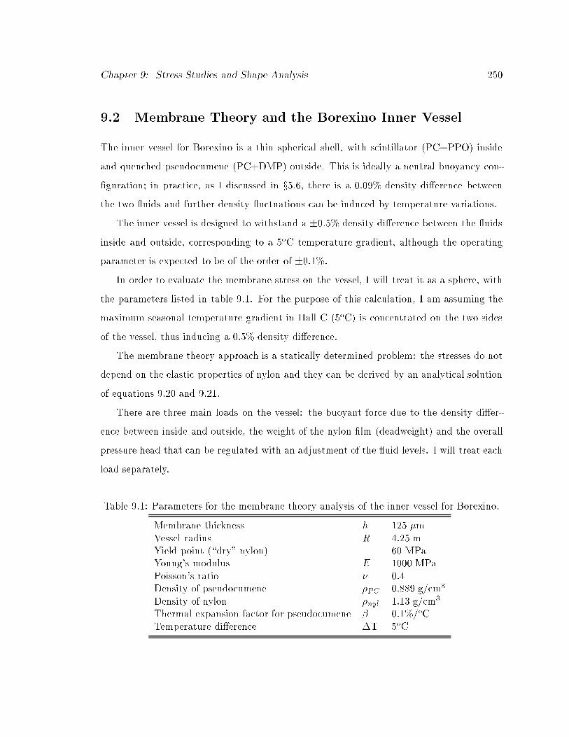
Chapter 9: Stress Studies and Shape Analysis 250
9.2 Membrane Theory and the Borexino Inner Vessel
The inner vessel for Borexino is a thin spherical shell, with scintillator (PC+PPO) inside
and quenched pseudocumene (PC+DMP) outside. This is ideally a neutral buoyancy con-
�guration; in practice, as I discussed in x5.6, there is a 0.09% density di�erence between
the two uids and further density uctuations can be induced by temperature variations.
The inner vessel is designed to withstand a �0:5% density di�erence between the uids
inside and outside, corresponding to a 5oC temperature gradient, although the operating
parameter is expected to be of the order of �0:1%.
In order to evaluate the membrane stress on the vessel, I will treat it as a sphere, with
the parameters listed in table 9.1. For the purpose of this calculation, I am assuming the
maximum seasonal temperature gradient in Hall C (5oC) is concentrated on the two sides
of the vessel, thus inducing a 0.5% density di�erence.
The membrane theory approach is a statically determined problem: the stresses do not
depend on the elastic properties of nylon and they can be derived by an analytical solution
of equations 9.20 and 9.21.
There are three main loads on the vessel: the buoyant force due to the density di�er-
ence between inside and outside, the weight of the nylon �lm (deadweight) and the overall
pressure head that can be regulated with an adjustment of the uid levels. I will treat each
load separately.
Table 9.1: Parameters for the membrane theory analysis of the inner vessel for Borexino.
Membrane thickness h 125 �mVessel radius R 4.25 mYield point (\dry" nylon) 60 MPaYoung's modulus E 1000 MPaPoisson's ratio � 0.4Density of pseudocumene �PC 0.889 g/cm3
Density of nylon �nyl 1.13 g/cm3
Thermal expansion factor for pseudocumene � 0.1%/oCTemperature di�erence �T 5oC

Chapter 9: Stress Studies and Shape Analysis 251
ring θ θ0
P
(a) ring model (b) membrane model
Figure 9.5: Axisymmetrical approximation in the two models: (a) the sphere supported bya ring or (b) the sphere supported by a membrane wrapped around it.
A further approximation needs to be done: the vessel has to be supported somewhere and
the �nal stress pro�le depends on how this is achieved. In Borexino, the weight is supported
by the hold-down system described in x5.6, which consists of two sets of 18 strings, one set
wrapped around the south pole and the other around the north pole (see also 5.9), so that
the vessel is held in place independently of the sign of the density uctuations (light or
heavy vessel). The ropes leave the vessel at a polar angle �0 = 36o (ropes wrapping around
the south pole and supporting a heavy vessel) or �0 = 144o (ropes wrapping around the
north pole and supporting a light vessel). In both cases, sin �0 = 0:56. In the upcoming
discussion I will focus on the �rst option (heavy vessel); as far as buoyancy goes, the results
will be the same if the temperature/density gradient goes in the opposite direction (it will
be enough to replace cos � with � cos � in the results).
This con�guration is clearly non axisymmetrical; the external loads are concentrated
at discrete � positions and induce shape deformations (lobes), which will be object of
the analysis presented in x9.3. Nevertheless, it makes sense to see what happens in the
symmetrical approximation, in order to estimate the stress acting on the vessel's poles.
Chapter 9: Stress Studies and Shape Analysis 252
In x9.2.1 I will apply to our case the formalism by Timoshenko et al. [172], where the
weight of the spherical vessel is supported by a ring at � = �0 as in �gure 9.5-a. In x9.2.2
I will modify the formalism to describe a situation closer to ours, where the weight of the
vessel is supported by a membrane wrapped around the sphere, as in �gure 9.5-b, equivalent
to wide strings that cover the whole surface. Later, in x9.3.4, I will revise these results in
view of the deformation induced by the strings.
9.2.1 Sphere Supported by a Ring
The stress and strain pro�les in a spherical shell are a standard problem, solved in structural
analysis textbooks (see, for instance, Timoshenko et al. [172] or Ugural [170]). Besides being
didactically valid, this method can provide an estimation of the stress at the poles, if there
are no strings.
The assumption is that a ring (the material is not important) holds the sphere, at � = �0
(�gure 9.5-a). This guarantees an axisymmetrical problem; away from the ring, the sphere's
surface is free and the external load only enters as a boundary condition. This approach
introduces a discontinuity of stress and strain at � = �0. According to the membrane theory,
this means that at the ring the membrane solution is not valid and the bending theory needs
to be used locally for a complete description of the shell.
Nylon Deadweight
The weight of the nylon (deadweight) pulls the �lm downwards and induces membrane
stress. There is an intrinsic discontinuity, in this problem: in the top hemisphere the
deadweight tends to compress the vessel, while in the bottom hemisphere the deadweight
tends to expand the vessel. The discontinuity is at � = 90o (�gure 9.6.a).
The vertical load, to be used in eq. 9.20, is:
F = 2�R2q (1� cos �); (9.28)
and the radial pressure, to be used in eq. 9.21 is:
pZ = +q cos �; (9.29)

Chapter 9: Stress Studies and Shape Analysis 253
F compression
Ftension
θ’
θ
pZ = q cosθ
θ’ = 180 - θ
pZ= - q cos θ’
= + q cos θ
f2
P1
P2= γ
2[f
2+R(1-cosθ)]
P2
P1= γ
1[f
1+R(1-cosθ)]f
1
(a) deadweight load (b) hydrostatic load
Figure 9.6: External loads acting on the inner vessel.
where q = �nylongh is the nylon's weight per unit area.
The solution of eq. 9.20 and eq. 9.21 provides the membrane force components:
� < �0 : N� =�Rq
1 + cos � N� = +Rq�
11 + cos � � cos �
�;
� > �0 : N� =Rq
1� cos � N� = �Rq�
11� cos � + cos �
�:
(9.30)
The hoop force is compressive for small angles and becomes tensile in � = 51:8o in the
top hemisphere. In the bottom hemisphere, the change happens at � = 128:2o.
The discontinuity at �0 is due to the total weight of the nylon (and thus the intensity
of the applied load); if �0 = 90o, we have:
�F = 2�R (N+� �N�
� ) = 2�R � 2Rq = 4�R2�nylongh = �nylongVnylon = mnylong: (9.31)
Hydrostatic Pressure and Buoyancy
The uid outside the sphere compresses it, while the uid inside the sphere tends to expand
it (�gure 9.6.b). If the two uids have the same density, the pressure is the same on the

Chapter 9: Stress Studies and Shape Analysis 254
two sides of the shell and the two e�ects cancel each other (neutral buoyancy). We are
interested, here, in the case where the densities di�er by a �nite amount.
The hydrostatic pressure depends on the latitude as follows:
� P1 = 1 [f1 + R(1� cos �)] is the internal pressure, with 1 = �1g = speci�c weight
inside;
� P2 = 2 [f2 +R(1� cos �)] is the external pressure, with 2 = �2g = speci�c weight
outside;
� ÆP0 = 1f1 � 2f2 is the pressure head, constant throughout the vessel. I will treat
that separately, in the next paragraph;
� � = 1 � 2 is the di�erence in speci�c weight on the two sides of the membrane,
positive if the inside is heavier than the outside.
If, for instance, the vessel is \heavy" and � > 0, the ring works to prevent the vessel from
falling. The vertical load, to be used in eq. 9.20, above the ring (� < �0) is:
F = �2�R2
Z �
0
R� (1� cos �) cos � sin � d�; (9.32)
while below the ring we need to consider the total weight of the liquid supported by the
ring, in addition to the pressure load. The solution of eq. 9.20 and eq. 9.21 provides the
membrane forces per unit length:
� < �0 : N� =� R2
6
�1� 2 cos2 �
1 + cos �
�N� =
� R2
6
�5� 6 cos� + 2 cos2 �
1 + cos �
�;
� > �0 : N� =� R2
6
�5 + 2 cos2 �
1� cos �
�N� =
� R2
6
�1� 6 cos� � 2 cos2 �
1� cos �
�:
(9.33)
Both stress components have the sign of � , always negative (compressive) for the light
vessel and always positive (tensile) for the heavy vessel. In this case, also, the value of the
discontinuity is proportional to the weight of the uid to be supported [172].

Chapter 9: Stress Studies and Shape Analysis 255
Pressure Head
According to the sign conventions in the previous paragraph, the net pressure head due to
the height of the uids inside and outside the vessel is equal to:
ÆP0 = 1f1 � 2f2 > 0 if it in ates in the sphere: (9.34)
This term acts as a constant pressure inside the sphere and causes a constant stress term,
una�ected by the discontinuity:
N� = N� =ÆP0R
2) �� = �� =
ÆP0R
2h: (9.35)
Comments
Figure 9.7 shows stress, strains and displacements calculated for the hydrostatic load. I did
not include, in the �gure, the contribution of a net pressure head, which provides an overall
shift of the stress, or of the the nylon deadweight, which only gives a small correction to
the hydrostatic term. With the vessel parameters in table 9.1, the deadweight stress at the
poles is equal to 0.033 MPa, small compared to the few MPa due to the hydrostatic term
(see also the results in table 9.2).
These plots have been calculated for ring at �0 = 90o. All the variables present a
discontinuity at the ring. The local solution, at �0, should be corrected with the bending
theory, but away from the ring the membrane solution will describe the stress properly. We
do not need to undertake the bending theory analysis here, though, since this problem is
not the one of interest for Borexino. What we can learn from this analysis is that if all the
load is concentrated at a parallel circle and the poles are not supported, the stress at the
pole has a maximum but �nite value, independent from what happens at the parallel where
the supporting ring is located. This maximum stress value, for a 0.5% density gradient,
is equal to 6.3 MPa, compared to the yield strength of about 60 MPa in dry nylon (see
discussion in {5).

Chapter 9: Stress Studies and Shape Analysis 256
−4 −2 0 2 40
1
2
3
4
5
6
z (m)
mer
idio
nal s
tres
s (M
Pa)
−4 −2 0 2 40
1
2
3
4
5
6
z (m)
hoop
str
ess
(MP
a)
−4 −2 0 2 4−0.2
0
0.2
0.4
0.6
z (m)
mer
idio
nal s
trai
n (%
)
−4 −2 0 2 4−0.2
0
0.2
0.4
0.6
z (m)
hoop
str
ain
(%)
−4 −2 0 2 40
5
10
15
20
z (m)
mer
idio
nal d
ispl
acem
ent (
mm
)
−4 −2 0 2 4−25
−20
−15
−10
−5
0
5
10
z (m)
radi
al d
ispl
acem
ent (
mm
)
−4 −2 0 2 4−10
−5
0
5
10
15
20
25
z (m)
horiz
onta
l dis
plac
emen
t (m
m)
−4 −2 0 2 4−20
−15
−10
−5
0
z (m)
vert
ical
dis
plac
emen
t (m
m)
Figure 9.7: Stress, strain and displacements for the vessel supported by a ring at � = 90o,as a function of the vertical coordinate z. The plot only includes the hydrostatic load, with� > 0 (heavy vessel), due to a 5oC temperature gradient. The horizontal and verticaldisplacements are those seen on a � = constant vertical cross section of the sphere.

Chapter 9: Stress Studies and Shape Analysis 257
9.2.2 Supporting Membrane Around the Sphere
In a second step, I assumed the support system consists of an ideal membrane wrapping the
sphere, a little like a plastic bag holding a beach ball in it (see �gure 9.5-b). The membrane
leaves the vessel at a certain angular position � = �0.
In this approximation, the ideal membrane exerts a radial force on the sphere, which
provides an inwards pressure constant throughout the membrane. At the point where the
membrane leaves the sphere, there is a vertical force that withstands the vessel's weight.
In the hypothesis that the sphere is heavy and wants to sink, the membrane must provide
an upwards force:
p = constant ) Fup = �pR2
Z �
�0sin � cos � d� d� = 2�pR2 sin
2 �02
: (9.36)
In order to resist the buoyant force and compensate the hydrostatic term, the vertical force
provided by the membrane has to be equal to Fup =43�R
3� , hence, the pressure from the
membrane is:
ph =4
3R�
1
sin2�0: (9.37)
Similarly, the term required to compensate the deadweight term is:
pw = 4h nylon1
sin2�0=
4q
sin2�0: (9.38)
For deadweight, hydrostatic and pressure head terms, we can use the same expressions
derived in x9.2.1, only keeping the solutions for � < �0. For larger � values, we add the
following extra terms of N� and N�:8>>>>><>>>>>:
�N� = Rp sin2 �0 � sin2 �2 sin2 �
= Rp2 sin2 �0
�cos2 �
1� cos2 ��cos2 �0sin2 �0
�;
�N� = �Rp sin2 �0 + sin2 �2 sin2 �
= �Rp2 sin2 �0
�cos2 �
1� cos2 �+ 1 + sin2 �0
sin2 �0
�:
(9.39)

Chapter 9: Stress Studies and Shape Analysis 258
−4 −2 0 2 40
0.5
1
1.5
2
2.5
z (m)
mer
idio
nal s
tres
s (M
Pa)
−4 −2 0 2 4−4
−2
0
2
4
6
z (m)
hoop
str
ess
(MP
a)
−4 −2 0 2 4
−0.1
−0.05
0
0.05
0.1
0.15
0.2
0.25
z (m)
mer
idio
nal s
trai
n (%
)
−4 −2 0 2 4−0.5
0
0.5
z (m)
hoop
str
ain
(%)
−4 −2 0 2 40
5
10
15
20
z (m)
mer
idio
nal d
ispl
acem
ent (
mm
)
−4 −2 0 2 4
−10
−5
0
5
z (m)
radi
al d
ispl
acem
ent (
mm
)
−4 −2 0 2 4−5
0
5
10
z (m)
horiz
onta
l dis
plac
emen
t (m
m)
−4 −2 0 2 4−15
−10
−5
0
z (m)
vert
ical
dis
plac
emen
t (m
m)
Figure 9.8: Stress, strain and displacements for the vessel supported by a membrane thatleaves it at the equator (�0 = 90o). The plots account for the buoyancy term due to a 5oCtemperature gradient and � > 0 (heavy vessel).

Chapter 9: Stress Studies and Shape Analysis 259
−4 −2 0 2 4−7
−6
−5
−4
−3
−2
−1
0
1
z (m)
mer
idio
nal s
tres
s (M
Pa)
−4 −2 0 2 4−25
−20
−15
−10
−5
0
5
z (m)
hoop
str
ess
(MP
a)
−4 −2 0 2 4−0.5
0
0.5
1
z (m)
mer
idio
nal s
trai
n (%
)
−4 −2 0 2 4−2.5
−2
−1.5
−1
−0.5
0
0.5
z (m)
hoop
str
ain
(%)
−4 −2 0 2 4−80
−60
−40
−20
0
z (m)
mer
idio
nal d
ispl
acem
ent (
mm
)
−4 −2 0 2 4−50
0
50
100
z (m)
radi
al d
ispl
acem
ent (
mm
)
−4 −2 0 2 4−20
−10
0
10
20
30
z (m)
horiz
onta
l dis
plac
emen
t (m
m)
−4 −2 0 2 4
0
20
40
60
80
100
z (m)
vert
ical
dis
plac
emen
t (m
m)
Figure 9.9: Stress, strain and displacements for the vessel supported by a membrane thatleaves it at �0 = 36o, as the ropes in Borexino will do. The plots account for the buoyancyterm due to a 5oC temperature gradient and � > 0 (heavy vessel). Note that the merid-ional stress is compressive, reaching a maximum at the equator. The hoop stress also iscompressive, with an increasing value as we approach the discontinuity.

Chapter 9: Stress Studies and Shape Analysis 260
Nylon Deadweight
In this approximation, the stress terms for the nylon deadweight problem become:
�� =
8>>>>><>>>>>:
�Rqh
11 + cos �
for � < �0;
+Rqh
�1
1� cos � � 2� 2 cos2 �0sin2 �0
�for � > �0:
(9.40)
�� =
8>>>>><>>>>>:
+Rqh
�1
1 + cos � � cos ��
for � < �0;
�Rqh
�1
1� cos � + cos � � 2 + 2 2� cos2 �0sin2 �0
�for � > �0:
(9.41)
Hydrostatic Pressure and Buoyancy
The same formalism, applied to the hydrostatic term, yields for the meridional stress:
�� =
8>>>>><>>>>>:
� R2
6h
�1� 2 cos2 �
1 + cos �
�for � < �0;
� R2
6h
�1 + 2 cos2 �
1� cos �� 4 cos
2 �0sin2 �0
�for � > �0;
(9.42)
and for the hoop stress:
�� =
8>>>>><>>>>>:
� R2
6h
�5� 6 cos � + 2 cos2 �
1 + cos �
�for � < �0;
� R2
6h
�5� 6 cos � � 2 cos2 �
1� cos � � 4 2� cos2 �0sin2 �0
�for � > �0:
(9.43)
Pressure Head
The pressure head term does not depend on how the vessel's weight is supported. The
resulting stress is the same as with the ring:
N� = N� =ÆP0R
2) �� = �� =
ÆP0R
2h: (9.44)

Chapter 9: Stress Studies and Shape Analysis 261
−4 −2 0 2 40
2
4
6
8
z (m)
mer
idio
nal s
tres
s (M
Pa)
−4 −2 0 2 4−20
−15
−10
−5
0
5
10
z (m)
hoop
str
ess
(MP
a)
−4 −2 0 2 40
0.5
1
1.5
z (m)
mer
idio
nal s
trai
n (%
)
−4 −2 0 2 4−2
−1.5
−1
−0.5
0
0.5
z (m)
hoop
str
ain
(%)
−4 −2 0 2 4−80
−60
−40
−20
0
z (m)
mer
idio
nal d
ispl
acem
ent (
mm
)
−4 −2 0 2 4
−50
0
50
100
z (m)
radi
al d
ispl
acem
ent (
mm
)
−4 −2 0 2 40
10
20
30
40
z (m)
horiz
onta
l dis
plac
emen
t (m
m)
−4 −2 0 2 40
20
40
60
80
100
z (m)
vert
ical
dis
plac
emen
t (m
m)
Figure 9.10: Stress, strain and displacements for the vessel supported by a membrane thatleaves it at �0 = 36o. The plots account for the buoyancy term due to a 5oC temperaturegradient and � > 0 (heavy vessel), combined with a pressure head of 400 Pa (4 cm water).This value is determined in order to have a tensile meridional stress at the equator. Thehoop stress is still compressive, below the discontinuity.
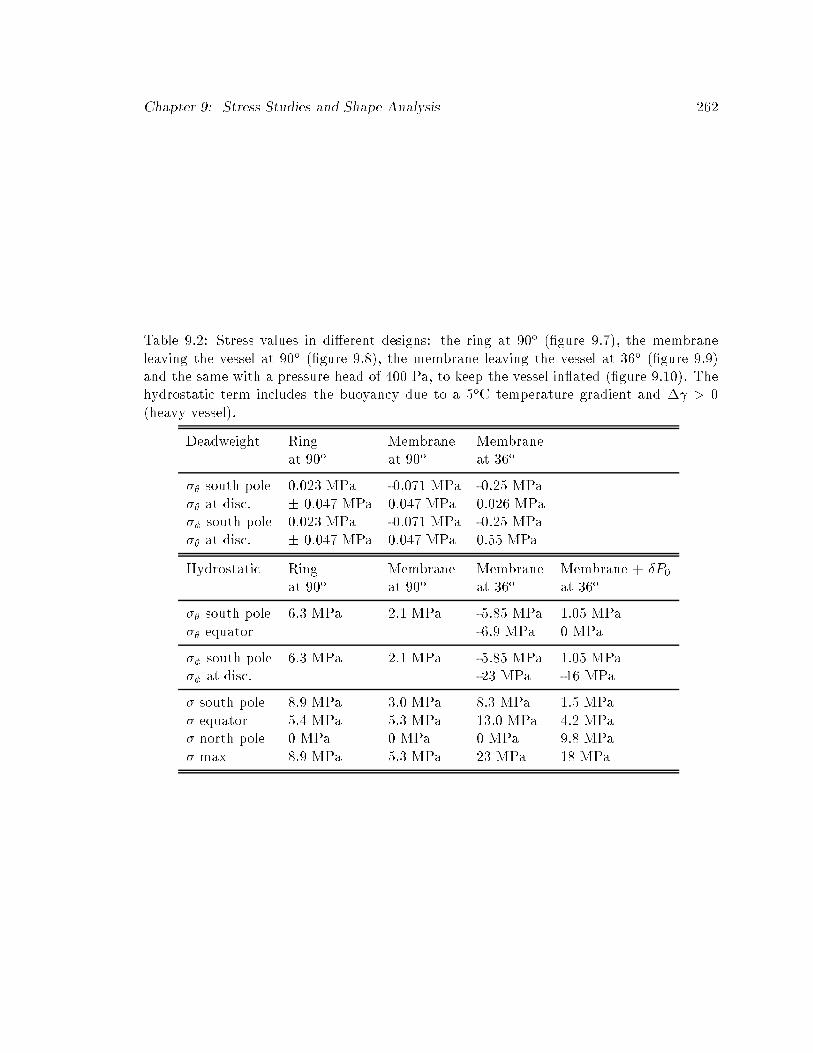
Chapter 9: Stress Studies and Shape Analysis 262
Table 9.2: Stress values in di�erent designs: the ring at 90o (�gure 9.7), the membraneleaving the vessel at 90o (�gure 9.8), the membrane leaving the vessel at 36o (�gure 9.9)and the same with a pressure head of 400 Pa, to keep the vessel in ated (�gure 9.10). Thehydrostatic term includes the buoyancy due to a 5oC temperature gradient and � > 0(heavy vessel).
Deadweight Ring Membrane Membraneat 90o at 90o at 36o
�� south pole 0.023 MPa -0.071 MPa -0.25 MPa�� at disc. � 0.047 MPa 0.047 MPa 0.026 MPa�� south pole 0.023 MPa -0.071 MPa -0.25 MPa�� at disc. � 0.047 MPa 0.047 MPa 0.55 MPa
Hydrostatic Ring Membrane Membrane Membrane + ÆP0at 90o at 90o at 36o at 36o
�� south pole 6.3 MPa 2.1 MPa -5.85 MPa 1.05 MPa�� equator -6.9 MPa 0 MPa
�� south pole 6.3 MPa 2.1 MPa -5.85 MPa 1.05 MPa�� at disc. -23 MPa -16 MPa
� south pole 8.9 MPa 3.0 MPa 8.3 MPa 1.5 MPa� equator 5.4 MPa 5.3 MPa 13.0 MPa 4.2 MPa� north pole 0 MPa 0 MPa 0 MPa 9.8 MPa� max 8.9 MPa 5.3 MPa 23 MPa 18 MPa

Chapter 9: Stress Studies and Shape Analysis 263
Comments
This approximation, with a membrane holding the vessel in place, is an axisymmetrical
analog of the strings in Borexino. It can be interpreted as the analog of an in�nite number
of strings or wide straps that cover the whole range of �.
While resisting buoyancy, the membrane (and the strings) exert a compressive stress on
the vessel, at the south pole. In the ring model, the south pole was a free surface and the
stress due to buoyancy was tensile. As in the ring model, the nylon deadweight is negligible
compared to the hydrostatic term, and even if there is no buoyancy it is very small, less
than 1 MPa.
The angle where the membrane leaves the vessel is important, because the resultant
force from the membrane is proportional to 1/sin2�0 and consequently the stress increases
as �0 gets closer to either the north or the south pole. I considered the two cases of a
membrane leaving the vessel at the equator (� = 90o) or at the angle where the strings
leave the vessel in Borexino (� = 36o). The two cases di�er by a factor 0.592=0.35 and the
resulting stress pro�les are very di�erent, as one can see from the plots in �gure 9.8 and 9.9
and from the numerical values in table 9.2.
The pressure head term can be used to regulate the overall stress pattern and shift it
to positive values, so that the vessel stays in ated. A minimum pressure head of 400 Pa is
needed in order to have tensile stress in the meridional direction (�� > 0) and maintain the
vessel in ated. The pressure head term adds about 7 MPa to both meridional and hoop
stress and the stress and strain pro�les become the ones in �gure 9.10, where I also show
the resulting displacements. In particular, the south pole is lifted up by the membrane for
a displacement of about 8 cm.
This scenario is not too distant from the real con�guration and it can be used for an
approximate estimation of the stress distribution; in reality, the load is concentrated on
the ropes, rather than on the membrane and the south pole is constrained by the pipes
that connect it to the outside. The maximum stress is at the discontinuity, where the
membrane leaves the vessel, but the numerical value should be reevaluated in term of the

Chapter 9: Stress Studies and Shape Analysis 264
bending theory. The expectation is that the vessel will adjust its shape and curvature, at
the discontinuity, so as to have a stress pro�le that continuously connects from the values
above to those below the discontinuity; the actual maximum stress is going to be lower than
the one quoted in the table, but not by much. I would like to remind, at this point, that
the yield point of dry nylon is of the order of 60 MPa; a 20 MPa stress value will not cause
a vessel failure, but it will still induce a considerable creep (44% at 12 MPa after 1 day,
according to the data in table 5.2).
A 5oC temperature di�erence between inside and outside the vessel is not likely to
happen or to hold for long time, but we need to do all that is possible to prevent it, with
a proper temperature control system, if we want to avoid a permanent deformation of the
vessel.

Chapter 9: Stress Studies and Shape Analysis 265
9.3 Shape Analysis in Presence of Strings
I will present in this section the results of a study of the deformation of the vessel shape
induced by the strings of the hold-down system. The system is the same described in x5.6
and in x9.2, with two sets of 18 ropes. I will focus on the case of a heavy vessel, with the
geometry shown in �gure 9.11.
θ0
Fmembrane
Buoyancy
δθ
δF = T δθcentripetalforce
Figure 9.11: Geometry of the scallops problem: vertical cross section of the sphere held bystrings and force diagram for the tension.
In a zero-buoyancy design, the vessel spherical shape is maintained by the overpressure
imposed from the outside with the pressure head. If there is a small density di�erence
between the uids inside and outside the vessel, the ropes of the hold down system need to
provide a total vertical force that withstands the resulting buoyancy. In the hypothesis of
ideal strings, with constant tension T and � = � � �, each rope locally exerts a centripetal
force: 8>>>><>>>>:
dF = T d�;
dFx = T sin � d�;
dFy = T cos � d�:
(9.45)
The total net upwards force exerted by n strings is equal to:
Fup = 2nTZ �0
0
cos � d� = 2nT sin �0 = 2nT sin �0: (9.46)
This force needs to balance the buoyancy force B = 43�R
3� . According to the formalism
in x9.2.1, � = (�in � �out) g is the di�erence in speci�c weights. The requirement for the

Chapter 9: Stress Studies and Shape Analysis 266
tension on each string is:
T =2�
3n
R3�
sin �0=
7003N
n sin �0=
12� 103N
nif �0 = 36o and 5oC temperature gradient:
The pressure exerted by each string on the vessel, assuming their width is w = 1mm, is:
�s =dF
d area=
T d�
wRd�=
2:8MPa
n: (9.47)
As the strings push the �lm towards the center, they deform its spherical shape and produce
scallops. I calculated the depth of such deformations, as a function of the applied pressure
head, with a model based on the following two assumptions:
1. for a thin nylon vessel, the elastic energy that goes into stretching and bending the
membrane is small;
2. to a �rst order approximation, resistance to the deformation is solely provided by the
overpressure that keeps the vessel in ated.
In other words, given an overpressure P inside the vessel, maintained through the pressure
head, the vessel wants to be spherical. The deformations induced by the strings generate a
restoring potential energy equal to P�V , where �V is the volume change.
Following the procedure sketched in [173], I calculated the deformed shape with a vari-
ational approach. Under a given load q, among all the possible shapes F that satisfy the
due constraints, the shell assumes a shape for which the functional:
W = U(F)�Aq(F) (9.48)
is stationary, that is, ÆW = 0 for an in�nitesimal shape variation. U is the energy of
deformation of the shell and Aq is the work performed by the external load q.
In a �rst order approximation, the membrane's elastic and bending energy can be ne-
glected (see x9.3.3) and the vessel shape is the one minimizing the functional:
W = P�V � AT ; (9.49)
where AT is the work performed by the tension in the straps.
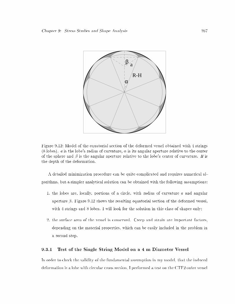
Chapter 9: Stress Studies and Shape Analysis 267
α
β
R-H
a
Figure 9.12: Model of the equatorial section of the deformed vessel obtained with 4 strings(8 lobes). a is the lobe's radius of curvature, � is its angular aperture relative to the centerof the sphere and � is the angular aperture relative to the lobe's center of curvature. H isthe depth of the deformation.
A detailed minimization procedure can be quite complicated and requires numerical al-
gorithms, but a simpler analytical solution can be obtained with the following assumptions:
1. the lobes are, locally, portions of a circle, with radius of curvature a and angular
aperture �. Figure 9.12 shows the resulting equatorial section of the deformed vessel,
with 4 strings and 8 lobes. I will look for the solution in this class of shapes only;
2. the surface area of the vessel is conserved. Creep and strain are important factors,
depending on the material properties, which can be easily included in the problem in
a second step.
9.3.1 Test of the Single String Model on a 4 m Diameter Vessel
In order to check the validity of the fundamental assumption in my model, that the induced
deformation is a lobe with circular cross section, I performed a test on the CTF2 outer vessel

Chapter 9: Stress Studies and Shape Analysis 268
T
Mg
M M
Mg
T
R = 2 m
O
A
D
F
E
α
β
(a) (b)
Figure 9.13: (a): The outer vessel for CTF2, with a single string to which known weightshave been attached. (b): Deformation induced by a string, with the variables used in theminimization.
prototype. This vessel has the shape of an ice cream cone (see �g. 9.13), the upper portion
being a hemisphere with 4 m diameter. During the test, the vessel was hanging from a crane
and was in ated with air. In this con�guration, there was no buoyancy, only an internal,
uniform overpressure maintained by an air blower. The minimum internal overpressure
required to keep the vessel in shape is �25 Pa (0.25 cm H2O). I attached known weights
to a string wrapped around the top endplate and measured the depth of the scallop thus
produced, as a function of the tension in the string and the pressure inside the vessel.

Chapter 9: Stress Studies and Shape Analysis 269
The Single String Model
In this test there is only one tensioned string and the pressure inside the vessel is constant.
The problem is thus symmetric in �, with only one scallop, whose width is not constrained
by neighbor strings. With several strings, the lobe width is limited by the distance between
strings and the problem loses it � symmetry. The basic assumptions of the model, in this
case, reduce to the following:
1. on a cross section, the deformation is a portion of a circle, as in �gure 9.13-b.
2. the arc length is conserved, after the deformation. In other words, I am neglecting
strain and creep. Anyway, it is easy to include these e�ects, if the membrane stretching
becomes important.
R� = a� (9.50)
3. the deformation ends at a point on the original sphere:
�OD = R�H (9.51)
�DE = (R�H) sin� = a sin � ) R�H = asin �
sin �(9.52)
�AD =
q�DF
2+ �AF
2= 2a sin
�
2(9.53)
2a sin�
2=q(R�H)2 + R2 � 2R(R�H) cos� (9.54)
Substituting eq. 9.52 in eq. 9.54, we obtain a relation that determines, for each value of
�, the corresponding �:
4a2 sin2�
2� a2
sin2 �
sin2 �� R2 + 2Ra sin �
cos�
sin�= 0 (9.55)
In the inextensible deformation approximation, where I neglect the membrane's stretch-
ing, eq. 9.50 can be used to reduce eq. 9.55 to:
4�2
�2sin2
�
2��2
�2sin2 �
sin2 �� 1 + 2
�
�sin �
cos�
sin�= 0 (9.56)

Chapter 9: Stress Studies and Shape Analysis 270
Table 9.3: Model predictions for di�erent values of P and T, in the 2 m vessel: a is thelobe radius of curvature, � is the angular aperture of the lobe with respect to the center ofthe sphere, � is the lobe angular aperture with respect to its center of curvature, H is thescallop depth and � is the membrane stress.
� P T a � � H �
[inches H2O] [Pa] [kg] [cm] [deg] [deg] [cm] [MPa]
7.0 119 7 100 8.3 16.5 2.1 0.606.3 108 7 100 9.1 18.3 2.5 0.545.6 97 7 100 10.2 20.5 3.2 0.485.1 88 7 100 11.3 22.6 3.9 0.444.7 81 7 100 12.2 24.4 4.5 0.414.4 76 7 100 13.0 26.0 5.1 0.383.8 65 7 100 15.4 30.7 7.1 0.323.0 52 7 100 19.2 38.5 11.2 0.262.9 50 7 100 20.3 40.5 12.4 0.252.2 38 7 100 26.8 53.5 21.4 0.19
This equation has two solutions: 8><>:
� = �;
� = 2�:(9.57)
The �rst corresponds to the trivial case of no deformation. The second is the one we are
looking for. In this case: 8>>>><>>>>:
� = 2�;
a = R2 ;
H = R (1� cos�):
(9.58)
The functional to be minimized is:
W =Z �=2
0
W� d� (9.59)
W� =
R�(R� a) +
a2
2sin 2� � a2 sin2 �
cos�
sin�
!PR � T
�R� a
sin �
sin�
�; (9.60)
which can be reduced to:
W 0 =PR2
T
��
2+sin 4�
8� sin3 � cos�
�� (1� cos�) : (9.61)

Chapter 9: Stress Studies and Shape Analysis 271
2 3 4 5 6 70
2
4
6
8
10
12
14
PR2/T
scal
lop
dept
h (c
m)
model predictionmeasurement
Figure 9.14: Measured scallop depth, as a function of the parameter � = PR2=T , comparedto the model. The numerical values are reported in table 9.4.
The minimization ofW 0 provides the value of �, the angular aperture of the deformation,
while all the other variables are then determined using eq. 9.58. Note that the result depends
on the sphere's radius R, on the internal overpressure P and on the tension in the string T
only through the parameter:
� =PR2
T: (9.62)
Scallop depth as a function of � = PR2=T
Table 9.3 reports the model predicted deformation in a few con�gurations, which I also
tested on the CTF2 outer vessel. I stretched a string between the two lobes of the scallop,
as in �gure 9.15, and measured D, the distance between the string and the deepest point of
the scallop. This value is, theoretically, equal to half the total deformation H. The results
are compared to the model prediction in table 9.4; the experimental error on D is of the
order of 0.1 mm. The same data are plotted in �gure 9.14.

Chapter 9: Stress Studies and Shape Analysis 272
Table 9.4: Comparison between the calculated depth of the deformation Htheor and themeasured deformation Dmeas for di�erent values of � = PR2=T . The data are plotted in�gure 9.14.
� Htheor Htheor/2 Dmeas
[cm] [cm] [cm]
7.0 2.1 1.0 1.26.3 2.5 1.3 1.55.6 3.2 1.6 1.75.1 3.9 1.9 2.04.7 4.5 2.3 2.54.4 5.1 2.6 2.63.8 7.1 3.6 3.83.0 11.2 5.6 5.22.9 12.4 6.2 6.12.2 21.4 10.7 10.5
−40 −30 −20 −10 0 10 20 30 40194
195
196
197
198
199
200
201
X (cm)
Y (
cm)
undeformed shape
scallop shape (model)
string between lobes
data points
Figure 9.15: Measurement of the pro�le in a few points of the scallop, compared to themodel (� = 4:7).

Chapter 9: Stress Studies and Shape Analysis 273
−600 −400 −200 0 200 400 600 8000.8
1
1.2
1.4
1.6
1.8
2
2.2
2.4
2.6
X (pixels)
Y (
pixe
ls)
Figure 9.16: Scallop pro�le extracted from a digitized picture and �t to a line plus twomirror portions of a circumference.
Scallop pro�le with a direct measurement
I compared the model pro�le to the real one by measuring the distance between the hor-
izontal string and the scallop surface, at di�erent positions. This type of measurement is
subject to errors that are of the same order of the discrepancy with the model, since in order
to measure the distance I had to touch the vessel and subject it to further deformations,
of the order of 0.1 mm. Nevertheless, the results, shown in �gure 9.15, are in a reasonably
good agreement with the model.
Pro�le with the aid of a digital camera
A better overlap between the model and the deformation induced by the string has been ob-
tained with a digital camera. I took pictures of the scallop and, with some image processing
and a �tting routine, I could extract the deformed pro�le from the pictures.
The data in �gure 9.16 were obtained with an internal overpressure P = 0:3200 = 81Pa

Chapter 9: Stress Studies and Shape Analysis 274
−50 −40 −30 −20 −10 0 10 20 30 40 50194
195
196
197
198
199
200
201
X (cm)
Y (
cm)
H/2
D
A B
P Q
C undeformed shape
H/2
scallop shape
Figure 9.17: Scallop pro�le extracted from a digitized picture, compared to the modelprediction.
and a tension on the string equal to T = 7 kg (� = 4:7).
Figure 9.16 shows the data extracted from the picture. The main source of error comes
from the fact that there was not a sharp contrast between the balloon and the background.
The data are �tted to a slanted line, which accounts for the angle at which I took the
picture, plus two mirror portions of circle.
After subtracting the line and applying the proper scale factors in abscissa and in or-
dinate, the scallop pro�le becomes the one in �gure 9.17, where I also overlapped the
undeformed balloon shape (dashed line)and the calculated shape (solid line).
The absolute calibration has been obtained with a string attached to the deformed
vessel, tangential in points P and Q. The measured scallop depth is D = 2:5 cm, while the
formalism predicts H=2 = 2:3 cm.
The agreement between the prediction and the data is very good; this can reassure us

Chapter 9: Stress Studies and Shape Analysis 275
that the model is correct, at least in the single string case.
9.3.2 The n-string Model
In Borexino there will be multiple strings holding the vessel and the equatorial cross section
will look like the lobed pattern in �gure 9.12. According to the conventions earlier de�ned,
the functional to be minimized is:
W =Z �
�0
TR
"�
�(R� a) +
a2
2Rsin
2R�
a�a2
R
cos�
sin�sin2
R�
a
!� 1 +
a
R sin�sin
R�
a
#d�
(9.63)
where:
- sin� = sin �2n sin �, and n is the number of strings (n = 18 in Borexino);
- � = R�a is the aperture angle of the lobe, if the surface area is conserved;
- H = R� a sin �sin� is the depth of the deformation, at the string;
- P = P (�) is the pressure as function of the latitude.
Note that, as in the previous case, pressure in the vessel and tension in the rope enter the
functional expression only through the parameter � = PR2=T .
Constant pressure case
Before dealing with the e�ect of buoyancy, it is worthwhile to examine the case where the
pressure inside the vessel is constant, as it would be if the vessel were in ated with air. I
followed two di�erent procedures:
1. In the �rst approach, I minimized W� separately at each latitude. This approach
diverges at the poles (� ! 0; �) and does not take into account the continuity of the
membrane shape. The result is valid in the neighborhood of the equator, though,
where if the internal pressure is large enough, the calculated local radius of curvature
is �nite. The result is similar to the one we would have with a cylindrical vessel

Chapter 9: Stress Studies and Shape Analysis 276
10 15 20 25 30 35 40 45 501
2
3
4
PR2/T
a (
m)
case 2case 1
10 15 20 25 30 35 40 45 500
2
4
6
8
PR2/T
H (
cm) case 2
case 1
Figure 9.18: Radius of curvature and scallop depth calculated at the equator in the twoapproaches. Case 1: energy functional minimization restricted to an equatorial disc ofthickness �. Case 2: energy functional minimization simultaneously performed on thewhole lobe, for � 2 (�0; �).
with strings running parallel to the axis and pushing the surface in. As � leaves the
equator, the radius of curvature a does not change much, but rapidly goes to zero
when approaching the poles. As a consequence, H \explodes". In this approach,
a = a(�; �):
2. In the second approach, I minimized the value of W =RW� d� as a function of a,
with the fundamental assumption that a is constant for � 2 (�0; �). What changes
approaching the poles is �, the angular aperture of the poles, so that the deformation
will go to zero at the poles, but the radius of curvature stays constant. This approach
accounts for the continuity in the polar direction and minimizes the overall energy
potential of the scallop, instead of � portions. The fundamental hypothesis is that:
a = a(�):

Chapter 9: Stress Studies and Shape Analysis 277
Figure 9.18 shows a comparison of the values of a and H at the equator, calculated by the
two models. The results are relatively in agreement, especially for the smaller values of �,
where a larger de ection is predicted. It is interesting to note that the radius of curvature
exhibits an exponential dependence on the parameter �. A �t yields:
a = p1 � p2 e�0:1085� (9.64)
where (p1; p2) = (3:7; 5:9)m in the �rst approach and (p1; p2) = (4:0; 6:8)m in the second.
PPPL test: in ation with air
In November 1999 I directed an in ation test for the Borexino inner vessel prototype at
the Princeton Plasma Physics Laboratory (PPPL), where we could take advantage of one
of their large generator rooms. Our team in ated a 8.5 m diameter prototype, built with
0.1 mm PA-6 Capran DF400 �lm. The vessel had been previously in ated in the Princeton
Jadwin Gymnasium, with an air blower, and taken up to an overpressure of 200 Pa (�2 cm
H2O). A picture of that �rst in ation test is shown in �gure 9.19. In the course of that
in ation, an initial 1% creep took place. During the PPPL test, the only stretching was
due to changes in the environmental conditions, relative humidity in particular. A 6-day
monitor of the diameter is shown in �gure 9.20: the diameter uctuated between 8.55 and
8.65 m in correlation with the relative humidity. The average diameter was 8.6 m, 1.2%
larger than the design 8.5 m.
For the �rst time, we experimented with the installation of 36 ropes, 30 m long, which
proved to be tricky. The ropes were diÆcult to keep in place and we had bundling problems;
as a consequence, it was established to mount on the �nal vessel nylon hoops to rail the
strings, in order to facilitate the installation. A picture of the in ated vessel, with the
two sets of ropes and 100 Pa (�1 cm) overpressure, is shown in �gure 9.21. In order to
measure the scallop formation, I mounted a scale on two of the ropes and tensioned them
with several di�erent values of T, by adjusting the rope's length. The pressure inside the
vessel was regulated with an air blower and monitored by a magnahelic gauge connected to
the bottom of the sphere.

Chapter 9: Stress Studies and Shape Analysis 278
Figure 9.19: In ation of the inner vessel prototype in the Princeton Jadwin Gymnasium.
−1 0 1 2 3 4 5 6
1
1.5
2
days
frac
tiona
l str
etch
(%
)
internal overpressure =1.016cm water
fractional stretch (%)relative humidity (%)
−1 0 1 2 3 4 5 60
50
100%
rel
ativ
e hu
mid
ity
Figure 9.20: Monitor of the vessel diameter during the PPPL in ation.
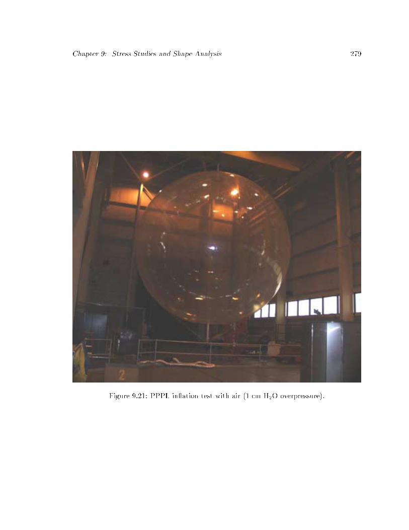
Chapter 9: Stress Studies and Shape Analysis 279
Figure 9.21: PPPL in ation test with air (1 cm H2O overpressure).

Chapter 9: Stress Studies and Shape Analysis 280
With a digital camera I took pictures of the scallops thus formed. For calibration
purposes, I attached ags at known � positions on the surface of the vessels, before the
in ation, and measured the distance between ags on the two sides of the scallop. I later
analyzed these pictures, with image processing software, in order to extract the shape and
�t it with my model.
Figure 9.22 shows two examples of the scallops pro�les I obtained. Overlapped are the
result of a �t with my model and the undeformed sphere. The �rst scallop in �gure 9.22 has
been obtained with a nominal � = 18:5, at � = 127o and it is an example of shallow scallop
(a=2.6 m, H=0.35 cm). The second scallop has been obtained with a nominal � = 18:5, at
� = 900 and it is an example of deep scallop (a=1.4 m, H=4.5 cm). The shape agreement
is good in all pictures and it con�rms the hypothesis that the lobe pro�le is constituted by
portions of a circle.
There are two main observations to be made on the (�; �) dependence. The �rst is that
the � dependence of a and H displays an asymmetry: the radius of curvature is relatively
constant on the southern hemisphere, but it becomes smaller, for deeper scallops, in the
upper hemisphere. The �t results, for some con�gurations, are reported in table 9.5. There
are two possible explanation for this e�ect: one is that the pressure inside the vessel was
not constant, but changed at the top due to a temperature gradient in the 10 m tall room.
The other is that the ropes were not ideal strings and the tension was not constant along
their length. At the top, they were subject to friction with the vessel and to the constraint
of wrapping around the north pole pipe and a railing ring; there factors likely induced a
higher tension and deeper scallops in the top hemisphere.
Moreover, the value of � is a�ected by two sources of error. The pressure was measured
at the bottom of the vessel and it is known only within 0.5 mm H2O, while the pressure
range for these measurements is between 2 and 12 mm H2O. The scale used to measure
the tension has a 0.25 kg precision, for measured tensions between 2 and 10 kg. Thus, the
relative error on � can be quite large and cannot be neglected.
In �gure 9.23 I show the �t results for H and a, with error bars for both � and the scallop
�t parameter. I only took into account the scallops at � = 127o, in these plots, because

Chapter 9: Stress Studies and Shape Analysis 281
−25 −20 −15 −10 −5 0 5 10 15 20 25
5
10
15
20
25
x (cm)
y (c
m)
−40 −30 −20 −10 0 10 20
5
10
15
20
Figure 9.22: Two examples of scallops, in the PPPL air in ation test. The �rst scallopcorresponds to a nominal � = 18:5, at � = 127o. The second one corresponds to � = 7:4, at� = 900.

Chapter 9: Stress Studies and Shape Analysis 282
1
1.5
2
2.5
3
3.5
4
5 7.5 10 12.5 15 17.5 20 22.5 25 27.5 30ζ=PR2/T
scal
lop
radi
us o
f cu
rvat
ure
a (m
)
0
0.5
1
1.5
2
2.5
3
3.5
4
4.5
5
5 7.5 10 12.5 15 17.5 20 22.5 25 27.5 30ζ=PR2/T
scal
lop
defo
rmat
ion
H (
m)
Figure 9.23: Measured versus calculated values of a (top) and H (bottom) for di�erentvalues of � = PR2=T . The error bars re ect the uncertainty on the measured value of Pand T.

Chapter 9: Stress Studies and Shape Analysis 283
Table 9.5: Measured radius of curvature for the scallops at di�erent latitudes, with di�erentvalues of �. From the air in ation test at PPPL.
� � = 7:5 � = 10:6 � = 16:4
53o 0.76 m 0.13 m 0.54 m71.5o 1.16 m 1.54 m 0.78 m90o 1.39 m 1.16 m108.5o 1.36 m 1.74 m 1.21 m127o 1.28 m 1.73 m 1.29 m
that was the closest position to where the rope tension and the pressure were measured and
where the nominal value of � was most signi�cative.
The conclusion we can draw from the in ation test with air is that the assumption of
circular cross section is correct and the n-string model at constant pressure agrees with the
observed shape. The calculated scallop depth and radius of curvature are in reasonable
agreement with the measured ones, within the experimental error on pressure and tension,
in the southern hemisphere.
On the other hand, the dependence of the depth on the polar coordinate shows an
asymmetry that is not predicted by the model. This asymmetry is likely to be due to the
non homogeneity of the experimental setup (T not constant along the rope, P changing
with altitude).
Buoyancy e�ects
The problem gains an additional level of complication once we include buoyancy and an
hydrostatic pressure that changes with �.
In the �rst approach, where I treated each � slice separately and minimized W�, a
solution exists only if the horizontal component of the pressure is large enough; otherwise,
the vessel cannot resist the centripetal force exerted by the string and the energy functional
has no minimum.
As a reference, I report in table 9.6 the predicted values of a, � and H at the equator, as
a function of the internal pressure. There is a minimum pressure requirement for the energy

Chapter 9: Stress Studies and Shape Analysis 284
Table 9.6: Case of 18 straps (� = 5o) and 0:5% density di�erence on the two sides of thevessel. The values for a, � and H have been calculated with a minimization of the energyfunctional W90o , evaluated at the equatorial plane (� = 90o).
Pressure at � = 90o pressure head P0 a � H[cm H2O] [cm H2O] [m] [deg] [cm]
2.7 0.8 0.79 27.0 15.02.8 0.9 0.94 22.6 10.42.9 1.0 1.07 19.9 8.03.0 1.1 1.18 18.0 6.43.1 1.2 1.29 16.5 5.33.2 1.3 1.38 15.4 4.53.3 1.4 1.47 14.4 3.93.4 1.5 1.56 13.7 3.53.5 1.6 1.63 13.0 3.13.6 1.7 1.71 12.4 2.8
functional W90o, evaluated at the equatorial disk, to have a minimum. For �T = 5oC, this
value is P � 300Pa (3 cm H2O), corresponding to about 100 Pa (1 cm H2O) pressure head
at the north pole.
Figure 9.24 shows how the deformation changes at di�erent latitudes with the design
operating parameter of �T = 1oC (0.1% density di�erence), with a pressure head of 100 Pa
(1 cm H2O) on top of the hydrostatic pressure. The model becomes unstable when ap-
proaching the south pole (� > 145o). Overlapped is the pro�le obtained with the second
approach I am about to describe.
This �rst approach has an intrinsic problem: the global deformation along the scallop
needs to be accounted for, in the minimization, and the whole functional:
W =ZW� d� (9.65)
should be minimized instead of each individual W�. The di�erence from the constant
pressure case is that as the pressure changes, the radius of curvature a cannot be treated
as a constant and I need to make an assumption on how a changes with �. The second

Chapter 9: Stress Studies and Shape Analysis 285
40 60 80 100 120 140 160 1800
0.2
0.4
0.6
0.8
1
1.2
θ
H (
m)
Case 1Case 2
1oC temperature gradient0.1% density difference100 Pa overpressure
Figure 9.24: Scallop depth H as a function of the latitude angle, for a 100 Pa (1 cmH2O) pressure head at the North pole and �T = 1oC (0.1% density di�erence). Case 1:minimization of W�. Case 2: minimization of W =
R ��0W� d�.
approach is based on the following statements:
1. the ropes are ideal string, with constant tension:
T =2�
3n
R3�
sin2 �0; (9.66)
2. the internal pressure changes with � as:
P (�) = P0 +R� (1� cos �); (9.67)
3. the local radius of curvature changes with � only through the pressure. Using the
results obtained in the constant pressure scenario (eq. 9.64):
a(�) = 4� a0e�0:1085 � m; � =
PR2
T; (9.68)
4. the lobe cross section is a portion of a circle;

Chapter 9: Stress Studies and Shape Analysis 286
40 60 80 100 120 140 160 1801
2
3
4
θ
a (
m)
40 60 80 100 120 140 160 1800
0.5
1
1.5
2
θ
H(c
m)
Figure 9.25: Case of 18 strings, with �0 = 36o, �T = 5oC and pressure head = 350 Pa,obtained from the solution of @
@a0
R ��0W�d� = 0. The pressure head is the minimum required
to maintain the vessel in ated. The same plots are obtained with �T = 1oC and pressurehead = 70 Pa.
5. stretching is negligible (conservation of surface area).
The energy functional (eq. 9.65) is minimized as a function of a0. A solution of:
@W
@a0= 0
provides a value for a0, from which I can obtain a(�) and H(�).
For n = 18 strings, �0 = 36o and � = 43:6N/m2 (the di�erence in speci�c gravity
due to a temperature gradient �T = 5oC), the vessel stays in ated if the applied overhead
pressure is at least equal to 350 Pa (3.5 cm water equivalent). The resulting a and H
pro�les are shown in �gure 9.25. For lower values of P0, the vessel behaves like an hot air
balloon: the bottom part stays in ated, with scallops, while the top part collapses inwards
and the vessel assumes a pear shape. If �T = 1oC, the minimum required pressure head is
P0;min = 70Pa.
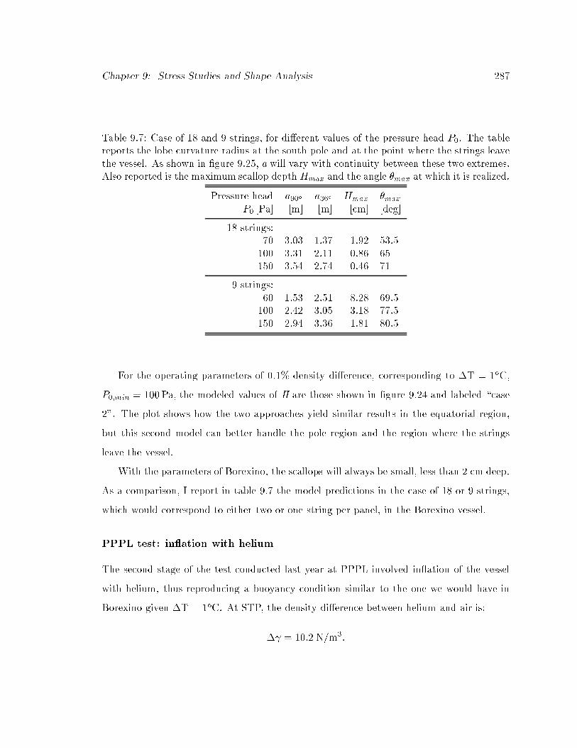
Chapter 9: Stress Studies and Shape Analysis 287
Table 9.7: Case of 18 and 9 strings, for di�erent values of the pressure head P0. The tablereports the lobe curvature radius at the south pole and at the point where the strings leavethe vessel. As shown in �gure 9.25, a will vary with continuity between these two extremes.Also reported is the maximum scallop depth Hmax and the angle �max at which it is realized.
Pressure head a90o a36o Hmax �max
P0 [Pa] [m] [m] [cm] [deg]
18 strings:70 3.03 1.37 1.92 53.5100 3.31 2.11 0.86 65150 3.54 2.74 0.46 71
9 strings:60 1.53 2.51 8.28 69.5100 2.42 3.05 3.18 77.5150 2.94 3.36 1.81 80.5
For the operating parameters of 0.1% density di�erence, corresponding to �T = 1oC,
P0;min = 100Pa, the modeled values of H are those shown in �gure 9.24 and labeled \case
2". The plot shows how the two approaches yield similar results in the equatorial region,
but this second model can better handle the pole region and the region where the strings
leave the vessel.
With the parameters of Borexino, the scallops will always be small, less than 2 cm deep.
As a comparison, I report in table 9.7 the model predictions in the case of 18 or 9 strings,
which would correspond to either two or one string per panel, in the Borexino vessel.
PPPL test: in ation with helium
The second stage of the test conducted last year at PPPL involved in ation of the vessel
with helium, thus reproducing a buoyancy condition similar to the one we would have in
Borexino given �T = 1oC. At STP, the density di�erence between helium and air is:
� = 10:2 N=m3:

Chapter 9: Stress Studies and Shape Analysis 288
Figure 9.26: PPPL in ation test with helium (0.2 cm H2O pressure at the south pole).

Chapter 9: Stress Studies and Shape Analysis 289
Table 9.8: Measured radius of curvature for the scallops at di�erent latitudes, with di�erentvalues of �. From the helium in ation test at PPPL. I report, for each column, both thenominal value of �0, at the south pole, and the one that actually �ts the model, as shownin the �gures. The error on a is about 10%.
nominal �0 4.7�2.6 19�9 33�17model �0 2.4 (�g. 9.27) 10.63 (�g. 9.28) 18.4 (�g. 9.29)
radius of curvature a :� = 53o 2.26 m 2.80 m 3.36 m� = 71:5o 2.49 m 2.13 m 3.24 m� = 90o 1.34 m 2.72 m 3.20 m� = 108:5o 0.73 m 2.56 m 2.91 m� = 127o 0.42 m 1.58 m 2.58 m
deformation H:� = 53o 0.87�0.35 cm 0.44�0.21 cm 0.21�0.13 cm� = 71:5o 0.93�0.28 cm 1.4�0.4 cm 0.35�0.11 cm� = 90o 5�1 cm 0.78�0.13 cm 0.41�0.13 cm� = 108:5o 16�3 cm 0.85�0.19 cm 0.55�0.10 cm� = 127o 34�6 cm 2.14�0.06 cm 0.59�0.06 cm
The test was conducted at atmospheric pressure Patm = 770mmHg, ground temperature T
= 21oC and 24% R.H.; assuming the helium gas was dry, the density di�erence was, then:
� = 8:9 N=m3;
which is exactly what we would have in Borexino with a �T = 1oC temperature gradient.
Figure 9.26 shows the vessel being in ated with Helium, with an overpressure at the
south pole equal to �20 Pa. Once the pressure at the bottom reached the value of 100 Pa
(1 cm H2O), the shape was back to spherical, as in the air test.
After tensioning the ropes, I measured the scallop deformation at di�erent angular
positions, with di�erent pressures P0, at the bottom of the vessel. Unfortunately, only
at the end of the test I realized the connections with the pressure gauge mounted at the
bottom were leaking and all the pressure measurements at the bottom are a�ected by a
large error. I report in table 9.8 the �t results and the nominal value of �0 (at the bottom)
at which they have been measured. The error on the nominal �0 is my best estimate, from
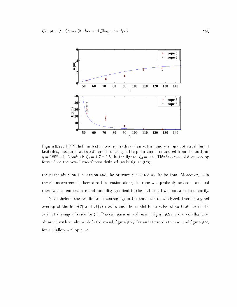
Chapter 9: Stress Studies and Shape Analysis 290
50 60 70 80 90 100 110 120 130 1400
2
4
6
η
a (
m)
rope 5rope 6
50 60 70 80 90 100 110 120 130 1400
10
20
30
40
50
η
H(c
m)
rope 5rope 6
Figure 9.27: PPPL helium test: measured radius of curvature and scallop depth at di�erentlatitudes, measured at two di�erent ropes. � is the polar angle, measured from the bottom:� = 180o��. Nominal: �0 = 4:7�2:6. In the �gure: �0 = 2:4. This is a case of deep scallopformation: the vessel was almost de ated, as in �gure 9.26.
the uncertainty on the tension and the pressure measured at the bottom. Moreover, as in
the air measurement, here also the tension along the rope was probably not constant and
there was a temperature and humidity gradient in the hall that I was not able to quantify.
Nevertheless, the results are encouraging: in the three cases I analyzed, there is a good
overlap of the �t a(�) and H(�) results and the model for a value of �0 that lies in the
estimated range of error for �0. The comparison is shown in �gure 9.27, a deep scallop case
obtained with an almost de ated vessel, �gure 9.28, for an intermediate case, and �gure 9.29
for a shallow scallop case.

Chapter 9: Stress Studies and Shape Analysis 291
50 60 70 80 90 100 110 120 130 1400
2
4
6
η
a (
m)
rope 5rope 6
50 60 70 80 90 100 110 120 130 1400
1
2
3
4
η
H(c
m)
rope 5rope 6
Figure 9.28: PPPL helium test: measured radius of curvature and scallop depth at di�erentlatitudes, measured at two di�erent ropes. Nominal: �0 = 19� 9. In the �gure: �0 = 10:4.
50 60 70 80 90 100 110 120 130 1400
2
4
6
η
a (
m)
rope 5rope 6
50 60 70 80 90 100 110 120 130 1400
0.5
1
1.5
2
η
H(c
m)
rope 5rope 6
Figure 9.29: PPPL helium test: measured radius of curvature and scallop depth at di�erentlatitudes, measured at two di�erent ropes. Nominal: �0 = 33� 17. In the �gure: �0 = 18:4.This is an example of shallow deformations.
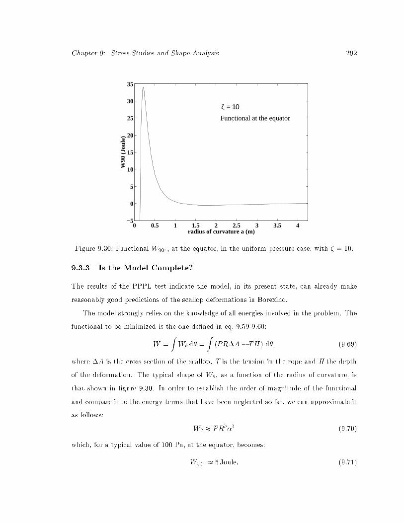
Chapter 9: Stress Studies and Shape Analysis 292
0 0.5 1 1.5 2 2.5 3 3.5 4−5
0
5
10
15
20
25
30
35
radius of curvature a (m)
W90
(Jo
ule)
ζ = 10 Functional at the equator
Figure 9.30: Functional W90o, at the equator, in the uniform pressure case, with � = 10.
9.3.3 Is the Model Complete?
The results of the PPPL test indicate the model, in its present state, can already make
reasonably good predictions of the scallop deformations in Borexino.
The model strongly relies on the knowledge of all energies involved in the problem. The
functional to be minimized is the one de�ned in eq. 9.59-9.60:
W =
ZW� d� =
Z(PR�A � TH) d�; (9.69)
where �A is the cross section of the scallop, T is the tension in the rope and H the depth
of the deformation. The typical shape of W�, as a function of the radius of curvature, is
that shown in �gure 9.30. In order to establish the order of magnitude of the functional
and compare it to the energy terms that have been neglected so far, we can approximate it
as follows:
W� � PR3�3 (9.70)
which, for a typical value of 100 Pa, at the equator, becomes:
W90o � 5 Joule: (9.71)

Chapter 9: Stress Studies and Shape Analysis 293
Membrane Energy
The elastic energy of a membrane under stress is equal to [170]:
Um =h
2
Z ZA(�x"x + �y"y + �xy xy) dx dy; (9.72)
which, using Hooke's law, can be approximated to the following, for an order of magnitude
estimate:
dUm = U�d� �h
2ER22��2 sin � d� (9.73)
U� ��h
ER2�2 � 2� 102 Joules (9.74)
This quantity, estimated for a stress value of 5 MPa, is larger than the P�V term of
the energy functional. The point is, though, that this energy term has a slow variation with
the radius of curvature, through the stress. It adds to the total potential energy but it does
not change the position of its minimum, as a function of a. The membrane energy is, in
general, not a�ected by changes in the shape and the curvature of the shell; the bending
energy is the term accounting for it.
Bending Energy
The bending energy of a membrane under stress is given by [170]:
Ub =D
2
Z ZA
h(�x + �y)
2 � 2(1� �)(�x�y � �2xy)idx dy (9.75)
where A represents the surface of the shell, �x and �y are the changes in curvature in the
x and y direction, respectively, and �xy is the twist of the midsurface. The intensity of the
bending energy depends on the material propertied through the exural rigidity:
D =Eh3
12 (1� �2)= 2� 10�4 Joules; (9.76)
for nylon with Young's modulus E = 1000MPa and Poisson's ratio � = 0:4. The only term
of relevance for us is the change in curvature in the azimuthal direction:
�x = �� =
�1
a�
1
R
�; (9.77)

Chapter 9: Stress Studies and Shape Analysis 294
dUb = U�d� � D�R2
�1
a�
1
R
�2sin � d�: (9.78)
Since the modi�ed radius of curvature is of the same order of magnitude as the sphere's
radius, the bending energy at the equator will have values of the order of:
U� � D� = 2� 10�5 Joule: (9.79)
It is evident that this energy does not a�ect the shape of the overall energy functional.
Gravitational energy
When deep scallops are formed in the vessel, a certain mass of uid is pushed upwards. The
uid's change of altitude induces an increase of the gravitational potential energy. This
term does not a�ect shallow scallops, since the volume change is very small, but it can
prevent the formation of deep scallops.
In the hydrostatic case, with 5oC temperature di�erence and a pressure head of 350 Pa or
with 1oC and 70 Pa, the scallop depth and the radius of curvature predicted by the existing
model are as in �gure 9.25. For each scallop, the volume of scintillator to be displaced is
about 40 l (36 kg mass). This quantity has a smooth dependence on the radius of curvature
and it can only slightly a�ect the determination of the minimum for the energy functional.
If the radius of curvature is 50% higher than what is shown in �gure 9.25, the volume of
displaced uid is 7 l. If it is 50% smaller, it is 300 l. The resulting potential energy actually
depends on where the uid goes: if it is pushed out of the vessel and up the pipe, it will
end up being removed from the vessel and the associated potential energy will not enter the
calculation. If it shifts up at � = 36o, where the strings leave the vessel, it will �t in 3 mm,
for a potential energy change of 0.7 Joule. How much the gravitational energy term a�ects
the scallop calculation depends on the kind of level control implemented for the scintillator
level. It is worthwhile including this gravitational e�ect in the model, but a �nite element
numerical algorithm is necessary for a precise calculation.
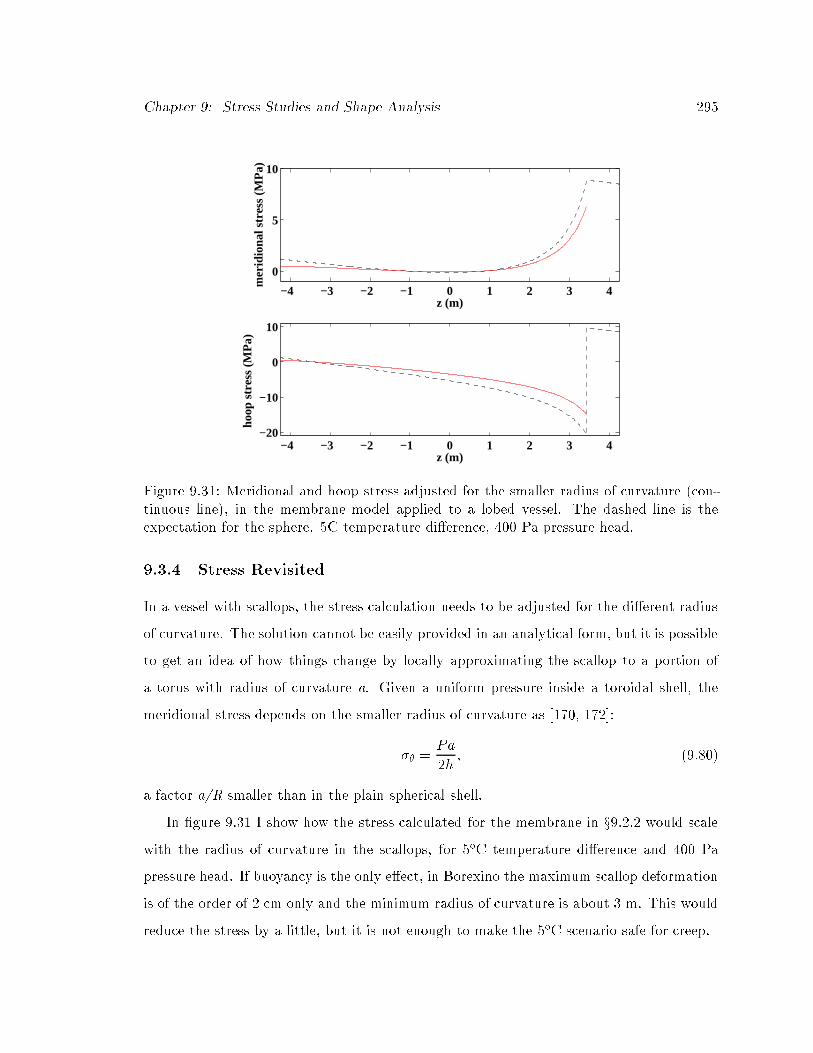
Chapter 9: Stress Studies and Shape Analysis 295
−4 −3 −2 −1 0 1 2 3 4
0
5
10
z (m)
mer
idio
nal s
tres
s (M
Pa)
−4 −3 −2 −1 0 1 2 3 4−20
−10
0
10
z (m)
hoop
str
ess
(MP
a)
Figure 9.31: Meridional and hoop stress adjusted for the smaller radius of curvature (con-tinuous line), in the membrane model applied to a lobed vessel. The dashed line is theexpectation for the sphere. 5C temperature di�erence, 400 Pa pressure head.
9.3.4 Stress Revisited
In a vessel with scallops, the stress calculation needs to be adjusted for the di�erent radius
of curvature. The solution cannot be easily provided in an analytical form, but it is possible
to get an idea of how things change by locally approximating the scallop to a portion of
a torus with radius of curvature a. Given a uniform pressure inside a toroidal shell, the
meridional stress depends on the smaller radius of curvature as [170, 172]:
�� =Pa
2h; (9.80)
a factor a/R smaller than in the plain spherical shell.
In �gure 9.31 I show how the stress calculated for the membrane in x9.2.2 would scale
with the radius of curvature in the scallops, for 5oC temperature di�erence and 400 Pa
pressure head. If buoyancy is the only e�ect, in Borexino the maximum scallop deformation
is of the order of 2 cm only and the minimum radius of curvature is about 3 m. This would
reduce the stress by a little, but it is not enough to make the 5oC scenario safe for creep.

Chapter 9: Stress Studies and Shape Analysis 296
If we want to compare the corrected stresses with those earlier reported in table 9.2, we
see that the improvement is from 18 MPa to 16 MPa at the discontinuity.
An alternative method to protect the vessel would be to deliberately oversize the panels
and induce deeper scallops, with the same approach that has been used for the super-
pressure balloons [174]. This way, we will have a non-spherical, lobed vessel by choice
and the vessel will be more protected against temperature and density uctuations, but the
radius of curvature should be signi�cantly smaller (of the order of 2 m) to make a di�erence.
This choice should be carefully considered for all the implications on the optics and the
signal detection that would come, in Borexino, from a non-symmetrical vessel.
9.4 Conclusion
In conclusion, my model predicts the deformations induced in the vessel by density uctu-
ations due to abrupt, non homogeneous temperature changes in the uids for Borexino.
The stress is calculated analytically, with models that approximate the Borexino topol-
ogy by an axially symmetrical one. These models are useful to establish the maximum
stress acting on the vessel membrane.
The deformation induced by the hold down ropes are calculated with a model that
minimizes the potential energy of the deformation; the model has been successfully tested
in an in ation test of the vessel prototype with air and with helium gas.
There are some assumptions in the model, though, which should still be veri�ed, pri-
marily the way the radius of curvature depends on the latitude and on the pressure. The
e�ect of gravitational energy in the displacement of a mass of uid should also be included
in the model. The e�ect of creep and membrane stretching could also have a signi�cant
impact on the lobe curvatre and should be included in the model. Another item to explore
in greater detail, possibly with the help of a numerical algorithm, is the non-symmetrical
stress pattern in the presence of lobes.
The current analytical model can be used to establish some of the operating parameters
for Borexino; this work is still in progress, but it appears a numerical model will be required.
Chapter 9: Stress Studies and Shape Analysis 297
The operating conditions of 0.1% density di�erence between inside and outside the vessel
are safe: the stress is low and the scallops are small. The 0.5% density di�erence due to a
5oC temperature gradient will not cause a vessel failure, since the maximum stress is less
than 20 MPa and the nylon yield is at 60 MPa or higher, but this scenario is of concern for
creep. An e�ective temperature control system should be implemented in order to prevent
this from happening.

Bibliography
[1] J. Updike. Telephone Poles and other Poems. Alfred A. Knopf, Inc., New York, 1963.
[2] W. Pauli, December 1930. Letter to the Physical Society of Tubingen.
[3] C.L. Jr. Cowan, F. Reines, F.B. Harrison, H.W. Kruse, and A.D. McGuire. \Detection
of the Free Neutrino: A Con�rmation". Science, 124 (1956), 103.
[4] J.N. Bahcall. \How the Sun Shines". Nobel e-museum, http://www.nobel.se, (2000).
[5] H.A. Bethe. Phys. Rev., 55 (1939), 434.
[6] J.N. Bahcall and M.H. Pinsonneault. Rev. Mod. Phys., 64 (1992), 885.
[7] J.N. Bahcall and R.K. Ulrich. Rev. Mod. Phys., 60 (1988), 297.
[8] J.N. Bahcall and M.H. Pinsonneault. Rev. Mod. Phys., 67 (1995), 781.
[9] S. Turck-Chieze and I. Lopes. Astrophys. J., 408 (1993), 347.
[10] A.S. Brun, S. Turck-Chieze, and P. Morel. Astrophys. J., 506 (1998), 913.
[11] J.N. Bahcall, S. Basu, and M.H. Pinsonneault. \How Uncertain Are Solar Neutrino
Predictions?". Phys. Lett. B, 433 (1998), 1.
[12] R. Davis Jr., D.S. Harmer, and K.C. Ho�man. Phys. Rev. Lett., 20 (1968), 1205.
[13] B.T. Cleveland, T. Daily, R. Davis Jr., et al. Astrophys. J., 496 (1998), 505.
[14] The SAGE Collaboration, J.N. Abdurashitov, et al. Phys. Rev. C, 9 (1999), 2246.
298

BIBLIOGRAPHY 299
[15] The GALLEX Collaboration, W. Hampel, et al. Phys. Lett. B, 447 (1999), 127.
[16] The GNO Collaboration, M. Altmann, et al. Phys. Lett. B, 490 (2000), 16.
[17] The Kamiokande collaboration, Y. Fukuda, et al. Phys. Rev. Lett., 77 (1996), 1683.
[18] The SuperKamiokande Collaboration, Y. Fukuda, et al. Phys. Rev. Lett., 81 (1998),
1158.
[19] The SNO Collaboration, J. Boger, et al. Nucl. Instrum. Methods A, 449 (2000), 172.
[20] J.N. Bahcall. http://www.sns.ias.edu/ jnb/, August 2000.
[21] S. Basu et al. Mon. Not. R. Astron. Soc., 292 (1997), 234.
[22] S. Turck Chieze et al. Solar Phys., 175 (1997), 247.
[23] S. Basu. Mon. Not. R. Astron. Soc., 298 (1998), 719.
[24] S. Basu et al. Astrophys. J., 460 (1996), 1064.
[25] V. Castellani, S. Degl'Innocenti, G. Fiorentini, M. Lissia, and B Ricci. Phys. Rev. D,
50 (1994), 4749.
[26] J.N. Bahcall. Neutrino Astrophysics. Cambdrige University Press, 1989.
[27] J. Faulkner and R.L. Gilliland. Astrophys. J., 299 (1985), 994.
[28] V. Castellani, S. Degl'Innocenti, and G. Fiorentini. Phys. Lett. B, 303 (1993), 68.
[29] N. Hata, S. Bludman, and P. Langacker. Phys. Rev. D, 49 (1994), 3622.
[30] G.L. Fogli, E. Lisi, and D. Montanino. Phys. Rev. D, 49 (1994), 3626.
[31] V. Berezinsky et al. Phys. Lett. B, 365 (1996), 185.
[32] K.M. Heeger and R.G.H. Robertson. Phys. Rev. Lett., 77 (1996), 3720.
[33] L. Wolfenstein. Phys. Rev. D, 17 (1978), 2369.

BIBLIOGRAPHY 300
[34] S.P. Mikeyev and A.Y. Smirnov. Sov. J. Nucl. Phys., 42 (1985), 913.
[35] P. Langacker et al. Phys. Rev. D, 27 (1983), 1228.
[36] W.C. Haxton. \Neutrino Oscillations and the Solar Neutrino Problem". Preprint
nucl-th/0004052, April 2000.
[37] S. Turck-Chieze et al. Astrophys. J., 335 (1988), 425.
[38] S.J. Parke. Phys. Rev. Lett., 57 (1986), 1275.
[39] P. Pizzocchero. Phys. Rev. D, 36 (1987), 2293.
[40] J.N. Bahcall and P.I. Krastev. \Does the Sun Appear Brighter at Night in Neutri-
nos?". Phys. Rev. C, 56 (1997), 2839{2857.
[41] J.N. Bahcall, P.I. Krastev, and A.Yu. Smirnov. \Is Large Mixing Angle MSW the
Solution of the Solar Neutrino Problems?". Phys. Rev. D, 60 (1999), 93001.
[42] J.N. Bahcall, P.I. Krastev, and A.Yu. Smirnov. \Where do we stand with solar
neutrino oscillations?". Phys. Rev. D, 58 (1998), 96016.
[43] J.G. Learned. \The Atmospheric Neutrino Anomaly: Muon Neutrino Disappearance".
Preprint hep-ex/0007056, July 2000.
[44] The SuperKamiokande Collaboration, Y. Fukuda, et al. \Evidence for Oscillation of
Atmospheric Neutrinos". Phys. Rev. Lett., 81 (1998), 1562.
[45] The SuperKamiokande Collaboration, Y. Fukuda, et al. \Measurement of the Solar
Neutrino Energy Spectrum Using Neutrino-Electron Scattering". Phys. Rev. Lett.,
82 (1999), 2430.
[46] J.N. Bahcall and P.I. Krastev. \Do hep neutrinos a�ect the solar neutrino energy
spectrum?". Phys. Lett. B, 436 (1998), 243.
[47] R. Escribano, J.M. Frere, A. Gevaert, and D. Monderen. \Boron abundance and solar
neutrino spectrum distortion". Phys. Lett. B, 444 (1998), 397.

BIBLIOGRAPHY 301
[48] V. Berezinsky, G. Fiorentini, and M. Lissia. \Vacuum Oscillations and excess of high
energy solar neutrino events observed in SuperKamiokande". Astropart. Phys., 12
(2000), 299.
[49] Y. Suzuki, for the SuperKamiokande Collaboration. In Neutrino 2000 - Proceedings
of the 19th Internationl Conference on Neutrino Physics and Astrophysics (Sudbury,
Canada, 2000), June 2000.
[50] G.L. Fogli, E. Lisi, D. Montanino, and A. Palazzo. \Day-night asymmetry of high and
low energy solar neutrino events in Super-Kamiokande and in the Sudbury Neutrino
Observatory". Phys. Rev. D, 62 (2000), 113003.
[51] The Borexino Collaboration, G. Alimonti, et al. \Ultra-low Background Measure-
ments in a Large Volume Underground Detector". Astropart. Phys., 8 (1998), 141.
[52] C. Galbiati. Data taking and analysis of the Counting Test Facility of Borexino. PhD
thesis, Universit�a degli Studi di Milano, 1999.
[53] F. Masetti, October 2000. Private communication.
[54] M. Ne�, October 1996. Note on laboratory measurements of quenching factors.
[55] J.B. Birks. The theory and practice of scintillation counting. Pergamon Press, 1974.
[56] G. Ranucci, A. Goretti, and P. Lombardi. \Pulse Shape Discrimination of Liquid
Scintillators". Nucl. Instrum. Methods A, 412 (1998), 374.
[57] M. Chen et al. \Quenching of undesired uorescence in a liquid scintillator particle
detector". Nucl. Instrum. Methods A, 420 (1999), 189.
[58] A. Ianni, May 2000. Private communication.
[59] M. Deutsch, editor. Proposal for a Cosmic Ray Detection System for the Borexino
Solar Neutrino Experiment. Massachussetts Institute of Technology, 1996.

BIBLIOGRAPHY 302
[60] M. Chen, editor. National Science Foundation Muon Veto Supplement Proposal for
the Borexino Experiment. Princeton University, Apr 1998.
[61] G. Ranucci et al. Nucl. Instrum. Methods A, 333 (1993), 553.
[62] E. Resconi. Measurements with the Upgraded Counting Test Facility (CTF-2) of the
Solar Neutrino Experiment Borexino. PhD thesis, Universit�a degli Studi di Genova,
2001.
[63] R. Winston and W.T.Welford. High collection nonimaging optics, page 132. Academic
Press, New York, 1989.
[64] J.B. Benziger et al. \A scintillator puri�cation system for a large scale solar neutrino
experiment". Nucl. Instrum. Methods A, 417 (1998), 278.
[65] M. Balata et al. \ The water puri�cation system for the low background Counting
Test Facility of the Borexino experiment at Gran Sasso". Nucl. Instrum. Methods A,
370 (1996), 605.
[66] L. Cadonati. Il controllo dei livelli di Radon in aria ed in acqua nell'ambito del
progetto Borexino: techniche di abbattimento e misure ad alta sensitivita'. Laurea
thesis, Universit�a degli Studi di Milano, 1995.
[67] V. Lagomarsino and G. Testera. \A gateless charge integrator for Borexino energy
measurement". Nucl. Instrum. Methods A, 430 (1999), 435.
[68] J. Maneira. In A. Mourao, M. Pimenta, and P. Sa, editors, Proc. Second Intern.
Workshop on "New Worlds in Astroparticle Physics", Faro, Portugal, page 131, 1998.
[69] M. Johnson et al. \A 222Rn Source for Low-background Liquid Scintillation Detec-
tors". Nucl. Instrum. Methods A, 414 (1998), 459.
[70] The Borexino Collaboration, G. Alimonti, et al. \Light propagation in a large volume
liquid scintillator". Nucl. Instrum. Methods A, 440 (2000), 360.

BIBLIOGRAPHY 303
[71] R. Von Hentig et al. \Determination of Radioactive Trace Elements in Ultra Low
Background Detectors by Means of Neutron Activation Analysis". Czech. J. Phys.,
49 Suppl. S1 (1999), 277{286.
[72] The Borexino Collaboration, G. Alimonti, et al. \A large-scale low background liquid
scintillator detector: the Counting Test Facility at Gran Sasso". Nucl. Instrum.
Methods A, 406 (1998), 411.
[73] The Borexino Collaboration, G. Alimonti, et al. \Measurement of the 14C abundance
in a low background liquid scintillator". Phys. Lett. B, 422 (1998), 349.
[74] J. Benziger, F.P. Calaprice, et al., editors. A Proposal for Participation in the Borex-
ino Solar Neutrino Experiment. Princeton University, 1996.
[75] M. Giammarchi, September 1998. Note on potassium in the CTF data.
[76] C. Grieb. Diploma thesis, Technische Universit�at M�unchen, 2001.
[77] S. Bonetti et al. Nucl. Instrum. Methods A, 329 (1993), 314.
[78] B. Caccianiga et al. \GENEB: GEneration of NEutrino and Background". Borexino
collaboration internal memo, INFN Milano, October 1997.
[79] I. Manno. \Tracking". Borexino collaboration internal memo, INFN Milano, Septem-
ber 1997.
[80] I. Manno. \Event Reconstruction in the C.T.F. (User's Guide)". Borexino collabora-
tion internal memo, INFN Milano, July 1994.
[81] W.R. Nelson et al. \The EGS4 code system". Technical report, SLAC-265 UC-32
(E/I/A), 1985.
[82] F. James. \MINUIT". Technical report, CERN Program Library, 1994.
[83] G. t'Hooft. Phys. Lett., B37 (1971), 195.

BIBLIOGRAPHY 304
[84] M.G. Giammarchi et al. \Neutrino oscillation simulation, neutrino uxes and neutrino
scattering in the Borexino Monte Carlo". Borexino collaboration internal memo,
INFN, Milano, October 1997.
[85] The Borexino Collaboration, C. Arpesella, et al. Borexino at Gran Sasso: proposal
for a real time detector for low energy solar neutrinos, volume 1{2. Ed. G. Bellini,
R.S. Raghavan et al. (INFN Milano), 1991.
[86] M. Ne�, October 1999. Private communication.
[87] J. Benziger, F.P. Calaprice, et al., editors. N.S.F. Borexino Proposal. Princeton
University, 1993.
[88] P. Belli et al. Il Nuovo Cimento A, 101 (1989), 959.
[89] M. Aglietta et al. Il Nuovo Cimento C, 12 (1989), 467.
[90] T. Hagner et al. \Muon-induced production of radioactive isotopes in scintillation
detectors". Astropart. Phys., 14 (2000), 33.
[91] F. von Feilitzsch et al. \The Borexino Muon Identi�cation System". Technical report,
TU-Muenchen Muon and NA54 group report, February 1998.
[92] E. Calabresu, N. Ferrari, G. Fiorentini, and M. Lissia. \Just so? Vacuum oscillations
and MSW: an update". Astropart. Phys., 4 (1995), 159.
[93] J.N. Bahcall, M. Fukugita, and P.I. Krastev. \How Does the Sun Shine?". Phys. Lett.
B, 374 (1996), 1.
[94] V. Barger, B. Kayser, J. Learned, T. Weiler, and K. Whisnant. \Fate of the sterile
neutrino". Phys. Lett. B, 489 (2000), 345.
[95] A. de Gouvea, A. Friedland, and H. Murayama. \Seasonal Variations of the 7Be Solar
Neutrino Flux". Phys. Rev. D, 60 (1999), 93011.

BIBLIOGRAPHY 305
[96] B. Faid, G.L. Fogli, E. Lisi, and D. Montanino. \Vacuum oscillations and variations of
solar neutrino rates in SuperKamiokande and Borexino". Astropart. Phys., 10 (1999),
93.
[97] G.L. Fogli, E. Lisi, and D. Montanino. \Fourier analysis of real-time, high-statistics
solar neutrino observations". Phys. Rev. D, 56 (1997), 4374.
[98] J. Bouchez et al. Z. Phys. C, 32 (1986), 499.
[99] E. Carlson. \Terrestrially enhanced neutrino oscillations". Phys. Rev. D, 34 (1986),
1454.
[100] A.H. Guth, L. Randall, and M. Serna. \Day-night and energy dependence of MSW
solar neutrinos for maximal mixing". JHEP, 9908 (1999), 018.
[101] J.N. Bahcall and P.I. Krastev. \Does the Sun appear brighter at night in neutrinos?".
Phys. Rev. C, 56 (1997), 2839.
[102] A. de Gouvea, A. Friedland, and H. Murayama. \Earth Matter E�ect in 7Be Solar
Neutrino Experiments". Preprint hep-ph/9910286, October 1999.
[103] The Kamland Collaboration and A. Suzuki. Nucl. Phys. B (Proc. Suppl.), 77 (1999),
171.
[104] R. Foot. Maximal �e oscillations, borexino and smoking guns. Phys. Lett. B, 483
(2000), 151.
[105] A. de Gouvea, A. Friedland, and H. Murayama. The dark side of the solar neutrino
parameter space. Preprint hep-ph/0002064, February 2000.
[106] G.L. Fogli, E. Lisi, D. Montanino, and A. Palazzo. \Testing solar neutrino MSW oscil-
lations at low �m2 through time variations of event rates in GNO and BOREXINO".
Phys. Rev. D, 61 (2000), 73009.
[107] S. Bonetti et al. \Ionization quenching: e�ects on e� and detection in Borexino
and CTF". Borexino collaboration internal memo, INFN, Milano, October 1998.
BIBLIOGRAPHY 306
[108] M. Aglietta et al. JETP Letters, 63 (1996), 791.
[109] R.S. Raghavan et al. Phys. Rev. Lett., 80 (1998), 635.
[110] C. Rotschild et al. Geophys. Res. Lett., 25 (1998), 1083.
[111] S. Schoenert. Nucl. Phys. B (Proc. Suppl.), 70 (1999), 195.
[112] R.S. Raghavan. Phys. Rev. Lett., 72 (1994), 1411.
[113] B. Caccianiga and M. Giammarchi. \Neutrinoless double beta decay with Xe-136
in BOREXINO and the BOREXINO Counting Test Facility". Astropart. Phys., 14
(2000), 15.
[114] A. Ianni and D. Montanino. Astropart. Phys., 10 (1999), 331.
[115] D.N. Schramm. Comm. Nucl. Part. Phys., 17 (1987), 239.
[116] R. Bionta et al. Phys. Rev. Lett., 58 (1987), 1494.
[117] K. Hirata et al. Phys. Rev. Lett., 58 (1987), 1490.
[118] L. Cadonati, F. Calaprice, and M. Chen. \Supernova neutrino detection in Borexino".
2000.
[119] L. Cadonati. \Supernova Neutrino Detection in Borexino". Borexino collaboration
internal memo, Princeton University, February 1999.
[120] K. Langanke, P. Vogel, and E. Kolbe. Phys. Rev. Lett., 76 (1996), 2629.
[121] M. Fukugita, Y. Kohyama, and K. Kubodera. Phys. Lett. B, 212 (1988), 139.
[122] J. Bernabeu and P. Pascual. Nucl. Phys. A, 324 (1979), 365.
[123] S.L. Mintz and M. Pourkaviani. \Theoretical calculations for neutrino-induced charged
current reactions in 12C and recent experimental results". Phys. Rev. C, 40(6) (1989), 2458.
[124] J. Engel, E. Kolbe, K. Langanke, and P. Vogel. Phys. Rev. C, 54 (1996), 2740.

BIBLIOGRAPHY 307
[125] Woosley et al. Astrophys. J., 356 (1990), 272.
[126] T.W. Donnelly and R.D. Peccei. \Neutral Current E�ects in Nuclei". Phys. Rep., 50 (1979),
1.
[127] J.S. O'Connell, T.W. Donnelly, and J.D. Walecka. \Semileptonic Weak Interactions with
12C". Phys. Rev. C, 6(3) (1972), 719.
[128] T.W. Donnelly. \Low-Energy Neutrino reactions with 12C and 16O". Phys. Lett. B, 43(2)
(1973), 93.
[129] E. Kolbe, K. Langanke, and S. Krewald. Phys. Rev. C, 49 (1994), 1122.
[130] E. Kolbe, K. Langanke, F.K. Thielemann, and P. Vogel. Phys. Rev. C, 52 (1995), 3437.
[131] E. Kolbe, K. Langanke, S. Krewald, and F.K. Thielemann. Nucl. Phys. A, 540 (1992), 599.
[132] A. Burrows et al. Phys. Rev. D, 45 (1992), 3361.
[133] \Particle Data Group". Eur. Phys. J. C, 3 (1998), 1.
[134] J.F. Beacom and P. Vogel. Phys. Rev. D, 58 (1998), 53010.
[135] J.F. Beacom and P. Vogel. Phys. Rev. D, 58 (1998), 93012.
[136] M. I. Kohan, editor. Nylon Plastics Handbook. Hanser/Gardner Publications, Inc., 1995.
[137] F. Rodriguez, editor. Principles of Polymer Systems. Francis & Taylor, 1996.
[138] Martin and Gardner. E�ect of long term humid aging on plastics. J. Polym. Engin. Sci., 21
(1981), 557.
[139] A.A. Popov and G.E. Zaikov. Macromol. Chem. Phys., C27 (3&4) (1987-1988), 379.
[140] Standard test method for tensile properties of thin plastic sheeting. ASTM D882.
[141] A.C. Reimschuessel and Y.J. Kim. J. Mater. Sci., 13 (1978), 243.
[142] Product cleanliness levels and contamination control program. MIL-STD-1246C.
[143] E. Harding, August 2000. Private communication.

BIBLIOGRAPHY 308
[144] N. Darnton. Adsorption properties of activated charcoal. Borexino collaboration internal
memo, Princeton University, April 1997.
[145] A. Pocar. Radon �ltering from air. Borexino collaboration internal memo, Princeton Univer-
sity, October 1999.
[146] J. Benziger, August 1999. Private communication.
[147] T. Shutt. Vessel tie-down ropes for Borexino. Borexino collaboration internal memo, Princeton
University, September 2000.
[148] J. Bigu. Nucl. Instrum. Methods A, 251 (1986), 366.
[149] M. W�ojcik et al. Nucl. Instrum. Methods B, 61 (1991), 8.
[150] M. W�ojcik et al. Radon di�usion through polymer membranes used in the solar neutrino
experiment borexino. Nucl. Instrum. Methods A, 449 (2000), 158.
[151] W. Gerrard. Gas Solubilities Widespread Applications. Pergamon Press, 1980.
[152] F. Masetti and U. Mazzuccato, April 1997. Private communication.
[153] M. W�ojcik, June 1997. Private communication.
[154] P. Debye and A. Bueche. J. Appl. Phys., 20 (1949), 518.
[155] R.S. Stein and J.J. Keane. The Scattering of Light from Thin Polymer Film. Experimental
Procedure. J. Polymer Sci., 17 (1955), 21.
[156] J.J. Keane, F.H. Norris, and R.S. Stein. Light Scattering from Oriented Polyethylene Films.
J. Polymer Sci., 20 (1956), 209.
[157] J.J. Keane and R.S. Stein. The Scattering of Light from Thin Polymer Film. Scattering from
Polyethylene. J. Polymer Sci., 20 (1956), 327.
[158] M. Johnson, 1997. Private communication.
[159] F. Masetti, April 1999. Private communication.
[160] Standard test method for haze and luminous transmittance of transparent plastics, 1977.
ASTM D1003.

BIBLIOGRAPHY 309
[161] C. Arpesella. Appl. Rad. Isot., 4 (1996), 991.
[162] H. Neder. Appl. Rad. Isot., 53 (2000), 191.
[163] http://www.e15.physik.tu-muenchen.de/borexino/memo.htm.
[164] I. Akabane. Technical report, Tama Chemicals Co Ltd Kawasaki Laboratory. Laboratory
Reports, 09/02/1993 and 12/05/1999.
[165] T. Florkowski, L. Morawska, and K. Rozanski. Nucl. Geophys., 2 (1988), 1.
[166] M. Laubenstein. \New method for measuring ultralow levels of radioactivity". Nucl. Instrum.
Methods A, 409 (1-3) (1998), 484.
[167] G. Heusser et al. \222Rn detection at the �Bq/m3 range in nitrogen gas and a new Rn
puri�cation technique for liquid nitrogen". Appl. Rad. Isot., 52 (2000), 691.
[168] G. Heusser, September 2000. Private communication.
[169] L. Cadonati. \Potassium Peak in the CTF2 Data". Borexino collaboration internal memo,
Princeton University, August 2000.
[170] A.C. Ugural. Stresses in Plates and Shells, Second Edition. McGraw-Hill, 1998.
[171] L.D. Landau and E.M. Lifshitz. Theory of Elasticity, Third Edition. Butterworth Heinemann,
1986.
[172] S. Timoshenko and S. Woinowsky-Krieger. Theory of Plates and Shells. McGraw-Hill, 1959.
[173] A.V. Pogorelov. Bending of Surfaces and Stability of Shells. American Mathematical Society,
1988.
[174] J.H. Smalley. Development of the e-Balloon. NCAR.