Journal of Computational and Applied Mathematics 37 (1991) 89-99 North-Holland

89

Zeros of the Hankel function of real order out of the principal Riemann sheet *

And&s Cruz Departamento de Fisica Tehica, Facultad de Ciencias, Universidad de Zaragoza, 50009 Zaragoza, Spain

Javier Esparza Departamento de Ingeneria Eltktrica e Informcitica, Escuela T. Superior de Ingenieros Industriales, 50015 Zaragoza, Spain

Javier Sesma Departamento de Fisica Tehica, Facultad de Ciencias, Universidad de Zaragoza, 50009 Zaragoza, Spain

Received 15 June 1990 Revised 3 December 1990

Abstract

Cruz, A., J. Esparza and J. Sesma, Zeros of the Hankel function of real order out of the principal Riemann sheet, Journal of Computational and Applied Mathematics 37 (1991) 89-99.

Zeros of the Hankel function of real order follow, as the order varies continuously, trajectories across different Riemann sheets of the complex plane. A discussion of the main features of these trajectories is presented.

Keywords: Hankel functions, zeros.

1. Introduction

The zeros of the Hankel function H,“)(z) of real order v play an important role in many physical problems. For instance, the physically acceptable solution of the Schrodinger equation for a quantum mechanical particle in a finite range potential is, in the region where the potential vanishes, essentially the Hankel function. Moreover, the trajectories of the zeros of H,“‘(z), for varying real order v, are the k-trajectories of the S-matrix singularities for quantum scattering by a hard sphere.

Information about the zeros of H,“‘(z) provided by classical treatises on special functions is rather insufficient. In particular, the behavior of the zeros as v varies is not discussed at all, and, consequently, the fact that the number of zeros is infinite for integer v and finite for half-integer v is not explained. This issue was considered by us, a few years ago, in a previous paper [3].

* This work was financially supported by the Cornision Interministerial de Ciencia y Tecnologla.

0377-0427/91/%03.50 0 1991 - Elsevier Science Publishers B.V. All rights reserved

90 A. Cruz et al. / Zeros of the Hankel function

According to our results, H,“‘(z) presents in the complex z-plane, for real v, an infinite number of zeros, zs( v), s = 1, 2, 3,. . . , that, for v decreasing from infinity to s - i, move along trajectories lying in the lower half-plane of the principal Riemann sheet. These trajectories cut the semiaxis arg z = -IT for v = s - : and go, almost vertically, to infinity in the quadrant - $71~ arg z < --71 for v = s - i. That means that v = s - i is a singular point (in fact, a branch point) of zs( v) considered as a function of v. The trajectory of zs( v) presents a discontinuity at that value of v and the question arises of how that trajectory proceeds for v < s - i. To answer this question, a prescription is needed about how to jump across the singularity at v = s - :. The most natural way of avoiding a singularity in a real variable is to assign it complex values by making a semicircular detour of infinitesimal radius around the singularity. In the case we are considering, if the detour goes below the singularity, that is, if v takes a small negative imaginary part, a new piece of the trajectory zs( v), corresponding to s - i < v < s - +, is found. For v = s - 5 a new discontinuity appears and the process of avoiding it must be repeated. Using always the same prescription, i.e., assigning when necessary a very small negative imaginary part to v, one obtains the trajectories shown in [3], that explain why H,‘y,,Z(z), n integer, possesses only a finite number of zeros. Those discontinuous trajectories contain, in their different pieces, the zeros of H,“‘(z), n integer, reported in [l, pp. 373, 3741.

A different way of circumventing the singularities leads to a different connection between pieces of trajectories, as we are going to show below. The possibility of avoiding the singularities by giving to v an infinitesimal positive imaginary part was not considered in [3] because the piece in the principal Riemann sheet became then spliced to pieces in other Riemann sheets, in which we were not interested at that moment.

In a current research on Coulomb waves [5] we are concerned with the zeros, in the complex z- plane, of the Whittaker function W .,,,,(z), the parameters c and v being real and associated respectively to the electric charge and the angular momentum. As is well known [2, p.2071, [6, p.131, W,,,,,(z) becomes proportional to z 1’2H(1)( +iz) in the limit c -+ 0. Therefore, the zeros of W,,,,.(z) for small c are close to those of H,“‘iiiz), and their trajectories for variable v tend, as c + 0, to the trajectories of the zeros of H,‘l’(:iz). But these trajectories are not uniquely determined; they depend, as mentioned above, on the prescription given to go round the discontinuities. Preliminary explorations seem to indicate that the trajectories of the zeros of W,,,,,(z) tend, for c + O+, to those of H,“)(iiz) reported in [3], that is, pieces connected by giving a small negative imaginary part to v at the singularities, whereas for c + O- the connection of the pieces corresponds to adding a small positive imaginary part to v.

The purpose of this paper is to generalize and complete the analysis initiated in [3], by considering the different pieces of the trajectories of the zeros zs( v) of H,“)(z) and by discussing how they are linked according to the prescription used to avoid the discontinuity points. In Section 2 we identify the. values of v at which the trajectories may intersect the coordinate axes. Section 3 is devoted to the discussion of the singularities of zs( v) in the different Riemann sheets and the connection rules resulting from the different ways of avoiding them. Some comments about the zeros of H,“‘(z) in each Riemann sheet are presented in Section 4. Finally, Section 5 contains some examples of trajectories obtained by adding to v an infinitesimal positive imaginary part.

For the sake of brevity, we denote by A, the mth Riemann sheet,

A,= {z: (2m-1)7r<arg z<(2m+l)~}, m=O, +l, f2,... . (1.1)

A. Cruz et al. / Zeros of the Hankel function 91

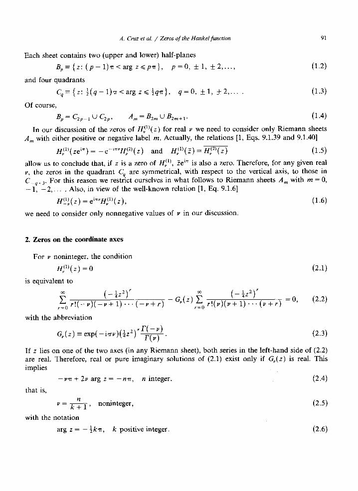
Each sheet contains two (upper and lower) half-planes

BP= {z: (p-l)T<argz<pn}, p=O, +l, +2 ,..., (1.2)

and four quadrants

C4= {z: +(4-l)a<arg z< +q~}, q=O, *l, +2 ,... . U-3)

Of course,

BP = C,,-, u CzP, A, = &I u &m+l* (1.4)

In our discussion of the zeros of H,“‘(z) for real v we need to consider only Riemann sheets A, with either positive or negative label m. Actually, the relations [l, Eqs. 9.1.39 and 9.1.401

H,“‘( ze’“) = - eein”H,(2)( z) and H,“‘(Z) = H,‘2’( z) (1.5)

allow us to conclude that, if z is a zero of H,“‘, Zei” is also a zero. Therefore, for any given real

v, the zeros in the quadrant C4 are symmetrical, with respect to the vertical axis, to those in

C- q+3. For this reason we restrict ourselves in what follows to Riemann sheets A, with m = 0,

-1, -2,... . Also, in view of the well-known relation [l, Eq. 9.1.61

H!!?(z) = e’““HJ(‘)( z), (1.6)

we need to consider only nonnegative values of v in our discussion.

2. Zeros on the coordinate axes

For v noninteger, the condition

H,“‘(Z) = 0

is equivalent to

(2.1)

go r!(-v)(-L$2-).r. (-v+ r) - G”(Z) f (-iz’)’

r=,T!(v)(v+l)**(v+r) =O, (2.2)

with the abbreviation

G,(z) =exp(-iqv)(fr’)‘w. P-3)

If z lies on one of the two axes (in any Riemann sheet), both series in the left-hand side of (2.2) are real. Therefore, real or pure imaginary solutions of (2.1) exist only if G,(z) is real. This implies

- VT + 2v arg z = -iz~, n integer, (2 *4)

that is,

v= &-> noninteger, (2.5)

with the notation

arg z = -ikT, k positive integer. (2.6)

92 A. Crux et al. / Zeros of the Hankel function

Results of numerical exploration, to be shown in Section 5, confirm preceding reasoning.

3. Singularities in the trajectories of the zeros

the correctness of the

Let us consider now the possibility of having zeros of H,?(z) at infinity for finite values of v. In [3] we found that such zeros occur in the quadrant C_, for half-integer values of v. Here we look at them in any Riemann sheet A,.

The starting point is the analytic continuation formula for the Hankel function [l, Eq. 9.1.371,

H,“)(z e-i2mn) = (sin(vn))-‘(sin((2m + l)v~)H,“)(z)

+ e-iVn sin(2mva)HJ2)( z)), m integer, (3.1)

where z is considered to be in the principal sheet A,,. If $z is large, approximate expressions [l, Eqs. 9.2.3 and 9.2.41 for the Hankel functions can be used to obtain

HY(1)(ze-i2”“) = ( A)1’2(sin(vT))-’ e-iVn’2(ei(z-V’4) sin((2m + l)v71)

The right-hand side vanishes when

+ e-i(r-n’4) sin(2mvT)). (3.2)

ei2(z-V4) = _ sin(2mvq) sin((2m + l)v?l) 3 v noninteger, (3.3)

or, explicitly,

x=%z=kn+ a~+ 4 arg Q, k integer, (3.4a)

y=sz= -iln IQ], (3.4b)

where Q represents the quotient

QE -

Therefore, zeros whenever

n

sin(2mvT) sin((2m + 1)v~) * (3.5)

in the Riemann sheet A _-m may go to infinity along nearly vertical lines

n

V=2m or v= (2m + 1) ’

n integer, v noninteger. (3 -6)

Of course, in the first case one has y + + cc and in the second one y + - co. Moreover, the real part of the zero going to infinity, given by (3.4), suffers a discontinuous

variation of iq as v passes through the singular values given by (3.6). The sign of this variation depends on the prescription used to connect values of v below and above the critical ones. Obviously, Q, whose argument appears in the right-hand side of (3.4a), changes sign at those values of v. Let us suppose, for definiteness, that Q is positive for v below a critical value v, and negative above it. This information is not sufficient to determine if arg Q has increased or decreased by 71 at v,. As mentioned in Section 1, the ambiguity can be removed by considering

A. CF-UZ et al. / Zeros of the Hankei function 93

complex values

v=v,+Av, ]Av] <v,,,

in the neighborhood of the critical points. In the case

vo= &,

(3.7)

(3 -8)

that is,

_Y+ +m, (3.9)

one has, toa good approximation,

‘Q a Av. (3.10)

Therefore, when ‘$?v increases through vo, arg Q increases by IT if zv -C 0 and decreases by IT if Y$v > 0. That is, for increasing v, the zero jumps by &r to the right when the singularity is avoided by giving to v a negative infinitesimal imaginary part, and to the left in the case of a positive one. On the contrary,

Q a (Av))’ (3.11)

for

v=&, 0 (3.12)

that is, for

y+ -cc. (3.13)

It is now immediate to check that, for increasing v, the zero jumps by HIT to the left if F$v c 0 and to the right for F$v > 0. The behavior of the zeros in both cases (3.8) and (3.12) can be summarized by saying that, as v increases through a singularity, they go vertically to infinity, make there a discontinuous jump of magnitude &r, clockwise if %v < 0 and counter-clockwise if $v > 0, and come back, vertically, into the finite z-plane.

4. Zeros of H,“’

The zeros of the Hankel function of integer order H,“’ in the principal Riemann sheet A, are well known [l, p.3731, [4]. They are located in the lower half-plane B, and are usually classified in two types:

(1) an infinite number of zeros just below the negative real semiaxis, with I8z I> n; and (2) a set of n zeros, with I %z I < n, which lie along the lower half of the boundary of an

eye-shaped domain around the origin. Here we are interested in zeros of H,“’ on any other half-plane B,. The analytic continuation

formula [l, Eq. 9.1.371 now gives

H,(*)(zeimn) = (-l)““(( m + l)H,“‘(z) + n~H,(~)(z)), (44

or, equivalently,

H,fl)(zeimn) = (-l)““(( m + l)H,“‘(Z) + m@)(Z)), (4.2)

94 A. Cruz et al. / Zeros of the Hankel function

Table 1 Zeros of HA’) in different Riemann sheets

Bo (- 2.404, - 0.341) (2.405,0.199) (- 2.405, -0.141) (2.405,O.llO) ( - 2.405, - 0.090) (- 5.520, - 0.345) (5.520,0.202) (- 5.520, - 0.143) (5.520,O.lll) ( - 5.520, - 0.091) ( - 8.654, - 0.346) (8.654,0.202) ( - 8.654, - 0.144) (8.654, 0.111) ( - 8.654, - 0.091)

(- 11.791, -0.346) (11.791,0.203) (- 11.791, -0.144) (11.791,0.111) (- 11.791, -0.091) ( - 14.935, - 0.348) (14.935,0.204) (- 14.935, - 0.145) (14.935, 0.112) (- 14.935, - 0.092)

Table 2 Zeros of H,“’ in different Riemann sheets

Bo B-2

( - 0.419, -0.577) (0.333,0.413) (- 0.286, - 0.337) (0.254, 0.291) (- 0.231, - 0.260) (- 3.832, -0.355) (3.832,0.208) ( - 3.832, - 0.147) (3.832,0.114) (- 3.832, - 0.093) ( - 7.016, - 0.349) (7.016,0.204) (- 7.016, - 0.145) (7.016, 0.112) ( - 7.016, - 0.092)

(- 10.173, - 0.348) (10.137, 0.203) (- 10.137, -0.144) (10.137, 0.112) (- 10.137, - 0.092) (- 13.326, - 0.348) (13.326, 0.204) (- 13.326, -0.145) (13.326, 0.112) (- 13.326, - 0.092)

Table 3 Zeros of H2(l) in different Riemann sheets

Bo B-1 B-2 B-3 B-4

(0.429, - 1.281) ( - 0.386, 1.101) (0.360, - 1.005) ( - 0.342, 0.941) (0.329, - 0.894) (- 1.317, - 0.836) (1.146, 0.652) (- 1.048, - 0.565) (0.981, 0.511) (- 0.931, - 0.473) (- 5.138, - 0.372) (5.136, 0.218) (- 5.136, -0.155) (5.136, 0.120) (- 5.136, - 0.098) (- 8.418, -0.356) (8.417, 0.208) (- 8.417, - 0.148) (8.417,0.115) (- 8.417, - 0.094)

(- 11.620, -0.351) (11.620, 0.206) (- 11.620, - 0.146) (11.620,0.113) (- 11.620, -0.092) ( - 14.796, - 0.350) (14.796, 0.205) (- 14.796, - 0.145) (14.796,0.113) (- 14.796, -0.092)

Table 4 Zeros of H3(l) in different Riemann sheets

Bo B-1 B-2 B-3 B-4

(1.308, - 1.682) (- 1.210,1.494) (1.153, - 1.392) (- 1.113, 1.324) (1.081, - 1.273) (- 0.432, - 1.959) (0.403, 1.774) (- 0.386, - 1.673) (0.373, 1.603) (- 0.364, - 1.551) (- 2.243, - 1.007) (2.020, 0.808) (- 1.890, - 0.713) (1.801, 0.654) (- 1.733, - 0.613) ( - 6.383, - 0.389) (6.381, 0.227) (- 6.381, - 0.161) (6.381,0.125) (- 6.380, - 0.102) ( - 9.762, - 0.363) (9.761, 0.212) (- 9.761, - 0.151) (9.761,0.117) (- 9.761, - 0.096)

(- 13.016, -0.356) (13.016, 0.208) (- 13.016, - 0.148) (13.016, 0.115) (- 13.016, -0.094)

A. Cruz et al. / Zeros of the Hankel function 95

Table 5 Zeros of Hi” in different Riemann sheets

Bo B-1 B-2 B

(-1.935, 1.606)

B-4

(2.204, - 1.978) (- 2.070, 1.783) (1.991, - 1.678) (1.892, - 1.553) (0.433, - 2.629) (- 0.411, 2.442) (0.398, - 2.338) ( - 0.389, 2.266) (0.382, - 2.211)

(- 1.305, - 2.426) (1.236, 2.237) (- 1.195, -2.132) (1.165, 2.060) (- 1.143, - 2.006) (- 3.182, - 1.138) (2.920, 0.927) ( - 2.767, - 0.826) (2.661, 0.763) (- 2.580, - 0.719) ( - 7.592, - 0.404) (7.590,0.236) ( - 7.589, - 0.168) (7.589, 0.130) ( - 7.589, - 0.106)

(- 11.066, - 0.371) (11.065,0.217) (- 11.065, - 0.154) (11.065, 0.119) (- 11.065, - 0.098) ( - 14.374, - 0.361) (14.374,0.211) (- 14.374, - 0.150) (14.374,0.116) ( - 14.374, - 0.095)

Table 6 Zeros of Hi” in different Riemann sheets

Bo B-1 B-2 B-3 B-‘l

(3.113, - 2.219) ( - 2.951, 2.017) (2.855, - 1.908) (- 2.787, 1.834) (2.735, - 1.779) (1.304, - 3.135) (- 1.249, 2.946)

(-0.433, - 3.296) (0.416, 3.109) ( - 2.190, - 2.794) (2.092, 2.601) ( - 4.130, - 1.247) (3.863, 1.026) ( - 8.776, - 0.417) (8.773, 0.244)

(- 12.340, - 0.378) (12.339, 0.221)

(1.217, - 2.840) (- 1.195, 2.766) (1.177, -2.710) ( - 0.405, - 3.003) (0.398, 2.929) (- 0.392, - 2.873) (- 2.033, - 2.494) (1.992, 2.420) (- 1.960, - 2.364) ( - 3.664, - 0.919) (3.544,0.853) (- 3.452, - 0.807) (- 8.772, - 0.173) (8.772, 0.134) (- 8.772, - 0.110)

( - 12.339, - 0.157) (12.339, 0.122) (- 12.339, - 0.100)

Table 7 Schematic trajectory, for decreasing real Y, of the first zero zr of the Hankel function H,“)(z)

Zl arg z1

(- 0.686,O)

(- fa, + cc), (:I? + 00) (0.827, 0)

(fir, - co), (- :n, - co) ( - 0.860,O)

(- :n, + cc), <an, + co) (0.874,O)

(&L -w),(+r, -cc)

(- 0.880, 0)

(- :n, + cc), (&n, + 00) (0.884,O)

(f? -w),(-:n, --co) (- 0.886, 0)

-n<, -co -n

-:n -2n _I 2= -37

- 171

-47

- pn

-5n

-+n -6n

-+%r -7n

96 A. Cruz et al. / Zeros of the Hankel function

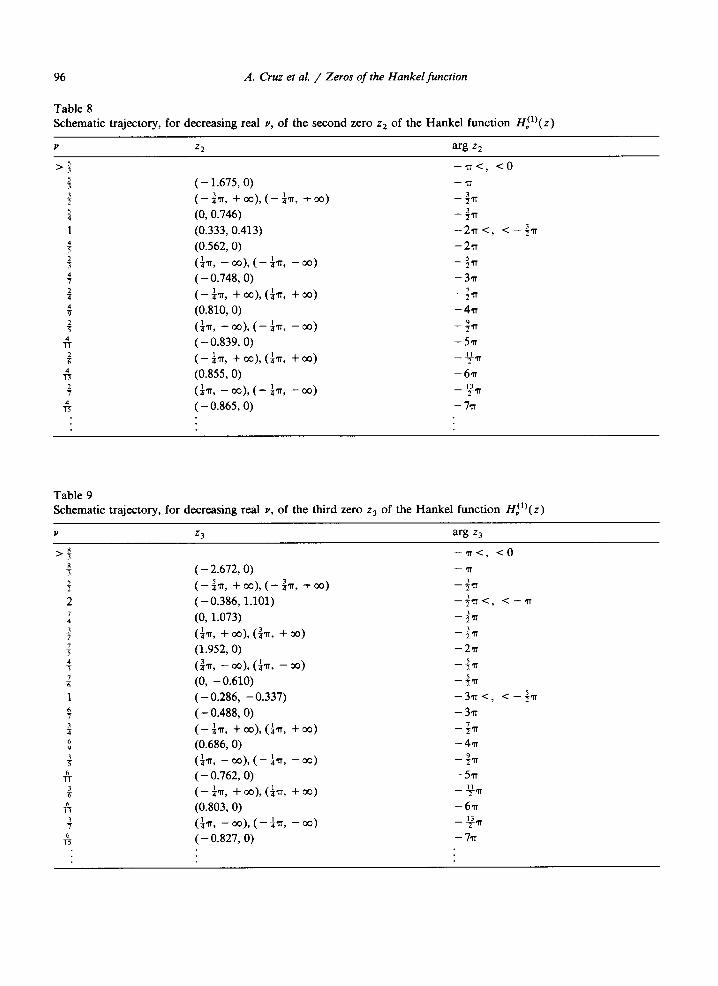
Table 8 Schematic trajectory, for decreasing real v, of the second zero zz of the Hankel function H,?(z)

V z2 as z2

(- 1.675,O)

(-+ll, +00),(-&r, +co)

(0,0.746)

(0.333,0.413)

(0.562,O)

t&r> -00),(-&r, -co) ( - 0.748, 0)

(- an, + cc), (:?I, + 00) (0.810,O)

($71, --w),(-:T, -co) ( - 0.839, 0)

(- ta, + m), (fT, + 00) (0.855, 0)

GIL - co), (- +n, - 00) (- 0.865,O)

-n<, -=o -n

-;?I - &l -2a<, < -+lT

-2q

-$?l

-37

-;q

-4T

- ;?l

-57r

-+n

-6a

-+l

-7T

Table 9 Schematic trajectory, for decreasing real v, of the third zero zs of the Hankel function H,!‘)(z)

z3

( - 2.672,O)

(-+t, +oo),(-&L +m) (-0.386, 1.101)

(0, 1.073)

tan, + co), (:a, + 00) (1.952,O)

(k -a)), (:n, - 00) (0, - 0.610)

( - 0.286, - 0.337)

(- 0.488,O)

(- 471, + co), (:I? + 00) (0.686,O)

(:q, -co),(-471, -00) ( - 0.762,O)

(- fll, + m), (f71, + 00) (0.803, 0)

(k - oo), (- $7, - 00) (- 0.827, 0)

ariz z3

--n-c, <o

-71

-+tt

-$l<, C--71

-+ll

-:n

-2n

-:n

-$I?

-3n<, -C-&l

-3,fr

-:?l

-4q

-$Tl

-5.n

-+l

-6~

“71

1;

A. Cru.z et al. / Zeros of the Hankel function 97

where z is assumed to lie in B,,. In view of the last relation, a simple way of searching for zeros of H,“’ in B_, is to consider a plot of the modulus and phase of H,“) in A, similar to that of H,“’ shown in [l, p.3591, and then to look for points z such that

(1) the phase of H,“’ in z be the opposite of that in Z plus or minus IT; and (2) the modulus of Hi”’ in z be m/( IYI + 1) times that in Z.

In what concerns this last condition, it is convenient to recall that the modulus of H,“‘(z) behaves in A, roughly like exp( - 3 z) except in the vicinity of its isolated zeros. Therefore, if one is looking for zeros in the half-plane B_,, one should explore regions in the neighborhood of points z, eeimn, where z, represents each zero of HA’) in B,. In other words, the pattern of zeros of H,“’ in B_, should be approximately the same as that obtained by rotating an angle of -WIT the pattern of zeros in Bo. The approximate positions of the zeros obtained in this way may serve as starting points for a more precise search.

This procedure has been used to determine the zeros of Hi’), n = 0, 1, 2, 3, 4, 5, in the half-planes B _ m, m = 1, 2, 3, 4. The Hankel function was expressed in terms of the Bessel ones [l, Eq. 9.1.31 and these were calculated by using their ascending series expansions [l, Eqs. 9.1.10 and 9.1.111. The results are shown in Tables l-6. For comparison, the zeros in B, are also shown. As far as we are interested mainly in qualitative features of the zeros of H,“‘, their positions are given only up to three decimal places, although the procedure certainly allows a more accurate determination.

Table 10 Schematic trajectory, for decreasing real Y, of the fourth zero zq of the Hankel function H,?(z)

V Z4 wit I4

(- 3.671, 0)

(--&b +co),(-h, +m) (- 1.210, 1.494)

(- 471, + m), (:T, + co) (1.146, 0.652) (1.459, 0)

(&, - oo), (& - co) (0, -1)

(-:II, -00),(--:n, -00) ( - 2.037, 0)

(-:T, +m),(-aT, +m) (0,0.527) (0.254,0.291) (0.437, 0)

(fn, -00),(--k -00) ( - 0.636,O)

(- :a, + co), (& + co) (0.721,O)

(471, -00),(-k -cc) ( - 0.769,O)

--n

-+n -in<, c-n -:n -2n<, <-+n -2a

-$n -$T

-+n -37 -;n -;v -4a<, <-;n -4n -fll -5n -q:71 -6n -y71 -77

98 A. Crux et al. / Zeros of the Hankel function

5. Trajectories of the zeros for varying real order

We have repeatedly mentioned that the trajectories of the zeros of H,‘l’ go to infinity for certain finite values of V. In consequence, one does not have a trajectory for each zero, but pieces of trajectories corresponding to values of v in the intervals between consecutive singularities. This puzzle of pieces in different Riemann sheets can be organized in whole trajectories, with v ranging from 0 to + co, only if a “protocol”, prescribing how to pass through the successive singularities, is attached to each trajectory. Moreover, the number of singularities in a trajectory and the values of v at which they appear depend on the protocol.

We showed in [3] a few whole trajectories obtained with the protocol; avoid every singularity by adding to v an infinitesimal negative imaginary part. The number of singularities was then finite (equal to the label s assigned to each trajectory) and all trajectories, coming from infinity for v decreasing from + co, ended for v = 0 at finite points of the principal Riemann sheet. But the protocol could be, instead, to add to v an infinitesimal positive imaginary part at all singularities. The trajectories present in this case an infinity of discontinuities and pass succes-

Table 11 Schematic trajectory, for decreasing real v, of the fifth zero z5 of the Hankel function H,“)(z)

V arg z5

>14 3 -n<, co Y (- 4.670, 0) -71

4 (-$71, +co),(-:q, +co> -3 271 4 (- 2.070, 1.783) -;n<, c--n

: (-$71, +03),(-k +to) -$r 13 r (0, 2.063) -:n

3 (0.403, 1.774) -2q-C, < -+n

: (&, + w), (in, + w) -+rr ‘j’ (3.037, 0) -27

; (k - co), ($7, - 03) - :7

2 (0.360, - 1.005) -:n<, <-2T

I: (- :a, -oo),(-a71, -03) -$n y (- 1.791,O) -311

: (--:71, +co),(-;P, +co) -+ll y (0,0.897) -;?l

: (in, + m), (k + 00) -:n p (2.078, 0) -4?r

2 (:? -cc), ($7, - 00) -&r

% (0, - 0.469) - ;I?

1 ( - 0.231, - 0.260) -5Tr<, c-p,

E ( - 0.399, 0) -57

: (- 471, + oo), (fa, + w) -J&T

+! (0.595, 0) -6a

: (&Y -co),(-:lT, -00) -+l

E (- 0.686,O) -77r

A. Cruz et al. / Zeros of the Hankel function 99

Rez ’ 4-

-4- I

-6 -4 -2 0 2 4 Imt

-4 4,s -4 4/?

-2 0 2 -2 0 2

Fig. 1. Trajectory of a zero of the Hankel function across different Biemann sheets. The three pictures show the trajectory followed by the fourth zero of H,“‘(z), for decreasing real v, successively in the Riemann sheets A-,, A-, and A _3. The dashed line in the first picture indicates the trajectory in the principal Riemann sheet A,. The different pieces of the trajectory are linked by adding to v a small positive imaginary part at the singularities. The cut in the z-plane is represented by a wavy line along the negative real semiaxis. The numbers along the trajectory correspond to

values of v.

sively from each Riemann sheet A _-m to the preceding one A _m_ 1 as v decreases. The limiting position of the zeros for Y = 0 is not defined, since they oscillate almost vertically from ($r, + cc) to ($a, - cc) or from ( - +r, - co) to ( - $r, + cc) for v decreasing from 2s/m to 2s/( m + l), m > 2s. Tables 7-11 and Fig. 1 intend to illustrate such intricate behavior.

Of course, different protocols, combining arbitrarily the two possible ways of avoiding all singularities, could also be considered. It is not difficult to get an idea of the tremendous variety of whole trajectories that would be obtained.

References

111 PI [31

M. Abramowitz and LA. Stegun, Eds., Handbook of Mathematical Functions (Dover, New York, 1965). H. Buchholz, The Confluent Hypergeometric Function (Springer, New York, 1969). A. Cruz and J. Sesma, Zeros of the Hankel function of real order and of its derivative, Math. Comp. 39 (1982) 639-645.

[41 B. Doring, Complex zeros of cylinder functions, Math. Comp. 20 (1966) 215-222.

151 J. Esparza and J. Sesma, Zeros of the Whittaker function associated to Coulomb waves, in preparation.

[61 L.J. Slater, Confluent Hypergeometric Functions (Cambridge Univ. Press, Cambridge, 1960).