XTCSD: Stata module to test for cross-sectional dependence in panel data models
16
The Stata Journal Editor H. Joseph Newton Department of Statistics Texas A & M University College Station, Texas 77843 979-845-3142; FAX 979-845-3144 [email protected] Editor Nicholas J. Cox Department of Geography Durham University South Road Durham City DH1 3LE UK [email protected] Associate Editors Christopher F. Baum Boston College Rino Bellocco Karolinska Institutet, Sweden and Univ. degli Studi di Milano-Bicocca, Italy A. Colin Cameron University of California–Davis David Clayton Cambridge Inst. for Medical Research Mario A. Cleves Univ. of Arkansas for Medical Sciences William D. Dupont Vanderbilt University Charles Franklin University of Wisconsin–Madison Joanne M. Garrett University of North Carolina Allan Gregory Queen’s University James Hardin University of South Carolina Ben Jann ETH Z¨ urich, Switzerland Stephen Jenkins University of Essex Ulrich Kohler WZB, Berlin Jens Lauritsen Odense University Hospital Stanley Lemeshow Ohio State University J. Scott Long Indiana University Thomas Lumley University of Washington–Seattle Roger Newson Imperial College, London Marcello Pagano Harvard School of Public Health Sophia Rabe-Hesketh University of California–Berkeley J. Patrick Royston MRC Clinical Trials Unit, London Philip Ryan University of Adelaide Mark E. Schaffer Heriot-Watt University, Edinburgh Jeroen Weesie Utrecht University Nicholas J. G. Winter University of Virginia Jeffrey Wooldridge Michigan State University Stata Press Production Manager Stata Press Copy Editor Lisa Gilmore Gabe Waggoner Copyright Statement: The Stata Journal and the contents of the supporting files (programs, datasets, and help files) are copyright c by StataCorp LP. The contents of the supporting files (programs, datasets, and help files) may be copied or reproduced by any means whatsoever, in whole or in part, as long as any copy or reproduction includes attribution to both (1) the author and (2) the Stata Journal. The articles appearing in the Stata Journal may be copied or reproduced as printed copies, in whole or in part, as long as any copy or reproduction includes attribution to both (1) the author and (2) the Stata Journal. Written permission must be obtained from StataCorp if you wish to make electronic copies of the insertions. This precludes placing electronic copies of the Stata Journal, in whole or in part, on publicly accessible web sites, fileservers, or other locations where the copy may be accessed by anyone other than the subscriber. Users of any of the software, ideas, data, or other materials published in the Stata Journal or the supporting files understand that such use is made without warranty of any kind, by either the Stata Journal, the author, or StataCorp. In particular, there is no warranty of fitness of purpose or merchantability, nor for special, incidental, or consequential damages such as loss of profits. The purpose of the Stata Journal is to promote free communication among Stata users. The Stata Journal, electronic version (ISSN 1536-8734) is a publication of Stata Press. Stata and Mata are registered trademarks of StataCorp LP.
Transcript of XTCSD: Stata module to test for cross-sectional dependence in panel data models

The Stata Journal
EditorH. Joseph NewtonDepartment of StatisticsTexas A & M UniversityCollege Station, Texas 77843979-845-3142; FAX [email protected]
EditorNicholas J. CoxDepartment of GeographyDurham UniversitySouth RoadDurham City DH1 3LE [email protected]
Associate Editors
Christopher F. BaumBoston College
Rino BelloccoKarolinska Institutet, Sweden andUniv. degli Studi di Milano-Bicocca, Italy
A. Colin CameronUniversity of California–Davis
David ClaytonCambridge Inst. for Medical Research
Mario A. ClevesUniv. of Arkansas for Medical Sciences
William D. DupontVanderbilt University
Charles FranklinUniversity of Wisconsin–Madison
Joanne M. GarrettUniversity of North Carolina
Allan GregoryQueen’s University
James HardinUniversity of South Carolina
Ben JannETH Zurich, Switzerland
Stephen JenkinsUniversity of Essex
Ulrich KohlerWZB, Berlin
Jens LauritsenOdense University Hospital
Stanley LemeshowOhio State University
J. Scott LongIndiana University
Thomas LumleyUniversity of Washington–Seattle
Roger NewsonImperial College, London
Marcello PaganoHarvard School of Public Health
Sophia Rabe-HeskethUniversity of California–Berkeley
J. Patrick RoystonMRC Clinical Trials Unit, London
Philip RyanUniversity of Adelaide
Mark E. SchafferHeriot-Watt University, Edinburgh
Jeroen WeesieUtrecht University
Nicholas J. G. WinterUniversity of Virginia
Jeffrey WooldridgeMichigan State University
Stata Press Production Manager
Stata Press Copy Editor
Lisa Gilmore
Gabe Waggoner
Copyright Statement: The Stata Journal and the contents of the supporting files (programs, datasets, and
help files) are copyright c© by StataCorp LP. The contents of the supporting files (programs, datasets, and
help files) may be copied or reproduced by any means whatsoever, in whole or in part, as long as any copy
or reproduction includes attribution to both (1) the author and (2) the Stata Journal.
The articles appearing in the Stata Journal may be copied or reproduced as printed copies, in whole or in part,
as long as any copy or reproduction includes attribution to both (1) the author and (2) the Stata Journal.
Written permission must be obtained from StataCorp if you wish to make electronic copies of the insertions.
This precludes placing electronic copies of the Stata Journal, in whole or in part, on publicly accessible web
sites, fileservers, or other locations where the copy may be accessed by anyone other than the subscriber.
Users of any of the software, ideas, data, or other materials published in the Stata Journal or the supporting
files understand that such use is made without warranty of any kind, by either the Stata Journal, the author,
or StataCorp. In particular, there is no warranty of fitness of purpose or merchantability, nor for special,
incidental, or consequential damages such as loss of profits. The purpose of the Stata Journal is to promote
free communication among Stata users.
The Stata Journal, electronic version (ISSN 1536-8734) is a publication of Stata Press. Stata and Mata are
registered trademarks of StataCorp LP.

The Stata Journal (2006)6, Number 4, pp. 482–496
Testing for cross-sectional dependence inpanel-data models
Rafael E. De HoyosDevelopment Prospects Group
The World BankWashington, DC
Vasilis SarafidisUniversity of Sydney
Sydney, [email protected]
Abstract. This article describes a new Stata routine, xtcsd, to test for thepresence of cross-sectional dependence in panels with many cross-sectional unitsand few time-series observations. The command executes three different test-ing procedures—namely, Friedman’s (Journal of the American Statistical Associ-ation 32: 675–701) (FR) test statistic, the statistic proposed by Frees (Journal ofEconometrics 69: 393–414), and the cross-sectional dependence (CD) test of Pe-saran (General diagnostic tests for cross-section dependence in panels [Universityof Cambridge, Faculty of Economics, Cambridge Working Papers in Economics,Paper No. 0435]). We illustrate the command with an empirical example.
Keywords: st0113, xtcsd, panel data, cross-sectional dependence
1 Introduction
A growing body of the panel-data literature concludes that panel-data models are likelyto exhibit substantial cross-sectional dependence in the errors, which may arise be-cause of the presence of common shocks and unobserved components that ultimatelybecome part of the error term, spatial dependence, and idiosyncratic pairwise depen-dence in the disturbances with no particular pattern of common components or spatialdependence. See, for example, Robertson and Symons (2000), Pesaran (2004), Anselin(2001), and Baltagi (2005, sec. 10.5). One reason for this result may be that duringthe last few decades we have experienced an ever-increasing economic and financialintegration of countries and financial entities, which implies strong interdependenciesbetween cross-sectional units. In microeconomic applications, the propensity of individ-uals to respond similarly to common “shocks”, or common unobserved factors, may beplausibly explained by social norms, neighborhood effects, herd behavior, and genuinelyinterdependent preferences.
The impact of cross-sectional dependence in estimation naturally depends on a va-riety of factors, such as the magnitude of the correlations across cross sections andthe nature of cross-sectional dependence itself. If we assume that cross-sectional depen-dence is caused by the presence of common factors, which are unobserved (and the effectof these components is therefore felt through the disturbance term) but uncorrelatedwith the included regressors, the standard fixed-effects (FE) and random-effects (RE)estimators are consistent, although not efficient, and the estimated standard errors are
c© 2006 StataCorp LP st0113

R. E. De Hoyos and V. Sarafidis 483
biased. Thus different possibilities arise in estimation. For example, one may choose toretain the FE/RE estimators and correct the standard errors by following the approachproposed by Driscoll and Kraay (1998).1 This method can be implemented in Stata byusing the command xtscc, which is forthcoming to Statalist by Daniel Hoechle. Or,one may attempt to obtain an efficient estimator in the first place by using the methodsput forward by Robertson and Symons (2000) and Coakley, Fuertes, and Smith (2002).
On the other hand, if the unobserved components that create interdependenciesacross cross sections are correlated with the included regressors, these approaches willnot work and the FE and RE estimators will be biased and inconsistent. Here one mayfollow the approach proposed by Pesaran (2006). Another method would be to applyan instrumental variables (IV) approach using standard FE IV or RE IV estimators.However, in practice, finding instruments that are correlated with the regressors andnot correlated with the unobserved factors would be difficult.
The impact of cross-sectional dependence in dynamic panel estimators is more se-vere. In particular, Phillips and Sul (2003) show that if there is sufficient cross-sectionaldependence in the data and this is ignored in estimation (as it is commonly done bypractitioners), the decrease in estimation efficiency can become so large that, in fact, thepooled (panel) least-squares estimator may provide little gain over the single-equationordinary least squares. This result is important because it implies that if one decidesto pool a population of cross sections that is homogeneous in the slope parametersbut ignores cross-sectional dependence, then the efficiency gains that one had hoped toachieve, compared with running individual ordinary least-squares regressions for eachcross section, may largely diminish.
Dealing specifically with short dynamic panel-data models, Sarafidis and Robertson(2006) show that if there is cross-sectional dependence in the disturbances, all estima-tion procedures that rely on IV and the generalized method of moments (GMM)—such asthose by Anderson and Hsiao (1981), Arellano and Bond (1991), and Blundell and Bond(1998)—are inconsistent as N (the cross-sectional dimension) grows large, for fixed T(the panel’s time dimension). This outcome is important given that error cross-sectiondependence is a likely practical situation and the desirable N -asymptotic properties ofthese estimators rely upon this assumption.2
The above indicates that testing for cross-sectional dependence is important in fit-ting panel-data models. When T > N , one may use for these purposes the Lagrangemultiplier (LM) test, developed by Breusch and Pagan (1980), which is readily availablein Stata through the command xttest2 (Baum 2001, 2003, 2004). On the other hand,when T < N , the LM test statistic enjoys no desirable statistical properties in that it
1. Using cluster–robust standard errors will not help here because the correlations across groups ofcross sections take nonzero values.
2. Intuitively, this result holds because for fixed T the common unobserved factor that is present inthe disturbances is not averaged away to zero as N → ∞, even if it is zero-mean distributed. Therefore,
p limN→∞n
1N
PNi (uituit−k)
o�= 0 ∀ k, which implies that there is no valid instrument to be used
with respect to a lagged value of the dependent variable, regardless of how large the difference apartin time between the instrument and the endogenous regressor is. See Sarafidis and Robertson (2006,sec. 3) for more details.

484 Testing for cross-sectional dependence
exhibits substantial size distortions.3 Thus there is clearly a need for testing for cross-sectional dependence in Stata when N is large and T is small—the most commonlyencountered situation in panels.
This article describes a new Stata command that implements three different testsfor cross-sectional dependence. The tests are valid when T < N and can be used withbalanced and unbalanced panels.
The rest of this article consists of the following: the next section describes threestatistical procedures designed to test for cross-sectional dependence in large-N , small-T panels—namely, Pesaran’s (2004) cross-sectional dependence (CD) test, Friedman’s(1937) statistic, and the test statistic proposed by Frees (1995).4 Section 3 describes thenewly developed Stata command xtcsd. Section 4 illustrates using xtcsd by means ofan empirical example based on gross product equations using a balanced panel datasetof states in the United States during 1970–1986. This is a widely cited dataset availablefrom Baltagi’s (2005) econometric textbook. A final section concludes the article.
2 Tests of cross-sectional dependence
Consider the standard panel-data model
yit = αi + β′xit + uit, i = 1, . . ., N and t = 1, . . .T (1)
where xit is a K × 1 vector of regressors, β is a K × 1 vector of parameters to beestimated, and αi represents time-invariant individual nuisance parameters. Under thenull hypothesis, uit is assumed to be independent and identically distributed (i.i.d.) overperiods and across cross-sectional units. Under the alternative, uit may be correlatedacross cross sections, but the assumption of no serial correlation remains.
3. See Pesaran (2004) or Sarafidis, Yamagata, and Robertson (2006).4. Two additional tests have been recently proposed by Sarafidis, Yamagata, and Robertson (2006)
and Pesaran, Ullah, and Yamagata (2006). The SYR test is based on a Sargan’s difference–type testand is relevant in short dynamic panel models. The PUY test is relevant in panel-data models withstrictly exogenous regressors and normal errors. The SYR test involves computing Sargan’s statisticfor overidentifying restrictions based on two different GMM estimators: one that uses the full set ofinstruments available (including those with respect to lags of the dependent variable) and another thatuses only a subset of instruments, in particular those with respect to the exogenous regressors. Under thenull hypothesis of cross-sectional independence, both GMM estimators are consistent, whereas underthe alternative of error cross-sectional dependence, the latter estimator remains consistent but theformer does not. Hence, a large value of the difference between the two statistics would imply that themoment conditions with respect to lags of the dependent variable are not valid—a direct consequenceof cross-sectional dependence. Since the proposed test can be implemented rather straightforwardly inStata, the test is not discussed further here. For more details, see the reference above.The PUY test statistic is essentially a bias-adjusted normal approximation to the LM test that is validfor N large and N small, in models with strictly exogenous regressors. Since the Pesaran et al. paperwas made publicly available after the xtcsd command had been completed, we do not discuss this testany further.
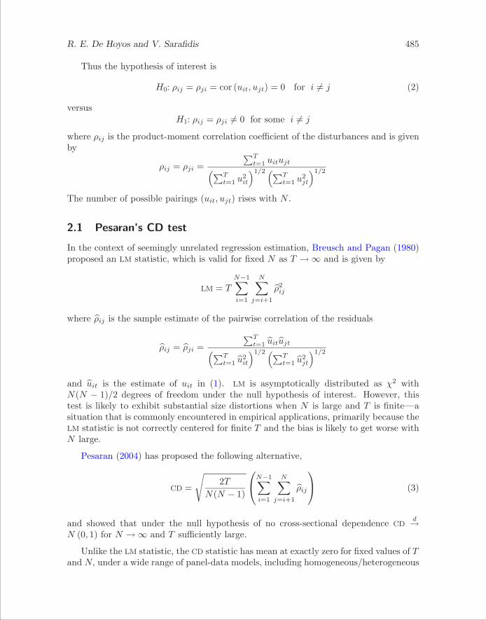
R. E. De Hoyos and V. Sarafidis 485
Thus the hypothesis of interest is
H0: ρij = ρji = cor (uit, ujt) = 0 for i �= j (2)
versusH1: ρij = ρji �= 0 for some i �= j
where ρij is the product-moment correlation coefficient of the disturbances and is givenby
ρij = ρji =∑T
t=1 uitujt(∑Tt=1 u2
it
)1/2 (∑Tt=1 u2
jt
)1/2
The number of possible pairings (uit, ujt) rises with N .
2.1 Pesaran’s CD test
In the context of seemingly unrelated regression estimation, Breusch and Pagan (1980)proposed an LM statistic, which is valid for fixed N as T → ∞ and is given by
LM = T
N−1∑i=1
N∑j=i+1
ρ2ij
where ρij is the sample estimate of the pairwise correlation of the residuals
ρij = ρji =∑T
t=1 uitujt(∑Tt=1 u2
it
)1/2 (∑Tt=1 u2
jt
)1/2
and uit is the estimate of uit in (1). LM is asymptotically distributed as χ2 withN(N − 1)/2 degrees of freedom under the null hypothesis of interest. However, thistest is likely to exhibit substantial size distortions when N is large and T is finite—asituation that is commonly encountered in empirical applications, primarily because theLM statistic is not correctly centered for finite T and the bias is likely to get worse withN large.
Pesaran (2004) has proposed the following alternative,
CD =
√2T
N(N − 1)
⎛⎝N−1∑i=1
N∑j=i+1
ρij
⎞⎠ (3)
and showed that under the null hypothesis of no cross-sectional dependence CDd→
N (0, 1) for N → ∞ and T sufficiently large.
Unlike the LM statistic, the CD statistic has mean at exactly zero for fixed values of Tand N, under a wide range of panel-data models, including homogeneous/heterogeneous

486 Testing for cross-sectional dependence
dynamic models and nonstationary models. For homogeneous and heterogeneous dy-namic models, the standard FE and RE estimators are biased (see Nickell [1981] andPesaran and Smith [1995]). However, the CD test is still valid because, despite the small-sample bias of the parameter estimates, the FE/RE residuals will have exactly mean zeroeven for fixed T , provided that the disturbances are symmetrically distributed.
For unbalanced panels, Pesaran (2004) proposes a slightly modified version of (3),which is given by
CD =
√2
N(N − 1)
⎛⎝N−1∑i=1
N∑j=i+1
√Tij ρij
⎞⎠ (4)
where Tij = #(Ti ∩ Tj) (i.e., the number of common time-series observations betweenunits i and j),
ρij = ρji =
∑t∈Ti∩Tj
(uit − ui
)(ujt − uj
){∑
t∈Ti∩Tj
(uit − ui
)2}1/2{∑
t∈Ti∩Tj
(ujt − uj
)2}1/2
and
ui =
∑t∈Ti∩Tj
uit
#(Ti ∩ Tj)
The modified statistic accounts for the fact that the residuals for subsets of t are notnecessarily mean zero.
2.2 Friedman’s test
Friedman (1937) proposed a nonparametric test based on Spearman’s rank correlationcoefficient. The coefficient can be thought of as the regular product-moment correlationcoefficient, that is, in terms of proportion of variability accounted for, except thatSpearman’s rank correlation coefficient is computed from ranks. In particular, if wedefine {ri,1, . . . , ri,T } to be the ranks of {ui,1, . . . , ui,T } [such that the average rank is(T + 1/2)], Spearman’s rank correlation coefficient equals5
rij = rji =∑T
t=1 {ri,t − (T + 1/2)} {rj,t − (T + 1/2)}∑Tt=1 {ri,t − (T + 1/2)}2
Friedman’s statistic is based on the average Spearman’s correlation and is given by
Rave =2
N (N − 1)
N−1∑i=1
N∑j=i+1
rij
5. Spearman’s rank correlation coefficient as calculated by the Stata spearman command is slightlydifferent in that it uses a definition of “average rank”.

R. E. De Hoyos and V. Sarafidis 487
where rij is the sample estimate of the rank correlation coefficient of the residuals. Largevalues of Rave indicate the presence of nonzero cross-sectional correlations. Friedmanshowed that FR = (T − 1) {(N − 1) Rave + 1} is asymptotically χ2 distributed with T−1degrees of freedom, for fixed T as N gets large. Originally Friedman devised the teststatistic FR to determine the equality of treatment in a two-way analysis of variance.
The CD and Rave share a common feature; both involve the sum of the pairwisecorrelation coefficients of the residual matrix rather than the sum of the squared corre-lations used in the LM test. This feature implies that these tests are likely to miss casesof cross-sectional dependence where the sign of the correlations is alternating—that is,where there are large positive and negative correlations in the residuals, which canceleach other out during averaging. Consider, for example, the following error structureof uit under H1,
uit = φift + εit (5)
where ft represents the unobserved factor that generates cross-sectional dependence, φi
indicates the impact of the factor on unit i, and εit is a pure idiosyncratic error withft ∼ i.i.d. (0, 1), φi ∼ i.i.d.
(0, σ2
φ
), and εit ∼ i.i.d.
(0, σ2
ε
). Here we have
cor (uit, ujt) =cov (uit, ujt)√
var (uit)√
var (ujt)=
E (φi) E (φj)√E (u2
it)√
E(u2
jt
) = 0
and thereby the CD and Rave statistics converge to 0 even if ft �= 0 and φi �= 0 for somei. This outcome implies that under alternative hypotheses of cross-sectional dependencein the disturbances with large positive and negative correlations but with E (φi) = 0,these tests would lack power and therefore may not be reliable.
To see the relevance of the above argument, consider the initial panel-data modelgiven by (1) and suppose that there is a single-factor structure in the disturbances, as in(5), except that the factor loadings are not mean zero, such that E (φi) �= 0. Apparently,the CD and Rave tests would not be subject to the problem mentioned above in thiscase. However, there is a subtle thing that needs to be taken into account; in panelswith N large and T finite, it is common practice to include common time effects (CTEs)in the regression model to capture “common trends” in the variation of the dependentvariable across cross sections. Using CTEs is equivalent to time demeaning of the data,which implies that the initial panel-data model can now be written as
(yit − y.t) = (αi − α) + β′ (xit − x.t) + (uit − u.t)(uit − u.t) =
(φi − φ
)ft + (εit − ε.t)
where y.t = 1N
∑Ni yit, and so on. As we can see, time demeaning of the data has
transformed the disturbances in terms of deviations from time-specific averages, andtherefore it has essentially removed the mean impact of the factors. This is the caseunless of course the factor loadings are mean zero in the first place, in which case timedemeaning is completely ineffective. Notice here two polar cases with regard to thevariance of the factor loadings; at one extreme, if the variance of the φi’s grows large,

488 Testing for cross-sectional dependence
time demeaning will be less effective because even if the mean impact of the factorshas been removed, there is still a considerable amount of cross-sectional dependence leftout in the disturbances. At the other extreme, if the variance of the φi’s is zero, timedemeaning removes cross-sectional dependence from the disturbances. Using CTEs willusually reduce cross-sectional dependence, but only to a certain extent.
Now suppose that the empirical researcher includes CTEs in the regression modeland wants to see whether there is any cross-sectional dependence left out in the dis-turbances. Here cov {(uit − u.t) (ujt − u.t)} = E
(φi − φ
)E(φj − φ
)= 0. Thus the
original problem emerges again in that the CD and Rave tests will lack power to detecta false null hypothesis, even if there is plenty of cross-sectional dependence left out inthe disturbances.6
2.3 Frees’ test
Frees (1995, 2004) proposed a statistic that is not subject to this drawback.7 In partic-ular, the statistic is based on the sum of the squared rank correlation coefficients andequals
R2ave =
2N (N − 1)
N−1∑i=1
N∑j=i+1
r2ij
As shown by Frees, a function of this statistic follows a joint distribution of twoindependently drawn χ2 variables. In particular, Frees shows that
FRE = N{
R2ave − (T − 1)−1
}d→ Q = a (T )
{x2
1,T−1 − (T − 1)}
+ b (T ){
x22,T (T−3)/2 − T (T − 3) /2
}where x2
1,T−1 and x22,T (T−3)/2 are independently χ2 random variables with T − 1 and
T (T − 3) /2 degrees of freedom, respectively, a (T ) = 4 (T + 2) /{
5 (T − 1)2 (T + 1)}
and b (T ) = 2 (5T + 6) / {5T (T − 1) (T + 1)}. Thus the null hypothesis is rejected ifR2
ave > (T − 1)−1 + Qq/N , where Qq is the appropriate quantile of the Q distribution.
6. Effectively, time demeaning causes the resulting factor loadings to be mean zero, which impliesthat the resulting correlation coefficients of the disturbances will alternate in sign, making the CD andRave tests inappropriate.
7. The testing procedure proposed by Sarafidis, Yamagata, and Robertson (2006) is not subject tothis drawback either.
R. E. De Hoyos and V. Sarafidis 489
−0.75 −0.50 −0.25 0.00 0.25 0.50 0.75 1.00 1.25 1.50 1.75 2.00 2.25 2.50 2.75
0.2
0.4
0.6
0.8
1.0
1.2Density
T=5
Q N(s=0.366)
−0.3 −0.2 −0.1 0.0 0.1 0.2 0.3 0.4 0.5
0.5
1.0
1.5
2.0
2.5
3.0
3.5
4.0Density
T=20
Q N(s=0.0996)
−0.6 −0.4 −0.2 0.0 0.2 0.4 0.6 0.8 1.0
0.25
0.50
0.75
1.00
1.25
1.50
1.75
2.00Density
T=10
Q N(s=0.195)
−0.25 −0.20 −0.15 −0.10 −0.05 0.00 0.05 0.10 0.15 0.20 0.25 0.30
1
2
3
4
5
6 Density
T=30
Q N(s=0.0666)
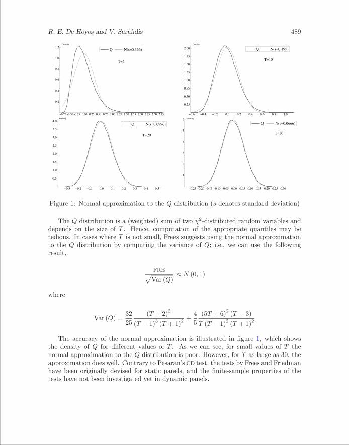
Figure 1: Normal approximation to the Q distribution (s denotes standard deviation)
The Q distribution is a (weighted) sum of two χ2-distributed random variables anddepends on the size of T . Hence, computation of the appropriate quantiles may betedious. In cases where T is not small, Frees suggests using the normal approximationto the Q distribution by computing the variance of Q; i.e., we can use the followingresult,
FRE√Var (Q)
≈ N (0, 1)
where
Var (Q) =3225
(T + 2)2
(T − 1)3 (T + 1)2+
45
(5T + 6)2 (T − 3)T (T − 1)2 (T + 1)2
The accuracy of the normal approximation is illustrated in figure 1, which showsthe density of Q for different values of T . As we can see, for small values of T thenormal approximation to the Q distribution is poor. However, for T as large as 30, theapproximation does well. Contrary to Pesaran’s CD test, the tests by Frees and Friedmanhave been originally devised for static panels, and the finite-sample properties of thetests have not been investigated yet in dynamic panels.
490 Testing for cross-sectional dependence
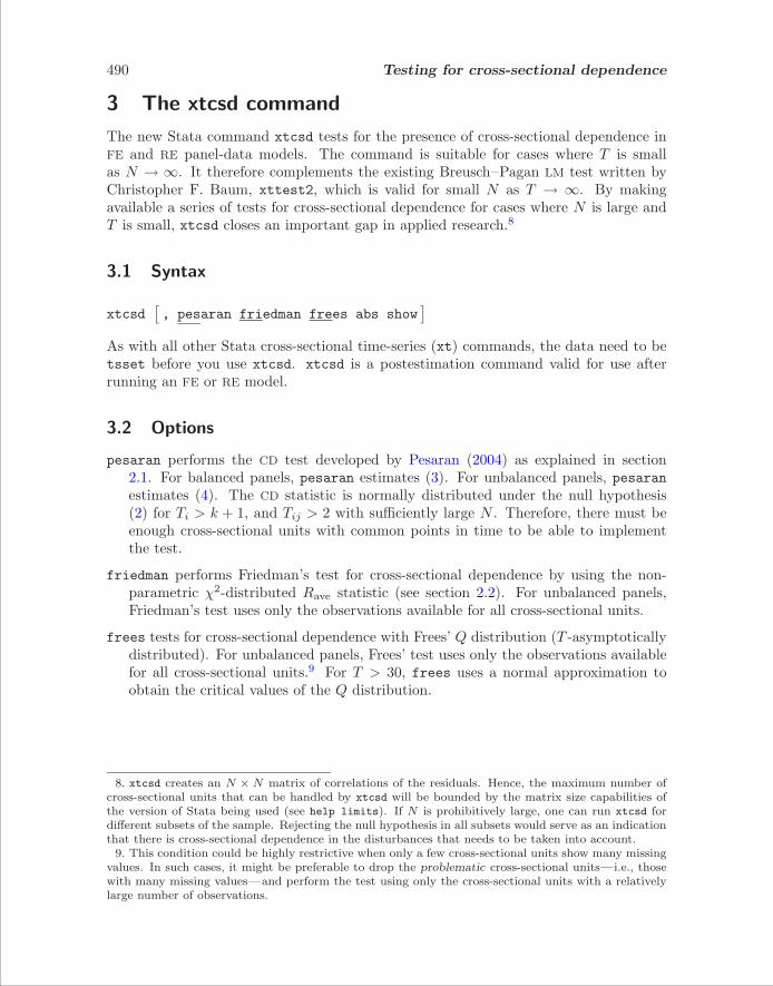
3 The xtcsd command
The new Stata command xtcsd tests for the presence of cross-sectional dependence inFE and RE panel-data models. The command is suitable for cases where T is smallas N → ∞. It therefore complements the existing Breusch–Pagan LM test written byChristopher F. Baum, xttest2, which is valid for small N as T → ∞. By makingavailable a series of tests for cross-sectional dependence for cases where N is large andT is small, xtcsd closes an important gap in applied research.8
3.1 Syntax
xtcsd[, pesaran friedman frees abs show
]As with all other Stata cross-sectional time-series (xt) commands, the data need to betsset before you use xtcsd. xtcsd is a postestimation command valid for use afterrunning an FE or RE model.
3.2 Options
pesaran performs the CD test developed by Pesaran (2004) as explained in section2.1. For balanced panels, pesaran estimates (3). For unbalanced panels, pesaranestimates (4). The CD statistic is normally distributed under the null hypothesis(2) for Ti > k + 1, and Tij > 2 with sufficiently large N . Therefore, there must beenough cross-sectional units with common points in time to be able to implementthe test.
friedman performs Friedman’s test for cross-sectional dependence by using the non-parametric χ2-distributed Rave statistic (see section 2.2). For unbalanced panels,Friedman’s test uses only the observations available for all cross-sectional units.
frees tests for cross-sectional dependence with Frees’ Q distribution (T -asymptoticallydistributed). For unbalanced panels, Frees’ test uses only the observations availablefor all cross-sectional units.9 For T > 30, frees uses a normal approximation toobtain the critical values of the Q distribution.
8. xtcsd creates an N × N matrix of correlations of the residuals. Hence, the maximum number ofcross-sectional units that can be handled by xtcsd will be bounded by the matrix size capabilities ofthe version of Stata being used (see help limits). If N is prohibitively large, one can run xtcsd fordifferent subsets of the sample. Rejecting the null hypothesis in all subsets would serve as an indicationthat there is cross-sectional dependence in the disturbances that needs to be taken into account.
9. This condition could be highly restrictive when only a few cross-sectional units show many missingvalues. In such cases, it might be preferable to drop the problematic cross-sectional units—i.e., thosewith many missing values—and perform the test using only the cross-sectional units with a relativelylarge number of observations.

R. E. De Hoyos and V. Sarafidis 491
abs computes the average absolute value of the off-diagonal elements of the cross-sectional correlation matrix of residuals. This option is useful to identify cases ofcross-sectional dependence where the sign of the correlations is alternating, with thelikely result of making the pesaran and friedman tests unreliable (see section 2.2).
show shows the cross-sectional correlation matrix of residuals.
4 Application
We illustrate xtcsd with an empirical example taken from Baltagi (2005, 25). Theexample refers to a Cobb–Douglas production function relationship investigating theproductivity of public capital in private production. The dataset consists of a balancedpanel of 48 U.S. states, each observed over 17 years (1970–1986). This dataset andsome explanatory notes can be found on the Wiley web site.10
Following Munnell (1990) and Baltagi and Pinnoi (1995), Baltagi (2005) considersthe following relationship,
ln gspit = α + β1 ln p capit + β2 ln pcit + β3 ln empit + β4unempit + uit (6)
where gspit denotes gross product in state i at time t; p cap denotes public capitalincluding highways and streets, water and sewer facilities, and other public buildings;pc denotes the stock of private capital; emp is labor input measured as employment innonagricultural payrolls; and unemp is the state unemployment rate included to capturebusiness cycle effects.
We begin the exercise by downloading the data and declaring that it has a panel-dataformat:
. use http://www.econ.cam.ac.uk/phd/red29/xtcsd_baltagi.dta
. tsset id tpanel variable: id (strongly balanced)time variable: t, 1970 to 1986
Once the dataset is ready for undertaking panel-data analysis, we run a version of(6) where we assume that uit is formed by a combination of a fixed component specificto the state and a random component that captures pure noise. Below are the resultsof the model using the FE estimator, also reported in Baltagi (2005, 26):
10. The database in plain format is available fromhttp://www.wiley.com/legacy/wileychi/baltagi/supp/PRODUC.prn; in the Stata Command window,type net from http://www.econ.cam.ac.uk/phd/red29/ to get the data in Stata format.

492 Testing for cross-sectional dependence
. xtreg lngsp lnpcap lnpc lnemp unemp, fe
Fixed-effects (within) regression Number of obs = 816Group variable (i): id Number of groups = 48
R-sq: within = 0.9413 Obs per group: min = 17between = 0.9921 avg = 17.0overall = 0.9910 max = 17
F(4,764) = 3064.81corr(u_i, Xb) = 0.0608 Prob > F = 0.0000
lngsp Coef. Std. Err. t P>|t| [95% Conf. Interval]
lnpcap -.0261493 .0290016 -0.90 0.368 -.0830815 .0307829lnpc .2920067 .0251197 11.62 0.000 .2426949 .3413185lnemp .7681595 .0300917 25.53 0.000 .7090872 .8272318unemp -.0052977 .0009887 -5.36 0.000 -.0072387 -.0033568_cons 2.352898 .1748131 13.46 0.000 2.009727 2.696069
sigma_u .09057293sigma_e .03813705
rho .8494045 (fraction of variance due to u_i)
F test that all u_i=0: F(47, 764) = 75.82 Prob > F = 0.0000
According to the results, once we account for state FE, public capital has no effectupon state gross product in the United States. An assumption implicit in estimating(6) is that the cross-sectional units are independent. The xtcsd command allows us totest the following hypothesis:
H0: cross-sectional independence
To test this hypothesis, we use the xtcsd command after fitting the above panel-datamodel. We initially use Pesaran’s (2004) CD test:
. xtcsd, pesaran abs
Pesaran’s test of cross sectional independence = 30.368, Pr = 0.0000
Average absolute value of the off-diagonal elements = 0.442
As we can see, the CD test strongly rejects the null hypothesis of no cross-sectionaldependence. Although it is not the case here, a possible drawback of the CD test isthat adding up positive and negative correlations may result in failing to reject the nullhypothesis even if there is plenty of cross-sectional dependence in the errors. Includingthe abs option in the xtcsd command, we can get the average absolute correlation ofthe residuals. Here the average absolute correlation is 0.442, which is a very high value.Hence, there is enough evidence suggesting the presence of cross-sectional dependencein (6) under an FE specification.
Next we corroborate these results by using the remaining two tests explained insection 2, i.e., Frees (1995) and Friedman (1937):
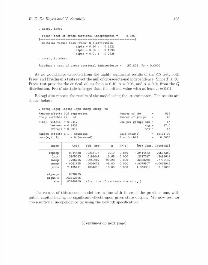
R. E. De Hoyos and V. Sarafidis 493
. xtcsd, frees
Frees’ test of cross sectional independence = 8.386|--------------------------------------------------------|
Critical values from Frees’ Q distributionalpha = 0.10 : 0.1521alpha = 0.05 : 0.1996alpha = 0.01 : 0.2928
. xtcsd, friedman
Friedman’s test of cross sectional independence = 152.804, Pr = 0.0000
As we would have expected from the highly significant results of the CD test, bothFrees’ and Friedman’s tests reject the null of cross-sectional independence. Since T ≤ 30,Frees’ test provides the critical values for α = 0.10, α = 0.05, and α = 0.01 from the Qdistribution. Frees’ statistic is larger than the critical value with at least α = 0.01.
Baltagi also reports the results of the model using the RE estimator. The results areshown below:
. xtreg lngsp lnpcap lnpc lnemp unemp, re
Random-effects GLS regression Number of obs = 816Group variable (i): id Number of groups = 48
R-sq: within = 0.9412 Obs per group: min = 17between = 0.9928 avg = 17.0overall = 0.9917 max = 17
Random effects u_i ~ Gaussian Wald chi2(4) = 19131.09corr(u_i, X) = 0 (assumed) Prob > chi2 = 0.0000
lngsp Coef. Std. Err. z P>|z| [95% Conf. Interval]
lnpcap .0044388 .0234173 0.19 0.850 -.0414583 .0503359lnpc .3105483 .0198047 15.68 0.000 .2717317 .3493649lnemp .7296705 .0249202 29.28 0.000 .6808278 .7785132unemp -.0061725 .0009073 -6.80 0.000 -.0079507 -.0043942_cons 2.135411 .1334615 16.00 0.000 1.873831 2.39699
sigma_u .0826905sigma_e .03813705
rho .82460109 (fraction of variance due to u_i)
The results of this second model are in line with those of the previous one, withpublic capital having no significant effects upon gross state output. We now test forcross-sectional independence by using the new RE specification:
(Continued on next page)

494 Testing for cross-sectional dependence
. xtcsd, pesaran
Pesaran’s test of cross sectional independence = 29.079, Pr = 0.0000
. xtcsd, frees
Frees’ test of cross sectional independence = 8.298|--------------------------------------------------------|
Critical values from Frees’ Q distributionalpha = 0.10 : 0.1521alpha = 0.05 : 0.1996alpha = 0.01 : 0.2928
. xtcsd, friedman
Friedman’s test of cross sectional independence = 144.941, Pr = 0.0000
The conclusion with respect to the existence or not of cross-sectional dependence inthe errors is not altered. The results show that there is enough evidence to reject the nullhypothesis of cross-sectional independence. The newly developed xtcsd Stata commandshows an easy way of performing three popular tests for cross-sectional dependence.
5 Concluding remarks
This article has described a new Stata postestimation command, xtcsd, which testsfor the presence of cross-sectional dependence in FE and RE panel-data models. Thecommand executes three different testing procedures—namely, Friedman’s (1937) teststatistic, the statistic proposed by Frees (1995), and the CD test developed by Pesaran(2004). These procedures are valid when T is fixed and N is large.11 xtcsd can alsoperform Pesaran’s CD test for unbalanced panels.
Our view is that all these tests for cross-sectional dependence should not be regardedas competing but rather as complementary. If T is large relative to N , the LM test maybe used. If N is large relative to T and the model is static, all different tests providedby xtcsd may be suitable, unless the empirical researcher has reason to believe that thecorrelation coefficients of the disturbances alternate in sign (or common time effects havebeen included in the model). In that case only the Frees test may be used.12 One canascertain whether this is the case by using the option abs, which computes the averageabsolute value of the off-diagonal elements of the cross-sectional correlation matrix ofthe residuals. If this takes a large value and the different tests provide contradictingresults in the sense that Pesaran’s and Friedman’s tests fail to reject the null hypothesis,whereas Frees’ test does not, inferences should be based on the latter. In dynamic panels,Pesaran’s test remains valid under FE/RE estimation (even if the estimated parametersare biased) and therefore it may be the preferred choice, since the properties of theremaining tests in dynamic panels are not yet known. On the other hand, if commontime effects have been included in the dynamic panel (and the panel is short), the testby Sarafidis, Yamagata, and Robertson (2006) may be used.
11. The CD test may also be used with both T and N large.12. However, Pesaran, Ullah, and Yamagata (2006) indicate that Frees’ test may not work well inmodels with explanatory variables when N is large.

R. E. De Hoyos and V. Sarafidis 495
In conclusion, the xtcsd command complements the Stata command xttest2 thattests for the presence of error cross-sectional dependence with T large and finite N .Hence, xtcsd closes an important gap in applied research.
6 Acknowledgments
Our code benefited greatly from Christopher F. Baum’s xttest2. We thank DavidDrukker and an anonymous referee for useful suggestions.
7 ReferencesAnderson, T. W., and C. Hsiao. 1981. Estimation of dynamic models with error com-
ponents. Journal of the American Statistical Association 76: 598–606.
Anselin, L. 2001. Spatial Econometrics. In A Companion to Theoretical Econometrics,ed. B. H. Baltagi, 310–330. Oxford: Blackwell Scientific Publications.
Arellano, M., and S. Bond. 1991. Some tests of specification for panel data: MonteCarlo evidence and an application to employment equations. Review of EconomicStudies 58: 277–297.
Baltagi, B. H. 2005. Econometric Analysis of Panel Data. 3rd ed. New York: Wiley.
Baltagi, B. H., and N. Pinnoi. 1995. Public capital stock and state productivity growth:Further evidence from an error components model. Empirical Economics 20: 351–359.
Baum, C. F. 2001. Residual diagnostics for cross-section time-series regression models.Stata Journal 1: 101–104.
———. 2003. Software updates: Residual diagnostics for cross-section time-series re-gression models. Stata Journal 3: 211.
———. 2004. Software updates: Residual diagnostics for cross-section time-series re-gression models. Stata Journal 4: 224.
Blundell, R., and S. Bond. 1998. Initial conditions and moment restrictions in dynamicpanel data models. Journal of Econometrics 87: 115–143.
Breusch, T., and A. Pagan. 1980. The Lagrange multiplier test and its application tomodel specification in econometrics. Review of Economic Studies 47: 239–253.
Coakley, J., A. Fuertes, and R. Smith. 2002. A principal components approach tocross-section dependence in panels. Unpublished manuscript.
Driscoll, J., and A. C. Kraay. 1998. Consistent covariance matrix estimation withspatially dependent data. Review of Economics and Statistics 80: 549–560.
Frees, E. W. 1995. Assessing cross-sectional correlation in panel data. Journal ofEconometrics 69: 393–414.

496 Testing for cross-sectional dependence
———. 2004. Longitudinal and Panel Data: Analysis and Applications in the SocialSciences. Cambridge: Cambridge University Press.
Friedman, M. 1937. The use of ranks to avoid the assumption of normality implicit inthe analysis of variance. Journal of the American Statistical Association 32: 675–701.
Munnell, A. 1990. Why has productivity growth declined? Productivity and publicinvestment. New England Economic Review (January/February): 3–22.
Nickell, S. J. 1981. Biases in dynamic models with fixed effects. Econometrica 49:1417–1426.
Pesaran, M. H. 2004. General diagnostic tests for cross section dependence in pan-els. University of Cambridge, Faculty of Economics, Cambridge Working Papers inEconomics No. 0435.
———. 2006. Estimation and inference in large heterogeneous panels with a multifactorerror structure. Econometrics 74: 967–1012.
Pesaran, M. H., and R. Smith. 1995. Estimating long-run relationships from dynamicheterogeneous panels. Journal of Econometrics 68: 79–113.
Pesaran, M. H., A. Ullah, and T. Yamagata. 2006. A bias-adjusted test of error crosssection dependence. http://www.econ.cam.ac.uk/faculty/pesaran/PUY10May06.pdf.
Phillips, P., and D. Sul. 2003. Dynamic panel estimation and homogeneity testing undercross section dependence. Econometrics Journal 6: 217–259.
Robertson, D., and J. Symons. 2000. Factor residuals in SUR regressions: Estimatingpanels allowing for cross sectional correlation. Unpublished manuscript.
Sarafidis, V., and D. Robertson. 2006. On the impact of cross section dependence inshort dynamic panel estimation.http://www.econ.cam.ac.uk/faculty/robertson/csd.pdf.
Sarafidis, V., T. Yamagata, and D. Robertson. 2006. A test of cross section dependencefor a linear dynamic panel model with regressors.http://www.econ.cam.ac.uk/faculty/robertson/HCSDtest14Feb06.pdf.
About the authors
Rafael E. De Hoyos works as a researcher at the Development Economics Prospects Group, theWorld Bank. His research includes topics such as policy evaluation, microeconometrics, andthe economics of poverty and inequality.
Vasilis Sarafidis is a lecturer at the University of Sydney, Discipline of Econometrics andBusiness Statistics. His current research interests focus on GMM estimation of linear dynamicpanel-data models with error cross-section dependence.