arX

iv:a

stro

-ph/

0606

690v

1 2

8 Ju

n 20

06

X-ray Spectroscopy of the Contact Binary VW Cephei1

David P. Huenemoerder, Paola TestaKavli Institute for Astrophysics and Space Research

Massachusetts Institute of TechnologyCambridge, MA 02139

dph@space.mit.edu, testa@space.mit.edu

and

Derek L. BuzasiUS Air Force Academy

Dept. of Physics,HQ USAFA/DFP

2354 Fairchild Dr., Ste. 2A31USAF Academy, CO 80840

Derek.Buzasi@usafa.af.mil

ABSTRACT

Short-period binaries represent extreme cases in the generation of stellar coronae via a ro-tational dynamo. Such stars are important for probing the origin and nature of coronae in theregimes of rapid rotation and activity saturation. VW Cep (P = 0.28 d) is a relatively bright,partially eclipsing, and very active object. Light curves made from Chandra/HETGS data showflaring and rotational modulation, but no eclipses. Velocity modulation of emission lines indicatesthat one component dominates the X-ray emission. The emission measure is highly structured,having three peaks. Helium-like triplet lines give electron densities of about 3 − 18 × 1010 cm−3.We conclude that the corona is predominantly on the polar regions of the primary star andcompact.

Subject headings: Stars: coronae – Stars: X-rays – Stars: Individual, VW Cep

1. Introduction

VW Cep (HD 197433), one of the X-ray-brightest of contact binaries, is a W-type W UMasystem — one in which the more massive andlarger star has lower mean surface brightness suchthat the deeper photometric eclipse occurs duringthe occultation of the smaller star. VW Cep hasan 0.28 d (24 ks) orbital period, is partially eclips-ing (i = 63◦), and has component spectral types ofK0 V and G5 V (Hill 1989; Hendry & Mochnacki2000), or, according to Khajavi, Edalati & Jassur

123 June 2006: Accepted for publication in The Astro-physical Journal

(2002), F5 and G0.

Among the coronally active binaries, activity isstrongly correlated with the rotation rate, and inparticular, the Rossby number, which is a mea-sure of the relative importance of Coriolis forcesin the convective layer, which is in turn relatedto the magnetic dynamo strength (Pallavicini1989). At periods below one day, activity satu-rates (Vilhu & Rucinski 1983; Cruddace & Dupree1984). Since the activity level, as defined byLx/Lbol, actually decreases with increasing rota-tion rate, this trend has been referred to as “super-saturation” (Prosser et al. 1996; Randich 1998;Jardine & Unruh 1999; James et al. 2000; Stepien,

1

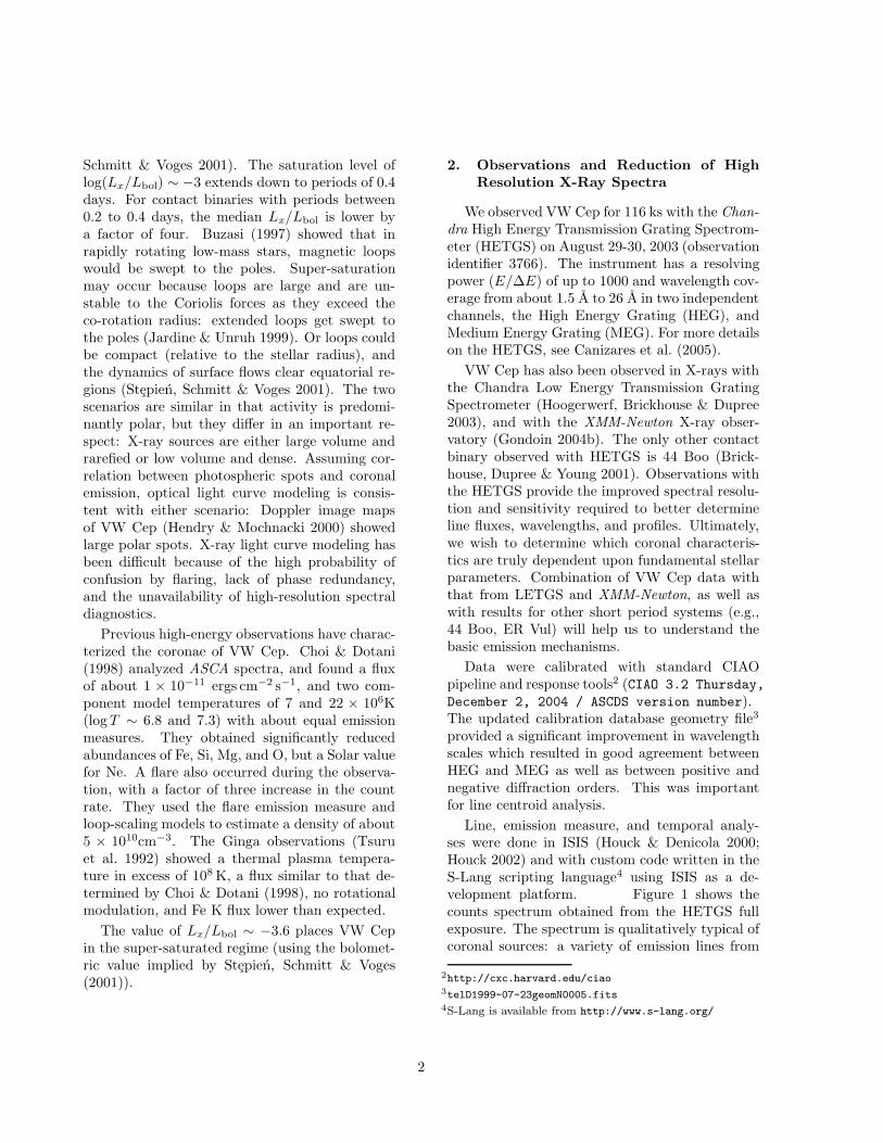
Schmitt & Voges 2001). The saturation level oflog(Lx/Lbol) ∼ −3 extends down to periods of 0.4days. For contact binaries with periods between0.2 to 0.4 days, the median Lx/Lbol is lower bya factor of four. Buzasi (1997) showed that inrapidly rotating low-mass stars, magnetic loopswould be swept to the poles. Super-saturationmay occur because loops are large and are un-stable to the Coriolis forces as they exceed theco-rotation radius: extended loops get swept tothe poles (Jardine & Unruh 1999). Or loops couldbe compact (relative to the stellar radius), andthe dynamics of surface flows clear equatorial re-gions (Stepien, Schmitt & Voges 2001). The twoscenarios are similar in that activity is predomi-nantly polar, but they differ in an important re-spect: X-ray sources are either large volume andrarefied or low volume and dense. Assuming cor-relation between photospheric spots and coronalemission, optical light curve modeling is consis-tent with either scenario: Doppler image mapsof VW Cep (Hendry & Mochnacki 2000) showedlarge polar spots. X-ray light curve modeling hasbeen difficult because of the high probability ofconfusion by flaring, lack of phase redundancy,and the unavailability of high-resolution spectraldiagnostics.

Previous high-energy observations have charac-terized the coronae of VW Cep. Choi & Dotani(1998) analyzed ASCA spectra, and found a fluxof about 1 × 10−11 ergs cm−2 s−1, and two com-ponent model temperatures of 7 and 22 × 106K(log T ∼ 6.8 and 7.3) with about equal emissionmeasures. They obtained significantly reducedabundances of Fe, Si, Mg, and O, but a Solar valuefor Ne. A flare also occurred during the observa-tion, with a factor of three increase in the countrate. They used the flare emission measure andloop-scaling models to estimate a density of about5 × 1010cm−3. The Ginga observations (Tsuruet al. 1992) showed a thermal plasma tempera-ture in excess of 108 K, a flux similar to that de-termined by Choi & Dotani (1998), no rotationalmodulation, and Fe K flux lower than expected.

The value of Lx/Lbol ∼ −3.6 places VW Cepin the super-saturated regime (using the bolomet-ric value implied by Stepien, Schmitt & Voges(2001)).

2. Observations and Reduction of High

Resolution X-Ray Spectra

We observed VW Cep for 116 ks with the Chan-dra High Energy Transmission Grating Spectrom-eter (HETGS) on August 29-30, 2003 (observationidentifier 3766). The instrument has a resolvingpower (E/∆E) of up to 1000 and wavelength cov-erage from about 1.5 A to 26 A in two independentchannels, the High Energy Grating (HEG), andMedium Energy Grating (MEG). For more detailson the HETGS, see Canizares et al. (2005).

VW Cep has also been observed in X-rays withthe Chandra Low Energy Transmission GratingSpectrometer (Hoogerwerf, Brickhouse & Dupree2003), and with the XMM-Newton X-ray obser-vatory (Gondoin 2004b). The only other contactbinary observed with HETGS is 44 Boo (Brick-house, Dupree & Young 2001). Observations withthe HETGS provide the improved spectral resolu-tion and sensitivity required to better determineline fluxes, wavelengths, and profiles. Ultimately,we wish to determine which coronal characteris-tics are truly dependent upon fundamental stellarparameters. Combination of VW Cep data withthat from LETGS and XMM-Newton, as well aswith results for other short period systems (e.g.,44 Boo, ER Vul) will help us to understand thebasic emission mechanisms.

Data were calibrated with standard CIAOpipeline and response tools2 (CIAO 3.2 Thursday,

December 2, 2004 / ASCDS version number).The updated calibration database geometry file3

provided a significant improvement in wavelengthscales which resulted in good agreement betweenHEG and MEG as well as between positive andnegative diffraction orders. This was importantfor line centroid analysis.

Line, emission measure, and temporal analy-ses were done in ISIS (Houck & Denicola 2000;Houck 2002) and with custom code written in theS-Lang scripting language4 using ISIS as a de-velopment platform. Figure 1 shows thecounts spectrum obtained from the HETGS fullexposure. The spectrum is qualitatively typical ofcoronal sources: a variety of emission lines from

2http://cxc.harvard.edu/ciao3telD1999-07-23geomN0005.fits4S-Lang is available from http://www.s-lang.org/

2

Fig. 1.— HETGS spectrum of VW Cep, 116 ks exposure. MEG (16433 counts) is the black line, and HEG(5269 counts) the gray. Insets show detail of the HEG spectrum (left) and MEG O VII triplet and N VIIregion (right).

highly ionized elements formed over a broad tem-perature region, from O VII, N VII, Ne IX, andFe XVII (log T ∼ 6.3–6.7), up to high temperaturespecies like S XV, S XVI, Ca XIX, and Fe XXV

(log T ∼ 7.2–7.8). It is apparent that iron hasa fairly low abundance relative to neon, given therelative weakness of the 15A and 17A Fe XVII linesrelative to the Ne IX 13A lines. The observed fluxin the 2–25 A is 8.4×10−12 ergs cm−2 s−1, and theluminosity (for a distance of 27.65 pc (Perrymanet al. 1997) is 7.7 × 1029 ergs s−1.

3. Analysis

3.1. Light and Phase Curves

The exposure lasted for five revolutions with-out interruption. Such phase redundancy is im-portant to discriminate intrinsic variability fromthat caused by rotational or eclipse modulation(for example, see the UV and X-ray monitoringstudies of AR Lac, Neff et al. (1989); Huenemo-erder et al. (2003b)). Figure 2 shows light curves5

of diffracted photons (HEG and MEG, orders −3to 3, excluding zeroth) covering the entire HETGSspectrum as well as for two wide bands covering

5Light and phase curves were made with custom software(the aglc S-Lang package) available on the ChandraContributed Software site:http://cxc.harvard.edu/cont-soft/software/aglc.1.2.3.html

Fig. 2.— Count rates of VW Cep in 2 ks bins. Inthe upper panel are light curves extracted from alldiffracted photons (1.5-26A; upper heavy curve),a “soft” band (12-26A; lower, thinner curve), anda “hard” band (1.5-8.3A; lower, thicker curve(blue)). The lower panel shows a hardness ratio(solid histogram), and the median of the hardnessfor the first 70 ks (light dotted line). We definedthe non-flare state as the first 80 ks. At the topwe show an axis in which the integer part givesthe number of rotations and the fractional part isthe phase.

3

short (“hard”, 1.5–8.3A) and long (“soft”, 12–26A) wavelength regions. The hardness countsratio (defined as (hard − soft)/(hard + soft))shows that the large increase after 80 ks is prob-ably a flare: proportionally more flux was emittedat shorter wavelengths, which are very sensitiveto high temperatures through thermal continuumemission. Conversely, the bump in count rate be-tween 20-30 ks does not show in hardness, andlikely is due to rotational modulation.

We assume that flares are hot and will thusshow a change in hardness, and that changes involume alone will primarily show a change in countrate. More complicated scenarios are possible,such as extended loops with temperature gradi-ents rotating in and out of view and causing bothhardness and count-rate variability on the timescale of a rotation. However, we know that flares— defined as hot, impulsive events with a grad-ual decay, in analogy to flares resolved on the Sun— are frequent on most active stars, and we willadopt the assumption as our working hypothesis.

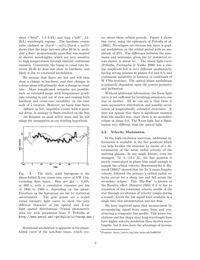
Fig. 3.— The dark, solid histogram is thephase-folded X-ray count-rate curve of VW Cep,excluding flare times. Bins are ∆φ = 0.025,or 600 s, with a cumulative exposure per binof 1800 to 2400 s, depending on the phase.Errorbars on the histogram are the 1σ statisticaluncertainties. The gray points are a scaledvisual intensity light curve to show the verydifferent character of the optical and X-raylight spatial distributions (Visual photometricdata are with permission from T. Pribulla athttp://www.astro.sk/∼pribulla/lc/vwcep.dat.)

Rotational modulation is apparent in the phase-folded curve of the non-flare times, which cov-

ers about three orbital periods. Figure 3 showsthis curve, using the ephemeris of Pribulla et al.(2002). No eclipses are obvious but there is grad-ual modulation on the orbital period with an am-plitude of 20%. The difference between the max-imum and minimum, given the 1σ statistical er-rors shown, is about 5σ. The visual light curve(Pribulla, Parimucha & Vanko 2000) has a sim-ilar amplitude but is very different qualitatively,having strong minima at phases 0.0 and 0.5, andcontinuous variability in between (a trademark ofW UMa systems). The optical phase modulationis primarily dependent upon the system geometryand inclination.

Without additional information, the X-ray lightcurve is not sufficient for localizing emission to onestar or another. All we can say is that there issome asymmetric distribution, and possible occul-tation of longitudinally extended structures. Itdoes not appear that there is significant emissionfrom the smaller star, since there is no secondaryeclipse at phase 0.0. The X-ray light has a distri-bution very different from the optical light.

3.2. Velocity Modulation

In the high-resolution spectrum, additional in-formation is available in the line positions whichcan help localize the emission by means of a de-termination of the mean radial velocity of theemitting plasma. In any single feature, even thestrongest, Ne X (12.1 A), the line position ispoorly constrained in phase bins small enough tosample the orbital velocity. Huenemoerder & Hu-nacek (2005)6 showed that the Ne X mean Dopplervelocity followed the primary’s orbital radial ve-locity except for a sharp rise and fall across thesecondary eclipse. This “flip-flop” is known asthe Rossiter effect (Rossiter 1924) if it is due toresolution of the rotational velocity profile of thestar through occultation of velocity ranges duringa transit. Given the low signal level available in asingle line, this interpretation was not firm.

We have improved upon that measurement byaccumulating signal from many lines and con-structing a composite line profile. This mixes res-olutions and line shape since long-wavelength lineshave higher velocity resolution than shorter wave-lengths, but it does have the advantage of increas-

6Preprint: http://arxiv.org/abs/astro-ph/0409258

4

ing signal greatly. Since HEG and MEG have dif-ferent resolutions and coverage, we kept their com-posites separate. To avoid blending, we chose onlyfairly isolated features, and these are flagged in the“Use” column of Table 1 with an “H” or an “M”.

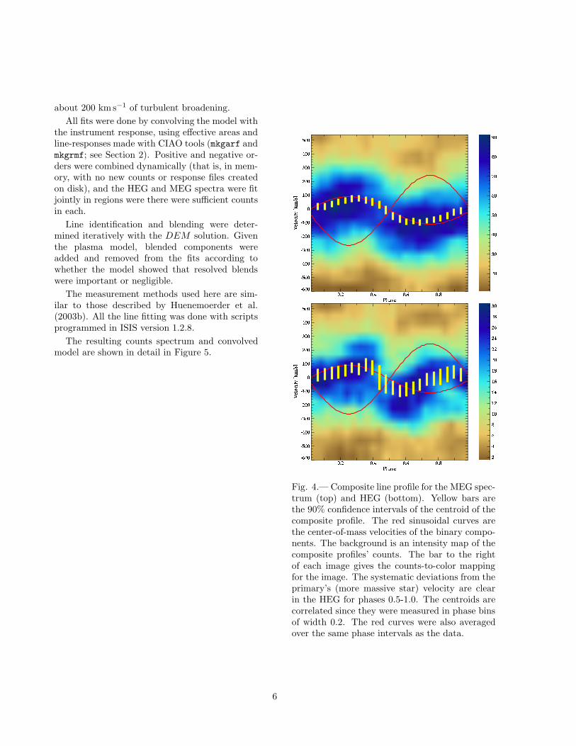
We accumulated spectra into 24 phase bins foreach of the HEG and MEG positive and negativefirst orders (96 distinct spectra). We then trans-formed about 15 lines in each spectrum from wave-length to a common velocity scale and summedthem. Finally, we combined plus and minus ordersover a range of phase bins (to further improve thesignal) and fit Gaussians to the composite profiles’cores (defined to be where the counts were greaterthan the maximum divided by 2e) separately foreach of HEG and MEG. This method is similar tothat used by Hoogerwerf, Brickhouse & Mauche(2004). We found that using five phase bins (arunning average over ∆φ = 0.2) was adequate toprovide enough phase resolution and signal with-out losing too much sensitivity to velocity changes.To quantify the significance of the fitted velocitycentroid, we computed the 90% confidence inter-vals (1.6σ) for the velocity. Figure 4 showsthe results. The composite line profiles makethe background image, with velocity on the y-axis,and phase on the x-axis, and the darker shading isfor higher intensity as indicated by the color-barto the right, mapping color to counts. The yel-low error bars are the 90% confidence limits of thecomposite profiles centroid averaged over 5 phasebins (∆φ = 0.2). The red curves show the stellarcenter of mass velocities, also averaged over thesame phase range as the data.

The composite velocity centroid very closely fol-lows the radial velocity of the primary (more mas-sive) star. The preliminary sharp velocity tran-sition at φ = 0.5 seen in neon (Huenemoerder &Hunacek 2005) is not apparent in the MEG curve,but the background HEG image does have a hintof a transition sharper than that due to the stellarradial orbital velocities.

There are significant systematic deviations fromthe orbital velocities apparent near φ = 0.8.Given the statistical uncertainties shown are 90%(1.6σ), the deviations from the expected velocityare about 2.5σ for each grating.

Note that the instrumental resolution is approx-imately 500 km s−1 FWHM at 12A for the MEG,and about half that for the HEG. We are able

to determine centroids to much higher precision(∼ 25 km s−1 for MEG; ∼ 45 km s−1 for HEG) be-cause have accumulated signal over multiple pro-files, and because each profile is over-sampled bythe spacecraft dither which randomizes line place-ment with respect to pixel boundaries. Hoogerw-erf, Brickhouse & Mauche (2004) achieved preci-sion of about ∼ 15 km s−1 from MEG spectra, andalso quote a statistical verification of the precisionof a Gaussian fitted centroid. Also for comparison,Ishibashi et al. (2006)7 using different techniqueson HETGS spectra of Capella, a low-orbital ve-locity sytem, obtained 3σ velocity uncertainties ofabout 20 km s−1 which is about 11 km s−1 for 90%confidence. It is not surprising that our precisionis somewhat less given the lower signal per phasebin and given more velocity smearing in phase forthis short period system.

The implications of the velocity centroid varia-tions with regard to geometric distribution of theemitting plasma will be discussed in Section 4.1 inconjunction with light curve variability, emissionmeasure, and density determinations.

3.3. Line Fluxes

Line fluxes, which are required for differen-tial emission measure (DEM) analysis, were mea-sured by fitting a the sum of a continuum modeland a number of Gaussians to narrow regions ofthe counts spectra. The parameters of the fits werethe Gaussian centroids and fluxes. The contin-uum and Gaussian widths were determined a pri-ori. For the continuum, we used a plasma modeldetermined iteratively from the emission measuresolution (see Section 3.4). For the first iteration,we fit a two-temperature plasma model to rela-tively line-free regions, as determined by the modeland instrument response. Since lines were measur-ably broader than the instrumental resolution, wedetermined the amount of excess line width re-quired at one wavelength for a strong, relativelyisolated line (Mg XII 8.4A), then scaled the widthwith wavelength, under the assumption that thebroadening is due to either rotational or orbitaleffects. However, we simply treated the broad-ening as a Gaussian, which was adequate for thepurposes of obtaining good fits to line fluxes andpositions. The excess required was equivalent to

7Preprint: http://arxiv.org/abs/astro-ph/0605383

5

about 200 km s−1 of turbulent broadening.

All fits were done by convolving the model withthe instrument response, using effective areas andline-responses made with CIAO tools (mkgarf andmkgrmf; see Section 2). Positive and negative or-ders were combined dynamically (that is, in mem-ory, with no new counts or response files createdon disk), and the HEG and MEG spectra were fitjointly in regions were there were sufficient countsin each.

Line identification and blending were deter-mined iteratively with the DEM solution. Giventhe plasma model, blended components wereadded and removed from the fits according towhether the model showed that resolved blendswere important or negligible.

The measurement methods used here are sim-ilar to those described by Huenemoerder et al.(2003b). All the line fitting was done with scriptsprogrammed in ISIS version 1.2.8.

The resulting counts spectrum and convolvedmodel are shown in detail in Figure 5.

Fig. 4.— Composite line profile for the MEG spec-trum (top) and HEG (bottom). Yellow bars arethe 90% confidence intervals of the centroid of thecomposite profile. The red sinusoidal curves arethe center-of-mass velocities of the binary compo-nents. The background is an intensity map of thecomposite profiles’ counts. The bar to the rightof each image gives the counts-to-color mappingfor the image. The systematic deviations from theprimary’s (more massive star) velocity are clearin the HEG for phases 0.5-1.0. The centroids arecorrelated since they were measured in phase binsof width 0.2. The red curves were also averagedover the same phase intervals as the data.

6

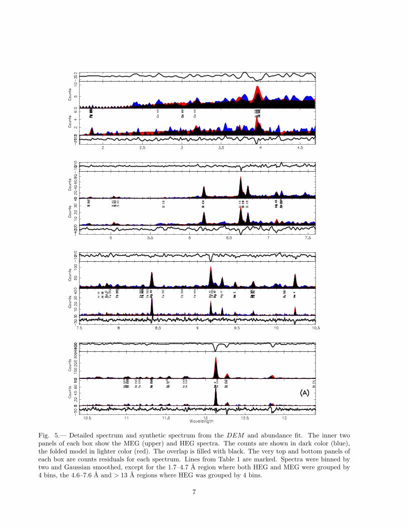
Fig. 5.— Detailed spectrum and synthetic spectrum from the DEM and abundance fit. The inner twopanels of each box show the MEG (upper) and HEG spectra. The counts are shown in dark color (blue),the folded model in lighter color (red). The overlap is filled with black. The very top and bottom panels ofeach box are counts residuals for each spectrum. Lines from Table 1 are marked. Spectra were binned bytwo and Gaussian smoothed, except for the 1.7–4.7 A region where both HEG and MEG were grouped by4 bins, the 4.6–7.6 A and > 13 A regions where HEG was grouped by 4 bins.

7

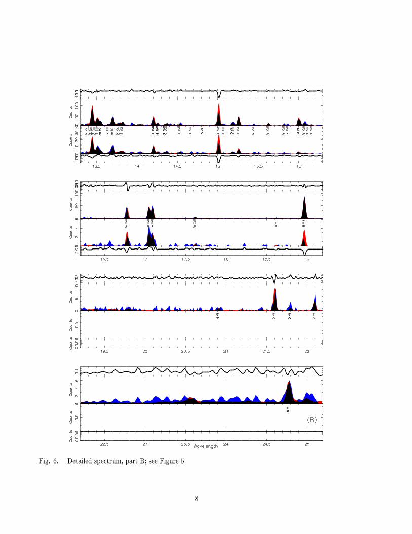
Fig. 6.— Detailed spectrum, part B; see Figure 5

8

All the line measurements are given in Table 1.We list more features than were used in analy-sis. Some were rejected because they had largewavelength residuals and so are misidentified orare strongly blended. Some were rejected becausethey had large flux residuals and so are misiden-tified or have poor atomic data. For example, theFe xvii 15 A line is nearly always under-predicted,which may be due to deficiencies in the atomicdata (Laming et al. 2000; Doron & Behar 2002;Gu 2002). Some lines were fit simply to provide agood determination of the flux and wavelength ofa nearby “interesting” feature. The “Use” columnof Table 1 indicates which lines were used in emis-sion measure reconstruction, or for composite lineprofiles. The density sensitive He-like triplet inter-combination and forbidden lines were not used inDEM reconstruction.

3.4. Emission Measure

The differential emission measure is a one di-mensional characterization of a plasma, and canbe defined as N2

e dV/dT , in which Ne is the elec-tron density, V is the emitting volume, and T thetemperature. The DEM is an important quantitybecause it represents the radiative loss portion ofthe underlying heating mechanism. An emissionmeasure can be derived from measurements of linefluxes and some assumptions about the homogene-ity and ionization balance of the emitting plasma.Derivation of the emission measure relies on de-tailed knowledge of fundamental atomic parame-ters. Even given accurate emissivities, the contri-bution functions versus temperature are broad sothe emission integral cannot be formally inverted.Hence there are many methods to regularize thesolution to obtain the emission measure and ele-mental abundances.

Huenemoerder & Hunacek (2005) used a sim-ple method described by Pottasch (1963), in whichthe DEM is approximated by a ratio of line lumi-nosity to average line emissivity at the tempera-ture of the maximum emissivity. Here we improveupon that by simultaneously fitting the DEM andabundances using a method similar to that de-scribed by Huenemoerder et al. (2003b), who alsodiscussed some of the caveats of emission measurereconstruction and gave relevant citations. Briefly,the relation between emissivity and flux is an ill-posed problem. To obtain a unique solution, under

assumptions of the model, a regularization termof some form must be included. Here we havereplaced explicit smoothing of the DEM in ourprior work with a regularization term, so that thefunctional form of the statistic we minimize is

χ2 =∑

l1

σ2l

[

Ll − AZ(l)

∑

t δtǫltDt

]2+ qP (D),(1)

in which l is a spectral feature index and t is thetemperature index. The measured quantities arethe line luminosities, Ll, with uncertainties σl.The a priori given information are the emissivities,ǫlt as defined by Raymond & Brickhouse (1996), δt

is the logarithmic bin size, and the source distance(which is implicit in L). The minimization pro-vides a solution for the differential emission mea-sure, D, and abundances of elements Z, AZ . Tonaturally constrain the DEM to be positive, weactually fit ln Dt. P (D) is a regularization term(or “penalty function”) which is only a function ofthe model, and q is a scale factor which specifiesthe relative importance of the regularization. ForP , we used the sum-squared second derivative ofthe DEM with respect to log T , and a multiplierto make the two terms of the statistic comparable.This form imposes a minimum smoothness on thesolution; the DEM cannot have large changes incurvature. We did not impose any regularizationon the abundances, since we have no intuitive biason their functional form.

The DEM fitting was done with custom soft-ware in ISIS. While ISIS has no built-in DEMreconstruction, it does have sophisticated plasmadatabase access and evaluation functions permit-ting efficient lookup and computation of emissivi-ties. It also provides for user-defined fit functionsand statistics, which made it straightforward todevelop a DEM model within its fitting and mod-eling infrastructure.

As an initial guess, we assumed cosmic abun-dances and a boxcar DEM ; the amplitude of thecentral temperature region was chosen to approx-imately produce the observed line counts, and theends were set to a very low value. The reason forleaving the DEM at the temperature extrema lowis that the DEM is not well constrained phys-ically there by lines, but the hot portion doesstrongly affect the continuum. Hence, we pre-ferred a solution in which emission weights are in-creased only if required by the fit to lines alone.The normalizations outside our regime of temper-

9

ature sensitivity, roughly log T = 6.4 (O vii) to 7.8(Fe xxv; the tail of Si xvi), were artificially con-strained to have negligible emissivity. The line-to-continuum ratio was fit post facto by scaling thenormalization of the DEM and abundances.

The model DEM was obtained iteratively. Foreach trial DEM , we generated a new continuummodel and re-fit the lines. After the second suchiteration, we reviewed line residuals and excludedthose which were very large (greater than 3σ), un-der the assumption that they were misidentified orblended. The final fit included only the selectedlines, and was post facto renormalized to repro-duce the observed line-to-continuum ratios in the8-11 A range. The line fluxes predicted by theDEM and abundance model are listed in Table 1,along with the residuals from the parametric fit,and their δχ value (last three columns). The“Use” column flags lines used in the DEM recon-struction with an “E”. Due to the iterative natureof the model, the measured line fluxes are slightlydependent upon the DEM solution through thedefinition of the continuum.

Figure 7 shows our final emission measure (inte-grated over logarithmic bins of width 0.1 dex), us-ing the Astrophysical Plasma Emission Database(APED, Version 1.3.1) for line emissivities (Smithet al. 2001), the ionization balance of Mazzottaet al. (1998), and Solar abundances from Anders& Grevesse (1989). The envelope shown was de-termined by computing the deviation in solutionsover a Monte-Carlo run of about 100 fits in whichthe line fluxes were varied according to their mea-sured statistical uncertainties, assuming a Gaus-sian distribution about their fitted values. Thisassumption would actually result in an enlargeduncertainty bounds, since the data are an esti-mate of the true mean, and the random pertur-bation would sometimes be toward the true mean,and sometimes away, perhaps further than the themeasured uncertainty and truth would allow.

Other sources of systematic error, the uncer-tainties in the atomic physics and in the instru-mental calibration, were not included, and proba-bly accounts for a similarly sized envelope. Whilesystematic uncertainties in atomic data are diffi-cult to incorporate explicitly, Huenemoerder et al.(2003b) applied an approximate method, in whichthey set a global lower limit on the line flux un-certainty of 25% (regardless of the statistical un-

certainty) and repeated the DEM reconstruction.They found a similar shaped distribution, butproportionally larger uncertainty. The importantquantity for understanding coronal activity is theoverall shape of the DEM , which seems reliableunder the current assumptions and calibration un-certainties.

There is sharp structure in the DEM with alarge peak at log T = 6.9, a second peak at 6.6, andhot tail from about 7.2 to 7.8. This is qualitativelysimilar to the simple provisional DEM of Huen-emoerder & Hunacek (2005), but with sharperstructure as expected from an iterative solution.

The fitted coronal abundances, relative to So-lar (since we do not know the stellar photosphericvalues), are shown in Figure 8. The uncertain-ties are the 1σ range as determined by the Monte-Carlo iteration, except for Ni and Ca. The lattertwo were not included in the DEM solution sincethey were weak and were not fit with parametricprofiles as were the strong lines (and so they donot appear in Table 1). Instead, we fit them postfacto by using the DEM and abundance solutionto define a plasma model, then adjusted the abun-dance of Ca by minimizing the residuals betweenthe binned counts and synthetic spectrum in theCa XIX He-like triplet near 3.2 A as a function ofCa abundance. There is a blend of Ar XVII here,but given the DEM , it is expected to be about anorder of magnitude weaker than Ca. For Ni, wesimilarly fit the Ni XIX lines at 14.043 and 14.077A, and Ni XIX 12.435 A. In each region, blendedFe lines had model fluxes 5-10 times weaker thanthe nickel lines. The Ca abundance uncertainty islarge because there are few counts and a relativelystrong continuum. The Ni has smaller uncertaintybecause there are more counts and weaker contin-uum.

3.5. Density

The helium-like triplets are well known as den-sity sensitive diagnostics, particularly the ratioof the forbidden (f) to inter-combination (i) linefluxes, commonly known as the R-ratio, R = f/i(Gabriel & Jordan 1969; Porquet & Dubau 2000;Porquet et al. 2001; Ness et al. 2001). A mildlytemperature sensitive diagnostic is the G-ratio,which is the sum, f + i, divided by the resonanceline (r) flux. The critical density increases withatomic number. In the HETGS range, the ions of

10

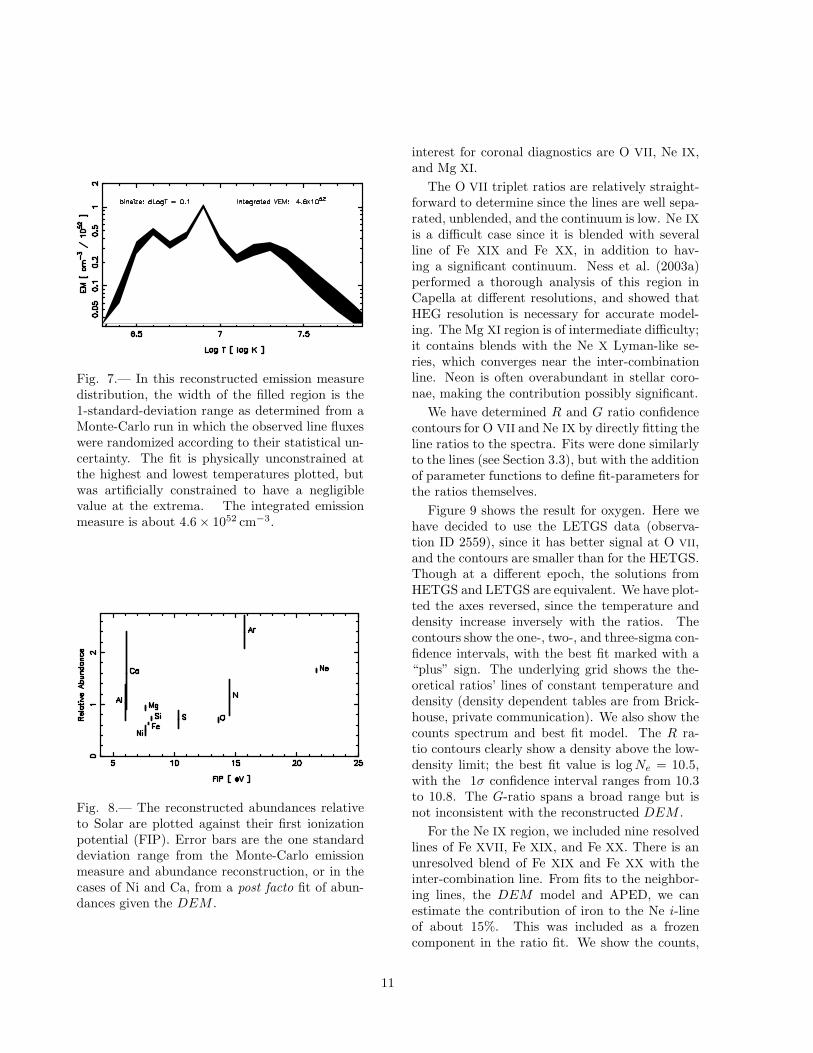
Fig. 7.— In this reconstructed emission measuredistribution, the width of the filled region is the1-standard-deviation range as determined from aMonte-Carlo run in which the observed line fluxeswere randomized according to their statistical un-certainty. The fit is physically unconstrained atthe highest and lowest temperatures plotted, butwas artificially constrained to have a negligiblevalue at the extrema. The integrated emissionmeasure is about 4.6 × 1052 cm−3.

Fig. 8.— The reconstructed abundances relativeto Solar are plotted against their first ionizationpotential (FIP). Error bars are the one standarddeviation range from the Monte-Carlo emissionmeasure and abundance reconstruction, or in thecases of Ni and Ca, from a post facto fit of abun-dances given the DEM .

interest for coronal diagnostics are O VII, Ne IX,and Mg XI.

The O VII triplet ratios are relatively straight-forward to determine since the lines are well sepa-rated, unblended, and the continuum is low. Ne IX

is a difficult case since it is blended with severalline of Fe XIX and Fe XX, in addition to hav-ing a significant continuum. Ness et al. (2003a)performed a thorough analysis of this region inCapella at different resolutions, and showed thatHEG resolution is necessary for accurate model-ing. The Mg XI region is of intermediate difficulty;it contains blends with the Ne X Lyman-like se-ries, which converges near the inter-combinationline. Neon is often overabundant in stellar coro-nae, making the contribution possibly significant.

We have determined R and G ratio confidencecontours for O VII and Ne IX by directly fitting theline ratios to the spectra. Fits were done similarlyto the lines (see Section 3.3), but with the additionof parameter functions to define fit-parameters forthe ratios themselves.

Figure 9 shows the result for oxygen. Here wehave decided to use the LETGS data (observa-tion ID 2559), since it has better signal at O vii,and the contours are smaller than for the HETGS.Though at a different epoch, the solutions fromHETGS and LETGS are equivalent. We have plot-ted the axes reversed, since the temperature anddensity increase inversely with the ratios. Thecontours show the one-, two-, and three-sigma con-fidence intervals, with the best fit marked with a“plus” sign. The underlying grid shows the the-oretical ratios’ lines of constant temperature anddensity (density dependent tables are from Brick-house, private communication). We also show thecounts spectrum and best fit model. The R ra-tio contours clearly show a density above the low-density limit; the best fit value is log Ne = 10.5,with the 1σ confidence interval ranges from 10.3to 10.8. The G-ratio spans a broad range but isnot inconsistent with the reconstructed DEM .

For the Ne IX region, we included nine resolvedlines of Fe XVII, Fe XIX, and Fe XX. There is anunresolved blend of Fe XIX and Fe XX with theinter-combination line. From fits to the neighbor-ing lines, the DEM model and APED, we canestimate the contribution of iron to the Ne i-lineof about 15%. This was included as a frozencomponent in the ratio fit. We show the counts,

11

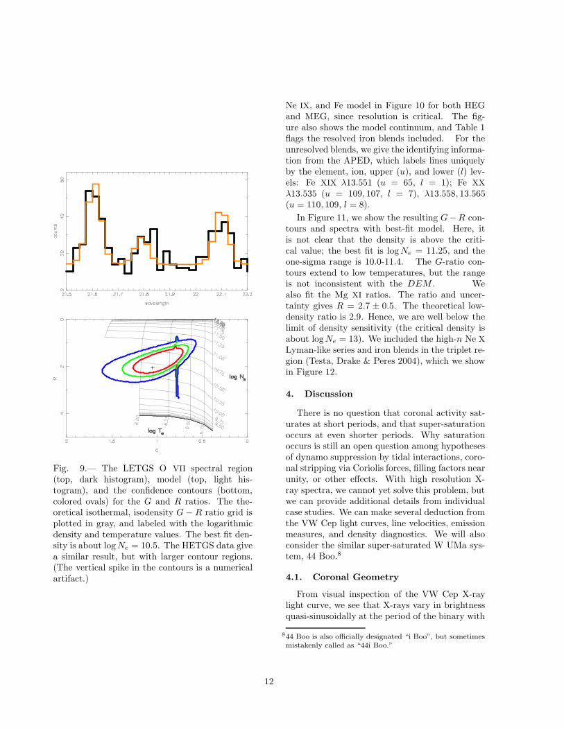
Fig. 9.— The LETGS O VII spectral region(top, dark histogram), model (top, light his-togram), and the confidence contours (bottom,colored ovals) for the G and R ratios. The the-oretical isothermal, isodensity G − R ratio grid isplotted in gray, and labeled with the logarithmicdensity and temperature values. The best fit den-sity is about log Ne = 10.5. The HETGS data givea similar result, but with larger contour regions.(The vertical spike in the contours is a numericalartifact.)

Ne IX, and Fe model in Figure 10 for both HEGand MEG, since resolution is critical. The fig-ure also shows the model continuum, and Table 1flags the resolved iron blends included. For theunresolved blends, we give the identifying informa-tion from the APED, which labels lines uniquelyby the element, ion, upper (u), and lower (l) lev-els: Fe XIX λ13.551 (u = 65, l = 1); Fe XX

λ13.535 (u = 109, 107, l = 7), λ13.558, 13.565(u = 110, 109, l = 8).

In Figure 11, we show the resulting G−R con-tours and spectra with best-fit model. Here, itis not clear that the density is above the criti-cal value; the best fit is log Ne = 11.25, and theone-sigma range is 10.0-11.4. The G-ratio con-tours extend to low temperatures, but the rangeis not inconsistent with the DEM . Wealso fit the Mg XI ratios. The ratio and uncer-tainty gives R = 2.7 ± 0.5. The theoretical low-density ratio is 2.9. Hence, we are well below thelimit of density sensitivity (the critical density isabout log Ne = 13). We included the high-n Ne X

Lyman-like series and iron blends in the triplet re-gion (Testa, Drake & Peres 2004), which we showin Figure 12.

4. Discussion

There is no question that coronal activity sat-urates at short periods, and that super-saturationoccurs at even shorter periods. Why saturationoccurs is still an open question among hypothesesof dynamo suppression by tidal interactions, coro-nal stripping via Coriolis forces, filling factors nearunity, or other effects. With high resolution X-ray spectra, we cannot yet solve this problem, butwe can provide additional details from individualcase studies. We can make several deduction fromthe VW Cep light curves, line velocities, emissionmeasures, and density diagnostics. We will alsoconsider the similar super-saturated W UMa sys-tem, 44 Boo.8

4.1. Coronal Geometry

From visual inspection of the VW Cep X-raylight curve, we see that X-rays vary in brightnessquasi-sinusoidally at the period of the binary with

844 Boo is also officially designated “i Boo”, but sometimesmistakenly called as “44i Boo.”

12

Fig. 10.— Ne IX region for MEG (top) and HEG(bottom), showing the counts (dark histogram),the Ne IX components (red-filled Gaussians), theiron components (green-filled Gaussians), and thecontinuum model (gray-filled region). The relativeintensity of the iron line blended with the Ne IX

inter-combination line was determined from neigh-boring iron lines. Note that the counts scale islogarithmic.

Fig. 11.— Ne IX spectral region (top, dark his-togram), model (top, light histogram), and theconfidence contours (bottom, colored ovals) forthe G and R ratios. The theoretical isothermal,isodensity G − R ratio grid is plotted in gray,and labeled with the logarithmic density and tem-perature values. The best-fit density is aboutlog Ne = 11.25.

13

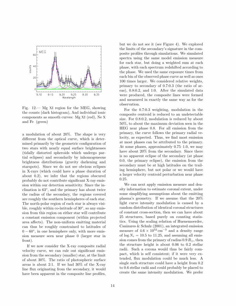
Fig. 12.— Mg XI region for the MEG, showingthe counts (dark histogram), And individual ioniccomponents as smooth curves: Mg XI (red), Ne X

and Fe (green)

a modulation of about 20%. The shape is verydifferent from the optical curve, which is deter-mined primarily by the geometric configuration oftwo stars with nearly equal surface brightnesses(tidally distorted spheroids which undergo par-tial eclipses) and secondarily by inhomogeneousbrightness distributions (gravity darkening andstarspots). Since we do not see obvious eclipsesin X-rays (which could have a phase duration ofabout 0.2), we infer that the regions obscuredprobably do not contribute significant X-ray emis-sion within our detection sensitivity. Since the in-clination is 63◦, and the primary has about twicethe radius of the secondary, the regions coveredare roughly the southern hemispheres of each star.The north-polar region of each star is always visi-ble, roughly within co-latitude of 30◦, so any emis-sion from this region on either star will contributea constant emission component (within projectedarea affects). The non-uniform emitting materialcan thus be roughly constrained to latitudes of0 − 60◦, in one hemisphere only, with more emis-sion measure seen near phase 0 (larger star infront).

If we now consider the X-ray composite radialvelocity curve, we can rule out significant emis-sion from the secondary (smaller) star, at the limitof about 30%. The ratio of photospheric surfaceareas is about 2:1. If we had 30% of the X-rayline flux originating from the secondary, it wouldhave been apparent in the composite line profiles,

but we do not see it (see Figure 4). We exploredthe limits of the secondary’s signature in the com-posite profiles through simulations. We simulatedspectra using the same model emission measurefor each star, but doing a weighted sum at eachphase, with each spectrum redshifted according tothe phase. We used the same exposure times fromeach bin of the observed phase curve as well as ones100 times larger. We considered relative weights,primary to secondary of 0.7:0.3 (the ratio of ar-eas), 0.8:0.2, and 1:0. After the simulated datawere produced, the composite lines were formedand measured in exactly the same way as for theobservation.

For the 0.7:0.3 weighting, modulation in thecomposite centroid is reduced to an undetectablesize. For 0.8:0.2, modulation is reduced by about50%, to about the maximum deviation seen in theHEG near phase 0.8. For all emission from theprimary, the curve follows the primary radial ve-locity, as expected. Thus, we find most emissionat most phases can be attributed to the primary.At some phases, approximately 0.75–1.0, we mayhave about 20% from the secondary. Since thereis no apparent eclipse of the secondary (at phase0.0, the primary eclipse), the emission from thesecondary must be at high latitudes on the trail-ing hemisphere, but not polar or we would havea larger velocity centroid perturbation near phase0.25.

We can next apply emission measure and den-sity information to estimate coronal extent, undersome simplifying assumptions about the emittingplasma’s geometry. If we assume that the 20%light curve intensity modulation is caused by arandom distribution of identical coronal structuresof constant cross-section, then we can have about25 structures, based purely on counting statis-tics. Using the scaling relation of Huenemoerder,Canizares & Schulz (2001), an integrated emissionmeasure of 4.6 × 1052 cm−3 and a density rangeof log Ne = 10.5 to 11.25, and assuming all emis-sion comes from the primary of radius 0.9 R⊙, thenthe structure height is about 0.06 to 0.2 stellarradii. Such a corona would thus be fairly com-pact, which is self consistent; if it were very ex-tended, flux modulation could be much less. Asingle such structure could have a height from 0.2to 0.6 stellar radii and could probably be placed tocreate the same intensity modulation. We prefer

14

the multiple structure hypothesis, but this is byno means a unique requirement of the data. If wespread the emitting volume more uniformly over ahemisphere, then for the above density range thefractional height is 0.02 to 0.03. We probably havea compact, polar corona.

Gondoin (2004b) reported an X-ray eclipse seenXMM-Newton light curves obtained 10 monthsprior to the CXO observations and concluded thatboth components were X-ray emitters. If the dipin XMM-Newton rate were really an eclipse, thenthis would indicate rather large and rapid changesin coronal structure. The XMM-Newton observa-tion, however, did not cover a single continuous or-bit, and the dip is offset from phase 0.0, so the in-terpretation is not definitive. Also contrary to ourresults, Gondoin (2004b) derived loops quite largein comparison to the stellar radii (20-80%), but ad-mittedly by methods which are not self-consistent.

4.2. Temperature Distribution, Heating,

Opacity

The differential emission measure (Figure 7) issimilar to other active stars, being highly struc-tured and spanning a broad range in temperature.Sanz-Forcada, Brickhouse & Dupree (2002, 2003)show a large collection of DEM distribtions witha variety of peaks, bumps, and tails. In our analy-sis, we included the flare times and this no doubtproduces the bump above log T = 7.1, similarly tothe results for II Peg (Huenemoerder, Canizares &Schulz 2001) and Proxima Cen (Gudel et al. 2004),which were modeled at different activity levels.

The most prominent peak in the VW CepDEM is well defined and narrow, with a slope ap-proximately proportional to T 4. Such a featurehas also been observed in other stars of differ-ent types (Brickhouse et al. 2000; Sanz-Forcada,Brickhouse & Dupree 2002). The DEM can giveus some insights into the underlying physics. Apossible interpretation of this recurrent feature islinked to the spatial location and temporal distri-bution of coronal heating. Testa, Peres & Reale(2005) have proposed a hydrodynamic model ofloops undergoing pulsed heating at their foot-points, which is able to reproduce the presenceof a peak and the steep rise of the DEM observedin these active stars. Whatever the mechanism,the heating in VW Cep does not look radicallydifferent from other coronal sources, at least as

manifested in the DEM .

The abundances do not show any strong trendwith the first ionization potential (FIP). While Arlooks unusually abundant in Figure 8, the statis-tical uncertainty is large. Furthermore, the mea-surement is also subject to systematic uncertaintyin placement of the continuum. The Ar abun-dance is probably not significantly different fromNe. The overall distribution looks very similar, forexample, to that of the RS CVn binary, AR Lac(Huenemoerder et al. 2003a). The Ne:O ratiowhich we derived from the iterative emission mea-sure and abundance reconstruction is 0.35 ± 0.03.This is comparable to the rather robust activestar mean of 0.41 found by Drake & Testa (2005)from temperature-insensitive line ratios. From theabundance analysis, we again have no reason tothink that the corona of a W UMa system, thoughsuper-saturated, differs from other coronally ac-tive stars.

We examined line ratios which have been usedfor opacity diagnostics. Fe xvii has been problem-atic, because the ratios systematically differ fromtheoretical values (Laming et al. 2000; Doron &Behar 2002; Gu 2002). VW Cep is no exception;its Fe xvii 15.01 A line is over-predicted. We findno significant differences in ratios from typical op-tically thin values shown in Testa et al. (2004) orNess et al. (2003b).

4.3. Comparison to 44 Boo

44 Boo is a contact binary system which isvery similar to VW Cep, having similar period,mass ratio, and spectral types. Its fundamentalcharacteristics are given by Hill, Fisher & Holm-gren (1989) and a velocity curve by Lu, Rucinski& Og loza (2001). Brickhouse, Dupree & Young(2001) have analyzed HETGS spectra and con-cluded that most emission is at high latitudes,compact, that there is a very compact emittingregion on the smaller star (the secondary) whichcauses a very brief dip in X-ray brightness whenit momentarily rotates out of view, and a largeremitting region near the pole of the primary whichgives rise to a quasi-sinusoidal brightness modula-tion, but which isn’t eclipsed. Gondoin (2004a)presented XMM-Newton observation of 44 Boowhich covered on orbital period. Based on theabsence of eclipses, he concluded that the coronamust be extended, though he presented other ar-

15

guments which led to compact loops.

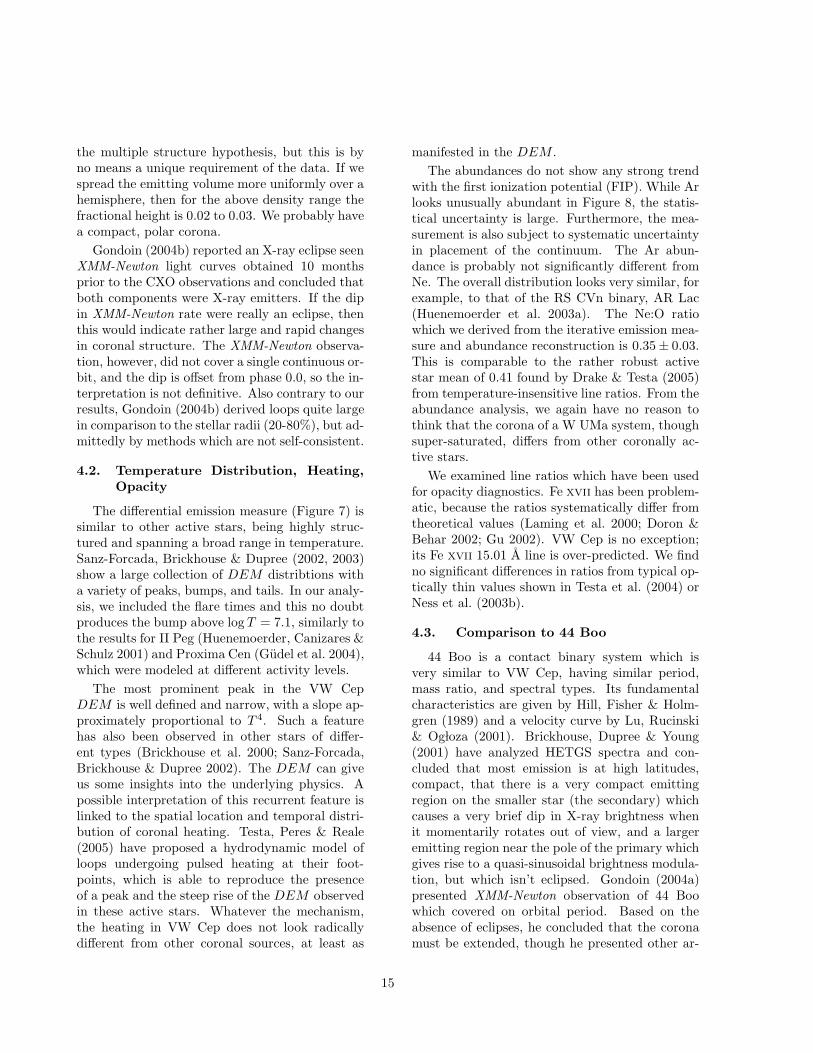
Using the same techniques applied to VW Cep,we have extracted the X-ray light and phase curvesand a composite line velocity curve from the sameHETGS observation used by Brickhouse, Dupree& Young (2001) (Observation ID 14). The lightcurve in Figure 13 shows three flares. The risein the final 10 ks, identified as a flare by Brick-house, Dupree & Young (2001), shows no in-crease in hardness, so we accept it into the phasedcurve. Our phased X-ray light curve (Figure 14)is qualitatively different from Brickhouse, Dupree& Young (2001).

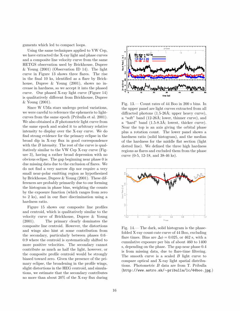
Since W UMa stars undergo period variations,we were careful to reference the ephemeris to light-curves from the same epoch (Pribulla et al. 2001).We also obtained a B photometric light curve fromthe same epoch and scaled it to arbitrary relativeintensity to display over the X-ray curve. We dofind strong evidence for the primary eclipse in thebroad dip in X-ray flux in good correspondencewith the B intensity. The rest of the curve is qual-itatively similar to the VW Cep X-ray curve (Fig-ure 3), having a rather broad depression with noobvious eclipse. The gap beginning near phase 0 isdue missing data due to the exclusion of flares. Wedo not find a very narrow dip nor require a verysmall near-polar emitting region as hypothesizedby Brickhouse, Dupree & Young (2001). These dif-ferences are probably primarily due to our formingthe histogram in phase bins, weighting the countsby the exposure function (which ranges from zeroto 2 ks), and in our flare discrimination using ahardness ratio.

Figure 15 shows our composite line profilesand centroid, which is qualitatively similar to thevelocity curve of Brickhouse, Dupree & Young(2001). The primary clearly dominates thecomposite line centroid. However, the distortionsand wings also hint at some contribution fromthe secondary, particularly between phases 0.6–0.9 where the centroid is systematically shifted tomore positive velocities. The secondary cannotcontribute as much as half the light, however, orthe composite profile centroid would be stronglybiased toward zero. Given the presence of the pri-mary eclipse, the broadening in the profile wings,slight distortions in the HEG centroid, and simula-tions, we estimate that the secondary contributesno more than about 20% of the X-ray flux during

Fig. 13.— Count rates of 44 Boo in 200 s bins. Inthe upper panel are light curves extracted from alldiffracted photons (1.5-26A; upper heavy curve),a “soft” band (12-26A; lower, thinner curve), anda “hard” band (1.5-8.3A; lowest, thicker curve).Near the top is an axis giving the orbital phaseplus a rotation count. The lower panel shows ahardness ratio (solid histogram), and the medianof the hardness for the middle flat section (lightdotted line). We defined the three high hardnessregions as flares and excluded them from the phasecurve (0-5, 12-18, and 38-46 ks).

Fig. 14.— The dark, solid histogram is the phase-folded X-ray count-rate curve of 44 Boo, excludingflare times. Bins are ∆φ = 0.025, or 462 s, with acumulative exposure per bin of about 460 to 1400s, depending on the phase. The gap near phase 0.4is from missing data, due to flare-time filtering.The smooth curve is a scaled B light curve tocompare optical and X-ray light spatial distribu-tions. Photometric B data are from T. Pribulla(http://www.astro.sk/∼pribulla/lc/44boo.jpg.)

16

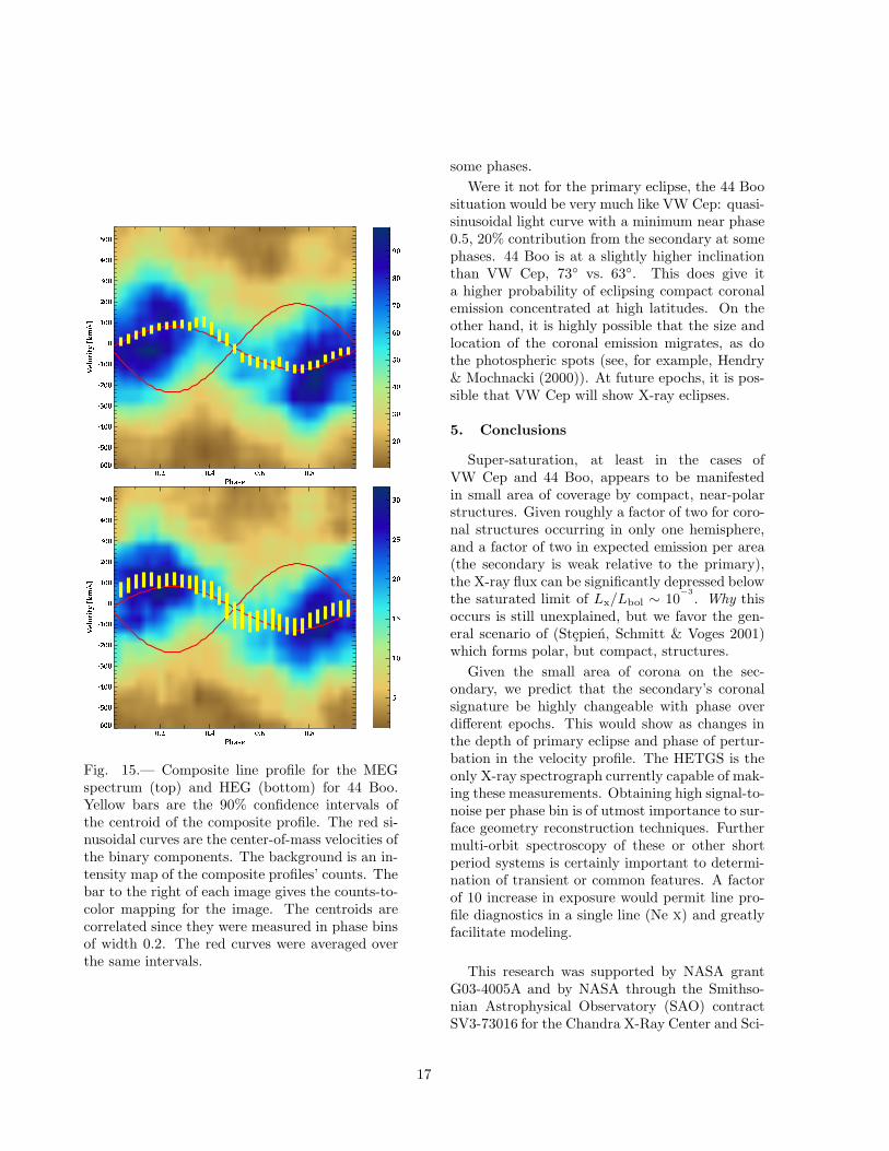
Fig. 15.— Composite line profile for the MEGspectrum (top) and HEG (bottom) for 44 Boo.Yellow bars are the 90% confidence intervals ofthe centroid of the composite profile. The red si-nusoidal curves are the center-of-mass velocities ofthe binary components. The background is an in-tensity map of the composite profiles’ counts. Thebar to the right of each image gives the counts-to-color mapping for the image. The centroids arecorrelated since they were measured in phase binsof width 0.2. The red curves were averaged overthe same intervals.

some phases.

Were it not for the primary eclipse, the 44 Boosituation would be very much like VW Cep: quasi-sinusoidal light curve with a minimum near phase0.5, 20% contribution from the secondary at somephases. 44 Boo is at a slightly higher inclinationthan VW Cep, 73◦ vs. 63◦. This does give ita higher probability of eclipsing compact coronalemission concentrated at high latitudes. On theother hand, it is highly possible that the size andlocation of the coronal emission migrates, as dothe photospheric spots (see, for example, Hendry& Mochnacki (2000)). At future epochs, it is pos-sible that VW Cep will show X-ray eclipses.

5. Conclusions

Super-saturation, at least in the cases ofVW Cep and 44 Boo, appears to be manifestedin small area of coverage by compact, near-polarstructures. Given roughly a factor of two for coro-nal structures occurring in only one hemisphere,and a factor of two in expected emission per area(the secondary is weak relative to the primary),the X-ray flux can be significantly depressed belowthe saturated limit of Lx/Lbol ∼ 10

−3

. Why thisoccurs is still unexplained, but we favor the gen-eral scenario of (Stepien, Schmitt & Voges 2001)which forms polar, but compact, structures.

Given the small area of corona on the sec-ondary, we predict that the secondary’s coronalsignature be highly changeable with phase overdifferent epochs. This would show as changes inthe depth of primary eclipse and phase of pertur-bation in the velocity profile. The HETGS is theonly X-ray spectrograph currently capable of mak-ing these measurements. Obtaining high signal-to-noise per phase bin is of utmost importance to sur-face geometry reconstruction techniques. Furthermulti-orbit spectroscopy of these or other shortperiod systems is certainly important to determi-nation of transient or common features. A factorof 10 increase in exposure would permit line pro-file diagnostics in a single line (Ne x) and greatlyfacilitate modeling.

This research was supported by NASA grantG03-4005A and by NASA through the Smithso-nian Astrophysical Observatory (SAO) contractSV3-73016 for the Chandra X-Ray Center and Sci-

17

ence Instruments.

Facilities: CXO(HETG) CXO(LETG).

REFERENCES

Anders, E., & Grevesse, N., 1989, Geochim. Cos-mochim. Acta, 53, 197

Brickhouse, N. S., Dupree, A. K., Edgar, R. J.,Liedahl, D. A., Drake, S. A., White, N. E., &Singh, K. P., 2000, ApJ, 530, 387

Brickhouse, N. S., Dupree, A. K., & Young, P. R.,2001, ApJ, 562, L75

Buzasi, D. L., 1997, ApJ, 484, 855

Canizares, C. R., et al., 2005, PASP, 117, 1144

Choi, C. S., & Dotani, T., 1998, ApJ, 492, 761

Cruddace, R. G., & Dupree, A. K., 1984, ApJ,277, 263

Doron, R., & Behar, E., 2002, ApJ, 574, 518

Drake, J. J., & Testa, P., 2005, Nature, 436, 525

Gudel, M., Audard, M., Reale, F., Skinner, S. L.,& Linsky, J. L., 2004, A&A, 416, 713

Gabriel, A. H., & Jordan, C., 1969, MNRAS, 145,241

Gondoin, P., 2004a, A&A, 426, 1035

Gondoin, P., 2004b, A&A, 415, 1113

Gu, M. F., 2002, ApJ, 579, L103

Hendry, P. D., & Mochnacki, S. W., 2000, ApJ,531, 467

Hill, G., 1989, A&A, 218, 141

Hill, G., Fisher, W. A., & Holmgren, D., 1989,A&A, 211, 81

Hoogerwerf, R., Brickhouse, N. S., & Dupree,A. K., 2003, AAS/High Energy AstrophysicsDivision, 35,

Hoogerwerf, R., Brickhouse, N. S., & Mauche,C. W., 2004, ApJ, 610, 411

Houck, J. C., 2002, in High Resolution X-ray Spec-troscopy with XMM-Newton and Chandra, ed.G. Branduardi-Raymont

Houck, J. C., & Denicola, L. A., 2000, in ASPConf. Ser. 216: Astronomical Data AnalysisSoftware and Systems IX, Vol. 9, 591

Huenemoerder, D. P., Boroson, B., Buzasi, D. L.,Preston, H. L., Schulz, N. S., Kastner, J. H., &Canizares, C. R., 2003a, in IAU Symposium

Huenemoerder, D. P., Canizares, C. R., Drake,J. J., & Sanz-Forcada, J., 2003b, ApJ, 595, 1131

Huenemoerder, D. P., Canizares, C. R., & Schulz,N. S., 2001, ApJ, 559, 1135

Huenemoerder, D. P., & Hunacek, A., 2005, Pro-ceedings of ”The 13th Cambridge Workshop onCool Stars, Stellar Systems, and the Sun”, ESASP–560, 661–664

Ishibashi, K., Dewey, D., Huenemoerder, D. P., &Testa, P., 2006, ApJ Letters, 0, (accepted)

James, D. J., Jardine, M. M., Jeffries, R. D.,Randich, S., Collier Cameron, A., & Ferreira,M., 2000, MNRAS, 318, 1217

Jardine, M., & Unruh, Y. C., 1999, A&A, 346, 883

Khajavi, M., Edalati, M. T., & Jassur, D. M. Z.,2002, Ap&SS, 282, 645

Laming, J. M., et al., 2000, ApJ, 545, L161

Lu, W., Rucinski, S. M., & Og loza, W., 2001, AJ,122, 402

Mazzotta, P., Mazzitelli, G., Colafrancesco, S., &Vittorio, N., 1998, A&AS, 133, 403

Neff, J. E., Walter, F. M., Rodono, M., & Linsky,J. L., 1989, A&A, 215, 79

Ness, J., Brickhouse, N. S., Drake, J. J., & Huen-emoerder, D. P., 2003a, ApJ, 598, 1277

Ness, J.-U., et al., 2001, A&A, 367, 282

Ness, J.-U., Schmitt, J. H. M. M., Audard, M.,Gudel, M., & Mewe, R., 2003b, A&A, 407, 347

Pallavicini, R., 1989, A&A Rev., 1, 177

Perryman, M. A. C., et al., 1997, A&A, 323, L49

Porquet, D., & Dubau, J., 2000, A&AS, 143, 495

18

Porquet, D., Mewe, R., Dubau, J., Raassen,A. J. J., & Kaastra, J. S., 2001, A&A, 376,1113

Pottasch, S. R., 1963, ApJ, 137, 945

Pribulla, T., Parimucha, S., & Vanko, M., 2000,Informational Bulletin on Variable Stars, 4847,1

Pribulla, T., Vanko, M., Parimucha, S., & Cho-chol, D., 2001, Informational Bulletin on Vari-able Stars, 5056, 1

Pribulla, T., Vanko, M., Parimucha, S., & Cho-chol, D., 2002, Informational Bulletin on Vari-able Stars, 5341, 1

Prosser, C. F., Randich, S., Stauffer, J. R.,Schmitt, J. H. M. M., & Simon, T., 1996, AJ,112, 1570

Randich, S., 1998, in ASP Conf. Ser. 154: CoolStars, Stellar Systems, and the Sun, 501

Raymond, J. C., & Brickhouse, N. C., 1996,Ap&SS, 237, 321

Rossiter, R. A., 1924, ApJ, 60, 15

Sanz-Forcada, J., Brickhouse, N. S., & Dupree,A. K., 2002, ApJ, 570, 799

Sanz-Forcada, J., Brickhouse, N. S., & Dupree,A. K., 2003, ApJS, 145, 147

Smith, R. K., Brickhouse, N. S., Liedahl, D. A., &Raymond, J. C., 2001, ApJ, 556, L91

Stepien, K., Schmitt, J. H. M. M., & Voges, W.,2001, A&A, 370, 157

Testa, P., Drake, J. J., & Peres, G., 2004, ApJ,617, 508

Testa, P., Drake, J. J., Peres, G., & DeLuca, E. E.,2004, ApJ, 609, L79

Testa, P., Peres, G., & Reale, F., 2005, ApJ, 622,695

Tsuru, T., Makishima, K., Ohashi, T., Sakao, T.,Pye, J. P., Williams, O. R., Barstow, M. A., &Takano, S., 1992, MNRAS, 255, 192

Vilhu, O., & Rucinski, S. M., 1983, A&A, 127, 5

This 2-column preprint was prepared with the AAS LATEXmacros v5.2.

19

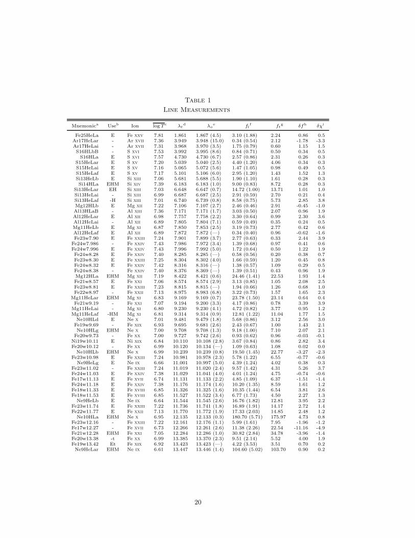
Table 1

Line Measurements

Mnemonica Useb Ion log T c λtd λo

e flf ft

g δfh δχi

Fe25HeLa E Fe xxv 7.81 1.861 1.867 (4.5) 3.10 (1.88) 2.24 0.86 0.5Ar17HeLar - Ar xvii 7.36 3.949 3.948 (15.0) 0.34 (0.54) 2.12 -1.78 -3.3Ar17HeLai - Ar xvii 7.31 3.968 3.970 (3.5) 1.75 (0.79) 0.60 1.15 1.5S16HLbB - S xvi 7.53 3.992 3.995 (8.6) 0.84 (0.71) 0.50 0.34 0.5

S16HLa E S xvi 7.57 4.730 4.730 (6.7) 2.57 (0.86) 2.31 0.26 0.3S15HeLar E S xv 7.20 5.039 5.040 (2.5) 4.40 (1.20) 4.06 0.34 0.3S15HeLai E S xv 7.16 5.065 5.072 (5.6) 1.47 (1.05) 0.98 0.49 0.5S15HeLaf E S xv 7.17 5.101 5.106 (6.0) 2.95 (1.20) 1.43 1.52 1.3Si13HeLb E Si xiii 7.06 5.681 5.688 (5.5) 1.90 (1.10) 1.61 0.28 0.3Si14HLa EHM Si xiv 7.39 6.183 6.183 (1.0) 9.00 (0.83) 8.72 0.28 0.3

Si13HeLar EH Si xiii 7.03 6.648 6.647 (0.7) 14.72 (1.00) 13.71 1.01 1.0Si13HeLai - Si xiii 6.99 6.687 6.687 (2.5) 2.91 (0.59) 2.70 0.21 0.4Si13HeLaf -H Si xiii 7.01 6.740 6.739 (0.8) 8.58 (0.75) 5.73 2.85 3.8Mg12HLb E Mg xii 7.22 7.106 7.107 (2.7) 2.46 (0.46) 2.91 -0.45 -1.0Al13HLaB - Al xiii 7.36 7.171 7.171 (1.7) 3.03 (0.50) 2.07 0.96 1.9Al12HeLar E Al xii 6.98 7.757 7.758 (2.2) 3.30 (0.64) 0.99 2.30 3.6Al12HeLai - Al xii 6.89 7.805 7.804 (7.1) 0.59 (0.49) 0.35 0.24 0.5Mg11HeLb E Mg xi 6.87 7.850 7.853 (2.5) 3.19 (0.73) 2.77 0.42 0.6Al12HeLaf E Al xii 6.89 7.872 7.872 (—) 0.34 (0.40) 0.96 -0.62 -1.6Fe23w7.90 E Fe xxiii 7.24 7.901 7.899 (3.7) 2.77 (0.63) 0.33 2.44 3.9

Fe24w7.986 - Fe xxiv 7.43 7.986 7.972 (3.4) 1.39 (0.68) 0.97 0.41 0.6Fe24w7.996 E Fe xxiv 7.43 7.996 7.992 (5.0) 1.72 (0.64) 0.50 1.22 1.9Fe24w8.28 E Fe xxiv 7.40 8.285 8.285 (—) 0.58 (0.56) 0.20 0.38 0.7Fe23w8.30 E Fe xxiii 7.25 8.304 8.302 (4.0) 1.66 (0.59) 1.20 0.45 0.8Fe24w8.32 E Fe xxiv 7.42 8.316 8.316 (—) 1.38 (0.57) 1.09 0.29 0.5Fe24w8.38 - Fe xxiv 7.40 8.376 8.369 (—) 1.39 (0.51) 0.43 0.96 1.9Mg12HLa EHM Mg xii 7.19 8.422 8.421 (0.6) 24.46 (1.41) 22.53 1.93 1.4Fe21w8.57 E Fe xxi 7.06 8.574 8.574 (2.9) 3.13 (0.85) 1.05 2.08 2.5Fe23w8.81 E Fe xxiii 7.23 8.815 8.815 (—) 1.94 (0.66) 1.26 0.68 1.0Fe22w8.97 - Fe xxii 7.13 8.975 8.983 (6.8) 3.22 (0.73) 1.57 1.65 2.3

Mg11HeLar EHM Mg xi 6.83 9.169 9.169 (0.7) 23.78 (1.50) 23.14 0.64 0.4Fe21w9.19 - Fe xxi 7.07 9.194 9.200 (3.3) 4.17 (0.86) 0.78 3.39 3.9

Mg11HeLai - Mg xi 6.80 9.230 9.230 (4.1) 4.72 (0.82) 3.77 0.95 1.2Mg11HeLaf -HM Mg xi 6.81 9.314 9.314 (0.9) 12.81 (1.22) 11.04 1.77 1.5

Ne10HLd E Ne x 7.01 9.481 9.479 (1.8) 5.68 (0.86) 3.12 2.56 3.0Fe19w9.69 - Fe xix 6.93 9.695 9.681 (2.6) 2.43 (0.67) 1.00 1.43 2.1Ne10HLg EHM Ne x 7.00 9.708 9.708 (1.3) 9.18 (1.00) 7.10 2.07 2.1

Fe20w9.73 - Fe xx 7.00 9.727 9.742 (2.6) 0.93 (0.62) 0.96 -0.03 -0.1Ni19w10.11 E Ni xix 6.84 10.110 10.108 (2.8) 3.67 (0.84) 0.86 2.82 3.4Fe20w10.12 - Fe xx 6.99 10.120 10.134 (—) 1.09 (0.63) 1.08 0.02 0.0

Ne10HLb EHM Ne x 6.99 10.239 10.239 (0.8) 19.50 (1.45) 22.77 -3.27 -2.3Fe23w10.98 E Fe xxiii 7.24 10.981 10.978 (2.3) 5.78 (1.22) 6.55 -0.77 -0.6

Ne9HeLg E Ne ix 6.66 11.001 10.997 (5.0) 4.39 (1.24) 4.02 0.38 0.3Fe23w11.02 - Fe xxiii 7.24 11.019 11.020 (2.4) 9.57 (1.42) 4.31 5.26 3.7Fe24w11.03 E Fe xxiv 7.38 11.029 11.041 (4.0) 4.01 (1.24) 4.75 -0.74 -0.6Fe17w11.13 E Fe xvii 6.74 11.131 11.133 (2.2) 4.85 (1.09) 6.37 -1.51 -1.4Fe24w11.18 E Fe xxiv 7.38 11.176 11.174 (1.6) 10.20 (1.35) 8.59 1.61 1.2Fe18w11.33 E Fe xviii 6.85 11.326 11.325 (1.6) 10.35 (1.44) 6.54 3.81 2.6Fe18w11.53 E Fe xviii 6.85 11.527 11.522 (3.4) 6.77 (1.73) 4.50 2.27 1.3

Ne9HeLb E Ne ix 6.64 11.544 11.545 (2.6) 16.76 (1.82) 12.81 3.95 2.2Fe23w11.74 E Fe xxiii 7.22 11.736 11.741 (1.8) 16.89 (1.91) 14.17 2.72 1.4Fe22w11.77 E Fe xxii 7.13 11.770 11.772 (1.9) 17.33 (2.03) 14.85 2.48 1.2

Ne10HLa EHM Ne x 6.95 12.135 12.133 (0.3) 180.70 (5.71) 175.97 4.73 0.8Fe23w12.16 - Fe xxiii 7.22 12.161 12.176 (1.1) 5.99 (1.61) 7.95 -1.96 -1.2Fe17w12.27 - Fe xvii 6.73 12.266 12.261 (2.6) 11.38 (2.26) 22.54 -11.16 -4.9Fe21w12.28 EHM Fe xxi 7.05 12.284 12.286 (1.0) 30.82 (2.84) 34.78 -3.96 -1.4Fe20w13.38 -t Fe xx 6.99 13.385 13.370 (2.3) 9.51 (2.14) 5.52 4.00 1.9Fe19w13.42 Et Fe xix 6.92 13.423 13.423 (—) 4.22 (3.53) 3.51 0.70 0.2Ne9HeLar EHM Ne ix 6.61 13.447 13.446 (1.4) 104.60 (5.02) 103.70 0.90 0.2

20

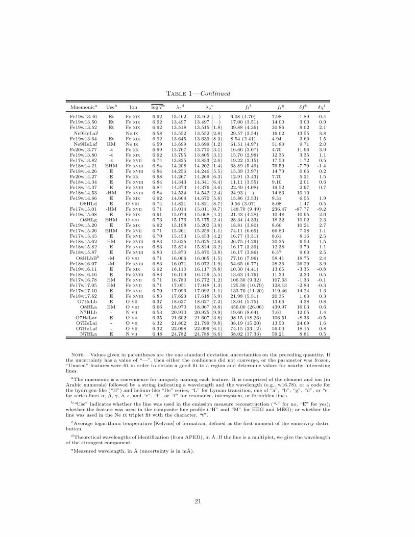
Table 1—Continued

Mnemonica Useb Ion log T c λtd λo

e flf ft

g δfh δχi

Fe19w13.46 Et Fe xix 6.92 13.462 13.462 (—) 6.08 (4.70) 7.98 -1.89 -0.4Fe19w13.50 Et Fe xix 6.92 13.497 13.497 (—) 17.00 (3.51) 14.00 3.00 0.9Fe19w13.52 Et Fe xix 6.92 13.518 13.515 (1.8) 39.88 (4.36) 30.86 9.02 2.1

Ne9HeLaij - Ne ix 6.58 13.552 13.552 (2.8) 29.57 (3.54) 16.02 13.55 3.8Fe19w13.64 Et Fe xix 6.92 13.645 13.639 (8.3) 8.54 (2.41) 4.94 3.60 1.5

Ne9HeLaf HM Ne ix 6.59 13.699 13.699 (1.2) 61.51 (4.97) 51.80 9.71 2.0Fe20w13.77 -t Fe xx 6.99 13.767 13.770 (3.1) 16.66 (3.07) 4.70 11.96 3.9Fe19w13.80 -t Fe xix 6.92 13.795 13.805 (3.1) 15.70 (2.98) 12.35 3.35 1.1Fe17w13.82 -t Fe xvii 6.74 13.825 13.833 (2.6) 19.22 (3.15) 17.50 1.72 0.5Fe18w14.21 EHM Fe xviii 6.84 14.208 14.202 (1.4) 68.89 (5.49) 76.59 -7.70 -1.4Fe18w14.26 E Fe xviii 6.84 14.256 14.246 (5.5) 15.39 (3.97) 14.73 0.66 0.2Fe20w14.27 E Fe xx 6.98 14.267 14.269 (6.3) 12.91 (3.43) 7.70 5.21 1.5Fe18w14.34 E Fe xviii 6.84 14.343 14.341 (6.4) 11.11 (3.55) 9.10 2.01 0.6Fe18w14.37 E Fe xviii 6.84 14.373 14.376 (3.6) 22.49 (4.08) 19.52 2.97 0.7Fe18w14.53 -HM Fe xviii 6.84 14.534 14.542 (2.4) 24.93 (—) 14.83 10.10 —Fe19w14.66 E Fe xix 6.92 14.664 14.670 (5.6) 15.86 (3.53) 9.31 6.55 1.9

O8HLd E O viii 6.74 14.821 14.821 (8.7) 9.56 (3.07) 8.08 1.47 0.5Fe17w15.01 -HM Fe xvii 6.71 15.014 15.011 (0.7) 148.70 (9.49) 236.47 -87.77 -9.2Fe19w15.08 E Fe xix 6.91 15.079 15.068 (4.2) 21.43 (4.28) 10.48 10.95 2.6

O8HLg EHM O viii 6.73 15.176 15.175 (2.4) 28.34 (4.33) 18.32 10.02 2.3Fe19w15.20 E Fe xix 6.92 15.198 15.202 (3.9) 18.81 (3.80) 8.60 10.21 2.7Fe17w15.26 EHM Fe xvii 6.71 15.261 15.259 (1.1) 74.11 (6.65) 66.83 7.28 1.1Fe17w15.45 E Fe xvii 6.70 15.453 15.453 (4.2) 16.77 (3.31) 8.61 8.16 2.5Fe18w15.62 EM Fe xviii 6.83 15.625 15.625 (2.6) 26.75 (4.29) 20.25 6.50 1.5Fe18w15.82 E Fe xviii 6.83 15.824 15.824 (3.2) 16.17 (3.39) 12.38 3.79 1.1Fe18w15.87 E Fe xviii 6.83 15.870 15.870 (3.8) 16.17 (3.86) 6.57 9.60 2.5

O8HLbBk -M O viii 6.71 16.006 16.005 (1.5) 77.16 (7.96) 58.41 18.75 2.4Fe18w16.07 -M Fe xviii 6.83 16.071 16.072 (1.9) 54.65 (6.77) 28.36 26.29 3.9Fe19w16.11 E Fe xix 6.92 16.110 16.117 (8.8) 10.30 (4.41) 13.65 -3.35 -0.8Fe18w16.16 E Fe xviii 6.83 16.159 16.159 (5.5) 13.63 (4.76) 11.30 2.33 0.5Fe17w16.78 EM Fe xvii 6.71 16.780 16.772 (1.2) 106.30 (9.32) 107.63 -1.33 -0.1Fe17w17.05 EM Fe xvii 6.71 17.051 17.048 (1.3) 125.30 (10.79) 128.13 -2.83 -0.3Fe17w17.10 E Fe xvii 6.70 17.096 17.092 (1.1) 133.70 (11.20) 119.46 14.24 1.3Fe18w17.62 E Fe xviii 6.83 17.623 17.618 (5.9) 21.98 (5.51) 20.35 1.63 0.3

O7HeLb E O vii 6.37 18.627 18.627 (7.2) 18.04 (5.75) 13.66 4.38 0.8O8HLa EM O viii 6.66 18.970 18.967 (0.8) 456.00 (26.06) 439.97 16.03 0.6N7HLb - N vii 6.53 20.910 20.925 (9.9) 19.66 (8.64) 7.61 12.05 1.4

O7HeLar E O vii 6.35 21.602 21.607 (3.8) 98.15 (18.26) 106.51 -8.36 -0.5O7HeLai - O vii 6.32 21.802 21.799 (9.8) 38.19 (15.20) 13.50 24.69 1.6O7HeLaf - O vii 6.32 22.098 22.099 (6.1) 74.15 (23.12) 56.00 18.15 0.8

N7HLa E N vii 6.48 24.782 24.788 (6.6) 68.02 (17.33) 59.21 8.81 0.5

Note.—Values given in parentheses are the one standard deviation uncertainties on the preceding quantity. Ifthe uncertainty has a value of “—”, then either the confidence did not converge, or the parameter was frozen.“Unused” features were fit in order to obtain a good fit to a region and determine values for nearby interestinglines.

aThe mnemonic is a convenience for uniquely naming each feature. It is comprised of the element and ion (inArabic numerals) followed by a string indicating a wavelength and the wavelength (e.g., w16.78), or a code forthe hydrogen-like (“H”) and helium-like “He” series, “L” for Lyman transition, one of “a”, “b”, “g”, “d”, or “e”for series lines α, β, γ, δ, ǫ, and “r”, “i”, or “f” for resonance, intersystem, or forbidden lines.

b“Use” indicates whether the line was used in the emission measure reconstruction (“-” for no, “E” for yes);whether the feature was used in the composite line profile (“H” and “M” for HEG and MEG); or whether theline was used in the Ne ix triplet fit with the character, “t”.

cAverage logarithmic temperature [Kelvins] of formation, defined as the first moment of the emissivity distri-bution.

dTheoretical wavelengths of identification (from APED), in A. If the line is a multiplet, we give the wavelengthof the strongest component.

eMeasured wavelength, in A (uncertainty is in mA).

21

fEmitted source line flux is 10−6 times the tabulated value in [phot cm−2 s−1].

gModel line flux is 10−6 times the tabulated value in [phot cm−2 s−1].

hLine flux residual, δf = fo − ft.

iδχ = (fo − ft)/σo.

jThe Ne ix intercombination line flux is blended with Fe xix 13.551 A, and with Fe xx 13.535, 13.558, 13.565A lines. The tabulated flux includes these blends. About 85% of the flux is from neon, as determined by theneighboring lines.

kThe O viii Lyman beta-like line is blended with Fe xviii 16.004 A, whose flux is about 1.17 times that ofFe xviii λ 15.62, according to our DEM and APED model. Hence, we estimate that the actual O8HLb flux is45.9 (8.6).

22