XCP – The Standard Protocol for ECU Development - Vector
116
Andreas Patzer | Rainer Zaiser XCP – The Standard Protocol for ECU Development Fundamentals and Application Areas
-
Upload
khangminh22 -
Category
Documents
-
view
3 -
download
0
Transcript of XCP – The Standard Protocol for ECU Development - Vector

Andreas Patzer | Rainer Zaiser
XCP – The Standard Protocolfor ECU Development
Fundamentals and Application Areas

Andreas Patzer | Rainer Zaiser
XCP – The Standard Protocol for ECU Development

Date December 2016Reproduction only with expressed permission from
Vector Informatik GmbH, Ingersheimer Str. 24, 70499 Stuttgart, Germany© 2016 by Vector Informatik GmbH. All rights reserved. This book is only intended for personal use, but not
for technical or commercial use. It may not be used as a basis for contracts of any kind. All information in this book was compiled with the greatest possible care, but Vector Informatik does not assume any guarantee or warranty whatsoever for the correctness of the information it contains. The liability of Vector Informatik is
excluded, except for malicious intent or gross negligence, to the extent that laws do not make it legally liable.
Information contained in this book may be protected by copyright and / or patent rights. Product names of software, hardware and other product names that are used in this book may be registered brands or otherwise
protected by branding laws, regardless of whether or not they are identified as registered brands.

XCPThe Standard Protocolfor ECU Development
Fundamentals and Application Areas
Andreas Patzer, Rainer Zaiser Vector Informatik GmbH

Table of Contents
Introduction ........................................................................................................................................... 7
1 Fundamentals of the XCP Protocol ...........................................................................................13
1.1 XCP Protocol Layer ................................................................................................................ 19 1.1.1 Identification Field ........................................................................................................21 1.1.2 Timestamp .....................................................................................................................21 1.1.3 Data Field ...................................................................................................................... 22
1.2 Exchange of CTOs .................................................................................................................. 22 1.2.1 XCP Command Structure .......................................................................................... 22 1.2.2 CMD ................................................................................................................................ 25 1.2.3 RES .................................................................................................................................. 28 1.2.4 ERR .................................................................................................................................. 28 1.2.5 EV .................................................................................................................................... 29 1.2.6 SERV ............................................................................................................................... 29 1.2.7 Calibrating Parameters in the Slave ....................................................................... 29
1.3 Exchanging DTOs – Synchronous Data Exchange ......................................................... 32 1.3.1 Measurement Methods: Polling versus DAQ ......................................................... 33 1.3.2 DAQ Measurement Method ...................................................................................... 34 1.3.3 STIM Calibration Method ........................................................................................... 42 1.3.4 XCP Packet Addressing for DAQ and STIM ........................................................... 43 1.3.5 Bypassing = DAQ + STIM ........................................................................................... 45 1.3.6 Time Correlation and Synchronization ................................................................... 45
1.4 XCP Transport Layers ...........................................................................................................49 1.4.1 CAN ................................................................................................................................. 49 1.4.2 CAN FD .......................................................................................................................... 52 1.4.3 FlexRay ........................................................................................................................... 54 1.4.4 Ethernet ......................................................................................................................... 57 1.4.5 SxI .................................................................................................................................... 59 1.4.6 USB ................................................................................................................................ 60 1.4.7 LIN .................................................................................................................................. 60
1.5 XCP Services ............................................................................................................................ 61 1.5.1 Memory Page Swapping .............................................................................................61 1.5.2 Saving Memory Pages – Data Page Freezing ....................................................... 63 1.5.3 Flash Programming ..................................................................................................... 63 1.5.4 Automatic Detection of the Slave ........................................................................... 65 1.5.5 Block Transfer Mode for Upload, Download and Flashing .................................66 1.5.6 Cold Start Measurement ........................................................................................... 67 1.5.7 Security Mechanisms with XCP ................................................................................68

2 ECU Description File A2L .............................................................................................................71
2.1 Setting Up an A2L File for an XCP Slave ......................................................................... 742.2 Manually Creating an A2L File ............................................................................................ 752.3 A2L Contents versus ECU Implementation ..................................................................... 76
3 Calibration Concepts ................................................................................................................... 79
3.1 Parameters in Flash .............................................................................................................. 803.2 Parameters in RAM ................................................................................................................823.3 Flash Overlay ...........................................................................................................................843.4 Dynamic Flash Overlay Allocation .....................................................................................853.5 RAM Pointer Based Calibration Concept per AUTOSAR .............................................86 3.5.1 Single Pointer Concept ...............................................................................................86 3.5.2 Double Pointer Concept .............................................................................................883.6 Flash Pointer Based Calibration Concept .......................................................................89
4 Application Areas of XCP ............................................................................................................ 91
4.1 Model in the Loop (MIL) ....................................................................................................... 934.2 Software in the Loop (SIL) .................................................................................................. 944.3 Hardware in the Loop (HIL) .................................................................................................954.4 Rapid Control Prototyping (RCP) ...................................................................................... 974.5 Bypassing ..................................................................................................................................984.6 Shortening Iteration Cycles with Virtual ECUs ........................................................... 101
5 Example of an XCP Implementation ......................................................................................105
5.1 Description of Functions ....................................................................................................1085.2 Parameterization of the Driver ........................................................................................ 110
6 Protocol Development Overview ..............................................................................................111
6.1 XCP Version 1.1 (2008) ......................................................................................................... 1126.2 XCP Version 1.2 (2013) .......................................................................................................... 1126.3 XCP Version 1.3 (2015).......................................................................................................... 113
The Authors..................................................................................................................................... 114Table of Abbreviations and Acronyms .....................................................................................116Literature ........................................................................................................................................ 117Web Addresses............................................................................................................................... 117Table of Figures .............................................................................................................................118Appendix – XCP Solutions at Vector ......................................................................................120Index ................................................................................................................................................. 122

7Introduction
Introduction
In optimal parameterization (calibration) of electronic ECUs, you calibrate parameter values during the system runtime and simultaneously acquire measured signals. The physical connection between the development tool and the ECU is via a measurement and calibration protocol. XCP has become established as a standard here.First, the fundamentals and mechanisms of XCP will be explained briefly and then the application areas and added value for ECU calibration will be discussed.
First, some facts about XCP:> XCP signifies “Universal Measurement and Calibration Protocol”. The “X” stands for the
variable and interchangeable transport layer.> It was standardized by an ASAM working committee (Association for Standardisation of
Automation and Measuring Systems). ASAM is an organization of automotive OEMs, suppliers and tool producers.
> XCP is the protocol that succeeds CCP (CAN Calibration Protocol).> The conceptual idea of the CAN Calibration Protocol was to permit read and write access
to internal ECU data over CAN. XCP was developed to implement this capability via different transmission media. Then one speaks of XCP on CAN, XCP on FlexRay or XCP on Ethernet.
> The primary applications of XCP are measurement and calibration of internal ECU parameters. Here, the protocol offers the ability to acquire measured values “event synchronous” to processes in ECUs. This ensures consistency of the data between one another.
To visualize the underlying idea, we initially view the ECU and the software running in it as a black box. In a black box, only the inputs into the ECU (e.g. CAN messages and sensor values) and the output from the ECU (e.g. CAN messages and actuator drives) are acquired. Details about the internal processing of algorithms are not immediately apparent and can only be determined from an analysis of the input and output data.
Now imagine that you had a look into the behavior of your ECU with every computation cycle. At any time, you could acquire detailed information on how the algorithm is running. You would no longer have a black box, but a white box instead with a full view of internal processes. That is precisely what you get with XCP!
What contribution can XCP make for the overall development process? To check the functionality of the attained development status, the developer can execute the code repeatedly. In this way, the developer finds out how the algorithm behaves and what might be optimized. It does not matter here whether a compiled code runs on a specific hardware or whether it is developed in a modelbased way and the application runs in the form of a model.
A central focus is on the evaluation of the algorithm process. For example, if the algorithm is running as a model in a development environment, such as Simulink from The MathWorks, it is helpful to developers if they can also acquire intermediate results to their applications, in order to obtain findings about other changes. In the final analysis, this method enables nothing other than read access to parameters so that they can be visualized and analyzed –

8 Introduction
and all of this at model runtime or retrospectively after a timelimited test run has been completed. A write access is needed if parameterizations are changed, e.g. if the proportional component of a PID controller is modified to adapt the algorithm behavior to the system under control. Regardless of where your application runs – focal points are always the detailed analysis of algorithm processes and optimization by changes to the parameterization.
This generalization can be made: The algorithms may exist in any type of executable form (code or model description). Different systems may be used as the runtime environment (Simulink, as DLL on the PC, on a rapid prototyping platform, in the ECU etc.). Process flows are analyzed by read access to data and acquisition of its timebased flow. Parameter sets are modified iteratively to optimize algorithms. To simplify the representation, the acquisition of data can be externalized to an external PCbased tool, although it is understood here that runtime environments themselves can even offer analysis capabilities.
Figure 1: Fundamental communication with a runtime environment
Application
Operating System
Runtime Environment
CommunicationPC Tool
The type of runtime environment and the form of communication generally differ from one another considerably. The reason is that the runtime environments are developed by different producers and are based on different solution approaches. Different types of protocols, configurations, measurement data formats, etc. make it a futile effort to try to exchange parameter sets and results in all development steps. In the end, however, all of these solutions can be reduced to read and write access at runtime. And there is a standard for this: XCP.
XCP is an ASAM standard whose Version 1.0 was released in 2003. The acronym ASAM stands for “Association for Standardisation of Automation and Measuring Systems.” Suppliers, vehicle OEMs and tool manufacturers are all represented in the ASAM working group. The purpose of the XCP working group is to define a generalized measurement and calibration protocol that can be used independent of the specific transport medium. Experience gained from working with CCP (CAN Calibration Protocol) flowed into the development as well.
XCP was defined based on the ASAM interfaces model. The following figure shows a measurement and calibration tool’s interfaces to the XCP Slave, to the description file and the connection to a higherlevel automation system.

9Introduction
Measurement andCalibration System
ASAM MCD-3 MC
ASAM MCD-1 MC
ASAMMCD-2 MC
ECU Description File
Upper LevelAutomation System
ECU
XCP Driver
XCP Driver*.A2L
Figure 2: The Interface Model of ASAM
Interface 1: “ASAM MCD-1 MC” between ECU and measurement & calibration systemThis interface describes the physical and the protocolspecific parts. Strictly speaking, a distinction was made between interfaces ASAP1a and ASAP1b here. The ASAP1b interface, however, never received general acceptance and for all practical purposes it has no relevance today. The XCP protocol is so flexible that it can practically assume the role of a general manufacturerindependent interface. For example, today all measurement and calibration hardware manufacturers offer systems (xETK, VX1000, etc.) which can be connected via the XCP on Ethernet standard. An ASAP1b interface – as it was still described for CCP – is no longer necessary.
Interface 2: “ASAM MCD-2 MC” A2L ECU description file As already mentioned, XCP works in an addressoriented way. Read or write accesses to objects are always based on an address entry. Ultimately, however, this would mean that the user would have to search for his ECU objects in the Master based on the address. That would be extremely inconvenient. To let users work with symbolic object names, for example, a file is needed that describes the relationship between the object name and the object address. The next chapter is devoted to this A2L description file.
Interface 3: “ASAM MCD-3 MC” automation interface This interface is used to connect another system to the measurement and calibration tool, e.g. for test bench automation. The interface is not further explained in this document, because it is irrelevant to understanding XCP.

10 Introduction
XCP is based on the MasterSlave principle. The ECU is the Slave and the measurement and calibration tool is the Master. A Slave may only communicate with one Master at any given time; on the other hand, the Master can simultaneous communicate with many Slaves.
Figure 3: An XCP Master can simultaneously communicate with multiple Slaves
Master
SlaveSlave Slave Slave
Bus
To be able to access data and configurations over the entire development process, XCP must be used in every runtime environment. Fewer tools would need to be purchased, operated and maintained. This would also eliminate the need for manual copying of configurations from one tool to another, a process that is susceptible to errors. This would simplify iterative loops, in which results from later work steps are transferred back to prior work steps.
But let us turn our attention away from what might be feasible to what is possible today: everything! XCP solutions are already used in a wide variety of work environments. It is the intention of this book to describe the main properties of the measurement and calibration protocol and introduce its use in the various runtime environments. What you will not find in this book: neither the entire XCP specification in detailed form, nor precise instructions for integrating XCP drivers in a specific runtime environment. It explains the relationships, but not the individual protocol and implementation details. Internet links in the appendix refer to openly available XCP driver source code and sample implementations, which let you understand and see how the implementation is made.
Screenshots of the PC tool used in this book were prepared using the CANape measurement and calibration tool from Vector. Other process flows are also explained based on CANape, in cluding how to create an A2L file and even more. With a costfree demo version, which is available to you in the Download Center of the Vector website at www.vector.com/canape_demo, you can see for yourself

131 Fundamentals of the XCP Protocol
1 Fundamentals of the XCP Protocol

14 1 Fundamentals of the XCP Protocol
Interface 1 of the ASAM interfaces model describes sending and receiving commands and data between the Slave and the Master. To achieve independence from a specific physical transport layer, XCP was subdivided into a protocol layer and a transport layer.
Figure 4: Subdivision of the XCP protocol into protocol layer and transport layer
CAN Ethernet FlexRay SxI USB ...
Depending on the transport layer, one refers to XCP on CAN, XCP on Ethernet, etc. The extendibility to new transport layers was proven as early as 2005 when XCP on FlexRay made its debut. The current version of the XCP protocol is Version 1.3, which was approved in 2015.
Adherence to the following principles was given high priority in designing the protocol:> Minimal resource usage in the ECU> Efficient communication> Simple Slave implementation > Plugandplay configuration with just a small number of parameters> Scalability

151 Fundamentals of the XCP Protocol
A key functionality of XCP is that it enables read and write access to the memory of the Slave.
Read access lets users measure the time response of an internal ECU parameter. ECUs are systems with discrete time behavior, whose parameters only change at specific time intervals: only when the processor recalculates the value and updates it in RAM. One of the great strengths of XCP lies in acquiring measured values from RAM which change synchronously to process flows or events in the ECU. This lets users evaluate direct relationships between timebased process flows in the ECU and the changing values. These are referred to as eventsynchronous measurements. The related mechanisms will be explained later in detail.
Write access lets the user optimize parameters of algorithms in the Slave. The accesses are addressoriented, i.e. the communication between Master and Slave references addresses in memory. So, the measurement of a parameter is essentially implemented as a request of the Master to the Slave: “Give me the value of memory location 0x1234”. Calibration of a parameter – the write access – to the Slave means: “Set the value at address 0x9876 to 5”.
An XCP Slave does not absolutely need to be used in ECUs. It may be implemented in different environments: from a modelbased development environment to hardwareintheloop and softwareintheloop environments to hardware interfaces that are used to access ECU memory via debug interfaces such as JTAG, NEXUS and DAP.
Figure 5: XCP Slaves can be used in many different runtime environments
Slave
Slave
Slave
Slave
Slave
PC
Measurement/Calibration Hardware*
* Debug Interfaces, Memory Emulator ...
HIL/SIL Systems
EXE/DLL
Prototype orECU Hardware
Simulink
MasterXCP

16 1 Fundamentals of the XCP Protocol
How can algorithms be optimized using read and write access to the ECU and what benefits does this offer? To be able to modify individual parameters at runtime in the ECU, there must be access to them. Not every type of memory permits this process. It is only possible to perform a read and write access to memory addresses in RAM (intentionally excluding the EEPROM here). The following is a brief summary of the differences between individual memory technologies: knowledge of them is very important to understanding over the further course of this book.
Memory Fundamentals
Today, flash memories are usually integrated in the microcontroller chips for ECUs and are used for longterm storage of code and data, even without power supply. The special aspect of a flash memory is that read and write access to individual bytes is indeed possible at any time, but writing of new contents can only be done blockwise, usually in rather large blocks.
Flash memories have a limited life, which is specified in terms of a maximum number of erasure cycles (depending on the specific technology the maximum may be up to one million cycles). This is also the maximum number of write cycles, because the memory must always be erased as a block before it can be written again. The reason for this lies in the memory structure: electrons are “pumped” via tunnel diodes. A bit is stored at a memory location as follows: electrons must be transported into the memory location over an electrically insulating layer. Once the electrons are then behind the insulating layer, they form an electric field with their charge, which is interpreted as a 1 when reading the memory location. If there are no electrons behind the layer, the cell information is interpreted as a 0. A 1 can indeed be set in this way, but not a 0. Setting to 0 (= erasing the 1) is performed in a separate erasing routine, in which electrons existing behind the insulating layer are discharged. However, for architectural reasons, such an erasing routine does not just act on single bytes, rather only on the group or block level. Depending on the architecture, blocks of 128 or 256 bytes are usually used. If one wishes to overwrite a byte within such a block, the entire block must first be erased. Then the entire contents of the block can be written back.
When this erasing routine is repeated multiple times, the insulating layer (“Tunnel Oxide Film”) can be damaged. This means that the electrons could slowly leak away, changing some of the information from 1 to 0 over the course of time. Therefore, the number of allowable flash cycles is severely limited in an ECU. In the production ECU, it is often only on the order of single digit numbers. This restriction is monitored by the Flash Boot Loader, which uses a counter to keep track of how many flash operations have already been executed. When the specified number is exceeded, the Flash Boot Loader rejects another flash request.
A RAM (Random Access Memory) requires a permanent power supply; otherwise it loses its contents. While flash memory serves the purpose of longterm storage of the application, the RAM is used to buffer computed data and other temporary information. Shutting off the power supply causes the RAM contents to be lost. In contrast to flash memory, it is easy to read and write to RAM.

171 Fundamentals of the XCP Protocol
This fact is clear: if parameters need to be changed at runtime, it must be assured that they are located in RAM. It is really very important to understand this circumstance. That is why we will look at the execution of an application in the ECU based on the following example:
In the application, the y parameters are computed from the sensor values x.
// Pseudocode representationa = 5;b = 2;y = a * x + b;
If the application is flashed in the ECU, the controller handles this code as follows after booting: the values of the x parameters correspond to a sensor value. At some time point, the application must therefore poll the sensor value and the value is then stored in a memory location assigned to the x parameters. Since this value always needs to be rewritten at runtime, the memory location can only lie in RAM.
The parameter y is computed. The values a and b, as factor and offset, are included as information in flash memory. They are stored as constants there. The value of y must also be stored in RAM, because once again that is the only place where write access is pos sible. At precisely which location in RAM the parameters x and y are located, or where a and b lie in flash, is set in the compiler/linker run. This is where objects are allocated to unique addresses. The relationship between object name, data type and address is documented in the linkermap file. The linkermap file is generated by the Linker run and can exist in different formats. Common to all formats, however, is that they contain the object name and address at a minimum.
In the example, if the offset b and factor a depend on the specific vehicle, the values of a and b must be individually adapted to the specific conditions of the vehicle. This means that the algorithm remains as it is, but the parameter values change from vehicle to vehicle.
In the normal operating mode of an ECU, the application runs from the flash memory. It does not permit any write accesses to individual objects. This means that parameter values which are located in the flash area cannot be modified at runtime. If a change to parameter values should be possible during runtime, the parameters to be modified must lie in RAM and not in flash. Now, how do the parameters and their initial values make their way into RAM? How does one solve the problem of needing to modify more parameters than can be simultaneously stored in RAM? These issues lead us to the topic of calibration concepts (see chapter 3).

18 1 Fundamentals of the XCP Protocol
Summary of XCP fundamentals
Read and write accesses to memory contents are available with the mechanisms of the XCP protocol. The accesses are made in an addressoriented way. Read access enables measurement of parameters from RAM, and write access enables calibration of the parameters in RAM. XCP permits execution of the measurement synchronous to events in the ECU. This ensures that the measured values correlate with one another. With every restart of a measurement, the signals to be measured can be freely selected. For write access, the parameters to be calibrated must be stored in RAM. This requires a calibration concept
This leads to two important questions:> How does the user of the XCP protocol know the correct addresses of the measurement
and calibration parameters in RAM?> What does the calibration concept look like?
The first question is answered in chapter 2 “ECUs description file A2L”. The topic of the calibration concept is addressed in chapter 3.

191.1 XCP Protocol Layer
1.1 XCP Protocol Layer
XCP data is exchanged between the Master and Slave in a messagebased way. The entire “XCP message frame” is embedded in a frame of the transport layer (in the case of XCP on Ethernet with UDP in a UDP packet). The frame consists of three parts: the XCP header, the XCP packet and the XCP tail.
In the following figure, part of a message is shown in red. It is used to send the current XCP frame. The XCP header and XCP tail depend on the transport protocol.
Figure 6: XCP packet
XCP Header
XCP Message (Frame)
XCP Packet
PID
IdentificationField
TimestampField
Data Field
FILL DAQ TIMESTAMP DATA
XCP Tail
The XCP packet itself is independent of the transport protocol used. It always contains three components: “Identification Field”, “Timestamp Field” and the current data field “Data Field”. Each Identification Field begins with the Packet Identifier (PID), which identifies the packet.
The following overview shows which PIDs have been defined:
0xFF
CMD
PID for frames from Master to Slave
PID for framesfrom Slave to Master
absolute orrelativeODT numberfor STIM
0xC0
0xBF
0x00
....
....
absolute orrelativeODT numberfor DAQ
0xFF
0xFE
0xFD
0xFC
RES
ERR
EV
SERV
0xFB
0x00
....
Figure 7: Overview of XCP Packet Identifier (PID)

20 1 Fundamentals of the XCP Protocol
Communication via the XCP packet is subdivided into one area for commands (CTO) and one area for sending synchronous data (DTO).
XCP Master
XCP Slave
CMD SERVRES ERR EVCTO
STIMDTO
Command / Response / Error / Event / Service Request Processor
DAQProcessor
STIMProcessor
DAQ STIMPGM CAL
BypassXCP Handler
Resources
DAQ
XCP Driver
Figure 8: XCP communication model with CTO/DTO
The acronyms used here stand for
CMD Command Packet sends commands RES Command Response Packet positive responseERR Error negative responseEV Event Packet asynchronous eventSERV Service Request Packet service requestDAQ Data AcQuisition send periodic measured valuesSTIM Stimulation periodic stimulation of the Slave
Commands are exchanged via CTOs (Command Transfer Objects). The Master initiates contact in this way, for example. The Slave must always respond to a CMD with RES or ERR. The other CTO messages are sent asynchronously. The Data Transfer Objects (DTO) are used to exchange synchronous measurement and stimulation data.

211.1 XCP Protocol Layer
1.1.1 Identification Field
Figure 9: Message identification
XCP Packet
PID
Identification Field
FILL DAQ TIMESTAMP DATA
When messages are exchanged, both the Master and Slave must be able to determine which message was sent by the other. This is accomplished in the identification field. That is why each message begins with the Packet Identifier (PID).
In transmitting CTOs, the PID field is fully sufficient to identify a CMD, RES or other CTO packet. In Figure 7, it can be seen that commands from the Master to the Slave utilize a PID from 0xC0 to 0xFF. The XCP Slave responds or informs the Master with PIDs from 0xFC to 0xFF. This results in a unique allocation of the PIDs to the individually sent CTOs.When DTOs are transmitted, other elements of the identification field are used (see chapter 1.3.4 “XCP Packet Addressing for DAQ and STIM”).
1.1.2 Timestamp
Figure 10: Timestamp
XCP Packet
TIMESTAMPPID FILL DAQ DATA
DTO packets use timestamps, but this is not possible in transmission of a CTO message. The Slave uses the timestamp to supply time information with measured values. That is, the Master not only has the measured value, but also the time point at which the measured value was acquired. The amount of time it takes for the measured value to arrive at the Master is no longer important, because the relationship between the measured value and the time point comes directly from the Slave. Transmission of a timestamp from the Slave is optional. This topic is discussed further in ASAM XCP Part 2 Protocol Layer Specification.

22 1 Fundamentals of the XCP Protocol
1.1.3 Data Field
Figure 11: Data field in the XCP packet
XCP Packet
DATA
Data Field
PID FILL DAQ TIMESTAMP
Finally, the XCP packet also contains the data stored in the data field. In the case of CTO packets, the data field consists of specific parameters for the different commands. DTO packets contain the measured values from the Slave and when STIM data is sent the values from the Master.
1.2 Exchange of CTOs
CTOs are used to transmit both commands from the Master to the Slave and responses from the Slave to the Master.
1.2.1 XCP Command Structure
The Slave receives a command from the Master and must react to it with a positive or negative response. The communication structure is always the same here:
Command (CMD):Position Type Description0 BYTE Command Packet Code CMD1..MAX_CTO1 BYTE Command specific Parameters
A unique number is assigned to each command. In addition, other specific parameters may be sent with the command. The maximum number of parameters is defined as MAX_CTO1 here. MAX_CTO indicates the maximum length of the CTO packets in bytes.
Positive response:Position Type Description0 BYTE Command Positive Response Packet Code = RES 0xFF1..MAX_CTO1 BYTE Command specific Parameters

231.2 Exchange of CTOs
Negative response:Position Type Description0 BYTE Error Packet Code = 0xFE1 BYTE Error code2..MAX_CTO1 BYTE Command specific Parameters
Specific parameters can be transmitted as supplemental information with negative responses as well and not just with positive responses. One example is when the connection is made between Master and Slave. At the start of a communication between Master and Slave, the Master sends a connect request to the Slave, which in turn must respond positively to produce a continuous pointtopoint connection.
Master à Slave: Connect Slave à Master: Positive Response
Connect command:Position Type Description0 BYTE Command Code = 0xFF1 BYTE Mode 00 = Normal 01 = user defined
Mode 00 means that the Master wishes XCP communication with the Slave. If the Master uses 0xFF 0x01 when making the connection, the Master is requesting XCP communication with the Slave. Simultaneously, it informs the Slave that it should switch to a specific – userdefined – mode.
Positive response of the Slave:Position Type Description0 BYTE Packet ID: 0xFF1 BYTE RESOURCE2 BYTE COMM_MODE_BASIC3 BYTE MAX_CTO, Maximum CTO size [BYTE]4 WORD MAX_DTO, Maximum DTO size [BYTE]6 BYTE XCP Protocol Layer Version Number (most significant byte only)7 BYTE XCP Transport Layer Version Number (most significant byte only)
The positive response of the Slave can assume a somewhat more extensive form. The Slave already sends communicationspecific information to the Master when making the connection. RESOURCE, for example, is information that the Slave gives on whether it supports such features as page switching or whether flashing over XCP is possible. With MAX_DTO, the Slave informs the Master of the maximum packet length it supports for transfer of the measured values, etc. You will find details on the parameters in ASAM XCP Part 2 Protocol Layer Specification.

24 1 Fundamentals of the XCP Protocol
XCP permits three different modes for exchanging commands and reactions between Master and Slave: Standard, Block and Interleaved mode.
Figure 12: The three modes of the XCP protocol: Standard, Block and Interleaved mode
MIN_ST
MAX_BS
Time
Master Slave
Time
Master Slave
Time
Master Slave
Standard Mode Block Mode Interleaved Mode
Request k+1
Response k
Response k+1
Request k Request k
Request k+1
Response k
Response k+1
Response k
Request k+1
Response k+1
Request kPart1
Part3
Part2
Part1
Part2
Part3
In the standard communication model, each request to a Slave is followed by a single response. Except with XCP on CAN, it is not permitted for multiple Slaves to react to a command from the Master. Therefore, each XCP message can always be traced back to a unique Slave. This mode is the standard case in communication.
The block transfer mode is optional and saves time in large data transfers (e.g. upload or download operations). Nonetheless, performance issues must be considered in this mode in the direction of the Slave. Therefore, minimum times between two commands (MIN_ST) must be maintained and the total number of commands must be limited to an upper limit MAX_BS. Optionally, the Master can read out these communication settings from the Slave with GET_COMM_MODE_INFO. The aforementioned limitations do not need to be observed in block transfer mode in the direction of the Master, because performance of the PC nearly always suffices to accept the data from a microcontroller.
The interleaved mode is also provided for performance reasons. But this method is also optional and – in contrast to block transfer mode – it has no relevance in practice.

251.2 Exchange of CTOs
1.2.2 CMD
Figure 13: Overview of the CTO packet structure
PID DATA
Data FieldIdentification Field
Timestamp Fieldempty for CTO
XCP CTO Packet
The Master sends a general request to the Slave over CMD. The PID (Packet Identifier) field contains the identification number of the command. The additional specific parameters are transported in the data field. Then the Master waits for a reaction of the Slave in the form of a RESponse or an ERRor.
XCP is also very scalable in its implementation, so it is not necessary to implement every command. In the A2L file, the available CMDs are listed in what is known as the XCP IF_DATA. If there is a discrepancy between the definition in the A2L file and the implementation in the Slave, the Master can determine, based on the Slave’s reaction, that the Slave does not even support the command. If the Master sends a command that is not implemented in the Slave, the Slave must acknowledge with ERR_CMD_UNKNOWN and no further activities are initiated in the Slave. This lets the Master know quickly that an optional command has not been implemented in the Slave. Some other parameters are included in the commands as well. Please take the precise details from the protocol layer specification in document ASAM XCP Part 2. The commands are organized in groups: Standard, Calibration, Page, Programming and DAQ measurement commands. If a group is not needed at all, its commands do not need to be implemented. If the group is necessary, certain commands must always be available in the Slave, while others from the group are optional.
The following overview serves as an example. The SET_CAL_PAGE and GET_CAL_PAGE commands in the page switching group are identified as not optional. This means that in an XCP Slave that supports page switching at least these two commands must be implemented. If page switching support is unnecessary in the Slave, these commands do not need to be implemented. The same applies to other commands.

26 1 Fundamentals of the XCP Protocol
Standard commands:Command PID OptionalCONNECT 0xFF NoDISCONNECT 0xFE NoGET_STATUS 0xFD NoSYNCH 0xFC NoGET_COMM_MODE_INFO 0xFB YesGET_ID 0xFA YesSET_REQUEST 0xF9 YesGET_SEED 0xF8 YesUNLOCK 0xF7 YesSET_MTA 0xF6 YesUPLOAD 0xF5 YesSHORT_UPLOAD 0xF4 YesBUILD_CHECKSUM 0xF3 YesTRANSPORT_LAYER_CMD 0xF2 YesUSER_CMD 0xF1 Yes
Calibration commands:Command PID OptionalDOWNLOAD 0xF0 NoDOWNLOAD_NEXT 0xEF YesDOWNLOAD_MAX 0xEE YesSHORT_DOWNLOAD 0xED YesMODIFY_BITS 0xEC Yes
Standard commands:Command PID OptionalSET_CAL_PAGE 0xEB NoGET_CAL_PAGE 0xEA NoGET_PAG_PROCESSOR_INFO 0xE9 YesGET_SEGMENT_INFO 0xE8 YesGET_PAGE_INFO 0xE7 YesSET_SEGMENT_MODE 0xE6 YesGET_SEGMENT_MODE 0xE5 YesCOPY_CAL_PAGE 0xE4 Yes

271.2 Exchange of CTOs
Periodic data exchange – basics:Command PID OptionalSET_DAQ_PTR 0xE2 NoWRITE_DAQ 0xE1 NoSET_DAQ_LIST_MODE 0xE0 NoSTART_STOP_DAQ_LIST 0xDE NoSTART_STOP_SYNCH 0xDD NoWRITE_DAQ_MULTIPLE 0xC7 YesREAD_DAQ 0xDB YesGET_DAQ_CLOCK 0xDC YesGET_DAQ_PROCESSOR_INFO 0xDA YesGET_DAQ_RESOLUTION_INFO 0xD9 YesGET_DAQ_LIST_INFO 0xD8 YesGET_DAQ_EVENT_INFO 0xD7 Yes
Periodic data exchange – static configuration: Command PID OptionalCLEAR_DAQ_LIST 0xE3 NoGET_DAQ_LIST_INFO 0xD8 Yes
Periodic data exchange – dynamic configuration: Command PID OptionalFREE_DAQ 0xD6 YesALLOC_DAQ 0xD5 YesALLOC_ODT 0xD4 YesALLOC_ODT_ENTRY 0xD3 Yes

28 1 Fundamentals of the XCP Protocol
Flash programming:Command PID OptionalPROGRAM_START 0xD2 NoPROGRAM_CLEAR 0xD1 NoPROGRAM 0xD0 NoPROGRAM_RESET 0xCF NoGET_PGM_PROCESSOR_INFO 0xCE YesGET_SECTOR_INFO 0xCD YesPROGRAM_PREPARE 0xCC YesPROGRAM_FORMAT 0xCB YesPROGRAM_NEXT 0xCA YesPROGRAM_MAX 0xC9 YesPROGRAM_VERIFY 0xC8 Yes
1.2.3 RES
If the Slave is able to successfully comply with a Master’s request, it gives a positive acknowledge with RES.
Position Type Description0 BYTE Packet Identifier = RES 0xFF1..MAX_CTO1 BYTE Command response data
You will find more detailed information on the parameters in ASAM XCP Part 2 Protocol Layer Specification.
1.2.4 ERR
If the request from the Master is unusable, it responds with the error message ERR and an error code.
Position Type Description0 BYTE Packet Identifier = ERR 0xFE1 BYTE Error code2..MAX_CTO1 BYTE Optional error information data
You will find a list of possible error codes in ASAM XCP Part 2 Protocol Layer Specification.

291.2 Exchange of CTOs
1.2.5 EV
If the Slave wishes to inform the Master of an asynchronous event, an EV can be sent to do this. Its implementation is optional.
Position Type Description0 BYTE Packet Identifier = EV 0xFD1 BYTE Event code2..MAX_CTO1 BYTE Optional event information data
You will find more detailed information on the parameters in ASAM XCP Part 2 Protocol Layer Specification.
Events will be discussed much more in relation to measurements and stimulation. This has nothing to do with the action of the XCP Slave that initiates sending of an EVENT. Rather it involves the Slave reporting a disturbance such as the failure of a specific functionality.
1.2.6 SERV
The Slave can use this mechanism to request that the Master execute a service.
Position Type Description0 BYTE Packet Identifier = SERV 0xFC1 BYTE Service request code2..MAX_CTO1 BYTE Optional service request data
You will find the Service Request Code table in ASAM XCP Part 2 Protocol Layer Specification.
1.2.7 Calibrating Parameters in the Slave
To change a parameter in an XCP Slave, the XCP Master must send the parameter’s location as well as the value itself to the Slave.XCP always defines addresses with five bytes: four for the actual address and one byte for the address extension. Based on a CAN transmission, only seven useful bytes are available for XCP messages. For example, if the calibrator sets a 4byte value and wants to send both pieces of information in one CAN message, there is insufficient space to do this. Since a total of nine bytes are needed to transmit the address and the new value, the change cannot be transmitted in one CAN message (seven useful bytes). The calibration request is therefore made with two messages from Master to Slave. The Slave must acknowledge both messages and in sum four messages are exchanged.

30 1 Fundamentals of the XCP Protocol
The following figure shows the communication between Master and Slave, which is necessary to set a parameter value. The actual message is located in the line with the envelope symbol. The interpretation of the message is shown by “expanding” it with the mouse.
Figure 14: Trace example from a calibration process in CANape
In the first message of the Master (highlighted in blue in Figure 14), the Master sends the command SET_MTA to the Slave with the address to which a new value should be written. In the second message, the Slave gives a positive acknowledge to the command with Ok:SET_MTA.
The third message DOWNLOAD transmits the hex value as well as the valid number of bytes. In this example, the valid number of bytes is four, because it is a float value. The Slave gives another positive acknowledge in the fourth message.
This completes the current calibration process. In the Trace display, you can recognize a terminating SHORT_UPLOAD – a special aspect of CANape, the measurement and calibration tool from Vector. To make sure that the calibration was performed successfully, the value is read out again after the process and the display is updated with the readout value. This lets the user directly recognize whether the calibration command was implemented. This command also gets a positive acknowledge with Ok:SHORT_UPLOAD.
When the parameter changes in the ECU’s RAM, the application processes the new value. A reboot of the ECU, however, would lead to erasure of the value and overwriting of the value in RAM with the original value from the flash (see chapter 3 “Calibration Concepts”). So, how can the modified parameter set be permanently saved?

311.2 Exchange of CTOs
Essentially, there are two possibilities:
A) Save the parameters in the ECUThe changed data in RAM could for example be saved in the ECU’s EEPROM: either automatically when ramping down the ECU, or manually by the user. A prerequisite is that the data can be stored in a nonvolatile memory of the Slave. In an ECU, this would be the EEPROM or flash. ECUs with thousands of parameters, however, are seldom able to provide so much unused EEPROM memory space, so this method is rare.
Another possibility is to write the RAM parameters back into the ECU’s flash memory. This method is relatively complex. A flash memory must first be erased before it can be rewritten. This, in turn, can only be done as a block. Consequently, it is not simply a matter of writing back individual bytes. You will find more on this topic in chapter 3 “Calibration Concepts”.
B) Save the parameters in the form of a file on the PCIt is much more common to store the parameters on the PC. All parameters – or subsets of them – are stored in the form of a file. Different formats are available for this; the simplest case is that of an ASCII text file, which only contains the name of the object and its value. Other formats also permit saving other information, such as findings about the maturity level of the parameter of the history of revisions.
Scenario: After finishing his or her work, the calibrator wishes to enjoy a free evening. So, the calibrator saves the executed changes in the ECU’s RAM in the form of a parameter set file on a PC. The next day, the calibrator wants to continue working where he or she left off. The calibrator starts the ECU. Upon booting, the parameters are initialized in RAM. However, the ECU does this using values stored in flash. This means that the changes of the previous day are no longer available in the ECU. To now continue where work was left off on the previous day, the calibrator transfers the contents of the parameter set file to the ECU’s RAM by XCP using the DOWNLOAD command.
Figure 15: Transfer of a parameter set file to an ECU’s RAM

32 1 Fundamentals of the XCP Protocol
Saving parameter set file in hex files and flashing
Flashing an ECU is another way to change the parameters in flash. They are then written to RAM as new parameters when the ECU is booted. A parameter set file can also be transferred to a C or H file and be made into the new flash file with another compiler/linker run. However, depending on the parameters of the code, the process of generating a flashable hex file could take a considerable amount of time. In addition, the calibrator might not have any ECU source code – depending on the work process. That would prevent this method from being available to the calibrator.
As an alternative, the calibrator can copy the parameter set file into the existing flash file.
Figure 16: Hex window
In the flash file, there is a hex file that contains both the addresses and the values. Now a parameter file can be copied to a hex file. To do this, CANape takes the address and the value from the parameter set file and updates the parameter value at the relevant location in the hex file. This results in a new hex file, which contains the changed parameter values. However, this Hex file must now possibly run through further process steps to obtain a flashable file. One recurring problem here is the checksums, which the ECU checks to determine whether it received the data correctly. If the flashable file exists, it can be flashed in the ECU and after the reboot the new parameter values are available in the ECU.
1.3 Exchanging DTOs – Synchronous Data Exchange
As depicted in Figure 8, DTOs (Data Transfer Objects) are available for exchanging synchronous measurement and calibration data. Data from the Slave are sent to the Master by DAQ – synchronous to internal events. This communication is subdivided into two phases: In an initialization phase, the Master communicates to the Slave which data the Slave should send for different events. After this phase, the Master initiates the measurement in the Slave and the actual measurement phase begins. From this point in time, the Slave sends the desired data to the Master, which only listens until it sends a “measurement stop” to the Slave. Triggering of measurement data acquisition and transmission is controlled by events in the ECU.

331.3 Exchanging DTOs – Synchronous Data Exchange
The Master sends data to the Slave by STIM. This communication also consists of two phases:In the initialization phase, the Master communicates to the Slave which data it will send to the Slave. After this phase, the Master sends the data to the Slave and the STIM processor saves the data. As soon as a related STIM event is triggered in the Slave, the data is transferred to the application memory.
1.3.1 Measurement Methods: Polling versus DAQ
Before explaining how eventsynchronous, correlated data is measured from a Slave, here is a brief description of another measurement method known as Polling. It is not based on DTOs, but on CTOs instead. Actually, this topic should be explained in a separate chapter, but a description of polling lets us derive, in a very elegant way, the necessity of DTObased measurement, so a minor side discussion at this point makes sense.
The Master can use the SHORT_UPLOAD command to request the value of a measurement para meter from the Slave. This is referred to as polling. This is the simplest case of a measure ment: sending the measured value of a measurement parameter at the time at which the SHORT_UPLOAD command has been received and executed.
In the following example, the measurement parameter “Triangle” is measured from the Slave:
Figure 17: Address information of the parameter “Triangle” from the A2L file
The address 0x60483 is expressed as an address with five bytes in the CAN frame: one byte for the address extension and four bytes for the actual address.
34 1 Fundamentals of the XCP Protocol
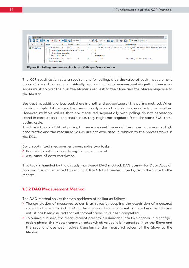
Figure 18: Polling communication in the CANape Trace window
The XCP specification sets a requirement for polling: that the value of each measurement parameter must be polled individually. For each value to be measured via polling, two messages must go over the bus: the Master’s request to the Slave and the Slave’s response to the Master.
Besides this additional bus load, there is another disadvantage of the polling method: When polling multiple data values, the user normally wants the data to correlate to one another. However, multiple values that are measured sequentially with polling do not necessarily stand in correlation to one another, i.e. they might not originate from the same ECU computing cycle. This limits the suitability of polling for measurement, because it produces unnecessarily high data traffic and the measured values are not evaluated in relation to the process flows in the ECU.
So, an optimized measurement must solve two tasks:> Bandwidth optimization during the measurement> Assurance of data correlation
This task is handled by the already mentioned DAQ method. DAQ stands for Data Acquisition and it is implemented by sending DTOs (Data Transfer Objects) from the Slave to the Master.
1.3.2 DAQ Measurement Method
The DAQ method solves the two problems of polling as follows:> The correlation of measured values is achieved by coupling the acquisition of measured
values to the events in the ECU. The measured values are not acquired and transferred until it has been assured that all computations have been completed.
> To reduce bus load, the measurement process is subdivided into two phases: In a configuration phase, the Master communicates which values it is interested in to the Slave and the second phase just involves transferring the measured values of the Slave to the Master.

351.3 Exchanging DTOs – Synchronous Data Exchange
How can the acquisition of measured values now be coupled to processes in the ECU? Figure 19 shows the relationship between calculation cycles in the ECU and the changes in parameters X and Y.
Calculationcycle n
Calculationcycle n+1
Calculationcycle n+2 time
10 8 6 4 2 0
10 8 6 4 2 0
E1 E1E1
X
Y
Calculate Y = XRead sensor X Figure 19: Events in the ECU
Let’s have a look at the sequence in the ECU: When event E1 (= end of computation cycle) is reached, then all parameters have been acquired and calculations have been made. This means that all values must match one another and correlate at this time point. This means that we use an eventsynchronous measurement method. This is precisely what is implemented with the help of the DAQ mechanism: When the algorithm in the Slave reaches the “Computational cycle completed” event, the XCP Slave collects the values of the measurement parameters, saves them in a buffer and sends them to the Master. This assumes that the Slave knows which parameters should be measured for which event.
An event does not absolutely have to be a cyclic, timeequidistant event, rather in the case of an engine controller, for example, it might be anglesynchronous. This makes the time interval between two events dependent on the engine rpm. A singular event, such as activation of a switch by the driver, is also an event that is not by any means equidistant in time.
The user selects the signals. Besides the actual measurement object, the user must select the underlying event for the measurement parameters. The events as well as the possible assignments of the measurement objects to the events must be stored in the A2L file.
Figure 20: Event definition in an A2L

36 1 Fundamentals of the XCP Protocol
In the normal case, it does not make any sense to be able to simultaneously assign a measured value to multiple events. Generally, a parameter is only modified within a single cycle (e.g. only at 10ms intervals) and not in multiple cycles (e.g. at 10ms and 100ms intervals).
Figure 21: Allocation of “Triangle” to possible events in the A2L
Figure 21 shows that the “Triangle” parameter can in principle be measured with the 1 ms, 10 ms and 100 ms events. The default setting is 10 ms.
Measurement parameters are allocated to events in the ECU during measurement configuration by the user.
Figure 22: Selecting events (measurement mode) for each measurement parameter
After configuring the measured signals, the user starts the measurement. The XCP Master lists the desired measurement parameters in what are known as DAQ lists. In these lists, the measured signals are each allocated to selected events. This configuration information is sent to the Slave before the actual start of measurement. Then the Slave knows which addresses it should read out and transmit when an event occurs. This distribution of the measurement into a configuration phase and a measurement phase was already mentioned at the very beginning of this chapter.
This solves both problems that occur in polling: bandwidth is used optimally, because the Master no longer needs to poll each value individually during the measurement and the measured values correlate with one another.

371.3 Exchanging DTOs – Synchronous Data Exchange
Figure 23: Excerpt from the CANape Trace window of a DAQ measurement
Figure 23 illustrates an example of commandresponse communication (color highlighting) between Master and Slave (overall it is significantly more extensive and is only shown in part here for reasons of space). This involves transmitting the DAQ configuration to the Slave. Afterwards, the measurement start is triggered and the Slave sends the requested values while the Master just listens.
Until now, the selection of a signal was described based on its name and allocation to a measurement event. But how exactly is the configuration transferred to the XCP Slave?
Let us look at the problem from the perspective of memory structure in the ECU: The user has selected signals and wishes to measure them. So that sending a signal value does not require the use of an entire message, the signals from the Slave are combined into message packets. The Slave does not create this definition of the combination independently, or else the Master would not be able to interpret the data when it received the messages. Therefore, the Slave receives an instruction from the Master describing how it should distribute the values to the messages.
The sequence in which the Slave should assemble the bytes into messages is defined in what are known as Object Description Tables (ODTs). The address and object length are important to uniquely identify a measurement object. An ODT provides the allocations of RAM contents from the Slave to assemble a message on the bus. According to the communication model, this message is transmitted as a DAQ DTO (Data Transfer Object).

38 1 Fundamentals of the XCP Protocol
RAM Cells
ODTaddress, lengthaddress, lengthaddress, lengthaddress, length
...
...
0123
PID 0 1 2 3
Figure 24: ODT: Allocation of RAM addresses to DAQ DTO
Stated more precisely, an entry in an ODT list references a memory area in RAM by the address and length of the object.
After receiving the measurement start command, at some point an event occurs that is associated with a measurement. The XCP Slave begins to acquire the data. It combines the individual objects into packets and sends them on the bus. The Master reads the bus message and can interpret the individual data, because it has defined the allocation of individual objects to packets itself and therefore it knows their relationships.
However, each packet has a maximum number of useful bytes, which depends on the transport medium that is used. In the case of CAN, this amounts to seven bytes. If more data needs to be measured, an ODT is no longer sufficient. If two or more ODTs need to be used to transmit the measured values, then the Slave must be able to copy the data into the correct ODT and the Master must be able to uniquely identify the received ODTs. If multiple measurement intervals of the ECU are used, the relationship between ODT and measurement interval must also be uniquely identifiable.

391.3 Exchanging DTOs – Synchronous Data Exchange
The ODTs are combined into DAQ lists in the XCP protocol. Each DAQ list contains a number of ODTs and is assigned to an event.
ODT #2 address, length
address, length
address, length
address, length
0
1
...
2
3
ODT #1 address, length
address, length
address, length
address, length
0
1
...
2
3
ODT #0 address, length
address, length
address, length
address, length
0
1
2
3
... PID=0 0 1 2 3 ...
PID=1 0 1 2 3 ...
PID=2 0 1 2 3 ...
Figure 25: DAQ list with three ODTs
For example, if the user uses two measurement intervals (= two different events in the ECU), then two DAQ lists are used as well. One DAQ list is needed per event used. Each DAQ list contains the entries related to the ODTs and each ODT contains references to the values in the RAM cells.
It is also possible for the Slave to transfer time information. A DAQ list represents the values belonging to a specific time event. Before these values in the Slave are recorded, the point in time of the event is noted and transferred within the first ODT. The timestamp is implemented using a counter. The time interval at which the counter is incremented is specified in the A2L.
DAQ lists are subdivided into the types: static, predefined and dynamic.

40 1 Fundamentals of the XCP Protocol
Static DAQ lists:If the DAQ lists and ODT tables are permanently defined in the ECU, as is familiar from CCP, they are referred to as static DAQ lists. There is no definition of which measurement parameters exist in the ODT lists, rather only the framework that can be filled (in contrast to this, see predefined DAQ lists).
In static DAQ lists, the definitions are set in the ECU code and are described in the A2L. Figure 26 shows an excerpt of an A2L, in which static DAQ lists are defined:
Figure 26: Static DAQ lists
In the above example, there is a DAQ list with the number 0, which is allocated to a 10ms event and can carry a maximum of two ODTs. The DAQ list with the number 1 has four ODTs and is linked to the 100 ms event.The A2L matches the contents of the ECU. In the case of static DAQ lists, the number of DAQ lists and the ODT lists they each contain are defined with the download of the application into the ECU. If the user now attempts to measure more signals with an event than fit in the allocated DAQ list, the Slave in the ECU will not be able to fulfill the requirements and the configuration attempt is terminated with an error. It does not matter that the other DAQ list is still fully available and therefore actually still has transmission capacity.
Predefined DAQ lists:Entirely predefined DAQ lists can also be set up in the ECU. However, this method is practically never used in ECUs due to the lack of flexibility for the user. It is different for analog measurement systems which transmit their data by XCP: Flexibility is unnecessary here, since the physical structure of the measurement system remains the same over its life.
411.3 Exchanging DTOs – Synchronous Data Exchange
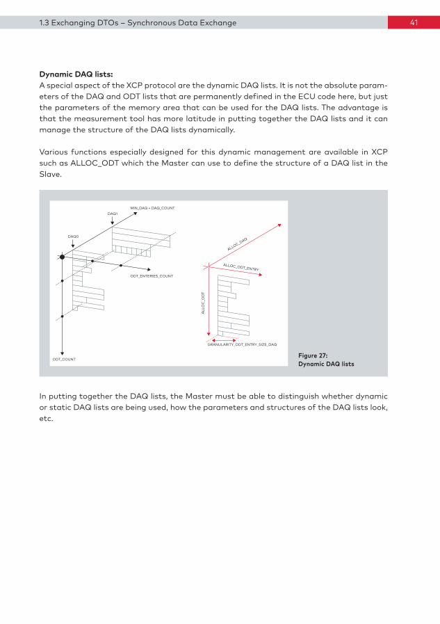
Dynamic DAQ lists: A special aspect of the XCP protocol are the dynamic DAQ lists. It is not the absolute parameters of the DAQ and ODT lists that are permanently defined in the ECU code here, but just the parameters of the memory area that can be used for the DAQ lists. The advantage is that the measurement tool has more latitude in putting together the DAQ lists and it can manage the structure of the DAQ lists dynamically.
Various functions especially designed for this dynamic management are available in XCP such as ALLOC_ODT which the Master can use to define the structure of a DAQ list in the Slave.
DAQ0
DAQ1MIN_DAQ + DAQ_COUNT
ODT_ENTERIES_COUNT
ALL
OC
_OD
T
GRANULARITY_ODT_ENTRY_SIZE_DAQ
ODT_COUNT
ALLOC_ODT_ENTRY
ALLOC_DAQ
Figure 27: Dynamic DAQ lists
In putting together the DAQ lists, the Master must be able to distinguish whether dynamic or static DAQ lists are being used, how the parameters and structures of the DAQ lists look, etc.

42 1 Fundamentals of the XCP Protocol
1.3.3 STIM Calibration Method
The XCP calibration method was already introduced in the chapter about exchanging CTOs. This type of calibration exists in every XCP driver and forms the basis for calibrating objects in the ECU. However, no synchronization exists between sending a calibration command and an event in the ECU.
In contrast to this, the use of STIM is not based on exchanging CTOs, rather on the use of DTOs with communication that is synchronized to an event in the Slave. The Master must therefore know to which events in the Slave it can even synchronize at all. This information must also exist in the A2L.
Figure 28: Event for DAQ and STIM
If the Master sends data to the Slave by STIM, the XCP Slave must be informed of the location in the packets at which the calibration parameters can be found. The same mechanisms are used here as are used for the DAQ lists.

431.3 Exchanging DTOs – Synchronous Data Exchange
1.3.4 XCP Packet Addressing for DAQ and STIM
Addressing of the XCP packets was already discussed at the beginning of this chapter. Now that the concepts of DAQ, ODT and STIM have been introduced, XCP packet addressing will be presented in greater detail.
During transmission of CTOs, the use of a PID is fully sufficient to uniquely identify a packet; however, this is no longer sufficient for transmitting measured values. The following figure offers an overview of the possible addressing that could occur with the DTOs:
XCP DTO Packet
PID TS
FILL DAQ TIMESTAMP DATA
PID
PID
PID
DAQ
DAQ TS
Identification Field Timestamp Field Data Field
Figure 29: Structure of the XCP packet for DTO transmissions
Transmission type: “absolute ODT numbers”
Absolute means that the ODT numbers are unique throughout the entire communication – i.e. across all DAQ lists. In turn, this means that the use of absolute ODT numbers assumes a transformation step that utilizes a socalled “FIRST_PID for the DAQ list.
If a DAQ list starts with the PID j, then the PID of the first packet has the value j, the second packet has the PID value j + 1, the third packet has the PID value j + 2, etc. Naturally, the Slave must ensure here that the sum of FIRST_PID + relative ODT number remains below the PID of the next DAQ list.
DAQlist: 0 ≤ PID ≤ kDAQlist: k + 1 ≤ PID ≤ mDAQlist: m + 1 ≤ PID ≤ netc.

44 1 Fundamentals of the XCP Protocol
In this case, the identification field is very simple:
Identification Field
absolute ODT number
PID
Figure 30: Identification field with absolute ODT numbers
Transmission type: “relative ODT numbers and absolute DAQ lists numbers”
In this case, both the DAQ lists number and the ODT number can be transmitted in the Identification Field. However, there is still space left over in the number of bytes that is available for the information:
Identification Field
PID DAQ
absolute DAQ list number
relative ODT numberFigure 31: ID field with relative ODT and absolute DAQ numbers (one byte)
In the figure, one byte is available for the DAQ number and one byte for the ODT number.
The maximum number of DAQ lists can be transmitted using two bytes:
Identification Field
PID DAQ
absolute DAQ list number
relative ODT numberFigure 32: ID field with relative ODT and absolute DAQ numbers (two bytes)
451.3 Exchanging DTOs – Synchronous Data Exchange
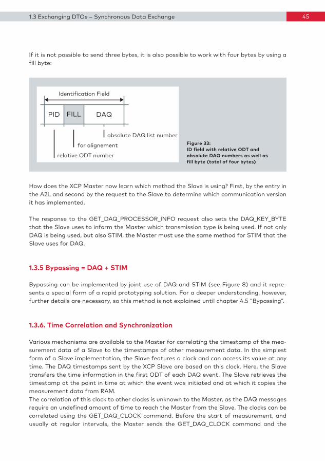
If it is not possible to send three bytes, it is also possible to work with four bytes by using a fill byte:
Identification Field
PID FILL DAQ
absolute DAQ list number
for alignement
relative ODT number
Figure 33: ID field with relative ODT and absolute DAQ numbers as well as fill byte (total of four bytes)
How does the XCP Master now learn which method the Slave is using? First, by the entry in the A2L and second by the request to the Slave to determine which communication version it has implemented.
The response to the GET_DAQ_PROCESSOR_INFO request also sets the DAQ_KEY_BYTE that the Slave uses to inform the Master which transmission type is being used. If not only DAQ is being used, but also STIM, the Master must use the same method for STIM that the Slave uses for DAQ.
1.3.5 Bypassing = DAQ + STIM
Bypassing can be implemented by joint use of DAQ and STIM (see Figure 8) and it represents a special form of a rapid prototyping solution. For a deeper understanding, however, further details are necessary, so this method is not explained until chapter 4.5 “Bypassing”.
1.3.6. Time Correlation and Synchronization
Various mechanisms are available to the Master for correlating the timestamp of the measurement data of a Slave to the timestamps of other measurement data. In the simplest form of a Slave implementation, the Slave features a clock and can access its value at any time. The DAQ timestamps sent by the XCP Slave are based on this clock. Here, the Slave transfers the time information in the first ODT of each DAQ event. The Slave retrieves the timestamp at the point in time at which the event was initiated and at which it copies the measurement data from RAM. The correlation of this clock to other clocks is unknown to the Master, as the DAQ messages require an undefined amount of time to reach the Master from the Slave. The clocks can be correlated using the GET_DAQ_CLOCK command. Before the start of measurement, and usually at regular intervals, the Master sends the GET_DAQ_CLOCK command and the

46 1 Fundamentals of the XCP Protocol
Slave responds with the current value of the Slave clock. Since the Master knows the point in time at which it sent the command, it can calculate a time offset between the Master clock and the Slave clock using the timestamp of the Slave and the point in time the command was sent. Naturally, this method is also afflicted with inaccuracies if the run time of the GET_DAQ_CLOCK command is not precisely defined or the point in time at which the clocks are read in the Master and Slave cannot be determined precisely when sending/receiving the command. This is why version 1.3 of the XCP specification provides improved methods enabling correlation of the Master and Slave clocks with a precision of just a few microseconds.
1.3.6.1 Multicast
For better correlation of the clocks of multiple Slaves to one another, the Master reads the clocks of multiple Slaves at the same time. For this purpose, the Master sends a command to all Slaves which are accessible using the same transport medium. Each Slave records the point in time at which it receives the command and transfers the value to the Master. To achieve maximum precision, two requirements must be fulfilled to the greatest degree possible:On the one hand, the Slave implementation should ensure (as in the past) that the recording of the timestamp is initiated as soon as possible upon receipt of the command. On the other hand, the latency times between the Slaves and the Master should be the same to the greatest degree possible.
The GET_DAQ_CLOCK_MULTICAST command is available for this purpose. The Slave responds with an EV_TIME_SYNC message, in which the timestamp is transferred.
XCP Slave Clockfree running
XCP Slave XCP Master
GET_DAQ_CLOCK_MULTICAST
EV_TIME_SYNC
GET_DAQ_CLOCK_MULTICAST
EV_TIME_SYNC
tFigure 34: XCP Slave with free-running clock

471.3 Exchanging DTOs – Synchronous Data Exchange
1.3.6.2. Grandmaster Clock
A further solution involves the time of the Slave already being synchronized/coordinated with another clock, the socalled grandmaster clock.
First, an explanation of the terms “synchronized” and “coordinated”:Stated simply, two clocks are synchronized with one another if they supply the identical timestamp when they are read at the same time.In contrast, clocks which are coordinated to one another do not necessarily need to supply the same timestamp. In both clocks, 1 second is exactly the same length.
IEEE 1588 with PTP (Precision Time Protocol) is used. In the first step, the XCP Master must know whether the Slave is linked to an external clock. As there can be more than one grandmaster clock in an overall system, information on the exact clock to which the Slave is linked must be available to the XCP Master.
XCP Slave XCP Master
GET_DAQ_CLOCK_MULTICAST
EV_TIME_SYNC
GET_DAQ_CLOCK_MULTICAST
EV_TIME_SYNC
t
XCP Slave Clocksynchronized to a
Grandmaster Clock
e.g. IEEE 1588
Grandmaster Clock
Figure 35: The clock of the XCP Slave is synchronized with the grandmaster clock

48 1 Fundamentals of the XCP Protocol
The XCP standard supports additional scenarios which can only briefly be sketched out here briefly. Further details can be found in the XCP specifications.
> Should it be possible to coordinate the XCP Slave clock with the external clock, but not synchronize them, there will be an offset between the grandmaster clock and the Slave clock. The XCP Master can request the details from the Slave using the TIME_CORRELATION_PROPERTIES command.
> The freerunning clock of the Slave cannot be synchronized with a grandmaster clock, but there is another clock in the Slave, e.g. a clock synchronized with the grandmaster clock in the Ethernet PHY of the Slave. If the Master receives both times at the same point in time, it can correlate the DAQ timestamp of the freerunning clock with the grandmaster clock and its own time domain.
> Another scenario arises when there is a freerunning clock of the XCP Slave and an ECU clock and the DAQ timestamps originate from the ECU clock. This is the case when an external XCP Slave, such as the VX1000 measurement and calibration hardware is used from Vector, is used.
> If all of the sketched solutions are combined, a total of three different clocks are involved: the freerunning Slave clock, a clock which is synchronized with a grandmaster clock and the ECU clock.
> In the last scenario, there is no Slave clock, but there is an ECU clock which is synchronized with a grandmaster clock.
Synchronization between the DAQ timestamps and the Master domain time can be realized for all scenarios in the Master using the XCP mechanisms.

491.4 XCP Transport Layers
1.4 XCP Transport Layers
A main requirement in designing the XCP protocol was that it must support different transport layers. At the time this document was defined, the following layers had been defined: XCP on CAN, FlexRay, Ethernet, SxI and USB. The bus systems CAN, LIN and FlexRay are explained on the Vector ELearning platform, as well as an introduction to AUTOSAR. For details see the website www.vectorelearning.com.
1.4.1 CAN
XCP was developed as a successor protocol of the CAN Calibration Protocols (CCP) and must absolutely satisfy the requirements of the CAN bus. The communication over the CAN bus is defined by the associated description file. Usually the DBC format is used, but in some isolated cases the AUTOSAR format ARXML is being used too.
A CAN message is identified by a unique CAN identifier. The communication matrix is defined in the description file: Who sends which message and how are the eight useful bytes of the CAN bus being used? The following figure illustrates the process:
DataFrame
ID=0x12 Sender Receiver
ID=0x34
ID=0x52 Receiver
Receiver
ReceiverSender
Receiver
Receiver
Sender
Sender Receiver
Sender
Sender
Receiver
Receiver
Receiver
ReceiverID=0x67
ID=0xB4
ID=0x3A5
CAN Node A
CANNode B
CANNode C
CANNode D
Figure 36: Definition of which bus nodes send which messages
The message with ID 0x12 is sent by CAN node A and all other nodes on the bus receive this message. In the framework of acceptance testing, CAN nodes C and D conclude that they do not need the message and they reject it. CAN node B, on the other hand, determines that its higherlevel layers need the message and they provide them via the Rx buffer. The CAN nodes are interlinked as follows:
50 1 Fundamentals of the XCP Protocol
CAN Node A
CAN
CAN Node C CAN Node D
CAN Node B
Host
TxBuffer
RxBuffer
AcceptanceTest
ReceiveSend
CAN Interface
Host
TxBuffer
RxBuffer
AcceptanceTest
ReceiveSend
CAN Interface
Host
Receive
AcceptanceTest
RxBuffer
Send
TxBuffer
CAN Interface
Host
Receive
AcceptanceTest
RxBuffer
Send
TxBuffer
CAN Interface
Figure 37: Representation of a CAN network
The XCP messages are not described in the communication matrix! If measured values are sent from the Slave via dynamic DAQ lists, e.g. with the help of XCP, the messages are assembled according to the signals selected by the user. If the signal selection changes, the message contents change as well. Nonetheless, there is a relationship between the communication matrix and XCP: CAN identifiers are needed to transmit the XCP messages over CAN. To minimize the number of CAN identifiers used, the XCP communication is limited to the use of just two CAN identifiers that are not being used in the DBC for “normal” communication. One identifier is needed to send information from the Master to the Slave; the other is used by the Slave for the response to the Master.
The excerpt from the CANape Trace window shows the CAN identifiers that are used under the “ID” column. In this example, just two different identifiers are used: 554 as the ID for the message from Master to Slave (direction Tx) and 555 for sending messages from the Slave to the Master (direction Rx).

511.4 XCP Transport Layers
Figure 38: Example of XCP-on-CAN communication
In this example, the entire XCP communication is handled by the two CAN identifiers 554 and 555. These two IDs may not be allocated for other purposes in this network.
The CAN bus transmits a maximum of eight useful bytes per message. In the case of XCP, however, we need information on the command used or the sent response. This is provided in the first byte of the CAN useful data. This means that seven bytes are available per CAN message for transporting useful data.
Figure 39: Representation of an XCP-on-CAN message
XCP Packet XCP Tail
FILL
XCP on CAN Message (Frame)
Control Fieldfor CAN
Control Field empty for CAN
XCP Headerempty for CAN
PID FILL DAQ TIMESTAMP DATA
In CANape, you will find an XCPonCAN demo with the virtual ECU XCPsim. You can learn about more details of the standard in ASAM XCP on CAN Part 3 Transport Layer Specification.

52 1 Fundamentals of the XCP Protocol
1.4.2 CAN FD
CAN FD (CAN with flexible data rate) is an extension of the CAN protocol developed by Robert Bosch GmbH. Its primary difference to CAN involves extending the useful data from 8 to 64 bytes. CAN FD also offers the option of sending the useful data at a higher data rate. After the arbitration phase, the data bytes are sent at a higher transmission rate than during the arbitration phase. This covers the need for greater bandwidth in automotive networks while preserving valuable experience gained from CAN development.The XCPonCANFD specification was defined in the XCPonCAN description of the XCP standard, Version 1.2 (June 2013).
Figure 40: Illustration of a CAN FD frame
EDL = Extended Data Length: CAN (dominant (0) = CAN frame Recessive (1) = CAN FD frame
BRS = Bit Rate Switch: CAN FD data phase starts immediately at sampling point of BRS: Dominant (0) = No change of bit rate for data phase Recessive (1) = Change to higher bit rate for data phase
ESI = Error State Indicator: Dominant (0) = CAN FD node is error active Recessive (1) = CAN FD node is error passive
Arbitration phase(standard bit rate)
Arbitration phase(standard bit rate)
Data phase(optional high bit rate)
1 11 1 1 1 1 1 1 1 1 7 31 4
DLC Data CRC EOF IFS
0…512 17/21
SO
F
Iden
tifi
er r1
IDE
ED
L r0
BR
S
ES
I
CR
C D
elim
.
AC
K
AC
K D
elim
.
Despite the largely similar modes of operation, this protocol requires extensions and modifications to the hardware and software. Among other things, CAN FD introduces three new bits to the control field:> Extended Data Length (EDL)> Bit Rate Switch (BRS) > Error State Indicator (ESI)

531.4 XCP Transport Layers
A recessive EDL bit (high level) distinguishes frames in extended CANFD format from those in standard CAN format, because they are identified by a dominant EDL bit (low level). Similarly, a recessive BRS bit causes the transmission of the data field to be switched to the higher bit rate. The ESI bit identifies the error state of a CAN FD node. Another four bits make up what is known as the Data Length Code (DLC), which represents the extended useful data length as a possible value of 12, 16, 20, 24, 32, 48 and 64 bytes.
The use of XCP on CAN FD assumes that a second transmission rate has been defined for the useful data in the A2L file. This is fully transparent to the user, who gets a complete A2L parameterization. A measurement configuration in the XCP Master considers the maximum packet length, and the user does not need to make any other settings.
CAN FD is supported in CANape, Version 12.0 and higher. Every CAN hardware product from Vector which begins with “VN” supports the CAN FD transport protocol.

54 1 Fundamentals of the XCP Protocol
1.4.3 FlexRay
A basic idea in the development of FlexRay was to implement a redundant system with deterministic time behavior. The connection redundancy was achieved by using two channels: channel A and channel B. If multiple FlexRay nodes (= ECUs) are redundantly interconnected and one branch fails, the nodes can switch over to the other channel to make use of the connection redundancy.
Figure 41: Nodes K and L are redundantly interconnected
CH ACH B
Node K Node L Node M Node N Node O
Deterministic behavior is achieved by transmitting data within defined time slots. Also defined here is which node sends which content in which time slot. These time slots are combined to form one cycle. The cycles repeat here, as long as the bus is active. The assembly of the time slots and their transport contents (who sends what at which time) is known as scheduling.
t1Slot 1 Slot 2 Slot 3 Slot 1 Slot 2 ... Real-time
t2 t3 t4 t5 t6
Communication Cycle Next Communication Cycle
Node K Node L Node M
Frame: a Frame: b Frame: x Frame: a Frame: b Frame: x
x
Slot13
TxRx
aDirection FrameSlot
13
TxRx
ab
Direction FrameSlot13
TxRx x
Direction Framea
Figure 42: Communication by slot definition

551.4 XCP Transport Layers
In the first communication cycle, node K sends frame a in slot 1. The scheduling is also stored in the software of nodes L and M. Therefore, the contents of frame a are passed to the next higher communication levels.
Scheduling is consolidated in a description file. This is not a DBC file, as in the case of CAN, rather it is a FIBEX file. FIBEX stands for “Field Bus Exchange Format” and could also be used for other bus systems. However, its current use is practically restricted to the description of the FlexRay bus. FIBEX is an XML format and the XCPonFlexRay specification relates to FIBEX Version 1.1.5 and FlexRay specification Version 2.1.
Sta
tic
Seg
men
t
Node L
Dyn
amic
Seg
men
t
Node M
Node LNode ONode N
Node L
Node O
Node L
Node K
ECUSlot
Node K
Node M
Channel
ABABABABABABABABAB
60 1 2 3 4 5 63
Cycles
...
7
1
3
4
5
6
2
b [rep: 1]
a [rep: 1]
d [rep: 1]
n [rep: 1]
m [rep: 1]
r [rep: 1]
a [rep: 1]
d [rep: 1]
n [rep: 1]
m [rep: 1]
r [rep: 1]
a [rep: 1]
d [rep: 1]
n [rep: 1]
m [rep: 1]
r [rep: 1]
a [rep: 1]
d [rep: 1]
n [rep: 1]
m [rep: 1]
r [rep: 1]
a [rep: 1]
d [rep: 1]
n [rep: 1]
m [rep: 1]
r [rep: 1]
a [rep: 1]
d [rep: 1]
n [rep: 1]
m [rep: 1]
r [rep: 1]
a [rep: 1]
d [rep: 1]
n [rep: 1]
m [rep: 1]
r [rep: 1]
u [rep: 4]
b [rep: 1]
b [rep: 1]
x [rep: 2]
o [rep: 1]o [rep: 1]
t [rep: 2]
w [rep: 4]
y [rep: 4]
o [rep: 1]
p [rep: 4]
v [rep: 8]
o [rep: 1]
t [rep: 2]
a [rep: 1]
d [rep: 1]
n [rep: 1]
m [rep: 1]
r [rep: 1]
o [rep: 1] o [rep: 1]
t [rep: 2]
w [rep: 4]
b [rep: 1]
b [rep: 1]
x [rep: 2]
o [rep: 1]
b [rep: 1]
y [rep: 4]
o [rep: 1]
p [rep: 4]
c [rep: 4]c [rep: 4]
b [rep: 1]
b [rep: 1] b [rep: 1]
b [rep: 1]b [rep: 1]
b [rep: 1] b [rep: 1]
b [rep: 1]b [rep: 1]
u [rep: 4]
x [rep: 2]
t [rep: 2]
b [rep: 1]
x [rep: 2]
Figure 43: Representation of a FlexRay communication matrix
Another format for describing bus communication has been defined as a result of the development of AUTOSAR solutions: the AUTOSAR Description File, which is available in XML format. The definition of XCPonFlexRay was taken into account in the AUTOSAR 4.0 specification. However, at the time of publication of this book this specification has not yet been officially approved and therefore it will not be discussed further.
Due to other properties of the FlexRay bus, it is not sufficient to just give the slot number as a reference to the contents. One reason is that multiplexing is supported: whenever a cycle is repeated, the transmitted contents are not necessarily the same. Multiplexing might specify that a certain piece of information is only sent in the slot in every second pass.

56 1 Fundamentals of the XCP Protocol
Instead of indicating the pure slot number, “FlexRay Data Link Layer Protocol Data Unit Identifiers” (FLX_LPDU_ID) are used, which can be understood as a type of generalized Slot ID. Four pieces of information are needed to describe such an LPDU:> FlexRay Slot Identifier (FLX_SLOT_ID)> Cycle Counter Offset (OFFSET)> Cycle Counter Repetition (CYCLE_REPETITION)> FlexRay Channel (FLX_CHANNEL)
... ... ... ... ... ... ... ... ... ... ... ... ... ...
...
...
...
...
. . .
LPDU_ID
Slot ID
Channel AChannel B
Cyc
le ID
...
...
... ... ... ... ... ... ... ... ... ... ... ... ... ... ...
...
...
...
...
.... . .
Figure 44: Representation of the FlexRay LPDUs
Scheduling also has effects on the use of XCP on FlexRay, because it defines what is sent precisely. This cannot be readily defined in XCP; not until the measurement runtime does the user define which measured values are sent by assembling signals. This means that it is only possible to choose which aspect of XCP communication can be used in which LPDU: CTO or DTO from Master to Slave or from Slave to Master.
The following example illustrates this process: the XCP Master may send a command (CMD) in slot n and Slave A gives the response (RES) in slot n + 2. XCPonFlexRay messages are always defined using LPDUs.
The A2L description file is needed for access to internal ECU parameters; the objects with their addresses in the ECU are defined in this file. In addition, the FIBEX file is necessary, so that the XCP Master knows which LPDUs it may send and to which LPDUs the XCP Slaves send their responses. Communication between XCP Master and XCP Slave(s) can only function through combination of the two files, i.e. by having an A2L file reference a FIBEX file.

571.4 XCP Transport Layers
Excerpt of an A2L with XCPonFlexRay parameter setting: …/begin XCP_ON_FLX … „XCPsim.xml“„Cluster_1“ …
In this example, “XCPsim.xml” is the reference from the A2L file to the FIBEX file.
... ... ... ... ... ... ... ... ... ... ... ... ... ...
...
...
...
...
. . .
Slot ID
Channel AChannel B
Cyc
le ID
...
...
... ... ... ... ... ... ... ... ... ... ... ... ... ... ...
...
...
...
...
...
. . .
XCP-dedicated LPDU_IDs
Figure 45: Allocation of XCP communication to LPDUs
You can read more details about XCP on FlexRay in CANape’s Online Help. Supplied with CANape is the FIBEX Viewer, which lets users conveniently view the scheduling. It is easy to allocate the XCP messages to the LPDUs by making driver settings for the XCPonFlexRay device in CANape.
The protocol is explained in detail in ASAM XCP on FlexRay Part 3 Transport Layer Specification. You will find an XCPonFlexRay demo in CANape with the virtual ECU XCPsim. The demo requires real Vector FlexRay hardware.
1.4.4 Ethernet
XCP on Ethernet can be used with either TCP/IP or UDP/IP. TCP is a protected transport protocol on Ethernet, in which the handshake method is used to detect any loss of a packet. In case of packet loss, TCP organizes a repetition of the packet. UDP does not offer this protection mechanism. If a packet is lost, UDP does not offer any mechanisms for repeated sending of the lost packet on the protocol level.
Not only can XCP on Ethernet be used with real ECUs, it can also be used for measurement and calibration of virtual ECUs. Here, a virtual ECU is understood as the use of code that would other wise run in the ECU as an executable program (e.g. DLL) on the PC. Entirely different resources are available here compared to an ECU (CPU, memory, etc.).

58 1 Fundamentals of the XCP Protocol
But first the actual protocol will be discussed. IP packets always contain the addresses of the sender and receiver. The simplest way to visualize an IP packet is as a type of letter that contains the addresses of the recipient and the sender. The addresses of individual nodes must always be unique. A unique address comprises the IP address and port number.
Figure 46: XCP packet with TCP/IP or UDP/IP
XCP Header XCP Packet
LEN CTR
XCP on Ethernet (TCP/IP and UDP/IP) Message (Frame)
Length (LEN)Control Fieldfor Ethernet
(TCP/ IP and UDP/IP)
Control Fieldempty for Ethernet
(TCP&IP and UDP&IP)
XCP Tailempty for Ethernet
(TCP/IP and UDP/IP)PID FILL DAQ TIMESTAMP DATA
The header consists of a Control Field with two words in Intel format (= four bytes). These words contain the length (LEN) and a counter (CTR). LEN indicates the number of bytes in the XCP packet. The CTR is used to detect the packet loss. UDP/IP is not a protected protocol. If a packet is lost, this is not recognized by the protocol layer. Packet loss is monitored by counter information. When the Master sends its first message to the Slave, it generates a counter number that is incremented with each additional transmission of a frame. The Slave responds with the same pattern: It increments its own counter with each frame that it sends. The counters of the Slave and the Master operate independently of one another. UDP/IP is well suited for sending measured values. If a packet is lost, then the measured values it contains are lost, resulting in a measurement gap. If this occurs infrequently, the loss might just be ignored. But if the measured data is to be used as the basis for fast control, it might be advisable to use TCP/IP.
An Ethernet packet can transport multiple XCP packets, but an XCP packet may never exceed the limits of a UDP/IP packet. In the case of XCP on Ethernet, there is no “Tail”, i.e. an empty control field.

591.4 XCP Transport Layers
Detection of XCP-on-Ethernet Slaves
With version 1.3 of the XCP standard, an expansion for XCP Slave detection was defined specifically for XCP on Ethernet. The Master can detect the XCP Slaves using the GET_SLAVE_ID command. Here, the Master broadcasts a multicast message (IPv4) with the IP address 239.255.0.0 on port 5556. Regardless of whether or not an XCP Slave already has a connection to a Master, the Slave must process the request and return a response.
The response of the Slave contains, among other things:> The IP address (IPv4)> The port number > TCP, UDP or both> Information on the status of whether or not there is already a connection to an XCP
Master
You will find more detailed information on the protocol in ASAM XCP on Ethernet Part 3 Transport Layer Specification. In CANape, you will also find an XCP on Ethernet demo with the virtual ECU XCPsim or with virtual ECUs in the form of DLLs, which have been implemented by Simulink models and the Simulink Coder.
1.4.5 SxI
SxI is a collective term for SPI or SCI. Since they are not buses, but instead are controller interfaces which are only suited for pointtopoint connections, there is no addressing in this type of transmission. The communication between any two nodes runs either synchronously or asynchronously.
Figure 47: XCP-on-SxI packet
XCP Header XCP Packet XCP Tail
XCP on Sxl Message (Frame)
Length (LEN)
Checksum (CS)
Control Fieldfor SxI
Control Fieldfor SxI
PID FILL DAQ TIMESTAMP DATALEN CTR FILL CS
The XCP header consists of a control field with two pieces of information: the length LEN and the counter. The length of these parameters may be in bytes or words (Intel format). LEN indicates the number of bytes of the XCP packet. The CTR is used to detect the loss of a packet. This is monitored in the same way as for XCP on Ethernet: with counter informa

60 1 Fundamentals of the XCP Protocol
tion. Under certain circumstances it may be necessary to add fill bytes to the packet, e.g. if SPI is used in WORD or DWORD mode or to avoid the message being shorter than the minimal packet length. These fill bytes are appended in the control field.
You will find more detailed information on the protocol in ASAM XCP on SxI Part 3 Transport Layer Specification.
1.4.6 USB
Currently, XCP on USB has no practical significance. Therefore, no further mention will be made of this topic; rather we refer you to ASAM documents that describe the standard: ASAM XCP on USB Part 3 Transport Layer Specification.
1.4.7 LIN
At this time, ASAM has not yet defined an XCPonLIN standard. However, a solution exists from Vector (XCPonLIN driver and CANape as XCPonLIN Master), which violates neither the LIN nor the XCP specification and is already being used on some customer projects. For more detailed information, please contact Vector.

611.5 XCP Services
1.5 XCP Services
This chapter contains a listing and explanation of other services that can be realized over XCP. They are all based on the already described mechanisms of communication with the help of CTOs and DTOs. Some XCP services have already been explained, e.g. synchronous data acquisition/stimulation and read/write access to device memory. The XCP specification does indeed uniquely define the different services; at the same time it indicates whether the service always needs to be implemented or whether it is optional. For example, an XCP Slave must support “Connect” for the Master to set up a connection. On the other hand, flashing over XCP is not absolutely necessary and the XCP Slave does not need to support it. This simply depends on the requirements of the project and the software. All of the services described in this chapter are optional.
1.5.1 Memory Page Switching
As already explained in the description of calibration concepts, parameters are normally located in flash memory and are copied to RAM as necessary. Some calibration concepts offer the option of switching memory segment pages from RAM and Flash. XCP describes a somewhat more general, generic approach, in which a memory segment may contain multiple switchable pages. Normally, this consists of a RAM page and a flash page. But multiple RAM pages or the lack of a flash page are conceivable as well.
For a better understanding of the XCP commands for page switching, the concepts of sector, segment and page will be explained once again at this point.
Segment 0Page 0
Seg
mem
t 0
Segment 1Page 0
Segment 1Page 1
Segment 1Page 2
Seg
mem
t 1
ECU access
address
XCP access
Sec
tor
2S
ecto
r 1S
ecto
r 0
Figure 48: Memory representation
62 1 Fundamentals of the XCP Protocol
From an XCP perspective, the memory of a Slave consists of a continuous memory that is addressed with a 40bit width. The physical layout of the memory is based on sectors. Know ledge of the flash sectors is absolutely necessary in flashing, because the flash memory can only be erased a block at a time.
The logical structure is based on what are known as segments; they describe where calibration data is located in memory. The start address and parameters of a segment do not have to be aligned with the start addresses and parameters of the physical sectors. Each segment can be subdivided into multiple pages. The pages of a segment describe the same parameters at the same addresses. The values of these parameters and read/write rights can be controlled individually for each page.
The allocation of an algorithm to a page within a segment must always be unique. Only one page may be active in a segment at any given time. This page is known as the “active page for the ECU in this segment.” The particular page that the ECU and the XCP driver actively access can be individually switched. No interdependency exists between these settings. Similar to the naming convention for the ECU, the active page for XCP access is referred to as the “active page for XCP access in this segment“.
In turn, this applies to each individual segment. Segments must be listed in the A2L file and each segment gets a number that is used to reference the segment. Within an XCP Slave, the SEGMENT_NUMBER must always begin at 0 and it is then incremented in consecutive numbers. Each segment has at least one page. The pages are also referenced by numbers. The first page is PAGE 0. One byte is available for the number, so that a maximum of 255 pages can be defined per segment.
The Slave must initialize all pages for all segments. The Master uses the command GET_CAL_PAGE to ask the Slave which page is currently active for the ECU and which page for XCP access. It can certainly be the case that mutual blocking may be necessary for the accesses. For example, the XCP Slave may not access a page, if this page is currently active for the ECU. As mentioned, there may be a dependency – but not necessarily. It is a question of how the Slave has been implemented.
If the Slave supports the optional commands GET_CAL_PAGE and SET_CAL_PAGE, then it also supports what is known as page switching. These two commands let the Master poll which pages are currently being used and if necessary it can switch pages for the ECU and XCP access. The XCP Master has full control over switching of pages. The XCP Slave cannot initiate switching by itself. But naturally the Master must respect any restrictions of the Slave implementation.
What is the benefit of switching?First, switching permits very quick changing of entire parameter sets – essentially a beforeandafter comparison. Second, the plant remains in a stable state, while the calibrator performs extensive parameter changes on another page in the ECU. This prevents the plant from going into a critical or unstable state, e.g. due to incomplete datasets during parameter setting.

631.5 XCP Services
1.5.2 Saving Memory Pages – Data Page Freezing
When a calibrator calibrates parameters on a page, there is the conceptual ability in XCP to save the data directly in the ECU. This involves saving the data of a RAM page to a page in nonvolatile memory. If the nonvolatile memory is flash, it must be taken into account that the segment start address and the segment size might not necessarily agree with the flash sectors, which represents a problem in erasing and rewriting the flash memory (see ASAM XCP Part 2 Protocol Layer Specification).
1.5.3 Flash Programming
Flashing means writing data in an area of flash memory. This requires precise knowledge of how the memory is laid out. A flash memory is subdivided into multiple sectors (physical sections), which are described by a start address and a length. To distinguish them from one another, they each get a consecutive identification number. One byte is available for this number, resulting in a maximum of 255 sectors.
SECTOR_NUMBER [0, 1, 2 … 255]
The information about the flash sectors is also part of the A2L data set.
Figure 49: Representation of driver settings for the flash area

64 1 Fundamentals of the XCP Protocol
Flashing can be implemented using what are referred to as “flash kernels”. A flash kernel is executable code that is sent to the Slave’s RAM area before the actual flashing; the kernel then handles communication with the XCP Master. It might contain the algorithm that is responsible for erasing the flash memory. For security and space reasons, very frequently this code is not permanently stored in the ECU’s flash memory. Under some circumstances, a converter might be used, e.g. if checksum or similar computations need to be performed.
Flashing with XCP roughly subdivides the overall flash process into three areas:> Preparation (e.g. for version control and therefore to check whether the new contents can
even be flashed)> Execution (the new contents are sent to the ECU) > Postprocessing (e.g. checksum checking etc.)
In the XCP standard, the primary focus is directed to the actual execution of flashing. Anyone who compares this operation to flashing over diagnostic protocols will discover that the processspecific elements, such as serial number handling with metadata, are supported in a rather spartan fashion in XCP. Flashing in the development phase was clearly the main focus in its definition and not the complex process steps that are necessary in endofline flashing.
Therefore, what is important in the preparation phase is to determine whether the new contents are even relevant to the ECU. There are no special commands for version control. Rather the practice has been to support those commands specific to the project.
The following XCP commands are available:
PROGRAM_START: Beginning of the flash procedureThis command indicates the beginning of the flash process. If the ECU is in a state that does not permit flashing (e.g. vehicle speed > 0), the XCP Slave must acknowledge with an ERRor. The actual flash process may not begin until the PROGRAM_START has been successfully acknowledged by the Slave.
PROGRAM_CLEAR: Call the current flash memory erasing routine Before flash memory can be overwritten with new contents, it must first be cleared. The call of the erasing routine via this command must be implemented in the ECU or be made available to the ECU with the help of the flash kernel.
PROGRAM_FORMAT: Select the data format for the flash data The XCP Master uses this command to define the format (e.g. compressed or encrypted) in which the data are transmitted to the Slave. If the command is not sent, the default setting is noncompressed and nonencrypted transmission.
PROGRAM: Transfer the data to the XCP SlaveFor the users who are very familiar with flashing via diagnostics: this command corresponds to TRANSFERDATA in diagnostics. Using this command, data is transmitted to the XCP Slave, which is then stored in flash memory.

651.5 XCP Services
PROGRAM_VERIFY: Request to check the new flash contentsThe Master can request that the Slave perform an internal check to determine whether the new contents are OK.
PROGRAM_RESET: Reset request to the SlaveRequest by the Master to the Slave to execute a Reset. Afterwards, the connection to the Slave is always terminated and a new CONNECT must be sent.
1.5.4 Automatic Detection of the Slave
The XCP protocol lets the Master poll the Slave about its protocolspecific properties. A number of commands are available for this.
GET_COMM_MODE_INFOThe response to this command gives the Master information about the various communication options of the Slave, e.g. whether it supports block transfer or interleaved mode or which minimum time intervals the Master must maintain between requests in these modes.
GET_STATUSThe response to this request returns all current status information of the Slave. Which resources (calibration, flashing, measurement, etc.) are supported? Are any types of memory activities (DAQ list configuration, etc.) still running currently? Are DTOs (DAQ, STIM) being exchanged right now?
GET_DAQ_PROCESSOR_INFOThe Master gets general information, which it needs to know about the Slave limitations: number of predefined DAQ lists, available DAQ lists and events, etc.
GET_DAQ_RESOLUTION_INFOOther information about the DAQ capabilities of the Slave is exchanged via this command: maximum number of parameters for an ODT for DAQ and for STIM, granularity of the ODT entries, number of bytes in timestamp transmission, etc.
GET_DAQ_EVENT_INFOWhen this command is used, the call is made once per ECU event. Information is transmitted here on whether the event can be used for DAQ, STIM or DAQ/STIM, whether the event occurs periodically and if so which cycle time it has, etc.

66 1 Fundamentals of the XCP Protocol
1.5.5 Block Transfer Mode for Upload, Download and Flashing
In the “normal” communication mode, each command from the Master is acknowledged by a response of the Slave. However, in some cases it may be desirable, for performance reasons, to use what is referred to as the block transfer mode.
MIN_ST
MAX_BS
Time
Master Slave
Response k
Request k+1
Request kPart1
Part3
Part2
Figure 50: Representation of the block transfer mode
The use of such a method accelerates the procedure when transmitting large amounts of data (UPLOAD, SHORT_UPLOAD, DOWNLOAD, SHORT_DOWNLOAD and PROGRAM). The Master can find out whether the Slave supports this method with the request GET_COMM_MODE_INFO. You will find more on this in ASAM XCP Part 2 Protocol Layer Specification.

671.5 XCP Services
1.5.6 Cold Start Measurement (during Power-On)
Even with the capabilities of XCP described to this point, it would be impossible to implement an eventdriven measurement that can in practice be executed early in the ECU’s start phase. The reason is that the measurement must be configured before the actual measurement takes place. If one attempts to do this, the ECU’s start phase has long been over by the time the first measured values are transmitted. The approach that is used to overcome this problem is based on a simple idea.
It involves separating the configuration and the measurement in time. After the configuration phase, the measurement is not started immediately; rather the ECU is shut down. After a reboot, the XCP Slave accesses the existing configuration directly and immediately begins to send the first messages. The difficulties associated with this are obvious: the configuration of the DAQ lists is stored in RAM, and therefore the information no longer exists after a reboot.
To enable what is known as the RESUME mode to enable a Cold Start Measurement, a nonvolatile memory is needed in the XCP Slave which preserves its data even when it is not being supplied with power. EEPROMs are used in this method. In this context, it is irrelevant whether it is a real EEPROM or one that is emulated by a flash memory.
You will find more details in ASAM XCP Part 1 Overview Specification in the chapter 1.4.2.2 “Advanced Features”.

68 1 Fundamentals of the XCP Protocol
1.5.7 Security Mechanisms with XCP
An unauthorized user should be prevented as much as possible from being able to make a connection to an ECU. The “seed & key” method is available for checking whether or not a connection attempt is authorized. The three different access types can be protected by seed & key: measurement / stimulation, calibration and flashing.
The “seed & key” method operates as follows: in the connect request by the Master, the Slave sends a random number (= seed) to the Master. Now, the Master must use an algorithm to generate a response (= key). The key is sent to the Slave. The Slave also computes the expected response and compares the key of the Master with its own result. If the two results agree, both the Master and Slave have used the same algorithm. Then the Slave accepts the connection to the Master. If there is no agreement, the Slave declines communication with the Master.
Normally, the algorithm is available as a DLL in the Master. So, if a user has the “seed & key” DLL and the A2L file, nothing stands in the way of accessing the ECU’s memory. When the ECU is approaching a production launch, the XCP driver is often deactivated. A unique sequence of individual diagnostic commands is usually used to restore XCP access to the ECU. This makes the XCP driver largely available even in production vehicles, but it is normally deactivated to protect against unauthorized manipulation of the ECU (see ASAM XCP Part 2 Protocol Layer Specification).
Whether or not seed & key or deactivation of the XCP driver is used in a project is implementationspecific and independent of the XCP specification.

712 ECU Description File A2L
2 ECU Description File A2L

72 2 ECU Description File A2L
One reason why an A2L file is needed has already been named: to allocate symbolic names to addresses. For example, if a software developer has implemented a PID controller and assigned the names P1, I1 and D1 in his application for the proportional, integral and differential components, then the calibrator should be able to access these parameters with their symbolic names. Let us take the following figure as an example:
Figure 51: Parameters in a calibration window
The user can conveniently modify values using symbolic names. Another example is provided by viewing signal variables that are measured from the ECU:
Figure 52: Signal response over time
In the legend, the user can read the logical names of the signals. The addresses at which the parameters were located in the ECU are of secondary importance in the offline analysis of values. Naturally, the correct address is needed to request the values in the ECU, but the numeric value of the address itself is of no importance to the user. The user uses the logical name for selection and visualization purposes. That is, the user selects the object by its name and the XCP Master looks for the associated address and data type in the A2L.

732 ECU Description File A2L
Another attribute of a parameter might be the definition of a minimum or maximum value. The value of the object would then have to lie within these limits. Imagine that you as the software developer define a parameter that has a direct effect on a power output stage. You must now prevent the user – whatever the user’s reasons might be – from configuring the output stage that would result in catastrophic damage. You can accomplish this by defining minimum and maximum values in the A2L to limit the permitted values.
Rules for conversion between physical and raw values are also defined in the A2L. You can visualize a simple example of such a conversion rule in a sensor that has an 8bit value. The numeric values output by the sensor lie between 0 and 255, but you wish to see the value as a percentage value. Mapping of the sensor value [0 … 255] to [0 … 100 %] is performed with a conversion rule, which in turn is stored in the A2L. If an object is measured, which exists as a raw value in the ECU and is also transmitted as such, the measurement and calibration tool uses the stored formula and visualizes the physical value.
Besides scalar parameters, characteristic curves and maps are frequently used. Some might utilize a proximity sensor such as a Hall sensor, which determines distance as a function of magnetic field strength and you may wish to use this distance value in your algorithm. The magnetic field and distance value do not run linear to one another. This nonlinearity of values would make formulation of the algorithm unnecessarily difficult. With the help of a characteristic curve, you can first linearize the values before you input the values into your algorithm as input variables.
Another application area for characteristic maps is their use as substitutes for complex computations. For example, if there is a relationship y = f(x) and the function f is associated with a lot of computing effort, it is often simpler to simply compute the values over the potential range of x in advance and store the results in the form of a table (= characteristic curve). If the value x is now in the ECU, the value y does not need to be computed at the controller’s runtime, rather the map returns the result y to the input variable x. It may be necessary to interpolate between two values, but that would be the extent of the calculations.
How is this characteristic curve stored in memory? Are all x values input first and then all y values? Or does storage follow the pattern: x1, y1; x2, y2; x3, y3 …? Since various options are available, the type of memory storage is defined in a storage scheme in the A2L.
The convenience for the user comes from the ability to work with symbolic names for parameters, the direct look at the physical values and access to complex elements such as characteristic maps, without having to concern oneself with complex storage schemes.
Another advantage is offered by the communication parameters. They are also defined in the A2L. In the communication between the measurement and calibration tool and the ECU, the parameter set from the A2L is used. The A2L contains everything that the measurement and calibration tool needs to communicate with the ECU.

74 2 ECU Description File A2L
2.1 Setting Up an A2L File for an XCP Slave
The A2L file is an ASCIIreadable file, which describes the following with the help of keywords:> Interfacespecific parameters between measurement and calibration tool and A2L file
(the description is located at the beginning of the A2L file and is located in what is referred to as the AML tree),
> Communication to the ECU,> Storage scheme for characteristic curves and maps (keyword RECORD_LAYOUT),> Conversion rules for converting raw values to physical values (keyword COMPU_METHOD),> Measurement parameters (keyword MEASUREMENT),> Calibration parameters (keyword CHARACTERISTIC) and> Events that are relevant for triggering a measurement keyword EVENT),
A summary of parameters and measurement parameters is made with the help of groups (keyword GROUP).
Example of a measurement parameter with the name “Shifter_B3”:
/begin MEASUREMENT Shifter_B3 „Single bit signal (bit from a byte shifting)“ UBYTE HighLow 0 0 0 1 READ_WRITE BIT_MASK 0x8 BYTE_ORDER MSB_LAST ECU_ADDRESS 0x124C02 ECU_ADDRESS_EXTENSION 0x0 FORMAT „%.3“ /begin IF_DATA CANAPE_EXT 100 LINK_MAP „byteShift“ 0x124C02 0x0 0 0x0 1 0x87 0x0 DISPLAY 0 0 20 /end IF_DATA /end MEASUREMENT
Example of a parameter map with the name KF1:
/begin CHARACTERISTIC KF1 „8*8 BYTE no axis“ MAP 0xE0338 __UBYTE_Z 0 Factor100 0 2.55 ECU_ADDRESS_EXTENSION 0x0 EXTENDED_LIMITS 0 2.55 BYTE_ORDER MSB_LAST BIT_MASK 0xFF /begin AXIS_DESCR FIX_AXIS NO_INPUT_QUANTITY BitSlice.CONVERSION 8 0 7 EXTENDED_LIMITS 0 7

752.1 Setting Up an A2L File for an XCP Slave
READ_ONLY BYTE_ORDER MSB_LAST FORMAT „%.0“ FIX_AXIS_PAR_DIST 0 1 8 /end AXIS_DESCR /begin AXIS_DESCR FIX_AXIS NO_INPUT_QUANTITY BitSlice.CONVERSION 8 0 7 EXTENDED_LIMITS 0 7 READ_ONLY BYTE_ORDER MSB_LAST FORMAT „%.0“ FIX_AXIS_PAR_DIST 0 1 8 /end AXIS_DESCR /begin IF_DATA CANAPE_EXT 100 LINK_MAP „map3_8_8_uc“ 0xE0338 0x0 0 0x0 1 0x87 0x0 DISPLAY 0 0 255 /end IF_DATA FORMAT „%.3“ /end CHARACTERISTIC
The ASCII text is not easy to understand. You will find a description of its structure in ASAM XCP Part 2 Protocol Layer Specification in chapter 2.
The sections below describe how to create an A2L. Let us focus on the actual contents of an A2L and their meanings and leave the details of the A2L description language to an editor. The A2L Editor that is supplied with CANape is used here.
2.2 Manually Creating an A2L File
The A2L mainly describes the contents of the memory of the XCP Slave. The contents depend on the application in the Slave, which was developed as C code. After the compiler/linker run of the application code, important elements of an A2L file already exist in the linkermap file: the names of the objects, their data types and memory addresses. Still lacking are the parameters for communication between XCP Master and Slave. Other information is usually needed such as minimum and maximum values of parameters, conversion rules, storage schemes for characteristic maps etc.
Let us begin by creating an empty A2L and the communication parameters: If you wish to create an A2L that describes an ECU with an XCPonCAN interface, for example, you create a new device in CANape and select XCP on CAN as the interface. Then you can supplement this with other communicationspecific information (e.g. CAN identifiers). After saving the file, you have an A2L that contains the entire communication content of the A2L. Still lacking are the definitions of the actual measurement and calibration parameters.
76 2 ECU Description File A2L
In the A2L Editor, the linkermap file is associated to the A2L. In a selection dialog, the user can now select those parameters from the map file which it needs in the A2L: scalar measurement and calibration parameters, characteristic curves and maps. The user can gradually add the desired parameters to the A2L step by step and group them. Other objectspecific information is also added using the editor.
What should be done when you modify your code, recompile it and link it? It is highly probable that the addresses of objects will change. Essentially, it is not necessary to generate a new A2L. If you wish to have objects just added to the code also be available in the A2L, you must of course add them to the A2L. Address updating is always necessary in the A2L. This is done with the editor; it searches for the relevant entry in the linkermap file based on the name of the A2L object, reads out the address and updates it in the A2L.
If your application changes very dynamically – objects are renamed, data types are adapted, parameters are deleted and others added – then the manual work method is impractical. To generate an A2L from a C code, other tools are available for automatic processing.
On the Vector homepage you will find information on the “ASAP2 ToolSet“ with which you can automate the generation of A2Ls from the source code in a batch process.
2.3 A2L Contents versus ECU Implementation
When an XCP Master tool reads in an A2L that does not fully match the ECU, misunderstandings in the communication might occur. For example, another value related to timestamp resolution might be in the A2L file that differs from the value implemented in the ECU. If this is the case, the problem must be detected and solved. The user gets support from the Master, who can poll the Slave via the protocol to determine what was really implemented in the Slave.
XCP offers a number of functions that were developed for automatic detection of the Slave. Of course, this assumes that automatic detection is implemented in the Slave. If the Master polls the Slave and the Slave’s responses do not agree with the parameter set of the A2L description file, the Master must decide which settings to use. In CANape, the information that is read out by the Slave is given a higher priority than the information from the A2L.

772.3 A2L Contents versus ECU Implementation
Here is an overview of possible commands that are used to find out something about the XCP implementation in the Slave:
GET_DAQ_PROCESSOR_INFOReturns general information on the DAQ lists: MAX_DAQ, MAX_EVENT_CHANNEL, MIN_DAQ
GET_DAQ_RESOLUTION_INFO Maximum parameter of an ODT entry for DAQ/STIM, time interval information
GET_DAQ_EVENT_INFO (Event_channel_number)Returns information for a specific time interval: Name and resolution of the time interval, number of DAQ lists that may be assigned to this time interval …
GET_DAQ_LIST_INFO (DAQ_List_Number)Returns information on the selected DAQ list: MAX_ODT, MAX_ODT_ENTRIES exist as predefined DAQ lists …

793 Calibration Concepts
3 Calibration Concepts

80 3 Calibration Concepts
ECU parameters are constant parameters that are adapted and optimized during the development of the ECU or an ECU variant. This is an iterative process, in which the optimal value of a parameter is found by repeated measurements and changes.
The calibration concept answers the question of how parameters in the ECU can be changed during an ECU’s development and calibration phases. There is not one calibration concept that exists, rather several. Which concept is utilized usually depends very much on the capabilities and resources of the microcontroller that is used. Normally, parameters are stored in the production ECU’s flash memory. The underlying program variables are defined as constants in the software. To make parameters modifiable at runtime during an ECU’s development, additional RAM memory is needed.
A calibration concept is concerned with such questions as these: How do the parameters initially find their way from flash to RAM? How is the microcontroller’s access to RAM rerouted? What does the solution look like when there are more parameters than can be simultaneously stored in RAM? How are the parameters copied back into flash? Are changes to the parameters persistent, i.e. are they preserved when the ECU is turned off?A distinction is made between transparent and nontransparent calibration concepts. Transparent means that the calibration tool does not need to be concerned with the above questions, because all necessary mechanisms are implemented in the ECU. Several methods are briefly introduced in the following.
3.1 Parameters in Flash
The software developer defines in the source code whether a parameter is a variable or a constant, i.e. whether a parameter is stored in flash or in RAM memory.
C code example:
const float factor = 0.5;
The “factor” parameter represents a constant with the value 0.5. During compiling and linking of the code, memory space is provided in flash for the “factor” object. The object is allocated an address that lies in the data area of the flash memory. The value 0.5 is found at the relevant address in the hex file and the address appears in the linkermap file.
The simplest conceivable calibration concept involves modifying the value in C code, generating a new hex file and flashing. However, this method is very laborious, because every value change must be made in code, resulting in the need for a compiler/linker run with subsequent flashing. An alternative approach would be to only modify the value in the hex file and then reflash this file. Every calibration tool is capable of doing this. It is referred to as “offline calibration” of the hex file, which is a very commonly used method.

813.1 Parameters in Flash
Under some circumstances, with certain compilers it may be necessary to explicitly ensure that parameters are always also stored in flash memory and not integrated in the code, for example and therefore do not appear at all in the linkermap file. Usually, one does not want to leave to chance where a constant is created in flash memory. The necessary means for accomplishing this are almost always compilerspecific pragma instructions. To prevent the compiler from embedding them in the code, it is generally sufficient to use the “volatile” attribute for constant parameters. A typical definition of a flash constant appears as in the following example: C code example:
#pragma section “FLASH_Parameter”volatile const float factor = 0.5;
It is normally not possible to calibrate parameters in flash online. Indeed, most microcontrollers are able to program their flash themselves, which is necessary for the purposes of reprogramming in the field. Nonetheless, flash memory always has the property of being organized into larger blocks (sectors), which can only be erased as a whole. It is practically impossible to flash just individual parameters, because the ECU normally does not have the resources to buffer the rest of the sector and reprogram it. In addition, this process would take too much time.
Some ECUs have the ability to store data in what is known as an EEPROM memory. In contrast to flash memories, EEPROM memories can erase and program each memory cell individually. The amount of available EEPROM memory is always considerably less than the available flash memory and it is usually limited to just a few kilobytes. EEPROM memory is often used to store programmable parameters in the service shop or to implement a persistence mechanism in the ECU, e.g. for the odometer. Online calibration would be conceivable here, but it is seldom used, because access to EEPROM cells is relatively slow and during the booting process EEPROM parameters are usually copied over to RAM memory, where it is possible to access them directly. ECUs which have no EEPROM memory often implement what is known as an EEPROM emulation. In this method, multiple small flash sectors are used in alternation to record parameter changes, so that the last valid value can always be determined. Online calibration would also be conceivable with this method.In both cases, the relevant memory accesses would then be intercepted in the software components of the XCP driver and implemented with the software routines of the EEPROM or the EEPROM emulation. The Vector XCP Professional driver offers the software hooks needed for this.

82 3 Calibration Concepts
3.2 Parameters in RAM
The most frequently used approach to modifying parameters at runtime (“online calibration”) is to create the parameters in the available RAM memory.
C code example:
#pragma section “RAM_Parameter”volatile float factor = 0.5;
This defines the parameter “factor” as a RAM variable with the initial value 0.5. During compiling and linking of the code, memory space is reserved for the object “factor” in RAM and the associated RAM address appears in the linkermap file. The initial value 0.5 is stored in flash memory and at the relevant location in the hex file. The addresses of the initial values in flash memory are defined by parameterization of the linker, but they do not appear in the linkermap file. During booting of the ECU, all RAM variables are initialized once with their initial values from flash memory. This is usually executed in the startup code of the compiler producer and the application programmer does not need to be concerned with it. The application uses the values of parameters located in RAM and they can be modified via normal XCP memory accesses.
From the perspective of the ECU software, calibration parameters in RAM are always still unchangeable, i.e. the application itself does not change them. Many compilers discover this fact by code analysis and simply optimize the necessary RAM memory space away. Normally, it is therefore also necessary to prevent the compiler from optimizing by using the “volatile” attribute.
From the perspective of the calibration tool, the RAM area in which the parameters are located is referred to as calibration RAM (memory that can be calibrated).
FLASH RAM
Parameters
Calibration RAM
Figure 53: Initial parameter setting in RAM
The calibration RAM does not need to consist of a fully contiguous RAM area. It may also be distributed into multiple areas or even in any desired way. Nonetheless, it offers significant advantages for organizing the parameters in just a few contiguous RAM areas and isolating them from other RAM parameters such as changing state variables and intermediate results. This is especially important if offline calibration of the calibration RAM with a hex file should be enabled. At the user’s request, the calibration tool must be able to load the

833.2 Parameters in RAM
parameters that were modified offline into the ECU during the transition from offline calibration to online calibration.
This case occurs very frequently. For example, when calibrators reconnect with their ECU on the next work day, they want to resume work at the point at which they stopped the evening before. However, booting of the ECU causes the flashed contents to be copied to the RAM as an initial dataset. To let users resume with work accomplished on the previous day, the parameter set file saved the previous evening in the ECU’s RAM must be loaded. This loading process may be time optimized by limiting the number of necessary transmissions to a minimum. It is advantageous here if the tool can quickly and reliably determine – by forming a checksum over larger contiguous areas – whether there are differences. If there are no differences between the calibration RAM contents in the ECU and the file modified using the tool, this area does not need to be transferred. If the memory area with the calibration parameters is not clearly defined, or if it includes parameters that are modified by the ECU software, a checksum calculation always shows a difference and the parameter values are transmitted, either from the ECU to the XCP Master or in a reverse direction. Depending on the transmission speed and amount of data, this transmission could take several minutes.
Another advantage of clearly defined memory segments is that the memory area for initial values in flash memory can be used for offline calibration. The contents of the flash memory are defined using flashable hex files. If the calibration tool knows the location of parameters in the hex file, it can modify their values and implement new initial values in the ECU by flashing the modified hex file. The calibration tool not only needs to know the location of parameters in RAM, but also the initial values in flash. A prerequisite is that the RAM memory segment must be initialized by copying from an identically laid out memory segment in flash, as is the usual practice in most compilers/linkers. If the addresses of parameters in RAM are in the A2L file, it is only necessary to let the tool know the offset to the start address of the calibration RAM, which it must add to get to the start address of the relevant flash area. This offset then applies to each individual parameter in the A2L.
The calibration tool can then either generate flashable hex files for this area itself, or it can place them directly on the original hex files of the linker to modify the initial values of parameters in the hex file.

84 3 Calibration Concepts
3.3 Flash Overlay
Many microcontrollers offer options for overlaying memory areas in flash with internal or external RAM. This process is referred to as flash emulation or flash overlay. A lot is possible, from the use of a Memory Management Unit all the way to dedicated mechanisms that precisely serve this purpose. In this case the parameters are created as parameters in flash just as in calibration concept 1. This method offers enormous advantages compared to the described calibration concept 2 “Parameters in RAM”:> No distinction is made between flash and RAM addresses. The flash addresses are always
located in the A2L file, the hex file and linkermap file. This produces clear relationships, the hex file is directly flashable and the A2L file matches it exactly.
> The overlay can be activated or deactivated as a whole, which enables lightningquick swapping between values in flash and those in RAM. They are referred to as the RAM page and the flash page of a memory segment. XCP supports control of memory page switching with special commands.
> The memory pages might be switched separately, e.g. for XCP access and ECU access, i.e. XCP could access a memory page while the ECU software works with the other page. This permits such operations as downloading of the offline calibration data to RAM, while the ECU is still working with the flash data; this avoids potential inconsistencies that could be problematic on a running ECU.
> The overlay with RAM does not need to be complete and it can be adapted to the application case. It is possible to work with less RAM than with flash. More on this later.
A typical procedure for connecting the calibration tool to the ECU with the subsequent download of values that were calibrated offline appears as follows:
Connects to the ECU CONNECTConnects XCP Master to RAM page SET_CAL_PAGE XCP to RAMChecksum calculation CALC_CHECKSUM
When a difference has been detected in the checksum calculation over the RAM area, first the user is normally asked how to proceed. Should the contents of ECU RAM be sent to the Master, or should the contents of a file on the Master page be sent to the ECU’s RAM? If the user decides to write the offline changes to the ECU, the subsequent process appears as follows:
ECU should use the dataset of the flash page SET_CAL_PAGE ECU to FLASHCopy file from Master to the RAM page DOWNLOAD …ECU should use the dataset of the RAM page SET_CAL_PAGE ECU to RAM
Afterwards, the memory page is always switched over to RAM, so that parameters can be modified. But the user can also explicitly indicate which memory page should be active in the ECU. For example, the behavior of the RAM parameter set can be compared to that of the flash parameter set, or in an emergency it can be switched back to a proven parameter set in flash at lightning speed.

853.4 Dynamic Flash Overlay Allocation
3.4 Dynamic Flash Overlay Allocation
The concepts for calibration RAM described so far are unproblematic if sufficient RAM is available for all parameters. But what if the total number of parameters does not fit into the available RAM area?
Here, it is advisable to overlay flash with RAM dynamically and do not overlay the affected flash memory with RAM until the actual write access to a parameter. This procedure can occur with a certain granularity and – depending on the implementation – it may be transparent to the calibration tool from the XCP perspective. If the XCP driver detects a write access to flash in the ECU which would lead to a change, a part of calibration RAM is used to copy over the relevant part of flash and activate the overlay mechanism for this part. This involves allocating the RAM, i.e. in a fixed layout and it is identified as utilized. However, the resources of the calibration RAM are limited. During the calibration process, RAM area that has already been allocated is no longer released, so the available calibration RAM dwindles with further requests. If the RAM resources are used up and a new allocation is required, the user is informed of the exhausted RAM resources. The user is offered the option of flashing or saving the changes made up to that point. This frees up the allocated RAM area again and the user can once again calibrate. The variant in which the ECU autonomously flashes the previously changed parameters is usually ruled out here for the reasons already cited in calibration concept “Parameter in Flash”.
In some cases, the download of a parameter set created offline might not be executable due to insufficient RAM resources. The only alternative is to flash it. The user can always cancel the changes from the tool and this releases the allocated RAM blocks again.
In this concept, page switching between the RAM and flash pages is also possible without any limitations. The parameters should be organized together in flash according to function, so that the available RAM blocks can be used as efficiently as possible. The software developer then specifies that the parameters, which belong together thematically, also lie in a contiguous memory area. After copying to RAM, the parameters needed for tuning the particular function are fully ready for use.

86 3 Calibration Concepts
3.5 RAM Pointer Based Calibration Concept per AUTOSAR
This concept does not require necessarily the use of an AUTOSAR operating system; it can even be used in a different environment – e.g. without an operating system. The concept exhibits a key similarity to the previous concept. The primary difference is that the substitution of flash for RAM is not implemented by hardware mechanisms, but by software mechanisms instead. The calibration parameters are always referenced by pointers from the ECU software. Flash or RAM contents are accessed by changing this pointer. The flash parameters to be modified are copied to a defined block with available RAM. This method can be implemented fully transparently from the XCP perspective, just as in the previous method. As an alternative, the user of the calibration tool can explicitly select the parameters to be modified by preselecting the desired parameters. The advantage of this is that resource utilization and loading is visible to the user and the user is not surprised by a lack of memory in the midst of working.
3.5.1 Single Pointer Concept
The pointer table is located in RAM. When booting the ECU, all pointers indicate the parameter values in flash. The location and parameters of the calibration RAM are indeed known, but it does not yet contain any parameter values after booting. Initially, the application works entirely from flash.
FLASH RAMPointertable
Parameters Figure 54: Initial situation after booting
When the user selects a parameter from the A2L file for the first time after booting and wishes to write access it, this triggers a copying operation within the ECU first. The XCP Slave determines that the address to which the access should be made is located in the flash area, and it copies the parameter value to the calibration RAM. A change is also made in the pointer table to ensure that the application no longer gets the parameter value from flash, but instead from the RAM area:
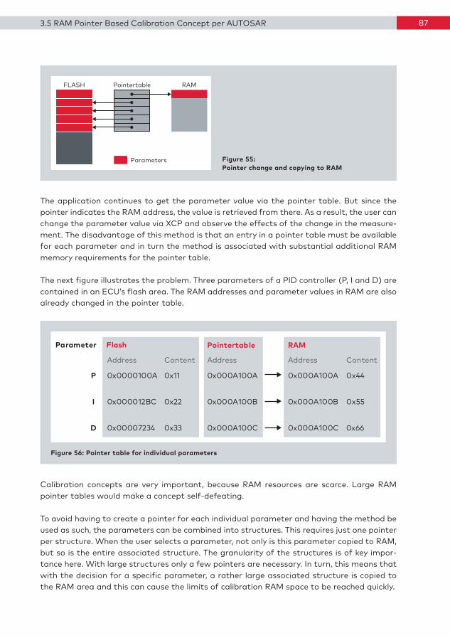
873.5 RAM Pointer Based Calibration Concept per AUTOSAR
FLASH RAMPointertable
Parameters Figure 55: Pointer change and copying to RAM
The application continues to get the parameter value via the pointer table. But since the pointer indicates the RAM address, the value is retrieved from there. As a result, the user can change the parameter value via XCP and observe the effects of the change in the measurement. The disadvantage of this method is that an entry in a pointer table must be available for each parameter and in turn the method is associated with substantial additional RAM memory requirements for the pointer table.
The next figure illustrates the problem. Three parameters of a PID controller (P, I and D) are contained in an ECU’s flash area. The RAM addresses and parameter values in RAM are also already changed in the pointer table.
Figure 56: Pointer table for individual parameters
Flash
0x11
0x22
0x33
0x0000100A
0x000012BC
0x00007234
Parameter
P
I
D
Pointertable
0x000A100A
0x000A100B
0x000A100C
RAM
0x44
0x55
0x66
0x000A100A
0x000A100B
0x000A100C
Address Address AddressContent Content
Calibration concepts are very important, because RAM resources are scarce. Large RAM pointer tables would make a concept selfdefeating.
To avoid having to create a pointer for each individual parameter and having the method be used as such, the parameters can be combined into structures. This requires just one pointer per structure. When the user selects a parameter, not only is this parameter copied to RAM, but so is the entire associated structure. The granularity of the structures is of key importance here. With large structures only a few pointers are necessary. In turn, this means that with the decision for a specific parameter, a rather large associated structure is copied to the RAM area and this can cause the limits of calibration RAM space to be reached quickly.
88 3 Calibration Concepts
Example: The calibration RAM should be 400 bytes in size. Four structures are defined in the software with the following parameters:
Structure A: 250 bytesStructure B: 180 bytesStructure C: 120 bytesStructure D: 100 bytes
When the user selects a parameter from structure A, the 250 bytes are copied from flash to the calibration RAM, and the user has XCP access to all parameters located in structure A. If the calibration task is limited to the parameters of this structure, the calibration RAM is fully sufficient. However, if the user selects another parameter located in a different structure, e.g. structure C, these 120 bytes must also be copied to the calibration RAM. Since the calibration RAM can handle 400 bytes, the user can access all parameters of structures A and C simultaneously.
If another selected parameter is not located in structure C, but rather in structure B, the 180 bytes of structure B would have to be copied to RAM in addition to the 250 bytes of structure A. However, since the space in RAM is inadequate for this, the user indeed has access to the parameters of structure A, but not to the data of structure B, because the ECU cannot execute the copy command.
You can learn more about how this approach works in CANape. Start CANape with the “AUTOSAR Single Pointered Demo” project. You will find more information on its use in CANape on the “Introduction” page of the project.
You will find a source code example under the “Demos” category at the Vector Download Center. A code example on how to use the calibration concept is contained in the “XCP Sample Implementation” under <Installation DIR>\Samples\CAN\CAN MPC55xx\XCPDemo.
3.5.2 Double Pointer Concept
A disadvantage of the single pointer concept is that memory page switching is not easy to implement. The calibration tool could simply describe the pointer table completely for page swapping, but this is not feasible in a short period of time without resulting in temporary inconsistencies and side effects. A tooltransparent implementation would double the memory space requirement for the pointer table, because when switching the memory page into flash, a copy of the previous pointer table would have to be created with RAM pointers.
For applications with large pointer tables, a transparent implementation or a fully consistent switching, there is the option of extending the method to a double pointer concept. To explain how this is done, we return once again to the initial RAM setting.

893.5 RAM Pointer Based Calibration Concept per AUTOSAR
Figure 57 represents the pointer table. It lies in RAM. As already mentioned, this table must be copied from flash into RAM. As a result, this table lies in flash memory. If another pointer is now used (a table pointer), which points to either the pointer table in RAM or in flash, one arrives at a double pointer solution.
FLASH RAMRAM
Pointertable
Tablepointer
FLASHPointertable
Figure 57: Double pointer concept
The parameter values are initially accessed via the table pointer. If the table pointer indicates the pointer table in RAM, the application essentially accesses the actual parameters via the contents of the RAM pointer table. The low access speed and the creation of more program code are disadvantages of this solution.
3.6 Flash Pointer Based Calibration Concept
This method was patented several years ago by the company ZF Friedrichshafen under the name “InCircuit2” and bears a strong resemblance to the pointerbased concept of AUTOSAR. Here too, the application in the ECU accesses parameter data using a pointer table. However, this pointer table is not located in RAM, but in flash instead. Changes to the pointer table can therefore only be made by flash programming. A tooltransparent implementation is not possible. The advantage lies in the RAM memory that is saved since it no longer contains the pointer table.
You can find out how this approach works in CANape. Start CANape with the “InCircuit2” project. You will find more information on its use in CANape on the “Introduction” page of the project.

914 Application Areas of XCP
4 Application Areas of XCP

92 4 Application Areas of XCP
When ECU calibrators think about the use of XCP, they are usually fixated on use of the protocol in the ECU.
Figure 58: Application areas and application cases
Slave
Slave
Slave
Slave
Slave
PC
Measurement/Calibration Hardware*
* Debug Interfaces, Memory Emulator ...
HIL/SIL Systems
EXE/DLL
Prototype orECU Hardware
Simulink
MasterXCP
In a survey of development processes, one encounters many different solution approaches for the development of electronics and software. HIL (Hardware in the Loop), SIL (Software in the Loop) and Rapid Prototyping are keywords here and they describe different scenarios. They always have a “plant” and a “controller” in common.
Figure 59: Plants and controllers
OffsetManipulated
VariableDisturbance
Variable
Controlled Variable(Actual Value)
Reference Variable(Set Value)
Controller Plant
In the context of automotive development, the controller is represented by the ECU and the plant is the physical system to be controlled such as the transmission, engine, side mirrors, etc.
The rough subdivision is made between different development approaches according to whether the controller or the plant runs in real or simulated mode. Some combinations will be described in greater detail.
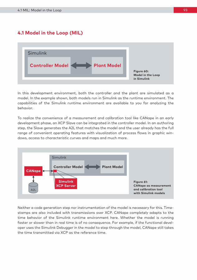
934.1 MIL: Model in the Loop
4.1 Model in the Loop (MIL)
Plant ModelController Model
Simulink
Figure 60: Model in the Loop in Simulink
In this development environment, both the controller and the plant are simulated as a model. In the example shown, both models run in Simulink as the runtime environment. The capabilities of the Simulink runtime environment are available to you for analyzing the behavior.
To realize the convenience of a measurement and calibration tool like CANape in an early development phase, an XCP Slave can be integrated in the controller model. In an authoring step, the Slave generates the A2L that matches the model and the user already has the full range of convenient operating features with visualization of process flows in graphic windows, access to characteristic curves and maps and much more.
Plant ModelController Model
Simulink
SimulinkXCP Server
CANape
A2L
Figure 61: CANape as measurement and calibration tool with Simulink models
Neither a code generation step nor instrumentation of the model is necessary for this. Timestamps are also included with transmissions over XCP. CANape completely adapts to the time behavior of the Simulink runtime environment here. Whether the model is running faster or slower than in real time is of no consequence. For example, if the functional developer uses the Simulink Debugger in the model to step through the model, CANape still takes the time transmitted via XCP as the reference time.

94 4 Application Areas of XCP
4.2 Software in the Loop (SIL)
Plant ModelController Model
Controller ModelWindows DLL
Simulink
Code Generation
Figure 62: Software in the Loop with Simulink environment
In this development step, code is generated from the model of the controller, which is then used in a PCbased runtime environment. Naturally, the controller may also have been developed without any sort of modelbased approach. The plant continues to be simulated. XCP can be used to measure and calibrate the controller. If the controller originates from a Simulink model, a code generation step (Simulink Coder with the target “CANape”) is used to generate the C code for a DLL and the associated A2L. If the Controller development is conducted based on manually written code, it is embedded in a C++ project that is delivered with CANape.
After compiling and linking, the DLL is used in the CANape context. With the support of the XCP connection, the algorithms in the DLL can be measured and calibrated exactly as if the application were already integrated in an ECU.
A2L
Plant ModelController Model
Controller ModelWindows DLL
Simulink
Code generation
CANapeFigure 63: CANape as SIL development platform

954.3 HIL: Hardware in the Loop
4.3 Hardware in the Loop (HIL)
Many different kinds of HIL systems are available. They range from very simple, costeffective systems all the way to very large and expensive expansion stages. The following figure shows the rough concept:
Plant Model
HIL Platform
ECU
I/O
Controller Model
Figure 64: HIL solution
The controller algorithm runs in a microcontroller platform (e.g. the ECU), while the plant continues to be simulated. Depending on the parameters and the complexity of the plant and the necessary I/O, requirements of the HIL platform and the associated costs can rise steeply. Since the ECU runs in real time, the model of the plant must also be computed in real time.
To now introduce XCP for optimization appears trivial, because another ECU is being added. The whole system looks like this:
ECU
I/OCANapePlant Model
HIL Platform
Controller ModelA2L
Figure 65: HIL with CANape as measurement and calibration tool
From CANape, the user has access to the algorithms in the ECU over XCP.

96
The Vector Tool CANoe is also used by many customers as a HIL system. With CANoe, a HIL system might look like this:
CANoe RT User PC
EthernetCANoe RT Server
Digital I/O Analog I/O
CAN
LIN
MOST
FlexRay
ECU
Plant Model
CANapeXCP
A2L
Figure 66: CANoe as HIL system
The ability to access XCP data directly from CANoe for testing purposes results in the following variant as well:
CANoe RT User PC
EthernetCANoe RT Server
Digital I/O Analog I/O
CAN
LIN
MOST
FlexRay
ECU
XCPPlant Model
A2L
Figure 67: CANoe as HIL system with XCP access to the ECU
Here the model of the plant runs on the CANoe realtime server. At the same time, XCP access to the ECU is also realized from CANoe. This gives a tool simultaneous access to the plant and the controller.
4 Application Areas of XCP

974.3 HIL: Hardware in the Loop
To round out the picture, yet another HIL solution option should be mentioned. The plant might also run as a DLL in CANape. This gives the user full access to the plant and to the controller over XCP.
Figure 68: CANape as HIL solution
ECU
ECU
PlantXCP
Plant ModelWindows DLL
CANape
XCP
A2L
A2L
4.4 Rapid Control Prototyping (RCP)
In this development phase, the control algorithm runs on realtime hardware instead of an ECU. This situation often occurs when the necessary ECU hardware is not yet available. Several platforms come in question as suitable hardware: from simple evaluation boards all the way to special automotivelevel hardware solutions, depending on which additional requirements need to be fulfilled. Here too, integration with XCP helps in setting up an OEMindependent tool chain.
Figure 69: Solution for Rapid Control Prototyping
XCP I/OEVA BoardCANape
Controller Model
Plant
A2L
The concepts “Rapid” and “Prototyping” describe the task very well. The aim is to develop a functional prototype as quickly as possible, to use and test it in the runtime environment. This just requires simple work steps throughout the entire process.

98
In the literature, the RCP approach is frequently subdivided into two areas: fullpassing and bypassing.
As depicted in Figure 69, the entire controller runs on separate realtime hardware. This method is known as fullpassing, because the entire controller runs on the controller hardware. It must have the necessary I/O to be able to interface with the plant. Very often, it is only possible to fulfill technical requirements for the I/O with suitable power electronics.
It is not only the I/O that represents a challenge; often functional elements of the ECU software (e.g. network management) are needed to enable functionality in a more complex network. However, if a complete ECU is used for Rapid Control Prototyping instead of a general controller platform, the complexity of the flash process, the size of the overall software, etc. all work against the requirement for “rapid” development.
In summary: the use of an entire ECU as the runtime environment for the controller offers the advantage that the necessary hardware and software infrastructure for the plant exists. The disadvantage lies in the high degree of complexity. The concept of bypassing was developed to exploit the advantages of the ECU infrastructure without being burdened by the disadvantages of high complexity.
4.5 Bypassing
When bypassing occurs, data is recorded from the ECU and processed outside the ECU, and the result is written back to the ECU. As both measurement and writing to the ECU must occur in sync with the ECU processes, DAQ and STIM mechanisms are used. At least two DAQ lists are required, one with the DAQ direction (from Slave to Master) and one with the STIM direction (from Master to Slave).
In Figure 70, the ECU is connected to the plant. The necessary I/O and software components are available in the ECU. In the bypassing hardware, an algorithm A1 runs, which occurs in Version A of the ECU. A1 is a new variant of the algorithm and should now be tried out on the real plant.
4 Application Areas of XCP

994.5 Bypassing
Figure 70: Basic principle of bypassing
I/O
XCP
ECU
Bypassing Hardware
BypassingHardware
CANapeECU
Plant
XCP
A2L
A2L
Controller Model
The bypassing hardware (a VN8900 device in the figure) and the ECU are interconnected over XCP. One goal here is to get the data needed for algorithm A1 from the ECU by DAQ; another goal is to stimulate the results of A1 back into the ECU. The following figure illustrates the schematic flow:
2.
3.
Bypassing Hardware
ECU
Algorithm A’
Algorithm A
1. XCP 4.
BypassingCoordinator
Figure 71: Bypassing flow
Depicted in the ECU is a blue function block in which the algorithm A runs. To ensure that A1 can now be used, the data enters algorithm A as an input variable and it is measured from the ECU by DAQ.
Step 1: In the ECU, the data is recorded and sent to the bypassing tool before the original function is calculated in the ECU. Normally, the input data in functions A and A1 is are identical. Step 2: The data transferred via DAQ is now transferred to algorithm A1.Step 3: The results of the calculation of algorithm A1 are transferred to the bypassing tool. Step 4: The data is transferred into the ECU via STIM. The ECU calculates algorithm A during this time. If the stimulated results are available and calculation of algorithm A is com

100 4 Application Areas of XCP
plete, the values calculated in the ECU are typically overwritten by the stimulated values of algorithm A1.
This makes it possible to use the value computed by algorithm A1 and not from A in the ECU’s overall control process. This method permits using a combination of the rapid substitution of algorithms on the bypassing hardware that incorporates the I/O and the ECU’s basic software.
Of course, performance limits of the transport protocol also affect bypassing. If short bypassing times are needed, access to the ECU by DAQ and STIM may also be performed via the controller’s debugging or trace interfaces. The Vector VX1000 measurement and calibration hardware converts the data into an XCPonEthernet data stream from the controller interface. In this process, up to one megabyte of data can be transported into the ECU.
Plant
XCP
ECU
Bypassing HardwareCANape
Controller ModelI/O
XCP
Debugging and Trace Interface
Measurement & CalibrationHardware VX1000
BypassingHardware A2L
Figure 72: Bypassing with real-time bypassing hardware and fast ECU access
In the figure, ECU access occurs via XCP on Ethernet, and calculation of the bypass algorithm occurs on separate bypassing hardware (VN8900 network interface) with a realtime operating system. This means that the variance of the calculation time is considerably smaller than with calculation on a laptop, as the processing time is not affected by other applications.

1014.6 Shortening Iteration Cycles with Virtual ECUs
4.6 Shortening Iteration Cycles with Virtual ECUs
Stimulation with data is necessary to optimize the algorithm in the ECU with the help of XCP. This can be done in the ECU in the framework of test drives. But there is yet another solution that is available with XCP, in which the algorithm does not run on an ECU; rather it runs on the PC in the form of executable code or as a model in Simulink in the form of a “virtual ECU.” This virtual ECU does not need to run in real time, because in this case no connection to a real system exists. It can run significantly faster – depending on the PC’s computing power.
The algorithm is stimulated by a previously logged measurement file, which contains all signals that are needed as input signals for the algorithm. The connection to CANape is set up over XCP. The user can perform the parameterization and measurement configuration. Afterwards, execution is started. Here the data from the test drive is fed into the algorithm as stimulation and the desired measurement parameters from the application are simultaneously measured out and saved to a measurement file.
NewMDF
Application
Para-meter
MDFtest drive
CANape
1. Set parameters
2. Start
3. Send test drive data
4. Measurement data
5. Analyze
Simulink/DLL
Slave
Figure 73: Short calibration cycles with virtual ECUs

102 4 Application Areas of XCP
After the calculation has been completed, a new measurement file is available to the user for analysis of ECU behavior. The length of time of the new measurement file precisely matches the length of the input measurement file. If the duration of a test drive is one hour, the algorithm on the PC might calculate the entire test drive in just a few seconds. Then a measurement result exists, which corresponds to a test of one hour duration. Based on the data analysis, the user makes decisions about parameterization and the iteration cycle is repeated.
Parameterizationvia XCP
Start
New software version
CANape Application as EXE or DLL on PC
Set values inworkspace
Start
Calculate model
End model calculation
Send measurement values from the model
Receive newmeasurement data
Analyze thenew data
Send measurementdata
Figure 74: Process flow with virtual ECUs
To shorten the iteration cycles, the algorithm is always stimulated with the same data. That makes the results with different parameters much more comparable, because the results are only influenced by the parameters that differ.
This process can of course be automated. The integrated script language of CANape performs an analysis of the measurement results, from which parameter calibration settings are derived and automatically executed. It is also possible to have the process controlled by an external optimization tool such as MATLAB over the CANape automation interface.

1055 Example of an XCP Implementation
5 Example of an XCP Implementation

106 5 Example of an XCP Implementation
To make it possible for an ECU to communicate over XCP, it is necessary to integrate an XCP driver in the ECU’s application. The example described below is of the XCP driver which you can download free of charge at the Download Center of the Vector website (www.vector.com/xcpdriver). This packet also contains some sample implementations for various transport layers and target platforms. The driver consists of the protocolLayer with the basic functionality needed for measurement and calibration. It does not include features such as Cold Start Measurement, Stimulation or flashing. You can purchase a full implementation as a product that is integrated in the Vector CANbedded or AUTOSAR environment.
The XCP protocol layer is placed over the XCP transport layer, which in turn is based on the actual bus communication. The implementation of the XCP protocol layer only consists of a single C file and a few H files (xcpBasix.c, xcpBasic.h, xcp_def.h and xcp_cfg.h). The examples include implementations for various transport layers, e.g. Ethernet and RS232. In the case of CAN, the transport layer is normally very simple and the various XCP message types are mapped directly to CAN messages. There are then separate fixed identifiers for the Tx and Rx directions.
The software interface between the transport and protocol layers is very simple. It contains just a few functions:> When the Slave receives an XCP message over the bus, it first arrives in the communica
tion driver, which routes the message to the XCP transport layer. The transport layer informs the protocol layer about the message with the function call XcpCommand().
> If the XCP protocol layer wishes to send a message (e.g. a response to an XCP command from the Master or a DAQ message), the message is routed to the transport layer by a call of the ApplXcpSend() function.
> The transport layer informs the protocol layer that the message was successfully sent by the function call XcpSendCallBack().
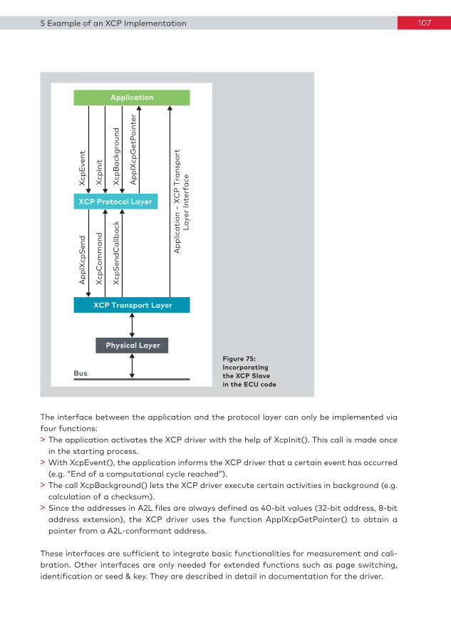
1075 Example of an XCP Implementation
Application
XCP Protocol Layer
XCP Transport Layer
Physical Layer
Bus
Xcp
Eve
nt
Xcp
Init
Xcp
Bac
kgro
und
App
lXcp
Get
Poin
ter
Xcp
Com
man
d
App
lXcp
Send
Xcp
Send
Cal
lbac
k
App
licat
ion
– X
CP
Tran
spor
tLa
yer
Inte
rfac
e
Figure 75: Incorporating the XCP Slave in the ECU code
The interface between the application and the protocol layer can only be implemented via four functions:> The application activates the XCP driver with the help of XcpInit(). This call is made once
in the starting process.> With XcpEvent(), the application informs the XCP driver that a certain event has occurred
(e.g. “End of a computational cycle reached”).> The call XcpBackground() lets the XCP driver execute certain activities in background (e.g.
calculation of a checksum).> Since the addresses in A2L files are always defined as 40bit values (32bit address, 8bit
address extension), the XCP driver uses the function ApplXcpGetPointer() to obtain a pointer from a A2Lconformant address.
These interfaces are sufficient to integrate basic functionalities for measurement and calibration. Other interfaces are only needed for extended functions such as page switching, identification or seed & key. They are described in detail in documentation for the driver.
108 5 Example of an XCP Implementation
5.1 Description of Functions
void XcpInit (void)
Task: Initialize the XCP driver.
Description: The application activates the XCP driver with XcpInit(). This command must be executed exactly once before any sort of XCP driver function may be called.
void XcpEvent (BYTE event)
Task:The application informs the XCP driver about which event occurred. A unique event number is assigned to each event here.
Description:In setting up the measurement configuration in the measurement and calibration tool, the user selects which measured values should be synchronously acquired with which events. The information on measured values and events originates from the A2L. The desired measurement configuration is communicated to the XCP driver in the form of DAQ lists.
Example of an event definition in an engine controller:XcpEvent (1); // Event 1 stands for the 10ms taskXcpEvent (2); // Event 2 stands for the 100ms taskXcpEvent (5); // Event 5 stands for the 1ms taskXcpEvent (8); // Event 8 is used for ignition angle synchronous measurements
BYTE XcpBackground (void)
Task:Execute background activities of the XCP driver.
Description:This function should be called periodically in a background or idle task. It is used by the XCP driver, for example, to compute the checksum, because the computation of a longer checksum in XcpCommand() could take an unacceptably long time. With each call of XcpBackground(), a partial checksum of 256 bytes is computed. The duration of a checksum computation therefore depends on the call frequency of XcpBackground(). There are no other requirements for the call frequency or periodicity. The return value 1 indicates that a checksum computation is currently running.

1095.1 Description of Functions
void XcpCommand (DWORD* pCommand)
Task:Interpret an XCP command.
Description:This function must be called each time the transport layer receives a XCP frame. The parameter is a pointer to the frame.
void ApplXcpSend (BYTE len, BYTE *msg)
Task:Transfer a frame to be sent to the transport layer.
Description:With this call, the protocol layer sends a message to the transport layer for transmission to the Master. The call XcpSendCallBack implements a handshake method between the protocol and transport layers.
BYTE XcpSendCallBack (void)
Task:The protocol layer uses this callback to inform the transport layer that the last message that was transferred to ApplXcpSend() was successfully transmitted.
Description:The protocol layer does not call an ApplXcpSend() command until XcpSendCallBack() indicates that the prior message was successfully transmitted. XcpSendCallBack() returns the value 0 (FALSE) if the XCP driver is in idle. If there are more frames to be sent, ApplXcpSend() is called directly from XcpSendCallBack().
BYTE *ApplXcpGetPointer (BYTE addr_ext, DWORD addr)
Task:Convert an A2Lconformant address to a pointer.
Description:The function maps the 40bit A2Lconformant addressing (32bit address + 8bit address extension) that is sent by the XCP Master to a valid pointer. The address extension can be used, for example, to distinguish different address areas or memory types.

110 5 Example of an XCP Implementation
5.2 Parameterization of the Driver
In many respects, the XCP driver is scalable and parameterizable to properly handle the wide variety of functional content, transport protocols and target platforms. All settings are made in the parameter file xcp_cfg.h. In the simplest case, they appear as follows:
/* Define protocol parameters */#define kXcpMaxCTO 8 /* Maximum CTO Message Length */#define kXcpMaxDTO 8 /* Maximum DTO Message Length */#define C_CPUTYPE_BIGENDIAN /* byte order Motorola */
/* Enable memory checksum */#define XCP_ENABLE_CHECKSUM#define kXcpChecksumMethod XCP_CHECKSUM_TYPE_ADD14
/* Enable calibration */#define XCP_ENABLE_CALIBRATION#define XCP_ENABLE_SHORT_UPLOAD
/* Enable data acquisition */#define XCP_ENABLE_DAQ #define kXcpDaqMemSize (512) /* Memory space reserved for DAQ */#define XCP_ENABLE_SEND_QUEUE
For a CAN transport layer, the appropriate CTO and DTO parameters of eight bytes are set. The driver must know whether it is running on a platform with Motorola or Intel byte order, in this case a MotorolaCPU (Big Endian). The remaining parameters activate the functionalities: measurement, calibration and checksum computation. The algorithm for checksum computation is configured (here summing of all bytes into a DWORD) and the parameter of the available memory is indicated for the measurement (here 512 bytes). The memory is primarily needed to store the DAQ lists and to buffer the data during the measurement. The parameter therefore determines the maximum possible number of measurement signals. In the driver documentation you will find more detailed information on estimating the necessary parameters.

1116 Protocol Development Overview
6 Protocol Development Overview

112 6 Protocol Development Overview
The following overview shows some of the essential developments of the XCP protocol, which was standardized in 2003.
6.1. XCP Version 1.1 (2008)
> Description of the same XCP interface using two different physical interfaces within the same A2L (e.g. “XCP on Vehicle CAN” and “XCP on Calibration CAN”)
> The new command WRITE_DAQ_MULTIPLE makes it possible to accelerate configuration of the Slave. Two ODTs appearing in succession in a DAQ list can be communicated in a single step.
> High time synchronization via “TIMESTAMP_EVENT.” Timestamp information is communicated by the Slave. The trigger can be initiated via an external synchronization cable.
> Compression of embedded A2L files
All expansions are optional. XCP 1.1 is thus compatible with XCP 1.0.
6.2. XCP Version 1.2 (2013)
> Parameters in the A2L for the definition of the required ECU resources via XCPDAQ measurement configurations (e.g. RAM usage, CPU execution time and required transfer bandwidth for CAN or Ethernet). The XCP Master can access the parameters, calculate resource usage for the measurement and warn the user if overshooting occurs.
> Prioritization control by the Master for transfer of the measurement data via CAN. The objective here is to not disturb the necessary communication flow of the vehicle CAN to the greatest degree possible.
> Calculation of the required bandwidth and limits for the transfer of data via TCP or UDP> Description of XCP on CAN FD
All expansions are optional. XCP 1.2 is thus compatible with XCP 1.1.

1136.3. XCP Version 1.3 (2015)
6.3. XCP Version 1.3 (2015)
> Improvement of the time correlation of XCP Slaves using multicast solutions found on the same network
> Time synchronization between XCP Slave timestamp and external clock, e.g. via IEEE 1588> Checking of the bypassing data flow and error handling
All expansions are optional. XCP 1.3 is thus compatible with XCP 1.2.

114 The Authors
Andreas Patzer
Mr. Patzer graduated in Electrical Engineering from the Technical University of Karlsruhe. In his studies he specialized in measurement and control engineering and information and industrial engineering. In 2003, he joined Vector Informatik GmbH in Stuttgart. Andreas Patzer has supported XCP projects from the very start, since XCP was standardized by ASAM e.V. in the same year he was hired.He currently manages the Customer Relations and Services area as a team leader for the Measurement & Calibration product line.
The Authors

115The Authors
Rainer Zaiser
Mr. Zaiser has a degree in Electrical Engineering from the University of Stuttgart. After graduating, he came directly to Vector Informatik GmbH in autumn 1988, where he has helped to create many of the standards that have become established in the automotive industry such as DBC, MDF, CCP, A2L and to a large extent XCP. From the start, he headed up the Measurement & Calibration and Network Interfaces product lines.

116
Table of Abbreviations and Acronyms
A2L File extension for an ASAM 2MC language fileAML ASAM 2 Meta LanguageASAM Association for Standardisation of Automation and Measuring SystemsBYP BypassingCAL CalibrationCAN Controller Area NetworkCCP CAN Calibration ProtocolCMD CommandCS ChecksumCTO Command Transfer ObjectCTR CounterDAQ Data Acquisition, Data Acquisition PacketDTO Data Transfer ObjectECU Electronic Control UnitERR Error PacketEV Event PacketFIBEX Field Bus Exchange Format LEN LengthMCD Measurement Calibration and DiagnosticsMTA Memory Transfer AddressODT Object Descriptor TablePAG PagingPGM ProgrammingPHY Physical Layer respectively description of the chip connecting a link layer
device to a physical medium, for example Ethernet PHY PID Packet IdentifierPTP Precision Time Protocol RES Command Response PacketSERV Service Request PacketSPI Serial Peripheral InterfaceSTD StandardSTIM Data Stimulation PacketTCP/IP Transfer Control Protocol / Internet ProtocolTS TimestampUDP/IP Unified Data Protocol / Internet ProtocolUSB Universal Serial BusXCP Universal Measurement and Calibration Protocol
Download Sending of data from Master to Slave Upload Sending of data from Slave to Master
Table of Abbreviations and Acronyms

117Literature & Web Addresses
Literature
XCP is specified by ASAM (Association for Standardisation of Automation and Measuring Systems). You will find details on the protocol and on ASAM at: www.asam.net
Web Addresses
Standardization committees:> ASAM, XCP protocolspecific documents, A2L specification, www.asam.net
Supplier of development software:> MathWorks, information on MATLAB, Simulink and Simulink Coder, www.mathworks.com > Vector Informatik GmbH, demo version of CANape, free of charge and openly available
XCP driver (basic version), comprehensive information on the topics of ECU calibration, testing and simulation, www.vector.com

118 Table of Figures
Table of Figures
Figure 1: Fundamental communication with a runtime environment ..........................................8Figure 2: The Interface Model of ASAM............................................................................................... 9Figure 3: An XCP Master can simultaneously communicate with multiple Slaves ..................10Figure 4: Subdivision of the XCP protocol into protocol layer and transport layer ................14Figure 5: XCP Slaves can be used in many different runtime environments ............................15Figure 6: XCP packet ..............................................................................................................................19Figure 7: Overview of XCP Packet Identifier (PID) .........................................................................19Figure 8: XCP communication model with CTO/DTO ....................................................................20Figure 9: Message identification .........................................................................................................21Figure 10: Timestamp ............................................................................................................................21Figure 11: Data field in the XCP packet ............................................................................................22Figure 12: The three modes of the XCP protocol: Standard, Block and Interleaved mode ...24Figure 13: Overview of the CTO packet structure ..........................................................................25Figure 14: Trace example from a calibration process .....................................................................30Figure 15: Transfer of a parameter set file to an ECU’s RAM .....................................................31Figure 16: Hex window ..........................................................................................................................32Figure 17: Address information of the parameter “Triangle” from the A2L file ......................33Figure 18: Polling communication in the CANape Trace window ................................................34Figure 19: Events in the ECU ...............................................................................................................35Figure 20: Event definition in an A2L .................................................................................................35Figure 21: Allocation of “Triangle” to possible events in the A2L ................................................36Figure 22: Selecting events (measurement mode) for each measurement parameter .........36Figure 23: Excerpt from the CANape Trace window of a DAQ measurement .........................37Figure 24: ODT: Allocation of RAM addresses to DAQ DTO .........................................................38Figure 25: DAQ list with three ODTs ..................................................................................................39Figure 26: Static DAQ lists ...................................................................................................................40Figure 27: Dynamic DAQ lists ..............................................................................................................41Figure 28: Event for DAQ and STIM ...................................................................................................42Figure 29: Structure of the XCP packet for DTO transmissions..................................................43Figure 30: Identification field with absolute ODT numbers ..........................................................44Figure 31: ID field with relative ODT and absolute DAQ numbers (one byte) .........................44Figure 32: ID field with relative ODT and absolute DAQ numbers (two bytes) ......................44Figure 33: ID field with relative ODT and absolute DAQ numbers as well as fill byte
(total of four bytes) ............................................................................................................45Figure 34: XCP Slave with freerunning clock .................................................................................46Figure 35: The clock of the XCP Slave is synchronized with the grandmaster clock .............47Figure 36: Definition of which bus nodes send which messages .................................................49Figure 37: Representation of a CAN network ..................................................................................50Figure 38: Example of XCPonCAN communication .....................................................................51Figure 39: Representation of an XCPonCAN message ...............................................................51Figure 40: Illustration of a CAN FD frame ........................................................................................52Figure 41: Nodes K and L are redundantly interconnected ...........................................................54Figure 42: Communication by slot definition ...................................................................................54Figure 43: Representation of a FlexRay communication matrix..................................................55Figure 44: Representation of the FlexRay LPDUs ...........................................................................56

119Table of Figures
Figure 45: Allocation of XCP communication to LPDUs ................................................................57Figure 46: XCP packet with TCP/IP or UDP/IP ................................................................................58Figure 47: XCPonSxI packet ..............................................................................................................59Figure 48: Memory representation .....................................................................................................61Figure 49: Representation of driver settings for the flash area ..................................................63Figure 50: Representation of the block transfer mode ..................................................................66Figure 51: Parameters in a calibration window ...............................................................................72Figure 52: Signal response over time .................................................................................................72Figure 53: Initial parameter setting in RAM .....................................................................................82Figure 54: Initial situation after booting ...........................................................................................86Figure 55: Pointer change and copying to RAM ..............................................................................87Figure 56: Pointer table for individual parameters .........................................................................87Figure 57: Double pointer concept ......................................................................................................89Figure 58: Application areas and application cases .......................................................................92Figure 59: Plants and controllers ........................................................................................................92Figure 60: Model in the Loop in Simulink ..........................................................................................93Figure 61: CANape as measurement and calibration tool with Simulink models ...................93Figure 62: Software in the Loop with Simulink environment .......................................................94Figure 63: CANape as SIL development platform ..........................................................................94Figure 64: HIL solution ...........................................................................................................................95Figure 65: HIL with CANape as measurement and calibration tool ...........................................95Figure 66: CANoe as HIL system .........................................................................................................96Figure 67: CANoe as HIL system with XCP access to the ECU ...................................................96Figure 68: CANape as HIL solution .....................................................................................................97Figure 69: RCP solution .........................................................................................................................97Figure 70: Basic principle of bypassing ..............................................................................................99Figure 71: Bypassing flow .....................................................................................................................99Figure 72: Bypassing with realtime bypassing hardware and fast ECU access ................. 100Figure 73: Short calibration cycles with virtual ECUs ................................................................. 101Figure 74: Process flow with virtual ECUs ..................................................................................... 102Figure 75: Incorporating the XCP Slave in the ECU code .......................................................... 107

120 Appendix – XCP Solutions at Vector
Appendix – XCP Solutions at Vector
Vector made a significant effort in giving shape to the XCP standard. Its extensive knowhow and vast experience were utilized to provide comprehensive XCP support:
Tools> The primary use area of CANape is in optimal parameterization (calibration) of electronic
control units (ECUs). During the system’s runtime, you calibrate parameter values and simultaneously acquire measured signals. The physical interface between CANape and the ECU is over XCP (for all standardized transport protocols) or CCP.
> Complete tool chain for generating and managing the necessary A2L description files (ASAP2 Tool-Set and CANape with the ASAP2 Editor).
> You use CANoe.XCP to access internal ECU values for testing and analysis tasks.
ECU InterfacesThe VX1000 measurement and calibration hardware offers the option of equipping ECUs with an XCPonEthernet interface. This involves connecting a Plug on Device (POD) to the ECU for direct access to the controller, e.g. over DAP, JTAG, Nexus, etc. The POD transmits the data to a base module, which operates as an XCP Slave and provides the data to the XCP Master on the PC over XCP on Ethernet. This makes it unnecessary to have an XCP Slave in the ECU. The user benefits from a high measurement data throughput rate of up to 50 MByte/s and short measurement intervals of less than 15 µs.
Embedded SoftwareCommunication modules with separate transport layers for CAN, FlexRay and Ethernet:> XCP Basic – free download at www.vector.com/xcpdriver, only contains basic XCP func
tions. Configuration of the XCP protocol and modification of the transport layer are performed manually in the source code. You need to integrate XCP Basic in your project yourself.
> XCP Professional – contains useful extensions to the ASAM specification and enables toolbased configuration. Available for Vector CANbedded basic software.
> MICROSAR XCP – contains the functional features of XCP Professional and is based on AUTOSAR specifications. Available for Vector MICROSAR basic software.
Services> Consultation for using XCP in your projects > Integration of XCP in your ECU
Training> You can learn about the underlying mechanisms and models of the protocol in the “XCP
Fundamentals Seminar”.> In the “CANape with XCP on FlexRay Workshop” you learn about FlexRay fundamentals
and the special aspects of XCP on FlexRay are explained, in particular dynamic bandwidth management.

121Special XCP Support by CANape
Special XCP Support by CANapeCANape was the first MCD tool to support the XCP 1.0 specification and was also the first XCP on FlexRay Master on the market.
A special technical feature of XCP on FlexRay is dynamic bandwidth management. Here, CANape identifies the available bandwidth provided for XCP in the FlexRay ClusterP and it allocates this bandwidth to the momentary application data traffic dynamically and very efficiently. The available bandwidth is thereby optimally used for XCP communication.
Moreover, CANape has a DLL interface. It enables support of XCP on any desired (userdefined) transport layer. This lets you integrate any desired test instrumentation or proprietary protocols in CANape. A code generator supports you in creating the XCPspecific share of such a driver.

122 Index
Index
AA2L 9, 10, 25, 35, 40, 42, 56, 57, 62, 63, 68,
71 – 76, 94, 108, 109, 116Address extension 29, 33, 38, 107, 109AML 25, 74, 116ASAM 7 – 9, 60, 116ASAP2 ToolSet 76
BBandwith optimization 34Bus load 34BYP 116Bypassing 45, 98, 100
CCAN 7, 8, 14, 24, 29, 33, 38, 49, 50, 51, 55,
75, 116CAN FD 52CCP 7, 8, 40, 49, 116CMD 25, 56, 116CTO 21, 22, 25, 116CTR 58, 59, 116CYCLE_REPETITION 56
DDAQ 22, 32 – 45, 65, 67, 77, 99, 100, 106,
108, 116DAQ_KEY_BYTE 45DBC 49Double Pointer Concept 88DOWNLOAD 30, 31, 66DTO 21, 22, 33, 37, 116
EECU 9, 74, 98, 99, 116ECU description file A2L 72 – 77EEPROM 16, 31, 67ERR 25, 28, 116Ethernet 57 – 59EV 29, 116Event 35, 38 – 40, 42,65, 67, 77, 108
FFIBEX 55 – 57Flash memory 16, 17, 61 – 64, 67FLX_CHANNEL 56FLX_LPDU_ID 56FLX_SLOT_ID 56Fullpassing 98
GGET_CAL_PAGE 25, 62GET_DAQ_EVENT_INFO 65, 77GET_DAQ_LIST_INFO 77GET_DAQ_PROCESSOR_INFO 45, 65, 77GET_DAQ_RESOLUTION_INFO 65, 77Grandmaster clock 47, 48
HHIL 92, 95 – 97
IIEEE 1588 47IF_DATA 25
KCommands 25Compile 76, 80, 82, 94
LLinking 80, 94LPDU 56
MMaturity level 31 MIL 93MTA 30, 116Multicast 46, 113
OODT 37 – 41, 43, 44, 65, 77, 116OFFSET 56

123Index
PPAG 116Page 61 – 63Page switching 62, 63Parameter 85PGM 116PID 8, 19, 21, 25, 43, 116Polling 33, 34, 36PTP 47
RRAM 16 – 18, 30, 31, 37, 39, 63, 67, 80, 82,
85, 86, 88Reboot 32RES 21, 28, 56, 116
SSector 61 – 63Segment 61 – 63SEGMENT_NUMBER 62SERV 29, 116SET_CAL_PAGE 25, 62SET_MTA 30SHORT_UPLOAD 30, 33, 66SIL 92, 94Single Pointer Concept 86STIM 33, 42, 43, 45, 65, 77, 100, 116Stimulation 29, 68, 101
TTask 108TCP/IP 57, 58, 116
UUDP/IP 57, 58, 116USB 60, 116
VVirtual ECU 101Volatile 81, 82VX1000 100

V3.
0 |
12/2
016
Get More Information
Visit our Website for:> News> Products> Demo Software> Support> Trainings Classes> Addresses
www.vector.com