1 X‐ray imaging of water motion during capillary imbibition:2 A study on how compaction bands impact fluid flow3 in Bentheim sandstone

4 A. Pons,1 C. David,2 J. Fortin,1 S. Stanchits,3 B. Menéndez,2 and J. M. Mengus4

5 Received 3 September 2010; revised 20 December 2010; accepted 5 January 2011; published XX Month 2011.

6 [1] To investigate the effect of compaction bands (CB) on fluid flow, capillary imbibition7 experiments were performed on Bentheim sandstone specimens (initial porosity ∼22.7%)8 using an industrial X‐ray scanner. We used a three‐step procedure combining (1) X‐ray9 imaging of capillary rise in intact Bentheim sandstone, (2) formation of compaction10 band under triaxial tests, at 185 MPa effective pressure, with acoustic emissions (AE)11 recording for localization of the induced damage, and (3) again X‐ray imaging of capillary12 rise in the damaged specimens after the unloading. The experiments were performed13 on intact cylindrical specimens, 5 cm in diameter and 10.5 cm in length, cored in different14 orientations (parallel or perpendicular to the bedding). Analysis of the images obtained at15 different stages of the capillary imbibition shows that the presence of CB slows down the16 imbibition and disturbs the geometry of water flow. In addition, we show that the CB17 geometry derived from X‐ray density maps analysis is well correlated with the AE location18 obtained during triaxial test. The analysis of the water front kinetics was conducted using a19 simple theoretical model, which allowed us to confirm that compaction bands act as a20 barrier for fluid flow, not fully impermeable though. We estimate a contrast of21 permeability of a factor of ∼3 between the host rock and the compaction bands. This22 estimation of the permeability inside the compaction band is consistent with estimations23 done in similar sandstones from field studies but differs by 1 order of magnitude from24 estimations from previous laboratory measurements.

25 Citation: Pons, A., C. David, J. Fortin, S. Stanchits, B. Menéndez, and J. M. Mengus (2011), X‐ray imaging of water motion26 during capillary imbibition: A study on how compaction bands impact fluid flow in Bentheim sandstone, J. Geophys. Res., 116,27 XXXXXX, doi:10.1029/2010JB007973.

28 1. Introduction

29 [2] In porous sedimentary rocks, strain localization com-30 monly develops along shear bands or compaction bands31 (CB). Whereas shear localization is associated with dilatant32 or compactive volumetric strain [Wong et al., 1997], com-33 paction bands are always associated with a reduction in34 porosity. As a consequence, these two localized modes35 of failure can significantly impact the regional fluid flow36 [Antonellini and Aydin, 1994; Sternlof et al., 2006].37 [3] Compaction bands are thin zones with significant38 reduced porosity that form normal to the most compressive39 stress. Such structures are observed in a wide range of40 high‐porosity sandstones in field [Mollema, 1996; Aydin

41and Ahmadov, 2009; Schultz, 2009] as well in laboratory42experiments [Olsson and Holcomb, 2000; Klein et al., 2001;43Baud et al., 2004; Fortin et al., 2009; Stanchits et al., 2009].44Millimeters thick and centimeters in planar extend in the45laboratory, or centimeters thick and tens of meters in planar46extend in the field, compaction bands always present a drastic47reduction in porosity: only a few percent in the compaction48band compared to the range of 18–25% porosity in the intact49sandstone. As a consequence, such changes in the pore50structure (variations in both pore throat diameter and con-51nectivity are expected) directly affect fluids paths and more52generally the permeability of the sedimentary rock. Indeed,53it has been shown that compaction bands act as a barrier for54the fluid flow. More precisely, Aydin and Ahmadov [2009]55report in the field a contrast of permeability of a factor of56∼5 between the host rock and the compaction bands, whereas57a contrast in a larger range of 20–400 is reported in the lab-58oratory [Vajdova et al., 2004].59[4] In the laboratory, the estimation of the effect of one60compaction band on the rock permeability is not obvious:61indeed, during deformation several compaction bands can62occur; thus, the measured permeability depends one this63complex structure. Then the permeability inside one com-

1École normale supérieure de Paris, Laboratoire de Géologie, UMRCNRS 8538, Paris, France.

2Laboratoire Géosciences et Environnement Cergy, Université deCergy‐Pontoise, Cergy‐Pontoise, France.

3German Research Center for Geosciences, GFZ Potsdam, Potsdam,Germany.

4IFP Énergies Nouvelles, Rueil‐Malmaison, France.

Copyright 2011 by the American Geophysical Union.0148‐0227/11/2010JB007973

JOURNAL OF GEOPHYSICAL RESEARCH, VOL. 116, XXXXXX, doi:10.1029/2010JB007973, 2011

XXXXXX 1 of 14

64 paction band, KCB, should be deduced by taking into65 account the number of localizations measured after loading66 considering that the permeability of the specimen equals the67 permeability of a series of compacted layers (permeability68 KCB) embedded in the intact rock (permeability Kintact)69 [Vajdova et al., 2004; Fortin et al., 2005]. In addition, in70 their estimation, Vajdova et al. [2004] make the assumption71 that all the compaction bands are crosscutting the entire72 specimen, which may be not always the case, as has been73 shown by the localization of the AE [Fortin et al., 2006;74 Stanchits et al., 2009].75 [5] X‐ray imaging can be a useful imaging technique for76 characterizing fluid flow patterns [David et al., 2008]. We77 follow a three steps methodology combining (1) X‐ray78 imaging of capillary rise in intact Bentheim sandstone,79 (2) formation of compaction band under triaxial tests with80 AE recording for localization of the induced damage, and81 (3) again X‐ray imaging of capillary rise in the damaged82 specimens after unloading. Doing so, we intend to address83 the following questions. How compaction bands modify84 flow in a sandstone? What can we learn from capillary rise85 experiments on microstructural changes in a compaction86 band? Can we estimate the change in rock permeability due87 to compaction bands from capillary imbibition kinetics?

88 2. Experimental Details

89 2.1. Rock Specimens

90 [6] A set of three cylindrical notched specimens were91 prepared at the GeoForschungsZentrum (GFZ Potsdam,92 Germany) from a block of Bentheim sandstone (Romberg93 quarry, Northwestern Germany). Bentheim sandstone is a94 Lower Cretaceous, homogeneous, yellow sandstone with a95 porosity, determined by mercury porosimetry, of ∼22.7% for96 this block which is slightly higher than the one used in pre-97 vious studies [David et al., 2008, 2011]. Results of mercury98 porosimetry present a range of pore entry radii between 599 and 25 mm with a peak clearly defined at 13.5 mm. The three100 specimens have a 50 mm diameter and 105 mm length. A101 0.8 mm wide and 5 mm deep circumferential notch has been

102machined in the central part of the specimen (Figure 1). The103purpose of this notch is to guide the development of com-104paction band [Tembe et al., 2006; Stanchits et al., 2009].105Neither polishing nor ultrasonic cleaning was applied. After106cleaning the specimens by flushing water, they were dried in107an oven at 60°C for at least 24 h. Then, to avoid any vari-108ability between the imbibition experiments before and after109mechanical deformation, patches of epoxy were put, at the110location of the piezoelectric transducers, before the first111imbibition experiment. Two specimens were cored parallel112to bedding (specimens Z1 and Z2), and one perpendicular113to bedding (specimen X2). Petrophysical properties and114some relevant attributes for each specimen are provided in115Table 1.

1162.2. Experimental Procedure

117[7] A three‐step procedure was followed [David et al.,1182008]: step 1, the dry intact specimens are placed inside119an X‐ray CT scanner during the capillary imbibition in120order to monitor the water motion inside the rock; step 2, the121specimens are then deformed under a triaxial loading, with122an AE recording, in order to induce compaction bands (CB);123and step 3, a second identical capillary imbibition run is124finally performed on the deformed specimens.

1252.3. Generation of Compaction Bands, Mechanical126Data, and Acoustic Emissions

1272.3.1. Mechanical Data128[8] In this paper we use the convention that compres-129sive stresses and compactive strains are positive. The130terms s1 and s3 represent the maximum and the minimum131principal stresses. The experiments were performed at the132GeoForschungsZentrum (Potsdam, Germany) under a con-133stant axial displacement rate of 20 mm/min (strain rate _" =1342 × 10−4 s−1), using a servohydraulic loading frame from135Material Testing Systems (MTS) with a load capacity of1364600 kN and a maximum confining pressure of 200 MPa.137The axial load was measured with an external load cell138with an accuracy of 1 kN and corrected for seal friction of139the loading piston.140[9] The specimens were saturated with distilled water and141deformed under drained condition at a constant pore pressure,142Pp = 10 MPa. The recording of the pore volume variation143during loading allowed the monitoring of the evolution of144connected pore volume from which volumetric strain can145be deduced. The effective confining pressure, Pc, was146maintained constant for all experiments, at Peff = Pc − Pp =

Figure 1. (a) Geometric configuration of a specimen in atriaxal test and (b) notch geometry.

t1:1Table 1. Properties of Each Specimen

X2 Z1 Z2

t1:2Coring direction witht1:3respect to the bedding

perpendicular parallel parallel

t1:4Porosity (%) 22.7 ± 0.2t1:5Mean graint1:6diameter (mm)

210a

t1:7Composition Quartz(95%) Clay(5%)b

t1:8Peak on Hg porosimetryt1:9spectrum (diametert1:10in mm)

26.2

t1:11Permeability (mdarcy) 900 1100 1100

t1:12aKlein and Reuschlé [2003].t1:13bVan Bareen et al. [1990].

PONS ET AL.: X‐RAY IMAGING OF WATER MOTION XXXXXXXXXXXX

2 of 14

147 185MPa. The notch was filled with a Teflon O ring ∼0.7 mm148 thick to prevent rupture of the Neoprene jacket used to149 separate specimens from the oil confining medium. The150 axial strain, "ax, was measured by a linear variable dis-151 placement transducer (LVDT) mounted at the end of the152 piston and corrected for the effective stiffness of the loading153 frame. In addition, two vertical extensometers (V1 and V2),154 mounted directly on the specimen, measured shortening155 between the upper and the lower halves of the specimen156 (Figure 2a). The monitoring of these mechanical data (stress157 and strain) during experiments allowed us to follow the158 formation of CB.159 2.3.2. Acoustic Emissions160 [10] To monitor the AE activity during loading, 12 pie-161 zoelectric P wave and four piezoelectric S wave sensors162 (PZT, 1 MHz resonant frequency) were glued directly onto163 the surface of the rock and sealed in the jacket with a two‐164 component epoxy (Figure 2). Two additional P wave sen-165 sors were installed in the axial direction (A1 and A2 in166 Figure 2b). The AE signals recording and hypocenter167 localization methodology are described by Stanchits et al.168 [2009]. Hypocenter location is determined with an accuracy169 <2 mm.

170 2.4. Capillary Imbibition Experiments and X‐Ray171 Imaging

172 [11] The capillary imbibition procedure can be described173 as follows: a dry specimen is placed on a stand inside the174 X‐ray CT scanner, such that its bottom surface is at the same175 level as the free surface of water reservoir which is main-176 tained constant during the all experiment by a continuous177 water supply. The scanner used is a GE Hispeed Fxi CT178 Scanner. The X‐ray tube voltage goes up to 140 kV,179 and current to 350 mA. The detector is composed of 816180 channels high‐resolution Hilight solid‐state detector. During181 imbibition, the scanner records one image of the central182 cross section of the specimen every 3 s. This image corre-183 sponds to a density map averaged over a 1 mm thickness184 slice. The lateral resolution of the scanner used is about

185400 mm. As the resolution is about twice the grain size, the186intensity of each pixel of the X‐ray images corresponds to187the average density of a volume including several grains188and pores.189[12] The analysis of the X‐ray images was performed with190ImageJ [Abramoff et al., 2004] and can be explained as191follows: first, a contrast enhancement technique was applied192to the raw images (Figure 3a) in order to improve the193interpretation of the images (Figure 3b). Then, we improved194the image analysis method used by David et al. [2008] in195order to extract a better geometry of the water front at each196time step (Figure 3b). In contrast with the former technique197where the water front geometry is approximated by an arc of198circle, we use here a parabolic fit (Figure 3c). The extraction199method of the water front usually provides 200 points or200more which permits a robust fit of the front by the following201formula at every time step: y(x) = c1 − c2x

2, where x is the202horizontal distance from the center and c1 and c2 are two203constants.204[13] From these curves (Figure 3d), the heights of water205front both in the center and at the vertical borders of the206specimen are estimated as a function of time. We also esti-207mate the local radius of curvature in the center of the speci-208men from the fitting equation.

2093. Results

210[14] In the following, we first present data from capillary211imbibition experiment done on intact specimens, then the212mechanical data obtained in step 2, and finally, the capillary213imbibition data from experiments done on deformed speci-214mens with emphasis on the comparison with the results215obtained in intact specimens.

2163.1. Capillary Imbibition Experiments on Intact217Specimens

2183.1.1. Geometry of the Water Front219[15] The water front during imbibition is not flat but220curved (Figure 3). This geometry can be quantified by the

Figure 2. (a) Picture of the specimen set up and (b) map of the outside surface of the specimen showinglocation of the different PZT.

PONS ET AL.: X‐RAY IMAGING OF WATER MOTION XXXXXXXXXXXX

3 of 14

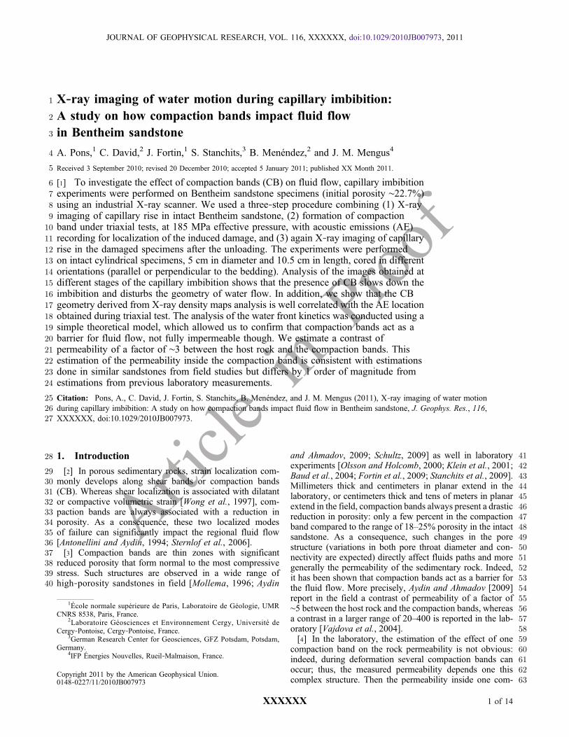
221 radius of curvature of the front in the center of the specimen.222 The magnitude and the evolution of the curvature may differ223 depending on the rock fabric, but a curvature is always224 observed [see David et al., 2011, 2008]. At the beginning of225 the imbibition, the water front is flat (radius of curvature226 greater than radius of the specimen). Then, as the water rise227 occurs, the front becomes more and more curved until the228 radius of curvature reaches a stable value (∼20 mm for X2229 and ∼15 mm for Z1 and Z2).230 3.1.2. Influence of Specimen Diameter231 [16] As said previously, we used specimens with 50 mm232 diameter and 105 mm length. Those specimens are bigger233 than the ones used in previous studies [David et al., 2008,234 2011] which present a 40 mm diameter and 80 mm length.235 This difference of size gave us the opportunity to explore the236 effect of specimen size on the capillary imbibition process237 for intact specimens.238 [17] The number of specimens studied with the corre-239 sponding core direction and diameter are given in Table 2.240 Figure 4 shows the evolution of the heights of the water241 front in the center (H) and at the border (h) as a function of242 the square root of time for all the specimens. At the243 beginning, H and h have a linear evolution as predicted by244 the linear approximation of capillary laws for small imbibed245 height. We observe that at any time and for each specimen246 the height in the center is higher than at the border. This is247 due to the curved shape of the water front. For the specimens248 characterized by a 50 mm diameter, we can see an horizontal249 step in the evolution of h around 50 mm (Figure 4b) which is250 due to the effect of the notch on image analysis (40 mm251 diameter specimens did not have notch).252 [18] Except for the small anisotropy relative to coring253 direction [see David et al., 2011], water rise kinetics in the254 center (Figure 4a) seems similar for all specimens without255 effect of specimen diameter. However, at the border there is256 a marked effect of specimen size (Figure 4b). Indeed, the257 water rise velocity at the border is always higher for small258 specimens (diameter of 40 mm).

2593.2. Mechanical Experiments and CB Localization

2603.2.1. Mechanical Data261[19] Figure 5 represents typical results obtained during a262triaxial experiment on specimen Z1 (parallel to the bedding).263During the loading, different stages can be separated: at the264beginning the specimen has a linear response (elastic stage),265then with progressive loading, the stiffness, i.e., the apparent266Young’s modulus, decreases and the specimen presents an267inelastic response.268[20] Figure 5a represents the differential stress as a func-269tion of the axial deformation derived from the LVDT, and in270the elastic stage, the Young’s modulus for elastic stage can271be calculated (Table 3). If we assume that the total defor-272mation is the sum of the elastic and the inelastic deformation273[Scholz, 1968], we can separate the elastic and the inelastic274strains. Figure 5b shows the inelastic strain derived from the275three strain measurements: the axial strain over the entire276specimen from LVDT mounted on the piston (MTS on277Figure 5), the axial deformation over a central part (60 mm)278of the specimen from the extensometers (extenso on Figure 5),279and the volumetric strain derived from the pore volume280change (volumetric on Figure 5). As shown by Stanchits et al.281[2009] the CB formation coincidewith an increase of inelastic282strain (Figure 5b). For the specimen Z1, the beginning of283the CB formation probably occurs at an axial strain of284∼0.65%. The three inelastic deformations measured by the285three methods, which integrate deformation over different286volumes, are slightly different (Figure 5). However, the dif-287ferences are consistent with the fact that almost all the

Figure 3. Summary of the image analysis procedure. (a) Raw image, (b) extraction of the edge of wetzone, (c) parabolic fit of the water front, and (d) measure of different parameters.

t2:1Table 2. Number of Specimens Studied Depending on Coret2:2Direction and Diameter

Parallel toBedding (Z)

Perpendicular toBedding (X)

t2:340 mm diameter 3 1t2:450 mm diameter 2 1

PONS ET AL.: X‐RAY IMAGING OF WATER MOTION XXXXXXXXXXXX

4 of 14

288 inelastic deformation occurs in the CB: (1) the inelastic axial289 strain seen by the LVDT is lower than the inelastic strain290 seen by the extensometers because they measure shortening291 only between the upper and the lower halves of the specimen292 (Figure 2), whereas the LVDT measures the shortening of all293 the specimen; and (2) the inelastic volumetric strain mea-294 sured from the pore volume variation is lower than the295 inelastic axial strain because of the inelastic radial strain.296 [21] Then, assuming that all the inelastic deformation297 is concentrated in the CB, the porosity reduction in the CB,298 DF can be deduced. In order to calculate this porosity299 reduction, we need to estimate the CB volume, in which300 inelastic deformation occurs.We consider it equals to the notch301 volume (radius r = 25 mm and thickness wnotch = 0.8 mm).302 We also assume that the volumetric strain is nearly equal to303 axial strain, i.e. we neglect the radial strain, an assumption304 which is valid in Bentheim sandstone in the light of the work305 of Stanchits et al. [2009]. Then, from the inelastic defor-306 mation, we deduce the change in volume of the CB during307 the test, which corresponds to the pore volume change308 assuming that the solid volume remains constant. The esti-309 mated porosity reduction for specimen Z1 is represented in310 Figure 5c using the three methods of strain measurement.311 The evolution of the porosity reduction is very similar312 whatever the measurement used and reaches at the end of the313 experiments a value of about 12%.314 [22] The mechanical results for all the specimens (Z1, Z2315 and X2) are represented in Figure 6. In Figure 6, the316 inelastic volumetric strain and the local porosity reduction317 were deduced from the pore volume change which is the318 most accurate method. The porosity reduction at the end of319 loading is about 18% for specimen X2, 12% for specimen320 Z1 and 6% for specimen Z2. The difference between the321 calculated porosity reduction for Z1 and Z2 can be explained322 as follows: in order to calculate the porosity reduction we323 use the mechanical data recorded during loading, but, for the324 specimen Z2 the loading was stopped before CB completion325 in order to have an “annular CB”. However, the AE location

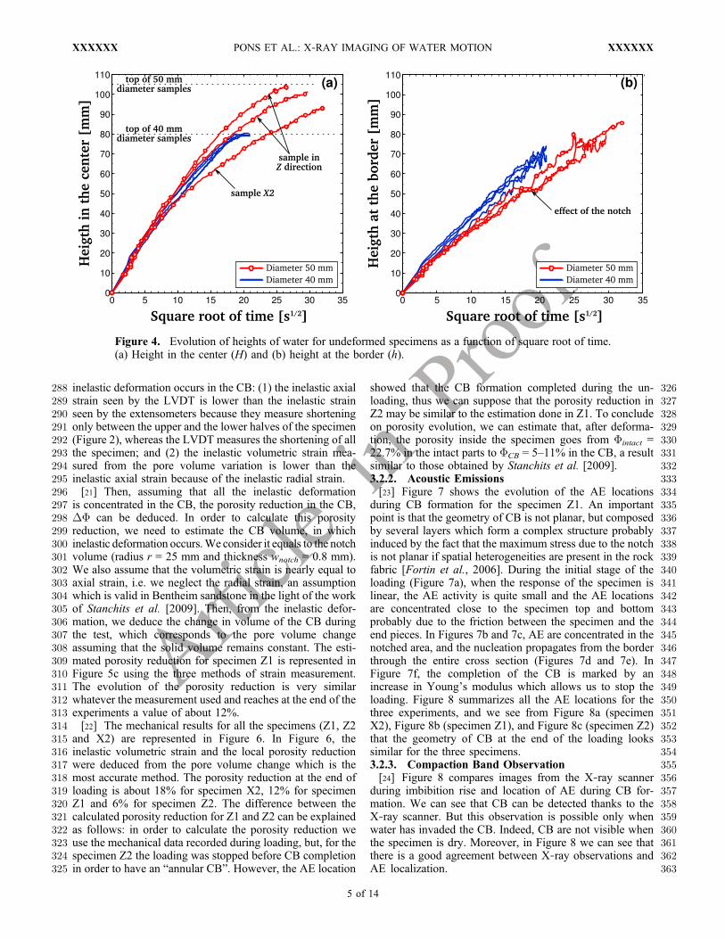
326showed that the CB formation completed during the un-327loading, thus we can suppose that the porosity reduction in328Z2 may be similar to the estimation done in Z1. To conclude329on porosity evolution, we can estimate that, after deforma-330tion, the porosity inside the specimen goes from Fintact =33122.7% in the intact parts to FCB = 5–11% in the CB, a result332similar to those obtained by Stanchits et al. [2009].3333.2.2. Acoustic Emissions334[23] Figure 7 shows the evolution of the AE locations335during CB formation for the specimen Z1. An important336point is that the geometry of CB is not planar, but composed337by several layers which form a complex structure probably338induced by the fact that the maximum stress due to the notch339is not planar if spatial heterogeneities are present in the rock340fabric [Fortin et al., 2006]. During the initial stage of the341loading (Figure 7a), when the response of the specimen is342linear, the AE activity is quite small and the AE locations343are concentrated close to the specimen top and bottom344probably due to the friction between the specimen and the345end pieces. In Figures 7b and 7c, AE are concentrated in the346notched area, and the nucleation propagates from the border347through the entire cross section (Figures 7d and 7e). In348Figure 7f, the completion of the CB is marked by an349increase in Young’s modulus which allows us to stop the350loading. Figure 8 summarizes all the AE locations for the351three experiments, and we see from Figure 8a (specimen352X2), Figure 8b (specimen Z1), and Figure 8c (specimen Z2)353that the geometry of CB at the end of the loading looks354similar for the three specimens.3553.2.3. Compaction Band Observation356[24] Figure 8 compares images from the X‐ray scanner357during imbibition rise and location of AE during CB for-358mation. We can see that CB can be detected thanks to the359X‐ray scanner. But this observation is possible only when360water has invaded the CB. Indeed, CB are not visible when361the specimen is dry. Moreover, in Figure 8 we can see that362there is a good agreement between X‐ray observations and363AE localization.

Figure 4. Evolution of heights of water for undeformed specimens as a function of square root of time.(a) Height in the center (H) and (b) height at the border (h).

PONS ET AL.: X‐RAY IMAGING OF WATER MOTION XXXXXXXXXXXX

5 of 14

364 3.3. Capillary Imbibition Experiments on Specimens365 With Compaction Bands

366 [25] Figure 9 presents all the results of imbibition experi-367 ments for the specimens with a 50 mm diameter, with368 (deformed specimens) and without CB (intact specimens).369 Each row corresponds to a specimen and each column to a370 given parameter. As we focus on the impact of CB, we371 represent in grey the areas which are affected by CB. We372 estimate this volume between heights 45 mm and 60 mm373 from the localizations of AE (Figure 7). All this volume374 does not correspond to a 15 mm thick CB but because of the375 complex structure of the CB, this thickness must be affected376 by the presence of CB. Figures 9a, 9b, and 9c represent the377 height of water in the center (solid line) and at the border

378(dashed line) for intact and deformed (squares and circles)379specimens. We can see that the water rise in the center is380slower in specimens with CB. In addition, in deformed381specimens, the water front slows down significantly in the382center when it reaches the area of the CB, but the rise is also383slower at the bottom of the specimen because of the damage

Figure 5. Mechanical data during loading for specimen Z1. (a) Loading curve and linear fit for thebeginning of the load, (b) inelastic axial and volumetric strain versus axial strain, and (c) local porosityreduction versus axial strain, estimated by three strain measurements assuming that inelastic deformationis only localized in the notch area (radius r = 25 mm and thickness wnotch = 0.8 mm).

t3:1Table 3. Summary of Young’s Modulus Measured During Elastict3:2Stage and Local Porosity

t3:3g X2 Z1 Z2

t3:4Young’s modulus (GPa) 23.8 24.9 25t3:5Porosity reduction at the end oft3:6loading (%)

17 12 6

PONS ET AL.: X‐RAY IMAGING OF WATER MOTION XXXXXXXXXXXX

6 of 14

384 due to piston friction (Figure 7). The water rise at the border385 does not seem to be affected by the presence of CB.386 [26] Consequently, a strong increase in the radius of cur-387 vature is observed when the center of the water front goes388 through the CB zone. This result is visible in Figures 9g, 9h,389 and 9i, which represent the radius of curvature of the390 water front in the center as a function of the square root391 of time. At the beginning of imbibition experiment the392 radius of curvature is larger for deformed specimen than393 for the intact ones. Then, when the water front reaches394 the volume affected by the CB, we observe an increase of395 the radius of curvature which corresponds to a flattening396 of the water front.397 [27] Finally, Figures 9d, 9e, and 9g show the velocity of398 the water front in the center of the specimen as a function of

399the square root of time for intact and deformed (circles)400specimen. To obtain this velocity, we first fit the height of401water versus time using the Washburn model for capillary402rise [Washburn, 1921]. The Washburn model expresses the403time t as a function of the height H reached by the water

front:

t Hð Þ ¼ HeS�

K�g� ln 1� H

He

� �� H

He

� �; ð1Þ

404where He = (2g cos(�))/(rgrpore) is the asymptotic height405reached by capillary imbibition, S is the saturation of the406specimen during imbibition, and K is the permeability.407While H � He = 1.4 m (value obtained for rpore = 13.2 mm

Figure 6. Mechanical data during loading for all specimens. (a) Loading curve and linear fit for thebeginning of the load, (b) inelastic volumetric strain versus axial strain, and (c) local porosity reductionversus axial strain, estimated from the pore volume change, assuming that inelastic deformation is onlylocalized in the notch area (radius r = 25 mm and thickness wnotch = 0.8 mm).

PONS ET AL.: X‐RAY IMAGING OF WATER MOTION XXXXXXXXXXXX

7 of 14

408 and � = 0), using the Taylor equation, equation (1) can be409 inverted [Gombia et al., 2008] as follows:

H tð Þ ¼ He 1� ePffiffit

pð Þ� �; ð2Þ

410where P is a polynom. Here we used a second‐order poly-411noms. Then derivation of the obtained curves give us the412water front velocity. For intact specimens, such a fit presents413a really good correlation coefficient, but for deformed

Figure 7. AE hypocenter distribution for specimen Z1. The second to fourth rows show projections of thecumulative hypocenter distribution in three different sections, divided by six time sequences (Figures 7a–f).First row shows the dependence of the differential stress and cumulative AE number versus axial strain foreach time sequence. The color code is the same for all the rows, demonstrating time sequences of AE eventsappearance for each snapshot (Figures 7a–f). The second row shows AE events in the X‐Y plane for37.5 mm < Z < 67.5 mm). For the rest, demonstrating projections Z‐Y and Z‐X, we selected AE eventslocated in a central cross section 4 mm wide.

Figure 8. Enhanced image at intermediate stage of capillary rise and location of all acoustic emissionsrecorded during triaxial test for specimens (a) X2, (b) Z1, and (c) Z2.

PONS ET AL.: X‐RAY IMAGING OF WATER MOTION XXXXXXXXXXXX

8 of 14

414 specimen, as permeability is not the same inside and outside415 the CB, we had to divide the time domain into two regions416 for the fit: the part before the water reaches the CB and the417 part within and beyond the CB. This technique induced a418 small step in velocity due to the fact that we need to adjust419 the two curves together. Abstracting this step, we can make420 two observations (Figure 9): (1) the water rise is always421 slower in deformed specimens than in intact specimens and422 (2) the velocity seems to be constant after going through the423 CB compared to the intact specimens in which the velocity424 always decreases. The asymptotic limits of the velocity are425 0.050 mm/s for specimens X2 and Z2 and 0.047 mm/s for426 specimen Z1.

427 4. Discussion

428 [28] Our data set allows us to address a number of ques-429 tions which will be discussed here. First, we will check on430 the effect of specimen size on the capillary imbibition re-431 sults. Second, the modeling of the capillary imbibition432 curves will be done by including additional features linked433 to the curvature of the water front interface. Then we will434 focus on the effect of compaction bands and propose a435 model taking into account their specific influence on the436 imbibition kinetics. Doing so our model is able to fix some

437constraints on the permeability of compaction bands com-438pared to that of the intact rock.

4394.1. Capillary Imbibition in Intact Specimens

4404.1.1. Specimen Size Effect441[29] Comparison of water front height in the center and at442the surface of the specimen for two specimen sizes (Figure 4)443shows an effect of specimen diameter on kinetics at the444border and not in the center. Indeed, except for the small445anisotropy relative to coring direction [see David et al.,4462011], water rise kinetics in the center is identical for all447specimens. However, water rise at the border differs between448specimens presenting a diameter of 40 mm or 50 mm. In449Figure 4b we see that the water front at the border propa-450gates slower for larger specimens. This observation could be451linked to the boundary conditions. Indeed, at the border,452there is a free boundary condition and the pressure is equal453to atmospheric pressure. This results in a reduced driving454force and therefore a slower imbibition kinetics. This effect455should be proportional to the wet surface in contact with the456atmosphere and therefore to the specimen radius. This is457consistent with the observation that if we would plot the458evolution of 2prh, which is the wet surface in contact with459the atmosphere, as a function of

ffiffit

p, the graph (not shown

Figure 9. (a–c) Comparison of the evolution of height in the center (solid line) and at the border (dashedline) between intact (red) and deformed specimens (blue and symbols). Each row corresponds to a specimenin this order: X2, Z1, and Z2. (d–f) The water rise velocity as a function of the height in the center for intactand deformed specimens. (g–i) The evolution of the radius of curvature. The intervals corresponding to thepassage of water front in the CB are represented by the gray areas (∼45 mm < z < 60 mm and time intervalscorresponding).

PONS ET AL.: X‐RAY IMAGING OF WATER MOTION XXXXXXXXXXXX

9 of 14

460 here) would be identical independently of the specimen461 radius r.462 [30] This specimen size dependence of the imbibition463 kinetics at the surface stresses the importance of measuring464 the kinetics inside the specimen as we do using the X‐ray465 scanner. Studying imbibition processes from the specimen466 surface should therefore be done with extreme caution.467 4.1.2. Kinetics of Water Imbibition468 [31] Capillary imbibition is governed by two forces: cap-469 illary forces and gravity. The first one depends on the470 physical properties of the fluids (density and surface ten-471 sion) and on the geometry of the pore network, in particular,472 the pore radius distribution. The second term only depends473 on water density.474 [32] As the water velocity is not very high, flow is laminar475 (Re ∼ 10−2) and the flow can be described by a Darcy’s476 flow. In first approximation, Darcy’s velocity can be written

v Hð Þ ¼ K

�

2� cos �ð ÞHreq

� �g

� �: ð3Þ

477 Figure 10a shows the water front velocity in the center as a478 function of the height, H, of water front in the center for479 intact cases for specimens X2 (circle) and Z1 and Z2480 (squares). In Darcy’s law, using the hypothesis of a 3‐D481 Poiseuille tubes assembly, the permeability K can be ex-482 pressed as a function of an equivalent pore radius req and the483 porosity: K ∼ (F req

2 )/24 [Guéguen and Palciauskas, 1994].484 The equivalent pore radius should have the same magnitude485 than pore entry radius obtained by mercury porosimetry. The486 pore entry spectrum presents a maximum at r = 13.5 mm, and487 the values extend from ∼5 mm to ∼20 mm. So, we can rep-488 resent Darcy velocity for the following values: F = 22.7%489 and req = 13.5 mm (Figure 10a). For this value of req the490 calculated equivalent permeability is ∼1700 mdarcy which is491 close to the permeability measured in saturated conditions:492 ∼1100 mdarcy (Table 1).493 [33] In Figure 10a we see that a Darcy flow with the494 Poiseuille tubes hypothesis could fit the water imbibition as495 long as the water height is small (H < 15 mm), but for higher

496water height Darcy flow overestimates water rise velocity. If497we compare this with the radius of curvature of the water498front (Figures 9g, 9h, and 9i), we observe that Darcy velocity499and real velocities diverge as soon as the water front curvature500is similar to the specimen radius.501[34] Different hypothesis can explain this divergence.502First, the divergence from Darcy’s law can come from a503variation in water saturation and so a variation in perme-504ability during imbibition. This problem is discussed by505David et al. [2011], and cannot be studied here with the506simple Poiseuille tubes hypothesis. An other explanation507can be given: due to the front curvature, not only is the flow508vertical but a radial flow appears. This radial flow would509slow down the water rise. Then the total flux which goes in510the specimen and corresponds to the Darcy flow is divided511in two fluxes: the vertical one and a radial one. And the512more curved the water front is, the bigger the radial flux is.513So we can assume that Darcy velocity (equation (3)) could514be corrected for water front velocity in the center by

v Hð Þ ¼ K

�

2� cos �ð ÞHreq

� �g

� �� Krad

��g�

R

rcðHÞ ; ð4Þ

515where Krad is the permeability in the radial direction, R is the516radius of the specimen, and rc(H) is the radius of curvature517of the water front which varies during imbibition and so518depends on the water height, H. The second term of519equation (4) corresponds to the lateral flux. R/rc is not the520exact hydraulic gradient, as rc is a local measurement done521at the center of specimen. Thus, a fitting parameter a (with522no dimension) is introduced. As a consequence, we decided523to simplify the equation as follows:

v Hð Þ ¼ K

�

2� cos �ð ÞHreq

� �g

� �� A

rc Hð Þ ;with K ¼ Fr2eq24

; ð5Þ

524where A is a fitting parameter expressed in m2/s. Figure 10b525represents the velocity of the water front for specimen Z1. In526Figure 10b, the result from classical Darcy’s law (equation (3))

Figure 10. (a) Velocity of water front in the middle for all intact specimens as a function of the height ofwater in the center (solid lines) compared to Darcy velocity for req = 13.5 mm (dashed line). (b) Velocityof water front for the specimen Z1 (squares) and the best fit using corrected Darcy law (circles).

PONS ET AL.: X‐RAY IMAGING OF WATER MOTION XXXXXXXXXXXX

10 of 14

527 is plotted (dashed line), and we add the best fit of the velocity528 with the corrected formula (equation (5)) using parameters529 A and req (circles in Figure 10b) obtained by the least squares530 method.531 [35] The best fit parameters are summarized in Table 4.532 We can see that for all specimens, the value of req is really533 close to the value of the Hg porosimetry spectrum. We can534 also notice that an anisotropy exists between the two coring535 directions. Indeed, the parameters which characterize the536 permeability in the direction perpendicular to the bedding,537 KX, i.e., req for X2 and A for Z1 and Z2, are smaller than the538 parameters which characterize the permeability in the539 direction parallel to the bedding, KZ, i.e. req for Z1 and Z2540 and A for X2. These observations are consistent with the541 anisotropic properties of Bentheim sandstone presented by542 David et al. [2011].

543 4.2. Visualization of Compaction Bands

544 [36] X‐ray scanner is sensitive to density contrast. The545 gray scale of the obtained images is related to the local546 density at the scale corresponding to the resolution of the547 methods (∼400 mm). Indeed, the higher the density, the548 lighter the image. This technique has been successfully used549 to visualize shear bands [e.g., Bésuelle et al., 2000], where550 the contrast in density between the host rock and the shear551 localization zone is high. In the case of CB, even if there is a552 density contrast between the intact rock and the compaction553 bands zone, a direct visualization of the CB from X‐ray554 images seems not to be possible, and previous studies used555 complex images analysis to observe CB structures [Louis et al.,556 2006, 2007; Charalampidou et al., 2011]. In our case, from557 Figure 8, we are able to see directly CB from X‐ray images,558 and this result may be attributed to the presence of water559 inside the specimen. Indeed, CB can be seen when the560 specimen is wet but not when it is dry, which means that561 density contrast between intact areas and CB is higher for562 wet condition than for dry condition. The different densities,563 rdry, and contrast density for dry condition, Drdry, are

�dryintact ¼ 1� Fintactð Þ�solid ; ð6Þ

�dryCB ¼ 1� FCBð Þ�solid ; ð7Þ

D�dry ¼ Fintact � FCBð Þ�solid : ð8Þ

564[37] When the specimen is invaded by the water, the565contrast density, Drwet, is

D�wet ¼ Fintact � FCBð Þ�solid þ FCBSCB � FintactSintactð Þ�water;ð9Þ

566where Sintact and SCB are water saturation in intact specimen567and in CB, respectively. The parameter Sintact measured after568completion of the imbibition test is about 60% due to het-569erogeneity in pore space dimension. This final saturation is570measured by monitoring the mass of the specimen during571imbibition experiment [see David et al., 2011]. As CB are572not observed when the specimen is dry, that means Drdry is573not large enough for the scanner density resolution. But we574observe CB when the specimen is wet; this implies that

FCBSCB � FintactSintact > 0; ð10Þ

575using FCB = 15%, Fintact = 22.7% and Sintact = 60%, this576condition is satisfied only when SCB > 96%. Such a value of577saturation is possible if the range of pore channel size is578small. Indeed, the smaller the pores, the larger the capillary579driving force for water invasion. For intact Bentheim, the pore580entry spectrum presents a single peak at radius r = 13.5 mm,581but the values extend from 5 to 20 mm. As a consequence,582water invades preferentially the small pores, and this may583explain why only 60% of the pore volume is filled with water584at the end.585[38] Inside the CB, the range of pore size is reduced (the586large pores are preferentially collapsed). Thus, we can587assume than almost all the pore volume inside the CB is588invaded and justify that SCB > 96%. We try to evaluate the589pore size distribution inside the CB using Hg porosimetry590on a small core drilled through the region containing CB,591but as the size of CB is really small and as the CB has a592complex geometry, the Hg porosimetry spectrum was mostly593dominated by the intact parts and almost no difference was594found with the intact rock spectrum.

5954.3. Effect of Damage and Compaction Band596on Capillary Rise

597[39] Regarding AE distribution (Figure 7), we can see that598AE are concentrated in the compaction band and at the bottom599and top parts of the specimen. This distribution suggests to600separate specimens in different areas with different proper-601ties, as shown in Figure 11. For each zone we will consider602different parameters A and req, with linear transition between603the zones. So if we know the geometry of the different604zones, we need six parameters to define the specimen. In the605“intact” zones where few AE were recorded, we assume that606properties have not changed, so, in fact only four parameters607are needed.6084.3.1. Effect of Damage Induced by End Piece Friction609[40] In order to highlight the effect of damage induced610by the end piece friction, we can compare the beginning of611the capillary rise before and after the mechanical test. From612Figures 9d, 9e, and 9f, we see clearly in the first stage of the613experiments that the water rise is slower in deformed spe-614cimens than in intact specimens. This fact suggests that the615permeability, and thus pore radius, in those damaged zones616is lower than in intact zones. This observation is in agree-

t4:1 Table 4. Best Fitting Parameters A, req for All Different Situationst4:2 and Height Hd the Bottom Damaged Zone

Deformed Specimens

t4:3 Intactt4:4 Specimens

DamagedPart

CompactionBand

t4:5 X2 Z1 Z2 X2 Z1 Z2 X2 Z1 Z2

t4:6 Porosity (%) 22.7 22.7 22.7 20 20 20 6 11 11t4:7 A (106 m2/s) 3.4 1.1 1.4 3.4 1.1 1.4 5.2 3.0 3.0t4:8 req (mm) 12.2 13.1 12.7 9.6 10.2 10.4 12.0 11.8 12.1t4:9 Hd (mm) ‐ ‐ ‐ 7 10 9 ‐ ‐ ‐t4:10 ∼Keq (mdarcy)a 1430 1640 1550 770 870 900 480 600 670

t4:11 aThe corresponding permeability estimated by Keq = (Freq2 )/24, where K

t4:12 is estimated by K = Freq2 /24.

PONS ET AL.: X‐RAY IMAGING OF WATER MOTION XXXXXXXXXXXX

11 of 14

617 ment with the studies of Dautriat et al. [2009] and Korsnes618 et al. [2006], who observed such end effects.619 [41] In order to quantify the permeability reduction in those620 zones, we focus on the velocity evolution before reaching621 the compaction band (H < 45 mm) for each specimen. In622 order to define the damaged zone, both parameters Ad and623 req

d , as defined in equation (5), and Hd the height of this624 zones are needed. Ad is assumed to be equal to the value

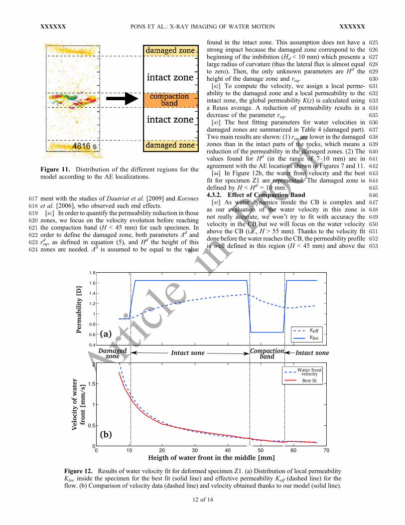
625found in the intact zone. This assumption does not have a626strong impact because the damaged zone correspond to the627beginning of the imbibition (Hd < 10 mm) which presents a628large radius of curvature (thus the lateral flux is almost equal629to zero). Then, the only unknown parameters are Hd the630height of the damage zone and req.631[42] To compute the velocity, we assign a local perme-632ability to the damaged zone and a local permeability to the633intact zone, the global permeability K(z) is calculated using634a Reuss average. A reduction of permeability results in a635decrease of the parameter req.636[43] The best fitting parameters for water velocities in637damaged zones are summarized in Table 4 (damaged part).638Two main results are shown: (1) req are lower in the damaged639zones than in the intact parts of the rocks, which means a640reduction of the permeability in the damaged zones. (2) The641values found for Hd (in the range of 7–10 mm) are in642agreement with the AE locations shown in Figures 7 and 11.643[44] In Figure 12b, the water front velocity and the best644fit for specimen Z1 are represented. The damaged zone is645defined by H < Hd = 10 mm.6464.3.2. Effect of Compaction Band647[45] As water dynamics inside the CB is complex and648as our evaluation of the water velocity in this zone is649not really accurate, we won’t try to fit with accuracy the650velocity in the CB but we will focus on the water velocity651above the CB (i.e., H > 55 mm). Thanks to the velocity fit652done before the water reaches the CB, the permeability profile653is well defined in this region (H < 45 mm) and above the

Figure 11. Distribution of the different regions for themodel according to the AE localizations.

Figure 12. Results of water velocity fit for deformed specimen Z1. (a) Distribution of local permeabilityKloc inside the specimen for the best fit (solid line) and effective permeability Keff (dashed line) for theflow. (b) Comparison of velocity data (dashed line) and velocity obtained thanks to our model (solid line).

PONS ET AL.: X‐RAY IMAGING OF WATER MOTION XXXXXXXXXXXX

12 of 14

654 CB (H > 55 mm). In order to obtain the best fit of the water655 velocity above CB, we need the equivalent pore radius656 req and the coefficient A inside the CB. The local perme-657 ability inside the CB is also calculated taking into account658 the porosity reduction inside the CB (Table 4).659 [46] Figure 12a shows the best permeability profile660 which permits to fit the velocity data for specimen Z1, and661 Figure 12b shows the best fit of the water front velocity662 for the same specimen. The fit of water front velocity above663 the CB is constrained by the values of req inside the CB.664 Indeed, as permeability inside the CB is much smaller than665 in the other parts, the global permeability K(z) (Figure 12a)666 and consequently the velocity above CB are constrained by667 the local permeability, and thus req, inside the CB. On the668 contrary the water velocity inside the CB is really dependent669 on the parameter A. Thus, this very simple model permits a670 good fit of the data, but the interpretation of all the different671 parameters must be done carefully.672 [47] The values of req inside the CB (Table 4) are in the673 same range as the values found in the intact part and do not674 correspond to what we should be expected from micro-675 structural observations [Stanchits et al., 2009]. This appar-676 ent inconsistency can be explained as follows: in our model677 we consider a CB of 10 mm thick because of the complex678 structure of the CB (Figure 7). Consequently the CB zone is679 not only composed by an effective CB, but also by some680 regions less damaged, and thus, our model overestimates681 req inside the effective CB.682 [48] Comparing permeability inside the CB, KCB, and in683 the intact parts, Kintact, we can obtain an estimation of per-684 meability reduction in the CB. This permeability is divided685 by 3 which is smaller than the ratio of 20–400 found by686 Vajdova et al. [2004] for Bentheim sandstone. But as said687 before, the estimation of permeability inside CB may be688 overestimated and the estimation of Vajdova et al. [2004]689 was during loading of the specimen. Moreover, field ob-690 servations [Aydin and Ahmadov, 2009] on similar sandstone691 (same porosity, same order of permeability) show a per-692 meability contrast of 5 between the CB and the host rock.

693 5. Conclusion

694 [49] To investigate the influence of compaction bands695 on fluid flow, we (1) conducted capillary imbibition ex-696 periments in intact Bentheim sandstone specimens (initial697 porosity ∼ 23%), (2) then induced compaction bands (CB) in698 the sandstone under triaxial compression experiments done699 at 185 MPa effective confining pressure, and (3) conducted700 capillary imbibition experiments in the deformed specimens.701 [50] From the mechanical data, we estimate a porosity702 reduction in the CB in the range of 12–18% in agreement703 with previous studies done on Bentheim sandstone [Tembe704 et al., 2006; Stanchits et al., 2009]. Moreover the imbibi-705 tion experiments provide useful insights for a more com-706 prehensive understanding of the coupling of compaction707 localization and fluid flow. Indeed, the study of capillary708 imbibition shows that the compaction bands clearly slow709 down the imbibition kinetics and disturb the geometry of710 water flow. These results confirm that a CB acts like a barrier711 for the fluid flow.712 [51] Previous studies [Louis et al., 2006, 2007] used com-713 plex analysis of X‐ray images to observe CB structures. In

714our imbibition experiments, we show that a direct visuali-715zation of the CB structure from X‐ray images may be pos-716sible when the specimens are wet. This observation is717explained by a water saturation inside the CB close to 100%,718which is possible as the porosity reduction in the localiza-719tion reduces drastically the pore channel size and enhances720the capillary driving forces. In addition, we show that there721is a very good agreement between the AE location recorded722during the triaxial experiments and the CB structure seen by723the X‐ray images.724[52] The direct measurement of the effect of compaction725bands on the rock permeability is not obvious. In their study,726Vajdova et al. [2004] fit the experimental data with a 1‐D727layered medium, with discrete layers of uniform thickness728with relatively low permeability embedded in a matrix with729high permeability. Using such a model, they are able to730estimate the contrast of permeability between the host rock731and the CB in the range of 20–400. In such model, they732make the assumption that the CB is crosscutting the entire733specimen.734[53] Here, to investigate the effect of compaction bands on735capillary imbibition, we used notched specimens in order to736induce only one localization. Using a simple model, we are737able to estimate a contrast of permeability of ∼3. Such a738difference with the study of Vajdova et al. [2004] may be739explained by the fact that in our case the CB does not740crosscutting the entire specimen, as it may be seen from the741X‐ray images or the AE localization. However, it is inter-742esting to note that the contrast of permeability found in this743study is consistent with the values reported in the field744[Aydin and Ahmadov, 2009] on similar sandstones.745[54] The existence of compaction bands has important746implication on the field scale and the results of our study747combining X‐ray imaging during imbibition experiments748and AE localization may constrain field interpretations or749reservoir modeling. Indeed, the systematic organization of750compaction bands within poorly consolidated sand and751sandstone may result in a complex permeability structure752that effectively localizes and compartmentalizes flow and753subsurface fluids.

754[55] Acknowledgments. We thank Georg Dresen for his support in755this project and Stefan Gehrman (both at GFZ) for preparing the notched756specimens. We also thank Jean‐Christian Colombier (UCP) and Marie‐757Claude Lynch (IFPEN) for technical support. Finally, we thank both758reviewers for their comments which helped to improve the manuscript.

759References760Abramoff, M. D., P. Maglhaes, and S. Ram (2004), Image processing with761ImageJ, Biophotonics Int., 11(7), 36–42.762Antonellini, M., and A. Aydin (1994), Effect of faulting on fluid flow in763porous sandstones: petrophysical properties, AAPG Bull., 78, 355–377.764Aydin, A., and R. Ahmadov (2009), Bed‐parallel compaction bands in765aeolian sandstone: Their identification, characterization and implications,766Tectonophysics, 479(3–4), 277–284, doi:10.1016/j.tecto.2009.08.033.767Baud, P., E. Klein, and T.‐F. Wong (2004), Compaction localization in768porous sandstones: Spatial evolution of damage and acoustic emission769activity, J. Struct. Geol., 26, 603–624, doi:10.1016/j.jsg.2003.09.002.770Bésuelle, P., J. Desrues, and S. Raynaud (2000), Experimental characterisa-771tion of the localisation phenomenon inside a Vosges sandstone in a triaxial772cell, Int. J. Rock Mech. Min., 37(8), 1223–1237, doi:10.1016/S1365-1609773(00)00057-5.774Charalampidou, E. M., S. A. Hall, S. Stanchits, H. Lewis, and G. Viggiani775(2011), Characterization of shear and compaction bands in a porous sand-

PONS ET AL.: X‐RAY IMAGING OF WATER MOTION XXXXXXXXXXXX

13 of 14

776 stone deformed under triaxial compression, Tectonophysics, doi:10.1016/777 j.tecto.2010.09.032, in press.778 Dautriat, J., N. Gland, J. Guelard, A. Dimanov, and J. L. Raphanel (2009),779 Axial and radial permeability evolutions of compressed sandstones: End780 effects and shear‐band induced permeability anisotropy, Pure Appl.781 Geophys., 166(5–7), 1037–1061, doi:10.1007/s00024-009-0495-0.782 David, C., B. Menéndez, and J.‐M.Mengus (2008), Influence of mechanical783 damage on fluid flow patterns investigated using CT scanning imaging784 and acoustic emissions techniques, Geophys. Res. Lett., 35, L16313,785 doi:10.1029/2008GL034879.786 David, C., B. Menéndez, L. Louis, and J.‐M.Mengus (2011), X‐ray imaging787 of water motion during capillary imbibition: Geometry and kinetics788 of water front in intact and damaged porous rocks, J. Geophys. Res.,789 doi:10.1029/2010JB007972, in press.790 Fortin, J., A. Schubnel, and Y. Guéguen (2005), Elastic wave velocities and791 permeability evolution during compaction of Bleurswiller sandstone, Int.792 J. Rock Mech. Min., 42, 873–889, doi:10.1016/j.ijrmms.2005.05.002.793 Fortin, J., S. Stanchits, G. Dresen, and Y. Guéguen (2006), Acoustic emis-794 sion and velocities associated with the formation of compaction bands in795 sandstone, J. Geophys. Res., 111, B10203, doi:10.1029/2005JB003854.796 Fortin, J., S. Stanchits, G. Dresen, and Y. Guéguen (2009), Acoustic797 emissions monitoring during inelastic deformation of porous sandstone:798 Comparison of three modes of deformation, Pure Appl. Geophys., 166,799 823–841, doi:10.1007/s00024-009-0479-0.800 Gombia, M., V. Bortolotti, R. J. S. Brown, M. Camaiti, and P. Fantazzini801 (2008), Models of water imbibition in untreated and treated porous media802 validated by quantitative magnetic resonance imaging, J. Appl. Phys.,803 103(9), 094913, doi:10.1063/1.2913503.804 Guéguen, Y., and V. Palciauskas (1994), Introduction to the Physics of805 Rocks, Princeton Univ. Press, Princeton, N. J.806 Klein, E., and T. Reuschlé (2003), A model for the mechanical behaviour807 of Bentheim sandstone in the brittle regime, Pure Appl. Geophys., 160(5),808 833–849, doi:10.1007/PL00012568.809 Klein, E., P. Baud, T. Reuschlé, and T.‐F. Wong (2001), Mechanical810 behavior and failure mode of Bentheim sandstone under triaxial compres-811 sion, Phys. Chem. Earth, Part A, 26, 21–25, doi:10.1016/S1464-1895812 (01)00017-5.813 Korsnes, R., R. Risnes, I. Faldaas, and T. Norland (2006), End effects on814 stress dependent permeability measurements, Tectonophysics, 426,815 239–251, doi:10.1016/j.tecto.2006.02.020.816 Louis, L., T. Wong, P. Baud, and S. Tembe (2006), Imaging strain locali-817 zation by X‐ray computed tomography: Discrete compaction bands in818 Diemelstadt sandstone, J. Struct. Geol., 28(5), 762–775, doi:10.1016/j.819 jsg.2006.02.006.820 Louis, L., T. Wong, and P. Baud (2007), Imaging strain localization by821 X‐ray radiography and digital image correlation: Deformation bands

822in Rothbach sandstone, J. Struct. Geol., 29(1), 129–140, doi:10.1016/823j.jsg.2006.07.015.824Mollema, P. (1996), Compaction bands: A structural analog for anti‐mode I825cracks in aeolian sandstone, Tectonophysics, 267(1–4), 209–228,826doi:10.1016/S0040-1951(96)00098-4.827Olsson, W. A., and D. J. Holcomb (2000), Compaction localization inporous828rock, Geophys. Res. Lett., 27, 3537–3540, doi:10.1029/2000GL011723.829Scholz, C. H. (1968), Microfracturing and the inelastic deformation of rock830in compression, J. Geophys. Res., 73(4), 1417–1432, doi:10.1029/831JB073i004p01417.832Schultz, R. A. (2009), Scaling and paleodepth of compaction bands, Nevada833and Utah, J. Geophys. Res., 114, B03407, doi:10.1029/2008JB005876.834Stanchits, S., J. Fortin, Y. Gueguen, and G. Dresen (2009), Initiation and835propagation of compaction bands in dry and wet Bentheim sandstone,836Pure Appl. Geophys., 166(5–7), 843–868, doi:10.1007/s00024-009-8370478-1.838Sternlof, K. R., M. Karimi‐Fard, D. D. Pollard, and L. J. Durlofsky (2006),839Flow and transport effects of compaction bands in sandstone at scales rel-840evant to aquifer and reservoir management, Water Resour. Res., 42,841W07425, doi:10.1029/2005WR004664.842Tembe, S., V. Vajdova, T. Wong, and W. Zhu (2006), Initiation and prop-843agation of strain localization in circumferentially notched samples of two844porous sandstones, J. Geophys. Res., 111, B02409, doi:10.1029/8452005JB003611.846Vajdova, V., P. Baud, and T. Wong (2004), Permeability evolution during847localized deformation in Bentheim sandstone, J. Geophys. Res., 109,848B10406, doi:10.1029/2003JB002942.849Van Bareen, J. P., M. W. Vos, and H. J. K. Heller (1990), Selection of850outcrop specimens, internal report, Delft Univ. of Technol, Delft,851Netherlands.852Washburn, E. W. (1921), The dynamics of capillary flow, Phys. Rev., 17(3),853273–283, doi:10.1103/PhysRev.17.273.854Wong, T.‐f., C. David, and W. Zhu (1997), The transition from brittle855faulting to cataclastic flow in porous sandstones: Mechanical deforma-856tion, J. Geophys. Res., 102, 3009–3025, doi:10.1029/96JB03281.

857C. David and B. Menéndez, Laboratoire Géosciences et Environnement858Cergy, Université de Cergy‐Pontoise, 5 mail Gay‐Lussac, F‐95031 Cergy‐859Pontoise, France.860J. Fortin and A. Pons, Laboratoire de Géologie, École normale supérieure861de Paris, UMR CNRS 8538, 24 rue Lhomond, F‐75252 Paris, France.862(apons@geologie.ens.fr)863J. M. Mengus, IFP Énergies Nouvelles, 1‐4 av. de Bois‐Préau, F‐92852864Rueil‐Malmaison, France.865S. Stanchits, German Research Center for Geosciences, GFZ Potsdam,866Telegrafenberg D423, D‐14473 Potsdam, Germany.

PONS ET AL.: X‐RAY IMAGING OF WATER MOTION XXXXXXXXXXXX

14 of 14